University of Wisconsin Milwaukee University of Wisconsin Milwaukee

UWM Digital Commons UWM Digital Commons

Cell and Molecular Biology 4e: What We Know and How We Found Out - All Versions Biological Sciences

1-2020

Basic Cell and Molecular Biology 4e: What We Know and How Basic Cell and Molecular Biology 4e: What We Know and How

Found Out Found Out

Gerald Bergtrom University of Wisconsin - Milwaukee, bergtrom@uwm.edu

Follow this and additional works at: https://dc.uwm.edu/biosci_facbooks_bergtrom

Part of the Biology Commons, Cell Biology Commons, and the Molecular Biology Commons

Recommended Citation Recommended Citation Bergtrom, Gerald, "Basic Cell and Molecular Biology 4e: What We Know and How Found Out" (2020). Cell and Molecular Biology 4e: What We Know and How We Found Out - All Versions. 12. https://dc.uwm.edu/biosci_facbooks_bergtrom/12

This Book is brought to you for free and open access by UWM Digital Commons. It has been accepted for inclusion in Cell and Molecular Biology 4e: What We Know and How We Found Out - All Versions by an authorized administrator of UWM Digital Commons. For more information, please contact open-access@uwm.edu.

CMB3e i

Basic CMB 4e

Cell and Molecular Biology

What We Know

& How We Found Out

Gerald Bergtrom

An Open Access, Open Education Resource (OER) interactive

electronic textbook (iText) published under a Creative

Commons (cc-by) License

Image Adapted From: Microarray

CMB3e i

Cell and Molecular Biology What We Know & How We Found Out

Basic CMB 4e

An Open Access, Open Education Resource (OER)

interactive electronic textbook (iText) published under

a Creative Commons (cc-by) license

By

Gerald Bergtrom, Ph.D.

Revised January, 2020

ISBN# 978-0-9961502-5-5

New in CMB4e: Reformatting, including

o An expanded ‘active’ Table of Contents (the original Table of Contents remains as the Table of Chapters)

o numbered figures with figure legends o New List of Figures and sources (Appendix I; other appendices

renumbered) Many content updates (new illustrations, figures, links) More than 50 pages of new and reformatted content, with new sections on:

Viruses, Proprioreception, Schrödinger’s cat (!), history of CRISPR/cas, ‘next gen’ DNA sequencing, directed evolution and more

New Challenge boxes (Annotated & Instructors’ editions)

Cover Microarray Image: From: A Microarray; the work of WikiPremed is published under a Creative Commons Attribution Share Alike (cc-by) 3.0 License.

CMB3e ii

Dedicated to:

Sydell, Aaron, Aviva, Edan, Oren and our extended family

whose patience and encouragement made this work possible,

my students from whose curiosity I received as much as I gave,

and the memory of my mentor Herbert Oberlander,

who gave me the time, opportunity

and tools to do science.

CMB3e iii

Creative Commons Licensure and Permissions

Written, Compiled and Curated Under

(Creative Commons with Attribution) License and Fair Use Rules of

Distribution*

The following is a human-readable summary of (and not a substitute for) the cc-by 4.0 license.

You are free to:

Share — copy and redistribute the material in any medium or format

Adapt — remix, transform, and build upon the material for any purpose, even

commercially. The licensor cannot revoke these freedoms as long as you follow the

license terms.

Under the following terms:

Attribution — You must give appropriate credit, provide a link to the license, and indicate

if changes were made. You may do so in any reasonable manner, but not in any way that

suggests the licensor endorses you or your use.

No additional restrictions — You may not apply legal terms or technological measures

that legally restrict others from doing anything the license permits.

Notices:

You do not have to comply with the license for elements of the material in the public

domain or where your use is permitted by an applicable exception or limitation.

No warranties are given. The license may not give you all of the permissions necessary for

your intended use. For example, other rights such as publicity, privacy, or moral rights

may limit how you use the material.

4th Edition, Published 2020

*At the author’s request, reviewed all externally sourced photographs and illustrations in CMB3e to verify

that each is accompanied by an appropriate open access indication, i.e., public domain, GNU, specific

Creative Commons license. Images created by Dr. Bergtrom or from his original research are so

designated. By random spot-check, I further verified the licensure and attribution status of >20 iText

images at random. I confirm to the best of my ability to make these determinations, that all images in

CMB3e meet open access standards. I can further state with confidence that for this edition (CMB4e), Dr.

Bergtrom revised or selected substitute photographs and illustrations to ensure that all images are licensed

without restrictions on commercial use (e.g., CC-0 , CC-BY or CC-BY-SA). This effort anticipates the

production of a commercial (albeit low cost) print version of CMB4e for which open access requirements

are more strict than for the online iText..

M.T. Bott, Senior Lecturer, Biological Sciences, University of Wisconsin-Milwaukee

CMB3e iv

Preface to CMB4e

A grasp of the logic and practice of science is essential to understand the rest of the world

around us. To that end, the CMB4e iText remains focused on experimental support for

what we know about cell and molecular biology, and on showing students the relationship

of cell structure and function.

Rather than trying to be a comprehensive reference book, the Basic CMB4e itext

selectively details investigative questions, methods and experiments that lead to our

understanding of cell biology. This focus is nowhere more obvious than in the chapter

learning objectives and in *web-links. In addition to external online resources, links to

the author’s short YouTube voice-over PowerPoint (VOP) videos with optional closed

captions are embedded near relevant text. Each video is identified by a play-video

symbol and can be opened by clicking a descriptive title or using QR bar codes, such as

the example below:

102 Golgi Vesicles & the Endomembrane System

The Learning objectives align with content and ask students to use new knowledge to

make connections and deepen their understanding of concept and experiment. All

external links are intended to expand or explain textual content and concepts and to

engage student curiosity. All images in the iText and just-in-time VOPs are by the author

or are from public domain or Creative Commons (CC) licensed sources.

Beyond the Basic CMB4e, a freely available Annotated version of the iText contains

interactive links and formative assessments in the form of Challenge boxes. The

Instructors CMB4e version models additional interactive features, including short 25

Words or Less writing assignments that can be incorporated into almost any course

management system, many of which the author has assigned as homework in his flipped,

blended course. These assessments aim to reinforce writing as well as critical thinking

skills. As a Sample Chapter, Chapter 1 of the Instructors version of CMB4e is freely

available for download; the complete Instructors version is available on request.

My goal in writing and updating this iText is to make the content engaging, free and

comparable in accuracy and currency to commercial textbooks. I encourage instructors

to use the interactive features of the iText (critical thought questions, YouTube videos,

etc.) to challenge their students.

*Note: Web links to the author’s own resources may occasionally be updated, but should

remain active. Links to resources selected (but not created) by the author were live at the

time of publication of the iText, but may disappear without notice!

CMB3e v

With all of these enhancements, I encourage students to think about

how good and great experiments were inspired and designed,

how alternative experimental results were predicted,

how data was interpreted and finally,

how investigators (and we!) arrive at the most interesting “next questions”.

The online iText is the most efficient way to access links and complete online

assignments. Nevertheless, you can download, read, study, and access many links with

a smart phone or tablet. And you can add your own annotations digitally or write in the

margins of a printout the old-fashioned way! Your instructor may provide additional

instructions for using your iText.

Special to Instructors from the Author

All versions of the Basic and Annotated versions of CMB4e are freely available as pdf

files to you and your students. To get the Instructors version you will need to fill out a

short form identifying yourself as an instructor. When you submit the form, you will get

pdf as well as MS-Word files for the Basic, Annotated and Instructor’s CMB4e. Once you

download the CMB4e iText(s) of your choice, you should find it an easy matter to use the

MS-Word file to add, subtract, modify or embellish any parts of it to suit your purposes (in

accordance with the Creative Commons CC-BY license under which it is published).

Common modifications are adding content of your own, or even that students uncover as

part of their studies (or as an assignment!). A useful enhancement of the iText is to add

links to your own assessments (quizzes, writing assignments) that take students directly

to a Quiz, Discussion Forum, DropBox, etc. in your Learning Management System, e.g.,

D2L, BlackBoard, Canvas, etc.) course site. This is seamless if students open the iText

from within your course site, but also works as long as both the iText and course site are

open at the same time. You can provide a customized version of the iText to your

students as a smaller pdf file (recommended) or as an MS-Word document.

As implied above, you ask your students participate in the improvement of the iText (for

fun or for credit!) and to share the results with others! One final caveat: whereas I provide

content updates, that have significant potential subject to confirmation, very current

research is not necessarily definitive. I hope that you (and perhaps your students!) will

enjoy creating and customizing interactive elements and digging in to some of the most

recent research included in the iText. Above all, I hope that your students will achieve a

better understanding of how scientists use skills of inductive and inferential logic to ask

questions and formulate hypotheses…, and how they apply concept and method to

testing those hypotheses.

CMB3e vi

Acknowledgements

Many thanks go to my erstwhile LTC (now CETL) colleagues Matthew Russell, Megan

Haak, Melissa Davey Castillo, Jessica Hutchings and Dylan Barth for inspiration in

suggesting ways to model how open course content can be made interactive and

engaging. I also thank my colleagues Kristin Woodward and Ann Hanlon in the Golda

Meir Library for their help in publishing the various online editions and versions of CMB

on the University of Wisconsin-Milwaukee Digital Commons open access platform

(http://dc.uwm.edu). I am most grateful to Ms. M. Terry Bott for reviewing and vetting the

images used in this iText as either in the public domain or designated with a Creative

Commons (CC) license as an open resource (see Creative Commons License page,

above). Most recently, I owe a debt of gratitude to our departmental lab manager (and

just down the hall neighbor) Jordan Gonnering for lots of hardware and software

assistance during the preparation of CMB4e. Last but not least I must acknowledge the

opportunity I was given at the University of Wisconsin-Milwaukee to teach, study and do

research in science and interactive pedagogy for more than 35 years. My research and

collegial experience at UW-M have left their mark on the content, concept and purpose of

this digital Open Education Resource (OER).

CMB3e vii

About the Author Dr. Bergtrom is Professor (Emeritus) of Biological Sciences and a former Learning

Technology Consultant in the UW-Milwaukee Center for Excellence in Teaching and

Learning. Scientific interests include cell and molecular biology and evolution.

Pedagogic interests are blended and online instruction and the use of technology to serve

more active and engaged teaching and learning. He has taught face-to-face, fully online,

blended and flipped classes at both undergraduate and graduate levels. He also

developed and co-instructed Teaching with Technology, an interdisciplinary course aimed

at graduate students that they might someday find themselves teaching. In his 40+ years

of teaching and research experience, he has tested and incorporated pedagogically

proven teaching technologies into his courses. His research papers have been

supplemented with publications on active blended, online and flipped classroom

methods1-3.

The first edition of his Open Access/Creative Commons electronic iText, Cell and

Molecular Biology–What We Know & How We Found Out first appeared in 20154.

Subsequent editions and versions followed in 20165, 20186 and 20197. The latest

editions are available at http://dc.uwm.edu/biosci_facbooks_bergtrom/. Older editions

(and versions) will remain available by request to the author.

1. Bergtrom, G. (2006) Clicker Sets as Learning Objects. Int. J. Knowl. & Learn. Obj.

2:105-110. (http://www.ijello.org/Volume2/v2p105-110Bergtrom.pdf) 2. Bergtrom, G. (2009) On Offering a Blended Cell Biology Course. J. Res. Center Ed.

Tech. 5(1) (http://www.rcetj.org/?type=art&id=91609&). 3. Bergtrom, G. (2011) Content vs. Learning: An Old Dichotomy in Science Courses. J.

Asynchr. Learning Networks 15:33-44 (http://jaln_v15n1_bergtrom.pdf) 4. Bergtrom, G. (2015) Cell and Molecular Biology: What We Know & How We Found

Out [CMB] (If necessary, please contact the author to access this edition) 5. Bergtrom, G. (2016) Cell and Molecular Biology: What We Know & How We Found

Out [CMB2e] (If necessary, please contact the author to access this edition ) 6. Bergtrom, G. (2018) Cell and Molecular Biology: What We Know & How We Found

Out [CMB3e] (If necessary, please contact the author to access this edition ) 7. Bergtrom, G. (2020) Cell and Molecular Biology: What We Know & How We Found

Out [CMB4e] (http://dc.uwm.edu/biosci_facbooks_bergtrom/)

CMB3e viii

Table of Chapters

(Click title to see first page of chapter)

Preface

Chapter 1: Cell Tour, Life’s Properties and Evolution, Studying Cells

Chapter 2: Basic Chemistry, Organic Chemistry and Biochemistry

Chapter 3: Details of Protein Structure

Chapter 4: Bioenergetics

Chapter 5: Enzyme Catalysis and Kinetics

Chapter 6: Glycolysis, the Krebs Cycle and the Atkins Diet

Chapter 7: Electron Transport, Oxidative Phosphorylation and

Photosynthesis

Chapter 8: DNA Structure, Chromosomes and Chromatin

Chapter 9: Details of DNA Replication & DNA Repair

Chapter 10: Transcription and RNA Processing

Chapter 11: The Genetic Code and Translation

Chapter 12: Regulation of Transcription and Epigenetic Inheritance

Chapter 13: Post-Transcriptional Regulation of Gene Expression

Chapter 14: Repetitive DNA, A Eukaryotic Genomic Phenomenon

Chapter 15: DNA Technologies

Chapter 16: Membrane Structure

Chapter 17: Membrane Function

Chapter 18: The Cytoskeleton and Cell Motility

Chapter 19: Cell Division and the Cell Cycle

Chapter 20: The Origins of Life

Epilogue

Appendix I: List of Illustrations & Sources

Appendix II: Context-Embedded YouTube Videos

Appendix III: Other Useful Links

CMB3e ix

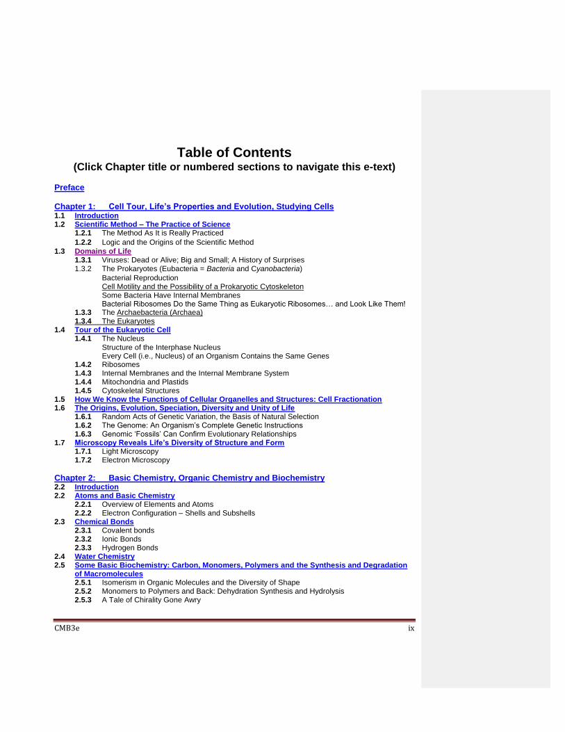
Table of Contents (Click Chapter title or numbered sections to navigate this e-text)

Preface Chapter 1: Cell Tour, Life’s Properties and Evolution, Studying Cells 1.1 Introduction 1.2 Scientific Method – The Practice of Science

1.2.1 The Method As It is Really Practiced

1.2.2 Logic and the Origins of the Scientific Method

1.3 Domains of Life 1.3.1 Viruses: Dead or Alive; Big and Small; A History of Surprises 1.3.2 The Prokaryotes (Eubacteria = Bacteria and Cyanobacteria)

Bacterial Reproduction Cell Motility and the Possibility of a Prokaryotic Cytoskeleton Some Bacteria Have Internal Membranes Bacterial Ribosomes Do the Same Thing as Eukaryotic Ribosomes… and Look Like Them!

1.3.3 The Archaebacteria (Archaea) 1.3.4 The Eukaryotes

1.4 Tour of the Eukaryotic Cell 1.4.1 The Nucleus

Structure of the Interphase Nucleus Every Cell (i.e., Nucleus) of an Organism Contains the Same Genes

1.4.2 Ribosomes 1.4.3 Internal Membranes and the Internal Membrane System 1.4.4 Mitochondria and Plastids 1.4.5 Cytoskeletal Structures

1.5 How We Know the Functions of Cellular Organelles and Structures: Cell Fractionation 1.6 The Origins, Evolution, Speciation, Diversity and Unity of Life

1.6.1 Random Acts of Genetic Variation, the Basis of Natural Selection 1.6.2 The Genome: An Organism’s Complete Genetic Instructions 1.6.3 Genomic ‘Fossils’ Can Confirm Evolutionary Relationships

1.7 Microscopy Reveals Life’s Diversity of Structure and Form 1.7.1 Light Microscopy 1.7.2 Electron Microscopy

Chapter 2: Basic Chemistry, Organic Chemistry and Biochemistry 2.2 Introduction 2.2 Atoms and Basic Chemistry

2.2.1 Overview of Elements and Atoms 2.2.2 Electron Configuration – Shells and Subshells

2.3 Chemical Bonds 2.3.1 Covalent bonds 2.3.2 Ionic Bonds 2.3.3 Hydrogen Bonds

2.4 Water Chemistry 2.5 Some Basic Biochemistry: Carbon, Monomers, Polymers and the Synthesis and Degradation

of Macromolecules 2.5.1 Isomerism in Organic Molecules and the Diversity of Shape 2.5.2 Monomers to Polymers and Back: Dehydration Synthesis and Hydrolysis 2.5.3 A Tale of Chirality Gone Awry

CMB3e x

Chapter 3: Details of Protein Structure 3.1 Introduction

3.2 Levels (Orders) of Protein Structure 3.2.1 Protein Primary Structure; Amino Acids and the C-N-C-N-… Polypeptide Backbone

Formation of peptide bonds leads to polypeptide primary structure Determining Protein Primary Structure - Polypeptide Sequencing

3.2.2 Protein Secondary Structure 3.2.3 Protein Tertiary Structure

3.3 Changes in Protein Shape Can Cause Disease 3.3.1 Sickle Cell Anemia 3.3.2 The Role of Misshapen and Mis-folded Proteins in Alzheimer’s Disease

The amyloid beta (A ) peptide The Tau protein Some Relatives of Alzheimer’s Disease

3.4 Protein Quaternary Structure, Prosthetic Groups Chemical Modifications 3.5 Domains, Motifs, and Folds in Protein Structure 3.6 Proteins, Genes and Evolution: How Many Proteins are We? 3.7 Directed Evolution: Getting Cells to Make New Proteins… for our use and pleasure 3.8 View Animated 3D Protein Images in the NCBI Database

Chapter 4: Bioenergetics 4.1 Introduction 4.2 Kinds of Energy 4.3 Deriving Simple Energy Relationships

4.3.1 Energy in the Universe: the Universe is a Closed System 4.3.2 Energy is Exchanged Between Systems in the Universe

4.3.3 How is Enthalpy Change (H) Determined?

4.3.4 How is Standard Free Energy Change (G0) Determined? 4.3.5 Working an Example Using These Equations for Closed Systems

4.4 Summary: The Properties of Closed Systems 4.5 Open Systems and Actual Free Energy Change

Chapter 5: Enzyme Catalysis and Kinetics 5.1 Introduction 5.2 Enzymes and the Mechanisms of Enzyme Catalysis

5.2.1 Structural Considerations of Catalysis 5.2.2 Energetic Considerations of Catalysis

5.3 Enzyme Regulation 5.4 Enzyme Kinetics

5.4.1 Why Study Enzyme Kinetics 5.4.2 How We Determine Enzyme Kinetics and Interpret Kinetic Data

Chapter 6: Glycolysis, the Krebs Cycle and the Atkins Diet 6.1 Introduction 6.2 Glycolysis, a Key Pathway in Energy Flow through Life 6.3 Some Details of Glycolysis

6.3.1 Glycolysis, Stage 1 6.3.2 Glycolysis, Stage 2

6.4 A Chemical and Energy Balance Sheet for Glycolysis

CMB3e xi

6.5 Gluconeogenesis 6.6 The Atkins Diet and Gluconeogenesis 6.7 The Krebs/TCA/Citric Acid Cycle

Chapter 7: Electron Transport, Oxidative Phosphorylation and Photosynthesis 7.1 Introduction 7.2 Electron Transport Chains 7.3 Electron Transport in Respiration

7.4 Oxidative Phosphorylation in Respiration 7.5 Photosynthesis

7.5.1 The Light-Dependent Reactions 7.5.2 The Light-Independent (“Dark” Reactions”)

C3 Photosynthesis - Light-Independent Reactions CAM Photosynthetic Pathway - Light-Independent Reactions C4 Photosynthetic Pathway - Light-Independent Reactions

7.6 Thoughts on the Origins and Evolution of Respiration and Photosynthesis

Chapter 8: DNA Structure, Chromosomes and Chromatin 8.1 Introduction 8.2 The Stuff of Genes

8.2.1 Griffith’s Experiment 8.2.2 The Avery-MacLeod-McCarty Experiment 8.2.3 The Hershey-Chase Experiment

8.3 DNA Structure 8.3.1 X-Ray Crystallography and the Beginnings of Molecular Biology 8.3.2 Wilkins, Franklin, Watson & Crick – DNA Structure Revealed 8.3.3 Meselson and Stahl’s Experiment – Replication is Semiconservative

8.4 Chromosomes 8.5 Genes and Chromatin in Eukaryotes 8.6 Structure and Organization of Bacterial DNA... and Bacterial Sex 8.7 Phage Can Integrate Their DNA Into the Bacterial Chromosome

Chapter 9: Details of DNA Replication & DNA Repair 9.1 Introduction 9.2 DNA Replication

9.2.1 Visualizing Replication and Replication Forks 9.2.2 Visualizing Bidirectional Replication

9.3 DNA Polymerases Catalyze Replication 9.4 The Process of Replication

9.4.1 Initiation 9.4.2 Elongation 9.4.3 Termination 9.4.4 Is Replication Processive? 9.4.5 One more Problem with Replication

9.5 DNA Repair 9.5.1 Germline vs. Somatic Mutations; A Balance Between Mutation and Evolution 9.5.2 What Causes DNA Damage?

9.6 Molecular Consequences of Uncorrected DNA Damage 9.6.1 Depurination 9.6.2 Pyrimidine Dimerization 9.6.3 Deamination

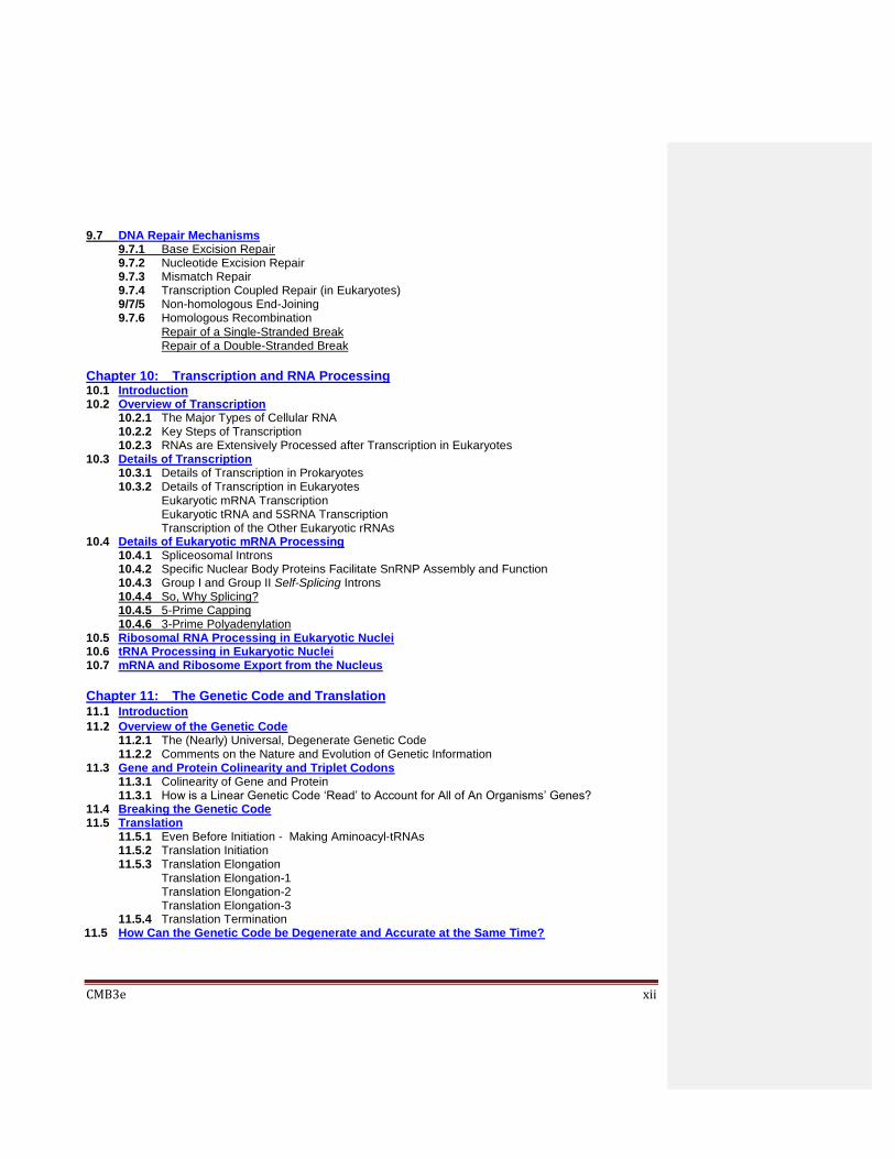
CMB3e xii

9.7 DNA Repair Mechanisms 9.7.1 Base Excision Repair 9.7.2 Nucleotide Excision Repair 9.7.3 Mismatch Repair 9.7.4 Transcription Coupled Repair (in Eukaryotes) 9/7/5 Non-homologous End-Joining 9.7.6 Homologous Recombination

Repair of a Single-Stranded Break Repair of a Double-Stranded Break

Chapter 10: Transcription and RNA Processing 10.1 Introduction 10.2 Overview of Transcription

10.2.1 The Major Types of Cellular RNA 10.2.2 Key Steps of Transcription 10.2.3 RNAs are Extensively Processed after Transcription in Eukaryotes

10.3 Details of Transcription 10.3.1 Details of Transcription in Prokaryotes 10.3.2 Details of Transcription in Eukaryotes Eukaryotic mRNA Transcription Eukaryotic tRNA and 5SRNA Transcription Transcription of the Other Eukaryotic rRNAs

10.4 Details of Eukaryotic mRNA Processing 10.4.1 Spliceosomal Introns 10.4.2 Specific Nuclear Body Proteins Facilitate SnRNP Assembly and Function 10.4.3 Group I and Group II Self-Splicing Introns 10.4.4 So, Why Splicing? 10.4.5 5-Prime Capping 10.4.6 3-Prime Polyadenylation

10.5 Ribosomal RNA Processing in Eukaryotic Nuclei 10.6 tRNA Processing in Eukaryotic Nuclei 10.7 mRNA and Ribosome Export from the Nucleus

Chapter 11: The Genetic Code and Translation 11.1 Introduction

11.2 Overview of the Genetic Code 11.2.1 The (Nearly) Universal, Degenerate Genetic Code 11.2.2 Comments on the Nature and Evolution of Genetic Information

11.3 Gene and Protein Colinearity and Triplet Codons 11.3.1 Colinearity of Gene and Protein 11.3.1 How is a Linear Genetic Code ‘Read’ to Account for All of An Organisms’ Genes?

11.4 Breaking the Genetic Code 11.5 Translation

11.5.1 Even Before Initiation - Making Aminoacyl-tRNAs 11.5.2 Translation Initiation 11.5.3 Translation Elongation

Translation Elongation-1 Translation Elongation-2 Translation Elongation-3

11.5.4 Translation Termination 11.5 How Can the Genetic Code be Degenerate and Accurate at the Same Time?

CMB3e xiii

Chapter 12: Regulation of Transcription and Epigenetic Inheritance 12.1 Introduction 12.2 Gene Regulation in Prokaryotes: the Lactose (lac) Operon

12.2.1 Working Out Regulation of the Lactose (lac) Operon in E. coli 12.2.2 Negative Regulation of the lac Operon by Lactose 12.2.3 Positive Regulation of the Lac Operon; Induction by Catabolite Activation 12.2.4 Lac Operon Regulation by Inducer Exclusion 12.2.5 Structure of the lac Repressor Protein and Additional Operator Sequences

12.3 Gene Regulation in Prokaryotes: the Tryptophan (trp) Operon 12.4 The Problem with Unregulated (Housekeeping) Genes in All Cells 12.5 Gene Regulation in Eukaryotes

12.5.1 Complexities of Eukaryotic Gene Regulation 12.5.2 Regulation of Gene Expression by Hormones that Enter Cells and Those That Don’t

How Steroid Hormones Regulate Transcription How Protein Hormones Regulate Transcription

12.6 Regulating Eukaryotic Genes Means Contending with Chromatin 12.7 Regulating all the Genes on a Chromosome at Once

12.8 Mechanoreceptors: Capturing Non-Chemical Signals 12.9 Epigenetics

12.9.1 Epigenetic Inheritance in Somatic Cells

12.9.2 Epigenetic Inheritance in the Germ-Line

Chapter 13: Post-Transcriptional Regulation of Gene Expression 13.1 Introduction 13.2 Post-transcriptional Control of Gene Expression

13.2.1 Riboswitches 13.2.3 CRISPR/Cas: a Prokaryotic Adaptive Immune System

The CRISPR/Cas ‘Immune’ Response Using CRISPR/Cas to Edit/Engineer Genes CRISPR…, the Power and the Controversy

13.2.3 The Small RNAs: miRNA and siRNA in Eukaryotes

Small Interfering RNA (siRNA) Micro RNAs (miRNA)

13.2.4 Long Non-Coding RNAs 13.2.5 Circular RNAs (CircRNA)

13.3 “Junk DNA” in Perspective 13.4 The RNA Methylome 13.5 Eukaryotic Translation Regulation

13.5.1 Specific Translation Control by mRNA Binding Proteins 13.5.2 Coordinating Heme and Globin Synthesis 13.5.3 Translational Regulation of Yeast GCN4

13.6 Protein Turnover in Eukaryotic Cells: Regulating Protein Half-Life

Chapter 14: Repetitive DNA, A Eukaryotic Genomic Phenomenon 14.1 Introduction 14.2 The Complexity of Genomic DNA

14.1.1 The Renaturation Kinetic Protocol 14.2.2 Renaturation Kinetic Data 14.2.3 Genomic Complexity 14.2.4 Functional Differences between Cot Classes of DNA

CMB3e xiv

14.3 The ‘Jumping Genes’ of Maize 14.3.1 Discovering the Genes of Mosaicism; the Unstable Ds Gene 14.3.2 The Discovery of Mobile Genes: the Ac/Ds System

14.4 Since McClintock: Transposons in Bacteria, Plants and Animals 14.4.1 Bacterial Insertion Sequences (IS Elements) 14.4.2 Composite Bacterial Transposons: Tn Elements 14.4.3 ComplexTransposons that Can Act Like Bacteriophage

14.5 Overview of Eukaryotic Transposable Elements 14.6 The Structure of Eukaryotic DNA (Class II) Transposons

14.6.1 Cut-and-Paste Transposition 14.6.2 Replicative Transposition

14.7 The Structure of Eukaryotic RNA (Class I) Transposons 14.7.1 LTR retrotransposons: The Yeast Ty element 14.7.2 Non-LTR Retrotransposons: LINEs 14.7.3 Non-LTR Retrotransposons: LINEs

14.10 Mechanisms of Retrotransposition 14.8.1 Extrachromosomally Primed Retrotransposition (e.g., of a LINE) 14.8.2 Target-Site Primed SINE Retrotransposition (e.g., of a SINE)

14.11 On the Evolution of Transposons, Genes and Genomes 14.9.1 A Common Ancestry DNA and RNA (i.e., All) Transposons 14.9.2 Retroviruses and LTR Retrotransposons Share a Common Ancestry 14.9.3 Transposons Can Be Acquired by Horizontal Gene Transfer

14.10 Evolutionary Roles of Transposition in Genetic Diversity 14.10.1 Transposons and Exon Shuffling 14.10.2 Transposon Genes and Immune System Genes Have History

14.11 Coping with the Dangers of Rampant Transposition

Chapter 15: DNA Technologies 15.1 Introduction 15.2 Make and Screen a cDNA Library

15.2.1 cDNA Construction 15.2.2 Cloning cDNAs into plasmid vectors 15.2.3 Preparing recombinant plasmid vectors containing cDNA inserts 15.2.4 Recombining plasmids and cDNA inserts and transforming host cells 15.2.5 Transforming host cells with recombinant plasmids 15.2.6 Plating a cDNA Library on Antibiotic-Agar to Select Recombinant Plasmids 15.2.7 Identifying Colonies Containing Plasmids with Inserts of Interest

15.3 DNA sequencing 15.3.1 Manual DNA Sequencing 15.3.2 Automated First Generation DNA Sequencing 15.3.3 Shotgun Sequencing 15.3.4 Next Generation DNA Sequencing

15.4 Genomic Libraries 15.4.1 Preparing Specific Length Genomic DNA for Cloning; the Southern Blot 15.4.2 Recombining Size-Restricted Genomic DNA with Phage DNA 15.4.3 Creating Infectious Viral Particles with Recombinant phage DNA 15.4.4 Screening a Genomic Library; Titering Recombinant Phage Clones 14.4.5 Screening a Genomic Library; Probing the Genomic Library 15.4.6 Isolating the Gene

15.5 The Polymerase Chain Reaction (PCR) 15.5.1 PCR – the Basic Process 15.5.2 The Many Uses of PCR

CMB3e xv

15.6 Genomic Approaches: The DNA Microarray 15.7 Ome-Sweet-Ome 15.8 From Genetic Engineering to Genetic Modification

Chapter 16: Membrane Structure 16.1 Introduction 16.2 Plasma Membrane Structure

16.2.1 The Phospholipid Bilayer 16.2.2 Models of Membrane Structure 16.2.3 Evidence for Membrane Structure 16.2.4 Chemical Factors Affecting Membrane Fluidity 16.2.5 Making and Experimenting with Artificial Membranes 16.2.6 Separate Regions of a Plasma Membrane with Unique Fluidity and Permeability Properties

16.3 Membrane Proteins 16.4 A Diversity of Membrane Protein Functions 16.5 Glycoproteins and Glycolipids 16.6 Glycoproteins and Human Health

Chapter 17: Membrane Function 17.1 Introduction 17.2 Membrane Transport

17.2.1 Passive Diffusion of Solutes 17.2.2 Facilitated Diffusion of Solutes and Ions

Carrier Proteins Ion Channels

17.3 Osmosis 17.3.1 Osmosis in Plant and Animal Cells 17.3.2 Osmosis in Plant Life 17.3.3 Osmosis in Animal Life 17.3.4 Summing Up

17.4 Active Transport 17.5 Ligand and Voltage Gated Channels in Neurotransmission

17.5.1 Measuring Ion Flow and Membrane Potential with a Patch-Clamp Device

17.5.2 Ion Channels in Neurotransmission 17.6 Endocytosis and Exocytosis

17.6.1 Endocytosis 17.6.2 Exocytosis

17.7 Directing the Traffic of Proteins in Cells 17.7.1 Proteins Packaged in RER are Made as Larger Precursor Proteins 17.7.2 Testing the Signal Hypothesis for Packaging Secreted Protein in RER

17.8 Synthesis of Integral Membrane Proteins 17.9 Moving and Sorting Proteins to Their Final Destinations

17.9.1 Traffic on the Endomembrane Highway 17.9.2 Nuclear Protein Traffic 17.9.3 Mitochondrial Protein Traffic

17.10 How Cells are Held Together and How They Communicate 17.10.1 Cell Junctions 17.10.2 Microvesicles and Exosomes 17.10.3 Cancer and Cell Junctions

CMB3e xvi

17.11 Signal Transduction 17.11.1 G-Protein Mediated Signal Transduction by PKA (Protein Kinase A) 17.11.2 Signal Transduction using PKC (Protein Kinase C) 17.11.3 Receptor Tyrosine Kinase-Mediated Signal Transduction

17.12 Signal Transduction in Evolution

Chapter 18: The Cytoskeleton and Cell Motility 18.1 Introduction 18.2 Overview of Cytoskeletal Filaments and Tubules

18.3 The Molecular Structure and Organization of Cytoskeletal Components 18.4 Microtubules are Dynamic Structures Composed of Tubulin Monomers

18.4.1 The Two Kinds of Microtubules in Spindle Fibers

Kinetochore Microtubules Polar Microtubules 18.4.2 Microtubules in Cilia and Flagella 18.4.3 Microtubule Motor Proteins Move Cargo from Place to Place in Cells 18.4.4 Demonstrating Sliding Microtubules 18.4.5 The Motor Protein Dynein Enables Axonemes to Bend

18.5 Microfilaments – Structure and Role in Muscle Contraction 18.5.1 The Thin (Micro-) Filaments and Thick Filaments of Skeletal Muscle 18.5.2 The Sliding Filament Model of Skeletal Muscle Contraction 18.5.3 The Contraction Paradox: Contraction and Relaxation Require ATP

18.6 Actin-Myosin Interactions In Vitro: Dissections and Reconstitutions 18.7 Allosteric Change and the Micro-Contraction Cycle 18.8 The Microcontraction Cycle Resolves the Contraction Paradox 18.9 Ca

++ Ions Regulate Skeletal Muscle Contraction

18.9.1 Muscle Contraction Generates Force 18.9.2 The Elastic Sarcomere: Do Myosin Rods Just Float in the Sarcomere?

18.10 Actin Microfilaments in Non-Muscle Cells 18.11 Both Actins and Myosins are Encoded by Large Gene Families 18.12 Intermediate Filaments

Chapter 19: Cell Division and the Cell Cycle 19.1 Introduction 19.2 Cell Division in a Prokaryote 19.3 Defining the Phases of the Eukaryotic Cell Cycle 19.4 When Cells Stop Dividing… 19.5 Regulation of the Cell Cycle

19.5.1 Discovery and Characterization of Maturation Promoting Factor (MPF) 19.5.2 Other Cyclins, CDKs and Cell Cycle Checkpoints

The G1 Checkpoint The G2 Checkpoint The M Checkpoint The Go State

19.6 When Cells Die 19.7 Disruption of the Cell Cycle Checkpoints Can Cause Cancer 19.8 p53 Protein Mediates Normal Cell Cycle Control

19.8.1 p53 is a DNA-Binding Protein 19.8.2 How p53 Works 19.8.3 The Centrality of p53 Action in Cell Cycle Regulation

‘Oncogenic Viruses’ p53 and Signal Transduction

CMB3e xvii

19.9 Cancer Cell Growth and Behavior; Cancer Treatment Strategies 19.9.1 Cancer Cell Origins, Growth and Behavior 19.9.2 Cancer Treatment Strategies

Chapter 20: The Origins of Life 20.1 Introduction 20.2 Thinking about Life’s Origins: A Short Summary of a Long History 20.3 Formation of Organic Molecules in an Earthly Reducing Atmosphere

20.3.1 Origins of Organic Molecules and a Primordial Soup 20.3.2 The Tidal Pool Scenario for an Origin of Polymers and Replicating Chemistries

20.4 Origins of Organic Molecules in a NON-Reducing Atmosphere 20.4.1 Panspermia – an Extraterrestrial Origin of Earthly Life 20.4.2 Extraterrestrial Origins of Organic molecules

20.5 Organic Molecular Origins Closer to Home 20.5.1 Origins in a High-Heat Hydrothermal Vent (Black Smoker) 20.5.2 Origins in an Alkaline Deep-Sea Vent (White Smoker)

20.6 Heterotrophs-First vs. Autotrophs-First: Some Evolutionary Considerations 20.7 A Summing Up 20.8 Origins of Life Chemistries in an RNA World 20.9 Experimental Evidence for an RNA World 20.10 Molecules Talk: Selecting Molecular Communication and Complexity

20.10.1 Intermolecular Communication: Establishment of Essential Interconnected Chemistries

20.10.2 Origins of Coordination 20.10.3 An RNA World: Origins of Information Storage and Retrieval 30.10.4 From Self-Replicating RNAs to Ribozymes to Enzymes; From RNA to DNA

Ribozymes Branch Out: Replication, Transcription and Translation Transfer of Information Storage from RNA to DNA

20.11 The Evolution of Biochemical Pathways 20.12 A Grand Summary and Some Conclusions

Epilog

Appendix I: List of Figures and Sources Appendix II: Context-Embedded YouTube Videos

Appendix III: Other Useful Links

Cell and Molecular Biology; What We Know & How We Found Out Comment [GKB1]: Use this space for your notes, questions and comments. Notes.

CMB3e 1

Chapter 1: Cell Tour, Life’s Properties and

Evolution, Studying Cells Life’s domains, Scientific method, Cell structures, Study methods (microscopy, cell fractionation,

functional analyses); Common ancestry, Genetic variation, Evolution, Species diversity

1.1 Introduction

You will read in this book about experiments that revealed secrets of cell and molecular

biology, many of which earned their researchers Nobel and other prizes. But let’s begin

here with a Tale of Roberts, two among many giants of science in the renaissance and

age of enlightenment whose seminal studies came too early to win a Nobel Prize.

One of these, Robert Boyle, was born in 1627 to wealthy, aristocrat parents. In his

teens, after the customary Grand Tour of renaissance Europe (France, Greece, Italy…)

and the death of his father, he returned to England in 1644, heir to great wealth. In the

mid-1650s he moved from his estates where he had set about studying physics and

chemistry, to Oxford. There he built a laboratory with his own money to do experiments

on the behavior of gasses under pressure. With a little help, he discovered Boyle’s Law,

confirming that the gasses obey mathematical rules. He is also credited with showing

that light and sound could travel through a vacuum, that something in air enables

combustion, that sound travels through air in waves, that heat and particulate motion

were related, and that the practice of alchemy was bogus! In fact, Boyle pretty much

converted alchemy to chemistry by doing chemical analysis, a term he coined. As a

chemist, he also rejected the old Greek concept of earth, air, fire and water elements.

CELLS: LEFT: Robert Hooke’s drawing of cork slices seen through a microscope froom his 1665)

Micrographia; MIDDLE: Row of windows to monks’ chambers (cells) as Hooke may have seen them.

a monk is drawn in the window at the left; RIGHT: a monk’s cell.

CMB3e 2

Instead, he defined elements as we still do today: the element is the smallest component

of a substance that cannot be further chemically subdivided. He did this a century before

Antoine Lavoisier listed and define the first elements! Based on his physical studies and

chemical analyses, Boyle even believed that the indivisible units of elements were atoms,

and that the behavior of elements could be explained by the motion of atoms. Boyle later

codified in print the scientific method that made him a successful experimental scientist.

The second of our renaissance Roberts was Robert Hooke, born in 1635. In contrast to

Boyle parents, Hooke’s were of modest means. They managed nonetheless to nurture

their son’s interest in things mechanical. While he never took the Grand Tour, he learned

well and began studies of chemistry and astronomy at Christ Church College, Oxford in

1653. To earn a living, he took a position as Robert Boyle’s assistant. It was with

Hooke’s assistance that Boyle did the experiments leading to the formulation of Boyle’s

Law. While at Oxford, he made friends and useful connections. One friend was the

architect Christopher Wren. In 1662, Boyle, a founding member of the Royal Society

of London, supported Hooke to become the society’s curator of experiments. However, to

support himself, Hooke hired on as professor of geometry at Gresham College (London).

After “the great fire” of London in 1666, Hooke, as city surveyor and builder, participated

with Christopher Wren in the design and reconstruction of the city. Interested in things

mechanical, he also studied the elastic property of springs, leading him to Hooke’s Law,

namely that the force required to compress a spring was proportional to the length that

the spring was compressed. In later years these studies led Hooke to imagine how a coil

spring might be used instead of a pendulum to regulate a clock. While he never invented

such a clock, he was appointed to a Royal Commission to find the first reliable method to

determine longitude at sea. He must have been gratified to know that the solution to

accurate determination of longitude at sea turned out to involve a coil-spring clock!

Along the way in his ‘practical’ studies, he also looked at little things; he published his

observations in Micrographia in 1665. Therein he described microscopic structures of

animal parts and even snowflakes. He also described fossils as having once been alive

and compared microscopic structures he saw in thin slices of cork to monk’s cells (rooms,

chambers) in a monastery. Hooke is best remembered for his law of elasticity and of

course, for coining the word cell, which we now know as the smallest unit of living things.

Now fast-forward almost 200 years to observations of plant and animal cells early in the

19th century. Many of these studies revealed common structural features including a

nucleus, a boundary wall and a common organization of cells into groups to form

multicellular structures of plants and animals and even lower life forms. These studies led

to the first two precepts of Cell Theory: (1) Cells are the basic unit of living things; (2)

Cells can have an independent existence. Later in the century when Louis Pasteur

disproved notions of spontaneous generation, and German histologists observed mitosis

and meiosis (the underlying events of cell division in eukaryotes) a third precept rounded

out Cell Theory: (3) Cells come from pre-existing cells. That is, they reproduce.

CMB3e 3

We begin this chapter with a reminder of the scientific method, that way of thinking

about our world that emerged formally in the 17th century. Then we take a tour of the cell,

reminding ourselves of basic structures and organelles. After the ‘tour’, we consider the

origin of life from a common ancestral cell and the subsequent evolution of cellular

complexity and the incredible diversity of life forms. Finally, we consider some of the

methods we use to study cells. Since cells are small, several techniques of microscopy,

cell dissection and functional/biochemical analysis are described to illustrate how we

come to understand cell function.

Learning Objectives

When you have mastered the information in this chapter, you should be able to:

1. compare and contrast hypotheses and theories and place them and other elements of

the scientific enterprise into their place in the cycle of the scientific method.

2. compare and contrast structures common to and that distinguish prokaryotes,

eukaryotes and archaea, and groups within these domains.

3. articulate the function of different cellular substructures.

4. explain how prokaryotes and eukaryotes accomplish the same functions, i.e. have the

same properties of life, even though prokaryotes lack most of the structures.

5. outline a procedure to study a specific cell organelle or other substructure.

6. describe how the different structures (particularly in eukaryotic cells) relate/interact

with each other to accomplish specific functions.

7. describe some structural and functional features that distinguish prokaryotes

(eubacteria), eukaryotes and archaea.

8. place cellular organelles and other substructures in their evolutionary context, i.e.,

describe their origins and the selective pressures that led to their evolution.

9. distinguish between the roles of random mutations and natural selection in evolution.

10. relate archaea to other life forms and speculate on their origins in evolution.

11. suggest why evolution leads to more complex ways of sustaining life.

12. explain how fungi are more like animals than plants.

1.2 Scientific Method – The Formal Practice of Science

Let’s focus here on the essentials of the scientific method originally inspired by Robert

Boyle, and then on how science is practiced today. Scientific method is one or another

standardized protocol for observing, asking questions about, and investigating natural

phenomena. Simply put, it says look/listen, infer, and test your inference. According to

the Oxford English Dictionary, all scientific practice relies on the systematic observation,

measurement, and experiment, and the formulation, testing and modification of

hypotheses. Here is the scientific method as you might read it a typical science textbook:

Read the science of others and Observe natural phenomena on your own.

Infer and state an hypothesis (explanation) based on logic and reason.

CMB3e 4

Hypotheses are declarative sentences that sound like fact but aren’t! Good

hypotheses are testable, easily turned into if/then (predictive) statements, or

just as readily into yes-or-no questions.

Design an experiment to test the hypothesis: results must be measurable

evidence for or against the hypothesis.

Perform that experiment and then observe, measure, collect data and test for

statistical validity (where applicable). Then, repeat the experiment.

Consider how your data supports or does not support your hypothesis and then

integrate your experimental results with earlier hypotheses and prior knowledge.

Finally, publish (i.e., make public) your experiments, results and conclusions. In

this way, shared data and experimental methods can be repeated and evaluated

by other scientists.

We’ll return to the scientific method and how it is practiced shortly.

So, what are scientific theories and laws and how do they fit into the scientific method?

Contrary to what many people think, a scientific theory is not a guess. Rather, a theory

is a statement well supported by experimental evidence and widely accepted by the

scientific community. In common parlance, theories might be thought of as ‘fact’, but

scientists recognize that they are still subject to testing and modification, and may even

be overturned. One of the most enduring and tested theories in biology is of course

Darwin’s Theory of Evolution. While some of Darwin’s notions have been modified over

time, they did not topple the theory. The modifications have only strengthened our

understanding that species diversity is the result of natural selection. For more recent

commentary on the evolutionary underpinnings of science, check out Dobzhansky T

(1973, Nothing in biology makes sense except in the light of evolution. Am. Biol. Teach.

35:125-129) and Gould, S.J. (2002, The Structure of Evolutionary Theory. Boston,

Harvard University Press). You can check out some of Darwin’s own work at

On_the_Origin_of_Species_by_C_Darwin.

A scientific Law is thought of as universal and even closer to ‘fact’ than a theory!

Scientific laws are most common in math and physics. In life sciences, we refer to

Mendel’s Law of Segregation and Law of Independent Assortment as much in his honor

as for their universal and enduring explanation of genetic inheritance in living things. But

Laws are not facts! Like Theories, Laws are always subject to experimental test.

Astrophysicists are actively testing universally accepted laws of physics. Strictly

speaking, Mendel’s Law of Independent Assortment should not even be called a law.

Indeed, it is not factual as he stated it! Check the Mendelian Genetics section of an

introductory textbook to see how chromosomal crossing over violates this law.

To sum up, in describing how we do science, the Wikipedia entry states that the goal of a

scientific inquiry is to obtain knowledge in the form of testable explanations (hypotheses)

that can predict the results of future experiments. This allows scientists to gain an

CMB3e 5

understanding of reality, and later use that understanding to intervene in its causal

mechanisms (such as to cure disease). The better an hypothesis is at making

predictions, the more useful it is. In the last analysis, think of hypotheses as educated

guesses and think of theories and/or laws not as proofs of anything, but as one or more

experimentally supported hypothesis that everyone agrees should serve as guideposts to

help us evaluate new observations and hypotheses.

In other words, hypotheses are the bread and butter of the scientific enterprise. Good

ones are testable and should predict either/or results of well-designed experiments.

Those results (observations, experimental data) should support or nullify the hypotheses

being tested. In either case, scientific data generates conclusions that inevitably lead to

new hypotheses whose predictive value will also be tested. If you get the impression that

scientific discovery is a cyclic process, that’s the point! Exploring scientific questions

reveals more questions than answers!

A word about well-designed experiments. Erwin Schrödinger (winner of the Nobel

Prize in physics in 1933) once proposed a thought experiment. Schrödinger wanted his

audience to understand the requirements of scientific investigation, but gained greater

fame (and notoriety) far beyond the world of theoretical physics. Perhaps you have heard

of his cat! Considered a founding father of quantum physics, he recognized that

adherence to scientific method is not strict and that we can (and should) occasionally

violate adherence to the dictates of scientific method.

In the now popular story of Schrödinger’s Cat, Schrödinger stated that if you sealed a

cat in a box with a toxic substance, how could you know if the cat was alive or dead

unless you open the box. Wearing his philosopher’s hat (yes, he had one!), he postulated

that until you open the box, the cat is both “dead and alive”. That is, until the box was

opened, the cat was in a sense, neither dead nor alive, but both! Often presented as little

more than an amusing puzzle, Schrödinger was in fact illustrating that there were two

alternate hypotheses: (1) the cat exposed to toxin survived, or (2) the cat exposed to

toxin died. Note that either hypothesis is a declarative sentence, and that either could be

tested. Just open the box!

In a twist however, Schrödinger added that by opening the box, the investigator would

become a factor in the experiment. For example, let’s say (for the sake of argument) that

you find a dead cat in the box. Is it possible that instead of dying from a poison, the cat

was scared to death by your act of opening the door! Or that the toxin made the cat more

likely to die of fright but was not lethal by itself? How then to determine whether it was

the toxin or your action that killed the cat? This made the puzzle even more beguiling,

and to the many laypersons, his greatest scientific contribution! But to a scientist, the

solution to the puzzle just means that a scientist must take all possible outcomes of the

experiment into account, including the actions of the experimenter, ensuring sound

CMB3e 6

experimental design with all necessary controls. The bottom line, and often the reason

that scientific manuscripts suffer negative peer review, is the absence or inadequacy of

control experiments. See more about Schrödinger’s cat at

https://www.youtube.com/watch?v=IOYyCHGWJq4.

1.2.1 The Method as It Is Really Practiced!

If you become a scientist, you may find that adherence to the ‘rules’ of scientific

method are honored as much in the breach as in their rigorous observance. An

understanding of those rules, or more appropriately principles of scientific method

guides prudent investigators to balance personal bias against the leaps of intuition that

successful science requires. Deviations from protocol are allowed! I think that we

would all acknowledge that the actual practice of science by would be considered a

success by almost any measure. Science is a way of knowing the world around us

through constant test, confirmation, and rejection that ultimately reveals new

knowledge, integrating that knowledge into our worldview.

An element often missing but integral to any scientific method is that doing science is

collaborative. Less than a century ago, many scientists worked alone. Again, Gregor

Mendel is an example, and his work was not appreciated until decades after he

published it. In this day and age, most publications have two or more coauthors who

contribute to a study. But the inherent collaborative nature of science extends beyond

just the investigators in a study. In fact, when a paper (or a research grant for that

matter) is submitted for consideration, other scientists are recruited to evaluate the

quality of hypotheses, lines of experimentation, experimental design and soundness of

its conclusions a submitted paper reports. This is peer review of fellow scientists is

part and parcel of good scientific investigation.

1.2.2 Logic and the Origins of the Scientific Method

The scientist, defined as a both observer and investigator of natural phenomena, is

only a few centuries old. Long before that, philosophers developed formal rules of

deductive and inferential logic to try and understand nature, humanity’s relationship to

nature, and the relationship of humans to each other. We owe to those philosophers

the logical underpinnings of science. They came up with systems of deductive and

inductive logic so integral to the scientific method. The scientific method grew from

those beginnings, along with increasing empirical observation and experimentation.

We recognize these origins when we award the Ph.D. (Doctor of Philosophy), our

highest academic degree! We are about to learn about the life of cells, their structure

and function, and their classification, or grouping based on those structures and

functions. Everything we know about life comes from applying the principles of

CMB3e 7

scientific method to our intuition. For a bemused take on how scientists think, check

out The Pleasure of Finding Things Out: The Best Short Works of Richard Feynman

(1999, New York, Harper Collins).

1.3 Domains of Life

We believe with good reason that all life on earth evolved from a common ancestral cell

that existed soon after life’s origins on our planet. All life was at first grouped into the true

bacteria and everything else! Now we separate living things into one of three domains:

Prokaryotes are among the first descendants of that common ancestral cell. They

lack nuclei (pro meaning before and karyon meaning kernel, or nucleus). They

include bacteria and cyanobacteria (blue-green algae).

Eukaryotes include all higher life forms, characterized by cells with true nuclei (Eu,

true; karyon, nucleus).

Archaebacteria, (meaning “old” bacteria) include many extremophile bacteria

(‘lovers’ of life at extreme temperatures, salinity, etc.). Originally classified as ancient

prokaryotes, Archaebacteria were shown by 1990 to be separate from prokaryotes

and eukaryotes, a third domain of life.

The archaea are found in such inhospitable environments as boiling hot springs or arctic

ice, although some also live in conditions that are more temperate. Carl Woese

compared the DNA sequences of genes for ribosomal RNAs in normal bacteria and

extremophiles. Based on sequence similarities and differences, he concluded that the

latter are in fact a domain separate from eubacteria as well as from eukaryotes. For a

review, see (Woese, C. 2004; A new biology for a new century. Microbiol. Mol. Biol. Rev.

68:173-186) The three domains of life (Archaea, Eubacteria and Eukarya) quickly

supplanted the older division of living things into five kingdoms: Monera (prokaryotes),

Protists, Fungi, Plants, Animals (all eukaryotes!). In a final surprise, the sequences of

archaebacterial genes clearly indicate a common ancestry of archaea and eukarya. The

evolution of the three domains is illustrated below (Fig.1.1).

Fig. 1.1: Evolution of 3 domains showing a close relationship between archaea and Eukarya.

CMB3e 8

From this branching, Archaea are not true bacteria! They share genes and proteins as

well as metabolic pathways found in eukaryotes but not in bacteria, supporting their close

evolutionary relationship to eukaryotes. That they also contain genes and proteins as

well as metabolic pathways unique to the group is further testimony to their domain

status. Understanding that all living organisms belong to one of three domains has

dramatically changed our understanding of evolution.

At this point you may be asking, “What about viruses?” Where do they belong in a tree of

life? In fact, viruses require live cellular hosts to reproduce, but are not themselves alive.

The place of viruses in evolution is an open question, one we will consider in a later

chapter. For now, let’s look at a few viruses and some of their peculiarities.

1.3.1. Viruses: Dead or Alive; Big and Small - A History of Surprises

Viruses that infect bacteria are called bacteriophage (phage meaning eaters, hence

bacteria eaters). Eukaryotic viruses include many that cause diseases in plants and

animals. In humans, the corona viruses that cause influenza, the common cold,

SARS and COVID-19 are retroviruses, with an RNA genome. Familiar retroviral

diseases also include HIV (AIDS), Ebola, Zika, yellow fever and some cancers. On

the other hand, Small pox, Hepatitis B, Herpes, chicken pox/shingles, adenovirus and

more are caused by DNA viruses.

Viruses were not identified as agents of disease until late in the 19th century, and we

have learned much in the ensuing century. In 1892, Dmitri Ivanofsky, a Russian

botanist, was studying plant diseases. One that damaged tobacco (and was thus of

agricultural significance) was the mosaic disease (Fig.1.2, below).

Fig. 1.2: Tobacco mosaic virus symptoms on a tobacco leaf.

CMB3e 9

Ivanofsky showed that extracts of infected tobacco leaves were themselves infectious.

The assumption was that the extracts would contain infectious bacteria. But his

extracts remained infectious even after passing them through a Chamberland-Pasteur

filter, one with a pore size so small that bacteria would not pass into the filtrate. Thus

the infectious agent(s) were not bacterial. Since the infectious material was not

cellular and depended on a host for reproduction with no independent life of its own,

they were soon given the name virus, a term that originally just meant toxin, or

poison. The virus that Ivanofsky studied is now called Tobacco Mosaic Virus, or TMV.

Invisible by light microscopy, viruses are sub-microscopic non-cellular bits of life-

chemistry that only become reproductive (come alive) when they parasitize a host cell.

Because many viruses cause disease in humans, we have learned much about how

they are similar and how they differ. In other chapters, we’ll learn how viruses have

even become tools for the study of cell and molecular biology. Here we’ll take a look

at one of the more recent surprises from virology, the study of viruses.

As eventually seen in the electron microscope, viruses (called virions or viral particles)

are typically 150 nm or less in diameter. And that is how we have

thought of viruses for over a century! But in 2002, a particle inside an amoeba,

originally believed to be a bacterium, was also shown by electron microscopy to be a

virus…, albeit a giant virus! Since this discovery, several more giant, or Megavirales

were discovered. Megavirales fall into two groups, pandoraviruses and mimiviruses.

At 1000nm (1 m) Megavirus chilensis (a pandoravirus) may be the largest. Compare

a few giant viruses to a bacterium (E. coli) and the AIDS virus Fig. 1.3 below.

Consider that a typical virus contains a relatively small genome, encoding an average

of 10 genes. In contrast, the M. chilensis genome contains 2.5x106 base pairs that

encode up to 1,100 proteins. Nevertheless, it still requires host cell proteins to infect

and replicate. What’s more surprising is that 75% of the putative coding genes in the

Fig. 1.3: Transmission electron micrographs of giant viruses, the AIDS (HIV) virus and the

bacterium E. coli. K. casanovai is at least the same size and M. horridgei is twice the size of

the bacterium. All the giant viruses, even the mimivirus, dwarf HIV, a typical eukaryotic virus.

CMB3e 10

recently sequenced 1.2 x106 base-pair mimivirus genome had no counterparts in

other viruses or cellular organisms! Equally surprising, some of the remaining 25%, of

mimiviruses genes encode proteins homologous to those used for translation in

prokaryotes and eukaryotes. If all, including the giant viruses, only use host cell

enzymes and ribosomal machinery to synthesize proteins, what are these genes doing

in a mimivirus genome?

Think of the surprises here as questions - the big ones concern where and when

Megavirales (giant viruses) evolved:

What are those genes with no cellular counterparts all about?

What were the selective advantages of large size and large genomes?

Were giant viruses once large free-living cells that invaded other cells, eventually

becoming parasites and eventually losing most but not all of their genes? Or were

they originally small viruses that incorporated host cell genes, resulting in

increased genome size and coding capacity?

Clearly, viruses cause disease. Most were identified precisely because they are

harmful to life. 2020 began with a novel corona virus (COVID-19) epidemic in Wuhan,

China that in a few short months became a pandemic, one we are confronting as this

is being written. It is interesting that so far, only a few viruses resident in human have

been shown to be beneficial. This is in marked contrast to bacteria, some clearly

harmful to humans and many that are not only beneficial, but are necessary symbionts

in our gut as part of our microbiome. The same is undoubtedly true of other living

things, especially animals.

Let’s now turn our attention to cells, entities that we define as living, with all of the properties of life…, starting with eubacteria. 1.3.2 The Prokaryotes (Eubacteria = Bacteria and Cyanobacteria)

Prokaryotic cells lack a nucleus and other eukaryotic organelles such as mitochondria,

chloroplasts, endoplasmic reticulum, and assorted eukaryotic vesicles and internal

membranes. Bacteria do contain bacterial microcompartments (BMCs), but these are

made up entirely of protein and are not surrounded by a phospholipid membrane.

These function for example in CO2 fixation to sequester metabolites toxic to the cells.

Click Bacterial Organelles for more information.

Bacteria are typically unicellular, although a few (like some cyanobacteria) live colonial

lives at least some of the time. Transmission and scanning electron micrographs and

an illustration of rod-shaped bacteria are shown in Fig. 1.4 below.

CMB3e 11

1.3.2.a Bacterial Reproduction

Without the compartments afforded by the internal membrane systems common to

eukaryotic cells, intracellular chemistries, from reproduction and gene expression

(DNA replication, transcription, translation) to all the metabolic biochemistry of life

happen in the cytoplasm of the cell. Bacterial DNA is a circular double helix that

duplicates as the cell grows. While not enclosed in a nucleus, bacterial DNA is

concentrated in a region of the cell called the nucleoid. When not crowded at high

density, bacteria replicate their DNA throughout the life of the cell, dividing by

binary fission. The result is the equal partition of duplicated bacterial

“chromosomes” into new cells. The bacterial chromosome is essentially naked

DNA, unassociated with proteins.

1.3.2.b Cell Motility and the Possibility of a Cytoskeleton

Movement of bacteria is typically by chemotaxis, a response to environmental

chemicals. Some may respond to other stimuli such as light (phototaxy). They

can move to or away from nutrients, noxious/toxic substances, light, etc., and

achieve motility in several ways. For example, many move using flagella made up

largely of the protein flagellin. Flagellin is absent from eukaryotic cell. On the

other hand, the cytoplasm of eukaryotic cells is organized within a complex

cytoskeleton of rods and tubes made of actin and tubulin proteins. Prokaryotes

were long thought to lack these or similar cytoskeletal components. However, two

bacterial genes that encode proteins homologous to eukaryotic actin and tubulin

were recently discovered. The MreB protein forms a cortical ring in bacteria

undergoing binary fission, similar to the actin cortical ring that pinches dividing

eukaryotic cells during cytokinesis (the actual division of a single cell into two

smaller daughter cells). This is modeled below (Fig.1.5) in the cross-section (right)

near the middle of a dividing bacterium (left).

Fig. 1.4: Transmission and scanning electron micrographs of the gram-negative E. coli bacterium

(left and middle), with its basic structure illustrated at the right).

CMB3e 12

The FtsZ gene encodes a bacterial homolog of eukaryotic tubulin proteins. It

seems that together with flagellin, the MreB and FtsZ proteins may be part of a

primitive prokaryotic cytoskeleton involved in cell structure and motility.

1.3.2.c Some Bacteria Have Internal Membranes

While bacteria lack organelles (the membrane-bound structures of eukaryotic

cells), internal membranes in some bacteria form as inward extensions, or

invaginations of plasma membrane. Some of these capture energy from sunlight

(photosynthesis) or from inorganic molecules (chemolithotrophy). Carboxysomes

(Fig. 1.6, below) are membrane bound photosynthetic vesicles in which CO2 is

fixed (reduced) in cyanobacteria. Photosynthetic bacteria have less elaborate

internal membrane systems.

1.3.2.d Bacterial Ribosomes Do the Same Thing as Eukaryotic Ribosomes…

and Look Like Them!

Ribosomes are the protein-synthesizing machines of life. Ribosomes of

prokaryotes are smaller than those of eukaryotes but are able to translate

eukaryotic messenger RNA (mRNA) in vitro. Underlying this common basic

Fig. 1.5: Illustrated cross section of a dividing bacterium showing location of MreB cortical ring protein (purple).

Fig. 1.6: Carboxysomes in a cyanobacterium, as seen by transmission electron microscopy.

CMB3e 13

function is the fact that the ribosomal RNAs of all species share base sequence

and structural similarities indicating a long and conserved evolutionary relationship.

Recall the similarities between RNA sequences that revealed the closer

relationship of archaea to eukarya than prokarya.

Clearly, the prokarya (eubacteria) are a diverse group of organisms, occupying

almost every wet, dry, hot or cold nook and cranny of our planet. Despite this

diversity, all prokaryotic cells share many structural and functional metabolic

properties with each other… and with the archaea and eukaryotes! As we have

seen with ribosomes, shared structural and functional properties support the

common ancestry of all life. Finally, we not only share common ancestry with

prokaryotes, we even share living arrangements with them. Our gut bacteria

represent up to 10X more cells than our own! Read more at The NIH Human

Microbiome Project. Also check out the following link for A Relationship Between

Microbiomes, Diet and Disease.

1.3.3 The Archaebacteria (Archaea)

Allessandro Volta, a physicist who gave his name to the ‘volt’ (electrical potential

energy), discovered methane producing bacteria (methanogens) way back in 1776!

He found them living in the extreme environment at the bottom of Lago Maggiore, a

lake shared by Italy and Switzerland. These unusual bacteria are chemoautotrophs

that get energy from H2 and CO2 and also generate methane gas in the process. It

was not until the 1960s that Thomas Brock (from the University of Wisconsin-Madison)

discovered thermophilic bacteria living at temperatures approaching 100oC in

Yellowstone National Park in Wyoming.

Organisms living in any extreme environment were soon nicknamed extremophiles.

One of the thermophilic bacteria, now called Thermus aquaticus, became the source

of Taq polymerase, the heat-stable DNA polymerase that made the polymerase chain

reaction (PCR) a household name in labs around the world! Extremophile and

“normal” bacteria are similar in size and shape(s) and lack nuclei. This initially

suggested that most extremophiles were prokaryotes. But as Carl Woese

demonstrated, it is the archaea and eukarya that share a more recent common

ancestry! While some bacteria and eukaryotes can live

in extreme environments, the archaea include the most diverse extremophiles. Here

are some of them:

• Acidophiles: grow at acidic (low) pH.

• Alkaliphiles: grow at high pH.

• Halophiles: require high [salt], e.g., Halobacterium salinarium.

CMB3e 14

• Methanogens: produce methane.

• Barophiles: grow best at high hydrostatic pressure.

• Psychrophiles: grow best at temperature 15 °C or lower.

• Xerophiles: growth at very low water activity (drought or near drought conditions).

• Thermophiles and hyperthermophiles: organisms that live at high temperatures.

Pyrolobus fumarii, a hyperthermophile, lives at 113°C! Thermus aquaticus, (noted

for its role in developing the polymerase chain reaction) normally lives at 70oC.

• Toxicolerants: grow in the presence of high levels of damaging elements (e.g.,

pools of benzene, nuclear waste).

Salt-loving and heat-loving bacteria are shown in the micrographs in Fig. 1.7 and 1.78

below.

Archaea were originally seen as oddities of life, thriving in unfriendly environments.

They also include organisms living in less extreme environments, including soils,

marshes and even in the human colon. They are also abundant in the oceans where

they are a major part of plankton, participating in the carbon and nitrogen cycles. In

the guts of cows, humans and other mammals, methanogens facilitate digestion,

generating methane gas in the process. In fact, cows have even been cited as a

major cause of global warming because of their prodigious methane emissions! On

the plus side, methanogenic Archaea are being exploited to create biogas and to treat

sewage. Other extremophiles are the source of enzymes that function at high

temperatures or in organic solvents. As already noted, some of these have become

part of the biotechnology toolbox.

Fig. 1.7: Left: Scanning electron micrograph of Halobacterium salinarium, a salt-loving bacterium.

Fig. 1.8: Right: Scanning electron micrograph of ‘heat-loving’ Thermus aquaticus bacteria.

CMB3e 15

1.3.4 The Eukaryotes

The volume of a typical eukaryotic cell is some 1000 times that of a typical bacterial

cell. Imagine a bacterium as a 100 square foot room (the size of a small bedroom, or

a large walk-in closet!) with one door. Now imagine a room 1000 times as big. That

is, imagine a 100,000 square foot ‘room’. You would expect many smaller rooms

inside such a large space, each with its own door(s). The eukaryotic cell is a lot like

that large space, with lots of interior “rooms” (i.e., organelles) with their own entryways

and exits. In fact, eukaryotic life would not even be possible without a division of labor

of eukaryotic cells among different organelles (the equivalence to the small rooms in

our metaphor).

The smaller prokaryotic “room” has a much larger plasma membrane surface area-to-

volume ratio than a typical eukaryotic cell, enabling required environmental chemicals

to enter and quickly diffuse throughout the cytoplasm of the bacterial cell. Chemical

communication between parts of a small cell is therefore rapid. In contrast, the

communication over a larger expanse of cytoplasm inside a eukaryotic cell requires

the coordinated activities of subcellular components and compartments. Such

communication can be relatively slow. In fact, eukaryotic cells have lower rates of

metabolism, growth and reproduction than do prokaryotic cells. The existence of large

cells required an evolution of divided labors supported by compartmentalization.

Fungi, more closely related to animal than plant cells, are a curious beast for a

number of reasons! For one thing, the organization of fungi and fungal cells is

somewhat less defined than animal cells. Structures between cells called septa

separate fungal hyphae, allow passage of cytoplasm and even organelles between

cells. Some primitive fungi have few or no septa, in effect creating coenocytes, which

are single giant cell with multiple nuclei. Fungal cells are surrounded by a wall, whose

principal component is chitin. Chitin is the same material that makes up the

exoskeleton of arthropods (which includes insects and lobsters!). Typical animal and

plant cells with organelles and other structures are illustrated below (Fig.1.9, Fig.1.10).

We end this look at the domains of life by noting that, while eukaryotes are a tiny

minority of all living species, “their collective worldwide biomass is estimated to be

equal to that of prokaryotes” (Wikipedia). And we already noted that the bacteria living

commensally with us humans represent 10 times as many cells as our own human

cells! Clearly, each of us (and probably most animals and even plants) owes as much

of its existence to its microbiome as it does to its human cells.

Keeping in mind that plants and animal cells share many internal structures and

organelles that perform the same or similar functions, let’s look at them and briefly

describe their functions.

CMB3e 16

Fig. 1.9: Illustration of the structural components of a typical animal cell.

Fig. 1.10: Illustration of the structural components of a typical plant cell.

CMB3e 17

1.4 Tour of the Eukaryotic Cell

Here we take a closer look at the division of labors among the organelles and structures

within eukaryotic cells. We’ll look at cells and their compartments in a microscope and

see how the organelles and other structures were isolated from cells and identified not

only by microscopy, but by biochemical and molecular analysis of their isolates.

1.4.1 The Nucleus

The nucleus separates the genetic blueprint (DNA) from the cell cytoplasm. Although

the eukaryotic nucleus breaks down during mitosis and meiosis as chromosomes form

and cells divide, it spends most of its time in its familiar form during interphase, the

time between cell divisions. This is where the status of genes and therefore of the

proteins produced in the cell, are regulated. rRNA, tRNA and mRNA are transcribed

from genes, processed in the nucleus, and exported to the cytoplasm through nuclear

pores. Other RNAs remain in the nucleus, typically participating in the regulation of

gene activity. In all organisms, dividing cells must produce and partition copies of their

duplicated genetic material equally between new daughter cells. Let’s look first at the

structural organization of the nucleus, and then at its role in the genetics of the cell

and of the whole organism.

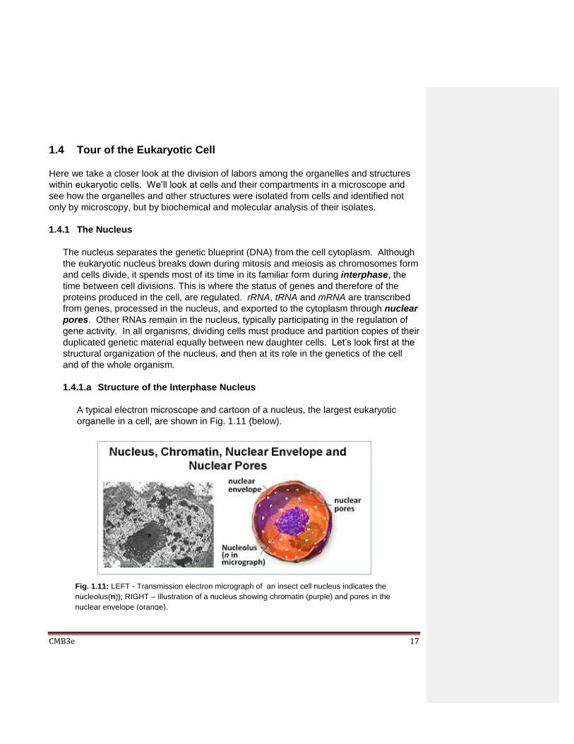
1.4.1.a Structure of the Interphase Nucleus

A typical electron microscope and cartoon of a nucleus, the largest eukaryotic

organelle in a cell, are shown in Fig. 1.11 (below).

Fig. 1.11: LEFT - Transmission electron micrograph of an insect cell nucleus indicates the

nucleolus(n)); RIGHT – Illustration of a nucleus showing chromatin (purple) and pores in the

nuclear envelope (orange).

CMB3e 18

This cross-section of an interphase nucleus reveals its double membrane, or

nuclear envelope. The outer membrane of the nuclear envelope is continuous

with the RER (rough endoplasmic reticulum). Thus, the lumen of the RER is

continuous with the space separating the nuclear envelope membranes. The

electron micrograph also shows a prominent nucleolus (labeled n) and a darkly

granular RER surrounding the nucleus. Zoom in on the micrograph; you may see

the double membrane of the nuclear envelope. You can also make out ribosomes

(small granules) bound to both the RER and the outer nuclear membrane. Nuclear

envelope pores (illustrated in the cartoon at the right) allow large molecules and

even particles to move in and out of the nucleus across both membranes. We

learn what some of this nuclear pore traffic is all about in later chapters.

104-2 The nucleus

The nucleus is not an unorganized space surrounded by the nuclear envelope, as

might appear in transmission electron micrographs. The nucleolus is the largest of

several inclusions that seem to segregate nuclear functions. Over 100 years ago

Santiago Ramón y Cajal reported other structures in the nuclei of neurons,

including what came to be known as Cajal bodies (CBs). His elegant hand-drawn

illustrations of nuclear bodies (made long before the advent of photomicrography)

can be seen at Cajal's Nuclear Bodies and Cajal's Beautiful Brain Cells. Cajal and

Camillo Golgi shared the Nobel Prize in Physiology or Medicine 1906 for their

studies of nerve cell structure. In the electron microscope, Cajal bodies (CBs)

look like coils of tangled thread, and were thus called coiled bodies (conveniently,

also CBs). Other nuclear bodies since identified include Gems, PML bodies,

nuclear speckles (or splicing speckles), histone locus bodies (HLBs), and

more! Different nuclear bodies are associated with specific proteins. Fig. 1.12

below illustrates the results of immunofluorescence localization of nuclear body

proteins. Nucleoli contain fibrillarin proteins and stain red because they have

been treated with red-fluorescence-tagged antifibrillarin antibodies. CBs contain

the protein coilin. They fluoresce pink because the nuclei were treated with

fluorescence-tagged anticoilin antibodies. Green-fluorescent antibodies to the

ASF/SF2 protein localize to nuclear speckles. As part of, or included in a nuclear

matrix, nuclear bodies organize and regulate different aspects of nuclear activity

and molecular function. The different nuclear bodies perform specific functions

and interact with each other and with proteins DNA and RNA to do so.

We will revisit some nuclear bodies in their working context in later chapters.

CMB3e 19

1.4.1.b Every Cell (i.e., Every Nucleus) of an Organism Contains the Same

Genes

We read earlier that bacteria are busy doubling and partitioning their naked DNA

chromosomes at the same time as they grow and divide by binary fission. In

eukaryotic cells, a cell cycle divides life into discrete consecutive events. During

most of the cell cycle, cells are in interphase and DNA is wrapped up in proteins in

a structure called chromatin. It is not merely the DNA, but chromatin that must be

duplicated when cells reproduce. Duplication of DNA also involves rearranging, or

disturbing the chromatin proteins resting on the DNA. This occurs before cell

division (mitosis and cytokinesis). As the time of cell division nears, chromatin

associates with even more proteins, condensing to form chromosomes, while the

nuclear envelope dissolves. You may recall that every somatic cell of a eukaryotic

organism contains paired homologous chromosomes, and therefore two copies of

every gene an organism owns. On the other hand, sperm and eggs contain one of

each pair of chromosomes, and thus one copy of each gene. Whether by mitosis

or meiosis, cytokinesis separates duplicated chromosomes to daughter cells.

In the fluorescence micrograph below of a cell in the metaphase stage of mitosis

(Fig.1.13), the chromosomes (blue) are just about to be pulled apart by

microtubules of the spindle apparatus (green). As the chromosomes separate and

daughter cells form, nuclei will reappear and chromosomes will de-condense.

Fig. 1.12: Simulated fluorescence micrograph showing the immunolocalization of antibodies

against fibrillarin, coilin and ASF/SF2 protein to nuclear bodies (nucleolus, Cajal Bodies and

nuclear speckles, respectively).

CMB3e 20

These events mark the major visible difference between cell division in bacteria

and eukaryotes. Cytokinesis begins near the end of mitosis. Sexual reproduction,

a key characteristic of eukaryotes, involves meiosis rather than mitosis. The

mechanism of meiosis, the division of germ cells leading to production of sperm

and eggs, is similar to mitosis except that the ultimate daughter cells have just one

each of the parental chromosomes, eventually to become the gametes (eggs or

sperm). Google meiosis and/or mitosis to remind yourself about the differences

between the two processes, meiosis and mitosis.

A key take-home message here is that every cell in a multicellular organism,

whether egg, sperm or somatic, contains the same genome (genes) in its nucleus.

This was understood since mitosis and meiosis were first described in the late 19th

century. However, it was finally demonstrated in 1962, when John Gurdon and

Shinya Yamanaka transplanted nuclei from the intestinal cells the frog Xenopus

laevis into enucleated eggs (eggs from which its own nucleus had been removed).

These ‘eggs’ grew and developed into normal tadpoles, proving that no genes are

lost during development, but just expressed differentially. We will revisit animal

cloning later in this book. But for now, it’s sufficient to know that Molly the cloned

frog was followed in 1996 by Dolly, the first cloned sheep, and then other animals,

all cloned from enucleated eggs transplanted with differentiated cell nuclei. Click

Cloning Cuarteterra for the 60 Minutes story of the cloning of Cuarteterra, a

champion polo mare whose clones are also champions! For their first animal

cloning experiments, Gurdon and Yamanaka shared the 2012 Nobel Prize form

Physiology or medicine.

Fig. 1.13: Fluorescence micrograph of a mitotic spindle treated with antibodies to chromosomal

proteins (blue) and spindle fiber proteins (green).

CMB3e 21

1.4.2 Ribosomes

On the other end of the size spectrum, ribosomes are evolutionarily conserved protein

synthesizing machines in all cells. They consist of a large and a small subunit, each

made up of multiple proteins and one or more molecules of ribosomal RNA (rRNA).

Ribosomes bind to messenger RNA (mRNA) molecules and then move along the

mRNA as they translate 3-base code words (codons) to link amino acids into

polypeptides. Multiple ribosomes can move along the same mRNA, becoming a

polyribosome, simultaneously translating the same polypeptide encoded by the

mRNA. The granular appearance of cytoplasm in electron micrographs is largely due

to the ubiquitous distribution of ribosomal subunits and polysomes in cells. Fig. 1.14

shows a polyribosome ‘string’ of ribosomes, or polysome for short.

In the illustration, ribosomes assemble at the left of the messenger RNA (mRNA) to form

the polysome. When they reach the end of the message, the ribosomes disassemble

from the RNA and release the finished polypeptide. In electron micrographs of leaf cells

from the dry, quiescent desiccation-tolerant dessert plant, Selaginella lepidophylla

(Fig.1.15, below), you can make out randomly distributed ribosomes and ribosomal

subunits (arrows, below left). In cells from a fully hydrated plant, you can see polysomes

as more organized strings of ribosomes (arrows, below right).

Fig. 1.14: To form a polysome, ribosomes (blue) assemble at the left on an mRNA molecule.

As they move along the mRNA from left to right, they translate the message into a

polypeptide (green), shown growing and emerging from ribosomes in the polysome.

CMB3e 22

Eukaryotic and prokaryotic ribosomes differ in the number of RNAs and proteins in their large and small subunits, and thus in their overall size. Isolated ribosomes and their subunits can be separated based on differences in mass. Fig.1.16 shows the difference in ribosomal subunit ‘size’, protein and ribosomal RNA (rRNA) composition.

Fig. 1.15: Transmission electron micrographs of cells from desiccated and fully hydrated

Selaginella lepidophylla plants. Free ribosomes or ribosomal subunits in the desiccated cells

(LEFT) appear to have organized to form polysomes in the hydrated plant cells (RIGHT).

Fig. 1.16: Key differences between prokaryotic and eukaryotic ribosomes: Eukaryotic ribosomes

and their subunits are larger and contain more proteins and larger ribosomal RNAs (rRNAs) than

those of bacteria. The components were separated by sucrose density gradient centrifugation in

which particles and macromolecules (like RNA) move through a sugar gradient at rates

dependent on their mass (in effect, their size).

CMB3e 23

The position of ribosomal subunits in the gradient is represented by an S value, after

Svedborg, who first used sucrose density gradients to separate macromolecules and

particles by mass. Note that ribosomal RNAs themselves also separate on sucrose

density gradients by size, hence their different S values.

101 Ribosomes & Polysomes 1.4.3 Internal membranes and the Endomembrane System

Microscopists of the 19th century saw many of sub-cellular structures using the art of

histology, staining cells to increase the visual contrast between cell parts. One of

these, Camillo Golgi, an early neurobiologist, developed a silver (black) stain that first

detected a network of vesicles we now call Golgi bodies or Golgi vesicles in nerve

cells. For his studies of membranes now named after him, Camillo Golgi shared the

1906 Nobel prize for Medicine or Physiology with Santiago Ramón y Cajal.

Many vesicles and vacuoles in cells, including Golgi vesicles, are part of the

endomembrane system. Proteins synthesized on the ribosomes of the RER (rough

endoplasmic reticulum) can enter the interior space (lumen) or can become part of

the RER membrane itself. The synthesis of RER, SER (smooth endoplasmic

reticulum), Golgi bodies, lysosomes, microbodies and other vesicular membranes

(as well as their protein content) all begin in the RER. The RER and protein contents

bud into transport vesicles that fuse with Golgi Vesicles (G in the electron micrograph

in Fig. 1.17).

In moving through the endomembrane system, packaged proteins undergo stepwise

modifications (maturation) before becoming biologically active (Fig.1.18, below). Some

proteins made in the endomembrane system are secreted by exocytosis. Others end

up in organelles such as lysosomes that contain hydrolytic enzymes. These

Fig. 1.17: Transmission electron micrograph of an insect cell showing Golgi bodies (G).

CMB3e 24

enzymes are activated when the lysosomes fuse with other organelles destined for

degradation. For example, food vacuoles form when a plasma membrane

invaginates, engulfing food particles. They then fuse with lysosomes to digest the

engulfed nutrients. Still other proteins synthesized by ribosomes on the RER are

incorporated into the RER membranes, destined to become part of lysosomes,

peroxisomes and even the plasma membrane itself.

100-2 The RER-Rough Endoplasmic Reticulum

102 Golgi Vesicles & the Endomembrane System

Autophagosomes are small vesicles that surround and eventually encapsulate tired

organelles (for example, worn out mitochondria), eventually merging with lysosomes

whose enzymes degrade their contents. In 2016, Yoshinori Ohsumi earned the Nobel

Prize in Physiology and Medicine for nearly 30 years of research unraveling the cell

and molecular biology of autophagy. Microbodies are a class of vesicles smaller

than lysosomes but formed by a similar process. Among them are peroxisomes that

break down toxic peroxides formed as a by-product of cellular biochemistry. Some

vesicles emerging from the RER lose their ribosomes to become part of the SER,

which has several different functions (e.g., alcohol detoxification in liver cells).

103-2 Smooth Endoplasmic Reticulum

Fig. 1.18: Illustration of ‘packaged’ protein traffic through a cell, from the RER to organelles (e.g.,

lysosomes) or to the plasma membrane for exocytosis (i.e., secretion). RER and Golgi vesicles are

major sites for the modification (i.e., maturation) of packaged proteins.

CMB3e 25

Other organelles include the contractile vacuoles of freshwater protozoa that expel excess water that enters cells by osmosis. Some protozoa have extrusomes, vacuoles that release chemicals or structures that deter predators or enable prey capture. A large aqueous central vacuole dominates the volume of many higher plant cells. When filled with water, they will push all other structures against the plasma membrane. In a properly watered plant, this water-filled vacuole exerts osmotic pressure that among other things, keeps plant leaves from wilting and stems upright.

1.4.4 Mitochondria and Plastids

Nearly all eukaryotic cells contain mitochondria, shown in Fig.1.19.

A double membrane surrounds the mitochondrion. Each contains and replicates its

own DNA, which contains genes encoding some mitochondrial proteins. Note that the

surface area of the inner mitochondrial membrane is increased by being folded into

cristae, which are sites of cellular respiration (aerobic nutrient oxidation).

Earlier, we speculated that some eukaryotic organelles could have originated within

bacteria. But mitochondria most likely evolved from a complete aerobic bacterium (or

proto-bacterium) that was engulfed by a primitive eukaryotic cell. The bacterium

Fig. 1.19: Transmission electron micrograph (LEFT) and drawing of a mitochondrion (RIGHT).

CMB3e 26

escaped destruction, becoming an endosymbiont in the host cell cytoplasm. Lynn

Margulis proposed the Endosymbiotic Theory in 1967 (Margulis, L. [Sagan, L],

1967. On the origin of mitosing cells. Journal of Theoretical Biology 14 (3): 225–274).

Read her paper at Margulis-Endosymbiosis. She proposed that chloroplasts (one

among several different plastids) also started as endosymbionts. Both mitochondria

and the plastids of plants and some algae have their own DNA, supporting their

origins as bacteria and cyanobacteria engulfed by primitive eukaryotic cells. Living at

first in symbiosis with the rest of the cell, they would eventually evolve into the

organelles that we are familiar with.

A handful of protozoa were discovered that lack mitochondria and other organelles.

This had suggested they might share ancestry with those primitive eukaryotes that

acquired mitochondria by endosymbiosis. However, since such cells contain other

organelles such as hydrogenosomes and mitosomes, it is thought more likely that

these species once had, but then lost mitochondria. Therefore, descendants of

ancient eukaryotic cells missing mitochondria probably no longer exist…, if they ever

existed at all! More evidence for the Endosymbiotic Theory is discussed elsewhere.

Chloroplasts and cyanobacteria contain chlorophyll and use a similar photosynthetic

mechanism to make glucose. Typical chloroplasts are shown (Fig. 1.20, below). The

one on the right is shows a few starch granules.

A leucoplast is a plastid. It is a chloroplast that has become filled with starch granules.

In the micrograph of a leucoplast in Fig.1.21 (below), you can see that because of the

accumulation of starch, the grana have become dispersed and indistinct.

Fig. 1.20: Transmission electron micrograph of chloroplast that could have begun

photosynthesizing (LEFT), and one that has photosynthesized long enough to

accumulated starch granules (RIGHT). S, starch granule; T, thylakoids.

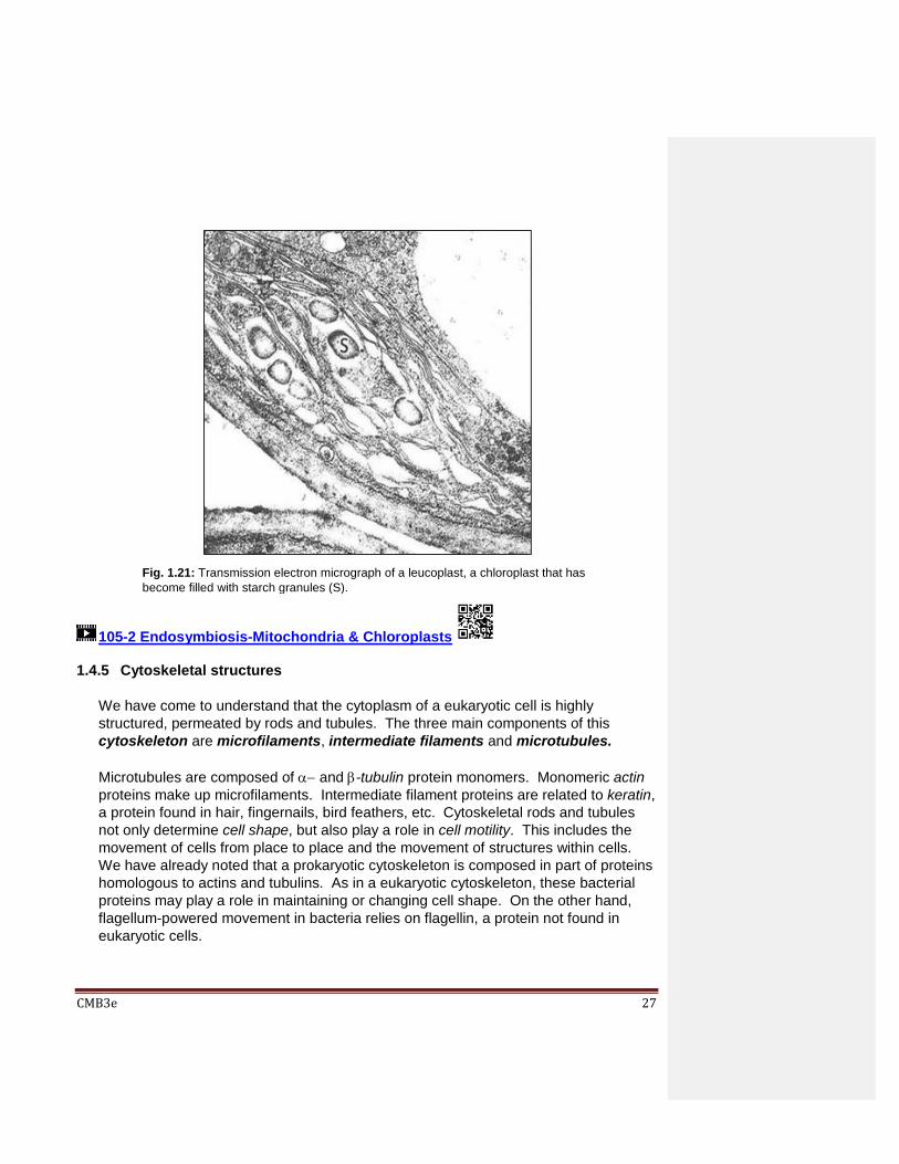
CMB3e 27

105-2 Endosymbiosis-Mitochondria & Chloroplasts

1.4.5 Cytoskeletal structures

We have come to understand that the cytoplasm of a eukaryotic cell is highly

structured, permeated by rods and tubules. The three main components of this

cytoskeleton are microfilaments, intermediate filaments and microtubules.

Microtubules are composed of and -tubulin protein monomers. Monomeric actin

proteins make up microfilaments. Intermediate filament proteins are related to keratin,

a protein found in hair, fingernails, bird feathers, etc. Cytoskeletal rods and tubules

not only determine cell shape, but also play a role in cell motility. This includes the

movement of cells from place to place and the movement of structures within cells.

We have already noted that a prokaryotic cytoskeleton is composed in part of proteins

homologous to actins and tubulins. As in a eukaryotic cytoskeleton, these bacterial

proteins may play a role in maintaining or changing cell shape. On the other hand,

flagellum-powered movement in bacteria relies on flagellin, a protein not found in

eukaryotic cells.

Fig. 1.21: Transmission electron micrograph of a leucoplast, a chloroplast that has

become filled with starch granules (S).

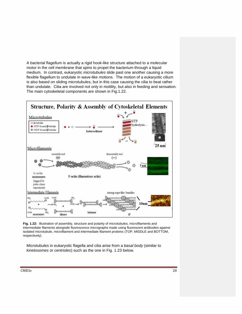
CMB3e 28

A bacterial flagellum is actually a rigid hook-like structure attached to a molecular

motor in the cell membrane that spins to propel the bacterium through a liquid

medium. In contrast, eukaryotic microtubules slide past one another causing a more

flexible flagellum to undulate in wave-like motions. The motion of a eukaryotic cilium

is also based on sliding microtubules, but in this case causing the cilia to beat rather

than undulate. Cilia are involved not only in motility, but also in feeding and sensation.

The main cytoskeletal components are shown in Fig.1.22.

Microtubules in eukaryotic flagella and cilia arise from a basal body (similar to

kinetosomes or centrioles) such as the one in Fig. 1.23 below.

Fig. 1.22: Illustration of assembly, structure and polarity of microtubules, microfilaments and

intermediate filaments alongside fluorescence micrographs made using fluorescent antibodies against

isolated microtubule, microfilament and intermediate filament proteins (TOP, MIDDLE and BOTTOM,

respectively).

CMB3e 29

Aligned in a flagellum or cilium, microtubules form an axoneme surrounded by plasma

membrane. In electron micrographs of cross sections, a ciliary or flagellar axoneme is

typically organized as a ring of nine paired microtubules (called doublets) around two

singlet microtubules. This 9+2 arrangement of microtubules is illustrated in Fig. 1.24.

Centrioles are themselves comprised of a ring of microtubules. In animal cells they

participate in spindle fiber formation during mitosis and are the point from which

microtubules radiate thorough the cell to help form and maintain its shape. These

structures do not involve axonemes. The spindle apparatus in plant cells, which

typically lack centrioles, form from an amorphous structure called the MTOC, or

MicroTubule Organizing Center, which serves the same purpose in mitosis and

meiosis as centrioles do in animal cells.

106-2 Filaments & Tubules of the Cytoskeleton

Fig. 1.23: Transmission electron micrograph showing a flagellum (#1) emerging from a basal

body (2). Number 3 is another basal body, this time in cross section.

Fig. 1.24: The characteristic “9+2” arrangement of microtubules seen in cross-sections of

eukaryotic cilia and flagella is maintained the axoneme, a structure remaining after removing the

plasma membrane from isolated cilia or flagella.

CMB3e 30

Elsewhere, we describe how microfilaments and microtubules interact with motor

proteins (dynein, kinesin, myosin, etc.) to generate force that results in the sliding of

filaments and tubules to allow cellular movement. You will see that motor proteins can

also carry cargo molecules from one place to another in a cell.

1.5 How We Know the Functions of Cellular Organelles and

Structures: Cell Fractionation

We can see and describe cell parts in the light or electron microscope, but we could not

definitively know their function until it became possible to release them from cells and

separate them from one another. This became possible with the advent of differential

centrifugation (the example of the separation of ribosomes and ribosomal components

was mentioned earlier). Under centrifugal force generated by a spinning centrifuge,

subcellular structures separate by differences in mass. Structures that are more massive

reach the bottom of the centrifuge tube before less massive ones. A cell fractionation

scheme is illustrated in Fig 1.25. Biochemical analysis of the isolated cell fractions can

reveal what different organelles and cellular substructures do.

107-2 Dissecting the Cell-a Cell Fractionation Scheme

Fig. 1.25: A cell fractionation involving disruption of cells and the isolation of sub-cellular

components, including organelles, ribosomes and a soluble fraction, the cytosol.

Separation is achieved by successive centrifugations at different speeds (centrifugal

forces) that sediment subcellular structures on the basis of mass; the lowest mass

structures require the highest G-forces (fastest spin), requiring an ultracentrifuge.

CMB3e 31

Cell fractionation separates cells into their constituent parts. The first step of a cell

fractionation is to break open the cells and release their contents. This can be done by

physical means such as grinding in a mortar and pestle, tissue grinder or similar device,

exposure to ultrasound or high pressure, or exposure to enzymes or other chemicals that

can selectively degrade the plasma membrane. The next step is to isolate the subcellular

organelles and particles from the cytoplasm (i.e., cytosol) by differential centrifugation.

The centrifugation of broken cells at progressively higher centrifugal force separates

particulate cell components based on their mass. At the end of this process, a researcher

will have isolated mitochondria, chloroplasts, nuclei, ribosomes etc. After re-suspension,

each pellet can be re-suspended and prepared for microscopy. Electron micrographs of

several isolated subcellular fractions are shown in Fig. 1.25, below.

These structures can be tentatively identified by microscopy based on their dimensions

and appearance. Molecular analyses and biochemical tests on the cell fractions then

help to confirm these identities.

108-2 Isolated Nuclei 109-2 Isolated RER

110-2 Isolated Golgi Vesicles 111-2 Lysosomes & Peroxisomes

112-2 Isolated Mitochondria 113-2 Isolated Chloroplasts

114-2 Isolated Membranes Form Vesicles

Fig. 1.26: Organelles isolated by cell fractionation from eukaryotic cells.

1.

CMB3e 32

Can you tell what organelles have been purified in each of these fractions based on the

electron micrographs alone? Consider the structures on the left as an example. These

were found in a low speed centrifugal pellet, implying that they are large structures. They

look a bit like nuclei, which are also the largest structures in a eukaryotic cell…, and

indeed that’s what they are! Physical separation combined with biochemical-molecular

analysis of subcellular structures has revealed their basic functions and continues to reveal previously un-noticed structures and functions in cells. What biochemical tests might you do to confirm the identities of the structures shown? All of cell and molecular biology is devoted to understanding how prokaryotic and

eukaryotic cells (and organisms) use their common structural and biochemical inheritance

to meet very different survival strategies. As you progress in your studies, watch for

experiments in which cell parts are separated and reassembled (i.e., reconstituted).

Reconstitution is a recurring experimental theme in the functional analysis of cell parts.

Look for it as you continue your studies. Also look another theme, namely how evolution

accounts for the common biochemistry and genetics of life…, and its structural diversity!

1.6 The Origins, Evolution, Speciation, Diversity and Unity of Life

The question of how life began has been with us since the beginnings or recorded history.

It is now accepted that there was a time, however brief or long, when the earth was a

lifeless (prebiotic) planet. Life’s origins on earth date to some 3.7-4.1 billion years ago

under conditions that favored the formation of the first cell, the first entity with all of the

properties of life.

But couldn’t those same conditions have spawned multiple cells independently, each with

all of the properties of life? If so, from which of these did life, as we know it today,

descend? Whether there were one or more different “first cells”, evolution (a property of

life) could only begin with ‘that or those’ cells.

115 Properties of Life

The fact that there is no evidence of cells of independent origin may reflect that they

never existed. Alternatively, we can propose that the cell we call our ancestor was

evolutionarily successful at the expense of other early life forms, which thus became

extinct. In any event, whatever this successful ancestor may have looked like, its

descendants would have evolved quite different biochemical and physiological solutions

to achieving and maintaining life’s properties. One of these descendants evolved the

solutions we see in force in all cells and organisms alive today, including a common

(universal) genetic code to store life’s information, as well as a common mechanism for

CMB3e 33

retrieving the encoded information. Francis Crick called is commonality the “Central

Dogma” of biology. That ancestral cell is called our Last Universal Common Ancestor,

or LUCA.

116 The Universal Genetic Code 117 Origins of Life

118 Life Origins vs Evolution Elsewhere we consider in more detail how we think about the origins of life. For the

moment, our focus is on evolution, the property of life that is the basis of speciation and

life’s diversity. Charles Darwin’s theory of evolution was an explanation of the structural

diversity of species. A naturalist, Darwin lived at a time of ferment where scientific

discovery was challenging religion. But by 1839, Charles Darwin had published his

Narrative of the Surveying Voyages of His Majesty's Ships Adventure and Beagle,

the first of many reports of his careful observations of nature, with the seeds of what was

to become his theory of natural selection. He published his more fully formed theory of

evolution by natural selection in 1859 in The Origin of Species. There he finally

acknowledged his evidence-based belief that that new species arise when beneficial traits

are selected from random genetic differences in individuals in a population, while less fit

individuals are culled from the population. If natural selection acting on individuals, the

emergence of new species (evolution) results from the persistence and spread of

selected, heritable changes through successive generations in a population. In this way,

evolution results in an increase in diversity and complexity at all levels of biological

organization, from species to individual organisms and all the way down to biomolecules.

Darwin recognized the discord his theory would generate between science and biblical

accounts of purposeful creation. He addressed the issue with great tact in introducing

The Origin of Species: “Although much remains obscure, and will long remain obscure, I

can entertain no doubt, after the most deliberate study and dispassionate judgement of

which I am capable, that the view which most naturalists entertain, and which I formerly

entertained–namely, that each species has been independently created–is erroneous.”

According to creationists, the exquisite eyes could only have formed by the intelligent

design of a creator. But see the article in National Geographic by E. Yong (Feb., 2016,

with photography by D. Littschwager). Over time science favored Darwin. With the

rediscovery of Mendel’s genetic experiments at the turn of the 20th century , it became

increasingly clear that it is an organism’s genes that are inherited, are passed down the

generations, and are the basis of an organism’s traits. It also became clear that Mendel

had found the genetic basis for Darwin’s theory and that the evolution of eyes can be

explained. Over time, science and religion have found ways to co-exist but as we know,

the controversy persists.

CMB3e 34

Repeated speciation occurs with the continual divergence of life forms from an ancestral

cell through natural selection and evolution. Our shared cellular structures, nucleic acid,

protein and metabolic chemistries (the ‘unity’ of life) supports our common ancestry with

all life. These shared features date back to our LUCA! Take as an example the fact that

most living things even share some early behaviors. Our biological clock is an

adaptation to our planet’s 24-hour daily cycles of light and dark that have been around

since the origins of life; all organisms studied so far seem to have one!. The discovery of

the genetic and molecular underpinnings of circadian rhythms (those daily cycles)

earned Jeffrey C. Hall, Michael Rosbash and Michael W. Young the 2017 Nobel Prize in

Medicine or Physiology (click Molecular Studies of Circadian Rhythms wins Nobel Prize to

learn more)!

The molecular relationships common to all living things largely confirm what we have

learned from the species represented in the fossil record. Morphological, biochemical

and genetic traits that are shared across species are defined as homologous and can be

used to reconstruct evolutionary histories. The biodiversity that scientists (in particular,

environmentalists) try to protect is the result of millions of years of speciation and

extinction. Biodiversity needs protection from the unwanted acceleration of evolution

arising from human activity, including blatant extinctions (think passenger pigeon), and

near extinctions (think American bison by the late 1800s). Think also of the

consequences of the introduction of invasive aquatic and terrestrial species and the

effects of climate change.

Let’s look at the biochemical and genetic unity among livings things. We’ve already

considered what happens when cells get larger when we tried to explain how larger cells

divide their labors among smaller intracellular structures and organelles. When

eukaryotic cells evolved further into multicellular organisms, it became necessary for the

different cells to communicate with each other and to respond to environmental cues.

Some cells evolved mechanisms to “talk” directly to adjacent cells and others evolved to

transmit electrical (neural) signals to other cells and tissues. Still other cells produced

hormones to communicate with cells far away, to which they had no physical attachment.

As species diversified to live in very different habitats, they also evolved very different

nutritional requirements, along with more extensive and elaborate biochemical pathways

to digest their nutrients and capture their chemical energy. Nevertheless, through billions

of years of evolution and astonishing diversification, the underlying genetics and

biochemistry of living things on this planet is remarkably unchanged. Early in the 20th

century, Albert Kluyver first recognized that cells and organisms vary in form appearance

in spite of an essential biochemical unity of all organisms (see Albert Kluyver in

Wikipedia). This unity amidst the diversity is a life paradox that we examine in this course.

CMB3e 35

1.6.1 Random Acts of Genetic Variation, the Basis of Natural Selection

DNA contains the genetic instructions for the structure and function of cells and

organisms. When and where a cell or organism’s genetic instructions are used (i.e., to

make RNA and proteins) are regulated. Genetic variation results from random

mutations. Genetic diversity arising from mutations is in turn, the basis of natural

selection during evolution.

119 The Random Basis of Evolution 1.6.2 The Genome: An Organism’s Complete Genetic Instructions

We’ve seen that every cell of an organism carries the DNA that includes genes and

other kinds DNA sequences. The genome of an organism is the entirety of its genetic

material (DNA, or for some viruses, RNA). The genome of a common experimental

strain of E. coli was sequenced by 1997 (Blattner FR et al. 1997The complete genome

sequence of Escherichia coli K-12. Science 277:1452-1474). Sequencing of the

human genome was completed by 2001, well ahead of the predicted schedule (Venter

JC 2001The sequence of the human genome. Science 291:1304-1351). As we have

seen in the re-classification of life from five kingdoms into three domains, nucleic acid

sequence comparisons can tell us a great deal about evolution. We now know that

evolution depends not only on gene sequences, but also, on a much grander scale, on

the structure of genomes. Genome sequencing has confirmed not only genetic

variation between species, but also considerable variation between individuals of the

same species. The genetic variation within species is the raw material of evolution. It

is clear from genomic studies that genomes have been shaped and modeled (or

remodeled) in evolution. We’ll consider genome remodeling in more detail elsewhere.

1.6.3 Genomic ‘Fossils’ Can Confirm Evolutionary Relationships.

It had been known for some time that gene and protein sequencing could reveal

evolutionary relationships and even familial relationships. Read about an early

demonstration of such relationships based on amino acid sequence comparisons

across evolutionary time in Zuckerkandl E and Pauling L. (1965) Molecules as

documents of evolutionary theory. J. Theor. Biol. 8:357-366. It is now possible to

extract DNA from fossil bones and teeth, allowing comparisons of extant and extinct

species. DNA has been extracted from the fossil remains of humans, other hominids,

and many animals. DNA sequencing reveals our relationship to animals (from bugs to

frogs to mice to chimps…) and to Neanderthals and our other hominid ancestors.

Unfortunately, DNA from organisms much older than 10,000 years is typically so

damaged or simply absent, that relationship building beyond that time is impossible.

CMB3e 36

Now in a clever twist, using what we know from gene sequences of species alive

today, investigators recently ‘constructed’ a genetic phylogeny suggesting the

sequences of genes of some of our long-gone progenitors, including bacteria (click

here to learn more: Deciphering Genomic Fossils). The comparison of these

‘reconstructed’ ancestral DNA sequences suggests when photosynthetic organisms

diversified and when our oxygenic planet became a reality.

Closer to home, many remains of ancestral humans have been discovered in the

Americas. These promise to unlock mysteries of human settlement of the continents,

but not without controversy. Indian tribal cultures treat their ancestors as sacred and

argue against sampling such remains for DNA Analysis. In one example a well

preserved ‘mummified’ body discovered in the Nevada desert in the 1940s. Tests of

hair and clothing fragments revealed that this Spirit Cave mummy was over 10,000

years old. The Fallon Paiute-Shoshone tribe that lives near the burial site asserted a

cultural relationship to the body and requested the right to its return to the tribe in

compliance with the Native American Graves Protection and Repatriation Act.

Anthropologists counter-asserted a need for further study of the body to learn more

about its origins and about native American origins in general. The dispute ended only

after 20 years. By the time DNA tests were allowed, the results established that the

remains was indeed that of an ancestor to the tribe, and the Spirit Cave mummy was

reburied with tribal rites at the beginning of 2018. To read more, see Resolving

American Indian Ancestry - a 60-Year Old Controversy or The-worlds-oldest-natural-

mummy-unlocks-secrets-ice-age-tribes-americas

120-2 Genomic Fossils-Molecular Evolution

1.7 Microscopy Reveals Life’s Diversity of Structure and Form

Broadly speaking, there are two kinds of microscopy. In Light Microscopy, the specimen

on the slide is viewed through optical glass lenses. In Electron Microscopy, the viewer is

looking at an image on a screen created by electrons passing through or reflected from

the specimen. For a sampling of light and electron micrographs, check out this Gallery of

Micrographs. Here we compare and contrast different microscopic techniques.

1.7.1 Light Microscopy

Historically one form or other of light microscopy has revealed much of what we know

of cellular diversity. Check out the Drawings of Mitosis for a reminder of how

eukaryotic cells divide and then check out The Optical Microscope for descriptions of

different variations of light microscopy (e.g., bright-field, dark field, phase-contrast,

CMB3e 37

fluorescence, etc.). Limits of magnification and resolution of 1200X and 2 m,

(respectively) are common to all forms of light microscopy. The main variations of

light microscopy are briefly described below.

Bright-Field microscopy is the most common kind of light microscopy, in which the

specimen is illuminated from below. Contrast between regions of the specimen

comes from the difference between light absorbed by the sample and light passing

through it. Live specimens lack contrast in conventional bright-field microscopy

because differences in refractive index between components of the specimen (e.g.,

organelles and cytoplasm in cells) diffuse the resolution of the magnified image.

This is why Bright-Field microscopy is best suited to fixed and stained specimens.

In Dark-field illumination, light passing through the center of the specimen is

blocked and the light passing through the periphery of the beam is diffracted

(“scattered”) by the sample. The result is enhanced contrast for certain kinds of

specimens, including live, unfixed and unstained ones.

In Polarized light microscopy, light is polarized before passing through the

specimen, allowing the investigator to achieve the highest contrast by rotating the

plane of polarized light passing through the sample. Samples can be unfixed,

unstained or even live.

Phase-Contrast or Interference microscopy enhances contrast between parts of a

specimen with higher refractive indices (e.g., cell organelles) and lower refractive

indices (e.g., cytoplasm). Phase–Contrast microscopy optics shift the phase of the

light entering the specimen from below by a half a wavelength to capture small

differences in refractive index and thereby increase contrast. Phase–Contrast

microscopy is a most cost-effective tool for examining live, unfixed and unstained

specimens.

In a fluorescence microscope, high-energy short wavelength (usually UV) light is

passed through a specimen that has been treated with a fluorescing chemical

covalently attached to other molecules (e.g., antibodies) that fluoresce when struck

by the light source. The fluorescent tag was chosen to recognize and bind specific

molecules or structures in a cell. Thus, in fluorescence microscopy, the visible

color of fluorescence marks the location of the target molecule/structure in the cell.

Confocal microscopy is a variant of fluorescence microscopy that enables imaging

through thick samples and sections. The result is often 3D-like, with much greater

depth of focus than other light microscope methods. Click at Gallery of Confocal

Microscopy Images to see a variety of confocal micrographs and related images;

look mainly at the specimens.

CMB3e 38

Lattice Light-Sheet Microscopy is a 100-year old variant of light microscopy that

allows us to follow subcellular structures and macromolecules moving about in

living cells. There has been renewed interest in this form of light microscopy.

Read more about this technique at Lattice Light Sheet Microscopy.

1.7.2 Electron Microscopy

Unlike light (optical) microscopy, electron microscopy generates an image by passing

electrons through, or reflecting electrons from a specimen, and capturing the electron

image on a screen. Transmission Electron Microscopy (TEM) can achieve much

higher magnification (up to 106X) and resolution (2.0 nm) than any form of optical

microscopy! Scanning Electron Microscopy (SEM) can magnify up to 105X with a

resolution of 3.0-20.0 nm. TEM, together with biochemical and molecular biological

studies, continues to reveal how different cell components work with each other. The

higher voltage in High Voltage Electron microscopy is an adaptation that allows TEM

through thicker sections than regular (low voltage) TEM. The result is micrographs

with greater resolution, depth and contrast. SEM allows us to examine the surfaces of

tissues, small organisms like insects, and even of cells and organelles. Check this link

to Scanning Electron Microscopy for a description of scanning EM, and look at the

gallery of SEM images at the end of the entry.

121-2 Electron Microscopy

Some iText & VOP Key words and Terms Actin Eukaryotes Nuclear envelope

Archaea Eukaryotic flagella Nuclear pores

Bacterial cell walls Evolution Nucleoid

Bacterial Flagella Exocytosis nucleolus

Binary fission Extinction Nucleus

Cell fractionation Hypothesis Optical microscopy

Cell theory Inference Plant cell walls

Chloroplasts Intermediate filaments Plasmid

chromatin keratin Progenote

Chromosomes Kingdoms Prokaryotes

Cilia LUCA Properties of life

Confocal microscopy Lysosomes Rough endoplasmic reticulum

CMB3e 39

Cytoplasm Meiosis Scanning electron microscopy

Cytoskeleton Microbodies Scientific method

Cytosol Microfilaments Secretion vesicles

Deduction Microtubules Smooth endoplasmic reticulum

Differential centrifugation Mitochondria Speciation

Diversity Mitosis Theory

Domains of life Motor proteins Tonoplast

Dynein Mutation Transmission electron microscopy

Endomembrane system Natural selection Tubulins

CMB3e 40

Chapter 2: Basic Chemistry, Organic Chemistry

and Biochemistry Atoms and Elements (protons, neutrons, electrons, atomic models); Chemical Bonds

(covalent, polar covalent, ionic, H-bonds); Water properties, chemistry, pH; Organic

molecules, monomers and polymers; biochemistry, chemical groups, condensation and

hydrolysis, macromolecules (polysaccharides, polypeptides, proteins, DNA, RNA), lipids

2.1 Introduction

In this chapter, we start with a review basic chemistry from atomic structure to

molecular bonds to the structure and properties of water, followed by a review of key

principles of organic chemistry - the chemistry of carbon-based molecules. You may find

it useful to have your old general chemistry textbook handy or check out the excellent

introduction to general chemistry by Linus Pauling (1988, General Chemistry New York,

Springer-Verlag). We’ll see how the polar covalent bonds define the structure and

explain virtually all of the properties of water. These range from the energy required to

melt a gram of ice to vaporize a gram of water to its surface tension to its ability to hold

heat…, not to mention its ability to dissolve a wide variety of solutes from salts to

Do you know? Did you guess correctly?

CMB3e 41

proteins and other macromolecules. We will distinguish water’s hydrophilic interactions

with solutes from its hydrophobic interactions with fatty molecules. Then we review

some basic biochemistry. Well-known biological molecules include monomers (sugars,

amino acids, nucleotides, lipids…) and polymers (polysaccharides, proteins, nucleic

acids, fats…).

Biochemical reactions that link glucose monomers into polymers on the one hand, and

break the polymers down on the other, are essential reactions for life… on earth and

probably anywhere else! On our planet, photosynthetic organisms link glucose

monomers into starch, a polysaccharide. Amylose is a simple starch, a large

homopolymer of repeating glucose monomers. Likewise, polypeptides are

heteropolymers of 20 different amino acids. DNA and RNA nucleic acids are also

heteropolymers, made using only four different nucleotides.

Digestive enzymes in your gut catalyze the hydrolysis, or breakdown of the plant or

animal polymers we ate back down to monomers. Hydrolysis adds a water molecule

across the bonds linking the monomers in the polymer, breaking the linkages. Our cells

then take up the monomers. Once in our cells, condensation (dehydration synthesis)

reactions remove water molecules from participating monomers to grow new polymers

that are more useful to us. Strictly speaking, triglycerides (fats) and phospholipids are

not macromolecules, but they are also broken down by hydrolysis and synthesized in

condensation reactions. Triglycerides are energy-rich molecules, while phospholipids

(chemical relatives of triglycerides) are the basis of cellular membrane structure.

Weak interactions between macromolecules e.g., hydrogen bonds (H-bonds),

electrostatic interactions, Van der Waals forces, etc., hold many cellular structures

and molecules together. While individually these bonds are weak, millions of them keep

the two complementary DNA strands tightly in a stable double helix, and thousands of

them can hold a polypeptide into its folded three-dimensional shape. We will see this

theme of strength in numbers repeated in other molecular and cellular structures.

Monomers also serve other purposes related to energy metabolism, cell signaling etc.

Depending on your chemistry background, you may find “Googling” these subjects

interesting and useful. The short VOPs in this chapter might also help as a guide to

understanding the basic chemistry and biochemistry presented here.

Learning Objectives

When you have mastered the information in this chapter, you should be able to:

1. compare and contrast the definitions of atom, element and molecule.

2. list differences between atoms, elements and molecules and between energy and

position-based atomic models.

CMB3e 42

3. describe sub-atomic particle behavior when they absorb and release energy.

4. state the difference between atomic shells and orbitals.

5. state how kinetic and potential energy apply to atoms and molecules.

6. explain the behavior of atoms or molecules that fluoresce when excited by high-

energy radiation…, and those that do not.

7. distinguish polar and non-polar covalent bonds and their physical-chemical properties.

8. predict the behavior of electrons in compounds held together by ionic interactions.

9. explain how the properties of water account for the solubility of macromolecules and

salts and the role of H-bonds in supporting those properties.

10. consider why some salts are not soluble in water in terms of water’s properties.

11. describe how molecular linkages form during polymer metabolism and place hydrolytic

and dehydration synthetic reactions in a metabolic context.

12. distinguish between chemical “bonds” and “linkages” in polymers.

13. categorize different chemical bonds based on their strengths.

2.2 Atoms and Basic Chemistry

The difference between elements and atoms is often confused in casual conversation.

Both terms describe matter, substances with mass. Different elements are different

kinds of matter distinguished by different physical and chemical properties. In turn, the

atom is the fundamental unit of matter…, that is, of an element. The number of positively

charged protons and neutral neutrons in an atomic nucleus account for most of the

mass of an atom. Each negatively charged electron that orbits a nucleus is about

1/2000th of the mass of a proton or neutron. Thus, they do not add much to the mass of

an atom. Electrons stay in atomic orbits because of electromagnetic forces, i.e., their

attraction to the positively charged nuclei. Nuclear size (mass) and the cloud of electrons

around its nucleus define structure of an atom. And that structure dictates the different

properties of the elements. Let’s take a closer look at the elements, their atoms and how

their atomic properties account for the formation of molecules and molecular structure.

2.2.1 Overview of Elements and Atoms

Recall that atoms are chemically most stable when they are electrically uncharged,

with an equal number of protons and electrons. Isotopes of the same element are

atoms with the same number of protons and electrons, but a different number of

neutrons. Therefore, isotopes are also chemically stable, but they may not be

physically stable. For example, the most abundant isotope of hydrogen contains one

CMB3e 43

proton, one electron and no neutrons. The nucleus of the deuterium isotope of

hydrogen contains one neutron and that of tritium contains two neutrons. Both

isotopes can be found in water molecules. Deuterium is stable. In contrast, the tritium

atom is radioactive, subject to nuclear decay over time. Whether physically stable or

not, all isotopes of an element share the same chemical and electromagnetic

properties and behave the same way in chemical reactions. The electromagnetic

forces that keep electrons orbiting their nuclei allow the formation of chemical bonds in

molecules. We model atoms to illustrate the average physical location of electrons

(the orbital model) on one hand, and their potential energy levels (the Bohr, or shell

model) on the other. Look at these atomic models for the element helium illustrated in

Fig. 2.1, below.

Up to two electrons move in a space defined as an orbital. In addition to occupying

different areas around the nucleus, electrons exist at different energy levels, moving

with different kinetic energy. Electrons can also absorb or lose energy, jumping or

falling from one energy level to another.

Fig. 2.1: The shell (Bohr) and orbital models of atoms respectively emphasize the energy of

electrons and the space occupied by the electrons moving around the atomic nucleus.

CMB3e 44

A unique atomic number (number of protons) and atomic mass (usually measured in

Daltons, or Da) characterize different elements. For example, the atomic number of

carbon (C) is 6, the number of protons in its nucleus. Its mass is 12 Da (that of 6

protons plus 6 neutrons, at 1 Da each). Remember that the mass of all the electrons

in a C atom is negligible! Find the C atom and look at some of the other atoms of

elements in the partial periodic table below (Fig. 2.2, below). Superscripted atomic

numbers and subscripted atomic mass numbers uniquely define each element. This

partial periodic table shows the elements essential for all life in greater or lesser

amounts, as well as some that may also be essential in humans.

122-2 Atoms & Elements

Fig. 2.2: The Periodic Table of the Elements, emphasizing those found in living things (blue,

purple, green or brown).

CMB3e 45

2.2.2 Electron Configuration – Shells and Subshells

The Bohr model of the atom reveals how electrons can absorb and release energy.

The shells indicate the energy levels of electrons. Electrons can absorb different

kinds of energy including electrical energy, radiation, and light (actually just a form of

radiation – weaker than some and stronger than others).

Beaming ultraviolet (UV) light at atoms can excite electrons. If an electron in an atom

absorbs a full quantum (a photon) of UV radiant energy, it will be boosted from the

ground state (the shell it normally occupies) into a higher shell, an excited state.

Excited electrons move at greater speed around the nucleus, with more kinetic

energy than it did at ground. Excited electrons also have more potential energy than

ground state electrons. This is because they are unstable, releasing some of the

energy gained during excitation as they return to ground, i.e., their starting energy

level, or shell (Fig. 2.3.)

CHALLENGE: What are some stronger forms of radiation, and what makes

them stronger?

Fig. 2.3: Excited electrons gain their energy by absorbing light. Absorbance of one photon

causes an electron to ‘jump’ to the next shell further from the atomic nucleus. Excited electrons

have potential energy that is released as the electron returns to ground state, releasing heat or

light (fluorescence).

CMB3e 46

Electrons falling back to ground typically release excitation energy as heat. Atoms whose excited electrons release their energy as light fluoresce; they are fluorescent. A fluorescent light is an example of this phenomenon. Electrical energy excites electrons out of atomic orbitals in the molecules coating the interior surface of the bulb. As all those excited electrons return to ground state, they fluoresce, releasing light. These atoms can be repeatedly excited by electricity. As we shall see, biologists and chemists have turned fluorescence into tools of biochemistry, molecular biology and microscopy. The ground state is also called the resting state, but

electrons at ground are by no means resting! They just move with less kinetic energy

excited electrons.

123 Electron Energy & Fluorescence

2.3 Chemical bonds

Atoms form bonds to make molecules, and there are three main classes of chemical

bonds. There are two kinds of covalent bonds; both are strong bonds. They involve

unequal or equal sharing of a pair of electrons. Unequal sharing of electrons results in

polar covalent bonds. Equal sharing forms non-polar covalent bonds. Ionic bonds

are created by electrostatic interactions between elements that gain or lose electrons.

Individually, ionic bonds are weaker than covalent bonds,. Hydrogen bonds (H-bon

ds) are in a class by themselves! These electrostatic interactions account for the physical

and chemical properties of water. They are also involved in interactions between and

within other molecules. Note that while atoms can share, gain or lose electrons in

chemical reactions, they will neither gain nor lose protons or neutrons. Let’s look more

closely at chemical bonds and how even the “weak” bonds are essential to life.

2.3.1 Covalent Bonds

Electrons are shared in covalent bonds. Hydrogen gas (H2) is a molecule, not an

atom! The two H atoms in the H2 molecule share their electrons equally. Likewise,

the carbon atom in methane (CH4) shares electrons equally with four hydrogen atoms.

A single pair of electrons in H2 forms the covalent bond between two H atoms in the

hydrogen molecule. In methane, the carbon (C) atom has four electrons in its outer

shell that it can share. Each H atom has a single electron to share. If the C atom

shares each of its four electrons with the electron in each of the four H atoms, there

will be four paired electrons (8 electrons in all) moving in filled orbitals around the

nucleus of the C atom some of the time, and one pair moving around each of the H

atomic nuclei some of the time. Thus, the outer shell of the C atom and each of the H

atoms are filled at least some of the time. This stabilizes the molecule. Remember

CMB3e 47

that atoms are most stable when their outer shells are filled and when each electron

orbital is filled (i.e., with a pair of electrons). The equal sharing of electrons in non-

polar covalent bonds in H2 and CH4 is shown in Fig. 2.4.

Polar covalent bonds form when electrons in a molecule are shared unequally. This

happens if the atomic nuclei in a molecule are very different in size, as is the case with

water (Fig. 2.5).

Fig. 2.4: Non-polar covalent bonds vs. polar covalent bonds.

Fig. 2.5: Electrons on the H atoms of water molecules are drawn close to the large, positively

charged nucleus of the O atom. Thus, the H atoms ‘lose’ electrons and acquire a partial positive

charge, while the oxygen atoms ‘gain’ those electrons and have a partial negative charge. The

resulting polar covalent water molecules attract other water molecules.

CMB3e 48

The larger nucleus of the oxygen atom in H2O attracts electrons more strongly than

does either of the two H atoms. As a result, the shared electrons spend more of their

time orbiting the O atom, such that the O atom carries a partial negative charge while

each of the H atoms carry a partial positive charge. The Greek letter delta ()

indicates partial charges in polar covalent bonds. In the two illustrations above,

compare the position of the paired electrons in water with those illustrated for

hydrogen gas or methane. Water’s polar covalent bonds allow it to attract and interact

with other polar covalent molecules, including other water molecules. The polar

covalent nature of water also goes a long way to explaining its physical and chemical

properties, and why water is essential to life on this planet!

124 Covalent Bonds

Both polar and non-polar covalent bonds play major roles in the structure of

macromolecules, as in the protein hormone insulin (Fig.2.6, below).

The X-ray image of a space-filling model of the hexameric form of stored insulin

(above left) emphasizes its tertiary structure in great detail. The ribbon diagram

(above right) highlights regions of internal secondary structure. When secreted from

Islets of Langerhans cells of the pancreas, active insulin is a dimer of A and B

Fig. 2.6: Computer-generated space-filling (LEFT) and ‘ribbon’ models (RIGHT) of

insulin structure.

CMB3e 49

polypeptides (blue and cyan in the ribbon diagram, respectively). The subunit

structure and the interactions holding the subunits together result from many

electrostatic interactions (including H-bonds) and other weak interactions. The

disulfide bonds (bridges) seen as yellow ‘Vs’ in the ribbon diagram stabilize the

associated A and B monomers. We will look at protein structure in more detail in an

upcoming chapter.

2.3.2 Ionic Bonds

Atoms that gain or lose electrons to achieve a filled outer shell acquire a negative or a

positive charge (respectively) to form ions,. Despite being electrically charged, ions

are stable because their outer electron shells are filled. Common table salt (Fig. 2.7,

below) is a good example.

Na (sodium) atoms can donate a single electron to Cl (chlorine) atoms, generating Na+

(sodium) and Cl- (chloride) ions. The oppositely charged ions then come together

forming an ionic bond, an electrostatic interaction of opposite charges that holds the

Na+ and Cl- ions together in crystal salt. Look up the Bohr models of these two

elements and see how ionization of each leaves filled outer shells (energy levels) in

the ions.

Fig. 2.7: Ionic bonds in table salt (NaCl) crystals; Opposite charges on Na+ and Cl

- hold the ions

together in a regular crystalline array.

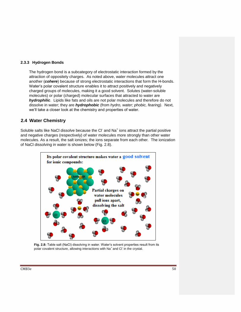
CMB3e 50

2.3.3 Hydrogen Bonds

The hydrogen bond is a subcategory of electrostatic interaction formed by the

attraction of oppositely charges. As noted above, water molecules attract one

another (cohere) because of strong electrostatic interactions that form the H-bonds.

Water’s polar covalent structure enables it to attract positively and negatively

charged groups of molecules, making it a good solvent. Solutes (water-soluble

molecules) or polar (charged) molecular surfaces that attracted to water are

hydrophilic. Lipids like fats and oils are not polar molecules and therefore do not

dissolve in water; they are hydrophobic (from hydro, water; phobic, fearing). Next,

we’ll take a closer look at the chemistry and properties of water.

2.4 Water Chemistry

Soluble salts like NaCl dissolve because the Cl- and Na+ ions attract the partial positive

and negative charges (respectively) of water molecules more strongly than other water

molecules. As a result, the salt ionizes; the ions separate from each other. The ionization

of NaCl dissolving in water is shown below (Fig. 2.8).

Fig. 2.8: Table salt (NaCl) dissolving in water. Water’s solvent properties result from its

polar covalent structure, allowing interactions with Na+

and Cl- in the crystal.

CMB3e 51

Water is also a good solvent for macromolecules (proteins, nucleic acids) with exposed

polar chemical groups on their surface that attract water molecules (Fig. 2.9).

125-2 Water-Hydrogen & Ionic Bonds

In addition to its being a good solvent, we recognize the following properties of water (all

of which result from its polar nature and H-bonding abilities):

Cohesion: the ability of water molecules to stick together via H-bonds.

High Surface tension: water’s high cohesion means that it can be hard to break the

surface; think the water strider, an insect that ‘walks on water’.

Adhesion: this results from water’s electrostatic interactions with ions and the partial

charges on polar covalent molecules or functional groups. Adhesion explains water’s

solvent properties and (at least in part) capillary action where water molecules ‘crawl’

along hydrophilic surfaces, often against the force of gravity.

High specific heat: The cohesion of water molecules is so strong that it takes a lot of

energy to separate the molecules and make them move faster. In other words, it

takes a lot of energy to heat water. Specifically, it takes 1 Kcal, (1 Calorie, with a

capital C) to heat a gram of water 1oC. Incidentally, high specific heat also explains

why water “holds its heat”, staying hotter longer that the pot it’s in!).

High heat of vaporization: It takes even more energy per gram of water to turn it into

water vapor!

One last property of water: it ionizes weakly to form H+ and OH- ions… or more correctly,

H3O+ and OH- ions. You can think of this as happening in the following two reactions:

Fig. 2.9: Charged groups on the macromolecule (e.g., protein) attract the partial charges

on water molecules, hydrating the molecule.

CMB3e 52

Acid molecules added to water will dissociate and release protons. This drives reaction 2

to form more H3O+ ions in the solution, in turn driving reaction 1 forward. A pH meter

measures the relative acidity or concentration of protons in a solution. Acidic solutions

have a pH below 7.0 (neutrality). Bases ionizing in water release hydroxyl (OH-) ions.

The increase in OH- ions removes protons from the solution, driving both reactions in

reverse and raising the pH of the solution. To summarize acid-base chemistry, when

dissolved in water, acids release H+ while bases accept H+. Since the pH of a solution is

the negative logarithm of the hydrogen ion concentration, a solution

at pH 7.0 is neutral.

below a pH of 7.0 is acidic.

above a pH of 7.0 is basic.

Check a basic chemistry textbook to be reminded of the relationship between pH and the

[H+] in a solution!

2.5 Some Basic Biochemistry: Carbon, Monomers, Polymers and the

Synthesis and Degradation of Macromolecules

Like evolution, the origin of life involved some prebiotic ‘natural selection’ of chemicals in

the environment. As with evolution, this chemical selection would favor expanding

increasing biochemical possibilities and diversity. In simple terms, atoms that could

interact with a maximal number of other atoms to form the largest number of stable

molecules would have been most likely to accumulate in the environment. The

tetravalent C atom met these criteria for chemical selection, proving ideal for building an

organic chemistry set.

At the same time, water turned out to be the perfect place to launch prebiotic chemical

selection experiments. Water persists as the life’s universal solvent, which explains why

evidence of water in places beyond our earth (other planets in our solar system, the

moons of other planets, other planets ion other solar systems) gets us all excited!

2.5.1 Isomerism in Organic Molecules and the Diversity of Shape

The carbon skeleton is a perfect platform of organic molecule diversity. The

differences in arrangement of atoms and functional chemical groups around C atom

result in isomerism. Isomers of an organic molecule have the same chemical

formula but different shapes (and so, potentially different chemical properties and

biochemical function). The larger the carbon skeleton of an organic molecule, the

CMB3e 53

greater the diversity of molecular shapes available for chemical selection. Look at the

examples of structural isomers and geometric isomers in Fig. 2.10.

It is easy to see that the structural isomers of C4H10 (Fig. 2.10, left and right) have

different shapes. You cannot convert one structural isomer to the other without

breaking covalent bonds. In the geometric isomers of C4H8 in the lower panel, the H

atoms on the double-bonded C atoms can be on the same (cis) or opposite (trans)

side of the planar double bond. Geometric isomers too, cannot be interconverted

without breaking chemical bonds. Optical isomers are yet a third kind of isomer.

They exist around optically active (asymmetric, or chiral) carbons. A chiral C is one

that is covalently linked to 4 different atoms and/or molecular groups. Optical isomers

(also called enantiomers) differ in shape, and just like structural and geometric

isomers, they can’t be converted from one to the other without breaking and re-making

covalent bonds. The principle of chirality is illustrated below in Fig. 2.11.

Fig. 2.10: Structural and geometric isomers of hydrocarbons create molecules with the same

chemical formula but different shapes.

CMB3e 54

Enantiomers are defined as optically active because they bend, or rotate light in

opposite directions in a polarimeter. Light passing through a solution of one optical

isomer is rotated in one direction while light passing through the other isomer is

rotated in the opposite direction. These directions are referred to

as l, or levo (meaning left) and d or dextro (meaning right). If a molecule has more

than one chiral C (glucose for example has four chiral carbons), its behavior in a

polarimeter will be based on the sum of optical activities of all the chiral carbons. The

common isomer of glucose in our diet is d-glucose. Glucose enantiomers are also

referred to as D and L respectively, a convention based on the configuration of the

four different atoms or groups around the last optically active carbon in a molecule (5C

in glucose). For glucose, d and l in fact correspond to D and L respectively. As we

will see for some molecules, the upper-case designation of a chiral molecule does not

always indicate how it bends light in a polarimeter, while the lower-case d and l always

do! The d- and l- isomers of glucose are illustrated in Fig. 2.12 (below), with chiral

carbons in red.

Fig. 2.11: The two different generic molecules (enantiomers) are mirror images of one another.

They form from alternate arrangements of the same molecular groups around a chiral carbon.

Fig. 2.12: Two straight chain forms of glucose (d-glucose and l-glucose) are enantiomers (optical

isomers), differing in the arrangement of the H atom and the OH group around C5.

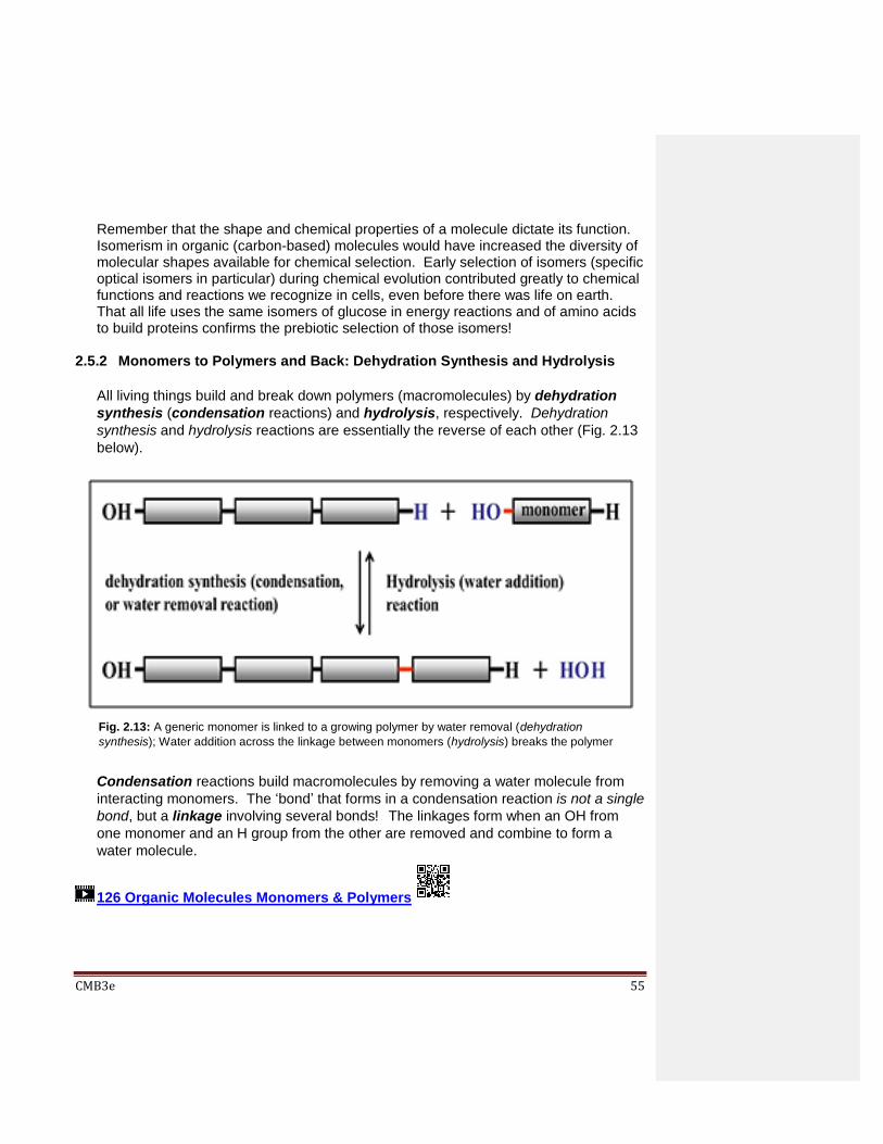
CMB3e 55

Remember that the shape and chemical properties of a molecule dictate its function. Isomerism in organic (carbon-based) molecules would have increased the diversity of molecular shapes available for chemical selection. Early selection of isomers (specific optical isomers in particular) during chemical evolution contributed greatly to chemical functions and reactions we recognize in cells, even before there was life on earth. That all life uses the same isomers of glucose in energy reactions and of amino acids to build proteins confirms the prebiotic selection of those isomers!

2.5.2 Monomers to Polymers and Back: Dehydration Synthesis and Hydrolysis

All living things build and break down polymers (macromolecules) by dehydration

synthesis (condensation reactions) and hydrolysis, respectively. Dehydration

synthesis and hydrolysis reactions are essentially the reverse of each other (Fig. 2.13

below).

Condensation reactions build macromolecules by removing a water molecule from

interacting monomers. The ‘bond’ that forms in a condensation reaction is not a single

bond, but a linkage involving several bonds! The linkages form when an OH from

one monomer and an H group from the other are removed and combine to form a

water molecule.

126 Organic Molecules Monomers & Polymers

Fig. 2.13: A generic monomer is linked to a growing polymer by water removal (dehydration

synthesis); Water addition across the linkage between monomers (hydrolysis) breaks the polymer

back down to monomers.

CMB3e 56

Repeated condensation reactions such as one between two amino acids (Fig. 2.14)

form the peptide linkages that build polypeptides during translation.

Cells perform repeated condensation reactions to build diverse polymers, including

polysaccharides and polynucleotides (the RNA and DNA nucleic acids). Consider the

polymerization of glucose monomers into storage or structural polysaccharides for

example. Cells use only (d)glucose to make polysaccharides. Here’s how this

works:

Straight-chain (d)glucose with four chiral carbons, becomes cyclic when dissolved in

water where the cyclic molecule acquires a fifth chiral carbon, namely, the #1 carbon.).

Since the #1 carbon is now optically active, the (d)glucose can form a new pair of

enantiomers in solution, called (d)glucose and (d)glucose.

Having selected d-glucose for most cellular energy metabolism, life then exploited the

additional chiral carbon in cyclic d-glucose to make the different polysaccharide

polymers we now find in plants and animals.

Fig. 2.14: Dehydration synthesis forms peptide linkage (circled); hydrolysis is the reverse

reaction.

CMB3e 57

In solution, 90% or glucose monomers are in the ring form, as show in Fig. 2.15 below.

The condensation reactions shown below link glucose monomers, forming storage

and structural polysaccharides (Fig. 2.16).

Fig. 2.15: When straight chain glucose forms a cyclic molecule in solution in water, C1 becomes

optically active (chiral), creating a racemic mixture of d)glucose and (d)glucose enantiomers.

Fig. 2.16: Polysaccharide sugar polymers form by dehydration synthesis: d)glucose monomers

polymerize to form energy-storage molecules (e.g., starch, glycogen), while -d-glucose monomers

polymerize to form structural polysaccharides (starch, cellulose).

CMB3e 58

The -OH (hydroxyl) groups on the #1 C of (d)glucose are below the glucose rings.

The condensation reaction removes a water molecule, linking the sugars by an 1,4

glycoside linkage in the dimer, connecting them by their # 1 and # 4 carbons. Other

linkages are possible. For example, diverse -glycoside linkages characterize

branched storage polysaccharides like glycogen in animals and the starches in

plants. On the other hand, when dglucose enantiomers polymerize, they form rigid

structural polysaccharides such as those of cellulose in plant cell walls. A modified

-glucose called N-acetyl glucosamine (not shown) polymerizes to form chitin, the

principal component of fungal cell walls and of the tough exoskeleton of arthropods

(insects, crustaceans). In another chapter, we’ll revisit the linkage of amino acids

during translation to build a polypeptide; only L amino acids are used to make

proteins! We’ll also look at the details of replication and transcription that cells use to

catalyze condensation reactions that synthesize DNA and RNA from nucleotide

monomers.

To summarize:

Linkages in the biopolymers are broken down and re-formed daily in our lives!

Digestion (the breakdown) begins after a meal. The hydrolysis of glycoside

linkages begins in your mouth. Further polysaccharide digestion and the

breakdown of peptide (among other) linkages continues in your stomach and small

intestines. Then our cells use condensation reactions to complete the job of

turning carrot- and cow-derived monomers into you or me!

Prebiotic chemical evolution has selected only one of the optical isomers

(enantiomers) of glucose, amino acid and other monomers with which to build

polymers. This is so even though some of the different isomers are available and

even used by cells for different purposes. The flexible (d)glucose polymers were

selected as storage polysaccharides to be used for energy. The storage

polysaccharides include plant starches and animal glycogen. Likewise, the rigid

inflexibility of (d)glucose polymers was selected precisely because it reinforced

cell structure and stability. Since all organisms store carbohydrate energy in

(d)glucose polymers and since (d)glucose polymers are almost universally

used to strengthen cell structure, these selections must have occurred early in the

history of life.

127-2 Carbohydrates-Sugars & Polysaccharides

128-2 Lipids-Triglycerides-Phospholipids

CMB3e 59

129-2 Proteins-Amino Acids & Polypeptides

130-2 DNA & RNA-Nucleotides & Nucleic Acids

To conclude this chapter and to emphasize the significance of chirality to life, here is

what can happen if the wrong isomer ends up in the wrong place at the wrong time…

2.5.3 A Tale of Chirality Gone Awry

Consider the story of Thalidomide, a tragic example of what happens when we are

unaware of enantiomeric possibilities. Introduced in 1957, Thalidomide was sold as

an over-the-counter anti-nausea drug for patients undergoing cancer therapies and as

a very effective morning sickness remedy for pregnant women. However, by the early

1960s, the birth of about 10,000 infants with severely deformed limbs was connected

to the drug. These deformities characterized the roughly half of these infants that

survived. Once the connection was made, the response was of course, to pull

Thalidomide off the market.

Thalidomide is a teratogen. Teratogens are substances or conditions (drugs,

chemicals, radiation, illness during pregnancy, etc.) that cause deformities during

embryogenesis and fetal development. The chemical bases of Thalidomide’s effects

are based on its enantiomeric (chiral) structure in which an amine-containing ring can

exist in front of, or behind the rest of the molecule. The structure of Thalidomide is

shown in Fig. 2.17 below.

Fig. 2.17: Two enantiomers (optical isomers) of Thalidomide (R and S) form in water.

CMB3e 60

The two enantiomers are referred to as ‘S’ and ‘R’. Of these, the S isomer is the

teratogen. While synthesis of pure R is possible, when used in treatment, R and S

easily interconvert, creating a racemic mixture. In the mother, S is transferred to the

embryo or fetus, with its terrible consequences.

Remarkably, there were relatively few cases of Thalidomide-induced birth deformities in the United States, largely because of the efforts of Frances Oldham Kelsey, the person in charge of FDA review of the drug. The German pharmaceutical company Chemie Grünenthal (developer Thalidomide) and an American pharmaceutical company had applied for FDA approval for U.S. distribution of the drug. But Dr. Oldham Kelsey refused approval on multiple occasions, arguing that the safety of Thalidomide had not been demonstrated. This was even before it was shown to cause birth deformities! In 1962 President Kennedy presented Dr. Oldham Kelsey the President's Award for Distinguished Federal Civilian Service for not allowing thalidomide to be approved for sale in the US without sufficient safety testing…, potentially saving thousands of lives. Of course, we already knew that cells synthesized polymers from specific optical isomers of their precursor monomers. So the sad Thalidomide story resulted from the untested effects of an unexpected optical isomer. Many countries quickly tightened their pre-approval drug testing regulations because of this tragedy.In a more hopeful twist of the tale, Thalidomide has turned out to be effective in treating cancer, leprosy, rheumatoid arthritis and other autoimmune diseases. Such therapeutic benefits may be due to its anti-inflammatory effects. The effects of thalidomide on tumor growth seem to be due to its inhibition of angiogenesis (development of blood vessels) in the tumors. Ironically, blockade of angiogenesis might also have contributed to the failure of proper limb growth during pregnancy. To conclude, when all is normal, the shapes of molecules have been uniquely selected for the specificity of reactions essential to life.

131-2 Shape & the Specificity of Molecular interactions

Some iText & VOP Key Words and Terms

acids and bases geometric isomers polar covalent bonds

adhesion glycogen polymers

-glucose glycoside linkage polynucleotides

amino acids heat of vaporization polypeptides

CMB3e 61

angiogenesis hydrogen bonds polysaccharides

atom hydrolysis potential energy

atomic mass hydrophilic properties of water

-glucose hydrophobic protons

Bohr model ionic bonds quantum

carbohydrates ionization racemic mixture

cellulose isomers RNA

chirality isotopes salts

chiral carbon kinetic energy scanning tunneling microscope

chitin lipids sharing electrons

cohesion macromolecules solutes

condensation reaction molecule specific heat

dehydration synthesis monomers starches

digestion neutrons structural isomers

DNA nucleotides surface tension

electron shell optical isomers teratogen(ic)

electrons orbitals Thalidomide

electrostatic interaction

partial charge triglycerides

element peptide linkage valence

enantiomers pH Van der Waals forces

ester linkage phosphate ester linkage

water ions

excitation phosphodiester linkage water of hydration

fats phospholipids

fluorescence photon

CMB3e 62

Chapter 3: Details of Protein Structure Protein Structure and Configuration: Primary, Secondary, Tertiary, Quaternary;

Protein Folding, Domains and Motifs, Studying Proteins

3.1 Introduction

The protein is the workhorse of cells, responsible for just about all aspects of life.

Comprised of one or more polypeptides, they:

are the catalysts that make biochemical reactions possible.

are membrane components that selectively let substances in and out of the cell.

allow cell-cell communication and cell’s response to environmental change.

form the internal structure of cells (cytoskeleton) and nuclei (nucleoskeleton).

enable the motility of cells and of things (particles, organelles…) inside cells.

are responsible for other cell functions too numerous to summarize here!

We owe much of what we know about biomolecular structure to the development of X-ray

crystallography. In fact, an early determination of the structure of insulin (as well as

penicillin and vitamin B12) using X-ray crystallography earned Dorothy Hodgkin’s the

1964 Nobel Prize in Chemistry. In this chapter, we look at the different levels (‘orders’) of

protein structure…, in fact what it takes to be a functional protein.

The primary structure (1o structure) of a polypeptide is its amino acid sequence.

Interactions between amino acids near each other in the sequence cause the polypeptide

to fold into secondary (2o) structures, including the-helix and the -pleated sheet (or

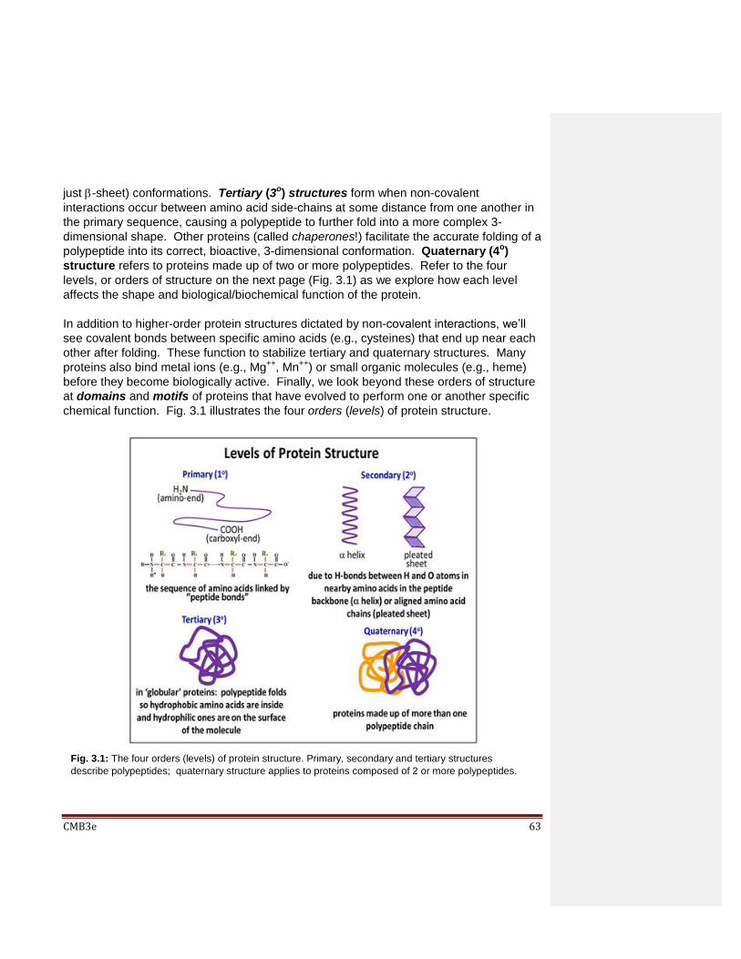
CMB3e 63

just -sheet) conformations. Tertiary (3o) structures form when non-covalent

interactions occur between amino acid side-chains at some distance from one another in

the primary sequence, causing a polypeptide to further fold into a more complex 3-

dimensional shape. Other proteins (called chaperones!) facilitate the accurate folding of a

polypeptide into its correct, bioactive, 3-dimensional conformation. Quaternary (4o)

structure refers to proteins made up of two or more polypeptides. Refer to the four

levels, or orders of structure on the next page (Fig. 3.1) as we explore how each level

affects the shape and biological/biochemical function of the protein.

In addition to higher-order protein structures dictated by non-covalent interactions, we’ll

see covalent bonds between specific amino acids (e.g., cysteines) that end up near each

other after folding. These function to stabilize tertiary and quaternary structures. Many

proteins also bind metal ions (e.g., Mg++, Mn++) or small organic molecules (e.g., heme)

before they become biologically active. Finally, we look beyond these orders of structure

at domains and motifs of proteins that have evolved to perform one or another specific

chemical function. Fig. 3.1 illustrates the four orders (levels) of protein structure.

Fig. 3.1: The four orders (levels) of protein structure. Primary, secondary and tertiary structures

describe polypeptides; quaternary structure applies to proteins composed of 2 or more polypeptides.

CMB3e 64

Clearly, in trying to understand molecular (especially macromolecular) function, a recurring theme emerges: the function of a protein depends on its conformation. In turn, protein conformation is based on the location and physical and chemical properties of critical functional groups, usually amino acid side chains. Watch for this theme as we

look at enzyme catalysis, the movement of molecules in and out of cells, the response of

cells to their environment, the ability of cells and organelles to move, how DNA replicates,

how gene transcription and protein synthesis are regulated… and just about everything a

cell does! We will conclude this chapter with a look at some techniques for studying

protein structure.

Learning Objectives

When you have mastered the information in this chapter, you should be able to:

1. define and distinguish between the orders of protein structure.

2. differentiate between -sheet, -helix and ‘random coil’ structures based on the

atomic interactions involved on each.

3. trace the path to the formation of a polypeptide; define its primary structure and how it

might be determined by its amino acid sequence.

4. describe how globular proteins arise from the hydrophobic and hydrophilic interactions

that drive protein folding and how changes in protein shape can cause disease.

5. formulate an hypothesis (or look one up) to explain why the amino acid glycine is a

disruptor of alpha helical polypeptide structure.

6. compare and contrast motif and domain structure of proteins and polypeptides, and

their contribution to protein function.

7. describe different techniques for studying proteins and the physical/chemical

differences between proteins that make each technique possible.

3.2 Levels (Orders) of Protein Structure

The three levels of polypeptide structure are primary, secondary and tertiary structure.

Quaternary structure refers to associations of two or more polypeptides, creating higher

order protein structures. Superimposed on these basic levels are other features of

protein structure. These are created by the specific amino acid configurations in the

mature, biologically active protein. Let’s begin with a look at primary structure.

3.2.1 Protein Primary Structure; L Amino Acids and the C-N-C-N-… Polypeptide

Backbone

The primary structure of a protein simply refers to the amino acid sequence of its

polypeptide chain(s). Cells use only 20 amino acids to make polypeptides and

proteins, although they do use a few additional amino acids for other purposes.

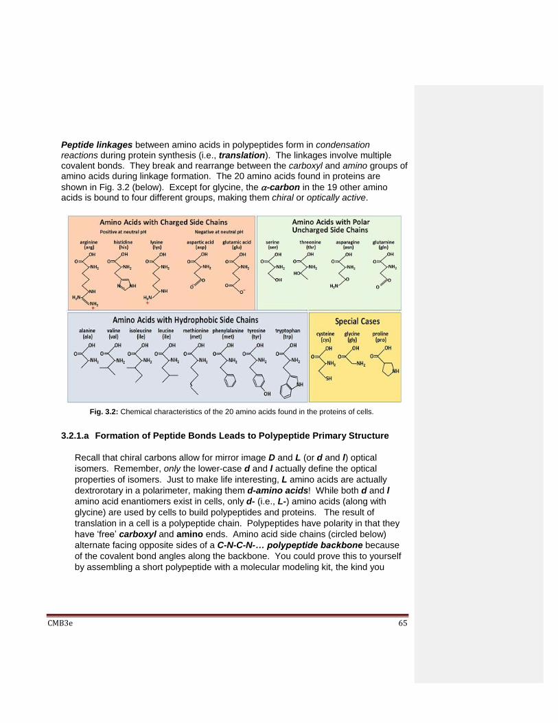
CMB3e 65

Peptide linkages between amino acids in polypeptides form in condensation reactions during protein synthesis (i.e., translation). The linkages involve multiple covalent bonds. They break and rearrange between the carboxyl and amino groups of amino acids during linkage formation. The 20 amino acids found in proteins are

shown in Fig. 3.2 (below). Except for glycine, the -carbon in the 19 other amino acids is bound to four different groups, making them chiral or optically active.

3.2.1.a Formation of Peptide Bonds Leads to Polypeptide Primary Structure

Recall that chiral carbons allow for mirror image D and L (or d and l) optical

isomers. Remember, only the lower-case d and l actually define the optical

properties of isomers. Just to make life interesting, L amino acids are actually

dextrorotary in a polarimeter, making them d-amino acids! While both d and l

amino acid enantiomers exist in cells, only d- (i.e., L-) amino acids (along with

glycine) are used by cells to build polypeptides and proteins. The result of

translation in a cell is a polypeptide chain. Polypeptides have polarity in that they

have ‘free’ carboxyl and amino ends. Amino acid side chains (circled below)

alternate facing opposite sides of a C-N-C-N-… polypeptide backbone because

of the covalent bond angles along the backbone. You could prove this to yourself

by assembling a short polypeptide with a molecular modeling kit, the kind you

Fig. 3.2: Chemical characteristics of the 20 amino acids found in the proteins of cells.

CMB3e 66

might have used in a chemistry class! The C-N-C-N-…backbone is the underlying

basis of higher orders, or levels of protein structure (see below). A partial

polypeptide is shown in Fig. 3.3 below.

132-2 Amino Acid Sequence & Protein Primary Structure

3.2.1.b. Determining Protein Primary Structure - Polypeptide Sequencing

Frederick Sanger demonstrated the first practical protein sequencing method when

he reported the amino acid sequence of the two polypeptides of Bovine (cow)

insulin. His technique involves stepwise hydrolysis (an Edman Degradation) of

polypeptide fragments in which each hydrolysis leaves behind a polypeptide

fragment shortened by one amino acid that can be identified. Sanger received a

Nobel Prize in 1958 for this feat. By convention, the display and counting of amino

acids always starts at the amino end (N-terminus), the end with a free NH2-group.

Primary structure is dictated directly by the gene encoding the protein. After

transcription of a gene, a ribosome translates the resulting mRNA into a

polypeptide. For some time now, the sequencing of DNA has replaced most direct

protein sequencing. The method of DNA sequencing, colloquially referred to as

the Sanger dideoxy method, quickly became widespread and was eventually

automated, enabling rapid gene (and even whole genome) sequencing. Now,

instead of directly sequencing polypeptides, we can infer amino acid sequences

from gene sequences isolated by cloning or revealed after complete genome

sequencing projects. This is the same Sanger who first sequenced proteins, and

yes…, he won a second Nobel Prize for the DNA sequencing work in 1980!

Fig. 3.3: Partial polypeptide; amino and carboxyl ends of a polypeptide define its polarity,

with positively charged amino and negatively charged carboxyl ends at physiological pH.

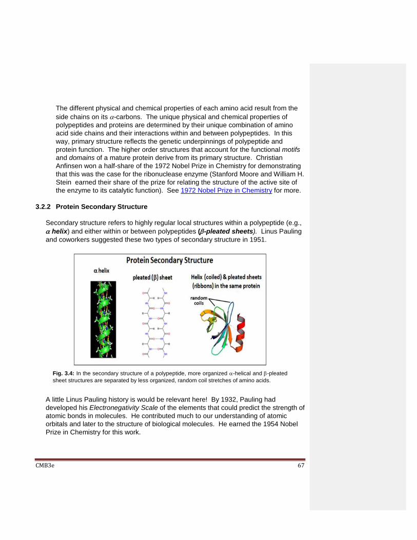
CMB3e 67

The different physical and chemical properties of each amino acid result from the

side chains on its -carbons. The unique physical and chemical properties of

polypeptides and proteins are determined by their unique combination of amino

acid side chains and their interactions within and between polypeptides. In this

way, primary structure reflects the genetic underpinnings of polypeptide and

protein function. The higher order structures that account for the functional motifs

and domains of a mature protein derive from its primary structure. Christian

Anfinsen won a half-share of the 1972 Nobel Prize in Chemistry for demonstrating

that this was the case for the ribonuclease enzyme (Stanford Moore and William H.

Stein earned their share of the prize for relating the structure of the active site of

the enzyme to its catalytic function). See 1972 Nobel Prize in Chemistry for more.

3.2.2 Protein Secondary Structure

Secondary structure refers to highly regular local structures within a polypeptide (e.g.,

helix) and either within or between polypeptides (-pleated sheets). Linus Pauling

and coworkers suggested these two types of secondary structure in 1951.

A little Linus Pauling history is would be relevant here! By 1932, Pauling had

developed his Electronegativity Scale of the elements that could predict the strength of

atomic bonds in molecules. He contributed much to our understanding of atomic

orbitals and later to the structure of biological molecules. He earned the 1954 Nobel

Prize in Chemistry for this work.

Fig. 3.4: In the secondary structure of a polypeptide, more organized -helical and -pleated

sheet structures are separated by less organized, random coil stretches of amino acids.

CMB3e 68

He and his colleagues later discovered that sickle cell anemia was due to an abnormal

hemoglobin. Then they went on to predict the alpha helical and pleated sheet

secondary structure of proteins. While he did not earn a second Nobel for these novel

studies of molecular genetics, Pauling did win the 1962 Nobel Peace prize for

convincing almost 10,000 scientists to petition the United Nations to vote to ban

atmospheric nuclear bomb tests. A more detailed review of his extraordinary life (e.g.,

at Linus Pauling-Short Biography) is worth a read! Coincidentally, Max. F. Perutz and

John C. Kendrew earned the 1962 Nobel Prize in Chemistry for their X-Ray

crystallographic studies of the 3-dimensional structure of hemoglobin. 1962 was a

good year for Nobel prizes for protein studies!

133-2 Protein Secondary Structure

The helix or sheets are a most stable arrangement of H-bonds in the chain(s), and

both are typically found in the same protein (at the right in Fig. 3.4). These regions of

ordered secondary structure in a polypeptide can be separated by varying lengths of

less structured peptide called random coils. All three of these elements of secondary

structure can occur in a single polypeptide or protein that has folded into its tertiary

structure, as shown at the right in the illustration. The pleated sheets are shown as

ribbons with arrowheads representing N-to-C or C-to-N polarity of the sheets. As you

can see, a pair of peptide regions forming a pleated sheet may do so either in the

parallel or antiparallel directions (look at the arrowheads of the ribbons), which will

depend on other influences dictating protein folding to form tertiary structure. Some

polypeptides never go beyond their secondary structure, remaining fibrous and

insoluble. Keratin is perhaps the best-known example of a fibrous protein, making

up hair, fingernails, bird feathers, and even filaments of the cytoskeleton. However,

most polypeptides and proteins do fold and assume tertiary structure, becoming

soluble globular proteins.

3.2.3 Protein Tertiary Structure

Polypeptides acquire their tertiary structure when hydrophobic and non-polar side

chains spontaneously come together to exclude water, aided by the formation of salt

bridges and H-bonds between polar side chains that find themselves inside the

globular polypeptide. In this way, helices or sheets are folded and incorporated

into globular shapes. The forces that cooperate to form and stabilize 3-dimensional

polypeptide and protein structures are illustrated below in Fig. 3.5.

CMB3e 69

Polar (hydrophilic) side chains that can find no other side-chain partners are typically

found on the outer surface of the ’globule’, where they interact with water and thus

dissolve the protein (recall water of hydration). Based on non-covalent bonds, tertiary

structures are nonetheless strong simply because of the large numbers of otherwise

weak interactions that form them. Nonetheless, covalent disulfide bonds between

cysteine amino acids in the polypeptide (shown above) can further stabilize tertiary

structure. Disulfide bonds (bridges) form when cysteines far apart in the primary

structure of the molecule end up near each other in a folded polypeptide. Then the

SH (sulfhydryl) groups in the cysteine side chains are oxidized, forming the disulfide

(–S-S- ) bonds (See Fig. 3.6, below).

Fig. 3.5: Tertiary structure is created by non-covalaent hydrophobic amino acid interactions as

well as H-bonding in the interior of a polypeptide, leaving charged (hydrophilic) amino acid side

chains to interact with water on the exterior of a typical “globular” protein. Stable covalent

disulfide bonds between cysteine amino acids help stabilize tertiary structures.

Fig. 3.6: Disulfide bridges form in oxidation reactions between SH (sulfhydryl) groups on cysteine

amino acids (‘residues’) in a polypeptide.

CMB3e 70

To better understand how disulfide bridges can support the 3-dimensional structure of

a protein, just imagine its physical and chemical environment. Changing the

temperature or salt concentration surrounding a protein might disrupt non-covalent

bonds involved in the 3D shape of the active protein. Unaffected by these changes,

disulfide bridges limit the disruption and enable the protein to re-fold correctly and

quickly when conditions return to normal (think homeostasis!).

134-2 Protein tertiary structure

135-2 Disulfide Bridges Stabilize 3o Structure

3.3 Changes in Protein Shape Can Cause Disease

While the conformation of a protein determines its biological function, an allosteric (shape) change can moderate or disrupt its function. Under normal circumstances, cells use changes in protein shape to regulate metabolism. Such allosteric regulation is well documented in familiar biochemical pathways such as glycolysis and is discussed in more detail elsewhere. Less well understood is how (or why) conformational change in some proteins cells can have devastating effects.

3.3.1 Sickle Cell Anemia

Mutant globin genes can cause hemoglobin disorders characterized by inefficient oxygen delivery by blood. In the 1940s, the British biochemist J.B.S. Haldane made a correlation between southern African regions with high incidences hemoglobin disorders and malaria, suggesting that heterozygous individuals (i.e., those that had only one copy of a mutant hemoglobin gene), were somehow protected from malaria. Sickle Cell Anemia is a well-known example of a hemoglobin disorder, caused by a

single base change in the gene for human -hemoglobin (one of the polypeptides in hemoglobin). Since red blood cells are rich in hemoglobin, the abnormal shape of the

-hemoglobin can cause the cells themselves to become sickle-shape. Sickled cells disrupt capillary flow and oxygen delivery, causing the symptoms of anemia. While Sickle Cell Anemia originated in Africa, it probably spread to the United States as a consequence (or even a cause) of the slave trade. This is in part because Europeans exploiting their African colonies’ natural resources were dying of malaria while the African natives seemed unaffected. Having brought malarial mosquitos to the new world as stowaways in the first place, the Europeans figured that African slaves would survive the illness in the Americas where they could not.

Individuals heterozygous for the have sickle cell trait and are generally unaffected

because at least some of their hemoglobin is normal. Homozygous individuals that

can make only the sickle cell -hemoglobin variant suffer more frequent and severe

CMB3e 71

suffer episodes of the disease. Stressors that can trigger sickling include infection or

dehydration. Compare normal red blood cells to a sickle cell in Fig. 3.7.

The sickle cell gene affects perhaps more than 100 million people worldwide, including

8-10% of African Americans. For more demographic information, see Sickle Cell Trait

Demographics Article and Sickle Cell Data from the CDC. In Africa, heterozygotes

with sickle cell trait are protected from malaria, confirming Haldane’s hypothesis. But

patients homozygous for the -hemoglobin mutation derive little benefit from its anti-

malarial effects.

In the meantime, despite a 33% reduction in cases of malaria in recent years, this disease caused by a mosquito-borne parasite still threatens half of the people on the planet, causing over a half-million deaths per year. There are treatments other than mosquito nets and killing mosquitos, but at this time, there is still no preventive vaccine.

3.3.2. The Role of Misshapen and Mis-Folded Proteins in Alzheimer’s Disease

Prion proteins, when first discovered, seemed to behave as infectious agents that

could reproduce without DNA or other nucleic acid. As you can imagine, this highly

unorthodox and novel hereditary mechanism generated its share of controversy.

Read about research on the cellular PrPc prion protein at en.wikipedia.org/wiki/Prion.

Of course, prions turn out not to be reproductive agents of infection after all. Recent

studies of prions have revealed several normal prion protein functions including roles

in memory formation in mice and in sporulation in yeast (Check out Prion Proteins

May Play a Role in Memory Formation).

Fig. 3.7: Light micrograph of a sickled erythrocyte (red blood cell).

CMB3e 72

A mutant version of the prion protein (PrPSc) is able to mis-fold and take on an

abnormal shape. The deformed PrPSc can then induce abnormal folding even other

prions, of other normal PrPc molecules. These events, illustrated in Fig. 3.8, result in

the formation of so-called amyloid plaques.

Abnormally folded prions (PrPSc) have been associated Alzheimer’s Disease.

Alzheimer’s Disease affects about 5.5 million Americans. PrPSc is also associated

with Mad Cow disease and Creutzfeldt-Jakob-Disease (mad cow disease in

humans), as well as Scrapie in sheep, among others. We are beginning to

understand that the role of prion proteins in Alzheimer’s Disease is less causal

than indirect.

3.3.2.a. The Amyloid Beta (A) peptide

Post-mortem brains of patients that suffered Alzheimer’s disease show

characteristic extracellular amyloid plaques to be composed largely of the

amyloid beta (A) peptide. Enzymatic cleavage of the amyloid precursor

protein (APP) generates extracellular 39-43 amino acid A peptides. Normally,

excess A peptides are themselves digested. Unregulated A peptide

formation however, leads to the formation of beta amyloid plaques seen in

Alzheimer’s disease (Fig. 3.9, below).

Fig. 3.8: Mutations in a normal gene for a prion protein (PrPc

) may produce some abnormally

folded prion proteins (PrPSc

). The misfolded PrPSc

molecules interact with other (even normal)

prions to mis-fold, precipitating PrPSc

proteins into aggregated amyloid plaques.

CMB3e 73

The scissors in the illustration represent two enzymes that digest the APP.

Prion proteins are not a proximal cause of Alzheimer’s Disease, but may have a

role in initiating events that lead to it. Normal prion protein (PrPc) is itself a

membrane receptor and is thought to bind A peptides, effectively preventing

their aggregation into plaques. An experimental reduction of PrPc was shown

to increase the extracellular A peptides. Presumably prion protein aggregation

induced by the mutant PrP protein (PrPsc) prevents prion proteins from binding

to A peptide, leading to its accumulation and ultimately to amyloid plaque

formation and neurodegeneration.

3.3.2.b. The Tau protein

A protein called tau is also associated with Alzheimer’s Disease. Misshapen

tau accumulating in neurofibrillary tangles in hippocampus brain neurons may

be a more immediate cause of the neuronal dysfunction associated with the

disease. In normal neurons, MAP-T (Microtubule-Associated Protein Tau) is

phosphorylated and then binds to and stabilizes microtubules. But when

neuronal tau becomes hyper-phosphorylated, its conformation changes. No

longer stabilized, the microtubules disassemble and the deformed tau proteins

form neurofibrillary tangles. Immunostaining of hippocampal neurons with

antibodies to tau protein localizes the neurofibrillary tangles, as seen in the

micrograph below in Fig. 3.10.

Fig. 3.9: Steps in the formation of -amyloid plaques. Amyloid precursor proteins (APP)

are embedded in cell membranes (upper left). Enzymes digest APP, releasing -amyloid

protein fragments (middle panel). Unregulated accumulation of -amyloid protein results

in the formation of extracellular amyloid plaques.

CMB3e 74

The formation of neurofibrillary tau protein tangles in a diseased neuron is

compared to normal neurons in Fig. 3.11, below.

The tangled clumps of tau proteins in this illustration are what stain deep purple

in the micrograph of immunostained neurons in the light micrograph.

Fig. 3.10: Non-fluorescent immunostaining of tau proteins of an Alzheimers brain reveals

tau tangles.

Fig. 3.11: The formation of tau tangles occurs in diseased neurons that cannot maintain

normal microtubule structure; in the absence of stabilizing tau molecules microtubules

degenerate and tau proteins clump.

CMB3e 75

There is no cure for Alzheimer’s disease, although treatments with

cholinesterase inhibitors seem to slow its advancement. For example, the drug

Aricept inhibits acetylcholine breakdown by acetylcholinesterase, thereby

enhancing cholinergic neurotransmission, which may in turn prolong brain

neural function. Unfortunately, there is as yet no treatment to restore lost

memories and the significant cognitive decline associated with Alzheimer’s

disease. Perhaps more promising in this respect is the recent detection in the

blood and serum of proteins or peptides associated with Alzheimer’s Disease.

Amyloid beta (Aβ ) and/or tau protein fragments that escape into the blood

stream can be detected 6-8 or more years before Alzheimer’s symptoms

appear. A neurofilament light chain (NfL) seen in a familial form of

Alzheimer’s Disease (among other neuropathies) is detectable at 16 years

before the symptoms!. The ability to detect of these Alzheimer’s marker

proteins or derived peptides so far in advance of symptoms raises hopes for

early monitoring of at-risk individuals and for new therapies for Alzheimer’s

disease. For brief reviews, see Alzheimer's Disease: The Early Detection of

Circulating Ab Peptides and Alzheimer's Disease: The Early Detection of

Circulating tau Peptides. For a recent report on tracking the NfL protein, see

Alzheimer's Disease: The Early Detection of Circulating Neurofilament Light

Chain Protein

3.3.2.c. Some Relatives of Alzheimer’s Disease

Some of the same protein abnormalities seen in Alzheimer’s disease also

characterize other neurodegenerative diseases as well as traumatic brain damage.

An abnormal accumulation of tau protein is diagnostic of CTE (Chronic Traumatic

Encephalopathy). In the early 20th century, disoriented boxers staggering about

after a fight were called ‘punch drunk’, suffering from dementia pugilistica. We now

know they suffered from CTE, as do other athletes exposed to repetitive mild-to-

severe brain trauma, such as football players. Immunostaining of whole brains and

brain tissue from autopsied CTE patients with antibodies to tau protein show

accumulations of abnormal tau proteins and tau neurofibrillary tangles very much

like those found in of Alzheimer’s patients. Many National Football League and

other football players have been diagnosed post-mortem with CTE, and many still

living show signs of degenerative cognition and behavior consistent with CTE (see

a List of_NFL_players_with_chronic_traumatic_encephalopathy to see how many!

Parkinson’s Disease is yet another example of a neurodegenerative disease that

results when a single protein changes shape in brain cells. Though they are not

characterized as plaques, aggregates can form in brain cells when the protein

alpha-synuclein undergoes anomalous conformational change. The change

CMB3e 76

results in MSA (Multiple System Atrophy) or Parkinson’s Disease. Click

https://www.sciencedirect.com/science/article/pii/S0925443911002250 to read

details of this recent research. Much of the high-resolution electron microscopy

that can reveal protein structure and capture the conformational changes we now

recognize comes from the work of Jacques Dubochet, Joachim Frank and Richard

Henderson who received the 2017 Chemistry Nobel Prize for Chemistry for

developing and refining cryo-electron microscopy for biomolecular imaging (see

2017 Nobel Prize for Chemistry for more).

3.4 Protein Quaternary Structure, Prosthetic Groups & Chemical

Modifications

Quaternary structure describes a protein composed of two or more polypeptides. Like

tertiary structure, such multimeric proteins are formed by non-covalent interactions and

may be stabilized disulfide bonds. Specifically, a dimer contains two, a trimer three, a

tetramer four polypeptides… and so on. Multimers made up of identical subunits are

referred to with a prefix of "homo-" (e.g. a homotetramer). Those made up of different

subunits are heteromers. The vertebrate hemoglobin molecule is a heterotetramer, with

two - and two - globins (Fig. 3.12).

Fig. 3.12: The vertebrate hemoglobin molecule, consisting of 4 globin subunits (two

and two polypeptides). Each globin is associated with a heme group bound to iron.

CMB3e 77

Prosthetic groups are organic molecules associated with proteins. Hemoglobins

exemplify the role of prosthetic groups in protein function. To be biologically active, globin

polypeptides must associate with heme, a cyclic organic molecule with iron at its center.

The iron is what reversibly binds oxygen. All kinds of organisms, from bacteria to plants

and animals and even in some anaerobic organisms contain some kind of hemoglobin

with a heme-like prosthetic group. Other proteins must be bound to different metal ions

(magnesium, manganese, cobalt…) to be biologically active.

136-2 Protein Quaternary Structure & Prosthetic Groups Chemical modifications are post-translational, enzyme catalyzed events required to

make a protein fully functional or to regulate its activity. Many polypeptides are structurally

modified by glycosylation (e.g., to make membrane glycoproteins). Others are

phosphorylated at one or more specific amino acids in the chain, to regulate their

biological activity. These modifications account for and enhance the molecular and

functional diversity of proteins within and across species.

3.5. Domains, Motifs, and Folds in Protein Structure

The structures of two different proteins in Fig. 3.13 share a common PH (Pleckstrin

Homology) domain (maroon).

Fig. 3.13: The Pleckstrin Homology (PH) domains shown here are an example of common

domains (maroon colored sequences) in two different proteins. Because they have a PH domain,

both proteins can interact with cell signaling factors with roles in intercellular communication.

CMB3e 78

These two and many other proteins have this domain, allowing them to bind a molecule of

phosphatidyl-inositol triphosphate that is generated as part of a common cell-signaling

pathway. The implication of this common domain is that a cell can have signaling

pathways that allowing it to respond to different signals that lead to the same response,

albeit under different conditions and probably at different times. Proteins are typically

described as consisting of several distinct sub-structures, discussed here.

A domain is an element of the protein's overall structure that is stable and often folds

independently of the rest of the protein chain. Like the PH domain above, many domains

are not unique to the protein products of one gene, but instead appear in a variety of

proteins. Proteins sharing more than a few common domains are encoded by members

of evolutionarily related genes comprising gene families. Genes for proteins that share

only one or a few domains may belong to gene superfamilies. Superfamily members

can have one function in common, but the rest of their sequences are otherwise

unrelated. Domain names often derive from their prominent biological function in the

protein they belong to (e.g., the calcium-binding domain of calmodulin), or from their

discoverers (the PH domain!). The domain swapping that gives rise to gene families and

superfamilies are natural genetic events. Because protein domains can also be

"swapped" on purpose by genetic engineering, we can make chimeric proteins with novel

functions.

137-2 Protein Domain Structure &Function Protein motifs are small regions of protein three-dimensional structure or amino acid

sequence shared among different proteins. They are recognizable regions of protein

structure that may (or may not) be defined by a unique chemical or biological function.

Supersecondary structure refers to a combination of secondary structure elements,

such as beta-alpha-beta units or the helix-turn-helix motif. They may be also referred to

as structural motifs. “Google” Supersecondary structure for examples.

A protein fold refers to a general aspect of protein architecture, like helix bundle, beta-

barrel, Rossman fold or other "folds" provided in the Structural Classification of Proteins

database. Click Protein Folds to read more about these structures.

3.6. Proteins, Genes and Evolution: How Many Proteins are We?

If evolution did not have to select totally new proteins for each new cellular function, then

how many genes does it take to make an organism? The number of genes in an

organism that encode proteins may be far fewer than the number of proteins they actually

make. Estimates have suggested that it takes from 19,000 to 25,000 coding genes to

CMB3e 79

make and operate a human and all its proteins (check out Pertea and Salzberg at

Estimating the number of genes in the human genome and Abascal F. et al. at Loose

ends: almost one in five human genes still have unresolved coding status. Nevertheless,

our cells (and those of eukaryotes generally) may express as many as 100,000 different

proteins. How is this possible? Are there more efficient ways to evolve new and useful

cellular tasks than evolving new genes?

As we already noted, the use of the same 20 amino acids to make proteins in all living

things speaks to their early (even pre-biotic) selection and to the common ancestry of all

living things. Complex conserved domain structures shared among otherwise different

proteins imply that evolution of protein function has occurred as much by recombinatorial

exchange of DNA segments encoding these substructures, as by an accumulation of

base substitutions in otherwise redundant genes. Likewise, motifs and folds might also be

shared in this way. Protein number can exceed gene number in eukaryotes, in part

because cells can produce different RNA variants from the same genes by alternate

splicing, which can create mRNAs that code different combinations of substructures from

same gene! Alternate splicing is discussed in detail in a later chapter. The conservation

of amino acid sequences across species (e.g., histones, globins, etc.) is testimony to the

common ancestry of eukaryotes. Along with the synthesis of alternate versions of an

RNA, an ongoing repurposing of useful regions of protein structure may prove a strategy

for producing new proteins without adding new genes to a genome.

3.7. Directed Evolution: Getting Cells to Make New Proteins… for our

use and pleasure

Investigators have long speculated that proteins with useful functions could be adapted to

human use. Enzyme additives in laundry detergents or spot-removers are already used

to digest organic stains. Such enzymes must be extracted from a suitable biological

source. But what if we could engineer even better versions of an enzyme? At the

molecular level, protein evolution is the natural selection of gene sequences that encode

functional polypeptides. This implies that variant ‘mutant’ versions of a gene encoding

related polypeptides already exist, from which nature can select one. Thus, changing

environmental circumstances might favor one variant protein over another. In nature,

mutations that could create polypeptide variants are entirely random. In other words, we

humans might wait a very long time before a better version of a protein, say an enzyme,

would be available for human use. Can we speed up the selective process to more

rapidly evolve better, more useful proteins? Yes we can!

Many industries (fuel, pharmaceutical…) have used molecular techniques to create new

proteins. It is possible to clone a desired gene, make targeted mutations in the gene and

then express them in suitable cells. The expressed proteins can then be screened for

CMB3e 80

e.g., mutant enzymes with improved or even novel useful activities. This is a far cry from

older techniques irradiating or otherwise mutagenizing cells or organisms that would then

be screened for mutants that looked interesting! Since we can now target mutations to a

single specific base within a gene, one that for example avoids a drastic change in protein

folding, it is possible to study the functional effects of subtle conformational changes in a

protein. The technique, called directed evolution, was originally pioneered by Frances

Arnold, who engineered enzymes that could make renewable fuels (e.g., isobutanol),

environmentally friendly pharmaceuticals, and enzymes that function hundreds of times

faster, and/or that function at a broader temperature range than their naturally occurring

counterparts. For these achievements, Frances Arnold was awarded the Nobel Prize for

Chemistry in 2018!

3.8. View Animated 3D Protein Images in the NCBI Database

We can’t see them with our own eyes, but viewed by X-Ray diffraction, proteins exhibit

exquisite diversity. You can get an X-Ray eye’s view of protein structures at National

Center for Biological Information’s Cn3D database. Here’s how to access three-

dimensional animated images of proteins from the database:

Click http://www.ncbi.nlm.nih.gov/Structure/CN3D/cn3dinstall.shtml to download the Cn3D-4.3.1_setup file (for Windows or Mac). The software will reside on your computer and will activate when you go to a macromolecule database search site.

Click http://www.ncbi.nlm.nih.gov/Structure/MMDB/docs/mmdb_search.html to enter

the protein structure database (Fig. 3.14):

Fig. 3.14: Screen-shot of the NCBI protein structure database leading to 3D Macromolecular

structures. http://www.ncbi.nlm.nih.gov/Structure/MMDB/docs/mmdb_search.html

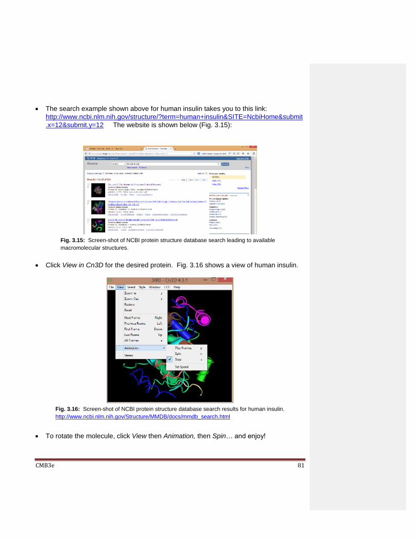
CMB3e 81

The search example shown above for human insulin takes you to this link:

http://www.ncbi.nlm.nih.gov/structure/?term=human+insulin&SITE=NcbiHome&submit

.x=12&submit.y=12 The website is shown below (Fig. 3.15):

Click View in Cn3D for the desired protein. Fig. 3.16 shows a view of human insulin.

To rotate the molecule, click View then Animation, then Spin… and enjoy!

Fig. 3.15: Screen-shot of NCBI protein structure database search leading to available

macromolecular structures.

http://www.ncbi.nlm.nih.gov/Structure/MMDB/docs/mmdb_search.html

Fig. 3.16: Screen-shot of NCBI protein structure database search results for human insulin.

http://www.ncbi.nlm.nih.gov/Structure/MMDB/docs/mmdb_search.html

CMB3e 82

Some iText & VOP Key Words and Terms

A functional groups primary structure

-carbon gene family prion

alpha helix gene superfamily protein folding

allosteric regulation glycosylation PrP

Alzheimer's disease helix-turn-helix motif quaternary structure

amino acid residues hemoglobin random coil

amino end hydrophobic interactions recombinatorial exchange

amyloid beta protein levels of protein structure salt bridges

amyloid plaques Mad Cow disease salt bridges

beta barrel multimer secondary structure

beta sheet NCBI Cn3D database sequence motifs

carboxyl end neurofibrillary tangles sickle cell anemia

catalysts nucleoskeleton side chains

chaperones orders of protein structure

structural domain

configuration Parkinson's disease structural motif

Creutzfeldt-Jakob disease

peptide bonds sulfhydryl groups

cytoskeleton peptide linkages tau protein

disulfide bonds phosphorylation tertiary structure

Edman degradation pleated sheet

enzymes polypeptide backbone

CMB3e 83

Chapter 4: Bioenergetics Thermodynamics (Free Energy, Enthalpy and Entropy), Chemical Energy,

Open vs. Closed Systems

4.1 Introduction

Three Laws of Thermodynamics describe the flow and transfer of energy in the

universe. They are:

1. Energy can neither be created nor destroyed (also stated as ‘universal energy is

constant’.

2. Universal entropy (disorder) is always increasing.

3. Entropy declines with temperature -as temperatures approach absolute zero, so

goes entropy.

In living systems, we do not have to worry about the third law because equations for

energy exchange in living systems already reflect the temperature dependence of entropy

change during reactions. Here we look at how we came to understand the basic

thermodynamic principles and how they apply to living systems. First, we will look at

different kinds of energy and at how redox reactions govern the flow of energy through

living things. Next, we’ll look at some simple arithmetic statements of the Laws of

Thermodynamics for closed systems and at how they apply to chemical reactions

conducted under standard conditions. Finally, since there is really no such thing as a

closed system, we look at the energetics of reactions occurring in open systems.

CMB3e 84

For an excellent discussion of how basic thermodynamic principles apply to living things,

you can also check out Lehninger A. (1971) Bioenergetics: The Molecular Basis of

Biological Energy Transformation. Benjamin Cummings, San Francisco.

Learning Objectives

When you have mastered the information in this chapter, you should be able to:

1. explain the difference between energy transfer and energy transduction.

2. compare and contrast potential vs. kinetic as well as other categories of energy (e.g.,

mass, heat, light…, etc.).

3. explain the reciprocal changes in universal free energy and entropy.

4. derive the algebraic relationship between free energy, enthalpy and entropy. 5. distinguish between exothermic, endothermic, exergonic, and endergonic reactions.

6. predict changes in free energy in a chemical reaction based on changes in the

concentrations of reactants and products in closed systems as well as open systems.

7. predict how and when an endothermic biochemical reaction will release free energy

(you should be able to do this after working some sample problems of closed system

energetics).

8. explain how an exergonic reaction occurring in a cell might be energetically

unfavorable.

9. explain and distinguish between the equilibrium and steady-state of reactions.

4.2 Kinds of Energy

We can easily recognize different kinds of energy around us like heat, light, electrical,

chemical, nuclear, sound, etc. And you probably know that energy in its different forms

is measurable (calories, joules, volts, decibels, quanta, photons…). Even mass is a form

of energy, as you may recall from Albert Einstein’s famous e=mc2 equation (the Law of

Relativity).

The problem in thinking about thermodynamics is that the universe is big and there are

too many kinds of energy to contemplate at once! To simplify, imagine only two kinds of

energy in the universe: potential energy and kinetic energy. A helpful example is a

dam. The water above the dam has potential energy. As the water flows over (or

through) the dam, its potential energy is released as kinetic energy. In the old days the

kinetic energy of flowing water could be used to power (i.e., turn) a millstone to grind

wheat and other grains into flour. These days, water is more likely to flow through a

hydroelectric dam where kinetic energy is converted (transduced) to electricity. In this

simple view, heat (molecular motion), electricity (a current of electrons), sound (waves),

and light (waves OR moving ‘particles’) are different forms of kinetic energy. The energy

of mass or its position in the universe is potential energy. For example, the energy in a

molecule of ATP is potential energy. Physicists talk a lot about potential energy and

about kinetic energy flow and conversion.

CMB3e 85

Here is an equally simple way to conceptualize energy: it is either useful or useless.

This concept led directly to the arithmetic formulation of the thermodynamic laws. In this

utilitarian way of thinking about energy, useless energy is entropy, while useful energy

can be any of the other forms of energy (potential or kinetic).

A key to understanding bioenergetics is to recognize the difference between closed and

open systems in the universe. Systems such as biochemical reactions in a test tube are

closed and will reach equilibrium. Closed systems are artificial and only possible in a

laboratory, where one can restrict and measure the amount of energy and mass getting

into or escaping the system. Cells on the other hand (in fact every reaction or event in

the rest of the universe) are open systems. Open systems readily exchange energy and

mass with their surroundings.

With this brief introduction, let’s imagine ourselves to be early scientists trying to

understand energy flow in the universe, asking how the Laws of Thermodynamics apply

to living systems (bioenergetics). We’ll see that the Laws can be demonstrated

precisely because all kinds of energy can be measured and all unites of energy can be

interconverted (e.g., volts into calories, light quanta into volts, joules into decibels, etc.).

138 Different Kinds of Energy; Chemical Equilibrium

4.3 Deriving Simple Energy Relationships

Thermodynamics Laws lead us to equations that help us understand how energy is

moves (i.e., flows) between components of the universe. As we’ll discuss, the universe is

most easily thought of as a giant closed system within which energy can be transferred

and even transduced (i.e., from one form to another) between those components. We

can’t measure energy flow in the universe as a whole. But we can isolate bits within the

universe so that we can quantify energy as it is transferred or transduced within a smaller,

more manageable closed system.

4.3.1 Energy in the Universe: the Universe is a Closed System

Consider an event, any event. I think we can agree that when stuff happens, the

participants in the happening go from an unstable state to a relatively more stable

state. For example, you are carrying a bag of marbles, the bag tears open and the

marbles fall to the floor, roll and spread out, eventually coming to a stop. At that point,

the marbles are in a more stable state than they were when you were holding the un-

ripped bag. We can all agree that gravity made the marbles fall from the bag. We

might then say that the fallen marbles are in a more stable state than they were in the

bag in your hands. That certainly seems true. If so, we could conclude that the drive

CMB3e 86

to greater stability is what made the marbles fall! In fact, regardless of the force or

impetus for the event, we say that the drive to achieve greater stability is what makes

stuff (i.e., events) happen! This is the Second Law of Thermodynamics: all

universal energy transfer events occur with an increase in stability…, that is, an

increase in entropy. We’ll consider the Second Law and entropy in detail shortly.

The tendency of things to go from unstable to more stable is a natural, rational state of

affairs…, like those marbles on the floor, or a messy bedroom with clothes strewn

about. Intuitively, messy and disordered is more stable than ordered. Of course,

marbles dropping or clothing going from folded and hung to wrinkled on the floor

releases energy (potential energy) as they fall (kinetic energy). If you don’t believe

that this release of energy is real, just think of how much energy you will need to pick

up the marbles or re-fold your clothes (after laundering them of course!).

We can model the flow of energy in the universe in a way that is consistent with

thermodynamic laws. Since the First law of Thermodynamics says that energy can

be neither created nor destroyed, a simple statement of the First Law could be:

Euniversal = Elight + Eheat + Eelectrical + Emass.... The equation sums up the different kinds of energy in the universe. Consider the circle (also called a Venn diagram) in Fig. 4.1 to be the universe.

Fig. 4.1: The sum of all things contained in the universe (e.g., as mass and other, more familiar

kinds of energy). In this simple “Venn” diagram, the universe is a closed system; nothing (mass,

energy) can get into or exit the universe, consistent with the First Law of Thermodynamics.

CMB3e 87

From this we conclude that energy cannot get in or out of the universe, but energy can

be transferred from one place to another or converted from one form to another. It

follows then that Euniversal is the sum of all kinds of energy in the universe, and that this

sum is a constant… in the words of the First law, universal energy is constant.

The equation below is consistent with this idea.

Elight + Eheat + Eelectrical + Emass +… = a constant

This is a simple arithmetic statement of the First Law of Thermodynamics.

139 First Law of Thermodynamics

If we go with the simpler binary notion of useful and useless energy, our equation

shortens to the sum of just two kinds of energy in the universe:

Euniversal = Guniversal + TSuniversal

In this equation, G is useful energy (“Gibbs” free energy ), S is useless energy

(entropy), and T is absolute temperature (included because of the third law). This is

also a statement of the First Law as shown in the revised Venn diagram in Fig. 4.2.

Fig. 4.2: Since even mass is a form of energy, the universe shown here consists of only two

components, entropy and free energy (defined as available to do work), still consistent with the

First law of Thermodynamics.

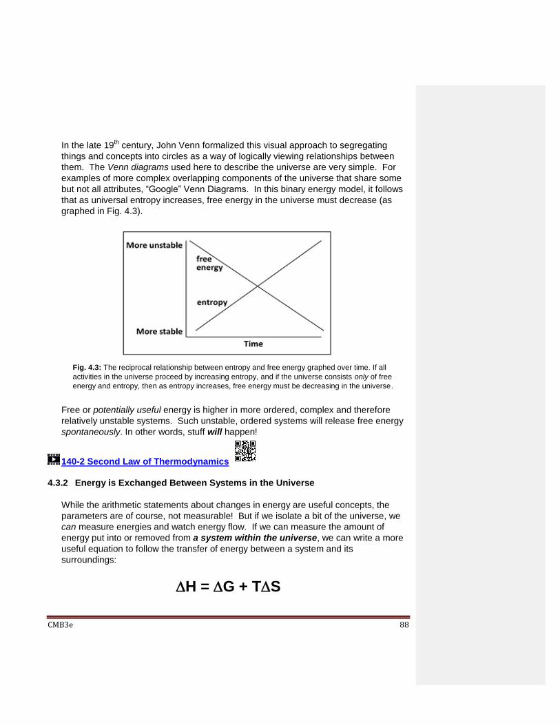
CMB3e 88

In the late 19th century, John Venn formalized this visual approach to segregating

things and concepts into circles as a way of logically viewing relationships between

them. The Venn diagrams used here to describe the universe are very simple. For

examples of more complex overlapping components of the universe that share some

but not all attributes, “Google” Venn Diagrams. In this binary energy model, it follows

that as universal entropy increases, free energy in the universe must decrease (as

graphed in Fig. 4.3).

Free or potentially useful energy is higher in more ordered, complex and therefore

relatively unstable systems. Such unstable, ordered systems will release free energy

spontaneously. In other words, stuff will happen!

140-2 Second Law of Thermodynamics

4.3.2 Energy is Exchanged Between Systems in the Universe

While the arithmetic statements about changes in energy are useful concepts, the

parameters are of course, not measurable! But if we isolate a bit of the universe, we

can measure energies and watch energy flow. If we can measure the amount of

energy put into or removed from a system within the universe, we can write a more

useful equation to follow the transfer of energy between a system and its

surroundings:

H = G + TS

Fig. 4.3: The reciprocal relationship between entropy and free energy graphed over time. If all

activities in the universe proceed by increasing entropy, and if the universe consists only of free

energy and entropy, then as entropy increases, free energy must be decreasing in the universe.

CMB3e 89

In this formula, H is the change (in enthalpy, i.e., as energy entering/leaving the

system in units of heat energy); G is change in free energy and S is change in

entropy; T is the absolute temperature (oK).

Heat given off in a reaction (or other event) is often confused with entropy. It is true

that much of the increase in entropy that occurs in living things is indeed in the form of

random molecular motion, or heat. But remember that heat can have its uses; not all

heat is entropic! Hence, it is more interesting (and accurate!) to think of energy in

terms of changes in enthalpy, free energy and entropy during energy transfers. Thus,

we must consider the arithmetic of energy transfers to involve not two, but three terms!

According to the equation H = G + TS, interacting systems in our universe would

seem to be closed systems. Accordingly, energy put into or removed from the system

(H) will be exactly balanced by increases and/or decreases in the other two terms in

the equation (G + TS). Recall that we refer to a system as closed not because it is

really closed, but because we can isolate them well enough to account for energy flow

into and out of the system. The value of this, or any algebraic equation with three

variables is that if you know two of the values, you can calculate the third! Here is a

simple situation to illustrate the point: If I put a liter of water on a burner and light the

flame, the water gets hot. If the temperature of the liter of water rises by 1oC, we

know that it has absorbed 1000 calories (one Kcal, or one food Calorie) of the heat

from the burner.

Since energy interactions depend on physical conditions such as temperature and air

pressure, we need to standardize those conditions when conducting experiments that

measure energy changes in experimentally isolated systems. For more on how

standardizing these physical parameters enables measuring energy change in

chemical reactions (in fact, any energy exchange), click the link below.

141 Deriving Closed System Thermodynamics

Turning to bioenergetics, let’s apply the equation H = G + TS to the conditions in

which chemical reactions occur in cells. Because most life on earth lives at sea level

where the air pressure is 1 atmosphere and the temperature is in the 20’s (Celsius),

typical determinations of H, G, and S are made under defined and well-controlled

standard conditions where T=298oK (25oC), an atmospheric pressure of pressures

of 1 atm, and a constant pH of 7.0. The latter is so defined because the pH inside of

a typical cell is close to neutral. In addition, measured values are adjusted to calculate

unimolar quantities of reactants (see below). Our equation for reactions under these

CMB3e 90

standard conditions becomes H = Go + TS, where Go is the standard free

energy change for a reaction conducted in a closed system under standard

conditions. H and S are still the enthalpy and entropy changes, but determined

under standard conditions.

What are unimolar conditions in practice? It means that if you measure the calories

released by burning (oxidizing) 180 mg of glucose, you must multiply the calories

released by 1000 to get (H). This will give you the calories that would have been

released by burning 180 gm (i.e., a whole mole) of the stuff.

Now we are ready to consider examples of how we determine the energetics of

reactions.

4.3.3 How is Enthalpy Change (H) Determined?

H (heat released or absorbed) in a chemical reaction can easily be determined by

conducting the reaction under standard conditions in a bomb calorimeter, essentially

an inner chamber surrounded by an outer chamber filled with water (Fig. 4.4).

Fig. 4.4: Basic design of a bomb calorimeter, with an inner chamber for conducting

reactions, and an outer chamber containing water with a thermometer to measure

temperature change (heat absorption or release, or H) during the reaction.

CMB3e 91

Food manufacturers determine the Calorie content of food by bomb calorimetry. As a

reaction takes place in the beaker, it will either release or absorb heat, either heating

or cooling the water in the calorimeter jacket, as measured by the thermometer. A

closed system reaction that releases heat as it reaches equilibrium is defined as

exothermic; the H for an exothermic reaction is negative. For example, a package

says that a chocolate bar has 90 Calories. This means that burning the bar will

generate 90 kilocalories (Kcal) of heat as measured in the calorimeter. Recall that

one Calorie (with a capital C) = 1000 calories, or one Kcal. One calorie (lower case) is

the energy needed to raise a gram of water by 1oC).

You are probably most familiar with reactions that release heat, but some chemical

reactions actually absorb heat. Take the common hospital cold pack for example.

Squeeze it to get it going and toss it in the calorimeter and then watch the temperature

in the calorimeter drop as the pack absorbs heat from the surroundings! Such

reactions are defined as endothermic, with a positive H. OK, so we can determine

the value of one of the energy parameters… we need to know at least one other,

either Go or S before the equation H = Go + TS becomes useful.

4.3.4 How is Standard Free Energy Change (G0) Determined?

As it turns out, Go or the standard free energy change is directly proportional to the

concentrations of reactants and products of a reaction conducted to completion (i.e.,

equilibrium) under standard conditions. Therefore, to determine Go, we need to

know or be able to measure the concentration of reactants and reaction products

before and after a chemical reaction (i.e., when the reaction reaches equilibrium).

Take the following generic chemical reaction:

2A + B <====> 2C + D

The following equation relates G0 to the equilibrium concentrations of A, B, C and D:

Go = -RTlnKeq = RTln [C]2[D]

[A]2[B]

In this equation, R is the gas constant (1.806 cal/mole-deg), T is 298oK and Keq is the

equilibrium constant. This is the Boltzman equation. As you can see, the Keq for

the reaction is the ratio of the product of the concentrations of the products (raised to

CMB3e 92

their stoichiometric powers) to the product of the concentrations of the reactants

(raised to their stoichiometric powers). Once you know (or have determined) the

equilibrium concentrations of reactants and products in a chemical reaction, you can

use this equation to calculate Go (standard free energy change) for a reaction.

Remember, if the Go is a negative number, the reaction is defined as exergonic.

We say that exergonic reactions release free energy. If the Go is a positive number,

the reaction absorbs free energy and is defined as endergonic.

142 Determining H & G in Closed Systems

4.3.5 Working an Example Using These Equations for Closed Systems

Consider the reaction:

This reaction endergonic If you do not know [X] and [Y] and therefore, G0, how can

you tell?

If you are given [X] and [Y], you can also do the math. Assume we measure the

concentrations of reactants and products for this reaction at equilibrium, with the

following results:

[X] = 2.5 Kcal/Mole; [Y] = 500 cal/Mole Try using the Boltzmann equation (above) to calculate the standard free energy for

this reaction. What is the Keq for this reaction? What is the Go for the reaction? If you did not come up with a Keq of 0.2 and an absolute value for the standard free

energy for|Go| of 866.2 Kcal/mole, re-calculate or collaborate with a classmate. Hint: make sure that you convert the units in your equation so that they are all the same!).

Based on the calculated value of Go, is this reaction in fact endergonic?

Now if you conduct the reaction in a bomb calorimeter, you find that it proceeds to

equilibrium with a H = -750 Kcal/Mole. What kind of reaction is this? Together with

the enthalpy change, it is now possible to use the equation H = Go + TS to

calculate an absolute value for the entropy change to be |S| = 116.2 cal/mol-deg for

the reaction. At equilibrium, the reaction proceeded with an increase in entropy under

standard conditions. Again, if you did not get the correct answer, re-calculate or

collaborate with a classmate.

143 Determining S in Closed System

X Y

CMB3e 93

4.4 Summary: The Properties of Closed Systems

First, let’s reiterate that there is no such thing as a closed system, unless of course the

universe is one! What we call a closed system is simply one in which we can measure

the energy going into or coming out of the system, and within which we can measure

energy transfers and transductions (changes from one kind of energy to another.

Features of closed systems can be defined by their properties:

Closed systems are experimentally defined by an investigator.

Defined Standard conditions apply.

Energy entering or leaving the system is measurable.

Reactions reach equilibrium regardless of reaction rate.

Product and reactant concentrations at equilibrium are constant (hence the

Keq)

Measured energy transfer/transduction values are constant (for a given set of

standard conditions).

Now let’s turn our attention to open systems, since that’s what cells are!

4.5 Open Systems and Actual Free Energy Change

Cells are open systems that are constantly exchanging mass and energy with their

environment; They never reach equilibrium. In addition, diverse organisms live under

very different atmospheric conditions and maintain different body temperatures (e.g., your

cat has a higher body temperature than you do!). Clearly, the conditions under which

cells conduct their biochemical reactions are decidedly non-standard. However, while

open systems do not reach equilibrium, they do achieve a steady state in which the rate

of input of energy and matter is equal to the rate of output of energy and matter. Think of

a biochemical pathway like glycolysis. If a cell’s energy needs are constant, the pathway

will reach a steady state. Of course, a cell’s need for energy (as ATP) can change as

energy needs change. If it does, then the steady state of ATP production will change to

meet the needs of the cell.

Later we will be discussing just how energy flows through living things, from sunlight into

chemical energy in nutrient molecules, into energy-rich fuels like ATP, and finally, into the

performance of all manner of cellular work. We characterize open systems by their

properties:

Open systems exchange energy and mass with their surroundings.

Open systems never reach equilibrium

CMB3e 94

They achieve steady state where the energy input rate = output rate.

The steady state can change.

In open systems, endergonic reactions can be energetically favorable

(spontaneous) and exergonic reactions can become energetically unfavorable.

Fortunately, there is an equation to determine free energy changes in open systems. For

our chemical reaction 2A + B <====> 2C + D, this equation would be:

G’ = Go + RTln [C]ss2

[D] ss

[A] ss2 [B] ss

Here, G’ is the actual free energy change for a reaction in an open system. Go is the

standard free energy change for the same reaction under standard conditions. In a

closed system. R is again the gas constant (1.806 cal/mole-deg) and T is the absolute

temperature in which the reaction is actually occurring. The subscript ‘ss’ designates

reactant and product concentrations measured under steady state conditions. You can

see here that this equation states a relationship between Go and G’. So, to determine

the actual free energy of a biochemical reaction in a cell (in fact in any living tissue), all

you need to know are the Go for the reaction, the steady state concentrations of reaction

components in the cells/tissues, and the absolute T under which the reactions are

occurring.

144 The Energetics of Open Systems

Elsewhere, we will use the reactions of the glycolytic pathway to exemplify the properties,

as well as the energetics of open and closed systems. At that time, pay careful attention

to the application of the terminology of energetics in describing energy flow in closed vs.

open systems.

Some iText & VOP Key Words and Terms

actual free energy endothermic Law of Conservation

ATP energy Laws of Thermodynamics

bioenergetics energy transduction light

Boltzman equation energy transfer mass

calories enthalpy open system properties

calorimeter entropy open systems

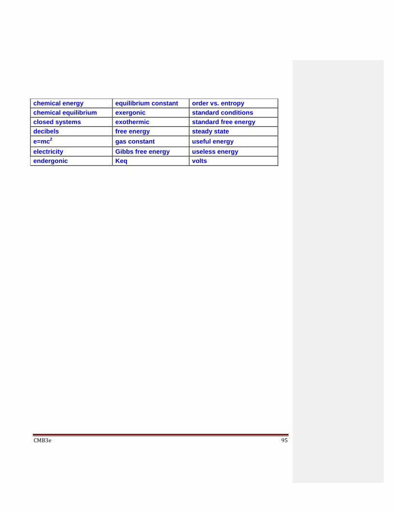
CMB3e 95

chemical energy equilibrium constant order vs. entropy

chemical equilibrium exergonic standard conditions

closed systems exothermic standard free energy

decibels free energy steady state

e=mc2 gas constant useful energy

electricity Gibbs free energy useless energy

endergonic Keq volts

CMB3e 96

Chapter 5: Enzyme Catalysis and Kinetics

Mechanism of Enzyme Catalysis, Induced Fit, Activation Energy, Determining and Understanding Enzyme Kinetics

5.1 Introduction By definition, all catalysts accelerate chemical reactions, including enzymes. But

enzymes and inorganic catalysts differ in important ways (Table 5.1 below).

https://www.youtube.com/watch?v=94M7B7bz-N0

Listen here: https://www.youtube.com/watch?v=bUfLHJg-CY0

Or here…

CMB3e 97

In this chapter, we look at the properties and mechanism of action of enzymes. These

include allosteric change (induced fit, enzyme regulation), energetic events (changes in

activation energy), and how enzymes work in open and closed (experimental) systems.

Most Enzymes are proteins, but as we’ll see later, a few are RNAs. Enzymes are long

polymers that can fold into intricate shapes. As a result, they can be more specific than

inorganic catalysts in which substrates they recognize and bind to. Finally, enzymes are

flexible and can be regulated in ways that rigid, inflexible, metallic inorganic catalysis

cannot. The specificity of an enzyme lies in the structure and flexibility of its active site.

We will see that the active site of an enzyme undergoes conformational change during

catalysis. The flexibility of enzymes also explains the ability of enzymes to respond

metabolites in a cell that indicate its biochemical status. When such metabolites bind to

an enzyme, they force a conformational change in the enzyme that can speed up or

Slow down the catalytic rate of the reaction, a phenomenon called allosteric regulation.

As you might imagine, changing the rate of a biochemical reaction can change the rate of

an entire biochemical pathway…, and ultimately the steady state concentrations of

products and reactants in the pathway.

To understand the importance of allosteric regulation, we’ll look at how we measure the

speed of enzyme catalysis. As we consider the classic early 20th century enzyme kinetic

studies of Leonor Michaelis and Maud Menten, we’ll focus on the significance of the Km

and Vmax values that they derived from their data. But before we begin our discussion

here, remember that chemical reactions are by definition, reversible. The action of

catalysts, either inorganic or organic, depends on this concept of reversibility.

Finally, let’s give a nod to recent human ingenuity that enabled enzyme action to turn an extracellular profit! You can now find enzymes in household cleaning products like spot removers and detergents, where they digest and remove stains caused by fats and pigmented proteins. Enzymes added to meat tenderizers also digest (hydrolyze) animal proteins down to smaller peptides. Enzymes can even clean a clogged drain!

Learning Objectives

When you have mastered the information in this chapter, you should be able to:

1. describe how the molecular flexibility of protein and RNA molecules make them ideal

biological catalysts.

2. compare and contrast the properties of inorganic and organic catalysts.

3. explain why catalysts do not change equilibrium concentrations of a reaction

conducted in a closed system.

4. compare the activation energies of catalyzed and un-catalyzed reactions and explain

the roles of allosteric effectors in enzymatic reactions.

5. discuss how allosteric sites interact with an enzyme's active site and explain the concept of the rate limiting reaction in a biochemical pathway.

CMB3e 98

6. write simple rate equations for chemical reactions. 7. write the possible rate equations for catalyzed reactions. 8. distinguish between Vmax and Km in the Michaelis-Menten kinetics equation. 9. state what Vmax and Km say about the progress of an enzyme catalyzed reaction.

10. interpret enzyme kinetic data and the progress of an enzyme-catalyzed reaction from this data.

11. more accurately identify Leonor Michaelis and Maud Menten!

5.2 Enzymes and the Mechanisms of Enzyme Catalysis

Studies by George Beadle and Edward Tatum correlating mutations with enzyme

deficiencies in Neurospora crassa (bread mold) and Drosophila melanogaster led them to

propose the one-gene/one-enzyme hypothesis in 1941. By 1958, they shared Nobel

Prize in Physiology and Medicine for this work and their hypothesis had already morphed

twice… first into the one-gene/one-protein, and then the one-gene/one-polypeptide

hypothesis. This rightfully revered history helped launch the age of molecular biology.

The subsequent discovery of RNA catalysts came as quite a surprise! The revelation of

RNA catalysts, dubbed ribozymes, earned Sidney Altman and Thomas Cech a Nobel

Prize in Chemistry in1989. Ribozymes are now known to catalyze RNA splicing (the

removal of unwanted regions of a precursor RNA). They also catalyze a step in protein

synthesis (translation) on ribosomes. In fact, almost no biochemical reaction exists that is

not directly the result of enzyme catalysis, from the digestion of nutrients in your mouth,

stomach and small intestines to pretty much every chemical reaction inside your cells

[check out Kornberg A (1989) Never a Dull Enzyme. Ann. Rev. Biochem. 58:1-30].

In this chapter the focus on the long history of protein enzyme catalysis. But as you

study, you may recognize that the mechanisms of enzyme catalysis described here

involve common essential features seen in all biocatalysts.

Enzymes are generally soluble in or outside cells while a few are part of membranes or

other cellular structures. In all cases, they bind to soluble substrates (the reactants in

enzyme-catalyzed reactions). The large size and exquisite diversity of protein structures

make enzymes highly specific catalysts. The specificity of an enzyme results from the

shape of the active site of the enzyme, which is dependent on the three-dimensional

arrangement of amino acids in and around the region. The substrates of a catalyzed

biochemical reaction are bound to and held in place on the enzyme while rapid bond

rearrangements take place. Their flexibility allows enzymes to change in shape at the

active site during catalysis. In addition, this flexibility enables small metabolites in cells to

interact with and change the shapes of many enzymes, changing their rates of catalysis.

The latter phenomenon enables allosteric regulation, allowing cells to control the rates

and even the direction of biochemical reactions and pathways. As we will see, enzymes

may also be bound to prosthetic groups or ions that contribute to the shape and activity of

the enzyme.

CMB3e 99

Any, understanding the mechanism of catalysis must also include knowing something

about the energetics of catalyzed reactions. We’ll see that enzymes lower the activation

energy of a chemical reaction, and that activation energy is an inherent energy barrier to

the reaction. We will look at the energetics of enzyme action.

In sum, we describe the action of biological catalysis in terms of the structural features of

the enzyme (active site shape, overall conformation, the affinities of the enzyme for its

substrates), as well as free energy changes that occur during catalysis. Of course,

structural and energy considerations of enzyme catalysis are related.

145 Enzymes vs. Other Catalysts 5.2.1 Structural Considerations of Catalysis

From a chemistry course, you may recall that the rate of an uncatalyzed reaction is

dependent on the concentration of the reactants in solution. This is the Law of Mass

Action, recognized in the19th century. Look at this simple reaction:

The Law of Mass Action makes two key assumptions:

1) At any given time following the start of the reaction, the rate of product formation is

proportional to the concentrations of the reactants and products ([A], [B], [C] and [D] in

this case).

2) Chemical reactions in the laboratory (i.e., a ‘closed system’) eventually reach

equilibrium, at which point the net rate of formation of reaction products is zero. (in

other words, the forward and reverse reactions occur at the same rate).

There are no products (i.e., C and D) at the start of the reaction written above. As

there are no products yet, the reaction rate should be directly proportional only to the

concentration of the reactants. The Law of Mass Action predicts that the chemical

reaction above will occur faster when A and B are first mixed together…, that is, at

higher concentrations of A & B. This is because there are more reactant molecules in

solution and a greater likelihood that they will collide in an orientation that allows the

bond rearrangements for the reaction to occur.

Of course, reactant concentrations decline as products accumulate over time and the

rate of formation of C & D slows down. At some point, as products accumulate they

should also influence the rate of their own production. Remember, all chemical

reactions are inherently reversible! So rising levels of products will begin to push the

reaction to form A and B, slowing down the net accumulation of C and D. You may

recall chemical rate equations from a chemistry course; these enable quantitation of

A + B C + D

CMB3e 100

reaction rates for our sample reaction. Here is the rate of formation of the products: C

& D formation rate = k1[A][B] – k-1[C][D], where k1[A][B] is the rate of the forward

reaction; k-1[C][D] is the rate of the reverse reaction. In this way, the equation

recognizes that the reaction is reversible. The equation states that the net reaction

rate is equal to the rate of the forward reaction (k1[A][B]) minus the rate of the back

reaction (k-1[C][D]). The equation is valid (applicable) at any time during the reaction.

k1 and k-1 are rate constants for the forward and reverse reactions, respectively.

So how do catalysts work? Catalysts increase chemical reaction rates by bringing

reactants together more rapidly than they would otherwise encounter each other

based just on random molecular motion in solution. This is possible because catalysts

have an affinity for their substrates. In the case of inorganic catalysts, relatively

weak, generic forces account for the affinity of reactants and inorganic catalysts.

Thus, a metallic catalyst (e.g., silver, platinum) attracts molecules with the appropriate

(usually charge) configuration. If the attraction (affinity) is sufficient, the metal will hold

reactants in place long enough to catalyze the bond rearrangements of a chemical

reaction.

Unlike inorganic catalysts, enzymes have evolved highly specific shapes with

physical-chemical properties. As a result, typical enzymes only attract the substrates

necessary for a particular biochemical reaction. The active site of an enzyme has an

exquisite, selective affinity for its substrate(s). This affinity is many times greater than

those of inorganic catalysts for generic reactants. The result is that enzymes are more

efficient and faster than inorganic catalysts. Early ideas of how substrate-enzyme

interaction could be so specific suggested a Lock and Key mechanism (Fig. 5.1).

Fig. 5.1: Illustration of the early Lock-&-Key mechanism for enzyme-substrate interaction,

in which the substrate key fits an enzyme lock.

CMB3e 101

According to this model, the affinity of enzyme for substrate engages the substrate

‘key’ in the tumblers (i.e. active site) of enzyme ‘lock’. Thus engaged , the substrate(s)

would undergo the bond rearrangements specific for the catalyzed reaction to

generate products and regenerate an unchanged enzyme. But X-ray crystallography

of enzyme-substrate interactions reveal that the active site of the enzymes change

shape during catalysis. This allosteric change suggested the Induced Fit mechanism

of enzyme action (modeled in Fig. 5.2).

In this model, enzyme-substrate affinity causes the substrate to bind to the enzyme surface. Once bound, the enzyme undergoes an allosteric change, drawing the substrate(s) more tightly into the active site and catalyzing the reaction. Of course, after the reaction products come off, the enzyme returns to its original shape.

146-2 Induced Fit Mechanism of Enzyme Action

5.2.2 Energetic Considerations of Catalysis

Consider the random motion of substrates in solution that occasionally encounter one

another. They even more rarely bump into one another in just the right orientation to

cause a reaction. This explains why adding more reactants or increasing the

temperature of a reaction can speed it up…, by increasing the number of random as

well as productive molecular collisions. Unlike molecules and reactions in a test tube,

living organisms do not have these options for increasing reaction rates.

Fig. 5.2: The Induced Fit mechanism of enzyme-substrate interaction. Initial interaction of

substrate with enzyme based on mutual affinity causes an allosteric change in the enzyme.

This results in the induced ‘better’ fit of substrate to enzyme, to be followed by catalysis.

CMB3e 102

But they do have enzymes! All catalysts work by lowering the activation energy (Ea)

for a reaction, thereby increasing the rate of the reaction. Activation energy is

essentially a barrier to getting interacting substrates together to actually undergo a

biochemical reaction.

Inorganic catalytic surfaces attract reactants where catalysis can occur. The

attractions are weak compared to those of enzymes and their substrates. An

enzyme’s active site attracts otherwise randomly distributed substrates very strongly,

making enzyme catalysis faster than inorganic catalysis. Again, cells cannot use

inorganic catalysts, most of which are insoluble and would attract reactants

indiscriminately... not a good way for cells to control metabolism! The advent of

enzymes with their specificity and high rate of catalysis was a key event in chemical

evolution required for the origins of life. As we saw, allosteric change during the

‘induction of fit’ enables specific catalysis. In fact, a catalyzed reaction will be faster

than the same reaction catalyzed by a piece of metal, and of course much faster

(millions of times faster!) than the uncatalyzed reaction. The energetics of catalysis

helps to explain why. Take a look at the energetics of a simple reaction in which A &

B are converted to C & D (Fig. 5.3).

Conducted in a closed system, enzyme-catalyzed reactions reach their equilibrium

more rapidly. As with all catalysts, enzymes are not consumed by the reactions they

catalyze, nor do they alter the equilibrium concentrations of reactants and products of

Fig. 5.3: Graph of change in free energy over time as chemicals A and B react. The high

Activation Energy peak in the graph is the free energy barrier that A and B must overcome

before much C and D can be made. This barrier is due mainly to thermal motion of the A and B

molecules, with only rare encounters in relatively dilute solutions. Enzymes are even more

efficient that inorganic catalysts in lowering the activation energy barrier to a reaction.

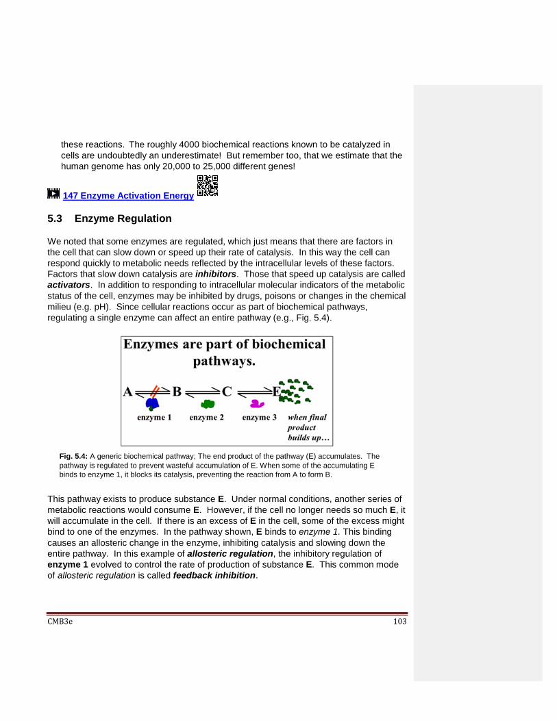
CMB3e 103

these reactions. The roughly 4000 biochemical reactions known to be catalyzed in

cells are undoubtedly an underestimate! But remember too, that we estimate that the

human genome has only 20,000 to 25,000 different genes!

147 Enzyme Activation Energy

5.3 Enzyme Regulation

We noted that some enzymes are regulated, which just means that there are factors in

the cell that can slow down or speed up their rate of catalysis. In this way the cell can

respond quickly to metabolic needs reflected by the intracellular levels of these factors.

Factors that slow down catalysis are inhibitors. Those that speed up catalysis are called

activators. In addition to responding to intracellular molecular indicators of the metabolic

status of the cell, enzymes may be inhibited by drugs, poisons or changes in the chemical

milieu (e.g. pH). Since cellular reactions occur as part of biochemical pathways,

regulating a single enzyme can affect an entire pathway (e.g., Fig. 5.4).

This pathway exists to produce substance E. Under normal conditions, another series of

metabolic reactions would consume E. However, if the cell no longer needs so much E, it

will accumulate in the cell. If there is an excess of E in the cell, some of the excess might

bind to one of the enzymes. In the pathway shown, E binds to enzyme 1. This binding

causes an allosteric change in the enzyme, inhibiting catalysis and slowing down the

entire pathway. In this example of allosteric regulation, the inhibitory regulation of

enzyme 1 evolved to control the rate of production of substance E. This common mode

of allosteric regulation is called feedback inhibition.

Fig. 5.4: A generic biochemical pathway; The end product of the pathway (E) accumulates. The

pathway is regulated to prevent wasteful accumulation of E. When some of the accumulating E

binds to enzyme 1, it blocks its catalysis, preventing the reaction from A to form B.

CMB3e 104

Enzymes can be regulated precisely because they can be bent out of shape (or into

shape for that matter!). Some small metabolites become chemical information when they

accumulate in cells, able to communicate cellular metabolic status. The result is a

decrease or increase enzyme activities to achieve an appropriate cellular response.

Whether an activator or an inhibitor of enzyme catalysis, regulatory molecules typically

bind to enzymes at allosteric regulatory sites, causing local conformational changes in

the enzyme that are transmitted to the active site. Enzyme inhibition will occur if a

change in shape reduces the affinity of enzyme for substrate… or if it reduces the rate of

bond rearrangements after the substrate has entered the active site. Enzyme activation

would occur if the allosteric effect were to increase this affinity and/or catalytic rate. The

mechanism of allosteric regulation of enzyme activity is shown in Fig. 5.5.

148-2 Allosteric Regulation of Enzyme Activity

5.4 Enzyme Kinetics Studying enzyme kinetics can tell us not only about the catalytic properties of a particular

enzyme, but can also reveal important properties of biochemical pathways. Thus, one

can determine a standard rate-limiting reaction under a given set of conditions by

comparing kinetic data for each enzyme in a biochemical pathway. But what else can we

do with kinetic data?

Fig 5.5: Allosteric effectors are small metabolites whose amounts in a cell reflect the

cell’s metabolic status. They bind to enzymes at a regulatory site, causing an allosteric

(conformational) change in the enzyme that affects the shape of the Active Site, either

inhibiting catalysis (as suggested here) or stimulating it.

CMB3e 105

5.4.1 Why Study Enzyme Kinetics?

Apart from its value in understanding how an individual enzyme actually works, kinetic

data has great clinical value. For example, if we know the kinetics of each enzyme in

the biochemical pathway to the synthesis of a liver metabolite in a healthy person, we

also know what is normally the rate-limiting (slowest) enzyme in the pathway.

Consider a patient whose blood levels of this metabolite are higher than normal.

Could this be because what was the normal rate-limiting reaction is no longer rate-

limiting in the patient? Which enzyme in the patient then, is newly rate-limiting? Is

there a possible therapy in having this information? One can ask similar questions of

an alternate scenario in which a patient is producing too little of the metabolite.

Reasons why a cellular biochemical would deviate from ‘normal’ levels include:

Viral & bacterial infection or environmental poisons: these can interfere with a

specific reaction in a metabolic pathway; remedies depend on this information!

Chronic illness resulting from mutational enzyme deficiencies: treatments

might include medications designed to enhance or inhibit (as appropriate) enzyme

activity.

Genetic illness tied to metabolic deficiency: if a specific enzyme is the culprit,

investigation of a pre- and/or post-natal course of treatment might be possible

(e.g., medication or perhaps even gene therapy).

Life-style changes and choices: these might include eating habits, usually

remediated by a change in diet.

Life-Style changes brought on by circumstance rather than choice: these are

changes due to aging. An all too common example is the onset of Type 2

Diabetes. This can be treated with medication and/or delayed by switching to a

low carb diet favoring hormonal changes that improve proper sugar metabolism.

Knowing the rate-limiting reaction(s) in biochemical pathways can identify regulated

enzymes. This in turn may lead to a remedy to correct a metabolic imbalance. As

noted, ribozymes are RNA molecules that catalyze biochemical reactions; their

kinetics can also be analyzed and classified. We will consider how enzymes are

regulated later, when we discuss glycolysis, a biochemical pathway that most living

things use to extract energy from nutrients. For now let’s look at an overview of

experimental enzyme kinetics and how we interpret kinetic data.

5.4.2 How We Determine Enzyme Kinetics and Interpret Kinetic Data

In enzyme kinetic studies, the enzyme is considered to be a reactant, albeit one that is

regenerated by the end of the reaction. The reaction begins when substrate are

added to the enzyme. In enzyme kinetic studies, the concentration of the enzyme is

CMB3e 106

held constant while reaction rates are measured after adding different amounts of

substrate. As a consequence, all catalyzed reactions will reflect saturation of the

enzyme at high concentration of substrate. This is the basis of saturation kinetics

illustrated in Fig.5.6.

From the illustration, the active sites on all the enzyme molecules are bound to

substrate molecules at high substrate concentration. Under these conditions, a

catalyzed reaction is proceeding at its fastest. Let’s generate some kinetic data to see

saturation in action. The experiment illustrated below (Fig. 5.7) will determine the

kinetics of the conversion of S to P by enzyme E.

Fig. 5.6: Saturation kinetics of an enzyme-catalyzed reaction. At high substrate

concentrations, all the active sites of all enzymes are occupied. Under these

conditions, the reaction occurs at its fastest rate.

Fig. 5.7: Experimental protocol for determining the kinetics of an enzyme-catalyzed reaction.

CMB3e 107

A series of reaction tubes are set up, each containing the same concentration of enzyme

([E]) but different concentrations of substrate ([S]). The concentration of P ([P]) produced

at different times beginning just after the start of the reaction in each tube is plotted to

determine the initial rate of P formation for each concentration of substrate tested. Fig.

5.8 below is such a plot.

In this hypothetical example, the rates of the reactions (amount of P made over time) do

not increase at substrate concentrations higher than 4 X10-5 M. The upper curves thus

represent the maximal rate of the reaction at the experimental concentration of enzyme.

We say that the maximal reaction rate occurs at saturation.

149 Measuring Enzyme Kinetics Next, we can estimate the initial reaction rate (vo) at each substrate concentration by

plotting the slope of the first few time points through the origin of each curve in the graph.

Consider the graph of the initial reaction rates estimated in this way in Fig. 5.9 (below).

The slope of each straight line is the vo for the reaction at a different [S] near the very

beginning of the reaction, when [S] is high and [P] is vanishingly low.

Fig. 5.8: This graph plots the rate of product (P) formation at 4 different substrate

concentrations, while holding the enzyme concentration constant.

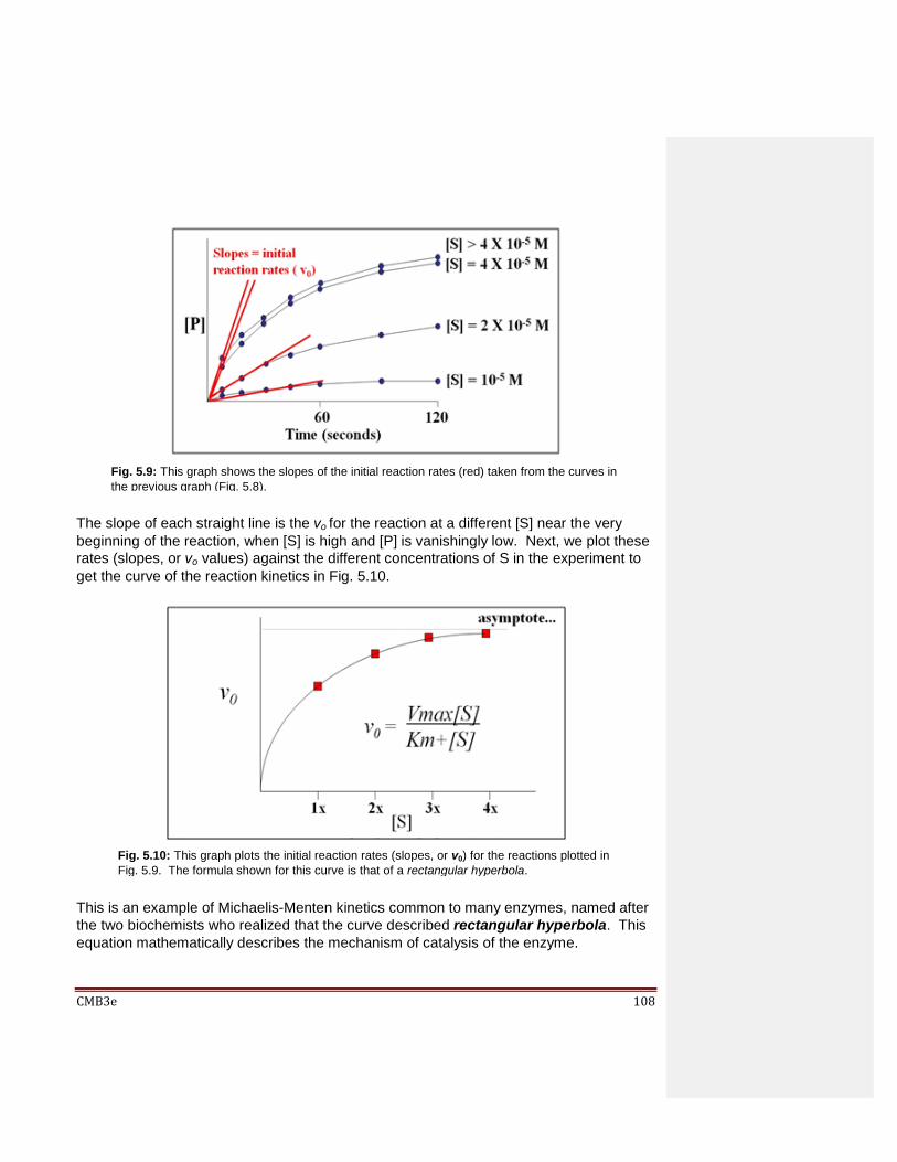
CMB3e 108

The slope of each straight line is the vo for the reaction at a different [S] near the very

beginning of the reaction, when [S] is high and [P] is vanishingly low. Next, we plot these

rates (slopes, or vo values) against the different concentrations of S in the experiment to

get the curve of the reaction kinetics in Fig. 5.10.

This is an example of Michaelis-Menten kinetics common to many enzymes, named after

the two biochemists who realized that the curve described rectangular hyperbola. This

equation mathematically describes the mechanism of catalysis of the enzyme.

Fig. 5.9: This graph shows the slopes of the initial reaction rates (red) taken from the curves in

the previous graph (Fig. 5.8).

Fig. 5.10: This graph plots the initial reaction rates (slopes, or v0) for the reactions plotted in

Fig. 5.9. The formula shown for this curve is that of a rectangular hyperbola.

CMB3e 109

The equation below mathematically describes a rectangular hyperbola:

You might be asked to understand the derivation of the Michaelis-Menten equation in a

Biochemistry course. You might even be asked to do the derivation yourself! We won’t

make you do that, but suffice it to say that Michaelis and Menten started with some

simple assumptions about how an enzyme-catalyzed reaction would proceed and then

wrote reasonable chemical and rate equations for those reactions. The goal here is to

understand those assumptions, to see how the kinetic data support those assumptions,

and to realize what the this tells us about how enzymes really work.

Here is one way to write the chemical equation for a simple reaction in which an enzyme

(E) catalyzes the conversion of substrate (S) to product (P):

Michaelis and Menten rationalized that this reaction might actually proceed in three steps.

In each step enzyme E is treated as a reactant in the conversion of S to P. The resulting

chemical equations are shown below.

Reasoning that the middle reaction (the conversion of E-S to E-P) would be the fastest

one and therefore would not be the rate-limiting reaction of catalysis, they only considered

the first and third reactions to be relevant in determining the overall kinetics of product

formation. Then they wrote the following rate equations for just these two chemical

reactions (as one would in an introductory chemistry course):

vE-S formation = k1[E][S] - k-1[E-S]

vP formation = k2[E-S] - k-2[E][P]

xa

x+b y =

S P

E

CMB3e 110

Both of these equations describe a straight line, which does not describe the observed

hyperbolic reaction kinetics. Solving either equation for [E-S] and substituting the solution

for [E-S] in the other equation left a single equation. But this equation also described a

straight line. Again, not the expected rectangular hyperbola. To arrive at a chemical rate

equation consistent with a rectangular hyperbola, Michaelis and Menten made several

assumptions, including those made by G. E. Briggs and J. B. S. Haldane about how E, S

and P would behave in a catalyzed reaction.

It was those assumptions allowed them to re-write each equation, combine and rewrite

them into a single mathematical equation that did indeed describe a rectangular

hyperbola. Here are Briggs and Haldane’s assumptions:

1. [S] >> [E] at the start and during the ‘steady state’.

2. [P] << [S] at the start of a reaction.

3. All E is bound to S at the start of the reaction.

4. [E]total = [E]free + [E-S] at all times.

We have already seen the equation that Michaelis and Menten derived and now known

as the Michaelis-Menten equation:

The take-home message here is that the assumptions about an enzyme-catalyzed

reaction are a good approximation of how the reaction proceeds over time.

Michaelis and Menten defined Vmax and Km as key kinetic factors in enzyme-catalyzed

reactions. In the generic example of substrate conversion to product, we saw that

increasing [S] results in a higher rate of product formation because a higher rate of

encounters of enzyme and substrate molecules. At some point however, increasing [S]

does not increase the initial reaction rate any further. Instead, vo asymptotically

approaches a theoretical maximum for the reaction, defined as Vmax, the maximum initial

rate. As we have already seen, Vmax occurs when all available enzyme active sites are

saturated (occupied by substrate). At this point, the intrinsic catalytic rate determines the

turnover rate of the enzyme. The substrate concentration at which the reaction rate has

reached ½Vmax is defined as KM (the Michaelis-Menten constant). The Km is a ratio of

rate constants remaining after rewriting the rate equations for the catalyzed reaction.

150 Graphing Enzyme Kinetic Data

v0

= Vmax[S]

Km + [S]

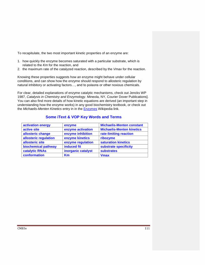
CMB3e 111

To recapitulate, the two most important kinetic properties of an enzyme are:

1. how quickly the enzyme becomes saturated with a particular substrate, which is

related to the Km for the reaction, and

2. the maximum rate of the catalyzed reaction, described by the Vmax for the reaction.

Knowing these properties suggests how an enzyme might behave under cellular

conditions, and can show how the enzyme should respond to allosteric regulation by

natural inhibitory or activating factors…, and to poisons or other noxious chemicals.

For clear, detailed explanations of enzyme catalytic mechanisms, check out Jencks WP

1987, Catalysis in Chemistry and Enzymology. Mineola, NY, Courier Dover Publications].

You can also find more details of how kinetic equations are derived (an important step in

understanding how the enzyme works) in any good biochemistry textbook, or check out

the Michaelis-Menten Kinetics entry in in the Enzymes Wikipedia link.

Some iText & VOP Key Words and Terms

activation energy enzyme Michaelis-Menten constant

active site enzyme activation Michaelis-Menten kinetics

allosteric change enzyme inhibition rate-limiting reaction

allosteric regulation enzyme kinetics ribozyme

allosteric site enzyme regulation saturation kinetics

biochemical pathway induced fit substrate specificity

catalytic RNAs inorganic catalyst substrates

conformation Km Vmax

CMB3e 112

Chapter 6: Glycolysis, the Krebs Cycle and the

Atkins Diet Glycolysis, Gluconeogenesis & the Krebs Cycle - Getting Energy from Food;

Enzyme Regulation & the Bioenergetics of Cellular Free Energy Capture; Liver Cells in Glucose metabolism; Fooling Your Body - Atkins (& Similar) Diets

6.1 Introduction

We used to get metabolic pathways charts like the one you see here free from vendors of

biochemical reagents. This one is a high-resolution image; if you zoom in, you can

actually read the content…, but don’t feel you must! The big picture is correct in macro-

detail, but the chart is likely out of date in small new details. In this chapter, we ‘zoom in’

on the small region in the middle of the chart, encompassing glycolysis and the Krebs

cycle.

We have looked at the principles governing thermodynamics (the flow of energy in the

universe) and bioenergetics (energy flow in living systems). We saw evidence that

energy can be exchanged between components in the universe, but that it can be neither

This (in fact any!) metabolic pathways chart highlights the centrality of the Krebs (citic acid) cycle

CMB3e 113

created nor destroyed. That makes the universe a closed system, a conclusion codified

as the First Law of Thermodynamics. Personally, I find it troubling that there is no

escape from the universe…, that is, until I remind myself that the universe is a pretty big

place, and I am only a small part of a small system. You can define systems for yourself:

the solar system, planet earth, the country you pledge allegiance to, your city or village,

your school, a farm or homestead…! Then you may derive comfort from the realization

that you can move from one system to another and even exchange goods and services

between them. This is a metaphor for energy flow between systems in the universe. We

also saw that the First Law applies to closed systems within the universe…, and that

there are no closed systems in the universe! Any system in the universe is open, always

exchanging energy and mass with neighboring systems. What we mean by the

term closed system is that we can define and isolate some small part of the universe,

and then measure any energy that this isolated system gives up to its environment, or

takes in from it. The simplest demonstration of the First Law in action was the bomb

calorimeter that measures heat released or absorbed during a chemical reaction.

The second concept said that energy flows from one place to another only when it can.

In the vernacular, we say that energy flows downhill. Anything that happens in the

universe (a galaxy moving through space, a planet rotating, getting out of bed in the

morning, coffee perking, your cells sugar burning, DNA replicating…) does so because

energy flows downhill. We saw that by definition, any happening or event in the universe,

however large or small, is spontaneous, that is, it occurs with a release of free energy.

Remember, spontaneous means “by itself” and not necessarily instantaneous or fast!

Finally, we noted that that when enzymes catalyze biochemical reactions in a closed

system, the reactions still reach equilibrium, despite the higher rate of the catalyzed

reaction. What does this tell you about the energetics of catalyzed reactions in closed

systems?

With this brief reminder about energy flow and what enzymes do, we’ll look at how our

cells capture nutrient free energy. This will include examples of the energetics of closed

systems that reach equilibrium, and open systems that don’t! First, we tackle glycolysis,

an anaerobic fermentation pathway for generating chemical energy from glucose, as

well as the first of several aerobic pathways of respiration. We’ll see that most of the

energy from glycolysis and respiration is captured in molecules of ATP, the universal

energy currency of life, used by cells to… live! Then we look at Gluconeogenesis, a

regulated reversal of glycolysis. We ask when, where and why we would want to make,

rather than burn glucose. Finally, we begin a discussion of respiration with a look at the

Krebs Cycle. The complete respiratory pathway can be summarized by the following

equation:

C6H12O6 + 6O2 6CO2 + 6H2O

CMB3e 114

The standard free energy change for this reaction (Go) is about -687Kcal/mole. This

is the maximum amount of nutrient free energy that is (at least in theory) available from

the complete respiration of a mole of glucose. Given a cost of about 7.3 Kcal to make

each mole of ATP (adenosine triphosphate), how many moles of ATP might a cell

produce after burning a mole of glucose? We’ll figure this out here.

Learning Objectives

When you have mastered the information in this chapter, you should be able to:

1. explain the difference between fermentation and respiratory glycolysis and the role of

redox reactions in both processes.

2. Calculate, compare and contrast Go and G’ for the same reaction, and explain any

differences in free energy in open and closed systems.

3. describe and explain the major events of the first stage of glycolysis and trace the free energy changes through the formation of G-3-P.

4. describe and explain the major events of the second stage of glycolysis and trace the free energy changes through the formation of pyruvate and lactic acid.

5. state the role of redox reactions in glycolysis and fermentation.

6. compare and contrast glucose (i.e., carbohydrates in general), ATP, NADH and

FADH2 as high-energy molecules. [Just for fun, click Power in the Primordial Soup to

read some far out speculations on prebiotic high-energy molecules that might have

been around when ATP was being hired for the job!].

7. explain why only a few cell types in the human body conduct gluconeogenesis.

8. explain how gluconeogenesis, an energetically unfavorable pathway, can occur at all.

9. explain why the Atkins Diet (and similar diets) work and speculate on any downsides.

10. explain the concept of a super-catalyst and explain why a super-catalyst like the Krebs

Cycle would have evolved.

11. explain the role of high energy linkages and electron carriers in the Krebs cycle. 12. compare phosphate ester linkages in ATP and GTP, and thioester linkage in acetyl-S-

CoA and succinyl-S-CoA in terms of energetics and their biochemical reactions.

13. speculate on why the Krebs Cycle in E. coli generates GTP molecules and why it

generates ATP molecules eukaryotes.

6.2 Glycolysis, a Key Pathway in Energy Flow through Life

One of the properties of life is that living things require energy. The pathways of energy

flow through life are shown in Fig. 6.1 (below). To begin with, recall that the most

common intracellular energy currency with which livings things “pay” for cellular work is

ATP. The energy to make ATP on planet earth ultimately comes from the sun via

photosynthesis. Recall that light energy fuels the formation of glucose and O2 from CO2

and water in green plants, algae, cyanobacteria and a few other bacteria. Photosynthesis

even produces some ATP directly, but not enough to fuel all cellular and organismic

growth and metabolism.

CMB3e 115

In fact, all cells, even plant cells, use fermentation and/or respiration (anaerobic or

aerobic processes respectively) to capture nutrient free energy (mostly) as ATP.

ATP is called a high-energy intermediate because its hydrolysis releases a large

amount to free energy. In the condensation reactions that make ATP, it takes about 7.3

Kcal of free energy to link a phosphate to ADP in a phosphate ester linkage.

Having captured nutrient free energy in a form that cells can use, ATP hydrolysis then

releases that free energy to fuel cellular work. Cellular work includes bending cilia,

whipping flagella, contracting muscles, transmitting neural information, building polymers

from monomers, and more. The free energy needed to make ATP in animal cells comes

exclusively from nutrients (sugars, fats, proteins). As noted, plants get free energy

directly from sunlight, but they mobilize nutrient free energy they make in much the same

way as the rest of us get it from what we eat!

Fig. 6.1: The flow of free energy through life, from visible light to chemical energy (e.g.,

photosynthesis of glucose) to the high energy intermediates like ATP (fermentation or

respiration ) and finally to cellular work.

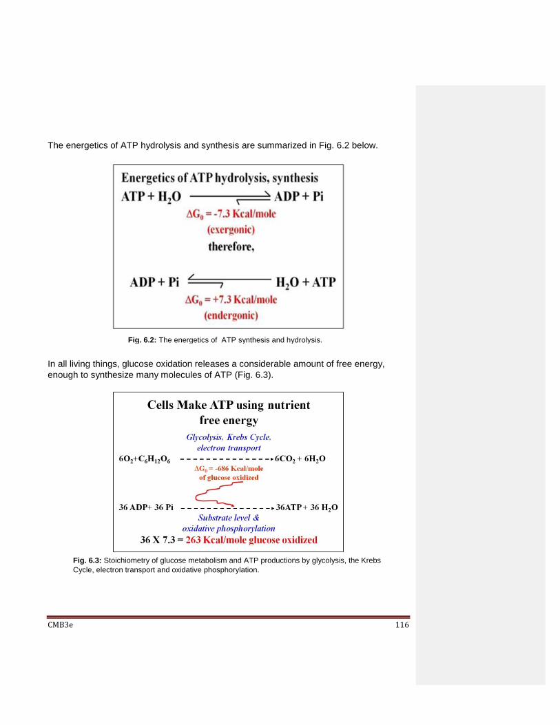
CMB3e 116

The energetics of ATP hydrolysis and synthesis are summarized in Fig. 6.2 below.

In all living things, glucose oxidation releases a considerable amount of free energy,

enough to synthesize many molecules of ATP (Fig. 6.3).

Fig. 6.2: The energetics of ATP synthesis and hydrolysis.

Fig. 6.3: Stoichiometry of glucose metabolism and ATP productions by glycolysis, the Krebs

Cycle, electron transport and oxidative phosphorylation.

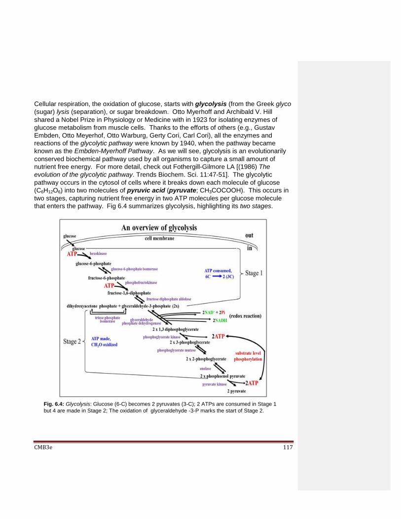
CMB3e 117

Cellular respiration, the oxidation of glucose, starts with glycolysis (from the Greek glyco

(sugar) lysis (separation), or sugar breakdown. Otto Myerhoff and Archibald V. Hill

shared a Nobel Prize in Physiology or Medicine with in 1923 for isolating enzymes of

glucose metabolism from muscle cells. Thanks to the efforts of others (e.g., Gustav

Embden, Otto Meyerhof, Otto Warburg, Gerty Cori, Carl Cori), all the enzymes and

reactions of the glycolytic pathway were known by 1940, when the pathway became

known as the Embden-Myerhoff Pathway. As we will see, glycolysis is an evolutionarily

conserved biochemical pathway used by all organisms to capture a small amount of

nutrient free energy. For more detail, check out Fothergill-Gilmore LA [(1986) The

evolution of the glycolytic pathway. Trends Biochem. Sci. 11:47-51]. The glycolytic

pathway occurs in the cytosol of cells where it breaks down each molecule of glucose

(C6H12O6) into two molecules of pyruvic acid (pyruvate; CH3COCOOH). This occurs in

two stages, capturing nutrient free energy in two ATP molecules per glucose molecule

that enters the pathway. Fig 6.4 summarizes glycolysis, highlighting its two stages.

Fig. 6.4: Glycolysis: Glucose (6-C) becomes 2 pyruvates (3-C); 2 ATPs are consumed in Stage 1

but 4 are made in Stage 2; The oxidation of glyceraldehyde -3-P marks the start of Stage 2.

CMB3e 118

Stage 1 of glycolysis actually consumes ATP. Phosphates are transferred from ATP first

to glucose and then to fructose-6-phosphate, reactions catalyzed by hexokinase and

phosphofructokinase respectively. So, these Stage 1 phosphorylations consume free

energy. Later, in Stage 2 of glycolysis, nutrient free energy is captured in ATP and

NADH (reduced nicotinamide adenine dinucleotide). NADH forms in redox reactions in

which NAD+ is reduced as some metabolite is oxidized. In Stage 2, it is glyceraldehyde-

3-phosphate that is oxidized…, but more later!

To summarize, by the end of glycolysis, a single starting glucose molecule has been split

into two molecules of pyruvate while four molecules of ATP and two molecules of NADH

have been produced. Pyruvate will be metabolized either anaerobically or aerobically.

The alternate fates of pyruvate are summarized in Fig. 6.5, below.

151 Overview of Glycolysis

Anaerobic (complete) glycolysis is a fermentation. Two NADH molecules are made per

glucose and two will reduce pyruvate at the end of the fermentation pathway. Thus by the

end complete glycolysis there is no consumption of O2 and no net oxidation of nutrient

(i.e., glucose). A familiar anaerobic glycolytic pathway is the production of alcohol by

yeast in the absence of oxygen. Another is the production of lactic acid by skeletal

muscle during strenuous exercise, which leads to the muscle fatigue you might have

experienced after especially vigorous workout. Muscle fatigue is due to a buildup of lactic

acid in the muscle cells that, under these conditions, can’t oxidize pyruvate, instead

reducing it to lactate. Other cell types produce different fermentative end-products while

Fig. 6.5: Alternate Fates of Pyruvate: Fermentation (the anaerobic reduction to e.g., alcohol,

lactate, etc.) or Respiration (aerobic oxidation of pyruvate using oxygen as a final electron

acceptor, resulting in H2O and CO2 production).

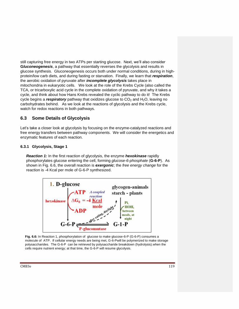
CMB3e 119

still capturing free energy in two ATPs per starting glucose. Next, we’ll also consider

Gluconeogenesis, a pathway that essentially reverses the glycolysis and results in

glucose synthesis. Gluconeogenesis occurs both under normal conditions, during in high-

protein/low carb diets, and during fasting or starvation. Finally, we learn that respiration,

the aerobic oxidation of pyruvate after incomplete glycolysis takes place in

mitochondria in eukaryotic cells. We look at the role of the Krebs Cycle (also called the

TCA, or tricarboxylic acid cycle in the complete oxidation of pyruvate, and why it takes a

cycle, and think about how Hans Krebs revealed the cyclic pathway to do it! The Krebs

cycle begins a respiratory pathway that oxidizes glucose to CO2 and H2O, leaving no

carbohydrates behind. As we look at the reactions of glycolysis and the Krebs cycle,

watch for redox reactions in both pathways.

6.3 Some Details of Glycolysis

Let’s take a closer look at glycolysis by focusing on the enzyme-catalyzed reactions and

free energy transfers between pathway components. We will consider the energetics and

enzymatic features of each reaction.

6.3.1 Glycolysis, Stage 1

Reaction 1: In the first reaction of glycolysis, the enzyme hexokinase rapidly

phosphorylates glucose entering the cell, forming glucose-6-phosphate (G-6-P). As

shown in Fig. 6.6, the overall reaction is exergonic; the free energy change for the

reaction is -4 Kcal per mole of G-6-P synthesized.

Fig. 6.6: In Reaction 1, phosphorylation of glucose to make glucose-6-P (G-6-P) consumes a

molecule of ATP. If cellular energy needs are being met, G-6-Pwill be polymerized to make storage

polysaccharides. The G-6-P can be retrieved by polysaccharide breakdown (hydrolysis).when the

cells require nutrient energy; at that time, the G-6-P will resume glycolysis.

CMB3e 120

The hexokinase reaction is a coupled reaction, in which phosphorylation of glucose

is coupled to ATP hydrolysis. The free energy of ATP hydrolysis (an energetically

favorable reaction) fuels glucose phosphorylation (an energetically unfavorable

reaction). The reaction is also biologically irreversible, as shown by the single

vertical arrow.

Excess dietary glucose can be stored in most cells (especially liver and kidney cells)

as a highly branched polymer of glucose monomers called glycogen. In green algae

and plants, glucose made by photosynthesis is stored as polymers of starch. When

glucose is necessary for energy, glycogen and starch hydrolysis form glucose-1-

phosphate (G-1-P) which is then converted to G-6-P. Let’s look at the energetics (free

energy flow) of the hexokinase-catalyzed reaction. This reaction can be seen as the

sum of two reactions in Fig 6.7.

Recall that ATP hydrolysis is an exergonic reaction, releasing ~7 Kcal/mole (rounding

down!) in a closed system under standard conditions. The condensation reaction of

glucose phosphorylation occurs with a Go of +3 Kcal/mole. This is an endergonic

reaction under standard conditions. Summing up the free energy changes of the two

reactions, we can calculate the overall Go of -4 Kcal/mole for the coupled reaction

under standard conditions in a closed system.

Fig. 6.7: Free energy flow (exchange) for Reaction1 of glycolysis.

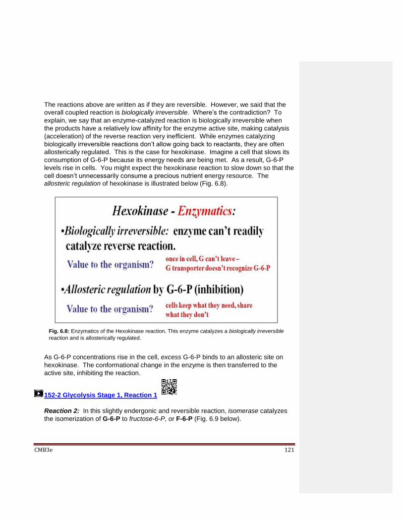
CMB3e 121

The reactions above are written as if they are reversible. However, we said that the

overall coupled reaction is biologically irreversible. Where’s the contradiction? To

explain, we say that an enzyme-catalyzed reaction is biologically irreversible when

the products have a relatively low affinity for the enzyme active site, making catalysis

(acceleration) of the reverse reaction very inefficient. While enzymes catalyzing

biologically irreversible reactions don’t allow going back to reactants, they are often

allosterically regulated. This is the case for hexokinase. Imagine a cell that slows its

consumption of G-6-P because its energy needs are being met. As a result, G-6-P

levels rise in cells. You might expect the hexokinase reaction to slow down so that the

cell doesn’t unnecessarily consume a precious nutrient energy resource. The

allosteric regulation of hexokinase is illustrated below (Fig. 6.8).

As G-6-P concentrations rise in the cell, excess G-6-P binds to an allosteric site on

hexokinase. The conformational change in the enzyme is then transferred to the

active site, inhibiting the reaction.

152-2 Glycolysis Stage 1, Reaction 1

Reaction 2: In this slightly endergonic and reversible reaction, isomerase catalyzes

the isomerization of G-6-P to fructose-6-P, or F-6-P (Fig. 6.9 below).

Fig. 6.8: Enzymatics of the Hexokinase reaction. This enzyme catalyzes a biologically irreversible

reaction and is allosterically regulated.

CMB3e 122

Reaction 3: In this biologically irreversible reaction, 6-phosphofructokinase (6-P-

fructokinase) catalyzes the phosphorylation of F-6-P to make fructose 1,6 di-

phosphate (F1,6 diP). In this is a coupled reaction ATP again provides the second

phosphate. The overall reaction is written as the sum of two reactions in Fig.6.10.

Fig. 6.9: Reaction 2 of glycolysis. G-6-P isomerase catalyzes the isomerization of G-6-P to F-6-P

(i.e., the isomerization of glucose to fructose). The reaction is endergonic and reversible.

Fig. 6.10: Reaction 3 of glycolysis. A kinase catalyzes phosphorylation of F-6-P to F1,6-di-P

in a biologically irreversible reaction, consuming a molecule of ATP.

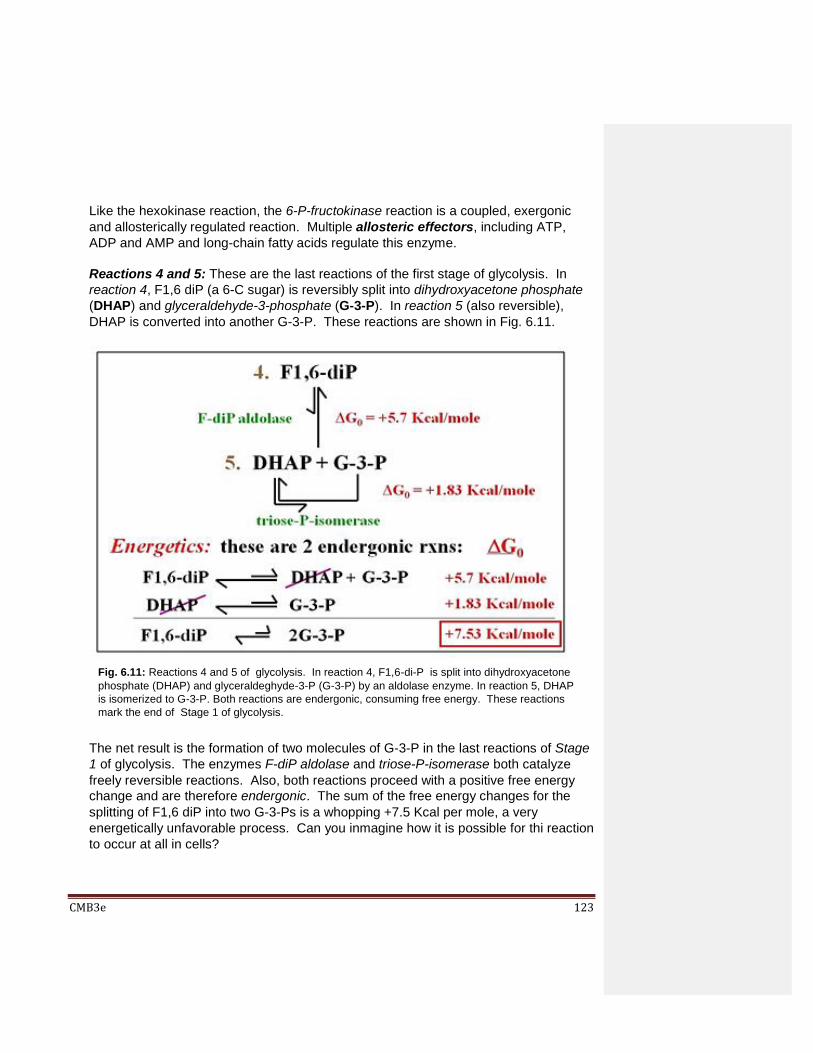
CMB3e 123

Like the hexokinase reaction, the 6-P-fructokinase reaction is a coupled, exergonic

and allosterically regulated reaction. Multiple allosteric effectors, including ATP,

ADP and AMP and long-chain fatty acids regulate this enzyme.

Reactions 4 and 5: These are the last reactions of the first stage of glycolysis. In

reaction 4, F1,6 diP (a 6-C sugar) is reversibly split into dihydroxyacetone phosphate

(DHAP) and glyceraldehyde-3-phosphate (G-3-P). In reaction 5 (also reversible),

DHAP is converted into another G-3-P. These reactions are shown in Fig. 6.11.

The net result is the formation of two molecules of G-3-P in the last reactions of Stage

1 of glycolysis. The enzymes F-diP aldolase and triose-P-isomerase both catalyze

freely reversible reactions. Also, both reactions proceed with a positive free energy

change and are therefore endergonic. The sum of the free energy changes for the

splitting of F1,6 diP into two G-3-Ps is a whopping +7.5 Kcal per mole, a very

energetically unfavorable process. Can you inmagine how it is possible for thi reaction

to occur at all in cells?

Fig. 6.11: Reactions 4 and 5 of glycolysis. In reaction 4, F1,6-di-P is split into dihydroxyacetone

phosphate (DHAP) and glyceraldeghyde-3-P (G-3-P) by an aldolase enzyme. In reaction 5, DHAP

is isomerized to G-3-P. Both reactions are endergonic, consuming free energy. These reactions

mark the end of Stage 1 of glycolysis.

CMB3e 124

Summing up, by the end of Stage 1 of glycolysis, two ATP molecules have been

consumed and one 6C carbohydrate has been split into two 3-C carbohydrates. We

have also seen two biologically irreversible and allosterically regulated enzymes.

153 Glycolysis Stage 1; Reactions 2-5 6.3.2 Glycolysis, Stage 2

We will follow just one of the two molecules of G-3-P generated by the end of Stage 1

of glycolysis, but remember that both are proceeding through Stage 2 (the rest of)

glycolysis.

Reaction 6: This is a redox reaction. G-3-P is oxidized to 1,3, diphosphoglyceric acid

(1,3, diPG) and NAD+ is reduced to NADH. The reaction catalyzed by the enzyme

glyceraldehyde-3-phopsphate dehydrogenase is shown in Fig. 6.12.

In this freely reversible endergonic reaction, a hydrogen molecule (H2) is removed

from G-3-P, leaving behind phosphoglyceric acid. This short-lived oxidation

intermediate is phosphorylated to make 1,3 diphosphoglyceric acid (1,3diPG). At the

same time, the hydrogen molecule is split into a hydride ion (H-) and a proton (H+).

The H- ions reduce NAD+ to NADH, leaving the protons behind in solution. Remember

that all of this is happening in the active site of the same enzyme!

Fig. 6.12: Reaction 6, a redox reaction catalyzed by G-3-P dehydrogenase, is freely reversible.

G-3-P is oxidized to1,3 diphosphoglyceric acid (1,3 diPG), transferring electrons as a hydride

(H-) ion to NAD

+ to make NADH.

CMB3e 125

Even though it catalyzes a reversible reaction, G-3-P dehydrogenase is allosterically

regulated. However, in contrast to the regulation of hexokinase, that of G-3-P

dehydrogenase is more complicated! The regulator is NAD+ and the mechanism of

allosteric regulation of G-3-P dehydrogenase by NAD+ is called negative cooperativity. It turns out that the higher the [NAD+] in the cell, the lower the affinity of the enzyme for more NAD+ and the faster the reaction in the cell! The mechanism is discussed at the link below.

154 Glycolysis Stage 2; Reaction 6

Reaction 7: This reaction, catalyzed by phosphoglycerate kinase, is freely reversible

and exergonic (Fig. 6.13), yielding ATP and 3-phosphoglyceric acid (3PG).

Catalysis of phosphate group transfer between molecules by kinases is called

substrate-level phosphorylation, one way of phosphorylating ADP to make ATP. In

this coupled reaction the free energy released by hydrolyzing a phosphate from

1,3diPG is used to make ATP. Remember that this reaction occurs twice per starting

glucose. Two ATPs have been synthesized to this point in glycolysis. We call 1,3

diPG a very high-energy phosphate compound.

Reaction 8: This freely reversible endergonic reaction moves the phosphate from the

number 3 carbon of 3PG to the number 2 carbon (Fig. 6.14, below).

Fig. 6.13: Reaction 7, a reversible, exergonic, coupled reaction generates ATP using free energy

released by the hydrolysis of one of the phosphates from 1,3diPG. The mechanism of ATP

synthesis here is called substrate-level phosphorylation.

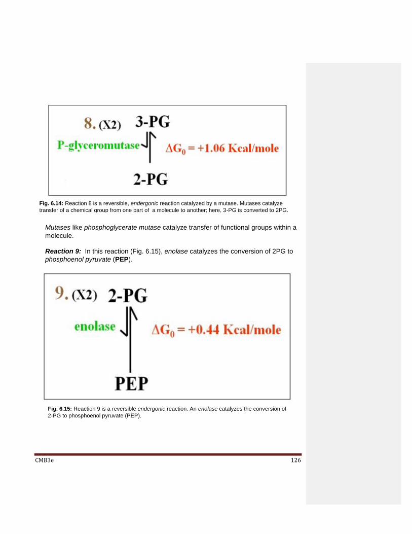
CMB3e 126

Mutases like phosphoglycerate mutase catalyze transfer of functional groups within a

molecule.

Reaction 9: In this reaction (Fig. 6.15), enolase catalyzes the conversion of 2PG to

phosphoenol pyruvate (PEP).

Fig. 6.14: Reaction 8 is a reversible, endergonic reaction catalyzed by a mutase. Mutases catalyze

transfer of a chemical group from one part of a molecule to another; here, 3-PG is converted to 2PG.

Fig. 6.15: Reaction 9 is a reversible endergonic reaction. An enolase catalyzes the conversion of

2-PG to phosphoenol pyruvate (PEP).

CMB3e 127

Reaction 10: This reaction results in the formation of pyruvic acid (pyruvate),

illustrated in Fig. 6.16 below).

Remember again, two pyruvates are produced per starting glucose molecule. The

enzyme pyruvate kinase couples the biologically irreversible, exergonic hydrolysis of a

phosphate from PEP and transfer of that phosphate to ADP in a coupled reaction.

The reaction product PEP, is another very high-energy phosphate compound.

Pyruvate kinase is allosterically regulated by ATP, citric acid, long-chain fatty acids,

F1,6 diP and one of its own substrates, PEP.

155-2 Glycolysis Stage 2; Reactions 7-10

As we have seen, there are alternate fates of pyruvate. a product of incomplete

glycolysis. One is the aerobic mitochondrial oxidation of pyruvate following incomplete

glycolysis. The other is an anaerobic fermentation, or complete glycolysis in which

pyruvate is reduced to one or another end product. Recall that muscle fatigue results

when skeletal muscle uses anaerobic fermentation to get energy during vigorous

exercise, reducing pyruvate to lactic acid. It is the accumulation of lactic acid in

skeletal muscle cells that causes muscle fatigue. The enzyme LDH (Lactate

dehydrogenase) that catalyzes the reduction of pyruvate to lactate, is regulated… but

not allosterically!. Instead, different types of muscle tissues regulate LDH by making

different versions of the enzyme. Click the Link below for a more detailed explanation.

156 Fermentation: Regulation of Pyruvate Reduction is NOT Allosteric!

Fig. 6.16: Reaction 10 is biologically irreversible. In a coupled reaction, pyruvate kinase

catalyzes a highly exergonic transfer of a phosphate on PEP to ADP to make ATP

CMB3e 128

6.4 A Chemical and Energy Balance Sheet for Glycolysis

Compare the balance sheets for complete glycolysis (fermentation) to lactic acid and

incomplete (aerobic) glycolysis, showing chemical products and energy transfers (Fig.

6.17).

There are two reactions in Stage 2 of glycolysis that each yield a molecule of ATP, each

occurring twice per starting glucose molecule. Stage 2 of glycolysis thus produces four

ATP molecules per glucose . Since Stage 1 consumed two ATPs, the net yield of

chemical energy as ATP by the end of glycolysis is two ATPs, whether complete to

lactate or incomplete to pyruvate! Because they can’t make use of oxygen, anaerobes

have to settle for the paltry 15 Kcal worth of ATP that they get from a fermentation. Since

there are 687 Kcal potentially available from the complete combustion of a mole of

glucose, there is a lot of free energy left to be captured during the rest of respiration (i.e.,

pyruvate oxidation.

157-2 Balance Sheet of Glycolysis

Fig. 6.17: Free energy and ATP yields of complete glycolysis (a fermentation) and incomplete

glycolysis (i.e., respiration). Percentages represent the efficiency of ATP production. They are

based on the ratios of the free energy captured as ATP to the free energy released by the different

pathways for metabolizing glucose. From the data, incomplete glycolysis is a more efficient way to

extract nutrient free energy.

CMB3e 129

Remember also that the only redox reaction in aerobic glycolysis is in Stage 2. This is the oxidation of G-3-P, a 3C glycolytic intermediate. Now check out the redox reaction a fermentation pathway. Since pyruvate, also a 3C intermediate, was reduced, there has been no net oxidation of glucose (i.e., glycolytic intermediates) in complete glycolysis. By this time, you will have realized that glycolysis is a net energetically favorable

(downhill, spontaneous) pathway in a closed system, with an overall negative Go.

Glycolysis is also normally spontaneous in most of our cells, driven by a constant need for

energy to do cellular work. Thus the actual free energy of glycolysis, or G’, is also

negative. In fact, glycolysis in actively respiring cells proceeds with release of more free

energy than it would in a closed system. In other words, the G’ for glycolysis in active

cells is more negative than the Go of glycolysis! Feel free to investigate the truth of this

statement on your own.

Before we proceed to discuss the aerobic fate of pyruvate, let’s look at gluconeogenesis,

the Atkins Diet and some not-so-normal circumstances when glycolysis essentially goes

in reverse, at least in a few cell types. Under these conditions, glycolysis is energetically

unfavorable, and even the otherwise exergonic reactions of glycolysis will be proceeding

with a negative G’.

6.5 Gluconeogenesis

In a well-fed animal, most cells can store a small amount of glucose as glycogen. All cells

break glycogen down when needed to retrieve nutrient energy as G-6-P. Glycogen

hydrolysis, or glycogenolysis, produces G-1-P that is converted to G-6-P, as we saw at

the top of Stage 1 of glycolysis. But glycogen in most cells is quickly used up between

meals. Therefore, most cells depend on a different, external source of glucose other than

diet. Those sources are liver (and to a lesser extent kidney) that can store large amounts

of glycogen after meals. In continual feeders (cows and other ruminants, glycogenolysis

is ongoing. Liver cell glycogenolysis supplies glucose to the blood for 6-8 hours between

meals in Intermittent feeders (like us), to be distributed as needed to all cells of the body.

Thus, you can expect to use up liver and kidney glycogen reserves after a good night’s

sleep, a period of intense exercise, or any prolonged period of low carbohydrate intake

(fasting or starvation).

Under these circumstances, animals use gluconeogenesis (literally, new glucose

synthesis) in liver and kidney cells to provide systemic glucose to nourish other cells. In

healthy individuals, the hormones glucagon and insulin regulate blood glucose

homeostasis by raising or lowering blood glucose levels based on cellular glucose

(energy) needs, thus protecting the organism from hypoglycemia (low blood sugar) and

CMB3e 130

hyperglycemia (high blood sugar) respectively. The gluconeogenic pathway produces

glucose from carbohydrate and non-carbohydrate precursors that include pyruvate,

lactate, glycerol and gluconeogenic amino acids. The latter are amino acids that can be

converted to alanine. The reactions of glycolysis and gluconeogenesis are shown side-by-

side in Fig. 6.18 (below).

Fig. 6.18: Comparison of incomplete glycolysis to gluconeogenesis. The two pathways are

essentially the reverse of one another, except for the bypass enzymes in gluconeogenesis

(shown in green), required to get around biologically irreversible enzymes of glycolysis.

CMB3e 131

Look for the bypass reactions catalyzed by carboxylases and phosphatases and the glycolytic reactions that function in reverse during gluconeogenesis. If glycolysis is an exergonic pathway, then gluconeogenesis must be an endergonic one. In fact, while glycolysis through two pyruvates generates a net of two ATPs, gluconeogenesis from two pyruvate to glucose costs 4 ATPs and two GTPs! Likewise, gluconeogenesis is only possible if the bypass enzymes are present. These are necessary to get around the three biologically irreversible reactions of glycolysis. Except for the bypass reactions, gluconeogenesis is essentially a reversal of glycolysis. As drawn in the pathways above, glycolysis and gluconeogenesis would seem to be cyclic. In fact this apparent cycle was recognized by Carl and Gerti Cori, who shared the 1947 Nobel Prize for Medicine or Physiology with Bernardo Houssay for discovering how glycogen is broken down to pyruvate in muscle (in fact most) cells) to be re-converted to glucose in liver cells. Named after the Coris, The Cori Cycle (Fig. 6.19) recognizes the interdependence of liver and muscle in glucose breakdown and re-synthesis.

In spite of this free energy requirement, gluconeogenesis is energetically favorable in liver and kidney cells! This is because the cells are open systems. The accumulation of pyruvate in liver cells and a rapid release of new glucose into the blood drives the energetically favorable reactions of gluconeogenesis forward. Therefore, under

Fig. 6.19: The Cori cycle reveals the relationship between glycolysis and gluconeogenesis. Lactic

acid produced by complete glycolysis in active skeletal muscle goes to the liver where it could be

converted to pyruvate, and then to glucose .

CMB3e 132

gluconeogenic conditions, glucose synthesis occurs with a negative G’, a decline in actual free energy. Of course, glycolysis and gluconeogenesis are not simultaneous! Which pathways operate in which cells is tightly controlled. Glycolysis is the norm in all cell types, even in liver and kidney. However, the cessation of glycolysis in favor of gluconeogenesis in the latter cells is under hormonal control. Hormonal control of gluconeogenesis is illustrated in Fig. 6.20, below.

Key in turning on liver gluconeogenesis is the role of glucocorticoid hormones. What causes the secretion of glucocorticoids? A long night’s sleep, fasting and in the extreme, starvation are forms of stress. Stress responses start in the hypothalamic-pituitary axis. Different stressors cause the hypothalamus to secrete a neurohormone that in turn,

Fig. 6.20: Control of gluconeogenesis by hormones of the hypothalamic-pituitaryaxis. A need for

glucose for energy stimulates hypothalamic hormones that in turn stimulates the release of

adrenocorticotropic hormone (ACTH) from the pituitary gland. ACTH then stimulates release of

glucocorticoids rom the adrenal glands. Glucocorticoid hormones stimulate many tissues to control

gluconeogenic glucose production as well as the use alternate nutrient fuels by many cells in the body.

CMB3e 133

stimulates the release of ACTH (adrenocorticotropic hormone) from the pituitary gland. ACTH then stimulates the release of cortisone and other glucocorticoids from the cortex (outer layer) of the adrenal glands. As the name glucocorticoid suggests, these hormones participate in the regulation of glucose metabolism. Here is what happens at times of low blood sugar (e.g., when carbohydrate intake is low):

1. Glucocorticoids stimulate the synthesis of gluconeogenic bypass enzymes in liver

cells.

2. Glucocorticoids stimulate protease synthesis in skeletal muscle, causing hydrolysis of the peptide bonds between amino acids. Gluconeogenic amino acids circulate to the liver where they are converted to pyruvate, a major precursor of gluconeogenesis.

Some amino acids are ketogenic; they are converted to Acetyl-S-CoA, a precursor to

ketone bodies.

3. Glucocorticoids stimulate increased levels of enzymes including lipases that catalyze

hydrolysis of the ester linkages in triglycerides (fat) in adipose and other cells. This

generates fatty acids and glycerol.

4. Glycerol circulates to liver cells that take it up convert it to G-3-P, augmenting

gluconeogenesis. Fatty acids circulate to liver cells where they are oxidized to Acetyl-

S-CoA that is then converted to ketone bodies. and released to the circulation.

5. Most cells use fatty acids as an alternate energy nutrient when glucose is limiting.

Heart and brain cells depend on glucose for energy, though under extreme conditions

(prolonged fasting, starvation), brain cells can use ketone bodies as energy source of

last resort..

Thus, essential roles of glucocorticoids include

1. enabling most cells to oxidize fats (fatty acids) for energy

2. allowing brain cells to use gluconeogenic glucose for energy, and in the extreme,

ketone bodies as an alternate energy source

3. allowing cardiac muscle to use gluconeogenic glucose as its energy source.

It’s a pity that we humans can’t use fatty acids as gluconeogenic substrates! Plants and

some lower animals have a glyoxalate cycle pathway that can convert fatty acid oxidation

products directly into gluconeogenic carbohydrates substrates. Lacking this pathway, we

(and higher animals in general) cannot convert fats to carbohydrates, in spite of the fact

that we can all too easily convert the latter to the former!

The dark side of bad eating habits is prolonged starvation that will eventually overwhelm

the gluconeogenic response. You see this in reports from third world regions suffering

starvation due to drought or other natural disaster, or war. The spindly arms and legs of

starving children result from muscle wasting as the body tries to provide the glucose

necessary for survival. When the gluconeogenic response is inadequate to the task, the

CMB3e 134

body can resort to ketogenic fat metabolism. Think of this as a last resort, leading to the

production of ketone bodies and the “acetone breath” in starving people or people with

severe eating disorders (e.g. anorexia nervosa).

6.6 The Atkins Diet and Gluconeogenesis

You may know that the Atkins Diet is an ultra-low carb diet. It is one of several low-carb

ketogenic diets. The glucocorticoid hormones released on a low carb diet trick the body

into a constant gluconeogenic state. While the liver can produce enough glucose for

brain and heart cells, the rest of the cells in our bodies switch to burning fats, hence the

weight loss. Carried to an extreme, a severe restriction of carbohydrate intake will result

high blood levels of ketones and “acetone breath”. Though discredited some years ago,

the Atkins Diet (and similar ones e.g., Paleo diet, South Beach diet) are now back in

favor.

When not exaggerated, low carb diets are important in the control of diabetes. In older

folks, type 2 (adult-onset) diabetics can control their disease with a low carb diet and a

drug called metformin, which blocks gluconeogenesis and therefore prevents glucose

synthesis from gluconeogenic substrates, at the same time stimulating cellular receptors

to take up available glucose. For more details on the mechanism of metformin action,

check out Hundal RS et al. [(2000) Mechanism by Which Metformin Reduces Glucose

Production in Type 2 Diabetes. Diabetes 49 (12): 2063–9]. Given the prevalence of

obesity and type 2 diabetes in the U.S., it’s likely that someone you know is taking

metformin or other similar medication!

158-2 Gluconeogenesis & the Atkins Diet

6.7 The Krebs/TCA/Citric acid cycle

Glycolysis through fermentative reactions produces ATP anaerobically. The evolution of

respiration (the aerobic use of oxygen to efficiently burn nutrient fuels) had to wait until

photosynthesis created the oxygenic atmosphere we live in now. Read more about the

source of our oxygenic atmosphere in Dismukes GC et al. [(2001) The origin of

atmospheric oxygen on earth: the innovation of oxygenic photosynthesis. Proc. Nat.

Acad. Sci. USA 98:2170-2175].

The Krebs cycle is the first pathway of mitochondrial oxygenic respiration in eukaryotic

cells. Evolution of the Krebs cycle no doubt occurred a few reactions at a time, perhaps

at first as a means of protecting anaerobic cells from the ‘poisonous’ effects of oxygen.

Later, natural selection fleshed out the aerobic Krebs cycle, electron transport and

CMB3e 135

oxidative phosphorylation metabolic pathways we see today. Whatever its initial utility,

these reactions were an adaptive response to the increase in oxygen in the earth’s

atmosphere. As we’ve seen, respiration is much more efficient pathway than glycolysis

for getting energy out of nutrients,. Animals rely on it, but even plants and photosynthetic

algae use the respiratory pathway when sunlight is not available! Here we focus on

oxidative reactions in mitochondria, beginning with pyruvate oxidation and continuing to

the redox reactions of the Krebs cycle.

After entering the mitochondria, pyruvate dehydrogenase catalyzes pyruvate oxidation to

Acetyl-S-Coenzyme A (Ac-S-CoA). Then the Krebs cycle completely oxidizes the Ac-S-

CoA. These mitochondrial redox reactions generate CO2 and lot of reduced electron

carriers (NADH, FADH2). The free energy released in these redox reactions is coupled to

the synthesis of only one ATP per pyruvate oxidized (i.e., two per the glucose we started

with!). It is the NADH and FADH2 molecules that have captured most of the free energy in

the original glucose molecules. The entry of pyruvate into the mitochondrion and its

oxidation are summarized in Fig. 6.21.

Pyruvate oxidation converts a 3C carbohydrate into acetate, a 2C acetate molecule,

releasing a molecule of CO2. In this highly exergonic reaction, CoA-SH forms a high-

energy thioester linkage with the acetate in Ac-S-CoA. The oxidation of pyruvic acid

results in the reduction of NAD+, the production of Ac-S-CoA and a molecule of CO2 (Fig.

6.22 below).

Fig. 6.21: Entry of pyruvate into mitochondrion, followed by its oxidation to acetyl-S-Coenzyme

A (acetyl-S-CoA).

CMB3e 136

The Krebs Cycle as it occurs in animals is summarized below in Fig. 6.23. Ac-S-CoA

from the oxidation of pyruvate enters the Krebs cycle in the first reaction, condensing with

oxaloacetate (OAA) to form citric acid (from which the cycle gets its first name).

Fig. 6.22: Pyruvate dehydrogenase catalyzes pyruvate oxidation to Ac-S-CoA, releasing a

molecule of CO2 and reducing NAD+ to NADH.

Fig. 6.23: Highlights of the Krebs Cycle. The first reaction is condensation of Acv-S-CoA and oxaloacetate (OAA)

to form citric acid (citrate). Four of the reactions in the cycle are redox reactions that create reduced electron

carriers (NADH, FADH2), while one reaction is coupled to GTP synthesis by substrate level phosphorylation.

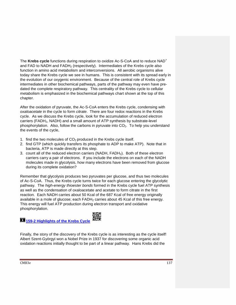
CMB3e 137

The Krebs cycle functions during respiration to oxidize Ac-S-CoA and to reduce NAD+

and FAD to NADH and FADH2 (respectively). Intermediates of the Krebs cycle also

function in amino acid metabolism and interconversions. All aerobic organisms alive

today share the Krebs cycle we see in humans. This is consistent with its spread early in

the evolution of our oxygenic environment. Because of the central role of Krebs cycle

intermediates in other biochemical pathways, parts of the pathway may even have pre-

dated the complete respiratory pathway. This centrality of the Krebs cycle to cellular

metabolism is emphasized in the biochemical pathways chart shown at the top of this

chapter.

After the oxidation of pyruvate, the Ac-S-CoA enters the Krebs cycle, condensing with

oxaloacetate in the cycle to form citrate. There are four redox reactions in the Krebs

cycle. As we discuss the Krebs cycle, look for the accumulation of reduced electron

carriers (FADH2, NADH) and a small amount of ATP synthesis by substrate-level

phosphorylation. Also, follow the carbons in pyruvate into CO2. To help you understand

the events of the cycle,

1. find the two molecules of CO2 produced in the Krebs cycle itself.

2. find GTP (which quickly transfers its phosphate to ADP to make ATP). Note that in

bacteria, ATP is made directly at this step.

3. count all of the reduced electron carriers (NADH, FADH2). Both of these electron

carriers carry a pair of electrons. If you include the electrons on each of the NADH

molecules made in glycolysis, how many electrons have been removed from glucose

during its complete oxidation?

Remember that glycolysis produces two pyruvates per glucose, and thus two molecules

of Ac-S-CoA. Thus, the Krebs cycle turns twice for each glucose entering the glycolytic

pathway. The high-energy thioester bonds formed in the Krebs cycle fuel ATP synthesis

as well as the condensation of oxaloacetate and acetate to form citrate in the first

reaction. Each NADH carries about 50 Kcal of the 687 Kcal of free energy originally

available in a mole of glucose; each FADH2 carries about 45 Kcal of this free energy.

This energy will fuel ATP production during electron transport and oxidative

phosphorylation.

159-2 Highlights of the Krebs Cycle Finally, the story of the discovery of the Krebs cycle is as interesting as the cycle itself!

Albert Szent-Györgyi won a Nobel Prize in 1937 for discovering some organic acid

oxidation reactions initially thought to be part of a linear pathway. Hans Krebs did the

CMB3e 138

elegant experiments showing that the reactions were part of a cyclic pathway. He

proposed (correctly!) that the cycle would be a supercatalyst that would catalyze the

oxidation of yet another organic acid. Some of the experiments are described by Krebs

and his coworkers in their classic paper: Krebs HA, et al. [(1938) The formation of citric

and α-ketoglutaric acids in the mammalian body. Biochem. J. 32: 113–117].

Hans Krebs and Fritz Lipmann shared the 1953 Nobel Prize in Physiology or Medicine.

Krebs was recognized for his discovery of TCA cycle, which more commonly carries his

name. Lipmann was recognized for proposing ATP as the mediator between food

(nutrient) energy and intracellular work energy, and for discovering the reactions that

oxidize pyruvate and synthesize Ac-S-CoA, bridging the Krebs Cycle and oxidative

phosphorylation (to be considered in the next chapter).

160 Discovery of the Krebs Cycle

You can read Krebs’ review of his own research in Krebs HA [(1970) The history of the

tricarboxylic acid cycle. Perspect. Biol. Med. 14:154-170]. For a classic read on how

Krebs described his supercatalyst suggestion, click Hans Krebs Autobiographical

Comments. For more about the life of Lipmann, check out the brief Nobel note on the

Fritz Lipmann Biography.

Some iText & VOP Key Words and Terms

Acetyl-S-coenzyme A (Ac-S-CoA)

free energy capture phosphatase enzymes

ADP, ATP, GDP, GTP fructose phosphate-ester linkage

aerobic G, G6P, F6P, F1,6-diP redox reactions

anaerobic gluconeogenesis reducing agent

Atkins Diet gluconeogenic amino acids

respiration

biochemical pathways glycolysis SDH (succinate dehydrogenase)

bioenergetics glyoxalate cycle spontaneous reaction

bypass reactions, enzymes

high energy bond (linkage)

stage 1

C6H12O6 (glucose) high energy molecules stage 2

cells as open systems isomerase enzymes standard conditions

CMB3e 139

Cori Cycle kinase enzymes steady state

dehydrogenase enzymes

Krebs (TCA, citric acid) cycle

stoichiometry of glycolysis

DHAP, G3P,1,3-diPG, 3PG, 2PG, PEP, Pyr

metabolic effects of low carb diet

substrate level phosphorylation

diabetes metformin Succinyl-S-CoA

energetics of glycolysis mitochondria super-catalyst

energy flow in cells mutase enzymes synthase enzymes

equilibrium NAD+ (oxidized nicotinamide adenine di-Phosphate)

thioester linkage

FAD (oxidized nicotinamide adenine di-Phosphate)

NADH (reduced nicotinamide adenine di-Phosphate)

G’ (actual free energy change)

FADH2 (reduced flavin adenine di-Phosphate)

nutrients Go (standard free energy change)

fermentation oxidation, reduction

free energy oxidizing agent

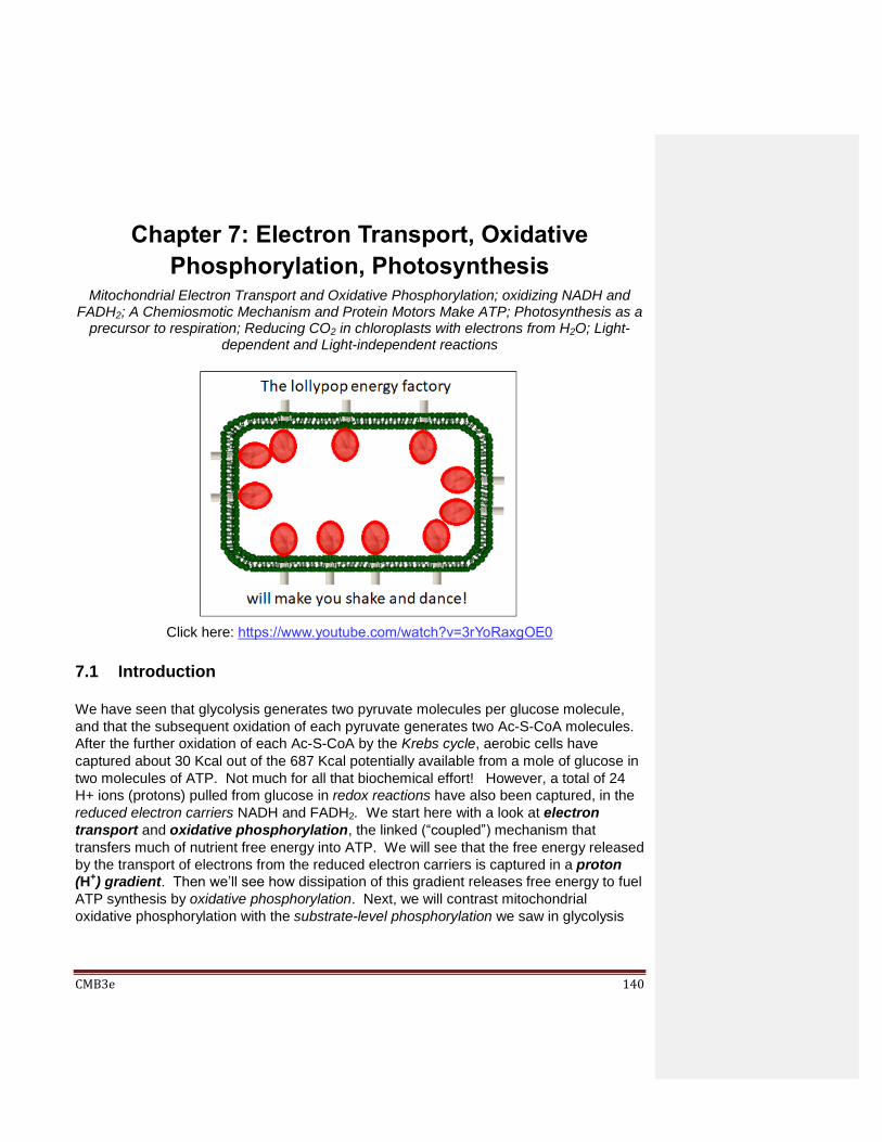
CMB3e 140

Chapter 7: Electron Transport, Oxidative

Phosphorylation, Photosynthesis Mitochondrial Electron Transport and Oxidative Phosphorylation; oxidizing NADH and

FADH2; A Chemiosmotic Mechanism and Protein Motors Make ATP; Photosynthesis as a precursor to respiration; Reducing CO2 in chloroplasts with electrons from H2O; Light-

dependent and Light-independent reactions

7.1 Introduction

We have seen that glycolysis generates two pyruvate molecules per glucose molecule,

and that the subsequent oxidation of each pyruvate generates two Ac-S-CoA molecules.

After the further oxidation of each Ac-S-CoA by the Krebs cycle, aerobic cells have

captured about 30 Kcal out of the 687 Kcal potentially available from a mole of glucose in

two molecules of ATP. Not much for all that biochemical effort! However, a total of 24

H+ ions (protons) pulled from glucose in redox reactions have also been captured, in the

reduced electron carriers NADH and FADH2. We start here with a look at electron

transport and oxidative phosphorylation, the linked (“coupled”) mechanism that

transfers much of nutrient free energy into ATP. We will see that the free energy released

by the transport of electrons from the reduced electron carriers is captured in a proton

(H+) gradient. Then we’ll see how dissipation of this gradient releases free energy to fuel

ATP synthesis by oxidative phosphorylation. Next, we will contrast mitochondrial

oxidative phosphorylation with the substrate-level phosphorylation we saw in glycolysis

Click here: https://www.youtube.com/watch?v=3rYoRaxgOE0

CMB3e 141

and the Krebs cycle. After presenting an energy balance sheet for respiration, we look at

how cells capture of free energy from alternate nutrients, and by photosynthesis (overall

the opposite of respiration). We conclude by comparing photosynthesis and respiration.

Learning Objectives

When you have mastered the information in this chapter, you should be able to:

1. explain the centrality of the Krebs Cycle to aerobic metabolism.

2. identify sources of electrons in redox reactions leading to and within the Krebs cycle.

3. illustrate the path of electrons from the Krebs cycle to and through the electron

transport chain.

4. trace the evolution of the electron transport chain from its location on an aerobic

bacterial membrane to its location in eukaryotic cells.

5. list the expected properties of a proton gate and a proton pump.

6. interpret experiments involving redox reactions, ATP synthesis and ATP hydrolysis

conducted with intact mitochondria and separated mitochondrial membranes.

7. distinguish between the pH, H+ and electrical gradients established by electron

transport.

8. explain the chemiosmotic mechanism of ATP synthesis and contrast it with substrate-

level phosphorylation.

9. compare and contrast the role of electron transport in respiration and photosynthesis

and discuss the evolution of each.

10. trace and explain the different paths that electrons can take in photosynthesis.

11. explain the presence of similar (or even identical) biochemical intermediates in

respiration and photosynthesis.

7.2 Electron Transport Chains

All cells use an electron transport chain (ETC) to oxidize substrates in exergonic

reactions. The electron flow from reduced substrates through an ETC is like the

movement of electrons between the poles of a battery. In the case of the battery, the

electron flow releases free energy to power a motor, light, cell phone, etc. During

mitochondrial respiration, reduced electron carriers (NADH, FADH2) are oxidized and

electrons flow down an ETC to molecular oxygen (O2) to make water. In plants and other

photosynthetic organisms, electron flow down ETC oxidizes NADPH (a phosphorylated

version of NADH), eventually reducing CO2 to sugars.

In both respiration and photosynthesis, the oxidation of energy-rich reduced electron

carriers releases free energy. This free energy of electron flow is coupled to the active

transport of protons (H+ ions) across a membrane by proton pumps. The proton pumps

create a chemical (proton) gradient and consequently a pH and electrical gradient. In a

kind of shorthand, we say that the free energy once in reduced substrates is now in an

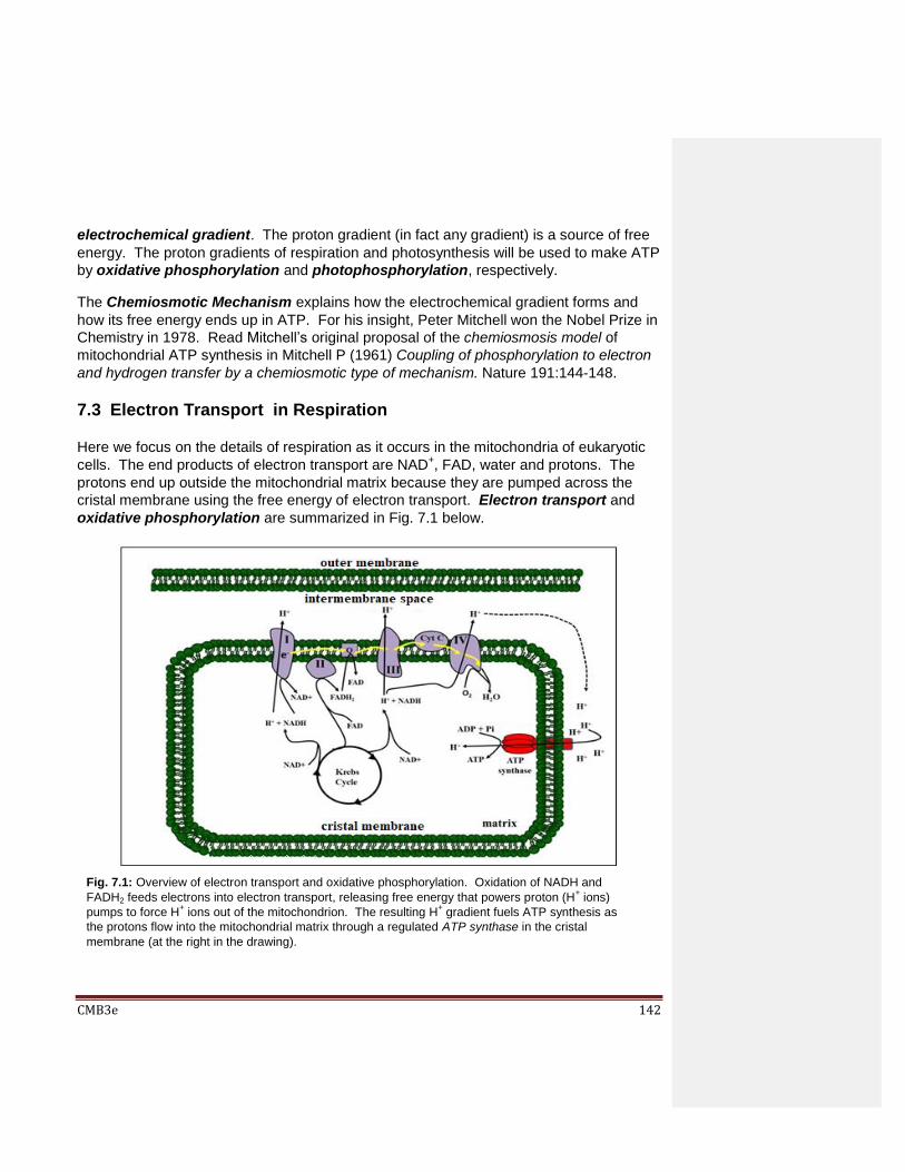
CMB3e 142

electrochemical gradient. The proton gradient (in fact any gradient) is a source of free

energy. The proton gradients of respiration and photosynthesis will be used to make ATP

by oxidative phosphorylation and photophosphorylation, respectively.

The Chemiosmotic Mechanism explains how the electrochemical gradient forms and

how its free energy ends up in ATP. For his insight, Peter Mitchell won the Nobel Prize in

Chemistry in 1978. Read Mitchell’s original proposal of the chemiosmosis model of

mitochondrial ATP synthesis in Mitchell P (1961) Coupling of phosphorylation to electron

and hydrogen transfer by a chemiosmotic type of mechanism. Nature 191:144-148.

7.3 Electron Transport in Respiration

Here we focus on the details of respiration as it occurs in the mitochondria of eukaryotic

cells. The end products of electron transport are NAD+, FAD, water and protons. The

protons end up outside the mitochondrial matrix because they are pumped across the

cristal membrane using the free energy of electron transport. Electron transport and

oxidative phosphorylation are summarized in Fig. 7.1 below.

Fig. 7.1: Overview of electron transport and oxidative phosphorylation. Oxidation of NADH and

FADH2 feeds electrons into electron transport, releasing free energy that powers proton (H+ ions)

pumps to force H+ ions out of the mitochondrion. The resulting H

+ gradient fuels ATP synthesis as

the protons flow into the mitochondrial matrix through a regulated ATP synthase in the cristal

membrane (at the right in the drawing).

CMB3e 143

Roman numbered protein complexes in the drawing above, along with Coenzyme Q (“Q”) and cytochrome C (Cyt C) constitute the ETC. The role of the respiratory ETC is to oxidize NADH or FADH2 to NAD+ and FAD respectively. The electrons from these reduced electron carriers are transferred from one ETC complex to the next. At the end of chain, electrons, protons and oxygen unite in complex IV to make water. Under standard conditions in a closed system, electron transport is downhill, with an overall

release of free energy (a negative Go) at equilibrium.

161 Electron Transport Oxidizes Reduced Electron Carriers

162-2 Finding the Free Energy of Electron Transport

163-2 Separating Electron Transport from Oxidative Phosphorylation In the illustration above, we can see three sites in the respiratory ETC that function as H+

pumps. At these sites, the negative change in free energy of electron transfer is large

and coupled to the action of a proton pump that forces protons out of the mitochondrial

matrix across the cristal membrane. Because the outer mitochondrial membrane is freely

permeable to protons, the gradient created is in effect, between the cytoplasm and the

mitochondrial matrix. The flow of protons back into the mitochondrial matrix through

lollipop-shaped ATP synthase complexes on the cristal membrane releases the gradient

free energy that will be harnessed to make ATP by oxidative phosphorylation.

164-2 Proton Pumps Store Free Energy of the ETC in Proton Gradients

7.4 Oxidative Phosphorylation in Respiration

Oxidative phosphorylation is the mechanism by which ATP captures the free energy in

the mitochondrial proton gradient. Most of the ATP made in aerobic organisms is made

by oxidative phosphorylation, rather than by substrate phosphorylation (the mechanism of

ATP synthesis in glycolysis or the Krebs cycle). Some aerobic biochemistry may have

evolved in response to the toxic effects of rising environmental oxygen levels. Later

elaboration of respiratory metabolism was undoubtedly selected because it turns out to be

more efficient at making ATP than anaerobic fermentations such as ‘complete’ glycolysis.

In other words, oxidative phosphorylation is more efficient than substrate-level

phosphorylation.

To summarize here, the movement of electrons down the electron transport chain fuels

three proton pumps that establish a proton gradient across the cristal membrane that

stores free energy. Oxidative phosphorylation then couples controlled diffusion of protons

CMB3e 144

back into the mitochondrial matrix through cristal membrane ATP synthases, fueling ATP

production. We say that the proton gradient has a proton motive force, recognizing the

three-part gradient – proton and pH gradient and a difference in electric potential.

The use of this proton motive force to make ATP is regulated. Conditions in the cell

control when the energy stored in this gradient will be released to make ATP. The switch

that allows protons to flow across the cristal membrane to relieve the proton gradient is an

ATP synthase, a tiny, complex enzymatic protein motor. For a clear discussion of this

complex enzyme, see P. D. Boyer (1997) The ATP synthase – a splendid molecular

machine. Ann. Rev. Biochem. 66:717-749. The capture of free energy of protons flowing

through this lollipop-shaped complex is shown in Fig. 7.2.

In mitochondria, the protons pumped out of the mitochondrial matrix (using the free

energy released by electron transport) can then flow back into the matrix through the ATP

synthase. If the three ETC sites in the cristal membrane that actively transport protons

are proton pumps, then the cristal membrane ATP synthase complexes function as

regulated proton gates that catalyzes ATP synthesis when protons are allowed to flow

through them. For their discovery of the details of ATP synthase function, P. D. Boyer

and J. E. Walker shared the Nobel Prize in Chemistry in 1997.

165-2 Proton Gates Capture Proton Gradient Free Energy as ATP

Fig. 7.2: The flow of protons through the cristal membrane ATP synthase relieves the proton

gradient, releasing free energy that fuels ATP synthesis in the mitochondrial matrix.

CMB3e 145

The ratio of ATP to ADP concentrations regulates proton flow through the ATP synthase

gates. A high ATP/ADP ratio in the mitochondrial matrix indicates that the cell does not

need more ATP, closing the proton gate so that the proton gradient cannot be relieved.

On the other hand, a low ATP/ADP ratio in the matrix means that the cell is hydrolyzing a

lot of ATP, and that the cell needs more. Then the proton gate opens, and protons flow

through cristal membrane ATP synthases back into the matrix down a concentration

gradient. As they flow, they release free energy to power a protein motor in the enzyme

that in turn, activates ATP synthesis.

Just as we did for glycolysis, we can count the ATPs and see how much free energy we

get from aerobic respiration, i.e., the complete oxidation of glucose. You can see this in

the link below.

166 A Balance Sheet for Respiration Recall that according to the endosymbiotic theory, aerobic bacteria are the evolutionary

ancestor to mitochondria; in fact, the cell membrane of aerobic bacteria house an ETC

and chemiosmotic mechanism of ATP generation much like that in mitochondria. And,

proton gradients do not only power ATP synthesis, but can also power cellular work quite

directly. Consider the bacterial flagellum driven directly by proton flow through cell

membrane proton gate/molecular motor complex (Fig. 7.3, below). Electron transport in

the cell membrane creates the gradient; relief of the gradient powers the flagellum.

Fig. 7.3: The plasma membrane ATPase of motile bacteria is a molecular motor that can e.g.,

spin a flagellum powered by protons flowing into the matrix to relieve a proton gradient.

CMB3e 146

7.5 Photosynthesis

Chemically, photosynthesis is the reverse reaction of respiration. Compare the two

reactions:

If respiration (reaction 1) is the complete oxidation of glucose to H2O and CO2, then

photosynthesis (reaction 2) is the reduction of CO2 using electrons from H2O to make

glucose. Photosynthesis is thus an endergonic reaction. During photosynthesis, sunlight,

specifically visible light, fuels the reduction of CO2 (Fig. 7.4, below).

Fig. 7.4: Summary of carbon flow through life. Organic carbon is oxidized to release free

energy and make ATP. Sunlight provides free energy for photosynthesis to turn inorganic

carbon (CO2) into organic carbon (e.g., glucose).

CMB3e 147

Photosynthesis began in the absence of oxygen; it came before oxygenic respiration on earth. Increasing oxygen in the atmosphere led to selection of oxygenic respiratory pathways (the Krebs cycle, electron transport and oxidative phosphorylation). When we look at photosynthesis in some detail, we will see that photosynthesis and respiration have electron transport-ATP synthesizing systems with similar features. This suggests that they share a common evolutionary ancestry. Elsewhere, we will consider what a common ancestral system might have looked like. Two biochemical pathways make up photosynthesis:

Light-dependent reactions that use visible light energy to remove electrons from

water, reduce electron carriers, pump protons and make ATP;

Light-independent reactions that use ATP to transfer electrons from the reduced

electron carriers to CO2 to synthesize glucose.

These two pathways are summarized in Fig. 7.5.

7.5.1 The Light-Dependent Reactions

Colored substances contain pigments that reflect the colors that we see and at the

same time, absorb all the other colors of visible light. Early studies asked which plant

pigments absorbed light that allowed (we say supported) photosynthesis. Chlorophyll,

the abundant pigment we see in plant tissues, is actually two separate green

pigments, chlorophyll a and chlorophyll b. One might therefore predict that light

absorbed by either or both chlorophylls will support photosynthesis. Fig. 7.6 (below)

illustrates the experiment that tested this hypothesis.

Fig. 7.5: The light dependent and light independent (‘dark’) reactions of photosynthesis.

The light-dependent reactions ‘split’ water, releasing oxygen and protons. The light-

independent reaction ‘fix’ CO2 in organic molecules.

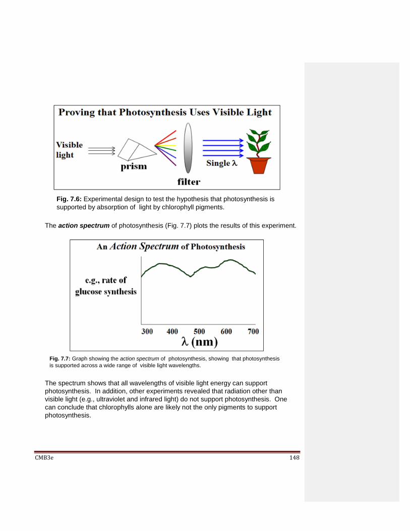
CMB3e 148

The action spectrum of photosynthesis (Fig. 7.7) plots the results of this experiment.

The spectrum shows that all wavelengths of visible light energy can support

photosynthesis. In addition, other experiments revealed that radiation other than

visible light (e.g., ultraviolet and infrared light) do not support photosynthesis. One

can conclude that chlorophylls alone are likely not the only pigments to support

photosynthesis.

Fig. 7.6: Experimental design to test the hypothesis that photosynthesis is

supported by absorption of light by chlorophyll pigments.

Fig. 7.7: Graph showing the action spectrum of photosynthesis, showing that photosynthesis

is supported across a wide range of visible light wavelengths.

CMB3e 149

Chlorophylls are easily purified from leaves. The graph below (Fig. 7.8) shows an

average absorbance spectrum of chlorophylls. The absorbance of chlorophyll a and

chlorophyll b are slightly different, but center at wavelengths at 450nm and 675nm.

From such absorbance spectra we can conclude that the chlorophylls support

photosynthesis, but that chlorophylls alone do not account for the action spectrum of

photosynthesis! In fact, other pigments absorbing elsewhere in the visible spectrum

also support photosynthesis. Of course, we knew that these other pigments are

present in leaves and other photosynthetic plant tissues, many of which we see as fall

colors. All of these pigments (including chlorophylls) are found in chloroplasts, the

organelles that conduct photosynthesis in plants. Take another look at the structure of

chloroplasts in the electron micrographs in Fig. 7.9.

Fig. 7.8: Graph plotting the absorbance spectrum of purified chlorophylls, showing

two main peaks of absorbance.

Fig. 7.9: Low (LEFT) and high (RIGHT) power transmission micrographs of typical

chloroplasts, thylakoid membranes and grana (thylakoid stacks).

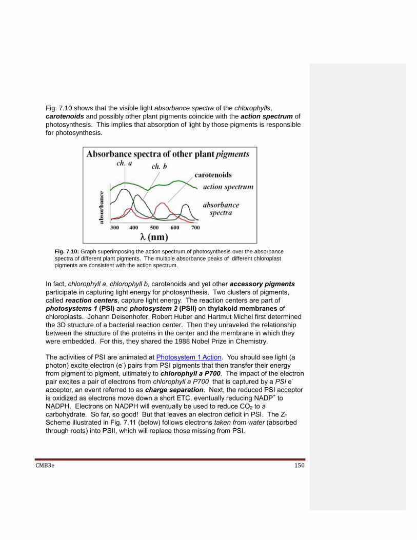
CMB3e 150

Fig. 7.10 shows that the visible light absorbance spectra of the chlorophylls,

carotenoids and possibly other plant pigments coincide with the action spectrum of

photosynthesis. This implies that absorption of light by those pigments is responsible

for photosynthesis.

In fact, chlorophyll a, chlorophyll b, carotenoids and yet other accessory pigments

participate in capturing light energy for photosynthesis. Two clusters of pigments,

called reaction centers, capture light energy. The reaction centers are part of

photosystems 1 (PSI) and photosystem 2 (PSII) on thylakoid membranes of

chloroplasts. Johann Deisenhofer, Robert Huber and Hartmut Michel first determined

the 3D structure of a bacterial reaction center. Then they unraveled the relationship

between the structure of the proteins in the center and the membrane in which they

were embedded. For this, they shared the 1988 Nobel Prize in Chemistry.

The activities of PSI are animated at Photosystem 1 Action. You should see light (a

photon) excite electron (e-) pairs from PSI pigments that then transfer their energy

from pigment to pigment, ultimately to chlorophyll a P700. The impact of the electron

pair excites a pair of electrons from chlorophyll a P700 that is captured by a PSI e-

acceptor, an event referred to as charge separation. Next, the reduced PSI acceptor

is oxidized as electrons move down a short ETC, eventually reducing NADP+ to

NADPH. Electrons on NADPH will eventually be used to reduce CO2 to a

carbohydrate. So far, so good! But that leaves an electron deficit in PSI. The Z-

Scheme illustrated in Fig. 7.11 (below) follows electrons taken from water (absorbed

through roots) into PSII, which will replace those missing from PSI.

Fig. 7.10: Graph superimposing the action spectrum of photosynthesis over the absorbance

spectra of different plant pigments. The multiple absorbance peaks of different chloroplast

pigments are consistent with the action spectrum.

CMB3e 151

Let’s summarize the flow of electrons from water through the Z-scheme. Light excites

an e- pair from the P680 form of chlorophyll a in PSII. A PSII electron acceptor in the

thylakoid membrane, identified as pheophytin, captures these electrons; this is

another photosynthetic charge separation. An electron transport chain oxidizes the

pheophytin, transferring e- pairs down to PSI. Some of the free energy released then

pumps protons from the stroma into the luminal space of the thylakoid membranes.

The gradient free energy fuels ATP synthesis as protons flow back into the stroma

through a chloroplast ATP synthase. The link at Action in the Z-Scheme animates the

entire Z-Scheme, showing first how PSI electrons reduce NADP+ and then how PSII

electrons replace missing PSI electrons, making ATP along the way. The oxygen

released by splitting water ends up in the atmosphere.

Since the goal of photosynthesis is to make and store glucose, photosynthesizing cells

get ATP for their energy needs by photophosphorylation during electron transport

through Z-scheme. However, Cyclic photophosphorylation can occur when the

cell’s need for ATP exceeds the capacity of the Z-scheme to supply it.

Fig. 7.11: The ‘Z-scheme’ of photosynthesis. Photosystems I and II (PSI, PSII) pigments absorb

light energy that excites electrons captured by electron acceptors. Electrons excited from PSI

reduce NADPH, the starting point of the light-independent reactions. Electrons excited out of

PSII come from water (‘splitting it to release oxygen). They will flow down a photosynthetic

electron transport chain to replace electrons lost from PSI. Along the way, free energy from

those excited electrons fuels ATP synthesis.

CMB3e 152

Cyclic photophosphorylation is illustrated in Fig. 7.12 below.

Cyclic Photophosphorylation is a variation on the light dependent reactions, a kind of

time-out to make ATP without reducing NADP+ (and ultimately, without reducing CO2

to make sugar). The cycle simply takes electrons excited to the PSI electron acceptor,

and instead of sending them to NADP+, deposits them on PC (plastocyanin) in the

electron transport chain between PSII and PSI. These electrons then flow down this

‘long line’ of the Z, right back to PSI, releasing their free energy to make ATP. In light,

the electrons just go up and around, hence the name Cyclic Photophosphorylation.

The path of electrons shown in Fig. 7.12 is also animated at Action in Cyclic

Photophosphorylation.

7.5.2 The Light-Independent (“Dark”) Reactions

As we have seen, the light-dependent reactions of photosynthesis require light energy

and water to generate O2, ATP and NADPH. In the light-independent (or ‘dark’)

reactions, the ATP and NADPH will provide free energy and electrons (respectively)

for carbon fixation (the reduction of CO2 to make carbohydrates). There are three

main pathways for the so-called “Dark Reactions”.

Fig. 7.12: In Cyclic Photophosphorylation electrons excited from PSI byp[ass PSII and are captured

by the photosynthetic electron transport chain and returned to return to PSI. ATP made by the Cycle

are used for cellular work when there is no need or capacity to make more sugar.

CMB3e 153

7.5.2.a C3 Photosynthesis - Light-Independent Reactions

CO2 enters photosynthetic tissues through stomata. Stomata are pores in leaves

that can be open or closed, depending on light, temperature and water availability.

In addition to allowing CO2 into photosynthetic tissues, stomata also function in

transpiration, which allows excess water in cells to leave the plants by transpiration

(sometimes called evapotranspiration). C3 photosynthesis is so named because its

first carbohydrate product is a 3-C molecule, 3-phosphoglyceric acid (3-PG). You

should recognize 3-PG; it is also a glycolytic intermediate. The Calvin Cycle is the

most common light-independent reaction pathway (Fig. 7.13). For its discovery, M.

Calvin received the Nobel Prize in Chemistry in 1961.

Fig. 7.13: Overview of the Calvin Cycle for carbon fixation in C3 (most) plants. Three RuBP

molecules fix 3 CO2 molecules, catalyzed by ribulose bisphosphate carboxylase –oxygenase

(RUBISCO). The three 6C molecules produced split into six 3C carbohydrates, becoming six

glyceraldehyde-3-P (GA3P in the illustration). Five of these go on to regenerate 3 RuBP

molecules.; the 6th GA3P waits for the Calvin Cycle to repeat, producing another GA3P. Two

GA3Ps from 2 turns of the cycle are substrates for glucose synthesis.

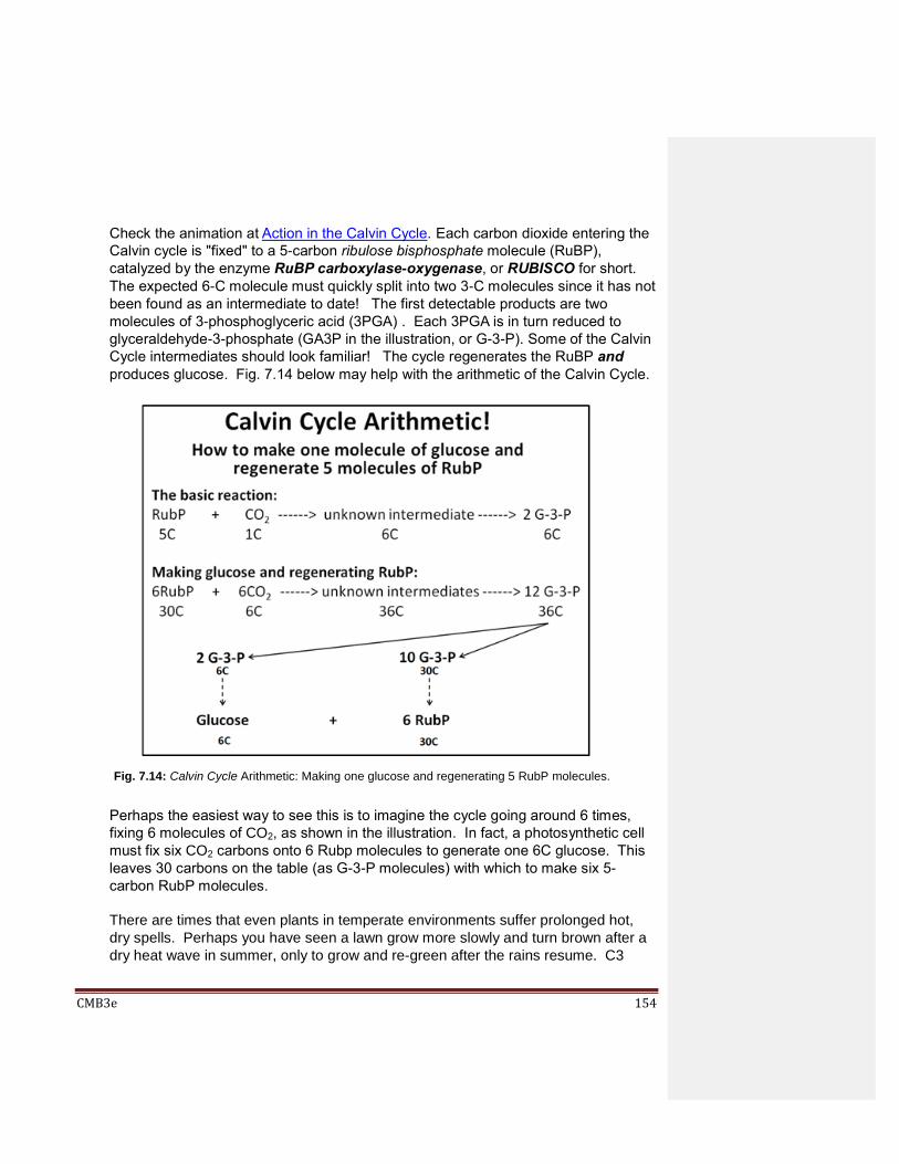
CMB3e 154

Check the animation at Action in the Calvin Cycle. Each carbon dioxide entering the

Calvin cycle is "fixed" to a 5-carbon ribulose bisphosphate molecule (RuBP),

catalyzed by the enzyme RuBP carboxylase-oxygenase, or RUBISCO for short.

The expected 6-C molecule must quickly split into two 3-C molecules since it has not

been found as an intermediate to date! The first detectable products are two

molecules of 3-phosphoglyceric acid (3PGA) . Each 3PGA is in turn reduced to

glyceraldehyde-3-phosphate (GA3P in the illustration, or G-3-P). Some of the Calvin

Cycle intermediates should look familiar! The cycle regenerates the RuBP and

produces glucose. Fig. 7.14 below may help with the arithmetic of the Calvin Cycle.

Perhaps the easiest way to see this is to imagine the cycle going around 6 times,

fixing 6 molecules of CO2, as shown in the illustration. In fact, a photosynthetic cell

must fix six CO2 carbons onto 6 Rubp molecules to generate one 6C glucose. This

leaves 30 carbons on the table (as G-3-P molecules) with which to make six 5-

carbon RubP molecules.

There are times that even plants in temperate environments suffer prolonged hot,

dry spells. Perhaps you have seen a lawn grow more slowly and turn brown after a

dry heat wave in summer, only to grow and re-green after the rains resume. C3

Fig. 7.14: Calvin Cycle Arithmetic: Making one glucose and regenerating 5 RubP molecules.

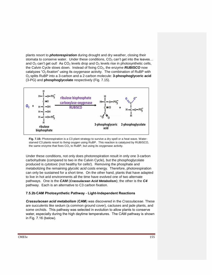
CMB3e 155

plants resort to photorespiration during drought and dry weather, closing their

stomata to conserve water. Under these conditions, CO2 can’t get into the leaves…

and O2 can’t get out! As CO2 levels drop and O2 levels rise in photosynthetic cells,

the Calvin Cycle slows down. Instead of fixing CO2, the enzyme RUBISCO now

catalyzes “O2 fixation” using its oxygenase activity. The combination of RuBP with

O2 splits RuBP into a 3-carbon and a 2-carbon molecule: 3-phosphoglyceric acid

(3-PG) and phosphoglycolate respectively (Fig. 7.15).

Under these conditions, not only does photorespiration result in only one 3-carbon

carbohydrate (compared to two in the Calvin Cycle), but the phosphoglycolate

produced is cytotoxic (not healthy for cells!). Removing the phosphate and

metabolizing the remaining glycolic acid costs energy. Therefore, photorespiration

can only be sustained for a short time. On the other hand, plants that have adapted

to live in hot arid environments all the time have evolved one of two alternate

pathways. One is the CAM (Crassulacean Acid Metabolism); the other is the C4

pathway. Each is an alternative to C3 carbon fixation.

7.5.2b CAM Photosynthetic Pathway - Light-Independent Reactions

Crassulacean acid metabolism (CAM) was discovered in the Crassulaceae. These

are succulents like sedum (a common ground cover), cactuses and jade plants, and

some orchids. This pathway was selected in evolution to allow plants to conserve

water, especially during the high daytime temperatures. The CAM pathway is shown

in Fig. 7.16 (below).

Fig. 7.15: Photorespiration is a C3 plant strategy to survive a dry spell or a heat wave. Water-

starved C3 plants resort to fixing oxygen using RuBP. This reaction is catalyzed by RUBISCO,

the same enzyme that fixes CO2 to RuBP, but using its oxygenase activity.

CMB3e 156

Stomata in chlorenchymal (mesophyll) leaf cells close during the day to minimize

water loss by transpiration. The stomata open at night, allowing plant tissues to

take up CO2. CAM plants fix CO2 by combining it with PEP (phosphoenol pyruvate)

to make oxaloacetate (OAA). This eventually produces malic acid that is stored in

plant cell vacuoles. By day, stored malic acid retrieved from the vacuoles splits into

pyruvate and CO2. The CO2 then enters chloroplasts and joins the Calvin Cycle to

make glucose and the starches. In sum, CAM plant mesophyll cells

open stomata to collect, fix and store CO2 as an organic acid at night.

close stomata to conserve water in the daytime.

re-fix the stored CO2 as carbohydrate using the NADPH and ATP from the light

reactions the next the day.

Fig. 7.16: Crassulacean Acid Metabolism in CAM plants. To survive in arid climates and

minimize water loss, CAM plants o[pen their stomata and fix CO2 in oxaloacetate (OAA) that is

converted to malic acid to be stored until daylight. Stomata close at daybreak to conserving

water, while malic acid releases CO2 to be re-fixed to make glucose.

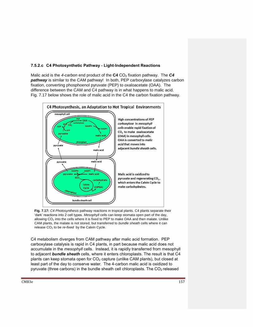
CMB3e 157

7.5.2.c C4 Photosynthetic Pathway - Light-Independent Reactions

Malic acid is the 4-carbon end product of the C4 CO2 fixation pathway. The C4

pathway is similar to the CAM pathway! In both, PEP carboxylase catalyzes carbon

fixation, converting phosphoenol pyruvate (PEP) to oxaloacetate (OAA). The

difference between the CAM and C4 pathway is in what happens to malic acid.

Fig. 7.17 below shows the role of malic acid in the C4 the carbon fixation pathway.

C4 metabolism diverges from CAM pathway after malic acid formation. PEP

carboxylase catalysis is rapid in C4 plants, in part because malic acid does not

accumulate in the mesophyll cells. Instead, it is rapidly transferred from mesophyll

to adjacent bundle sheath cells, where it enters chloroplasts. The result is that C4

plants can keep stomata open for CO2 capture (unlike CAM plants), but closed at

least part of the day to conserve water. The 4-carbon malic acid is oxidized to

pyruvate (three carbons) in the bundle sheath cell chloroplasts. The CO2 released

Fig. 7.17: C4 Photosynthesis pathway reactions in tropical plants. C4 plants separate their

‘dark’ reactions into 2 cell types. Mesophyll cells can keep stomata open part of the day,

allowing CO2 into the cells where it is fixed to PEP to make OAA and then malate. Unlike

CAM plants, the malate is not stored, but transferred to bundle sheath cells where it can

release CO2 to be re-fixed by the Calvin Cycle.

CMB3e 158

enters the Calvin cycle to be rapidly fixed by RUBISCO. Of course, this system

allows more efficient water use and faster carbon fixation under dry high heat

conditions than does C3 photosynthesis. Corn is perhaps the best-known C4 plant!

By the way, can you recognize several more intermediates common to respiration

and the light-independent photosynthetic reactions?

7.6 Thoughts on the Origins and Evolution of Respiration and Photosynthesis

We can assume that the abundance of chemical energy on our cooling planet favored the

formation of cells that could capture free energy from energy-rich nutrients in the absence

of any oxygen. For a time, we thought that the first cells would have extracted nutrient

free energy by non-oxidative, fermentation pathways. But they would have been

voracious feeders, quickly depleting their environmental nutrient resources. In this

scenario, the evolution of autotrophic life saved heterotrophic life from an early extinction!

That is because autotrophs could create organic molecules by extracting free energy from

inorganic molecules or from light. An alternative scenario that is gaining traction,

suggests that the first cells may have started with oxidative reactions that used something

other than oxygen as a final electron acceptor. In this scenario (to be considered in more

detail elsewhere), non-oxygenic ‘oxidative’ chemistries came first, followed by the

evolution of anoxic fermentative chemistries, then followed by photosynthesis, and finally

respiratory pathways. In either scenario, we can safely assume that photosynthesis

existed before oxygenic respiration.

We also assume that oxygenic photoautotrophs that capture free energy from light would

become the most abundant autotrophs, if for no other reason than sunlight is always

available (at least during the day), and oxygen is abundant in the air! The early

photoautotrophs were likely the ancestors of today’s cyanobacteria. In fact, a

phylogenetic study of many genes including “plastid-encoded proteins, nucleus-encoded

proteins of plastid origin…, as well as wide-ranging genome data from cyanobacteria”

suggests a common ancestry of freshwater cyanobacteria and eukaryotic chloroplasts

(Ponce-Toledo, R.I. et al., 2017, An Early-Branching Freshwater Cyanobacterium at the

Origin of Plastids. Current Biology 27:386-391).

Finally, let’s think about the origins of respiratory metabolism and the endosymbiotic

origins of mitochondria? Let’s start by asking how respiration co-opted photosynthetic

electron transport reactions that captured the electrons from H2O needed to reduce CO2,

turning those reactions to the task of burning sugars back to H2O and CO2. As

photosynthetic organisms emerged and atmospheric oxygen increased, elevated oxygen

levels would have been toxic to most living things. Still, some autotrophic cells must have

had a pre-existing genetic potential to conduct detoxifying respiratory chemistry. These

would have been facultative aerobes with the ability to switch from photosynthesis to

CMB3e 159

respiration when oxygen levels rose. Today’s purple non-sulfur bacteria (e.g.,

Rhodobacter sphaeroides) are just such facultative aerobes! Perhaps we aerobes

descend from the ancestors of Rhodobacter-like cells that survived and spread from

localized environments where small amounts of oxygen threatened their otherwise strictly

anaerobic neighbors. Is it possible that the endosymbiotic critter that became the first

mitochondrion in a eukaryotic cell was not just any aerobic bacterium, but a purple

photosynthetic bacterium?

Some iText & VOP Key Words and Terms

active transport of

protons

energy efficiency of

glucose metabolism PEP carboxylase

ATP synthase energy flow in glycolysis pH gradient

bacterial flagellum energy flow in the Krebs

Cycle pheophytin

C4 photosynthesis F1 ATPase photosynthesis

Calvin Cycle FAD Photosystems

CAM photosynthesis FADH2 proton gate

carotene Light-dependent

reactions proton gradient

chemiosmotic

mechanism

Light-independent

reactions proton pump

Chlorophyll a Malic acid PSI electron acceptor

Chlorophyll b mitochondria PSII electron acceptor

complex I, II, III, IV molecular motor redox reactions

Crassulaceae NAD+ reduced electron carriers

cristal membrane NADH RUBISCO

Cyclic

photophosphorylation NADP+ RuBP

cytochromes NADPH Splitting water

Dark Reactions outer membrane stoichiometry of glycolysis

electrochemical gradient

oxidative phosphorylation

stoichiometry of the Krebs Cycle

electron transport system (chain)

oxidative phosphorylation

substrate-level phosphorylation

endosymbiotic theory P680 Z-scheme

energy efficiency of glucose metabolism

P700

CMB3e 160

Chapter 8: DNA, Chromosomes and Chromatin The “Stuff of Genes”; The Double Helix; Chromosomes and Chromatin;

Naked, Circular Bacterial DNA

8.1 Introduction

Here we look at classic experiments that led to our understanding that genes are

composed of DNA. We already knew that genes were on chromosomes (chromo –

colored; soma-body), that the shapes of chromosomes of a species were unique, and that

we could characterize a species by the appearance (karyotype) of its chromosomes.

Early 20th century gene mapping even showed the relative location (locus) of genes on

linear eukaryotic chromosomes. We’ll see that eukaryotic chromosomes are highly

condensed structures composed of DNA and protein, visible only during mitosis or

meiosis. During the much longer interphase portion of the eukaryotic cell cycle,

chromosomes de-condense to chromatin, a less organized form of protein-associated

DNA in the nucleus. Compared to eukaryotic cells, bacteria contain a tiny amount of

much more simply organized DNA. Nevertheless, we’ll learn here that bacterial gene

mapping first revealed that the bacterial ‘chromosome’ to be just a small closed, naked

circular DNA double helix. Since cells must alter patterns of gene expression over time

and in response to environment, understanding the structure and organization of DNA in

cells is essential to an understanding of how and when cells turn genes on and off. While

CMB3e 161

we consider how cells regulate gene expression in an upcoming chapter, keep in mind

that that the cells of a eukaryotic organism contain the same species-specific DNA, as do

the cells of a given prokaryotic species. Here we’ll consider that eukaryotic chromatin is

the gatekeeper of gene activity, a situation quite different from bacterial cells.

Learning Objectives

When you have mastered the information in this chapter, you should be able to:

1. summarize the evidence that led to acceptance that genes are made of DNA.

2. discuss how Chargaff’’s DNA base ratios support DNA as the “stuff of genes”.

3. interpret the results of Griffith, Avery et al. and Hershey & Chase, in historical context.

4. outline and explain how Watson and Crick built their model of a DNA double helix. 5. distinguish between conservative, semiconservative and dispersive replication. 6. describe and/or draw the progress of a viral infection.

7. trace the fate of 35SO4 (sulfate) into proteins synthesized in cultured bacteria.

8. distinguish between the organization of DNA in chromatin and chromosomes and

speculate on how this organization impacts replication.

9. list some different uses of karyotypes.

10. compare and contrast euchromatin and heterochromatin structure and function.

11. outline an experiment to purify histone H1 from chromatin.

12. formulate an hypothesis to explain why chromatin is found only in eukaryotes.

13. describe the roles of different histones in nucleosome structure.

14. explain the role of Hfr strains in mapping genes in E. coli.

15. explain the chemical rationale of using different salt concentrations to extract 10 nm nucleosome fibers vs. 30nm solenoid structures from chromatin.

8.2 The Stuff of Genes

That all eukaryotic cells contain a nucleus was understood by the late 19th century. By

then, histological studies had shown that nuclei contained largely proteins and DNA. At

around the same time, the notion that the nucleus contains genetic information was

gaining traction. Mendel’s Laws of Inheritance, presented in 1865, were not widely

understood, probably because they relied on a strong dose of arithmetic and statistics, at

a time when the utility of quantitative biology was not much appreciated. But, following the

re-discovery three decades later, the number of traits in any given organism and their

Mendelian patterns of inheritance increased rapidly. But evidence that DNA was the stuff

of genes was slow to follow..

In 1910, Albrecht Kossel received the 1910 Nobel Prize in Physiology or Medicine for his

discovery of the adenine, thymine, cytosine and guanine (the four DNA bases), as well as

of uracil in RNA. At that time, DNA was known as a small, simple molecule, made up of

only the four nucleotides (see DNA Structure below for additional historical perspective).

CMB3e 162

So, the question was how could such a small, simple account for the inheritance of so

many different physical traits? The recognition that enzyme activities were inherited in

the same way as morphological characteristics led to the one-gene-one enzyme

hypothesis that earned G. W. Beadle, E. L. Tatum and J. Lederberg the 1958 Nobel Prize

for Physiology and Medicine. When enzymes were later shown to be proteins, the

hypothesis became one-gene-one protein. When proteins were shown to be composed

of one or more polypeptides, the final hypothesis became one-gene-one-polypeptide.

However, this relationship between genes and polypeptides failed to shed any light on

how DNA might be the genetic material. In fact, quite the contrary! As chains of up to 20

different amino acids, polypeptides and proteins had the potential for enough structural

diversity to account for the growing number of heritable traits in a given organism. Thus,

proteins seemed more likely candidates for the molecules of inheritance. The

experiments you will read about here began around the start of World War I and lasted

until just after World War 2. During this time, we learned that DNA was no mere tetramer,

but was in fact a long polymer. This led to some very clever experiments that eventually

forced the scientific community to the conclusion that DNA, not protein, was the genetic

molecule, despite being composed of just four monomeric units. Finally, we look at the

classic work of Watson, Crick, Franklin and Wilkins that revealed the structure of the

genetic molecule.

8.2.1 Griffith’s Experiment

Fred Neufeld, a German bacteriologist studying pneumococcal bacteria in the early

1900s discovered three immunologically different strains of Streptococcus pneumonia

(Types I, II and III). The virulent strain (Type III) was responsible for much of the

mortality during the Spanish Flu (influenza) pandemic of 1918-1920. This pandemic

killed between 20 and 100 million people, many because the influenza viral infection

weakened the immune system of infected individuals, making them susceptible to

bacterial infection by Streptococcus pneumonia.

In the 1920s, Frederick Griffith was working with virulent wild type (Type III) and

benign (Type II) strains of S. pneumonia. The two strains were easy to tell apart in

petri dishes because the virulent strain grew as morphologically smooth colonies,

while the benign strain formed rough colonies. For this reason, the two bacterial

strains were called S and R, respectively. As we now know, S cells are coated with a

polysaccharide (mucus) capsule making their colonies appear smooth. In contrast, R

cell colonies look rough (don’t glisten) because they lack the polysaccharide coating.

Griffith knew that injecting mice with S cells killed them within about a day! Injecting

the non-lethal R cells on the other hand, caused no harm. Then, he surmised that

perhaps, the exposure of mice to the R strain of S. pneumonia would immunize them

against lethal infection by subsequent exposure to S cells.

CMB3e 163

His experimental protocol and results, published in 1928, are summarized in Fig. 8.1

(below).

To test his hypothesis, Griffith injected mice with R cells. Sometime later, he injected

them with S cells. Unfortunately, the attempt to immunize the mice against S.

pneumonia was unsuccessful! The control mice injected with S strain cells and the

experimental mice that received the R strain cells first and then S cells, all died in

short order! As expected, mice injected with R cells only survived. Griffith also

checked the blood of his mice for the presence of bacterial cells:

Mice injected with benign R (rough) strain cells survived and after plating blood

from the mice on nutrient medium, no bacterial cells grew.

Many colonies of S cells grew from the blood of dead mice injected with S cells.

Griffith performed two other experiments, shown in the illustration:

He injected mice with heat-killed S cells; these mice survived. Blood from these

mice contained no bacterial cells. This was expected since heating the S cells

should have the same effect as pasteurization has on bacteria in milk!

Griffith also injected mice with a mixture of live R cells and heat-killed S cells, in

the hope that the combination might induce immunity in the mouse where injecting

the R cells alone had failed. You can imagine his surprise when, far from being

mmunized against S-cell infection, the injected mice died and abundant S cells had

accumulated in their blood.

Fig. 8.1: The experiments of F. Griffith demonstrating the existence of a chemical that

could transfer a genetic trait (i.e., virulence) between bacteria (see text for details).

CMB3e 164

Griffith realized that something important had happened in his experiments. In the

mixture of live R cells and heat-killed S cells, something released from the dead S

cells had transformed some R cells. Griffith named this “something” the transforming

principle, a molecule present in the debris of dead S cells and sometimes acquired by

a few live R cells, turning them into virulent S cells.

8.2.2 The Avery-MacLeod-McCarty Experiment

While Griffith didn’t know the chemical identity of his transforming principle, his experiments led to studies that proved DNA to be the stuff of genes. With improved molecular purification techniques developed in the 1930s, O. Avery, C. MacLeod, and M. McCarty transformed R cells in vitro (that is, without the help of a mouse!). They purified heat-killed S-cell components (DNA, proteins, carbohydrates, lipids…) and separately tested the transforming ability of each molecular component on R cells in a test tube. Since only the DNA fraction of the dead S cells could cause transformation, Avery et al. concluded that DNA must be the Transforming Principle. Fig. 8.2 (below) summarizes the experiments of Avery et al. But despite the evidence , DNA was not readily accepted as the stuff of genes.

The sticking point was that DNA was composed of only four nucleotides. Even though scientists knew that DNA was a large polymer, they still thought of DNA as that simple molecule, for example a polymer made up of repeating sequences of the four nucleotides, for example, …AGCTAGCTAGCTAGCTAGCT… Only the seemingly endless combinations of 20 amino acids in proteins promised the biological specificity

Fig. 8.2: The experiments of O. Avery et al. demonstrating for the first time that the

chemical stuff of genes, of inheritance is DNA (see text for details).

CMB3e 165

necessary to account for an organism’s many genetic traits. Lacking structural diversity, DNA was explained as a mere scaffold for protein genes. To adapt Marshal McLuhan’s famous statement that the medium is the message (i.e., airwaves do not merely convey, but are the message), many still believed that proteins are the medium of genetic information as well as the functional message itself. The reluctance of influential scientists of the day to accept a DNA transforming principle deprived its discoverers of the Nobel Prize stature it deserved. After new evidence made further resistance to that acceptance untenable, even the Nobel Committee admitted that failure to award a Nobel Prize for the discoveries of Avery et al. was an error. The key experiments of Alfred Hershey and Martha Chase finally put to rest any notion that proteins were genes

167-2 Transformation In & Out of Mice-Griffith, McCarty et al. 8.2.3 The Hershey-Chase Experiment

Earlier we learned that viruses cannot live an independent life! Bacterial viruses,

called bacteriophage or just phage for short, consist of DNA inside a protein capsule.

The life cycle of bacterial viruses is shown below in Fig. 8.3 (below).

Phages are inert particles until they bind to and infect bacterial cells. Phage particles

added to a bacterial culture could be seen attach to bacterial surfaces in an electron

microscope. Investigators found that they could detach phage particles from bacteria

by agitation in a blender (similar to one you might have in your kitchen). Centrifugation

Fig. 8.3: Life cycle of a bacteriophage: The phage coat remains attached to a cell after

infection, but the chemicals inside the phage enter the infected cell.

CMB3e 166

then separated the bacterial cells in a pellet at the bottom of the centrifuge tube,

leaving the detached phage particles in the supernatant. By adding phage to bacteria

and then detaching the phage from the bacteria at different times, it was possible to

determine how long it the phage had to remain attached before the bacteria become

infected. It turned out that pelleted cells that had been attached to phage for short

times would survive and reproduce when re-suspended in growth medium. But

pelleted cells left attached to phage for longer times had become infected. When

centrifugally separated from the detached phage and resuspended in fresh medium,

these cells would go on and lyse, producing new phage. Therefore, the transfer of

genetic information for virulence from virus to phage took some time. The viral genetic

material responsible for infection and virulence was apparently no longer associated

with the phage capsule, which could be recovered from the centrifugal supernatant.

Alfred Hershey and Martha Chase designed an experiment to determine whether the

DNA enclosed by the viral protein capsule or the capsule protein itself caused phage

to infect the bacterium. In the experiment, they separately grew E. coli cells infected

with T2 bacteriophage in the presence of either 32P or 35S (radioactive isotopes of

phosphorous and sulfur, respectively). The result was to generate phage that

contained either radioactive DNA or radioactive proteins, but not both (recall that only

DNA contains phosphorous and only proteins contain sulfur). They then separately

infected fresh E. coli cells with either 32P- or 35S-labeled, radioactive phage. Their

experiment is described in Fig. 8.4 (below).

Fig. 8.4: The experiments of Alfred Hershey and Martha Chase demonstrating that the

chemical stuff of viral genes is DNA (see text for details)

CMB3e 167

Phage and cells were incubated with either 32P or 35S just long enough to allow

infection. Some of each culture was allowed to go on and lyse to prove that the cells

were infected. The remainder of each mixture was sent to the blender. After

centrifugation of each blend, the pellets and supernatants were examined to see

where the radioactive proteins or DNA had gone. From the results, the 32P always

ended up in the pellet of bacterial cells while the 35S was found in the phage remnant

in the supernatant. Hershey and Chase concluded that the genetic material of

bacterial viruses was DNA and not protein, just as Avery et al. had suggested that

DNA was the bacterial transforming principle.

Given the earlier resistance to “simple” DNA being the genetic material, Hershey and

Chase used cautious language in framing their conclusions. They need not have; all

subsequent experiments confirmed that DNA was the genetic material. Concurrent

with these confirmations were experiments demonstrating that DNA might not be

(indeed, was not) such a simple, uncomplicated molecule! For their final contributions

to pinning down DNA as the “stuff of genes”, Alfred D. Hershey shared the 1969 Nobel

Prize in Physiology or Medicine with Max Delbruck and Salvador E. Luria. Why

didn’t Martha Chase share in the recognition of the Nobel Prize, given that she was

Hershey’s sole co-author on the paper presenting their findings?. You may well ask!

168 Hershey and Chase: Viral Genes are in Viral DNA

8.3 DNA Structure

By 1878, a substance in the pus of wounded soldiers derived from cell nuclei (called

nuclein) was shown to be composed of 5 bases (the familiar ones of DNA and RNA). The

four bases known to make up DNA (as part of nucleotides) were thought to be connected

through the phosphate groups in short repeating chains of four nucleotides. By the

1940s, we knew that DNA was a long polymer. Nevertheless, it was still considered too

simple to account for genes (see above). After the Hershey and Chase experiments, only

a few holdouts would not accept DNA as the genetic material. So when DNA was

accepted DNA as the stuff of genes, the next questions were

Was what did DNA look like?

How did its structure account for its ability to encode and reproduce life?

While the nature of DNA, its composition of 4 nucleotides had been known for some time,

it became mandatory to explain how such a “simple molecule” could inform the thousands

of proteins necessary for life. The answer to this question was to lie at least in part in an

understanding of the physical structure of DNA, made possible by the advent of X-Ray

Crystallography.

CMB3e 168

8.3.1 X-Ray Crystallography and the Beginnings of Molecular Biology

If a substance can be crystallized, the crystal will diffract X-rays at angles revealing

regular (repeating) structures of the crystal. William Astbury demonstrated that high

molecular weight DNA had just such a regular structure. His crystallographs

suggested DNA to be a linear polymer of stacked bases (nucleotides), each nucleotide

separated from the next by 0.34 nm. Astbury is also remembered for coining the term

“molecular biology” to describe his studies. The term now covers as all aspects of

biomolecular structure, as well as molecular functions (e.g. replication, transcription,

translation, gene regulation…).

In an irony of history, the Russian biologist Nikolai Koltsov had already intuited in 1927

that the basis of genetic transfer of traits would be a "giant hereditary molecule" made

up of "two mirror strands that would replicate in a semi-conservative fashion using

each strand as a template". A pretty fantastic inference if you think about it since it

was proposed long before Watson and Crick and their colleagues worked out the

structure of the DNA double-helix!

8.3.1 Wilkins, Franklin, Watson & Crick – DNA Structure Revealed

Maurice Wilkins, an English biochemist, was the first to isolate highly pure, high

molecular weight DNA. Working in Wilkins laboratory, Rosalind Franklin was able to

crystalize this DNA and produce very high-resolution X-Ray diffraction images of the

DNA crystals. Franklin’s most famous (and definitive) crystallograph was “Photo 51”

(Fig. 8.5).

Fig. 8.5: Photo 51, the X-Ray crystallograph of DNA taken by Rosalind Franklin revealed 3

crucial molecular dimensions that ultimately led to the double helical DNA model.

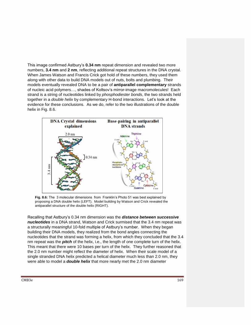
CMB3e 169

This image confirmed Astbury’s 0.34 nm repeat dimension and revealed two more

numbers, 3.4 nm and 2 nm, reflecting additional repeat structures in the DNA crystal.

When James Watson and Francis Crick got hold of these numbers, they used them

along with other data to build DNA models out of nuts, bolts and plumbing. Their

models eventually revealed DNA to be a pair of antiparallel complementary strands

of nucleic acid polymers…, shades of Koltsov’s mirror-image macromolecules! Each

strand is a string of nucleotides linked by phosphodiester bonds, the two strands held

together in a double helix by complementary H-bond interactions. Let’s look at the

evidence for these conclusions. As we do, refer to the two illustrations of the double

helix in Fig. 8.6.

Recalling that Astbury’s 0.34 nm dimension was the distance between successive

nucleotides in a DNA strand, Watson and Crick surmised that the 3.4 nm repeat was

a structurally meaningful 10-fold multiple of Astbury’s number. When they began

building their DNA models, they realized from the bond angles connecting the

nucleotides that the strand was forming a helix, from which they concluded that the 3.4

nm repeat was the pitch of the helix, i.e., the length of one complete turn of the helix.

This meant that there were 10 bases per turn of the helix. They further reasoned that

the 2.0 nm number might reflect the diameter of helix. When their scale model of a

single stranded DNA helix predicted a helical diameter much less than 2.0 nm, they

were able to model a double helix that more nearly met the 2.0 nm diameter

Fig. 8.6: The 3 molecular dimensions from Franklin’s Photo 51 was best explained by

proposing a DNA double helix (LEFT). Model building by Watson and Crick revealed the

antiparallel structure of the double helix (RIGHT).

CMB3e 170

requirement. In building their double helix, Watson and Crick realized that bases in

opposing strands would come together to form H-bonds, holding the helix together.

However, for their double helix to have a constant diameter of 2.0 nm, they also

realized that the smaller pyrimidine bases, Thymine (T) and Cytosine (C), would

have to H-bond to the larger purine bases, Adenine (A) and Guanosine (G)…, and

that neither A-G nor C-T would form pairs in the double helix.

Now to the question of how a “simple” DNA molecule could have the structural

diversity needed to encode thousands of different polypeptides and proteins. In early

studies, purified E. coli DNA was chemically hydrolyzed down to nucleotide

monomers. The hydrolysis products contained nearly equal amounts of each base,

reinforcing the notion that DNA was that simple molecule that could not encode

genes. But Watson and Crick had private access to revealing data from Erwin

Chargaff. Chargaff had determined the base composition of DNA isolated from

different species, including E. coli. He found that the base composition of DNA from

different species was not always equimolar, meaning that for some species, the DNA

was not composed of equal amounts of each of the four bases (see some of this data

in Table 8.1).

The mere fact that DNA from some species could have base compositions that

deviated from equimolarity put to rest the argument that DNA had to be a very simple

sequence. Finally it was safe to accept that to accept the obvious, namely that DNA

sequences could vary almost infinitely and could indeed be the stuff of genes.

Chargaff’s data also showed a unique pattern of base ratios. Although the base

compositions could vary between species, the A/T and G/C ratio was always one, for

every species; likewise, the ratio of (A+C)/(G+T) and (A+G)/(C+T). From this

information, Watson and Crick inferred that A (a purine) would H-bond with T (a

pyrimidine), and G (a purine) would H-bond with C (a pyrimidine) in the double helix.

When building their model with this new information, they also found H-bonding

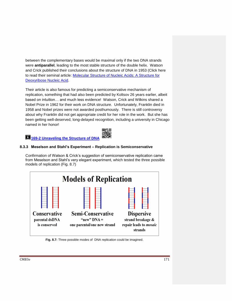
CMB3e 171

between the complementary bases would be maximal only if the two DNA strands

were antiparallel, leading to the most stable structure of the double helix. Watson

and Crick published their conclusions about the structure of DNA in 1953 (Click here

to read their seminal article: Molecular Structure of Nucleic Acids: A Structure for

Deoxyribose Nucleic Acid.

Their article is also famous for predicting a semiconservative mechanism of

replication, something that had also been predicted by Koltsov 26 years earlier, albeit

based on intuition… and much less evidence! Watson, Crick and Wilkins shared a

Nobel Prize in 1962 for their work on DNA structure. Unfortunately, Franklin died in

1958 and Nobel prizes were not awarded posthumously. There is still controversy

about why Franklin did not get appropriate credit for her role in the work. But she has

been getting well-deserved, long-delayed recognition, including a university in Chicago

named in her honor!

169-2 Unraveling the Structure of DNA

8.3.3 Meselson and Stahl’s Experiment – Replication is Semiconservative

Confirmation of Watson & Crick’s suggestion of semiconservative replication came from Meselson and Stahl’s very elegant experiment, which tested the three possible models of replication (Fig. 8.7)

Fig. 8.7: Three possible modes of DNA replication could be imagined.

CMB3e 172

In their experiment, E. coli cells were grown in medium containing 15N, a ‘heavy’

nitrogen isotope. After many generations, all of the DNA in the cells had become

labeled with the heavy isotope. At that point, the 15N-tagged cells were placed back

in medium containing the more common, ‘light’ 14N isotope and allowed to grow for

exactly one generation. Fig. 8.8 (below) shows Meselson and Stahl’s predictions for

their experiment. Meselson and Stahl knew that 14N-labeled and 15N-labeled DNA

would form separate bands after centrifugation on CsCl chloride density gradients.

They tested their predictions by purifying and centrifuging the DNA from the 15N-

labeled cells grown in 14N medium for one generation. They found that this DNA

formed a single band with a density between that of 15N-labeled DNA and 14N-labeled

DNA, eliminating the conservative model of DNA replication (possibility #1), as

Watson and Crick had also predicted. That left two possibilities: replication was either

semiconservative (possibility #2) or dispersive (possibility #3). The dispersive model

was eliminated when DNA isolated from cells grown for a 2nd generation on 14N were

shown to contain two bands of DNA on the CsCl density gradients.

170 Replication is Semiconservative

Fig. 8.8: Meselson and Stahl predict experimental outcomes based on 3 possible modes of

DNA replication.

CMB3e 173

8.4 Chromosomes

We understood from the start of the 20th century that eukaryotic chromosomes contained

genes. Therefore, it becomes necessary to understand the relationship between

chromosomes, chromatin, DNA and genes. As noted earlier, chromosomes are a

specialized, condensed version of chromatin, with key structural features shown in Fig

8.9.

We now know that the compact structure of a chromosome prevents damage to the DNA

during cell division. This damage can occur when forces on centromeres generated by

mitotic or meiotic spindle fibers pull chromatids apart. As the nucleus breaks down during

mitosis or meiosis, late 19th century microscopists saw chromosomes condense from the

dispersed cytoplasmic background. These chromosomes remained visible as they

separated, moving to opposite poles of the cell during cell division. Such observations of

chromosome behavior during cell division pointed to their role in heredity. Check out the

chromatids being separated during anaphase of mitosis in the computer-colorized

micrograph at https://www.flickr.com/photos/185778834@N06/49363817053/.

It is possible to distinguish one chromosome from another by karyotyping. When cells in

metaphase of mitosis are placed under pressure, they burst and the chromosomes

spread apart. Fig. 8.10 (below) shows such a chromosome spread. By the early 1900s,

the number, sizes and shapes of chromosomes were shown to be species-specific.

What’s more, a close look at chromosome spreads revealed that chromosomes came in

morphologically matched pairs. This was so reminiscent of Gregor Mendel’s paired

hereditary factors that chromosomes were then widely accepted as the structural seat of

genetic inheritance.

Fig. 8.9: Light micrograph of a human female chromosome stained for banding patters,

showing the centromere constriction and defining telomeres (chromosome ends).

CMB3e 174

Cutting apart micrographs like the one above (and below!) and pairing the chromosomes

by their morphology generates a karyotype. Paired human homologs are easily

identified in the colorized micrograph (Fig. 8.11, below).

Seen in cells in mitosis, all dividing human cells contain 23 pairs of homologous chromosomes. The karyotype is from a female; note the pair of homologous sex (“X”) chromosomes (lower right of the inset). X and Y chromosomes in males are not truly

Fig. 8.10: Spread of human mitotic cell chromosomes.

Fig. 8.11: Computer-colorized human karyotype.

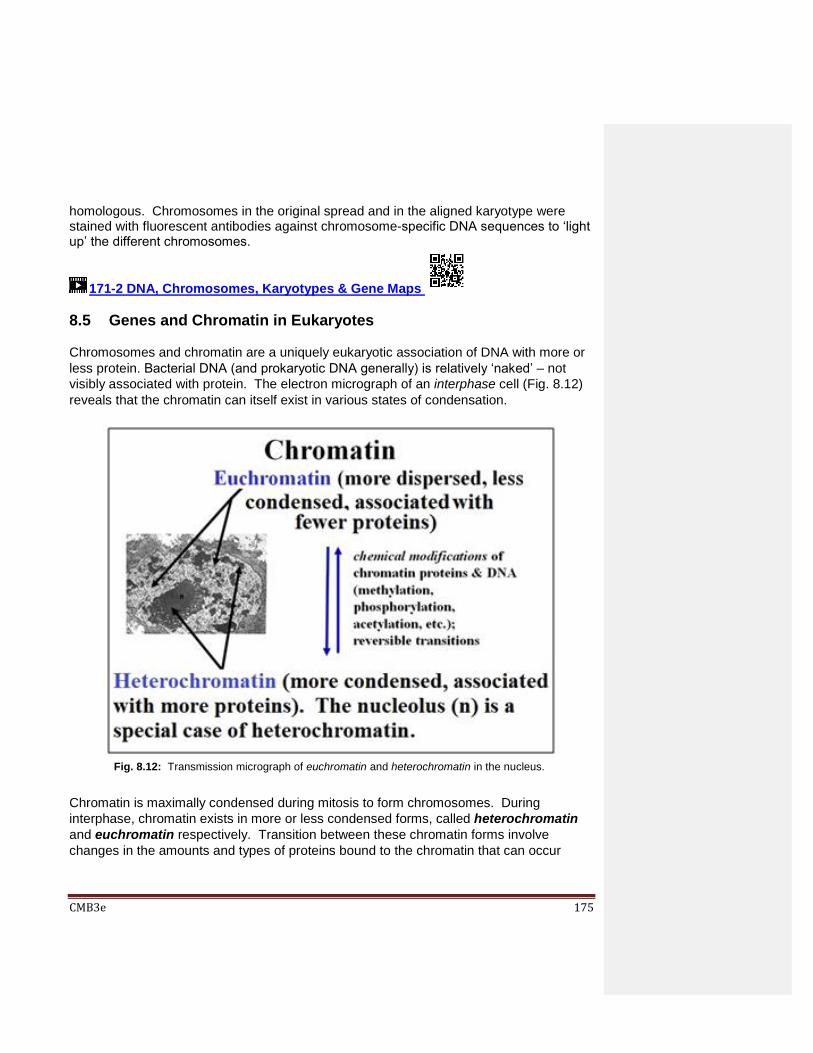
CMB3e 175

homologous. Chromosomes in the original spread and in the aligned karyotype were stained with fluorescent antibodies against chromosome-specific DNA sequences to ‘light up’ the different chromosomes.

171-2 DNA, Chromosomes, Karyotypes & Gene Maps

8.5 Genes and Chromatin in Eukaryotes

Chromosomes and chromatin are a uniquely eukaryotic association of DNA with more or

less protein. Bacterial DNA (and prokaryotic DNA generally) is relatively ‘naked’ – not

visibly associated with protein. The electron micrograph of an interphase cell (Fig. 8.12)

reveals that the chromatin can itself exist in various states of condensation.

Chromatin is maximally condensed during mitosis to form chromosomes. During

interphase, chromatin exists in more or less condensed forms, called heterochromatin

and euchromatin respectively. Transition between these chromatin forms involve

changes in the amounts and types of proteins bound to the chromatin that can occur

Fig. 8.12: Transmission micrograph of euchromatin and heterochromatin in the nucleus.

CMB3e 176

during gene regulation, i.e., when genes are turned on or off. Experiments to be

descrived later showed that aactive genes tend to be in the more dispersed euchromatin

where enzymes of replication and transcription have easier access to the DNA.

Transcriptionally inactive genes are heterochromatic, obscured by additional chromatin

proteins present in heterochromatin.

We can define three levels of chromatin organization in general terms:

1. DNA wrapped around histone proteins (nucleosomes) like "beads on a string".

2. Multiple nucleosomes coiled (condensed) into 30 nm fiber (solenoid) structures.

3. Higher-order packing of the 30 nm fiber to form the familiar metaphase chromosome.

These aspects of chromatin structure were determined by gentle disruption of the nuclear

envelope of nuclei, followed by salt extraction of extracted chromatin. Salt extraction

dissociates most of the proteins from the chromatin. The results of a low [salt] extraction

ar shown in Fig. 8.13 (below).

Fig. 8.13: Low salt fractionation of interphase nuclei yields 10nm nucleosome beads on a string.

CMB3e 177

When the low salt extract is centrifuged and the pellet resuspended, the remaining

chromatin looks like beads on a string. DNA-wrapped nucleosomes are the beads, which

are in turn linked by uniform lengths of the metaphorical DNA ‘string’.

After a high salt chromatin extraction, the structure visible in the electron microscope is

the 30nm solenoid, the coil of nucleosomes modeled in Fig. 8.14. As shown in the

illustration, simply increasing the salt concentration of an already extracted nucleosome

preparation will cause the ‘necklace’ to fold into the 30nm solenoid structure.

In fact, there are at least the five levels (orders) of chromatin structure (Fig. 8.15 below).

The first order is the string of beads. DNA-wrapped nucleosomes are the beads, which

are linked by uniform lengths of the metaphorical DNA ‘string’ ( # 1 in the illustration).

Fig. 8.14: High salt chromatin extraction from nuclei, or high salt treatment of 10 nm filaments

yields 30 nm solenoid structures, essentially coils of 10 nm filaments.

Research by G. Bergtrom

CMB3e 178

The next order (# 2) is the high salt chromatin extract, the 30 nm fiber solenoid. or coil of

nucleosomes). Other extraction protocols revealed other aspects of chromatin structure

shown in #s 3 and 4. Chromosomes seen in metaphase of mitosis are the ‘highest order’,

most condensed form of chromatin.

Fig. 8.15: Chromatin organization: different levels (orders) of chromatin structure result from

differential association of DNA with different chromosomal proteins.

CMB3e 179

Results of a DNA nuclease digestion of the beads-on-a-string are shown in Fig. 8.16.

A brief digestion of nucleosome ‘necklaces’ deoxy-ribonuclease I (DNAse I) degrades

DNA between the ‘beads’ leaving behind shortened 10nm filaments of different lengths.

After a longer digestion, single beads bund to small amounts of DNA remain.

Roger Kornberg, one son of Nobel Laureate Arthur Kornberg (discoverer of the first DNA

polymerase enzyme of replication-see the next chapter), participated in the discovery and

characterization of nucleosomes while still a post-doc! He found that each nucleosome is

associated with about 200 base pairs of DNA. Electrophoresis of DNA extracted from

digests of nucleosome beads-on-a-string preparations revealed that nucleosomes are

separated by a “linker” DNA stretch of about 80 base pairs. DNA extracted from the

nucleosomes was about 147 base pairs long, a closer estimate of the DNA wrapped

around the proteins of the nucleosome. It is appropriate to note here that Roger Kornberg

earned the 2006 Nobel Prize for Chemistry for his work on eukaryotic transcription and

the structure of RNA polymerase (among other things), topics we cover in a later chapter!

Five histone proteins could be isolated from nucleosomes and were separated by

electrophoresis; the results are illustrated in Fig. 8.17 (below). Histones are basic

proteins containing many lysine and arginine amino acids. Their positively charged side

chains enable these amino acids bind to the acidic, negatively charged phosphodiester

backbone of double helical DNA. The DNA wraps around an octamer of histones (2 each

of 4 of the histone proteins) to form the nucleosome. About a gram of histones is

associated with each gram of DNA.

Fig. 8.16: Short times 10 nm filament digestion with DNase I leaves behind shortened beads on

a string. A long time of digestion releases single nucleosomes associated with some DNA.

CMB3e 180

172-2 Nucleosomes-DNA and Protein

173-2 Chromatin Structure-Dissecting Chromatin As you might guess, an acidic extraction of chromatin should selectively remove the basic histone proteins, leaving behind an association of DNA with non-histone proteins. This proves to be the case. An electron micrograph of the chromatin remnant after an acid extraction of metaphase chromosomes is shown in Fig. 8.18. DNA freed of the regularly spaced histone-based nucleosomes, loops out, away from the long axis of the chromatin. Dark material along this axis is a protein scaffolding that makes up what’s left after histone extraction. Much of this protein is topoisomerase, an enzyme that prevents DNA from breaking apart under the strain of replication (to be detailed in a later chapter).

Fig. 8.17: Electrophoretic separation of five histones extracted from 10 nm filaments .

Fig. 8.18: Acid extraction of chromatin removes histones, leaving non-histone proteins behind.

(see original micrograph at https://www.flickr.com/photos/185778834@N06/49368658231/

CMB3e 181

8.6 Structure, Organization of Bacterial DNA… and Bacterial Sex Sexual reproduction allows compatible genders (think male and female) to share genes, a

strategy that increases species diversity. It turns out that bacteria and other single celled

organisms can also share genes… and spread diversity. We will close this chapter with a

look at sex (E. coli style!), and gene-mapping experiments showing linearly arranged

genes on a circular bacterial DNA molecule (the bacterial ‘chromosome’).

E. coli sex begins when F+ and F- cells meet. These “opposite” mating type cells can

share DNA during conjugation. F+ cells contain the fertility, or F plasmid, a small

circular DNA molecule that is separate from the E. coli chromosome. The F plasmid has

genes that encode sex pili on F+ cells as well as factors needed to form a mating bridge,

or conjugation tube. Fig. 8.19 illustrates the behavior of the F plasmid during

conjugation.

When an F+ (donor) cell encounters an F- (recipient) cell, sex pili on the donor cell initiate

recognition. Next, the conjugation tube forms, linking the cytoplasms of the two cells.

After nicking one strand of the F plasmid DNA, the nicked strand begins to roll across the

conjugation tube into the recipient F- cell. The DNA strand entering the recipient cell

replicates, as does the intact circle remaining in the donor cell (replicating DNA is shown

in red in the illustration).

Fig. 8.19: Bacterial conjugation (sex in bacteria): The F plasmid (Fertility plasmid) can transfer

bacterial chromosomal DNA from the F+ mating strain of E. coli to an opposite, F- mating strain,

leading to a measure of genetic diversity.

CMB3e 182

E. coli conjugation can have different outcomes:

1. One outcome is that one of two semi-conservatively replicated F plasmids remains in

the donor cell and another is now in the recipient cell. In this case, the recipient cell

becomes a new F+ donor cell!

2. The other outcome is integration of the F plasmid into recipient cell chromosomal

DNA. Insertion is typically at specific sites in the DNA where there is sufficient

sequence similarity between the plasmid and chromosomal DNA to allow insertion by

recombination. The result is that the recipient cell becomes an Hfr (High-frequency

recombination) cell. This cell will produce Hfr strain progeny cells.

Note that in both cases, the outcome is to change the mating type of the recipient F- cell into a strain that can initiate mating with other F- cells. These two possible results of conjugation in E. coli are shown in Fig. 8.20 (below).

Hfr cells readily express their integrated F plasmid genes, and like F+ cells, develop sex pili and form a conjugation tube with an F- cell. One strand of the bacterial chromosomal DNA will be nicked at the original insertion site of the F plasmid. The next events parallel the replicative transfer of an F plasmid during F+/F- conjugation, except that only part of the Hfr donor chromosomal DNA is transferred (Fig. 8.21, below). In this illustration, the F plasmid has inserted in front of’ an A gene so that when it enters the conjugation tube, it

Fig. 8.20: Possible results of conjugation in E. coli. The F plasmid transferred from an F+ donor

cell may or may not integrate into the F- (recipient) cell. If integration occurs, the recipient cell

becomes Hfr, with a high frequency of conjugation.

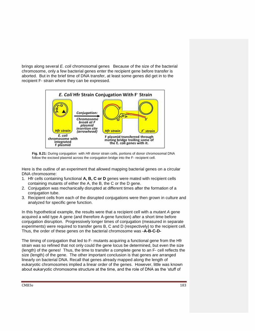
CMB3e 183

brings along several E. coli chromosomal genes Because of the size of the bacterial chromosome, only a few bacterial genes enter the recipient gene before transfer is aborted. But in the brief time of DNA transfer, at least some genes did get in to the recipient F- strain where they can be expressed.

Here is the outline of an experiment that allowed mapping bacterial genes on a circular DNA chromosome: 1. Hfr cells containing functional A, B, C or D genes were mated with recipient cells

containing mutants of either the A, the B, the C or the D gene. 2. Conjugation was mechanically disrupted at different times after the formation of a

conjugation tube. 3. Recipient cells from each of the disrupted conjugations were then grown in culture and

analyzed for specific gene function.

In this hypothetical example, the results were that a recipient cell with a mutant A gene acquired a wild type A gene (and therefore A-gene function) after a short time before conjugation disruption. Progressively longer times of conjugation (measured in separate experiments) were required to transfer gens B, C and D (respectively) to the recipient cell. Thus, the order of these genes on the bacterial chromosome was -A-B-C-D- The timing of conjugation that led to F- mutants acquiring a functional gene from the Hfr strain was so refined that not only could the gene locus be determined, but even the size (length) of the genes! Thus, the time to transfer a complete gene to an F- cell reflects the size (length) of the gene. The other important conclusion is that genes are arranged linearly on bacterial DNA. Recall that genes already mapped along the length of eukaryotic chromosomes implied a linear order of the genes. However, little was known about eukaryotic chromosome structure at the time, and the role of DNA as the ‘stuff of

Fig. 8.21: During conjugation with Hfr donor strain cells, portions of donor chromosomal DNA

follow the excised plasmid across the conjugation bridge into the F- recipient cell.

CMB3e 184

genes’ was not appreciated. These bacterial mating experiments demonstrated for the first time that genes are linearly arranged not just along a chromosome, but also along the DNA molecule. Over time, many bacterial genes were mapped all along the E. coli chromosome by isolating many different Hfr strains in which an F plasmid had inserted into different sites around the DNA circle. These Hfr strains were mated to F- bacteria, each with mutations in one or another known bacterial gene. As in the original ‘ABCD’ experiment, the order of many genes was determined, and even shown to be linked at a greater or lesser distance to those ABCD genes and each other. Using the different Hfr strains (numbered in the diagram) in conjugation experiments, it was shown that in fact, the different Hfr cells transferred different genes into the recipient cells in the order implied by the chromosome map illustrated Fig. 8.22 below. What’s more, when the experiment was done with Hfr4 (in this generic diagram); the order of genes transferred after longer times of conjugation was found to be -V-W-X-Y-Z-A-B…. The obvious conclusion from experiments like these was that the E. coli DNA molecule (its ‘chromosome’) is a closed circle! We will see visual evidence of circular E. coli chromosomes in the next chapter, with some discussion of how this evidence informed our understanding of DNA replication.

Fig. 8.22: Map of the E. coli chromosome based on conjugation of F- recipient cells with

different strains of Hfr donor cells indicated as Hfr 1, 2 , etc. The different Hfr donors are cells

in which the Hfr plasmid integrated at different place on a recipient cell chromosome. When

these different Hfr strains transfer DNA to new F- cells, they bring along different regions of the

donor cell chromosome (and thus different genes) into their conjugated F- cells.

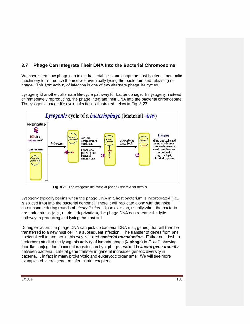
CMB3e 185

8.7 Phage Can Integrate Their DNA Into the Bacterial Chromosome We have seen how phage can infect bacterial cells and coopt the host bacterial metabolic machinery to reproduce themselves, eventually lysing the bacterium and releasing ne phage. This lytic activity of infection is one of two alternate phage life cycles. Lysogeny id another, alternate life-cycle pathway for bacteriophage. In lysogeny, instead of immediately reproducing, the phage integrate their DNA into the bacterial chromosome. The lysogenic phage life cycle infection is illustrated below in Fig. 8.23.

Lysogeny typically begins when the phage DNA in a host bacterium is incorporated (i.e.,

is spliced into) into the bacterial genome. There it will replicate along with the hoist

chromosome during rounds of binary fission. Upon excision, usually when the bacteria

are under stress (e.g., nutrient deprivation), the phage DNA can re-enter the lytic

pathway, reproducing and lysing the host cell.

During excision, the phage DNA can pick up bacterial DNA (i.e., genes) that will then be transferred to a new host cell in a subsequent infection. The transfer of genes from one bacterial cell to another in this way is called bacterial transduction. Esther and Joshua

Lederberg studied the lysogenic activity of lambda phage ( phage) in E. coli, showing

that like conjugation, bacterial transduction by phage resulted in lateral gene transfer between bacteria. Lateral gene transfer in general increases genetic diversity in bacteria…, in fact in many prokaryotic and eukaryotic organisms. We will see more examples of lateral gene transfer in later chapters.

Fig. 8.23: The lysogenic life cycle of phage (see text for details

CMB3e 186

Recall that Joshua Lederberg shared a 1958 Nobel Prize with G. W. Beadle and E. Tatum

Prize for proposing the one gene-one enzyme hypothesis (later shown to be the one

gene-one polypeptide relationship). Esther Lederberg had studied earlier with Bead;le,

Tatum and her husband at Stanford University in1944 and many credit her with helping

her mentors win their 1958 Nobel prize. In her own right, held adjunct or directorial

positions at the University of Wisconsin-Madison and Stanford University, where her other

seminal research included discovery of lambda phage (1950), invention of the replica

plating technique (1951), demonstration of lambda phage transduction in E. coli and the

discovery of the F (fertility) factor in E. coli. To explore why was never a faculty member

or a Nobel Laureate, click https://www.whatisbiotechnology.org/Lederberg_Esther

Some iText & VOP Key Words and Terms

10 nm fiber double helix mutations

30 nm fiber euchromatin non-histone proteins

5' -to-3' replication F and Hfr plasmids nuclear proteins

antiparallel DNA strands F- strain nucleosomes

bacterial conjugation F+ strain recipient cell

base ratios fertility plasmid replication

beads-on-a-string heterochromatin S. pneumonia type III-S

chromatin Hfr strain S. pneumonia type II-R

chromosomes histone octamer semi-conservative replication

conjugation tube histone proteins sex pili

conservative replication influenza solenoid fiber

deoxyribonuclease karyotype spindle fibers

discontinuous replication levels of chromatin packing

transforming principle

dispersive replication mating bridge X & Y chromosomes

DNA metaphase chromatin X-ray crystallography

donor cell mitosis & meiosis X-ray diffraction

CMB3e 187

Chapter 9: Details of DNA Replication and Repair Replicons, Replication Origins and Forks; Bidirectional Replication; The

Many Enzymes of Replication; Okazaki Fragments; Mechanisms, Actions

and Enzymes of DNA Repair; When DNA Repair Fails

9.1 Introduction

Replication begins at one or more origins of replication along DNA, where helicase

enzymes catalyze unwinding of the double helix. DNA unwinding creates replicating

bubbles, or replicons, with replication forks at either end. Making a new DNA strand

starts with making an RNA primer with RNA nucleotides and primase enzymes. DNA

nucleotides are then added to the 3’-ends of primers by a DNA polymerase. Later, other

DNA polymerases catalyze removal of the RNA primers and replacement of the

hydrolyzed ribonucleotides with new deoxyribonucleotides. Finally, DNA ligases stitch

together the fragments of new DNA synthesized at the replication forks. This complex

mechanism is common to the replication of ‘naked’ prokaryotic DNA and of chromatin-

encased eukaryotic DNA, and must therefore have arisen early in the evolution of

replication biochemistry. In this chapter, we look at the details of replication as well as

differences in detail between prokaryotic and eukaryotic replication that arise because of

differences in DNA packing. As with any complex process with many moving parts,

CMB3e 188

replication is error-prone. Therefore, we will also look at how the overall fidelity of

replication relies mechanisms of DNA repair that target specific kinds of replication

mistakes, or mutations. At the same time, lest we think that uncorrected errors in

replication are always a bad thing, they usually do not have bad outcomes. We will see

instead that they leave behind the mutations necessary for natural selection and the

evolution of diversity.

Learning Objectives

When you have mastered the information in this chapter, you should be able to:

1. explain how Cairns interpreted his theta () images.

2. compare and contrast the activities of enzymes required for replication. 3. describe the order of events at an origin of replication and at each replication fork.

4. compare unidirectional and bidirectional DNA synthesis from an origin of replication.

5. outline the basic synthesis and proofreading functions of a DNA polymerase.

6. identify the major players and their roles in the initiation of replication.

7. explain how Okazaki’s experimental results were not entirely consistent with how both

strands of DNA replicate.

8. list the major molecular players (enzymes, etc.) that elongate a growing DNA strand.

9. list the non-enzymatic players in replication and describe their functions.

10. describe how the structure of telomerase enables proper replication.

11. compare the activities of topoisomerases 1 and 2.

12. explain the reasoning behind the hypothesis of processive replication.

13. compare and contrast the impacts of germline and somatic mutations.

14. describe common forms of DNA damage.

15. list enzymes of replication that were adapted to tasks of DNA repair.

16. explain why a DNA glycosylase is useful in DNA repair.

17. explain the connection between ‘breast cancer genes’ and DNA repair.

9.2 DNA Replication

As we’ve seen, DNA strands have directionality, with a 5’ nucleotide-phosphate end and

a 3’ deoxyribose hydroxyl end. This is even true for circular bacterial chromosomes…, if

the circle is broken! Because the strands of the double helix are antiparallel, the 5’ end of

one strand aligns with the 3’end of the other at both ends of the double helix. In

presenting the complementary pairing of bases in the double helix, Watson and Crick

immediately realized that the base sequence of one strand of DNA can be used as a

template to make a new complementary strand. As we’ll see, this structure of DNA

puzzlement surrounding how replication proceeds begins with experiments that visualize

replicating DNA.

CMB3e 189

9.2.1 Visualizing Replication and Replication Forks

Recall the phenomenon of bacterial conjugation that allowed the demonstration that

bacterial chromosomes were circular. In 1963, John Cairns confirmed this fact by

direct visualization of bacterial DNA. He cultured E. coli cells for long periods on 3H-

thymidine (3H-T) to make all of their cellular DNA radioactive. He then disrupted the

cells gently to minimize damage to the DNA. The DNA released was allowed to settle

and adhere to membranes. A sensitive film was placed over the membrane and time

was allowed for the radiation to expose the film. After Cairns developed the films

(autoradiographs), he examined them in the electron microscope. He saw tracks of

silver grains in the autoradiographs (the same kind of silver grains that create an

image on film in old-fashioned photography). Look at the two drawings of Cairn’s

autoradiographs in Fig. 9.1 below. Cairns measured the length of the “silver” tracks,

which usually consisted of three possible closed loops, or circles. The circumferences

of two of these circles were always equal, their length closely predicted by the DNA

content of a single, non-dividing cell. Cairns therefore interpreted these images to be

bacterial DNA in the process of replication.

Cairns called these replicating chromosomes theta images because they resembled

the Greek letter theta (. From his many autoradiographs, he arranged a sequence

of his images (shown in Fig. 9.2, below) to illustrate his inference that replication

starts at a single origin of replication on the bacterial chromosome, proceeding

around the circle to completion.

Fig. 9.1: Illustration of J. Cairns’ autoradiographs of DNA extracted from E. coli cells allowed to

grow on 3H- thymidine for more than one generation of cells so that all cellular DNA would

become radioactive. Silver tracks represented in the figure are exposures of bacterial

chromosomal DNA.

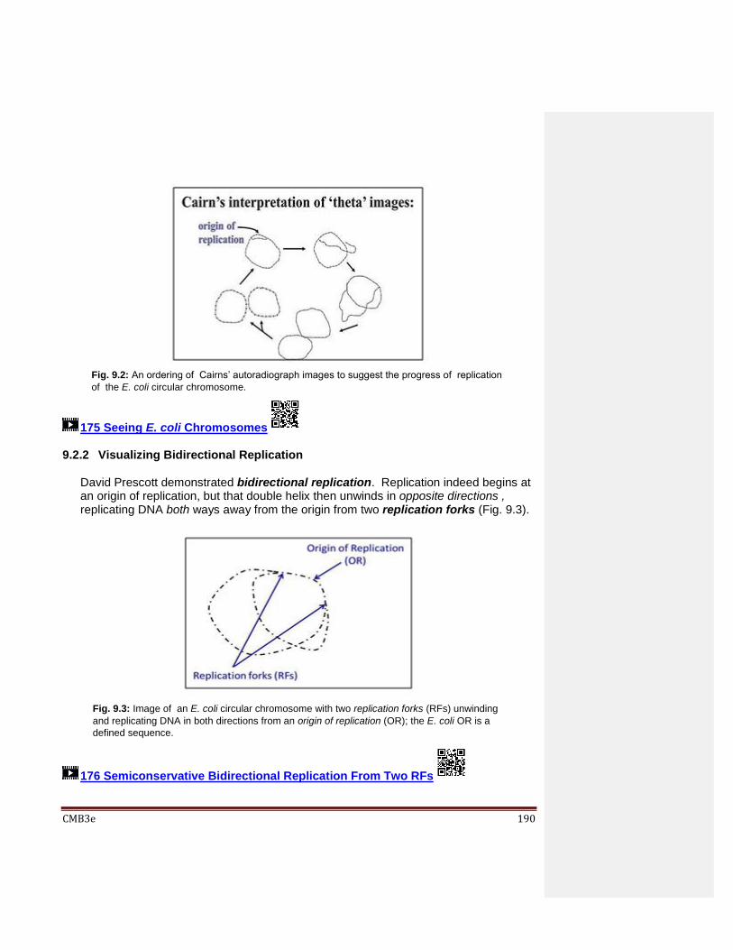
CMB3e 190

175 Seeing E. coli Chromosomes

9.2.2 Visualizing Bidirectional Replication David Prescott demonstrated bidirectional replication. Replication indeed begins at an origin of replication, but that double helix then unwinds in opposite directions , replicating DNA both ways away from the origin from two replication forks (Fig. 9.3).

176 Semiconservative Bidirectional Replication From Two RFs

Fig. 9.2: An ordering of Cairns’ autoradiograph images to suggest the progress of replication

of the E. coli circular chromosome.

Fig. 9.3: Image of an E. coli circular chromosome with two replication forks (RFs) unwinding

and replicating DNA in both directions from an origin of replication (OR); the E. coli OR is a

defined sequence.

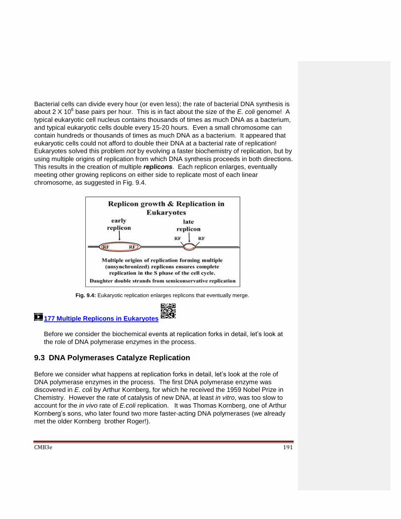
CMB3e 191

Bacterial cells can divide every hour (or even less); the rate of bacterial DNA synthesis is

about 2 X 106 base pairs per hour. This is in fact about the size of the E. coli genome! A

typical eukaryotic cell nucleus contains thousands of times as much DNA as a bacterium,

and typical eukaryotic cells double every 15-20 hours. Even a small chromosome can

contain hundreds or thousands of times as much DNA as a bacterium. It appeared that

eukaryotic cells could not afford to double their DNA at a bacterial rate of replication!

Eukaryotes solved this problem not by evolving a faster biochemistry of replication, but by

using multiple origins of replication from which DNA synthesis proceeds in both directions.

This results in the creation of multiple replicons. Each replicon enlarges, eventually

meeting other growing replicons on either side to replicate most of each linear

chromosome, as suggested in Fig. 9.4.

177 Multiple Replicons in Eukaryotes

Before we consider the biochemical events at replication forks in detail, let’s look at

the role of DNA polymerase enzymes in the process.

9.3 DNA Polymerases Catalyze Replication

Before we consider what happens at replication forks in detail, let’s look at the role of

DNA polymerase enzymes in the process. The first DNA polymerase enzyme was

discovered in E. coli by Arthur Kornberg, for which he received the 1959 Nobel Prize in

Chemistry. However the rate of catalysis of new DNA, at least in vitro, was too slow to

account for the in vivo rate of E.coli replication. It was Thomas Kornberg, one of Arthur

Kornberg’s sons, who later found two more faster-acting DNA polymerases (we already

met the older Kornberg brother Roger!).

Fig. 9.4: Eukaryotic replication enlarges replicons that eventually merge.

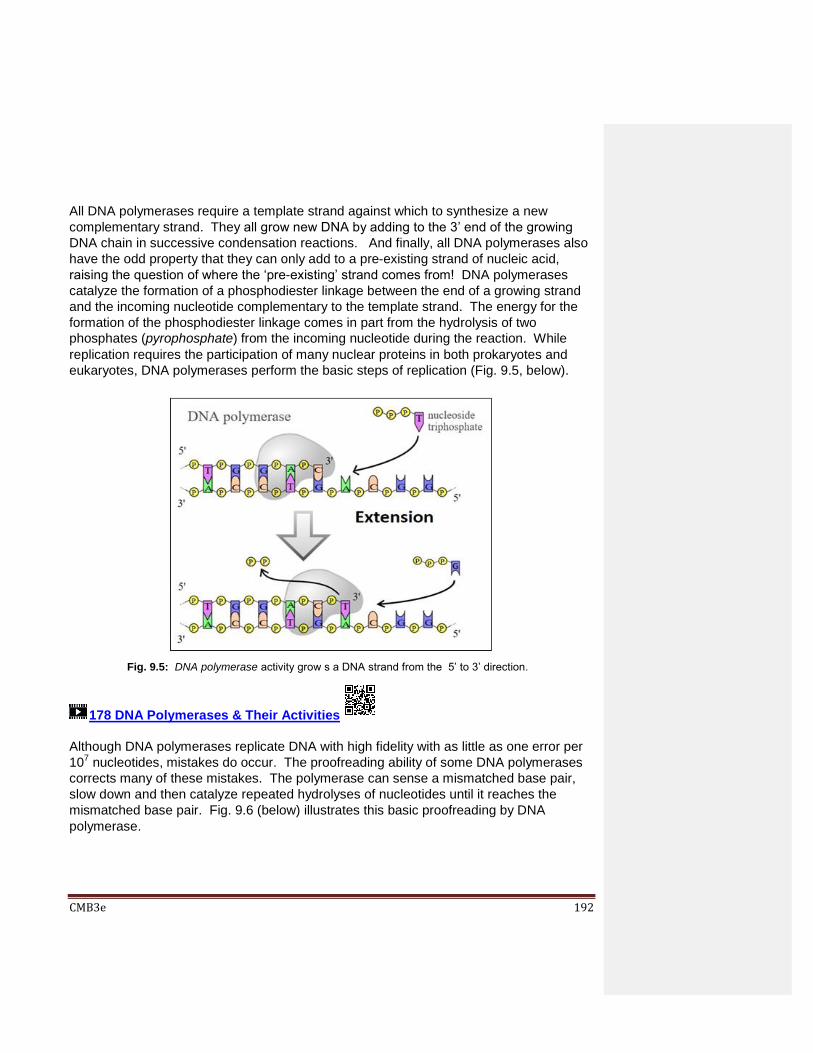
CMB3e 192

All DNA polymerases require a template strand against which to synthesize a new

complementary strand. They all grow new DNA by adding to the 3’ end of the growing

DNA chain in successive condensation reactions. And finally, all DNA polymerases also

have the odd property that they can only add to a pre-existing strand of nucleic acid,

raising the question of where the ‘pre-existing’ strand comes from! DNA polymerases

catalyze the formation of a phosphodiester linkage between the end of a growing strand

and the incoming nucleotide complementary to the template strand. The energy for the

formation of the phosphodiester linkage comes in part from the hydrolysis of two

phosphates (pyrophosphate) from the incoming nucleotide during the reaction. While

replication requires the participation of many nuclear proteins in both prokaryotes and

eukaryotes, DNA polymerases perform the basic steps of replication (Fig. 9.5, below).

178 DNA Polymerases & Their Activities

Although DNA polymerases replicate DNA with high fidelity with as little as one error per

107 nucleotides, mistakes do occur. The proofreading ability of some DNA polymerases

corrects many of these mistakes. The polymerase can sense a mismatched base pair,

slow down and then catalyze repeated hydrolyses of nucleotides until it reaches the

mismatched base pair. Fig. 9.6 (below) illustrates this basic proofreading by DNA

polymerase.

Fig. 9.5: DNA polymerase activity grow s a DNA strand from the 5’ to 3’ direction.

CMB3e 193

After mismatch repair, the DNA polymerase resumes its forward movement. Of course,

not all mistakes are caught by this or other repair mechanisms (see DNA Repair, below).

Mutations in the eukaryotic germ line cells that elude correction can cause genetic

diseases. However, most of these are the mutations that fuel evolution.

Without mutations in germ line cells (egg and sperm), there would be no mutations and

no evolution, and without evolution, life itself would have reached a quick dead end!

Other replication mistakes can generate mutations somatic cells. If these somatic

mutations escape correction, they can have serious consequences, including the

generation of tumors and cancers.

9.4 The Process of Replication

As noted, DNA replication is a sequence of repeated condensation (dehydration

synthesis) reactions linking nucleotide monomers into a DNA polymer. Like all biological

polymerizations, replication proceeds in three enzymatically catalyzed and coordinated

steps: initiation, elongation and termination.

Fig. 9.6: Detection of replication errors and correction by DNA polymerase proofreading.

CMB3e 194

9.4.1 Initiation

As we have seen, DNA synthesis starts at one or more origins or replication. These

are DNA sequences targeted by initiator proteins in E. coli (Fig. 9.7).

After breaking hydrogen bonds at the origin of replication, the DNA double helix is

progressively unzipped in both directions (i.e., by bidirectional replication). The

separated DNA strands serve as templates for new DNA synthesis. Sequences at

replication origins that bind to initiation proteins tend to be rich in adenine and thymine

bases. This is because A-T base pairs have two hydrogen (H-) bonds that require

less energy to break than the three H-bonds holding G-C pairs together. Once

initiation proteins loosen H-bonds at a replication origin, DNA helicase uses the

energy of ATP hydrolysis to further unwind the double helix. DNA polymerase III is

the main enzyme that then elongates new DNA. Once initiated, a replication bubble

(replicon) forms as repeated cycles of elongation proceed at opposite replication forks.

179 Replication Initiation in E. coli

Recall that new nucleotides are only added to the free 3' hydroxyl group of a pre-

existing nucleic acid strand. Since no known DNA polymerase can start synthesizing

new DNA strands from scratch, this is a problem!

Fig. 9.7: Initiation proteins recognize and begin unwinding the double helix by bending E. coli DNA

at the OR. Helicase then continues to unwind the DNA. SSBs (single stranded binding proteins)

stabilize unwound DNA as DNA polymerase and other enzymes begin replication in both directions

away from the OR.

CMB3e 195

If DNA polymerases require a primer, a nucleic acid strand to which to add

nucleotides, then what is the primer and where does it come from? Since RNA

polymerases, enzymes that catalyze RNA synthesis) are the only polymerases that

grow a new nucleic acid strand from scratch (i.e., from the first base) against a DNA

template, it was suggested that the primer might be RNA. After synthesizing a short

RNA primer, new deoxynucleotides would be added at its 3’ end by DNA polymerase.

Discovery of short stretches of RNA at the 5’ end of Okazaki fragments confirmed the

notion of RNA primers. We now know that cells use primase, a special RNA

polymerase used during replication, to make RNA primers against DNA templates

before a DNA polymerase can grow the DNA strands at replication forks. We’ll see

below that the requirement for RNA primers is nowhere more in evidence in events at

a replication fork.

9.4.2 Elongation

Looking at elongation at one replication fork we see another problem. One of the two

new DNA strands can grow continuously towards the replication fork as the double

helix unwinds. But what about the other strand? Either this other strand must grow in

pieces in the opposite direction, or it must wait to begin synthesis until the double helix

is fully unwound. The problem is illustrated in Fig. 9.8 (below left).

The best resolution of the problem is that one strand of DNA must be replicated in fragments, that must be stitched (i.e., ligated) together, as suggested in Fig. 9.9 (above right).

Fig. 9.8: 5’-to-3’ replication creates the problem at the replication fork shown here.

Fig. 9.9: Hypothesis proposing that at least one DNA strand at a replication fork (the lagging

strand) is synthesized in pieces, each starting with an RNA primer, that must be later correctly

stitched together.

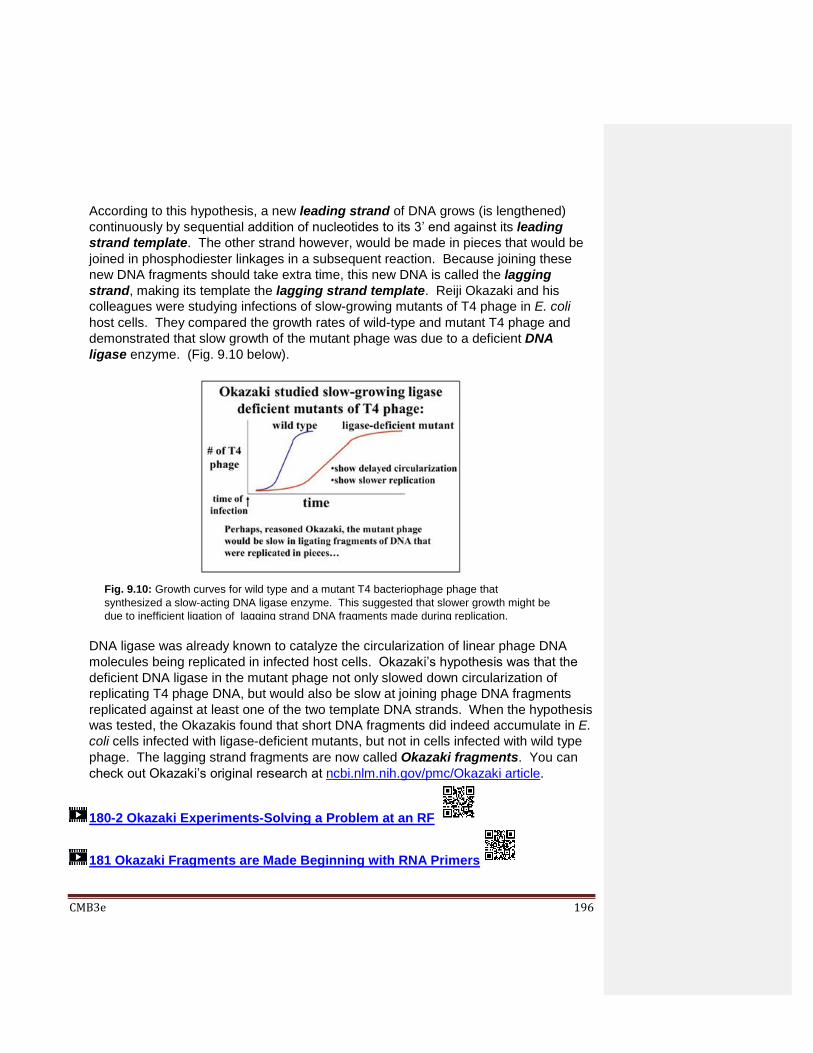
CMB3e 196

According to this hypothesis, a new leading strand of DNA grows (is lengthened)

continuously by sequential addition of nucleotides to its 3’ end against its leading

strand template. The other strand however, would be made in pieces that would be

joined in phosphodiester linkages in a subsequent reaction. Because joining these

new DNA fragments should take extra time, this new DNA is called the lagging

strand, making its template the lagging strand template. Reiji Okazaki and his

colleagues were studying infections of slow-growing mutants of T4 phage in E. coli

host cells. They compared the growth rates of wild-type and mutant T4 phage and

demonstrated that slow growth of the mutant phage was due to a deficient DNA

ligase enzyme. (Fig. 9.10 below).

DNA ligase was already known to catalyze the circularization of linear phage DNA

molecules being replicated in infected host cells. Okazaki’s hypothesis was that the

deficient DNA ligase in the mutant phage not only slowed down circularization of

replicating T4 phage DNA, but would also be slow at joining phage DNA fragments

replicated against at least one of the two template DNA strands. When the hypothesis

was tested, the Okazakis found that short DNA fragments did indeed accumulate in E.

coli cells infected with ligase-deficient mutants, but not in cells infected with wild type

phage. The lagging strand fragments are now called Okazaki fragments. You can

check out Okazaki’s original research at ncbi.nlm.nih.gov/pmc/Okazaki article.

180-2 Okazaki Experiments-Solving a Problem at an RF

181 Okazaki Fragments are Made Beginning with RNA Primers

Fig. 9.10: Growth curves for wild type and a mutant T4 bacteriophage phage that

synthesized a slow-acting DNA ligase enzyme. This suggested that slower growth might be

due to inefficient ligation of lagging strand DNA fragments made during replication.

CMB3e 197

Each Okazaki fragment would have to begin with a 5’ RNA primer, creating yet

another dilemma! The RNA primer must be replaced with deoxynucleotides before

stitching the fragments together. This process in fact happens (Fig. 9.11, below).

Removal of RNA primer nucleotides from Okazaki fragments requires the action of

DNA polymerase I. This is the slow-acting DNA polymerase first characterized by

Arthur Kornberg. DNA polymerase I has the unique ability to catalyze hydrolysis of

the phosphodiester bonds between the RNA (or DNA) nucleotides from the 5’-end of a

nucleic acid strand.

Flap Endonuclease 1 (FEN 1) also plays a role in removing ‘flaps’ of nucleic acid from

the 5’ ends of the fragments often displaced by polymerase as it replaces the

replication primer. At the same time as the RNA nucleotides are removed, DNA

polymerase I catalyzes their replacement by the appropriate deoxynucleotides.

Finally, when a fragment is entirely DNA, DNA ligase links it to the rest of the already

assembled lagging strand DNA. Because of its 5’ exonuclease activity (not found in

other DNA polymerases), DNA polymerase 1 also plays unique roles in DNA repair

(discussed further below).

As Cairn’s suggested and others demonstrated, replication proceeds in two directions

from the origin to form a replicon with its two replication forks (RFs). Each RF has a

primase associated with the replication of Okazaki fragments along lagging strand

templates. Fig. 9.12below illustrates the requirement for primases at replication forks.

Fig. 9.11: Steps in the synthesis of DNA against the lagging template strand (see text for details).

CMB3e 198

Now we can ask what happens when replicons reach the ends of linear chromosomes

in eukaryotes.

182 Replication Elongation in E. coli

9.4.3 Termination

In prokaryotes, replication is complete when two replication forks meet after replicating

their portion of the circular DNA molecule. In eukaryotes, many replicons fuse to

become larger replicons, eventually reaching the ends of the chromosomes. And

now…, , there is still another problem, illustrated in Fig. 9.13!

Fig. 9.12: A pair of replication forks (RFs), each assembling proteins and enzymes required for

replication, including DNA primases.

Fig. 9.13: In linear chromosomes, the lagging strand at the end (telomere) of a double helix can’t be

primed and thus cannot be replicated, causing chromosome shortening at each cell division.

CMB3e 199

When a replicon nears the end of a double-stranded DNA molecule, i.e., at the end of

a chromosome, the strand synthesized continuously stops when it reaches the 5’ end

of its template DNA. In theory, synthesis of a last Okazaki fragment can be primed

from the 3’ end of the lagging template strand. The illustration above implies removal

of a primer from the penultimate Okazaki fragment and DNA polymerase-catalyzed

replacement with DNA nucleotides. But what about that last Okazaki fragment?

Would its primer be hydrolyzed? Moreover, without a free 3’ end to add to, how are

those RNA nucleotides replaced with DNA nucleotides? The problem here is that

every time a cell replicates, one strand of new DNA (likely both) would get shorter and

shorter. Of course, this would not do…, and does not happen! Eukaryotic replication

undergoes a termination process involving extending the length of one of the two

strands by the enzyme telomerase, as illustrated in Fig. 9.14 below.

Telomerase consists of several proteins and an RNA. From the drawing, the RNA

component serves as a template for 5’-> 3’ extension of the problematic DNA strand.

The protein with the requisite reverse transcriptase activity is called Telomerase

Reverse Transcriptase, or TERT. The Telomerase RNA Component is called TERC.

Carol Greider, Jack Szostak and Elizabeth Blackburn shared the 2009 Nobel Prize in

Physiology or Medicine for discovering telomerase.

183 Telomere Replication Prevents Chromosome Shortening

Fig. 9.14: The ribonucleoprotein enzyme telomerase resolves the dangers of chromosome

shortening by using its RNA sequence to generate repeats on the telomeric end of lagging

strand DNAs (see text and illustration for details).

CMB3e 200

We know now that differentiated, non-dividing cells no longer produce the telomerase

enzyme, while telomerase genes are active in dividing cells (e.g., stem cells) and

cancer cells, which contain abundant telomerase.

9.4.4 Is Replication Processive?

Drawings of replicons and replication forks suggest separate events on each DNA

strand. Yet events at replication forks seem to be coordinated. Thus replication may

be processive, meaning both new DNA strands are replicated in the same direction at

the same time, smoothing out the process. How might this be possible? The drawing

in Fig. 9.15 shows lagging strand template DNA bending, so that it faces in the same

direction as the leading strand at the replication fork.

184 Processive Replication

The replisome structure cartooned at the replication fork consists of clamp proteins,

primase, helicase, DNA polymerase and single-stranded binding proteins among

others.

Fig. 9.15: The Processive Replication hypothesis unites all components needed to replicate

both strands of DNA in a replisome, so the both strands are replicated in the same direction.

CMB3e 201

Newer techniques of visualizing replication by real-time fluorescence videography

have called the processive model into question, suggesting that the replication

process is anything but smooth! Are lagging and leading strand replication not in fact

coordinated? Alternatively, is the jerky movement of DNA elongation in the video an

artifact, so that the model of smooth, coordinated replication integrated at a replisome

still valid? Or is coordination defined and achieved in some other way? Check out the

video yourself in the article at 2017 Real-Time Fluorescent Replication Video.

9.4.5 One more problem with replication

Cairns recorded many images of E. coli of the sort shown in Fig. 9.16.

The coiled, twisted appearance of the replicating circles were interpreted to be a

natural consequence of trying to pull apart helically intertwined strands of DNA… or

intertwined strands of any material! As the strands continued to unwind, the DNA

should twist into a supercoil of DNA. Increased DNA unwinding would cause the

phosphodiester bonds in the DNA to rupture, fragmenting the DNA. Obviously, this

does not happen. Experiments were devised to demonstrate supercoiling, and to test

Fig. 9.16: Unwinding a circular DNA molecule ( or any double helix that is rigidly associated

with chromosomal proteins wherever it is not replicating) causes the DNA to twist and coil on

itself, a phenomenon called supercoiling. Cairns’ saw such supercoils in E. coli chromosomes.

CMB3e 202

hypotheses explaining how cells would relax the supercoils during replication. Testing

these hypotheses revealed the topoisomerase enzymes. These enzymes bind and

hold on to DNA, catalyze hydrolysis of phosphodiester bonds, control unwinding of the

double helix, and finally catalyze the re-formation of the phosphodiester linkages. It is

important to note that the topoisomerases are not part of a replisome, but can act far

from a replication fork, probably responding to the tensions anywhere in the

supercoiled DNA. Recall that topoisomerases comprise much of the protein lying

along eukaryotic chromatin.

185-2 Topoisomerases Relieve Supercoiling During Replication

We have considered most of the molecular players in replication. Below is a list of the key replication proteins and their functions (Table 9.2, from DNA Replication in Wikipedia):

DNA Repair

We generally accept the notion that replication faithfully duplicates the genetic material,

occasional making mistakes (mutating). At the same time, evolution would not be

possible without mutation, and mutation is not possible without at least some adverse

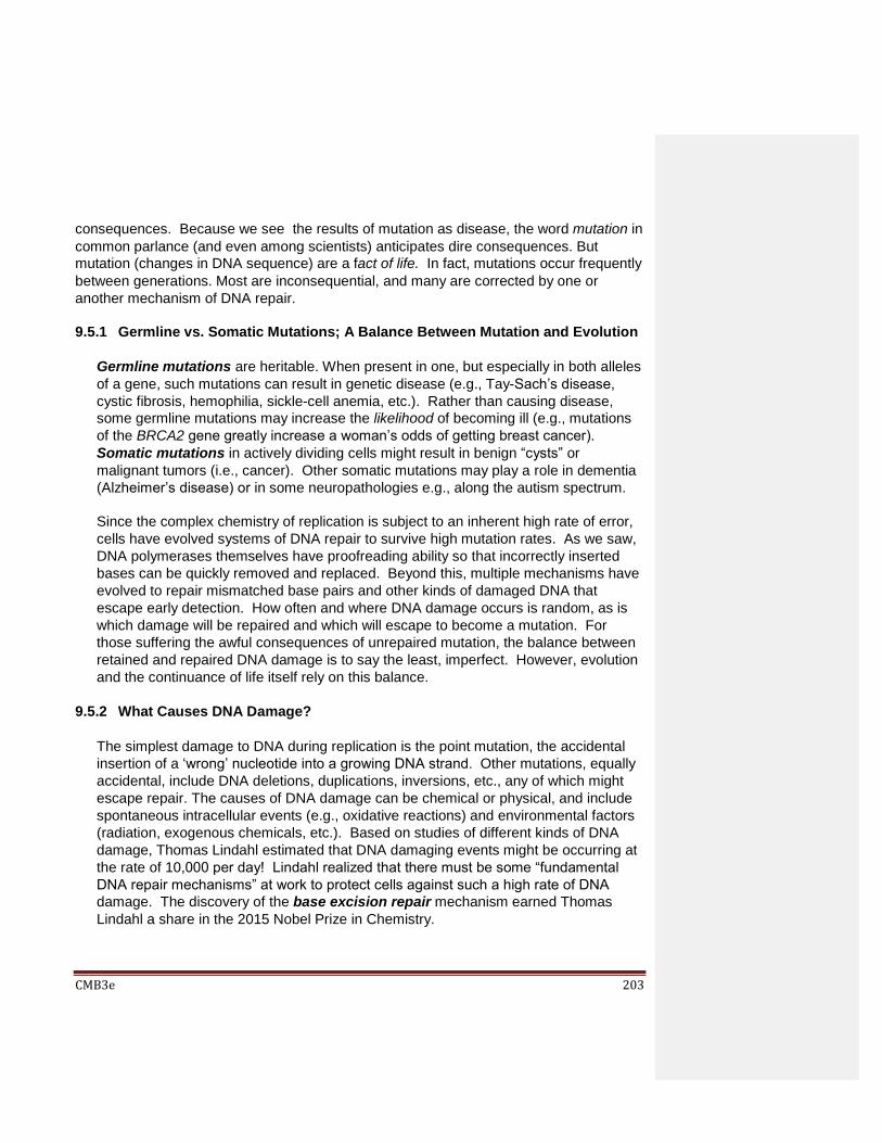
CMB3e 203

consequences. Because we see the results of mutation as disease, the word mutation in

common parlance (and even among scientists) anticipates dire consequences. But

mutation (changes in DNA sequence) are a fact of life. In fact, mutations occur frequently

between generations. Most are inconsequential, and many are corrected by one or

another mechanism of DNA repair.

9.5.1 Germline vs. Somatic Mutations; A Balance Between Mutation and Evolution

Germline mutations are heritable. When present in one, but especially in both alleles

of a gene, such mutations can result in genetic disease (e.g., Tay-Sach’s disease,

cystic fibrosis, hemophilia, sickle-cell anemia, etc.). Rather than causing disease,

some germline mutations may increase the likelihood of becoming ill (e.g., mutations

of the BRCA2 gene greatly increase a woman’s odds of getting breast cancer).

Somatic mutations in actively dividing cells might result in benign “cysts” or

malignant tumors (i.e., cancer). Other somatic mutations may play a role in dementia

(Alzheimer’s disease) or in some neuropathologies e.g., along the autism spectrum.

Since the complex chemistry of replication is subject to an inherent high rate of error,

cells have evolved systems of DNA repair to survive high mutation rates. As we saw,

DNA polymerases themselves have proofreading ability so that incorrectly inserted

bases can be quickly removed and replaced. Beyond this, multiple mechanisms have

evolved to repair mismatched base pairs and other kinds of damaged DNA that

escape early detection. How often and where DNA damage occurs is random, as is

which damage will be repaired and which will escape to become a mutation. For

those suffering the awful consequences of unrepaired mutation, the balance between

retained and repaired DNA damage is to say the least, imperfect. However, evolution

and the continuance of life itself rely on this balance.

9.5.2 What Causes DNA Damage?

The simplest damage to DNA during replication is the point mutation, the accidental

insertion of a ‘wrong’ nucleotide into a growing DNA strand. Other mutations, equally

accidental, include DNA deletions, duplications, inversions, etc., any of which might

escape repair. The causes of DNA damage can be chemical or physical, and include

spontaneous intracellular events (e.g., oxidative reactions) and environmental factors

(radiation, exogenous chemicals, etc.). Based on studies of different kinds of DNA

damage, Thomas Lindahl estimated that DNA damaging events might be occurring at

the rate of 10,000 per day! Lindahl realized that there must be some “fundamental

DNA repair mechanisms” at work to protect cells against such a high rate of DNA

damage. The discovery of the base excision repair mechanism earned Thomas

Lindahl a share in the 2015 Nobel Prize in Chemistry.

CMB3e 204

Specific environmental factors that can damage DNA include UV light, X-rays and

other radiation, as well as chemicals (e.g., toxins, carcinogens, and even drugs, etc.).

Both germline and somatic cells can be affected. While mutations can and do cause

often debilitating diseases, it is instructive to keep the impact of mutations in

perspective. Most mutations are actually silent; they do not cause disease. And

among mutations that could cause disease, much of the DNA damage is repaired.

Cells correct more than 99.9% of mistaken base changes before they have a chance

to become mutations. That is why we think of replication as a “faithful” process. Let’s

look at some common types of DNA damage that are usually repaired:

Pyrimidine dimers, typical of adjacent thymines (less often cytosines) in a single

DNA strand, caused by UV exposure

Depurination; the hydrolytic removal of guanine or adenine from the #1 C (carbon)

of deoxyribose in a DNA strand

Deamination: hydrolytic removal of amino (-NH2) groups from guanine (most

common), cytosine or adenine

Oxidative damage of deoxyribose with any base, but most commonly purines

Inappropriate methylation of any bases, but most commonly purines

DNA strand breakage during replication or from radiation or chemical exposure

9.6 Molecular Consequences of Uncorrected DNA Damage

While bacteria suffer DNA damage, we will focus here on eukaryotes since they have

evolved the most sophisticated repair mechanisms. Remember that unrepaired DNA

damage will be passed on to daughter cells in mitosis, or might be passed on to the next

generation if the mutation occurs in a germline cell.

9.6.1 Depurination

This is the spontaneous hydrolytic removal of guanine or adenine from the #1 carbon

(C#1) of deoxyribose in a DNA strand. Its frequency of 5000 depurinations per cell

per day emphases the high rate of DNA damage that demands a fix! If not repaired,

depurination results in a single base-pair deletion in the DNA of one chromosome after

replication, leaving the DNA in the same region of the other chromosome unchanged.

Fig 9.17 (below) shows the effects of depurination.

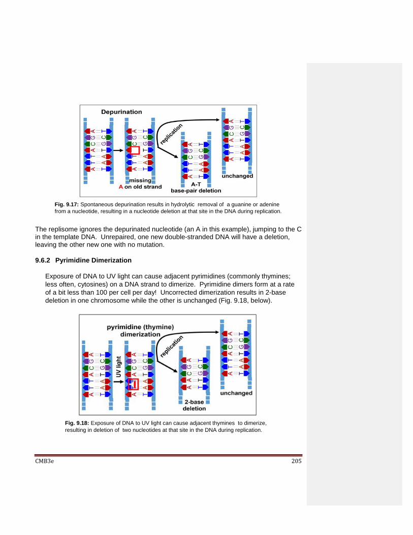
CMB3e 205

The replisome ignores the depurinated nucleotide (an A in this example), jumping to the C in the template DNA. Unrepaired, one new double-stranded DNA will have a deletion, leaving the other new one with no mutation.

9.6.2 Pyrimidine Dimerization

Exposure of DNA to UV light can cause adjacent pyrimidines (commonly thymines;

less often, cytosines) on a DNA strand to dimerize. Pyrimidine dimers form at a rate

of a bit less than 100 per cell per day! Uncorrected dimerization results in 2-base

deletion in one chromosome while the other is unchanged (Fig. 9.18, below).

Fig. 9.17: Spontaneous depurination results in hydrolytic removal of a guanine or adenine

from a nucleotide, resulting in a nucleotide deletion at that site in the DNA during replication.

Fig. 9.18: Exposure of DNA to UV light can cause adjacent thymines to dimerize,

resulting in deletion of two nucleotides at that site in the DNA during replication.

CMB3e 206

You can predict that correction of this radiation-induced damage will either involve

disrupting the dimers (in this case thymine dimers), or removal and replacement of the

dimerized bases by monomeric bases.

9.6.3 Deamination

Fig. 9.19 shows the consequences of deamination to a DNA base sequence.

Deamination is the hydrolytic removal of amino (-NH2) groups from guanine (most

common), cytosine or adenine, at a rate of 100 per cell per day. Deamination does

not affect thymine (because it has no amino groups!). Uncorrected deamination

results in a base substitution on one chromosome (actually, a T-A pair substitution for

the original C-G in this example) and no change on the other. Deamination of adenine

or guanine results in unnatural bases (hypoxanthine and xanthine, respectively).

These are easily recognized and corrected by DNA repair systems. The U-A base

pair remains occasionally un-repaired.

9.7 DNA Repair Mechanisms

Many enzymes and proteins are involved in DNA repair. Some of these function in

normal replication, mitosis and meiosis, but were co-opted for DNA repair activities.

These molecular co-optations are so vital to normal cell function that some repair

activities and molecular players are highly conserved in evolution. Among the DNA repair

pathways that have been identified, we will look at Base Excision Repair, Nucleotide

Excision Repair, Transcription Coupled Repair, Non-homologous End-Joining, and

Homologous Recombination (of these, the last is perhaps the most complex).

Fig. 9.19: -NH2 removal (deamination) of a base in one DNA strand results in a base

substitution during replication.

CMB3e 207

9.7.1 Base Excision Repair On detection of an incorrect. e.g., oxidized, open-ring, deaminated bases or bases

containing saturated C=C bonds, DNA glycosylases catalyze hydrolysis of the

damaged base from their deoxyribose in the DNA. For more on these enzymes click

https://en.wikipedia.org/wiki/DNA_glycosylase Fig. 9.20 shows base excision repair.

9.7.2 Nucleotide Excision Repair

The discovery of nucleotide excision repair earned Aziz Sancar a share in the 2015 Nobel Prize in Chemistry. Fig 9.21 illustrates nucleotide excision repair for a pyrimidine dimer.

Fig. 9.20: Base Excision Repair mechanisms can detect and fix e.g., a deamination prior to

replication (see text for details).

Fig. 9.21: Nucleotide Excision Repair mechanisms can detect and fix e.g., a pyrimidine

dimer prior to replication (see text for details).

CMB3e 208

In this example, an Excision Nuclease recognizes a pyrimidine dimer and hydrolyzes phosphodiester bonds between nucleotides several bases away from either side of the dimer. A DNA helicase then unwinds and separates the DNA fragment containing the dimerized bases from the damaged DNA strand. Finally, DNA polymerase acts 5’-3’ to fill in the gap and DNA ligase seals the remaining nick to complete the repair.

9.7.3 Mismatch repair

DNA Mismatch Repair occurs when DNA polymerase proofreading misses an

incorrect base insertion into a new DNA strand. This repair mechanism relies on the

fact that double-stranded DNA shows a specific pattern of methylation. The discovery

of the mismatch repair mechanism earned Paul Modrich a share in the 2015 Nobel

Prize in Chemistry. These methylation patterns are related to epigenetic patterns of

gene activity and chromosome structure that are expected to be inherited by daughter

cells. When DNA replicates, the methyl groups on the template DNA strands remain,

but the newly synthesized DNA is un-methylated. In fact, it will take some time for

methylation enzymes to locate and methylate the appropriate nucleotides in the new

DNA. In the intervening time, several proteins and enzymes can detect inappropriate

base pairing (the mismatches) and initiate mismatch repair as illustrated in Fig. 9.22.

9.7.4 Transcription Coupled Repair (in Eukaryotes)

If an RNA polymerase reading a template DNA encounters a nicked template or one

with an unusual base substitution, it might stall transcription and “not know what to do

next”. Thus at a loss, a normal transcript would not be made and the cell might not

Fig. 9.22: DNA Mismatch Repair can detect and fix post-replication errors (i.e., mismatched base

pairing (see text for details).

CMB3e 209

survive. No big deal in a tissue comprised of thousands if not millions of cells, right?

Nevertheless, Transcription Coupled Repair exists! In this repair pathway, if RNA

polymerase encounters a DNA lesion (i.e., damaged DNA) while transcribing a

template strand, it will indeed stall. This allows time for coupling proteins to reach

the stalled polymerase and enable repair machinery (e.g., by base, or nucleotide

excision) to effect the repair. Once the repair is complete, the RNA polymerase

‘backs up’ along the template strand with the help of other factors, and resumes

transcription of the corrected template.

9.7.5 Non-homologous End-Joining

DNA replication errors can cause double stranded breaks, as can environmental

factors (ionizing radiation, oxidation, etc.). Repair by non-homologous end-joining

deletes damaged and adjacent DNA and rejoins ‘cut’ ends (Fig. 9.23).

Once the site of a double-stranded break is recognized, nucleotides hydrolyzed from

the ends of both strands at the break-site leave ‘blunt ends’. Next, several proteins

(Ku among others) bring DNA strands together and further hydrolyze single DNA

strands to create staggered (overlapping, or complementary) ends. The overlapping

ends of these DNA strands form H-bonds. Finally, DNA ligase seals the H-bonded

overlapping ends of DNA strands, leaving a repair with deleted bases.

In older people, there is evidence of more than 2000 ‘footprints’ of this kind of repair

per cell. How is this possible? This quick-fix repair often works with no ill effects

because most of the eukaryotic genome does not encode genes or even regulatory

DNA (whose damage would otherwise be more serious).

Fig. 9.23: Non-Homologous End-Joining detects and repairs double-stranded breaks in

DNA, but can leave nucleotide deletions (see text for details).

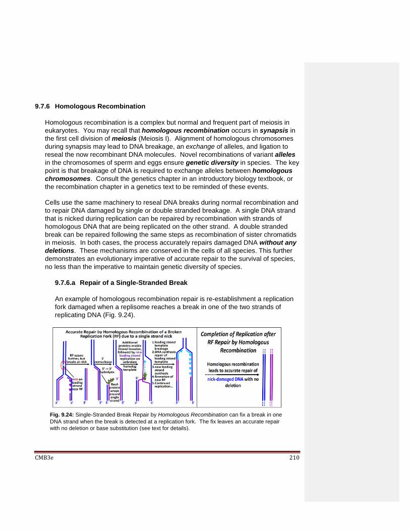
CMB3e 210

9.7.6 Homologous Recombination

Homologous recombination is a complex but normal and frequent part of meiosis in

eukaryotes. You may recall that homologous recombination occurs in synapsis in

the first cell division of meiosis (Meiosis I). Alignment of homologous chromosomes

during synapsis may lead to DNA breakage, an exchange of alleles, and ligation to

reseal the now recombinant DNA molecules. Novel recombinations of variant alleles

in the chromosomes of sperm and eggs ensure genetic diversity in species. The key

point is that breakage of DNA is required to exchange alleles between homologous

chromosomes. Consult the genetics chapter in an introductory biology textbook, or

the recombination chapter in a genetics text to be reminded of these events.

Cells use the same machinery to reseal DNA breaks during normal recombination and

to repair DNA damaged by single or double stranded breakage. A single DNA strand

that is nicked during replication can be repaired by recombination with strands of

homologous DNA that are being replicated on the other strand. A double stranded

break can be repaired following the same steps as recombination of sister chromatids

in meiosis. In both cases, the process accurately repairs damaged DNA without any

deletions. These mechanisms are conserved in the cells of all species. This further

demonstrates an evolutionary imperative of accurate repair to the survival of species,

no less than the imperative to maintain genetic diversity of species.

9.7.6.a Repair of a Single-Stranded Break

An example of homologous recombination repair is re-establishment a replication

fork damaged when a replisome reaches a break in one of the two strands of

replicating DNA (Fig. 9.24).

Fig. 9.24: Single-Stranded Break Repair by Homologous Recombination can fix a break in one

DNA strand when the break is detected at a replication fork. The fix leaves an accurate repair

with no deletion or base substitution (see text for details).

CMB3e 211

Such a break may have occurred prior to replication itself, and repair begins when

the replication fork (RF) reaches the lesion. In the first step, a 5’-3’ exonuclease

trims template DNA back along its newly synthesized complement. Next, RecA

protein monomers (each with multiple DNA binding sites) bind to the single-

stranded DNA to form a nucleoprotein filament. With the help of additional

proteins, the 3’ end of the ‘filament’ scans the ‘other’ replicating strand for

homologous sequences. When such sequences are found, the RecA-DNA

filament binds to the homologous sequences and the filament of new DNA

‘invades’ the homologous (i.e., opposite) double stranded DNA, separating its

template and newly replicated DNA. After strand invasion, replication of a

leading strand continues from the 3’ end of the invading strand. A new RF is

established as the leading strand template is broken and re-ligated to the original

break; New lagging strand replication then resumes at the new (re-built) RF. The

result is an accurate repair of the original damage, with no deletions or insertions

of DNA.

RecA is a bacterial protein, an example of another of those evolutionarily

conserved proteins. Its homolog in Archaea is called RadA. In Eukaryotes, the

homolog is called Rad51, where it initiates synapsis during meiosis. Thus, it

seems that a role for RecA and its conserved homologs in DNA repair predated its

use in synapsis and crossing over in eukaryotes! For more about the functions of

RecA protein and its homologs, click The functions of RecA.

9.7.6.b Repair of a Double-Stranded Break

Homologous recombination can also repair a double-stranded DNA break with the aid of a number of enzymes and other proteins. Here is a list of proteins involved in these homologous recombination pathways:

MRX, MRN: bind at double-stranded break; recruit other factors.

Sae2: an endonuclease (active when phosphorylated).

Sgs1: a helicase.

Exo1, Dna2: single strand exonucleases.

RPA, Rad51, DMC1: proteins that bind to overhanging DNA to form a

nucleoprotein filament and initiate strand invasion at similar sequences.

Alternate repair pathways are summarized in Fig. 9.25 (below). The activities of

other enzymes in the drawing are identified. Not shown in the illustration are two

gene products that interact with some of the proteins that mediate the repair

pathway. These are products of the BRCA1 and BRCA2 genes (the same ones

that when mutated, increase the likelihood of a woman getting

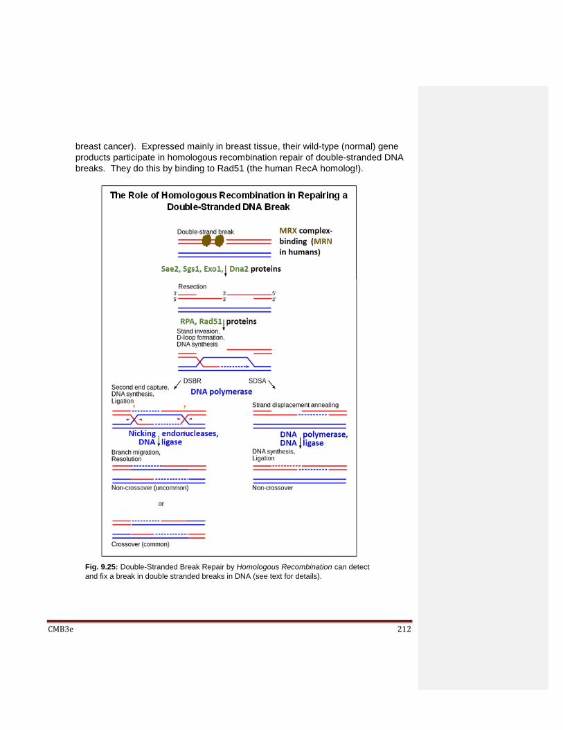
CMB3e 212

breast cancer). Expressed mainly in breast tissue, their wild-type (normal) gene

products participate in homologous recombination repair of double-stranded DNA

breaks. They do this by binding to Rad51 (the human RecA homolog!).

Fig. 9.25: Double-Stranded Break Repair by Homologous Recombination can detect

and fix a break in double stranded breaks in DNA (see text for details).

CMB3e 213

When mutated, the BRCA proteins function poorly and DNA in the affected cells is

not efficiently repaired. This is the likely basis of the increased chance of getting

breast cancer. It doesn’t help matters that the normal BRCA1 protein also plays a

role in mismatch repair… and that the mutated protein can’t! To end this chapter,

here is a bit of weird science! Read all about the genome of a critter, nearly 17%

of which is comprised of foreign DNA, possibly the result of Extreme DNA Repair

of the Spaced-Out Tardigrade Genome

Some iText & VOP Key Words and Terms

base excision repair initiation replicons

bidirectional replication initiator proteins replisome

Central Dogma lagging strand S phase of the cell cycle

clamp proteins leading strand satellite DNA

condensation reactions methylation single-strand binding proteins

deamination mutations siRNA

density gradient centrifugation

nucleotide excision repair supercoiling

depurination Okazaki fragments T2 phage

direct repeats origin of replication tardigrade

discontinuous replication

phosphate backbone telomerase

DNA ligase phosphodiester linkage telomeres

DNA mismatch repair primase theta images

DNA polymerase I, II and III

primer topoisomerases

DNA repair processive replication transcription-coupled repair

DNA sequence phylogeny

proofreading transposase

DNA strand breakage pyrimidine dimers triplets genetic code

DNA topology pyrophosphate VLP

elongation RadA protein VNTRs

env RecA protein

helicase replication

high-speed blender replication fork

CMB3e 214

Chapter 10: Transcription and RNA Processing RNA Transcription, RNA Polymerases, Initiation, Elongation, Termination, Processing

10.1 Introduction

Transcription, the synthesis of RNA based on a DNA template, is the central step of the

Central Dogma proposed by Crick in 1958. The basic steps of transcription are the same

as for replication: initiation, elongation and termination. The differences between

transcription in prokaryotes and eukaryotes are in the details. Here are some:

E. coli uses a single RNA polymerase enzyme to transcribe all kinds of RNAs while

eukaryotic cells use different RNA polymerases to catalyze the syntheses of

ribosomal RNA (rRNA), transfer RNA (tRNA) and messenger RNA (mRNA).

In contrast to eukaryotes, some bacterial genes are part of operons whose mRNAs

encode multiple polypeptides.

Most RNA transcripts in prokaryotes emerge from transcription ready to use

Eukaryotic transcripts synthesized as longer precursors undergo processing by

trimming, splicing or both!

DNA in bacteria is virtually ‘naked’ in the cytoplasm while eukaryotic DNA is wrapped

up in chromatin proteins in a nucleus.

In bacterial cells the association of ribosomes with mRNA and the translation of a

polypeptide can begin even before the transcript is finished. This is because these

cells have no nucleus. In eukaryotic cells, RNAs must exit the nucleus before they

encounter ribosomes in the cytoplasm.

CMB3e 215

In this chapter, you will meet bacterial polycistronic mRNAs (transcripts of operons

that encode more than one polypeptide) and the split genes of eukaryotes (with their

introns and exons. We will look at some details of transcription of the three major

classes of RNA and then at how eukaryotes process precursor transcripts into mature,

functional RNAs. Along the way, we will see one example of how protein structure has

evolved to interact with DNA.

Learning Objectives

When you have mastered the information in this chapter, you should be able to:

1. discriminate between the three steps of transcription in pro- and eukaryotes, and the

factors involved in each.

2. state an hypothesis for why eukaryotes evolved complex RNA processing steps.

3. speculate on why any cell in its right mind would have genes containing introns and

exons so that their transcripts would have to be processed by splicing.

4. articulate the differences between RNA and DNA structure.

5. explain the need for sigma factors in bacteria.

6. speculate on why eukaryotes do not have operons.

7. list structural features of proteins that bind and recognize specific DNA sequences.

8. explain how proteins that do not bind specific DNA sequences can still bind to specific

regions of the genome.

9. formulate an hypothesis for why bacteria do not polyadenylate their mRNAs as much

as eukaryotes do.

10. formulate an hypothesis for why bacteria do not cap their mRNAs.

10.2 Overview of Transcription

Transcription is the first step of the “central dogma” of information transfer from DNA to

protein in which genetic information in genes is transcribed into RNA. As we will see,

some RNAs are translated into polypeptides while others serve functional and even

enzymatic roles in the cell. We begin with a look at the main kinds of RNA in cells.

10.2.1 The Major Types of Cellular RNA

All cells make three main kinds of RNA: ribosomal RNA (rRNA), transfer RNA (tRNA)

and messenger RNA (mRNA). rRNA is a structural as well as enzymatic component

of ribosomes, the protein-synthesizing machine in the cell. Quantitatively, rRNAs are

by far the most abundant RNAs in the cell and mRNAs, the least. Three rRNAs and

about 50 ribosomal proteins make up the two subunits of a bacterial ribosome, as

illustrated in Fig. 10.1 below. tRNAs decode base sequences in mRNAs into amino

acids during protein synthesis (translation) to convert a nucleic acid sequence

information into the amino acid sequences of polypeptides.

CMB3e 216

tRNAs attached to amino acids bind to ribosomes based on codon-anticodon

recognition (Fig. 10.2).

186 Transcription Overview: Ribosomes and Ribosomal RNAs

187 Transcription Overview: Demonstrating the Major RNAs

In 2009, Venkatraman Ramakrishnan, Thomas A. Steitz and Ada Yonath received the Nobel Prize in Chemistry for their studies on the structure and molecular biology of the ribosome.

Fig. 10.1: Ribosomal RNAs and proteins in a bacterial ribosome.

Fig. 10.2: Transfer RNA (tRNA) associated with a ribosome, held in place by

codon/anticodon complementarity as well as tRNA-ribosomal forces.

CMB3e 217

The fact that genes are inside the eukaryotic nucleus and that the synthesis of

polypeptides encoded by those genes happens in the cytoplasm led to the proposal

that there must be an mRNA. Sidney Brenner eventually confirmed the existence of

mRNAs. Check out his classic experiment in Brenner S. (1961, An unstable

intermediate carrying information from genes to ribosomes for protein synthesis.

Nature 190:576-581).

Before we look at details of transcription, recall for future reference that multiple

ribosomes can load an mRNA and move along the same mRNA as polyribosomes

(polysomes), translating multiple copies of the same polypeptide (Fig. 10.3).

10.2.2 Key Steps of Transcription

In transcription, an RNA polymerase uses the template DNA strand of a gene to

catalyze synthesis of a complementary, antiparallel RNA strand. RNA polymerases

use ribose nucleotide triphosphate (NTP) precursors, in contrast to the DNA

polymerases, which use deoxyribose nucleotide (dNTP) precursors. In addition,

RNAs incorporate uracil (U) nucleotides into RNA strands instead of the thymine (T)

nucleotides that end up in new DNA. Another contrast to replication that we have

already seen is that RNA synthesis does not require a primer. With the help of

transcription initiation factors, RNA polymerase locates the transcription start site

of a gene and begins synthesis of a new RNA strand from scratch. Finally, like

replication, transcription is error-prone.

We can identify several of the DNA sequences that characterize a gene in the

summary of the basic steps of transcription in Fig. 10.4 below. The promoter is the

binding site for RNA polymerase. It usually lies 5’ to, or upstream of the transcription

Fig. 10.3: Polysomes form along an mRNA. Multiple ribosomes can assemble

at the 5’ end of an mRNA and then sequentially translate multiple polypeptides

CMB3e 218

start site (the bent arrow). Binding of the RNA polymerase positions the enzyme near

the transcription start site, where it will start unwinding the double helix and begin

synthesizing new RNA.

The transcribed grey DNA region in each of the three panels is the transcription unit

of the gene. Termination sites are typically 3’ to, or downstream from the transcribed

region of the gene. By convention, upstream refers to DNA 5’ to a given reference

point on the DNA (e.g., the transcription start-site of a gene). Downstream then, refers

to DNA 3’ to a given reference point on the DNA.

188-2 Transcription Overview- The Basics of RNA Synthesis Some bacterial transcription units encode more than one mf RNA. Bacterial operons

are an example of this phenomenon. The resulting mRNAs can be translated into

multiple polypeptides at the same time.

Fig. 10.4: Transcription - The basic Steps: Initiation is the recognition of a promoter sequence

near the transcription start site by RNA polymerase. Elongation is the successive addition of

nucleotides to a growing RNA strand. Termination occurs at the end of the gene, releasing the

newly made RNA.

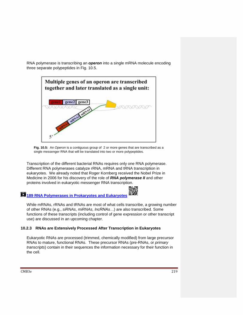
CMB3e 219

RNA polymerase is transcribing an operon into a single mRNA molecule encoding

three separate polypeptides in Fig. 10.5.

Transcription of the different bacterial RNAs requires only one RNA polymerase.

Different RNA polymerases catalyze rRNA, mRNA and tRNA transcription in

eukaryotes. We already noted that Roger Kornberg received the Nobel Prize in

Medicine in 2006 for his discovery of the role of RNA polymerase II and other

proteins involved in eukaryotic messenger RNA transcription.

189 RNA Polymerases in Prokaryotes and Eukaryotes

While mRNAs, rRNAs and tRNAs are most of what cells transcribe, a growing number

of other RNAs (e.g., siRNAs, miRNAs, lncRNAs…) are also transcribed. Some

functions of these transcripts (including control of gene expression or other transcript

use) are discussed in an upcoming chapter.

10.2.3 RNAs are Extensively Processed After Transcription in Eukaryotes

Eukaryotic RNAs are processed (trimmed, chemically modified) from large precursor

RNAs to mature, functional RNAs. These precursor RNAs (pre-RNAs, or primary

transcripts) contain in their sequences the information necessary for their function in

the cell.

Fig. 10.5: An Operon is a contiguous group of 2 or more genes that are transcribed as a

single messenger RNA that will be translated into two or more polypeptides.

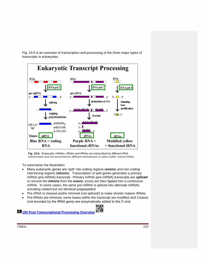
CMB3e 220

Fig. 10.6 is an overview of transcription and processing of the three major types of

transcripts in eukaryotes.

To summarize the illustration:

Many eukaryotic genes are ‘split’ into coding regions (exons) and non-coding

intervening regions (introns). Transcription of split genes generates a primary

mRNA (pre-mRNA) transcript. Primary mRNA (pre-mRNA) transcripts are spliced

to remove the introns from the exons; exons are then ligated into a continuous

mRNA. In some cases, the same pre-mRNA is spliced into alternate mRNAs

encoding related but not identical polypeptides!

Pre-rRNA is cleaved and/or trimmed (not spliced!) to make shorter mature rRNAs.

Pre-tRNAs are trimmed, some bases within the transcript are modified and 3 bases

(not encoded by the tRNA gene) are enzymatically added to the 3’-end.

190 Post Transcriptional Processing Overview

Fig. 10.6: Eukaryotic mRNAs, rRNAs and tRNAs are transcribed by different RNA

polymerases and are processed by different mechanisms to yield usable, mature RNAs.

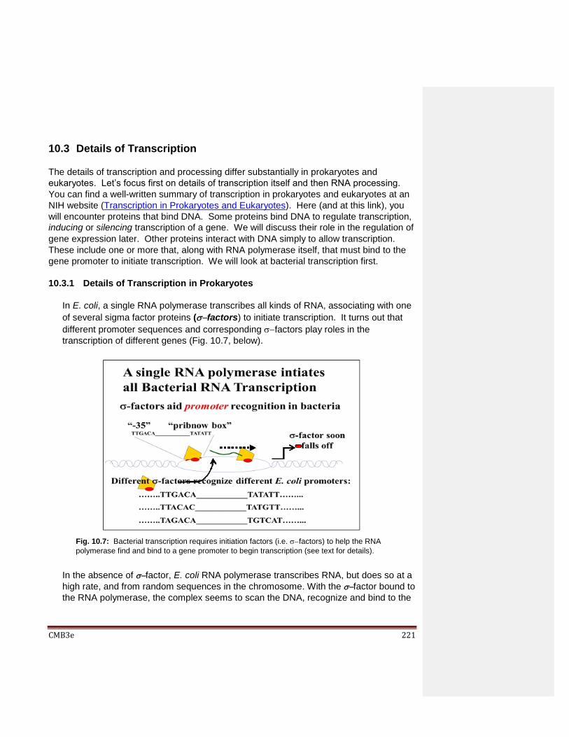
CMB3e 221

10.3 Details of Transcription

The details of transcription and processing differ substantially in prokaryotes and

eukaryotes. Let’s focus first on details of transcription itself and then RNA processing.

You can find a well-written summary of transcription in prokaryotes and eukaryotes at an

NIH website (Transcription in Prokaryotes and Eukaryotes). Here (and at this link), you

will encounter proteins that bind DNA. Some proteins bind DNA to regulate transcription,

inducing or silencing transcription of a gene. We will discuss their role in the regulation of

gene expression later. Other proteins interact with DNA simply to allow transcription.

These include one or more that, along with RNA polymerase itself, that must bind to the

gene promoter to initiate transcription. We will look at bacterial transcription first.

10.3.1 Details of Transcription in Prokaryotes

In E. coli, a single RNA polymerase transcribes all kinds of RNA, associating with one

of several sigma factor proteins (factors) to initiate transcription. It turns out that

different promoter sequences and corresponding factors play roles in the

transcription of different genes (Fig. 10.7, below).

In the absence of factor, E. coli RNA polymerase transcribes RNA, but does so at a

high rate, and from random sequences in the chromosome. With the factor bound to

the RNA polymerase, the complex seems to scan the DNA, recognize and bind to the

Fig. 10.7: Bacterial transcription requires initiation factors (i.e. factors) to help the RNA

polymerase find and bind to a gene promoter to begin transcription (see text for details).

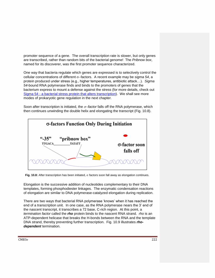
CMB3e 222

promoter sequence of a gene. The overall transcription rate is slower, but only genes

are transcribed, rather than random bits of the bacterial genome! The Pribnow box,

named for its discoverer, was the first promoter sequence characterized.

One way that bacteria regulate which genes are expressed is to selectively control the

cellular concentrations of different factors. A recent example may be sigma 54, a

protein produced under stress (e.g., higher temperatures, antibiotic attack…). Sigma

54-bound RNA polymerase finds and binds to the promoters of genes that the

bacterium express to mount a defense against the stress (for more details, check out

Sigma 54 - a bacterial stress protein that alters transcription). We shall see more

modes of prokaryotic gene regulation in the next chapter.

Soon after transcription is initiated, the factor falls off the RNA polymerase, which

then continues unwinding the double helix and elongating the transcript (Fig. 10.8).

Elongation is the successive addition of nucleotides complementary to their DNA

templates, forming phosphodiester linkages. The enzymatic condensation reactions

of elongation are similar to DNA polymerase-catalyzed elongation during replication.

There are two ways that bacterial RNA polymerase ‘knows’ when it has reached the

end of a transcription unit. In one case, as the RNA polymerase nears the 3’ end of

the nascent transcript, it transcribes a 72 base, C-rich region. At this point, a

termination factor called the rho protein binds to the nascent RNA strand. rho is an

ATP-dependent helicase that breaks the H-bonds between the RNA and the template

DNA strand, thereby preventing further transcription. Fig. 10.9 illustrates rho-

dependent termination.

Fig. 10.8: After transcription has been initiated, factors soon fall away as elongation continues.

CMB3e 223

In the other mechanism of termination, a sequence of the RNA forming near the 3’ end

of the transcript folds into a secondary structure hairpin loop that serves as a

termination signal, causing the dissociation of the RNA polymerase, template DNA

and the new RNA transcript. The role of the hairpin loop in rho-independent

termination is shown in Fig. 10.10 (below).

191 Details of Prokaryotic Transcription

Fig. 10.9: rho-dependent termination of bacterial transcription involves recognition of

sequences at the end of the gene and transcript

Fig. 10.10: rho-independent termination of bacterial transcription involves complementary

bases near the end of the transcript that form a stem/loop, or hairpin loop structure that

serves as a termination signal.

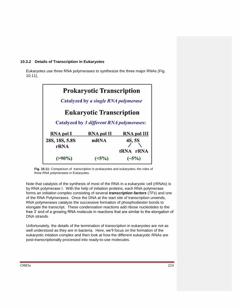
CMB3e 224

10.3.2 Details of Transcription in Eukaryotes

Eukaryotes use three RNA polymerases to synthesize the three major RNAs (Fig.

10.11).

Note that catalysis of the synthesis of most of the RNA in a eukaryotic cell (rRNAs) is

by RNA polymerase I. With the help of initiation proteins, each RNA polymerase

forms an initiation complex consisting of several transcription factors (TFs) and one

of the RNA Polymerases. Once the DNA at the start site of transcription unwinds,

RNA polymerases catalyze the successive formation of phosphodiester bonds to

elongate the transcript. These condensation reactions add ribose nucleotides to the

free 3’ end of a growing RNA molecule in reactions that are similar to the elongation of

DNA strands.

Unfortunately, the details of the termination of transcription in eukaryotes are not as

well understood as they are in bacteria. Here, we’ll focus on the formation of the

eukaryotic intiation complex and then look at how the different eukaryotic RNAs are

post-transcriptionally processed into ready-to-use molecules.

Fig. 10.11: Comparison of transcription in prokaryotes and eukaryotes; the roles of

three RNA polymerases in Eukaryotes.

CMB3e 225

10.3.2.a Eukaryotic mRNA Transcription

Fig. 10.12 shows the multiple steps of eukaryotic mRNA transcription initiation.

Transcription of eukaryotic mRNAs by RNA polymerase II begins with sequential

assembly of a eukaryotic initiation complex at a gene promoter. The typical

promoter for a protein-encoding gene contains a TATA sequence motif, or TATA

box and other short upstream sequences that recruit components of the initiation

complex.

TATA-binding protein (TBP) first binds to the TATA box along with TFIID

(transcription factor IID). This intermediate in turn recruits TFIIA and TFIIB. TFIIE,

TFIIF and TFIIH are added to form the core initiation complex. Finally, several

other initiation factors and RNA polymerase II bind to complete the mRNA

Fig. 10.12: Eukaryotic mRNA transcription initiation starts with recognition of a promoter

TATA box by initiation factor TFIID. The association of a series of initiation factors

follows. RNA polymerase II binds last. Its phosphorylation starts transcription.

CMB3e 226

transcription initiation complex. Phosphorylation adds several phosphates to the

amino-terminus of the RNA polymerase, after which some of the TF’s dissociate

from the initiation complex. The remaining RNA polymerase-transcription factor

complex can now start making the mRNA.

The first task of the complete initiation complex is to unwind the template DNA

strands at the start site of transcription. Unlike prokaryotic RNA polymerase,

eukaryotic RNA Polymerase II does not have an inherent DNA helicase activity.

For this, eukaryotic gene transcription relies on the multi-subunit TFIIH protein, two

of whose subunits have an ATP-dependent helicase activity. This helicase is not

required for elongation of the RNA strand. Consistent with the closer relationship

of archaea to eukaryotes (rather than to prokaryotes), archaeal mRNA transcription

initiation resembles that of eukaryotes, albeit requiring fewer initiation factors

during formation of an initiation complex.

192-2 Eukaryotic mRNA Transcription

A significant difference between prokaryotic and eukaryotic transcription is that

RNA polymerases and other proteins involved at a eukaryotic gene promoter do

not see naked DNA. Instead, they must recognize specific DNA sequences behind

a coat of chromatin proteins. On the other hand, all proteins that interact with DNA

have in common a need to recognize the DNA sequences to which they must

bind…, within the double helix. In other words, they must see the bases within the

helix, and not on its uniformly electronegative phosphate backbone surface. To

this end, they must penetrate the DNA, usually through the major groove of the

double helix. We will see that DNA regulatory proteins face the same problems in

achieving specific shape-based interactions!

193-2 Recognition of Transcription Factors at Promoters

10.3.2.b Eukaryotic tRNA and 5S rRNA Transcription

Transcription of 5S rRNA and tRNAs by RNA Polymerase III is unusual in that the

promoter sequence to which it binds (with the help of initiation factors) is not

upstream of the transcribed sequence, but lies within the transcribed sequence.

RNA polymerase III, along with structural relatives of the core RNA polymerase II

TFs (TBP, TFIIB, TFIIE, TFIIF…) form a core initiation complex at 5S RNA and

tRNA gene promoters. Other gene-specific TFs add to this core complex. The

completed initiation complex allows re-positioning the RNA polymerase III to

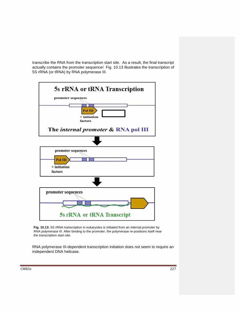
CMB3e 227

transcribe the RNA from the transcription start site. As a result, the final transcript

actually contains the promoter sequence! Fig. 10.13 illustrates the transcription of

5S rRNA (or tRNA) by RNA polymerase III.

RNA polymerase III-dependent transcription initiation does not seem to require an

independent DNA helicase.

Fig. 10.13: 5S rRNA transcription in eukaryotes is initiated from an internal promoter by

RNA polymerase III. After binding to the promoter, the polymerase re-positions itself near

the transcription start-site.

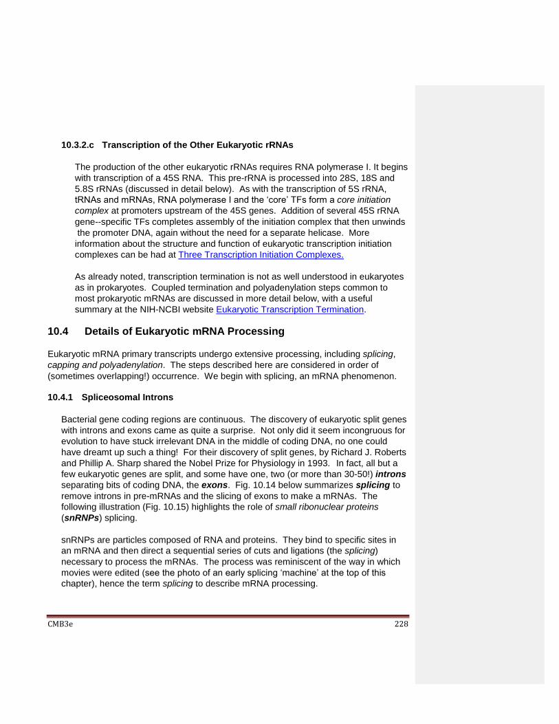
CMB3e 228

10.3.2.c Transcription of the Other Eukaryotic rRNAs

The production of the other eukaryotic rRNAs requires RNA polymerase I. It begins

with transcription of a 45S RNA. This pre-rRNA is processed into 28S, 18S and

5.8S rRNAs (discussed in detail below). As with the transcription of 5S rRNA,

tRNAs and mRNAs, RNA polymerase I and the ‘core’ TFs form a core initiation

complex at promoters upstream of the 45S genes. Addition of several 45S rRNA

gene--specific TFs completes assembly of the initiation complex that then unwinds

the promoter DNA, again without the need for a separate helicase. More

information about the structure and function of eukaryotic transcription initiation

complexes can be had at Three Transcription Initiation Complexes.

As already noted, transcription termination is not as well understood in eukaryotes

as in prokaryotes. Coupled termination and polyadenylation steps common to

most prokaryotic mRNAs are discussed in more detail below, with a useful

summary at the NIH-NCBI website Eukaryotic Transcription Termination.

10.4 Details of Eukaryotic mRNA Processing

Eukaryotic mRNA primary transcripts undergo extensive processing, including splicing,

capping and polyadenylation. The steps described here are considered in order of

(sometimes overlapping!) occurrence. We begin with splicing, an mRNA phenomenon.

10.4.1 Spliceosomal Introns

Bacterial gene coding regions are continuous. The discovery of eukaryotic split genes

with introns and exons came as quite a surprise. Not only did it seem incongruous for

evolution to have stuck irrelevant DNA in the middle of coding DNA, no one could

have dreamt up such a thing! For their discovery of split genes, by Richard J. Roberts

and Phillip A. Sharp shared the Nobel Prize for Physiology in 1993. In fact, all but a

few eukaryotic genes are split, and some have one, two (or more than 30-50!) introns

separating bits of coding DNA, the exons. Fig. 10.14 below summarizes splicing to

remove introns in pre-mRNAs and the slicing of exons to make a mRNAs. The

following illustration (Fig. 10.15) highlights the role of small ribonuclear proteins

(snRNPs) splicing.

snRNPs are particles composed of RNA and proteins. They bind to specific sites in

an mRNA and then direct a sequential series of cuts and ligations (the splicing)

necessary to process the mRNAs. The process was reminiscent of the way in which

movies were edited (see the photo of an early splicing ‘machine’ at the top of this

chapter), hence the term splicing to describe mRNA processing.

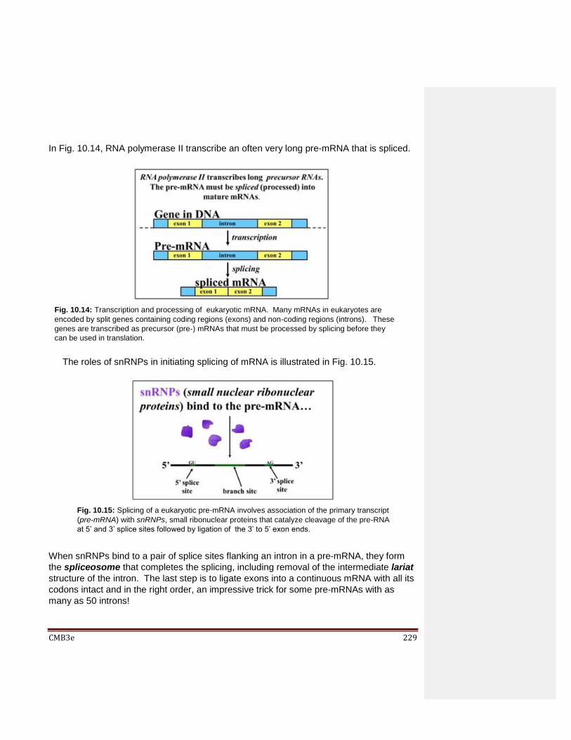
CMB3e 229

In Fig. 10.14, RNA polymerase II transcribe an often very long pre-mRNA that is spliced.

The roles of snRNPs in initiating splicing of mRNA is illustrated in Fig. 10.15.

When snRNPs bind to a pair of splice sites flanking an intron in a pre-mRNA, they form

the spliceosome that completes the splicing, including removal of the intermediate lariat

structure of the intron. The last step is to ligate exons into a continuous mRNA with all its

codons intact and in the right order, an impressive trick for some pre-mRNAs with as

many as 50 introns!

Fig. 10.14: Transcription and processing of eukaryotic mRNA. Many mRNAs in eukaryotes are

encoded by split genes containing coding regions (exons) and non-coding regions (introns). These

genes are transcribed as precursor (pre-) mRNAs that must be processed by splicing before they

can be used in translation.

Fig. 10.15: Splicing of a eukaryotic pre-mRNA involves association of the primary transcript

(pre-mRNA) with snRNPs, small ribonuclear proteins that catalyze cleavage of the pre-RNA

at 5’ and 3’ splice sites followed by ligation of the 3’ to 5’ exon ends.

CMB3e 230

Spliceosome action is summarized in Fig. 10.16 and in the animated in the mRNA

splicing link below. Imagine this happening as many as 30 times in just a single pre-

actin mRNA!

194-2 The Discovery of Split Genes 195 mRNA Splicing 10.4.2 Specific Nuclear Body Proteins Facilitate SnRNP Assembly and Function Recall the organization of nuclei facilitated by nuclear bodies. Nuclear speckles are

associated regions of high mRNA transcription, processing and splicing (check out the

animation at http://www.caltech.edu/news/cartography-nucleus-82442 for a 3-dimensional

localization of markers of nuclear body activity.

Cajal bodies (CBs) and Gems are nuclear bodies that are similar in size and have

related functions in assembling spliceosomal SnRNPs. Some splicing defects correlate

with mutations in the coil protein that associate with Cajal bodies; others correlate with

mutations in SMN proteins normally associated with Gems. One hypothesis was that

CBs and Gems interact in SnRNP and spliceosome assembly…, but how?

Consider the results of an experiment in which antibodies to coilin and the SMN protein

were localized in undifferentiated and differentiated neuroblastoma cells (Fig. 10.17,

below).

Fig. 10.16: Formation of a spliceosome by the binding of snRNPs to an mRNA leads to

hydrolysis of splice sites and the formation of a lariat structure from the intron remnants.

CMB3e 231

A and C in Fig. 10.17 are undifferentiated cells in culture; B and D are cells that were

stimulated to differentiate. In the fluorescence micrographs at the right, arrows point

to fluorescent nuclear bodies. We would expect that fluorescent antibodies to coilin

(green) to localize to CBs and antibodies to SMN protein (red) to bind to Gems. This

is what happens in the nuclei of undifferentiated cells (panel C). But in panel D, the

two antibodies co-localize, suggesting that the CBs and Gems aggregate in the

differentiated cells. This would explain the need for both coilin and SMN protein to

produce functional SnRNPs. The CBs and Gems may be aggregating in differentiated

cells due to an observed increase in expression of the SMN protein. This could lead

to Gems more able to associate with the CBs. This and similar experiments

demonstrate that different nuclear bodies do have specific functions. They are not

random structural artifacts but have evolved to organize nuclear activities in time and

space in ways that are essential to the cell.

10.4.3 Group I and Group II Self-Splicing Introns While Eukaryotic Spliceosomal introns are spliced using snRNPs as described above,

Group I or Group II introns are removed by different mechanisms. Group I introns

interrupt mRNA and tRNA genes in bacteria and in mitochondrial and chloroplast

genes. They are occasionally found in bacteriophage genes, but rarely in nuclear

genes, and then only in lower eukaryotes. Group I introns are self-splicing! Thus,

they are ribozymes that do not require snRNPs or other proteins for splicing activity.

Instead, they fold into a secondary stem-loop structure that positions catalytic

nucleotides at appropriate splice sites to excise themselves, and also re-ligate the

Fig. 10.17: Immunofluorescence staining with antibodies to coilin and SMN protein show that

Cajal bodies and Gems aggregate when undifferentiated cells (panels A and C) are stimulated to

differentiate (panels B and D). Since mutations in coilin and SMN proteins are associated with

splicing defects, co-localization of Cajal bodies and Gems suggests their co-involvement of

snRNP function.

CMB3e 232

exons. Group II introns in chloroplast and mitochondrial rRNA, mRNA, tRNA and

some bacterial mRNAs can be quite long. They form complex stem-loop tertiary

structures and self-splice, at least in a test tube! However, Group II introns encode

proteins required for their own splicing in vivo. Like spliceosomal introns, they form a

lariat structure at an A residue branch site. All this suggests that the mechanism of

spliceosomal intron splicing evolved from that of Group II introns.

10.4.4 So, Why Splicing?

The puzzle implied by this question is of course, why do higher organisms have split

genes in the first place? While the following discussion can apply to all splicing, it will

reference mainly spliceosomal introns. Here are some answers to the question “Why

splicing?”

Introns in nuclear genes are typically longer (often much longer!) than exons.

Since they are non-coding, they are large targets for mutation. In effect, non-

coding DNA, including introns can buffer the ill effects of random mutations.

You may recall that gene duplication on one chromosome (and loss of a copy from its homolog) arise from unequal recombination (non-homologous crossing over). It occurs when similar DNA sequences align during synapsis of meiosis. In an organism that inherits a chromosome with both gene copies, the duplicate can accumulate mutations as long as the other retains original function. The diverging gene then becomes part of a pool of selectable DNA, the grist of evolution. Descendants of organisms that inherit the duplicated genes have diversified the gene pool, again increasing the potential for evolution and species diversity.

Unequal recombination can also occur between similar sequences (e.g., in introns) in the same or different genes, resulting in a sharing of exons between genes. After unequal recombination between introns flanking an exon, one gene will acquire another exon while the other will lose it. Once again, as long as an organism retains a copy of the participating genes with original function, the organism can make the required protein and survive. Meanwhile, the gene with the extra exon may produce the same protein, but one with a new structural domain and function. Like a complete duplicate gene, one with a new exon that adds a new function to an old gene has been entered in the pool of selectable DNA. Thus, this phenomenon of exon shuffling increases species diversity! Exon shuffling has occurred, creating proteins with different overall functions that nonetheless share at least one domain and one common function.

An example discussed earlier involves calcium-binding proteins that regulate many cellular processes. Structurally related calcium (Ca++) binding domains are common to many otherwise structurally and functionally unrelated proteins.

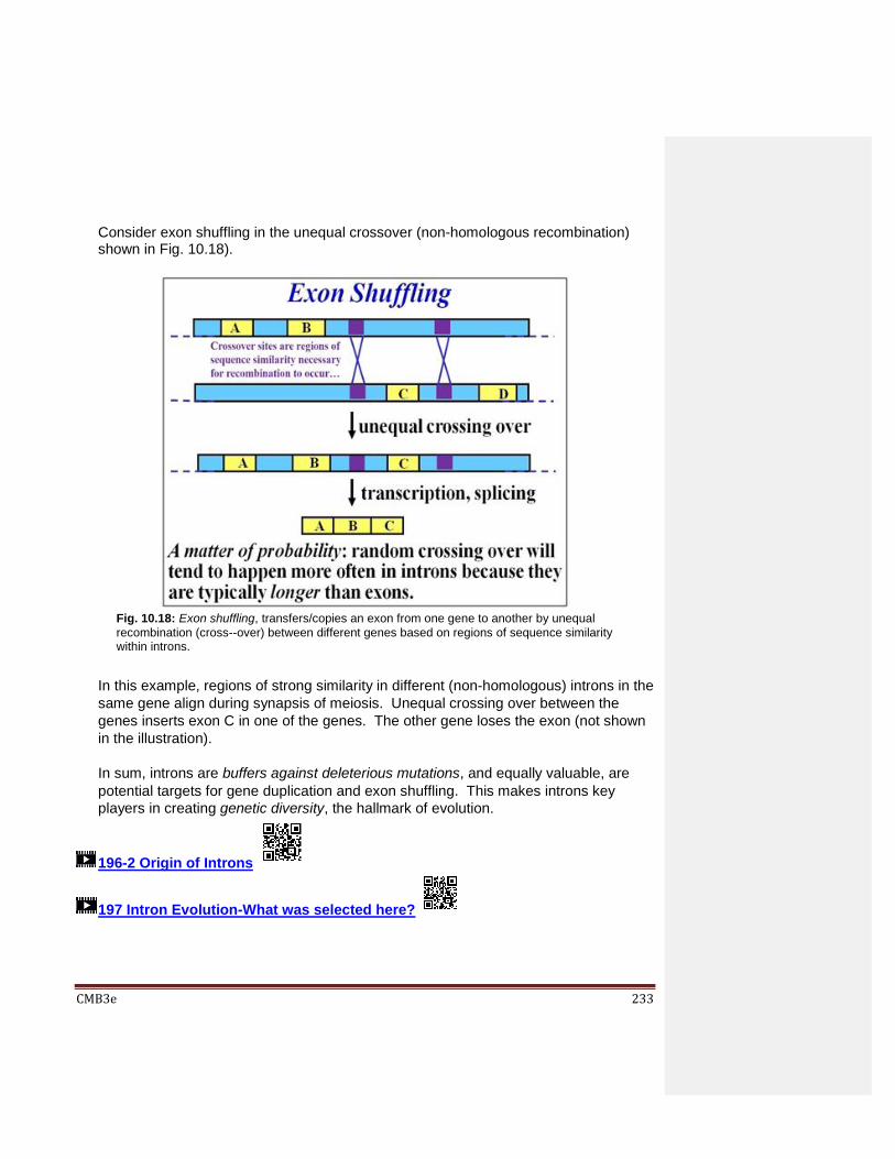
CMB3e 233

Consider exon shuffling in the unequal crossover (non-homologous recombination) shown in Fig. 10.18).

In this example, regions of strong similarity in different (non-homologous) introns in the

same gene align during synapsis of meiosis. Unequal crossing over between the

genes inserts exon C in one of the genes. The other gene loses the exon (not shown

in the illustration).

In sum, introns are buffers against deleterious mutations, and equally valuable, are

potential targets for gene duplication and exon shuffling. This makes introns key

players in creating genetic diversity, the hallmark of evolution.

196-2 Origin of Introns

197 Intron Evolution-What was selected here?

Fig. 10.18: Exon shuffling, transfers/copies an exon from one gene to another by unequal

recombination (cross--over) between different genes based on regions of sequence similarity within introns.

CMB3e 234

10.4.5 5-Prime Capping

A methyl guanosine cap added 5’-to-5’ to an mRNA functions in part to help mRNAs

leave the nucleus and associate with ribosomes. The cap is added to an exposed 5’

end, even as transcription and splicing are still in progress. A capping enzyme places

a methylated guanosine residue at the 5’-end of the mature mRNA. Fig. 10.19 shows

the 5’ cap structure (check marks are 5’-3’ linked nucleotides).

10.4.6 3-Prime Polyadenylation

A poly(A) polymerase catalyzes the addition of adenine monophosphates (AMPs) to

the 3’ end of most eukaryotic mRNAs, even before any splicing is complete. Poly-

adenylation requires ATP and can add several hundred AMPs to the 3’ terminus of an

mRNA. The enzyme binds to an AAUAA sequence near the 3’ end of an mRNA to

start adding the AMPs. Polyadenylation after transcription termination is illustrated

below in Fig. 10.20.

Fig. 10.19: mRNA capping results from a 5’–to–5’ condensation reaction linking

the 5’ end of an mRNA to a methylated guanidine triphosphate (CH3-GTP) .

CMB3e 235

The result of polyadenylation is a 3’ poly (A) tail whose functions include assisting in

the transit of mRNAs from the nucleus and regulating the half-life of mRNAs in the

cytoplasm. The poly (A) tail shortens each time a ribosome completes translating the

mRNA.

198 mRNA 5' Capping and 3' Polyadenylation

10.5 Ribosomal RNA Processing in Eukaryotic Nuclei

In most eukaryotes, a large rRNA gene transcribes a 45S precursor transcript containing

(from shortest to longest) 5.8S rRNA, 18SrRNA and 28S rRNA. The ‘S’ stands for

Svedberg, the biochemist who developed the sedimentation velocity ultra-centrifugation

technique to separate molecules like RNA by size. The higher the S value, the larger the

molecule and therefore the faster it moves through the viscous sugar gradient during

centrifugation. RNA Polymerase I transcribes 45S precursor rRNAs (pre-RNAs) from

multiple large transcription units in the genome. One such unit is shown below in Fig.

10.21.

Fig. 10.20: mRNA polyadenylation; this is the addition of multiple adenine nucleotides to

the 3’ end of an mRNA, catalyzed by the enzyme poly(A) polymerase. Other than histone

mRNAs, most eukaryotic mRNAs are polyadenylated.

CMB3e 236

The 45S pre-rRNA is processed by cleavage. The many copies (200-400!) of the 45S

gene in eukaryotic cells might be expected, since making proteins (and therefore

ribosomes) will be an all-consuming cellular activity. In humans, 45S genes (45S rDNA)

are distributed among five acrocentric chromosomes (those that have a centromere very

near one end of the chromosome). The 45S rDNA in chromosomes is packed in the

nucleolus inside nuclei. Because these genes are present in so many copies and

organized into a specific region of chromatin, it is possible to visualize 45S transcription in

progress in electron micrographs such as the ones in Fig. 10.22 (below). Because the

images of nucleolar DNA looked like old-fashioned brushs used to clean the chimney of a

kerosene lamp, they were called lampbrush DNA, or lampbrush chromosomes. They get

this shape from 45S genes in undergoing transcription, from which the nascent RNAs

extending from the DNA template look like the bristles of the lampbrush.

Fig. 10.21: Post-transcriptional processing of the 45S rRNA encoding three of the four eukaryotic

rRNAs by hydrolytic cleavage. Cleavage is catalyzed by endonucleases that recognize differential

methylation patterns of rRNA regions and transcribed spacer regions of the 45S precursor RNA.

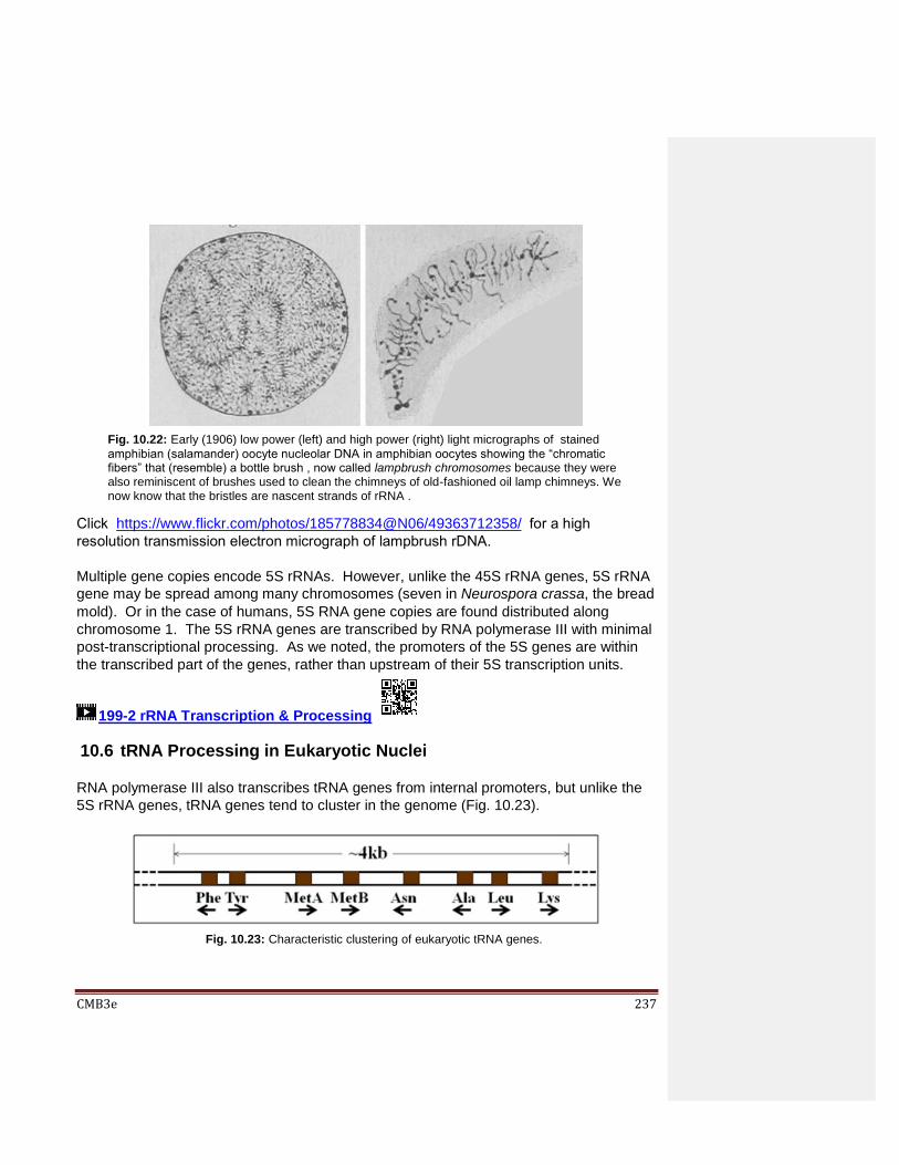
CMB3e 237

Click https://www.flickr.com/photos/185778834@N06/49363712358/ for a high

resolution transmission electron micrograph of lampbrush rDNA.

Multiple gene copies encode 5S rRNAs. However, unlike the 45S rRNA genes, 5S rRNA

gene may be spread among many chromosomes (seven in Neurospora crassa, the bread

mold). Or in the case of humans, 5S RNA gene copies are found distributed along

chromosome 1. The 5S rRNA genes are transcribed by RNA polymerase III with minimal

post-transcriptional processing. As we noted, the promoters of the 5S genes are within

the transcribed part of the genes, rather than upstream of their 5S transcription units.

199-2 rRNA Transcription & Processing

10.6 tRNA Processing in Eukaryotic Nuclei

RNA polymerase III also transcribes tRNA genes from internal promoters, but unlike the

5S rRNA genes, tRNA genes tend to cluster in the genome (Fig. 10.23).

Fig. 10.22: Early (1906) low power (left) and high power (right) light micrographs of stained

amphibian (salamander) oocyte nucleolar DNA in amphibian oocytes showing the “chromatic fibers” that (resemble) a bottle brush , now called lampbrush chromosomes because they were also reminiscent of brushes used to clean the chimneys of old-fashioned oil lamp chimneys. We now know that the bristles are nascent strands of rRNA .

Fig. 10.23: Characteristic clustering of eukaryotic tRNA genes.

CMB3e 238

Also unlike 5S rRNA genes, tRNA primary transcripts are processed by

trimming,

enzymatic addition of a -C-C-A base triplet at the 3’ end, and

the modification of bases internal to the molecule

A yeast tRNA showing these modifications is illustrated in Fig. 10.24.

The tRNA folds into several hairpin loops based on internal H-bond formation between

complementary bases in the molecule. The 3’-terminal A residue of the –C-C-A add-on to

this (and every) tRNA will bind to an amino acid specific for the tRNA.

200-2 tRNA Transcription and Processing

10.7 mRNA and Ribosome Export from the Nucleus

The synthesis and processing of rRNAs are coincident with the assembly of the ribosomal

subunits (Fig. 10.25, below).

Fig. 10.24: Structure of a yeast tRNA.

ergtrom

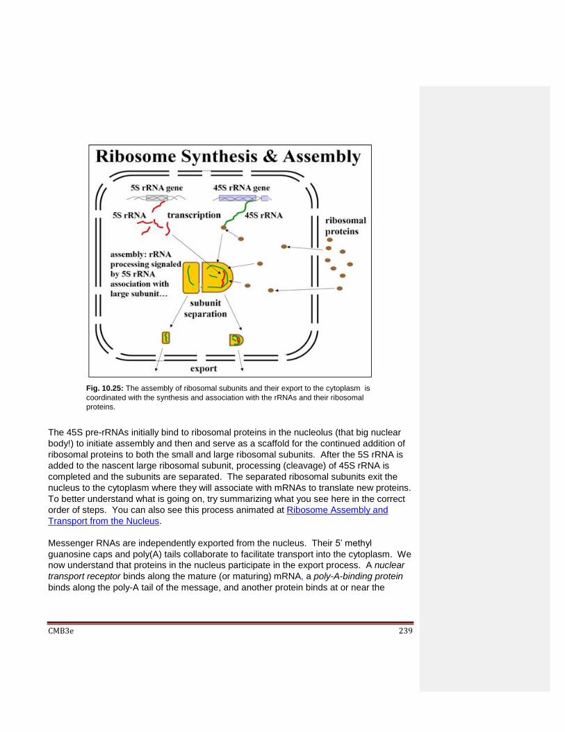
CMB3e 239

The 45S pre-rRNAs initially bind to ribosomal proteins in the nucleolus (that big nuclear

body!) to initiate assembly and then and serve as a scaffold for the continued addition of

ribosomal proteins to both the small and large ribosomal subunits. After the 5S rRNA is

added to the nascent large ribosomal subunit, processing (cleavage) of 45S rRNA is

completed and the subunits are separated. The separated ribosomal subunits exit the

nucleus to the cytoplasm where they will associate with mRNAs to translate new proteins.

To better understand what is going on, try summarizing what you see here in the correct

order of steps. You can also see this process animated at Ribosome Assembly and

Transport from the Nucleus.

Messenger RNAs are independently exported from the nucleus. Their 5’ methyl

guanosine caps and poly(A) tails collaborate to facilitate transport into the cytoplasm. We

now understand that proteins in the nucleus participate in the export process. A nuclear

transport receptor binds along the mature (or maturing) mRNA, a poly-A-binding protein

binds along the poly-A tail of the message, and another protein binds at or near the

Fig. 10.25: The assembly of ribosomal subunits and their export to the cytoplasm is

coordinated with the synthesis and association with the rRNAs and their ribosomal

proteins.

CMB3e 240

methyl guanosine CAP itself. These interactions enable transport of the mRNA through

nuclear pores. After the mRNA is in the cytoplasm, the nuclear transport receptor re-

cycles back into the nucleus while a translation initiation factor replaces the protein bound

to the CAP. Fig. 10.26 summarizes the nuclear transport process for mRNAs.

See a more detailed description of mRNA transport from the nucleus at this link: mRNA

Export from the Nucleus . The mature mRNA, now in the cytoplasm, is ready for

translation. Translation is the process of protein synthesis mediated by ribosomes and a

host of translation factors (including the initiation factor in Fig. 10.25. The genetic code

directs polypeptide synthesis during translation. Details of translation will be discussed

shortly.

Some iText & VOP Key Words and Terms

16S rRNA internal promoters rRNA

18S rRNA introns rRNA cleavage

23S rRNA lariat rRNA endonucleases

28SrRNA mature RNA transcript -factor

45S pre-rRNA mRNA SINEs

Fig. 10.26: Role of CAP and poly-A binding proteins and a nuclear transport factor in

the export of an mRNA to the cytoplasm.

CMB3e 241

45S rRNA methylation mRNA capping snRNP

4S rRNA mRNA polyadenylation

spacer RNA

5'-methyl guanosine capping

mRNA splicing splice sites

5S rRNA operons spliceosome

8S rRNA poly (A) polymerase Svedberg unit

adenine poly(A) tail TATA binding protein

Alu polycistronic RNA TBP

branch sites Pribnow box termination

crossing over promoter TFIIB, TFGIIE, TFIIF, TFIIH

cytosine recombination transcription

DNA binding proteins regulatory DNA sequence

transcription start site

E. coli RNA polymerase

regulatory factor transcription unit

elongation rho termination factor translation

eukaryotic RNA polymerases

rho-independent termination

transposition

exon shuffling ribonucleoproteins transposons

exons RNA polymerase I tRNA

guanine RNA polymerase II tRNA processing

helitrons RNA polymerase III upstream v. downstream

helix-turn-helix motif RNA processing uracil

initiation RNA secondary structure

CMB3e 242

Chapter 11: The Genetic Code and Translation The Genetic Code, tRNA (Adapter) Molecules, Translation (Protein Synthesis)

11.1 Introduction

While evidence was accumulating that DNA was “the stuff of genes”, many still believed

that proteins were genes, at least until the experiments of Hershey and Chase. It was in

this somewhat ambivalent context that investigators wondered about how genes (whether

proteins or nucleic acids) might encode metabolically functional proteins such as

enzymes… that of course are also proteins. In 1944, the physicist-philosopher Erwin

Schrödinger published What Is Life? The Physical Aspect of the Living Cell. Targeting

the lay reader, Schrödinger took a stab at explaining life, heredity and development in

terms of physical laws. Here in his own words is what he had to say about the chemistry

of heredity that when deciphered, would dictate structures, or “patterns” of development

(abridging and highlighting, courtesy of your author!):

THE HEREDITARY CODE-SCRIPT (from https://criv.pw/v9v.pdf) …Now, this pattern is known to be determined by the structure of that one cell, the

fertilized egg. Moreover, we know that it is essentially determined by the structure of

only a small part of that cell, its large nucleus. This nucleus… usually appears as a

network of chromatine, distributed over the cell. But in the processes of cell division

CMB3e 243

(mitosis and meiosis) it is seen to consist of a set of particles, usually fibre-shaped or

rod-like, called the chromosomes, which number in man, 48 (2 X 24)… I ought to

have spoken of two sets, in order to use the expression in the customary strict

meaning of the biologist. For the two sets are almost entirely alike. As we shall see in

a moment, one set comes from the mother (egg cell), one from the father (fertilizing

spermatozoon). It is these chromosomes, or probably only an axial skeleton fibre of

what we actually see under the microscope as the chromosome, that contain in

some kind of code-script the entire pattern of the individual's future

development and of its functioning in the mature state. Every complete set of

chromosomes contains the full code; so there are, as a rule, two copies of the latter in

the fertilized egg cell, which forms the earliest stage of the future individual. In calling

the structure of the chromosome fibres a code-script we mean that the all-penetrating

mind, once conceived by Laplace, to which every causal connection lay immediately

open, could tell from their structure whether the egg would develop, under suitable

conditions, into a black cock or into a speckled hen, into a fly or a maize plant, a

rhododendron, a beetle, a mouse or a woman. To which we may add, that the

appearances of the egg cells are very often remarkably similar; and even when they

are not, as in the case of the comparatively gigantic eggs of birds and reptiles, the

difference is not been so much the relevant structures as in the nutritive material

which in these cases is added for obvious reasons. But the term code-script is, of

course, too narrow. The chromosome structures… are at the same time

instrumental in bringing about the development they foreshadow. They are law-code

and executive power -or, to use another simile, they are architect's plan and

builder's craft -in one.

Once again, keep in mind that these speculations presage the identification of DNA as the genetic chemical. The terms code, broken and deciphered themselves came from the recent World War II history. Winning the war relied on breaking enemy codes (see the Enigma Machine at the top of this chapter), as well as hiding our own strategic battle information from the enemy (recall or look up the history of the Navajo code talkers). In this chapter we look at just how the genetic code in DNA (and in fact in messenger RNA) was broken. We describe the elegant experiments that first deciphered the amino acid meaning of a few 3-base codons, and then all 64 codons. Of these, 61 encode amino acids and three are stop codons. Experiments similar to those that broke the genetic code also led to our under-standing of the mechanism of protein synthesis. Early studies indicated that genes and proteins are colinear, i.e., that the length of a gene was directly proportional to the polypeptide it encoded. It would follow then, that the lengths of mRNAs are also collinear with their translation products. Colinearity suggested the obvious hypotheses that translation proceeded in three steps (initiation, elongation and termination), just like transcription itself.

CMB3e 244

We now know that initiation is a complex process involving the assembly of a translation machine near the 5’ end of the mRNA. This machine consists of ribosomes, mRNA, several initiation factors and a source of chemical energy. Since mature mRNAs are actually longer than needed to specify a polypeptide (even after splicing!), one function of initiation factors is to position the ribosome and associated proteins near a start codon. The start codon specifies the first amino acid in a new polypeptide. Once the initiation complex forms, elongation begins. Cycles of condensation reactions on the ribosome connect amino acids by peptide linkages, growing the chain from its amino-end to its carboxyl-end. Translation ends when the ribosome moving along the mRNA encounters a stop codon. We will look at how we came to understand the discrete steps of translation.

Learning Objectives

When you have mastered the information in this chapter, you should be able to:

1. compare and contrast the mechanisms and energetics of initiation, elongation and

termination of translation and transcription.

2. speculate on why the genetic code is universal (or nearly so).

3. justify early thinking about a 4-base genetic code.

4. justify early thinking about an overlapping genetic code (for example, one in which the

last base of a codon could be the first base of the next codon in an mRNA.

5. explain why all tRNA structures share some, but not other features.

6. compare and contrast the roles of the ribosomal A, E and P sites in translation.

7. trace the formation of an aminoacyl-tRNA and the bacterial Initiation Complex.

8. describe the steps of translation that require chemical energy from NTPs.

9. formulate an hypothesis to explain why stop codons all begin with the base U.

10. create a set of rules for inferring an amino acid sequence from a DNA sequence.

11. speculate about why large eukaryotic genomes encode so few proteins.

11.2 Overview of the Genetic Code

The genetic code is the information for linking amino acids into polypeptides in an order

based on the base sequence of 3-base code words (codons) in a gene and its

messenger RNA (mRNA). With a few exceptions (some prokaryotes, mitochondria,

chloroplasts), the genetic code is universal – it’s the same in all organisms from viruses

and bacteria to humans. Here we’ll look at the genetic code itself and how information in

the nucleotide sequences of transcribed genes is translated into polypeptides.

11.2.1 The (Nearly) Universal, Degenerate Genetic Code

The genetic code is the information to link amino acids into polypeptides in an order

based on 3-base code words, or codons in a gene and its mRNA. Fig. 11.1 (below) is

a representation of the genetic code in the ‘language’ of RNA.

CMB3e 245

There is a single codon for methionine and for tryptophan), but two or more for each of

the other 18 amino acids. For the reason, we call the genetic code degenerate.

Three stop codons in the Standard Genetic Code ‘tell’ ribosomes the location of the

last amino acid to add to a polypeptide. The last amino acid itself can be any amino

acid consistent with the function of the polypeptide being made. In contrast, evolution

has selected AUG as the start codon for all polypeptides (regardless of their function)

and for the insertion of methionine within a polypeptide. Thus, all polypeptides begin

life with a methionine at their amino-terminal end. We will see in detail that ribosomes

are mRNA translation machines and that the biological equivalent of the Enigma

Machine is the tRNA decoding device. Each amino acid attaches to a tRNA whose

short sequence contains a 3-base anticodon that is complementary to an mRNA

codon. Enzymatic reactions catalyze the dehydration synthesis reactions that link

amino acids by peptide bonds in the order specified by mRNA codons.

201 The Genetic Code Dictionary

Fig. 11.1: The Universal RNA Genetic Code Dictionary.

CMB3e 246

11.2.2 Comments on the Nature and Evolution of Genetic Information

The near-universality of the genetic code from bacteria to humans implies that the

code originated early in evolution. It is probable that portions of the code were in

place even before life began. Once in place however, the genetic code was highly

constrained against evolutionary change. The degeneracy of the genetic code

enabled (and contributed to) this constraint by permitting many base changes that do

not affect the amino acid encoded in a codon.

The near universality of the genetic code and its resistance to change are features of

our genomes that allow us to compare genes and other DNA sequences to establish

evolutionary relationships between organisms (species), groups of organisms (genus,

family, order, etc.) and even individuals within a species.

In addition to constraints imposed by a universal genetic code, some organisms show

codon bias, a preference to use of some but not other codons in their genes. Codon

bias is seen in organisms that favor A-T rich codons, or in organisms that prefer

codons richer in G and C. Interestingly, codon bias in genes often accompanies a

broader corresponding genomic nucleotide bias. An organism with an AT codon bias

may also have an AT-rich genome (likewise GC-rich codons in GC-rich genomes).

You can recognize genome nucleotide bias in Chargaff’s base ratios!

Finally, we often think of genetic information as genes in terms of proteins. Obvious

examples of non-coding genetic information include genes for rRNAs and tRNAs. The

amount of these kinds of informational DNA (i.e., genes for polypeptides, tRNAs and

rRNAs) as a proportion of total DNA can range across species, although it is higher in

prokaryotes than eukaryotes. For example, ~88% of the E. coli circular chromosome

encodes polypeptides, while that figure is less ~1.5% for humans. Some less obvious

informative DNA sequences in higher organisms are transcribed (e.g., introns). Other

informative DNA in the genome is never transcribed. The latter include regulatory

DNA sequences, DNA sequences that support chromosome structure and other DNAs

that contribute to development and phenotype. As for that amount of truly non-

informative (useless) DNA in a eukaryotic genome, that amount is steadily shrinking

as we sequence entire genomes, identify novel DNA sequences and discover novel

RNAs (topics covered elsewhere in this text).

11.3 Gene and Protein Colinearity and Triplet Codons

Serious efforts to understand how proteins are encoded began after Watson and Crick

used the experimental evidence of Maurice Wilkins and Rosalind Franklin (among others)

to determine the structure of DNA. Most hypotheses about the genetic code assumed

that DNA (i.e., genes) and polypeptides were colinear.

CMB3e 247

11.3.1 Colinearity of Gene and Protein

For genes and proteins, colinearity just means that the length of a DNA sequence in a

gene is proportional to the length of the polypeptide encoded by the gene. The gene

mapping experiments in E. coli already discussed certainly supported this hypothesis.

Fig. 11.2 illustrates the concept of colinearity of gene and protein.

If the genetic code is collinear with the polypeptides it encodes, then a one-base codon obviously does not work because such a code would only account for four amino acids. A two-base genetic code also doesn’t work because it could only account for 16 (42) of the twenty amino acids found in proteins. However, three-nucleotide codons could code for a maximum of 43 or 64 amino acids, more than enough to encode the 20 amino acids. And of course, a 4-base code also works; it satisfies the expectation that genes and proteins are collinear, with the’ advantage’ that there would be 256 possible codons to choose from (i.e., 44 possibilities).

11.3.2 How is a Linear Genetic Code ‘Read’ to Account for All of An Organisms’

Genes?

George Gamow (a Russian Physicist working at George Washington University) was

the first to propose triplet codons to encode the twenty amino acids, the simplest

hypothesis to account for the colinearity of gene and protein, and for encoding 20

amino acids. Once colinearity of gene and protein was accepted, a concern was

whether there is enough DNA in an organism’s genome to fit the all codons it needs to

make all of its proteins? Assuming that genomes did not have a lot of extra DNA

laying around, how might genetic information be compressed into short DNA

sequences in a way that is consistent with the colinearity of gene and polypeptide.

Fig. 11.2: Colinearity of genes and proteins (polypeptides) in bacteria.

CMB3e 248

One idea assumed that there were 20 meaningful 3-base codons (one for each amino

acid) and 44 meaningless codons, and that the meaningful codons in a gene (i.e., an

mRNA) would be read and translated in an overlapping manner. A code where

codons overlap by one base is shown in Fig. 11.3. You can figure out how

compressed a gene could get with codons that overlapped by two bases.

As attractive as an overlapping codon hypothesis was in achieving genomic

economies, it sank of its own weight almost as soon as it was floated! If you look

carefully at the example above, you can see that each succeeding amino acid would

have to start with a specific base. A look back at the table of 64 triplet codons quickly

shows that only one of 16 amino acids, those that begin with a C can follow the first

one in the illustration. Based on the amino acid sequences already accumulating in

the literature, it was clear that virtually any amino acid could follow another in a

polypeptide. Therefore, overlapping genetic codes are untenable. The genetic code

must be non-overlapping!

Sidney Brenner and Frances Crick performed elegant experiments that directly

demonstrated the non-overlapping genetic code. They showed that bacteria with a

single base deletion in the coding region of a gene failed to make the expected

Fig. 11.3: A single-base overlapping genetic code would get more genetic information in less DNA!

CMB3e 249

protein. Likewise, deleting two bases from the gene. On the other hand, bacteria

containing a mutant version of the gene in which three bases were deleted were able

to make the protein. But the protein it made was slightly less active than bacteria with

genes with no deletions.

The next issue was whether there were only 20 meaningful codons and 44

meaningless ones. If only 20 triplets actually encoded amino acids, how would the

translation machinery recognize the correct 20 codons to translate? What would

prevent the translational machinery from ‘reading the wrong’ triplets, i.e., reading an

mRNA out of phase? If for example, the translation machinery began reading an

mRNA from the second or third bases of a codon, wouldn’t it likely encounter a

meaningless 3-base sequence in short order?

One speculation was that the code was punctuated. That is, perhaps there were the

chemical equivalent of commas between the meaningful triplets. The commas would

be of course, additional nucleotides. In such a punctuated code, the translation

machinery would recognize the ‘commas’ and would not translate any meaningless 3-

base triplet, avoiding out-of-phase translation attempts. Of course, a code with

nucleotide commas would increase the amount of DNA needed to specify a

polypeptide by a third!

So, Crick proposed the Commaless Genetic Code. He divided the 64 triplets into 20

meaningful codons that encoded the amino acids, and 44 meaningless ones that did

not. The result was such that when the 20 meaningful codons are placed in any order,

any of the triplets read in overlap would be among the 44 meaningless codons. In

fact, he could arrange several different sets of 20 and 44 triplets with this property!

Crick had cleverly demonstrated how to read the triplets in correct sequence without

nucleotide commas.

202 Speculations About a Triplet Code

As we know now, the genetic code is indeed commaless… but not in the sense that

Crick had envisioned. What’s more, thanks to the experiments described next, we

know that ribosomes read the correct codons in the right order because they know

exactly where to start reading the mRNA!

11.4 Breaking the Genetic Code

Breaking the code began when Marshall Nirenberg and Heinrich J. Matthaei decoded the

first triplet. They fractionated E. coli and then identified which fractions had to be added

back together in order to get polypeptide synthesis in a test tube (in vitro translation).

CMB3e 250

Nirenberg et al.’s fractionation of E. coli is illustrated below in Fig. 11.4.

Check out the original work in the classic paper by Nirenberg MW and Matthaei JH [(1961) The dependence of cell-free protein synthesis in E. coli upon naturally occurring or synthetic polyribo-nucleotides. Proc. Natl. Acad. Sci. USA 47:1588-1602]. The various cell fractions isolated by this protocol were added back together along with amino acids (one of which was radioactive) and ATP as an energy source. After a short incubation, Nirenberg and his coworkers looked for the presence of high molecular weight radioactive proteins as evidence of cell-free protein synthesis.

They found that all four final sub-fractions (1-4 above) must be added together to make

radioactive proteins in the test tube. One of the essential cell fractions consisted of RNA

that had been gently extracted from ribosome (fraction 2 in the illustration). Reasoning

that this RNA might be mRNA, they substituted a synthetic poly(U) preparation for this

fraction in their cell-free protein synthesizing mix, expecting poly(U) to encode a simple

repeating amino acid. Nirenberg and Matthaei set up 20 reaction tubes, with a different

amino acid in each…, and made only poly-phenylalanine. The experiment is illustrated

below in Fig. 11.5.

Fig. 11.4: Nirenberg et al.’s fractionation of bacterial cell RNAs.

CMB3e 251

So, the triplet codon UUU means phenylalanine. When other polynucleotides were

synthesized by G. Khorana, poly(A) and poly(C) were shown in quick succession to make

poly-lysine and poly-proline in this experimental protocol. Thus, AAA and CCC must

encode lysine and proline respectively. With a bit more difficulty and ingenuity, poly di-

and tri-nucleotides used in the cell free system were able to decipher additional codons.

203 Deciphering the First Codon In 1968, M. W. Nirenberg, H. G. Khorana and R. W. Holley shared the Nobel Prize in

Physiology or Medicine for their contributions to our understanding of protein synthesis

(see what Holley’s contributions were below!). Deciphering the rest of the genetic code

was based on Crick’s realization that chemically, amino acids have no attraction for either

DNA or RNA (or triplets thereof). Instead, he predicted the existence of an adaptor

molecule that would contain nucleic acid and amino acid information on the same

molecule. Today we recognize this molecule as tRNA, the genetic decoding device.

Nirenberg and Philip Leder designed the experiment that pretty much broke the rest of the

genetic code. They did this by adding individual amino acids to separate test tubes

containing tRNAs, in effect causing the synthesis of specific aminoacyl-tRNAs. They

then mixed their amino acid-bound tRNAs with isolated ribosomes and synthetic triplets.

Fig. 11.5: Nirenberg et al.’s reconstitution of fractionated bacterial cell RNAs.

CMB3e 252

Since they had already shown that synthetic 3-nucleotide fragments would bind to

ribosomes, they hypothesized that triplet-bound ribosomes would in turn, bind appropriate

amino acid-bound tRNAs. Fig. 11.6 summarizes their experiment.

Various combinations of tRNA, ribosomes and aminoacyl-tRNAs were placed over a filter.

Nirenberg and Leder knew that aminoacyl-tRNAs alone passed through the filter and that

ribosomes did not. They predicted then, that triplets would associate with the ribosomes,

and further, that this complex would bind the tRNA with the amino acid encoded by the

bound triplet. This 3-part complex would also be retained by the filter, allowing the

identification of the amino acid retained on the filter, and therefore the triplet code-word

that had enabled binding the amino acid to the ribosome. Once deciphered, it was found

that 61 of the codons specify amino acids, clearly making the code degenerate.

204 Deciphering all 64 Triplet Codons

After the code was largely deciphered, Robert Holley actually sequenced a yeast tRNA.

This first successful sequencing of a nucleic acid was possible because the RNA was

short and contained several modified bases that facilitated the sequencing chemistry.

Fig. 11.6: Nirenberg and Leder’s experiment that led to breaking the entire genetic code.

CMB3e 253

Holley found the amino acid alanine at one end of his tRNA and he found one of the

anticodons for an alanine codon roughly in the middle of the tRNA sequence. From

regions of internal sequence complementarity, Holley predicted that this (and other)

tRNAs would fold and assume a stem-loop, or cloverleaf structure with a central

anticodon loop. Fig. 11.7 shows the stem-loop structure of a phenylalanine tRNA (left)

and a subsequent computer-generated with a now familiar “L”-shaped molecular structure

(right). Note the amino acid attachment site at the 3’-end at the top of the molecule,

and the anticodon loop at the other, bottom ‘end’.

205-2 tRNA Structure and Base Modifications

After a brief overview of translation, we’ll break this process down into its 3 steps and see how aminoacyl-tRNAs function in the initiation and elongation steps of translation, as well as the special role of an initiator tRNA.

Fig. 11.7: Cloverleaf (LEFT) and computer-generated 3D (RIGHT) structures of a

phenylalanyl- tRNA.

CMB3e 254

11.5 Translation

Like any polymerization in a cell, translation occurs in three steps: initiation brings a

ribosome, mRNA and an initiator tRNA together to form an initiation complex.

Elongation is the successive addition of amino acids to a growing polypeptide.

Termination is signaled by sequences (one of the stop codons) in the mRNA and

protein termination factors that interrupt elongation and release a finished

polypeptide. The events of translation occur at specific A, P and E sites on the

ribosome (Fig. 11.8).

11.5.1 Even Before Initiation - Making Aminoacyl-tRNAs

Translation is perhaps the most energy-intensive job a cell must do, beginning with the

attachment of amino acids to their tRNAs. The basic amino-acylation reaction is the

same for all amino acids. A specific aminoacyl-tRNA synthase attaches each tRNA

to (i.e., charges) an appropriate amino acid. Charging tRNAs (also called amino acid

activation) proceeds in several steps and requires ATP. In the first step, ATP and an

appropriate amino acid bind to the aminoacyl-tRNA synthase. ATP is hydrolyzed,

releasing a pyrophosphate (PPi) and leaving an enzyme-AMP-amino acid complex.

Next, the amino acid is transferred to the enzyme, releasing the AMP. Finally, the

tRNA binds to the enzyme, the amino acid is transferred to the tRNA and the intact

enzyme is regenerated and released. The charged tRNA is now ready to use in

translation. The steps of amino acid activation are illustrated in Fig. 11.9 (below).

Fig. 11.8: A, P and E sites, mainly on the large ribosomal subunit, involved in mRNA translation.

CMB3e 255

Several studies had already established that polypeptides are synthesized from their

amino (N-) terminal end to their carboxyl (C-) terminal end. When it became possible

to determine the amino acid sequences of polypeptides, it turned out that around 40%

of E. coli proteins had an N-terminal methionine. This suggested that all proteins

begin with a methionine, but that the methionine was subsequently removed in an

post-translation processing step. It also turned out that two different tRNAs for

methionine could be isolated, even though there is only one codon for methionine (Fig.

11.10 below).

One of the tRNAs was bound to a methionine modified by formylation, creating a

formyl-methionine-tRNAfmet (or fmet-tRNAf for short). The other was attached to an

unmodified methionine and called methionine-tRNAmet (met-tRNAmet for short),.

Fig. 11.9: Three steps of amino acid activation (tRNA acylation) require ATP hydrolysis.

Fig. 11.10: Discovery of met-tRNA and formyl-met-tRNA, despite only one codon for methionine.

CMB3e 256

tRNAf and tRNAmet each have an anticodon to AUG, the only codon for methionine.

But they have different base sequences and are encoded by different tRNA genes.

tRNAmet is used to insert methionine in the middle of a polypeptide. tRNAf is the

initiator tRNA and is only used to start new polypeptides with formylmethionine. In

prokaryotes, the amino group on methionine on met-tRNAf is formylated by a

formylating enzyme to make the fmet-tRNAf. This enzyme does not recognize

methionine on met-tRNAmet.

In E. coli, a formylase enzyme removes the formyl group from all N-terminal formyl

methionines at some point after translation has begun. As we noted, the methionines

themselves (and sometimes more N-terminal amino acids) are also removed from

about 60% of E. coli polypeptides. Eukaryotes have inherited both the initiator tRNAf

and the tRNAmet, using only met-tRNAf during initiation…, but the latter is never

actually formylated in the first place! What’s more, methionine is absent from the N-

terminus of virtually all mature eukaryotic polypeptides.

Early in evolution, the need for an initiator tRNA must have ensured a correct starting

point for translation on an mRNA and therefore growth of a polypeptide from one end

to the other, that is, from its N- to its C-terminus. At one time, formylation of the N-

terminal methionine may have served to block accidental addition of amino acids to

the N-terminus of a polypeptide. Today, formylation seems to be a kind of molecular

appendix in bacteria. In eukaryotes at least, evolution has selected other features to

replace actual formylation as the protector of the N-terminus of polypeptides.

11.5.2 Translation Initiation

Now that we have charged the tRNAs, we can look more closely at the three steps of

translation. Understanding translation initiation began with cell fractionation of E. coli,

the purification of molecular components required for cell-free (in vitro) protein

synthesis and finally, reconstitution experiments. Cellular RNA was purified and the

30S ribosomal subunit was separated from a ribosomal extract. These were then

added to initiation factor proteins purified from the bacterial cells. Reconstitution

experiments revealed that when added to each other in the correct order, the

separated fractions, along with the purified initiation factors, formed a stable 30S

ribosomal subunit-mRNA complex. We now know that a Shine-Delgarno sequence

in mRNAs forms H-bonds with its complementary sequence in the 16S rRNA in 30S

ribosomal subunit. The Shine-Delgarno sequence is a short nucleotide sequence in

the 5’ untranslated region (5’-UTR) of the mRNA, just upstream of the initiator AUG

codon. The stable binding of the small ribosomal subunit to the mRNA requires the

participation of initiation factors IF1 and IF3. In this event, IF1 and IF3 as well as the

mRNA are bound to the 30S ribosomal subunit (shown in Fig. 11.11).

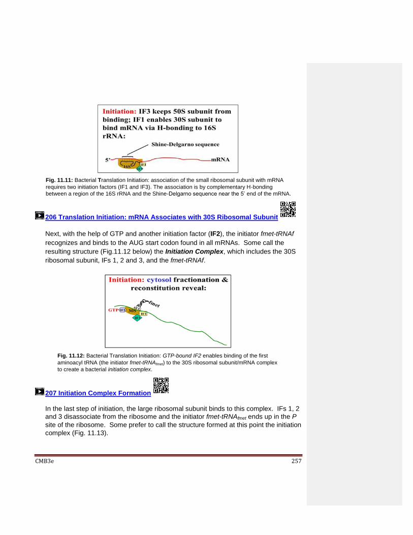
CMB3e 257

206 Translation Initiation: mRNA Associates with 30S Ribosomal Subunit

Next, with the help of GTP and another initiation factor (IF2), the initiator fmet-tRNAf

recognizes and binds to the AUG start codon found in all mRNAs. Some call the

resulting structure (Fig.11.12 below) the Initiation Complex, which includes the 30S

ribosomal subunit, IFs 1, 2 and 3, and the fmet-tRNAf.

207 Initiation Complex Formation

In the last step of initiation, the large ribosomal subunit binds to this complex. IFs 1, 2

and 3 disassociate from the ribosome and the initiator fmet-tRNAfmet ends up in the P

site of the ribosome. Some prefer to call the structure formed at this point the initiation

complex (Fig. 11.13).

Fig. 11.11: Bacterial Translation Initiation: association of the small ribosomal subunit with mRNA

requires two initiation factors (IF1 and IF3). The association is by complementary H-bonding

between a region of the 16S rRNA and the Shine-Delgarno sequence near the 5’ end of the mRNA.

Fig. 11.12: Bacterial Translation Initiation: GTP-bound IF2 enables binding of the first

aminoacyl tRNA (the initiator fmet-tRNAfmet) to the 30S ribosomal subunit/mRNA complex

to create a bacterial initiation complex.

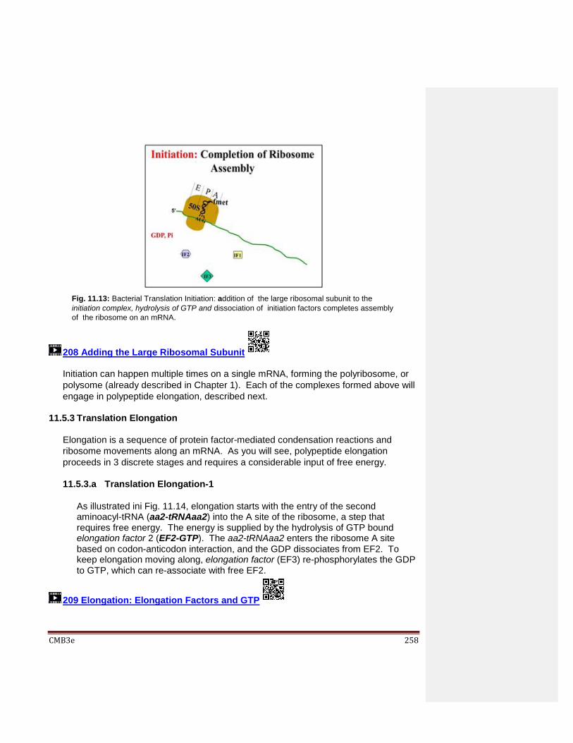
CMB3e 258

208 Adding the Large Ribosomal Subunit

Initiation can happen multiple times on a single mRNA, forming the polyribosome, or

polysome (already described in Chapter 1). Each of the complexes formed above will

engage in polypeptide elongation, described next.

11.5.3 Translation Elongation

Elongation is a sequence of protein factor-mediated condensation reactions and

ribosome movements along an mRNA. As you will see, polypeptide elongation

proceeds in 3 discrete stages and requires a considerable input of free energy.

11.5.3.a Translation Elongation-1

As illustrated ini Fig. 11.14, elongation starts with the entry of the second aminoacyl-tRNA (aa2-tRNAaa2) into the A site of the ribosome, a step that requires free energy. The energy is supplied by the hydrolysis of GTP bound elongation factor 2 (EF2-GTP). The aa2-tRNAaa2 enters the ribosome A site based on codon-anticodon interaction, and the GDP dissociates from EF2. To keep elongation moving along, elongation factor (EF3) re-phosphorylates the GDP to GTP, which can re-associate with free EF2.

209 Elongation: Elongation Factors and GTP

Fig. 11.13: Bacterial Translation Initiation: addition of the large ribosomal subunit to the

initiation complex, hydrolysis of GTP and dissociation of initiation factors completes assembly

of the ribosome on an mRNA.

CMB3e 259

11.5.3.b Translation Elongation-2

Peptidyl transferase, a ribozyme component of the ribosome itself, links the

incoming amino acid to a growing chain in a condensation reaction. Fig. 11.15

illustrates the result of peptidyl transferase action.

In this reaction, the fmet is transferred from the initiator tRNAf in the P site to aa2-

tRNAaa2 in the A site, forming a peptide linkage with aa2.

210 Elongation: A Ribozyme Catalyzes Peptide Linkage Formation

Fig. 11.14: Bacterial Translation Elongation 1: EF2-GTP and EF3 facilitate entry of the second

aminoacyl tRNA into the A site of the ribosome to begin elongation; GTP is hydrolyzed.

Fig. 11.15: Bacterial Translation Elongation 2: The peptidyl transferase ribozyme (part of the

ribosome) catalyzes peptide bond formation between the fmet on its tRNAf and the second amino

acid (aa2). fmet is transferred from its tRNAf as it condenses with an aa2 still linked to its tRNAaa2.

CMB3e 260

11.5.3.c Translation Elongation 3

Translocase catalyzes GTP hydrolysis as the ribosome moves (translocates) along

an mRNA. Then, the next mRNA codon is exposed in the A site of the ribosome and

the first tRNA (tRNAf) ends up on the E site (at the left in Fig. 11.16 below).

The tRNAf, no longer attached to an amino acid, will exit the E site as the next (3rd)

aa-tRNA enters the empty A site based on a specific codon-anticodon interaction

(assisted by elongation factors and powered by GTP hydrolysis) to begin another

cycle of elongation. Note that in each cycle of elongation, an ATP is consumed to

attach each amino acid to its tRNA, and two GTPs are hydrolyzed in the cycle itself.

In other words, at the cost of three NTPs, protein synthesis is the most expensive

polymer synthesis reaction in cells!

211 Elongation: Translocase Moves Ribosome Along mRNA

212 Adding the Third Amino Acid

213 Big Translation Energy Costs

As polypeptides elongate, they emerge from a groove in the large ribosomal subunit.

As noted, a formylase enzyme in E. coli cytoplasm removes the formyl group from

the exposed initiation fmet from all growing polypeptides. While about 40% of E. coli

Fig. 11.16: Bacterial Translation Elongation 3: Translocase on the ribosome catalyzes its movement

along the mRNA, exposing the next codon in the A site; a peptidyl tRNA is now in the P site.

CMB3e 261

polypeptides still begin with methionine, specific proteases catalyze the hydrolytic

removal of the amino-terminal methionine (and sometimes even more amino acids)

from the other 60% of polypeptides. The removal of the formyl group and one or

more N-terminal amino acids from new polypeptides are examples of post-

translational processing.

214 The Fates of fMet and Met; Cases of Post-Translational Processing 11.5.4 Translation Termination

Translation of an mRNA by a ribosome ends when translocation exposes one of the

three stop codons in the A site of the ribosome. Stop codons are situated some

distance from the 3’ end of an mRNA. The region between a stop codon to the end of

the mRNA is called the 3’ untranslated region of the messenger RNA (3’UTR). With

no aminoacyl-tRNA to recognize stop codons (UAA, UAG or UGA), the ribosome

actually stalls. The slow-down allows termination factor protein to enter the A site,

causing release of the new polypeptide and disassembly of the ribosomal subunits

from the mRNA. This requires energy from yet another GTP hydrolysis. After

dissociation, ribosomal subunits can be reassembled with an mRNA for another round

of protein synthesis. Fig 11.17 illustrates translation termination.

215-2 Translation Termination

Fig. 11.17: Bacterial Translation Termination: Translation stalls when the ribosome reaches a

termination codon, GTP is hydrolyzed and a protein termination (release) factor enters the A site.

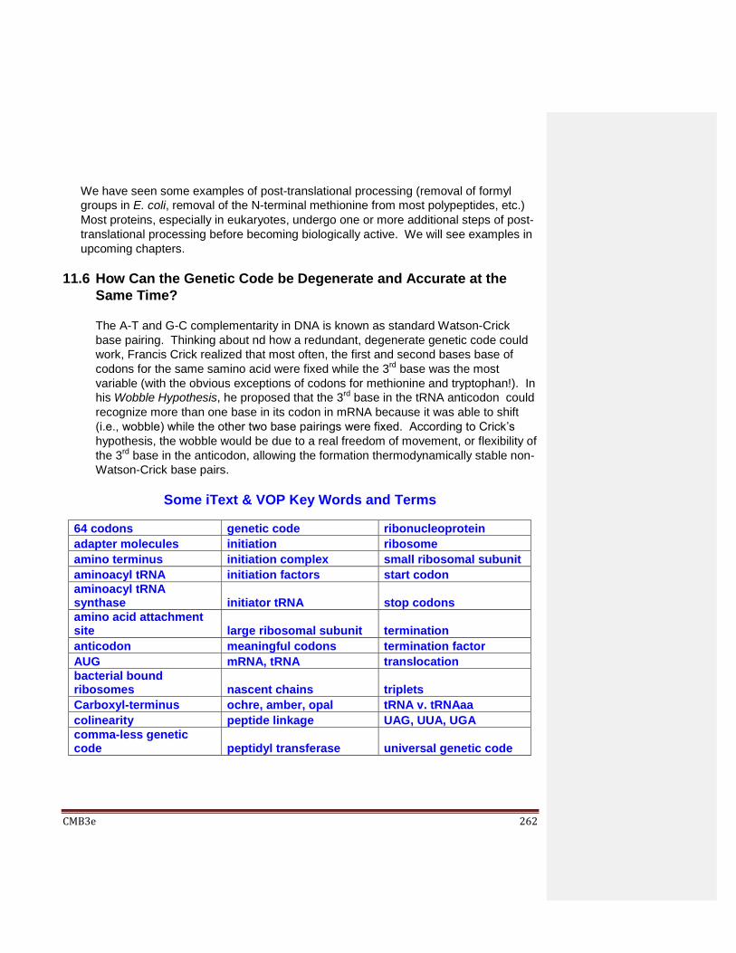
CMB3e 262

We have seen some examples of post-translational processing (removal of formyl

groups in E. coli, removal of the N-terminal methionine from most polypeptides, etc.)

Most proteins, especially in eukaryotes, undergo one or more additional steps of post-

translational processing before becoming biologically active. We will see examples in

upcoming chapters.

11.6 How Can the Genetic Code be Degenerate and Accurate at the

Same Time?

The A-T and G-C complementarity in DNA is known as standard Watson-Crick

base pairing. Thinking about nd how a redundant, degenerate genetic code could

work, Francis Crick realized that most often, the first and second bases base of

codons for the same samino acid were fixed while the 3rd base was the most

variable (with the obvious exceptions of codons for methionine and tryptophan!). In

his Wobble Hypothesis, he proposed that the 3rd base in the tRNA anticodon could

recognize more than one base in its codon in mRNA because it was able to shift

(i.e., wobble) while the other two base pairings were fixed. According to Crick’s

hypothesis, the wobble would be due to a real freedom of movement, or flexibility of

the 3rd base in the anticodon, allowing the formation thermodynamically stable non-

Watson-Crick base pairs.

Some iText & VOP Key Words and Terms

64 codons genetic code ribonucleoprotein

adapter molecules initiation ribosome

amino terminus initiation complex small ribosomal subunit

aminoacyl tRNA initiation factors start codon

aminoacyl tRNA synthase initiator tRNA stop codons

amino acid attachment site large ribosomal subunit termination

anticodon meaningful codons termination factor

AUG mRNA, tRNA translocation

bacterial bound ribosomes nascent chains triplets

Carboxyl-terminus ochre, amber, opal tRNA v. tRNAaa

colinearity peptide linkage UAG, UUA, UGA

comma-less genetic code peptidyl transferase universal genetic code

CMB3e 263

degenerate genetic code polypeptide UUU

elongation polysome Wobble Hypothesis

free v. bound ribosomes reading phase

CMB3e 264

Chapter 12: Regulation of Transcription and

Epigenetic Inheritance Gene repression and induction (prokaryotes); Multiple transcription factors (eukaryotes);

Regulatory elements in DNA; Memories of gene regulation (epigenetics)

12.1 Introduction

Cells regulate their metabolism in several ways. We have already seen that allosterically

regulated enzymes monitor the cellular levels of metabolites. Recall that glycolytic

intermediates rise and fall in cells based on cellular energy needs, binding to or

dissociating from allosteric sites. Allosteric enzymes respond to interaction with

allosteric effectors with an increase or decrease in catalytic activity.

Cells can also control absolute levels of enzymes and other proteins by turning genes on

and off, typically by controlling transcription. Transcription regulation usually starts with

extracellular environmental signaling. The signals are chemicals in the air, in the water or

in the case of multicellular organisms, in blood, lymph or other extracellular fluids.

Bacterial and protist genes often respond to environmental toxins or fluctuating nutrient

levels. Familiar signal molecules in higher organisms include hormones released at

the appropriate time in a sequential developmental program of gene expression, or in

response to nutrient levels in body fluids.

Some signal molecules get into cells and binding to specific intracellular receptors to

convey their instructions. Others bind to cell surface receptors that transduce their

‘information’ into intracellular molecular signals. When signaling leads to gene regulation,

CMB3e 265

responding cells ultimately produce transcription factors. These in turn recognize and

bind to specific regulatory DNA sequences associated with the genes that they control.

DNA sequences that bind transcription factors are relatively short. They can lie proximal

(close) to the transcription start site of a gene, and/or in the case of eukaryotes, distal to

(far from) it. We will see that binding some regulatory DNA sequences are enhancers,

turning on or increasing gene transcription. Others are silencers, down-regulating, or

suppressing transcription of a gene. Finally, DNA regulatory sequences are hidden

behind a thicket of chromatin proteins in eukaryotes. When patterns of gene expression

in cells change during development, chromatin is re-organized, cells differentiate, and

new tissues and organs form. To this end, new patterns of gene expression and

chromatin configuration in a cell must be remembered in its descendants.

In this chapter, we look at the path from cell recognition of a signal molecule to the

interaction of regulatory proteins with DNA in both prokaryotic and eukaryotic cells. We

also consider how eukaryotic cells remember instructions that alter chromatin

configuration and patterns of gene expression, topics in the field of epigenetics.

Learning Objectives

When you have mastered the information in this chapter, you should be able to:

1. compare and contrast transcription factors and so-called cis-acting elements.

2. discuss the role of DNA bending in the regulation of gene expression.

3. explain the benefits of organizing bacterial genes into operons, and why some

bacterial genes are not part of operons.

4. compare and contrast regulation of the lac and trp operons in E. coli.

5. define and describe regulatory genes and structural genes in E. coli.

6. discuss why a fourth gene was suspected in lac operon regulation.

7. distinguish between gene repression and de-repression and between positive and

negative gene regulation, using real or hypothetical examples. For example, explain

how it is possible to have repression by positive regulation.

8. draw and label all functional regions of prokaryotic and eukaryotic genes.

9. compare and contrast different mechanisms of gene regulation in eukaryotic cells.

10. describe the transcription initiation complex of a regulated gene in eukaryotes.

11. define and articulate differences between gene expression and transcription

regulation.

12. define a gene. 13. distinguish between the roles of enhancers and other cis-acting elements in

transcription regulation.

14. compare and contrast the genome and the epigenome.

CMB3e 266

12.2 Gene Regulation in Prokaryotes: the Lactose (lac) Operon

Many prokaryotic genes are organized in operons that are linked genes transcribed into

a single mRNA encoding two or more proteins. Operons usually encode proteins with

related functions. Regulating the activity of an operon (rather than multiple single genes

encoding single proteins) allows better coordination of the synthesis of several proteins at

once. In E. coli, the regulated lac operon encodes three enzymes involved in the

metabolism of lactose (an alternative nutrient to glucose). Regulation of an operon (or of

a single gene for that matter) can be by repression or by induction. When a small

metabolite in a cell binds to a regulatory repressor or inducer protein, the protein

undergoes an allosteric change that allows it to bind to a regulatory DNA sequence…, or

to un-bind from the DNA.

We will see examples of such regulation in the lac and trp operons. Regulation of the

Lac operon genes is an example of gene repression as well as induction. We’ll see

that Trp (tryptophan) operon regulation is by gene repression. In both operons, changes

in levels of intracellular metabolites reflect the metabolic status of the cell, eliciting

appropriate changes in gene transcription. Let’s start with a look at lac operon regulation.

216 Overview of Prokaryotic Gene Regulation

The mRNA transcribed from the lac operon is simultaneously translated into three

enzymes, as shown in Fig. 12.1.

Fig. 12.1: Transcription of the E. coli lac operon produces a single mRNA encoding three

polypeptides (nicknamed ‘z’, ‘y’ and ‘a’) which is translated into 3 enzymes involved in

lactose metabolism.

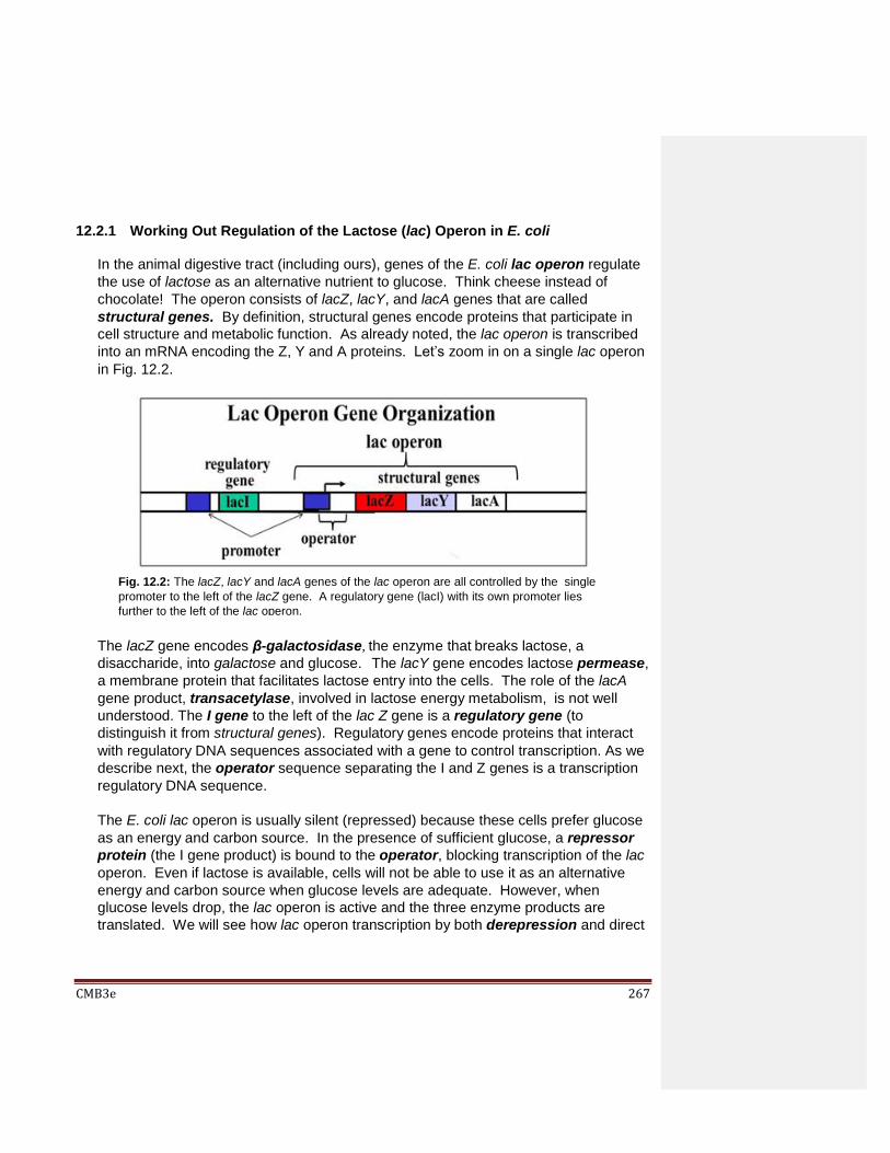
CMB3e 267

12.2.1 Working Out Regulation of the Lactose (lac) Operon in E. coli

In the animal digestive tract (including ours), genes of the E. coli lac operon regulate

the use of lactose as an alternative nutrient to glucose. Think cheese instead of

chocolate! The operon consists of lacZ, lacY, and lacA genes that are called

structural genes. By definition, structural genes encode proteins that participate in

cell structure and metabolic function. As already noted, the lac operon is transcribed

into an mRNA encoding the Z, Y and A proteins. Let’s zoom in on a single lac operon

in Fig. 12.2.

The lacZ gene encodes β-galactosidase, the enzyme that breaks lactose, a

disaccharide, into galactose and glucose. The lacY gene encodes lactose permease,

a membrane protein that facilitates lactose entry into the cells. The role of the lacA

gene product, transacetylase, involved in lactose energy metabolism, is not well

understood. The I gene to the left of the lac Z gene is a regulatory gene (to

distinguish it from structural genes). Regulatory genes encode proteins that interact

with regulatory DNA sequences associated with a gene to control transcription. As we

describe next, the operator sequence separating the I and Z genes is a transcription

regulatory DNA sequence.

The E. coli lac operon is usually silent (repressed) because these cells prefer glucose

as an energy and carbon source. In the presence of sufficient glucose, a repressor

protein (the I gene product) is bound to the operator, blocking transcription of the lac

operon. Even if lactose is available, cells will not be able to use it as an alternative

energy and carbon source when glucose levels are adequate. However, when

glucose levels drop, the lac operon is active and the three enzyme products are

translated. We will see how lac operon transcription by both derepression and direct

Fig. 12.2: The lacZ, lacY and lacA genes of the lac operon are all controlled by the single

promoter to the left of the lacZ gene. A regulatory gene (lacI) with its own promoter lies

further to the left of the lac operon.

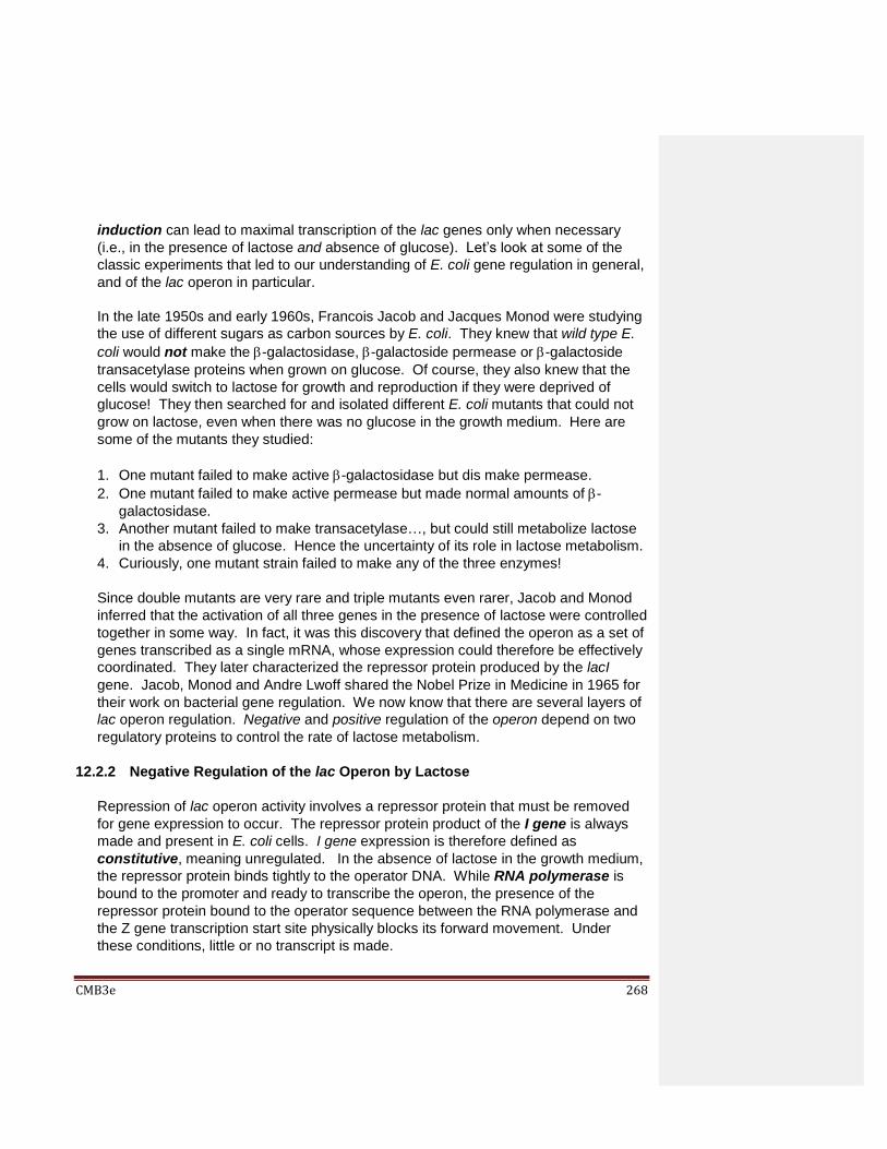
CMB3e 268

induction can lead to maximal transcription of the lac genes only when necessary

(i.e., in the presence of lactose and absence of glucose). Let’s look at some of the

classic experiments that led to our understanding of E. coli gene regulation in general,

and of the lac operon in particular.

In the late 1950s and early 1960s, Francois Jacob and Jacques Monod were studying

the use of different sugars as carbon sources by E. coli. They knew that wild type E.

coli would not make the -galactosidase, -galactoside permease or -galactoside

transacetylase proteins when grown on glucose. Of course, they also knew that the

cells would switch to lactose for growth and reproduction if they were deprived of

glucose! They then searched for and isolated different E. coli mutants that could not

grow on lactose, even when there was no glucose in the growth medium. Here are

some of the mutants they studied:

1. One mutant failed to make active -galactosidase but dis make permease.

2. One mutant failed to make active permease but made normal amounts of -

galactosidase.

3. Another mutant failed to make transacetylase…, but could still metabolize lactose

in the absence of glucose. Hence the uncertainty of its role in lactose metabolism.

4. Curiously, one mutant strain failed to make any of the three enzymes!

Since double mutants are very rare and triple mutants even rarer, Jacob and Monod

inferred that the activation of all three genes in the presence of lactose were controlled

together in some way. In fact, it was this discovery that defined the operon as a set of

genes transcribed as a single mRNA, whose expression could therefore be effectively

coordinated. They later characterized the repressor protein produced by the lacI

gene. Jacob, Monod and Andre Lwoff shared the Nobel Prize in Medicine in 1965 for

their work on bacterial gene regulation. We now know that there are several layers of

lac operon regulation. Negative and positive regulation of the operon depend on two

regulatory proteins to control the rate of lactose metabolism.

12.2.2 Negative Regulation of the lac Operon by Lactose

Repression of lac operon activity involves a repressor protein that must be removed

for gene expression to occur. The repressor protein product of the I gene is always

made and present in E. coli cells. I gene expression is therefore defined as

constitutive, meaning unregulated. In the absence of lactose in the growth medium,

the repressor protein binds tightly to the operator DNA. While RNA polymerase is

bound to the promoter and ready to transcribe the operon, the presence of the

repressor protein bound to the operator sequence between the RNA polymerase and

the Z gene transcription start site physically blocks its forward movement. Under

these conditions, little or no transcript is made.

CMB3e 269

Fig 12.3 shows the lac repressor protein in its repressed state.

If cells are grown in the presence of lactose, the lactose entering the cells is converted

to allolactose. Allolactose in turn, binds to the repressor sitting on the operator DNA

to form a 2-part complex, as shown in Fig. 12.4.

Fig. 12.3: Negative regulation of the lac operon: The I gene transcribes a repressor protein.

When bound to the operator sequence (between the promoter and beginning of the Z

gene), RNA polymerase is blocked and the operon cannot be transcribed. Transcription will

require derepression (i.e., removal of the repressor protein).

Fig. 12.4: Negative regulation of the lac operon: When present, lactose enters cells and is

converted to allolactose. Accumulating allolactose binds to the lac repressor protein.

Z Y

CMB3e 270

The allosterically altered repressor dissociates from the operator and RNA polymerase

can transcribe the lac operon genes (Fig. 12.5).

12.2.3 Positive Regulation of the Lac Operon; Induction by Catabolite Activation

The second control mechanism regulating lac operon expression is mediated by CAP

(cAMP-bound catabolite activator protein or cAMP receptor protein). When glucose

is available, cellular levels of cAMP are low in the cells and CAP is in an inactive

conformation. On the other hand, if glucose levels are low, cAMP levels rise and bind

to the CAP, activating it. If lactose levels are also low, the cAMP-bound CAP will have

no effect. If lactose is present and glucose levels are low, then allolactose binds the

lac repressor causing it to dissociate from the operator region. Under these

conditions, the cAMP-bound CAP can bind to the operator in lieu of the repressor

protein. In this case, rather than blocking RNA polymerase, the activated cAMP-

bound CAP induces even more efficient lac operon transcription. The result is

synthesis of higher levels of lac enzymes that facilitate efficient cellular use of lactose

as an alternative to glucose as an energy source. Fig. 12.6 shows maximal lac

operon activation in high lactose and low glucose.

Fig. 12.5: Negative regulation of the lac operon: Allolactose binding causes allosteric change in the

lac repressor that then dissociates from the operator sequence, allowing RNA polymerase to

transcribe the operon.

CMB3e 271

217 Regulation of the lac Operon

cAMP-bound CAP is a transcription inducer. It forces DNA in the promoter-operator

region to bend (Fig. 12.7).

Fig. 12.6: Positive regulation of the lac operon: If lactose is present but glucose is unavailable, the

operon is derepressed AND induced. Increased cAMP binds the Catabolite Activator Protein (CAP),

which binds to the lac operator, inducing) lac gene transcription The lac operon is maximally

transcribed under these conditions.

Fig. 12.7: Positive regulation of the lac operon: cAMP-CAP-bound operator bends the double helix.

This loosens the H- bonds between the bases, making transcription factor access to template

strands easier.

CMB3e 272

Binding of CAMP-CAP to the double helix loosens H-bonds between the strands

making it easier for RNA polymerase to find and bind the promoter…, and for

transcription to begin.

In recent years, additional layers of lac operon regulation have been uncovered. In

one case, the ability of lac permease to transport lactose across the cell membrane is

regulated. In another, additional operator sequences have been discovered to interact

with a multimeric repressor to control lac gene expression. We’ll consider Inducer

Exclusion first.

12.2.4 Lac Operon Regulation by Inducer Exclusion

When glucose levels are high (even in the presence of lactose), phosphate is

consumed in order to phosphorylate glycolytic intermediates. This keeps cytoplasmic

phosphate levels low. Under these conditions, an unphosphorylated elongation factor

(EIIAGlc) binds to the lactose permease in the cell membrane, preventing the enzyme

from bringing lactose into the cell. The role of phosphorylated and unphosphorylated

EIIAGlc in regulating the lac operon are shown in Fig. 12.8.

Fig. 12.8: lac operon regulation by inducer exclusion: High glucose levels accelerate glycolysis,

depleting cellular phosphate. Low phosphate leads to the dephosphorylation of EIIAGlc, among

other proteins. Dephosphorylated EIIAGlc is an inhibitor of lactose permease (i.e., the lacA

protein). Without active permease, lactose can’t get into cells, allolactose cannot be made, and the

lac gene cannot be transcribed.

CMB3e 273

High glucose levels block lactose entry into the cells, effectively preventing allolactose

formation and derepression of the lac operon. Inducer exclusion is thus a logical way

for the cells to handle an abundance of glucose, whether or not lactose is present. On

the other hand, if glucose levels are low in the growth medium, phosphate

concentrations in the cells rise sufficiently for a specific kinase to phosphorylate the

EIIAGlc. Phosphorylated EIIAGlc then undergoes an allosteric change and dissociates

from the lactose permease, making it active so that more lactose can enter the cell. In

other words, the inducer is not “excluded” under these conditions!

The kinase that phosphorylates EIIAGlc is part of a phosphoenolpyruvate (PEP)-

dependent phosphotransferase system (PTS) cascade. When extracellular glucose

levels are low, the cell activates the PTS system in an effort to bring whatever glucose

is around into the cell. The last enzyme in the PTS phosphorylation cascade is the

kinase that phosphorylates EIIAGlc. Now activated, phosphorylated EIIAGlc dissociates

from the lactose permease. The now active permease can bring available lactose

from the medium into the cell.

12.2.5 Structure of the lac Repressor Protein and Additional Operator Sequences

The lac repressor encoded by the I gene is a tetramer of identical subunits (Fig.12.9).

Each subunit contains a helix-turn-helix motif capable of binding to DNA. However,

the operator DNA sequence downstream of the promoter in the operon consists of a

pair of inverted repeats spaced apart in such a way that they can only interact with two

Fig. 12.9: Computer generated structure of the tetrameric lac repressor bound to DNA via helix-

turn-helix motifs.

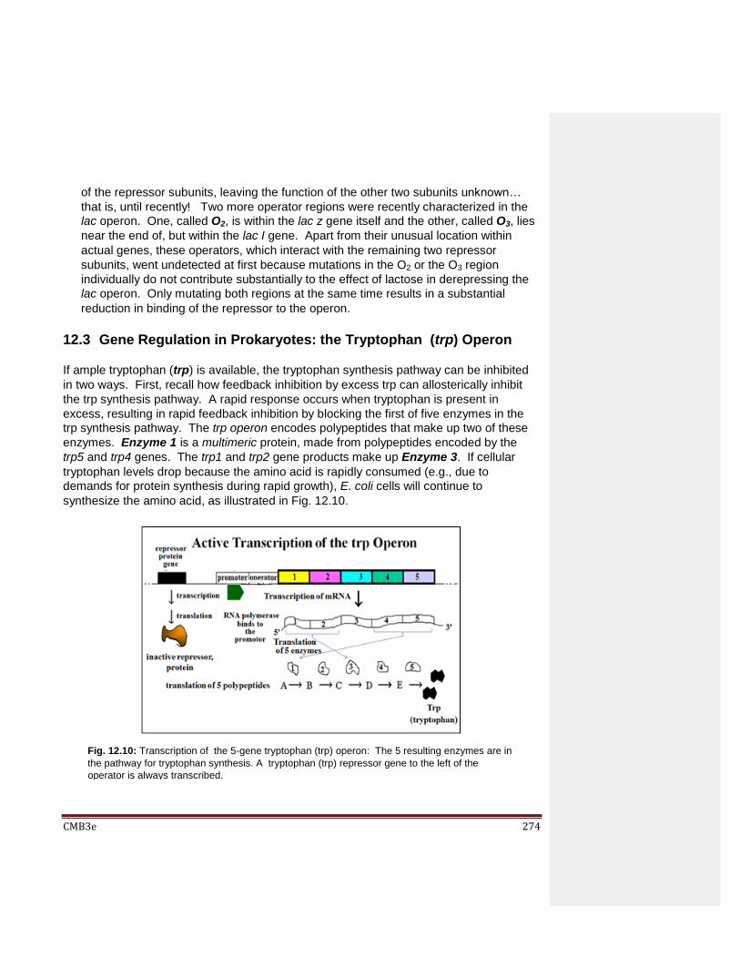
CMB3e 274

of the repressor subunits, leaving the function of the other two subunits unknown…

that is, until recently! Two more operator regions were recently characterized in the

lac operon. One, called O2, is within the lac z gene itself and the other, called O3, lies

near the end of, but within the lac I gene. Apart from their unusual location within

actual genes, these operators, which interact with the remaining two repressor

subunits, went undetected at first because mutations in the O2 or the O3 region

individually do not contribute substantially to the effect of lactose in derepressing the

lac operon. Only mutating both regions at the same time results in a substantial

reduction in binding of the repressor to the operon.

12.3 Gene Regulation in Prokaryotes: the Tryptophan (trp) Operon

If ample tryptophan (trp) is available, the tryptophan synthesis pathway can be inhibited

in two ways. First, recall how feedback inhibition by excess trp can allosterically inhibit

the trp synthesis pathway. A rapid response occurs when tryptophan is present in

excess, resulting in rapid feedback inhibition by blocking the first of five enzymes in the

trp synthesis pathway. The trp operon encodes polypeptides that make up two of these

enzymes. Enzyme 1 is a multimeric protein, made from polypeptides encoded by the

trp5 and trp4 genes. The trp1 and trp2 gene products make up Enzyme 3. If cellular

tryptophan levels drop because the amino acid is rapidly consumed (e.g., due to

demands for protein synthesis during rapid growth), E. coli cells will continue to

synthesize the amino acid, as illustrated in Fig. 12.10.

Fig. 12.10: Transcription of the 5-gene tryptophan (trp) operon: The 5 resulting enzymes are in

the pathway for tryptophan synthesis. A tryptophan (trp) repressor gene to the left of the

operator is always transcribed.

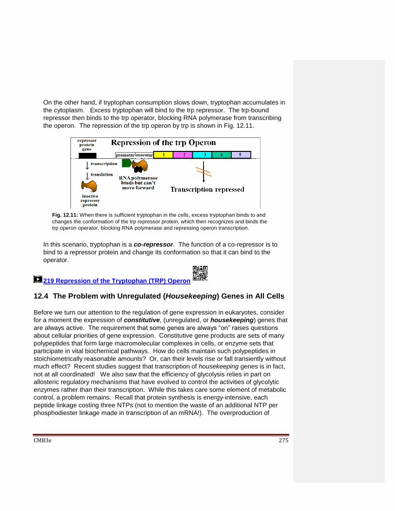
CMB3e 275

On the other hand, if tryptophan consumption slows down, tryptophan accumulates in

the cytoplasm. Excess tryptophan will bind to the trp repressor. The trp-bound

repressor then binds to the trp operator, blocking RNA polymerase from transcribing

the operon. The repression of the trp operon by trp is shown in Fig. 12.11.

In this scenario, tryptophan is a co-repressor. The function of a co-repressor is to

bind to a repressor protein and change its conformation so that it can bind to the

operator.

219 Repression of the Tryptophan (TRP) Operon

12.4 The Problem with Unregulated (Housekeeping) Genes in All Cells

Before we turn our attention to the regulation of gene expression in eukaryotes, consider

for a moment the expression of constitutive, (unregulated, or housekeeping) genes that

are always active. The requirement that some genes are always “on” raises questions

about cellular priorities of gene expression. Constitutive gene products are sets of many

polypeptides that form large macromolecular complexes in cells, or enzyme sets that

participate in vital biochemical pathways. How do cells maintain such polypeptides in

stoichiometrically reasonable amounts? Or, can their levels rise or fall transiently without

much effect? Recent studies suggest that transcription of housekeeping genes is in fact,

not at all coordinated! We also saw that the efficiency of glycolysis relies in part on

allosteric regulatory mechanisms that have evolved to control the activities of glycolytic

enzymes rather than their transcription. While this takes care some element of metabolic

control, a problem remains. Recall that protein synthesis is energy-intensive, each

peptide linkage costing three NTPs (not to mention the waste of an additional NTP per

phosphodiester linkage made in transcription of an mRNA!). The overproduction of

Fig. 12.11: When there is sufficient tryptophan in the cells, excess tryptophan binds to and

changes the conformation of the trp repressor protein, which then recognizes and binds the

trp operon operator, blocking RNA polymerase and repressing operon transcription.

CMB3e 276

proteins would seem to be a waste of energy, and thus an evolutionary ‘mistake’. While

we may not know just how expensive it is to express housekeeping genes, whatever the

expense, these energy expenses are the cost of evolving complex structures and

biochemical pathways vital to their everyday function and survival. This is a good

example of a major precept of evolutionary theory: evolution is an accumulation of

improvements brought about by natural selection; it is not the result of perfect design in

advance. Now back to our focus on regulated gene expression… in eukaryotes.

12.5 Gene Regulation in Eukaryotes

Let’s recall an experiment described earlier and illustrated in Fig. 12.12.

Results of this experiment provided the evidence that even very different cells of an

organism contain the same genes. In fact in any multicellular eukaryotic organism, every

cell contains the same genes in their DNA. Therefore, the different cell types in an

organism differ not in which genes they contain, but which sets of genes they express!

Looked at another way, cells differentiate when they turn on new genes and turn off old

ones. Thus, gene regulation produces different sets of gene products during

differentiation, leading to cells that look and function differently in the organism.

220 An Experiment: All of an Organism's Cells Have the Same Genome

Fig. 12.12: Replacement of an egg nucleus with that from an adult cell enabled cloning of embryos

and eventually complete organisms, proving that adult cells contain all of the genes required to

program development of, and to make the organism.

CMB3e 277

Compared to prokaryotes, many steps in eukaryotes lie between the transcription of an

mRNA and the accumulation of a polypeptide end product. Eleven of these steps are

shown below in the pathway from gene to protein Fig. 12.13.

Theoretically, cells could turn on, turn off, speed up or slow down any of the steps in this

pathway, changing the steady state concentration of a polypeptide in the cells. But the

expression of a single gene is typically controlled at only one or a few steps. As is the

case in bacteria, control of transcription initiation is perhaps the most common form of

eukaryotic gene regulation,(in principle if not in detail).

221-2 Many Options for Regulating Eukaryotic Genes

Fig. 12.13: Potentials for gene regulation in eukaryotes: Control of transcript and/or

protein abundance, as well as protein activity can regulate cellular metabolism.

CMB3e 278

12.5.1 Complexities of Eukaryotic Gene Regulation

Gene regulation in eukaryotes is more complex than in prokaryotes. This is in part

because their genomes are larger and because they encode more genes. For

example, the E. coli genome houses about 5,000 genes, compared to around 25,000

genes in humans. Furthermore, eukaryotes can produce even more than 25,000

proteins by alternative splicing of mRNAs and in at least a few cases, by initiating

transcription from alternative start sites in the same gene. And of course, the activity

of many more genes must be coordinated without the benefit of multigene operons!

Finally, eukaryotic gene regulation is made more complicated because all nuclear

DNA is wrapped in protein in the form of chromatin.

All organisms control gene activity with transcription factors that bind to specific

DNA sequences (cis regulatory elements). In eukaryotes, these elements can be

proximal to (near) the promoter of a gene, or distal to (quite far from) the gene they

regulate. Fig. 12.14 is a eukaryotic gene, mapped to show its typical components

(promoter, introns, exons…) and its associated cis-acting regulatory elements.

Enhancers are typical distal cis elements that recognize and bind transcription factors

to increase the rate of transcription of a gene. Oddly enough, these short DNA

elements can be in the 5’ or 3’ non-translated region of the gene or even within

introns, often thousands of base pairs away from the promoter and transcription start-

site of the genes they control.

Fig. 12.14: Cis-acting sequence elements associated with a gene function as gene regulators

when bound to regulatory proteins (trans-acting factors). Regulatory sequences may be near

the gene promoter (proximal) or far from it (distal). Enhancers are examples of distal

regulatory sequences.

CMB3e 279

Upstream regulatory regions of eukaryotic genes (to the left of a gene promoter as

shown above) often have distal binding sites for more than a few transcription factors,

some with positive (enhancing) and others with negative (silencing) effects. Of

course, which of these DNA regions are active in controlling a gene depends on which

transcription factor(s) are present in the nucleus. Sets of positive regulators can work

together to coordinate and maximize gene expression when needed, and sets of

negative regulators may bind negative regulatory elements to silence a gene.

222-2 Transcription Factors Bind DNA Near & Far In eukaryotes we saw that the initiation of transcription involves many transcription

factors (TFs) and RNA polymerase II acting at a gene promoter to form a

transcription pre-initiation complex. TFIID, (or TATA binding protein) is one of

the first factors to bind, causing the DNA in the promoter region to bend, much like the

CAP protein in bacteria. Once bound, TFIID recruits other transcription factors to the

promoter. As in bacteria, bending the DNA loosens H-bonds between bases,

facilitating unwinding the double helix near the gene. Bending eukaryotic DNA also

brings regulatory proteins on distal enhancer sequences far from the promoter close to

proteins bound to more proximal regulatory elements, as shown in Fig. 12.15.

Nucleotide methylation sites may facilitate regulatory protein-enhancer binding. When

such regulatory proteins, here called activators (i.e., of transcription), bind to their

enhancers, they acquire an affinity for protein cofactors that enable recognition and

Fig. 12.15: Assembly of a eukaryotic transcription complex on a regulated gene. Distal

regulatory protein/DNA interactions can cause DNA bending, recruiting transcription initiation

factors and proximal regulatory factors to the transcription complex.

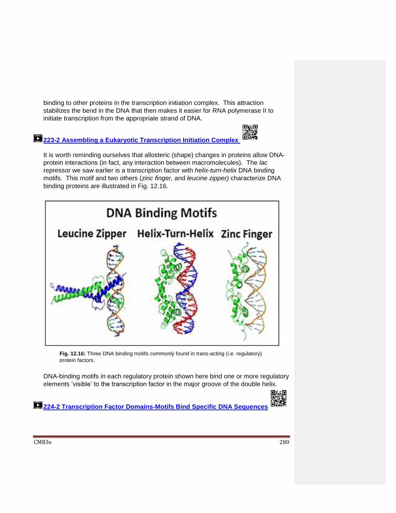
CMB3e 280

binding to other proteins in the transcription initiation complex. This attraction

stabilizes the bend in the DNA that then makes it easier for RNA polymerase II to

initiate transcription from the appropriate strand of DNA.

223-2 Assembling a Eukaryotic Transcription Initiation Complex

It is worth reminding ourselves that allosteric (shape) changes in proteins allow DNA-

protein interactions (in fact, any interaction between macromolecules). The lac

repressor we saw earlier is a transcription factor with helix-turn-helix DNA binding

motifs. This motif and two others (zinc finger, and leucine zipper) characterize DNA

binding proteins are illustrated in Fig. 12.16.

DNA-binding motifs in each regulatory protein shown here bind one or more regulatory

elements ‘visible’ to the transcription factor in the major groove of the double helix.

224-2 Transcription Factor Domains-Motifs Bind Specific DNA Sequences

Fig. 12.16: Three DNA binding motifs commonly found in trans-acting (i.e. regulatory)

protein factors.

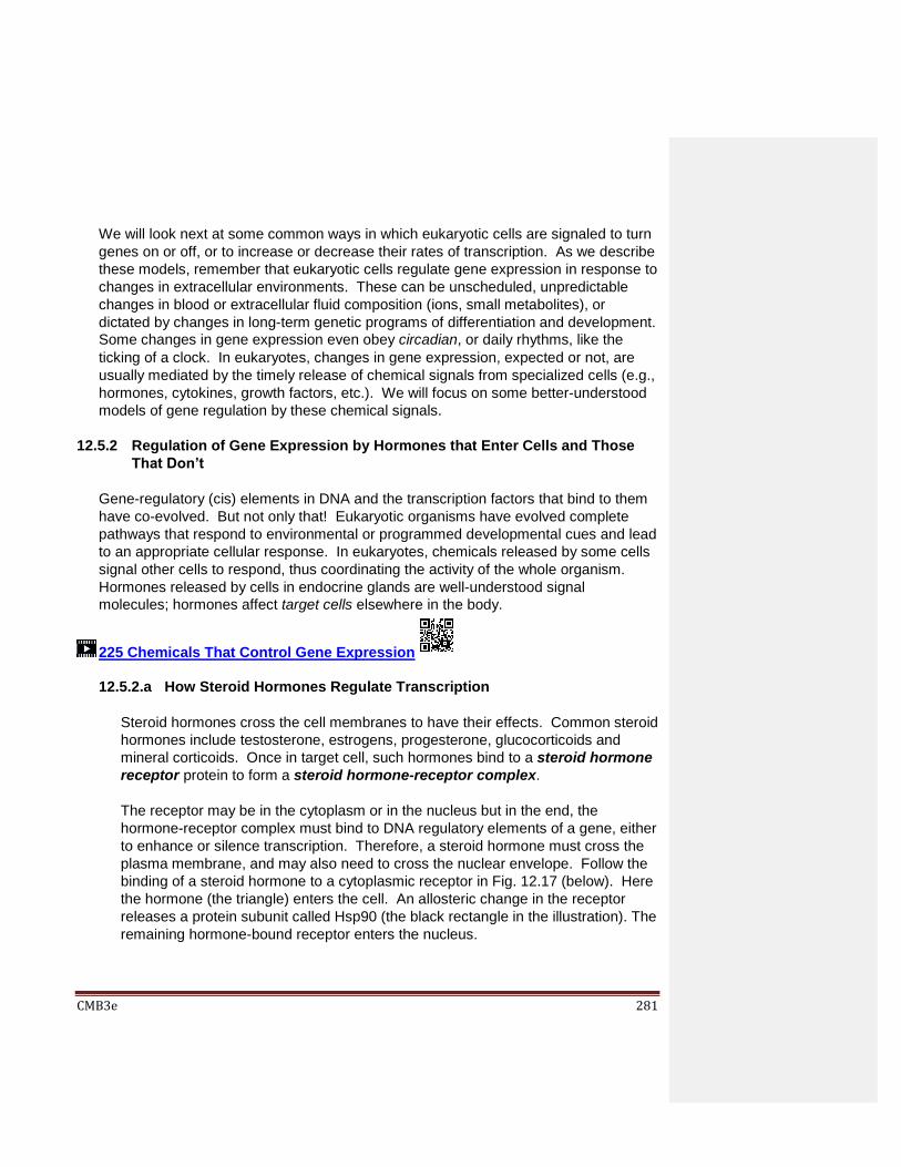
CMB3e 281

We will look next at some common ways in which eukaryotic cells are signaled to turn

genes on or off, or to increase or decrease their rates of transcription. As we describe

these models, remember that eukaryotic cells regulate gene expression in response to

changes in extracellular environments. These can be unscheduled, unpredictable

changes in blood or extracellular fluid composition (ions, small metabolites), or

dictated by changes in long-term genetic programs of differentiation and development.

Some changes in gene expression even obey circadian, or daily rhythms, like the

ticking of a clock. In eukaryotes, changes in gene expression, expected or not, are

usually mediated by the timely release of chemical signals from specialized cells (e.g.,

hormones, cytokines, growth factors, etc.). We will focus on some better-understood

models of gene regulation by these chemical signals.

12.5.2 Regulation of Gene Expression by Hormones that Enter Cells and Those

That Don’t

Gene-regulatory (cis) elements in DNA and the transcription factors that bind to them

have co-evolved. But not only that! Eukaryotic organisms have evolved complete

pathways that respond to environmental or programmed developmental cues and lead

to an appropriate cellular response. In eukaryotes, chemicals released by some cells

signal other cells to respond, thus coordinating the activity of the whole organism.

Hormones released by cells in endocrine glands are well-understood signal

molecules; hormones affect target cells elsewhere in the body.

225 Chemicals That Control Gene Expression

12.5.2.a How Steroid Hormones Regulate Transcription

Steroid hormones cross the cell membranes to have their effects. Common steroid

hormones include testosterone, estrogens, progesterone, glucocorticoids and

mineral corticoids. Once in target cell, such hormones bind to a steroid hormone

receptor protein to form a steroid hormone-receptor complex.

The receptor may be in the cytoplasm or in the nucleus but in the end, the

hormone-receptor complex must bind to DNA regulatory elements of a gene, either

to enhance or silence transcription. Therefore, a steroid hormone must cross the

plasma membrane, and may also need to cross the nuclear envelope. Follow the

binding of a steroid hormone to a cytoplasmic receptor in Fig. 12.17 (below). Here

the hormone (the triangle) enters the cell. An allosteric change in the receptor

releases a protein subunit called Hsp90 (the black rectangle in the illustration). The

remaining hormone-bound receptor enters the nucleus.

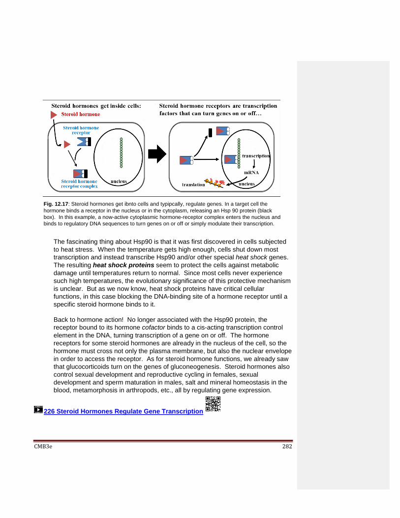
CMB3e 282

The fascinating thing about Hsp90 is that it was first discovered in cells subjected

to heat stress. When the temperature gets high enough, cells shut down most

transcription and instead transcribe Hsp90 and/or other special heat shock genes.

The resulting heat shock proteins seem to protect the cells against metabolic

damage until temperatures return to normal. Since most cells never experience

such high temperatures, the evolutionary significance of this protective mechanism

is unclear. But as we now know, heat shock proteins have critical cellular

functions, in this case blocking the DNA-binding site of a hormone receptor until a

specific steroid hormone binds to it.

Back to hormone action! No longer associated with the Hsp90 protein, the

receptor bound to its hormone cofactor binds to a cis-acting transcription control

element in the DNA, turning transcription of a gene on or off. The hormone

receptors for some steroid hormones are already in the nucleus of the cell, so the

hormone must cross not only the plasma membrane, but also the nuclear envelope

in order to access the receptor. As for steroid hormone functions, we already saw

that glucocorticoids turn on the genes of gluconeogenesis. Steroid hormones also

control sexual development and reproductive cycling in females, sexual

development and sperm maturation in males, salt and mineral homeostasis in the

blood, metamorphosis in arthropods, etc., all by regulating gene expression.

226 Steroid Hormones Regulate Gene Transcription

Fig. 12.17: Steroid hormones get ibnto cells and typipcally, regulate genes. In a target cell the

hormone binds a receptor in the nucleus or in the cytoplasm, releasing an Hsp 90 protein (black

box). In this example, a now-active cytoplasmic hormone-receptor complex enters the nucleus and

binds to regulatory DNA sequences to turn genes on or off or simply modulate their transcription.

CMB3e 283

12.5.2.b How Protein Hormones Regulate Transcription

Compared to steroids, proteins are of course large and soluble, with highly

charged surfaces. Even protein-derived hormones like adrenalin, though small,

are charged and hydrophilic. Large and/or hydrophilic signal molecules cannot get

across the phospholipid barrier of the plasma membrane. To have any effect at all,

they must bind to receptors on the surface of cells. These receptors are typically

membrane glycoproteins. The information carried by protein hormones must be

conveyed into the cell indirectly by a process called signal transduction. One of

two well-known pathways of signal transduction is illustrated below in Fig. 12.18.

In this pathway, hormone binding to a cell-surface receptor results in formation of

cAMP, a second messenger. cAMP forms when the hormone-receptor in the

membrane binds to and activates a membrane-bound adenylate cyclase enzyme.

Fig. 12.18:Large or polar signal molecules bind to membrane receptors, resulting in signal

transduction, Here, a second messenger molecule (cAMP) forms in the cytoplasm to deliver

the hormonal message. A phosphorylation cascade leads to responses including gene

regulation and/or control of existing protein activity.

CMB3e 284

Once formed, cAMP binds to and activates a protein kinase to initiate a protein

phosphorylation cascade in the cytoplasm. The cascade is a series of protein

phosphorylations. The last in the series phosphorylated proteins can often be (as

suggested in the illustration) one of many activating or inactivating enzymes that

regulate cellular metabolism, or it could be an activated transcription factor that

binds to a cis-regulatory DNA sequence to regulate gene expression.

Some hormones bind to membrane receptors that are themselves protein kinases.

In this case, binding of the signal protein (e.g. hormone) to its receptor causes an

allosteric change that activates the linked receptor kinase, starting the

phosphorylation cascade without the aid of cAMP. The cascade ends with the

activation of an active transcription factor as shown in Fig. 12.19.

We’ll take a closer look at signal transduction in another chapter.

227 Signal Transduction Can Lead to Gene Regulation

Fig. 12.19: Enzyme-linked receptors transduce hormonal signals directly, activating receptor

kinases on the cytoplasmic surface of the cell, initiating phosphorylation cascades leading to

any of several responses.

CMB3e 285

12.6 Regulating Eukaryotic Genes Means Contending with Chromatin

Consider again the different levels of chromatin structure (Fig. 12.20).

Transcription factors bind specific DNA sequences by detecting them through the grooves

(mainly the major groove) in the double helix. The drawing above reminds us however,

that unlike the nearly naked DNA of bacteria, eukaryotic (nuclear) DNA is coated with

Fig. 12.20: Chromatin Organization: different levels of chromatin structure

result from differential association of DNA with chromosomal proteins.

CMB3e 286

proteins that in aggregate, are greater in mass than the DNA that they cover. The

protein-DNA complex of the genome is of course, chromatin. Again as a reminder, DNA

coated with histone proteins forms the 9 nm diameter beads-on-a-string structure in which

the beads are the nucleosomes. The association of specific non-histone proteins with

the nucleosome ‘necklace’ causes it to fold over on themselves to form the 30 nm

solenoid. As we saw earlier, it is possible to selectively extract chromatin. Take a

second look at the results of typical extractions of chromatin from isolated nuclei (Fig.

12.21).

Further accretion of non-histone proteins leads to more folding and the formation of

euchromatin and heterochromatin characteristic of non-dividing cells. In dividing cells,

the chromatin further condenses to form the chromosomes that separate during either

mitosis or meiosis.

Fig. 12.21: High salt chromatin extraction from nuclei (or high salt treatment of 10 nm filaments) yields 30 nm solenoid structures, essentially coils of 10 nm filaments.

CMB3e 287

Recall that biochemical analysis of the 10 nm filament extract revealed that the DNA

wraps around histone protein octamers, the nucleosomes or beads in this beads-on-a-

string structure. Histone proteins are highly conserved in the eukaryotic evolution; they

are not found in prokaryotes. They are also very basic (many lysine and arginine

residues) and therefore very positively charged. This explains why they are able to

arrange themselves uniformly along DNA, binding to the negatively charged

phosphodiester backbone of DNA in the double helix.

Since the DNA in euchromatin is less tightly packed than it is in heterochromatin, perhaps

active genes are to be found in euchromatin and not in heterochromatin. Experiments in

which total nuclear chromatin extracts were isolated and treated with the enzyme

deoxyribonuclease (DNAse) revealed that the DNA in active genes was degraded more

rapidly than non-transcribed DNA. More detail on these experiments can be found in the

two links below.

228 Question: Is Euchromatic DNA Transcribed?

229 Experiment and Answer: Euchromatin is Transcribed

The results of such experiments are consistent with the suggestion that active genes are

more accessible to DNAse because they are in less coiled, or less condensed chromatin.

DNA in more condensed chromatin is surrounded by more proteins, and thus is less

accessible to, and protected from DNAse attack. When packed up in chromosomes

during mitosis or meiosis, all genes are largely inactive.

Regulating gene transcription must occur in non-dividing cells or during the interphase of

cells, times when it is easier to silence or activate genes by chromatin remodeling (i.e.,

changing the shape of chromatin). Changing chromatin conformation involves chemical

modification of chromatin proteins and DNA. For example, chromatin can be modified by

histone acetylation, de-acetylation, methylation and phosphorylation reactions, catalyzed

by histone acetyltransferases (HAT enzymes), de-acetylases, methyl transferases and

kinases, respectively. For example, acetylation of lysines near the amino end of histones

H2B and H4 tends to unwind nucleosomes and open the underlying DNA for transcription.

De-acetylation promotes condensation of the chromatin in the affected regions of DNA.

Likewise, methylation of lysines or arginines (basic amino acids that characterize

histones!) in H3 and H4 typically opens up DNA for transcription, while demethylation has

the opposite effect. These chemical modifications affect recruitment of other proteins that

alter chromatin conformation and ultimately activate or block transcription. This reversible

acetylation and its effect on chromatin are illustrated in Fig. 12.22 (below).

CMB3e 288

Nucleosomes themselves can move, slide and otherwise be repositioned by

complexes that hydrolyze ATP for energy to accomplish the physical shifts. Some

cancers are associated with mutations in genes for proteins involved in chromatin

remodeling. Failures of normal remodeling could adversely affect normal cell cycling

and normal replication. In fact, a single, specific pattern of methylation may mark DNA

in multiple cancer types (check out Five Cancers with the Same Genomic Signature -

Implications).

12.7 Regulating all Genes on a Chromosome at Once Recall that male cells have only one X chromosome and that one of the X chromosomes

in human female adult somatic cells is inactivated, visible in the nucleus as a Barr body.

Inactivation of one of the X chromosomes in Drosophila females. But both males and

females require X chromosomes gene expression during embryogenesis. At that time,

given the difference in X chromosome gene dosage between males and females, how do

male embryos get by with only on X chromosome?

Experiments looking at the expression of X chromosome genes in male and female flies

revealed similar levels of gene products. It turns out that A protein, called CLAMP

(Chromatin-Linked Adaptor for Male-specific lethal Protein), was shown to bind to GAGA

nucleotide repeats lying between the genes for histones 3 and 4. There are about 100

repeats of the five-gene histone locus on X chromosomes, and so, about 100 GAGA

repeats. All those CLAMP proteins bound to those GAGA repeats can interact with a

nuclear body called HLB (Histone Locus Body). The HLB was previously implicated in

higher levels of X chromosome gene expression. A recent study suggests that once

bound to the GAGA sequences, CLAMP recruits MSL (Male-Specific-Lethal) proteins to

form an MSL complex. This complex (the associated HLB/CLAMP/ MSL) has been

Fig. 12.22: Chemical modification of histones can open or close chromatin to transcription.

CMB3e 289

shown to boost X chromosome gene transcription in male fruit flies. The resulting MSL

protein complexes that form then globally increase X chromosome gene expression,

compensating for the lower X gene dosage in males. Read the original research at

Increasing the Gene Expression of an Entire X Chromosome (L.E. Reider et al. (2018)

Genes & Development 31:1-15). And finally, there is emerging evidence that the HLB

action may also be involved in inactivation of an entire female X chromosome later in

embryogenesis in females!

12.8 Mechanoreceptors: Capturing Non-Chemical Signals

A discussion of hormone and other signal molecule-based signal transduction would be

incomplete without acknowledging that cells sometimes need to respond to mechanical

stimuli, such as pressure or stretching. There are receptors called piezoreceptors for

that (piezo, meaning squeeze, or press)! Piezoreceptors in cells lining the urinary

bladder signal when the bladder is full, with the expected response. Piezoreceptors in the

endothelial cells of blood vessels alert the cells to changes in blood pressure and mediate

appropriate responses. In sensory cells in the skin, piezoreceptors enable nerve ending

responses to touch or pain. Another example of piezoreception is found in cellular

proprioreceptors, as in proprio, meaning one’s own self, or in other words, a kind of self-

awareness receptor. Proprioreceptors in joints respond to changes in posture to let us

know where our arms and legs are at any given moment! The domain structure of one

piezoreceptor protein was shown to include springy domains that could respond to

mechanical forces. Fig. 12.23 illustrates how a piezoreceptor may respond to pressure or

stretch to open an Ca++ channel.

Click https://www.nature.com/piezoreceptors for more details on piezoreceptors.

Fig. 12.23: Extracellular pressure (arrowheads) on a CED domain or activating spring-like arms by

stretching the cell membrane (e.g., from inside the cell (arrow) opens a piezo-linked ion channel.

CMB3e 290

12.9 Epigenetics

Aristotle thought that an embryo emerged from an amorphous mass, a “less fully

concocted seed with a nutritive soul and all bodily parts”. The much later development of

the microscope led to more detailed (if inaccurate) descriptions of embryonic

development. In 1677, no less a luminary than Anton von Leeuwenhoek, looking at a

human sperm with his microscope, thought he saw a miniature human inside! The tiny

human, or homunculus, became the epitome of preformation theory.

William Harvey, also in the 17th century, described changes in morphology in the

developing embryos of chickens (and other animals). Harvey coined the term epigenesis

to counter the notion that any tiny adult structures in eggs or sperm simply grew bigger

during embryonic gestation. Meanwhile, other experiments were leading embryologists to

the conclusion that the physical and chemical environment of an embryo strongly affected

development. Thus temperature, pH, and in the case of chicken eggs, the position of

Incubation can affect embryonic development. In a series of very elegant experiments

reported in 1924, Hans Speeman reported that cells associated with differentiation of one

region of an embryo could be transplanted to a different part of the same embryo, or to

another embryo entirely, where it would induce new tissue development. He won the

1935 Nobel Prize in Physiology and Medicine for his discovery of embryonic organizers

that induced morphogenesis.

Other embryologists demonstrated that cells killed by freezing or boiling still induced

morphogenesis after being placed on an embryo. This clearly implicated a role for actual

chemicals in embryogenesis. The fact that differences in physical or chemical

environment could affect embryonic development led many to conclude that environment

played the dominant role and that genes played only a minor one in an organism’s

ultimate phenotype. Unlike most of his fellow embryologists, Conrad Waddington

believed in a more equitable role of genes and environment in determining phenotype.

Adapting the term epigenesis, he coined the term epigenetics to describe the impact of

environment on embryonic development (1942, The Epigenotype. Endeavour. 1: 18–20).

At the time, the concept of epigenetics led to the nature vs. nurture controversy.

According to the nature side, inheritance was mainly genetic, while the nurture side gave

the dominant role to the environmental chemistry. We now know that differences in

environmental influence can and do cause individuals with the same genes (genotype) to

vary in appearance (phenotype). A modern version of the nature vs. nurture argument

has more to do with complex traits, for example how much do genetics vs. environment

influence intelligence, psychology and behavior. There is much to-do and little evidence

to resolve these questions, and likely too many factors affecting these traits to separate

them experimentally.

CMB3e 291

These days, epigenetic (epi meaning ‘over’ or above) studies look closely at protein

interactions in eukaryotes affecting gene expression, in other words at interactions

superimposed on genes. These interactions change the structure NOT of genes or DNA,

but of the proteins (and other molecules) that affect how DNA and genes are used. As

we have seen, the control of transcription involves transcription factors that recognize and

bind to regulatory sequences in DNA such as enhancers or silencers. These protein-DNA

interactions often require selective structural changes in the conformation of the

chromatin surrounding genes. These changes can be profound and stable, and they are

not easily undone.

12.9.1 Epigenetic Inheritance in Somatic Cells

Examples of somatic cell epigenetics include the inheritance of chromatin protein

alterations that accompany changes in gene expression that occur in development.

Given an appropriate signal, say a hormone at the right time, a few cells respond with

chromatin rearrangements and the expression of a new set of genes. The new

pattern of gene expression defines a cell that has differentiated. Hundreds, even

thousands of such changes to chromatin and gene expression accompany progress

from fertilized egg to fully mature eukaryotic organism. Every one of these changes in

a cell is passed on to future generations of cells by mitosis, accounting for different

tissues and organs in the organism. In this way, the many different epigenomes

representing our differentiated cells are heritable.

Thus, somatic cell epigenetics is the study of when and how undifferentiated cells

(embryonic and later, adult stem cells) acquire their differentiated characteristics and

how they then pass on the information for differentiated state to progeny cells. As we’ll

see shortly, epigenetic inheritance is not limited to somatic cells, but can span

generations! First, let’s look at this brief history of our changing understanding of

evolution…

Let’s start with Jean-Baptiste Lamarck who proposed (for instance) that the ancestors

of giraffes had short necks, but evolved longer and longer necks because longer

necks enabled them to reach food higher up in the trees. That character would be

inherited by the next giraffe generation. According to Lamarck, evolution was

purposeful, with the goal of improvement. Later, Darwin published his ideas about

evolution by natural selection, where nature selects from pre-existing traits in

individuals (the raw material of evolution). The individual that just randomly happens

to have a useful trait then has a survival (reproductive) edge in an altered

environment. Evolution is thus not purposeful. Later still, with the rediscovery of

Mendel’s genetic experiments, it became increasingly clear that it is an organism’s

genes that are inherited, are passed down the generations, and are the basis of an

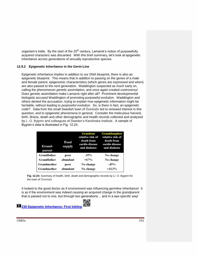
CMB3e 292

organism’s traits. By the start of the 20th century, Lamarck’s notion of purposefully

acquired characters was discarded. With this brief summary, let’s look at epigenetic

inheritance across generations of sexually reproductive species.

12.9.2 Epigenetic Inheritance in the Germ-Line

Epigenetic inheritance implies in addition to our DNA blueprint, there is also an

epigenetic blueprint. This means that in addition to passing on the genes of a male

and female parent, epigenomic characteristics (which genes are expressed and when)

are also passed to the next generation. Waddington suspected as much early on,

calling the phenomenon genetic assimilation, and once again created controversy!

Does genetic assimilation make Lamarck right after all? Prominent developmental

biologists accused Waddington of promoting purposeful evolution. Waddington and

others denied the accusation, trying to explain how epigenetic information might be

heritable, without leading to purposeful evolution. So, is there in fact, an epigenetic

code? Data from the small Swedish town of Överkalix led to renewed interest in this

question, and to epigenetic phenomena in general. Consider the meticulous harvest,

birth, illness, death and other demographic and health records collected and analyzed

by L. O. Bygren and colleagues at Sweden’s Karolinska Institute. A sample of

Bygren’s data is illustrated in Fig. 12.24.

It looked to the good doctor as if environment was influencing germline inheritance! It

is as if the environment was indeed causing an acquired change in the grandparent

that is passed not to one, but through two generations… and in a sex-specific way!

230 Epigenetic Inheritance: First Inkling

Fig. 12.24: Summary of health, birth, death and demographic records by L/. O. Bygren for

the town of Överkalix

CMB3e 293

This phenomenon was subsequently demonstrated experimentally. In one experiment,

pregnant rats were exposed to a toxin. Rat pups born to exposed mothers suffered a

variety of illnesses. This might be expected if the toxic effects on the mother were visited

on the developing pups, for example through the placenta. However, when the diseased

male rat pups matured and mated with females, the pups in the new litter grew up

suffering the same maladies as the male parent. This even though the pregnant females

in this case were NOT exposed to the toxins. Because the original female was already

pregnant when she was exposed, the germ line cells (eggs, sperm) of her litter had not

suffered mutations in utero. This could only mean that the epigenetic patterns of gene

expression caused by the toxin in pup germ line cells (those destined to become sperm &

eggs) in utero were retained during growth to sexual maturity, to be passed on to their

progeny even while gestating in a normal unexposed female.

231-2 Experimental Demonstration of Germ-Line Epigenetic Inheritance For some interesting experimental findings on how diet influences epigenetic change in

Drosophila click Dietary Change Causes Heritable Change in Drosophila Epigenome. For

recent evidence for a role of male DNA methylation in trans-generational epigenetic

inheritance, check out More on Epigenetic Inheritance across Generations. For an

amusing (but accurate) explanation of epigenetics, check out the YouTube at

https://www.youtube.com/watch?v=kp1bZEUgqVI. So, given the reality of epigenetic

inheritance, let’s consider a most intriguing question: Is epigenetic inheritance (like

Mendelian genetic inheritance) the result of natural selection?

A number of studies have correlated adverse conditions during pregnancy in animals

(including humans) with high incidences of health, behavioral and other anomalies in the

adults. This was the case in Holland for children and grandchildren of mothers pregnant

during the famine of the last winter of WWII, a season that became known as the Dutch

Hunger Winter of 1944-1945. As adults, these descendants had higher incidences heart

disease, obesity and diabetes. Such correlations were attributed to epigenetic changes in

embryonic DNA in utero (read more at Moms-environment-during-pregnancy-can-affect-

her-grandchildren.

Here is the question that should occur to us: Why should so many survivors of life in an

undernourished womb have suffered the same epigenetic changes at the same time? A

study of methylation patterns in specific DNA regions in survivors of Dutch Hunger Winter

pregnancies and a control group that missed the famine suggests an intriguing answer.

The study found unique DNA methylation patterns in those surviving adults. To explain

the survival of so many newborns that then suffered adult health anomalies, the

investigators suggested first that epigenetic modifications occur at random in embryos…,

CMB3e 294

and then suggested that some of these (i.e., the ones that marked the suffering adults)

were selected during the pregnancy because they actually conferred a survival advantage

to embryos (see details and a more complete discussion at Natural Selection in utero).

Could the many known cases of epigenetic inheritance by large cohorts of individuals be

explained by the survival advantages of epigenetic natural selection? In other words,

could epigenetic inheritance be subject to natural selection in the same way as genetic

inheritance…, perhaps with more complex results?

These days, the term epigenetics describes heritable changes in chromatin modifications

and gene expression. We now know that epigenetic configurations of chromatin that are

most stable include patterns of histone modification (acetylation, phosphorylation,

methylation…) or DNA (methylation, phosphorylation…). Such changes can convert the

30nm fiber to the 10nm ‘beads-on-a-string’ nucleosome necklace… and vice versa. Such

changes in chromatin (chromatin remodeling) lead to altered patterns of gene expression,

whether during normal development or when deranged by environmental factors

(abundance or limits on nutrition, toxins/poisons or other life-style choices). The active

study of DNA methylation patterns even has its own name, methylomics! Check out

Epigenetics Definitions and Nomenclature for more epigenetic nomenclature.

Let’s close this chapter with some socially, culturally and personally relevant questions

and some observations. For example, consider that the epigenetic consequences of

smog that Los Angelinos endured for decades are not known. And apart from the

obvious effects of lead toxicity to folks drinking lead-laden water in Flint Michigan

(especially in children), any epigenetic effects of the exposure remain to be seen.

Epigenetics continues to be a hot topic, so there’s more to think about! If environmental

causes of epigenetic change persist in a unique or isolated location or demographic,

could the natural selection of epigenetic traits result in geographic or demographic

differences in epigenetic characters just as it has done for genetic characters? Can we

trace an epigenetic ancestry in the same way as our genetic one? That seems to be the

case in a recent comparison of patterns of methylation of DNA between Mexican and

Puerto Ricans of Hispanic origin. The study revealed that DNA regions known to be

sensitive to diesel emissions or intra-uterine exposure to tobacco (and even social

stressors) were differentially methylated in the two groups. A summary of this study

(elifesciences-articles/20532.pdf) is at biotechniques.com/epigenetics-culture-&-ethnicity.

Finally, can we think of epigenetic selection of what are clearly harmful traits, as instead

analogous to genetic selection of -globin gene mutations (e.g., sickle cell anemia) that

confer a survival advantage in one context (a prevalence of malarial parasites in

mosquitoes) but are harmful in another?

CMB3e 295

Here’s a bottom line you cannot avoid! Can you be sure that your smoking habit will not

affect the health of your children or grandchildren? What about your eating habits?

Drinking? It is not just a little scary to know that I have a gullible germline epigenome that

can be influenced by my behavior, good and bad. And that my children (and maybe

grandchildren) will inherit my epigenetic legacy long before they get my house and my

money. And even that may not be the limit; epigenetic memory in C. elegans can stretch

to 14 generations (see Epigenetic Memory in Caenorhabditis elegans)! Also, read about

epigenetic inheritance resulting from Dad’s cocaine use at Sins of the Father.

Some iText & VOP Key Words and Terms

10 nm fiber galactose pseudogene

3' non-transcribed DNA galactoside transacetylase

PTS

30 nm solenoid fiber gene activation regulatory genes

5' non-transcribed DNA gene derepression second messenger

adaptive immune system gene expression nucleosomes

adult stem cells gene induction O1 and O2 lac operators

Allolactose gene regulation operator

antisense RNA gene repression operon regulation

basic v. non-basic proteins

HAT enzymes PEP-dependent P-transferase system

beads-on-a-string helix-turn-helix motif phage DNA

-galactosidase heterochromatin phosphodiester backbone

cAMP histone acetylation phosphorylation cascade cAMP receptor protein histone kinases pluripotent cells

CAP protein histone methyl transferases

polycistronic mRNA

CAT box histone methylation positive regulation

catabolite activator protein

histone phosphorylation promoter

chromatin remodeling housekeeping genes proximal regulatory element

cis-acting elements inducer exclusion signal transduction

condensed chromatin interphase steroid hormone receptors developmental program introns steroid hormones

differential gene expression

lac operon structural genes

distal regulatory element lacI gene TATA box

CMB3e 296

DNA bending lactose tetrameric lac repressor

DNAse lactose permease totipotent cells

embryonic stem cells lactose repressor transcription factors

enhancers lacZ, lacY and lacA genes

transcription regulation

environmental signals leucine zipper motif transcription start site

epigenome levels of chromatin structure

translation regulation

euchromatin major groove trp operon

exons minor groove trp repressor

extended chromatin miRNA (micro RNA) zinc finger motif

fully differentiated cells negative regulation

CMB3e 297

Chapter 13: Post Transcriptional Regulation of

Gene Expression Regulating gene expression with short and long non-coding RNAs, CRISPR-Cas

and protein phosphorylation; Control gene expression by regulating translation

13.1 Introduction

The metabolic potential of cells is flexible, depending on various mechanisms that

ultimately determine the levels and activities of proteins that dictate a cell’s metabolic

state. We have seen some of these regulatory mechanisms:

the regulation of transcription by extracellular chemical signals or developmental

chemical prompts, and

the control of enzyme or other protein activity by allosteric regulation or chemical

modification (e.g., phosphorylation or dephosphorylation).

In this chapter, we look at different kinds of post-transcriptional regulation, events

somewhere between mRNA transcription and controls on the activity of finished proteins.

These control mechanisms are most diverse in eukaryotes. Like other pathways for

regulating gene expression, post-transcriptional regulation begins with extracellular

chemical signaling. Responses include changes in the rate of polypeptide translation,

and changes in macromolecular turnover rate (e.g., changes in the half-life of specific

RNAs and proteins in cells). Regardless of mechanism, each up- or down-regulation of

CMB3e 298

gene expression contributes to changes in the steady state of a particular RNA or protein

required for proper cell function. In considering post-transcriptional regulation, we will see

how cells use specific proteins and different non-coding RNA transcripts to target

unwanted proteins or RNAs for degradation.

Learning Objectives

When you have mastered the information in this chapter, you should be able to:

1. explain what it is about C. elegans makes it a model organism for studying

development and the regulation of gene expression.

2. compare and contrast the origins and functions of miRNA and siRNA. 3. search for examples of miRNAs, siRNAs, lncRNAs and circRNAs that regulate the

expression of specific genes and explain their mechanisms.

4. explain how a riboswitch functions to control bacterial gene expression.

5. explain the origins and roles of bacterial CRISPR-Cas immune system components.

6. explain how eif2 activity is modulated to coordinate red cell heme and globin levels.

7. describe how eukaryotic cells degrade unwanted proteins and speculate on how

bacteria might do so.

8. answer the questions “How did junk DNA arise?” and “Does junk DNA have value?”

13.2 Post-transcriptional Control of Gene Expression

Not too long ago we thought that very little of the eukaryotic genome was ever

transcribed. We also thought that the only non-coding RNAs were tRNAs and rRNAs.

Now we know that other RNAs play roles in gene regulation and the degradation of spent

cellular DNA or unwanted foreign DNA. These are discussed in detail below.

13.2.1 Riboswitches

The riboswitch is a bacterial transcription mechanism for regulating gene expression.

While this mechanism is not specifically post-transcriptional, it is included here

because the action occurs after transcription initiation and aborts completion of an

mRNA. When the mRNA for an enzyme in the guanine synthesis pathway is

transcribed, it folds into stem-&-loop structures. Enzyme synthesis will continue for as

long as the cell needs to make guanine. But if guanine accumulates in the cell,

excess guanine will bind stem-loop elements near the 5’ end of the mRNA, causing

the RNA polymerase and the partially completed mRNA dissociate from the DNA,

prematurely ending transcription. The ability to form folded, stem-loop structures at

the 5’ ends of bacterial mRNAs seems to have allowed the evolution of translation

regulation strategies. Whereas guanine interaction with the stem-loop structure of an

emerging 5’ mRNA can abort its own transcription, similar small metabolite/mRNA and

even protein/mRNA interactions can also regulate (in this case prevent) translation.

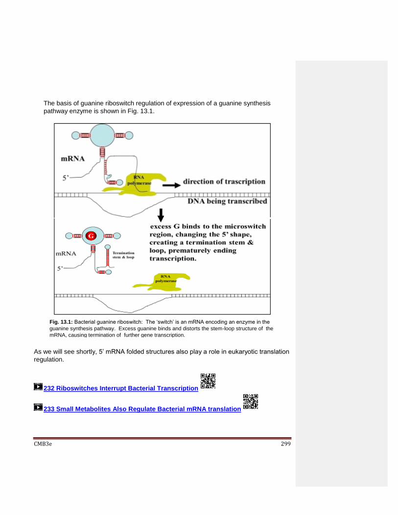
CMB3e 299

The basis of guanine riboswitch regulation of expression of a guanine synthesis

pathway enzyme is shown in Fig. 13.1.

As we will see shortly, 5’ mRNA folded structures also play a role in eukaryotic translation

regulation.

232 Riboswitches Interrupt Bacterial Transcription

233 Small Metabolites Also Regulate Bacterial mRNA translation

Fig. 13.1: Bacterial guanine riboswitch: The ‘switch’ is an mRNA encoding an enzyme in the

guanine synthesis pathway. Excess guanine binds and distorts the stem-loop structure of the

mRNA, causing termination of further gene transcription.

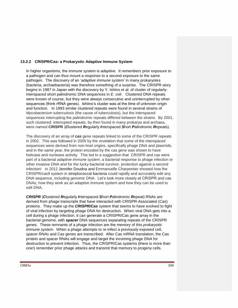
CMB3e 300

13.2.2 CRISPR/Cas: a Prokaryotic Adaptive Immune System

In higher organisms, the immune system is adaptive. It remembers prior exposure to

a pathogen and can thus mount a response to a second exposure to the same

pathogen. The discovery of an ‘adaptive immune system’ in many prokaryotes

(bacteria, archaebacteria) was therefore something of a surprise. The CRISPR story

begins in 1987 in Japan with the discovery by Y. Ishino et al. of cluster of regularly-

interspaced short palindromic DNA sequences in E. coli. Clustered DNA repeats

were known of course, but they were always consecutive and uninterrupted by other

sequences (think rRNA genes). Ishiino’s cluster was at the time of unknown origin

and function. In 1993 similar clustered repeats were found in several strains of

Mycobacterium tuberculosis (the cause of tuberculosis), but the interspaced

sequences interrupting the palindromic repeats differed between the strains. By 2001,

such clustered, interrupted repeats, by then found in many prokarya and archaea,

were named CRISPR (Clustered Regularly Interspaced Short Palindromic Repeats).

The discovery of an array of cas gene repeats linked to some of the CRISPR repeats

in 2002. This was followed in 2005 by the revelation that some of the interspaced

sequences were derived from non-host origins, specifically phage DNA and plasmids,

and in the same year, the protein encoded by the cas gene was shown to have

helicase and nuclease activity. This led to a suggestion that CRISPR and cas were

part of a bacterial adaptive immune system, a bacterial response to phage infection or

other invasive DNA and for the lucky bacterial survivor, protection against a second

infection! In 2012 Jennifer Doudna and Emmanuelle Charpentier showed how the

CRISPR/cas9 system in streptococcal bacteria could rapidly and accurately edit any

DNA sequence, including genomic DNA. Let’s look more closely at CRISPR and cas

DNAs, how they work as an adaptive immune system and how they can be used to

edit DNA.

CRISPR (Clustered Regularly Interspaced Short Palindromic Repeat) RNAs are

derived from phage transcripts that have interacted with CRISPR-Associated (Cas)

proteins. They make up the CRISPR/Cas system that seems to have evolved to fight

of viral infection by targeting phage DNA for destruction. When viral DNA gets into a

cell during a phage infection, it can generate a CRISPR/Cas gene array in the

bacterial genome, with spacer DNA sequences separating repeats of the CRISPR

genes. These remnants of a phage infection are the memory of this prokaryotic

immune system. When a phage attempts to re-infect a previously exposed cell,

spacer RNAs and Cas genes are transcribed. After Cas mRNA translation, the Cas

protein and spacer RNAs will engage and target the incoming phage DNA for

destruction to prevent infection. Thus, the CRISPR/Cas systems (there is more than

one!) remember prior phage attacks and transmit that memory to progeny cells.

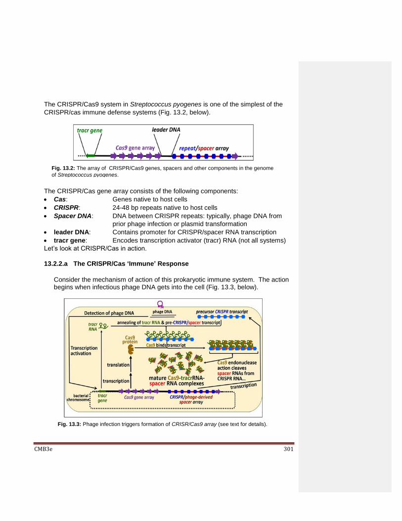
CMB3e 301

The CRISPR/Cas9 system in Streptococcus pyogenes is one of the simplest of the

CRISPR/cas immune defense systems (Fig. 13.2, below).

The CRISPR/Cas gene array consists of the following components:

Cas: Genes native to host cells

CRISPR: 24-48 bp repeats native to host cells

Spacer DNA: DNA between CRISPR repeats: typically, phage DNA from

prior phage infection or plasmid transformation

leader DNA: Contains promoter for CRISPR/spacer RNA transcription

tracr gene: Encodes transcription activator (tracr) RNA (not all systems)

Let’s look at CRISPR/Cas in action.

13.2.2.a The CRISPR/Cas ‘Immune’ Response

Consider the mechanism of action of this prokaryotic immune system. The action begins when infectious phage DNA gets into the cell (Fig. 13.3, below).

Fig. 13.2: The array of CRISPR/Cas9 genes, spacers and other components in the genome

of Streptococcus pyogenes.

Fig. 13.3: Phage infection triggers formation of CRISR/Cas9 array (see text for details).

CMB3e 302

Let’s summarize what has happened here:

a) Incoming phage DNA was detected after phage infection.

b) Then the tracr and Cas genes are transcribed along with the CRISPR/spacer

region. Cas mRNAs are translated to make the Cas protein. Remember, the

spacer DNAs in the CRISPR region are the legacy of a prior phage infection.

c) CRISPR/spacer RNA forms hydrogen bonds with a complementary region of

the tracr RNA as the two RNAs associate with Cas proteins.

d) Cas protein endonucelases hydrolyze spacer RNA from CRISPR RNA

sequences. The spacer RNAs remain associated with the complex while the

actual, imperfectly palindromic CRISPR sequences (shown in blue in the

illustration above) fall off.

In the next steps, phage-derived spacer RNAs, now called guide RNAs (or

gRNAs) ‘guide’ mature Cas9/tracrRNA/spacer RNA complexes to new incoming

phage DNA resulting from a phage attack. Fig. 13.4 (below) illustrates the

association of the complex with the incoming phage DNA and subsequent events.

Once again, let’s summarize:

a) Spacer (i.e., gRNA) in the complex targets incoming phage DNA.

b) Cas helicase unwinds incoming phage DNA at complementary regions.

c) gRNA H-bonds to incoming phage DNA.

Fig. 13.4: Phage spacers in a CRISPR/Cas9 array (derived from an earlier phage infection)

protects against phage re-infection (see text for details) .

CMB3e 303

d) Cas endonucleases create a double-stranded break (hydrolytic cleavage) at

specific sites in incoming phage DNA. Because precise site DNA strand

cleavage is guided by RNA molecules, CRISPR/Cas endonucleases are

classified as type V restriction enzymes.

e) The incoming phage DNA is destroyed and a new phage infection is aborted.

Check out More about CRISPR in Wikipedia to learn more about how bacteria

acquire spacer DNAs, and therefore how this primitive adaptive immune system

‘remembers’) in the first place.

13.2.2.b Using CRISPR/Cas to Edit/Engineer Genes

Early studies demonstrated the reproducible cleavage of incoming phage DNA at

specific nucleotides. Several labs quickly realized that it might be possible to

adapt the system to cut DNA at virtually any specific nucleotide in a target DNA! It

has turned out that the system works both in vivo and in vitro, allowing virtually

unlimited potential for editing genes and RNAs in a test tube… or in any cell. Here

is the basic process:

a) Engineer gDNA with a Cas-specific DNA sequence that targets a desired target

in genomic DNA.

b) Fuse the gDNA to tracr DNA to make a single guide DNA (sgDNA) so that it

can be made as a single guide transcript (sgRNA).

c) Engineer a CRISPR/Cas9 gene array that substitutes this sgDNA for its original

spacer DNAs.

d) Place engineered array in a plasmid next to regulated promoters.

e) Transform cells by ‘electroporation’ (works for almost any cell type!)

f) Activate the promoter to transcribe the CRISPR/Cas9 genes…

The applications are powerful… and controversial!

13.2.2.c CRISPR…, the Power and the Controversy

The application of gene editing with CRISPR/Cas systems has already facilitated

studies of gene function in vitro, in cells and in whole organisms. Click CRISPR

Applications from NEB for a description of CRISPR/Cas applications already on

the market! The efficiency of specific gene editing using CRISPR/Cas systems

holds great promise for understanding basic gene structure and function, for

determining the genetic basis of disease, and for accelerating the search for gene

therapies. Here are a few examples of how CRISPR/Cas editing is being applied.

One can engineer an sgRNA with desired mutations targeting specific sites in chromosomal DNA. Then clone sgRNA into the CRISPR/Cas9 array on a plasmid. After transformation of appropriate cells, the engineered

CMB3e 304

CRISPR/Cas9 forms a complex with target DNA sequences. Following nicking of both strands of the target DNA, DNA repair can insert the mutated guide sequences into the target DNA. The result is loss or acquisition of DNA

sequences at specific, exact sites, or Precision Gene Editing. The ability to do

this in living cells that has excited the basic and clinical research communities.

Before transforming cells, engineer the CRISPR/Cas9 gene array on the plasmid to eliminate both endonuclease activities from the Cas protein. Upon transcription of the array in transformed cells, the CRISPR/Cas9-sgRNA still finds an sgRNA-targeted gene. However, lacking CAS protein endonuclease activities, the complex that forms just sits there blocking transcription. This technique is sometimes referred to as CRISPRi (CRISPER interference), by analogy to RNA interference or RNAi (see below). Applied to organisms (and

not just in vitro or to cells), it mimics the much more difficult knockout mutation

experiments that have been used in studies of behavior of cells or organisms

rendered unable to express a specific protein.

There are now several working CRISPR/Cas systems capable of Precision

Gene Editing. They are exciting for their speed, precision, their prospects for

rapid, targeted gene therapies to fight disease, and their possibilities to alter

entire populations (called Gene Drive). By inserting modified genes into the

germline cells of target organisms, gene drive can render harmless entire

malarial mosquito populations, to eliminate pesticide resistance in e.g. insects,

eliminate herbicide resistance in undesirable plants, or genetically eliminate

invasive species. For more information, click Gene drive; for an easy read

about this process and the controversies surrounding applications of CRISPR

technologies to mosquitoes in particular, check out J. Adler, (2016) A World

Without Mosquitoes. Smithsonian, 47(3) 36-42, 84.

It is possible to delete an entire chromosome from cells. This bit of global

genetic engineering relies on identifying multiple unique sequences on a single

chromosome and then targeting these sites for CRISPR/Cas. When the

system is activated, the chromosome is cut at those sites, fragmenting it

beyond the capacity of DNA repair mechanisms to fix the situation. Imagine the

possibilities for therapeutically removing aneuploidies, e.g., extra

chromosomes such as found in trisomy 21 (the cause of Down’s Syndrome),

or those correlated with some cancers. Click Using CRISPR/Cas9 to delete a

chromosome to learn more.

For yet another twist on CRISPR power, check CRISPR-Based ID of genes in

situ in Chromatin in Fixed Cells to read about a technique to identify and locate

specific DNA sequences in cells without disturbing chromatin structure.

CMB3e 305

But a ‘dark side’ of the CRISPR/cas (and now, related gene editing technologies)

was quickly recognized by its practitioners, notably Jennifer Doudna herself. If for

no other reason than its efficiency and simplicity, applications of CRISPR to

precision gene editing has raised ethical issues. Clearly, the potential exists for

abuse, or even for use with no beneficial purpose at all. It is significant that, as in

all discussions of biological ethics, scientists are very much engaged in the

conversation. Listen to Dr. Doudna talk about CRISPR and its potential to do good

in the world, and its potential to be abused by the foolish and unscrupulous

(https://www.youtube.com/watch?v=TdBAHexVYzc).

We will no doubt continue to edit genes with CRISPR/Cas, and we can look for a

near future Nobel Prize for its discovery and application! If you still have qualms,

maybe RNA editing will be the answer. Check out the link at Why edit RNA? for an

overview of the possibilities! Finally, “mice and men” (and women and babies too)

have antibodies to Cas9 proteins, suggesting prior exposure to microbial

CRISPR/Cas9 antigens. This observation may limit clinical applications of the

technology! See Uncertain Future of CRISPR-Cas9 Technology.

13.2.3 The Small RNAs: miRNA and siRNA in Eukaryotes

Micro RNAs (miRNAs) and small interfering RNAs (siRNAs) are found in C.

elegans, a small nematode (roundworm) that quickly became a model for studies

of cell and molecular biology and development shown in a fluorescence

micrograph in Fig. 13.5 below.

Fig. 13.5: Anatomic the roundworm Caenorhabditis elegans.

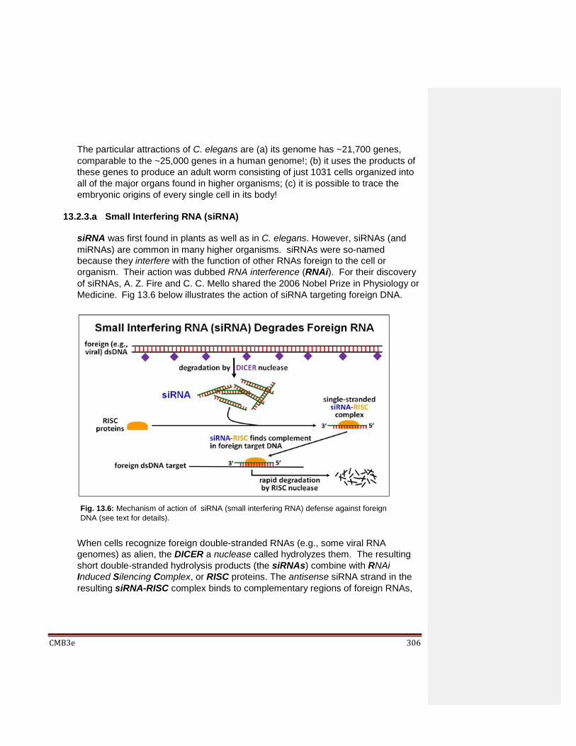
CMB3e 306

The particular attractions of C. elegans are (a) its genome has ~21,700 genes,

comparable to the ~25,000 genes in a human genome!; (b) it uses the products of

these genes to produce an adult worm consisting of just 1031 cells organized into

all of the major organs found in higher organisms; (c) it is possible to trace the

embryonic origins of every single cell in its body!

13.2.3.a Small Interfering RNA (siRNA)

siRNA was first found in plants as well as in C. elegans. However, siRNAs (and

miRNAs) are common in many higher organisms. siRNAs were so-named

because they interfere with the function of other RNAs foreign to the cell or

organism. Their action was dubbed RNA interference (RNAi). For their discovery

of siRNAs, A. Z. Fire and C. C. Mello shared the 2006 Nobel Prize in Physiology or

Medicine. Fig 13.6 below illustrates the action of siRNA targeting foreign DNA.

When cells recognize foreign double-stranded RNAs (e.g., some viral RNA

genomes) as alien, the DICER a nuclease called hydrolyzes them. The resulting

short double-stranded hydrolysis products (the siRNAs) combine with RNAi

Induced Silencing Complex, or RISC proteins. The antisense siRNA strand in the

resulting siRNA-RISC complex binds to complementary regions of foreign RNAs,

Fig. 13.6: Mechanism of action of siRNA (small interfering RNA) defense against foreign

DNA (see text for details).

CMB3e 307

targeting them for degradation. Cellular use of RISC to control gene expression in

this way may have derived from the use of RISC proteins by miRNAs as part of a

cellular defense mechanism, to be discussed next. Custom-designed siRNAs

have been used to disable expression of specific genes in order to study their

function in vivo and in vitro. Both siRNAs and miRNAs are being investigated as

possible therapeutic tools to interfere with RNAs whose expression leads to cancer

or other diseases.

234 siRNA Post Transcriptional Regulation

235 Did siRNA Coopt RISC strategy to Trash Corrupt or Worn out RNA?

For an example check out a YouTube video of unexpected results of an RNAi

experiment at https://www.youtube.com/watch?v=-3XboKthxM8. In the experiment

described, RNAi was used to block embryonic expression of the orthodenticle

(odt) gene that is normally required for the growth of horns in a dung beetle. The

effect of this knock-out mutation was, as expected, to prevent horn growth. What

was unexpected however, was the development of an eye in the middle of the

beetle’s head (‘third eye’ in the micrograph). The 3rd eye not only looks like an

eye, but is a functional one. This was demonstrated by preventing normal eye

development in odt-knockout mutants. The 3rd eye appeared and was responsive

to light! Keep in mind that this was a beetle with a 3rd eye, not Drosophila! To

quote Justin Kumar from Indiana University, who though not involved in the

research, stated that “…lessons learned from Drosophila may not be as generally

applicable as I or other Drosophilists, would like to believe … The ability to use

RNAi in non-traditional model systems is a huge advance that will probably lead to

a more balanced view of development.”

13.2.3.b Micro RNAs (miRNA)

miRNAs target unwanted endogenous cellular RNAs for degradation. miRNAs are

transcribed from genes now known to be widely distributed in eukaryotes. As they

are transcribed, pre-miRNAs fold into a stem-loop structure that is lost during

cytoplasmic processing. Like SiRNAs, mature miRNAs combine with RISC

proteins. The RISC protein-miRNA complex targets old or no-longer needed

mRNAs or mRNAs damaged during transcription. An estimated 250 miRNAs in

humans may be sufficient to H-bond to diverse target RNAs; only targets with

strong complementarity to a RISC protein-miRNA complex will be degraded.

The pathway from pre-miRNA transcription through processing ultimately to target

mRNA degradation is shown in Fig. 13.7, below.

CMB3e 308

236 miRNA Post-Transcriptional Regulation

13.2.4 Long Non-Coding RNAs

Long non-coding RNAs (lncRNAs) are a yet another class of eukaryotic RNAs. The

latter include transcripts of antisense, intronic, intergenic, pseudogene and retroposon

DNA. Retroposons are one kind of transposon, or mobile DNA element; pseudogenes

are recognizable genes with mutations that make them non-functional. While some

lncRNAs might turn out to be incidental transcripts that the cell simply destroys, others

have a role in regulating gene expression.

A recently discovered lncRNA is XistAR that, along with the Xist gene product, is

required to form Barr bodies. Barr bodies form in human females when one of the X

chromosomes in somatic cells is inactivated. For a review of lncRNAs, see Lee, J.T.

(2012. Epigenetic Regulation by Long Noncoding RNAs; Science 338, 1435-1439).

Fig. 13.7: Mechanism of action of miRNA (micro RNA) in degrading unwanted (e.g., old or

damaged ) RNA (see text for details).

CMB3e 309

An even more recent article (at lncRNAs and smORFs) summarizes the discovery that

some long non-coding RNAs contain short open reading frames (smORFs) that are

actually translated into short peptides of 30+ amino acids! Who knows? The human

genome may indeed contain more than 21,000-25,000 protein-coding genes!

13.2.5 Circular RNAs (circRNA)

Though discovered more than 20 years ago, circular RNAs (circRNAs) are made in

different eukaryotic cell types. Click Circular RNAs (circRNA) to learn more about this

peculiar result of alternative splicing. At first circRNAs were hard to isolate. When

they were isolated, circRNAs contained “scrambled” exonic sequences and were

therefore thought to be nonfunctional errors of mRNA splicing. In fact, circRNAs are

fairly stable. Their levels can rise and fall in patterns suggesting that they are

functional molecules. Levels of one circRNA, called circRims1, rise specifically

during neural development. In mice, other circRNAs accumulate during synapse

formation, likely influencing how these neurons will ultimately develop and function.

Thus, circRNAs do not seem to be ‘molecular mistakes’. In fact, errors in their own

synthesis may be correlated with disease! Speculation on the functions of circRNAs

also includes roles in gene regulation, particularly the genes or mRNAs from which

they themselves are derived.

13.3 “Junk DNA” in Perspective

Not long ago we thought that less than 5% of a eukaryotic genome was transcribed (i.e.,

as mRNA, rRNA and tRNA), and that much of the non-transcribed genome served a

structural function… or no function!. The latter, labeled junk DNA, included non-descript

intergenic sequences, pseudogenes, ‘dead’ transposons, long stretches of intronic DNA,

etc. Thus, junk DNA was DNA we could do without. Junk DNAs were thought to be

accidental riders in our genomes, hitchhikers picked up on the evolutionary road. But,

while miRNA genes are a small proportion of a eukaryotic genome, their discovery, and

that of more abundant lnc RNAs suggest a far greater amount of functional DNA in the

genome. Might there be in fact, no such thing as “junk DNA”?

The debate about how much of our genomic DNA is a relic of past evolutionary

experiments and without genetic purpose continues. Read all about it at Junk DNA - not

so useless after all and Only 8.2% of human DNA is functional. Perhaps we need to re-

think what it means for DNA to be “junk” or to be without “genetic purpose”. Maintenance

of more than 90% of our own DNA with no known genetic purpose surely comes at an

energy cost. At the same time, all of that DNA is grist for future selection, a source of the

diversity required for long-term survival. The same natural selection that picks up

‘hitchhiker’ DNA sequences, as we have seen, can at some point, put them to work!

CMB3e 310

13.4 The RNA Methylome

Call this an RNA epi-transcriptome if you like! Recall that methyl groups direct cleavage

of ribosomal RNAs from eukaryotic 45S pre-RNA transcripts. tRNAs among other

transcripts, are also post-transcriptionally modified. Known since the 1970s, such

modifications were thought to be non-functional. But are they?

13.5 Eukaryotic Translation Regulation

mRNAs are made to be translated, and so they are! Nonetheless, translation is

regulated, largely by controlling translation initiation. Here’s a reminder of the basics of

eukaryotic initiation… In many respects, the overall process is similar to prokaryotic

translation initiation described elsewhere. The 40S ribosomal subunit itself can bind to

and scan an mRNA, seeking the start site of an ORF (open reading frame) encoding a

polypeptide. When GTP-bound eukaryotic initiation factor 2 (GTP-eIF2) binds met-tRNAf,

it forms a ternary complex (TC). The TC can associate with the scanning 40S subunit.

When a TC-associated scanning subunit encounters the start site of the ORF, scanning

stalls. Additional eIFs help form the initiation complex, positioning the initiator tRNA

anticodon over the start site AUG in the mRNA. The initiation complex then recruits the

large (60S) ribosomal subunit.

Consider translation initiation in eukaryotes ( Fig. 13.8, below). Note that the binding of

the 60S ribosomal subunit to the initiation complex (lower left) causes the release of all

the eIFs and hydrolysis of the GTP on eIF2; GDP remains bound to eIF2 upper right).

Fig. 13.8: Review of the steps in translation initiation (see text for details).

CMB3e 311

For protein syntheses to continue, new GTP must replace GDP on eIF2. Another

initiation factor, eIF2B, facilitates this GTP/GDP swap, recycling GTP-eIF2 for use in

initiation. The regulation of translation is superimposed on these basic processes. But

where? What steps in initiation are controlled?

We know that CAP and poly(A) tails on mRNAs are required for efficient translation

because mRNAs engineered to lack one and/or the other are poorly translated. But there

is little evidence that cells control capping or polyadenylation, or the structures

themselves. Instead, translation is regulated, largely by targeting interactions with

structural features and sequences in the 5’ region of mRNAs. Fig. 13.9 (below) shows

key structural motifs in a gene that can contribute to translational control.

Regulation of translation may be global, affecting the synthesis of many polypeptides.

Or it may be specific, affecting a single polypeptide. Global regulation involves changes

in the activity of eukaryotic initiation factors (eIFs) that would typically affect all cellular

protein synthesis. Specific regulation involves binding sequences or regions on one or a

few mRNAs that recognize and bind specific regulatory proteins and/or other molecules.

In the latter case, such binding controls translation of only those mRNAs, without

affecting general protein biosynthesis. We will consider three examples of translational

control of gene expression.

13.5.1 Specific Translation Control by mRNA Binding Proteins

Translation initiation complexes typically scan the 5’-UTR of an mRNA. When it finds

the translation start site, it can bind the large subunit and begin translating the

polypeptide. Here we consider the control of synthesis of ferritin, a cytplasmic iron-

binding protein. Iron is of course insoluble and must be bound to proteins, both in cells

Fig. 13.9: Regions and specific sequences known to be involved in regulating translation.

CMB3e 312

and in the blood (the latter is a story for another time and place!). Once in the cell, iron

binds to the ferritin. As you may guess, cellular iron metabolism depends of levels of

ferritin in the cell, which is regulated at the level of translation.

Ferritin is actually a two-subunit protein, and the 5’-UTR of the mRNAs for both

polypeptide chains contain iron-responsive elements (IREs). These IREs are stem-

loop structures that specifically recognize and bind iron regulatory proteins (IRP1,

IRP2). In iron-deficient cells, the IRPs normally bind to the IRE to block ferritin

translation as illustrated in Fig. 13.10 (below).

Normally, the initiation complex scans the 5’-UTR of an mRNA. When it finds the

normal translation start site, it can bind the large subunit and begin translating the

polypeptide. In iron-deficient cells, scanning by the initiation complex is thought to be

physically blocked by steric hindrance.

13.5.2 Coordinating Heme and Globin Synthesis

Consider that reticulocytes (the precursors to erythrocytes, the red blood cells in

mammals) synthesize globin proteins. They also synthesize heme, an iron-bound

porphyrin-ring molecule. Each globin must bind to a single heme to make a

hemoglobin protein subunit. Clearly, it would not do for a reticulocyte to make too

much globin protein and not enough heme, or vice versa. It turns out that hemin (a

precursor to heme) regulates the initiation of translation of both and globin

mRNAs. Recall that, to sustain globin mRNA translation, the GDP-eIF2 generated

Fig. 13.10: Specific inhibition of ferritin polypeptide synthesis by iron regulatory proteins.

CMB3e 313

after each cycle of translation elongation must be exchanged for fresh GTP. This is

facilitated by the eIF2B initiation factor. eIF2B can exist in phosphorylated (inactive)

or un-phosphorylated (active) states. Making sure that globin is not under- or

overproduced relative to heme biosynthesis involves controlling levels of active vs.

inactive eIF2B by hemin. Hemin accumulates when there is not enough globin

polypeptide to combine with heme in the cell.

Excess hemin binds and inactivates an HCR kinase, preventing phosphorylation of

eIF2B. Since unphosphorylated eiF2B is active, it facilitates the GTP/GDP swap

needed to allow continued translation. Thus, ongoing initiation ensures that globin

mRNA translation can keep up with heme levels. In other words, if hemin production

gets ahead of globin, it will promote more globin translation. When globin and heme

levels become approximately equimolar, hemin is no longer in excess. It then

dissociates from the active HCR kinase. The now- active kinase catalyzes eIF2B

phosphorylation. Phospho-eIF2B is inactive and cannot facilitate the GTP/GDP swap

on eIF2. Globin mRNA translation initiation, thus blocked, allows a lower rate of globin

polypeptide translation to keep pace with heme synthesis. Fig. 13.11 (below)

illustrates the regulation of globin mRNA translation initiation by hemin.

237 Translation Regulation of Globin Polypeptide Synthesis

Fig. 13.11: Regulation of globin mRNA Translation initiation by hemin, a heme precursor

(see text for details)

CMB3e 314

13.5.3 Translational Regulation of Yeast GCN4

Like the coordination of heme and globin production, the regulation of the GCN4

protein is based on controlling the ability of the cells to swap GTP for GDP on eIF2.

However, this regulation is quite a bit more complex, despite the fact that yeast is a

more primitive eukaryote! GCN4 is a global transcription factor that controls the

transcription of as many as 30 genes in pathways for the synthesis of 19 out of the 20

amino acids! The discovery that amino acid starvation caused yeast cells to increase

their production of amino acids in the cells led to the discovery of the General Amino

Acid Control (GAAC) mechanism involving GCN4. GCN is short for General Control

Nondepressible, referring to its global, positive regulatory effects. It turns out that the

GCN4 protein is also involved in stress gene expression, glycogen homeostasis,

purine biosynthesis…, in fact in the action of up to 10% of all yeast genes! Here we

focus on the GAAC mechanism.

Yeast cells provided with ample amino acids do not need to synthesize them. Under

these conditions, GCN4 is present at basal (i.e., low) levels. On the other hand, when

the cells are starved of amino acids, GCN4 levels increase as much as ten-fold within

two hours, resulting in an increase in general amino acid synthesis. Amino acid

starvation signals an increase in the activity of GCN2, a protein kinase. The GCN2

kinase catalyzes phosphorylation of GDP-eIF2. As we have seen, phosphorylated

eIF2B cannot exchange GTP for GDP on the eIF2, with results shown in Fig.13.12.

Fig. 13.12: Role of GCN2 kinase in regulating translation by phosphorylating initiation factor

eIF2B, preventing formation of an initiation complex (see text for details).

CMB3e 315

There is a paradox here. You would expect a slowdown in GTP-eIF2 regeneration to

inhibit overall protein synthesis, and it does. However, the reduced levels of GTP-

eIF2 somehow also stimulate translation of the GCN4 mRNA, leading to increased

transcription of the amino acid synthesis genes. In other words, amino acid starvation

leads yeast cells to use available substrates to make their own amino acids in order

that protein synthesis can continue… at the same time as initiation complex formation

is disabled! Let’s accept that paradox for now and look at how amino acid starvation

leads to increased translation of the GCN4 protein and the up-regulation of amino acid

biosynthesis pathways. To begin with, we are going to need to understand the

structure of GCN4 mRNA. In Fig. 13.13 below, note the 4 short uORFs in the 5’UTR

of the RNA; these play a key role in GCN4 translation regulation.

Recall that eIF2 binds with GTP and the initiator met-tRNA to form a ternary complex

(TC). .We also noted earlier TC-associated 40S ribosomal subunits scan mRNAs to

find open reading frame translation start sites, allowing initiation complexes form.

When a 60S ribosomal subunit binds, polypeptide translation starts. But while uORFs

in the GCN4 mRNA encode only a few amino acids before encountering a stop codon,

they can also be recognized during scanning. When TCs and 40S subunits are

plentiful, they engage uORFs in preference to the GCN4 coding region ORF (Fig.

13.14).

Fig. 13.13: Multiple short open reading frames (uORFs) in the 5’ untranslated region (5’UTR)

of GCN4 mRNA play a role in regulating its translation.

Fig. 13.14: GCN4 translation is reduced when cellular amino acid levels are normal (see text for

details).

CMB3e 316

Under these conditions, active eIF2B allows the GTP/GDP swap on GDP-eIF2,

leading to efficient GTP-eIF2 recycling and high TC levels. TCs bound to small (40S)

subunits during scanning and/or at the start sites of uORFs, form initiation complexes

that then bind 60S ribosomal subunits and begin uORF translation. The effect is to

slow down scanning past the uORFs, thereby inhibiting initiation complex formation at

the actual GCN4 ORF.

What happens in amino acid-starved cultures of yeast cells, when GTP-eIF2 cannot

be efficiently regenerated and TCs are in short supply? To review, amino acid

starvation signals an increase in GCN2 kinase activity resulting in phosphorylation and

inactivation of eIF2B. Inactive phospho-eIF2 will not facilitate the GTP/GDP swap at

GDP-eIF2, inhibiting overall protein synthesis. The resulting reduction in GTP-eIF2

also lowers the levels of TC and TC-associated 40S subunits. In Fig. 13.15, see how

this phenomenon up-regulates GCN4 translation, even as the translation of other

mRNAs has declined.

Under these conditions, initiation complex formation at uORFs is less likely, and scanning by remaining TC-40S complexes is more likely to reach the GCN4 ORF and increase GCN4 translation! The increased production of the gene-regulatory GCN4 protein then turns on virtually all of the genes for enzymes of amino acid biosynthesis. The cells thus make their own amino acids when the medium has few to contribute! For a good review of the translation-level regulation in general, and of GCN4, click Regulation of GCN4 Translation.

13.6 Protein Turnover in Eukaryotic Cells: Regulating Protein Half-Life

We have already seen that organelles have a finite life span, or half-life. Recall that

lysosomes participate in destroying worn out mitochondria, including their molecular

components. We also saw the role of small RNAs (especially miRNA) in destroying old,

Fig. 13.15: GCN4 translation is highest when cellular amino acid levels are reduced (amino acid

starvation). GCN4 then regulates the expression of many genes, including those encoding

enzymes needed for amino acid synthesis (see text for details).

CMB3e 317

damaged or otherwise unwanted RNAs from cells. All cell structures and molecules have

a finite half-life, defined as the time it takes for half of them to disappear in the absence

of new synthesis of the structure or molecule. As we already know, the steady-state level

of any cellular structure or molecule exists when the rate of its manufacture or synthesis

is balanced by the rate of its turnover. Of course, steady state levels of things can

change. For example, the level of gene expression (the amount of a final RNA or protein

gene product in a cell) can change if rates of transcription, processing or turnover change.

We should also expect the same for the steady-state levels of cellular proteins. Here we

consider the factors that govern the half-life of cellular proteins.

The half-life of different proteins seems to be inherent in their structure. Thus, some

amino acid side chains are more exposed at the surface of the protein and are thus more

susceptible to change or damage over time than others. Proteins with fewer ‘vulnerable’

amino acids should have a longer half-life than those with more of them. Proteins

damaged by errors of translation, folding, processing gone awry or just worn out from use

or ‘old age’ will be targeted for destruction. All molecules have a half-life! The

mechanism for detecting and destroying unwanted old, damaged or misbegotten proteins

involves a 76-amino acid polypeptide called ubiquitin that targets the protein for

destruction, delivering it to a large complex of polypeptides called the proteasome. Here

is what happens:

1. The first step is to activate an ubiquitin. This starts when ATP hydrolysis fuels the

binding of ubiquitin to an ubiquitin-activating enzyme.

2. An ubiquitin-conjugating enzyme then replaces the ubiquitin-activation enzyme.

3. The protein destined for destruction replaces the ubiquitin-conjugating enzyme. 4. Several more ubiquitins then bind to this complex.

5. The poly-ubiquinated protein delivers its protein to one of the 19S ‘CAP’ structures

of a proteasome.

6. After binding to one of the CAP structures of a proteasome, the poly-ubiquinated

target proteins dissociate and the ubiquitins are released and recycled as the target

protein unfolds (powered by ATP hydrolysis). The unfolded protein then enters a 20S

core proteasome.

The target protein is digested to short peptide fragments by proteolytic enzymes in the

interior of the proteasome core. The fragments are release from the CAP complex at the

other end of the proteasome and digested down to free amino acids in the cytoplasm.

There is a mind-boggling variety of proteins in a cell…, and there are as many as 600

different ubiquitin proteins, encoded by as many genes! Presumably, each ubiquitin

handles a subclass of proteins based on common features of their structure. The

structurally complex 26S proteasome is smaller than a eukaryotic small ribosomal subunit

(40S), but it is nevertheless one of the largest cytoplasmic particles, even without the

benefit of any RNA in its structure!

CMB3e 318

Fig 13.16 details the role of ubiquitin in the degradation of a worn-out protein by a

proteasome. Click on Proteasomes in Action to see an animated version of this

illustration.

Some iText & VOP Key Words and Terms

19S proteasome cap complex gene editing RISC endonuclease

20S proteasome complex global transcription factor RISC proteins

amino acid starvation globin RNA interference

Fig. 13.15: Mechanism of ubiquitin and proteasome action in the removal/destruction of old and

damaged proteins in cells, and the recycling of their amino acids (see text for details).

CMB3e 319

Barr Bodies gRNA RNA turnover rates

C. elegans GTP/GDP swap RNAi

Cas GTP-eiF2 recycling RNA-induced silencing complex

Cas helicase activity half life sgRNA

Cas9 endonuclease HCR kinase siRNA (small interfering RNA)

circRNA heme small RNAs

circular RNA hemin smORF

CRISPR HRC kinase spacer RNA

CRISPR interference Initiation complex scanning steady state

CRISPR/Cas iron regulatory protein Streptococcus pyogenes

CRISPR/Cas9 gene array IRP tracr

CRISPRi Junk DNA tracr gene

dicer lncRNA tracr RNA

eiF2 phosphorylation long non-coding RNA translation elongation

eiF2B micro RNA ubiquitin

EIIAGlc miRNA ubiquitination

Ferritin mRNA scanning uORF

GAAC proteasome XistAR

GCN2 protein turnover rates Yeast GCN4

GDP-eIF2 riboswitch

Gene Drive RISC

CMB3e 320

Chapter 14: Repetitive DNA, A Eukaryotic

Genomic Phenomenon

Mini-Satellite DNA, Microsatellite DNA, Telomeres, Ribosomal RNA genes,

Transposons (Selfish, Junk DNA or Architects of the Genome?)

14.1 Introduction

Because of their small size, bacterial genomes have few repetitive DNA sequences. In

contrast, repetitive DNA sequences make up a large part of a eukaryotic genome. Much

of this repeated DNA consists of identical or nearly identical sequences of varying length

repeated many times in a genome. Examples include satellite DNA (minisatellite and

microsatellite DNA) and transposons, or transposable elements. Here we look at

experiments that first revealed the existence and proportion of repeated DNA in genomes.

Next we describe Barbara McClintock’s even earlier (and pretty amazing!) discovery of

transposable elements. After we describe the different classes of transposons and

different mechanisms of transposition, we tackle the question of why they and other

repetitive DNAs even exist. Elsewhere we introduced the notion of junk DNA as DNA

sequences that serve no known purpose. Is repeated DNA actually junk DNA? In

particular, are transposable elements junk? We are now learning that transposons and

other repetitive DNAs can have specific functions, from regulating gene expression to

reshaping genomes to increasing genetic diversity in evolution. So, far from being ‘junk’,

much redundant DNA exists in genomes because of evolutionary selection.

Learning Objectives

When you have mastered the information in this chapter, you should be able to:

1. compare and contrast renaturation kinetic data.

2. explain CoT curves and DNA complexity.

3. list physical and chemical properties of main band and satellite DNAs.

CMB3e 321

4. outline an experiment to determine if a given sequence of DNA is repetitive or not.

5. summarize how Barbara McClintock revealed the genetics of maize mosaicism.

6. outline the experiments suggesting that the Ds gene moves from one locus to

another in the maize genome.

7. compare and contrast cut-&-paste and replicative transposition.

8. compare the behaviors of autonomous and non-autonomous transposons.

9. list the differences between Mu phage infection and transposition.

10. describe the common structural features of transposons.

11. compare the mechanisms of LINE and SINE transposition.

12. speculate on how species avoid potentially lethal consequences of transposition.

13. speculate on which came first in evolution: DNA transposons, RNA transposons or

retroviruses, and explain your reasoning.

14.2 The Complexity of Genomic DNA

By the 1960s, when Roy Britten and Eric Davidson were studying eukaryotic gene

regulation, they knew that there was more than enough DNA to account for the genes

needed to encode an organism. It was also likely that DNA was more structurally

complex than originally thought. They knew that cesium chloride (CsCl) density

gradient centrifugation separated molecules based on differences in density and that

fragmented DNA would separate into main and minor bands of different density in the

centrifuge tube. The minor band was dubbed satellite DNA, recalling the Sputnik satellite

recently launched by Russia (or moons as satellites of planets!). DNA bands of different

density could not exist if the proportions of A, G, T and C in DNA (already known to be

species-specific) were the same throughout a genome. Instead, there must be regions of

DNA that are richer in A-T than G-C pairs and vice versa. Analysis of satellite bands that

moved further on the gradient (i.e., that were more dense) than the main band were

indeed richer in GC content. Those that lay above the main band were more AT-rich.

Consider early estimates of how many genes it might take to make a human, mouse,

chicken or petunia: about 100,000! We know now that it takes fewer! Nevertheless, even

with inflated estimates of the number of genes it takes to make a typical eukaryote, their

genomes contain 100-1000 times more DNA than necessary to account for 100,000

genes. How then to explain this extra DNA? Britten and Davidson’s elegant experiments

that measured DNA renaturation kinetics revealed some physical characteristics of

genes and so-called ‘extra’ DNA. Let’s look at these experiments in some detail.

14.2.1 The Renaturation Kinetic Protocol

The first step in a renaturation kinetic experiment is to shear DNA isolates to an

average size of 10 Kbp by pushing high molecular weight DNA through a hypodermic

needle at constant pressure. The resulting double-stranded fragments (dsDNA

CMB3e 322

fragments) are heated to 1000C to denature (separate) the two strands. The

solutions are then cooled to 600C to allow the single stranded DNA (ssDNA)

fragments to slowly re-form complementary double strands. At different times after

incubation at 60oC, the partially renatured DNA was sampled and ssDNA and dsDNA

were separated and quantified. The experiment is summarized in Fig. 14.1.

14.2.2 Renaturation Kinetic Data

Britten and Davidson then plotted the percent of DNA that had renatured over time.

Fig. 14.2 is the plot of data from a renaturation kinetics experiment using rat DNA,

showing the rate of dsDNA formed at different times (out to many days!).

In this example, the DNA fragments could be placed in three main groups with

different overall rates of renaturation. Britten and Davidson reasoned that the dsDNA

that had formed most rapidly was composed of sequences that must be more highly

repetitive than the rest of the DNA. The rat genome also had a lesser amount of more

moderately repeated dsDNA fragments that took longer to anneal than the highly

Fig. 14.1: Renaturation kinetics protocol: Double-stranded (ds)DNA is mechanically sheared

to ~10Kb fragments, heated to denature the DNA, then cooled to let single strands find their

complements and renature.

Fig. 14.2: Plot of rat dsDNA formed over time during renaturation of denatured DNA.

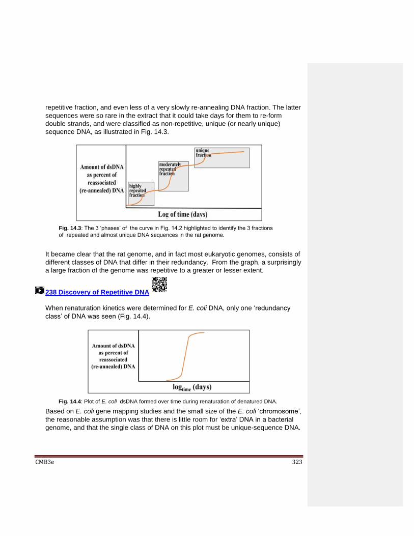
CMB3e 323

repetitive fraction, and even less of a very slowly re-annealing DNA fraction. The latter

sequences were so rare in the extract that it could take days for them to re-form

double strands, and were classified as non-repetitive, unique (or nearly unique)

sequence DNA, as illustrated in Fig. 14.3.

It became clear that the rat genome, and in fact most eukaryotic genomes, consists of

different classes of DNA that differ in their redundancy. From the graph, a surprisingly

a large fraction of the genome was repetitive to a greater or lesser extent.

238 Discovery of Repetitive DNA

When renaturation kinetics were determined for E. coli DNA, only one ‘redundancy

class’ of DNA was seen (Fig. 14.4).

Based on E. coli gene mapping studies and the small size of the E. coli ‘chromosome’,

the reasonable assumption was that there is little room for ‘extra’ DNA in a bacterial

genome, and that the single class of DNA on this plot must be unique-sequence DNA.

Fig. 14.3: The 3 ‘phases’ of the curve in Fig. 14.2 highlighted to identify the 3 fractions

of repeated and almost unique DNA sequences in the rat genome.

Fig. 14.4: Plot of E. coli dsDNA formed over time during renaturation of denatured DNA.

CMB3e 324

14.2.3 Genomic Complexity

Britten and Davidson defined the relative amounts of repeated and unique (or single-

copy) DNA sequences in an organism’s genome as its genomic complexity. Thus,

prokaryotic genomes have a lower genomic complexity than eukaryotes. Using the

same data as is in the previous two graphs, Britten and Davidson demonstrated the

difference between eukaryotic and prokaryotic genome complexity by a simple

expedient. Instead of plotting the fraction of dsDNA formed vs. time of renaturation,

they plotted the percent of re-associated DNA against the concentration of the re-

natured DNA multiplied by the time that DNA took to reanneal (the CoT value).

When CoT values from rat and E. coli renaturation data are plotted on the same

graph, you get the CoT curves in the graph in Fig. 14.5.

This deceptively simple extra calculation (from the same data!) allows direct

comparison of the complexities of different genomes. These CoT curves tell us that

~100% of the bacterial genome consists of unique sequences (curve at the far right),

compared to the rat genome with two DNA redundancy classes…, and at the right of

the curve, a small fraction of unique sequence DNA. Prokaryotic genomes are indeed

largely composed of unique (non-repetitive) sequence DNA that must include single-

copy genes (or operons) that encode proteins, ribosomal RNAs and transfer RNAs.

239 CoT Curves and DNA Complexity Explained!

Fig. 14.5: DNA complexity revealed by plotting rat and E. coli DNA renaturation kinetics as the

percent of re-associated dsDNA over CoT (Concentration of re-associated dsDNA X Time).

CMB3e 325

14.2.4 Functional Differences between Cot Classes of DNA

The next question of course was what kinds of sequences are repeated and which are

‘unique’ in eukaryotic DNA? Eukaryotic satellite DNAs, transposons and ribosomal

RNA genes were early suspects. To start answering these questions, satellite DNA

was isolated from the CsCl gradients, made radioactive and then heated to separate

the DNA strands. In a separate experiment, renaturing rat DNA was sampled at

different times of renaturation. The isolated Cot fractions were once again denatured

and mixed with heat-denatured radioactive satellite DNA. The mixture was then cooled

a second time to allow renaturation. The experimental protocol is illustrated in Fig.

14.6.

The results of this experiment showed that radioactive satellite DNA only annealed to

DNA from the low Cot fraction of DNA. Satellite DNA is thus highly repeated in the

eukaryotic genome.

In similar experiments, isolated radioactive rRNAs made radioactive formed RNA-DNA

hybrids when mixed and cooled with the denatured middle CoT of eukaryotic DNA.

Thus, rRNA genes were moderately repetitive. With the advent of recombinant DNA

technologies, the redundancy of other kinds of DNA were explored using cloned

genes (encoding rRNAs, mRNAs, transposons and other sequences) to probe DNA

fractions obtained from renaturation kinetics experiments. Results of such

experiments are summarized in Table 14.1(below ).

Fig. 14.6: Experimental demonstration of satellite DNA in low CoT renaturation

kinetic fractions (see text for details).

CMB3e 326

The table compares properties (lengths, copy number, functions, percent of the

genome, location in the genome, etc.) of different kinds of repetitive sequence DNA.

The observation that most of a eukaryotic genome is made up of repeated DNA, and

that transposons can be as much as 80% of a genome was a surprise! We’ll focus

next on the different kinds of transposable elements.

240 Identifying Different Kinds of DNA Each CoT Fraction

241 Some Repetitive DNA Functions

14.3 The ‘Jumping Genes’ of Maize

Barbara McClintock’s report that bits of DNA could jump around and integrate themselves

into new loci in DNA was so dramatic and arcane that many thought the phenomenon

was either a one-off, or not real! Only with the subsequent discovery of transposons in

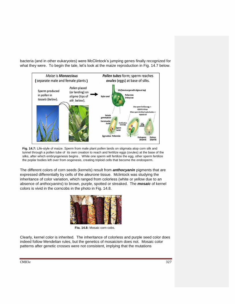
CMB3e 327

bacteria (and in other eukaryotes) were McClintock’s jumping genes finally recognized for

what they were. To begin the tale, let’s look at the maize reproduction in Fig. 14.7 below.

The different colors of corn seeds (kernels) result from anthocyanin pigments that are

expressed differentially by cells of the aleurone tissue. Mclintock was studying the

inheritance of color variation, which ranged from colorless (white or yellow due to an

absence of anthocyanins) to brown, purple, spotted or streaked. The mosaic of kernel

colors is vivid in the corncobs in the photo in Fig. 14.8.

Clearly, kernel color is inherited. The inheritance of colorless and purple seed color does indeed follow Mendelian rules, but the genetics of mosaicism does not. Mosaic color patterns after genetic crosses were not consistent, implying that the mutations

Fig. 14.7: Life-style of maize. Sperm from male plant pollen lands on stigmata atop corn silk and

tunnel through a pollen tube of its own creation to reach and fertilize eggs (ovules) at the base of the

silks, after which embryogenesis begins . While one sperm will fertilize the egg, other sperm fertilize

the poplar bodies left over from oogenesis, creating triploid cells that become the endosperm.

Fig. 14.8: Mosaic corn cobs.

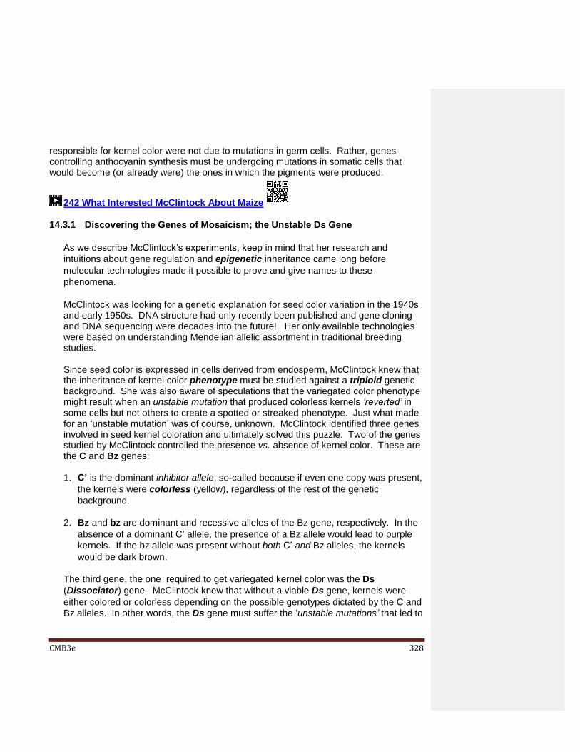
CMB3e 328

responsible for kernel color were not due to mutations in germ cells. Rather, genes controlling anthocyanin synthesis must be undergoing mutations in somatic cells that would become (or already were) the ones in which the pigments were produced.

242 What Interested McClintock About Maize

14.3.1 Discovering the Genes of Mosaicism; the Unstable Ds Gene

As we describe McClintock’s experiments, keep in mind that her research and

intuitions about gene regulation and epigenetic inheritance came long before

molecular technologies made it possible to prove and give names to these

phenomena.

McClintock was looking for a genetic explanation for seed color variation in the 1940s and early 1950s. DNA structure had only recently been published and gene cloning and DNA sequencing were decades into the future! Her only available technologies were based on understanding Mendelian allelic assortment in traditional breeding studies.

Since seed color is expressed in cells derived from endosperm, McClintock knew that the inheritance of kernel color phenotype must be studied against a triploid genetic background. She was also aware of speculations that the variegated color phenotype might result when an unstable mutation that produced colorless kernels ‘reverted’ in some cells but not others to create a spotted or streaked phenotype. Just what made for an ‘unstable mutation’ was of course, unknown. McClintock identified three genes involved in seed kernel coloration and ultimately solved this puzzle. Two of the genes studied by McClintock controlled the presence vs. absence of kernel color. These are the C and Bz genes: 1. C’ is the dominant inhibitor allele, so-called because if even one copy was present,

the kernels were colorless (yellow), regardless of the rest of the genetic

background.

2. Bz and bz are dominant and recessive alleles of the Bz gene, respectively. In the

absence of a dominant C’ allele, the presence of a Bz allele would lead to purple

kernels. If the bz allele was present without both C’ and Bz alleles, the kernels

would be dark brown.

The third gene, the one required to get variegated kernel color was the Ds

(Dissociator) gene. McClintock knew that without a viable Ds gene, kernels were

either colored or colorless depending on the possible genotypes dictated by the C and

Bz alleles. In other words, the Ds gene must suffer the ‘unstable mutations’ that led to

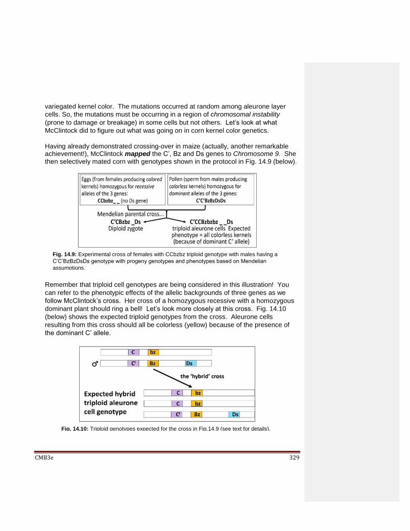
CMB3e 329

variegated kernel color. The mutations occurred at random among aleurone layer

cells. So, the mutations must be occurring in a region of chromosomal instability

(prone to damage or breakage) in some cells but not others. Let’s look at what

McClintock did to figure out what was going on in corn kernel color genetics.

Having already demonstrated crossing-over in maize (actually, another remarkable achievement!), McClintock mapped the C’, Bz and Ds genes to Chromosome 9. She then selectively mated corn with genotypes shown in the protocol in Fig. 14.9 (below).

Remember that triploid cell genotypes are being considered in this illustration! You

can refer to the phenotypic effects of the allelic backgrounds of three genes as we

follow McClintock’s cross. Her cross of a homozygous recessive with a homozygous

dominant plant should ring a bell! Let’s look more closely at this cross. Fig. 14.10

(below) shows the expected triploid genotypes from the cross. Aleurone cells

resulting from this cross should all be colorless (yellow) because of the presence of

the dominant C’ allele.

Fig. 14.9: Experimental cross of females with CCbzbz triploid genotype with males having a

C’C’BzBzDsDs genotype with progeny genotypes and phenotypes based on Mendelian

assumptions.

Fig. 14.10: Triploid genotypes expected for the cross in Fig.14.9 (see text for details).

CMB3e 330

But while there were indeed many colorless kernels on the hybrid cob, there were

also many mosaic kernels with dark spots or streaks against a colorless background.

McClintock’s interpretation of events is illustrated in Fig. 14.11 (below).

According to McClintock, if some aleurone layer cells in some kernels suffered

chromosome breakage at the Ds (Dissociator) locus (indicated by the double slash,

//), the C’ allele is inactivated. Without a functional C’ allele, the operative genotype

in the affected cells is CCbzbz. These cells then revert to making the brow pigment

as directed by the bz allele. When these cells divide, they create clusters of brown

cells surrounded by cells with an unbroken chromosome (and thus an active C’ allele),

creating a mosaic, i.e., the appearance of pigment spots or streaks in the kernel

against the otherwise colorless background in the surrounding cells.

243 Variegated Maize Kernels Result from “Loss” of the Ds Gene 14.3.2 The Discovery of Mobile Genes: the Ac/Ds System

The experiments just described were reproducible using a single breeding stock of

maize. But when McClintock tried to repeat the experiments by crossing the

homozygous dominant males with homozygous recessive females from a different

breeding stock, all the kernels of the progeny cobs were colorless, as if the Ds gene

had not caused any chromosomal damage.

It seemed that the Ds gene contributed by the male was unable to function (i.e.,

‘break’) in females of this new breeding stock. McClintock hypothesized that the

female in the original cross must have contributed a factor that could somehow

activate the Ds gene to break, and that this factor, yet another gene, was absent or

inactive in the females of the new breeding stock. McClintock called the new factor

Fig. 14.11: McClintock’s interpretation of the results of the triploid cross shown in Fig.14.9

(See text for details).

CMB3e 331

the activator, or Ac gene. Based on the dependence of Ds on the Ac locus,

McClintock recognized that these ‘genes’ were part of as a 2-element, Ac/Ds system

influencing mosaicism in maize kernels. She then demonstrated that Ac-dependent

Ds ‘breakage’ was in some cases also associated with inactivation of a normal Bz

gene, leading to a loss of purple color kernels. It was at this point that McClintock

concluded that far from simply ‘breaking’ the chromosome at a fragile Ds locus, the Ds

gene had actually moved to (or into) the Bz gene, disrupting its function. Again, this

could not happen in the absence of an active Ac gene. McClintock had discovered the

first transposon, earning her the 1983 Nobel Prize in Physiology or Medicine! View

an homage, brief history and summary of McClintock’s work and impact at

https://www.youtube.com/watch?v=ZHho1c-EbTY&t=46s.

With the advent of recombinant DNA technologies, we now know that:

1. the Ds element is a transposon missing a gene for a transposase enzyme

required for transposition.

2. the Ac element has this gene and is capable of independent transposition.

3. Ac provides the transposase needed to mobilize itself and the Ds element.

4. the sequence similarity of Ds and Ac elements supports their common ancestry.

The basic structural features of the maize Ac/Ds system are:

Ac is 4563 bp long

Ds is a truncated version of Ac.

There are eleven bp inverted repeats at either end of the Ac and Ds element

There are eight bp direct repeats (NOT inverted repeats) of ‘target DNA’ at the

site of insertion of either transposon.

Look for these features as we describe prokaryotic and eukaryotic transposons.

244 Discovery of Mobile Elements and the Ac-Ds System

245 The Ac-Ds System Today

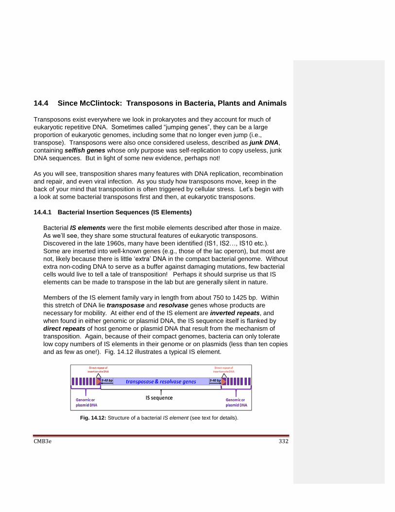
CMB3e 332

14.4 Since McClintock: Transposons in Bacteria, Plants and Animals

Transposons exist everywhere we look in prokaryotes and they account for much of

eukaryotic repetitive DNA. Sometimes called “jumping genes”, they can be a large

proportion of eukaryotic genomes, including some that no longer even jump (i.e.,

transpose). Transposons were also once considered useless, described as junk DNA,

containing selfish genes whose only purpose was self-replication to copy useless, junk

DNA sequences. But in light of some new evidence, perhaps not!

As you will see, transposition shares many features with DNA replication, recombination

and repair, and even viral infection. As you study how transposons move, keep in the

back of your mind that transposition is often triggered by cellular stress. Let’s begin with

a look at some bacterial transposons first and then, at eukaryotic transposons.

14.4.1 Bacterial Insertion Sequences (IS Elements)

Bacterial IS elements were the first mobile elements described after those in maize.

As we’ll see, they share some structural features of eukaryotic transposons.

Discovered in the late 1960s, many have been identified (IS1, IS2…, IS10 etc.).

Some are inserted into well-known genes (e.g., those of the lac operon), but most are

not, likely because there is little ‘extra’ DNA in the compact bacterial genome. Without

extra non-coding DNA to serve as a buffer against damaging mutations, few bacterial

cells would live to tell a tale of transposition! Perhaps it should surprise us that IS

elements can be made to transpose in the lab but are generally silent in nature.

Members of the IS element family vary in length from about 750 to 1425 bp. Within

this stretch of DNA lie transposase and resolvase genes whose products are

necessary for mobility. At either end of the IS element are inverted repeats, and

when found in either genomic or plasmid DNA, the IS sequence itself is flanked by

direct repeats of host genome or plasmid DNA that result from the mechanism of

transposition. Again, because of their compact genomes, bacteria can only tolerate

low copy numbers of IS elements in their genome or on plasmids (less than ten copies

and as few as one!). Fig. 14.12 illustrates a typical IS element.

Fig. 14.12: Structure of a bacterial IS element (see text for details).

CMB3e 333

14.4.2 Composite Bacterial Transposons: Tn Elements

If a pair of IS elements should lie close to each other, separated by a short stretch of

genomic or plasmid DNA, they can transpose together, carrying the DNA between

them as part of a composite transposon, or Tn element. If some of the DNA

between IS elements in a Tn element contains antibiotic resistance genes, its

transposition can carry and spread these genes to other DNA in the cell. Tn elements

(like IS elements) are present in low copy number. Fig. 14.13 (below) illustrates a

generic Tn element.

Antibiotic resistance genes have the medical community worried; their spread has led

to antibiotic-resistant pathogens that cause diseases that are increasingly hard and

even impossible to treat. Earlier we saw genetic ‘transformation’ of streptococcal cells

that pick up virulence genes in DNA from dead cell. We routinely transform cells with

plasmids as part of recombinant DNA experiments. But bacteria can transfer plasmid

DNA between themselves quite naturally. During bacterial conjugation, an F (fertility)

plasmid normally transfers DNA between compatible bacterial mating types (review

bacterial conjugation elsewhere in this text for more details). An F plasmid containing

a Tn element harboring an antibiotic resistance gene can thus be passed from donor

to recipient during conjugation. The Tn element can then transpose into to the

recipient bacterial genome. In this way, transposition is a major pathway for the

transfer and spread of antibiotic resistance.

14.4.3 Complex Transposons that Can Act Like Bacteriophage

Bacterial Complex Transposons also contain other genes in addition to those

required for mobility. Some complex transposons resemble a bacteriophage, or as in

the case of phage Mu, actually are phage! In fact, Mu can function either as an

infectious phage that reproduces in an infected cell, or as a transposon in the bacterial

genome. Transposon genes in Mu phage are illustrated below (Fig. 14.14).

Fig. 14.13: Structure of a bacterial Tn element (see text for details).

CMB3e 334

After infecting a bacterium, Mu can enter the lytic phase of its life cycle, replicating its

DNA, producing and ultimately releasing new infectious phage ‘particles’ by lysing the

host bacterial cell. Alternatively, like other phage, Mu can undergo lysogeny, inserting its

DNA into the host cell chromosome. Integrated copies of Mu can excise and re-enter the

lytic phase to produce more phage, usually if some environmental stress threatens host

bacterial survival. But, a third lifestyle choice, transposition, is available to Mu once the

phage integrates into the bacterial chromosome. The three lifestyle options for Mu phage

are illustrated in the next few pages. Fig 14.15 (below) illustrates the lytic and lysogenic

lifestyle options for a bacterial virus, and the next illustration (Fig. 14.16) shows the

additional lifestyle options of Mu phage; the phage DNA can act as a transposable

element while in the lysogenic pathway!

Fig. 14.14: Structure of a complex transposon (Mu phage - see text for details).

Fig. 14.15: Life cycle options for bacteriophage (see text for details).

CMB3e 335

246 Bacterial Mobile Elements As we turn to a description of eukaryotic transposons, look for similarities to bacterial IS and Tn elements.

14.5 Overview of Eukaryotic Transposable Elements

There are two classes transposons in eukaryotes:

Class I (RNA) Transposons: These move/’jump’ by transcription of RNA at one locus,

followed by reverse transcription and integration of the cDNA back into genomic DNA at a

different location. Called retrotransposons they may be derived from (or be the source

of) retroviruses since active retroviruses excise from and integrate into DNA much like

retrotransposons. Retroposons are a sub-class of retrotransposons (see below).

Class II (DNA) Transposons: These move by one of two mechanisms. In the cut-&-

paste pathway, the transposon leaves one locus and integrates at another. In the

replicative pathway, the original transposon remains in place while new copies are

mobile.

Fig. 14.16: The transposon option for Mu Phage (see text for details).

CMB3e 336

Table 14.2 (below) shows the distribution and proportion of genomes represented by

different classes/types of transposable elements. The table confirms that in contrast to

eukaryotes, bacteria contain relatively few transposons, while eukaryotes vary widely in

transposon load (transposons as a percentage of genomic DNA). Transposon load can

range from as low as 4% to more than 70% in different organisms.

Table 14.3 (below) summarizes transposable elements by class, sub-type, size, genomic

distribution, mechanism of transposition, etc. Between tables 14.2 and 14.3, we can

conclude the following:

Transposon load is not correlated with evolutionary complexity of organisms.

Shared transposons have different evolutionary histories in different organisms.

Where transposons remain active, they continue to shape genomic landscapes,

especially in organisms with a high transposons load.

We will revisit some of these conclusions later, after looking at the structure and

mechanism of mobility of different eukaryotic transposable elements.

247 Introduction to Eukaryotic Transposons

CMB3e 337

CMB3e 338

14.6 Structure of Eukaryotic DNA (Class II) Transposons

Active eukaryotic DNA transposons share structural features with bacterial mobile

elements, including genes required for transposition, flanking inverted repeats and

flanking insertion-site direct repeats of host cell DNA. As we’ll see, Class II transposons

can ‘jump’ by cut-and-paste or replicative mechanisms. Fig. 14.17 illustrates the

characteristic structure of a eukaryotic DNA transposon.

14.6.1 Cut-and-Paste Transposition

This mechanism moves a copy from one location and transposes it to another

location. As its name suggests, replicative transposition leaves a copy of the original

transposon in place while inserting a new copy elsewhere in the genome (Fig. 14.18).

Fig. 14.17: Structure of a eukaryotic Class II DNA transposon (see text for details).

Fig. 14.18: Cut-&-paste transposition of a DNA transposon (see text for details).

CMB3e 339

Note that after transcription of the transposase gene, the enzyme nicks the DNA and

trims the 3’OH ends to create a staggered cut to excise the transposon. The

transposase actually brings the transposon ends together during the cut step and

mediates its insertion at a new DNA site. After ligation of the 3’OH ends of the

transposon to the 5’OH at the insertion site, replication replaces the missing bases,

generating the direct repeats of host cell genomic DNA at the insertion site. A final

ligation step completes transposition.

14.6.2 Replicative Transposition

In replicative transposition, the transposon is also nicked and trimmed at its source (original) insertion site. But unlike cut-and-paste mechanisms, source transposons are not excised. Fig 14.19 (below) details the steps of replicative transposition.

After nicking the 3’ ends of the transposon at the insertion site, transposase holds the

transposon ends together while catalyzing a hydrolytic attack of DNA at a new

insertion site. This is followed by priming of transposon strand replication from the

3’OH ends of the insertion site DNA strands. A cointegrate structure forms in which

each transposon copy has been made by semi-conservative replication. The

cointegrate is resolved by one of two recombinational mechanisms. The result leaves

copies of the transposon at both the original site and the new insertion site.

Fig. 14.19: Replicative transposition of a DNA transposon (see text for details).

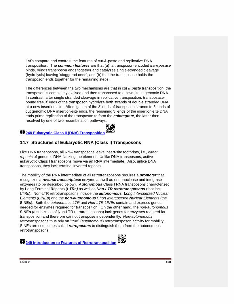
CMB3e 340

Let’s compare and contrast the features of cut-&-paste and replicative DNA

transposition. The common features are that (a) a transposon-encoded transposase

binds, brings transposon ends together and catalyzes single-stranded cleavage

(hydrolysis) leaving ‘staggered ends’, and (b) that the transposase holds the

transposon ends together for the remaining steps.

The differences between the two mechanisms are that in cut & paste transposition, the

transposon is completely excised and then transposed to a new site in genomic DNA.

In contrast, after single stranded cleavage in replicative transposition, transposase-

bound free 3’ ends of the transposon hydrolyze both strands of double stranded DNA

at a new insertion site. After ligation of the 3’ ends of transposon strands to 5’ ends of

cut genomic DNA insertion-site ends, the remaining 3’ ends of the insertion-site DNA

ends prime replication of the transposon to form the cointegrate, the latter then

resolved by one of two recombination pathways.

248 Eukaryotic Class II (DNA) Transposition

14.7 Structures of Eukaryotic RNA (Class I) Transposons

Like DNA transposons, all RNA transposons leave insert-site footprints, i.e., direct

repeats of genomic DNA flanking the element. Unlike DNA transposons, active

eukaryotic Class I transposons move via an RNA intermediate. Also, unlike DNA

transposons, they lack terminal inverted repeats.

The mobility of the RNA intermediate of all retrotransposons requires a promoter that

recognizes a reverse transcriptase enzyme as well as endonuclease and integrase

enzymes (to be described below). Autonomous Class I RNA transposons characterized

by Long Terminal Repeats (LTRs) as well as Non-LTR retrotransposons (that lack

LTRs). Non-LTR retrotransposons include the autonomous Long Interspersed Nuclear

Elements (LINEs) and the non-autonomous Short Interspersed Nuclear Elements (the

SINEs). Both the autonomous LTR and Non-LTR LINEs contain and express genes

needed for enzymes required for transposition. On the other hand, the non-autonomous

SINEs (a sub-class of Non-LTR retrotransposons) lack genes for enzymes required for

transposition and therefore cannot transpose independently. Non-autonomous

retrotransposons thus rely on “true” (autonomous) retrotransposon activity for mobility.

SINEs are sometimes called retroposons to distinguish them from the autonomous

retrotransposons.

249 Introduction to Features of Retrotransposition

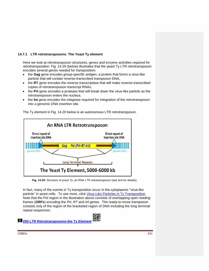
CMB3e 341

14.7.1 LTR retrotransposons: The Yeast Ty element

Here we look at retrotransposon structures, genes and enzyme activities required for retrotransposition. Fig. 14.20 (below) illustrates that the yeast Ty LTR retrotransposon encodes several genes needed for transposition:

the Gag gene encodes group-specific antigen, a protein that forms a virus-like

particle that will contain reverse-transcribed transposon DNA,

the RT gene encodes the reverse transcriptase that will make reverse-transcribed

copies of retrotransposon transcript RNAs.

the Prt gene encodes a protease that will break down the virus-like particle as the

retrotransposon enters the nucleus.

the Int gene encodes the integrase required for integration of the retrotransposon

into a genomic DNA insertion site.

The Ty element in Fig. 14.20 below is an autonomous LTR retrotransposon.

In fact, many of the events in Ty transposition occur in the cytoplasmic “virus-like

particle” in yeast cells. To see more, click Virus-Like Particles in Ty Transposition.

Note that the Pol region in the illustration above consists of overlapping open reading

frames (ORFs) encoding the Prt, RT and Int genes. The ready-to-move transposon

consists only of the region of the bracketed region of DNA including the long terminal

repeat sequences.

250 LTR Retrotransposons-the Ty Element

Fig. 14.20: Structure of yeast Ty, an RNA LTR retrotransposon (see text for details).

CMB3e 342

14.7.2 Non-LTR Retrotransposons: LINEs

Like LTR retrotransposons, LINEs (Long Interspersed Nuclear Elements) also encode

enzymes needed for transposition and like other transposons, generate target-site

direct repeats flanking the inserted element (Fig. 14.21). But they do not have the

long terminal repeats! Instead, their ORFs (genes) are flanked by 5’ and a 3’

untranslated regions (UTRs).

The 5’ UTR contains a promoter from which cellular RNA polymerase II can transcribe

the downstream genes (see the Transcription chapter). The second of these (ORF2)

encodes the reverse transcriptase and an integrase activity essential for transposition

of the LINE. All Class I (RNA-intermediate) autonomous transposons share the

following features:

a) a Promoter in the 5’ UTR from which they can be transcribed

b) a Reverse Transcriptase that generates a cDNA copy of the transposable

element

c) RNAse H (an endonuclease) that degrades the transcript after reverse

transcription

d) Integrase (like a transposase) that catalyzes insertion of the retrotransposon copy

at insertion sites

251 Non-LTR Retrotransposons: LINEs 14.7.3 Non-LTR Retrotransposons: SINEs

Non-LTR SINE retrotransposons typically lack genes, but their non-genic DNA is

nonetheless flanked by 5’ and 3’ UTRs. RNA polymerase III, which also transcribes

transfer RNAs, also transcribes SINEs. However, to transpose, they rely on the

Fig. 14.21: Structure of a LINE, a non-LTR retrotransposon (see text for details).

CMB3e 343

concurrent activity of a Non-LTR transposon (a LINE) to provide the requisite

enzymatic activities. A typical SINE (e.g., the Alu element) is shown in Fig. 14.22

(below).

252 Non-LTR Retrotransposons: SINEs

14.8 Mechanisms of Retrotransposition

There are two mechanisms of retrotransposition: Extrachromosomally Primed

Retrotransposition (LTR retrotransposons for example) and Insertion Target-Site

Primed Retrotransposition (non-LTR Retrotransposons like LINEs and SINEs). We will

considered these two mechanisms next.

14.8.1 Extrachromosomally Primed Retrotransposition (e.g., of a LINE)

As its name suggests, in extrachromosomally primed retrotransposition, a separate circular reverse transcript of the retrotransposon attacks, nicks and integrates into a genomic insertion site (Fig. 14.23, below). In this mechanism, reverse transcriptase creates a cDNA copy of a transcribed retro-element. Integrase/endonuclease then binds the cDNA copy, holding the ends together, in effect circularizing it. This isolable ribonucleoprotein resembles an intasome, a structure similar to the nucleoprotein complex that catalyzes integration of retroviral cDNAs during lysogeny. The three-dimensional structure of a retroviral intasome interacting with DNA and nucleosomes was recently determined (for more, see Retroviral Intasome 3D Structure). In this

Fig. 14.22: Structure of the Alu SINE, a non-LTR retrotransposon, or retroposon (see

text for details).

CMB3e 344

form, the retrotransposon attacks DNA at an insertion site, creating staggered ends. After insertion, the gaps in the DNA are filled in. Ligation seals the retrotransposon in its new location, creating direct insertion site repeats.

253 Extrachromosomally Primed Retrotransposition

14.8.2 Target-Site Primed SINE Retrotransposition (e.g., of a SINE)

A key feature of target-site primed retrotransposition (retroposition) is the absence of

an integrase-bound, separate circular double-stranded reverse transcript (Fig. 14.24

below). In SINE transposition, RNA polymerase III (the same enzyme that catalyzes

tRNA and 5S rRNA transcription) transcribes the SINE. If a LINE is concurrently

transcribed, its enzymes will be made.

When its integrase-endonuclease catalyzes hydrolysis of one strand of DNA at a new

insertion site, the 3’OH end of this strand can prime reverse transcription of the one

SINE cDNA strand by the LINE reverse transcriptase. After hydrolysis of the second

target site DNA strand, its 3’-OH end primes replication of the second strand of the

SINE cDNA. Integrase completes insertion of the copy-SINE in its new genomic

location.

Fig. 14.23: Extrachromosomally-primed transposition of a LINE (see text for details).

CMB3e 345

254 Target Primed Retrotransposition

14.9 On the Evolution of Transposons, Genes and Genomes

We noted that transposons in bacteria carry antibiotic resistance genes, a clear example

of benefits of transposition in prokaryotes. Of course, prokaryotic genomes are small, as

is the typical bacterial transposon load. Yeast species also have low transposon load.

But, what can we make of the high transposon load in eukaryotes? To many geneticists,

the fact that genes encoding proteins typically represent only 1-2% of a eukaryotic

genome suggested that the rest of the genome was informationally non-essential. Even

though transposons turn out to be much of the non-coding DNA in some eukaryotic

genomes, they seemed to serve no purpose other than their own replication. These large

amounts of transposon DNA were dubbed selfish DNA and their genes, selfish genes.

So, are transposons just junk DNA, some kind of invasive or leftover genomic baggage?

Given their propensity to jump around and potential to raise havoc in genomes, how do

tolerate and survive them? Is the sole ‘mission’ of transposons really just to reproduce

themselves? Or are transposons in fact neither selfish nor junk?

Fig. 14.24: Target-primed transposition of a LINE (see text for details).

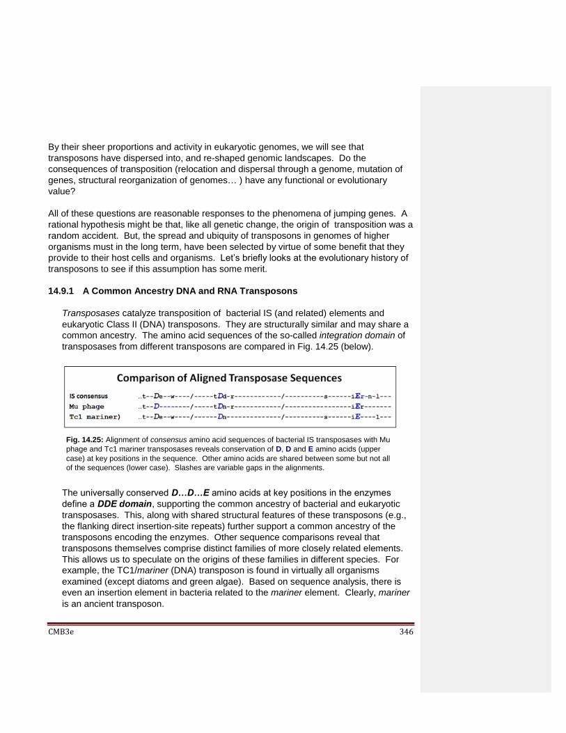
CMB3e 346

By their sheer proportions and activity in eukaryotic genomes, we will see that

transposons have dispersed into, and re-shaped genomic landscapes. Do the

consequences of transposition (relocation and dispersal through a genome, mutation of

genes, structural reorganization of genomes… ) have any functional or evolutionary

value?

All of these questions are reasonable responses to the phenomena of jumping genes. A

rational hypothesis might be that, like all genetic change, the origin of transposition was a

random accident. But, the spread and ubiquity of transposons in genomes of higher

organisms must in the long term, have been selected by virtue of some benefit that they

provide to their host cells and organisms. Let’s briefly looks at the evolutionary history of

transposons to see if this assumption has some merit.

14.9.1 A Common Ancestry DNA and RNA Transposons

Transposases catalyze transposition of bacterial IS (and related) elements and

eukaryotic Class II (DNA) transposons. They are structurally similar and may share a

common ancestry. The amino acid sequences of the so-called integration domain of

transposases from different transposons are compared in Fig. 14.25 (below).

The universally conserved D…D…E amino acids at key positions in the enzymes

define a DDE domain, supporting the common ancestry of bacterial and eukaryotic

transposases. This, along with shared structural features of these transposons (e.g.,

the flanking direct insertion-site repeats) further support a common ancestry of the

transposons encoding the enzymes. Other sequence comparisons reveal that

transposons themselves comprise distinct families of more closely related elements.

This allows us to speculate on the origins of these families in different species. For

example, the TC1/mariner (DNA) transposon is found in virtually all organisms

examined (except diatoms and green algae). Based on sequence analysis, there is

even an insertion element in bacteria related to the mariner element. Clearly, mariner

is an ancient transposon.

Fig. 14.25: Alignment of consensus amino acid sequences of bacterial IS transposases with Mu

phage and Tc1 mariner transposases reveals conservation of D, D and E amino acids (upper

case) at key positions in the sequence. Other amino acids are shared between some but not all

of the sequences (lower case). Slashes are variable gaps in the alignments.

CMB3e 347

This amount and diversity of conservation bespeaks an early evolution of the enzymes

of transposition, and of transposition itself, within and even between species. Linear,

or vertical descent (the ‘vertical” transmission of transposons from parents to

progeny) is the rule. However, the presence of similar transposons in diverse species

is best explained by interspecific DNA sharing, or horizontal transfer. That is, a

transposon in one organism must have been the ‘gift’ of an organism of a different

species! This is further discussed below. Clearly, moveable genes have been a part

of life for a long time, speaking more to an adaptive value for organisms than to the

parasitic action of a selfish, rogue DNA!

14.9.2 Retroviruses and LTR Retrotransposons Share a Common Ancestry

The integration domain of retrotransposon transposases and retrovirus integrases also

share significant sequence similarities, as shown in the amino acid sequence

alignment in Fig. 14.26 below.

Here the conserved D…D…E amino acids at key positions in DDE domains support

the common ancestry of Class I (RNA transposon) retroviral integrases and the Class

II (DNA transposon) transposases. In other words, all transposons may share a

common ancestry. But the common ancestry of retrotransposons and retroviruses

raises yet other questions: Did transposons (specifically retrotransposons) arise as

defective versions of integrated retrovirus DNA (i.e., reverse transcripts of retroviral

RNA)? Or, did retroviruses emerge when retrotransposons evolved a way to leave

their host cells. To approach this question, let’s first compare mechanisms of

retroviral infection and retrotransposition.

LTR retrotransposons and retroviruses both contain flanking long terminal repeats in

addition to the structural similarities of the enzymes they encode. However,

retrotransposition occurs within the nucleus of a cell while retroviruses must first infect

Fig. 14.26: Comparison amino acid sequences of the COPIA retrotransposon and a retroviral (HIV)

integrase with typical transposase sequences. The alignments reveal conservation of the D, D and

E amino acids in the DDE domain of the enzymes. Other amino acids are shared between some

but not all of the sequences (lower case). Slashes are variable gaps in the alignments.

CMB3e 348

a host cell before the retroviral DNA can be replicated and new viruses produced

(check out Visualizing Retroviral Infection to see how immunofluorescence microscopy

using antibodies to single-stranded cDNAs was used to track the steps of HIV

infection!).

A key structural difference between retrotransposons and most retroviruses is the

ENV gene-encoded protein envelope surrounding retroviral DNA. After infection, the

incoming retrovirus sheds its envelope proteins and viral RNA is reverse transcribed.

After the reverse transcripts enter the nucleus, transcription of genes and translation

of enzymes necessary for the replication of the viral cDNA leads to the production of

new enveloped infectious viruses that will eventually lyse the infected cell…, but here

are two curious phenomena:

First, retroviral DNA, like any genomic DNA, is mutable. If a mutation inactivates one

of the genes required for infection and retroviral release, it could become an LTR

retrotransposon. Such a genetically damaged retroviral integrate might still be

transcribed and its mRNAs translated. If detected by its own reverse transcriptase,

the erstwhile viral genomes would be copied. The cDNAs, instead of being packaged

into infectious viral particles, would become a source of so-called endogenous

retroviruses (ERVs). In fact, ERVs exist, making up a substantial portion of the

mammalian genome (8% in humans)… and do in fact, behave like LTR

retrotransposons!

Second, yeast TY elements transcribe several genes during retrotransposition (see

the list above), producing not only reverse transcriptase and integrase, but also a

protease and a structural protein called Gag (Group-specific antigen). All of the

translated proteins enter the nucleus. Mimicking the retroviral ENV protein, the Gag

protein makes up most of a coat protein called VLP (virus-like particle). VLP

encapsulates additional retrotransposon RNA in the cytoplasm, along with the other

proteins. Double-stranded reverse transcripts (cDNAs) of the viral RNA are then

made within the VLPs. But, instead of bursting out of the cell, encapsulated cDNAs

(i.e., new retrotransposons) shed their VLP coat and re-enter the nucleus, where they

can now integrate into genomic target DNA. Compare this to the description of

retroviral infection. During infection, retroviral envelope proteins attach to cell

membranes and release their RNA into the cytoplasm. There, reverse transcriptase

copies viral RNA into double-stranded cDNAs that then enter the nucleus where they

can integrate into host cell DNA. When transcribed, the integrated retroviral DNA

produces transcripts that are translated in the cytoplasm into proteins necessary to

form an infectious viral particle. The resulting viral RNAs are encapsulated by an ENV

(envelope) protein encoded in the viral genome. Of course, unlike VLP-coated

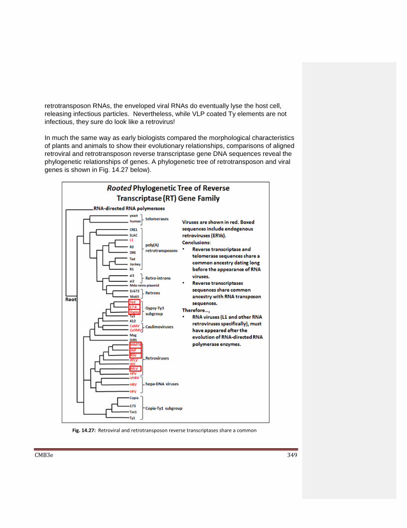
CMB3e 349

retrotransposon RNAs, the enveloped viral RNAs do eventually lyse the host cell,

releasing infectious particles. Nevertheless, while VLP coated Ty elements are not

infectious, they sure do look like a retrovirus!

In much the same way as early biologists compared the morphological characteristics

of plants and animals to show their evolutionary relationships, comparisons of aligned

retroviral and retrotransposon reverse transcriptase gene DNA sequences reveal the

phylogenetic relationships of genes. A phylogenetic tree of retrotransposon and viral

genes is shown in Fig. 14.27 below).

Fig. 14.27: Retroviral and retrotransposon reverse transcriptases share a common

evolutionary ancestor.

CMB3e 350

The data in the analysis supports the evolution of retroviruses from retrotransposon

ancestors. From the ‘tree’, TY3 and a few other retrotransposons share common

ancestry with Ted, 17.6 and Gypsy ERVs (boxed) in the ”Gypsi-TY3 subgroup”.

Further, this sub-group shares common ancestry with more distantly related

retroviruses (e.g., MMTV, HTLV…), as well as the even more distantly related (older,

longer diverged!) Copia-TY1 transposon sub-group. This and similar analyses

strongly suggest that retroviruses evolved from a retrotransposon lineage. For a

review of retroposon and retrovirus evolution, check Lerat P. & Capy P. (1999,

Retrotransposons and retroviruses: analysis of the envelope gene. Mol. Biol. Evol.

19(9): 1198-1207).

14.9.3 Transposons Can Be Acquired by Horizontal Gene Transfer

As noted, transposons are inherited vertically, meaning that they are passed from cell

to cell or parents to progeny by reproduction. But they also may have spread between

species by horizontal gene transfer. This just means that organisms exposed to

DNA containing transposons might inadvertently pick up such DNA and become

transformed as the transposon becomes part of the genome. Accidental mobility of

transposons between species would have been rare, but an exchange of genes by

horizontal gene transfer would have accelerated with the evolution of retroviruses.

Once again, despite the potential to disrupt the health an organism, retroviral activity

might also have supported a degree genomic diversity useful to organisms.

255 Transposon Evolution

14.10 Evolutionary Roles of Transposition in Genetic Diversity

Here we’ll see how transposition can affect genes and genetic diversity. We’ll also

consider parallels between transposition and the generation of immunological diversity,

and a provocative notion that our immune system owes at least some of its evolutionary

history to transposons, or at least to mechanisms of transposition!

14.10.1 Transposons and Exon Shuffling

A role for unequal recombination in moving exons in and out of different eukaryotic

split genes was described earlier. This kind of exon shuffling could happen when

short DNA sequences in two different introns misalign during meiotic synapsis,

allowing unequal crossing over. Expression of a gene with a ‘new’ exon produces a

protein with a new domain and a new activity. If the new domain is not harmful,

especially in only one of two alleles of a gene, the mutation need not be lethal, and

genetic diversity and the potential for evolution is increased!

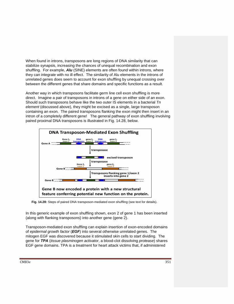
CMB3e 351

When found in introns, transposons are long regions of DNA similarity that can

stabilize synapsis, increasing the chances of unequal recombination and exon

shuffling. For example, Alu (SINE) elements are often found within introns, where

they can integrate with no ill effect. The similarity of Alu elements in the introns of

unrelated genes does seem to account for exon shuffling by unequal crossing over

between the different genes that share domains and specific functions as a result.

Another way in which transposons facilitate germ line cell exon shuffling is more

direct. Imagine a pair of transposons in introns of a gene on either side of an exon.

Should such transposons behave like the two outer IS elements in a bacterial Tn

element (discussed above), they might be excised as a single, large transposon

containing an exon. The paired transposons flanking the exon might then insert in an

intron of a completely different gene! The general pathway of exon shuffling involving

paired proximal DNA transposons is illustrated in Fig. 14.28, below.

In this generic example of exon shuffling shown, exon 2 of gene 1 has been inserted

(along with flanking transposons) into another gene (gene 2).

Transposon-mediated exon shuffling can explain insertion of exon-encoded domains

of epidermal growth factor (EGF) into several otherwise unrelated genes. The

mitogen EGF was discovered because it stimulated skin cells to start dividing. The

gene for TPA (tissue plasminogen activator, a blood-clot dissolving protease) shares

EGF gene domains. TPA is a treatment for heart attack victims that, if administered

Fig. 14.28: Steps of paired DNA transposon-mediated exon shuffling (see text for details).

CMB3e 352

rapidly after the attack, can dissolve the clot and allow coronary artery blood flow to

heart muscle to resume. Other genes that contain EGF domains include those for

Neu and Notch proteins, both involved in cellular differentiation and development.

Some exon shuffling events may have been mediated by LINE transposition and by a

special group of recently discovered transposons called helitrons. Helitrons replicate

by a rolling circle mechanism. If you are curious about helitrons, do a google search

to learn more about them, and what role they may have had in refashioning and

reconstructing genomes in evolution.

14.10.2 Transposon Genes and Immune System Genes Have History

Several important eukaryotic genes may have been derived from transposons.

Perhaps the most intriguing example of this is to be found in the complex vertebrate

immune system.

Our immune system includes immunoglobulins (antibodies). You inherited genes

for immunoglobulin proteins from your parents. These genes contain multiple variant

V, D, and J regions linked to a C region. V, D, J and C are defined as Variable,

Joining, Diversity and Constant DNA regions, respectively. These regions recombine

to create many diverse V-D-J-C immunoglobulin antibody molecules (the D region is

not always included in the final recombined gene). The gene rearrangements occur

during the maturation of stem cells in bone marrow that will become immune cells (B

or T lymphocytes). In response to challenge by foreign substances called antigens,

(e.g., proteins on a bacterial surface or toxins released by invading cells), our immune

system responds; B or T lymphocytes will be selected that contain the rearranged

immunoglobulin genes able to make immunoglobulins that can recognize, bind and

eliminate the invading antigens.

A discussion of the molecular biology of the immune system is beyond our scope

here. Suffice it to say that the recombinational pathway of immunoglobulin gene

rearrangements includes enzymatic activities very similar to those of transposition. In

fact, the so-called RAG1 enzyme active in immunoglobulin gene rearrangement is

closely related to genes in a family of transposons (transib) found in invertebrates and

fungi. It looks like immune gene rearrangement might have origins in transposition!

14.11 Coping with the Dangers of Rampant Transposition

Most organisms do not have the high transposon load that we have. Given a general

tendency of transposons to insert at random into new DNA loci, how come we exist at all?

Isn’t the danger of transposition into essential gene sequences magnified by the

CMB3e 353

possibility of multiple simultaneous transpositions of elements generated by cut-and-paste

and especially replicative mechanisms? Indeed, transposons have been found in genes

that are inactive as a result. An obvious explanation for our survival of transposon activity

is that most transposition is into the >90% percent of the genome that does not code for

proteins. Another is that eukaryotic organisms have two copies of every gene, so that if

one is inactive, the other may sustain us. Beyond this, several mechanisms exist to

silence a transposon after transposition has occurred, mitigating the dangers of rampant

transposition. As long as a transposition is not lethal (e.g., because its integration does

not disrupt an activity essential to life), the cell and organisms can survive the event. In

time, mutations at the ends of transposons or in the genes responsible for transposition

would eventually render them inactive. Finally, there may be more direct curbs on

transposition. Recall that the small interfering RNAs (siRNAs) we encountered earlier

may complement and target viral RNAs for destruction (see the Transcription chapter for

more information on siRNAs). There is some evidence that siRNAs similarly target

transposon transcripts.

Summing up, transposon activity is moderated by mutational loss of function and/or by

more direct mechanisms that limit transposition and thus genetic damage. If an

accumulation of transposons to a high load were deleterious, they would have been

eliminated from genomes. Instead we see persistent transposons in many species,

suggesting that frequent transposition is largely neutral, increasing options for diversity in

the selection of new genotypes and phenotypic characteristics. We also know now that

transposons can function in genetic regulation. Thus, transposons in general are neither

selfish nor junk. Check out these links for more: Not junk after all? and Eulogy for Junk

DNA.

256 Transposons-Junk or Not

Some iText & VOP Key Words and Terms

Alu Gag non-homologous recombination

anthocyanins genomic complexity Non-LTR transposons

antibiotic resistance genes heterochromatin protease

antibodies immune system protein coat

autonomous transposon immunoglobulin prt

bacterial composite transposons

integrase renaturation kinetics

CMB3e 354

bacterial IS elements inverted repeats Repetitive DNA

bacterial Tn elements jumping genes replicative transposition

bacteriophage L1 resolvase

centromere LINE retrotransposon

chromatin LTR (long terminal repeats)

retrovirus

chromosomes LTR transposons RNA transposon

Class I transposon lysis satellite DNA

Class II transposon lysogeny SINE

cointegrate lytic pathway of phage spindle fibers

CoT curves maize Ac (activator) gene

telomeres

cut-and-paste transposition

maize Ds (dissociator) gene

transposase

density gradient centrifugation

mariner triploid endosperm

direct repeats McClintock Ty

DNA sequence phylogeny mosaicism viral infection

exon shuffling Mu phage

fertility (F) plasmids non-autonomous transposon

CMB3e 355

Chapter 15: DNA Technologies

Manipulating DNA; cDNA libraries, Genomic Libraries, DNA Sequencing,

PCR, Microarrays, Genomics, Transcriptomics, Proteomics

15.1 Introduction

We start this chapter by looking at technologies that led to genetic engineering. The

ability of make recombinant DNA is such a seminal technology that just realizing it could

be done and then doing it in a test tube for the first time earned Paul berg a half-share in

the 1980 Nobel Prize in Chemistry (the other half was shared by Walter Gilbert and

Frederick Sanger for studies that enabled efficient DNA sequencing). First we’ll look at

cDNA synthesis (the synthesis of DNA copies of RNA), something retroviruses routinely

do as part of their reproductive pathway.

The retrovirus first injects its RNA into target cells where it transcribes a reverse transcriptase enzyme. The enzyme reverse-transcribes a copy DNA (cDNA) complementary to the viral RNA. The same reverse transcriptase enzyme then makes a double stranded cDNA, or (ds)cDNA, which then replicates. These cDNAs are transcribed into new viral RNA genomes and mRNAs for viral proteins. The latter encapsulate the RNA genomes into new viruses.

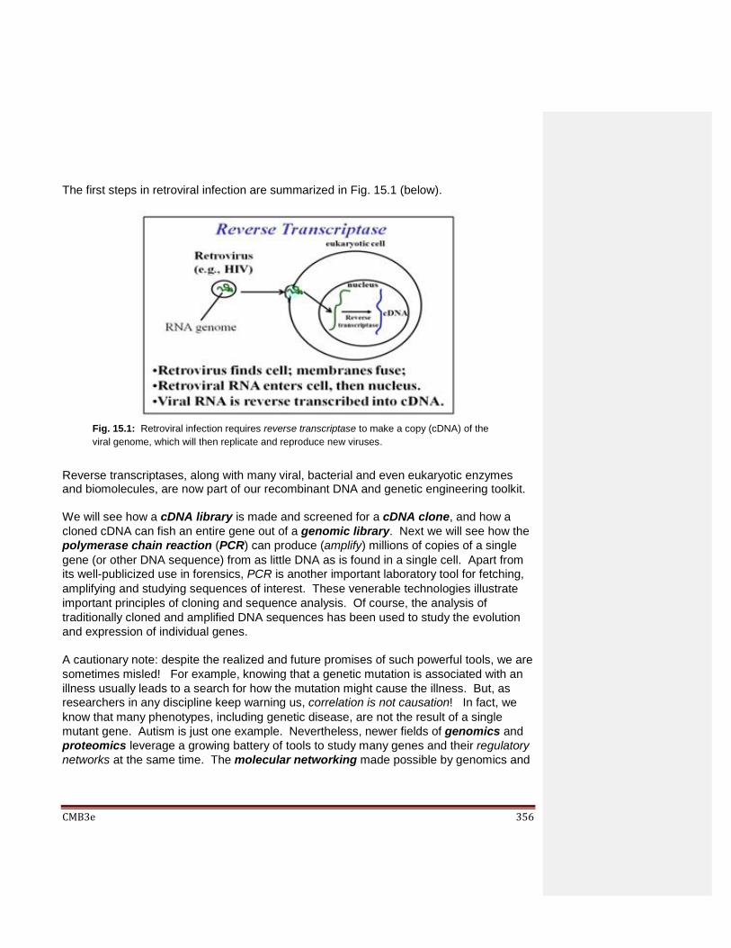
CMB3e 356

The first steps in retroviral infection are summarized in Fig. 15.1 (below).

Reverse transcriptases, along with many viral, bacterial and even eukaryotic enzymes and biomolecules, are now part of our recombinant DNA and genetic engineering toolkit.

We will see how a cDNA library is made and screened for a cDNA clone, and how a

cloned cDNA can fish an entire gene out of a genomic library. Next we will see how the

polymerase chain reaction (PCR) can produce (amplify) millions of copies of a single

gene (or other DNA sequence) from as little DNA as is found in a single cell. Apart from

its well-publicized use in forensics, PCR is another important laboratory tool for fetching,

amplifying and studying sequences of interest. These venerable technologies illustrate

important principles of cloning and sequence analysis. Of course, the analysis of

traditionally cloned and amplified DNA sequences has been used to study the evolution

and expression of individual genes.

A cautionary note: despite the realized and future promises of such powerful tools, we are

sometimes misled! For example, knowing that a genetic mutation is associated with an

illness usually leads to a search for how the mutation might cause the illness. But, as

researchers in any discipline keep warning us, correlation is not causation! In fact, we

know that many phenotypes, including genetic disease, are not the result of a single

mutant gene. Autism is just one example. Nevertheless, newer fields of genomics and

proteomics leverage a growing battery of tools to study many genes and their regulatory

networks at the same time. The molecular networking made possible by genomics and

Fig. 15.1: Retroviral infection requires reverse transcriptase to make a copy (cDNA) of the

viral genome, which will then replicate and reproduce new viruses.

CMB3e 357

proteomics (and other colorful holistic terms we’ll discuss later) promise to get us past

naïve and often incorrect notions of causation. We may be soon able to identify many

correlations that might sum up if not to causation, at least to a propensity to genetic

illness. We’ll look at some of these tools of leverage!

257 Overview of DNA Technologies Learning Objectives

When you have mastered the information in this chapter, you should be able to:

1. suggest molecular techniques to design experiments (e.g., how would you use

cDNA or a PCR product to clone a gene).

2. determine when to make or use a cDNA library or a genomic library.

3. outline an experiment to purify rRNA from eukaryotic cells.

4. outline an experiment to isolate and clone a human cDNA for further study

5. explain why you might want to clone and express a human growth hormone gene.

6. list components needed to make a cDNA library using purified poly(A) RNA.

7. list the components needed to make a genomic library from isolated genomic DNA.

8. compare PCR and genomic cloning as strategies for isolating a gene.

9. outline a strategy for using fly DNA to obtain copies of a human DNA sequence.

10. ask a research question that requires screening a genomic library for a specific

gene.

11. ask a question that requires using a microarray to obtain a gene you want to study.

15.2 Make and Screen a cDNA Library

The first step in making a cDNA library is to isolate cellular mRNA. This mRNA extract

should represent all of the transcripts in the cells at the time of isolation, or the cell’s

transcriptome. This term is used by analogy to genome. However, a genome is all of

the genetic information of an organism. In contrast, a transcriptome (usually eukaryotic)

reflects all of the genes expressed in a given cell type at a moment in time. Reverse-

transcribed cDNAs from an mRNA extract are also referred to as a transcriptome.

A cDNA library is a tube full of bacterial cells that have taken up (i.e., been transformed

with) plasmids recombined with cDNAs. cDNA libraries that are made from mRNAs taken

from different cell types or the same cells grown under different conditions are in effect,

different transcriptomes. Each reflects mRNAs transcribed in cells at the moment of their

extraction. When cells in a cDNA library are spread out on a nutrient agar petri dish, each

cell grows into a colony of cells; each cell in the colony is the clone of a starting cell.

cDNA libraries can be used isolate and sequence the DNA encoding a polypeptide that

you are studying.

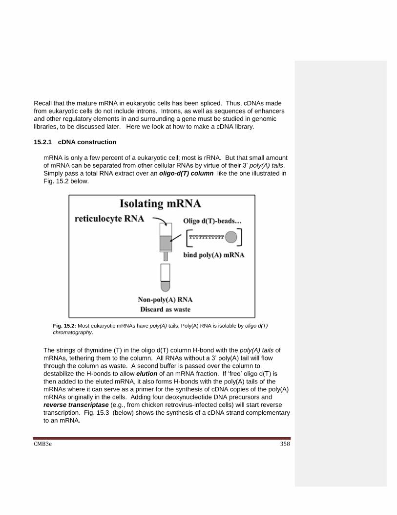
CMB3e 358

Recall that the mature mRNA in eukaryotic cells has been spliced. Thus, cDNAs made

from eukaryotic cells do not include introns. Introns, as well as sequences of enhancers

and other regulatory elements in and surrounding a gene must be studied in genomic

libraries, to be discussed later. Here we look at how to make a cDNA library.

15.2.1 cDNA construction

mRNA is only a few percent of a eukaryotic cell; most is rRNA. But that small amount

of mRNA can be separated from other cellular RNAs by virtue of their 3’ poly(A) tails.

Simply pass a total RNA extract over an oligo-d(T) column like the one illustrated in

Fig. 15.2 below.

The strings of thymidine (T) in the oligo d(T) column H-bond with the poly(A) tails of

mRNAs, tethering them to the column. All RNAs without a 3’ poly(A) tail will flow

through the column as waste. A second buffer is passed over the column to

destabilize the H-bonds to allow elution of an mRNA fraction. If ‘free’ oligo d(T) is

then added to the eluted mRNA, it also forms H-bonds with the poly(A) tails of the

mRNAs where it can serve as a primer for the synthesis of cDNA copies of the poly(A)

mRNAs originally in the cells. Adding four deoxynucleotide DNA precursors and

reverse transcriptase (e.g., from chicken retrovirus-infected cells) will start reverse

transcription. Fig. 15.3 (below) shows the synthesis of a cDNA strand complementary

to an mRNA.

Fig. 15.2: Most eukaryotic mRNAs have poly(A) tails; Poly(A) RNA is isolable by oligo d(T)

chromatography.

CMB3e 359

After heating to separate the cDNAs from the mRNAs, the cDNA is replicated to

produce double-stranded, or (ds)cDNA (Fig.15.4).

Synthesis of the second cDNA strand is also catalyzed by reverse transcriptase!

Second strand synthesis is primed by the 3’ end of a stem-loop structure that can form

with most mRNAs. Reverse transcriptase is also a DNA polymerase, recognizing

DNA as well as RNA templates, with the same 5’-to-3’ DNA polymerizing activity as all

Fig. 15.3: Reverse transcriptase supplied with deoxynucleotides, mRNAs and an oligo d(T)

primer will catalyze synthesis of DNA copies (cDNAs) of the mRNAs.

Fig. 15.4: The first cDNA strand often forms a loop at its 3’ end that can serve as a primer to

synthesize a (ds)cDNA. Reverse transcriptase is also a DNA polymerase, and can catalyze 2nd

strand synthesis.

CMB3e 360

DNA and RNA polymerases. After 2nd cDNA strand synthesis, an S1 nuclease (a

specifically single-stranded endonuclease originally isolated from an East Asian

fungus!) is added to open the loop of the (ds) cDNA structure and trim the rest of the

single-stranded DNA. What remains is the (ds)cDNA.

258 Isolate mRNA and Make cDNA 259 Reverse Transcriptase

15.2.2 Cloning cDNAs into plasmid vectors

To understand cDNA cloning and other aspects of making recombinant DNA, let’s look

again at what’s in the recombinant DNA tool kit. In addition to reverse transcriptase

and S1 nuclease, other enzymes in the ‘kit’ include restriction endonucleases (REs

or restriction enzymes for short) and DNA ligase. The natural function of REs in

bacteria is to recognize and hydrolyze specific restriction site sequences in phage

DNA, destroying the phage DNA and avoiding infection. Restriction sites are typically

short palindromes, usually 4-6 base pairs long, whose sequences read the same in

both directions. Some restriction enzymes cut through the two strands of the double

helix to leave blunt ends. Others make a staggered cut on each strand at their

restriction site leave behind complementary (‘sticky’) ends (Fig. 15.5).

If you digest two dsDNAs from different sources (e.g. species) with an RE that makes

a staggered cut, the resulting fragments will have the same sticky ends. If you mix

these DNAs, their ‘complementary ends will form H-bonds linking the fragments. If the

Fig. 15.5: Bacterial restriction endonucleases (REs) recognize and hydrolyze ‘foreign’ DNA (e.g.,

phage DNA), blocking infection; most REs cut DNA at specific short DNA sequences; often leaving

staggered ends.

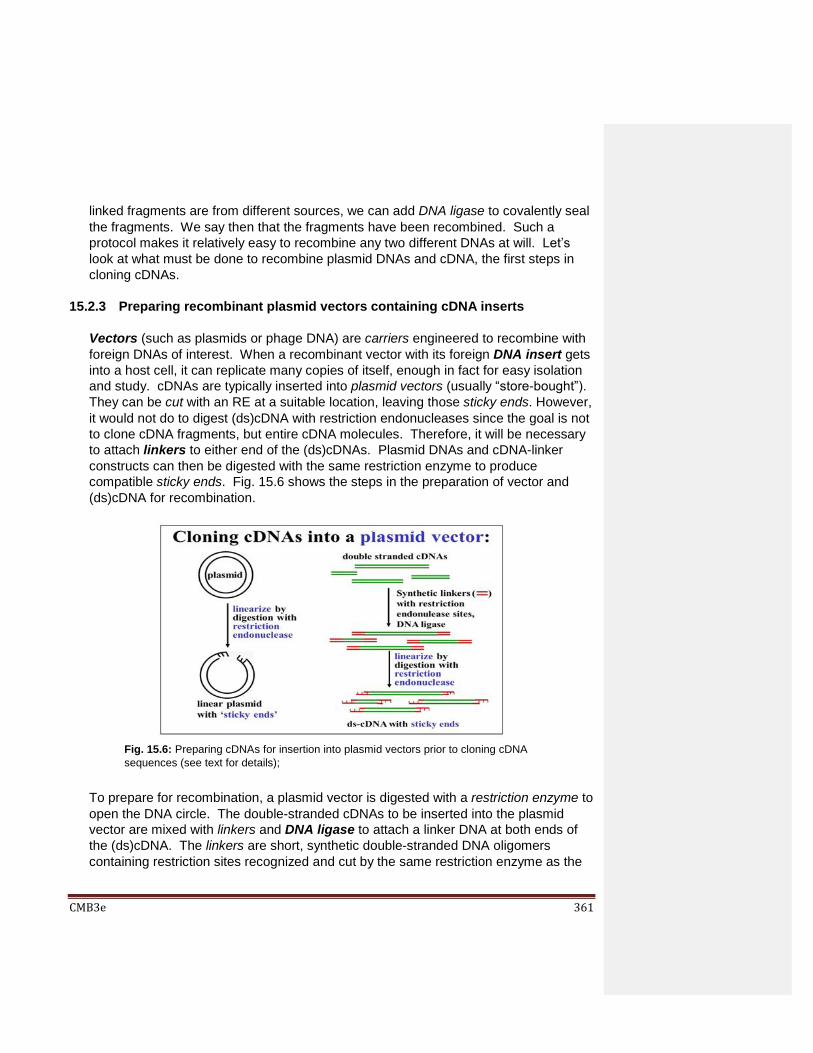
CMB3e 361

linked fragments are from different sources, we can add DNA ligase to covalently seal

the fragments. We say then that the fragments have been recombined. Such a

protocol makes it relatively easy to recombine any two different DNAs at will. Let’s

look at what must be done to recombine plasmid DNAs and cDNA, the first steps in

cloning cDNAs.

15.2.3 Preparing recombinant plasmid vectors containing cDNA inserts

Vectors (such as plasmids or phage DNA) are carriers engineered to recombine with

foreign DNAs of interest. When a recombinant vector with its foreign DNA insert gets

into a host cell, it can replicate many copies of itself, enough in fact for easy isolation

and study. cDNAs are typically inserted into plasmid vectors (usually “store-bought”).

They can be cut with an RE at a suitable location, leaving those sticky ends. However,

it would not do to digest (ds)cDNA with restriction endonucleases since the goal is not

to clone cDNA fragments, but entire cDNA molecules. Therefore, it will be necessary

to attach linkers to either end of the (ds)cDNAs. Plasmid DNAs and cDNA-linker

constructs can then be digested with the same restriction enzyme to produce

compatible sticky ends. Fig. 15.6 shows the steps in the preparation of vector and

(ds)cDNA for recombination.

To prepare for recombination, a plasmid vector is digested with a restriction enzyme to

open the DNA circle. The double-stranded cDNAs to be inserted into the plasmid

vector are mixed with linkers and DNA ligase to attach a linker DNA at both ends of

the (ds)cDNA. The linkers are short, synthetic double-stranded DNA oligomers

containing restriction sites recognized and cut by the same restriction enzyme as the

Fig. 15.6: Preparing cDNAs for insertion into plasmid vectors prior to cloning cDNA

sequences (see text for details);

CMB3e 362

plasmid. Once the linkers are attached to the ends of the plasmid DNAs, they are

digested with the appropriate restriction enzyme. This leaves both the (ds)cDNAs and

the plasmid vectors with staggered, complementary sticky ends.

260 Restriction Enzymes and Recombinant DNA

15.2.4 Recombining plasmids and cDNA inserts and transforming host cells

The next step is to mix the cut plasmids with the digested linker-ended cDNAs in just

the right proportions so that most of the cDNAs form H-bonds with most of the sticky

plasmid ends. Once the H-bonds have connected (annealed) to the cDNAs to plasmid

DNA, adding DNA ligase forms phosphodiester bonds between plasmid and cDNA

insert, completing the recombinant circle of DNA. This process of making

recombinant plasmids is shown in Fig. 15.7, below.

In early cloning experiments, an important consideration was how to generate

plasmids with only one copy of a given cDNA insert, rather than lots of re-ligated

plasmids with no inserts or lots of plasmids with multiple inserts. Using better-

engineered vector and linker combinations, this issue became less important.

261 Recombine a cDNA Insert with a Plasmid Vector

Fig. 15.7: Making recombinant plasmids containing cDNA inserts (see text for details).

CMB3e 363

15.2.5 Transforming host cells with recombinant plasmids

The recombinant DNA molecules are now ready for the next step, creation of a cDNA

library. The recombinant DNAs are added to E. coli (or other) host cells, made

permeable so that they are easily transformed. Fig. 15.8 (below) shows the

transformation step that results in a tube full of cells that is the cDNA library.

Recall that transformation as defined by Griffith is the bacterial uptake of foreign DNA

leading to a genetic change. The transforming principle in cloning is the

recombinant plasmid!

262 Making the cDNA Library

15.2.6 Plating a cDNA Library on Antibiotic-Agar to Select Recombinant Plasmids

After all these treatments, not all plasmid molecules in the mix are recombinant; some

cells in the mix haven’t even taken up a plasmid. So when the recombinant cells are

plated on agar, how do you tell which of the colonies that grow came from cells that

took up a recombinant plasmid? Both the host strain of E. coli and plasmid vectors

Fig. 15.8: Making the cDNA library (see text for details).

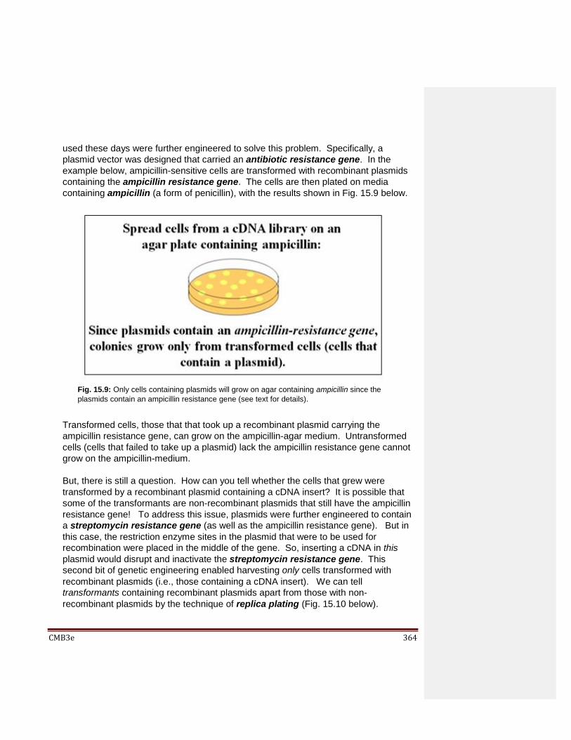
CMB3e 364

used these days were further engineered to solve this problem. Specifically, a

plasmid vector was designed that carried an antibiotic resistance gene. In the

example below, ampicillin-sensitive cells are transformed with recombinant plasmids

containing the ampicillin resistance gene. The cells are then plated on media

containing ampicillin (a form of penicillin), with the results shown in Fig. 15.9 below.

Transformed cells, those that that took up a recombinant plasmid carrying the

ampicillin resistance gene, can grow on the ampicillin-agar medium. Untransformed

cells (cells that failed to take up a plasmid) lack the ampicillin resistance gene cannot

grow on the ampicillin-medium.

But, there is still a question. How can you tell whether the cells that grew were

transformed by a recombinant plasmid containing a cDNA insert? It is possible that

some of the transformants are non-recombinant plasmids that still have the ampicillin

resistance gene! To address this issue, plasmids were further engineered to contain

a streptomycin resistance gene (as well as the ampicillin resistance gene). But in

this case, the restriction enzyme sites in the plasmid that were to be used for

recombination were placed in the middle of the gene. So, inserting a cDNA in this

plasmid would disrupt and inactivate the streptomycin resistance gene. This

second bit of genetic engineering enabled harvesting only cells transformed with

recombinant plasmids (i.e., those containing a cDNA insert). We can tell

transformants containing recombinant plasmids apart from those with non-

recombinant plasmids by the technique of replica plating (Fig. 15.10 below).

Fig. 15.9: Only cells containing plasmids will grow on agar containing ampicillin since the

plasmids contain an ampicillin resistance gene (see text for details).

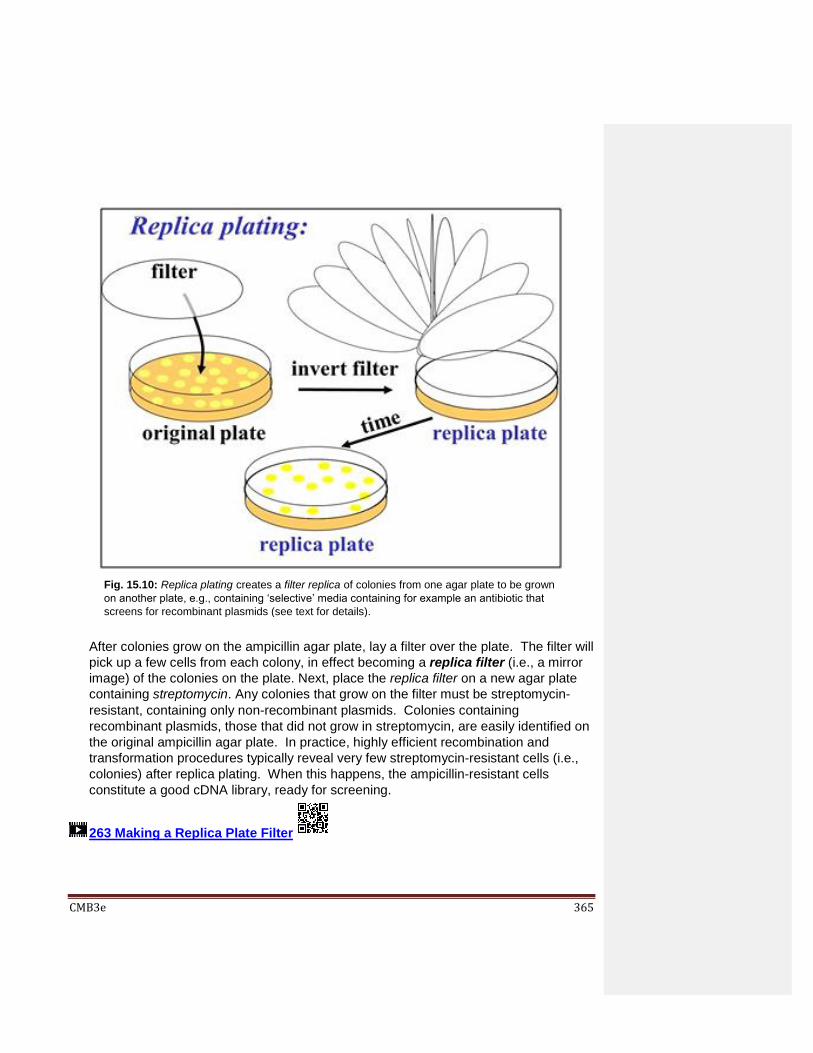
CMB3e 365

After colonies grow on the ampicillin agar plate, lay a filter over the plate. The filter will

pick up a few cells from each colony, in effect becoming a replica filter (i.e., a mirror

image) of the colonies on the plate. Next, place the replica filter on a new agar plate

containing streptomycin. Any colonies that grow on the filter must be streptomycin-

resistant, containing only non-recombinant plasmids. Colonies containing

recombinant plasmids, those that did not grow in streptomycin, are easily identified on

the original ampicillin agar plate. In practice, highly efficient recombination and

transformation procedures typically reveal very few streptomycin-resistant cells (i.e.,

colonies) after replica plating. When this happens, the ampicillin-resistant cells

constitute a good cDNA library, ready for screening.

263 Making a Replica Plate Filter

Fig. 15.10: Replica plating creates a filter replica of colonies from one agar plate to be grown

on another plate, e.g., containing ‘selective’ media containing for example an antibiotic that

screens for recombinant plasmids (see text for details).

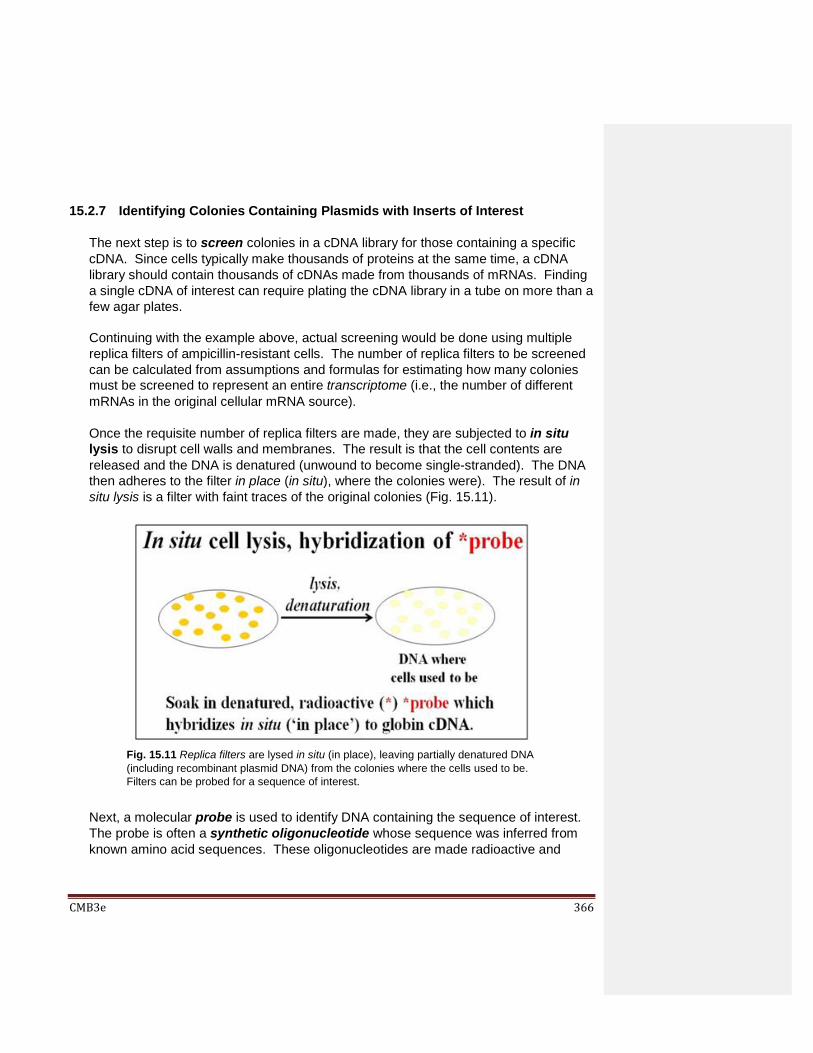
CMB3e 366

15.2.7 Identifying Colonies Containing Plasmids with Inserts of Interest

The next step is to screen colonies in a cDNA library for those containing a specific

cDNA. Since cells typically make thousands of proteins at the same time, a cDNA

library should contain thousands of cDNAs made from thousands of mRNAs. Finding

a single cDNA of interest can require plating the cDNA library in a tube on more than a

few agar plates.

Continuing with the example above, actual screening would be done using multiple

replica filters of ampicillin-resistant cells. The number of replica filters to be screened

can be calculated from assumptions and formulas for estimating how many colonies

must be screened to represent an entire transcriptome (i.e., the number of different

mRNAs in the original cellular mRNA source).

Once the requisite number of replica filters are made, they are subjected to in situ

lysis to disrupt cell walls and membranes. The result is that the cell contents are

released and the DNA is denatured (unwound to become single-stranded). The DNA

then adheres to the filter in place (in situ), where the colonies were). The result of in

situ lysis is a filter with faint traces of the original colonies (Fig. 15.11).

Next, a molecular probe is used to identify DNA containing the sequence of interest.

The probe is often a synthetic oligonucleotide whose sequence was inferred from

known amino acid sequences. These oligonucleotides are made radioactive and

Fig. 15.11 Replica filters are lysed in situ (in place), leaving partially denatured DNA

(including recombinant plasmid DNA) from the colonies where the cells used to be.

Filters can be probed for a sequence of interest.

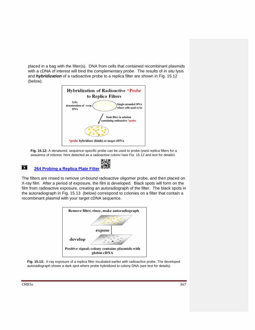
CMB3e 367

placed in a bag with the filter(s). DNA from cells that contained recombinant plasmids

with a cDNA of interest will bind the complementary probe. The results of in situ lysis

and hybridization of a radioactive probe to a replica filter are shown in Fig. 15.12

(below).

264 Probing a Replica Plate Filter The filters are rinsed to remove un-bound radioactive oligomer probe, and then placed on

X-ray film. After a period of exposure, the film is developed. Black spots will form on the

film from radioactive exposure, creating an autoradiograph of the filter. The black spots in

the autoradiograph in Fig. 15.13 (below) correspond to colonies on a filter that contain a

recombinant plasmid with your target cDNA sequence.

Fig. 15.12: A denatured, sequence-specific probe can be used to probe lysed replica filters for a

sequence of interest, here detected as a radioactive colony (see Fig. 15.12 and text for details).

Fig. 15.13:. X-ray exposure of a replica filter incubated earlier with radioactive probe. The developed

autoradiograph shows a dark spot where probe hybridized to colony DNA (see text for details).

CMB3e 368

Once a positive clone is identified on the film, the corresponding recombinant colony is

located on the original plate. This colony is grown up in a liquid culture and the

plasmid DNA is isolated. At that point, the cDNA can be sequenced and the amino

acid sequence encoded by the cloned cDNA can be inferred from the genetic code

dictionary. This will verify that the cDNA insert in fact encodes a protein of interest.

Once verified as containing the desired sequence, recombinant plasmids can be

isolated. tagged (made radioactive or fluorescent) and used to

probe for the genes from which they originated.

identify and quantitate the mRNA even locate the transcripts in the cells.

quantitatively measure amounts of specific mRNAs.

Isolated plasmid cDNAs can even be expressed in suitable cells to make the encoded

protein. These days, diabetics no longer receive pig insulin, but get synthetic human

insulin human made from expressed human cDNAs. Moreover, while the introduction

of the polymerase chain reaction (PCR, see below) has superseded some uses of

cDNAs, they still play a role in genome-level and transcriptome-level studies.

265 Pick a Clone From a Replica Filter and Play With It!

15.3 DNA sequencing

Foe some perspective, we should note that RNA sequencing actually came first, when

Robert Holley sequenced a tRNA in 1965. The direct sequencing of tRNAs was possible

because they are small, short nucleic acids and because many of the bases in tRNAs are

chemically modified after transcription. Twelve years late in 1977, two different methods

for sequencing DNA were reported. One method, developed by Allan Maxam and Walter

Gilbert involved DNA fragmentation and sequencing of the small fragments of DNA, and

then aligning the overlapping sequences of the short fragments to assemble longer

sequences. This became known as Maxam-Gilbert DNA sequencing. The other

method was developed by Frederick Sanger and colleagues in England. This is the DNA

synthesis-based di-deoxy-DNA sequencing technique. Sanger and Gilbert both won a

Nobel Prize in Chemistry in 1983 for their DNA sequencing work. However, because of

its simplicity, Sanger’s method quickly became the standard for sequencing all manner of

cloned DNAs, including the complete sequencing of a genome, that of a bacteriophage

(bacterial virus) called φX174.

At the same time as the advances in sequencing technology were occurring, so were

some of the early developments in recombinant DNA technology. Together these led to

more efficient and rapid cloning and sequencing of DNA from increasingly diverse

sources. The first focus was of course on genes and genomes of important model

organisms, such as E. coli, C. elegans, yeast (S. cerevisiae)…, and of course, us! By

CMB3e 369

1995, Craig Venter and colleagues at the Institute for Genomic Research had completed

the sequence of an entire bacterial genome (Haemophilus influenzae) and by 2001,

Venter’s private group along with Frances Collins and colleagues at the NIH had

published a first draft of the sequence of the human genome. Venter had proven the

efficacy of a whole-genome sequencing approach called shotgun sequencing, which was

much faster than the gene-by-gene, fragment-by-fragment ‘linear’ sequencing strategy

being used by other investigators (more later!). Since Sanger’s di-deoxynucleotide DNA

sequencing method remains a common and economical methodology, let’s consider the

basics of the protocol. Here are the details…

15.3.1 Manual DNA Sequencing

Given a template DNA (e.g., a plasmid cDNA), Sanger used in vitro replication

protocols to demonstrate that he could:

replicate DNA under conditions that randomly stopped nucleotide addition at every

possible position in growing strands.

separate and then detect these DNA fragments of replicated DNA.

Recall that DNA polymerases catalyze the formation of phosphodiester bonds by

linking the phosphate of a nucleotide triphosphate to the free 3’ OH of a

deoxynucleotide at the end of a growing DNA strand. Recall also that the ribose sugar

in the deoxynucleotide precursors of replication lack a 2’ OH (hydroxyl) group.

Sanger’s trick was to add di-deoxynucleotide triphosphates to his in vitro replication

mix. The ribose on a di-deoxynucleotide triphosphate (ddNTP) lacks a 3’ OH, as well

a 2’ OH (Fig. 15.14).

Fig. 15.14: Chemical structure of a di-deoxynucleotide.

CMB3e 370

Adding a di-deoxynucleotide to a growing DNA strand stops replication. No further

nucleotides can add to the 3’-end of the replicating DNA strand because the 3’–OH

necessary for the dehydration synthesis of the next phosphodiester bond is absent!

Because they can stop replication in actively growing cells, ddNTPs such as di-

deoxyadenosine (tradename, cordycepin) are anti-cancer chemotherapeutic drugs.

266 Treating Cancer with Dideoxynucleosides

A look at a manual DNA sequencing reveals what is going on in the sequencing

reactions. Four reaction tubes are set up, each containing the template DNA to be

sequenced. Each tube also contains a primer of known sequence and the our

required deoxynucleotide precursors necessary for replication. Fig. 15.15 (below)

shows the set-up for manual DNA sequencing.

A different ddNTP, (ddATP, ddCTP, ddGTP or ddTTP) is added to each of the four

tubes. Finally, DNA polymerase is added to each tube to start the DNA synthesis

reaction. During DNA synthesis, different length fragments of new DNA accumulate

as the ddNTPs are incorporated at random opposite complementary bases in the

template DNA being sequenced.

A short time after adding the DNA polymerase to begin the reactions, the mixture is

heated to separate the DNA strands and fresh DNA polymerase is added to replace

the enzyme destroyed by heating and repeat the synthesis reactions. These reactions

are repeated as many as 30 times in order to produce enough radioactive DNA

fragments to be detected. The expectations of these sequencing reactions in the four

tubes are illustrated in Fig 15.16 (below).

Fig. 15.15: The four tubes in a manual DNA sequencing protocol contain the same ingredients,

except that each contains a different di-deoxynucleotide.

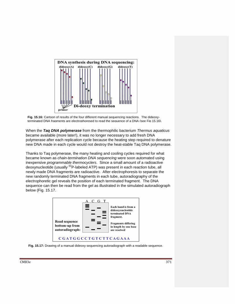
CMB3e 371

When the Taq DNA polymerase from the thermophilic bacterium Thermus aquaticus

became available (more later!), it was no longer necessary to add fresh DNA

polymerase after each replication cycle because the heating step required to denature

new DNA made in each cycle would not destroy the heat-stable Taq DNA polymerase.

Thanks to Taq polymerase, the many heating and cooling cycles required for what

became known as chain-termination DNA sequencing were soon automated using

inexpensive programmable thermocyclers. Since a small amount of a radioactive

deoxynucleotide (usually 32P-labeled ATP) was present in each reaction tube, all

newly made DNA fragments are radioactive. After electrophoresis to separate the

new randomly terminated DNA fragments in each tube, autoradiography of the

electrophoretic gel reveals the position of each terminated fragment. The DNA

sequence can then be read from the gel as illustrated in the simulated autoradiograph

below (Fig. 15.17.

Fig. 15.16: Cartoon of results of the four different manual sequencing reactions. The dideoxy-

terminated DNA fragments are electrophoresed to read the sequence of a DNA (see Fig 15.16).

Fig. 15.17: Drawing of a manual dideoxy sequencing autoradiograph with a readable sequence.

CMB3e 372

The DNA sequence can be read by reading the bases from the bottom of the film,

starting with the C at the bottom of the C lane. Try reading the sequence yourself!

267 Manual Dideoxy Sequencing 15.3.2 Automated First Generation DNA Sequencing

The first semi-automated DNA sequencing method was invented in Leroy Hood’s

California lab in 1986. Though it was still Sanger’s di-deoxy sequencing, a radioactive

phosphate-labeled nucleotide was no longer necessary. Instead, the four dideoxy-

nucleotides in the sequencing reaction were each tagged for detection with a different

fluorescent dye. Sequence reaction products are electrophoresed on an automated

DNA sequencer. Migrating di-deoxy-terminated DNA fragments pass through a

beam of UV light and a detector ‘sees’ the fluorescence of each DNA fragment. The

color and order of the fragments is sent to a computer, generating a colored plot

showing the order and length, and thus their sequences (Fig. 15.18).

A most useful feature of this sequencing method is that a template DNA could be

sequenced in a single tube containing all the required components, including all four

dideoxynucleotides! That’s because the fluorescence detector in the sequencing

machine separately sees all the short ddNTP-terminated fragments as they move

through the electrophoretic gel. Hood’s innovations were quickly commercialized

making major (including many genome) sequencing projects possible. Automated

DNA sequencing rapidly augmented large sequence databases in the U.S. and

Europe. In the U.S., the NCBI (National Center for Biological Information) maintains

the a sequence database and despite its location, archives virtually all DNA

sequences determined worldwide. New ‘tiny’ DNA sequencers have made

sequencing DNA so portable that in 2016, one was even used in the International

Space Station (see a photo of one at the top of this chapter!). New tools and protocols

Fig. 15.18: Automated DNA sequence chromatograph readout.

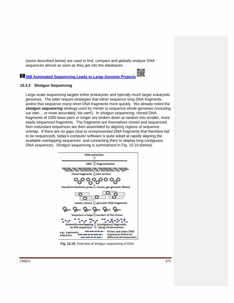
CMB3e 373

(some described below) are used to find, compare and globally analyze DNA

sequences almost as soon as they get into the databases.

268 Automated Sequencing Leads to Large Genome Projects 15.3.3 Shotgun Sequencing

Large-scale sequencing targets entire prokaryotic and typically much larger eukaryotic

genomes. The latter require strategies that either sequence long DNA fragments

and/or that sequence many short DNA fragments more quickly. We already noted the

shotgun sequencing strategy used by Venter to sequence whole genomes (including

our own… or more accurately, his own!). In shotgun sequencing, cloned DNA

fragments of 1000 base pairs or longer are broken down at random into smaller, more

easily sequenced fragments. The fragments are themselves cloned and sequenced.

Non-redundant sequences are then assembled by aligning regions of sequence

overlap. If there are no gaps (due to unrepresented DNA fragments that therefore fail

to be sequenced), today’s computer software is quite adept at rapidly aligning the

available overlapping sequences and connecting them to display long contiguous

DNA sequences. Shotgun sequencing is summarized in Fig. 15.19 (below).

Fig. 15.19:.Overview of shotgun sequencing of DNA.

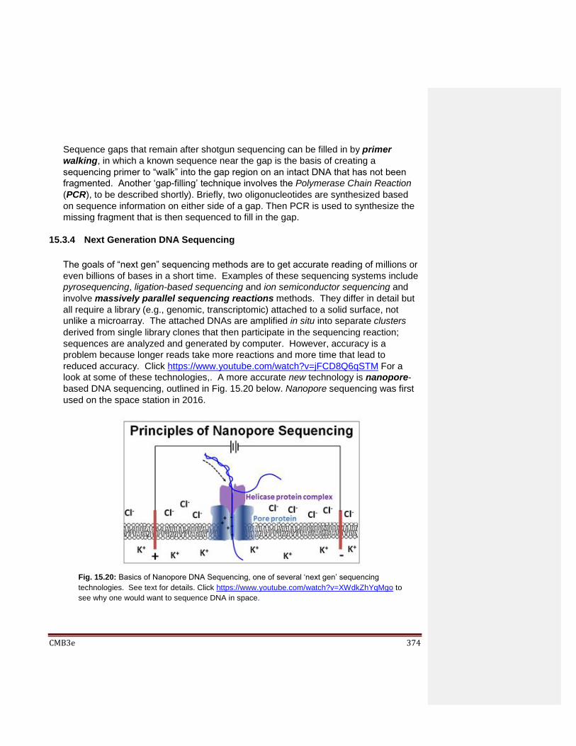
CMB3e 374

Sequence gaps that remain after shotgun sequencing can be filled in by primer

walking, in which a known sequence near the gap is the basis of creating a

sequencing primer to “walk” into the gap region on an intact DNA that has not been

fragmented. Another ‘gap-filling’ technique involves the Polymerase Chain Reaction

(PCR), to be described shortly). Briefly, two oligonucleotides are synthesized based

on sequence information on either side of a gap. Then PCR is used to synthesize the

missing fragment that is then sequenced to fill in the gap.

15.3.4 Next Generation DNA Sequencing

The goals of “next gen” sequencing methods are to get accurate reading of millions or

even billions of bases in a short time. Examples of these sequencing systems include

pyrosequencing, ligation-based sequencing and ion semiconductor sequencing and

involve massively parallel sequencing reactions methods. They differ in detail but

all require a library (e.g., genomic, transcriptomic) attached to a solid surface, not

unlike a microarray. The attached DNAs are amplified in situ into separate clusters

derived from single library clones that then participate in the sequencing reaction;

sequences are analyzed and generated by computer. However, accuracy is a

problem because longer reads take more reactions and more time that lead to

reduced accuracy. Click https://www.youtube.com/watch?v=jFCD8Q6qSTM For a

look at some of these technologies,. A more accurate new technology is nanopore-

based DNA sequencing, outlined in Fig. 15.20 below. Nanopore sequencing was first

used on the space station in 2016.

Fig. 15.20: Basics of Nanopore DNA Sequencing, one of several ‘next gen’ sequencing

technologies. See text for details. Click https://www.youtube.com/watch?v=XWdkZhYqMgo to

see why one would want to sequence DNA in space.

CMB3e 375

This device uses an artificial phospholipid membrane in which are embedded an

engineered helicase/motor-pore protein complex. The nanopore itself is derived

from Mycobacterium smegmatis porin A (MspA). A voltage is applied across the

membrane to create a membrane potential. Double stranded DNA is propelled into

the helicase where it is unwound. The resulting single stranded molecules then are

pass through a tiny hole (the nanopore) in the MspA porin. As the ssDNA (or RNA)

pass through the pore, its charge configurations disturb the electrical field in the porin.

These disturbances are different for each nucleotide, generating a unique signal that

is detected and recorded and displayed in almost real time on small computer.

First generation automated dideoxy Sanger sequencing is still widely used to analyze individual genes or PCR products (see below). But next generation DNA sequencing and small devices like the one used in the space station can also be used in the field , not only for research, but for example, to quickly identify microbial agents of disease. Next generation sequencing protocols and devices are already providing long and increasingly more accurate data required for research and for clinical applications.

15.4 Genomic Libraries

A tube full of recombinant bacteriophage can be defined as a genomic library. Each

phage DNA molecule should contain a fragment of cellular DNA from a foreign organism.

A good genomic library will contain a representation of all of possible fragments of an

organism’s genome. Bacteriophage are often used to clone genomic DNA fragments

because:

• phage genomes are bigger than plasmids and can be engineered to remove large

amounts of DNA that are not needed for infection and replication in host cells.

• the missing DNA can then be replaced by large foreign DNA inserts, fragments as

long as 18-20kbp (kilobase pairs), nearly 20X longer than cDNA inserts in plasmids.

• purified phage coat proteins can be mixed with the recombined phage DNA to make

infectious phage particles (i.e., recombinant phage).

• Infection of host bacteria by these ‘particles’ leads to replication of the recombinant

phage DNA, new phage production, cell lysis and the release of lots of new

recombinant phage.

Consider the following bit of math: A typical mammalian genome consists of more than 2

billion base pairs. Inserts in plasmids are very short, rarely exceeding 1000 base pairs.

Dividing 2,000,000,000 by 1000, you get 2 million, a minimum number of recombinant

plasmid clones that must be screened to find a sequence of interest. In fact, you would

need many more than this number of clones to find the smaller parts of a gene that add

up to a whole gene! Of course, part of the solution to this “needle in a haystack” dilemma

is to clone larger DNA inserts in more accommodating vectors. Hence the value of a

bacteriophage vector.

CMB3e 376

From this brief description, you may recognize the common strategy for genetically

engineering a cloning vector: determine the minimum properties that your vector must

have and remove non-essential DNA sequences. Consider the Yeast Artificial

Chromosome (YAC), hosted by (replicated in) yeast cells. YACs can accept humongous

foreign DNA inserts! This is because to be a chromosome that will replicate in a yeast

cell requires one centromere and two telomeres… and little else! Recall that

telomeres are needed in replication to keep the chromosome from shortening during

replication of the DNA. The centromere is needed to attach chromatids to spindle fibers

so that they can separate during anaphase in mitosis (and meiosis). So along with

a centromere and two telomeres, just include restriction sites to enable recombination

with inserts as long as 2000 Kbp. That’s a YAC! The tough part of course is keeping a

2000Kbp long DNA fragment intact long enough to get it into the YAC.

Whatever the vector of choice, sequencing its insert can tell us many things. It can show

us how a gene is regulated by confirming known and revealing new regulatory DNA

sequences. It can show us neighboring genes, helping us to map genes on a

chromosome. Genomic DNA sequences from one species can probe for similar

sequences in other species, allowing comparative sequence analysis that can tell us a

great deal about gene evolution and the evolution of species. One early surprise from

gene sequencing studies was that we share many common genes and DNA sequences

with other species, like yeast, worms, flies and of course vertebrates…, including our

more closely related mammalian friends. You may already know that chimpanzee and

human genomes are 99% similar. And we have already seen comparative sequence

analysis showing how proteins with different functions in the same (and even across)

species nevertheless share structural domains.

Let’s look at how we would make a phage genomic library that targets a specific gene of

interest. As you will see, the principles are similar to cloning a foreign DNA into a

plasmid, or in fact any other vector, but the numbers and details used here exemplify

cloning in phage.

15.4.1 Preparing Specific Length Genomic DNA for Cloning; the Southern Blot

To begin with, high molecular weight (i.e., long molecules of) the desired genomic

DNA are isolated, purified and then digested with a restriction enzyme. Usually, the

digest is partial, aiming to generate overlapping DNA fragments of random length.

The digested DNA is mixed with ethidium bromide, a fluorescent dye that binds to

DNA. After electrophoresis on agarose gels and exposed to UV light, the DNA

appears as a bright fluorescent smear. If we wanted to clone the complete genome of

an organism, we could recombine all of this DNA with suitably digested vector DNA.

CMB3e 377

But, since we are only after one gene, we can reduce the number of clones to be

screened in order to find our sequence of interest. In the early days of cloning we

would do this by creating a Southern blot (named after Edward Southern, the

inventor of the technique). This technique lets us identify the size of genomic DNA

fragments most likely to contain a desired gene. To summarize the steps to make a

Southern Blot:

a) Digest genomic DNA with one or more restriction endonucleases.

b) Run the digest products on an agarose gel to separate fragments by size (length).

The DNA appears as a smear when stained with a fluorescent dye.

c) Place a filter on the gel. The DNA transfers (blots) to the filter for e.g., 24 hours.

d) Remove the blotted filter and place it in a bag containing a solution that can

denature the DNA.

e) Add radioactive probe (e.g., cDNA) containing the gene or sequence of interest.

The probe hybridizes (bind) to complementary genomic sequences on the filter.

f) Prepare an autoradiograph of the filter and see a ‘band’ representing the size of

genomic fragments of DNA that include the sequence of interest.

The Southern blot protocol is illustrated in Fig. 15.21 (below).

Fig. 15.21:.Overview of Southern blotting, a technique that transfers electrophoresed DNA

to a filter for hybridization with a probe (see text for details).

CMB3e 378

Once you know the size (or size range) of restriction digest fragments that contain the DNA you want to study, you are ready to run another gel of digested genomic DNA, and this time…,

a) cut out the piece of gel containing fragments of the size that that ‘lit up’ with your

probe in the autoradiograph.

b) remove (elute) the DNA from the gel piece into a suitable buffer.

c) prepare the DNA for insertion into (recombination with) a genomic cloning vector.

15.4.2 Recombining Size-Restricted Genomic DNA with Phage DNA

After elution of restriction digested DNA fragments of the right size range from the

gels, we mix the DNA with compatibly digested phage DNA at concentrations that

favor the formation of H-bonds between the ends of the phage DNA and the genomic

fragments (rather than with each other!). Addition of DNA ligase covalently links the

recombined DNA molecules. These steps are abbreviated in the illustration in Fig.

15.22.

The recombinant phage that are made next will contain sequences that become the genomic library.

Fig. 15.22:.Genomic DNA restriction enzyme digest is mixed with phage vector with

compatible ‘sticky’ ends and ligated to make recombinant DNAs.

CMB3e 379

15.4.3 Creating Infectious Viral Particles with Recombinant phage DNA

The next step is to package the recombined phage DNA by adding purified viral coat

proteins to make infectious phage particles (Fig. 15.23).

269 Genomic Libraries: Make and Package Recombinant Phage DNA

Packaged phage are added to a culture tube full of host bacteria (e.g., E. coli). After

infection the recombinant DNA enters the cells where it replicates and directs the

production of new phage that eventually lyse the host cell (Fig. 15.24).

Fig. 15.23:.Mixing recombinant phage DNA with phage coat proteins creates infectious

recombinant phage particles.

Fig. 15.24:.Recombinant phage infection, the replication of phage DNA and production of

new phage leads to host cell lysis, allowing the collection of new recombinant phage.

CMB3e 380

The recombined vector can also be introduced directly into the host cells by

transduction, which is to phage DNA what transformation is to plasmid DNA.

Whether by infection or transduction, the recombinant phage DNA ends up in host

cells which produce new phage that eventually lyse the host cell. The released

phages go on to infect more host cells until all cells have lysed. What remains is a

tube full of lysate containing cell debris and lots of recombinant phage particles.

270 Infect Host with Recombinant Phage to Make a Genomic Library

Just a note on some other vectors for genomic DNA cloning… For large genomes,

the goal is to choose a vector able to house larger fragments of ‘foreign’ DNA so that

you end up screening fewer clones. We’ve seen that phage vectors accommodate

larger foreign DNA inserts than plasmid vectors, and YACs even more… Given a

large enough eukaryotic genome, it may be necessary to screen more than a hundred

thousand clones in a phage-based genomic library.

Apart from size-selection of genomic fragments before inserting them into a vector,

selecting the appropriate vector is just as important. Table 15.1 lists commonly used

vectors and the sizes of inserts they will accept.

Vector type Insert size (thousands of bases)

Plasmids up to 15

Phage lambda (λ) up to 25

Cosmids up to 45

Bacteriophage P1 70 to 100

P1 artificial chromosomes (PACs) 130 to 150

Bacterial artificial chromosomes (BACs) 120 to 300

Yeast artificial chromosomes (YACs) 250 to 2000

Click on the links to these vectors if you wish to learn more about them. We will

continue this example by screening a phage lysate genomic library for a recombinant

phage with a genomic sequence of interest.

15.4.4 Screening a Genomic Library; Titering Recombinant Phage Clones

A bacterial lawn is made by plating so many bacteria on the agar plate that they

simply grow together rather than as separate colonies. If a small amount of phage is

evenly plated over the bacterial lawn, each virus will infect one cell. Subsequent lysis

CMB3e 381

of this cell releases many phage, each infecting neighboring cells. After a day or so of

repeated cycled of lysis and infection, plaques (clearings ) appear in the lawn at the

site of the first infection Each plaque shown in the illustration in Fig. 15.25 (below) is a

clone of the original phage particle.

To screen a phage genomic library, the phage lysate is titered on bacterial lawns. In

a typical titration, a phage lysate might be diluted 10-fold with a suitable medium.

This dilution is further diluted 10-fold… and so on. Each serial 10X dilution is then

spread on a bacterial (e.g., E. coli) lawn. The plaques formed on each lawn are then

counted. Remember, a plaque is a clone of a single virus.

Let’s say that you spread 10 l of an undiluted lysate on a bacterial lawn. After a day

or so you see lots of tiny plaques and after staring at the plate. You figure that there

are thousands of plaques on the lawn. But you have also made serial 10X dilutions of

the lysate on bacterial lawns. On the lawn plated with 10 ml of the 8th serial dilution of

the lysate you count 176 large, well-separated plaques. So, there must have been

1,408 (8 X 176) phage particles in 10 l of the original undiluted lysate.

15.4.5 Screening a Genomic Library; Probing the Genomic Library

To represent a complete genomic library, you will need many plates of a serial 10X

dilutions, containing say, ~500-1000 plaques per plate If size-selected fragments (e.g.,

identified by Southern blotting) were cloned to make a partial genomic library,

then there will be fewer plaques to be screened to find a sequence of interest. Since

plaques contain a lot of phage DNA not yet packaged at the time of lysis it is possible

Fig. 15.25:.Phage plaques formed on a bacterial lawn; each plaque is a genomic clone.

CMB3e 382

to transfer that DNA directly to filters by to replica plating (similar to replica plating of

bacterial colonies). The replica filters are treated to denature the DNA and then

hybridized to a probe with a known sequence. In the early days of cloning, the probes

were often a sequenced cDNA previously isolated from libraries of the same or

different (usually related) species.

.

After soaking the filters in a radioactively-labeled probe, an X-Ray film is placed over

the filter, exposed and developed. Black spots will form where the film lay over a

plaque containing genomic DNA complementary to the probe. In the example

illustrated in Fig. 15.26, a globin cDNA might have been used to probe our partial

genomic library (globin genes were in fact among the first to be cloned!).

15.4.6 Isolating the Gene

Cloned genomic DNA fragments are much longer than any gene of interest, and

always longer than any cDNA from a cDNA library. They are also embedded in a

genome that is thousands of times as long as the gene itself, making the selection of

an appropriate vector necessary. If the genome can be screened from a reasonable

number of cloned phage (~100,000 plaques for instance), the one plaque producing a

positive signal on the autoradiograph would be further studied. This plaque should

Fig. 15.26:.Replica filters of plaques probed with a sequence of interest (in this case a globin

DNA sequence) locate autoradiographic spots where probe hybridized to recombinant phage.

CMB3e 383

contain the gene of interest. At this point, we seem to have identified a clone

containing a globin gene sequence. We can use this clone to infect yet more host

cells and grow up much more of the globin gene-containing DNA for further study.

271 Screen a Genomic Library, Pick and Grow a Phage Clone

Given that a gene of interest might be a short sequence embedded in a large genomic

insert that is as long as 20kbp, we can further isolate the gene from neighboring DNA.

The traditional strategy again involves Southern blotting. The cloned DNA is purified

and digested with restriction endonucleases, and the digest fragments are separated

by agarose gel electrophoresis. A Southern blot is made on e.g., a nylon filter and

the filter is soaked in a solution that denatures the DNA on the blot. The filter is then

probed with the same tagged probe used to find the positive clone (plaque). The

smallest DNA fragment containing the gene of interest can then be subcloned in a

suitable vector and grown to provide enough target sequence DNA for further study.

15.5 The Polymerase Chain Reaction (PCR)

The polymerase chain reaction (PCR) can amplify a region of DNA from any source, like

DNA fragments obtained from a fossil or residue left at a crime scene, or even from a

single cell. This amplification usually takes just a few hours, generating millions of copies

of the desired target DNA sequence. The result is the purification of a specific region of

DNA from surrounding sequences in a single reaction! Kary B. Mullis was awarded a

Nobel Prize in 1993 for his development of PCR, which is now the basis of innumerable

research studies of gene structure, function and evolution as well as applications in

criminal forensics, medical diagnostics and other commercial uses. PCR is described in

detail below.

272 PCR: Design and Synthesize Opposing Oligonucleotide Primers

273 PCR: The Amplification Reaction 15.5.1 PCR – the Basic Process

Typical PCR relies on knowing just two bits of DNA sequence that will be used to

design and synthesize short oligonucleotide sequences (oligomers) in the laboratory.

The oligomers must be complementary to sequences on the opposite strands of

double-stranded DNA containing the gene to be studied, with their 3’ ends facing

(opposing) each other on either side of the sequence to be amplified. This way the

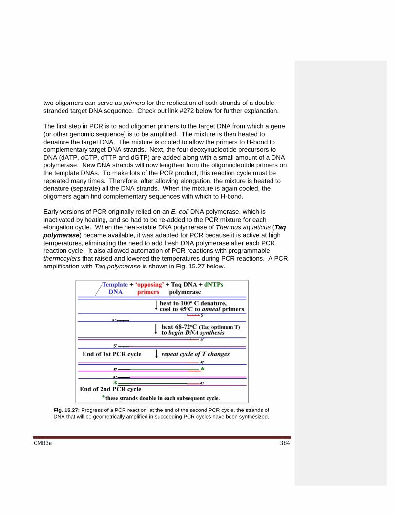
CMB3e 384

two oligomers can serve as primers for the replication of both strands of a double

stranded target DNA sequence. Check out link #272 below for further explanation.

The first step in PCR is to add oligomer primers to the target DNA from which a gene

(or other genomic sequence) is to be amplified. The mixture is then heated to

denature the target DNA. The mixture is cooled to allow the primers to H-bond to

complementary target DNA strands. Next, the four deoxynucleotide precursors to

DNA (dATP, dCTP, dTTP and dGTP) are added along with a small amount of a DNA

polymerase. New DNA strands will now lengthen from the oligonucleotide primers on

the template DNAs. To make lots of the PCR product, this reaction cycle must be

repeated many times. Therefore, after allowing elongation, the mixture is heated to

denature (separate) all the DNA strands. When the mixture is again cooled, the

oligomers again find complementary sequences with which to H-bond.

Early versions of PCR originally relied on an E. coli DNA polymerase, which is

inactivated by heating, and so had to be re-added to the PCR mixture for each

elongation cycle. When the heat-stable DNA polymerase of Thermus aquaticus (Taq

polymerase) became available, it was adapted for PCR because it is active at high

temperatures, eliminating the need to add fresh DNA polymerase after each PCR

reaction cycle. It also allowed automation of PCR reactions with programmable

thermocylers that raised and lowered the temperatures during PCR reactions. A PCR

amplification with Taq polymerase is shown in Fig. 15.27 below.

Fig. 15.27: Progress of a PCR reaction: at the end of the second PCR cycle, the strands of

DNA that will be geometrically amplified in succeeding PCR cycles have been synthesized.

CMB3e 385

You can see from the illustration that the second cycle of PCR has generated the two

DNA strands that will be templates for doubling and re-doubling the desired product

after each subsequent cycle. A typical PCR reaction might involve 30 PCR cycles,

resulting in a nearly exponential amplification of the desired sequence. The products

of PCR amplification are in such abundance that they can be seen under fluorescent

illumination on an ethidium bromide-stained agarose gel (Fig. 15.28, below).

Because they are so plentiful, PCR- amplified DNAs can be sequenced and used in

many subsequent studies. In this gel, the first lane (on the left) contains a DNA

ladder, a mixture of DNAs of known lengths that can be used to estimate the size of

the bright bands (i.e., PCR products) in the remaining lanes. In this example, the four

PCR products were amplified from the same cloned genomic DNA using different

combinations of oligonucleotide primers.

15.5.2 The many Uses of PCR

PCR-amplified products can be labeled with radioactive or fluorescent tags to screen

cDNA or genomic libraries, to probe where a DNA sequence of interest migrates on a

Southern or a blot, or to determine where an RNA sequence of interest migrates on a

Northern blot (a fanciful name for RNAs that are separated by size on gels and blotted

to filter). In a major PCR advance, Quantitative PCR was developed to study

Fig. 15.28: Agarose gel electrophoresis of PCR amplified DNAs, stained with ethidium bromide

to be detectable under fluorescent light: PCR products of the amplification of a globin gene

clone from the insect Chironomus thummi. The sizes (lengths in base pairs) of the 4 PCR

products in lanes 2-5 are close to those of the bands in the standard DNA size ladder in lane 1.

CMB3e 386

differential gene expression and gene regulation. The technique allows cDNA

amplifications from RNAs under conditions that detect not only the presence, but also

the relative amounts of specific transcripts being made in cells.

Variant PCR protocols and applications are manifold and often quite inventive! For a

list, click Variations on Basic PCR. A recent CRISPR/Cas9 variant amplifies DNA and

may lead to PCR at 370C, eliminating the need for a thermocycler altogether! This

could prove especially useful for conducting PCR in the field. While not yet ready for

prime time, check out PCR with Cas9 and without a thermocycler! for more. And in

addition to technological advances, PCR has broad applications in research, forensic

science, history, anthropology, etc… and maybe even a study of your own genealogy.

Let’s look at three of these.

1. Forensics

Another application of PCR is in forensic science, to identify a person or organism

by comparing its DNA to some standard (or control) DNA. Fig. 15.29 is an

example of one of these acrylamide gel DNA fingerprints.

Using this technology, it is now possible to detect genetic relationships between

near and distant relatives (as well as to exclude such relationships), determine

paternity, demonstrate evolutionary relationships between organisms and solve

recent and even ‘cold-case’ crimes. Alu sequences are ~300bp short interspersed

elements (SINES) that are highly repeated throughout the human genome. DNA

fingerprinting is possible in part because each of us has a unique number and

distribution of Alu SINEs in our genome. To read more about Alu sequences and

human diversity, click Alu Sequences and Human Diversity. Click Sir Alec Jeffries

to learn about the origins of DNA fingerprinting in real life… and on all those TV

CSI programs! Check out https://www.future-science.com/btn/news/apr18/07 for a

brief history of the birth of DNA fingerprinting and to see how analysis of changes

in gene activity that occur after death may even help ID criminals. For a video on

DNA fingerprinting, click Alu and DNA fingerprinting.

Fig. 15.29: Electrophoretic DNA fingerprint.

CMB3e 387

2. History

Other intriguing examples of the use of PCR for identification include establishing

the identities of Egyptian mummies, the Russian Tsar deposed and killed during

the Russian revolution (along with his family members), and the recently unearthed

body of King Richard the 3rd of England.

3. Who are your Ancestors?

Tracing your ethnic, racial and regional ancestry is related to DNA fingerprinting, in that it relies on PCR amplification of genes and other variable DNA regions and comparison of these your sequences to distinguishing DNA markers in large sequence databases. Prices for these services have come down, and as a result, their popularity has gone up in recent years. Typically, you provide spit or a salivary (buccal) swab to the service and they amplify and sequence the DNA in your samples. The analysis compares your DNA sequences to database sequences looking for patterns of ethnic and regional markers that you might share with the database(s). Based on these comparisons, you are provided with a (more…, or less) accurate map of your DNA-based ancestry. Folks who are spending around $100.00 (less when on sale!) often ask how accurate these analyses are and what do they really mean. For example, what does it mean if your DNA says you are 5% native American? In fact, different services can sometimes give you different results! You can get some answers and explanations

at DNA Ancestry Testing.

274 The Power of PCR: Some Examples

15.6 Genomic Approaches: The DNA Microarray

Traditionally, when cellular levels of a protein were known to change in response to a

chemical effector, molecular studies focused on control of the transcription of its gene.

These studies often revealed that the control of gene expression was at the level of

transcription, turning a gene on or off through interactions of transcription factors with

DNA. However, protein levels are also controlled post-transcriptionally, by regulating

the rate of mRNA translation or degradation. Studies of transcriptional and post-

transcriptional regulation mechanisms are seminal to our understanding of how the

correct protein is made in the right amounts at the right time.

CMB3e 388

We may have suspected, but now we know that control of gene expression and cellular

responses can be more complex than increasing or decreasing the transcription of a

single gene or translation of a single protein. Newer technologies make possible the

study of the expression of virtually all genes in a cell at the same time, a broadly defined

field of investigation called genomics. Such studies can reveal networks of regulated

genes that must be understood to more fully explain the developmental and physiological

changes in an organism. Using similar terminology, transcriptomics looks at a cell’s

transcriptome, allowing the study of ‘webs’ of interactive RNAs. Let’s look at a simulated

microarray illustrating how multiple transcripts can be detected simultaneously on one

microarray (Fig. 15.30).

Microarrays are typically made by ‘spotting’ nucleic acids (e.g., cloned DNA from a

genomic or cDNA library, PCR products, oligonucleotides…) on a glass slide, or chip. In

the language of microarray analysis, the slides are the probes. Spotting a chip is a

robotic process. Because the DNA spots are microscopic, a cell-specific transcriptome

(e.g., a cDNA library) can fit on a single chip. A small prokaryotic or viral genome

microarray might also fit on a single chip. Larger genomes might need several slides. In

the simulated microarray above, the three colors would represent different fluorescent

Fig. 15.30: Simulated glass slide microarray showing multiple color fluorescent spots,

indicating a hunt for more than one DNA sequence at the same time.

CMB3e 389

tags on specific DNA sequences for three different genes. If the spots were cDNAs

synthesized from cellular RNA extracts, the microarray results would indicate that at least

three different genes of interest were being actively transcribed in those cells at the time

of RNA extraction.

In another use of microarrays, spotted genomic clones could be used to probe a mixture

of fluorescently tagged target cDNAs, also made from cellular mRNAs. This experiment

is asking not if specific genes are expressed in a cell but rather, which and how many

genes are being expressed in the cell at the time of mRNA extraction. It is an approach

to characterizing a cell’s transcriptome). This is a more global question. Identifying the

proteins encoded by all those genes would be the next step. Microarrays can be

quantitative so that the brightness (intensity) of the signal from each probe can be

measured. Quantitative microarrays can be designed to show how global gene

expression changes in cells during normal differentiation or in response to chemical

signals. DNA microarrays are also valuable for genotyping, (i.e. characterizing the genes

in an organism), and they are so sensitive that they can even distinguish between two

genes or regions of DNA that differ by a single nucleotide. Click Single Nucleotide

Polymorphisms, or SNPs to learn more.

By analogy to genomics, and transcriptomics, proteomics is the field of study of global

protein interactions. Primary tools of proteomics include mass spectroscopy and more

recently, Protein Microarrays. Mass spectroscopy can identify the presence of specific

proteins and protein variants in samples, and has even been applied to the analysis of a

Leonardo Da Vinci painting (Donna Nuda) to determine if it was actually painted by the

renaissance master, an artist(s) of his school, or someone else entirely (click Proteomics

Enlisted to Determine Artistic Provenance to learn the verdict!). Protein microarrays are

in some ways similar to DNA microarrays, but can look globally at protein-protein

interactions, as well as the different states of proteins under different cellular conditions.

Read even more about these exciting developments and their impact on basic and clinical

research at Protein Microarrays from ncbi..

Now think about this! Can we create a proteomic library analogous to a genomic library?

This would seem a daunting prospect, but efforts are underway. Check out A stab at

mapping the Human Proteome for original research leading to the sampling of a tissue-

specific human proteome, and click Strategies for Approaching the Proteome for more

general information.

As you can see, microarrays and related technologies are powerful tools that can shift

our focus from how single molecules influence events, to thinking about webs of

biochemical interactions that could more completely explain molecular and physiological

causes and effects. Table 15.2(below, adapted from Wikipedia) summarizes different

applications of microarrays.

CMB3e 390

The Power of Microarrays Application or

Technology Synopsis

Gene expression profiling

In a transcription (mRNA or gene expression) profiling experiment the expression levels of thousands of genes are simultaneously monitored to study the effects of certain treatments, diseases, and developmental stages on gene expression.

Comparative genomic hybridization

Assessing genome content in different cells or closely related organisms, where one organism’s genome is the probe for a target genome from a different species.

GeneID

Small microarrays to check IDs of organisms in food and feed for genetically modified organisms (GMOs), mycoplasmas in cell culture, or pathogens for disease detection. These detection protocols often combine PCR and microarray technology.

CHIP; chromatin immunoprecipitation

DNA sequences bound to a particular protein can be isolated by immunoprecipitating the protein. The fragments can be hybridized to a microarray (such as a tiling array) allowing the determination of protein binding site occupancy throughout the genome.

DamID

Analogously to ChIP, genomic regions bound by a protein of interest can be isolated and used to probe a microarray to determine binding site occupancy. Unlike ChIP, DamID does not require antibodies but makes use of adenine methylation near the protein's binding sites to selectively amplify those regions, introduced by expressing minute amounts of protein of interest fused to bacterial DNA adenine methyltransferase.

SNP detection

Identifying single nucleotide polymorphism among alleles within or between populations. Some microarray applications make use of SNP detection, including Genotyping, forensic analysis, measuring predisposition to disease, identifying drug-candidates, evaluating germline mutations in individuals or somatic mutations in cancers, assessing loss of heterozygosity, or genetic linkage analysis.

Alternative splicing detection

An exon junction array design uses probes specific to the expected or potential splice sites of predicted exons for a gene. It is of intermediate density, or coverage, to a typical gene expression array (with 1-3 probes per gene) and a genomic tiling array (with hundreds or thousands of probes per gene). It is used to assay the expression of alternative splice forms of a gene. Exon arrays have a different design, employing probes designed to detect each individual exon for known or predicted genes, and can be used for detecting different splicing isoforms.

Tiling array

Genome tiling arrays consist of overlapping probes designed to densely represent a genomic region of interest, sometimes as large as an entire human chromosome. The purpose is to empirically detect expression of transcripts or alternatively spliced forms which may not have been previously known or predicted.

275-2 The Power of Microarrays

CMB3e 391

15.7 Ome-Sweet-Ome

Early molecular technologies, including the ones described in this chapter, were applied

to understanding the structure, function and regulation of specific genes. Some of the

more recent technologies (e.g., microarrays) are well adapted to holistic approaches to

understanding cell function. Terms we have already seen (genome, epigenome,

transcriptome) were coined in an effort to define the different objects of study whose

underlying network of molecular interactions can more accurately explain cell function.

Distinguishing these objects of study can be difficult, and their overlap in cells can be

confusing. Here is a short compendium of …omes with an attempt at clarification:

Genome - total DNA content of a cell, identical in every cell of an organism

Proteome –a cell’s protein profile and steady state at any given moment

Exome - A cell’s total coding DNA (excluding non-coding DNA)

Metabolome - A cell’s metabolic landscape (i.e., metabolic status)

Epigenome - A cell’s total DNA-modification/chromatin topography

Methylome – The pattern of methylation of DNA in the genome

Paleoproteome: Profile of proteins found in ancient remains by mass spectroscopy

transcriptome: A cell’s RNA transcript profile and steady state at any given moment

epitranscriptome: a map of chemical modifications of RNAs that inform their function

metabolome: all of the small metabolytes in a defined sample (cell, organelle, tissue,

etc.)

One might be excused for assuming that such cellular profiles would be the same for all

cells in a tissue, only changing as gene expression is regulated during development or

when signaled by extracellular events or chemical signals. But, even genomic and

exomic profiles can change! Recall somatic mutations in dividing cells, and genome loss

in some cells (e.g., erythrocytes that emerge from our reticulocytes). Studies of large

numbers of individual cells suggest profile variation even in cells of the same tissue or cell

culture. How and why this is so is a rapidly growing new area of study, made possible by

new tools for studying DNA, RNA and proteins molecules in single cells (see Mapping

Protein Networks, The Dark Proteome, What on earth is Paleoproteomics?, A Human

Transcriptome Study, Nature vs. Nurture: Influences on Epigenome and Methylome,

Epitranscriptomics-Functional Chemical Modifications of RNAs. Can you name the next

…ome? Maybe the chondrome (see Mining Mitochondrial Genes).

15.8 From Genetic Engineering to Genetic Modification

By enabling us to focus on how genes and their regulation have evolved, genomic,

transcriptomic and proteomic technologies have vastly increased our knowledge of how

cells work at a molecular level. We continue to add to our knowledge of disease process

and in at least a few cases, how we can treat disease. The use of technologies to

genetically modify organisms is more controversial, despite the best of human intentions.

CMB3e 392

Some genetically modified organisms (GMOs) aim to increase food productivity to better

feed the world. The introduction ‘beneficial’ genes into some GMOs have made

drought-resistant crops to increase the range where major food crops can be grown.

pest-resistant crops to reduce reliance on environmentally toxic chemical pesticides.

herbicide-resistant crops that survive chemicals used to destroy harmful plants.

The quest for “improved” plant and animal varieties has been going on since before

recorded history. Farmers have been cross-breeding cows, sheep, dogs, and crop

varieties from corn to wheat, hoping to find faster growing, larger, hardier, (you name it)

varieties. It is the manipulation of DNA (the essence of the genetic material itself) that is

at the root of controversy. Controversy is reflected in opinions that GMO foods are

potentially dangerous, and that their cultivation should be banned. But the general

consensus is that attempting to ban GMOs is too late! In fact, you are probably already

partaking of some GMO foods without even knowing it. Perhaps the good news is that

after many years of GMO crops already in our food stream, the emerging scientific

consensus is that GMO foods are no more harmful than unmodified foods. The current

debate is whether or not to label foods that are (or contain) GMO ingredients as

genetically modified. In an odd but perhaps amusing take on the discomfort some folks

feel about GMOs, a startup company has genetically modified Petunias. When grown in

water, their flowers are white, but when ‘watered’ with beer, they will produce pink flowers

or purple flowers depending on how much beer they get (Check it out at Can Beautiful

Flowers Change Face?). According to the company, they seek “to bring what it sees as

the beauty of bioengineering to the general public” (and perhaps some profit as well?).

Finally, new CRISPR and related tools can precisely edit any DNA sequences. While not

yet ready for prime time, one CRISPR-based protocol even promises to amplify genes

from DNA without prior denaturation at 37oC, i.e., without the need for a thermocycler

(check out PCR with Cas9 and without a thermocycler for more). Unlike the “quack

medicines” of old, these tools have the real potential to cure disease, destroy disease-

carrying vectors, cure cancer, improve crops and… possibly alter the course of evolution.

We may also need to mobilize such technologies to cope with the coming effects of

climate change! The speed with which one can accomplish such good (or evil) is truly

awesome.

Some iText & VOP Key Words and Terms

2', 3' di-deoxy CTP chemotherapy genome regulatory networks

alternative splicing genome projects restriction endonucleases

automated DNA sequencing genomic library reticulocyte

CMB3e 393

autoradiography insert DNA reverse transcriptase

BACs and YACs library screening RNA probes

bacterial artificial chromosome vectors linkers RNAse

blunt ends Northern blot shotgun sequencing

cDNA oligo d(T) column single nucleotide polymorphisms

cDNA hairpin loop PCR SNPs

cDNA library PCR Southern blot

cDNA probes PCR primers sticky ends

chemiluminescence PCR steps systematics

cosmid vectors phage lambda vectors Taq polymerase

di-deoxy termination plasmids thermophilic bacteria

di-deoxy sequencing method poly(A) tail

thermophilic DNA polymerases

DNA ligase polymerase chain reaction Thermus aquaticus

DNA sequencing primer transcriptome

elution primer walking transformation

ethidium bromide probe hybridization vectors

fluorescence proteome Western blot

forensics recombinant vector yeast artificial chromosomes

Genetic (DNA) fingerprint recombination

CMB3e 394

Chapter 16: Membrane Structure Membrane Structure and Function: the fluid mosaic, membrane proteins,

glycoproteins, glycolipids

16.1 Introduction

All cellular membranes share the same phospholipid bilayer construction, all restrict the

flow of substances from one side to the other (i.e., they are semipermeable), and all are

a fluid mosaic of proteins attached to or embedded in the phospholipid bilayer. Specific

proteins and phospholipids structurally and functionally differentiate between one kind of

cellular membrane and another. Integral proteins are held in the membrane by a

hydrophobic domain that anchors them to the hydrophobic interior of the membrane.

Some integral membrane proteins span the phospholipid bilayer, with hydrophilic

domains on either side of the membrane. In the case of the plasma membrane, the

hydrophilic domains of such transmembrane proteins interact with the watery

extracellular fluid on one side and the aqueous cytoplasm on the other. Once embedded

in the fatty acid interior of a membrane, integral membrane proteins cannot escape! In

contrast, peripheral membrane proteins are more loosely held in place by hydrophilic

interactions with charged features of the membrane surface (phospholipid

CMB3e 395

heads, hydrophilic surface domains of integral proteins). Integral membrane proteins are

often glycoproteins whose sugars face the outside of the cell. Cells thus present a sugar

coating, or glycocalyx, to the outside world. As cells form tissues and organs, they

become bound to extracellular proteins that they themselves or other cells secrete to form

an extracellular matrix. We will spend much of this chapter looking at characteristic

structures and biological activities of plasma membrane proteins and their functions.

Learning Objectives

When you have mastered the information in this chapter, you should be able to:

1. distinguish between components of the membrane that can move (diffuse) laterally

in the membrane from those that can flip (switch) from the outer to the inner surface

of the phospholipid bilayer.

2. compare the fluid mosaic membrane to earlier membrane models and cite the

evidence for and against each.

3. describe how cells might make their plasma membranes and suggest an experiment

that would demonstrate your hypothesis.

4. distinguish between transmembrane and peripheral membrane proteins and provide

specific examples of each.

5. Determine whether a newly discovered protein might be a membrane protein.

6. predict the effect of molecular and physical influences on membrane fluidity.

7. suggest how organisms living in warm tropical waters have adapted to the higher

temperatures. Likewise, fish living under the arctic ice.

8. explain how salmon are able to spend part of their lives in the ocean and another

part swimming upstream in freshwater, without their cells shriveling or exploding.

9. list the diverse functions of membrane proteins.

10. speculate on why only eukaryotic cells have evolved sugar coated cell surfaces.

11. compare and contrast the glycocalyx and extracellular matrix of cells.

16.2 Plasma Membrane Structure In eukaryotic cells, the plasma membrane surrounds a cytoplasm filled with ribosomes

and organelles. Organelles are structures that are themselves encased in membranes.

Some organelles (nuclei, mitochondria, chloroplasts) are even surrounded by double

membranes. All cellular membranes are composed of two layers of phospholipids

embedded with proteins. All are selectively permeable (semi-permeable), allowing only

certain substances to cross the membrane. The unique functions of cellular membranes

are due to their different phospholipid and protein compositions. Decades of research

have revealed these functions (see earlier discussions of mitochondrial and chloroplast

function for instance). Here we’ll describe general features of membranes, using the

plasma membrane as our example.

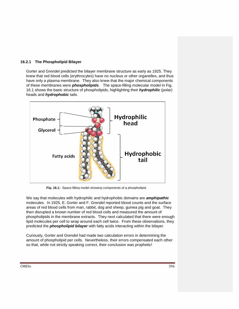
CMB3e 396

16.2.1 The Phospholipid Bilayer

Gorter and Grendel predicted the bilayer membrane structure as early as 1925. They

knew that red blood cells (erythrocytes) have no nucleus or other organelles, and thus

have only a plasma membrane. They also knew that the major chemical components

of these membranes were phospholipids. The space-filling molecular model in Fig.

16.1 shows the basic structure of phospholipids, highlighting their hydrophilic (polar)

heads and hydrophobic tails.

We say that molecules with hydrophilic and hydrophobic domains are amphipathic

molecules. In 1925, E. Gorter and F. Grendel reported blood counts and the surface

areas of red blood cells from man, rabbit, dog and sheep, guinea pig and goat. They

then disrupted a known number of red blood cells and measured the amount of

phospholipids in the membrane extracts. They next calculated that there were enough

lipid molecules per cell to wrap around each cell twice. From these observations, they

predicted the phospholipid bilayer with fatty acids interacting within the bilayer.

Curiously, Gorter and Grendel had made two calculation errors in determining the

amount of phospholipid per cells. Nevertheless, their errors compensated each other

so that, while not strictly speaking correct, their conclusion was prophetic!

Fig. 16.1: Space-filling model showing components of a phospholipid.

CMB3e 397

Fig. 16.2. shows some common membrane phospholipids.

Amphipathic molecules mixed with water spontaneously aggregate to ‘hide’ their

hydrophobic regions from the water, forming actual structures called liposomes that

sediment when centrifuged!

276-2 Membrane Lipids & Phospholipid Bilayer

277-2 Experiments with & Uses of Liposomes

Liposome membrane structure is consistent with the predicted phospholipid bilayer in

which the hydrophobic tails interact with each other and the polar heads face away

from each other, forming a phospholipid bilayer. This led to a picture of membrane

architecture based on phospholipid interactions in which the fatty acid tails make up

the hydrophobic interior of the membrane with hydrophilic external surfaces facing

opposite, aqueous sides of the membrane.

Fig. 16.2: Examples of common membrane phospholipids.

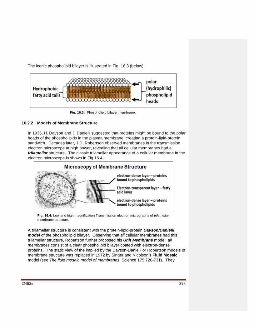
CMB3e 398

The iconic phospholipid bilayer is illustrated in Fig. 16.3 (below)

16.2.2 Models of Membrane Structure

In 1935, H. Davson and J. Danielli suggested that proteins might be bound to the polar

heads of the phospholipids in the plasma membrane, creating a protein-lipid-protein

sandwich. Decades later, J.D. Robertson observed membranes in the transmission

electron microscope at high power, revealing that all cellular membranes had a

trilamellar structure. The classic trilamellar appearance of a cellular membrane in the

electron microscope is shown in Fig.16.4.

A trilamellar structure is consistent with the protein-lipid-protein Davson/Danielli

model of the phospholipid bilayer. Observing that all cellular membranes had this

trilamellar structure, Robertson further proposed his Unit Membrane model: all

membranes consist of a clear phospholipid bilayer coated with electron-dense

proteins. The static view of the implied by the Davson-Danielli or Robertson models of

membrane structure was replaced in 1972 by Singer and Nicolson’s Fluid Mosaic

model (see The fluid mosaic model of membranes. Science 175:720-731). They

Fig. 16.3: Phospholipid bilayer membrane.

Fig. 16.4: Low and high magnification Transmission electron micrographs of trilamellar

membrane structure.

CMB3e 399

suggested that, in addition to peripheral proteins that bind to the membrane

surfaces, many integral membrane proteins actually span their membranes.

Integral membrane proteins were imagined as a mosaic of protein ‘tiles’ embedded in

a phospholipid medium. But unlike a mosaic of glazed tiles set in a firm, cement-like

structure, the protein ‘tiles’ were predicted to float in a phospholipid sea.

In the model, membrane proteins are anchored in membranes by one or more

hydrophobic domains; with hydrophilic domains facing either or both aqueous external

and cytosolic environments. Thus, like phospholipids themselves, membrane proteins

are amphipathic. We know that cells expose different surface structural and functional

features to their aqueous environments. Since the exposed domains of membrane

proteins would be different on opposite sides of a membrane, we say that cellular

membranes are asymmetric. Fig 16.5 (below) is a model of the plasma membrane of

a cell including its integral, peripheral proteins and glycoproteins.

In this model, some integral proteins have a hydrophobic domain that does not span

the membrane, but that anchors it to one side of the membrane. Peripheral (or so-

called “surface”) proteins are also shown. These are less firmly bound to the

membrane by charge interactions with the polar phosphate groups of phospholipids,

or with the polar domains of integral membrane proteins.

Fig. 16.5: Model of the eukaryotic plasma membrane demonstrating asymmetry, with a sugarless

cytoplasmic surface and a glycoprotein rich extracellular surface.

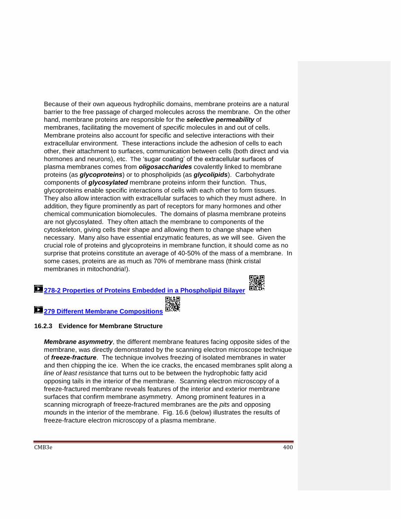
CMB3e 400

Because of their own aqueous hydrophilic domains, membrane proteins are a natural

barrier to the free passage of charged molecules across the membrane. On the other

hand, membrane proteins are responsible for the selective permeability of

membranes, facilitating the movement of specific molecules in and out of cells.

Membrane proteins also account for specific and selective interactions with their

extracellular environment. These interactions include the adhesion of cells to each

other, their attachment to surfaces, communication between cells (both direct and via

hormones and neurons), etc. The ‘sugar coating’ of the extracellular surfaces of

plasma membranes comes from oligosaccharides covalently linked to membrane

proteins (as glycoproteins) or to phospholipids (as glycolipids). Carbohydrate

components of glycosylated membrane proteins inform their function. Thus,

glycoproteins enable specific interactions of cells with each other to form tissues.

They also allow interaction with extracellular surfaces to which they must adhere. In

addition, they figure prominently as part of receptors for many hormones and other

chemical communication biomolecules. The domains of plasma membrane proteins

are not glycosylated. They often attach the membrane to components of the

cytoskeleton, giving cells their shape and allowing them to change shape when

necessary. Many also have essential enzymatic features, as we will see. Given the

crucial role of proteins and glycoproteins in membrane function, it should come as no

surprise that proteins constitute an average of 40-50% of the mass of a membrane. In

some cases, proteins are as much as 70% of membrane mass (think cristal

membranes in mitochondria!).

278-2 Properties of Proteins Embedded in a Phospholipid Bilayer

279 Different Membrane Compositions

16.2.3 Evidence for Membrane Structure

Membrane asymmetry, the different membrane features facing opposite sides of the

membrane, was directly demonstrated by the scanning electron microscope technique

of freeze-fracture. The technique involves freezing of isolated membranes in water

and then chipping the ice. When the ice cracks, the encased membranes split along a

line of least resistance that turns out to be between the hydrophobic fatty acid

opposing tails in the interior of the membrane. Scanning electron microscopy of a

freeze-fractured membrane reveals features of the interior and exterior membrane

surfaces that confirm membrane asymmetry. Among prominent features in a

scanning micrograph of freeze-fractured membranes are the pits and opposing

mounds in the interior of the membrane. Fig. 16.6 (below) illustrates the results of

freeze-fracture electron microscopy of a plasma membrane.

CMB3e 401

Other features shown here are also consistent with phospholipid membrane structure.

280-2 Freeze Fracture Electron Microscopy of Cell Membranes

Cytochemical studies also confirmed plasma membrane asymmetry, showing that only

the external surfaces of plasma membranes are sugar coated, Check the link below

for more detailed descriptions of the experiments.

281-2 EM Cytochemical Demonstration of Membrane Asymmetry

Finally, membrane asymmetry was also demonstrated biochemically. In one

experiment, whole cells treated with proteolytic enzymes, followed by extraction of the

membranes and then isolation of membrane proteins. In a second experiment,

plasma membranes were isolated from untreated cells first, and then treated with the

enzymes. In a third experiment, proteins were extracted from plasma membranes

isolated from untreated cells. Electrophoretic separation of the three protein extracts

by size demonstrated that different components of integral membrane proteins were

Fig. 16.6: Illustration of a scanning electron micrograph of freeze-fractured plasma

membrane with pits and mounds showing on opposing phospholipid layers of the membrane.

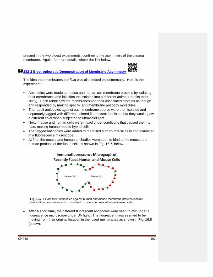
CMB3e 402

present in the two digest experiments, confirming the asymmetry of the plasma

membrane. Again, for more details, check the link below.

282-2 Electrophoretic Demonstration of Membrane Asymmetry

The idea that membranes are fluid was also tested experimentally. Here is the

experiment:

Antibodies were made to mouse and human cell membrane proteins by isolating

their membranes and injection the isolates into a different animal (rabbits most

likely). Each rabbit saw the membranes and their associated proteins as foreign

and responded by making specific anti-membrane antibody molecules.

The rabbit antibodies against each membrane source were then isolated and

separately tagged with different colored fluorescent labels so that they would glow

a different color when subjected to ultraviolet light.

Next, mouse and human cells were mixed under conditions that caused them to

fuse, making human-mouse hybrid cells.

The tagged antibodies were added to the fused human-mouse cells and examined

in a fluorescence microscope.

At first, the mouse and human antibodies were seen to bind to the mouse and

human portions of the fused cell, as shown in Fig. 16.7, below.

After a short time, the different fluorescent antibodies were seen to mix under a

fluorescence microscope under UV light. The fluorescent tags seemed to be

moving from their original location in the fused membranes as shown in Fig. 16.8

(below).

Fig. 16.7: Fluorescent antibodies against human and mouse membrane proteins localize

their cell surface antigens (i.e., proteins) on opposite poles of recently fused cells.

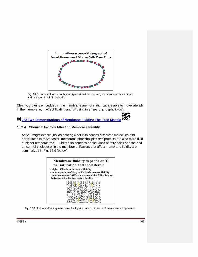
CMB3e 403

Clearly, proteins embedded in the membrane are not static, but are able to move laterally

in the membrane, in effect floating and diffusing in a “sea of phospholipids”.

283 Two Demonstrations of Membrane Fluidity: The Fluid Mosaic 16.2.4 Chemical Factors Affecting Membrane Fluidity

As you might expect, just as heating a solution causes dissolved molecules and

particulates to move faster, membrane phospholipids and proteins are also more fluid

at higher temperatures. Fluidity also depends on the kinds of fatty acids and the and

amount of cholesterol in the membrane. Factors that affect membrane fluidity are

summarized in Fig. 16.9 (below).

Fig. 16.8: Immunofluorescent human (green) and mouse (red) membrane proteins diffuse

and mix over time in fused cells.

Fig. 16.9: Factors affecting membrane fluidity (i.e. rate of diffusion of membrane components).

CMB3e 404

Fatty acids of phospholipids with more unsaturated (C=C) carbon bonds have more

kinks, or bends. These tend to push apart the phospholipid tails. With more space

between the fatty acid tails, membrane components can move more freely. Thus,

higher levels of polyunsaturated fatty acids in a membrane make it more fluid. On the

other hand, cholesterol molecules tend to fill the space between fatty acids in the

hydrophobic interior of the membrane. This reduces the lateral mobility of the

phospholipid and protein components in the membrane. By reducing fluidity,

cholesterol reduces membrane permeability to some ions.

Evolution has adapted cell membranes to different and changing environments to

maintain the fluidity necessary for proper cell function. Poikilothermic, or cold-

blooded organisms from prokaryotes to fish and reptiles, do not regulate their body

temperatures. When exposed to lower temperatures, poikilotherms respond by

increasing the unsaturated fatty acid content of their cell membranes. At higher

temperatures, they increase membrane saturated fatty acid content. Thus, the cell

membranes of fish living under the arctic ice maintain fluidity by having high levels of

both monounsaturated and polyunsaturated fatty acids. What about fish species that

range across warmer and colder environments (or that live in climates with changing

seasons). These fish regulate their cell membrane composition adjust to the demands

of their changing environment.

The warm-blooded (homeothermic) mammals and birds maintain a more or less

constant body temperature. Thus their membrane composition is also relatively

constant. But there is a paradox! Their cell membranes are very fluid, with a higher

ratio of polyunsaturated fat to monounsaturated fats than say, reptiles. But the

paradox is resolved when we understand that this greater fluidity supports the higher

metabolic rate of the warm-blooded species compared to poikilotherms. Just compare

the life styles of almost any mammal to a lazy floating alligator, or a snake basking in

the shade of a rock!

284-2 Factors Influencing Membrane Fluidity 16.2.5 Making and Experimenting with Artificial Membranes

Membrane-like structures can form spontaneously. When phospholipids interact in an

aqueous environment, they aggregate to exclude their hydrophobic fatty tails from

water, forming micelles. Micelles are spherical phospholipid monolayer vesicles that

self-assemble, a natural aggregation of the hydrophobic fatty acid domains of these

amphipathic molecules. Fig. 16.10 (below) illustrates a micelle.

CMB3e 405

Micelles can further aggregate into spherical phospholipid bilayer liposomes (Fig. 16.11).

Liposomes behave somewhat like cells, for example forming a pellet at the bottom of a

tube when centrifuged. Liposomes can be custom designed from different kinds of

phospholipids and amphipathic proteins that become integral to their membranes. When

liposomes are prepared in the presence of specific proteins or other molecules that can’t

cross the membrane, they become trapped in the vesicles. The trapped molecules

cannot get out of this synthetic ‘organelle’. Such were the studies that allowed the

identification of the mitochondrial respiratory chain complexes. The ability to manipulate

liposome content and membrane composition also make them candidates for drug

delivery to specific cells and tissues (google liposome for more information).

16.2.6 Separate Regions of a Plasma Membrane with Unique Fluidity and

Permeability Properties

As we will see shortly, fluidity does not result in an equal diffusion of all membrane

components around the cell membrane surface. Instead, extracellular connections

between cells along with intracellular connections of the membrane to differentiated

Fig. 16.10: Micelles are phosholipid monolayers that can self-assemble in water.

Fig. 16.10: A liposome is a synthetic lipid bilayer that can be formed from micelles.

CMB3e 406

regions of the cytoskeleton, effectively compartmentalize the membrane into sub-

regions. To understand this, imagine a sheet of epithelial like those in the cartoon

below (Fig. 16.11).

This sheet of cells exposes one surface with unique functions to the inside of the

organ they line. It exposes the opposite surface, one with a quite different function, to

the other side of the sheet. The lateral surfaces of the cells are yet another

membrane compartment, one that functions to connect and communicate between the

cells in the sheet. Components, i.e., membrane proteins illustrated with different

symbolic shapes and colors, may remain fluid within a compartment. Of course, a

tissue-level macro-differentiation of cell membranes enabling cell-cell and cell-

environmental interactions makes intuitive sense. The new possibility that cellular

membranes are even more compartmentalized was perhaps less anticipated.

In fact, membranes are further divided into micro-compartments. Within these

compartments, components are fluid but seldom move between compartments.

Studies indicate that cytoskeletal elements create and maintain these micro-

discontinuities. For example, integral membrane proteins are immobilized in

membranes if they are attached to cytoskeletal fibers (e.g., actin) in the cytoplasm.

Furthermore, when aggregates of these proteins line up due to similar interactions,

they form kind of fence, inhibiting other membrane components from crossing. By

analogy, this mechanism of micro-compartmentalization is called the Fences and

Pickets model in which proteins attached to the cytoskeleton serve as the pickets (the

usually white pointy boards attached to the fence!).

Fig. 16.12: Properties of plasma membranes may be different in ways determined by cell-cell

associations during tissue development. Lavender, green and blue regions indicate basic

differentiation of a sheet of epithelial cells.

CMB3e 407

The movement across the fences (i.e., from one membrane compartment to another)

is infrequent. Extra kinetic energy is presumably needed for a molecule to ‘jump’ a

fence between compartments. Hence, this kind of motion (hop diffusion) differs from

the Brownian motion implied by the original fluid mosaic model.

285-2 Regional Differentiation of a Plasma Membrane Domains

16.3 Membrane Proteins

Of course, membrane proteins themselves have domains. These provide catalytic and

other activities inside and outside of cells and organelles, and keep them attached to the

membrane. Like phospholipids, membrane proteins are amphipathic, with hydrophobic

domains that non-covalently interact strongly within the fatty acid interior of membranes.

Some integral membrane proteins span the entire membrane, with hydrophilic domains

facing the cytosol or cell exterior. Peripheral proteins bind to a membrane surface

through non-covalent interactions. Different membrane proteins are shown in Fig. 16.13.

286-2 Domains of membrane proteins

Hydrophobic amino acids of membrane proteins are organized into functional

domains. These consist of one or more alpha-helical regions that interact with the

fatty acid interior of the membranes. Hydrophilic domains tend to have more tertiary

structure. These domains face the aqueous cytosol and cell exterior. Two trans-

membrane proteins are cartooned below in Fig 16.14.

Fig. 16.13: Integral membrane proteins may penetrate or span the membrane; Also shown

are peripheral proteins and lipoproteins.

CMB3e 408

The protein on the left in Fig. 16.14 crosses the membrane once, while the one on the

right crosses the membrane three times. How a transmembrane protein inserts into

the membrane during synthesis dictates the locations of its N- and C-terminus.

Transmembrane proteins can a membrane more than once. The number of times

determines the location of its N- and C-termini. N-terminal end of a plasma membrane

polypeptide always ends up exposed to the outside of the cell.

Alpha helical domains that anchor proteins in membranes are mostly non-polar and

hydrophobic themselves. For example, consider the amino acids in the alpha-helical

domain of the red blood cell membrane protein glycophorin A, that prevents red blood

cells from aggregating, or clumping in the circulation. One glycophorin A polypeptide

with its hydrophobic trans-membrane alpha helix is cartooned below in Fig. 16.15.

Glycophorin A monomers pair to form dimers in the plasma membrane.

Fig. 16.14: Integral transmembrane proteins cross the membrane one or more times.

Fig. 16.15: Hydrophobic amino acids of glycophorin form a helix that spans the red

blood cell plasma membrane

CMB3e 409

Proteins that span membranes multiple times may include amino acids with charged

polar side chains, provided that these side chains interact between helices so that

they are shielded from the fatty acid environment in the membrane. Because of these

hydrophilic interactions, such proteins can create pores for the transport of polar

molecules and ions. We will see some of these proteins later. Integral membrane

proteins that do not span the membrane also have a hydrophobic helical domain that

anchors them in the membrane, while their hydrophilic domains typically interact with

intracellular or extracellular molecules that can hold cells in place, give cells and

tissues their structure, etc.

The very presence of hydrophobic alpha-helical domains in trans-membrane proteins

makes them difficult if not impossible to isolate from membranes in a biologically

active form. But the peripheral polypeptide cytochrome c readily dissociates from

cristal membranes, making it easy to purify. The inability to purify other biologically

active cristal membrane electron carriers is what slowed our understanding of the

structure/function of the mitochondrial electron transport system.

It is possible to determine the primary structure of a polypeptide encoded by a gene

before the protein itself has been isolated. Just by knowing the DNA sequence of a

gene, we can infer the amino acid sequence of the protein encoded by the gene.

Then we can identify all of the hydrophobic amino acids in the inferred sequence and

generate a hydrophobicity (or hydropathy) plot such as the one in Fig. 16.16 below.

Fig. 16.16: Hydropathy plots correlate amino acid hydrophobicity with its position in a polypeptide.

Long regions of hydrophobic amino acids suggest a possible membrane protein domain.

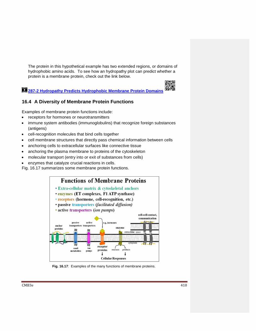
CMB3e 410

The protein in this hypothetical example has two extended regions, or domains of

hydrophobic amino acids. To see how an hydropathy plot can predict whether a

protein is a membrane protein, check out the link below.

287-2 Hydropathy Predicts Hydrophobic Membrane Protein Domains

16.4 A Diversity of Membrane Protein Functions

Examples of membrane protein functions include:

receptors for hormones or neurotransmitters

immune system antibodies (immunoglobulins) that recognize foreign substances

(antigens)

cell-recognition molecules that bind cells together

cell membrane structures that directly pass chemical information between cells

anchoring cells to extracellular surfaces like connective tissue

anchoring the plasma membrane to proteins of the cytoskeleton

molecular transport (entry into or exit of substances from cells)

enzymes that catalyze crucial reactions in cells.

Fig. 16.17 summarizes some membrane protein functions.

Fig. 16.17: Examples of the many functions of membrane proteins.

CMB3e 411

Transmembrane proteins perform most of the functions illustrated here. However,

peripheral membrane proteins also play vital roles in membrane function. Cytochrome c

is an example. It is a redox component loosely bound to the rest of the electron transport

system in the mitochondrial cristal membrane. Other peripheral membrane proteins may

serve to regulate transport or signaling activities of transmembrane protein complexes or

may mediate connections between the membrane and cytoskeletal elements. As shown

here, peripheral proteins do not penetrate membranes. They bind reversibly to the

internal or external surfaces of the biological membrane with which they are associated.

Check out major membrane protein functions, actions and cellular locations in Table 16.1

(below). We’ll look at some of these functions in more detail shortly.

Some Functions of Membrane Proteins Basic Function Specific Actions Examples

Facilitated transport Regulate diffusion of substances

across membranes along a

concentration gradient

Ca++ & other ion channels, glucose

transporters

Active transport Use energy to move ions from

low to high concentration across

membranes

Mitochondrial protein pumps, the

Na+/K+ ion pump in neurons

Signal transduction Bind signal molecues unable to

enter cells to convey information

from nals to cytoplasm, leading to

a cellular response

Receptor proteins for hormones,

growth factors, antibody/antigen

interactions, cytokine mediation of

inflammatory responses etc.

Cell-cell

interactions

Cell-cell recognition and binding

to form tissues

Formation of desmosomes, gap

junctions and tight junctions

Anchors to

cytoskeleton

Link membrane proteins to

cytoskeleton

Give cells their shape, cell movement

and response to molecular signals

Enzymatic Usually multifunctional proteins

with enzymatic activities

F1 ATP synthase that use proton

gradient to make ATP; adenylyl

cyclase that makes cAMP during

signal transduction; some receptor

proteins that are linked to enzymatic

domains in the cytoplasm.

288-2 Diversity of Membrane Protein Structure & Function

289-2 Pore Proteins May Cross the Membrane Many Times

290-2 Red Blood Cell (Erythrocyte) Membrane Protein Functions

CMB3e 412

16.5 Glycoproteins and Glycolipids

Membrane proteins are often covalently linked to oligosaccharides, which are branched

glycoside-linked sugars (averaging around 15 sugar residues). As glycans, they are the

sugars linked to glycoproteins and glycolipids.

Glycoproteins are rare in the cytosol, but common on secreted and membrane proteins.

Oligosaccharides are typically linked to proteins via the hydroxyl group on serine or

threonine amino acids(O-glycosylation) and occasionally to modified amino acids (e.g.,

hydroxylysine, hydroxyproline) or to the amide nitrogen on asparagine (N-glycosylation).

As a major feature of the glycocalyx, oligosaccharide domains of glycoproteins and

glycolipids are the ‘face’ of a plasma membrane that communicates with the extracellular

world. Fig. 16.18 illustrates the glycocalyx.

Oligosaccharides begin their synthesis in the rough endoplasmic reticulum (RER), with

the creation of a core glycoside. These partial glycans are enzymatically linked to

compatible amino acids of a membrane protein. As these proteins travel through the

Golgi vesicles of the endomembrane system, terminal glycosylation attaches more

sugars to the core glycoside to complete glycoprotein synthesis. When vesicles budding

from the trans-Golgi vesicles fuse with the plasma membrane, the sugars on the

glycoproteins end up on the exterior cell surface. This is illustrated in the link below.

291 The Path to Sugar Coated Cells

Fig. 16.18: The glycocalyx is the sugar- rich region on the extracellular surface of cells, the

result of covalently bound sugars on glycoproteins and glycolipids. It is the basis of many cell

functions and is associated with other macromolecules to form an extracellular matrix.

CMB3e 413

Like glycoproteins, glycolipids are only found on the extracellular surface. They are

synthesized in much the same way as glycoproteins. Specific enzymes catalyze initial

glycosylation of phospholipids and polypeptides, followed by terminal glycosylation

reactions. Glycoproteins, glycolipids and proteoglycans on cell surfaces play critical roles

in cell-cell recognition and the formation of tissues. They recognize and bind to

carbohydrate receptors (lectins) on adjacent cells, leading to cell-cell attachment as well

as intracellular responses in the interacting cells. Glycoproteins and glycolipids also

mediate the interaction of cells with extracellular molecular signals and with chemicals of

the ECM, or extracellular matrix (Fig. 16.19). The ECM includes components of

connective tissue, basement membranes, in fact any surface to which cells attach.

292-2 The Extracellular Matrix

Fig. 16.19: The extracellular matrix (ECM) forms when proteins (e.g., fibronectin, collagen)

and other macromolecules (e.g., proteoglycans) associate non-covalently with membrane

proteins and elements of the glycocalyx.

CMB3e 414

16.6 Glycoproteins and Human Health

We’ll close this chapter with a few examples of glycoproteins that play crucial roles in

human physiology. Let’s look first at the major human A, B, AB, O and Rh blood groups

that result from the presence or absence of glycoprotein antigens embedded in red blood

cell membranes and the presence or absence in the blood, of antibodies against the

antigens.

Typically an exposure to antigens (foreign substances like bacteria, viruses, toxins…)

generates immunoglobulins, the antibody molecules of our immune system. The

immunoglobulins are glycoproteins. Since blood group antibodies already in the blood of

a healthy person are not a response to foreign antigen invasion they are something of a

paradox!

You probably know that these blood groups must be compatible for a successful blood

transfusion. A mismatch between donor and recipient can be devastating. An interaction

of the red cell antigens of one blood group with antibodies in another blood group will

cause the red cells to clump, restricting blood flow and ultimately killing the transfusion

recipient. Fig. 16.20 summarizes why transfusions with mismatched A, B, AB, O blood

groups must be avoided.

Fig. 16.20: Blood groups with membrane proteins and elements of the glycocalyx (see text for details).

CMB3e 415

From the table above, you can see why type O blood is called the universal donor, and

thus in high demand by clinics and hospitals. Thanks to enzymes produced by members

of the gut microbiome, the absolute requirement that blood groups must be matched for

safe transfusions may someday be a thing of the past! One of these enzymes is a

glycosidase that can digest the sugars on A and B antigens on the surfaces A, B and AB

blood cells. This effectively converts them to type O red blood cells! Check the Red

Cross website (http://www.redcrossblood.org/learn-about-blood/blood-types.html ) or

https://en.wikipedia.org/wiki/Blood_type for more detail about blood groups. For a

summary of the research on enzymatically converting all blood types to type O, see

www.eurekalert.org/conversion of A, B and AB to O type blood. To read about how we

come to have blood groups in the irst placen click on Evolution of Blood Groups.

Another red blood cell antigen is the Rh (rhesus) factor. Rhesus factors are antigens

originally shown to define blood types in rhesus monkeys, but humans have equivalent

antigens, so human Rh blood groups have nothing to do with the monkeys! People either

have their own Rh factor and are Rh+…, or they don’t have the factor and are Rh-. When

an Rh- recipient receives blood from an Rh+ donor, the recipient’s immune system makes

anti-Rh antibodies in the usual way. This too can cause blood cell clumping with bad

consequences. A well known example is when an Rh- pregnant woman is carrying an

Rh+ fetus; if mother and baby’s blood should mix, the mother will make antibodies to the

Rh factor that could cause foetal heamolytic disease, damaging and destroying fetal red

blood cells.

A word to the wise: While you should be ‘typed’ in the event you need a transfusion, it’s

always a good idea to know your own ABO and Rh blood groups!

The last example here involves the cell surface major histocompatibility complex (MHC)

glycoproteins that distinguish self from non-self in body tissues and organs. Major organ

transplantation (liver, kidneys, heart) from donors into patients with failing organs has

become if not routine, then at least increasingly common. Before a transplant, MHC

tissue typing determines donor and recipient compatibility to reduce the chances of the

rejection of the transplanted organ. Since available donors are few and good matches

even fewer, patients wait on prioritized lists for a matched organ. Even when MHC typing

is a match for a patient, the immune systems of transplant recipients are suppressed with

hormones to further reduce chances of rejection. Unlike the limited number of blood

groups, many MHC proteins are analyzed to determine a match. Thus, it is not practical

(or routinely necessary) to ‘know’ your MHC type! In the next chapter, we look at

membrane functions intrinsic to cellular existence itself.

CMB3e 416

Some iText & VOP Key Words and Terms

amphipathic molecules glycolipids peripheral membrane

proteins

asparagine glycosylation phospholipid bilayer

cell membrane Golgi vesicles plasma membrane

cell-cell attachment Hydropathy plot poikilothermic organisms

cytoskeleton hydrophilic phosphate heads

RER

Davson–Danielli membrane model

hydrophobic fatty acid tails

Rough endoplasmic reticulum

endomembrane system hydrophobicity plot saturated fatty acids

exocytosis hydroxyproline serine

extracellular matrix (ECM)

hydroxylysine temperature effects on membranes

fluid mosaic integral membrane proteins

threonine

freeze fracture method membrane asymmetry transmembrane proteins

membrane evolution membrane proteins unsaturated fatty acids

glycan N-glycosylation

glycocalyx O-glycosylation

CMB3e 417

Chapter 17: Membrane Function

Passive, facilitated and active transport, the traffic of proteins in cells, cell-

cell interactions, excitability and signal transduction

17.1 Introduction

Small molecules like O2 or CO2 can cross cellular membranes unassisted; neither the

hydrophilic surfaces nor the hydrophobic interior of the phospholipid bilayer are barriers to

their transit. On the other hand, most molecules (even water) need the help of membrane

transport proteins to get in or out of cells and organelles. Transport proteins can act as

gates that might be open or closed. When open, these gates permit the diffusion of

molecules into or out of cells along a concentration gradient so that their concentrations

equalize across the membrane. Like the passive diffusion of small gasses, facilitated

diffusion by membrane proteins does not require an input of energy. In contrast, some

transport proteins are actually pumps, using chemical energy to move molecules across

membranes against a concentration gradient. The result of this active transport is to

concentrate solutes on one side of a membrane. For example, pumps that create sodium

and potassium ion gradients are responsible for the excitability of cells. Recall that this

is one of the fundamental properties of life: the ability of cells and organisms to respond to

stimuli.

CMB3e 418

As you read this chapter, look for how allosteric changes regulate membrane function.

We’ll consider how:

membrane gates and pumps work.

membrane protein interactions allow cells to self-assemble into tissues and organs.

cells direct protein traffic to the cytoplasm, into membranes themselves, into

organelles…, or out of the cell.

membrane proteins participate in direct communication between adjacent cells.

membrane proteins are receptors for more long-distance communications,

responding to neurotransmitters, hormones, and other external chemical signals.

Learning Objectives

When you have mastered the information in this chapter, you should be able to:

1. explain how and why one cell’s plasma membrane differs from that of another cell

type.

2. explain how and why the plasma membrane differs from other membranes in the

same cell.

3. determine if solutes cross a plasma membrane by passive or facilitated diffusion.

4. explain how salmon can spend part of their lives in the ocean and part swimming

upstream in freshwater to spawn, without their cells shriveling or bursting.

5. explain how active transport stores chemical energy (recall electron transport and

oxidative phosphorylation).

6. explain the role of active transport in maintaining/restoring a cell’s resting potential.

7. compare and contrast different kinds of gated channels.

8. describe the order of ion movements that generate an action potential.

9. define and compare exocytosis, pinocytosis, phagocytosis and receptor-mediated

endocytosis.

10. distinguish between signal molecules that enter cells to deliver their chemical

message and those deliver their message only as far as the plasma membrane.

11. trace an intracellular response to a steroid hormone to a likely cellular effect.

12. trace a liver cell response to adrenalin from the plasma membrane to glycogenolysis

(glycogen breakdown) in the cytoplasm of the cell.

13. compare the signal transduction activities of different G-protein receptors leading to

the first active kinase enzyme in a phosphorylation cascade.

14. explain how a liver cell can respond the same way to two different hormones (e.g.,

adrenalin and glucagon)…, and why this should be possible.

15. describe/explain how a phosphorylation cascade amplifies the cellular response to a

small amount of an effector (signal) molecule.

16. discuss the differences and interactions between the glycocalyx, basement membrane

and extracellular matrix (ECM).

17. explain ECM functions and identify components involved in those functions.

CMB3e 419

18. describe how the molecular structure of fibronectin supports its different functions.

19. describe some structural relationships between cell surfaces and the cytoskeleton.

20. compare and contrast the structures and functions of the different cell junctions.

21. distinguish between the structures and functions of cadherins, clathrin, COPs, adaptin,

selectins, SNAREs and CAMs.

22. state an hypothesis to explain why some cancer cells divide without forming a tumor.

17.2 Membrane Transport

The first control on the passage of molecules across membranes is the semi-permeable

character of the membrane itself. Molecules move in and out of cells in one of three

ways: passive diffusion, facilitated transport and active transport.

Only a few small, relatively uncharged molecules can cross a membrane unassisted (i.e.,

by passive diffusion). Hydrophilic molecules that must enter or leave cells do so with

help, i.e., by facilitated transport. Passive and facilitated transport release the free energy

inherent in concentration gradients as molecules diffuse across a membrane. In contrast,

active transport consumes energy to create concentration gradients of specific solutes.

The specificity of facilitated and active transport lies in integral membrane proteins that

recognize and bind specific solutes for transport. As you may predict, allosteric regulation

of these proteins controls the movement of their target molecules into or out of cells.

Despite its polarity, many believed that the small water molecules crossed membranes

without help. Indeed, it does to a limited extent. However, others suspected that given its

highly charged polar covalent bonds relative to its small size, water molecules require an

assist to get across membranes efficiently. Let’s begin with a closer look at passive

diffusion and diffusion by facilitated transport, followed by osmosis (a special case of

facilitated diffusion of water), and finally at active transport.

17.2.1 Passive Diffusion of Solutes

Diffusion across membranes does not require energy. In fact, diffusion can release

energy - recall the movement of protons through the F1 ATPase proton gate that

synthesizes ATP during mitochondrial oxidative phosphorylation. Passive diffusion in

solution is the movement of molecules over time by random motion (also called

Brownian motion) from regions of higher concentration to regions of lower

concentration. Significant passive diffusion across cellular membranes is limited to a

few molecules, mostly gasses like O2, CO2, and N2, that can freely cross the

hydrophobic phospholipid barrier. The rapid diffusion of gasses is essential for

O2 and CO2 exchange between the alveolar capillaries and cells of the lungs during

physiological respiration. O2 and CO2 exchange also occurs in mitochondria during

cellular respiration.

CMB3e 420

The rate of diffusion of a molecule is dependent only on its own concentration. It is

unaffected by the concentration of other molecules. Over time, random motion of

solutes within and across compartments results in a dynamic equilibrium for each

different solute over time. At equilibrium, solute molecules continue to diffuse across

the membrane, but for each molecule moving across in one direction, another

molecule of the same solute crosses in the other direction.

17.2.2 Facilitated Diffusion of Solutes and Ions

Like passive diffusion, facilitated diffusion is the spontaneous (downhill) passage of

molecules or ions across membranes through specific transmembrane proteins. The

kinetics of passive and facilitated diffusion reveals the differences between the two

processes. To understand the latter, recall that the rate of enzyme catalysis is

saturable. That is, as the concentration of substrate is increased, the rate of the

catalyzed reaction approaches a maximum (Vmax). This occurs when all enzyme

molecules in solution are bound to substrate molecules. The same saturation

phenomenon applies to facilitated transport – the rate of diffusion of a solute across a

membrane is directly proportional to the concentration of the solute, but is limited by

the number of transport proteins in the membrane. Fig. 17.1 plots the kinetics of

passive and facilitated diffusion.

Fig. 17.1: Graph plotting rates of passive and facilitated transport show that facilitated

diffusion is a saturable process.

CMB3e 421

Perhaps you see another similarity between facilitated diffusion and enzyme catalysis

in this graph! Relative rates of facilitated diffusion are typically rapid, compared to

those of passive diffusion. This is because the allosteric changes that accompany

facilitated transport are rapid, just as they are during enzyme catalysis. Fig. 17.2

illustrates three kinds of facilitated transport of solutes.

The GLUT (GLUcose Transporter) protein (Fig.17.2, left) allows glucose uniport, the

specific transport of a single substance in or out of cells. In symport (Fig.17.2,

middle) glucose transporters couple the simultaneous movement of glucose and

sodium ions, for example in kidney cells. The SGLT (Sodium-GLucose Transporter)

serves a similar function in small intestine cells, enabling absorption of dietary glucose

and sodium. Antiport (Fig.17.2, right) allows the specific exchange of molecules

across a membrane. In the example shown, ATP leaves the mitochondrial matrix,

crossing the cristal membrane at the same time as ADP enters the matrix. Whether

by uniport, symport or antiport, each solute will independently cross a membrane

down its concentration gradient, moving from higher concentration to where it is at a

lower concentration. Recall that diffusion along a gradient releases free energy that

depends on relative concentrations of the solutes.

Proteins mediating facilitated transport are of two kinds: carrier proteins allow solute

transport. Ions, with their high charge-to-mass ratio, need help to cross the

hydrophobic membrane barrier. This is the job of channel proteins that essentially

serve as ion pores. Like all transporter proteins, both carrier and channel proteins

undergo allosteric changes during transport. They are also typically subject to

allosteric regulation, rather than being in a constant ‘open’ state. Examples of

facilitated diffusion are considered in more detail below.

Fig. 17.2: Three kinds of facilitated diffusion (see text for details).

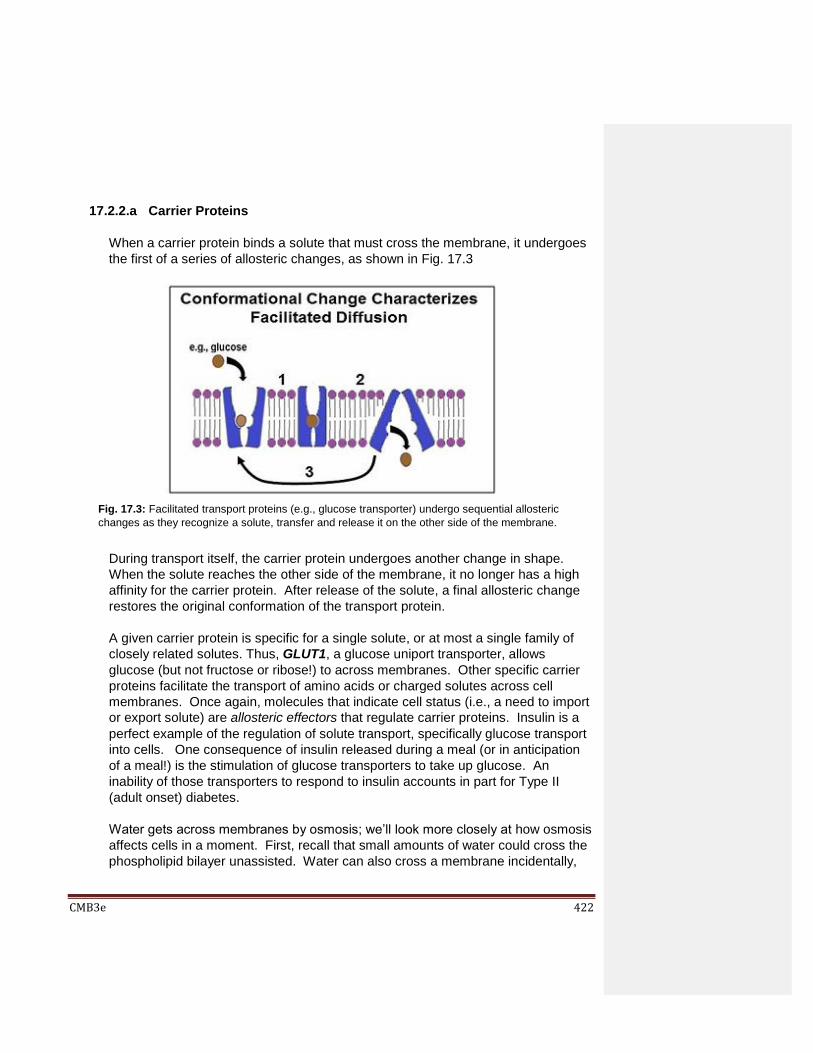
CMB3e 422

17.2.2.a Carrier Proteins

When a carrier protein binds a solute that must cross the membrane, it undergoes

the first of a series of allosteric changes, as shown in Fig. 17.3

During transport itself, the carrier protein undergoes another change in shape.

When the solute reaches the other side of the membrane, it no longer has a high

affinity for the carrier protein. After release of the solute, a final allosteric change

restores the original conformation of the transport protein.

A given carrier protein is specific for a single solute, or at most a single family of

closely related solutes. Thus, GLUT1, a glucose uniport transporter, allows

glucose (but not fructose or ribose!) to across membranes. Other specific carrier

proteins facilitate the transport of amino acids or charged solutes across cell

membranes. Once again, molecules that indicate cell status (i.e., a need to import

or export solute) are allosteric effectors that regulate carrier proteins. Insulin is a

perfect example of the regulation of solute transport, specifically glucose transport

into cells. One consequence of insulin released during a meal (or in anticipation

of a meal!) is the stimulation of glucose transporters to take up glucose. An

inability of those transporters to respond to insulin accounts in part for Type II

(adult onset) diabetes.

Water gets across membranes by osmosis; we’ll look more closely at how osmosis

affects cells in a moment. First, recall that small amounts of water could cross the

phospholipid bilayer unassisted. Water can also cross a membrane incidentally,

Fig. 17.3: Facilitated transport proteins (e.g., glucose transporter) undergo sequential allosteric

changes as they recognize a solute, transfer and release it on the other side of the membrane.

CMB3e 423

when ions flow through their channel proteins. But most osmosis involves

facilitated diffusion mediated by aquaporins. Some aquaporins only transport

water. Others have evolved to co-facilitate the transport of glucose (see above),

glycerol, urea, ammonia, carbon dioxide and even ions (protons) along with water.

Like other carrier proteins, aquaporins are allosterically regulated to allow cells to

meet their specific water balance requirements. So fundamental was the

understanding of water balance that the discovery of aquaporins earned Peter

Agre a Nobel Prize in Chemistry in 2003.

Since Agre’s discovery (in 1992), several genetic diseases have been linked to

aquaporin gene mutations. Kidney cells are critically involved in vertebrate water

balance and have many aquaporins in their membranes. In a rare form of

diabetes, abnormal aquaporins cause the kidneys to excrete unusually large

volumes of water. In another example, aquaporin gene mutations lead to the

development of cataracts in both eyes. Since their initial discovery, aquaporins

have been described in bacteria and plants. To learn more, click Aquaporins -

Wikipedia.

17.2.2.b Ion Channels

Allosteric regulation of ion channel proteins controls ion homeostasis in blood and

extracellular fluids within narrow limits. Often, multiple integral proteins contribute

to the formation of an ion channel. When stimulated, channel proteins rearrange to

open a pore allowing specific ion transport. Some ion channels, like the glucose-

sodium ion symport system noted above, mobilize the energy of diffusion of one

solute (the ion in this case) to rapidly transport another solute through the same

channel (acting like an ion channel and a carrier protein). Finally, ion channels are

responsible for the excitability of cells, where Na+ , K+ and Ca++ channels

collaborate in ion movements into and out of cells leading to neuronal or muscle

cell responses (more shortly!).

293-2 Passive & Facilitated Transport

17.3 Osmosis

Osmosis is the diffusion of water across membranes from lower to higher solute

concentrations, an essential cellular activity. It allows cells to use water to maintain

cellular integrity or to adapt to changes in the solute composition in the extracellular

environment. Osmosis relies on the facilitated transport of water by aquaporins. The

passive diffusion of water molecules can be demonstrated with artificial (e.g., dialysis)

CMB3e 424

membranes. If solute concentrations are higher on one side of the membrane, water will

cross the membrane “trying” to equalize the solute concentrations on both sides of the

membrane. In effect, water movement is from the side of a membrane where the free

water molecule concentration is higher (i.e., where the concentration of solute is lower) to

the side where the concentration of free water is lower (i.e., where the concentration of

solute is higher).

17.3.1 Osmosis in Plant and Animal Cells

We could present this section in the context of free water concentrations, but we will

do so in the more familiar terms of solute concentrations. Osmosis affects plant and

animal cells according to the same principles, but with different effects. The effects of

different experimental solute concentrations on animal cells are illustrated in Fig. 17.4.

If the solute concentration inside and outside the cell is the same, there is no net water

movement into or out of the cells. The extracellular medium and cytosol are said to be

isotonic to each other. When water diffuses into the cells from a low solute medium,

the medium is said to by hypotonic to (less concentrated than) the cytosol. In this

case, movement of water into a cell lowers the cytosol solute concentration. Animal

cells swell and burst in a hypotonic solution. Animal cells in hypertonic solutions

(with higher solute concentrations than the cytosol) shrivel up as water leaves the cell.

From this brief description, you should conclude that water crosses from the hypotonic

to the hypertonic side of a membrane.

Fig. 17.4: Effects of differences in solute concentrations inside and outside animal cells

on the movement of water into or out of the cells, i.e., Osmosis (see text for details).

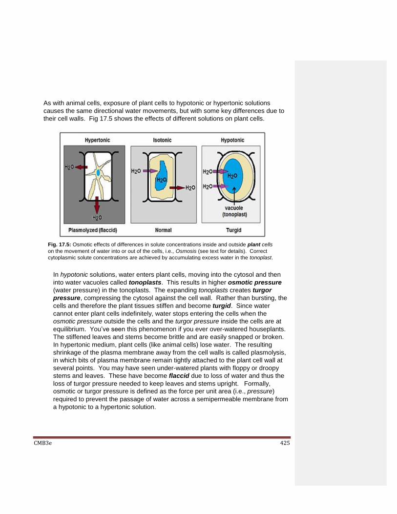
CMB3e 425

As with animal cells, exposure of plant cells to hypotonic or hypertonic solutions

causes the same directional water movements, but with some key differences due to

their cell walls. Fig 17.5 shows the effects of different solutions on plant cells.

In hypotonic solutions, water enters plant cells, moving into the cytosol and then

into water vacuoles called tonoplasts. This results in higher osmotic pressure

(water pressure) in the tonoplasts. The expanding tonoplasts creates turgor

pressure, compressing the cytosol against the cell wall. Rather than bursting, the

cells and therefore the plant tissues stiffen and become turgid. Since water

cannot enter plant cells indefinitely, water stops entering the cells when the

osmotic pressure outside the cells and the turgor pressure inside the cells are at

equilibrium. You’ve seen this phenomenon if you ever over-watered houseplants.

The stiffened leaves and stems become brittle and are easily snapped or broken.

In hypertonic medium, plant cells (like animal cells) lose water. The resulting

shrinkage of the plasma membrane away from the cell walls is called plasmolysis,

in which bits of plasma membrane remain tightly attached to the plant cell wall at

several points. You may have seen under-watered plants with floppy or droopy

stems and leaves. These have become flaccid due to loss of water and thus the

loss of turgor pressure needed to keep leaves and stems upright. Formally,

osmotic or turgor pressure is defined as the force per unit area (i.e., pressure)

required to prevent the passage of water across a semipermeable membrane from

a hypotonic to a hypertonic solution.

Fig. 17.5: Osmotic effects of differences in solute concentrations inside and outside plant cells

on the movement of water into or out of the cells, i.e., Osmosis (see text for details). Correct

cytoplasmic solute concentrations are achieved by accumulating excess water in the tonoplast.

CMB3e 426

17.3.2 Osmosis in Plant Life

While individual plant cells respond to changes in solute concentrations, these

changes are rapidly communicated to adjacent cells through plasmodesmata.

These structures connect the plasma membranes of adjacent cells through their

cell walls, allowing rapid, direct sharing of physical and chemical information. A

plasmodesma is illustrated in Fig. 17.6.

In this way, effects on osmotic pressure in a few cells created by changes in water

availability are transmitted to adjacent cells, affecting turgor pressure in those cells

and, ultimately, in plant tissues.

Finally, plant life depends on water! Recall that plant cells require a continual

supply of water for use in photosynthesis, to provide hydrogen to reduce CO2 to

glucose. Photosynthesis as well as the loss of excess water from plant tissues

(especially leaves) by transpiration lowers cellular osmotic pressure. As water

moves up from the roots to replace water used and lost by leaf cells, the osmotic

pressure drops in the fine root hair cells (with their high surface area). This draws

Fig. 17.6: Plasmodesmata are cell wall ‘tunnels’ connecting plat cells that allow direct

movement of water between cells to transmit and balance changes in osmotic pressure

in one part of a plant (e.g., roots) throughout the plant (see text for details).

CMB3e 427

water into the root cells by osmosis. Thus, osmotic pressure is the main force

driving water into plants and, defying gravity, moving it up from the roots to the rest

of the plant.

17.3.3 Osmosis in Animal Life

Changes in osmotic environment can stress or kill an organism. For example,

freshwater organisms (protozoa or fish) placed in sea water will die. Likewise, salt-

water fish placed in freshwater. But cells and organisms can osmoregulate

(control the osmotic pressure in their cells), at least to a point. For example, as a

Paramecium take on water, a contractile vacuole expels excess water to prevent

the cell from bursting (Fig. 17.7).

Water constantly enters these freshwater protists because the solute concentration

in the cytosol is always higher than the freshwater water they live in. To cope with

a constant uptake of water, their contractile vacuoles collect excess water and then

contract to expel the water. At a high-energy cost, Paramecia constantly pump

water out of the cell to maintain water balance (i.e., correct osmotic pressure).

Another protist strategy for coping with change in environmental solute

concentrations (e.g., salinity) is to pump salts (or suitable salt solute substitutes in

or out of the cell, as needed (For some details, see Protist Osmoregulation Genes

Acquired by Eukaryotes from Bacteria by Horizontal Gene Transfer.

Larger organisms like freshwater fish cope with their hypotonic environment by

urinating a lot! At the other end of the spectrum, salt-water fish cope with the high

solute concentration of solutes (salts) in their environment by excreting excess salt.

Salmon spend time in seawater growing to maturity and later swim upstream in

Fig. 17.7: Light micrograph of Paramecium highlighting a contractile vacuole, an

organelle that pumps out excess water from the cell, protecting it from osmotic shock.

CMB3e 428

fresh water to spawn. You can imagine how salmon and similar organisms have to

osmoregulate to adapt to their changing, very different environments. In this

case, osmoregulation begins when hormonal changes respond to changes in

living circumstance and dictate a compensatory response.

17.3.4 Summing Up

Osmosis is the movement of water across membranes to where solutes are at high

concentration. At the same time, solutes diffuse across membranes, moving in or

out of cells to where they are at lower concentration, either passively or by

facilitated transport. We’ve evolved different facilitated transport proteins specific

for different solutes. And finally, most water crosses membranes by facilitated

diffusion through aquaporin proteins that serve as pores in cellular membranes.

294-2 Osmosis

17.4 Active Transport

Excitability (adaptation) is another of the defining properties of life. This property of all

cells is based on chemical and electrical reactivity. Neurotransmitters released at a

synapse cross the synaptic cleft from a “sending” neuron to a responding cell (another

neuron or a muscle cell). The neurotransmitter binds to receptors on the responding cell

resulting in a membrane depolarization, a rapid change in the electrical potential

difference across the cell membrane. While responses to neurotransmitters occur in

fractions of a second, all kinds of cells are responsive, albeit not always as fast as

neurons or muscle cells.

Changes in the membrane polarity of any cell depend on unequal concentrations of ions

inside and outside cells. These ionic differences across membranes are what enable all

cells, but especially as neurons and muscle cells to respond to chemical and other (e.g.,

electrical) signals. Thus, cells have a resting potential due to a higher [K+] in the

cytosol and higher [Cl-] and [Na+] outside the cell.

The measured resting potential (difference in charge or potential difference) of most

cells is typically between -50mv to -70mv. These numbers are negative because there is

a higher concentration of negative (i.e. Cl-) ions inside the cell than outside. These ion

concentration gradients permit physiological response to chemical or other signals. They

change when cells are excited, when they (quite normally) leak ions. Whether incidental

or intentional, the correct ion balance must be restored to maintain excitability. The relative concentrations of K+, Cl- and Na+ ions accounting for a cell’s resting potential are shown in Fig. 17.8 (below).

CMB3e 429

Maintaining a cell’s resting portential requires energy is accomplished by the ATP-

dependent Na+/K+ pump, an active transport protein complex. Follow the allosteric

changes as the Na+/K+ pump (Fig. 17.9 below) as it works to restore ion gradients.

Fig. 17.8: A cell’s resting potential results from an ion concentration imbalance across the plasma

membrane. Sodium and chloride ions concentrations are higher inside cells while potassium ions levels

are higher outside the cell. Thus the cytoplasm is slightly negative compared to the extracellular fluid.

Fig. 17.9: After a change in the resting potential (e.g., depolarization) of a cell, ion balance across

the cell membrane is restored by an ATP-powered sodium/potassium pump (see text for details).

CMB3e 430

In operation, the ATPase domain of the Na+/K+ pump protein hydrolyzes ATP, leaving a

phosphate attached to the pump and inducing the first of several allosteric changes in the

pump proteins (Step 1 in the illustration). In its new conformation, the pump binds three

Na+ ions, causing a second conformational change that in turn releases the Na+ ions into

the extracellular fluid (Step 2). The release of Na+ ions outside the cell causes a third

allosteric change (Step 3), after which two K+ ions from the extracellular fluid are able to

bind to the pump protein. K+ binding causes the hydrolysis of the phosphate from the

pump protein, returning it to its original conformation (Step 4) and releasing the two K+

ions into the cytosol. The Na+/K+ pump is ready for action again!

295 Potassium Leakage Helps to Maintain Cellular Resting Potentials

296 Active Transport by the Sodium/Potassium Pump

For his discovery of the ATPase-powered sodium/potassium pump and his studies of how it works to maintain intracellular ion balance, Jens C. Skou earned a share of the Nobel Prize in Chemistry 1997. Read more at Nobelprize/chemistry//skou.

17.5 Ligand and Voltage Gated Channels in Neurotransmission

Ligand- and voltage-gated channels play a major role in neurotransmission and muscle

contraction by regulating a flow of ions into and out of responding cells. With the advent

of the patch clamp device (Fig, 17.5.1, below) it became possible to correlate ion flow

with measurements of membrane potential and to define the sequence of electrical and

chemical events leading to muscle contraction.

Fig. 17.10: A patch clamp device can measure ion flow through voltage-gated channels in a

membrane during a depolarization event.(see text for details).

CMB3e 431

17.5.1 Measuring Ion Flow and Membrane Potential With a Patch-Clamp Device

When neurotransmitters bind to their receptors, ion channels in responding neuron or

muscle cells open. The resulting influx of Na+ ions disrupts the resting potential of

the target cell. The effect is transient if the membrane potential remains negative. But

if enough Na+ ions enter the cell, the membrane becomes depolarized. If the cell

experiences hyperpolarization, a localized reversal of normal membrane polarity

(say from –70 mV to +65mV or more) will generate an action potential. This action

potential will travel like a current along the neural or muscle cell membrane, eventually

triggering a physiological response, e.g., the excitation of the next nerve cell in a

neuronal pathway or contraction of the muscle cell.

In this example of patch clamp measurements, closing the power supply switch sends

an electrical charge to the cell, opening a voltage-gated ion channel. A potassium

sensor in the device then detects a flow of K+ ions through the channel, out of the cell.

Simultaneously, a volt meter registers the resulting change in membrane potential. In

addition to voltage-gated ion channels, the patch clamp device can measure ion flow

through ligand-gated ion channels and mechanically-gated ion channels. The

former channels are receptor-ion gates that open when they bind an effector molecule.

Mechanically-gated ion channels detect physical pressure or stress that result in a

local membrane deformation, opening the channel (recall piezoreceptors discussed

earlier).

297 Patch Clamp Device Records Membrane Potential and Ion Flow

298 Patch Clamp Measures Resting Potential and Depolarization

299 Gated Ion Channels

300-2 Types of Ion Gated Channels Finally, cells maintain a high intracellular concentration of K+ ions, causing K+ ions to slowly leak from the cell, a phenomenon detectable by a patch-clamp. The presence of negative ions (Cl- ions as well as organic anions) inside a cell limits the leakage. This creates the electronegative interior of a cell relative to outside the cell, i.e., the resting potential across its plasma membrane. The patch-clamp technique has been used to correlate the flow of ions and changes in membrane potential when a neuron fires, causing an action potential in a responding cell (e.g., Fig. 17.11, below).

CMB3e 432

In the illustration, follow the opening and closing of ion channels and the resulting flow

of ions. A shift from resting potential, and possibly an action potential will result from

facilitated diffusion of specific ions into or out of the cell through gated ion channels

that must open and close in sequence. The behavior of two different voltage-gated

ion channels is illustrated in the graph. Electrical stimulation opens Na+ channels and

Na+ ions rush into the cell. This reduces the membrane potential from the resting state

to zero. If the Na+ influx continues, it can make the cytoplasm more positive than the

extracellular fluid, which may lead to an action potential. If the reversal in polarity is

high enough, a voltage-gated K+ opens and potassium ions rush out of the cell,

restoring the resting potential of the cell.

A cell can continue to respond to stimuli with action potentials for as long as there is

sufficient Na+ outside the cell and K+ inside the cell. While active transport of Na+ and

K+ is not required to re-establish the resting potential, it will eventually be

necessary to restore the balance of the two cations in the cell. If a nerve or muscle

cell fires several times (or even if it just leaks ions), the [K+] inside the cell and the

[Na+] outside the cell can drop to a point where the cell cannot generate an action

potential when stimulated. Ultimately, it is the role of ATP-dependent Na+/K+ pumps

to restore the appropriate Na+-K+ balance across the responding cell membrane. As

Fig. 17.11: Voltage changes across e.g., a muscle cell membrane during an action potential

correlated with the flow of specific ions, determined with the patch clamp device (see text for

details).

CMB3e 433

we have seen, each cycle of pumping exchanges 3 Na+ ions from the intracellular

space for 2 K+ ions from the extracellular space. The pump has two effects:

It restores Na+ concentrations in the extracellular space relative to the cytoplasm.

It restores K+ concentrations in the cytoplasm relative to the extracellular space.

301 Gated Ion Channels Open & Close in Order During an Action Potential

Together with the higher negative ion concentrations in the cytosol, the unequal

exchange of Na+ for K+ ions maintains the resting potential of the cell over the long

term and ensures that nerve and muscle cells remain excitable. Next, we will take a

closer look at the role of both ligand-gated and voltage-gated ion channels in

neurotransmission.

17.5.2 Ion Channels in Neurotransmission

Action potentials result in an orderly, sequential opening and closing of voltage- and

ligand-gated channels along the neuronal axon. In the link below, you can see the

sequential cycles of voltage-gated channels that propagate a localized action

potential (membrane depolarization) along an axon towards a synapse.

302 Propagating an Action Potential Along an Axon

When a propagated depolarization reaches a synapse, gated ion channels either open

or close in the neuron and the responding cell. The cooperation of voltage- and

ligand-gated channels at a neuromuscular junction is illustrated in Fig. 17.12, below.

As you can see from the illustration, after a neuron fires, an electrical impulse (a

moving region of hyperpolarization) travels down the axon to the nerve ending. At the

nerve ending, the traveling charge difference (electrical potential) across the cell

membrane stimulates a Ca++-specific voltage-gated channel to open. Ca++ ions then

flow into the cell because they are at higher concentrations in the synaptic cleft than in

the cytoplasm. The Ca++ ions cause synaptic vesicles to fuse with the membrane at

the nerve ending, releasing neurotransmitters into the synaptic cleft that cross the cleft

and bind to a receptor on the responding cell plasma membrane. This receptor is a

ligand-gated channel (also called a chemically-gated channel). Binding of the

neurotransmitter ligand opens the gated channel. The rapid diffusion of Na+ ions into

the cell then creates an action potential that leads to the cellular response, in this

case, muscle contraction. We have already seen both the role of K+ channels in

restoring the membrane resting potential after an action potential, and the role of the

sodium/potassium pump in restoring the cellular Na+/K+ balance.

CMB3e 434

303-2 The Role of Gated Ion Channels at a Neuromuscular Junction

17.6 Endocytosis and Exocytosis

Endocytosis internalizes extracellular molecules (e.g., proteins), insoluble particles, or

even microorganisms. The main pathways of endocytosis are phagocytosis,

pinocytosis and receptor-mediated endocytosis. Pinocytosis of molecules is non-

specific. Phagocytosis is also non-specific, internalizing large structures (e.g., bacteria,

food particles…). In contrast, receptor-mediated endocytosis is specific for substances

recognized by a cell-surface receptor. Some endocytotic processes are even used to

recycle membrane components. Exocytosis is the secretion of large molecules like

Fig. 17.12: Neurotransmission starts with an action potential in the cell body of a neuron. The action

potential is propagated along the axon to the nerve terminal synapse. The depolarization pulse initiates

Ca++ flow into the neuron through voltage-gated channels that causes neurotransmitter release into the

synaptic cleft. The neurotransmitter binds to a ligand gated channel on the responding cell, causing

Na+ ions to flow into the responding cell, leading to an action potential (see text for details).

CMB3e 435

digestive enzymes and peptide/polypeptide hormones, each of which must exit the cell to

the extracellular fluid or circulation. Exocytotic pathways also deliver membrane proteins

to the cell surface, either new or to replace older, worn out proteins.

17.6.1 Endocytosis

The three main kinds of endocytosis are summarized in (Fig.17.13).

1. Phagocytosis (above left): phagocytes extend pseudopodia by membrane

evagination. The pseudopodia of amoeba (and amoeboid cells generally) engulf

particles of food that end up in digestive vesicles (phagosomes) inside the

cytosol. Phagocytes are a class of white blood cells that are part of our immune

system. They engulf foreign particles that must be eliminated from the body. A

lysosome fuses with the phagosome, after which inactive hydrolytic enzymes

Fig. 17.13: Illustration of three main kinds of endocytosis, routes/mechanisms of import

of extracellular materials into cells (see text for details).

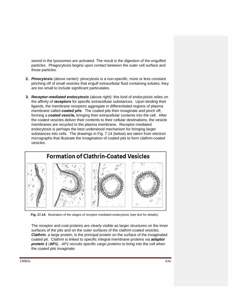
CMB3e 436

stored in the lysosomes are activated. The result is the digestion of the engulfed

particles. Phagocytosis begins upon contact between the outer cell surface and

those particles.

2. Pinocytosis (above center): pinocytosis is a non-specific, more or less constant

pinching off of small vesicles that engulf extracellular fluid containing solutes; they

are too small to include significant particulates.

3. Receptor-mediated endocytosis (above right): this kind of endocytosis relies on

the affinity of receptors for specific extracellular substances. Upon binding their

ligands, the membrane receptors aggregate in differentiated regions of plasma

membrane called coated pits. The coated pits then invaginate and pinch off,

forming a coated vesicle, bringing their extracellular contents into the cell. After

the coated vesicles deliver their contents to their cellular destinations, the vesicle

membranes are recycled to the plasma membrane. Receptor-mediated

endocytosis is perhaps the best understood mechanism for bringing larger

substances into cells. The drawings in Fig. 7.14 (below) are taken from electron

micrographs that illustrate the invagination of coated pits to form clathrin-coated

vesicles.

The receptor and coat proteins are clearly visible as larger structures on the inner

surfaces of the pits and on the outer surfaces of the clathrin-coated vesicles.

Clathrin, a large protein, is the principal protein on the surface of the invaginated

coated pit. Clathrin is linked to specific integral membrane proteins via adaptor

protein 1 (AP1). AP1 recruits specific cargo proteins to bring into the cell when

the coated pits invaginate.

Fig. 17.14: Illustration of the stages of receptor-mediated endocytosis (see text for details).

CMB3e 437

Some details of receptor-mediated endocytosis are illustrated below in Fig.17.15.

In the illustration, substances to be internalized have bound to cell membrane

receptors. The receptors then cluster to form a coated pit. Assisted by the

protein dynamin (a GTPase), the coated pits invaginate. The final pinch-off of a

coated vesicle requires GTP hydrolysis (not shown). Once internalized, the

coated vesicles lose their clathrin and associated adaptor protein coat. The

uncoated vesicle fuses with an early endosome to form a sorting vesicle (i.e.,

late endosome). Sorting vesicles separate imported content from the receptors.

The latter are recycled to the membrane. The vesicle that remains is now a

lysosome, containing digestive enzymes that will catalyze hydrolysis of the vesicle

contents. The digest products are then released for cellular use. To watch live

video of fluorescently labeled proteins (the bright spots) entering cells by receptor-

mediated endocytosis at Receptor-mediated endocytosis - esp. watch two left

panels.

Fig. 17.15: Molecular details of receptor-mediated endocytosis (see text for

details).

CMB3e 438

A well-known example of receptor-mediated endocytosis is the uptake of

cholesterol bound to low density lipoprotein (LDL), a complex of phospholipid,

protein and cholesterol (Fig. 17.16, below).

A single LDL complex carries as many as 15,000 molecules of cholesterol. LDL,

sometimes called “bad cholesterol”, is not good for you at high levels. On the other

hand, high-density lipoprotein (HDL) is “good cholesterol”. As one gets older, it is

important to monitor one’s HDL/LDL ratio; the higher it is the better!

17.6.2 Exocytosis and the Formation of Protein Storage Organelles

Maintaining cell size or volume seems to be a built-in component of the machinery of

receptor-mediated endocytosis that balances endocytosis with membrane recycling.

However, exocytosis is also necessary to restore plasma membrane internalized by

pinocytosis and phagocytosis, and for eliminating cellular waste products. It is also

the end-point of a complex process of packaging proteins destined for secretion,

intracellular storage (e.g., in lysosomes, peroxisomes, etc.) or insertion into the

membrane itself. While endocytotic and secretion vesicles form in ‘opposite

directions’, they both share common structural features with the plasma membrane,

Fig. 17.16: A low-density lipoprotein coated with cholesterol (see text for details).

CC-BY 3,0; Adapted from Prassi & Laggner (Intech Open Access Publisher) at

https://cdn.intechopen.com/pdfs-wm/39539.pdf

CMB3e 439

from which they are derived and with which they fuse (respectively). The formation

of both lysosomes and secretion vesicles begins in the rough endoplasmic

reticulum (RER), followed by passage and maturation through Golgi vesicles, as

illustrated in Fig. 17.17 below.

As we have seen, many secretory and membrane proteins are glycoproteins, and their

glycosylation begins in the RER. Check the link below to review the process.

291 The Path to Sugar Coated Cells

Fig. 17.17: Rough endoplasmic reticulum (RER), Golgi and other vesicles participate in the

trafficking of proteins destined for secretion or vesicular packaging/storage in the cell (see text for

details).

CMB3e 440

A cell often produces many packaged protein at the same time. This requires sorting each

protein to the right place – extracellular fluids, lysosomes, peroxisomes and other

‘microbodies’, and of course, membranes themselves. How do they do it? Some

representative packaged proteins are listed in Table 17.1, below.

17.7 Directing the Traffic of Proteins in Cells

Each polypeptide protein translated by ribosomes from a sequence of bases in an mRNA

has a specific functional location, either in the cytoplasm, on cellular membranes, inside

organelles or in extracellular fluids. In this section we consider the movement and sorting

of proteins from RER through vesicles of the endomembrane system as well as the

transport of proteins into and out of organelles.

17.7.1 Proteins Packaged in RER are Made as Larger Precursor Proteins

All protein synthesis begins with the formation of an initiation complex and subsequent

elongation cycles of peptide bond formation and carboxyl-terminal amino acid

addition. But proteins to be packaged for secretion or into lysosomes, peroxisomes or

other microbodies, complete translation elongation directly into the cisternae

(enclosed spaces) of the RER. What was the traffic signal that led some proteins to

the RER while others went elsewhere or remained in the cytoplasm?

Cellular Proteins Segregated From the Cytoplasm

Hormones

Immune System

Proteins Neurotransmitters Other

insulin

immunoglobulin G

(IgG), a class of

circulating antibodies)

acetylcholine EGF (Epidermal growth

factor)

growth hormone IgM and other cell

membrane antibodies

dopamine, adrenaline

noradrenaline, other

monoamines

NGF (Neural growth

factor)

follicle stimulating

hormone (FSH)

MHC (cell surface)

Major Histocompatibility

Complex) proteins

serotonin Fibrinogen (& other blood

clotting factors)

oxytocin

some amino acids

(glutamate, aspartate,

glycine)

Fibronectin (and other

extracellular matrix

proteins

prolactin Plant cell wall components

ACTH

(adrenocorticotropic

hormone)

Trypsin, pepsin, etc. (gut

digestive enzymes)

Chloroplast and

mitochondrial proteins

Nuclear proteins

CMB3e 441

A good model system for studying secretory protein synthesis turns out to be mouse

myeloma cells, cancerous lymphocytes of the immune system. The normal cells

make immunoglobulin G (IgG) molecules with light and heavy chain polypeptide

subunits (IgGs are circulating antibodies). The myeloma cells make only IgG light

chains easily isolated from cell culture medium.

In an early experiment mouse myeloma cells were cultured under different conditions

and the secreted IgG light chain produced was analyzed (Fig. 17.18, below). The

experiment revealed that secreted mouse light chain IgG proteins made in an in vitro

translation system were in fact larger than proteins naturally secreted by the cells.

Here’s how the experiment was done:

In one part of the experiment described above, myeloma cells were grown in the

presence of radioactive amino acids. The resulting radioactive IgG light chain

polypeptides were isolated (follow the red arrows). In another part of the experiment,

mRNA was separately extracted from another batch of the myeloma cells and added

to a cell-free translation system containing radioactive amino acids. The radioactive

Fig. 17.18: Determining the role of RER in the synthesis of secretory and other packaged

protein synthesis (see text for details).

CMB3e 442

polypeptide synthesized in vivo and in vitro were separated on electrophoretic gels

and autoradiographed (follow the blue arrows, above). From the autoradiograph

(lower right of the illustration) you see that the mature, secreted polypeptides made in

vivo had migrated faster on the gel than those translated in vitro. So, the cell-free

translation product was indeed, larger than the mature secreted polypeptide. To

explain these results, Gunther Blobel and colleagues extended the Signal Hypothesis,

proposing that the signal was a short N-terminal signal peptide that directs a growing

secretory polypeptide to the RER. They further proposed that the signal peptide is a

temporary ‘traffic’ signal, removed by an RER-associated enzyme as the polypeptide

crossed the RER membrane into the cisternal space.

304 Formulating the Signal Hypothesis: Early Experiments

17.7.2 Testing the Signal Hypothesis for Packaging Secreted Proteins in RER

In the test of the Signal Hypothesis (which won Blobel the 1999 Nobel Prize in

Physiology or Medicine), isolates of RER membranes were included with mouse

myeloma cell mRNA in cell-free protein synthesis systems. This time, when secreted

and cell-free synthesized IgG light chain polypeptides were electrophoresed and the

gel autoradiographed, both polypeptides were the same size as the mature, secreted

polypeptides. Therefore as predicted, RER contains processing activity, i.e., a signal

peptidase that removes the signal peptide! The steps of the signal hypothesis that

emerged from the experiments of Blobel and his colleagues are illustrated in Fig.

17.19 (below).

Fig. 17.19: Molecular details (steps) of the Signal Hypothesis (see text for details).

CMB3e 443

Recall that protein translation starts with assembly of an initiation complex, followed by

polypeptide elongation. During elongation, the growing polypeptide moves through

and emerges from a channel, or groove in the large ribosomal subunit. As the N-

terminal signal sequence (i.e., the signal peptide) of a secretory polypeptide emerges

from this groove, it interacts with the RER membrane. Beginning at the lower left in

Fig. 17.19, the steps of the process are:

1. An SRP (signal recognition particle) binds to the hydrophobic signal peptide.

2. Elongation stops until the SRP-ribosome complex finds the RER membrane.

3. The ribosome-SRP complex binds to an SRP receptor on the RER membrane.

4. The SRP detaches from the growing polypeptide chain and is recycled.

5. Translation elongation resumes through a translocation channel; a signal

peptidase in the RER membrane catalyzes co-translational hydrolysis of the

signal peptide, which remains embedded in the RER membrane.

6. Elongation continues and the growing polypeptide begins to fold in the RER.

305 Testing the Signal Hypothesis

306-2 Details of the Signal Hypothesis

Step 2 above requires that the SRP find and bind to the signal peptide before the

nascent polypeptide gets too long and starts to fold into a 3D (tertiary) conformation.

It turns out the ribosome itself may keep the signal peptide available by destabilizing

electrostatic interactions that would otherwise lead to premature folding and an

undoubtedly incorrect conformation. For more on ribosome involvement in protein

folding, check out the link at Protein Folding-Destabilizing One Protein Strand at a

Time.

Bacteria secrete proteins that assist in nutrient scavenging as well as cell wall

synthesis and they use a secretory mechanism similar to that of eukaryotes, with

obvious differences in detail. Partially elongated signal peptides guide mRNA-bound

ribosomes to the cytoplasmic side of the plasma membrane, where the ribosomes

bind and then pass elongating proteins through the plasma membrane into the space

between the cell membrane and wall. As the protein exits the cell, a bacterial signal

peptidase (SPase) cleaves the signal peptide.

Early on, we discovered that antibiotics stop bacterial growth either by disrupting the cell wall or otherwise killing the cells outright. We now know that some antibiotics (e.g., arylomycins) disrupt plasma membrane SPase function, preventing proteins required in the space between the cell wall and membrane from ever making it out of the cell. Once used against Staphylococcus aurease, arylomycins are no longer

CMB3e 444

effective because many strains have become resistant to these antibiotics (click Bacterial Signal Peptidase and Antibiotic Resistance to read about the mechanism of arylomycin resistance). As you may already know, S. aurease is now resistant to many antibiotics, and illness from untreatable infections has its own name, MRSA (Methicillin-Resistant Staph Aurease - dig on your own to see more about methicillin resistance). While named for methicillin resistance, the MRSA acronym has also come to describe untreatable S. aurease infections in general.

Apparently, the basic mechanism for the secretion of proteins evolved early and is

conserved in prokaryotes. We turn now to well-studied mechanisms, for packaging

proteins into eukaryotic organelles and into membranes themselves.

17.8 Synthesis of Integral Membrane Proteins

Integral membrane proteins may span a membrane one or more times (Fig. 17.20), or

may simply be anchored at one end and be embedded in the membrane.

Fig. 17.20: Integral membrane-spanning proteins have one or more very hydrophobic stop transfer

signals in addition to their signal sequence. Such membrane proteins cross the membranes one or

more times during their synthesis.

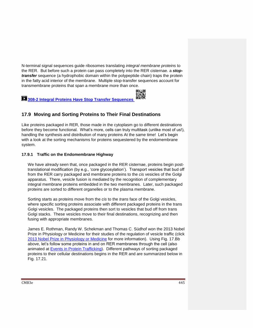
CMB3e 445

N-terminal signal sequences guide ribosomes translating integral membrane proteins to

the RER. But before such a protein can pass completely into the RER cisternae. a stop-

transfer sequence (a hydrophobic domain within the polypeptide chain) traps the protein

in the fatty acid interior of the membrane. Multiple stop-transfer sequences account for

transmembrane proteins that span a membrane more than once.

308-2 Integral Proteins Have Stop Transfer Sequences

17.9 Moving and Sorting Proteins to Their Final Destinations

Like proteins packaged in RER, those made in the cytoplasm go to different destinations

before they become functional. What’s more, cells can truly multitask (unlike most of us!),

handling the synthesis and distribution of many proteins At the same time! Let’s begin

with a look at the sorting mechanisms for proteins sequestered by the endomembrane

system.

17.9.1 Traffic on the Endomembrane Highway

We have already seen that, once packaged in the RER cisternae, proteins begin post-

translational modification (by e.g., ‘core glycosylation’). Transport vesicles that bud off

from the RER carry packaged and membrane proteins to the cis vesicles of the Golgi

apparatus. There, vesicle fusion is mediated by the recognition of complementary

integral membrane proteins embedded in the two membranes. Later, such packaged

proteins are sorted to different organelles or to the plasma membrane.

Sorting starts as proteins move from the cis to the trans face of the Golgi vesicles,

where specific sorting proteins associate with different packaged proteins in the trans

Golgi vesicles. The packaged proteins then sort to vesicles that bud off from trans

Golgi stacks. These vesicles move to their final destinations, recognizing and then

fusing with appropriate membranes.

James E. Rothman, Randy W. Schekman and Thomas C. Südhof won the 2013 Nobel

Prize in Physiology or Medicine for their studies of the regulation of vesicle traffic (click

2013 Nobel Prize in Physiology or Medicine for more information). Using Fig. 17.Bb

above, let’s follow some proteins in and on RER membranes through the cell (also

animated at Events in Protein Trafficking). Different pathways of sorting packaged

proteins to their cellular destinations begins in the RER and are summarized below in

Fig. 17.21.

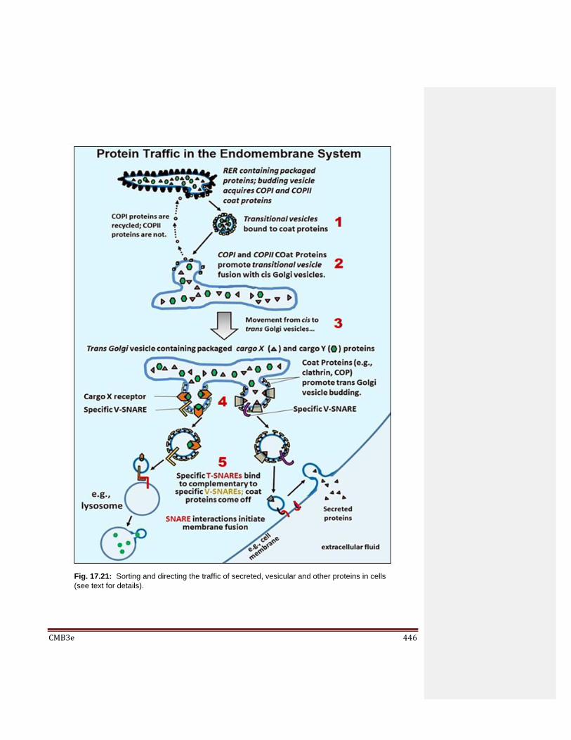
CMB3e 446

Fig. 17.21: Sorting and directing the traffic of secreted, vesicular and other proteins in cells

(see text for details).

CMB3e 447

Here are the steps:

1. Transition vesicles carrying their mix of packaged proteins bud off from the RER

with the help of COPI and COPII coat proteins, dissociating from ribosomes.

Transition vesicles however, remain associated with the COP proteins.

2. These vesicles fuse with cis Golgi vesicles, a process also mediated by COP

proteins. COPI proteins detach during or after fusion, recycling back to the RER.

3. Packaged proteins and membrane proteins are further processed as the pass

through the Golgi vesicle stack, for example undergoing terminal glycosylation.

4. A key step in sorting packaged proteins occurs as vesicles bud off from the trans

Golgi face with the help of clathrin and other COP proteins and specific cargo

receptor proteins. The cargo receptor proteins recruit specific packaged proteins

(now called cargo proteins), enriching them in their nascent vesicles. V-SNARE

(for vesicle-SNARE) proteins also associate with the vesicles; these will guide

them to their ultimate destination.

When V-SNARE proteins on their vesicles bind to complementary T-SNARE (for

target-SNARE) proteins on receiving membranes, the membranes fuse.

Some vesicles follow a pathway to organelles, fusing with lysosomes or similar

vesicles to stock them with appropriate enzymes and other protein content.

Coat proteins come off the fusing vesicle and are recycled, while vesicle

contents are transferred into the next vesicle.

Vesicles containing secretory proteins typically fuse to form larger secretory

vesicles. Then, secretion vesicles fuse with the plasma membrane, releasing

their contents to the extracellular fluid. Once again, coat proteins and clathrin

dissociate from the secretory vesicle during fusion. Secretory vesicles often

remain in the cytoplasm, storing their proteins until cells are signaled to release

them from the cell.

Other players have been left out of this discussion, notably those that hydrolyze

nucleotide triphosphates to provide the energy for protein trafficking. In addition, you

may recognize molecular players such as clathrin also play a role receptor-mediated

endocytosis. Maybe that’s not a surprise! After all, endocytosis is at least partly

molecular traffic in the opposite direction of vesicle formation and secretion.

17.9.2 Nuclear Protein Traffic

We saw earlier that large molecules (mRNAs, tRNAs) and even whole particles (i.e.,

ribosomal subunits) cross the nuclear envelope through nuclear pores. What about

those large proteins headed for the nucleus? It turns out that these proteins have

nuclear localization signals rich in positively charged amino acids (lysine, proline)

that enable binding to the negatively charged domain of a nuclear transport receptor

protein in the cytosol (Fig. 17.22, below).

CMB3e 448

As the complex of the two proteins approach a nuclear pore, it interacts with nuclear

pore fibrils, causing the pore to open. The two bound proteins then cross the double

membrane of the nuclear envelope where they accumulate against a concentration

gradient. This active transport comes from ATP hydrolysis as the nuclear proteins

enter the nucleus.

17.9.3 Mitochondrial Protein Traffic

Recall that mitochondria contain their own genome and translational machinery. Thus

they transcribe RNAs and translate proteins of their own. However, genes in the

nucleus encode many of the proteins found in mitochondria. Fig. 17.23 illustrates how

mitochondria import these proteins.

Fig. 17.22: Nuclear proteins made in the cytoplasm contain a positively charged nuclear

localization signal. This signal binds to the electronegative region of a nuclear transport

receptor that then binds nuclear pore fibrils, guiding the protein into the nucleus.

CMB3e 449

Unlike the co-translational packaging of proteins by the RER, mitochondrial protein

transfer is post-translational. This means that mitochondrial proteins formed in the

cytoplasm have already folded into a tertiary structure. However, the folded protein

exposes an N-terminal signal peptide on its surface that recognizes and binds to a

receptor protein at the outer mitochondrial membrane. The receptor protein spans

both the mitochondrial outer membrane (OM) and cristal membrane (CM). The

receptor protein delivers the protein to membrane contact proteins that also span

both mitochondrial membranes. The membrane contact proteins act as channels, or

pores, through which the mitochondrial protein will cross into the mitochondrial matrix.

But there is a problem: the folded protein cannot cross the membrane by itself,

precisely because it is folded!

The entry of a completed mitochondrial protein now sitting in the cytoplasm requires a

so-called chaperone protein, in this case the HSP70 (heat-shock 70). HSP70

controls unfolding of the mitochondrial protein as it passes into the matrix. Upon

removal of the signal peptide by a mitochondrial signal peptidase, another HSP70

Fig. 17.23: Nuclear proteins destined for mitochondria are synthesized with an N-terminal

mitochondrial signal sequence that is removed by a mitochondrial signal peptidase. Since

polysomes do not attach to mitochondria, a different mechanism engages the N-terminal

signal with membrane proteins required for transfer (see text and figure for details).

CMB3e 450

molecule resident in the mitochondrion facilitates refolding of the protein into a

biologically active shape. Recall that HSPs were initially discovered as 70 Kd proteins

that accumulated in in heat stressed organisms.

309 Protein Traffic to Nuclei and Mitochondria 17.10 How Cells are Held Together and How They Communicate

Proteins and glycoproteins on cell surfaces play a major role in how cells interact with

their surroundings and with other cells. We’ll look first at some of the proteins in the

glycocalyx of adjacent cells that interact to form different kinds of cell-cell junctions.

Then we’ll see how some of these proteins interact with extracellular proteins and

carbohydrates to form the extracellular matrix (ECM). Still other membrane proteins

are part of receptor systems that bind hormones and other signaling molecules at the cell

surface, conveying information into the cell by signal transduction.

17.10.1 Cell Junctions

Cell junctions serve different functions in cells and tissues. In healthy cells they serve

to bind cells tightly, to give tissues structural integrity and to allow cells in contact with

one another to pass chemical information directly between them. Electron

micrographs and illustrations different cell junctions are shown in Fig. 17.24 (below).

1. Tight Junctions (zonula occludens) are typical in sheets of epithelial cells that line

the lumens of organs (e.g., intestines, lungs, etc.). Zonula refers to the fact that

these structures form a band encircling an entire cell, attaching it to all surrounding

cells. Occludens refers to the ‘water-tight’ seal or occluding barrier of tight

junctions that stops extracellular fluids from crossing to the other side of a sheet of

cells by passing between cells. Tight junction membrane proteins (TJMPs)

create this waterproof barrier.

2. Desmosomes (adherens junctions) essentially glue (adhere) cells together, giving

tissues their strength. Belt desmosomes (zonula adherens) surround entire cells,

strongly binding them to adjacent cells. Spot desmosomes (macula adherens) act

like rivets, attaching cells at spots. In both cases, cadherin proteins cross cell

membranes from intracellular plaque proteins, spanning the intercellular space to

link adjacent cell membranes together. Plaques are in turn, connected to

intermediate filaments (keratin) of the cytoskeleton, further strengthening

intercellular attachments and thus, the tissue cell layer.

CMB3e 451

Fig. 17.24: Tight, Gap and Adherens junctions between animal cells involve different

membrane proteins (see text for details).

CMB3e 452

3. Gap junctions enable chemical communication between cells. Connexon

structures made of connexin proteins act as pores that open to allow direct

movement of ions and small molecules between cells. Communication by ion or

molecular movement is quite rapid, ensuring that all cells in a sheet or other tissue

in one metabolic state can respond to each other and switch to another state

simultaneously. In plants, we have seen the plasmodesmata that perform

functions similar to the gap junctions of animal cells.

310-2 Cell Junction Structure and Function Many of the glycocalyx proteins that interact to form junctions between cells are

glycoproteins. Generally, proteins that interact to bind cells together are called ICAMs

(Intercellular Cell Adhesion Molecules). Fig. 17.25 illustrates several examples of

membrane proteins that enable cell-cell recognition and adhesion.

Selectins are one kind of ICAM. During blood clotting, selectins on one platelet

recognize and bind to specific receptors on other platelets, contributing to the clot.

NCAMs are another kind of ICAM, ones with sugary immunoglobulin domains that

interact specifically to enable neural connections.

Fig. 17.25: Glycocalyx protein interactions; roles in cell-cell recognition and attachment.

CMB3e 453

We’ve already seen the calcium-dependent cadherins involved in forming

adherens junctions (desmosomes). These are essentially the ‘glue’ that binds cells

together to form strong cohesive tissues and sheets of cells. Cell-Cell binding

begins with recognition and connection via the glycocalyx and extracellular matrix.

311-2 Glycocalyx-Sugars Covalently link to Plasma Membrane Proteins

312 Cell Adhesion Molecule Functions in the Glycocalyx

17.10.2 Microvesicles and Exosomes

Of the several ways cells take up material from their environment, we saw that

Pinocytosis, or bulk transport seems to be a random process in which tiny bits of

plasma membrane engulf small amounts of extracellular fluids along with their ionic,

particle and other solute contents. Pinocytotic vesicles range from 0.5 to 5 mm in

diameter. On the other hand, exosomes and microvesicles are circular bits of

plasma membrane and endosome (respectively) that are shed by cells into the

extracellular space. Known by several names, these extracellular vesicles (EVs) were

first reported in the 1980s as small vesicles released by reticulocytes. At around

1000nm (1 mm), microvesicles are similar in size to pinocytotic vesicles. Exosomes

are about a tenth the size of microvesicles, ranging in size from 40-100nm in diameter

(see Fig.17.26 below).

There is much evidence that microvesicles and exosomes are not artifacts. For

example:

Microvesicles such as those from melanoma cells (Fig. 17.26, left panel) may be

normally released, suggesting that they are not cellular waste products.

Fig. 17.26: LEFT: Transmission electron micrograph of a Melanoma cell exosomes (bar,

100nm). Some of the larger vesicles show an irregular, cup-like shape (arrows). RIGHT:

Transmission electron micrograph of a reticulocyte endosome containing exosomes about

to fuse with the plasma membrane (bar, 200 nm).

CMB3e 454

reticulocyte endosomal vesicles were caught in the act of fusing with the cell

membrane, releasing exosomes with their contents (Fig. 17.26, right panel).

microvesicles released by dendritic cells are able to stimulate T cells, both of which

are cells of the immune system.

We can conclude that microvesicles are physiologically significant structures. We

know that cells talk to each other by releasing chemicals that can act over short or

long distances. Familiar examples include information transfer by hormones of the

endocrine system, neurotransmitters of the nervous system and chemicals released

into the intercellular space. Microvesicles are are clearly part of normal reticulocyte

maturation to erythrocytes but may also participate in intercellular communication.

Are exosomes yet another unique mechanism of intercellular communication ( see

Exosomes and Intercellular Communication).

17.10.3 Cancer and Cell Junctions

During embryogenesis, cells migrate from a point of origin by attaching to and moving

along an extracellular matrix (ECM), which acts as a path to the cell’s final

destination. This ECM (or basal lamina) is made up of secretions from other cells…,

or from the migrating cells themselves! One major secretion is fibronectin. One of its

functions is to bind to integral membrane proteins called integrins, attaching the cells

to the ECM. During development, integrins respond to fibronectin by signaling cell

and tissue differentiation, complete with the formation of appropriate cell junctions. An

orderly sequence of gene expression and membrane protein syntheses enables

developing cells to recognize each other as different or the same (see Fig. 17.27).

Fig. 17.27: Migration and attachment of cells during development requires the synthesis of

membrane proteins that recognize and bind proteins on the membranes and glycocalyx of other

cells, forming cell junctions that enable tissue formation.

CMB3e 455

The specificity of membrane proteins prevents incorrect cell-cell associations. Integrin

is an early cell membrane protein that binds many proteins to form a glycocalyx, and

can also acts as a receptor, transducing signals by binding cell-surface proteins of

other cells.

An early difference between eukaryotic normal and cancer cells is how they grow in

culture. Normal cells settle to the bottom of a culture dish when placed in growth

medium. Then they grow and divide, increasing in number until they reach

confluence, when a single layer of cells completely covers the bottom of the dish.

The cells in this monolayer seem to ‘know’ to stop dividing, as if they had completed

formation of a tissue, e.g., a layer of epithelial cells. This phenomenon, originally

called contact inhibition, implies that cells let each other know when they have

finished forming a tissue and can stop cycling and dividing. In contrast, cancer cells

do not stop dividing at confluence. Instead, they continue to grow and divide, piling up

in multiple layers.

Among other deficiencies, cancer cells do not form gap junctions and typically have

fewer cadherens and integrins in their membranes. Thus, cancer cells cannot inform

each other of when they reach confluence. Neither can they form firm adherens

junctions. In vivo, a paucity of integrins would inhibit cancer cells from binding and

responding to fibronectin. Therefore, they also have difficulty attaching firmly to an

extracellular matrix, which may explain why many cancers metastasize or spread

from their original site of formation. These differences in growth in culture between

normal and cancer cells are shown in Fig. 17.28.

Fig. 17.28: Behavior of normal and cancer cells growng on surfaces in cell culture.

CMB3e 456

Density-dependent inhibition (aka. Contact Inhibition) occurs when cells multiplying

and spreading on a surface cease dividing when there is no more room on the

surface. Cancer cells have lost the property of contact inhibition and keep growing

over one another in layers. Loss of contact inhibition is correlated with an absence of

gap junctions in cancer cells.

313 Formation of a Glycocalyx, Normal Development and Cancer

314-2 Role of the Extracellular Matrix in Cell Migration & Development

17.11 Signal Transduction

When hydrophobic chemical effector molecules such as steroid hormones reach a target

cell, they can cross the hydrophobic membrane and bind to an intracellular receptor to

initiate a response. When large effector molecules (e.g., protein hormones) or highly

polar hormones (e.g., adrenalin) reach a target cell, they can’t cross the cell membrane.

Instead, they bind to transmembrane protein receptors on cell surfaces. A conformational

change initiated on the extracellular domain of the membrane receptor protein induces

further allosteric change on its cytoplasmic domain. A sequential series of molecular

events then converts information delivered by the external effector into intracellular

information, a process called signal transduction. A general outline of signal

transduction events is illustrated in Fig. 17.29.

Fig. 17.29: Signal transduction by effectors (e.g., hormones) can lead to many different effects in

the cytoplasm as well as in nuclei.

CMB3e 457

Many effects of signal transduction are mediated by a sequence, or cascade of protein

phosphorylations catalyzed by protein kinases inside the cell. Here we will consider G

Protein-linked and enzyme-linked receptors.

315-2 Introduction to Signal Transduction

17.11.1 G-Protein Mediated Signal Transduction by PKA (Protein Kinase A)

GTP-binding proteins (G-Proteins) transduce extracellular signals by inducing the

synthesis of second messenger molecules in the cells. When hormones or other

effector (signal) molecules bind to a membrane receptor, an allosteric change

on the extracellular domain of the receptor is transmitted to the cytoplasmic domain of

the receptor, increasing its affinity for trimeric G-proteins embedded in the cytoplasmic

surface of responsive cell membranes. G- protein trimers consist of , and

subunits. Fig. 17.30 illustrates seven steps of G-protein-mediated signal transduction.

The receptor changes shape upon binding its effector signal molecule (steps 1 and 2).

In this altered conformation, the receptor recognizes and binds to the G-protein trimer

(step 3). Upon binding of the trimer to the receptor, GTP displaces GDP on the

subunit of the G-protein (step 4). After a conformational change in the subunit , it

Fig. 17.30: G-proteins cycle between bound GTP and bound GDP. They are intermediates in

signal transduction between an active, effector-bound membrane receptor and adenylate cyclase

(see text for details of the different steps).

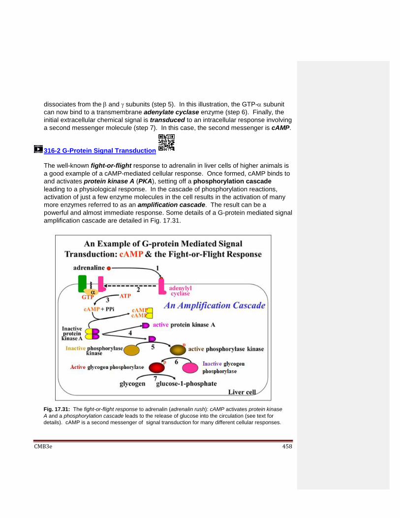
CMB3e 458

dissociates from the and subunits (step 5). In this illustration, the GTP- subunit

can now bind to a transmembrane adenylate cyclase enzyme (step 6). Finally, the

initial extracellular chemical signal is transduced to an intracellular response involving

a second messenger molecule (step 7). In this case, the second messenger is cAMP.

316-2 G-Protein Signal Transduction

The well-known fight-or-flight response to adrenalin in liver cells of higher animals is

a good example of a cAMP-mediated cellular response. Once formed, cAMP binds to

and activates protein kinase A (PKA), setting off a phosphorylation cascade

leading to a physiological response. In the cascade of phosphorylation reactions,

activation of just a few enzyme molecules in the cell results in the activation of many

more enzymes referred to as an amplification cascade. The result can be a

powerful and almost immediate response. Some details of a G-protein mediated signal

amplification cascade are detailed in Fig. 17.31.

Fig. 17.31: The fight-or-flight response to adrenalin (adrenalin rush): cAMP activates protein kinase

A and a phosphorylation cascade leads to the release of glucose into the circulation (see text for

details). cAMP is a second messenger of signal transduction for many different cellular responses.

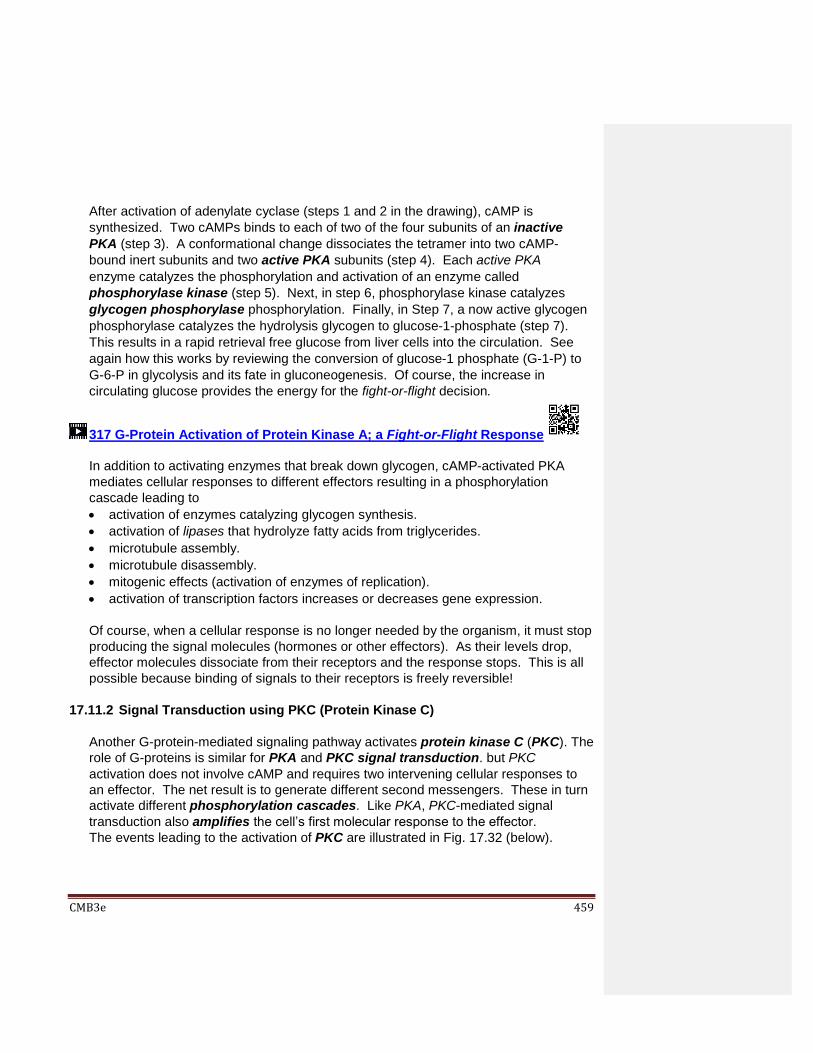
CMB3e 459

After activation of adenylate cyclase (steps 1 and 2 in the drawing), cAMP is

synthesized. Two cAMPs binds to each of two of the four subunits of an inactive

PKA (step 3). A conformational change dissociates the tetramer into two cAMP-

bound inert subunits and two active PKA subunits (step 4). Each active PKA

enzyme catalyzes the phosphorylation and activation of an enzyme called

phosphorylase kinase (step 5). Next, in step 6, phosphorylase kinase catalyzes

glycogen phosphorylase phosphorylation. Finally, in Step 7, a now active glycogen

phosphorylase catalyzes the hydrolysis glycogen to glucose-1-phosphate (step 7).

This results in a rapid retrieval free glucose from liver cells into the circulation. See

again how this works by reviewing the conversion of glucose-1 phosphate (G-1-P) to

G-6-P in glycolysis and its fate in gluconeogenesis. Of course, the increase in

circulating glucose provides the energy for the fight-or-flight decision.

317 G-Protein Activation of Protein Kinase A; a Fight-or-Flight Response

In addition to activating enzymes that break down glycogen, cAMP-activated PKA

mediates cellular responses to different effectors resulting in a phosphorylation

cascade leading to

activation of enzymes catalyzing glycogen synthesis.

activation of lipases that hydrolyze fatty acids from triglycerides.

microtubule assembly.

microtubule disassembly.

mitogenic effects (activation of enzymes of replication).

activation of transcription factors increases or decreases gene expression.

Of course, when a cellular response is no longer needed by the organism, it must stop

producing the signal molecules (hormones or other effectors). As their levels drop,

effector molecules dissociate from their receptors and the response stops. This is all

possible because binding of signals to their receptors is freely reversible!

17.11.2 Signal Transduction using PKC (Protein Kinase C)

Another G-protein-mediated signaling pathway activates protein kinase C (PKC). The

role of G-proteins is similar for PKA and PKC signal transduction. but PKC

activation does not involve cAMP and requires two intervening cellular responses to

an effector. The net result is to generate different second messengers. These in turn

activate different phosphorylation cascades. Like PKA, PKC-mediated signal

transduction also amplifies the cell’s first molecular response to the effector.

The events leading to the activation of PKC are illustrated in Fig. 17.32 (below).

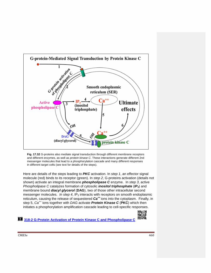
CMB3e 460

Here are details of the steps leading to PKC activation. In step 1, an effector signal

molecule (red) binds to its receptor (green). In step 2, G-proteins activation (details not

shown) activate an integral membrane phospholipase C enzyme. In step 3, active

Phospholipase C catalyzes formation of cytosolic inositol triphosphate (IP3) and

membrane bound diacyl glycerol (DAG), two of those other intracellular second

messenger molecules. In step 4, IP3 interacts with receptors on smooth endoplasmic

reticulum, causing the release of sequestered Ca++ ions into the cytoplasm. Finally, in

step 5, Ca++ ions together with DAG activate Protein Kinase C (PKC) which then

initiates a phosphorylation amplification cascade leading to cell-specific responses.

318-2 G-Protein Activation of Protein Kinase C and Phospholipase C

Fig. 17.32 G-proteins also mediate signal transduction through different membrane receptors

and different enzymes, as well as protein kinase C. These interactions generate different 2nd

messenger molecules that lead to a phosphorylation cascade and many different responses

in different target cells (see text for details of the steps).

CMB3e 461

Protein Kinase C mediated effects include:

Neurotransmitter release.

Hormone (growth hormone, leutinizing hormone, testosterone) secretion leading to

cell growth, division and differentiation.

Glycogen hydrolysis, fat synthesis.

Additional independent phospholipase C effects include:

Liver glycogen breakdown.

Pancreatic amylase secretion.

Platelet aggregation

PKA and PKC are both serine-threonine kinases that place phosphates on serine or

threonine in target polypeptides. Let’s consider tyrosine kinases next.

17.11.3 Receptor Tyrosine Kinase-Mediated Signal Transduction

The intracellular activity of Tyrosine Kinase receptors is in the cytoplasmic domain

of the receptor itself. When bound to its effector, receptor-kinases catalyze the

phosphorylation of specific tyrosine amino acids in target proteins. While studying the

action of nerve growth factor (NGF) and epidermal growth factor (EGF) in

stimulating growth and differentiation of nerve and skin, Stanley Cohen and Rita Levi-

Montalcini discovered the EGF receptor, the first enzyme-linked tyrosine kinase, and

won the 1986 Nobel Prize in Physiology or Medicine for their discovery! Watch the

animation of receptor kinase signal transduction at the link below (a description is

provided in the next few paragraphs).

319 Receptor Kinase Signal Transduction

Monomer membrane receptor kinases dimerize when they bind effector ligands, at

which point sulfhydryl group-containing SH2 proteins bind to each monomer. This

activates the kinase domain of the receptor. After multiple cross-phosphorylations of

the receptor monomers, the SH2 proteins fall away allowing the receptors to interact

with other cytoplasmic proteins to continue the response pathway. The characteristic

response to EGF and NGF signaling is cellular proliferation. Not surprisingly, the

mutations correlated with cancer cells often lie in signaling pathways leading to cell

proliferation (growth and division). Cancer-causing genes, or oncogenes, were first

discovered in viruses, but as humans, we own our own oncogenes! For being the

first to show that eukaryotic cells were actually the origin of a chicken retrovirus (the

Rous Sarcoma Virus), J. Michael Bishop and Harold Varmus earned the 1964 Nobel

Prize in Physiology or Medicine. Oncogenes turn out to be mutations of animal genes

CMB3e 462

for proteins involved in mitogenic signal transduction pathways. Under normal

circumstances, mitogenic chemical signals bind to their receptors and induce target

cells to begin dividing. MAP kinase phosphorylates transcription factors and other

nuclear proteins affecting gene activity leading to cell proliferation differentiation, as

shown in Fig. 17.33.

The Ras protein-mediated activation of a phosphorylation cascade leading to the MAP

(mitogen-activated protein) kinase is an example of such a signal transduction

pathway. This pathway plays a central role in many receptor kinase signaling

pathways. The Ras gene was one of those originally discovered as an oncogene

whose mutation leads to uncontrolled cell division, i.e., cancer. Ras gene/protein

activity may in fact be responsible for up to 30% of all cancers!

320-2 The RAS Oncogene-its Normal Mitogenic Effects and Cancer

Fig. 17.33: The effects of MAP kinase include phosphorylation and activation of DNA-

binding transcription factors and other nuclear proteins that lead to cell proliferation.

CMB3e 463

17.12 Signal Transduction in Evolution

We saw that signal transduction typically takes a few signal molecules interacting with

a few cell surface receptors to amplify a response in a cascade of enzyme-catalyzed

reactions (typically phosphorylations) that activate or inactivate target proteins.

Amplification cascades can take a single effector-receptor interaction and magnify its

effect in the cell by orders of magnitude, making the signaling systems rapid and

highly efficient. The range of cellular and systemic (organismic) responses to the

same chemical signal is broad and complex. Different cell types can have receptors

for the same effector but may respond differently. For example, adrenalin targets cells

of the liver and blood vessels among others, with different effects in each. As it

happens, adrenalin is also a neurotransmitter. Apparently, as organisms evolved,

they responded to environmental imperatives, adapting by co-opting already existing

signaling systems in the service of new pathways. Just as the same signal

transduction event can lead to different pathways of response in different cells,

evolution has allowed different signal transduction pathways to engage in crosstalk.

This occurs when two different signal transduction pathways intersect in the same

cells. In one example, the cAMP produced at the front end of the PKA signaling

pathway can activate (or under the right circumstances, inhibit) enzymes in the MAP

kinase pathway. These effects result in changes in the levels of active or inactive

transcription factors and can therefore modulate the expression of a gene using two

(or more) signals. We are only beginning to understand what looks less like a linear

pathway and more like a web of signal transduction.

Some iText & VOP Key Words and Terms

action potential fight-or-flight peroxisomes

active transport flaccid phagocytosis

adaptin free energy phospholipase C

adenylate cyclase G protein subunits phosphorylase kinase

adherens junctions gap junctions pinocytosis

adrenaline gluconeogenesis PKA

allosteric change

regulates transport GLUT1 PKC

antiport glycolysis plasmodesmata

aquaporins good cholesterol plasmolysis

bad cholesterol G-Protein-linked receptors poikilothermic organisms

basal lamina Heat shock protein potential difference

belt desmosomes HSP70 protein Protein kinase A

CMB3e 464

Ca++ ions hydrophilic corridor protein kinase C

cadherin hypertonic protein packaging

cargo receptor hypotonic protein phosphorylation

carrier proteins IgG light chain proton gate

cell adhesion molecules inositol triphosphate proton pump

cell-cell attachment integrin receptor-mediated

endocytosis

cell-cell recognition ion channels RER membrane

cell-free translation ion flow resting potential

channel proteins ion pumps secondary active

transporters

chaperone proteins IP3 serine-threonine kinases

cholesterol effects in

membranes isotonic signal peptide

clathrin LDL (low density

lipoprotein) signal recognition particle

coated pits ligand (chemically) gated

channels signal sequence

coated vesicle lysosome signal transduction

connexins MAP kinase Smooth endoplasmic

reticulum

contact inhibition mechanically gated

channels sodium-potassium pump

contractile vacuole membrane depolarization solute concentration

gradients

COP membrane hyperpolarization solute transport

cotransport membrane invagination sorting vesicle

coupled transport membrane potential spot desmosomes

cytoskeleton microbodies stop-transfer sequence

DAG mitochondrial membrane

contact proteins symport

diffusion kinetics mitogenic effects tight junction membrane

proteins

early endosome nerve growth factor tight junctions

ECM neurotransmitters TJMPs

effector molecules NGF tonoplast

EGF nuclear envelope T-SNARE

endocytosis nuclear pore fibrils turgid

endomembrane system nuclear transport receptor turgor pressure

CMB3e 465

Chapter 18: The Cytoskeleton & Cell Motility Microfilaments, intermediate filaments and microtubules – roles in cell structure,

secretion, cell migration, organelle and muscle movements

18.1 Introduction

The cell as it appears in a microscope was long thought to be a bag of liquid surrounded

by a membrane. The electron microscope revealed a cytoskeleton composed of thin

and thick rods, tubes and filaments that organize and maintain cell shape and that are

responsible for cell motility. We will see that intracellular structures and organelles are

enmeshed in these microfilaments, intermediate filaments and microtubules. To start

this chapter, we revisit these structures and more closely examine how they work to

support cell shape, motility and overall organization. Remember that cell motility includes

the movement of cells and organisms, as well as the movements of organelles (e.g.,

vesicles) and other structures inside the cell. Of course, these movements are not

random…, and they require chemical energy. After a close look at movements in and of

cells, we’ll look at the interaction of actin and myosin in skeletal muscle contraction.

We’ll look a famous paradox arising from early studies showing that that ATP was

required for muscle contraction but also for relaxation. Then we look at experiments that

resolve the paradox. Animals control skeletal muscle contraction, but some muscles

contract rhythmically or with little or no control on the part of the animal - think cardiac

muscles of the heart, or smooth muscles like those in the digestive and circulatory

systems. We will focus here on the regulation of skeletal muscle contraction by calcium

ions and regulatory proteins in the response of so-called voluntary (i.e., skeletal) muscles

to neural commands. Finally, we’ll look at skeletal muscle elasticity and how it

contributes to their function.

CMB3e 466

Learning Objectives

When you have mastered the information in this chapter, you should be able to:

1. compare and contrast roles of cytoskeletal structures in different kinds of cell motility.

2. distinguish between the roles of microfilaments, microtubules and intermediate

filaments in the maintenance and alteration of cell shape and structure.

3. suggest how ciliary and spindle fiber microtubules can maintain their length.

4. explain how spindle fiber microtubules can change their length.

5. propose an experiment to show which part of a motor protein has ATPase activity.

6. Describe the key experiments that led to the actin-myosin contraction paradox.

7. outline the steps of the micro-contraction cycle involving myosin and actin.

8. compare and contrast muscle and flagellar structure and function.

9. explain why smooth muscles do not show striations in the light microscope.

10. outline the structure of a skeletal muscle, from a whole muscle down to a sarcomere.

11. propose alternate hypotheses to explain hereditary muscle weakness involving

specific proteins/genes and suggest how you might test for one of them in a patient

with muscle weakness symptoms.

18.2 Overview of Cytoskeletal Filaments and Tubules

In a light microscope, typical eukaryotic cells look like a membrane-bound sac of

cytoplasm containing a nucleus and assorted organelles. But by the late 19th century,

microscopists had described the appearance of fibers that accompanied a dramatic

change the structure of dividing cells. No doubt you recognize this as mitosis in which

duplicated chromosomes (chromatids) materialize just as the nuclear membrane

dissolves and spindle fibers form. Over time the fibers seem to pull the chromatids apart

to opposite poles of the cell. Spindle fibers turn out to be bundles of microtubules, each

of which is a polymer of tubulin proteins. Let’s look again at a fluorescence micrograph

of a mitosing metaphase cell (Fig. 18.1); most of the cell other than what is fluorescing is

not visible in the micrograph.

Fig. 18.1: Fluorescence micrograph of the mitotic spindle treated with antibodies to

chromosomal proteins (blue) and spindle fiber proteins (green).

CMB3e 467

To get this image, antibodies were made against purified microtubule, kinetochore and

chromosomal proteins (or DNA), and then linked to different fluorophores (organic

molecular fluorescent tags). When the tagged antibodies were added to dividing cells in

metaphase, they bound to their respective fibers. In a fluorescence microscope, the

fluorophores emit different colors of visible light. Microtubules are green, metaphase

chromosomes are blue, and kinetochores are red in the micrograph.

Both mitosis and meiosis are very visible examples of movements within cells. As for

movement in whole organisms, early-to-mid 20th century studies asked what the

striations (stripes) seen in skeletal muscle by light microscopy might have to do with

muscle contraction. The striations turned out to be composed of an isolable protein

complex that investigators called actomyosin (acto for active; myosin for muscle).

Electron microscopy later revealed that actomyosin (or actinomyosin) is composed of

thin filaments (actin) and thick filaments (myosin) that slide past one another during

muscle contraction.

Electron microscopy also hinted at a more complex cytoplasmic structure of cells in

general. The cytoskeleton consists of fine rods and tubes in more or less organized

states that permeate the cell. As noted, the most abundant of these are microfilaments,

microtubules and intermediate filaments. Though myosin is less abundant, it is

nonetheless present in non-muscle cells. Microtubules account for chromosome

movements of mitosis and meiosis and together with microfilaments (i.e., actin), they

enable organelle movement inside cells (you may have seen cytoplasmic streaming of

Elodea chloroplasts in a biology lab exercise). Microtubules also underlie the movements

of the cilia and flagella that power the movement of whole cells like paramecium,

amoeba, phagocytes, etc. Actin and myosin enable muscle contraction and thus, higher

animal movement. Finally, the cytoskeleton is a dynamic structure. Its fibers not only

account for the movements of cell division, but they also give cells their shape and

mechanical strength. All of the fibers can disassemble, reassemble and rearrange,

allowing cells to change shape. These changes range from the pseudopods extended by

amoeboid cells to the spindle fibers that stretch cells in mitosis and meiosis to constriction

of a dividing cell that eventually pinches off daughter cells…, and more! In this chapter

we look in some detail at the roles of these tubules and filaments in cell structure and

different forms of cell motility

18.3 The Molecular Structure and Organization of Cytoskeletal

Components

Of the three main cytoskeletal fibers, intermediate filaments serve a mainly structural role

in cells. Microtubules and microfilaments have dual functions, dynamically maintaining

cell shape and enabling cell motility. For example, when attached to the plasma

CMB3e 468

membrane, microfilaments maintain cell shape. And when they interact with motor

proteins (e.g., myosin), they can pull or push against a muscle cell membrane, changing

the shape of the cell. Likewise, motor proteins such as dynein and kinesin can move

cargo back and forth along microtubule tracks from one point to another in the cell. We

will look at how motor proteins interact with microtubules and microfilaments shortly.

Let’s take another look at the drawings and micrographs of the three main cytoskeletal

filaments of eukaryotic cells that we saw earlier in the text (Fig. 18.2).

321-2 Introduction to the Cytoskeleton

Fig. 18.2: Illustration of assembly, structure and polarity of microtubules, microfilaments and

intermediate filaments alongside fluorescence micrographs made using fluorescent antibodies

against isolated microtubule, microfilament and intermediate filament proteins (TOP, MIDDLE

and BOTTOM, respectively).

CMB3e 469

The location and general functions of microtubules, microfilaments and intermediate filaments was demonstrated by immunofluorescence microscopy. Fluorescence micrographs like those in Fig. 18.3 (below) show the different locations of fibers in cells.

These localizations are consistent with known functions of the major cytoskeletal

component filaments in cell structure and motility. Despite the small size of prokaryotic

cells, they too were recently found have previously unsuspected cytoplasmic structures

that could serve as a cytoskeleton (ncbi-A Prokaryotic Cytoskeleton?). So perhaps all

(not just eukaryotic) cells are more than an unorganized bag of fluid sap! Next, we

consider specific roles of microtubules, microfilaments, intermediate filaments and related

proteins in the eukaryotic cytoskeleton.

322-2 Microtubules, Microfilaments and Intermediate Filaments in Cells

Fig. 18.3: Illustration and immunofluorescence microscope localization of microtubules,

microfilaments and intermediate filaments in cells.

Illustration by G. Bergtrom

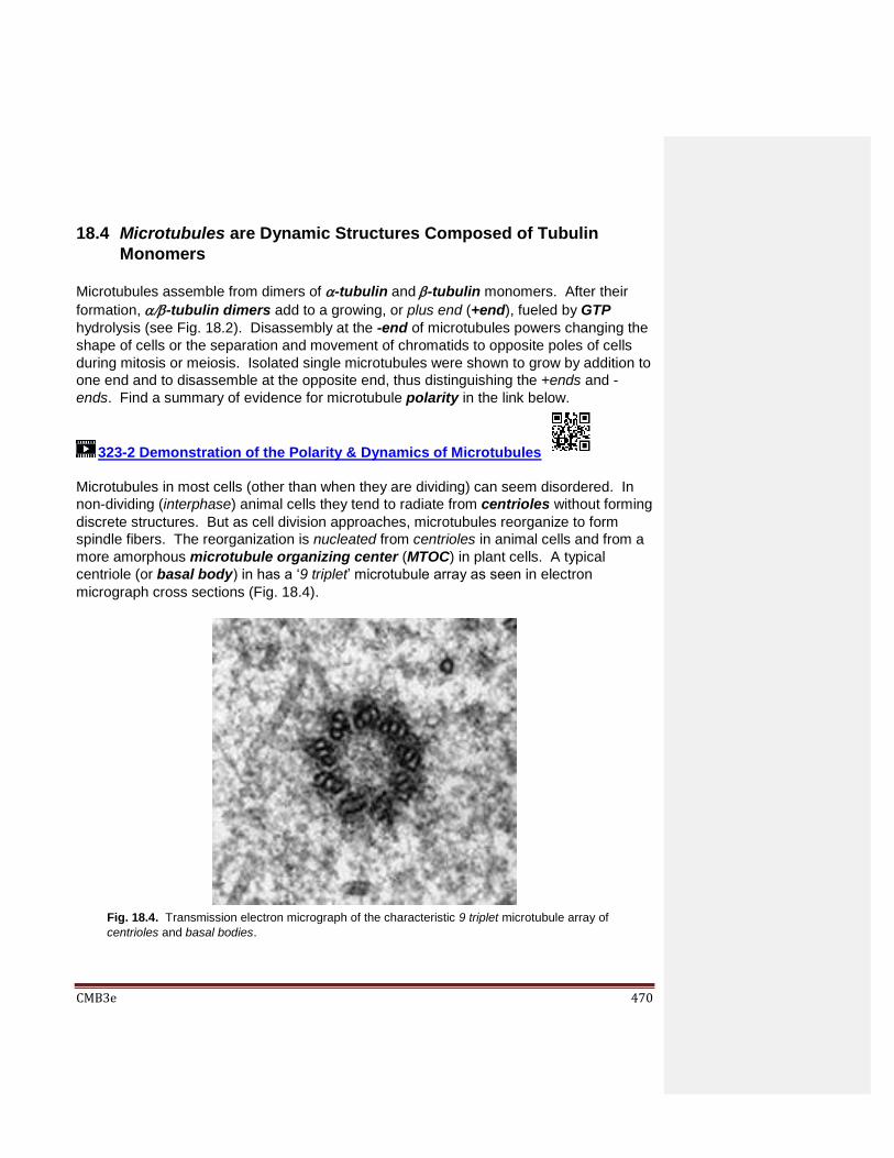
CMB3e 470

18.4 Microtubules are Dynamic Structures Composed of Tubulin

Monomers

Microtubules assemble from dimers of -tubulinand-tubulin monomers. After their

formation, -tubulin dimers add to a growing, or plus end (+end), fueled by GTP

hydrolysis (see Fig. 18.2). Disassembly at the -end of microtubules powers changing the

shape of cells or the separation and movement of chromatids to opposite poles of cells

during mitosis or meiosis. Isolated single microtubules were shown to grow by addition to

one end and to disassemble at the opposite end, thus distinguishing the +ends and -

ends. Find a summary of evidence for microtubule polarity in the link below.

323-2 Demonstration of the Polarity & Dynamics of Microtubules

Microtubules in most cells (other than when they are dividing) can seem disordered. In

non-dividing (interphase) animal cells they tend to radiate from centrioles without forming

discrete structures. But as cell division approaches, microtubules reorganize to form

spindle fibers. The reorganization is nucleated from centrioles in animal cells and from a

more amorphous microtubule organizing center (MTOC) in plant cells. A typical

centriole (or basal body) in has a ‘9 triplet’ microtubule array as seen in electron

micrograph cross sections (Fig. 18.4).

Fig. 18.4. Transmission electron micrograph of the characteristic 9 triplet microtubule array of

centrioles and basal bodies.

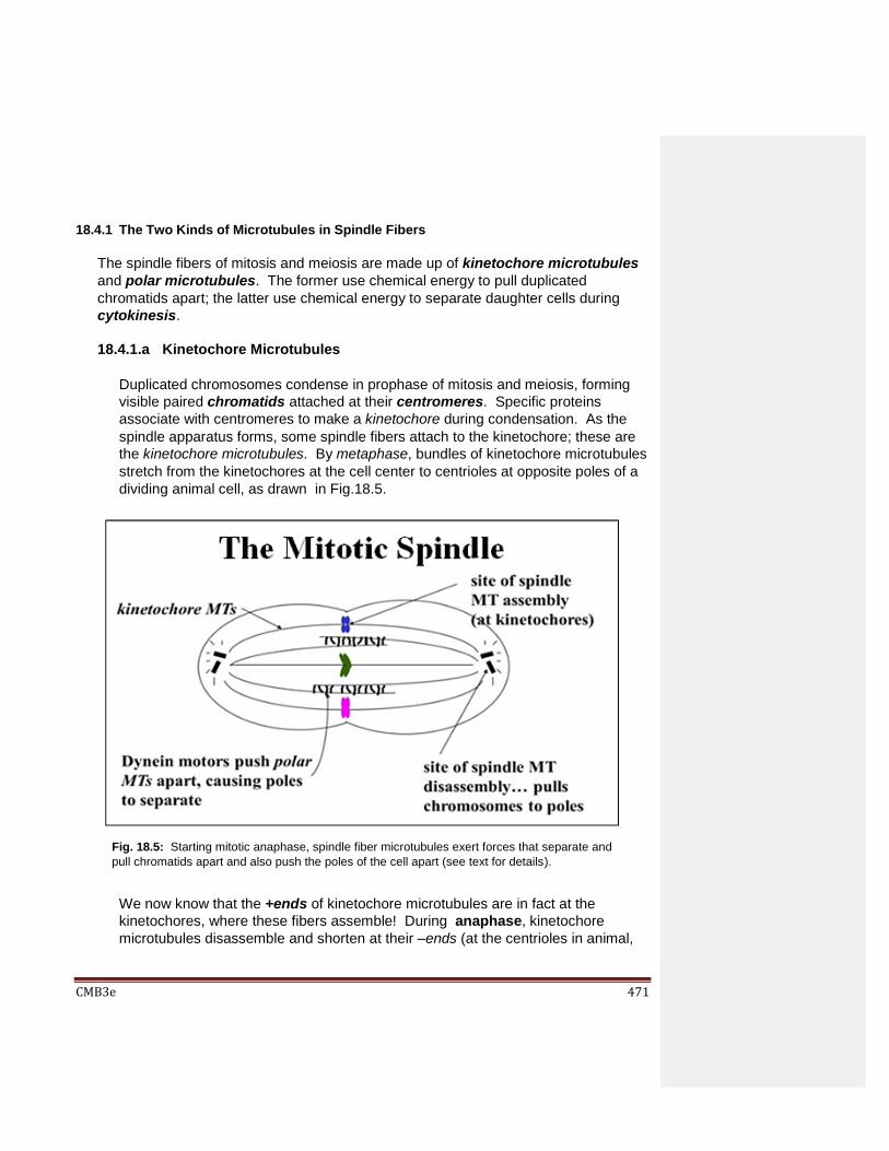
CMB3e 471

18.4.1 The Two Kinds of Microtubules in Spindle Fibers

The spindle fibers of mitosis and meiosis are made up of kinetochore microtubules

and polar microtubules. The former use chemical energy to pull duplicated

chromatids apart; the latter use chemical energy to separate daughter cells during

cytokinesis.

18.4.1.a Kinetochore Microtubules

Duplicated chromosomes condense in prophase of mitosis and meiosis, forming

visible paired chromatids attached at their centromeres. Specific proteins

associate with centromeres to make a kinetochore during condensation. As the

spindle apparatus forms, some spindle fibers attach to the kinetochore; these are

the kinetochore microtubules. By metaphase, bundles of kinetochore microtubules

stretch from the kinetochores at the cell center to centrioles at opposite poles of a

dividing animal cell, as drawn in Fig.18.5.

We now know that the +ends of kinetochore microtubules are in fact at the

kinetochores, where these fibers assemble! During anaphase, kinetochore

microtubules disassemble and shorten at their –ends (at the centrioles in animal,

Fig. 18.5: Starting mitotic anaphase, spindle fiber microtubules exert forces that separate and

pull chromatids apart and also push the poles of the cell apart (see text for details).

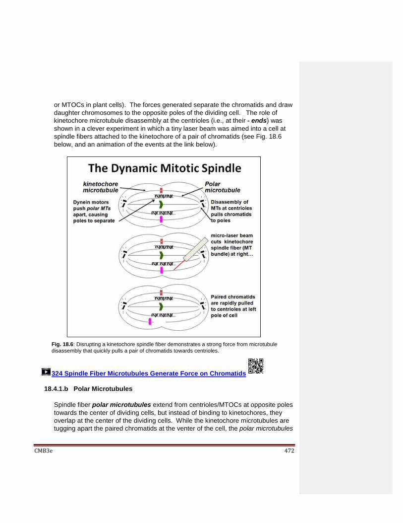
CMB3e 472

or MTOCs in plant cells). The forces generated separate the chromatids and draw

daughter chromosomes to the opposite poles of the dividing cell. The role of

kinetochore microtubule disassembly at the centrioles (i.e., at their - ends) was

shown in a clever experiment in which a tiny laser beam was aimed into a cell at

spindle fibers attached to the kinetochore of a pair of chromatids (see Fig. 18.6

below, and an animation of the events at the link below).

324 Spindle Fiber Microtubules Generate Force on Chromatids

18.4.1.b Polar Microtubules

Spindle fiber polar microtubules extend from centrioles/MTOCs at opposite poles

towards the center of dividing cells, but instead of binding to kinetochores, they

overlap at the center of the dividing cells. While the kinetochore microtubules are

tugging apart the paired chromatids at the venter of the cell, the polar microtubules

Fig. 18.6: Disrupting a kinetochore spindle fiber demonstrates a strong force from microtubule

disassembly that quickly pulls a pair of chromatids towards centrioles.

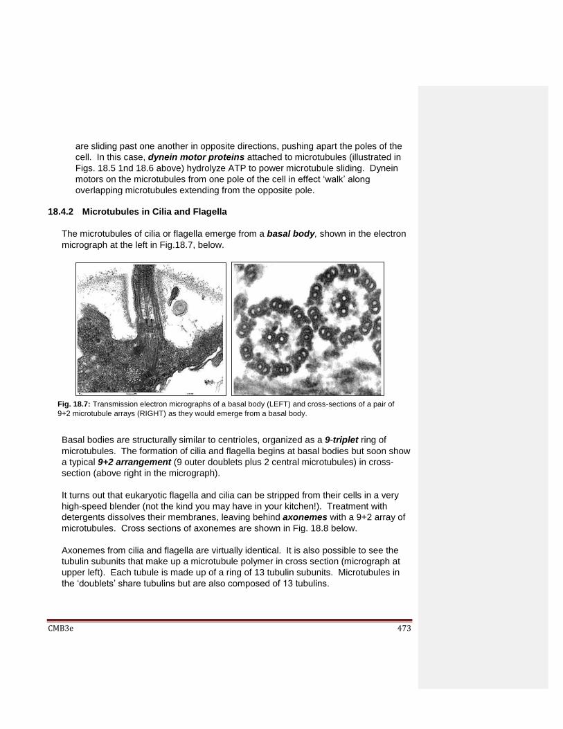
CMB3e 473

are sliding past one another in opposite directions, pushing apart the poles of the

cell. In this case, dynein motor proteins attached to microtubules (illustrated in

Figs. 18.5 1nd 18.6 above) hydrolyze ATP to power microtubule sliding. Dynein

motors on the microtubules from one pole of the cell in effect ‘walk’ along

overlapping microtubules extending from the opposite pole.

18.4.2 Microtubules in Cilia and Flagella

The microtubules of cilia or flagella emerge from a basal body, shown in the electron

micrograph at the left in Fig.18.7, below.

Basal bodies are structurally similar to centrioles, organized as a 9-triplet ring of

microtubules. The formation of cilia and flagella begins at basal bodies but soon show

a typical 9+2 arrangement (9 outer doublets plus 2 central microtubules) in cross-

section (above right in the micrograph).

It turns out that eukaryotic flagella and cilia can be stripped from their cells in a very

high-speed blender (not the kind you may have in your kitchen!). Treatment with

detergents dissolves their membranes, leaving behind axonemes with a 9+2 array of

microtubules. Cross sections of axonemes are shown in Fig. 18.8 below.

Axonemes from cilia and flagella are virtually identical. It is also possible to see the

tubulin subunits that make up a microtubule polymer in cross section (micrograph at

upper left). Each tubule is made up of a ring of 13 tubulin subunits. Microtubules in

the ‘doublets’ share tubulins but are also composed of 13 tubulins.

Fig. 18.7: Transmission electron micrographs of a basal body (LEFT) and cross-sections of a pair of

9+2 microtubule arrays (RIGHT) as they would emerge from a basal body.

CMB3e 474

When fully formed, the 25 nm diameter microtubules appear to be a hollow cylinder.

When isolated, they typically come along with the dynein motor proteins and other

Microtubule-Associated Proteins (MAPs) indicated in the micrograph at the right.

These proteins hold microtubules together in an axoneme and play a role in motility.

18.4.3 Microtubule Motor Proteins Move Cargo from Place to Place in Cells

Motor proteins such as dynein and kinesin, are ATPases; they use the free energy of

ATP hydrolysis to power intracellular motility. Let’s take a closer look at how these

two major motor proteins carry cargo from place to place inside of cells. Organelles

are a typical cargo. Examples include vesicles formed at the trans Golgi face

containing secretory proteins, pigments or neurotransmitters. Secretory vesicles

move along microtubule tracks to the plasma membrane for exocytosis. Vesicles

containing neurotransmitters move from the cell body of neurons along microtubule

Fig. 18.8: Transmission electron micrographs of axonemes show that microtubules are made

up of a ring of 13 tubulins (LEFT). Microtubules in cilia or flagella are arranged in typical 9+2

arrays (MIDDLE). The enlarged cross-section illustrates specific microtubule-associated

proteins (MAPs) that maintain the 9+2 structure, including dynein motors that powers motility.

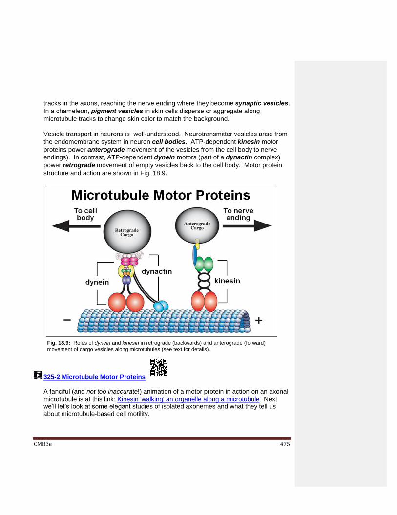
CMB3e 475

tracks in the axons, reaching the nerve ending where they become synaptic vesicles.

In a chameleon, pigment vesicles in skin cells disperse or aggregate along

microtubule tracks to change skin color to match the background.

Vesicle transport in neurons is well-understood. Neurotransmitter vesicles arise from

the endomembrane system in neuron cell bodies. ATP-dependent kinesin motor

proteins power anterograde movement of the vesicles from the cell body to nerve

endings). In contrast, ATP-dependent dynein motors (part of a dynactin complex)

power retrograde movement of empty vesicles back to the cell body. Motor protein

structure and action are shown in Fig. 18.9.

325-2 Microtubule Motor Proteins

A fanciful (and not too inaccurate!) animation of a motor protein in action on an axonal microtubule is at this link: Kinesin 'walking' an organelle along a microtubule. Next we’ll let’s look at some elegant studies of isolated axonemes and what they tell us about microtubule-based cell motility.

Fig. 18.9: Roles of dynein and kinesin in retrograde (backwards) and anterograde (forward)

movement of cargo vesicles along microtubules (see text for details).

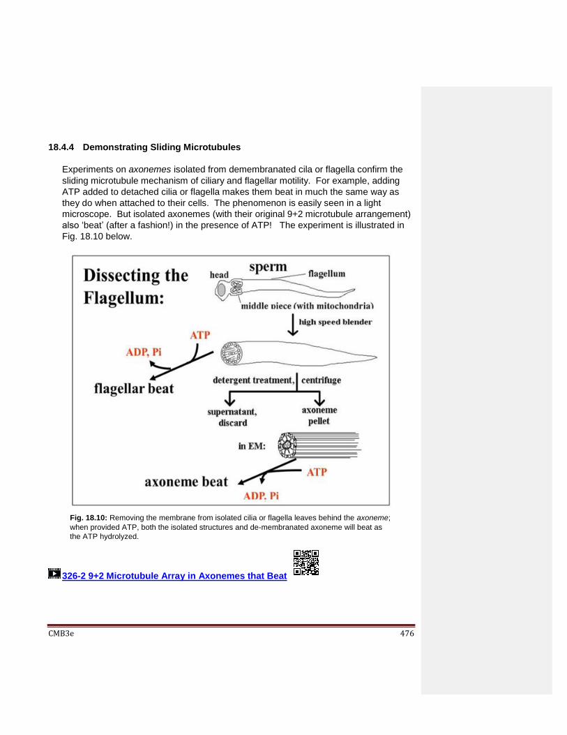
CMB3e 476

18.4.4 Demonstrating Sliding Microtubules

Experiments on axonemes isolated from demembranated cila or flagella confirm the

sliding microtubule mechanism of ciliary and flagellar motility. For example, adding

ATP added to detached cilia or flagella makes them beat in much the same way as

they do when attached to their cells. The phenomenon is easily seen in a light

microscope. But isolated axonemes (with their original 9+2 microtubule arrangement)

also ‘beat’ (after a fashion!) in the presence of ATP! The experiment is illustrated in

Fig. 18.10 below.

326-2 9+2 Microtubule Array in Axonemes that Beat

Fig. 18.10: Removing the membrane from isolated cilia or flagella leaves behind the axoneme;

when provided ATP, both the isolated structures and de-membranated axoneme will beat as

the ATP hydrolyzed.

CMB3e 477

Selective addition of different detergents removes radial spokes, nexin and other proteins

from the axoneme, causing the microtubules to separate. Dissociated microtubule doublets

and central ‘singlets’ can then be observed in the electron microscope. When such separated

microtubules are dialyzed to remove the detergents, doublet microtubules re-associate to form

sheets as shown in Fig. 18.11.

ATP added to reconstituted microtubule doublets causes the microtubules to separate as

the ATP is hydrolyzed. When such preparations are fixed for electron microscopy

immediately after adding the ATP, they are caught in the act of sliding. See this animated

in the first link below (#327-2).

327-2 Proof of Sliding Microtubules in Flagella and Cilia

328 Bacterial Flagella are Powered by a Proton Gradient

329 The Effects of Different Drugs on Microtubules... and Cancer

Fig. 18.11: Detergents can dissociate axonemes into individual and doublet microtubules. Dialysis

of separated microtubules to remove the detergent cause the microtubules to re-associate (or

reconstitute) into a sheet with connections resembling those seen in intact axonemes.

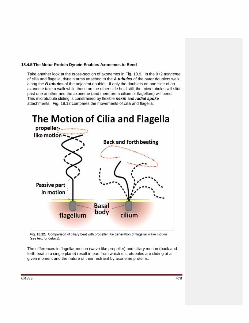
CMB3e 478

18.4.5 The Motor Protein Dynein Enables Axonemes to Bend

Take another look at the cross-section of axonemes in Fig. 18.9. In the 9+2 axoneme

of cilia and flagella, dynein arms attached to the A tubules of the outer doublets walk

along the B tubules of the adjacent doublet. If only the doublets on one side of an

axoneme take a walk while those on the other side hold still, the microtubules will slide

past one another and the axoneme (and therefore a cilium or flagellum) will bend.

This microtubule sliding is constrained by flexible nexin and radial spoke

attachments. Fig. 18.12 compares the movements of cilia and flagella.

The differences in flagellar motion (wave-like propeller) and ciliary motion (back and

forth beat in a single plane) result in part from which microtubules are sliding at a

given moment and the nature of their restraint by axoneme proteins.

Fig. 18.12: Comparison of ciliary beat with propeller like generation of flagellar wave motion

(see text for details).

CMB3e 479

18.5 Microfilaments – Structure and Role in Muscle Contraction

At 7 nm in diameter, microfilaments (actin filaments) are the thinnest cytoskeletal

component. Globular actin (G-actin) monomers polymerize to form linear F-actin

polymers. Two polymers then combine to form a twin-helical actin microfilament. As

with microtubules, microfilaments have a +end to which new actin monomers are added

to assemble F-actin, and a –end at which they disassemble when they are in a dynamic

state, such as when a cell is changing shape. When one end of a microfilament is

anchored to a cellular structure, for example to plaques in the cell membrane, motor

proteins like myosin can use ATP to generate a force that deforms the plasma membrane

and thus, the shape of the cell. One of the best-studied examples of myosin/actin

interaction is in skeletal muscle where the sliding of highly organized thick myosin rods

and the thin actin microfilaments results in muscle contraction.

18.5.1 The Thin (Micro-) Filaments and Thick Filaments of Skeletal Muscle

Bundles of parallel muscle cells make up a skeletal muscle. Thin sections of skeletal

muscle cells (myocytes) appear striated in the light microscope (Fig. 18.13).

The dark purplish structures surrounding the myocyte are mitochondria, which will

provide the ATP to fuel contraction. Skeletal muscle is made up of ‘aligned’, bundled

myocytes. The bundled myocytes (also called myofibers) are further organized into

fascicles that are finally bundled into a muscle.

Fig. 18.13: Light micrograph of skeletal muscle stained to showing characteristic striations.

CMB3e 480

The blowout illustration in Fig. 18.14 (below) shows the anatomical organization and

fine structure of a muscle (left panel).

Light passing through the more or less ordered regions of the sarcomere will bend to

different degrees becauase the regions each have a different refractive index.

Polarizing light microscopy detects these differences, enhancing the contrast between

the regions of the sarcomere, defining them as either isotropic (i.e., with a low

refractive index) or anisotropic (with a high refractive index). High-resolution

electron microscopy from the 1940s revealed the fine structure of skeletal muscle

(right panel), allowing characterization of the sarcomere. The dark bands of the

striations in the light micrograph of myocytes are regions of aligned, adjacent

sarcomeres. Based on light and electron microscopy, we can define thegions regions

of the sarcomere:

• The A or Anisotropic band of overlapping, aligned actin and myosin filaments in

the middle of the sarcomere is more ordered than the I band and so, has a higher

refractive index.

• The I band or isotropic band, has a low refractive index compared to the A band.

It is largely made up of thin (actin) microfilaments.

• A pair of Z lines demarcate the sarcomere (Z for zwischen, German for between).

Fig. 18.14: Skeletal muscle organization and the anatomy of a muscle cell sarcomere

(see text for details).

Fro

m: h

ttp

://u

plo

ad.w

ikim

edia

.org

/wik

iped

ia/c

om

mo

ns/

a/a4

/Sar

com

ere.

gif

CMB3e 481

• The H zone is a region where myosin does not overlap actin filaments.

• An M line lies at the center of the H zone.

The multiple repeating sarcomeres of myocytes aligned in register in the fascicles are

what give the appearance of striations in whole muscles.

18.5.2 The Sliding Filament Model of Skeletal Muscle Contraction

Electron microscopy of relaxed and contracted muscle is consistent with the sliding of

thick and thin filaments during contraction (Fig 18.15).

Additional key structures of the sarcomere can be seen in the drawing at the right.

Note that, in the sarcomeres of a contracted muscle cell, the H zone has almost

disappeared. While the width of the A band has not changed after contraction, the

width of the I bands has decreased and the Z-lines are closer. The best explanation

here was the Sliding Filament Hypothesis (model) of skeletal muscle contraction.

330-2 The Sliding Filament Model of Skeletal Muscle Contraction

18.5.3 The Contraction Paradox: Contraction and Relaxation Require ATP

The role of ATP in fueling the movement of sliding filaments during skeletal muscle

contraction was based in part on experiments with glycerinated fibers. These are

muscle fibers that were soaked in glycerin to permeabilize the plasma membrane.

Fig. 18.15: Transmission electron micrograph and a corresponding illustration showing sarcomere

shortening, consistent with the sliding of filaments during skeletal muscle contraction.

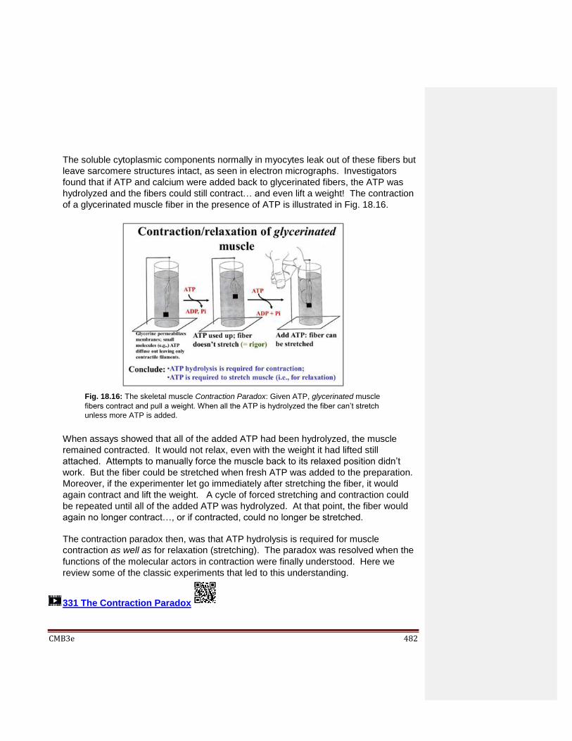
CMB3e 482

The soluble cytoplasmic components normally in myocytes leak out of these fibers but

leave sarcomere structures intact, as seen in electron micrographs. Investigators

found that if ATP and calcium were added back to glycerinated fibers, the ATP was

hydrolyzed and the fibers could still contract… and even lift a weight! The contraction

of a glycerinated muscle fiber in the presence of ATP is illustrated in Fig. 18.16.

When assays showed that all of the added ATP had been hydrolyzed, the muscle

remained contracted. It would not relax, even with the weight it had lifted still

attached. Attempts to manually force the muscle back to its relaxed position didn’t

work. But the fiber could be stretched when fresh ATP was added to the preparation.

Moreover, if the experimenter let go immediately after stretching the fiber, it would

again contract and lift the weight. A cycle of forced stretching and contraction could

be repeated until all of the added ATP was hydrolyzed. At that point, the fiber would

again no longer contract…, or if contracted, could no longer be stretched.

The contraction paradox then, was that ATP hydrolysis is required for muscle

contraction as well as for relaxation (stretching). The paradox was resolved when the

functions of the molecular actors in contraction were finally understood. Here we

review some of the classic experiments that led to this understanding.

331 The Contraction Paradox

Fig. 18.16: The skeletal muscle Contraction Paradox: Given ATP, glycerinated muscle

fibers contract and pull a weight. When all the ATP is hydrolyzed the fiber can’t stretch

unless more ATP is added.

CMB3e 483

18.6 Actin-Myosin Interactions in vitro: Dissections and

Reconstitutions

Several experiments hinted at the interaction of actin and myosin in contraction. For

example, actomyosin was first observed as the main component of viscous skeletal

muscle homogenates. Under appropriate conditions, adding ATP to such actomyosin

preparations caused a decrease in viscosity. However, after the added ATP was

hydrolyzed, the mixture became viscous again. Extraction of the non-viscous preparation

(before it re-congealed and before the ATP was consumed) led to the biochemical

separation of the two main substances we now recognize as the actin and myosin (thin

and thick) filaments of contraction. What’s more, adding these components back together

reconstituted the viscous actomyosin (now renamed actinomyosin). Adding ATP once

again to the reconstituted solution eliminated its viscosity. The ATP-dependent viscosity

changes of actinomyosin solutions were consistent with an ATP-dependent separation of

thick and thin filaments. Do actin and myosin also separate in glycerinated muscles

exposed to ATP, allowing them to stretch and relax. This question was answered with the

advent of electron microscopy. The purification of skeletal muscle myosin from actin (still

attached to Z Lines) is cartooned in Fig. 18.17, showing what the separated components

looked like in the electron microscope.

Fig. 18.17: Overview of the isolation of actin thin filaments (still on Z-Lines) from myosin

thick filaments.

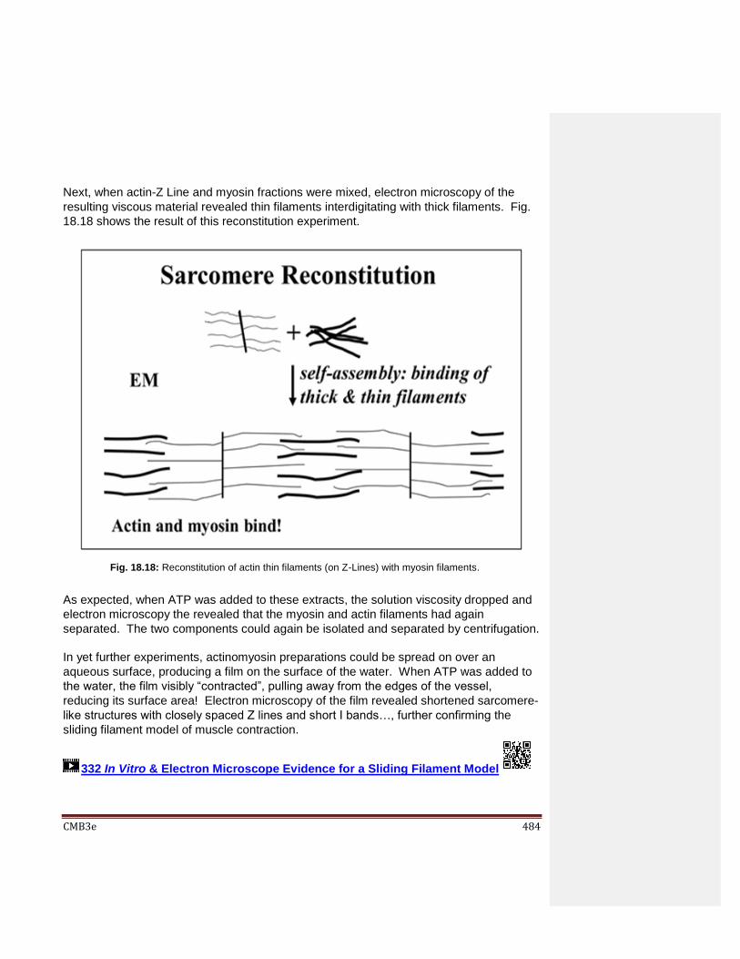
CMB3e 484

Next, when actin-Z Line and myosin fractions were mixed, electron microscopy of the

resulting viscous material revealed thin filaments interdigitating with thick filaments. Fig.

18.18 shows the result of this reconstitution experiment.

As expected, when ATP was added to these extracts, the solution viscosity dropped and

electron microscopy the revealed that the myosin and actin filaments had again

separated. The two components could again be isolated and separated by centrifugation.

In yet further experiments, actinomyosin preparations could be spread on over an

aqueous surface, producing a film on the surface of the water. When ATP was added to

the water, the film visibly “contracted”, pulling away from the edges of the vessel,

reducing its surface area! Electron microscopy of the film revealed shortened sarcomere-

like structures with closely spaced Z lines and short I bands…, further confirming the

sliding filament model of muscle contraction.

332 In Vitro & Electron Microscope Evidence for a Sliding Filament Model

Fig. 18.18: Reconstitution of actin thin filaments (on Z-Lines) with myosin filaments.

CMB3e 485

When actin and myosin were further purified from isolated actinomyosin, the thick myosin

rods could be dissociated into large myosin monomers. In fact, at ~599Kd, myosin

monomers are among the largest known proteins. Thus, thick filaments are massive

polymers of huge myosin monomers! The molecular structure of myosin thick filaments is

shown in Fig. 18.19.

An early observation of isolated mammalian actin filaments was that they had no ATPase

activity. On the other hand, while isolated myosin preparations did have an ATPase

activity, they would only catalyze ATP hydrolysis very slowly compared to intact muscle

fibers. Faster ATP hydrolysis occurred only if myosin filaments were mixed with

microfilaments (either on or detached from Z-lines). In the electron microscope, isolated

myosin protein monomers appeared to have a double-head and single tail regions.

Biochemical analysis showed that the monomers themselves were composed of the two

heavy chain and two pairs of light chain polypeptides shown in the illustration above.

Fig. 18.19: Structure of a skeletal muscle myosin filament and the myosin monomer. Shown is myosin II, the thick filament that spans both sides of the H zone in a sarcomere (upper). The head-&-tail structure of a myosin monomer is shown in the high magnification electron micrograph and is illustrated in the cartoon (lower). The myosin monomer is itself a polymer of four polypeptides.

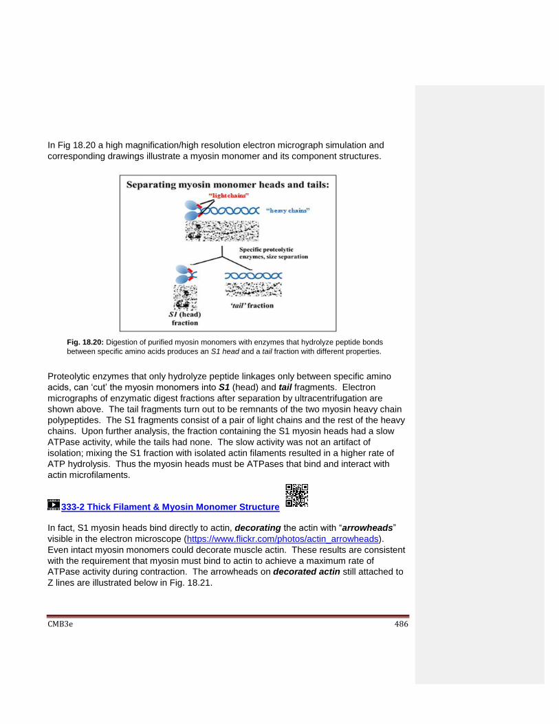
CMB3e 486

In Fig 18.20 a high magnification/high resolution electron micrograph simulation and

corresponding drawings illustrate a myosin monomer and its component structures.

Proteolytic enzymes that only hydrolyze peptide linkages only between specific amino

acids, can ‘cut’ the myosin monomers into S1 (head) and tail fragments. Electron

micrographs of enzymatic digest fractions after separation by ultracentrifugation are

shown above. The tail fragments turn out to be remnants of the two myosin heavy chain

polypeptides. The S1 fragments consist of a pair of light chains and the rest of the heavy

chains. Upon further analysis, the fraction containing the S1 myosin heads had a slow

ATPase activity, while the tails had none. The slow activity was not an artifact of

isolation; mixing the S1 fraction with isolated actin filaments resulted in a higher rate of

ATP hydrolysis. Thus the myosin heads must be ATPases that bind and interact with

actin microfilaments.

333-2 Thick Filament & Myosin Monomer Structure In fact, S1 myosin heads bind directly to actin, decorating the actin with “arrowheads”

visible in the electron microscope (https://www.flickr.com/photos/actin_arrowheads).

Even intact myosin monomers could decorate muscle actin. These results are consistent

with the requirement that myosin must bind to actin to achieve a maximum rate of

ATPase activity during contraction. The arrowheads on decorated actin still attached to

Z lines are illustrated below in Fig. 18.21.

Fig. 18.20: Digestion of purified myosin monomers with enzymes that hydrolyze peptide bonds

between specific amino acids produces an S1 head and a tail fraction with different properties.

CMB3e 487

Note that the ‘arrowheads’ always face in opposite directions on either side of the Z line. These opposing arrowheads suggest that the actin filaments attached to the two Z-Lines of a sarcomere are drawn towards each other along the opposite sides of bipolar myosin rods. This is consistent with sliding filaments that draw Z-lines closer together during skeletal muscle contraction, shortening the sarcomeres. For a more dramatic look at decorated actin, Check out the ‘arrowheads’ in the electron micrograph at https://www.slideserve.com/brinda/muscle-structure-physiology-j-rosenbluth-0409

334-2 Myosin Monomers & S1 Heads Decorate Actin

18.7 Allosteric Change and the Micro-Contraction Cycle

Whereas dynein and kinesin are motor proteins that ‘walk’ along microtubules, myosins

are motor proteins that walk along microfilaments. All of these motor proteins are

ATPases that use the free energy of ATP hydrolysis to effect conformational changes

that result in the walking, i.e., motility. In skeletal muscle, allosteric changes in myosin

heads enable the myosin rods to do the walking along F-actin filaments. When placed in

sequence, the different myosin head conformations illustrated in Fig. 18.22 (below) are

the likely changes that would occur during a micro-contraction cycle.

Fig. 18.21: Illustration of myosin decoration by myosin monomer S1 fragments, showing opposing

polarity of actin filaments on opposite sides of the Z-line.

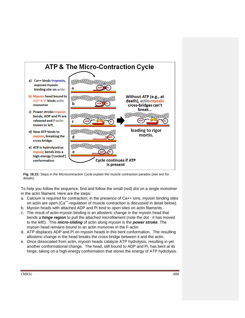
CMB3e 488

To help you follow the sequence, find and follow the small (red) dot on a single monomer

in the actin filament. Here are the steps:

a. Calcium is required for contraction; in the presence of Ca++ ions, myosin binding sites

on actin are open (Ca++-regulation of muscle contraction is discussed in detail below).

b. Myosin heads with attached ADP and Pi bind to open sites on actin filaments.

c. The result of actin-myosin binding is an allosteric change in the myosin head that

bends a hinge region to pull the attached microfilament (note the dot - it has moved

to the left!). This micro-sliding of actin along myosin is the power stroke. The

myosin head remains bound to an actin monomer in the F-actin

d. ATP displaces ADP and Pi on myosin heads in this bent conformation. The resulting

allosteric change in the head breaks the cross-bridge between it and the actin.

e. Once dissociated from actin, myosin heads catalyze ATP hydrolysis, resulting in yet

another conformational change. The head, still bound to ADP and Pi, has bent at its

hinge, taking on a high-energy conformation that stores the energy of ATP hydrolysis.

Fig. 18.22: Steps in the Microcontraction Cycle explain the muscle contraction paradox (see text for

details).

CMB3e 489

Micro-contraction cycles of actin sliding along myosin continue as long as ATP and

Ca++ are available. During repetitive micro-contraction cycles, myosin heads on the thick

filaments pull actin filaments attached to Z-lines as stored free energy is released during

power strokes, bringing the Z lines closer to each other. The result is the shortening of

the sarcomere and ultimately of muscle cells and of course, the entire muscle. When the

muscle no longer needs to contract, the Ca++ required for contraction is withdrawn,

micro-contraction cycles cease, the myosin heads remain in the high-energy conformation

of step e, and the muscle can relax (stretch). Neural stimulation can effect another

release of Ca++ that will gain signal contraction.

The micro-contraction cycle also stops when ATP is gone, usually a more permanent

state brought about by death! But this time, myosin heads remain bound to the actin

filaments in the state of muscle contraction at the time of death. This is rigor mortis at

the molecular level (see the illustration above). At the level of whole muscle, rigor mortis

results in the inability to stretch or otherwise move body parts when ATP has once and for

all departed.

18.8 The Micro-contraction Cycle Resolves the Contraction Paradox

The micro-contraction cycle resolves the contraction paradox:

ATP is necessary for muscle contraction: In step e in the illustration above, as ATP

on myosin heads is hydrolyzed, the heads change from a low-energy to a high-energy

conformation. The myosin heads can now bind to actin monomers (step b in the

micro-contraction cycle). This results in the power stroke (step c). Free energy

released by an allosteric change in myosin pulls the actin along the myosin, in effect

causing a micro-shortening of the sarcomere, in other words, contraction!

ATP is necessary for muscle relaxation: At the end of step c, myosin remains

bound to actin until ATP can again bind to the myosin head. Binding of ATP in step d

displaces ADP and inorganic phosphate (Pi)… and breaks actin-myosin cross-bridges.

A removal of Ca++ from sarcomeres at the end of a contraction event blocks myosin

binding sites on actin, while the rapid breakage of actin-myosin cross-bridges by ATP-

myosin binding allows muscle relaxation and the sliding apart of the actin and myosin

filaments (i.e., stretching). This leaves the myosin heads in the ‘cocked’ (high-energy)

conformation, ready for the next round of contraction.

No more paradox! The displacement of ADP and Pi by ATP binding to myosin heads

breaks actin-myosin cross-bridges, allowing for relaxation (stretching). The hydrolysis of

ATP bound to myosin cocks the myosin head in a high free-conformation that is released

during the microcontraction power stroke.

CMB3e 490

Electron microscopic examination of myosin monomer heads at different ionic strengths

provides visual evidence that myosin heads are flexible and can take on alternate stable

conformations, as would be expected during the micro-contraction cycle (Fig 18.23).

The arrows point to myosin heads in different conformations. This visualization was

made possible by treatment of the preparations with anti-myosin antibodies

(immunoglobulins). See a cool video of conformational change in myosin monomers at

Myosin heads in Action.

335-2 Actin-Myosin Contraction Cycle Resolves the Contraction Paradox

336-2 ATP Binding & Hydrolysis Changes Myosin Head Conformation

18.9 Ca++ Ions Regulate Skeletal Muscle Contraction

Typically, the neurotransmitter acetylcholine released by a motor neuron binds to

receptors on muscle cells to initiate contraction. Early experiments had already revealed

that Ca++ was required along with ATP to get glycerinated skeletal muscle to contract. It

was later demonstrated that Ca++ ions were stored in the sarcoplasmic reticulum (the

smooth endoplasmic reticulum) of intact muscle cells. As we have seen, an action

potential generated in the cell body of a neuron propagates along an axon to the nerve

terminal, or synapse. The action potential at a neuromuscular junction that initiates

contraction is summarized in the illustration in Fig. 18.24 (below).

Fig. 18.23: The ability of flexible myosin heads to bend and change conformation is consistent with their proposed activity during the micro-contraction cycle.

CMB3e 491

In a similar fashion, an action potential generated at a neuromuscular junction travels

along the sarcolemma (the muscle plasma membrane) to points where it is continuous

with transverse tubules (T-tubules). The action potential then moves along the T-

tubules and then along the membranes of the sarcoplasmic reticulum. This propagation

of an action potential opens Ca++ channels in the sarcoplasmic reticulum, releasing Ca++

to bathe myofibril sarcomeres where they bind to one of three troponin molecules to

allow skeletal muscle contraction, i.e., to allow filaments to slide. The three troponins

and a tropomyosin molecule are bound to actin filaments. Experiments using anti-

troponin and anti-tropomyosin antibodies localized the three proteins in electron

micrographs at regularly spaced intervals along actin filaments, as modeled in Fig. 18.25

below.

Fig. 18.24: Innervation leads to Ca++ release from sarcoplasmic reticulum to regulate contraction

(see text for details).

CMB3e 492

In resting muscle, tropomyosin (a fibrous protein) lies along the actin filament where it covers up the myosin binding sites of seven G-actin monomer subunits in the microfilament. Click https://www.e-sciencecentral.org/articles/Figure.php?xn=am/am-47-226&id=f1-am-47-226 to see an electron micrograph of negatively stained actin bound to the regularly spaced tropomyosin molecules shown in the illustration above. The ‘cross-section drawn in Fig. 18.26 (below) illustrates how troponin T (tropomyosin-

binding troponin) and troponin I (inhibitory troponin) hold the tropomyosin in place, and

how the binding of Ca++ ions to troponin C regulates contraction. A chain reaction of

conformational changes begins when Ca++ ions bind to troponin-C. The result is that the

three-subunit troponin complexes bound to tropomyosin shift position along the filament

to expose the myosin-binding sites on the G-actin subunits. Only after this shift can ATP-

bound myosin in turn bind to actin and initiate the micro-contraction cycle discussed

earlier. The regulation of contraction by Ca++ is animated in the link below.

337 Regulation of Skeletal Muscle Contraction by Calcium

Fig. 18.25: Skeletal muscle thin filaments consist of actin associated with troponins and

tropomyosin. These actin-associated proteins participate in the response to Ca++ ions to

regulate interactions with myosin.

CMB3e 493

18.9.1 Muscle Contraction Generates Force

Contraction by ATP-powered sliding of thin along thick filaments generates force on

the Z-lines. In three dimensions, the Z-lines are actually Z-disks to which the actin

thin filaments are attached. The protein -actinin in the Z-disks anchors the ends of

the actin filaments to the disks so that when the filaments slide, the Z-disks are drawn

closer, shortening the sarcomeres. Another Z-disk protein, desmin, is an intermediate

filament organized around the periphery of Z-disks. Desmin connects multiple Z-disks

in a myofibril. By keeping the Z-Disks in register, muscle cell, and ultimately whole

muscle contraction is coordinated. Finally, actin filaments at the ends of the muscle

cell must be connected to the plasma membrane for a muscle cell to shorten during

myofibril contraction. Several proteins, including syntrophins and dystrophin

(another intermediate filament protein) anchor the free ends of microfilaments coming

from Z-disks to the cell membrane.

Still other proteins anchor the cell membrane in this region to the extracellular matrix

(tendons) that are in turn, attached to bones! Force generated by myosin hydrolysis of

ATP and the sliding of filaments in individual sarcomeres are thus transmitted to the

ends of muscles to effect movement. If the name dystrophin sounds familiar, it

should! The gene and its protein were named for a mutation that causes muscular

dystrophy, resulting in a progressive muscle weakening.

338 Contraction Generates Force Against Z Disks and Cell Membranes

Fig. 18.26: Ca++ ions initiate uncovering myosin binding sites on actin by binding to

troponin-C, resulting in allosteric changes in the troponins and ultimately tropomyosin.

CMB3e 494

18.9.2 The Elastic Sarcomere: Do Myosin Rods Just Float in the Sarcomere?

In fact, myosin rods do not “float” in sarcomeres, but are anchored to proteins in the Z

discs and M-lines. In 1954, R. Natori realized that when contracted muscle relaxes, it

lengthens beyond its resting state, then shortening again to its resting length. He

proposed that this elasticity must be due to a fiber in the sarcomere. Twenty-five

years later, the elastic structure was identified as titin, a protein that holds several

molecular records! The gene for titin contains the largest number of exons (363) of

known proteins. After actin and myosin, titin is also the most abundant protein in

muscle cells. At almost 4 x 106 Da, the aptly named titin is the also the largest known

polypeptide, much larger than even myosin! Extending from the Z discs to the M line

of sarcomeres, titin coils around thick filaments along the way. Titin is anchored at Z-

disks by -actinin and telethonin proteins. At the M-line, titin binds to a myosin-

binding protein C (MYBPC3) and to calmodulin, among others (myomesin,

obscurin, skelamin…). Some if not all of these proteins must participate in keeping

the myosin thick filaments positioned and in register in the sarcomere. This is similar

to how desmin binds Z-disks to each other to keep sarcomeres in register. The

location of titin and several other sarcomere proteins is illustrated in Fig. 18.27

(below).

Fig. 18.27: Structure of titin and its location in the sarcomere (see text for details).

CMB3e 495

Coiled titin molecules (red in the illustration) extend from the Z to M lines. The

colorized electron micrograph of one extended titin molecule in the middle of the

illustration above should convince you of the length (35,213 amino acids!) of this huge

polypeptide. Titin’s elastic features are largely in a region labeled P in the electron

micrograph that lies between Z discs and the ends of myosin rods. The many domains

of this P region are shown expanded at the bottom of Fig. 18.27.

With all the binding (and other) functions, you might expect that titin has many

domains. It does! They include Ig (immunoglobulin) domains, fibronectin domains

(not shown here) and PEVK and N2A domains that help bind titin to -actinin in Z-

disks. Which and how many Ig and/or PEVK domains are present in a particular

muscle depends on which alternative splicing pathway is used to form a titin mRNA.

Over a micron long, titin functions as a molecular spring, as Natori predicted. Its

coiled domains compress during contraction, passively storing some of the energy of

contraction.

When a skeletal muscle relaxes, Ca++ is withdrawn from the sarcomere. ATP can still

displace ADP from myosin heads, breaking actin-myosin cross-bridges. When actin

and myosin dissociate in the absence of Ca++ , the troponins and tropomyosin reverse

their conformational changes, once again covering myosin head binding sites on F-

actin. The muscle then stretches, typically under the influence of gravity or an

opposing set of muscles. But when a muscle relaxes, what prevents it from stretching

too far, or if that is even possible, how does a muscle fiber take correctiove action?

The answer is built in tto the structure of titin.

During contraction, 244 individually folded titin domains were compressed. During

relaxation, these domains de-compress; the stored energy of compression thus also

helps to power relaxation. At the same time, titin connections limit the stretch so that

a potentially overstretched muscle can ‘bounce’ back to its normal relaxed length. In a

particularly elegant experiment, R. Linke et al. provided a visual demonstration of

myofiber elasticity consistent with the coiled spring model of titin structure. They

made antibodies to peptide domains on either side of the PEVK domain of titin (N2A

and I20-I22) and attached them to nanogold particles. The gold particles are

electron dense and will appear as black granules in transmission electron microscopy.

Here is the experiment: Individual myofibers were stretched to different lengths, fixed

for electron microscopy and treated with the nanogold-linked antibodies. The

antibodies localize to and define the boundaries of the titin PEVK domains in

myofibers stretched to different lengths (Fig. 18.28, below, showing electron

micrographs with simulated localization of nanogold particles that reflect the actual

results).

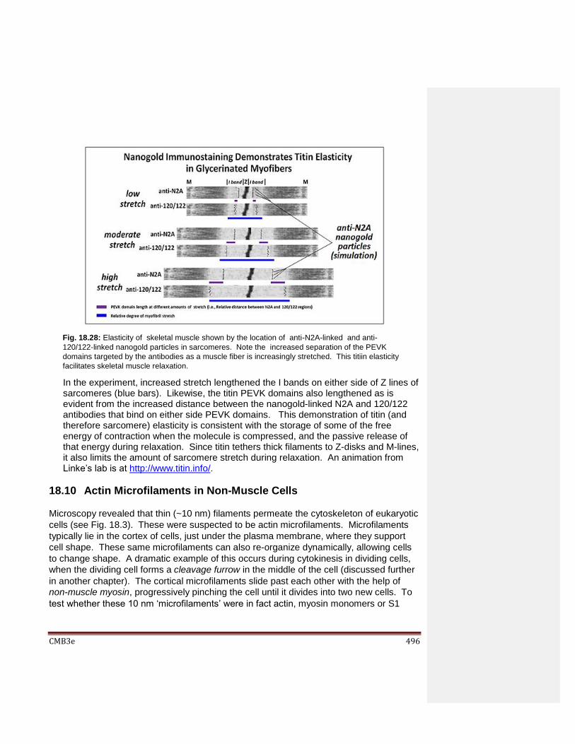
CMB3e 496

In the experiment, increased stretch lengthened the I bands on either side of Z lines of sarcomeres (blue bars). Likewise, the titin PEVK domains also lengthened as is evident from the increased distance between the nanogold-linked N2A and 120/122 antibodies that bind on either side PEVK domains. This demonstration of titin (and therefore sarcomere) elasticity is consistent with the storage of some of the free energy of contraction when the molecule is compressed, and the passive release of that energy during relaxation. Since titin tethers thick filaments to Z-disks and M-lines, it also limits the amount of sarcomere stretch during relaxation. An animation from Linke’s lab is at http://www.titin.info/.

18.10 Actin Microfilaments in Non-Muscle Cells

Microscopy revealed that thin (~10 nm) filaments permeate the cytoskeleton of eukaryotic

cells (see Fig. 18.3). These were suspected to be actin microfilaments. Microfilaments

typically lie in the cortex of cells, just under the plasma membrane, where they support

cell shape. These same microfilaments can also re-organize dynamically, allowing cells

to change shape. A dramatic example of this occurs during cytokinesis in dividing cells,

when the dividing cell forms a cleavage furrow in the middle of the cell (discussed further

in another chapter). The cortical microfilaments slide past each other with the help of

non-muscle myosin, progressively pinching the cell until it divides into two new cells. To

test whether these 10 nm ‘microfilaments’ were in fact actin, myosin monomers or S1

Fig. 18.28: Elasticity of skeletal muscle shown by the location of anti-N2A-linked and anti-

120/122-linked nanogold particles in sarcomeres. Note the increased separation of the PEVK

domains targeted by the antibodies as a muscle fiber is increasingly stretched. This titiin elasticity

facilitates skeletal muscle relaxation.

CMB3e 497

myosin head fragments were placed atop actins isolated from many different cell types.

When viewed in the electron microscope, such preparations always revealed that the 10

nm microfilaments were decorated with arrowheads, just like S1 fragment decorated

muscle cell actin or Z line-bound actin. Clearly, the cytoplasmic microfilaments are a

form of F-actin. Check out the arrowheads on cortical ring actin in cells in cytokinesis

after treatment with S1 fragments at https://www.flickr.com/photos/actin_arrowheads.

Also, see the role of cortical filaments in cell division at Cortical Actin Filament Action in

Cytokinesis. Of course, actin microfilaments are involved in all manner of cell motility in

addition to their role in cell division. They enable cell movement and cytoplasmic

streaming inside cells. And while they give intestinal microvilli strength, they even enable

them to move independent of the passive pressures of peristalsis.

Microfilaments are found throughout the eukarya, and they are readily identified since

most if not all of them can be decorated my S1 fragments or intact myosin monomers.

The S1 myosin-decorated actin filaments you see at the link above were in sea urchin

embryos! Other examples of microfilaments in cell motility include the ability of amoeba

and other phagocytic cells to extend pseudopodia to engulf food or foreign particles (e.g.,

bacteria), respectively.

A well-studied example of microfilament-powered cell movement is the spread of

fibroblast cells along surfaces. These migrating cells extend thin filipodia into the

direction of movement by assembling actin bundles along the axis of cell movement. In

Fig. 18.29 (below), actin stress fibers that maintain cell shape fluoresce green in the

immunofluorescence micrograph (left) and the dual roles of actin in fibroblast shape and

movement are also illustrated at the right.

Fig. 18.29: In the anti-actin immunofluorescence micrograph of fibroblasts, actin localizes with

stress fibers which help maintain cell shape (LEFT). Actin also localizes in lamellipodia and

retraction fibers in migrating fibroblasts (RIGHT), orienting in the direction of movement.

CMB3e 498

The extension of filipodia at the moving front of a fibroblast is mainly based on actin

assembly and disassembly (not unlike motility based on microtubules). A retraction

fiber forms at the hind-end of the cell as the fibroblast moves forward. The retraction

fiber remains attached to the surface (substratum) on which it is migrating until actin-

myosin interactions (in fact, sliding) causes retraction of most of this ‘fiber’ back into

the body of the cell. Studies of non-muscle cell motility suggest the structure and

interacting molecular components of stress fibers modeled in Fig. 18.30 (below).

The illustration suggests roles for actin-binding proteins in the sliding of overlapping

myosin and actin filaments during movement. This model may also explain the

cytoplasmic streaming that distributes cellular components and nutrients throughout a

cell. In fact, the movements of both involve actin-myosin interactions. Filamin in this

drawing is shown holding actin filaments together at an angle, while -actinin also

helps to bundle the actin filaments. Titin (not shown) also seems to be associated

with stress fibers. Unlike highly organized skeletal muscle sarcomeres, the proteins

and filaments in stress fibers are not part of Z- or M-line superstructures. Could

something like these less-organized non-muscle stress fiber filament bundles be

evolutionary ancestors of muscle cell sarcomeres?

18.11 Both Actins and Myosins are Encoded by Large Gene Families

Actins may be the most abundant protein in cells! At least six different actin isoforms

encoded by a large actin gene family have nearly identical amino acid sequences, all

of which are involved in cytoskeletal function. The -actin isoform predominates.

Genes for some isoforms are expressed in a cell-specific manner.

Fig. 18.30: The molecular structure of stress fibers; myosin as well as other actin-binding

proteins interact with actin in non-muscle cell motility.

CMB3e 499

Are all actin isoforms functionally significant? Myosin monomers (or S1 heads)

decorate virtually all actins. This makes one wonder if any one actin is an adaptation,

however subtle, such that the absence of one isoform would pose a significant threat

to the survival of an organism? Since amino acid sequence differences between

actins would not predict dramatically different protein function, could they underlie

some as yet unknown physiological advantage to different cells?

In mice, the loss of a -actin gene has little effect on the organism, while loss of the -

actin gene in mice is lethal at embryonic stages. So what is the function of -actin?

Does it even have one? Or is it a vestigial protein that like our appendix once served

a now long-lost function? In contrast, studies in humans show that a non-lethal -actin

mutation correlates with delayed development and later neurological problems (e.g.,

epilepsy), kidney and heart abnormalities. Nevertheless, people with such mutations

can lead nearly normal, healthy lives (Beta-Actin Gene Mutations and Disease).

Like the actins, myosin genes encoding variant isoforms comprise a large eukaryotic

gene family. All isoforms have ATPase activity, and some (if not all) are clearly

involved in cell motility. Unique functions are not yet known for other isoforms, but

different myosin monomers can decorate actin, and myosins from one species can

decorate actin filaments of other species, even across wide phylogenetic distances.

The question of why there are so many isoforms of actin and myosin is the subject of ongoing

research.

18.12 Intermediate Filaments

These 10 nm filaments are proteins with extended secondary structure that don’t readily

fold into tertiary structures, and they have no enzymatic activity. Recall their intercellular

location in desmosomes where they firmly bind cells together to confer tensile strength to

tissues. Within cells, intermediate filaments permeate the cells where they participate in

regulating and maintaining cell shape. Recall their role in anchoring actin to either Z-

disks or plasma membrane plaques in muscle cells, transmitting the forces of contraction

to the shortening of the sarcomeres and then to the actual shortening of a muscle. The

extracellular keratins that make up fur, hair, fingernails and toenails, are proteins related

to intermediate filaments. Keratins are bundles of rigid, insoluble extracellular proteins

that align and bind to form stable, unchanging secondary structures. Finally, intracellular

intermediate filaments are not confined to the cytoplasm; lamins are intermediate

filaments that make up structural elements of the nuclear lamina, a kind of

nucleoskeleton.

As we saw earlier, intermediate filament subunits have a common structure consisting of

a pair of monomers. The monomers are non-polar; i.e., unlike microtubules and actin

filaments, they do not have ‘plus’ and ‘minus’ ends. Globular domains at the C- and N-

CMB3e 500

terminal ends of monomer filaments are separated by coiled rod regions. The basic unit

of intermediate filament structure is a dimer of monomers. Dimers further aggregate to

form tetramers and larger filament bundles. Like microtubules and actin filaments,

intermediate filament bundles can disassemble and reassemble as needed when cells

change shape. Unlike microtubules and actin, intermediate filaments can stretch, a

property conferred by the coiled rod regions of the filaments. This should be reminiscent

of titin molecules! The structural features of intermediate filaments are illustrated in the

cartoon in Fig. 18.31 below.

In the bundled intermediate filaments that permeate the cytoplasm of cells, the ability to

stretch contributes to the viscosity of cytoplasm and is even called viscoelasticity. This

elastic property is thought to allow actins and microtubules a some freedom of movement

of and within cells. Like the actins, there are many isforms of intermediate filaments.

Some iText & VOP Key Words and Terms

"9+2" F-actin myosin ATPase

tubulin F-actin polarity myosin

A-band flagella myosin "heads"

acetylcholine fluorescence microscopy neuromuscular junction

acidic keratin force transduction nuclear lamina

Fig. 18.31: Coiled secondary structure of the proteins permits elasticity of intermediate

filament bundles that contribute to the viscosity of cytoplasm.

CMB3e 501

actin G-actin plus and minus ends

actin-binding proteins hair, horn protofilaments

actin-myosin interactions I-band pseudopodia

actin-myosin paradox intermediate filaments sarcomere

action potential intestinal microvilli sarcoplasmic reticulum

amoeboid movement keratin sarcolemma

ATPase keratin isoforms scales, feathers, fingernails

axoneme lamins secretion vesicle transport

tubulin membrane depolarization skeletal muscle contraction

basal body microfilaments skeletal muscle relaxation

basic keratin microtubule assembly end sliding filament model

Ca++ regulation of contraction

microtubule disassembly end syncytium

Ca++ release v. active transport microtubule doublets thick and thin filaments

cell motility microtubule organizing center titin

centriole microtubule polarity transverse (T) tubules

cilia microtubule-associated proteins tread-milling

contraction regulation microtubules tropomyosin

cortical cellular microfilaments

mitotic, meiotic spindle fibers troponin I

creatine phosphate M-line troponin T

cross-bridges motor proteins troponins

cytoplasmic streaming MTOC troponin C

cytoskeleton muscle cell tubulin heterodimer

desmosomes muscle fiber tubulins

dynein myocyte viscoelasticity

evolution of actin genes myofiber Z-disks

evolution of myosin genes myofibril Z-line

CMB3e 502

Chapter 19: Cell Division and the Cell Cycle

Separation of replication from cell division in eukaryotes; cell cycle checkpoints,

cyclins and MPF, apoptosis, cancer, radiation, chemotherapy, immunotherapy

19.1 Introduction

Bacteria divide by binary fission, duplicating their nearly ‘naked’ circular chromosomes as

the cell enlarges and divides into two daughter cells. Under favorable conditions, bacteria

(E. coli for example) can divide every 20-40 minutes. Many eukaryotic cells stop dividing

when they reach maturity (their terminally differentiated state) while those that do divide

may have varying life spans between divisions, ranging from 15-24 hours. Cell division

begins with mitosis, the condensation of chromosomes from chromatin. Cytokinesis is

the process near the end of mitosis that actually divides one cell into two new cells after

duplicated chromosomes are safely on opposite sides of the cell. Although mitosis lasts

only about an hour in the life of the typical eukaryotic cell, it has been parsed into 4 or 5

phases (depending on whose text you are reading!); it is the last of these phases that

overlaps cytokinesis. Usually, mitosis and cytokinesis together take about 1.5 hours.

CMB3e 503

By far the longest period between successive cell divisions or the cell cycle is

interphase, so-called because 19th century microscopists who described mitosis saw

nothing happening in cells when they were not actually dividing. But by the 1970s,

experiments had shown that interphase itself was divisible into discrete phases of cellular

activity called G1, S and G2 (occurring in that order). It turns out that kinases regulate

progress through the cell cycle, catalyzing timely protein phosphorylations. The first of

these kinases to be discovered was mitosis-promoting factor (MPF). Kinase-regulated

events are checkpoints a cell must pass through in order to enter the next phase of the

cell cycle. As you might guess, the failure of a checkpoint can have serious

consequences. One consequence is carcinogenesis, the runaway proliferation of

cancer cells. We begin this chapter with a brief description of binary fission in E. coli,

followed by a closer look at the eukaryotic cell cycle. We close with a look at alternate

fates of eukaryotic cells and at details of cellular end-of-life events, including apoptosis,

or programed cell death).

Learning Objectives

When you have mastered the information in this chapter, you should be able to:

1. describe the phases of the cell cycle and what occurs in each. 2. interpret experiments leading to our understanding of the separation of chromosomal

events from duplication of the DNA contained in those chromosomes. 3. describe the role of cyclin and cdk (cyclin-dependent kinase) in MPF. 4. compare the roles of different cyclins and cdks in regulating the cell cycle. 5. define cell-cycle checkpoints and how/why they monitor progress through the cell

cycle, including their roles in detecting DNA damage and pathways to apoptosis.

6. state an hypothesis to explain how cell cycling errors can transform normal cells into

cancer cells.

7. list some examples of apoptosis in humans and other organisms.

8. compare and contrast examples of apoptosis and necrosis. 9. formulate an hypothesis to account for the degradation of cyclin after mitosis. 10. research and explain how different chemotherapeutic agents work and the

biochemical or molecular basis of their side effects.

19.2 Cell Division in a Prokaryote

The life of actively growing bacteria is not separated into discrete times for duplicating

genes (i.e., DNA synthesis) and then binary fission (dividing and partitioning the

duplicated DNA into new cells). Instead, the single circular chromosmome of a typical

bacterium is replicating even before fission is complete, so that the new daughter cells

already contained partially duplicated chromosomes. Cell growth, replication and fission

as it might be seen in E. coli are illustrated below in Fig. 19.1.

CMB3e 504

339 Binary Fission In marked contrast to to bacteria, the life cycle of a typical eukaryotic cell is divided into

sepatrate events. Next we will see how the timing of separated events of the cell cycle

was discovered.

19.3 Phases of Cell Division in Eukaryotes

Depending on cell type, typical eukaryotic cells have a roughly 16-24 hour cell cycle

divided into phases. One of these, mitosis, was discovered In the late 1800s using light

microscopy (you may have seen mitosing onion root tip cells in a biology class

laboratory). In any cluster of cells some were seen to lose their nuclei and to form

chromosomes (from chroma, colored; soma, bodies). In mitosis, paired chromosomes

(chromatids) are attached at their centromeres. The chromatids were seen to separate

and to be pulled apart by spindle fibers. Once separated and on their way to opposite

poles of dividing cells they are once again called chromosomes. Thus homologous

chromosomes were equally partioned to the daughter cells at the end of cell division.

Fig. 19.1: Bacteria divide by binary fission. When growing in culture, they divide continually,

partially replicating their circular DNA molecules during one division in preparation for the next.

CMB3e 505

Because the same chromosomal behavior was observed in mitosis in diverse organisms,

chromosomes were soon recognized as the stuff of inheritance, the carrier of genes!

The events of mitosis, lasting about an hour, were seen as occurring in 4 phases over that short time (Fig. 19.2).

To the early microscopists, this short period of intense mitotic activity was in stark

contrast to a much longer ‘quiet’ time in the life of the cell. For lack of a more descriptive

term, they called this period interphase. Also, depending on whom you ask, cytokinesis

(the cell movements that actually divide a cell in two) is not part of mitosis. In that sense,

we can think of three stages in the life of a cell: interphase, mitosis and cytokinesis. Of

course, it turned out that interphase is not cellular ‘quiet time’ at all!

19.4 Defining the Phases of the Eukaryotic Cell Cycle

Correlation of the inheritance of specific traits with the inheritance of chromosomes was

shown early in the early 20th century, most elegantly in genetic studies of the fruit fly,

Drosophila melanogaster. At that time, chromosomes were assumed to contain the

genetic material and that both were duplicated during mitosis. The first clue that this was

not so came only after the discovery that DNA was in fact the chemical stuff of genes.

The experiment outlined in Fig. 19.3 (below) distinguished the time of chromosome

formation from the time of DNA duplication.

Fig. 19.2: Mitosis and cytokinesis in eukaryotic cells are separated in time, and mitosis is

further divisible into 5 phases.

CMB3e 506

Here are the details of the experiment:

1. Cultured cells were incubated with 3H-thymine, the radioactive base that cells will

incorporate into deoxythymidine triphosphate (dTTP, one of the four nucleotide

precursors to DNA synthesis).

2. After a short period of culture, unincorporated 3H-thymine was washed away and the

cells were fixed and spread on a glass slide.

3. Slides were dipped in a light-sensitive emulsion, containing chemicals similar to the

light sensitive chemicals found in the emulsion-side of film (do you remember

photographic film!!?).

4. After sufficient time to allow the radioactivity on the slide to ‘expose’ the emulsion, the

slides were developed (in much the same way as developing photographic film).

5. The resulting autoradiographs in the microscope revealed images in the form of dark

spots created by exposure to hot (i.e., radioactive) DNA.

If DNA replicates in chromosomes undergoing mitosis, then when the developed film is

placed back over the slide, any dark spots should lie over the cells in mitosis, and not

over cells that are not actively dividing. But observation of the autoradiographs showed

that none of the cells in mitosis were radioactively labeled. On the other hand, some of

the cells in interphase were! Therefore, DNA synthesis must take place sometime in

interphase, before mitosis and cytokinesis, as illustrated in Fig. 19.4, below.

Fig. 19.3: First experiment demonstrating that replication and cell division in eukaryotes are

separate events. (see text for details

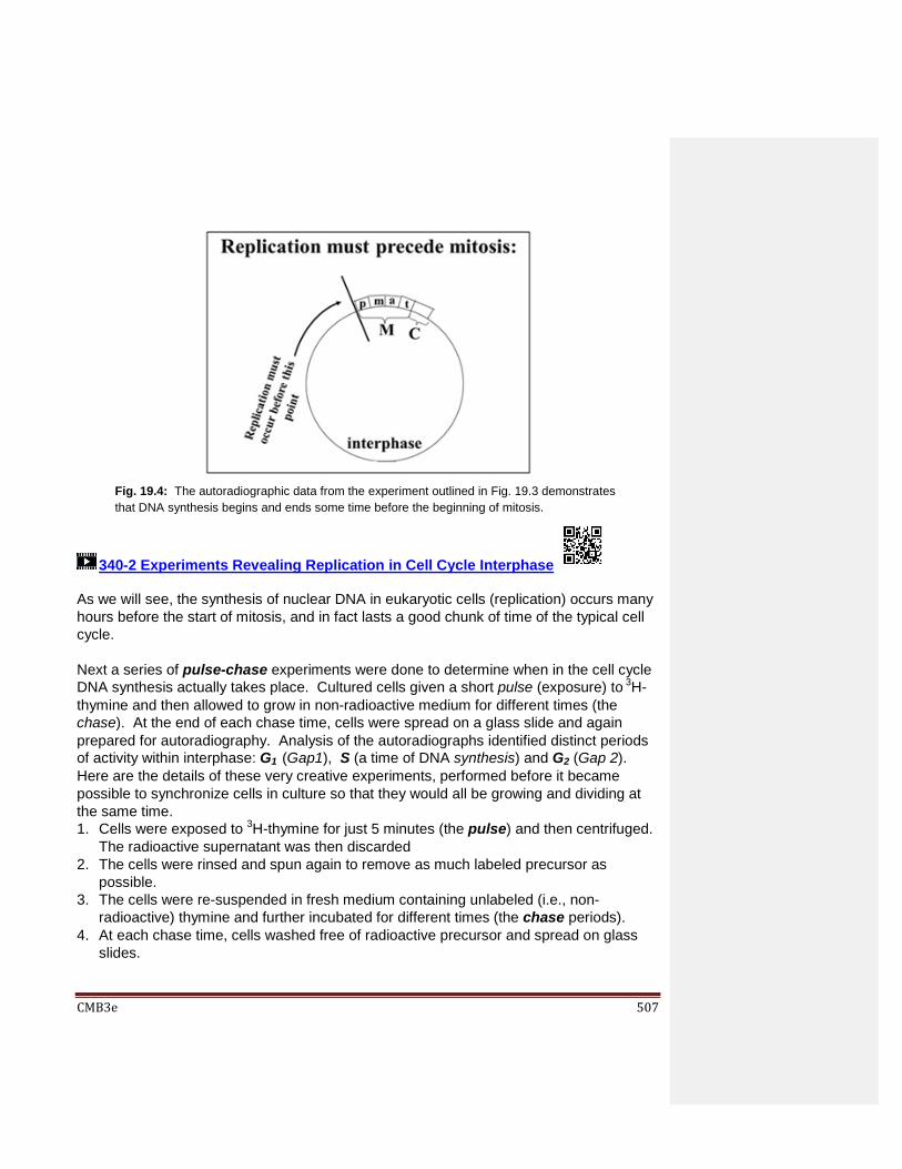
CMB3e 507

340-2 Experiments Revealing Replication in Cell Cycle Interphase As we will see, the synthesis of nuclear DNA in eukaryotic cells (replication) occurs many

hours before the start of mitosis, and in fact lasts a good chunk of time of the typical cell

cycle.

Next a series of pulse-chase experiments were done to determine when in the cell cycle

DNA synthesis actually takes place. Cultured cells given a short pulse (exposure) to 3H-

thymine and then allowed to grow in non-radioactive medium for different times (the

chase). At the end of each chase time, cells were spread on a glass slide and again

prepared for autoradiography. Analysis of the autoradiographs identified distinct periods

of activity within interphase: G1 (Gap1), S (a time of DNA synthesis) and G2 (Gap 2).

Here are the details of these very creative experiments, performed before it became

possible to synchronize cells in culture so that they would all be growing and dividing at

the same time.

1. Cells were exposed to 3H-thymine for just 5 minutes (the pulse) and then centrifuged.

The radioactive supernatant was then discarded

2. The cells were rinsed and spun again to remove as much labeled precursor as

possible.

3. The cells were re-suspended in fresh medium containing unlabeled (i.e., non-

radioactive) thymine and further incubated for different times (the chase periods).

4. At each chase time, cells washed free of radioactive precursor and spread on glass

slides.

Fig. 19.4: The autoradiographic data from the experiment outlined in Fig. 19.3 demonstrates

that DNA synthesis begins and ends some time before the beginning of mitosis.

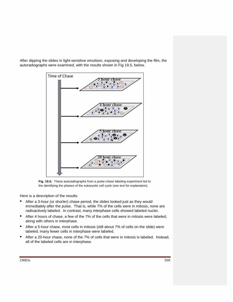
CMB3e 508

After dipping the slides in light-sensitive emulsion, exposing and developing the film, the

autoradiographs were examined, with the results shown in Fig 19.5, below.

Here is a description of the results:

• After a 3-hour (or shorter) chase period, the slides looked just as they would

immediately after the pulse. That is, while 7% of the cells were in mitosis, none are

radioactively labeled. In contrast, many interphase cells showed labeled nuclei.

• After 4 hours of chase, a few of the 7% of the cells that were in mitosis were labeled,

along with others in interphase.

• After a 5-hour chase, most cells in mitosis (still about 7% of cells on the slide) were

labeled; many fewer cells in interphase were labeled.

• After a 20-hour chase, none of the 7% of cells that were in mitosis is labeled. Instead,

all of the labeled cells are in interphase.

Fig. 19.5: These autoradiographs from a pulse-chase labeling experiment led to

the identifying the phases of the eukaryotic cell cycle (see text for explanation).

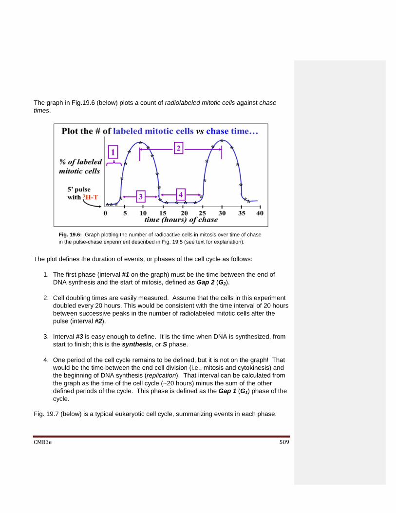
CMB3e 509

The graph in Fig.19.6 (below) plots a count of radiolabeled mitotic cells against chase

times.

The plot defines the duration of events, or phases of the cell cycle as follows:

1. The first phase (interval #1 on the graph) must be the time between the end of

DNA synthesis and the start of mitosis, defined as Gap 2 (G2).

2. Cell doubling times are easily measured. Assume that the cells in this experiment

doubled every 20 hours. This would be consistent with the time interval of 20 hours

between successive peaks in the number of radiolabeled mitotic cells after the

pulse (interval #2).

3. Interval #3 is easy enough to define. It is the time when DNA is synthesized, from

start to finish; this is the synthesis, or S phase.

4. One period of the cell cycle remains to be defined, but it is not on the graph! That

would be the time between the end cell division (i.e., mitosis and cytokinesis) and

the beginning of DNA synthesis (replication). That interval can be calculated from

the graph as the time of the cell cycle (~20 hours) minus the sum of the other

defined periods of the cycle. This phase is defined as the Gap 1 (G1) phase of the

cycle.

Fig. 19.7 (below) is a typical eukaryotic cell cycle, summarizing events in each phase.

Fig. 19.6: Graph plotting the number of radioactive cells in mitosis over time of chase

in the pulse-chase experiment described in Fig. 19.5 (see text for explanation).

CMB3e 510

During G1, S and G2 of interphase, the cell grows in size, preparing for the next cell

division. As you might guess, G1 includes synthesis of enzymes and other proteins

needed next for replication.

DNA replicates in the S phase, along with the synthesis of new histone and other proteins

that will be needed to assemble new chromatin. G2 is the shortest time of interphase and

is largely devoted to preparing the cell for the next round of mitosis and cytokinesis.

Among the proteins whose synthesis increases in this time are the tubulins and proteins

responsible for condensing chromatin into paired chromatids representing the duplicated

chromosomes. Cohesin is a more recently discovered protein made in the run-up to

mitosis. It holds centromeres of chromatids together until they are ready to separate.

341-2 Events in the Phases of the Cell Cycle

Fig. 19.7: A typical eukaryotic cell cycle: phases G1, S and G2 follow cytokinesis; G2 immediately

precedes prophase of mitosis. The length of time for each phase differs for different cell types.

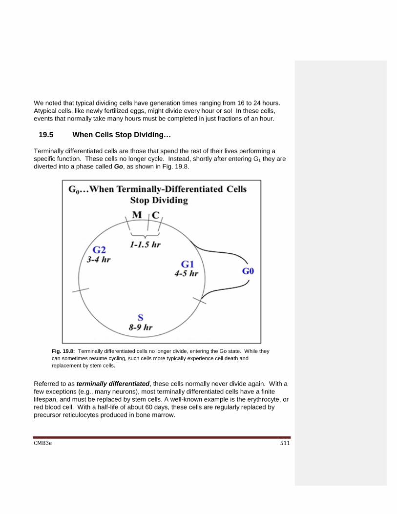
CMB3e 511

We noted that typical dividing cells have generation times ranging from 16 to 24 hours.

Atypical cells, like newly fertilized eggs, might divide every hour or so! In these cells,

events that normally take many hours must be completed in just fractions of an hour.

19.5 When Cells Stop Dividing…

Terminally differentiated cells are those that spend the rest of their lives performing a

specific function. These cells no longer cycle. Instead, shortly after entering G1 they are

diverted into a phase called Go, as shown in Fig. 19.8.

Referred to as terminally differentiated, these cells normally never divide again. With a

few exceptions (e.g., many neurons), most terminally differentiated cells have a finite

lifespan, and must be replaced by stem cells. A well-known example is the erythrocyte, or

red blood cell. With a half-life of about 60 days, these cells are regularly replaced by

precursor reticulocytes produced in bone marrow.

Fig. 19.8: Terminally differentiated cells no longer divide, entering the Go state. While they

can sometimes resume cycling, such cells more typically experience cell death and

replacement by stem cells.

CMB3e 512

19.6 Regulation of the Cell Cycle

Progress through the cell cycle is regulated. The cycle can be controlled or put on ‘pause’

at any one of several phase transitions. Such checkpoints monitor whether the cell is on

track to complete a successful cell division event. Superimposed on these controls are

signals that promote cell differentiation. Embryonic cells differentiate as the embryo

develops. Even after terminal differentiation of cells that form all adult tissues and

organs, adult stem cells will divide and differentiate to replace worn out cells. Once

differentiated, cells are typically signaled in G1 to enter Go and stop cycling. In some

circumstances cells in Go are recruited to resume cycling. However, if this resumption

should occur by mistake, the cells may be transformed to cancer cells. Here we consider

how the normal transition between phases of the cell cycle is controlled.

19.6.1 Discovery and Characterization of Maturation Promoting Factor (MPF)

To monitor their progress through the cell cycle, cells produce internal chemical

signals that tell them when it’s time to begin replication or mitosis, or even when to

enter into Go when they reach their terminally differentiated state. The experiment

that first demonstrated a chemical regulator of the cell cycle involved fusing very large

frog’s eggs! The experiment is described in Fig. 19.9.

Fig. 19.9: Experiment leading to the discovery of meiosis-promoting factor (MPF), the first

known chemical regulator of cell division.

CMB3e 513

The hypothesis tested here was that frog oocyte cytoplasm from germinal vesicle

stage oocytes (i.e., oocytes in mid-meiosis) contain a chemical that causes the cell to

lose its nuclear membrane, condense its chromatin into chromosomes and enter

meiosis. The test was to withdraw cytoplasm from one of these large, mid-meiotic

oocytes with a fine hypodermic needle and inject it into a pre-meiotic oocyte. The

result of the experiment was that the mid-meiotic oocyte cytoplasm induced premature

meiosis in the immature oocyte. Subsequently a maturation promoting factor

(MPF) was isolated from the mid-meiotic cells that when injected into pre-meiotic cells,

caused them to enter meiosis. MPF turns out to be a protein kinase made up of two

polypeptide subunits (Fig. 19.10).

MPF was then also shown to stimulate somatic cells in G2 to enter premature mitosis.

So (conveniently) MPF can also be Mitosis Promoting Factor! Hereafter we will

discuss the effects of MPF as being equivalent in mitosis and meiosis. When active,

MPF targets many cellular proteins.

342 Discovery of MPF Kinase and Its Role in Meiosis and Mitosis

Fig. 19.10: MPF was shown to be a two-subunit protein kinase that transfers phosphates

from ATP to several different proteins.

CMB3e 514

Assays of MPF activity as well as the actual levels of the two subunits over time during

the cell cycle are graphed in Fig. 19.11.

One subunit of MPF is cyclin. The other subunit, cyclin-dependent kinase (cdk),

contains the kinase enzyme active site. Both subunits must be bound to make an

active kinase. Cyclin was so-named because its levels rise gradually after cytokinesis,

peak at the next mitosis, and then fall. Levels of the cdk subunit do not change

significantly during the life of the cell. Because the kinase activity of MPF requires

cyclin, it tracks the rise in cyclin near the end of the G2, and its fall after mitosis.

Cyclin begins to accumulate in G1, rising gradually and binding to more and more cdk

subunits. MPF reaches a threshold concentration in G2 that triggers entry into mitosis.

For their discovery of these central molecules Leland H. Hartwell, R. Timothy Hunt,

and Paul M. Nurse won the 2001 Nobel Prize in Physiology or Medicine.

19.6.2 Other Cyclins, CDKs and Cell Cycle Checkpoints

Other chemical signals accumulate at different points in the cell cycle. For example,

when cells in S are fused with cells in G1, the G1 cells begin synthesizing DNA

(visualized as 3H-thymine incorporation).

Fig. 19.11: Graph comparing plots of cellular cdk and cyclin levels over time with one of MPF

activity (see text for details).

CMB3e 515

Fig 19.12 describes an experiment showing control of progress to different phases of

the cell cycle.

An S phase factor could be isolated from the S phase cells. This factor also turns out

to be a two-subunit protein kinase, albeit a different one from MPF. Just as MPF

signals cells in G2 to begin mitosis, the S phase kinase signals cells in G1 to enter the

S phase of the cell cycle and to start replicating DNA. MPF and the S phase kinase

govern activities at two of several cell cycle checkpoints. In each case, the activity of

the kinases is governed by prior progress through the cell cycle. In other words, if the

cell is not ready to begin mitosis, active MPF production is delayed until it is.

Likewise, the S phase kinase will not be activated until the cell is ready to begin DNA

synthesis.

343 Cell Cycle Control at Check Points and the Go "Phase"

The sequence of signals that control progress through the cell cycle is probably more

intricate and extensive than we currently know, but the best-described checkpoints are

in G1, G2 and M (Fig. 19.13, below).

Fig. 19.12: Cell fusion experiments revealed additional chemical regulators of the cell

cycle activity (see text for details).

CMB3e 516

We generally envision checkpoints as monitoring and blocking progress until essential

events of a current phase of the cell cycle phase are completed. These kinases are

part of molecular sensing mechanisms that act by phosphorylating cytoplasmic and/or

nuclear proteins required by upcoming phases of the cycle. Let’s take a look at some

events that are monitored at these checkpoints in more detail.

19.5.2.a The G1 Checkpoint

The G1 checkpoint controls the transition from the G1 to the S phase of the cell

cycle. If actively dividing cells (e.g., stem cells) in G1 fail to complete their

preparation for replication, the S-phase kinase won’t be produced and the cells

won’t proceed the S phase until the preparatory biochemistry catches up with the

rest of the cycle. To enter S, a cell must be ready to make proteins of replication,

like DNA polymerases, helicases, primases…, among others. Only when these

molecules have accumulated to (or become active at) appropriate levels, is it “safe”

Fig. 19.13: Simplified diagram of cell cycle checkpoints at which progress through the cycle is

assessed. If progress through a phase is incomplete, cell cycle regulators (kinases) delay onset

of the next phase. (see text for details).

CMB3e 517

to enter S and begin replicating DNA. Now, what about those cells that are fully

differentiated? Terminally differentiated cells stop producing the active G1

checkpoint kinase and stop dividing. Thus they are arrested in Go (see below).

19.5.2.b The G2 Checkpoint

Passage through the G2 checkpoint is only possible if DNA made in the prior S

phase is not damaged. Or if it was, that the damage has been (or can be) repaired

(review the proofreading functions of DNA polymerase and the various DNA repair

pathways). Cells that do successfully complete replication and pass the G2

checkpoint must prepare to make the proteins necessary for the upcoming mitotic

phase. These include nuclear proteins necessary to condense chromatin into

chromosomes, tubulins for making microtubules, etc. Only when levels of these

and other required proteins reach a threshold can the cell begin mitosis. Consider

the following two tasks required of the G2 checkpoint (in fact, any checkpoint):

sensing whether prior phase activities have been successfully completed.

delaying transition to the next phase if those activities are unfinished.

But what if sensing is imperfect and a checkpoint is leaky? A recent study

suggests that either the G2 checkpoint is leaky, or at least, that incomplete

activities in the S phase are tolerated, and that some DNA repair is not resolved

until mitosis is underway in M! Check it out at DNA repair and replication during

mitosis.

19.5.2.c The M Checkpoint

The M checkpoint is monitored by the original MPF-catalyzed phosphorylation of

proteins that

a) bind to chromatin causing it to condense and form chromatids,

b) lead to the breakdown of the nuclear envelope, and

c) enable spindle fiber formation.

We have seen that the tension in the spindle apparatus at metaphase tugs at the

kinetochores holding the duplicated chromatids together. When this tension

reaches a threshold, MPF peaks and an activated separase enzyme causes the

chromatids to separate at their centromeres. Beginning in anaphase, continuing

tension in the spindle apparatus draws the new chromosomes to opposite poles of

the cell. Near the end of mitosis and cytokinesis, proteins phosphorylated by MPF

initiate the breakdown of cyclin in the cell. Passing the M checkpoint means that

the cell will complete mitosis and cytokinesis, and that each daughter cell will enter

a new G1 phase.

CMB3e 518

Dividing yeast cells seem to have only the three checkpoints discussed here.

More complex eukaryotes use more cyclins and cdks to control the cell cycle at

more checkpoints. Different cyclins show cyclic patterns of synthesis, while their

cdks remain at constant levels throughout the cell cycle (as in MPF). Different

gene families encode evolutionarily conserved cdks or cyclins. But each cyclin/cdk

pair has been coopted in evolution to monitor different cell cycle events and to

catalyze phosphorylation of phase-specific proteins. To learn more, see Elledge

SJ (1996) Cell Cycle Checkpoints: Preventing an Identity Crisis. Science

274:1664-1672.

344-2 Cyclin/cdk Checkpoints for Cell Cycle Phases

19.5.2.d The Go State

Go is not really a phase of the cell cycle, since cells in Go have reached a

terminally differentiated state and have stopped dividing. Terminally differentiated

cells in tissues and organs no longer divide. But even these cells have finite half-

lives (recall our red blood cells that must be replaced every 60 days or so).

Because cells in many tissues are in Go and can’t divide, they must be replaced by

stem cells, which can divide and differentiate. Some cells live so long in Go that

they are nearly never replaced (muscle cells, neurons). Other cells live short lives

in Go (e.g., stem cells, some embryonic cells). For example, a lymphocyte is a

differentiated immune system white blood cell type.

However, exposure of lymphocytes to foreign chemicals or pathogens activates

mitogens that cause them to re-enter the cell cycle from Go. The newly divided

cells then make the antibodies that neutralize toxic chemicals and fight off the

pathogens. The retinoblastoma (Rb) protein is such a mitogen, a transcription

factor that turns on genes that lead to cell proliferation.

What if cells cycle when they shouldn’t? What if they are inappropriately signaled

to exit Go? Such cells are in trouble! Having escaped normal controls on cell

division, they can become a focal point of cancer cell growth. You can guess from

its name that the retinoblastoma gene was discovered as a mutation that causes

retinal cancer. For more about the normal function of the Rb protein and its

interaction with a G1 cdk, check out the link below.

345-2 Rb Gene Encodes Transcription Factor Regulatory Subunit

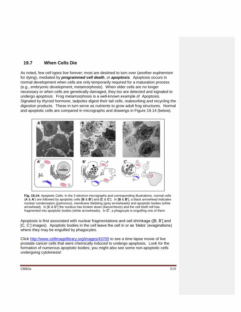
CMB3e 519

19.7 When Cells Die

As noted, few cell types live forever; most are destined to turn over (another euphemism

for dying), mediated by programmed cell death, or apoptosis. Apoptosis occurs in

normal development when cells are only temporarily required for a maturation process

(e.g., embryonic development, metamorphosis). When older cells are no longer

necessary or when cells are genetically damaged, they too are detected and signaled to

undergo apoptosis. Frog metamorphosis is a well-known example of Apoptosis.

Signaled by thyroid hormone, tadpoles digest their tail cells, reabsorbing and recycling the

digestion products. These in turn serve as nutrients to grow adult frog structures. Normal

and apoptotic cells are compared in micrographs and drawings in Figure 19.14 (below).

Apoptosis is first associated with nuclear fragmentations and cell shrinkage ([B, B’] and [C, C’] images). Apoptotic bodies in the cell leave the cell in or as ‘blebs’ (evaginations) where they may be engulfed by phagocytes. Click http://www.cellimagelibrary.org/images/43705 to see a time lapse movie of live prostate cancer cells that were chemically induced to undergo apoptosis. Look for the formation of numerous apoptotic bodies; you might also see some non-apoptotic cells undergoing cytokinesis!

Fig. 19.14: Apoptotic Cells: In the 3 electron micrographs and corresponding illustrations, normal cells (A & A’) are followed by apoptotic cells [B & B’] and [C & C’]. In [B & B’], a black arrowhead indicates

nuclear condensation (pyknosos), membrane blebbing (grey arrowheads) and apoptotic bodies (white arrowhead). In [C & C’] the nucleus has broken down (karyorrhexis) and the cell itself cell has fragmented into apoptotic bodies (white arrowheads). In C’, a phagocyte is engulfing one of them.

CMB3e 520

We now understand the basic metabolic pathway leading to apoptosis. During development, apoptotic cell death starts with an external signal programmed to appear at a specific time in development. Similar signals appear in response to cell obsolescence or genetic damage. The biochemical pathway to apoptosis is illustrated in Fig. 19.15 (below).

The signal molecule acts on target cells to induce transcription of Bcl2 genes. Bcl2

proteins Bak and Bax are outer mitochondrial membrane channel components that allow

the release of cytochrome C into the cytoplasm. This sets off molecular events leading to

apoptosis. Mitochondrial exit of cytochrome C is possible because it is a peripheral

membrane protein, only loosely bound to the cristal membrane. It exists in equilibrium

between membrane-bound and unbound states. As some cytochrome C molecules exit

the intermembrane space, others detach from the cristal membrane and follow. In the

cytosol, cytochrome C binds to adaptor proteins that then aggregate. The cytochrome c-

adaptor complex has a high affinity for a biologically inactive procaspase. Binding of

procaspase to the cytochrome C-adaptor complex causes an allosteric change in the

procaspase, releasing an active caspase. Caspases are proteolytic enzymes that start

the auto-digestion of the cell. For their work in identifying apoptosis genes, Sydney

Brenner, H. Robert Horvitz and John E. Sulston shared the 2002 Nobel Prize in

Physiology or Medicine.

Fig. 19.15: Biochemical steps of apoptosis, or programmed cell death (see text for details).

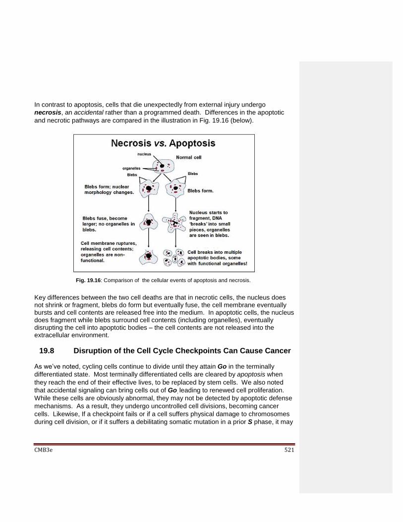
CMB3e 521

In contrast to apoptosis, cells that die unexpectedly from external injury undergo

necrosis, an accidental rather than a programmed death. Differences in the apoptotic

and necrotic pathways are compared in the illustration in Fig. 19.16 (below).

Key differences between the two cell deaths are that in necrotic cells, the nucleus does not shrink or fragment, blebs do form but eventually fuse, the cell membrane eventually bursts and cell contents are released free into the medium. In apoptotic cells, the nucleus does fragment while blebs surround cell contents (including organelles), eventually disrupting the cell into apoptotic bodies – the cell contents are not released into the extracellular environment.

19.8 Disruption of the Cell Cycle Checkpoints Can Cause Cancer

As we’ve noted, cycling cells continue to divide until they attain Go in the terminally

differentiated state. Most terminally differentiated cells are cleared by apoptosis when

they reach the end of their effective lives, to be replaced by stem cells. We also noted

that accidental signaling can bring cells out of Go, leading to renewed cell proliferation.

While these cells are obviously abnormal, they may not be detected by apoptotic defense

mechanisms. As a result, they undergo uncontrolled cell divisions, becoming cancer

cells. Likewise, If a checkpoint fails or if a cell suffers physical damage to chromosomes

during cell division, or if it suffers a debilitating somatic mutation in a prior S phase, it may

Fig. 19.16: Comparison of the cellular events of apoptosis and necrosis.

CMB3e 522

self-destruct in response to a consequent biochemical anomaly. This is another example

of apoptosis. But if a physically damaged or mutated cells should escape apoptotic

clearance, it too may begin proliferating, producing cancer cells. Apoptotic clearance and

uncontrolled cancer cell proliferation are compared in Fig. 19.17.

346-2 Regulating Cell Death - Apoptosis vs. Necrosis

19.9 p53 Protein Mediates Normal Cell Cycle Control

Cancerous growth may result if a normal dividing cell suffers a somatic mutation that

disrupts normal cell cycle control. Think over-expression of cdk for example, or imagine

cyclin levels in daughter cells that never drop; such cells would never stop cycling.

Other possibilities include a cell in Go that is stimulated to begin cycling again by an

inappropriate encounter with a hormone or other signal. If undetected, these anomalies

can transform normal cells to cancer cells. This is apparently the case for a mutation in

the human p53 gene that causes Li-Fraumeni syndrome. The symptoms include a high

incidence of early-age bone, blood and breast cancers (see Li-Fraumeni syndrome for

more details). The role of p53 protein in regulating cancer cell formation was shown

using knockout mice. We noted earlier the use of knockout mutations in studies of

specific gene function. Fig. 19.18 is a protocol for making such mutations in mice.

19.17: Results of non-cancer cell divisions in which abnormal cells are targeted for apoptosis,

and cancer cell division, in which damaged or altered cells escape apoptotic controls.

CMB3e 523

For their demonstration how knockout organisms could be engineered using molecular

technologies, Mario R. Capecchi, Martin J. Evans and Oliver Smithies shared the 2007

Nobel Prize in Physiology or Medicine (read all about it at The Knockout Nobel Prize).

The role of p53 protein in regulating cancer cell formation in mice was shown in a

knockout experiment when the normal mouse p53 genes were replaced with a pair of

mutant p53 genes unable to make functional p53 protein. The resulting knock-out mice

developed tumors and cancers at a much higher rate than normal mice. In general, many

knock-out organisms have been created to study the effects of loss-of-function

mutations in vivo (i.e., in whole animals). Using similar strategies, knock-in protocols can

insert normal genes into an organism lacking the genes, allowing study of the effects of

gain-of-function mutations.

19.8.1 p53 is a DNA-Binding Protein

If a cell in Go is stimulated to begin cycling again by an inappropriate encounter with a

hormone or other signal, it may be transformed into a cancer cell. It is the job of the

p53 protein to detect these anomalies and enable dividing cells to repair the damage

before proceeding through cell cycle check points. Failing that, the p5 protein will

signal apoptosis of the cell. p53 is a DNA-binding, gene-regulatory protein. Fig. 19.19

(below) shows the structure of the P53 protein and how it binds to the DNA double

helix.

Fig, 19.18: Making knockout mutant mice. Specific nucleotides in a cloned gene of interest are altered by site-directed mutagenesis. The altered gene is inserted into embryonic stem cells where it recombines with and replaces the homologous gene already in the chromosome. Recombinant clones are selected re-injected into embryos that are then incubated in the uteri of ‘foster mother’ mice. Knockout mice in the newborn litter can be selected and studied for the effects of removing a gene.

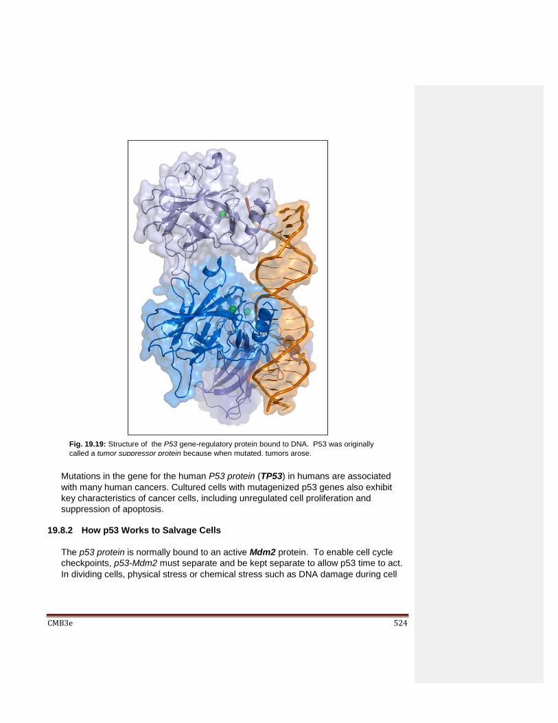
CMB3e 524

Mutations in the gene for the human P53 protein (TP53) in humans are associated

with many human cancers. Cultured cells with mutagenized p53 genes also exhibit

key characteristics of cancer cells, including unregulated cell proliferation and

suppression of apoptosis.

19.8.2 How p53 Works to Salvage Cells

The p53 protein is normally bound to an active Mdm2 protein. To enable cell cycle

checkpoints, p53-Mdm2 must separate and be kept separate to allow p53 time to act.

In dividing cells, physical stress or chemical stress such as DNA damage during cell

Fig. 19.19: Structure of the P53 gene-regulatory protein bound to DNA. P53 was originally

called a tumor suppressor protein because when mutated, tumors arose.

CMB3e 525

growth can activate an ATM kinase. ATM kinase in turn, phosphorylates Mdm2,

causing it to dissociate from p53. The same kinase also phosphorylates another

kinase, Chk2, as well as the now ‘free’ p53. ATM kinase-initiated events are further

detailed below in Fig. 19.20.

Each of the proteins and enzymes phosphorylated by the ATM kinase has a role in

cell cycle checkpoint function and cell cycle arrest while errors are corrected:

1. Now separated from Mdm2, Phospho-p53 actively up-regulates several genes,

including the p21 gene.

2. The P21 protein binds to cdks; cyclins can’t bind P21-cdks.

3. Active Phospho-Chk2 catalyzes cyclin phosphorylation; phospho-cyclins can’t

bind to p21-cdks.

4. The inability of cyclins to bind cdks specifically blocks the cell cycle between the

G1 and S, and the G2-to-M phases.

Fig. 19.21 (below) illustrates the kinase-mediated events at cell cycle checkpoints.

The cell cycle will remain arrested while the cell attempts to finish essential

biochemical activities necessary to correct stress-induced or other physical or

chemical aberrations before moving on to the next phase of the cycle. If DNA repairs

or other corrections are successful, the cell can progress to the next phase. But what

happens if repairs are unsuccessful?

19.20: Normal function of the P53 gene-regulatory protein (see text for details).

CMB3e 526

19.8.3 How p53 Works When Cells Can’t Be Saved

If DNA repair or other corrections fail, the damaged cell is routed to apoptosis. In this

case, proteasomes target the Chk2-cyclin complex for degradation. Likewise, any

P53 remaining bound to unphosphorylated Mdm2 is also targeted for proteasome

destruction. The result is that any cell unable to correct effects of stress or chemical

damage, or to repair DNA damage, is target for apoptosis.

Levels and activity of p53 (as well as the other proteins discussed above) control both

the amount of p53 protein available to respond to cell cycling anomalies and the

responses themselves. While phosphorylation (activation) of p53 leads to a rapid

arrest of the cell cycle, it also results in the activation of genes for proteins required for

DNA repair and for proteins required for apoptosis, just in case repair efforts fail!

The interactions of p53 with different proteins leading to alternate cell fates are

summarized in Fig. 19.22, below.

19.21: Role of the P53 in decision-making at cell cycle checkpoints. (see text for details).

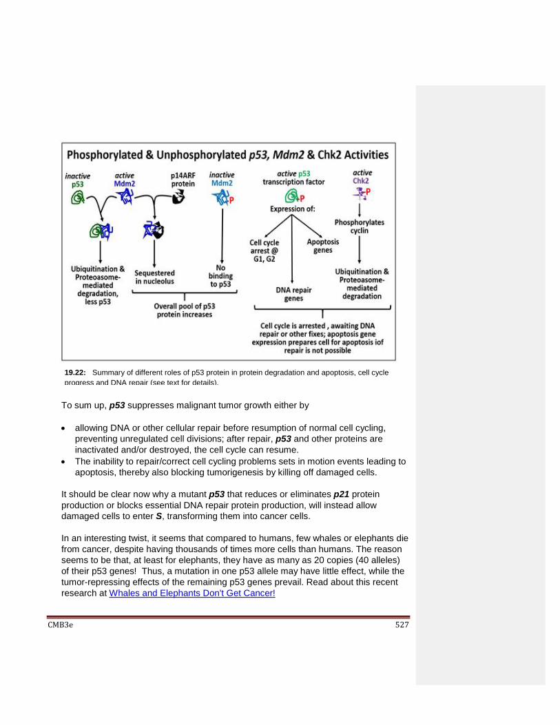
CMB3e 527

To sum up, p53 suppresses malignant tumor growth either by

allowing DNA or other cellular repair before resumption of normal cell cycling,

preventing unregulated cell divisions; after repair, p53 and other proteins are

inactivated and/or destroyed, the cell cycle can resume.

The inability to repair/correct cell cycling problems sets in motion events leading to

apoptosis, thereby also blocking tumorigenesis by killing off damaged cells.

It should be clear now why a mutant p53 that reduces or eliminates p21 protein

production or blocks essential DNA repair protein production, will instead allow

damaged cells to enter S, transforming them into cancer cells.

In an interesting twist, it seems that compared to humans, few whales or elephants die

from cancer, despite having thousands of times more cells than humans. The reason

seems to be that, at least for elephants, they have as many as 20 copies (40 alleles)

of their p53 genes! Thus, a mutation in one p53 allele may have little effect, while the

tumor-repressing effects of the remaining p53 genes prevail. Read about this recent

research at Whales and Elephants Don't Get Cancer!

19.22: Summary of different roles of p53 protein in protein degradation and apoptosis, cell cycle

progress and DNA repair (see text for details).

CMB3e 528

19.8.4 The Centrality of p53 Action in Cell Cycle Regulation

Because of its multiple roles in regulating and promoting DNA repair, and in controlling

cell cycle checkpoints, p53 has been called “the Guardian of the Genome”! Here is

further evidence of this central role.

19.8.4.a ‘Oncogenic Viruses’

Cancer causing viruses include Human Papilloma Virus (HPV), Epstein Barr Virus

(EBV), human immunodeficiency virus (HIV), Hepatitis B and C viruses (HBV,

HCV), Human herpes virus 8 (HHV-8) and simian virus 40 (SV40). The SV40 virus

was discovered as contaminant of polio vaccines that were used in the 1960s.

While an association of SV40 and cancer in humans is as yet unproven, there is a

demonstrated link between SV40, p53 and cancer in other mammals. After

infection of cells by SV40, viral DNA enters the nucleus where it can integrate into

the host cell genome. Such SV40 infections are usually latent, (i.e., they cause no

harm) but when activated, they can lead to cellular transformation and the growth

of malignant sarcomas in muscles as well as tumors in other organs. Upon

activation, RNA polymerase II in the infected cells transcribes the SV40 genes to

produce enzymes that replicate viral DNA and encapsulate the DNA in a

membrane envelope to make new viral particles.

Since the relatively small SV40 genome does not encode all of the enzymes and

factors need for viral DNA replication, the infected cells also provide these factors,

producing them only during the S phase. At that time, the SV40 large T antigen

(already made soon after infection) enters the host cell nucleus where it regulates

transcription of genes essential to viral replication and viral particle formation.

While that may be OK for the SV40 viruses, the kicker is that the large T antigen

also binds to p53, interfering with transcription of proteins whose genes are

regulated by p53. Unable to exercise checkpoint functions, the host cell starts

dividing uncontrollably, forming cancerous tumors. Deregulation of the cell cycle

by large T antigen ensures progress to the S phase and unregulated co-replication

of viral and host cell DNA.

19.8.4.b p53 and Signal Transduction

Stress can activate signal transduction pathways. For example, mutations affecting

the MAPK (MAP kinase) signaling pathway can lead to tumorigenesis. This can be

explained by the observation that when activated, the MAPK pathway leads to

CMB3e 529

amplified production of a kinase that phosphorylates p53. Active phospho-p53 in

turn augments activation of the MAPK signal transduction pathway. You may

recall that MAPK signal transduction typically ends with a mitogenic response.

Another example of p53 interaction is with FAK (focal adhesion kinase) proteins.

FAK activity is increased by integrin-mediated signal transduction. Recall that

membrane integrins bind fibronectin, contributing to formation of the extracellular

matrix, or ECM. Elevated FAK activity participates in the regulation of cell-cell and

cell-ECM adhesion at focal adhesion points. Another role for FAK is to bind

directly to inactive p53 and increase p53-Mdm2 binding. As we have just seen,

persistent p53-Mdm2 is targeted for ubiquitination… and ultimate destruction! In

fact, abnormally high levels of FAK are associated with many different tumor cell

lines (colon, breast, thyroid, ovarian, melanoma, sarcoma…). These result when

p53 is unable properly to activate cell cycle checkpoints. While the interactions

implied here are complex and under active study, these p53 activities certainly

confirm its central role as both guardian of the genome and as guardian of cell

division.

19.9 Cancer Cell Growth and Behavior; Cancer Treatment Strategies

Different cancer cell types have different growth and other behavioral properties. You may

have heard of slow-growing and fast-growing cancers. Colon cancers are typically

slow growing. Periodic colonoscopies that detect and remove colorectal tumors in

middle-age or older people can prevent the disease (although the risks of disease and the

procedure itself must be balanced). Pancreatic cancers are fast growing and usually go

undetected until they reach an advanced stage. The twin goals of medical research are

to detect the different cancers early enough for successful intervention, and of course, to

find effective treatments.

19.9.1 Cancer Cell Origins, Growth and Behavior

A single mutated cell in a tissue can become the growth point of a tumor, essentially a

mass of cells cloned from the original mutated one. Benign tumors or growths (for

example breast and uterine fibroids in women, or common moles in any of us) usually

stop growing and are not life threatening. They are often surgically removed for the

comfort of the patient (or because cells in some otherwise benign tumors may have a

potential to become cancerous). Malignant tumors (also called malignant

neoplasms) are cancerous and can grow beyond the boundaries of the tumor itself.

When tumor cells are shed they may enter the bloodstream and travel to other parts of

the body, the phenomenon called metastasis. Cancer cells that metastasize can

become the focal point of new tumor formation in many different tissues. Because

CMB3e 530

cancer cells continue to cycle and replicate their DNA, they can undergo yet more

somatic mutations. These further changes can facilitate metastasis and cancer cell

growth in different locations in the body.

19.9.2 Cancer Treatment Strategies

There are many different kinds of cancers originating in different tissues of the body.

They all share the property of uncontrolled cell division, albeit for different molecular

(and not always well-understood) reasons. The two major cancer treatment strategies

developed in the 20th century all aim at disrupting replication in some way.

Radiation therapy relies on the fact that most cells in our bodies do not divide.

They aim mutagenic radiation at tumors in the hope that replicating DNA will be

mutated at so many sites (i.e., genes) that the tumor cells can no longer survive or

replicate properly.

Chemotherapy is used to attack tumors that do not respond well to radiation or that are not easily be reached by radiation technologies, and to fight cancers that do not even form focused tumors (such as lymphomas and leukemias involving lymph and blood cells). These chemotherapies also aim to derange replication or mitotic activities. For example, recall cordycepin (dideoxyadenosine triphosphate, or ddATP). When present during replication, ddATP is incorporated into a growing DNA chain, after which no additional nucleotides can be added to the DNA strand. That makes ddATP a potent chemotherapeutic disruptor of replication. Taxol is another chemo drug. In this case, it prevents the depolymerization of spindle fiber microtubules, thus blocking mitotic anaphase and telophase in the latter part of the

M and C phases of the cycle. Colchicine (a plant alkaloid) attacks cancer (and

other dividing) cells by blocking microtubule polymerization in the first place, thus

preventing spindle fiber formation in mitotic prophase.

These therapies are not effective against all cancers and of course, they don’t target

specific kinds of cancer cells. Their success relies simply on the fact that cancer cells

proliferate rapidly and constantly while other cell types do not. Many if not all of the

side effects of radiation and chemotherapies result from the damage done to normal

dividing cells (e.g., hair follicle cells accounting for hair loss among many cancer

patients, depletion of blood cells that fail to be replaced by stem cells in bone marrow).

Much research now is focused on mobilizing the body’s own immune system to create

more specific, targeted cancer treatments.

In a fascinating bit of history, more than 100 years ago, Dr. William B. Coley injected a

terminal cancer patient with streptococcal bacteria. Remarkably, this and many

subsequent patients emerged tumor-free upon his recovery from the infection (for

CMB3e 531

details, check out The Earliest Cancer Immunotherapy Trials). The phenomenon of

“Dr. Coley’s Toxins” was initially thought to be an anti-tumor effect of the bacteria. But

by 1948 it was widely attributed to the immune response activated by the infection. It

seems that our immune system can recognize cancer cell surface molecules as

foreign, but only mounts a weak immune defense that cannot clear those cells. Those

cells that survive continue to proliferate, causing cancer.

In the 1990s, scientists were revisiting the immune response to cancer, and by the

turn of the 21st century, studies of cancer immunotherapy picked up steam (and more

substantial research funding!). Recent animal immunotherapy experiments and

human clinical trials are promising. A few immunotherapies have already been

approved by the U.S. FDA (Food and Drug Administration).

There are different, sometimes overlapping approaches to cancer immunotherapy. All

are based on the fact that cancer cells that have mutated in some way and are

producing aberrant proteins that the immune system can see as foreign enough to

elicit an immune response, however slight. The goal now is to create conditions for a

strong immune response to the cancer cell antigens.

Some immunotherapies seek to boost that innate immune response. Others seek

isolate or synthesize unique cancer cell antigens in vitro that upon injection, will

generate an immune response in the patient strong enough to kill the cancer cells.

Some immunotherapies are summarized below in Table 19.1. As you can see from

the table, immuno-targeting cancer cells has already proven to be highly effective. In

some cases, the therapy is an example of personalized medicine, in which treatments

are uniquely tailored to you as a patient.

Known Issues with immunotherapies are that

they are time and labor intensive…, and costly to produce.

while they may ‘cure’ you, they likely won’t not work on someone else.

like radiation and chemotherapy, immunotherapies come with their own unpleasant

and sometimes severe side effects.

NOTE: In the table, the term checkpoint inhibitor in the context of immunotherapies is different than the term checkpoints describing portals to progress through the eukaryotic cell cycle. A more detailed discussion of cancer immunotherapies is on the cancer.gov website at Cancer Treatment Immunotherapy.

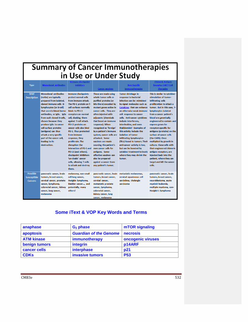
CMB3e 532

Some iText & VOP Key Words and Terms

anaphase G2 phase mTOR signaling

apoptosis Guardian of the Genome necrosis

ATM kinase immunotherapy oncogenic viruses

benign tumors integrin p14ARF

cancer cells interphase p21

CDKs invasive tumors P53

CMB3e 533

cell cycle LFS PD-1 checkpoint protein

cell cycle checkpoints Li-Fraumeni Syndrome PD-L1

chemotherapy M checkpoint programmed cell death

Chk2 M phase of the cell cycle prophase

colchicine malignant tumors protein phosphorylation

cyclin MAPK proteasome

cyclin level in cell cycle maturation radiation therapy

cytokinesis maturation promoting factor

S phase

dideoxyNTP chemotherapy

Mdm2 signal transduction

elephant p53 genes metaphase SV40

FAK metastasis T antigens

Go of the cell cycle mitosis taxol

G1 checkpoint mitosis promoting factor telophase

G1 phase mitotic phases tumor suppressor protein

G2 checkpoint MPF ubiquitination

CMB3e 534

Chapter 20: Origins of Life

A short history; Origins under reductive vs. non-reductive conditions; Prebiotic

chemical and metabolic evolution; Origins of communication (catalysis,

autocatalysis, co-catalysis, biochemical pathways; Transition from the RNA World

20.1 Introduction

It is nearly universally accepted that there was a time, however brief or long, when the

earth was a lifeless planet. Given that the cell is the basic unit of life, and that to be alive

is to possess all of the properties of life, any cell biology textbook would be remiss

without addressing the questions of when and how the first cells appeared on our planet.

Abiogenesis is the origin of life from non-living matter. Of course, any observation of

abiogenesis in nature is no longer possible! But experiment and educated guesswork

makes it possible to construct reasonable (if sometimes conflicting) scenarios to explain

the origins of life, and hence our very existence.

In this chapter, we will see that different scenarios require consistent assumptions about

climatic, geologic, thermodynamic and chemical conditions that favored abiogenesis. The

right conditions would lead to a prebiotic accumulation of organic molecules, chemical

reactions and proto-structures that could support the formation of a cell. One might

reasonably speculate such a prebiotic laboratory would have led to experiments in

chemical evolution, which best survived and interacted in a hostile pre-biotic

environment, even before the origin of the first cell… or cells. Hence the chapter title

“Origins of Life”!

CMB3e 535

While many consider the creation of the first cell to be a singular, one-off event, it has

been argued that multiple independent origins were not only possible under these

conditions, but also probable! According to Jeremy England, of MIT, the laws of

thermodynamics dictate that "... when a group of atoms is driven by an external source of

energy (like the sun or chemical fuel) and surrounded by a heat bath (like the ocean or

atmosphere), matter inexorably acquires the key physical attribute(s) associated with life”

(Statistical Physics of Self Replication). Here is a reminder of those key attributes, or

properties of life:

Evolution: long-term adaptation/speciation

Cell-based: the cell is the fundamental unit of life

Complexity: dynamic order; allows physical/biochemical change

Homoeostasis: living things maintain balance between change and order

Requires Energy: needed to do work, i.e., all cellular functions

Irritability: immediate sensitivity and response to stimuli

Reproduction: sort of self-explanatory, yes?!

Development: programmed change; most obvious in multicellular

organisms, but found in some form in all organisms.

Remember that to be alive is to possess not just some, but all of these properties! If

entities with all of the properties of life (i.e., cells) did originate independently, they would

have reproduced to form separate populations of cells, each of which would embark on

an independent evolutionary pathway. In this scenario, less successful populations would

go extinct as successful ones become dominant. Successful organisms would have

spread, spawning populations, evolving and generating new species. This could go on

until all other independent lineages of life were extinct.

The take-home message here is that if conditions on a prebiotic earth favored the

formation of the ‘first cell’, then why not the formation of two or dozens or even hundreds

of ‘first cells’? We may never know, because there are no survivors of such lineages. If

they ever existed, they are now extinct! We will see the evidence that there is only one

successful population of cells from which the common ancestor of all known living things.

As to the question of when life began, we’ll look at geological and geochemical evidence

suggesting the presence of life on earth as early as 4.1 billion years ago. As for how life

began, this remains the subject of ongoing speculation. All of the scenarios described

below attempt to understand the physical, chemical and energetic conditions that might

have been the ideal laboratory for prebiotic “chemistry experiments”.

What all Origins of Life scenarios must share are the following:

prebiotic synthesis of organic molecules & polymers

origins of catalysis & replicative chemistry

CMB3e 536

sources of free energy to sustain prebiotic chemistry

beginnings of metabolism sufficient for life

origins of molecular communication (information storage and retrieval)

enclosure of life’s chemistry behind a semipermeable boundary

Let’s consider some tricky definitions. If one believes the origin of life was so unlikely that

it could only have happened once (still a common view), then the very first cell, the

progenote, is the progenitor of us all, the common ancestor of all living things. The

evolutionary tree in Fig. 20.1 (below) puts the progenote at the root of the tree.

The progenote, that first and only cell, would have given rise to multiple lineages, i.e., as it

reproduced, some cells would have diverged into separate and multiple species. In other

words, the descendants of the progenote would have evolved from the get-go. Like any

populations of cells and organisms, whether from of a single or many ‘progenotes’,

descendant populations would have competed for resources (and ultimately survival) on

an early earth. Thus one of these lineages (the dashed line in the illustration) would have

survived as others fell to extinction, a process that continues today as the fossil record

attests. Now let’s imagine multiple independent ‘first cells’. How would that change our

view of life’s descent?

Fig.20.1: Descent (evolution and speciation) from a single progenitor cell formed by

abiogenesis on a prebiotic earth.

CMB3e 537

Figure 20.2 illustrates a likely scenario.

Based on this illustration, we can surmise that:

1. Independent descent from independent ‘first cells’ may have occurred, but without

evidence we must assume that the evolution of all but one of them led to extinction of

their lineage, leaving only one evolutionary path to life on earth.

2. The descendants of a ‘first cell’ that survived (illustrated on the right) includes many

lineages that went extinct, and a surviving lineage that includes the ancestor to us all

as well as extinctions that continue to this day.

In other words, whether or not life had one or many origins in a permissive prebiotic

environment, we can anchor our assumptions the evolution of life from a single origin.

We’ll see clear evidence to support that all organisms alive today are descended from a

single cell. In a scenario where only one cell population survives the competition with

other populations, its evolved cells would have been the source of our Last Universal

Common Ancestor, or LUCA. The LUCA must be that highly evolved cell whose

genome, biochemistry and basic metabolic infrastructure is shared among all things alive

today (Fig. 20.3).

Fig.20.2: Descent (evolution and speciation) from multiple ‘first’ cells.

CMB3e 538

This and similar evolutionary trees for known living things on earth are based on studies

of nucleotide sequences of many genes in existing organisms. Whatever the prebiotic

pathway (or pathways) to the first living cells on earth, computers can be used to trace

differences in gene nucleotide sequences back to changes that would have begun in a

single common ancestor that we have defined as our LUCA.

Let’s think about the basis for our conclusion that descendants of multiple ‘first cells’ are

no longer with us. If there were multiple origins, then each of these first cells may have

survived long enough to produce its own lineage of evolved cell populations. But cells in

each of these independent lineages would have evolved biochemistries and cellular

structures that that differ from one another. Perhaps it will be easiest to imagine that they

evolved very different genetic codes, even if they used RNA and DNA as their genetic

material, and even if the best solution to storing and retrieving genetic information was the

3 base codon for their amino acids. But which codons encode which amino acids was a

fortuitous choice in evolution, made by LUCA’s ancestors. So if life originated multiple

times and any descendants survived to this day, we would expect them to have a different

Fig. 20.3: Evolutionary (i.e., phylogenetic) tree of all living organisms, showing descent from the Last Universal Common Ancestor (LUCA) of the 3 domains of life (Bacteria, Archea and Eukaryota).

CMB3e 539

genetic code, if not some very unusual way to store genetic information. Since there is no

evidence for different genetic codes among organisms alive today, we conclude either

that all but one multiple progenote lineage went extinct, or that they never happened.

Either way, among the descendants of our progenote is a lineage, a population that

includes the first cell that must have had a DNA genome, with the same genetic code

used by virtually all organisms alive today. This LUCA, our LUCA, and its descendants

display the high level of conservation of gene and protein sequences that we find today.

We’ll look at more supporting evidence that this is so as we move through this chapter;

this evidence is perhaps the strongest support for realized expectations.

We’ll begin by looking at the following basic requirements of any life-origins scenario:

reduction of inorganic molecules to form organic molecules

a source of free energy to fuel the formation of organic molecules

a scheme for catalytic acceleration of biochemical reactions

separation of early biochemical ‘experiments’ by a semipermeable boundary.

Then, we’ll consider some proposed scenarios for the creation of organic molecules:

import of organic molecules (or even life itself) from extraterrestrial sources.

organic molecule synthesis on an earth with a reducing atmosphere.

organic molecule synthesis on an earth with a non-reducing atmosphere.

We’ll explore alternate free-energy sources and pathways to the essential chemistry of

life dictated by these different beginnings. Then we look at possible scenarios of

chemical evolution that must have occurred before life itself. Finally, we consider how

primitive (read “simpler”) biochemistries could have evolved into the present-day

metabolisms shared by all existing life forms…, including its shared genetic code!

347 What any Life Origins Scenario Must Explain Learning Objectives

When you have mastered the information in this chapter, you should be able to:

1. explain how organic molecules would capture chemical energy on a prebiotic earth.

2. list the essential chemistries required for life and why they might have been selected

during chemical evolution.

3. discuss the different fates of prebiotically synthesized organic monomers and

polymers and how these fates would influence the origins of the first cells on earth.

4. compare and contrast two scenarios for extraterrestrial origins of organic molecules.

5. summarize the arguments against Oparin’s primordial soup hypothesis.

6. summarize the evidence supporting origins of life in a non-reducing earth atmosphere.

7. compare the progenote and the LUCA.

8. discuss the evidence suggesting an origin of cellular life in the late Hadean eon.

CMB3e 540

9. describe how life might have begun in deep ocean vents – compare the possibilities of

life beginning in black smokers vs. white smokers.

10. argue for and against an autotroph-first scenario for cellular origins.

11. explain why some investigators place significance on the early origins of free energy

storage in inorganic proton gradients.

12. define autocatalysis, co-catalysis and co-catalytic sets; provide examples.

13. define coevolution.

14. describe the significance and necessity of coevolution before life. In what ways is

coevolution a feature of living things? Explain.

20.2 Thinking about Life’s Origins: A Short Summary of a Long History

By all accounts, the earth must have been a very unpleasant place soon after its

formation! For that reason, the period from 4.8 to 4.0 billion years ago is called the

Hadean Eon, after Hades, the hell of the ancient Greeks!

Until recently, geological, geochemical and fossil evidence suggested that life arose

between 3.8 and 4.1 billion years ago. The 2017 discovery of evidence for life in 3.95

billion year-old sedimentary rocks in Labrador points to an even earlier origin of life, (see

From Canada Comes the Oldest Evidence of Life on Earth). In fact, questions about

life’s origins are probably “as old as the hills…” or at least as old as the ancient Greeks!

We only have records of human notions of life’s origins dating from biblical accounts and,

just a bit later, from Aristotle’s musings. While Aristotle did not suggest that life began in

hell, he and other ancient Greeks did speculate about life’s origins by spontaneous

generation, in the sense of abiogenesis (life originating from non-life). He further

speculated that the origins of life were gradual. Later, the dominant theological accounts

of creation in Europe in the middle ages muted any notions of origins and evolution.

While a few mediaeval voices ran counter to strict biblical readings of the creation stories,

it was not until the Renaissance in the 14th-17th century that an appreciation of ancient

Greek humanism was reawakened, and with it, scientific curiosity and the ability to

engage in rational questioning and research.

You may recall that Louis Pasteur in the mid-19th century put to rest any lingering notions

of life forming from dead (e.g., rotten, or fecal) matter. He showed that life would not form

in sterilized nutrient solutions unless the broth was exposed to the air. Fewer know that

much earlier, Anton Van Leeuwenhoek (the 17th century sheriff of Delft, amateur lens

grinder and microscopist who first described pond water bacteria and protozoan

animalcules) had already tested the notion of spontaneous generation. By observing

open and sealed containers of meat over time, he became convinced that ‘large’ animals

like fleas and frogs do not arise de novo from putrid meat or slime. He also declared that

insects come from other insects, and not from the flowers that they visited. No lesser a

CMB3e 541

light than Charles Darwin suggested in 1859 that life might have begun in a "warm little

pond, with all sorts of ammonia and phosphoric salts, light, heat, electricity, &c., present,

that a proteine compound was chemically formed ready to undergo still more complex

changes." He even realized that these chemical constituents would not have survived in

the atmosphere and waters of his day, but must have done so in a prebiotic world. In On

the Origin of Species, he referred to life having been ‘created’. There, Darwin was not

referring to a biblical basis of creation; he clearly meant that life originated “by some

wholly unknown process" at a time before which there was no life.

Finally, Pasteur’s 1861 contribution was the irrefutable, definitive proof that ‘invisible’

microbial life likewise did not arise by spontaneous generation. Thus for creatures

already on earth, they could only arise by biogenesis (life-from-life), the opposite of

abiogenesis, a term that now applies to only the first origins of life! Among Darwin’s

friends and contemporaries were Charles Lyell and Roderick Murchison, both geologists

who understood much about the slow geological changes that shaped the earth. Darwin

was therefore familiar with the concept of extended periods of geological time, amounts of

time he believed was necessary for the natural selection of traits leading to species

divergence.

Fast-forward to the 1920s when J.H.B.S. Haldane and A. Oparin offered an hypothesis

about the life’s origins based on notions of the chemistry and physical conditions they

believed might have existed on a prebiotic earth. Their proposal assumed that the

earth’s atmosphere was hot, hellish and reducing (i.e., filled with inorganic molecules able

to give up electrons and hydrogens). There are more than a few hypotheses for which

chemicals were already present on earth, or that formed when the planet formed about

4.8 billion years ago. We’ll start our exploration with Oparin and Haldane’s reducing

atmosphere. Then we look at possibility that life began under non-reducing conditions,

with passing reference to a few other ideas!

348 Early Ideas to Explain the Origins of Life

20.3 Formation of Organic Molecules in an Earthly Reducing

Atmosphere

A prerequisite to prebiotic chemical experimentation is a source of organic molecules.

Just as life requires energy (to do anything and everything), converting inorganic

molecules into organic molecules requires an input of free energy. As we have seen,

most living things today get free energy by oxidizing nutrients or directly from the sun by

photosynthesis. Recall that all the chemical energy sustaining life today ultimately comes

from the sun. But before there were cells, how did organic molecules form from inorganic

precursors? Oparin and Haldane hypothesized a reducing atmosphere on the prebiotic

CMB3e 542

earth, rich in inorganic molecules with reducing power (like H2, NH3, CH4, and H2S) as

well as CO2 to serve as a carbon source. The predicted physical conditions on this

prebiotic earth were:

• lots of water (oceans).

• hot (no free O2).

• lots ionizing (e.g., X-, -) radiation from space, (no protective ozone layer).

• frequent ionizing (electrical) storms generated in an unstable atmosphere.

• volcanic and thermal vent activity.

20.3.1 Origins of Organic Molecules and a Primordial Soup

Oparin suggested that abundant sources of free energy fueled the reductive synthesis

of the first organic molecules to create what he called a “primeval soup”. No doubt, he

called this primeval concoction a “soup” because it would have been rich in chemical

(nutrient) free energy. Urey, who had already won the 1934 Nobel Prize in Chemistry

for discovering deuterium, and Miller tested the prediction that, under Haldane and

Oparin’s prebiotic earth conditions, inorganic molecules could produce the organic

molecules in what came known as the primordial soup. In their classic experiment a

mix of inorganic molecules provided with an energy source were reduced to very

familiar organic molecules, supporting the Oparin/Haldane proposal (Fig. 20.4).

Fig. 20.4: The Miller & Urey experiment: organic molecules seen in living things today can be made

in the lab under reducing conditions like those expected in a prebiotic earth atmosphere.

CMB3e 543

Miller’s earliest published data indicated the presence of several organic molecules in

their ocean flask, including a few familiar metabolic organic acids (lactate, acetate,

several amino acids…) as well as several highly reactive aldehydes and nitriles. The

latter can interact in spontaneous chemical reactions to form organic compounds.

Later analyses further revealed purines, carbohydrates and fatty acids in the flask.

Later still, 50 years after Miller’s experiments (and a few years after his death), some

un-analyzed sample collection tubes from those early experiments were discovered.

When the contents of these tubes were analyzed with newer, more sensitive detection

techniques, they were shown to contain additional organic molecules not originally

reported, including 23 amino acids (to read more, click Surprise Goodies in the Soup!).

Clearly, the thermodynamic and chemical conditions proposed by Oparin and Haldane

could support the reductive synthesis of organic molecules. At some point, Oparin

and Haldane’s evolving chemistries would have to have been internalized inside of

semipermeable aggregates (or boundaries) destined to become cells. Examples of

such structures are discussed below. A nutrient-rich primordial soup would likely have

favored the genesis of heterotrophic cells that could use environmental nutrients for

energy and growth, implying an early evolution of fermentative pathways similar to

glycolysis. But, these first cells would quickly consume the nutrients in the soup,

quickly ending the earth’s new vitality!

To stop life from becoming a dead-end experiment, one must propose the early

evolution of some populations of cells that could capture free energy from inorganic

molecules (chemoautotrophs) or even sunlight (photoautotrophs). As energy-rich

organic nutrients in the ‘soup’ declined, autotrophs (e.g., photoautotrophs that could

split water using solar energy) would be selected. Photoautotrophs would fix CO2,

reducing it with H- ions from water. Photoautotrophy (photosynthesis) would thus

replenish carbohydrates and other nutrients in the oceans and add O2 to the

atmosphere. At first, oxygen would have been toxic to most cells, but some of those

cells already had the ability to survive oxygen. Presumably these spread, evolving

into cells that could respire, i.e., use oxygen to burn environmental nutrients.

Respiratory metabolism must have followed hard on the heels of the spread of

photosynthesis. After photosynthesis emerged, sometime between 3.5 and 2.5 billion

years ago (the Archaean Eon), photosynthetic and aerobic cells and organisms

achieved a natural balance to become the dominant species in our oxygen-rich world.

20.3.2 The Tidal Pool Scenario for an Origin of Polymers and Replicating

Chemistries

In this scenario, prebiotic organic monomers is concentrated in tidal pools in the heat

of a primordial day, followed by dehydration synthesis and polymerization. The

formation of polymer linkages is an ‘uphill’ reaction requiring free energy. Very high

CMB3e 544

temperatures (the heat of baking) can link monomers by dehydration synthesis in the

laboratory and may have done so in tidal pool sediments to form random polymers.

This scenario further assumes the dispersal of these polymers from the tidal pools

with the ebb and flow of high tides. Fig. 20.5 illustrates the tidal pool scenario.

Fig. 20.5: Scenario for the synthesis of prebiotic polymers in tidal pools.

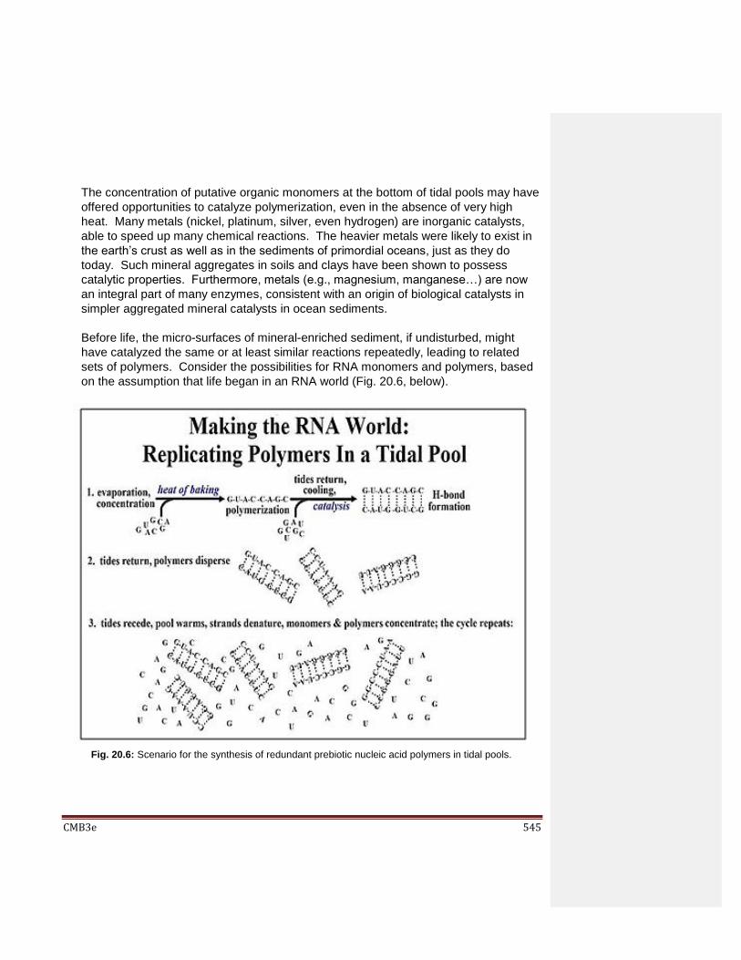
CMB3e 545

The concentration of putative organic monomers at the bottom of tidal pools may have

offered opportunities to catalyze polymerization, even in the absence of very high

heat. Many metals (nickel, platinum, silver, even hydrogen) are inorganic catalysts,

able to speed up many chemical reactions. The heavier metals were likely to exist in

the earth’s crust as well as in the sediments of primordial oceans, just as they do

today. Such mineral aggregates in soils and clays have been shown to possess

catalytic properties. Furthermore, metals (e.g., magnesium, manganese…) are now

an integral part of many enzymes, consistent with an origin of biological catalysts in

simpler aggregated mineral catalysts in ocean sediments.

Before life, the micro-surfaces of mineral-enriched sediment, if undisturbed, might

have catalyzed the same or at least similar reactions repeatedly, leading to related

sets of polymers. Consider the possibilities for RNA monomers and polymers, based

on the assumption that life began in an RNA world (Fig. 20.6, below).

Fig. 20.6: Scenario for the synthesis of redundant prebiotic nucleic acid polymers in tidal pools.

CMB3e 546

The result predicted here is the formation not only of RNA polymers (perhaps only

short ones at first), but of H-bonded double-stranded RNA molecules that might

effectively replicate at each cycle of concentration, polymerization and dispersal.

Heat and the free energy released by these same reactions could have supported

polymerization, while catalysis would have enhanced the fidelity of RNA replication.

Of course, in the tidal pool scenario, repeated high heat or other physical or chemical

attack might also degrade newly formed polymers. But what if some RNA double

strands were more resistant to destruction? Such early RNA duplexes would

accumulate at the expense of the weaker, more susceptible ones. Only the fittest

replicated molecules would be selected and persist in the environment. The

environmental accumulation of structurally related, replicable and stable polymers

reflects a prebiotic chemical homeostasis (one of those properties of life!).

349 Life Origins in a Reducing Atmosphere?

Overall, this scenario hangs together nicely, and has done for many decades. But

there are now questions challenging the premise of a prebiotic reducing environment.

New evidence points to an earth atmosphere that was not at all reducing, casting

doubt on the idea that heterotrophs were the first cells on the planet. Recent

proposals posit alternative sources of prebiotic free energy and organic molecules that

look quite different from those assumed by Oparin, Haldane, Urey and Miller.

20.4 Origins of Organic Molecules in a NON-Reducing Atmosphere

A prebiotic non-reducing atmosphere is based on several assumptions: (1) The early

earth would have had insufficient gravity to hold H2 and other light gasses; thus

“outgassing” would have resulted in a loss of H2 and other reducing agents from the

atmosphere. (2) Geological evidence suggests that the earth’s oceans and crust formed

early in the Hadean Eon, just a few hundred million years after formation of the planet. (3)

Studies of 4.4-billion-year-old (early Hadean Eon) Australian zircon crystals suggest that

their oxidation state is the same as modern day rocks, meaning that the early Hadean

atmosphere was largely N2 and CO2, a distinctly non-reducing one! Solid geological

evidence of cellular life dates to 3.5-3.95 billion years ago (i.e., the Archaean Eon). Softer

evidence of microbial life exists in the form of graphite and other ‘possible’ remains as old

as 4.1 billion years ago, near the end of the Hadean Eon.

If this is true, the discovery of an oxidizing Hadean atmosphere at least 3 billion years

earlier (4.4 billion years ago) argues that life began in a non-reducing atmosphere, in

which case, regardless of whether life began 3.5 or even 4.1 billion years ago, the

evidence suggests that life’s beginnings had to contend with a non-reducing environment.

CMB3e 547

A colorized image of the Australian zircon is shown below in Fig. 20.7.

Before we look more closely at other evidence of life origins under non-reducing

conditions, let’s consider the Panspermia, the possibility that life came to earth from

extraterrestrial sources and a related hypothesis that prebiotic organic molecules came

from extraterrestrial sources. Then we’ll return to the question of how cells might have

formed in localized, favorable terrestrial environments.

20.4.1 Panspermia – an Extraterrestrial Origin of Earthly Life

Panspermia posits that life itself arrived on our planet by hitchhiking on comets or

meteorites. Since these are unlikely to have sustained life in space, they must have

been a kind of interstellar ‘mailbox’ into which dormant life forms were deposited. The

cells in the mailboxes must have been cryptobiotic. Examples of cryptobiosis exist

today (e.g., bacterial spores, brine shrimp!). Once delivered to earth’s life-friendly

environment, such organisms would emerge from dormancy, eventually populating the

planet. There is however, no evidence of dormant or cryptobiotic life on comets or

meteorites, and no hard evidence to support Panspermia. On the other hand, there is

evidence at least consistent with an extraterrestrial source of organic molecules, and

plenty to support more terrestrial origins of life. In any case, notions of Panspermia

(and even extraterrestrial sources of organic molecules) just beg the question of the

conditions that would have led to the origins of life elsewhere!

Fig. 20.7: Analysis of this Australian zircon supports the presence of an oxidizing

atmosphere on a prebiotic earth. Photo Courtesy of J.W.Valley et al.

CMB3e 548

Not a favored scenario, panspermia is still intriguing in the sense that it is in line with a

likelihood that organic molecules formed soon after the Big Bang. Moreover, if ready-

made organic molecules and water were available, we can expect (and many do!) that

there is life on other planets. This possibility has stimulated discussion and serious

funding of programs looking for signs of extraterrestrial life. It supported the earlier

Search for Extraterrestrial Intelligence (SETI) program based on the assumption that

life not only exists elsewhere, but that it evolved high level communication skills (and

why not?)! More recently NASA funded Rover’s search for signs (and discovery) of

signs of water on Mars. For a fascinating story about meteorites from Mars that

contain water and that are worth more than gold, click Martian Obsession.

And then there is this! Maybe, just maybe we have exported earthly life to comets

when they bumped into us and skittered away instead of crashing and burning

(evidence suggests this is so). And maybe, just maybe they scraped up a few upper

atmospheric microbes along their way to other outer-space encounters (colonies of

such microbes exist) . And maybe, just maybe such encounters could have led to

exoplanetary life. Read about the possibilities and realities at Maybe_just_maybe.

Finally, maybe, just maybe, our attempt to share the gift of life can explain organic

molecules on some space objects that come near or actually visit us from time to time!

20.4.2 Extraterrestrial Origins of Organic molecules

Even if life did not come to us ready-made, could organic molecules have arrived on

earth from outer space? They are abundant, for example in interstellar clouds, and

could have become part of the earth as the planet formed around 4.8 billion years ago.

In this case there was no need to create them de novo. Comets, meteorites and

asteroids contain organic molecules. Comet and meteorite bombardments common

3.8 or more billion years ago and could have delivered organic molecules during fiery

impacts on our planet.. If so, the question of how (not on earth!) free energy and

inorganic molecular precursors reacted to form organic molecules is moot!

A related hypothesis suggests that those fiery hits themselves provided the free

energy necessary to synthesize organic molecules from inorganic ones… a synthesis-

on-arrival scenario. With this hypothesis on the one hand, we are back to an organic

oceanic primordial soup. On the other, some have suggested that organic molecules

produced in this way (not to mention any primordial life forms) would likely have been

destroyed by the same ongoing impacts by extraterrestrial bodies; witness the

relatively recent dinosaur extinction by an asteroid impact off the coast of Mexico

some 65.5 million years ago.

350 Life Origins in a Non-Reducing Atmosphere?

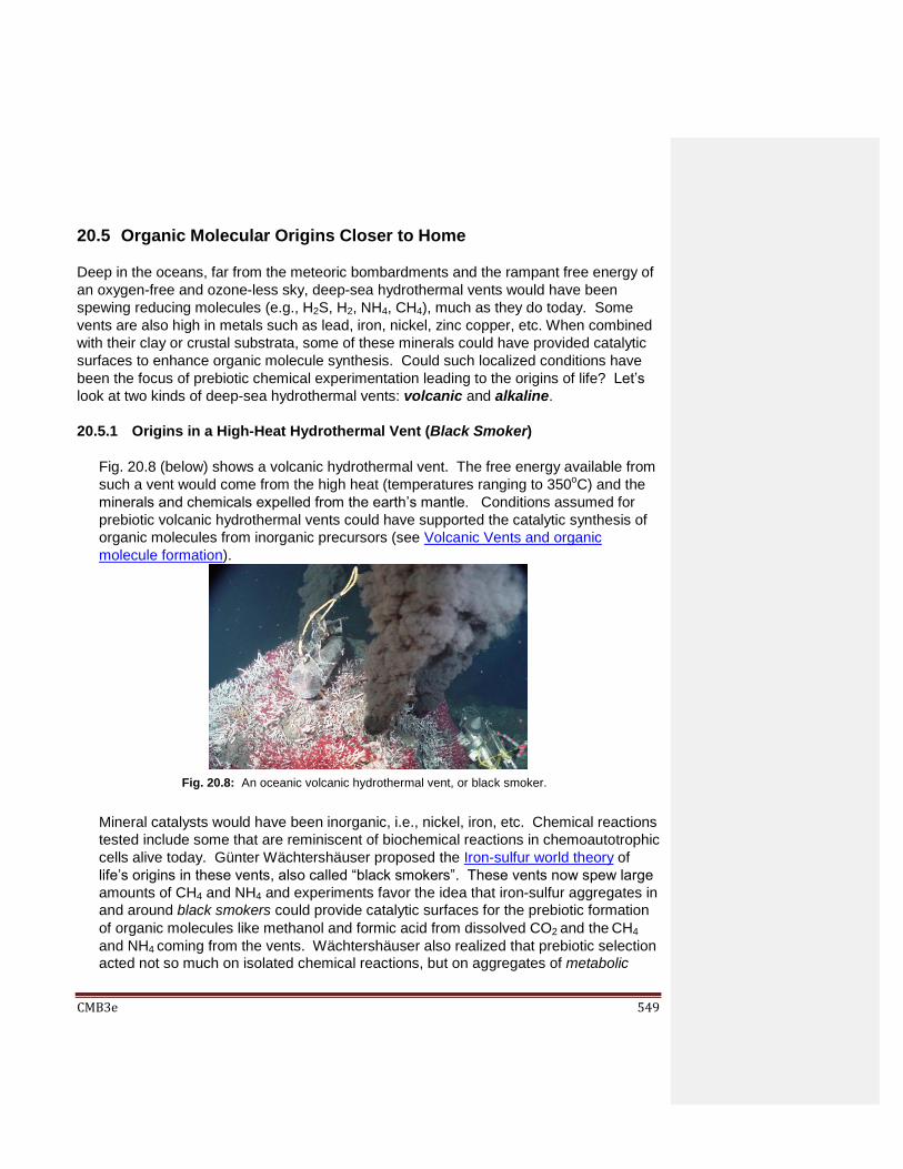
CMB3e 549

20.5 Organic Molecular Origins Closer to Home

Deep in the oceans, far from the meteoric bombardments and the rampant free energy of

an oxygen-free and ozone-less sky, deep-sea hydrothermal vents would have been

spewing reducing molecules (e.g., H2S, H2, NH4, CH4), much as they do today. Some

vents are also high in metals such as lead, iron, nickel, zinc copper, etc. When combined

with their clay or crustal substrata, some of these minerals could have provided catalytic

surfaces to enhance organic molecule synthesis. Could such localized conditions have

been the focus of prebiotic chemical experimentation leading to the origins of life? Let’s

look at two kinds of deep-sea hydrothermal vents: volcanic and alkaline.

20.5.1 Origins in a High-Heat Hydrothermal Vent (Black Smoker)

Fig. 20.8 (below) shows a volcanic hydrothermal vent. The free energy available from

such a vent would come from the high heat (temperatures ranging to 350oC) and the

minerals and chemicals expelled from the earth’s mantle. Conditions assumed for

prebiotic volcanic hydrothermal vents could have supported the catalytic synthesis of

organic molecules from inorganic precursors (see Volcanic Vents and organic

molecule formation).

Mineral catalysts would have been inorganic, i.e., nickel, iron, etc. Chemical reactions

tested include some that are reminiscent of biochemical reactions in chemoautotrophic

cells alive today. Günter Wächtershäuser proposed the Iron-sulfur world theory of

life’s origins in these vents, also called “black smokers”. These vents now spew large

amounts of CH4 and NH4 and experiments favor the idea that iron-sulfur aggregates in

and around black smokers could provide catalytic surfaces for the prebiotic formation

of organic molecules like methanol and formic acid from dissolved CO2 and the CH4

and NH4 coming from the vents. Wächtershäuser also realized that prebiotic selection

acted not so much on isolated chemical reactions, but on aggregates of metabolic

Fig. 20.8: An oceanic volcanic hydrothermal vent, or black smoker.

CMB3e 550

reactions. We might think of such metabolic aggregates as biochemical pathways or

multiple integrated pathways. Wächtershäuser proposed the selection of cyclic

chemical reactions that released free energy that could be used by other reactions.

This prebiotic metabolic evolution of reaction chemistries (rather than a simpler

chemical evolution) would have been essential to the origins of life. A variety of

extremophiles (e.g., thermophilic archaea) now living in and around black smokers

seems to be testimony to black smoker origins of life.

While the idea of selecting metabolic pathways has great merit, there are problems

with a life-origins scenario in volcanic hydrothermal vents. For one thing, their high

temperatures would have destroyed as many organic molecules as were created.

Also, the extremophilic archaea now found around these volcanic vents cannot be the

direct descendants of any cells that might have originated there. Woese’s phylogeny

clearly shows that archaea share a lineage with eukaryotes (not eubacteria). Thus,

extremophilic cellular life originating in the vents must have given rise to a more

moderate LUCA first, before then dying off themselves. Then, extremophiles would

once again have had to evolve independently to re-colonize the vents! Such twists

and turns over time mitigate against an extremophiles-first origins scenario. Given

these concerns, recent proposals focus on life origins in less extreme alkaline

hydrothermal vents.

20.5.2 Origins in an Alkaline Deep-Sea Vent (White Smoker)

Of the several scenarios discussed here, an origin of autotrophic life in alkaline vents

is one of the more satisfying alternatives to a soupy origin of heterotrophic cells. For

starters, at temperatures closer to 100oC -150oC, alkaline vents (white smokers) are

not nearly as hot as are black smokers. An alkaline vent is shown below in Fig. 20.9.

Fig. 20.9: An oceanic volcanic hydrothermal vent, or White smoker.

CMB3e 551

Other chemical and physical conditions of alkaline vents are also consistent with an

origins-of-life scenario dependent on metabolic evolution. For one thing, the interface

of alkaline vents with acidic ocean waters has the theoretic potential to generate many

different organic molecules [Shock E, Canovas P. (2010) The potential for abiotic

organic synthesis and biosynthesis at seafloor hydrothermal systems. Geofluids 10 (1-

2):161-92)].

In laboratory simulations of alkaline vent conditions, the presence of dissolved CO2

favors serpentinization, a reaction of water and heat with serpentinite, an iron-

containing mineral found on land and in the oceanic crust. Fig. 20.10 is a sample of

serpentinite.

Experimental serpentinization produces hydrocarbons and a warm aqueous oxidation

of iron produces H2 that could account for abundant H2 in today’s white smoker

emissions. Also, during serpentinization, a mineral called olivine [(Mg+2, Fe+2)2SiO4]

reacts with dissolved CO2 to form methane (CH4). So, the first precondition of life’s

earthly origins, the energetically favorable creation of organic molecules, is possible in

alkaline vents.

Fig. 20.10: Serpentinite from Deer Lake in upper Michigan. It is a mineral also found in the

oceanic crust that under conditions found in an alkaline vent, can form methane from CO2 .

CMB3e 552

Proponents of cellular origins in a late-Hadean non-reducing ocean also realized that

organic molecules formed in an alkaline (or any) vent would disperse and be rapidly

neutralized in the wider acidic ocean waters. Somehow, origins on a non-reducing

planet had to include some way to contain newly formed organic molecules from the

start, and a way to power further biochemical evolution. What then, were the

conditions in an alkaline vent that could have contained organic molecules and led to

metabolic evolution and ultimately, life? Let’s consider an intriguing proposal that gets

at an answer!

The porous rock structure of today’s alkaline vents provides micro-spaces or micro-

compartments that might have captured alkaline liquids emitted by white smokers. It

turns out that conditions in today’s alkaline vents also support the formation of

hydrocarbon biofilms. Micro-compartments lined with such biofilms could have

formed a primitive prebiotic membrane against a rocky “cell wall”, within which alkaline

waters would be trapped. The result would be a natural proton gradient between the

alkaline solutions of organic molecules trapped in the micro-compartments and the

surrounding acidic ocean waters. Did all this happen? Perhaps! Without a nutrient-

rich environment, heterotrophs-first is not an option. That leaves only the alternate

option: an autotrophs-first scenario for the origins of life. Nick Lane and his

coworkers proposed that proton gradients were the selective force behind the

evolution of early metabolic chemistries in the alkaline vent scenario (Prebiotic Proton

Gradient Energy Fuels Origins of Life). Organized around biofilm compartments,

prebiotic structures and chemistries would have harnessed the free energy of the

natural proton gradients. In other words, the first protocells, and then cells, may have

been chemoautotrophs.

Last but not least, how might chemoautotrophic chemistries on a non-reducing planet

have supported polymer formation, as well as polymer replication? Today we see

storage and replication of information in nucleic acids as separate from enzymatic

catalysis of biochemical reactions. But are they all that separate? If replication is the

faithful reproduction of the information needed for a cell, then enzymatic catalysis

ensures the redundant production of all molecules essential to make the cell! Put

another way, if catalyzed polymer synthesis is the replication of the workhorse

molecules that accomplish cellular tasks, then what we call ‘replication’ is nothing

more than the replication of nucleic acid information needed to faithfully reproduce

these workhorse molecules. Was there an early coordinated, concurrent selection of

mechanisms for the catalyzed metabolism as well as catalyzed polymer synthesis and

replication? We’ll return to these questions shortly, when we consider the origins of

life in an RNA world.

CMB3e 553

Life-origins in a non-reducing (and oxygen-free) atmosphere raise additional

questions. Would proton gradients provide enough free energy to fuel and organize

life’s origins? If so, how did cells arising from prebiotic chemiosmotic metabolism

actually harness the energy of a proton gradient? Before life, were protocells already

able to transduce gradient free energy into chemical free energy? When was ATP

selected to hold chemical free energy from the start? Or was it selected from the start

of metabolism? Alternatively, was the relief of the gradient coupled at first to the

synthesis of other high-energy intermediate compounds with e.g., thioester linkages?

Later on, how did cells formed in alkaline vents escape the vents to colonize the rest

of the planet?

However proton gradient free energy was initially captured, the chemoautotrophic

LUCA must already have been using membrane-bound proton pumps and an ATPase

to harness gradient free energy to make ATP, since all of its descendants do so.

Finally, when did photoautotrophy (specifically oxygenic photoautotrophy) evolve?

Was it a late evolutionary event? Is it possible that photosynthetic cells evolved quite

early among some of the chemoautotrophic denizens of the white smokers, biding

their time before exploding on the scene to create our oxygenic environment?

351 Life Origins in a Thermal Vent

20.6 Heterotrophs-First vs. Autotrophs-First: Some Evolutionary

Considerations

In the alkaline vent scenario, chemiosmotic metabolism predated life. Therefore, the first

chemoautotrophic cells did not need the fermentative reactions required by cells in a

heterotrophs-first origin scenario. Even though all cells alive today incorporate a form of

glycolytic metabolism, glycolysis may in fact, not be the oldest known biochemical

pathway, as we have thought for so long.

In support of a later evolution of glycolytic enzymes, those of the archaea show little

structural resemblance to those of bacteria. If fermentative heterotrophy was a late

evolutionary development, then LUCA and its early descendants would lack a well-

developed glycolytic pathway. Instead, the LUCA must have been one of many

‘experimental’ autotrophic cells, most likely a chemoautotroph deriving free energy from

inorganic chemicals in the environment. To account for heterotrophy in the three domains

of life, it must have evolved separately in the two antecedent branches descending from

the last universal common ancestor of bacterial, archaeal and eukaryotic organisms. The

evolution of similar traits (fermentative biochemical pathways in this case) in unrelated

organisms is called convergent evolution.

CMB3e 554

Fig. 20.11 below superimposes an autotrophs-first scenario and separate evolution of

heterotrophy by the two branches of an autotrophic LUCA on a familiar phylogeny, tracing

the spread of fermentative pathways in all living things.

20.7 A Summing Up

Speculation about life’s origins begins by trying to identify a source of free energy with

which to make organic molecules. The first cells might have been heterotrophs formed in

a reducing earth environment, from which autotrophs later evolved. On the other hand,

the earliest cells may have been autotrophs formed under non-reducing conditions in the

absence of a primordial soup. Then, only after these autotrophs had produced enough

nutrient free energy to sustain themselves, did heterotrophs belatedly emerge. Evidence

suggesting that the earth’s atmosphere was a non-reducing one more than 4 billion years

ago (soon after the formation of the planet), and suggesting life on earth 3.95 billion years

Fig. 20.11: Evolutionary (i.e., phylogenetic) tree of all living organisms reveals 3 domains of life:

Bacteria (Prokarya), Archaebacteria (Archea) and Eukaryotes (Eukaryota).

CMB3e 555

ago favor metabolic origins of autotrophic life in a thermal vent, likely an alkaline one.

Questions nevertheless remain about life-origins under non-reducing conditions. Even

the composition of the prebiotic atmosphere is still in contention (see Non-Reducing

earth-Not so fast!).

For now, let us put these concerns aside and turn to events that get us from the LUCA

and its early descendants to the still more elaborated chemistries common to all cells

today. The descriptions that follow are educated guesses about early pathways on the

road to the familiar cellularity now on earth. They mainly speculate on the selection of

catalytic mechanisms, replicative metabolism, the web of intersecting biochemical

pathways, and the even more intricate chemical communications that organize cell

function and complexity.

352 Phylogenetic Support for Autotrophs-First Origins of Life

20.8 Origins of Life Chemistries in an RNA World

Following the origins of organic monomers in a reducing environment in the tidal pool

scenario, the energy for polymer formation came from cycling temperatures on an

overheated earth. In that scenario, we considered how chains of nucleotides might have

been synthesized and even replicated to form populations of nucleic acids with similar

sequences. But if the prebiotic environment was non-reducing, where would the energy

have come from to make any polymers, let alone ones that could replicate themselves? If

you guessed that the energy was provided by a proton gradient between biofilm-enclosed

acidic proto-cells and an alkaline ocean…, you would have been right! In this case,

polymers would have been synthesized in enclosed spaces, and not in tidal pools only to

be dispersed and diluted in the wider oceans. But then, how would replicative,

informational and catalytic chemistries have arisen from these organic monomers and

polymers? Polypeptides would have formed, but they have no inherent chemical or

structural basis for self-replication. Unlike polypeptides, we saw in describing the tidal

pool scenario that polynucleotides (nucleic acids) do! In fact, evidence is accumulating to

support the hypothesis that life originated in a RNA world:

Today’s RNAs include ribozymes that catalyze their own replication (e.g., self-splicing

introns).

Some RNAs are part of ribonucleoproteins with at least co-catalytic activity (recall

ribosomes, spliceosomes and the secretory signal recognition particle). Retroviruses (e.g., HIV) store their genetic information in RNA genomes that may

have been integral to the emergence of cellular life

CMB3e 556

Ribozymes, ribonucleoprotein structures and retroviruses may be legacies of a prebiotic

RNA world. In fact, in an ‘in vitro evolution study’, self-replicating ribozyme polymerases

in a test tube become more efficient at replicating a variety of increasingly longer and

more complex RNAs over time. For more about these autocatalysts, click Artificial

Ribozyme Evolution Supports Early RNA World.

There are hypothetical RNA world scenarios for the origins of replicating, catalytic

polymers, and even a real organic chemical autocatalyst that can catalyze its own

synthesis. So, which may have come first? A self-replicating RNA or some other self-

replicating molecule, even a self-replicating organic molecule? Arguably, chemical

evolution of an autocatalytic RNA is a stretch, but at least one organic molecule, Amino-

Adenosine Triacid-Ester (AATE), is a present-day self-replicating autocatalyst. Could an

organic molecule like AATE have been a prebiotic prelude to the RNA world? Fig. 20.12

shows the structure and replication of AATE.

Fig. 20.12: Aminoadenosine triacid ester (AATE) catalyzes its own replication by the

mechanism suggested here.

CMB3e 557

The replicative reaction proceeds in the following steps:

The aminoadenosine triacid ester binds another molecule of aminoadenosine.

The two aminoadenosines, now in opposite orientations, can attract and bind a

second ester.

After bond-rearrangements, the molecule separates into two molecules of AATE. This reaction is catalytic because the stereochemistry of the reacting molecules creates

an affinity of the aminoadenosine ester molecule first for an another free aminoadenosine

molecule, and then for a second free ester. The structure formed allows (i.e., catalyzes)

linkage of the second aminoadenosine and ester followed by the separation of both AATE

molecules. Subtle, sequential changes in the molecular conformation of the molecules

result in the changes in affinities of the molecules for each other. In the replicative

reaction, the AATE, free ester and free aminoadenosine concentrations would drive the

reaction. Could AATE-like molecules have been progenitors of autocatalyzed polymer

replication? Could replication of a prebiotic AATE-like molecule have led to an RNA

world? Could primitive RNAs have been stabilized by binding to short prebiotic peptides,

becoming forerunners of ribozymes? The possibility of a prebiotic AATE-like molecule is

intriguing because the ‘triacid’ includes a nucleotide base, the purine adenosine! On the

other hand, the possibility of prebiotic replicating RNA-peptide complexes implies the

origins of life in an RNA-Protein world (rather than exclusively RNA-world)! Whether life

began in an RNA world or an RNA-protein world, catalyzed replication is of course

another property of life.

353 AATE: An Autocatalytic, Self-Replicating Organic Molecule

20.9 Experimental Evidence for an RNA World So far, we have discussed circumstantial evidence and at least one candidate for a precursor to an RNA world. But could the chemistries necessary to link RNA bases into ribonucleic acids bases have existed under conditions assumed to exist on earth at the time of life’s origins? Consider the following study… Investigators probing an RNA world hypothesis for the origins of life reported the

requirements for RNA replication in a test tube. Adding salt, magnesium ions, a bit of

RNA primer and A, U, G and C (precursor bases to RNA) to a buffered basic solution…

resulted in RNA synthesis! The replication reaction was slow and prone to error.

Nevertheless, RNA was synthesized against the primer under these conditions which

mimic aquatic candidates for life’s beginnings, supporting an RNA world scenario. The

study further found that adding the base inosine to the reactions increased the rate as

well as the accuracy of RNA replication under what were otherwise the same conditions.

CMB3e 558

Of course, this is not what happens today! First of all, the bases are part of nucleosides

and nucleotides that are the actual precursors of replication. Also, while inosine is in fact

found in some tRNAs, it does not result from the use of inosine nucleotide precursors, but

from the chemical modification (deamination) of adenine bases already in the transcript

as seen in Fig. 20.13 (below).

OK, calling inosine the “missing ingredient” in life’s origins might be hyperbole. Still, if

cell-free RNA synthesis using nucleobases is more efficient with inosine than without it,

could inosine have participated in an early RNA world at life’s origins, to be later replaced

by our DNA world? Read more possible roles for inosine or other unusual bases in an

prebiotic RNA world at https://www.livescience.com/64355-missing-ingredient-in-origin-of-

life.html?utm_source=notification.

20.10 Molecules Talk: Selecting Molecular Communication and

Complexity

In our complex human society, we define communication by its specificity. Without a

careful choice of words, our speech would at best, be a source of magnificent

misunderstanding…, or just plain babel! What does this mean for prebiotic chemistries?

In terms of prebiotic chemical evolution, selection by definition would have favored the

protective accumulation of longer-lived molecular aggregates. Over time, the same

selective imperatives would create webs of such aggregates, increasing the range and

specificity of molecular interactions in a challenging environment. If this were to have

occurred in an enclosed proto-cellular space, it would have resulted in a primitive

molecular communication and the potential for a growing complexity (another property of

life!). In fact, all of the properties of life must have accompanied the achievement of more

Fig. 20.13: The deamination of adenine in a ribonucleotide chain to inosine in a tRNA by

the adenine deaminase enzyme.

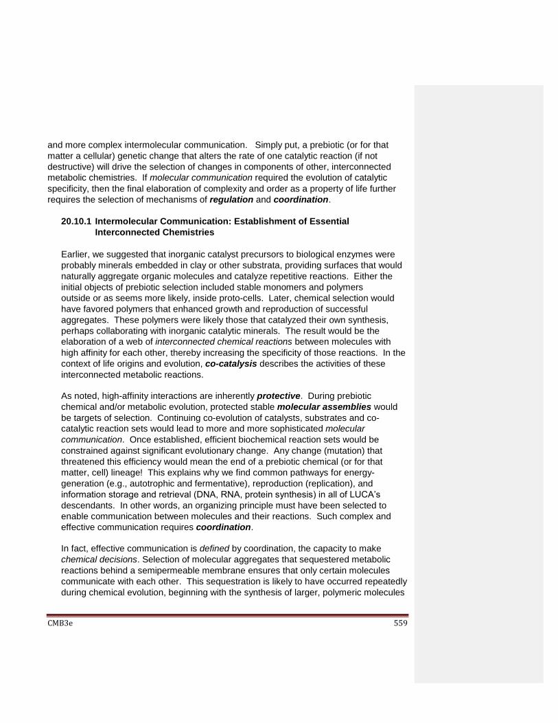
CMB3e 559

and more complex intermolecular communication. Simply put, a prebiotic (or for that

matter a cellular) genetic change that alters the rate of one catalytic reaction (if not

destructive) will drive the selection of changes in components of other, interconnected

metabolic chemistries. If molecular communication required the evolution of catalytic

specificity, then the final elaboration of complexity and order as a property of life further

requires the selection of mechanisms of regulation and coordination.

20.10.1 Intermolecular Communication: Establishment of Essential

Interconnected Chemistries

Earlier, we suggested that inorganic catalyst precursors to biological enzymes were

probably minerals embedded in clay or other substrata, providing surfaces that would

naturally aggregate organic molecules and catalyze repetitive reactions. Either the

initial objects of prebiotic selection included stable monomers and polymers

outside or as seems more likely, inside proto-cells. Later, chemical selection would

have favored polymers that enhanced growth and reproduction of successful

aggregates. These polymers were likely those that catalyzed their own synthesis,

perhaps collaborating with inorganic catalytic minerals. The result would be the

elaboration of a web of interconnected chemical reactions between molecules with

high affinity for each other, thereby increasing the specificity of those reactions. In the

context of life origins and evolution, co-catalysis describes the activities of these

interconnected metabolic reactions.

As noted, high-affinity interactions are inherently protective. During prebiotic

chemical and/or metabolic evolution, protected stable molecular assemblies would

be targets of selection. Continuing co-evolution of catalysts, substrates and co-

catalytic reaction sets would lead to more and more sophisticated molecular

communication. Once established, efficient biochemical reaction sets would be

constrained against significant evolutionary change. Any change (mutation) that

threatened this efficiency would mean the end of a prebiotic chemical (or for that

matter, cell) lineage! This explains why we find common pathways for energy-

generation (e.g., autotrophic and fermentative), reproduction (replication), and

information storage and retrieval (DNA, RNA, protein synthesis) in all of LUCA’s

descendants. In other words, an organizing principle must have been selected to

enable communication between molecules and their reactions. Such complex and

effective communication requires coordination.

In fact, effective communication is defined by coordination, the capacity to make

chemical decisions. Selection of molecular aggregates that sequestered metabolic

reactions behind a semipermeable membrane ensures that only certain molecules

communicate with each other. This sequestration is likely to have occurred repeatedly

during chemical evolution, beginning with the synthesis of larger, polymeric molecules

CMB3e 560

and possibly, an aggregation of primitive lipoidal molecules. We can think of

increasingly effective catalysis in an enclosed environment as a conversation

mediated by good speakers! Thus, coordination is a property that started with

prebiotic chemistry and likely co-evolved with life itself.

20.10.2 Origins of Coordination

Let’s look some possible structures churning around in the prebiotic chemistry set that

might have self-assembled and sequestered compatible chemistries of life. Along with

the alkaline vent biofilm compartment, coacervates, proteinoid microspheres and

liposomes have been considered as possible progenitors of biological membranes.

Each can be made in the laboratory. They are demonstrably semipermeable, and in

some cases can even replicate! The production of coacervates, proteinoid

microspheres and liposomes is summarized in Fig. 20.14.

Oparin had proposed that the action of sunlight in the absence of oxygen could cause ionized, oppositely charged organic molecules (e,g, amino acids, carbohydrates, etc.) to form droplets from organic molecules in his primordial soup. These coacervates were actually produced in 1932, visualized by microscopy and demonstarted to be a semi-permeable compartment. They even behaved as if they were able to grow and reproduce (also as Oparin originally suggested they might). In the 1950s, Sidney Fox produced proteinoid microspheres from short peptides that formed spontaneously

Fig. 20.14: Proteinoid microspheres, coacervates and liposomes can all be made in a laboratory

and are candidates for boundary structures that could have protected early prebiotic organic

molecules and reactions. Click the link at https://www.flickr.com/Candidates for Early

Coompartments to see micrographs of these synthetic compartments.

CMB3e 561

from aqueous amino acid solutions heated to dryness (not unlike what happens in the tidal pool scenario of polymer formation from organic monomers). These can be seen by light and electron microscopy. While liposomes are easily made in a laboratory, it isn’t clear that they existed on a pre-biotic earth. Nevertheless, cell membranes must have had acquired their phospholipid bilayer structure by the time of LUCA since we all have them! Prior to LUCA (perhaps in or soon after formation of our progenote), chemical rearrangements must have occurred to enable incorporation of a phospholipid bilayer into whatever starting boundary life started with. We have already considered the biofilm proposed for cellular origins in an alkaline vent. The formation of such biofilms would have separated acidic ocean protons from the interior of such protocells, creating a proton gradient. Such a gradient could have driven the early evolution of chemiososis as a means of capturing chemical energy, complete with the eventual selection of ATP synthases and the enzymes of proton transport, again because all cells descendent from LUCA posess these biochemistries.

Of course, proteinoid microspheres, coacervates, biofilm-based ‘membranes and

liposomes are not alive, and are therefore not cells. But one or another of them must

have been where the enhanced coordination of molecular communication required

for life began.

354-2 Protected Molecular Communication-Semipermeable Membranes

An important take-home message here is that whatever the original structure of the

first cells, they arose soon after the organic chemical prerequisites of life began to

acquire familiar metabolic functions. We need to see chemical and structural progress

to cellularity as concurrent metabolic evolutionary events. At some point, selection of

sequestered biochemistries led to protocells, then to the first cell or cells, each with

all of the properties of life.

Finally, selection of highly specific communication between cellular molecules allowed

cells themselves to talk to one another, engage in group activities, and eventually join

together to form multicellular organisms. Multicellularity is of course a characteristic of

many if not most eukaryotes. But watch a great TED Talk on bacterial intercellular

communication by Dr. Bonnie Bassler at Intercellular Communication in Bacteria.

20.10.3 An RNA World: Origins of Information Storage and Retrieval

Let us accept for now that molecular communication began concurrently with the

packaging of interconnected co-catalytic sets into semipermeable structures. Then

the most ‘fit’ of these structures were selected for efficient coordination of meaningful,

timely chemical messages. In the last abnalysis, coordination requires information

CMB3e 562

processing, storage and retrieval, something we recognize in Francis Crick’s

Central Dogma of information flow from DNA to RNA to protein. Cells and organisms

do coordination quite well, but what do its beginnings look like? The answer may lie in

the pre-biotic RNA world we discussed earlier. Fig. 20.15 below is a statement of The

Central Dogma, modified to account for reverse transcription and the behavior of

retroviruses.

We do not really know how cells came to rely on DNA to store, pass on and mobilize

genetic information, but we have presented reasons to believe that the first replicating

nucleic acid was RNA, creating an RNA world. Here is the evidence that leads us to

this conclusion.

Based on the stem-and-loop and other structures that form when RNA molecules

undergo internal H-bonding, we know that RNAs can take on varied and intricate

shapes.

Diverse conformations are consistent with the evolution of specificity in the

interaction of RNAs with themselves and/or with other molecules in the prebiotic

environment.

RNAs, either alone as autocatalysts (for example, self-splicing mRNAs) or in

catalytic ribonucleoprotein complexes (e.g., ribosomes) exist in cells today.

Some of these RNAs (specifically rRNAs), have a long phylogenetic heritage, shared by cells in all three domains of life.

The propensity of single stranded RNA molecules to fold based on internal H-bonding

can lead to those diverse three-dimensional shapes (tertiary structure). These

structures could have interacted with other molecules in a prebiotic environment.

Because they could be replicated according to different prebiotic scenarios, the same

Fig. 20.15: Genetic information flows from DNA to RNA to protein (the Central Dogma)

but can also flow from RNA to DNA by reverse transcription.

CMB3e 563

RNAs could also pass on simple genetic information contained in their base

sequences. The combination of informational and catalytic properties in a single

molecule is illustrated in Fig. 20.16 below.

The capacity of RNAs to be catalysts and warehouses of genetic information at the

same time speaks to an efficient candidate for the first dual or multi-purpose polymer,

a property that is not known and cannot be demonstrated for DNA. Read more about

the proposed ‘RNA worlds’ in which life may have begun in Cech TR (2012) [The RNA

Worlds in Context. In Cold Spring Harbor Perspectives in Biology (Cold Spring Harbor,

NY: Cold Spring Harbor press) 4(7):a006742e].

355 Self-Replication: Information, Communication & Coordination

20.10.4 From Self-Replicating RNAs to Ribozymes to Enzymes; From RNA to

DNA

What might RNA catalysis beyond self-replication have looked like in simpler times?

Consider the interaction between a two hypothetical RNAs and different hypothetical

amino acids bound to each (Fig. 20.17 below).

Fig. 20.16: RNA Sequences contain genetic information, and in retroviruses, they are

molecules of inheritance. As single stranded molecules, RNAs can fold into 3-dimensional

shapes, creating specific shapes that can act as catalysts (e.g., ribozymes). Thus RNAs can

combine information storage with catalytic activities.

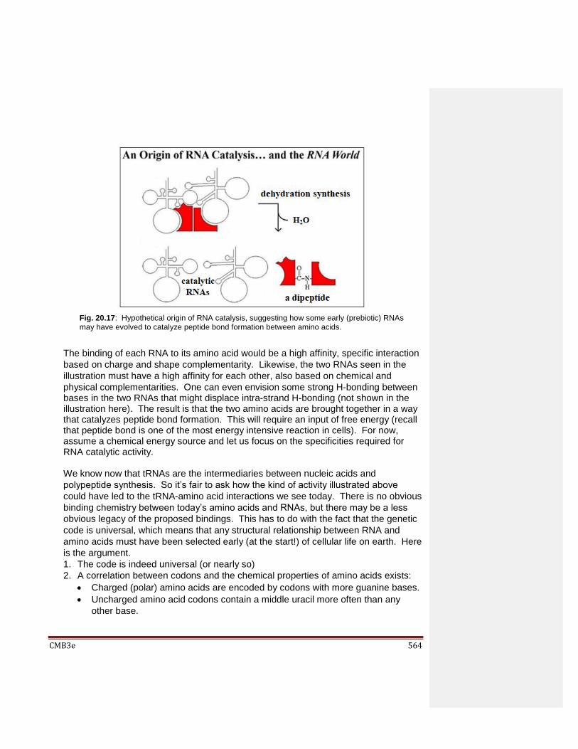
CMB3e 564

The binding of each RNA to its amino acid would be a high affinity, specific interaction

based on charge and shape complementarity. Likewise, the two RNAs seen in the

illustration must have a high affinity for each other, also based on chemical and

physical complementarities. One can even envision some strong H-bonding between bases in the two RNAs that might displace intra-strand H-bonding (not shown in the illustration here). The result is that the two amino acids are brought together in a way that catalyzes peptide bond formation. This will require an input of free energy (recall that peptide bond is one of the most energy intensive reaction in cells). For now, assume a chemical energy source and let us focus on the specificities required for RNA catalytic activity.

We know now that tRNAs are the intermediaries between nucleic acids and

polypeptide synthesis. So it’s fair to ask how the kind of activity illustrated above

could have led to the tRNA-amino acid interactions we see today. There is no obvious

binding chemistry between today’s amino acids and RNAs, but there may be a less

obvious legacy of the proposed bindings. This has to do with the fact that the genetic

code is universal, which means that any structural relationship between RNA and

amino acids must have been selected early (at the start!) of cellular life on earth. Here

is the argument.

1. The code is indeed universal (or nearly so)

2. A correlation between codons and the chemical properties of amino acids exists:

Charged (polar) amino acids are encoded by codons with more guanine bases.

Uncharged amino acid codons contain a middle uracil more often than any

other base.

Fig. 20.17: Hypothetical origin of RNA catalysis, suggesting how some early (prebiotic) RNAs may have evolved to catalyze peptide bond formation between amino acids.

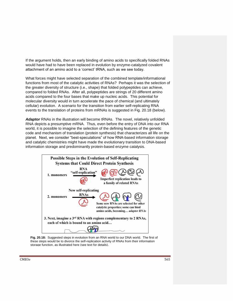
CMB3e 565

If the argument holds, then an early binding of amino acids to specifically folded RNAs

would have had to have been replaced in evolution by enzyme-catalyzed covalent

attachment of an amino acid to a ‘correct’ tRNA, such as we see today.

What forces might have selected separation of the combined template/informational

functions from most of the catalytic activities of RNAs? Perhaps it was the selection of

the greater diversity of structure (i.e., shape) that folded polypeptides can achieve,

compared to folded RNAs. After all, polypeptides are strings of 20 different amino

acids compared to the four bases that make up nucleic acids. This potential for

molecular diversity would in turn accelerate the pace of chemical (and ultimately

cellular) evolution. A scenario for the transition from earlier self-replicating RNA

events to the translation of proteins from mRNAs is suggested in Fig. 20.18 (below).

Adaptor RNAs in the illustration will become tRNAs. The novel, relatively unfolded

RNA depicts a presumptive mRNA. Thus, even before the entry of DNA into our RNA

world, it is possible to imagine the selection of the defining features of the genetic

code and mechanism of translation (protein synthesis) that characterizes all life on the

planet. Next, we consider “best-speculations” of how RNA-based information storage

and catalytic chemistries might have made the evolutionary transition to DNA-based

information storage and predominantly protein-based enzyme catalysis.

Fig. 20.18: Suggested steps in evolution from an RNA world to our DNA world. The first of

these steps would be to divorce the self-replication activity of RNAs from their information storage function, as illustrated here (see text for details).

CMB3e 566

20.10.4.1 Ribozymes Branch Out: Replication, Transcription and Translation

The term co-catalysis could very well describe biochemical reactions in which a

catalyst accelerates a chemical reaction whose product feeds back in some way

on its own synthesis. We saw this in action when we discussed allosteric enzyme

regulation and the control of biochemical pathways. Catalytic feedback loops must

have been significant events in the evolution of the intermolecular communication

and metabolic coordination required for life. Here we consider some scenarios for

the transition from an RNA world to something more recognizable as today’s

nucleic acid information storage and protein-based catalytic metabolism.

If early RNAs catalyzed their own replication, they were functioning as primitive

ribozymes. If some of these ribozymes bound and polymerized amino acids, they

may have catalyzed the synthesis of short peptides. What if some of the

polypeptides occasionally bound to their shapely catalytic RNAs and enhanced the

catalytic properties of the aggregate? What if one of these enhanced the rate of

synthesis of its own RNA, or evolved to catalyze other reactions useful to life?

Such a structure might presage the ribosome, which is a ribonucleoprotein with

catalytic properties. If later in evolution, a peptide changed just enough to

accomplish the catalysis on its own, it might dissociate from its RNA, flying solo as

a protein enzyme catalyst. This idea is illustrated below in Fig. 20.19.

Fig. 20.19: If RNAs could bind peptides whose synthesis they catalyze, evolution could

have selected ribozymes from some RNA-peptide complexes that did not separate. Later,

the peptides themselves could have evolved to take over catalytic functions from ribozymes.

CMB3e 567

Selection favoring the synthesis of short oligopeptides and polypeptides is

consistent with a catalytic diversification that led to the dominance of protein

catalysts, i.e., enzymes. The primitive enzyme shown here must have been

selected because at first, it assisted the autocatalytic replication of the RNA itself!

Over time, the enzyme would evolve along with the RNA. This co-evolution then

eventually replaced autocatalytic RNA replication with the enzyme-catalyzed RNA

synthesis we recognize as transcription today. In this scenario, self-splicing pre-

mRNAs and ribozymes are surviving remnants of an RNA world!

356 Information Storage and Retrieval in an RNA World

Let’s turn now to some ideas about how an RNA world could make the transition to

the DNA-RNA-protein world we have today.

20.10.4.2 Transfer of Information Storage from RNA to DNA

The transfer of function from RNA to DNA is by no means a settled issue among

students of life origins and early evolution. A best guess is that the elaboration of

protein enzymes begun in the RNA world would lead to reverse transcriptase-like

enzymes that copied RNA information into DNA molecules. The basic transfer

scenario is illustrated below in Fig 20.20.

Fig. 20.20: A final evolutionary scenario gets us from the RNA world to a DNA world that

governs most life on earth today.

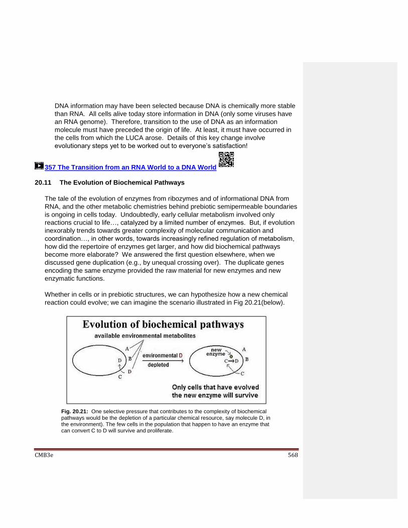
CMB3e 568

DNA information may have been selected because DNA is chemically more stable

than RNA. All cells alive today store information in DNA (only some viruses have

an RNA genome). Therefore, transition to the use of DNA as an information

molecule must have preceded the origin of life. At least, it must have occurred in

the cells from which the LUCA arose. Details of this key change involve

evolutionary steps yet to be worked out to everyone’s satisfaction!

357 The Transition from an RNA World to a DNA World 20.11 The Evolution of Biochemical Pathways

The tale of the evolution of enzymes from ribozymes and of informational DNA from

RNA, and the other metabolic chemistries behind prebiotic semipermeable boundaries

is ongoing in cells today. Undoubtedly, early cellular metabolism involved only

reactions crucial to life…, catalyzed by a limited number of enzymes. But, if evolution

inexorably trends towards greater complexity of molecular communication and

coordination…, in other words, towards increasingly refined regulation of metabolism,

how did the repertoire of enzymes get larger, and how did biochemical pathways

become more elaborate? We answered the first question elsewhere, when we

discussed gene duplication (e.g., by unequal crossing over). The duplicate genes

encoding the same enzyme provided the raw material for new enzymes and new

enzymatic functions.

Whether in cells or in prebiotic structures, we can hypothesize how a new chemical

reaction could evolve; we can imagine the scenario illustrated in Fig 20.21(below).

Fig. 20.21: One selective pressure that contributes to the complexity of biochemical

pathways would be the depletion of a particular chemical resource, say molecule D, in the environment). The few cells in the population that happen to have an enzyme that can convert C to D will survive and proliferate.

CMB3e 569

Here we are assuming that a cell acquires molecule D required for an essential

function, from an external, environmental source. What happens if levels of D in the

environment become limiting? Clearly, cells would die without enough D. That is,

unless some cells in the population already have a duplicated, redundant gene that

has mutated and now encodes an enzyme with the ability to make D in the cell. Such

a cell might have existed with other cells without the mutation, but a D-limited

environment would select the mutant cell for survival and reproduction.

358 Origins and Evolution of Biochemical Pathways

In a similar scenario, a mutation in a duplicated gene could result in a novel enzyme

activity that can convert some molecule (e.g., C or D) in the cell into a new molecular

product. If the new enzyme and molecular product do not kill or debilitate the cell, the cell

might survive to be selected by some future exigency.

20.12 A Grand Summary and Some Conclusions Our consideration of how life began on earth was intentionally placed at the end of this

textbook, after we tried to get a handle on how cells work. Clearly any understanding of

life origins scenarios is very much a matter of informed, if divergent speculations.

Alternative notions for the origins of life entertained here all address events that presaged

life under ‘best-guess’ hypothetical conditions. After trying to get a grip on prebiotic

events, we asked how we got from what could have happened under a given set of

prebiotic conditions to the cellular life we recognize today.

All proposals recognize that the first cells had all of the properties of life (including

evolution itself). Starting with that common understanding, all arguable scenarios try to

navigate pathways from primitive, less controlled chemistries to more regulated and

coordinated metabolisms, in other words from chemical simplicity to biochemical

complexity. The chemical and metabolic evolution that began before life may have

overlapped in time with cellular evolution, at least until the LUCA. While chemical

evolution was mainly a series of selections by the physicality of a prebiotic world, the

evolution of life contends with both that physical world, and with life itself. LUCA, the

universal common ancestor, had already escaped the RNA world, replicating DNA,

transcribing RNA and translating mRNAs into polypeptides, all behind a semipermeable

phospholipid bilayer. Whether a heterotroph or (increasingly more likely) an autotroph,

LUCA used the energy of ATP to power all of its cellular work, as do its descendants.

Thus, cellular evolution, in fact all life after the LUCA, is focused on continued selection of

the complexities of metabolism that enables the spread and diversification of life from

wherever it started.

CMB3e 570

The selection of chemistries and traits encoded by already existing, accumulated random neutral genetic changes, continues to this day to increase the diversity of species and their spread to virtually every conceivable ecological niche on the planet. The overall take-home message of this chapter should be an understanding of how the molecular basis of evolution can help us understand how life may have begun and been sustained on earth (or anywhere for that matter). In turn, speculation about life’s origins informs us about how the properties of life were selected under a set of reasonably likely prebiotic physical and chemical conditions.

Some iText & VOP Key Words and Terms

AATE deep sea hydrothermal vent progenote

abiogenesis Hadean eon proteinoid microsphere

adaptor RNA heat of baking protocell

alkaline hydrothermal vent heterotrophs-first reducing atmosphere

aminoadenosine triacid ester ionizing radiation retroviruses

Archean eon Last universal common ancestor ribonucleoproteins

autocatalysis liposome ribozymes

autotrophs-first LUCA RNA world

biofilm metabolic evolution Serpentinite

biogenesis molecular communication serpentinite

black smoker non-reducing atmosphere serpentinization

chemoautotrophs ozone layer spontaneous generation

chemoautotrophs Panspermia tidal pool scenario

coacervate photoautotrophs white smoker

co-catalysis primordial soup zircon

CMB3e 571

Epilogue

We began this textbook with a testimony to the marvels of what science can accomplish.

In Chapter 1 we defined the scientific enterprise as both intuitive and disciplined and

learned that the goal of learning science and its methods is to prepare us to ask creative

questions and to answer them. In Chapter 1 we learned that prebiotic chemical evolution

set the stage for life’s origins and that evolution is a key property of life itself, leading

inexorably to the incredible diversity of life on which Darwin predicated his theory. In

Chapter 1 we noted the natural role of extinction in favoring diversity… and finally, how

recent human activity accelerated the near extinction of the American bison and the final

extinction of the passenger pigeon. The role of evolution in creating diversity is

emphasized throughout the book. This is a moment to consider the threat of human

activity to life on earth that has only increased since the last known passenger pigeon

died in 1914. Here are some more recent threats.

Big cities (notably Los Angeles) had a smog problem dating back to the 1940’s. After

much resistance to evidence that auto emissions were the cause, public acceptance

came in the 1950s. Congress responded in 1963 by passing the first Clean Air Act

and set some emission standards 2 years later. In 1975 the U.S. mandated catalytic

converters on all new cars. California still has some of the worst air in the country.

But “worst” isn’t as bad as it used to be. Ozone levels in Los Angeles are just 40

percent of what they were in the mid-1970s, and that’s with more than twice the

number of cars.” (From S. Gardener (1914) https://www.marketplace.org/battle-

against-air-pollution/).

Nevertheless, Los Angeles can still show us smog, as in the photo below:

Plagues, epidemics and pandemics have been with us since ancient times. More

recent ones include a flu pandemic that may have started in Russia in 1889 that

killed an estimated million people worldwide by 1890. WW I began 24 years later,

By Diliff-Own work; CC-BY-SA 3.0, https://commons.wikimedia.org/w/index.php?curid=464376

CMB3e 572

ending in 1918 with 20 million (mostly men) dead. Then the influenza pandemic of

1918 wasted no time killing an estimated 50,000,000+ men and women worldwide,

proving once again, that nature always gets the upper hand. The 2009 swine flu

(H1N1pdm09) pandemic that killed 100,000-500,000+ people worldwide. And there

were other (e.g., SARS in 2002-03, the ‘bird flu in 2003-07) more gentle reminders

that nature can still plague us. And now we have a novel corona virus (COVID-19).

How we respond to natural challenges also impacts human life. The COVID-19

respiratory disease that surfaced in China in late 2019 drives this home. By March 11,

2020 with >250,000 infected world-wide and >10,000 dead, the World Health

Organization (WHO) called COVID-19 a pandemic. As of this writing (still in March!),

cases double every few days in some countries (Italy, Spain, France) and U.S. states

like Washington, New York and Louisiana… with predictions of worse to come.

Epidemics and pandemics still happen, but we’ve learned much since early plagues.

Recent scientific successes against COVID19 were to sequence its genome and to

develop a PCR-based test for the disease. Serological tests based on antibody-

detection of viral antigens were also quickly developed (for some details, see

https://en.wikipedia.org/wiki/COVID-19_testing).

As individuals, our social response is often to rally around our relatives, neighbors and

even strangers to help them through tough times. We bring them food and medical

supplies and keep up their spirits if they are in quarantine or physically isolated by

their illness. Unfortunately as a group or polity, we are curiously remiss, as illustrated

by some of the mis-steps and their consequences. For example, as the disease

spread rapidly in China, its sometimes secretive government slowed international

recognition of COVID19’s pandemic potential. While China seems to have contained

COVID-19, reaction to the pandemic has been variable and reluctant beyond China’s

borders. Timid governmental action in some countries has led to shortages of medical

equipment and personnel, an economic crash, looming unemployment, public

uncertainty, and ill-advised behavior (e.g., large gatherings that ignore social

COVID-19 Viral Particle: Public Domain;

https://phil.cdc.gov/Details.aspx?pid=23313

(CDC/Alissa Eckert, MS; Dan Higgins, MAMS)

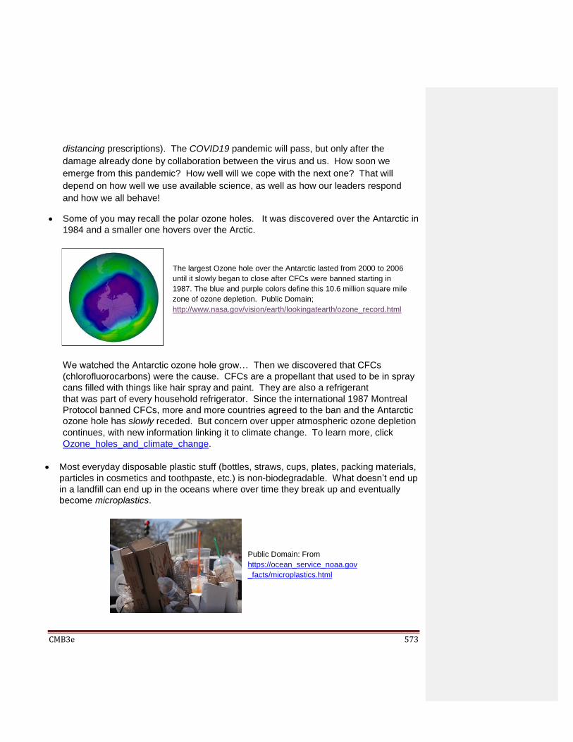
CMB3e 573

distancing prescriptions). The COVID19 pandemic will pass, but only after the

damage already done by collaboration between the virus and us. How soon we

emerge from this pandemic? How well will we cope with the next one? That will

depend on how well we use available science, as well as how our leaders respond

and how we all behave!

Some of you may recall the polar ozone holes. It was discovered over the Antarctic in

1984 and a smaller one hovers over the Arctic.

We watched the Antarctic ozone hole grow… Then we discovered that CFCs

(chlorofluorocarbons) were the cause. CFCs are a propellant that used to be in spray

cans filled with things like hair spray and paint. They are also a refrigerant

that was part of every household refrigerator. Since the international 1987 Montreal

Protocol banned CFCs, more and more countries agreed to the ban and the Antarctic

ozone hole has slowly receded. But concern over upper atmospheric ozone depletion

continues, with new information linking it to climate change. To learn more, click

Ozone_holes_and_climate_change.

Most everyday disposable plastic stuff (bottles, straws, cups, plates, packing materials,

particles in cosmetics and toothpaste, etc.) is non-biodegradable. What doesn’t end up

in a landfill can end up in the oceans where over time they break up and eventually

become microplastics.

The largest Ozone hole over the Antarctic lasted from 2000 to 2006

until it slowly began to close after CFCs were banned starting in

1987. The blue and purple colors define this 10.6 million square mile

zone of ozone depletion. Public Domain;

http://www.nasa.gov/vision/earth/lookingatearth/ozone_record.html

Public Domain: From

https://ocean_service_noaa.gov

_facts/microplastics.html

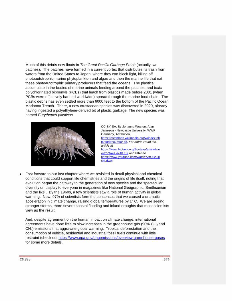
CMB3e 574

Much of this debris now floats in The Great Pacific Garbage Patch (actually two

patches). The patches have formed in a current vortex that distributes its trash from

waters from the United States to Japan, where they can block light, killing off

photoautotrophic marine phytoplankton and algae and then the marine life that eat

these photoautotrophic primary producers that feed the oceans. The plastics

accumulate in the bodies of marine animals feeding around the patches, and toxic

polychlorinated biphenyls (PCBs) that leach from plastics made before 2001 (when

PCBs were effectively banned worldwide) spread through the marine food chain. The

plastic debris has even settled more than 6000 feet to the bottom of the Pacific Ocean

Marianna Trench. There, a new crustacean species was discovered in 2020, already

having ingested a polyethylene-derived bit of plastic garbage. The new species was

named Eurythenes plasticus

Fast forward to our last chapter where we revisited in detail physical and chemical

conditions that could support life chemistries and the origins of life itself, noting that

evolution began the pathway to the generation of new species and the spectacular

diversity on display to everyone in magazines like National Geographic, Smithsonian

and the like . By the 1960s, a few scientists saw a role of human activity in global

warming. Now, 97% of scientists form the consensus that we caused a dramatic

acceleration in climate change, raising global temperatures by 10 C. We are seeing

stronger storms, more severe coastal flooding and inland droughts that most scientists

view as the result.

And, despite agreement on the human impact on climate change, international

agreements have done little to slow increases in the greenhouse gas (90% CO2 and

CH4) emissions that aggravate global warming. Tropical deforestation and the

consumption of vehicle, residential and industrial fossil fuels continue with little

restraint (check out https://www.epa.gov/ghgemissions/overview-greenhouse-gases

for some more details.

CC-BY-SA; By Johanna Weston, Alan

Jameson - Newcastle University, WWF

Germany, Attribution,

https://commons.wikimedia.org/w/index.ph

p?curid=87860438. For more, Read the

article at

https://www.biotaxa.org/Zootaxa/article/vie

w/zootaxa.4748.1.9 and listen to

https://www.youtube.com/watch?v=QBqQi

6xLdww.

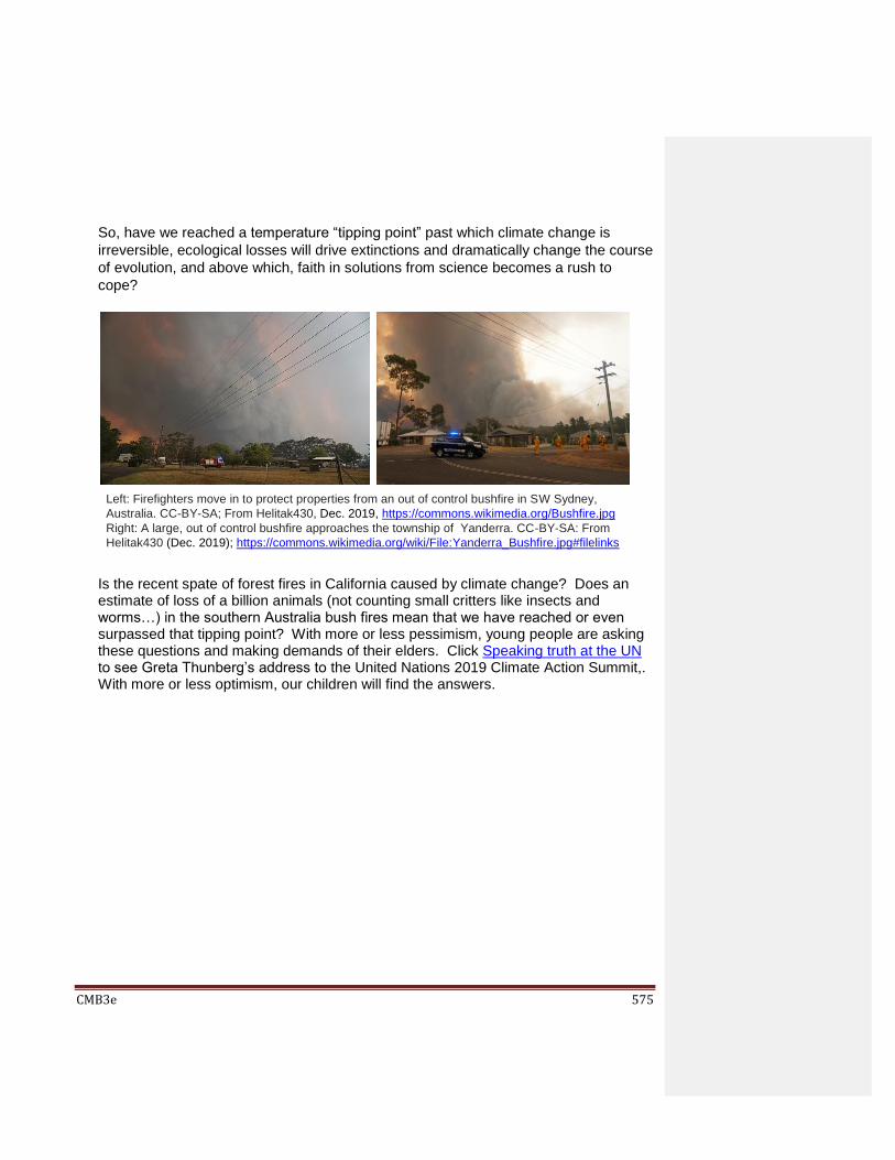
CMB3e 575

So, have we reached a temperature “tipping point” past which climate change is

irreversible, ecological losses will drive extinctions and dramatically change the course

of evolution, and above which, faith in solutions from science becomes a rush to

cope?

Is the recent spate of forest fires in California caused by climate change? Does an estimate of loss of a billion animals (not counting small critters like insects and worms…) in the southern Australia bush fires mean that we have reached or even surpassed that tipping point? With more or less pessimism, young people are asking these questions and making demands of their elders. Click Speaking truth at the UN to see Greta Thunberg’s address to the United Nations 2019 Climate Action Summit,. With more or less optimism, our children will find the answers.

Left: Firefighters move in to protect properties from an out of control bushfire in SW Sydney,

Australia. CC-BY-SA; From Helitak430, Dec. 2019, https://commons.wikimedia.org/Bushfire.jpg

Right: A large, out of control bushfire approaches the township of Yanderra. CC-BY-SA: From

Helitak430 (Dec. 2019); https://commons.wikimedia.org/wiki/File:Yanderra_Bushfire.jpg#filelinks

CMB3e 576

Appendix I: List of Figures & Sources

Chapter 1

Chapter Top-Art: Public Domain: left, R. Hooke, (1865) Micrographia’; middle, 19th century travelogue; right, Debbie

Stinson photograph from https://notesfromstillsong.blogspot.com/2012/02/eremitical-life.html ; and

https://www.pinterest.com/pin/138485757266449322/

Fig. 1.1: Evolution of three domains showing a closer relationship between archaebacteria and Eukaryotes. Illustration by G. Bergtrom Fig. 1.2: Tobacco mosaic virus symptoms on a tobacco leaf.

USDA Forest Service, http://www.forestryimages.org/browse/detail.cfm?imgnum=1402027 and

https://en.wikipedia.org/wiki/Tobacco_mosaic_virus#/media/File:Tobacco_mosaic_virus_symptoms_tobacco.jpg

Fig. 1.3: Transmission electron micrographs of giant viruses, the AIDS (HIV) virus and the bacterium E. coli. K.

casanovai is at least the same size and M. horridgei is twice the size of the bacterium. All the giant viruses, even the

mimivirus, dwarf HIV, a typical eukaryotic virus. Illustration by G. Bergtrom

Fig. 1.4: Transmission and scanning electron micrographs of the gram-negative E. coli bacterium (left and middle), with

its basic structure illustrated at the right.

CC0, From Peter Highton estate, Un. of Edinburgh:; https://commons.Wikimedia.org/w/index.php?curid=50418351

CC-0,From photo by Eric Erbe, digital colorization by Christopher Pooley at USDA, EMU, ARS (ARS materials are in

the public domain https://commons.wikimedia.org/w/index.php?curid=958857

Illustration by G. Bergtrom Fig. 1.5: Illustrated cross section of a dividing bacterium showing location of MreB cortical ring protein (purple).

Public domain; Adapted From: https://en.m.wikipedia.org/wiki/File:FtsZ_Filaments.svg

Fig. 1.6: Carboxysomes in a cyanobacterium, as seen by transmission electron microscopy. CC-BY; From:

http://en.wikipedia.org/wiki/File:Carboxysomes_EM.jpg Fig. 1.7: Scanning electron micrograph of Halobacterium salinarium, a salt-loving bacterium. CC-BY; Adapted from:

https://openi.nlm.nih.gov/imgs/512/185/3495301/PMC3495301_gbi0010-0424-f2.png

Fig. 1.8: Scanning electron micrograph of ‘heat-loving’ Thermus aquaticus bacteria. CC-0 (public domain) Adapted

From: https://upload.wikimedia.org/wikipedia/commons/4/48/Thermus aquaticus.JPG

Fig. 1.9: Illustration of the structural components of a typical animal cell. Source: Public Domain; From Mariana Ruiz,

Image: Animal cell structure.svg https://commons.wikimedia.org/w/index.php?curid=4266142

Fig. 1.10: Illustration of the structural components of a typical plant cell. Source: Public Domain; From Mariana Ruiz,

Image: Animal cell structure.svg, https://commons.wikimedia.org/w/index.php?curid=4266142 Fig. 1.11: LEFT - Transmission electron micrograph of an insect cell nucleus indicates the nucleolus(n)); RIGHT –

Illustration of a nucleus showing chromatin (purple) and pores in the nuclear envelope (orange).

Left ; From Bergtrom et al., (1977) J. Ultrastr. Res. 60:395-406: Research by G. Bergtrom

Right; CC BY 3.0; Blausen.com staff (2014). "Medical gallery of Blausen Medical 2014". WikiJ. Medicine 1(12).

DOI:10.15347/wjm/2014.010. Own work-https://commons.wikimedia.org/w/index.php?curid=28223971

Fig. 1.12: Simulated fluorescence micrograph showing the immunolocalization of antibodies against fibrillarin, coilin and

ASF/SF2 protein to nuclear bodies (nucleolus, Cajal Bodies and nuclear speckles, respectively). Illustration by G.

Bergtrom, adapted from a fluorescence micrograph in https://www.ncbi.nlm.nih.gov/pmc/articles/PMC138913/12

Fig. 1.13: Fluorescence micrograph of a mitotic spindle treated with antibodies to chromosomal proteins (blue) and

spindle fiber proteins (green). Public Domain; From: Afunguy-Transferred to Commons by Lije also using

CommonsHelper; https://commons.wikimedia.org/w/index.php?curid=5148470

Fig. 1.14: To form a polysome, ribosomes (blue) assemble at the left on an mRNA molecule. As they move along the

mRNA from left to right, they translate the message into a polypeptide (green), shown growing and emerging from

ribosomes in the polysome. Illustration by G. Bergtrom. Fig. 1.15: Transmission electron micrographs of cells from desiccated and fully hydrated Selaginella lepidophylla

plants. Free ribosomes or ribosomal subunits in the desiccated cells (LEFT) appear to have organized to form

polysomes in the hydrated plant cells (RIGHT). From Bergtrom et al. (1982) J. Ultrastr. Res 78:269-282. Research by

G. Bergtrom

CMB3e 577

Fig. 1.16: An illustration of the differences between prokaryotic and eukaryotic ribosomes; Eukaryotic ribosomes and

their subunits are larger and contain more proteins and larger ribosomal RNAs (rRNAs) than those of e.g., bacteria.

The components were separated by sucrose density gradient centrifugation in which particles and macromolecules (like

RNA) move through a sugar gradient at rates dependent on their mass (in effect, their size). Illustration by G.

Bergtrom

Fig. 1.17: Transmission electron micrograph of an insect cell showing Golgi bodies (G). Adapted from Bergtrom and

Robinson (1977) J. Ultrastr. Res. 60:395-405. Research by G. Bergtrom

Fig. 1.18: Illustration of ‘packaged’ protein traffic through a cell, from the RER to organelles (e.g., lysosomes) or to the

plasma membrane for exocytosis (i.e., secretion). RER and Golgi vesicles are major sites for the modification (i.e.,

maturation) of packaged proteins. Illustration by G. Bergtrom

Fig. 1.19: Transmission electron micrograph of mitochondria (LEFT) and drawing of a mitochondrion (RIGHT).

Electron micrograph from: Bergtrom et al. (1977) J. Ultrastr. Res. 60:395-405. Research by G. Bergtrom

Public Domain; By Mariana Ruiz Villarreal LadyofHats, https://commons.wikimedia.org/w/index.php?curid=6195050 Fig. 1.20: Transmission electron micrograph of chloroplast that could have begun photosynthesizing (LEFT), and one

that has photosynthesized long enough to accumulated starch granules (RIGHT). S, starch granule; T, thylakoids.

Left: GNU Free Documentation License; By and3k & caper437-Own work by uploaders,

https://commons.wikimedia.org/w/index.php?curid=7153916

Right: CC-BY; Transmission electron micrograph of chloroplast [T=thylakoids, S = starch] ; Adapted from PLOS one:

http://redoxbiologycenter.unl.edu/ee00b8d7-d7fc-43f8-bab9-5570b2dbd731.pdf

Fig. 1.21: Transmission electron micrograph of a leucoplast, a chloroplast that has become filled with starch granules

(S). From Bergtrom et al. J. Ultrastr. Res. 78:269-282. Research by G. Bergtrom Fig. 1.22: Illustration of assembly, structure and polarity of microtubules, microfilaments and intermediate filaments

alongside fluorescence micrographs made using fluorescent antibodies against isolated microtubule, microfilament and

intermediate filament proteins (TOP, MIDDLE and BOTTOM, respectively).

CC-BY 2.0; Adapted from: http://bmcbiochem.biomedcentral.com/articles/10.1186/1471-2091-9-23 Open Access

CC-BY-SA-2.5 and GNU.org; Adapted from https://en.wikipedia.org/wiki/media/MEF_microfilaments.jpg, By Y

Tambe (Y tambe's file) via Wikimedia Commons

CC-BY; Adapted from: www.plosone.org/article/info:doi/10.1371/journal.pone.0012115

Illustrations by G. Bergtrom

Fig. 1.23: Transmission electron micrograph showing a flagellum (#1) emerging from a basal body (2). Number 3 is

another basal body, this time in cross section. Public Domain, By Dartmouth Electron Microscope Facility, Dartmouth

College – http://remf.dartmouth.edu/imagesindex.html , https://commons.wikimedia.org/w/index.php?curid=2787228 Fig. 1.24: The characteristic “9+2” arrangement of microtubules seen in cross-sections of eukaryotic cilia and flagella is

maintained the axoneme, a structure remaining after removing the plasma membrane from isolated cilia or flagella.

Illustration by G. Bergtrom

Fig. 1.24: A cell fractionation involving disruption of cells and the isolation of sub-cellular components, including

organelles, ribosomes and a soluble fraction, the cytosol. Separation is achieved by successive centrifugations at

different speeds (centrifugal forces) that sediment subcellular structures on the basis of mass; the lowest mass

structures require the highest G-forces (fastest spin), requiring an ultracentrifuge. Illustration by G. Bergtrom Fig. 1.25: Organelles isolated by cell fractionation from eukaryotic cells.

1. CC-BY-NC-ND-SA; Adapted from Hancock, 2009:

https://openi.nlm.nih.gov/detailedresult.php?img=PMC2762040_pone.0007560.g001&query=isolated+nuclei&it=xg&re

q=4&npos=23

2. CC-BY-NC-ND-SA Adapted from Siekevitz and Palade , 1956:

https://openi.nlm.nih.gov/detailedresult.php?img=PMC2854378_JCB_201002147R_GS_Fig1&query=isolated+rough+

endoplasmic+reticulum&it=xg&req=4&npos=5

3. CC-BY-NC-ND-SA Adapted from Beznoussenko et al., 2015;

https://openi.nlm.nih.gov/detailedresult.php?img=PMC4394477_ijms-16-05299-

g005b&query=isolated+golgi+vesicles&it=xg&req=4&npos=1

4. CC-BY-NC-ND-SA; Adapted from Soubannier et al., 2012

https://openi.nlm.nih.gov/imgs/512/66/3530470/PMC3530470_pone.0052830.g001.png?keywords=absences

5. CC-BY-SA: Adapted from S. Saleh, https://commons.wikimedia.org/wiki/File:Chloroplast.jpeg

6. CC-BY-SA 4.0; Adapted from Boone et al. Isolation of Plasma Membrane from HeLa Cell,

https://www.ncbi.nlm.nih.gov/pmc/articles/PMC2107758/

7. CC-BY 2.0: From https://media.springernature.com/lw785/springer-static/image/art%3A10.1186%2F1471-2172-10-

41/MediaObjects/12865_2009_Article_261_Fig3_HTML.jpg

CMB3e 578

Chapter 2 Chapter Top-Art: Images and videos are released under the Pixabay License and may be used freely for almost any

purpose - even commercially. Attribution” mariolayaquerevalu MARIO OLAYA • Age

52 • TRUJILLO/PERU • Member since Oct. 5, 2017 Fig. 2.1: The shell (Bohr) and orbital models of atoms respectively emphasize the energy of electrons and space

occupied by the electrons moving around the atomic nucleus. Illustration by G. Bergtrom Fig. 2.2: The Periodic Table of the Elements, emphasizing those found in living things (blue, purple, green or brown).

Illustration by G. Bergtrom

Fig. 2.3: Excited electrons gain their energy by absorbing light. Absorbance of one photon causes an electron to ‘jump’

to the next shell further from the atomic nucleus. Excited electrons have potential energy that is released as the

electron returns to ground state, releasing heat or light (fluorescence). Illustration by G. Bergtrom

Fig. 2.4: Non-polar covalent bonds vs. polar covalent bonds. Illustration by G. Bergtrom

Fig. 2.5: Electrons on the H atoms of water molecules are drawn close to the large, positively charged nucleus of the O

atom. Thus, the H atoms ‘lose’ electrons and acquire a partial positive charge, while the oxygen atoms ‘gain’ those

electrons and have a partial negative charge. The resulting polar covalent water molecules attract other water

molecules. Illustration by G. Bergtrom

Fig. 2.6: Computer-generated space-filling (LEFT) and ‘ribbon’ models (RIGHT) of insulin structure. Source: CC-BY 2.5

http://commons.wikimedia.org/wiki/File:InsulinMonomer.jpg Fig. 2.7: Ionic bonds in table salt (NaCl) crystals; Opposite charges on Na

+ and Cl

- hold the ions together in a regular

crystalline array. Illustration by G. Bergtrom Fig. 2.8: Table salt (NaCl) dissolving in water. Water’s solvent properties result from its polar covalent structure,

allowing interactions with Na+

and Cl- in the crystal. Illustration by G. Bergtrom

Fig. 2.9: Charged groups on the macromolecule (e.g., protein) attract the partial charges on water molecules, hydrating

the molecule. Illustration by G. Bergtrom

Fig. 2.10: Structural and geometric isomers of hydrocarbons create molecules with the same chemical formula but

different shapes. Illustration by G. Bergtrom

Fig. 2.11: The two different generic molecules (enantiomers) are mirror images of one another. They form from

alternate arrangements of the same molecular groups around a chiral carbon. Illustration by G. Bergtrom

Fig. 2.12: Two straight chain forms of glucose (d-glucose and l-glucose) are enantiomers (optical isomers), differing in

the arrangement of the H atom and the OH group around C5. Illustration by G. Bergtrom Fig. 2.13: A generic monomer is linked to a growing polymer by water removal (dehydration synthesis); Water addition

across the linkage between monomers (hydrolysis) breaks the polymer back down to monomers. Illustration by G.

Bergtrom Fig. 2.14: Dehydration synthesis forms peptide linkage (circled); hydrolysis is the reverse reaction. Illustration by G.

Bergtrom

Fig. 2.15: When straight chain glucose forms a cyclic molecule in solution in water, C1 becomes optically active

Fig. 2.16:

energy- -d-glucose monomers polymerize to form structural

polysaccharides (starch, cellulose. Illustration by G. Bergtrom Fig. 2.17: Two enantiomers (optical isomers) of Thalidomide (R and S) form in water. Public Domain; By Vaccinationist

- (R)-(+)-Thalidomide & (S)-(−)-Thalidomide on PubChem,

https://commons.wikimedia.org/w/index.php?curid=50750574

Chapter 3 Chapter Top-Art: Attribution: Released into the public domain by Attribution: Released into the Public Domain by

Ysangkok: https://en.wikipedia.org/wiki/File:US_Beef_cuts.svg Fig. 3.1: The four orders (levels) of protein structure. Primary, secondary and tertiary structures describe polypeptides

Fig. 3.2: Chemical characteristics of the 20 amino acids found in the proteins of cells. Illustrated by G. Bergtrom

Fig. 3.3: Partial polypeptide; the amino and carboxyl ends of a polypeptide define the polarity of the molecule, with

positively charged amino and negatively charged carboxyl ends at physiological pH. Illustration by G. Bergtrom

CMB3e 579

Fig. 3.4: In the secondary structure of a polypept - -pleated sheet structures are

separated by less organized, random coil stretches of amino acids.

CC BY-SA 3.0; From: en:User:Bikadi, https://commons.wikimedia.org/w/index.php?curid=16236442

Public Domain; From: Fvasconcellos - Own work. Created by uploader upon request by Opabinia regalis,

https://commons.wikimedia.org/w/index.php?curid=1587088

CC-0 (public domain); From: Jo, H et al. BMC Structural Biology (cc-by Open Access,

http://bmcstructbiol.biomedcentral.com/articles/10.1186/s12900-014-0024-y

Fig. 3.5: Tertiary structure is created by non-covalent hydrophobic amino acid interactions as well as H-bonding in the

interior of a polypeptide, leaving charged (hydrophilic) amino acid side chains to interact with water on the exterior of a

typical “globular” protein. Stable covalent disulfide bonds between cysteine amino acids help stabilize tertiary structures.

Illustration by G. Bergtrom Fig. 3.6: Disulfide bridges form in oxidation reactions between SH (sulfhydryl) groups on cysteine amino acids

(‘residues’) in a polypeptide. Illustration by G. Bergtrom Fig. 3.7: Light micrograph of a sickled erythrocyte (red blood cell). CC BY 3.0; By OpenStax College - Anatomy &

Physiology, Connexions Web site; http://cnx.org/content/col11496/1.6/ Fig. 3.8: Mutations in a normal gene for a prion protein (PrP

c) may produce some abnormally folded prion proteins

(PrPSc

). The misfolded PrPSc

molecules interact with other (even normal) prions to mis-fold, precipitating PrPSc

proteins

into aggregated amyloid plaques. Adapted from: CC-BY-SA: M. R. Muntada (217) Prions: Special Proteins;

https://allyouneedisbiology.wordpress.com/2017/11/12/prions-special-proteins/

Fig. 3.9: Steps in the formation of -amyloid plaques. Amyloid precursor proteins (APP) are embedded in cell

membranes (upper left). Enzymes digest APP, releasing -amyloid protein fragments (middle panel). Unregulated

accumulation of -amyloid protein results in the formation of extracellular amyloid plaques.

Public Domain; By ADEAR: "Alzheimer's Disease Education and Referral Center, a service of the National Institute

on Aging." - http://www.nia.nih.gov/Alzheimers/Resources/HighRes.htm,

https://commons.wikimedia.org/w/index.php?curid=4475153

Public Domain ; By National institute on aging -

http://www.nia.nih.gov/Alzheimers/Publications/UnravelingTheMystery/Part1/Hallmarks.htm

https://commons.wikimedia.org/w/index.php?curid=3481613

Public Domain,; By National institute on aging -

http://www.nia.nih.gov/Alzheimers/Publications/UnravelingTheMystery/Part1/Hallmarks.htm ,

https://commons.wikimedia.org/w/index.php?curid=3481649 Fig. 3.10: Non-fluorescent immunostaining of tau proteins of an Alzheimer’s brain reveals tau tangles.

CC-BY-SA 3.0; From Wikimedia Commons User Patho; Neurofibrillary tangles in the Hippocampus of an old person

with Alzheimer-related pathology, immunohistochemistry for tau protein.JPG

Fig. 3.11: The formation of tau tangles occurs in diseased neurons that cannot maintain normal microtubule structure;

in the absence of stabilizing tau molecules microtubules degenerate and tau proteins clump. Public Domain; Adapted

from: https://commons.wikimedia.org/wiki/File:TANGLES_HIGH.jpg

Fig. 3.12: The vertebrate hemoglobin molecule, consisting of 4 globin subunits (two and two polypeptides). Each

globin is associated with a heme group bound to iron. GNU Free Documentation License; Adapted from:

https://en.wikipedia.org/wiki/Hemoglobin Fig. 3.13: The Pleckstrin Homology (PH) domains shown here are an example of common domains (maroon colored

sequences) in two different proteins. Because they have a PH domain, both proteins can interact with cell signaling

factors with roles in intercellular communication. CC BY-SA 3.0; By Fdardel - Own work,

https://commons.wikimedia.org/w/index.php?curid=17659815 Fig. 3.14: Screen-shot of the NCBI protein structure database leading to 3D Macromolecular structures.

http://www.ncbi.nlm.nih.gov/Structure/MMDB/docs/mmdb_search.html

Fig. 3.15: Screen-shot of NCBI protein structure database search leading to available macromolecular structures.

http://www.ncbi.nlm.nih.gov/Structure/MMDB/docs/mmdb_search.html

Fig. 3.16: Screen-shot of NCBI protein structure database search results for human insulin.

http://www.ncbi.nlm.nih.gov/Structure/MMDB/docs/mmdb_search.html

Chapter 4 Chapter Top-Art: Public Domain; https://pixabay.com/photos/space-universe-night-sky-sky-fog-11099/ (Wikiimages)

Fig. 4.1: The sum of all things contained in the universe (e.g., as mass and other, more familiar kinds of energy). In this

simple “Venn” diagram, the universe is a closed system; nothing (mass, energy) can get into or exit the universe,

consistent with the First Law of Thermodynamics. Illustration by G. Bergtrom

CMB3e 580

Fig. 4.2: Since even mass is a form of energy, the universe shown here consists of only two components, entropy and

free energy (defined as available to do work), still consistent with the First law of Thermodynamics. Illustration by G.

Bergtrom Fig. 4.3: The reciprocal relationship between entropy and free energy graphed over time. If all activities in the universe

proceed by increasing entropy, and if the universe consists only of free energy and entropy, then as entropy increases,

free energy must be decreasing in the universe. Illustration by G. Bergtrom Fig. 4.4: Basic design of a bomb calorimeter, with an inner chamber for conducting reactions, and an outer chamber

reaction. Illustration by G. Bergtrom

Chapter 5 Chapter Top-Art: Illustration by G, Bergtrom

Fig. 5.1: Illustration of the early Lock-&-Key mechanism for enzyme-substrate interaction, in which the substrate key fits

an enzyme lock. Illustration by G. Bergtrom

Fig. 5.2: The Induced Fit mechanism of enzyme-substrate interaction. Initial interaction of substrate with enzyme

based on mutual affinity causes an allosteric change in the enzyme. This results in the induced ‘better’ fit of substrate

to enzyme, to be followed by catalysis. Illustration by G. Bergtrom

Fig. 5.3: Graph of change in free energy over time as chemicals A and B react. The high Activation Energy peak in the

graph is the free energy barrier that A and B must overcome before much C and D can be made. This barrier is due

mainly to thermal motion of the A and B molecules, with only rare encounters in relatively dilute solutions. Enzymes

are even more efficient that inorganic catalysts in lowering the activation energy barrier to a reaction. Illustration by G.

Bergtrom Fig. 5.4: A generic biochemical pathway in which the final product of three enzymatic reactions accumulates. To

prevent wasteful accumulation of the final product, the pathway is regulated, in this case, when some of the

accumulating reaction product (E) binds to enzyme 1, blocking the reaction from A to form B. Illustration by G.

Bergtrom Fig 5.5: Allosteric effectors are small metabolites whose amounts in a cell reflect the cell’s metabolic status. They bind

to enzymes at a regulatory site, causing an allosteric (conformational) change in the enzyme that affects the shape of

the Active Site, either inhibiting catalysis (as suggested here) or stimulating it. Illustration by G. Bergtrom

Fig. 5.6: Saturation kinetics of an enzyme-catalyzed reaction. At high substrate concentrations, all the active sites of all

enzymes are occupied. Under these conditions, the reaction occurs at its fastest rate. Illustration by G. Bergtrom Fig. 5.7: Experimental protocol for determining the kinetics of an enzyme-catalyzed reaction. Illustration by G.

Bergtrom Fig. 5.8: This graph plots the rate of product (P) formation at 4 different substrate concentrations, while holding the

enzyme concentration constant. Illustration by G. Bergtrom Fig. 5.9: This graph shows the slopes of the initial reaction rates (red) taken from the curves in the previous graph (Fig.

5.8). Illustration by G. Bergtrom

Fig. 5.10: This graph plots the initial reaction rates (slopes, or v0) for the reactions plotted in Fig. 5.9. The formula

shown for this curve is that of a rectangular hyperbola. Illustration by G. Bergtrom

Chapter 6 Chapter Top-Art: From Evans Love - Own work, CC BY-SA 4.0, https://commons.wikimedia.org/w/index.php?curid=51014735 Fig. 6.1: The flow of free energy through life, from visible light to chemical energy (e.g., photosynthesis of glucose) to

the high energy intermediates like ATP (fermentation or respiration ) and finally to cellular work. Illustration by G.

Bergtrom Fig. 6.2: The energetics of ATP synthesis and hydrolysis. Illustration by G. Bergtrom

Fig. 6.3: Stoichiometry of glucose metabolism and ATP productions by glycolysis, the Krebs Cycle, electron transport

and oxidative phosphorylation. Illustration by G. Bergtrom

Fig. 6.4: Glycolysis: Glucose (6-C) becomes 2 pyruvates (3-C); 2 ATPs are consumed in Stage 1 but 4 are made in

Stage 2; The oxidation of glyceraldehyde -3-P marks the start of Stage 2. Illustration by G. Bergtrom

Fig. 6.5: Alternate Fates of Pyruvate: Fermentation (the anaerobic reduction to e.g., alcohol, lactate, etc.) or Respiration

(aerobic oxidation of pyruvate using oxygen as a final electron acceptor, resulting in H2O and CO2 production).

Illustration by G. Bergtrom

CMB3e 581

Fig. 6.6: In Reaction 1, phosphorylation of glucose to make glucose-6-P (G-6-P) consumes a molecule of ATP. If

cellular energy needs are being met, G-6-Pwill be polymerized to make storage polysaccharides. The G-6-P can be

retrieved by polysaccharide breakdown (hydrolysis).when the cells require nutrient energy; at that time, the G-6-P will

resume glycolysis. Illustration by G. Bergtrom Fig. 6.7: Free energy flow (exchange) for Reaction1 of glycolysis. Illustration by G. Bergtrom

Fig. 6.8: Enzymatics of the Hexokinase reaction. This enzyme catalyzes a biologically irreversible reaction and is

allosterically regulated. Illustration by G. Bergtrom

Fig. 6.9: Reaction 2 of glycolysis. G-6-P isomerase catalyzes the isomerization of G-6-P to F-6-P (i.e., the isomerization

of glucose to fructose). The reaction is endergonic and reversible. Illustration by G. Bergtrom

Fig. 6.10: Reaction 3 of glycolysis. A kinase catalyzes phosphorylation of F-6-P to F1,6-di-P in a biologically irreversible

reaction, consuming a molecule of ATP. Illustration by G. Bergtrom Fig. 6.11: Reactions 4 and 5 of glycolysis. In reaction 4, F1,6-di-P is split into dihydroxyacetone phosphate (DHAP)

and glyceraldeghyde-3-P (G-3-P) by an aldolase enzyme. In reaction 5, DHAP is isomerized to G-3-P. Both reactions

are endergonic, consuming free energy. These reactions mark the end of Stage 1 of glycolysis. Illustration by G.

Bergtrom Fig. 6.12: Reaction 6, a redox reaction catalyzed by G-3-P dehydrogenase, is freely reversible. G-3-P is oxidized to1,3

diphosphoglyceric acid (1,3 diPG), transferring electrons as a hydride (H-) ion to NAD

+ to make NADH. Illustration by G.

Bergtrom

Fig. 6.13: Reaction 7, a reversible, exergonic, coupled reaction generates ATP using free energy released by the

hydrolysis of one of the phosphates from 1,3diPG. The mechanism of ATP synthesis here is called substrate-level

phosphorylation. Illustration by G. Bergtrom

Fig. 6.14: Reaction 8 is a reversible, endergonic reaction catalyzed by a mutase. Mutases catalyze transfer of a

chemical group from one part of a molecule to another; here, 3-PG is converted to 2PG. Illustration by G. Bergtrom

Fig. 6.15: Reaction 9 is a reversible endergonic reaction. An enolase catalyzes the conversion of 2-PG to phosphoenol

pyruvate (PEP). Illustration by G. Bergtrom

Fig. 6.16: Reaction 10 is catalyzed by a kinase that transfers the phosphate on PEP to ADP to make ATP and

pyruvate. Pyruvate kinase catalyzes a coupled, highly exergonic and biologically irreversible reaction. Illustration by G.

Bergtrom

Fig. 6.17: Free energy and ATP yields of complete glycolysis (a fermentation) and incomplete glycolysis (i.e.,

respiration). Percentages represent the (efficiency of ATP production. They are based on the ratios of the free energy

captured as ATP to the free energy released by the different pathways for metabolizing glucose. Froom the data,

incomplete glycolysis is a more efficient way to extract nutrient free energy. Illustration by G. Bergtrom Fig. 6.18: Comparison of incomplete glycolysis to gluconeogenesis. The two pathways are essentially the reverse of

one another, except for the bypass enzymes in gluconeogenesis (shown in green), required to get around biologically

irreversible enzymes of glycolysis. Illustration by G. Bergtrom Fig. 6.19: The Cori cycle reveals the relationship between glycolysis and gluconeogenesis. Lactic acid produced by

complete glycolysis in active skeletal muscle goes to the liver where it could be converted to pyruvate, and then to

glucose . CC-BY-SA 3.0; From https://commons.wikimedia.org/wiki/File:Cori_Cycle.SVG and GNU Free Documentation

License User:Petaholmes, user:PDH, user:Eyal Bairey Fig. 6.20: Control of gluconeogenesis by hormones of the hypothalamic-pituitary axis. A need for glucose for energy

stimulates hypothalamic hormones that in turn stimulates the release of adrenocorticotropic hormone (ACTH) from the

pituitary gland. ACTH then stimulates release of glucocorticoids rom the adrenal glands. Glucocorticoid hormones

stimulate many tissues to control gluconeogenic glucose production as well as the use alternate nutrient fuels by many

cells in the body. Illustration by G. Bergtrom Fig. 6.21: Entry of pyruvate into mitochondrion, followed by its oxidation to acetyl-S-Coenzyme A (acetyl-S-CoA).

Illustration by G. Bergtrom Fig. 6.22: Pyruvate dehydrogenase catalyzes pyruvate oxidation to Ac-S-CoA, releasing a molecule of CO2 and

reducing NAD+ to NADH. Illustration by G. Bergtrom

Fig. 6.23: Highlights of the Krebs Cycle. The first reaction is condensation of Acv-S-CoA and oxaloacetate (OAA) to

form citric acid (citrate). Four of the reactions in the cycle are redox reactions that create reduced electron carriers

(NADH, FADH2), while one reaction is coupled to GTP synthesis by substrate level phosphorylation. Illustration by G.

Bergtrom

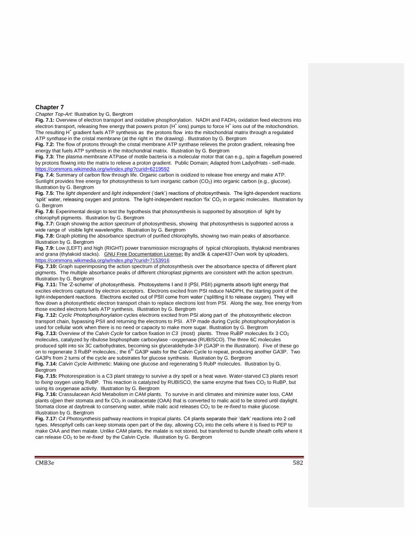
CMB3e 582

Chapter 7 Chapter Top-Art: Illustration by G, Bergtrom

Fig. 7.1: Overview of electron transport and oxidative phosphorylation. NADH and FADH2 oxidation feed electrons into

electron transport, releasing free energy that powers proton (H+ ions) pumps to force H

+ ions out of the mitochondrion.

The resulting H+ gradient fuels ATP synthesis as the protons flow into the mitochondrial matrix through a regulated

ATP synthase in the cristal membrane (at the right in the drawing) . Illustration by G. Bergtrom Fig. 7.2: The flow of protons through the cristal membrane ATP synthase relieves the proton gradient, releasing free

energy that fuels ATP synthesis in the mitochondrial matrix. Illustration by G. Bergtrom

Fig. 7.3: The plasma membrane ATPase of motile bacteria is a molecular motor that can e.g., spin a flagellum powered

by protons flowing into the matrix to relieve a proton gradient. Public Domain; Adapted from LadyofHats - self-made.

https://commons.wikimedia.org/w/index.php?curid=6219592 Fig. 7.4: Summary of carbon flow through life. Organic carbon is oxidized to release free energy and make ATP.

Sunlight provides free energy for photosynthesis to turn inorganic carbon (CO2) into organic carbon (e.g., glucose).

Illustration by G. Bergtrom Fig. 7.5: The light dependent and light independent (‘dark’) reactions of photosynthesis. The light-dependent reactions

‘split’ water, releasing oxygen and protons. The light-independent reaction ‘fix’ CO2 in organic molecules. Illustration by

G. Bergtrom

Fig. 7.6: Experimental design to test the hypothesis that photosynthesis is supported by absorption of light by

chlorophyll pigments. Illustration by G. Bergtrom

Fig. 7.7: Graph showing the action spectrum of photosynthesis, showing that photosynthesis is supported across a

wide range of visible light wavelengths. Illustration by G. Bergtrom Fig. 7.8: Graph plotting the absorbance spectrum of purified chlorophylls, showing two main peaks of absorbance.

Illustration by G. Bergtrom

Fig. 7.9: Low (LEFT) and high (RIGHT) power transmission micrographs of typical chloroplasts, thylakoid membranes

and grana (thylakoid stacks). GNU Free Documentation License; By and3k & caper437-Own work by uploaders,

https://commons.wikimedia.org/w/index.php?curid=7153916

Fig. 7.10: Graph superimposing the action spectrum of photosynthesis over the absorbance spectra of different plant

pigments. The multiple absorbance peaks of different chloroplast pigments are consistent with the action spectrum.

Illustration by G. Bergtrom Fig. 7.11: The ‘Z-scheme’ of photosynthesis. Photosystems I and II (PSI, PSII) pigments absorb light energy that

excites electrons captured by electron acceptors. Electrons excited from PSI reduce NADPH, the starting point of the

light-independent reactions. Electrons excited out of PSII come from water (‘splitting it to release oxygen). They will

flow down a photosynthetic electron transport chain to replace electrons lost from PSI. Along the way, free energy from

those excited electrons fuels ATP synthesis. Illustration by G. Bergtrom

Fig. 7.12: Cyclic Photophosphorylation cycles electrons excited from PSI along part of the photosynthetic electron

transport chain, bypassing PSII and returning the electrons to PSI. ATP made during Cyclic photophosphorylation is

used for cellular work when there is no need or capacity to make more sugar. Illustration by G. Bergtrom Fig. 7.13: Overview of the Calvin Cycle for carbon fixation in C3 (most) plants. Three RuBP molecules fix 3 CO2

molecules, catalyzed by ribulose bisphosphate carboxylase –oxygenase (RUBISCO). The three 6C molecules

produced split into six 3C carbohydrates, becoming six glyceraldehyde-3-P (GA3P in the illustration). Five of these go

on to regenerate 3 RuBP molecules.; the 6th GA3P waits for the Calvin Cycle to repeat, producing another GA3P. Two

GA3Ps from 2 turns of the cycle are substrates for glucose synthesis. Illustration by G. Bergtrom Fig. 7.14: Calvin Cycle Arithmetic: Making one glucose and regenerating 5 RubP molecules. Illustration by G.

Bergtrom

Fig. 7.15: Photorespiration is a C3 plant strategy to survive a dry spell or a heat wave. Water-starved C3 plants resort

to fixing oxygen using RuBP. This reaction is catalyzed by RUBISCO, the same enzyme that fixes CO2 to RuBP, but

using its oxygenase activity. Illustration by G. Bergtrom Fig. 7.16: Crassulacean Acid Metabolism in CAM plants. To survive in arid climates and minimize water loss, CAM

plants o[pen their stomata and fix CO2 in oxaloacetate (OAA) that is converted to malic acid to be stored until daylight.

Stomata close at daybreak to conserving water, while malic acid releases CO2 to be re-fixed to make glucose.

Illustration by G. Bergtrom Fig. 7.17: C4 Photosynthesis pathway reactions in tropical plants. C4 plants separate their ‘dark’ reactions into 2 cell

types. Mesophyll cells can keep stomata open part of the day, allowing CO2 into the cells where it is fixed to PEP to

make OAA and then malate. Unlike CAM plants, the malate is not stored, but transferred to bundle sheath cells where it

can release CO2 to be re-fixed by the Calvin Cycle. Illustration by G. Bergtrom

CMB3e 583

Chapter 8 Chapter Top-Art: Photos from left to right:

Fair use, https://en.wikipedia.org/w/index.php?curid=22197113

http://www.nobelprize.org/nobel_prizes/medicine/laureates/1958/

Public Domain, https://commons.wikimedia.org/w/index.php?curid=3677045

CC-BY https://journals.plos.org/plosbiology/article?id=10.1371/journal.pbio.0030341

Public Domain, https://commons.wikimedia.org/w/index.php?curid=15615954

Public Domain, https://commons.wikimedia.org/w/index.php?curid=15616085

Fair use, https://en.wikipedia.org/w/index.php?curid=24959067 Fig. 8.1: The experiments of F. Griffith demonstrating the existence of a chemical that could transfer a genetic trait

(i.e., virulence) between bacteria (see text for details). Illustration by G. Bergtrom Fig. 8.2: The experiments of O. Avery et al. demonstrating for the first time that the chemical stuff of genes, of

inheritance is DNA (see text for details). Illustration by G. Bergtrom

Fig. 8.3: Life cycle of a bacteriophage: The phage coat remains attached to a cell after infection, but the chemicals

inside the phage enter the infected cell. Illustration by G. Bergtrom Fig. 8.4: The experiments of Alfred Hershey and Martha Chase demonstrating that the chemical stuff of viral genes is

DNA (see text for details). Illustration by G. Bergtrom

Fig. 8.5: Photo 51, the X-Ray crystallograph of DNA taken by Rosalind Franklin revealed 3 crucial molecular

dimensions that ultimately led to the double helical DNA model. Fair Use (Ref. Wikipedia); By Source (WP:NFCC#4),

https://en.wikipedia.org/w/index.php?curid=38068629; https://en.wikipedia.org/wiki/Photo_51 Fig. 8.6: The 3 molecular dimensions from Franklin’s Photo 51 was best explained by proposing a DNA double helix

(LEFT). Model building by Watson and Crick revealed the antiparallel structure of the double helix (RIGHT).

Public domain; From: https://commons.wikimedia.org/wiki/File:DNA_double_helix_vertikal.PNG

CC BY-SA 3.0; By Madprime (talk · contribs) - Own work The source code of this SVG is valid. This vector image was created with Inkscape., https://commons.wikimedia.org/w/index.php?curid=1848174

Fig. 8.7: Three possible modes of DNA replication could be imagined. Illustration by G. Bergtrom

Fig. 8.8: Meselson and Stahl predict experimental outcomes based on 3 possible modes of DNA replication. Illustrated

by G. Bergtrom Fig. 8.9: Light micrograph of a human female chromosome stained for banding patters, showing the centromere

constriction and defining telomeres (chromosome ends). Public Domain; Adapted from National Human Genome

Research Institute; Cropped from Human male karyotype.jpg,

https://commons.wikimedia.org/w/index.php?curid=40960106 Fig. 8.10: Spread of human mitotic cell chromosomes. CC BY-SA 3.0; By Steffen Dietzel - Own work,

https://commons.wikimedia.org/w/index.php?curid=1369763 Fig. 8.11: Computer-colorized human karyotype. Public Domain; Adapted From

https://commons.wikimedia.org/w/index.php?curid=7853183C Courtesy: National Human Genome Research Institute -

Found on :National Human Genome Research (USA); copied from wikipedia:en.

Fig. 8.12: Transmission micrograph of euchromatin and heterochromatin in the nucleus. From Bergtrom et al., (1977)

J. Ultrastr. Res. 60:395-406; Research by G. Bergtrom

Fig. 8.13: Low salt fractionation of interphase nuclei yields 10nm nucleosome beads on a string.

Upper; From Bergtrom et al., (1977) J. Ultrastr. Res. 60:395-406: Research by G. Bergtrom;

Lower left; CC-BY-SA 3.0; Adapted from:

https://commons.wikimedia.org/wiki/File:Chromatin_nucleofilaments_%28detail%29.png

Fig. 8.14: High salt chromatin extraction from nuclei, or high salt treatment of 10 nm filaments yields 30 nm solenoid

structures, essentially coils of 10 nm filaments.

Electron micrograph of nucleus, From Bergtrom et al., (1977) J. Ultrastr. Res. 60:395-406: Research by G. Bergtrom

CC-BY-SA 3.0; Adapted from:

https://commons.wikimedia.org/wiki/File:Chromatin_nucleofilaments_%28detail%29.png

CC BY-SA 4.0; Alt: Adapted from: Richard Wheeler https://en.wikipedia.org/w/index.php?curid=53563761

Fig. 8.15: Five different levels (orders) of chromatin structure (see text for deatiils). CC-BY-SA 3.0; Adapted

From https://en.wikipedia.org/wiki/Chromatin.

Fig. 8.16: Short times of DNase I digestion of 10 nm filaments leaves behind shortened beads on a string. A long time

of DNase I digestion releases single nucleosomes associated with some DNA. Illustration by G. Bergtrom Fig. 8.17: Electrophoresis of nucleosomal proteins from digested 10 nm filaments reveals five different histones with the

stoichiometry shown. Illustration by G. Bergtrom

CMB3e 584

Fig. 8.18: Acid extraction of chromatin to remove histones and leave more basic non-histone proteins behind. See

original micrograph at https://www.flickr.com/photos/185778834@N06/49368658231/ Illustration by G.

Bergtrom.

Fig. 8.19: Bacterial conjugation (sex in bacteria): The F plasmid (Fertility plasmid) can transfer bacterial chromosomal

DNA from the F+ mating strain of E. coli to an opposite, F- mating strain, leading to a measure of genetic diversity.

Illustration by G. Bergtrom Fig. 8.20: Possible results of conjugation in E. coli. The F plasmid transferred from an F

+ donor cell may or may not

integrate into the F- (recipient) cell. If integration occurs, the recipient cell becomes Hfr, with a high frequency of

conjugation. Illustration by G. Bergtrom Fig. 8.21: During conjugation with Hfr donor strain cells, portions of donor chromosomal DNA follow the excised

plasmid across the conjugation bridge into the F- recipient cell. Illustration by G. Bergtrom Fig. 8.22: Map of the E. coli chromosome based on conjugation of F

- recipient cells with different strains of Hfr donor

cells indicated as Hfr 1, 2 , etc. The different Hfr donors are cells in which the Hfr plasmid integrated at different place

on a recipient cell chromosome. When these different Hfr strains transfer DNA to new F- cells, they bring along different

regions of the donor cell chromosome (and thus different genes) into their conjugated F- cells Illustration by G.

Bergtrom

Fig. 8.23: The lysogenic life cycle of phage (see text for details).Illustration by G. Bergtrom

Chapter 9 Chapter Top-Art: From CC BY-SA 2.0; By Ion Chibzii from Chisinau, Moldova. "Hands of mother”

https://commons.wikimedia.org/w/index.php?curid=12799400 Fig. 9.1: Illustration of J. Cairns’ autoradiographs of DNA extracted from E. coli cells allowed to grow on

3H- thymidine

for more than one generation of cells so that all cellular DNA would become radioactive. Silver tracks represented in

the figure are exposures of bacterial chromosomal DNA. Illustration by G. Bergtrom

Fig. 9.2: An ordering of Cairns’ autoradiograph images to suggest the progress of replication of the E. coli circular

chromosome. Illustration by G. Bergtrom

Fig. 9.3: Image of an E. coli circular chromosome with two replication forks (RFs) unwinding and replicating DNA in

both directions from an origin of replication (OR); the E. coli OR is a defined sequence. Illustration by G. Bergtrom

Fig. 9.4: Eukaryotic replication enlarges replicons that eventually merge

Fig. 9.5: DNA polymerase activity grows a DNA strand from the 5’ to 3’ direction. CC BY-SA 3.0; Adapted from: I.

Madprime, https://commons.Wikimedia.org/w/index.php?curid=2527732

Fig. 9.6: Detection of replication errors and correction by DNA polymerase proofreading. CC BY-SA 3.0; Adapted

from: I. Madprime, https://commons.Wikimedia.org/w/index.php?curid=2527732

Fig. 9.7: Initiation proteins recognize and begin unwinding the double helix by bending E. coli DNA at the OR.

Helicase then continues to unwind the DNA. SSBs (single stranded binding proteins) stabilize unwound DNA as DNA

polymerase and other enzymes begin replication in both directions away from the OR. Illustration by G. Bergtrom Fig. 9.8: 5’-to-3’ replication creates the problem at the replication fork shown here. Illustration by G. Bergtrom

Fig. 9.9: Hypothesis proposing that at least one DNA strand at a replication fork (the lagging strand) is synthesized in

pieces, each starting with an RNA primer that must be later correctly stitched together. Illustration by G. Bergtrom Fig. 9.10: Growth curves for wild type and a mutant T4 bacteriophage phage that synthesized a slow-acting DNA ligase

enzyme. This suggested that slower growth might be due to inefficient ligation of lagging strand DNA fragments made

during replication. the Illustration by G. Bergtrom

Fig. 9.11: Steps in the synthesis of DNA against the lagging template strand (see text for details). Illustration by G.

Bergtrom Fig. 9.12: A pair of replication forks (RFs), each assembling proteins and enzymes required for replication, including

DNA primases. Illustration by G. Bergtrom

Fig. 9.13: The problem with linear chromosomes is that the lagging strand at the end (telomere) of a double helix can’t

be primed and thus cannot be replicated, causing chromosome shortening at each cell division. Illustration by G.

Bergtrom

Fig. 9.14: The ribonucleoprotein enzyme telomerase resolves the dangers of chromosome shortening by using its RNA

sequence to generate repeats on the telomeric end of lagging strand DNAs (see text and illustration for details).

Illustration by G. Bergtrom

CMB3e 585

Fig. 9.15: The Processive Replication hypothesis unites all components needed to replicate both strands of DNA in a

replisome, so the both strands are replicated in the same direction. Illustration by G. Bergtrom

Fig. 9.16: Unwinding a circular DNA molecule (or any double helix that is rigidly associated with chromosomal proteins

wherever it is not replicating) causes the DNA to twist and coil on itself, a phenomenon called supercoiling. Cairns’ saw

such supercoils in E. coli chromosomes. Illustration by G. Bergtrom

Fig. 9.17: Spontaneous depurination results in hydrolytic removal of a guanine or adenine from a nucleotide, resulting

in a nucleotide deletion at that site in the DNA during replication. Illustration by G. Bergtrom

Fig. 9.18: Exposure of DNA to UV light can cause adjacent thymines to dimerize, resulting in deletion of two

nucleotides at that site in the DNA during replication. Illustration by G. Bergtrom

Fig. 9.19: -NH2 removal (deamination) of a base in one DNA strand results in a base substitution during replication.

Illustration by G. Bergtrom Fig. 9.20: Base Excision Repair mechanisms can detect and fix e.g., a deamination prior to replication (see text for

details). Illustration by G. Bergtrom Fig. 9.21: Nucleotide Excision Repair mechanisms can detect and fix e.g., a pyrimidine dimer prior to replication (see

text for details). Illustration by G. Bergtrom Fig. 9.22: DNA Mismatch Repair can detect and fix post-replication errors (i.e., mismatched base pairing (see text for

details).

CC-BY 4.0; Adapted from Kenji Fukui, https://commons.wikimedia.org/wiki/File:DNA_mismatch_repair_Ecoli.png

Illustration by G. Bergtrom

Fig. 9.23: Non-Homologous End-Joining detects and repairs double-stranded breaks in DNA, but can leave nucleotide

deletions (see text for details). Illustration by G. Bergtrom

Fig. 9.24: Single-Stranded Break Repair by Homologous Recombination can fix a break in one DNA strand when the

break is detected at a replication fork. The fix leaves an accurate repair with no deletion or base substitution (see text

for details). Illustration by G. Bergtrom Fig. 9.25: Double-Stranded Break Repair by Homologous Recombination can detect and fix a break in double stranded

breaks in DNA (see text for details). Illustration by G. Bergtrom

Chapter 10 Chapter Top-Art: Photo by G. Bergtrom

Fig. 10.1: Ribosomal RNAs and proteins in a bacterial ribosome. Illustration by G. Bergtrom

Fig. 10.2: Transfer RNA (tRNA) associated with a ribosome, held in place by codon/anticodon complementarity as well

as tRNA-ribosomal forces. Illustration by G. Bergtrom Fig. 10.3: Polysomes form along an mRNA. Multiple ribosomes can assemble at the 5’ end of an mRNA and then

sequentially translate multiple polypeptides Illustration by G. Bergtrom Fig. 10.4: Transcription - The basic Steps: Initiation is the recognition of a promoter sequence near the transcription

start site by RNA polymerase. Elongation is the successive addition of nucleotides to a growing RNA strand.

Termination occurs at the end of the gene, releasing the newly made RNA. Illustration by G. Bergtrom

Fig. 10.5: An Operon is a contiguous group of 2 or more genes that are transcribed as a single messenger RNA that

will be translated into two or more polypeptides. Illustration by G. Bergtrom

Fig. 10.6: Eukaryotic mRNAs, rRNAs and tRNAs are transcribed by different RNA polymerases and are processed by

different mechanisms to yield usable, mature RNAs. Illustration by G. Bergtrom

Fig. 10.7: Bacterial transcription requires initiation factors (i.e. factors) to help the RNA polymerase find and bind to a

gene promoter to begin transcription (see text for details). Illustration by G. Bergtrom

Fig. 10.8: After transcription has been initiated, factors soon fall away as elongation continues. Illustration by G.

Bergtrom

Fig. 10.9: rho-dependent termination of bacterial transcription involves recognition of sequences at the end of the gene

and transcript. Illustration by G. Bergtrom Fig. 10.10: rho-independent termination of bacterial transcription involves complementary bases near the end of the

transcript that form a stem/loop, or hairpin loop structure that serves as a termination signal. Illustration by G.

Bergtrom

Fig. 10.11: Comparison of transcription in prokaryotes and eukaryotes; the roles of three RNA polymerases in

Eukaryotes. Illustration by G. Bergtrom Fig. 10.12: Eukaryotic mRNA transcription initiation begins with recognition of a gene promoter (including the TATA

box) by initiation factor TFIID. The sequential association of a series of initiation factors and finally, RNA polymerase II

with the mRNA. RNA polymerase phosphorylation starts transcription. Illustration by G. Bergtrom

CMB3e 586

Fig. 10.13: 5S rRNA transcription in eukaryotes is initiated from an internal promoter by RNA polymerase III. After

binding to the promoter, the polymerase re-positions itself near the transcription start-site. Illustration by G. Bergtrom Fig. 10.14: Transcription and processing of eukaryotic mRNA. Many mRNAs in eukaryotes are encoded by split genes

containing coding regions (exons) and non-coding regions (introns). These genes are transcribed as precursor (pre-)

mRNAs that must be processed by splicing before they can be used in translation Illustration by G. Bergtrom

Fig. 10.15: Splicing of a eukaryotic pre-mRNA involves association of the primary transcript (pre-mRNA) with snRNPs,

small ribonuclear proteins that catalyze cleavage of the pre-RNA at 5’ and 3’ splice sites followed by ligation of the 3’ to

5’ exon ends. Illustration by G. Bergtrom Fig. 10.16: Formation of a spliceosome by the binding of snRNPs to an mRNA leads to hydrolysis of splice sites and

the formation of a lariat structure from the intron remnants. Illustration by G. Bergtrom

Fig. 10.17: Immunofluorescence staining with antibodies to coilin and SMN protein show that Cajal bodies and Gems

aggregate when undifferentiated cells (panels A and C) are stimulated to differentiate (panels B and D). Since

mutations in coilin and SMN proteins are associated with splicing defects, co-localization of Cajal bodies and Gems

suggests their co-involvement of snRNP function. Creative Commons Deed, NC, Attribution 2.5 Adapted from:

https://www.ncbi.nlm.nih.gov/pubmed/19735367 Fig. 10.18: Exon shuffling, transfer/copying of an exon from one gene to another, can occur by unequal recombination

(cross--over) between different genes based on regions of sequence similarity within introns. Illustration by G.

Bergtrom

Fig. 10.19: mRNA capping results from a 5’–to–5’ condensation reaction linking the 5’ end of an mRNA to a methylated

guanidine triphosphate (CH3-GTP) . Illustration by G. Bergtrom Fig. 10.20: mRNA polyadenylation; this is the addition of multiple adenine nucleotides to the 3’ end of an mRNA,

catalyzed by the enzyme poly(A) polymerase. Other than histone mRNAs, most eukaryotic mRNAs are polyadenylated.

Illustration by G. Bergtrom

Fig. 10.21: Post-transcriptional processing of the 45S rRNA encoding three of the four eukaryotic rRNAs by hydrolytic

cleavage. Illustration by G. Bergtrom

Fig. 10.22: Early (1906) low power (left) and high power (right) light micrographs of stained amphibian (salamander)

oocyte nucleolar DNA in amphibian oocytes showing the “chromatic fibers” that (resemble) a bottle brush , now called

lampbrush chromosomes because they were also reminiscent of brushes used to clean the chimneys of old-fashioned

oil lamp chimneys. We now know that the bristles are nascent strands of rRNA . For a more recent, high resolution

transmission electron micrograph, see http://www.cellimagelibrary.org/images/11043. Public Domain; O. Hertwig,

Image:O.Hertwig1906Fig2-6.jpg. & https://commons.wikimedia.org/wiki/File:O.Hertwig1906Fig5.jpg Fig. 10.23: Characteristic clustering of eukaryotic tRNA genes. Illustration by G. Bergtrom

Fig. 10.24: Structure of a yeast tRNA. Illustration by G. Bergtrom

Fig. 10.25: The assembly of ribosomal subunits and their export to the cytoplasm is coordinated with the synthesis and

association with the rRNAs and their ribosomal proteins. Illustration by G. Bergtrom Fig. 10.26: Role of CAP and poly-A binding proteins and a nuclear transport factor in the export of an mRNA to the

cytoplasm. Illustration by G. Bergtrom

Chapter 11 Chapter Top-Art: Both images are in the Public Domain; other source information not found

Fig. 11.1: The Universal RNA Genetic Code Dictionary. CC-BY-SA; From: https://en.wikipedia.org/wiki/Genetic_code

Fig. 11.2: Colinearity of genes and proteins (polypeptides) in bacteria. Illustration by G. Bergtrom

Fig. 11.3: A single-base overlapping genetic code would get more genetic information in less DNA! Illustration by G.

Bergtrom

Fig. 11.4: Nirenberg et al.’s fractionation of bacterial cell RNAs. Illustration by G. Bergtrom

Fig. 11.5: Nirenberg et al.’s reconstitution of fractionated bacterial cell RNAs. Illustration by G. Bergtrom

Fig. 11.6: Nirenberg and Leder’s experiment that led to breaking the entire genetic code. Illustration by G. Bergtrom

Fig. 11.7: Cloverleaf (LEFT) and computer-generated 3D (RIGHT) structures of a phenylalanyl- tRNA. Sources:

CC BY-SA 3.0; By Yikrazuul - Own work, https://commons.wikimedia.org/w/index.php?curid=10126790

CC-BY 3.0; Adapted from Qinhua Zhou at English Wikipedia; https://creativecommons.org/licenses/by/3.0) via

Wikimedia Commons

Fig. 11.8: A, P and E sites, mainly on the large ribosomal subunit, involved in mRNA translation. Illustration by G.

Bergtrom

Fig. 11.9: Three steps of amino acid activation (tRNA acylation) require ATP hydrolysis. Illustration by G. Bergtrom

Fig.11.10: Discovery of met-tRNA and formyl-met-tRNA, despite only one codon for methionine. Illustration by G.

Bergtrom

CMB3e 587

Fig. 11.11: Bacterial Translation Initiation: association stabilized of the small ribosomal subunit with an mRNA requires

two initiation factors (IF1 and IF3). The association is by complementary H-bonding between a region of the 16S rRNA

and the Shine-Delgarno sequence near the 5’ end of the mRNA. Illustration by G. Bergtrom Fig. 11.12: Bacterial Translation Initiation: GTP-bound IF2 enables binding of the first aminoacyl tRNA (the initiator

fmet-tRNAfmet) to the 30S ribosomal subunit/mRNA complex to create a bacterial initiation complex. Illustration by G.

Bergtrom Fig. 11.13: Bacterial Translation Initiation: addition of the large ribosomal subunit to the initiation complex, hydrolysis of

GTP and dissociation of initiation factors completes assembly of the ribosome on an mRNA. Illustration by G.

Bergtrom

Fig. 11.14: Bacterial Translation Elongation: EF2-GTP and EF3 facilitate entry of the second aminoacyl tRNA into the A

site of the ribosome to begin elongation; GTP is hydrolyzed. Illustration by G. Bergtrom Fig. 11.15: Bacterial Translation Elongation: The peptidyl transferase ribozyme (part of the ribosome) catalyzes peptide

bond formation between the fmet on its tRNAf and the second amino acid (aa2). The fmet is transferred from its tRNAf

as it condenses with an aa2 still linked to its tRNAaa2 Illustration by G. Bergtrom

Fig. 11.16: Bacterial Translation Elongation: Translocase (on the ribosome) catalyzes movement of the ribosome along

the mRNA, exposing the next codon in the A site with its attached peptidyl tRNA now in the peptidyl (P) site.

Illustration by G. Bergtrom Fig. 11.17: Bacterial Translation Termination: translocation stalls when the ribosome reaches a termination codon for

which there is no corresponding aminoacyl tRNA.. Then, GTP is hydrolyzed as a protein release factor enters A site,

causing release of the new polypeptide and dissociation of the ribosome from the mRNA. Illustration by G. Bergtrom

Chapter 12 Chapter Top-Art: Illustration by G, Bergtrom

Fig. 12.1: Transcription of the E. coli lac operon produces a single mRNA encoding three polypeptides (nicknamed ‘z’,

‘y’ and ‘a’) which is translated into 3 enzymes involved in lactose metabolism. Illustration by G. Bergtrom

Fig. 12.2: The lacZ, lacY and lacA genes of the lac operon are all controlled by the single promoter to the left of the

lacZ gene. A regulatory gene (lacI) with its own promoter lies further to the left of the lac operon. Illustration by G.

Bergtrom

Fig. 12.3: Negative regulation of the lac operon: The I gene transcribes a repressor protein. When bound to the

operator sequence (between the promoter and beginning of the Z gene), RNA polymerase is blocked and the operon

cannot be transcribed. Transcription will require derepression (i.e., removal of the repressor protein). Illustration by G.

Bergtrom

Fig. 12.4: Negative regulation of the lac operon: When present, lactose enters cells and is converted to allolactose.

Accumulating allolactose binds to the lac repressor protein. Illustration by G. Bergtrom

Fig. 12.5: Negative regulation of the lac operon: Allolactose binding causes allosteric change in the lac repressor that

then dissociates from the operator sequence, allowing RNA polymerase to transcribe the operon. Illustration by G.

Bergtrom Fig. 12.6: Positive regulation of the lac operon: If lactose is present but glucose is unavailable, the operon is

derepressed AND induced. Increased cAMP binds the Catabolite Activator Protein (CAP), which binds to the lac

operator, inducing) lac gene transcription The lac operon is maximally transcribed under these conditions. Illustration

by G. Bergtrom

Fig. 12.7: Positive regulation of the lac operon: cAMP-CAP-bound operator bends the double helix. This loosens the H-

bonds between the bases, making transcription factor access to template strands easier. Illustration by G. Bergtrom

Fig. 12.8: lac operon regulation by inducer exclusion: High glucose levels accelerate glycolysis, depleting cellular

phosphate. Low phosphate leads to the dephosphorylation of EIIAGlc, among other proteins. Dephosphorylated

EIIAGlc is an inhibitor of lactose permease (i.e., the lacA protein). Without active permease, lactose can’t get into cells,

allolactose cannot be made, and the lac gene cannot be transcribed. Illustration by G. Bergtrom

Fig. 12.9: Computer generated structure of the tetrameric lac repressor bound to DNA via helix-turn-helix motifs. CC-

BY-SA; From: http://en.wikipedia.org/wiki/Lac_repressor Fig. 12.10: Transcription of the 5-gene tryptophan (trp) operon: The 5 resulting enzymes are in the pathway for

tryptophan synthesis. A tryptophan (trp) repressor gene to the left of the operator is always transcribed. Illustration by

G. Bergtrom Fig. 12.11: When there is sufficient tryptophan in the cells, excess tryptophan binds to and changes the conformation of

the trp repressor protein, which then recognizes and binds the trp operon operator, blocking RNA polymerase and

repressing operon transcription. Illustration by G. Bergtrom

CMB3e 588

Fig. 12.12: Replacement of an egg nucleus with that from an adult cell enabled cloning of embryos and eventually

complete organisms, proving that adult cells contain all of the genes required to program development of, and to make

the organism. Illustration by G. Bergtrom

Fig. 12.13: Potentials for gene regulation in eukaryotes: Control of transcript and/or protein abundance, as well as

protein activity can regulate cellular metabolism. CC-BY-SA 3.0; Adapted From https://en.wikipedia.org/wiki/Chromatin;

Illustration by G. Bergtrom Fig. 12.14: Cis-acting sequence elements associated with a gene function as gene regulators when bound to regulatory

proteins (trans-acting factors). Regulatory sequences may be near the gene promoter (proximal) or far from it (distal).

Enhancers are examples of distal regulatory sequences. Illustration by G. Bergtrom

Fig. 12.15: Assembly of a eukaryotic transcription complex on a regulated gene. Distal regulatory protein/DNA

interactions can cause DNA bending, recruiting transcription initiation factors and proximal regulatory factors to the

transcription complex. CC BY 3.0; Adapted from Kelvinsong - Own work,

https://commons.wikimedia.org/w/index.php?curid=23272278 and

https://en.wikipedia.org/wiki/Transcription_factor#/media/File:Transcription_Factors.svg

Fig. 12.16: Three DNA binding motifs commonly found in trans-acting (i.e. regulatory) protein factors.

CC BY-SA 4.0; By Latacca - Own work, https://commons.wikimedia.org/w/index.php?curid=37140265

CC BY-SA 3.0; By Zephyris at the English language Wikipedia,

https://commons.wikimedia.org/w/index.php?curid=2426895

Public Domain; From: Boghog at en.wikipedia - Own work Public Domain,

https://commons.wikimedia.org/w/index.php?curid=15966067 Fig. 12.17: Steroid hormones regulate genes. Once in a target cell, the hormone binds a receptor either in the

nucleus, or as in this example, in the cytoplasm. An active cytoplasmic hormone-receptor complex forms and

translocates to the nucleus. Inside the nucleus, the steroid hormone receptor complex becomes transcription factor,

binding to regulatory DNA sequences to turn genes on or off or simply modulate their transcription. Illustrated by G.

Bergtrom Fig. 12.18:Large or polar signal molecules bind to membrane receptors, resulting in signal transduction, Here, a second

messenger molecule (cAMP) forms in the cytoplasm to deliver the hormonal message. A phosphorylation cascade

leads to responses including gene regulation and/or control of existing protein activity. Illustration by G. Bergtrom

Fig. 12.19: Enzyme-linked receptors transduce hormonal signals directly, activating receptor kinases on the

cytoplasmic surface of the cell, initiating phosphorylation cascades leading to any of several responses. Illustration by

G. Bergtrom Fig. 12.20: Chromatin Organization: different levels of chromatin structure result from differential association of DNA

with chromosomal proteins. CC-BY-SA 3.0; Adapted From https://en.wikipedia.org/wiki/Chromatin

Fig. 12.21: Low or high salt nuclear chromatin extraction yields 10 nm filaments or 30 nm solenoids respectively.,

From Bergtrom et al., (1977) J. Ultrastr. Res. 60:395-406: Research by G. Bergtrom; Research by G. Bergtrom

Lower left; Public Domain; from Wikimedia Commons, Electron micrograph of decondensed chromatin from chicken

erythrocytes; https://commons.wikimedia.org/wiki/File:Chromatin_nucleofilaments.png

Lower right;; Adapted from OpenStax Biology 2nd Edition, licensed under a Creative Commons Attribution 4.0

International License,

Fig. 12.22: Chemical modification of histones can open or close chromatin to transcription. CC BY-SA 1.0; By

Annabelle L. Rodd, Katherine Ververis, and Tom C. Karagiannis.

http://www.hindawi.com/journals/lymph/2012/290685/, https://en.wikipedia.org/w/index.php?curid=42441420 Fig. 12.23: Extracellular pressure (arrowheads) on a CED domain or activating spring-like arms by stretching the cell

membrane (e.g., from inside the cell (arrow) opens a piezo-linked ion channel. Illustration by G. Bergtrom

Fig. 12.24: Summary of health, birth, death and demographic records by L/. O. Bygren for the town of Överkalix

Chapter 13 Chapter Top-Art: Illustration by G, Bergtrom, and recycling bin photos courtesy of Pixabay.com; Public Domain,

https://pixabay.com/vectors/recycle-bin-container-recycling-24543/ and https://pixabay.com/vectors/recycling-container-

bin-boxes-41078/

Fig. 13.1: Bacterial guanine riboswitch: The ‘switch’ is an mRNA encoding an enzyme in the guanine synthesis

pathway. Excess guanine binds and distorts the stem-loop structure of the mRNA, causing termination of further gene

transcription. Illustration by G. Bergtrom Fig. 13.2: The array of CRISPR/Cas9 genes, spacers and other components in the genome of Streptococcus

pyogenes. Illustration by G. Bergtrom

Fig. 13.3: Phage infection triggers formation of CRISPR/Cas9 array (see text for details). Illustration by G. Bergtrom

CMB3e 589

Fig. 13.4: Phage spacers in a CRISPR/Cas9 array (derived from an earlier phage infection) protects against phage re-

infection (see text for details) . Illustration by G. Bergtrom Fig. 13.5: Anatomic illustration of the roundworm Caenorhabditis elegans. CC-BY 2.5 J.D. McGhhee (2007) The C.

elegans intestine, Worm Book -The Online Review of C. elegans Biology;

http://www.wormbook.org/chapters/www_intestine/intestine.html

Fig. 13.6: Mechanism of action of siRNA (small interfering RNA) defense against foreign DNA (see text for details).

Illustration by G. Bergtrom

Fig. 13.7: Mechanism of action of miRNA (micro RNA) in degrading unwanted (e.g., old or damaged ) RNA (see text

for details). Illustration by G. Bergtrom

Fig. 13.8: Review of the steps in translation initiation (see text for details). Illustration by G. Bergtrom

Fig. 13.9: Regions and specific sequences known to be involved in regulating translation. Illustration by G. Bergtrom

Fig. 13.10: Specific inhibition of ferritin polypeptide synthesis by iron regulatory proteins. Illustration by G. Bergtrom

Fig. 13.11: Regulation of globin mRNA Translation initiation by hemin, a heme precursor (see text for details)

Illustration by G. Bergtrom

Fig. 13.12: Role of GCN2 kinase in regulating translation by phosphorylating initiation factor eIF2B, preventing

formation of an initiation complex (see text for details). Illustration by G. Bergtrom

Fig. 13.13: Multiple short open reading frames (uORFs) found in the 5’ untranslated region (5’UTR) of GCN4 mRNA

play a role in regulating its translation. Illustration by G. Bergtrom

Fig. 13.14: GCN4 translation is reduced when cellular amino acid levels are normal (see text for details). Illustration by

G. Bergtrom Fig. 13.15: GCN4 translation is highest when cellular amino acid levels are reduced (amino acid starvation). GCN4

then regulates the expression of many genes, including those encoding enzymes needed for amino acid synthesis (see

text for details). Illustration by G. Bergtrom

Fig. 13.15: Mechanism of ubiquitin and proteasome action in the removal/destruction of old and damaged proteins in

cells, and the recycling of their amino acids (see text for details). Illustration by G. Bergtrom

Chapter 14 Chapter Top-Art: Public Domain

Fig. 14.1: Renaturation kinetics protocol: Double-stranded (ds)DNA is mechanically sheared to ~10Kb fragments,

heated to denature the DNA, then cooled to let single strands find their complements and renature. Illustration by G.

Bergtrom Fig. 14.2: Plot of rat dsDNA formed over time during renaturation of denatured DNA. Illustration by G. Bergtrom

Fig. 14.3: The 3 ‘phases’ of the curve in Fig. 14.2 highlighted to identify the 3 fractions of repeated and almost unique

DNA sequences in the rat genome. Illustration by G. Bergtrom

Fig. 14.4: Plot of E. coli dsDNA formed over time during renaturation of denatured DNA. Illustration by G. Bergtrom

Fig. 14.5: DNA complexity revealed by plotting rat and E. coli DNA renaturation kinetics as the percent of re-

associated dsDNA over CoT (Concentration of re-associated dsDNA X Time). Illustration by G. Bergtrom

Fig. 14.6: Experimental demonstration of satellite DNA in low CoT renaturation kinetic fractions (see text for details).

Illustration by G. Bergtrom

Fig. 14.7: Life-style of maize.

Left, CC-BY-SA 3.0: From https://commons.wikimedia.org/wiki/File:Corntassel_7095.jpg ; By Spedona

(en:Image:Corntassel 7095.jpg) via Wikimedia Commons

Middle, CC-BY-SA 3.0; From: https://commons.wikimedia.org/wiki/File:Cornsilk_7091.jpg ; By The original uploader

was Pollinator at English Wikipedia [GFDL (http://www.gnu.org/copyleft/fdl.html] via Wikimedia Commons

Right, CC-BY 3.0; From: Kiesselbach, T. A. https://commons.wikimedia.org/wiki/File:Double_Fertilization.jpg ,By The

original uploader at English Wikipedia (Transferred from en.wikipedia to Commons, via Wikimedia Commons

Fig. 14.8: Mosaic corn cobs. GNU Free Documentation License, V. 1.2 https://en.wikipedia.org/wiki/Maize

Fig. 14.9: Experimental cross of females with CCbzbz triploid genotype with males having a C’C’BzBzDsDs genotype

with progeny genotypes and phenotypes based on Mendelian assumptions. Illustration by G. Bergtrom Fig. 14.10: Triploid genotypes expected the cross in Fig.14.9 (see text for details). Illustration by G. Bergtrom

Fig. 14.11: McClintock’s interpretation of the results of the triploid cross shown in Fig.14.9 ( see text for details).

Illustration by G. Bergtrom

Fig. 14.12: Structure of a bacterial IS element (see text for details). Illustration by G. Bergtrom

Fig. 14.13: Structure of a bacterial Tn element (see text for details). Illustration by G. Bergtrom

CMB3e 590

Fig. 14.14: Structure of a complex transposon (Mu phage - see text for details). Illustration by G. Bergtrom

Fig. 14.15: Life cycle options for bacteriophage (see text for details). Illustration by G. Bergtrom

Fig. 14.16: The transposon option for Mu Phage (see text for details). Illustration by G. Bergtrom

Fig. 14.17: Structure of a eukaryotic Class II DNA transposon (see text for details). Illustration by G. Bergtrom

Fig. 14.18: Cut-&-paste transposition of a DNA transposon (see text for details). Illustration by G. Bergtrom

Fig. 14.19: Replicative transposition of a DNA transposon (see text for details). Illustration by G. Bergtrom

Fig. 14.20: Structure of yeast Ty, an RNA LTR retrotransposon (see text for details). Illustration by G. Bergtrom

Fig. 14.21: Structure of a LINE, a non-LTR retrotransposon (see text for details). Illustration by G. Bergtrom

Fig. 14.22: Structure of the Alu SINE, a non-LTR retrotransposon , or retroposon (see text for details). Illustration by

G. Bergtrom

Fig. 14.23: Extrachromosomally-primed transposition of a LINE (see text for details). Illustration by G. Bergtrom

Fig. 14.24: Target-primed transposition of a LINE (see text for details). Illustration by G. Bergtrom

Fig. 14.25: Alignment of consensus amino acid sequences of bacterial IS transposases with Mu phage and Tc1 mariner

transposases reveals conservation of D, D and E amino acids (upper case) at key positions in the sequence. Other

amino acids are shared between some but not all of the sequences (lower case). Slashes are variable gaps in the

alignments. Adapted from https://www.researchgate.net/publication/11063189_Presence_of_a_Characteristic_D-D-

E_Motif_in_IS1_Transposase Fig. 14.26: Comparison amino acid sequences of the COPIA retrotransposon and a retroviral (HIV) integrase with

typical transposase sequences. The alignments reveal conservation of the D, D and E amino acids in the DDE domain

of the enzymes. Other amino acids are shared between some but not all of the sequences (lower case). Slashes are

variable gaps in the alignments. Adapted from

https://www.researchgate.net/publication/11063189_Presence_of_a_Characteristic_D-D-E_Motif_in_IS1_Transposase Fig. 14.27: Retroviral and retrotransposon reverse transcriptases share a common evolutionary ancestor. Tree drawn

by G. Bergtrom, based on data from Nakamura et al. 1997 and Eickbush 1994 Fig. 14.28: Steps of paired DNA transposon-mediated exon shuffling (see text for details). Illustration by G. Bergtrom

Chapter 15 Chapter Top-Art: Public Domain NASA .gov image; https://commons.wikimedia.org/wiki/File:First-

ever_sequencing_of_DNA_in_space,_performed_by_Kate_Rubins_on_the_ISS._128f0462_sequencer_1.jpg Fig. 15.1: Retroviral infection requires reverse transcriptase to make a copy (cDNA) the viral genome, which will then

replicate and reproduce new viruses. Illustration by G. Bergtrom

Fig. 15.2: Most eukaryotic mRNAs have poly(A) tails; Poly(A) RNA is isolable by oligo d(T) chromatography.

Illustration by G. Bergtrom

Fig. 15.3: Reverse transcriptase supplied with deoxynucleotides, mRNAs and an oligo d(T) primer will catalyze

synthesis of DNA copies (cDNAs) of the mRNAs. Illustration by G. Bergtrom

Fig. 15.4: The first cDNA strand often forms a loop at its 3’ end that can serve as a primer to synthesize a (ds)cDNA.

Reverse transcriptase is also a DNA polymerase, and can catalyze 2nd

strand synthesis. Illustration by G. Bergtrom Fig. 15.5: Bacterial restriction endonucleases (REs) recognize and hydrolyze ‘foreign’ DNA (e.g., phage DNA),

blocking infection; most REs cut DNA at specific short DNA sequences; often leaving staggered ends. Illustration by G.

Bergtrom

Fig. 15.6: Preparing cDNAs for insertion into plasmid vectors prior to cloning cDNAs sequences (see text for details);

Illustration by G. Bergtrom

Fig. 15.7: Making recombinant plasmids containing cDNA inserts (see text for details). Illustration by G. Bergtrom

Fig. 15.8: Making the cDNA library (see text for details). Illustration by G. Bergtrom

Fig. 15.9: Only cells containing plasmids will grow on agar containing ampicillin since the plasmids contain an

ampicillin resistance gene (see text for details). Illustration by G. Bergtrom Fig. 15.10: Replica plating creates a filter replica of colonies from one agar plate to be grown on another plate, e.g.,

containing ‘selective’ media containing for example an antibiotic that screens for recombinant plasmids (see text for

details). Illustration by G. Bergtrom

Fig. 15.11: Replica filters are lysed in situ (in place), leaving partially denatured DNA (including recombinant plasmid

DNA) from the colonies where the cells used to be. Filters can be probed for a sequence of interest. Illustration by G.

Bergtrom Fig. 15.12: A denatured, sequence-specific probe can be used to probe lysed replica filters for a sequence of interest,

here detected as a radioactive colony (see Fig. 15.12 and text for details). Illustration by G. Bergtrom Fig. 15.13:. X-ray exposure of a replica filter incubated earlier with radioactive probe. The developed autoradiograph

shows a dark spot where probe hybridized to colony DNA (see text for details). Illustration by G. Bergtrom

CMB3e 591

Fig. 15.14: Chemical structure of a di-deoxynucleotide. Illustration by G. Bergtrom

Fig. 15.15: The four tubes in a manual DNA sequencing protocol contain the same ingredients, except that each

contains a different di-deoxynucleotide. Illustration by G. Bergtrom Fig. 15.16: Cartoon of results of the four different manual sequencing reactions. The dideoxy-terminated DNA

fragments are electrophoresed to read the sequence of a DNA (see Fig 15.16). Illustration by G. Bergtrom

Fig. 15.17: Drawing of a manual dideoxy sequencing autoradiograph with a readable sequence. Illustration by G.

Bergtrom

Fig. 15.18:. Automated DNA sequence chromatograph readout. CC BY 3.0; Adapted from Intechopen book (Book

chapters are distributed under the Creative Commons Attribution 3.0) https://www.intechopen.com/books/nucleic-acids-

from-basic-aspects-to-laboratory-tools/nucleic-acid-isolation-and-downstream-applications

Fig. 15.19:.Overview of shotgun sequencing of DNA. CC-0 (Public domain, By İnfoCan, from Wikimedia Commons);

https://commons.wikimedia.org/wiki/File:DNA_Sequencing_gDNA_libraries_tr.jpg

Fig. 15.20: Basics of Nanopore DNA Sequencing, one of several ‘next gen’ sequencing technologies. See text for

details. Illustration by G. Bergtrom

Fig. 15.21:.Overview of Southern blotting, a technique that transfers electrophoresed DNA to a filter for hybridization

with a probe (see text for details). Illustration by G. Bergtrom

Fig. 15.22:.Genomic DNA restriction enzyme digest is mixed with phage vector with compatible ‘sticky’ ends and ligated

to make recombinant DNAs. Illustration by G. Bergtrom

Fig. 15.23:.Mixing recombinant phage DNA with phage coat proteins creates infectious recombinant phage particles.

Illustration by G. Bergtrom Fig. 15.24:.Recombinant phage infection, the replication of phage DNA and production of new phage leads to host cell

lysis, allowing the collection of new recombinant phage. Illustration by G. Bergtrom Fig. 15.25:.Phage plaques formed on a bacterial lawn; each plaque is a genomic clone. Illustration by G. Bergtrom

Fig. 15.26:.Replica filters of plaques probed with a sequence of interest (in this case a globin DNA sequence) locates

autoradiographic spots where probe hybridized to recombinant phage. Illustration by G. Bergtrom

Fig. 15.27: Progress of a PCR reaction: at the end of the second PCR cycle, the strands of DNA that will be

geometrically amplified in succeeding PCR cycles have been synthesized. Illustration by G. Bergtrom

Fig. 15.28: Agarose gel electrophoresis of PCR amplified DNAs, stained with ethidium bromide to be detectable under

fluorescent light: PCR products of the amplification of a globin gene clone from the insect Chironomus thummi. The

sizes (lengths in base pairs) of the 4 PCR products in lanes 2-5 are close to those of the bands in the standard DNA

size ladder in lane 1. Adapted from Kao et al. (1994), J. Mol. Evol. 38: 241-249. Research by G. Bergtrom Fig. 15.29: Electrophoretic DNA fingerprint. Public domain; By James Tourtellotte, photo editor of CBP Today[1],

http://www.cbp.gov/xp/cgov/newsroom/multimedia/photo_gallery/afc/laboratories/13_5flab_5fhiresa.xml (file

Cbp13_5flab_5fhires.jpg, part of America's Frontline Photography / CBP Laboratories Photography),

https://commons.wikimedia.org/w/index.php?curid=2875876 Fig. 15.30: Simulated glass slide microarray showing multiple color fluorescent spots, indicating a hunt for more than

one DNA sequence at the same time. Illustration by G. Bergtrom

Chapter 16 Chapter Top-Art: Public Domain; https://pixabay.com/photos/lion-mosaic-art-museum-berlin-510159/

Fig. 16.1: Space-filling model showing components of a phospholipid. CC-BY; Adapted from OpenStax Biology 2nd

Edition, licensed under a Creative Commons Attribution 4.0 International License, Fig. 16.2: Examples of common membrane phospholipids. Public Domain CC-0 1.0: Adapted from

https://commons.wikimedia.org/w/index.php?curid=63827468

Fig. 16.3: Phospholipid bilayer membrane. Public Domain; Adapted from Mariana Ruiz Villarreal, LadyofHats - Own

work, https://commons.wikimedia.org/w/index.php?curid=3032610

Fig. 16.4: Low and high magnification Transmission electron micrographs of trilamellar membrane structure.

Public domain; Adapted from: http://en.wikipedia.org/wiki/History_of_cell_membrane_theory By Sandraamurray Fig. 16.5: Model of the eukaryotic plasma membrane demonstrating asymmetry, with a sugarless cytoplasmic surface

and a glycoprotein rich extracellular surface. Public domain, from:

https://commons.wikimedia.org/wiki/File:Cell_membrane_detailed_diagram_en.svg or

https://upload.wikimedia.org/wikipedia/commons/thumb/d/da/Cell_membrane_detailed_diagram_en.svg/877px-

Cell_membrane_detailed_diagram_en.svg.png By LadyofHats.

Fig. 16.6: Illustration of a scanning electron micrograph of freeze-fractured plasma membrane with pits and mounds

showing on opposing phospholipid layers of the membrane. Illustration by G. Bergtrom

CMB3e 592

Fig. 16.7: Fluorescent antibodies against human and mouse membrane proteins localize their cell surface antigens

(i.e., proteins) on opposite poles of recently fused cells. Illustration by G. Bergtrom Fig. 16.8: Immunofluorescent human (green) and mouse (red) membrane proteins diffuse and mix over time in fused

cells. Illustration by G. Bergtrom Fig. 16.9: Factors affecting membrane fluidity (i.e. rate of diffusion of membrane components). Illustration by G.

Bergtrom Fig. 16.10: Illustration of a micelle. Public domain; Adapted from:

https://upload.wikimedia.org/wikipedia/commons/c/c6/Phospholipids_aqueous_solution_structures.svg Fig. 16.11: A liposome is a synthetic lipid bilayer that can be formed from micelles. Public domain; Adapted from:

https://upload.wikimedia.org/wikipedia/commons/c/c6/Phospholipids_aqueous_solution_structures.svg

Fig. 16.12: Properties of plasma membranes may be different in ways determined by cell-cell associations during tissue

development. Lavender, green and blue regions indicate basic differentiation of a sheet of epithelial cells. Illustration by

G. Bergtrom Fig. 16.13: Integral membrane proteins may penetrate or span the membrane; Also shown are peripheral proteins and

lipoproteins. Illustration by G. Bergtrom Fig. 16.14: Integral transmembrane proteins cross the membrane one or more times. Illustration by G. Bergtrom

Fig. 16.15: Hydrophobic amino acids of glycophorin form a helix that spans the red blood cell plasma membrane.

Illustration by G. Bergtrom

Fig. 16.16: Hydropathy plot s correlate the degree of amino acid hydrophobicity with its position in a polypeptide. Long

regions of hydrophobic amino acids suggest a possible membrane protein domain Illustration by G. Bergtrom Fig. 16.17: Examples of the many functions of membrane proteins. Illustration by G. Bergtrom

Fig. 16.18: The glycocalyx is the sugar- rich region on the extracellular surface of cells, the result of covalently bound

sugars on glycoproteins and glycolipids. It is the basis of many cell functions and is associated with other

macromolecules to form an extracellular matrix. CC-BY; Adapted from: http://cnx.org/The Glycocalyx with Illustration by

G. Bergtrom

Fig. 16.19: The extracellular matrix (ECM) forms when proteins (e.g., fibronectin, collagen) and other macromolecules

(e.g., proteoglycans) associate non-covalently with membrane proteins and elements of the glycocalyx. CC-BY; From:

http://cnx.org/Extracellular Matrix

Fig. 16.20: Blood groups with membrane proteins and elements of the glycocalyx (see text for details). Public domain;

Adapted from InvictaHOG - Own work, Public Domain, https://commons.wikimedia.org/w/index.php?curid=1088507

Chapter 17 Chapter Top-Art: Illustration by G. Bergtrom and Public Domain: https://pixabay.com/illustrations/traffic-lights-traffic-

light-phases-2147790/ Fig. 17.1: Graph plotting rates of passive and facilitated transport show that facilitated diffusion is a saturable process.

Illustration by G. Bergtrom Fig. 17.2: Three kinds of facilitated diffusion (see text for details). Illustration by G. Bergtrom

Fig. 17.3: Facilitated transport proteins (e.g., glucose transporter) undergo sequential allosteric changes as they

recognize a solute (e.g., glucose) and then transfer and release it on the other side of the membrane. Illustration by G.

Bergtrom

Fig. 17.4: Effects of differences in solute concentrations inside and outside animal cells on the movement of water into

or out of the cells, i.e., Osmosis (see text for details). Illustration by G. Bergtrom

Fig. 17.5: Osmotic effects of differences in solute concentrations inside and outside plant cells on the movement of

water into or out of the cells, i.e., Osmosis (see text for details). Correct cytoplasmic solute concentrations are achieved

by accumulating excess water in the tonoplast. Illustration by G. Bergtrom

Fig. 17.6: Plasmodesmata are cell wall ‘tunnels’ connecting plat cells that allow direct movement of water between

cells to transmit and balance changes in osmotic pressure in one part of a plant (e.g., roots) throughout the plant (see

text for details). Illustration by G. Bergtrom

Fig. 17.7: Light micrograph of Paramecium highlighting a contractile vacuole, an organelle that pumps out excess

water from the cell, protecting it from osmotic shock. CC-BY-SA 3.0; From:

http://commons.wikimedia.org/wiki/File:Paramecium_caudatum_Ehrenberg,_1833.jpg

Fig. 17.8: The resting potential of a cell results from an ionic concentration imbalance across the plasma membrane.

Sodium and chloride ions concentrations are higher inside cells while potassium ions are at higher levels outside the

cell. Thus, the cytoplasm is slightly negative compared to the extracellular fluid. Illustration by G. Bergtrom Fig. 17.9: After a change in the resting potential (e.g., depolarization) of a cell, the ion balance across the cell

membrane is restored by an ATP-powered sodium/potassium pump (see text for details). Illustration by G. Bergtrom

CMB3e 593

Fig. 17.10: A patch clamp device can measure ion flow through voltage-gated channels in a membrane during a

depolarization event.(see text for details). Illustration by G. Bergtrom Fig. 17.11: Voltage changes across e.g., a muscle cell membrane during an action potential correlated with the flow of

specific ions, determined with the patch clamp device (see text for details). Illustration by G. Bergtrom Fig. 17.12: Neurotransmission starts with an action potential in the cell body of a neuron. The resulting action potential

is propagated down the axon to the nerve terminal synapse. The depolarization pulse initiates Ca++ flow into the

neuron through voltage-gated channels that eventually cause neurotransmitter release into the synaptic cleft between

the neuron and the responding cell. The neurotransmitter binds to a ligand gated channel on the responding cell,

causing Na+ ions to flow into the responding cell, leading to an action potential (see text for details). Illustration by G.

Bergtrom

Fig. 17.13: Illustration of three main kinds of endocytosis, routes/mechanisms of import of extracellular materials into

cells (see text for details). Illustration by G. Bergtrom

Fig. 17.14: Illustration of the stages of receptor-mediated endocytosis (see text for details).. Drawn by G. Bergtrom

based on http://www.zoology.ubc.ca/~berger/b200sample/unit_8_protein_processing/images_unit8/14_18.jpg

Fig. 17.15: Molecular details of receptor-mediated endocytosis (see text for details). Illustration by G. Bergtrom

Fig. 17.16: A low-density lipoprotein coated with cholesterol (see text for details). Illustration by G. Bergtrom

Fig. 17.17: Rough endoplasmic reticulum (RER), Golgi and other vesicles participate in the trafficking of proteins

destined for secretion or vesicular packaging/storage in the cell (see text for details). Illustration by G. Bergtrom

Fig. 17.18: Determining the role of RER in the synthesis of secretory and other packaged protein synthesis (see text

for details). Illustration by G. Bergtrom Fig. 17.19: Molecular details (steps) of the Signal Hypothesis (see text for details). Illustration by G. Bergtrom

Fig. 17.20: Integral membrane-spanning proteins have one or more very hydrophobic stop transfer signals in addition

to their signal sequence. Such membrane proteins cross the membranes one or more times during their synthesis.

Illustration by G. Bergtrom Fig. 17.21: Sorting and directing the traffic of secreted, vesicular and other proteins in cells (see text for details).

Illustration by G. Bergtrom Fig. 17.22: Nuclear proteins made in the cytoplasm contain a positively charged nuclear localization signal. This signal

binds to the electronegative region of a nuclear transport receptor that then binds nuclear pore fibrils, guiding the

protein into the nucleus. Illustration by G. Bergtrom Fig. 17.23: Nuclear proteins destined for mitochondria are synthesized with an N-terminal mitochondrial signal

sequence that is removed by a mitochondrial signal peptidase. Since polysomes do not attach to mitochondria, a

different mechanism engages the N-terminal signal with membrane proteins required for transfer (see text and figure for

details). Illustration by G. Bergtrom Fig. 17.24: Tight, Gap and Adherens junctions between animal cells involve different membrane proteins (see text for

details).

Public domain (all drawings); Top left, https://commons.wikimedia.org/wiki/File:Cellular_tight_junction-en.svg; Middle,

https://commons.wikimedia.org/wiki/File:Gap_cell_junction-en.svg; Top right,

https://en.wikipedia.org/wiki/Adherens_junction;

CC BY-SA 2.5 Lower left micrograph adapted from Eric Yale Hayden,

https://commons.wikimedia.org/w/index.php?curid=6223080;

Public domain; Middle https://en.wikipedia.org/wiki/Gap_junction#/media/File:Annular_Gap_Junction_Vesicle.jpg,

CC-BY-SA; http://www.cellimagelibrary.org/images/7620 (M. Farquhar & G.E. Palade (1963) J. Cell Biol. 17:375-

412.) Fig. 17.25: Glycocalyx protein interactions; roles in cell-cell recognition and attachment. Illustration by G. Bergtrom

Fig. 17.26: LEFT, Transmission electron micrograph of a Melanoma cell exosomes (bar, 100nm). Some of the larger

vesicles show an irregular, cup-like shape (arrows). RIGHT: Transmission electron micrograph of a reticulocyte

endosome containing exosomes about to fuse with the plasma membrane (bar, 200 nm.

CC-BY-NC-SA 3.0 https://www.ncbi.nlm.nih.gov/pmc/articles/PMC3575529/

CC-BY-NC-SA 3.0 https://www.ncbi.nlm.nih.gov/pmc/articles/PMC3575527/

Fig. 17.27: Migration and attachment of cells during development requires the synthesis of membrane proteins that will

recognize and bind proteins on the membranes and glycocalyx of other cells, forming cell junctions and enabling tissue

formation. At the same time, the specificity of these membrane proteins prevents incorrect cell-cell associations.

Integrin is an early cell membrane protein ‘receptor’ that interacts with many proteins to form a glycocalyx and then

respond to cell-surface proteins of other cells. Illustration by G. Bergtrom

CMB3e 594

Fig. 17.28: Density-dependent inhibition (aka. Contact Inhibition) occurs when cells multiplying and spreading on a

surface cease dividing when there is no more room on the surface. Cancer cells have lost the property of contact

inhibition and keep growing over one another in layers. Loss of contact inhibition is correlated with an absence of gap

junctions in cancer cells. Illustration by G. Bergtrom Fig. 17.29: Signal transduction by effectors (e.g., hormones) can lead to many different effects in the cytoplasm as well

as in nuclei. Illustration by G. Bergtrom Fig. 17.30: G-proteins cycle between bound GTP and bound GDP. They are intermediates in signal transduction

between an active, effector-bound membrane receptor and adenylate cyclase (see text for details of the different steps).

Illustration by G. Bergtrom

Fig. 17.31: The fight-or-flight response to adrenalin (adrenalin rush): cAMP activates protein kinase A; a

phosphorylation cascade leads to the release of glucose into the circulation (see text for details). cAMP is a second

messenger of signal transduction for many different cellular responses. Illustration by G. Bergtrom

Fig. 17.32 G-proteins also mediate signal transduction through different membrane receptors and different enzymes, as

well as protein kinase C. These interactions generate different 2nd messenger molecules that lead to a phosphorylation

cascade and many different responses in different target cells (see text for details of the steps). Illustration by G.

Bergtrom

Fig. 17.33: The effects of MAP kinase include phosphorylation and activation of DNA-binding transcription factors and

other nuclear proteins that lead to cell proliferation. Illustration by G. Bergtrom

Chapter 18 Chapter Top-Art: Public Domain; https://pixabay.com/vectors/lifting-box-wood-heavy-crate-24401/ Fig. 18.1: Fluorescence micrograph of the mitotic spindle treated with antibodies to chromosomal proteins (blue) and

spindle fiber proteins (green). Public Domain; From: Afunguy-Transferred to Commons by Lije also using

CommonsHelper; https://commons.wikimedia.org/w/index.php?curid=5148470 Fig. 18.2: Illustration of assembly, structure and polarity of microtubules, microfilaments and intermediate filaments

alongside fluorescence micrographs made using fluorescent antibodies against isolated microtubule, microfilament and

intermediate filament proteins (TOP, MIDDLE and BOTTOM, respectively).

CC-BY 2.0; Adapted from: http://bmcbiochem.biomedcentral.com/articles/10.1186/1471-2091-9-23 Open Access

CC-BY-SA-2.5 and GNU.org; Adapted from

https://en.wikipedia.org/wiki/Cytoskeleton#/media/File:MEF_microfilaments.jpg Y Tambe (Y Tambe's file) via

Wikimedia Commons

CC-BY; Adapted from: www.plosone.org/article/info:doi/10.1371/journal.pone.0012115

Illustrations by G. Bergtrom

Fig. 18.3: Illustration and immunofluorescence microscopic localization of microtubules, microfilaments and

intermediate filaments in cells.

Public domain; From: https://en.wikipedia.org/wiki/Fluorescence_microscope

CC-BY-SA 3.0From: http://en.wikipedia.org/wiki/Vimentin#mediaviewer/File:VIMENTIN.JPG By Simon Caulton

Fig. 18.4. Transmission electron micrograph of the characteristic 9 triplet microtubule array of centrioles and basal

bodies. From: Chernov et el. (2008) BMC Biochemistry2008; 9:23: Public Domain;

http://commons.wikimedia.org/wiki/File:Spindle_centriole; _embryonic_brain_mouse_-_TEM.jpg Fig. 18.5: Starting mitotic anaphase, spindle fiber microtubules exert forces that separate and pull chromatids apart

and also push the poles of the cell apart (see text for details). Illustration by G. Bergtrom

Fig. 18.6: Disrupting a kinetochore spindle fiber demonstrates a strong force from microtubule disassembly that quickly

pulls a pair of chromatids towards centrioles. Illustration by G. Bergtrom Fig. 18.7: Transmission electron micrographs of a basal body (LEFT) and cross-sections of a pair of 9+2 microtubule

arrays (RIGHT) as they would emerge from a basal body.

Public domain; From: http://en.wikipedia.org/wiki/File:Chlamydomonas_TEM_09.jpg as per:

http://remf.dartmouth.edu/imagesindex.html

Public domain; From: http://en.wikipedia.org/wiki/File:Chlamydomonas_TEM_17.jpg as per:

http://remf.dartmouth.edu/imagesindex.html

CMB3e 595

Fig. 18.8: Transmission electron micrographs of axonemes show that microtubules are made up of a ring of 13 tubulins

(LEFT). Microtubules in cilia or flagella are arranged in typical 9+2 arrays (MIDDLE). The enlarged cross-section

illustrates specific microtubule-associated proteins (MAPs) that maintain the 9+2 structure, including dynein motors

that powers motility.

CC-BY 4.0; Adapted from: http://bmcbiochem.biomedcentral.com/articles/10.1186/1471-2091-9-23 Public domain;

From: http://en.wikipedia.org/wiki/File:Chlamydomonas_TEM_17.jpg as per:

http://remf.dartmouth.edu/imagesindex.html

Illustration of axoneme components by G. Bergtrom Fig. 18.9: Roles of dynein and kinesin in retrograde (backwards) and anterograde (forward) movement of cargo

vesicles along microtubules (see text for details). CC-BY; Adapted from J.E. Duncan & L.S.B. Goldstein (2006) The Genetics of Axonal Transport and Axonal Transport

Disorders, PLOS Cognitive Neuroscience Channel at https://doi.org/10.1371/journal.pgen.0020124

Fig. 18.10: Removing the membrane from isolated cilia or flagella leaves behind the axoneme; when provided ATP,

both the isolated structures and demembranated axoneme will beat as the ATP hydrolyzed. Illustration by G. Bergtrom Fig. 18.11: Detergents can dissociate axonemes into individual and doublet microtubules. Dialysis of separated

microtubules to remove the detergent cause the microtubules to re-associate (reconstitute) into a sheet with

connections resembling those seen in intact axonemes.. Illustration by G. Bergtrom Fig. 18.12: Comparison of ciliary beat with propeller like generation of flagellar wave motion (see text for details).

CC-BY 3.0; From: http://en.wikipedia.org/wiki/File:Flagellum-beating.svg Fig. 18.13: Light micrograph of skeletal muscle stained to showing characteristic striations. CC-BY: From OpenStax:

Anatomy and Physiology; https://openstax.org/books/anatomy-and-physiology/pages/10-1-overview-of-muscle-tissues Fig. 18.14: Skeletal muscle organization and the anatomy of a muscle cell sarcomere (see text for details).

CC-BY 4.0; From: https://commons.wikimedia.org/wiki/File:1007_Muscle_Fibes_(large).jpg By OpenStax via

Wikimedia Commons

CC-0 (Public Domain) From: http://upload.wikimedia.org/wikipedia/commons/a/a4/Sarcomere.gif By User:Sameerb

(en:WP; Author User:Sameerb in English WP) , via Wikimedia Commons

Fig. 18.15: Transmission electron micrograph and a corresponding illustration showing sarcomere shortening,

consistent with the sliding of filaments during skeletal muscle contraction.

CC-BY-SA 4.0 (LEFT); From: https://www.mrgscience.com/topic-112-movement.html

GNU FDL (RIGHT); Adapted from https://upload.wikimedia.org/wikipedia/commons/6/6e/Sarcomere.svg By

Richfield, David (2014). "Medical gallery of David Richfield". WikiJournal of Medicine 1 (2).

DOI:10.15347/wjm/2014.009. ISSN 2002-4436 (GFDL licensure: http://www.gnu.org/copyleft/fdl.html),from Wikimedia

Commons

Fig. 18.16: The skeletal muscle Contraction Paradox: Given ATP, glycerinated muscle fibers contract and pull a weight.

When all the ATP is hydrolyzed the fiber can’t stretch unless more ATP is added. Illustration by G. Bergtrom Fig. 18.17: Overview of the isolation of actin thin filaments (still on Z-Lines) from myosin thick filaments. Illustration by

G. Bergtrom

Fig. 18.18: Reconstitution of actin thin filaments (on Z-Lines) with myosin filaments. Illustration by G. Bergtrom

Fig. 18.19: Structure of a skeletal muscle myosin filament and the myosin monomer. Shown is myosin II, the thick

filament that spans both sides of the H zone in a sarcomere (upper). The head-&-tail structure of a myosin monomer is shown in the high magnification electron micrograph and is illustrated in the cartoon (lower). The myosin monomer is itself a polymer of four polypeptides.

CC-BY 4.0; Adapted from http://plosbiology.org/article/info%3Adoi%2F10.1371%2Fjournal.pbio.0020356 By D. Hostetter et al. (2004) PLoS Biology

CC-BY 4.0; Adapted from: Adapted from http://journals.plos.org/plosone/article?id=10.1371/journal.pone.0093272 By H. Sugi et al. (2014) PLOS One; PLoS ONE 9(6): e93272; doi:10.1371/journal.pone.0093272

Illustrations by G. Bergtrom Fig. 18.20: Digestion of purified myosin monomers with enzymes that hydrolyze peptide bonds between specific amino

acids produces an S1 head and a tail fraction with different properties.

CC-BY 4.0; Adapted from http://journals.plos.org/plosone/article?id=10.1371/journal.pone.0093272 , By H. Sugi et al.

(2014) PLOS One; PLoS ONE 9(6): e93272; doi:10.1371/journal.pone.0093272

Illustrations by G. Bergtrom

Fig. 18.21: Illustration of myosin decoration by myosin monomer S1 fragments, showing opposing polarity of actin

filaments on opposite sides of the Z-line. Illustration by G. Bergtrom

CMB3e 596

Fig. 18.22: Steps in the Micro-contraction Cycle explain the muscle contraction paradox (see text for details).

Illustration by G. Bergtrom Fig. 18.23: The ability of flexible myosin heads to bend and change conformation is consistent with their proposed

activity during the micro-contraction cycle. CC-BY 4.0; Adapted from http://journals.plos.org/plosone/article?id=10.1371/journal.pone.0093272 By H. Sugi et al. (2014) PLoS ONE 9(6): e93272; doi:10.1371/journal.pone.0093272 Fig. 18.24: Innervation leads to Ca++ release from sarcoplasmic reticulum to regulate contraction (see text for details).

CC-BY 4.0; From S. Guarnieri et al. (2013) https://doi.org/10.1371/journal.pone.0053267 and

https://journals.plos.org/plosone/article?id=10.1371/journal.pone.0053267#pone-0053267-g006

CC-BY4.0; https://opentextbc.ca/anatomyandphysiology/chapter/10-2-skeletal-muscle/

Overlay text and illustration by G. Bergtrom Fig. 18.25: Skeletal muscle thin filaments consist of actin associated with troponins and tropomyosin. These actin-

associated proteins participate in the response to Ca++ ions to regulate interactions with myosin.

Public domain; Adapted from: https://upload.wikimedia.org/wikipedia/commons/thumb/a/a3/Myofilament.svg/994px-

Myofilament.svg.png Fig. 18.26: Ca++ ions initiate uncovering myosin binding sites on actin by binding to troponin-C, resulting in allosteric

changes in the troponins and ultimately tropomyosin. Illustration by G. Bergtrom

Fig. 18.27: Structure of titin and its location in the sarcomere (see text for details)

CC-BY 4.0: Colorized micrograph of titin adapted from Zsolt Mártonfalvi and Miklós Kellermayer (2014):

http://journals.plos.org/plosone/article?id=10.1371/journal.pone.0085847

Illustration by G. Bergtrom

Fig. 18.28: Elasticity of skeletal muscle shown by the location of anti-N2A-linked and anti-120/122-linked nanogold

particles in sarcomeres. Note the increased separation of the PEVK domains targeted by the antibodies as a muscle

fiber is increasingly stretched. This titiin elasticity facilitates skeletal muscle relaxation. [Copyrighted free use; Adapted

from https://commons.wikimedia.org/w/index.php?curid=764619, By User:Sameerb (en:WP; Author User:Sameerb in

English WP), via Wikimedia Commons. Adaptations included adding simulated nanogold particles and elongating parts

of the sarcomere to create an image replicating results of work from the laboratory of Wolfgang Linke. Fig. 18.29: In the anti-actin immunofluorescence micrograph of fibroblasts, actin localizes with stress fibers which help

maintain cell shape (LEFT). Actin also localizes in lamellipodia and retraction fibers in migrating fibroblasts (RIGHT),

orienting in the direction of movement.

Adapted from CC BY-SA 3.0 https://commons.wikimedia.org/w/index.php?curid=378394 By Y Tambe - Y Tambe's file

Illustration by G. Bergtrom Fig. 18.30: The molecular structure of stress fibers; myosin as well as other actin-binding proteins interact with actin in

non-muscle cell motility. Illustration by G. Bergtrom Fig. 18.31: Coiled secondary structure of the proteins permits elasticity of intermediate filament bundles that contribute

to the viscosity of cytoplasm. Illustration by G. Bergtrom

Chapter 19 Chapter Top-Art: Public Domain: https://pixabay.com/photos/microscope-sea-urchin-egg-splitting-1276131/

Fig. 19.1: Bacteria divide by binary fission. When growing in culture, they divide continually, partially replicating their

circular DNA molecules during one division in preparation for the next. Illustration by G. Bergtrom Fig. 19.2: Mitosis and cytokinesis in eukaryotic cells are separated in time, and mitosis is further divisible into 5

phases. Illustration by G. Bergtrom Fig. 19.3: First experiment demonstrating that replication and cell division in eukaryotes are separate events. (see text

for details). Illustration by G. Bergtrom

Fig. 19.4: The autoradiographic data from the experiment outlined in Fig. 19.3 demonstrates that DNA synthesis

begins and ends some time before the beginning of mitosis. Illustration by G. Bergtrom

Fig. 19.5: These autoradiographs from a pulse-chase labeling experiment led to the identifying the phases of the

eukaryotic cell cycle (see text for explanation). Illustration by G. Bergtrom Fig. 19.6: Graph plotting the number of radioactive cells in mitosis over time of chase in the pulse-chase experiment

described in Fig. 19.5 (see text for explanation). Illustration by G. Bergtrom

Fig. 19.7: A typical eukaryotic cell cycle: phases G1, S and G2 follow cytokinesis, and G2 immediately precedes

prophase of mitosis. The length of time for each phase differs for different cell types. Illustration by G. Bergtrom

Fig. 19.8: Terminally differentiated cells no longer divide, entering the Go state. While they can sometimes resume

cycling, such cells more typically experience cell death and replacement by stem cells. Illustration by G. Bergtrom

CMB3e 597

Fig. 19.9: Experiment leading to the discovery of meiosis-promoting factor (MPF), the first known chemical regulator of

cell division. Illustration by G. Bergtrom Fig. 19.10: MPF was shown to be a two-subunit protein kinase that transfers phosphates from ATP to several different

proteins. Illustration by G. Bergtrom Fig. 19.11: Graph comparing plots of cellular cdk and cyclin levels over time with one of MPF activity (see text for

details). Illustration by G. Bergtrom Fig. 19.12: Cell fusion experiments revealed additional chemical regulators of the cell cycle activity (see text for details).

Illustration by G. Bergtrom Fig. 19.13: Simplified diagram of cell cycle checkpoints at which progress through the cycle is assessed. If progress

through a phase is incomplete, cell cycle regulators (kinases) delay onset of the next phase (see text for details).

Illustration by G. Bergtrom Fig. 19.14: Apoptotic Cells: In the 3 electron micrographs and corresponding illustrations, normal cells (A & A’) are

followed by apoptotic cells [B & B’] and [C & C’]. In [B & B’], a black arrowhead indicates nuclear condensation

(pyknosos), membrane blebbing (grey arrowheads) and apoptotic bodies (white arrowhead). In [C & C’] the nucleus

has broken down (karyorrhexis) and the cell itself cell has fragmented into apoptotic bodies (white arrowheads). In C’,

a phagocyte is engulfing one of them.

Electron micrographs, CC-BY; Adapted from: V. Wilhelmi et al. (2013) Zinc Oxide Nanoparticles Induce Necrosis and

Apoptosis in Macrophages in a p47phox- and Nrf2-Independent Manner.

https://journals.plos.org/plosone/article?id=10.1371/journal.pone.0065704

Illustrations: Public Domain; File adapted from a German Wikipedia entry:

https://commons.wikimedia.org/wiki/File:Apoptosis.png or http://de.wikipedia.org/wiki/Bild:Apoptose-german.png

Fig. 19.15: Biochemical steps of apoptosis, or programmed cell death (see text for details). Illustration by G. Bergtrom

Fig. 19.16: Comparison of the cellular events of apoptosis and necrosis. Public Domain; Adapted from National Institute

on Alcohol Abuse and Alcoholism (NIAAA) via Wikimedia Commons;

https://commons.wikimedia.org/wiki/File:Structural_changes_of_cells_undergoing_necrosis_or_apoptosis.png Fig. 19.17: Results of non-cancer cell divisions in which abnormal cells are targeted for apoptosis, and cancer cell

division, in which damaged or altered cells escape apoptotic controls. Illustration by G. Bergtrom Fig. 19.18: Making knockout mutant mice. Specific nucleotides in a cloned gene of interest are altered by site-directed

mutagenesis. The altered gene is inserted into embryonic stem cells where it recombines with and replaces the

homologous gene already in the chromosome. Recombinant clones are selected re-injected into embryos that are then

incubated in the uteri of ‘foster mother’ mice. Knockout mice in the newborn litter can be selected and studied for the

effects of removing a gene. Illustration by G. Bergtrom Fig. 19.19: Structure of the P53 gene-regulatory protein bound to DNA. P53 was originally called a tumor suppressor

protein because when mutated, tumors arose. CC-BY-SA 3.0; From Thomas Splettstoesser, via Wikimedia Commons

https://upload.wikimedia.org/wikipedia/commons/b/bb/P53.png

Fig. 19.20: Normal function of the P53 gene-regulatory protein (see text for details). Illustration by G. Bergtrom

Fig. 19.21: Role of the P53 in decision-making at cell cycle checkpoints (see text for details). Illustration by G.

Bergtrom Fig. 19.22: Summary of different roles of p53 protein in protein degradation and apoptosis, cell cycle progress and DNA

repair (see text for details). Illustration by G. Bergtrom

Chapter 20 Chapter Top-Art: Public Domain photos; https://pixabay.com/illustrations/sperium-cum-sperm-dark-winner-

326157/ and https://pixabay.com/photos/halloween-pumpkin-scary-giant-309296/

Fig. 20.1: Descent (evolution and speciation) from a single progenitor cell formed by abiogenesis on a prebiotic earth.

Illustration by G. Bergtrom Fig. 20.2: Descent (evolution and speciation) from multiple ‘first cells’. Illustration by G. Bergtrom Fig. 20.3: Evolutionary (i.e., phylogenetic) tree of all living organisms, showing descent from the Last Universal

Common Ancestor (LUCA) of the 3 domains of life (Bacteria, Archaea and Eukaryota). Public Domain; Adapted from: https://en.wikipedia.org/wiki/Phylogenetic_tree Fig. 20.4: Classic Miller & Urey experiment showing that organic molecules found in living things today could be

synthesized in a laboratory under reducing conditions similar to those expected for a prebiotic earth atmosphere. Illustration by G. Bergtrom Fig. 20.5: Scenario for the synthesis of prebiotic polymers in tidal pools. Illustration by G. Bergtrom

CMB3e 598

Fig. 20.6: Scenario for the synthesis of redundant prebiotic nucleic acid polymers in tidal pools. Illustration by G.

Bergtrom Fig. 20.7: Analysis of this Australian zircon supports an oxidizing atmosphere on a prebiotic earth.

Valley, J. W. et al. (2014) Hadean age for a post-magma-ocean zircon confirmed by atom-probe tomography, Nature

Geoscience vol. 7, p 219-223; http://dx.doi.org/10.1038/ngeo2075; Used by permission of JW Valley, University of

Wisconsin - Madison; http://geoscience.wisc.edu/geoscience/people/faculty/ john-valley/john-valley-incle-on-zircons/

Fig. 20.8: An oceanic volcanic hydrothermal vent, or black smoker. Public domain:

https://oceanservice.noaa.gov/facts/vents.html

Fig. 20.9: An oceanic volcanic hydrothermal vent, or White smoker. Public domain:

http://oceanexplorer.noaa.gov/explorations/04fire/logs/hirez/champagne_vent_hirez.jpg Fig. 20.10: Serpentinite from Deer Lake in upper Michigan. It is a mineral also found in the oceanic crust that under

conditions found in an alkaline vent, can form methane from CO2 . Public Domain, USGS publication. From Bornhorst &

Johnson (1993). Geology of volcanic rocks in the south half of the Ishpeming Greenstone Belt, Michigan. USGS

Bulletin 1904-P. 13 pp.; http://www.jsjgeology.net/Deer-Lake-Peridotite.htm

Fig. 20.11: Evolutionary (i.e., phylogenetic) tree of all living organisms reveals 3 domains of life: Bacteria (Prokarya),

Archaebacteria (archaea) and Eukaryotes (Eukaryota). Public Domain; Adapted from: https://en.wikipedia.org/wiki/Phylogenetic_tree Fig. 20.12: Aminoadenosine triacid ester (AATE) catalyzes its own replication by the mechanism suggested here.

Illustration by G. Bergtrom Fig. 20.13: The deamination of adenine in a ribonucleotide chain to inosine in a tRNA by the adenine deaminase

enzyme. Illustration by G. Bergtrom

Fig. 20.14: Proteinoid microspheres, coacervates and liposomes can all be made in a laboratory and are candidates

for boundary structures that could have protected early prebiotic organic molecules and reactions.

Illustration by G. Bergtrom

Fig. 20.15: Genetic information flows from DNA to RNA to protein (the Central Dogma) but can also flow from RNA to

DNA by reverse transcription. Illustration by G. Bergtrom

Fig. 20.16: RNA Sequences contain genetic information, and in retroviruses, they are molecules of inheritance. As

single stranded molecules, RNAs can fold into 3-dimensional shapes, creating specific shapes that can act as catalysts

(e.g., ribozymes). Thus RNAs can combine information storage with catalytic activities. Illustration by G. Bergtrom Fig. 20.17: Hypothetical origin of RNA catalysis, suggesting how some early (prebiotic) RNAs may have evolved to

catalyze peptide bond formation between amino acids. Illustrated by G. Bergtrom Fig. 20.18: Suggested steps in evolution from an RNA world to our DNA world. The first of these steps would be to

divorce the self-replication activity of RNAs from their information storage function, as illustrated here (see text for details). Illustration by G. Bergtrom Fig. 20.19: If RNAs could bind peptides whose synthesis they catalyze, evolution could have selected ribozymes from

some RNA-peptide complexes that did not separate. Later, the peptides themselves could have evolved to take over

catalytic functions from ribozymes. Illustration by G. Bergtrom Fig. 20.20: A final evolutionary scenario gets us from the RNA world to a DNA world that governs most life on earth

today. Illustration by G. Bergtrom Fig. 20.21: One selective pressure that contributes to the complexity of biochemical pathways would be the depletion of

a particular chemical resource, say molecule D, in the environment). The few cells in the population that happen to have

an enzyme that can convert C to D will survive and proliferate. Illustration by G. Bergtrom

CMB3e 599

Appendix II: Context-Embedded YouTube Videos Chapter 1: Cell Tour, Life’s Properties and Evolution, Studying Cells

100-2 The RER-Rough Endoplasmic Reticulum

101 Ribosomes and Polysomes

102 Golgi Vesicles and the Endomembrane System

103-2 Smooth Endoplasmic Reticulum104-2 The Nucleus

105-2 Endosymbiosis-Mitochondria & Chloroplasts

106-2 Filaments & Tubules of the Cytoskeleton

107-2 Dissecting the Cell-a Cell Fractionation Scheme

108-2 Isolated Nuclei

109-2 Isolated RER

110-2 Isolated Golgi Vesicles

111-2 Lysosomes & Peroxisomes

112-2 Isolated Mitochondria

113-2 Isolated Chloroplasts

114-2 Isolated Membranes Form Vesicles

115 Properties of Life

116 The Universal Genetic Code

117 Origins of Life

118 Life Origins vs Evolution

119 The Random Basis of Evolution

120-2 Genomic Fossils-Molecular Evolution

121-2 Electron Microscopy

Chapter 2: Basic Chemistry, Organic Chemistry and Biochemistry

122-2 Atoms and Elements

123 Electron Energy and Fluorescence

124 Covalent Bonds

125-2 Water-Hydrogen & Ionic Bonds

126 Organic Molecules Monomers and Polymers

127-2 Carbohydrates-Sugars & Polysaccharides

CMB3e 600

128-2 Lipids-Triglycerides-Phospholipids

129-2 Proteins-Amino Acids & Polypeptides

130-2 DNA & RNA-Nucleotides & Nucleic Acids

131-2 Shape & the Specificity of Molecular interactions

Chapter 3: Details of Protein Structure

132-2 Amino Acid Sequence & Protein Primary Structure

133-2 Protein Secondary Structure

134-2 Protein Tertiary structure

135-2 Disulfide Bridges Stabilize 3o Structure

136-2 Protein Quaternary Structure & Prosthetic Groups

137-2 Protein Domain Structure &Function

Chapter 4: Bioenergetics

138 Different Kinds of Energy; Chemical Equilibrium

139 First Law of Thermodynamics

140-2 Second Law of Thermodynamics

141 Deriving Closed System Thermodynamics

142 Determining H and G in Closed Systems

143 Determining S in Closed System

144 The Energetics of Open Systems

Chapter 5: Enzyme Catalysis and Kinetics

145 Enzymes vs Other Catalysts

146-2 Induced Fit mechanism of Enzyme Action

147 Enzyme Activation Energy

148-2 Allosteric Regulation of Enzyme Activity

149 Measuring Enzyme Kinetics

150 Graphing Enzyme Kinetic Data

Chapter 6: Glycolysis, The Krebs Cycle and the Atkins Diet

151 Overview of Glycolysis

152-2 Glycolysis Stage 1, Reaction 1

153 Glycolysis Stage 1; Reactions 2-5

154 Glycolysis Stage 2; Reaction 6

CMB3e 601

155-2 Glycolysis Stage 2; Reactions 7-10

156 Fermentation: Regulation of Pyruvate Reduction is NOT Allosteric!

157-2 Balance Sheet of Glycolysis

158-2 Gluconeogenesis & the Atkins Diet

159-2 Highlights of the Krebs Cycle

160 Discovery of the Krebs Cycle

Chapter 7: Electron Transport, Oxidative Phosphorylation and

Photosynthesis

161 Mitochondrial Electron Transport Oxidizes Reduced Electron Carriers

162-2 Finding the Free Energy of Electron Transport

163-2 Separating Electron Transport from Oxidative Phosphorylation

164-2 Proton Pumps Store Free Energy of the ETC in Proton Gradients

165-2 Proton Gates Capture Proton Gradient Free Energy as ATP

166 Balance Sheet of Respiration

Chapter 8: DNA Structure, Chromosomes and Chromatin

167-2 Transformation In & Out of Mice-Griffith, McCarty et al.

168 Hershey and Chase: Viral Genes are in Viral DNA

169-2 Unraveling the Structure of DNA

170 Replication is Semiconservative

171-2 DNA, Chromosomes, Karyotypes & Gene Maps

172-2 Nucleosomes-DNA and Protein

173-2 Chromatin Structure-Dissecting Chromatin

174-2 Histones and Non-Histone Proteins

Chapter 9: DNA Replication and Repair

175 Seeing E. coli Chromosomes

176 Semiconservative Bidirectional Replication From Two RFs

177 Multiple Replicons in Eukaryotes

178 DNA Polymerases and Their Activities

179 Replication Initiation in E coli

180-2 Okazaki Experiments-Solving a Problem at an RF

181 Okazaki Fragments are Made Beginning with RNA Primers

CMB3e 602

182 Replication Elongation in E coli

183 Telomerase Replicates Telomeres to Prevent Chromosome Shortening

184 Processive Replication

185-2 Topoisomerases Relieve Supercoiling During Replication

Chapter 10: Transcription and RNA Processing

186 Transcription Overview: Ribosomes and Ribosomal RNAs

187 Transcription Overview: Demonstrating the Major RNAs

188-2 Transcription Overview- Basics of RNA Synthesis

189 RNA Polymerases in Prokaryotes and Eukaryotes

190 Post Transcriptional Processing Overview

191 Details of Prokaryotic Transcription

192-2 Eukaryotic mRNA Transcription

193 Recognition of Transcription factors at Promoters

194-2 The Discovery of Split Genes

195 mRNA Splicing

196-2 Origin of Introns

197 Intron Evolution: What was selected here?

198 mRNA 5' Capping and 3' Polyadenylation

199-2 rRNA Transcription & Processing

200-2 tRNA Transcription and Processing

Chapter 11: The Genetic Code and Translation

201 The Genetic Code Dictionary

202 Speculations About a Triplet Code

203 Deciphering the First Codon

204 Deciphering all 64 Triplet Codons

205-2 tRNA Structure and Base Modifications

206 Translation Initiation: mRNA Associates with 30S Ribosomal Subunit

207 Initiation Complex Formation

208 Adding the Large Ribosomal Subunit

209 Elongation: Elongation Factors and GTP

210 Elongation: A Ribozyme Catalyzes Peptide Linkage Formation

211 Elongation: Translocase Moves Ribosome Along mRNA

CMB3e 603

212 Adding the Third Amino Acid

213 Big Translation Energy Costs

214 The Fates of fMet and Met; Cases of Post-Translational Processing

215-2 Translation Termination

Chapter 12: Regulation of Transcription and Epigenetic Inheritance

216 Overview of Prokaryotic Gene Regulation

217 Regulation of the lac Operon

219 Repression of the Tryptophan (TRP) Operon

220 An Experiment: All of an Organism's Cells Have the Same Genome

221-2 Many Options for Regulating Eukaryotic Genes

222-2 Transcription Factors Bind DNA Near & Far

223-2 Assembling a Eukaryotic Transcription Initiation Complex

224-2 Transcription Factor Domains-Motifs Bind Specific DNA Sequences

225 Chemicals That Control Gene Expression

226 Steroid Hormones Regulate Gene Transcription

227 Signal Transduction Can Lead to Gene Regulation

228 Question: Is Euchromatic DNA Transcribed?

229 Experiment and Answer: Euchromatin is Transcribed

230 Epigenetic Inheritance: First Inkling

231-2 Experimental Demonstration of Germ-Line Epigenetic Inheritance

Chapter 13: Post-Transcriptional Regulation of Gene Expression

232 Riboswitches Interrupt Bacterial Transcription

233 Small Metabolites Also Regulate Bacterial mRNA translation

234 siRNA Post-Transcriptional Regulation

235 Did siRNA Coopt RISC from a Strategy to Trash Corrupt or worn out RNA?

236 miRNA Post-Transcriptional Regulation

237 Translation Regulation of Globin Polypeptide Synthesis

Chapter 14: Repetitive DNA; A Eukaryotic Phenomenon

238 Discovery of Repetitive DNA

239 CoT Curves and DNA Complexity Explained!

240 Identifying Different Kinds of DNA Each CoT Fraction

CMB3e 604

241 Some Repetitive DNA Functions

242 What Interested McClintock About Maize

243 Variegated Maize Kernels result from “Loss” of the Ds Gene

244 Discovery of Mobile Elements and the Ac-Ds System

245 The Ac-Ds System Today

246 Bacterial Mobile Elements

247 Introduction to Eukaryotic Transposons

248 Eukaryotic Class II (DNA) Transposition

249 Introduction to Features of Retrotransposition

250 LTR Retrotransposons

251 LINEs (Long Interspersed Nuclear Elements): LTR Retrotransposons

252 SINEs (Short Interspersed Nuclear Elements): Non-LTR Retrotransposons

253 Extrachromosomally Primed Retrotransposition

254 Target Primed Retrotransposition

255 Transposon Evolution

256 Transposons-Junk or Not

Chapter 15: DNA Technologies

257 Overview of DNA Technologies

258 Isolate mRNA and Make cDNA

259 Reverse Transcriptase

260 Restriction Enzymes and Recombinant DNA

261 Recombine a cDNA Insert with a Plasmid Vector

262 Making the cDNA Library

263 Making a Replica Plate

264 Probing a Replica Plate Filter

265 Probe Replica Filters, Get a Clone and Play With It!

266 Treating Cancer with Dideoxynucleosides

267 Manual Dideoxy Sequencing

268 Automated Sequencing Leads to Large Genome Projects

269 Genomic Libraries: Make and Package Recombinant Phage DNA

270 Infect Host with Recombinant Phage to Make a Genomic Library

271 Screen a Genomic Library, Pick and Grow a Phage Clone

CMB3e 605

272 PCR: Design and Synthesize Opposing Oligonucleotide Primers

273 PCR: The Amplification Reaction

274 The Power of PCR: Some Examples

275-2 The Power of Microarrays

Chapter 16: Membrane Structure

276-2 Membrane Lipids & Phospholipid Bilayer

277-2 Experiments with & Uses of Liposomes

278-2 Properties of Proteins Embedded in a Phospholipid Bilayer

279 Different Membrane Compositions

280-2 Freeze Fracture Electron Microscopy of Cell Membranes

281-2 EM Cytochemical Demonstration of Membrane Asymmetry

282-2 Electrophoretic Demonstration of Membrane Asymmetry

283 Two Demonstrations of Membrane Fluidity: The Fluid Mosaic

284-2 Factors Influencing Membrane Fluidity

285-2 Membrane Domains-Regional Differentiation of a Plasma Membrane

286-2 Domains of Membrane Proteins

287-2 Hydropathy Predicts Hydrophobic Domains and Membrane Proteins

288-2 Diversity of Membrane Protein Structure & Function

289-2 Pore Proteins May Cross the Membrane Many Times

290-2 Red Blood Cell (Erythrocyte) Membrane Protein Functions

291 The Path to Sugar Coated Cells

292-2 The Extracellular Matrix

Chapter 17: Membrane Function

293-2 Passive & Facilitated Diffusion

294-2 Osmosis

295 Potassium Leakage Helps to Maintain Cellular Resting Potentials

296 Active Transport by the Sodium/Potassium Pump

297 A Patch Clamp Device Can Record Membrane Potential and Ion Flow

298 Patch Clamp Measurement of Membrane Resting Potential and

Depolarization

299 Gated Ion Channels

300-2 Types of Ion Gated Channels

CMB3e 606

301 Gated Ion Channels Open and Close in Sequence During an Action Potential

302 Propagating an Action Potential Along an Axon

303-2 Gated Ion Channels Open & Close During an Action Potential

304 Formulating the Signal Hypothesis: Early Experiments

305 Testing the Signal Hypothesis

306-2 Details of the Signal Hypothesis

308-2 Integral Proteins Have Stop Transfer Sequences

309 Protein Traffic to Nuclei and Mitochondria

310-2 Cell Junction Structure and Function

311-2 Glycocalyx-Sugars Covalently link to Plasma Membrane Proteins

312 Cell Adhesion Molecule Functions in the Glycocalyx

313 Formation of a Glycocalyx, Normal Development and Cancer

314 The Role of the Extracellular Matrix in Cell Migration and Development

315-2 Introduction to Signal Transduction

316-2 G-Protein Signal Transduction

317 G-Protein Activation of Protein Kinase A and the Fight-or-Flight Response

318-2 G-Protein Activation of Protein Kinase C and Phospholipase C

319 Receptor Kinase Signal Transduction

320-2 The RAS Oncogene-its Normal Mitogenic Effects and Cancer

Chapter 18: The Cytoskeleton and Cell Motility

321-2 Introduction to the Cytoskeleton

322-2 Microtubules, Microfilaments and Intermediate Filaments in Cells

323-2 Demonstration of the Polarity & Dynamics of Microtubules

324 Microtubules in Mitotic Spindle Fibers Generate Force on Chromatids

325-2 Microtubule Motor Proteins

326-2 9+2 Microtubule Array in Axonemes that Beat

327-2 Proof of Sliding Microtubules in Flagella and Cilia

328 Bacterial Flagella are Powered by a Proton Gradient

329 The Effects of Different Drugs on Microtubules... and Cancer

330-2 The Sliding Filament Model of Skeletal Muscle Contraction

331 The Contraction Paradox

CMB3e 607

332 In Vitro and Electron Microscope Evidence for a Sliding Filament Model

333-2 Thick Filament & Myosin Monomer Structure

334-2 Myosin Monomers & S1 Heads Decorate Actin

335-2 An Actin-Myosin Contraction Cycle Resolves the Contraction Paradox

336-2 ATP Binding & Hydrolysis Changes Myosin Head Conformation

337 Regulation of Skeletal Muscle Contraction by Calcium

338 Contraction Generates Force Against Z Disks and Cell Membranes

Chapter 19: Cell Division and the Cell Cycle

339 Binary Fission

340-2 Experiments Revealing Replication in Cell Cycle Interphase

341-2 Events in the Phases of the Cell Cycle

342 Discovery of MPF Kinase and Its Role in Meiosis and Mitosis

343 Cell Cycle Control at Check Points and the Go "Phase"

344-2 Cyclin-cdk Checkpoints for Cell Cycle Phases

345-2 Rb Gene Encodes Transcription Factor Regulatory Subunit

346-2 Regulating Cell Death - Apoptosis vs. Necrosis

Chapter 20: The Origins of Life

347 What any Life Origins Scenario Must Explain

348 Early Ideas to Explain the Origins of Life

349 Life Origins in a Reducing Atmosphere?

350 Life Origins in a Non-Reducing Atmosphere?

351 Life Origins in a Thermal Vent

352 Phylogenetic Support for Autotrophs-First Origins of Life

353 AATE: An Autocatalytic, Self-Replicating Organic Molecule

354-2 Protected Molecular Communication-Semipermeable Membranes

355 Self-Replication: Information, Specificity, Communication, Coordination

356 Information Storage and Retrieval in an RNA World

357 The Transition from an RNA World to a DNA World

358 Origins and Evolution of Biochemical Pathways

CMB3e 608

Appendix III: Other Useful Links

Chapter 1 Origin of Species

Bacterial Organelles

The NIH Human Microbiome Project.

A Relationship Between Microbiomes, Diet and Disease

Margulis L. Endosymbiotic theory

Molecular Studies of Circadian Rhythms wins Nobel Prize

Albert Kluyver in Wikipedia

Deciphering Genomic Fossils

Gallery of Micrographs

Drawings of Mitosis

The Optical Microscope

Gallery of Confocal Microscopy Images

RNA Organization in a New Light

Scanning Electron Microscopy

Chapter 3 1972 Nobel Prize in Chemistry

Linus Pauling-Short Biography

http://www.hematology.org/Patients/Anemia/Sickle-Cell-Trait.aspx

https://www.cdc.gov/ncbddd/sicklecell/data.html

https://en.wikipedia.org/wiki/Prion

Prion Proteins May Play a Role in Memory Formation

A Role for Amyloid Proteins in Yeast Sporulation

Synuclein Allostery and Aggregation in Parkinson's Disease

Supersecondary structure

Structural Classification of Proteins

Protein Folds

Estimating the number of genes in the human genome

http://www.ncbi.nlm.nih.gov/Structure/CN3D/cn3dinstall.shtml

http://www.ncbi.nlm.nih.gov/Structure/MMDB/docs/mmdb_search.html

NCBI-Search for Human Insulin Structure

Chapter 5 Enzymes

Chapter 6 Power in the Primordial Soup

https://www.ncbi.nlm.nih.gov/pmc/articles/PMC1264001/

CMB3e 609

Chapter 7 Photosystem 1 Action

Action in the Z-Scheme

Action in Cyclic Photophosphorylation

Action in the Calvin Cycle

Chapter 8 Molecular Structure of Nucleic Acids: A Structure for Deoxyribose Nucleic Acid

Chapter 9 ncbi.nlm.nih.gov/pmc/Okazaki article

2017 Real-Time Fluorescent Replication Video

DNA Replication in Wikipedia

The functions of RecA

Extreme DNA Repair of the Spaced-Out Tardigrade Genome

Chapter 10 Transcription in Prokaryotes and Eukaryotes

Sigma 54 - a bacterial stress protein that alters transcription

Eukaryotic Transcription Termination

Ribosome Assembly and Transport from the Nucleus

mRNA Export from the Nucleus

Chapter 11 Peptides from translation of mRNA 3'UTR

Chapter 12 Five Cancers with the Same Genomic Signature - Implications

Seeing DNA (and Chromatin) Clearly Now

Dietary Change Causes Heritable Change in Drosophila Epigenome

More on Epigenetic Inheritance across Generations

Epigenetics Definitions and Nomenclature

Epigenetic Memory in Caenorhabditis elegans

Chapter 13 More about CRISPR in Wikipedia

CRISPR Applications from NEB

Gene drive

Using CRISPR/Cas9 to delete a chromosome

Why edit RNA?

Uncertain Future of CRISPR-Cas9 Technology

Circular RNAs (circRNA)

Junk DNA - not so useless after all

Only 8.2% of human DNA is functional

Regulation of GCN4 Translation

Proteasome in Action

CMB3e 610

Chapter 14 Virus-Like Particles in Ty Transposition

Retroviral Intasome 3D Structure

Visualizing Retroviral Infection

Not junk after all?

Eulogy for Junk DNA

Chapter 15 Plasmids

Phage lambda (λ) Cosmids

Bacteriophage P1 P1 artificial chromosomes (PACs) Bacterial artificial chromosomes (BACs) Yeast artificial chromosomes (YACs) Sir Alec Jeffries Alu and DNA fingerprinting Alu Sequences and Human Diversity Variations on Basic PCR DNA Ancestry Testing Proteomics Techniques-Wikipedia Protein Microarrays from ncbi A stab at mapping the Human Proteome Strategies for Approaching the Proteome Single Nucleotide Polymorphisms Sequence of the 32 Billion Base Pair Axolotl Genome https://www.nature.com/articles/nature25458 Mapping Protein Networks The Dark Proteome A Human Transcriptome Study Nature vs. Nurture: Influences on Epigenome and Methylome Mining Mitochondrial Genes Can Beautiful Flowers Change Face?

Chapter 16 http://www.redcrossblood.org/learn-about-blood/blood-types.html

https://en.wikipedia.org/wiki/Blood_type

Evolution of Blood Groups

Chapter 17 Aquaporins - Wikipedia

Protist Osmoregulation Genes Acquired by Eukaryotes from Bacteria by Horizontal Gene Transfer

Receptor-mediated endocytosis - esp. watch two left panels

Protein Folding – Destabilizing One Protein Strand at a Time

Bacterial Signal Peptidase and Antibiotic Resistance

Events in Protein Trafficking

2013 Nobel Prize in Physiology or Medicine

CMB3e 611

Chapter 18 NCBI-A Prokaryotic Cytoskeleton?

Kinesin 'walking' an organelle along a microtubule

Cortical Actin Filament Action in Cytokinesis

Beta-Actin Gene Mutations and Disease

Chapter 19 DNA repair and replication during mitosis

Whales and Elephants Don't Get Cancer!

Chapter 20 Statistical Physics of Self-Replication

From Canada Comes the Oldest Evidence of Life on Earth

Charles Darwin

Surprise Goodies in the Soup!

Martian Obsession

Volcanic Vents and organic molecule formation

Iron-sulfur world theory

Prebiotic Proton Gradient Energy Fuels Origins of Life

Non-reducing earth-Not so fast!

Artificial Ribozyme Evolution Supports Early RNA World

Intercellular Communication in Bacteria

Enzyme Evolution on a Cooling Planet

Stephen Hawking on the Evolution of Artificial Intelligence