A report on the bottled water industry in Florida. - Cynthia Barnett
Upload
khangminh22Category
view
2download
0
1
Economic Optimization Analysis of the Development Process on a Field in the Barnett Shale Formation EME 580 Final Report Chukwuma Uzoh Jiahang Han Li Wei Hu Nithiwat Siripatrachai Tunde Osholake Xu Chen
2010-5-3
2
Table of Content PROBLEM STATEMENT _____________________________________________________ 1
NOVELTY _______________________________________________________________________ 1
Executive Summary ___________________________________________________________ 2
Chapter 1: Critical Literature Review _____________________________________________ 5
Geology __________________________________________________________________________ 5
Geological background of Barnett Shale in Fort Worth Basin ___________________________________ 5
Introduction _____________________________________________________________________________ 5
Drilling and Completion ____________________________________________________________ 7
Introduction ______________________________________________________________________________ 7
Drilling Techniques________________________________________________________________________ 7
Advantages of Horizontal Wells over Vertical Wells _____________________________________________ 8
Advantages of Vertical Wells over Horizontal Wells _____________________________________________ 9
Factors to be considered when choosing a drilling technique _______________________________________ 9
Drilling Process __________________________________________________________________________ 10
Stimulation ______________________________________________________________________ 15
The Hydraulic Fracturing Process ___________________________________________________________ 15
Fracture design __________________________________________________________________________ 15
In-situ stress ____________________________________________________________________________ 17
Fracture Modeling ________________________________________________________________________ 19
Propping Agents and Fracture Conductivity ___________________________________________________ 20
Fracturing Fluids and Additives _____________________________________________________________ 21
Additives to the Fluid _____________________________________________________________________ 21
Four kinds of fracturing fluid might be used for our project: _______________________________________ 22
Reservoir Simulation ______________________________________________________________ 24
Model of Natural Fracture ________________________________________________________________ 28
Model of Hydraulic Fracture ______________________________________________________________ 30

3
CO2 Injection for Enhanced Gas Recovery ____________________________________________ 34
CO2 Injection Technique _________________________________________________________________ 35
Starting Time for Injection _______________________________________________________________ 35
Health, Safety, Environment ________________________________________________________ 37
Impact of Drilling ________________________________________________________________________ 38
Impact of Drilling Fluids __________________________________________________________________ 40
Hydraulic Fracturing ______________________________________________________________________ 40
Potential effects of using CO2 injection for EGR ________________________________________________ 44
Regulations _____________________________________________________________________________ 46
Economic Analysis ________________________________________________________________ 49
Prediction of Future Price __________________________________________________________________ 49
Discount Cash Flow (DCF) analysis__________________________________________________________ 52
Internal Return Rate (IRR) _________________________________________________________________ 52
Chapter 2: Analysis and Design ________________________________________________ 53
Method used to choose the production area ___________________________________________ 53
Factors Affecting Production: Finding of an area with higher production potential _____________________ 53
Site Selection – Property Maps ______________________________________________________________ 57
Reservoir Heterogeneity ___________________________________________________________ 60
Method and benefits ______________________________________________________________________ 60
Reservoir parameters for simulation __________________________________________________________ 61
Well Design ______________________________________________________________________ 62
Drilling fluid design ______________________________________________________________________ 62
Casing design ___________________________________________________________________________ 63
Cementing ______________________________________________________________________________ 64
Production Tubing ________________________________________________________________________ 65
Perforation Design _______________________________________________________________________ 66
Drilling Rig _____________________________________________________________________________ 66
Drilling Bit _____________________________________________________________________________ 71
Drilling Efficiency _______________________________________________________________________ 73

4
Development of the Field ___________________________________________________________ 74
Design and Life-Cycle Considerations for Unconventional Reservoir Wells __________________________ 74
Well Orientation _________________________________________________________________________ 76
Drainage Area ___________________________________________________________________________ 77
Well Spacing ____________________________________________________________________________ 77
Stimulation ______________________________________________________________________ 78
Fracture analysis _________________________________________________________________________ 78
Proppant selection ________________________________________________________________________ 80
Additive selection: _______________________________________________________________________ 83
Fracture design __________________________________________________________________________ 85
PKN model _____________________________________________________________________________ 86
The schedule of the fracture job _____________________________________________________________ 88
Reservoir Simulation ______________________________________________________________ 91
Effect of Hydraulic Fracturing on Production __________________________________________________ 95
Fracture fluid recycling technique ___________________________________________________ 98
Design _________________________________________________________________________________ 98
Economic analysis ________________________________________________________________ 99
Regression For Future Price _______________________________________________________________ 100
NPV calculation and analysis ______________________________________________________________ 102
Chapter 3: Results __________________________________________________________ 106
Simulation results for the optimized case for each block ________________________________ 106
Block 1 Case 1 _________________________________________________________________________ 106
Block 2 Case 3 _________________________________________________________________________ 108
Block 3 Case 1 _________________________________________________________________________ 110
Block 4 Case 2 _________________________________________________________________________ 112
Field Production Rate ____________________________________________________________________ 114
Field Cumulative Production ______________________________________________________________ 115
Simulation results for CO2 injection ________________________________________________ 116
Block 2 Case 3 with CO2 Injection for 5 years _________________________________________________ 116

5
Block 4 Case 2 with CO2 Injection for 5 years _________________________________________________ 119
Effect of Injection Period _________________________________________________________________ 121
Block 4 Case 2 with continuous injection since the beginning of production _________________________ 126
Economic Analysis _______________________________________________________________ 128
Future Price Prediction ___________________________________________________________________ 128
DCF Analysis Results and Comparison ______________________________________________________ 130
Chapter 4: Discussion _______________________________________________________ 140
Discussion on NPV for the optimized case ____________________________________________ 140
Possible way to make CO2 injection profitable ________________________________________ 141
Carbon credit ___________________________________________________________________________ 141
Chapter 5: Conclusion _______________________________________________________ 143
REFERENCE: _____________________________________________________________ 144
Appendix __________________________________________________________________ 148
Simulation results for every case ___________________________________________________ 148
Monthly Forecast price ___________________________________________________________ 157
Monthly future price data. ________________________________________________________ 160
Future price used for NPV calculation ______________________________________________ 160
Drilling Calculations _____________________________________________________________ 165
6
Figure 1: Real fractures in shale reservoir vs equal main fracture ............................................................................ 16
Figure 2: fracture distribution on the horizontal well ................................................................................................. 16
Figure 3: The PKN model describe fracture with a constant height. .......................................................................... 20
Figure 4: Discretized Reservoir Map .......................................................................................................................... 24
Figure 5: Langmuir Isotherm ...................................................................................................................................... 26
Figure 6: Actual and idealized model of natural fracture ........................................................................................... 28
Figure 7: Composite Model of Naturally Fractured Reservoir ................................................................................... 30
Figure 8: Primary Fracture Model and Network Fracture Model from CMG ........................................................... 31
FIgure 9: CH4 and CO2 Isotherm for Shale (Nuttall et a., 2006) ............................................................................... 34
Figure 10: Incremental methane produced by CO2 injection after primary depletion ............................................... 36
Figure 11: Natural gas past and forecast price, unit MSCF/$, source: EIA ............................................................ 50
Figure 12: NYMEX Natural Gas Forward price (future price) Curve, source: NYMEX data .................................... 51
Figure 13: Comparison of core-derived TOC with estimated TOC from resistivity/porosity log data.(Source: Grieser
and Bray; Identification of Production Potential in Unconventional Reservoir,2007) ............................................... 53
Figure 14: Iso-Vitrinite Reflectance (Ro) map for Fort Worth Basin area ................................................................. 55
Figure 15: North Texas Barnett log strip showing brittle/ductile shale intervals from Young’s modulus and
Poisson’s ratio cross-plot. (Source: Grieser and Bray; Identification of Production Potential in Unconventional
Reservoir,2007) ........................................................................................................................................................... 55
Figure 16: Stratigraphic section of Fort Worth Basin. ............................................................................................... 56
Figure 17: Area with higher production potential ...................................................................................................... 57
Figure 18: Iso-Permeability Map of Barnett Shale ..................................................................................................... 58
Figure 19: Isopach of Barnett Shale............................................................................................................................ 58
Figure 20: Iso-Porosity of Barnett Shale .................................................................................................................... 59
Figure 21: Iso-Porosity of Barnett Shale .................................................................................................................... 59
Figure 22: Divide reservoir into four homogeneous blocks ........................................................................................ 60
Figure 23: A FlexRig, and a Climate-controlled driller’s cabin on the latest generation FlexRig allowed addition of
more electronic controls, and joystick controls for block ............................................................................................ 71
Figure 24: A VM519HU drill bit designed by Varel International and Chesapeake Energy for drilling in the Barnett
Shale. The new design, optimized for improved hydraulic flow and increased rate of penetration, has five blades, 3/4
in. cutters and a hydraulic package ............................................................................................................................. 72
Figure 25: Horizontal well with multi fracture stages ................................................................................................ 79

7
Figure 26: proppants selection chart .......................................................................................................................... 80
Figure 27: Fracture fluid selection chart .................................................................................................................... 81
Figure 28: Water consumption in hydraulic fracturing ............................................................................................... 82
Figure 29: Lakes distribution near our field ............................................................................................................... 83
Figure 30:Cumulative Production from SPE 125532.................................................................................................. 92
Figure 31: Cumulative Production from Validation Run ............................................................................................ 92
Figure 32: Local Grid Refinements to Model Hydraulic Fracture .............................................................................. 95
Figure 33: Hydraulic Fractured Horizontal Well in Block 1 ...................................................................................... 95
Figure 34: Production rate comparisons between well with hydraulic fracture and without hydraulic fracture ...... 96
Figure 35: Cumulative production comparisons between well with hydraulic fracture and without hydraulic fracture
..................................................................................................................................................................................... 96
Figure 36: Schematic Diagram of our Recycling Technique....................................................................................... 99
Figure 37: Block 1 Case 1 Production Rate .............................................................................................................. 106
Figure 38: Block 1 Case 1 Cumulative Production ................................................................................................... 107
Figure 39: Block 1 Case 1 Pressure distribution after 35 years ............................................................................... 107
Figure 40: Block 2 Case 3 Production Rate .............................................................................................................. 108
Figure 41: Block 2 Case 3 Cumulative Production ................................................................................................... 109
Figure 42: Block 2 Case 3 Pressure distribution after 35 years ............................................................................... 109
Figure 43: Block 3 Case 1 Production Rate .............................................................................................................. 110
Figure 44: Block 3 Case 1 Cumulative Production ................................................................................................... 111
Figure 45: Block 3 Case 1 Pressure distribution after 35 years ............................................................................... 111
Figure 46: Block 4 Case 2 Production Rate .............................................................................................................. 112
Figure 47: Block 4 Case 2 Cumulative Production ................................................................................................... 113
Figure 48: Block 4 Case 2 Pressure distribution after 35 years ............................................................................... 113
Figure 49: Field Production Rate ............................................................................................................................. 114
Figure 50: Field Cumulative Production .................................................................................................................. 115
Figure 51: Production Rate for Block 2 Case 3 with EGR for 5 years ..................................................................... 116
Figure 52: Cumulative Production for Block 2 Case 3 with EGR for 5 years .......................................................... 117
Figure 53: CO2 Injection for Block 2 Case 3 with EGR for 5 years ......................................................................... 117
Figure 54: Pressure distribution after 35 years for Block 2 Case 3 with EGR for 5 years ....................................... 118
Figure 55: Production Rate for Block 4 Case 2 with EGR for 5 years ..................................................................... 119
8
Figure 56: Cumulative Production for Block 4 Case 2 with EGR for 5 years .......................................................... 119
Figure 57: CO2 Injection for Block 4 Case 2 with EGR for 5 years ......................................................................... 120
Figure 58: Pressure distribution after 35 years for Block 4 Case 2 with EGR for 5 years ....................................... 120
Figure 59: Pressure distribution after 35 years for Block 2 Case 1 with EGR for 5 years ....................................... 121
Figure 60: Pressure distribution after 35 years for Block 2 Case 1 with EGR for 10 years ..................................... 122
Figure 61: Pressure distribution after 35 years for Block 2 Case 1 with EGR for 25 years ..................................... 122
Figure 62: Methane Production Rate for different Injection Scenarios .................................................................... 123
Figure 63: Cumulative Gas Production for different Injection Scenarios ................................................................. 123
Figure 64: Cumulative CO2 Injection for different Injection Scenarios ................................................................... 124
Figure 65: Methane and CO2 Production ................................................................................................................. 125
Figure 66: Production Rate for Block 4 Case 2 with early Continuous CO2 Injection ............................................ 126
Figure 67: Cumulative Production for Block 4 Case 2 with early continuous CO2 Injection .................................. 126
Figure 68: CO2 Injection for Block 4 Case 2 with early continuous CO2 Injection ................................................. 127
Figure 69: Pressure distribution after 25 years for Block 4 Case 2 with early CO2 Injection ................................. 127
Figure 70: Forecast price and future price. Future price before 2018 comes from the Henry Hub data. Future price
between 2019 and 2035 comes from our regression result. Future price after 2036 comes from formula (4). The blue
line shows the forecast price from EIA. ..................................................................................................................... 129
Figure 71: DCF analysis for block 1 without hydraulic fracture .............................................................................. 131
Figure 72: DCF analysis for block 2 without hydraulic fracture .............................................................................. 131
Figure 73: DCF analysis for block 3 without hydraulic fracture .............................................................................. 132
Figure 74: DCF analysis for block 4 without hydraulic fracture .............................................................................. 132
Figure 75: DCF analysis for block 1 with hydraulic fracture ....................................................................................... 133
Figure 76: DCF analysis for block 2 with hydraulic fracture ................................................................................... 133
Figure 77: DCF analysis for block 3 with hydraulic fractur2 ................................................................................... 134
Figure 78: DCF analysis for block 4 with hydraulic fractur2 ................................................................................... 134
Figure 79: Comparison between with and without CO2 injection for block 2 .......................................................... 135
Figure 80: Comparison between with and without CO2 injection for block 3 .......................................................... 136
Figure 81: Comparison between with and without CO2 injection for block 4 .......................................................... 136
Figure 82: NPV for 35 years ..................................................................................................................................... 138
Figure 83: Monthly return on investment .................................................................................................................. 140
Figure 84: Block 1 case 2 Production Rate ............................................................................................................... 148

9
Figure 85: Block 1 Case 2 Cumulative Production ................................................................................................... 149
Figure 86: Block 1 Case 2 Pressure distribution after 35 years ............................................................................... 149
Figure 87: Block 2 Case 1 Production Rate .............................................................................................................. 150
Figure 88: Block 2 Case 1 Cumulative Production ................................................................................................... 150
Figure 89: Block 2 Case 1 Pressure distribution after 35 years ............................................................................... 151
Figure 90: Block 2 Case 2 Production Rate .............................................................................................................. 151
Figure 91: Block 2 Case 2 Production Rate .............................................................................................................. 152
Figure 92: Block 2 Case 2 Pressure distribution after 35 years ............................................................................... 152
Figure 93: Block 2 Case 2 Production Rate .............................................................................................................. 153
Figure 94: Block 2 Case 2 Cumulative Production ................................................................................................... 153
Figure 95: Block 2 Case 2 Pressure distribution after 35 years ............................................................................... 154
Figure 96: Block 4 Case 1 Production Rate .............................................................................................................. 154
Figure 97: Block 4 Case 1 Cumulative Production ................................................................................................... 155
Figure 98: Block 4 Case 1 Pressure distribution after 35 years ............................................................................... 155
Figure 99: Block 4 Case 3 Production Rate .............................................................................................................. 156
Figure 100: Case 3 Cumulative Production .............................................................................................................. 156
Figure 101: Block 4 Case 3 Pressure distribution after 35 years ............................................................................. 157

1
PROBLEM STATEMENT
It is crucial to determine how integrated technologies such as drilling using flex rig and
enhanced gas recovery using CO2 injection, can be used to explore and develop an area in the
Barnett shale economically and with the acceptable environmental impact.
NOVELTY
1. New geological maps
2. Explore a new area in Barnett shale using integrated analysis and techniques
a. Drilling using Flex Rig
b. CO2 Injection for enhanced gas recovery
3. Fracturing recycling fluid recycling plant
4. New model for economic analysis
2
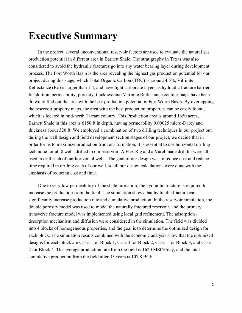
Executive Summary In the project, several unconventional reservoir factors are used to evaluate the natural gas
production potential in different area in Barnett Shale. The stratigraphy in Texas was also considered to avoid the hydraulic fractures go into any water bearing layer during development process. The Fort Worth Basin is the area revealing the highest gas production potential for our project during this stage, which Total Organic Carbon (TOC) is around 4.5%, Vitrinite Reflectance (Ro) is larger than 1.4, and have tight carbonate layers as hydraulic fracture barrier. In addition, permeability, porosity, thickness and Vitrinite Reflectance contour maps have been drawn to find out the area with the best production potential in Fort Worth Basin. By overlapping the reservoir property maps, the area with the best production properties can be easily found, which is located in mid-north Tarrant country. This Production area is around 1650 acres, Barnett Shale in this area is 6150 ft in depth, having permeability 0.00025 micro-Darcy and thickness about 320 ft. We employed a combination of two drilling techniques in our project but during the well design and field development section stages of our project, we decide that in order for us to maximize production from our formation, it is essential to use horizontal drilling technique for all 8 wells drilled in our reservoir. A Flex Rig and a Varel made drill bit were all used to drill each of our horizontal wells. The goal of our design was to reduce cost and reduce time required in drilling each of our well, so all our design calculations were done with the emphasis of reducing cost and time.
Due to very low permeability of the shale formation, the hydraulic fracture is required to increase the production from the field. The simulation shows that hydraulic fracture can significantly increase production rate and cumulative production. In the reservoir simulation, the double porosity model was used to model the naturally fractured reservoir, and the primary transverse fracture model was implemented using local grid refinement. The adsorption / desorption mechanism and diffusion were considered in the simulation. The field was divided into 4 blocks of homogeneous properties, and the goal is to determine the optimized design for each block. The simulation results combined with the economic analysis show that the optimized designs for each block are Case 1 for Block 1, Case 3 for Block 2, Case 1 for Block 3, and Case 2 for Block 4. The average production rate from the field is 1620 MSCF/day, and the total cumulative production from the field after 35 years is 107.8 BCF.

3
The stimulation strategy used was hydraulic fracturing to create high conductivity channel for gas. Results from simulation proved multi-stages hydraulic fracturing is the best way to make our projects profitable. Geology data showed the reservoir is over pressured reservoir. Temperature in the reservoir is 190F. In-situ stress is 4000-5000 psi. White sand and ultra light sand are chosen to be proppants by following field proppants selection chart. We also use field chart to choose slick water with HPG cross linked gel for fracturing fluid. Due to the in-situ stress direction and nature fractures distribution’s uncertainty, we modify the real fracture situation to ideal situation.
The CO2 was injected to the formation with constant bottom hole pressure of 5,000 psi. The continuous injection after the reservoir reaches its economic limit was simulated in this project. The model was run for 30 years of conventional production followed by 5 years of CO2 injection for enhance gas recovery. Since our formation has very low permeability, only hydraulically fractured horizontal well can be used for CO2 injection for enhance gas recovery. Due to higher cost of hydraulically fractured horizontal well, one of the horizontal well was converted into an injector and start injecting CO2 into the formation. Different injection periods were investigated including continuous injection since the beginning of production. The incremental recovery in the producing well could be up to 16% for the case with 25 years of injection and the amount of injected CO2 is 1,100,000 tons. However, the overall production is lower as one of the producing well was converted into an injector. The effect of CO2 breakthrough is relatively small for the case with 5 and 10 years of injection but slightly higher for the case with 25 years of injection. Higher injection pressure would result in higher increase in the amount of injected CO2 and the incremental gas recovery. The incremental gas recovery and the amount of injected CO2 depend on the injection period and injection pressure.
We predict natural gas future price and assume that we’ll sell natural gas by this price. Since the production of natural gas lasts several decades, it is crucial to determine the price over different years. What’s more, the adjustment of risk also plays an important role in evaluation of the project. To meet the two criteria above, we use monthly forecast price in 2010-2011, yearly forecast price in 2012-2035 and monthly forecast price in 2010-2018 to predict monthly future price in 2010-2050. The future price can reflect the volatility of price and can avoid the risk involved in the decision process.

4
Finally a series of discounted cash flow (DCF) analysis was used to evaluate the financial performance of different cases in the project. By comparing the 35 years Net Present Value of the production project under different production methods, it was obvious that producing natural gas with only hydraulic fracture stimulation was the most profitable way to produce gas in Barnett Shale. Producing gas without hydraulic fracture by horizontal wells have around 13.5 years payback period and an extremely low annual return rate, which is about 2.18%; producing gas with CO2 injection stimulation starting from the 30th year will decrease the NPV of the whole project, even after consider the current price of carbon credit, which is $21.5/ton, producing gas with CO2 injection is still not profitable than producing with hydraulic fractures stimulation only. According to our calculation, price of carbon credit needs to be $81.3/ton to make the projection with CO2 injection as profitable as the producing with hydraulic fractures stimulation only. Also some financial suggestions are given in the discussion section basing on the monthly return on investment (ROI). After 14 years production, the monthly ROI drops below the current 30 years U.S. Treasury Bill rate, the company has to decide whether to keep running the project until it earns the maximum profit on this reservoir, or sells the project to another company and pursuits a higher ROI by reinvestment by the received cash. Lots of factors need to be considered to make the decision in the real world, for example, return rate of the reinvestment, discounted price of the project, T-bill rate, time of selling the project, investment risk, etc. Since it is not the purpose of out project, we will not make advance discussion in the report.

5
Chapter 1: Critical Literature Review
Geology
Geological background of Barnett Shale in Fort Worth Basin
Barnett Shale is a Mississippian Marine shelf deposit, its thickness ranges from 200 ft in the southwest region to 1000 ft in the northeast near the Munster arch. And Fort Worth Basin is located in north-central Texas, which is bounded on the north, northeast, and east by faulted basement uplift of Red River Arch, the Muenster Arch, and the Ouachita Structural Front. The southern limit is defined by Llano Uplift.
In the Fort Worth area, the Barnett is organic rich (TOC 4.5%) and composed of fine-grained, non-siliciclastic rocks with extremely low permeability. The organic matter in the shale could be as high as 200 scf/ton (Montgomery et al. 2005). Besides, the Barnett Shale is composed of two producing intervals notated as the upper and lower Barnett which separated by the Forestburg limestone in this area. The historical data indicates that when production from lower and upper Barnett is commingled, the lower Barnett contribution is 75-80% of the total (Shelley et al. 2008). The stratigraphy research indicates that the Barnett Shale in core Fort Worth area is encased by tight carbonates, which is the Marble Fall limestone on the top and the Viola limestone at the bottom (Janwadkar et al. 2006), acting as fracture barriers during the completion. Since the Viola Limestone pinches out west of the Fort Worth area, the hydraulic fracture in the lower Barnett could go into the porous Ellenberger, which is a known water source, and lead to high water production.
Introduction
The geology task was separated into four parts:
1. Selection of research area by evaluating production potential. 2. Gathering of reservoir characteristics in the research area. 3. Construction of reservoir data maps to select the best production site. 4. Providing a reservoir input data to reservoir engineer to run the simulations.
6
The success of the geology team will be the first and critical step for any reservoir development project, which will provide necessary reservoir characteristics to reservoir engineer, drilling engineer, simulation engineer, etc. However, it is much difficult to determine the production area for shale formations than most conventional reservoirs because shale plays are both the source rock and producing rock in the same package. Considering the fact that the group will not drilling any test wells, gathering reservoir data will also pose some difficulty, because well logging and other reservoir data are very limited. Several methods and factors that have been proven adequate in identifying production potential in unconventional reservoir will be used to select the production area, such as TOC estimation, Vitrinite Reflectance test. The hydraulic fracture barriers will also be considered during the site determination. In addition, the reservoir properties contour maps will be developed to select the best drilling and production site.

7
Drilling and Completion
Introduction
Drilling is one of the most important segments of natural gas exploration; holes are bore into the ground at depth from 1,000 to 13,000 ft, thereby allowing the production of natural gas from reservoir beneath the ground to be possible. It is essential to explain the various drilling techniques and process that will employed in our project.
The drilling techniques utilized by operators to drill shale gas wells are similar to the drilling techniques that have been industry standards for drilling of conventional gas wells. While both drilling technique when applied to conventional gas reservoir tends to be profitable, that is not the case for shale gas reservoir. Instead stimulation approach such as hydraulic fracturing has to be applied to make a shale gas well profitable. In some case, even vertical drilling when combined with hydraulic fracturing may not be profitable in a shale gas reservoir. These reasons are discussed later in this section. The major difference between shale gas reservoirs and conventional gas reservoirs is the extremely low permeability (0.0001 md) encountered in shale gas reservoirs. The extremely low permeability of shale gas reservoir makes production from it unprofitable. Therefore a stimulation technique that can significantly improve permeability (from about 0.0001 md to about 1,000 md) and also production from shale gas reservoirs has to be used to ensure commercial production from these reservoirs.
Drilling Techniques
There are various techniques or ways a well can be drilled. The three common types are vertical drilling, directional drilling and horizontal drilling. The three common techniques are explained briefly below.
Vertical Wells (drilling)
Vertical wells are the conventional dug wells that have been in extensive use in the industry. According to literature, Vertical wells have been used in the development of field in the Barnett shale. Vertical wells are cheaper to drill than a horizontal well but the fact is that production from a vertical well compared to that of a horizontal well may not be as economically lucrative.
8
Horizontal / Directional Wells (Drilling)
Horizontal drilling is the process of drilling a well from the surface to a subsurface location just above the target oil or gas reservoir called the “kickoff point”, then deviating the well bore from the vertical plane around a curve to intersect the reservoir at the “entry point” with a near-horizontal inclination, and remaining within the reservoir until the desired bottom hole location is reached. Directional drilling is quite similar to horizontal drilling. In most cases they are drilled to achieve the same objective. The difference between traditional directional or slant drilling and modern day horizontal drilling, is that with directional drilling it can take up to 2,000 feet for the well to bend from drilling at a vertical to drilling horizontally. Modern horizontal drilling, however, can make a 90 degree turn in only a few feet.
The evolution of Barnett shale formation toward favoring horizontal well over vertical wells is a result in the improvement in horizontal well drilling technology. While both wells may be used to extract natural gas from the shale, operators are increasingly relying on horizontal wells drilling and completions to recover resources. One of the reasons for this is the fact that horizontal drilling provides more exposure to a formation than does a vertical well. For example, typically in shale formations, a vertical well may be exposed to as little as 50 ft of formation while a horizontal well may be exposed to a lateral length from 2,000 to 6,000 ft of the formation. This allows gas to be produced from various zones in the formation which increases the rate of production significantly. Apart from the fact that that horizontal well exposes the formation to much more area than a vertical well in the Barnett shale, there are much advantages of drilling a horizontal well rather than a vertical well in the Barnett shale.
Advantages of Horizontal Wells over Vertical Wells
The advantages of a horizontal well over vertical well are numerous this includes; the reduction in surface disturbance. For example, the complete development of a 1-square mile section could require 16 vertical wells located on separated well pad. Alternatively, about 6 horizontal wells drilled from only one well pad can access the same reservoir volume or even more. A large number of vertical wells are required since low permeability reservoirs require closely spaced vertical wells to effectively drain the reservoir. As can be seen, only one hole on the surface has to be drilled in other to drill about 6 horizontal wells while 16 holes on the surface has to be drilled for 16 vertical wells, thereby causing a lot of surface disturbance, surface deformation of the land and also reduces the effect of the impact associated with drilling

9
activities on wildlife and its surrounding habitat Horizontal wells also allow the ability to access drilling locations that would otherwise be inaccessible if vertical drilling is to be used. In our project, a combination of vertical drilling and horizontal drilling will be used. Decision and reason for why they were used will be discussed later on in the field development report.
Advantages of Vertical Wells over Horizontal Wells
The advantages of vertical wells over horizontal well includes; high cost of drilling a horizontal well as compared to drilling a vertical well. In the U.S., a new horizontal well drilled from the surface, cost 1.5 to 2.5 times more than a vertical well. Two allied technologies are currently being adapted to horizontal drilling in the effort to reduce costs. They are the use of coiled tubing rather than conventional drill pipe for both drilling and completion operations and the use of smaller than conventional diameter (slim) holes.
Generally only one zone at a time can be produced using a horizontal well. If the reservoir has multiple pay-zones, especially with large differences in vertical depth, or large differences in permeability, it is not easy to drain all layers using a single horizontal well, whereas a vertical well can be used to drain a reservoir from several layers.
According to Joshi, the overall commercial success rate of horizontal wells in the U.S. is about 65%, while a vertical well has a higher rate of success. So the risk involve in drilling a vertical well over a horizontal well is significantly less. But as more horizontal well are drilled yearly, their success ratio should increase.
Factors to be considered when choosing a drilling technique
The selection of a drilling technique is based on several factors which have to be analyzed by the drilling engineers before drilling process can begin. These factors include the objective of the project, location of the target reservoir, the budget (authority for expenditure), and the geology of the reservoir system, the permeability, the anticipated drainage radius, the environmental constraint, the target depth, and much more.
The objective of the project deals with the task the well is supposed to perform when drilled. Vertical wells are recommended for a situation where an injection of CO2 into the shale formation has to be done, this is because drilling a new horizontal well for injection purposes is
10
not cost effective and also horizontal wells for injection without hydraulic fracture in our low permeability reservoir will not yield desired result, so there is less risk involved by using a vertical well for CO2 injection purposes. Horizontal wells are preferred for production reasons in the Barnett shale. Horizontal/slant wells are the preferred choice when a the location of the reservoir is beneath a major surface obstruction such as mountains or other topographical features which prohibits the building of preparation sites needed to carry out vertical drilling. The geology of the reservoir also affects the selected drilling technique. A horizontal well is less effective than a vertical well when the geology of the reservoir is lenticular. Likewise a vertical well is less effective than a horizontal well when we have a blanket type reservoir. Depending on the investment budget, decisions have to be made between selecting a vertical well and a horizontal well. If the budget size is small, a cheaper vertical well should be selected as the drilling technique and vice versa. Other factors have been discussed in earlier sections of this report.
Drilling Process
In the process of drilling, drilling fluid design, casing design and cementing are done at appropriate stages to ensure the success of the well. After a well has been drilled and tested, and it has been determined that a commercial worthy amount of gas can be produced from the well, the well is thereby completed by cementing, setting casing pipes, setting tubing pipes, and perforation of production area to allow fluids to flow into the well from the reservoir.
Casing
In the drilling process, drilling fluid design, casing design and cementing are done at appropriate stages to ensure the success of the well. The casing is a borehole pipe separating the formation from the borehole. During the course of drilling a well, it is necessary to run casing (that is, to lower the casing string into the well and – usually – cementing it in place) at a number of depth intervals. According to SPE publication 112073 ,”Casing is run for many reasons such as: provide a permanent, stable wellbore of precisely known diameter through which subsequent drilling, completion and production operations may be conducted” .The casings are also used to isolate the wellbore fluids from the sub-surface formations and formation fluids, prevent inter-formational flow, prevent water migration to producing formation, permit production only from specified zone(s) by selective perforation during well completion operations., control pressures

11
during drilling, and finally provide a means of attaching the necessary surface valves (for example, blow-out preventers) and connections to control and handle the produced fluids.
Casings are classified into various groups depending on the objective they are require to carry out. There 4 classifications of casing, conductor casing, surface casing, intermediate casing and production casing.
Conductor Casing is the first string of casing in the hole ran to a maximum depth 300 ft. It is needed to circulate the drilling fluid to the shale shaker without eroding the unconsolidated surface sediments below the drill rig when drilling is initiated. It also protects the subsequent casing strings from corrosion and may be used to provide structural support for a portion of the well-head load such as a BOP (blow-out preventer).
Surface casing is required to Prevents cave-in of weak near-surface sediments and protects fresh-water bearing strata from contamination. In the state of Texas, surface casing are require to be from the top to the depth of 800 ft to 1300 ft. It also supports any subsequent casing strings and protects them from corrosion. Because of their implications for safety and the environment, conductor and surface casing are generally required by law.
Intermediate Casing is required for deeper wells that penetrate over-pressured formations, lost circulation zones, unstable shale sections or salt sections
Production Casing is set through the productive interval. It provides a stable production interval that can be re-entered later in the life of the well. If open hole completion is not utilized, production casing is perforated at the production interval usually using an explosive perforator gun that fires shaped-charges through the casing steel.
In our project conductor casing, surface casing and production casing will be used because we are drilling to a depth of about 6,000 ft, so intermediate casing is not needed.
Cementing
Well cementing is the process of mixing and placing cement slurry in the annular space between casing and the open hole. Well cementing can be classified into two types depending on the objectives; we have the primary cementing and the secondary (remedial) cementing. Cementing of casing annuli is a universal practice done for a number of reasons such as: Providing bond and support for set casing, restricting fluid movement between formation and the

12
surface through the annulus. The cementing process also prevents the pollution of fresh water formations, corrosion of casing strings, seals off abnormal pressure or lost circulation zones, stop the movement of fluids into fractured formations, close an abandoned well or a portion of a well(sidetracking)
The required properties of a cement slurry or set cement vary accordingly to the objective of the cement job. Thus for a casing job, the cement must: Yield a slurry of given density while still exhibiting desired properties, Be easily mixed and pumped, Meet the optimum rheological properties required for drilling fluid removal, Must be impermeable to annular gas while setting, Develop strength quickly once place, Develop casing and formation bond strength
Tubing
Tubing is a small diameter pipe that is run into the well to just above the bottom to conduct the gas and maybe water (produced fluids) to the surface. Tubing is a special steel pipe that ranges from 3 to 11.5 centimeter in diameter and comes in length of about 10 meter. There are various grading of tubing according to API that can be combined to ensure the most economical and yet effective tubing strings to use in the production of fluids. One major useful of tubing is to protect the casing strings from corrosion by produced fluids. Because casing has been cemented in the well, it is very difficult to repair casing. The tubing string is however suspended in the well and can be pulled from the well to repair or replace it.
Surface Equipments
To complete the well, surface equipments along with the choke needs to be installed at the wellhead in addition to cementing, casing and tubing. The wellhead is the permanent, large, forged or cast steel fitting on the surface of the ground on top of the well. It consists of the larger, lower casing head from which the casing component hangs from. It also consists of the tubing head from which the production tubing component hangs from. It also consists of the Christmas tree which has valves to help control flow of gas from the well. Christmas tree consists of a master valve, wing valve, a swab valve, a pressure gauge and a choke. A choke is an orifice that is used to control the fluid flow rate or downstream pressure of the wellbore, the smaller the orifice, the lower the flow rate. Chokes can be fixed size or adjustable depending on specification.
13
Drilling Fluid
Currently, there are three main types of drilling fluid used in drilling a shale reservoir: water-based mud (WBM), lime-based mud (LBM), and synthetic-base mud (SBM). Each drilling fluid and its advantages and disadvantages will be discussed and analyzed. The drilling results may be different for each field; however, they can be used for case studies and play an important role in selecting the drilling fluid for the next well. A proper mud program design that takes into account chemical and thermal effects can improve wellbore stability.
Osisanya and Aremu discuss the effect of adding various polymers in “Evaluation of the Inhibitive Nature of Various Polymers Against Various Shales”. Water-based mud with addition of KCl was studied in this literature. In general, addition of polymers to a generic water-based drilling fluid reduces shale dispersion and shale swelling. Water-based drilling fluid with addition of polymers controls shale stability. The results from various polymers were slightly different. Osisanya and Aremu found that shale dispersion decreased further with the addition of 3% KCl, but adding KCl increased water loss. Zhang et al. state that, for low-perm shales, chemical interactions between the shale and water-based fluids are significant. The use of lime-based mud was discussed in “Mechanism for Wellbore Stabilization with Lime-Based Muds” by Hale and Mody. This type of drilling fluid has been used when drilling CO2-containing formation and other potentially harmful contaminants. In addition, unlike other types of drilling fluid, LBM actively stabilizes the hole. However, the presence of lime is detrimental to cuttings stability in fresh water due to the high alkalinity.
Finally, synthetic-based mud was used in drilling wells in eastern Venezuela, and the wells were successfully drilled with no mud-related wellbore problem. Twynam et al. address the results in “Successful Use of a Synthetic Drilling Fluid in Eastern Venezuela”. Various reasons for the use of synthetic based drilling fluid in shale in Venezuela were addressed. At the beginning of the operation, WBM were used. Troublesome shales and claystones, coupled with complex tectonic stresses, were causes for numerous hole cleaning and wellbore instability incidents. The decision was made to switch to SBM. The results from using SBM were improved hole stability, faster completion of wells, lower drilling costs, reduced environmental impact, improved health and safety. However, the cost per unit of synthetic fluid is higher than other type of drilling fluid making it less attractive.
Drilling history proved that WBM, LBM, and SBM increase well bore stability in drilling of shale formation. WBM were capable of success in drilling, but the efficiency was not optimized.

14
The advantage of LBM is its ability to stabilize formation containing CO2. As described in the literature, drilling with SBM yielded the best results, but it comes with higher cost per unit. Therefore, for the best results of drilling and completion and minimum wellbore instability, SBM is recommended for our new horizontal well as it provides more lubricity and minimize the wellbore problems stated in the introduction.

15
Stimulation
Stimulation techniques have evolved since the beginning of shale production, demonstrating a significant impact on a well’s ultimate performance and a resource play’s economic viability. For the shale reservoir’s low permeability, mass hydraulic fracture is the main simulation method.
The Hydraulic Fracturing Process
Hydraulic fracturing consists of blending special chemicals to make the appropriate fracturing fluid and then pumping the blended fluid into the pay zone at high enough rates and pressures to wage and extend a fracture hydraulically. First, a net fluid, called a “pad,” is pumped to initiate the fracture and to establish propagation. This is followed by slurry of fluid mixed with a propping agent (often called a “proppant”). This slurry continues to extend the fracture and concurrently carries the proppant deeply into fracture. After the materials are pumped, the fluid chemically breaks back to a lower viscosity and flows back out the well.
Fracture design
Our reservoir is of low permeability, the main task for hydraulic fracturing is to create long fractures which make our fracture connected to larger drainage area.
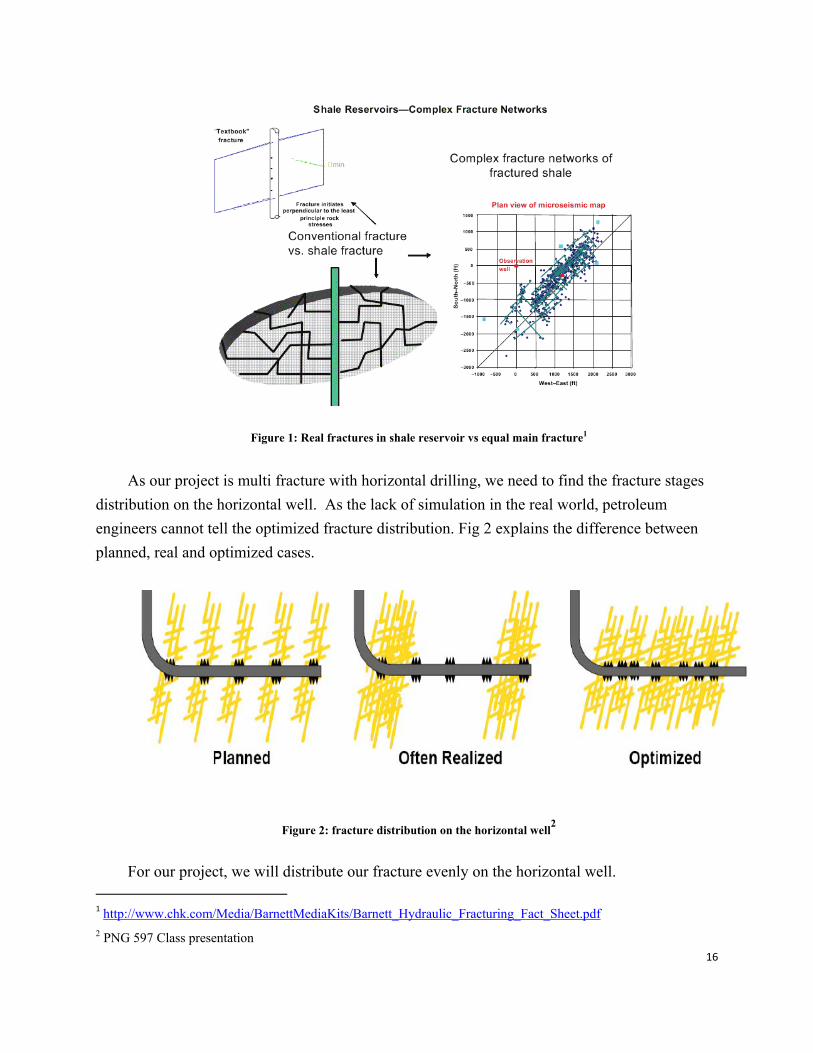
The fracture’s direction is perpendicular to the minimum in-situ stress. For the barnett shale, the minimum in-situ stress is not locked in one direction. Usually, we fracture a net in the shale formation, like figure 1. This figure explains the real fracture situation in the shale formation. However our current available model can’t explain the real fracture situation in Barnett shale. What the engineers do is to make a big main fracture, make it equal to the fracture net, to explain the fracture situation. The main fracture is like what we call it “text book fracture”. And with only one main fracture, reservoir engineer can create reservoir model easily. For our project, we are going to create one main fracture for each fracturing stage.
16
Figure 1: Real fractures in shale reservoir vs equal main fracture1
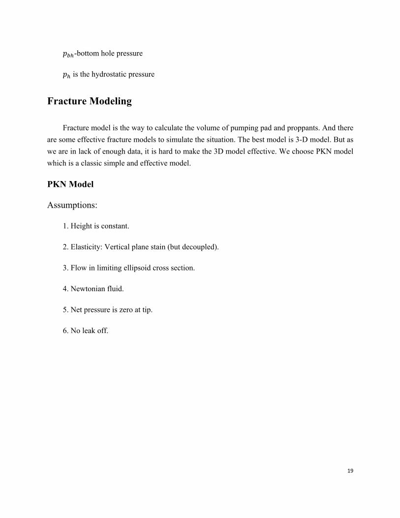
As our project is multi fracture with horizontal drilling, we need to find the fracture stages distribution on the horizontal well. As the lack of simulation in the real world, petroleum engineers cannot tell the optimized fracture distribution. Fig 2 explains the difference between planned, real and optimized cases.
Figure 2: fracture distribution on the horizontal well2
For our project, we will distribute our fracture evenly on the horizontal well. 1 http://www.chk.com/Media/BarnettMediaKits/Barnett_Hydraulic_Fracturing_Fact_Sheet.pdf 2 PNG 597 Class presentation

17
In-situ stress
In-situ stress is important in calculating fracture parameters. The present in-situ stress state in a rock at depth is a complex interaction of rock and reservoir properties, tectonics, and burial history. Prats3 showed that the differential horizontal effective stress induced by changes in depth, temperature, strain, or pressure could be written as
(1)
- Poisson’s ratio,
- Total overburden stress
p- Reservoir pressure
Where the first term on the right side accounts for the effective over-burden stress, the second term accounts for thermal stresses, and the last two terms account for tectonic strains. Variations in the equation are function of depth and time.
In general, none of the variations in these parameters are known, so the calculation is currently more of academic than practical interest.
Compare with equation 1, we have another equation in use. It is not as complete as the previous one. Nevertheless, the new equation indicates that the horizontal in-situ stress in a relaxed, normally pressured basin will typically be 0.55 to 0.7psi/ft, and this is often observed; some successful has been reported in using this approach``.
(2)
Sp is calculated from Sp logging.
(3)
3 SPE (DEC.1981) 658-62

18
- Poisson’s ratio,
- Total overburden stress
p- Reservoir pressure
- Externally generated stress
Friction in tubing
Friction in tubing is a important part in calculating operating pressure. We use Lord and McGowen’s Method to calculate the friction during pumping our fracture slurry
∆
∆2.38 . . 0.1639 ln 0.28 exp , (4)
∆ -friction pressure drop, psi
∆ -friction drop of unladen fluid, psi
-average fluid velocity, ft/sec
-HPG concentration, lbm/1,000gal
-proppants concentration
Lord and McGowen method is developed with delayed crosslinked HPG gels which be used assuming no significant crosslinking at the wellbore temperature of 75 F
Maximum operating pressure
∆ (5)
∆ -friction drop of unladen fluid, psi
19
-bottom hole pressure
is the hydrostatic pressure
Fracture Modeling
Fracture model is the way to calculate the volume of pumping pad and proppants. And there are some effective fracture models to simulate the situation. The best model is 3-D model. But as we are in lack of enough data, it is hard to make the 3D model effective. We choose PKN model which is a classic simple and effective model.
PKN Model
Assumptions:
1. Height is constant.
2. Elasticity: Vertical plane stain (but decoupled).
3. Flow in limiting ellipsoid cross section.
4. Newtonian fluid.
5. Net pressure is zero at tip.
6. No leak off.

20
Figure 3: The PKN model describe fracture with a constant height.4
(6)
Equation 6 is the correlation related fracture width with fracture fluid rate and volume. After calculate the necessary parameters, I will give them to reservoir engineer to do the final field simulation.
Limitations:
This model is based on assumption that height is constant. It does not reflect the real fracture situation. Fluid is Newtonian which means water is the fracture fluid. None leak off can under evaluate the frac-fluid consumption.
Propping Agents and Fracture Conductivity
The purpose of the propping agent is to keep the walls of the fracture apart so that a conductive path to the well bore is retained after pumping has stopped and the fluid pressure has dropped below that required to hold the fracture open. Ideally, the proppant will provide flow conductivity large enough to make negligible any pressure losses in the fracture during fluid production. In practice, this idea might not be achieved because the selection of proppants involved may affected by the economics and practical considerations.
4 PNG 597 class presentation

21
Four main factors evaluating proppant quality include:
(1) High roundness, Sphericity (2) High strength
(3) Low density
We intend to choose 40/70 mesh sand, which will yield the best fracture conductivity 100md-ft using a constant proppant concentration 0.2 ppg. As the Barnett shale has ability of maintaining long production, we might use silica sand.
Fracturing Fluids and Additives
Fracturing fluids are pumped into underground formations to simulate oil and gas production. To achieve successful simulation, the fracturing fluid must have certain physical and chemical properties.
1. It should be compatible with the formation material and formation fluids. 2. It should be capable of suspending proppants and transporting them to fracture,
and, through its inherent viscosity, to develop the necessary fracture width to accept proppants or allow deep acid penetration.
3. It should have low fluid loss and low friction pressure. 4. It should be easy cleaned, cost effective, and stable.
Additives to the Fluid
It is important to select right additives to make the pad effective.
Biocides: use to kill micro creatures in the formation. Those creatures might affect PH or temperature which will make the fracturing pad fail.
Breakers: use to break gel and make them easy to flow back
Buffers: use to control PH
Surfactants and non-emulsifiers: make the breaker act with gel easier

22
Clay stabilizers: protect the formation from deforming
Fluid-loss Additives: eliminate the damage from fluid loss
Friction reducer: save power when engineers try to pumping the fluid
Diverting agents: make the additives and proppants easier to transport
Four kinds of fracturing fluid might be used for our project:
For different wells have different properties, we choose 4 kind of fracture fluid to do the fracturing jobs. Each kind of fracture fluid has its own characterization.
1.Slick water with delayed cross linking gel- these have a couple of advantages which include that its more economic than oil condensate, Methanol or acid, Water-based; imbustible; they are not highly combustible, good leak off behavior, easy viscous control, good proppants suspending, Easy to pump; less pressure required.
The disadvantages of these include that this requires that lots of water is required, and it usually causes poor clean up
2. Form-based fluid- the advantages of these include that it minimize the amount of fluid placed on the formation and improves recovery of fracturing fluid by the inherent energy in the gas. Also in processing foam, one typically uses 65 to 80 percent less water than in conventional treatments. Finally it’s easy to clean after fracture treatment.
And its disadvantages include that small variations in the water or gas mixing rates can cause the loss of foam stability, also N2 foam is not very dense; therefore, pumping pressures will be large compared with gelled water and it requires sufficient polymer stabilizers.
3. Energized fracturing fluid- this has a Fast flow back, Good fluid loss behavior and the incorporation of inert gases into a fracturing fluid will yield proportionally better fluid efficiency

23
But it has a few disadvantages which include that the solution of CO2 might affect the fracturing fluid balance, high equipments quality required and it has low proppants suspending efficiency
Details of the procedure and the step taken to achieve the simulation of the area will be explained in the report including the fracturing pressures and injection rates. As well implementation of CO2 injection.
4. Seawater based fracturing fluid- this is a relative new technology which is mainly used in offshore project. Its main advantage is that using seawater to substitute fresh water can reduce water consumption. And after pretreatment, seawater can be used as slick water. The disadvantage is it needs effort in desalting and purifying. And it also needs a lot more additives to make sure it’s good fracture fluid performance.
The situation of hydraulic fracturing job in Barnett shale
The Barnett shale began to employ slick water fracturing at 1997. For each fracture stage, about 0.8 to 1.5 million gallons is used. 10%~12% of the fracture fluid is used as pad. 75%~85% of the fracture fluid is used as sand laden slurry. The range for pumping rate is from 70 bpm to 100 bpm. The maximum proppant concentration is about 2.0 ppg.

24
Reservoir Simulation
Figure 4: Discretized Reservoir Map
Commercial reservoir simulation software called CMG will be used in this project to determine the production profile from the reservoir. The module that will be used in this project is GEM which is able to handle compositional model and with the coalbed methane extension, the adsorbed gas will be considered in the simulation. The key parameter in the production of oil and gas is the permeability. Higher production can be expected from high-permeability reservoirs. Shale reservoir is considered as double porosity system. The double porosity means there exist 2 areas where gas can be stored: matrix and fracture. The matrix has extremely low permeability. On the other hand, fracture has relatively higher permeability, but it is still low compared to conventional reservoirs. Gas flow can occur only in the fracture. Flow in fracture can be described by Darcy’s Law. Due to extremely low permeability, gas stored in the matrix is governed by diffusion or Fick’s Law. Therefore, the production is mainly controlled by the fracture permeability.
Darcy’s Law:
(7)

25
Fick’s Law:
(8)
Where v = velocity (ft/s) k = fracture permeability (mD) μ = viscosity (cP) = potential (psia) C = molar concentration s = distance between two points (ft)
Equation 7 describes the flow in the fracture which is caused by difference in potential between two points. Equation 8 shows the Fick’s law which is diffusion. Flow in the matrix occurs from the difference in concentration between two points instead of Darcy flow. This is because of extremely low matrix permeability.
(9)
Where P = reservoir pressure (psia) PL = Langmuir pressure (psia) VL = Langmuir volume (scf) C = Gas content (scf/ton)
Apart from gas stored in matrix and fracture, gas is also adsorbed into the shale surface. The adsorption and desorption of gas can be described by Langmuir isotherm. As shown in Equation 9, the parameters that control the desorption mechanism is the reservoir pressure, Langmuir pressure, and Langmuir volume. Gas content is used to describe the amount of adsorbed gas per unit volume of shale (or coal).

26
Figure 5: Langmuir Isotherm5
Fig5 shows the relationship between pressure and gas adsorption capacity for coal. As shown in the figure, the slope of the Langmuir isotherm is steeper at lower pressure. Thus, adsorbed gas desorbs more at lower pressure. After the reservoir is put on production, the reservoir pressure decreases as the production continues. Following the Langmuir isotherm, the amount of desorbed gas can be calculated by multiplying the gas content difference between the corresponding initial pressure and the final pressure with the volume of shale. The adsorbed gas of shale formation is relatively small compared to that of coal bed.
Since shale formation has low- to ultra low permeability, gas flows through only the natural fracture of the reservoir as it has relatively higher permeability compared to the permeability of the matrix. The shale block which is called matrix has extremely low permeability; therefore, gas flow inside matrices is not governed by Darcy’s law. The gas flow in the matrix blocks is governed by diffusion (Equation 8). The gas production is very low, and it might not be economical to develop the field. Therefore, well stimulation techniques must be applied to increase the permeability of the reservoir, and therefore the production of the field. In reservoir simulation, some assumptions need to be made to simplify the problem and minimize modeling and computational time. First, the shale reservoir contains mainly methane. In the actual shale reservoir, not only free gas is stored in the fractures, but also small amount of water. We will assume that the water in the shale reservoir is negligible. Once the reservoir pressure is lowered,
5 Adapted from Evaluation of Coalbed Methane Reservoirs by K. Aminian

27
the adsorbed gas will desorb and flow through fractures to the well. As shown in Table1, the required parameters for the simulation will be provided by the geologist, drilling engineer, and stimulation engineer. These properties will be assigned to each block in the model. The analysis lies in the determination of how to model the natural and artificial fractures.
Table 1 Required Parameters in Reservoir Simulation
Parameter Unit
Reservoir Properties
Matrix Permeability (mD) Fracture Permeability (mD) Matrix Porosity (Fraction) Fracture Porosity (Fraction) Fracture Spacing (ft) Thickness (ft) Depth (ft) Compressibility of Formation (1/psi) Reference Pressure for compressibility (psi)
Langmuir Pressure (psi) Langmuir Volume (SCF/ton) Initial Reservoir Pressure (psi) Reservoir Temperature (F) Gas Saturation (Fraction)
Design Characteristics
Drainage Area (acre) # of Hydraulic Fracture (#) HF Spacing (ft) HF Conductivity (mD-ft) Hydraulic Fracture Width (ft) Hydraulic Fracture Permeability (mD) Fracture Half length (ft) Lateral Length of Horizontal Well (ft) Production Pressure at the Well (psi) Production Period (years)

28
Model of Natural Fracture
Figure 6: Actual and idealized model of natural fracture6
Fig.6 shows the actual shale formation and the idealized model. In reservoir simulation, the naturally fractured reservoir will be assumed to be idealized. The model of matrix and natural fracture are described by Warren and Root (1963). The continuity equation for two dimensional flows in natural fracture with adsorbed gas is shown in Equation 10.
(10)
Where k = permeability μ = viscosity P2 = fracture pressure P1 = matrix pressure 1, 2 = dimensionless porosity of matrix and fracture, respectively C1,C2 = total compressibility of matrix and fracture
Equation 10 is similar to continuity equation for flow in porous media. The major difference is the third term on the left hand side of Equation 10. The third term which is called source term describes how much the fluid is dumped into the fracture at that time. This term explains the gas is desorbed and flows into the fracture.
6 Adapted from “The Behavior of Naturally Fractured Reservoirs” by Warren and Root

29
The material balance equation for coalbed methane and shale reservoirs was originally developed by King (1990). Both coal and shale share similar adsorption and desorption mechanisms, and therefore, the same material balance equation can be used to explain the shale formation. However, shale has less adsorbed gas compared to coal.
(11)
(12) Where Gp = cumulative gas production
Gi = gas initially in place
Gremaining = gas currently in place
Both free gas and adsorbed gas are integrated in Equation 12. The first term on the right hand side of Equation 12 is the difference between free gas initially in place and free gas currently in place. The second term on the right hand side of Equation 12 is the difference between adsorbed gas initially in place and adsorbed gas currently in place.
The idealization of the naturally fractured reservoir would not heavily affect the production rate and the cumulative production because we can control the fracture permeability and fracture spacing. It is possible to model the natural fracture in two ways: Single Porosity Model and Double Porosity Model. With the concept of matrix and natural fracture, the reservoir can be described by single porosity model. The natural fractures can be modeled as extremely fined grids placed between blocks in the model. The blocks represent the shale matrix; the extremely fined grid represents the natural fractures. Single porosity system can be used to model the natural fractures. The advantage of this model is that we might have a slightly better representation of the reservoir, but the modeling and computational time increases significantly because we have more grids in the reservoir, making single porosity model less attractive.
The second approach to model natural fracture is the double porosity model. In this model, we have separate porosities for matrix and fracture. This model allows us to embed the natural fracture inside each block. The fractures are evenly distributed throughout the model. The advantage of using double porosity model is a decrease in modeling time while capturing the

30
same concept of matrix and natural fracture. For this reason, the double porosity model will be used in our project.
Model of Hydraulic Fracture
Figure 7: Composite Model of Naturally Fractured Reservoir7
Composite Hydraulic Fracture Model
Yu and Yang develop a composite reservoir model for heterogeneous reservoir. As shown in Figure 7, the fractures around wellbore should be modeled as a composite naturally fractured reservoir where there are two regions with different reservoir properties. In Figure 7, zone one represents the hydraulically fractured area; zone two demonstrates the outer area which is not stimulated. In other words, the hydraulic fracture should be modeled as a cracked zone around the well bore, and this cracked zone has relatively higher permeability and smaller fracture spacing. In the reservoir simulation, different properties will be assigned for each zone as shown on the right of Figure 7.
7 Adapted from “A New Model of a Fractured Well in a Radial, Composite Reservoir” by Chu and Shank

31
Figure 8: Primary Fracture Model and Network Fracture Model from CMG8
Transverse Fracture Model
The hydraulic fracture can be modeled as very fined grids with high permeability. As shown in Figure 8, the hydraulic fracture model can be divided into two categories depending on the distribution of proppant – the primary fracture model (Case 1) and the network fracture model (Case 2). These models and distributions of proppant are discussed in “Modeling Well Performance in Shale-Gas Reservoirs” by Cipolla et al. There are two possible proppant distribution scenarios – the proppant is concentrated in a primary or main fracture and the proppant is evenly distributed in the fracture network as shown in Figure 8. For the primary fracture model (Case 1), in the reservoir simulation, the hydraulic fractures can be modeled by implementing local grid refinement and assigning high permeability to that block. The fracture network model (Case 2) can be done by adding fractures perpendicular to the main fracture; however, the overall permeability of this hydraulic fracture model is lower than that of the first model. This is because the concentration of proppant which keeps the fractures open is lower in Case 2, and the overburden stress from the formation closes the network resulting in a decrease in fracture permeability.
8 Adapted from “Modeling Well Performance in Shale-Gas Reservoirs” by Cipolla et al.

32
There is no clear-cut answer which model is better. Fortunately, Cipolla et al. state, “the proppant may not be transported into complex network fractures and may be restricted within in a primary fracture.” In other words, it is likely that the result from stimulation will be the primary fracture because the fracture network may not be present. Therefore, in this project, the primary fracture model will be used. In addition, studies have been done with this model, and the results have been verified. Therefore, our approach in the reservoir simulation can yield acceptable results. The expected results from the simulation are the production rate (MSCF/day)
9 and cumulative production of the well (MMSCF) 10.
Another concept that needs to be discussed is hydraulic fracture conductivity. As shown in Equation 13, the conductivity is defined as the product of fracture permeability and the fracture width. The unit of the conductivity is in mD-ft.
· (13)
The conductivity we will use in our simulation is 100 mD-ft. In modeling, the fracture width and hydraulic fracture conductivity can be varied as long as the product of the two values satisfies Equation 13.
In our reservoir simulation, we’ll assume the perfect scenario for drilling and completion i.e. the well is perfectly placed in the planned location. With all the above information in mind, the model of the reservoir for this project will be double porosity model with adsorbed gas in the shale matrix. By using CMG, the adsorbed gas and diffusion will be integrated in the simulation which results in more accurate simulation results. The natural fractures are equally spaced and embedded in the model. The artificial fractures from stimulation will create only primary fracture (Case 1 in Figure 8).
When economic analysis is included in the consideration of the field, an optimized approach to develop a field can be determined with the results from the simulation. Drilling more horizontal wells with long lateral length and multi-stage hydraulic fracturing will surely increase the natural gas production, but it might not be economical for the company. The most economical approach in the development of the field depends on many factors, for example, drilling type, number of hydraulic fracturing, and lateral length. According to “The Role of Economics on Well Fracture Design and Completions of Marcellus Shale Wells” by Schweitzer 9 MSCF = 1000 Standard Cubic Feet
10 MMSCF = 106 SCF

33
and Bilgesu, the optimized approach is to drill a horizontal well with lateral length of 4,000 ft and 9 fracture stages with fracture half length of 1,000 ft. Although the study was done in Marcellus shale, to minimize computational time, we will use this optimized approach for our project. More detailed discussion of the optimized combination of drilling and stimulation techniques should be found in the section of “Cost Related to Drilling and Completion”.

34
CO2 Injection for Enhanced Gas Recovery
Adsorption/desorption mechanism
Figure 9: CH4 and CO2 Isotherm for Shale (Nuttall et a., 2006)
In addition to well stimulation technique, CO2 injection for enhanced gas recovery technique can be implemented to further increase methane production from the shale reservoir. The Langmuir isotherm will be used to explain the adsorption/desorption mechanism. As shown in Fig9, at the same reservoir pressure, methane isotherm (represented by black dotted line) has relatively lower adsorption gas compared to that of carbon dioxide. As organic matters like shale have greater sorption affinity for CO2 than methane, after the injection of CO2, shale adsorbs the injected CO2 and releases methane resulting in an increase in production. Thus, the injection of CO2 can theoretically enhance methane production from the shale reservoir. Furthermore, shale can adsorb significant amount of CO2 due to its large surface areas which results in reducing emission of CO2 to the atmosphere. In the analysis of CO2 injection, there are two aspects that need to be considered. The first aspect is the injection technique i.e. whether cyclic or continuous injection enhances more methane production. The second aspect is the starting time for injection i.e. whether the CO2 injection will be injected simultaneously with the methane production in the early life of the reservoir or injected after the conventional gas production reaches economic limits.

35
CO2 Injection Technique
Schepers et al. investigate two CO2 injection techniques – cyclic CO2 injection and continuous injection – with simulation software to determine the EGR potential in “Reservoir Modeling and Simulation of the Devonian Gas Shale of eastern Kentucky for Enhanced Gas Recovery and CO2 Storage”. In the simulation of this study, CO2 was injected into the wells after 9 years of production, and the simulation was run for another 20 years to determine the incremental gas recovery (the total production period is 29 years). In the first scenario (cyclic CO2 injection), the simulation was run with the optimum for cyclic CO2 injection which was found to be 5 days of injection, 1 month of soaking, and 3 months of production. Schepers et al. found that the disadvantage of cyclic CO2 injection is that some of the sorbed CO2 desorbs and is consequently reproduced. For the studied field, the incremental gas recovery does not improve with this injection technique. For the continuous injection scenario, Schepers et al. state that the continuous injection scenario seems to be of potential success showing significant increases in recovery and total CO2 injection of 300 tons over a period of 1.5 months. Some of the well needs to be shut in when the CO2 breakthrough the production well and the CO2 production reaches its limit. This may affect the total production. Oldenburg and Benson suggest in “CO2 Injection for Enhanced Gas Production and Carbon Sequestration” that injecting CO2 at relatively deeper levels in a reservoir while producing from higher levels will allow an operator to decrease CO2 upcoming and mixing. This is because strong density contrast that causes CO2 to fill the reservoir from the bottom up, making an effective vertical and lateral sweep. For our project, continuous injection of CO2 at the deeper level in Barnett shale can increase methane production as well as sequestrate CO2 into the shale formation.
Starting Time for Injection
Jikich et al. consider 2 scenarios of the starting time of CO2 injection in “Enhanced Gas Recovery with Carbon Dioxide Sequestration: A Simulation Study of Effects of Injection Strategy and Operational Parameters”. The first scenario is the simultaneous CO2 injection and methane production at the beginning of the production. The results from this scenario are an accelerated methane recovery until CO2 reaches the production well and an improved CO2 retention. However, this method is detrimental to total methane production. Thus, this method is recommended if high gas production needs to be produced quickly. The second scenario is the starting of injection after the primary natural gas production reaches its economic limit. This

36
scenario yields an increase in methane recovery with the maximum amount of incremental gas recovery of 10% of the original gas in place.
Figure 10: Incremental methane produced by CO2 injection after primary depletion11
For our project, we will investigate the feasibility of CO2 injection for enhanced gas recovery for our field development in Barnett shale. Our primary goal is to maximize the production of methane while the sequestration of CO2 is the secondary goal. The approach we will take is the analysis based on computational results from technical papers. The scenario we will primarily consider is the continuous injection of CO2 after the primary depletion. The injection of CO2 at deeper level to create a sweep pattern will also be considered. To determine whether this technique is feasible, economic analysis needs to be applied as profits from incremental methane recovery using CO2 injection technique after the abandonment might not be economical.
11 Adapted from “Enhanced Gas Recovery with Carbon Dioxide Sequestration: A Simulation Study of Effects of Injection Strategy and
Operational Parameters” by Jijich et al.
37
Health, Safety, Environment
According to SPE 116599 environmental consideration of shale development, this states that” to substantially reduce the environmental impact of drilling operations, the process of drilling a well needs to be viewed holistically and environmental benefits need to be linked to financial savings”. The Drilling and stimulation activities during shale play development have a great impact on the environment. This was controlled and minimized during our field development by the use of various new techniques and technologies bound by the state policy One of the most challenging environmental problems linked with our drilling is disposing of its wastewater, which is usually constituted of heavy metals, chemicals and hydrocarbons. On most sites, the waste is collected in open, dirt-brimmed waste pits where it sits until it's transported off to treatment facilities or injection wells, in the meantime, during the short period is may remain open, the fluids can evaporate or seep into the earth, or even overflow if rain or snow overfills the pit, but in this case waste water treatment plants where used to recycled some of the water for re-use and the excess to be transported for irrigation purposes. To critically review the environmental, health and safety issues associated with the field development (Barnett area), this report will analyze the HES of every aspect of the development procedure individually.
As earlier discussed in the previous sections, natural gas is currently an important aspect of the nation’s energy supply. Currently, there exists an extensive framework of federal, state, and local requirements designed to handle various activities carried out during the natural gas development process. According to SPE 121038 - Evaluating the Environmental Implications of Hydraulic Fracturing in Shale Gas Reservoirs “These regulations are mainly enforced by state agencies and include such things as ensuring conservation of gas resources, prevention and handling of waste, preserving air quality, and protection of the rights of both surface and mineral owners while protecting the environment” .Also the environmental impact of using CO2 injection as a technique for enhanced gas recovery. An important contribution to shale gas development which was employed in our development is the horizontal drilling and cost-effective hydraulic fracturing (slick water) technologies. These two processes have enhanced shale gas development to move into areas that previously would have been inaccessible with minimum environmental disturbance.

38
Impact of Drilling
Most times the idea for people about natural gas drilling in the Barnett Shale is that the rig used for the drilling activity is permanent, or long-term, equipment on the site. The rig is one of the first and most conspicuous equipment for the development on site. For this development, the flex drilling rig unit was used to drill horizontal wells. This was about the best choice and was selected over other units so as to meet the environmental polices regulated by the state. The flex rig was selected due to its low noise hence providing a reduction in the noise level usually caused by the regular rigs. According to Chesapeake 2009 publication on drilling the Barnett shale “In urban settings, a sound engineer measures current background noise at the drilling site and evaluates the topography and proximity of neighbors to determine what sound reduction measures are necessary”. Other environmental factors considered where; it’s low emission capacity so as to meet the Clean Air Act, then its speed and accuracy (which reduces the occurrence and release of NORMS) and its safety. As earlier discussed, Drill sites are selected based on a number of factors, these include the availability of land suitable to drill on; state drilling permits; nearness to buildings, parks and other infrastructure proximity to natural gas pipelines or the feasibility of installing new pipelines; ; geologic considerations; as well as a company's lease position in the area. One major environmental consideration made by the team for this natural gas drilling development was the surface disturbance required for access roads and well pads and then the conclusion was to go with horizontal drilling. As described further in the literature, horizontal drilling brings a significantly reduction to surface disturbance and other potential environmental effects.
Reducing Surface Disturbance
According to SPE 112765 Barnett Shale Drilling and Geological Complexities - Advanced Technologies Provide the Solution “Complete development of a 1-square mile section could require 16 vertical wells each located on a separate well pad. Alternatively, six to eight horizontal wells (potentially more), drilled from only one well pad, could access the same reservoir volume, or even more”, thus limiting the habitat breakdown, impacts to the general public, and the finally environmental hazards. Clearly, the use of horizontal well techniques by the team significantly reduced the overall environmental disturbance, and gave access to more reservoir area with minimum surface disturbance.

39
Reducing Wildlife Impacts
Current studies have shown that activities associated with gas development can majorly affect wildlife and its habitat during the exploration, development, operations, and abandonment phases. Our implementation of horizontal wells and multi-well pads on development of shale gas plays not only reduced surface area disturbances by reducing the total number of wells to be drilled and well pad sites constructed, but also resulted in fewer roadways and utility corridors. This overall reduction in a project’s footprint resulted in significantly less disturbance to the habitat and the ecosystem currently on the field while allowing for more operational flexibility allowing gas to be produced without disturbing some of these resources. This ability to reduce surface disturbance is especially important in certain critical habitats.
Groundwater protection from Gas well drilling
For ground water protection Cementing and casing program that protects the aquifers from any natural gas drilling activities is employed. According to SPE 112765 Barnett Shale Drilling and Geological Complexities - Advanced Technologies Provide the Solution, “The hole is first drilled using freshwater mud, which is a mixture of freshwater and bentonite clay. As the natural gas well is drilled, the clay actually plates out on the side of the hole, forming what is called a “wall cake,” preventing any migration of well bore fluid into the aquifer before it is cased.” Casing calculation and design was carried out by the drilling team and the proper steel casing was designed according to the state regulations to avoid underground water pollution. By the drilling team, the steel casings which is usually surrounded by layers of concrete was installed to isolate the natural gas well from the drinking water aquifers through which the well penetrates. The depth at which the surface casing should extend is mandated by the Railroad Commission of Texas (RRC). In Barnett Shale operations, State gas regulatory programs place great emphasis on protecting groundwater. Our well construction requirements consisted of installing multiple layers of protective steel casing and cement that are specifically designed and installed to protect fresh water aquifers and to ensure that the producing zone is isolated from overlying formations. The surface casing is was set to a depth of 1,200 - 1,300 feet, more than 400 feet below the Aquifer in the Barnett play. When it is conclusive about the productivity of natural gas well, additional strings of casing and tubing are put in place through the aquifers to provide even better separation between the natural gas stream and the fresh water tables. The five layers of steel casing and cement which go into the construction of a natural gas well virtually eliminate the possibility of the contamination of any freshwater zones. The RRC also requires documentation of drinking water aquifer intervals, the design and installation of surface casing relative to those
40
intervals, and the reporting of characteristics of the wellbore along with completion and production data was given by the team.
Impact of Drilling Fluids
The environmental impact of the drilling fluid used for the shale development practices is a very important aspect of the process. So many factors are considered before use of drilling fluids. For the development, as a result of space availability, the drilling team decided to use steel storage tanks and pits so as to secure the fluids from environmental hazards. As discussed in the previous section, drilling is a regulated practice managed at the state level, and while state gas agencies have the ability to require operators to vary standard practices, the agencies typically do so only when it is necessary to protect the gas resources and the environment. Also these pits may also serve as a storage facility for additional make-up water for drilling fluids or to store water used in the hydraulic fracturing of wells. Our water storage pits were also used to hold water for hydraulic fracturing purposes are typically lined to minimize the loss of water from infiltration. The use of pits as water storage facilities are becoming an important tool in the shale gas industry because the drilling and hydraulic fracturing of these wells often requires significant volumes of water as the base fluid for both purposes. The Synthetic based Mud-fluid (SBM) was used since it was available effective and met the environmental standards required by the state. The SBMs was preferred over water-based fluids in our process for both their ability to drill a gauge hole, thereby minimizing drilling problems and little or no environmental impact.
Hydraulic Fracturing
In shale gas development, fracture fluids are primarily water-based fluids with about 1% mixture of additives which enhance the water capacity for the sand proppant into the fractures. The various types of chemical additives added for our stimulation treatment was dependent on the conditions of the specific well being fractured and the state regulation. A typical fracture treatment will use very low concentrations of between 3 and 12 additive chemicals depending on the characteristics of the water and the shale formation to be stimulated. The most common fluids currently being used for fracture treatments in the gas shale plays are water-based fracturing fluids mixed with friction-reducing additives (called slick water). This was employed by the stimulation unit and the various additives included the following with the various reasons why they were used in reasonable quantities;

41
HPG also used in house hold cleaners and swimming pool cleaners. Friction reducers also used in water treatment, candy and make-up remover. Breaker also used in hair cosmetics and house hold plastics. Clay stabilizers (KCL) also used in low sodium table salt substitute. Surfactants also used in glass cleaner, antiperspirant, hair color. PH-control also used in detergents, washing soda, water softener and soap. Cross linkers also used in soaps and laundry detergents. Biocides also used in disinfectant, used to sterilize medical equipment. Corrosion Inhibitors also used in pharmaceuticals and plastics
The main purpose of friction reducers is to increase the ability of fracturing fluids and proppant to be pumped to the target zone at a higher rate and reduced pressure than if water alone were used. Other additives like the biocides was to prevent microorganism growth and to reduce bio-fouling of the fractures; corrosion inhibitor and other stabilizers to prevent corrosion of metal pipes used for production; and acids that are used to remove drilling mud damage within the near-wellbore area. According to SPE 119900 Critical Evaluation of Additives Used in Shale Slick water Fracs “The make-up of fracturing fluid varies from one geologic basin or formation to another”. Considering the environmental implication of the additives, it’s important to understand that most industrial processes use chemicals and almost any chemical can be hazardous in large enough quantities or if not handled properly. Even chemicals that go into our food or drinking water can be hazardous. For example, drinking water treatment plants use large quantities of chlorine. When used and handled properly, it is safe for workers and near-by residents and provides clean, safe drinking water for the community. This also applies to all the other chemical additives that were used by the stimulation team used in the treatment, although the risk is low; the potential exists for unplanned releases that could have serious effects on human health and the environment. In analysis, our hydraulic fracturing procedure used a number of chemical additives that could be hazardous, but were safe due to proper handling according to environmental requirements and state regulation. In addition, many of these additives are common chemicals which people regularly encounter in everyday life.
Water Availability
Drilling and hydraulic fracturing activities of a horizontal shale gas well may typically require between 2 to 4 million gallons of water, with about 3 million gallons being most common. Amount of water needed could vary substantially between wells. According to SPE 122931- Environmental Considerations of Modern Shale Gas Development, “Water for drilling and hydraulic fracturing of these wells frequently comes from surface water bodies such as rivers and lakes, but can also come from ground water, private water sources, municipal water, and re-used

42
produced water”. While the water volumes needed to drill and stimulate shale gas wells are large, they generally represent a small percentage of the total water resource use in the shale gas basins. Calculations indicate that water use will range from less than 0.1% to 0.8% by basin. Survey shows that this volume is small in terms of the overall surface water budget for an area; however, operators need this water when drilling activity is occurring, requiring that the water be procured over a relatively short period of time. Most of the water used by both the stimulation and drilling team was obtained from the nearby lakes and water bodies. Understanding local water needs can help operators develop a water storage or management plan that will meet with acceptance in neighboring communities, environmental concerns and state regulations. Although the water needed for drilling an individual well may represent a small volume over a large area, the withdrawals may have a cumulative impact to watersheds over the short term. The potential impact on the environment was evaded by working with local water resource managers and complying with regulations to develop a plan outlining when and where withdrawals will occur. In the Barnett shale play basins, one major key to the successful development of shale gas is the identification of water supplies capable of meeting the needs of a development company for drilling and fracturing water without interfering with community needs. While a variety of options exist, the conditions of obtaining water are complex and vary by region and even within a region such that developers will also need to understand local water laws.
Water Management
From study, after a hydraulic fracture treatment, when the pumping pressure has been relieved from the well, the water-based fracturing fluid, mixed with any natural formation water present, begins to flow back through the well casing to the wellhead. It will be observed that this produced water may also contain dissolved constituents from the formation itself. These dissolved constituents are usually naturally occurring compounds and may vary from one shale play to the next or even according to the various areas within the shale play. Also according to IPTC 11028, “Initial produced water can vary from fresh (<5,000 ppm Total Dissolved Solids (TDS)) to varying degrees of saline (5,000 ppm to 100,000 ppm TDS or higher)”. The majority of fracturing fluid used for the treatment is recovered in a matter of several hours to a couple of weeks. The quantity of produced water is usually less than the volume of fluid pumped during treatment. In some basins and shale gas plays, the volume of produced water may account for less than 30% to more than 70% of the original fracture fluid volume. In some cases, flow back of fracturing fluid in produced water can continue for several months after gas production has begun.

43
States, local governments, and shale gas operators due to environmental concerns seek to manage produced water in a way that protects surface and ground water resources contamination and reduces future demands for fresh water. Hence the idea being adopted by most regulators and operators as stated in SPE 122931- Environmental Considerations of Modern Shale Gas Development “Reduce, Re-use, and Recycle of treatment water” these groups are examining both traditional and innovative approaches to managing shale gas produced water. The Health Environment and Safety (HES) team decided to implement the use of a water treatment plant so as to reduce the impact on the fresh water availability. Underground injection has traditionally been the primary disposal option for natural gas produced water but this was not employed by the team. With reference to a publication by Chesapeake Energy, “Re-use of fracturing fluids is being evaluated by service companies and operators to determine the degree of treatment and make-up water necessary for re-use”. The application of on-site, self contained treatment facilities and the treatment methods employed by the HES team was dictated by flow rate and total water volumes to be treated, constituents and their concentrations requiring removal, treatment objectives and water reuse or discharge requirements. In some cases it would be more practical to treat the water to a quality that could be reused for a subsequent hydraulic fracturing job, or other industrial use, rather than treating to discharge to a surface water body or for use as drinking water. New water treatment technologies and new applications of existing technologies are being developed and used to treat shale gas produced water. In the development process, the treated water was reused as fracturing make-up water, irrigation water, and in some cases even drinking water. Recycling or reuse of produced water was able to significantly decrease water demands and provide additional water resources for drought-stricken or arid areas. While challenges still existed, progress was being made. New technologies and new variations on old technologies are being introduced on a regular basis, and some industry researchers are pursuing ways to reduce the amount of treatment needed. According to a publication by Texas SDW council in early 2009, studies were underway to determine the minimum acceptable quality of water that could successfully be used in fracture treatment. If hydraulic fracturing procedures or fluid additives can be developed that will allow use of water with a high total dissolved salts (TDS) content, then more treatment options become viable and more water can be reused. Treatment and re-use of produced water could reduce water withdrawal needs as well as the need for additional disposal options. This approach could also help to resolve many of the concerns associated with these withdrawals in the various states.

44
Naturally Occurring Radioactive Material (NORM)
From geologic studies, some soils and formations contain low levels of radioactive material. This naturally occurring radioactive material (NORM) usually emits low levels of radiation, to which everyone is exposed on a daily and regular basis. Usually radiation from natural sources is also called “background radiation”. Other sources of background radiation include radiation from space and sources that occur naturally in the human body. In addition to the background radiation at the earth’s surface, NORM can also be brought to the surface in the natural gas production process but this was reduced by the drilling team with the use of the accurate and efficient flex drilling rig unit. According to the health assessment publication by Chesapeake “When NORM is associated with natural gas production, it begins as small amounts of uranium and thorium within the rock”. These elements, along with some of their decay elements, notably radium226 and radium228, can be brought to the surface in drill cuttings and produced water. Radon, a gaseous decay element of radium, can come to the surface along with the shale gas.
When NORM is carried to the earth surface, it remains in the rock pieces of the drill cuttings, remains in solution with produced water, or, under certain conditions, precipitates out in scales or sludge. Considering the fact that the radiation from this NORM is weak and cannot penetrate some materials, hence the team used dense materials such as the steel pipes and tanks manufactured for the drilling process. The principal concern for NORM in the and gas industry is that, over time, it can become concentrated in field production equipment and as sludge or sediment inside tanks and process vessels that have an extended history of contact with formation water. Currently there are no existing federal regulations that specifically address the handling and disposal of NORM wastes. Instead, states producing natural gas are responsible for promulgating and administering regulations to control the re-use and disposal of NORM-contaminated equipment, produced water, and wastes. Although regulations vary by state, in Texas, if NORM concentrations are less than regulatory standards, operators are allowed to dispose of the material by methods approved for standard field waste. Conversely, if NORM concentrations are above regulatory limits, then the material must be disposed of at a licensed facility.
Potential effects of using CO2 injection for EGR
Carbon dioxide injection in geological formations is a way to achieve an increase in well productivity over the years and large-scale reductions in emissions. The dominant safety concern

45
about CO2 injection is potential leaks that can cause potential local and regional environmental hazards. These leaks can either be slow or rapid. Gradual and dispersed leaks will have very different effects than episodic and isolated ones. A leak could be caused by a well blowout or reactivation of earlier unidentified geological structures due to for instance micro seismic or earth quack events. A sudden leak also could result from a slow leak if the CO2 is temporarily confined in the near-surface environment during injection and then abruptly released. From chemical composition CO2 being a nontoxic at low concentrations can cause asphyxiation primarily by displacing oxygen at high concentrations. Given potential risks and uncertainties, the implementation of effective measurement, monitoring, and verification tools, complying with state regulations on CO2 injection and procedures will play a critical role in managing the potential leakage risks.
Risks associated with leakage from geologic reservoirs beneath the ocean floor are less than risks of leakage from reservoirs under land. According to a study carried out in 2001 by National Laboratory, Livermore, “The risks due to storage of CO2 in geological reservoirs fall into two broad categories: global risks and local risks”. Global risks involve the release of stored CO2 to the atmosphere that may contribute significantly to climate change if some fraction leaks from the injected formation. In addition, if CO2 leaks out of injected formation, local risks include hazards for humans, ecosystems and groundwater. With regard to global risks, observations and analysis of current CO2 injection sites, natural systems, engineering systems and models indicate that the likelihood or probability of leakage in appropriately selected and managed reservoirs is nearly absent or very negligible over long periods of time. In some cases, injection well failures or leakage up abandoned wells could create a sudden and rapid release of CO2. This type of release is likely to be detected quickly and stopped using techniques that are available today for containing well blow-outs. A concentration of CO2 greater than 7–10% in air would cause immediate dangers to human life and health. Also hazards primarily affect drinking-water aquifers and ecosystems where CO2 accumulates in the zone between the surface and the top of the water table. Groundwater can be affected both by CO2 leaking directly into an aquifer and by brines that enter the aquifer as a result of being displaced by CO2 during the injection process. There may also be acidification of soils and displacement of oxygen in soils in this scenario. Additionally, if leakage to the atmosphere were to occur in low-lying areas with little wind, or in sumps and basements overlying these diffuse leaks, humans and animals would be harmed if a leak were to go undetected. Finally According to the study by Texas EPA. “After CO2 is injected into a saline formation, it may continue as a separate free-gas phase, a supercritical phase, or dissolve in the formation water. When CO2 is in a separate free-gas phase, if the density of the CO2 is less than that of the formation water and even at depths equal to or greater than 800 m

46
where CO2 is supercritical the buoyancy of the CO2 will cause the it to rise and spread laterally beneath the reservoir cap rock. When the CO2 contacts the formation water, it will dissolve and lower the pH of the solution. The exposure experiments of this study have been structured to study both of these processes since both types of “plumes” can come into contact with existing wells. It is very important to understand the chemical interactions between injected CO2 and existing cements that could potentially lead to leakage”
Regulations
The development and production of natural gas in the U.S., including shale gas, are regulated under a complex set of federal, state, and local laws that tend to address every aspect of exploration and operation. Stated by the Texas regulatory agencies, all of the laws, regulations, and permits that apply to conventional natural gas exploration and production activities also apply to shale gas development. The U.S. Environmental Protection Agency (EPA) administers most of the federal laws, although development on federally owned land is managed primarily by the Bureau of Land Management (BLM), which is part of the Department of the Interior, and the U.S. Forest Service, which is part of the Department of Agriculture. Also, each state in which natural gas is produced has one or more regulatory agencies that permit wells, including their design, location, spacing, operation, and abandonment, as well as environmental activities and discharges, including water management, use, additives and disposal, air emissions, underground injection, wildlife impacts, surface disturbance, and worker health and safety. Many of the federal laws are implemented by the states under agreements and plans approved by the appropriate federal agencies. Those laws and their delegation are discussed below.
Regulation of Impacts on Water Quality
In shale development, potential impacts to water quality are primarily regulated under several federal agencies and the accompanying state programs. The primary federal agencies governing water quality issues related to shale gas development are the Clean Water Act and the Safe Drinking Water Act
47
Clean Water Act
The Clean Water Act (CWA) is the primary federal law in the U.S. governing pollution of surface water. The main responsibility of this act is to protect water quality, and includes regulation of pollutant limits on the discharge of gas-related produced water. The CWA establishes the basic structure for regulating discharges of pollutants into the waters of the U.S. and quality standards for surface waters.
Safe Drinking Water Act
The Safe Drinking Water Act (SDWA) is responsible to protect public health by regulating the nation's public drinking water supply. The law requires many actions to protect drinking water and its sources, including rivers, lakes, reservoirs, springs, and ground water wells. SDWA authorizes the U.S. EPA (Energy policy Act and Environment protection agency) to set national health-based standards for drinking water to protect against both naturally occurring and man-made contaminants that may be found in drinking water. EPA, states, and municipal water system agencies then work together to make sure that these standards are met. According to a publication by the department of energy, the author states, “As one aspect of the protection of drinking water supplies, the SDWA establishes a framework for the Underground Injection Control (UIC) program to prevent the injection of liquid wastes into underground sources of drinking water (USDWs)”.
Regulation of Impacts on Air Quality
Air quality impacts are regulated under the Clean Air Act (CAA). This Act sets national standards for emissions of certain pollutants and requires permits for some industrial operations.
Clean Air Act
The CAA is the primary means by which EPA regulates potential emissions that could affect air quality. The EPA regulates these pollutants by creating human health-based and/or environmentally and scientifically based criteria for setting permissible levels. As a result of the implementation of the CAA, air quality has improved significantly across the U.S. during the last few decades and existing regulations should continue to reduce air pollution emissions during the next twenty years or longer.

48
Air Permits
These are legal documents that facility owners and operators must abide by and work with. These permits specifies what construction is allowed in the area, what emission limits must be met, how the emission source must be operated, and under what conditions. Shale gas producers usually need air quality permits for a number of emissions sources, including gas compressor engines, glycol dehydrators, truck emission and flares. Although these permits may differ across the country, they all contain specific conditions designed to ensure state and federal standards are met and to prevent any significant degradation in air quality as a result of a proposed activity.
Regulation of Impacts to Land
Due to impacts to land from shale gas operations which include solid waste disposal and surface disturbances that may impact the beauty of environment or may affect wildlife habitat, agencies and acts such as the RCRA are established to control these impacts
Resource Conservation and Recovery Act (RCRA)
RCRA established goals for protecting human health and the environment, conserving resources, and reducing the amount of waste. There were proposed hazardous waste management standards by RCRA that included reduced requirements for some industries, including natural gas, with large volumes.

49
Economic Analysis
Prediction of Future Price
People treat the price as a constant in the simple model of calculating net present value (NPV) for a project. This model lacks the ability to address the change of prices. However, in the real world, commodity prices, especially prices of fuels over a long period, are volatile. To deal with that, people add a part called “risk analysis”, in which they allow the price to change by a certain percentage, and see what the effect to NPV is. The difficulties lay in how to determine the percentage. Prices of petroleum and natural gas change dramatically in long periods, and the highest price over the lowest is sometimes greater than 400% in a period of ten years. However, if we allow the price to drop 30% in the model, positive NPV will turn to negative most of the time. And if we allow price to shift up 30%, negative can also turn to positive. As a result, risk analysis for price changing often gets meaningless. What’s more, the determination of price-changing percentage usually lack support from statistics.
In a more complex model for calculating NPV, people may use forecast price instead of a constant. For our case, the forecast price of natural gas for the next 30 years can be got from the Energy Information Administration (EIA). The 95% confidence level for every spot price (price at a certain time point) is usually provided with the forecast price. However, even with a confidence level, the forecast price cannot describe the risk we faced when holding price-changing commodity. The situation for us is: if we use the lowest (highest) point in 95% confidence interval, the final NPV is lower (higher) than real. If we use the forecast price, we get expected NPV without considering risk. The confidence level provides a good view to sense the effect of risk; however, this kind of two dimensional (risk & NPV) analysis is not enough for decision. Given that firms in the market are willing to give up some of the expected value to avoid the risk of profit changing (sometimes called “risk premium”), we are not able to compare two projects with high profit & high risk and low profit & low risk, respectively. What’s more, many researches (Kahn E et al, 1993; Awerbuch S, 1993, 1994) have found that the beta of natural gas is negative (i.e. when the markets common price rise (drop), the price of natural gas tend to drop (rise)), which is not normal and gives challenge for our estimate.
In order to involve the risk in NPV calculating, the third method uses the future market price (also called future price), instead of forecast price. Future price is generated by companies’

50
contract of buying and selling some amount of good at a future time point at a certain price. In future price, companies add their consideration of risk and their ability to afford risk. As a result, a commonly accepted future price is a good indication for a commodity’s spot price at a future time with risk. As long as there is a given future price, this model is perfect for decision with risk. The weakness of future price is that we can only find prices for the next 6 years, since companies do not make contract at a ten-year level.
Figure 11: Natural gas past and forecast price, unit MSCF/$, source: EIA

51
Figure 12: NYMEX Natural Gas Forward price (future price) Curve, source: NYMEX data
There have been pretty much work showing the expected value of natural gas spot price is different from the expected value of future price. Walls (1995) studies the behavior of natural gas spot market and proves the natural gas future price is inefficient in at least 3 of the 13 spot markets, i.e. the future market price is not near the expect value of the forecast spot price. John H. Herbert (1993) studies the relationship of monthly spot price and future price and gets a linear regression model between the two prices. John H. Herbert (1993)’s work also shows that the natural gas futures market is inefficient. Chinn et al. (2001) find that natural gas future price is biased for estimating the future spot price, thus different from forecast price, given that forecast price is unbiased estimator for future spot price. Mark Bolinger, Ryan Wiser, William Golove (2004) also point out three reasons to explain the difference between the forward price and the forecast price, i.e. hedging pressure, systematic risk and transaction cost.
Mark Bolinger, Ryan Wiser, William Golove (2004) argue that the price risk for natural gas cannot be omitted. In our project, we can either calculate NPV with the third method or adjusting the second method by risk premium. Risk premium is difficult to be adjusted in the second model, at the same time long term future price is unavailable in the third model. Bolinger et al. (2003) argues that utilities and others conducting such analysis tend to rely primarily on

52
uncertain long-term forecasts of spot natural gas prices, rather than on prices that can be locked in through futures, swap, or fixed-price physical supply contracts, i.e. simply using the second model without any risk adjusting. Actually, this kind of activity will lead to falsely calculated NPV and can cause further problem is the financial decisions.
In our work, we try to study the relationship between future market price and forecast price, thus avoid the mistake by existing models.
Discount Cash Flow (DCF) analysis
Discounted cash flow (DCF) analysis is a method used to evaluate a project, company, or asset using the concepts of the time value of money. All future cash flows are estimated and discounted to give their present values (PVs), and the sum of all discounted cash flow is called net present value (NPV), which is used to evaluate the profits of different development methods in our project. The general equation to calculate NPV will be:
NPV ∑ Incoming Cashflow Outgoing Cashflow 1 Discount Rate (13)
Internal Return Rate (IRR)
Internal rate of return on an investment or potential investment is the annualized effective compounded return rate that can be earned on the invested capital. It can be calculated by solving for the following equation:
NPV ∑ Incoming Cashflow Outgoing Cashflow 1 r (14)

53
Chapter 2: Analysis and Design
Method used to choose the production area
Factors Affecting Production: Finding of an area with higher
production potential
It is difficult to find shale areas with high productivity because traditional well log techniques are based on conventional formation such as sandstone, limestone and dolomite, which is optimized to identify conventional reservoir parameters. The complexity of the mineral composition of shale and its variation in density, resistivity, and radioactivity could cause serious error in porosity and saturation calculation.
Figure 13: Comparison of core-derived TOC with estimated TOC from resistivity/porosity log data.(Source: Grieser
and Bray; Identification of Production Potential in Unconventional Reservoir,2007)
Grieser and Bray believe in “Identification of Production Potential in Unconventional Reservoir” that locating high total organic material carbon (TOC), mature kerogen type III

54
organic material, mineral composition, and areas prone to fracture network development by specialized logging and analysis technique is the key to successful completion of a shale play.
Estimated Total Organic Carbon (TOC):
TOC cannot be measured by logging tools directly, but it can be calculated by its unique effects shown on standard log measurements. Grieser and Bray suggest estimating TOC volume by resistivity/porosity overlay analysis (Passey, et al.). There is a strong correlation between resistivity and the volume of organic material, because carbon is not electrically measured. The adequacy of the analysis method can be proven by Figure 13, which shows that estimated TOC data have a strong correlation with the core TOC date. The estimated TOC will also be used to correct the density and neutron porosity. The data after correction can be applied in traditional method to compute porosity and lithology. In our project, we use resistivity/porosity overlay analysis to calculate estimated TOC. We find out that in the Fort Worth Basin area, the average TOC is about 4.5% and it is the highest number in Texas
Thermal maturity of the reservoir: Vitrinite Reflectance (Ro)
Table 2: Values and Significance of Vitrinite Reflectance (Ro) (Source: Syfan et al.; Case History: G-Function analysis
Proves Beneficial in Barnett Shale Application,2007)
The Barnett Shale is a thermogenic reservoir, thus the thermal maturity of the reservoir can
help determine if it contains gas, oil or no hydrocarbons. Thermal maturity can be estimated by
measuring vitrinite reflectance (Ro) in the lab, the higher number indicates the higher possibility
to produce gas, see Table 2. The vitrinite reflectance (Ro) will be the second factor we take into
account when evaluating the production potential. Since we build up our simulation model for
dry gas reservoir, the Ro value in our research area should larger than 1.4 to match the
assumption best. The only region which Ro value is larger than 1.4 and also located in Fort
Worth Basin is the north Tarrant country, see Figure 14.

55
Figure 14: Iso-Vitrinite Reflectance (Ro) map for Fort Worth Basin area
Rock mechanics factors: BRIT-FT, TOC-FT, sigma_h_min_azimuth
Figure 15: North Texas Barnett log strip showing brittle/ductile shale intervals from Young’s modulus and Poisson’s
ratio cross-plot. (Source: Grieser and Bray; Identification of Production Potential in Unconventional Reservoir,2007)
Poisson’s ratio and Young’s modulus are two of the parameters used to identify ductile and brittle intervals in the shale and to determine stress barriers. Cross-plot of Poisson’s ratio and Young’s modulus can be used to identify different lithologic layers (Grieser and Bray, 2007). It
Brittle Region
Ductile Region

56
can be observed in Figure15 that conventional shale’s plot in the lower right side and Barnett shale plots in the more brittle region in the plot.
Grieser et al. discussed the relationship between production rate and hydrocarbon feet (HC-FT) in “Data Analysis of Barnett Shale Completions”. HC-FT factor is commonly used to measure the reservoir quality in conventional reservoir, the higher HC-TC usually result in higher production. However, the “production rate- HCFT plot” in Barnett shale reservoir does not show a trend line. This spread is mainly the result of the differences in organic content and the fracture-simulation; this also indicates that there are big differences in reservoir evaluation between shale gas reservoir and conventional reservoir. Thus, finding an area which is “brittle” in Barnett shale should be important in our project, because brittle shale has better potential than ductile shale to connect highest amount of rock volume to the parent wellbore during stimulation process (Grieser et al., 2007). However, after lots of research, we found that there are not enough public data for us to find out the difference of brittleness between different regions in Fort Worth Basin. So we actually didn’t put the BRIT-FT and other rock mechanics into account.
Hydraulic Fracture Barriers
To avoid the hydraulic fractures going into the water bearing formations, we have to make sure that our production area is encased by tight formation, which will not be penetrated during the hydraulic fracturing process. Fig. 16 is the stratigraphic section from north to west of Fort-Worth Basin.
Figure 16: Stratigraphic section of Fort Worth Basin.

57
Since Ellenburger is a proven water source layer, our production area should be protected by a relatively harder layer. We can see in Figure 16 that the area on the right of the red line is encased by Marble Fall on the top and Viola Limestone at the bottom. Marble Falls is an inter-bedded carbonate/shale layer and Viola is a relatively harder and less porous limestone, they both can become the barriers of the process of hydraulic fracture. It means that our research location should be at the north of the mid Tarrant country.
After reviewing the factors we have mentioned above, our geology team located our research area at the East portion of the Fort Worth Basin, which is an undeveloped area at the south-east of the present Barnett Shale core production area, see the region marked by red in Figure 17. The selected area has enough thickness (300 ft~800 ft), high TOC (4.5%), and moderated Ro value (1.3~1.7), and is enclosed by tight carbonates which can act as fracture barriers during the completion process.
Figure 17: Area with higher production potential
Site Selection – Property Maps
Below are the reservoir permeability, thickness, and porosity maps which were drawn by our geologists. The reservoir is coming from more than twenty SPE papers and five company

58
report. The property maps can show us the local area with higher production potential, which helped us determine the final production site.
Permeability
We know thatBarnett Shale is a extremely low permeability reservoir. In Fort Wort area, its permeability ranges from 0.00015~0.00030 micro-darcy. Figure18 show the permeability distribution of the Barnett Shale in the Fort Worth area. The red area indicates the area with the highest permeability in mid-Tarrant, which is 0.00025 mD.
Figure 18: Iso-Permeability Map of Barnett Shale
Thickness
Figure 19: Isopach of Barnett Shale

59
Isopach is a map showing the thickness of Barnett Shale around the area. Usually the thicker the formation, the higher the production rate we can get. The green area in Figure 19 shows the area in Tarrant where Barnett Shale is thicker than 300 ft.
Porosity
Figure 20: Iso-Porosity of Barnett Shale
Porosity is also an important production potential factor. The blue area in Figure 20 shows the area in Tarrant which porosity is larger than 3.5.
Figure 21: Iso-Porosity of Barnett Shale

60
Overlap all three reservoir Property map, then we can find out an area with the best production factor and the highest production potential. The result shows in Figure 21, the gray area in Figure 21 is our final production area. However, dealing with such a heterogeneous reservoir our team will spend too much time on the reservoir simulation for every case that we want to test. In next section, a reservoir approximation method will be presented.
Reservoir Heterogeneity
Method and benefits
Figure 22: Divide reservoir into four homogeneous blocks
Running the simulation for a large heterogeneous reservoir will spend a lot of time putting data into each single finite element and running the simulation. To solve this problem, we divide the heterogeneous reservoir into four blocks and assume that each of them is a homogeneous block, see Figure 22.

61
Table 3 Input reservoir properties of different blocks
Properties Block1 Block2 Block3 Block4
Size (acre) 257.98 343.74 462.78 587.26
Depth (ft) 6125.0 6130.0 6158.7 6203.5
Thickness (ft) 362.5 337.5 312.5 287.5
Preservoir
(psia) 3307.5 3310.2 3325.7 3349.9
φm
(%) 3.5 3.5 3.6 3.6
According to the reservoir property maps, different blocks in Figure 22 have different reservoir data. Table 3 shows the different input reservoir data for four reservoir blocks. Depth, thickness, and porosity are calculated by the linear interpolations of the contour lines.
Reservoir parameters for simulation
Other than the reservoir data showing in table 3, there are some other reservoir data useful for the reservoir simulation, see table 4.
Table 4: Other reservoir input data
Km 0.00025 mD
Kf 0.002 mD
Φf 0.1 %
C 1.01*10^-5 psi^-1
Tr 200 ℉
PL 635 psia
VL 89 scf/ton

62
Well Design
In this section, we will design one horizontal well. This design process is applicable to other horizontal wells that are drilled in the development of our entire reservoir.
The horizontal well to be designed is the 4,000 lateral lengths with 9 hydraulic fracture stages.
Questions to be addressed are to what depth are we drilling? What is the initial pressure of reservoir? And much more. These questions will be answered in the design process below.
The deepest depth that was drilled was approximately 6,160 ft. before making transition to drilling a 4,000 ft. long lateral hole. So combining the horizontal length and the vertical length of the entire well, we drilled more than 10,000 ft. for each well in our reservoir. A flex drilling rig, a Varel VM519HU drilling bit with various sizes (inches) is utilized.
Drilling fluid design
Drilling fluid that was employed in drilling all the 8 wells in our reservoir is a synthetic-base mud (SBM). The density and the volume of the drilling fluid were also considered.
The density of the drilling mud was calculated using the pressure gradient of the formation that was being drilled. Since the pressure of the formation at 6,160 ft is 3349.9 psi, the pressure gradient of the formation was therefore 0.544 psi/ft. The pressure gradient of a normally pressure formation is in the range of 0.42 to 0.46 psi/ft. Since the formation we are drilling is over pressured, it is necessary to use a density that will counterbalance this over pressured formation or else a kick or a blowout may occur during drilling. Using the formula below that divides the pressure gradient of a formation by a hydrostatic constant (0.052); we calculate the density of the drilling fluid to be used while drilling in our reservoir.
ρ = P.G/0.052 (14)
Where: ρ is the density of drilling fluid
P.G is the pressure gradient of the formation, and 0.052 is the hydrostatic constant.

63
The density of drilling fluid to be used will be in the range of 10.20 to 10.60 pounds per gallon (ppg) unless otherwise. If the pressure gradient encountered at any depth is greater or less than the pressure gradient of our formation, then appropriate density modification will be done to the drilling fluid to avoid encountering unnecessary problems associated with drilling.
Since we are drilling about 10,160 ft of hole in the formation, it is essential to estimate the volume of drilling fluids that will be required to drill one of the wells in our reservoir.
From calculation shown in appendix, the total volume of synthetic based mud that will be needed to drill each of our well is approximately 500 barrels. About 44 barrels is needed to drill a hole of 12 1/2 inches diameter and 300 ft depth. About 75 barrels is needed to drill a hole of 8 3/4
inches from depth of 300 ft to 1300 ft. Almost 380 barrels of SBM is needed to drill from 1,300 ft to 6,160 ft and also the 4,000 lateral length of the well. This is shown on Table 5 below
Table 5: Volume of drilling fluid used
Sections Volume of drilling fluid used in barrels (bbl)
300 ft 44 300 – 1300 ft 75
1,300 – 6,160 and 4,000 lateral 380
Casing design
Three casing stings will be used in casing our well, and the respective setting depths will be calculated with respect to factors such as axial tension, burst pressure and collapse pressure. Each casing grade must pass these three tests before it can be used.
The most important performance test a casing should pass includes:
1. Axial Tension: This results from the weight of the casing string suspended below a joint of interest.
2. Burst Pressure: The minimum internal pressure that will cause the casing to rupture in the absence of external pressure and axial loading.
3. Collapse Pressure: The minimum external pressure that will cause the casing walls to collapse in the absence of internal pressure and axial loading.

64
All the casings selected for each segment of our well should have strength that will be able to overcome stress or deformation caused by axial tension, burst pressure and collapse pressure. We will carry out our design with the use of design factors. Design factors are essentially “safety factors” that allow us to design safe reliable casing strings. Each operator may have his own set of design factors, based on his experience, and the condition of the pipe. The design factor our company will utilize is shown below. The reason why we select this design factor is because they are extensively used in the industry and they have been proven to be reliable over the past 60 years.
• Collapse – 1.125 • Burst – 1.1 • Tension – 1.8
A conductor casing string, a surface casing string and a production casing string will be used in the vertical section of our well. Reasons for selecting these casing strings are explained in the literature review section. Since the depth of our well is 6,160 ft, we will not require an intermediate casing. An open hole completion would be employed in the 4000 ft long horizontal section of our well. Reason for a open hole completion is to help save cost associated with fatherly running 4000 ft. of production casing.
All casing design calculations are shown in the appendix. From design calculations, the casing grades we selected are shown in Table 6 below.
Table 6: Casing grades selected from API table
Sections Casing Grades Selected from API Table Top – 300 ft K–55, 36 lb/ft weight, short round thread Top – 1300 ft J–55, 20 lb/ft weight, short round thread
Top – 6,160 or (4,000 lateral if to be cased) K–55, 9.5 lb/ft weight, short round thread 4,000 lateral Open hole completion
Cementing
During drilling process, casing of the well is done at several stages. A proper cementing job is required to develop casing and formation bond strength. It is essential to determine the volume of cement, the API classification of cement, the volume of water, the sacks of cement that will be

65
used in the course of drilling a well in our reservoir. According to API specification, there are 8 class of cement used in oil and gas well cement. They range from class A to class H. The cement class that is selected is based on the objective of the cement job to be tackled. In our project, the class D Portland cement is selected for our cement job because it can be used for well depth of 6,000 to 10,000 ft and it requires very low amount of water to mix it, about 4.3 to 4.5 gallons per sack of cement used. Compared to the other classes of cement available, its low water requirement and the depth and temperature for which it can be used for fits our reservoir perfectly. This is the major reason why we chose a class D Portland cement.
The volume of cement slurry required for the cementing of our well is calculated and is shown in the appendices and Table 7 below. The total volume of cement slurry needed for the complete casing of the vertical section of our well is approximately 150 barrels. About 765 sacks of class D Portland cement is needed with about 82 barrels of water to mix. At least 150 barrels cement slurry in total is required for the cement job for one well in our reservoir. Density of the slurry mixed is 16.251 pounds per gallon (ppg).
Table 7: Volume of drilling fluid used
Sections Volume of drilling fluid used in barrels (bbl) 300 ft. 17
300 – 1300 ft. 27 1,300 – 6,160 104
4,000 ft. lateral length N/A – Open hole completion
Production Tubing
The production tubing to use is selected from API list specifications. The tubing to use is selected based on criteria such as production casing inside diameter, cost, and corrosion.
Before selection of an optimum tubing to use, tubing stress analysis has to be performed. The reason for undertaking tubing stress analysis includes: to define the weight, grade and, to some extent, to influence the metallurgy and size of the completion; to ensure that the selected tubing will withstand all projected installation and service loads for the life of the well. If it cannot, then it is necessary to revise the design, to plan for work over or to put in place measures to limit the load, for example limiting the injection pressure or rate during stimulation; to assist
66
in the definition of surface equipment such as wellheads, Christmas trees and flow lines by assessing load cases such as shut-in pressures and flowing temperatures; to ensure that the tubing can be run into the well and eventually pulled out; to ensure that through tubing interventions are not adversely affected by stress effects such as buckling. Similar to casing design, the various stress analysis done for tubing includes axial tension test, burst pressure test, collapse pressure test and much more. Before a tubing string is selected, it has to pass the various stress tests. Tubing design calculation cannot be shown in this report because we do not have any access to tubing API specification tables 5CT (2005) for low alloy and L80 13Cr steel and ISO 13680 (2000) for corrosion- resistant alloys. In our project, we will use production tubing that has an outside diameter less than 4 1/2 inches, that is able to withstand reservoir temperature of 200 deg F, a tubing that can withstand corrosion caused by fluid being produced from our reservoir and finally, it should be able to last the entire lifetime of production for about 35 years.
Perforation Design
No perforation will be required for our well since the 4,000 ft. horizontal lateral length production interval is not cased, we used an open hole completion for this section. If in the future, we decide to case the 4,000 ft. lateral lengths, we will require perforations equivalent to the amount of hydraulic fracture stage that we want to carry out, in this case 9 equally spaced perforations with 3 clusters per perforation will be used. Even though there are several advantages of cased and perforated completions over open hole completions, the main reason we selected open hole completions is to reduce cost. Since casing and perforated completions does not equate to increase gas production, we overlooked the advantages it offers over open hole completion. To satisfy curiosity, the advantages of cased and perforated completions over open hole completions are as follows: upfront selectivity in production and injection; ability to add zones at a later date. It is also possible to re-perforate zones plugged by scales and other deposits; ease of use with smart completions or where isolation packers are used.
Drilling Rig
Rotary drilling rigs are used for almost all gas well drilling done today. The hole is drilled by rotating a drill bit to which a downward force is applied. The bit is turned by rotating the

67
entire drill string with a rotary table at the surface and a downward force is applied to the bit by using sections of heavy thick-walled pipe called drill collars. The combination of the drill pipe and a drill collar is a known as a drill string. The cuttings are lifted to the surface by circulating fluids down the drill string, through the drill bit, and up the annular space between the hole and the drill string. Even though drilling rigs differ greatly in outward appearance and method of deployment, all rotary rigs have the same basic drilling equipment. The main components of a rotary rig are explained briefly below.
Rig Power System
As the name implies, the Power system component of a drilling rig provides power or electricity to the other components of the drilling rig. Most rig power is consumed by the fluid circulating system and the hoisting system. The other rig systems require little amount of power. Fortunately, the hoisting and the circulating system are not used simultaneously, so the same engine can be used to generate power for both systems. Total power requirement for most rigs are from 1000 to 3000 hp. Early drilling rigs were powered by steam but due to high fuel consumptions of fuel and lack of portability of large boiler plants, it has become impossible to use steam powered rigs. The modern rigs are powered by internal-combustion diesel engines and are generally sub-classified as the diesel electric type or the direct drive type depending on the method used to transmit power. Diesel electric rigs are those that in which the main rig engines are used to generate electricity while the Direct drive rigs accomplish power transmission with the aid of internal combustion engines using gears, chains and belts rather than the use of generators and motors. The cost of a direct-drive system is considerably less than that of a diesel electric rig.
Hoisting System
The function of a hoisting system is to provide a means of lowering or raising drill stings, casing strings and other subsurface equipment into and out of the hole. Two routine drilling operations a hoisting system performs include making a connection and making a trip. Making a connection refers to the periodic process of adding a new joint to the drill pipe as the depth of the hole increases. Making a trip involves the removal of the drill string from the hole to change a portion of the down-hole assembly and then lowering the drill string back into the bottom of the hole. Trips are usually made to change a dull drill bit. The principal component of a hoisting system is the derrick, the block and tackle, and the draw-works. The Derrick helps provide the vertical height required to raise sections of pipes from or lower them into the hole. The greater

68
the height, the longer the section of pipe that can be handled and, thus, the faster a long string of pipe can be inserted in or removed from the hole. The Block and Tackle’s principal function is to provide mechanical advantage, which permits easier handling of large loads. The Draw-works provides the hoisting and braking power required to raise or lower the heavy strings of pipe.
Fluid Circulating System
The major function of the fluid circulating system is to remove the rock cuttings from the hole as drilling progresses. The drilling fluid helps in the transport of the rock cuttings down the hole up to the surface. The drilling fluid is pumped into the drill string, through the drill string into the drill bit, through the nozzle of the drill bit and up the annular space (with the rock cutting collected) between the drill string and the hole to the surface.
The principal component of the rig circulating system includes mud pumps, mud pits, mud mixing equipment, and contaminant removal equipment.
Rotary System
The rotary system consists of all the equipment needed to achieve bit rotation. The main parts of the rotary system include the swivel, the Kelly, the rotary table, the rotary drive, the drill-pipe, and the drill collar. The swivel supports the weight of the drill-string and permit rotation. The bail of the swivel is attached to the hook of the travelling block, and the gooseneck of the swivel provides a downward pointing connection for the rotary hose. The Kelly is the first section of pipe below the swivel. The outside cross section of the Kelly is square or hexagonal to permit it to be gripped easily turning. Kelly helps transmit torque through the Kelly bushings, which fit inside the master bushing of the rotary table. A rotary drive is the source of power that is used to turn a rotary table, thereby creating the rotation in the drill string and the drill bit.
Well control system
As will be discussed under the problems encountered while drilling, the primary duty of a well control system is to prevent the flow of formation fluid into the wellbore. The system detects kick, and prevents kick from becoming blowouts which can result in fatal disasters.
Well monitoring system

69
Safety and efficiency consideration require constant monitoring of the well to detect drilling problems quickly. A driller control unit is used to record parameter such as depth, penetration rate, hook load, rotary speed, rotary torque, pump rate, pump pressure, mud density, mud temperature, mud salinity, gas content in the mud, hazardous gas content of air, pit level, and mud flow rate. In addition to assisting drillers in detecting drilling problems, it also provides good history records of various aspect of the drilling operation that can aid geological, engineering and supervisory personnel.
Flex Rig
In our project, we will be employing a Flex Rig to carry out all our drilling activities. It has all the components that a conventional drilling rig possesses as we have discussed above, the only different is that the flex drilling rig is automatically control by an operator in the control room compartment of the rig.
A Flex Rig is a computerized drilling unit that allows the operator to punch a hole in the ground and move quickly between drilling locations. The Flex Rig uses variable frequency drives and a computerized driller that precisely controls the weight applied to the drill bit, the amount of torque and the pressure of the drilling fluid.
The Flex Rig can drill through depths of about 8,000 to 18,000 feet and cost about 15 million dollars to build. There are a total of 127 flex-rigs in the world at the moment, this signals that Flex Rig is a new technology and the use will be employed in our project. Even though Flex-rigs are more expensive than a conventional drilling rig, the benefits a flex rig provides over a traditional drilling rig are immense. These benefits are explained below:
Flex Rigs saves time and ultimately money by moving quickly from well to well.
According to Tulsa world news article, Flex Rigs, on average, drill wells about 22 percent faster than the 16 other conventional rigs in use in the Tulsa region.
Mike Zanghi, wells manager for BP’s onshore business unit in the USA, says that in the Arkoma Basin, Oklahoma, drillers using conventional rigs were averaging 34 days per 10,000 feet, the industry standard measure of drilling efficiency. The performance when we used one of these higher technology rigs, along with the other components of common process, was 27 days

70
per 10,000 feet. Zanghi points out, ‘It made a tremendous difference. Having a rig with higher technology allows you to move toward the technical limits.
Companies like Williams co inc. do pay more per day to use a FlexRig than other equipment. But even with a premium day rate, companies involved in exploration and production still see a savings. Williams co inc. spends about 5 percent less when it uses a FlexRig compared with a conventional rig.
Oklahoma City-based Devon Energy Corp., the nation’s largest independent producer of oil and natural gas, uses a dozen Flex Rigs in the Barnett Shale, a natural gas-rich formation in North Texas. David Fortenberry, drilling manager for the company’s central division, said the rigs save time and money. Devon will typically spend $30,000 to $50,000 per day on a rig, so reducing the number of days can result in real savings for the company. This year, Devon plans to drill about 500 horizontal wells in the Barnett Shale. Fortenberry estimated that Flex Rigs save the company about $200,000 per well.
Flex Rigs reduces noise pollution
The electric motors and computerized system also reduce the noise associated with applying the brake on a rig. “It helps because the general population is not used to the noise,” Fortenberry said. In the Barnett, drilling companies are typically working in more urban areas and often drill wells near homes.
Flex Rigs improves safety
The rigs’ automated features also reduce drilling accidents that could injure drilling workers boring a well. Devon energy said the rigs are five times as safe as their conventional rigs. For instance, FlexRig drillers work from an air-conditioned cabin instead of standing on the rig floor. H&P, developer of the FlexRigs, can also monitor each rig from its offices in Tulsa. Company engineers can diagnose problems and alert the operators to possible safety hazards.

71
Figure 23: A Flex Rig, and a Climate-controlled driller’s cabin on the latest generation Flex Rig allowed addition of
more electronic controls, and joystick controls for block
Drilling Bit
Drilling engineers deal with many challenges before and during drilling a new well even in a known area. There are many parameters related to hardware and daily operations that are planned and also modified as the drilling progress. Bit selection is one of the important parameters for planning and designing a new gas well.
The selection of a proper bit is a difficult task since the factors affecting the bit performance are complex relationships between formation properties, bit hardware design, and operational parameters. The selection of the drill type to use is based on rate of penetration data, and cost per foot drilled data from well previously drilled. The bit type with the highest rate of penetration or minimum cost per foot is the two commonly used criteria for selecting the bit for the next interval. Additional factors such as hydraulics, formation hardness, bit design, and operational parameters are also considered in the selection process. Due to the number of
Climate-controlled
driller’s cabin
Climate-controlled
driller’s cabin
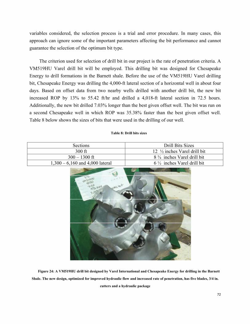
72
variables considered, the selection process is a trial and error procedure. In many cases, this approach can ignore some of the important parameters affecting the bit performance and cannot guarantee the selection of the optimum bit type.
The criterion used for selection of drill bit in our project is the rate of penetration criteria. A VM519HU Varel drill bit will be employed. This drilling bit was designed for Chesapeake Energy to drill formations in the Barnett shale. Before the use of the VM519HU Varel drilling bit, Chesapeake Energy was drilling the 4,000-ft lateral section of a horizontal well in about four days. Based on offset data from two nearby wells drilled with another drill bit, the new bit increased ROP by 13% to 55.42 ft/hr and drilled a 4,018-ft lateral section in 72.5 hours. Additionally, the new bit drilled 7.03% longer than the best given offset well. The bit was run on a second Chesapeake well in which ROP was 35.38% faster than the best given offset well. Table 8 below shows the sizes of bits that were used in the drilling of our well.
Table 8: Drill bits sizes
Sections Drill Bits Sizes 300 ft 12 ½ inches Varel drill bit
300 – 1300 ft 8 ¾ inches Varel drill bit 1,300 – 6,160 and 4,000 lateral 6 ½ inches Varel drill bit
Figure 24: A VM519HU drill bit designed by Varel International and Chesapeake Energy for drilling in the Barnett
Shale. The new design, optimized for improved hydraulic flow and increased rate of penetration, has five blades, 3/4 in.
cutters and a hydraulic package

73
Drilling Efficiency
The goal of the drilling engineer for our project is to maximize drilling efficiency and reduce cost associated with drilling. This goal was achieved with the use of a Flex drilling Rig, and a Varel made VM519HU drilling bit specially designed for Chesapeake Energy. As we can see in the table below (Table 9 and 10), a Varel bit improved rate of penetration from 48.13 ft/hr to 55.42 ft/hr. This reduces a day from the total amount of days required to drill our well. Also the utilization of a FlexRig cut down drill time for a 10,000 ft dug well from 34 days to 27 days. Even though FlexRigs are more expensive per day, we saved a total of about 300,000 dollars from our drilling cost. Tables 9 and 10 show the improved drilling efficiency associated with FlexRigs and Varel designed bit.
For a total 10,160 ft drilled per one well
Table 9: The improved drilling efficiency associated with FlexRigs and Varel designed bit for 10,160 ft per well
Bit Type Rate of Penetration (ft/hr) Days Hours
Varel bit 55.42 8 183.33 Chesapeake old bit-1 48.13 9 211.09 Chesapeake old bit-2 41.52 11 244.58
For a total 10,000 ft drilled per one well
Table 10: The improved drilling efficiency associated with FlexRigs and Varel designed bit for 10,000 ft per well
RIG TYPE DRILLING TIME (DAYS) Flex Drilling Rig 27
Conventional Drilling Rig 34
About 22 % faster than a conventional rig

74
Development of the Field
In this section we will discuss the considerations, the reasons and the assumptions we used in the development of our field for a 35 year production period. This section pertains to drilling development. The reservoir engineer and the drilling engineer made decisions such as: what direction should we place our wells; if so, what is the drainage area of the wells we drill; how many wells should be placed in our field to effectively drain the reservoir; what are the well spacing used in our field; how many wells are drilled in the field. All the questions above and much more will be answered in this section.
Design and Life-Cycle Considerations for Unconventional Reservoir
Wells
This part has to do with factors that need to be considered during the design of each well that will help drain and produce from our reservoir. In reality, an initial well is drilled in the field. This well is called a wildcat well. Its main objective is to use as a source of collecting data that will be analyzed to help estimate the size of the field and the total gas in-place in our field. The wildcat well is usually recommended to be drilled by the geologist. Most of the time, this well is a vertical well. We will not be drilling this well in our reservoir because of our assumption that we already have data to help estimate our region of production, and we will not be producing from this well at any point in time.
Shale gas reservoir brings unique problems to the design topic that range from issue of well spacing to wellbore orientation. Most of these issues have to be addressed before a well is drilled and should be addressed as part of a reservoir management plan.
When considering the life cycle of a well, the life and overall development of the field is likely the most critical component. Question such as “How long will the field produce?”, “Does the well need to survive the entire life of the field?”, and “Will secondary or tertiary recovery be needed?” need to be addressed early in the well planning sequence. The path that will be followed in our reservoir life process will begin from discovery, followed by delineation, field development, primary production, secondary or tertiary production (if needed), and end with abandonment.

75
Well design and life-cycle consideration are addressed from three aspects: upfront reservoir development, initial well completion, and well life and long-term consideration.
Upfront Reservoir Development
Several upfront considerations must be accounted for in developing plans for a shale gas reservoir. One of this is to determine the orientation of the well, will it be vertical or horizontal. This choice depends on many factors including geology of the reservoir system, the permeability of the reservoir, and the anticipated drainage area of the well.
Another design parameter that needs to be considered early in field planning and re-evaluated throughout development life is the required well spacing. Optimal well spacing in unconventional reservoirs is very unlike the radial drainage, equally spaced well patterns common in conventional reservoirs.
A final consideration for early development is the need for specialized tubular metallurgy if secondary and or tertiary recovery method will be used later in the life of our reservoir.
Initial Well Completion
As field planning is undertaken, the initial well completion has to be taken into account. Since most shale gas wells needs to be stimulated, generally hydraulically fractured, the extreme circumstances that the wells are placed under during such treatment must be taken into account during well completion planning.
The maximum treating pressure and the rate is a main concern. In areas where well spacing is very close, in other to reduce cost, lower grades of casing are frequently used. If hydraulic fracturing is the stimulation method that will be implemented, the casing must be able to withstand the generated high pressure conditions. In long horizontal well intervals, pressure losses that result from pipe friction can be significant. To overcome this rate/ pressure concern, adequate modeling for the range of necessary hydraulic fracturing parameter should be performed before the well is drilled and completed.
The number of treatment stages should also be accounted for while planning initial completion, along with the isolation and diversion of the stages.
Well Life and Long-Term considerations

76
The duration of a shale gas well’s life can be significantly longer than a conventional well because of the low permeability of the reservoir and the associated drainage profile. Shale gas reservoirs exhibit hyperbolic decline which indicates a possibility of an extended life time. Therefore well design has to be conducive to such long lives and the processes that may occur during the extended period of time.
The ability to lift liquid and/ or prevent liquid loading is a key concern. Liquids in a shale gas system can significantly decrease the amount of natural gas production. The ability to remove such liquids must be addressed. Adequate space in the well for velocity strings or other such liquid-removal systems needs to be considered, along with the appropriate time to install these systems.
Another problem in wells that needs to be considered in shale gas wells is Corrosion. Corrosion is a problem that occurs in both conventional reservoir wells and unconventional reservoir wells but since unconventional reservoir wells has a longer life time, so corrosion has more time in which to occur. Therefore steps should be taken to minimize corrosion from the onset of production in shale gas wells. If Horizontal wells are going to be used in field development then corrosion prevention has to be seriously considered because horizontal well completions are even more susceptible to corrosion issues because of the difficulties with obtaining an adequate primary-cement job and the possibility of water pooling in undulating laterals.
A certain situation that needs to be prepared for is the effect of continuous refracturing that will occur during the life time of a well so adequate well completion must be installed in the initial completion stage for a new well.
Lastly issue that needs to be addressed when dealing with shale gas wells is the future abandonment of these wells. If amount of wells that will be drilled during field development will be much due to the need for wells to be closely spaced, the economic and environment impact for such massive abandonment should not be underestimated.
Well Orientation
During reservoir development and field planning, one of the key decisions we were faced with was the direction to place our wells in each of the four blocks of our reservoir. Geological factors such as faults and stress profile are major deciding factors in well placement. But in our
77
design, since there are no faults in our reservoir, we did not have to worry about what direction to drill our well. Our wells were placed in the plane parallel to the minimum stress which enables us to create a hydraulic fracture in a direction perpendicular to our minimum in-situ stress. The stress profile of our reservoir indicates that the maximum stress was in the z- direction (vertical plane) of our Cartesian plane and the minimum stress was in the x and y direction (horizontal plane) of our Cartesian plane.
Drainage Area
The well orientation has effect on the drainage area and vice versa. If we compare the drainage area associated with placing either 2 or 3 well in one of our reservoir block, we observe that the scenario where we placed 2 wells amounts in a higher drainage area as compare to a scenario where 3 wells are placed in the reservoir. This effect is caused by interference between wells. Interference occurs when the boundary of two or more wells are in communication with the other, it limits the drainage area allowable for each well. Our goal in our design process was to maximize the drainage area of our individual wells, which allows us to drill the least amount of wells in each block. The only situation that overrules over design criteria was a situation when a block is not effectively drained by the least amount of wells. In that case, we drill an extra well in that block. This decision certainly affects the orientation of our wells. To maximize the drainage area of each of our well when a new well is drilled, we sometimes have to change the direction of our wells in the horizontal (x and y direction) plane.
Well Spacing
Well placing strategies was not one of the determining factors in the planning of our field. Our 8 wells were placed non-uniformly in each of our four reservoir blocks with emphasis on maximizing drainage area associated with each of our wells without compromising the effective depletion of our reservoir which results in reducing cost associated with drilling.

78
Stimulation
Fracture analysis
Many factors influence the effectiveness and cost of a fracturing treatment. In essence, we have very little control over where and how fractures will ultimately propagate in subsurface strata. Our current efforts are limited to selecting:
(1) the appropriate types of materials (e.g., fluids, additives, and proppants);
(2) the appropriate volumes of materials;
(3) the injection rates for pumping these materials;
(4) the schedule for injecting the materials.
Hydraulic fracturing equipment
Our reservoir engineers recommend horizontal wells and multi stages fracture. Hydraulic fracturing equipment we are going to use in our fields consists of a slurry blender, series of high pressure, high volume fracturing pumps (typically powerful triplex, or quintiplex pumps) and a monitoring unit. Associated equipment includes fracturing tanks, high pressure treating iron, a chemical additive unit (used to accurately monitor chemical addition) low pressure pipes and gauges for flow rate, fluid density, and treating pressure. Fracturing equipment operates over a range of pressures and injection rates, and can reach up to 100 MPa(15,000 psi) and 265 L/s (100 barrels per minute).
The location of fracturing along the length of the borehole can be controlled by inserting tough inflatable plugs, also known as bridge plugs, below and above the region to be fractured. This allows a borehole to be progressively fractured along the length of the bore, without leaking fracture fluid out through previously fractured regions. The plugs are inserted into the bore deflated, then expanded to seal off the borehole into a small working region. Piping through the upper plug admits fracturing fluid and proppant into the working region. This method is commonly referred to as "plug and perf." Figure 25 shows the multi-stage fracture technology. From the picture we can see that we use several plugs to isolate each fracture stage.

79
Figure 25: Horizontal well with multi fracture stages12
Target formation description
Based on data from geologist, our target formation is a very good fracture candidate.
Average young's modulus: 4.45 MMpsia (Poisson's Ratio: 0.235);
Average Formation Compressibility 1.01*10^-5 [psi^-1];
Average pressure 3,400 [psia];
Average pressure gradient 0.54 [psia/ft];
Average overburden pressure gradient 1 [psi/ft];
Average water saturation 33% (we assume that we only have dry gas);
12 http://www.halliburton.com/ps/default.aspx?navid=198&pageid=1186&prodgrpid=PRG::IU4NUNKAJ

80
In the chosen place we also have limestone at the top and the bottom, which can ensure our fracture dimension. We can control our fracture in the target formation without worry about fracture aquifer formation.
Average pressure gradient 0.54 [psia/ft], our reservoir is not a low pressure reservoir. Barnett shale has a lot of natural fracture. The average fracture width is around 0.002 inch. We make them accounted into our main fracture calculation.
Proppant selection
In order to get optimized gas flow, the fracture conductivity should be at least 100 md-ft. Based on this requirements and in-situ stress, Ottawa white sand / proppant is our choice. Figure 26 shows the select procession. Our reservoir in-situ stress is far less than 6,100 psi. Comparing with ceramic, white sand is more economic. If we use ceramic as our proppant, the cost of our fracture might be doubled for proppant is one of the main cost in hydraulic fracturing.
We try to use sand coated with resin. The reason of coating with resin is proppants could connect with each other. In this way, these proppants could not be flowed back and could maintain their conductivity. Besides sand, we have a new type of proppant called ultra light sand which is made of chemically modified walnut hull and coated with resin. This one could be used for formation which doesn’t between 5,000 psi and 6,000 psi net closure pressure and 200F temperature.
Figure 26: proppants selection chart13
13 PNG 597 class presentation
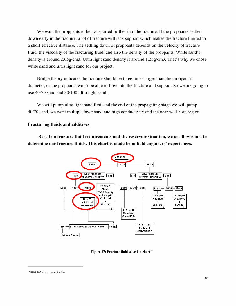
81
We want the proppants to be transported further into the fracture. If the proppants settled down early in the fracture, a lot of fracture will lack support which makes the fracture limited to a short effective distance. The settling down of proppants depends on the velocity of fracture fluid, the viscosity of the fracturing fluid, and also the density of the proppants. White sand’s density is around 2.65g/cm3. Ultra light sand density is around 1.25g/cm3. That’s why we chose white sand and ultra light sand for our project.
Bridge theory indicates the fracture should be three times larger than the proppant’s diameter, or the proppants won’t be able to flow into the fracture and support. So we are going to use 40/70 sand and 80/100 ultra light sand.
We will pump ultra light sand first, and the end of the propagating stage we will pump 40/70 sand, we want multiple layer sand and high conductivity and the near well bore region.
Fracturing fluids and additives
Based on fracture fluid requirements and the reservoir situation, we use flow chart to determine our fracture fluids. This chart is made from field engineers’ experiences.
Figure 27: Fracture fluid selection chart14
14 PNG 597 class presentation

82
Our reservoir is producing dry gas. This flow chart is useful for our work. The reservoir temperature is about 190 F in place. Our choice falls to the left part of the flow chart. The reservoir is not a low pressure reservoir. The formation is not water sensitive. We can generate our decision about fracturing fluid-Slick water with delayed cross linking gel (HPG).
We have also considered water based fracturing pad for our hydraulic fracturing job. However, our reservoir’s location is about 5 hours drive to the sea, and the cost of a seawater treatment is also high comparing to use fresh water. We have access to fresh water. It is more economic for us to use fresh water than seawater. Figure 27 shows the location of our field (red spot). We can see clearly water distribution near our field.
Figure 28 shows the consumption of water and sand in hydraulic fracturing. Especially the consumption of water is very huge. The water used for one fracture stage is between 0.8 to 1.5 million gallons of water.
Figure 28: Water consumption in hydraulic fracturing15
15 Chesapeake energy corporation 2009

83
Figure 29: Lakes distribution near our field16
Additive selection:
In order to make our fracturing fluid effective, we need additives in our fracturing pad. The main reason to choose these additives is to compatible with water based fracturing fluid and cross linked HPG
1. HPG: Powder HPG gum; delayed hydration polymer, contains no internal breaker,
low residue, 1%~3% residue, after break.
The reason to choose this type of gel is HPG has higher viscosity than linear gel and it can transport the sand easily. Delayed hydration time can make sure gel is fully dissolved into the slick water. Comparing with other kind of gel, HPG has 3% residue at most. It can make sure we can wash out most of the gel.
2. Friction reducers: Liquid; high anionic polyacrylamic friction reducer for water; typical loading from .25~ 1 gal/1,000 gal
16 Google map
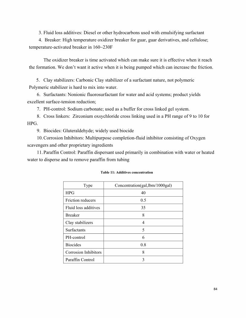
84
3. Fluid loss additives: Diesel or other hydrocarbons used with emulsifying surfactant 4. Breaker: High temperature oxidizer breaker for guar, guar derivatives, and cellulose;
temperature-activated breaker in 160~230F
The oxidizer breaker is time activated which can make sure it is effective when it reach the formation. We don’t want it active when it is being pumped which can increase the friction.
5. Clay stabilizers: Carbonic Clay stabilizer of a surfactant nature, not polymeric Polymeric stabilizer is hard to mix into water.
6. Surfactants: Nonionic fluorosurfactant for water and acid systems; product yields excellent surface-tension reduction;
7. PH-control: Sodium carbonate; used as a buffer for cross linked gel system. 8. Cross linkers: Zirconium oxsychloride cross linking used in a PH range of 9 to 10 for
HPG. 9. Biocides: Gluteraldehyde; widely used biocide 10. Corrosion Inhibitors: Multipurpose completion-fluid inhibitor consisting of Oxygen
scavengers and other proprietary ingredients 11. Paraffin Control: Paraffin dispersant used primarily in combination with water or heated
water to disperse and to remove paraffin from tubing
Table 11: Additives concentration
Type Concentration(gal,lbm/1000gal)
HPG 40
Friction reducers 0.5
Fluid loss additives 35
Breaker 8
Clay stabilizers 4
Surfactants 5
PH-control 6
Biocides 0.8
Corrosion Inhibitors 8
Paraffin Control 3

85
Fracture design
In this part, we calculate different parameters that affect our fracture.
In-situ stress
We use the following equation to calculate our reservoir minimum in-situ stress.
(15)
0 (Usually this value is very small; we assume 0 external pressure in our field)
4173
Friction in tubing
We use Lord and McGowen’s Method to calculate the friction during pumping our fracture slurry
∆
∆2.38 . . 0.1639 ln 0.28 exp (16)
=17.156q/
=56(ft/sec) (at case that pumping rate is 80 bpm)
The ratio to is
=0.0583 q/
=0.714( lbm HPG-sec)/(1,000 gal-ft) [0.374kg.s/m4]

86
∆ 0.40429 . .
∆ 3056.3
∆ =748.6psi (friction of fracture fluid pad)
Fracture fluid slurry friction is
∆ = ∆ exp (-1.406+0.028 exp (17)
∆ is bigger than ∆ . We use ∆ to calculate the maximum operating
pressure.
Maximum operating pressure
∆ (18)
is the hydrostatic pressure
=2653 psi
PKN model
G=
E: young’s modulus
G=1.8MMpsi
(19)
W: fracture width

87
hf: fracture height
: Minimum in-situ stress
P: fluid pressure
G: shear modulus of the formation
(20)
W: fracture width
hf: fracture height
: Minimum in-situ stress
P: fluid pressure
G: shear modulus of the formation
PKN model needs an initial fracture height which remains constant during the calculation
The calculation procession is like try and error. We will try to match each value for the pumping equipments requirement.
We use reservoir thickness as the initial fracture height.
In the real situation, we cannot make the whole fracture effective. From experience of the field engineers, only 30% of the fracture length is effective. That’s why we use effective length for simulation.

88
Table 12: fracture design calculation results
Name units 1 2 3 4 Length ft 1600 2100 2100 1900
effective length ft 500 725 700 625 Length effectiveness % 31.25 34.52 33.33 32.89
Width ft 1.01 1.24 1.31 1,29 Height ft 362 337 312 287
pumping rate bbl per min 80 90 90 80
friction in tube(pad) psi 748.6 911.5 911.5 748.6 maximum op pressure psi 7768.6 9683.6 9186.6 7772.6
The schedule of the fracture job
The water cost for one fracture stage is around 0.8~1.5 million gallon. We use 1.1 million gallon per fracture to make our fracture job schedule. Around 10% of the fluid is used as the fluid pad. Around 80% of the fluid is used as the fracture slurry. The rest of the fluid is used for flow back issues.
Table 13: The schedule of the fracture job
parameters one frac@case1
one frac@case2
one frac@case3
one frac@case4
pre-pad fluid volume (gallon) 10,000 10,000 10,000 10,000
C HPG
(gallon) 0 0 0 0
C sand ( lbm) 0 0 0 0
TIME (min) 4 3.6 3.6 4
Pad fluid volume (gallon) 80,000 80,000 80,000 80,000
C HPG
(gallon) 0 0 0 0
C sand ( lbm) 0 0 0 0
TIME (min) 32 28.8 28.8 32
stage 1 fluid volume (gallon) 120,000 120,000 120,000 120,000
C HPG
(gallon) 4,800 4,800 4,800 4,800
C sand ( lbm) 60 60 60 60
TIME (min) 48 43.2 43.2 48

89
stage 2 fluid volume (gallon) 100,000 100,000 100,000 100,000
C HPG
(gallon) 4,000 4,000 4,000 4,000
C sand ( lbm) 50 50 50 50
TIME (min) 40 36 36 40
stage 3 fluid volume (gallon) 100,000 100,000 100,000 100,000
C HPG
(gallon) 4,000 4,000 4,000 4,000
C sand ( lbm) 50 50 50 50
TIME (min) 125 125 125 125
stage 4 fluid volume (gallon) 100,000 100,000 100,000 100,000
C HPG
(gallon) 4,000 4,000 4,000 4,000
C sand ( lbm) 100 100 100 100
TIME (min) 40 36 36 40
stage 5 fluid volume (gallon) 100,000 100,000 100,000 100,000
C HPG
(gallon) 4,000 4,000 4,000 4,000
C sand ( lbm) 100 100 100 100
TIME (min) 40 36 36 40
stage 6 fluid volume (gallon) 120,000 120,000 120,000 120,000
C HPG
(gallon) 4,800 4,800 4,800 4,800
C sand ( lbm) 180 180 180 180
TIME (min) 48 43.2 43.2 48
stage 7 fluid volume (gallon) 100,000 100,000 100,000 100,000
C HPG
(gallon) 4,000 4,000 4,000 4,000
C sand ( lbm) 150 150 150 150
TIME (min) 40 36 36 40
stage 8 fluid volume (gallon) 100,000 100,000 100,000 100,000
C HPG
(gallon) 4,000 4,000 4,000 4,000
C sand ( lbm) 200 200 200 200
TIME (min) 40 36 36 40
water injection
fluid volume (gallon) 80,000 80,000 80,000 80,000

90
C HPG
(gallon) 0 0 0 0
C sand ( lbm) 0 0 0 0
TIME (min) 32 28.8 28.8 32
Consumption
HPG ( gallon) 33,600 33,600 33,600 33,600
Sand ( lbm) 890 890 890 890
Time ( min) 489 453 453 489

91
Reservoir Simulation
The reservoir simulation software will be used to determine the best configuration for developing the field. To ensure high reliability of the simulation results, a validation run was made and compared with the results in the literature. The purpose of the validation is to see if the production profiles (cumulative production and production rate) from our model match results in the literature. Table 14 shows the input data set for the validation run. Due to limited information on the inputs from the literature, some inputs need to be assumed using the typical values for shale properties and design characteristics.
Table 14: Validation Inputs
Parameters Unit Inputs from SPE 125532
Shale Typical Values Input for
Validation Min Max
Reservoir Properties
Matrix Permeability (mD) 0.00001 0.0000001 0.01 0.00001
Fracture Permeability (mD) - 0.0001 3 0.0001
Matrix Porosity (Fraction) 0.03 0.02 0.16 0.03
Fracture Porosity (Fraction) - 0.001 0.03 0.002
Fracture Spacing (ft) - 1 40 20
Thickness (ft) 300 50 1500 300
Depth (ft) 7000 1000 15000 7000
Compressibility of Formation (1/psi) - 0.00005 0.0005 0.00005
Ref. Pressure for compressibility (psi) - 14.7 8000 14.7
Langmuir Pressure (psi) - 200 800 440
Langmuir Volume (SCF/ton) - 50 200 88
Initial Reservoir Pressure (psi) 3800 3000 8000 3800
Reservoir Temperature (F) 180 130 300 180
Water Saturation (Fraction) 0 0 0.1 0
Design Characteristics
Drainage Area (acre) 187.33 40 250 187.33
# of Hydraulic Fracture (#) - 1 8 4
HF Spacing (ft) 600 200 600 600
HF Conductivity (mD-ft) - 5 200 20
Hydraulic Fracture Width (ft) - 0.333 0.333 4.2
Hydraulic Fracture Permeability (mD) - 15.02 600.60 4.76
Fracture Half length (ft) - 250 2000 545
Lateral Length of Horizontal Well (ft) 3000 1000 1650 3000
Production Pressure at the Well (psi) 1000 14.70 4000 1000
Production Period (years) 35 30 50 35

92
Figure 30:Cumulative Production from SPE 125532
Figure 31: Cumulative Production from Validation Run

93
Figure 30 shows the results from SPE 125532 “Modeling Well Performance in Shale Gas Reservoir” by Cipolla et al. In the literature, the hydraulic fracture network model has been used in the simulation. However, assigning higher conductivity of the fracture can adjust the model to be equivalent or similar to the model in the literature. The red solid line in Figure 30 shows the cumulative production which will be compared to the results from our model. Figure 31 shows the cumulative production using the data in the last column of Table 14. Our result shows a good match with only 5% error in cumulative production after 30 years of production. The shapes of the cumulative production are similar as well. Now that the model is validated, the input sets for each block will be generated.
The total size of the reservoir is 1651.76 acres. Since the variations of reservoir properties in the selected area are small, the area can be divided into 4 blocks of homogeneous properties. The goal is to determine the design characteristics for each block that will yield the highest net present value (NPV). The properties of each block are listed in Table 16. The design characteristics for different cases are shown in Table 15. Once the well location is determined, the expected results are the production rate and cumulative gas production from the reservoir.
Table 15: Reservoir Properties for Each Block

94
Table 16: Design Characteristics for Each Block
The size of the block controls the length of the horizontal well. In general, the lateral length of a horizontal well is at least half of the length of the drainage area. The length of the horizontal well consequently controls the number of hydraulic fracture. The hydraulic fracture spacing typically ranges from 200 to 400 ft. The concept of conductivity which was discussed in Chapter 1 is applied to determine the width and permeability of the hydraulic fracture. The input sets shown in Table 15 and Table 16 will be implemented in CMG for reservoir simulation.

95
Effect of Hydraulic Fracturing on Production
Figure 32 shows a sample model of Block 3 Case 3. The local grid refinement was applied to create a hydraulic fracture. The block which represents the hydraulic fracture has higher permeability. The necessity for hydraulic fracture in the development of shale gas reservoir will be discussed.
Figure 32: Local Grid Refinements to Model Hydraulic Fracture
Figure 33: Hydraulic Fractured Horizontal Well in Block 1

96
Figure 34: Production rate comparisons between well with hydraulic fracture and without hydraulic fracture
Figure 35: Cumulative production comparisons between well with hydraulic fracture and without hydraulic fracture
Figure 33 shows the hydraulic fractured horizontal well in Block 1. The production rate and cumulative production from the same well with hydraulic fracture and without hydraulic fracture were simulated and compared. Figure 34 and Figure 35 show the production rate and cumulative production for the well in Block 1, respectively. The well with hydraulic fractures

97
can produce methane at higher rate compared to the well without hydraulic fracture. Over the simulated period, the well can maintain higher production rate. The cumulative production is increased over 130% for the well with hydraulic fracture. Therefore, it is necessary to create hydraulic fractures to increase production from tight system like shale gas reservoir.
The simulation will be run for 35 years for conventional production to determine the optimized scenario for each block. The optimized cases for Block 2 and 4 will be re-run with enhance gas recovery technique using CO2 injection to determine the feasibility of this technique. CO2 injection for enhance gas recovery will be discussed in the following section.

98
Fracture fluid recycling technique
Recycling produced water for use as a fracturing fluid can significantly reduce the amount of fresh water that needs to be sourced for shale well completions. Most of the produced water is recycled for re-use as the fracturing fluid. This is a very capital intensive project and requires a lot of funds for the plant to be set in place. But the HES unit decided to go with this in order to comply with the SWDA acts and other environmental regulations set by the state of Texas on waste disposal
Design
Mobile heated distillation system
During flow back about 30-70% of the treatment fluid volume is recovered. This technique recycles Vaporizes the fracture flow-back wastewater and condenses it into clean, distilled water and the remaining concentrated water removed for disposal or utilized for controlling pressures in another well completion as a “kill fluid. For this process about 80% of the produced water is recovered during this recycling process. This plant is onsite mobile equipment powered by on site natural gas to carry out the recycling process. This process involves 4 stages, first, the produced water is piped and stored in a steel storage thank where it is left for some hours to settle after which it is passed through a steel pipe to a distillation unit which is powered by onsite natural gas . The produced water is heated in the distillation unit which also contains iron control agents in there so as to reduce the iron content of the water. After which the evaporated water is piped and channeled to the condensation unit there it is left to cool for hours. The condensed water is then flowed into another steel tank where it will eventually be mixed with some amount of fresh water to make up the required amount needed and then taken to the to the unite for mixture with the additives before being used to stimulate the next well and the waste concentrated from the distillation unit is sent to another tank where it will be loaded in to trucks for disposal at the waste centre or used as a kill fluid for some wells.

99
Schematic Diagram of our Recycling Technique
Produced water
storage tank
Condensation unit
Fresh distilled waterWaste concentrate
Produced/flow back waterFrom well
Distillation unit
80% of produced water20% of produced water
Frac fluid
+ additives
HeatPower from natural gas on site
Back to new wells
Figure 36: Schematic Diagram of our Recycling Technique
Economic analysis
In this section, future price and a series of discounted cash flow (DCF) analysis will be presented. By comparing the Net Present Value (NPV) of the projects which producing gas under different conditions for thirty-five years, we are able to find out the best production method and the optimized term for gas production. By the discounted cash flow analysis, we will also provide suggestions to make CO2 injection enhanced gas recovery profitable.

100
Regression For Future Price
Data Source and Description
We get short term monthly forecast price, long term yearly forecast price and monthly future price.
The short term forecast price is a monthly price, obtained from EIA short term energy outlook (EIA STEO)17. The price is the average US well head price and shown as nominal real-time dollars, i.e. all the forecast price means show the price at the dollar of the forecast time. The time range of the data is from Jan 2010 to Dec 2011.
We get the long term yearly forecast price from EIA annual energy outlook (EIA AEO)18. We choose the average well head price for natural gas. The price is shown in the value of 2008 dollars. The time range of the yearly forecast price is from 2012 to 2035.
The future gas price comes from the Henry Hub natural gas prior settled future price. The monthly future price is shown in real-time nominal dollars. The time range is from Apr 2010 to Dec 2018.
Data Retreatment
In this part, we generally need to change the long term yearly forecast price in 2008 dollars to monthly price in real-time nominal dollars.19
Firstly, we set the discount rate as 3% (which is a 20 years average in US). Our yearly price is multiplied by a factor (1+3%)(YEAR-2008). Thus we get a yearly price in real-time nominal dollars.
20080 (1 3%)YEARP P −= × + , (21)
17 EIA STEO, 2010. http:// tonto.eia.doe.gov/cfapps/ STEO_Query/steotables.cfm? tableNumber=16
18 EIA AEO, 2010. http://www.eia.doe.gov/oiaf/aeo/excel/aeotab_13.xls
19 Since discounting effect exists between different years, a certain amount of money generally losses its value as time passed by. 1 dollar in 2008
is generally worth more than 1 dollar in 2009 and less than 1 dollar in 2007. Here, the forecast price is shown in the unit of 2008 dollars, not in
the unit of dollar for its prediction time, that’s why we need to convert it to real-time nominal dollars.

101
P0 is the original we get from EIA AEO in 2008 dollars.
Secondly, we need to create a monthly price by the yearly forecast price. The monthly price is important for the following three reasons:
a) The discounting factor is different between different months;
b) The price in a year varies a lot, i.e. in summer, the natural gas price is generally lower and in winter when residents need heating, the natural gas price is generally higher; and
c) Monthly price gives us more data for regression. We estimate the price shift between months by setting the 2010 and 2011 monthly price as standard sample.
, , 2010, 2010, , 2011, 2011,1 1( ) ( )2 2i j i average average j i average average jP P P P P P P= − + + − +
(21)
In which Pi,j indicates the forecast price in the j’th month of the i’th year. Pi,average indicates the yearly price of the i’th year.
By formula (19), we can successfully convert yearly price to an approximate monthly price, i.e. we capture the price changes by months in a year.20
Regression Model and Result
We run a regression to predict the monthly future price after 2018 (when we have no observed data).
1 1 2 3 3Futp Futp Futp Forepα β β β ε= + × + × + × + (22)
In which Futp indicates the future price at a spot time, Futp1 gives the future price one month before the spot time, Futp3 indicates the future price three months before the spot time, Forep captures the effect of forecast price, and ε is an error term.
20 Generally speaking, natural gas price is usually lower in summer and higher in winter. The heating demand in winter just raises the price of
natural gas.

102
In this modal, we use the future price before some time to predict the future price at a certain spot time. This is valid because the future price acts as a time serial trend more than determined by factors at the same spot time. Forep in this model is important because it is the only variable that captures an outside effect rather than future price itself. If we do not have forecast price here, the future price will just go as its own pattern, which is not true in the real world.
By formula (22), we can successfully convert yearly price to an approximate monthly price, i.e. we capture the price changes by months in a year.21
NPV calculation and analysis
Discount Rate
To start the DCF analysis, we assume that the average discount rate is 3% per year for our project, in this case, the equivalent monthly discount will become
1.03 1 0.25%
The above number will be used to discount the incoming and outgoing cash flow in the analysis, see Table 17.
Table 17: Future incoming and outgoing cash flow
Incoming Cash flow Discount term unit Discount rate Sales of gas month 0.25%
Outgoing Cash flow Discount term unit Discount rate Operating cost month 0.25%
Land lease month 0.25% CO2 Injection month 0.25%
Royalty month 0.25% Administration month 0.25%
21 Generally speaking, natural gas price is usually lower in summer and higher in winter. The heating demand in
winter just raises the price of natural gas.

103
Income
We assume that all the gas we produce can be sold without transportation cost, and the sales of gas are the only income source which has been considered in our project.
To calculate the present value per SCF of gas, the accumulative production data receiving from our reservoir engineer needs to be redistributed under the unit of month, multiply by the future price data (Appendix A), and then be discounted by the monthly discount rate 0.25%. In this way, the NPV of the sales for the thirty-five years term will become:
NPV of Sales Monthly Gas Production Corresponding Future Price 1.0025
Cost
Since the costs of drilling, hydraulic fracture and water recycle have already been optimized; we can consider their cost as one-time fixed cost. That is to say we do not have to consider the costs of time for them in the economic analysis. Besides, we assume that geology research, well logs and reservoir simulation do not cost time, so their costs will also become fixed costs of the project which do not need to be discounted.
Table 18: List of Cost in the DCF Analysis
Drilling (ft) (USD/per well) 500 1900000
1000 2000000 2000 2100000 3000 2200000 4000 2300000
Hydraulic Fracture (ft) (USD/per stage) 250 200000 500 250000 750 300000
1000 350000 Geology Research and Logs 76000 USD/per well
Reservoir Simulation 100000 USD Operating cost 10 USD/Day per well Water recycle 4.43 USD/barrel
Land lease 17500 USD/acre for three years CO2 Injection 15 USD/ton

104
Table 18 is a list of amounts of different costs incurred in our project, these data have been consider as cost data for the NPV calculation in the DCF analysis. Note that the actual costs of drilling and hydraulic fracture for different cases will be the linear interpolation values of the cost data in table 18.
To calculate the negative term of NPV, all the future outgoing cash flows listed in table 17 should be discounted by the equation below:
NPV of Cost Total Monthly Cost 1.0025
NPV of Rotalty and Administration
Gas Sales Total Monthly Cost 0.42 1.0025
Analysis Code Development
Our Discounted cash flow (DCF) analysis codes (Appendix B) are developed using the MATLAB software for three difference cases:
a) Production without hydraulic fracture,
b) Production with hydraulic fracture and
c) Production with hydraulic fracture and CO2 injection.
The price data, cost data and discount rate can all be changed separately to observe the change in NPV curve result from changing different parameters. The net present value (NPV) of the projects will be calculated by combining the positive and negative terms of NPV, which can be briefly described by:
NPV of Project NPV of Sales NPV of Cost NPV of Rotalty and Administration
Royalty 25% of net profit Administration 27% of net profit

105
As we described in the simulation’s chapter, we have two to three sets of well direction and hydraulic fractures designs in each homogeneous reservoir block. We will run the DCF analysis for all sets of designs and find out the best design for each block in each case, and then compare their return rate, payback period and NPV. Furthermore, we will provide economic suggestions base on the DFC analysis result.

106
Chapter 3: Results
Simulation results for the optimized case for each
block
Using the reservoir modeling technique combined with the analyzed design characteristics, the input data sets were implemented in the CMG and simulated. The case with the highest net present value (NPV) is shown here, and the other simulation results are shown in the Appendix.
Block 1 Case 1
Figure 37: Block 1 Case 1 Production Rate

107
Figure 38: Block 1 Case 1 Cumulative Production
Figure 39: Block 1 Case 1 Pressure distribution after 35 years

108
Block 1 has the drainage area of 257.98 acres. Only one horizontal well can be placed in this block. Therefore, two cases were investigated: the case with 4,000 lateral length and 3,000 lateral length. The longer lateral length can be hydraulically fractured for 9 stages while the shorter can be fractured only 7 stages. As shown in Figure 37 and Figure 38, after 35 years, the well can produce gas at rate approximately 130 MSCF/day and the cumulative production is 16.9 BCF22. Figure 39 shows the pressure distribution after 35 years of production. As we produce gas at constant bottom hole pressure of 1,000 psi, it can be seen that the pressure around the well drops near 1,000 psi and the area farther from the well bore and fractures has the approximate pressure of 2,300 psi.
Block 2 Case 3
Figure 40: Block 2 Case 3 Production Rate
22 1 Billion Cubic Feet (BCF) = 106 MSCF

109
Figure 41: Block 2 Case 3 Cumulative Production
Figure 42: Block 2 Case 3 Pressure distribution after 35 years

110
Block 2 has the drainage area of 343.7 acres. We were able to place two horizontal well of 2,000 ft lateral length. The well is placed in the x-direction. Figure 40 and Figure 41 show the production rate and cumulative production from this configuration, respectively. The average production rate is roughly 2,200 MSCF/day. The cumulative production from two well is approximately 20.6 BCF. After 35 years, the pressure around the well drops to near specified well bottom hole pressure. This means the reservoir is effectively drained with the two horizontal wells.
Block 3 Case 1
Figure 43: Block 3 Case 1 Production Rate

111
Figure 44: Block 3 Case 1 Cumulative Production
Figure 45: Block 3 Case 1 Pressure distribution after 35 years

112
This block has the drainage area of 462.78 acres. Two configurations were investigated in this block. The optimized case is the case with 4,000 ft lateral length placing in the x-direction with 9 fracture stages. The methane was drained effectively as the pressure at the area farther from the well has pressure approximately 1,500 psi. From Figure 43, the production rate for each well after 35 years is at 225 MSCF/day. As shown in Figure 44, the cumulative production from this block is approximately 32.33 BCF.
Block 4 Case 2
Figure 46: Block 4 Case 2 Production Rate

113
Figure 47: Block 4 Case 2 Cumulative Production
Figure 48: Block 4 Case 2 Pressure distribution after 35 years

114
Block 4 is the largest block in our selected area with the drainage area of 587 acres. The best configuration in this block is placing 3 horizontal wells in the y-direction, and each well has 9 fracture stages. As shown in Figure 46 and Figure 47, the productions from each well are equal as each well has similar drainage area. The cumulative production from this block is 37.8 BCF. In Figure 48, the pressure distribution after 35 years is very low in the area near the wells, and the area farther has the pressure around 1800 psi.
Field Production Rate
Figure 49: Field Production Rate
Figure 49 shows the production rate from each block and the total production from the field. The average field production is approximately 27,715 MSCF/day, and the field production rate after 35 years of production is approximately 1620 MSCF/day.
1
10
100
1000
10000
100000
1000000
10000000
1/1/10 6/24/15 12/14/20 6/6/26 11/27/31 5/19/37 11/9/42 5/1/48
Prod
uction
Rate [M
SCF/da
y]
Date
Field Production Rate
Total
Block 1
Block 2
Block 3
Block 4

115
Field Cumulative Production
Figure 50: Field Cumulative Production
Figure 50 shows the cumulative production from each block and the cumulative production from the field. The cumulative field production is 107.8 BCF or 0.1078 trillion cubic feet (TCF). According to EIA23, U.S. natural gas consumption in 2009 is approximately 22.8 TCF. The cumulative production from our field after 35 years can supply natural gas only 0.5% of U.S. annual natural gas consumption.
23 http://tonto.eia.doe.gov/dnav/ng/ng_cons_sum_dcu_nus_m.htm
0
20000000
40000000
60000000
80000000
100000000
120000000
1/1/10 6/24/15 12/14/20 6/6/26 11/27/31 5/19/37 11/9/42 5/1/48
Cumulative Prod
uction
[MMSCF]
Date
Field Cumulative Production
Total
Block 1
Block 2
Block 3
Block 4

116
Simulation results for CO2 injection
CO2 injection for enhance gas recovery is investigated for the optimized cases for block 2 and 4. We selected these two blocks because block 2 has two horizontal wells and block 4 has 3 horizontal wells, and the effect of CO2 injection for enhance gas recovery can be studied for different field designs. The results are shown below.
Block 2 Case 3 with CO2 Injection for 5 years
Figure 51: Production Rate for Block 2 Case 3 with EGR for 5 years

117
Figure 52: Cumulative Production for Block 2 Case 3 with EGR for 5 years
Figure 53: CO2 Injection for Block 2 Case 3 with EGR for 5 years

118
Figure 54: Pressure distribution after 35 years for Block 2 Case 3 with EGR for 5 years
Figure 51-54 shows the production rate, cumulative production, CO2 injection, and pressure distribution after 35 years, respectively. After 30 years of production, CO2 is injected into the formation for enhance gas recovery. Figure 51 and Figure 52 show that the production from one well is stopped (production rate is zero and cumulative production does not increase). The red line in Figure 53 shows the cumulative CO2 injection. After 5 years of injection, 781,241.2 tons of CO2 is injected into the formation. It can be seen that the injection rate is higher at the beginning and slows down later. As shown in Figure 54, the pressure around the injector has high pressure, especially in the fractures. Shale has very tight formation, therefore, the injecting pressure of 5,000 psi and the injection period is too low to sweep the methane to the producing well. The incremental gas production from the producing well is very low.

119
Block 4 Case 2 with CO2 Injection for 5 years
Figure 55: Production Rate for Block 4 Case 2 with EGR for 5 years
Figure 56: Cumulative Production for Block 4 Case 2 with EGR for 5 years

120
Figure 57: CO2 Injection for Block 4 Case 2 with EGR for 5 years
Figure 58: Pressure distribution after 35 years for Block 4 Case 2 with EGR for 5 years

121
Block 4 has three hydraulically fractured horizontal wells, and the middle well is converted to an injector to create a sweep in both directions. The reservoir pressure around the injector is increased to 3,500 psi as can be seen in Figure 58. The remaining producers have the production rates of 194.75 MSCF/day after 35 years. Compared to the production rate for the case without CO2 injection, the production after 35 years is 176.15 MSCF/day. Thus, the CO2 injection increases the production rate approximately 10.5%. The total CO2 injected is roughly 1,007,110.21 tons.
Effect of Injection Period
Figure 59: Pressure distribution after 35 years for Block 2 Case 1 with EGR for 5 years

122
Figure 60: Pressure distribution after 35 years for Block 2 Case 1 with EGR for 10 years
Figure 61: Pressure distribution after 35 years for Block 2 Case 1 with EGR for 25 years
Block 2 Case 1 was used to investigate the effect of injection period. Five, ten, and twenty five years of injection periods were simulated in this case. Figure 59, Figure 60 and Figure 61 show the pressure distribution for Block 2 Case 1 with different injection period. We can see that

123
the longer we inject CO2, the higher reservoir pressure we achieve and the area with high pressure is larger. Furthermore, the CO2 sweeps the methane in the area between the wells to the producing well.
Figure 62: Methane Production Rate for different Injection Scenarios
Figure 63: Cumulative Gas Production for different Injection Scenarios

124
Figure 64: Cumulative CO2 Injection for different Injection Scenarios
Figure 62 shows the production rate for different scenarios. The case with 5 years of injection has slightly higher production rate compare to the case without injection. Similarly, the case with 10 years of injection has relatively higher production rate compared to the case with 5 years of injection. The production rate for the case with 25 years of CO2 injection is maintained over the injection period with the CO2 injection technique. The cumulative production of the well increases approximately 16% for the case with 25 years of injection. However, for the case with shorter injection period, the incremental gas recovery is insignificant. In Figure 64, the total injected CO2 in tons for 5, 10, and 25 years are approximately 615,000, 835,000, and 1,100,000 tons, respectively.
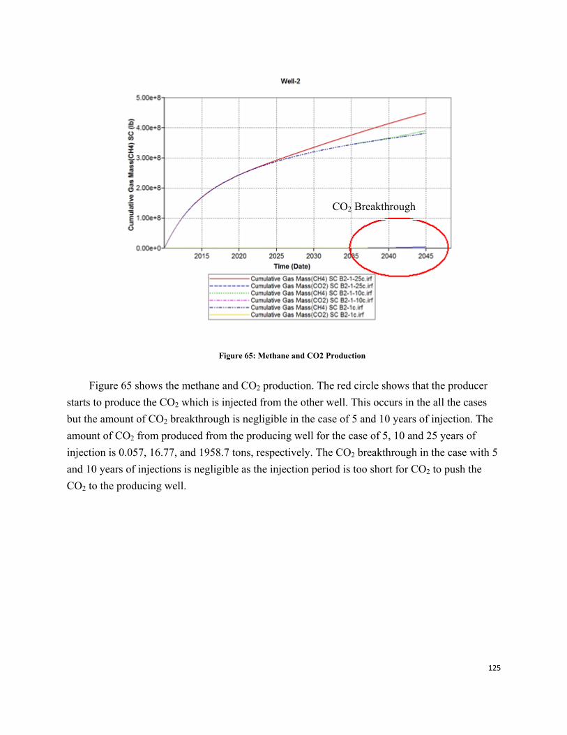
125
Figure 65: Methane and CO2 Production
Figure 65 shows the methane and CO2 production. The red circle shows that the producer starts to produce the CO2 which is injected from the other well. This occurs in the all the cases but the amount of CO2 breakthrough is negligible in the case of 5 and 10 years of injection. The amount of CO2 from produced from the producing well for the case of 5, 10 and 25 years of injection is 0.057, 16.77, and 1958.7 tons, respectively. The CO2 breakthrough in the case with 5 and 10 years of injections is negligible as the injection period is too short for CO2 to push the CO2 to the producing well.
CO2 Breakthrough

126
Block 4 Case 2 with continuous injection since the beginning of
production
Figure 66: Production Rate for Block 4 Case 2 with early Continuous CO2 Injection
Figure 67: Cumulative Production for Block 4 Case 2 with early continuous CO2 Injection
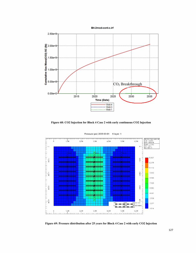
127
Figure 68: CO2 Injection for Block 4 Case 2 with early continuous CO2 Injection
Figure 69: Pressure distribution after 25 years for Block 4 Case 2 with early CO2 Injection
CO2 Breakthrough

128
Figure 66 to Figure 69 show the simulation results for the Block 4 Case 2 with continuous CO2 injection at the beginning of the production. It is important to note that due to limited access to CMG in the computer lab, the simulation had to stop after 7 hours of simulation. The results are shown only the 25 years of production and injection. Figure 66 shows the production rate comparison with the case with only 5 years of injection and the case without CO2 injection. At year 2035, the production rate of the producing well is at 1600 MSCF/day. Comparing this result with the case for injection for 25 years after the well has produced for 10 years, the difference in production rate is only 100 MSCF/day which is roughly 6.6% increase in production rate. The injection is very slow at the beginning because it is difficult to inject CO2 into the formation which is initially saturated with methane. Figure 68 shows that the producing wells start to produce the CO2 after 28 years of injection. The amount of produced CO2 is relatively small compared to the amount of injected CO2.
Economic Analysis
Future Price Prediction
We run an ordinary least square (OLS)24 regression by the software STATA. The regression result is in Table 19.
Table 19: Regression result for future price prediction
From the result we can see that all the coefficients are significant, and the R-square25 reaches as high as 97%, which shows that our regression can predict the future price with a very
24 When we have a group of coefficients, we can get a predicted value of dependent variable by a group of independent variables. The difference
of predict value and observed value is called residual. Square of residual shows how the predicted result differs from the observed one. The OLS
regression tries to find such a group of coefficients that minimize the sum of residual squares.
_cons .0618443 .1156058 0.53 0.594 -.1675426 .2912312 forep .381739 .074571 5.12 0.000 .2337739 .529704 futp3 -.2535679 .0461484 -5.49 0.000 -.3451363 -.1619995 futp1 .8376666 .0822412 10.19 0.000 .6744824 1.000851 futp Coef. Std. Err. t P>|t| [95% Conf. Interval
Total 86.0779128 102 .843901106 Root MSE = .15878 Adj R-squared = 0.9701 Residual 2.49592589 99 .025211373 R-squared = 0.9710 Model 83.5819869 3 27.8606623 Prob > F = 0.0000 F( 3, 99) = 1105.08 Source SS df MS Number of obs = 103

129
high confidence level. F (3, 99) and “Prob > F” are F-test statistics measure the possibility of all the coefficient equal to 0 at the same time. The value of “Prob > F” equals 0.0000 means that the possibility that all coefficients are 0’s, i.e. our model can predict nothing, is 0.0000.
For the years after 2035, we do not even have forecast price. In this part, we cannot run the regression above. The method we use here is to assume that the natural gas will keep the same value of 2035, i.e. nominal price changes with the discounting rate.
2035, 2035, (1 3%)i
i j jFutp Futp −= × + (23)
In which Futpi,j indicates the future price for the j’th month in the i’th year, and Futp2035,j gives the future price for the j’th month in 2035.
Figure 70: Forecast price and future price. Future price before 2018 comes from the Henry Hub data. Future price
between 2019 and 2035 comes from our regression result. Future price after 2036 comes from formula (4). The blue line
shows the forecast price from EIA.
Every up-and-down period in the graph is one year. The main reason is price will go higher in winter due to the heating demand. We also point out from the graph that our future price is a
25 R-square is a parameter that can measure how much the estimate model is consistent with the observed value.
0
5
10
15
20
25
30
Jan/10
Feb/12
Mar/14
Apr/16
May/18
Jun/20
Jul/22
Aug/24
Sep/26
Oct/28
Nov/30
Nov/32
Nov/34
Nov/36
Nov/38
Nov/40
Nov/42
Nov/44
Nov/46
Nov/48
Price $/M
SCF
Forecast Price and Future Price
Forep
FutP

130
litter lower than the forecast price. The difference between the future price and the forecast price captures the risk premium26, i.e. the amount we would like to give out to avoid risk.
Using this price, we have automatically adjusted the risk, and we treat all the NPV derived from this future price as NPV without risk.
DCF Analysis Results and Comparison
Accumulative NPV curves for ten sets of well designs in the reservoir will be shown below for both productions with and without hydraulic fracture. For the productions with CO2 injection and hydraulic fracture, we will only show the comparison of the best sets of well design in each homogeneous reservoir block.
No Hydraulic Fracture
Table 20: Years Accumulative NPV Result-No Hydraulic Fracture
Block No. Best Design Payback period Accumulative NPV (USD) Payback Period for Whole Project
1 Case 1 89 months 9,352,174
163 months 2 Case 1 210 months 6,320,659
3 Case 1 203 months 8,776,838
4 Case 2 162 months 14,132,809
26 Most of the people are risk‐avoid people, i.e. if there’s a value v1 with risk, someone will consider it as a value v2 without risk, and v1>v2. The
difference of v1 and v2 is the risk premium for him. Since different individuals have different risk preference, they have different risk premium
for the same risk level. In this paper, the risk premium we get is a market‐commonly‐accepted risk premium.

131
Figure 71: DCF analysis for block 1 without hydraulic fracture
Figure 72: DCF analysis for block 2 without hydraulic fracture

132
Figure 73: DCF analysis for block 3 without hydraulic fracture
Figure 74: DCF analysis for block 4 without hydraulic fracture

133
With Hydraulic Fracture Only
It can be observed above that most of cases are not profitable when producing gas without hydraulic fracture. When considering the NPV of the whole project, even the best situation takes more than 13 years to pay back. Comparing with the normal payback period 8 months to 3 years, 13 years is too long to be attractive to the investor.
Figure 75: DCF analysis for block 1 with hydraulic fracture
Figure 76: DCF analysis for block 2 with hydraulic fracture

134
Figure 77: DCF analysis for block 3 with hydraulic fractur2
Figure 78: DCF analysis for block 4 with hydraulic fractur2
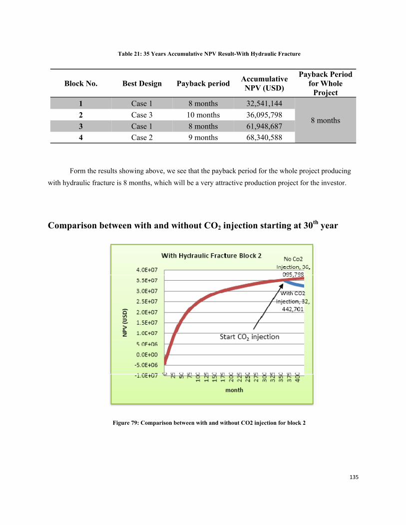
135
Table 21: 35 Years Accumulative NPV Result-With Hydraulic Fracture
Block No. Best Design Payback period Accumulative NPV (USD)
Payback Period for Whole
Project 1 Case 1 8 months 32,541,144
8 months 2 Case 3 10 months 36,095,798 3 Case 1 8 months 61,948,687 4 Case 2 9 months 68,340,588
Form the results showing above, we see that the payback period for the whole project producing with hydraulic fracture is 8 months, which will be a very attractive production project for the investor.
Comparison between with and without CO2 injection starting at 30th year
Figure 79: Comparison between with and without CO2 injection for block 2

136
Figure 80: Comparison between with and without CO2 injection for block 3
Figure 81: Comparison between with and without CO2 injection for block 4
FromTable 21, we know the best well design case for each reservoir blocks. We only run the analysis code for the best cases when injecting CO2 in the last five years.

137
It can be observed that the accumulative NPV started to drop at the 30th year, which is also the time that we start the CO2 injection. It simply means that under no government incentive, yield from increased gas production by CO2 injection is not able to offset the cost for CO2 injection.
Table 22: Years Accumulative NPV Comparison
Block No. NPV-Without CO2 NPV-With CO2 5-year Term NPV Difference
2 36,095,798 32,442,701 -3,653,097 USD
3 61,948,687 56,283,268 -5,665,419 USD
4 68,340,588 64,005,581 -4,335,007 USD

138
35 years accumulative NPV comparison
From the comparison of result below, we can see that with stimulation the production by hydraulic fracture can increases 660% of NPV compared to no hydraulic fracture project in the 35 years term. Besides, 5 years CO2 injection decreases NPV by 7% compared to the project with hydraulic fracture only. Table 23 presents the 35 years discounted return on investments (ROI) of three production situations. With the data in Table 23, we can also calculate the annual geometric average rate of return, also known as the time-weighted rate of return. Since the ROI in Table 23 has already been discounted, the geometric average rate of return will become:
rDiscounted ROI
n , when n number of period
By calculations, the annual geometric average rate of return of the project without hydraulic fracture is about 0.0218, which is much lower than current rate in the U.S. 30 Years Treasury Bill (about 0.053), which has extremely low investment risk. It means that the opportunity cost is too high and it is totally not an attractive investment. However, for the project with hydraulic fracture, the geometric average rate of return is about 0.2467, and for the project with CO2 injection is about 0.2278. They are both much higher than the yield of T-Bill, it means that these two production projects are economical attractive.
Figure 82: NPV for 35 years
26,181,427
198,916,218185,262,696
No Hydraulic Fracture
Hydraulic Fracture
CO2 Injection
NPV for 35 years
NPV for 35 years

139
Table23: Years Yield Analysis
BLOCK No Hydraulic Fracture
Hydraulic Fracture
CO2 Injection
1 9,352,174 32,531,144 32,531,144 2 6,320,659 36,095,798 32,442,701 3 8,776,838 61,948,687 56,283,268 4 1,731,756 68,340,588 64,005,581
Total(USD) 26,181,427 198,916,218 185,262,696 Investment(USD) 14,848,481 20,647,268 20,647,268
ROI 0.763 8.634 7.973

140
Chapter 4: Discussion
Discussion on NPV for the optimized case From previous section, we know that the project only with hydraulic fracture has the highest
35-years Net Present Value and the highest Return on Investment. In this section, we will look into the monthly return rate and see the financial performance of the project.
We breakdown the investment into 420 months and then we can get the average investment amount in a month of the project. Then we divide the monthly profit cash flows by the monthly average investment, we will get the monthly Return on Investment, see Figure 83 below:
Figure 83: Monthly return on investment
The ROI is extremely high at the beginning, and also fall very fast as well. After around 9.4 years (113 months), the monthly ROI drop below the 35-years average ROI, this is 8.634. What is more, after 14 years (168 months), the ROI drop below 30 years T-bill return rate, which is currently around 4.7. After this point, the company has two options:
1) Keep producing gas until the project reaches its maximum NPV, which will be more than 35 years. The record we have for the NPV have not reach the peak yet.
‐20
0
20
40
60
80
100
120
1 21 41 61 81 101
121
141
161
181
201
221
241
261
281
301
321
341
361
381
401
ROI
Month
Monthly ROI

141
2) Sell the reservoir and production facilities to other company. Through reinvestment with the cash we get, we could receive a higher return rate than simply keep running the project. However, no company will buy the project at its full residual price. That is to say, before we sell the project at a discounted residual price, it needs to be calculated that the price is high enough to make our reinvestment’s return higher than the return by simply keeping the project running.
The choice really depends on situations, a lot of factors need to be considered, for example, discounted price of the project, T-bill rate, time of selling the project, investment risk, etc. Since it is not the purpose of out project, we will not make the assumption and calculation here.
Possible way to make CO2 injection profitable
Carbon credit
A carbon credit is a generic term meaning that a value has been assigned to a reduction or offset of greenhouse gas emissions. Selling carbon credit could be a possible way to make our project using CO2 injection enhanced gas recovery profitable. Assume that the income from selling carbon credit still needs to be taxed, the calculation will be:
Price of carbon credit Difference to Target NPV C CO C CO
1 Tax , (24)
Consider the CO2 injection period which is the last five years of the project, the result presented in Table 24 using the general equation above.

142
Table 24: Price of carbon credit which could make production stop losing money or more profitable than producing
with hydraulic fracture only
For Year
Ended
NPV decreased by CO2 injection
(USD)
NPV difference between
projects with and without
CO2 injection
(USD)
Cost of CO2 injection
(USD)
Price of carbon credit to make CO2 injection stop losing money
(USD/ton)
Price of carbon credit to make project with
CO2 injection become more
profitable than with hydraulic
fracture only(USD/ton)
31th 3,853,753 4,806,846 6,830,467 15.45754853 19.28043872
32th 2,162,147 7,834,150 3,697,278 16.0217633 58.05196775
33th 1,527,780 10,156,628 2,519,519 16.61308954 110.4432327
34th 1,164,737 12,052,014 1,858,120 17.17360123 177.7022992
35th 922,925 13,653,522 1,441,497 17.54121106 259.5003966
Total 9,631,342 48,503,159 16,346,880 16.14206391 81.2909652
Table 24 showing that with the average price of carbon credit $16.142, the project with CO2 injection will not be a loss; and with the average price of carbon credit $81.291, the project with CO2 injection can earn as much as the project with hydraulic fractures only. Recently, a company in Middlefield, Ohio, Molten Metal Equipment, bought carbon credit for $21.50/ton. It means that it is totally possible to make the project with CO2 injection stop losing money. However, the current price of carbon credit is still too low to make our project with CO2 as profitable as the project with hydraulic fracture only.

143
Chapter 5: Conclusion The selected area in Fort Worth Basin has the highest natural gas production potential in
Texas. The goal for well design and field development was to optimize drilling efficiency and minimize cost. This was achieved by the use of a Flex drilling rig to drill each of the 8 wells in our reservoir. Even though the daily cost to use a Flex Rig is about $56000 when compared to the cost of using conventional drilling rig ($50000) with about $6000 difference, the rate of drilling is 7 days faster using Flex Rig and overall, we save about 200,000 dollars a well using Flex Rig. Also the use of different sizes of Varel drilling bit designed for Chesapeake Energy help us save at least a day from our drilling time due to the increased rate of penetration Varel bits offered by this bit over the previous drill bit that has been used by Chesapeake Energy. Also the open hole completion that we utilized for the 4,000 ft horizontal lateral length help us save a lot of money and time. All the cost and savings were combined into one drilling cost and taking into consideration during our NPV calculations. The effects on the NPV were not as much as we would expect since we made so much profit from the total production from our Reservoir. For the stimulation treatment, Sand and ultra light sand as the proppant and Slick water with HPG cross linked gel as the fracture fluid. The Equipment for the project had a treating pressure of about 10,000 psi, pumping rate 90 bbl per minute, For one fracture, 3,360 bbl gel, 890 lbm, and 1.1 million bbl water are used and the time for one fracture job is about 470 minutes.
Finally, its was can be observed the production of natural gas in Barnett Shale by horizontal wells without hydraulic fracture stimulation has annual rate of return 2.18% and 163 months payback period, which is not economically attractive. It can be observed the price of carbon credit needs to be $16.15/ton to offset the loss from CO2 injection. To make the project with CO2 injection as profitable as the project with hydraulic fracture only, the price of carbon credit needs to be $81.29/ton. Producing natural gas in Barnett Shale by horizontal wells with hydraulic fracture stimulation has the highest 35 years net present value $198,916,218, the highest rate of return 24.67% and only 8 months payback period, which is also the optimized result in our project. Then the ROI of the optimized project will be lower than the 30 years U.S. T-bill return rate after 168 months, a decision has to be made either to keep running the project or reinvest by the cash selling the project.

144
REFERENCE: • Grieser, B., Bray, J.:“Identification of Production Potential in Unconventional
Reservoir,” paper SPE 106623 presented at the 2007 SPE Preduction and Operations Symposium held in Oklahoma City, Oklahoma, U.S.A., 31 March-3 April.
• Syfan, F.E.Jr., Newman, S.C., Meyer, B.R., Behrendt, D.M.:”Case History: G-Function analysis Proves Beneficial in Barnett Shale Application,” paper SPE 110091 presented at the 2007 SPE Annual Technical Conference and Exhibition in Anaheim, California, 11-14 November.
• Passey, Q.R., Creaney, S., Kulla, J.B., Moretti, F.J., Stroud, J.D.:”A Practical Model for Organic Richness from Porosity and Resistivity Logs,” American Association of Petroleum Geologists Bulletin, V.74 No 12, December 1990.
• Grieser, B., Shelley, B., Johnson, B.J., Fielder, E.O., Heinze, J.R., Werline, J.R.:”Data Analysis of Barnett Shale Completions”, paper SPE 100674 presented at the 2007 SPE Annual Technical Conference, San Antonio, Texas, U.S.A..
• Warren, J.E., Root, P.J.: “The Behavior of Naturally Fractured Reservoirs,” paper SPE 426. September 1963.
• King, G.R.: “Material Balance Techniques for Coal Seam and Devonian Shale Gas Reservoirs,” paper SPE 20730. September 1990.
• Yu, J.P., Yang, Jian-ru.: “Development of Composite Reservoir Model for Heterogeneous Reservoir Studies,” paper SPE 21266 presented at the 1990 SPE Eastern Regional Meeting, Columbus, Ohio, 31 October-2 November.
• Chen, C., Raghavan, R.: “Modeling a Fractured Well in a Composite Reservoir,” paper SPE 28393, December 1995.
• Cipolla, C.L., Lolon, E.P.,Erdle, J.C.,Tathed, V.: “Modeling Well Performance in Shale-Gas Reservoirs,” paper SPE 125532 presented at the 2009 SPE/EAGE Reservoir Characterization and Simulation Conference, Abu Dhabi, UAE, 19-21 October.
• “Recent advances in hydraulic fracturing”, John L. GIDLEY; Stephen A. Holditch…volume 12
• “Width of hydraulic fractures”, T. K. PERKINS; L. R.KERN SPE 89 • “Successful multistage hydraulic fracturing treatment using a seawater based
polymore-free fluid sustem executed from a supply vessel; Lebada vest field, blasck sea offshore romania” Tom bukowac Rafik B.. SPE 121204
145
• “A Comparison of Freshwater- and Seawater-Based Borate-Crosslinked Fracturing Fluids” Phillip C. Harris, SPE, and Diederik van Batenburg, SPE,spe50777
• “Tight gas resource and technology appraisal: sensitivity analysis of the national petroleum council estimates” Brashear, J.P.; Rosenberg, J. I. SPE 12862
• BJ services publication on shale gas simulation 2002 • Schepers, K.C., Nuttall, B., Oudinot, A.Y., Gonzalez, R.: “Reservoir Modeling
and Simulation of the Devonian Gas Shale of eastern Kentucky for Enhanced Gas Recovery and CO2 Storage,” paper SPE 126620 presented at the 2009 Annual SPE International Conference, San Diego, California, USA, 10-11 November.
• Oldenburg, C.M., Benson, S.M.: “CO2 Enhanced Gas Recovery Studied for an Example Gas Reservoir,” paper SPE 74367 presented at the 2002 SPE International Petroleum Conference and Exhibition, Villahermosa, Mexico, 10-12 February.
• Jikich, S.S., Smith, D.H., Sams, W.N., Bromhal, G.S.: “Enhanced Gas Recovery with Carbon Dioxide Sequestration: A Simulation Study of Effects of Injection Strategy and Operational Parameters,” paper SPE 84813 presented at the 2003 SPE Eastern Regional/AAPG Eastern Section Joint Meeting, Pittsburgh, Pennsylvania, USA, 6-10 September.
• Kuuskraa, V. A., Koperna, G., Schmoker, J., and Quinn, J.; “Barnett Shale Rising Star in Fort Worth Basin” Oil and Gas Journal, Vol. 96, No. 21, May 25, 1998, pp. 67-76.
• Reeves, S. R., Kuuskraa, V. A., and Hill D. G.; “New Basins Invigorate U.S. Gas Shales Play”, Oil and Gas Journal, Vol. 94, No. 4, January 22, 1996, pp. 53-58.
• Railroad Commission of Texas, "Barnett Shale Information – Updated July 30, 2008."
on-line document: http://www.rrc.state.tx.us/barnettshale/index.html
• Railroad Commission of Texas, "Newark, East (Barnett Shale) Field – Map – April 17, 2008." RRC Geographic Information Systems, Austin, Texas.
on-line database: http://www.rrc.state.tx.us/divisions/og/maps/index.html
• U.S. Environmental Protection Agency and the Gas Research Institute, "Methane Emissions from the Natural Gas Industry." EPA/600/SR-96/080, GRI-94/0257. June 1996.
• on-line document: http://www.epa.gov/gasstar/documents/emissions_report/1_executiveummary.pdf and

146
http://www.p2pays.org/ref%5C07/06348.pdf
• U.S. Environmental Protection Agency, "Greenhouse • The Barnett Shale, Visitors Guide to the Hottest Gas Play in the US, Pickering
Energy Partners • Barnett Shale Groundwater Use Estimates, Jean-Philippe Nicot, PE, PG, and Eric
Potter, PG • Barnett Shale: Detailed Discussion, Scott Montgomery, IHS Energy Petroleum
Frontiers Excerpt • Evaluation of Hydrocarbon Generation and Storage in the Barnett Shale, Ft.
Worth Basin, Texas, Dan Jarvie, Humble Geochemical Services • Evaluation of the Barnett Shale, Doug Boone, IHS Energy • Awerbuch, S., 1993. The surprising role of risk in utility integrated resource
planning. The Electricity Journal 6 (3), 20–33. • Awerbuch, S., 1994. Risk-adjusted IRP: it’s easy!!! In: Proceedings of the
NARUC-DOE Fifth National Conference on Integrated Resource Planning, Kalispell, Montana, pp. 228–269.
• Bolinger, M., Wiser, R., Golove, W., 2003. Accounting for Fuel Price Risk: Using Forward Natural Gas Prices Instead of Gas Price Forecasts to Compare Renewable to Gas-Fired Generation. LBNL-53587, Lawrence Berkeley National Laboratory, Berkeley, CA.
• Chinn, M.D., LeBlanc, M., Coibon, O., 2001. The predictive characteristics of energy futures: recent evidence for crude oil, natural gas, gasoline and heating oil. UCSC Economics Working Paper No. 490
• JOHN H. HERBERT.The relation of monthly spot to futures prices for natural gas. Energy(Oxford) 18:1111, 1119-1124, Elsevier Science, 1993.
• Kahn, E., Stoft, S., 1993 (unpublished draft). Analyzing Fuel Price Risks Under Competitive Bidding. Lawrence Berkeley National Laboratory, Berkeley, CA.
• Mark Bolinger, Ryan Wiser, William Golove, 2004. Accounting for fuel price risk when comparing renewable to gas-fired generation: the role of forward natural gas prices.
• Walls, W.D., 1995. An econometric analysis of the market for natural gas futures. The Energy Journal 16 (1), 71–83.
• Energy Information Administration: “Drilling sideways – A Review of Horizontal Well Technology and Its Domestic Application,” April 1993.

147
R. Schweitzer, H.I. Bilgesu.: “The Role of Economics on Well and Fracture Design Completions of Marcellus Shale Wells,” paper SPE 125975 presented at the 2009 SPE Eastern Regional Meeting, Charleston, West Virginia, USA, 23-25 September.
• S.D. Joshi, SPE, Joshi Technologies international, inc. “ Cost/Benefits of horizontal wells,” paper spe 83621
• Jennifer L. Miskimins, SPE, Colorado school of mines. “ Design and life-cycle consideration for unconventional-reservoir wells,” SPE production and operation
• The barnet shale formation, Horizontal drilling in north texas. http://www.expertreviewof.com/
• U.S Department of energy. Office of fossil energy, National energy technology laboratory. “ Modern Shale gas development in the United States: A primer.” April 2009
• Hyne, Norman : Non-Technical Guide To Petroleum Geology, Exploration, Drilling And Production. Penn Well Publishing Company. 2003
• Bourgoyne Adam, Chenevert Martin, Millheim Keith, F.S. Young. Applied Drilling Engineering. SPE Textbook Series, Vol.2

148
Appendix
Simulation results for every case
The results for the optimized case for each block are shown in the Results section. For the cases which are not optimum cases, the production rate, cumulative production, and pressure distribution after 35 years will be shown.
Block 1 Case 2
Figure 84: Block 1 case 2 Production Rate

149
Figure 85: Block 1 Case 2 Cumulative Production
Figure 86: Block 1 Case 2 Pressure distribution after 35 years

150
Block 2 Case 1
Figure 87: Block 2 Case 1 Production Rate
Figure 88: Block 2 Case 1 Cumulative Production

151
Figure 89: Block 2 Case 1 Pressure distribution after 35 years
Block 2 Case 2
Figure 90: Block 2 Case 2 Production Rate

152
Figure 91: Block 2 Case 2 Production Rate
Figure 92: Block 2 Case 2 Pressure distribution after 35 years

153
Block 3 Case 2
Figure 93: Block 2 Case 2 Production Rate
Figure 94: Block 2 Case 2 Cumulative Production

154
Figure 95: Block 2 Case 2 Pressure distribution after 35 years
Block 4 Case 1
Figure 96: Block 4 Case 1 Production Rate

155
Figure 97: Block 4 Case 1 Cumulative Production
Figure 98: Block 4 Case 1 Pressure distribution after 35 years

156
Block 4 Case 3
Figure 99: Block 4 Case 3 Production Rate
Figure 100: Case 3 Cumulative Production

157
Figure 101: Block 4 Case 3 Pressure distribution after 35 years
It is to be noted that for Block 4 Case 3, the production rates and cumulative productions from each well are not equal because the drainage areas for each well are different. As shown in Figure 101, the drainage area for the left well (Well-1) is greater than the right well (Well-2), and the right well has greater drainage area than the middle well (Well-3). Consequently, Well-1 has the highest production rate and cumulative production followed by Well-2 and Well-3.
Monthly Forecast price
The prices after 2013 are converted from yearly forecast price. (all price in real-time nominal dollars)
Table 25: Monthly forecast price
Jan Feb Mar Apr May Jun
2010 5.13 4.89 4.71 4.55 4.48 4.55
2011 5.33 5.53 5.57 5.22 5.03 5.00
2012 6.57 6.55 6.48 6.23 6.10 6.12

158
2013 6.72 6.70 6.63 6.37 6.24 6.26
2014 6.86 6.84 6.77 6.52 6.39 6.41
2015 7.27 7.25 7.18 6.92 6.79 6.81
2016 7.60 7.58 7.51 7.26 7.13 7.15
2017 7.83 7.81 7.74 7.48 7.35 7.37
2018 8.12 8.10 8.03 7.77 7.64 7.66
2019 8.44 8.42 8.35 8.10 7.97 7.99
2020 8.86 8.84 8.77 8.52 8.39 8.41
2021 9.25 9.23 9.16 8.91 8.78 8.80
2022 9.78 9.76 9.69 9.44 9.31 9.33
2023 10.11 10.09 10.02 9.76 9.63 9.65
2024 10.34 10.32 10.25 9.99 9.86 9.88
2025 10.76 10.74 10.67 10.41 10.28 10.30
2026 11.32 11.30 11.23 10.98 10.85 10.87
2027 11.88 11.86 11.79 11.53 11.40 11.42
2028 12.61 12.59 12.52 12.27 12.14 12.16
2029 13.40 13.38 13.31 13.05 12.92 12.94
2030 14.27 14.25 14.18 13.92 13.79 13.81
2031 15.30 15.28 15.21 14.95 14.82 14.84
2032 15.95 15.93 15.86 15.60 15.47 15.49
2033 16.48 16.46 16.39 16.13 16.00 16.02
2034 17.39 17.37 17.30 17.05 16.92 16.94
2035 18.17 18.15 18.08 17.83 17.70 17.72
Jul Aug Sep Oct Nov Dec
2010 4.63 4.66 4.73 4.75 4.92 5.06
2011 5.02 5.10 5.14 5.18 5.24 5.39

159
2012 6.17 6.22 6.28 6.31 6.42 6.57
2013 6.31 6.37 6.42 6.45 6.57 6.71
2014 6.46 6.51 6.57 6.60 6.71 6.86
2015 6.86 6.92 6.97 7.00 7.12 7.26
2016 7.20 7.25 7.31 7.34 7.45 7.60
2017 7.42 7.48 7.53 7.56 7.68 7.82
2018 7.71 7.77 7.82 7.85 7.97 8.11
2019 8.04 8.09 8.15 8.18 8.29 8.44
2020 8.46 8.51 8.57 8.60 8.71 8.86
2021 8.85 8.90 8.96 8.99 9.10 9.25
2022 9.38 9.43 9.49 9.52 9.63 9.78
2023 9.70 9.76 9.81 9.84 9.96 10.10
2024 9.93 9.99 10.04 10.07 10.19 10.33
2025 10.35 10.41 10.46 10.49 10.61 10.75
2026 10.92 10.97 11.03 11.06 11.17 11.32
2027 11.47 11.53 11.58 11.61 11.73 11.87
2028 12.21 12.26 12.32 12.35 12.46 12.61
2029 12.99 13.05 13.10 13.13 13.25 13.39
2030 13.86 13.92 13.97 14.00 14.12 14.26
2031 14.89 14.95 15.00 15.03 15.15 15.29
2032 15.54 15.60 15.65 15.68 15.80 15.94
2033 16.07 16.13 16.18 16.21 16.33 16.47
2034 16.99 17.04 17.10 17.13 17.24 17.39
2035 17.77 17.82 17.88 17.91 18.02 18.17

160
Monthly future price data.
(all prices are in real-time nominal dollar)
Table 26: Observed future prices
2010 2011 2012 2013 2014 2015 2016 2017 2018
Jan 5.32 6.00 6.33 6.63 6.96 7.27 7.58 7.90
Feb 5.28 5.95 6.30 6.60 6.93 7.25 7.56 7.88
Mar 5.17 5.77 6.09 6.39 6.72 7.04 7.35 7.67
Apr 3.87 4.95 5.34 5.63 5.93 6.23 6.54 6.85 7.17
May 3.93 4.95 5.33 5.59 5.89 6.19 6.49 6.80 7.13
Jun 4.01 4.99 5.37 5.64 5.94 6.25 6.56 6.87 7.21
July 4.10 5.05 5.43 5.71 6.02 6.33 6.64 6.96 7.30
Aug 4.17 5.11 5.48 5.77 6.08 6.39 6.71 7.02 7.36
Sep 4.21 5.14 5.51 5.80 6.11 6.43 6.74 7.05 7.38
Oct 4.31 5.24 5.61 5.91 6.22 6.53 6.84 7.14 7.47
Nov 4.68 5.49 5.86 6.16 6.47 6.78 7.09 7.40 7.74
Dec 5.10 5.79 6.13 6.43 6.75 7.06 7.37 7.68 8.03
Future price used for NPV calculation
The prices before 2018 are observed data, and prices after 2018 are prediction estimators.
Table 27: Future prices used for NPV calculation
time FutP time Futp time Futp time FutpJan-10 Apr-20 8.25 Jul-30 12.84 Oct-40 19.11
Feb-10 May-20 8.08 Aug-30 12.80 Nov-40 19.24
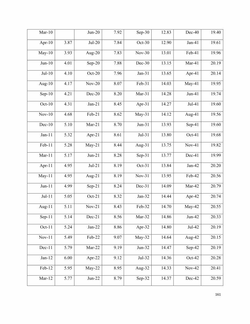
161
Mar-10 Jun-20 7.92 Sep-30 12.83 Dec-40 19.40
Apr-10 3.87 Jul-20 7.84 Oct-30 12.90 Jan-41 19.61
May-10 3.93 Aug-20 7.83 Nov-30 13.01 Feb-41 19.96
Jun-10 4.01 Sep-20 7.88 Dec-30 13.15 Mar-41 20.19
Jul-10 4.10 Oct-20 7.96 Jan-31 13.65 Apr-41 20.14
Aug-10 4.17 Nov-20 8.07 Feb-31 14.03 May-41 19.95
Sep-10 4.21 Dec-20 8.20 Mar-31 14.28 Jun-41 19.74
Oct-10 4.31 Jan-21 8.45 Apr-31 14.27 Jul-41 19.60
Nov-10 4.68 Feb-21 8.62 May-31 14.12 Aug-41 19.56
Dec-10 5.10 Mar-21 8.70 Jun-31 13.93 Sep-41 19.60
Jan-11 5.32 Apr-21 8.61 Jul-31 13.80 Oct-41 19.68
Feb-11 5.28 May-21 8.44 Aug-31 13.75 Nov-41 19.82
Mar-11 5.17 Jun-21 8.28 Sep-31 13.77 Dec-41 19.99
Apr-11 4.95 Jul-21 8.19 Oct-31 13.84 Jan-42 20.20
May-11 4.95 Aug-21 8.19 Nov-31 13.95 Feb-42 20.56
Jun-11 4.99 Sep-21 8.24 Dec-31 14.09 Mar-42 20.79
Jul-11 5.05 Oct-21 8.32 Jan-32 14.44 Apr-42 20.74
Aug-11 5.11 Nov-21 8.43 Feb-32 14.70 May-42 20.55
Sep-11 5.14 Dec-21 8.56 Mar-32 14.86 Jun-42 20.33
Oct-11 5.24 Jan-22 8.86 Apr-32 14.80 Jul-42 20.19
Nov-11 5.49 Feb-22 9.07 May-32 14.64 Aug-42 20.15
Dec-11 5.79 Mar-22 9.19 Jun-32 14.47 Sep-42 20.19
Jan-12 6.00 Apr-22 9.12 Jul-32 14.36 Oct-42 20.28
Feb-12 5.95 May-22 8.95 Aug-32 14.33 Nov-42 20.41
Mar-12 5.77 Jun-22 8.79 Sep-32 14.37 Dec-42 20.59

162
Apr-12 5.34 Jul-22 8.69 Oct-32 14.45 Jan-43 20.80
May-12 5.33 Aug-22 8.67 Nov-32 14.56 Feb-43 21.18
Jun-12 5.37 Sep-22 8.72 Dec-32 14.70 Mar-43 21.42
Jul-12 5.43 Oct-22 8.80 Jan-33 15.00 Apr-43 21.37
Aug-12 5.48 Nov-22 8.91 Feb-33 15.22 May-43 21.16
Sep-12 5.51 Dec-22 9.04 Mar-33 15.34 Jun-43 20.94
Oct-12 5.61 Jan-23 9.27 Apr-33 15.27 Jul-43 20.80
Nov-12 5.86 Feb-23 9.42 May-33 15.10 Aug-43 20.75
Dec-12 6.13 Mar-23 9.48 Jun-33 14.94 Sep-43 20.79
Jan-13 6.33 Apr-23 9.38 Jul-33 14.84 Oct-43 20.88
Feb-13 6.30 May-23 9.21 Aug-33 14.82 Nov-43 21.03
Mar-13 6.09 Jun-23 9.06 Sep-33 14.87 Dec-43 21.20
Apr-13 5.63 Jul-23 8.97 Oct-33 14.94 Jan-44 21.43
May-13 5.59 Aug-23 8.97 Nov-33 15.05 Feb-44 21.82
Jun-13 5.64 Sep-23 9.02 Dec-33 15.19 Mar-44 22.06
Jul-13 5.71 Oct-23 9.10 Jan-34 15.64 Apr-44 22.01
Aug-13 5.77 Nov-23 9.21 Feb-34 15.98 May-44 21.80
Sep-13 5.80 Dec-23 9.35 Mar-34 16.20 Jun-44 21.57
Oct-13 5.91 Jan-24 9.53 Apr-34 16.17 Jul-44 21.42
Nov-13 6.16 Feb-24 9.65 May-34 16.02 Aug-44 21.37
Dec-13 6.43 Mar-24 9.69 Jun-34 15.84 Sep-44 21.42
Jan-14 6.63 Apr-24 9.58 Jul-34 15.71 Oct-44 21.51
Feb-14 6.60 May-24 9.40 Aug-34 15.67 Nov-44 21.66
Mar-14 6.39 Jun-24 9.25 Sep-34 15.70 Dec-44 21.84
Apr-14 5.93 Jul-24 9.18 Oct-34 15.77 Jan-45 22.07

163
May-14 5.89 Aug-24 9.18 Nov-34 15.88 Feb-45 22.47
Jun-14 5.94 Sep-24 9.24 Dec-34 16.02 Mar-45 22.72
Jul-14 6.02 Oct-24 9.32 Jan-35 16.42 Apr-45 22.67
Aug-14 6.08 Nov-24 9.43 Feb-35 16.72 May-45 22.45
Sep-14 6.11 Dec-24 9.56 Mar-35 16.91 Jun-45 22.22
Oct-14 6.22 Jan-25 9.82 Apr-35 16.87 Jul-45 22.06
Nov-14 6.47 Feb-25 9.99 May-35 16.71 Aug-45 22.01
Dec-14 6.75 Mar-25 10.08 Jun-35 16.53 Sep-45 22.06
Jan-15 6.96 Apr-25 9.99 Jul-35 16.42 Oct-45 22.16
Feb-15 6.93 May-25 9.82 Aug-35 16.38 Nov-45 22.31
Mar-15 6.72 Jun-25 9.67 Sep-35 16.42 Dec-45 22.49
Apr-15 6.23 Jul-25 9.58 Oct-35 16.49 Jan-46 22.73
May-15 6.19 Aug-25 9.57 Nov-35 16.60 Feb-46 23.14
Jun-15 6.25 Sep-25 9.62 Dec-35 16.74 Mar-46 23.40
Jul-15 6.33 Oct-25 9.70 Jan-36 16.91 Apr-46 23.35
Aug-15 6.39 Nov-25 9.81 Feb-36 17.22 May-46 23.13
Sep-15 6.43 Dec-25 9.94 Mar-36 17.42 Jun-46 22.89
Oct-15 6.53 Jan-26 10.25 Apr-36 17.37 Jul-46 22.72
Nov-15 6.78 Feb-26 10.48 May-36 17.21 Aug-46 22.67
Dec-15 7.06 Mar-26 10.60 Jun-36 17.03 Sep-46 22.72
Jan-16 7.27 Apr-26 10.54 Jul-36 16.91 Oct-46 22.82
Feb-16 7.25 May-26 10.37 Aug-36 16.87 Nov-46 22.98
Mar-16 7.04 Jun-26 10.21 Sep-36 16.91 Dec-46 23.17
Apr-16 6.54 Jul-26 10.11 Oct-36 16.98 Jan-47 23.41
May-16 6.49 Aug-26 10.09 Nov-36 17.10 Feb-47 23.84

164
Jun-16 6.56 Sep-26 10.13 Dec-36 17.24 Mar-47 24.11
Jul-16 6.64 Oct-26 10.21 Jan-37 17.42 Apr-47 24.05
Aug-16 6.71 Nov-26 10.32 Feb-37 17.74 May-47 23.82
Sep-16 6.74 Dec-26 10.46 Mar-37 17.94 Jun-47 23.57
Oct-16 6.84 Jan-27 10.77 Apr-37 17.89 Jul-47 23.41
Nov-16 7.09 Feb-27 10.99 May-37 17.72 Aug-47 23.35
Dec-16 7.37 Mar-27 11.11 Jun-37 17.54 Sep-47 23.40
Jan-17 7.58 Apr-27 11.04 Jul-37 17.42 Oct-47 23.50
Feb-17 7.56 May-27 10.88 Aug-37 17.38 Nov-47 23.66
Mar-17 7.35 Jun-27 10.72 Sep-37 17.42 Dec-47 23.86
Apr-17 6.85 Jul-27 10.62 Oct-37 17.49 Jan-48 24.11
May-17 6.80 Aug-27 10.60 Nov-37 17.61 Feb-48 24.55
Jun-17 6.87 Sep-27 10.64 Dec-37 17.76 Mar-48 24.83
Jul-17 6.96 Oct-27 10.72 Jan-38 17.94 Apr-48 24.77
Aug-17 7.02 Nov-27 10.83 Feb-38 18.27 May-48 24.53
Sep-17 7.05 Dec-27 10.96 Mar-38 18.48 Jun-48 24.28
Oct-17 7.14 Jan-28 11.34 Apr-38 18.43 Jul-48 24.11
Nov-17 7.40 Feb-28 11.63 May-38 18.26 Aug-48 24.06
Dec-17 7.68 Mar-28 11.80 Jun-38 18.07 Sep-48 24.11
Jan-18 7.90 Apr-28 11.75 Jul-38 17.94 Oct-48 24.21
Feb-18 7.88 May-28 11.59 Aug-38 17.90 Nov-48 24.37
Mar-18 7.67 Jun-28 11.42 Sep-38 17.94 Dec-48 24.58
Apr-18 7.17 Jul-28 11.31 Oct-38 18.01 Jan-49 24.84
May-18 7.13 Aug-28 11.28 Nov-38 18.14 Feb-49 25.29
Jun-18 7.21 Sep-28 11.32 Dec-38 18.29 Mar-49 25.58

165
Jul-18 7.30 Oct-28 11.39 Jan-39 18.48 Apr-49 25.51
Aug-18 7.36 Nov-28 11.50 Feb-39 18.82 May-49 25.27
Sep-18 7.38 Dec-28 11.64 Mar-39 19.03 Jun-49 25.01
Oct-18 7.47 Jan-29 12.04 Apr-39 18.98 Jul-49 24.83
Nov-18 7.74 Feb-29 12.34 May-39 18.80 Aug-49 24.78
Dec-18 8.03 Mar-29 12.52 Jun-39 18.61 Sep-49 24.83
Jan-19 8.12 Apr-29 12.48 Jul-39 18.48 Oct-49 24.94
Feb-19 8.11 May-29 12.32 Aug-39 18.44 Nov-49 25.11
Mar-19 8.01 Jun-29 12.15 Sep-39 18.48 Dec-49 25.32
Apr-19 7.81 Jul-29 12.03 Oct-39 18.55 Jan-50 25.58
May-19 7.58 Aug-29 12.00 Nov-39 18.68 Feb-50 26.05
Jun-19 7.43 Sep-29 12.03 Dec-39 18.84 Mar-50 26.34
Jul-19 7.38 Oct-29 12.10 Jan-40 19.04 Apr-50 26.28
Aug-19 7.41 Nov-29 12.21 Feb-40 19.38 May-50 26.03
Sep-19 7.49 Dec-29 12.35 Mar-40 19.60 Jun-50 25.76
Oct-19 7.59 Jan-30 12.79 Apr-40 19.55 Jul-50 25.58
Nov-19 7.71 Feb-30 13.12 May-40 19.37 Aug-50 25.52
Dec-19 7.84 Mar-30 13.33 Jun-40 19.17 Sep-50 25.57
Jan-20 8.09 Apr-30 13.30 Jul-40 19.03 Oct-50 25.68
Feb-20 8.26 May-30 13.14 Aug-40 18.99 Nov-50 25.86
Mar-20 8.34 Jun-30 12.96 Sep-40 19.03 Dec-50 26.08
Drilling Calculations
The following part shows the process of drilling calculation.


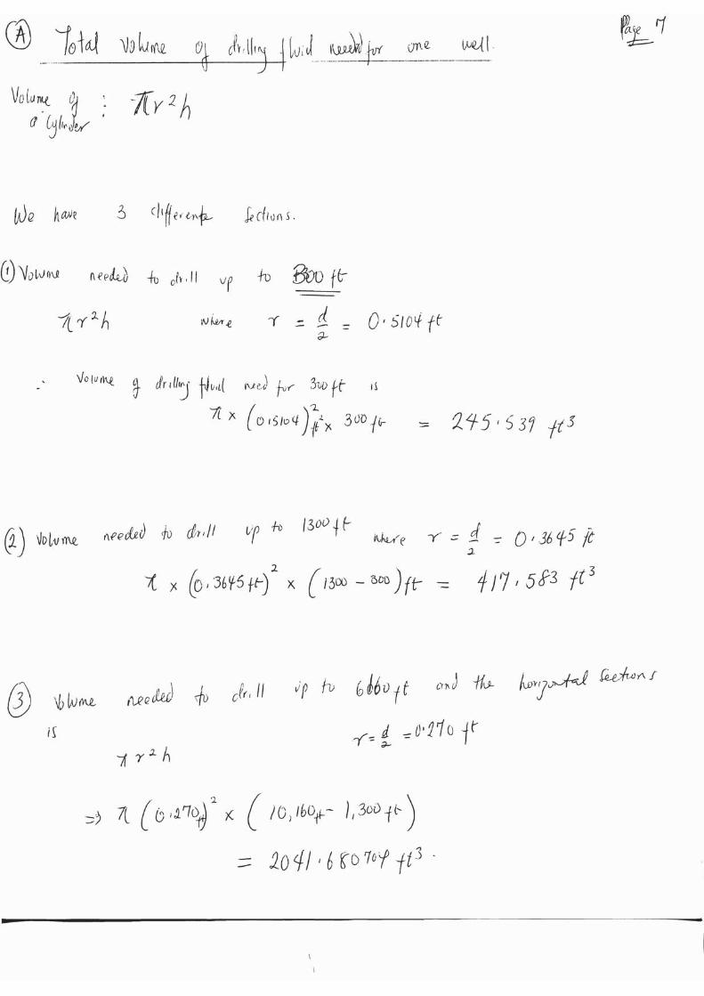
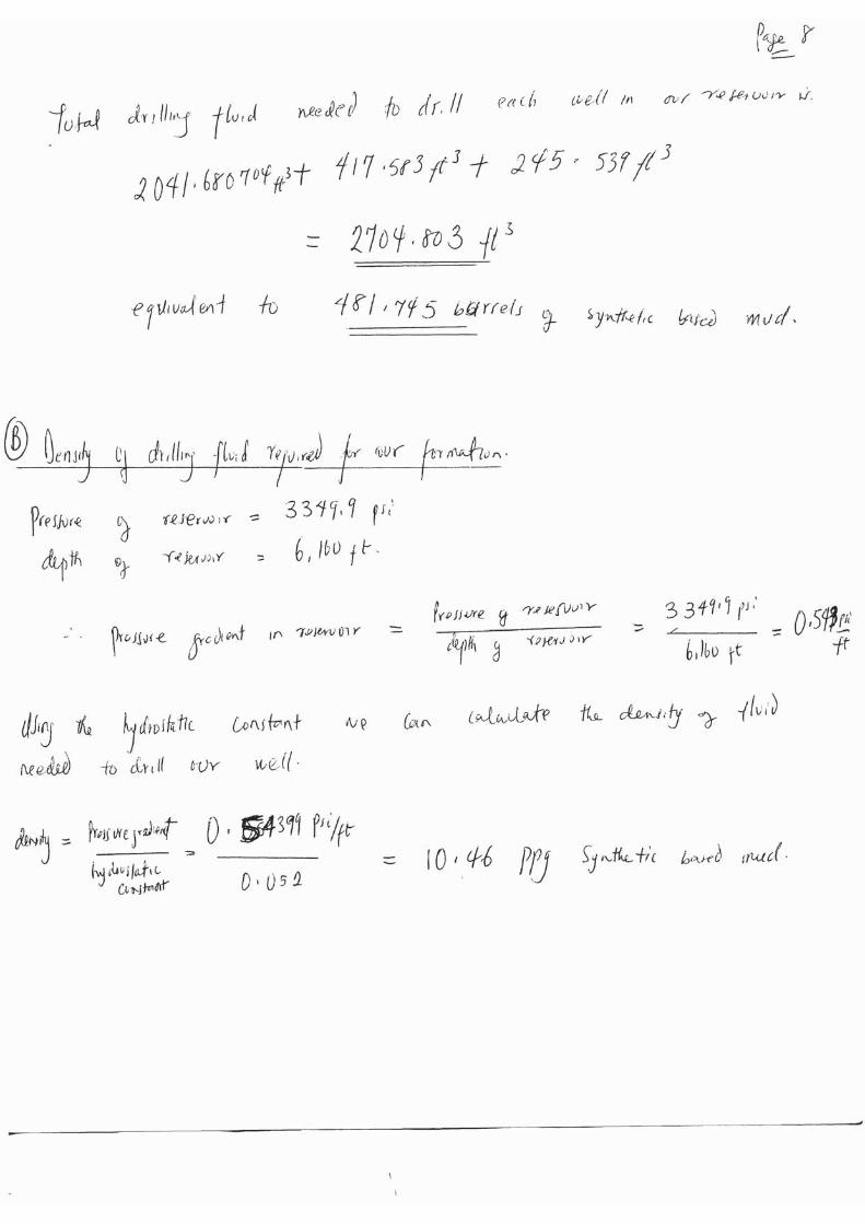


Copyright © 2022 FDOKUMEN