Automatic Piano Sheet Music Transcription with Machine ...

© 2021 Fernandes Saputra, Un Greffin Namyu, Vincent, Derwin Suhartono and Aryo Pradipta Gema. This open access

article is distributed under a Creative Commons Attribution (CC-BY) 4.0 license.

Journal of Computer Science

Original Research Paper

Automatic Piano Sheet Music Transcription with Machine

Learning

1Fernandes Saputra, 1Un Greffin Namyu, 1Vincent, 1Derwin Suhartono and 2Aryo Pradipta Gema

1Computer Science Department, School of Computer Science, Bina Nusantara University, Jakarta, 11480, Indonesia 2Epigene Labs, 7 Square Gabriel Fauré, Paris 75017, France

Article history

Received: 23-09-2020

Revised: 02-03-2021

Accepted: 03-03-2021

Corresponding Author:

Derwin Suhartono

Computer Science Department,

School of Computer Science,

Bina Nusantara University,

Jakarta, 11480, Indonesia

Email: [email protected]

Abstract: Automatic Music Transcription (AMT) is becoming more and

more popular throughout the day, it has piqued the interest of many in

addition to academic research. A successful AMT system would be able to

bridge multiple ranges of interactions between people and music, including

music education. The goal of this research is to transcribe an audio input to

music notation. Research methods were conducted by training multiple

neural networks architectures in different kinds of cases. The evaluation used

two approaches, those were objective evaluation and subjective evaluation.

The result of this research was an achievement of 74.80% F1 score and

73.3% out of 30 respondents claimed that Bidirectional Long Short-Term

Memory (BiLSTM) has the best result. It could be concluded that BiLSTM is

the best architecture suited for automatic music transcription.

Keywords: Automatic Music Transcription, Recurrent Neural Network,

Convolutional Neural Network

Introduction

Artificial intelligence has been a hot topic as of late

due to its powerful capabilities in helping humans, as

such, a lot of applications are now applying it as their

base program. Multiple products of artificial intelligence

could be seen in various fields, one of its best features is

data mining, analyzing chunks of massive data then

returning a particular characteristic from that data.

The popular feature of extracting characteristics is also widely used in other scopes of artificial intelligence. Currently, there has been a lot of research that also challenges artificial intelligence in the topic of

voice processing. As the name suggests, voice processing is the ability of artificial intelligence to retrieve useful information or any characteristic that it could extract from the input, which here is a signal that was converted from the given audio (Joshi et al., 2017). The program is going to receive the audio which then

analyzed and turned into a chain of signals so that the machine could understand and process. This field has a close relation with Automatic Music Transcription (AMT). AMT focuses on how to compute and convert a given audio input into a music signal which later transforms into music notation (sheet music). In respect

to voice processing, AMT is called the musical equivalent of automatic voice recognition, in the sense that both tasks involve converting signals to symbolic

sequences (Benetos et al., 2018). It has been one of the many challenging tasks even for an artificial

intelligence model to discern the audio input regardless of the noises, frequency, etc. and finally return the expected music notation.

Furthermore, AMT is also closely associated with

image processing, as sometimes, musical objects,

usually music notation, could be recognized as a

two-dimensional pattern with respect to time and

frequency, widely known as a spectrogram. From the

spectrogram that audio generated, it was then treated as

the input of an image processing artificial intelligence

where the characteristic of the spectrogram is going to

be extracted and identified. As AMT becomes more and more popular throughout

the day, it has piqued the interest of many in addition to academic research. A successful AMT system would be able to bridge multiple ranges of interactions between people and music, including music education (by producing sheet music, it helps in the process of education), music creation, music production, music search, musicology (Benetos et al., 2018).

Problem Definition

The ability to transcribe music audio into music

notation (sheet music) is one of many fascinating

examples of human intelligence. It requires perception in

Fernandes Saputra et al. / Journal of Computer Science 2021, 17 (3): 178.187

DOI: 10.3844/jcssp.2021.178.187

179

analyzing complex auditory scenes, cognitive ability

(recognizing musical objects), previous knowledge of

the corresponding theory and interference when testing

new combinations in music notation (Benetos et al.,

2018). However, not many have that kind of capability,

some people are still struggling to even define what note

the audio is playing on. Furthermore, when listening to

music by ear, it is quite hard to pin-point the exact and

correct note. This is also the same as how different

artificial intelligence’s architectures or algorithms will

have the result, not all artificial intelligence has the

capabilities to process audio and have a great result at

the end. Therefore, this research will address which of

the available algorithms available will be able to give the

best result to perform an audio processing task. The

problems that could be derived from the statements

above are: What is the difference in the F1-score used

between Convolutional Neural Network (CNN), Long

Short-Term Memory (LSTM), Multilayer Perceptron

(MLP), Deep Neural Network (DNN) and Bidirectional

Long Short-Term Memory (BiLSTM)? And

subsequently what is the most suitable neural network

architecture in processing sequential data (music) for

automatic music transcription?

Related Works

In the first paper from (Sigtia et al., 2016), the paper

proposed an architecture for an end-to-end approach of

transcribing a piece of piano music into music notes. The

proposed model is a combination of an acoustic model of

CNN with the addition of music language model RNN

NADE which is later compared with other architectures.

This paper used full musical pieces from the MIDI

Aligned Piano Sounds (MAPS) (Emiya et al., 2010)

dataset which contained 270 pieces of classical music

and MIDI annotations for training and testing the models

in which 210 of the pieces are synthesized recordings

and the rest are real recordings. The configuration for the

training and testing was 80% of the data for training

(216 musical pieces) and the remaining 20% is for

testing (54 pieces). The paper transforms the input

audio to a time-frequency representation where the

representation chosen is Constant Q Transform (CQT)

over Short Time Fourier Transform (STFT). There are 2

reasons for choosing CQT over STFT, the first reason is

that CQT has much lower dimensional representation

than the STFT in which it is useful when using neural

network acoustic models as it reduces the number of

parameters in the model and the second reason is that

CQT is better suited as time-frequency representation for

music signals, since the frequency axis is linear in pitch.

The next paper is by (Li et al., 2017) which

observed DNN and LSTM in music transcription tasks.

The authors claimed that it is inefficient to deal with

the audio files directly and therefore it will be

transformed into spectrograms to extract features. The

method used in this research is CQT due to its

advantages as it provides a logarithmic frequency

domain and is better in other reports.

This research also uses the MAPS dataset specifically

the MUS part (pieces of music) as the authors claim it is

an outstanding dataset due to each .wav file having a

corresponding text document with ground truth for all

pitches. The total number of pieces of music is 270

(around 11 GB) and the data is split into training,

validation and test sets with 60:20:20 percentage ratio.

Using the MAPS dataset, music files are down sampled

to 16 kHz providing a 32-millisecond duration per

frame. There are 252 features which account for 36

features per octaves. Labels are also generated with 88

labels for each frame. The DNN architecture uses a

ReLU activation function for hidden layers and a

sigmoid activation function for the output. LSTM uses

hyperbolic tangent activation function hidden layers and

sigmoid activation function for the output layer.

Another paper is from (Hawthorne et al., 2017), in

this paper tried to make a transcription pipeline from an

audio into a MIDI file. It uses two architectures to

predict two different things which are combined on a

certain stage to not only predict when notes are played

but also the onset of those notes. The paper itself uses

MAPS datasets which consists of music created with

synthesizers and music created with digital piano and the

authors of this paper also ensure that the same music

piece was not present in more than one set.

The onset and frame detectors used in this study are

built upon the convolutional layer and will be followed by

a bidirectional LSTM with 128 units in both directions

(forward and backward) and then connected to a fully

connected sigmoid layer with 88 outputs to represent the

88 piano keys. The output of the onset detector is then

concatenated with the output of a fully connected sigmoid

of the frame activation detector which is then followed by

BiLSTM. Finally, the output of it is followed by a fully

connected sigmoid layer with 88 outputs.

The authors also compared the proposed

architecture with other similar works and had the best

result. Furthermore, the authors also discussed the need

for more data and more rigorous evaluation. In this

paper, the authors claimed that MAPS dataset has the

main drawback of not providing the needed large

dataset to best measure transcription quality and

therefore will not be able to further improve the result.

There are a lot of papers restricting the data used in

evaluation by only using the first 30 sec or less of each

file. This is due to only using the “close” collection

from each of the test sets and improving the evaluation

score. However, this method was believed to result in

an evaluation that is not representative to transcript the

real-world transcription task.


DOI: 10.3844/jcssp.2021.178.187

180

Kelz et al. (2016) attempted to explore the limitation

of simple approaches in the task of automatic music

transcription in which the authors conduct an in-depth

analysis of neural network based framewise transcription

with detailed analysis of the most suitable input

representations for transcription systems in neural

networks and other hyper-parameter tuning that would

greatly affect the performance of the neural network. The

dataset used in these experiments is the MAPS dataset. It

provides MIDI-aligned recordings of a lot of classical

music pieces. The pieces were rendered using high

quality piano samples as well as real recording from

Disklavier. The author claimed that it ensured clean

annotation and therefore will have almost no label-

noise. The configuration dataset for training and testing

is split to 80:20| percent of each of the categories. This

research tested DNN, ConvNet and AllConv with

different types of hyper parameter tuning for around

3000 runs with a Tesla K40 GPU and each run was

roughly 8-9 h resulting in a total of 900 days of

compute time for this research. The results of all the

runs were that the most important hyper-parameters are

learning rate and spectrogram type. This paper also

used the practical recommendation for training the

neural networks with Stochastic Gradient Descent

(SGD) and the author claimed that strategies that

dynamically adapt the learning rate such as Adam helped

to a certain extent, but still not spare the tuning of the

initial learning rate and its schedule.

A paper from (Dua et al., 2020), also uses RNN-

LSTM model to estimate sheet music generation. The highlighted method from this research is, to improve the accuracy of generated sheet music by using source separation and chord separation. Source separation separates the vocal and non-vocal part from the audio. Chord estimation can be done by dividing the non-vocal

part into drums, bass, melodies and etc. This method is useful for amateurs who just started in learning music and relies heavily on sheet music such as songs that are not too popular such as songs from local bands may not have sheet music at all.

The DSD100 dataset has 100 songs with 44.1 kHz sample rate each with the non-vocal part separated into its component which are bass, drum and other components. Features used to train the model are the

magnitudes of the spectrogram of audio signals. Using magnitude spectra of the mixed signal and magnitude spectra of the target sources which are bass, drum, music and vocal as an input. The output of the network for each epoch are the estimated signal of each source (bass, drum, music and vocal).

Mixed signals are passed on to a Multi cell RNN

containing 3 GRU cells with each of them having 256

units. This RNN model is connected to a dense layer with

Rectified Linear Unit (ReLU) as the activation function

that outputs the estimated signal of each source.

For chord estimation, pitch is the basic unit of a chord

which is a function of the sound’s fundamental frequency.

A set of harmonic pitches that contains two or more

pitches is called a chord containing the non-vocal part

obtained from the source separation method makes a

combination of pitches which means that several chords

are also played in a series. The pitches are then passed on

to a trained feature extractor model to estimate the chords.

Dataset and Features

Dataset

In this project, the data that are going to be used for

training is in the form of music files. The music files or

dataset are collected from MIDI Aligned Piano Music or

widely known as MAPS dataset as the current best

dataset that is available in the formats of music such as

random chords, random notes and real pieces of music

from famous composers such as Mozart, Chopin and

Beethoven. The dataset also provides a different

recording environment including large room, close and

digitally recorded music. The dataset which is used will

be the real pieces of music which include 270 files.

Music files are in WAV format with its corresponding

MIDI file and a text file that explains which pitches were

pressed on the piano and also the onset and offset time.

On this stage, music file names are looked up and are

stored in an array. These files will then be opened on the

next stage to be processed. The data coming from a

music file can be represented with a one-dimensional

array for mono and two-dimensional array for stereo (left

and right channel) of floats with the length of seconds

times sampling rate.

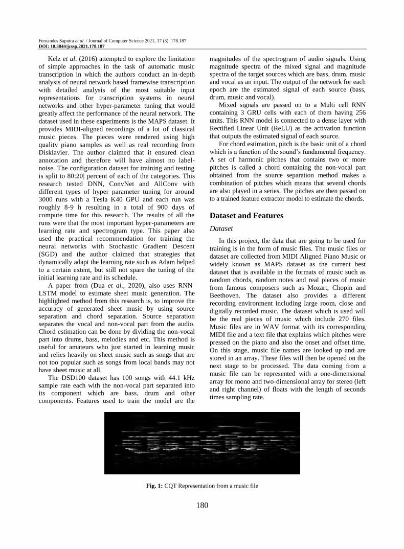
Fig. 1: CQT Representation from a music file


DOI: 10.3844/jcssp.2021.178.187

181

Features

Figure 1 is an example of CQT that was generated

from a music file. Constant-Q Transform (CQT) is

closely related to the Fourier transform which has the

same function of mapping frequencies. The difference is

that CQT has geometrically spaced center frequencies.

Which is very useful because every MIDI pitch also has

geometrically spaced frequencies:

0 2 0,...k

bkf f k (1)

where, b denotes the number of filters per octave. To

make the filter domain adjacent to each other, the k-th

filter is chosen as:

1

1 2 1cq bk k k kf f f

(2)

This calculation resulting in a constant ratio of

frequency to resolution:

11

2 1k bcq

k

fQ

(3)

The advantages of CQT compared to Fourier

transform is that if the number of filters per octave is 12

and f0 which is the minimal center frequency as the

frequency of MIDI pitch of 0, then the k-th cq-bin will

correspond to the MIDI pitch of k (Blankertz, 2001).

When this step is finished, we are left with a similar

two-dimensional array shape across architectures, which

shape is 252 features and some number of frames

depending on time annotated by -1.

Labels

To generate labels, a different approach is used by

different code bases. For instance, LSTM and MLP the

labels are generated by looking at provided text files

such as Fig. 1 and for CNN, the labels are generated by

parsing the MIDI files.

In piano, the number of possible pitches is 88. The

numbers from the MidiPitch column represent a vector

that has a dimension of 88. With this, the label of each

frame can be set to one if the MidiPitch is played in the

current frame and zero if otherwise. These files are then

saved with each file having frames corresponding to the

audio. This means if the audio frames are set to 50000

frames then the label will also have 50000 frames. With

this, each audio file has its corresponding label.

This step will produce a two-dimensional array like

the generated CQT from the previous step. This matrix

has the shape of 88 labels and some number of frames

depending on time annotated by -1.

Methods

Multi-Layer Perceptron and Deep Neural Network

In standardization, the mean and standard deviation

are calculated for each feature and the values are then

subtracted by mean and divided by the standard

deviation resulting in data with a standard deviation of

one. This is done to avoid common problems known as

vanishing gradient and exploding gradient where the data

are too small or too far apart.

The formula is shown below:

_i i

i new

i

x xx

std

(4)

This is done without modifying the shape of the

CQT. MLP and DNN are the same. The difference in

name is made to differentiate the approach used to build

the model. In MLP a naive approach is used which can

be used as a basis. By naive, it means that there is no

consideration to fight back overfitting. In Fig. 2, there is

only one hidden layer with 100 nodes for each classifier

or label and this approach is called a one-versus-all

approach. A one-versus-all approach is basically training

several binary classifier models simultaneously to each

predict a certain pattern. As this problem has 88

expected labels, there are 88 binary classification

models. Each having a hidden layer with 100 nodes with

ReLU activation and 1 node output with sigmoid.

In the case of DNN as shown in the figure, there are 3

hidden dense layers used for training as shown in Fig. 3

with Deep Neural Network with each layer having 256

units paired with a dropout layer at the rate of 0.2. Each

hidden layer is using ReLU activation function and the

output was set using a sigmoid function. The loss

function is Mean Squared Error.

Convolutional Neural Network

The model used for CNN is taken from previous

research of (Bereket and Shi, 2017). As shown in Fig. 4,

the input is in the form of (252, 7, 1) which is the result

of a windowed CQT. The input CQT is in the shape of

(252, 7, 50). The first convolutional layer has 50 filters

with a kernel size of (5, 25) maintaining its original size

and activation function of hyperbolic tangent followed

by a max pooling layer sized (1, 3) reducing the size to

(84, 7, 50). The second convolutional layer also has 50

filters with the same max pooling layer size and dropout

rate but with a different kernel size which is (3, 5) where

3 and 5 is along the frame axis and frequency axis

outputting the same shape (84, 7, 50) which then put

through a max pooling with the shape of (1, 3) for the

second time down sampling it to (28, 7, 50). After that, it

will be flattened resulting in the shape of (9800) and


DOI: 10.3844/jcssp.2021.178.187

182

followed by two fully connected layers with each layer

using sigmoid functions. The first fully connected layer

or the third layer consists of 1000 hidden nodes and the

second fully connected layer or the fourth layer, consists

of 200 nodes. The output layer has 88 nodes with

sigmoid function which is the same as the label

generated so that the output can be compared to which

MIDI pitch is activated in the label. Binary cross entropy

loss function is used for each node. The structures used

are the exact same as the one used in (Bereket and Shi,

2017). As the dataset used in the paper is different, the

models are run again with the same MAPS dataset and

configurations (epoch and early stops) to unify the input

and expected output in order to make it comparable.

Fig. 2: MLP One-Versus-All Architecture

Fig. 3: DNN architecture

1

Input layer Hidden layer Output layer

1 1 99

100

1

99

100

252 88

Input

layer

Hidden

layer

Hidden

layer

Hidden

layer

Output

layer

i0

O0

O1


DOI: 10.3844/jcssp.2021.178.187

183

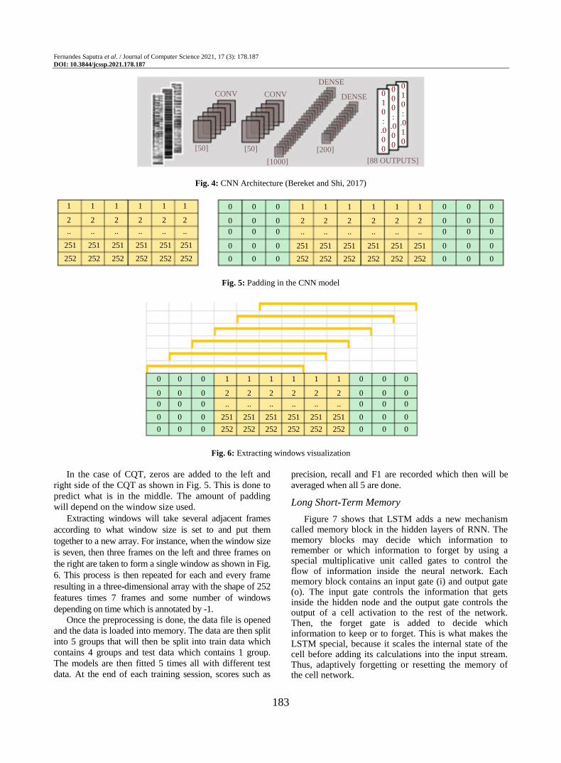
Fig. 4: CNN Architecture (Bereket and Shi, 2017)

Fig. 5: Padding in the CNN model

Fig. 6: Extracting windows visualization

In the case of CQT, zeros are added to the left and

right side of the CQT as shown in Fig. 5. This is done to

predict what is in the middle. The amount of padding

will depend on the window size used.

Extracting windows will take several adjacent frames

according to what window size is set to and put them

together to a new array. For instance, when the window size

is seven, then three frames on the left and three frames on

the right are taken to form a single window as shown in Fig.

6. This process is then repeated for each and every frame

resulting in a three-dimensional array with the shape of 252

features times 7 frames and some number of windows

depending on time which is annotated by -1.

Once the preprocessing is done, the data file is opened

and the data is loaded into memory. The data are then split

into 5 groups that will then be split into train data which

contains 4 groups and test data which contains 1 group.

The models are then fitted 5 times all with different test

data. At the end of each training session, scores such as

precision, recall and F1 are recorded which then will be

averaged when all 5 are done.

Long Short-Term Memory

Figure 7 shows that LSTM adds a new mechanism called memory block in the hidden layers of RNN. The memory blocks may decide which information to remember or which information to forget by using a special multiplicative unit called gates to control the flow of information inside the neural network. Each memory block contains an input gate (i) and output gate (o). The input gate controls the information that gets inside the hidden node and the output gate controls the output of a cell activation to the rest of the network. Then, the forget gate is added to decide which information to keep or to forget. This is what makes the LSTM special, because it scales the internal state of the cell before adding its calculations into the input stream. Thus, adaptively forgetting or resetting the memory of the cell network.

0

1

0

:

.0

0

0

0

0

0

:

.0

0

0

0

1

0

:

.0

1

0

CONV CONV

DENSE

DENSE

[50] [50]

[1000]

[200]

[88 OUTPUTS]

1 1 1 1 1 1

2 2 2 2 2 2

.. .. .. .. .. ..

251 251 251 251 251 251

252 252 252 252 252 252

0 0 0 1 1 1 1 1 1 0 0 0

0 0 0 2 2 2 2 2 2 0 0 0

0 0 0 .. .. .. .. .. .. 0 0 0

0 0 0 251 251 251 251 251 251 0 0 0

0 0 0 252 252 252 252 252 252 0 0 0

0 0 0 1 1 1 1 1 1 0 0 0

0 0 0 2 2 2 2 2 2 0 0 0

0 0 0 .. .. .. .. .. .. 0 0 0

0 0 0 251 251 251 251 251 251 0 0 0

0 0 0 252 252 252 252 252 252 0 0 0


DOI: 10.3844/jcssp.2021.178.187

184

Fig. 7: An Individual Memory Cell of A LSTM Architecture (Morín, 2017)

Fig. 8: BLSTM Architecture

In normalization, the maximum and minimum are

recorded and then the values are capped to 0.0 to 1.0. In

the case of LSTM and DNN, an extra step is taken which

is subtracting the mean from the data. This is done

without modifying the shape of the CQT.

There are 3 hidden LSTM layers and each layer is as

shown in the Fig. 8 (Morín, 2017), with each layer

having 256 units. Using a batch size of 100 frames. The

input matrix size is then modified from [frames, features]

to [frames/100, 100, features] which makes the input size

of the network [100, features]. Using hyperbolic tangent

as the optimal activation function for LSTM. The output

layer has 88 units using the sigmoid activation function.

Mean Squared Error is used for the loss function with a

dropout rate of 0.2 to avoid overfitting.

Bidirectional Long Short-Term Memory

Fs represent inputs whereas the FOs represent outputs.

The dotted arrows symbolize the direction of the Bi-

LSTM (forward or backward). The solid arrows

symbolize the data going from one layer to the other layer.

The Bidirectional LSTM used has the exact same

number of layers with its LSTM counterpart. There are 3

Bi-directional LSTM layers with the shape of (100, 256),

followed by a dense or classification layer with the shape

of (100, 88). This means that there are 3 LSTM layers

going forward and 3 LSTM layers going backward with

the shape of (100, 256) followed by a dense layer. At the

very end of the BiLSTM layer, both outputs from the

forward and backward LSTM layer are concatenated

forming an array with 512 elements before being passed

to the next layer. This means that not only will it know

what is in the past but also what will come afterward,

providing a better context.

Results

Table 1 shows the confusion matrix on class 7 of

BiLSTM on a single music. The model predicted all of

the true labels as false (false negatives). This happened

as there is only a fraction of class 7 on the training data.

Table 2 shows the confusion matrix on class 54 of

BiLSTM. Here, the model predicted most of the true

labels as true some of them as false (false negatives) and

predicted a fraction of false labels as true (false

positives). The class scored 0.72 on F1-score. But note

that this can be affected by the sample vector.

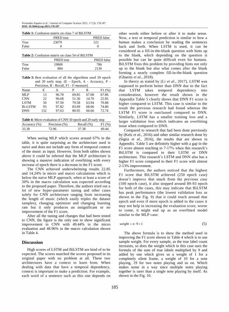
By looking at Table 3, it can be inferred that BiLSTM is superior when compared to the other architecture even though DNN has much higher epoch in most of the cases.

ht-1 ht+1 ht

Xt-1 Xt Xt+1

tanh

tanh

F BiLSTM BiLSTM BiLSTM

BiLSTM BiLSTM BiLSTM F+1

FO

FO+1


DOI: 10.3844/jcssp.2021.178.187

185

Table 1: Confusion matrix on class 7 of BiLSTM

PRED true PRED false

True 23079 521

False 0 0

Table 2: Confusion matrix on class 54 of BiLSTM

PRED true PRED false

True 19800 786

False 884 2130

Table 3: Best evaluation of all the algorithms used 50 epoch

and 20 early stop. (E - Epoch, A - Accuracy, P -

Precision, R - Recall, F1 - F-measure)

Name E A P R F1 (%)

MLP 13 96.78 69.85 67.08 67.86

CNN 22 96.68 51.30 14.70 22.85

LSTM 50 97.50 79.58 63.94 70.88

Bi-LSTM 93 97.82 83.09 68.06 74.80

DNN 152 97.63 80.05 66.66 72.74

Table 4: Micro evaluation of CNN 50 epoch and 20 early stop

Accuracy (%) Precision (%) Recall (%) F1 (%)

33.38 72.96 37.38 49.44

When seeing MLP which scores around 67% in the

table, it is quite surprising as the architecture used is

naive and does not include any form of temporal context

of the music as input. However, from both tables shown

above it could be inferred that the MLP architecture is

showing a massive indication of overfitting with every

increase of epoch there is a decrease in the F1 score. The CNN achieved underwhelming results 22.85

and 14.24% in micro and macro calculations which is below the naive MLP approach, when at least a score of 50% in the macro calculation was expected according to the proposed paper. Therefore, the authors tried out a lot of new hyper-parameter tuning and other cases solely for CNN architecture ranging from increasing the length of music (which easily triples the dataset samples), changing optimizer and changing learning rate but it only produces an insignificant or no improvement of the F1 score.

After all the tuning and changes that had been tested to CNN, the figure is the only one to show significant improvement in CNN with 49.44% in the micro evaluation and 48.96% in the macro calculation shown in Table 4.

Discussion

High scores of LSTM and BiLSTM are kind of to be expected. The scores matched the scores proposed in its original paper with no problem at all. These two

architectures have a context to learn from. When dealing with data that have a temporal dependency, context is important to make a prediction. For example, each word of a sentence such as this one depends on

other words either before or after it to make sense. Now, a text or temporal prediction is similar to how a human makes a conclusion by reading the sentences back and forth. When LSTM is used, it can be considered as a fill-in-the-blank question with hints up to the blank, which depending on the question is

possible but can be quite difficult even for humans. BiLSTM fixes this problem by providing hints not only up to the blank but also what comes after the blank forming a nearly complete fill-in-the-blank question (Ghaeini et al., 2018).

In theory as stated by (Li et al., 2017), LSTM was

supposed to perform better than DNN due to the fact

that LSTM takes temporal dependency into

consideration, however the result shown in the

Appendix Table 5 clearly shows that DNN F1 score is

higher compared to LSTM. This case is similar to the

result the previous research had found whereas the

LSTM F1 score is outclassed compared to DNN.

Similarly, LSTM has a smaller training loss and a

larger validation loss which indicates an overfitting

issue when compared to DNN.

Compared to research that had been done previously

by (Kelz et al., 2016) and other similar research done by

(Sigtia et al., 2016), the results that are shown in

Appendix. Table 5 are definitely higher with a gap in the

F1 score almost reaching to 7-17% when this research’s

BiLSTM is compared to their LSTM or DNN

architecture. This research’s LSTM and DNN also has a

higher F1 score compared to their F1 score with almost

2-13% improvement.

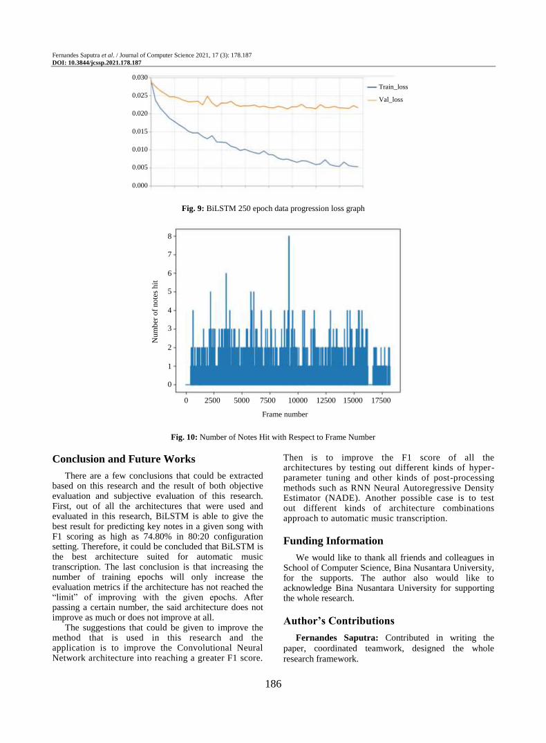
Furthermore, the authors noticed that the highest

F1 score that BiLSTM achieved (250 epoch case)

doesn’t improve that much from the previous case

(100 epoch case), it also stopped around 89-93 epoch

for both of the cases, this may indicate that BiLSTM

has peak performance (the lowest validation loss as

shown in the Fig. 9) that it could reach around that

epoch and even if more epoch is added to the cases it

may not help in increasing the evaluation score, worse

to come, it might end up as an overfitted model

similar to the MLP case:

9 1weight n (5)

The above formula is to show the method used in

improving the F1 score shown in Table 4 which is to use sample weight. For every sample, as the true label count increases, so does the weight which in this case uses the formula of the sum of true labels multiplied by 9 and added by one which gives us a weight of 1 for a completely silent frame, a weight of 10 for a note playing, 19 for two notes playing and so on. Which makes sense in a way since multiple notes playing together is rarer than a single note playing by itself. As shown in the Fig. 10.


DOI: 10.3844/jcssp.2021.178.187

186

Fig. 9: BiLSTM 250 epoch data progression loss graph

Fig. 10: Number of Notes Hit with Respect to Frame Number

Conclusion and Future Works

There are a few conclusions that could be extracted based on this research and the result of both objective evaluation and subjective evaluation of this research. First, out of all the architectures that were used and evaluated in this research, BiLSTM is able to give the best result for predicting key notes in a given song with F1 scoring as high as 74.80% in 80:20 configuration setting. Therefore, it could be concluded that BiLSTM is the best architecture suited for automatic music transcription. The last conclusion is that increasing the number of training epochs will only increase the evaluation metrics if the architecture has not reached the “limit” of improving with the given epochs. After passing a certain number, the said architecture does not improve as much or does not improve at all.

The suggestions that could be given to improve the method that is used in this research and the application is to improve the Convolutional Neural Network architecture into reaching a greater F1 score.

Then is to improve the F1 score of all the architectures by testing out different kinds of hyper-parameter tuning and other kinds of post-processing methods such as RNN Neural Autoregressive Density Estimator (NADE). Another possible case is to test out different kinds of architecture combinations approach to automatic music transcription.

Funding Information

We would like to thank all friends and colleagues in School of Computer Science, Bina Nusantara University, for the supports. The author also would like to acknowledge Bina Nusantara University for supporting the whole research.

Author’s Contributions

Fernandes Saputra: Contributed in writing the

paper, coordinated teamwork, designed the whole

research framework.

0.030

0.025

0.020

0.015

0.010

0.005

0.000

Train_loss

Val_loss

8

7

6

5

4

3

2

1

0

0 2500 5000 7500 10000 12500 15000 17500

Nu

mb

er o

f no

tes

hit

Frame number


DOI: 10.3844/jcssp.2021.178.187

187

Un Greffin Namyu: Coordinated the compilation of

the dataset, participated in the implementation as well

and contributed in manuscript writing.

Vincent: Played main role in the implementation of

the research, elaborated a lot of resources to meet the

requirements.

Derwin Suhartono: As well as corresponding author

lead the team to contribute to the state of the art,

managed all experiments finished in time, as well as

ensured novelty in the manuscript.

Aryo Pradipta Gema: Directed all research works

especially from machine learning perspective and also

observed the whole manuscript before submission.

Ethics

This article is original and contains unpublished

material. The corresponding author confirms that all of

the other authors have read and approved the manuscript

and no ethical issues involved.

References

Benetos, E., Dixon, S., Duan, Z., & Ewert, S. (2018).

Automatic music transcription: An overview. IEEE

Signal Processing Magazine, 36(1), 20-30. https://doi.org/10.1109/MSP.2018.2869928

Bereket, M., & Shi, K. (2017). An AI approach to

automatic natural music transcription.

Blankertz, B. (2001). The constant Q transform.

Retrieved from http://doc.ml.tu-

berlin.de/bbci/material/publications/Bla_constQ.pdf

Dua, M., Yadav, R., Mamgai, D., & Brodiya, S. (2020). An Improved RNN-LSTM based Novel Approach for Sheet Music Generation. Procedia Computer Science, 171, 465-474. https://doi.org/10.1016/j.procs.2020.04.049

Emiya, V., Bertin, N., David, B., & Badeau, R. (2010). MAPS-A piano database for multipitch estimation and automatic transcription of music.

Ghaeini, R., Hasan, S. A., Datla, V., Liu, J., Lee, K., Qadir, A., ... & Farri, O. (2018). Dr-bilstm: Dependent reading bidirectional lstm for natural language inference. arXiv preprint arXiv:1802.05577.

Hawthorne, C., Elsen, E., Song, J., Roberts, A., Simon, I., Raffel, C., ... & Eck, D. (2017). Onsets and frames: Dual-objective piano transcription. arXiv preprint arXiv:1710.11153.

Joshi, S., Kumari, A., Pai, P., Sangaonkar, S., & D'Souza, M. (2017). Voice recognition system. Journal for Research, 3(01).

Kelz, R., Dorfer, M., Korzeniowski, F., Böck, S., Arzt, A., & Widmer, G. (2016). On the potential of simple framewise approaches to piano transcription. arXiv preprint arXiv:1612.05153.

Li, L., Ni, I., & Yang, L. (2017). Music Transcription Using Deep Learning.

Morín, D. G. (2017). Deep Neural Network for Piano Music Transcription. DT2119 Speech and Speaker Recognition course's project at KTH Royal Institute of Technology. Report of Deep Neural Networks for Piano Music Transcription.

Sigtia, S., Benetos, E., & Dixon, S. (2016). An end-to-end neural network for polyphonic piano music transcription. IEEE/ACM Transactions on Audio, Speech and Language Processing, 24(5), 927-939. https://doi.org/10.1109/TASLP.2016.2533858

Appendix

Table 5: Micro evaluation of all the architectures in every Scenario

No Architecture Early stop Epoch Accuracy (%) Precision (%) Recall (%) F1 (%)

1 MLP (20 Epoch) 10 13 96.78±0.93 69.85±9.42 67.08±3.28 67.86±3.96

2 MLP (50 Epoch) 15 19 96.76±0.79 68.94±7.78 67.01±3.10 67.58±3.53

3 MLP (100 Epoch) 20 23 96.66±0.86 67.98±8.75 66.87±2.53 66.95±3.66

4 CNN (20 Epoch) 10 12 96.67±0.12 50.37±2.60 12.72±1.13 20.28±1.52

5 CNN (50 Epoch) 15 17 96.68±0.095 51.52±3.16 13.93±0.89 21.93±1.36

6 CNN (100 Epoch) 20 22 96.68±0.089 51.30±2.93 14.70±0.82 22.85±1.27

7 LSTM (20 Epoch) 10 20 97.33±0.2 79.34±1.6 59.23±3.7 67.74±2.2

8 LSTM (50 Epoch) 15 50 97.50±0.2 79.58±2.2 63.94±2.7 70.88±2.2

9 LSTM (100 Epoch) 20 78 97.46±0.2 77.92±1.7 64.88±2.7 70.75±1.5

10 LSTM (250 Epoch) 20 73 97.42±0.2 78.08±2.8 63.54±2.9 70.02±2.4

11 Bidirectional LSTM (20 Epoch) 10 20 97.45±0.2 80.81±2.8 60.70±3.2 69.27±2.5




15 DNN (20 Epoch) 10 20 97.20±0.22 78.40±2.26 56.42±1.03 65.60±1.16

16 DNN (50 Epoch) 15 50 97.48±0.24 79.11±1.68 63.69±2.04 70.56±1.87

17 DNN (100 Epoch) 20 100 97.58±0.25 78.81±1.76 66.94±1.79 72.39±1.80

18 DNN (250 Epoch) 20 152 97.63±0.26 80.05±2.13 66.66±2.02 72.74±1.90

Automatic Piano Sheet Music Transcription with Machine ...

Documents

Transcript of Automatic Piano Sheet Music Transcription with Machine ...