AutoCAD 2010 Tutor for Engineering Graphics
1055
-
Upload
khangminh22 -
Category
Documents
-
view
0 -
download
0
Transcript of AutoCAD 2010 Tutor for Engineering Graphics

AutoCAD 2010 Tutorfor Engineering Graphics

This page intentionally left blank

AutoCAD 2010 Tutorfor Engineering Graphics
ALAN J. KALAMEJA
Australia • Brazil • Japan • Korea • Mexico • Singapore • Spain • United Kingdom • United States

AutoCAD 2010 Tutor for EngineeringGraphics, 1e
Alan J. Kalameja
Vice President, Career and Professional Editorial:Dave Garza
Director of Learning Solutions: Sandy Clark
Acquisitions Editor: Stacy Masucci
Managing Editor: Larry Main
Senior Product Manager: John Fisher
Senior Editorial Assistant: Dawn Daugherty
Vice President, Career and ProfessionalMarketing: Jennifer McAvey
Marketing Director: Deborah Yarnell
Marketing Manager: Jimmy Stephens
Associate Marketing Manager: Mark Pierro
Production Director: Wendy Troeger
Production Manager: Mark Bernard
Content Project Manager: Angela Iula
Senior Art Director: David Arsenault
Technology Project Manager: Joe Pliss
Production Technology Analyst: Tom Stover
© 2010 Delmar Cengage Learning
ALL RIGHTS RESERVED. No part of this work covered by the copyright hereinmay be reproduced, transmitted, stored, or used in any form or by any meansgraphic, electronic, or mechanical, including but not limited to photocopying,recording, scanning, digitizing, taping, Web distribution, information net-works, or information storage and retrieval systems, except as permitted un-der Section 107 or 108 of the 1976 United States Copyright Act, without theprior written permission of the publisher.
For product information and technology assistance, contact us atCengage Learning Customer & Sales Support, 1-800-354-9706
For permission to use material from this text or product,submit all requests online at www.cengage.com/permissions.
Further permissions questions can be e-mailed [email protected]
Library of Congress Control Number: 2009930894
ISBN-13: 978-1-4354-8617-1
ISBN-10: 1-4354-8617-X
Delmar5 Maxwell DriveClifton Park, NY 12065-2919USA
Cengage Learning is a leading provider of customized learning solutions withoffice locations around the globe, including Singapore, the United Kingdom,Australia, Mexico, Brazil, and Japan. Locate your local office at: international.cengage.com/region
Cengage Learning products are represented in Canada by Nelson Education, Ltd.
To learn more about Delmar, visit www.cengage.com/delmar
Purchase any of our products at your local college store or at our preferredonline store www.ichapters.com
Notice to the ReaderPublisher does not warrant or guarantee any of the products described herein or perform any independentanalysis in connection with any of the product information contained herein. Publisher does not assume, andexpressly disclaims, any obligation to obtain and include information other than that provided to it by themanufacturer. The reader is expressly warned to consider and adopt all safety precautions that might beindicated by the activities described herein and to avoid all potential hazards. By following the instructionscontained herein, the reader willingly assumes all risks in connection with such instructions. The publishermakes no representations or warranties of any kind, including but not limited to, the warranties of fitness forparticular purpose or merchantability, nor are any such representations implied with respect to the materialset forth herein, and the publisher takes no responsibility with respect to such material. The publisher shallnot be liable for any special, consequential, or exemplary damages resulting, in whole or part, from thereaders’ use of, or reliance upon, this material.
Printed in the United States of America1 2 3 4 5 XX 13 12 11 10 09
Introduction xiii
CHAPTER 1 GETTING STARTED WITH AUTOCAD 1The 2D Drafting & Annotation Workspace 1 • The AutoCAD ClassicWorkspace 2 • The Initial SetupWorkspace 3 • Accessing Workspaces 3• The Status Bar 4 • Communicating with AutoCAD 7 • TheApplication Menu 8 • The Menu Bar 9 • Toolbars from the AutoCADClassic Workspace 10 • Activating Toolbars 11 • Docking Toolbars 11• Toolbars from the 2D Drafting & Annotation Workspace 12 • RibbonDisplay Modes 12 • Dialog Boxes and Icon Menus 13 • Tool Palettes 13• Right-Click Shortcut Menus 14 • Command Aliases 14 • Starting aNew Drawing 15 • Opening an Existing Drawing 16 • Basic DrawingCommands 18 • Constructing Lines 19 • The Direct Distance Mode forDrawing Lines 21 • Using Object Snap for Greater Precision 23• Object Snap Modes 25 • Choosing Running Object Snap 32 • PolarTracking 33 • Setting a Polar Snap Value 35 • Setting a Relative PolarAngle 37 • Object Snap Tracking Mode 38 • Using TemporaryTracking Points 40 • Alternate Methods Used for Precision Drawing:Cartesian Coordinates 41 • Absolute Coordinate Mode for DrawingLines 43 • Relative Coordinate Mode for Drawing Lines 43 • PolarCoordinate Mode for Drawing Lines 43 • Combining Coordinate Modesfor Drawing Lines 44 • Constructing Circles 45 • ConstructingPolylines 47 • Erasing Objects 49 • Saving a Drawing File 50• Exiting an AutoCAD Drawing Session 52 • End of Chapter Problemsfor Chapter 1 64
v

CHAPTER 2 DRAWING SETUP AND ORGANIZATION 65Setting Drawing Units 65 • Entering Architectural Values for DrawingLines 66 • Setting the Limits of the Drawing 68 • Using Grid in aDrawing 68 • Setting a Snap Value 69 • Controlling Snap and GridThrough the Drafting Settings Dialog Box 70 • Controlling DynamicInput 71 • The Alphabet of Lines 71 • Organizing a Drawing throughLayers 72 • The Layer Properties Manager Palette 73 • Creating NewLayers 75 • Deleting Layers 77 • Auto-Hiding the Layer PropertiesManager Palette 77 • Assigning Color to Layers 78 • AssigningLinetypes to Layers 79 • Assigning Lineweight to Layers 80 • TheLineweight Settings Dialog Box 81 • The Linetype Manager Dialog Box 82• Locked Layers 83 • The Layers Control box 84 • Control of LayerProperties 84 • The Properties Toolbar 85 • Making a Layer Current 85• Using the Layer Previous Command 86 • Right-Click Support forLayers 87 • Other Right-Click Layer Controls 87 • Controlling theLinetype Scale 87 • Advanced Layer Tools 89 • Additional Layer Tools 92• Creating Template Files 101
CHAPTER 3 AUTOCAD DISPLAY AND BASIC SELECTIONOPERATIONS 110
Viewing Your Drawing with Zoom 110 • Zooming with a Wheel Mouse 112• Zooming in Real Time 113 • Using ZOOM-All 114 • Using ZOOM-Center 114 • Using ZOOM-Extents 115 • Using ZOOM-Window 116• Using ZOOM-Previous 117 • Using ZOOM-Object 117 • UsingZOOM-Scale 118 • Using ZOOM-In 118 • Using ZOOM-Out 119• Panning a Drawing 119 • Creating Named Views 120 • CreatingObject Selection Sets 125 • Cycling through Objects 130 • Pre-SelectingObjects 130 • The QSELECT Command 131
CHAPTER 4 MODIFYING YOUR DRAWINGS 142Methods of Selecting Modify Commands 142 • Level I ModifyCommands 143 • Moving Objects 143 • Copying Objects 145• Scaling Objects 146 • Rotating Objects 148 • Creating Fillets andRounds 150 • Creating Chamfers 154 • Offsetting Objects 157• Trimming Objects 160 • Extending Objects 163 • Breaking Objects 166• Level II Modify Commands 169 • Creating Arrays 170 • CreatingRectangular Arrays 170 • Creating Polar Arrays 173 • MirroringObjects 175 • Stretching Objects 177 • Editing Polylines 180• Exploding Objects 185 • Lengthening Objects 186 • Joining Objects 187• Undoing and Redoing Operations 188 • End of Chapter Problems forChapter 4 203
vi Con t e n t s

CHAPTER 5 PERFORMING GEOMETRICCONSTRUCTIONS 204
Methods of Selecting Other Draw Commands 204 • Constructing Arcs 205• Creating a Boundary 207 • Additional Options for Creating Circles 210• Quadrant versus Tangent OSNAP Option 218 • Creating Filled-inDots (Donuts) 219 • Constructing Elliptical Shapes 220 • CreatingPoint Object 223 • Dividing Objects into Equal Spaces 224• Measuring Objects 225 • Creating Polygons 226 • Creating a RayConstruction Line 227 • Creating Rectangle Objects 228 • Creating aRevision Cloud 230 • Creating Splines 232 • Masking Techniques withthe WIPEOUT Command 234 • Creating Construction Lines with theXLINE Command 235 • Ogee or Reverse Curve Construction 236 • Endof Chapter Problems for Chapter 5 248
CHAPTER 6 WORKING WITH TEXT, FIELDS, AND TABLES 249AutoCAD Text Commands 249 • Adding Multiline Text in the AutoCADClassic Workspace 250 • Multiline text commands - Group I 252• Multiline text commands - Group II 253 • Text Justification Modes 253• Justifying Multiline Text 254 • Indenting Text 255 • Formatting withTabs 256 • Bulleting and Numbering Text 256 • Formatting FractionalText 257 • Changing the Mtext Width and Height 257 • Multiline Textand the Ribbon 258 • Importing Text into Your Drawing 259 • MultilineText Symbols 260 • Creating Paragraphs of Text 261 • OrganizingText by Columns 261 • Creating Single Line Text 263 • AdditionalSingle Line Text Applications 264 • Editing Text 266 • GloballyModifying the Height of Text 268 • Globally Modifying the Justification ofText 269 • Spell-Checking Text 270 • Creating Different Text Styles 272• Fields 274 • Creating Tables 277 • Tables and Microsoft Excel 282• Creating Table Styles 282
CHAPTER 7 OBJECT GRIPS AND CHANGING THEPROPERTIES OF OBJECTS 304
Using Object Grips 304 • Object Grip Modes 306 • Activating theGrip Shortcut Menu 308 • Modifying the Properties of Objects 318• Using the Quick Properties Tool 321 • Using the Quick Select DialogBox 322 • Using the PickAdd Feature of the Properties Palette 326• Performing Mathematical Calculations 326 • Using the Layer ControlBox to Modify Object Properties 328 • Double-Click Edit on Any Object 331• Matching the Properties of Objects 332
Con t en t s vii

CHAPTER 8 MULTIVIEW AND AUXILIARY VIEWPROJECTIONS 350
One-View Drawings 350 • Two-View Drawings 352 • Three-ViewDrawings 355 • Creating Auxiliary Views 368 • Constructing an AuxiliaryView 369 • Creating Auxiliary Views Using Xlines 371 • TransferringDistances with the OFFSET Command 372 • Constructing the True Size ofa Curved Surface 374 • End of Chapter Problems for Chapter 8 384
CHAPTER 9 CREATING SECTION VIEWS 385The BHATCH Command 385 • Available Hatch Patterns 387 • SolidFill Hatch Patterns 389 • Gradient Patterns 390 • Hatch PatternSymbol Meanings 391 • Hatching Islands 392 • Hatch Pattern Scaling 393• Hatch Pattern Angle Manipulation 394 • Trimming Hatch and FillPatterns 394 • Modifying Associative Hatches 395 • Editing HatchPatterns 397 • Advanced Hatching Techniques 398 • Precision HatchPattern Placement 400 • Inherit Hatching Properties 401 • ExcludeHatch Objects from Object Snaps 401 • End of Chapter Problems forChapter 9 410
CHAPTER 10 ADDING DIMENSIONS TO YOUR DRAWING 411Methods of Choosing Dimension Commands 411 • Basic DimensionCommands Linear Dimensions 412 • Aligned Dimensions 414 • ContinueDimensions 416 • Baseline Dimensions 417 • The QDIM Command 418• Diameter and Radius Dimensioning 421 • Using QDIM for Radius andDiameter Dimensions 422 • Spacing Dimensions 423 • Applying Breaksin Dimensions 424 • Inspection Dimensions 425 • Adding JoggedDimensions426 • AddingArcDimensions426 • Linear JogDimensions427• Leader Lines 428 • The QLEADER Command 428 • Annotating withMultileaders 429 • Dimensioning Angles 433 • Dimensioning Slots 434• Adding Ordinate Dimensions 435 • Editing Dimensions 438• Geometric Dimensioning and Tolerancing (GDT) 441 • DimensionSymbols 444 • Character Mapping for Dimension Symbols 444 • Gripsand Dimensions 445 • End of Chapter Problems for Chapter 10 456
CHAPTER 11 MANAGING DIMENSION STYLES 457The Dimension Style Manager Dialog Box 457 • The Lines Tab 460• The Symbols and Arrows Tab 464 • The Text Tab 468 • The Fit Tab 473• The Primary Units Tab 477 • The Alternate Units Tab 480 • TheTolerances Tab 482 • Controlling the Associativity of Dimensions 484• Using Dimension Types in Dimension Styles 486 • Overriding aDimension Style 489 • Modifying the Dimension Style of an Object 491• Creating Multileader Styles 492 • End of Chapter Problems forChapter 11 510
viii Con t en t s

CHAPTER 12 ANALYZING 2D DRAWINGS 511Using Measure Geometry Commands 511 • Finding the Area of anEnclosed Shape 511 • Finding the Area of an Enclosed Polyline or Circle 512• Finding the Area of a Shape by Subtraction 514 • Using Fields in AreaCalculations 516 • Measuring lines 519 • Interpretation of Angleswhen Measuring Lines 520 • Measuring a Radius 521 • Measuring anAngle 521 • The Id (Identify) Command 522 • The LIST Command 523• Additional Inquiry Commands 523 • Checking the Accuracy ofC-Lever.Dwg 528 • Solutions to the Questions on C-Lever 529 • End ofChapter Problems for Chapter 12 542
CHAPTER 13 CREATING PARAMETRIC DRAWINGS 543Displaying Parametric Menus 543 • Geometric Constraints 544• Methods of Choosing Constraints 545 • Displaying Constraints 545• Deleting Constraints 545 • The Constraints Dialog Box 546• Drawing With Individual Lines vs Polylines 547 • Applying Horizontaland Vertical Constraints 548 • Applying Parallel and PerpendicularConstraints 549 • Applying Coincident Constraints 551 • ApplyingCollinear Constraints to Lines 553 • Applying a Concentric Constraint 555• Applying Tangent Constraints 555 • Applying Equal Constraints 556• Applying a Fix Constraint 557 • Auto Constraining 558 • EstablishingDimensional Relationships 559 • Dimension Name Format 560• Adding Dimensional Constraints 560 • Working With Parameters 560• End of Chapter Problems for Chapter 13 577
CHAPTER 14 WORKING WITH DRAWING LAYOUTS 578Model Space 578 • Model Space and Layouts 579 • Layout Features 580• Setting Up a Page 581 • Floating Model Space 583 • ScalingViewport Images 584 • Controlling the List of Scales 585 • LockingViewports 586 • Maximizing a Viewport 586 • Creating a Layout 588• Using a Wizard to Create a Layout 594 • Arranging ArchitecturalDrawings in a Layout 595 • Creating Multiple Drawing Layouts 597• Using Layers to Manage Multiple Layouts 600 • Additional LayerTools that Affect Viewports 601 • Associative Dimensions and Layouts 604• Hatch Scaling Relative to Paper Space 606 • Quick View Layouts 607• Quick View Drawings 609
CHAPTER 15 PLOTTING YOUR DRAWINGS 619Configuring a Plotter 619 • Plotting from a Layout 622 • EnhancingYour Plots with Lineweights 625 • Creating a Color-Dependent PlotStyle Table 629 • Publishing Multiple Drawing Sheets 635 • Publishingto the Web 637
Con t en t s ix

CHAPTER 16 WORKING WITH BLOCKS 644What Are Blocks? 644 • Methods of Selecting Block Commands 645• Creating a Local Block Using the Block Command 646 • InsertingBlocks 648 • Applications of Block Insertions 650 • Trimming to BlockObjects 651 • Extending to Block Objects 651 • Exploding Blocks 652• ManagingUnusedBlockDatawith the PurgeDialog Box 652 • RedefiningBlocks 654 • Blocks and the DIVIDE Command 657 • Blocks and theMEASURE Command 657 • Renaming Blocks 658 • Tables and Blocks 659• Additional Tips for Working with Blocks 660 • Inserting Blocks withDesignCenter 661 • DesignCenter Components 663 • Using the TreeView 663 • Inserting Blocks through the DesignCenter 665 • InsertingBlocks Using the Tool Palette 666 • Working with Multiple Drawings 671• Advanced Block Techniques—Creating Dynamic Blocks 673 • End ofChapter Problems for Chapter 16 708
CHAPTER 17 WORKINGWITH ATTRIBUTES 709What Are Attributes? 709 • Creating Attributes Through the AttributeDefinition Dialog Box 710 • System Variables That Control Attributes 711• Creating Multiple Lines of Attributes 718 • Fields and Attributes 720• Controlling the Display of Attributes 721 • Editing Attributes 722 • TheEnhancedAttributeEditorDialogBox722 • The Block AttributeManager 724• Editing Attribute Values Globally 728 • Redefining Attributes 732• Extracting Attributes 737
CHAPTER 18 WORKINGWITH EXTERNAL REFERENCES ANDRASTER IMAGE AND DWF FILES 743
Comparing External References and Blocks 743 • Choosing ExternalReference Commands 744 • Attaching an External Reference 746• Overlaying an External Reference 749 • The XBIND Command 753• In-Place Reference Editing 754 • Binding an External Reference 757• Clipping an External Reference 759 • Other Options of the ExternalReferences Palette 761 • External Reference Notification Tools 762• Using Etransmit 764 • Working with Raster Images 764 • ControllingImages Through DRAWORDER 770
CHAPTER 19 ADVANCED LAYOUT TECHNIQUES 779Arranging Different Views of the Same Drawing 779 • Creating a DetailPage in Layout Mode 785 • Additional Viewport Creation Methods 790• Rotating Viewports 795 • Matching the Properties of Viewports 795• Annotation Scale Concepts 797 • Creating An Annotative Style 798• Annotative Scaling Techniques 799 • Viewing Controls for AnnotativeScales 800 • Annotative Linetype Scaling 802 • Creating An AnnotativeText Style 804 • Creating An Annotative Dimension Style 808 • Workingwith Annotative Hatching 811
x Con t en t s

CHAPTER 20 SOLID MODELING FUNDAMENTALS 823Working in the 3D Modeling Workspace 823 • Creating User CoordinateSystems 825 • The UCS–Specify Origin of UCS and Origin Option 827• The UCS–3point Option 829 • The UCS–X/Y/Z Rotation Options 830• The UCS–Object Option 831 • The UCS–Face Option 832 • TheUCS–ViewOption 832 • UsingDynamic UCSMode 833 • Using the UCSDialogBox 836 • Controlling theDisplay of theUCS Icon 837 • TheAppearance ofthe3D Coordinate System Icon 838 • The Plan Command 839 • Viewing3D Models with Orbit 839 • Viewing with Free Orbit 840 • Viewingwith Constrained Orbit 841 • Viewing with Continuous Orbit 841• Viewing 3D Models with the ViewCube 841 • Using the SteeringWheel 844 • The View Toolbar 845 • Shading Solid Models 846• Creating a Visual Style 847 • SolidModeling Commands 847 • CreatingSolid Primitives 849 • Using Boolean Operations on Solid Primitives 852• Creating Solid Unions 853 • Subtracting Solids 854 • CreatingIntersections 855 • Creating Intersections 857 • Creating SolidExtrusions 859 • Creating Revolved Solids 862 • Creating a Solid bySweeping 863 • Creating a Solid by Lofting 865 • Creating a Helix 868• Helix Applications 870 • Creating Polysolids 870 • Filleting SolidModels 872 • Chamfering Solid Models 873 • Obtaining Mass Propertiesof a SolidModel874 • SystemVariables thatAffect SolidModels875 • Endof Chapter Problems for Chapter 20 888
CHAPTER 21 CONCEPT MODELING, EDITING SOLIDS, ANDMESH MODELING 889
Conceptual Modeling 889 • Using Grips to Modify Solid Models 891• Manipulating Subobjects 893 • Adding Edges and Faces to a SolidModel 895 • Pressing and Pulling Bounding Areas 896 • Using Press andPull on Blocks 898 • Additional Methods for Editing Solid Models 901• Moving Objects in 3D 902 • Aligning Objects in 3D 903 • RotatingObjects in 3D 905 • Mirroring Objects in 3D 908 • Arraying Objects in3D 909 • Detecting Interferences of Solid Models 911 • Slicing SolidModels 912 • Editing Solid Features 916 • Extruding (Face Editing) 917 •
Moving (Face Editing) 918 • Rotating (Face Editing) 919 • Offsetting(Face Editing) 920 • Tapering (Face Editing) 921 • Deleting (FaceEditing) 922 • Copying (Face Editing) 923 • Imprinting (Body Editing) 924• Separating Solids (Body Editing) 925 • Shelling (Body Editing) 925 •
Cleaning (Body Editing) 926 • Mesh Modeling 927 • End of ChapterProblems for Chapter 21 952
Con t en t s xi

CHAPTER 22 CREATING 2D MULTIVIEW DRAWINGS FROM ASOLID MODEL 953
The SOLVIEW and SOLDRAW Commands 953 • Creating OrthographicViews 957 • Creating an Auxiliary View 958 • Creating a SectionView 960 • Creating an Isometric View 962 • Extracting 2D Views withFLATSHOT 964 • End of Chapter Problems For Chapter 22 972
CHAPTER 23 PRODUCING RENDERINGS AND MOTIONSTUDIES 973
An Introduction to Renderings 973 • An Overview of ProducingRenderings 975 • Creating and Placing Lights for Rendering 980 • AnIntroduction to Materials 988 • Working with Materials 991 • UsingMaterial Templates 996 • Assigning Materials by Layer 1000 • Applyinga Background 1003 • Walking and Flying Through a Model 1008• Animating the Path of a Camera 1009
Index 1016
xii Con t e n t s
INTRODUCTIONEngineering graphics is the process of defining an object graphically before it isconstructed and used by consumers. Previously, this process for producing a drawinginvolved the use of drawing aids such as pencils, ink pens, triangles, T-squares, and soforth to place an idea on paper before making changes and producing blue-line printsfor distribution. The basic principles and concepts of producing engineering draw-ings have not changed, even when the computer is used as a tool.
This text uses the basics of engineering graphics to produce 2D drawings and 3Dcomputer models using AutoCAD and a series of tutorial exercises that follow eachchapter. Following the tutorials in most chapters, problems are provided to enhanceyour skills in producing engineering drawings. A brief description of each chapterfollows:
Chapter 1 -- Getting Started with AutoCADThis first chapter introduces you to the following fundamental AutoCAD concepts:Screen elements and workspaces; use of function keys; opening an existing drawingfile; using Dynamic Input for feedback when accessing AutoCAD commands; basicdrawing techniques using the LINE, CIRCLE, and PLINE commands; understand-ing absolute, relative, and polar coordinates; using the Direct Distance modefor drawing lines; using all Object snap modes, and polar and object trackingtechniques; using the ERASE command; and saving a drawing. Drawing tutorialsfollow at the end of this chapter.
Chapter 2 -- Drawing Setup and OrganizationThis chapter introduces the concept of drawing in real-world units through the set-ting of drawing units and limits. The importance of organizing a drawing throughlayers is also discussed through the use of the Layer Properties Manager palette.Color, linetype, and lineweight are assigned to layers and applied to drawing objects.Advanced Layer tools such as isolating, filtering, and states, and how to create tem-plate files are also discussed in this chapter.
Chapter 3 -- AutoCAD Display and Basic Selection OperationsThis chapter discusses the ability to magnify a drawing using numerous options ofthe ZOOM command. The PAN command is also discussed as a means of staying in a
xiii

zoomed view and moving the display to a new location. Productive uses of real-timezooms and pans along with the effects a wheel mouse has on ZOOM and PAN areincluded. All object selection set modes are discussed, such as Window, Crossing,Fence, and All, to name a few. Finally, this chapter discusses the ability to save theimage of your display and retrieve the saved image later through the View Managerdialog box.
Chapter 4 -- Modifying Your DrawingsThis chapter is organized into two parts. The first part covers basic modificationcommands and includes the following: MOVE, COPY, SCALE, ROTATE, OFFSET,FILLET, CHAMFER, TRIM, EXTEND, and BREAK. The second part covers advancedmethods of modifying drawings and includes ARRAY, MIRROR, STRETCH, PEDIT,EXPLODE, LENGTHEN, JOIN, UNDO, and REDO. Tutorial exercises follow at theend of this chapter as a means of reinforcing these important tools used inAutoCAD.
Chapter 5 -- Performing Geometric ConstructionsThis chapter discusses how AutoCAD commands are used for constructing geomet-ric shapes. The following drawing-related commands are included in this chapter:ARC, DONUT, ELLIPSE, POINT, POLYGON, RAY, RECTANG, SPLINE, andXLINE. Tutorial exercises are provided at the end of this chapter.
Chapter 6 -- Working with Text, Fields, and TablesUse this chapter for placing text in your drawing. Various techniques for accomplish-ing this task include the use of the MTEXT and DTEXT commands. The creation oftext styles and the ability to edit text once it is placed in a drawing are also included. Amethod of creating intelligent text, called Fields, is discussed in this chapter. Creatingtables, table styles, and performing summations on tables are also covered here.Tutorial exercises are included at the end of this chapter.
Chapter 7 -- Object Grips and Changing the Properties of ObjectsThe topic of grips and how they are used to enhance the modification of a drawing ispresented. The ability to modify objects through Quick Properties and the PropertiesPalette are discussed in great detail. A tutorial exercise is included at the end of thischapter to reinforce the importance of changing the properties of objects.
Chapter 8 -- Multiview and Auxiliary View ProjectionsDescribing shapes and producing multiview drawings using AutoCAD are the focusof this chapter. The basics of shape description are discussed, along with proper use oflinetypes, fillets, rounds, and chamfers. Tutorial exercises on creating multiviewdrawings are available at the end of this chapter segment. This chapter continues byshowing how to produce auxiliary views. Items discussed include rotating the snap atan angle to project lines of sight perpendicular to a surface to be used in preparationof the auxiliary view. A tutorial exercise on creating auxiliary views is provided in thischapter segment.
Chapter 9 -- Creating Section ViewsHatching techniques through the use of the Hatch and Gradient dialog box are dis-cussed in this chapter. The ability to apply a gradient hatch pattern is also discussed.
xiv In t r o du c t i on
Tutorial exercises that deal with the topic of section views follow at the end of thechapter.
Chapter 10 -- Adding Dimensions to Your DrawingThis chapter utilizes various Try It! exercises on how to place linear, diameter, andradius dimensions. The powerful QDIM command is also discussed, which allowsyou to place baseline, continuous, and other dimension groups in a single operation.A tutorial exercise is provided at the end of this chapter.
Chapter 11 -- Managing Dimension StylesA thorough discussion of the use of the Dimension Styles Manager dialog box is in-cluded in this chapter. The ability to create, modify, manage, and override dimensionstyles is discussed. A detailed tutorial exercise is provided at the end of this chapter.
Chapter 12 -- Analyzing 2D DrawingsThis chapter provides information on analyzing a drawing for accuracy purposes. TheMEASUREGEOM command is discussed in detail, along with the area, distance, andangle options. Also discussed are how these command options are used to determinethe accuracy of various objects in a drawing. A tutorial exercise follows that allowsusers to test their drawing accuracy.
Chapter 13 -- Creating Parametric DrawingsThis chapter introduces the concept of using geometric constraints to create geomet-ric relationships between selected objects. In this chapter, you will learn a majority ofthe constraint types and how to apply them to drawing objects. You will also beshown the power of controlling the objects in a design through the use of parameters.A number of Try It! exercises are available to practice with the various methods ofconstraining objects. Two tutorials are also available at the end of the chapter to guideyou along with assigning constraints to objects.
Chapter 14 -- Working with Drawing LayoutsThis chapter deals with the creation of layouts before a drawing is plotted out. A lay-out takes the form of a sheet of paper and is referred to as Paper Space. A wizard toassist in the creation of layouts is also discussed. Once a layout of an object is created,scaling through the Viewports toolbar is discussed. The creation of numerous layoutsfor the same drawing is also introduced, including a means of freezing layers only incertain layouts. The use of Quick View Drawings and Layouts is also discussed tomanage drawing views and layouts. Various exercises are provided throughout thischapter to reinforce the importance of layouts.
Chapter 15 -- Plotting Your DrawingsPrinting or plotting your drawings out is discussed in this chapter through a series oftutorial exercises. One tutorial demonstrates the use of the Add-A-Plotter wizard toconfigure a new plotter. Plotting from a layout is discussed through a tutorial. Thisincludes the assignment of a sheet size. Tutorial exercises are also provided to create acolor-dependent plot style. Plot styles allow you to control the appearance of yourplot. Other tutorial exercises available in this chapter include publishing drawingsand plotting drawings for use on a web site.
I n t r o d u c t i o n xv
Chapter 16 -- Working with BlocksThis chapter covers the topic of creating blocks in AutoCAD. Creating local andglobal blocks such as doors, windows, and pipe symbols will be demonstrated. TheInsert dialog box is discussed as a means of inserting blocks into drawings. The chap-ter continues by explaining the many uses of the DesignCenter. This feature allowsthe user to display a browser containing blocks, layers, and other named objects thatcan be dragged into the current drawing file. The use of tool palettes is also discussedas a means of dragging and dropping blocks and hatch patterns into your drawing.This chapter also discusses the ability to open numerous drawings through the Mul-tiple Document Environment and transfer objects and properties between drawings.The creation of dynamic blocks, an advanced form of manipulating blocks, is alsodiscussed, with numerous examples to try out. A tutorial exercise can be found atthe end of this chapter.
Chapter 17 -- Working with AttributesThis chapter introduces the purpose for creating attributes in a drawing. A series offour commands step the user to a better understanding of attributes. The first com-mand is ATTDEF and is used to define attributes. The ATTDISP command is used tocontrol the display of attributes in a drawing. Once attributes are created and assignedto a block, they can be edited through the ATTEDIT command. Finally, attributeinformation can be extracted using the ATTEXT command or Attribute Extractionwizard. Extracted attributes can then be imported into such applications as MicrosoftExcel and Access. Various tutorial exercises are provided throughout this chapter tohelp the user become better acquainted with this powerful feature of AutoCAD.
Chapter 18 -- Working with External References and Raster Imageand DWF FilesThe chapter begins by discussing the use of External References in drawings. Anexternal reference is a drawing file that can be attached to another drawing file.Once the referenced drawing file is edited or changed, these changes are automati-cally seen once the drawing containing the external reference is opened again. Per-forming in-place editing of external references is also demonstrated. Importingimage files is also discussed and demonstrated in this chapter. Working withDWF overlay files is also discussed in this chapter. A tutorial exercise follows atthe end of this chapter to let the user practice using external references.
Chapter 19 -- Advanced Layout TechniquesThis very important chapter is designed to utilize advanced techniques used in layingout a drawing before it is plotted. The ability to lay out a drawing consisting of variousimages at different scales is also discussed. The ability to create user-defined rectan-gular viewports through the Viewports Toolbar is demonstrated. The creation ofnon-rectangular viewports will also be demonstrated. Another important topic dis-cussed is the application of Annotation Scales and how they affect the drawing scaleof text, dimensions, linetypes, and crosshatch patterns. A tutorial exercise follows tolet the user practice this advanced layout technique.
xvi In t r o du c t i on

Chapter 20 -- Solid Modeling FundamentalsThe chapter begins with a discussion on the use of the 3D Modeling workspace.Creating User Coordinate Systems and how they are positioned to construct objectsin 3D is a key concept to master in this chapter. Creating User Coordinate Systemsdynamically is also shown. The display of 3D images through View Cube, SteeringWheel, and the 3DORBIT command are discussed along with the creation of visualstyles. Creating various solid primitives such as boxes, cones, and cylinders is dis-cussed in addition to the ability to construct complex solid objects through the useof the Boolean operations of union, subtraction, and intersection. The chapter con-tinues by discussing extruding, rotating, sweeping, and lofting operations for creatingsolid models in addition to filleting and chamfering solid models. Tutorial exercisesfollow at the end of this chapter.
Chapter 21 -- Concept Modeling, Editing Solids, and Mesh ModelingThis chapter begins with a detailed study on how concept models can easily be cre-ated by dragging on grips located at key locations of a solid primitive. The ability topress and pull faces of a solid model and easily change its shape is also discussed. The3DALIGN and 3DROTATE commands are discussed as a means of introducing theediting capabilities of AutoCAD on solid models. Modifications can also be madeto a solid model through the use of the SOLIDEDIT command, which is discussedin this chapter. The ability to extrude existing faces, imprint objects, and create thinwalls with the Shell option is also demonstrated. The topic of mesh modeling willalso be discussed. The editing of faces and edges will be demonstrated as a means ofcreating a conceptual surface model that can then be converted into a solid. Tutorialexercises can be found at the end of this chapter.
Chapter 22 -- Creating 2D Multiview Drawings from a Solid ModelOnce the solid model is created, the SOLVIEW command is used to lay out 2D viewsof the model, and the SOLDRAW command is used to draw the 2D views. Layers areautomatically created to assist in the annotation of the drawing through the use ofdimensions. The use of the FLATSHOT command is also explained as another meansof projecting 2D geometry from a 3D model. A tutorial exercise is available at theend of this chapter, along with instructions on how to apply the techniques learnedin this chapter to other solid models.
Chapter 23 -- Producing Renderings and Motion StudiesThis chapter introduces you to the uses and techniques of producing renderings from3D models in AutoCAD. A brief overview of the rendering process is covered, alongwith detailed information about placing lights in your model, producing scenes fromselected lighting arrangements, loading materials through the materials library sup-plied in AutoCAD, attaching materials to your 3D models, creating your own cus-tom materials, applying a background to your rendered image, and experimentingwith the use of motion path animations for creating walkthroughs of 3D models.
AutoCAD 2010 Support Docs.pdfExtra information is supplied on the CD that accompanies this book. Also, variouschapters have drawing problems that are designed to enhance your skills.
I n t r o d u c t i o n xvii

HOW THIS BOOK WAS PRODUCEDThe following hardware and software tools were used to create this version of theAutoCAD Tutor Book:
Hardware: Precision Workstation by Dell Computer Corporation
CAD Software: AutoCAD 2010 by Autodesk, Inc
Word Processing: Microsoft Word by Microsoft Corporation
Screen Capture Software: SnagIt! By TechSmith
Image Manipulation Software: Paint Shop Pro by Jasc Software, Inc.
Page Proof Review Software: Acrobat 7.0 by Adobe Corporation
ONLINE COMPANIONThis new edition contains a special Internet companion piece. TheOnlineCompan-ion is your link to AutoCAD on the Internet. Monthly updates include a commandof the month, FAQs, and tutorials. You can find the Online Companion at:
http://www.autodeskpress.com/resources/olcs/index.aspx
ACKNOWLEDGMENTSI wish to thank the staff at Autodesk Press for their assistance with this document,especially John Fisher, Sandy Clark, and StacyMasucci. I would also like to recognizeHeidi Hewett, Guillermo Melantoni, and Sean Wagstaff of Autodesk, Inc. forsharing their technical knowledge on the topic of MeshModeling that can be foundin Chapter 21.
The publisher and author would like to thank and acknowledge the many profes-sionals who reviewed the manuscript to help us publish this AutoCAD text. A specialacknowledgment is due to the following instructors, who reviewed the chapters indetail:
Wen. M. Andrews, J. Sargeant Reynolds Community College, Richmond, VA
Kirk Barnes, Ivy Tech State College, Bloomington, IN
Paul Ellefson, Hennepin Technical College, Brooklyn Park, MN
Rajit Gadh, University of Wisconsin, Madison, WI
Gary J. Masciadrelli, Springfield Technical Community College, Springfield, MA
ABOUT THE AUTHORAlan J. Kalameja is the Department Head of Design and Construction at TridentTechnical College, located in Charleston, South Carolina. He has been at the collegefor more than 27 years and has been using AutoCAD since 1984. He has authoredthe AutoCADTutor for Engineering Graphics in Release 10, 12, 14, and AutoCAD2000 through 2010. He is also one of the principal authors involved in creating theAutodesk Inventor 2010 Essentials PLUS book. All of his books are published byThomson Delmar Learning.
xviii I n t r o du c t i o n
CONVENTIONSAll tutorials in this publication use the following conventions in the instructions:
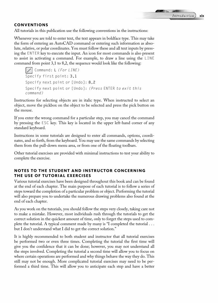
Whenever you are told to enter text, the text appears in boldface type. This may takethe form of entering an AutoCAD command or entering such information as abso-lute, relative, or polar coordinates. You must follow these and all text inputs by press-ing the ENTER key to execute the input. An icon for most commands is also presentto assist in activating a command. For example, to draw a line using the LINEcommand from point 3,1 to 8,2, the sequence would look like the following:
Command: L (For LINE)
Specify first point: 3,1
Specify next point or [Undo]: 8,2
Specify next point or [Undo]: (Press ENTER to exit thiscommand)
Instructions for selecting objects are in italic type. When instructed to select anobject, move the pickbox on the object to be selected and press the pick button onthe mouse.
If you enter the wrong command for a particular step, you may cancel the commandby pressing the ESC key. This key is located in the upper left-hand corner of anystandard keyboard.
Instructions in some tutorials are designed to enter all commands, options, coordi-nates, and so forth, from the keyboard. You may use the same commands by selectingthem from the pull-down menu area, or from one of the floating toolbars.
Other tutorial exercises are provided with minimal instructions to test your ability tocomplete the exercise.
NOTES TO THE STUDENT AND INSTRUCTOR CONCERNINGTHE USE OF TUTORIAL EXERCISESVarious tutorial exercises have been designed throughout this book and can be foundat the end of each chapter. The main purpose of each tutorial is to follow a series ofsteps toward the completion of a particular problem or object. Performing the tutorialwill also prepare you to undertake the numerous drawing problems also found at theend of each chapter.
As you work on the tutorials, you should follow the steps very closely, taking care notto make a mistake. However, most individuals rush through the tutorials to get thecorrect solution in the quickest amount of time, only to forget the steps used to com-plete the tutorial. A typical comment made by many is “I completed the tutorial . . .but I don’t understand what I did to get the correct solution.”
It is highly recommended to both student and instructor that all tutorial exercisesbe performed two or even three times. Completing the tutorial the first time willgive you the confidence that it can be done; however, you may not understand allthe steps involved. Completing the tutorial a second time will allow you to focus onwhere certain operations are performed and why things behave the way they do. Thisstill may not be enough. More complicated tutorial exercises may need to be per-formed a third time. This will allow you to anticipate each step and have a better
I n t r o d u c t i o n xix

idea what operation to perform in each step. Only then will you be comfortable andconfident to attempt the many drawing problems that follow the tutorial exercises.
The CD-ROM in the back of the book contains AutoCAD drawing files for the TryIt! exercises. To use drawing files, copy files to your hard drive, then remove theirread-only attribute. Files cannot be used without AutoCAD. Files are located in the /Drawing Files/ directory.
SUPPLEMENTSe.resource™—This is an educational resource that creates a truly electronic classroom.It is a CD-ROM containing tools and instructional resources that enrich your class-room and make your preparation time shorter. The elements of e.resource link directlyto the text and tie together to provide a unified instructional system. Spend your timeteaching, not preparing to teach.
ISBN 1-4180-2048-6
Features contained in e.resource include:
• Syllabus: Lesson plans created by chapter. You have the option of using theselesson plans with your own course information.
• Chapter Hints: Objectives and teaching hints that provide the basis for a lectureoutline that helps you to present concepts and material.
• PowerPoint® Presentation: These slides provide the basis for a lecture outline thathelps you to present concepts and material. Key points and concepts can be graphi-cally highlighted for student retention. There are more than 300 slides, coveringevery chapter in the text.
• Exam View Computerized Test Bank:More than 600 questions of varying levels ofdifficulty are provided in true/false and multiple-choice formats. Exams can be gen-erated to assess student comprehension or questions can be made available to thestudent for self-evaluation.
• Video and Animation Resources: These AVI files graphically depict the executionof key concepts and commands in drafting, design, and AutoCAD and let you bringmultimedia presentations into the classroom.
Spend your time teaching, not preparing to teach!
xx I n t r o du c t i o n

CHAPTER
1
Getting Started withAutoCAD
This chapter begins with an explanation of the components that make up a typicalAutoCAD display screen. You will learn various methods of selecting commands:some from the Menu Bar, others from toolbars, some from the Ribbon, and stillothers by entering the command from the keyboard. You will learn how to begin anew drawing. Once in a drawing, you will construct line segments with the LINEcommand in addition to drawing lines accurately with the Direct Distance mode, ab-solute coordinates, relative coordinates, and polar coordinates. Object Snap will bediscussed as a way to construct all types of objects with greater precision. Additionaldrawing aids such as Object Snap Tracking and Polar Tracking will be discussed.Other basic drawing commands such as constructing circles and polylines will beshown. You will also be introduced to the ERASE command for removing drawingobjects.
THE 2D DRAFTING & ANNOTATION WORKSPACEThe initial load of AutoCAD displays in a workspace. Workspaces are consideredtask-oriented environments that use a default drawing template and even launchsuch items as toolbars and palettes, depending on the workspace. By default, Auto-CAD loads the 2D Drafting & Annotation workspace as shown in the followingimage. This workspace controls the display of what is called the Ribbon, which isused for accessing the more popular commands in AutoCAD. This workspace con-tains other items such as the Application Menu, the Quick Access Toolbar, thegraphic cursor, and the InfoCenter for getting information about commands asshown in the following image. Three other workspaces are supplied with AutoCAD,namely Initial Setup Workspace, AutoCAD Classic, and 3D Modeling. The 3DModeling workspace will be discussed in greater detail in Chapter 20.
1

THE AUTOCAD CLASSIC WORKSPACEA second workspace is provided, namely AutoCAD Classic, which is shown in thefollowing image. This workspace differs from the previous workspace in that a num-ber of extra toolbars display in the upper, left, and right vertical portions of the displayscreen. Also, the Tool Palette displays, which allows you to drag and drop commandsfor use. This workspace does not display the Ribbon although this can be turned on ifyou want to use it.
While major differences occur at the top of the display screen when you are activatingdifferent workspaces, most of the tools available at the bottom of the screen arecommon to both workspaces. Study the various screen components as shown in thefollowing image.
FIGURE 1.1
FIGURE 1.3
FIGURE 1.2
2 Au t oCAD 2010 Tu t o r f o r Eng in e e r i n g Graph i c s

THE INITIAL SETUP WORKSPACEWhen you initially load AutoCAD, one of the dialog boxes that appears is shown inthe following image on the left. In this dialog box, you can choose a discipline such asArchitecture or Manufacturing, to name a few. When the AutoCAD display screenappears, a tool palette that relates to this discipline will be present. The third work-space is called Initial Setup. You can choose Initial SetupWorkspace from theWork-spaces menu as shown on the right in the following image.
Let’s say you initially loaded AutoCAD and you chose the Architecture discipline.You can easily change to a different discipline by right-clicking in a blank part ofyour screen and choosing Options from the menu as shown in the following imageon the left. This will launch the Options dialog box. Click on the User Preferencestab and notice the Initial Setup button as shown in the following image on the right.Clicking this button will launch the dialog box in the previous image that allows youto change to a different discipline.
ACCESSING WORKSPACESHow you switch to different workspaces depends on the current workspace that youare in. For instance, if the current workspace is AutoCAD Classic, you can click inthe Workspaces toolbar, as shown in the following image on the left, and choose adifferent workspace. If however, the current workspace is 2D Drafting and Annota-tion, you would click on theWorkspace Switching Icon located in the bottom right ofthe display screen as shown in the following image on the right. This would activate amenu that displays all available workspaces to choose from. The presence of the
FIGURE 1.5
FIGURE 1.4
Chap t e r 1 • Ge t t i n g S t a r t e d w i t h Au t oCAD 3

checkmark alongside the 2D Drafting & Annotation workspace signifies that it iscurrent. In addition to using these pre-existing workspaces, you can also arrangeyour screen to your liking and save these screen changes as your own customworkspace.
NOTE A Default AutoCAD workspace may be present in the list shown in the previous image. Thisworkspace is automatically created if you are upgrading from a previous version ofAutoCAD.
THE STATUS BARThe status bar, illustrated in the following image, is used to toggle ON or OFF thefollowing modes: Coordinate Display, Snap, Grid, Ortho, Polar Tracking, ObjectSnap (OSNAP), Object Snap Tracking (OTRACK), Dynamic User CoordinateSystem (DUCS), Dynamic Input (DYN), Line Weight (LWT), and Quick Proper-ties (QP). Click the button once to turn the mode on or off. A button with a bluecolor indicates that the mode is on. For example, the following image illustratesOrtho turned off (gray color) and Polar turned on (blue color). Right-clicking onany button in the status bar activates the menu shown in the following image. Click-ing on Use Icons will change the graphic icons to text mode icons.
FIGURE 1.6
FIGURE 1.7
4 Au t oCAD 2010 Tu t o r f o r Eng in e e r i n g Graph i c s

The following table gives a brief description of each component located in thestatus bar:
Button Tool Description
CoordinateDisplay
Toggles the coordinate display, located in thelower-left corner of the status bar, ON or OFF.When the coordinate display is off, the coordi-nates are updated when you pick an area of thescreen with the cursor. When the coordinate dis-play is on, the coordinates dynamically changewith the current position of the cursor.
SNAP Toggle Snap mode ON or OFF. The SNAP com-mand forces the cursor to align with grid points.The current snap value can be modified and can berelated to the spacing of the grid.
GRID Toggles the display of the grid ON or OFF. Theactual grid spacing is set by the DSETTINGS ORGRID command and not by this function key.
ORTHO Toggles Ortho mode ON or OFF. Use this key toforce objects such as lines to be drawn horizon-tally or vertically.
POLAR Toggles the Polar Tracking ON or OFF. PolarTracking can force lines to be drawn at any angle,making it more versatile than Ortho mode. ThePolar Tracking angles are set through a dialog box.Also, if you turn Polar Tracking on, Ortho mode isdisabled, and vice versa.
OSNAP Toggles the current Object Snap settings ON orOFF. This will be discussed later in this chapter.
OTRACK Toggles Object Snap Tracking ON or OFF. Thisfeature will also be discussed later in this chapter.
DUCS Toggles the Dynamic User Coordinate System ON orOFF. This feature is used mainly for modeling in 3D.
DYN Toggles Dynamic Input ON or OFF. When turnedon, your attention is directed to your cursor posi-tion as commands and options are executed.When turned off, all commands and options areaccessed through the Command prompt at thebottom of the display screen.
LWT Toggles Lineweight ON or OFF. When turned off,no lineweights are displayed. When turned on,lineweights that have been assigned to layers aredisplayed in the drawing.
QuickProperties
When turned on, this tool will list the mostpopular properties of a selected object.
Right-clicking one of the buttons displays the shortcut menu in the following image.Choose Settings to access various dialog boxes that control certain features associatedwith the button. These controls will be discussed later in this chapter and also in
Chap t e r 1 • Ge t t i n g S t a r t e d w i t h Au t oCAD 5

Chapter 2. Depending on which button is clicked on, additional tools may be avail-able as shown by right-clicking on SNAP, POLAR, or OSNAP.
You can also access most tools located in the status bar through the function keyslocated at the top of any standard computer keyboard. The following table describeseach function key.
Function Key Definitions
F1 Displays AutoCAD Help Topics
F2 Toggle Text/Graphics Screen
F3 Object Snap settings ON/OFF
F4 Toggle Tablet Mode ON/OFF
F5 Toggle Isoplane Modes
F6 Toggle Dynamic UCS ON/OFF
F7 Toggle Grid Mode ON/OFF
F8 Toggle Ortho Mode ON/OFF
F9 Toggle Snap Mode ON/OFF
F10 Toggle Polar Mode ON/OFF
F11 Toggle Object Snap Tracking ON/OFF
F12 Toggle Dynamic Input (DYN) ON/OFF
NOTE Most of the function keys are similar in operation to the modes found in the statusbar except for the following:
When you press F1, the AutoCAD Help Topics dialog box is displayed.
Pressing F2 takes you to the text screen consisting of a series of previous promptsequences. This may be helpful for viewing the previous command sequence in text form.
Use F4 to toggle Tablet mode ON or OFF. This mode is only activated when the digitizingtablet has been calibrated for the purpose of tracing a drawing into the computer.
Pressing F5 scrolls you through the three supported Isoplane modes used toconstructisometric drawings (Right, Left, and Top).
Pressing CTRL+SHIFT+P toggles Quick Properties mode ON or OFF.
FIGURE 1.8
6 Au t oCAD 2010 Tu t o r f o r Eng in e e r i n g Graph i c s

Additional Status Bar ControlsLocated at the far right end of the status bar are additional buttons separated into fourdistinct groups used to manage the appearance of the AutoCAD display screen andthe annotation scale of a drawing. These items include Quick View Layouts andDrawings, Display tools, Annotation Scale tools, the Workspace Switching tool,the Toolbar Unlocking tool, the Status Bar menu tool, and the Clean Screen tool.When annotative objects such as text and dimensions are created, they are scaledbased on the current annotation scale and automatically displayed at the correctsize. This feature will be discussed in greater detail in Chapter 19. The following ta-ble gives a brief description of the remaining buttons found in this area.
Button Tool Description
Workspace Switching Allows you to switch between the work-spaces already defined in the drawing.
Toolbar/WindowPositions Toggle
Locks the position of all toolbars on thedisplay screen.
Status Bar MenuControls
Activates a menu used for turning on oroff certain status bar buttons.
Clean Screen Removes all toolbars from the screen,giving your display an enlarged appear-ance. Click this button again to returnthe toolbars to the screen.
COMMUNICATING WITH AUTOCAD
The Command LineHow productive the user becomes in using AutoCAD may depend on the degree ofunderstanding of the command execution process with AutoCAD. One of the meansof command execution is through the command prompt that is located at the bottomof the display screen. As a command is selected from a toolbar, AutoCAD promptsthe user with a series of steps needed to complete this command. In the followingimage, the CIRCLE command is chosen as the command. The next series of lines inthe command line prompts the user to first specify or locate a center point for thecircle. After this is accomplished, you are then prompted to specify the radius of thecircle. These actions are also called the default prompt.
FIGURE 1.9
Chap t e r 1 • Ge t t i n g S t a r t e d w i t h Au t oCAD 7
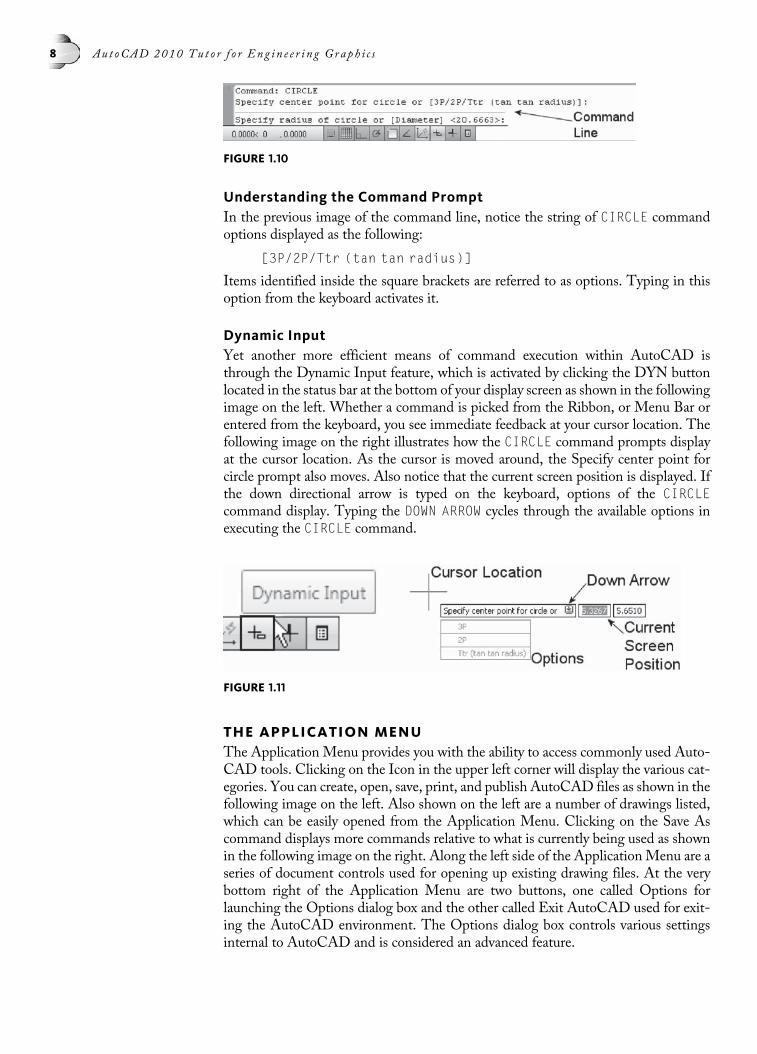
Understanding the Command PromptIn the previous image of the command line, notice the string of CIRCLE commandoptions displayed as the following:
[3P/2P/Ttr (tan tan radius)]
Items identified inside the square brackets are referred to as options. Typing in thisoption from the keyboard activates it.
Dynamic InputYet another more efficient means of command execution within AutoCAD isthrough the Dynamic Input feature, which is activated by clicking the DYN buttonlocated in the status bar at the bottom of your display screen as shown in the followingimage on the left. Whether a command is picked from the Ribbon, or Menu Bar orentered from the keyboard, you see immediate feedback at your cursor location. Thefollowing image on the right illustrates how the CIRCLE command prompts displayat the cursor location. As the cursor is moved around, the Specify center point forcircle prompt also moves. Also notice that the current screen position is displayed. Ifthe down directional arrow is typed on the keyboard, options of the CIRCLEcommand display. Typing the DOWN ARROW cycles through the available options inexecuting the CIRCLE command.
THE APPLICATION MENUThe Application Menu provides you with the ability to access commonly used Auto-CAD tools. Clicking on the Icon in the upper left corner will display the various cat-egories. You can create, open, save, print, and publish AutoCAD files as shown in thefollowing image on the left. Also shown on the left are a number of drawings listed,which can be easily opened from the Application Menu. Clicking on the Save Ascommand displays more commands relative to what is currently being used as shownin the following image on the right. Along the left side of the ApplicationMenu are aseries of document controls used for opening up existing drawing files. At the verybottom right of the Application Menu are two buttons, one called Options forlaunching the Options dialog box and the other called Exit AutoCAD used for exit-ing the AutoCAD environment. The Options dialog box controls various settingsinternal to AutoCAD and is considered an advanced feature.
FIGURE 1.11
FIGURE 1.10
8 Au t oCAD 2010 Tu t o r f o r Eng in e e r i n g Graph i c s
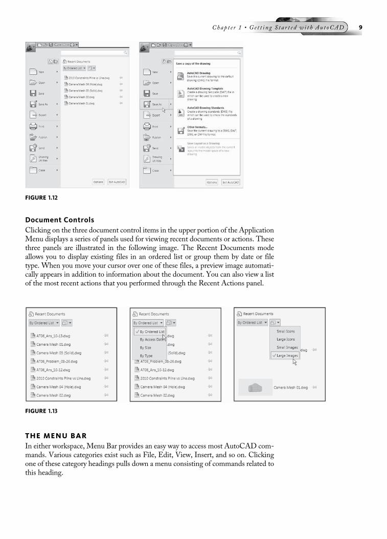
Document ControlsClicking on the three document control items in the upper portion of the ApplicationMenu displays a series of panels used for viewing recent documents or actions. Thesethree panels are illustrated in the following image. The Recent Documents modeallows you to display existing files in an ordered list or group them by date or filetype. When you move your cursor over one of these files, a preview image automati-cally appears in addition to information about the document. You can also view a listof the most recent actions that you performed through the Recent Actions panel.
THE MENU BARIn either workspace, Menu Bar provides an easy way to access most AutoCAD com-mands. Various categories exist such as File, Edit, View, Insert, and so on. Clickingone of these category headings pulls down a menu consisting of commands related tothis heading.
FIGURE 1.12
FIGURE 1.13
Chap t e r 1 • Ge t t i n g S t a r t e d w i t h Au t oCAD 9
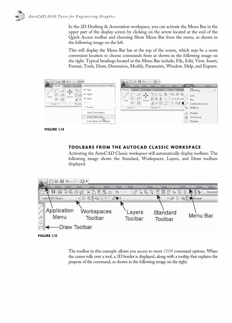
In the 2D Drafting & Annotation workspace, you can activate the Menu Bar in theupper part of the display screen by clicking on the arrow located at the end of theQuick Access toolbar and choosing Show Menu Bar from the menu, as shown inthe following image on the left.
This will display the Menu Bar bar at the top of the screen, which may be a moreconvenient location to choose commands from as shown in the following image onthe right. Typical headings located in the Menu Bar include, File, Edit, View, Insert,Format, Tools, Draw, Dimension, Modify, Parametric, Window, Help, and Express.
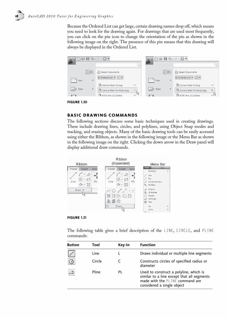
TOOLBARS FROM THE AUTOCAD CLASSIC WORKSPACEActivating the AutoCAD Classic workspace will automatically display toolbars. Thefollowing image shows the Standard, Workspaces, Layers, and Draw toolbarsdisplayed.
The toolbar in this example allows you access to most ZOOM command options. Whenthe cursor rolls over a tool, a 3D border is displayed, along with a tooltip that explains thepurpose of the command, as shown in the following image on the right.
FIGURE 1.14
FIGURE 1.15
10 Au t oCAD 2010 Tu t o r f o r Eng in e e r i n g Graph i c s

ACTIVATING TOOLBARSMany toolbars are available to assist the user in executing other types of commands.When working in the AutoCAD Classic workspace, six toolbars are already active ordisplayed in all drawings: Draw, Layers, Modify, Properties, Standard, and Styles. Toactivate a different toolbar, move the cursor over the top of any command button andpress the right mouse button. A shortcut menu appears that displays all toolbars, asshown in the following image. In this example, placing a check beside Text displaysthis toolbar.
DOCKING TOOLBARSIt is considered good practice to line the top or side edges of the display screen withtoolbars. The method of moving toolbars to the sides of your screen is called docking.Press down on the toolbar title strip and slowly drag the toolbar to the top of thescreen until the toolbar appears to jump. Letting go of the mouse button docks thetoolbar to the top of the screen as shown in the following image. Practice this bydocking various toolbars to your screen.
TIPTo prevent docking, press the CTRL key as you drag the toolbar. This allows you to movethe toolbar into the upper or lower portions of the display screen without the toolbar dock-ing. Also, if a toolbar appears to disappear, it might actually be alongside or below toolbarsthat already exist. Closing toolbars will assist in finding the missing one.
FIGURE 1.17
FIGURE 1.16
FIGURE 1.18
Chap t e r 1 • Ge t t i n g S t a r t e d w i t h Au t oCAD 11

TOOLBARS FROM THE 2D DRAFTING &ANNOTATION WORKSPACEWhile inside of the 2D Drafting & Annotation workspace, it is possible to displaytoolbars as in the AutoCAD Classic workspace. To accomplish this, click on the ar-row at the end of the Quick Access Toolbar and pick Show Menu Bar, as shown inthe following image on the left. When the menu bar displays, click on Tools followedby Toolbars and AutoCAD as shown in the following image on the right. This willdisplay all of the toolbars similar to those that are present in the AutoCAD ClassicWorkspace. Pick one of the names from the list to show the toolbar on the displayscreen.
RIBBON DISPLAY MODESA small button with an arrow is displayed at the end of the Ribbon tabs. This buttonallows you to minimize the Ribbon and display more of your screen. Three modes areavailable, as shown in the following image, that allow you to minimize to the titlepanels, minimize to the tabs, or show the full Ribbon.
FIGURE 1.19
FIGURE 1.20
12 Au t oCAD 2010 Tu t o r f o r Eng in e e r i n g Graph i c s

DIALOG BOXES AND ICON MENUSSettings and other controls can be changed through dialog boxes. Illustrated in thefollowing image on the left is the Drawing Units dialog box, which will be discussedin Chapter 2. Illustrated in the following image on the right is the Hatch PatternPalette. This palette provides an icon menu that makes it easy to choose the desiredhatch pattern. Simply select the pattern by reviewing the small images (icons) andclick it. Palettes are similar to dialog boxes with the exception that palettes allow forthe display of small images. Certain dialog boxes can be increased in size by movingyour cursor over their borders; this is true of the Hatch Pattern Palette dialog box.When two arrows appear, hold down the pick button of the mouse (usually the leftbutton) and stretch the dialog box in that direction. If the cursor is moved to the cor-ner of the dialog box, the box is stretched in two directions. These methods can alsobe used to make the dialog box smaller, although there is a default size for the dialogboxes, which limits smaller sizes. The dialog box cannot be stretched if no arrowsappear when you move your cursor over the border of the dialog box; this is true ofthe Drawing Units dialog box as well.
TOOL PALETTESCommands can also be accessed from a number of tool palettes. To launch the ToolPalette, click the Tool Palettes Window button, which is located in the Standardtoolbar of the AutoCAD Classic workspace, as shown in the following image. Ifyou are in the 2D Drafting & Annotation workspace, first click on the View tab andselect Tool Palettes. The Tool Palette is a long, narrow bar that consists of numeroustabs. Three tabs, namely, Modify (A), Draw (B), and Architectural (C) are illustratedbelow. Use these tabs to access the more popular drawing and modify commands.While this image shows three palettes, in reality only one will be present onyour screen at any one time. Simply click a different tab to display the commandsassociated with the tab.
FIGURE 1.21
FIGURE 1.22
Chap t e r 1 • Ge t t i n g S t a r t e d w i t h Au t oCAD 13

RIGHT-CLICK SHORTCUT MENUSMany shortcut or cursor menus have been developed to assist with the rapid access tocommands. Clicking the right mouse button activates a shortcut menu that providesaccess to these commands. The Default shortcut menu is illustrated in the followingimage on the left. It is displayed whenever you right-click in the drawing area and nocommand or selection set is in progress.
Illustrated in the following image on the right is an example of the Edit shortcutmenu. This shortcut consists of numerous editing and selection commands. Thismenu activates whenever you right-click in the display screen with an object or groupof objects selected but no command is in progress.
Right-clicking in the command prompt area of the display screen activates the short-cut menu, as shown in the following image on the left. This menu provides quickaccess to the Options dialog box, which is used to control various settings in Auto-CAD. Also, a record of the six most recent commands is kept, which allows the userto select from this group of previously used commands.
Illustrated in the following image on the right is an example of a Command-Modeshortcut menu. When you enter a command and right-click, this menu displays op-tions of the command. This menu supports a number of commands. In the followingimage, the 3P, 2P, and Ttr (tan tan radius) listings are all options of the CIRCLEcommand.
COMMAND ALIASESCommands can be executed directly through keyboard entry. This practice is popularfor users who are already familiar with the commands. However, users must know thecommand name, including its exact spelling. To assist with the entry of AutoCAD
FIGURE 1.23
FIGURE 1.24
14 Au t oCAD 2010 Tu t o r f o r Eng in e e r i n g Graph i c s

commands from the keyboard, numerous commands are available in shortened form,referred to as aliases. For example, instead of typing in LINE, all that is required is L.The letter E can be used for the ERASE command, and so on. These command aliasesare listed throughout this book. The complete list of all command aliases can befound under the Express Menu Bar by clicking Tools and Command Alias Editoras shown in the following image. The AutoCAD Command Alias Editor will ap-pear, displaying all of the commands that have their names shortened. Once you arecomfortable with the keyboard, command aliases provide a fast and efficient methodof activating AutoCAD commands.
STARTING A NEW DRAWINGTo begin a new drawing file, select the QNEW command using one of the follow-
ing methods:
• From the Quick Access toolbar
• From the Standard toolbar of the AutoCAD Classic workspace
• From the Application Menu (New)
• From the keyboard (NEW)Command: QNEW
Entering the NEW command displays the dialog box illustrated in the following image.This dialog box provides a list of templates to use for starting a new drawing.
FIGURE 1.25
Chap t e r 1 • Ge t t i n g S t a r t e d w i t h Au t oCAD 15

NOTE A QNEW command is also available for creating new drawings. This command is similar tothe NEW command but provides the option of starting with a pre-selected template.
OPENING AN EXISTING DRAWINGThe OPEN command is used to edit a drawing that has already been created. Select
this command from one of the following:
• From the Quick Access toolbar
• From the Standard toolbar of the AutoCAD Classic workspace
• From the Application Menu (Open)
• From the keyboard (OPEN)
When you select this command, a dialog box appears similar to the following image.Listed in the field area are all files that match the type shown at the bottom of thedialog box. Because the file type is .DWG, all drawing files supported by AutoCADare listed. To choose a different folder, use standardWindows file management tech-niques by clicking in the Look in field. This displays all folders associated with thedrive. Clicking the folder displays any drawing files contained in it.
FIGURE 1.26
FIGURE 1.27
16 Au t oCAD 2010 Tu t o r f o r Eng in e e r i n g Graph i c s

Additional tools are available in the Application Menu to assist in locating drawingsto open. These tools include Recent Documents, Open Documents, and RecentActions. Illustrated in the following image is an example of clicking on RecentDocuments, which is located in the lower-left corner of theApplicationMenu.Noticethe ordered list of all drawings that were recently opened enabling you to select thesemore efficiently.
When viewing files from the Ordered List Panel, clicking on the Ordered List iconwill expand the menu to include a number of options to display files. The default set-ting to display files is through Icons as shown in the following image on the left.Changing to Small Images will change the Ordered List to small images of each fileas shown on the right. You can also change the Ordered List types to Medium oreven Large Images.
FIGURE 1.28
FIGURE 1.29
Chap t e r 1 • Ge t t i n g S t a r t e d w i t h Au t oCAD 17
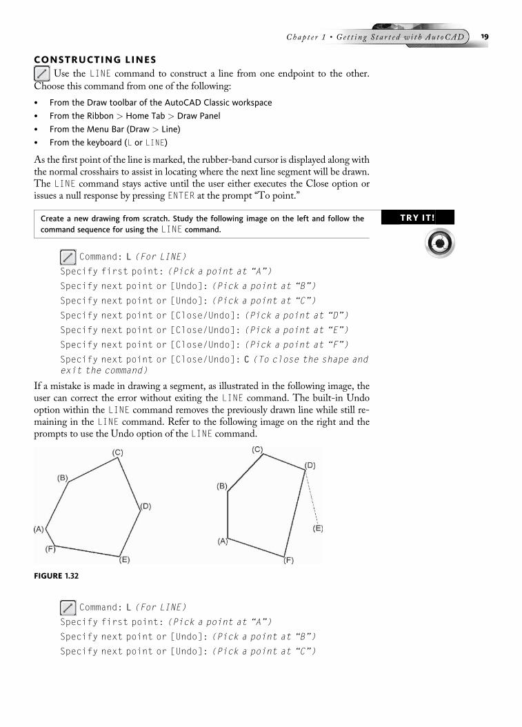
Because the Ordered List can get large, certain drawing names drop off, which meansyou need to look for the drawing again. For drawings that are used most frequently,you can click on the pin icon to change the orientation of the pin as shown in thefollowing image on the right. The presence of this pin means that this drawing willalways be displayed in the Ordered List.
BASIC DRAWING COMMANDSThe following sections discuss some basic techniques used in creating drawings.These include drawing lines, circles, and polylines, using Object Snap modes andtracking, and erasing objects. Many of the basic drawing tools can be easily accessedusing either the Ribbon, as shown in the following image or the Menu Bar as shownin the following image on the right. Clicking the down arrow in the Draw panel willdisplay additional draw commands.
The following table gives a brief description of the LINE, CIRCLE, and PLINEcommands:
Button Tool Key-In Function
Line L Draws individual or multiple line segments
Circle C Constructs circles of specified radius ordiameter
Pline PL Used to construct a polyline, which issimilar to a line except that all segmentsmade with the PLINE command areconsidered a single object
FIGURE 1.30
FIGURE 1.31
18 Au t oCAD 2010 Tu t o r f o r Eng in e e r i n g Graph i c s
CONSTRUCTING LINESUse the LINE command to construct a line from one endpoint to the other.
Choose this command from one of the following:
• From the Draw toolbar of the AutoCAD Classic workspace
• From the Ribbon > Home Tab > Draw Panel
• From the Menu Bar (Draw > Line)
• From the keyboard (L or LINE)
As the first point of the line is marked, the rubber-band cursor is displayed along withthe normal crosshairs to assist in locating where the next line segment will be drawn.The LINE command stays active until the user either executes the Close option orissues a null response by pressing ENTER at the prompt “To point.”
TRY IT!Create a new drawing from scratch. Study the following image on the left and follow thecommand sequence for using the LINE command.
Command: L (For LINE)
Specify first point: (Pick a point at “A”)
Specify next point or [Undo]: (Pick a point at “B”)
Specify next point or [Undo]: (Pick a point at “C”)
Specify next point or [Close/Undo]: (Pick a point at “D”)
Specify next point or [Close/Undo]: (Pick a point at “E”)
Specify next point or [Close/Undo]: (Pick a point at “F”)
Specify next point or [Close/Undo]: C (To close the shape andexit the command)
If a mistake is made in drawing a segment, as illustrated in the following image, theuser can correct the error without exiting the LINE command. The built-in Undooption within the LINE command removes the previously drawn line while still re-maining in the LINE command. Refer to the following image on the right and theprompts to use the Undo option of the LINE command.
Command: L (For LINE)
Specify first point: (Pick a point at “A”)
Specify next point or [Undo]: (Pick a point at “B”)
Specify next point or [Undo]: (Pick a point at “C”)
FIGURE 1.32
Chap t e r 1 • Ge t t i n g S t a r t e d w i t h Au t oCAD 19

Specify next point or [Close/Undo]: (Pick a point at “D”)
Specify next point or [Close/Undo]: (Pick a point at “E”)
Specify next point or [Close/Undo]: U (To undo or remove thesegment from “D” to “E” and still remain in the LINE command)
Specify next point or [Close/Undo]: (Pick a point at “F”)
Specify next point or [Close/Undo]: End (For Endpoint mode)
of (Select the endpoint of the line segment at “A”)
Specify next point or [Close/Undo]: (Press ENTER to exit thiscommand)
Continuing LinesAnother option of the LINE command is the Continue option. The dashed line seg-ment in the following image was the last segment drawn before the LINE commandwas exited. To pick up at the last point of a previously drawn line segment, type theLINE command and press ENTER. This activates the Continue option of the LINEcommand.
Command: L (For LINE)
Specify first point: (Press ENTER to activate Continue Mode)
Specify next point or [Undo]: (Pick a point at “B”)
Specify next point or [Undo]: (Pick a point at “C”)
Specify next point or [Close/Undo]: End (For Endpoint mode)
of (Select the endpoint of the vertical line segment at “D”)
Specify next point or [Close/Undo]: (Press ENTER to exit thiscommand)
Dynamic Input and LinesWith Dynamic Input turned on in the status bar, additional feedback can be obtainedwhen drawing line segments. In addition to the command prompt and down arrowbeing displayed at your cursor location, a dynamic distance and angle are displayed toassist you in the construction of the line segment, as shown in the following image.
FIGURE 1.33
FIGURE 1.34
20 Au t oCAD 2010 Tu t o r f o r Eng in e e r i n g Graph i c s

Command prompts for using Dynamic Input now appear in the drawing windownext to the familiar AutoCAD cursor.
• When constructing line segments, dynamic dimensions in the form of a distance andan angle appear on the line. If the distance dimension is highlighted, entering a newvalue from your keyboard will change its value.
• Pressing the TAB key allows you to switch you between the distance dimension andthe angle dimension, where you can change its value.
• By default in Dynamic Input, coordinates for the second point of a line are consid-ered relative. In other words, you do not need to type the @ symbol in front of thecoordinate. The @ symbol means “last point” and will be discussed in greater detaillater in this chapter.
• You can still enter relative and polar coordinates as normal using the @ symbol ifyou desire. These older methods of coordinate entry override the default dynamicinput setting.
• The appearance of an arrow symbol in the Dynamic Input prompt area indicates thatthis command has options associated with it. To view these command options,press the DOWN ARROW key on your keyboard. These options will display on yourscreen. Continue pressing the DOWN ARROW until you reach the desired commandoption and then press the ENTER key to select it.
• Dynamic Input can be toggled ON or OFF in the status bar by clicking the DYN but-ton or by pressing the F12 function key.
THE DIRECT DISTANCE MODE FOR DRAWING LINESAnother method is available for constructing lines, and it is called drawing by DirectDistance mode. In this method, the direction a line will be drawn in is guided by thelocation of the cursor. You enter a value, and the line is drawn at the specified distanceat the angle specified by the cursor. This mode works especially well for drawinghorizontal and vertical lines. The following image illustrates an example of how theDirect Distance mode is used.
TRY IT!Create a new drawing from scratch. Turn Ortho mode on in the status bar. Then use the fol-lowing command sequence to construct the line segments using the Direct Distance modeof entry.
Command: L (For LINE)
Specify first point: 2.00,2.00
Specify next point or [Undo]: (Move the cursor to the rightand enter a value of 7.00 units)
Specify next point or [Undo]: (Move the cursor up and enter avalue of 3.00 units)
Specify next point or [Close/Undo]: (Move the cursor to theleft and enter a value of 4.00 units)
Specify next point or [Close/Undo]: (Move the cursor down andenter a value of 1.00 units)
Specify next point or [Close/Undo]: (Move the cursor to theleft and enter a value of 2.00 units)
Specify next point or [Close/Undo]: C (To close the shape andexit the command)
Chap t e r 1 • Ge t t i n g S t a r t e d w i t h Au t oCAD 21

TIP If Ortho mode is currently turned on, you can temporarily turn Ortho off while in the LINEcommand by pressing the SHIFT key as you drag your cursor to draw the next line.
The following image shows another example of an object drawn with Direct Distancemode. Each angle was constructed from the location of the cursor. In this example,Ortho mode is turned off.
TRY IT! Create a new drawing from scratch. Be sure Ortho mode is turned off.
Then use the following command sequence to construct the line segments using thedirect distance mode of entry.
Command: L (For LINE)
Specify first point: (Pick a point at “A”)
Specify next point or [Undo]: (Move the cursor and enter 3.00)
Specify next point or [Undo]: (Move the cursor and enter 2.00)
Specify next point or [Close/Undo]: (Move the cursor andenter 1.00)
Specify next point or [Close/Undo]: (Move the cursor andenter 4.00)
Specify next point or [Close/Undo]: (Move the cursor andenter 2.00)
Specify next point or [Close/Undo]: (Move the cursor andenter 1.00)
Specify next point or [Close/Undo]: (Move the cursor andenter 1.00)
Specify next point or [Close/Undo]: C (To close the shape andexit the command)
FIGURE 1.35
22 Au t oCAD 2010 Tu t o r f o r Eng in e e r i n g Graph i c s

USING OBJECT SNAP FOR GREATER PRECISIONA major productivity tool that allows locking onto key locations of objects is ObjectSnap. The following image is an example of the construction of a vertical line con-necting the endpoint of the fillet with the endpoint of the line at “A.”The LINE com-mand is entered and the Endpoint mode activated. When the cursor moves over avalid endpoint, an Object Snap symbol appears along with a tooltip indicating whichOSNAP mode is currently being used. Another example of the use of Object Snap isin dimensioning applications where exact endpoints and intersections are needed.
TRY IT!Open the drawing file 01_Endpoint. Use the illustration in the following image and the com-mand sequence below to draw a line segment from the endpoint of the arc to the endpointof the line.
Command: L (For LINE)
Specify first point: End (For Endpoint mode)
of (Pick the endpoint of the fillet at “A” illustrated in thefollowing image)
Specify next point or [Undo]: End (For Endpoint mode)
of (Pick the endpoint of the line at “B”)
Specify next point or [Undo]: (Press ENTER to exit thiscommand)
Perform the same operation to the other side of this object using the Endpoint modeof OSNAP. The results are shown in the following image on the right.
Object Snap modes can be selected in a number of different ways. Illustrated in thefollowing image is the status bar. Right clicking on the Object Snap icon displays themenu containing most Object Snap tools. The following table gives a brief descrip-tion of each Object Snap mode. In this table, notice the Key-In column. When theObject Snap modes are executed from keyboard input, only the first three letters arerequired.
FIGURE 1.37
FIGURE 1.36
Chap t e r 1 • Ge t t i n g S t a r t e d w i t h Au t oCAD 23

The following table gives a brief description of each Object Snap mode:
Button Tool Key-In Function
Center CEN Snaps to the centers of circles and arcs
Endpoint END Snaps to the endpoints of lines and arcs
Extension EXT Creates a temporary extension line or arcwhen your cursor passes over the end-point of objects; you can specify newpoints along the temporary line
From FRO Snaps to a point at a specified distanceand direction from a selected referencepoint
Insert INS Snaps to the insertion point of blocksand text
Intersection INT Snaps to the intersections of objects
ApparentIntersection
INT Mainly used in creating 3D wireframemodels; finds the intersection of pointsnot located in the same plane
Midpoint MID Snaps to the midpoint of lines and arcs
Midpoint Be-tween 2 Points
M2P Snaps to the middle of two selectedpoints
Nearest NEA Snaps to the nearest point found alongany object
Node NOD Snaps to point objects (includingdimension definition points) and textobjects (including multiline text anddimension text)
None NON Disables Object Snap
Osnap Settings OSNAP Launches the Drafting Settings dialogbox and activates the Object Snap tab
Parallel PAR Draws an object parallel to anotherobject
Perpendicular PER Snaps to a perpendicular location on anobject
Quadrant QUA Snaps to four key points located on acircle
Tangent TAN Snaps to the tangent location of arcs andcircles
FIGURE 1.38
24 Au t oCAD 2010 Tu t o r f o r Eng in e e r i n g Graph i c s

The following image shows the Object Snap modes that can be activated when youhold down SHIFT or CTRL and press the right mouse button while within a com-mand such as LINE or MOVE. This shortcut menu will appear wherever the cursor iscurrently positioned.
OBJECT SNAP MODES
Center (Cen)Use the Center mode to snap to the center of a circle or arc. To accomplish this,
activate the mode by clicking the Center button and moving the cursor along the edgeof the circle or arc, as shown in the following image. Notice the AutoSnap symbolappearing at the center of the circle or arc.
Endpoint (End)The Endpoint mode is one of the more popular Object Snap modes; it is helpful
in snapping to the endpoints of lines or arcs as shown in the following image. Oneapplication of Endpoint is during the dimensioning process, where exact distancesare needed to produce the desired dimension. Activate this mode by clicking theEndpoint button, and then move the cursor along the edge of the object to snap tothe endpoint. In the case of the line or arc shown in the following image, the cursor
FIGURE 1.39
FIGURE 1.40
Chap t e r 1 • Ge t t i n g S t a r t e d w i t h Au t oCAD 25

does not actually have to be positioned at the endpoint; favoring one end automaticallysnaps to the closest endpoint.
Extension (Ext)When you acquire a line or an arc, the Extension mode creates a temporary path
that extends from the object. Once the Extension Object Snap is selected, move yourcursor over the end of the line at “A,” as shown in the following image, to acquireit. Moving your cursor away provides an extension at the same angle as the line. Toun-acquire an extension, simply move your cursor over the end of the line again.A tooltip displays the current extension distance and angle. Acquiring the end of thearc at “B” provides the radius of the arc and displays the current length in the tooltip.
From (Fro)Use the From mode along with a secondary Object Snap mode to establish a
reference point and construct an offset from that point. Open the drawing file01_Osnap From. In the following image, the circle needs to be drawn 1.50 units inthe X and Y directions from point “A.” The CIRCLE command is activated and theObject Snap From mode is used in combination with the Object Snap Intersectionmode. The From option requires a base point. Identify the base point at the intersec-tion of corner “A.” The next prompt asks for an offset value; enter the relative coordi-nate value of @1.50,1.50 (this identifies a point 1.50 units in the positive X directionand 1.50 units in the positive Y direction). This completes the use of the From optionand identifies the center of the circle at “B.” Study the following command sequenceto accomplish this operation:
TRY IT! Open the drawing file 01_Osnap From. Use the illustration and prompt sequence below forconstructing a circle inside the shape with the aid of the Object Snap From mode.
FIGURE 1.42
FIGURE 1.41
26 Au t oCAD 2010 Tu t o r f o r Eng in e e r i n g Graph i c s

Command: C (For CIRCLE)
Specify center point for circle or [3P/2P/Ttr (tan tanradius)]: From
Base point: Int (For Intersection Mode)
of (Select the intersection at “A” in the following image)
<Offset>: @1.50,1.50
Specify radius of circle or [Diameter]: D (For Diameter)
Specify diameter of circle: 1.25
Insert (Ins)The Insert mode snaps to the insertion point of an object. In the case of the text
object in the following image on the left, activating the Insert mode and positioningthe cursor anywhere on the text snaps to its insertion point, in this case at the lower-left corner of the text at “A.” The other object illustrated in the following image onthe right is called a block. It appears to be constructed with numerous line objects;however, all objects that make up the block are considered to be a single object.Blocks can be inserted in a drawing. Typical types of blocks are symbols such as doors,windows, bolts, and so on—anything that is used several times in a drawing. In orderfor a block to be brought into a drawing, it needs an insertion point, or a point ofreference. The Insert mode, when you position the cursor on a block, will snap tothe insertion point at “B” of that block.
Intersection (Int)Another popular Object Snap mode is Intersection. Use this mode to snap to the
intersection of two objects. Position the cursor anywhere near the intersection of twoobjects and the intersection symbol appears. See the following image.
FIGURE 1.43
FIGURE 1.44
Chap t e r 1 • Ge t t i n g S t a r t e d w i t h Au t oCAD 27

Extended Intersection (Int)Another type of intersection snap is the Extended Intersection mode, which is usedto snap to an intersection not considered obvious from the previous example. ThesameObject Snap Intersection button is utilized for performing an extended intersec-tion operation. The following image shows two lines that do not intersect. Activatethe Extended Intersection mode and pick both lines. Notice the intersection symbolpresent where the two lines, if extended, would intersect.
Midpoint (Mid)The Midpoint mode snaps to the midpoint of objects. Line and arc examples are
shown in the following image.When activating theMidpoint mode, touch the objectanywhere with some portion of the cursor; the midpoint symbol appears at the exactmidpoint of the object.
Midpoint of Two Selected Points (M2P)This Object Snap mode snaps to the midpoint of two selected points. To access thismode, type either M2P or MTP at the command prompt.While this Object Snap modeis not accessible through a toolbar button, it can be found by pressing SHIFT + RightMouse Button to display the Object Snap menu, as shown in the following image onthe left.
FIGURE 1.46
FIGURE 1.45
FIGURE 1.47
28 Au t oCAD 2010 Tu t o r f o r Eng in e e r i n g Graph i c s
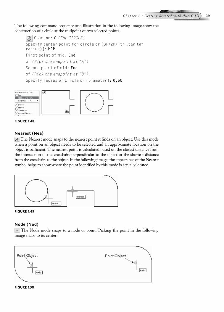
The following command sequence and illustration in the following image show theconstruction of a circle at the midpoint of two selected points.
Command: C (For CIRCLE)
Specify center point for circle or [3P/2P/Ttr (tan tanradius)]: M2P
First point of mid: End
of (Pick the endpoint at “A”)
Second point of mid: End
of (Pick the endpoint at “B”)
Specify radius of circle or [Diameter]: 0.50
Nearest (Nea)The Nearest mode snaps to the nearest point it finds on an object. Use this mode
when a point on an object needs to be selected and an approximate location on theobject is sufficient. The nearest point is calculated based on the closest distance fromthe intersection of the crosshairs perpendicular to the object or the shortest distancefrom the crosshairs to the object. In the following image, the appearance of the Nearestsymbol helps to show where the point identified by this mode is actually located.
Node (Nod)The Node mode snaps to a node or point. Picking the point in the following
image snaps to its center.
FIGURE 1.48
FIGURE 1.49
FIGURE 1.50
Chap t e r 1 • Ge t t i n g S t a r t e d w i t h Au t oCAD 29

Parallel (Par)Use the Parallel mode to construct a line parallel to another line. In the following
image, the LINE command is started and a beginning point of the line is picked. TheParallel mode is activated by selecting the Parallel icon and then hovering the cursorover the existing line. The existing line is highlighted at “A” and the Parallel symbolappears. Finally, moving the cursor to the approximate position that makes the newline parallel to the one just selected allows the Parallel mode to construct a parallelline, the tracking path and the tooltip giving the current distance and angle. Theresult of this mode is illustrated in the following image on the right.
Perpendicular (Per)The Perpendicular mode is helpful for snapping to an object normal (or perpen-
dicular) from a previously identified point. The following image shows a line segmentdrawn perpendicular from the point at “A” to the inclined line “B.” A 90° angle isformed with the perpendicular line segment and the inclined line “B.” With thismode, the user can also construct lines perpendicular to circles.
Quadrant (Qua)Circle quadrants are defined as points located at the 0°, 90°, 180°, and 270° posi-
tions of a circle, as in the following image. Using the Quadrant mode will snap to oneof these four positions as the edge of a circle or arc is selected. In the example of thecircle in the following image, the edge of the circle is selected by the cursor location.The closest quadrant to the cursor is selected.
FIGURE 1.51
FIGURE 1.52
FIGURE 1.53
30 Au t oCAD 2010 Tu t o r f o r Eng in e e r i n g Graph i c s

Tangent (Tan)The Tangent mode is helpful in constructing lines tangent to other objects such as
the circles in the following image. In this case, the Deferred Tangent mode is beingused in conjunction with the LINE command. The point at “A” is first picked at thebottom of the circle using the Tangent mode.When dragged to the next location, theline will be tangent at point “A.”Then, with Tangent mode activated and the locationat “B” picked, the line will be tangent to the large circle near “B.”The results are illus-trated in the following image on the right.
TRY IT!Open the drawing file 01_Tangent. Follow this command sequence for constructing a linesegment tangent to two circles:
Command: L (For LINE)
Specify first point: Tan (For Tangent mode)
from (Select the circle near “A”)
Specify next point or [Undo]: Tan (For Tangent mode)
to (Select the circle near “B”)
TRY IT!Open the drawing file 01_Osnap. Various objects consisting of lines, circles, arcs, points,and blocks need to be connected with line segments at their key locations. Use the promptsequence and the following image for performing this operation.
Command: L (For LINE)
Specify first point: End
of (Pick the endpoint at “A”)
Specify next point or [Undo]: Nod
of (Pick the node at “B”)
Specify next point or [Undo]: Tan
to (Pick the circle at “C”)
Specify next point or [Close/Undo]: Int
of (Pick the intersection at “D”)
Specify next point or [Close/Undo]: Int
of (Pick the line at “E”)
and (Pick the horizontal line at “F”)
Specify next point or [Close/Undo]: Qua
of (Pick the circle at “G”)
Specify next point or [Close/Undo]: Cen
of (Pick the arc at “H”)
FIGURE 1.54
Chap t e r 1 • Ge t t i n g S t a r t e d w i t h Au t oCAD 31
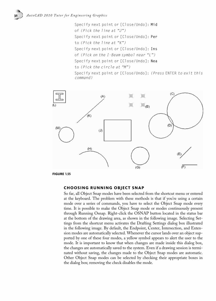
Specify next point or [Close/Undo]: Mid
of (Pick the line at “J”)
Specify next point or [Close/Undo]: Per
to (Pick the line at “K”)
Specify next point or [Close/Undo]: Ins
of (Pick on the I-Beam symbol near “L”)
Specify next point or [Close/Undo]: Nea
to (Pick the circle at “M”)
Specify next point or [Close/Undo]: (Press ENTER to exit thiscommand)
CHOOSING RUNNING OBJECT SNAPSo far, all Object Snap modes have been selected from the shortcut menu or enteredat the keyboard. The problem with these methods is that if you’re using a certainmode over a series of commands, you have to select the Object Snap mode everytime. It is possible to make the Object Snap mode or modes continuously presentthrough Running Osnap. Right-click the OSNAP button located in the status barat the bottom of the drawing area, as shown in the following image. Selecting Set-tings from the shortcut menu activates the Drafting Settings dialog box illustratedin the following image. By default, the Endpoint, Center, Intersection, and Exten-sion modes are automatically selected. Whenever the cursor lands over an object sup-ported by one of these four modes, a yellow symbol appears to alert the user to themode. It is important to know that when changes are made inside this dialog box,the changes are automatically saved to the system. Even if a drawing session is termi-nated without saving, the changes made to the Object Snap modes are automatic.Other Object Snap modes can be selected by checking their appropriate boxes inthe dialog box; removing the check disables the mode.
FIGURE 1.55
32 Au t oCAD 2010 Tu t o r f o r Eng in e e r i n g Graph i c s

These Object Snap modes remain in effect during drawing until you click theOSNAP button illustrated in the status bar in the following image; this turns offthe current running Object Snap modes. To reactivate the running Object Snapmodes, click the OSNAP button again and the previous set of Object Snap modeswill be back in effect. Object Snap can also be activated and reactivated by pressingthe F3 function key. It is also important to note that anytime you select an ObjectSnap from the toolbar, cursor menu, or by typing it in, it overrides the RunningOsnap for that single operation. This ensures that you only snap to that specificmode and not accidentally to one of the set Running Osnaps.
POLAR TRACKINGPreviously in this chapter, the Direct Distance mode was highlighted as an efficientmeans of constructing orthogonal lines without the need for using one of the coordi-nate modes of entry. However, it did not lend itself to lines at angles other than 0°,90°, 180°, and 270°. Polar Tracking has been designed to remedy this. This modeallows the cursor to follow a tracking path that is controlled by a preset angular incre-ment. The POLAR button located at the bottom of the display in the Status areaturns this mode on or off. Right-clicking POLAR in the status bar at the bottom ofthe screen and picking Settings will display the Drafting Settings dialog box shown inthe following image and the Polar Tracking tab.
FIGURE 1.56
FIGURE 1.57
Chap t e r 1 • Ge t t i n g S t a r t e d w i t h Au t oCAD 33
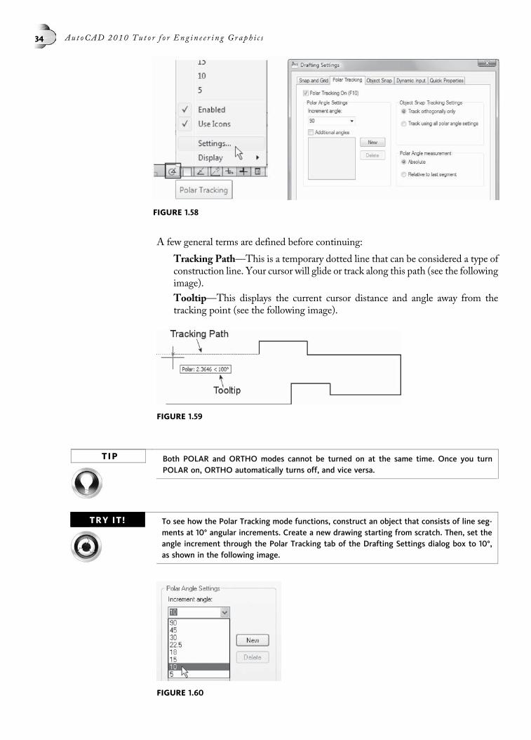
A few general terms are defined before continuing:
Tracking Path—This is a temporary dotted line that can be considered a type ofconstruction line. Your cursor will glide or track along this path (see the followingimage).
Tooltip—This displays the current cursor distance and angle away from thetracking point (see the following image).
TIP Both POLAR and ORTHO modes cannot be turned on at the same time. Once you turnPOLAR on, ORTHO automatically turns off, and vice versa.
TRY IT! To see how the Polar Tracking mode functions, construct an object that consists of line seg-ments at 10° angular increments. Create a new drawing starting from scratch. Then, set theangle increment through the Polar Tracking tab of the Drafting Settings dialog box to 10°,as shown in the following image.
FIGURE 1.58
FIGURE 1.59
FIGURE 1.60
34 Au t oCAD 2010 Tu t o r f o r Eng in e e r i n g Graph i c s

Start the LINE command, anchor a starting point at “A,” and move the cursor to theupper-right until the tooltip reads 20° as shown in the following image on the left.Enter a value of 2 units for the length of the line segment.
Move the cursor up and to the left until the tooltip reads 110°, as shown in the follow-ing image on the right, and enter a value of 2 units. (This will form a 90° angle withthe first line.)
Move the cursor until the tooltip reads 20°, as shown in the following image on theleft, and enter a value of 1 unit.
Move the cursor until the tooltip reads 110°, as shown in the following image on theright, and enter a value of 1 unit.
Move the cursor until the tooltip reads 200°, as shown in the following image on theleft, and enter a value of 3 units.
Move the cursor to the endpoint, as shown in the following image on the right, or usethe Close option of the LINE command to close the shape and exit the command.
SETTING A POLAR SNAP VALUEAn additional feature of using polar snap is illustrated in the following image. Click-ing the Snap and Grid tab of the Drafting Settings dialog box displays the dialog box
FIGURE 1.61
FIGURE 1.62
FIGURE 1.63
Chap t e r 1 • Ge t t i n g S t a r t e d w i t h Au t oCAD 35
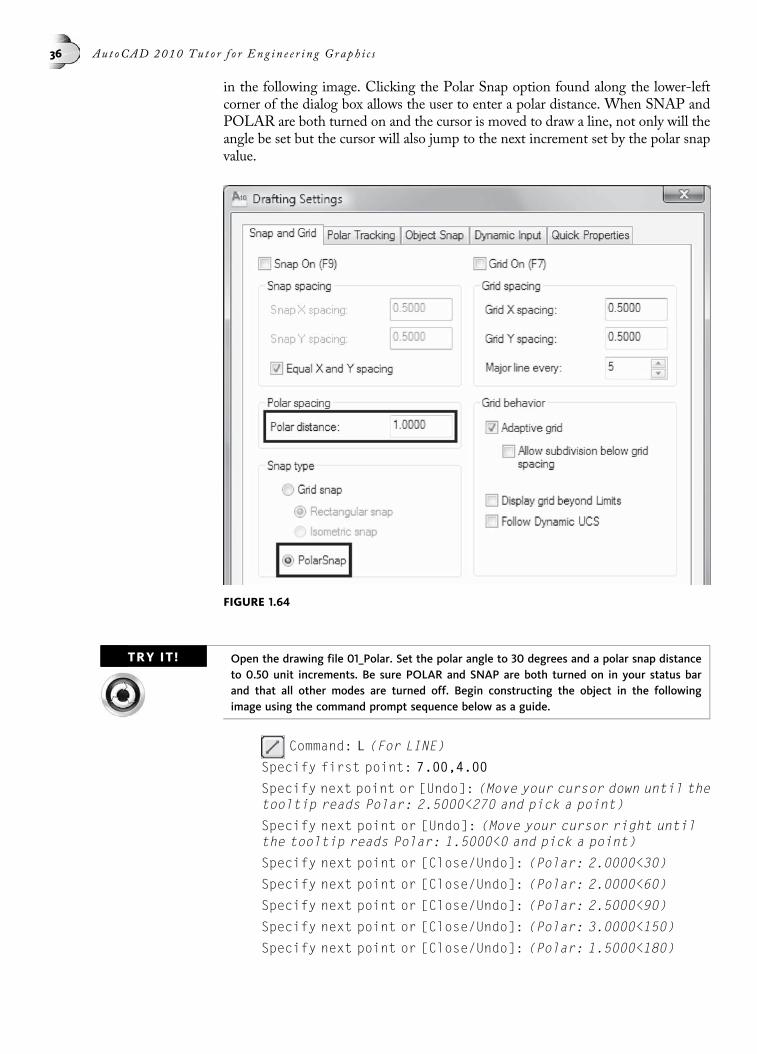
in the following image. Clicking the Polar Snap option found along the lower-leftcorner of the dialog box allows the user to enter a polar distance. When SNAP andPOLAR are both turned on and the cursor is moved to draw a line, not only will theangle be set but the cursor will also jump to the next increment set by the polar snapvalue.
TRY IT! Open the drawing file 01_Polar. Set the polar angle to 30 degrees and a polar snap distanceto 0.50 unit increments. Be sure POLAR and SNAP are both turned on in your status barand that all other modes are turned off. Begin constructing the object in the followingimage using the command prompt sequence below as a guide.
Command: L (For LINE)
Specify first point: 7.00,4.00
Specify next point or [Undo]: (Move your cursor down until thetooltip reads Polar: 2.5000<270 and pick a point)
Specify next point or [Undo]: (Move your cursor right untilthe tooltip reads Polar: 1.5000<0 and pick a point)
Specify next point or [Close/Undo]: (Polar: 2.0000<30)
Specify next point or [Close/Undo]: (Polar: 2.0000<60)
Specify next point or [Close/Undo]: (Polar: 2.5000<90)
Specify next point or [Close/Undo]: (Polar: 3.0000<150)
Specify next point or [Close/Undo]: (Polar: 1.5000<180)
FIGURE 1.64
36 Au t oCAD 2010 Tu t o r f o r Eng in e e r i n g Graph i c s

Specify next point or [Close/Undo]: (Polar: 2.5000<240)
Specify next point or [Close/Undo]: (Polar: 2.5000<120)
Specify next point or [Close/Undo]: (Polar: 1.5000<180)
Specify next point or [Close/Undo]: (Polar: 3.0000<210)
Specify next point or [Close/Undo]: (Polar: 2.5000<270)
Specify next point or [Close/Undo]: (Polar: 2.0000<300)
Specify next point or [Close/Undo]: (Polar: 2.0000<330)
Specify next point or [Close/Undo]: (Polar: 1.5000<0)
Specify next point or [Close/Undo]: (Polar: 2.5000<90)
Specify next point or [Close/Undo]: C (To close the shape)
SETTING A RELATIVE POLAR ANGLEAn additional feature of using polar snap is illustrated in the following image. Whenactivating the Polar tab of the Drafting Settings dialog box, located in the lower-rightcorner are two settings that deal with the Polar Angle measurement; they are Abso-lute and Relative to last segment.
Absolute—This is the default setting when dealing with Polar Angle measure-ment. This setting controls all angle measurements based on the position of thecurrent user coordinate system, the icon located in the lower-left corner of allAutoCAD drawing screens.
Relative to last segment—When changing the Polar Angle measurement toRelative to last segment, the Polar Tracking angle is based on the last linesegment drawn.
FIGURE 1.65
FIGURE 1.66
Chap t e r 1 • Ge t t i n g S t a r t e d w i t h Au t oCAD 37

To get a better understanding of the two different Polar Angle measurement settings,study the following image. The illustration on the left is an example of the Absolutesetting. The 150° angle was drawn from point (A) to point (B). This angle is derivedfrom the absolute position of angle 0° (zero) set by default to the 3 o’clock position asdefined in the Drawing Units dialog box. In the illustration on the right, the sameline segment is drawn. However, this time the Relative to last segment setting isused. Notice how the 120° angle is calculated. The angle is based on the last line seg-ment, not on an angle calculated in relation to 0° (zero). This is the reason for theparallel line segment at (C).
OBJECT SNAP TRACKING MODEObject Snap Tracking works in conjunction with Object Snap. Before you can trackfrom an Object Snap point, you must first set an Object Snap mode or modes fromthe Object Snap tab of the Drafting Settings dialog box. Object Snap Tracking can betoggled ON or OFF with the OTRACK button, which is located in the status barshown in the following image.
The advantage of using Object Snap Tracking is in the ability to choose or acquirepoints to be used for construction purposes. Acquired points are temporarily selectedby hovering the cursor over the point versus selecting with the mouse. Care must betaken when acquiring points that the points are in fact not picked. They are used onlyfor construction purposes. For example, two line segments need to be added to theobject, as shown in the following image on the left, to form a rectangle. Here is howyou perform this operation using Polar Tracking.
FIGURE 1.68
FIGURE 1.67
38 Au t oCAD 2010 Tu t o r f o r Eng in e e r i n g Graph i c s

TRY IT!Open the drawing file 01_Otrack Lines. Notice in the status bar that POLAR, OSNAP,and OTRACK are all turned on. Be sure that Running Osnap is set to Endpoint mode. Enterthe LINE command and pick a starting point for the line at “A.” Then, move the cursor di-rectly to the left until the tooltip reads 180° as shown in the following image on the left.The starting point for the next line segment is considered acquired.
Rather than enter the length of this line segment, move your cursor over the top of thecorner at “B” to acquire this point (be careful not to pick the point here). Then moveyour cursor up until the tooltip reads 90° as shown in the following image on theright.
Move your cursor up until the tooltip now reads angles of 90° and 180°. Also noticethe two tracking paths intersecting at the point of the two acquired points. Pickingthis point at “C” will construct the horizontal line segment as shown in the followingimage on the left. Finally, slide your cursor to the endpoint at “D” to complete therectangle as shown in the following image on the right.
TIPPausing the cursor over an existing acquired point a second time removes the trackingpoint from the object.
TRY IT!Open the drawing file 01_Otrack Pipes. Set Running Osnap mode to Midpoint. Set the polarangle to 90 degrees. Be sure POLAR, OSNAP, and OTRACK are all turned on. Enterthe LINE command and connect all fittings with lines illustrated in the following image.
FIGURE 1.70
FIGURE 1.69
Chap t e r 1 • Ge t t i n g S t a r t e d w i t h Au t oCAD 39
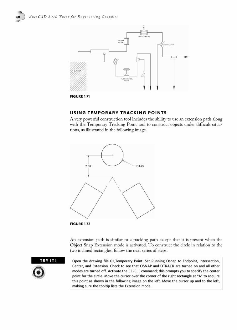
USING TEMPORARY TRACKING POINTSA very powerful construction tool includes the ability to use an extension path alongwith the Temporary Tracking Point tool to construct objects under difficult situa-tions, as illustrated in the following image.
An extension path is similar to a tracking path except that it is present when theObject Snap Extension mode is activated. To construct the circle in relation to thetwo inclined rectangles, follow the next series of steps.
TRY IT! Open the drawing file 01_Temporary Point. Set Running Osnap to Endpoint, Intersection,Center, and Extension. Check to see that OSNAP and OTRACK are turned on and all othermodes are turned off. Activate the CIRCLE command; this prompts you to specify the centerpoint for the circle. Move the cursor over the corner of the right rectangle at “A” to acquirethis point as shown in the following image on the left. Move the cursor up and to the left,making sure the tooltip lists the Extension mode.
FIGURE 1.72
FIGURE 1.71
40 Au t oCAD 2010 Tu t o r f o r Eng in e e r i n g Graph i c s

With the point acquired at “A,”move the cursor over the corner of the left rectangle at“B” and acquire this point. Move the cursor up and to the right, making sure the tool-tip lists the Extension mode, as shown in the following image on the right.
Move the cursor until both acquired points intersect as shown in the following imageon the right. The center of the circle is located 2 units above this intersection. Clickthe Object Snap Temporary Tracking button and pick this intersection as shown inthe following image on the right.
Next, move the cursor directly above the temporary tracking point, as shown in thefollowing image on the left. The tooltip should read 90°. Entering a value of 2 unitsidentifies the center of the circle.
The completed construction operation is illustrated in the following image on theright.
ALTERNATE METHODS USED FOR PRECISION DRAWING:CARTESIAN COORDINATESBefore drawing precision geometry such as lines and circles, it is essential to have anunderstanding of coordinate systems. The Cartesian or rectangular coordinate systemis a system constructed of an orthogonal axis intersecting at an origin that creates fourquadrants, allowing location of any point by specifying the coordinates. A coordinate ismade up of a horizontal and vertical pair of numbers identified as X and Y. The coor-dinates are then plotted on a type of graph or chart. An example of a rectangular coor-dinate system is shown in the following image. The coordinates of the origin are 0,0.
FIGURE 1.74
FIGURE 1.73
Chap t e r 1 • Ge t t i n g S t a r t e d w i t h Au t oCAD 41

From the origin, all positive directions move up and to the right. All negative directionsmove down and to the left.
The coordinate axes are divided into four quadrants that are labeled I, II, III, and IV,as shown in the following image. In Quadrant I, all X and Y values are positive.Quadrant II has a negative X value and positive Y value. Quadrant III has negativevalues for X and Y. Quadrant IV has positive X values and negative Y values.
NOTE When you begin a drawing in AutoCAD, the screen display reflects Quadrant I of theCartesian coordinate system, as shown in the following image. The origin 0,0 is located inthe lower-left corner of the drawing screen.
For each set of (X,Y) coordinates, X values represent distances from the origin hori-zontally to the right if positive and horizontally to the left if negative. Y values repre-sent distances from the origin vertically up if positive and vertically down if negative.The following image shows a series of coordinates plotted on the number lines. Onecoordinate is identified in each quadrant to show the positive and negative values. Asan example, coordinate 3,2 in Quadrant I represents a point 3 units to the right and2 units vertically up from the origin. The coordinate –5,3 in Quadrant II represents apoint 5 units to the left and 3 units vertically up from the origin. Coordinate –2,–2 inQuadrant III represents a point 2 units to the left and 2 units vertically down from theorigin. Lastly, coordinate 2,–4 in Quadrant IV represents a point 2 units to the rightand 4 units vertically down from the origin.
FIGURE 1.75
42 Au t oCAD 2010 Tu t o r f o r Eng in e e r i n g Graph i c s

ABSOLUTE COORDINATE MODE FOR DRAWING LINESWhen drawing geometry such as lines, the user must use a method of entering precisedistances, especially when accuracy is important. This is the main purpose of usingcoordinates. The simplest and most elementary form of coordinate values is absolutecoordinates. Absolute coordinates conform to the following format:
X,Y
One problem with using absolute coordinates is that all coordinate values refer backto the origin 0,0. This origin on the AutoCAD screen is usually located in the lower-left corner when a new drawing is created. The origin will remain in this corner unlessit is altered with the LIMITS command.
RELATIVE COORDINATE MODE FOR DRAWING LINESWith absolute coordinates, the horizontal and vertical distance from the origin at 0,0must be kept track of at all times in order for the correct coordinate to be entered.With complicated objects, this is difficult to accomplish, and as a result, the wrongcoordinate may be entered. It is possible to reset the last coordinate to become a neworigin or 0,0 point. The new point would be relative to the previous point, and for thisreason, this point is called a relative coordinate. The format is as follows:
@X,Y
In this format, we use the same X and Y values with one exception: the At symbol or@ resets the previous point to 0,0 and makes entering coordinates less confusing.
POLAR COORDINATE MODE FOR DRAWING LINESAnother popular method of entering coordinates is the polar coordinate mode. Theformat is as follows:
@Distance,Direction
FIGURE 1.76
Chap t e r 1 • Ge t t i n g S t a r t e d w i t h Au t oCAD 43

As the preceding format implies, the polar coordinate mode requires a knowndistance and a direction. The @ symbol resets the previous point to 0,0. The directionis preceded by the < symbol, which reads the next number as a polar or angular direc-tion. The following image illustrates the directions supported by the polar coordinatemode.
COMBINING COORDINATE MODES FOR DRAWING LINESSo far, the preceding pages concentrated on using each example of coordinate modes(absolute, relative, and polar) separately to create geometry. While the examplesfocused on each individual mode, it is important to note that maximum productivityis usually obtained through use of a combination of modes during a drawing session.It is fairly common to use one, two, or three coordinate modes in combination withone another. In the following image, the drawing starts with an absolute coordinate,changes to a polar coordinate, and changes again to a relative coordinate. The usershould develop proficiency in each mode in order to be most productive.
TRY IT! Create a new drawing file starting from scratch. Turn Dynamic Input off for this Try It! exer-cise. Use the LINE command prompts below and the following image to construct theshape. When finished, you can turn Dynamic Input back on.
Command: L (For LINE)
Specify first point: 2,2 (at “A”)Absolute
Specify next point or [Undo]: @3<90 (to “B”)Polar
Specify next point or [Undo]: @2,2 (to “C”)Relative
Specify next point or [Close/Undo]: @6<0 (to “D”)Polar
Specify next point or [Close/Undo]: @5<270(to “E”)Polar
Specify next point or [Close/Undo]: @3<180(to “F”)Polar
Specify next point or [Close/Undo]: @3<90 (to “G”)Polar
Specify next point or [Close/Undo]: @2<180 (to “H”)Polar
Specify next point or [Close/Undo]: @-3,-3 (back to “A”)Relative
Specify next point or [Close/Undo]: (Press ENTER to exit thiscommand)
FIGURE 1.77
44 Au t oCAD 2010 Tu t o r f o r Eng in e e r i n g Graph i c s
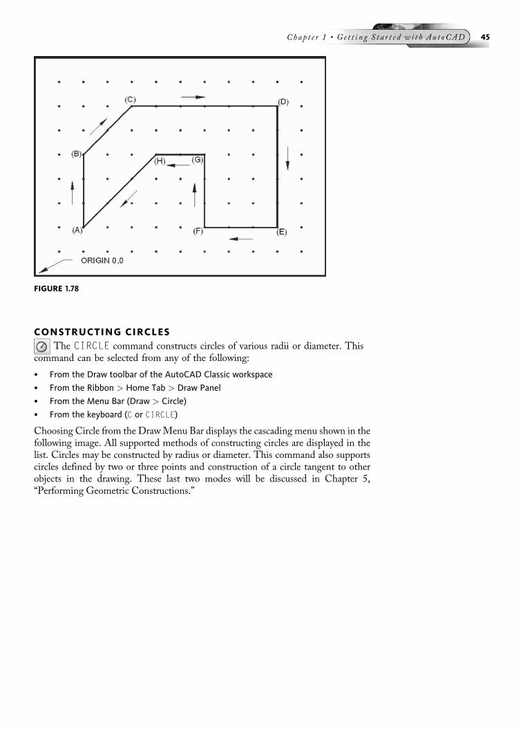
CONSTRUCTING CIRCLESThe CIRCLE command constructs circles of various radii or diameter. This
command can be selected from any of the following:
• From the Draw toolbar of the AutoCAD Classic workspace
• From the Ribbon > Home Tab > Draw Panel
• From the Menu Bar (Draw > Circle)
• From the keyboard (C or CIRCLE)
Choosing Circle from the DrawMenu Bar displays the cascading menu shown in thefollowing image. All supported methods of constructing circles are displayed in thelist. Circles may be constructed by radius or diameter. This command also supportscircles defined by two or three points and construction of a circle tangent to otherobjects in the drawing. These last two modes will be discussed in Chapter 5,“Performing Geometric Constructions.”
FIGURE 1.78
Chap t e r 1 • Ge t t i n g S t a r t e d w i t h Au t oCAD 45

Circle by Radius ModeUse the CIRCLE command and the Radius mode to construct a circle by a radius valuethat you specify. After selecting a center point for the circle, the user is prompted toenter a radius for the desired circle.
TRY IT! Create a new drawing file starting from scratch. Use the CIRCLE command prompts belowand the illustration in the following image on the left to construct a circle by radius.
Command: C (For CIRCLE)
Specify center point for circle or [3P/2P/Ttr (tan tanradius)]: (Mark the center at “A”)
Specify radius of circle or [Diameter]: 1.50
Circle by Diameter ModeUse the CIRCLE command and the Diameter mode to construct a circle by a diametervalue that you specify. After selecting a center point for the circle, you are promptedto enter a diameter for the desired circle.
TRY IT! Create a new drawing file starting from scratch. Use the CIRCLE command prompts belowand the illustration in the following image on the right to construct a circle by diameter.
Command: C (For CIRCLE)
Specify center point for circle or [3P/2P/Ttr (tan tanradius)]: (Mark the center at “A”)
Specify radius of circle or [Diameter]: D (For Diameter)
Specify diameter of circle: 3.00
FIGURE 1.79
FIGURE 1.80
46 Au t oCAD 2010 Tu t o r f o r Eng in e e r i n g Graph i c s

Dynamic Input and CirclesWhen using Dynamic Input mode for constructing circles, notice the appearance of adynamic radius readout when you drag your cursor as shown in the following image.Simply enter the desired radius or press the DOWN ARROW key twice on your keyboardto select the Diameter option, press ENTER, and provide a diameter value.
CONSTRUCTING POLYLINESPolylines are similar to individual line segments except that a polyline can consist
of numerous segments and still be considered a single object. Width can also beassigned to a polyline, unlike regular line segments; this makes polylines perfect fordrawing borders and title blocks. Polylines can be constructed by selecting any of thefollowing:
• From the Draw toolbar of the AutoCAD Classic workspace
• From the Ribbon > Home Tab > Draw Panel
• From the Menu Bar (Draw > Polyline)
• From the keyboard (PL or PLINE)
Study the following images and their corresponding command sequences that followto use the PLINE command.
TRY IT!Create a new drawing file starting from scratch. Follow the command prompt sequence andillustration below to construct the polyline.
Command: PL (For PLINE)
Specify start point: (Pick a point at “A” in the followingimage)
Current line-width is 0.0000
Specify next point or [Arc/Close/Halfwidth/Length/Undo/Width]: W (For Width)
Specify starting width <0.0000>: 0.10
Specify ending width <0.1000>: (Press ENTER to accept thedefault)
Specify next point or [Arc/Close/Halfwidth/Length/Undo/Width]: (Pick a point at “B”)
Specify next point or [Arc/Close/Halfwidth/Length/Undo/Width]: (Pick a point at “C”)
FIGURE 1.81
Chap t e r 1 • Ge t t i n g S t a r t e d w i t h Au t oCAD 47
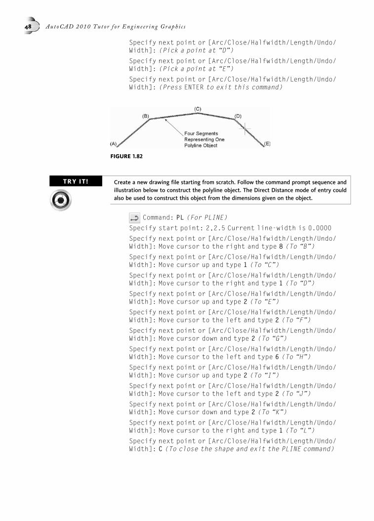
Specify next point or [Arc/Close/Halfwidth/Length/Undo/Width]: (Pick a point at “D”)
Specify next point or [Arc/Close/Halfwidth/Length/Undo/Width]: (Pick a point at “E”)
Specify next point or [Arc/Close/Halfwidth/Length/Undo/Width]: (Press ENTER to exit this command)
TRY IT! Create a new drawing file starting from scratch. Follow the command prompt sequence andillustration below to construct the polyline object. The Direct Distance mode of entry couldalso be used to construct this object from the dimensions given on the object.
Command: PL (For PLINE)
Specify start point: 2,2.5 Current line-width is 0.0000
Specify next point or [Arc/Close/Halfwidth/Length/Undo/Width]: Move cursor to the right and type 8 (To “B”)
Specify next point or [Arc/Close/Halfwidth/Length/Undo/Width]: Move cursor up and type 1 (To “C”)
Specify next point or [Arc/Close/Halfwidth/Length/Undo/Width]: Move cursor to the right and type 1 (To “D”)
Specify next point or [Arc/Close/Halfwidth/Length/Undo/Width]: Move cursor up and type 2 (To “E”)
Specify next point or [Arc/Close/Halfwidth/Length/Undo/Width]: Move cursor to the left and type 2 (To “F”)
Specify next point or [Arc/Close/Halfwidth/Length/Undo/Width]: Move cursor down and type 2 (To “G”)
Specify next point or [Arc/Close/Halfwidth/Length/Undo/Width]: Move cursor to the left and type 6 (To “H”)
Specify next point or [Arc/Close/Halfwidth/Length/Undo/Width]: Move cursor up and type 2 (To “I”)
Specify next point or [Arc/Close/Halfwidth/Length/Undo/Width]: Move cursor to the left and type 2 (To “J”)
Specify next point or [Arc/Close/Halfwidth/Length/Undo/Width]: Move cursor down and type 2 (To “K”)
Specify next point or [Arc/Close/Halfwidth/Length/Undo/Width]: Move cursor to the right and type 1 (To “L”)
Specify next point or [Arc/Close/Halfwidth/Length/Undo/Width]: C (To close the shape and exit the PLINE command)
FIGURE 1.82
48 Au t oCAD 2010 Tu t o r f o r Eng in e e r i n g Graph i c s
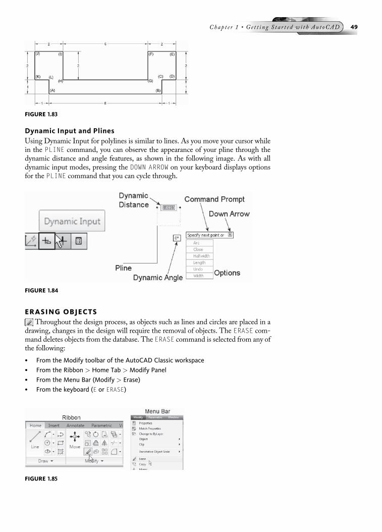
Dynamic Input and PlinesUsing Dynamic Input for polylines is similar to lines. As you move your cursor whilein the PLINE command, you can observe the appearance of your pline through thedynamic distance and angle features, as shown in the following image. As with alldynamic input modes, pressing the DOWN ARROW on your keyboard displays optionsfor the PLINE command that you can cycle through.
ERASING OBJECTSThroughout the design process, as objects such as lines and circles are placed in a
drawing, changes in the design will require the removal of objects. The ERASE com-mand deletes objects from the database. The ERASE command is selected from any ofthe following:
• From the Modify toolbar of the AutoCAD Classic workspace
• From the Ribbon > Home Tab > Modify Panel
• From the Menu Bar (Modify > Erase)
• From the keyboard (E or ERASE)
FIGURE 1.83
FIGURE 1.84
FIGURE 1.85
Chap t e r 1 • Ge t t i n g S t a r t e d w i t h Au t oCAD 49
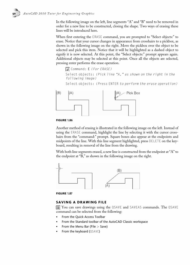
In the following image on the left, line segments “A” and “B” need to be removed inorder for a new line to be constructed, closing the shape. Two ways of erasing theselines will be introduced here.
When first entering the ERASE command, you are prompted to “Select objects:” toerase. Notice that your cursor changes in appearance from crosshairs to a pickbox, asshown in the following image on the right. Move the pickbox over the object to beselected and pick this item. Notice that it will be highlighted as a dashed object tosignify it is now selected. At this point, the “Select objects:” prompt appears again.Additional objects may be selected at this point. Once all the objects are selected,pressing enter performs the erase operation.
Command: E (For ERASE)
Select objects: (Pick line “A,” as shown on the right in thefollowing image)
Select objects: (Press ENTER to perform the erase operation)
Another method of erasing is illustrated in the following image on the left. Instead ofusing the ERASE command, highlight the line by selecting it with the cursor cross-hairs from the “command:” prompt. Square boxes also appear at the endpoints andmidpoints of the line. With this line segment highlighted, press DELETE on the key-board, resulting in removal of the line from the drawing.
With both line segments erased, a new line is constructed from the endpoint at “A” tothe endpoint at “B,” as shown in the following image on the right.
SAVING A DRAWING FILEYou can save drawings using the QSAVE and SAVEAS commands. The QSAVE
command can be selected from the following:
• From the Quick Access Toolbar
• From the Standard toolbar of the AutoCAD Classic workspace
• From the Menu Bar (File > Save)
• From the keyboard (QSAVE)
FIGURE 1.86
FIGURE 1.87
50 Au t oCAD 2010 Tu t o r f o r Eng in e e r i n g Graph i c s

The SAVEAS command can be selected from any of the following:
• From the Menu Bar (File > Save As)
• From the keyboard (SAVEAS)
These commands are found on the File menu, as shown in the following image on theleft.
SaveSelecting Save from the File Menu Bar, as shown in the previous image, activates
the QSAVE command, which stands for Quick Save. If a drawing file has never beensaved and this command is selected, the dialog box shown on the right in the previousimage is displayed. Once a drawing file has been initially saved, selecting this com-mand causes an automatic save and the Save Drawing As dialog box is no longerdisplayed.
Save AsUsing the SAVEAS command always displays the dialog box shown on the right in theprevious image. Simply click the Save button or press ENTER to save the drawing un-der the current name, which is displayed in the field. This command is more popularfor saving the current drawing under an entirely different name. Simply enter the newname in place of the highlighted name in the field. Once a drawing is given a newname through this command, it also becomes the new current drawing file.
The ability to exchange drawings with past releases of AutoCAD is still important tomany industry users. When the Files of type field is selected in the following image, adrop-down list appears. Use this list to save a drawing file in AutoCAD 2004, 2000,and even R14 formats. The user can also save a drawing file as a Drawing Standard(.dws), a Drawing Template (.dwt), and a Drawing Interchange Format (.dxf). TheDrawing Interchange Format is especially useful with opening up an AutoCADdrawing in a competitive CAD system.
FIGURE 1.88
Chap t e r 1 • Ge t t i n g S t a r t e d w i t h Au t oCAD 51

EXITING AN AUTOCAD DRAWING SESSIONIt is good practice to properly exit any drawing session. One way of exiting is bychoosing the Exit option from the File menu, as shown in the following image onthe left. You can also use the CLOSE command to end the current AutoCAD drawingsession.
Whenever an AutoCAD drawing session is exited, a built-in safeguard provides asecond chance to save the drawing, especially if changes were made and a Save wasnot performed. You may be confronted with three options, illustrated in the Auto-CAD alert dialog box shown in the following image on the right. By default, theYes button is highlighted.
If changes were made to a drawing but no Save was performed, the user can now savethem by clicking the Yes button before exiting the drawing. Changes to the drawingwill be saved and the software exits back to the operating system.
If changes were made but the user does not want to save them, clicking the No buttonis appropriate. Changes to the drawing will not be saved and the software exits back tothe operating system.
If changes are made to the drawing and the Exit option is chosen mistakenly, clickingthe Cancel button cancels the Exit option and returns the user to the current drawing.
FIGURE 1.89
FIGURE 1.90
52 Au t oCAD 2010 Tu t o r f o r Eng in e e r i n g Graph i c s

TUTORIAL EXERCISE: 01_GAGE BLOCK.DWG
PurposeThis tutorial is designed to allow you to construct a one-view drawing of the Gage Blockusing Polar Tracking and Direct Distance mode.
System SettingsUse the current default settings for the limits of this drawing, (0,0) for the lower-leftcorner and (12,9) for the upper-right corner.
Suggested CommandsOpen the drawing file called 01_Gage Block. The LINE command will be used entirely forthis tutorial in addition to the Polar Tracking and Direct Distance modes. Running ObjectSnap should already be set to the following modes: Endpoint, Center, Intersection, andExtension.
STEP 1Begin this tutorial by first turning Polar Tracking on. This can be accomplished by clickingPolar in the status bar located at the bottom of your display screen. Then activate theLINE command and follow the next series of prompt sequences to complete thisobject.
Command: L (For LINE)
Specify first point: 1,1
Specify next point or [Undo]: Move cursor to the right andtype 7.5
Specify next point or [Undo]: Move cursor up and type 3
Specify next point or [Close/Undo]: Move cursor to the leftand type 1.5
FIGURE 1.91
Chap t e r 1 • Ge t t i n g S t a r t e d w i t h Au t oCAD 53

Specify next point or [Close/Undo]: Move cursor up and type1.75
Specify next point or [Close/Undo]: Move cursor to the leftand type 1.5
Specify next point or [Close/Undo]: Move cursor down and type1.5
Specify next point or [Close/Undo]: Move cursor to the leftand type 1.5
Specify next point or [Close/Undo]: Move cursor up and type1.5
Specify next point or [Close/Undo]: Move cursor to the leftand type 1.5
Specify next point or [Close/Undo]: Move cursor down andtype 2
Specify next point or [Close/Undo]: Move cursor to the leftand type 1.5
Specify next point or [Close/Undo]: C (To close the shape)
TUTORIAL EXERCISE: 01_ANGLE BLOCK.DWG
This tutorial is designed to allow you to construct a one-view drawing of the AngleBlock using a combination of Polar Tracking, Direct Distance mode, and relativecoordinates.
System SettingsUse the current default settings for the limits of this drawing, (0,0) for the lower-leftcorner and (12,9) for the upper-right corner.
FIGURE 1.92
54 Au t oCAD 2010 Tu t o r f o r Eng in e e r i n g Graph i c s

Suggested CommandsOpen the drawing file called 01_Angle Block. The LINE command will be used entirely forthis tutorial in addition to the Polar Tracking and Direct Distance modes. Running ObjectSnap should already be set to the following modes: Endpoint, Center, Intersection, andExtension.
STEP 1Begin this tutorial by first checking that Polar Tracking is turned on. Then activate theLINE command and follow the next series of prompt sequences to complete thisobject.
Command: L (For LINE)
Specify first point: 3,1
Specify next point or [Undo]: Move cursor to the right andtype 5
Specify next point or [Undo]: @1.5,2.25
Specify next point or [Close/Undo]: Move cursor up and type1.25
Specify next point or [Close/Undo]: Move cursor to the leftand type 2
Specify next point or [Close/Undo]: Move cursor down and type1.25
Specify next point or [Close/Undo]: Move cursor to the leftand type 2.75
Specify next point or [Close/Undo]: @-1.75,2
Specify next point or [Close/Undo]: @-1.75,-3.25
Specify next point or [Close/Undo]: Move cursor to the rightand type 1.75
Specify next point or [Close/Undo]: C (To close the shape)
TUTORIAL EXERCISE: 01_ANGLE PLATE.DWG
FIGURE 1.93
Chap t e r 1 • Ge t t i n g S t a r t e d w i t h Au t oCAD 55

This tutorial is designed to allow you to construct a one-view drawing of the AnglePlate using Polar Tracking set to relative mode and Direct Distance mode.
System SettingsUse the current default settings for the limits of this drawing, (0,0) for the lower-leftcorner and (12,9) for the upper-right corner.
Suggested CommandsOpen the drawing file called 01_Angle Plate. The LINE command will be used entirely forthis tutorial in addition to the Polar Tracking and Direct Distance modes. Polar Trackingwill need to be set to a new incremental angle of 15°. Also, Polar Tracking will need to beset to relative mode. Running Object Snap should already be set to the following modes:Endpoint, Center, Intersection, and Extension.
STEP 1Right-click polar in the status bar at the bottom of the display screen and pick Settingsfrom the menu as shown in the following image on the left. When the Drafting Settingsdialog box appears, click the Polar Tracking tab. While in this tab, set the IncrementalAngle to 15° under Polar Angle Settings area. Then set the Polar Angle measurement toRelative to last segment, as shown in the following image on the right. Click the OK but-ton to save the settings and exit the Drafting Settings dialog box.
STEP 2After setting the angle increment and relative mode under the Polar Tracking tab of theDrafting Settings dialog box, activate the LINE command and follow the next series ofprompt sequences to complete this object.
Command: L (For LINE)
Specify first point: 3,1
Specify next point or [Undo]: (Move your cursor to the rightuntil the polar tooltip reads 0° and enter 5)
Specify next point or [Undo]: (Move your cursor until thepolar tooltip reads 45° and enter 2.5)
Specify next point or [Close/Undo]: (Move your cursor untilthe polar tooltip reads 330° and enter 3)
FIGURE 1.94
56 Au t oCAD 2010 Tu t o r f o r Eng in e e r i n g Graph i c s

Specify next point or [Close/Undo]: (Move your cursor untilthe polar tooltip reads 60° and enter 3)
Specify next point or [Close/Undo]: (Move your cursor untilthe polar tooltip reads 75° and enter 3.75)
Specify next point or [Close/Undo]: (Move your cursor untilthe polar tooltip reads 75° and enter 3.5)
Specify next point or [Close/Undo]: (Move your cursor untilthe polar tooltip reads 30° and enter 1.75)
Specify next point or [Close/Undo]: (Move your cursor untilthe polar tooltip reads 270° and enter 6.5)
Specify next point or [Close/Undo]: (Move your cursor untilthe polar tooltip reads 120° and enter 2.5)
Specify next point or [Close/Undo]: C (To close the shape)
STEP 3When finished with this problem, change the Increment angle under Polar Angle Settingsback to 90° and the Polar Angle measurement back to Absolute, as shown in the followingimage.
FIGURE 1.95
Chap t e r 1 • Ge t t i n g S t a r t e d w i t h Au t oCAD 57

TUTORIAL EXERCISE: 01_PATTERN.DWG
PurposeThis tutorial is designed to allow you to construct a one-view drawing of the Patternusing Polar Tracking techniques.
System SettingsUse the current default settings for the limits of this drawing, (0,0) for the lower-leftcorner and (12,9) for the upper-right corner.
LayersCreate the following layer with the format:
Name Color Linetype
Object Green Continuous
Suggested CommandsOpen the drawing file called 01_Pattern. The LINE command will be used entirely for thistutorial in addition to the Polar Tracking mode. Running Object Snap should already beset to the following modes: Endpoint, Center, Intersection, and Extension. Dynamic Inputhas been turned off for this exercise.
STEP 1Open the drawing file 01_Pattern. Activate the Drafting Settings dialog box, click the PolarTracking tab, and change the Increment angle setting to 10° as shown in the followingimage on the left. Verify that POLAR, OSNAP, and OTRACK are all turned on.
FIGURE 1.96
58 Au t oCAD 2010 Tu t o r f o r Eng in e e r i n g Graph i c s

STEP 2Activate the LINE command, select a starting point, move your cursor to the right, andenter a value of 4 units as shown in the following image on the right. Notice that yourline is green because the current layer, Object, has been assigned the green color.
Command: L (For LINE)
Specify first point: 3,1
Specify next point or [Undo]: (Move your cursor to the rightand enter 4)
STEP 3While still in the LINE command, move your cursor directly up, and enter a value of3 units as shown in the following image on the left.
Specify next point or [Undo]: (Move your cursor up and enter 3)
STEP 4While still in the LINE command, move your cursor up and to the right until the tooltipreads 10°, and enter a value of 2 units as shown in the following image on the right.
Specify next point or [Close/Undo]: (Move your cursor up andto the right at a 10° angle and enter 2)
STEP 5While still in the LINE command, move your cursor up and to the left until the tooltipreads 100°, and enter a value of 2 units as shown in the following image on the left.
Specify next point or [Close/Undo]: (Move your cursor up andto the left at a 100° angle and enter 2)
FIGURE 1.97
FIGURE 1.98
Chap t e r 1 • Ge t t i n g S t a r t e d w i t h Au t oCAD 59

STEP 6While still in the LINE command, first acquire the point at “A.” Then move your cursorbelow and to the left until the Polar value in the tooltip reads 190°, and pick the point at“B” as shown in the following image on the right.
Specify next point or [Close/Undo]: (Acquire the point at “A”and pick the new point at “B”)
STEP 7While still in the LINE command, move your cursor directly up, and enter a value of1 unit as shown on the left in the following image.
Specify next point or [Close/Undo]: (Move your cursor up andenter 1)
STEP 8While still in the LINE command, first acquire the point at “C.” Then move your cursor tothe left until the tooltip reads Polar: < 180°, and pick the point at “D” as shown on theright in the following image.
Specify next point or [Close/Undo]: (Acquire the point at “C”and pick the new point at “D”)
FIGURE 1.99
FIGURE 1.100
60 Au t oCAD 2010 Tu t o r f o r Eng in e e r i n g Graph i c s
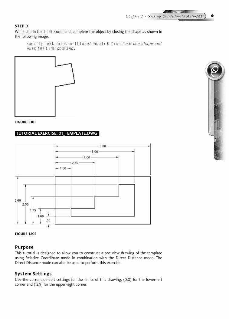
STEP 9While still in the LINE command, complete the object by closing the shape as shown inthe following image.
Specify next point or [Close/Undo]: C (To close the shape andexit the LINE command)
TUTORIAL EXERCISE: 01_TEMPLATE.DWG
PurposeThis tutorial is designed to allow you to construct a one-view drawing of the templateusing Relative Coordinate mode in combination with the Direct Distance mode. TheDirect Distance mode can also be used to perform this exercise.
System SettingsUse the current default settings for the limits of this drawing, (0,0) for the lower-leftcorner and (12,9) for the upper-right corner.
FIGURE 1.101
FIGURE 1.102
Chap t e r 1 • Ge t t i n g S t a r t e d w i t h Au t oCAD 61

LayersThe following layer has already been created:
Name Color LinetypeObject Green Continuous
Suggested CommandsThe LINE command will be used entirely for this tutorial, in addition to a combination ofcoordinate systems. The ERASE command could be used (however, using this commandwill force the user to exit the LINE command), although a more elaborate method ofcorrecting mistakes while using the LINE command is to execute the Undo option. Thisoption allows the user to delete (or undo) previously drawn lines without having to exitthe LINE command. The Object Snap From mode will also be used to construct linesfrom a point of reference. The coordinate mode of entry and the Direct Distance modewill be used throughout this tutorial exercise.
STEP 1Open the drawing file 01_Template.dwg. Then use the LINE command to draw the outerperimeter of the box using the Direct Distance mode. Because the box consists of hori-zontal and vertical lines, Ortho mode is first turned on; this forces all movements to be inthe horizontal or vertical direction. To construct a line segment, move the cursor in thedirection in which the line is to be drawn and enter the exact value of the line. The line isdrawn at the designated distance in the current direction of the cursor. Repeat thisprocedure for the other lines that make up the box, as shown in the following image.
Command: L (For LINE)
Specify first point: 2,2
Specify next point or [Undo]: (Move the cursor to the rightand enter a value of 6.00 units)
Specify next point or [Undo]: (Move the cursor up and enter avalue of 3.00 units)
Specify next point or [Close/Undo]: (Move the cursor to theleft and enter a value of 6.00 units)
Specify next point or [Close/Undo]: C (To close the shape)
FIGURE 1.103
62 Au t oCAD 2010 Tu t o r f o r Eng in e e r i n g Graph i c s

STEP 2The next step is to draw the stair step outline of the template using the LINE commandagain. However, we first need to identify the starting point of the template.
Absolute coordinates could be calculated, but in more complex objects this would be dif-ficult. A more efficient method is to use the Object Snap From mode along with theObject Snap Intersection mode to start the line relative to another point. Both ObjectSnap selections are found on the Object Snap toolbar. Use the following commandsequence and image as guides for performing this operation.
Command: L (For LINE)
Specify first point: From
Base point: Int
of (Pick the intersection at “A” as shown in the followingimage)
<Offset>: @1.00,0.50
The relative coordinate offset value begins a new line a distance of 1.00 units in theX direction and 0.50 units in the Y direction.
Continue with the LINE command to construct the stair step outline shown in the follow-ing image. Use the Direct Distance mode to accomplish this task. In this example, DirectDistance mode is a good choice to use, especially since all lines are either horizontal orvertical. Use the following command sequence to construct the object with this alternatemethod.
Specify next point or [Undo]: (Move the cursor to the rightand enter a value of 4.00 units)
Specify next point or [Undo]: (Move the cursor up and enter avalue of 2.00 units)
Specify next point or [Close/Undo]: (Move the cursor to theleft and enter a value of 1.00 units)
Specify next point or [Close/Undo]: (Move the cursor down andenter a value of 0.75 units)
Specify next point or [Close/Undo]: (Move the cursor to theleft and enter a value of 1.50 units)
Specify next point or [Close/Undo]: (Move the cursor down andenter a value of 0.75 units)
Specify next point or [Close/Undo]: (Move the cursor to theleft and enter a value of 1.50 units)
Specify next point or [Close/Undo]: C (To close the shape)
Chap t e r 1 • Ge t t i n g S t a r t e d w i t h Au t oCAD 63

END OF CHAPTER PROBLEMS FOR CHAPTER 1Please refer to the CD that is supplied with this book and locate the file AutoCAD Tutor2010 Support Docs.pdf. In addition to extra information supplied in this chapter,end-of-chapter problems are also available to provide additional practice.
FIGURE 1.104
64 Au t oCAD 2010 Tu t o r f o r Eng in e e r i n g Graph i c s

CHAPTER
2
Drawing Setup andOrganization
Chapter covers a number of drawing setup commands. The user will learn how toassign different units of measure with the UNITS command. The default sheet sizecan also be increased on the display screen with the LIMITS command. Controllingthe grid and snap will be briefly discussed through the Snap and Grid tab located inthe Drafting Settings dialog box. The major topic of this chapter is the discussion oflayers. All options of the Layer Properties Manager palette will be demonstrated,along with the ability to assign color, linetype, and lineweight to layers. The LayerControl box and Properties toolbar will provide easy access to all layers, colors, line-types, and lineweights used in a drawing. Controlling the scale of linetypes throughthe LTSCALE command will also be discussed. Advanced layer tools such as FilteringLayers and creating Layer States will be introduced. This chapter concludes with asection on creating template files.
SETTING DRAWING UNITSThe Drawing Units dialog box is available for interactively setting the units of a draw-ing. Choosing Units from the Format heading of the Application Menu activates thedialog box illustrated in the following image.
FIGURE 2.1
2
65

By default, decimal units are set along with four-decimal-place precision. The follow-ing systems of units are available: Architectural, Decimal, Engineering, Fractional, andScientific (see the left side of the following image). Architectural units are displayedin feet and fractional inches. Engineering units are displayed in feet and decimal inches.Fractional units are displayed in fractional inches. Scientific units are displayed inexponential format.
Methods of measuring angles supported in the Drawing Units dialog box includeDecimal Degrees, Degrees/Minutes/Seconds, Grads, Radians, and Surveyor’s Units(see the middle of the following image). Accuracy of decimal degree for angles may beset between zero and eight places.
Selecting Direction in the main Drawing Units dialog box displays the DirectionControl dialog box shown in the following image on the right. This dialog box isused to control the direction of angle zero in addition to changing whether anglesare measured in the counterclockwise or clockwise direction. By default, angles aremeasured from zero degrees in the east and in the counterclockwise direction.
ENTERING ARCHITECTURAL VALUES FOR DRAWING LINESThe method of entering architectural values in feet and inches is a little different fromthe method for entering them in decimal places. To designate feet, you must enter theapostrophe symbol ( 0) from the keyboard after the number. For example, “ten feet”would be entered as (10 0), as shown in the following image. When feet and inchesare necessary, you cannot use the Spacebar to separate the inch value from the footvalue. For example, thirteen feet seven inches would be entered as (13 07), as shownin the following image. If you do use the Spacebar after the (13 0) value, this is inter-preted as the enter key and your value is accepted as (13 0). If you have to enter feet,inches, and fractions of an inch, use the hyphen (-) to separate the inch value from thefractional value. For example, to draw a line seventeen feet eleven and one-quarterinches, you would enter the following value in at the keyboard: (17 011-1/4). See thefollowing image. Placing the inches symbol ( 00) is not required since all numbersentered without the foot symbol are interpreted as inches.
FIGURE 2.2
66 Au t oCAD 2010 Tu t o r f o r Eng i n e e r i n g Graph i c s

TRY IT!Open the drawing file 02_Architectural. Verify that the units setting is in architectural unitsby activating the Drawing Units dialog box. With the following image as a guide, use theDirect Distance mode of entry to construct the shape using architectural values.
Command: L (For LINE)
Specify first point:
Specify next point or [Undo]: (Move your cursor to the rightand enter a value of 10 0)
Specify next point or [Undo]: (Move your cursor up and enter avalue of 4 06)
Specify next point or [Close/Undo]: (Move your cursor to theright and enter a value of 13 07-1/2)
Specify next point or [Close/Undo]: (Move your cursor up andenter a value of 4 09-1/2)
Specify next point or [Close/Undo]: (Move your cursor to theleft and enter a value of 7 0)
Specify next point or [Close/Undo]: (Move your cursor up andenter a value of 3 0)
Specify next point or [Close/Undo]: (Move your cursor to theleft and enter a value of 16 07-1/2)
Specify next point or [Close/Undo]: C (To close the shape andexit the LINE command)
FIGURE 2.3
FIGURE 2.4
Chap t e r 2 • Drawing S e t up and Organ i za t i on 67
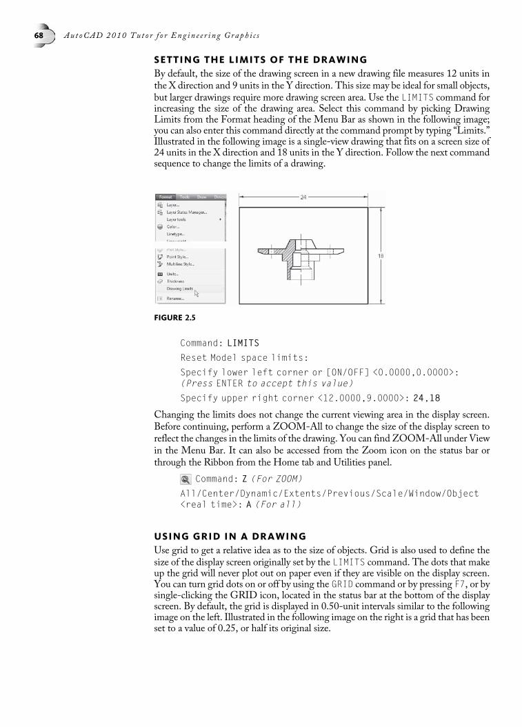
SETTING THE LIMITS OF THE DRAWINGBy default, the size of the drawing screen in a new drawing file measures 12 units inthe X direction and 9 units in the Y direction. This size may be ideal for small objects,but larger drawings require more drawing screen area. Use the LIMITS command forincreasing the size of the drawing area. Select this command by picking DrawingLimits from the Format heading of the Menu Bar as shown in the following image;you can also enter this command directly at the command prompt by typing “Limits.”Illustrated in the following image is a single-view drawing that fits on a screen size of24 units in the X direction and 18 units in the Y direction. Follow the next commandsequence to change the limits of a drawing.
Command: LIMITS
Reset Model space limits:
Specify lower left corner or [ON/OFF] <0.0000,0.0000>:(Press ENTER to accept this value)
Specify upper right corner <12.0000,9.0000>: 24,18
Changing the limits does not change the current viewing area in the display screen.Before continuing, perform a ZOOM-All to change the size of the display screen toreflect the changes in the limits of the drawing. You can find ZOOM-All under Viewin the Menu Bar. It can also be accessed from the Zoom icon on the status bar orthrough the Ribbon from the Home tab and Utilities panel.
Command: Z (For ZOOM)
All/Center/Dynamic/Extents/Previous/Scale/Window/Object<real time>: A (For all)
USING GRID IN A DRAWINGUse grid to get a relative idea as to the size of objects. Grid is also used to define thesize of the display screen originally set by the LIMITS command. The dots that makeup the grid will never plot out on paper even if they are visible on the display screen.You can turn grid dots on or off by using the GRID command or by pressing F7, or bysingle-clicking the GRID icon, located in the status bar at the bottom of the displayscreen. By default, the grid is displayed in 0.50-unit intervals similar to the followingimage on the left. Illustrated in the following image on the right is a grid that has beenset to a value of 0.25, or half its original size.
FIGURE 2.5
68 Au t oCAD 2010 Tu t o r f o r Eng i n e e r i n g Graph i c s

TRY IT!Open the drawing file 02_Grid. Use the following command sequence and illustrations forusing the GRID command.
Command: GRID
Specify grid spacing(X) or [ON/OFF/Snap/Major/aDaptive/Limits/Follow/Aspect] <0.5000>: On
Command: GRID
Specify grid spacing(X) or [ON/OFF/Major/aDaptive/Limits/Follow/Snap/Aspect] <0.5000>: 0.25
NOTEOne advantage of using a grid is the ability to create objects where scale is not importantsuch as electrical symbols. You only want to make sure that all of the symbols are propor-tional to each other. This technique of using a grid will be covered in Chapter 16.
SETTING A SNAP VALUEIt is possible to have the cursor lock on to or snap to a grid dot, as illustrated in thefollowing image on the left; this is the purpose of the SNAP command. By default, thecurrent snap spacing is 0.50 units. Even though a value is set, the snap must be turnedon for the cursor to be positioned on a grid dot. You can accomplish this by usingthe SNAP command (as shown in the following sequence), by pressing F9, or bysingle-clicking SNAP icon in the status bar at the bottom of the display screen.
Some drawing applications require that the snap be rotated at a specific angular value(see the following image on the right). Changing the snap in this fashion also affectsthe cursor. Use the following command sequence for rotating the snap.
TRY IT!Open the drawing file 02_Snap. Use the command sequence below and the illustration inthe following image for using the SNAP command.
Command: SN (For SNAP)
Specify snap spacing or [ON/OFF/Aspect/Style/Type]<0.5000>: On
Command: SN (For SNAP)
FIGURE 2.6
Chap t e r 2 • Drawing S e t up and Organ i za t i on 69
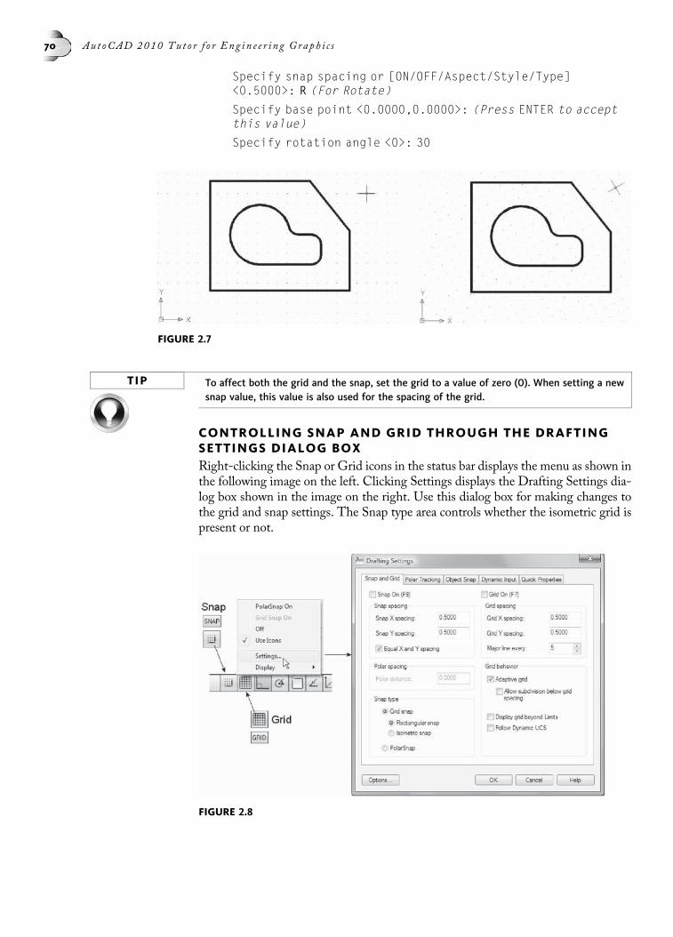
Specify snap spacing or [ON/OFF/Aspect/Style/Type]<0.5000>: R (For Rotate)
Specify base point <0.0000,0.0000>: (Press ENTER to acceptthis value)
Specify rotation angle <0>: 30
TIP To affect both the grid and the snap, set the grid to a value of zero (0). When setting a newsnap value, this value is also used for the spacing of the grid.
CONTROLLING SNAP AND GRID THROUGH THE DRAFTINGSETTINGS DIALOG BOXRight-clicking the Snap or Grid icons in the status bar displays the menu as shown inthe following image on the left. Clicking Settings displays the Drafting Settings dia-log box shown in the image on the right. Use this dialog box for making changes tothe grid and snap settings. The Snap type area controls whether the isometric grid ispresent or not.
FIGURE 2.8
FIGURE 2.7
70 Au t oCAD 2010 Tu t o r f o r Eng i n e e r i n g Graph i c s
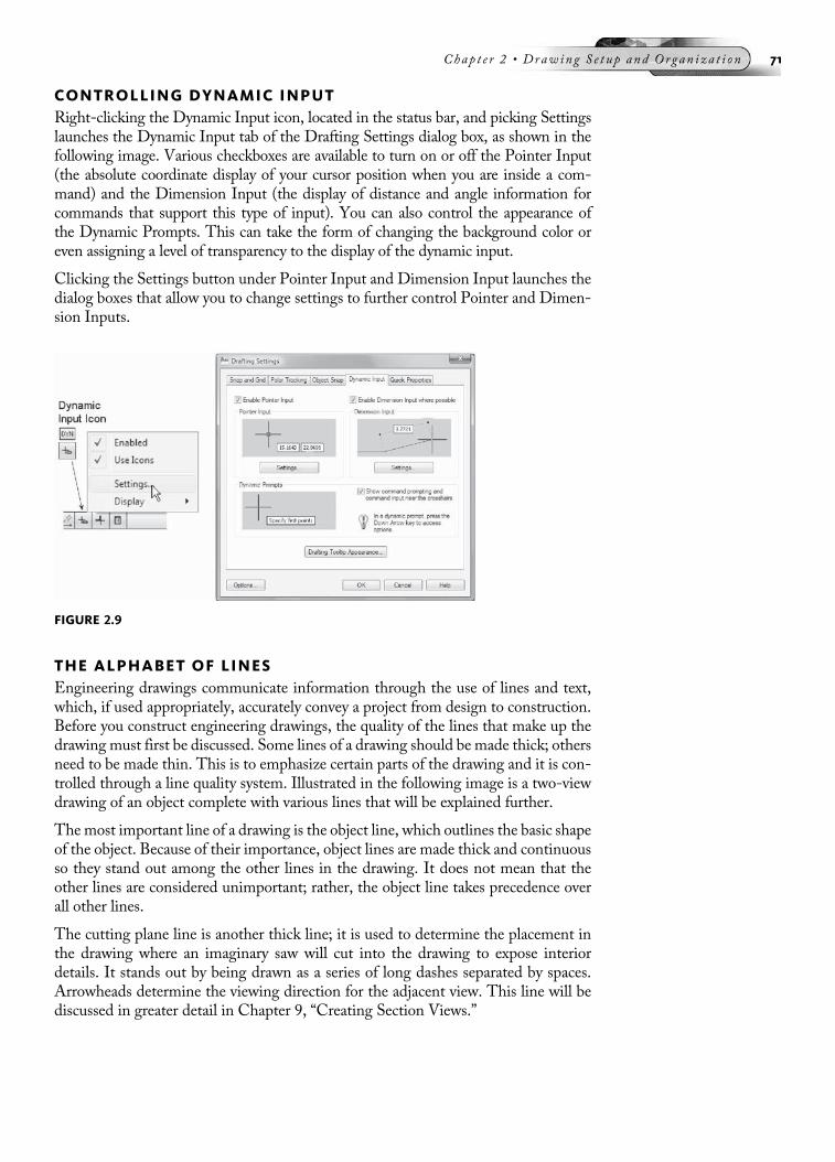
CONTROLLING DYNAMIC INPUTRight-clicking the Dynamic Input icon, located in the status bar, and picking Settingslaunches the Dynamic Input tab of the Drafting Settings dialog box, as shown in thefollowing image. Various checkboxes are available to turn on or off the Pointer Input(the absolute coordinate display of your cursor position when you are inside a com-mand) and the Dimension Input (the display of distance and angle information forcommands that support this type of input). You can also control the appearance ofthe Dynamic Prompts. This can take the form of changing the background color oreven assigning a level of transparency to the display of the dynamic input.
Clicking the Settings button under Pointer Input and Dimension Input launches thedialog boxes that allow you to change settings to further control Pointer and Dimen-sion Inputs.
THE ALPHABET OF LINESEngineering drawings communicate information through the use of lines and text,which, if used appropriately, accurately convey a project from design to construction.Before you construct engineering drawings, the quality of the lines that make up thedrawing must first be discussed. Some lines of a drawing should be made thick; othersneed to be made thin. This is to emphasize certain parts of the drawing and it is con-trolled through a line quality system. Illustrated in the following image is a two-viewdrawing of an object complete with various lines that will be explained further.
The most important line of a drawing is the object line, which outlines the basic shapeof the object. Because of their importance, object lines are made thick and continuousso they stand out among the other lines in the drawing. It does not mean that theother lines are considered unimportant; rather, the object line takes precedence overall other lines.
The cutting plane line is another thick line; it is used to determine the placement inthe drawing where an imaginary saw will cut into the drawing to expose interiordetails. It stands out by being drawn as a series of long dashes separated by spaces.Arrowheads determine the viewing direction for the adjacent view. This line will bediscussed in greater detail in Chapter 9, “Creating Section Views.”
FIGURE 2.9
Chap t e r 2 • Drawing S e t up and Organ i za t i on 71

The hidden line is a thin weight line used to identify edges that become invisible in aview. It consists of a series of dashes separated by spaces.Whether an edge is visible orinvisible, it still must be shown with a line.
The dimension line is a thin line used to show the numerical distance between twopoints. The dimension text is placed within the dimension line, and arrowheads areplaced at opposite ends of the dimension line.
The extension line is another thin continuous line, used as a part of the overall dimen-sion. Extension lines provide a means to move dimension lines away from the objectinto a clear area where they can easily be seen and interpreted.
When you use the cutting Plane line to create an area to cut or slice, the surfaces in theadjacent view are section lined using the section line, a thin continuous line.
Another important line used to identify the centers of symmetrical objects such ascylinders and holes is the centerline. It is a thin line consisting of a series of longand short dashes. It is a good practice to dimension to centerlines; for this reasoncenterlines, extension lines, and dimensions are made the same line thickness.
The phantom line consists of a thin line made with a series of two short dashes andone long dash. It is used to simulate the placement or movement of a part or compo-nent without actually detailing the component.
The long break line is a thin line with a “zigzag” symbol used to establish where anobject is broken to simulate a continuation of the object.
ORGANIZING A DRAWING THROUGH LAYERSAs a means of organizing objects, a series of layers should be devised for every drawing.You can think of layers as a group of transparent sheets that combine to form the com-pleted drawing. The illustration in the following image on the left displays a drawingconsisting of object lines, dimension lines, and border. An example of organizing thesethree drawing components by layers is illustrated in the following image on the right.Only the drawing border occupies a layer called “Border.” The object lines occupy alayer called “Object,” and the dimension lines are drawn on a layer called
FIGURE 2.10
72 Au t oCAD 2010 Tu t o r f o r Eng i n e e r i n g Graph i c s

“Dimension.”At times, it may be necessary to turn off the dimension lines for a clearerview of the object. Creating all dimensions on a specific layer allows you to turn off thedimensions while viewing all other objects on layers that are still turned on.
THE LAYER PROPERTIES MANAGER PALETTEThe Layer Properties Manager palette is the tool used to create and manage
layers. This palette is activated through the following methods: clicking the LayerProperties Manager button from the toolbar located in the AutoCAD Classic work-space, as shown in the following image on the left; choosing Format followed byLayer from the Menu Bar, as shown in the following image on the left; or clickingthe Layer Properties Manager button from the Ribbon, as shown in the followingimage on the right.
TheLayer PropertiesManager palette, illustrated in the following image, is divided intotwo separate panes. The first pane on the left is the Tree View pane used for displayinglayer filter,group,orstate information.ThemainbodyoftheLayerPropertiesManager istheListViewpane.This area lists the individual layers that currently exist in thedrawing.
FIGURE 2.11
FIGURE 2.12
Chap t e r 2 • Drawing S e t up and Organ i za t i on 73

The layer information located in the List View pane is sometimes referred to as layerstates that allow you to perform the following operations: turning layers on or off,freezing or thawing layers, locking or unlocking layers, assigning a color, linetype,lineweight, and plot style to a layer or group of layers, as shown in the followingimage. A brief explanation of each layer state is provided below:
Status—When a green checkmark is displayed, this layer is considered current.
Name—Displays the name of the layer.
On/Off—Makes all objects created on a certain layer visible or invisible on thedisplay screen. The On state is symbolized by a yellow light bulb. The Off statehas a light bulb icon shaded black.
Freeze—This state is similar to the Off mode; objects frozen appear invisible onthe display screen. Freeze, however, is considered a major productivity tool usedto speed up the performance of a drawing. This is accomplished by not calculat-ing any frozen layers during drawing regenerations. A snowflake icon symbolizesthis layer state.
Thaw—This state is similar to the On mode; objects on frozen layers reappearon the display screen when they are thawed. The sun icon symbolizes this layerstate.
Lock—This state allows objects on a certain layer to be visible on the displayscreen while protecting them from accidentally being modified through an edit-ing command. A closed padlock icon symbolizes this layer state.
Unlock—This state unlocks a previously locked layer and is symbolized by anopen padlock icon.
Color—This state displays a color that is assigned to a layer and is symbolized bya square color swatch along with the name of the color. By default, the color whiteis assigned to a layer.
FIGURE 2.14
FIGURE 2.13
74 Au t oCAD 2010 Tu t o r f o r Eng i n e e r i n g Graph i c s
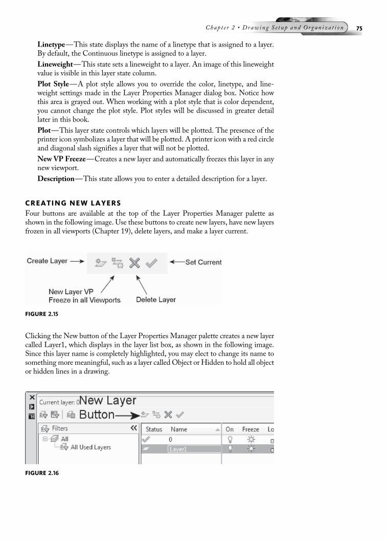
Linetype—This state displays the name of a linetype that is assigned to a layer.By default, the Continuous linetype is assigned to a layer.
Lineweight—This state sets a lineweight to a layer. An image of this lineweightvalue is visible in this layer state column.
Plot Style—A plot style allows you to override the color, linetype, and line-weight settings made in the Layer Properties Manager dialog box. Notice howthis area is grayed out. When working with a plot style that is color dependent,you cannot change the plot style. Plot styles will be discussed in greater detaillater in this book.
Plot—This layer state controls which layers will be plotted. The presence of theprinter icon symbolizes a layer that will be plotted. A printer icon with a red circleand diagonal slash signifies a layer that will not be plotted.
New VP Freeze—Creates a new layer and automatically freezes this layer in anynew viewport.
Description—This state allows you to enter a detailed description for a layer.
CREATING NEW LAYERSFour buttons are available at the top of the Layer Properties Manager palette asshown in the following image. Use these buttons to create new layers, have new layersfrozen in all viewports (Chapter 19), delete layers, and make a layer current.
Clicking the New button of the Layer Properties Manager palette creates a new layercalled Layer1, which displays in the layer list box, as shown in the following image.Since this layer name is completely highlighted, you may elect to change its name tosomething more meaningful, such as a layer called Object or Hidden to hold all objector hidden lines in a drawing.
FIGURE 2.16
FIGURE 2.15
Chap t e r 2 • Drawing S e t up and Organ i za t i on 75

Illustrated in the following image is the result of changing the name of the layer fromLayer1 to Object. You could also have entered “OBJECT” or “object” and thesenames would appear in the palette.
You can also be descriptive with layer names. In the following image, a layer has beencreated called “Section (this layer is designed to control section lines).” You areallowed to add spaces and other characters in the naming of a layer. Because of spacelimitations, the entire layer name may not display until you move your cursor over thetop of the layer name. As a result, the layer name will appear truncated as in the layerSection (in the following image).
If more than one layer needs to be created, it is not necessary to continually click theNew button. A more efficient method would be to perform either of the followingoperations: After creating a new Layer1, change its name to Dimension followed bya comma (,). This automatically creates a new Layer1 as shown in the followingimage. Continue creating new layer names followed by the comma. You could alsopress ENTER twice, which would create another new layer.
FIGURE 2.18
FIGURE 2.17
76 Au t oCAD 2010 Tu t o r f o r Eng i n e e r i n g Graph i c s
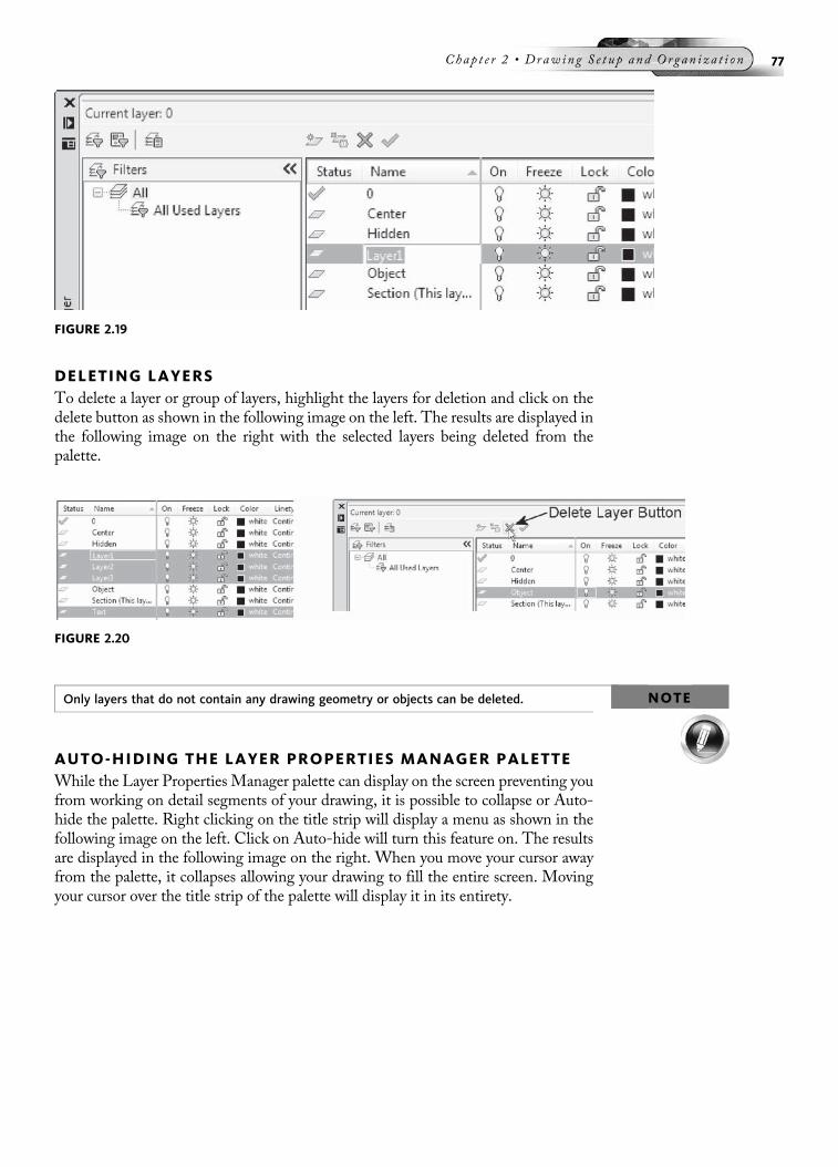
DELETING LAYERSTo delete a layer or group of layers, highlight the layers for deletion and click on thedelete button as shown in the following image on the left. The results are displayed inthe following image on the right with the selected layers being deleted from thepalette.
NOTEOnly layers that do not contain any drawing geometry or objects can be deleted.
AUTO-HIDING THE LAYER PROPERTIES MANAGER PALETTEWhile the Layer Properties Manager palette can display on the screen preventing youfrom working on detail segments of your drawing, it is possible to collapse or Auto-hide the palette. Right clicking on the title strip will display a menu as shown in thefollowing image on the left. Click on Auto-hide will turn this feature on. The resultsare displayed in the following image on the right. When you move your cursor awayfrom the palette, it collapses allowing your drawing to fill the entire screen. Movingyour cursor over the title strip of the palette will display it in its entirety.
FIGURE 2.20
FIGURE 2.19
Chap t e r 2 • Drawing S e t up and Organ i za t i on 77

ASSIGNING COLOR TO LAYERSOnce you select a layer from the list box of the Layer Properties Manager palette andthe color swatch is selected in the same row as the layer name, the Select Color dialogbox shown in the following image is displayed. Three tabs allow you to select threedifferent color groupings. The three groupings (Index Color, True Color, and ColorBooks) are described as follows.
Index Color TabThis tab, shown in the following image, allows you to make color settings based on255 AutoCAD Color Index (ACI) colors. Standard, Gray Shades, and Full ColorPalette areas are available for you to choose colors from.
True Color TabUse this tab to make color settings using true colors, also known as 24-bit color. Twocolor models are available for you to choose from, namely Hue, Saturation, andLuminance (HSL), or Red, Green, and Blue (RGB). Through this tab, you canchoose from over 16 million colors, as shown in the following image on the left.
FIGURE 2.22
FIGURE 2.21
78 Au t oCAD 2010 Tu t o r f o r Eng i n e e r i n g Graph i c s

Color Books TabUse the Color Books tab to select colors that use third-party color books (such asPantone) or user-defined color books. You can think of a color book as similar tothose available in hardware stores when selecting household interior paints. Whenyou select a color book, the name of the selected color book will be identified in thistab, as shown in the following image on the right.
NOTEThe Index tab will be used throughout this text. However, you are encouraged to experi-ment with the True Color and Color Books tabs.
ASSIGNING LINETYPES TO LAYERSSelecting the name Continuous next to the highlighted layer activates the SelectLinetype dialog box, as shown in the following image. Use this dialog box to dynam-ically select preloaded linetypes to be assigned to various layers. By default, theContinuous linetype is loaded for all new drawings.
To load other linetypes, click the Load button of the Select Linetype dialog box; thisdisplays the Load or Reload Linetypes dialog box, as shown in the following image.
Use the scroll bars to view all linetypes contained in the file ACAD.LIN. Noticethat, in addition to standard linetypes such as HIDDEN and PHANTOM, a few
FIGURE 2.24
FIGURE 2.23
Chap t e r 2 • Drawing S e t up and Organ i za t i on 79
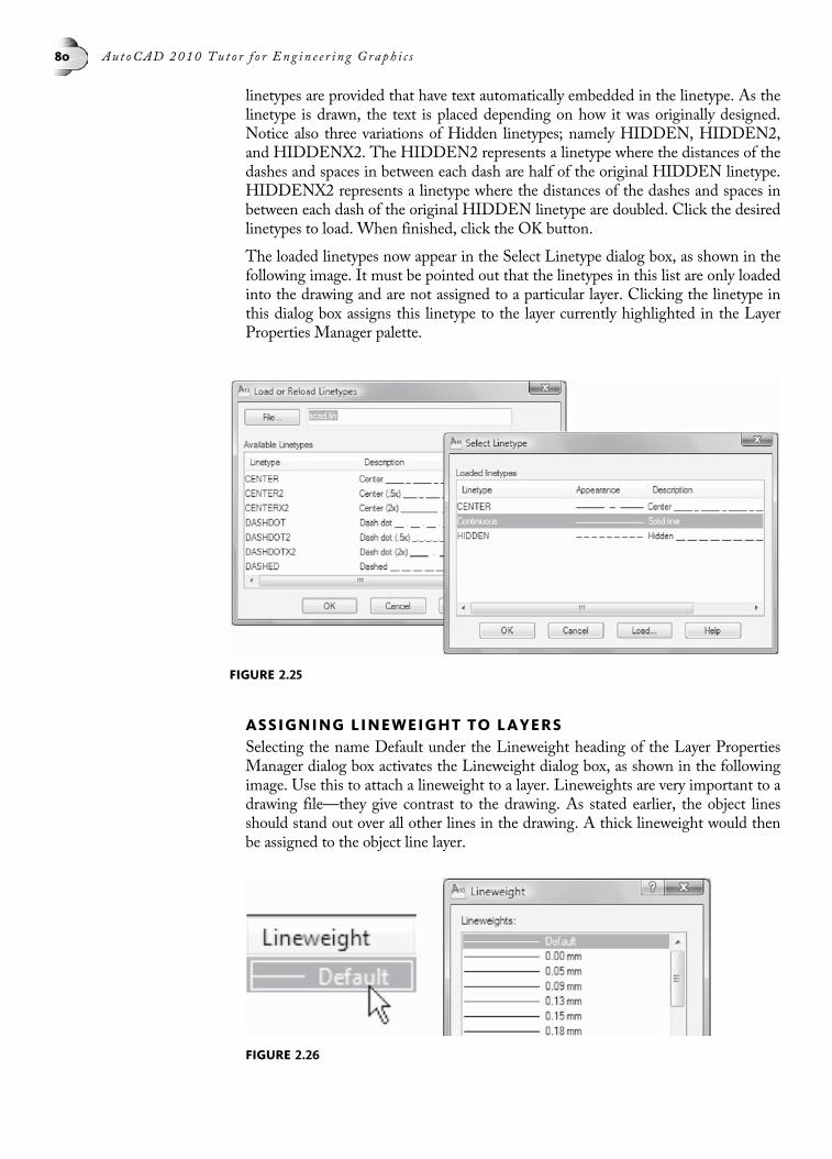
linetypes are provided that have text automatically embedded in the linetype. As thelinetype is drawn, the text is placed depending on how it was originally designed.Notice also three variations of Hidden linetypes; namely HIDDEN, HIDDEN2,and HIDDENX2. The HIDDEN2 represents a linetype where the distances of thedashes and spaces in between each dash are half of the original HIDDEN linetype.HIDDENX2 represents a linetype where the distances of the dashes and spaces inbetween each dash of the original HIDDEN linetype are doubled. Click the desiredlinetypes to load. When finished, click the OK button.
The loaded linetypes now appear in the Select Linetype dialog box, as shown in thefollowing image. It must be pointed out that the linetypes in this list are only loadedinto the drawing and are not assigned to a particular layer. Clicking the linetype inthis dialog box assigns this linetype to the layer currently highlighted in the LayerProperties Manager palette.
ASSIGNING LINEWEIGHT TO LAYERSSelecting the name Default under the Lineweight heading of the Layer PropertiesManager dialog box activates the Lineweight dialog box, as shown in the followingimage. Use this to attach a lineweight to a layer. Lineweights are very important to adrawing file—they give contrast to the drawing. As stated earlier, the object linesshould stand out over all other lines in the drawing. A thick lineweight would thenbe assigned to the object line layer.
FIGURE 2.26
FIGURE 2.25
80 Au t oCAD 2010 Tu t o r f o r Eng i n e e r i n g Graph i c s

In the following image on the left, a lineweight of 0.50 mm has been assigned toall object lines and a lineweight of 0.30 has been assigned to hidden lines. However,all lines in this figure appear to consist of the same lineweight. This is due to thelineweight feature being turned off. Notice in this figure the Lineweight icon inthe Status bar. Use this button to toggle ON or OFF the display of assigned line-weights. Clicking the Lineweight icon, as shown in the following image on the right,turns the lineweight function on (the icon will turn a blue color.) It should be notedthat the assigned lineweight will be plotted whether or not the LWT button isactivated.
THE LINEWEIGHT SETTINGS DIALOG BOXYou have probably already noticed that when you turn on the lineweights throughthe LWT button, all lineweights may appear thick. In a complicated drawing, thelineweights could be so thick that it would be difficult to interpret the purpose ofthe drawing. To give your lineweights a more pleasing appearance, a dialog box isavailable to control the display of your lineweights. This control does not affect theplotted lineweights assigned; only what is displayed on the screen. Clicking Formatfollowed by Lineweight, found in the Menu Bar, as shown in the following imageon the left, displays the Lineweight Settings dialog box. Notice the position of theslider bar in the Adjust Display Scale area of the dialog box. Sliding the bar to theleft near the Min setting reduces the width of all lineweights. Try experimentingwith this on any lineweight assigned to a layer. If you think your lineweights appeartoo thin, slide the bar to the right near the Max setting and observe the results.Continue to adjust your lineweights until they have a pleasing appearance in yourdrawing.
FIGURE 2.27
Chap t e r 2 • Drawing S e t up and Organ i za t i on 81

THE LINETYPE MANAGER DIALOG BOXChoosing Format followed by Linetype, found in the Menu Bar, as shown in thefollowing image on the left displays the Linetype Manager dialog box. This dialogbox is designed mainly to preload linetypes.
Clicking the Load button activates the Load or Reload Linetypes dialog box illus-trated in a previous segment of this chapter. You can select individual linetypes in thisdialog box or load numerous linetypes at once by pressing CTRL and clicking eachlinetype. Clicking the OK button loads the selected linetypes into the dialog box.
The Linetype Manager dialog box, as shown in the following image, also displays anumber of extra linetype details (click Show Details). The Global scale factor valuehas the same effect as the LTSCALE command. Also, setting a different value in theCurrent object scale box can scale the linetype of an individual object.
FIGURE 2.29
FIGURE 2.28
82 Au t oCAD 2010 Tu t o r f o r Eng i n e e r i n g Graph i c s

LOCKED LAYERSObjects on locked layers remain visible on a drawing; they cannot, however, beselected when performing editing operations. Quite often, it can be difficult to distin-guish objects on layers that are locked from normal layers. To assist with the identifi-cation of locked objects, a lock icon appears when you move your cursor over an objectconsidered locked, as shown in the following image on the left. You can also set a fadefactor when viewing locked layers. This is another way of distigushing regular layersfrom those that are locked. Expanding the Layers pane in the Ribbon will display theLocked Layer Fading button as shown in the following image. Next to this button is aslider bar. When turned on, you can move the slider bar to the left or right dependingon the desired amount of fading.
Notice that the following image on the left has objects on a locked layer faded to 50%while the image on the right is faded 80%. Notice how the objects on the left appeardarker than those on the right due to the larger fade factor.
FIGURE 2.31
FIGURE 2.30
Chap t e r 2 • Drawing S e t up and Organ i za t i on 83
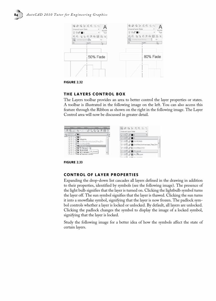
THE LAYERS CONTROL BOXThe Layers toolbar provides an area to better control the layer properties or states.A toolbar is illustrated in the following image on the left. You can also access thisfeature through the Ribbon as shown on the right in the following image. The LayerControl area will now be discussed in greater detail.
CONTROL OF LAYER PROPERTIESExpanding the drop-down list cascades all layers defined in the drawing in additionto their properties, identified by symbols (see the following image). The presence ofthe light bulb signifies that the layer is turned on. Clicking the lightbulb symbol turnsthe layer off. The sun symbol signifies that the layer is thawed. Clicking the sun turnsit into a snowflake symbol, signifying that the layer is now frozen. The padlock sym-bol controls whether a layer is locked or unlocked. By default, all layers are unlocked.Clicking the padlock changes the symbol to display the image of a locked symbol,signifying that the layer is locked.
Study the following image for a better idea of how the symbols affect the state ofcertain layers.
FIGURE 2.33
FIGURE 2.32
84 Au t oCAD 2010 Tu t o r f o r Eng i n e e r i n g Graph i c s

THE PROPERTIES TOOLBARIn addition to the Layers Property Manager Palette, a number of other toolbars sup-porting layer properties are also available. The Properties toolbar, as shown in thefollowing image on the left provides three areas to better access options for the controlof Colors, Linetypes, and Lineweights. A fourth area controls plot styles and is notdiscussed in this book. You can also access these same properties through the Proper-ties pane of the Ribbon as shown in the following image on the right.
NOTEWhile the Properties toolbar and pane allow you to change color, linetype, and lineweight onthe fly, it is poor practice to do so. Check to see that each category in the Properties toolbarreads “ByLayer,” which means that layers control this category.
MAKING A LAYER CURRENTVarious methods can be employed to make a layer current to draw on. Select a
layer in the Layer Properties Manager palette and then click the Current button tomake the layer current.
Picking a layer name from the Layer Control box, as shown in the following image onthe left, will also make the layer current.
The Make Object’s Layer Current button, located in the Ribbon as shown in the fol-lowing image on the right, allows you to make a layer the new current layer by clickingan object in the drawing. The layer is now made current based on the layer of theselected object.
FIGURE 2.35
FIGURE 2.34
Chap t e r 2 • Drawing S e t up and Organ i za t i on 85

Command: LAYMCUR
Select object whose layer will become current: (Pick anobject)
USING THE LAYER PREVIOUS COMMANDThe Layer Previous button is used to undo changes that you have made to layer
settings such as color or lineweight. This button can be found on the left in the Layerstoolbar (2DDrafting &AnnotationWorkspace) or on the right in the Layers pane ofthe Ribbon as shown in the following image. You could even turn a number of layersoff and use the Layer Previous command to have the layers turned back on in a singlestep. This command can also be entered from the keyboard in the following promptsequence:
Command: LAYERP
There are a few exceptions to the use of the Layer Previous command:
• If you rename a layer and change its properties, such as color or lineweight, issuingthe Layer Previous command restores the original properties but does not changethe layer name back to the original.
• Purged or deleted layers will not be restored by using Layer Previous.
• If you add a new layer, issuing the Layer Previous command will not remove the newlayer.
FIGURE 2.37
FIGURE 2.36
86 Au t oCAD 2010 Tu t o r f o r Eng i n e e r i n g Graph i c s

RIGHT-CLICK SUPPORT FOR LAYERSWhile inside the Layer Properties Manager, right-clicking inside the layer informa-tion area displays the shortcut menu in the following image. Use this menu to makethe selected layer current, to make a new layer based on the selected layer, to select alllayers in the dialog box, or to clear all layers. You can even select all layers except forthe current layer. This shortcut menu provides you with easier access to commonlyused layer manipulation tools.
OTHER RIGHT-CLICK LAYER CONTROLSIf you right-click one of the layer header names (Name, On, Freeze, etc.), you get themenu illustrated in the following image. This menu allows you to turn off headernames as a means of condensing the list of headers and making it easier to interpretthe layers that you are using. Other areas of this menu allow you to maximize all col-umns in order to view all information in full regarding layers. By default, the Namecolumn is frozen. This means when you scroll to the left or right to view the otherlayer properties, the Name column does not scroll and allows you to view informationat the end of the Layer Properties Manager palette.
CONTROLLING THE LINETYPE SCALEOnce linetypes are associated with layers and placed in a drawing, a LTSCALE com-mand is available to control their scale. On the left side of the following image, thedefault linetype scale value of 1.00 is in effect. This scale value acts as a multiplier forall linetype distances. In other words, if the hidden linetype is designed to have dashes0.25 units long, a linetype scale value of 1.00 displays the dash of the hidden line at a
FIGURE 2.39
FIGURE 2.38
Chap t e r 2 • Drawing S e t up and Organ i za t i on 87

value of 0.25 units. The LTSCALE command displays the following commandsequence:
Command: LTS (For LTSCALE)
Enter new linetype scale factor <1.0000>: (Press ENTER toaccept the default or enter another value)
TRY IT! Open the drawing file 02_LTScale. Follow the directions, command prompts, and illustra-tions below for using the LTSCALE command.
In the middle of the following image, a linetype scale value of 0.50 units has beenapplied to all linetypes. As a result of the 0.50 multiplier, instead of all hidden linedashes measuring 0.25 units, they now measure 0.125 units.
Command: LTS (For LTSCALE)
Enter new linetype scale factor <1.0000>: 0.50
On the right side of the following image, a linetype scale value of 2.00 units has beenapplied to all linetypes. As a result of the 2.00 multiplier, instead of all hidden linedashes measuring 0.25 units, they now measure 0.50 units. Notice how a large multi-plier displays the centerlines as what appears to be a continuous linetype. The lines arenot long enough to display the size of dashes specified.
Command: LTS (For LTSCALE)
Enter new linetype scale factor <0.5000>: 2.00
TRY IT! Open the drawing file 02_Floor Plan illustrated in the following image on the left. This floorplan is designed to plot out at a scale of 1/8 00 ¼ 1 00 00. This creates a scale factor of 96 (foundby dividing 1 0 by 1/8 00). A layer called “Dividers” was created and assigned the Hidden line-type to show all red hidden lines as potential rooms in the plan. However, the hidden linesdo not display. For all linetypes to show as hidden, this multiplier should be applied to thedrawing through the LTSCALE command.
Since the drawing was constructed in real-world units or full size, the linetypes are con-verted to these units beginning with the multiplier of 96, as shown in the followingimage on the right, through the LTSCALE command.
Command: LTS (For LTSCALE)
Enter new linetype scale factor <1.0000>: 96
FIGURE 2.40
88 Au t oCAD 2010 Tu t o r f o r Eng i n e e r i n g Graph i c s
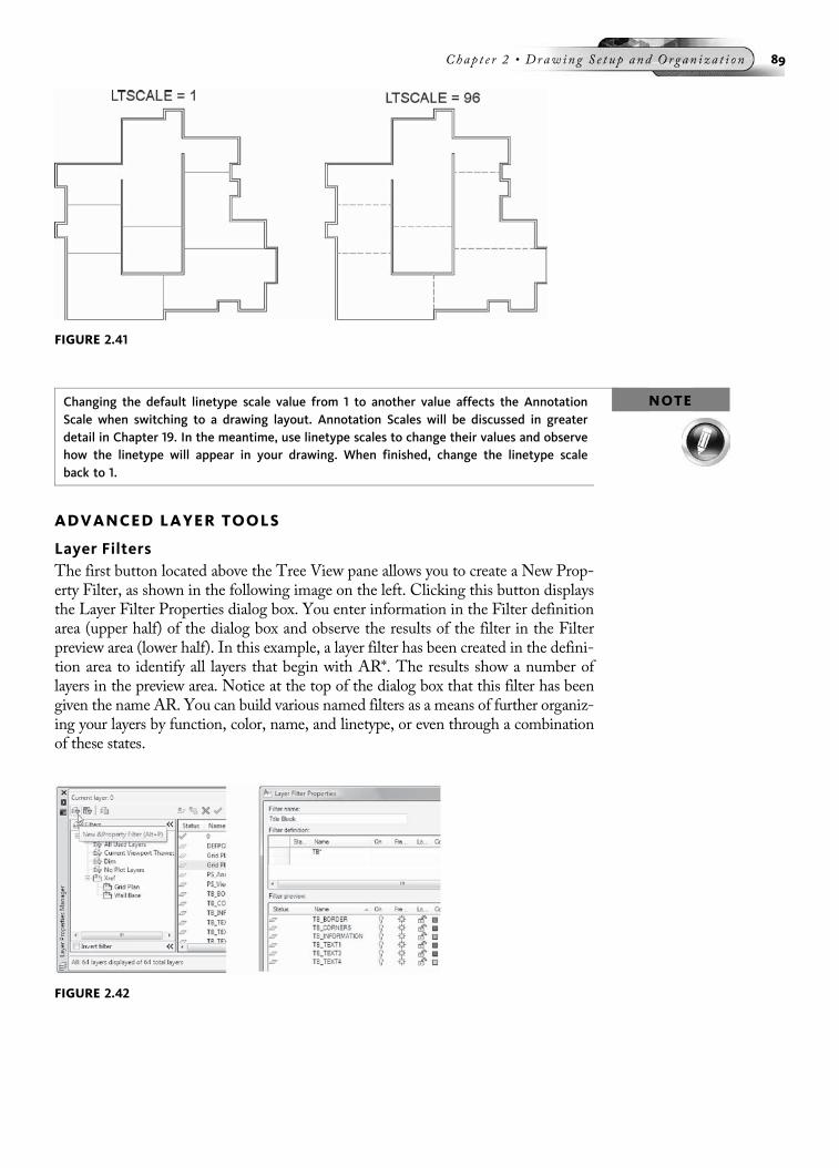
NOTEChanging the default linetype scale value from 1 to another value affects the AnnotationScale when switching to a drawing layout. Annotation Scales will be discussed in greaterdetail in Chapter 19. In the meantime, use linetype scales to change their values and observehow the linetype will appear in your drawing. When finished, change the linetype scaleback to 1.
ADVANCED LAYER TOOLS
Layer FiltersThe first button located above the Tree View pane allows you to create a New Prop-erty Filter, as shown in the following image on the left. Clicking this button displaysthe Layer Filter Properties dialog box. You enter information in the Filter definitionarea (upper half) of the dialog box and observe the results of the filter in the Filterpreview area (lower half). In this example, a layer filter has been created in the defini-tion area to identify all layers that begin with AR*. The results show a number oflayers in the preview area. Notice at the top of the dialog box that this filter has beengiven the name AR. You can build various named filters as a means of further organiz-ing your layers by function, color, name, and linetype, or even through a combinationof these states.
FIGURE 2.42
FIGURE 2.41
Chap t e r 2 • Drawing S e t up and Organ i za t i on 89
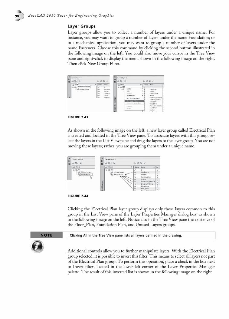
Layer GroupsLayer groups allow you to collect a number of layers under a unique name. Forinstance, you may want to group a number of layers under the name Foundation; orin a mechanical application, you may want to group a number of layers under thename Fasteners. Choose this command by clicking the second button illustrated inthe following image on the left. You could also move your cursor in the Tree Viewpane and right-click to display the menu shown in the following image on the right.Then click New Group Filter.
As shown in the following image on the left, a new layer group called Electrical Planis created and located in the Tree View pane. To associate layers with this group, se-lect the layers in the List View pane and drag the layers to the layer group. You are notmoving these layers; rather, you are grouping them under a unique name.
Clicking the Electrical Plan layer group displays only those layers common to thisgroup in the List View pane of the Layer Properties Manager dialog box, as shownin the following image on the left. Notice also in the Tree View pane the existence ofthe Floor_Plan, Foundation Plan, and Unused Layers groups.
NOTE Clicking All in the Tree View pane lists all layers defined in the drawing.
Additional controls allow you to further manipulate layers. With the Electrical Plangroup selected, it is possible to invert this filter. This means to select all layers not partof the Electrical Plan group. To perform this operation, place a check in the box nextto Invert filter, located in the lower-left corner of the Layer Properties Managerpalette. The result of this inverted list is shown in the following image on the right.
FIGURE 2.44
FIGURE 2.43
90 Au t oCAD 2010 Tu t o r f o r Eng i n e e r i n g Graph i c s

Layer States ManagerThe Layer States Manager allows you to group a number of layer settings under aunique name and then retrieve this name later to affect the display of a drawing.This layer tool can be selected from the Layer Properties Manager palette, as shownin the following image on the left. This launches the Layer States Manager dialogbox. First, you arrange your drawing in numerous states by turning off certain layers.As you do this, you assign a unique name in the Layer States Manager dialog box.
Once you have created numerous states, you test them out by double-clicking on aname such as “Only Walls Layers Visible” as shown in the following image on theleft. Your drawing should update to only display the walls as shown in the followingimage on the right.
FIGURE 2.47
FIGURE 2.45
FIGURE 2.46
Chap t e r 2 • Drawing S e t up and Organ i za t i on 91

It is considered good practice to create a layer state that displays all layers. That way,when you call up various states, you can always get all layers back by calling up this all-layers state. In the following image on the left is the “All Layers Visible” state.Double-clicking on this state will display all layers in the drawing as shown in thefollowing image on the right.
ADDITIONAL LAYER TOOLSClicking Format in theMenu Bar, followed by Layer Tools, displays more layer com-mands that can be used to further manage layers. The display of all of these tools isshown in the following image on the left. A special toolbar called Layers II is alsoavailable, as shown in the following image on the right.
Menu Bar Title Command Description
Make Objects LayerCurrent
LAYMCUR Makes the layer of a selected objectcurrent
Layer Previous LAYERP Undoes any changes made to the set-tings of layers such as color, linetype, orlineweight
FIGURE 2.49
FIGURE 2.48
92 Au t oCAD 2010 Tu t o r f o r Eng i n e e r i n g Graph i c s

Menu Bar Title Command Description
Layer Walk LAYWALK Activates a dialog box that isolateslayers in sequential order
Layer Match LAYMCH Changes the layer of selected objects tothat of a selected object
Change to Current Layer LAYCUR Changes the layer of selected objects tothe current layer
Copy Objects toNew Layer
COPYTOLAYER Copies objects to other layers
Layer Isolate LAYISO Isolates layers of selected objects byturning all other layers off
Isolate Layer to CurrentViewport
LAYVPI Isolates an object’s layer in a viewport
Layer Unisolate LAYUNISO Turns on layers that were turned offwith the last LAYISO command
Layer Off LAYOFF Turns off the layers of selected objects
Turn All Layers On LAYON Turns all layers on
Layer Freeze LAYFRZ Freezes the layers of selected objects
Thaw All Layers LAYTHW Thaws all layers
Layer Lock LAYLCK Locks the layers of selected objects
Layer Unlock LAYULK Unlocks the layers of selected objects
Layer Merge LAYMRG Merges two layers, and then removesthe first layer from the drawing
Layer Delete LAYDEL Permanently deletes layers fromdrawings
NOTEThe file 02_Facilities Plan.dwg is available in the Try It! folder for you to use on the followingadditional layer tools.
Match Object’s Layer (Laymch)The Match Object’s Layer command allows you to change the layers of selected
objects to match the layer of a selected destination object. The command is LAYMCH;first select the objects to be changed, such as the three chairs shown in the followingimage. Next select the object on the destination layer, as in the shelf at “D.”The threechairs now belong to the same layer as the shelf.
Command: LAYMCH
Select objects to be changed:
Select objects: (Select the three chairs labeled “A,” “B,”and “C”)
Select objects: (Press ENTER to continue)
Select object on destination layer or [Name]: (Pick the shelfat “D”)
3 objects changed to layer “Furniture.”
Chap t e r 2 • Drawing S e t up and Organ i za t i on 93

Change to Current Layer (Laycur)The Change to Current Layer command is used to change the layer of one or
more objects to the current layer. The command is LAYCUR. This command is partic-ularly helpful if objects were constructed on the wrong layer. In the following image,the three chairs labeled “A,” “B,” and “C” were drawn on the wrong layer. First makethe desired layer current; in the following image, the current layer is Furniture. Select-ing the three chairs after issuing the LAYCUR command changes the three chairs tothe Furniture layer.
Command: LAYCUR
Select objects to be changed to the current layer: (Select thethree chairs “A,” “B,” and “C”)
Select objects: (Press ENTER to change the three objects tothe current layer)
3 objects changed to layer “Furniture” (the current layer)
FIGURE 2.51
FIGURE 2.50
94 Au t oCAD 2010 Tu t o r f o r Eng i n e e r i n g Graph i c s
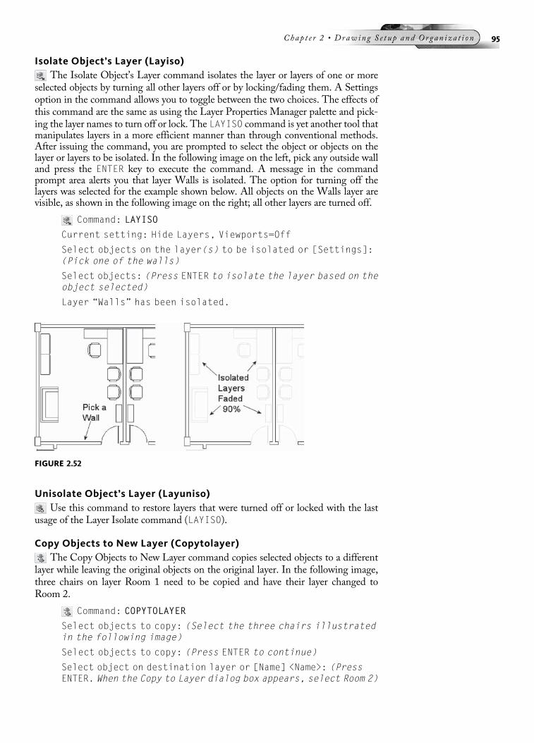
Isolate Object’s Layer (Layiso)The Isolate Object’s Layer command isolates the layer or layers of one or more
selected objects by turning all other layers off or by locking/fading them. A Settingsoption in the command allows you to toggle between the two choices. The effects ofthis command are the same as using the Layer Properties Manager palette and pick-ing the layer names to turn off or lock. The LAYISO command is yet another tool thatmanipulates layers in a more efficient manner than through conventional methods.After issuing the command, you are prompted to select the object or objects on thelayer or layers to be isolated. In the following image on the left, pick any outside walland press the ENTER key to execute the command. A message in the commandprompt area alerts you that layer Walls is isolated. The option for turning off thelayers was selected for the example shown below. All objects on the Walls layer arevisible, as shown in the following image on the right; all other layers are turned off.
Command: LAYISO
Current setting: Hide Layers, Viewports=Off
Select objects on the layer(s) to be isolated or [Settings]:(Pick one of the walls)
Select objects: (Press ENTER to isolate the layer based on theobject selected)
Layer “Walls” has been isolated.
Unisolate Object’s Layer (Layuniso)Use this command to restore layers that were turned off or locked with the last
usage of the Layer Isolate command (LAYISO).
Copy Objects to New Layer (Copytolayer)The Copy Objects to New Layer command copies selected objects to a different
layer while leaving the original objects on the original layer. In the following image,three chairs on layer Room 1 need to be copied and have their layer changed toRoom 2.
Command: COPYTOLAYER
Select objects to copy: (Select the three chairs illustratedin the following image)
Select objects to copy: (Press ENTER to continue)
Select object on destination layer or [Name] <Name>: (PressENTER. When the Copy to Layer dialog box appears, select Room 2)
FIGURE 2.52
Chap t e r 2 • Drawing S e t up and Organ i za t i on 95
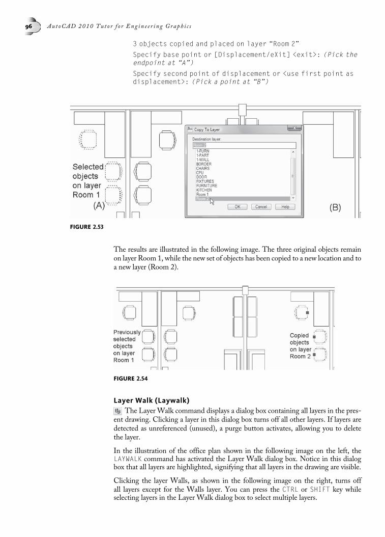
3 objects copied and placed on layer “Room 2”
Specify base point or [Displacement/eXit] <exit>: (Pick theendpoint at “A”)
Specify second point of displacement or <use first point asdisplacement>: (Pick a point at “B”)
The results are illustrated in the following image. The three original objects remainon layer Room 1, while the new set of objects has been copied to a new location and toa new layer (Room 2).
Layer Walk (Laywalk)The Layer Walk command displays a dialog box containing all layers in the pres-
ent drawing. Clicking a layer in this dialog box turns off all other layers. If layers aredetected as unreferenced (unused), a purge button activates, allowing you to deletethe layer.
In the illustration of the office plan shown in the following image on the left, theLAYWALK command has activated the Layer Walk dialog box. Notice in this dialogbox that all layers are highlighted, signifying that all layers in the drawing are visible.
Clicking the layer Walls, as shown in the following image on the right, turns offall layers except for the Walls layer. You can press the CTRL or SHIFT key whileselecting layers in the Layer Walk dialog box to select multiple layers.
FIGURE 2.54
FIGURE 2.53
96 Au t oCAD 2010 Tu t o r f o r Eng i n e e r i n g Graph i c s

Freeze Object’s Layer (Layfrz)The Freeze Object’s Layer command freezes layers by picking objects to control
the layers to be frozen. Again, the Layer Properties Manager palette and the LayerControl box are normally used to perform all layer freeze operations.
Command: LAYFRZ
Current settings: Viewports=Vpfreeze, Block nestinglevel=Block
Select an object on the layer to be frozen or [Settings/Undo]:(Pick a chair)
Layer “Chairs” has been frozen.
Select an object on the layer to be frozen or [Settings/Undo]:(Pick a shelf)
Layer “Furniture” has been frozen.
Select an object on the layer to be frozen or [Settings/Undo]:(Pick a sink)
Layer “Fixtures” has been frozen.
Select an object on the layer to be frozen or [Settings/Undo]:(Pick a refrigerator)
Layer “Kitchen” has been frozen.
Select an object on the layer to be frozen or [Settings/Undo]:(Pick a door)
Layer “Doors” has been frozen.
Select an object on the layer to be frozen or [Settings/Undo]:(Press ENTER to complete this command. The results should besimilar to the following image.)
FIGURE 2.55
Chap t e r 2 • Drawing S e t up and Organ i za t i on 97
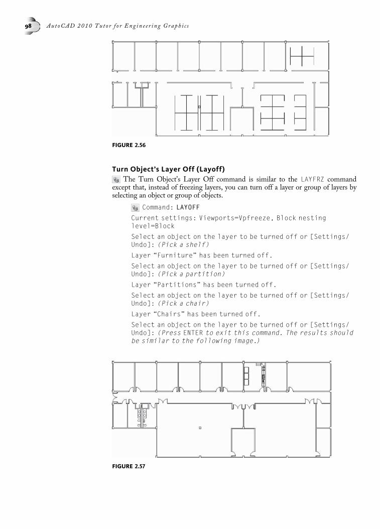
Turn Object’s Layer Off (Layoff)The Turn Object’s Layer Off command is similar to the LAYFRZ command
except that, instead of freezing layers, you can turn off a layer or group of layers byselecting an object or group of objects.
Command: LAYOFF
Current settings: Viewports=Vpfreeze, Block nestinglevel=Block
Select an object on the layer to be turned off or [Settings/Undo]: (Pick a shelf)
Layer “Furniture” has been turned off.
Select an object on the layer to be turned off or [Settings/Undo]: (Pick a partition)
Layer “Partitions” has been turned off.
Select an object on the layer to be turned off or [Settings/Undo]: (Pick a chair)
Layer “Chairs” has been turned off.
Select an object on the layer to be turned off or [Settings/Undo]: (Press ENTER to exit this command. The results shouldbe similar to the following image.)
FIGURE 2.57
FIGURE 2.56
98 Au t oCAD 2010 Tu t o r f o r Eng i n e e r i n g Graph i c s
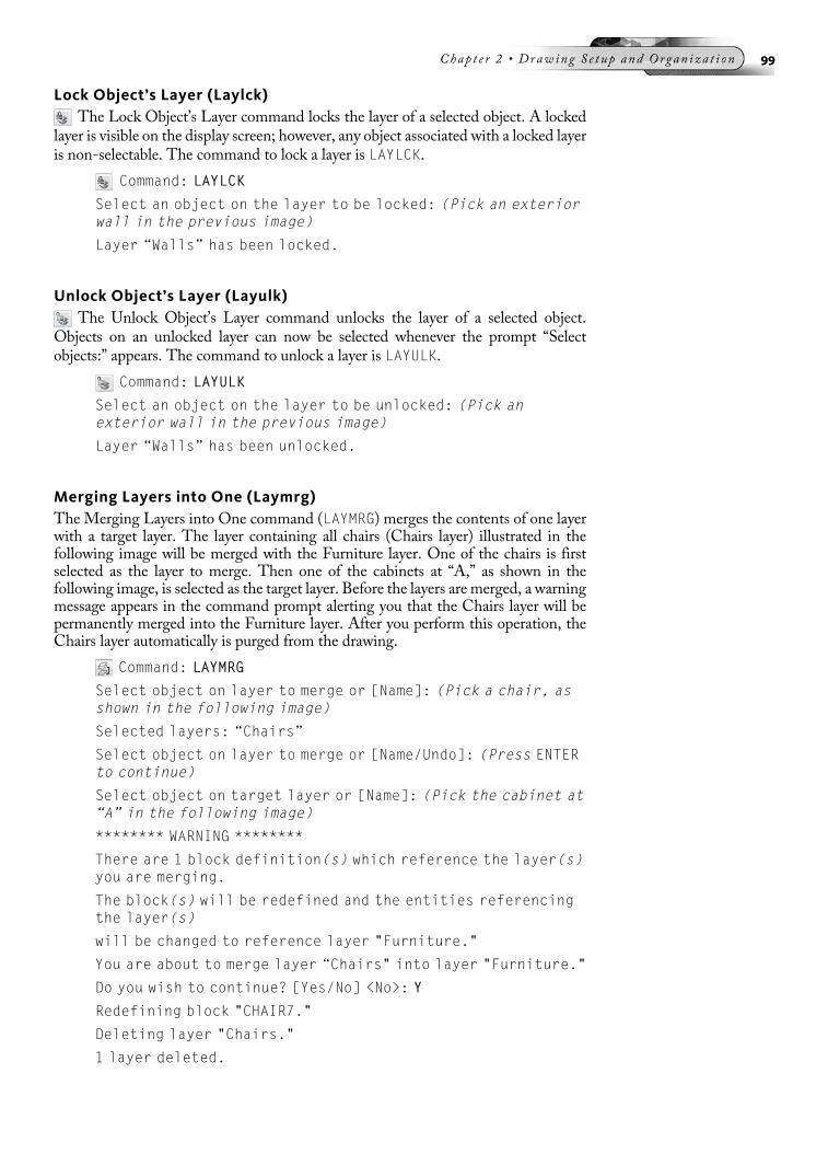
Lock Object’s Layer (Laylck)The Lock Object’s Layer command locks the layer of a selected object. A locked
layer is visible on the display screen; however, any object associated with a locked layeris non-selectable. The command to lock a layer is LAYLCK.
Command: LAYLCK
Select an object on the layer to be locked: (Pick an exteriorwall in the previous image)
Layer “Walls” has been locked.
Unlock Object’s Layer (Layulk)The Unlock Object’s Layer command unlocks the layer of a selected object.
Objects on an unlocked layer can now be selected whenever the prompt “Selectobjects:” appears. The command to unlock a layer is LAYULK.
Command: LAYULK
Select an object on the layer to be unlocked: (Pick anexterior wall in the previous image)
Layer “Walls” has been unlocked.
Merging Layers into One (Laymrg)The Merging Layers into One command (LAYMRG) merges the contents of one layerwith a target layer. The layer containing all chairs (Chairs layer) illustrated in thefollowing image will be merged with the Furniture layer. One of the chairs is firstselected as the layer to merge. Then one of the cabinets at “A,” as shown in thefollowing image, is selected as the target layer. Before the layers are merged, a warningmessage appears in the command prompt alerting you that the Chairs layer will bepermanently merged into the Furniture layer. After you perform this operation, theChairs layer automatically is purged from the drawing.
Command: LAYMRG
Select object on layer to merge or [Name]: (Pick a chair, asshown in the following image)
Selected layers: “Chairs”
Select object on layer to merge or [Name/Undo]: (Press ENTERto continue)
Select object on target layer or [Name]: (Pick the cabinet at“A” in the following image)
******** WARNING ********
There are 1 block definition(s) which reference the layer(s)you are merging.
The block(s) will be redefined and the entities referencingthe layer(s)
will be changed to reference layer "Furniture."
You are about to merge layer “Chairs" into layer "Furniture."
Do you wish to continue? [Yes/No] <No>: Y
Redefining block "CHAIR7."
Deleting layer "Chairs."
1 layer deleted.
Chap t e r 2 • Drawing S e t up and Organ i za t i on 99

If you are not sure about the layer to merge, you can use the Name option, whichlaunches the Merge Layers dialog box, as shown in the following image. You canthen choose the layer by name. The same warning appears in the command promptarea that alerts you that the layer name and all of the objects on the layer (Chairs) willbe merged with the target.
Deleting All Objects on a Layer (Laydel)Use the Layer Delete command (LAYDEL) to delete all objects on a specified layer.First select one of the chairs, as shown in the following image on the left. The chairis located on the Chairs layer. Before all objects on this layer are deleted, a messageappears in the command prompt, asking whether you really want to perform thisoperation. Answering “Yes” deletes all objects assigned to the layer in additionto purging the layer from the drawing. Although this tool has many beneficial advan-tages, you must exercise care in deciding when to use it and when not to use it.
Command: LAYDEL
Select object on layer to delete or [Name]: (Pick the chair at“A” in the following image)
Selected layers: Chairs
Select object on layer to delete or [Name/Undo]: (Press ENTERto continue)
******** WARNING ********
There are 1 block definition(s) which reference the layer(s)you are deleting.
FIGURE 2.59
FIGURE 2.58
100 Au t oCAD 2010 Tu t o r f o r Eng i n e e r i n g Graph i c s
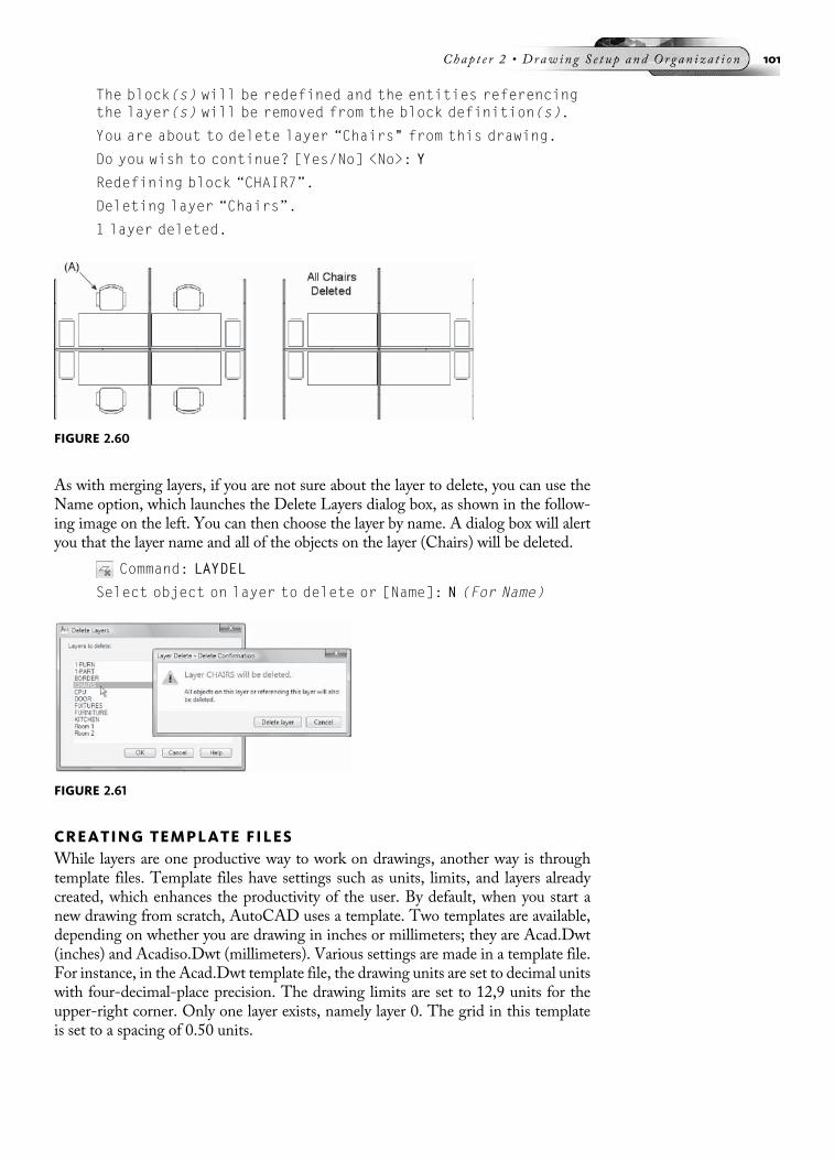
The block(s) will be redefined and the entities referencingthe layer(s) will be removed from the block definition(s).
You are about to delete layer “Chairs" from this drawing.
Do you wish to continue? [Yes/No] <No>: Y
Redefining block “CHAIR7”.
Deleting layer “Chairs”.
1 layer deleted.
As with merging layers, if you are not sure about the layer to delete, you can use theName option, which launches the Delete Layers dialog box, as shown in the follow-ing image on the left. You can then choose the layer by name. A dialog box will alertyou that the layer name and all of the objects on the layer (Chairs) will be deleted.
Command: LAYDEL
Select object on layer to delete or [Name]: N (For Name)
CREATING TEMPLATE FILESWhile layers are one productive way to work on drawings, another way is throughtemplate files. Template files have settings such as units, limits, and layers alreadycreated, which enhances the productivity of the user. By default, when you start anew drawing from scratch, AutoCAD uses a template. Two templates are available,depending on whether you are drawing in inches or millimeters; they are Acad.Dwt(inches) and Acadiso.Dwt (millimeters). Various settings are made in a template file.For instance, in the Acad.Dwt template file, the drawing units are set to decimal unitswith four-decimal-place precision. The drawing limits are set to 12,9 units for theupper-right corner. Only one layer exists, namely layer 0. The grid in this templateis set to a spacing of 0.50 units.
FIGURE 2.61
FIGURE 2.60
Chap t e r 2 • Drawing S e t up and Organ i za t i on 101
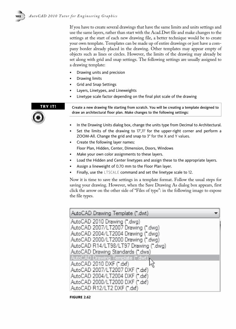
If you have to create several drawings that have the same limits and units settings anduse the same layers, rather than start with the Acad.Dwt file and make changes to thesettings at the start of each new drawing file, a better technique would be to createyour own template. Templates can be made up of entire drawings or just have a com-pany border already placed in the drawing. Other templates may appear empty ofobjects such as lines or circles. However, the limits of the drawing may already beset along with grid and snap settings. The following settings are usually assigned toa drawing template:
• Drawing units and precision
• Drawing limits
• Grid and Snap Settings
• Layers, Linetypes, and Lineweights
• Linetype scale factor depending on the final plot scale of the drawing
TRY IT! Create a new drawing file starting from scratch. You will be creating a template designed todraw an architectural floor plan. Make changes to the following settings:
• In the Drawing Units dialog box, change the units type from Decimal to Architectural.
• Set the limits of the drawing to 17’,11’ for the upper-right corner and perform aZOOM-All. Change the grid and snap to 3" for the X and Y values.
• Create the following layer names:
• Floor Plan, Hidden, Center, Dimension, Doors, Windows
• Make your own color assignments to these layers.
• Load the Hidden and Center linetypes and assign these to the appropriate layers.
• Assign a lineweight of 0.70 mm to the Floor Plan layer.
• Finally, use the LTSCALE command and set the linetype scale to 12.
Now it is time to save the settings in a template format. Follow the usual steps forsaving your drawing. However, when the Save Drawing As dialog box appears, firstclick the arrow on the other side of “Files of type”: in the following image to exposethe file types.
FIGURE 2.62
102 Au t oCAD 2010 Tu t o r f o r Eng i n e e r i n g Graph i c s
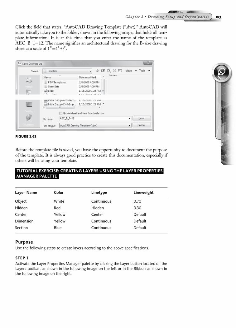
Click the field that states, “AutoCAD Drawing Template (*.dwt).” AutoCAD willautomatically take you to the folder, shown in the following image, that holds all tem-plate information. It is at this time that you enter the name of the template asAEC_B_1¼12. The name signifies an architectural drawing for the B-size drawingsheet at a scale of 1 00¼1 0-0 00.
Before the template file is saved, you have the opportunity to document the purposeof the template. It is always good practice to create this documentation, especially ifothers will be using your template.
TUTORIAL EXERCISE: CREATING LAYERS USING THE LAYER PROPERTIESMANAGER PALETTE
Layer Name Color Linetype Lineweight
Object White Continuous 0.70
Hidden Red Hidden 0.30
Center Yellow Center Default
Dimension Yellow Continuous Default
Section Blue Continuous Default
PurposeUse the following steps to create layers according to the above specifications.
STEP 1Activate the Layer Properties Manager palette by clicking the Layer button located on theLayers toolbar, as shown in the following image on the left or in the Ribbon as shown inthe following image on the right.
FIGURE 2.63
Chap t e r 2 • Drawing S e t up and Organ i za t i on 103

STEP 2Once the Layer Properties Manager palette displays, notice on your screen that only onelayer is currently listed, namely Layer 0. This happens to be the default layer, which is thelayer that is automatically available to all new drawings. Since it is poor practice to con-struct any objects on Layer 0, new layers will be created not only for object lines but forhidden lines, centerlines, dimension objects, and section lines as well. To create theselayers, click the New button as shown in the following image
Notice that a layer is automatically added to the list of layers. This layer is called Layer1 asshown in the following image. While this layer is highlighted, enter the first layer name,“Object.”
Entering a comma after the name of the layer allows more layers to be added to the listingof layers without having to click the New button. Once you have entered the commaafter the layer “Object” and the new layer appears, enter the new name of the layer as“Hidden.” Repeat this procedure of using the comma to create multiple layers for“Center,” “Dimension,” and “Section.” Press ENTER after typing in “Section.” The com-plete list of all layers created should be similar to the illustration shown in the followingimage.
FIGURE 2.66
FIGURE 2.64
FIGURE 2.65
104 Au t oCAD 2010 Tu t o r f o r Eng i n e e r i n g Graph i c s
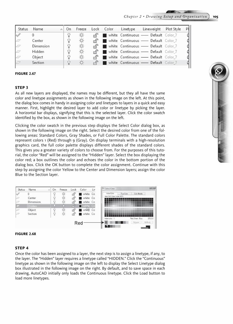
STEP 3As all new layers are displayed, the names may be different, but they all have the samecolor and linetype assignments as shown in the following image on the left. At this point,the dialog box comes in handy in assigning color and linetypes to layers in a quick and easymanner. First, highlight the desired layer to add color or linetype by picking the layer.A horizontal bar displays, signifying that this is the selected layer. Click the color swatchidentified by the box, as shown in the following image on the left.
Clicking the color swatch in the previous step displays the Select Color dialog box, asshown in the following image on the right. Select the desired color from one of the fol-lowing areas: Standard Colors, Gray Shades, or Full Color Palette. The standard colorsrepresent colors 1 (Red) through 9 (Gray). On display terminals with a high-resolutiongraphics card, the full color palette displays different shades of the standard colors.This gives you a greater variety of colors to choose from. For the purposes of this tuto-rial, the color “Red” will be assigned to the “Hidden” layer. Select the box displaying thecolor red; a box outlines the color and echoes the color in the bottom portion of thedialog box. Click the OK button to complete the color assignment. Continue with thisstep by assigning the color Yellow to the Center and Dimension layers; assign the colorBlue to the Section layer.
STEP 4Once the color has been assigned to a layer, the next step is to assign a linetype, if any, tothe layer. The “Hidden” layer requires a linetype called “HIDDEN.” Click the “Continuous”linetype as shown in the following image on the left to display the Select Linetype dialogbox illustrated in the following image on the right. By default, and to save space in eachdrawing, AutoCAD initially only loads the Continuous linetype. Click the Load button toload more linetypes.
FIGURE 2.68
FIGURE 2.67
Chap t e r 2 • Drawing S e t up and Organ i za t i on 105
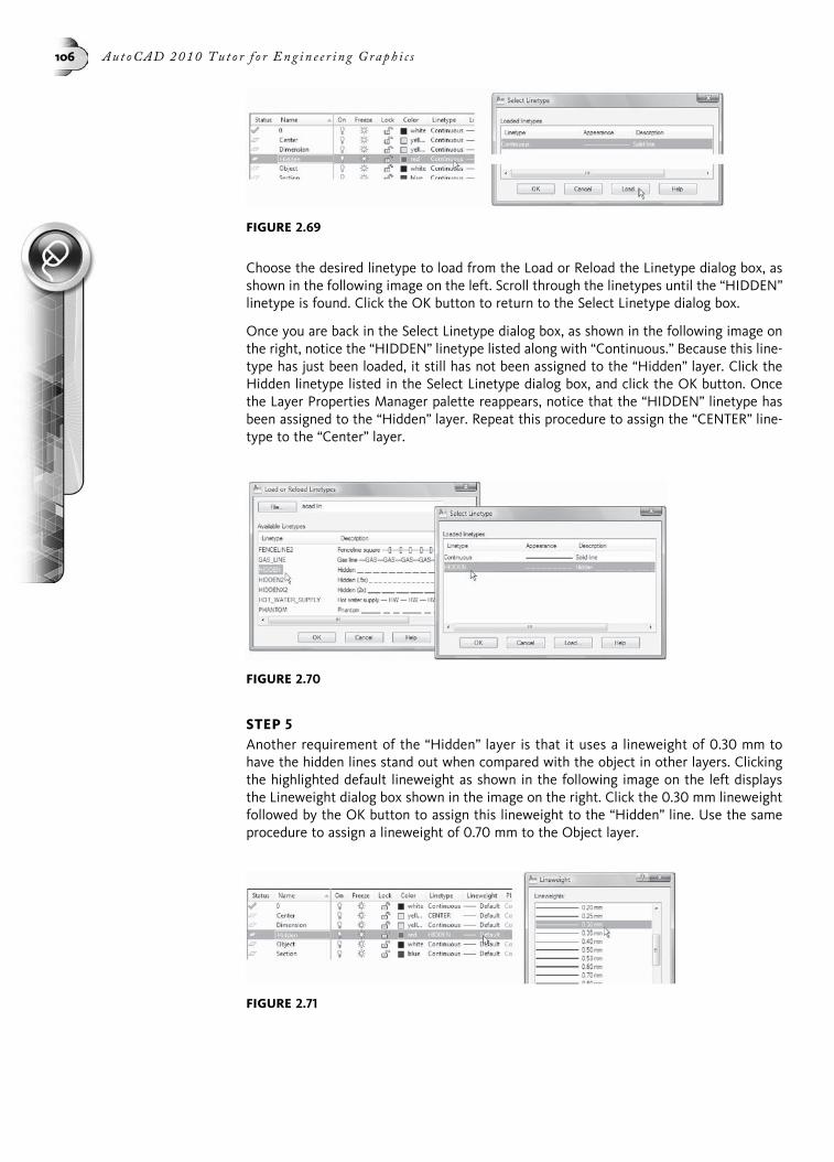
Choose the desired linetype to load from the Load or Reload the Linetype dialog box, asshown in the following image on the left. Scroll through the linetypes until the “HIDDEN”linetype is found. Click the OK button to return to the Select Linetype dialog box.
Once you are back in the Select Linetype dialog box, as shown in the following image onthe right, notice the “HIDDEN” linetype listed along with “Continuous.” Because this line-type has just been loaded, it still has not been assigned to the “Hidden” layer. Click theHidden linetype listed in the Select Linetype dialog box, and click the OK button. Oncethe Layer Properties Manager palette reappears, notice that the “HIDDEN” linetype hasbeen assigned to the “Hidden” layer. Repeat this procedure to assign the “CENTER” line-type to the “Center” layer.
STEP 5Another requirement of the “Hidden” layer is that it uses a lineweight of 0.30 mm tohave the hidden lines stand out when compared with the object in other layers. Clickingthe highlighted default lineweight as shown in the following image on the left displaysthe Lineweight dialog box shown in the image on the right. Click the 0.30 mm lineweightfollowed by the OK button to assign this lineweight to the “Hidden” line. Use the sameprocedure to assign a lineweight of 0.70 mm to the Object layer.
FIGURE 2.70
FIGURE 2.69
FIGURE 2.71
106 Au t oCAD 2010 Tu t o r f o r Eng i n e e r i n g Graph i c s

STEP 6Once you have completed all color and linetype assignments, the Layer PropertiesManager palette should appear similar to the following image. Clicking the X in thecorner of the palette will dismiss the palette, save all layer assignments, and return youto the drawing editor.
Activate the Layer Properties Manager palette and click on the Name box at the top ofthe list of layers to reorder the layers. Now, the layers are listed in reverse alphabeticalorder (see the following image). This same effect occurs when you click on the On,Freeze, Color, Linetype, Lineweight, and Plot header boxes.
The following image displays the results of clicking the Color header: all colors arereordered, starting with Red (1) and followed by Yellow (2), Blue (5), and White (7).
FIGURE 2.74
FIGURE 2.72
FIGURE 2.73
Chap t e r 2 • Drawing S e t up and Organ i za t i on 107

TEMPLATE CREATION EXERCISES FOR CHAPTER
Architectural ApplicationCreate an Architectural template (dwt) that contains the following setup information.
Use the Drawing Units dialog box to set the units of the drawing to Architectural. Keepthe remaining default values for all other unit settings.
Use the Layer Properties Manager palette to create the layers contained in the tablebelow:
Layer Name Color Linetype Lineweight
Border Blue (5) Continuous 1.00Center Green (3) Center 0.25Dimension Green (3) Continuous 0.25Doors Red (2) Continuous 0.50Electrical Green (3) Continuous 0.50Elevations White (7) Continuous 0.70Foundation Cyan (4) Continuous 0.50Furniture Red (1) Continuous 0.50Hatching Magenta (6) Continuous 0.50Hidden Red (1) Hidden 0.50HVAC Cyan (4) Continuous 0.50Misc Green (3) Continuous 0.50Plumbing Cyan (4) Continuous 0.50Text Green (3) Continuous 0.50Viewports Gray (9) Continuous 0.25Walls White (7) Continuous 0.70Windows Yellow (2) Continuous 0.50
When finished making the changes to the drawing units and layer assignments, save thisfile as a new AutoCAD template called ARCH-Imperial.DWT (imperial units are in feetand inches).
Mechanical ApplicationCreate a Mechanical template (dwt) that contains the following setup information.
Use the Drawing Units dialog box to set the units of the drawing to Mechanical. Alsochange the precision to two decimal places. Keep the remaining default values for allother unit settings.
Use the Layer Properties Manager palette to create the layers contained in the tablebelow:
Layer Name Color Linetype Lineweight
Border Blue (5) Continuous 1.00Center Green (3) Center 0.25Construction Gray (8) Continuous 0.25Dimension Green (3) Continuous 0.25Hatching Magenta (6) Continuous 0.50Hidden Red (1) Hidden 0.50
2
108 Au t oCAD 2010 Tu t o r f o r Eng i n e e r i n g Graph i c s

Layer Name Color Linetype Lineweight
Misc Green (3) Continuous 0.50Object White (7) Continuous 0.70Phantom Cyan (4) Phantom 0.50Text Green (3) Continuous 0.50Viewports Gray (9) Continuous 0.25
When you are finished making the changes to the drawing units and layer assignments,save this file as a new AutoCAD template called MECH-Imperial.DWT (imperial units arein inches).
Civil ApplicationCreate a Civil template (dwt) that contains the following setup information.
Use the Drawing Units dialog box to set the units of the drawing to Decimal. Also, changethe precision to two decimal places. Keep the remaining default values for all other unitsettings.
Use the Layer Properties Manager palette to create the layers contained in the tablebelow:
Layer Name Color Linetype Lineweight
Border Blue (5) Continuous 1.00Building Outline White (7) Continuous 0.70Center Green (3) Center 0.25Contour Lines – Existing White (7) Dashed 0.50Contour Lines – New Magenta (6) Continuous 0.50Dimension Green (3) Continuous 0.25Drainage Cyan (4) Divide 0.50Fire Line Red (1) Continuous 0.50Gas Line Red (1) Gas_Line 0.50Hatching Magenta (6) Continuous 0.50Hidden Red (1) Hidden 0.50Misc Green (3) Continuous 0.50Parking Yellow (2) Continuous 0.50Property Line Green (3) Phantom 0.80Sewer White (7) Continuous 0.50Text Green (3) Continuous 0.50Viewports Gray (9) Continuous 0.25Water Line Cyan (4) Continuous 0.50Wetlands Green (3) Dashdot 0.50
When finished making the changes to the drawing units and layer assignments, save thisfile as a new AutoCAD template called CIVIL-Imperial.DWT (imperial units are in feet andinches).
Chap t e r 2 • Drawing S e t up and Organ i za t i on 109

CHAPTER
3AutoCAD Display and
Basic SelectionOperations
This chapter introduces you to the various ways of viewing your drawing. A numberof options of the ZOOM command will be explained first, followed by a review of pan-ning and understanding how a wheel mouse is used with AutoCAD. User-definedportions of a drawing screen called views will also be introduced in this chapter. Youwill be introduced to various Object Selection methods such as window, crossing,crossing polygon, window polygon, fence, and previous, to name just a few.
VIEWING YOUR DRAWING WITH ZOOMThe ability to magnify details in a drawing or reduce the drawing to see it in its en-tirety is a function of the ZOOM command. It does not take much for a drawing tobecome very busy, complicated, or dense when displayed in the drawing editor.Therefore, use the ZOOM command to work on details or view different parts of thedrawing. Zoom can be selected through the following menus as shown in the follow-ing image: Zoom toolbar, Menu Bar, and Ribbon.
The Zoom toolbar contains the more popular tools of the ZOOM command.
Another way to choose options of the ZOOM command is through the Menu Barfound at the top of the display screen. Choosing Zoom from the ViewMenu Bar dis-plays the various options of the ZOOM command. These options include zooming inreal time, zooming to the previous display, using a window to define a boxed area tozoom to, dynamic zooming, zooming to a user-defined scale factor, zooming basedon a center point and a scale factor, or performing routine operations such as zoomingin or out, zooming all, or zooming to the extents of the drawing. All these modes willbe discussed in the pages that follow.
ZOOM commands can also be selected from the Ribbon when operating in the 2DDrafting & Annotation Workspace.
You can also activate the ZOOM command from the keyboard by entering either ZOOMor the letter Z, which is its command alias.
110

The following table illustrates each ZOOM command function and the icon or buttonthat it relates to.
The following image illustrates a floor plan. To work on details of this and otherdrawings, use the ZOOM command to magnify or reduce the display screen. Thefollowing are the options of the ZOOM command (note that nX and nXP refer tothe relative scale factors, which will be explained later in the chapter):
Command: Z (For ZOOM)
Specify corner of window, enter a scale factor (nX or nXP), or
[All/Center/Dynamic/Extents/Previous/Scale/Window/Object] <real time>: (enter one of the listed options)
FIGURE 3.1
Button Tool Function
ZOOM-Window Zooms to a rectangular area by specifying twodiagonal points
ZOOM-Dynamic Uses a viewing box to zoom in to a portion of adrawing
ZOOM-Scale Zooms the display based on a specific scale factor
ZOOM-Center Zooms to an area of the drawing based on a centerpoint and magnification value
ZOOM-Object Zooms to the largest possible magnification based onthe objects selected
ZOOM-In Magnifies the display screen by a scale factor of 2
ZOOM-Out De-magnifies the display screen by a scale factor of .5
ZOOM-All Zooms to the largest possible magnification based onthe current grid setting or drawing extents, whicheveris larger
ZOOM-Extents Zooms to the largest possible magnification based onall objects in the drawing
ZOOM-Realtime Zooms dynamically when the user moves the cursor upor down
ZOOM-Previous Zooms to the previous view
Chap t e r 3 • Au t oCAD Di s p l a y and Ba s i c S e l e c t i o n Op e r a t i o n s 111

Executing the ZOOM command and picking a blank part of the screen places you inautomatic ZOOM-Windowmode. Selecting another point zooms in to the specifiedarea. Refer to the following command sequence to use this mode of the ZOOM com-mand on the floor plan as shown in the following image on the left.
Command: Z (For ZOOM)
Specify corner of window, enter a scale factor (nX or nXP), or
[All/Center/Dynamic/Extents/Previous/Scale/Window/Object] <real time>: (Mark a point at “A”)
Other corner: (Mark a point at “B”)
The ZOOM-Window option is automatically invoked once you select a blank part ofthe screen and then pick a second point. The resulting magnified portion of thescreen appears as shown in the following image on the right.
ZOOMING WITH A WHEEL MOUSEOne of the easiest ways for performing zooming and panning operations is throughthe mouse. Most computers are equipped with a standard Microsoft two-buttonmouse with the addition of a wheel, as illustrated in the following image. Rollingthe wheel forward zooms in to, or magnifies, the drawing. Rolling the wheel back-ward zooms out of, or reduces, the drawing.
Pressing and holding the wheel down, as shown in the following image on the right,places you in Realtime PAN mode. The familiar hand icon on the display screenidentifies this mode.
Pressing CTRL and then depressing the wheel places you in Joystick Pan mode (seethe following image). This mode is identified by a pan icon similar to that shown inthe middle of the following image. This icon denotes all directions in whichpanning may occur. Moving the mouse in any direction with the wheel depresseddisplays the icon in the following image on the right, which shows the direction ofthe pan. The farther away from the center dot you move your cursor, the faster thepanning takes place.
FIGURE 3.2
FIGURE 3.3
112 Au t oCAD 2010 Tu t o r f o r Eng i n e e r i n g Graph i c s

The wheel can also function like a mouse button. Double-clicking on the wheel, as inthe following image, performs a ZOOM-Extents and is extremely popular forviewing the entire drawing on the display screen.
ZOOMING IN REAL TIMEA powerful option of the ZOOM command is performing screen magnifications or
reductions in real time. This is the default option of the command. Issuing theRealtime option of the ZOOM command displays a magnifying glass icon with a pos-itive sign and a negative sign above the magnifier icon. Identify a blank part of thedrawing editor, press down the Pick button of the mouse (the left mouse button),and move in an upward direction to zoom into the drawing in real time. Identify ablank part of the drawing editor, press down the Pick button of the mouse, andmove in a downward direction to zoom out of the drawing in real time. Use thefollowing command sequence and illustration in the following image on the leftfor performing this task.
Command: Z (For ZOOM)
Specify corner of window, enter a scale factor (nX or nXP), or
[All/Center/Dynamic/Extents/Previous/Scale/Window/Object] <real time>: (Press ENTER to accept Realtime asthe default)
Identify the lower portion of the drawing editor, press and hold down the Pick buttonof the mouse, and move the Realtime cursor up; notice the image zooming in.
Once you are in the Realtime mode of the ZOOM command, press the right mousebutton to activate the shortcut menu, as shown in the following image on the right.Use this menu to switch between Realtime ZOOM and Realtime PAN, whichgives you the ability to pan across the screen in real time. The ZOOM-Window,Original (Previous), and Extents options are also available in the cursor menu.
FIGURE 3.4
FIGURE 3.5
Chap t e r 3 • Au t oCAD Di s p l a y and Ba s i c S e l e c t i o n Op e r a t i o n s 113
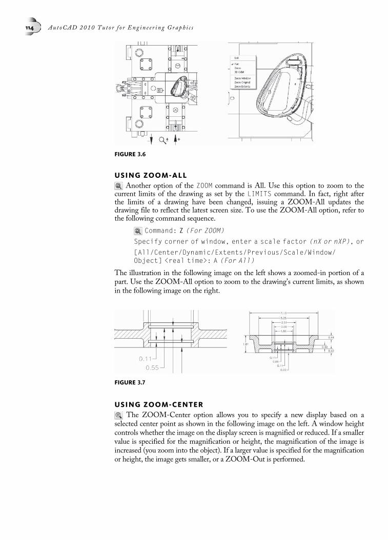
USING ZOOM-ALLAnother option of the ZOOM command is All. Use this option to zoom to the
current limits of the drawing as set by the LIMITS command. In fact, right afterthe limits of a drawing have been changed, issuing a ZOOM-All updates thedrawing file to reflect the latest screen size. To use the ZOOM-All option, refer tothe following command sequence.
Command: Z (For ZOOM)
Specify corner of window, enter a scale factor (nX or nXP), or
[All/Center/Dynamic/Extents/Previous/Scale/Window/Object] <real time>: A (For All)
The illustration in the following image on the left shows a zoomed-in portion of apart. Use the ZOOM-All option to zoom to the drawing’s current limits, as shownin the following image on the right.
USING ZOOM-CENTERThe ZOOM-Center option allows you to specify a new display based on a
selected center point as shown in the following image on the left. A window heightcontrols whether the image on the display screen is magnified or reduced. If a smallervalue is specified for the magnification or height, the magnification of the image isincreased (you zoom into the object). If a larger value is specified for the magnificationor height, the image gets smaller, or a ZOOM-Out is performed.
FIGURE 3.6
FIGURE 3.7
114 Au t oCAD 2010 Tu t o r f o r Eng i n e e r i n g Graph i c s

TRY IT!Open the drawing file 03_Zoom Center. Follow the illustrations and command sequencebelow to perform a zoom based on a center point.
Command: Z (For ZOOM)
Specify corner of window, enter a scale factor (nX or nXP), or
[All/Center/Dynamic/Extents/Previous/Scale/Window/Object] <real time>: C (For Center)
Center point: (Mark a point at the center of circle “A” asshown on the left)
Magnification or Height <7.776>: 2
USING ZOOM-EXTENTSThe image of the pump in the following image on the left reflects a ZOOM-All
operation. Use this option to display the entire drawing area based on the drawinglimits even if the objects that make up the image appear small. Instead of performinga zoom based on the drawing limits, ZOOM-Extents uses the extents of the imageon the display screen to perform the zoom. The following image on the right showsthe largest possible image displayed as a result of using the ZOOM command and theExtents option.
TRY IT!Open the drawing file 03_Zoom Extents. Follow the illustrations and command sequencebelow to perform a zoom based on the drawing limits (All) and the objects in the drawing(Extents).
Command: Z (For ZOOM)
Specify corner of window, enter a scale factor (nX or nXP), or
[All/Center/Dynamic/Extents/Previous/Scale/Window/Object] <real time>: A (For All)
Command: Z (For ZOOM)
Specify corner of window, enter a scale factor (nX or nXP), or
[All/Center/Dynamic/Extents/Previous/Scale/Window/Object] <real time>: E (For Extents)
FIGURE 3.8
Chap t e r 3 • Au t oCAD Di s p l a y and Ba s i c S e l e c t i o n Op e r a t i o n s 115
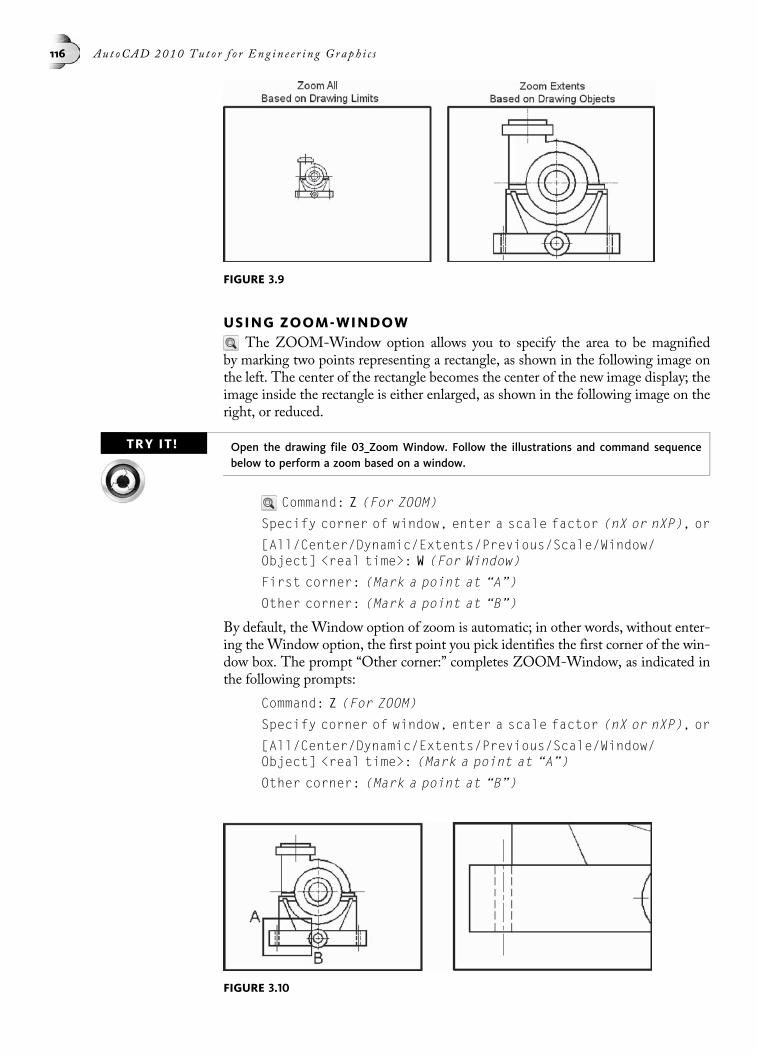
USING ZOOM-WINDOWThe ZOOM-Window option allows you to specify the area to be magnified
by marking two points representing a rectangle, as shown in the following image onthe left. The center of the rectangle becomes the center of the new image display; theimage inside the rectangle is either enlarged, as shown in the following image on theright, or reduced.
TRY IT! Open the drawing file 03_Zoom Window. Follow the illustrations and command sequencebelow to perform a zoom based on a window.
Command: Z (For ZOOM)
Specify corner of window, enter a scale factor (nX or nXP), or
[All/Center/Dynamic/Extents/Previous/Scale/Window/Object] <real time>: W (For Window)
First corner: (Mark a point at “A”)
Other corner: (Mark a point at “B”)
By default, the Window option of zoom is automatic; in other words, without enter-ing the Window option, the first point you pick identifies the first corner of the win-dow box. The prompt “Other corner:” completes ZOOM-Window, as indicated inthe following prompts:
Command: Z (For ZOOM)
Specify corner of window, enter a scale factor (nX or nXP), or
[All/Center/Dynamic/Extents/Previous/Scale/Window/Object] <real time>: (Mark a point at “A”)
Other corner: (Mark a point at “B”)
FIGURE 3.9
FIGURE 3.10
116 Au t oCAD 2010 Tu t o r f o r Eng i n e e r i n g Graph i c s
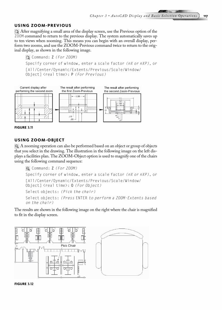
USING ZOOM-PREVIOUSAfter magnifying a small area of the display screen, use the Previous option of the
ZOOM command to return to the previous display. The system automatically saves upto ten views when zooming. This means you can begin with an overall display, per-form two zooms, and use the ZOOM-Previous command twice to return to the orig-inal display, as shown in the following image.
Command: Z (For ZOOM)
Specify corner of window, enter a scale factor (nX or nXP), or
[All/Center/Dynamic/Extents/Previous/Scale/Window/Object] <real time>: P (For Previous)
USING ZOOM-OBJECTA zooming operation can also be performed based on an object or group of objects
that you select in the drawing. The illustration in the following image on the left dis-plays a facilities plan. The ZOOM-Object option is used to magnify one of the chairsusing the following command sequence:
Command: Z (For ZOOM)
Specify corner of window, enter a scale factor (nX or nXP), or
[All/Center/Dynamic/Extents/Previous/Scale/Window/Object] <real time>: O (For Object)
Select objects: (Pick the chair)
Select objects: (Press ENTER to perform a ZOOM-Extents basedon the chair)
The results are shown in the following image on the right where the chair is magnifiedto fit in the display screen.
FIGURE 3.11
FIGURE 3.12
Chap t e r 3 • Au t oCAD Di s p l a y and Ba s i c S e l e c t i o n Op e r a t i o n s 117
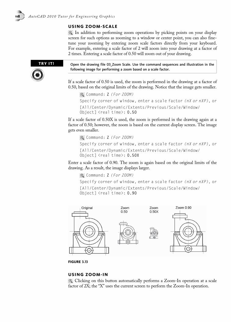
USING ZOOM-SCALEIn addition to performing zoom operations by picking points on your display
screen for such options as zooming to a window or center point, you can also fine-tune your zooming by entering zoom scale factors directly from your keyboard.For example, entering a scale factor of 2 will zoom into your drawing at a factor of2 times. Entering a scale factor of 0.50 will zoom out of your drawing.
TRY IT! Open the drawing file 03_Zoom Scale. Use the command sequences and illustration in thefollowing image for performing a zoom based on a scale factor.
If a scale factor of 0.50 is used, the zoom is performed in the drawing at a factor of0.50, based on the original limits of the drawing. Notice that the image gets smaller.
Command: Z (For ZOOM)
Specify corner of window, enter a scale factor (nX or nXP), or
[All/Center/Dynamic/Extents/Previous/Scale/Window/Object] <real time>: 0.50
If a scale factor of 0.50X is used, the zoom is performed in the drawing again at afactor of 0.50; however, the zoom is based on the current display screen. The imagegets even smaller.
Command: Z (For ZOOM)
Specify corner of window, enter a scale factor (nX or nXP), or
[All/Center/Dynamic/Extents/Previous/Scale/Window/Object] <real time>: 0.50X
Enter a scale factor of 0.90. The zoom is again based on the original limits of thedrawing. As a result, the image displays larger.
Command: Z (For ZOOM)
Specify corner of window, enter a scale factor (nX or nXP), or
[All/Center/Dynamic/Extents/Previous/Scale/Window/Object] <real time>: 0.90
USING ZOOM-INClicking on this button automatically performs a Zoom-In operation at a scale
factor of 2X; the “X” uses the current screen to perform the Zoom-In operation.
FIGURE 3.13
118 Au t oCAD 2010 Tu t o r f o r Eng i n e e r i n g Graph i c s

USING ZOOM-OUTClicking on this button automatically performs a Zoom-Out operation at a scale
factor of 0.5X; the “X” uses the current screen to perform the Zoom-Out operation.
PANNING A DRAWINGAs you perform numerous ZOOM-Window and ZOOM-Previous operations, it
becomes apparent that it would be nice to zoom in to a detail of a drawing and simplyslide the drawing to a new area without changing the magnification; this is the pur-pose of the PAN command. In the following image, the ZOOM-Window option isused to construct a rectangle around the Top view to magnify it.
The result is shown in the following image on the right. Now the Bottom view needsto be magnified to view certain dimensions. Rather than use ZOOM-Previous andthen ZOOM-Window again to magnify the Bottom view, use the PAN command.
Command: P (For PAN)
Press ESC or ENTER to exit, or right-click to display shortcutmenu.
Issuing the PAN command displays the Hand symbol. Pressing the Pick button downat “A” and moving the Hand symbol to the right at “B” as shown in the followingimage on the right pans the screen and displays a new area of the drawing in the cur-rent zoom magnification.
The Bottom view is now visible after the drawing is panned from the Top view to theBottom view, with the same display screen magnification as shown in the followingimage on the left. Pan can also be used transparently; that is, while in a current com-mand, you can select the PAN command, which temporarily interrupts the currentcommand, performs the pan, and then restores the current command.
FIGURE 3.14
Chap t e r 3 • Au t oCAD Di s p l a y and Ba s i c S e l e c t i o n Op e r a t i o n s 119

CREATING NAMED VIEWSAn alternate method of performing numerous zooms is to create a series of views
of key parts of a drawing. Then, instead of using the ZOOM command, restore thenamed view to perform detail work. This named view is saved in the database of thedrawing for use in future editing sessions. Named Views can be found in the ViewMenu Bar, as shown in the following image on the left, or from the View tab of theRibbon as shown in the following image on the right. You can activate this samedialog box through the keyboard by entering the following at the command prompt:
Command: V (For VIEW)
Clicking on either one of these items will activate the View Manager dialog box asshown in the following image.
FIGURE 3.15
FIGURE 3.16
120 Au t oCAD 2010 Tu t o r f o r Eng i n e e r i n g Graph i c s
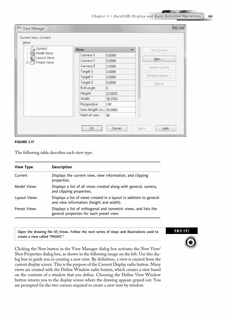
The following table describes each view type:
TRY IT!Open the drawing file 03_Views. Follow the next series of steps and illustrations used tocreate a view called “FRONT.”
Clicking the New button in the View Manager dialog box activates the New View/Shot Properties dialog box, as shown in the following image on the left. Use this dia-log box to guide you in creating a new view. By definition, a view is created from thecurrent display screen. This is the purpose of the Current Display radio button. Manyviews are created with the Define Window radio button, which creates a view basedon the contents of a window that you define. Choosing the Define View Windowbutton returns you to the display screen where the drawing appears grayed out. Youare prompted for the two corners required to create a new view by window.
FIGURE 3.17
View Type Description
Current Displays the current view, view information, and clippingproperties.
Model Views Displays a list of all views created along with general, camera,and clipping properties.
Layout Views Displays a list of views created in a layout in addition to generaland view information (height and width).
Preset Views Displays a list of orthogonal and isometric views, and lists thegeneral properties for each preset view.
Chap t e r 3 • Au t oCAD Di s p l a y and Ba s i c S e l e c t i o n Op e r a t i o n s 121

As illustrated in the following image on the right, a rectangular window is definedaround the Front view using points “A” and “B” as the corners. This turns the imagecaptured inside of the view white and leaves the other images grayed out. Press ENTERto accept this as the new view.
Accepting the window created in the previous image redisplays the New View/ShotProperties dialog. Clicking OK saves the view name FRONT under the ModelViews heading in the View Manager dialog box, as shown in the following image.
FIGURE 3.18
FIGURE 3.19
122 Au t oCAD 2010 Tu t o r f o r Eng i n e e r i n g Graph i c s
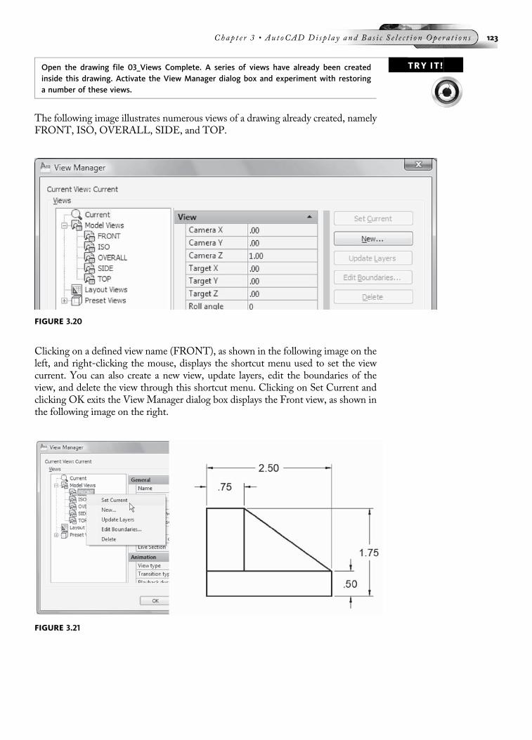
TRY IT!Open the drawing file 03_Views Complete. A series of views have already been createdinside this drawing. Activate the View Manager dialog box and experiment with restoringa number of these views.
The following image illustrates numerous views of a drawing already created, namelyFRONT, ISO, OVERALL, SIDE, and TOP.
Clicking on a defined view name (FRONT), as shown in the following image on theleft, and right-clicking the mouse, displays the shortcut menu used to set the viewcurrent. You can also create a new view, update layers, edit the boundaries of theview, and delete the view through this shortcut menu. Clicking on Set Current andclicking OK exits the View Manager dialog box displays the Front view, as shown inthe following image on the right.
FIGURE 3.20
FIGURE 3.21
Chap t e r 3 • Au t oCAD Di s p l a y and Ba s i c S e l e c t i o n Op e r a t i o n s 123
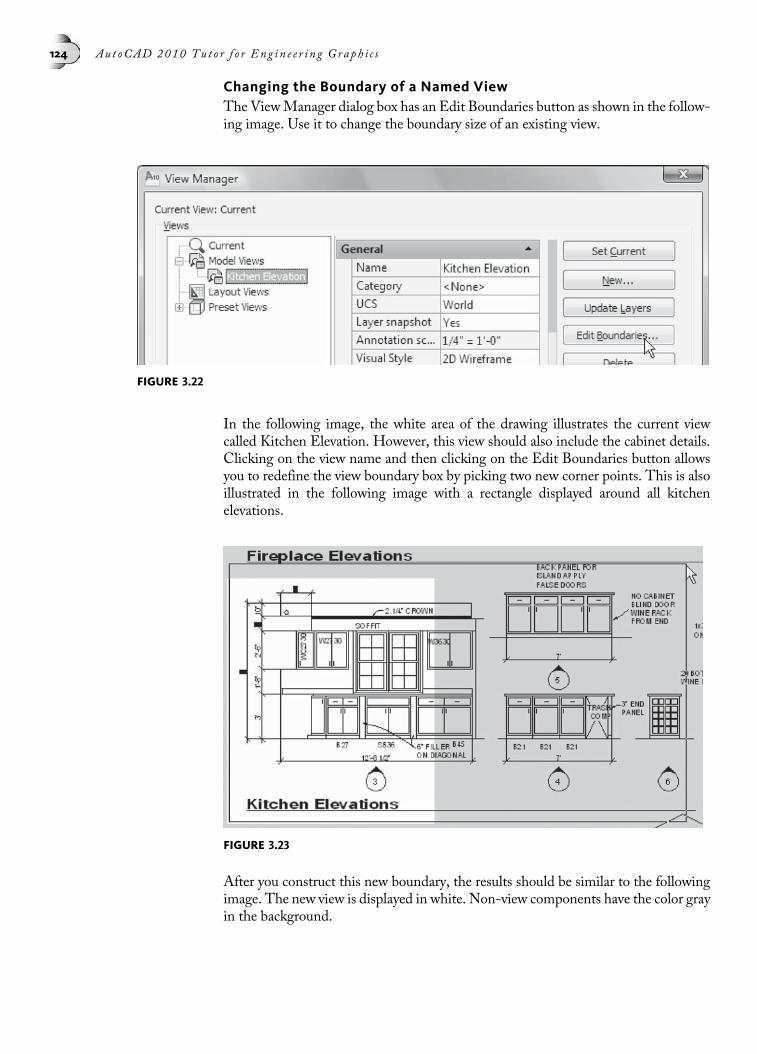
Changing the Boundary of a Named ViewThe ViewManager dialog box has an Edit Boundaries button as shown in the follow-ing image. Use it to change the boundary size of an existing view.
In the following image, the white area of the drawing illustrates the current viewcalled Kitchen Elevation. However, this view should also include the cabinet details.Clicking on the view name and then clicking on the Edit Boundaries button allowsyou to redefine the view boundary box by picking two new corner points. This is alsoillustrated in the following image with a rectangle displayed around all kitchenelevations.
After you construct this new boundary, the results should be similar to the followingimage. The new view is displayed in white. Non-view components have the color grayin the background.
FIGURE 3.22
FIGURE 3.23
124 Au t oCAD 2010 Tu t o r f o r Eng i n e e r i n g Graph i c s
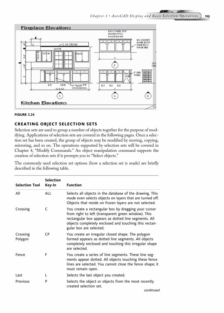
CREATING OBJECT SELECTION SETSSelection sets are used to group a number of objects together for the purpose of mod-ifying. Applications of selection sets are covered in the following pages. Once a selec-tion set has been created, the group of objects may be modified by moving, copying,mirroring, and so on. The operations supported by selection sets will be covered inChapter 4, “Modify Commands.” An object manipulation command supports thecreation of selection sets if it prompts you to “Select objects.”
The commonly used selection set options (how a selection set is made) are brieflydescribed in the following table.
FIGURE 3.24
Selection ToolSelectionKey-In Function
All ALL Selects all objects in the database of the drawing. Thismode even selects objects on layers that are turned off.Objects that reside on frozen layers are not selected.
Crossing C You create a rectangular box by dragging your cursorfrom right to left (transparent green window). Thisrectangular box appears as dotted line segments. Allobjects completely enclosed and touching this rectan-gular box are selected.
CrossingPolygon
CP You create an irregular closed shape. The polygonformed appears as dotted line segments. All objectscompletely enclosed and touching this irregular shapeare selected.
Fence F You create a series of line segments. These line seg-ments appear dotted. All objects touching these fencelines are selected. You cannot close the fence shape; itmust remain open.
Last L Selects the last object you created.
Previous P Selects the object or objects from the most recentlycreated selection set.
continued
Chap t e r 3 • Au t oCAD Di s p l a y and Ba s i c S e l e c t i o n Op e r a t i o n s 125

Object Pre-HighlightWhenever you move your cursor on an object, the object pre-highlights. This providesan easy way to select the correct object, especially in busy drawings. In the followingimage, the cursor is moved over the rectangle that surrounds the 128 text object. Thisaction pre-highlights this rectangle until you move your cursor off this object.
Selecting Objects by Individual PicksWhen AutoCAD prompts you with “Select objects,” a pickbox appears as the cursoris moved across the display screen, as shown in the following image on the left. As youmove your cursor over an object, the object highlights and turns bold to signify that itis selectable, as shown in the following image on the right. An object remainshighlighted once it is selected.
Selection ToolSelectionKey-In Function
Window W You create a rectangular box by dragging your cursorfrom left to right (transparent blue window). Thisrectangular box appears as solid lines. All objectscompletely enclosed in this rectangular box areselected. Objects touching the edges of the boxare ignored.
WindowPolygon
WP You create an irregular closed shape. The polygonformed appears as solid line segments. All objectscompletely enclosed and touching this irregular shapeare selected.
FIGURE 3.25
FIGURE 3.26
continued
126 Au t oCAD 2010 Tu t o r f o r Eng i n e e r i n g Graph i c s
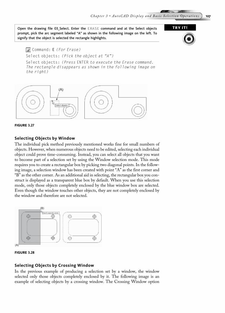
TRY IT!Open the drawing file 03_Select. Enter the ERASE command and at the Select objectsprompt, pick the arc segment labeled “A” as shown in the following image on the left. Tosignify that the object is selected the rectangle highlights.
Command: E (For Erase)
Select objects: (Pick the object at “A”)
Select objects: (Press ENTER to execute the Erase command.The rectangle disappears as shown in the following image onthe right)
Selecting Objects by WindowThe individual pick method previously mentioned works fine for small numbers ofobjects. However, when numerous objects need to be edited, selecting each individualobject could prove time-consuming. Instead, you can select all objects that you wantto become part of a selection set by using the Window selection mode. This moderequires you to create a rectangular box by picking two diagonal points. In the follow-ing image, a selection window has been created with point “A” as the first corner and“B” as the other corner. As an additional aid in selecting, the rectangular box you con-struct is displayed as a transparent blue box by default. When you use this selectionmode, only those objects completely enclosed by the blue window box are selected.Even though the window touches other objects, they are not completely enclosed bythe window and therefore are not selected.
Selecting Objects by Crossing WindowIn the previous example of producing a selection set by a window, the windowselected only those objects completely enclosed by it. The following image is anexample of selecting objects by a crossing window. The Crossing Window option
FIGURE 3.27
FIGURE 3.28
Chap t e r 3 • Au t oCAD Di s p l a y and Ba s i c S e l e c t i o n Op e r a t i o n s 127

requires two points to define a rectangle, as does theWindow selection option. In thefollowing image, a transparent green rectangle with dashed edges is used to select ob-jects, using “A” and “B” as corners for the rectangle; however, this time the crossingwindow was used. The highlighted objects illustrate the results. All objects that aretouched by or enclosed by the crossing rectangle are selected. Because the transparentgreen crossing rectangle passes through the three circles without enclosing them, theyare still selected by this object selection mode.
Selecting Objects by a FenceUse this mode to create a selection set by drawing a line or group of line segmentscalled a fence. Any object touched by the fence is selected. The fence does not haveto end exactly where it was started. In the following image, all objects touched by thefence are selected, as represented by the dashed lines.
TRY IT! Open the drawing file 03_Fence. Follow the command sequence below and the illustrationto select a group of objects using a fence.
Command: E (For Erase)
Select objects: F (For Fence)
First fence point: (Pick a first fence point)
Specify endpoint of line or [Undo]: (Pick a second fencepoint)
Specify endpoint of line or [Undo]: (Pick a third fence point)
Specify endpoint of line or [Undo]: (Press ENTER to exit fencemode)
Select objects: (Press ENTER to execute the Erase command)
FIGURE 3.29
FIGURE 3.30
128 Au t oCAD 2010 Tu t o r f o r Eng i n e e r i n g Graph i c s

Removing Objects from a Selection SetAll the previous examples of creating selection sets have shown you how to create newselection sets. What if you select the wrong object or objects? Instead of canceling outof the command and trying to select the correct objects, you can use the Remove op-tion to remove objects from an existing selection set. As illustrated in the followingimage on the left, a selection set has been created and made up of all the highlightedobjects. However, the outer lines and arcs were mistakenly selected as part of theselection set. The Remove option allows you to remove highlighted objects from aselection set. To activate Remove, press SHIFT and pick the object or objects youwant removed; this works only if the Select objects prompt is present. When thehighlighted objects are removed from the selection set, as shown in the followingimage on the right, they regain their original display intensity.
Selecting the Previous Selection SetWhen you create a selection set of objects, this grouping is remembered until anotherselection set is made. The new selection set replaces the original set of objects. Let’ssay you moved a group of objects to a new location on the display screen. Now youwant to rotate these same objects at a certain angle. Rather than select the same set ofobjects to rotate, you would pick the Previous option or type P at the Select objectsprompt. This selects the previous selection set. The buffer holding the selection set iscleared whenever you use the U command to undo the previous command.
Selecting Objects by a Crossing PolygonWhen you use the Window or Crossing Window mode to create selection sets, twopoints specify a rectangular box for selecting objects. At times, it is difficult to selectobjects by the rectangular window or crossing box because in more cases than not,extra objects are selected and have to be removed from the selection set.
TRY IT!Open the drawing file 03_Select CP. The following image shows a mechanical part with a“C”-shaped slot. Rather than use Window or Crossing Window modes, you can pick theCrossing Polygon mode (CPolygon) or type CP at the Select objects prompt. You simplypick points representing a polygon. Any object that touches or is inside the polygon isadded to a selection set of objects. As illustrated in the following image on the left, thecrossing polygon is constructed using points “1” through “5.” A similar but different selec-tion set mode is the Window Polygon (WPolygon). Objects are selected using this modewhen they lie completely inside the Window Polygon, which is similar to the regularWindow mode.
FIGURE 3.31
Chap t e r 3 • Au t oCAD Di s p l a y and Ba s i c S e l e c t i o n Op e r a t i o n s 129

CYCLING THROUGH OBJECTSAt times, the process of selecting objects can become quite tedious. Often, objects liedirectly on top of each other. As you select the object to delete, the other object selectsinstead. To remedy this, press and hold the SHIFT key and press the spacebar whenprompted to “Select objects.”This activates Object Selection Cycling and enables youto scroll through all objects in the vicinity of the pickbox by pressing the spacebar.A message appears in the prompt area when you begin scrolling, alerting you thatcycling is on; you can now pick objects until the desired object is highlighted. Press-ing ENTER not only accepts the highlighted object but toggles cycling off. In the fol-lowing image and with selection cycling on, the first pick selects the circle, the secondpick selects the line segment, and the third pick selects the rectangle. Keep pickinguntil the desired object highlights.
TRY IT! Open the drawing file 03_Cycle and experiment using this feature on the object illustratedin the previous image.
PRE-SELECTING OBJECTSYou can bypass the Select objects prompt by pre-selecting objects at the Commandprompt. Notice that when you pick an object, not only does it highlight, but a seriesof blue square boxes also appears. These objects are called grips and will be discussedin greater detail in Chapter 7. To cancel or deselect the object, press the ESC key andnotice that even the grips disappear. You could also pick a blank part of your screen atthe Command prompt. Moving your cursor to the right and picking a point has thesame effect as using the Window option of Select objects. Only objects completelyinside the window are selected. If you pick a blank part of your screen at the Com-mand prompt and move your cursor to the left, this has the same effect as using the
FIGURE 3.32
FIGURE 3.33
130 Au t oCAD 2010 Tu t o r f o r Eng in e e r i n g Graph i c s

Crossing option of Select objects in which any items touched by or completelyenclosed by the box are selected.
TIPPressing CTRL+ A at the Command prompt selects all objects in the entire drawing anddisplays the blue grip boxes. This even selects objects that are on a layer that has beenturned off, but does not select those on a layer that is frozen or locked.
THE QSELECT COMMANDYet another way of creating a selection set is by matching the object type and prop-erty with objects currently in use in a drawing. This is the purpose of the QSELECT(Quick Select) command. This command can be chosen from the Tools Menu Bar,as shown in the following image on the left, or from the Ribbon by choosing theHome tab and locating the Utilities panel as shown in the middle which launchesthe dialog box on the right.
TRY IT!Open the drawing file 03_Qselect and activate the Quick Select dialog box. This commandworks only if objects are defined in a drawing; the Quick Select dialog box does not displayin a drawing file without any objects drawn. Clicking in the Object type field displays all ob-ject types currently used in the drawing. This enables you to create a selection set by theobject type. For instance, to select all line segments in the drawing file, click on Line in theObject type field, as illustrated in the following image on the left.
Clicking the OK button at the bottom of the dialog box returns you to the drawingand highlights all the line segments in the drawing, as shown in the following imageon the right.
FIGURE 3.34
FIGURE 3.35
Chap t e r 3 • Au t oCAD Di s p l a y and Ba s i c S e l e c t i o n Op e r a t i o n s 131
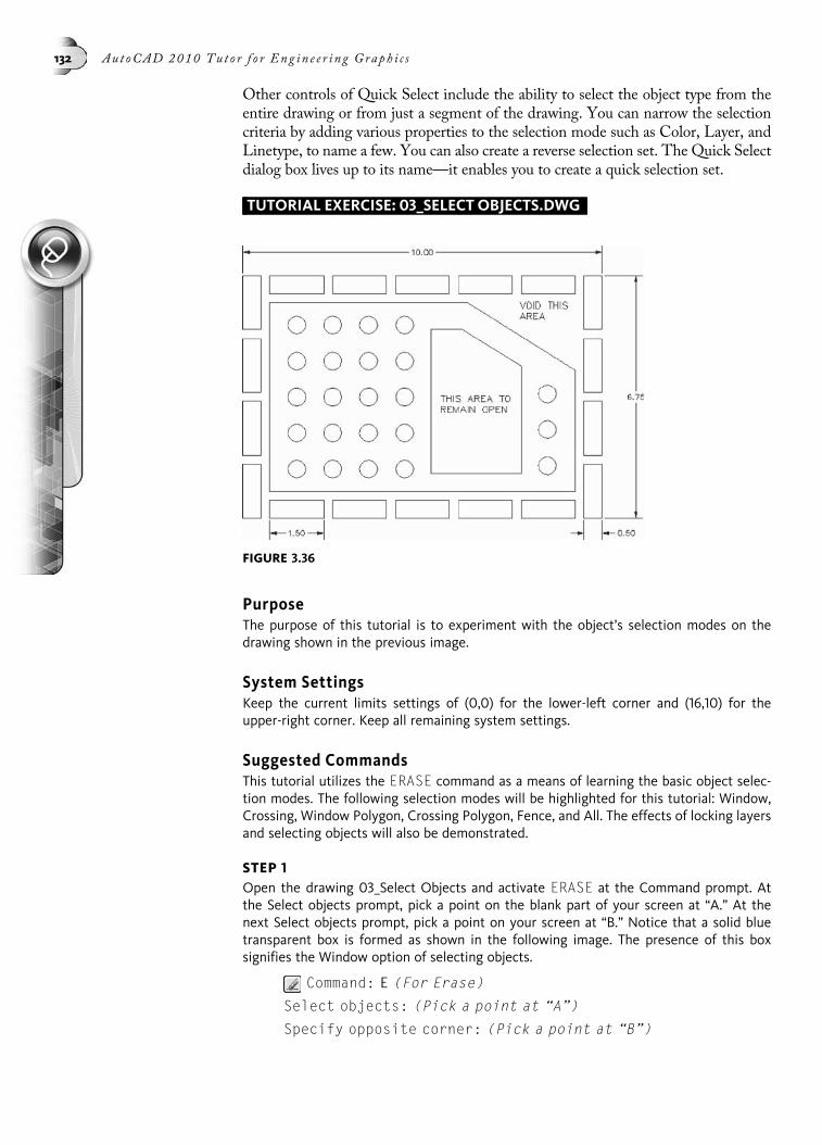
Other controls of Quick Select include the ability to select the object type from theentire drawing or from just a segment of the drawing. You can narrow the selectioncriteria by adding various properties to the selection mode such as Color, Layer, andLinetype, to name a few. You can also create a reverse selection set. The Quick Selectdialog box lives up to its name—it enables you to create a quick selection set.
TUTORIAL EXERCISE: 03_SELECT OBJECTS.DWG
PurposeThe purpose of this tutorial is to experiment with the object’s selection modes on thedrawing shown in the previous image.
System SettingsKeep the current limits settings of (0,0) for the lower-left corner and (16,10) for theupper-right corner. Keep all remaining system settings.
Suggested CommandsThis tutorial utilizes the ERASE command as a means of learning the basic object selec-tion modes. The following selection modes will be highlighted for this tutorial: Window,Crossing, Window Polygon, Crossing Polygon, Fence, and All. The effects of locking layersand selecting objects will also be demonstrated.
STEP 1Open the drawing 03_Select Objects and activate ERASE at the Command prompt. Atthe Select objects prompt, pick a point on the blank part of your screen at “A.” At thenext Select objects prompt, pick a point on your screen at “B.” Notice that a solid bluetransparent box is formed as shown in the following image. The presence of this boxsignifies the Window option of selecting objects.
Command: E (For Erase)
Select objects: (Pick a point at “A”)
Specify opposite corner: (Pick a point at “B”)
FIGURE 3.36
132 Au t oCAD 2010 Tu t o r f o r Eng i n e e r i n g Graph i c s

The result of selecting objects by a window is illustrated in the following image. Onlythose objects completely surrounded by the window are highlighted. Pressing ENTER per-forms the erase operation. Before continuing on to the next step, issue the U (UNDO)command, which negates the previous erase operation.
STEP 2With the entire object displayed on the screen, activate the ERASE command again. Atthe Select objects prompt, pick a point on the blank part of your screen at “A.” At theSpecify opposite corner prompt, pick a point on your screen at “B.” Notice that the trans-parent box is now dashed and green in appearance as shown in the following image. Thepresence of this box signifies the Crossing option of selecting objects.
FIGURE 3.37
FIGURE 3.38
Chap t e r 3 • Au t oCAD Di s p l a y and Ba s i c S e l e c t i o n Op e r a t i o n s 133

Command: E (For ERASE)
Select objects: (Pick a point at “A”)
Specify opposite corner: (Pick a point at “B”)
The result of selecting objects by a crossing window is illustrated in the following image.Notice that objects touched by the crossing box, as well as those objects completely sur-rounded by the crossing box, are highlighted. Pressing ENTER performs the erase opera-tion. Before continuing on to the next step, issue the U (UNDO) command, whichnegates the previous ERASE operation.
STEP 3Activate the ERASE command again. At the Select objects prompt, pick a point on theblank part of your screen at “A.” At the Specify opposite corner prompt, pick a point on
FIGURE 3.39
FIGURE 3.40
134 Au t oCAD 2010 Tu t o r f o r Eng in e e r i n g Graph i c s

your screen at “B” as shown in the following image. The presence of this transparent bluebox signifies the Window option of selecting objects.
Command: E (For Erase)
Select objects: (Pick a point at “A”)
Specify opposite corner: (Pick a point at “B”)
The result of selecting objects by a window is illustrated in the following image on theleft. Notice that a number of circles and rectangles have been selected along with asingle dimension. Unfortunately, the rectangles and the dimension were selected bymistake. Rather than cancel the ERASE command and select the objects again, pressand hold down the SHIFT key and click on the highlighted rectangles and dimension.Notice how this operation deselects the objects (see the following image on the right).Pressing ENTER performs the erase operation. Before continuing on to the next step,issue the U (UNDO) command, which negates the previous ERASE operation.
FIGURE 3.41
FIGURE 3.42
Chap t e r 3 • Au t oCAD Di s p l a y and Ba s i c S e l e c t i o n Op e r a t i o n s 135
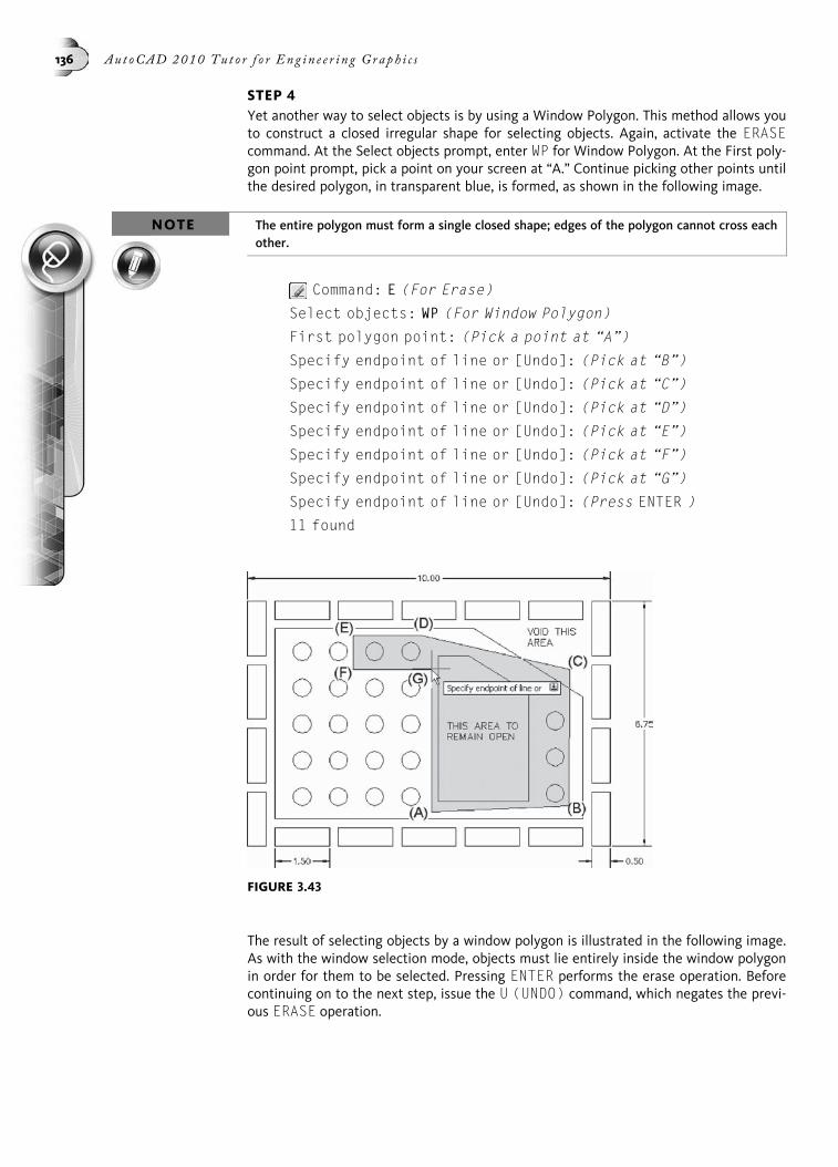
STEP 4Yet another way to select objects is by using a Window Polygon. This method allows youto construct a closed irregular shape for selecting objects. Again, activate the ERASEcommand. At the Select objects prompt, enter WP for Window Polygon. At the First poly-gon point prompt, pick a point on your screen at “A.” Continue picking other points untilthe desired polygon, in transparent blue, is formed, as shown in the following image.
NOTE The entire polygon must form a single closed shape; edges of the polygon cannot cross eachother.
Command: E (For Erase)
Select objects: WP (For Window Polygon)
First polygon point: (Pick a point at “A”)
Specify endpoint of line or [Undo]: (Pick at “B”)
Specify endpoint of line or [Undo]: (Pick at “C”)
Specify endpoint of line or [Undo]: (Pick at “D”)
Specify endpoint of line or [Undo]: (Pick at “E”)
Specify endpoint of line or [Undo]: (Pick at “F”)
Specify endpoint of line or [Undo]: (Pick at “G”)
Specify endpoint of line or [Undo]: (Press ENTER )
11 found
The result of selecting objects by a window polygon is illustrated in the following image.As with the window selection mode, objects must lie entirely inside the window polygonin order for them to be selected. Pressing ENTER performs the erase operation. Beforecontinuing on to the next step, issue the U (UNDO) command, which negates the previ-ous ERASE operation.
FIGURE 3.43
136 Au t oCAD 2010 Tu t o r f o r Eng in e e r i n g Graph i c s

NOTEA Crossing Polygon (CP) mode is also available to select objects that touch the crossingpolygon or are completely surrounded by the polygon. A green polygonal shape displays asit is being created.
STEP 5Objects can also be selected by a fence. This is represented by a crossing line segment.Any object that touches the crossing line is selected. You can construct numerous cross-ing line segments. You cannot use the Fence mode to surround objects as with theWindow or Crossing modes. Activate the ERASE command again. At the Select objectsprompt, enter F, for FENCE. At the First fence point prompt, pick a point on your screenat “A.” Continue constructing crossing line segments until you are satisfied with theobjects being selected (see the following image).
Command: E (For Erase)
Select objects: F (For Fence)
First fence point: (Pick at “A”)
Specify endpoint of line or [Undo]: (Pick at “B”)
Specify endpoint of line or [Undo]: (Pick at “C”)
Specify endpoint of line or [Undo]: (Pick at “D”)
Specify endpoint of line or [Undo]: (Pick at “E”)
Specify endpoint of line or [Undo]: (Press ENTER to create theselection set)
FIGURE 3.44
Chap t e r 3 • Au t oCAD Di s p l a y and Ba s i c S e l e c t i o n Op e r a t i o n s 137

The result of selecting objects by a fence is illustrated in the following image. Notice thatobjects touched by the fence are highlighted. Pressing ENTER performs the erase opera-tion. Before continuing on to the next step, issue the U (UNDO) command, whichnegates the previous ERASE operation.
STEP 6When situations require you to select all objects in the entire database of a drawing, theAll option is very efficient. Activate the ERASE command again. At the Select objectsprompt, enter ALL. Notice that in the following image all objects are selected by thisoption.
Command: E (For Erase)
Select objects: All
FIGURE 3.45
FIGURE 3.46
138 Au t oCAD 2010 Tu t o r f o r Eng i n e e r i n g Graph i c s

Pressing ENTER performs the erase operation. Before continuing on to the next step,issue the U (UNDO) command, which negates the previous ERASE operation.
NOTEThe All option also selects objects even on layers that are turned off. The All option does notselect objects on layers that are frozen.
STEP 7Before performing another ERASE operation on a number of objects, activate the LayerProperties Manager palette, select the “Circles” layer, and click the lock icon, as shown inthe following image. This operation locks the “Circles” layer.
To see what effect this has on selecting objects, activate the ERASE command again. Atthe Select objects prompt, pick a point on the blank part of your screen at “A.” At theSpecify opposite corner prompt, pick a point on your screen at “B.” You have once againselected a number of objects by a green crossing box (see the following image).
Command: E (For Erase)
Select objects: (Pick a point at “A”)
Specify opposite corner: (Pick a point at “B”)
20 were on a locked layer.
FIGURE 3.47
FIGURE 3.48
Chap t e r 3 • Au t oCAD Di s p l a y and Ba s i c S e l e c t i o n Op e r a t i o n s 139

The result of selecting objects by a crossing window is illustrated in the following image.Notice that even though a group of circles was completely surrounded by the crossingwindow, the circles do not highlight because they belong to a locked layer. PressingENTER performs the erase operation. Before continuing on to the next step, issue theU (UNDO) command, which negates the previous ERASE operation.
STEP 8This final step illustrates the use of the ZOOM-All and ZOOM-Extents commands andhow they differ. First activate the ZOOM command and use the All option (a button isavailable for performing this operation).
Command: Z (For ZOOM)
Specify corner of window, enter a scale factor (nX or nXP), or
FIGURE 3.49
FIGURE 3.50
140 Au t oCAD 2010 Tu t o r f o r Eng i n e e r i n g Graph i c s

[All/Center/Dynamic/Extents/Previous/Scale/Window/Object] <real time>: A (For All)
The result is illustrated in the following image. Performing a ZOOM-All zooms the displaybased on the current drawing limits (the limits of this drawing have been established as0,0 for the lower-left corner and 16,10 for the upper-right corner).
Now activate the ZOOM command and use the Extents option (a button is also availablefor performing this operation).
Command: Z (For ZOOM)
Specify corner of window, enter a scale factor (nX or nXP), or
[All/Center/Dynamic/Extents/Previous/Scale/Window/Object] <real time>: E (For Extents)
The result is illustrated in the following image. This zoom is performed to the limits thatcontain all the objects currently in the drawing.
FIGURE 3.51
FIGURE 3.52
Chap t e r 3 • Au t oCAD Di s p l a y and Ba s i c S e l e c t i o n Op e r a t i o n s 141

CHAPTER
4
Modifying YourDrawings
The heart of any CAD system is its ability to modify and manipulate existing geom-etry, and AutoCAD is no exception. Many modify commands relieve the designer ofdrudgery and mundane tasks, and this allows more productive time for conceptualiz-ing the design. This chapter will break all AutoCAD modify commands down intotwo separate groupings. The first grouping is called Level I and will cover the MOVE,COPY, SCALE, ROTATE, OFFSET, FILLET, CHAMFER, TRIM EXTEND, and BREAKcommands. The second grouping is called Level II and will cover the ARRAY, MIRROR,STRETCH, PEDIT, EXPLODE, LENGTHEN, JOIN, UNDO, and REDO commands.A number of small exercises accompany each command in order to reinforce the impor-tance of its use.
METHODS OF SELECTING MODIFY COMMANDSAs with all commands, you can find the main body of modify commands on theRibbon (2D Drafting and Annotation workspace) and Menu Bar both shown in thefollowing image.
You can also enter all modify commands directly from the keyboard either using theirentire name or through command aliasing, as in the following examples:
Enter F for the FILLET command
Enter M for the MOVE command
FIGURE 4.1
142
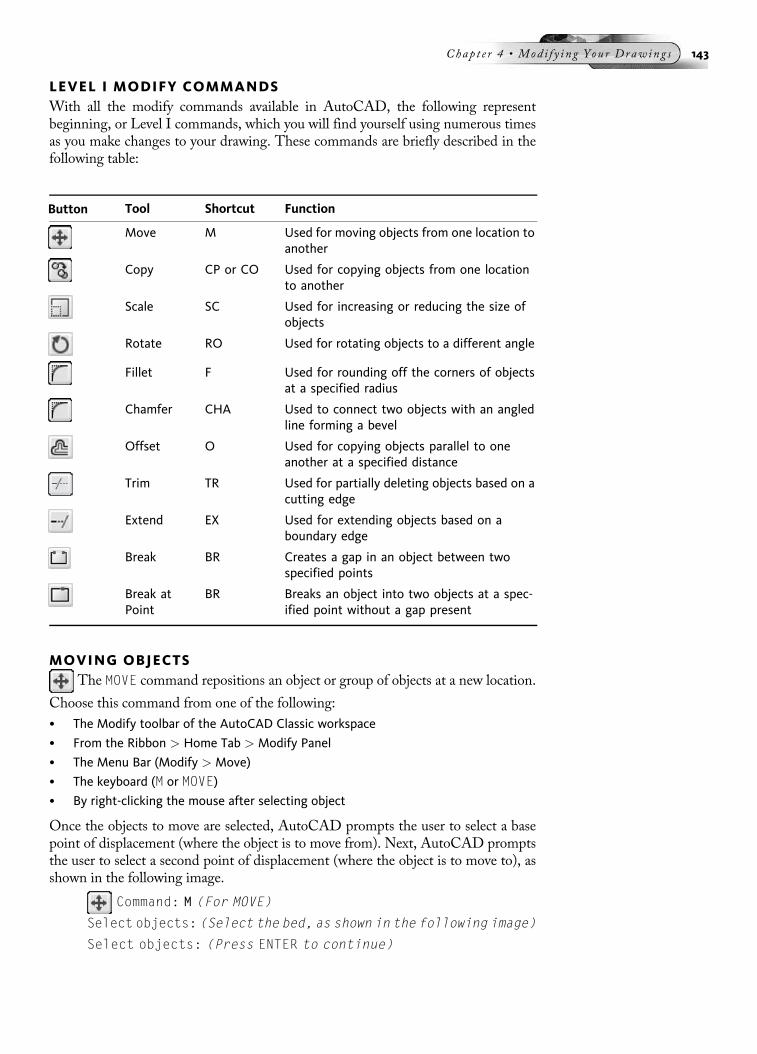
LEVEL I MODIFY COMMANDSWith all the modify commands available in AutoCAD, the following representbeginning, or Level I commands, which you will find yourself using numerous timesas you make changes to your drawing. These commands are briefly described in thefollowing table:
MOVING OBJECTSThe MOVE command repositions an object or group of objects at a new location.
Choose this command from one of the following:
• The Modify toolbar of the AutoCAD Classic workspace
• From the Ribbon > Home Tab > Modify Panel
• The Menu Bar (Modify > Move)
• The keyboard (M or MOVE)• By right-clicking the mouse after selecting object
Once the objects to move are selected, AutoCAD prompts the user to select a basepoint of displacement (where the object is to move from). Next, AutoCAD promptsthe user to select a second point of displacement (where the object is to move to), asshown in the following image.
Command: M (For MOVE)
Select objects: (Select the bed, as shown in the following image)
Select objects: (Press ENTER to continue)
Button Tool Shortcut Function
Move M Used for moving objects from one location toanother
Copy CP or CO Used for copying objects from one locationto another
Scale SC Used for increasing or reducing the size ofobjects
Rotate RO Used for rotating objects to a different angle
Fillet F Used for rounding off the corners of objectsat a specified radius
Chamfer CHA Used to connect two objects with an angledline forming a bevel
Offset O Used for copying objects parallel to oneanother at a specified distance
Trim TR Used for partially deleting objects based on acutting edge
Extend EX Used for extending objects based on aboundary edge
Break BR Creates a gap in an object between twospecified points
Break atPoint
BR Breaks an object into two objects at a spec-ified point without a gap present
Chap t e r 4 • Mod i f y i n g You r Drawing s 143
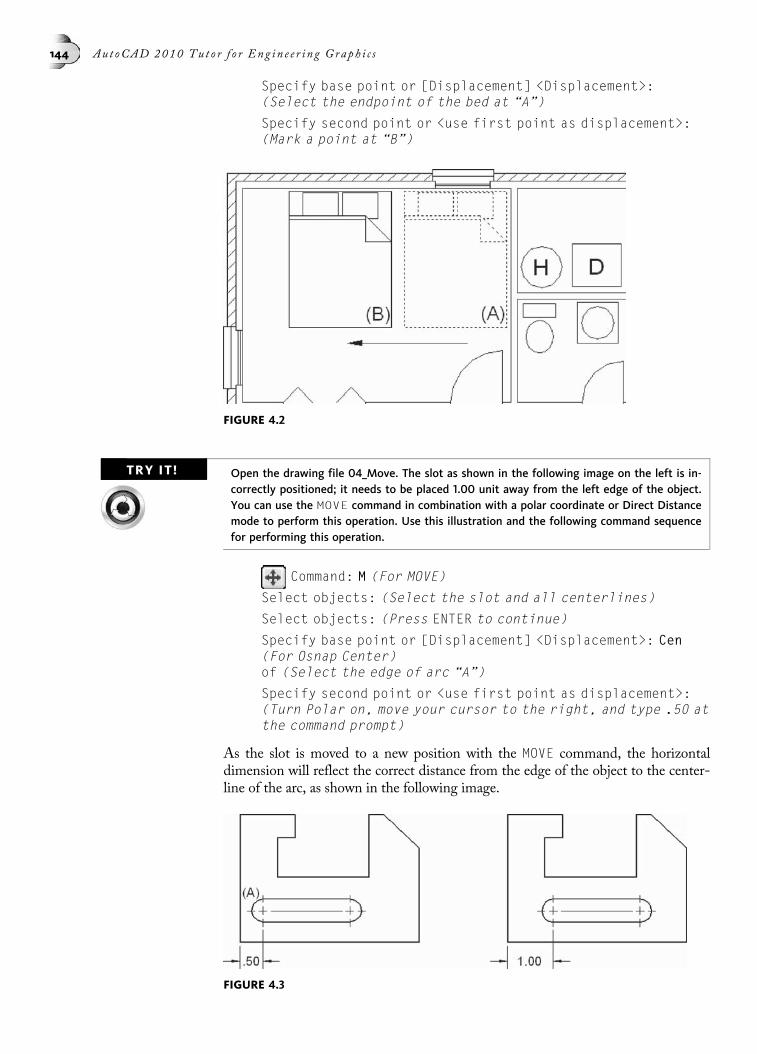
Specify base point or [Displacement] <Displacement>:(Select the endpoint of the bed at “A”)
Specify second point or <use first point as displacement>:(Mark a point at “B”)
TRY IT! Open the drawing file 04_Move. The slot as shown in the following image on the left is in-correctly positioned; it needs to be placed 1.00 unit away from the left edge of the object.You can use the MOVE command in combination with a polar coordinate or Direct Distancemode to perform this operation. Use this illustration and the following command sequencefor performing this operation.
Command: M (For MOVE)
Select objects: (Select the slot and all centerlines)
Select objects: (Press ENTER to continue)
Specify base point or [Displacement] <Displacement>: Cen(For Osnap Center)of (Select the edge of arc “A”)
Specify second point or <use first point as displacement>:(Turn Polar on, move your cursor to the right, and type .50 atthe command prompt)
As the slot is moved to a new position with the MOVE command, the horizontaldimension will reflect the correct distance from the edge of the object to the center-line of the arc, as shown in the following image.
FIGURE 4.2
FIGURE 4.3
144 Au t oCAD 2010 Tu t o r f o r Eng i n e e r i n g Graph i c s

Press and Drag MoveIf accuracy is not important and you simply need to move an object or group of objectsto a new approximate location, you can use a press and drag technique. First, selectthe objects at the command prompt. Then, press and hold down the left mousebutton on one of the highlighted objects (not one of the blue grips), and drag theobjects to the new location.
COPYING OBJECTSThe COPY command is used to duplicate an object or group of objects.
Choose this command from one of the following:
• The Modify toolbar of the AutoCAD Classic workspace
• From the Ribbon > Home Tab > Modify Panel
• The Menu Bar (Modify > Copy)
• The keyboard (CP or COPY)
• By right-clicking the mouse after selecting object
Once the COPY command is executed, the multiple copy mode is on. To duplicatenumerous objects while staying inside the COPY command, simply keep picking newsecond points of displacement and the objects will copy to these new locations, asshown in the following image. Once the copy is completed, press ENTER or ESC toEXIT.
Command: CP (For COPY)
Select objects: (Select the chair to copy)
Select objects: (Press ENTER to continue)
Specify base point or [Displacement/mode} <Displacement>:(Pick a reference point for the copy operation)
Specify second point or <use first point as displacement>:(Pick a location for the first copy)
Specify second point or [Exit/Undo] <Exit>: (Pick a locationfor the second copy)
Specify second point or [Exit/Undo] <Exit>: (Pick a locationfor the third copy)
Specify second point or [Exit/Undo] <Exit>: (Press ENTER orESC to exit this command)
FIGURE 4.4
Chap t e r 4 • Mod i f y i n g You r Drawing s 145

TRY IT! Open the drawing file 04_Copy Multiple. Follow the command sequence in the previous ex-ample to copy the three holes multiple times. Use the intersection of “A” as the base pointfor the copy. Then copy the three holes to the intersections located at “B,” “C,” “D,” “E,” “F,”“G,” “H,” and “J,” as shown in the following image on the left. The results are illustrated inthe following image on the right.
Press and Drag CopyAs with the MOVE command, you can also use the press and drag technique to copyobjects to a new approximate location. First, select the objects at the commandprompt. Then, press and hold down the right mouse button on one of the highlightedobjects (not one of the blue grips), and drag the objects to the new location. Whenyou release the mouse button a menu displays, as shown in the following image.Select the Copy Here item to copy the item or group of items.
SCALING OBJECTS
Use the SCALE command to change the overall size of an object. The size may be
larger or smaller in relation to the original object or group of objects. The SCALEcommand requires a base point and scale factor to complete the command. Choosethis command from one of the following:
• The Modify toolbar of the AutoCAD Classic workspace
• From the Ribbon > Home Tab > Modify Panel
• The Menu Bar (Modify > Scale)
• The keyboard (SC or SCALE)
• By right-clicking the mouse after selecting object
TRY IT! Open the drawing file 04_Scale1. With a base point at “A” and a scale factor of 0.50, theresults of using the SCALE command on a group of objects are shown in the following image.
Command: SC (For SCALE)
Select objects: All
Select objects: (Press ENTER to continue)
FIGURE 4.5
FIGURE 4.6
146 Au t oCAD 2010 Tu t o r f o r Eng i n e e r i n g Graph i c s

Specify base point: (Select the endpoint of the line at “A”)
Specify scale factor or [Copy/Reference] <1.0000>: 0.50
TRY IT!Open the drawing file 04_Scale2. The example in the following image shows the effects ofidentifying a new base point in the center of the object.
Command: SC (For SCALE)
Select objects: All
Select objects: (Press ENTER to continue)
Specify base point: (Pick a point near “A”)
Specify scale factor or [Copy/Reference] <1.0000>: 0.40
NOTEAfter identifying the base point for the scaling operation, you can use the Copy option tocreate a scaled copy of the objects you are scaling.
SCALE—ReferenceSuppose you are given a drawing that has been scaled down in size. However, no oneknows what scale factor was used. You do know what one of the distances should be.In this special case, you can use the Reference option of the SCALE command to identifyendpoints of a line segment that act as a reference length. Entering a new length valuecould increase or decrease the entire object proportionally.
TRY IT!Open the drawing file 04_Scale Reference. Study the following image and the followingprompts for performing this operation.
FIGURE 4.7
FIGURE 4.8
Chap t e r 4 • Mod i f y i n g You r Drawing s 147

Command: SC (For SCALE)
Select objects: (Pick a point at “A”)
Specify opposite corner: (Pick a point at “B”)
Select objects: (Press ENTER to continue)
Specify base point: (Select the edge of the circle to identifyits center)
Specify scale factor or [Copy/Reference] <1.0000>: R (ForReference)
Specify reference length <1.0000>: (Select the endpoint ofthe line at “C”)
Specify second point: (Select the endpoint of the line at “D”)
Specify new length or [Points] <1.0000>: 2.00
Because the length of line “CD” was not known, the endpoints were picked after theReference option was entered. This provided the length of the line to AutoCAD.The final step to perform was to make the line 2.00 units, which increased the sizeof the object while also keeping its proportions.
ROTATING OBJECTS
The ROTATE command changes the orientation of an object or group of objects
by identifying a base point and a rotation angle that completes the new orientation.Choose this command from one of the following:
• The Modify toolbar of the AutoCAD Classic workspace
• From the Ribbon > Home Tab > Modify Panel
• The Menu Bar (Modify > Rotate)
• The keyboard (RO or ROTATE)
• By right-clicking the mouse after selecting object
The following image shows an object, complete with crosshatch pattern, that needs tobe rotated to a 30° angle using point “A” as the base point.
TRY IT! Open the drawing file 04_Rotate. Use the following prompts and image to perform therotation.
FIGURE 4.9
148 Au t oCAD 2010 Tu t o r f o r Eng i n e e r i n g Graph i c s

Command: RO (For ROTATE)
Current positive angle in UCS: ANGDIR=counterclockwiseANGBASE=0
Select objects: All
Select objects: (Press ENTER to continue)
Specify base point: (Select the endpoint of the line at “A”)
Specify rotation angle or [Copy/Reference] <0>: 30
NOTEAfter identifying the base point for the rotating operation, you can use the Copy option tocreate a rotated copy of the objects you are rotating.
ROTATE—ReferenceAt times it is necessary to rotate an object to a desired angular position. However, thismust be accomplished even if the current angle of the object is unknown. To maintainthe accuracy of the rotation operation, use the Reference option of the ROTATE com-mand. The following image shows an object that needs to be rotated to the 30°-angleposition. Unfortunately, we do not know the angle in which the object currently lies.Entering the Reference angle option and identifying two points create a known angleof reference. Entering a new angle of 30° rotates the object to the 30° position fromthe reference angle.
TRY IT!Open the drawing file 04_Rotate Reference. Use the following prompts and image toaccomplish this.
Command: RO (For ROTATE)
Current positive angle in UCS: ANGDIR=counterclockwiseANGBASE=0
Select objects: (Select the object in the following image)
Select objects: (Press ENTER to continue)
Specify base point: (Pick either the edge of the circle or twoarc segments to locate the center)
Specify rotation angle or [Copy/Reference] <0>: R (ForReference)
Specify the reference angle <0>: (Pick either the edge of thecircle or two arc segments to locate the center)
FIGURE 4.10
Chap t e r 4 • Mod i f y i n g You r Drawing s 149

Specify second point: Mid
of (Select the line at “A” to establish the reference angle)
Specify the new angle or [Points] <0>: 30
CREATING FILLETS AND ROUNDSMany objects require highly finished and polished surfaces consisting of ex-
tremely sharp corners. Fillets and rounds represent the opposite case, where cornersare rounded off, either for ornamental purposes or as required by design. Generally afillet consists of a rounded edge formed in the corner of an object, as illustrated in thefollowing image. A round is formed at an outside corner. Fillets and rounds are pri-marily used where objects are cast or made from poured metal. The metal forms moreeasily around a shape that has rounded corners instead of sharp corners, which usuallybreak away. Some drawings have so many fillets and rounds that a note is used toconvey the size of them all, similar to “All Fillets and Rounds .125 Radius.”
AutoCAD provides the FILLET command, which allows you to enter a radius fol-lowed by the selection of two lines. The result is a fillet of the specified radius to thetwo lines selected. The two lines are also automatically trimmed, leaving the radiusdrawn from the endpoint of one line to the endpoint of the other line. Choose thiscommand from one of the following:
• The Modify toolbar of the AutoCAD Classic workspace
• From the Ribbon > Home Tab > Modify Panel
FIGURE 4.11
FIGURE 4.12
150 Au t oCAD 2010 Tu t o r f o r Eng i n e e r i n g Graph i c s

• The Menu Bar (Modify > Fillet)
• The keyboard (F or FILLET)
Filleting by RadiusIllustrated in the following image is an example of setting a radius in the FILLETcommand for creating rounded-off corners.
TRY IT!Open the drawing file 04_Fillet. Follow the illustration in the following image on the leftand command sequence below to place fillets at the three corner locations.
Command: F (For FILLET)
Current settings: Mode = TRIM, Radius = 0.0000
Select first object or [Undo/Polyline/Radius/Trim/Multiple]: R (For Radius)
Specify fillet radius <0.0000>: 0.25
Select first object or [Undo/Polyline/Radius/Trim/Multiple]: (Select at “A”)
Select second object or shift-select to apply corner: (Selectat “B”)
Command:
(Press ENTER to re-execute this command)
Repeat this procedure for creating additional fillets using lines “BC” and “CD.”When finished, your display should appear similar to the illustration in the followingimage on the right.
Fillet as a Cornering ToolA very productive feature of the FILLET command is its use as a cornering tool. Toaccomplish this, set the fillet radius to a value of 0. This produces a corner out of twononintersecting objects.
TRY IT!Open the drawing file 04_Fillet Corner1. Follow the illustration on the left in the followingimage on the left and the command sequence below for performing this task.
Command: F (For FILLET)
Current settings: Mode = TRIM, Radius = 0.5000
FIGURE 4.13
Chap t e r 4 • Mod i f y i n g You r Drawing s 151

Select first object or [Undo/Polyline/Radius/Trim/Multiple]: R (For Radius)
Enter fillet radius <0.5000>: 0
Select first object or [Undo/Polyline/Radius/Trim/Multiple]: (Select line “A”)
Select second object or SHIFT-select to apply corner: (Selectline “B”)
Repeat the procedure for the remaining two corners using lines “BC” and “CD.”When finished, your display should appear similar to the illustration on the right inthe following image on the right.
TIP Even with a fillet radius set to a positive value, such as .50, you can easily apply a corner totwo lines by holding down the SHIFT key when picking the second object. The use of theSHIFT key in this example temporarily sets the fillet radius to zero. Releasing the SHIFTkey sets the fillet radius back to the current value, in this case .50.
Performing Multiple FilletsSince the filleting of lines is performed numerous times, a multiple option is availablethat automatically repeats the FILLET command. This option can be found by pick-ing Multiple from the Cursor menu or by typing M for MULTIPLE at the commandprompt.
TRY IT! Open the drawing file 04_Fillet Multiple. Activate the FILLET command and verify that theradius is set to 0. Use the Multiple option to make the command repeat. Then click onthe corners until your object appears similar to the illustration in the following imageon the right. If you make a mistake by picking two lines incorrectly, type U to undo thisoperation and still remain in the FILLET command.
FIGURE 4.14
FIGURE 4.15
152 Au t oCAD 2010 Tu t o r f o r Eng i n e e r i n g Graph i c s
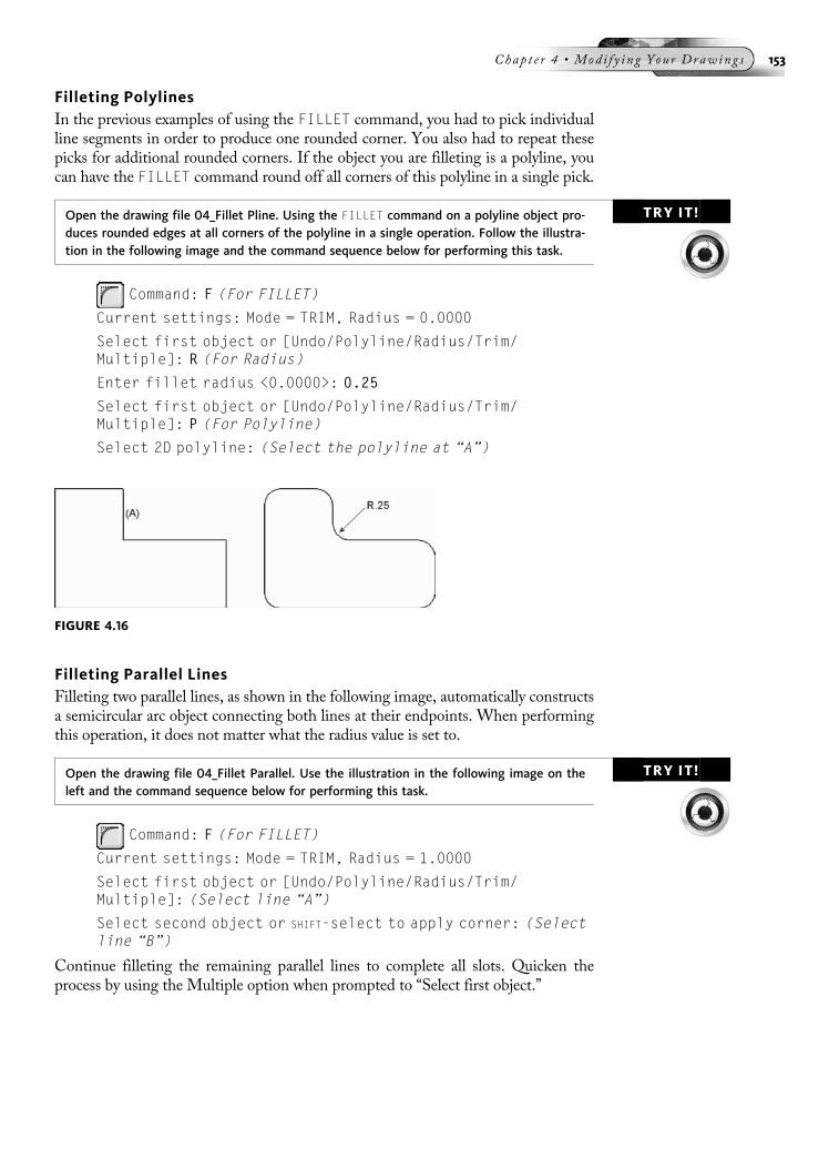
Filleting PolylinesIn the previous examples of using the FILLET command, you had to pick individualline segments in order to produce one rounded corner. You also had to repeat thesepicks for additional rounded corners. If the object you are filleting is a polyline, youcan have the FILLET command round off all corners of this polyline in a single pick.
TRY IT!Open the drawing file 04_Fillet Pline. Using the FILLET command on a polyline object pro-duces rounded edges at all corners of the polyline in a single operation. Follow the illustra-tion in the following image and the command sequence below for performing this task.
Command: F (For FILLET)
Current settings: Mode = TRIM, Radius = 0.0000
Select first object or [Undo/Polyline/Radius/Trim/Multiple]: R (For Radius)
Enter fillet radius <0.0000>: 0.25
Select first object or [Undo/Polyline/Radius/Trim/Multiple]: P (For Polyline)
Select 2D polyline: (Select the polyline at “A”)
Filleting Parallel LinesFilleting two parallel lines, as shown in the following image, automatically constructsa semicircular arc object connecting both lines at their endpoints. When performingthis operation, it does not matter what the radius value is set to.
TRY IT!Open the drawing file 04_Fillet Parallel. Use the illustration in the following image on theleft and the command sequence below for performing this task.
Command: F (For FILLET)
Current settings: Mode = TRIM, Radius = 1.0000
Select first object or [Undo/Polyline/Radius/Trim/Multiple]: (Select line “A”)
Select second object or SHIFT-select to apply corner: (Selectline “B”)
Continue filleting the remaining parallel lines to complete all slots. Quicken theprocess by using the Multiple option when prompted to “Select first object.”
FIGURE 4.16
Chap t e r 4 • Mod i f y i n g You r Drawing s 153
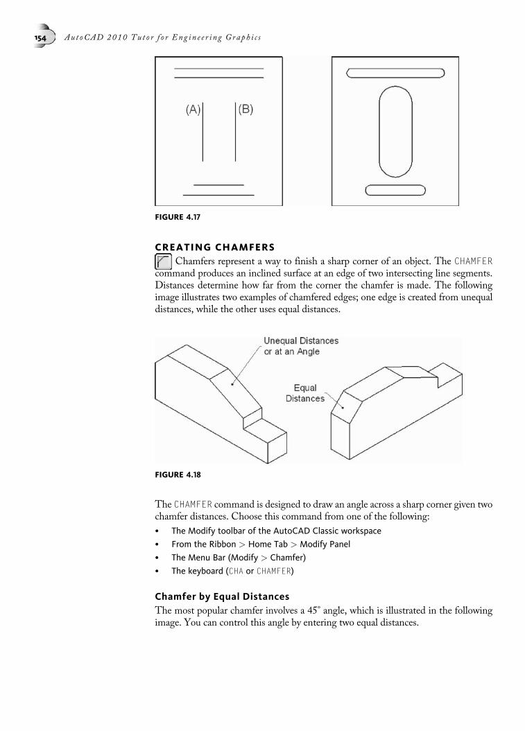
CREATING CHAMFERSChamfers represent a way to finish a sharp corner of an object. The CHAMFER
command produces an inclined surface at an edge of two intersecting line segments.Distances determine how far from the corner the chamfer is made. The followingimage illustrates two examples of chamfered edges; one edge is created from unequaldistances, while the other uses equal distances.
The CHAMFER command is designed to draw an angle across a sharp corner given twochamfer distances. Choose this command from one of the following:
• The Modify toolbar of the AutoCAD Classic workspace
• From the Ribbon > Home Tab > Modify Panel
• The Menu Bar (Modify > Chamfer)
• The keyboard (CHA or CHAMFER)
Chamfer by Equal DistancesThe most popular chamfer involves a 45° angle, which is illustrated in the followingimage. You can control this angle by entering two equal distances.
FIGURE 4.17
FIGURE 4.18
154 Au t oCAD 2010 Tu t o r f o r Eng i n e e r i n g Graph i c s
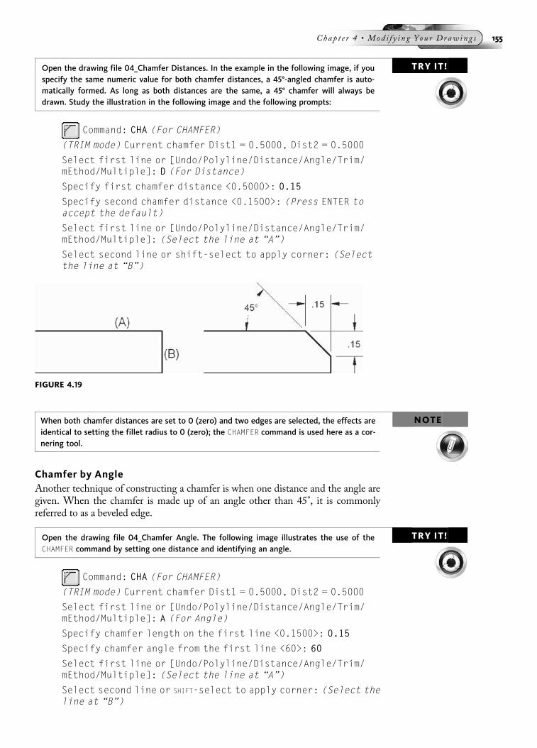
TRY IT!Open the drawing file 04_Chamfer Distances. In the example in the following image, if youspecify the same numeric value for both chamfer distances, a 45°-angled chamfer is auto-matically formed. As long as both distances are the same, a 45° chamfer will always bedrawn. Study the illustration in the following image and the following prompts:
Command: CHA (For CHAMFER)
(TRIM mode) Current chamfer Dist1 = 0.5000, Dist2 = 0.5000
Select first line or [Undo/Polyline/Distance/Angle/Trim/mEthod/Multiple]: D (For Distance)
Specify first chamfer distance <0.5000>: 0.15
Specify second chamfer distance <0.1500>: (Press ENTER toaccept the default)
Select first line or [Undo/Polyline/Distance/Angle/Trim/mEthod/Multiple]: (Select the line at “A”)
Select second line or shift-select to apply corner: (Selectthe line at “B”)
NOTEWhen both chamfer distances are set to 0 (zero) and two edges are selected, the effects areidentical to setting the fillet radius to 0 (zero); the CHAMFER command is used here as a cor-nering tool.
Chamfer by AngleAnother technique of constructing a chamfer is when one distance and the angle aregiven. When the chamfer is made up of an angle other than 45°, it is commonlyreferred to as a beveled edge.
TRY IT!Open the drawing file 04_Chamfer Angle. The following image illustrates the use of theCHAMFER command by setting one distance and identifying an angle.
Command: CHA (For CHAMFER)
(TRIM mode) Current chamfer Dist1 = 0.5000, Dist2 = 0.5000
Select first line or [Undo/Polyline/Distance/Angle/Trim/mEthod/Multiple]: A (For Angle)
Specify chamfer length on the first line <0.1500>: 0.15
Specify chamfer angle from the first line <60>: 60
Select first line or [Undo/Polyline/Distance/Angle/Trim/mEthod/Multiple]: (Select the line at “A”)
Select second line or SHIFT-select to apply corner: (Select theline at “B”)
FIGURE 4.19
Chap t e r 4 • Mod i f y i n g You r Drawing s 155
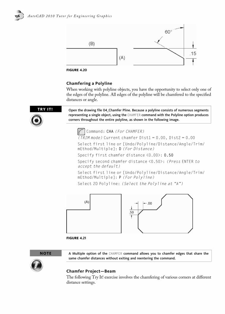
Chamfering a PolylineWhen working with polyline objects, you have the opportunity to select only one ofthe edges of the polyline. All edges of the polyline will be chamfered to the specifieddistances or angle.
TRY IT! Open the drawing file 04_Chamfer Pline. Because a polyline consists of numerous segmentsrepresenting a single object, using the CHAMFER command with the Polyline option producescorners throughout the entire polyline, as shown in the following image.
Command: CHA (For CHAMFER)
(TRIM mode) Current chamfer Dist1 = 0.00, Dist2 = 0.00
Select first line or [Undo/Polyline/Distance/Angle/Trim/mEthod/Multiple]: D (For Distance)
Specify first chamfer distance <0.00>: 0.50
Specify second chamfer distance <0.50>: (Press ENTER toaccept the default)
Select first line or [Undo/Polyline/Distance/Angle/Trim/mEthod/Multiple]: P (For Polyline)
Select 2D Polyline: (Select the Polyline at “A”)
NOTE A Multiple option of the CHAMFER command allows you to chamfer edges that share thesame chamfer distances without exiting and reentering the command.
Chamfer Project—BeamThe following Try It! exercise involves the chamfering of various corners at differentdistance settings.
FIGURE 4.20
FIGURE 4.21
156 Au t oCAD 2010 Tu t o r f o r Eng i n e e r i n g Graph i c s

TRY IT!Open the drawing file 04_Chamfer Beam. Using the illustration provided in the followingimage, follow these directions: Apply equal chamfer distances of 0.25 units to corners“AB,” “BC,” “DE,” and “EF.” Set new equal chamfer distances to 0.50 units and apply thesedistances to corners “GH” and “JK.” Set a new first chamfer distance to 1.00; set a secondchamfer distance to 0.50 units. Apply the first chamfer distance to line “L” and the secondchamfer distance to line “H.” Complete this object by applying the first chamfer distance toline “M” and the second chamfer distance to line “K.”
OFFSETTING OBJECTSThe OFFSET command is commonly used for creating a copy of one object that isparallel to another. Choose this command from one of the following:
• The Modify toolbar of the AutoCAD Classic workspace
• From the Ribbon > Home Tab > Modify Panel
• The Menu Bar (Modify > Offset)
• The keyboard (O or OFFSET)
Offsetting Using a Through PointOne method of offsetting is to identify a point to offset through, called a throughpoint. Once an object is selected to offset, a through point is identified. The selectedobject offsets to the point shown in the following image.
TRY IT!Open the drawing file 04_Offset Through. Refer to the following image and commandsequence to use this method of the OFFSET command.
Command: O (For OFFSET)
Current settings: Erase source=No Layer=SourceOFFSETGAPTYPE=0
Specify offset distance or [Through/Erase/Layer] <Through>:T (For Through)
FIGURE 4.22
Chap t e r 4 • Mod i f y i n g You r Drawing s 157

Select object to offset or [Exit/Undo] <Exit>: (Select theline at “A”)
Specify through point or [Exit/Multiple/Undo] <Exit>: Nod(For Osnap Node)
of (Select the point at “B”)
Select object to offset or [Exit/Undo] <Exit>: (Press ENTERto exit this command)
Offsetting by a DistanceAnother method of offsetting is by a specified offset distance, as shown in the
following image, where the objects need to be duplicated at a set distance from existinggeometry. The COPY command could be used for this operation; a better commandwould be OFFSET. This allows you to specify a distance and a side for the offset tooccur. The result is an object parallel to the original object at a specified distance. Allobjects in the following image need to be offset 0.50 toward the inside of the originalobject.
TRY IT! Open the drawing file 04_Offset Shape. See the command sequence and following image toperform this operation.
Command: O (For OFFSET)
Current settings: Erase source=No Layer=SourceOFFSETGAPTYPE=0
Specify offset distance or [Through/Erase/Layer] <Through>:0.50
Select object to offset or [Exit/Undo] <Exit>: (Select thehorizontal line at “A”)
Specify point on side to offset or [Exit/Multiple/Undo]<Exit>: (Pick a point anywhere on the inside near “B”)
Repeat the preceding procedure for the remaining lines by offsetting them inside theshape, as shown in the following image on the left.
Notice that when all lines were offset, the original lengths of all line segments weremaintained. Because all offsetting occurs inside, the segments overlap at their inter-section points, as shown in the middle of the following image. In one case, at “A” and“B,” the lines did not meet at all. The FILLET command is used to edit all lines toform a sharp corner. You can accomplish this by setting the fillet radius to 0.
Command: F (For FILLET)
Current settings: Mode = TRIM, Radius = 0.5000
FIGURE 4.23
158 Au t oCAD 2010 Tu t o r f o r Eng i n e e r i n g Graph i c s
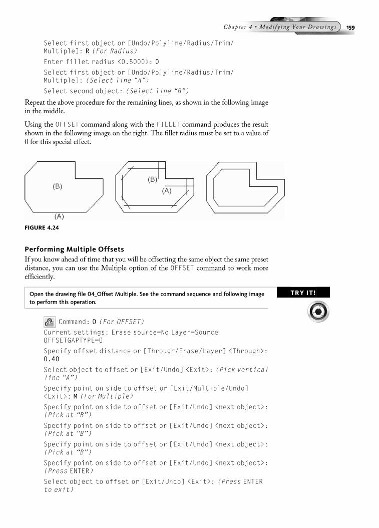
Select first object or [Undo/Polyline/Radius/Trim/Multiple]: R (For Radius)
Enter fillet radius <0.5000>: 0
Select first object or [Undo/Polyline/Radius/Trim/Multiple]: (Select line “A”)
Select second object: (Select line “B”)
Repeat the above procedure for the remaining lines, as shown in the following imagein the middle.
Using the OFFSET command along with the FILLET command produces the resultshown in the following image on the right. The fillet radius must be set to a value of0 for this special effect.
Performing Multiple OffsetsIf you know ahead of time that you will be offsetting the same object the same presetdistance, you can use the Multiple option of the OFFSET command to work moreefficiently.
TRY IT!Open the drawing file 04_Offset Multiple. See the command sequence and following imageto perform this operation.
Command: O (For OFFSET)
Current settings: Erase source=No Layer=SourceOFFSETGAPTYPE=0
Specify offset distance or [Through/Erase/Layer] <Through>:0.40
Select object to offset or [Exit/Undo] <Exit>: (Pick verticalline “A”)
Specify point on side to offset or [Exit/Multiple/Undo]<Exit>: M (For Multiple)
Specify point on side to offset or [Exit/Undo] <next object>:(Pick at “B”)
Specify point on side to offset or [Exit/Undo] <next object>:(Pick at “B”)
Specify point on side to offset or [Exit/Undo] <next object>:(Pick at “B”)
Specify point on side to offset or [Exit/Undo] <next object>:(Press ENTER)
Select object to offset or [Exit/Undo] <Exit>: (Press ENTERto exit)
FIGURE 4.24
Chap t e r 4 • Mod i f y i n g You r Drawing s 159

Other Offset OptionsOther options of the OFFSET command include Erase and Layer. When the Eraseoption is used, the original object you select to offset is erased after the offset copy ismade. When using the Layer option, the object being offset can take on the layerproperties of the source object or can be based on the current layer. When using thesource, the offset copy takes on the same layer as the source object you pick with off-setting. You could also make a new layer current. Using the Current Layer modewhen offsetting changes all offset copies to the current layer. These extra offset modesallow you more flexibility with using this command.
TRIMMING OBJECTSUse the TRIM command to partially delete an object or a group of objects based
on a cutting edge. Choose this command from one of the following:
• The Modify toolbar of the AutoCAD Classic workspace
• From the Ribbon > Home Tab > Modify Panel
• The Menu Bar (Modify > Trim)
• The keyboard (TR or TRIM)
Selecting Individual Cutting EdgesAs illustrated on the left in the following image on the left, the four dashed lines areselected as cutting edges. Next, segments of the circles are selected to be trimmedbetween the cutting edges.
TRY IT! Open the drawing file 04_Trim Basics. Use the following image and the command sequencebelow to perform this task.
Command: TR (For TRIM)
Current settings: Projection=UCS Edge=None
Select cutting edges ...
Select objects or <select all>: (Select the four dashed linesin the following image on the left)
Select objects: (Press ENTER to continue)
Select object to trim or shift-select to extend or [Fence/Crossing/Project/Edge/eRase/Undo]: (Select the circleareas at “A” through “D”)
Select object to trim or SHIFT-select to extend or [Fence/Crossing/Project/Edge/eRase/Undo]: (Press ENTER to exitthis command)
The results of performing trim on this object are illustrated in the following image onthe right.
FIGURE 4.25
160 Au t oCAD 2010 Tu t o r f o r Eng i n e e r i n g Graph i c s
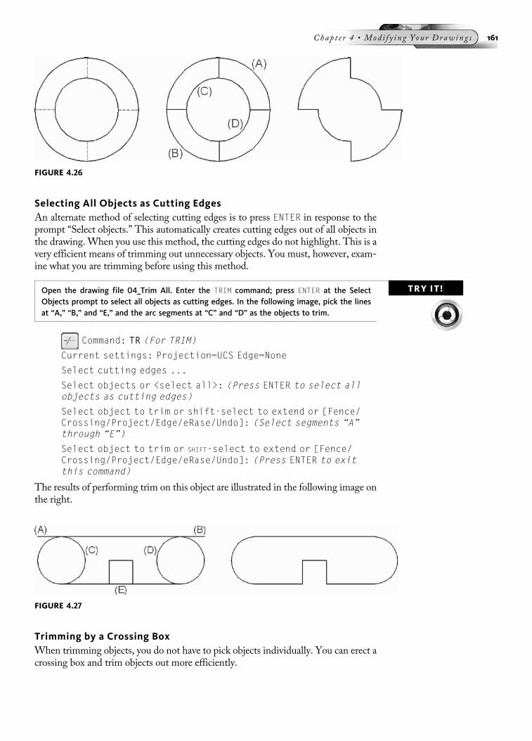
Selecting All Objects as Cutting EdgesAn alternate method of selecting cutting edges is to press ENTER in response to theprompt “Select objects.” This automatically creates cutting edges out of all objects inthe drawing. When you use this method, the cutting edges do not highlight. This is avery efficient means of trimming out unnecessary objects. You must, however, exam-ine what you are trimming before using this method.
TRY IT!Open the drawing file 04_Trim All. Enter the TRIM command; press ENTER at the SelectObjects prompt to select all objects as cutting edges. In the following image, pick the linesat “A,” “B,” and “E,” and the arc segments at “C” and “D” as the objects to trim.
Command: TR (For TRIM)
Current settings: Projection=UCS Edge=None
Select cutting edges ...
Select objects or <select all>: (Press ENTER to select allobjects as cutting edges)
Select object to trim or shift-select to extend or [Fence/Crossing/Project/Edge/eRase/Undo]: (Select segments “A”through “E”)
Select object to trim or SHIFT-select to extend or [Fence/Crossing/Project/Edge/eRase/Undo]: (Press ENTER to exitthis command)
The results of performing trim on this object are illustrated in the following image onthe right.
Trimming by a Crossing BoxWhen trimming objects, you do not have to pick objects individually. You can erect acrossing box and trim objects out more efficiently.
FIGURE 4.26
FIGURE 4.27
Chap t e r 4 • Mod i f y i n g You r Drawing s 161
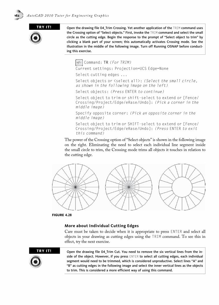
TRY IT! Open the drawing file 04_Trim Crossing. Yet another application of the TRIM command usesthe Crossing option of “Select objects.” First, invoke the TRIM command and select the smallcircle as the cutting edge. Begin the response to the prompt of “Select object to trim” byclicking a blank part of your screen; this automatically activates Crossing mode. See theillustration in the middle of the following image. Turn off Running OSNAP before conduct-ing this exercise.
Command: TR (For TRIM)
Current settings: Projection=UCS Edge=None
Select cutting edges ...
Select objects or <select all>: (Select the small circle,as shown in the following image on the left)
Select objects: (Press ENTER to continue)
Select object to trim or shift-select to extend or [Fence/Crossing/Project/Edge/eRase/Undo]: (Pick a corner in themiddle image)
Specify opposite corner: (Pick an opposite corner in themiddle image)
Select object to trim or SHIFT-select to extend or [Fence/Crossing/Project/Edge/eRase/Undo]: (Press ENTER to exitthis command)
The power of the Crossing option of “Select objects” is shown in the following imageon the right. Eliminating the need to select each individual line segment insidethe small circle to trim, the Crossing mode trims all objects it touches in relation tothe cutting edge.
More about Individual Cutting EdgesCare must be taken to decide when it is appropriate to press ENTER and select allobjects in your drawing as cutting edges using the TRIM command. To see this ineffect, try the next exercise.
TRY IT! Open the drawing file 04_Trim Cut. You need to remove the six vertical lines from the in-side of the object. However, if you press ENTER to select all cutting edges, each individualsegment would need to be trimmed, which is considered unproductive. Select lines “A” and“B” as cutting edges in the following image and select the inner vertical lines as the objectsto trim. This is considered a more efficient way of using this command.
FIGURE 4.28
162 Au t oCAD 2010 Tu t o r f o r Eng i n e e r i n g Graph i c s

Trimming Exercise—Floor PlanUse any technique that you have learned to trim the walls of the floor plan in order forthe object to appear similar to the illustration in the following image.
TRY IT!Open the drawing file 04_Trim Walls. Using the following image as a guide, use the TRIMcommand to trim away the extra overshoots and complete the floor plan illustrated in thefigure.
TIPWhile inside the TRIM command, you can easily toggle to the EXTEND command by holdingdown the SHIFT key at the following command prompt:
Select object to trim or shift-select to extend or [Fence/Crossing/Project/Edge/eRase/Undo]:
EXTENDING OBJECTS
The EXTEND command is used to extend objects to a specified boundary edge.
Choose this command from one of the following:
• The Modify toolbar of the AutoCAD Classic workspace
• From the Ribbon > Home Tab > Modify Panel
FIGURE 4.29
FIGURE 4.30
Chap t e r 4 • Mod i f y i n g You r Drawing s 163

• The Menu Bar (Modify > Extend)
• The keyboard (EX or EXTEND)
Selecting Individual Boundary EdgesIn the following image, select all dashed objects as the boundary edges. After pressingENTER to continue with the command, select the lines at “A,” “B,” “C,” and “D” toextend these objects to the boundary edges. If you select the wrong end of an object,use the Undo feature, which is an option of the command, to undo the change andrepeat the procedure at the correct end of the object.
TRY IT! Open the drawing file 04_Extend Basics. Use the following illustration and commandsequence for accomplishing this task.
Command: EX (For EXTEND)
Current settings: Projection=UCS Edge=None
Select boundary edges ...
Select objects or <select all>: (Select the objects repre-sented by dashes)
Select objects: (Press ENTER to continue)
Select object to extend or shift-select to trim or [Fence/Crossing/Project/Edge/Undo]: (Select the ends of the linesat “A” through “D”)
Select object to extend or shift-select to trim or [Fence/Crossing/Project/Edge//Undo]: (Press ENTER to exit thiscommand)
TIP An alternate method of selecting boundary edges is to press ENTER in response to the“Select objects” prompt. This automatically creates boundary edges out of all objects in thedrawing. When you use this method, however, the boundary edges do not highlight.
Extending Multiple ObjectsThe EXTEND command can be used for extending multiple objects. After identifyingthe boundary edges, you can use a number of crossing boxes to identify numerousitems to extend. This is a very productive method of using this command.
FIGURE 4.31
164 Au t oCAD 2010 Tu t o r f o r Eng i n e e r i n g Graph i c s

TRY IT!Open the drawing file 04_Extend Multiple. To extend multiple objects such as the line seg-ments shown in the following image, select the lines at “A” and “B” as the boundary edgeand use the Crossing mode to create two crossing boxes, represented by the dashed rectan-gles. This extends all line segments to intersect with the boundaries.
Command: EX (For EXTEND)
Current settings: Projection=UCS Edge=None
Select boundary edges ...
Select objects or <select all>: (Select the lines at “A”and “B”)
Select objects: (Press ENTER to continue)
Select object to extend or shift-select to trim or [Fence/Crossing/Project/Edge/Undo]: C (For Crossing or you canclick a blank area as you did earlier with the TRIM command)
Specify first corner: (Pick a point to start the firstrectangle)
Specify opposite corner: (Pick a second point for the firstrectangle)
Select object to extend or shift-select to trim or [Fence/Crossing/Project/Edge/Undo]: (Press ENTER to exit thiscommand)
Repeat this procedure to extend the lines on the other side of the concrete block.
Toggling from Extend to TrimWhile inside the EXTEND command, you can easily toggle to the TRIM command byholding down the SHIFT key at the following command prompt:
Select object to extend or shift-select to trim or [Fence/Crossing/Project/Edge/Undo]: (Pressing SHIFT while pickingobjects activates the TRIM command.)
FIGURE 4.32
Chap t e r 4 • Mod i f y i n g You r Drawing s 165

The next Try It! exercise illustrates this technique.
TRY IT! Open the drawing file 04_Extend and Trim. First, activate the EXTEND command and pressENTER, which selects all edges of the object in the following image as boundary edges. Whenpicking the edges to extend, click on the ends of the lines from “A” through “J,” as shown inthe following image. At this point, do not exit the command. Press and hold down the SHIFTkey; this activates the TRIM command. Now pick all of the ends of the lines until your shapeappears like the illustration in the following image on the right. The use of the SHIFT keywhen trimming or extending provides a quick means of switching between commands.
Extend Exercise—Piping Diagram
TRY IT! Open the drawing file 04_Extend Pipe. Enter the EXTEND command and press ENTER whenthe “Select objects:” prompt appears. This selects all objects as boundary edges. Select theends of all magenta lines representing pipes as the objects to extend. They will extend tointersect with the adjacent pipe fitting. Your finished drawing should appear similar to thefollowing image.
BREAKING OBJECTSThe BREAK command is used to partially delete a segment of an object. Choose thiscommand from one of the following:
• The Modify toolbar of the AutoCAD Classic workspace
• From the Ribbon > Home Tab > Modify Panel
• The Menu Bar (Modify > Break)
• The keyboard (BR or BREAK)
FIGURE 4.34
FIGURE 4.33
166 Au t oCAD 2010 Tu t o r f o r Eng i n e e r i n g Graph i c s

Breaking an ObjectThe following command sequence and image show how the BREAK command isused.
TRY IT!Open the drawing file 04_Break Gap. Turn off Running OSNAP prior to conducting thisexercise. Use the following prompts and illustrations to break the line segment.
Command: BR (For BREAK)
Select objects: (Select the line at “A”)
Specify second break point or [First point]: (Pick the lineat “B”)
Identifying a New First Break PointIn the previous example of using the BREAK command, the location where the objectwas selected became the first break point. You can select the object and then beprompted to pick a new first point. This option resets the command and allows youto select an object to break followed by two different points that identify the break.The following exercise illustrates this technique.
TRY IT!Open the drawing file 04_Break First. Utilize the First option of the BREAK command alongwith OSNAP options to select key objects to break. The following command sequence andimage demonstrate using the First option of the BREAK command:
Command: BR (For BREAK)
Select object: (Select the line)
Specify second break point or [First point]: F (For First)
Specify first break point: Int
of (Pick the intersection of the two lines at “A”)
Specify second break point: End
of (Pick the endpoint of the line at “B”)
FIGURE 4.35
Chap t e r 4 • Mod i f y i n g You r Drawing s 167

Breaking CirclesCircles can also be broken into arc segments with the BREAK command. There is onlyone rule to follow when breaking circles: you must pick the two break points in acounterclockwise direction when identifying the endpoints of the segment to beremoved.
TRY IT! Open the drawing file 04_Break Circle. Study the following command sequence and imagefor breaking circles.
Command: BR (For BREAK)
Select objects: (Select the circle)
Specify second break point or [First point]: F (For First)
Specify first break point: (Pick at “First Point”)
Specify second break point: (Pick at “Second Point”)
Break at PointYou can also break an object at a selected point. The break is so small that you cannotfind it no matter how much you zoom into the break point. As illustrated on the leftin the following image, the line is highlighted to prove that it consists of a continuousobject. Clicking on the Break at Point tool in theModify toolbar activates the followingcommand sequence:
Command: BR (For BREAK)
Select object: (Select the line anywhere)
FIGURE 4.36
FIGURE 4.37
168 Au t oCAD 2010 Tu t o r f o r Eng i n e e r i n g Graph i c s

Specify second break point or [First point]: F (For Firstpoint)
Specify first break point: Mid
of (Pick the midpoint of the line)
Specify second break point: @ (For previous point)
The results are illustrated in the following image on the right. Here the line is againselected. Notice that only half of the line selects because the line is broken at itsmidpoint.
NOTEThe Break At tool automates the command sequence listed above. For this tool tooperate correctly you may have to turn off running OSNAP.
LEVEL II MODIFY COMMANDSThis second grouping of modify commands is designed to perform more powerfulediting operations compared with the Level I modify commands already discussedin this chapter. These commands are briefly described in the following table:
FIGURE 4.38
Button Tool Key-In Function
Array AR Creates multiple copies of objects in a rect-angular or circular pattern
Mirror MI Creates a mirror image of objects based on anaxis of symmetry
Stretch S Used for moving or stretching the shape of anobject
Pedit PE Used for editing polylines
Explode X Breaks a compound object such as a polyline,block, or dimension into individual objects
Lengthen LEN Changes the length of lines and arcs
Join JO Joins collinear objects to form a single un-broken object
Undo U Used for backtracking or reversing the actionof the previously used command
Redo RD Reverses the effects of the previously usedUNDO command operation
Chap t e r 4 • Mod i f y i n g You r Drawing s 169

CREATING ARRAYSIf you need to create copies of objects that form rectangular or circular patterns, theARRAY command is available to help with this task. This is a very powerful commandthat is dialog-box driven. If performing a rectangular array, you will need to supplythe number of rows and columns for the pattern in addition to the spacing bet-ween these rows and columns. When performing a circular or polar array, you needto supply the center point of the array, the number of items to copy, and the angle tofill. The next series of pages documents both methods of performing arrays. Choosethis command from one of the following:
• The Modify toolbar of the AutoCAD Classic workspace
• From the Ribbon > Home Tab > Modify Panel
• The Menu Bar (Modify > Array)
• The keyboard (AR or ARRAY)
CREATING RECTANGULAR ARRAYSCreating Rectangular Patterns with Positive Offset
The Array dialog box allows you to arrange multiple copies of an object or group
of objects in a rectangular or polar (circular) pattern. When creating a rectangular ar-ray, you are prompted to enter the number of rows and columns for the array. A row isa group of objects that are copied vertically in the positive or negative direction. Acolumn is a group of objects that are copied horizontally, also in the positive or nega-tive direction.
TRY IT! Open the drawing file 04_Array Rectangular Positive. Suppose the object illustrated in thefollowing image on the left needs to be copied in a rectangular pattern consisting of threerows and three columns. You also want a row spacing of .50 units and a column spacing of1.25 units. The row offset would be 1.00 and the column offset would be 2.00 (measuredcenter to center or from the same location on each object) in order to space the rectangularshapes away from one another. The result is illustrated in the following image on the right.
Clicking Array in the Modify Menu Bar displays the Array dialog box. When it ap-pears, make the following changes. Be sure the Rectangular Array option is selected atthe top left corner of the dialog box. Enter 3 for the number of rows and 3 for thenumber of columns. For Row Offset, enter a value of 1.00 units. For Column Offset,enter a value of 2.00 units. Click the Select objects button in the upper-right corner of
FIGURE 4.39
170 Au t oCAD 2010 Tu t o r f o r Eng i n e e r i n g Graph i c s

the dialog box. This returns you to the drawing. Pick the rectangle and the two diag-onal line segments. Pressing ENTER when finished returns you to the Array dialogbox. The Array dialog box should now appear similar to the following image.
Observe the pattern in the preview image and notice that it has been updated toreflect three rows and three columns. Notice also that the Preview < button in thelower-right corner of the dialog box is active. Click this button to preview what therectangular pattern will look like in your drawing. Also notice the following promptwill appear in the Command prompt or attached to your cursor location: “Pick orpress ESC to return to dialog or <Right-click to accept array>:” Right-clicking willaccept the array pattern as is. If you notice an error in the array pattern, press theESC key. This returns you to the Array dialog box and allows you to make changesto any value. The results of performing the rectangular array are illustrated in thefollowing image.
TIPWhen performing rectangular arrays, a reference point must be established from the objectto be arrayed and the distance between the objects determined. Not only must the spacingdistance be used, but also the overall size of the object plays a role in determining the off-set distances. With the total height of the original object at 0.50 and a required spacing be-tween rows of 0.50, both object height and spacing result in a distance of 1.00 from onereference point on an object to the next. A center-to-center distance is often specified onengineering drawings, which becomes the row or column offset required.
FIGURE 4.40
FIGURE 4.41
Chap t e r 4 • Mod i f y i n g You r Drawing s 171

Creating Rectangular Patterns with Negative OffsetsIn the previous array example, the rectangular array illustrates a pattern that runs tothe right of and above the original figure. At times these directions change to the leftof and below the original object. The only change occurs in the distances betweenrows and columns, where negative values dictate the direction of the rectangulararray, as shown in the following image on the right.
TRY IT! Open the drawing file 04_Array Rectangular Negative. Follow the illustration in the imageand the following command prompt sequence for performing this operation.
Activate the Array dialog box, as shown in the following image on the right. Whilein Rectangular Array mode, set the number of rows to 3 and the number of columnsto 2. Because the directions of the array will be to the left of and below the originalobject, both row and column distances will be negative values. When finished, pre-view the array; if the results are similar to the illustration in the following image on theleft, right-click to accept the results and create the rectangular array pattern.
TRY IT! Open the drawing 04_Array I-Beam and create a rectangular pattern consisting of 4 rowsand 5 columns. Create a space of 20 0 between both rows and columns. Dimensions may beadded at a later time. The results are displayed in the following image.
FIGURE 4.42
172 Au t oCAD 2010 Tu t o r f o r Eng i n e e r i n g Graph i c s

NOTEThe I-beam and footing were converted to a block object with the insertion point located atthe center of the footing. For this reason, the I-beams can be arrayed from their centers.
CREATING POLAR ARRAYSPolar arrays allow you to create multiple copies of objects in a circular or polar pattern.After selecting the objects to array, you pick a center point for the array in addition tothe number of items to copy and the angle to fill.
TRY IT!Open the drawing file 04_Array Polar and activate the Array dialog box. Be sure to selectthe Polar Array option at the top of the dialog box. Click the Select objects button at thetop of the dialog box and pick the circle at “A” and the center line at “B” as the objects toarray. For the Center point of the array, click the Select objects button and pick the inter-section at “C” (this works only if the Intersection OSNAP mode is checked). Enter 4 for theTotal number of items and be sure the Angle to fill is set to 360 (degrees). Also, verify thatthe box is checked next to Rotate items as copied. The Array dialog box should appear sim-ilar to the illustration shown in the following image on the right. Observe the results inthe image icon and click the Preview < button to see the results. Right-click to accept theresults and complete the array operation.
FIGURE 4.43
Chap t e r 4 • Mod i f y i n g You r Drawing s 173

The results are illustrated in the following image on the left. This image also illu-strates the creation of 4 holes that fill an angle of 180° in the clockwise direction.Notice in the Array dialog box shown on the right that an angle of –180° is given.This negative value drives the array in the clockwise direction. Remember thatpositive angles drive polar arrays in the counterclockwise direction.
TRY IT! Open the drawing file 04_Array Polar Rotate. Illustrated in the following image are threedifferent results for arraying noncircular objects. The image on the right illustrates a polararray formed by rotating the square object as it is being copied. In the middle image, thesquare object is not being rotated as it is being copied. This results in the reference pointat “B” pulling the arrayed pattern slightly to the right and off the main circular center line.To array rectangular or square objects in a polar pattern without rotating the objects, firstconvert the square or rectangle to a block with an insertion point located in the center ofthe square, as shown in the following image on the right (this process will be covered indetail in Chapter 16). Now all squares lie an equal distance from their common center.
FIGURE 4.45
FIGURE 4.44
174 Au t oCAD 2010 Tu t o r f o r Eng i n e e r i n g Graph i c s

MIRRORING OBJECTSThe MIRROR command is used to create a mirrored copy of an object or group of
objects. When performing a mirror operation, you have the option of deleting theoriginal object, which would be the same as flipping the object, or keeping the origi-nal object along with the mirror image, which would be the same as flipping andcopying. Choose this command from one of the following:
• The Modify toolbar of the AutoCAD Classic workspace
• From the Ribbon > Home Tab > Modify Panel
• The Menu Bar (Modify > Mirror)
• The keyboard (MI or MIRROR)
Mirroring and CopyingThe default action of the MIRROR command is to copy and flip the set of objects youare mirroring. After selecting the objects to mirror, you identify the first and secondpoints of a mirror line. You then decide to keep or delete the source objects. The mirroroperation is performed in relation to the mirror line. Usually, most mirroring is per-formed in relation to horizontal or vertical lines. As a result, it is usually recommendedto turn on ORTHOmode to force orthogonal mirror lines (horizontal or vertical).
TRY IT!Open the drawing file 04_Mirror Copy. Refer to the following prompts and image for usingthe MIRROR command:
Command: MI (For MIRROR)
Select objects: (Select a point near “X”)
Specify opposite corner: (Select a point near “Y”)
Select objects: (Press ENTER to continue)
Specify first point of mirror line: (Select the endpoint ofthe centerline at “A”)
Specify second point of mirror line: (Select the endpoint ofthe centerline at “B”)
Erase source objects? [Yes/No] <N>: (Press ENTER for default)
Because the original object needed to be retained by the MIRROR operation, the imageresult is shown in the following image on the right. The MIRROR command workswell when symmetry is required.
FIGURE 4.46
Chap t e r 4 • Mod i f y i n g You r Drawing s 175

Mirroring by FlippingThe illustration in the following image is a different application of the MIRROR com-mand. It is required to have all items that make up the bathroom plan flip but notcopy to the other side. This is a typical process involving “what if” scenarios.
TRY IT! Open the drawing file 04_Mirror Flip. Use the following command prompts to perform thistype of mirror operation. The results are displayed in the following image on the right.
Command: MI (For MIRROR)
Select objects: All (This selects all objects)
Select objects: (Press ENTER to continue)
Specify first point of mirror line: Mid
of (Select the midpoint of the line at “A”)
Specify second point of mirror line: Perto (Select line “B,” which is perpendicular to point “A”)
Erase source objects? [Yes/No] <N>: Y (For Yes)
FIGURE 4.47
FIGURE 4.48
176 Au t oCAD 2010 Tu t o r f o r Eng i n e e r i n g Graph i c s

Mirroring TextIn addition to mirroring other object types, text can also be mirrored, as in the followingimage of the duplex complex. Rather than copying and moving the text intoposition for the matching duplex half, you can include the text in the mirroringoperation.
TRY IT!Open the drawing file 04_Mirror Duplex. Use the MIRROR command and create a mirrorimage of the Duplex floor plan using line “AB” as the points for the mirror line. Do notdelete the source objects. Your finished results should be similar to the following image.
More Information on Mirroring TextThere may be times when you mirror text, but the text is not right-reading. Themirror operation makes the text backwards and unreadable. This usually occurs witholder AutoCAD drawings.
If this happens, a special system variable called MIRRTEXT is available. This variablemust be entered at the Command prompt. If this variable is set to a value of 1 (or on),change the value to 0 (Zero, or off). Using the MIRROR command now will display thetext right-reading.
Command: MIRRTEXT
Enter new value for MIRRTEXT <1>: 0(To prevent text from beingmirrored)
STRETCHING OBJECTSUse the STRETCH command to move a portion of a drawing while still preserving
the connections to parts of the drawing remaining in place. Choose this commandfrom one of the following:
• The Modify toolbar of the AutoCAD Classic workspace
• From the Ribbon > Home Tab > Modify Panel
FIGURE 4.49
Chap t e r 4 • Mod i f y i n g You r Drawing s 177
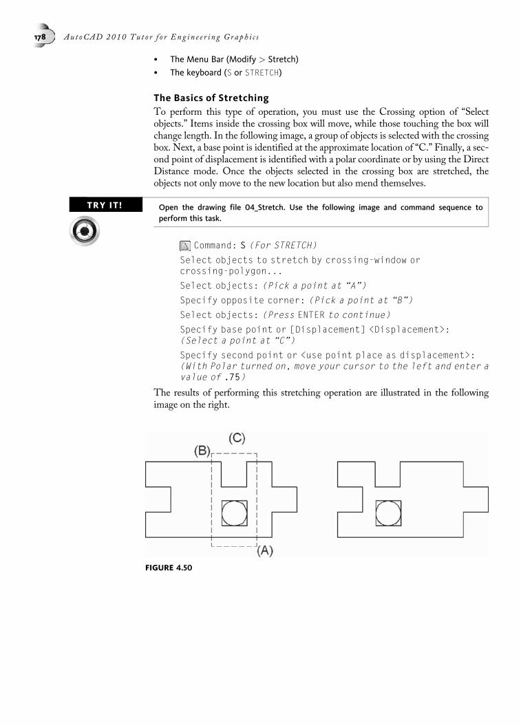
• The Menu Bar (Modify > Stretch)
• The keyboard (S or STRETCH)
The Basics of StretchingTo perform this type of operation, you must use the Crossing option of “Selectobjects.” Items inside the crossing box will move, while those touching the box willchange length. In the following image, a group of objects is selected with the crossingbox. Next, a base point is identified at the approximate location of “C.” Finally, a sec-ond point of displacement is identified with a polar coordinate or by using the DirectDistance mode. Once the objects selected in the crossing box are stretched, theobjects not only move to the new location but also mend themselves.
TRY IT! Open the drawing file 04_Stretch. Use the following image and command sequence toperform this task.
Command: S (For STRETCH)
Select objects to stretch by crossing-window orcrossing-polygon...
Select objects: (Pick a point at “A”)
Specify opposite corner: (Pick a point at “B”)
Select objects: (Press ENTER to continue)
Specify base point or [Displacement] <Displacement>:(Select a point at “C”)
Specify second point or <use point place as displacement>:(With Polar turned on, move your cursor to the left and enter avalue of .75)
The results of performing this stretching operation are illustrated in the followingimage on the right.
FIGURE 4.50
178 Au t oCAD 2010 Tu t o r f o r Eng i n e e r i n g Graph i c s
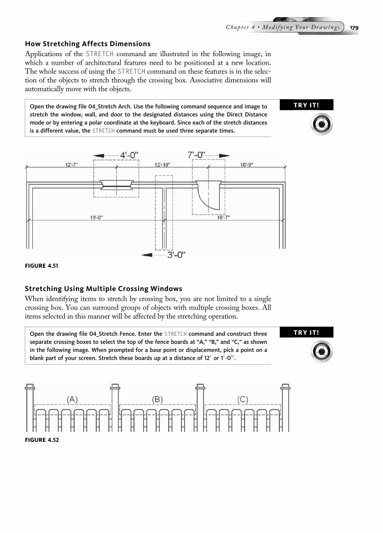
How Stretching Affects DimensionsApplications of the STRETCH command are illustrated in the following image, inwhich a number of architectural features need to be positioned at a new location.The whole success of using the STRETCH command on these features is in the selec-tion of the objects to stretch through the crossing box. Associative dimensions willautomatically move with the objects.
TRY IT!Open the drawing file 04_Stretch Arch. Use the following command sequence and image tostretch the window, wall, and door to the designated distances using the Direct Distancemode or by entering a polar coordinate at the keyboard. Since each of the stretch distancesis a different value, the STRETCH command must be used three separate times.
Stretching Using Multiple Crossing WindowsWhen identifying items to stretch by crossing box, you are not limited to a singlecrossing box. You can surround groups of objects with multiple crossing boxes. Allitems selected in this manner will be affected by the stretching operation.
TRY IT!Open the drawing file 04_Stretch Fence. Enter the STRETCH command and construct threeseparate crossing boxes to select the top of the fence boards at “A,” “B,” and “C,” as shownin the following image. When prompted for a base point or displacement, pick a point on ablank part of your screen. Stretch these boards up at a distance of 12 0 or 1 0-0 00.
FIGURE 4.51
FIGURE 4.52
Chap t e r 4 • Mod i f y i n g You r Drawing s 179

The results of performing the stretch operation on the fence are illustrated in thefollowing image. When you have to stretch various groups of objects in a singleoperation, you can create numerous crossing boxes to better perform this task.
EDITING POLYLINESEditing polylines can lead to interesting results. A few of these options will be
explained in the following pages. Choose this command from one of the following:
• The Modify II toolbar of the AutoCAD Classic workspace
• From the Ribbon > Home Tab > Modify Panel (Expanded)
• The Menu Bar (Modify > Object > Polyline)
• The keyboard (PE or PEDIT)
Changing the Width of a PolylineIllustrated in the following image on the left is a polyline of width 0.00. The PEDITcommand is used to change the width of the polyline to 0.10 units, as shown in thefollowing image on the right.
TRY IT! Open the drawing file 04_Pedit Width. Refer to the following command sequence to use thePEDIT command with the Width option.
Command: PE (For PEDIT)
Select polyline or [Multiple]: (Select the polyline)
Enter an option [Open/Join/Width/Edit vertex/Fit/Spline/Decurve/Ltype gen/Undo]: W (For Width)
Specify new width for all segments: 0.10
Enter an option [Open/Join/Width/Edit vertex/Fit/Spline/Decurve/Ltype gen/Undo]: (Press ENTER to exit this command)
FIGURE 4.53
FIGURE 4.54
180 Au t oCAD 2010 Tu t o r f o r Eng i n e e r i n g Graph i c s

Joining Objects into a Single PolylineIt is very easy to convert regular objects such as lines and arcs into polylines (circlescannot be converted). As you can convert individual objects into polylines, the resultsare a collection of individual polylines. As long as the polyline endpoints match withone another, these polylines can be easily joined into one single polyline object usingthe Join option of the PEDIT command.
TRY IT!Open the drawing file 04_Pedit Join. Refer to the following command sequence and imageto use this command.
Command: PE (For PEDIT)
Select polyline or [Multiple]: (Select the line at “A”)
Object selected is not a polyline
Do you want to turn it into one? <Y> (Press ENTER)
Enter an option [Close/Join/Width/Edit vertex/Fit/Spline/Decurve/Ltype gen/Undo]: J (For Join)
Select objects: (Pick a point at “B”)
Specify opposite corner: (Pick a point at “C”)
Select objects: (Press ENTER to join the lines)
56 segments added to polyline
Enter an option [Open/Join/Width/Edit vertex/Fit/Spline/Decurve/Ltype gen/Undo]: (Press ENTER to exit this command)
Curve GenerationPolylines can be edited to form various curve-fitting shapes. Two curve-fitting modesare available, namely, Splines, and Fit Curves.
Generating SplinesThe Spline option produces a smooth-fitting curve based on control points in theform of the vertices of the polyline.
TRY IT!Open the drawing file 04_Pedit Spline Curve. Refer to the following command sequenceand image to use this command.
FIGURE 4.55
Chap t e r 4 • Mod i f y i n g You r Drawing s 181

Command: PE (For PEDIT)
Select polyline or [Multiple]: (Select the polyline frame)
Enter an option [Close/Join/Width/Edit vertex/Fit/Spline/Decurve/Ltype gen/Undo]: S (For Spline)
Enter an option [Close/Join/Width/Edit vertex/Fit/Spline/Decurve/Ltype gen/Undo]: (Press ENTER to exit this command)
The results of creating a spline curve from a polyline are shown in the following imageon the right.
Generating Fit CurvesThe Fit Curve option passes entirely through the control points, producing a moreexaggerated curve.
TRY IT! Open the drawing file 04_Pedit Fit Curve. Refer to the following command sequence andimage to use this command.
Command: PE (For PEDIT)
Select polyline or [Multiple]: (Select the polyline)
Enter an option [Close/Join/Width/Edit vertex/Fit/Spline/Decurve/Ltype gen/Undo]: F (For Fit)
Enter an option [Close/Join/Width/Edit vertex/Fit/Spline/Decurve/Ltype gen/Undo]: (Press ENTER to exit this command)
The results of creating a fit curve from a polyline are shown in the following image onthe right.
Linetype Generation of PolylinesThe Linetype Generation option of the PEDIT command controls the pattern of thelinetype from polyline vertex to vertex. In the polyline illustrated in the followingimage on the left, the hidden linetype is generated from the first vertex to the secondvertex. An entirely different pattern is formed from the second vertex to the third ver-tex, and so on. The polyline illustrated in the following image on the right has thelinetype generated throughout the entire polyline. In this way, the hidden linetype issmoothed throughout the polyline.
FIGURE 4.56
FIGURE 4.57
182 Au t oCAD 2010 Tu t o r f o r Eng i n e e r i n g Graph i c s

TRY IT!Open the drawing file 04_Pedit Ltype Gen. Refer to the following command sequence andimage to use this command.
Command: PE (For PEDIT)
Select polyline or [Multiple]: (Select the polyline)
Enter an option [Close/Join/Width/Edit vertex/Fit/Spline/Decurve/Ltype gen/Undo]: L (For Ltype gen)
Enter polyline linetype generation option [ON/OFF] <Off>: On
Enter an option [Close/Join/Width/Edit vertex/Fit/Spline/Decurve/Ltype gen/Undo]: (Press ENTER to exit this command)
Offsetting Polyline ObjectsOnce a group of objects has been converted to and joined into a single polyline object,the entire polyline can be copied at a parallel distance using the OFFSET command.
TRY IT!Open the drawing file 04_Pedit Offset. Use the OFFSET command to copy the shape in thefollowing image a distance of 0.50 units to the inside.
Command: O (For OFFSET)
Specify offset distance or [Through/Erase/Layer] <Through>:0.50
Select object to offset or [Exit/Undo] <Exit>: (Select thepolyline at “A”)
Specify point on side to offset or [Exit/Multiple/Undo]<Exit>: (Select a point anywhere near “B”)
Select object to offset or [Exit/Undo] <Exit>: (Press ENTERto exit this command)
Because the object was converted to a polyline, all objects are offset at the same time,as shown in the following image on the right.
FIGURE 4.59
FIGURE 4.58
Chap t e r 4 • Mod i f y i n g You r Drawing s 183
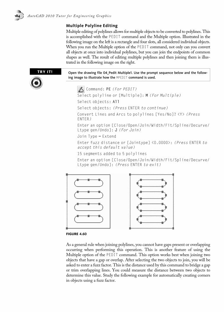
Multiple Polyline EditingMultiple editing of polylines allows for multiple objects to be converted to polylines. Thisis accomplished with the PEDIT command and the Multiple option. Illustrated in thefollowing image on the left is a rectangle and four slots, all considered individual objects.When you run the Multiple option of the PEDIT command, not only can you convertall objects at once into individual polylines, but you can join the endpoints of commonshapes as well. The result of editing multiple polylines and then joining them is illus-trated in the following image on the right.
TRY IT! Open the drawing file 04_Pedit Multiple1. Use the prompt sequence below and the follow-ing image to illustrate how the MPEDIT command is used.
Command: PE (For PEDIT)
Select polyline or [Multiple]: M (For Multiple)
Select objects: All
Select objects: (Press ENTER to continue)
Convert Lines and Arcs to polylines [Yes/No]? <Y> (PressENTER)
Enter an option [Close/Open/Join/Width/Fit/Spline/Decurve/Ltype gen/Undo]: J (For Join)
Join Type = Extend
Enter fuzz distance or [Jointype] <0.0000>: (Press ENTER toaccept this default value)
15 segments added to 5 polylines
Enter an option [Close/Open/Join/Width/Fit/Spline/Decurve/Ltype gen/Undo]: (Press ENTER to exit)
As a general rule when joining polylines, you cannot have gaps present or overlappingoccurring when performing this operation. This is another feature of using theMultiple option of the PEDIT command. This option works best when joining twoobjects that have a gap or overlap. After selecting the two objects to join, you will beasked to enter a fuzz factor. This is the distance used by this command to bridge a gapor trim overlapping lines. You could measure the distance between two objects todetermine this value. Study the following example for automatically creating cornersin objects using a fuzz factor.
FIGURE 4.60
184 Au t oCAD 2010 Tu t o r f o r Eng i n e e r i n g Graph i c s

TRY IT!Open the drawing file 04_Pedit Multiple2. In this example, one of the larger gaps was mea-sured to be .12 units in length. As a result, a fuzz factor slightly larger than this calculatedvalue is used (.13 units). The completed object is illustrated in the following image onthe right. You may have to experiment with various fuzz factors before you arrive at thedesired results.
Command: PE (For PEDIT)
Select polyline or [Multiple]: M (For Multiple)
Select objects: All
Select objects: (Press ENTER to continue)
Convert Lines and Arcs to polylines [Yes/No]? <Y> (PressENTER)
Enter an option [Close/Open/Join/Width/Fit/Spline/Decurve/Ltype gen/Undo]: J (For Join)
Join Type = Extend
Enter fuzz distance or [Jointype] <0.25>: .13
11 segments added to polyline
Enter an option [Close/Open/Join/Width/Fit/Spline/Decurve/Ltype gen/Undo]: (Press ENTER to exit)
EXPLODING OBJECTSUsing the EXPLODE command on a polyline, dimension, or block separates the
single object into its individual parts. Choose this command from one of the following:
• The Modify toolbar of the AutoCAD Classic workspace
• From the Ribbon > Home Tab > Modify Panel
• The Menu Bar (Modify > Explode)
• The keyboard (X or EXPLODE)
Illustrated in the following image on the left is a polyline that is considered oneobject. Using the EXPLODE command and selecting the polyline breaks the polylineinto numerous individual objects, as shown in the following image on the right.
Command: X (For EXPLODE)
Select objects: (Select the polyline)
Select objects: (Press ENTER to perform the explodeoperation)
FIGURE 4.61
Chap t e r 4 • Mod i f y i n g You r Drawing s 185
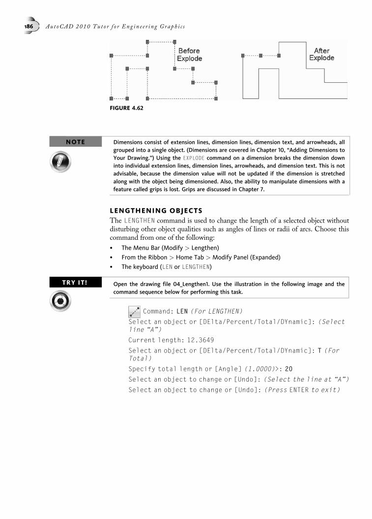
NOTE Dimensions consist of extension lines, dimension lines, dimension text, and arrowheads, allgrouped into a single object. (Dimensions are covered in Chapter 10, “Adding Dimensions toYour Drawing.”) Using the EXPLODE command on a dimension breaks the dimension downinto individual extension lines, dimension lines, arrowheads, and dimension text. This is notadvisable, because the dimension value will not be updated if the dimension is stretchedalong with the object being dimensioned. Also, the ability to manipulate dimensions with afeature called grips is lost. Grips are discussed in Chapter 7.
LENGTHENING OBJECTSThe LENGTHEN command is used to change the length of a selected object withoutdisturbing other object qualities such as angles of lines or radii of arcs. Choose thiscommand from one of the following:
• The Menu Bar (Modify > Lengthen)
• From the Ribbon > Home Tab > Modify Panel (Expanded)
• The keyboard (LEN or LENGTHEN)
TRY IT! Open the drawing file 04_Lengthen1. Use the illustration in the following image and thecommand sequence below for performing this task.
Command: LEN (For LENGTHEN)
Select an object or [DElta/Percent/Total/DYnamic]: (Selectline “A”)
Current length: 12.3649
Select an object or [DElta/Percent/Total/DYnamic]: T (ForTotal)
Specify total length or [Angle] (1.0000)>: 20
Select an object to change or [Undo]: (Select the line at “A”)
Select an object to change or [Undo]: (Press ENTER to exit)
FIGURE 4.62
186 Au t oCAD 2010 Tu t o r f o r Eng i n e e r i n g Graph i c s

TIPAfter supplying the new total length of any object, be sure to select the desired end tolengthen when you are prompted to select an object to change.
JOINING OBJECTSFor special cases in which individual line segments need to be merged together
as a single segment, the JOIN command can be used to accomplish this task. Usuallythis occurs when gaps occur in line segments and all segments lie in the same line ofsight. This condition is sometimes referred to as collinear. Rather than connect thegaps with additional individual line segments, considered very unproductive and poorin practice, use join to connect all segments as one. Choose this command from oneof the following:
• The Modify toolbar of the AutoCAD Classic workspace
• From the Ribbon > Home Tab > Modify Panel (Expanded)
• The Menu Bar (Modify > Join)
• The keyboard (J or JOIN)
TRY IT!Open the drawing file 04_Join. Pick one line segment at “A” as the source. Then select theother line segment at “B” to join to the source. Use the following command prompt andimage to join various segments using the JOIN command.
Command: J (For Join)
Select source object: (Select line “A”)
Select lines to join to source: (Select line “B”)
Select lines to join to source: (Press ENTER to join thesegments)
1 line joined to source
Continue using the JOIN command on the other line segments. A different JOINcommand must be used for each group of line segments that appears broken in thefollowing image.
FIGURE 4.63
Chap t e r 4 • Mod i f y i n g You r Drawing s 187

UNDOING AND REDOING OPERATIONSThe UNDO command can be used to undo the previous task or command action whilethe REDO command reverses the effects of any previous undo. Choose thesecommands from one of the following:
• The Standard toolbar of the AutoCAD Classic workspace
• The Quick Access Toolbar
• The Menu Bar (Edit > Undo) or (Edit > Redo)
• The keyboard (U or UNDO) or (REDO)
• Select anywhere in the drawing and right-click
For example, if you draw an arc followed by a line followed by a circle, issuing theUNDO command will undo the action caused by the most recent command; in thiscase, the circle would be removed from the drawing database. This represents one ofthe easiest ways to remove data or backtrack the drawing process.
Expanding the Undo list found in the Standard toolbar, shown in the followingimage on the left, allows you to undo several actions at once. From this example, noticethat the Rectangle, Line, and Circle actions are highlighted for removal.
You can also reverse the effect of the UNDO command by using REDO immediatelyafter the undo operation.
Clicking the REDO command button from the Standard toolbar negates one undooperation. You can click on this button to cancel the effects of numerous undooperations.
As with undo, you can also redo several actions at once through the Redo list shownin the following image on the right. This list can be accessed from the Quick Accesstoolbar.
FIGURE 4.64
188 Au t oCAD 2010 Tu t o r f o r Eng i n e e r i n g Graph i c s

NOTEWhen grouping actions to be undone, you cannot, in the previous image, for example, high-light Line, skip Trim, and highlight Fillet to be removed. The groupings to undo must bestrung together in this dialog box. Redo only works if you have undone a previous opera-tion. Otherwise, redo remains inactive.
TUTORIAL EXERCISE: ANGLE.DWG
PurposeThis tutorial is designed to allow you to construct a one-view drawing of the angle asshown in the previous image using the ARRAY and LENGTHEN commands.
System SettingsUse the Drawing Units dialog box and change the precision of decimal units from 4 to 2places. Use the current default settings for the limits of this drawing, (0,0) for the lower-left corner, and (12,9) for the upper-right corner. Check to see that the following ObjectSnap modes are already set: Endpoint, Extension, Intersection, and Center.
FIGURE 4.65
FIGURE 4.66
Chap t e r 4 • Mod i f y i n g You r Drawing s 189
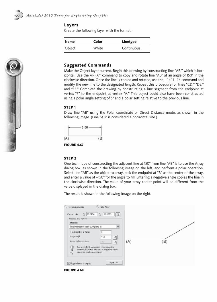
LayersCreate the following layer with the format:
Suggested CommandsMake the Object layer current. Begin this drawing by constructing line “AB,” which is hor-izontal. Use the ARRAY command to copy and rotate line “AB” at an angle of 150° in theclockwise direction. Once the line is copied and rotated, use the LENGTHEN command andmodify the new line to the designated length. Repeat this procedure for lines “CD,” “DE,”and “EF.” Complete the drawing by constructing a line segment from the endpoint atvertex “F” to the endpoint at vertex “A.” This object could also have been constructedusing a polar angle setting of 5° and a polar setting relative to the previous line.
STEP 1Draw line “AB” using the Polar coordinate or Direct Distance mode, as shown in thefollowing image. (Line “AB” is considered a horizontal line.)
STEP 2One technique of constructing the adjacent line at 150° from line “AB” is to use the Arraydialog box, as shown in the following image on the left, and perform a polar operation.Select line “AB” as the object to array, pick the endpoint at “B” as the center of the array,and enter a value of −150° for the angle to fill. Entering a negative angle copies the line inthe clockwise direction. The value of your array center point will be different from thevalue displayed in the dialog box.
The result is shown in the following image on the right.
Name Color Linetype
Object White Continuous
FIGURE 4.67
FIGURE 4.68
190 Au t oCAD 2010 Tu t o r f o r Eng i n e e r i n g Graph i c s

STEP 3The array operation allowed line “AB” to be rotated and copied at the correct angle,namely −150°. However, the new line is the same length as line “AB.” Use the LENGTHENcommand to increase the length of the new line to a distance of 5.00 units. Use the Totaloption, specify the new total length of 5.00, and select the end of the line at “1” as theobject to change, as shown in the following image on the left.
Command: LEN (For LENGTHEN)
Select an object or [DElta/Percent/Total/DYnamic]: T (ForTotal)
Specify total length or [Angle] <1.00)>: 5.00
Select an object to change or [Undo]: (Pick the end of the lineat “1”)
Select an object to change or [Undo]: (Press ENTER to exitthis command)
The result is shown in the following image on the right.
STEP 4Use the Array dialog box, shown in the following image on the left, and perform a polaroperation. Select line “BC” as the object to array, pick the endpoint at “C” as the center ofthe array, and enter a value of −55° for the angle to fill. Entering a negative angle copiesthe line in the clockwise direction.
FIGURE 4.70
FIGURE 4.69
Chap t e r 4 • Mod i f y i n g You r Drawing s 191

STEP 5Then use the LENGTHEN command to reduce the length of the new line from 5.00 unitsto 3.00 units. Use the Total option, specify the new total length of 3.00, and selectthe end of the line at “1” as the object to change, as shown in the following image on theleft.
Command: LEN (For LENGTHEN)
Select an object or [DElta/Percent/Total/DYnamic]: T (ForTotal)
Specify total length or [Angle] <5.00)>: 3.00
Select an object to change or [Undo]: (Pick the end of the lineat “1”)
Select an object to change or [Undo]: (Press ENTER to exitthis command)
The result is shown in the following image on the right.
STEP 6Use the Array dialog box and perform another polar operation. Select line “CD” as theobject to array, as shown in the following image on the left, pick the endpoint at “D” asthe center of the array, and enter a value of 120° for the angle to fill. Entering a positiveangle copies the line in the counterclockwise direction.
Then use the LENGTHEN command to reduce the length of the new line from 3.00 unitsto 1.00 unit, as shown on the right in the following image on the right.
Command: LEN (For LENGTHEN)
Select an object or [DElta/Percent/Total/DYnamic]: T (ForTotal)
Specify total length or [Angle] <3.00)>: 1.00
Select an object to change or [Undo]: (Pick the end of the lineat “1”)
Select an object to change or [Undo]: (Press ENTER to exitthis command)
FIGURE 4.71
192 Au t oCAD 2010 Tu t o r f o r Eng i n e e r i n g Graph i c s
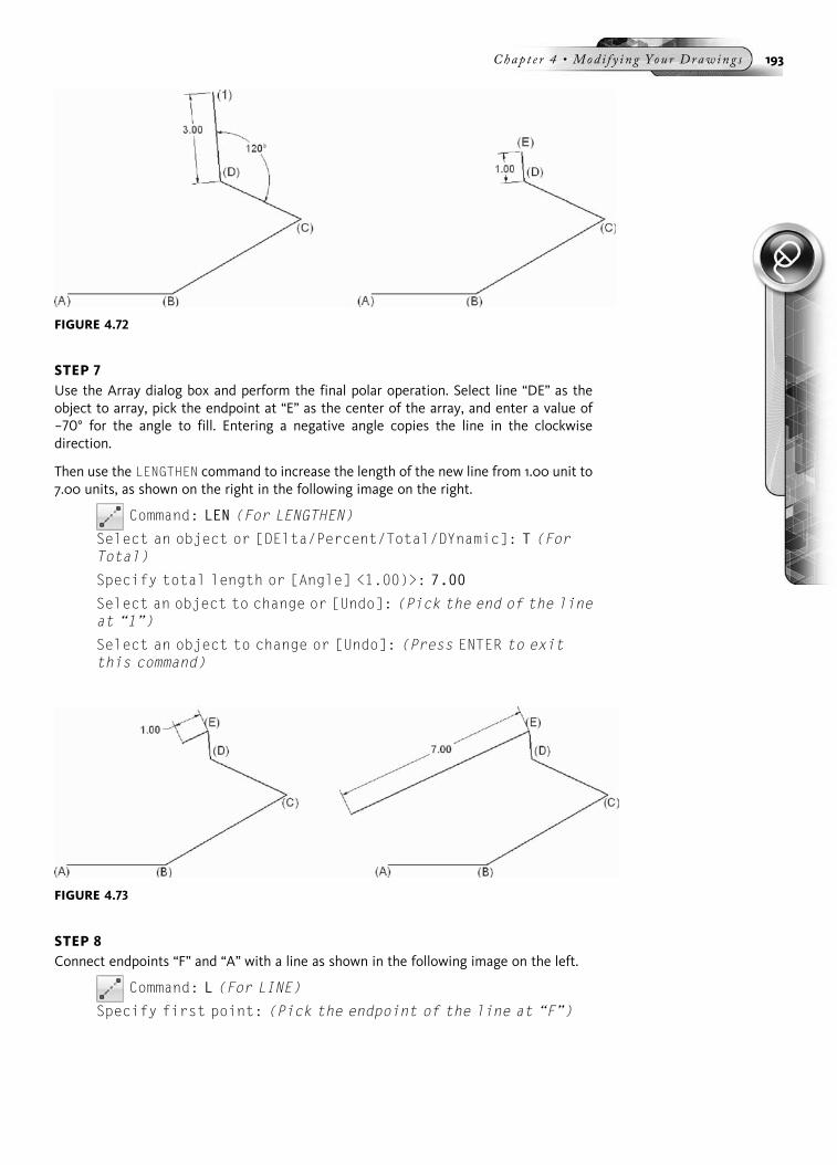
STEP 7Use the Array dialog box and perform the final polar operation. Select line “DE” as theobject to array, pick the endpoint at “E” as the center of the array, and enter a value of−70° for the angle to fill. Entering a negative angle copies the line in the clockwisedirection.
Then use the LENGTHEN command to increase the length of the new line from 1.00 unit to7.00 units, as shown on the right in the following image on the right.
Command: LEN (For LENGTHEN)
Select an object or [DElta/Percent/Total/DYnamic]: T (ForTotal)
Specify total length or [Angle] <1.00)>: 7.00
Select an object to change or [Undo]: (Pick the end of the lineat “1”)
Select an object to change or [Undo]: (Press ENTER to exitthis command)
STEP 8Connect endpoints “F” and “A” with a line as shown in the following image on the left.
Command: L (For LINE)
Specify first point: (Pick the endpoint of the line at “F”)
FIGURE 4.73
FIGURE 4.72
Chap t e r 4 • Mod i f y i n g You r Drawing s 193

Specify next point or [Undo]: (Pick the endpoint of the lineat “A”)
Specify next point or [Undo]: (Press ENTER to exit thiscommand)
The completed drawing is illustrated in the following image on the right. You may adddimensions at a later date.
TUTORIAL EXERCISE: GASKET.DWG
PurposeThis tutorial is designed to allow you to construct a one-view drawing of the gasket usingthe Array dialog box.
System SettingsUse the current default settings for the units and limits of this drawing, (0,0) for the lower-left corner and (12,9) for the upper-right corner. Check to see that the following ObjectSnap modes are already set: Endpoint, Extension, Intersection, Center, and Quadrant.
FIGURE 4.75
FIGURE 4.74
194 Au t oCAD 2010 Tu t o r f o r Eng i n e e r i n g Graph i c s

LayersCreate the following layers with the format:
Suggested CommandsDraw the basic shape of the object using the LINE and CIRCLE commands. Lay out a cen-terline circle; draw one of the gasket tabs at the top of the center circle. Use the Arraydialog box to create four copies in the −180° direction and two copies in the 80° direction.Trim out the excess arc segments to form the gasket. Convert the outer profile of thegasket into one continuous polyline object and offset this object .125 units to the outsideof the gasket.
STEP 1Use existing unit and limit settings. Create an Object and a Center layer. Assign the Centerlinetype to the Center layer.
Make the Object layer current and construct a circle of 2.00 radius with its center atabsolute coordinate 4.00,4.00, as shown in the following image on the left.
Make the Center layer current and construct a circle of 2.25 radius using the previouscenter point, as shown in the following image on the right. Change the linetype scalefrom 1.00 to 0.50 units using the LTSCALE (LTS) command.
STEP 2Make the Object layer current again and construct a circle of radius .75 0 from the quad-rant at the top of the centerline circle, as shown in the following image on the left. Alsoconstruct a circle of .75 0 in diameter from the same quadrant at the top of the centerlinecircle, as shown in the following image on the right.
Name Color Linetype
Object White ContinuousCenter Yellow Center
FIGURE 4.76
Chap t e r 4 • Mod i f y i n g You r Drawing s 195

STEP 3Copy the two top circles just created in a polar (circular) pattern using the Array dialogbox. Use the center of the 2.00-radius circle as the center point of the array. Change thetotal number of items to 4 and the angle to fill to −180°, as shown in the following imageon the left. The negative angle drives the array in the clockwise direction, as shown in thefollowing image on the right.
STEP 4Perform another array operation on the top two circles. Again, use the center of the2.00-radius circle as the center point of the array. Change the total number of items to2 and the angle to fill to 80°, as shown in the following image on the left. The positiveangle drives the array in the counterclockwise direction, as shown in the following imageon the right.
FIGURE 4.78
FIGURE 4.77
196 Au t oCAD 2010 Tu t o r f o r Eng i n e e r i n g Graph i c s

STEP 5Trim out the inside edges of the five circles labeled “A” through “E” using the dashedcircle as the cutting edge, as shown in the following image on the left. The results aredisplayed on the right.
STEP 6Use the TRIM command again. Select the five dashed arc segments as cutting edges andtrim away the portions labeled “A” through “E,” as shown in the following image on theleft. The results are displayed on the right.
FIGURE 4.80
FIGURE 4.79
Chap t e r 4 • Mod i f y i n g You r Drawing s 197

STEP 7Fillet the inside corners of the .75-radius arcs with the 2.00-radius arc using the FILLETcommand and a radius set to .25 0. These corners are marked by a series of points, shownin the following image on the left. The results are displayed on the right.
STEP 8Create the large 1.50-radius hole in the center of the gasket using the CIRCLE command.Change the outer perimeter of the gasket into one continuous polyline object using thePEDIT command. Use the Join option of this command to accomplish this task. Finally,create a copy of the outer profile of the gasket a distance of .125 0 using the OFFSET com-mand. Offset the profile to the outside at “A” as shown in the following image on the left.The completed gasket is displayed on the right.
FIGURE 4.82
FIGURE 4.81
198 Au t oCAD 2010 Tu t o r f o r Eng i n e e r i n g Graph i c s

TUTORIAL EXERCISE: TILE.DWG
PurposeThis tutorial is designed to use the OFFSET and TRIM commands to complete the drawingof the floor tile shown in the previous image.
System SettingsUse the Drawing Units dialog box and change the units of measure from decimal to archi-tectural units. Keep the remaining default settings. Use the LIMITS command andchange the limits of the drawing to (0,0) for the lower-left corner and (10 0,8 0) forthe upper-right corner. Use the ZOOM command and the All option to fit the new drawinglimits to the display screen.
Check to see that the following Object Snap modes are currently set: Endpoint, Extension,Intersection, and Center.
FIGURE 4.84
FIGURE 4.83
Chap t e r 4 • Mod i f y i n g You r Drawing s 199

LayersCreate the following layer with the format:
Suggested CommandsMake the Object layer current. Use the RECTANGLE command to begin the inside squareof the tile. The OFFSET command is used to copy the inner square a distance of 5 0 toform the outer square. The ARRAY command is used to copy selected line segments in arectangular pattern at a specified distance. The TRIM command is then used to form theinside tile patterns.
STEP 1Verify that the current units are set to architectural and that the drawing limits set to 10’,8’ for the upper-right corner. Be sure to perform a ZOOM-All on your screen. Draw theinner 3 0-0 00 square using the RECTANGLE command, as shown in the following image onthe left. Then offset the square 5 00 to the outside using the OFFSET command, as shownin the following image on the right. Because the square was drawn as a polyline, theentire shape offsets to the outside.
STEP 2Notice that when you click on the inner square in the following image on the left, theentire object highlights because it consists of a single polyline object. Use the EXPLODEcommand to break up the inner square into individual line segments. Now when you clickon a line that is part of the inner square, only that line highlights, as shown in the followingimage on the right. This procedure is required in order to perform the next step.
Name Color Linetype
Object White Continuous
FIGURE 4.85
200 Au t oCAD 2010 Tu t o r f o r Eng i n e e r i n g Graph i c s

STEP 3You will now begin laying out the individual tiles with a spacing of 3 00 between each. TheArray dialog box will be used to accomplish this. Activate the Array dialog box, changethe number of rows to 1 and the number of columns to 12. Also change the distancebetween columns to 3 00. Finally, pick the line at “A” as the object to array, as shown inthe following image on the left. Your display should appear similar to the illustration inthe following image on the right.
STEP 4The bottom horizontal line needs to be copied multiple times vertically. Activate theArray dialog box; change the number of rows to 12 and the number of columns to 1.Also change the distance between rows to 3 00. Finally, pick the line at “A” as the objectto array, as shown in the following image on the left. Your display should appear similarto the illustration in the following image on the right.
FIGURE 4.87
FIGURE 4.86
Chap t e r 4 • Mod i f y i n g You r Drawing s 201

STEP 5The TRIM command will now be used to clean up the inner lines and form the 3 0 tiles.When using TRIM, do not press ENTER and select all cutting edges. This would becounterproductive. Instead, select the two vertical dashed lines, as shown in the followingimage on the left. Then trim away the horizontal segments in zones “A” through “D,” asshown in the following image on the right. Remember that if you make a mistake andtrim the wrong line, you can enter U in the command line to restore the previous trimmedline and pick the correct line.
STEP 6Use the TRIM command again to finish cleaning up the object. Select the two horizontaldashed lines as cutting edges, as shown in the following image on the left. Then trimaway the vertical segments in zones “A” through “E,” as shown in the following imageon the right. This completes this exercise on creating the tile.
FIGURE 4.89
FIGURE 4.88
202 Au t oCAD 2010 Tu t o r f o r Eng i n e e r i n g Graph i c s

END OF CHAPTER PROBLEMS FOR CHAPTER 4Please refer to the CD that is supplied with this book and locate the file AutoCAD Tutor2010 Support Docs.pdf. In addition to extra information supplied in this chapter,end-of-chapter problems are also available to provide additional practice.
FIGURE 4.90
Chap t e r 4 • Mod i f y i n g You r Drawing s 203

CHAPTER
5
Performing GeometricConstructions
In Chapter 1, the LINE, CIRCLE, and PLINE commands were introduced. The re-mainder of the drawing commands used for object creation are introduced in thischapter and include the following: ARC, BOUNDARY, CIRCLE-2P, CIRCLE-3P,CIRCLE-TTR, CIRCLE-TTT, DONUT, ELLIPSE, POINT, DIVIDE, MEASURE,POLYGON, RAY, RECTANG, REVCLOUD, SPLINE, WIPEOUT, and XLINE.
Various scenarios of the CIRCLE-TTR command will be used to show the power ofhow AutoCAD can be used to create circles tangent to other object types. When cov-ering the POINT command, the Point Style dialog box will also be discussed as ameans of changing the appearance of points in your drawing. Multilines will also becovered, as will the ability to create a multiline style and then edit any intersections ofa multiline.
METHODS OF SELECTING OTHER DRAW COMMANDSYou can find the main body of draw commands on the Ribbon, Menu Bar, and DrawTool Palette as shown in the following image.
Refer to the following table for a complete listing of all buttons, tools, shortcuts,and functions of most drawing commands.
FIGURE 5.1
204
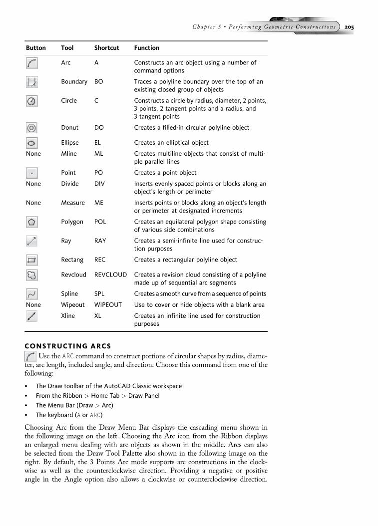
Button Tool Shortcut Function
Arc A Constructs an arc object using a number ofcommand options
Boundary BO Traces a polyline boundary over the top of anexisting closed group of objects
Circle C Constructs a circle by radius, diameter, 2 points,3 points, 2 tangent points and a radius, and3 tangent points
Donut DO Creates a filled-in circular polyline object
Ellipse EL Creates an elliptical object
None Mline ML Creates multiline objects that consist of multi-ple parallel lines
Point PO Creates a point object
None Divide DIV Inserts evenly spaced points or blocks along anobject’s length or perimeter
None Measure ME Inserts points or blocks along an object’s lengthor perimeter at designated increments
Polygon POL Creates an equilateral polygon shape consistingof various side combinations
Ray RAY Creates a semi-infinite line used for construc-tion purposes
Rectang REC Creates a rectangular polyline object
Revcloud REVCLOUD Creates a revision cloud consisting of a polylinemade up of sequential arc segments
Spline SPL Creates a smooth curve from a sequence of points
None Wipeout WIPEOUT Use to cover or hide objects with a blank area
Xline XL Creates an infinite line used for constructionpurposes
CONSTRUCTING ARCSUse the ARC command to construct portions of circular shapes by radius, diame-
ter, arc length, included angle, and direction. Choose this command from one of thefollowing:
• The Draw toolbar of the AutoCAD Classic workspace
• From the Ribbon > Home Tab > Draw Panel
• The Menu Bar (Draw > Arc)
• The keyboard (A or ARC)
Choosing Arc from the Draw Menu Bar displays the cascading menu shown inthe following image on the left. Choosing the Arc icon from the Ribbon displaysan enlarged menu dealing with arc objects as shown in the middle. Arcs can alsobe selected from the Draw Tool Palette also shown in the following image on theright. By default, the 3 Points Arc mode supports arc constructions in the clock-wise as well as the counterclockwise direction. Providing a negative or positiveangle in the Angle option also allows a clockwise or counterclockwise direction.
Chap t e r 5 • Pe r f o rm ing Ge ome t r i c C on s t r u c t i o n s 205

All other arc modes support the ability to construct arcs only in the counterclock-wise direction. Three arc examples will be demonstrated in the next series of pages,namely, how to construct an arc by 3 Points, by a Starting point, Center point, andEnding point, and how to Continue arcs.
3 Points Arc ModeBy default, arcs are drawn with the 3 Points method. The first and third points iden-tify the endpoints of the arc. This arc may be drawn in either the clockwise or coun-terclockwise direction.
TRY IT! Create a new drawing file starting from scratch. Use the following command sequence andimage to construct a 3-point arc.
Command: A (For ARC)
Specify start point of arc or [Center]: (Pick a point at “A”)
Specify second point of arc or [Center/End]: (Pick a pointat “B”)
Specify end point of arc: (Pick a point at “C”)
Start, Center, End ModeUse this ARC mode to construct an arc by defining its start point, center point, andendpoint. This arc will always be constructed in a counterclockwise direction.
FIGURE 5.2
FIGURE 5.3
206 Au t oCAD 2010 Tu t o r f o r Eng i n e e r i n g Graph i c s
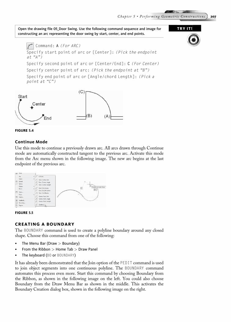
TRY IT!Open the drawing file 05_Door Swing. Use the following command sequence and image forconstructing an arc representing the door swing by start, center, and end points.
Command: A (For ARC)
Specify start point of arc or [Center]: (Pick the endpointat “A”)
Specify second point of arc or [Center/End]: C (For Center)
Specify center point of arc: (Pick the endpoint at “B”)
Specify end point of arc or [Angle/chord Length]: (Pick apoint at “C”)
Continue ModeUse this mode to continue a previously drawn arc. All arcs drawn through Continuemode are automatically constructed tangent to the previous arc. Activate this modefrom the Arc menu shown in the following image. The new arc begins at the lastendpoint of the previous arc.
CREATING A BOUNDARYThe BOUNDARY command is used to create a polyline boundary around any closedshape. Choose this command from one of the following:
• The Menu Bar (Draw > Boundary)
• From the Ribbon > Home Tab > Draw Panel
• The keyboard (BO or BOUNDARY)
It has already been demonstrated that the Join option of the PEDIT command is usedto join object segments into one continuous polyline. The BOUNDARY commandautomates this process even more. Start this command by choosing Boundary fromthe Ribbon, as shown in the following image on the left. You could also chooseBoundary from the Draw Menu Bar as shown in the middle. This activates theBoundary Creation dialog box, shown in the following image on the right.
FIGURE 5.4
FIGURE 5.5
Chap t e r 5 • Pe r f o rm ing Ge ome t r i c C on s t r u c t i o n s 207

Before you use this command, it is good practice to create a separate layer to holdthe polyline object; this layer could be called “Boundary” or “BP,” for BoundaryPolyline. Unlike the Join option of the PEDIT command, which converts individualobjects to polyline objects, the BOUNDARY command traces a polyline in the currentlayer on top of individual objects.
TRY IT! Open the drawing file 05_Boundary Extrusion. Activate the Boundary dialog box and clickthe Pick Points button. Then pick a point inside the object illustrated in the following image.Notice how the entire object is highlighted. To complete the command, press ENTER whenprompted to select another internal point, and the polyline will be traced over the top ofthe existing objects.
Command: BO (For BOUNDARY)
(The Boundary Creation dialog box appears. Click the PickPoints button.)
Pick internal point: (Pick a point at “A” in the followingimage)
Selecting everything...
Selecting everything visible...
Analyzing the selected data...
Analyzing internal islands...
Pick internal point: (Press ENTER to construct the boundary)
boundary created 1 polyline
FIGURE 5.6
FIGURE 5.7
208 Au t oCAD 2010 Tu t o r f o r Eng i n e e r i n g Graph i c s
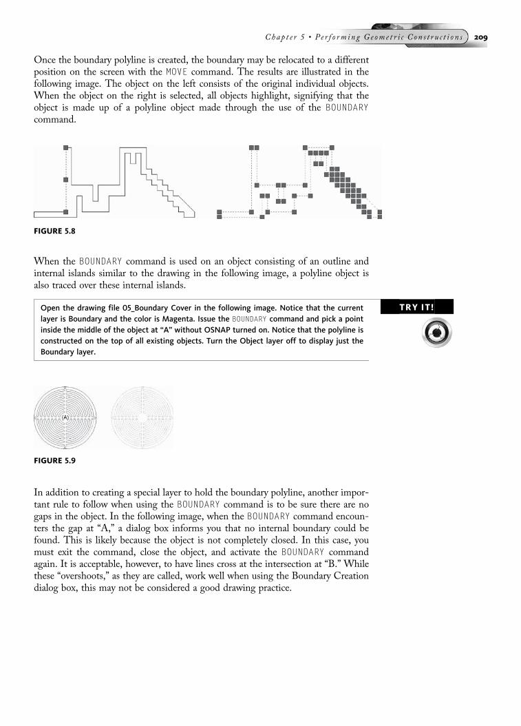
Once the boundary polyline is created, the boundary may be relocated to a differentposition on the screen with the MOVE command. The results are illustrated in thefollowing image. The object on the left consists of the original individual objects.When the object on the right is selected, all objects highlight, signifying that theobject is made up of a polyline object made through the use of the BOUNDARYcommand.
When the BOUNDARY command is used on an object consisting of an outline andinternal islands similar to the drawing in the following image, a polyline object isalso traced over these internal islands.
TRY IT!Open the drawing file 05_Boundary Cover in the following image. Notice that the currentlayer is Boundary and the color is Magenta. Issue the BOUNDARY command and pick a pointinside the middle of the object at “A” without OSNAP turned on. Notice that the polyline isconstructed on the top of all existing objects. Turn the Object layer off to display just theBoundary layer.
In addition to creating a special layer to hold the boundary polyline, another impor-tant rule to follow when using the BOUNDARY command is to be sure there are nogaps in the object. In the following image, when the BOUNDARY command encoun-ters the gap at “A,” a dialog box informs you that no internal boundary could befound. This is likely because the object is not completely closed. In this case, youmust exit the command, close the object, and activate the BOUNDARY commandagain. It is acceptable, however, to have lines cross at the intersection at “B.” Whilethese “overshoots,” as they are called, work well when using the Boundary Creationdialog box, this may not be considered a good drawing practice.
FIGURE 5.8
FIGURE 5.9
Chap t e r 5 • Pe r f o rm ing Ge ome t r i c C on s t r u c t i o n s 209
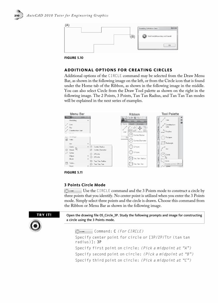
ADDITIONAL OPTIONS FOR CREATING CIRCLESAdditional options of the CIRCLE command may be selected from the Draw MenuBar, as shown in the following image on the left, or from the Circle icon that is foundunder the Home tab of the Ribbon, as shown in the following image in the middle.You can also select Circle from the Draw Tool palette as shown on the right in thefollowing image. The 2 Points, 3 Points, Tan Tan Radius, and Tan Tan Tan modeswill be explained in the next series of examples.
3 Points Circle ModeUse the CIRCLE command and the 3 Points mode to construct a circle by
three points that you identify. No center point is utilized when you enter the 3 Pointsmode. Simply select three points and the circle is drawn. Choose this command fromthe Ribbon or Menu Bar as shown in the following image.
TRY IT! Open the drawing file 05_Circle_3P. Study the following prompts and image for constructinga circle using the 3 Points mode.
Command: C (For CIRCLE)
Specify center point for circle or [3P/2P/Ttr (tan tanradius)]: 3P
Specify first point on circle: (Pick a midpoint at “A”)
Specify second point on circle: (Pick a midpoint at “B”)
Specify third point on circle: (Pick a midpoint at “C”)
FIGURE 5.10
FIGURE 5.11
210 Au t oCAD 2010 Tu t o r f o r Eng i n e e r i n g Graph i c s

2 Points Circle ModeUse the CIRCLE command and the 2 Points mode to construct a circle by
selecting two points. Choose this command from the Ribbon or Menu Bar as shownin the following image. These points form the diameter of the circle. No center pointis utilized when you use the 2 Points mode.
TRY IT!Open the drawing file 05_Circle_2P. Study the following prompts and image for construct-ing a circle using the 2 Points mode.
Command: C (For CIRCLE)
Specify center point for circle or [3P/2P/Ttr (tan tanradius)]: 2P
Specify first end point of circle’s diameter: (Pick amidpoint at “A”)
Specify second end point of circle’s diameter: (Pick amidpoint at “B”)
Constructing an Arc Tangent to Two Lines Using CIRCLE-TTRIllustrated in the following image on the left are two inclined lines. The
purpose of this example is to connect an arc tangent to the two lines at a specifiedradius. The CIRCLE-TTR (Tangent-Tangent-Radius) command will be used herealong with the TRIM command to clean up the excess geometry. To assist with thisoperation, the OSNAP-Tangent mode is automatically activated when you use theTTR option of the CIRCLE command.
First, use the CIRCLE-TTR command to construct an arc tangent to both lines, asshown in the following image in the middle.
FIGURE 5.12
FIGURE 5.13
Chap t e r 5 • Pe r f o rm ing Ge ome t r i c C on s t r u c t i o n s 211
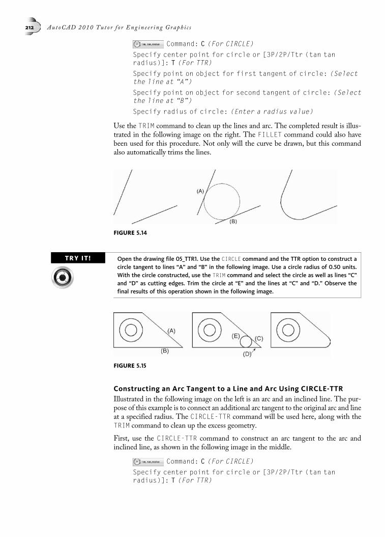
Command: C (For CIRCLE)
Specify center point for circle or [3P/2P/Ttr (tan tanradius)]: T (For TTR)
Specify point on object for first tangent of circle: (Selectthe line at “A”)
Specify point on object for second tangent of circle: (Selectthe line at “B”)
Specify radius of circle: (Enter a radius value)
Use the TRIM command to clean up the lines and arc. The completed result is illus-trated in the following image on the right. The FILLET command could also havebeen used for this procedure. Not only will the curve be drawn, but this commandalso automatically trims the lines.
TRY IT! Open the drawing file 05_TTR1. Use the CIRCLE command and the TTR option to construct acircle tangent to lines “A” and “B” in the following image. Use a circle radius of 0.50 units.With the circle constructed, use the TRIM command and select the circle as well as lines “C”and “D” as cutting edges. Trim the circle at “E” and the lines at “C” and “D.” Observe thefinal results of this operation shown in the following image.
Constructing an Arc Tangent to a Line and Arc Using CIRCLE-TTRIllustrated in the following image on the left is an arc and an inclined line. The pur-pose of this example is to connect an additional arc tangent to the original arc and lineat a specified radius. The CIRCLE-TTR command will be used here, along with theTRIM command to clean up the excess geometry.
First, use the CIRCLE-TTR command to construct an arc tangent to the arc andinclined line, as shown in the following image in the middle.
Command: C (For CIRCLE)
Specify center point for circle or [3P/2P/Ttr (tan tanradius)]: T (For TTR)
FIGURE 5.14
FIGURE 5.15
212 Au t oCAD 2010 Tu t o r f o r Eng i n e e r i n g Graph i c s

Specify point on object for first tangent of circle: (Selectthe arc at “A”)
Specify point on object for second tangent of circle: (Selectthe line at “B”)
Specify radius of circle: (Enter a radius value)
Take note that the radius must be greater than or equal to half the distance betweenthe circle and the line; otherwise, the second circle cannot be constructed. Use theTRIM command to clean up the arc and line. The completed result is illustrated inthe following image on the right.
TRY IT!Open the drawing file 05_TTR2. Using the following image as a guide, use the CIRCLE com-mand and the TTR option to construct a circle tangent to the line at “A” and arc at “B.” Usea circle radius value of 0.50 units. Construct a second circle tangent to the arc at “C” andline at “D” using the default circle radius value of 0.50 units. With the circles constructed,use the TRIM command, press ENTER to select all cutting edges, and trim the lines at “E”and “J” and the arc at “F” and “H,” in addition to the circles at “G” and “K.” Observe thefinal results of this operation shown in the following image.
Constructing an Arc Tangent to Two Arcs Using CIRCLE-TTRMethod #1Illustrated in the following image on the left are two arcs. The purpose of this exam-ple is to connect a third arc tangent to the original two at a specified radius. TheCIRCLE-TTR command will be used here along with the TRIM command to cleanup the excess geometry.
Use the CIRCLE-TTR command to construct an arc tangent to the two original arcs,as shown in the following image in the middle.
Command: C (For CIRCLE)
Specify center point for circle or [3P/2P/Ttr (tan tanradius)]: T (For TTR)
FIGURE 5.16
FIGURE 5.17
Chap t e r 5 • Pe r f o rm ing Ge ome t r i c C on s t r u c t i o n s 213
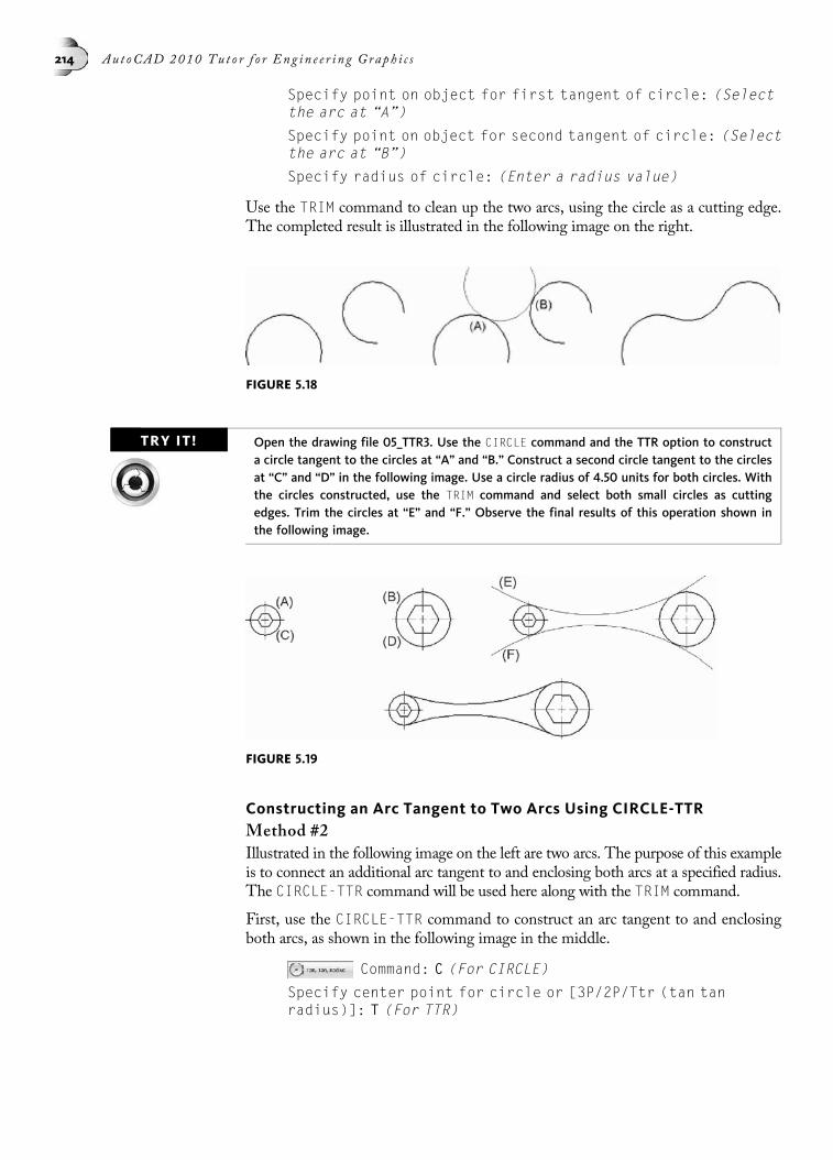
Specify point on object for first tangent of circle: (Selectthe arc at “A”)
Specify point on object for second tangent of circle: (Selectthe arc at “B”)
Specify radius of circle: (Enter a radius value)
Use the TRIM command to clean up the two arcs, using the circle as a cutting edge.The completed result is illustrated in the following image on the right.
TRY IT! Open the drawing file 05_TTR3. Use the CIRCLE command and the TTR option to constructa circle tangent to the circles at “A” and “B.” Construct a second circle tangent to the circlesat “C” and “D” in the following image. Use a circle radius of 4.50 units for both circles. Withthe circles constructed, use the TRIM command and select both small circles as cuttingedges. Trim the circles at “E” and “F.” Observe the final results of this operation shown inthe following image.
Constructing an Arc Tangent to Two Arcs Using CIRCLE-TTRMethod #2Illustrated in the following image on the left are two arcs. The purpose of this exampleis to connect an additional arc tangent to and enclosing both arcs at a specified radius.The CIRCLE-TTR command will be used here along with the TRIM command.
First, use the CIRCLE-TTR command to construct an arc tangent to and enclosingboth arcs, as shown in the following image in the middle.
Command: C (For CIRCLE)
Specify center point for circle or [3P/2P/Ttr (tan tanradius)]: T (For TTR)
FIGURE 5.18
FIGURE 5.19
214 Au t oCAD 2010 Tu t o r f o r Eng i n e e r i n g Graph i c s
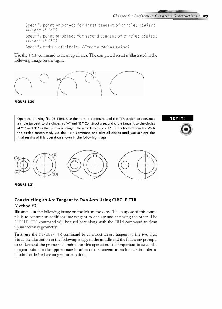
Specify point on object for first tangent of circle: (Selectthe arc at “A”)
Specify point on object for second tangent of circle: (Selectthe arc at “B”)
Specify radius of circle: (Enter a radius value)
Use the TRIM command to clean up all arcs. The completed result is illustrated in thefollowing image on the right.
TRY IT!Open the drawing file 05_TTR4. Use the CIRCLE command and the TTR option to constructa circle tangent to the circles at “A” and “B.” Construct a second circle tangent to the circlesat “C” and “D” in the following image. Use a circle radius of 1.50 units for both circles. Withthe circles constructed, use the TRIM command and trim all circles until you achieve thefinal results of this operation shown in the following image.
Constructing an Arc Tangent to Two Arcs Using CIRCLE-TTRMethod #3Illustrated in the following image on the left are two arcs. The purpose of this exam-ple is to connect an additional arc tangent to one arc and enclosing the other. TheCIRCLE-TTR command will be used here along with the TRIM command to cleanup unnecessary geometry.
First, use the CIRCLE-TTR command to construct an arc tangent to the two arcs.Study the illustration in the following image in the middle and the following promptsto understand the proper pick points for this operation. It is important to select thetangent points in the approximate location of the tangent to each circle in order toobtain the desired arc tangent orientation.
FIGURE 5.20
FIGURE 5.21
Chap t e r 5 • Pe r f o rm ing Ge ome t r i c C on s t r u c t i o n s 215

Command: C (For CIRCLE)
Specify center point for circle or [3P/2P/Ttr (tan tanradius)]: T (For TTR)
Specify point on object for first tangent of circle: (Selectthe arc at “A”)
Specify point on object for second tangent of circle: (Selectthe arc at “B”)
Specify radius of circle: (Enter a radius value)
Use the TRIM command to clean up the arcs. The completed result is illustrated in thefollowing image on the right.
TRY IT! Open the drawing file 05_TTR5. Use the CIRCLE command and the TTR option to construct acircle tangent to the circles at “A” and “B.” Construct a second circle tangent to the circlesat “C” and “D” in the following image. Use a circle radius of 3.00 units for both circles. Withthe circles constructed, use the TRIM command and trim all circles until you achieve thefinal results of this operation shown in the following image.
Constructing a Line Tangent to Two Arcs or CirclesIllustrated in the following image on the left are two circles. The purpose of this ex-ample is to connect the two circles with two tangent lines. This can be accomplishedwith the LINE command and the OSNAP-Tangent option.
Use the LINE command to connect two lines tangent to the circles, as shown in thefollowing image in the middle. The following procedure is used for the first line. Usethe same procedure for the second.
Command: L (For LINE)
Specify first point: Tan
to (Select the circle near “A”)
Specify next point or [Undo]: Tan
to (Select the circle near “B”)
FIGURE 5.22
FIGURE 5.23
216 Au t oCAD 2010 Tu t o r f o r Eng i n e e r i n g Graph i c s
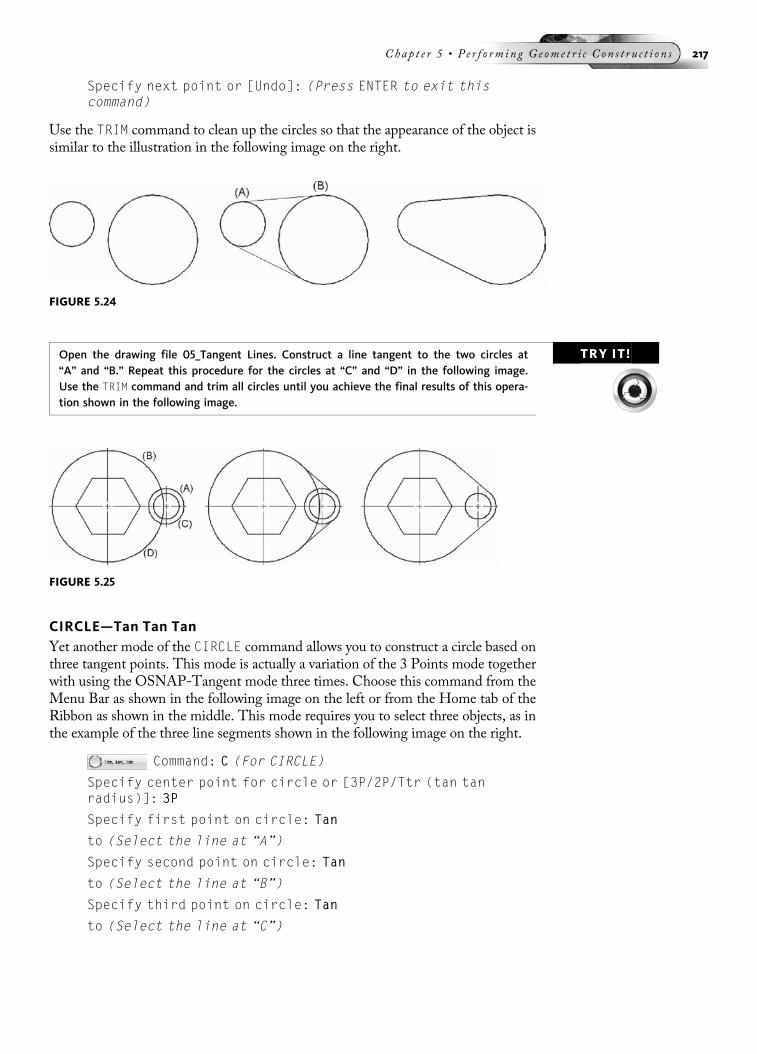
Specify next point or [Undo]: (Press ENTER to exit thiscommand)
Use the TRIM command to clean up the circles so that the appearance of the object issimilar to the illustration in the following image on the right.
TRY IT!Open the drawing file 05_Tangent Lines. Construct a line tangent to the two circles at“A” and “B.” Repeat this procedure for the circles at “C” and “D” in the following image.Use the TRIM command and trim all circles until you achieve the final results of this opera-tion shown in the following image.
CIRCLE—Tan Tan TanYet another mode of the CIRCLE command allows you to construct a circle based onthree tangent points. This mode is actually a variation of the 3 Points mode togetherwith using the OSNAP-Tangent mode three times. Choose this command from theMenu Bar as shown in the following image on the left or from the Home tab of theRibbon as shown in the middle. This mode requires you to select three objects, as inthe example of the three line segments shown in the following image on the right.
Command: C (For CIRCLE)
Specify center point for circle or [3P/2P/Ttr (tan tanradius)]: 3P
Specify first point on circle: Tan
to (Select the line at “A”)
Specify second point on circle: Tan
to (Select the line at “B”)
Specify third point on circle: Tan
to (Select the line at “C”)
FIGURE 5.24
FIGURE 5.25
Chap t e r 5 • Pe r f o rm ing Ge ome t r i c C on s t r u c t i o n s 217

The result is illustrated in the following image on the right, with the circle beingconstructed tangent to the edges of all three line segments.
TRY IT! Open the drawing file 05_TTT. Use the illustration in the previous image and the PREVIOUScommand sequence for constructing a circle tangent to three lines.
QUADRANT VERSUS TANGENT OSNAP OPTIONVarious examples have been given on previous pages concerning drawing lines tan-gent to two circles, two arcs, or any combination of the two. The object in the follow-ing image on the left illustrates the use of the OSNAP-Tangent option when usedwith the LINE command.
Command: L (For LINE)
Specify first point: Tan
to (Select the arc near “A”)
Specify next point or [Undo]: Tan
to (Select the arc near “B”)
Specify next point or [Undo]: (Press ENTER to exit thiscommand)
Note that the angle of the line formed by points “A” and “B” is neither horizontal norvertical. This is a typical example of the capabilities of the OSNAP-Tangent option.
The object illustrated in the following image on the right is a modification of the ex-ample on the left with the inclined tangent lines changed to horizontal and verticaltangent lines. This example is to show that two OSNAP options are available for per-forming tangencies, namely OSNAP-Tangent and OSNAP-Quadrant. However, itis up to you to evaluate under what conditions to use these OSNAP options. In theexample on the right, you can use the OSNAP-Tangent or OSNAP-Quadrant op-tion to draw the lines tangent to the arcs. The Quadrant option could be used onlybecause the lines to be drawn are perfectly horizontal or vertical. Usually it is impos-sible to know this ahead of time, and in this case, the OSNAP-Tangent optionshould be used whenever possible.
FIGURE 5.26
218 Au t oCAD 2010 Tu t o r f o r Eng i n e e r i n g Graph i c s

CREATING FILLED-IN DOTS (DONUTS)Use the DONUT command to construct a filled-in circle. Choose this command fromone of the following:
• The Menu Bar (Draw > Donut)
• From the Ribbon > Home Tab > Draw Panel (Expanded)
• The keyboard (DO or DONUT)
This object belongs to the polyline family. The menus used for constructing a donutare illustrated in the following image on the left. The donut on the right has an insidediameter of 0.50 units and an outside diameter of 1.00 units. When you place donutsin a drawing, the Multiple option is automatically invoked. This means you can placeas many donuts as you like until you exit the command.
TRY IT!Create a new drawing file starting from scratch. Use the following command sequence forconstructing this type of donut.
Command: DO (For DONUT)
Specify inside diameter of donut <0.50>: (Press ENTER toaccept the default)
Specify outside diameter of donut <1.00>: (Press ENTER toaccept the default)
Specify center of donut or <exit>: (Pick a point to place thedonut)
Specify center of donut or <exit>: (Pick a point to placeanother donut or press ENTER to exit this command)
Setting the inside diameter of a donut to a value of zero (0) and an outside diameter toany other value constructs a donut representing a dot, also shown in the followingimage on the right.
FIGURE 5.27
Chap t e r 5 • Pe r f o rm ing Ge ome t r i c C on s t r u c t i o n s 219

TRY IT! Create a new drawing file starting from scratch. Use the following command sequence forconstructing this type of donut.
Command: DO (For DONUT)
Specify inside diameter of donut <0.50>: 0
Specify outside diameter of donut <1.00>: 0.25
Specify center of donut or <exit>: (Pick a point to place thedonut)
Specify center of donut or <exit>: (Pick a point to placeanother donut or press ENTER to exit this command)
TRY IT! Open the drawing file 05_Donut. Activate the DONUT command and set the inside diameterto 0 and the outside diameter to .05. Place four donuts at the intersections of the electricalcircuit, as shown in the following image.
CONSTRUCTING ELLIPTICAL SHAPESUse the ELLIPSE command to construct a true elliptical shape. Choose thiscommand from one of the following:
• The Draw toolbar of the AutoCAD Classic workspace
• From the Ribbon > Home Tab > Draw Panel
FIGURE 5.28
FIGURE 5.29
220 Au t oCAD 2010 Tu t o r f o r Eng i n e e r i n g Graph i c s

• The Menu Bar (Draw > Ellipse)
• The keyboard (EL or ELLIPSE)
Menus used for creating elliptical shapes are shown in the following image on the leftand in the middle. Before studying the three examples for ellipse construction, see theillustration in the following image on the right to view two important parts of anyellipse, namely its major and minor diameters.
You can construct an ellipse by marking two points, which specify one of its axes, asshown in the following image. These first two points also identify the angle with whichthe ellipse will be drawn. Responding to the prompt “Specify distance to other axis or[Rotation]” with another point identifies half of the other axis. The rubber-banded lineis added to assist you in this ellipse construction method.
TRY IT!Create a new drawing file starting from scratch. Use the illustration in the following imageand the command sequence to construct an ellipse by locating three points.
Command: EL (For ELLIPSE)
Specify axis endpoint of ellipse or [Arc/Center]: (Pick apoint at “A”)
Specify other endpoint of axis: (Pick a point at “B”)
Specify distance to other axis or [Rotation]: (Pick a pointat “C”)
You can also construct an ellipse by first identifying its center. You can pick pointsto identify its axes or use polar coordinates to accurately define the major and minordiameters of the ellipse, as shown in the following image on the left.
FIGURE 5.30
FIGURE 5.31
Chap t e r 5 • Pe r f o rm ing Ge ome t r i c C on s t r u c t i o n s 221

TRY IT! Create a new drawing file starting from scratch. Use the illustration in the following imageon the left and the following command sequence for constructing an ellipse based on a cen-ter. Use a polar coordinate or the Direct Distance mode for locating the two axis endpointsof the ellipse. For this example turn Polar or Ortho modes on.
Command: EL (For ELLIPSE)
Specify axis endpoint of ellipse or [Arc/Center]: C (ForCenter)
Specify center of ellipse: (Pick a point at “A”)
Specify endpoint of axis: (Move your cursor to the right andenter a value of 2.50)
Specify distance to other axis or [Rotation]: (Move yourcursor straight up and enter a value of 1.50)
The last method of constructing an ellipse, as shown in the following image on theright, illustrates constructing an ellipse by way of rotation. Identify the first twopoints for the first axis. Reply to the prompt “Specify distance to other axis or [Rota-tion]” with Rotation. The first axis defined is now used as an axis of rotation thatrotates the ellipse into a third dimension.
TRY IT! Create a new drawing file starting from scratch. Use the illustration in the following imageon the right and the following command sequence for constructing an ellipse based on arotation around the major axis.
Command: EL (For ELLIPSE)
Specify axis endpoint of ellipse or [Arc/Center]: C (ForCenter)
Specify center of ellipse: (Pick a point at “A”)
Specify endpoint of axis: (Pick a point at “B”)
Specify distance to other axis or [Rotation]: R (ForRotation)
Specify rotation around major axis: 80
FIGURE 5.32
222 Au t oCAD 2010 Tu t o r f o r Eng i n e e r i n g Graph i c s

CREATING POINT OBJECTUse the POINT command to identify the location of a point on a drawing, which
may be used for reference purposes. Choose this command from one of the following:
• The Draw toolbar of the AutoCAD Classic workspace
• From the Ribbon > Home Tab > Draw Panel (Expanded)
• The Menu Bar (Draw > Point)
• The keyboard (PO or POINT)
Choose Point from the Menu Bar, as shown in the following image on the left.Clicking on the Single Point option allows for the creation of one point. If numer-ous points need to be constructed in the same operation, choose the Multiple Pointoption. This option can also be selected from the Ribbon as shown in the followingimage in the middle. The OSNAP Node or Nearest option is used to snap topoints. By default, a point is displayed as a dot on the screen. Illustrated in the fol-lowing image on the right is an object constructed using points that have been chan-ged in appearance to resemble Xs.
Command: PO (For point)
Current point modes: PDMODE=3 PDSIZE=0.0000
Specify a point: (Pick the new position of a point)
Specify a point: (Either pick another point location or pressESC to exit this command)
Setting a New Point StyleBecause the appearance of the default point as a dot may be confused with theexisting grid dots already on the screen, a mechanism is available to change theappearance of the point. Choosing Point Style from the Format heading inthe Menu Bar, as shown in the following image on the left, displays the Point Styledialog box shown on the right. Use this icon menu to set a different point mode andpoint size.
TIPOnly one point style may be current in a drawing. Once a point is changed to a currentstyle, the next drawing regeneration updates all points to this style.
FIGURE 5.33
Chap t e r 5 • Pe r f o rm ing Ge ome t r i c C on s t r u c t i o n s 223
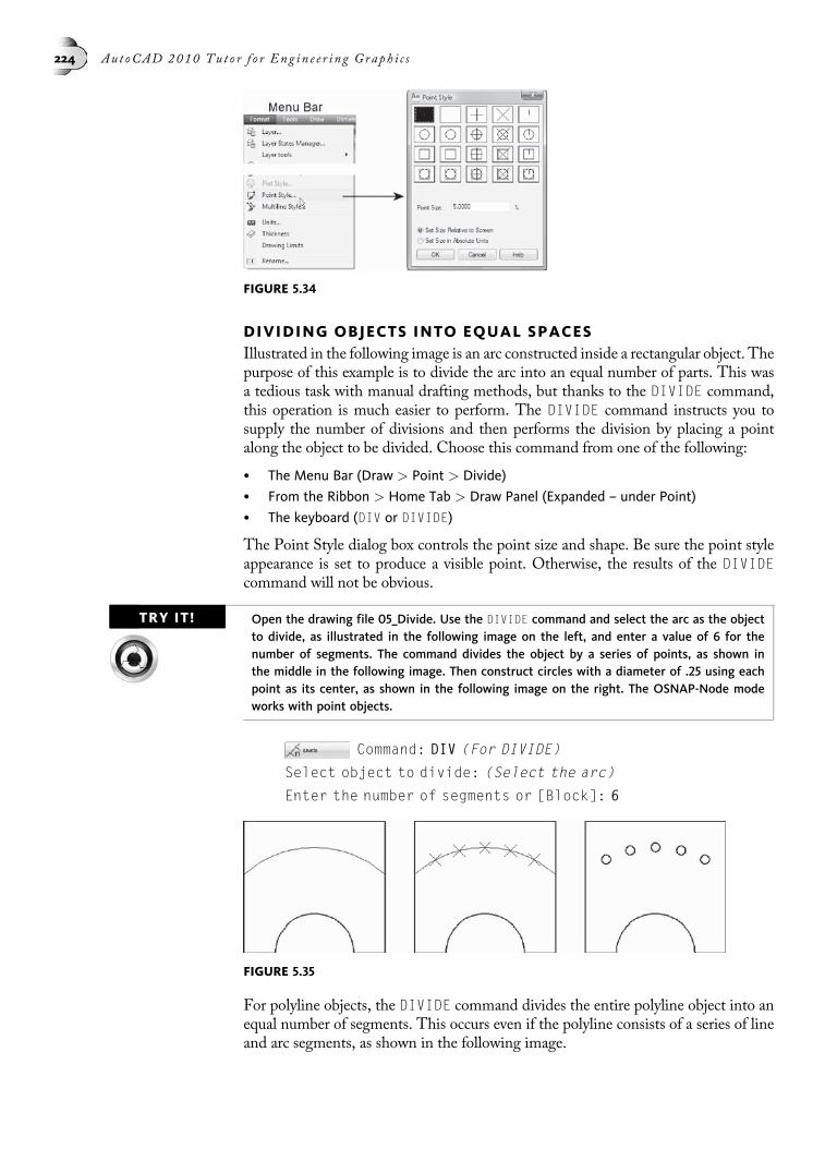
DIVIDING OBJECTS INTO EQUAL SPACESIllustrated in the following image is an arc constructed inside a rectangular object. Thepurpose of this example is to divide the arc into an equal number of parts. This wasa tedious task with manual drafting methods, but thanks to the DIVIDE command,this operation is much easier to perform. The DIVIDE command instructs you tosupply the number of divisions and then performs the division by placing a pointalong the object to be divided. Choose this command from one of the following:
• The Menu Bar (Draw > Point > Divide)
• From the Ribbon > Home Tab > Draw Panel (Expanded – under Point)
• The keyboard (DIV or DIVIDE)
The Point Style dialog box controls the point size and shape. Be sure the point styleappearance is set to produce a visible point. Otherwise, the results of the DIVIDEcommand will not be obvious.
TRY IT! Open the drawing file 05_Divide. Use the DIVIDE command and select the arc as the objectto divide, as illustrated in the following image on the left, and enter a value of 6 for thenumber of segments. The command divides the object by a series of points, as shown inthe middle in the following image. Then construct circles with a diameter of .25 using eachpoint as its center, as shown in the following image on the right. The OSNAP-Node modeworks with point objects.
Command: DIV (For DIVIDE)
Select object to divide: (Select the arc)
Enter the number of segments or [Block]: 6
For polyline objects, the DIVIDE command divides the entire polyline object into anequal number of segments. This occurs even if the polyline consists of a series of lineand arc segments, as shown in the following image.
FIGURE 5.34
FIGURE 5.35
224 Au t oCAD 2010 Tu t o r f o r Eng i n e e r i n g Graph i c s

TRY IT!Open the drawing file 05_Divide Pline. Use the DIVIDE command and select the outer poly-line as the object to divide, as shown in the following image on the left, and enter a value of9 for the number of segments. The command divides the entire polyline by a series ofpoints, as shown on the right.
Command: DIV (For DIVIDE)
Select object to divide: (Select the outer polyline shape)
Enter the number of segments or [Block]: 9
MEASURING OBJECTSThe MEASURE command takes an object such as a line or an arc and measures alongit depending on the length of the segment. The MEASURE command, similar to theDIVIDE command, places a point on the object at a specified distance given in theMEASURE command. Choose this command from one of the following:
• The Menu Bar (Draw > Point > Measure)
• From the Ribbon > Home Tab > Draw Panel (Expanded – under Point)
• The keyboard (ME or MEASURE)
It is important to note that as a point is placed along an object during the measur-ing process, the object is not automatically broken at the location of the point.Rather, the point is commonly used to construct from, along with the OSNAP-Node option. Also, the measuring starts at the endpoint closest to the point youused to select the object.
Choose Point from the Draw Menu Bar, and then choose the MEASURE command.
TRY IT!Open the drawing file 05_Measure. Use the illustration in the following image and thecommand sequence below to perform this operation.
Command: ME (For MEASURE)
Select object to measure: (Select the left end of the diagonalline, as shown in the following image on the left)
Specify length of segment or [Block]: 1.25
The results, shown in the following image, illustrate various points placed at 1.25 in-crements. As with the DIVIDE command, the appearance of the points placed alongthe line is controlled through the Point Style dialog box.
FIGURE 5.36
Chap t e r 5 • Pe r f o rm ing Ge ome t r i c C on s t r u c t i o n s 225

CREATING POLYGONSThe POLYGON command is used to construct a regular polygon. Choose this
command from one of the following:
• The Draw toolbar of the AutoCAD Classic workspace
• From the Ribbon > Home Tab > Draw Panel
• The Menu Bar (Draw > Polygon)
• The keyboard (POL or POLYGON)
You create polygons by identifying the number of sides for the polygon, locating apoint on the screen as the center of the polygon, specifying whether the polygon isinscribed or circumscribed, and specifying a circle radius for the size of the polygon.Polygons consist of a closed polyline object with width set to zero.
TRY IT! Create a new drawing file starting from scratch. Use the following command sequence toconstruct the inscribed polygon, as shown in the following image on the left.
Command: POL (For POLYGON)
Enter number of sides <4>: 6
Specify center of polygon or [Edge]: (Mark a point at “A,” asshown in the following image on the left)
Enter an option [Inscribed in circle/Circumscribed aboutcircle] <I>: I (For Inscribed)
Specify radius of circle: 1.00
TRY IT! Create a new drawing file starting from scratch. Use the following command sequence toconstruct the circumscribed polygon, as shown in the following image on the right.
Command: POL (For POLYGON)
Enter number of sides <4>: 6
Specify center of polygon or [Edge]: (Pick a point at “A,” asshown in the following image on the right)
Enter an option [Inscribed in circle/Circumscribed aboutcircle] <I>: C (For Circumscribed)
Specify radius of circle: 1.00
FIGURE 5.37
FIGURE 5.38
226 Au t oCAD 2010 Tu t o r f o r Eng i n e e r i n g Graph i c s
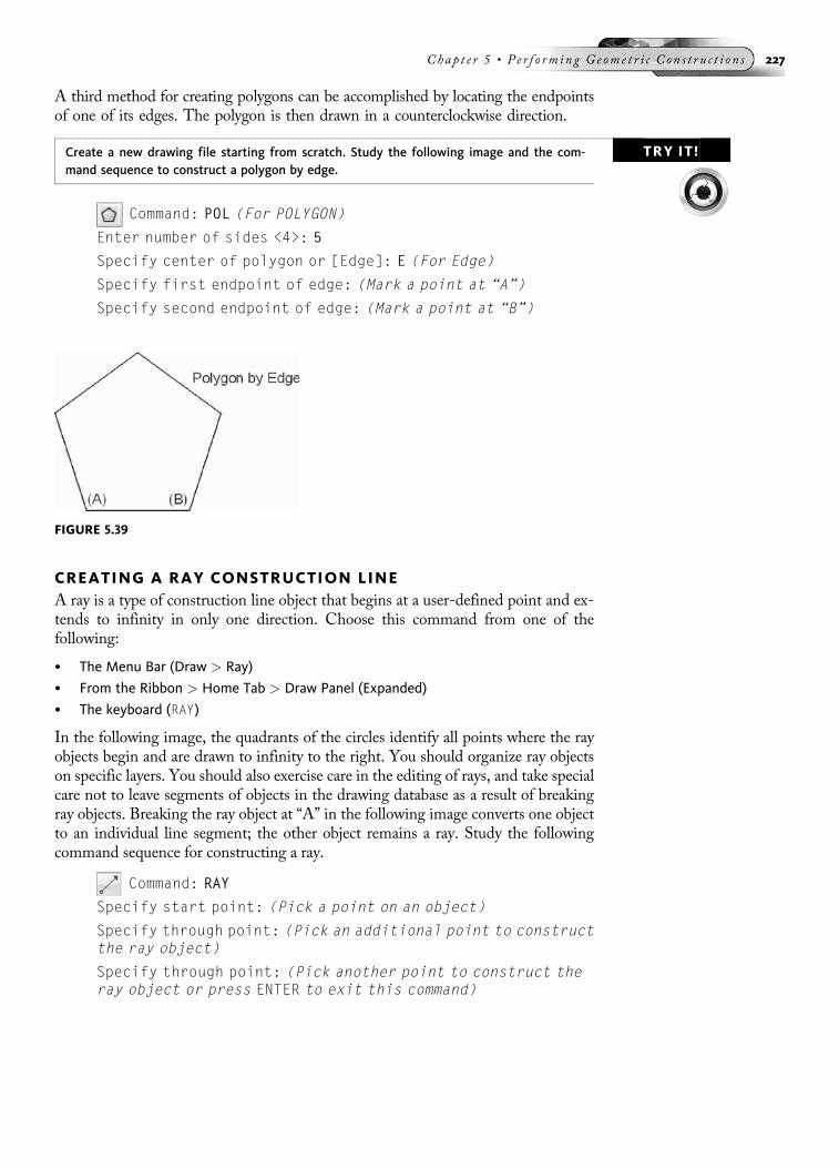
A third method for creating polygons can be accomplished by locating the endpointsof one of its edges. The polygon is then drawn in a counterclockwise direction.
TRY IT!Create a new drawing file starting from scratch. Study the following image and the com-mand sequence to construct a polygon by edge.
Command: POL (For POLYGON)
Enter number of sides <4>: 5
Specify center of polygon or [Edge]: E (For Edge)
Specify first endpoint of edge: (Mark a point at “A”)
Specify second endpoint of edge: (Mark a point at “B”)
CREATING A RAY CONSTRUCTION LINEA ray is a type of construction line object that begins at a user-defined point and ex-tends to infinity in only one direction. Choose this command from one of thefollowing:
• The Menu Bar (Draw > Ray)
• From the Ribbon > Home Tab > Draw Panel (Expanded)
• The keyboard (RAY)
In the following image, the quadrants of the circles identify all points where the rayobjects begin and are drawn to infinity to the right. You should organize ray objectson specific layers. You should also exercise care in the editing of rays, and take specialcare not to leave segments of objects in the drawing database as a result of breakingray objects. Breaking the ray object at “A” in the following image converts one objectto an individual line segment; the other object remains a ray. Study the followingcommand sequence for constructing a ray.
Command: RAY
Specify start point: (Pick a point on an object)
Specify through point: (Pick an additional point to constructthe ray object)
Specify through point: (Pick another point to construct theray object or press ENTER to exit this command)
FIGURE 5.39
Chap t e r 5 • Pe r f o rm ing Ge ome t r i c C on s t r u c t i o n s 227

CREATING RECTANGLE OBJECTSUse the RECTANG command to construct a rectangle by defining two points.
Choose this command from one of the following:
• The Draw toolbar of the AutoCAD Classic workspace
• From the Ribbon > Home Tab > Draw Panel
• The Menu Bar (Draw > Rectangle)
• The keyboard (REC or RECTANG or RECTANGLE)
Rectangle by Picking Two Diagonal PointsAs illustrated in the following image, two diagonal points are picked to define therectangle. The rectangle is drawn as a single polyline object.
Command: REC (For RECTANG)
Specify first corner point or [Chamfer/Elevation/Fillet/Thickness/Width]: (Pick a point at “A”)
Specify other corner point or [Area/Dimensions/Rotation]:(Pick a point at “B”)
Changing Rectangle PropertiesOther options of the RECTANG command enable you to construct a chamfer or fillet atall corners of the rectangle, to assign a width to the rectangle, and to have the rectan-gle drawn at a specific elevation and at a thickness for 3D purposes. Illustrated in thefollowing image, a rectangle is constructed with a chamfer distance of .20 units; thewidth of the rectangle is also set at .05 units. A relative coordinate value of 4.00,1.00 is used to construct the rectangle 4 units in the X direction and 1 unit in theY direction. The @ symbol resets the previous point at “A” to zero.
FIGURE 5.40
FIGURE 5.41
228 Au t oCAD 2010 Tu t o r f o r Eng i n e e r i n g Graph i c s
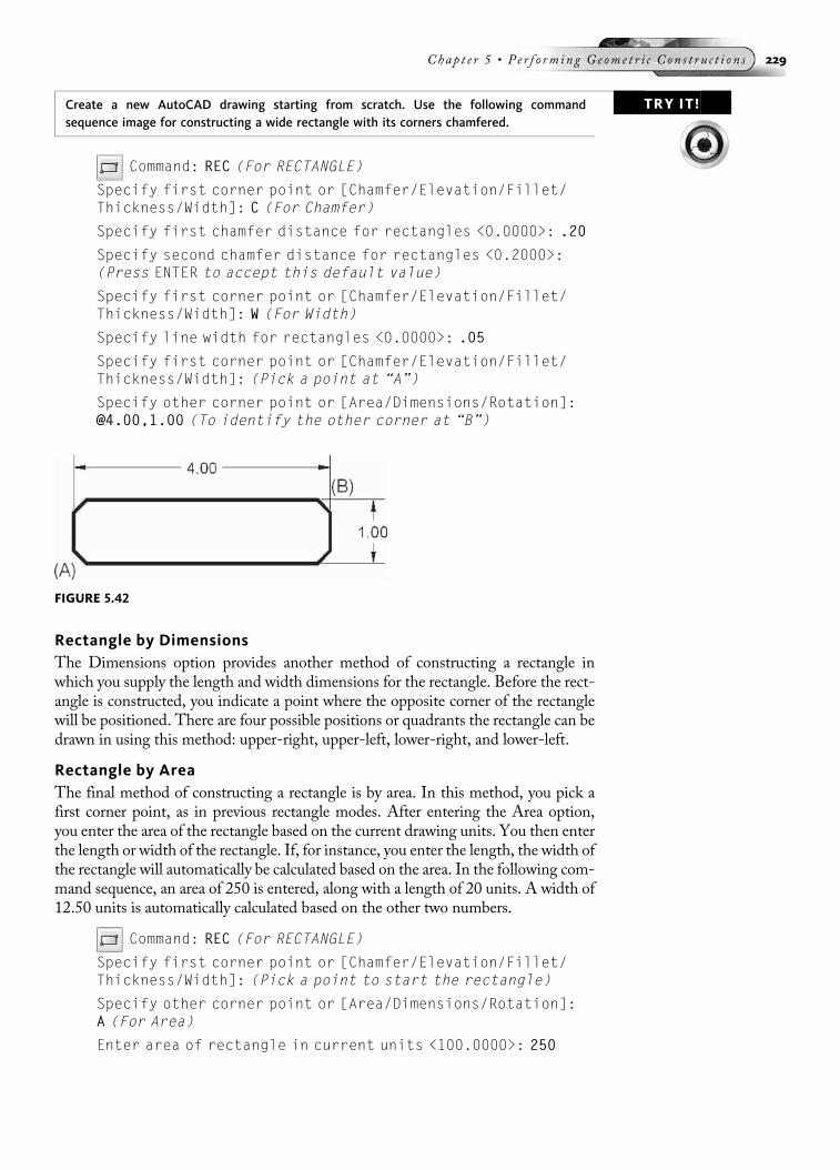
TRY IT!Create a new AutoCAD drawing starting from scratch. Use the following commandsequence image for constructing a wide rectangle with its corners chamfered.
Command: REC (For RECTANGLE)
Specify first corner point or [Chamfer/Elevation/Fillet/Thickness/Width]: C (For Chamfer)
Specify first chamfer distance for rectangles <0.0000>: .20
Specify second chamfer distance for rectangles <0.2000>:(Press ENTER to accept this default value)
Specify first corner point or [Chamfer/Elevation/Fillet/Thickness/Width]: W (For Width)
Specify line width for rectangles <0.0000>: .05
Specify first corner point or [Chamfer/Elevation/Fillet/Thickness/Width]: (Pick a point at “A”)
Specify other corner point or [Area/Dimensions/Rotation]:@4.00,1.00 (To identify the other corner at “B”)
Rectangle by DimensionsThe Dimensions option provides another method of constructing a rectangle inwhich you supply the length and width dimensions for the rectangle. Before the rect-angle is constructed, you indicate a point where the opposite corner of the rectanglewill be positioned. There are four possible positions or quadrants the rectangle can bedrawn in using this method: upper-right, upper-left, lower-right, and lower-left.
Rectangle by AreaThe final method of constructing a rectangle is by area. In this method, you pick afirst corner point, as in previous rectangle modes. After entering the Area option,you enter the area of the rectangle based on the current drawing units. You then enterthe length or width of the rectangle. If, for instance, you enter the length, the width ofthe rectangle will automatically be calculated based on the area. In the following com-mand sequence, an area of 250 is entered, along with a length of 20 units. A width of12.50 units is automatically calculated based on the other two numbers.
Command: REC (For RECTANGLE)
Specify first corner point or [Chamfer/Elevation/Fillet/Thickness/Width]: (Pick a point to start the rectangle)
Specify other corner point or [Area/Dimensions/Rotation]:A (For Area)
Enter area of rectangle in current units <100.0000>: 250
FIGURE 5.42
Chap t e r 5 • Pe r f o rm ing Ge ome t r i c C on s t r u c t i o n s 229
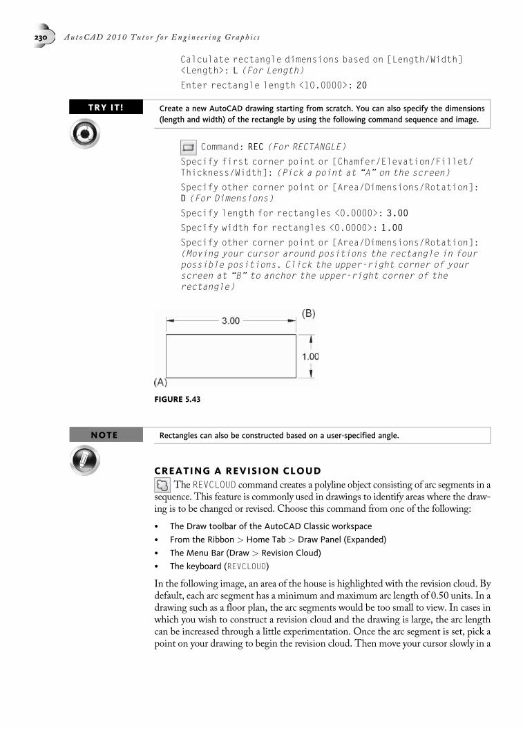
Calculate rectangle dimensions based on [Length/Width]<Length>: L (For Length)
Enter rectangle length <10.0000>: 20
TRY IT! Create a new AutoCAD drawing starting from scratch. You can also specify the dimensions(length and width) of the rectangle by using the following command sequence and image.
Command: REC (For RECTANGLE)
Specify first corner point or [Chamfer/Elevation/Fillet/Thickness/Width]: (Pick a point at “A” on the screen)
Specify other corner point or [Area/Dimensions/Rotation]:D (For Dimensions)
Specify length for rectangles <0.0000>: 3.00
Specify width for rectangles <0.0000>: 1.00
Specify other corner point or [Area/Dimensions/Rotation]:(Moving your cursor around positions the rectangle in fourpossible positions. Click the upper-right corner of yourscreen at “B” to anchor the upper-right corner of therectangle)
NOTE Rectangles can also be constructed based on a user-specified angle.
CREATING A REVISION CLOUDThe REVCLOUD command creates a polyline object consisting of arc segments in a
sequence. This feature is commonly used in drawings to identify areas where the draw-ing is to be changed or revised. Choose this command from one of the following:
• The Draw toolbar of the AutoCAD Classic workspace
• From the Ribbon > Home Tab > Draw Panel (Expanded)
• The Menu Bar (Draw > Revision Cloud)
• The keyboard (REVCLOUD)
In the following image, an area of the house is highlighted with the revision cloud. Bydefault, each arc segment has a minimum and maximum arc length of 0.50 units. In adrawing such as a floor plan, the arc segments would be too small to view. In cases inwhich you wish to construct a revision cloud and the drawing is large, the arc lengthcan be increased through a little experimentation. Once the arc segment is set, pick apoint on your drawing to begin the revision cloud. Then move your cursor slowly in a
FIGURE 5.43
230 Au t oCAD 2010 Tu t o r f o r Eng i n e e r i n g Graph i c s

counterclockwise direction. You will notice the arc segments of the revision cloudbeing constructed. Continue surrounding the object, while at the same time headingback to the origin of the revision cloud. Once you hover near the original start, theend of the revision cloud snaps to the start and the command ends, leaving the revi-sion cloud as the polyline object. Study the command prompt sequence below and theillustration in the following image for the construction of a revision cloud.
Command: REVCLOUD
Minimum arc length: 1/2 00 Maximum arc length: 1/2 00 Style:Normal
Specify start point or [Arc length/Object/Style] <Object>: A(For Arc length)
Specify minimum length of arc <1/2 00>: 24
Specify maximum length of arc <2 0>: (Press ENTER)
Specify start point or [Arc length/Object/Style] <Object>:(Pick a point on your screen to start the revision cloud.Surround the item with the revision cloud by moving yourcursor in a counterclockwise direction. When you approach thestart point, the revision cloud closes and the commandexits.)
Guide crosshairs along cloud path...
Revision cloud finished.
Calligraphy Revision CloudsThe Calligraphy option of creating revision clouds allows you to enhance the use
of this command and make your drawings more dramatic. Use the followingcommand sequence and image, which illustrate this feature.
Command: REVCLOUD
Minimum arc length: 24.0000 Maximum arc length: 24.0000Style: Normal
Specify start point or [Arc length/Object/Style] <Object>:S (For Style)
FIGURE 5.44
Chap t e r 5 • Pe r f o rm ing Ge ome t r i c C on s t r u c t i o n s 231

Select arc style [Normal/Calligraphy] <Normal>: C (ForCalligraphy)
Arc style = Calligraphy
Specify start point or [Arc length/Object/Style] <Object>:(Pick a starting point)
Guide crosshairs along cloud path...
Revision cloud finished.
CREATING SPLINESUse the SPLINE command to construct a smooth curve given a sequence of
points. Choose this command from one of the following:
• The Draw toolbar of the AutoCAD Classic workspace
• From the Ribbon > Home Tab > Draw Panel (Expanded)
• The Menu Bar (Draw > Spline)
• The keyboard (SPL or SPLINE)
You have the option of changing the accuracy of the curve given a tolerance range.The basic command sequence follows, which constructs the spline segment shownin the following image on the left.
Command: SPL (For SPLINE)
Specify first point or [Object]: (Pick a first point)
Specify next point: (Pick another point)
Specify next point or [Close/Fit tolerance] <start tangent>:(Pick another point)
Specify next point or [Close/Fit tolerance] <start tangent>:(Pick another point)
Specify next point or [Close/Fit tolerance] <start tangent>:(Press ENTER to continue)
Specify start tangent: (Press ENTER to accept)
Specify end tangent: (Press ENTER to accept the end tangentposition, which exits the command and places the spline)
The spline may be closed to display a continuous segment, as shown in the followingimage on the right. Entering a different tangent point at the end of the commandchanges the shape of the curve connecting the beginning and end of the spline.
Command: SPL (For SPLINE)
Specify first point or [Object]: (Pick a first point)
FIGURE 5.45
232 Au t oCAD 2010 Tu t o r f o r Eng i n e e r i n g Graph i c s

Specify next point: (Pick another point)
Specify next point or [Close/Fit tolerance] <start tangent>:(Pick another point)
Specify next point or [Close/Fit tolerance] <start tangent>:(Pick another point)
Specify next point or [Close/Fit tolerance] <start tangent>:C (To Close)
Specify tangent: (Press ENTER to exit the command and placethe spline)
TRY IT!Open the drawing file 05_ Spline Rasp Handle, as shown in the following image on the left.Turn OSNAP on and set Running OSNAP to Node. This allows you to snap to points whendrawing splines or other objects. Construct a spline by connecting all points between “A”and “B.” Construct an arc with its center at “C,” the start point at “D,” and the ending pointat “B.” Connect points “D” and “E” with a line segment. Construct another spline by con-necting all points between “E” and “F.” Construct another arc with its center at “G,” thestart point at “H,” and the ending point at “F.” Connect points “H” and “A” with a linesegment.
FIGURE 5.46
FIGURE 5.47
Chap t e r 5 • Pe r f o rm ing Ge ome t r i c C on s t r u c t i o n s 233

MASKING TECHNIQUES WITH THE WIPEOUT COMMANDTo mask or hide objects in a drawing without deleting them or turning off layers, theWIPEOUT command could be used. Choose this command from one of the following:
• The Menu Bar (Draw > Wipeout)
• From the Ribbon > Home Tab > Draw Panel (Expanded)
• The keyboard (WIPEOUT)
This command reads the current drawing background color and creates a mask overanything defined by a frame. In the illustration in the following image on the left,a series of text objects needs to be masked over. The middle image shows a four-sided frame that was created over the text using the following command promptsequence:
Command: WIPEOUT
Specify first point or [Frames/Polyline] <Polyline>: (Pick afirst point)
Specify next point: (Pick a second point)
Specify next point or [Undo]: (Pick a third point)
Specify next point or [Close/Undo]: (Pick a fourth point)
Specify next point or [Close/Undo]: (Press ENTER to exit thecommand and create the wipeout)
As the text seems to disappear, the wipeout frame is still visible. A visible frame isimportant if you would like to unmask or delete the wipeout. If you want to hide allwipeout frames, use the following command sequence:
Command: WIPEOUT
Specify first point or [Frames/Polyline] <Polyline>: F (ForFrames)
Enter mode [ON/OFF] <ON>: Off
Now all wipeout frames in the current drawing are turned off, as shown in theillustration in the following image on the right.
NOTE You could also create a predefined polyline object and then convert it into a wipeout usingthe Polyline option of the WIPEOUT command.
FIGURE 5.48
234 Au t oCAD 2010 Tu t o r f o r Eng i n e e r i n g Graph i c s
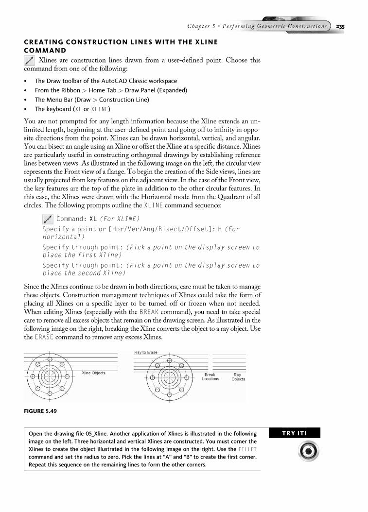
CREATING CONSTRUCTION LINES WITH THE XLINECOMMAND
Xlines are construction lines drawn from a user-defined point. Choose thiscommand from one of the following:
• The Draw toolbar of the AutoCAD Classic workspace
• From the Ribbon > Home Tab > Draw Panel (Expanded)
• The Menu Bar (Draw > Construction Line)
• The keyboard (XL or XLINE)
You are not prompted for any length information because the Xline extends an un-limited length, beginning at the user-defined point and going off to infinity in oppo-site directions from the point. Xlines can be drawn horizontal, vertical, and angular.You can bisect an angle using an Xline or offset the Xline at a specific distance. Xlinesare particularly useful in constructing orthogonal drawings by establishing referencelines between views. As illustrated in the following image on the left, the circular viewrepresents the Front view of a flange. To begin the creation of the Side views, lines areusually projected from key features on the adjacent view. In the case of the Front view,the key features are the top of the plate in addition to the other circular features. Inthis case, the Xlines were drawn with the Horizontal mode from the Quadrant of allcircles. The following prompts outline the XLINE command sequence:
Command: XL (For XLINE)
Specify a point or [Hor/Ver/Ang/Bisect/Offset]: H (ForHorizontal)
Specify through point: (Pick a point on the display screen toplace the first Xline)
Specify through point: (Pick a point on the display screen toplace the second Xline)
Since the Xlines continue to be drawn in both directions, care must be taken to managethese objects. Construction management techniques of Xlines could take the form ofplacing all Xlines on a specific layer to be turned off or frozen when not needed.When editing Xlines (especially with the BREAK command), you need to take specialcare to remove all excess objects that remain on the drawing screen. As illustrated in thefollowing image on the right, breaking the Xline converts the object to a ray object. Usethe ERASE command to remove any excess Xlines.
TRY IT!Open the drawing file 05_Xline. Another application of Xlines is illustrated in the followingimage on the left. Three horizontal and vertical Xlines are constructed. You must corner theXlines to create the object illustrated in the following image on the right. Use the FILLETcommand and set the radius to zero. Pick the lines at “A” and “B” to create the first corner.Repeat this sequence on the remaining lines to form the other corners.
FIGURE 5.49
Chap t e r 5 • Pe r f o rm ing Ge ome t r i c C on s t r u c t i o n s 235
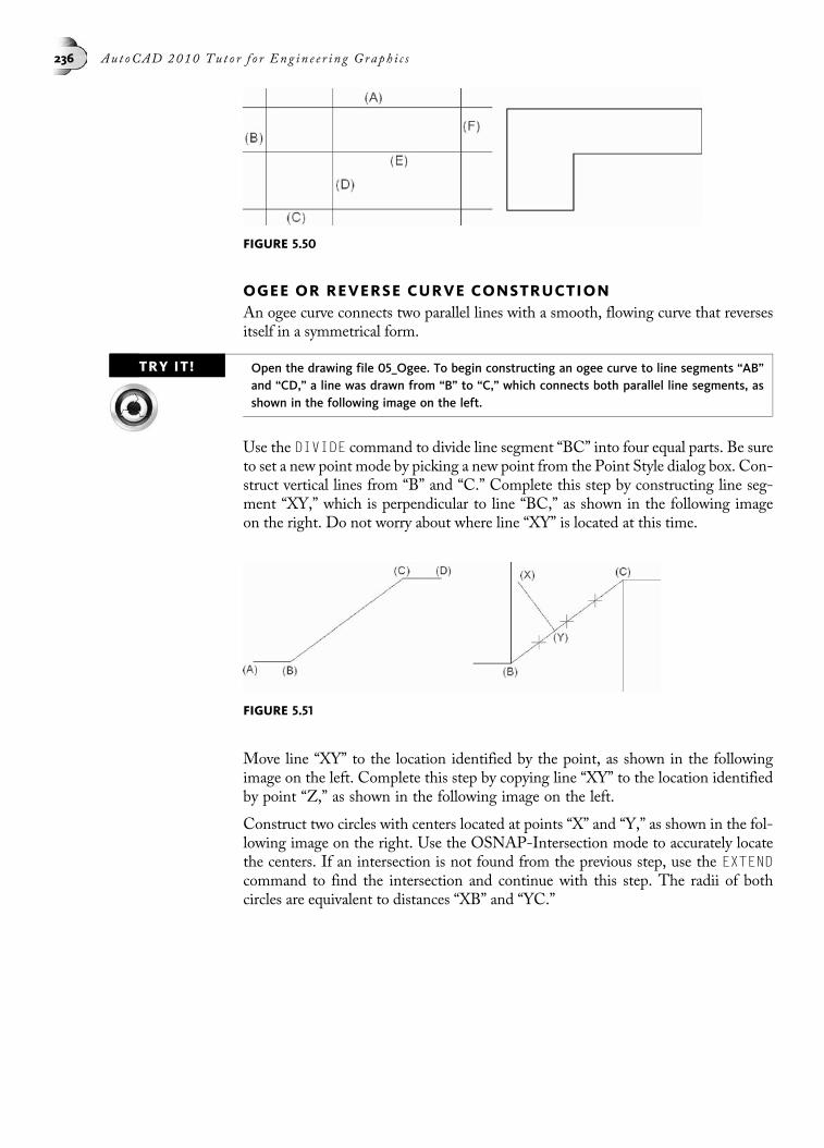
OGEE OR REVERSE CURVE CONSTRUCTIONAn ogee curve connects two parallel lines with a smooth, flowing curve that reversesitself in a symmetrical form.
TRY IT! Open the drawing file 05_Ogee. To begin constructing an ogee curve to line segments “AB”and “CD,” a line was drawn from “B” to “C,” which connects both parallel line segments, asshown in the following image on the left.
Use the DIVIDE command to divide line segment “BC” into four equal parts. Be sureto set a new point mode by picking a new point from the Point Style dialog box. Con-struct vertical lines from “B” and “C.” Complete this step by constructing line seg-ment “XY,” which is perpendicular to line “BC,” as shown in the following imageon the right. Do not worry about where line “XY” is located at this time.
Move line “XY” to the location identified by the point, as shown in the followingimage on the left. Complete this step by copying line “XY” to the location identifiedby point “Z,” as shown in the following image on the left.
Construct two circles with centers located at points “X” and “Y,” as shown in the fol-lowing image on the right. Use the OSNAP-Intersection mode to accurately locatethe centers. If an intersection is not found from the previous step, use the EXTENDcommand to find the intersection and continue with this step. The radii of bothcircles are equivalent to distances “XB” and “YC.”
FIGURE 5.50
FIGURE 5.51
236 Au t oCAD 2010 Tu t o r f o r Eng i n e e r i n g Graph i c s
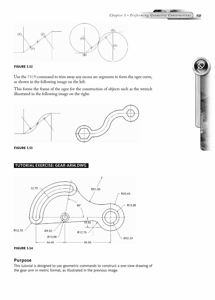
Use the TRIM command to trim away any excess arc segments to form the ogee curve,as shown in the following image on the left.
This forms the frame of the ogee for the construction of objects such as the wrenchillustrated in the following image on the right.
TUTORIAL EXERCISE: GEAR-ARM.DWG
PurposeThis tutorial is designed to use geometric commands to construct a one-view drawing ofthe gear-arm in metric format, as illustrated in the previous image.
FIGURE 5.52
FIGURE 5.53
FIGURE 5.54
Chap t e r 5 • Pe r f o rm ing Ge ome t r i c C on s t r u c t i o n s 237

System SettingsUse the Drawing Units dialog box to change the number of decimal places past the zerofrom four to two. Keep the remaining default unit values. Using the LIMITS command,keep (0,0) for the lower-left corner and change the upper-right corner from (12,9) to(265.00,200.00). Perform a ZOOM-All after changing the drawing limits. Since a layercalled “Center” must be created to display centerlines, use the LTSCALE command andchange the default value of 1.00 to 15.00. This makes the long and short dashes of thecenterlines appear on the display screen. Check to see that the following Object Snapmodes are already set: Endpoint, Extension, Intersection, and Center.
LayersCreate the following layers with the format:
Name Color Linetype
Center Yellow Center
Construction Gray Center
Dimension Yellow Continuous
Object White Continuous
Suggested CommandsBegin a new drawing called Gear-arm. The object consists of a combination of circles andarcs along with tangent lines and arcs. Before beginning, be sure to set Object as the newcurrent layer. Construction lines will be used as a layout tool to mark the centers of keycircles and arcs. The CIRCLE-TTR command will be used for constructing tangent arcsto existing geometry. Use the ARC command to construct a series of arcs for the left sideof the gear-arm. The TRIM command will be used to trim circles, lines, and arcs to formthe basic shape.
STEP 1Begin constructing the gear-arm by creating construction geometry that will be used tocreate all circles. First make the Construction layer current and use the LINE commandto lay out the long horizontal line and middle vertical line. Then use the OFFSET com-mand to copy the vertical line at the specified distances. Also, create a line 70 unitslong at an 80° angle, as shown in the following image.
238 Au t oCAD 2010 Tu t o r f o r Eng i n e e r i n g Graph i c s
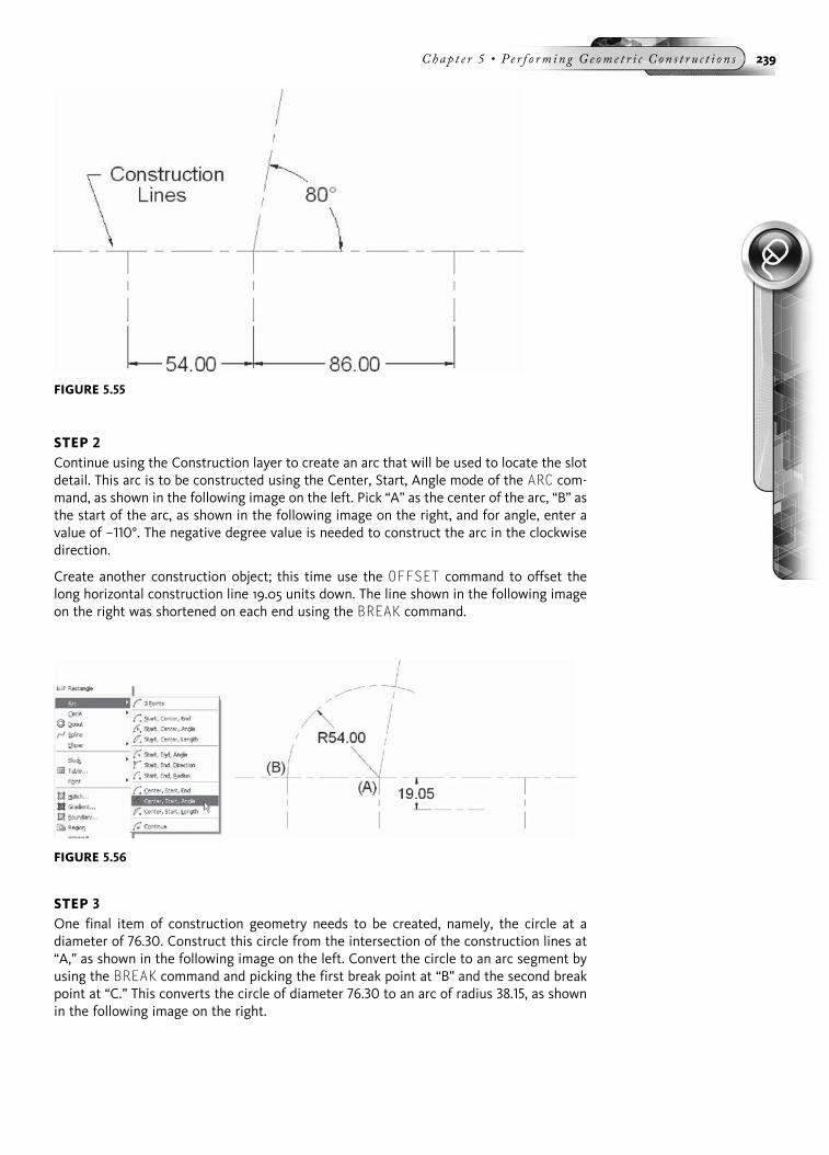
STEP 2Continue using the Construction layer to create an arc that will be used to locate the slotdetail. This arc is to be constructed using the Center, Start, Angle mode of the ARC com-mand, as shown in the following image on the left. Pick “A” as the center of the arc, “B” asthe start of the arc, as shown in the following image on the right, and for angle, enter avalue of −110°. The negative degree value is needed to construct the arc in the clockwisedirection.
Create another construction object; this time use the OFFSET command to offset thelong horizontal construction line 19.05 units down. The line shown in the following imageon the right was shortened on each end using the BREAK command.
STEP 3One final item of construction geometry needs to be created, namely, the circle at adiameter of 76.30. Construct this circle from the intersection of the construction lines at“A,” as shown in the following image on the left. Convert the circle to an arc segment byusing the BREAK command and picking the first break point at “B” and the second breakpoint at “C.” This converts the circle of diameter 76.30 to an arc of radius 38.15, as shownin the following image on the right.
FIGURE 5.55
FIGURE 5.56
Chap t e r 5 • Pe r f o rm ing Ge ome t r i c C on s t r u c t i o n s 239

STEP 4Using the following image as a guide, create all circles using the intersection of the con-struction line geometry as the centers for the circles. All circles are given with diameterdimensions.
STEP 5Use the ARC CENTER, START, END command to create the arc shown in the followingimage on the left. Pick “A” as the center of the arc, “B” as the start, and “C” as the end ofthe arc. You must use a combination of Object Snaps in order for the arcs to be drawncorrectly. Following these steps constructs the outer arc of the gear-arm. Use the sameARC CENTER, START, END command to create the inside arc using a different set ofpoints.
When finished creating the outer arc segments, create the two inner arc segments, asshown in the following image on the right, using the same ARC CENTER, START, ENDcommand. Continue to use Object Snap to pick valid intersections in order to create themost accurate set of arcs.
FIGURE 5.57
FIGURE 5.58
FIGURE 5.59
240 Au t oCAD 2010 Tu t o r f o r Eng i n e e r i n g Graph i c s

STEP 6Use the CIRCLE-TTR command to construct a circle tangent to two existing circles. Pickthe two dashed circles as the objects to be made tangent, as shown in the followingimage on the left, and enter a radius value of 51.
After the circle is created, enter the TRIM command, pick the two dashed circles as cut-ting edges, and pick the upper edge of the large 51-radius circle. The results of this opera-tion are illustrated in the following image on the right.
STEP 7Enter the TRIM command again, pick the two dashed arcs as cutting edges, and pick thetwo inside edges of the 25.4-diameter circles, as shown in the following image on the left.The results of this operation are illustrated in the following image on the right.
STEP 8Do the same procedure to clean up the geometry that makes up the inner slot. Enter theTRIM command, pick the two dashed arcs as cutting edges, and pick the two inside edgesof the 12.75-diameter circles, as shown in the following image on the left. The results ofthis operation are illustrated in the following image on the right.
FIGURE 5.60
FIGURE 5.61
FIGURE 5.62
Chap t e r 5 • Pe r f o rm ing Ge ome t r i c C on s t r u c t i o n s 241

STEP 9Construct a new circle of diameter 25.50 from the intersection of the construction lineand arc, as shown in the following image on the left. Then draw a line segment that istangent with the bottom of the arc and top of the circle just constructed, as shown inthe following image on the right.
STEP 10Use the TRIM command to clean up all unnecessary segments of geometry. Select alldashed objects as cutting edges, as shown in the following image on the left. Trim objectsuntil your display appears similar to the illustration in the following image on the right.
STEP 11Erase all unnecessary construction geometry, as shown in the following image on the left.Notice that the arc and 70° angle line both remain and will be used later to define thecenters of the gear-arm.
Next create centerlines to mark the centers of all circles. Switch to the Center layer.A system variable that controls centerlines and marks called dimcen must first be enteredfrom the keyboard and changed to a value of −.05. The negative value constructs thesmall dash and long segment, all representing the centerline. Entering a value of .05would only mark the center of circles by constructing two short intersecting line seg-ments. Then use the DIMCENTER (or DCE for short) command and pick the edge of acircle or arc segment to place the centerline. The results should appear similar to theillustration in the following image on the right.
FIGURE 5.63
FIGURE 5.64
242 Au t oCAD 2010 Tu t o r f o r Eng i n e e r i n g Graph i c s

STEP 12The completed gear-arm drawing is illustrated as shown in the following image on the left.The finished object may be dimensioned as an optional step, as shown in the followingimage on the right.
TUTORIAL EXERCISE: PATTERN1.DWG
FIGURE 5.65
FIGURE 5.66
FIGURE 5.67
Chap t e r 5 • Pe r f o rm ing Ge ome t r i c C on s t r u c t i o n s 243

PurposeThis tutorial is designed to use various Draw commands to construct a one-view drawingof Pattern1, as shown in the previous image. Refer to the following special systemsettings and suggested command sequences.
System SettingsUse the Drawing Units dialog box to change the number of decimal places past the zerofrom four to two. Keep the remaining default unit values. Using the LIMITS command,keep (0,0) for the lower-left corner and change the upper-right corner from (12,9) to(21.00,16.00). Perform a ZOOM-All after changing the drawing limits. Check to see thatthe following Object Snap modes are already set: Endpoint, Extension, Intersection, andCenter.
Setting OSNAP Mode would also be helpful with completing this exercise.
LayersCreate the following layers with the format:
Name Color Linetype
Object White Continuous
Center Yellow Center
Dimension Yellow Continuous
Suggested CommandsBegin constructing Pattern1 by first creating four circles by relative coordinate mode.Then use the CIRCLE-TTR command/option to draw tangent arcs to the circles alreadydrawn. Use the TRIM command to clean up and partially delete circles to obtain the out-line of the pattern. Then add the 2.00-diameter holes followed by the center markers,using the DIMCENTER (DCE) command.
STEP 1Check that the current layer is set to Object. See the following image for the dimensionsand table for locating the centers of all circles. Use the CIRCLE command to create thecircle at “A” whose center point is located at coordinate 9.50, 4.50 and which has a diam-eter of 4.00 units. Locate circle “B” at relative coordinate @-2.25,3.00 and assign a diam-eter of 5.00 units. The relative coordinate is based on the previous circle. Continue bydrawing circle “C” using the center point at relative coordinate @5.25,3.50 and assign adiameter of 3.50 units. Construct the last circle, “D,” with center point @-.75,-2.50 and adiameter of 3.00 units. Notice that when using relative coordinate mode, you do notneed to draw construction geometry and then erase it later.
244 Au t oCAD 2010 Tu t o r f o r Eng i n e e r i n g Graph i c s
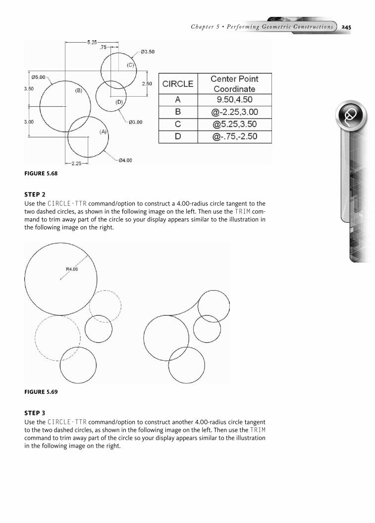
STEP 2Use the CIRCLE-TTR command/option to construct a 4.00-radius circle tangent to thetwo dashed circles, as shown in the following image on the left. Then use the TRIM com-mand to trim away part of the circle so your display appears similar to the illustration inthe following image on the right.
STEP 3Use the CIRCLE-TTR command/option to construct another 4.00-radius circle tangentto the two dashed circles, as shown in the following image on the left. Then use the TRIMcommand to trim away part of the circle so your display appears similar to the illustrationin the following image on the right.
FIGURE 5.68
FIGURE 5.69
Chap t e r 5 • Pe r f o rm ing Ge ome t r i c C on s t r u c t i o n s 245

STEP 4Use the CIRCLE-TTR command/option to construct a 6.00-radius circle tangent to thetwo dashed circles, as shown in the following image on the left. Then use the TRIM com-mand to trim away part of the circle so your display appears similar to the illustration inthe following image on the right.
STEP 5Use the CIRCLE-TTR command/option to construct a .75-radius circle tangent to thetwo dashed circles, as shown in the following image on the left. Then use the TRIM com-mand to trim away part of the circle so your display appears similar to the illustration inthe following image on the right.
FIGURE 5.70
FIGURE 5.71
246 Au t oCAD 2010 Tu t o r f o r Eng i n e e r i n g Graph i c s

STEP 6Use the TRIM command, select all dashed arcs, shown in the following image on the left,as cutting edges, and trim away the circular segments to form the outline of the Pattern1drawing. When finished, your display should appear similar to the illustration in the fol-lowing image on the right.
STEP 7Use the CIRCLE command to construct a total of three circles of 2.00 diameter. Use thecenters of arcs “A,” “B,” and “C,” as shown in the following image on the left, as the cen-ters for the circles. Switch to the Center layer, change the DIMCEN system variable to avalue of .07, and use the DIMCENTER command to place center marks identifying thecenters of all circles and arcs, as shown in the following image on the right.
FIGURE 5.72
FIGURE 5.73
Chap t e r 5 • Pe r f o rm ing Ge ome t r i c C on s t r u c t i o n s 247

END OF CHAPTER PROBLEMS FOR CHAPTER 5Please refer to the CD that is supplied with this book and locate the file AutoCAD Tutor2010 Support Docs.pdf. In addition to extra information supplied in this chapter,end-of-chapter problems are also available to provide additional practice.
FIGURE 5.74
248 Au t oCAD 2010 Tu t o r f o r Eng i n e e r i n g Graph i c s

CHAPTER
6
Working with Text,Fields, and Tables
AutoCAD provides a robust set of text commands that allow you to place differenttext objects, edit those text objects, and even globally change the text height withoutaffecting the justification. The heart of placing text in a drawing is through the MTEXTcommand. This chapter discusses the uses of the DTEXT command, which stands forDynamic Text or Single Line Text. In this chapter, you will also be given informationon how to edit text created with the MTEXT and DTEXT commands. The SCALETEXTand JUSTIFYTEXT commands will be explained in detail, as will the ability to createcustom text styles and assign different text fonts to these styles. Intelligent text in theform of fields will also be discussed in this chapter, as will the creation of tables.
AUTOCAD TEXT COMMANDSAll text commands can be located easily by launching the Menu Bar, Ribbon, or Texttoolbar, as shown in the following image. The two main modes for entering text areMultiline Text (the MTEXT command) and Single Line Text (the DTEXT command).
FIGURE 6.1
249

Study the information in the following table for a brief description of each textcommand.
Button Tool Shortcut Function
Multiline Text MT Creates paragraphs of text as a singleobject
Single Line Text DT Creates one or more lines of text; each lineof text is considered a separate object
Edit Text ED Used for editing multiline and single linetext in addition to dimension and attributetext
Find and Replace FIND Used for finding, replacing, selecting, orzooming in to a particular text object
Spell Check SP Performs a spell check on a drawing
Text Style ST Launches the Text Style dialog box used forcreating different text styles
SCALETEXT None Used for scaling selected text objectswithout affecting their locations
JUSTIFYTEXT None Used for justifying selected text objectswithout affecting their locations
SPACETRANS None Converts text heights between ModelSpace and Paper Space (Layout mode)
ADDING MULTILINE TEXT IN THE AUTOCADCLASSIC WORKSPACE
The MTEXT command allows for the placement of text in multiple lines. EnteringMT (MTEXT) from the command prompt displays the following prompts:
Command: MT (For MTEXT)
Current text style: “GENERAL NOTES” Text height: 0.2000Annotative: No
Specify first corner: (Pick a point at “A” to identify onecorner of the Mtext box)
Specify opposite corner or [Height/Justify/Line spacing/Rotation/Style/Width/Columns]: (Pick another cornerforming a box)
Picking a first corner displays a user-defined box with an arrow at the bottom, as shownin the following image. This box defines the area where the multiline text will beplaced. If the text cannot fit on one line, it will wrap to the next line automatically.
FIGURE 6.2
250 Au t oCAD 2010 Tu t o r f o r Eng i n e e r i n g Graph i c s

After you click a second point marking the other corner of the insertion box, the TextEditor Ribbon appears, along with the Multiline Text Editor. The parts of theseitems are shown in the following image. One of the advantages of this tool is thetransparency associated with the Multiline Text Editor. As you begin entering text,you can still see your drawing in the background. This editor can also be moved tonew locations without exiting the editing session.
Notice in the following image other important areas of the Text Editor Ribbon. Thecurrent text style and font are displayed, in addition to the text height. You can makethe text bold, italicized, or underlined by using the B, I, and U buttons present in thetoolbar.When you have finished entering the text, click the Close Text Editor buttonto dismiss the Text Editor Ribbon and text editor and place the text in the drawing.
As you begin to type, your text appears in the Text Editor box shown in the followingimage. As the multiline text is entered, it automatically wraps to the next line depend-ing on the size of the initial bounding box. Tabs and indents can be utilized as neces-sary, and even the size of the box can be modified, if required.
NOTEClicking a blank part of your screen after you are finished entering text in the previousexample will also exit the Text Editor Ribbon.
FIGURE 6.3
FIGURE 6.4
Chap t e r 6 • Work i n g w i t h T ex t , F i e l d s , a nd Tab l e s 251

Another method of displaying additional options of the Multiline Text Editor is toright-click inside the text box. This displays the menu shown in the following image.
MULTILINE TEXT COMMANDS - GROUP IThe Text Editor Ribbon has a wealth of controls available to manipulate text items.These buttons will be explained in two separate groups. The following table willexplain these controls and buttons.
Button Tool Function
Standard Text Style Name Displays the current text style. Click the down arrow tochange to a different text style.
Txt Text Font Name Displays the current text font
Annotative Turns annotative scale on or off
0.2000 Text Height Displays the current text height
Bold Used to change highlighted text to bold
Italics Used to change highlighted text to italics
Underline Used to underline highlighted text
Overline Used to place a line over the top of highlighted text
Undo Used to undo the previous text option and remain inthe Text Editor Ribbon
Redo Used to redo the previous undo
Fraction Stack Used for turning stacked fraction mode on or off
Color Used to change the color of highlighted text
Ruler Displays a ruler used for setting tabs and indents
X Close Text Editor Used to accept the current multiline text and exit theText Editor Ribbon
Options Used to display additional text options
FIGURE 6.5
252 Au t oCAD 2010 Tu t o r f o r Eng i n e e r i n g Graph i c s

MULTILINE TEXT COMMANDS - GROUP IIThe following table explains Group II controls and buttons located in the TextEditor Ribbon.
Button Tool Function
Columns Displays a menu used to control the type of text columngenerated
MtextJustification
Displays a menu consisting of nine text justification modes
Paragraph Displays the Paragraph dialog box used for changing suchitems as indentations that affect paragraph text
Left Justifies the left edge of text with the left edge of themargin
Center Justifies mtext objects to the center
Right Justifies the right edge of text with the right edge of themargin
Justify Adjusts the horizontal spacing of text so the text is alignedevenly along the right and left margins
Distribute Distributes mtext across the width of the mtext box andadjusts the spacing in between individual letters
Line Spacing Displays a menu used for changing the spacing in betweenlines of text
Numbering Displays a menu used for applying bullets and numbers totext
Field Used for inserting a field
Uppercase Used for changing all highlighted text to uppercase
Lowercase Used for changing all highlighted text to lowercase
Symbol Displays a menu for selecting special text characters andsymbols
Oblique Angle Determines the forward or backward slant of text
Tracking Used to increase or decrease the space between selectedtext characters
Width Factor Used to create wide or narrow text characters
TEXT JUSTIFICATION MODESThe following image illustrates a sample text item and the various locations by whichthe text can be justified. By default, when you place text, it is left justified. These jus-tification modes are designed to work in combination with one another. For example,one common justification is to have the text middle centered. Options in text com-mands allow you to pick Middle Center from a menu or type MC in at the keyboard.The same type of combination is available for the other justification modes.
Chap t e r 6 • Work i n g w i t h T ex t , F i e l d s , a nd Tab l e s 253

JUSTIFYING MULTILINE TEXTVarious justification modes are available to change the appearance of the text in yourdrawing. Justification modes can be retrieved by clicking the Justification buttonfound in the Text Editor Ribbon as shown in the following image. Clicking thisbutton displays the nine modes.
Additionally, Paragraph Alignment modes are also available in the second row of theText Formatting dialog box, as shown in the following image. These justificationmodes are similar to those found in word processors and allow you to align individualparagraphs in the text editor. Paragraphs are separated by hard returns (pressing theENTER key).
FIGURE 6.6
FIGURE 6.7
254 Au t oCAD 2010 Tu t o r f o r Eng i n e e r i n g Graph i c s

INDENTING TEXTMultiline text can be indented in order to align text objects to form a list or table.A ruler, illustrated in the following image, consisting of short and longer tick marksdisplays the current paragraph settings.
The tabs and indents that you set before you start to enter text apply to the wholemultiline text object. If you want to set tabs and indents to individual paragraphs,click on a paragraph or select multiple paragraphs to apply the indentations.
Two sliders are available on the left side of the ruler to show the amount of indenta-tion applied to the various multiline text parts. In the following image, the top slideris used to indent the first line of a paragraph. A tooltip is available to remind you ofthis function.
In the following image, a bottom slider is also available. This slider controls theamount of indentation applied to the other lines of the paragraph. You can see theresults of using this slider in the following image.
FIGURE 6.8
FIGURE 6.9
FIGURE 6.10
Chap t e r 6 • Work i n g w i t h T ex t , F i e l d s , a nd Tab l e s 255

NOTE If you set tabs and indents prior to starting to enter multiline text, the tabs are applied tothe whole multiline object.
FORMATTING WITH TABSYou can further control your text by adding tabs. The long tick marks on the rulershow the default tab stops. Clicking the Tab Style button toggles to four differenttab modes, as shown in the following image on the left. When you click the ruler toset your own tabs, the ruler displays a small, default L-shaped marker at each customtab stop, as shown in the following image. When you anchor your cursor in front of asentence and press the TAB key on your keyboard, the text aligns to the nearest tabmarker. To remove a custom tab stop, drag the marker off the ruler.
BULLETING AND NUMBERING TEXTMultiline text can also be formatted in a numbered, bulleted, or alphabetic characterlist, either uppercase or lowercase. The four types of lists are illustrated in the follow-ing image.
FIGURE 6.11
FIGURE 6.12
256 Au t oCAD 2010 Tu t o r f o r Eng i n e e r i n g Graph i c s
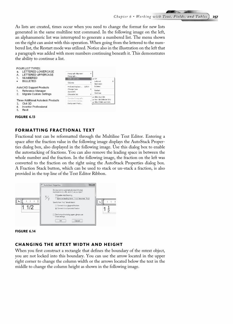
As lists are created, times occur when you need to change the format for new listsgenerated in the same multiline text command. In the following image on the left,an alphanumeric list was interrupted to generate a numbered list. The menu shownon the right can assist with this operation. When going from the lettered to the num-bered list, the Restart mode was utilized. Notice also in the illustration on the left thata paragraph was added with more numbers continuing beneath it. This demonstratesthe ability to continue a list.
FORMATTING FRACTIONAL TEXTFractional text can be reformatted through the Multiline Text Editor. Entering aspace after the fraction value in the following image displays the AutoStack Proper-ties dialog box, also displayed in the following image. Use this dialog box to enablethe autostacking of fractions. You can also remove the leading space in between thewhole number and the fraction. In the following image, the fraction on the left wasconverted to the fraction on the right using the AutoStack Properties dialog box.A Fraction Stack button, which can be used to stack or un-stack a fraction, is alsoprovided in the top line of the Text Editor Ribbon.
CHANGING THE MTEXT WIDTH AND HEIGHTWhen you first construct a rectangle that defines the boundary of the mtext object,you are not locked into this boundary. You can use the arrow located in the upperright corner to change the column width or the arrows located below the text in themiddle to change the column height as shown in the following image.
FIGURE 6.13
FIGURE 6.14
Chap t e r 6 • Work i n g w i t h T ex t , F i e l d s , a nd Tab l e s 257

NOTE When dragging the center arrows to change the column height, you can form columns bydragging the arrows up and notice the creation of the columns as shown in the followingimage.
NOTE Grips provide another method for changing the size of the text box once the text hasalready been created. Clicking the multiline text object as it appears in your drawing causesblue boxes called grips to appear in the four corners of the text box. Picking one of thesegrips and moving to the left or right increases or decreases the size of the text box. Gripswill be covered in greater detail in chapter 7.
MULTILINE TEXT AND THE RIBBONAll of the text examples presented up to this point illustrated placing text throughthe AutoCAD Classic workspace. Text can also be placed through the 2D Draftingand Annotation workspace that utilizes the Annotation tab of the Ribbon as shownin the following image. Basic text commands are contained in this area.
FIGURE 6.15
FIGURE 6.17
FIGURE 6.16
258 Au t oCAD 2010 Tu t o r f o r Eng i n e e r i n g Graph i c s

When you activate the Multiline Text command and generate the rectangular textbox, a new menu appears in the Ribbon as shown in the following image. Theseheadings allow you to control the text style, formatting, paragraph, text insertion,and other text options. This gives you a more robust set of text related commandsall at your fingertips.
IMPORTING TEXT INTO YOUR DRAWINGIf you have existing files created in a word processor, you can import these files di-rectly into AutoCAD and have them converted into mtext objects. As illustrated inthe following image, right-click on the Multiline Text Editor box to display themenu; then pick Import Text. An open file dialog box displays, allowing you to pickthe desired file to import. The Import Text feature of the Multiline Text Editor sup-ports two file types: those ending in a TXT extension and those ending in the RTF(rich text format) extension. Text with the TXT extension conforms to the currentAutoCAD text style regarding font type. Text with the RTF extension remembersformatting and font settings from the word-processing document that it was origi-nally created in.
The finished result of this text-importing operation is illustrated in the following im-age. The text on the left, imported with the TXT extension, conformed to the presenttext style, which has a font of Arial assigned to it. The text on the right was importedwith the RTF extension. Even with the text style being set to Arial, the RTF-imported text displays in the Times New Roman font. This is the font in which itwas originally created in the word-processing document.
FIGURE 6.18
FIGURE 6.19
Chap t e r 6 • Work i n g w i t h T ex t , F i e l d s , a nd Tab l e s 259

MULTILINE TEXT SYMBOLSWhile in the Multiline Text Editor, right-clicking on the text window and selectingSymbol, as shown in the following image, displays various symbols that can be incor-porated into your drawing.
The table illustrated in the following image shows all available multiline text symbolsalong with their meanings.
FIGURE 6.20
FIGURE 6.21
FIGURE 6.22
260 Au t oCAD 2010 Tu t o r f o r Eng i n e e r i n g Graph i c s

CREATING PARAGRAPHS OF TEXTClicking the Paragraph button of the Text Editor Ribbon opens the Paragraph dialogbox. This feature allows you to set indentations for the first lines of paragraphs and forthe entire paragraph. In addition to indents, you can also specify the type of tab stop,paragraph spacing, and the spacing of lines in a paragraph.
The Tab area of the dialog box allows you to set left, center, right, and decimal tabs.You can also add or remove tabs using the appropriate control buttons.
The Left Indent area allows you to set the indentation value for the first line of text.The Hanging indent allows you to set indentations to the selected or currentparagraphs.
The Right Indent area applies an indentation to the entire selected or currentparagraph.
Placing a check in the Paragraph Alignment box activates five alignment propertiesfor the selected or current paragraph.
Placing a check in the Paragraph Spacing box activates controls for setting the spac-ing before or after the selected or current paragraph. The spacing between two para-graphs is calculated from the total of the After value and the Before value.
Placing a check in the Paragraph Line Spacing box allows you to set the spacingbetween individual lines in the selected or current paragraph.
ORGANIZING TEXT BY COLUMNSThis feature in the Text Editor Ribbon allows you to create columns of an mtextobject. You begin by first creating an mtext object consisting of a single column. Youthen choose one of the two different column methods, (Dynamic Columns and StaticColumns) from the Columns menu, as shown in the following image on the left.
Dynamic Columns allow columns of text to flow, causing columns to be added orremoved. You can control this flow through the Auto height or Manual heightmodes.
Static Columns allow you to specify the width, height, and number of columns. Inthis way, all columns share the same height.
FIGURE 6.23
Chap t e r 6 • Work i n g w i t h T ex t , F i e l d s , a nd Tab l e s 261

Other column options include the following:
No Columns specifies no columns for the current mtext object.
Insert Column Break ALT þ ENTER inserts a manual column break.
Column Settings displays the Column Settings dialog box shown in the followingimage on the right. Through this dialog box, you specify the column and gutterwidth, height, and number of columns. Grips are used to edit the width and heightof the column.
TRY IT! Open the drawing file 06_Specifications. The text in this drawing consists of one long col-umn. You will arrange this text in three columns, which will allow all text to be visible onthe drawing sheet. Activate the Mutliline Text Editor by entering the ED command and pick-ing any text object. Click the Columns button located in the Text Editor Ribbon. Click theDynamic Columns from the menu followed by Manual Height as shown in the followingimage. Click the Close Text Editor button to dismiss the Text Editor Ribbon.
When you return to the drawing, click the multiline text object and notice an arrowgrip present at the very bottom of the text paragraph as shown in the following imageon the left. Pick this grip and move the bottom of the paragraph up. As you do this,two or three columns appear, as shown in the following image on the right.
FIGURE 6.24
FIGURE 6.25
262 Au t oCAD 2010 Tu t o r f o r Eng i n e e r i n g Graph i c s

Zoom in to the columns of text and keep adjusting the arrow grips at the bottom ofeach paragraph until your text display matches the following image. In this image,notice that Part Two and Part Three are at the top of their respective columns.
CREATING SINGLE LINE TEXTSingle line text is another method of adding text to your drawing. The actual
command used to perform this operation is DTEXT, which stands for Dynamic Textmode and which allows you to place a single line of text in a drawing and view the textas you type it. This command can be found on the Ribbon in either the Home orAnnotate tabs. You might also choose the command the Draw Menu Bar, as shownin the following image.
FIGURE 6.26
FIGURE 6.27
Chap t e r 6 • Work i n g w i t h T ex t , F i e l d s , a nd Tab l e s 263

When using the DTEXT command, you are prompted to specify a start point, height,and rotation angle. You are then prompted to enter the actual text. As you do this,each letter displays on the screen. When you are finished with one line of text, press-ing ENTER drops the Insert bar to the next line, where you can enter more text. Press-ing ENTER again drops the Insert bar down to yet another line of text, as shown in thefollowing image on the left. Pressing enter at the “Enter text” prompt exits the DTEXTcommand and permanently adds the text to the database of the drawing, as shown inthe following image on the right.
Command: DT (For DTEXT)
Current text style: “Standard” Text height: 0.2000Annotative: No
Specify start point of text or [Justify/Style]: (Picka point at “A”)
Specify height <0.2000>: 0.50
Specify rotation angle of text <0>: (Press ENTER to acceptthis default value)
(Enter text:) ENGINEERING (After this text is entered,press ENTER to drop to the next line of text)
(Enter text:) GRAPHICS (After this text is entered, pressENTER to drop to the next line of text)
(Enter text:) (Either add more text or press ENTER to exitthis command and place the text)
ADDITIONAL SINGLE LINE TEXT APPLICATIONSWhen you place a line of text using the DTEXT command and press ENTER, the Insertbar drops down to the next line of text. This sequence continues until you pressENTER at the “Enter text” prompt, which exits the command and places the text per-manently in the drawing. You can also control the placement of the Insert bar byclicking a new location in response to the “Enter text” prompt. In the following im-age, various labels need to be placed in the pulley assembly. The first label, “BASEPLATE,” is placed with the DTEXT command. Without pressing ENTER, immedi-ately pick a new location at “B” and place the text “SUPPORT.” Continue this
FIGURE 6.28
FIGURE 6.29
264 Au t oCAD 2010 Tu t o r f o r Eng i n e e r i n g Graph i c s

process with the other labels. The Insert bar at “E” denotes the last label that needs tobe placed. When you perform this operation, pressing ENTER one last time at the“Enter text”: prompt places the text and exits the command. Follow the commandsequence below for a better idea of how to perform this operation.
TRY IT!Open the drawing file 06_Pulley Text. Use the following image and command sequence toperform this operation.
Command: DT (For DTEXT)
Current text style: “Standard” Text height: 0.2500Annotative: No
Specify start point of text or [Justify/Style]: (Pick a pointat “A”)
Specify height <0.2500>: (Press ENTER to accept this defaultvalue)
Specify rotation angle of text <0>: (Press ENTER to acceptthis default value)
Enter text: BASE PLATE (After this text is entered, pickapproximately at “B”)
Enter text: SUPPORT (After this text is entered, pickapproximately at “C”)
Enter text: SHAFT (After this text is entered, pickapproximately at “D”)
Enter text: PULLEY (After this text is entered, pickapproximately at “E”)
Enter text: (Enter BUSHING for this part and then press ENTER)
Enter text: (Press ENTER to exit this command)
FIGURE 6.30
Chap t e r 6 • Work i n g w i t h T ex t , F i e l d s , a nd Tab l e s 265

EDITING TEXTText constructed with the MTEXT and DTEXT commands is easily modified with
the DDEDIT command. Start this command by choosing Edit . . . , which is found inthe Object and Text cascades of the Modify Menu Bar, as shown in the followingimage on the left. Selecting the multiline text object displays the Multiline TextEditor, as shown in the following image on the right. This is the same dialog box asthat used to initially create text through the MTEXT command. Use this dialog box tochange the text height, font, color, and justification. The DDEDIT command can alsobe accessed from the Modify > Object > Text Menu Bar.
NOTE A quicker way to edit multiline text is to double-click the text object. This launches theMultiline Text Editor and Text Editor Ribbon. You could also enter ED in from the Commandprompt to edit a multiline text object.
TRY IT! Open the drawing file 06_Edit Text1. Find the Edit text command in the Modify Menu Bar oruse the following command sequence to display the Multiline Text Editor.
Command: ED (For DDEDIT)
Select an annotation object or [Undo]: (Select the Mtextobject and the Multiline Text Editor appears. Perform anytext editing task and click the Close Text Editor button)
Select an annotation object or [Undo]: (Pick another Mtextobject to edit or press ENTER to exit this command)
TRY IT! Open the drawing file 06_Edit Text2. Activate the Multiline Text Editor by entering the EDcommand and picking any text object. In this dialog box, the text is currently drawn in theRomanD font and needs to be changed to Arial. To accomplish this, first highlight all thetext. Next, change to the desired font, as shown in the following image.
FIGURE 6.31
266 Au t oCAD 2010 Tu t o r f o r Eng i n e e r i n g Graph i c s

Since all text was highlighted, changing the font to Arial updates all text, as shown inthe following image. Clicking the Close Text Editor button dismisses the dialog boxand changes the text font in the drawing.
When editing mtext objects, you can selectively edit only certain words that are partof a multiline text string. To perform this task, highlight the text to change and applythe new formatting style, such as font, underscore, or height, to name a few.
TRY IT!Open the drawing file 06_Edit Text3. Activate the Multiline Text Editor by entering the EDcommand and picking any text object. In the following image, the text “PLACING” needs tobe underscored, the text “AutoCAD” needs to be changed to a Swiss font, and the text“MTEXT” needs to be increased to a text height of 0.30 units. When performing this typeof operation, you need to highlight only the text object you want to change. Clicking theClose Text Editor button dismisses the dialog box and changes the individual text objectsin the drawing.
FIGURE 6.32
FIGURE 6.33
Chap t e r 6 • Work i n g w i t h T ex t , F i e l d s , a nd Tab l e s 267

Using the DDEDIT (ED) command or double-clicking a text object created with theDTEXT command, as shown in the following image on the left, displays a field, asshown in the following image on the right. Use this to change text in the field pro-vided. Font, justification, and text height are not supported in this field.
GLOBALLY MODIFYING THE HEIGHT OF TEXTThe height of a text object can be easily changed through a command found in the
Modify Menu Bar. Click Object, followed by Text, and then Scale. This commandallows you to pick a text object and change its text height. The important feature ofthis command is that scaling has no effect on the justification of the text. This meansthat after scaling the text, you should not have to move each individual text item to anew location.
TRY IT! Open the drawing file 06_Scale Text, illustrated in the following image. All offices in thisfacilities plan have been assigned room numbers. One of the room numbers (ROOM 114)has a text height of 12 00, while all other room numbers are 8 00 in height. You could editeach individual room number until all match the height of ROOM 114, or you could usethe SCALETEXT command by using the following command sequence:
Command: SCALETEXT
Select objects: (Pick all 16 mtext objects except forROOM 114)
Select objects: (Press ENTER to continue)
Enter a base point option for scaling
[Existing/Left/Center/Middle/Right/TL/TC/TR/ML/MC/MR/BL/BC/BR] <Existing>: (Press ENTER to accept this value)
Specify new model height or [Paper height/Match object/Scalefactor] <8.0000>: M (For Match object)
Select a text object with the desired height: (Pick the textidentified by ROOM 114)
Height=12.0000
FIGURE 6.34
FIGURE 6.35
268 Au t oCAD 2010 Tu t o r f o r Eng i n e e r i n g Graph i c s
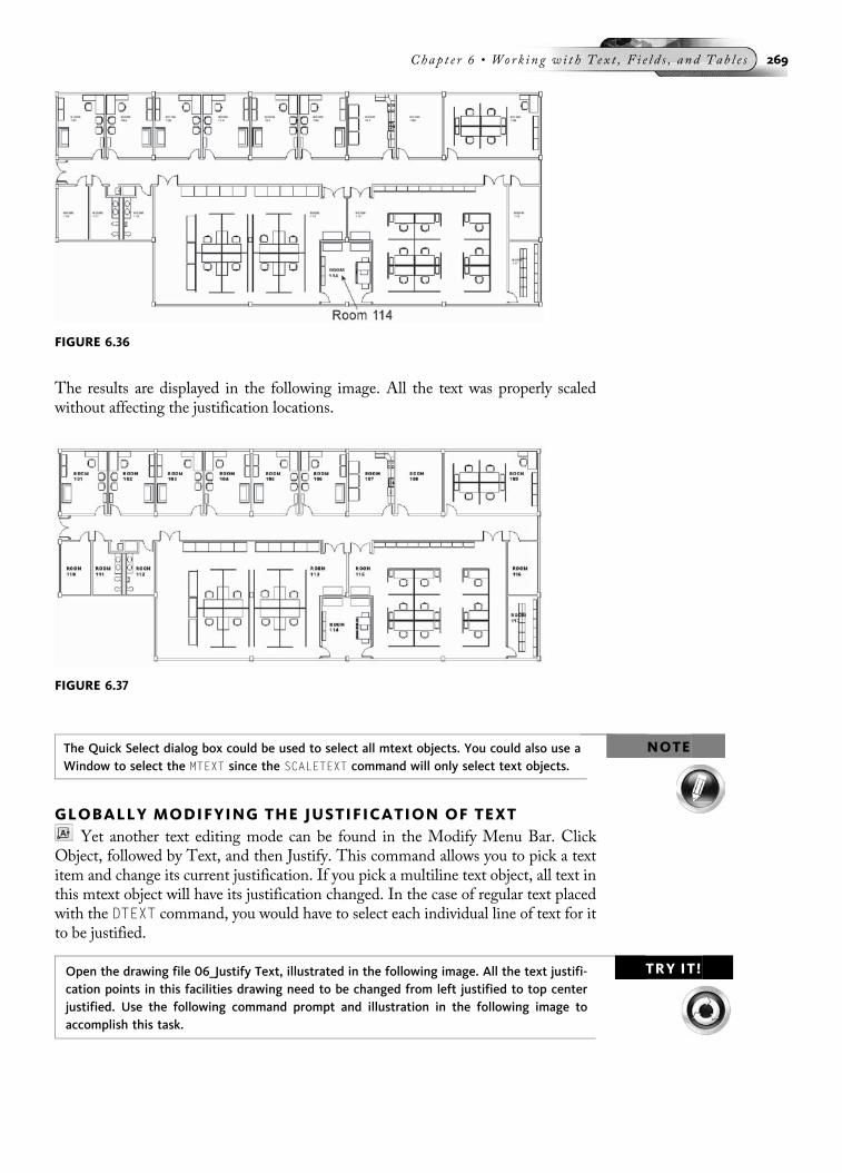
The results are displayed in the following image. All the text was properly scaledwithout affecting the justification locations.
NOTEThe Quick Select dialog box could be used to select all mtext objects. You could also use aWindow to select the MTEXT since the SCALETEXT command will only select text objects.
GLOBALLY MODIFYING THE JUSTIFICATION OF TEXTYet another text editing mode can be found in the Modify Menu Bar. Click
Object, followed by Text, and then Justify. This command allows you to pick a textitem and change its current justification. If you pick a multiline text object, all text inthis mtext object will have its justification changed. In the case of regular text placedwith the DTEXT command, you would have to select each individual line of text for itto be justified.
TRY IT!Open the drawing file 06_Justify Text, illustrated in the following image. All the text justifi-cation points in this facilities drawing need to be changed from left justified to top centerjustified. Use the following command prompt and illustration in the following image toaccomplish this task.
FIGURE 6.36
FIGURE 6.37
Chap t e r 6 • Work i n g w i t h T ex t , F i e l d s , a nd Tab l e s 269

Command: JUSTIFYTEXT
Select objects: (Select all 17 text objects)
Select objects: (Press ENTER to continue)
Enter a justification option
[Left/Align/Fit/Center/Middle/Right/TL/TC/TR/ML/MC/MR/BL/BC/BR] <Left>: TC (For Top Center)
The results are illustrated in the following image. All text objects have been globallychanged from left justified to top center justified.
SPELL-CHECKING TEXTSpell-checking is an important part of the drawing documentation process. Words,notes, or engineering terms that are spelled correctly elevate the drawing to a higherlevel of professionalism. Spell-checking a drawing can be activated through theMenuBar, Ribbon, or Text toolbar, as shown in the following image.
FIGURE 6.38
FIGURE 6.39
270 Au t oCAD 2010 Tu t o r f o r Eng i n e e r i n g Graph i c s

Issue the SPELL command and click the Start button to begin the spell-check. The“Where to Check” drop-down list provides the option of checking the entire drawingor limiting the check to the current space/layout or to only selected text items. The“Not in Dictionary” box displays the first word that is suspected of being spelledwrong. It wasn’t found in the current dictionary. A drop-down list and Dictionariesbutton is provided to select other dictionaries. The Suggestions area displays all pos-sible alternatives to the word identified as being misspelled. The Ignore button allowsyou to skip the current word; this would be applicable especially in the case of acro-nyms such as CAD and GDT. Clicking Ignore All skips all remaining words thatmatch the current word. The Change button replaces the word “Not in the dictio-nary” with the word in the Suggestions box. The “Add to Dictionary” button addsthe current word to the current dictionary. In the following image, the word“DIRECION” was identified as being misspelled. Notice that the correct word,“DIRECTION,” is listed as a suggested correction. Clicking the Change button re-places the misspelled word and continues with the spell-checking operation untilcompleted.
After completing the spell-checking operation, the mtext object is displayed in thefollowing image.
FIGURE 6.40
FIGURE 6.41
Chap t e r 6 • Work i n g w i t h T ex t , F i e l d s , a nd Tab l e s 271

TRY IT! Open the drawing 06_Spell Check1 and perform a spell-check operation on this mtextobject.
CREATING DIFFERENT TEXT STYLESA text style is a collection of settings that are applied to text placed with the DTEXT orMTEXT command. These settings could include presetting the text height and font, inaddition to providing special effects, such as an oblique angle for inclined text.Choose Text Style. . . from the, Annotation tab of the Ribbon, Format Menu Bar,or from the Text toolbar, shown in the following image.
FIGURE 6.44
FIGURE 6.43
FIGURE 6.42
272 Au t oCAD 2010 Tu t o r f o r Eng i n e e r i n g Graph i c s
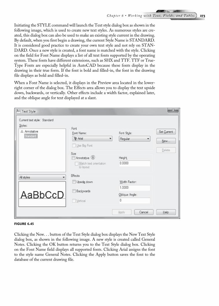
Initiating the STYLE command will launch the Text style dialog box as shown in thefollowing image, which is used to create new text styles. As numerous styles are cre-ated, this dialog box can also be used to make an existing style current in the drawing.By default, when you first begin a drawing, the current Style Name is STANDARD.It is considered good practice to create your own text style and not rely on STAN-DARD. Once a new style is created, a font name is matched with the style. Clickingon the field for Font Name displays a list of all text fonts supported by the operatingsystem. These fonts have different extensions, such as SHX and TTF. TTF or True-Type Fonts are especially helpful in AutoCAD because these fonts display in thedrawing in their true form. If the font is bold and filled-in, the font in the drawingfile displays as bold and filled-in.
When a Font Name is selected, it displays in the Preview area located in the lower-right corner of the dialog box. The Effects area allows you to display the text upsidedown, backwards, or vertically. Other effects include a width factor, explained later,and the oblique angle for text displayed at a slant.
Clicking the New. . . button of the Text Style dialog box displays the New Text Styledialog box, as shown in the following image. A new style is created called GeneralNotes. Clicking the OK button returns you to the Text Style dialog box. Clickingon the Font Name field displays all supported fonts. Clicking Arial assigns the fontto the style name General Notes. Clicking the Apply button saves the font to thedatabase of the current drawing file.
FIGURE 6.45
Chap t e r 6 • Work i n g w i t h T ex t , F i e l d s , a nd Tab l e s 273

The Text Style Control BoxThe Styles toolbar provides a convenient method for changing styles. Use the TextStyle Control box illustrated in the following image on the left to make an existingtext style current. This control box allows you to change from one text style to anothereasily. The Text panel of the Ribbon also provides a drop-down list for selecting thecurrent text style in a more graphical form, as shown in the following image on theright.
NOTE You can also highlight a text object and use the Text Style Control box to change theselected text to a different text style. This action is similar to changing an object from onelayer to another through the Layer Control box.
FIELDSFields are a type of intelligent text that you can add to your drawings. In the followingimage, fields are identified by a distinctive gray background, which is not present onregular text. Fields are intended for items that tend to change during the life cycle of adrawing, such as the designer’s name, checker, creation date of the drawing, anddrawing number, as shown in the following image.
FIGURE 6.46
FIGURE 6.47
FIGURE 6.48
274 Au t oCAD 2010 Tu t o r f o r Eng i n e e r i n g Graph i c s

The FIELD command can be selected from the Insert Menu Bar, as shown in thefollowing image on the left. This activates the Field dialog box, which consists ofField categories, Field names, Author, and Format information. Rather than cyclethrough all field names, you can pick a field category, which limits the amount ofitems in the Field names area.
By default, all fields are available under the Field names area. You can specify a certainField category to narrow down the list of field names. Illustrated in the following im-age on the left is a list of all field categories; the Date & Time category is selected.This activates specific field names only related to this category, as shown in the fol-lowing image on the right. With the Field name SaveDate highlighted, notice all theexamples that pertain to when the drawing was last saved. There is also a Hints areathat gives examples of various month, day, and year notations.
Fields and Multiline TextWhile placing multiline text, you can create a field through the Text Editor Ribbon,as shown in the following image. This allows you to place numerous fields at onetime. Right-clicking on the text box and then picking Insert Field from the menualso activates the Field dialog box.
FIGURE 6.49
FIGURE 6.50
FIGURE 6.51
Chap t e r 6 • Work i n g w i t h T ex t , F i e l d s , a nd Tab l e s 275

The results of creating a field are illustrated in the following image on the left. In thisexample, the following field categories were used: Filename and Date. The time entryis a subset of the Date field.
Whenever field information changes, such as the date and time, you may needto update the field in order to view the latest information. Updating fields is ac-complished by clicking Update Fields, which is located under the Tools Menu Bararea, as shown in the following image in the middle. When picking this command,you are prompted to select the field. In the following image on the right, the dateautomatically changed. Whenever you open a drawing that contains fields, thefields will automatically update to reflect the most up-to-date information.
Fields and Drawing PropertiesWhen creating some fields, information is displayed as a series of four dashed lines.This is to signify that the information contained in the field name either has not beenentered or has not been updated. In the following image, the Author, Subject, andTitle fields need to be completed before the correct information displays.
In the previous illustration of the Author, Subject, and Title field names, activatingthe Drawing Properties dialog box (pick Drawing Properties from the File MenuBar), as shown in the following image on the left, allows you to fill in this informa-tion.When returning to the drawing, click the ToolsMenu Bar, select Update Fields,and pick the field that needs updating. The information listed in the Drawing Prop-erties dialog box will be transferred to the specific fields, as shown in the followingimage on the right.
FIGURE 6.52
FIGURE 6.53
276 Au t oCAD 2010 Tu t o r f o r Eng i n e e r i n g Graph i c s
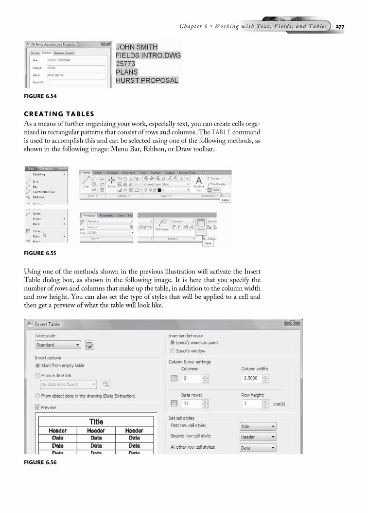
CREATING TABLESAs a means of further organizing your work, especially text, you can create cells orga-nized in rectangular patterns that consist of rows and columns. The TABLE commandis used to accomplish this and can be selected using one of the following methods, asshown in the following image: Menu Bar, Ribbon, or Draw toolbar.
Using one of the methods shown in the previous illustration will activate the InsertTable dialog box, as shown in the following image. It is here that you specify thenumber of rows and columns that make up the table, in addition to the column widthand row height. You can also set the type of styles that will be applied to a cell andthen get a preview of what the table will look like.
FIGURE 6.54
FIGURE 6.55
FIGURE 6.56
Chap t e r 6 • Work i n g w i t h T ex t , F i e l d s , a nd Tab l e s 277
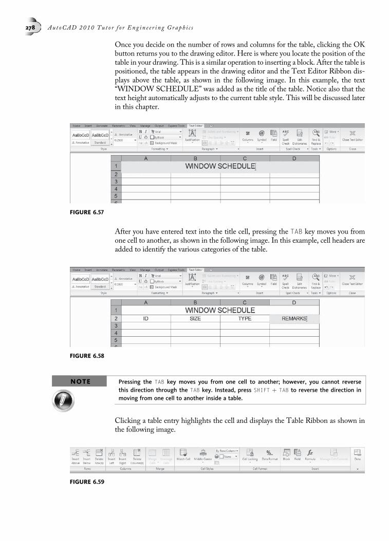
Once you decide on the number of rows and columns for the table, clicking the OKbutton returns you to the drawing editor. Here is where you locate the position of thetable in your drawing. This is a similar operation to inserting a block. After the table ispositioned, the table appears in the drawing editor and the Text Editor Ribbon dis-plays above the table, as shown in the following image. In this example, the text“WINDOW SCHEDULE” was added as the title of the table. Notice also that thetext height automatically adjusts to the current table style. This will be discussed laterin this chapter.
After you have entered text into the title cell, pressing the TAB key moves you fromone cell to another, as shown in the following image. In this example, cell headers areadded to identify the various categories of the table.
NOTE Pressing the TAB key moves you from one cell to another; however, you cannot reversethis direction through the TAB key. Instead, press SHIFT þ TAB to reverse the direction inmoving from one cell to another inside a table.
Clicking a table entry highlights the cell and displays the Table Ribbon as shown inthe following image.
FIGURE 6.57
FIGURE 6.58
FIGURE 6.59
278 Au t oCAD 2010 Tu t o r f o r Eng i n e e r i n g Graph i c s

The Table Ribbon has numerous controls for manipulating tables. The followingchart will explain these buttons.
Button Tool Function
Insert Row Above Inserts a row above a selected cell
Insert Row Below Inserts a row below a selected cell
Delete Row Deletes an entire row
Insert Column Left Inserts a column to the left of a selected cell
Insert Column Right Inserts a column to the right of a selected cell
Delete Column Deletes an entire column
Merge Cells Merges all selected cells or cells by row or column
Unmerge Cells Unmerges selected cells
Cell Borders Launches the Cell Border Properties dialog boxdesigned to control the display of cell borders
Middle Center Align Displays nine text alignment modes that deal withtables
Locking Displays a menu used for locking the cell content, cellformat, or both. Also used for unlocking cells
Data Format Launches the Table Cell Format dialog box used fordefining the data type of a cell or group of cells
Insert Block Launches the Insert a Block in a Table dialog box usedfor placing and fitting blocks in table cells
Insert Field Launches the Field dialog box designed for creating afield in a table cell
Insert Formula Displays a menu used for performing summations andother calculations on a group of cells
Manage Cell Content Displays the Manage Cell Content dialog box used forchanging the order of cell content as well as changingthe direction in which cell content will display
Match Cell Matches the contents of a source cell withdestination cell
Cell Style Displays a drop-down list that allows you to change to adifferent cell style
Link Cell Displays the Select Data Link dialog box that lists thecurrent links with Excel
Download Changes Used for downloading changes from a source file to thetable
Merging Cells in a TableThere are times when you need to merge cells in the rows or columns of a table.To accomplish this, first pick inside a cell, then hold down the SHIFT key as youpick the cells you want to merge with it. Then pick the Merge Cells button followed
Chap t e r 6 • Work i n g w i t h T ex t , F i e l d s , a nd Tab l e s 279

by All from the menu, as shown in the following image. The final example of mergingthe cells that contain the “FLOOR” text is also shown in the following image.
Modifying a TableThe modification of table cells, table rows, and even the overall size of the table isgreatly enhanced through the use of grips. You can achieve different results depend-ing on the table grip that is selected. For instance, first select the table to display allgrips. Then, select the grip in the upper-left corner of the table and move your cursor.This action moves the table to a new location. Selecting the grip in the upper-rightcorner of the table and then dragging your cursor left or right increases or decreasesthe spacing of all table columns. Selecting the grip in the lower-left corner of the tableincreases the spacing between rows. Study the following image to see how other gripsaffect the sizing of a table. Grips will be covered in greater detail in chapter 7.
NOTE When using grips to stretch rows or columns in a table, you may want to turn runningOSNAP off. Otherwise, if OSNAP Endpoint is set, your table may stretch back to its originallocation, giving the appearance that the operation did not work.
Autofilling Cells in a TableTables can, at times, require a lot of repetitive data entry. In the table example in thefollowing image, you could easily copy and paste identical information from one cellto the next. Another very powerful tool exists in tables that allows text to be created
FIGURE 6.60
FIGURE 6.61
280 Au t oCAD 2010 Tu t o r f o r Eng i n e e r i n g Graph i c s

incrementally such as the room numbers in the image. This is accomplished throughthe Autofill feature of tables.
Cell 3A illustrated in the following image on the left is populated with the number“1.” If you know the next number below the “1” will be “2” and so on, first click in cell3A. Notice the light blue diamond shaped grip in the lower-right corner of the cell.Click on this grip and move your cursor in a downward direction as shown in thefollowing image in the middle. You will notice your cursor changing to differentnumbers the more you drag the cursor. This image illustrates how the numbers “1”through “8” can be autofilled. The results are shown in the following image on theright with the Autofill feature creating the proper incremental data.
Autofill also works with regular text entries. If you want to reproduce the word“VINYL” in the remaining cells below, click on the cell with the word. When thelight blue diamond grip appears, drag your cursor to the cells that will contain thesame text. The results are shown in the following image on the right with the Autofillfeature being used to automatically place identical text entries into table cells.
FIGURE 6.62
FIGURE 6.63
FIGURE 6.64
Chap t e r 6 • Work i n g w i t h T ex t , F i e l d s , a nd Tab l e s 281
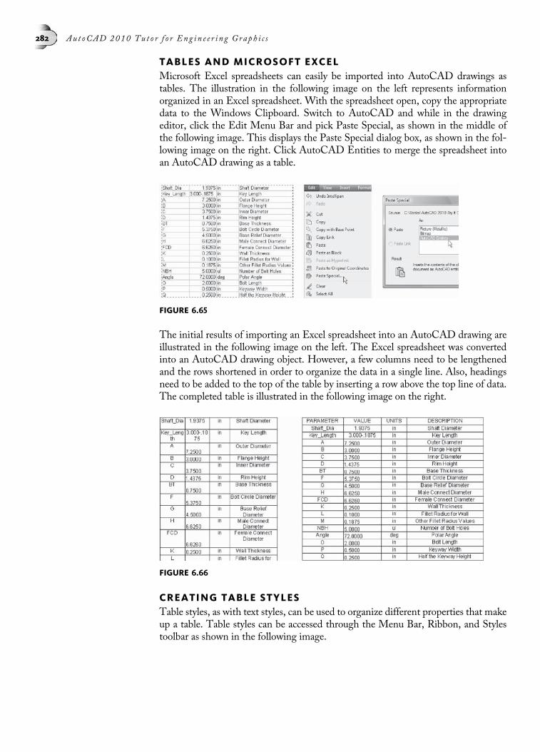
TABLES AND MICROSOFT EXCELMicrosoft Excel spreadsheets can easily be imported into AutoCAD drawings astables. The illustration in the following image on the left represents informationorganized in an Excel spreadsheet. With the spreadsheet open, copy the appropriatedata to the Windows Clipboard. Switch to AutoCAD and while in the drawingeditor, click the Edit Menu Bar and pick Paste Special, as shown in the middle ofthe following image. This displays the Paste Special dialog box, as shown in the fol-lowing image on the right. Click AutoCAD Entities to merge the spreadsheet intoan AutoCAD drawing as a table.
The initial results of importing an Excel spreadsheet into an AutoCAD drawing areillustrated in the following image on the left. The Excel spreadsheet was convertedinto an AutoCAD drawing object. However, a few columns need to be lengthenedand the rows shortened in order to organize the data in a single line. Also, headingsneed to be added to the top of the table by inserting a row above the top line of data.The completed table is illustrated in the following image on the right.
CREATING TABLE STYLESTable styles, as with text styles, can be used to organize different properties that makeup a table. Table styles can be accessed through the Menu Bar, Ribbon, and Stylestoolbar as shown in the following image.
FIGURE 6.65
FIGURE 6.66
282 Au t oCAD 2010 Tu t o r f o r Eng i n e e r i n g Graph i c s

Clicking on either one of the Table Style listings shown in the previous image willdisplay the Table Style dialog box, as shown in the following image. Clicking theNew button displays the Create New Table Style dialog box, in which you enter thename of the table style.
Clicking Continue allows you to make various changes to a table based on the type ofcell. For example, in the following image three tabs can be used to make changes tothe text that occupies a cell in a table based on whether the text is cell data, the columnheads of a cell, or even the title cell of the table. These text settings can be used toemphasize the information in the cells. For example, you would want the title of thetable to stand out with a larger text height than the column headings. You might alsowant the column headings to stand out over the data in the cells below. Also, as in thefollowing image, you can change the direction of the table. By default, a table is cre-ated in the downward direction. You may want to change this direction to upward.
FIGURE 6.67
FIGURE 6.68
Chap t e r 6 • Work i n g w i t h T ex t , F i e l d s , a nd Tab l e s 283

The following image illustrates three tabs containing information that can be modi-fied for the cell type. In this image, the Data cell type is selected.
To make changes to the Header or Title cells, select the cell type in the Cell Stylesfield, as shown in the following image, and modify the information in the tabs asdesired.
FIGURE 6.69
FIGURE 6.70
284 Au t oCAD 2010 Tu t o r f o r Eng i n e e r i n g Graph i c s

TUTORIAL EXERCISE : 06_PUMP_ASSEMBLY.DWG
PurposeThis tutorial is designed to create numerous text styles and add different types of textobjects to the title block illustrated in the previous image.
System SettingsSince this drawing is already provided on the CD, open an existing drawing file called06_Pump_Assembly. Follow the steps in this tutorial for creating a number of text stylesand then placing text in the title block area. Check to see that the following Object Snapmodes are already set: Endpoint, Extension, Intersection, Center.
LayersVarious layers have already been created for this drawing. Since this tutorial covers thetopic of text, the current layer is Text.
FIGURE 6.71
FIGURE 6.72
Chap t e r 6 • Work i n g w i t h T ex t , F i e l d s , a nd Tab l e s 285

Suggested CommandsOpen the drawing called 06_Pump_Assembly. In this tutorial you will create four textstyles called Company Info, Title Block Text, Disclaimer, and General Notes. The text styleCompany Info will be applied to one part of the title block. Title Block Text will be appliedto a majority of the title block, where questions such as Drawn By, Date, and Scale areasked. Also, the Drawn By, Date, and Drawing Number will be supplied by creating fields.A disclaimer will be imported into the title block in the Disclaimer text style. Finally, aseries of notes will be imported in the General Notes text style. Once these general notesare imported, a spell-check operation will be performed on the notes.
STEP 1Opening the drawing file 06_Pump _Assembly displays an image similar to the followingimage. The purpose of this tutorial is to fill in the title block area with a series of text, mul-tiline text, and field objects. Also, a series of general notes will be placed to the right ofthe pump assembly. Before you place the text, four text styles will be created to assistwith the text creation. The four text styles are also identified in the following image. Thetext style Company Info will be used to place the name of the company and drawing title.Information in the form of scale, date, and who performed the drawing will be handled bythe text style Title Block Text. A disclaimer will be imported from an existing .TXT file avail-able on the CD; this will be accomplished in the Disclaimer text style. A listing of six gen-eral notes is also available on the CD. It is in .RTF format, originally created in MicrosoftWord. It will be imported into the drawing and placed in the General Notes text style.
Since you will be locating various justification points for the placement of text, turn OSNAPoff by single-clicking OSNAP in the Status bar at the bottom of the display screen.
STEP 2Before creating the first text style, first see what styles are already defined in the drawingby choosing Text Style. . . from the Format Menu Bar, as shown in the following image onthe left. This displays the Text Style dialog box, as shown in the following image on theright. The Styles text box displays the current text styles defined in the drawing. EveryAutoCAD drawing contains the STANDARD text style. This is created by default and cannotbe deleted. Also, the Title Block Headings text style was already created. This text style wasused to create the headings in each title block box, for example, “Scale” and “Date.”
FIGURE 6.73
FIGURE 6.74
286 Au t oCAD 2010 Tu t o r f o r Eng i n e e r i n g Graph i c s

STEP 3Create the first text style by clicking the New. . . button, as shown in the following image.This activates the New Text Style dialog box, also shown in the following image. For StyleName, enter Company Info. When finished, click the OK button. This takes you back tothe Text Style dialog box, as shown in the following image on the right. In the Font area,verify that the name of the font is Arial. Notice the font appearing in the Preview area. Ifnecessary, click the Apply button to complete the text style creation process.
STEP 4Using the same procedure outlined in Step 3, create the following new text styles:Disclaimer, General Notes, and Title Block Text. Verify that the Arial font is assigned toall of these style names. Keep all other remaining default text settings. When finished,your display should appear similar to the following image.
STEP 5Make the Company Info style current by selecting it in the Style text box and clicking theSet Current button. Add multiline text under the Company Info text style. Change thetext height for both entries to .25 units. Middle-Center justify the text. Add the textPUMP ASSEMBLY inside the text formatting box. Click the Close Text Editor button toplace the text. Repeat this procedure for placing the text THE K-GROUP in the next titleblock space.
Command: MT (For MTEXT)
MTEXT Current text style: “Company Info” Text height: 0.20Annotative: No
Specify first corner: (Pick a point at “A”)
FIGURE 6.75
FIGURE 6.76
Chap t e r 6 • Work i n g w i t h T ex t , F i e l d s , a nd Tab l e s 287

Specify opposite corner or [Height/Justify/Line spacing/Rotation/Style/Width/Columns]: H (For Height)
Specify height <0.20>: .25
Specify opposite corner or [Height/Justify/Line spacing/Rotation/Style/Width/Columns]: J (For Justify)
Enter justification [TL/TC/TR/ML/MC/MR/BL/BC/BR] <TL>: MC(For Middle Center)
Specify opposite corner or [Height/Justify/Line spacing/Rotation/Style/Width/Columns]: (Pick a point at “B”)
STEP 6Change the current text style to Title Block Text, as shown in the following image. Beginplacing fields into the title block. Click Insert Field under the Insert Menu Bar, as shown inthe following image. When the Field dialog box appears, pick Author under the Fieldnames and click the OK button to dismiss the dialog box. Place this in the space identifiedas Drawn By, as shown in the following image on the right. Use a height of .10 for all ofthe next series of entries. Notice the appearance of four dashes inside a gray rectangle.This will be filled in when you enter your name in the appropriate area of the Propertiesdialog box later on in this exercise. Use the following command sequence to assist in theplacing of this first field.
Command: FIELD
MTEXT Current text style: “Title Block Text” Text height:0.20
Specify start point or [Height/Justify]: H (For Height)
Specify height <0.20>: .10
Specify start point or [Height/Justify]: (Pick a point insideof the area identified as Drawn By)
FIGURE 6.77
288 Au t oCAD 2010 Tu t o r f o r Eng i n e e r i n g Graph i c s

STEP 7Place a new field for the Date category. Activate the Field dialog box, as shown in thefollowing image, and pick the Date Field name. Also select the format of the date fromthe list of examples located in this dialog box. Place this field under the DATE heading,as shown in the following image. Notice that the date is automatically calculated basedon the current date setting on your computer.
Command: FIELD
MTEXT Current text style: “Title Block Text” Text height:0.10
Specify start point or [Height/Justify]: (Pick a point insideof the area identified as Date)
STEP 8Place a new field for the Filename category. Activate the Field dialog box, as shown in thefollowing image, and pick the Filename Field name. Pick Uppercase for the Format. Alsoclick the radio button next to Filename only. This limits the number of letters in the draw-ing name. Locate this field under the DWG NO. heading name, as shown in the followingimage.
Command: FIELD
MTEXT Current text style: “Title Block Text” Text height:0.10
Specify start point or [Height/Justify]: (Pick a point insideof the area identified as DWG NO.)
FIGURE 6.78
FIGURE 6.79
Chap t e r 6 • Work i n g w i t h T ex t , F i e l d s , a nd Tab l e s 289

STEP 9While still in the Title Block Text style, use the Single Line text command and add thefollowing entries to the title block using the following prompts and image as guides.
Command: DT (For DTEXT)
Current text style: “Title Block Text” Text height: 0.10Annotative: No
Specify start point of text or [Justify/Style]: (Pick a pointapproximately at “A”)
Specify height <0.10>: (Press ENTER to accept this defaultvalue)
Specify rotation angle of text <0d0’>: (Press ENTER to acceptthis default value)
Enter text: ADRIAN CULPEPPER (After this text is entered,pick approximately at “B”)
Enter text: (Use the table and figure below to enter theremaining text; when complete, press ENTER twice to exit thiscommand)
Text Title Block Area
B SIZE (at “B”)
JOHNNY MOSS APPROVED BY (at “C”)
1 0 ¼ 1 0-0 00 SCALE (at “D”)
0 REV (at “E”)
1 OF 1 SHEET (at “F”)
FIGURE 6.80
FIGURE 6.81
290 Au t oCAD 2010 Tu t o r f o r Eng i n e e r i n g Graph i c s

STEP 10Open the Text Style dialog box and double-click the Disclaimer text style, as shown inthe following image. Activate the MTEXT command, pick a first corner at “A,” and pick asecond corner at “B.” While in the Text Formatting dialog box, use the toolbar to changethe text height to .08, right-click on the text editor, and pick Import Text from the menu,as shown in the following image.
Command: MT (For MTEXT)
MTEXT Current text style: “Disclaimer” Text height: 0.20Annotative: No
Specify first corner: (Pick a point at “A”)
Specify opposite corner or [Height/Justify/Line spacing/Rotation/Style/Width/Columns]: (Pick a point at “B”)
When the Select File dialog box appears, click the location of your CD and pick the file06_Disclaimer.txt, as shown in the following image on the left. Since this informationwas already created in an application outside AutoCAD, it will be imported into theMultiline Text Editor. Click the OK button to place the text in the title block, as shownin the following image on the right.
STEP 11Before placing the last text object, zoom to the extents of the drawing. Then click theGeneral Notes text style located in the Text Style Control box (located on the Styles tool-bar or the Annotate tab of the Ribbon, as shown in the following image on the left. Usethe MTEXT command to create a rectangle to the right of the Pump Assembly, as shownin the following image on the right. This will be used to hold a series of general notes inmultiline text format.
Command: MT (For MTEXT)
Current text style: “General Notes” Text height: 0.12Annotative: No
FIGURE 6.82
FIGURE 6.83
Chap t e r 6 • Work i n g w i t h T ex t , F i e l d s , a nd Tab l e s 291

Specify first corner: (Pick a point at “A”)
Specify opposite corner or [Height/Justify/Line spacing/Rotation/Style/Width/Columns]: (Pick a point at “B”)
When the Multiline Text Editor appears, click the Import Text. . . button, as shown in thefollowing image on the left. Then click the location of your CD and select the file06_GENERAL_NOTES.rtf, as shown in the following image on the right. Make sure the filetype you are searching for in the Select File dialog box is set to RTF. This RTF file (rich textfile) was created outside AutoCAD in Microsoft Word.
STEP 12The results of this operation are displayed in the following image on the left. However,the text appears to be displayed in a different font. This is due to the fact that when filesare imported in .RTF format, the original format of the text is kept. This means that theTimes New Roman font was used even though the current text style uses the Arial font.
While still inside the Text Editor Ribbon, highlight all the general notes and change thefont to Arial, as shown in the following image on the right.
FIGURE 6.84
FIGURE 6.85
292 Au t oCAD 2010 Tu t o r f o r Eng i n e e r i n g Graph i c s

One more item needs to be taken care of before you leave the Text Editor Ribbon. High-light all the text directly under the heading of GENERAL NOTES, as shown in the follow-ing image. Click the Numbering button. This creates a numbered list based on allhighlighted lines of text, as shown in the following image. If necessary, change the taband paragraph indent to match the following image. When finished, click the Close TextEditor button to return to the drawing and place the general notes.
STEP 13Use the SPELL command and pick “Selected objects” from the Where to check field. Pickthe Select objects button and click the multiline text object that holds the six generalnotes. Click the Start button and the Check Spelling dialog box appears, as shown inthe following image; make the corrections to the words CONCRETE, MOTOR, andPROPERLY.
FIGURE 6.86
FIGURE 6.87
Chap t e r 6 • Work i n g w i t h T ex t , F i e l d s , a nd Tab l e s 293

STEP 14In a previous step, you created a field for the author of the drawing. However, this fielddisplayed as empty. You will now complete the title block by filling in the information andcompleting the Author field. Click Drawing Properties, found under the File Menu Bar, asshown in the following image on the left. When the 06_Pump Assembly.dwg Propertiesdialog box appears, enter your name in the Author text box, as shown in the followingimage in the middle.
When you return to your drawing, the Author field located in the title block is still notreflecting your name. Click Update Fields, found under the Tools Menu Bar area as shownin the following image on the right, and select the field to place your name in the titleblock.
STEP 15The completed title block and general notes area are displayed in the following image.
FIGURE 6.88
FIGURE 6.89
294 Au t oCAD 2010 Tu t o r f o r Eng i n e e r i n g Graph i c s

TUTORIAL EXERCISE : 06_TABLE.DWG
PurposeThis tutorial is designed to create a new table style and then a new table object, as shownin the previous image.
System SettingsSince this drawing is already provided on the CD, open an existing drawing file called06_Table. Two text styles are already created for this exercise; namely Architectural andTitle.
LayersA Table layer is already created for this drawing.
FIGURE 6.90
FIGURE 6.91
Chap t e r 6 • Work i n g w i t h T ex t , F i e l d s , a nd Tab l e s 295

Suggested CommandsOpen the drawing called 06_Table. You will create a new table style called Door Schedule.Changes will be made to the Data, Heading, and Data fields through the Table Styledialog box. Next, you will create a new table consisting of six columns and eleven rows.Information related to the door schedule will be entered in at the Title, Heading, andData fields.
STEP 1Open the existing drawing file 06_Table. Activate the Text Style dialog box (STYLE com-mand) and notice the two text styles already created, as shown in the following image onthe left, namely, Title and Architectural. The Title text style uses the Arial font whileArchitectural uses the CityBlueprint font.
Next, activate the Table Style dialog box and create a new table style called Door Sched-ule, as shown in the following image on the right.
STEP 2Clicking the Continue button located in the previous image takes you to the main NewTable Style dialog box. Use the information in the following image to change the proper-ties with the Cell styles set to Data.
Use the information in the following image to change the properties under the Headercell style.
FIGURE 6.92
FIGURE 6.93
FIGURE 6.94
296 Au t oCAD 2010 Tu t o r f o r Eng i n e e r i n g Graph i c s

Use the information in the following image to change the properties under the Title cellstyle.
STEP 3Click the OK button to return to the Table Style dialog box. Verify the Door Schedulestyle is the current table style, as shown in the following image (you can double-clickany table style name from the list to make it current). When finished, close the TableStyle dialog box.
STEP 4Activate the TABLE command and while in the Insert Table dialog box, create a table con-sisting of six columns and eleven rows using the new Door Schedule table style. Click theOK button to place the table in a convenient location on your screen.
FIGURE 6.95
FIGURE 6.96
FIGURE 6.97
Chap t e r 6 • Work i n g w i t h T ex t , F i e l d s , a nd Tab l e s 297
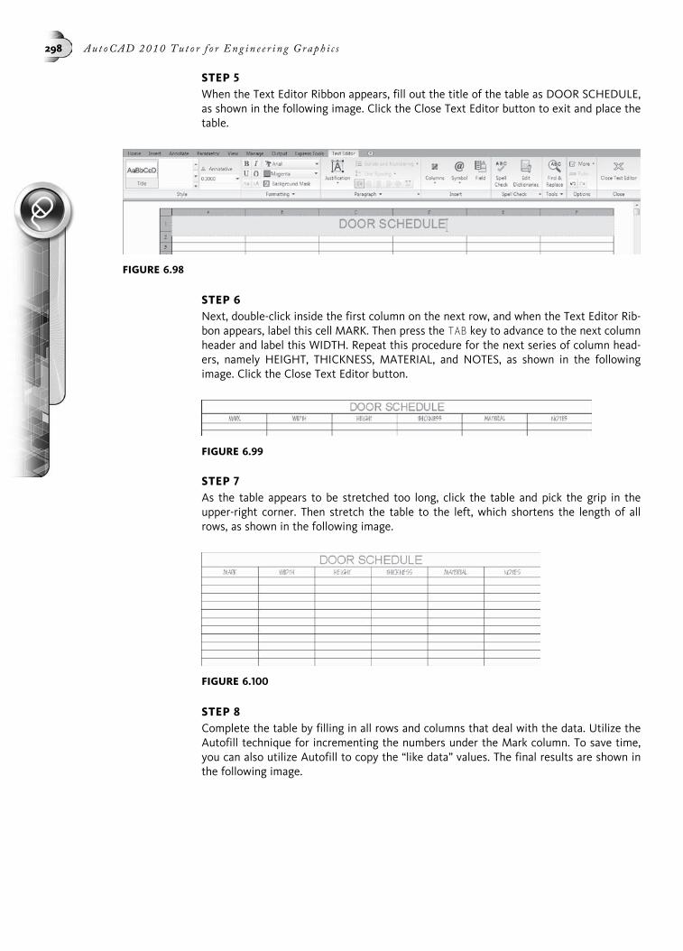
STEP 5When the Text Editor Ribbon appears, fill out the title of the table as DOOR SCHEDULE,as shown in the following image. Click the Close Text Editor button to exit and place thetable.
STEP 6Next, double-click inside the first column on the next row, and when the Text Editor Rib-bon appears, label this cell MARK. Then press the TAB key to advance to the next columnheader and label this WIDTH. Repeat this procedure for the next series of column head-ers, namely HEIGHT, THICKNESS, MATERIAL, and NOTES, as shown in the followingimage. Click the Close Text Editor button.
STEP 7As the table appears to be stretched too long, click the table and pick the grip in theupper-right corner. Then stretch the table to the left, which shortens the length of allrows, as shown in the following image.
STEP 8Complete the table by filling in all rows and columns that deal with the data. Utilize theAutofill technique for incrementing the numbers under the Mark column. To save time,you can also utilize Autofill to copy the “like data” values. The final results are shown inthe following image.
FIGURE 6.98
FIGURE 6.99
FIGURE 6.100
298 Au t oCAD 2010 Tu t o r f o r Eng i n e e r i n g Graph i c s
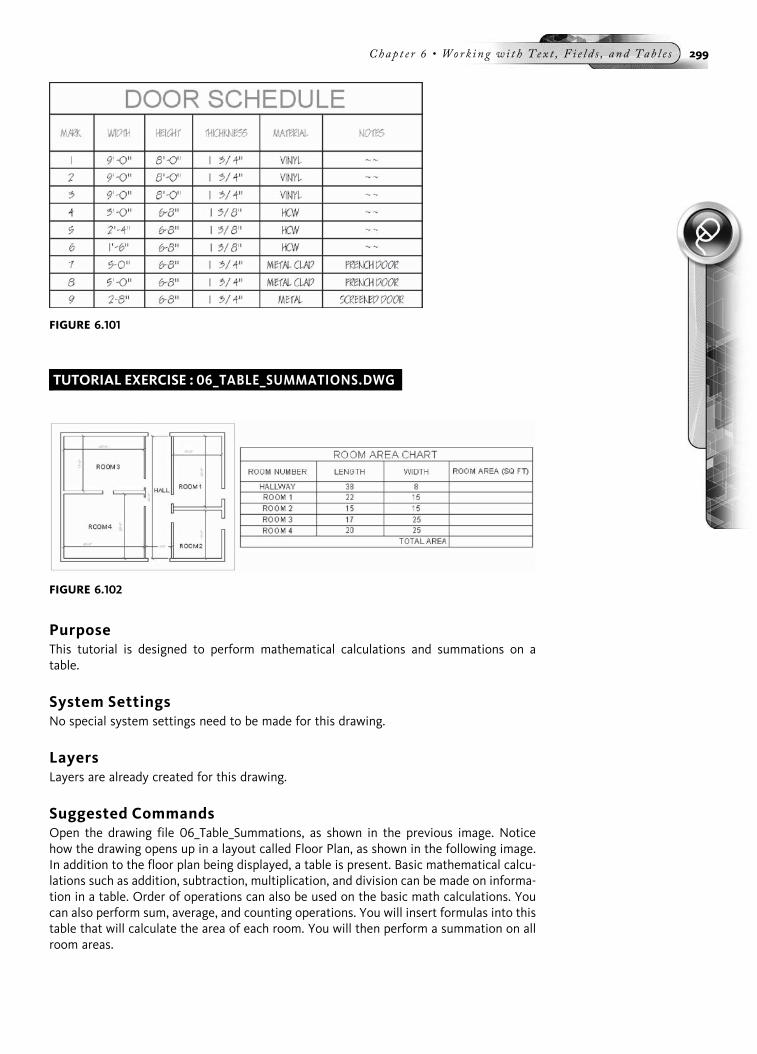
TUTORIAL EXERCISE : 06_TABLE_SUMMATIONS.DWG
PurposeThis tutorial is designed to perform mathematical calculations and summations on atable.
System SettingsNo special system settings need to be made for this drawing.
LayersLayers are already created for this drawing.
Suggested CommandsOpen the drawing file 06_Table_Summations, as shown in the previous image. Noticehow the drawing opens up in a layout called Floor Plan, as shown in the following image.In addition to the floor plan being displayed, a table is present. Basic mathematical calcu-lations such as addition, subtraction, multiplication, and division can be made on informa-tion in a table. Order of operations can also be used on the basic math calculations. Youcan also perform sum, average, and counting operations. You will insert formulas into thistable that will calculate the area of each room. You will then perform a summation on allroom areas.
FIGURE 6.101
FIGURE 6.102
Chap t e r 6 • Work i n g w i t h T ex t , F i e l d s , a nd Tab l e s 299

STEP 1Zoom in to the table. You will first assign a formula that calculates the area of theHallway. Click the cell that will hold the area of the Hallway; the Table toolbar displaysas shown in the following image. Click the Insert Formula button, and when the menudisplays, as shown in the following image, click Equation.
STEP 2Clicking the Equation in the previous step displays the Text Editor Ribbon, as shown inthe following image. In the highlighted cell, you will need to multiply the Hallway length(38) by the width (8). You should not enter these numbers directly into the equation cell.Rather, enter the column and row number of each value. For example, the value 38 isidentified by B3 and the value 8 is identified by C3. Enter these two cell identifiers sepa-rated by the multiplication symbol (*). Your display should appear similar to the followingimage.
STEP 3Exiting the Text Formatting dialog box creates a field in the cell the calculation was beingperformed in, as shown in the following image. This field is easily recognized by the typi-cal gray text background. Placing information as a field means if the information in thelength and width cells changes, the field information will automatically recalculate itself.
FIGURE 6.103
FIGURE 6.104
300 Au t oCAD 2010 Tu t o r f o r Eng i n e e r i n g Graph i c s

STEP 4Follow steps 1 and 2 to calculate the area of Room 1. Be careful to use the correct cellidentifying letters and numbers for this area calculation, as shown in the following image.You could also use the Autofill feature of tables as shown in earlier portions of this chap-ter for creating incremental copies of cells.
NOTEAn equation can be started by simply clicking on a cell and typing the equal “¼” sign.
STEP 5Continue inserting equations to calculate the area of Rooms 2, 3, and 4, as shown in thefollowing image.
FIGURE 6.105
FIGURE 6.106
FIGURE 6.107
Chap t e r 6 • Work i n g w i t h T ex t , F i e l d s , a nd Tab l e s 301

STEP 6With the individual room areas calculated, you will now perform a summation that willadd all current area fields. First, click on the cell in which the summation will be per-formed. When the Table toolbar appears, click the Insert Formula button followed bySum, as shown in the following image.
STEP 7After selecting Sum from the menu in the previous step, you will be prompted for thefollowing:
• Select first corner of table cell range.
• Answer this prompt by picking a point inside the upper-left corner of the cell thatdisplays an area of 304. You will be prompted a second time.
• Select second corner of table cell range:
• Answer this prompt by picking a point inside the lower-right corner of the cell thatdisplays an area of 500.
• This action identifies the cells to perform the summations.
FIGURE 6.108
FIGURE 6.109
302 Au t oCAD 2010 Tu t o r f o r Eng i n e e r i n g Graph i c s

STEP 8After you select the second corner of the table cell range in the previous step, the equa-tion is automatically created to add the values of cells D3 through D7, as shown in thefollowing image.
STEP 9The final results are displayed in the following image. This completes this tutorial exercise.
FIGURE 6.110
FIGURE 6.111
Chap t e r 6 • Work i n g w i t h T ex t , F i e l d s , a nd Tab l e s 303

CHAPTER
7Object Grips andChanging the
Properties of Objects
This chapter begins with a discussion of what grips are and how they are used to editportions of your drawing. Various Try It! exercises are available to practice usinggrips. This chapter continues by examining a number of methods used to modifyobjects. These methods are different from the editing commands learned in Chapter 4.Sometimes you will want to change the properties of objects such as layer, color, andeven linetype. This is easily accomplished through the Properties Palette. The MatchProperties command will also be introduced in this chapter. This powerful commandallows you to select a source object and have the properties of the source transferredto other objects that you pick.
USING OBJECT GRIPSAn alternate method of editing is to use object grips. A grip is a small box appearingat key object locations such as the endpoints and midpoints of lines and arcs or thecenter and quadrants of circles. Once grips are selected, the object may be stretched,moved, rotated, scaled, or mirrored. Grips are at times referred to as visual ObjectSnaps because your cursor automatically snaps to all grips displayed along an object.
TRY IT! Open the drawing file called 07_Grip Objects. While in the Command: prompt, click on eachobject type displayed in the following image to activate the grips. Examine the grip loca-tions on each object.
304

Changing the settings, color, and size of grips is accomplished under the Selectiontab of the Options dialog box. Right-clicking on a blank part of your screen andchoosing Options… from the menu, as shown in the following image on the left,displays the main Options dialog box. Click on the Selection tab to display the gripsettings, as shown in the following image on the right.
The following grip settings are explained as follows:
Grip size—Use the Grip Size area to move a slider bar to the left to make the gripsmaller or to the right to make the grip larger.
Unselected grip color—Controls the color for an unselected grip. It is goodpractice to change the Unselected grip color to a light color if you are using ablack screen background.
Selected grip color—Controls the color for a grip that is selected.
Hover grip color—Controls the color of an unselected grip when your cursorpauses over it.
FIGURE 7.2
FIGURE 7.1
Chap t e r 7 • Ob j e c t G r i p s a nd Chan g i n g t h e P r o p e r t i e s o f Ob j e c t s 305

Enable grips—By default, grips are enabled; a check in the Enable grips boxmeans that grips will display when you select an object.
Enable grips within blocks—Normally a single grip is placed at the insertionpoint when a block is selected. Check the Enable grips within blocks box if youwant grips to be displayed along with all individual objects that make up theblock.
Enable grip tips—Some custom objects support grip tips. This controls the dis-play of these tips when your cursor hovers over the grip on a custom object thatsupports grip tips.
Object selection limit for display of grips—By default, this value is set to 100.This means that when you select less than 100 objects, grips will automaticallyappear on the highlighted objects. When you select more than 100 objects, thedisplay of grips is suppressed.
OBJECT GRIP MODESThe following image shows the main types of grips. When an object is first selected,the object highlights and the square grips are displayed in the default color of blue. Inthis example of a line, the grips appear at the endpoints and midpoint. The entireobject is subject to the many grip edit commands. As you pause your cursor over agrip, the grip turns green. You will also see the angle and distance of this line, asshown in the middle of the following image, provided that dynamic input is turnedon. When one of the grips is selected, it turns red by default, as shown on the rightside of the following image. As you move your cursor, dynamic input appears in theform of direction and angle fields used to assist in making changes to this line. If dy-namic input is turned off, distance and angle feedback do not appear. Once a grip isselected, the following prompts appear in the command prompt area:
** STRETCH **
Specify stretch point or [Base point/Copy/Undo/eXit]:(Press the SPACEBAR)
** MOVE **
Specify move point or [Base point/Copy/Undo/eXit]: (Pressthe SPACEBAR)
** ROTATE **
Specify rotation angle or [Base point/Copy/Undo/Reference/eXit]: (Press the SPACEBAR)
** SCALE **
Specify scale factor or [Base point/Copy/Undo/Reference/eXit]: (Press the SPACEBAR)
** MIRROR **
Specify second point or [Base point/Copy/Undo/eXit]: (Pressthe SPACEBAR to begin STRETCH mode again or enter X to exitgrip mode)
306 Au t oCAD 2010 Tu t o r f o r Eng i n e e r i n g Graph i c s

NOTEWhen you hover your cursor over an unselected grip, the grip turns green underneath yourcursor to signify that it is selectable.
Tomove from one edit command mode to another, press the Spacebar. Once an edit-ing operation is completed, pressing ESC removes the highlight and removes the gripsfrom the object. The following image shows various examples of each editing mode.
In the case of using grips with arcs, directional arrows display when grips appear. Usethese arrows to guide you through the various directions in which the grips can bestretched, as shown in the following image.
FIGURE 7.3
FIGURE 7.4
Chap t e r 7 • Ob j e c t G r i p s a nd Chan g i n g t h e P r o p e r t i e s o f Ob j e c t s 307

ACTIVATING THE GRIP SHORTCUT MENUIn the following image, a horizontal line has been selected and grips appear. Therightmost endpoint grip has been selected. Rather than use the Spacebar to scrollthrough the various grip modes, click the right mouse button. Notice that a shortcutmenu on grips appears. This provides an easier way of navigating from one grip modeto another.
TRY IT! Open the drawing file 07_Grip Shortcut. Click on any object, pick on a grip, and then pressthe right mouse button to activate the grip shortcut menu.
FIGURE 7.5
FIGURE 7.6
308 Au t oCAD 2010 Tu t o r f o r Eng i n e e r i n g Graph i c s

Using the Grip—STRETCH ModeThe STRETCH mode of grips operates similarly to the normal STRETCH command.Use STRETCH mode to move an object or group of objects and have the resultsmend themselves similar to the following image. The line segments “A” and “B” areboth too long by two units. To decrease these line segments by two units, use theSTRETCH mode by selecting lines “A,” “B,” and “C” at the command prompt. Next,while holding down SHIFT, select the grips “D,” “E,” and “F.” This selects multiplegrips and turns the grips red and ready for the stretch operation. Release SHIFT andpick the grip at “E” again. The stretch mode appears in the command prompt area.The last selected grip is considered the base point. Moving your cursor to the leftand entering a value of 2.00 stretches the three highlighted grip objects to the left adistance of two units. To remove the object highlight and grips, press ESC at thecommand prompt.
TRY IT!Open the drawing file 07_Grip Stretch. Use the illustration in the following image and theprompt sequence below to perform this task.
Command: (Select the three dashed lines labeled “A,” “B,” and“C” as shown in the following image. Then, while holding downSHIFT, select the grips at “D,” “E,” and “F.” Release theSHIFT key and pick the grip at “E” again)
**STRETCH**
Specify stretch point or [Base point/Copy/Undo/eXit]: (Turnon Ortho or Polar mode, move your cursor to the left, andtype 2)
Command: (Press ESC to remove the object highlight and grips)
Using the Grip—SCALE ModeUsing the scale mode of object grips allows an object to be uniformly scaled in boththe X and Y directions. This means that a circle, such as the one shown in the follow-ing image, cannot be converted to an ellipse through different X and Y values. As thegrip is selected, any cursor movement drags the scale factor until a point is marked
FIGURE 7.7
Chap t e r 7 • Ob j e c t G r i p s a nd Chan g i n g t h e P r o p e r t i e s o f Ob j e c t s 309
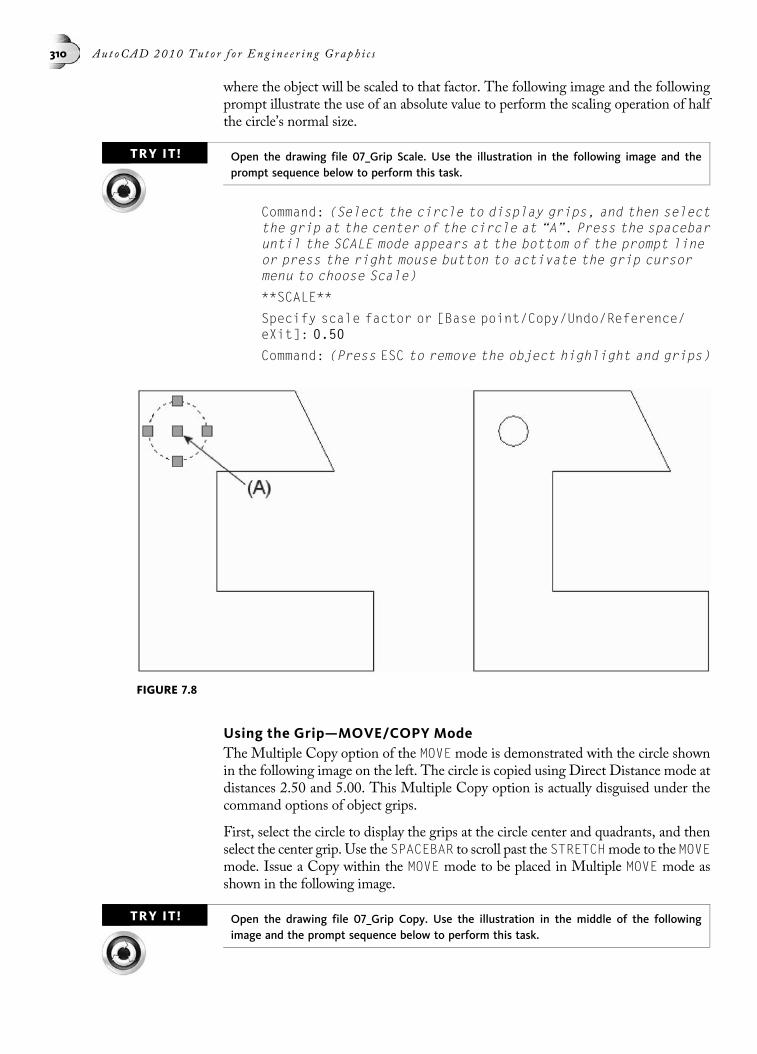
where the object will be scaled to that factor. The following image and the followingprompt illustrate the use of an absolute value to perform the scaling operation of halfthe circle’s normal size.
TRY IT! Open the drawing file 07_Grip Scale. Use the illustration in the following image and theprompt sequence below to perform this task.
Command: (Select the circle to display grips, and then selectthe grip at the center of the circle at “A”. Press the spacebaruntil the SCALE mode appears at the bottom of the prompt lineor press the right mouse button to activate the grip cursormenu to choose Scale)
**SCALE**
Specify scale factor or [Base point/Copy/Undo/Reference/eXit]: 0.50
Command: (Press ESC to remove the object highlight and grips)
Using the Grip—MOVE/COPY ModeThe Multiple Copy option of the MOVE mode is demonstrated with the circle shownin the following image on the left. The circle is copied using Direct Distance mode atdistances 2.50 and 5.00. This Multiple Copy option is actually disguised under thecommand options of object grips.
First, select the circle to display the grips at the circle center and quadrants, and thenselect the center grip. Use the SPACEBAR to scroll past the STRETCHmode to the MOVEmode. Issue a Copy within the MOVE mode to be placed in Multiple MOVE mode asshown in the following image.
TRY IT! Open the drawing file 07_Grip Copy. Use the illustration in the middle of the followingimage and the prompt sequence below to perform this task.
FIGURE 7.8
310 Au t oCAD 2010 Tu t o r f o r Eng i n e e r i n g Graph i c s

Command: (Select the circle to activate the grips at thecenter and quadrants; select the grip at the center of thecircle at “A.” Then press the SPACEBAR until the MOVE modeappears at the bottom of the prompt line or press the rightmouse button to activate the grip cursor menu to choose Move)
**MOVE**
Specify move point or [Base point/Copy/Undo/eXit]: C (ForCopy)
**MOVE (multiple)**
Specify move point or [Base point/Copy/Undo/eXit]: (Moveyour cursor straight down and enter a value of 2.50)
**MOVE (multiple)**
Specify move point or [Base point/Copy/Undo/eXit]: (Moveyour cursor straight down and enter a value of 5.00)
**MOVE (multiple)**
Specify move point or [Base point/Copy/Undo/eXit]: X (For exit)
Command: (Press ESC to remove the object highlight and grips)
Using the Grip—MIRROR ModeUse the grip-MIRROR mode to flip an object along a mirror line similar to the oneused in the regular MIRROR command. Follow the prompts for the MIRROR optionif an object needs to be mirrored but the original does not need to be saved. This per-forms the mirror operation but does not produce a copy of the original. If the originalobject needs to be saved during the mirror operation, use the Copy option of MIRRORmode. This places you in multiple MIRROR mode. Locate a base point and a secondpoint to perform the mirror operation. See the following image.
TRY IT!Open the drawing file 07_Grip Mirror. Use the illustration in the following image and theprompt sequence below to perform this task.
Command: (Select the circle in the following image to enablegrips, and then select the grip at the center of the circle.Press the SPACEBAR until the MIRROR mode appears at the bottomof the prompt line or press the right mouse button to activatethe grip cursor menu to choose Mirror)
FIGURE 7.9
Chap t e r 7 • Ob j e c t G r i p s a nd Chan g i n g t h e P r o p e r t i e s o f Ob j e c t s 311

**MIRROR**
Specify second point or [Base point/Copy/Undo/eXit]: C (ForCopy)
**MIRROR (multiple)**
Specify second point or [Base point/Copy/Undo/eXit]: B (ForBase Point)
Base point: Mid
of (Pick the midpoint at “A”)
**MIRROR** (multiple)
Specify second point or [Base point/Copy/Undo/eXit]: (Moveyour cursor straight up and enter a value of 1.00)
**MIRROR** (multiple)
Specify second point or [Base point/Copy/Undo/eXit]: X (ForExit)
Command: (Press ESC to remove the object highlight and grips)
Using the Grip—ROTATE ModeNumerous grips may be selected with window or crossing boxes. At the commandprompt, pick a blank part of the screen; this should place you in Window/Crossingselection mode. Picking up or below and to the right of the previous point places youin Window selection mode; picking up or below and to the left of the previous pointplaces you in Crossing selection mode. This method is used on all objects shown inthe following image. Selecting the lower-left grip and using the SPACEBAR to ad-vance to the ROTATE option allows all objects to be rotated at a defined angle in rela-tion to the previously selected grip.
FIGURE 7.10
312 Au t oCAD 2010 Tu t o r f o r Eng i n e e r i n g Graph i c s

TRY IT!Open the drawing file 07_Grip Rotate. Use the illustration in the following image and theprompt sequence below to perform this task.
Command: (Pick near “X,” then near “Y” to create a windowselection set and enable all grips in all objects. Select thegrip at the lower-left corner of the object. Then press theSPACEBAR until the ROTATE mode appears at the bottom ofthe prompt line or click the right mouse button to activatethe grip cursor menu to choose Rotate)
**ROTATE**
Specify rotation angle or [Base point/Copy/Undo/Reference/eXit]: 30
Command: (Press ESC to remove the object highlight and grips)
Using Grip—Hover ModeWhen you hover your cursor over a grip, information displays to help you analyze theobject selected. In the case of the line as shown in the following image on the left,hovering over the grip at the end of the line segment displays the length and angleof the line. If you pick the grip at the end of the line as shown in the following imageon the right, you can make changes to the length and angle just as if you were con-structing the line from the beginning. Use the TAB key to change from editing thelength to editing the angle. This provides a very quick and efficient way to viewingdistances and angles or making changes to values through the use of grips.
FIGURE 7.11
Chap t e r 7 • Ob j e c t G r i p s a nd Chan g i n g t h e P r o p e r t i e s o f Ob j e c t s 313
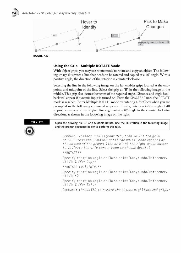
Using the Grip—Multiple ROTATE ModeWith object grips, you may use rotate mode to rotate and copy an object. The follow-ing image illustrates a line that needs to be rotated and copied at a 40° angle. With apositive angle, the direction of the rotation is counterclockwise.
Selecting the line in the following image on the left enables grips located at the end-points and midpoint of the line. Select the grip at “B” in the following image in themiddle. This grip also locates the vertex of the required angle. Distance and angle feed-back will appear if dynamic input is turned on. Press the SPACEBAR until the ROTATEmode is reached. Enter Multiple ROTATEmode by entering C for Copy when you areprompted in the following command sequence. Finally, enter a rotation angle of 40to produce a copy of the original line segment at a 40° angle in the counterclockwisedirection, as shown in the following image on the right.
TRY IT! Open the drawing file 07_Grip Multiple Rotate. Use the illustration in the following imageand the prompt sequence below to perform this task.
Command: (Select line segment “A”; then select the gripat “B.” Press the SPACEBAR until the ROTATE mode appears atthe bottom of the prompt line or click the right mouse buttonto activate the grip cursor menu to choose Rotate)
**ROTATE**
Specify rotation angle or [Base point/Copy/Undo/Reference/eXit]: C (For Copy)
**ROTATE (multiple)**
Specify rotation angle or [Base point/Copy/Undo/Reference/eXit]: 40
Specify rotation angle or [Base point/Copy/Undo/Reference/eXit]: X (For Exit)
Command: (Press ESC to remove the object highlight and grips)
FIGURE 7.12
314 Au t oCAD 2010 Tu t o r f o r Eng i n e e r i n g Graph i c s

Using Grip Offset Snap for RotationsAllMultiple Copy modes within grips may be operated in a snap location mode whileyou hold down the CTRL key. Here’s how it works. In the following image on the left,the vertical centerline and circle are selected. The objects highlight and the gripsappear. A multiple copy of the selected objects needs to be made at an angle of 45°.The grip ROTATE option is used in Multiple Copy mode.
TRY IT!Open the drawing file 07_Grip Offset Snap Rotate. Use the illustration in the followingimage and the prompt sequence below to perform this task.
Command: (Select centerline segment “A” and circle “B”; andthen select the grip near the center of circle “C.” Press theSPACEBAR until the ROTATE mode appears at the bottom of theprompt line)
**ROTATE**
Specify rotation angle or [Base point/Copy/Undo/Reference/eXit]: C (For Copy)
**ROTATE (multiple)**
Specify rotation angle or [Base point/Copy/Undo/Reference/eXit]: B (For Base Point)
Base point: Cen
of (Select the circle at “C” to snap to the center of thecircle)
**ROTATE (multiple)**
Specify rotation angle or [Base point/Copy/Undo/Reference/eXit]: 45
Rather than enter another angle to rotate and copy the same objects, hold down theCTRL key, which places you in offset snap location mode. Moving the cursor snapsthe selected objects to the angle just centered, namely 45°, as shown in the middle ofthe following image.
**ROTATE (multiple)**
Specify rotation angle or [Base point/Copy/Undo/Reference/eXit]: (Hold down the CTRL key and move the circle andcenterline until it snaps to the next 45° position shown inthe middle of the following image)
FIGURE 7.13
Chap t e r 7 • Ob j e c t G r i p s a nd Chan g i n g t h e P r o p e r t i e s o f Ob j e c t s 315

**ROTATE (multiple)**
Specify rotation angle or [Base point/Copy/Undo/Reference/eXit]: X (For Exit)
Command: (Press ESC to remove the object highlight and grips)
The Rotate-Copy-Snap Location mode could allow you to create the circles illus-trated on the right side of the following image without the aid of the ARRAY com-mand. Since all angle values are 45°, continue holding down CTRL to snap to thenext 45° location, and mark a point to place the next group of selected objects.
Using Grip Offset Snap for MovingAs with the previous example of using Offset Snap Locations for rotate mode, thesesame snap locations apply to MOVE mode. The illustration in the following image onthe left shows two circles along with a common centerline. The circles and centerlineare first selected, which highlights these three objects and activates the grips. Theintent is to move and copy the selected objects at 2-unit increments.
TRY IT! Open the drawing file 07_Grip Offset Snap Move. Use the illustration in the following imageand the prompt sequence below to perform this task.
Command: (Select the two circles and centerline to activatethe grips; select the grip at the midpoint of the centerline.Then press the SPACEBAR until the MOVE mode appears at thebottom of the prompt line or click the right mouse button toactivate the grip cursor menu to choose Move)
**MOVE**
Specify move point or [Base point/Copy/Undo/eXit]: C (ForCopy)
**MOVE (multiple)**
Specify move point or [Base point/Copy/Undo/eXit]: (Moveyour cursor straight down and enter a value of 2.00)
In the middle of the following image, instead of remembering the previous distanceand entering it to create another copy of the circles and centerline, hold down CTRLand move the cursor down again to see the selected objects snap to the distancealready specified.
FIGURE 7.14
316 Au t oCAD 2010 Tu t o r f o r Eng i n e e r i n g Graph i c s

**MOVE (multiple)**
Specify move point or [Base point/Copy/Undo/eXit]: (Holddown the CTRL key and move the cursor down to have the selectedobjects snap to another 2.00-unit distance)
**MOVE (multiple)**
Specify move point or [Base point/Copy/Undo/eXit]: X (To exit)
Command: (Press ESC to remove the object highlight and grips)
The illustration on the right side of the following image shows the completed holelayout, the result of using the Offset Snap Location method of object grips.
Grip Project—Lug.Dwg
TRY IT!Open the drawing file 07_Lug. Use the illustration in the following image and the promptsequence below to perform this task.
Using the illustration in the following image as a guide, make the following changesto the lug:
1. Use the Grip-Stretch mode to join the endpoint of the inclined line at (A) with theendpoint of the horizontal line also at (A).
2. Use the Grip-Stretch mode to join the endpoint of the inclined line at (B) with theendpoint of the horizontal line also at (B).
3. Use the Grip-Stretch mode, pick the 1.50 diameter dimension, make the grip locatedon the dimension text hot, and position the dimension text in the lower-right cornerof the object.
4. Use the Grip-Scale mode, pick the 1.50 diameter dimension and the circle, make thegrip located at the center of the circle hot, and use a scale factor of .50 to reduce thesize of the circle by half. Notice that the dimension recalculates to reflect thischange.
5. Use the Grip-Mirror mode, and pick the circle, 1.50 diameter dimension, two verticallines, both fillets, and the horizontal line at (E). Pick one of the grips to make it hot.Use the midpoint of the long horizontal line of the object as the new base point. TurnOrtho on and move your cursor down to establish the mirror line.
6. Use the Grip-Stretch mode to increase the size of the .50 throat at (F) to a new dis-tance of 1.25. Pick both fillets and the three line segments attached to the fillets.Hold down the SHIFT key and select the grips at the endpoints of both fillets andthe middle of the horizontal line. Release the SHIFT key and pick the grip at the
FIGURE 7.15
Chap t e r 7 • Ob j e c t G r i p s a nd Chan g i n g t h e P r o p e r t i e s o f Ob j e c t s 317

midpoint of the horizontal line again. Move your cursor up (either Ortho or Polarmode needs to be turned on) and type a value of .75.
7. The completed exercise is illustrated in the following image on the right.
MODIFYING THE PROPERTIES OF OBJECTSAt times, objects are drawn on the wrong layer, color, or even in the wrong line-
type. The lengths of line segments are incorrect, or the radius values of circles and arcsare incorrect. Eliminating the need to erase these objects and reconstruct them totheir correct specifications, a series of tools are available to modify the properties ofthese objects. One such tool is the Properties Palette which can be selected fromeither the Ribbon, Menu Bar or the Standard Toolbar as shown in the followingimage on the left. This will display the Properties Palette as shown in the followingimage on the right.
FIGURE 7.16
FIGURE 7.17
318 Au t oCAD 2010 Tu t o r f o r Eng i n e e r i n g Graph i c s

Illustrated in the following image are two line segments. One of the line segments hasbeen pre-selected, as shown by the highlighted appearance and the presence of grips.
Clicking on the Properties button on the Standard toolbar in the following image dis-plays the Properties Palette. This palette displays information about the objectalready selected; in this case the information is about the line segment, which is iden-tified at the top of the palette.
When changing a selected object to a different layer, click on the layer field in thefollowing image on the left and the current layer displays (in this example, LayerObject). Clicking the down arrow displays all layers defined in the drawing. Clickingon one of these layers changes the selected object to a different layer.
A number of options that control the Properties Palette are illustrated in the follow-ing image on the right. You can elect to move, size, or close the Properties Palettefrom this menu. You can allow or prevent the Properties Palette from docking.Auto-hiding displays the Properties Palette when your cursor lies anywhere insidethe window. When your cursor moves off of the Properties Palette, the window col-lapses to display only the blue side strip. Checking Description controls the display ofa description area located at the bottom of the palette.
Three line segments are illustrated in the following image and all three segments havebeen pre-selected, as shown by their highlighted appearance and the presence ofgrips.
FIGURE 7.18
FIGURE 7.19
Chap t e r 7 • Ob j e c t G r i p s a nd Chan g i n g t h e P r o p e r t i e s o f Ob j e c t s 319
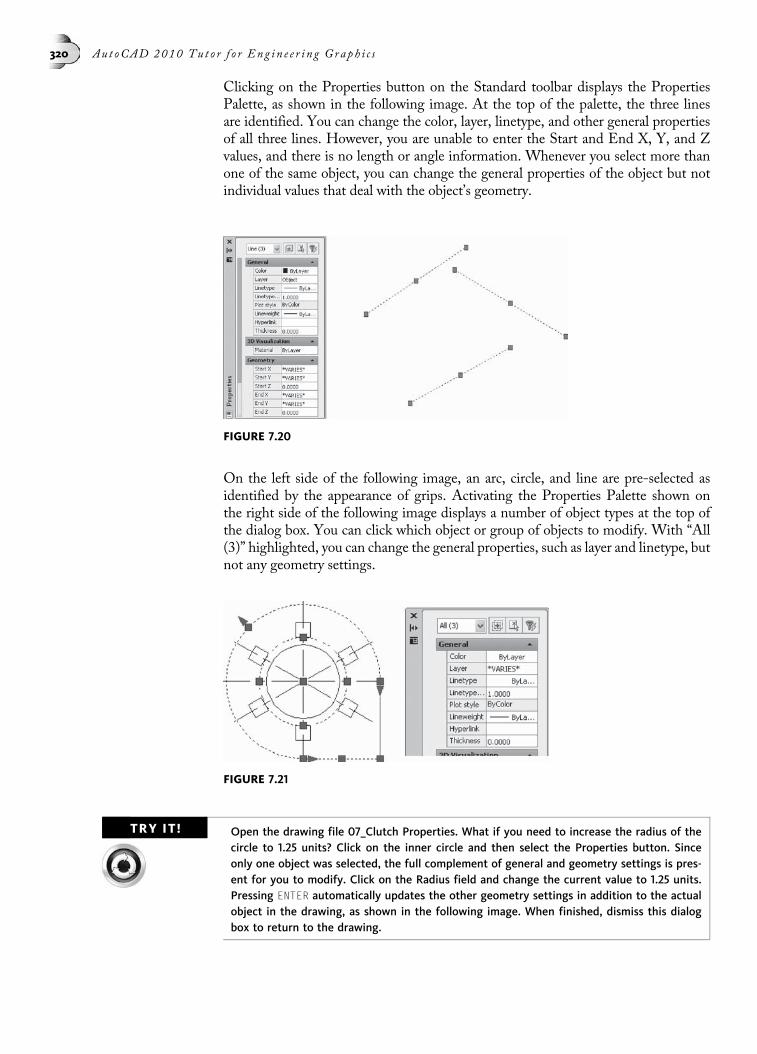
Clicking on the Properties button on the Standard toolbar displays the PropertiesPalette, as shown in the following image. At the top of the palette, the three linesare identified. You can change the color, layer, linetype, and other general propertiesof all three lines. However, you are unable to enter the Start and End X, Y, and Zvalues, and there is no length or angle information. Whenever you select more thanone of the same object, you can change the general properties of the object but notindividual values that deal with the object’s geometry.
On the left side of the following image, an arc, circle, and line are pre-selected asidentified by the appearance of grips. Activating the Properties Palette shown onthe right side of the following image displays a number of object types at the top ofthe dialog box. You can click which object or group of objects to modify. With “All(3)” highlighted, you can change the general properties, such as layer and linetype, butnot any geometry settings.
TRY IT! Open the drawing file 07_Clutch Properties. What if you need to increase the radius of thecircle to 1.25 units? Click on the inner circle and then select the Properties button. Sinceonly one object was selected, the full complement of general and geometry settings is pres-ent for you to modify. Click on the Radius field and change the current value to 1.25 units.Pressing ENTER automatically updates the other geometry settings in addition to the actualobject in the drawing, as shown in the following image. When finished, dismiss this dialogbox to return to the drawing.
FIGURE 7.20
FIGURE 7.21
320 Au t oCAD 2010 Tu t o r f o r Eng i n e e r i n g Graph i c s
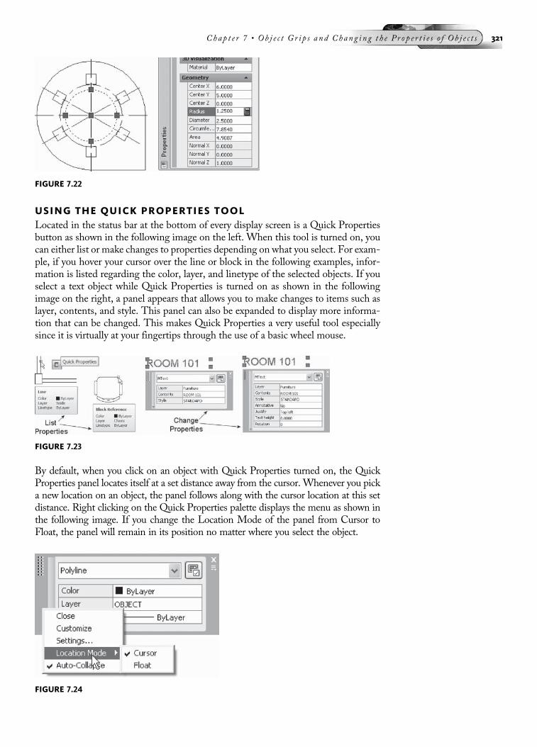
USING THE QUICK PROPERTIES TOOLLocated in the status bar at the bottom of every display screen is a Quick Propertiesbutton as shown in the following image on the left. When this tool is turned on, youcan either list or make changes to properties depending on what you select. For exam-ple, if you hover your cursor over the line or block in the following examples, infor-mation is listed regarding the color, layer, and linetype of the selected objects. If youselect a text object while Quick Properties is turned on as shown in the followingimage on the right, a panel appears that allows you to make changes to items such aslayer, contents, and style. This panel can also be expanded to display more informa-tion that can be changed. This makes Quick Properties a very useful tool especiallysince it is virtually at your fingertips through the use of a basic wheel mouse.
By default, when you click on an object with Quick Properties turned on, the QuickProperties panel locates itself at a set distance away from the cursor. Whenever you picka new location on an object, the panel follows along with the cursor location at this setdistance. Right clicking on the Quick Properties palette displays the menu as shown inthe following image. If you change the Location Mode of the panel from Cursor toFloat, the panel will remain in its position no matter where you select the object.
FIGURE 7.22
FIGURE 7.23
FIGURE 7.24
Chap t e r 7 • Ob j e c t G r i p s a nd Chan g i n g t h e P r o p e r t i e s o f Ob j e c t s 321

Another feature of Quick Properties is to display more settings found under theQuick Properties tab of the Drafting Settings dialog box as shown in the followingimage. Experiment with the various settings under this dialog box to see how it affectsthe display of the Quick Properties panel.
USING THE QUICK SELECT DIALOG BOXAt various times in a drawing, you need to build a selection set and modify the prop-erties of these selected objects. However, there can be numerous objects in a drawingand if you attempt to select objects through the conventional methods such as win-dow or crossing, you may accidentally ignore a few objects. A tool is available inwhich you enter certain parameters and AutoCAD selects the objects based on theseparameters; this tool is called Quick Select. This tool can be activated by right-clicking on a blank part of your screen to display the menu in the following imageon the left where you can select Quick Select. You can also choose Quick Selectfrom the Tools Menu Bar or under the Utilities panel of the Ribbon as shown inthe following image on the right.
FIGURE 7.25
FIGURE 7.26
322 Au t oCAD 2010 Tu t o r f o r Eng i n e e r i n g Graph i c s
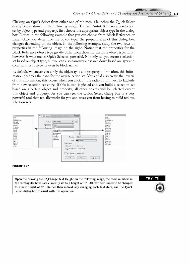
Clicking on Quick Select from either one of the menus launches the Quick Selectdialog box as shown in the following image. To have AutoCAD create a selectionset by object type and property, first choose the appropriate object type in the dialogbox. Notice in the following example that you can choose from Block Reference orLine. Once you determine the object type, the property area of this dialog boxchanges depending on the object. In the following example, study the two rows ofproperties in the following image on the right. Notice that the properties for theBlock Reference object type greatly differ from those for the Line object type. This,however, is what makes Quick Select so powerful. Not only can you create a selectionset based on object type, but you can also narrow your search down based on layer andcolor for most objects or even by block name.
By default, whenever you apply the object type and property information, this infor-mation becomes the basis for the new selection set. You could also create the inverseof this information; this occurs when you click on the radio button next to Excludefrom new selection set entry. If this button is picked and you build a selection setbased on a certain object and property, all other objects will be selected exceptthis object and property. As you can see, the Quick Select dialog box is a verypowerful tool that actually works for you and saves you from having to build tediousselection sets.
TRY IT!Open the drawing file 07_Change Text Height. In the following image, the room numbers inthe rectangular boxes are currently set to a height of 18 00. All text items need to be changedto a new height of 12 00. Rather than individually changing each text item, use the QuickSelect dialog box to assist with this operation.
FIGURE 7.27
Chap t e r 7 • Ob j e c t G r i p s a nd Chan g i n g t h e P r o p e r t i e s o f Ob j e c t s 323

First, activate the Properties Palette and click on the Quick Select button, as shown inthe following image on the left. This represents another method of activating QuickSelect. Once inside the Quick Select dialog box, click on the Object type window andselect “Text,” as shown on the right side of the following image.
Clicking the OK button at the bottom of the Quick Select dialog box returns you toyour drawing. Notice that all text is highlighted and a text height of 18.0000 is listedin the Properties Palette. Change this value to 12, as shown in the following image.
FIGURE 7.28
FIGURE 7.29
324 Au t oCAD 2010 Tu t o r f o r Eng i n e e r i n g Graph i c s

When finished changing the text height in the Properties Palette, press the ENTERkey followed by the ESC key and notice that all text in the following image has beenchanged to the new height of 12 00.
FIGURE 7.30
FIGURE 7.31
Chap t e r 7 • Ob j e c t G r i p s a nd Chan g i n g t h e P r o p e r t i e s o f Ob j e c t s 325

USING THE PICKADD FEATURE OF THE PROPERTIESPALETTEAnother very interesting feature is available to you inside the Properties Palette; it isthe pickadd button located in the following image. To see how it operates, follow thenext exercise.
TRY IT! Open the drawing file 07_PickAdd. A number of object types ranging from lines to text tomultiline text and polylines with dimensions are displayed. Activate the Properties Paletteand pick on one object. Notice that it highlights, the grips appear, and information aboutthe object is displayed in the Properties Palette. Suppose, however, that you want to list in-formation about another object. You must first press ESC to deselect the original object.Now select a different object and this information is displayed in the Properties Palette.This time, select the PICKADD button in the following image on the left. Notice that the but-ton changes in appearance. Instead of the “plus” sign, a “1” is displayed in the followingimage on the right. Click on any object and notice the information displayed in the Proper-ties Palette. Without pressing ESC, click on another object. The original object deselects andthe new object highlights with its information displayed in the Properties Palette. Very sim-ply, the pickadd button eliminates the need for the ESC key when displaying informationabout individual objects.
NOTE Changing the PICKADD button affects all drawings. Since this change is global, click thePICKADD button to set it back to the “plus” sign before continuing on.
PERFORMING MATHEMATICAL CALCULATIONSA mathematical calculator is available to assist in making a variety of calculations
while still remaining in an AutoCAD drawing. The calculator is activated by clickingon QuickCalc, found under Tools in the Menu Bar, as shown in the following imageon the left. This launches the calculator, as shown in the following image on the right.The calculator resembles the Properties Palette and can be manipulated in the samefashion. When you perform calculations throughout the design cycle, these calcula-tions are stored in a History area. Calculations in this area can be retrieved for lateruse. As you enter numbers and mathematical functions such as addition and subtrac-tion from the supplied keypads, they are displayed in the Input area of the calculator.Four tabbed areas control the methods by which calculations are made. They areNumber Pad, Scientific, Units Conversion, and Variables.
FIGURE 7.33
FIGURE 7.32
326 Au t oCAD 2010 Tu t o r f o r Eng i n e e r i n g Graph i c s

Each of the four tabbed areas of the calculator are illustrated in the following image.A brief description of each follows:
Numeric Pad: This area of the calculator is used to perform the most basic of mathe-matical functions. Clicking on a number or function places this information in theInput area of the calculator.
Scientific: Use this tabbed area to enter trigonometric and other advanced functions.
Units Conversion: This area is used to convert units from one system to another. Youenter the units type, the unit type to convert from, and the units to convert to. Enter-ing a numeric value to convert displays the converted value.
Variables: This area contains a series of shortcut commands that can be used forperforming specialized operations.
When you are using the Properties Palette and you need to change the value of one ofthe Geometry listings, a calculator icon is present. Clicking this icon launches theQuickCalc dialog box, as shown in the following image on the right. Entering amathematical formula in the Input area and clicking the Apply button sends the cal-culated value back to the Properties Palette and change the highlighted object.
FIGURE 7.34
TABLE 7.1 The following table illustrates the variable names and their functions
Variable Function
PHI Golden Ratio (1.61803399)
DEE Finds the distance between two endpoints
ILLI Finds the intersection of two lines defined by four endpoints
MEE Finds the midpoint between two endpoints
NEE Finds the unit vector in the XY plane normal (perpendicular) totwo endpoints
RAD Obtains the radius from a circle, arc, or polyline arc segment
VEE Finds a vector from two endpoints
VEE1 Finds a unit vector from two endpoints
Chap t e r 7 • Ob j e c t G r i p s a nd Chan g i n g t h e P r o p e r t i e s o f Ob j e c t s 327

USING THE LAYER CONTROL BOX TO MODIFYOBJECT PROPERTIESIf all you need to do is to change an object or a group of objects from one layer toanother, the Layer Control box can easily perform this operation.
TRY IT! Open the drawing file 07_Change Layer. In the following image, select the arc and two linesegments. Notice that the current layer is 0 in the Layer Control box. These objects need tobe on the OBJECT layer.
Click on the Layer Control box to display all layers defined in the drawing. Thenclick on the desired layer for all highlighted objects (in this case, the OBJECT layerin the following image).
Notice that in the following image, with the objects still highlighted, the layer listedis OBJECT. This is one of the quickest and most productive ways of changing anobject from one layer to another.
FIGURE 7.37
FIGURE 7.35
FIGURE 7.36
328 Au t oCAD 2010 Tu t o r f o r Eng i n e e r i n g Graph i c s

TRY IT!Open the drawing file 07_Mosaic. In the following image, this drawing consists of 5 differ-ent types of objects all drawn on Layer 0: circles, squares drawn as closed polylines, lines,text (the letter X), and text (the letter Y). The Quick Select dialog box will be used to selectthese object types individually.
Once you have selected them, change the objects to the correct layers, which are alsosupplied with this drawing and identified in the following image on the left.
First, activate the Quick Select dialog box from the Tools Menu Bar, shown in thefollowing image in the middle. In the Object type box, select Circle, as you see in thefollowing image on the right, and click the OK button.
With all circles selected, click the Layer Control box and pick the Circles layer asshown in the following image. All circles in the mosaic pattern should turn red.Press ESC to remove the object highlight.
FIGURE 7.38
FIGURE 7.39
Chap t e r 7 • Ob j e c t G r i p s a nd Chan g i n g t h e P r o p e r t i e s o f Ob j e c t s 329

Next, you need to select all the text with the letter “X” and change this text to the layercalled X Text. Activate the Quick Select dialog box and make the following changes:Change the Object type to Text, set the Properties to Contents, and enter “X” as thevalue. Your display should be similar to the dialog box in the following image on theleft. Click the OK button to dismiss the Quick Select dialog box and select all textwith the letter “X.”
Change all letters to the X Text layer in the Layer Control box, as shown in the fol-lowing image on the right. Press ESC to remove the object highlight and grips. Followthe same procedures for changing all line segments to the Lines layer, all polylines tothe Pline Squares layer, and all “Y” text to the Y Text layer.
TRY IT! Open the drawing file 07_Qselect Duplex. Use the illustration in the following image andthe information below to change the items to their proper layers.
Change all lines to the Walls layer
Change all text to the Room Labels layer
Change the blocks “Door” and “Louver” to the Door layer
Change the block “Window” to the Window layer
Change the blocks “Countertop,” “Range,” “Sink,” and“Refrigerator” to the Countertop layer
FIGURE 7.40
FIGURE 7.41
330 Au t oCAD 2010 Tu t o r f o r Eng i n e e r i n g Graph i c s

TIPFor the blocks, see the illustration in the following image for supplying the correct informa-tion in the Quick Select dialog box; change the Object type to Block Reference. Change theProperties to Name. Click the down arrow next to the Value heading and select the desiredblock from the list provided. Then, after clicking the OK button and all desired blocks areselected, change the highlighted blocks to the correct layer. Follow this procedure for se-lecting the Window, Countertop, Range, Sink, Door, Louver, and Refrigerator blocks.
DOUBLE-CLICK EDIT ON ANY OBJECTDouble-clicking on any object provides you with a quick way of launching the Prop-erties Palette or other related dialog boxes depending on the object type. For instance,double-clicking on a line segment launches the Properties Palette, which displays in-formation about the line. Double-clicking on a text object displays the Edit Text dia-log box, allowing you to enter or delete words. Whenever the Properties Palette islaunched and you want to modify a different object, first press ESC to deselect thecurrent object. You may also want to dismiss the Properties Palette.
TRY IT!Open the drawing file 07_Double Click Edit. In the following image, double-click on themagenta centerline and the Properties Palette launches with information about the line.Press ESC and dismiss the Properties Palette. Double-click on the word “BLOCK” to launchthe Edit Text function. Press ESC to exit the edit function when finished. Double-click onthe sentence “THE OBJECT SHOWN ABOVE IS A WINDOW SYMBOL” to launch the Multi-line Text Editor dialog box. Press ESC to dismiss the dialog box when finished. Double-clickon the hatch pattern and to launch the Hatch Edit dialog box. Pressing ESC dismisses thisdialog box when finished. Continue by double-clicking on the circle, dimension, and rectan-gle and observe the type of dialog box launched through this method. Press ESC to dismissthe dialog boxes when finished with each operation.
FIGURE 7.43
FIGURE 7.42
Chap t e r 7 • Ob j e c t G r i p s a nd Chan g i n g t h e P r o p e r t i e s o f Ob j e c t s 331
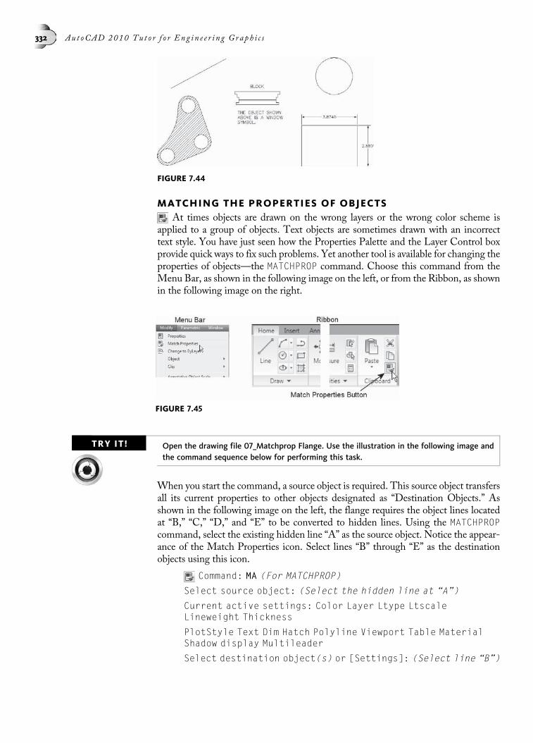
MATCHING THE PROPERTIES OF OBJECTSAt times objects are drawn on the wrong layers or the wrong color scheme is
applied to a group of objects. Text objects are sometimes drawn with an incorrecttext style. You have just seen how the Properties Palette and the Layer Control boxprovide quick ways to fix such problems. Yet another tool is available for changing theproperties of objects—the MATCHPROP command. Choose this command from theMenu Bar, as shown in the following image on the left, or from the Ribbon, as shownin the following image on the right.
TRY IT! Open the drawing file 07_Matchprop Flange. Use the illustration in the following image andthe command sequence below for performing this task.
When you start the command, a source object is required. This source object transfersall its current properties to other objects designated as “Destination Objects.” Asshown in the following image on the left, the flange requires the object lines locatedat “B,” “C,” “D,” and “E” to be converted to hidden lines. Using the MATCHPROPcommand, select the existing hidden line “A” as the source object. Notice the appear-ance of the Match Properties icon. Select lines “B” through “E” as the destinationobjects using this icon.
Command: MA (For MATCHPROP)
Select source object: (Select the hidden line at “A”)
Current active settings: Color Layer Ltype LtscaleLineweight Thickness
PlotStyle Text Dim Hatch Polyline Viewport Table MaterialShadow display Multileader
Select destination object(s) or [Settings]: (Select line “B”)
FIGURE 7.44
FIGURE 7.45
332 Au t oCAD 2010 Tu t o r f o r Eng i n e e r i n g Graph i c s

Select destination object(s) or [Settings]: (Select line “C”)
Select destination object(s) or [Settings]: (Select line “D”)
Select destination object(s) or [Settings]: (Select line “E”)
Select destination object(s) or [Settings]: (Press ENTER toexit this command)
The results appear in the flange illustrated in the following image on the right, wherethe continuous object lines were converted to hidden lines. Not only did the linetypeproperty get transferred, but the color, layer, lineweight, and linetype scale informa-tion did as well.
To get a better idea of what object properties are affected by the MATCHPROP com-mand, reenter the command, pick a source object, and instead of picking a destina-tion object immediately, enter S for Settings. This displays the Property Settingsdialog box in the following image.
Command: MA (For MATCHPROP)
Select source object: (Select the hidden line at “A” in theprevious image)
Current active settings: Color Layer Ltype LtscaleLineweight Thickness
PlotStyle Dim Text Hatch Polyline Viewport Table MaterialShadow display Multileader
Select destination object(s) or [Settings]: S (For Settings;this displays the Property Settings dialog box in thefollowing image)
Any box with a check displayed in it transfers that property from the source object toall destination objects. If you need to transfer only the layer information and not thecolor and linetype properties of the source object, remove the checks from the Colorand Linetype properties before you select the destination objects. This prevents theseproperties from being transferred to any destination objects.
FIGURE 7.46
Chap t e r 7 • Ob j e c t G r i p s a nd Chan g i n g t h e P r o p e r t i e s o f Ob j e c t s 333

Matching Dimension PropertiesThe MATCHPROP command can control special properties of dimensions, text, hatchpatterns, polylines, viewports, and tables. The Dimension property will be featurednext as shown in the following image. (Even though the topic of dimensions willnot be covered until Chapter 10, this concept is introduced here.)
TRY IT! Open the drawing file 07_Matchprop Dim. The following image shows two blocks: the blockassigned a dimension value of 46.6084 was dimensioned with the METRIC dimension stylewith the Arial font applied. The block assigned a dimension value of 2.3872 was dimensionedwith the STANDARD dimension style with the TXT font applied. Both blocks need to bedimensioned with the METRIC dimension style. Issue the MATCHPROP command and selectthe 46.6084 dimension as the source object and then select the 2.3872 dimension as thedestination object.
FIGURE 7.47
FIGURE 7.48
334 Au t oCAD 2010 Tu t o r f o r Eng i n e e r i n g Graph i c s

Command: MA (For MATCHPROP)
Select source object: (Select the dimension at “A” in thefollowing image)
Current active settings: Color Layer Ltype LtscaleLineweight Thickness
PlotStyle Dim Text Hatch Polyline Viewport Table MaterialShadow display Multileader
Select destination object(s) or [Settings]: (Select thedimension at “B”)
Select destination object(s) or [Settings]: (Press ENTER toexit this command)
The results are shown in the following image on the right, with the METRIC di-mension style applied to the STANDARD dimension style through the use of theMATCHPROP command. Because the text font was associated with the dimensionstyle, it also changed in the destination object.
Matching Text PropertiesThe following is an example of how the MATCHPROP command affects a text objectwith the Text property shown in the following image.
TRY IT!Open the drawing file 07_Matchprop Text. The following image shows two text items dis-played in different fonts. The text “Coarse Knurl” at “A” was constructed with a text stylecalled Arial. The text “Medium Knurl” at “B” was constructed with the default text stylecalled STANDARD. Use the following command sequence to match the STANDARD textstyle with the Arial text style using the MATCHPROP command.
FIGURE 7.49
FIGURE 7.50
Chap t e r 7 • Ob j e c t G r i p s a nd Chan g i n g t h e P r o p e r t i e s o f Ob j e c t s 335

Command: MA (For MATCHPROP)
Select source object: (Select the text at “A”)
Current active settings: Color Layer Ltype Ltscale Line-weight Thickness
PlotStyle Dim Text Hatch Polyline Viewport Table MaterialShadow display Multileader
Select destination object(s) or [Settings]: (Select the textat “B”)
Select destination object(s) or [Settings]: (Press ENTER toexit this command)
The result is shown in the following image on the right. Both text items now sharethe same text style. Notice that the text string stays intact when text properties arematched. Only the text style of the source object is applied to the destination object.
Matching Hatch PropertiesA source hatch object can also be matched to a destination pattern with the MATCH-PROP command and the Hatch property as shown in the following image (Eventhough the topic of hatching will not be covered until Chapter 9, this concept is in-troduced here.)
TRY IT! Open the drawing file 07_Matchprop Hatch. In the following image, the crosshatch patternsat “B” and “C” are at the wrong angle and scale. They should reflect the pattern at “A”because it is the same part. Use the MATCHPROP command, select the hatch pattern at “A”as the source object, and select the patterns at “B” and “C” as the destination objects.
Command: MA (For MATCHPROP)
Select source object: (Select the hatch pattern at “A”)
Current active settings: Color Layer Ltype LtscaleLineweight Thickness
FIGURE 7.51
FIGURE 7.52
336 Au t oCAD 2010 Tu t o r f o r Eng i n e e r i n g Graph i c s

PlotStyle Dim Text Hatch Polyline Viewport Table MaterialShadow display Multileader
Select destination object(s) or [Settings]: (Select thehatch pattern at “B”)
Select destination object(s) or [Settings]: (Press ENTER toexit this command)
The results appear in the following image on the right, where the source hatch patternproperty was applied to all destination hatch patterns.
Matching Polyline PropertiesA source polyline object can also be matched to a destination pattern with theMATCHPROP command and the Polyline property as shown in the following image.
TRY IT!Open the drawing file 07_Matchprop Pline. In the following image, the polyline at “B” is atthe wrong width. It should match the width of the polyline at “A.” Using the MATCHPROPcommand, select the polyline at “A” as the source object, and select the polyline at “B” asthe destination object.
Command: MA (For MATCHPROP)
Select source object: (Select the polyline at “A”)
Current active settings: Color Layer Ltype LtscaleLineweight Thickness
PlotStyle Dim Text Hatch Polyline Viewport Table MaterialShadow display Multileader
FIGURE 7.53
FIGURE 7.54
Chap t e r 7 • Ob j e c t G r i p s a nd Chan g i n g t h e P r o p e r t i e s o f Ob j e c t s 337
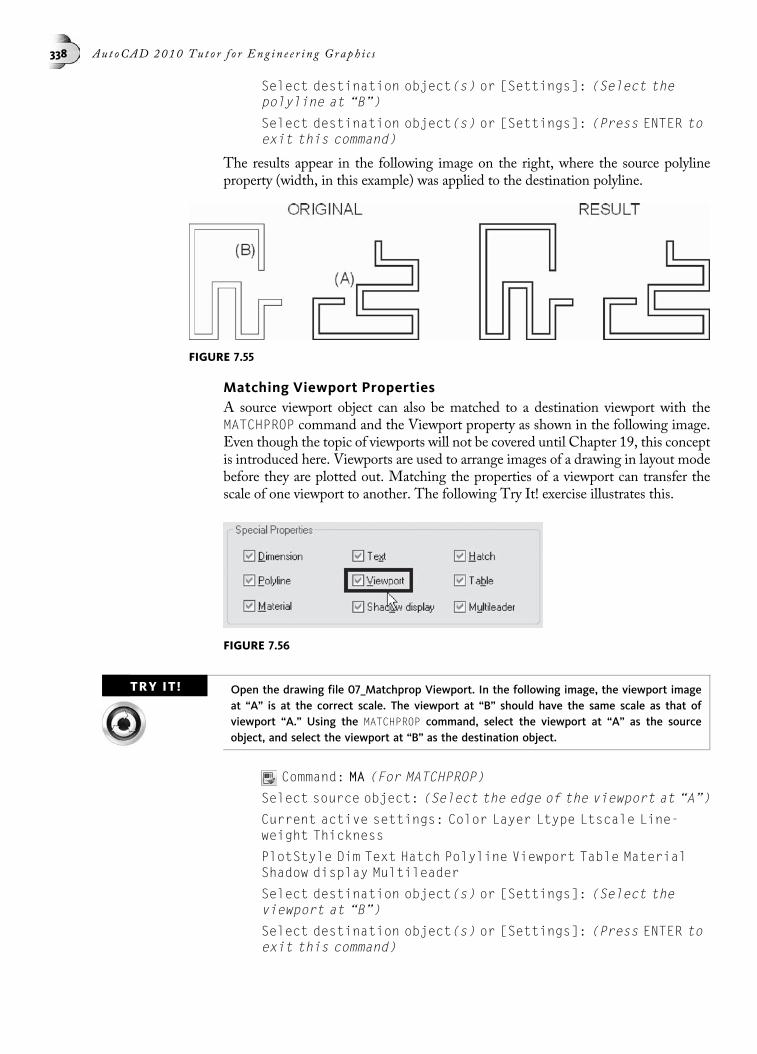
Select destination object(s) or [Settings]: (Select thepolyline at “B”)
Select destination object(s) or [Settings]: (Press ENTER toexit this command)
The results appear in the following image on the right, where the source polylineproperty (width, in this example) was applied to the destination polyline.
Matching Viewport PropertiesA source viewport object can also be matched to a destination viewport with theMATCHPROP command and the Viewport property as shown in the following image.Even though the topic of viewports will not be covered until Chapter 19, this conceptis introduced here. Viewports are used to arrange images of a drawing in layout modebefore they are plotted out. Matching the properties of a viewport can transfer thescale of one viewport to another. The following Try It! exercise illustrates this.
TRY IT! Open the drawing file 07_Matchprop Viewport. In the following image, the viewport imageat “A” is at the correct scale. The viewport at “B” should have the same scale as that ofviewport “A.” Using the MATCHPROP command, select the viewport at “A” as the sourceobject, and select the viewport at “B” as the destination object.
Command: MA (For MATCHPROP)
Select source object: (Select the edge of the viewport at “A”)
Current active settings: Color Layer Ltype Ltscale Line-weight Thickness
PlotStyle Dim Text Hatch Polyline Viewport Table MaterialShadow display Multileader
Select destination object(s) or [Settings]: (Select theviewport at “B”)
Select destination object(s) or [Settings]: (Press ENTER toexit this command)
FIGURE 7.55
FIGURE 7.56
338 Au t oCAD 2010 Tu t o r f o r Eng i n e e r i n g Graph i c s

The results appear in the following image, where the source viewport property (scaleof the image) was applied to the destination viewport. Notice also that the layer of theviewport “B” was changed from 0 to Vports.
Match Properties and TablesA source table object can be matched to a destination table using the Table property,as shown in the following image. When one table is matched with another, the tablestyle of the source table updates the table style of the destination table.
FIGURE 7.57
FIGURE 7.58
FIGURE 7.59
Chap t e r 7 • Ob j e c t G r i p s a nd Chan g i n g t h e P r o p e r t i e s o f Ob j e c t s 339

TRY IT! Open the drawing file 07_Matchprop Table. In the following image, one table has the titlestrip originating at the top and the other table title originates at the bottom. Using theMATCHPROP command, select the table on the left as the source object, and select the tableon the right as the destination object.
Command: MA (For MATCHPROP)
Select source object: (Select the table in the followingimage on the left)
Current active settings: Color Layer Ltype LtscaleLineweight Thickness
PlotStyle Dim Text Hatch Polyline Viewport Table MaterialShadow display Multileader
Select destination object(s) or [Settings]: (Select thetable on the right in the following image on the right)
Select destination object(s) or [Settings]: (Press ENTER toexit this command)
In the following image, notice how the table on the right changes to the downwarddirection arrangement as controlled by the table style.
NOTE You may have to move the table into position.
FIGURE 7.60
FIGURE 7.61
340 Au t oCAD 2010 Tu t o r f o r Eng i n e e r i n g Graph i c s

TUTORIAL EXERCISE: 07_MODIFY-EX.DWG
PurposeThis tutorial exercise is designed to change the properties of existing objects displayedin the above image.
System SettingsSince this drawing is provided on the CD, open an existing drawing file called “07_Modify-Ex.”Follow the steps in this tutorial for changing various objects to the correct layer, text style,and dimension style.
LayersLayers have already been created in this drawing.
Suggested CommandsBegin this tutorial by using the Properties Palette to change the isometric object to a dif-ferent layer. Continue by changing the text height and layer of the view identifiers(FRONT, TOP, SIDE, ISOMETRIC). The MATCHPROP command will be used to transfer theproperties from one dimension to another, one text style to another, and one hatch pat-tern to another. The Layer Control box will be used to change the layer of various objectslocated in the Front and Top views.
STEP 1Loading this drawing displays the objects in a page layout called “Orthographic Views.”Page layout is where the drawing will be plotted out in the future. This name is presentnext to the Model tab in the bottom portion of the drawing screen. Since a majority ofchanges will be made in Model mode, click on the Model tab near the bottom of the dis-play screen. Your drawing will appear similar to the following image.
FIGURE 7.62
Chap t e r 7 • Ob j e c t G r i p s a nd Chan g i n g t h e P r o p e r t i e s o f Ob j e c t s 341

STEP 2While in the Model environment, select all lines that make up the isometric view in thefollowing image. You can accomplish this by using the Window mode from the Commandprompt. If you accidentally select the word ISOMETRIC, de-select this word. Activate theProperties Palette and click on the Layer field. This displays the current layer the objectsare drawn on (DIM) in the following image. Click the down arrow to display the otherlayers and pick the OBJECT layer. This changes all selected objects that make up the iso-metric view to the OBJECT layer. Press ESC to remove the object highlight and the gripsfrom the drawing.
STEP 3Select the view titles (FRONT, TOP, SIDE, ISOMETRIC). These text items need to be chan-ged to a height of 0.15 and the TEXT layer. With all four text objects highlighted, and theProperties Palette already active, click on the Layer field, and click the down arrow tochange the selected objects to the TEXT layer in the following image.
FIGURE 7.63
FIGURE 7.64
342 Au t oCAD 2010 Tu t o r f o r Eng i n e e r i n g Graph i c s
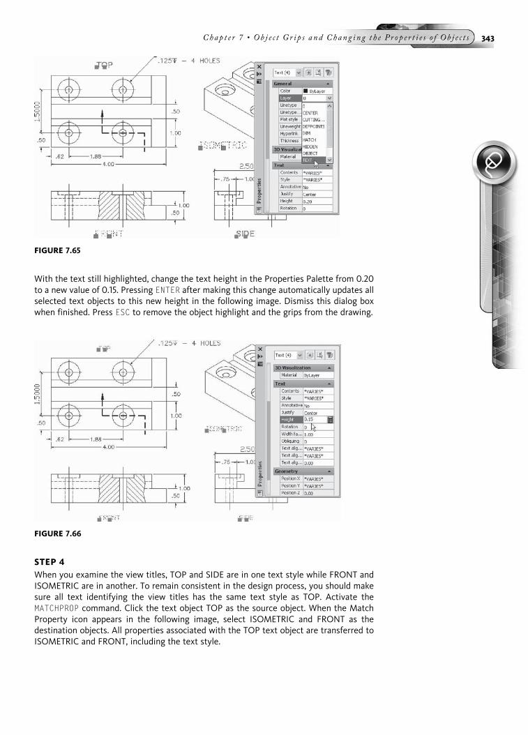
With the text still highlighted, change the text height in the Properties Palette from 0.20to a new value of 0.15. Pressing ENTER after making this change automatically updates allselected text objects to this new height in the following image. Dismiss this dialog boxwhen finished. Press ESC to remove the object highlight and the grips from the drawing.
STEP 4When you examine the view titles, TOP and SIDE are in one text style while FRONT andISOMETRIC are in another. To remain consistent in the design process, you should makesure all text identifying the view titles has the same text style as TOP. Activate theMATCHPROP command. Click the text object TOP as the source object. When the MatchProperty icon appears in the following image, select ISOMETRIC and FRONT as thedestination objects. All properties associated with the TOP text object are transferred toISOMETRIC and FRONT, including the text style.
FIGURE 7.65
FIGURE 7.66
Chap t e r 7 • Ob j e c t G r i p s a nd Chan g i n g t h e P r o p e r t i e s o f Ob j e c t s 343

Command: MA (for MATCHPROP)
Select source object: (Select the text object “TOP,” whichshould highlight in the following image)
Current active settings: Color Layer Ltype Ltscale Line-weight Thickness
PlotStyle Dim Text Hatch Polyline Viewport Table MaterialShadow display Multileader
Select destination object(s) or [Settings]: (Select the textobject “ISOMETRIC”)
Select destination object(s) or [Settings]: (Select the textobject “FRONT”)
Select destination object(s) or [Settings]: (Press ENTER toexit this command)
STEP 5Notice the dimensions in this drawing. Two dimensions stand out above the rest (the1.5000 vertical dimension in the Top view and the 2.5000 horizontal dimension in theSide view). Again, to remain consistent in the design process, you should make sure alldimensions have the same appearance (dimension text height, number of decimal places,whether they are broken inside instead of placed above the dimension line). Activatethe MATCHPROP command again by clicking on the button in the Ribbon. Click the 4.00horizontal dimension in the Top view as the source object. When the Match Propertyicon appears, as shown in the following image, select the 1.5000 and 2.5000 vertical di-mensions as the destination objects. All dimension properties associated with the 4.00dimension are transferred to the 1.5000 and 2.5000 dimensions.
Command: MA (for MATCHPROP)
Select source object: (Select the 4.00 dimension, whichshould highlight)
FIGURE 7.67
344 Au t oCAD 2010 Tu t o r f o r Eng i n e e r i n g Graph i c s
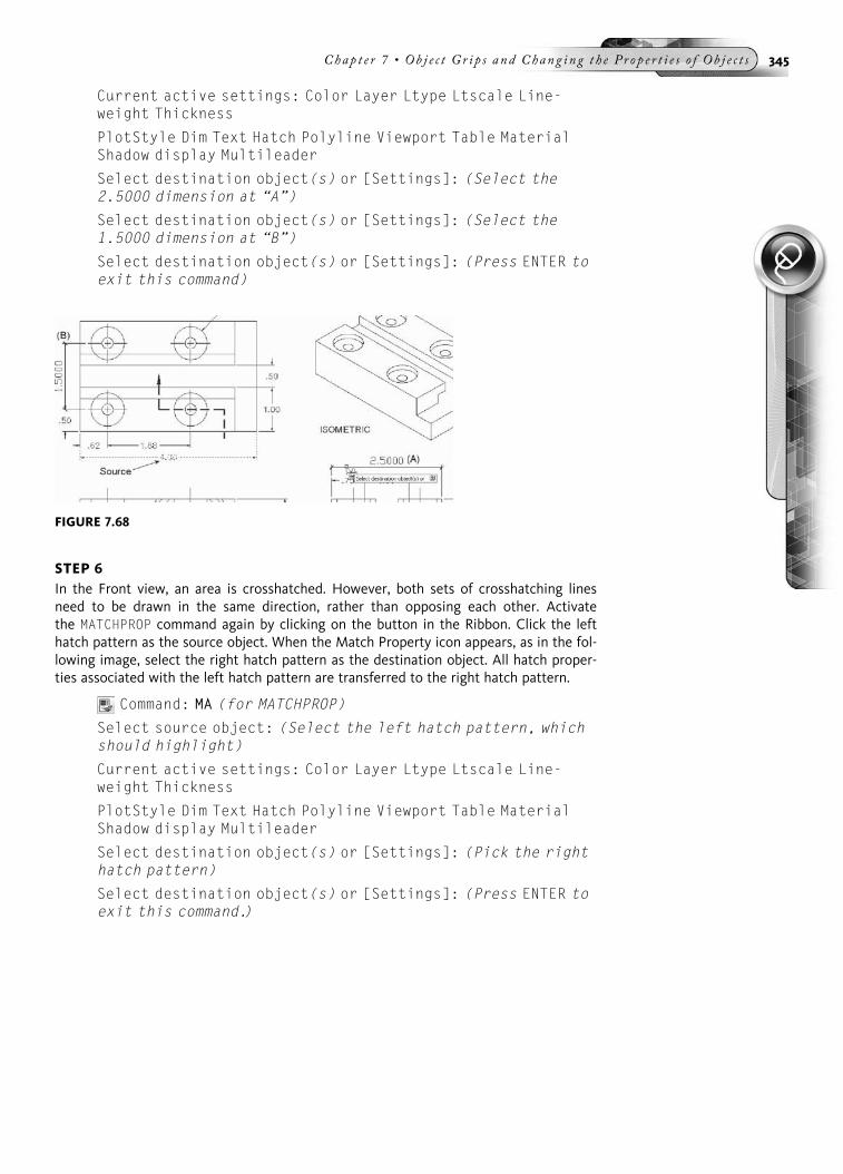
Current active settings: Color Layer Ltype Ltscale Line-weight Thickness
PlotStyle Dim Text Hatch Polyline Viewport Table MaterialShadow display Multileader
Select destination object(s) or [Settings]: (Select the2.5000 dimension at “A”)
Select destination object(s) or [Settings]: (Select the1.5000 dimension at “B”)
Select destination object(s) or [Settings]: (Press ENTER toexit this command)
STEP 6In the Front view, an area is crosshatched. However, both sets of crosshatching linesneed to be drawn in the same direction, rather than opposing each other. Activatethe MATCHPROP command again by clicking on the button in the Ribbon. Click the lefthatch pattern as the source object. When the Match Property icon appears, as in the fol-lowing image, select the right hatch pattern as the destination object. All hatch proper-ties associated with the left hatch pattern are transferred to the right hatch pattern.
Command: MA (for MATCHPROP)
Select source object: (Select the left hatch pattern, whichshould highlight)
Current active settings: Color Layer Ltype Ltscale Line-weight Thickness
PlotStyle Dim Text Hatch Polyline Viewport Table MaterialShadow display Multileader
Select destination object(s) or [Settings]: (Pick the righthatch pattern)
Select destination object(s) or [Settings]: (Press ENTER toexit this command.)
FIGURE 7.68
Chap t e r 7 • Ob j e c t G r i p s a nd Chan g i n g t h e P r o p e r t i e s o f Ob j e c t s 345
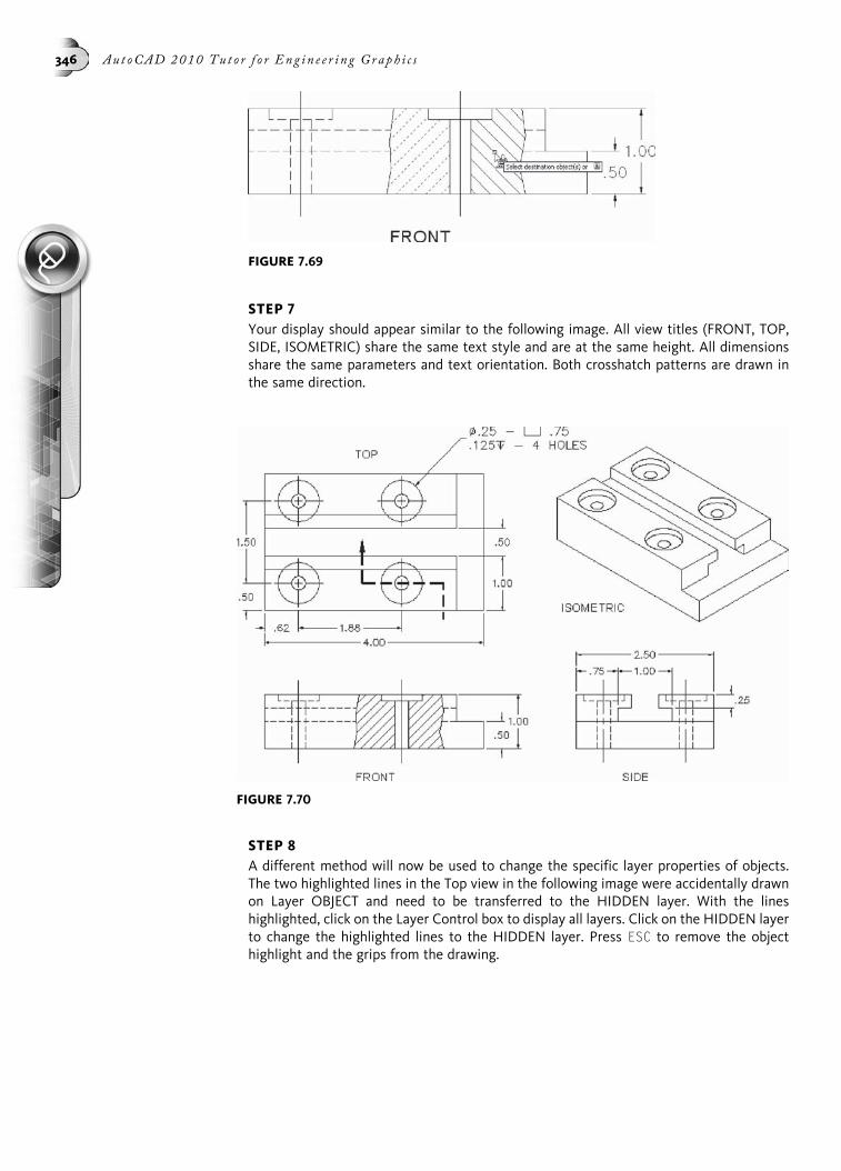
STEP 7Your display should appear similar to the following image. All view titles (FRONT, TOP,SIDE, ISOMETRIC) share the same text style and are at the same height. All dimensionsshare the same parameters and text orientation. Both crosshatch patterns are drawn inthe same direction.
STEP 8A different method will now be used to change the specific layer properties of objects.The two highlighted lines in the Top view in the following image were accidentally drawnon Layer OBJECT and need to be transferred to the HIDDEN layer. With the lineshighlighted, click on the Layer Control box to display all layers. Click on the HIDDEN layerto change the highlighted lines to the HIDDEN layer. Press ESC to remove the objecthighlight and the grips from the drawing.
FIGURE 7.69
FIGURE 7.70
346 Au t oCAD 2010 Tu t o r f o r Eng i n e e r i n g Graph i c s

NOTEYou may need to Regen the drawing in order to get the dashes to appear in the hiddenlines.
STEP 9The two highlighted lines in the Front view in the following image were accidentallydrawn on the TEXT Layer and need to be transferred to the CENTER layer. With the lineshighlighted, click on the Layer Control box to display all layers. Click on the CENTER layerto change the highlighted lines to the CENTER layer. Press ESC to remove the objecthighlight and the grips from the drawing.
FIGURE 7.71
FIGURE 7.72
Chap t e r 7 • Ob j e c t G r i p s a nd Chan g i n g t h e P r o p e r t i e s o f Ob j e c t s 347

STEP 10Your display should appear similar to the following image. Notice the hidden lines in theTop view and the centerlines in the Front view.
STEP 11Click on the Orthographic Views tab. Select the rectangular viewport and change thisobject’s layer to “Viewport” in the following image.
FIGURE 7.73
FIGURE 7.74
348 Au t oCAD 2010 Tu t o r f o r Eng i n e e r i n g Graph i c s

STEP 12Turn off the Viewport layer. Your display should appear similar to the following image.This completes this tutorial exercise.
FIGURE 7.75
Chap t e r 7 • Ob j e c t G r i p s a nd Chan g i n g t h e P r o p e r t i e s o f Ob j e c t s 349

CHAPTER
8Multiview andAuxiliary ViewProjections
Before any object is made in production, some type of drawing needs to be created.This is not just any drawing, but rather an engineering drawing consisting of overallobject sizes with various views of the object organized on the computer screen. Thefirst portion of this chapter introduces the topic of creating multiview projections andincludes methods of constructing one-view, two-view, and three-view drawings usingAutoCAD commands.
The second portion of this chapter introduces the topic of creating auxiliary views.Sometimes three views are still not enough to describe an object, especially if featuresare located on an inclined surface. To produce a view perpendicular to the inclinedsurface, an auxiliary view is drawn.
ONE-VIEW DRAWINGSAn important rule to remember concerning multiview drawings is to draw onlyenough views to accurately describe the object. In the drawing of the gasket in thefollowing image, Front and Side views are shown. However, the Side view is so nar-row that it is difficult to interpret the hidden lines drawn inside. A better approachwould be to leave out the Side view and construct a one-view drawing consisting ofjust the Front view.
350

Begin the one-view drawing of the gasket by first laying out centerlines marking thecenters of all circles and arcs, as shown in the following image on the left. A layercontaining centerlines could be used to show all lines as centerlines.
Use the CIRCLE command to lay out all circles representing the bolt holes of the gas-ket, as shown in the following image on the right. A layer containing continuousobject lines could be used for these circles. You could use the OFFSET command toform the large rectangle on the inside of the gasket. If lines of the rectangle extendpast each other, use the FILLET command set to a value of 0. Selecting two lines ofthe rectangle will form a corner. Repeat this procedure for any other lines that do notform exact corners.
Use the TRIM command to begin forming the outside arcs of the gasket, as shown inthe following image on the left.
Use the FILLET command set to the desired radius to form a smooth transition fromthe arcs to the outer rectangle, as shown in the following image on the right.
FIGURE 8.2
FIGURE 8.1
Chap t e r 8 • Mul t i v i ew and Aux i l i a r y V i ew Pr o j e c t i o n s 351

TWO-VIEW DRAWINGSBefore attempting any drawing, determine how many views need to be drawn.A minimum number of views are needed to describe an object. Drawing extra viewsis not only time-consuming, but it may also result in two identical views with mistakesin each view. You must interpret which is the correct set of views. The illustration inthe following image on the left is a three-view multiview drawing of a coupler. Thecircles and hidden circle identify the Front view. Except for their rotation angles, theTop and Right Side views are identical. In this example, or for other symmetricalobjects, only two views are needed to accurately describe the object being drawn.The Top view has been deleted to leave the Front and Right Side views. The Sideview could have easily been deleted in favor of leaving the Front and Top views.This decision is up to the designer, depending on sheet size and which views arebest suited for the particular application. The desired two view drawing is displayedas shown in the following image on the right.
TRY IT! Open the drawing file 08_R-Guide. Use the following images and descriptions for construct-ing a two-view drawing of this object.
To illustrate how AutoCAD is used as the vehicle for creating a two-view engineeringdrawing, study the two-view drawing along with the pictorial drawing illustrated in thefollowing image to get an idea of how the drawing will appear.
FIGURE 8.4
FIGURE 8.3
352 Au t oCAD 2010 Tu t o r f o r Eng in e e r i n g Graph i c s
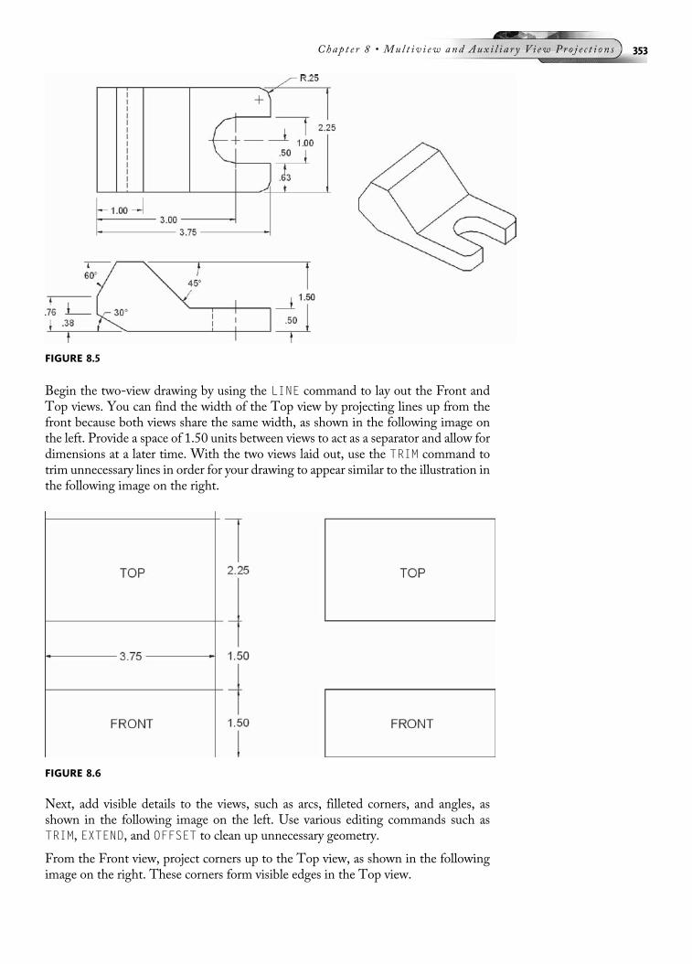
Begin the two-view drawing by using the LINE command to lay out the Front andTop views. You can find the width of the Top view by projecting lines up from thefront because both views share the same width, as shown in the following image onthe left. Provide a space of 1.50 units between views to act as a separator and allow fordimensions at a later time. With the two views laid out, use the TRIM command totrim unnecessary lines in order for your drawing to appear similar to the illustration inthe following image on the right.
Next, add visible details to the views, such as arcs, filleted corners, and angles, asshown in the following image on the left. Use various editing commands such asTRIM, EXTEND, and OFFSET to clean up unnecessary geometry.
From the Front view, project corners up to the Top view, as shown in the followingimage on the right. These corners form visible edges in the Top view.
FIGURE 8.5
FIGURE 8.6
Chap t e r 8 • Mul t i v i ew and Aux i l i a r y V i ew Pr o j e c t i o n s 353

Use the same projection technique to project features from the Top view to the Frontview, as shown in the following image on the left. Then use the TRIM command todelete any geometry that appears in the 1.50 dimension space. The views now mustconform to engineering standards by showing which lines are visible and which areinvisible, as shown in the following image on the right. Use the Layer Control box tochange the line in the Top view from the Object layer to the Hidden layer. In thesame manner, the slot visible in the Top view is hidden in the Front view. Againchange the line in the Front view to the Hidden layer. Since the slot in the Topview represents a circular feature, use the DIMCENTER command to place a centermarker at the center of the semicircle. To show in the Front view that the hiddenline represents a circular feature, add one centerline consisting of one short dash andtwo longer dashes. Be sure this line is drawn on the Center layer. If the slot in the Topview were square instead of circular, centerlines would not be necessary.
FIGURE 8.7
FIGURE 8.8
354 Au t oCAD 2010 Tu t o r f o r Eng in e e r i n g Graph i c s

THREE-VIEW DRAWINGSIf two views are not enough to describe an object, draw three views: Front, Top, andRight Side views.
TRY IT!Open the drawing file 08_Guide Block. Use the following images and descriptions forconstructing a three-view drawing of this object.
A three-view drawing of the guide block, as illustrated in orthographic and pictorialformats in the following image, will be the focus of this segment. Notice the brokensection exposing the Spotface operation above a drill hole.
Begin this drawing by laying out all views using overall dimensions of width, depth,and height, as shown in the following image. The LINE and OFFSET commands arepopular commands used to accomplish this. Provide a space between views to accom-modate dimensions at a later time.
FIGURE 8.9
FIGURE 8.10
Chap t e r 8 • Mul t i v i ew and Aux i l i a r y V i ew Pr o j e c t i o n s 355
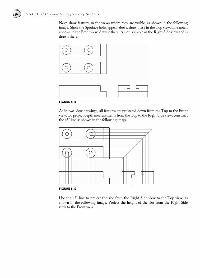
Next, draw features in the views where they are visible, as shown in the followingimage. Since the Spotface holes appear above, draw these in the Top view. The notchappears in the Front view; draw it there. A slot is visible in the Right Side view and isdrawn there.
As in two-view drawings, all features are projected down from the Top to the Frontview. To project depth measurements from the Top to the Right Side view, constructthe 45° line as shown in the following image.
Use the 45° line to project the slot from the Right Side view to the Top view, asshown in the following image. Project the height of the slot from the Right Sideview to the Front view.
FIGURE 8.11
FIGURE 8.12
356 Au t oCAD 2010 Tu t o r f o r Eng in e e r i n g Graph i c s
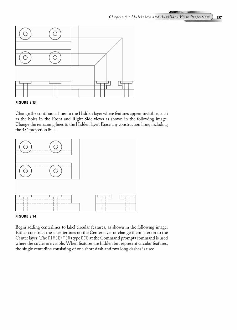
Change the continuous lines to the Hidden layer where features appear invisible, suchas the holes in the Front and Right Side views as shown in the following image.Change the remaining lines to the Hidden layer. Erase any construction lines, includingthe 45°-projection line.
Begin adding centerlines to label circular features, as shown in the following image.Either construct these centerlines on the Center layer or change them later on to theCenter layer. The DIMCENTER (type DCE at the Command prompt) command is usedwhere the circles are visible. When features are hidden but represent circular features,the single centerline consisting of one short dash and two long dashes is used.
FIGURE 8.14
FIGURE 8.13
Chap t e r 8 • Mul t i v i ew and Aux i l i a r y V i ew Pr o j e c t i o n s 357
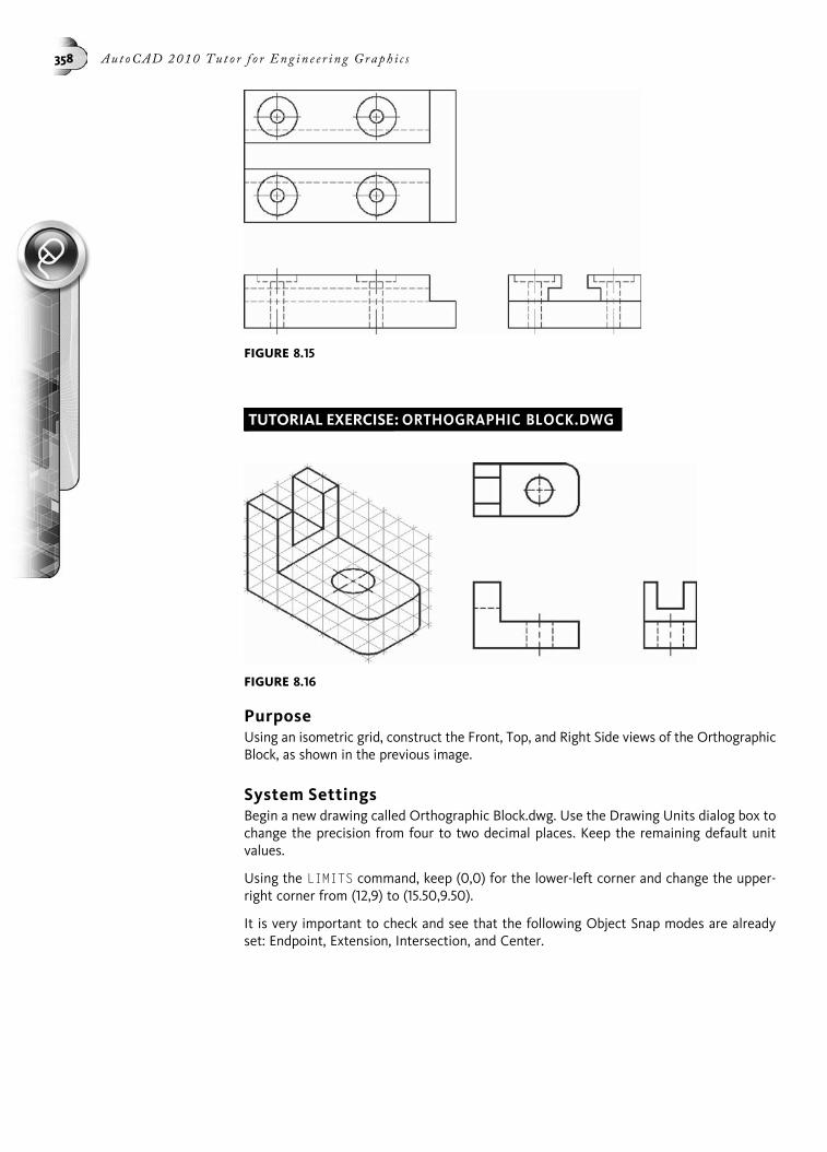
TUTORIAL EXERCISE:ORTHOGRAPHIC BLOCK.DWG
PurposeUsing an isometric grid, construct the Front, Top, and Right Side views of the OrthographicBlock, as shown in the previous image.
System SettingsBegin a new drawing called Orthographic Block.dwg. Use the Drawing Units dialog box tochange the precision from four to two decimal places. Keep the remaining default unitvalues.
Using the LIMITS command, keep (0,0) for the lower-left corner and change the upper-right corner from (12,9) to (15.50,9.50).
It is very important to check and see that the following Object Snap modes are alreadyset: Endpoint, Extension, Intersection, and Center.
FIGURE 8.16
FIGURE 8.15
358 Au t oCAD 2010 Tu t o r f o r Eng in e e r i n g Graph i c s

LayersCreate the following layers with the format:
Name Color Linetype
Object Green Continuous
Hidden Red Hidden
Center Yellow Center
Suggested CommandsBegin this tutorial by laying out the three primary views using the LINE and OFFSETcommands. Use a grid spacing of 0.25 units for all distance calculations.
Use the TRIM command to clean up any excess line segments. As an alternative projectionmethod, use temporary tracking points in combination with Object Snap options to addfeatures in other views.
STEP 1Begin constructing the Orthographic Block by laying out the Front, Top, and Right Sideviews using only the overall dimensions. Do not be concerned about details such as holesor slots; these will be added to the views in a later step. The length of the object shown inthe following image on the left is 8 grid units (2 inches). The height of the object is 5 gridunits (1.25 inches); the depth of the object is 4 units (1 inch). The distance between viewsis 5 grid units (1.25 inches).
STEP 2Once the overall dimensions have been used to lay out the Front, Top, and Right Sideviews, begin adding visible details to the views. The “L” shape is added to the Frontview; the hole and corner fillets are added to the Top view; the rectangular slot is addedto the Right Side view, as shown in the following image on the right. Refer to the isometricview of this object at the beginning of this tutorial for the dimensions of the “L” shape, thehole, corner fillets, and the rectangular slot.
STEP 3Begin projecting the visible edges from hole and slot features onto other views. Slotinformation is added to the Top view and height information is projected onto the RightSide view from the Front view. At this point, only add visible information to other viewswhere required, as shown in the following image on the left.
FIGURE 8.17
Chap t e r 8 • Mul t i v i ew and Aux i l i a r y V i ew Pr o j e c t i o n s 359

STEP 4Now project all hidden features to the other views. The hole projection is hidden in theFront view along with the slot visible in the Right Side view. The hole is also hiddenin the Right Side view, as shown in the following image on the right. Notice how the45° angle is used to project the hole from the Top view to the Right Side view.
STEP 5The completed multiview drawing solution is illustrated in the following image on the left.Dimensions are added to document the exact size of the object, as shown in the followingimage on the right. Proper placement of dimensions will be discussed in Chapter 10.
FIGURE 8.19
FIGURE 8.18
360 Au t oCAD 2010 Tu t o r f o r Eng in e e r i n g Graph i c s

TUTORIAL EXERCISE: 08_SHIFTER.DWG
PurposeThis tutorial is designed to allow the user to construct a three-view drawing of the08_Shifter as shown in the previous image.
System SettingsUse the settings from the previous tutorial and check to see that the following ObjectSnap modes are already set: Endpoint, Extension, Intersection, and Center.
LayersCreate two additional layers:
Name Color Linetype
Dimension Yellow Continuous
Projection Cyan Continuous
Suggested CommandsThe primary commands used during this tutorial are OFFSET and TRIM. The OFFSETcommand is used for laying out all views before the TRIM command is used to clean upexcess lines. Since different linetypes represent certain features of a drawing, the LayerControl box is used to convert to the desired linetype needed as set in the Layer PropertiesManager dialog box. Once all visible details are identified in the primary views, projectthe visible features to the other views using the LINE command. A 45° inclined line isconstructed to project lines from the Top view to the Right Side view and vice versa.
FIGURE 8.20
Chap t e r 8 • Mul t i v i ew and Aux i l i a r y V i ew Pr o j e c t i o n s 361
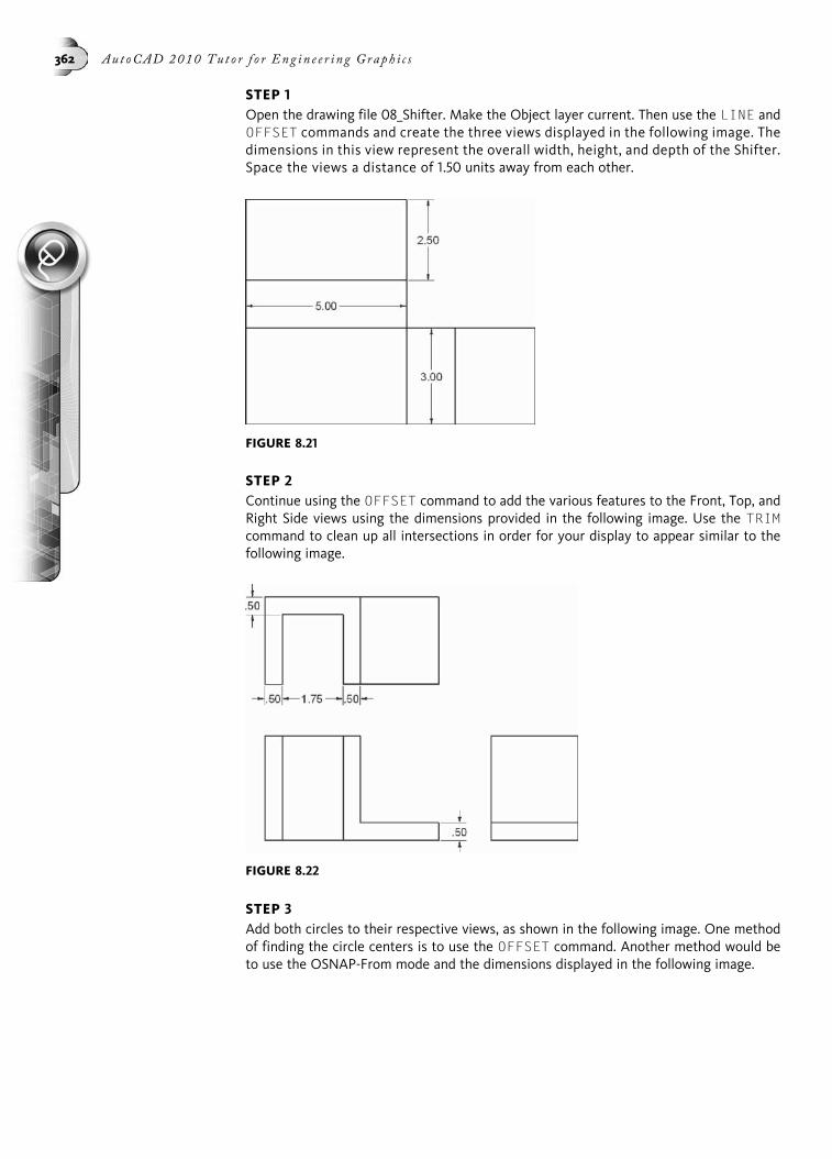
STEP 1Open the drawing file 08_Shifter. Make the Object layer current. Then use the LINE andOFFSET commands and create the three views displayed in the following image. Thedimensions in this view represent the overall width, height, and depth of the Shifter.Space the views a distance of 1.50 units away from each other.
STEP 2Continue using the OFFSET command to add the various features to the Front, Top, andRight Side views using the dimensions provided in the following image. Use the TRIMcommand to clean up all intersections in order for your display to appear similar to thefollowing image.
STEP 3Add both circles to their respective views, as shown in the following image. One methodof finding the circle centers is to use the OFFSET command. Another method would beto use the OSNAP-From mode and the dimensions displayed in the following image.
FIGURE 8.21
FIGURE 8.22
362 Au t oCAD 2010 Tu t o r f o r Eng in e e r i n g Graph i c s
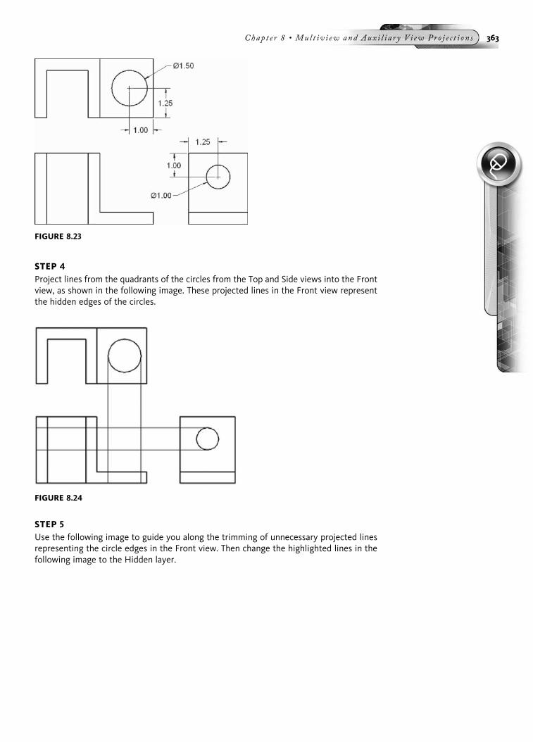
STEP 4Project lines from the quadrants of the circles from the Top and Side views into the Frontview, as shown in the following image. These projected lines in the Front view representthe hidden edges of the circles.
STEP 5Use the following image to guide you along the trimming of unnecessary projected linesrepresenting the circle edges in the Front view. Then change the highlighted lines in thefollowing image to the Hidden layer.
FIGURE 8.23
FIGURE 8.24
Chap t e r 8 • Mul t i v i ew and Aux i l i a r y V i ew Pr o j e c t i o n s 363
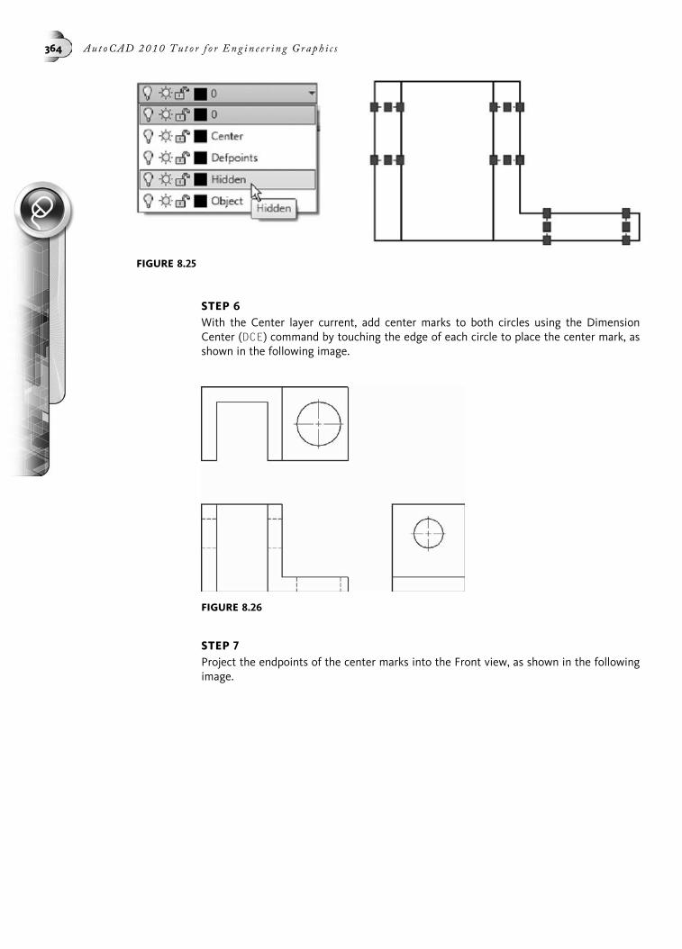
STEP 6With the Center layer current, add center marks to both circles using the DimensionCenter (DCE) command by touching the edge of each circle to place the center mark, asshown in the following image.
STEP 7Project the endpoints of the center marks into the Front view, as shown in the followingimage.
FIGURE 8.25
FIGURE 8.26
364 Au t oCAD 2010 Tu t o r f o r Eng in e e r i n g Graph i c s
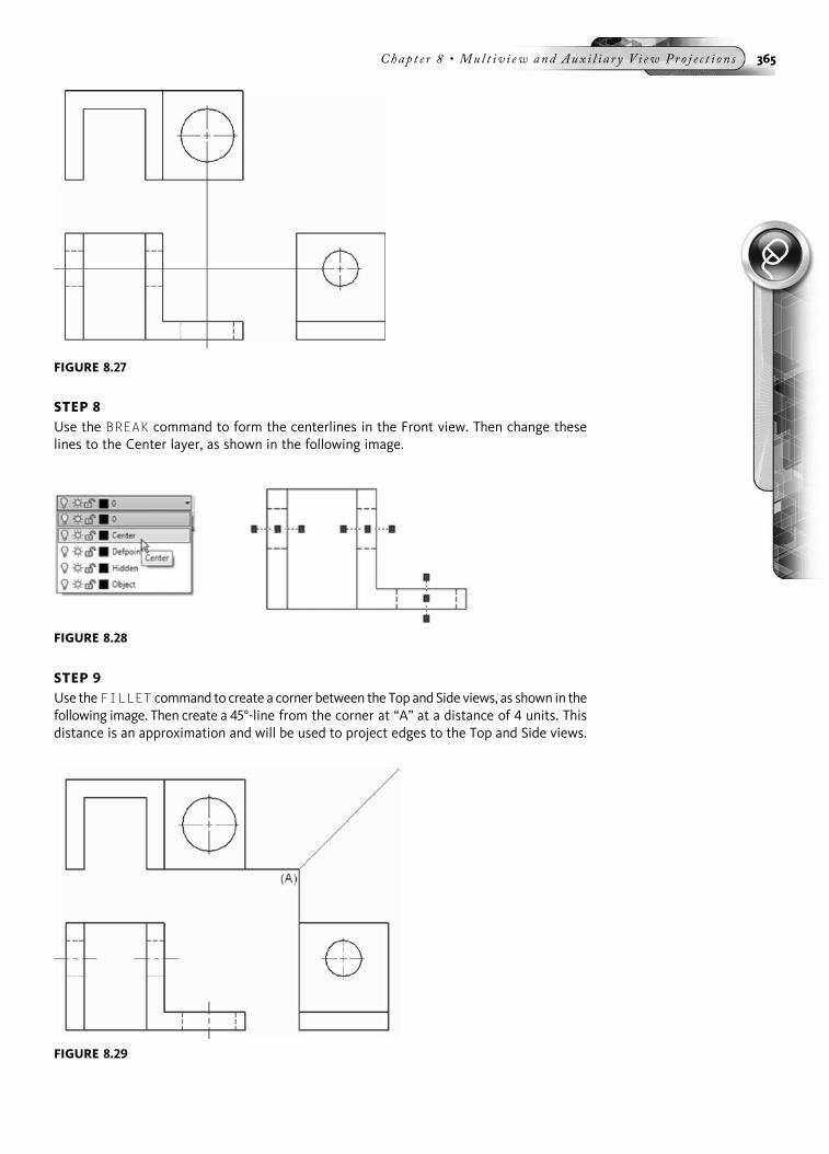
STEP 8Use the BREAK command to form the centerlines in the Front view. Then change theselines to the Center layer, as shown in the following image.
STEP 9Use theFILLET command to create a corner between the Top andSide views, as shown in thefollowing image. Then create a 45°-line from the corner at “A” at a distance of 4 units. Thisdistance is an approximation and will be used to project edges to the Top and Side views.
FIGURE 8.28
FIGURE 8.27
FIGURE 8.29
Chap t e r 8 • Mul t i v i ew and Aux i l i a r y V i ew Pr o j e c t i o n s 365

STEP 10Project lines from the edges of the circles in the Top view to intersect with the 45° angle.Then continue constructing lines into the Side view, as shown in the following image.
STEP 11Use the TRIM and BREAK commands to clean up lines in the Side view, as shown in thefollowing image. Then change these lines to the Hidden and Center layers.
STEP 12Project lines from the edges of the circles in the Side view to intersect with the 45° angle.Then continue constructing lines into the Top view, as shown in the following image.
FIGURE 8.30
FIGURE 8.31
366 Au t oCAD 2010 Tu t o r f o r Eng in e e r i n g Graph i c s

STEP 13Use the TRIM and BREAK commands to clean up lines in the Top view, as shown in thefollowing image. Then change these lines to the Hidden and Center layers.
STEP 14Erase the 45°-angle line, trim the corner connecting the Top and Side views, and extendthe hidden line in the Side view to the top of the line at “A.” This line represents ahidden edge. The completed orthographic drawing of the Shifter is shown in the followingimage.
FIGURE 8.32
FIGURE 8.33
Chap t e r 8 • Mul t i v i ew and Aux i l i a r y V i ew Pr o j e c t i o n s 367

CREATING AUXILIARY VIEWSDuring the discussion of multiview drawings, we discovered that you need to drawenough views of an object to accurately describe it. In most cases, this requires aFront, Top, and Right Side view. Sometimes additional views are required, such asLeft Side, Bottom, and Back views, to show features not visible in the three primaryviews. Other special views, such as sections, are created to expose interior details forbetter clarity. Sometimes all these views are still not enough to describe the object,especially when features are located on an inclined surface. To produce a view perpen-dicular to this inclined surface, an auxiliary view is constructed as shown in thefollowing image. This portion of the chapter will describe where auxiliary views areused and how they are projected from one view to another. A tutorial exercise is pre-sented to show the steps in the construction of an auxiliary view.
FIGURE 8.34
FIGURE 8.35
368 Au t oCAD 2010 Tu t o r f o r Eng in e e r i n g Graph i c s
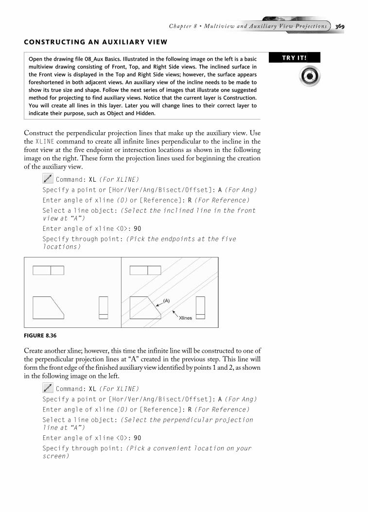
CONSTRUCTING AN AUXILIARY VIEW
TRY IT!Open the drawing file 08_Aux Basics. Illustrated in the following image on the left is a basicmultiview drawing consisting of Front, Top, and Right Side views. The inclined surface inthe Front view is displayed in the Top and Right Side views; however, the surface appearsforeshortened in both adjacent views. An auxiliary view of the incline needs to be made toshow its true size and shape. Follow the next series of images that illustrate one suggestedmethod for projecting to find auxiliary views. Notice that the current layer is Construction.You will create all lines in this layer. Later you will change lines to their correct layer toindicate their purpose, such as Object and Hidden.
Construct the perpendicular projection lines that make up the auxiliary view. Usethe XLINE command to create all infinite lines perpendicular to the incline in thefront view at the five endpoint or intersection locations as shown in the followingimage on the right. These form the projection lines used for beginning the creationof the auxiliary view.
Command: XL (For XLINE)
Specify a point or [Hor/Ver/Ang/Bisect/Offset]: A (For Ang)
Enter angle of xline (0) or [Reference]: R (For Reference)
Select a line object: (Select the inclined line in the frontview at “A”)
Enter angle of xline <0>: 90
Specify through point: (Pick the endpoints at the fivelocations)
Create another xline; however, this time the infinite line will be constructed to one ofthe perpendicular projection lines at “A” created in the previous step. This line willform the front edge of the finished auxiliary view identified by points 1 and 2, as shownin the following image on the left.
Command: XL (For XLINE)
Specify a point or [Hor/Ver/Ang/Bisect/Offset]: A (For Ang)
Enter angle of xline (0) or [Reference]: R (For Reference)
Select a line object: (Select the perpendicular projectionline at “A”)
Enter angle of xline <0>: 90
Specify through point: (Pick a convenient location on yourscreen)
FIGURE 8.36
Chap t e r 8 • Mul t i v i ew and Aux i l i a r y V i ew Pr o j e c t i o n s 369
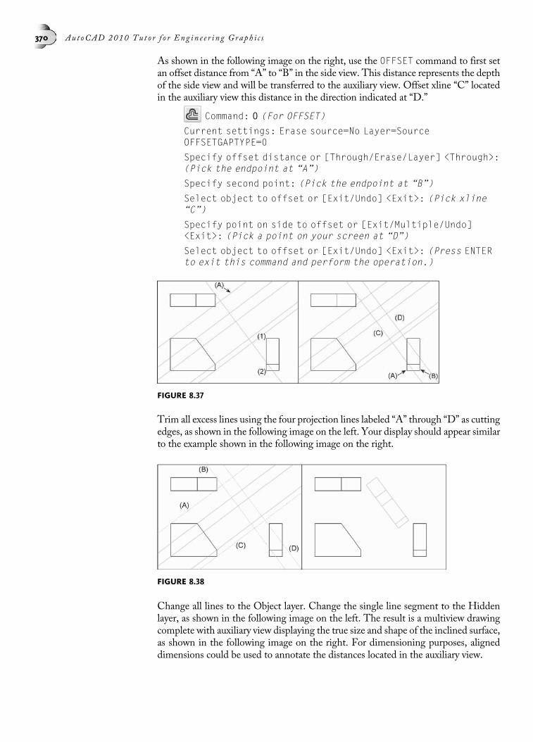
As shown in the following image on the right, use the OFFSET command to first setan offset distance from “A” to “B” in the side view. This distance represents the depthof the side view and will be transferred to the auxiliary view. Offset xline “C” locatedin the auxiliary view this distance in the direction indicated at “D.”
Command: O (For OFFSET)
Current settings: Erase source=No Layer=SourceOFFSETGAPTYPE=0
Specify offset distance or [Through/Erase/Layer] <Through>:(Pick the endpoint at “A”)
Specify second point: (Pick the endpoint at “B”)
Select object to offset or [Exit/Undo] <Exit>: (Pick xline“C”)
Specify point on side to offset or [Exit/Multiple/Undo]<Exit>: (Pick a point on your screen at “D”)
Select object to offset or [Exit/Undo] <Exit>: (Press ENTERto exit this command and perform the operation.)
Trim all excess lines using the four projection lines labeled “A” through “D” as cuttingedges, as shown in the following image on the left. Your display should appear similarto the example shown in the following image on the right.
Change all lines to the Object layer. Change the single line segment to the Hiddenlayer, as shown in the following image on the left. The result is a multiview drawingcomplete with auxiliary view displaying the true size and shape of the inclined surface,as shown in the following image on the right. For dimensioning purposes, aligneddimensions could be used to annotate the distances located in the auxiliary view.
FIGURE 8.37
FIGURE 8.38
370 Au t oCAD 2010 Tu t o r f o r Eng in e e r i n g Graph i c s

CREATING AUXILIARY VIEWS USING XLINESThe following image shows an object consisting of front and right side views in addi-tion to an isometric or pictorial view. To construct the perpendicular projector linesthat will be used to create the auxiliary view, the XLINE command is used. Xlinesare considered construction lines and were discussed in Chapter 5. The Angle andReference options of the XLINE command provide an easy way to construct the per-pendicular projection lines. You first enter the Angle option followed by the Refer-ence option. You will be prompted to select an object; pick line segment “AE,” asshown in the following image. Then enter an angle of 90° as the angle of the xline,and pick the endpoints at “A” through “E” to construct the xline objects. By default,all xlines are drawn infinitely in two directions. You can trim, fillet, and even breakxlines.
Command: XL (For XLINE)
XLINE Specify a point or [Hor/Ver/Ang/Bisect/Offset]:A (For Ang)
Enter angle of xline (0) or [Reference]: R (For Reference)
Select a line object: (Select line segment “AE”)
Enter angle of xline <0>: 90
Specify through point: (Pick the endpoints of points “A”through “E”)
FIGURE 8.39
FIGURE 8.40
Chap t e r 8 • Mul t i v i ew and Aux i l i a r y V i ew Pr o j e c t i o n s 371

With the perpendicular projection lines constructed, next construct a base edge thatis perpendicular to the projection lines. This base edge normally forms one of theedges of the auxiliary view. In the following example, line segment “1-2” located inthe right side view coincides with xline segment “1-2” found in the auxiliary view.
Command: XL (For XLINE)
XLINE Specify a point or [Hor/Ver/Ang/Bisect/Offset]: A (ForAng)
Enter angle of xline (0) or [Reference]: R (For Reference)
Select a line object: (Pick the xline at “1”)
Enter angle of xline <0>: 90
Specify through point: (Pick an approximate location in thedrawing to locate the base edge of the auxiliary view.)
TRANSFERRING DISTANCES WITH THE OFFSET COMMANDWith the perpendicular projectors constructed along with the base edge using xlines,the next step is to transfer distances from one view and create the auxiliary view. Theauxiliary view in our example is a depth type. All views projected from the front viewshow depth. This means that the distances along the projectors can be transferredfrom the depth dimensions in a top or right side view. In this example the depthwill be transferred from the right side view using the OFFSET command. To accom-plish this, enter offset and for the offset distance, pick the endpoint at “A” in the rightside view, as shown in the following image. For the second point, pick the endpointat “B.” These two endpoints form the depth of the right side view. To transfer thisdistance to the auxiliary view, pick line “C” as the object to offset and then pick alocation at “D” as the side to perform the offset shown in the following image.
Command: O (For OFFSET)
Current settings: Erase source=No Layer=SourceOFFSETGAPTYPE=0
Specify offset distance or [Through/Erase/Layer] <Through>:(Pick the endpoint at “A”)
FIGURE 8.41
372 Au t oCAD 2010 Tu t o r f o r Eng in e e r i n g Graph i c s
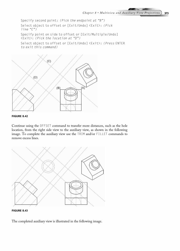
Specify second point: (Pick the endpoint at “B”)
Select object to offset or [Exit/Undo] <Exit>: (Pickline “C”)
Specify point on side to offset or [Exit/Multiple/Undo]<Exit>: (Pick the location at “D”)
Select object to offset or [Exit/Undo] <Exit>: (Press ENTERto exit this command)
Continue using the OFFSET command to transfer more distances, such as the holelocation, from the right side view to the auxiliary view, as shown in the followingimage. To complete the auxiliary view use the TRIM and/or FILLET commands toremove excess lines.
The completed auxiliary view is illustrated in the following image.
FIGURE 8.42
FIGURE 8.43
Chap t e r 8 • Mul t i v i ew and Aux i l i a r y V i ew Pr o j e c t i o n s 373

CONSTRUCTING THE TRUE SIZE OF A CURVED SURFACE
TRY IT! Open the file 08_Aux Curve.dwg as shown in the following image on the left. From frontand right side views, an auxiliary view will be created to display the true size and shape ofthe inclined surface. Notice that a layer called Construction has already been created and iscurrent. This layer will be used throughout this tutorial exercise.
Construct the perpendicular projection lines that make up the auxiliary view. Use theXLINE command to create three infinite lines perpendicular to the incline in the frontview at the three locations shown in the following image on the right. These form theprojection lines used for beginning the auxiliary view.
Command: XL (For XLINE)
Specify a point or [Hor/Ver/Ang/Bisect/Offset]: A (For Ang)
Enter angle of xline (0) or [Reference]: R (For Reference)
Select a line object: (Select the inclined line in the frontview)
Enter angle of xline <0>: 90
Specify through point: (Pick the three locations)
FIGURE 8.44
FIGURE 8.45
374 Au t oCAD 2010 Tu t o r f o r Eng in e e r i n g Graph i c s

Create another xline; however, this time the infinite line will be constructed to oneof the perpendicular projection lines created in the previous step. This line will formthe back edge of the finished auxiliary view identified by points 1 and 2 shown in thefollowing image on the left.
Command: XL (For XLINE)
Specify a point or [Hor/Ver/Ang/Bisect/Offset]: A (For Ang)
Enter angle of xline (0) or [Reference]: R (For Reference)
Select a line object: (Select one of the perpendicularprojection lines)
Enter angle of xline <0>: 90
Specify through point: (Pick a location)
Trim the back corners of the projection lines. Your display should appear as shown inthe following image on the right.
Set an offset distance from “A” to “B” in the side view. This distance represents thedepth of the object and will be transferred to the auxiliary view. Offset the xlinelocated in the auxiliary view this distance in the direction indicated in the followingimage on the left.
Command: O (For OFFSET)
Current settings: Erase source=No Layer=SourceOFFSETGAPTYPE=0
Specify offset distance or [Through/Erase/Layer] <Through>:(Pick the endpoint at “A”)
Specify second point: (Pick the endpoint at “B”)
Select object to offset or [Exit/Undo] <Exit>: (Pick xline“C”)
Specify point on side to offset or [Exit/Multiple/Undo]<Exit>: (Pick a point on your screen at “D”)
Select object to offset or [Exit/Undo] <Exit>: (Press ENTERto exit this command and perform the operation.)
Set another offset distance from “A” to “B” in the side view; then offset back line “C”located in the auxiliary view this distance to “D,” as shown in the following image onthe right.
FIGURE 8.46
Chap t e r 8 • Mul t i v i ew and Aux i l i a r y V i ew Pr o j e c t i o n s 375

Trim and erase lines until your display appears as shown in the following image onthe left. Construct a horizontal xline from the lower point of the incline. Then offsetthis xline at .25 increments. Your display should appear as shown in the followingimage on the right.
Construct an angled xline perpendicular to every intersection along the incline. Youshould have 5 xlines constructed from these points. Your display should appear asshown in the following image on the left. Create an offset distance from “A” to “B”along line segment 1 in the side view. Then offset the back line “C” this distance at“D” in the auxiliary view, as shown in the following image on the right.
Place points at their respective intersections, as shown in the following image on theleft. The purpose of the points is to identify a segment of the arc to be constructedin the auxiliary view. Perform the same series of steps to locate the remainingpoints that make up the curve in the auxiliary view, as shown in the following imageon the right.
FIGURE 8.47
FIGURE 8.48
FIGURE 8.49
376 Au t oCAD 2010 Tu t o r f o r Eng in e e r i n g Graph i c s

Use the SPLINE command to create a spline connecting all points along the auxiliaryview, as shown in the following image on the left. Use the Osnap-Node mode forlocking onto each point. Make the Object layer current. Then change the visible linesof the auxiliary view to the Object layer. Turn off the Construction layer. Your displayshould appear similar to the example in the following image on the right.
TUTORIAL EXERCISE: 08_BRACKET.DWG
FIGURE 8.50
FIGURE 8.51
FIGURE 8.52
Chap t e r 8 • Mul t i v i ew and Aux i l i a r y V i ew Pr o j e c t i o n s 377

PurposeThis tutorial is designed to allow you to construct an auxiliary view of the inclined surfacefor the bracket shown in the previous image.
System SettingsSince this drawing is provided on CD, edit an existing drawing called 08_Bracket. Followthe steps in this tutorial for the creation of an auxiliary view.
LayersThe following layers have already been created with the following format:
Name Color Linetype
CEN Yellow Center
DIM Yellow Continuous
HID Red Hidden
OBJ Cyan Continuous
Suggested CommandsBegin this tutorial by using the OFFSET command to construct a series of lines parallelto the inclined surface containing the auxiliary view. Next construct lines perpendicular tothe inclined surface. Use the CIRCLE command to begin laying out features that lie in theauxiliary view. Use ARRAY to copy the circle in a rectangular pattern. Add centerlines usingthe DIMCENTER command. Insert a predefined view called Top. A three-view drawingconsisting of Front, Top, and auxiliary views is completed.
STEP 1Begin the construction of the auxiliary view by using the OFFSET command to copy aline parallel to the inclined line located in the Front view, as shown in the following imageon the left. Use an offset distance of 8.50, pick line “A” as the object to offset, and picknear “B” as the side to perform the offset. Then use the OFFSET command again to offsetline “B” to the side at “C” at a distance of 6.00 units.
The previous two lines formed using the OFFSET command define the depth of theauxiliary view. To determine the width of the auxiliary view, use the XLINE commandto construct the two perpendicular projection lines, as shown in the following image.Project the two xlines from the endpoints of the Front view at “D” and “E” at an angleperpendicular to line “A,” as shown in the following image on the right.
FIGURE 8.53
378 Au t oCAD 2010 Tu t o r f o r Eng in e e r i n g Graph i c s

STEP 2Use the ZOOM-Window option to magnify the display of the auxiliary view similar to theillustration in the following image on the left. Then use the FILLET command to createfour corners using the lines labeled “A” through “D.” The fillet radius should be set to 0 inorder to form the corners. The results are displayed in the following image on the right.
STEP 3When you are finished with the filleting operation, activate the View Manager dialog box,as shown in the following image on the left, and click the New button. When the NewView/Shot Properties dialog box appears, as shown in the following image on the right,verify that the view will be defined based on the Current display; a radio button shouldbe active for this mode. Then save the display to a new name, AUX.
STEP 4Use the ZOOM-Previous option or other ZOOM mode to demagnify the screen back tothe original display. Use XLINE to create a perpendicular projection from the endpointof the centerline at “A,” as shown in the following image on the left. Use the Referenceoption and pick the centerline. Keep the default angle of 0.
This is one of the construction lines that will be used for finding the centers of the circularfeatures located in the auxiliary view.
Then use the OFFSET command to create the other construction line, as shown in thefollowing image on the right. Use an offset distance of 3.00, pick line “B” as the objectto offset, and pick a point near “C,” as shown in the following image on the right.
FIGURE 8.54
FIGURE 8.55
Chap t e r 8 • Mul t i v i ew and Aux i l i a r y V i ew Pr o j e c t i o n s 379

STEP 5Activate the View Manager dialog box and set the view AUX current, as shown in thefollowing image on the left. Then draw two circles of diameters 3.00 and 1.50 from thecenter at “A,” as shown in the following image on the right, using the CIRCLE command.For the center of the second circle, you can use the @ option to pick up the previouspoint that was the center of the first circle.
STEP 6Use the OFFSET command to offset the centerline the distance of .25 units, as shown inthe following image on the left. Perform this operation on both sides of the centerline.Both offset lines form the width of the .50 slot.
Then use the TRIM command to trim away portions of the offset lines, using the twocircles as cutting edges. When finished, your display should resemble the illustration inthe following image on the right.
FIGURE 8.56
FIGURE 8.57
380 Au t oCAD 2010 Tu t o r f o r Eng in e e r i n g Graph i c s

STEP 7Use the ERASE command to delete the two lines at “A” and “B,” as shown in the followingimage on the left. Standard centerlines will be placed here later, marking the center of bothcircles.
Two more construction lines need to be made. These lines will identify the center of thesmall .37-diameter circle. Use the OFFSET command to create offsets for the lines illus-trated in the following image on the right. Offset distances of .75 and 1.00 are used toperform this task. Also be careful to offset the correct line at the specified distance.
STEP 8Draw a circle of .37 units in diameter from the intersection of the two lines created in thelast OFFSET command, as shown in the following image on the left. Then use the ERASEcommand to delete the two lines labeled “A” and “B.” A standard center marker will beplaced later at the center of this circle.
For the next phase of this step, make the CEN layer current through the Layer ControlBox. The DIMCENTER command (or DCE for short) will be used to create the centermark for the .37-diameter circle. Type DCE at the command prompt and pick the edge ofthe circle at “C,” as shown in the middle of the following image, to place this center mark.
Next, use the ROTATE command to rotate the center marker parallel to the edges of theauxiliary view. Activate the ROTATE command and pick the centerlines. For the basepoint of the rotation, pick a point at the center of the circle at “D” using OSNAP Centeror Intersection mode. For the rotation angle, use OSNAP Perpendicular and pick the linenear “E.” The centerlines should rotate parallel to the edge of the auxiliary, as shown inthe following image on the right.
FIGURE 8.58
FIGURE 8.59
Chap t e r 8 • Mul t i v i ew and Aux i l i a r y V i ew Pr o j e c t i o n s 381

STEP 9Since the remaining seven holes form a rectangular pattern, use the Array dialog box, asshown in the following image on the left, and perform a rectangular array based on the.37-diameter circle and center marks. The number of rows is two and the number ofcolumns is four. The distance between rows is 4.50 units and between columns is �0.75units. Set the angle of the array by picking two points. To accomplish this, click the Pickangle of array button as shown in the following image and pick the endpoint at “A” firstand the endpoint at “B” next. This creates the angle of the array at 330°. Also be sure toselect the circle and centerlines as the objects to array. Performing a preview results inthe array displayed in the following image on the right.
STEP 10Use the FILLET command set to a radius of .75 to place a radius along the two cornersof the auxiliary, as shown in the following image on the left.
Place a center mark in the center of the two large circles using the DIMCEN (or DCE forshort) command. When prompted to select the arc or circle, pick the edge of the largecircle. The results are displayed in the middle of the following image.
Then rotate the center mark using the ROTATE command. Use OSNAP Perpendicular toset the rotation angle. The results are displayed in the following image on the right.
FIGURE 8.60
FIGURE 8.61
382 Au t oCAD 2010 Tu t o r f o r Eng in e e r i n g Graph i c s

STEP 11Activate the View Manager dialog box, as shown in the following image, and set the viewnamed OVERALL current. This should return your display to view all views of the Bracket.
STEP 12Complete the drawing of the bracket by activating the Insert dialog box as shown in thefollowing image and inserting an existing block called TOP into the drawing. This blockrepresents the complete Top view of the drawing. Use an insertion point of 0,0 for placingthis view in the drawing. Your display should appear similar to the following image.
FIGURE 8.62
FIGURE 8.63
Chap t e r 8 • Mul t i v i ew and Aux i l i a r y V i ew Pr o j e c t i o n s 383

END OF CHAPTER PROBLEMS FOR CHAPTER 8Please refer to the CD that is supplied with this book and locate the file AutoCAD Tutor2010 Support Docs.pdf. In addition to extra information supplied in this chapter,end-of-chapter problems are also available to provide additional practice.
FIGURE 8.64
384 Au t oCAD 2010 Tu t o r f o r Eng in e e r i n g Graph i c s
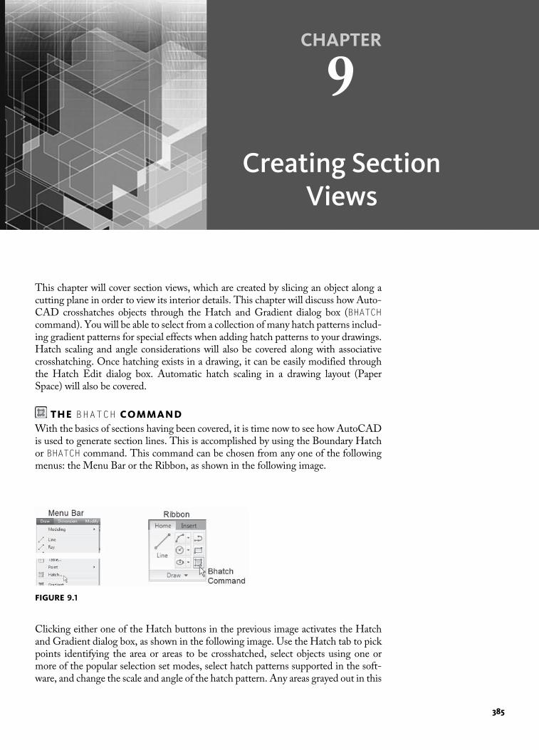
CHAPTER
9
Creating SectionViews
This chapter will cover section views, which are created by slicing an object along acutting plane in order to view its interior details. This chapter will discuss how Auto-CAD crosshatches objects through the Hatch and Gradient dialog box (BHATCHcommand). You will be able to select from a collection of many hatch patterns includ-ing gradient patterns for special effects when adding hatch patterns to your drawings.Hatch scaling and angle considerations will also be covered along with associativecrosshatching. Once hatching exists in a drawing, it can be easily modified throughthe Hatch Edit dialog box. Automatic hatch scaling in a drawing layout (PaperSpace) will also be covered.
THE BHATCH COMMANDWith the basics of sections having been covered, it is time now to see how AutoCADis used to generate section lines. This is accomplished by using the Boundary Hatchor BHATCH command. This command can be chosen from any one of the followingmenus: the Menu Bar or the Ribbon, as shown in the following image.
Clicking either one of the Hatch buttons in the previous image activates the Hatchand Gradient dialog box, as shown in the following image. Use the Hatch tab to pickpoints identifying the area or areas to be crosshatched, select objects using one ormore of the popular selection set modes, select hatch patterns supported in the soft-ware, and change the scale and angle of the hatch pattern. Any areas grayed out in this
FIGURE 9.1
385
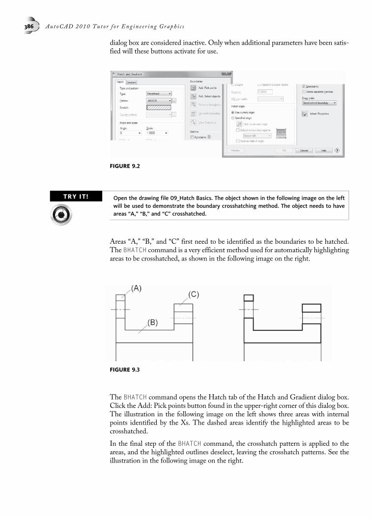
dialog box are considered inactive. Only when additional parameters have been satis-fied will these buttons activate for use.
TRY IT! Open the drawing file 09_Hatch Basics. The object shown in the following image on the leftwill be used to demonstrate the boundary crosshatching method. The object needs to haveareas “A,” “B,” and “C” crosshatched.
Areas “A,” “B,” and “C” first need to be identified as the boundaries to be hatched.The BHATCH command is a very efficient method used for automatically highlightingareas to be crosshatched, as shown in the following image on the right.
The BHATCH command opens the Hatch tab of the Hatch and Gradient dialog box.Click the Add: Pick points button found in the upper-right corner of this dialog box.The illustration in the following image on the left shows three areas with internalpoints identified by the Xs. The dashed areas identify the highlighted areas to becrosshatched.
In the final step of the BHATCH command, the crosshatch pattern is applied to theareas, and the highlighted outlines deselect, leaving the crosshatch patterns. See theillustration in the following image on the right.
FIGURE 9.2
FIGURE 9.3
386 Au t oCAD 2010 Tu t o r f o r Eng in e e r i n g Graph i c s

AVAILABLE HATCH PATTERNSThe Hatch tab holds numerous hatch patterns in a drop-down list box, shown in thefollowing image. Clicking on a pattern in this listing makes the pattern current.
Selecting the pattern (…) button or ellipses next to the pattern name, as shown in thefollowing image on the left, activates the Hatch Pattern Palette dialog box. Here, aseries of tabs are present that display a number of crosshatching patterns already cre-ated and ready for use, as shown in the following image on the right. Select a particu-lar pattern by clicking on the pattern itself. If the wrong pattern was selected, simplychoose the correct one or move to another tab to view other patterns for use.
FIGURE 9.4
FIGURE 9.5
FIGURE 9.6
Chap t e r 9 • Cr e a t i n g S e c t i o n V i ew s 387

Once a hatch pattern is selected, the name is displayed in the Hatch and Gradientdialog box, as shown in the following image. If the scaling and angle settings lookfavorable, click the Add: Pick points button. The command prompt requires you toselect an internal point or points.
Continue working with the drawing file 09_Hatch Basics. Click in the three areasmarked by the X, as shown in the following image on the left. Notice that these areashighlight. If these areas are correct, press ENTER to return to the Hatch and Gradientdialog box.
When you are back in the Hatch and Gradient dialog box, you now have the optionof first previewing the hatch to see if all settings and the appearance of the pattern aredesirable. Click the Preview button in the lower-left corner of the dialog box to ac-complish this. The results appear in the following image on the right. At this pointin the process, the pattern is still not permanently placed on the object. Pressingthe ENTER key to exit Preview mode returns you to the main Hatch and Gradientdialog box. If the hatch pattern is correct in appearance, click the OK button to placethe pattern with the drawing.
FIGURE 9.7
FIGURE 9.8
388 Au t oCAD 2010 Tu t o r f o r Eng in e e r i n g Graph i c s

SOLID FILL HATCH PATTERNSActivating the Hatch and Gradient dialog box and clicking on the pattern (…) but-ton or ellipses followed by the Other Predefined tab displays the dialog box as shownin the following image on the left. Additional patterns are available and include brick,roof, and other construction-related materials. One powerful pattern is calledSOLID. This pattern is used to fill in an enclosed area with a solid color based onthe current layer. The illustration in the following image on the right shows a typicalapplication of filling in the walls of a floor plan with a solid color.
TRY IT!Open the drawing file 09_Hatch Solid1. The object shown in the following image on the leftillustrates a thin wall that needs to be filled in. The BHATCH command used with the SOLIDhatch pattern can perform this task very efficiently. When you pick an internal point, theentire closed area is filled with a solid pattern and placed on the current layer with thesame color and other properties of the current layer.
The solid hatch pattern shown in the following image on the right was placed withone internal point pick.
TRY IT!Open the drawing file 09_Hatch Solid2. Applying the SOLID hatch pattern to the object, asshown in the following image on the left, can easily be accomplished with the BHATCH com-mand. This object also is a thin-wall example, with the addition of various curved edges andfillets.
The solid hatch pattern also works for curved outlines. The illustration in the follow-ing image on the right displays the solid pattern, completely filling in the outlinewhere all corners consist of some type of curve generated by the FILLET command.
FIGURE 9.9
FIGURE 9.10
Chap t e r 9 • Cr e a t i n g S e c t i o n V i ew s 389

GRADIENT PATTERNSA gradient hatch pattern is a solid hatch fill that makes a smooth transition from a
lighter shade to a darker shade. Predefined patterns such as linear, spherical, and ra-dial sweep are available to provide different effects. As with the vector hatch patternsthat have always been supplied with AutoCAD, the angle of the gradient patterns canalso be controlled. Gradient patterns can also be associative; the pattern updates if theboundary is changed. To edit a gradient pattern, simply double-click it to launchthe Hatch Edit dialog box. As with hatch patterns, clicking on Gradient in any ofthe following menu items will launch the Gradient tab of the Hatch and Gradientdialog box: Menu Bar or Ribbon. A few of the controls for this tab of the dialogbox are explained as follows:
• One Color—When this option is selected, a color swatch with a Browse button and aShade and Tint slider appears. The One Color option designates a fill that usesa smooth transition between darker shades and lighter tints of a single color.
• Two Color—When this option is selected, a color swatch and Browse button displayfor colors 1 and 2. This option allows the fill to transition smoothly between two colors.
• Color Swatch—This is the default color displayed as set by the current color in thedrawing. This option specifies the color to be used for the gradient fill. The presenceof the three dots, called ellipses (. . .), next to the color swatch signifies the Browsebutton. Use this to display the Select Color dialog box, similar to the dialog used forassigning colors to layers. Use this dialog box to select color based on the AutoCADIndex Color, True Color, or Color Book.
• Shade and Tint Slider—This option designates the amount of tint and shade applied tothe gradient fill of one color. Tint is defined as the selected color mixed with white.Shade is defined as the selected color mixed with black.
• Centered Option—Use this option for creating special effects with gradient patterns.When this option is checked, the gradient fill appears symmetrical. If the option is notselected, AutoCAD shifts the gradient fill up to the left. This position creates theillusion that a light source is located to the left of the object.
• Angle—Set an angle that affects the gradient pattern fill. This angle setting is inde-pendent of the angle used for regular hatch patterns.
• Gradient Patterns—Nine gradient patterns are available for you to apply. Theseinclude linear sweep, spherical, and parabolic.
FIGURE 9.11
390 Au t oCAD 2010 Tu t o r f o r Eng in e e r i n g Graph i c s

The example of the house elevation in the following image illustrates parabolic linearsweep being applied above and below the house.
HATCH PATTERN SYMBOL MEANINGSListed below are a number of hatch patterns and their purposes. For example, if youare constructing a mechanical assembly in which you want to distinguish plastic ma-terial from steel, use the patterns ANSI34 and ANSI32, respectively. Patterns thatbegin with AR- have architectural applications. Refer to the following list for the pur-poses of other materials and their associated hatch patterns.
FIGURE 9.12
FIGURE 9.13
Chap t e r 9 • Cr e a t i n g S e c t i o n V i ew s 391
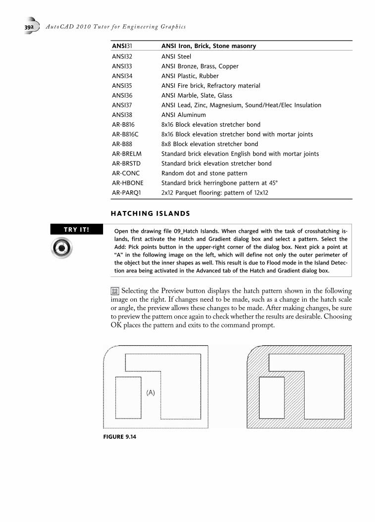
ANSI31 ANSI Iron, Brick, Stone masonry
ANSI32 ANSI Steel
ANSI33 ANSI Bronze, Brass, Copper
ANSI34 ANSI Plastic, Rubber
ANSI35 ANSI Fire brick, Refractory material
ANSI36 ANSI Marble, Slate, Glass
ANSI37 ANSI Lead, Zinc, Magnesium, Sound/Heat/Elec Insulation
ANSI38 ANSI Aluminum
AR-B816 8x16 Block elevation stretcher bond
AR-B816C 8x16 Block elevation stretcher bond with mortar joints
AR-B88 8x8 Block elevation stretcher bond
AR-BRELM Standard brick elevation English bond with mortar joints
AR-BRSTD Standard brick elevation stretcher bond
AR-CONC Random dot and stone pattern
AR-HBONE Standard brick herringbone pattern at 45°
AR-PARQ1 2x12 Parquet flooring: pattern of 12x12
HATCHING ISLANDS
TRY IT! Open the drawing file 09_Hatch Islands. When charged with the task of crosshatching is-lands, first activate the Hatch and Gradient dialog box and select a pattern. Select theAdd: Pick points button in the upper-right corner of the dialog box. Next pick a point at“A” in the following image on the left, which will define not only the outer perimeter ofthe object but the inner shapes as well. This result is due to Flood mode in the Island Detec-tion area being activated in the Advanced tab of the Hatch and Gradient dialog box.
Selecting the Preview button displays the hatch pattern shown in the followingimage on the right. If changes need to be made, such as a change in the hatch scaleor angle, the preview allows these changes to be made. After making changes, be sureto preview the pattern once again to check whether the results are desirable. ChoosingOK places the pattern and exits to the command prompt.
FIGURE 9.14
392 Au t oCAD 2010 Tu t o r f o r Eng in e e r i n g Graph i c s

HATCH PATTERN SCALINGHatching patterns are predefined in size and angle. When you use the BHATCH com-mand, the pattern used is assigned a scale value of 1.00, which will draw the patternexactly the way it was originally created.
TRY IT!Open the drawing file 09_Hatch Scale. Activate the Hatch and Gradient dialog box, acceptall default values, and pick internal points to hatch the object as shown in the following im-age on the left.
Entering a different scale value for the pattern in the Hatch and Gradient dialog boxeither increases or decreases the spacing between crosshatch lines. The illustration inthe following image on the right is an example of the ANSI31 pattern with a newscale value of 0.50.
As you can decrease the scale of a pattern to hatch small areas, you can also scale thepattern up for large areas. The illustration in the following image has a hatch scale of2.00, which doubles all distances between hatch lines.
Use care when hatching large areas. In this image, the total length of the object mea-sures 190.50 mm. If the hatch scale of 1.00 were used, the pattern would take on afilled appearance. This results in numerous lines being generated, which increases thesize of the drawing file. A value of 25.4, the number of millimeters in an inch, is usedto scale hatch lines for metric drawings.
TRY IT!Open the drawing file 09_Hatch Scale mm. Activate the Hatch and Gradient dialog box andchange the pattern scale to 25.4 units. Click the Add: Pick points button to pick internalpoints to crosshatch the object illustrated in the following image.
FIGURE 9.15
FIGURE 9.16
Chap t e r 9 • Cr e a t i n g S e c t i o n V i ew s 393
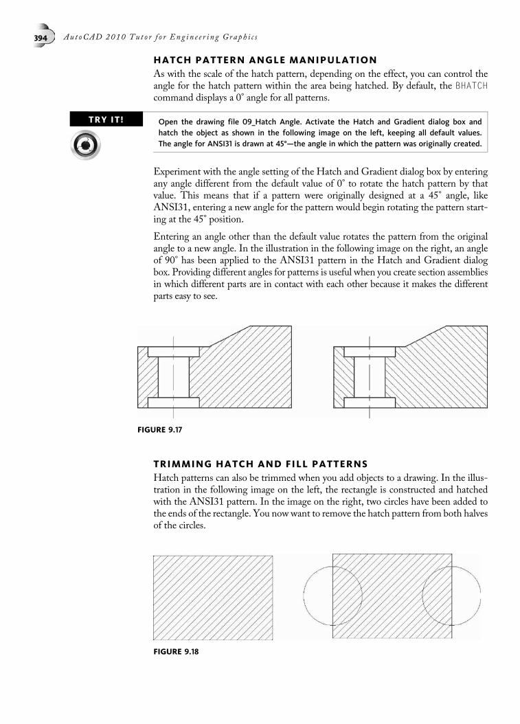
HATCH PATTERN ANGLE MANIPULATIONAs with the scale of the hatch pattern, depending on the effect, you can control theangle for the hatch pattern within the area being hatched. By default, the BHATCHcommand displays a 0° angle for all patterns.
TRY IT! Open the drawing file 09_Hatch Angle. Activate the Hatch and Gradient dialog box andhatch the object as shown in the following image on the left, keeping all default values.The angle for ANSI31 is drawn at 45°—the angle in which the pattern was originally created.
Experiment with the angle setting of the Hatch and Gradient dialog box by enteringany angle different from the default value of 0° to rotate the hatch pattern by thatvalue. This means that if a pattern were originally designed at a 45° angle, likeANSI31, entering a new angle for the pattern would begin rotating the pattern start-ing at the 45° position.
Entering an angle other than the default value rotates the pattern from the originalangle to a new angle. In the illustration in the following image on the right, an angleof 90° has been applied to the ANSI31 pattern in the Hatch and Gradient dialogbox. Providing different angles for patterns is useful when you create section assembliesin which different parts are in contact with each other because it makes the differentparts easy to see.
TRIMMING HATCH AND FILL PATTERNSHatch patterns can also be trimmed when you add objects to a drawing. In the illus-tration in the following image on the left, the rectangle is constructed and hatchedwith the ANSI31 pattern. In the image on the right, two circles have been added tothe ends of the rectangle. You now want to remove the hatch pattern from both halvesof the circles.
FIGURE 9.17
FIGURE 9.18
394 Au t oCAD 2010 Tu t o r f o r Eng in e e r i n g Graph i c s
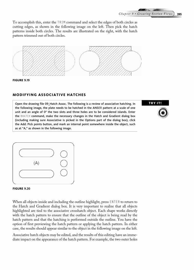
To accomplish this, enter the TRIM command and select the edges of both circles ascutting edges, as shown in the following image on the left. Then pick the hatchpatterns inside both circles. The results are illustrated on the right, with the hatchpattern trimmed out of both circles.
MODIFYING ASSOCIATIVE HATCHES
TRY IT!Open the drawing file 09_Hatch Assoc. The following is a review of associative hatching. Inthe following image, the plate needs to be hatched in the ANSI31 pattern at a scale of oneunit and an angle of 0° the two slots and three holes are to be considered islands. Enterthe BHATCH command, make the necessary changes in the Hatch and Gradient dialog box(including making sure Associative is picked in the Options part of the dialog box), clickthe Add: Pick points button, and mark an internal point somewhere inside the object, suchas at “A,” as shown in the following image.
When all objects inside and including the outline highlight, press ENTER to return tothe Hatch and Gradient dialog box. It is very important to realize that all objectshighlighted are tied to the associative crosshatch object. Each shape works directlywith the hatch pattern to ensure that the outline of the object is being read by thehatch pattern and that the hatching is performed outside the outline. You have theoption of first previewing the hatch pattern or applying the hatch pattern. In eithercase, the results should appear similar to the object in the following image on the left.
Associative hatch objects may be edited, and the results of this editing have an imme-diate impact on the appearance of the hatch pattern. For example, the two outer holes
FIGURE 9.20
FIGURE 9.19
Chap t e r 9 • Cr e a t i n g S e c t i o n V i ew s 395

need to be increased in size by a factor of 1.5; also, the middle hole needs to be reposi-tioned to the other side of the object, as shown in the following image on the right.Not only does using the MOVE command allow you to reposition the hole, but whenthe move is completed, the hatch pattern mends itself automatically to the movedcircle. In the same manner, using the SCALE command to increase the size of thetwo outer circles by a value of 1.5 units makes the circles larger and automaticallymends the hatch pattern.
Illustrated in the following image on the left, the length of the slots needs to be short-ened. Also, hole “A” needs to be deleted. Use the STRETCH command to shorten theslots. Use the crossing box at “B” to select the slots and stretch them one unit to theright. Use the ERASE command to delete hole “A.”
The result of the editing operations is shown in the following image on the right.In this figure, associative hatching has been enhanced for members to be erased whilethe hatch pattern still maintains its associativity. The inner hole was deleted usingthe ERASE command. After the ERASE command was executed, the hatch patternupdated itself and hatched through the area once occupied by the hole.
Once a hatch pattern is placed in the drawing, it does not update itself to any newadditions in the form of closed shapes in the drawing. Illustrated in the following im-age on the left, a rectangle was added at the center of the object. Notice, however, that
FIGURE 9.21
FIGURE 9.22
396 Au t oCAD 2010 Tu t o r f o r Eng in e e r i n g Graph i c s
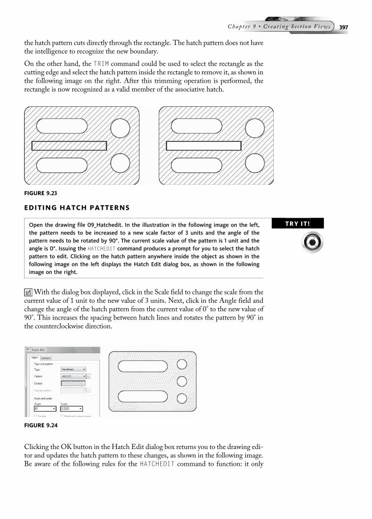
the hatch pattern cuts directly through the rectangle. The hatch pattern does not havethe intelligence to recognize the new boundary.
On the other hand, the TRIM command could be used to select the rectangle as thecutting edge and select the hatch pattern inside the rectangle to remove it, as shown inthe following image on the right. After this trimming operation is performed, therectangle is now recognized as a valid member of the associative hatch.
EDITING HATCH PATTERNS
TRY IT!Open the drawing file 09_Hatchedit. In the illustration in the following image on the left,the pattern needs to be increased to a new scale factor of 3 units and the angle of thepattern needs to be rotated by 90°. The current scale value of the pattern is 1 unit and theangle is 0°. Issuing the HATCHEDIT command produces a prompt for you to select the hatchpattern to edit. Clicking on the hatch pattern anywhere inside the object as shown in thefollowing image on the left displays the Hatch Edit dialog box, as shown in the followingimage on the right.
With the dialog box displayed, click in the Scale field to change the scale from thecurrent value of 1 unit to the new value of 3 units. Next, click in the Angle field andchange the angle of the hatch pattern from the current value of 0° to the new value of90°. This increases the spacing between hatch lines and rotates the pattern by 90° inthe counterclockwise direction.
Clicking the OK button in the Hatch Edit dialog box returns you to the drawing edi-tor and updates the hatch pattern to these changes, as shown in the following image.Be aware of the following rules for the HATCHEDIT command to function: it only
FIGURE 9.23
FIGURE 9.24
Chap t e r 9 • Cr e a t i n g S e c t i o n V i ew s 397
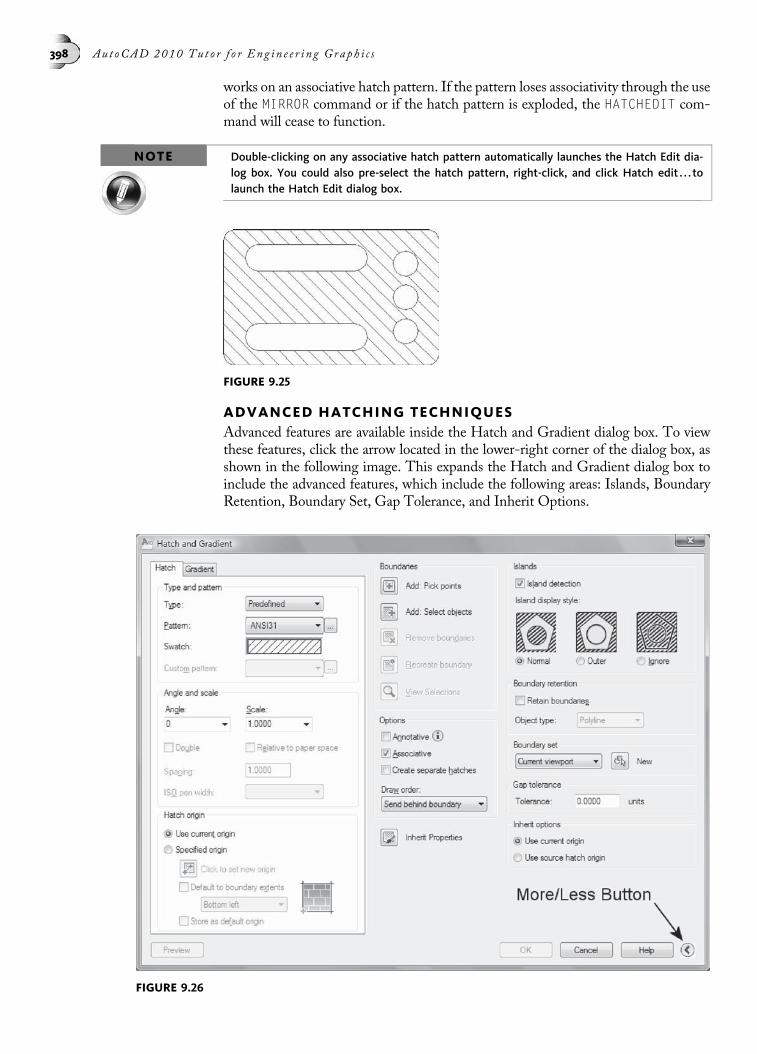
works on an associative hatch pattern. If the pattern loses associativity through the useof the MIRROR command or if the hatch pattern is exploded, the HATCHEDIT com-mand will cease to function.
NOTE Double-clicking on any associative hatch pattern automatically launches the Hatch Edit dia-log box. You could also pre-select the hatch pattern, right-click, and click Hatch edit . . . tolaunch the Hatch Edit dialog box.
ADVANCED HATCHING TECHNIQUESAdvanced features are available inside the Hatch and Gradient dialog box. To viewthese features, click the arrow located in the lower-right corner of the dialog box, asshown in the following image. This expands the Hatch and Gradient dialog box toinclude the advanced features, which include the following areas: Islands, BoundaryRetention, Boundary Set, Gap Tolerance, and Inherit Options.
FIGURE 9.25
FIGURE 9.26
398 Au t oCAD 2010 Tu t o r f o r Eng in e e r i n g Graph i c s
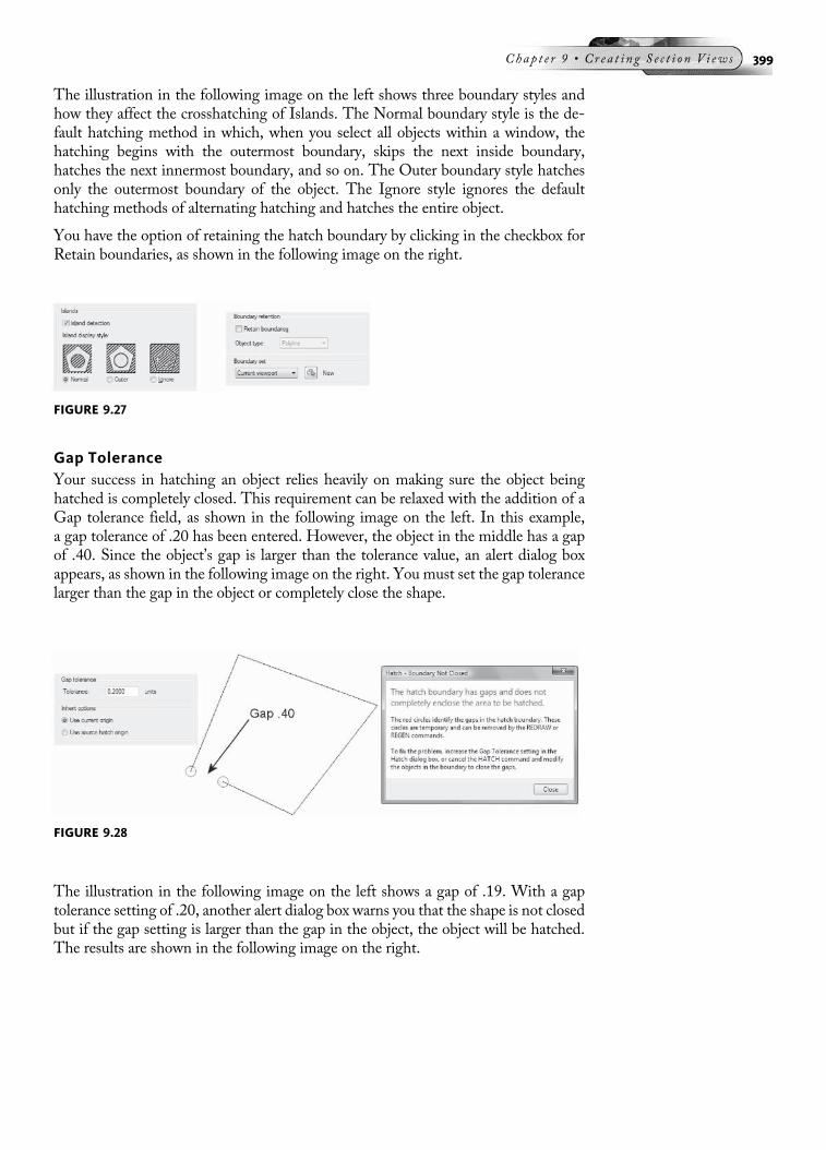
The illustration in the following image on the left shows three boundary styles andhow they affect the crosshatching of Islands. The Normal boundary style is the de-fault hatching method in which, when you select all objects within a window, thehatching begins with the outermost boundary, skips the next inside boundary,hatches the next innermost boundary, and so on. The Outer boundary style hatchesonly the outermost boundary of the object. The Ignore style ignores the defaulthatching methods of alternating hatching and hatches the entire object.
You have the option of retaining the hatch boundary by clicking in the checkbox forRetain boundaries, as shown in the following image on the right.
Gap ToleranceYour success in hatching an object relies heavily on making sure the object beinghatched is completely closed. This requirement can be relaxed with the addition of aGap tolerance field, as shown in the following image on the left. In this example,a gap tolerance of .20 has been entered. However, the object in the middle has a gapof .40. Since the object’s gap is larger than the tolerance value, an alert dialog boxappears, as shown in the following image on the right. You must set the gap tolerancelarger than the gap in the object or completely close the shape.
The illustration in the following image on the left shows a gap of .19. With a gaptolerance setting of .20, another alert dialog box warns you that the shape is not closedbut if the gap setting is larger than the gap in the object, the object will be hatched.The results are shown in the following image on the right.
FIGURE 9.27
FIGURE 9.28
Chap t e r 9 • Cr e a t i n g S e c t i o n V i ew s 399

PRECISION HATCH PATTERN PLACEMENTAt times, you want to control where the hatch pattern begins inside a shape. In thefollowing image, a brick pattern was applied without any special insertion base points.In this image, the pattern seems to be laid out based on the center of the rectangle. Asthe brick pattern reaches the edges of the rectangle, the pattern just ends. This occursbecause the hatch pattern uses a current origin point to be constructed from. Thiscontrol can be found in the main Hatch and Gradient dialog box under the Hatchorigin area, as shown in the following image on the left.
To have more control over the origin of the hatch pattern, you can click the Specificorigin radio button, as shown in the following image on the left, and click the buttonClick to set new origin. You can then select the new origin of the hatch pattern backin your drawing. The results are shown in the following image on the right, with thehatch pattern origin located at the lower-left corner of the rectangle.
FIGURE 9.29
FIGURE 9.30
FIGURE 9.31
400 Au t oCAD 2010 Tu t o r f o r Eng in e e r i n g Graph i c s

INHERIT HATCHING PROPERTIES
TRY IT!Open the drawing file 09_Hatch Inherit. The illustration in the following image on the leftconsists of a simple assembly drawing. At least three different hatch patterns are displayedto define the different parts of the assembly. Unfortunately, a segment of one of the parts wasnot hatched, and it is unclear what pattern, scale, and angle were used to place the pattern.
Whenever you are faced with this problem, click the Inherit Properties button in themain Hatch and Gradient dialog box, as shown in the following image. Clicking onthe pattern at “A” sets the pattern, scale, and angle to match the selected pattern.
To complete the hatch operation, click an internal point in the empty area. Right-click and select ENTER from the shortcut menu. The hatch pattern is placed in thisarea, and it matches that of the other patterns to identify the common parts, as shownin the following image on the right.
EXCLUDE HATCH OBJECTS FROM OBJECT SNAPSAt times, it is easy to mistakenly snap to the endpoint of a hatch pattern instead of theendpoint of the perimeter of an object. This usually happens when adding linear di-mensions to a drawing, as shown in the following image on the left. To prevent thisfrom happening, activate the Options dialog box, select the Drafting tab, and place acheck in the box next to Ignore Hatch Objects, as shown in the following imageon the right. Object Snap modes will now ignore endpoints and intersections ofhatch patterns.
FIGURE 9.32
Chap t e r 9 • Cr e a t i n g S e c t i o n V i ew s 401
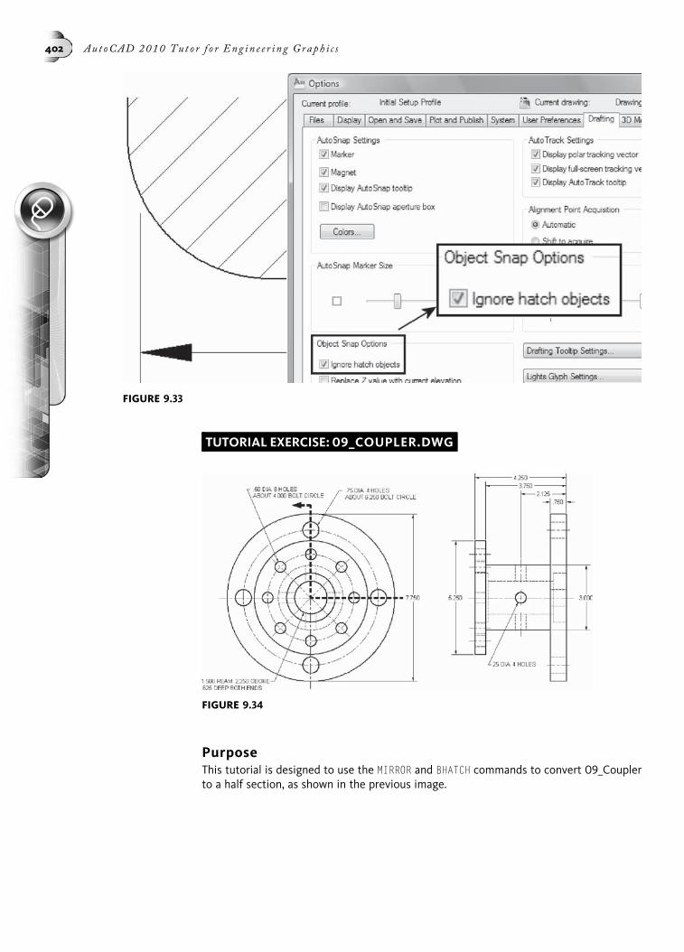
TUTORIAL EXERCISE: 09_COUPLER.DWG
PurposeThis tutorial is designed to use the MIRROR and BHATCH commands to convert 09_Couplerto a half section, as shown in the previous image.
FIGURE 9.33
FIGURE 9.34
402 Au t oCAD 2010 Tu t o r f o r Eng in e e r i n g Graph i c s

System SettingsSince this drawing is provided on CD, edit an existing drawing called 09_Coupler. Followthe steps in this tutorial for converting the upper half of the object to a half section. AllUnits, Limits, Grid, and Snap values have been previously set.
LayersThe following layers are already created:
Name Color Linetype
Object White Continuous
Center Yellow Center
Hidden Red Hidden
Hatch Magenta Continuous
Cutting Plane Line Yellow Dashed
Dimension Yellow Continuous
Suggested CommandsConvert one-half of the object to a section by erasing unnecessary hidden lines. Usethe Layer Control box and change the remaining hidden lines to the Object layer. Issuethe BHATCH command and use the ANSI31 hatch pattern to hatch the upper half ofthe 09_Coupler on the Hatch layer.
STEP 1Use the MIRROR command to copy and flip the upper half of the Side view and form thelower half. When in Object Selection mode, use the Remove option to deselect the maincenterline, hole centerlines, and hole as shown in the following image on the left. If theseobjects are included in the mirror operation, a duplicate copy of these objects will becreated.
Command: MI (For MIRROR)
Select objects: (Pick a point at “A”)
Specify opposite corner: (Pick a point at “B”)
Select objects: (Hold down the SHIFT key and pick centerlines“C” and “D” to remove them from the selection set)
Select objects: (With the SHIFT key held down, pick a pointat “E”)
Specify opposite corner: (With the SHIFT key held down, pick apoint at “F”)
Select objects: (Press ENTER to continue)
Specify first point of mirror line: (Select the endpoint ofthe centerline near “C”)
Specify second point of mirror line: (Select the endpoint ofthe centerline near “D”)
Erase source objects? [Yes/No] <N>: (Press ENTER to performthe mirror operation)
Begin converting the upper half of the Side view to a half section by using the ERASE com-mand to remove any unnecessary hidden lines and centerlines from the view as shown inthe following image on the right.
Chap t e r 9 • Cr e a t i n g S e c t i o n V i ew s 403

Command: E (For ERASE)
Select objects: (Carefully select the hidden lines labeled“G,” “H,” “J,” and “K”)
Select objects: (Select the centerline labeled “L”)
Select objects: (Press ENTER to execute the erase command)
STEP 2Since the remaining hidden lines actually represent object lines when shown in a full sec-tion, use the Layer Control box in the following image to convert all highlighted hiddenlines from the Hidden layer to the Object layer.
STEP 3Remove unnecessary line segments from the upper half of the converted section usingthe TRIM command. Use the horizontal line at “A” as the cutting edge, and select thetwo vertical segments at “B” and “C” as the objects to trim, as shown in the followingimage on the left.
Make the Hatch layer the current layer. Then, use the BHATCH command to displaythe Hatch and Gradient dialog box. Use the pattern “ANSI31” and keep all defaultsettings. Click the Add: Pick points button. When the drawing reappears, click inside
FIGURE 9.35
FIGURE 9.36
404 Au t oCAD 2010 Tu t o r f o r Eng in e e r i n g Graph i c s

areas “D,” “E,” “F,” and “G,” as shown in the following image on the right. When finishedselecting these internal points, press ENTER to return to the Hatch and Gradientdialog box.
STEP 4The complete hatched view is shown in the following image.
FIGURE 9.37
FIGURE 9.38
Chap t e r 9 • Cr e a t i n g S e c t i o n V i ew s 405
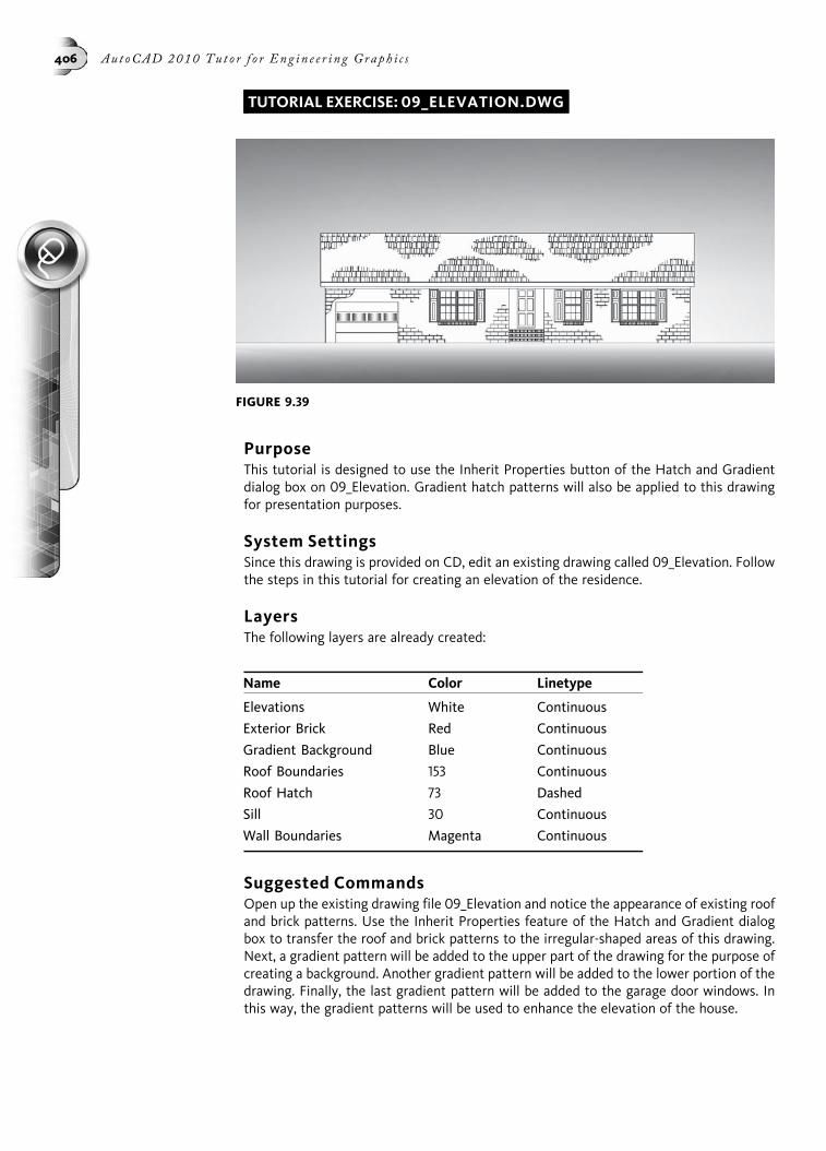
TUTORIAL EXERCISE: 09_ELEVATION.DWG
PurposeThis tutorial is designed to use the Inherit Properties button of the Hatch and Gradientdialog box on 09_Elevation. Gradient hatch patterns will also be applied to this drawingfor presentation purposes.
System SettingsSince this drawing is provided on CD, edit an existing drawing called 09_Elevation. Followthe steps in this tutorial for creating an elevation of the residence.
LayersThe following layers are already created:
Name Color Linetype
Elevations White Continuous
Exterior Brick Red Continuous
Gradient Background Blue Continuous
Roof Boundaries 153 Continuous
Roof Hatch 73 Dashed
Sill 30 Continuous
Wall Boundaries Magenta Continuous
Suggested CommandsOpen up the existing drawing file 09_Elevation and notice the appearance of existing roofand brick patterns. Use the Inherit Properties feature of the Hatch and Gradient dialogbox to transfer the roof and brick patterns to the irregular-shaped areas of this drawing.Next, a gradient pattern will be added to the upper part of the drawing for the purpose ofcreating a background. Another gradient pattern will be added to the lower portion of thedrawing. Finally, the last gradient pattern will be added to the garage door windows. Inthis way, the gradient patterns will be used to enhance the elevation of the house.
FIGURE 9.39
406 Au t oCAD 2010 Tu t o r f o r Eng in e e r i n g Graph i c s
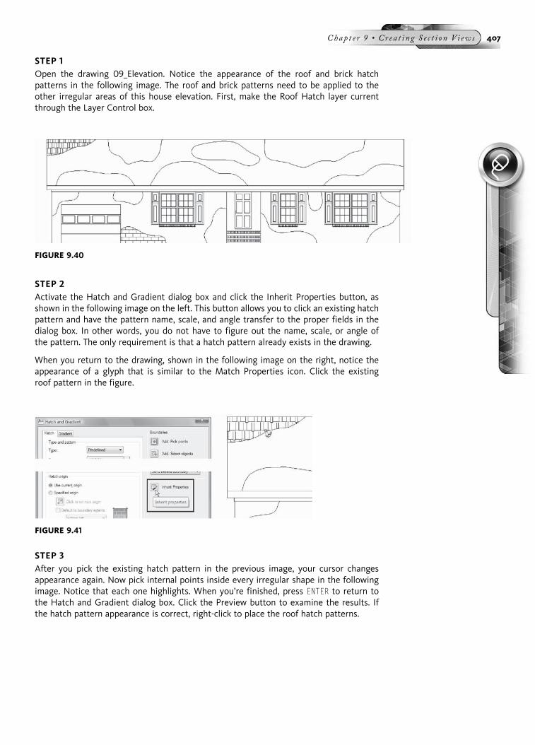
STEP 1Open the drawing 09_Elevation. Notice the appearance of the roof and brick hatchpatterns in the following image. The roof and brick patterns need to be applied to theother irregular areas of this house elevation. First, make the Roof Hatch layer currentthrough the Layer Control box.
STEP 2Activate the Hatch and Gradient dialog box and click the Inherit Properties button, asshown in the following image on the left. This button allows you to click an existing hatchpattern and have the pattern name, scale, and angle transfer to the proper fields in thedialog box. In other words, you do not have to figure out the name, scale, or angle ofthe pattern. The only requirement is that a hatch pattern already exists in the drawing.
When you return to the drawing, shown in the following image on the right, notice theappearance of a glyph that is similar to the Match Properties icon. Click the existingroof pattern in the figure.
STEP 3After you pick the existing hatch pattern in the previous image, your cursor changesappearance again. Now pick internal points inside every irregular shape in the followingimage. Notice that each one highlights. When you’re finished, press ENTER to return tothe Hatch and Gradient dialog box. Click the Preview button to examine the results. Ifthe hatch pattern appearance is correct, right-click to place the roof hatch patterns.
FIGURE 9.40
FIGURE 9.41
Chap t e r 9 • Cr e a t i n g S e c t i o n V i ew s 407

STEP 4Next, make the Exterior Brick layer current using the Layer Control box. Then activate theHatch and Gradient dialog box, click the Inherit Properties button, pick the existing brickpattern, and click inside every irregular shape in the following image until each one high-lights. Preview the hatch pattern and right-click if the results are correct.
STEP 5To give the appearance that the hatch patterns are floating on the roof and wall, use theLayer Control box to turn off the two layers that control the boundaries of these patterns,namely, Roof Boundaries and Wall Boundaries. Your display should appear similar to thefollowing image.
FIGURE 9.42
FIGURE 9.43
FIGURE 9.44
408 Au t oCAD 2010 Tu t o r f o r Eng in e e r i n g Graph i c s

STEP 6A number of gradient hatch patterns will now be applied to the outer portions of theelevation. First perform a ZOOM-EXTENTS. Then change the current layer to GradientBackground using the Layer Control box, as shown in the following image.
Command: Z (For ZOOM)
Specify corner of window, enter a scale factor (nX or nXP), or
[All/Center/Dynamic/Extents/Previous/Scale/Window/Object] <real time>:
E (For Extents)
STEP 7You will now apply a gradient hatch pattern to the upper portion of the elevation plan.Activate the Hatch and Gradient dialog box, click the Gradient tab, and pick the patternas shown in the following image on the left. Then click the Add: Pick points button andclick an internal point in the figure of the elevation. Once the boundary highlights, pressENTER, preview the hatch, and right-click to place the hatch pattern.
STEP 8Apply another gradient hatch pattern to the lower portion of the elevation plan. Activatethe Hatch and Gradient dialog box, click the Gradient tab, and pick the pattern as shownin the following image on the left. Then click the Add: Pick points button and click aninternal point in the figure of the elevation. Once the boundary highlights, press ENTER,preview the hatch, and right-click to place the hatch pattern.
FIGURE 9.45
FIGURE 9.46
Chap t e r 9 • Cr e a t i n g S e c t i o n V i ew s 409

STEP 9Apply gradient patterns to each of the garage windows, as shown in the following image,by using the BHATCH command for each of the four windows.
STEP 10If the boundary lines that define the elevation disappear, send the gradient patterns backusing the Draw Order feature, as shown in the following image.
END OF CHAPTER PROBLEMS FOR CHAPTER 9Please refer to the CD that is supplied with this book and locate the file AutoCAD Tutor2010 Support Docs.pdf. In addition to extra information supplied in this chapter, end-of-chapter problems are also available to provide additional practice.
FIGURE 9.47
FIGURE 9.48
FIGURE 9.49
410 Au t oCAD 2010 Tu t o r f o r Eng in e e r i n g Graph i c s
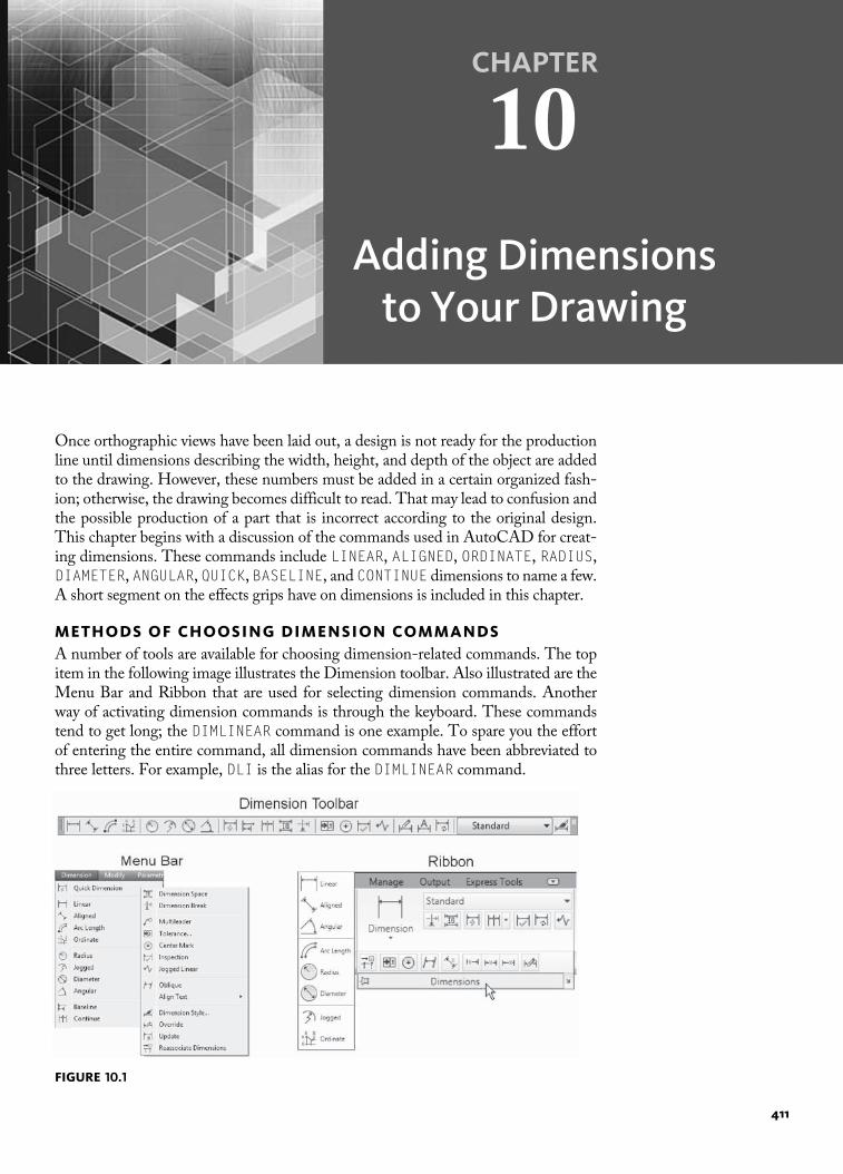
CHAPTER
10
Adding Dimensionsto Your Drawing
Once orthographic views have been laid out, a design is not ready for the productionline until dimensions describing the width, height, and depth of the object are addedto the drawing. However, these numbers must be added in a certain organized fash-ion; otherwise, the drawing becomes difficult to read. That may lead to confusion andthe possible production of a part that is incorrect according to the original design.This chapter begins with a discussion of the commands used in AutoCAD for creat-ing dimensions. These commands include LINEAR, ALIGNED, ORDINATE, RADIUS,DIAMETER, ANGULAR, QUICK, BASELINE, and CONTINUE dimensions to name a few.A short segment on the effects grips have on dimensions is included in this chapter.
METHODS OF CHOOSING DIMENSION COMMANDSA number of tools are available for choosing dimension-related commands. The topitem in the following image illustrates the Dimension toolbar. Also illustrated are theMenu Bar and Ribbon that are used for selecting dimension commands. Anotherway of activating dimension commands is through the keyboard. These commandstend to get long; the DIMLINEAR command is one example. To spare you the effortof entering the entire command, all dimension commands have been abbreviated tothree letters. For example, DLI is the alias for the DIMLINEAR command.
FIGURE 10.1
411

Study the following table for a brief description of each tool.
Button Tool Shortcut Function
Linear DLI Creates a horizontal, vertical, or rotateddimension
Aligned DAL Creates a linear dimension parallel to anobject
Arc Length DAR Dimensions the total length of an arc
Ordinate DOR Creates an ordinate dimension based onthe current position of the User Coordi-nate System (UCS)
Radius DRA Creates a radius dimension
Jogged DJO Creates a jogged dimension
Diameter DIA Creates a diameter dimension
Angular DAN Creates an angular dimension
Quick Dimension QDIM Creates a quick dimension
Continue DCO Creates a continued dimension
Baseline DBA Creates a baseline dimension
Dimension Space — Adjusts the spacing of parallel linear andangular dimensions to be equal
Dimension Break — Creates breaks in dimension, extension,and leader lines
Tolerance TOL Activates the Tolerance dialog box
Center Mark DCE Places a center mark inside a circle oran arc
Inspection — Creates an inspection dimension
Jogged Linear DJL Creates a jogged linear dimension
Edit DED Used to edit a dimension
Text Edit — Used to edit the text of a dimension
Update — Used for updating existing dimensions tochanges in the current dimension style
Dimstyle Dialog D Activates the Dimension Style Managerdialog box
BASIC DIMENSION COMMANDSLINEAR DIMENSIONS
The Linear Dimensioning mode generates either a horizontal or vertical dimen-sion, depending on the location of the dimension. The following prompts illustratethe generation of a horizontal dimension with the DIMLINEAR command. Noticethat identifying the dimension line location at “C” in the following image automati-cally generates a horizontal dimension.
TRY IT! Open the drawing file 10_Dim Linear1. Verify that OSNAP is on and set to Endpoint. Use thefollowing command sequence and image for performing this dimensioning task.
Command: DLI (For DIMLINEAR)
Specify first extension line origin or <select object>:(Select the endpoint of the line at “A”)
412 Au t oCAD 2010 Tu t o r f o r Eng in e e r i n g Graph i c s
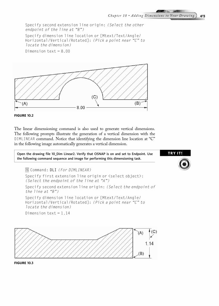
Specify second extension line origin: (Select the otherendpoint of the line at “B”)
Specify dimension line location or [Mtext/Text/Angle/Horizontal/Vertical/Rotated]: (Pick a point near “C” tolocate the dimension)
Dimension text = 8.00
The linear dimensioning command is also used to generate vertical dimensions.The following prompts illustrate the generation of a vertical dimension with theDIMLINEAR command. Notice that identifying the dimension line location at “C”in the following image automatically generates a vertical dimension.
TRY IT!Open the drawing file 10_Dim Linear2. Verify that OSNAP is on and set to Endpoint. Usethe following command sequence and image for performing this dimensioning task.
Command: DLI (For DIMLINEAR)
Specify first extension line origin or <select object>:(Select the endpoint of the line at “A”)
Specify second extension line origin: (Select the endpoint ofthe line at “B”)
Specify dimension line location or [Mtext/Text/Angle/Horizontal/Vertical/Rotated]: (Pick a point near “C” tolocate the dimension)
Dimension text = 1.14
FIGURE 10.2
FIGURE 10.3
Chap t e r 10 • Add in g D imen s i o n s t o Y ou r Draw ing 413
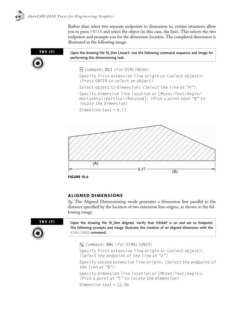
Rather than select two separate endpoints to dimension to, certain situations allowyou to press ENTER and select the object (in this case, the line). This selects the twoendpoints and prompts you for the dimension location. The completed dimension isillustrated in the following image.
TRY IT! Open the drawing file 10_Dim Linear3. Use the following command sequence and image forperforming this dimensioning task.
Command: DLI (For DIMLINEAR)
Specify first extension line origin or <select object>:(Press ENTER to select an object)
Select object to dimension: (Select the line at “A”)
Specify dimension line location or [Mtext/Text/Angle/Horizontal/Vertical/Rotated]: (Pick a point near “B” tolocate the dimension)
Dimension text = 9.17
ALIGNED DIMENSIONSThe Aligned Dimensioning mode generates a dimension line parallel to the
distance specified by the location of two extension line origins, as shown in the fol-lowing image.
TRY IT! Open the drawing file 10_Dim Aligned. Verify that OSNAP is on and set to Endpoint.The following prompts and image illustrate the creation of an aligned dimension with theDIMALIGNED command.
Command: DAL (For DIMALIGNED)
Specify first extension line origin or <select object>:(Select the endpoint of the line at “A”)
Specify second extension line origin: (Select the endpoint ofthe line at “B”)
Specify dimension line location or [Mtext/Text/Angle]:(Pick a point at “C” to locate the dimension)
Dimension text = 12.06
FIGURE 10.4
414 Au t oCAD 2010 Tu t o r f o r Eng in e e r i n g Graph i c s
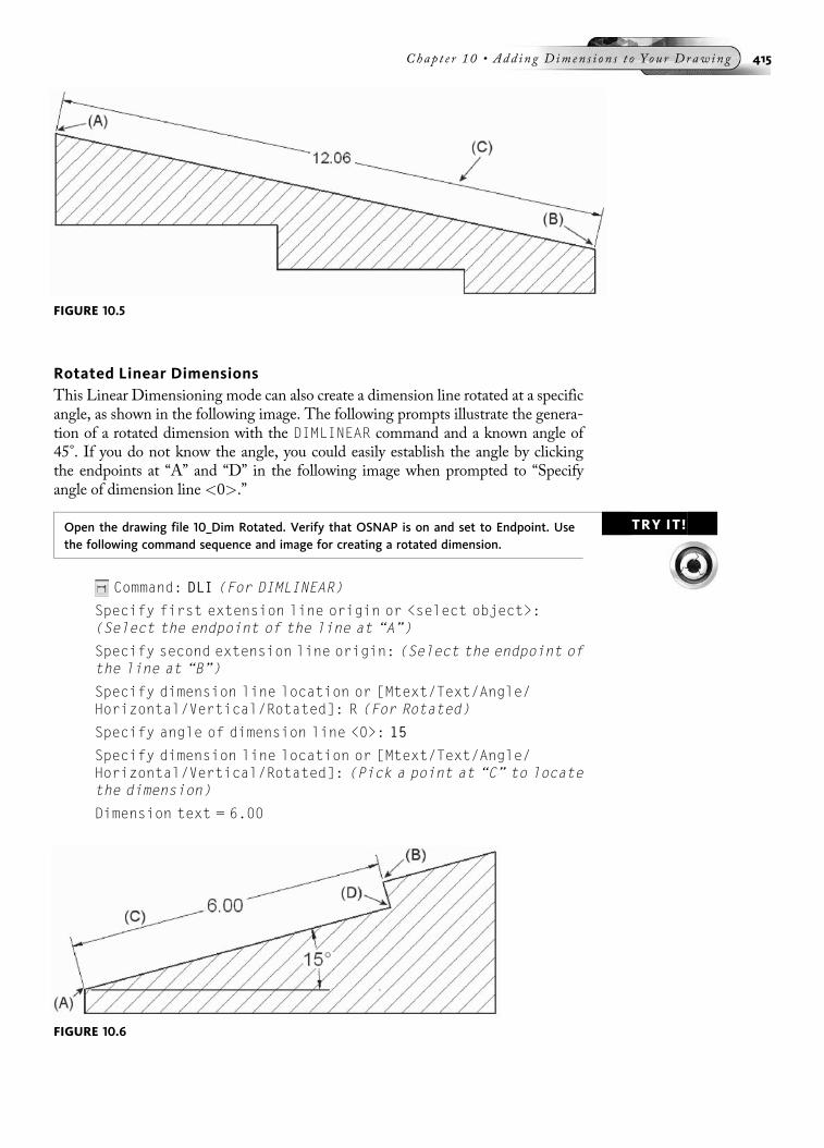
Rotated Linear DimensionsThis Linear Dimensioning mode can also create a dimension line rotated at a specificangle, as shown in the following image. The following prompts illustrate the genera-tion of a rotated dimension with the DIMLINEAR command and a known angle of45°. If you do not know the angle, you could easily establish the angle by clickingthe endpoints at “A” and “D” in the following image when prompted to “Specifyangle of dimension line <0>.”
TRY IT!Open the drawing file 10_Dim Rotated. Verify that OSNAP is on and set to Endpoint. Usethe following command sequence and image for creating a rotated dimension.
Command: DLI (For DIMLINEAR)
Specify first extension line origin or <select object>:(Select the endpoint of the line at “A”)
Specify second extension line origin: (Select the endpoint ofthe line at “B”)
Specify dimension line location or [Mtext/Text/Angle/Horizontal/Vertical/Rotated]: R (For Rotated)
Specify angle of dimension line <0>: 15
Specify dimension line location or [Mtext/Text/Angle/Horizontal/Vertical/Rotated]: (Pick a point at “C” to locatethe dimension)
Dimension text = 6.00
FIGURE 10.5
FIGURE 10.6
Chap t e r 10 • Add in g D imen s i o n s t o Y ou r Draw ing 415

CONTINUE DIMENSIONSThe power of grouping dimensions for ease of reading has already been explained.
The following image shows yet another feature of dimensioning in AutoCAD: thepractice of using continue dimensions. With one dimension already placed with thedimlinear command, you issue the DIMCONTINUE command, which prompts you forthe second extension line location. Picking the second extension line location stringsthe dimensions next to each other or continues the dimension.
TRY IT! Open the drawing file 10_Dim Continue. Verify that Running OSNAP is on and set toEndpoint. Use the following command sequence and image for creating continue dimensions.
Command: DLI (For DIMLINEAR)
Specify first extension line origin or <select object>:(Select the endpoint of the line at “A”)
Specify second extension line origin: (Select the endpointof the line at “B”)
Specify dimension line location or [Mtext/Text/Angle/Horizontal/Vertical/Rotated]: (Locate the 1.75 horizontaldimension)
Dimension text = 1.75
Command: DCO (For DIMCONTINUE)
Specify a second extension line origin or [Undo/Select]<Select>: (Select the endpoint of the line at “C”)
Dimension text = 1.25
Specify a second extension line origin or [Undo/Select]<Select>: (Select the endpoint of the line at “D”)
Dimension text = 1.50
Specify a second extension line origin or [Undo/Select]<Select>: (Select the endpoint of the line at “E”)
Dimension text = 1.00
Specify a second extension line origin or [Undo/Select]<Select>: (Press ENTER when finished)
Select continued dimension: (Press ENTER to exit thiscommand)
FIGURE 10.7
416 Au t oCAD 2010 Tu t o r f o r Eng in e e r i n g Graph i c s

BASELINE DIMENSIONSYet another aid in grouping dimensions is the DIMBASELINE command. Continue
dimensions place dimensions next to each other; baseline dimensions establish a baseor starting point for the first dimension, as shown in the following image. Anydimensions that follow in the DIMBASELINE command are calculated from thecommon base point already established. This is a very popular mode to use whenone end of an object acts as a reference edge. When you place dimensions using theDIMBASELINE command, a default baseline spacing setting of 0.38 units controls thespacing of the dimensions from each other. The DIMBASELINE command is initiatedafter the DIMLINEAR command.
TRY IT!Open the drawing file 10_Dim Baseline. Verify that Running OSNAP is on and set to End-point. Use the following command sequence and image for creating baseline dimensions.
Command: DLI (For DIMLINEAR)
Specify first extension line origin or <select object>:(Select the endpoint of the line at “A”)
Specify second extension line origin: (Select the endpoint ofthe line at “B”)
Specify dimension line location or [Mtext/Text/Angle/Horizontal/Vertical/Rotated]: (Locate the 1.75 horizontaldimension)
Dimension text = 1.75
Command: DBA (For DIMBASELINE)
Specify a second extension line origin or [Undo/Select]<Select>: (Select the endpoint of the line at “C”)
Dimension text = 3.00
Specify a second extension line origin or [Undo/Select]<Select>: (Select the endpoint of the line at “D”)
Dimension text = 4.50
Specify a second extension line origin or [Undo/Select]<Select>: (Select the endpoint of the line at “E”)
Dimension text = 5.50
Specify a second extension line origin or [Undo/Select]<Select>: (Press ENTER when finished)
Select base dimension: (Press ENTER to exit this command)
Chap t e r 10 • Add in g D imen s i o n s t o Y ou r Draw ing 417

THE QDIM COMMANDA more efficient means of placing a series of continued or baseline dimensions is
the QDIM, or Quick Dimension, command. You identify a number of valid cornersrepresenting intersections or endpoints of an object and all dimensions are placed.
Continuous ModeIn the following image, a crossing box is used to identify all corners to dimension to.
When you have finished identifying the crossing box and press the ENTER key, apreview of the dimensioning mode appears, as in the following image. During thispreview mode, you can right-click and have a shortcut menu appear. This allowsyou to select other dimension modes.
FIGURE 10.9
FIGURE 10.8
418 Au t oCAD 2010 Tu t o r f o r Eng in e e r i n g Graph i c s

When the dimension line is identified, as in the following image, all continueddimensions are placed.
TRY IT!Open the drawing file 10_Qdim Continuous. Follow the command sequence below and pre-vious images for performing this dimensioning task.
Command: QDIM
Select geometry to dimension: (Pick a point at “A”)
Specify opposite corner: (Pick a point at “B”)
Select geometry to dimension: (Press ENTER to continue)
Specify dimension line position, or
[Continuous/Staggered/Baseline/Ordinate/Radius/Diameter/datumPoint/Edit/settings]
<Continuous>: (Change to a different mode or locate thedimension line at “C”)
Staggered ModeBy default, the QDIM command places continued dimensions. Before locating the di-mension line, you have the option of placing the staggered dimensions in the follow-ing image. The process with this style begins with adding dimensions to inside detailsand continuing outward until all features are dimensioned.
FIGURE 10.11
FIGURE 10.10
Chap t e r 10 • Add in g D imen s i o n s t o Y ou r Draw ing 419

TRY IT! Open the drawing file 10_Qdim Staggered. Activate the QDIM command and pick the lineslabeled “A” through “H,” as shown in the following image on the left. Change to the Stag-gered mode. Your display should appear similar to the illustration in the following imageon the right.
Baseline ModeAnother option of the QDIM command is the ability to place baseline dimensions. Aswith all baseline dimensions, an edge is used as the baseline, or datum. All dimen-sions are calculated from the left edge, as shown in the following image. The datum-Point option of the QDIM command allows you to select the right edge of the object inthe following image as the new datum or baseline.
TRY IT! Open the drawing file 10_Qdim Baseline. Activate the QDIM command and identify the sameset of objects as in the first Qdim exercise. Change to the Baseline mode. Your displayshould appear similar to the illustration in the following image.
Ordinate ModeThe Ordinate option of the QDIM command calculates dimensions from a known 0,0corner. The main Ordinate dimensioning topic will be discussed in greater detail laterin this chapter. A new User Coordinate System must first be created in the corner ofthe object. Then the QDIM command is activated along with the Ordinate options to
FIGURE 10.12
FIGURE 10.13
420 Au t oCAD 2010 Tu t o r f o r Eng in e e r i n g Graph i c s

display the results, as shown in the following image. Dimension lines are not used inordinate dimensions, in order to simplify the reading of the drawing.
TRY IT!Open the drawing file 10_Qdim Ordinate. Activate the QDIM command and identify thesame set of objects as in the first Qdim exercise. Change to the Ordinate mode. Your dis-play should appear similar to the illustration in the following image.
TIPThe QDIM command can also be used to edit an existing group of dimensions. Activate thecommand, select all existing dimensions with a crossing box, and enter an option to changethe style of all dimensions.
DIAMETER AND RADIUS DIMENSIONINGArcs and circles should be dimensioned in the view where their true shape is visible.The mark in the center of the circle or arc indicates its center point, as shown in thefollowing image. You may place the dimension text either inside or outside the circle;you may also use grips to aid in the dimension text location of a diameter or radiusdimension. When dimensioning a small radius, an arc extension line is formed,depending on where you locate the radius dimension text.
TRY IT!Open the drawing file 10_Dim Radial. Use the following command sequence and image forplacing diameter and radius dimensions.
Command: DDI (For DIMDIAMETER)
Select arc or circle: (Select the edge of the large circle)
Dimension text = 2.50
Specify dimension line location or [Mtext/Text/Angle]:(Pick a point to locate the diameter dimension)
Command: DDI (For DIMDIAMETER)
Select arc or circle: (Select the edge of the small circle)
Dimension text = 1.00
Specify dimension line location or [Mtext/Text/Angle]:(Pick a point to locate the diameter dimension)
Command: DRA (For DIMRADIUS)
FIGURE 10.14
Chap t e r 10 • Add in g D imen s i o n s t o Y ou r Draw ing 421
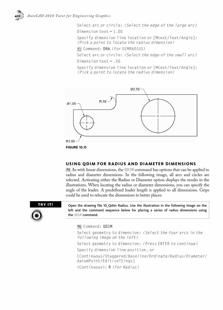
Select arc or circle: (Select the edge of the large arc)
Dimension text = 1.00
Specify dimension line location or [Mtext/Text/Angle]:(Pick a point to locate the radius dimension)
Command: DRA (For DIMRADIUS)
Select arc or circle: (Select the edge of the small arc)
Dimension text = .50
Specify dimension line location or [Mtext/Text/Angle]:(Pick a point to locate the radius dimension)
USING QDIM FOR RADIUS AND DIAMETER DIMENSIONSAs with linear dimensions, the QDIM command has options that can be applied to
radius and diameter dimensions. In the following image, all arcs and circles areselected. Activating either the Radius or Diameter option displays the results in theillustrations. When locating the radius or diameter dimensions, you can specify theangle of the leader. A predefined leader length is applied to all dimensions. Gripscould be used to relocate the dimensions to better places.
TRY IT! Open the drawing file 10_Qdim Radius. Use the illustration in the following image on theleft and the command sequence below for placing a series of radius dimensions usingthe QDIM command.
Command: QDIM
Select geometry to dimension: (Select the four arcs in thefollowing image on the left)
Select geometry to dimension: (Press ENTER to continue)
Specify dimension line position, or
[Continuous/Staggered/Baseline/Ordinate/Radius/Diameter/datumPoint/Edit/seTtings]
<Continuous>: R (For Radius)
FIGURE 10.15
422 Au t oCAD 2010 Tu t o r f o r Eng in e e r i n g Graph i c s

TRY IT!Open the drawing file 10_Qdim Diameter. Use the illustration in the following image on theright and the command sequence below for placing a series of diameter dimensions usingthe QDIM command.
Command: QDIM
Select geometry to dimension: (Select the four circles in thefollowing image on the right)
Select geometry to dimension: (Press ENTER to continue)
Specify dimension line position, or
[Continuous/Staggered/Baseline/Ordinate/Radius/Diameter/datumPoint/Edit/seTtings]
<Continuous>: D (For Diameter)
Specify dimension line position, or
[Continuous/Staggered/Baseline/Ordinate/Radius/Diameter/datumPoint/Edit/seTtings]
<Diameter>: (Pick a point to locate the diameter dimension)
SPACING DIMENSIONSThis tool is used to adjust the spacing between parallel linear and angular
dimensions to be equal. You can automatically have this tool calculate the dimen-sion spacing distance based on the dimension text height. You can also specify avalue for the dimensions to be separated by. These parameters work well for base-line dimensions. In the case of continue dimensions, entering a value of 0 lines upall continue dimensions.
TRY IT!Open the drawing file 10_Dim Spacing. Use the following command sequence and image forperforming this operation on both baseline and continue dimensions.
Command: DIMSPACE
Select base dimension: (Select dimension “A”)
Select dimensions to space: (Select dimensions “B”, “C”,and “D”)
Select dimensions to space: (Press ENTER to continue)
Enter value or [Auto] <Auto>: A (For Auto)
FIGURE 10.16
Chap t e r 10 • Add in g D imen s i o n s t o Y ou r Draw ing 423
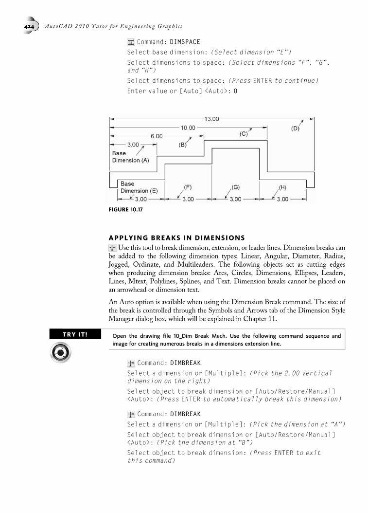
Command: DIMSPACE
Select base dimension: (Select dimension “E”)
Select dimensions to space: (Select dimensions “F”, “G”,and “H”)
Select dimensions to space: (Press ENTER to continue)
Enter value or [Auto] <Auto>: 0
APPLYING BREAKS IN DIMENSIONSUse this tool to break dimension, extension, or leader lines. Dimension breaks can
be added to the following dimension types; Linear, Angular, Diameter, Radius,Jogged, Ordinate, and Multileaders. The following objects act as cutting edgeswhen producing dimension breaks: Arcs, Circles, Dimensions, Ellipses, Leaders,Lines, Mtext, Polylines, Splines, and Text. Dimension breaks cannot be placed onan arrowhead or dimension text.
An Auto option is available when using the Dimension Break command. The size ofthe break is controlled through the Symbols and Arrows tab of the Dimension StyleManager dialog box, which will be explained in Chapter 11.
TRY IT! Open the drawing file 10_Dim Break Mech. Use the following command sequence andimage for creating numerous breaks in a dimensions extension line.
Command: DIMBREAK
Select a dimension or [Multiple]: (Pick the 2.00 verticaldimension on the right)
Select object to break dimension or [Auto/Restore/Manual]<Auto>: (Press ENTER to automatically break this dimension)
Command: DIMBREAK
Select a dimension or [Multiple]: (Pick the dimension at “A”)
Select object to break dimension or [Auto/Restore/Manual]<Auto>: (Pick the dimension at “B”)
Select object to break dimension: (Press ENTER to exitthis command)
FIGURE 10.17
424 Au t oCAD 2010 Tu t o r f o r Eng in e e r i n g Graph i c s
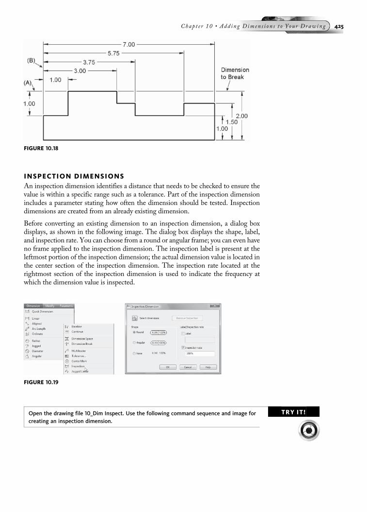
INSPECTION DIMENSIONSAn inspection dimension identifies a distance that needs to be checked to ensure thevalue is within a specific range such as a tolerance. Part of the inspection dimensionincludes a parameter stating how often the dimension should be tested. Inspectiondimensions are created from an already existing dimension.
Before converting an existing dimension to an inspection dimension, a dialog boxdisplays, as shown in the following image. The dialog box displays the shape, label,and inspection rate. You can choose from a round or angular frame; you can even haveno frame applied to the inspection dimension. The inspection label is present at theleftmost portion of the inspection dimension; the actual dimension value is located inthe center section of the inspection dimension. The inspection rate located at therightmost section of the inspection dimension is used to indicate the frequency atwhich the dimension value is inspected.
TRY IT!Open the drawing file 10_Dim Inspect. Use the following command sequence and image forcreating an inspection dimension.
FIGURE 10.18
FIGURE 10.19
Chap t e r 10 • Add in g D imen s i o n s t o Y ou r Draw ing 425

Command: DIMINSPECT
(When the Inspection Dimension dialog box displays, changethe shape to Angular and place checks in the label andInspection rate boxes, as shown in the following image onthe left. Enter “A” as the label designation and click theSelect dimensions button)
Select dimensions: (Pick the 8.00 vertical dimension onthe right)
Select dimensions: (Press ENTER to return to the dialog box;click OK)
ADDING JOGGED DIMENSIONSAt times, you need to add a radius dimension to a large arc. When creating the
radius dimension, the center for the dimension is placed outside the boundaries ofthe drawing. To give better control over these situations, you can create a jog in theradius. This is represented by a zigzag appearance, or jog, in the leader holdingthe radius dimension. Use the following command sequence and image for creatinga jogged radius dimension.
Command: DJO (For DIMJOGGED)
Select arc or circle: (Select the arc in the following image)
Specify center location override: (Locate the center at “A”)
Dimension text = 23.1588
Specify dimension line location or [Mtext/Text/Angle]:(Locate the dimension line)
Specify jog location: (Pick a point at “B”)
ADDING ARC DIMENSIONSYou can also dimension the length of an arc using the Dimension Arc command
(DIMARC, or the shortcut DAR). After you select the arc, extension lines are created atthe endpoints of the arc and a dimension arc is constructed parallel to the arc beingdimensioned. The arc symbol is placed with the dimension text. This symbol canalso be located above the dimension text. This technique will be covered in thenext chapter.
FIGURE 10.20
426 Au t oCAD 2010 Tu t o r f o r Eng in e e r i n g Graph i c s

Command: DAR (For DIMARC)
Select arc or polyline arc segment: (Select the arc)
Specify arc length dimension location, or [Mtext/Text/Angle/Partial]: (Locate the dimension)
Dimension text = 10.8547
LINEAR JOG DIMENSIONSJog lines are used to represent a dimension value that does not display the actualmeasurement. Typically, the actual measurement value of the dimension is smallerthan the displayed value. The Linear Jog dimension tool is used for creating thistype of jogged dimension.
TRY IT!Open the drawing file 10_Dim Linear Jog. Use the following command sequence and imagefor creating a jog along a linear dimension.
Command: DJL (For DIMJOGLINE)
Select dimension to add jog or [Remove]: (Select dimension “A”)
Specify jog location (or press Enter): (Pick the jog locationat “B”)
FIGURE 10.21
FIGURE 10.22
Chap t e r 10 • Add in g D imen s i o n s t o Y ou r Draw ing 427

LEADER LINESA leader line is a thin, solid line leading from a note or dimension and ending with anarrowhead, as illustrated at “A” in the following image. The arrowhead should alwaysterminate at an object line such as the edge of a hole or an arc. A leader to a circle orarc should be radial; this means it is drawn so that if extended, it would pass throughthe center of the circle, as illustrated at “B.” Leaders should cross as few object lines aspossible and should never cross each other. The short horizontal shoulder of a leadershould meet the dimension illustrated at “A.” It is poor practice to underline the di-mension with the horizontal shoulder, as illustrated at “C.” Example “C” also illus-trates a leader not lined up with the center or radial. This may affect the appearance ofthe leader. Again, check your company’s standard practices to ensure that this exam-ple is acceptable.
Yet another function of a leader is to attach notes to a drawing, as illustrated at “D.”Notice that the two notes attached to the view have different terminators: arrows anddots. Dots are sometimes used as terminators when the note is referring to an entiresurface. It is good practice to be consistent with the type of terminators for theduration of the drawing.
THE QLEADER COMMANDThe QLEADER command, or Quick Leader, provides numerous controls for placingleaders in your drawing. The QLEADER command is actually Leader and must beentered in at the command prompt with LE.
TRY IT! Open the drawing file 10_Qleader. Study the prompt sequence below and the followingimage for this command.
Command: LE (For QLEADER)
Specify first leader point, or [Settings]<Settings>: Nea to(Pick the point nearest at “A”)
Specify next point: (Pick a point at “B”)
Specify next point: (Press ENTER to continue)
Specify text width <0.00>: (Press ENTER to accept thisdefault)
Enter first line of annotation text <Mtext>: (Press ENTER todisplay the Multiline Text Editor dialog box. Enter “2X R.20”.Click the OK button to place the leader)
FIGURE 10.23
428 Au t oCAD 2010 Tu t o r f o r Eng in e e r i n g Graph i c s

Pressing ENTER at the first Quick Leader prompt displays the Leader Settings dialogbox that consists of three tabs used for controlling leaders. The Annotation tab dealswith the object placed at the end of the leader. By default, the MText radio button isselected, allowing you to add a note through the Multiline Text Editor dialog box.You could also copy an object at the end of the leader, have a geometric tolerancingsymbol placed in the leader, have a pre-defined block placed in the leader, or leave theleader blank.
Command: LE (For QLEADER)
Specify first leader point, or [Settings]<Settings>: (PressENTER to accept the default value and display the LeaderSettings dialog box in the following image)
The Leader Line & Arrow tab in the following image allows you to draw a leader lineconsisting of straight segments or in the form of a spline object. You can control thenumber of points used to define the leader; a maximum of three points is more thanenough to create your leader. You can even change the arrowhead type.
The Attachment tab in the following image allows you to control how text is attachedto the end of the leader through various justification modes. The settings in the figureare the default values.
ANNOTATING WITH MULTILEADERSMultileaders allow for leader lines to be aligned, collected, added, or removed. Thesetypes of leaders allow for more control than traditional leaders. Choose multileader
FIGURE 10.25
FIGURE 10.24
Chap t e r 10 • Add in g D imen s i o n s t o Y ou r Draw ing 429

tools from the Menu Bar, Multileader Toolbar (found in the AutoCAD ClassicWorkspace), or Ribbon as shown in the following image.
The following table illustrates each multileader tool along with a brief description.
Button Tool Function
MLEADER Creates a multileader
— Adds a multileader
— Removes a multileader
MLEADERALIGN Aligns a number of multileaders
MLEADERCOLLECT Collects a number of multileaders
MLEADERSTYLE Launches the Multileader Style Properties dialog box
Creating MultileadersThe following Try It! exercise allows you to place a number of multileaders that
identify various parts of a wood plane.
TRY IT! Open the drawing file 11 _Wood_Plane. This drawing consists of a typical plane used inwoodworking. Use the MLEADER command to place a number of multileaders that identifyvarious parts of the wood plane.
Command: MLEADER
Specify leader arrowhead location or [leader Landing first/Content first/Options] <Options>: (Pick a point at “A”)
Specify leader landing location: (Pick a point at “B.” Whenthe Text Formatting toolbar appears, enter the name of thewood plane part. When finished, click the OK button to dismissthe Text Formatting toolbar and place the multileader asshown in the following image on the left)
Continue placing additional multileaders to identify additional wood plane parts, asshown in the following image on the right.
FIGURE 10.26
430 Au t oCAD 2010 Tu t o r f o r Eng in e e r i n g Graph i c s
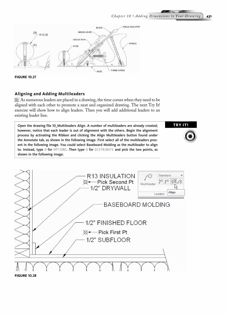
Aligning and Adding MultileadersAs numerous leaders are placed in a drawing, the time comes when they need to be
aligned with each other to promote a neat and organized drawing. The next Try It!exercise will show how to align leaders. Then you will add additional leaders to anexisting leader line.
TRY IT!Open the drawing file 10_Multileaders Align. A number of multileaders are already created;however, notice that each leader is out of alignment with the others. Begin the alignmentprocess by activating the Ribbon and clicking the Align Multileaders button found underthe Annotate tab, as shown in the following image. First select all of the multileaders pres-ent in the following image. You could select Baseboard Molding as the multileader to alignto. Instead, type O for OPTIONS. Then type D for DISTRIBUTE and pick the two points, asshown in the following image.
FIGURE 10.27
FIGURE 10.28
Chap t e r 10 • Add in g D imen s i o n s t o Y ou r Draw ing 431
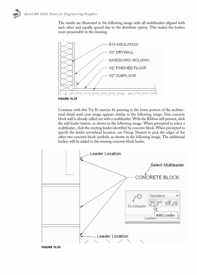
The results are illustrated in the following image with all multileaders aligned witheach other and equally spaced due to the distribute option. This makes the leadersmore presentable in the drawing.
Continue with this Try It! exercise by panning to the lower portion of the architec-tural detail until your image appears similar to the following image. One concreteblock wall is already called out with a multileader. With the Ribbon still present, clickthe add leader button, as shown in the following image. When prompted to select amultileader, click the existing leader identified by concrete block. When prompted tospecify the leader arrowhead location, use Osnap Nearest to pick the edges of theother two concrete block symbols, as shown in the following image. The additionalleaders will be added to the existing concrete block leader.
FIGURE 10.29
FIGURE 10.30
432 Au t oCAD 2010 Tu t o r f o r Eng in e e r i n g Graph i c s
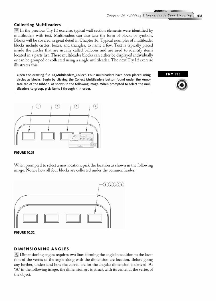
Collecting MultileadersIn the previous Try It! exercise, typical wall section elements were identified by
multileaders with text. Multileaders can also take the form of blocks or symbols.Blocks will be covered in great detail in Chapter 16. Typical examples of multileaderblocks include circles, boxes, and triangles, to name a few. Text is typically placedinside the circles that are usually called balloons and are used to identify itemslocated in a parts list. These multileader blocks can either be displayed individuallyor can be grouped or collected using a single multileader. The next Try It! exerciseillustrates this.
TRY IT!Open the drawing file 10_Multileaders_Collect. Four multileaders have been placed usingcircles as blocks. Begin by clicking the Collect Multileaders button found under the Anno-tate tab of the Ribbon, as shown in the following image. When prompted to select the mul-tileaders to group, pick items 1 through 4 in order.
When prompted to select a new location, pick the location as shown in the followingimage. Notice how all four blocks are collected under the common leader.
DIMENSIONING ANGLESDimensioning angles requires two lines forming the angle in addition to the loca-
tion of the vertex of the angle along with the dimension arc location. Before goingany further, understand how the curved arc for the angular dimension is derived. At“A” in the following image, the dimension arc is struck with its center at the vertex ofthe object.
FIGURE 10.31
FIGURE 10.32
Chap t e r 10 • Add in g D imen s i o n s t o Y ou r Draw ing 433

TRY IT! Open the drawing file 10_Dim Angle. Use the following command sequence and image forperforming this operation on both angles.
Command: DAN (For DIMANGULAR)
Select arc, circle, line, or <specify vertex>: (Selectline “A”)
Select second line: (Select line “B”)
Specify dimension arc line location or [Mtext/Text/Angle/Quadrant]: (Pick a point at “C” to locate the dimension)
Dimension text = 53
DIMENSIONING SLOTSFor slots, first select the view where the slot is visible. Two methods of dimensioningthe slot are illustrated in the following image. With the first method, you call out aslot by locating the center-to-center distance of the two semicircles, followed by aradius dimension to one of the semicircles; which radius dimension is selected de-pends on the available room to dimension. A second method involves the samecenter-to-center distance followed by an overall distance designating the width ofthe slot. This dimension is the same as the diameter of the semicircles. It is goodpractice to place this dimension inside the slot if room is available.
TRY IT! Open the drawing file 10_Dim Slot1. Use this file for practice in placing dimensions on theslot, as shown in the following image.
FIGURE 10.33
FIGURE 10.34
434 Au t oCAD 2010 Tu t o r f o r Eng in e e r i n g Graph i c s

A more complex example in the following image involves slots formed by curves andangles. Here, the radius of the circular center arc is called out. Angles reference eachother for accuracy. The overall width of the slot is dimensioned, which happens to bethe diameter of the semicircles at opposite ends of the slot.
TRY IT!Open the drawing file 10_Dim Slot2. Use this file for practice in placing dimensions on theangular slot in the following image. Use the DIMALIGN command to place the .48 dimen-sion. Use OSNAP-Nearest to identify the location at “A” and OSNAP-Perpendicular to iden-tify the location at “B.”
ADDING ORDINATE DIMENSIONSThe plate in the following image on the left consists of numerous drill holes with a
few slots, in addition to numerous 90°-angle cuts along the perimeter. This object isnot considered difficult to draw or make because it consists mainly of drill holes.However, conventional dimensioning techniques make the plate appear complex be-cause a dimension is required for the location of every hole and slot in both the X andY directions. Add standard dimension components such as extension lines, dimen-sion lines, and arrowheads, and it is easy to get lost in the complexity of the dimen-sions even on this simple object.
A better dimensioning method, called ordinate, or datum, dimensioning, is illus-trated in the following image on the right. Here, dimension lines or arrowheads arenot drawn; instead, one extension line is constructed from the selected feature to alocation specified by you. A dimension is added to identify this feature in either theX or Y direction. It is important to understand that all dimension calculations occurin relation to the current User Coordinate System (UCS), or the current 0,0 origin. Inthe following image, with the 0,0 origin located in the lower-left corner of the plate,all dimensions in the horizontal and vertical directions are calculated in relation tothis 0,0 location. Holes and slots are called out with the DIMDIAMETER command.The following illustrates a typical ordinate dimensioning command sequence:
Command: DOR (For DIMORDINATE)
Specify feature location: (Select a feature using anOsnap option)
FIGURE 10.35
Chap t e r 10 • Add in g D imen s i o n s t o Y ou r Draw ing 435

Specify leader endpoint or [Xdatum/Ydatum/Mtext/Text/Angle]: (Locate a point outside of the object)
Dimension text = Calculated value
To understand how to place ordinate dimensions, see the example in the following im-age and the prompt sequence below. Before you place any dimensions, a new User Co-ordinate System must be moved to a convenient location on the object with the UCScommand and the Origin option. All ordinate dimensions will reference this new ori-gin because it is located at coordinate 0,0. At the command prompt, enter DOR (forDIMORDINATE) to begin ordinate dimensioning. Select the quadrant of the arc at “A”as the feature. For the leader endpoint, pick a point at “B.”Be sure Ortho mode is on. Itis also helpful to snap to a convenient snap point for this and other dimensions alongthe direction. This helps in keeping all ordinate dimensions in line with one another.
TRY IT! Open the drawing file 10_Dim Ordinate. Follow the next series of figures and the followingcommand sequences to place ordinate dimensions.
Command: DOR (For DIMORDINATE)
Specify feature location: Qua
of (Select the quadrant of the slot at “A” as shown in thefollowing image on the left)
Specify leader endpoint or [Xdatum/Ydatum/Mtext/Text/Angle]: (Locate a point at “B” as shown in the following imageon the left)
Dimension text = 1.50
With the previous example highlighting horizontal ordinate dimensions, placing ver-tical ordinate dimensions is identical, as shown in the following image on the right.With the UCS still located in the lower-left corner of the object, select the feature at“A,” using either the Endpoint or Quadrant mode. Pick a point at “B” in a convenientlocation on the drawing. Again, it is helpful if Ortho is on and you snap to a grid dot.
Command: DOR (For DIMORDINATE)
Specify feature location: Qua
of (Select the quadrant of the slot at “A,” as shown in thefollowing image on the right)
FIGURE 10.36
436 Au t oCAD 2010 Tu t o r f o r Eng in e e r i n g Graph i c s

Specify leader endpoint or [Xdatum/Ydatum/Mtext/Text/Angle]: (Locate a point at “B,” as shown in the followingimage on the right)
Dimension text = 3.00
When spaces are tight to dimension to, two points not parallel to the X or Y axis willresult in a “jog” being drawn, as shown in the following image on the left. It is stillhelpful to snap to a grid dot when performing this operation; however, be sure Orthois turned off.
Command: DOR (For DIMORDINATE)
Specify feature location: End
of (Select the endpoint of the line at “A,” as shown in thefollowing image on the left)
Specify leader endpoint or [Xdatum/Ydatum/Mtext/Text/Angle]: (Locate a point at “B,” as shown in the followingimage on the left)
Dimension text = 2.00
Ordinate dimensioning provides a neat and easy way of organizing dimensions formachine tool applications. Only two points are required to place the dimensionthat references the current location of the UCS, as shown in the following imageon the right.
FIGURE 10.37
FIGURE 10.38
Chap t e r 10 • Add in g D imen s i o n s t o Y ou r Draw ing 437
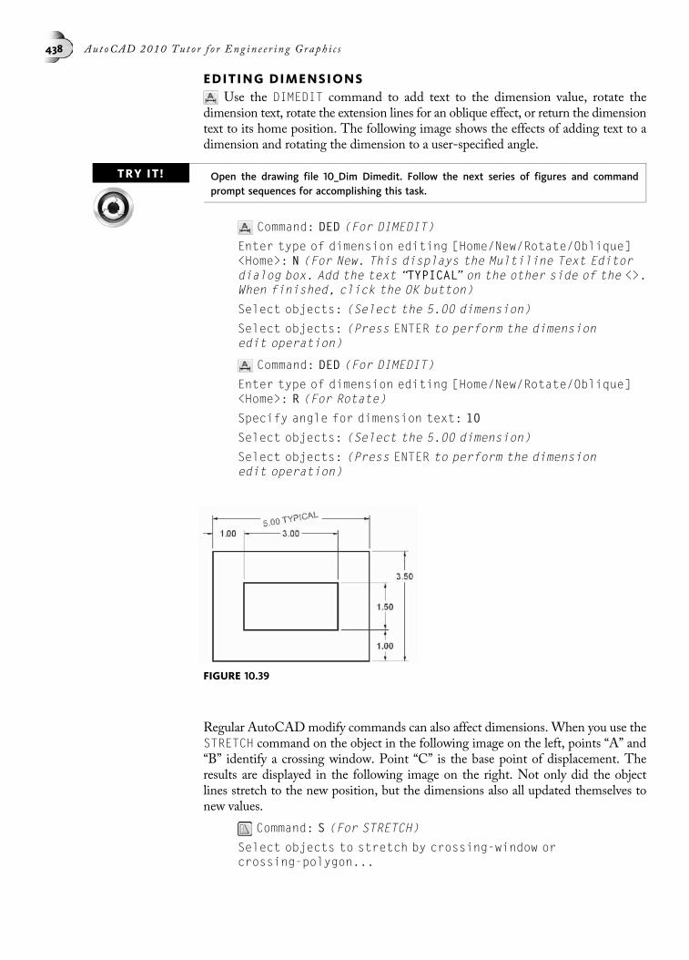
EDITING DIMENSIONSUse the DIMEDIT command to add text to the dimension value, rotate the
dimension text, rotate the extension lines for an oblique effect, or return the dimensiontext to its home position. The following image shows the effects of adding text to adimension and rotating the dimension to a user-specified angle.
TRY IT! Open the drawing file 10_Dim Dimedit. Follow the next series of figures and commandprompt sequences for accomplishing this task.
Command: DED (For DIMEDIT)
Enter type of dimension editing [Home/New/Rotate/Oblique]<Home>: N (For New. This displays the Multiline Text Editordialog box. Add the text “TYPICAL” on the other side of the <>.When finished, click the OK button)
Select objects: (Select the 5.00 dimension)
Select objects: (Press ENTER to perform the dimensionedit operation)
Command: DED (For DIMEDIT)
Enter type of dimension editing [Home/New/Rotate/Oblique]<Home>: R (For Rotate)
Specify angle for dimension text: 10
Select objects: (Select the 5.00 dimension)
Select objects: (Press ENTER to perform the dimensionedit operation)
Regular AutoCADmodify commands can also affect dimensions. When you use theSTRETCH command on the object in the following image on the left, points “A” and“B” identify a crossing window. Point “C” is the base point of displacement. Theresults are displayed in the following image on the right. Not only did the objectlines stretch to the new position, but the dimensions also all updated themselves tonew values.
Command: S (For STRETCH)
Select objects to stretch by crossing-window orcrossing-polygon...
FIGURE 10.39
438 Au t oCAD 2010 Tu t o r f o r Eng in e e r i n g Graph i c s

Select objects: (Pick a point at “A”)
Specify opposite corner: (Pick a point at “B” to activate thecrossing window)
Select objects: (Press ENTER to continue)
Specify base point or [Displacement] <Displacement>: (Pick apoint at “C”; it could also be anywhere on the screen)
Specify second point or <use first point as displacement>:(Use the Direct Distance mode; with ORTHO mode on, move yourcursor to the left and type .75 to perform the stretch)
One of the other options of the DIMEDIT command is the ability for you to move androtate the dimension text and still have the text return to its original or home location.This is the purpose of the Home option. Selecting the 5.75 dimension returns it to itsoriginal position, as shown in the following image. However, you would have to usethe New option of the DIMEDIT command to remove the text “TYPICAL.”
Command: DED (For DIMEDIT)
Enter type of dimension editing [Home/New/Rotate/Oblique]<Home>: H (Press ENTER to continue)
Select objects: (Select the 5.00 dimension)
Select objects: (Press ENTER to perform the dimensionedit operation)
FIGURE 10.40
FIGURE 10.41
Chap t e r 10 • Add in g D imen s i o n s t o Y ou r Draw ing 439
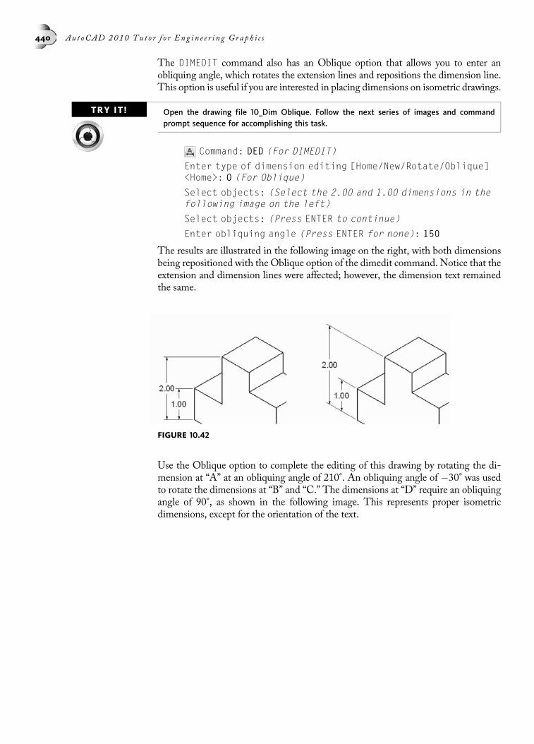
The DIMEDIT command also has an Oblique option that allows you to enter anobliquing angle, which rotates the extension lines and repositions the dimension line.This option is useful if you are interested in placing dimensions on isometric drawings.
TRY IT! Open the drawing file 10_Dim Oblique. Follow the next series of images and commandprompt sequence for accomplishing this task.
Command: DED (For DIMEDIT)
Enter type of dimension editing [Home/New/Rotate/Oblique]<Home>: O (For Oblique)
Select objects: (Select the 2.00 and 1.00 dimensions in thefollowing image on the left)
Select objects: (Press ENTER to continue)
Enter obliquing angle (Press ENTER for none): 150
The results are illustrated in the following image on the right, with both dimensionsbeing repositioned with the Oblique option of the dimedit command. Notice that theextension and dimension lines were affected; however, the dimension text remainedthe same.
Use the Oblique option to complete the editing of this drawing by rotating the di-mension at “A” at an obliquing angle of 210°. An obliquing angle of �30° was usedto rotate the dimensions at “B” and “C.” The dimensions at “D” require an obliquingangle of 90°, as shown in the following image. This represents proper isometricdimensions, except for the orientation of the text.
FIGURE 10.42
440 Au t oCAD 2010 Tu t o r f o r Eng in e e r i n g Graph i c s

Flipping Dimension ArrowsYou can control the placement of dimension arrows by first selecting the dimensionsand then right-clicking one of the arrows to display the menu in the following image.Clicking Flip Arrow from this menu flips this arrowhead. The other arrowhead re-mains normal. In the illustration on the right, the Flip Arrow mode was used twice toflip both arrowheads to the outside of the extension lines.
GEOMETRIC DIMENSIONING AND TOLERANCING (GDT)In the object in the following image, approximately 1000 items need to be manu-
factured based on the dimensions of the drawing. Also, once constructed, all objectsneed to be tested to be sure the 90° surface did not deviate over 0.005 units from itsbase. Unfortunately, the wrong base was selected as the reference for all dimensions.Which should have been the correct base feature? As all items were delivered, theywere quickly returned because the long 8.80 surface drastically deviated from the re-quired 0.005 unit deviation or zone. This is one simple example that demonstratesthe need for using geometric dimensioning and tolerancing techniques. First, thismethod deals with setting tolerances to critical characteristics of a part. Of course,
FIGURE 10.43
FIGURE 10.44
Chap t e r 10 • Add in g D imen s i o n s t o Y ou r Draw ing 441
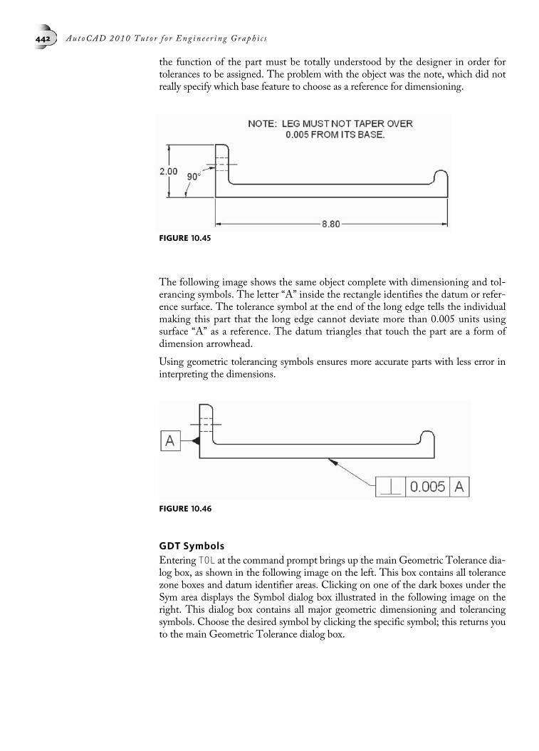
the function of the part must be totally understood by the designer in order fortolerances to be assigned. The problem with the object was the note, which did notreally specify which base feature to choose as a reference for dimensioning.
The following image shows the same object complete with dimensioning and tol-erancing symbols. The letter “A” inside the rectangle identifies the datum or refer-ence surface. The tolerance symbol at the end of the long edge tells the individualmaking this part that the long edge cannot deviate more than 0.005 units usingsurface “A” as a reference. The datum triangles that touch the part are a form ofdimension arrowhead.
Using geometric tolerancing symbols ensures more accurate parts with less error ininterpreting the dimensions.
GDT SymbolsEntering TOL at the command prompt brings up the main Geometric Tolerance dia-log box, as shown in the following image on the left. This box contains all tolerancezone boxes and datum identifier areas. Clicking on one of the dark boxes under theSym area displays the Symbol dialog box illustrated in the following image on theright. This dialog box contains all major geometric dimensioning and tolerancingsymbols. Choose the desired symbol by clicking the specific symbol; this returns youto the main Geometric Tolerance dialog box.
FIGURE 10.45
FIGURE 10.46
442 Au t oCAD 2010 Tu t o r f o r Eng in e e r i n g Graph i c s

The illustration in the following image shows a chart outlining all geometric toler-ancing symbols supported in the Symbol dialog box. Alongside each symbol is thecharacteristic controlled by the symbol. Tolerances of form such as Flatness andStraightness can be applied to surfaces without a datum being referenced. On theother hand, tolerances of orientation such as Angularity and Perpendicularity requiredatums as reference.
With the symbol placed inside this dialog box, you now assign such items as tolerancevalues, maximum material condition modifiers, and datums. In the following image,the tolerance of Parallelism is to be applied at a tolerance value of 0.005 units toDatum “A.”
FIGURE 10.47
FIGURE 10.48
FIGURE 10.49
Chap t e r 10 • Add in g D imen s i o n s t o Y ou r Draw ing 443

DIMENSION SYMBOLSIn today’s global economy, the transfer of documents in the form of drawings isbecoming a standard way of doing business. As drawings are shared with a subsidiaryof an overseas company, two different forms of language may be needed to interpretthe dimensions of the drawing. In the past, this has led to confusion in interpretingdrawings, and as a result, a system of dimensioning symbols has been developed. It ishoped that a symbol will be easier to recognize and interpret than a note in a differentlanguage about the particular feature being dimensioned.
The following image shows some of the more popular dimensioning symbols in usetoday on drawings. Notice how the symbols are designed to make as clear and consis-tent an interpretation of the dimension as possible. As an example, the Deep orDepth symbol displays an arrow pointing down. This symbol is used to identifyhow far into a part a drill hole goes. The Arc Length symbol identifies the length ofan arc, and so on.
CHARACTER MAPPING FOR DIMENSION SYMBOLSIllustrated in the following image is a typical counterbore operation and the correctdimension layout. The QLEADER command was used to begin the diameter dimen-sion. The counterbore and depth symbols were generated with the MTEXT commandalong with the Unicode Character Mapping dialog box. In any case, the first step inusing the dimension symbols is to first create a new text style, for which you can useany name.
FIGURE 10.50
FIGURE 10.51
444 Au t oCAD 2010 Tu t o r f o r Eng in e e r i n g Graph i c s
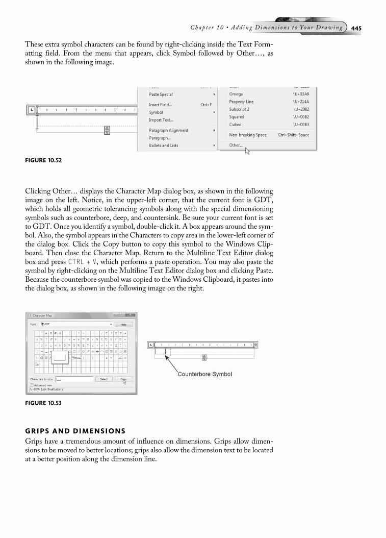
These extra symbol characters can be found by right-clicking inside the Text Form-atting field. From the menu that appears, click Symbol followed by Other. . . , asshown in the following image.
Clicking Other… displays the Character Map dialog box, as shown in the followingimage on the left. Notice, in the upper-left corner, that the current font is GDT,which holds all geometric tolerancing symbols along with the special dimensioningsymbols such as counterbore, deep, and countersink. Be sure your current font is setto GDT. Once you identify a symbol, double-click it. A box appears around the sym-bol. Also, the symbol appears in the Characters to copy area in the lower-left corner ofthe dialog box. Click the Copy button to copy this symbol to the Windows Clip-board. Then close the Character Map. Return to the Multiline Text Editor dialogbox and press CTRL + V, which performs a paste operation. You may also paste thesymbol by right-clicking on the Multiline Text Editor dialog box and clicking Paste.Because the counterbore symbol was copied to theWindows Clipboard, it pastes intothe dialog box, as shown in the following image on the right.
GRIPS AND DIMENSIONSGrips have a tremendous amount of influence on dimensions. Grips allow dimen-sions to be moved to better locations; grips also allow the dimension text to be locatedat a better position along the dimension line.
FIGURE 10.52
FIGURE 10.53
Chap t e r 10 • Add in g D imen s i o n s t o Y ou r Draw ing 445
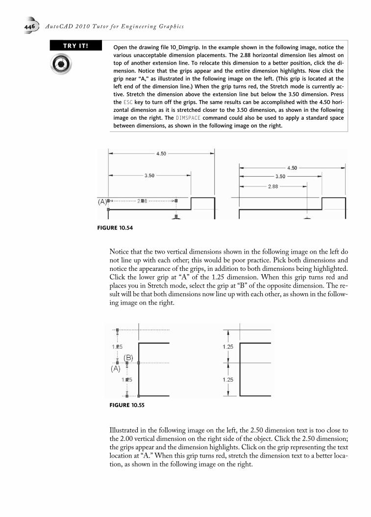
TRY IT! Open the drawing file 10_Dimgrip. In the example shown in the following image, notice thevarious unacceptable dimension placements. The 2.88 horizontal dimension lies almost ontop of another extension line. To relocate this dimension to a better position, click the di-mension. Notice that the grips appear and the entire dimension highlights. Now click thegrip near “A,” as illustrated in the following image on the left. (This grip is located at theleft end of the dimension line.) When the grip turns red, the Stretch mode is currently ac-tive. Stretch the dimension above the extension line but below the 3.50 dimension. Pressthe ESC key to turn off the grips. The same results can be accomplished with the 4.50 hori-zontal dimension as it is stretched closer to the 3.50 dimension, as shown in the followingimage on the right. The DIMSPACE command could also be used to apply a standard spacebetween dimensions, as shown in the following image on the right.
Notice that the two vertical dimensions shown in the following image on the left donot line up with each other; this would be poor practice. Pick both dimensions andnotice the appearance of the grips, in addition to both dimensions being highlighted.Click the lower grip at “A” of the 1.25 dimension. When this grip turns red andplaces you in Stretch mode, select the grip at “B” of the opposite dimension. The re-sult will be that both dimensions now line up with each other, as shown in the follow-ing image on the right.
Illustrated in the following image on the left, the 2.50 dimension text is too close tothe 2.00 vertical dimension on the right side of the object. Click the 2.50 dimension;the grips appear and the dimension highlights. Click on the grip representing the textlocation at “A.”When this grip turns red, stretch the dimension text to a better loca-tion, as shown in the following image on the right.
FIGURE 10.54
FIGURE 10.55
446 Au t oCAD 2010 Tu t o r f o r Eng in e e r i n g Graph i c s

It is very easy to use grips to control the placement of diameter and radius dimensions.As shown in the following image on the left, click the diameter dimension; the gripsappear in addition to the diameter dimension being highlighted. Click the grip thatlocates the dimension text at “A.” When this grip turns red, relocate the diameterdimension text to a better location using the Stretch mode, as shown in the followingimage in the middle.
The completed object, with dimensions edited through grips, is displayed in thefollowing image on the right.
TUTORIAL EXERCISE: 10_FIXTURE.DWG
FIGURE 10.56
FIGURE 10.57
FIGURE 10.58
Chap t e r 10 • Add in g D imen s i o n s t o Y ou r Draw ing 447

PurposeThe purpose of this tutorial is to add dimensions to the drawing of 10_Fixture.
System SettingsThe drawing in the previous image is already constructed. Follow the steps in this tutorialfor adding dimensions. Be sure the Endpoint and Intersection Object Snap modes are set.
LayersLayers have already been created for this tutorial.
Suggested CommandsUse the DIMCENTER, DIMLINEAR, DIMCONTINUE, DIMBASELINE, DIMDIAMETER, andDIMRADIUS commands for placing dimensions throughout this tutorial.
STEP 1Open the drawing file 10_Fixture, which can be found on the CD. A series of linear, base-line, continue, radius, and diameter dimensions will be added to this view. Before con-tinuing, verify that running OSNAP is set to Endpoint and Intersection modes and thatOSNAP is turned on.
A number of dimension styles have been created to control various dimension properties.You will learn more about dimension styles in Chapter 11. For now, make the Center Markdimension style current by clicking its name in the Dimension Styles Control box, asshown in the following image.
NOTE The Dimension Styles control box can be found under the Annotation tab of the Ribbon. Youcan also select this control box from the Styles or Dimension toolbar. The Styles toolbarautomatically displays if you make AutoCAD Classic the current workspace.
FIGURE 10.59
448 Au t oCAD 2010 Tu t o r f o r Eng in e e r i n g Graph i c s

STEP 2Using the DIMCENTER command (DCE), add a center mark to identify the center of thecircular features. Touch the edge of the arc to place the center mark. The CenterMark dimension style already allows a small and long dash to be constructed. See thefollowing image.
Command: DCE (For DIMCENTER)
Select arc or circle: (Pick the edge of the arc in thefollowing image)
STEP 3Now that the center mark is properly placed, it is time to begin adding the horizontal andvertical dimensions. Before performing these tasks, first make the Mechanical dimensionstyle current by clicking its name in the Dimension Styles Control box (located under theAnnotate tab of the Ribbon), as shown in the following image.
STEP 4Verify in the Status bar that OSNAP is turned on. Then place a linear dimension of5.50 units from the intersection at “A” to the intersection at “B,” as shown in thefollowing image.
Command: DLI (For DIMLINEAR)
Specify first extension line origin or <select object>: (Pickthe intersection at “A”)
Specify second extension line origin: (Pick the intersectionat “B”)
Specify dimension line location or
FIGURE 10.60
FIGURE 10.61
Chap t e r 10 • Add in g D imen s i o n s t o Y ou r Draw ing 449
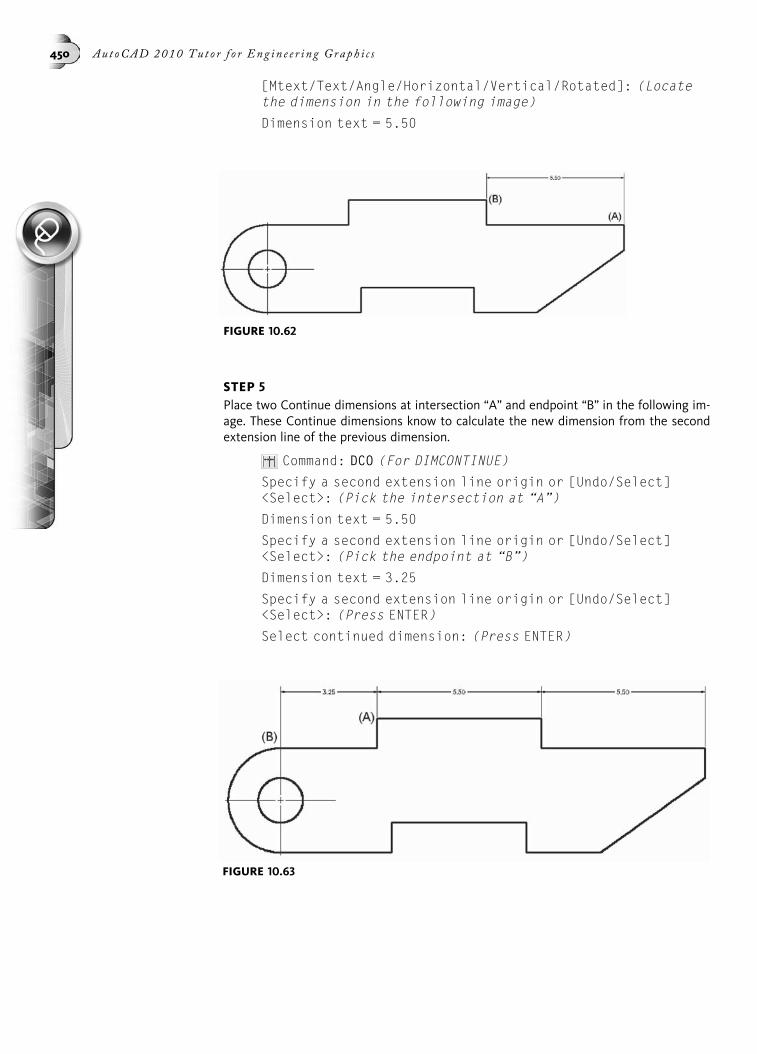
[Mtext/Text/Angle/Horizontal/Vertical/Rotated]: (Locatethe dimension in the following image)
Dimension text = 5.50
STEP 5Place two Continue dimensions at intersection “A” and endpoint “B” in the following im-age. These Continue dimensions know to calculate the new dimension from the secondextension line of the previous dimension.
Command: DCO (For DIMCONTINUE)
Specify a second extension line origin or [Undo/Select]<Select>: (Pick the intersection at “A”)
Dimension text = 5.50
Specify a second extension line origin or [Undo/Select]<Select>: (Pick the endpoint at “B”)
Dimension text = 3.25
Specify a second extension line origin or [Undo/Select]<Select>: (Press ENTER)
Select continued dimension: (Press ENTER)
FIGURE 10.62
FIGURE 10.63
450 Au t oCAD 2010 Tu t o r f o r Eng in e e r i n g Graph i c s

STEP 6Place a linear dimension of 3.50 units from the intersection at “A” to the intersection at“B,” as shown in the following image.
Command: DLI (For DIMLINEAR)
Specify first extension line origin or <select object>: (Pickthe intersection at “A”)
Specify second extension line origin: (Pick the intersectionat “B”)
Specify dimension line location or
[Mtext/Text/Angle/Horizontal/Vertical/Rotated]: (Locatethe dimension in the following image)
Dimension text = 3.50
STEP 7Add a series of baseline dimensions, as shown in the following image. All baseline dimen-sions are calculated from the first extension line of the previous dimension (the lineardimension measuring 3.50 units).
Command: DBA (For DIMBASELINE)
Specify a second extension line origin or [Undo/Select]<Select>: (Pick the intersection at “A”)
Dimension text = 6.00
Specify a second extension line origin or [Undo/Select]<Select>: (Pick the intersection at “B”)
Dimension text = 10.50
Specify a second extension line origin or [Undo/Select]<Select>: (Press ENTER)
Select base dimension: (Press ENTER)
FIGURE 10.64
Chap t e r 10 • Add in g D imen s i o n s t o Y ou r Draw ing 451

STEP 8Add a diameter dimension to the circle using the DIMDIAMETER command (DDI). Thenadd a radius dimension to the arc using the DIMRADIUS command (DRA), as shown inthe following image.
Command: DDI (For DIMDIAMETER)
Select arc or circle: (Pick the edge of the circle at “A”)
Dimension text = 1.50
Specify dimension line location or [Mtext/Text/Angle]:(Locate the diameter dimension in the following image)
Command: DRA (For DIMRADIUS)
Select arc or circle: (Pick the edge of the arc at “B”)
Dimension text = 1.75
Specify dimension line location or [Mtext/Text/Angle]:(Locate the diameter dimension in the following image)
STEP 9Place a vertical dimension of 3.50 units using the DIMLINEAR command (DLI). Pick thefirst extension line origin at the intersection at “A” and the second extension line originat the intersection at “B,” as shown in the following image.
FIGURE 10.66
FIGURE 10.65
452 Au t oCAD 2010 Tu t o r f o r Eng in e e r i n g Graph i c s

Command: DLI (For DIMLINEAR)
Specify first extension line origin or <select object>:(Pick the intersection at “A”)
Specify second extension line origin: (Pick the intersectionat “B”)
Specify dimension line location or
[Mtext/Text/Angle/Horizontal/Vertical/Rotated]: (Locatethe dimension in the following image)
Dimension text = 3.50
STEP 10Add an angular dimension of 144° using the DIMANGULAR command (DAN), as shown inthe following image.
Command: DAN (For DIMANGULAR)
Select arc, circle, line, or <specify vertex>: (Pick the lineat “A”)
Select second line: (Pick the line at “B”)
Specify dimension arc line location or [Mtext/Text/Angle/Quadrant]: (Locate the dimension in the following image)
Dimension text = 144
FIGURE 10.68
FIGURE 10.67
Chap t e r 10 • Add in g D imen s i o n s t o Y ou r Draw ing 453

STEP 11The next series of dimensions involves placing linear dimensions so that one extensionline is constructed by the dimension and the other is actually an object line that alreadyexists. You need to turn off one extension line while leaving the other extension lineturned on. This is accomplished by using an existing dimension style. Make the First Ex-tension Off dimension style current by clicking its name in the Dimension Styles Controlbox (located under the Annotate tab of the Ribbon), as shown in the following image. Thisdimension style will suppress or turn off the first extension line while leaving the secondextension line visible. This prevents the extension line from being drawn on top of theobject line.
STEP 12Add the two linear dimensions to the slots by using the following command sequencesand image as a guide.
Command: DLI (For DIMLINEAR)
Specify first extension line origin or <select object>:
(Pick the intersection at “A”)
Specify second extension line origin:
(Pick the intersection at “B”)
Specify dimension line location or
[Mtext/Text/Angle/Horizontal/Vertical/Rotated]: (Locatethe dimension in the following image)
Dimension text = 1.00
Command: DLI (For DIMLINEAR)
Specify first extension line origin or <select object>:
(Pick the intersection at “C”)
Specify second extension line origin:
(Pick the intersection at “D”)
Specify dimension line location or
[Mtext/Text/Angle/Horizontal/Vertical/Rotated]: (Locatethe dimension in the following image)
Dimension text = 1.00
FIGURE 10.69
454 Au t oCAD 2010 Tu t o r f o r Eng in e e r i n g Graph i c s

The completed fixture drawing with all dimensions is shown in the following image.
TUTORIAL EXERCISE: 10_DIMENSION VIEWS.DWG
PurposeThe purpose of this tutorial is to add dimensions to the three-view drawing named10_Dimension Views.dwg.
System SettingsThe drawing in the previous image is already constructed. Dimensions must be added tovarious views to call out overall distances, in addition to features such as cuts and slots.Be sure the Object Snap modes Endpoint, Center, Intersect, and Extension are set.
LayersLayers have already been created for this tutorial.
Suggested CommandsUse the DIMLINEAR command for horizontal and vertical dimensions on different viewsin this drawing.
FIGURE 10.71
FIGURE 10.70
Chap t e r 10 • Add in g D imen s i o n s t o Y ou r Draw ing 455

STEP 1Open the drawing file 10_Dimension Views.dwg. Linear dimensions are placed identifyingthe overall length, width, and depth dimensions. The DIMLINEAR command is used toperform this task, as shown in the following image on the left.
STEP 2Detail dimensions that identify cuts and slots are placed. Because these cuts are visible inthe Front view, the dimensions are placed there, as shown in the following image in themiddle. The DIMCONTINUE command (DCO) could be used for the second 1.00dimension.
STEP 3Once the spaces between the Front, Top, and Right Side views are used up by dimen-sions, the outer areas are used for placing additional dimensions such as the two horizon-tal dimensions in the following image on the right. Again, use DIMCONTINUE (DCO) forthe second dimension. Use grips to adjust dimension text locations if necessary.
END OF CHAPTER PROBLEMS FOR CHAPTER 10Please refer to the CD that is supplied with this book and locate the file AutoCAD Tutor2010 Support Docs.pdf. In addition to extra information supplied in this chapter,end-of-chapter problems are also available to provide additional practice.
FIGURE 10.72
456 Au t oCAD 2010 Tu t o r f o r Eng in e e r i n g Graph i c s

CHAPTER
11
ManagingDimension Styles
Dimensions have different settings that could affect the group of dimensions.These settings include the control of the dimension text height, the size and typeof arrowhead used, and whether the dimension text is centered in the dimensionline or placed above the dimension line. These are but a few of the numerous set-tings available to you. In fact, some settings are used mainly for architectural appli-cations, while other settings are only for mechanical uses. As a means of managingthese settings, dimension styles are used to group a series of dimension settings un-der a unique name to determine the appearance of dimensions. This chapter willcover in detail the Dimension Style Manager dialog box and the following tabs as-sociated with it: Lines, Symbols and Arrows; Text; Fit; Primary Units; AlternateUnits; and Tolerances. Additional topics include overriding a dimension style andmodifying the dimension style of an object.
THE DIMENSION STYLE MANAGER DIALOG BOXBegin the process of creating a dimension style by choosing Dimension Style . . . fromthe Dimension pull-down menu, as shown in the following image on the left. Youcan also pick Dimension Style from the Dimension toolbar, Menu Bar, and Ribbonas shown in the following image on the right. Entering the keyboard command DDIMor D is another way of accessing a Dimension Style.
457

Performing any of the actions in the previous image will launch the Dimension StyleManager dialog box, shown in the following image. The current dimension style islisted as Standard. There is also an Annotative dimensions style present; this will bediscussed in Chapter 19. The Standard dimension style is automatically availablewhen you create any new drawing. In the middle of the dialog box is an image iconthat displays how some dimensions will appear based on the current value of thedimension settings. Various buttons are also available to set a dimension style tocurrent, create a new dimension style, make modifications to an existing dimensionstyle, display dimension overrides, and compare the differences and similarities of twodimension styles.
FIGURE 11.2
FIGURE 11.1
458 Au t oCAD 2010 Tu t o r f o r Eng i n e e r i n g Graph i c s
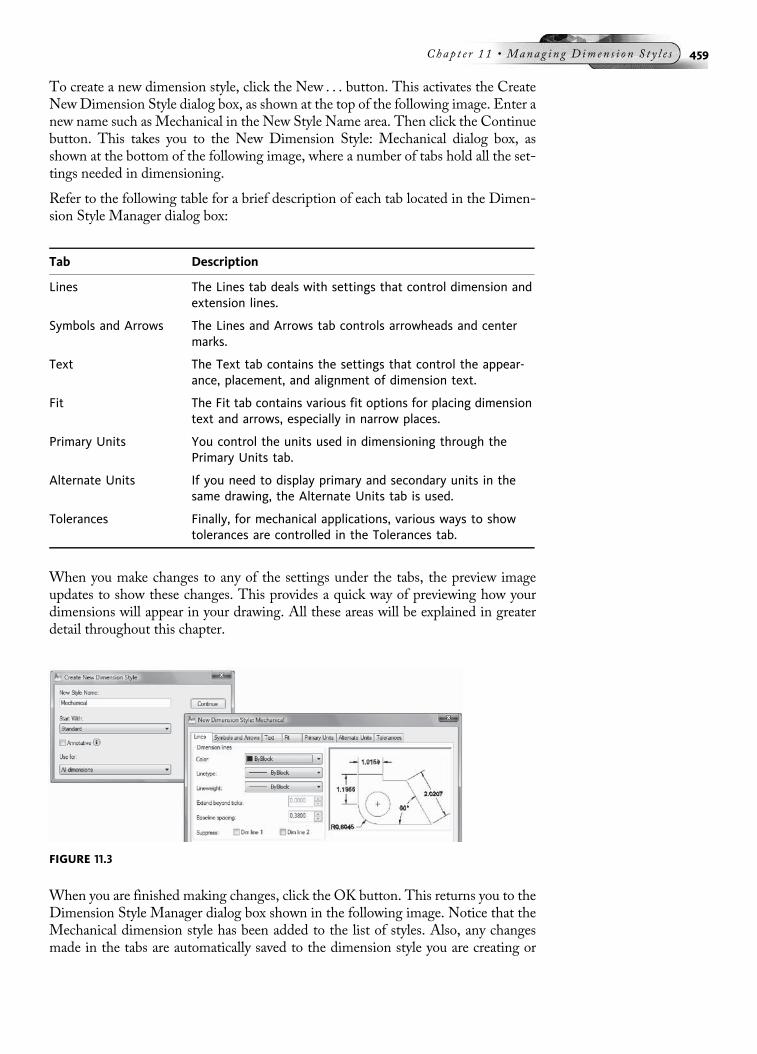
To create a new dimension style, click the New . . . button. This activates the CreateNewDimension Style dialog box, as shown at the top of the following image. Enter anew name such as Mechanical in the New Style Name area. Then click the Continuebutton. This takes you to the New Dimension Style: Mechanical dialog box, asshown at the bottom of the following image, where a number of tabs hold all the set-tings needed in dimensioning.
Refer to the following table for a brief description of each tab located in the Dimen-sion Style Manager dialog box:
Tab Description
Lines The Lines tab deals with settings that control dimension andextension lines.
Symbols and Arrows The Lines and Arrows tab controls arrowheads and centermarks.
Text The Text tab contains the settings that control the appear-ance, placement, and alignment of dimension text.
Fit The Fit tab contains various fit options for placing dimensiontext and arrows, especially in narrow places.
Primary Units You control the units used in dimensioning through thePrimary Units tab.
Alternate Units If you need to display primary and secondary units in thesame drawing, the Alternate Units tab is used.
Tolerances Finally, for mechanical applications, various ways to showtolerances are controlled in the Tolerances tab.
When you make changes to any of the settings under the tabs, the preview imageupdates to show these changes. This provides a quick way of previewing how yourdimensions will appear in your drawing. All these areas will be explained in greaterdetail throughout this chapter.
When you are finished making changes, click the OK button. This returns you to theDimension Style Manager dialog box shown in the following image. Notice that theMechanical dimension style has been added to the list of styles. Also, any changesmade in the tabs are automatically saved to the dimension style you are creating or
FIGURE 11.3
Chap t e r 11 • Manag i n g D imen s i o n S t y l e s 459

modifying. Click Mechanical and then pick the Set Current button to make this stylethe current dimension style. Clicking the Close button returns you to your drawing.Let’s get a closer look at all the tabs and their settings. Type the letter D to reopenthe Dimension Style Manager. Make sure Mechanical is highlighted and click theModify . . . button.
THE LINES TABThe Modify Dimension Style: Mechanical dialog box in the following imagedisplays the Lines tab, which will now be discussed in greater detail. This tab con-sists of four main areas dealing with dimension lines and extension lines.
FIGURE 11.4
460 Au t oCAD 2010 Tu t o r f o r Eng i n e e r i n g Graph i c s
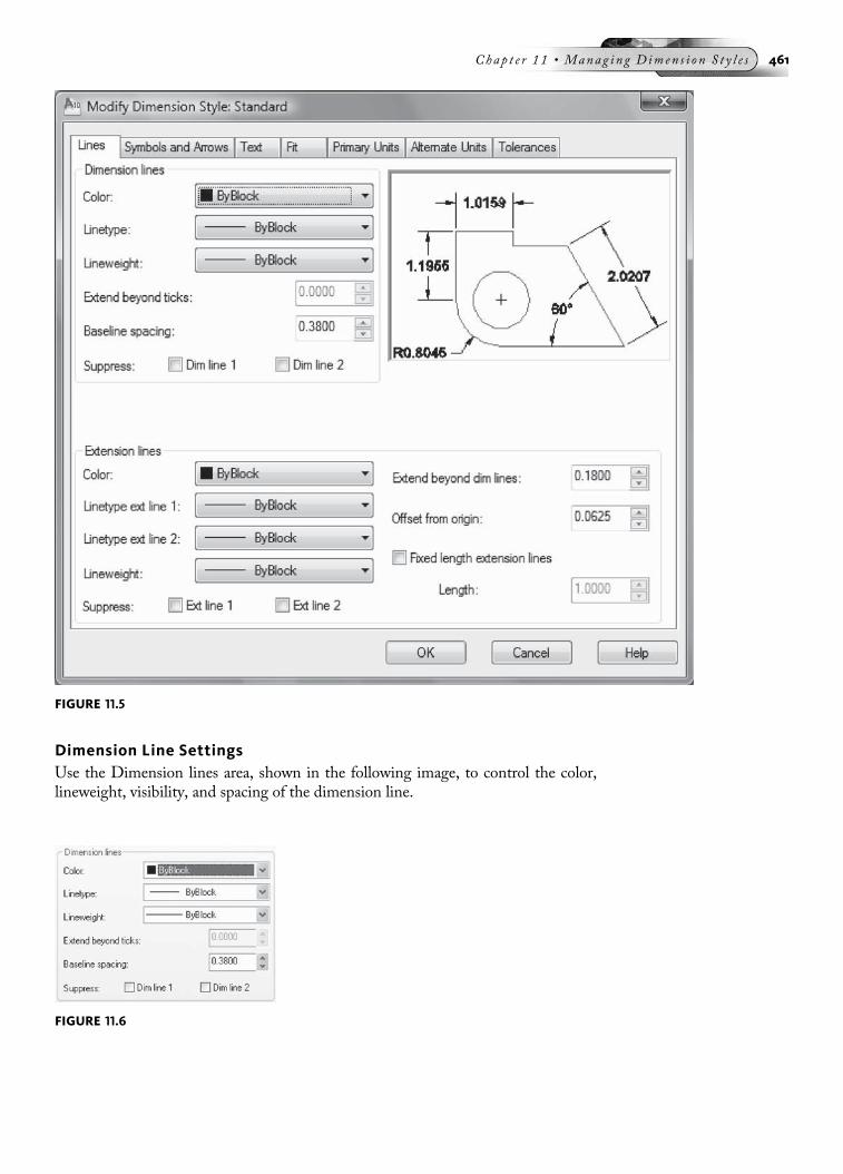
Dimension Line SettingsUse the Dimension lines area, shown in the following image, to control the color,lineweight, visibility, and spacing of the dimension line.
FIGURE 11.6
FIGURE 11.5
Chap t e r 11 • Manag i n g D imen s i o n S t y l e s 461

The Baseline spacing setting in the Dimension lines area controls the spacing ofbaseline dimensions, because they are placed at a distance from each other similar tothe illustration in the following image on the left. This value affects the DIMBASELINEcommand (or DBA for short).
By default, dimension line suppression is turned off. To turn on suppression of di-mension lines, place a check in the Dim line 1 or Dim line 2 box next to Suppress.This operation turns off the display of dimension lines for all dimensions placed un-der this dimension style. See the illustration in the following image on the right. Thismay be beneficial where tight spaces require that only the dimension text be placed.
Extension LinesThe Extension lines area controls the color, the distance the extension extends pastthe arrowhead, the distance from the object to the end of the extension line, and thevisibility of extension lines, as shown in the following image. Additional controlsallow you to set a different linetype for extension lines and provide the ability to usea fixed length value for all extension lines.
The Extend beyond dim lines setting controls how far the extension extends past thearrowhead or dimension line, as shown in the following image on the left. By default,a value of 0.18 is assigned to this setting.
The Offset from origin setting controls how far away from the object the extensionline will start, as shown in the following image on the right. By default, a value of 0.06is assigned to this setting.
FIGURE 11.7
FIGURE 11.8
462 Au t oCAD 2010 Tu t o r f o r Eng i n e e r i n g Graph i c s
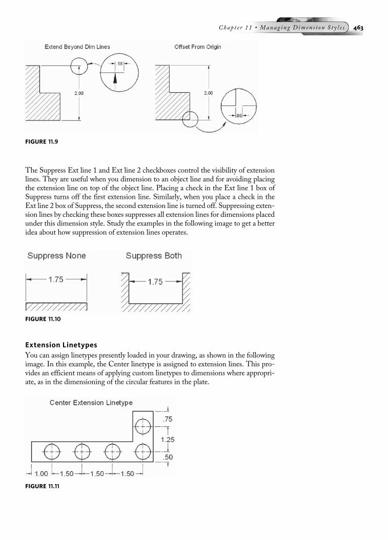
The Suppress Ext line 1 and Ext line 2 checkboxes control the visibility of extensionlines. They are useful when you dimension to an object line and for avoiding placingthe extension line on top of the object line. Placing a check in the Ext line 1 box ofSuppress turns off the first extension line. Similarly, when you place a check in theExt line 2 box of Suppress, the second extension line is turned off. Suppressing exten-sion lines by checking these boxes suppresses all extension lines for dimensions placedunder this dimension style. Study the examples in the following image to get a betteridea about how suppression of extension lines operates.
Extension LinetypesYou can assign linetypes presently loaded in your drawing, as shown in the followingimage. In this example, the Center linetype is assigned to extension lines. This pro-vides an efficient means of applying custom linetypes to dimensions where appropri-ate, as in the dimensioning of the circular features in the plate.
FIGURE 11.9
FIGURE 11.10
FIGURE 11.11
Chap t e r 11 • Manag i n g D imen s i o n S t y l e s 463

Fixed Length Extension LinesFixed length extension lines is a setting found under the Extension lines area of theLines tab. It sets a user-defined length for all extension lines. In the illustration in thefollowing image on the left, extension lines of varying lengths are displayed. All ex-tension lines begin by default .0625 units away from the object. Illustrated on theright is another example of how extension lines are displayed at a fixed length of .25units. Notice that all extension lines are the same length in this example. This value iscalculated from where the endpoint of the arrow intersects with the extension to thebottom of the extension line. As you can see, this results in very short extension linesthat are all the same length.
THE SYMBOLS AND ARROWS TABThe Symbols and Arrows tab controls four main areas, as shown in the followingimage, namely, the size and type of arrowheads, the size and type of center marks,the style of the arc length symbol, and the angle formed when placing a radiusjog dimension.
FIGURE 11.12
464 Au t oCAD 2010 Tu t o r f o r Eng i n e e r i n g Graph i c s
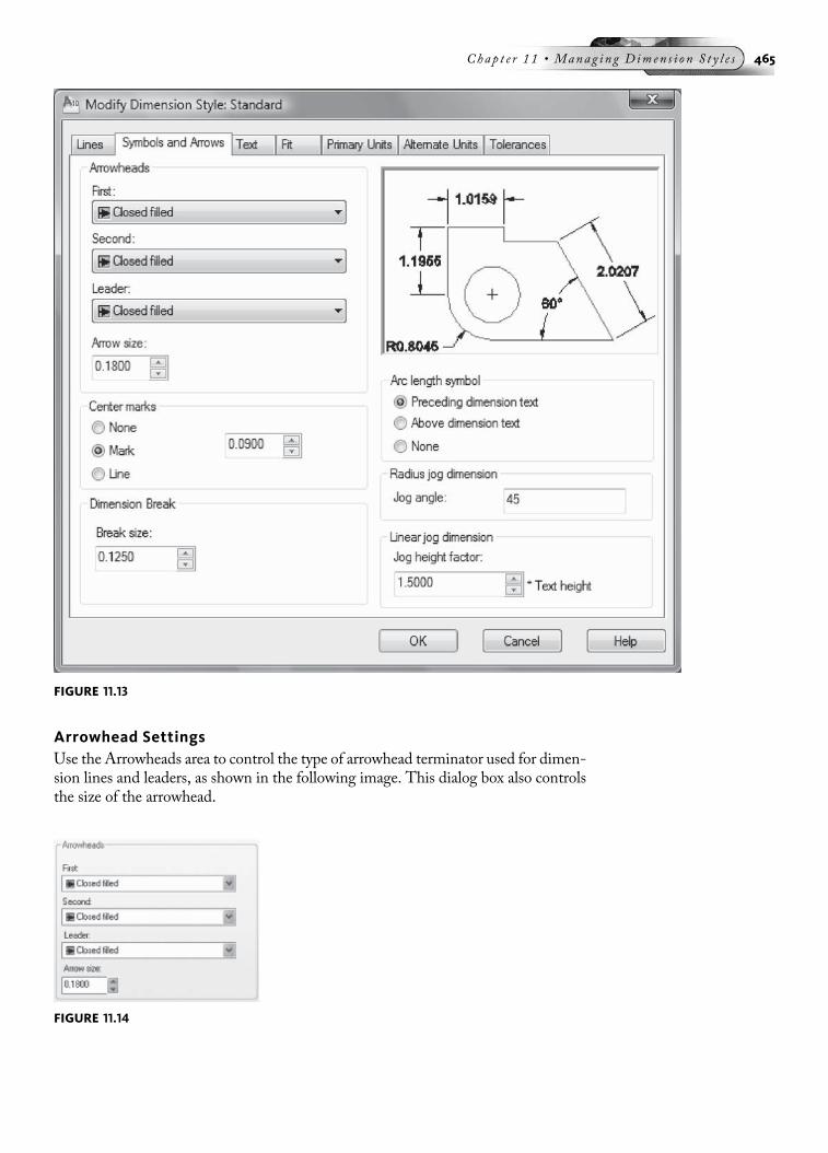
Arrowhead SettingsUse the Arrowheads area to control the type of arrowhead terminator used for dimen-sion lines and leaders, as shown in the following image. This dialog box also controlsthe size of the arrowhead.
FIGURE 11.13
FIGURE 11.14
Chap t e r 11 • Manag i n g D imen s i o n S t y l e s 465

Clicking on the First box displays a number of arrowhead terminators. Choosethe desired terminator from the list, as shown in the following image on the left.When you choose the desired arrowhead from the First box, the Second box auto-matically updates to the selection made in the First box. If you choose an arrow-head from the Second field, the first and second arrowheads may be different atopposite ends of the dimension line; this is desired in some applications. Choosinga terminator in the Leader box displays the arrowhead that will be used wheneveryou place a leader.
Illustrated in the following image on the right is the complete set of arrowheads,along with their names. The last arrow type in the image on the left is a User Arrow,which allows you to create your own custom arrowhead.
Use the Arrow size setting to control the size of the arrowhead terminator. By default,the arrow size is set to .18 units, as shown in the following image.
Center Mark SettingsThe Center marks for circles area allows you to control the type of center marker usedwhen identifying the centers of circles and arcs. You can make changes to these set-tings by clicking the three center mark modes: None, Mark, or Line, as shown in thefollowing image on the left. The Size box controls the size of the small plus mark (þ).If Mark or Line is chosen, these lines will show up when placing radius and dia-meter dimensions.
FIGURE 11.15
FIGURE 11.16
466 Au t oCAD 2010 Tu t o r f o r Eng i n e e r i n g Graph i c s
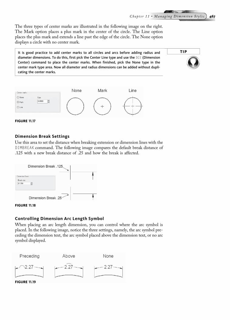
The three types of center marks are illustrated in the following image on the right.The Mark option places a plus mark in the center of the circle. The Line optionplaces the plus mark and extends a line past the edge of the circle. The None optiondisplays a circle with no center mark.
TIPIt is good practice to add center marks to all circles and arcs before adding radius anddiameter dimensions. To do this, first pick the Center Line type and use the DCE (DimensionCenter) command to place the center marks. When finished, pick the None type in thecenter mark type area. Now all diameter and radius dimensions can be added without dupli-cating the center marks.
Dimension Break SettingsUse this area to set the distance when breaking extension or dimension lines with theDIMBREAK command. The following image compares the default break distance of.125 with a new break distance of .25 and how the break is affected.
Controlling Dimension Arc Length SymbolWhen placing an arc length dimension, you can control where the arc symbol isplaced. In the following image, notice the three settings, namely, the arc symbol pre-ceding the dimension text, the arc symbol placed above the dimension text, or no arcsymbol displayed.
FIGURE 11.17
FIGURE 11.18
FIGURE 11.19
Chap t e r 11 • Manag i n g D imen s i o n S t y l e s 467

Controlling the Radius Dimension Jog AngleYou can control the angle of a jog dimension, as shown in the following image. Bydefault, a 45° angle defines the jog, as shown on the left. Notice the effects of enteringa 30° or 70° angle in the other examples in this image.
Controlling the Linear Jog Height FactorThis area is used to set the jog based on a multiplication factor. All jogs take this fac-tor and multiply it by the current dimension text height. The following image com-pares the default 1.50 jog height factor with that of a 3.00 jog height factor. Noticethat the lower jog is larger than the upper jog.
THE TEXT TABUse the Text tab shown in the following image to change the text appearance,for example, height; the text placement, for example, centered vertically and horizon-tally; and the text alignment, for example, always horizontal or parallel with thedimension line.
FIGURE 11.20
FIGURE 11.21
468 Au t oCAD 2010 Tu t o r f o r Eng i n e e r i n g Graph i c s

Text AppearanceThe Text height setting controls the size of the dimension text, as shown in thefollowing image on the left. By default, a value of 0.18 is assigned to this setting.
Placing a check in the Draw frame around text box draws a rectangular box aroundall dimensions, as shown in the following image on the right. This can be done toemphasize the dimension text. It also is a way of calling out a basic dimension.
FIGURE 11.22
FIGURE 11.23
Chap t e r 11 • Manag i n g D imen s i o n S t y l e s 469
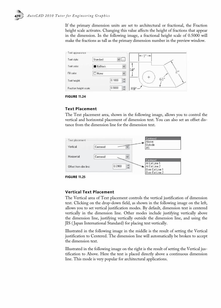
If the primary dimension units are set to architectural or fractional, the Fractionheight scale activates. Changing this value affects the height of fractions that appearin the dimension. In the following image, a fractional height scale of 0.5000 willmake the fractions as tall as the primary dimension number in the preview window.
Text PlacementThe Text placement area, shown in the following image, allows you to control thevertical and horizontal placement of dimension text. You can also set an offset dis-tance from the dimension line for the dimension text.
Vertical Text PlacementThe Vertical area of Text placement controls the vertical justification of dimensiontext. Clicking on the drop-down field, as shown in the following image on the left,allows you to set vertical justification modes. By default, dimension text is centeredvertically in the dimension line. Other modes include justifying vertically abovethe dimension line, justifying vertically outside the dimension line, and using theJIS ( Japan International Standard) for placing text vertically.
Illustrated in the following image in the middle is the result of setting the Verticaljustification to Centered. The dimension line will automatically be broken to acceptthe dimension text.
Illustrated in the following image on the right is the result of setting the Vertical jus-tification to Above. Here the text is placed directly above a continuous dimensionline. This mode is very popular for architectural applications.
FIGURE 11.24
FIGURE 11.25
470 Au t oCAD 2010 Tu t o r f o r Eng i n e e r i n g Graph i c s

The following image illustrates the result of setting the Vertical justification mode tooutside. All text, including that contained in angular and radial dimensions, will beplaced outside the dimension lines and leaders.
Horizontal Text PlacementAt times, dimension text needs to be better located in the horizontal direction; this isthe purpose of the Horizontal justification area. Illustrated in the following image arethe five modes of justifying text horizontally. By default, the horizontal text justifica-tion is centered in the dimension.
Clicking the Centered option of the Horizontal justification area displays the dimen-sion text, as shown in the following image on the left. This is the default settingbecause it is the most commonly used text justification mode in dimensioning.
Clicking the At Ext Line 1 option displays the dimension text as shown in thefollowing image in the middle, where the dimension text slides close to the firstextension line. Use this option to position the text out of the way of other dimensions.Notice the corresponding option to have the text positioned nearer to the secondextension line.
Clicking the Over Ext Line 1 option displays the dimension text parallel to andover the first extension line, as shown in the following image on the right. Noticethe corresponding option to position dimension text over the second extension line.
FIGURE 11.26
FIGURE 11.27
FIGURE 11.28
Chap t e r 11 • Manag i n g D imen s i o n S t y l e s 471

The last item of the Text placement area deals with setting an offset distance from thedimension line. When you place dimensions, a gap is established between the insideends of the dimension lines and the dimension text. Entering different values dependingon the desired results can control this gap. Study the examples in the following image inthe middle and on the right, which have different text offset settings. Entering a value ofzero (0) forces the dimension lines to touch the edge of the dimension text. Negativevalues are not supported.
Text AlignmentUse the Text alignment area shown in the following image on the left to control thealignment of text. Dimension text can be placed either horizontally or parallel(aligned) to the edge of the object being dimensioned. An ISO (InternationalStandards Organization) standard is also available for metric drawings. Click on theappropriate radio button to turn the desired text alignment mode on.
If the Horizontal radio button is clicked, all text will be read horizontally, as shown inthe following image in the middle. This includes text located inside and outside theextension lines.
Clicking the Aligned with dimension line radio button displays the alignment resultsshown in the following image on the right. Here all text is read parallel to the edgebeing dimensioned. Not only will vertical dimensions align the text vertically, butthe 2.06 dimension used to dimension the incline is also parallel to the edge.
FIGURE 11.29
FIGURE 11.30
472 Au t oCAD 2010 Tu t o r f o r Eng i n e e r i n g Graph i c s

THE FIT TABUse the Fit tab in the following image to control how text and/or arrows are displayedif there isn’t enough room to place both inside the extension lines. You could placethe text over the dimension with or without a leader line. The Scale for dimensionfeatures area is very important when you dimension inModel Space or when you scaledimensions to Paper Space units. You can even fine-tune the placement of text man-ually and force the dimension line to be drawn between extension lines.
FIGURE 11.31
FIGURE 11.32
Chap t e r 11 • Manag i n g D imen s i o n S t y l e s 473

Fit OptionsThe Fit options area, shown in the following image on the left, has the radio buttonset for Either text or arrows (best fit). AutoCAD will decide to move either text orarrows outside extension lines. It will determine the item that fits the best. This set-ting is illustrated in the preview area in the following image on the right. It so hap-pens that the preview image is identical when you click the radio button for Arrows.This tells AutoCAD to move the arrowheads outside the extension lines if there isn’tenough room to fit both text and arrows.
Clicking the Text radio button of the Fit options area updates the preview image, asshown in the following image. Here you are moving the dimension text outside theextension lines if the text and arrows do not fit. Since the value 1.0159 is the onlydimension that does not fit, it is placed outside the extension lines, but the arrowsare drawn inside the extension lines.
Clicking the Both text and arrows radio button updates the preview image, as shownin the following image, where the 1.0159 dimension text and arrows are both placedoutside the extension lines.
FIGURE 11.33
FIGURE 11.34
474 Au t oCAD 2010 Tu t o r f o r Eng i n e e r i n g Graph i c s

If you click the radio button for Always keep text between ext lines, the result is illus-trated in the preview image in the following image. Here all dimension text, includingthe radius dimension, is placed between the extension lines.
If you click the radio button for Either the text or the arrows (best fit) and you alsoplace a check in the box for Suppress arrows if they don’t fit inside the extension lines,the dimension line is turned off only for dimensions that cannot fit the dimensiontext and arrows. This is illustrated in the following image.
Text PlacementYou control the placement of the text if it is not in the default position. Your choices,shown in the following image, are Beside the dimension line, which is the default,Over dimension line, with leader, or Over dimension line, without leader.
FIGURE 11.35
FIGURE 11.36
FIGURE 11.37
Chap t e r 11 • Manag i n g D imen s i o n S t y l e s 475

If you click the radio button for Text in the Fit options area and you click the radiobutton for Over dimension line, with leader, you get the result that is illustrated in thefollowing image in the middle. For the 1.0159 dimension that does not fit, the textis placed outside the dimension line with the text connected to the dimension linewith a leader.
If you click the radio button for Text in the Fit options area and you click the radiobutton for Over dimension line, without leader, the result is illustrated in the follow-ing image on the right. For the 1.0159 dimension that does not fit, the text is placedoutside the dimension. No leader is used.
Scale for Dimension FeaturesThis area allows you to set values that globally affect all current dimension settingsthat are specified by sizes or distances. The first setting, Annotative, can either beturned on or off. Annotative dimension styles create dimensions in which all theelements of the dimension, such as text, spacing, and arrows, scale uniformly bythe annotation scale. This concept will be discussed in greater detail in Chapter 19.Clicking the radio button next to Scale dimensions to layout allows you to havedimensions automatically scaled to Paper Space units inside a layout, as shown inthe following image on the left. The scale of the viewport will control the scale ofthe dimensions.
Clicking the radio button next to Use overall scale of allows you to enter a multiplierthat will affect all other values set in the various tabs of the Dimension Style Managerdialog box. The illustrations in the following image show the effects of overall scalefactors of 1.00 and 2.00. The dimension text, arrows, origin offset, and extensionbeyond the arrow have all doubled in size.
FIGURE 11.38
FIGURE 11.39
476 Au t oCAD 2010 Tu t o r f o r Eng i n e e r i n g Graph i c s

TRY IT!Open the drawing file 11_Dimscale. A simple floor plan is displayed in the following imageon the left. This floor plan is designed to be plotted at a scale of 1/2 00 ¼ 1 00 00. Also displayedin this floor plan are dimensions in the magenta color. However, the dimensions are toosmall to be viewed. Set the Scale for dimension features found under the Fit tab of theDimension Style dialog box to 24 (1 0 (12 00) divided by 1/2 is 24). The dimension values andtick marks should now be visible, as shown in the following image on the right.
Fine-TuningYou have two options to add further control of the fitting of dimension text in theFine-tuning area, as shown in the following image on the left. You can have totalcontrol for horizontally justifying dimension text if you place a check in the box forPlace text manually when dimensioning. You can also force the dimension line to bedrawn between extension lines by placing a check in this box. The results aredisplayed in the following image on the right.
THE PRIMARY UNITS TABUse the Primary Units tab, shown in the following image, to control settings affectingthe primary units. This includes the type of units the dimensions will be constructedin (decimal, engineering, architectural, and so on) and whether the dimension textrequires a prefix or suffix.
FIGURE 11.40
FIGURE 11.41
Chap t e r 11 • Manag i n g D imen s i o n S t y l e s 477

Linear and Angular Dimension UnitsThe Linear dimensions area of the Primary Units tab, shown in the previous image,has various settings that deal with primary dimension units. A few of the settings dealwith the format when working with fractions. This area activates only if you are work-ing in architectural or fractional units. Even though you may be drawing in architec-tural units, the dimension units are set by default to decimal. You can also designatethe decimal separator as a Period, Comma, or Space.
Clicking on the box for Unit format, as shown in the following image on the left,displays the types of units you can apply to dimensions. You also control the precisionof the primary units by clicking on the Precision box.
In a similar way, clicking on the box for Units format in the Angular dimensionscategory, as shown in the following image on the right, displays the various formatsangles can be displayed in. The precision of these angle units can also be controlledby clicking on the Precision box.
FIGURE 11.42
478 Au t oCAD 2010 Tu t o r f o r Eng i n e e r i n g Graph i c s
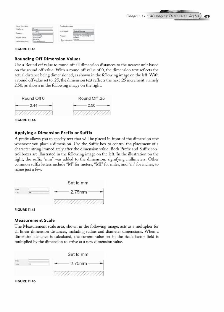
Rounding Off Dimension ValuesUse a Round off value to round off all dimension distances to the nearest unit basedon the round off value. With a round off value of 0, the dimension text reflects theactual distance being dimensioned, as shown in the following image on the left. Witha round off value set to .25, the dimension text reflects the next .25 increment, namely2.50, as shown in the following image on the right.
Applying a Dimension Prefix or SuffixA prefix allows you to specify text that will be placed in front of the dimension textwhenever you place a dimension. Use the Suffix box to control the placement of acharacter string immediately after the dimension value. Both Prefix and Suffix con-trol boxes are illustrated in the following image on the left. In the illustration on theright, the suffix “mm” was added to the dimension, signifying millimeters. Othercommon suffix letters include “M” for meters, “MI” for miles, and “in” for inches, toname just a few.
Measurement ScaleThe Measurement scale area, shown in the following image, acts as a multiplier forall linear dimension distances, including radius and diameter dimensions. When adimension distance is calculated, the current value set in the Scale factor field ismultiplied by the dimension to arrive at a new dimension value.
FIGURE 11.43
FIGURE 11.44
FIGURE 11.45
FIGURE 11.46
Chap t e r 11 • Manag i n g D imen s i o n S t y l e s 479

Illustrated in the following image on the left, and with a linear scale value of 1.00, thedimension distances are taken at their default values.
Illustrated in the following image on the right, the linear scale value has been changedto 2.00 units. This means 2.00 will multiply every dimension distance; the result isthat the previous 3.00 and 2.00 dimensions are changed to 6.00 and 4.00, respec-tively. In a similar fashion, having a linear scale value set to 0.50 will reduce all dimen-sion values to half their original values.
THE ALTERNATE UNITS TABUse the Alternate Units tab, shown in the following image, to enable alternate units,set the units and precision of the alternate units, set a multiplier for all units, use around-off distance, and set a prefix and suffix for these units. You also have two place-ment modes for displaying these units. By default, alternate units are placed besideprimary units. The alternate units are enclosed in square brackets. With two sets ofunits being displayed, your drawing could tend to become very busy. An applicationof using Alternate Units would be to display English and metric dimension values,since some design firms require both.
FIGURE 11.47
480 Au t oCAD 2010 Tu t o r f o r Eng i n e e r i n g Graph i c s

Alternate UnitsOnce alternate units are enabled, all items in the Alternate Units area become active,as shown in the following image on the left. By default, the alternate unit value isplaced in brackets alongside the calculated dimension value, as shown in the follow-ing image on the right. This value depends on the current setting in theMultiplier forall units field. This factor, set to 25.40 in the following image, is used as a multiplierfor all calculated alternate dimension values.
FIGURE 11.48
FIGURE 11.49
Chap t e r 11 • Manag i n g D imen s i o n S t y l e s 481

You could also click the radio button next to Below primary value, as shown inthe following image on the left. This places the primary dimension above the dimen-sion line and the alternate dimension below it, as shown in the following image onthe right.
THE TOLERANCES TABThe Tolerances tab shown in the following image consists of various fields used tocontrol the five types of tolerance settings: None, Symmetrical, Deviation, Limits,and Basic. Depending on the type of tolerance being constructed, an Upper valueand Lower value may be set to call out the current tolerance variance. The Verticalposition setting allows you to determine where the tolerance will be drawn in relationto the location of the body text. The Scaling for height setting controls the text size ofthe tolerance. Usually this value is smaller than the body text size.
FIGURE 11.50
482 Au t oCAD 2010 Tu t o r f o r Eng i n e e r i n g Graph i c s

Tolerance FormatThe five tolerance types available in the drop-down list are illustrated in the followingimage. A tolerance setting of None uses the calculated dimension value without ap-plying any tolerances. The Symmetrical tolerance uses the same value set in the Upperand Lower value. The Deviation tolerance setting will have a value set in the Uppervalue and an entirely different value set in the Lower value. The Limits tolerance willuse the Upper and Lower values and place the results with the larger limit dimensionplaced above the smaller limit dimension. The Basic tolerance setting does not addany tolerance value; instead, a box is drawn around the dimension value.
FIGURE 11.51
Chap t e r 11 • Manag i n g D imen s i o n S t y l e s 483

CONTROLLING THE ASSOCIATIVITY OF DIMENSIONS
The DIMASSOC System VariableThe associativity of dimensions is controlled by the DIMASSOC variable. By default,this value is set to 2 for new drawings. This means that the dimension is associatedwith the object being dimensioned. Associativity means that if the object changes sizeor if some element of an object changes location, the dimension associated with theobject will change as well.
When this variable is set to 1, the dimension is called nonassociative. Dimensions ofthis type exist in older AutoCAD drawings. This dimension is not associated withthe object being dimensioned; however, it is possible to have the dimension valueautomatically updated using conventional AutoCAD editing commands.
The DIMASSOC variable can also be set to 0, which will create exploded dimensions.There is no association between the various elements of the dimension. All dimen-sion lines, extension lines, arrowheads, and dimension text are drawn as separateobjects. This means that grips will not have any effect on this dimension. You cannotstretch an object and have this dimension update to the object’s new length. Youcannot make a change in the Dimension Styles Manager dialog box and have thisdimension affected. In other words, never set this variable to 0. The same effectscan be achieved by using the EXPLODE command on a dimension; this is not recom-mended and is poor practice.
TRY IT! Open the drawing 11_Dimassoc2. The object in the following image on the left has dimen-sions placed with the dimassoc variable set to 2. Another polyline shape on the right hasvarious dimensions placed on its outside. Click the polyline on the left to activate its grips.Click the grip at “A” and stretch the polyline vertex up and to the left. Notice that alldimension locations, orientations, and values are automatically updated. Click the polylinevertex at “B” and stretch this vertex up and to the right. The same results occur, with thedimension elements being updated based on the new location of the object. Use grips torealign any dimension that is not updated to a new location.
FIGURE 11.52
484 Au t oCAD 2010 Tu t o r f o r Eng i n e e r i n g Graph i c s
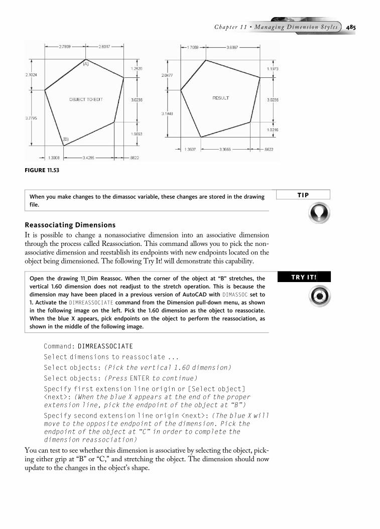
TIPWhen you make changes to the dimassoc variable, these changes are stored in the drawingfile.
Reassociating DimensionsIt is possible to change a nonassociative dimension into an associative dimensionthrough the process called Reassociation. This command allows you to pick the non-associative dimension and reestablish its endpoints with new endpoints located on theobject being dimensioned. The following Try It! will demonstrate this capability.
TRY IT!Open the drawing 11_Dim Reassoc. When the corner of the object at “B” stretches, thevertical 1.60 dimension does not readjust to the stretch operation. This is because thedimension may have been placed in a previous version of AutoCAD with DIMASSOC set to1. Activate the DIMREASSOCIATE command from the Dimension pull-down menu, as shownin the following image on the left. Pick the 1.60 dimension as the object to reassociate.When the blue X appears, pick endpoints on the object to perform the reassociation, asshown in the middle of the following image.
Command: DIMREASSOCIATE
Select dimensions to reassociate ...
Select objects: (Pick the vertical 1.60 dimension)
Select objects: (Press ENTER to continue)
Specify first extension line origin or [Select object]<next>: (When the blue X appears at the end of the properextension line, pick the endpoint of the object at “B”)
Specify second extension line origin <next>: (The blue X willmove to the opposite endpoint of the dimension. Pick theendpoint of the object at “C” in order to complete thedimension reassociation)
You can test to see whether this dimension is associative by selecting the object, pick-ing either grip at “B” or “C,” and stretching the object. The dimension should nowupdate to the changes in the object’s shape.
FIGURE 11.53
Chap t e r 11 • Manag i n g D imen s i o n S t y l e s 485

You will be able to identify associated dimensions by clicking the dimension whilein the reassociate command. The familiar X is surrounded by a blue box, as shownin the previous image on the right. If you do not see the blue box, the dimension isnot associative.
Reassociating works only on nonassociative dimensions that have their dimassocvalue set to 1. The process of Reassociation does not have any effect on explodeddimensions (dimassoc set to 0).
While AutoCAD gives you this ability to reassociate dimensions, it would be verytime-consuming to perform this task on hundreds of dimensions in a drawing.Reassociation is ideal when dealing with only a few dimensions.
USING DIMENSION TYPES IN DIMENSION STYLESIn addition to creating dimension styles, you can assign dimension types to dimen-sion styles. The purpose of using dimension types is to reduce the number of dimen-sion styles defined in a drawing. For example, the object in the following imageconsists of linear dimensions with three-decimal-place accuracy, a radius dimensionwith one-decimal-place accuracy, and an angle dimension with a box surrounding thenumber. Normally you would have to create three separate dimension styles to createthis effect. However, the linear, radius, and angular dimensions consist of what arecalled dimension types.
FIGURE 11.54
486 Au t oCAD 2010 Tu t o r f o r Eng i n e e r i n g Graph i c s

Dimension types appear similar to the following image when assigned to the Me-chanical dimension style. Before creating an angular dimension, you create the di-mension type and make changes in various tabs located in the Modify DimensionStyle dialog box. These changes will apply only to the angular dimension type. Toexpose the dimension types, click the New button in the main Dimension StyleMan-ager dialog box.
When the Create New Dimension Style dialog box appears, as shown in the follow-ing image, click on the Use for box. This box usually displays All dimensions. Noticeall dimension types appearing. You can make changes to dimension settings thatwill apply only for linear, angular, radius, diameter, and ordinate dimensions. Also,a dimension type for Leaders and Tolerances is available. Highlight this option andthen click the Continue button.
FIGURE 11.55
FIGURE 11.56
Chap t e r 11 • Manag i n g D imen s i o n S t y l e s 487

This takes you to the New Dimension Style: Mechanical: Leader dialog box, shownin the following image. Any changes you make in the tabs will apply only wheneveryou place a leader dimension. The use of dimension types is an efficient means ofkeeping the number of dimension styles down to a manageable level.
FIGURE 11.58
FIGURE 11.57
488 Au t oCAD 2010 Tu t o r f o r Eng i n e e r i n g Graph i c s
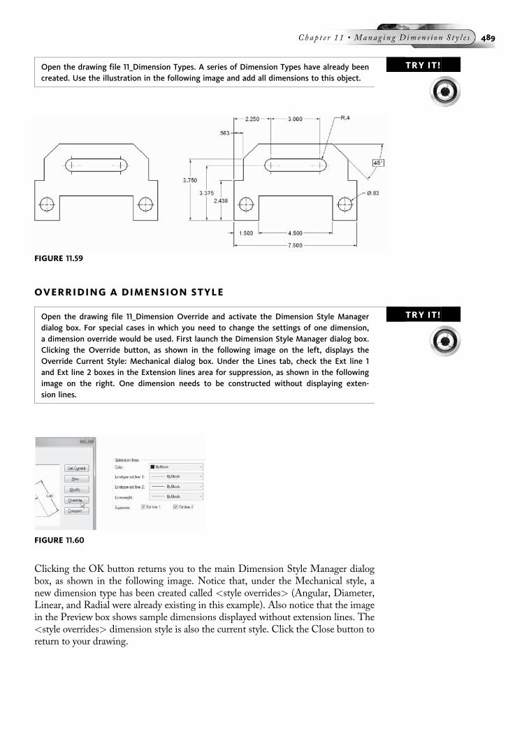
TRY IT!Open the drawing file 11_Dimension Types. A series of Dimension Types have already beencreated. Use the illustration in the following image and add all dimensions to this object.
OVERRIDING A DIMENSION STYLE
TRY IT!Open the drawing file 11_Dimension Override and activate the Dimension Style Managerdialog box. For special cases in which you need to change the settings of one dimension,a dimension override would be used. First launch the Dimension Style Manager dialog box.Clicking the Override button, as shown in the following image on the left, displays theOverride Current Style: Mechanical dialog box. Under the Lines tab, check the Ext line 1and Ext line 2 boxes in the Extension lines area for suppression, as shown in the followingimage on the right. One dimension needs to be constructed without displaying exten-sion lines.
Clicking the OK button returns you to the main Dimension Style Manager dialogbox, as shown in the following image. Notice that, under the Mechanical style, anew dimension type has been created called <style overrides> (Angular, Diameter,Linear, and Radial were already existing in this example). Also notice that the imagein the Preview box shows sample dimensions displayed without extension lines. The<style overrides> dimension style is also the current style. Click the Close button toreturn to your drawing.
FIGURE 11.59
FIGURE 11.60
Chap t e r 11 • Manag i n g D imen s i o n S t y l e s 489
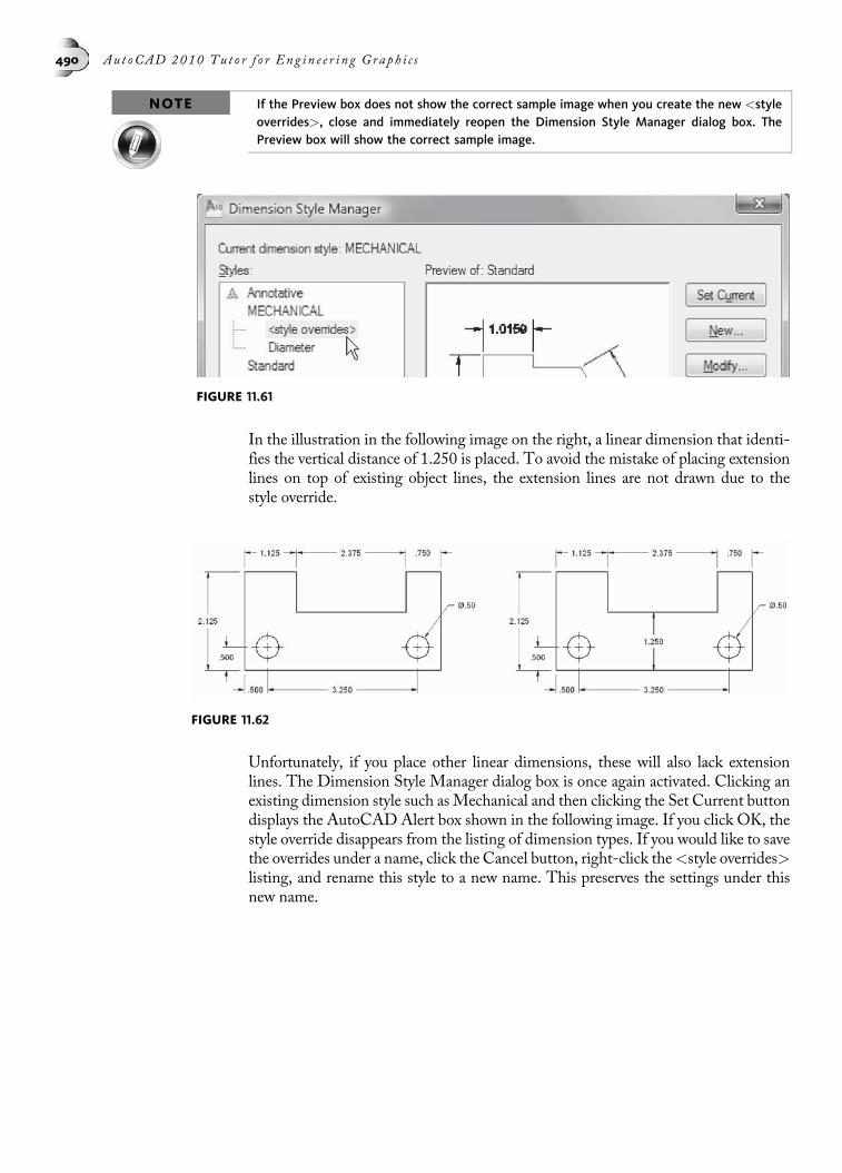
NOTE If the Preview box does not show the correct sample image when you create the new <styleoverrides>, close and immediately reopen the Dimension Style Manager dialog box. ThePreview box will show the correct sample image.
In the illustration in the following image on the right, a linear dimension that identi-fies the vertical distance of 1.250 is placed. To avoid the mistake of placing extensionlines on top of existing object lines, the extension lines are not drawn due to thestyle override.
Unfortunately, if you place other linear dimensions, these will also lack extensionlines. The Dimension Style Manager dialog box is once again activated. Clicking anexisting dimension style such asMechanical and then clicking the Set Current buttondisplays the AutoCAD Alert box shown in the following image. If you click OK, thestyle override disappears from the listing of dimension types. If you would like to savethe overrides under a name, click the Cancel button, right-click the<style overrides>listing, and rename this style to a new name. This preserves the settings under thisnew name.
FIGURE 11.61
FIGURE 11.62
490 Au t oCAD 2010 Tu t o r f o r Eng i n e e r i n g Graph i c s
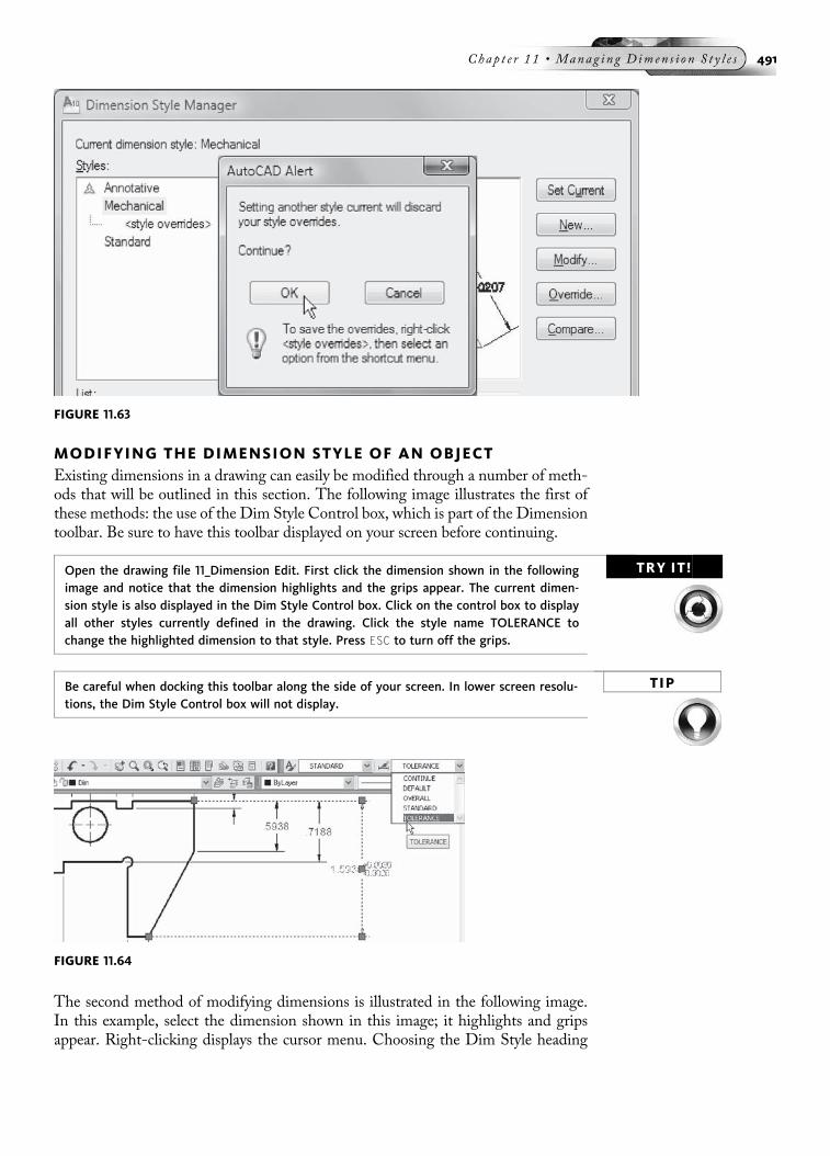
MODIFYING THE DIMENSION STYLE OF AN OBJECTExisting dimensions in a drawing can easily be modified through a number of meth-ods that will be outlined in this section. The following image illustrates the first ofthese methods: the use of the Dim Style Control box, which is part of the Dimensiontoolbar. Be sure to have this toolbar displayed on your screen before continuing.
TRY IT!Open the drawing file 11_Dimension Edit. First click the dimension shown in the followingimage and notice that the dimension highlights and the grips appear. The current dimen-sion style is also displayed in the Dim Style Control box. Click on the control box to displayall other styles currently defined in the drawing. Click the style name TOLERANCE tochange the highlighted dimension to that style. Press ESC to turn off the grips.
TIPBe careful when docking this toolbar along the side of your screen. In lower screen resolu-tions, the Dim Style Control box will not display.
The second method of modifying dimensions is illustrated in the following image.In this example, select the dimension shown in this image; it highlights and gripsappear. Right-clicking displays the cursor menu. Choosing the Dim Style heading
FIGURE 11.63
FIGURE 11.64
Chap t e r 11 • Manag i n g D imen s i o n S t y l e s 491

displays the cascading menu of all dimension styles defined in the drawing. Click theTOLERANCE style to change the highlighted dimension to the new style.
The third method of modifying dimensions begins with selecting the overall lengthdimension shown in the following image. Again, the dimension highlights and gripsappear. Clicking the Properties button displays the Properties Window, shown inthe following image. Click the Alphabetic tab to display all dimension settings andcurrent values. If you click on the name box next to Dim style, all dimension styleswill appear in the field. Click the OVERALL style to change the highlighted dimen-sion to the new style. Close the Properties Palette and press the ESC key to turn offthe grips.
CREATING MULTILEADER STYLESAs with the Dimension Style Manager, you can create different styles of multileadersusing the Multileader Style Manager. Choosing Multileader Style either from theMenu Bar or from the Ribbon launches the Multileader Style Manager dialog boxshown in the following image.
FIGURE 11.66
FIGURE 11.65
492 Au t oCAD 2010 Tu t o r f o r Eng i n e e r i n g Graph i c s
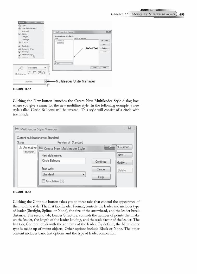
Clicking the New button launches the Create New Multileader Style dialog box,where you give a name for the new multiline style. In the following example, a newstyle called Circle Balloons will be created. This style will consist of a circle withtext inside.
Clicking the Continue button takes you to three tabs that control the appearance ofthe multiline style. The first tab, Leader Format, controls the leader and includes typeof leader (Straight, Spline, or None), the size of the arrowhead, and the leader breakdistance. The second tab, Leader Structure, controls the number of points that makeup the leader, the length of the leader landing, and the scale factor of the leader. Thelast tab, Content, deals with the contents of the leader. By default, the Multileadertype is made up of mtext objects. Other options include Block or None. The othercontent includes basic text options and the type of leader connection.
FIGURE 11.67
FIGURE 11.68
Chap t e r 11 • Manag i n g D imen s i o n S t y l e s 493

While in the Content tab, changing mtext to Block activates block options, as shownin the following image. Changing the source block to circle updates the previewimage of the multileader.
Returning back to the Multileader Style Manager dialog box allows you to make thenew style, namely Circle Balloons, the current style, as shown in the followingimage on the left. The results of using this style in a drawing are shown in thefollowing image on the right.
FIGURE 11.69
FIGURE 11.70
494 Au t oCAD 2010 Tu t o r f o r Eng i n e e r i n g Graph i c s
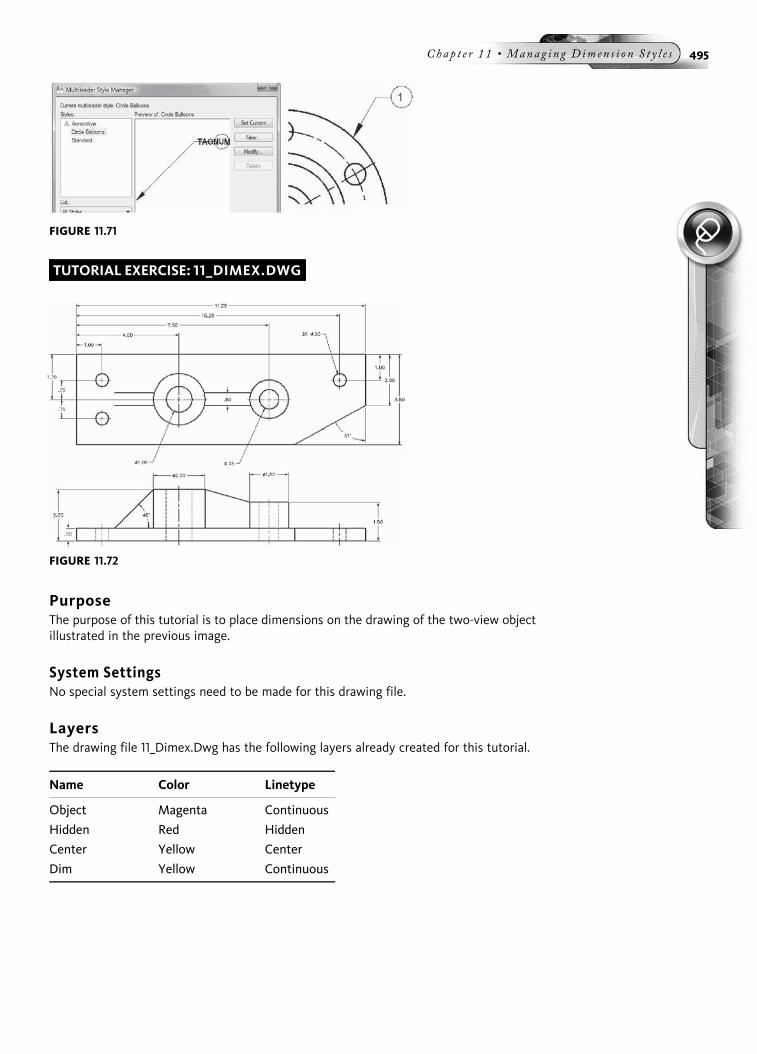
TUTORIAL EXERCISE: 11_DIMEX.DWG
PurposeThe purpose of this tutorial is to place dimensions on the drawing of the two-view objectillustrated in the previous image.
System SettingsNo special system settings need to be made for this drawing file.
LayersThe drawing file 11_Dimex.Dwg has the following layers already created for this tutorial.
Name Color Linetype
Object Magenta Continuous
Hidden Red Hidden
Center Yellow Center
Dim Yellow Continuous
FIGURE 11.71
FIGURE 11.72
Chap t e r 11 • Manag i n g D imen s i o n S t y l e s 495

Suggested CommandsOpen the drawing called 11_Dimex. The following dimension commands will be used:DIMLINEAR, DIMCONTINUE, DIMBASELINE, DIMCENTER, DIMRADIUS, DIMDIA-METER, DIMANGULAR, and LEADER. All dimension commands may be chosen from theDimension toolbar or the Dimension pull-down menu, or entered from the keyboard.Use the ZOOM command to get a closer look at details and features that are beingdimensioned.
STEP 1To prepare for the dimensioning of the drawing, type D to activate the DimensionStyle Manager dialog box. Click the New button, which activates the Create NewDimension Style dialog box shown in the following image. In the New Style Name area,enter MECHANICAL. Click the Continue button to create the style, as shown in the fol-lowing image.
STEP 2When the New Dimension Style: MECHANICAL dialog box appears, make the followingchanges in the Lines tab, as shown in the following image on the left: Change the size ofthe Extend beyond dim lines from a value of 0.18 to a new value of 0.07. Switch to theSymbols and Arrows tab and change the Arrow size to from 0.18 to 0.12. Also changethe Center marks to Line, as shown in the following image on the right.
FIGURE 11.73
FIGURE 11.74
496 Au t oCAD 2010 Tu t o r f o r Eng i n e e r i n g Graph i c s

STEP 3Next, click the Text tab and change the Text height from a value of 0.18 to a new value of0.12, as shown in the following image on the left. Then click the Primary Units tab andchange the number of decimal places from 4 to 2. Also place a check in the box next toLeading in the Zero suppression area, as shown in the following image on the right. Thisturns off the leading zero for dimension values under 1 unit. When finished, click the OKbutton to return to the main Dimension Style Manager dialog box.
STEP 4You will now create a dimension type dealing with all diameter dimensions and make achange to the center mark settings for this type. Click the New button to display theCreate New Dimension Style dialog box. In the Use for box, click Diameter dimensions,as shown in the following image on the left, and then click the Continue button. Clickthe Symbols and Arrows tab and change the Center marks setting to None, as shownin the following image on the right. This prevents center marks from being displayedwhen placing diameter dimensions. When finished, click the OK button to return to themain Dimension Styles Manager dialog box.
STEP 5In the Dimension Style Manager dialog box, click MECHANICAL in the Styles area. Thenclick the Set Current button to make MECHANICAL the current dimension style. Yourdisplay should appear similar to the following image. Click the Close button to save allchanges and return to the drawing.
FIGURE 11.76
FIGURE 11.75
Chap t e r 11 • Manag i n g D imen s i o n S t y l e s 497

STEP 6Begin placing center markers to identify the centers of all circular features in the Topview. Use the DIMCENTER command (or the shortcut DCE) to perform this operation oncircles “A” through “E,” as shown in the following image.
STEP 7Use the QDIM command to place a string of baseline dimensions. First select the individ-ual lines labeled “A” through “F,” as shown in the following image. When the group ofdimensions previews as continued dimensions, change this grouping to baseline and clicka location to place the baseline group of dimensions, as shown in the following image.Use grips to place the text as shown.
FIGURE 11.78
FIGURE 11.79
FIGURE 11.77
498 Au t oCAD 2010 Tu t o r f o r Eng i n e e r i n g Graph i c s
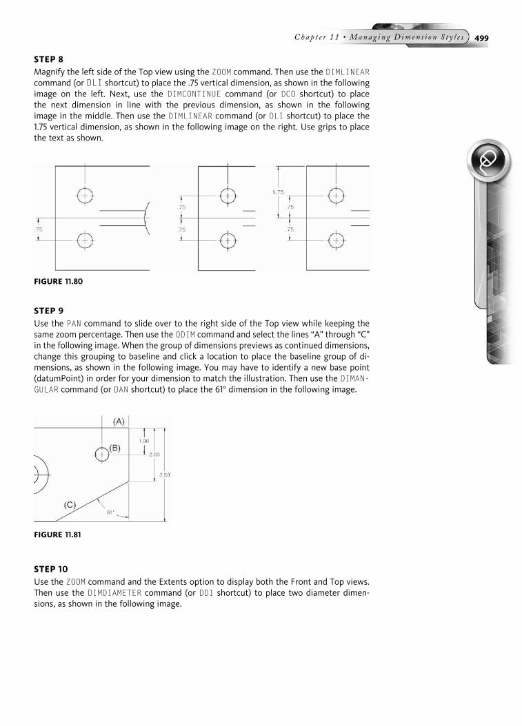
STEP 8Magnify the left side of the Top view using the ZOOM command. Then use the DIMLINEARcommand (or DLI shortcut) to place the .75 vertical dimension, as shown in the followingimage on the left. Next, use the DIMCONTINUE command (or DCO shortcut) to placethe next dimension in line with the previous dimension, as shown in the followingimage in the middle. Then use the DIMLINEAR command (or DLI shortcut) to place the1.75 vertical dimension, as shown in the following image on the right. Use grips to placethe text as shown.
STEP 9Use the PAN command to slide over to the right side of the Top view while keeping thesame zoom percentage. Then use the QDIM command and select the lines “A” through “C”in the following image. When the group of dimensions previews as continued dimensions,change this grouping to baseline and click a location to place the baseline group of di-mensions, as shown in the following image. You may have to identify a new base point(datumPoint) in order for your dimension to match the illustration. Then use the DIMAN-GULAR command (or DAN shortcut) to place the 61° dimension in the following image.
STEP 10Use the ZOOM command and the Extents option to display both the Front and Top views.Then use the DIMDIAMETER command (or DDI shortcut) to place two diameter dimen-sions, as shown in the following image.
FIGURE 11.80
FIGURE 11.81
Chap t e r 11 • Manag i n g D imen s i o n S t y l e s 499
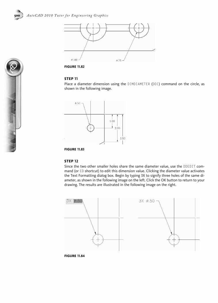
STEP 11Place a diameter dimension using the DIMDIAMETER (DDI) command on the circle, asshown in the following image.
STEP 12Since the two other smaller holes share the same diameter value, use the DDEDIT com-mand (or ED shortcut) to edit this dimension value. Clicking the diameter value activatesthe Text Formatting dialog box. Begin by typing 3X to signify three holes of the same di-ameter, as shown in the following image on the left. Click the OK button to return to yourdrawing. The results are illustrated in the following image on the right.
FIGURE 11.83
FIGURE 11.82
FIGURE 11.84
500 Au t oCAD 2010 Tu t o r f o r Eng i n e e r i n g Graph i c s

STEP 13One more dimension needs to be placed in the Top view: the .50 width of the rib.Unfortunately, because of the placement of this dimension, extension lines will be drawnon top of the object’s lines. This is poor practice. To remedy this, a dimension overridewill be created. To do this, activate the Dimension Style Manager dialog box and clickthe Override button, as shown in the following image on the left. This displays the Over-ride Current Style: MECHANICAL dialog box. In the Lines tab, place checks in the boxesto Suppress (turn off) Ext line 1 and Ext line 2 in the Extension lines area, as shown in thefollowing image in the middle.
Click the OK button and notice the new <style overrides> listing under MECHANICAL,as shown in the following image on the right. Notice also that the preview image lacksextension lines. Click the Close button to return to the drawing.
STEP 14Pan to the middle area of the Top view and place the .50 rib-width dimension while inthe dimension style override, as shown in the following image. This dimension shouldbe placed without having any extension lines visible. Also, use grips to drag the dimen-sion text inside the visible object lines (temporarily turn off OSNAP to better accomplishthis task).
STEP 15The completed Top view, including dimensions, is illustrated in the following image. Usethis figure to check that all dimensions have been placed and all features such as holesand fillets have been properly identified.
FIGURE 11.85
FIGURE 11.86
Chap t e r 11 • Manag i n g D imen s i o n S t y l e s 501

STEP 16The Front view in the following image will be the focus for the next series of dimension-ing steps. Again use the ZOOM and PAN commands whenever you need to magnify or slideto a better drawing view position.
STEP 17Before continuing, activate the Dimension Style Manager dialog box, click the MECHAN-ICAL style, and then click the Set Current button. An AutoCAD Alert box displays, asshown in the following image. Making MECHANICAL current discards any style over-rides. Click the OK button to discard the changes because you need to return to havingextension lines visible in linear dimensions.
FIGURE 11.88
FIGURE 11.87
FIGURE 11.89
502 Au t oCAD 2010 Tu t o r f o r Eng i n e e r i n g Graph i c s

STEP 18Place two horizontal linear dimensions that signify the diameters of the two cylindersusing the DIMLINEAR command, as shown in the following image. Also add the 1.50 ver-tical dimension to the side of the Front view, as shown in the following image.
STEP 19Use the QDIM command to place the vertical baseline dimensions, as shown in the follow-ing image. Also place the 45° angular dimension in this image.
STEP 20The remaining step is to add the diameter symbol to the 2.00 and 1.50 dimensions, sincethe dimension is placed on a cylindrical object. Double-click on the 2.00 dimension, right-click, and when the menu appears as shown in the following image, pick Symbol followedby Diameter to place the diameter symbol. Do the same for the 1.50 dimension.
FIGURE 11.90
FIGURE 11.91
Chap t e r 11 • Manag i n g D imen s i o n S t y l e s 503

Once you have completed all dimensioning steps, your drawing should appearsimilar to the following image. Use grips to close the gaps between the extension andcenterlines.
FIGURE 11.93
FIGURE 11.92
504 Au t oCAD 2010 Tu t o r f o r Eng i n e e r i n g Graph i c s
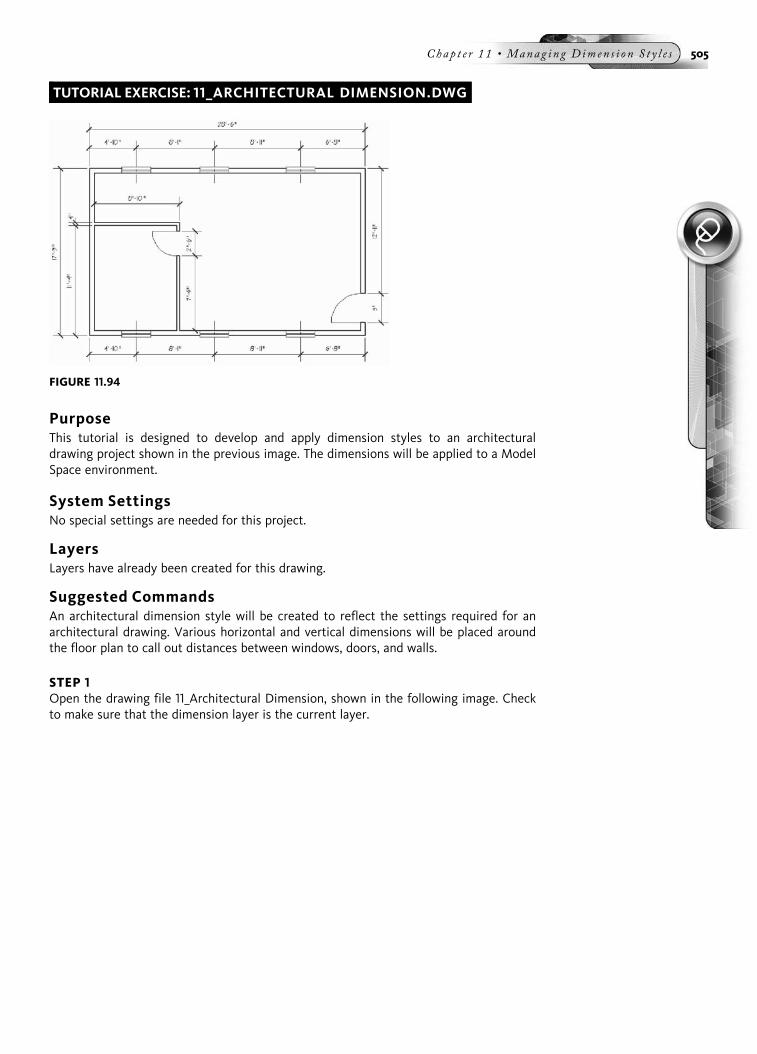
TUTORIAL EXERCISE: 11_ARCHITECTURAL DIMENSION.DWG
PurposeThis tutorial is designed to develop and apply dimension styles to an architecturaldrawing project shown in the previous image. The dimensions will be applied to a ModelSpace environment.
System SettingsNo special settings are needed for this project.
LayersLayers have already been created for this drawing.
Suggested CommandsAn architectural dimension style will be created to reflect the settings required for anarchitectural drawing. Various horizontal and vertical dimensions will be placed aroundthe floor plan to call out distances between windows, doors, and walls.
STEP 1Open the drawing file 11_Architectural Dimension, shown in the following image. Checkto make sure that the dimension layer is the current layer.
FIGURE 11.94
Chap t e r 11 • Manag i n g D imen s i o n S t y l e s 505

STEP 2The Dimension Style Manager will be used to set up characteristics of the dimensionsused in architectural applications. Activate the Dimension Style Manager dialog box byclicking Dimension Style, located in the Format pull-down menu. Clicking the New . . .button launches the Create New Dimension Style dialog box, as shown in the followingimage. Replace Copy of Standard in the New Style Name field with Architectural. Thisdimension style will initially be based on the current standard dimension style andapplied to all dimensions that are placed in the drawing. Click the Continue button tomake various changes to the dimension settings.
STEP 3Note that the name Architectural is now displayed in the title bar of the New DimensionStyle dialog box, as shown in the following image. In the Symbols and Arrows section,change the arrowhead style to Architectural tick. When you change the First arrowhead,it also changes the Second arrowhead. Also change the arrow size to 1/8 00, or .125, asshown in the following image.
FIGURE 11.96
FIGURE 11.95
506 Au t oCAD 2010 Tu t o r f o r Eng i n e e r i n g Graph i c s
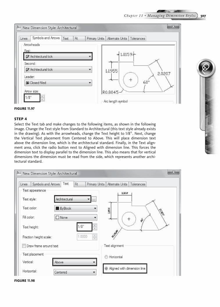
STEP 4Select the Text tab and make changes to the following items, as shown in the followingimage. Change the Text style from Standard to Architectural (this text style already existsin the drawing). As with the arrowheads, change the Text height to 1/8 00. Next, changethe Vertical Text placement from Centered to Above. This will place dimension textabove the dimension line, which is the architectural standard. Finally, in the Text align-ment area, click the radio button next to Aligned with dimension line. This forces thedimension text to display parallel to the dimension line. This also means that for verticaldimensions the dimension must be read from the side, which represents another archi-tectural standard.
FIGURE 11.97
FIGURE 11.98
Chap t e r 11 • Manag i n g D imen s i o n S t y l e s 507

STEP 5Next, select the Fit tab and change the overall scale of the dimension. The overall scale isbased on the plotting scale when plotting is done from the model tab. The anticipatedplotting scale for this drawing is 1/4 00 ¼ 1 0. Because 1/4 00 divides 48 times into 1 0, type48 in the Use overall scale of field, as shown in the following image.
STEP 6Next, choose the Primary Units tab. In the Linear dimensions section, change the Unitformat option to Architectural. Also, change the precision to 0 0-0 00. Your display shouldappear similar to the following image.
FIGURE 11.99
FIGURE 11.100
508 Au t oCAD 2010 Tu t o r f o r Eng i n e e r i n g Graph i c s
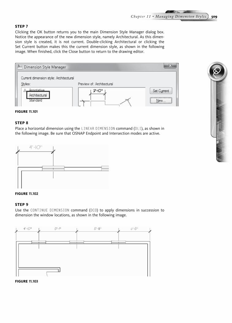
STEP 7Clicking the OK button returns you to the main Dimension Style Manager dialog box.Notice the appearance of the new dimension style, namely Architectural. As this dimen-sion style is created, it is not current. Double-clicking Architectural or clicking theSet Current button makes this the current dimension style, as shown in the followingimage. When finished, click the Close button to return to the drawing editor.
STEP 8Place a horizontal dimension using the LINEAR DIMENSION command (DLI), as shown inthe following image. Be sure that OSNAP Endpoint and Intersection modes are active.
STEP 9Use the CONTINUE DIMENSION command (DCO) to apply dimensions in succession todimension the window locations, as shown in the following image.
FIGURE 11.103
FIGURE 11.101
FIGURE 11.102
Chap t e r 11 • Manag i n g D imen s i o n S t y l e s 509

STEP 10Next add an overall length dimension using the LINEAR DIMENSION command (DLI), asshown in the following image.
STEP 11Continue adding other dimensions to the floor plan, including those defining vertical andinterior dimensions of the building, as shown in the following image.
END OF CHAPTER PROBLEMS FOR CHAPTER 11Please refer to the CD that is supplied with this book and locate the file AutoCAD Tutor2010 Support Docs.pdf. In addition to extra information supplied in this chapter, end-of-chapter problems are also available to provide additional practice.
FIGURE 11.105
FIGURE 11.104
510 Au t oCAD 2010 Tu t o r f o r Eng i n e e r i n g Graph i c s

CHAPTER
12
Analyzing2DDrawings
This chapter will show how a series of commands may be used to calculate distancesand angles of selected objects. It will also show how surface areas may be calculated oncomplex geometric shapes. The following pages highlight all of AutoCAD’s MeasureGeometry commands and show how you can use them to display useful informationon an object or group of objects.
USING MEASURE GEOMETRY COMMANDSYou can choose AutoCAD’s Measure Geometry commands by using the InquiryMenu Bar, or the Ribbon, as illustrated in the following image.
FINDING THE AREA OF AN ENCLOSED SHAPEThe AREA option of the MEASUREGEOM command is used to calculate the
area through the selection of a series of points. Select the endpoints of all vertices inthe following image with the OSNAP-Endpoint option. Once you have selected thefirst point along with the remaining points in either a clockwise or counterclockwisepattern, respond to the prompt “Next point:” by pressing ENTER to calculate the area
FIGURE 12.1
511
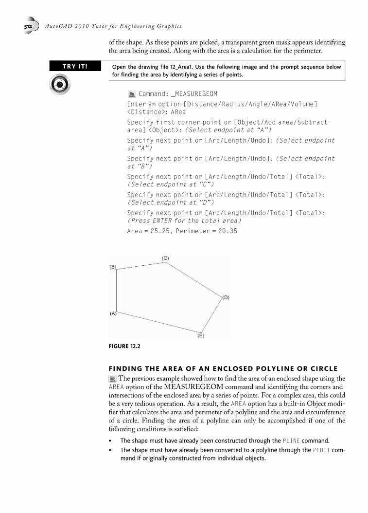
of the shape. As these points are picked, a transparent green mask appears identifyingthe area being created. Along with the area is a calculation for the perimeter.
TRY IT! Open the drawing file 12_Area1. Use the following image and the prompt sequence belowfor finding the area by identifying a series of points.
Command: _MEASUREGEOM
Enter an option [Distance/Radius/Angle/ARea/Volume]<Distance>: ARea
Specify first corner point or [Object/Add area/Subtractarea] <Object>: (Select endpoint at “A”)
Specify next point or [Arc/Length/Undo]: (Select endpointat “A”)
Specify next point or [Arc/Length/Undo]: (Select endpointat “B”)
Specify next point or [Arc/Length/Undo/Total] <Total>:(Select endpoint at “C”)
Specify next point or [Arc/Length/Undo/Total] <Total>:(Select endpoint at “D”)
Specify next point or [Arc/Length/Undo/Total] <Total>:(Press ENTER for the total area)
Area = 25.25, Perimeter = 20.35
FINDING THE AREA OF AN ENCLOSED POLYLINE OR CIRCLEThe previous example showed how to find the area of an enclosed shape using the
AREA option of the MEASUREGEOM command and identifying the corners andintersections of the enclosed area by a series of points. For a complex area, this couldbe a very tedious operation. As a result, the AREA option has a built-in Object modi-fier that calculates the area and perimeter of a polyline and the area and circumferenceof a circle. Finding the area of a polyline can only be accomplished if one of thefollowing conditions is satisfied:
• The shape must have already been constructed through the PLINE command.
• The shape must have already been converted to a polyline through the PEDIT com-mand if originally constructed from individual objects.
FIGURE 12.2
512 Aut oCAD 2010 Tu t o r f o r Eng in e e r i n g Graph i c s

TRY IT!Open the drawing file 12_Area2. Use the following image and the prompt sequence belowfor finding the area of both shapes.
Command: _MEASUREGEOM
Enter an option [Distance/Radius/Angle/ARea/Volume]<Distance>: ARea
Specify first corner point or [Object/Add area/Subtractarea] <Object>: O (For Object)
Select objects: (Select the polyline at “A”)
Area = 24.88, Perimeter = 19.51
Command: Command: _MEASUREGEOM
Enter an option [Distance/Radius/Angle/ARea/Volume]<Distance>: ARea
Specify first corner point or [Object/Add area/Subtractarea] <Object>: O (For Object)
Select objects: (Select the circle at “B”)
Area = 7.07, Circumference = 9.42
TRY IT!Open the drawing file 12_Extrude1. In the following image, either convert all line segmentsinto a single polyline object or use the BOUNDARY command to trace a polyline on the top ofall the line segments. In either case, answer Question 1 regarding 12_Extrude1.
FIGURE 12.3
FIGURE 12.4
Chap t e r 12 • Ana l y z i n g 2D Drawing s 513

TRY IT! Open the drawing file 12_Extrude2. In the following image, either convert all line segmentsinto a single polyline object or use the BOUNDARY command to trace a polyline on the top ofall the line segments. In either case, answer Question 1 regarding 12_Extrude2.
FINDING THE AREA OF A SHAPE BY SUBTRACTIONYou may wish to calculate the area of a shape with holes cut through it. The steps
you use to calculate the total surface area are: (1) calculate the area of the outline and(2) subtract the objects inside the outline. All individual objects, except circles, mustfirst be converted to polylines through the PEDIT command. Next, find the overallarea and add it to the database using the Add mode of the AREA option. Exit theAdd mode and remove the inner objects using the Subtract mode of the AREA com-mand. Remember that all objects must be in the form of a circle or polyline. Thismeans that the inner shape at “B” in the following image on the left must also be con-verted to a polyline through the PEDIT command before the area is calculated. Caremust be taken when selecting the objects to subtract. If an object is selected twice, it issubtracted twice and may yield an inaccurate area in the final calculation. As you addobjects, a transparent green mask appears to identify the area being added; when yousubtract objects, a transparent brown mask appears to identify the area being sub-tracted as shown in the following image on the right.
In the following image, the total area with the circle and rectangle removed is30.4314.
TRY IT! Open the drawing file 12_Area3. Use the following image and the prompt sequence to verifythis area calculation.
FIGURE 12.5
514 Aut oCAD 2010 Tu t o r f o r Eng in e e r i n g Graph i c s

Command: Command: _MEASUREGEOM
Enter an option [Distance/Radius/Angle/ARea/Volume]<Distance>: ARea
Specify first corner point or [Object/Add area/Subtractarea] <Object>: A (For Add)
Specify first corner point or [Object/Subtract area]: O(For Object)
(ADD mode) Select objects: (Select the polyline at “A”)
Area = 47.5000, Perimeter = 32.0000
Total area = 47.5000
(ADD mode) Select objects: (Press ENTER to exit ADD mode)
Area = 47.5000, Perimeter = 32.0000
Total area = 47.5000
Specify first corner point or [Object/Subtract area]: S(For Subtract)
Specify first corner point or [Object/Add area]: O(For Object)
(SUBTRACT mode) Select objects: (Select the rectangle at “B”)
Area = 10.0000, Perimeter = 13.0000
Total area = 37.5000
(SUBTRACT mode) Select objects: (Select the circle at “C”)
Area = 7.0686, Circumference = 9.4248
Total area = 30.4314
(SUBTRACT mode) Select objects: (Press ENTER to exitSUBTRACT mode)
(SUBTRACT mode) Select objects: (Press ENTER to exit)
TRY IT!Open the drawing file 12_Shield. In the following image, use the BOUNDARY command totrace a polyline on the top of all the line segments. Subtract all four-sided shapes from themain shape using the AREA option of the MEASUREGEOM command. Answer Question 1regarding 12_Shield.
FIGURE 12.6
Chap t e r 12 • Ana l y z i n g 2D Drawing s 515
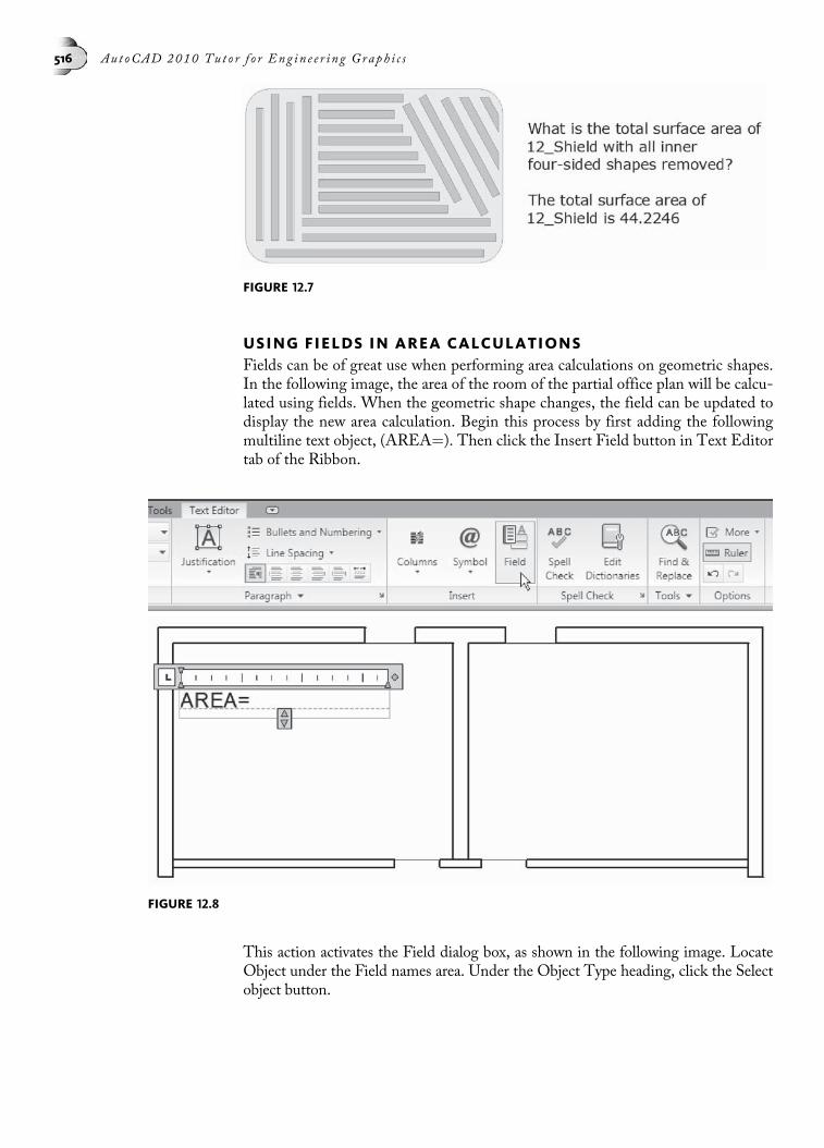
USING FIELDS IN AREA CALCULATIONSFields can be of great use when performing area calculations on geometric shapes.In the following image, the area of the room of the partial office plan will be calcu-lated using fields. When the geometric shape changes, the field can be updated todisplay the new area calculation. Begin this process by first adding the followingmultiline text object, (AREA¼). Then click the Insert Field button in Text Editortab of the Ribbon.
This action activates the Field dialog box, as shown in the following image. LocateObject under the Field names area. Under the Object Type heading, click the Selectobject button.
FIGURE 12.8
FIGURE 12.7
516 Aut oCAD 2010 Tu t o r f o r Eng in e e r i n g Graph i c s

Clicking the Select object button in the previous image returns you to the drawingeditor. Once you are there, select the rectangular polyline shape, as shown in thefollowing image.
This returns you back to the Field dialog box, as shown in the following image.Notice that the property changed to Area and the Format changed to Architectural.The Preview area shows the current area calculation. Click the OK button to exit theField dialog box.
FIGURE 12.10
FIGURE 12.9
Chap t e r 12 • Ana l y z i n g 2D Drawing s 517

The results are illustrated in the following image. A field consisting of the squarefootage information is added to the end of the multiline text. Notice also that the fieldis identified by the text with the gray background.
In the following image, the room was stretched 6 0 to the left. Regenerating the draw-ing screen updates the field to reflect the change in the square footage calculation, asshown in the following image.
FIGURE 12.12
FIGURE 12.11
518 Aut oCAD 2010 Tu t o r f o r Eng in e e r i n g Graph i c s
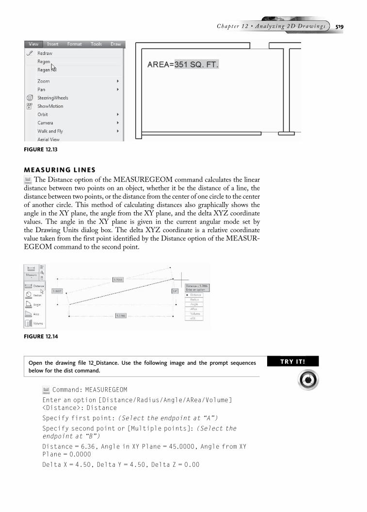
MEASURING LINESThe Distance option of the MEASUREGEOM command calculates the linear
distance between two points on an object, whether it be the distance of a line, thedistance between two points, or the distance from the center of one circle to the centerof another circle. This method of calculating distances also graphically shows theangle in the XY plane, the angle from the XY plane, and the delta XYZ coordinatevalues. The angle in the XY plane is given in the current angular mode set bythe Drawing Units dialog box. The delta XYZ coordinate is a relative coordinatevalue taken from the first point identified by the Distance option of the MEASUR-EGEOM command to the second point.
TRY IT!Open the drawing file 12_Distance. Use the following image and the prompt sequencesbelow for the dist command.
Command: MEASUREGEOM
Enter an option [Distance/Radius/Angle/ARea/Volume]<Distance>: Distance
Specify first point: (Select the endpoint at “A”)
Specify second point or [Multiple points]: (Select theendpoint at “B”)
Distance = 6.36, Angle in XY Plane = 45.0000, Angle from XYPlane = 0.0000
Delta X = 4.50, Delta Y = 4.50, Delta Z = 0.00
FIGURE 12.14
FIGURE 12.13
Chap t e r 12 • Ana l y z i n g 2D Drawing s 519
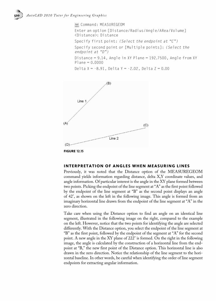
Command: MEASUREGEOM
Enter an option [Distance/Radius/Angle/ARea/Volume]<Distance>: Distance
Specify first point: (Select the endpoint at “C”)
Specify second point or [Multiple points]: (Select theendpoint at “D”)
Distance = 9.14, Angle in XY Plane = 192.7500, Angle from XYPlane = 0.0000
Delta X = -8.91, Delta Y = -2.02, Delta Z = 0.00
INTERPRETATION OF ANGLES WHEN MEASURING LINESPreviously, it was noted that the Distance option of the MEASUREGEOMcommand yields information regarding distance, delta X,Y coordinate values, andangle information. Of particular interest is the angle in the XY plane formed betweentwo points. Picking the endpoint of the line segment at “A” as the first point followedby the endpoint of the line segment at “B” as the second point displays an angleof 42°, as shown on the left in the following image. This angle is formed from animaginary horizontal line drawn from the endpoint of the line segment at “A” in thezero direction.
Take care when using the Distance option to find an angle on an identical linesegment, illustrated in the following image on the right, compared to the exampleon the left. However, notice that the two points for identifying the angle are selecteddifferently. With the Distance option, you select the endpoint of the line segment at“B” as the first point, followed by the endpoint of the segment at “A” for the secondpoint. A new angle in the XY plane of 222° is formed. On the right in the followingimage, the angle is calculated by the construction of a horizontal line from the end-point at “B,” the new first point of the Distance option. This horizontal line is alsodrawn in the zero direction. Notice the relationship of the line segment to the hori-zontal baseline. In other words, be careful when identifying the order of line segmentendpoints for extracting angular information.
FIGURE 12.15
520 Aut oCAD 2010 Tu t o r f o r Eng in e e r i n g Graph i c s
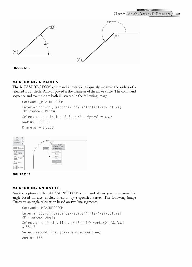
MEASURING A RADIUSThe MEASUREGEOM command allows you to quickly measure the radius of aselected arc or circle. Also displayed is the diameter of the arc or circle. The commandsequence and example are both illustrated in the following image.
Command: _MEASUREGEOM
Enter an option [Distance/Radius/Angle/ARea/Volume]<Distance>: Radius
Select arc or circle: (Select the edge of an arc)
Radius = 0.5000
Diameter = 1.0000
MEASURING AN ANGLEAnother option of the MEASUREGEOM command allows you to measure theangle based on arcs, circles, lines, or by a specified vertex. The following imageillustrates an angle calculation based on two line segments.
Command: _MEASUREGEOM
Enter an option [Distance/Radius/Angle/ARea/Volume]<Distance>: Angle
Select arc, circle, line, or <Specify vertex>: (Selecta line)
Select second line: (Select a second line)
Angle = 37°
FIGURE 12.17
FIGURE 12.16
Chap t e r 12 • Ana l y z i n g 2D Drawing s 521
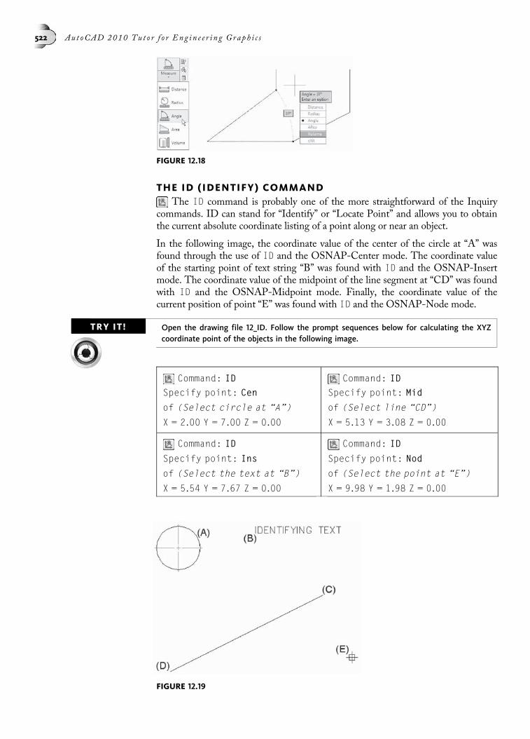
THE ID (IDENTIFY) COMMANDThe ID command is probably one of the more straightforward of the Inquiry
commands. ID can stand for “Identify” or “Locate Point” and allows you to obtainthe current absolute coordinate listing of a point along or near an object.
In the following image, the coordinate value of the center of the circle at “A” wasfound through the use of ID and the OSNAP-Center mode. The coordinate valueof the starting point of text string “B” was found with ID and the OSNAP-Insertmode. The coordinate value of the midpoint of the line segment at “CD” was foundwith ID and the OSNAP-Midpoint mode. Finally, the coordinate value of thecurrent position of point “E” was found with ID and the OSNAP-Node mode.
TRY IT! Open the drawing file 12_ID. Follow the prompt sequences below for calculating the XYZcoordinate point of the objects in the following image.
Command: IDSpecify point: Cen
of (Select circle at “A”)
X = 2.00 Y = 7.00 Z = 0.00
Command: IDSpecify point: Mid
of (Select line “CD”)
X = 5.13 Y = 3.08 Z = 0.00
Command: ID
Specify point: Ins
of (Select the text at “B”)
X = 5.54 Y = 7.67 Z = 0.00
Command: ID
Specify point: Nod
of (Select the point at “E”)
X = 9.98 Y = 1.98 Z = 0.00
FIGURE 12.19
FIGURE 12.18
522 Aut oCAD 2010 Tu t o r f o r Eng in e e r i n g Graph i c s

THE LIST COMMANDUse the LIST command to obtain information about an object or group of objects.
In the following image, two rectangles are displayed along with a circle, but are therectangles made up of individual line segments or a polyline object? Using the LISTcommand on each object informs you that the first rectangle at “A” is a polyline. Inaddition to the object type, you also can obtain key information such as the layer thatthe object resides on, area and perimeter information for polylines, and circumferenceinformation for circles.
TRY IT!Open the drawing file 12_List. Study the prompt sequence below for using the list command.
Command: LI (For LIST)
Select objects: (Select the object at “A”)
Select objects: (Press ENTER to list the information on thisobject)
LWPOLYLINE Layer: “0bject”
Space: Model space
Handle = 2B
Closed
Constant width 0.0000
area 3.3835
perimeter 7.6235
at point X= 4.7002 Y= 4.1846 Z= 0.0000
at point X= 7.1049 Y= 4.1846 Z= 0.0000
at point X= 7.1049 Y= 5.5916 Z= 0.0000
at point X= 4.7002 Y= 5.5916 Z= 0.0000
ADDITIONAL INQUIRY COMMANDSThe following Inquiry commands may not be used all of the time. However, they maycome in handy when you want a readout of the time spent in the drawing editor orwhen you want to review the status of a drawing. You can even get a list of all systemvariables used in every AutoCAD drawing session.
FIGURE 12.20
Chap t e r 12 • Ana l y z i n g 2D Drawing s 523

Command Shortcut Description
Time TIME Displays the time spent in the drawing editor.
Status STATUS Displays important information on the currentdrawing.
Set Variable SETVAR Used for making changes to one of the many systemvariables internal to AutoCAD.
TUTORIAL EXERCISE: C-LEVER.DWG
PurposeThis tutorial is designed to show you various methods of constructing the C-Lever objectin the previous image. Numerous questions will be asked about the object, requiringthe use of the following options of the MEASUREGEOM command: Area, Distance, Angle,and Radius.
System SettingsUse the Drawing Units dialog box and change the number of decimal places past the zerofrom four units to three units. Keep the default drawing limits at (0.000,0.000) for thelower-left corner and (12.000,9.000) for the upper-right corner. Check to see that the fol-lowing Object Snap modes are already set: Endpoint, Extension, Intersection, and Center.
LayersCreate the following layers with the format:
Name Color Linetype
Boundary Magenta Continuous
Object Yellow Continuous
FIGURE 12.21
524 Aut oCAD 2010 Tu t o r f o r Eng in e e r i n g Graph i c s
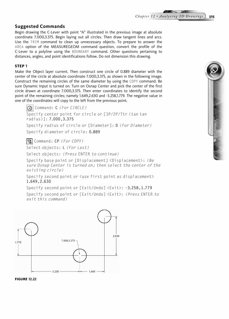
Suggested CommandsBegin drawing the C-Lever with point “A” illustrated in the previous image at absolutecoordinate 7.000,3.375. Begin laying out all circles. Then draw tangent lines and arcs.Use the TRIM command to clean up unnecessary objects. To prepare to answer theAREA option of the MEASUREGEOM command question, convert the profile of theC-Lever to a polyline using the BOUNDARY command. Other questions pertaining todistances, angles, and point identifications follow. Do not dimension this drawing.
STEP 1Make the Object layer current. Then construct one circle of 0.889 diameter with thecenter of the circle at absolute coordinate 7.000,3.375, as shown in the following image.Construct the remaining circles of the same diameter by using the COPY command. Besure Dynamic Input is turned on. Turn on Osnap Center and pick the center of the firstcircle drawn at coordinate 7.000,3.375. Then enter coordinates to identify the secondpoint of the remaining circles; namely 1.649,2.630 and -3.258,1.779. The negative value inone of the coordinates will copy to the left from the previous point.
Command: C (For CIRCLE)
Specify center point for circle or [3P/2P/Ttr (tan tanradius)]: 7.000,3.375
Specify radius of circle or [Diameter]: D (For Diameter)
Specify diameter of circle: 0.889
Command: CP (For COPY)
Select objects: L (For Last)
Select objects: (Press ENTER to continue)
Specify base point or [Displacement] <Displacement>: (Besure Osnap Center is turned on; then select the center of theexisting circle)
Specify second point or <use first point as displacement>1.649,2.630
Specify second point or [Exit/Undo] <Exit>: -3.258,1.779
Specify second point or [Exit/Undo] <Exit>: (Press ENTER toexit this command)
FIGURE 12.22
Chap t e r 12 • Ana l y z i n g 2D Drawing s 525

STEP 2Construct three more circles, as shown in the following image. Even though these objectsactually represent arcs, circles will be drawn now and trimmed later to form the arcs.
Command: C (For CIRCLE)
Specify center point for circle or [3P/2P/Ttr (tan tanradius)]: (Select the edge of the circle at “A” to snap toits center)
Specify radius of circle or [Diameter] <0.445>: 1.067
Command: C (For CIRCLE)
Specify center point for circle or [3P/2P/Ttr (tan tanradius)]: (Select the edge of the circle at “B” to snap toits center)
Specify radius of circle or [Diameter] <1.067>: 0.889
Command: C (For CIRCLE)
Specify center point for circle or [3P/2P/Ttr (tan tanradius)]: (Select the edge of the circle at “C” to snap toits center)
Specify radius of circle or [Diameter] <0.889>: 0.711
STEP 3Construct lines tangent to the three outer circles, as shown in the following image.
Command: L (For LINE)
Specify first point: Tan
to (Select the outer circle near “A”)
Specify next point or [Undo]: Tan
to (Select the outer circle near “B”)
Specify next point or [Undo]: (Press ENTER to exitthis command)
Command: L (For LINE)
Specify first point: Tan
to (Select the outer circle near “C”)
Specify next point or [Undo]: Tan
FIGURE 12.23
526 Aut oCAD 2010 Tu t o r f o r Eng in e e r i n g Graph i c s

to (Select the outer circle near “D”)
Specify next point or [Undo]: (Press ENTER to exitthis command)
STEP 4Construct a circle tangent to the two circles in the following image, using the CIRCLEcommand with the Tangent-Tangent-Radius option (TTR).
Command: C (For CIRCLE)
Specify center point for circle or [3P/2P/Ttr (tan tanradius)]: TTR
Specify point on object for first tangent of circle: (Selectthe outer circle near “A”)
Specify point on object for second tangent of circle: (Selectthe outer circle near “B”)
Specify radius of circle <0.711>: 2.845
STEP 5Use the TRIM command to clean up and form the finished drawing. Pressing ENTER at the“Select objects:” prompt selects all objects as cutting edges although the objects do nothighlight, as shown in the following image. Study the following prompts for selecting theobjects to trim.
FIGURE 12.25
FIGURE 12.24
Chap t e r 12 • Ana l y z i n g 2D Drawing s 527
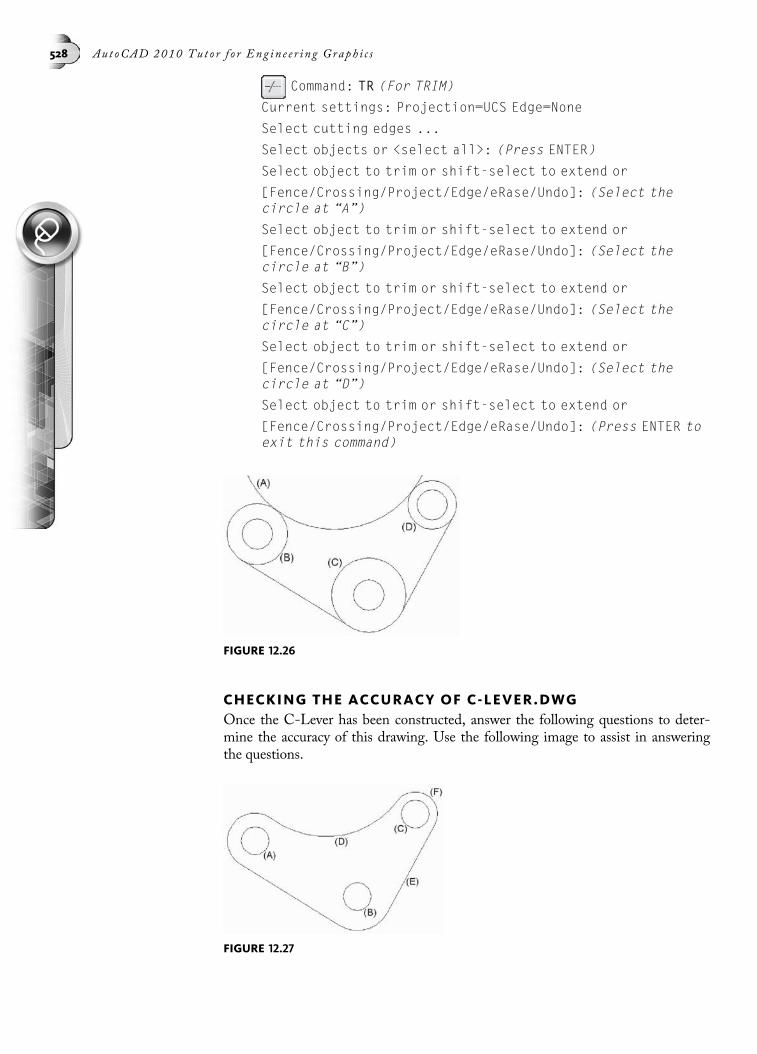
Command: TR (For TRIM)
Current settings: Projection=UCS Edge=None
Select cutting edges ...
Select objects or <select all>: (Press ENTER)
Select object to trim or shift-select to extend or
[Fence/Crossing/Project/Edge/eRase/Undo]: (Select thecircle at “A”)
Select object to trim or shift-select to extend or
[Fence/Crossing/Project/Edge/eRase/Undo]: (Select thecircle at “B”)
Select object to trim or shift-select to extend or
[Fence/Crossing/Project/Edge/eRase/Undo]: (Select thecircle at “C”)
Select object to trim or shift-select to extend or
[Fence/Crossing/Project/Edge/eRase/Undo]: (Select thecircle at “D”)
Select object to trim or shift-select to extend or
[Fence/Crossing/Project/Edge/eRase/Undo]: (Press ENTER toexit this command)
CHECKING THE ACCURACY OF C-LEVER.DWGOnce the C-Lever has been constructed, answer the following questions to deter-mine the accuracy of this drawing. Use the following image to assist in answeringthe questions.
FIGURE 12.27
FIGURE 12.26
528 Aut oCAD 2010 Tu t o r f o r Eng in e e r i n g Graph i c s

1. What is the total area of the C-Lever with all three holes removed?Answer: _______________
2. What is the total distance from the center of circle “A” to the center of circle “B”?Answer: _______________
3. What is the angle formed in the XY plane from the center of circle “C” to the centerof circle “B”?Answer: _______________
4. What is the delta X,Y distance from the center of circle “C” to the center of circle “A”?Answer: _______________
5. What is the absolute coordinate value of the center of arc “D”?Answer: _______________
6. What is the total length of line “E”?Answer: _______________
7. What is the total length of arc “F”?Answer: _______________
A solution for each question follows, complete with the method used to arrive at the answer.Apply these methods to any type of drawing that requires the use of MEASUREGEOMcommands.
SOLUTIONS TO THE QUESTIONS ON C-LEVERQuestion 1What is the total area of the C-Lever with all three holes removed?
First make the Boundary layer current. Then use the BOUNDARY command and pick apoint inside the object at “A” in the following image. This traces a polyline around allclosed objects on the Boundary layer.
Command: BO (For BOUNDARY)
(When the Boundary Creation dialog box appears, click thePick points button.)
Select internal point: (Pick a point inside of the objectat “Y”)
Selecting everything...
Selecting everything visible...
Analyzing the selected data...
Analyzing internal islands...
Select internal point: (Press ENTER to create the boundaries)
BOUNDARY created 4 polylines
Next, turn off the Object layer. All objects on the Boundary layer should be visible.Then use the MEASUREGEOM command and the Area option to add and sub-tract objects to arrive at the final area of the object.
Command: _MEASUREGEOM
Enter an option [Distance/Radius/Angle/ARea/Volume]<Distance>: ARea
Specify first corner point or [Object/Add area/Subtractarea/eXit] <Object>: Add
Chap t e r 12 • Ana l y z i n g 2D Drawing s 529

Specify first corner point or [Object/Subtract area/eXit]: Object
(ADD mode) Select objects: (Select the edge of the shapenear “X”)
Area = 15.611, Perimeter = 17.771
Total area = 15.611
(ADD mode) Select objects: (Press ENTER to continue)
Area = 15.611, Perimeter = 17.771
Total area = 15.611
Specify first corner point or [Object/Subtract area/eXit]:Subtract
Specify first corner point or [Object/Add area/eXit]: Object
(SUBTRACT mode) Select objects: (Select circle “A”)
Area = 0.621, Circumference = 2.793
Total area = 14.991
(SUBTRACT mode) Select objects: (Select circle “B”)
Area = 0.621, Circumference = 2.793
Total area = 14.370
(SUBTRACT mode) Select objects: (Select circle “C”)
Area = 0.621, Circumference = 2.793
Total area = 13.749
(SUBTRACT mode) Select objects: (Press ENTER)
Area = 0.621, Circumference = 2.793
Total area = 13.749
The total area of the C-Lever with all three holes removed is 13.749.
Question 2What is the total distance from the center of circle “A” to the center of circle “B”?
Use the MEASUREGEOM command along with the Distance option to calculate thedistance from the center of circle “A” to the center of circle “B” in the following im-age. Be sure to use the OSNAP-Center mode for locating the centers of all circles.
FIGURE 12.28
530 Aut oCAD 2010 Tu t o r f o r Eng in e e r i n g Graph i c s

Command: _MEASUREGEOM
Enter an option [Distance/Radius/Angle/ARea/Volume]<Distance>: Distance
Specify first point: (Select the edge of the circle at “A”)
Specify second point or [Multiple points]: (Select the edgeof the circle at “B”)
Distance = 3.712, Angle in XY Plane = 331, Angle fromXY Plane = 0
Delta X = 3.258, Delta Y = -1.779, Delta Z = 0.000
The total distance from the center of circle “A” to the center of circle “B” is 3.712.
Question 3What is the angle formed in the XY plane from the center of circle “C” to the centerof circle “B”?
Use the DIST (Distance) command to calculate the angle from the center of circle “C”to the center of circle “B” in the following image. Be sure to use the OSNAP-Centermode for locating the centers of all circles.
Command: _MEASUREGEOM
Enter an option [Distance/Radius/Angle/ARea/Volume]<Distance>: _distance
Specify first point: (Select the edge of the circle at "C")
Specify second point or [Multiple points]: (Select the edgeof the circle at "B")
Distance = 3.104, Angle in XY Plane = 238, Angle fromXY Plane = 0
Delta X = -1.649, Delta Y = -2.630, Delta Z = 0.000
The angle formed in the XY plane from the center of circle “C” to the center of circle“B” is (D), 238°. Notice the two different angle calculations. While an angle of 122° isdisplayed in the following image on the right, the angle of 238° that is listed in thecommand prompt is more correct. This is due to the angle in the XY plane which iscalculated in the counterclockwise direction. The angle of 122° was calculated in theclockwise direction.
FIGURE 12.29
Chap t e r 12 • Ana l y z i n g 2D Drawing s 531

Question 4What is the delta X,Y distance from the center of circle “C” to the center of circle “A”?
Use the Distance option of the MEASUREGEOM command to calculate the deltaX,Y distance from the center of circle “C” to the center of circle “A” in the followingimage. Be sure to use the OSNAP-Center mode. Notice that additional informationis given when you use the Distance option. For the purpose of this question, we willbe looking only for the delta X,Y distance. The DIST command displays the relativeXYZ distances. Since this is a 2D problem, only the X and Y values will be used.
Command: MEASUREGEOM
Enter an option [Distance/Radius/Angle/ARea/Volume]<Distance>: Distance
Specify first point: (Select the center of circle “C”)
Specify second point or [Multiple points]: (Select the centerof circle “A”)
Distance = 4.980, Angle in XY Plane = 190, Angle fromXY Plane = 0
Delta X = -4.907, Delta Y = -0.851, Delta Z = 0.000
The delta X,Y distance from the center of circle “C” to the center of circle “A” is�4.907,�0.851.
FIGURE 12.31
FIGURE 12.30
532 Aut oCAD 2010 Tu t o r f o r Eng in e e r i n g Graph i c s

Question 5What is the absolute coordinate value of the center of arc “D”?
The ID command is used to get the current absolute coordinate information on adesired point, as shown in the following image. This command displays the XYZcoordinate values. Since this is a 2D problem, only the X and Y values will be used.
Command: ID
Specify point: Cen
of (Select the edge of the arc at “D”)
X = 5.869 Y = 8.223 Z = 0.000
The absolute coordinate value of the center of arc “D” is 5.869,8.223.
Question 6What is the total length of line “E”?
Use the Distance option of the MEASUREGEOM command to find the totallength of line “E” in the following image. Be sure to use the OSNAP-Endpointmode. Notice that additional information is given when you use the Distance option.For the purpose of this question, we will be looking only for the distance.
Command: _MEASUREGEOM
Enter an option [Distance/Radius/Angle/ARea/Volume]<Distance>: Distance
Specify first point: (Select the endpoint of the line at “X”)
Specify second point or [Multiple points]: (Select theendpoint of the line at “Y”)
Distance = 3.084, Angle in XY Plane = 64, Angle fromXY Plane = 0
Delta X = 1.328, Delta Y = 2.783, Delta Z = 0.000
The total length of line “E” is 3.084.
FIGURE 12.32
Chap t e r 12 • Ana l y z i n g 2D Drawing s 533

Question 7What is the total length of arc “F”?
The LIST command is used to calculate the lengths of arcs. However, a little prepa-ration is needed before you perform this operation. If arc “F” is selected, as shown onthe left in the following image, notice that the entire outline is selected because it is apolyline. Use the EXPLODE command to break the outline into individual objects. Usethe LIST command to get a listing of the arc length, as shown on the right in thefollowing image.
Command: X (For EXPLODE)
Select objects: (Select the edge of the dashed polyline in thefollowing image)
Select objects: (Press ENTER to perform the explodeoperation)
Command: LI (For LIST)
Select objects: (Select the edge of the arc at “F” in thefollowing image)
Select objects: (Press ENTER to continue)
ARC Layer: “Boundary”
Space: Model space
Handle = 94
center point, X= 8.649 Y= 6.005 Z= 0.000
radius 0.711
start angle 334
end angle 141
length 2.071
The total length of arc “F” is 2.071.
FIGURE 12.33
534 Aut oCAD 2010 Tu t o r f o r Eng in e e r i n g Graph i c s

TUTORIAL EXERCISE: 12_FIELD_CALC.DWG
PurposeThis tutorial is designed to utilize the Field function of AutoCAD to calculate the area ofan object.
System SettingsThis drawing has drawing settings already created.
LayersLayers already exist in this drawing.
Suggested CommandsOpen the drawing 12_Field_Calc.Dwg and activate the multiline text command. Set thetext height to 12 and add a text header dealing with the Area. Then activate the Field dia-log box and select a polyline object in the drawing. This retrieves the area informationand adds this text calculation to the Text Formatting dialog box. Once the field is added,stretching the original polyline shape and regenerating the drawing recalculates the area.
STEP 1Open the drawing 12_Field_Calc.Dwg. Activate the Text Formatting dialog box, changethe text height to 5, and add the text (AREA¼), as shown in the following image. Con-tinue by clicking on the Insert Field button.
FIGURE 12.35
FIGURE 12.34
Chap t e r 12 • Ana l y z i n g 2D Drawing s 535
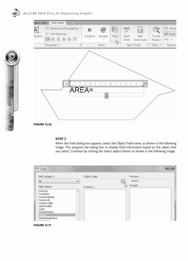
STEP 2When the Field dialog box appears, select the Object Field name, as shown in the followingimage. This prepares the dialog box to display field information based on the object thatyou select. Continue by clicking the Select object button as shown in the following image.
FIGURE 12.37
FIGURE 12.36
536 Aut oCAD 2010 Tu t o r f o r Eng in e e r i n g Graph i c s

STEP 3Clicking the Select object button returns you to the drawing editor, where you can selectthe polyline shape of the object. This action again returns you to the Field dialog box.Verify the following changes in this dialog box: under the Field names category, pickObject; under the Property category, pick Area; under the Format category, pick Decimal.Then click the OK button to exit the Field dialog box.
STEP 4The results are illustrated in the following image. A field consisting of the square footageinformation is added to the end of the multiline text.
FIGURE 12.39
FIGURE 12.38
Chap t e r 12 • Ana l y z i n g 2D Drawing s 537

STEP 5Now click the polyline shape to display grips, choose a number of grips, and stretch thevertices of the polyline to new locations as shown in the following image. Your displaymay not match the following image exactly. You will notice that the square footagedoes not automatically update itself.
STEP 6To update the field information and change the area for the new polyline shape, click theREGEN command found under the View Menu Bar, as shown in the following image. No-tice that the area field has changed to reflect the new size of the closed polyline shape.
FIGURE 12.41
FIGURE 12.40
538 Aut oCAD 2010 Tu t o r f o r Eng in e e r i n g Graph i c s

NOW TRY THIS!Start a new drawing and save it as Main Rocker. Begin the construction of the Main Rockerby keeping the default units set to decimal but changing the number of decimal places pastthe zero from four to two. Be sure the system of angle measure is set to decimal degreesand the number of decimal places for the display of angles is zero. Keep all remaining de-fault unit values. Use the LIMITS command to change the drawing limits to (0.00,0.00) forthe lower-left corner and (15.00,12.00) for the upper-right corner.
TRY IT!Begin the drawing by placing the center of the regular hexagon and 2.25-radius arc at coor-dinate (6.25,6.50).
Refer to the drawing of Main Rocker and answer the following questions.
1. What is the distance from the center of the 1.00-diameter hole “A” to the center ofthe other 1.00-diameter hole “B”?Answer: _______________
2. What is the absolute coordinate value of the center of the 3.00-radius arc “C”?Answer: _______________
3. What is the total length of line “G”?Answer: _______________
4. What is the length of the 2.25-radius arc segment “E”?Answer: _______________
5. What is the angle formed in the XY plane from the center of the 1.00-diameter circle“B” to the center of the 2.25-radius arc “D”?Answer: _______________
FIGURE 12.42
Chap t e r 12 • Ana l y z i n g 2D Drawing s 539

6. What is the total surface area of Main Rocker with the hexagon and both1.00-diameter holes removed?Answer: _______________
7. What is the total length of arc “D”?Answer: _______________
NOW TRY THIS! Start a new drawing and save it as Pattern4. Even though this is a metric drawing, no speciallimits need be set. Keep the default setting of decimal units precision to zero. Be sure thesystem of angle measure is set to decimal degrees and the number of decimal places forthe display of angles is zero. Keep all remaining default unit values.
TRY IT! Begin the drawing as shown in the following image by constructing Pattern4 at vertex “A”at absolute coordinate (50,30).
Even though this is a metric drawing, no special limits need be set. Keep the default setting ofdecimal units precision to zero. Be sure the system of angle measure is set to decimal degreesand the number of decimal places for the display of angles is zero. Keep all remaining defaultunit values.
Begin the drawing, as shown in the following image, by constructing Pattern4 with vertex “A”at absolute coordinate (50,30).
FIGURE 12.43
540 Aut oCAD 2010 Tu t o r f o r Eng in e e r i n g Graph i c s
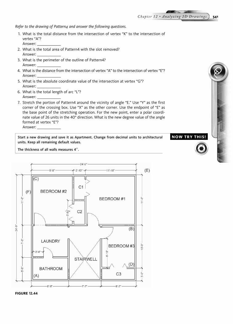
Refer to the drawing of Pattern4 and answer the following questions.
1. What is the total distance from the intersection of vertex “K” to the intersection ofvertex “A”?Answer: _______________
2. What is the total area of Pattern4 with the slot removed?Answer: _______________
3. What is the perimeter of the outline of Pattern4?Answer: _______________
4. What is the distance from the intersection of vertex “A” to the intersection of vertex “E”?Answer: _______________
5. What is the absolute coordinate value of the intersection at vertex “G”?Answer: _______________
6. What is the total length of arc “L”?Answer: _______________
7. Stretch the portion of Pattern4 around the vicinity of angle “E.” Use “Y” as the firstcorner of the crossing box. Use “X” as the other corner. Use the endpoint of “E” asthe base point of the stretching operation. For the new point, enter a polar coordi-nate value of 26 units in the 40° direction. What is the new degree value of the angleformed at vertex “E”?Answer: _______________
NOW TRY THIS!Start a new drawing and save it as Apartment. Change from decimal units to architecturalunits. Keep all remaining default values.
The thickness of all walls measures 4 00.
FIGURE 12.44
Chap t e r 12 • Ana l y z i n g 2D Drawing s 541

Refer to the drawing of Apartment and answer the following questions.
1. What is the total area in square feet of all bedrooms?Answer: _______________
2. What is the distance from the intersection of the corner at “A” to the intersection ofthe corner at “B”?Answer: _______________
3. What is the total area in square feet of all closets (C1, C2, and C3)?Answer: _______________
4. What is the total area in square feet of the laundry and bathroom?Answer: _______________
5. What is the distance from the intersection of the corner at “C” to the intersection ofthe corner at “D”?Answer: _______________
6. What is the angle in the XY plane from the intersection of the wall corner at “A” tothe intersection of the wall corner at “D”?Answer: _______________
7. Stretch the floor plan up at a distance of 2 0-5 00. Use “E” and “F” as the locations of thecrossing box. What is the new total area of Bedroom #1, Bedroom #2, C1, and C2?Answer: _______________
END OF CHAPTER PROBLEMS FOR CHAPTER 12Please refer to the CD that is supplied with this book and locate the file AutoCAD Tutor2010 Support Docs.pdf. In addition to extra information supplied in this chapter, end-of-chapter problems are also available to provide additional practice.
542 Aut oCAD 2010 Tu t o r f o r Eng in e e r i n g Graph i c s

CHAPTER
13
Creating ParametricDrawings
Geometric constraints allow you to create geometric relationships between selectedobjects. An example would be to apply the Equal constraint to all holes on an object.Then when one of the holes is dimensioned with a dimensional constraint and youchange the value of the hole, all holes that share the same Equal constraint change toreflect the currently dimensioned diameter. In this chapter, you will learn a majorityof the constraint types and how to apply them to drawing objects. You will also beshown the power of controlling the objects in a design through the use of parameters.A number of Try It! exercises are available to practice with the various methods ofconstraining objects. Two tutorials are also available at the end of the chapter to guideyou along with assigning constraints to objects.
DISPLAYING PARAMETRIC MENUSCommands used for accessing geometric and dimensional constraints are all illus-trated in the following image. You can choose to work in the Ribbon, Menu Bar, orthe Parametric Toolbar.
FIGURE 13.1
543

GEOMETRIC CONSTRAINTSThe following table illustrates the various geometric constraints available completewith constraint name, constraint icon, and a description of the constraint.
Constraint Icon Description
Coincident A point is constrained to lie on another point orcurve (line, arc, etc).
Collinear Two selected lines will line up along a single line. Ifthe first line moves, so will the second. The two linesegments do not have to be touching.
Concentric Arcs or circles will share the same center point.
Equal If two arcs or circles are selected, they will have thesame radius or diameter. If two lines are selected.they will become the same length. If you selectmultiple similar objects such as lines, circles, andarcs before using the Equal constraint, theconstraint is applied to all of them.
Fix Applying a fixed constraint to a point or points willprevent the selected objects from moving.
Horizontal Lines are positioned parallel to the X-axis.
Parallel Lines will be repositioned so that they are parallelto one another. The first line sketched will stay inits position and the second will move to becomeparallell to the first.
Perpendicular Lines will be repositioned at 90° angles to oneanother. The first line selected will stay in itsposition and the second will rotate until the anglebetween them is 90°.
Smooth A spline and another spline, line, or arc that connectat an endpoint with a coincident constraint.
Symmetric Selected points defining the selected geometry aremade symmetric about the selected line.
Tangent An arc, circle, or line will become tangent to anotherarc or circle.
Vertical Lines are positioned parallel to the Y-axis.
544 Au t oCAD 2010 Tu t o r f o r Eng i n e e r i n g Graph i c s

METHODS OF CHOOSING CONSTRAINTSGeometric constraints can be easily chosen from theMenu Bar as shown in the follow-ing image on the left or the Ribbon as shown in the following image on the right.
DISPLAYING CONSTRAINTSAs constraints are placed, they can be viewed through the Show All button locatedunder the Parametric tab of the Ribbon as shown in the following image on the left.When dealing with complicated objects involving numerous constraints, you can usethe Hide All button to turn off all constraints as shown in the following image on theright. Another command not shown is the Show button. Clicking on this button andpicking an object will show the constraints for only the selected object.
DELETING CONSTRAINTSAs constraints are placed, at times they may need to be deleted. To perform this,right-click on the constraint and pick Delete from the menu as shown in the follow-ing image. You could also pick the constraint and hit the Delete key in any standardkeyboard to remove the constraint from the object.
FIGURE 13.2
FIGURE 13.3
Chap t e r 13 • Cr e a t i n g Pa r ame t r i c Draw ing s 545

THE CONSTRAINTS DIALOG BOXYou can control the way constraints display through the Constraint Settings dialogbox. Clicking on the small arrow in the lower-right corner of the Geometric panelas shown in the following image on the left displays the Constraint Settings dialogbox as shown in the following image on the right. By default, all constraints havechecks in the respective boxes meaning all constraints will be displayed on objects.
The following image on the left shows the Geometric tab of the Constraint Settingsdialog box where all constraints are checked. The results of this are displayed in thefollowing image on the right. You will notice the various constraints includingPerpendicular, Parallel, Tangent, Concentric, Equal, and Horizonal.
FIGURE 13.4
FIGURE 13.5
546 Au t oCAD 2010 Tu t o r f o r Eng i n e e r i n g Graph i c s

What if you only wanted to see the Perpendicular, Parallel, and Horizontal con-straints displayed on the object. Activating the Geometric tab of the Constraint Set-tings dialog box allows you to remove the check from Tangent, Concentric, andEqual as shown in the following image on the left. The results are shown in the fol-lowing image on the right where only the Perpendicular, Parallel, and Horizontalconstraints display.
DRAWING WITH INDIVIDUAL LINES VS POLYLINESHow you construct lines may impact the kind of results you get when applying con-straints to line segments. In the following image, a number of line segments weredrawn. When a dimension constraint (dimension) was applied to the height of theobject, only the vertical line segment moved to the dimension. The remaining linesegments were unaffected by the dimensional constraint. This means before applyingdimensional constraints to an object consisting of individual line segments, the end-points of the lines must first be constrained using the Coincident constraint. This willbe covered in a later segment of this chapter.
FIGURE 13.7
FIGURE 13.6
Chap t e r 13 • Cr e a t i n g Pa r ame t r i c Draw ing s 547

The following image is similar to the previous with the exception that all line seg-ments were converted to a single polyline before applying geometric constraints ordimensional constraints. Placing the dimensional constraint for the total height of12.00 stretches the polyline shape and does not result in gaps in the object that requireCoincident constraints. This method of converting objects to a polyline for constraintsalso works for more complicated shapes that involve curves and arcs.
APPLYING HORIZONTAL AND VERTICAL CONSTRAINTSApplying a horizontal or vertical constraint to an object is very straightforward. Theresults are objects that are constrained either horizontally or vertically. If you changeyour mind and wish to add a dimension consisting of an angle, you must first deletethe horizontal or vertical constraint. The following Try It! illustrates the creation ofHorizontal and Vertical constraints.
FIGURE 13.9
FIGURE 13.8
548 Au t oCAD 2010 Tu t o r f o r Eng i n e e r i n g Graph i c s
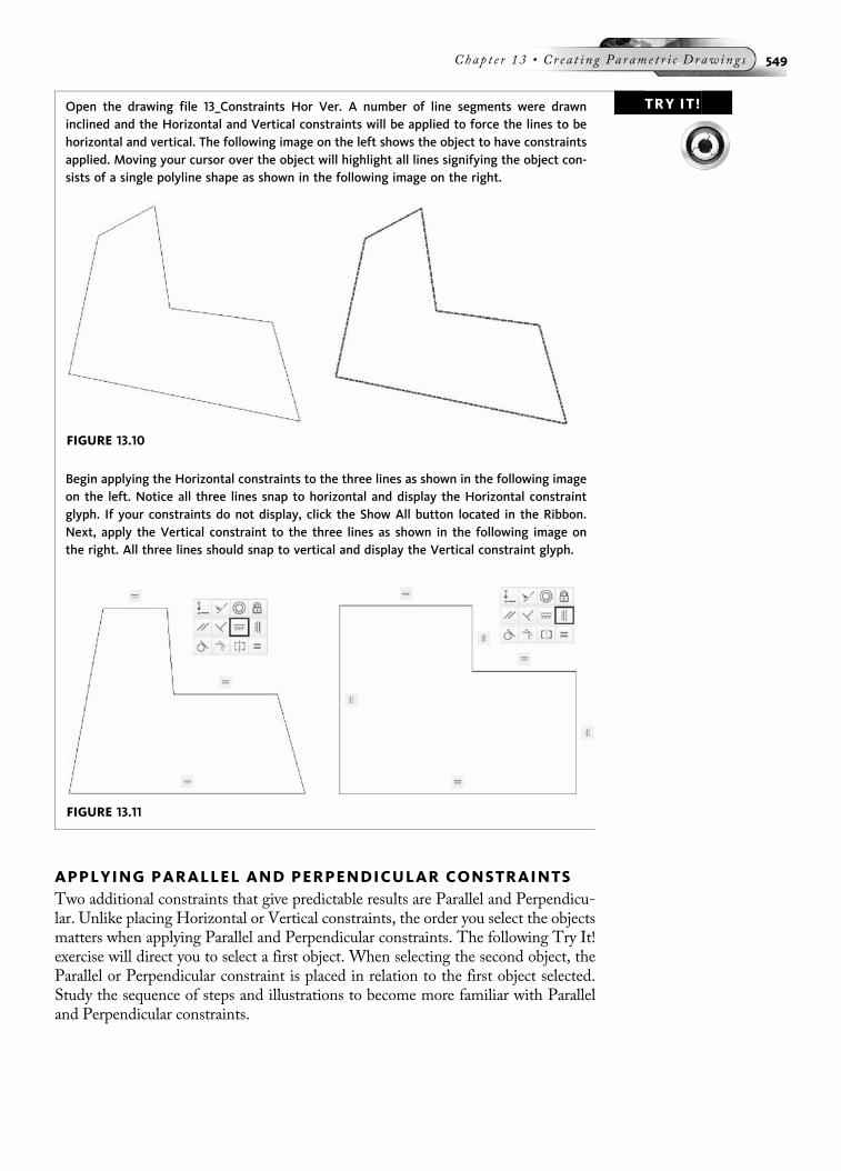
TRY IT!Open the drawing file 13_Constraints Hor Ver. A number of line segments were drawninclined and the Horizontal and Vertical constraints will be applied to force the lines to behorizontal and vertical. The following image on the left shows the object to have constraintsapplied. Moving your cursor over the object will highlight all lines signifying the object con-sists of a single polyline shape as shown in the following image on the right.
Begin applying the Horizontal constraints to the three lines as shown in the following imageon the left. Notice all three lines snap to horizontal and display the Horizontal constraintglyph. If your constraints do not display, click the Show All button located in the Ribbon.Next, apply the Vertical constraint to the three lines as shown in the following image onthe right. All three lines should snap to vertical and display the Vertical constraint glyph.
APPLYING PARALLEL AND PERPENDICULAR CONSTRAINTSTwo additional constraints that give predictable results are Parallel and Perpendicu-lar. Unlike placing Horizontal or Vertical constraints, the order you select the objectsmatters when applying Parallel and Perpendicular constraints. The following Try It!exercise will direct you to select a first object. When selecting the second object, theParallel or Perpendicular constraint is placed in relation to the first object selected.Study the sequence of steps and illustrations to become more familiar with Paralleland Perpendicular constraints.
FIGURE 13.10
FIGURE 13.11
Chap t e r 13 • Cr e a t i n g Pa r ame t r i c Draw ing s 549

TRY IT! Open the drawing file 13_Constraints Per Par. A number of line segments were drawn asangles and the Parallel and Perpendicular constraints will be applied to force the lines to beparallel and perpendicular (at a 90° angle). The following image shows the object to haveconstraints applied. Moving your cursor over the object will highlight all lines signifyingthe object consists of a single polyline shape. Also, to make the parallel and perpendicularconstraints more predictable, the bottom line of the object has already had the Horizontaland Fix constraints applied. Applying the Fix constraint prevents the line from moving whilethe other constraints are being placed. Also notice the appearance of the Constraints glyph.This glyph appears when moving your cursor over an object that has constraints applied.
Begin by clicking on the Parallel constraint button. When prompted to select objects, pickline “A” followed by line “B.” Because line “A” was picked first, selecting line “B” makes itparallel to line “A.” This is a great technique for determining which line will be affectedahead of time. Continue by applying Parallel constraints to the lines on the left side of theobject as shown in the following image. Pick line “C” followed by line “D” to make line “D”parallel to line “C.” Apply the last Parallel constraint using lines “E” and “F” as guides. Whenfinished, your object should appear similar as shown in the following image.
FIGURE 13.12
FIGURE 13.13
550 Au t oCAD 2010 Tu t o r f o r Eng i n e e r i n g Graph i c s

Next, click on the Perpendicular constraint button. When prompted to select objects, pickline “A” followed by line “B.” Because line “A” was picked first, selecting line “B” makes itperpendicular to line “A.” Continue by applying a Perpendicular constraint to the lines onthe right side of the object as shown in the following image. Pick line “C” followed by line“D” to make line “D” perpendicular to line “C.”
APPLYING COINCIDENT CONSTRAINTSWe have already discussed the advantages polylines have over regular line segmentswith placing constraints. This does not mean it is wrong to work with individual linesegments. In this case when working with the endpoints of individual line segments,use the Coincident constraint. Follow the prompts that tell you to select the endpointof the first object and then the second object. Both endpoints will snap together;Osnap-Endpoint is not enough to automatically apply the Coincident constraint.
FIGURE 13.14
Chap t e r 13 • Cr e a t i n g Pa r ame t r i c Draw ing s 551

TRY IT! Open the drawing file 13_Constraints Coincident as shown in the following image. When linesegments are drawn but do not meet, a Coincident constraint can be applied to the ends ofboth line segments.
Click on the Coincident Constraint button and pick the endpoint of the line as shown in thefollowing image on the left. Continue by selecting the endpoint of the line as shown in the fol-lowing image in the middle. This action will join the endpoints of both line segments and placea blue dot as shown in the following image on the right. The presence of the blue dot signifiesthe Coincident constraint was applied. Also, if you move your cursor over the blue dot, theCoincident constraint glyph will display.
While this creates the coincident constraint at one corner of the object, this constraint mustnow be applied to the remaining corners as shown in the following image.
ą
FIGURE 13.16
FIGURE 13.15
552 Au t oCAD 2010 Tu t o r f o r Eng i n e e r i n g Graph i c s

APPLYING COLLINEAR CONSTRAINTS TO LINESApplying a Collinear keeps the selected objects in the same line with each other. Thelines do not have to be touching in order to perform this task. Study the following TryIt! and images designed to place Collinear constraints.
TRY IT!Open the drawing file 13_Constraints Collinear. The object in the following image consistsof a single polyline object. This will help keep the endpoints intact when applying the Col-linear constraints. As with some of the other contraint methods, order is important. Pickthe Collinear constraint button and for the first object, pick line “A” and for the secondobject, pick line “B.” This will constrain the lines in the same axis or line of sight. Continueapplying Collinear constraints to the lines in the following order; First line “C,” Secondline “D”; First line “E,” Second line “F”; and First line “G,” Second line “H.”
FIGURE 13.17
Chap t e r 13 • Cr e a t i n g Pa r ame t r i c Draw ing s 553
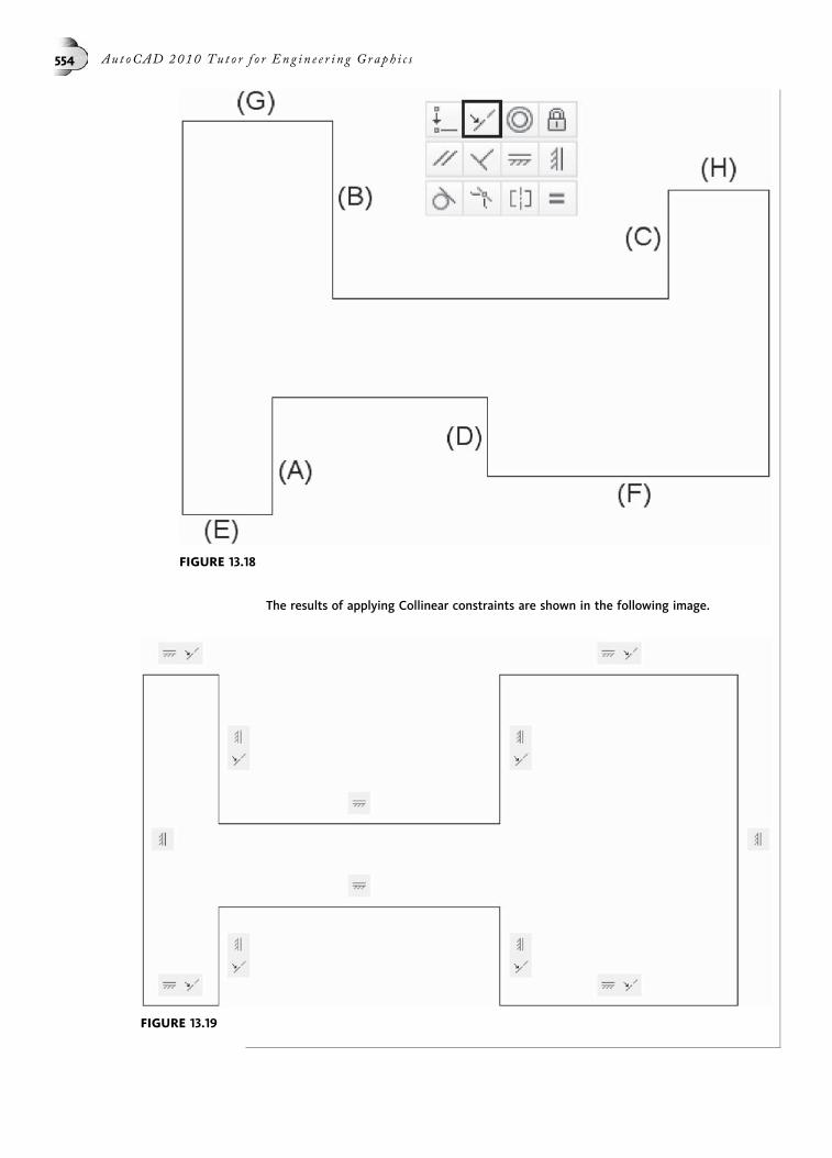
The results of applying Collinear constraints are shown in the following image.
FIGURE 13.18
FIGURE 13.19
554 Au t oCAD 2010 Tu t o r f o r Eng i n e e r i n g Graph i c s

APPLYING A CONCENTRIC CONSTRAINTAnother useful constraint forces the centers of arcs and circles to share the samecenterpoint; this constraint is called Concentric and is illustrated in the followingTry It! exercise.
TRY IT!Open the drawing file 13_Constraints Concentric. A number of constraints were already ap-plied to the line segments. Click on the Concentric button as shown in the following imageon the left and pick the first arc at “A” followed by the second arc at “B.” The results areshown in the following image on the right. Notice how both arcs now share the same cen-terpoint which is another way of saying they are Concentric with each other.
APPLYING TANGENT CONSTRAINTSTangent constraints are very powerful in making lines tangent to curves or for mak-ing curves tangent to other curves. Study the next Try It! exercise for applyingTangent constraints.
TRY IT!Open the drawing file 13_Constraints Tangent. The object in the following image on the leftconsists of a polyline perimeter. Included in the perimeter are a number of lines and arcsegments. This object looks complete until displaying grips, making the grips active, andstretching the grip to a new location. The results may be similar to the following image onthe right. While the lines and arcs originally appeared to be tangent, they actually were not.
FIGURE 13.20
FIGURE 13.21
Chap t e r 13 • Cr e a t i n g Pa r ame t r i c Draw ing s 555
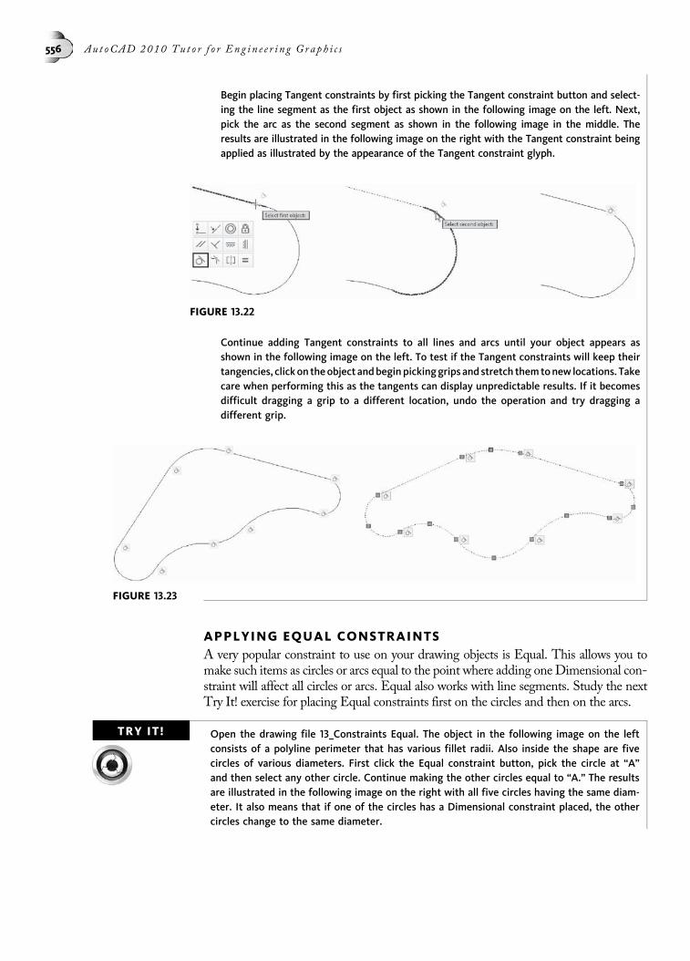
Begin placing Tangent constraints by first picking the Tangent constraint button and select-ing the line segment as the first object as shown in the following image on the left. Next,pick the arc as the second segment as shown in the following image in the middle. Theresults are illustrated in the following image on the right with the Tangent constraint beingapplied as illustrated by the appearance of the Tangent constraint glyph.
Continue adding Tangent constraints to all lines and arcs until your object appears asshown in the following image on the left. To test if the Tangent constraints will keep theirtangencies, click on theobject andbeginpickinggrips and stretch themtonew locations. Takecare when performing this as the tangents can display unpredictable results. If it becomesdifficult dragging a grip to a different location, undo the operation and try dragging adifferent grip.
APPLYING EQUAL CONSTRAINTSA very popular constraint to use on your drawing objects is Equal. This allows you tomake such items as circles or arcs equal to the point where adding one Dimensional con-straint will affect all circles or arcs. Equal also works with line segments. Study the nextTry It! exercise for placing Equal constraints first on the circles and then on the arcs.
TRY IT! Open the drawing file 13_Constraints Equal. The object in the following image on the leftconsists of a polyline perimeter that has various fillet radii. Also inside the shape are fivecircles of various diameters. First click the Equal constraint button, pick the circle at “A”and then select any other circle. Continue making the other circles equal to “A.” The resultsare illustrated in the following image on the right with all five circles having the same diam-eter. It also means that if one of the circles has a Dimensional constraint placed, the othercircles change to the same diameter.
FIGURE 13.22
FIGURE 13.23
556 Au t oCAD 2010 Tu t o r f o r Eng i n e e r i n g Graph i c s

Next, apply the Equal constraint to make all of the radii the same value. Click on the Equalconstraint button and before selecting the arc, enter the Multiple option. Then select thearc in the lower left corner of the object. You will then be prompted to select the objectsyou want to make equal to the first. Select the remaining arcs and press Enter. The resultsare illustrated in the following image on the right. Unfortunately a few of the arcs appearto have changed their position in the perimeter of the polyline. This is to be expectedwhen applying constraints. A series of Tangent constraints will need to be applied in orderto fix the issue with the arcs.
APPLYING A FIX CONSTRAINTA Fix constraint fixes the position of an object so it no longer can move. This is a niceconstraint to lock down your design. As you apply more geometric and dimensionalconstraints, the fixed component will remain unchanged in the drawing. Study thenext Try It! exercise on how the Fix constraint affects an object.
TRY IT!Open the drawing file 13_Constraints Fix. Click on the Fix constraint button as shown in thefollowing image on the left and pick the lower left corner of the object. You will notice theappearance of the padlock glyph signifying a Fix constraint is about to be placed. The re-sults are shown in the following image on the right. Notice the addition of the Fix con-straint to the drawing.
FIGURE 13.24
FIGURE 13.25
Chap t e r 13 • Cr e a t i n g Pa r ame t r i c Draw ing s 557

AUTO CONSTRAININGThe Auto Constrain button allows for constraints to be applied to selected objects ina drawing automatically. Choose this command from the Parametric tab as shownin the following image. Also follow the next Try It! exercise to see how the AutoConstrain command applies constraints to objects in a drawing.
TRY IT! Open the drawing file 13_Constraints Auto. The object in the following image on the leftconsists of individual lines and three circles. Clicking on the Auto Constrain button and se-lecting all objects including circles and arcs will display the drawing as shown in the follow-ing image on the right. Notice how various constraints such as Concentric, Tangent, Parallel,Equal, and Perpendicular were applied as shown in the following image on the right. Youcan even see the individual blue dots at the intersections of all lines and arcs signifyingthat Coincident constraints were applied through the Auto Constrain operation.
FIGURE 13.27
FIGURE 13.28
FIGURE 13.26
558 Au t oCAD 2010 Tu t o r f o r Eng i n e e r i n g Graph i c s

One other item needs to be noted. When placing constraints automatically through theAuto Constraint command, a command prompt appears allowing you to type S for Set-tings, which takes you to the AutoConstrain tab of the Constraint Settings dialog box.Use this dialog box to control which constraints are available and in what order they areapplied as shown in the following image.
ESTABLISHING DIMENSIONAL RELATIONSHIPSOnce geometric constraints are applied, the next step is to place Dimensional constraintsas a means of putting limits on the geometry. For example, you would add aDimensionalconstraint to call out the total length of an object; or you could add a Dimensional con-straint to call out the diameter of a circle or the radius of an arc. Dimensional constraintscan be selected from the Menu bar as shown in the following image on the left or fromthe Ribbon as shown in the following image on the right.
FIGURE 13.29
FIGURE 13.30
Chap t e r 13 • Cr e a t i n g Pa r ame t r i c Draw ing s 559
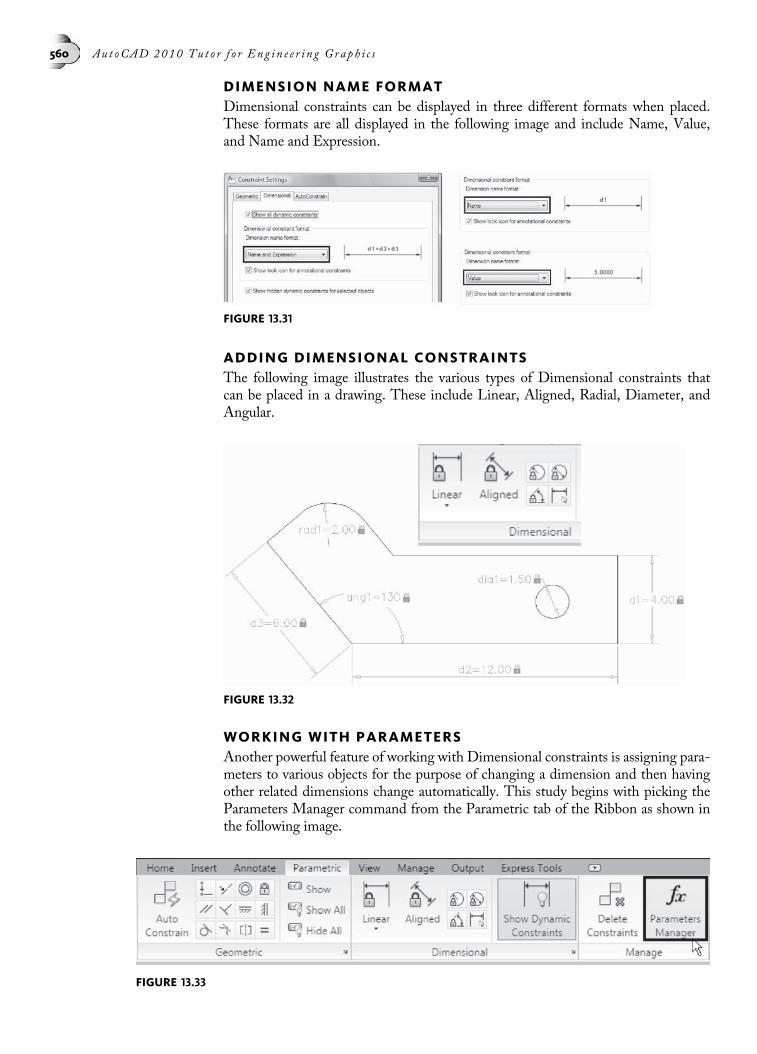
DIMENSION NAME FORMATDimensional constraints can be displayed in three different formats when placed.These formats are all displayed in the following image and include Name, Value,and Name and Expression.
ADDING DIMENSIONAL CONSTRAINTSThe following image illustrates the various types of Dimensional constraints thatcan be placed in a drawing. These include Linear, Aligned, Radial, Diameter, andAngular.
WORKING WITH PARAMETERSAnother powerful feature of working with Dimensional constraints is assigning para-meters to various objects for the purpose of changing a dimension and then havingother related dimensions change automatically. This study begins with picking theParameters Manager command from the Parametric tab of the Ribbon as shown inthe following image.
FIGURE 13.31
FIGURE 13.32
FIGURE 13.33
560 Au t oCAD 2010 Tu t o r f o r Eng i n e e r i n g Graph i c s
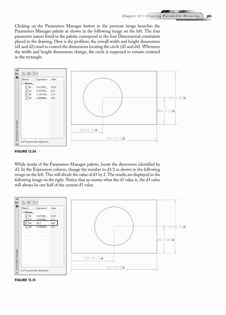
Clicking on the Parameters Manager button in the previous image launches theParameters Manager palette as shown in the following image on the left. The fourparameter names listed in the palette correspond to the four Dimensional constraintsplaced in the drawing. Here is the problem; the overall width and height dimensions(d1 and d2) need to control the dimensions locating the circle (d3 and d4). Wheneverthe width and height dimensions change, the circle is supposed to remain centeredin the rectangle.
While inside of the Parameters Manager palette, locate the dimension identified byd3. In the Expression column, change the number to d1/2 as shown in the followingimage on the left. This will divide the value of d1 by 2. The results are displayed in thefollowing image on the right. Notice that no matter what the d1 value is, the d3 valuewill always be one half of the current d1 value.
FIGURE 13.34
FIGURE 13.35
Chap t e r 13 • Cr e a t i n g Pa r ame t r i c Draw ing s 561

Next, while inside of the ParametersManager palette, locate the dimension identifiedby d4. In the Expression column, change the number to d2/2 as shown in the follow-ing image on the left. This will divide the value of d2 by 2. The results are displayed inthe following image on the right. Notice that no matter what the d2 value is, the d4value will always be one half of the current d2 value.
Now test if changing both the width and height dimensions will keep the circle cen-tered. In the following image change the d1 dimension value to 13 and the d2 dimen-sion value to 8.75. Notice in the following image the two locator dimensions d3 andd4 adjust to keep the circle centered in the rectangle. Create a similar scenario to see ifyou can keep the circle centered in the box by just creating a rectangle with a circleinside and placing the four dimensional constraints.
FIGURE 13.36
562 Au t oCAD 2010 Tu t o r f o r Eng i n e e r i n g Graph i c s

TUTORIAL EXERCISE: 13_LEVER.DWG
PurposeThis tutorial is designed to show you various methods of applying geometric constraintsand parametric dimensions to the lever as shown on the right in the previous image.
FIGURE 13.37
FIGURE 13.38
Chap t e r 13 • Cr e a t i n g Pa r ame t r i c Draw ing s 563

System SettingsAll system settings are already set for this drawing.
LayersThe following layers are already created for this drawing:
Name Color Linetype
Dimensions Red Continuous
Object Black Continuous
Suggested CommandsBegin by first dragging on the existing object and observe the results. Undo a stretchingof grips before continuing on. Next, a series of constraints will be applied to the objects.Dimensional constraints will be added to define the shape. Once all constraints and di-mensions are placed, changes will be made to selected dimensions to display a differentlever shape.
STEP 1Before adding constraints, it is considered good practice to select on a few of the objectsin order for you to determine which constraints to add. For example, clicking on the outerline of the lever as shown in the following image on the left highlights the entire perime-ter. This is a sign the perimeter was created as a polyline and no coincident constraints(from one endpoint to another endpoint) need to be applied. Also, experiment with theouter perimeter of the lever by clicking on the perimeter to display the grips and thenstretch various endpoints as shown in the following image on the right. What may appearas tangent edges on the left will show a different result on the right. Undo to get back tothe original object. Various constraints will now be added to the lever. This will includegeometric constraints as well as dimensional constraints.
STEP 2From the Parametric tab, identify and click the Tangent constraint from the Ribbon tomake it active. Then select near the endpoints of the two arcs as shown in the followingimage on the left. Do the same for edges that consist of lines and arcs. The results areillustrated in the following image on the right. Notice the placement of the Tangent
FIGURE 13.39
564 Au t oCAD 2010 Tu t o r f o r Eng i n e e r i n g Graph i c s

constraint glyphs; there should be six sets of edges to make the lines and arcs tangentwith each other. As constraints are added to objects, they may become too numerous tointerpret. You can turn off the constraints before placing a new set by clicking on theHide All button also shown in the following image on the right.
STEP 3Next from the Parametric tab, identify and click the Equal constraint from the Ribbon tomake it active. Then select the three arcs as shown in the following image on the left. Theresults are illustrated in the following image on the right. Notice the placement of theEqual constraint glyphs; there should be three to identify the three arcs being affected.
STEP 4You may have noticed that after applying the equal constraints to the arcs, the circlesinside of the lever may have slightly shifted to a new location. To have the circles sharethe same center point as the arcs, click the Concentric constraint from the Ribbon tomake it active. Then select a circle and an arc as shown in the following image on theleft. Apply this constraint to the remaining two sets of circles and arcs. The results are
FIGURE 13.40
FIGURE 13.41
Chap t e r 13 • Cr e a t i n g Pa r ame t r i c Draw ing s 565
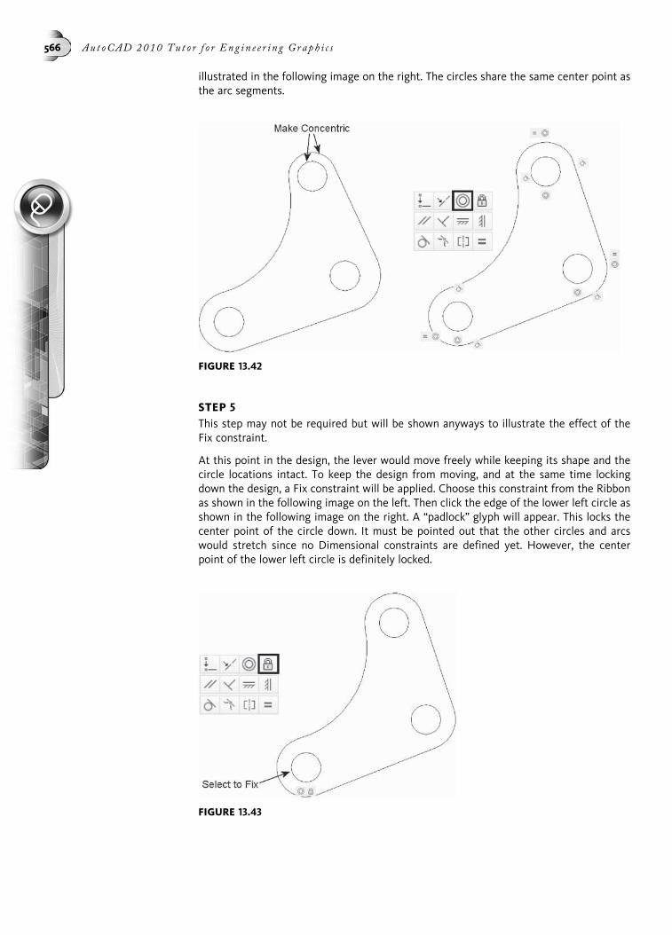
illustrated in the following image on the right. The circles share the same center point asthe arc segments.
STEP 5This step may not be required but will be shown anyways to illustrate the effect of theFix constraint.
At this point in the design, the lever would move freely while keeping its shape and thecircle locations intact. To keep the design from moving, and at the same time lockingdown the design, a Fix constraint will be applied. Choose this constraint from the Ribbonas shown in the following image on the left. Then click the edge of the lower left circle asshown in the following image on the right. A “padlock” glyph will appear. This locks thecenter point of the circle down. It must be pointed out that the other circles and arcswould stretch since no Dimensional constraints are defined yet. However, the centerpoint of the lower left circle is definitely locked.
FIGURE 13.42
FIGURE 13.43
566 Au t oCAD 2010 Tu t o r f o r Eng i n e e r i n g Graph i c s
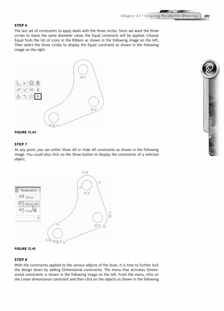
STEP 6The last set of constraints to apply deals with the three circles. Since we want the threecircles to share the same diameter value, the Equal constraint will be applied. ChooseEqual from the list of icons in the Ribbon as shown in the following image on the left.Then select the three circles to display the Equal constraint as shown in the followingimage on the right.
STEP 7At any point, you can either Show All or Hide All constraints as shown in the followingimage. You could also click on the Show button to display the constraints of a selectedobject.
STEP 8With the constraints applied to the various objects of the lever, it is time to further lockthe design down by adding Dimensional constraints. The menu that activates Dimen-sional constraints is shown in the following image on the left. From the menu, click onthe Linear dimensional constraint and then click on the objects as shown in the following
FIGURE 13.45
FIGURE 13.44
Chap t e r 13 • Cr e a t i n g Pa r ame t r i c Draw ing s 567

image in the middle to place these dimensions. As a dimension is placed, it also highlightsallowing you to change its value. If the dimension does not appear, click the Show Dy-namic Constraints button as shown in the following image on the right. This will displaythe dimension. Place the remaining dimensions using the values in the following image.
STEP 9Using the following image on the left as a guide, place the a radius dimension for thesmall arcs (R1.00), place another radius dimension for the large arc (R2.75), and finallyplace a diameter dimension on one of the three circles (1.00 diameter). The dialog boxas shown in the following image on the right is used to display the dimensions if theydo not show.
FIGURE 13.46
FIGURE 13.47
568 Au t oCAD 2010 Tu t o r f o r Eng i n e e r i n g Graph i c s
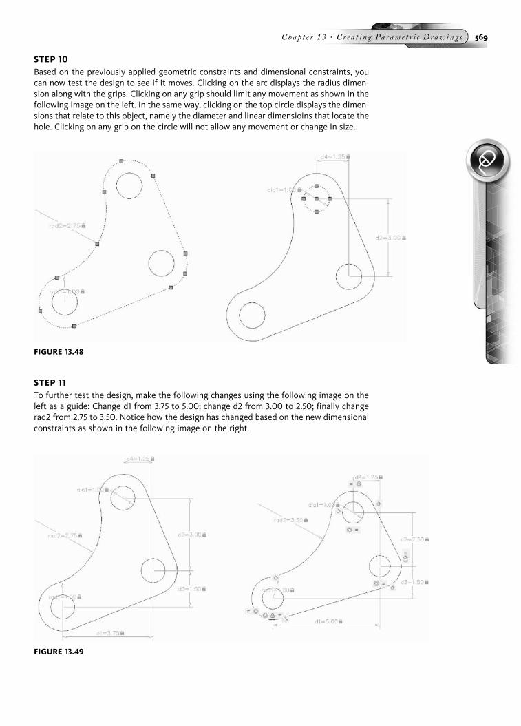
STEP 10Based on the previously applied geometric constraints and dimensional constraints, youcan now test the design to see if it moves. Clicking on the arc displays the radius dimen-sion along with the grips. Clicking on any grip should limit any movement as shown in thefollowing image on the left. In the same way, clicking on the top circle displays the dimen-sions that relate to this object, namely the diameter and linear dimensioins that locate thehole. Clicking on any grip on the circle will not allow any movement or change in size.
STEP 11To further test the design, make the following changes using the following image on theleft as a guide: Change d1 from 3.75 to 5.00; change d2 from 3.00 to 2.50; finally changerad2 from 2.75 to 3.50. Notice how the design has changed based on the new dimensionalconstraints as shown in the following image on the right.
FIGURE 13.48
FIGURE 13.49
Chap t e r 13 • Cr e a t i n g Pa r ame t r i c Draw ing s 569
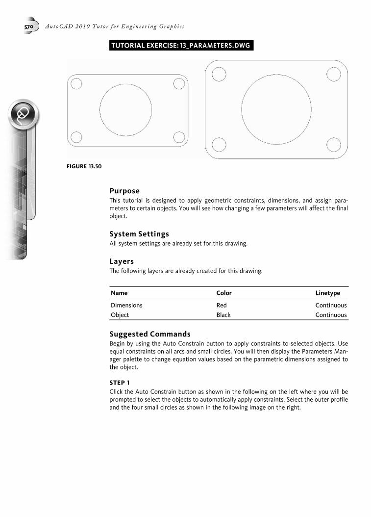
TUTORIAL EXERCISE: 13_PARAMETERS.DWG
PurposeThis tutorial is designed to apply geometric constraints, dimensions, and assign para-meters to certain objects. You will see how changing a few parameters will affect the finalobject.
System SettingsAll system settings are already set for this drawing.
LayersThe following layers are already created for this drawing:
Name Color Linetype
Dimensions Red Continuous
Object Black Continuous
Suggested CommandsBegin by using the Auto Constrain button to apply constraints to selected objects. Useequal constraints on all arcs and small circles. You will then display the Parameters Man-ager palette to change equation values based on the parametric dimensions assigned tothe object.
STEP 1Click the Auto Constrain button as shown in the following on the left where you will beprompted to select the objects to automatically apply constraints. Select the outer profileand the four small circles as shown in the following image on the right.
FIGURE 13.50
570 Au t oCAD 2010 Tu t o r f o r Eng i n e e r i n g Graph i c s
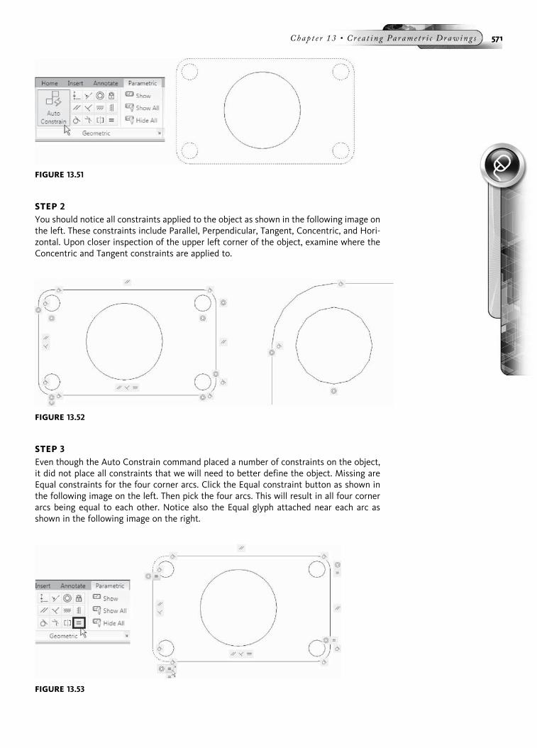
STEP 2You should notice all constraints applied to the object as shown in the following image onthe left. These constraints include Parallel, Perpendicular, Tangent, Concentric, and Hori-zontal. Upon closer inspection of the upper left corner of the object, examine where theConcentric and Tangent constraints are applied to.
STEP 3Even though the Auto Constrain command placed a number of constraints on the object,it did not place all constraints that we will need to better define the object. Missing areEqual constraints for the four corner arcs. Click the Equal constraint button as shown inthe following image on the left. Then pick the four arcs. This will result in all four cornerarcs being equal to each other. Notice also the Equal glyph attached near each arc asshown in the following image on the right.
FIGURE 13.52
FIGURE 13.53
FIGURE 13.51
Chap t e r 13 • Cr e a t i n g Pa r ame t r i c Draw ing s 571

STEP 4As with the arcs in the previous step, also missing are Equal constraints for the four smallcircles. Click the Equal constraint button as shown in the following image on the left.Then pick the four circles. This will result in all four small circles being equal to eachother. Notice also the Equal glyph attached near each circle as shown in the followingimage on the right. Before continuing on to the next step, hide all constraints as you pre-pare to add dimensional constraints to the object.
STEP 5Begin adding linear dimension to overall length and height of the object. Click the Lineardimensional button as shown in the following image on the left. Then place a horizontallinear dimension and change the dimension value to 8.00. Next place a vertical lineardimension and change its dimension value to 5.00 as shown in the following image onthe right. Note that traditional AutoCAD dimensions such as DLI (DimLinear) and DRA(DimRadius) do not have the same effect as dimensional constraints.
STEP 6Next click on the Dimensional Radius button as shown in the following image on the left.Then place a radius dimension by clicking on the arc in the upper left corner. If need be,change the radius value to .50 as shown in the following image on the right. Notice allradii change to the value of .50 since the Equal constraint was applied to all arcs in a pre-vious step.
FIGURE 13.54
FIGURE 13.55
572 Au t oCAD 2010 Tu t o r f o r Eng i n e e r i n g Graph i c s

STEP 7As with the radius dimension, click on the Dimensional Diameter button as shown in thefollowing image on the left. Then place a diameter dimension by clicking on the circle inthe upper left corner. If need, change the diameter value to .50 as shown in the followingimage on the right. Notice all circle diameters change to the value of .50 since the Equalconstraint was applied to all circles in a previous step.
STEP 8Add another diameter dimension to the large hole near the center of the object. Changethe dimension value to 2.50 as shown in the following image.
FIGURE 13.56
FIGURE 13.57
Chap t e r 13 • Cr e a t i n g Pa r ame t r i c Draw ing s 573

STEP 9Add two more Linear dimensional constraints as shown in the following image. These di-mensions will define the location of the large 2.50 diameter circle. Rather than changevalues, use the default values for both of these linear dimensions. Their values will bechanged when parameters are assigned in a later step.
STEP 10Parameters will now be added to the existing dimensions. Clicking on the ParametersManager button will launch the Parameters Manager palette as shown on the left in thefollowing image. Notice the dimension labeled d3. This represents the horizontal dimen-sion that locates the large circle. We really want the circle to be horizontally located atthe center of the object. To do this, click on the Expression next to d3 and change it tod1/2. This will take the overall dimension value of 8.00 (d1) and divide it by 2. No matterwhat d1 changes to, the circle will remain centered horizontally.
FIGURE 13.58
FIGURE 13.59
574 Au t oCAD 2010 Tu t o r f o r Eng i n e e r i n g Graph i c s

STEP 11Now notice the dimension labeled d4. This represents the vertical dimension that locatesthe large circle. We really want the circle to be located vertically at the center of the ob-ject. To do this, click on the Expression next to d4 and change it to d2/2. This will take theoverall dimension value of 5.00 (d2) and divide it by 2. No matter what d2 changes to, thecircle will remain centered vertically as shown in the following image on the right.
STEP 12For the next parameter, identify the dimension dia1 in the Parameter Manager palette asshown in the following image on the left and change the Expression to rad1. Wheneverthe radius value changes (which is controlled by the rad1 parameter) the diameter valuewill also change. Notice in the following image on the right that the radius parameter iscurrently set to .50, which is the same for the diameter values of the 4 small holes.
FIGURE 13.60
FIGURE 13.61
Chap t e r 13 • Cr e a t i n g Pa r ame t r i c Draw ing s 575

STEP 13Finally, identify the parameter dia2 in the Parameter Manager palette and change the Ex-pression to rad1*5 as shown on the left in the following image. Since the * is the same asa multiplication operation, the radius value in rad1 will be multiplied 5 times. This resultsin the circle diameter as shown in the following image on the right.
STEP 14Test that the parameters work by entering new values in the Parameters Manager paletteas shown in the following image on the left. Change the expression in d1 from 8.00 to11.25. Change the expression in d2 from 5.00 to 7.75. Finally change the rad1 expressionfrom .50 to 1.10. The results of making these changes is illustrated in the following imageon the right.
FIGURE 13.62
FIGURE 13.63
576 Au t oCAD 2010 Tu t o r f o r Eng i n e e r i n g Graph i c s

END OF CHAPTER PROBLEMS FOR CHAPTER 13Please refer to the CD that is supplied with this book and locate the file AutoCAD Tutor2010 Support Docs.pdf. In addition to extra information supplied in this chapter, end-of-chapter problems are also available to provide additional practice.
FIGURE 13.64
Chap t e r 13 • Cr e a t i n g Pa r ame t r i c Draw ing s 577
CHAPTER
14
Working withDrawing Layouts
CREATING DRAWING LAYOUTS
Up to this point in the book, all drawings have been constructed in Model Space.This consisted of drawings composed of geometry such as arcs, circles, lines, andeven dimensions. You can even plot your drawing from Model Space; however, thisgets a little tricky, especially when you attempt to plot the drawing at a known scale, oreven trickier if multiple details need to be arranged on a single sheet at different scales.
You can elect to work in two separate spaces on your drawing, namely Model Spaceand Layout mode, sometimes referred to as Paper Space. Typically, part geometryand dimensions are drawn in Model Space. However, items such as notes, annota-tions, and title blocks are laid out separately in a drawing layout, which is designedto simulate an actual sheet of paper. To arrange a single view of a drawing or multipleviews of different drawings, you arrange a series of viewports in the drawing layout toview the images. These viewports are mainly rectangular in shape and can be madeany size. You can even create circular and polygonal viewports. A viewports tool al-lows you to scale the image inside the viewport. In this way, a series of images may bescaled differently even though the drawing layout will be plotted out at a scale of 1:1.
This chapter introduces you to the controls used in a drawing layout to manage infor-mation contained in a viewport. A tutorial exercise is provided to help you practicecreating drawing layouts.
MODEL SPACEBefore starting on the topic of Paper Space, you must first understand the environ-ment in which all drawings are originally constructed, namely Model Space. It is herethat the drawing is drawn full size or in real-world units. Model Space is easily iden-tified by the appearance of the User Coordinate System icon located in the lower-leftcorner of the active drawing area in the following image. This icon is associated withthe Model Space environment. Some past and present users of AutoCAD have feltthat it clutters the display screen and gets in the way of geometry, and they have used
578

the UCSICON command to turn the icon off. While these points may seem true, theicon should be present at all times to identify the space you are working in. If you areutilizing the AutoCAD Classic workspace, another indicator that you are in ModelSpace is the presence of the Model tab, located just below the User CoordinateSystem icon, also in the following image.
MODEL SPACE AND LAYOUTSYou have already seen that Model Space is the environment set aside for constructingyour drawing in real-world units or full size, as shown in the following image on theleft. Model space can be easily recognized by the familiar User Coordinate Systemicon found in the lower-left corner of every model space screen.
In the AutoCADClassic workspace, clicking the Layout1 tab found in the lower-leftcorner of the display screen activates the layout environment. Paper Space is consid-ered an area used to lay out your drawing before it is plotted. Layouts are also used toplace title block information and notes associated with the drawing. The drawing il-lustrated in the following image on the right has been laid out in Paper Space andshows a sheet of paper with the drawing surrounded by a viewport. The dashed linesalong the outer perimeter of the sheet are referred to as margins. Anything inside themargins will plot; for this reason, this is called the printable area. Notice also atthe bottom of the screen that the Layout1 tab is activated. Both tabs at the bottom ofthe screen can be used to easily display your drawing in either Model Space or PaperSpace. Also notice the icon in the lower-left corner of the illustration; this icon is inthe form of a triangle and is used to quickly identify the Paper Space environment.
FIGURE 14.1
Chap t e r 14 • Work i n g w i t h Drawing Lay ou t s 579

LAYOUT FEATURESWhen you draw and plot from Model Space, the limits of the drawing have to beproperly set depending on the scale of the drawing and the sheet of paper the drawingis planned for. Also, title block information has to be scaled depending on the scale ofthe drawing. The text height that made up the notes in a drawing also has to be scaleddepending on the scale of the drawing. Finally, the scale of the drawing is applied tothe Plot Settings tab of the Plot dialog box, which scales the drawing for placementon a certain sheet of paper. There can be many problems when you use this method.For instance, a certain design office assigned an individual to plot all drawings pro-duced by the engineers and designers. It was this individual’s responsibility to plot thedrawings at the proper scale. However, with numerous drawings to plot, it was easy toget the plot scales confused. As a result, drawings were plotted at the wrong scale.This not only cost paper but valuable time. This scenario is the reason for using lay-outs; all drawings, no matter how many details are arranged, are plotted at 1¼ 1 withlittle or no error encountered, through the use of layouts. Plotting becomes the fun-damental reason for using the layout environment. Here are a few other reasons forarranging a drawing in a layout:
• Layouts are based on the actual sheet size. If you are plotting a drawing on a D-sizesheet of paper, you use the actual size (36 � 24) in Paper Space.
• Title blocks and the text used for notes do not have to be scaled when placed ina layout.
• Viewports created in a layout are user-defined. Viewports created in Model Space aredependent on a configuration set by AutoCAD. In a layout, the viewports can be ofdifferent sizes and shapes, depending on the information contained in the viewport.
• Multiple viewports can be created in a single layout, as in Model space. However,the images assigned to different layout viewports can be assigned different scales.Also, the control of layers in a layout is viewport-dependent. In other words, layersturned on in one viewport can be turned off or frozen in another viewport.
• All drawings, no matter how many viewports are created or details arranged, areplotted out at a scale of 1 ¼ 1.
FIGURE 14.2
580 Aut oCAD 2010 Tu t o r f o r Eng in e e r i n g Graph i c s

SETTING UP A PAGEBefore creating viewports in a layout, it is customary to first set up a page based on thesheet size, plotted scale, and plot style. To begin the process of setting up a page,right-click Layout1 or Quick View Layouts, depending on your workspace, andpick Page Setup Manager, as shown in the following image.
Performing the previous task displays the Page Setup Manager dialog box shown inthe following image on the left. The purpose of this initial dialog box is to create aseries of page setups under unique names. These page setup names can hold informa-tion such as plotter name, page sizes, and plot style tables used for pen assignmentswhen plotting. To create a page setup, click the New button to display the New PageSetup dialog box shown in the following image on the right. When creating the newpage setup name, try to give the page a name that will give you a hint for its intendedpurpose. In this dialog box, a new page setup name was entered: C-Size (DWF6).The “C” refers to the size of the drawing sheet. The DWF6 refers to the type ofplot device. DWF stands for Drawing Web Format and is used to plot a drawingout to a file. Once in this DWF form, the file can be sent to others literally aroundthe globe for review.
Clicking the OK button in the New Page Setup dialog box displays a larger, morecomprehensive, Page Setup dialog box, as shown in the following image. The follow-ing areas will now be explained:
Printer/plotter—Area A: Use this area to choose the plotter you will be output-ting to. Even though you may not be ready to plot, you can still designate a plot-ter. In this image the DWF6 ePlot.pc3 file will be used.
Paper size—Area B: This area holds all paper sizes. It is very important to knowthat these paper sizes are based on the plotter you selected back in Area A.
Plot style table (pen assignments)—Area C: This area is used to communicatewith AutoCAD. Plot style will be assigned to this page for plotting purposes.
FIGURE 14.3
FIGURE 14.4
Chap t e r 14 • Work i n g w i t h Drawing Lay ou t s 581

Another important area to take note of is the Plot scale. This is the plotted scale thatthe layout will be based on. Since the main purpose of creating a layout is to plot at ascale of 1 to 1, the scale 1:1 reflects this practice. This also means that the informationcontained in the layout has already been scaled. This will be explained in greater detaillater in this chapter.
A more detailed look at the available paper sizes is illustrated in the following imageon the left. Again, these paper sizes are a direct result of the printer/plotter you areusing. Notice in this image a number of paper sizes that have the word “expand” as-sociated with them. These paper sizes have a larger printable area as opposed to thepaper sizes that are not identified with “expand.”
Illustrated in the following image on the right are the default Plot style tables that areavailable when AutoCAD is loaded. Plot style tables control the appearance of aprinted drawing, which can include color, linetype, and even lineweight. For example,the acad.ctb table is designed for a color plot. Whatever objects are red will plot out inthe color red (provided you are using a color printer). The monochrome.ctb plot styletakes all colors and plots them out as black objects on a white sheet of paper. Noticeother color tables that plot out objects in different shades of gray (Grayscale.ctb) and anumber of screening plot styles. These are useful when you want to fade away a group ofobjects. A screening factor of 25% would have the objects faded more than a screenfactor of 50%, and so on.
FIGURE 14.5
582 Aut oCAD 2010 Tu t o r f o r Eng in e e r i n g Graph i c s

Once the proper page settings are made, clicking the OK button in the previousdialog box returns you to the Page Setup Manager. Notice that the new page setupis listed. Clicking the Set Current button assigns the new settings to your layout.Clicking the Close button returns you to the drawing layout tab.
NOTEWhen you make a number of changes in the Page Setup dialog box and then save yourdrawing, these settings are automatically saved inside the drawing.
FLOATING MODEL SPACENotice the appearance of the drafting triangle icon in the lower-left corner of thedisplay screen. This signifies that you are presently in the Paper Space environment.Another indicator in the AutoCAD Classic workspace is that the Paper button willactivate in the status bar located at the bottom of the display screen. While in PaperSpace, operations such as adding a border, title block, and general notes are usuallyperformed. Paper Space is also the area in which you plot your drawing.
When a viewport is created in a layout, the drawing image automatically fills up theviewport. Some operations need to be performed in Model Space without leaving theLayout environment; this is referred to as working in floating Model Space. To acti-vate floating Model Space, double-click inside a viewport. The UCS icon will nor-mally display, as shown in the following image on the right. Notice that the icon
FIGURE 14.6
FIGURE 14.7
Chap t e r 14 • Work i n g w i t h Drawing Lay ou t s 583
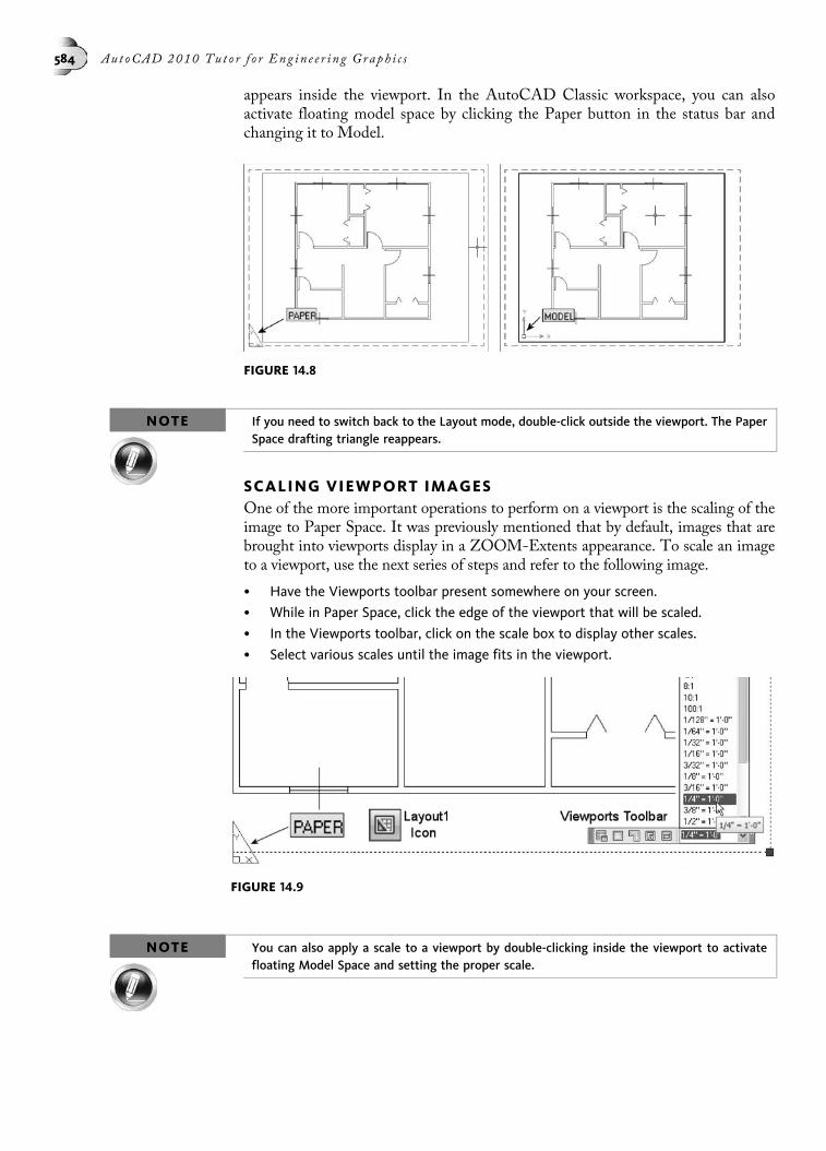
appears inside the viewport. In the AutoCAD Classic workspace, you can alsoactivate floating model space by clicking the Paper button in the status bar andchanging it to Model.
NOTE If you need to switch back to the Layout mode, double-click outside the viewport. The PaperSpace drafting triangle reappears.
SCALING VIEWPORT IMAGESOne of the more important operations to perform on a viewport is the scaling of theimage to Paper Space. It was previously mentioned that by default, images that arebrought into viewports display in a ZOOM-Extents appearance. To scale an imageto a viewport, use the next series of steps and refer to the following image.
• Have the Viewports toolbar present somewhere on your screen.
• While in Paper Space, click the edge of the viewport that will be scaled.
• In the Viewports toolbar, click on the scale box to display other scales.
• Select various scales until the image fits in the viewport.
NOTE You can also apply a scale to a viewport by double-clicking inside the viewport to activatefloating Model Space and setting the proper scale.
FIGURE 14.8
FIGURE 14.9
584 Aut oCAD 2010 Tu t o r f o r Eng in e e r i n g Graph i c s

If you find that the image is very close to fitting but is cut off by one edge of aviewport, there are two options to resolve the problem:
• Stretch the viewport (using grips or the STRETCH command).
• Pan the image into position.
A combination of both methods usually proves to be the most successful.
To pan the image, double-click inside the viewport to start floating Model Space.You will notice the thick borders on the viewport. Using the PAN command or hold-ing down the wheel on a wheel mouse, move the image to fit the viewport. Once theimage is panned into position, double-click outside the viewport on the drawing sur-face (usually the area surrounding the drawing sheet) to return from the floatingModel Space back to the layout space.
CONTROLLING THE LIST OF SCALESYou will notice that when setting the scale of the image inside the Paper Space view-port, the list of scales is very long. You may find yourself using only certain scales andignoring others. You could also be confronted with assigning a scale that is not pres-ent on the list. All these situations can be easily handled through the use of the EditScale List dialog box, which is activated by picking Scale List from the Format head-ing of the Menu Bar, as shown in the following image.
Various buttons are available that allow you to add, edit, or delete scales from the list.Clicking the Add button displays the Add Scale dialog box, as shown in the followingimage on the left. In this dialog box, a new scale of 1:1000 is being created since it isnot available in the default scale list. Clicking the Edit button displays the Edit Scaledialog box, as shown in the following image on the right. Here an existing scale isbeing edited to reflect the new scale of 1:500.
FIGURE 14.10
FIGURE 14.11
Chap t e r 14 • Work i n g w i t h Drawing Lay ou t s 585

Clicking the Delete button removes a scale from this list. You can also rearrangescales so that your most popular scales always appear at the top of the list. Simply clickthe Move Up button to move the selected scale up the list or the Move Down buttonto arrange the selected scale at the bottom of the list.
LOCKING VIEWPORTSWhen you have scaled the contents of a floating Model Space viewport, it is very easyto accidentally change this scale by rolling the wheel of the mouse or performinganother zoom operation. To prevent accidental panning and zooming of a viewportimage once it has been scaled, a popular technique is to lock the viewport. To performthis task, use these steps and refer to following image:
• Be sure you are in Layout mode (look for the drafting triangle in the lower-left corner).
• Select the viewport to lock. It will highlight and grips will appear. If Quick Propertiesare activated, as shown in the image on the right, you can lock the display by select-ing “Yes.”
• You can also use a right-click menu to lock the viewport. Right-click your screen.A menu will appear.
• Select Display Locked followed by “Yes.”
Yet another method that can be used for locking viewports is shown in the followingimage. After the edge of a viewport is selected, you can click the Lock/Unlock View-port button that is available at the right end of the status bar. This provides a moreconvenient area for locking or unlocking viewports.
NOTE When you lock a viewport, your scale will be grayed out inside the Viewports toolbar. If youneed to change the scale of an image inside a viewport, you must first unlock the viewport.
MAXIMIZING A VIEWPORTThe VPMAX command is designed to maximize the size of a viewport in a layout. Thisis especially helpful when editing drawings with small viewports. It also eliminates theneed to constantly switch betweenModel Space and a Layout. The VPMAX command
FIGURE 14.12
FIGURE 14.13
586 Aut oCAD 2010 Tu t o r f o r Eng in e e r i n g Graph i c s
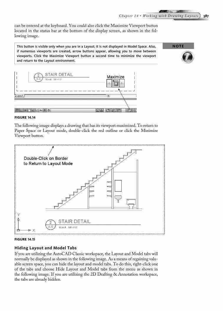
can be entered at the keyboard. You could also click the Maximize Viewport buttonlocated in the status bar at the bottom of the display screen, as shown in the fol-lowing image.
NOTEThis button is visible only when you are in a Layout; it is not displayed in Model Space. Also,if numerous viewports are created, arrow buttons appear, allowing you to move betweenviewports. Click the Maximize Viewport button a second time to minimize the viewportand return to the Layout environment.
The following image displays a drawing that has its viewport maximized. To return toPaper Space or Layout mode, double-click the red outline or click the MinimizeViewport button.
Hiding Layout and Model TabsIf you are utilizing the AutoCADClassic workspace, the Layout andModel tabs willnormally be displayed as shown in the following image. As a means of regaining valu-able screen space, you can hide the layout and model tabs. To do this, right-click oneof the tabs and choose Hide Layout and Model tabs from the menu as shown inthe following image. If you are utilizing the 2D Drafting & Annotation workspace,the tabs are already hidden.
FIGURE 14.14
FIGURE 14.15
Chap t e r 14 • Work i n g w i t h Drawing Lay ou t s 587

To redisplay the tabs on the screen, right-click the Model or Layout buttons, right-click, and pick Display Layout and Model Tabs, as shown in the following image.
CREATING A LAYOUT
TRY IT! Open the drawing file 14_Gasket1. The illustration in the following image on the left showsthe drawing originally created in Model Space. This drawing is required to be laid out inPaper Space.
Click the Quick View Layout button to display all model and layout views. Pick theLayout1 icon; a layout is automatically created, as shown in the following image.
It is good practice to rename the Layout1 tab located at the bottom of your screen. Dothis by first picking the Quick View Layouts button and double-clicking the Layout1text. Rename Layout1 to One ViewDrawing, as shown in the following image on the
FIGURE 14.16
FIGURE 14.17
FIGURE 14.18
588 Aut oCAD 2010 Tu t o r f o r Eng in e e r i n g Graph i c s
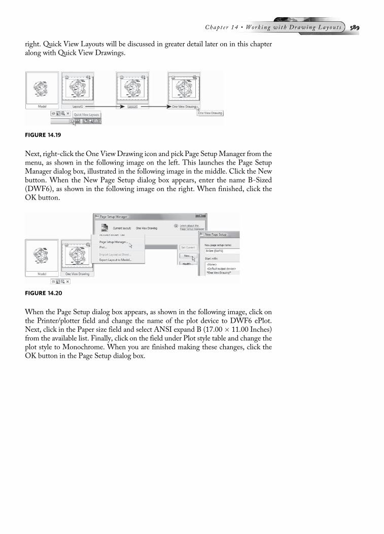
right. Quick View Layouts will be discussed in greater detail later on in this chapteralong with Quick View Drawings.
Next, right-click the One ViewDrawing icon and pick Page SetupManager from themenu, as shown in the following image on the left. This launches the Page SetupManager dialog box, illustrated in the following image in the middle. Click the Newbutton. When the New Page Setup dialog box appears, enter the name B-Sized(DWF6), as shown in the following image on the right. When finished, click theOK button.
When the Page Setup dialog box appears, as shown in the following image, click onthe Printer/plotter field and change the name of the plot device to DWF6 ePlot.Next, click in the Paper size field and select ANSI expand B (17.00 � 11.00 Inches)from the available list. Finally, click on the field under Plot style table and change theplot style to Monochrome. When you are finished making these changes, click theOK button in the Page Setup dialog box.
FIGURE 14.19
FIGURE 14.20
Chap t e r 14 • Work i n g w i t h Drawing Lay ou t s 589

When you return to the Page Setup Manager dialog box; double-click the B-Size(DWF6) layout to make it current, as shown in the following image. Click the Closebutton to continue with laying out this drawing.
Because you increased the size of the sheet, the image of the gasket in the viewport didnot grow in size. The size of the viewport depends on the scale applied in this next step.
Rather than activating floatingModel Space, simply click the edge of the viewport, asshown in the following image. Locate the Viewports button on the right side of thestatus bar. Clicking this button displays the Viewports toolbar, as shown in the fol-lowing image on the right. The number inside the field in this image is the currentscale of the image inside the viewport. Whenever you create a drawing layout, theimage is automatically zoomed to the extents of the viewport. For this reason, thedesired scale will never be correctly displayed in this area.
To have the image properly scaled inside the viewport, click the down arrow in theViewports button. This displays the drop-down list of all standard scales. These in-clude standard engineering and architectural scales. The image is assigned a scale of1:1, which is applied to the viewport.
FIGURE 14.22
FIGURE 14.21
590 Aut oCAD 2010 Tu t o r f o r Eng in e e r i n g Graph i c s

You can see in the following image on the left that the gasket has grown inside theviewport. However, it is properly scaled. The viewport needs to be increased in size toaccommodate the scaled image of the gasket. Clicking the viewport once displaysgrips located at the four corners, as shown in the following image on the left. Usethese grips to size the viewport to the image. Accomplish this by clicking one of thegrips in the corner and stretching the viewport to a new location, as shown in thefollowing image on the right.
The results of this operation are displayed in the following image. Press ESC toremove the object highlight and the grips.
FIGURE 14.23
FIGURE 14.24
Chap t e r 14 • Work i n g w i t h Drawing Lay ou t s 591
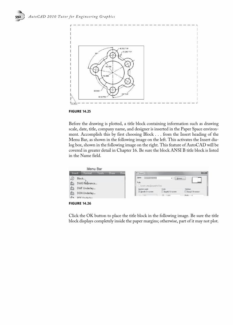
Before the drawing is plotted, a title block containing information such as drawingscale, date, title, company name, and designer is inserted in the Paper Space environ-ment. Accomplish this by first choosing Block . . . from the Insert heading of theMenu Bar, as shown in the following image on the left. This activates the Insert dia-log box, shown in the following image on the right. This feature of AutoCAD will becovered in greater detail in Chapter 16. Be sure the block ANSI B title block is listedin the Name field.
Click the OK button to place the title block in the following image. Be sure the titleblock displays completely inside the paper margins; otherwise, part of it may not plot.
FIGURE 14.25
FIGURE 14.26
592 Aut oCAD 2010 Tu t o r f o r Eng in e e r i n g Graph i c s
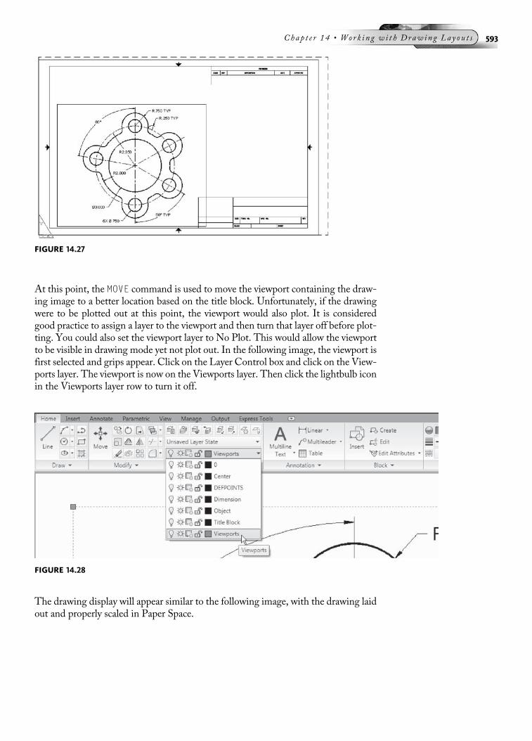
At this point, the MOVE command is used to move the viewport containing the draw-ing image to a better location based on the title block. Unfortunately, if the drawingwere to be plotted out at this point, the viewport would also plot. It is consideredgood practice to assign a layer to the viewport and then turn that layer off before plot-ting. You could also set the viewport layer to No Plot. This would allow the viewportto be visible in drawing mode yet not plot out. In the following image, the viewport isfirst selected and grips appear. Click on the Layer Control box and click on the View-ports layer. The viewport is now on the Viewports layer. Then click the lightbulb iconin the Viewports layer row to turn it off.
The drawing display will appear similar to the following image, with the drawing laidout and properly scaled in Paper Space.
FIGURE 14.28
FIGURE 14.27
Chap t e r 14 • Work i n g w i t h Drawing Lay ou t s 593
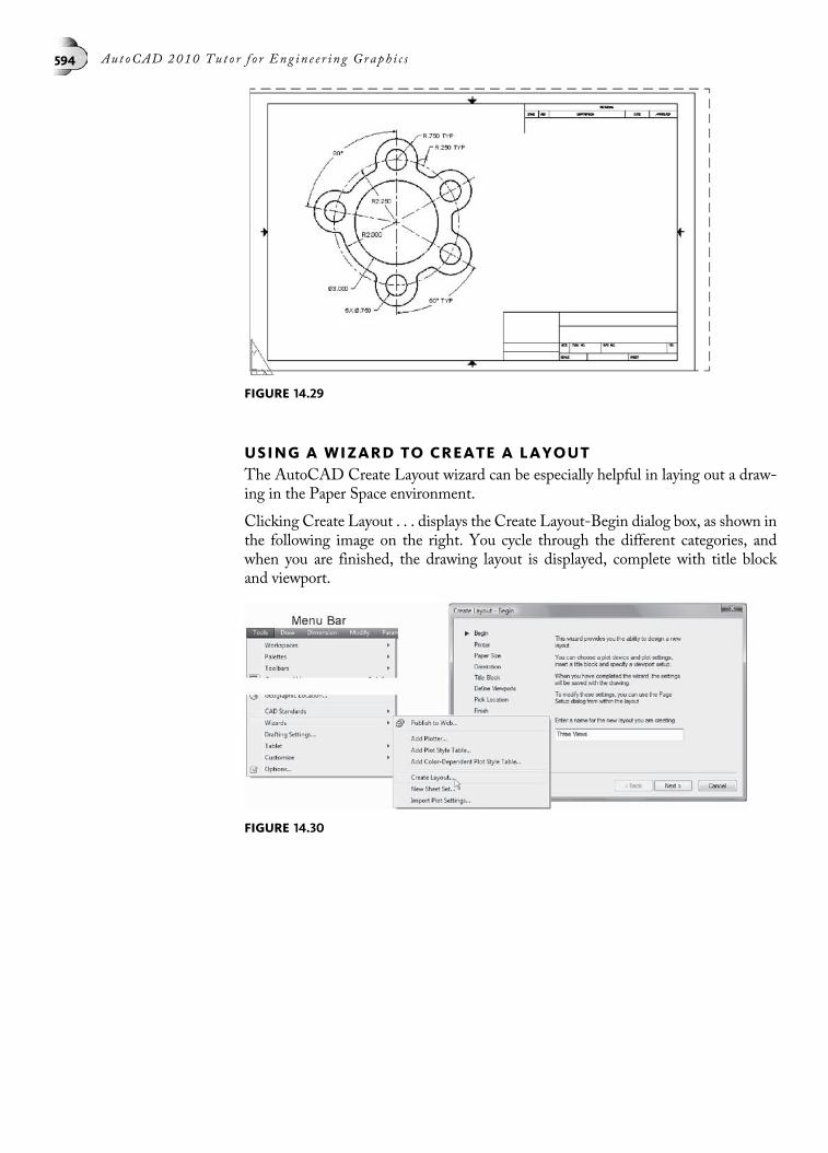
USING A WIZARD TO CREATE A LAYOUTThe AutoCAD Create Layout wizard can be especially helpful in laying out a draw-ing in the Paper Space environment.
Clicking Create Layout . . . displays the Create Layout-Begin dialog box, as shown inthe following image on the right. You cycle through the different categories, andwhen you are finished, the drawing layout is displayed, complete with title blockand viewport.
FIGURE 14.30
FIGURE 14.29
594 Aut oCAD 2010 Tu t o r f o r Eng in e e r i n g Graph i c s
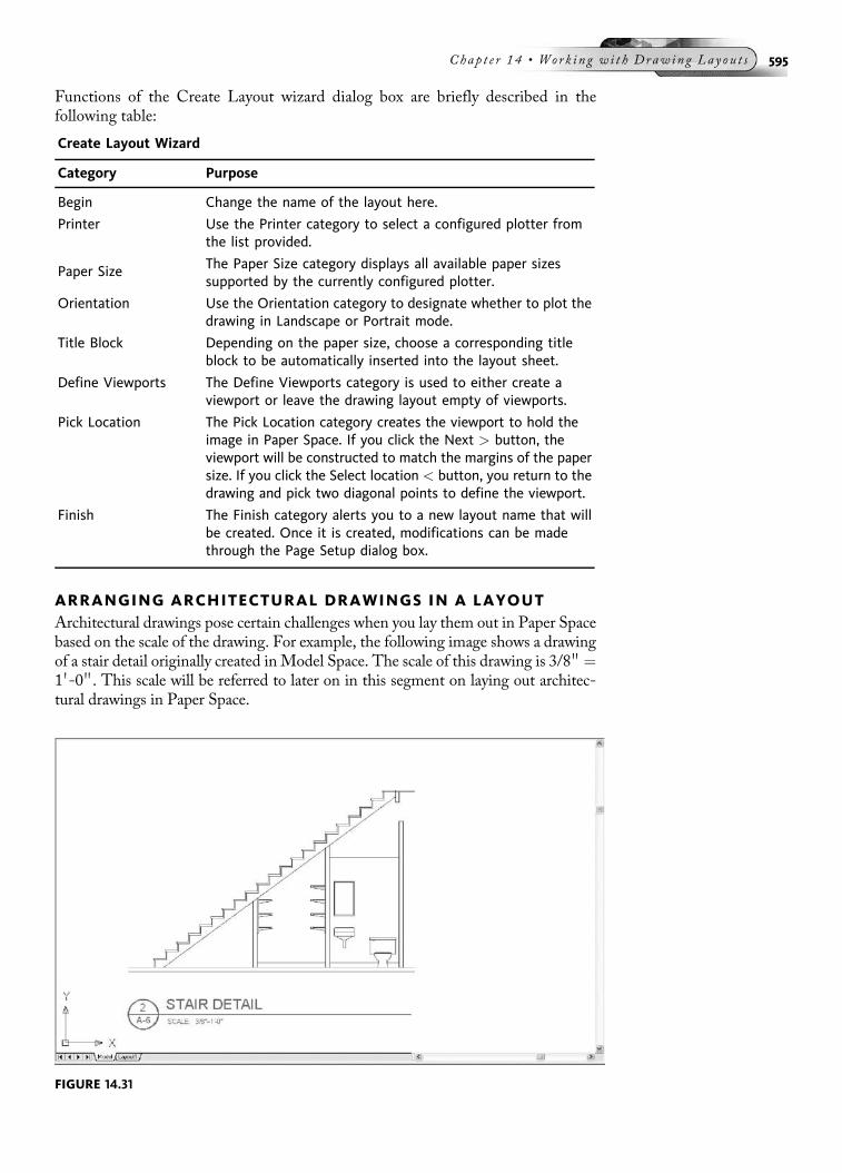
Functions of the Create Layout wizard dialog box are briefly described in thefollowing table:
Create Layout Wizard
Category Purpose
Begin Change the name of the layout here.
Printer Use the Printer category to select a configured plotter fromthe list provided.
Paper Size The Paper Size category displays all available paper sizessupported by the currently configured plotter.
Orientation Use the Orientation category to designate whether to plot thedrawing in Landscape or Portrait mode.
Title Block Depending on the paper size, choose a corresponding titleblock to be automatically inserted into the layout sheet.
Define Viewports The Define Viewports category is used to either create aviewport or leave the drawing layout empty of viewports.
Pick Location The Pick Location category creates the viewport to hold theimage in Paper Space. If you click the Next > button, theviewport will be constructed to match the margins of the papersize. If you click the Select location < button, you return to thedrawing and pick two diagonal points to define the viewport.
Finish The Finish category alerts you to a new layout name that willbe created. Once it is created, modifications can be madethrough the Page Setup dialog box.
ARRANGING ARCHITECTURAL DRAWINGS IN A LAYOUTArchitectural drawings pose certain challenges when you lay them out in Paper Spacebased on the scale of the drawing. For example, the following image shows a drawingof a stair detail originally created in Model Space. The scale of this drawing is 3/8 00 ¼1 0-0 00. This scale will be referred to later on in this segment on laying out architec-tural drawings in Paper Space.
FIGURE 14.31
Chap t e r 14 • Work i n g w i t h Drawing Lay ou t s 595

TRY IT! Open the drawing file 14_Stair Detail. Click the Layout1 tab (if the tabs are hidden, right-clicka blank part of your screen, choose Options. In the Options dialog box, click on the Displaytab and place a check in the box next to Display Layout and Model tabs) or use the CreateLayout wizard to arrange the stair detail in Paper Space so that your drawing appearssimilar to the following image. Use the Page Setup Manager dialog box to create a newpage setup that uses the DWF6 ePlot plot device, the ANSI expand C sheet, and the Mono-chrome plot style table. In the figure, we see the drawing sheet complete with a viewportthat holds the image and an ANSI C title block that has been inserted. Because theillustration in the following image is now visible in Paper Space, it is not necessarily scaledto 3/8 00 ¼ 1 0-0 00. Click the edge of the viewport. Activate the Viewports toolbar and scalethe image in the viewport to the 3/8 ¼ 1 0-0 00 scale. Notice, in the figure, a complete listingof the more commonly used architectural scales.
Changing the viewport to a different layer and then turning that layer off displays thecompleted layout of the stair detail in the following image. Since the purpose of PaperSpace is to lay out a drawing and scale the image inside the viewport, this drawing willbe plotted at a scale of 1:1.
NOTE Another common practice is to set the layer that contains all viewports to a No Plot state inthe Layer Properties Manager palette. The viewport will always remain visible in your layout.However, when previewing your image before plotting, the viewport will disappear. ExitingPlot Preview will make the viewport reappear.
FIGURE 14.32
596 Aut oCAD 2010 Tu t o r f o r Eng in e e r i n g Graph i c s

CREATING MULTIPLE DRAWING LAYOUTSThe methods explained so far have dealt with the arrangement of a single layout inPaper Space. AutoCAD provides for greater flexibility when working in Paper Spaceby enabling you to create multiple layouts of the same drawing. This will be explainedthrough the following image, which shows a floor plan complete with electrical plan.Individual layouts will be created to display separate images of the floor and electricalplans.
First verify that the Model and Layout tabs are displayed on the screen. If they arenot, right-click the Model or Layout1 button on the status bar and select “DisplayModel and Layout tabs.” To create a new layout, click on the Floor Plan layout tabas shown in the following image on the left. Then press the CTRL key while draggingyour cursor. You will notice a small page icon with a “plus” sign indicating the FloorPlan layout will be copied. The results are displayed in the following image on theright. Notice the addition of the layout Floor Plan (2) in the list of layouts.
FIGURE 14.34
FIGURE 14.33
Chap t e r 14 • Work i n g w i t h Drawing Lay ou t s 597

You can also create multiple layouts. In this example, first click on the Floor Plan andhold down the SHIFT key while you select the Electrical Plan layout tab as shown inthe following image on the left. Then press the CTRL key while dragging your cursor.You will notice a small multiple page icon with a “plus” sign indicating the Floor Planand Electrical Plan layouts will be copied. The results are displayed in the followingimage on the right. Notice the addition of the layout Floor Plan (2) and ElectricalPlan (2) in the list of layouts.
When you want to move a layout to a new location and, in effect, change the order ofthe layouts, click on the layout and drag it to its new location as shown in the follow-ing image. In this example, the CTRL key is not utilized since you are moving thelayout and not copying it.
When you copy a layout, all information inside the viewport, such as title block, view-port, and viewport scale/layer state information, is copied. Renaming layouts moreappropriately is customary at this stage. In the following image, the FoundationPlan layout was renamed to Furniture Plan. This was accomplished by double-clicking on the Foundation Plan layout tab. This will highlight all text in the tab.Entering new text renames the layout.
At times, layouts need to be deleted or removed from the drawing entirely. To deletethe HVAC Plan layout in the next example, right-click on the HVAC Plan layouttab and select Delete from the menu as shown in the following image on the left.An AutoCAD alert box will prompt you to delete the layout by clicking on the OKbutton. Notice from the alert box that the Model tab cannot be deleted.
FIGURE 14.36
FIGURE 14.37
FIGURE 14.38
FIGURE 14.35
598 Aut oCAD 2010 Tu t o r f o r Eng in e e r i n g Graph i c s

TRY IT!Open the drawing 14_Facilities_Plan. Notice that a number of layouts were created that cor-respond to the various room numbers, as shown in the following image. However, the roomnumbers are out of order and need to be rearranged starting with the lowest room numberand going to the highest room number. The Overall layout should be reordered directly af-ter the Model tab. Use the drag and drop technique illustrated in Figure 14.37 to rearrangeall the layout tabs in order.
After performing the reordering operation, your screen should appear similar to thefollowing image.
FIGURE 14.40
FIGURE 14.41
FIGURE 14.39
Chap t e r 14 • Work i n g w i t h Drawing Lay ou t s 599
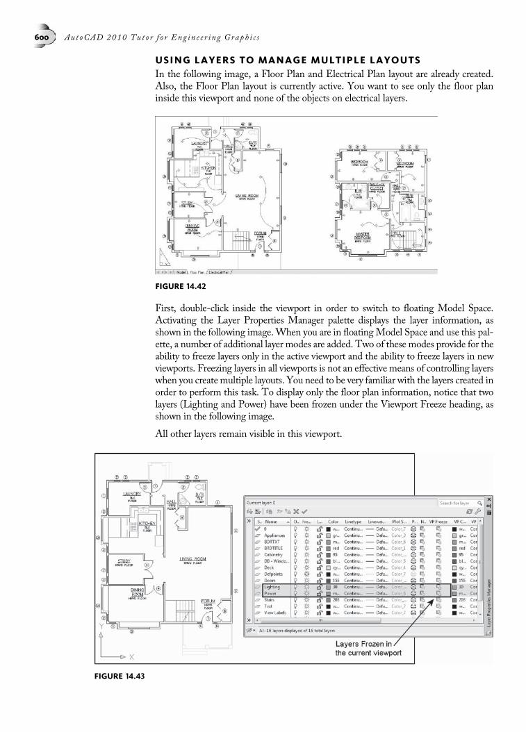
USING LAYERS TO MANAGE MULTIPLE LAYOUTSIn the following image, a Floor Plan and Electrical Plan layout are already created.Also, the Floor Plan layout is currently active. You want to see only the floor planinside this viewport and none of the objects on electrical layers.
First, double-click inside the viewport in order to switch to floating Model Space.Activating the Layer Properties Manager palette displays the layer information, asshown in the following image.When you are in floatingModel Space and use this pal-ette, a number of additional layer modes are added. Two of these modes provide for theability to freeze layers only in the active viewport and the ability to freeze layers in newviewports. Freezing layers in all viewports is not an effective means of controlling layerswhen you create multiple layouts. You need to be very familiar with the layers created inorder to perform this task. To display only the floor plan information, notice that twolayers (Lighting and Power) have been frozen under the Viewport Freeze heading, asshown in the following image.
All other layers remain visible in this viewport.
FIGURE 14.42
FIGURE 14.43
600 Aut oCAD 2010 Tu t o r f o r Eng in e e r i n g Graph i c s

The resulting image is displayed in the following image with only the floor planinformation visible in the viewport. The electrical layers have been frozen only inthis viewport and do not display.
NOTEYou can also freeze layers in the current viewport through the Layer control box, as shownin the following image.
ADDITIONAL LAYER TOOLS THAT AFFECT VIEWPORTSAdditional controls on layers in viewports are available through the Layer PropertiesManager palette. The following image illustrates the Electrical Plan layout thatwas created in the previous segment. Sometimes, you want to add special effectsto your layouts such as changing the color, linetype, or even the lineweight just inthe current viewport.
FIGURE 14.44
FIGURE 14.45
Chap t e r 14 • Work i n g w i t h Drawing Lay ou t s 601

After double-clicking inside the Electrical Plan layout, launch the Layer PropertiesManager palette to display all layers in the drawing. For the purposes of this example,all layers except for those dealing with electrical components will have the colorchanged to a light gray. The reason is to dim or fade the floor plan out in order togive emphasis on the electrical layers. In the following image, a number of layers areselected and then their colors changed to 9 or light gray through the VP Color col-umn. Notice also in the following image the presence of the VP Linetype and VPLineweight columns. You can also change the linetype and lineweight of selectedlayers. These changes are only present in the current viewport.
The results of performing this operation are illustrated in the following image wherethe floor plan components display faintly while the electrical components stand out.
FIGURE 14.46
FIGURE 14.47
602 Aut oCAD 2010 Tu t o r f o r Eng in e e r i n g Graph i c s

The following image identifies those layers that have had either the color, linetype, orlineweight overridden. These layers are highlighted with a light blue background. Ifyou need to return the control of colors, linetypes, or lineweights back to their originalstate, highlight the layers you want to affect and right-click. The menu illustrated inthe following image will appear. Click “Remove Viewport Overrides for” followed by“Selected Layers” and then “In Current Viewport only.”
Whenever performing viewport color, linetype, or lineweight overrides, a special layergroup is automatically created to help you manage these items. In the following imageof the Layer Properties Manager palette, notice the new layer group called ViewportOverrides. Clicking this name displays the layers that had their color overridden inthe previous step.
FIGURE 14.48
FIGURE 14.49
Chap t e r 14 • Work i n g w i t h Drawing Lay ou t s 603

NOTE The information contained in the Layer Properties Manager palette can get quite numerousand overwhelming. To better manage this information, a special menu exists that allows youto turn off those layer states that you do not use on a regular basis. To activate this menu,move your cursor into one of the layer state headings and right-click to display the menushown in the following image. Additional controls allow you to maximize all columns or asingle column. You can even reset all columns back to their default widths.
ASSOCIATIVE DIMENSIONS AND LAYOUTSDimensioning all objects in Model Space was once considered the only reasonableand reliable method to dimension multiple objects. The main reason was becausethere was no associativity with the Model Space objects and dimensions placed in aLayout or Paper Space. This has changed. Once you scale the Model Space objectsinside a layout, the scale of the layout has a direct bearing on the dimensions beingplaced. This is accomplished only if the DIMASSOC variable is set to 2.
FIGURE 14.50
FIGURE 14.51
604 Aut oCAD 2010 Tu t o r f o r Eng in e e r i n g Graph i c s

TRY IT!Open the drawing file 14_Inlay. Two viewports are arranged in a single layout called InlayFloor Tile, as shown in the following image. The images inside these viewports are scaleddifferently; the main inlay pattern in the left viewport is scaled to 3/4 00 ¼ 1 0-0 00. The detailimage in the right viewport has been scaled to 3 00 ¼ 1 00-0 00. The DIMASSOC variable is cur-rently set to 2. This allows you to dimension the objects in Paper Space at two differentscales and still have the correct dimensions appear.
While in Paper Space, use the DIMLINEAR command and place a few linear dimen-sions on the main inlay plan in the left viewport. Now switch and add a few lineardimensions in the right viewport. Zoom in to a few of the dimensions and see thatthey reflect theModel Space distances. Place more dimensions on the main inlay pat-tern and detail using a combination of dimension commands. Observe the correctvalues being placed.
Next, click and drag each viewport to a more convenient location on the drawingscreen. Notice that the dimensions move along with the viewports.
FIGURE 14.52
FIGURE 14.53
Chap t e r 14 • Work i n g w i t h Drawing Lay ou t s 605

NOTE If you drag viewports around and the dimensions do not keep up with the viewports, tryentering the DIMREGEN command from the keyboard. This should update all dimensions tothe new viewport positions.
HATCH SCALING RELATIVE TO PAPER SPACEWhile in a layout, you have the opportunity to scale a hatch pattern relative to thecurrent Paper Space scale in a viewport. In this way, you can easily have AutoCADcalculate the hatch pattern scale, since this is determined by the scale of the imageinside a viewport. Open the file 14_Valve Gasket. This drawing consists of a smallgasket that does not have crosshatching applied to the thin inner border. If youhatched this shape using the default hatch settings while in Model Space, the gasketwould appear similar to the illustration in the following image. Notice that the hatchpattern spacing is too large. You would need to experiment with various hatch scalesin order to achieve the desired hatch results.
A better way to approach this problem would be to enter Paper Space, activate float-ing Model Space, and produce the hatch pattern from there. While inside a floatingModel Space viewport, activate the Hatch and Gradient dialog box. Notice the Rela-tive to paper space checkbox. Placing a check in this box activates this feature, asshown in the following image on the left. This feature is grayed out if you try to hatchin Model Space.
FIGURE 14.54
FIGURE 14.55
606 Aut oCAD 2010 Tu t o r f o r Eng in e e r i n g Graph i c s

The finished gasket with hatching applied is illustrated in the following image on theright. Notice how the hatch scale is based on the viewport scale.
TRY IT!Open the drawing file 14_Hatch Partial Plan. The inner walls of the object in the followingimage need to be crosshatched. Apply the technique of making the hatch scale relativethrough the Hatch and Gradient dialog box. The results are illustrated in the followingimage on the right.
QUICK VIEW LAYOUTSThe Quick View tool allows you to preview and switch between open drawings andlayouts associated with drawings. Two modes are available through the Quick Viewtool; namely Quick View Layouts and Quick View Drawings. Each tool is activatedfrom the status bar located at the bottom of the display screen as shown in the follow-ing image.
Clicking on the Quick View Layouts button as shown in the following image on theleft will display the model space and layouts of the current drawing in a row.
Clicking on the Quick ViewDrawings button as shown in the following image on theright will display all drawings currently opened.
FIGURE 14.57
FIGURE 14.56
Chap t e r 14 • Work i n g w i t h Drawing Lay ou t s 607
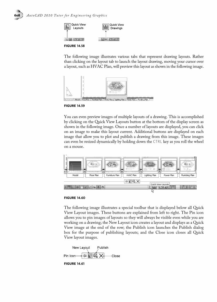
The following image illustrates various tabs that represent drawing layouts. Ratherthan clicking on the layout tab to launch the layout drawing, moving your cursor overa layout, such as HVACPlan, will preview this layout as shown in the following image.
You can even preview images of multiple layouts of a drawing. This is accomplishedby clicking on the Quick View Layouts button at the bottom of the display screen asshown in the following image. Once a number of layouts are displayed, you can clickon an image to make this layout current. Additional buttons are displayed on eachimage that allow you to plot and publish a drawing from this image. These imagescan even be resized dynamically by holding down the CTRL key as you roll the wheelon a mouse.
The following image illustrates a special toolbar that is displayed below all QuickView Layout images. These buttons are explained from left to right. The Pin iconallows you to pin images of layouts so they will always be visible even while you areworking on a drawing; the New Layout icon creates a layout and displays as a QuickView image at the end of the row; the Publish icon launches the Publish dialogbox for the purpose of publishing layouts; and the Close icon closes all QuickView layout images.
FIGURE 14.58
FIGURE 14.59
FIGURE 14.60
FIGURE 14.61
608 Aut oCAD 2010 Tu t o r f o r Eng in e e r i n g Graph i c s

QUICK VIEW DRAWINGSAs with Quick View layouts, Quick View drawings allow you to display everydrawing currently open as shown in the following image. The image of the currentdrawing will appear highlighted.
If you move your cursor over an image of a drawing that contains layouts, all layoutsfor that drawing are displayed above the Quick View drawing as shown in the follow-ing image. From there, you can make drawings or layouts current by double-clickingon the image.
The following image illustrates a special toolbar that is displayed below all QuickView Drawing images. These buttons are explained from left to right. The Pin iconallows you to pin images of drawings so they will always be visible even while you areworking on a drawing; the New icon creates a new drawing file and displays the file asa Quick View image at the end of the row; the Open icon launches the Open dialogbox for the purpose of opening drawing files; and the Close icon closes all Quick ViewDrawing images.
FIGURE 14.62
FIGURE 14.63
FIGURE 14.64
Chap t e r 14 • Work i n g w i t h Drawing Lay ou t s 609

TUTORIAL EXERCISE: 14_HVAC.DWG
PurposeThis tutorial is designed to create multiple layouts of the HVAC drawing in the previousimage in Paper Space.
System SettingsAll unit, limit, and plotter settings have already been made in this drawing. This exerciseutilizes the display of model and layout tabs. These automatically display when using theAutoCAD Classic workspace. To display the model and layout tabs in the 2D Drafting andAnnotation workspace, right-click on a blank part of the display screen and chooseOptions from the menu. When the Options dialog box displays, click on the Display taband under the Layout Elements heading, place a check in the box next to Display Layoutand Model tabs.
LayersLayers have already been created for this exercise.
Suggested CommandsYou will begin by opening the drawing file 14_HVAC Dwg. Layout1 has already beencreated for you, An architectural title block has been inserted into Paper Space and theimage has already been scaled to 1/8 00 ¼ 1 0-0 00. This layout, which will be renamed GridLines, will be modified by freezing the layers that pertain to the floor and HVAC. This isaccomplished while in floating Model Space such that the layers are only frozen in thatviewport. From this layout, create another layout called Floor Plan. While in floatingModel Space, freeze the layers that pertain to the grid lines and HVAC plans. Fromthis layout, create another layout called HVAC Plan. While in floating Model Space,freeze the layers that pertain to the grid lines. Turn off all viewports and edit drawingtitles for each layout.
FIGURE 14.65
610 Aut oCAD 2010 Tu t o r f o r Eng in e e r i n g Graph i c s

STEP 1Illustrated in the following image is a layout of an HVAC plan (heating, venting, and airconditioning). A viewport already exists and the image inside the viewport has beenscaled to a value of 1/8 00 ¼ 1 0-0 00. A border also exists in this layout. The goal is to createtwo extra layouts that show different aspects of the HVAC plan. One layout will displayonly the grid pattern used to lay out the plan. Another layout will show just the floor planinformation. The third layout will show the HVAC and floor plans together.
STEP 2Before you start to create the new layouts, the viewport present in the existing layoutneeds to be locked. This will prevent any accidental zooming in and out while inside float-ing Model Space. To lock a viewport, click the edge of the viewport and pick the Lock/Unlock Viewport icon shown in the following image. When the viewport is locked, youcannot change the Viewport Scale. Another method used for locking a viewport is to clickthe edge of the viewport, right-click, and choose Display Locked followed by Yes from themenu, Locking viewports is good practice and should be performed before creating anyextra layouts. Now that this viewport is locked, the copied viewports created in other lay-outs will also be locked.
STEP 3Next, double-click on the Layout1 tab, located in the lower-left corner of the displayscreen. Rename this layout to Grid Lines, as shown in the following image. It is alwaysgood practice to give your layouts meaningful names.
FIGURE 14.66
FIGURE 14.67
Chap t e r 14 • Work i n g w i t h Drawing Lay ou t s 611
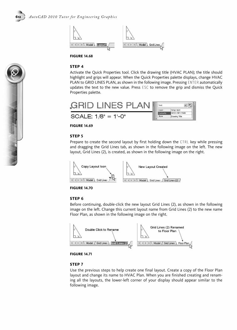
STEP 4Activate the Quick Properties tool. Click the drawing title (HVAC PLAN); the title shouldhighlight and grips will appear. When the Quick Properties palette displays, change HVACPLAN to GRID LINES PLAN, as shown in the following image. Pressing ENTER automaticallyupdates the text to the new value. Press ESC to remove the grip and dismiss the QuickProperties palette.
STEP 5Prepare to create the second layout by first holding down the CTRL key while pressingand dragging the Grid Lines tab, as shown in the following image on the left. The newlayout, Grid Lines (2), is created, as shown in the following image on the right.
STEP 6Before continuing, double-click the new layout Grid Lines (2), as shown in the followingimage on the left. Change this current layout name from Grid Lines (2) to the new nameFloor Plan, as shown in the following image on the right.
STEP 7Use the previous steps to help create one final layout. Create a copy of the Floor Planlayout and change its name to HVAC Plan. When you are finished creating and renam-ing all the layouts, the lower-left corner of your display should appear similar to thefollowing image.
FIGURE 14.68
FIGURE 14.69
FIGURE 14.70
FIGURE 14.71
612 Aut oCAD 2010 Tu t o r f o r Eng in e e r i n g Graph i c s

STEP 8Click the Grid Lines tab. Double-click anywhere inside the viewport, as shown in thefollowing image; this places you in floating Model Space. You will need to turn off alllayers that deal with the floor plan and HVAC, which leave only the layers with the gridlines visible.
Activate the Layer control box, as shown in the following image, and freeze the layersDOORS, FLOOR, HVAC DIM, and HVAC SUP in the current viewport by clicking theappropriate icon. The frozen layers pertain to the floor plan and HVAC plan.
Double-click anywhere outside the viewport to return to Paper Space. Your drawingshould appear similar to the following image. Notice that only the columns and grid linesappear visible in this layout.
FIGURE 14.72
FIGURE 14.73
Chap t e r 14 • Work i n g w i t h Drawing Lay ou t s 613

STEP 9Click the Floor Plan tab. Double-click anywhere inside the viewport, as shown in the fol-lowing image; this places you in floating Model Space. You will need to turn off all layersthat deal with the grid lines and HVAC.
Activate the Layer control box, shown in the following image, and freeze the layers in thecurrent viewport that pertain to the grid lines plan and HVAC plan (GRID, GRID DIM,GRID ID, GRID_LINES, HVAC DIM, and HVAC SUP).
FIGURE 14.74
FIGURE 14.75
614 Aut oCAD 2010 Tu t o r f o r Eng in e e r i n g Graph i c s

Double-click anywhere outside the viewport to return to Paper Space. Use the QuickProperties palette to change the drawing title from GRID LINES PLAN, as shown in thefollowing image, to FLOOR PLAN. Do this by first selecting GRID LINES PLAN, whichwill launch the Quick Properties palette allowing you to change the content of the text.When finished, press ESC to remove the palette and grip.
Your drawing now displays only floor plan information, as shown in the following image,while the HVAC and GRID layers are frozen only in this viewport.
STEP 10Click the HVAC Plan tab. Double-click anywhere inside the viewport, as shown in the fol-lowing image; this places you in floating Model Space. You will need to turn off all layersthat deal with the grid lines plan.
Activate the Layer control box, as shown in the following image, and freeze the layers inthe current viewport that pertain to the grid lines plan (COLUMNS, GRID, GRID DIM,GRID ID, and GRID_LINES).
FIGURE 14.76
FIGURE 14.77
Chap t e r 14 • Work i n g w i t h Drawing Lay ou t s 615
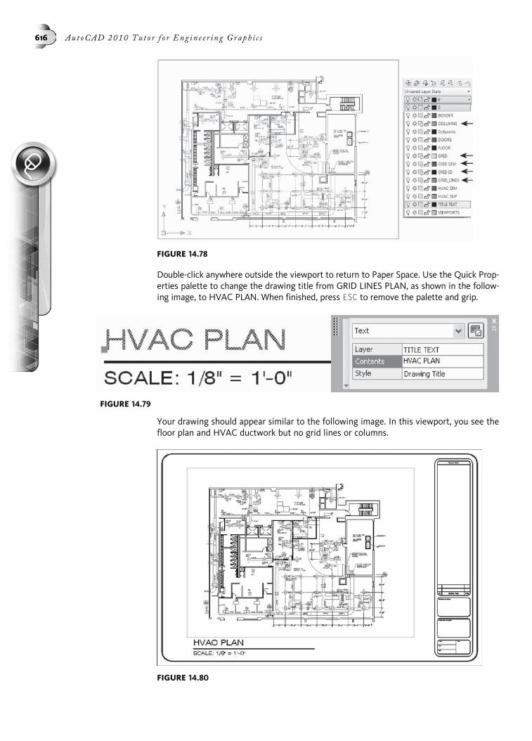
Double-click anywhere outside the viewport to return to Paper Space. Use the Quick Prop-erties palette to change the drawing title from GRID LINES PLAN, as shown in the follow-ing image, to HVAC PLAN. When finished, press ESC to remove the palette and grip.
Your drawing should appear similar to the following image. In this viewport, you see thefloor plan and HVAC ductwork but no grid lines or columns.
FIGURE 14.78
FIGURE 14.79
FIGURE 14.80
616 Aut oCAD 2010 Tu t o r f o r Eng in e e r i n g Graph i c s
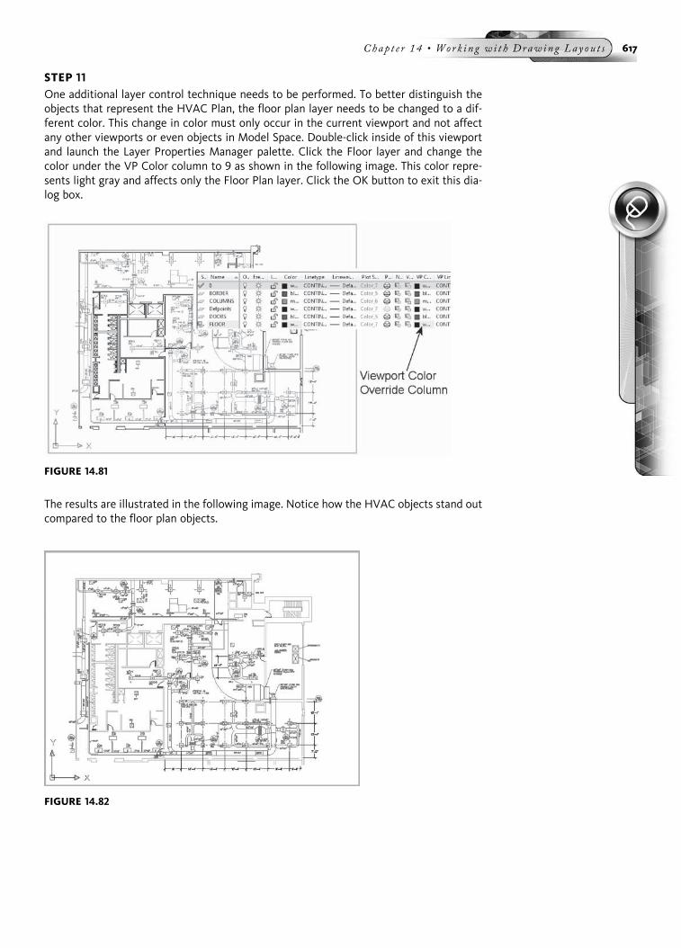
STEP 11One additional layer control technique needs to be performed. To better distinguish theobjects that represent the HVAC Plan, the floor plan layer needs to be changed to a dif-ferent color. This change in color must only occur in the current viewport and not affectany other viewports or even objects in Model Space. Double-click inside of this viewportand launch the Layer Properties Manager palette. Click the Floor layer and change thecolor under the VP Color column to 9 as shown in the following image. This color repre-sents light gray and affects only the Floor Plan layer. Click the OK button to exit this dia-log box.
The results are illustrated in the following image. Notice how the HVAC objects stand outcompared to the floor plan objects.
FIGURE 14.81
FIGURE 14.82
Chap t e r 14 • Work i n g w i t h Drawing Lay ou t s 617

STEP 12In the event you need to change the color of the Floor layer back to its original colorassignment, activate the Layer Properties Manager palette and right-click Color 9 underthe VP Color column to display the menu shown in the following image. From this menu,click Remove Viewport Overrides for followed by Color and then In Current Viewportonly. This changes the color of the Floor layer back to its original color assignment.
STEP 13Turn off the Viewports layer. The completed drawing is displayed in the following image.This exercise illustrated how to create multiple layouts. It also illustrated how to freezelayers in one viewport and have the same layers visible in other viewports. If the View-ports layer is set to No Plot through the Layer Properties Manager palette, performing aplot preview will not display the Viewports layer.
FIGURE 14.84
FIGURE 14.83
618 Aut oCAD 2010 Tu t o r f o r Eng in e e r i n g Graph i c s
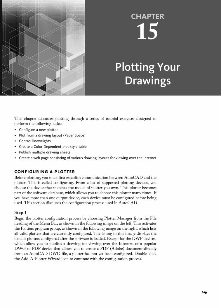
CHAPTER
15
Plotting YourDrawings
This chapter discusses plotting through a series of tutorial exercises designed toperform the following tasks:
• Configure a new plotter
• Plot from a drawing layout (Paper Space)
• Control lineweights
• Create a Color Dependent plot style table
• Publish multiple drawing sheets
• Create a web page consisting of various drawing layouts for viewing over the Internet
CONFIGURING A PLOTTERBefore plotting, you must first establish communication between AutoCAD and theplotter. This is called configuring. From a list of supported plotting devices, youchoose the device that matches the model of plotter you own. This plotter becomespart of the software database, which allows you to choose this plotter many times. Ifyou have more than one output device, each device must be configured before beingused. This section discusses the configuration process used in AutoCAD.
Step 1Begin the plotter configuration process by choosing Plotter Manager from the Fileheading of the Menu Bar, as shown in the following image on the left. This activatesthe Plotters program group, as shown in the following image on the right, which listsall valid plotters that are currently configured. The listing in this image displays thedefault plotters configured after the software is loaded. Except for the DWF devices,which allow you to publish a drawing for viewing over the Internet, or a popularDWG to PDF device that allows you to create a PDF (Adobe) document directlyfrom an AutoCAD DWG file, a plotter has not yet been configured. Double-clickthe Add-A-Plotter Wizard icon to continue with the configuration process.
619

Step 2Double-clicking the Add-A-Plotter Wizard icon displays the Add Plotter - Intro-duction Page dialog box, as shown in the following image. This dialog box statesthat you are about to configure a Windows or non-Windows system plotter. Thisconfiguration information will be saved in a file with the extension .PC3. Click theNext > button to continue on to the next dialog box.
Step 3In the Add Plotter-Begin dialog box shown in the following image on the left, decidehow the plotter will be controlled by the computer you are currently using, by a net-work plot server, or by an existing system printer where changes can be made specifi-cally for AutoCAD. Click the radio button next to My Computer. Then click theNext > button to continue on to the next dialog box.
Use the Add Plotter-Plotter Model dialog box, as shown in the following image onthe right, to associate your plotter model with AutoCAD. You would first choose theappropriate plotter manufacturer from the list provided. Once this is done, all modelssupported by the manufacturer appear to the right. If your plotter model is not listed,you are told to consult the plotter documentation for a compatible plotter. For thepurposes of this tutorial, click Hewlett-Packard in the list of Manufacturers. Clickthe DesignJet 750C Plus C3195A for the plotter model. A Driver Info dialog boxmay appear, giving you more directions regarding the type of HP DeskJet plotterselected. Click the Continue button to move on to the next dialog box used in theplotter configuration process.
FIGURE 15.1
FIGURE 15.2
620 Aut oCAD 2010 Tu t o r f o r Eng in e e r i n g Graph i c s

Step 4PCP and PC2 files have been in existence for many years. They were designed to holdplotting information such as pen assignments. In this way, you used the PCP or PC2files to control pen settings instead of constantly making pen assignments every timeyou perform a plot; at least this is how pen assignments were performed in past ver-sions of AutoCAD. The Add Plotter-Import PCP or PC2 dialog box, shown in thefollowing image on the left, allows you to import those files for use in AutoCAD in aPC3 format. If you will not be using any PCP or PC2 files from previous versions ofAutoCAD, click the Next > button to move on to the next dialog box.
In the Add Plotter-Ports dialog box, shown in the following image on the right, clickthe port used for communication between your computer and the plotter. The LPT1port will be used for the purposes of this tutorial. Place a check in its box and thenclick the Next > button to continue on to the next dialog box.
Step 5In the Add Plotter-Plotter Name dialog box, shown in the following image on theleft, you have the option of giving the plotter a name other than the name displayedin the dialog box. For the purpose of this tutorial, accept the name that is given. Thisname will be displayed whenever you use the Page Setup and Plot dialog boxes.
The last dialog box is displayed in the following image on the right. In the AddPlotter-Finish dialog box, you can modify the default settings of the plotter you justconfigured. You can also test and calibrate the plotter if desired. Click the Finish but-ton to dismiss the Add Plotter-Finish dialog box.
FIGURE 15.3
FIGURE 15.4
Chap t e r 15 • P l o t t i n g Y ou r Draw ing s 621

Step 6Exiting the Add Plotter dialog box returns you to the Plotters program group,shown in the following image. Notice that the icon for the DesignJet 750C Plusplotter has been added to this list. This completes the steps used to configure theDesignJet 750C Plus plotter. Follow these same steps if you need to configure an-other plotter.
PLOTTING FROM A LAYOUTOpen the drawing 15-Center Guide to step through the process of plotting the draw-ing from Layout mode or Paper Space.
Step 1Open the drawing 15_Center_Guide.Dwg. This drawing should already be laid outin Paper Space. A layout called Four Views should be present at the bottom of thescreen next to the Model tab.
Step 2Begin the process of plotting this drawing by choosing Plot… from the File headingof the Menu Bar, as shown in the following image. You could also choose the ploticon from the Standard toolbar. You can also type the word Plot or hold down theCTRL key and type the letter P.
FIGURE 15.5
FIGURE 15.6
622 Aut oCAD 2010 Tu t o r f o r Eng in e e r i n g Graph i c s
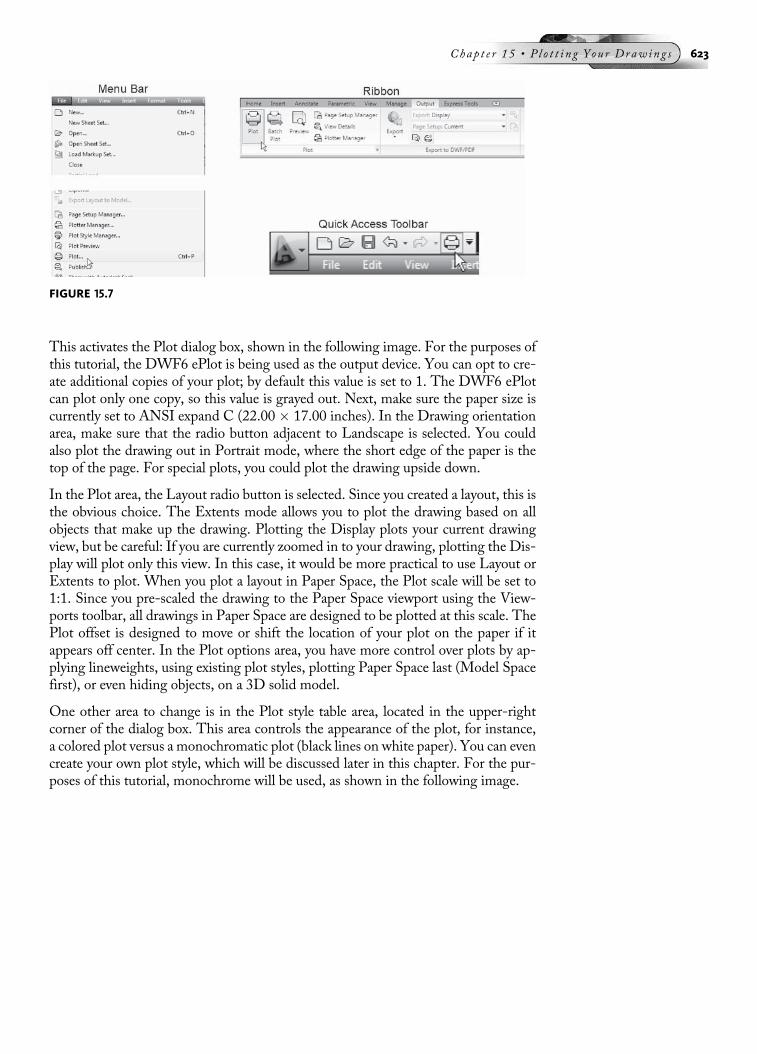
This activates the Plot dialog box, shown in the following image. For the purposes ofthis tutorial, the DWF6 ePlot is being used as the output device. You can opt to cre-ate additional copies of your plot; by default this value is set to 1. The DWF6 ePlotcan plot only one copy, so this value is grayed out. Next, make sure the paper size iscurrently set to ANSI expand C (22.00 � 17.00 inches). In the Drawing orientationarea, make sure that the radio button adjacent to Landscape is selected. You couldalso plot the drawing out in Portrait mode, where the short edge of the paper is thetop of the page. For special plots, you could plot the drawing upside down.
In the Plot area, the Layout radio button is selected. Since you created a layout, this isthe obvious choice. The Extents mode allows you to plot the drawing based on allobjects that make up the drawing. Plotting the Display plots your current drawingview, but be careful: If you are currently zoomed in to your drawing, plotting the Dis-play will plot only this view. In this case, it would be more practical to use Layout orExtents to plot. When you plot a layout in Paper Space, the Plot scale will be set to1:1. Since you pre-scaled the drawing to the Paper Space viewport using the View-ports toolbar, all drawings in Paper Space are designed to be plotted at this scale. ThePlot offset is designed to move or shift the location of your plot on the paper if itappears off center. In the Plot options area, you have more control over plots by ap-plying lineweights, using existing plot styles, plotting Paper Space last (Model Spacefirst), or even hiding objects, on a 3D solid model.
One other area to change is in the Plot style table area, located in the upper-rightcorner of the dialog box. This area controls the appearance of the plot, for instance,a colored plot versus a monochromatic plot (black lines on white paper). You can evencreate your own plot style, which will be discussed later in this chapter. For the pur-poses of this tutorial, monochrome will be used, as shown in the following image.
FIGURE 15.7
Chap t e r 15 • P l o t t i n g Y ou r Draw ing s 623
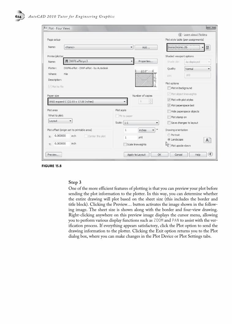
Step 3One of the more efficient features of plotting is that you can preview your plot beforesending the plot information to the plotter. In this way, you can determine whetherthe entire drawing will plot based on the sheet size (this includes the border andtitle block). Clicking the Preview… button activates the image shown in the follow-ing image. The sheet size is shown along with the border and four-view drawing.Right-clicking anywhere on this preview image displays the cursor menu, allowingyou to perform various display functions such as ZOOM and PAN to assist with the ver-ification process. If everything appears satisfactory, click the Plot option to send thedrawing information to the plotter. Clicking the Exit option returns you to the Plotdialog box, where you can make changes in the Plot Device or Plot Settings tabs.
FIGURE 15.8
624 Aut oCAD 2010 Tu t o r f o r Eng in e e r i n g Graph i c s

NOTEYou can also plot from Model Space. However, this is more involved because you must bringborders, title blocks, and notes into Model Space. Also, the sizes of notes and dimensions inModel Space must be properly sized to plot correctly.
ENHANCING YOUR PLOTS WITH LINEWEIGHTSThis section on plotting describes the process of assigning lineweights to objects andthen having the lineweights appear in the finished plot. Open the drawing called15_V_Step.Dwg, shown in the following image, and notice that you are currently inModel Space (the Model tab is current at the bottom of the screen). Follow the nextseries of steps to assign lineweights to a drawing before it is plotted.
FIGURE 15.9
FIGURE 15.10
Chap t e r 15 • P l o t t i n g Y ou r Draw ing s 625
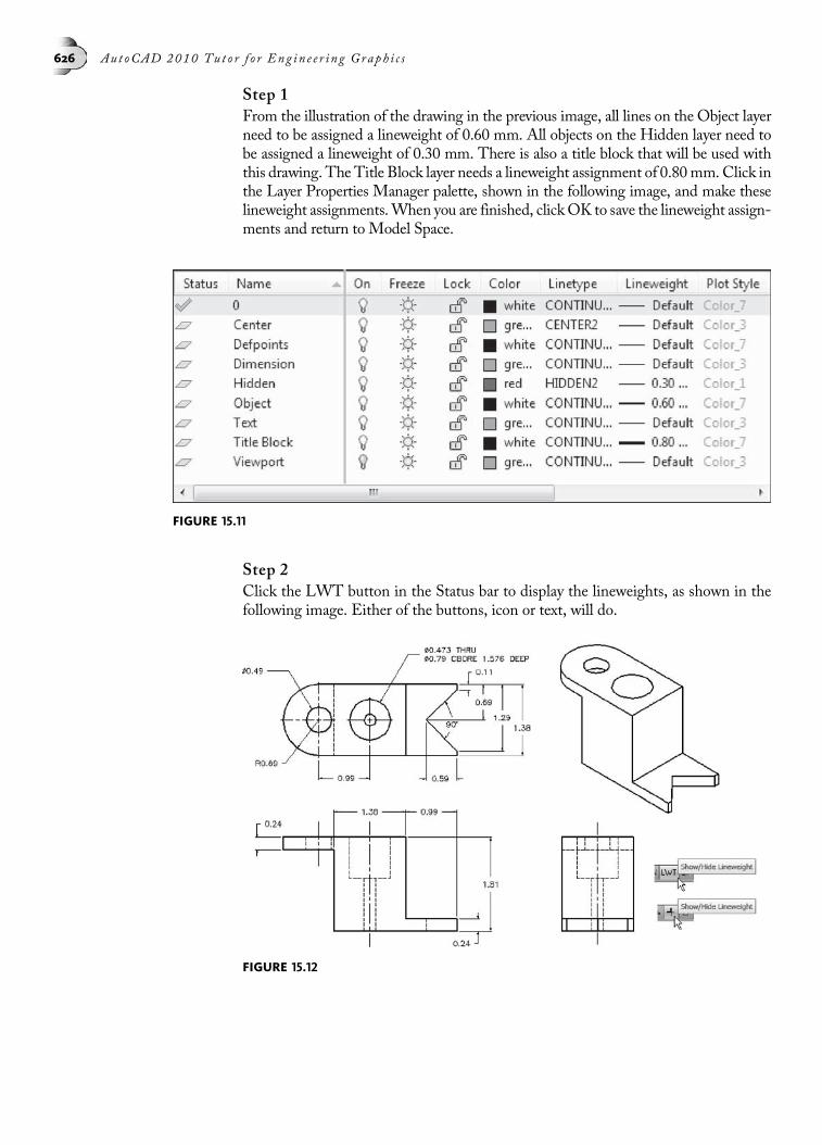
Step 1From the illustration of the drawing in the previous image, all lines on the Object layerneed to be assigned a lineweight of 0.60 mm. All objects on the Hidden layer need tobe assigned a lineweight of 0.30 mm. There is also a title block that will be used withthis drawing. The Title Block layer needs a lineweight assignment of 0.80mm. Click inthe Layer Properties Manager palette, shown in the following image, and make theselineweight assignments.When you are finished, clickOK to save the lineweight assign-ments and return to Model Space.
Step 2Click the LWT button in the Status bar to display the lineweights, as shown in thefollowing image. Either of the buttons, icon or text, will do.
FIGURE 15.11
FIGURE 15.12
626 Aut oCAD 2010 Tu t o r f o r Eng in e e r i n g Graph i c s

You can control the lineweight scale to have the linetypes give off a more pleasingappearance in your drawing. Clicking Lineweight under the Format heading of theMenu Bar displays the Lineweight Settings dialog box, as shown in the followingimage. Notice the slider bar in the area called Adjust Display Scale. This controlsonly the way lineweights display. Use this slider bar to reduce or increase the scale ofthe lineweights when they are viewed in your drawing. In the following image, theslider bar has been adjusted toward the minimum side of the scale. This shouldmake the lineweights better to read in the drawing. Click the OK button to returnto the drawing and observe the results.
All hidden and object lines have been reduced in scale in the following image. Thisaction adds to the clarity and appearance of the drawing. If after making changes tothe lineweights you decide to increase the scale, return to the Lineweight Settingsdialog box and readjust the slider bar until you achieve the desired results.
Step 3Clicking the Orthographic Views tab switches you to Paper Space, as shown inthe following image. The lineweights do not appear in Paper Space at first glance.Zooming in to the drawing displays all lineweights at their proper widths.
FIGURE 15.13
FIGURE 15.14
Chap t e r 15 • P l o t t i n g Y ou r Draw ing s 627

Step 4Activate the Plot dialog box, as shown in the following image. Verify that the currentplot device is the DWF6 ePlot. If this is not the device, click the Plot Device tab toactivate this plotter.
Step 5Click the Preview… button; your display should appear similar to the following image.Notice that the viewport is not present in the plot preview. The Viewports layer waseither turned off or set to a non-plot state inside the Layer Properties Manager palette.To view the lineweights in Preview mode, zoom in to segments of your drawing.
FIGURE 15.15
FIGURE 15.16
628 Aut oCAD 2010 Tu t o r f o r Eng in e e r i n g Graph i c s

CREATING A COLOR-DEPENDENT PLOT STYLE TABLEThis section of the chapter is devoted to the creation of a Color Dependent plot styletable. Once the table is created, it will be applied to a drawing. From there, the draw-ing will be previewed to see how this type of plot style table affects the final plot.Open the drawing 15_Color_R-Guide.Dwg. Your display should appear similar tothe following image. A two-view drawing together with an isometric view is arrangedin a layout called Orthographic Views.
The drawing is also organized by layer names and color assignments. The object is tocreate a Color Dependent plot style table where all layers will plot out black. Also,through the Color Dependent plot style table, the hidden lines will be assigned a
FIGURE 15.17
FIGURE 15.18
Chap t e r 15 • P l o t t i n g Y ou r Draw ing s 629
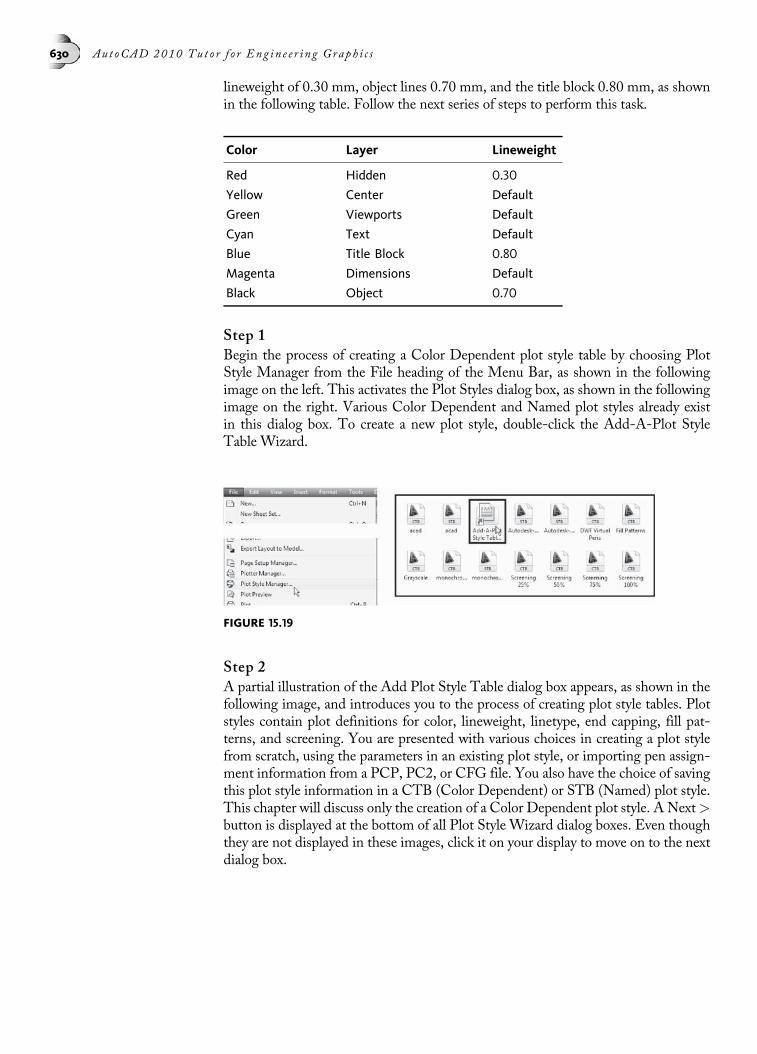
lineweight of 0.30 mm, object lines 0.70 mm, and the title block 0.80 mm, as shownin the following table. Follow the next series of steps to perform this task.
Color Layer Lineweight
Red Hidden 0.30
Yellow Center Default
Green Viewports Default
Cyan Text Default
Blue Title Block 0.80
Magenta Dimensions Default
Black Object 0.70
Step 1Begin the process of creating a Color Dependent plot style table by choosing PlotStyle Manager from the File heading of the Menu Bar, as shown in the followingimage on the left. This activates the Plot Styles dialog box, as shown in the followingimage on the right. Various Color Dependent and Named plot styles already existin this dialog box. To create a new plot style, double-click the Add-A-Plot StyleTable Wizard.
Step 2A partial illustration of the Add Plot Style Table dialog box appears, as shown in thefollowing image, and introduces you to the process of creating plot style tables. Plotstyles contain plot definitions for color, lineweight, linetype, end capping, fill pat-terns, and screening. You are presented with various choices in creating a plot stylefrom scratch, using the parameters in an existing plot style, or importing pen assign-ment information from a PCP, PC2, or CFG file. You also have the choice of savingthis plot style information in a CTB (Color Dependent) or STB (Named) plot style.This chapter will discuss only the creation of a Color Dependent plot style. A Next>button is displayed at the bottom of all Plot Style Wizard dialog boxes. Even thoughthey are not displayed in these images, click it on your display to move on to the nextdialog box.
FIGURE 15.19
630 Aut oCAD 2010 Tu t o r f o r Eng in e e r i n g Graph i c s

Step 3In the partial illustration of the Add Plot Style Table-Begin dialog box, shown in thefollowing image on the left, four options are available for you to choose, depending onhow you want to create the plot style table. Click the Start from scratch radio buttonto create this plot style from scratch. If you have made pen assignments from previousreleases of AutoCAD, you can import them through this dialog box. Click theNext > button to display the next dialog box. This Plot Style Table will be startedfrom scratch.
In the partial illustration of the Add Plot Style Table-Pick Plot Style Table dialogbox, shown in the following image on the right, click the Color-Dependent Plot StyleTable radio button to make this the type of plot style you will create. Click the Next>button to display the next dialog box.
Step 4Use the Add Plot Style Table-File Name dialog box, shown as a partial image in thefollowing image on the left, to assign a name to the plot style table. Enter the nameOrtho_Drawings in the File name area. The extension CTB is automatically addedto this file name. Click the Next > button to display the next dialog box.
The Finish dialog box, shown in the following image on the right, alerts you that aplot style called Ortho_Drawings.ctb has been created. However, you want to have allcolors plot out black and you need to assign different lineweights to a few of thelayers. To accomplish this, click the Plot Style Table Editor… button as shown inthis image.
FIGURE 15.21
FIGURE 15.20
Chap t e r 15 • P l o t t i n g Y ou r Draw ing s 631

Step 5Clicking the Plot Style Table Editor… button displays the Plot Style Table Editordialog box, as shown in the following image. Notice the name of the plot style tablepresent at the top of the dialog box. Also, three tabs are available for making changesto the current plot style table (Ortho-Drawings.ctb). The first tab is General and dis-plays file information about the current plot style table being edited. It is consideredgood practice to add a description to further document the purpose of this plot styletable. It must be pointed out at this time that this plot style table will be used on otherdrawings besides the current one. Rather, if layers are standard across projects, thesame plot style dialog box can be used. This is typical information that can be enteredin the Description area.
Step 6Clicking the Table View tab activates the dialog box, as shown in the following imageon the left. You can use the horizontal scroll bar to get a listing of all 255 colors alongwith special properties that can be changed. This information is presented in aspreadsheet format. You can click in any of the categories under a specific color andmake changes, which will be applied to the current plot style table. The color andlineweight changes will be made through the next tab.
Clicking the Form View tab displays the dialog box shown in the following imageon the right. Here the colors are arranged vertically with the properties displayed onthe right.
FIGURE 15.22
FIGURE 15.23
632 Aut oCAD 2010 Tu t o r f o r Eng in e e r i n g Graph i c s

Click Color 1 (Red) and change the Color property to Black. Whatever is red in yourdrawing will plot out in the color black. Since red is used to identify hidden lines, clickin the Lineweight area and set the lineweight for all red lines to 0.30 mm.
For Color 2 (Yellow), Color 3 (Green), Color 4 (Cyan), and Color 6 (Magenta),change the color to Black in the Properties area. All colors can be selected at one timeby holding down CTRL while picking each of them. Changes can then be made to allcolors simultaneously. Whatever is yellow, green, cyan, or magenta will plot out in thecolor black. No other changes need to be made in the dialog box for these colors.
Step 7Click Color 5 (Blue), as shown in the following image on the left, and change theColor property to Black. Whatever is blue in your drawing will plot out in the colorblack. Since blue is used to identify the title block lines, click in the Lineweight areaand set the lineweight for all blue lines to 0.80 mm.
Click Color 7 (Black), as shown on the right in the following image on the right, andchange the Color property to Black. Since black is used to identify the object lines,click in the Lineweight area and set the lineweight for all object lines to 0.70 mm.
This completes the editing process of the current plot style table. Click the Save &Close button; this returns you to the Finish dialog box. Clicking the Finish buttonreturns you to the Plot Styles dialog box. Close this box to display your drawing.
FIGURE 15.24
FIGURE 15.25
Chap t e r 15 • P l o t t i n g Y ou r Draw ing s 633

Step 8Activate the Plot dialog box in the Plot device tab, verify that the plotter is the DWF6ePlot plotter (this plotter has been used in all plotting tutorials throughout this chap-ter). In the Plot style table (pen assignments) area, make the current plot styleOrtho_Drawings.ctb, as shown in the following image on the left. Notice at the topof the dialog box that the plot style table will be saved to this layout. This means thatif you need to plot this drawing again in the future, you will not have to look for thedesired plot style table.
Click the Plot Settings tab in the Plot dialog box and verify in the lower-right cornerof the dialog box under Plot options that you will be plotting with plot styles, asshown in the following image on the right. Click the Preview button to display theresults. Unless a plotter is attached to your computer, it is not necessary to click theOK button.
Step 9The results of performing a plot preview are illustrated in the following image. Noticethat all lines are black even though they appear in color in the drawing file.
FIGURE 15.26
FIGURE 15.27
634 Aut oCAD 2010 Tu t o r f o r Eng in e e r i n g Graph i c s
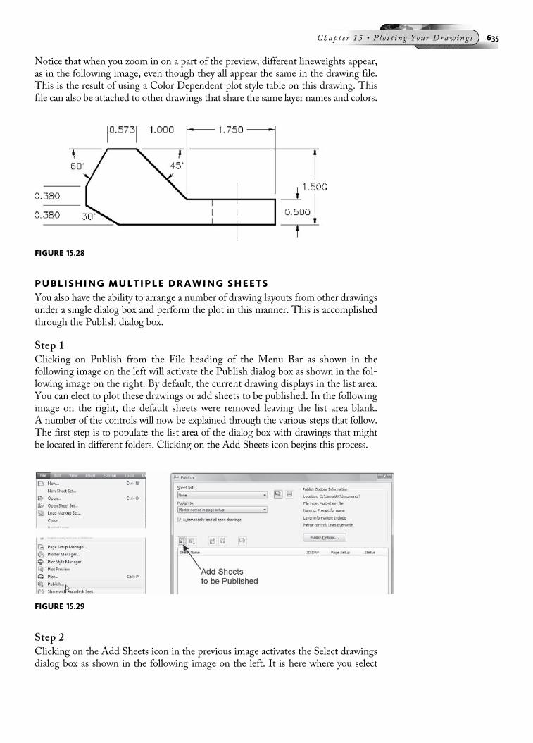
Notice that when you zoom in on a part of the preview, different lineweights appear,as in the following image, even though they all appear the same in the drawing file.This is the result of using a Color Dependent plot style table on this drawing. Thisfile can also be attached to other drawings that share the same layer names and colors.
PUBLISHING MULTIPLE DRAWING SHEETSYou also have the ability to arrange a number of drawing layouts from other drawingsunder a single dialog box and perform the plot in this manner. This is accomplishedthrough the Publish dialog box.
Step 1Clicking on Publish from the File heading of the Menu Bar as shown in thefollowing image on the left will activate the Publish dialog box as shown in the fol-lowing image on the right. By default, the current drawing displays in the list area.You can elect to plot these drawings or add sheets to be published. In the followingimage on the right, the default sheets were removed leaving the list area blank.A number of the controls will now be explained through the various steps that follow.The first step is to populate the list area of the dialog box with drawings that mightbe located in different folders. Clicking on the Add Sheets icon begins this process.
Step 2Clicking on the Add Sheets icon in the previous image activates the Select drawingsdialog box as shown in the following image on the left. It is here where you select
FIGURE 15.29
FIGURE 15.28
Chap t e r 15 • P l o t t i n g Y ou r Draw ing s 635

multiple drawings to publish (or plot.) Once the drawings are selected, clicking theSelect button at the bottom of the Select Drawings dialog box (not shown in thisillustration) will return you to the Publish dialog box. Notice all of the drawing infor-mation that is now visible in the list area of this dialog box. Listed are drawings to beplotted fromModel and Layouts as shown in the following image on the right by thedifferent icons. Notice also that the three Model icons are struck with a red line sig-nifying that a page setup has not been created for these. The main reason for this isthat most drawings are plotted from layout mode.
Step 3If you want to plot only layouts, right-click and pick Remove All from the menu. Thiswill make the list area blank again. Before adding sheets, right-click and remove thecheck next to Remove Model When Adding Sheets. Now when you click the AddSheets button, only the layout sheets are displayed in the list area of the Publish dialogbox as shown in the following image.
Step 4Another way of controlling the contents of what will be plotted is through a series oficons that allow you to add or remove drawings and even change their order. The fivebuttons illustrated in the following image include Add Sheets, Remove Sheets, MoveSheet Up, Move Sheet Down, and Preview. This provides more control as you buildthe list of drawings to be published.
FIGURE 15.30
FIGURE 15.31
636 Aut oCAD 2010 Tu t o r f o r Eng in e e r i n g Graph i c s
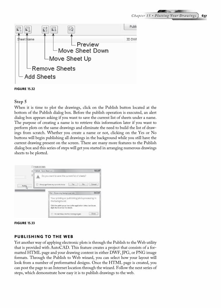
Step 5When it is time to plot the drawings, click on the Publish button located at thebottom of the Publish dialog box. Before the publish operation is executed, an alertdialog box appears asking if you want to save the current list of sheets under a name.The purpose of creating a name is to retrieve this information later if you want toperform plots on the same drawings and eliminate the need to build the list of draw-ings from scratch. Whether you create a name or not, clicking on the Yes or Nobuttons will begin publishing all drawings in the background while you still have thecurrent drawing present on the screen. There are many more features to the Publishdialog box and this series of steps will get you started in arranging numerous drawingssheets to be plotted.
PUBLISHING TO THE WEBYet another way of applying electronic plots is through the Publish to theWeb utilitythat is provided with AutoCAD. This feature creates a project that consists of a for-matted HTML page and your drawing content in either DWF, JPG, or PNG imageformats. Through the Publish to Web wizard, you can select how your layout willlook from a number of preformatted designs. Once the HTML page is created, youcan post the page to an Internet location through the wizard. Follow the next series ofsteps, which demonstrate how easy it is to publish drawings to the web.
FIGURE 15.32
FIGURE 15.33
Chap t e r 15 • P l o t t i n g Y ou r Draw ing s 637

Step 1Open the drawing file 15_Publish to Web. Notice that four layouts exist, namelyFour Views, Front View, Top View, and Right Side View. All four of these layoutswill be arranged in a single web page to demonstrate how easy it is to perform thistask. This example demonstrates how you can publish various layouts of the samedrawing to the web; you can also publish different drawings as well.
Begin the process of publishing to the web by clicking the File heading of the MenuBar followed by Publish to Web…, as shown in the following image on the left. Thislaunches the Publish to Web wizard as shown in the following image on the right. Inthis first dialog box (called Begin), be sure the radio button next to Create NewWebPage is selected. If you already have an existing web page that needs updating or edit-ing, you can click the radio button next to Edit Existing Web Page. When finished,click the Next > button and continue on to the next step of this wizard.
Step 2In the Create Web Page dialog box shown in the following image, add the name ofthe web page as Four Views with Details; then specify the location of this web page. Itis also good practice to add a description of the web page in the event that others willbe manipulating your web page. After completing the description, click the Next >button to go to the next step.
FIGURE 15.34
638 Aut oCAD 2010 Tu t o r f o r Eng in e e r i n g Graph i c s

Step 3When the Select Image Type dialog box appears, you have the opportunity to pickthe type of image that the drawings will be generated in. By default, your web pagewill be created in DWFx format, as shown in the following image on the left. Theseare vector-based images of your drawing that are designed to be viewed using InternetExplorer 7 or with the free Autodesk Design Review viewer. A second image type isDWF. These are vector-based images of your drawing that are also viewed with thefree Autodesk Design Review viewer. Another image type option consists of JPGimages. JPG files consist of raster images that do not perform very well if your draw-ing contains a lot of text. However, for this tutorial exercise, JPG will be the imageformat used. Yet another image format is displayed in the following image on theright. The PNG formats are also raster-based representations of your AutoCADdrawing. They produce high-quality images when compared with JPG files. Be surethat the image type reads JPG and click the Next > button when finished.
FIGURE 15.35
FIGURE 15.36
Chap t e r 15 • P l o t t i n g Y ou r Draw ing s 639

Step 4The next step in the process of publishing to the web is to select a web template. TheSelect Template dialog box in the following image displays four different templatesfor you to choose from. Click each one to preview each template at the right of thedialog box. For this tutorial, click Array of Thumbnails and click the Next > buttonwhen finished.
Step 5The next step when publishing to the web is the selection of a theme. The illustrationin the following image on the left shows seven possible themes that you can apply.Click each one to preview the contents. For this tutorial, the Classic theme will beused, which is illustrated in the following image on the right. When finished, clickthe Next > button to continue.
Step 6The next step displays the Enable i-drop dialog box, shown in the following image.Placing a check in the Enable i-drop box allows those who visit your web page to dragand drop drawing files into their session of AutoCAD. While this is a very powerfulfeature, we will not be demonstrating it during this tutorial. Click the Next> buttonto continue.
FIGURE 15.37
FIGURE 15.38
640 Aut oCAD 2010 Tu t o r f o r Eng in e e r i n g Graph i c s

Step 7The next dialog box allows you to add the drawings that will make up the web page.As illustrated in the following image on the left, the drawing name is listed along withlayout and label information. The label can be any name or series of names that youwish to appear in your web page. After filling in a description of this drawing, clickthe Add -> button to add the label to the image list. Under the Layout headingshown in the following image on the right, click Front View as the new layout, adda description, and click the Add -> button to add this label to the image list.
Do the same for the Right Side View and Top View. After adding the four layouts tothe image list, your dialog should appear similar to the following image. Click theNext > button to continue.
FIGURE 15.39
FIGURE 15.40
Chap t e r 15 • P l o t t i n g Y ou r Draw ing s 641

Step 8The Generate Images dialog box, shown in the following image on the left, createsthe web page in the folder that you specified earlier. Clicking the Next > buttonof this dialog box pauses your system while all the layouts are plotted. This maytake time depending on the number and complexity of drawings being published.Be sure the radio button next to “Regenerate images for drawings that have changed”is selected.
After the regeneration of all images, the Preview and Post dialog box appears, asshown in the following image on the right. You can either preview your results orpost the web page to a web site at a later time. Click the Preview button.
Step 9Clicking the Preview button in the previous step launches Microsoft InternetExplorer and displays your web page, as shown in the following image.
FIGURE 15.41
FIGURE 15.42
642 Aut oCAD 2010 Tu t o r f o r Eng in e e r i n g Graph i c s

To view each image separately, click the thumbnail to enlarge the image and showmore detail (see the image of the four views in the following image). DismissingInternet Explorer takes you back to the Preview and Post dialog box. Click the Finishbutton to end this task.
FIGURE 15.44
FIGURE 15.43
Chap t e r 15 • P l o t t i n g Y ou r Draw ing s 643

CHAPTER
16
Working with Blocks
This chapter begins the study of how blocks are created and merged into drawingfiles. This is a major productivity enhancement and is considered an electronic tem-plate similar to those methods used with block templates in manual drafting practices.The first segment of this chapter will discuss what blocks are and how they are cre-ated. Blocks are typically inserted in the current drawing but can be inserted in anydrawing by utilizing the proper commands and techniques. The chapter continues bydiscussing other topics such as redefining blocks and the effects blocks have on tableobjects. Dynamic blocks provide even greater control of block objects. A number ofdynamic block techniques will be utilized. Next, this chapter continues with a discus-sion about using the Insert dialog box and the DesignCenter to bring blocks intodrawings. The DesignCenter is a special feature that allows blocks to be inserted indrawings with drag and drop techniques. In addition, blocks found in other drawingscan easily be inserted in the current drawing from the DesignCenter. Yet anotherfeature, the Tool Palette, allows you to organize blocks and hatch patterns in one con-venient area. These object types can then be shared with the current drawing throughdrag and drop techniques. Finally, the chapter will discuss the use of MDE (MultipleDesign Environment). This feature allows the opening of multiple drawings withina single AutoCAD session and provides a convenient method of exchanging data,such as blocks, between one drawing and another. As an added bonus to AutoCADusers, a series of block libraries is supplied with the package. These block librariesinclude such application areas as mechanical, architectural, electrical, piping, andwelding, to name just a few.
WHAT ARE BLOCKS?Blocks usually consist of smaller components of a larger drawing. Typical examplesinclude doors and windows for floor plans, nuts, and bolts for mechanical assem-blies, and resistors and transistors for electrical schematics. In the following image,which shows an electrical schematic, all resistors, capacitors, tetrodes, and diodesare considered blocks that make up the total drawing of the electrical schematic.The capacitor is highlighted as one of these components.
644

Blocks are created and then inserted in a drawing.When creating the block, you mustfirst provide a name for the block. The capacitor illustrated in the following imageon the left was assigned the name CAPACITOR. Also, when you create a block,an insertion point is required. This acts as a reference point from which the blockwill be inserted. In the illustration in the following image on the left, the insertionpoint of the block is the left end of the line.
At times, blocks have to be rotated into position. In the illustration in the followingimage on the right, notice that one capacitor is rotated at a 45° angle while the othercapacitor is rotated 270°. In this way the same block can be used numerous timeseven though it is positioned differently in the drawing.
METHODS OF SELECTING BLOCK COMMANDSCommands that deal with blocks can be selected from one of four menu areas;Menu Bar, Ribbon, and Draw Toolbar as shown in the following image.
FIGURE 16.1
FIGURE 16.2
Chap t e r 16 • Work in g w i t h B l o c k s 645

You can also enter block-related commands from the keyboard, either using theirentire name or through command aliases, as in the following examples. These com-mands will be discussed in greater detail in the following pages.
Enter B to activate the Block Definition dialog box (BLOCK).
Enter I to activate the Insert dialog box (INSERT).
Enter W to activate the Write Block dialog box (WBLOCK).
Enter ADC to activate the DesignCenter (ADCENTER).
CREATING A LOCAL BLOCK USING THE BLOCK COMMANDThe illustration in the following image on the left is a drawing of a hex head bolt. Thisdrawing consists of one polygon, representing the hexagon, a circle, indicating that thehexagon is circumscribed about the circle, and two centerlines. Rather than copy theseindividual objects numerous times throughout the drawing, you can create a blockusing the BLOCK command. Selecting Block from the Draw Menu Bar and thenselecting Make activates the Block Definition dialog box, illustrated in the followingimage on the right. Entering the letter b from the keyboard also activates the BlockDefinition dialog box.
When you create a block, the numerous objects that make up the block are all consid-ered a single object. This dialog box allows for the newly created block to be mergedinto the current drawing file. This means that a block is available only in the drawingit was created in; it cannot be shared directly with other drawings. (The WBLOCK
FIGURE 16.3
FIGURE 16.4
646 Au t oCAD 2010 Tu t o r f o r Eng in e e r i n g Graph i c s

command is used to create global blocks that can be inserted in any drawing file. Thiscommand will be discussed later on in this chapter.)
To create a block through the Block Definition dialog box, enter the name of theblock, such as “Hexbolt,” in the Name field, as shown in the following image. Youcan use up to 255 alphanumeric characters when naming a block.
Next, click the Select objects button; this returns you to the drawing editor. Create awindow from “A” to “B” around the entire hex bolt to select all objects, as shown inthe previous image. When finished, press ENTER. This returns you to the BlockDefinition dialog box, where a previewed image of the block you are about to createis displayed in the upper-right corner of the dialog box, as shown in the followingimage. Whenever you create a block, you can elect to allow the original objects thatmade up the hex bolt to remain on the screen (click Retain button), to be replacedwith an instance of the block (click Convert to Block button), or to be removed afterthe block is created (click Delete button). Click the Delete radio button to erase theoriginal objects after the block is created. If the original objects that made up the hexbolt are unintentionally removed from the screen during this creation process, theOOPS command can be used to retrieve all original objects to the screen.
The next step is to create a base point or insertion point for the block. This is con-sidered a point of reference and should be identified at a key location along theblock. By default, the Base point in the Block Definition dialog box is located at0,0,0. To enter a more appropriate base-point location, click the Pick point button;this returns you to the drawing editor and allows you to pick the center of the hexbolt at “C,” as shown in the previous image. Once this point is selected, you arereturned to the Block Definition dialog box; notice how the Base point informationnow reflects the key location along the block, as shown in the following image.
Yet another feature of the Block Definition dialog box allows you to add a descriptionfor the block. Many times the name of the block hides the real meaning of the block,especially if the block name consists of only a few letters. Click on the Descriptionfield and add the following statement: “This is a hexagonal head bolt.” This allowsyou to refer to the description in case the block name does not indicate the true
FIGURE 16.5
Chap t e r 16 • Work in g w i t h B l o c k s 647
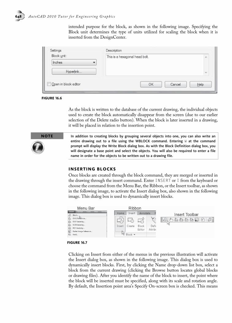
intended purpose for the block, as shown in the following image. Specifying theBlock unit determines the type of units utilized for scaling the block when it isinserted from the DesignCenter.
As the block is written to the database of the current drawing, the individual objectsused to create the block automatically disappear from the screen (due to our earlierselection of the Delete radio button). When the block is later inserted in a drawing,it will be placed in relation to the insertion point.
NOTE In addition to creating blocks by grouping several objects into one, you can also write anentire drawing out to a file using the WBLOCK command. Entering W at the commandprompt will display the Write Block dialog box. As with the Block Definition dialog box, youwill designate a base point and select the objects. You will also be required to enter a filename in order for the objects to be written out to a drawing file.
INSERTING BLOCKSOnce blocks are created through the block command, they are merged or inserted inthe drawing through the insert command. Enter INSERT or I from the keyboard orchoose the command from theMenu Bar, the Ribbon, or the Insert toolbar, as shownin the following image, to activate the Insert dialog box, also shown in the followingimage. This dialog box is used to dynamically insert blocks.
Clicking on Insert from either of the menus in the previous illustration will activatethe Insert dialog box, as shown in the following image. This dialog box is used todynamically insert blocks. First, by clicking the Name drop-down list box, select ablock from the current drawing (clicking the Browse button locates global blocksor drawing files). After you identify the name of the block to insert, the point wherethe block will be inserted must be specified, along with its scale and rotation angle.By default, the Insertion point area’s Specify On-screen box is checked. This means
FIGURE 16.6
FIGURE 16.7
648 Au t oCAD 2010 Tu t o r f o r Eng in e e r i n g Graph i c s

you will be prompted for the insertion point at the command prompt area of thedrawing editor. The default values for the scale and rotation insert the block at theoriginal size and orientation. It was already mentioned that a block consists of severalobjects combined into a single object. The Explode box determines whether theblock is inserted as one object or the block is inserted and then exploded back to itsindividual objects. Once the name of the block, such as Hexbolt, is selected, click theOK button.
The following prompts complete the block insertion operation:
Specify insertion point or [Basepoint/Scale/X/Y/Z/Rotate/PScale/PX/PY/PZ/PRotate]: (Mark a point at “A” in thefollowing image to insert the block)
If the Specify On-screen boxes are also checked for Scale and Rotation, the followingprompts will complete the block insertion operation.
Specify insertion point or [Basepoint/Scale/X/Y/Z/Rotate/PScale/PX/PY/PZ/PRotate]: (Mark a point at “A,” as shown inthe following image, to insert the block)
Enter X scale factor, specify opposite corner, or [Corner/XYZ] <1>: (Press ENTER to accept default X scale factor)
Enter Y scale factor <use X scale factor>: (Press ENTER toaccept default)
Specify rotation angle <0>: (Press ENTER to accept thedefault rotation angle and insert the block, as shown inthe following image)
If blocks are already defined as part of the database of the current drawing, they maybe selected from the Name drop-down list box, as shown in the following image onthe right.
FIGURE 16.8
Chap t e r 16 • Work in g w i t h B l o c k s 649
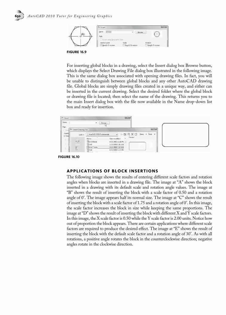
For inserting global blocks in a drawing, select the Insert dialog box Browse button,which displays the Select Drawing File dialog box illustrated in the following image.This is the same dialog box associated with opening drawing files. In fact, you willbe unable to distinguish between global blocks and any other AutoCAD drawingfile. Global blocks are simply drawing files created in a unique way, and either canbe inserted in the current drawing. Select the desired folder where the global blockor drawing file is located; then select the name of the drawing. This returns you tothe main Insert dialog box with the file now available in the Name drop-down listbox and ready for insertion.
APPLICATIONS OF BLOCK INSERTIONSThe following image shows the results of entering different scale factors and rotationangles when blocks are inserted in a drawing file. The image at “A” shows the blockinserted in a drawing with its default scale and rotation angle values. The image at“B” shows the result of inserting the block with a scale factor of 0.50 and a rotationangle of 0°. The image appears half its normal size. The image at “C” shows the resultof inserting the block with a scale factor of 1.75 and a rotation angle of 0°. In this image,the scale factor increases the block in size while keeping the same proportions. Theimage at “D” shows the result of inserting the block with different X and Y scale factors.In this image, the X scale factor is 0.50 while the Y scale factor is 2.00 units. Notice howout of proportion the block appears. There are certain applications where different scalefactors are required to produce the desired effect. The image at “E” shows the result ofinserting the block with the default scale factor and a rotation angle of 30°. As with allrotations, a positive angle rotates the block in the counterclockwise direction; negativeangles rotate in the clockwise direction.
FIGURE 16.9
FIGURE 16.10
650 Au t oCAD 2010 Tu t o r f o r Eng in e e r i n g Graph i c s

TRIMMING TO BLOCK OBJECTSThe ability to trim to a block object is possible through the TRIM command. As youselect cutting edges on the block to trim to, the command isolates the cutting edgesfrom the remainder of the objects that make up the block. In the following image,the outside edges of the bolt act as cutting edges.
TRY IT!To test this feature, open the drawing 16_Trim Plates and use the following image as aguide. The bolt is a block. Activate the TRIM command, pick the edges of the bolt at “A”and “B” as cutting edges, and pick the lines at “C” through “E” as the objects to trim.
The result of using the TRIM command is illustrated in the following image onthe right.
EXTENDING TO BLOCK OBJECTSAs with the TRIM command, objects can be extended to boundary edges that arepart of a block with the EXTEND command. Selecting boundary edges that consistof block components isolates these objects. This enables you to extend objects tothese boundary edges.
FIGURE 16.11
FIGURE 16.12
Chap t e r 16 • Work in g w i t h B l o c k s 651

TRY IT! To test this feature, open the drawing 16_Extend Plates and use the following image as aguide. Again the bolt is a block. Activate the EXTEND command, pick the edges of thebolt at “A” and “B” as boundary edges, and pick the lines at “C” through “H” as the objectsto extend.
The result of using the EXTEND command on block objects as cutting edges is illus-trated in the following image on the right.
EXPLODING BLOCKSIt has already been mentioned that as blocks are inserted in a drawing file, they areconsidered one object even though they consist of numerous individual objects. Attimes it is necessary to break a block up into its individual parts. The EXPLODE com-mand is used for this.
Illustrated in the following image on the left is a block that has been selected. Noticethat the entire block highlights and the insertion point of the block is identified bythe presence of the grip. Using the EXPLODE command on a block results in the fol-lowing image on the right. Here, when one of the lines is selected, only that objecthighlights. Exploding a block breaks the block back up into its individual objects.As a result, you must determine when it is appropriate to explode a block.
MANAGING UNUSED BLOCK DATA WITHTHE PURGE DIALOG BOXAutoCAD stores named objects (blocks, dimension styles, layers, linetypes, multilinestyles, plot styles, shapes, table styles, and text styles) with the drawing. When thedrawing is opened, AutoCAD determines whether other objects in the drawing
FIGURE 16.13
FIGURE 16.14
652 Au t oCAD 2010 Tu t o r f o r Eng in e e r i n g Graph i c s

reference each named object. If a named object is unused and not referenced, you canremove the definition of the named object from the drawing by using the PURGEcommand. This is a very important productivity technique used for compressing orcleaning up the database of the drawing. Picking File from the Menu Bar, followedby Drawing Utilities, displays Purge…, as shown in the following image on the left.Clicking Purge… displays the Purge dialog box, as shown in the following imageon the right.
The Blocks category is expanded by clicking the “þ.” This produces the list of all theitems that are currently unused in the drawing that can be removed, as shown in thefollowing image on the left. Clicking the item DIGITIZE, right-clicking, and thenpicking Purge from the shortcut menu (or simply clicking the button at the bottomof the dialog box) displays the Confirm Purge dialog box, as shown in the followingimage in the middle. Click the Yes button and the block is removed from the listeditems, as shown in the following image on the right.
Other controls are available in the Purge dialog box, such as the ability to view itemsthat cannot be purged and the capability of purging nested items. An example ofpurging a nested item would be purging a block definition that lies inside anotherblock definition. Entering PU at the Command prompt also activates the Purgedialog box.
FIGURE 16.15
FIGURE 16.16
Chap t e r 16 • Work in g w i t h B l o c k s 653

TIP The layer “0,” Standard text and dimension styles, and the Continuous linetype cannot bepurged from a drawing.
TRY IT! Open the drawing file 16_Purge, as shown in the following image on the left. Activate thePurge dialog box and click the Purge All button. You will be prompted to remove all itemsindividually through the Confirm Purge dialog box, as shown in the following image on theright. Answer Yes to each item you want purged or Yes to All, until all items, includingblocks, layers, linetypes, text styles, dimension styles, and multiline styles, have beenremoved from the database of the drawing.
REDEFINING BLOCKSAt times, a block needs to be edited. Rather than erase all occurrences of the blockin a drawing, you can redefine it. This is considered a major productivity techniquebecause all blocks that share the same name as the block being redefined will auto-matically update to the latest changes. The illustration in the following image onthe left shows various blocks inserted in a drawing. The block name is Step Guideand the insertion point is at the lower-left corner of the object.
TRY IT! The drawing file 16_Block Redefine has been provided on CD for you to experiment with re-defining blocks. When the drawing appears on your screen, as shown in the following imageon the left, double-click any block in the drawing. This launches the Edit Block Definitiondialog box, as shown in the following image on the right. A list of all blocks defined in thedrawing appear. Click Step Guide from the list and click the OK button.
FIGURE 16.17
654 Au t oCAD 2010 Tu t o r f o r Eng in e e r i n g Graph i c s
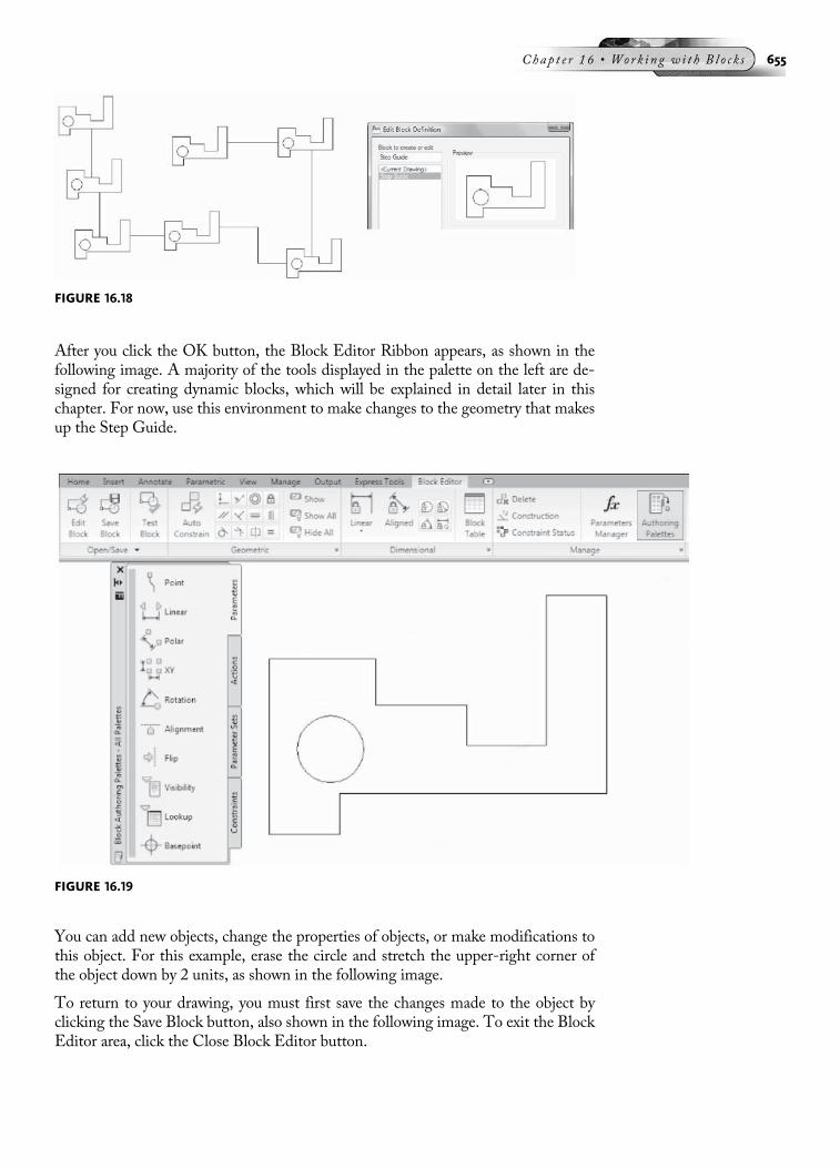
After you click the OK button, the Block Editor Ribbon appears, as shown in thefollowing image. A majority of the tools displayed in the palette on the left are de-signed for creating dynamic blocks, which will be explained in detail later in thischapter. For now, use this environment to make changes to the geometry that makesup the Step Guide.
You can add new objects, change the properties of objects, or make modifications tothis object. For this example, erase the circle and stretch the upper-right corner ofthe object down by 2 units, as shown in the following image.
To return to your drawing, you must first save the changes made to the object byclicking the Save Block button, also shown in the following image. To exit the BlockEditor area, click the Close Block Editor button.
FIGURE 16.18
FIGURE 16.19
Chap t e r 16 • Work in g w i t h B l o c k s 655

When you return to the drawing editor, notice that all Step Guide blocks have beenupdated to the changes made in the Block Editor. This provides a very productivemethod of making changes to all blocks in a drawing. This method works only ifblocks have not been exploded in a drawing. It is for this reason that you must exercisecaution when exploding blocks in a drawing.
FIGURE 16.20
FIGURE 16.21
656 Au t oCAD 2010 Tu t o r f o r Eng in e e r i n g Graph i c s

BLOCKS AND THE DIVIDE COMMANDThe DIVIDE command was already covered in Chapter 5. It allows you to select anobject, give the number of segments, and place point objects at equally spaced dis-tances depending on the number of segments. The DIVIDE command has a Blockoption that allows you to place blocks at equally spaced distances.
TRY IT!Open the drawing file 16_Speaker. In the following image, a counter-bore hole and center-line need to be copied 12 times around the elliptical centerline so that each hole is equallyspaced from others. (The illustration of the block CBORE is displayed at twice its normalsize.) Because the ARRAY command is used to copy objects in a rectangular or circularpattern, that command cannot be used for an ellipse. The DIVIDE command’s Block optionallows you to specify the name of the block and the number of segments. In the followingimage, the elliptical centerline is identified as the object to divide. Follow the commandsequence to place the block CBORE in the elliptical pattern:
Command: DIV (For DIVIDE)
Select object to divide: (Select the elliptical centerline)
Enter the number of segments or [Block]: B (For Block)
Enter name or block to insert: CBORE
Align block with object? [Yes/No] <Y>: (Press ENTER to accept)
Enter the number of segments: 12
The results are illustrated in the following image on the right. Notice how the ellipti-cal centerline is divided into 12 equal segments by 12 blocks called CBORE. Inthis way, any object may be divided through the use of blocks.
BLOCKS AND THE MEASURE COMMANDAs with the DIVIDE command, the MEASURE command offers increased productiv-ity when you measure an object and insert blocks at the same time.
TRY IT!Open the drawing file 16_Chain. In the following image, a polyline path will be divided into0.50-length segments using the block CHAIN2. The perimeter of the polyline was calculatedby the LIST command to be 22.00 units, which is evenly divisible by 0.50 and will allowthe insertion of 44 blocks. Follow the command prompt sequence below for placing a seriesof blocks called CHAIN2 around the polyline path to create a linked chain.
FIGURE 16.22
Chap t e r 16 • Work in g w i t h B l o c k s 657

Command: ME (For MEASURE)
Select object to measure: (Pick the polyline path)
Specify length of segment or [Block]: B (For Block)
Enter name of block to insert: CHAIN2
Align block with object? [Yes/No] <Y>: (Press ENTER to accept)
Specify length of segment: 0.50
The result is illustrated in the following image on the left, with all chain links beingmeasured along the polyline path at increments of 0.50 units.
Answering No to the prompt “Align block with object? [Yes/No] <Y>” displays theresults, as shown in the following image on the right. Here all blocks are insertedhorizontally and travel in 0.50 increments. While the polyline path has beensuccessfully measured, the results are not acceptable for creating the chain.
RENAMING BLOCKSBlocks can be renamed to make their meanings more clear through the RENAMEcommand. This command can be found in the Format Menu Bar, as shown in thefollowing image on the left, and when selected displays a dialog box similar to theone illustrated in the following image on the right. Clicking Blocks in the dialogbox lists all blocks defined in the current drawing. One block with the name REF1was abbreviated, and we wish to give it a full name. Clicking the name REF1 pastesit in the Old Name field. Type the desired full name REFRIGERATOR in theRename To field and click the Rename To button to rename the block.
FIGURE 16.23
FIGURE 16.24
658 Au t oCAD 2010 Tu t o r f o r Eng in e e r i n g Graph i c s

TABLES AND BLOCKSIn the following image, electrical symbols and their descriptions are arranged in thelegend to call out the symbols in a table. To add blocks to a table, click inside the cellthat will hold the block and right-click to display the menu; then click Insert,followed by Block….
When the Insert a Block in a Table Cell dialog appears, locate the name of the blockto insert, as shown in the following image.
FIGURE 16.25
FIGURE 16.26
FIGURE 16.27
Chap t e r 16 • Work in g w i t h B l o c k s 659

The results are illustrated in the following image, where the Ground Fault blockis inserted into the highlighted cell of the table. Because the AutoFit function ischecked in the previous figure, the block will be scaled to fit inside the cell, no matterhow large or small the block is. The title of the symbol was also added to the tableby double-clicking inside the cell to launch the Text Formatting toolbar.
NOTE You can type the TINSERT command in at the command prompt to insert a block intoa table cell. After selecting the cell in which to insert the block, the Insert Block in Tabledialog box appears. Select a block from the list to be inserted into the selected table cell.
ADDITIONAL TIPS FOR WORKING WITH BLOCKS
Create Blocks on Layer 0Blocks are best controlled, when dealing with layer colors, linetypes, and lineweights,by being drawn on Layer 0, because it is considered a neutral layer. By default, Layer 0is assigned the color White and the Continuous linetype. Objects drawn on Layer 0and then converted to blocks take on the properties of the current layer when insertedin the drawing. The current layer controls color, linetype, and lineweight.
Create Blocks Full Size If ApplicableThe illustration in the following image on the left shows a drawing of a refrigerator,complete with dimensions. In keeping with the concept of drawing in realworld unitsin CAD or at full size, individual blocks must also be drawn at full size in order forthem to be inserted in the drawing at the correct proportions. For this block, con-struct a rectangle 28 units in the X direction and 24 units in the Y direction. Createa block called Refrigerator by picking the rectangle. When testing out this block,be sure to be in a drawing that is set to the proper units based on a scale such as ½ 00 ¼1 0-0 00 or ¼ 00 ¼ 1 0-0 00. These are typical architectural scales, and the block of therefrigerator will be in the correct proportions on these types of sheet sizes.
One exception to the full-size rule is illustrated in the following image on the right.Rather than create each door block separately to account for different door sizes, cre-ate the door so as to fit into a 1-unit by 1-unit square. The purpose of drawing thedoor block inside a 1-unit square is to create only one block of the door and insert itat a scale factor matching the required door size. For example, for a 2 0-8 00 door, enter2 08 or 32 when prompted for the X and Y scale factors. For a 3 0-0 00 door, enter 3 0 or 36
FIGURE 16.28
660 Au t oCAD 2010 Tu t o r f o r Eng in e e r i n g Graph i c s

when prompted for the scale factors. Numerous doors of different types can be insertedin a drawing using only one block of the door. Also try using a negative scale factor tomirror the door as it is inserted.
Use Grid When Proportionality, but Not Scale, Is ImportantSometimes blocks represent drawings in which the scale of each block is not impor-tant. In the previous example of the refrigerator, scale was very important in orderfor the refrigerator to be drawn according to its full-size dimensions. This is not thecase, as shown in the following image on the left, of the drawing of the resistor block.Electrical schematic blocks are generally not drawn to any specific scale; however, it isimportant that all blocks are proportional to one another. Setting up a grid is goodpractice in keeping all blocks at the same proportions. Whatever the size of the grid,all blocks are designed around the same grid size. The result is shown in the followingimage on the right; with four blocks being drawn with the same grid, their propor-tions look acceptable.
INSERTING BLOCKS WITH DESIGNCENTERDesignCenter provides an additional means of inserting blocks and drawings evenmore efficiently than through the Insert dialog box. This feature has the distinct ad-vantage of inserting specific blocks internal to one drawing into another drawing.If the DesignCenter is not present, you can load it by choosing Palettes and thenDesignCenter from the Menu Bar as shown in the following image on the left orthe Tools Menu Bar, as shown in the following image on the right.
FIGURE 16.29
FIGURE 16.30
Chap t e r 16 • Work in g w i t h B l o c k s 661

When used for the first time, the DesignCenter loads in the middle of the screen. AnAuto-hide feature for the DesignCenter allows it to hide (collapse) once you movethe cursor outside the DesignCenter window. This helps clear the drawing areawhen the DesignCenter is not being used. To expand it again, simply move the cursorover the DesignCenter title bar. A shortcut menu allows you to turn the Auto-hideand docking features on or off as desired, as shown in the following image. If youprefer that the DesignCenter remain on the screen, you can still dock it to the leftor right side of the AutoCAD drawing screen. The DesignCenter can be resized asthe user requires. You can unload it by clicking the X in the title bar, selectingDesignCenter from the Tools Menu Bar, clicking the DesignCenter button on theStandard toolbar, or entering the ADCCLOSE command at the keyboard.
TIP The DesignCenter can also be launched by pressing and holding down the CTRL key andtyping 2 (CTRL+2).
Block libraries may be prepared in different formats in order for them to be usedthrough the DesignCenter. One method is to place all global blocks in one folder. TheDesignCenter identifies this folder and graphically lists all drawing files to be inserted.
FIGURE 16.31
FIGURE 16.32
662 Au t oCAD 2010 Tu t o r f o r Eng in e e r i n g Graph i c s
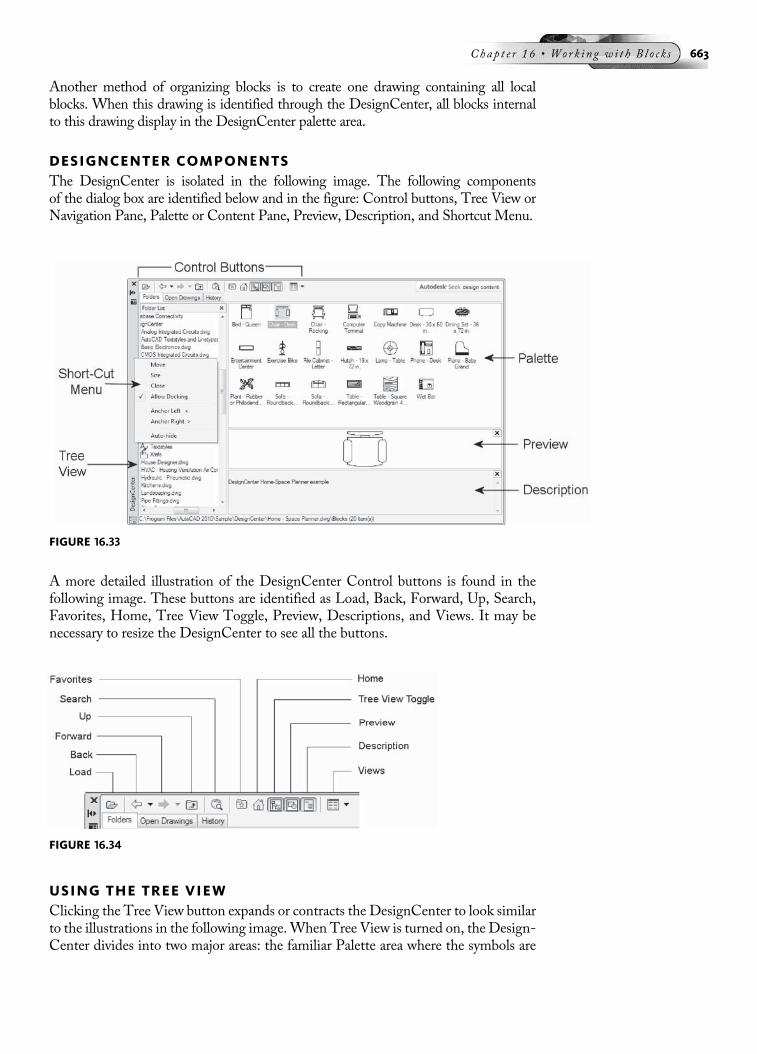
Another method of organizing blocks is to create one drawing containing all localblocks. When this drawing is identified through the DesignCenter, all blocks internalto this drawing display in the DesignCenter palette area.
DESIGNCENTER COMPONENTSThe DesignCenter is isolated in the following image. The following componentsof the dialog box are identified below and in the figure: Control buttons, Tree View orNavigation Pane, Palette or Content Pane, Preview, Description, and Shortcut Menu.
A more detailed illustration of the DesignCenter Control buttons is found in thefollowing image. These buttons are identified as Load, Back, Forward, Up, Search,Favorites, Home, Tree View Toggle, Preview, Descriptions, and Views. It may benecessary to resize the DesignCenter to see all the buttons.
USING THE TREE VIEWClicking the Tree View button expands or contracts the DesignCenter to look similarto the illustrations in the following image.When Tree View is turned on, the Design-Center divides into two major areas: the familiar Palette area where the symbols are
FIGURE 16.33
FIGURE 16.34
Chap t e r 16 • Work in g w i t h B l o c k s 663
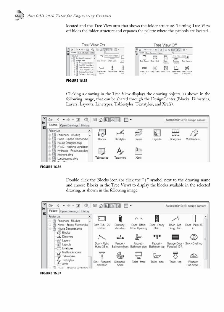
located and the Tree View area that shows the folder structure. Turning Tree Viewoff hides the folder structure and expands the palette where the symbols are located.
Clicking a drawing in the Tree View displays the drawing objects, as shown in thefollowing image, that can be shared through the DesignCenter (Blocks, Dimstyles,Layers, Layouts, Linetypes, Tablestyles, Textstyles, and Xrefs).
Double-click the Blocks icon (or click the “þ” symbol next to the drawing nameand choose Blocks in the Tree View) to display the blocks available in the selecteddrawing, as shown in the following image.
FIGURE 16.35
FIGURE 16.36
FIGURE 16.37
664 Au t oCAD 2010 Tu t o r f o r Eng in e e r i n g Graph i c s

INSERTING BLOCKS THROUGH THE DESIGNCENTERThe following image displays a typical floor plan drawing along with the Design-Center (docked to the left side of the screen), showing the blocks identified in thecurrent drawing. If no blocks are found internal to the drawing, the Palette area willbe empty.
The DesignCenter operates on the “drag and drop” principle. Select the desired blocklocated in the Palette area of the DesignCenter, drag it out, and drop it into the de-sired location of the drawing. The following image shows a queen-size bed draggedand dropped into the bedroom area of the floor plan.
When performing a basic drag and drop operation with the left mouse button, all youhave to do is identify where the block is located and drop it into that location (the useof running object snaps can ensure that the blocks are dropped in a specific location).What if the block needs to be scaled or rotated? If the drag and drop method is per-formed with the right mouse button, a shortcut menu is provided, as shown in thefollowing image. Selecting Insert Block from the shortcut menu displays the Insertdialog box, covered earlier in this chapter, which allows you to specify different scaleand rotation values. The following image shows a rocking chair inserted and rotatedinto position in the corner of the room. Instead of dragging the block with the rightmouse button, double-click the block in the Palette area and the Insert dialog box isprovided immediately.
FIGURE 16.38
FIGURE 16.39
Chap t e r 16 • Work in g w i t h B l o c k s 665
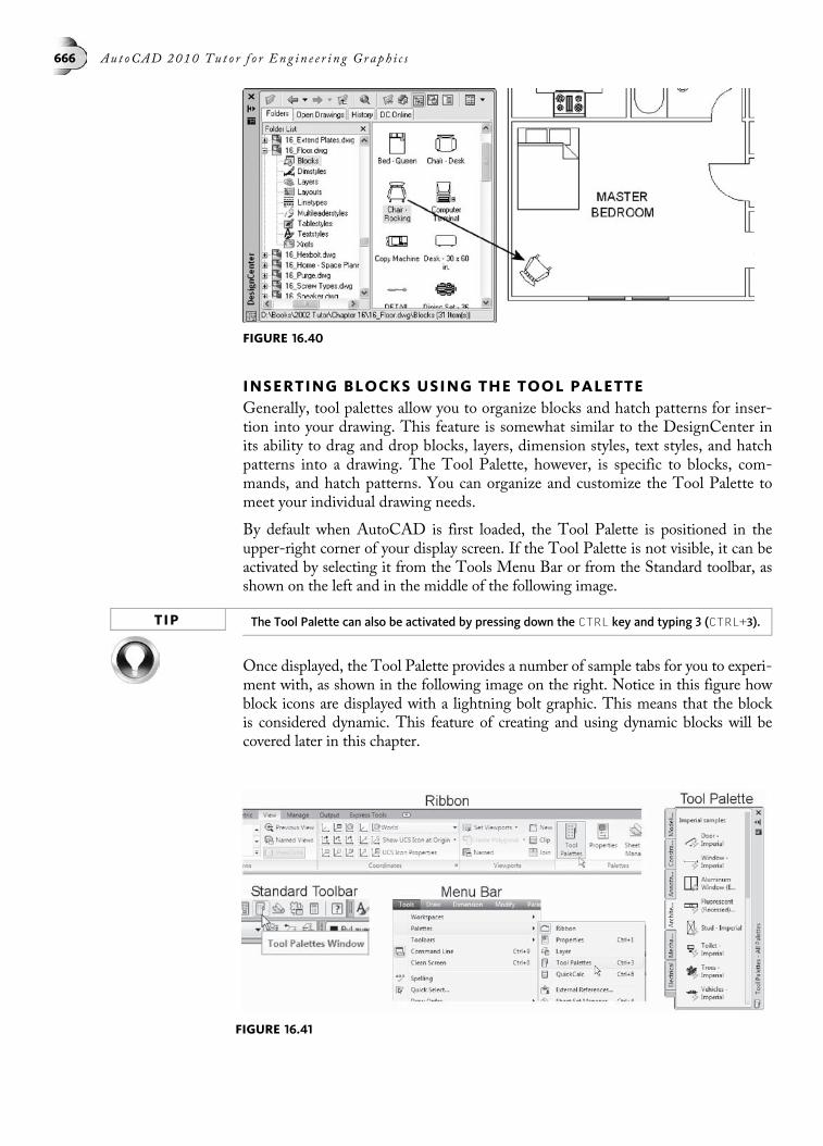
INSERTING BLOCKS USING THE TOOL PALETTEGenerally, tool palettes allow you to organize blocks and hatch patterns for inser-tion into your drawing. This feature is somewhat similar to the DesignCenter inits ability to drag and drop blocks, layers, dimension styles, text styles, and hatchpatterns into a drawing. The Tool Palette, however, is specific to blocks, com-mands, and hatch patterns. You can organize and customize the Tool Palette tomeet your individual drawing needs.
By default when AutoCAD is first loaded, the Tool Palette is positioned in theupper-right corner of your display screen. If the Tool Palette is not visible, it can beactivated by selecting it from the Tools Menu Bar or from the Standard toolbar, asshown on the left and in the middle of the following image.
TIP The Tool Palette can also be activated by pressing down the CTRL key and typing 3 (CTRL+3).
Once displayed, the Tool Palette provides a number of sample tabs for you to experi-ment with, as shown in the following image on the right. Notice in this figure howblock icons are displayed with a lightning bolt graphic. This means that the blockis considered dynamic. This feature of creating and using dynamic blocks will becovered later in this chapter.
FIGURE 16.40
FIGURE 16.41
666 Au t oCAD 2010 Tu t o r f o r Eng in e e r i n g Graph i c s

Additional tool palettes are available to assist in your design capabilities. To accessthese extra palettes, click the area located in the lower-left corner of any tool palette,as shown in the following image. A long list activates alongside the existing palette.A number of the palettes consist of blocks that can be dragged and dropped into adrawing. Other palettes such as Lighting and Cameras deal with the 3D renderingmodule contained in AutoCAD. Notice also a number of material palettes. Thesealso deal with 3D rendering.
Illustrated in the following image is an example of placing hatch patterns. In thisexample, a concrete pattern is dragged from the Tool Palette, as shown in the fol-lowing image on the right, and dropped into a closed area of your drawing, as inthe fireplace hearth illustrated in the figure. The results are shown in the followingimage, with the hatching pattern applied to the closed area.
The Tool Palette has a number of very powerful features to automate its operation.For example, in the following image, a Vehicles symbol is selected. Right-clickingthis block activates a shortcut menu. The following options are available:
Cut—Cutting the block from the Tool Palette to the Windows clipboard
Copy—Copying the block to the Windows clipboard
Delete—Deleting this block from the Tool Palette
Rename—Changing the name of this block in the Tool Palette
Properties—Changing the properties of this block in the Tool Palette
FIGURE 16.42
FIGURE 16.43
Chap t e r 16 • Work in g w i t h B l o c k s 667

The Properties option allows you to modify the object’s properties to suit yourspecific needs. Select the Properties option, as shown in the following image onthe left. This activates the Tool Properties dialog box, as shown in the middle ofthe following image. All the information in the fields can be changed and appliedto this symbol. For example, suppose you need to change the insertion scale of thisblock for a number of drawings. Changing the scale in the Tool Properties dialogbox changes the block’s scale as it is inserted into the drawing. This feature is alsoavailable for hatch patterns when using the Tool Palette. Scrolling down this dialogbox displays a heading for Custom Properties. In the illustration in the followingimage on the right, numerous versions of the block are displayed. This is becausethe item selected was constructed as a dynamic block.
Creating a New Tool PaletteThe process for creating new tool palettes is very easy and straightforward. First,right-click anywhere inside the Tool Palette to display the menu illustrated in thefollowing image on the left. Options of this Tool Palette menu include:
Allow Docking—Allows the Tool Palette to be docked to the sides of your dis-play screen. Removing the check disables this feature.
Auto-Hide—When checked, this feature collapses the Tool Palette so onlythe thin blue strip is displayed. When you move your cursor over the blue strip,the Tool Palette redisplays.
Transparency—Activates a Transparency dialog box, which controls theopaqueness of the Tool Palette.
View Options—Activates the View Options dialog box, which controls the sizeof the hatch and block icons and whether the icon is labeled or not.
Delete Tool Palette—Deletes the Tool Palette. A warning dialog box appearsasking whether you really want to perform this operation.
Rename Tool Palette—Renames the Tool Palette.
Customize—Activates the Customize dialog box, which allows you to create anew Tool Palette.
New Palette—Creates a blank Tool Palette.
FIGURE 16.44
668 Au t oCAD 2010 Tu t o r f o r Eng in e e r i n g Graph i c s

Click the New Palette option, as shown in the following image on the left. Thisautomatically creates a blank Tool Palette. As illustrated in the following image onthe right, a new Tool Palette name, Electrical, has been entered in the field.
Once the Tool Palette name is entered, a tab is created for this palette, as shown inthe following image on the right. To add blocks and hatch patterns to this new pal-ette, activate the DesignCenter, search for the folder that contains the symbols youwish to place in the Tool Palette, and drag and drop these blocks or hatch patternsfrom the DesignCenter into the Tool Palette, as shown in the following image onthe left.
If you want to create a new Tool Palette from one whole drawing in the Design-Center, activate the DesignCenter and go to the drawing that contains the blocks.Right-clicking this drawing displays the menu, as shown in the following image onthe left. Clicking the Create Tool Palette option creates the Tool Palette using thesame name as the DesignCenter drawing. The new Tool Palette contains all blocksfrom this drawing, as shown in the following image on the right.
FIGURE 16.45
FIGURE 16.46
Chap t e r 16 • Work in g w i t h B l o c k s 669
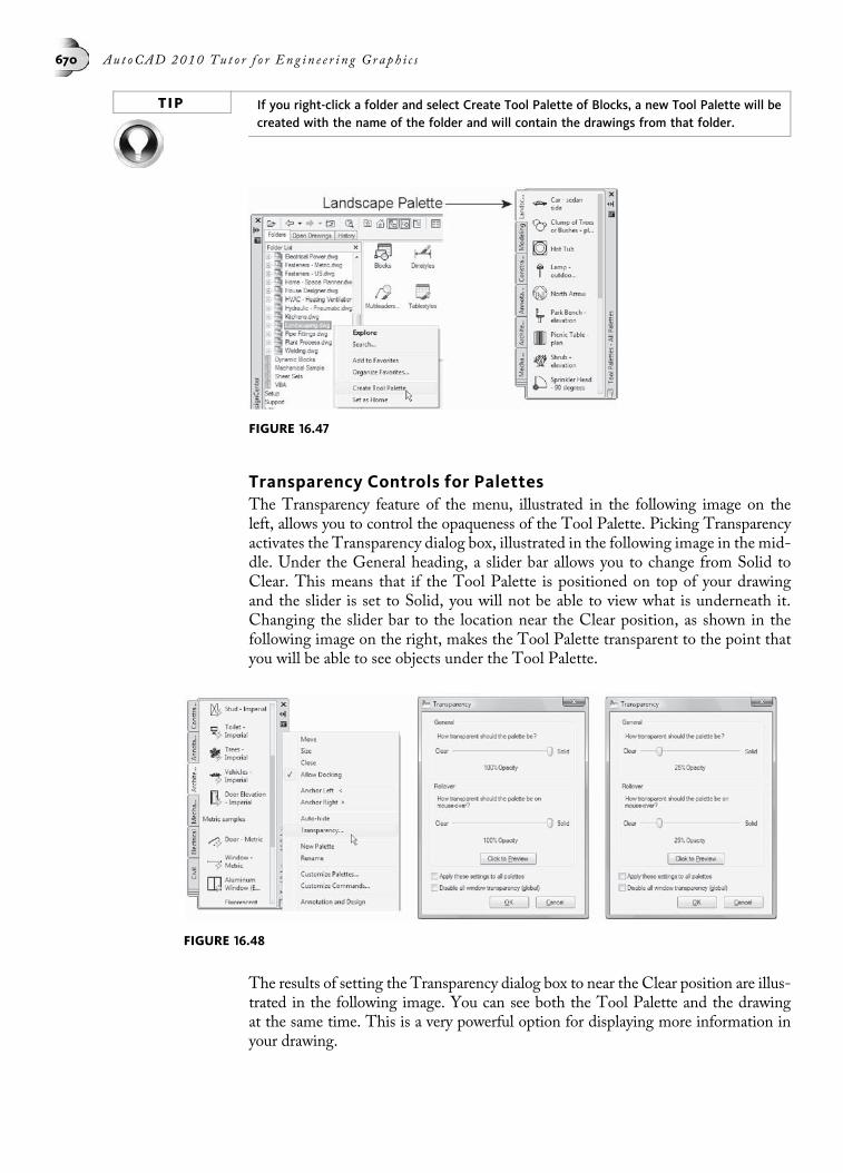
TIP If you right-click a folder and select Create Tool Palette of Blocks, a new Tool Palette will becreated with the name of the folder and will contain the drawings from that folder.
Transparency Controls for PalettesThe Transparency feature of the menu, illustrated in the following image on theleft, allows you to control the opaqueness of the Tool Palette. Picking Transparencyactivates the Transparency dialog box, illustrated in the following image in the mid-dle. Under the General heading, a slider bar allows you to change from Solid toClear. This means that if the Tool Palette is positioned on top of your drawingand the slider is set to Solid, you will not be able to view what is underneath it.Changing the slider bar to the location near the Clear position, as shown in thefollowing image on the right, makes the Tool Palette transparent to the point thatyou will be able to see objects under the Tool Palette.
The results of setting the Transparency dialog box to near the Clear position are illus-trated in the following image. You can see both the Tool Palette and the drawingat the same time. This is a very powerful option for displaying more information inyour drawing.
FIGURE 16.47
FIGURE 16.48
670 Au t oCAD 2010 Tu t o r f o r Eng in e e r i n g Graph i c s

WORKING WITH MULTIPLE DRAWINGSThe Multiple Design Environment allows users to open multiple drawings withina single session of AutoCAD, as shown in the following image. This feature, likeDesignCenter, allows the sharing of data between drawings. You can easily copyand move objects, such as blocks, from one drawing to another.
Opening Multiple DrawingsRepeat the OPEN command as many times as necessary to open all drawings you willneed. In fact, you can select multiple drawings in the Select File dialog box by holdingdown CTRL or SHIFT as you select the files, as shown in the following image.
FIGURE 16.49
FIGURE 16.50
Chap t e r 16 • Work in g w i t h B l o c k s 671

Once the drawings are open, use CTRLþF6 or CTRLþTAB to switch back and forthbetween the drawings. To efficiently work between drawings, you may wish to tile orcascade the drawing windows utilizing the Window Menu Bar, as shown inthe following image. A list of all the open drawings is displayed at the bottom of theWindow Menu Bar. Selecting one of the file names is another convenient way toswitch between drawings. Remember to use the CLOSE command (Window or FileMenu Bar) to individually close any drawings that are not being used. To close alldrawings in a single operation, the CLOSEALL command (Window Menu Bar) canbe used. If changes were made to any of the drawings, you will be prompted to savethose changes before the drawing closes.
FIGURE 16.51
FIGURE 16.52
672 Au t oCAD 2010 Tu t o r f o r Eng in e e r i n g Graph i c s
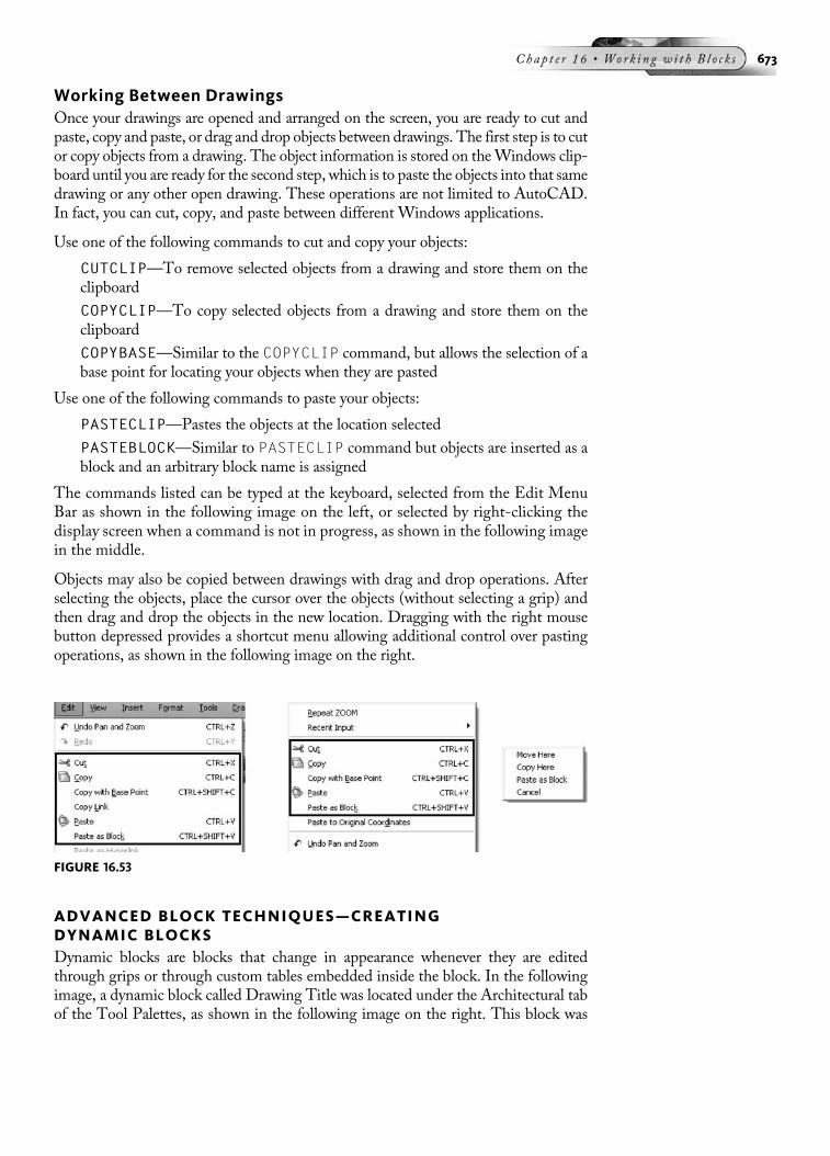
Working Between DrawingsOnce your drawings are opened and arranged on the screen, you are ready to cut andpaste, copy and paste, or drag and drop objects between drawings. The first step is to cutor copy objects from a drawing. The object information is stored on theWindows clip-board until you are ready for the second step, which is to paste the objects into that samedrawing or any other open drawing. These operations are not limited to AutoCAD.In fact, you can cut, copy, and paste between different Windows applications.
Use one of the following commands to cut and copy your objects:
CUTCLIP—To remove selected objects from a drawing and store them on theclipboard
COPYCLIP—To copy selected objects from a drawing and store them on theclipboard
COPYBASE—Similar to the COPYCLIP command, but allows the selection of abase point for locating your objects when they are pasted
Use one of the following commands to paste your objects:
PASTECLIP—Pastes the objects at the location selected
PASTEBLOCK—Similar to PASTECLIP command but objects are inserted as ablock and an arbitrary block name is assigned
The commands listed can be typed at the keyboard, selected from the Edit MenuBar as shown in the following image on the left, or selected by right-clicking thedisplay screen when a command is not in progress, as shown in the following imagein the middle.
Objects may also be copied between drawings with drag and drop operations. Afterselecting the objects, place the cursor over the objects (without selecting a grip) andthen drag and drop the objects in the new location. Dragging with the right mousebutton depressed provides a shortcut menu allowing additional control over pastingoperations, as shown in the following image on the right.
ADVANCED BLOCK TECHNIQUES—CREATINGDYNAMIC BLOCKSDynamic blocks are blocks that change in appearance whenever they are editedthrough grips or through custom tables embedded inside the block. In the followingimage, a dynamic block called Drawing Title was located under the Architectural tabof the Tool Palettes, as shown in the following image on the right. This block was
FIGURE 16.53
Chap t e r 16 • Work in g w i t h B l o c k s 673

then dragged and dropped into the drawing. Clicking this block displays the normalinsertion point grip. However, notice a second grip, which appears as an arrowpointing in the right direction. This grip identifies a stretching action associatedwith the dynamic block. When you click this arrow and move your cursor, thatportion of the dynamic block changes, giving the block a different appearancewithout redefining or exploding the block. In this example, the arrow grip is de-signed to stretch the line. Notice also that dynamic blocks are identified in theTool Palette by the appearance of a lightning bolt icon.
The creation process begins with the Block Editor. This can be accessed by double-clicking the block, which displays the Edit Block Definitions dialog box. This is thesame dialog box used when redefining a block. You select the block name from the listand click the OK button. At this point, you enter the Block Editor environment, asshown in the following image. It is here that you make assignments to the dynamicblock. The first step is to assign a parameter to the block. In the following image, aLinear Parameter was selected from the list of parameters in the toolbar and assignedto the geometry, in this case a line segment. This parameter usually is named Dis-tance by default. In this example, the default name was renamed to a term withmore meaning, Title Line Length. The Properties Palette is used for this renamingtask. Once a parameter is present in the Block Editor, an action item such as Stretchis linked to the parameter. It is the action item that allows the block to change whenedited back in the drawing editor. In this example, two action items are present,namely, Stretch and Move. The Stretch action allows the line to be stretched todifferent lengths. The Move action is required in order to move the VPSCALEattribute along with the line as it is being stretched.
FIGURE 16.54
674 Au t oCAD 2010 Tu t o r f o r Eng in e e r i n g Graph i c s

When you are satisfied with the parameter and action assignments and wish to testthe features out on the block, you first click the Save button to save the changes to theblock name and then click the Close Block Editor button, as shown in the followingimage, to return to the drawing editor. Notice in the following image that all BlockAuthoring commands can either be found in the Ribbon or through the AutoCADClassic workspace.
FIGURE 16.55
FIGURE 16.56
Chap t e r 16 • Work in g w i t h B l o c k s 675
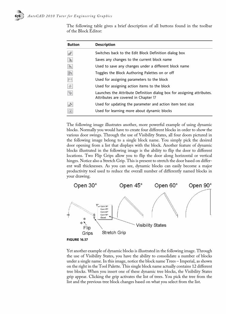
The following table gives a brief description of all buttons found in the toolbarof the Block Editor:
Button Description
Switches back to the Edit Block Definition dialog box
Saves any changes to the current block name
Used to save any changes under a different block name
Toggles the Block Authoring Palettes on or off
Used for assigning parameters to the block
Used for assigning action items to the block
Launches the Attribute Definition dialog box for assigning attributes.Attributes are covered in Chapter 17
Used for updating the parameter and action item text size
Used for learning more about dynamic blocks
The following image illustrates another, more powerful example of using dynamicblocks. Normally you would have to create four different blocks in order to show thevarious door swings. Through the use of Visibility States, all four doors pictured inthe following image belong to a single block name. You simply pick the desireddoor opening from a list that displays with the block. Another feature of dynamicblocks illustrated in the following image is the ability to flip the door to differentlocations. Two Flip Grips allow you to flip the door along horizontal or verticalhinges. Notice also a Stretch Grip. This is present to stretch the door based on differ-ent wall thicknesses. As you can see, dynamic blocks can easily become a majorproductivity tool used to reduce the overall number of differently named blocks inyour drawing.
Yet another example of dynamic blocks is illustrated in the following image. Throughthe use of Visibility States, you have the ability to consolidate a number of blocksunder a single name. In this image, notice the block name Trees – Imperial, as shownon the right in the Tool Palette. This single block name actually contains 12 differenttree blocks. When you insert one of these dynamic tree blocks, the Visibility Statesgrip appear. Clicking the grip activates the list of trees. You pick the tree from thelist and the previous tree block changes based on what you select from the list.
FIGURE 16.57
676 Au t oCAD 2010 Tu t o r f o r Eng in e e r i n g Graph i c s

The following table gives a brief description of each dynamic block grip.
DynamicBlock Grip Name Description
Insertion Grip The original grip that displays at the insertionpoint of a block; can also be used for moving theblock to a new location
Lengthen Allows the block to be lengthened or shortenedby stretching, scaling, or arraying
Alignment Positions or aligns the block based on an object;the positioning occurs when you move the blocknear the object
Flip Allows the entire block or items inside the blockto be flipped
Rotate Allows the entire block or items inside the blockto be rotated
List Allows you to choose from a list of items
Before you begin the process of designing dynamic blocks, here are a few items toconsider:
• For what intended purpose are you designing this dynamic block?
• How do you want this block to change when it is being edited?
• What parameters are needed in order to create changes in the block?
• What actions need to be assigned to the parameters?
• Do you need the block to contain various size values in order to make incrementalchanges?
• Do you want to organize various blocks under a single name and control what isdisplayed through Visibility States?
• Do you want to create a table consisting of different values and change the size ofa block through the table?
FIGURE 16.58
Chap t e r 16 • Work in g w i t h B l o c k s 677
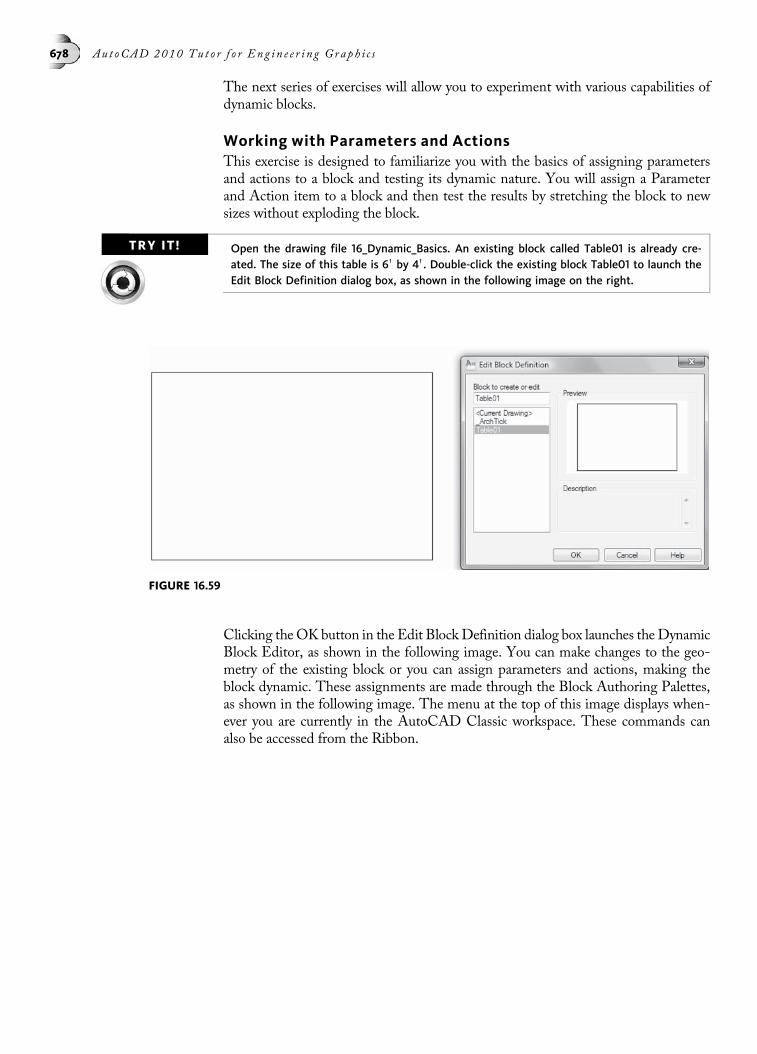
The next series of exercises will allow you to experiment with various capabilities ofdynamic blocks.
Working with Parameters and ActionsThis exercise is designed to familiarize you with the basics of assigning parametersand actions to a block and testing its dynamic nature. You will assign a Parameterand Action item to a block and then test the results by stretching the block to newsizes without exploding the block.
TRY IT! Open the drawing file 16_Dynamic_Basics. An existing block called Table01 is already cre-ated. The size of this table is 6 0 by 4 0. Double-click the existing block Table01 to launch theEdit Block Definition dialog box, as shown in the following image on the right.
Clicking the OK button in the Edit Block Definition dialog box launches the DynamicBlock Editor, as shown in the following image. You can make changes to the geo-metry of the existing block or you can assign parameters and actions, making theblock dynamic. These assignments are made through the Block Authoring Palettes,as shown in the following image. The menu at the top of this image displays when-ever you are currently in the AutoCAD Classic workspace. These commands canalso be accessed from the Ribbon.
FIGURE 16.59
678 Au t oCAD 2010 Tu t o r f o r Eng in e e r i n g Graph i c s
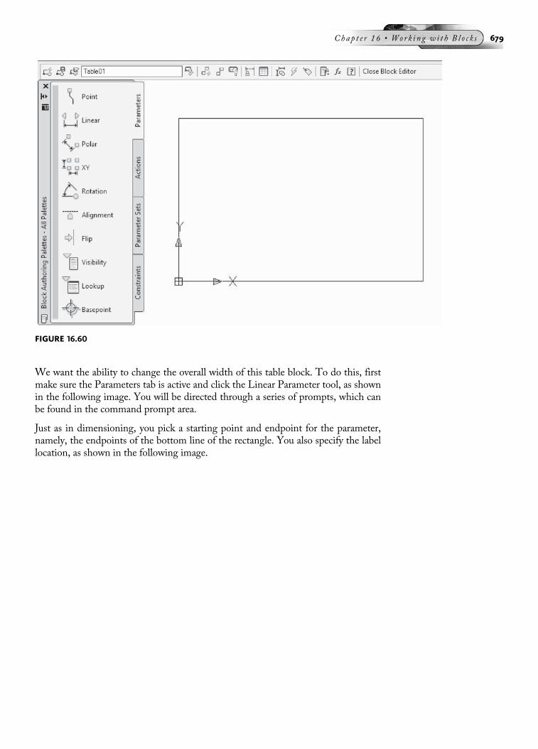
We want the ability to change the overall width of this table block. To do this, firstmake sure the Parameters tab is active and click the Linear Parameter tool, as shownin the following image. You will be directed through a series of prompts, which canbe found in the command prompt area.
Just as in dimensioning, you pick a starting point and endpoint for the parameter,namely, the endpoints of the bottom line of the rectangle. You also specify the labellocation, as shown in the following image.
FIGURE 16.60
Chap t e r 16 • Work in g w i t h B l o c k s 679
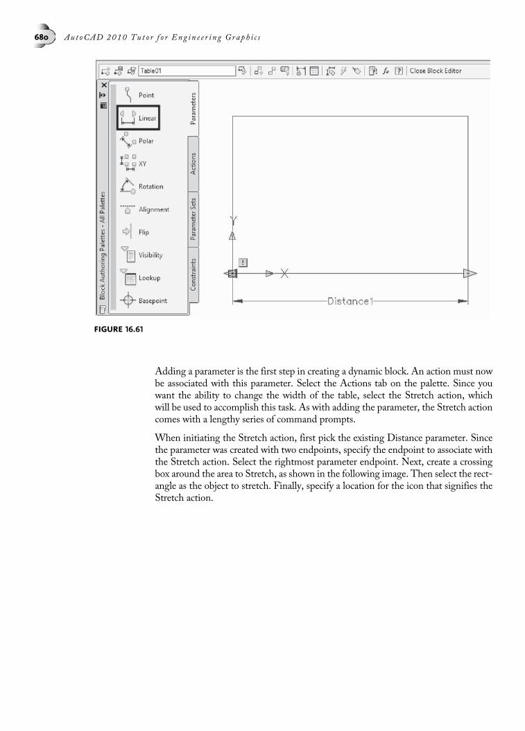
Adding a parameter is the first step in creating a dynamic block. An action must nowbe associated with this parameter. Select the Actions tab on the palette. Since youwant the ability to change the width of the table, select the Stretch action, whichwill be used to accomplish this task. As with adding the parameter, the Stretch actioncomes with a lengthy series of command prompts.
When initiating the Stretch action, first pick the existing Distance parameter. Sincethe parameter was created with two endpoints, specify the endpoint to associate withthe Stretch action. Select the rightmost parameter endpoint. Next, create a crossingbox around the area to Stretch, as shown in the following image. Then select the rect-angle as the object to stretch. Finally, specify a location for the icon that signifies theStretch action.
FIGURE 16.61
680 Au t oCAD 2010 Tu t o r f o r Eng in e e r i n g Graph i c s

The following image illustrates all the components that make up the dynamicblock. The Stretch icon should be positioned near the side of the object the actionoccurs at. Notice also the Alert icon. One more action needs to be created in orderfor the Alert icon to disappear. For the purposes of this exercise, we will not needan additional action because we will be stretching this rectangle only to the right.When you are finished assigning parameters and actions, click the Save BlockDefinition button to save these changes to the block. To return to the drawingeditor, click the Close Block Editor button.
FIGURE 16.62
Chap t e r 16 • Work in g w i t h B l o c k s 681
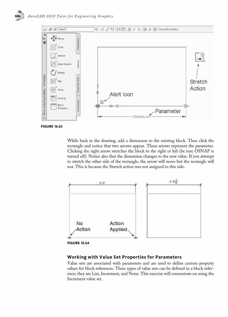
While back in the drawing, add a dimension to the existing block. Then click therectangle and notice that two arrows appear. These arrows represent the parameter.Clicking the right arrow stretches the block to the right or left (be sure OSNAP isturned off). Notice also that the dimension changes to the new value. If you attemptto stretch the other side of the rectangle, the arrow will move but the rectangle willnot. This is because the Stretch action was not assigned to this side.
Working with Value Set Properties for ParametersValue sets are associated with parameters and are used to define custom propertyvalues for block references. Three types of value sets can be defined in a block refer-ence; they are List, Increment, and None. This exercise will concentrate on using theIncrement value set.
FIGURE 16.63
FIGURE 16.64
682 Au t oCAD 2010 Tu t o r f o r Eng in e e r i n g Graph i c s

TRY IT!Open the drawing file 16_Dynamic_Value_Sets. We will be using the same table block fromthe previous Try It! exercise. However, instead of stretching the table to the right at ran-dom lengths, we want to better control the stretching operation. We want to stretch thistable in increments of 6 00. We also do not want the table to get narrower than 4 0 or widerthan 8 0. We will be able to control these items through the Value Set associated with theDistance parameter.
Double-click the block to activate the Edit Block Definition dialog box and click theOK button to enter the Block Authoring environment. Use the Properties commandto activate the Properties Palette, and click the Distance parameter. Change theparameter name from Distance to Table Width, as shown in the following image.This gives the parameter a more meaningful name. Actions can also be renamedthrough the Properties Palette.
With the Properties Palette active and the Table Width parameter selected, scrolldown to the bottom of the Properties Palette and notice the Value Set category. It ishere that you activate one of the three Value Set types. For this example, make theIncrement type active. This also displays other information related to this type.Change the Distance Increment field to 6 00, change the Distance Minimum fieldto 4 0, and change the Distance Maximum field to 8 0, as shown in the followingimage. As you make these changes, notice the appearance of tick marks signifyingthese three values.
FIGURE 16.65
Chap t e r 16 • Work in g w i t h B l o c k s 683
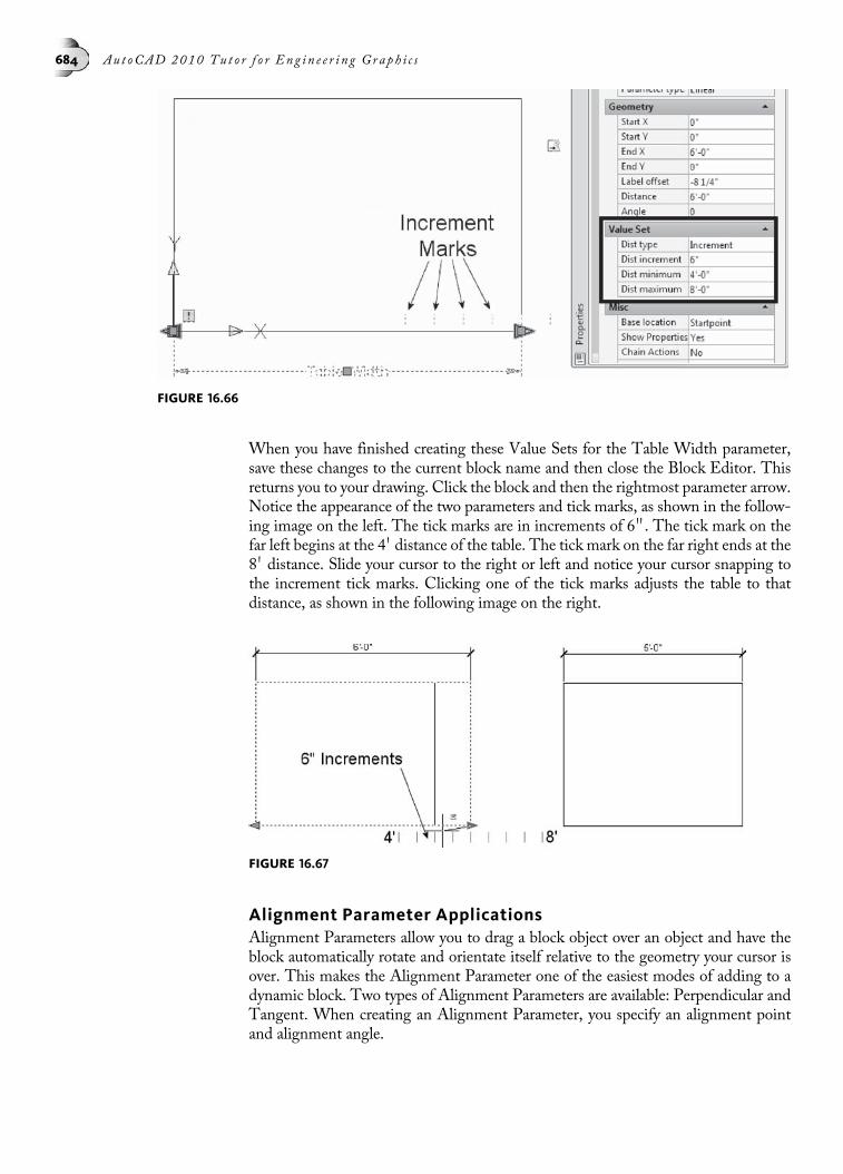
When you have finished creating these Value Sets for the Table Width parameter,save these changes to the current block name and then close the Block Editor. Thisreturns you to your drawing. Click the block and then the rightmost parameter arrow.Notice the appearance of the two parameters and tick marks, as shown in the follow-ing image on the left. The tick marks are in increments of 6 00. The tick mark on thefar left begins at the 4 0 distance of the table. The tick mark on the far right ends at the8 0 distance. Slide your cursor to the right or left and notice your cursor snapping tothe increment tick marks. Clicking one of the tick marks adjusts the table to thatdistance, as shown in the following image on the right.
Alignment Parameter ApplicationsAlignment Parameters allow you to drag a block object over an object and have theblock automatically rotate and orientate itself relative to the geometry your cursor isover. This makes the Alignment Parameter one of the easiest modes of adding to adynamic block. Two types of Alignment Parameters are available: Perpendicular andTangent. When creating an Alignment Parameter, you specify an alignment pointand alignment angle.
FIGURE 16.66
FIGURE 16.67
684 Au t oCAD 2010 Tu t o r f o r Eng in e e r i n g Graph i c s

TRY IT!Open the drawing file 16_Dynamic_Alignment. A block of a sink is already defined in thisdrawing. Double-click the block to activate the Edit Block Definition dialog box, and clickthe OK button to enter the Block Authoring environment, as shown in the following image.
Before continuing, make the following preparations: turn on Polar, turn on and setOSNAP mode to Quadrant, and turn on OTRACK. Then click the AlignmentParameter tool in the Block Authoring Palette.
For the base point of the alignment, move your cursor over the top of the ellipse, trackstraight up, and enter a value of 2, as shown in the following image on the left. Forthe alignment direction,move your cursor to the right of the last knownpoint andpick ablankpartofyourscreen, as showninthemiddleof the following image.TheAlignmentParameter appears, as shown in the following image on the right. The AlignmentParameter being used for this application is Perpendicular.
FIGURE 16.68
FIGURE 16.69
Chap t e r 16 • Work in g w i t h B l o c k s 685

Saving this sink block and exiting the Block Editor returns you to the drawingeditor. Clicking the sink block, as shown in the following image on the left, exposesthe Perpendicular Alignment Parameter. Click this Alignment Parameter, moveyour cursor to any of the inner walls of the bathroom plan, and notice the sinkautomatically rotating at an angle perpendicular to the wall. When you are satisfiedwith the desired orientation, click to place the block, as shown in the followingimage on the right.
Scale and Angle Offset ApplicationsThis application of dynamic blocks allows you to increase or decrease the angle direc-tion of a part of the block relative to a parameter.
TRY IT! Open the drawing file 16_Dynamic_Offsets. Two door blocks are already defined in thisdrawing. Double-click the left door block to activate the Edit Block Definition dialog boxand click the OK button to enter the Block Authoring environment. Activate the LinearParameter. For the Start Point, click the bottom endpoint of the line, and for the End Point,click the bottom endpoint of the arc. Specify the label location below the door block; thelabel should read Distance.
Click the Distance Parameter you just created and activate the Properties Palette.In the palette, change the Property Label from Distance to Door Width. Under theValue Set area, change the Distance Type to Increment, change the Distance Incre-ment to 2 00, change the Distance Minimum to 1 0, and change the DistanceMaximumto 3 0. Refer to the illustration in the following image on the right for these changes.
FIGURE 16.70
686 Au t oCAD 2010 Tu t o r f o r Eng in e e r i n g Graph i c s

Next, activate the Scale Action, select Door Width as the parameter, and selectthe line and arc as the objects to scale. Press ENTER to continue. Specify the actionlocation, as shown in the following image on the right.
Click the Save Block Definition button to save these changes, and then click theClose Block Editor button to return to the drawing editor.
FIGURE 16.72
FIGURE 16.71
Chap t e r 16 • Work in g w i t h B l o c k s 687
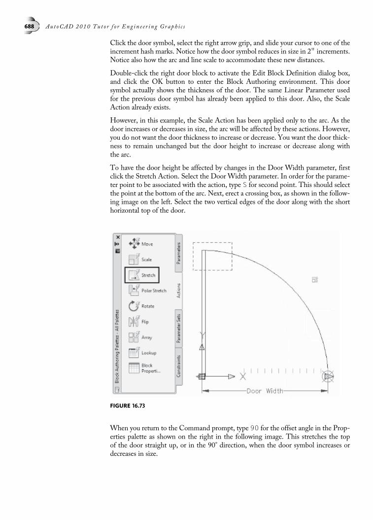
Click the door symbol, select the right arrow grip, and slide your cursor to one of theincrement hash marks. Notice how the door symbol reduces in size in 2 00 increments.Notice also how the arc and line scale to accommodate these new distances.
Double-click the right door block to activate the Edit Block Definition dialog box,and click the OK button to enter the Block Authoring environment. This doorsymbol actually shows the thickness of the door. The same Linear Parameter usedfor the previous door symbol has already been applied to this door. Also, the ScaleAction already exists.
However, in this example, the Scale Action has been applied only to the arc. As thedoor increases or decreases in size, the arc will be affected by these actions. However,you do not want the door thickness to increase or decrease. You want the door thick-ness to remain unchanged but the door height to increase or decrease along withthe arc.
To have the door height be affected by changes in the Door Width parameter, firstclick the Stretch Action. Select the Door Width parameter. In order for the parame-ter point to be associated with the action, type S for second point. This should selectthe point at the bottom of the arc. Next, erect a crossing box, as shown in the follow-ing image on the left. Select the two vertical edges of the door along with the shorthorizontal top of the door.
When you return to the Command prompt, type 90 for the offset angle in the Prop-erties palette as shown on the right in the following image. This stretches the topof the door straight up, or in the 90° direction, when the door symbol increases ordecreases in size.
FIGURE 16.73
688 Au t oCAD 2010 Tu t o r f o r Eng in e e r i n g Graph i c s
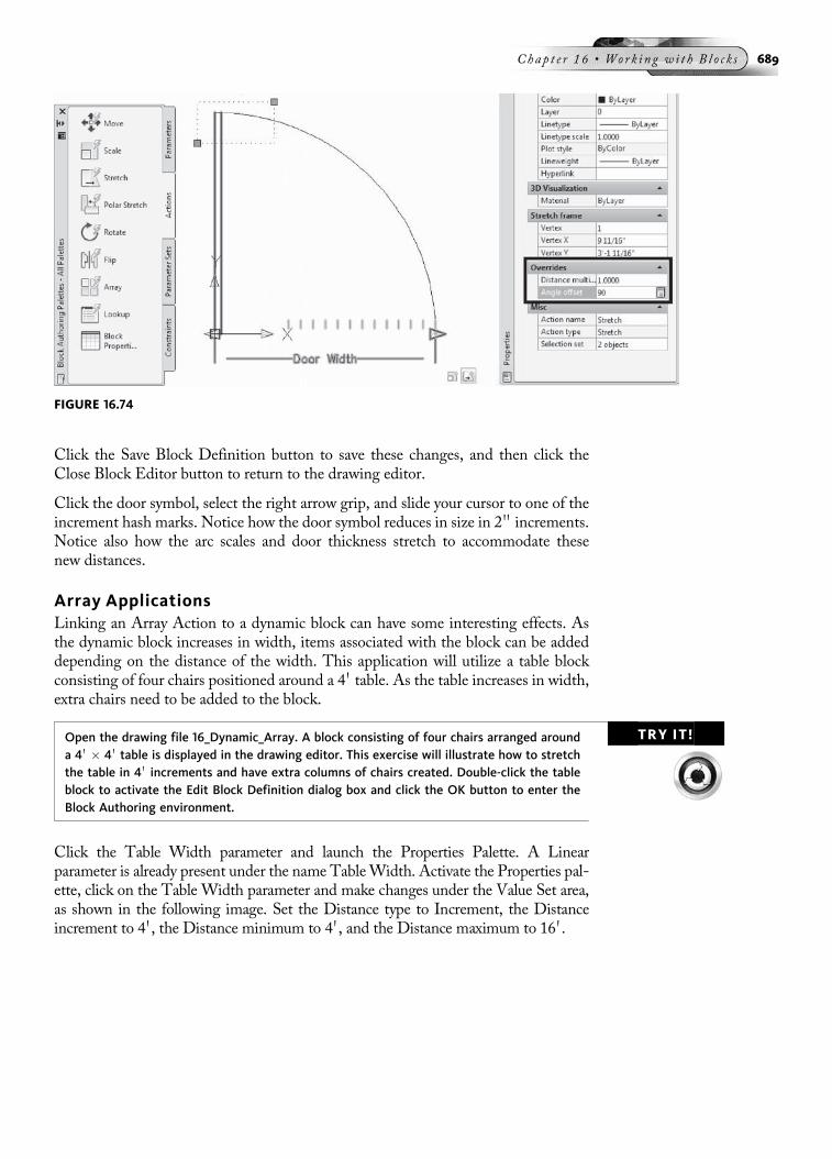
Click the Save Block Definition button to save these changes, and then click theClose Block Editor button to return to the drawing editor.
Click the door symbol, select the right arrow grip, and slide your cursor to one of theincrement hash marks. Notice how the door symbol reduces in size in 2 00 increments.Notice also how the arc scales and door thickness stretch to accommodate thesenew distances.
Array ApplicationsLinking an Array Action to a dynamic block can have some interesting effects. Asthe dynamic block increases in width, items associated with the block can be addeddepending on the distance of the width. This application will utilize a table blockconsisting of four chairs positioned around a 4 0 table. As the table increases in width,extra chairs need to be added to the block.
TRY IT!Open the drawing file 16_Dynamic_Array. A block consisting of four chairs arranged arounda 4 0 � 4 0 table is displayed in the drawing editor. This exercise will illustrate how to stretchthe table in 4 0 increments and have extra columns of chairs created. Double-click the tableblock to activate the Edit Block Definition dialog box and click the OK button to enter theBlock Authoring environment.
Click the Table Width parameter and launch the Properties Palette. A Linearparameter is already present under the name TableWidth. Activate the Properties pal-ette, click on the Table Width parameter and make changes under the Value Set area,as shown in the following image. Set the Distance type to Increment, the Distanceincrement to 4 0, the Distance minimum to 4 0, and the Distance maximum to 16 0.
FIGURE 16.74
Chap t e r 16 • Work in g w i t h B l o c k s 689

Next, assign a Stretch Action to the right end of the table and rightmost positionedchair, as shown in the following image. After activating the Stretch Action, pick theTable Width parameter. In order for the parameter point to associate with the action,type S for second point. Create a crossing box to surround the rightmost chair andright end of the table, and select the table and rightmost chair as the objects to stretch.Locate the Stretch Action icon in a convenient location of your screen.
If you experiment by stretching this new block in the drawing editor, you will findthat the table and rightmost chair stretch; however, the two chairs located in the 90°and 270° positions remain in their original positions. We want these two chairs to becopied or arrayed at a specified distance depending on how long the table stretches.To perform this operation, click the Array Action button back in the Block Author-ing editor. Select the Table Width parameter, select both chairs, as shown in thefollowing image, and enter a Column Width distance of 3 011 as the distance fromone chair to another. Locate the Array Action icon in a convenient screen location.
FIGURE 16.76
FIGURE 16.75
690 Au t oCAD 2010 Tu t o r f o r Eng in e e r i n g Graph i c s

Click the Save Block Definition button to save these changes, and then click theClose Block Editor button to return to the drawing editor.
When you return to the drawing editor, click the block of the table and chairs, pickthe right arrow grip as shown in the following image on the left, and begin stretchingthe table. For example, when you stretch the table to a new length of 8 0, two newcolumns of chairs are added. Stretch to a new length of 16 00 and your screen shouldappear similar to the illustration in the following image on the right.
Using Lookup Parameters and TablesA Lookup Parameter allows you to create a lookup property whose value is con-trolled by a table of custom properties located in the block. While inside this table,you add a series of different input properties that are tied directly to a single param-eter or multiple parameters assigned to the block. You also create lookup propertiesthat are tied to the input properties. These lookup properties appear as a list insidethe block once you return to the drawing editor. You then pick different lookupproperties from the list in order to make changes to the block. This concept ofcreating lookup properties will be demonstrated in the next Try It! exercise.
FIGURE 16.78
FIGURE 16.77
Chap t e r 16 • Work in g w i t h B l o c k s 691
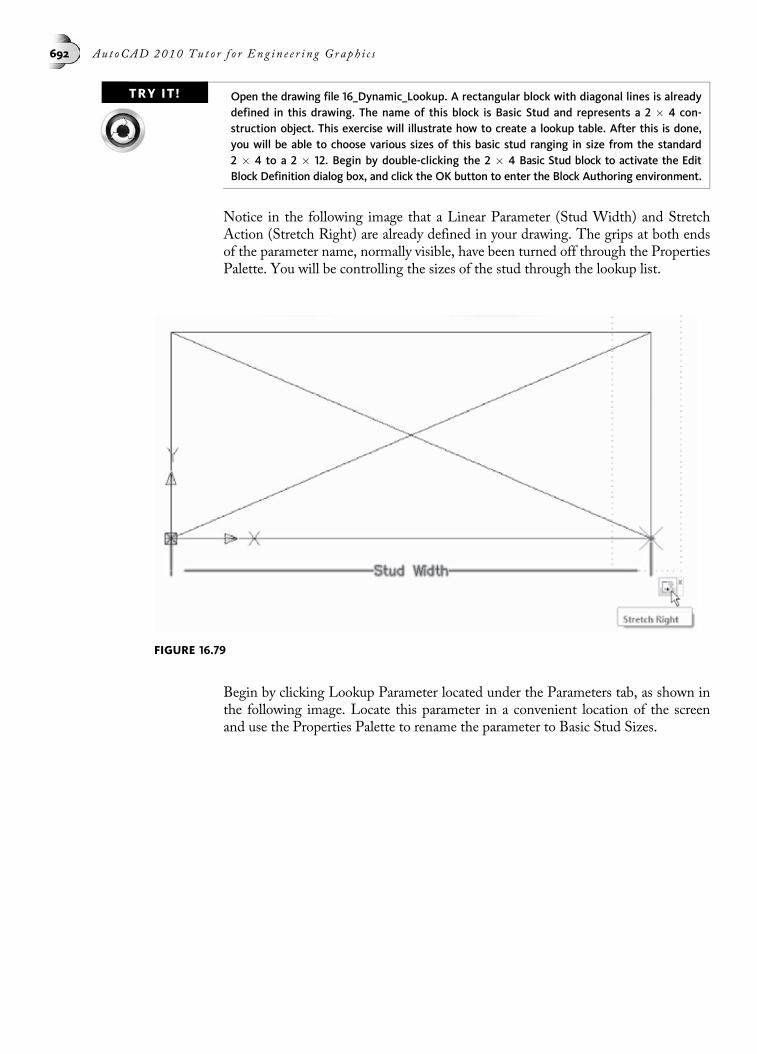
TRY IT! Open the drawing file 16_Dynamic_Lookup. A rectangular block with diagonal lines is alreadydefined in this drawing. The name of this block is Basic Stud and represents a 2 � 4 con-struction object. This exercise will illustrate how to create a lookup table. After this is done,you will be able to choose various sizes of this basic stud ranging in size from the standard2 � 4 to a 2 � 12. Begin by double-clicking the 2 � 4 Basic Stud block to activate the EditBlock Definition dialog box, and click the OK button to enter the Block Authoring environment.
Notice in the following image that a Linear Parameter (Stud Width) and StretchAction (Stretch Right) are already defined in your drawing. The grips at both endsof the parameter name, normally visible, have been turned off through the PropertiesPalette. You will be controlling the sizes of the stud through the lookup list.
Begin by clicking Lookup Parameter located under the Parameters tab, as shown inthe following image. Locate this parameter in a convenient location of the screenand use the Properties Palette to rename the parameter to Basic Stud Sizes.
FIGURE 16.79
692 Au t oCAD 2010 Tu t o r f o r Eng in e e r i n g Graph i c s

Create a Lookup Action item by selecting this item from the Block AuthoringPalette, as shown in the following image on the left. Associate this action with aparameter by picking the Basic Stud Sizes Lookup Parameter that you just createdin the previous step. Locate the Lookup Action next to the Basic Stud Sizes LookupParameter. After you select a screen position for the action location, the PropertyLookup Table dialog box appears, as shown in the following image on the right.Click the Add Properties button.
When the Add Parameter Properties dialog box appears, as shown in the followingimage on the left, notice the linear parameter listed. For this example, this is the onlyparameter that will be used. In more complicated Lookup Actions, you may havenumerous parameter names to choose from. For now, click the OK button to acceptthis parameter name.
This returns you to the Property Lookup Table dialog box. Notice the column forStud Width. Start entering the values for various stud widths, such as 3.5, 5.5, 7.5,9.5, and 11.5, as shown on the left side of this dialog box.
You also need to fill in the right column of the dialog box under the heading LookupProperties Basic Stud Sizes. These are the listings that will be visible when you returnto the drawing editor and test the Basic Stud block for its various sizes. Under this
FIGURE 16.81
FIGURE 16.80
Chap t e r 16 • Work in g w i t h B l o c k s 693

column, enter the following sizes; 2� 4, 2� 6, 2� 8, 2� 10, and 2� 12. Be certainthese correspond with the StudWidth values on the left side of the dialog box. Whenyou are finished, your dialog box should appear similar to the illustration in thefollowing image on the right.
When you return to the Block Editor screen, change the name of the Lookup Actionitem to Basic Stud Table. Save the block and close the Block Editor to return to thedrawing editor. Click the Block and notice the appearance of the Lookup Parameter.Click the down arrow in the Lookup grip and test the various Basic Stud Sizes bypicking them from the list, as shown in the following image.
Creating Dynamic Block TablesUsing Lookup tables is one way to display variations of the same part. Anothermethod is through block tables. However before using a block table, it is consideredgood practice to incorporate Constraint Parameters and Geometric Constraintsinto your design. This simplifies the number of parameters controlling the blockwhile at the same time using these parameters in equations and tables for creatingdifferent variations of an object. In the following image of the I-Beam, a number ofConstraint Parameters in the form of dimensions are present. These dimensionswere placed while in the Block Editor from the Constraints tab of the Block AuthoringPalette as shown in the following image on the left.
FIGURE 16.83
FIGURE 16.82
694 Au t oCAD 2010 Tu t o r f o r Eng in e e r i n g Graph i c s
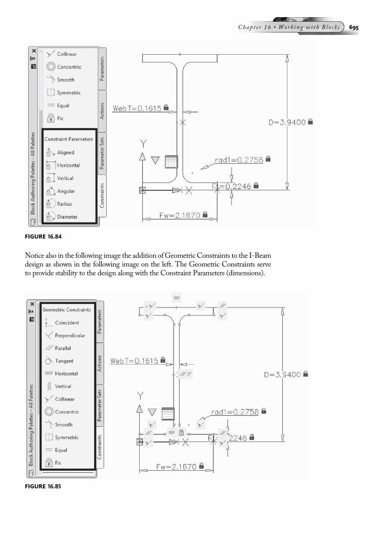
Notice also in the following image the addition ofGeometric Constraints to the I-Beamdesign as shown in the following image on the left. The Geometric Constraints serveto provide stability to the design along with the Constraint Parameters (dimensions).
FIGURE 16.84
FIGURE 16.85
Chap t e r 16 • Work in g w i t h B l o c k s 695

With the creation of theGeometric Constraints andConstraint Parameters (dimensions),the Parameters Manager dialog box is used to arrange the information for the purposeof making changes to the expressions and observing the affects on the I-Beam.
An evenmore efficientway of driving a dynamic block is through anExcel spread sheet.The same I-Beam is illustrated in the following image on the left. The spreadsheetgenerated inExcel.While in theBlockPropertiesTableon the right, youcaneasily copythe contents of theExcel spreadsheet andpaste it into thedialog box. Itmust bepointedout that the columnheaders at the topof theBlockPropertiesTabledialogbox (Size,D,Web7, Fw, and Ft) were all generated from the Parameters Manager in the previousimage. Also, the order of the parameters must match those in Excel.
FIGURE 16.86
FIGURE 16.87
696 Au t oCAD 2010 Tu t o r f o r Eng in e e r i n g Graph i c s

TUTORIAL EXERCISE: ELECTRICAL SCHEMATIC
PurposeThis tutorial is designed to lay out electrical blocks such as resistors, transistors, diodes,and switches to form an electrical schematic, as shown in the previous image.
System SettingsCreate a new drawing called ELECT_SYMB to hold the electrical blocks. Keep all defaultunits and limits settings. Set the grid and snap commands to 0.0750 units. This will beused to assist in the layout of the blocks. Once this drawing is finished, create anothernew drawing called ELECTRICAL_SCHEM1. This drawing will show the layout of an electri-cal schematic. Keep the default units but use the LIMITS command to set the upper-right corner of the display screen to (17.0000, 11.0000). Grid and snap do not have tobe set for this drawing.
LayersCreate the following layers for ELECTRICAL_SCHEM1 with the format:
Name Color Linetype
Border White Continuous
Blocks Red Continuous
Wires Blue Continuous
Suggested CommandsThis tutorial begins by creating a new drawing called ELECT_SYMB, which will hold allelectrical blocks. You will use the image below as a guide in drawing all electrical blocks.A grid with spacing 0.0750 would provide further assistance with the drawing of theblocks. Once all blocks are drawn, the BLOCK command is used to create blocks out ofthe individual blocks. You will save this drawing and create a new drawing file calledELECTRICAL_SCHEM1. The DesignCenter will be used to drag and drop the internal blocksfrom the drawing ELECT_SYMB into the new drawing, ELECTRICAL_SCHEM1. Finally, youwill connect all blocks with lines that represent wires and electrical connections, addblock identifiers, and save the drawing.
FIGURE 16.88
Chap t e r 16 • Work in g w i t h B l o c k s 697
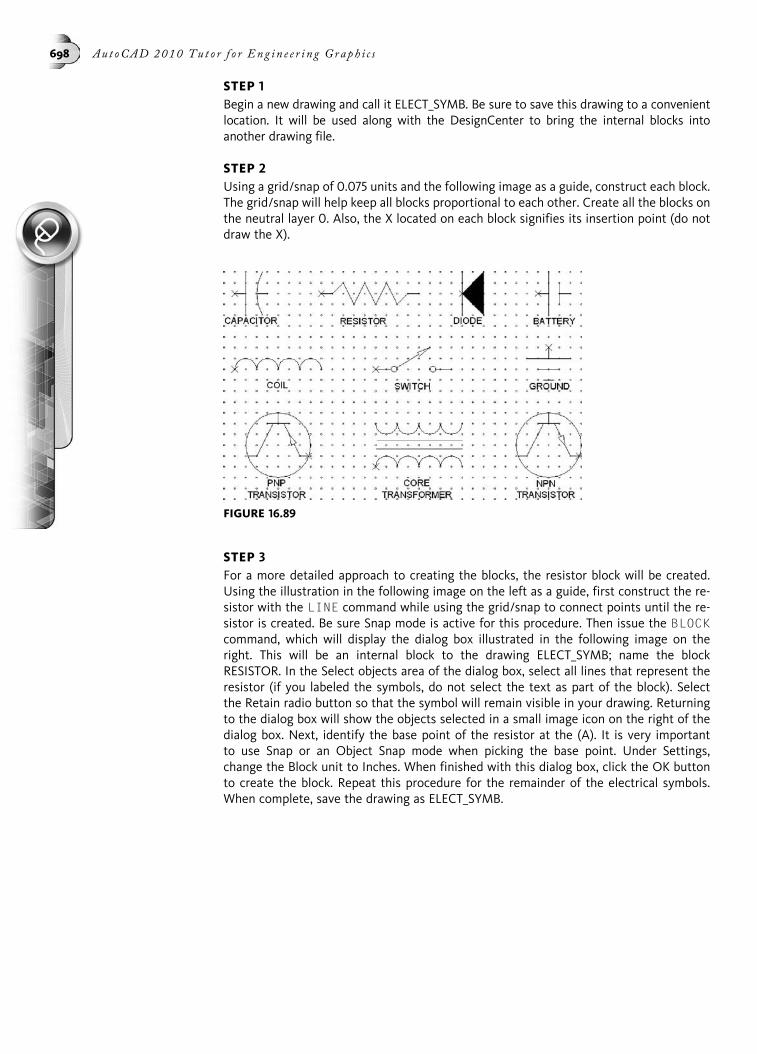
STEP 1Begin a new drawing and call it ELECT_SYMB. Be sure to save this drawing to a convenientlocation. It will be used along with the DesignCenter to bring the internal blocks intoanother drawing file.
STEP 2Using a grid/snap of 0.075 units and the following image as a guide, construct each block.The grid/snap will help keep all blocks proportional to each other. Create all the blocks onthe neutral layer 0. Also, the X located on each block signifies its insertion point (do notdraw the X).
STEP 3For a more detailed approach to creating the blocks, the resistor block will be created.Using the illustration in the following image on the left as a guide, first construct the re-sistor with the LINE command while using the grid/snap to connect points until the re-sistor is created. Be sure Snap mode is active for this procedure. Then issue the BLOCKcommand, which will display the dialog box illustrated in the following image on theright. This will be an internal block to the drawing ELECT_SYMB; name the blockRESISTOR. In the Select objects area of the dialog box, select all lines that represent theresistor (if you labeled the symbols, do not select the text as part of the block). Selectthe Retain radio button so that the symbol will remain visible in your drawing. Returningto the dialog box will show the objects selected in a small image icon on the right of thedialog box. Next, identify the base point of the resistor at the (A). It is very importantto use Snap or an Object Snap mode when picking the base point. Under Settings,change the Block unit to Inches. When finished with this dialog box, click the OK buttonto create the block. Repeat this procedure for the remainder of the electrical symbols.When complete, save the drawing as ELECT_SYMB.
FIGURE 16.89
698 Au t oCAD 2010 Tu t o r f o r Eng in e e r i n g Graph i c s

STEP 4Begin another new drawing called ELECTRICAL_SCHEM1. Activate the DesignCenter.Click the Tree View icon and expand the DesignCenter to display the folders on yourhard drive. Locate the correct folder in which the drawing ELECT_SYMB was saved andclick it. Double-click ELECT_SYMB and select Blocks to display the internal blocks, as illus-trated in the following image. These internal blocks can now be inserted in any AutoCADdrawing file.
STEP 5Make the Blocks layer current and begin dragging and dropping the blocks into thedrawing, as shown in the following image. Double-clicking an image of a block located inthe DesignCenter launches the Insert dialog box should you need to change the scale orrotation angle of the block. In the case of the electrical schematic, it is not critical to placethe blocks exactly, because they are moved to better locations when connected to linesthat represent wires.
FIGURE 16.90
FIGURE 16.91
Chap t e r 16 • Work in g w i t h B l o c k s 699

STEP 6Make the Wires layer current and begin connecting all the blocks to form the schematic,as shown in the following image. Some type of Object Snap mode such as Endpoint orInsert must be used for the wire lines to connect exactly with the endpoints of the blocks.If spaces get tight or if the blocks look too crowded, move the block to a better locationand continue drawing lines to form the schematic. Hint: The STRETCH command is a fastand easy way to reposition the blocks without having to reconnect the wires.
STEP 7Add text (place it on the Blocks layer) identifying all resistors, transistors, diodes, andswitches by number. The text height used was 0.12; however, this could vary dependingon the overall size of your schematic. Also, certain areas of the schematic show connec-tions with the presence of a dot at the intersection of the connection. Use the DONUTcommand with an inside diameter of 0.00 and an outside diameter of 0.075. Place donutson the Wires layer in all locations, as shown in the following image.
FIGURE 16.92
FIGURE 16.93
700 Au t oCAD 2010 Tu t o r f o r Eng in e e r i n g Graph i c s
TUTORIAL EXERCISE: 16_DYNAMIC_SWITCH_PLATE.DWG
PurposeThis tutorial is designed to link an Array action to a dynamic block. As the dynamic blockincreases in width, items associated with the block can be added, depending on the width.
System SettingsNo special system settings need to be made for this exercise.
LayersNo special layers need to be created for this exercise.
Suggested CommandsThis application will utilize a switch plate consisting of a basic rectangular shape andthree openings: two circular openings that represent screw holes and a rectangular open-ing used to accept the switch. As the switch plate increases in width, extra openings willautomatically be added to the block.
FIGURE 16.94
FIGURE 16.95
Chap t e r 16 • Work in g w i t h B l o c k s 701
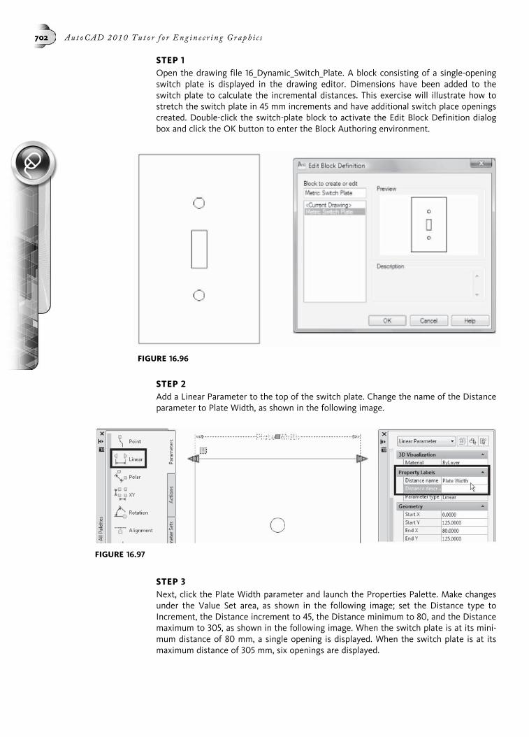
STEP 1Open the drawing file 16_Dynamic_Switch_Plate. A block consisting of a single-openingswitch plate is displayed in the drawing editor. Dimensions have been added to theswitch plate to calculate the incremental distances. This exercise will illustrate how tostretch the switch plate in 45 mm increments and have additional switch place openingscreated. Double-click the switch-plate block to activate the Edit Block Definition dialogbox and click the OK button to enter the Block Authoring environment.
STEP 2Add a Linear Parameter to the top of the switch plate. Change the name of the Distanceparameter to Plate Width, as shown in the following image.
STEP 3Next, click the Plate Width parameter and launch the Properties Palette. Make changesunder the Value Set area, as shown in the following image; set the Distance type toIncrement, the Distance increment to 45, the Distance minimum to 80, and the Distancemaximum to 305, as shown in the following image. When the switch plate is at its mini-mum distance of 80 mm, a single opening is displayed. When the switch plate is at itsmaximum distance of 305 mm, six openings are displayed.
FIGURE 16.96
FIGURE 16.97
702 Au t oCAD 2010 Tu t o r f o r Eng in e e r i n g Graph i c s
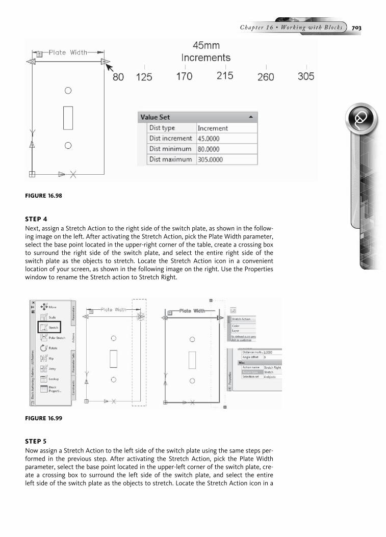
STEP 4Next, assign a Stretch Action to the right side of the switch plate, as shown in the follow-ing image on the left. After activating the Stretch Action, pick the Plate Width parameter,select the base point located in the upper-right corner of the table, create a crossing boxto surround the right side of the switch plate, and select the entire right side of theswitch plate as the objects to stretch. Locate the Stretch Action icon in a convenientlocation of your screen, as shown in the following image on the right. Use the Propertieswindow to rename the Stretch action to Stretch Right.
STEP 5Now assign a Stretch Action to the left side of the switch plate using the same steps per-formed in the previous step. After activating the Stretch Action, pick the Plate Widthparameter, select the base point located in the upper-left corner of the switch plate, cre-ate a crossing box to surround the left side of the switch plate, and select the entireleft side of the switch plate as the objects to stretch. Locate the Stretch Action icon in a
FIGURE 16.99
FIGURE 16.98
Chap t e r 16 • Work in g w i t h B l o c k s 703

convenient location of your screen, as shown in the following image. Use the Propertieswindow to rename the Stretch action to Stretch Left.
STEP 6If you experiment by stretching this new block back in the drawing editor, you will findthat the switch plate will stretch; however, the screw holes and switch opening will re-main in their original positions. We want these openings to be copied or arrayed at aspecified distance, depending on how much the switch plate stretches. To perform thisoperation, click the Array Action button back in the Block Authoring editor. Select thePlate Width parameter, select all three openings, as shown in the following image, andenter a Column Width distance of 45 mm as the distance from one set of openings toanother. Locate the Array Action icon in a convenient screen location.
Click the Save Block Definition button to save these changes, and then click the CloseBlock Editor button to return to the drawing editor.
STEP 7When you return to the drawing editor, click the block of the switch plate, pick the rightarrow grip, and begin stretching the switch plate. When you stretch the switch plate to anew length of 305 mm, which represents the maximum distance, a series of six switch
FIGURE 16.101
FIGURE 16.100
704 Au t oCAD 2010 Tu t o r f o r Eng in e e r i n g Graph i c s

openings are created, as shown on the right in the following image on the right. Thiscompletes this tutorial exercise on creating a dynamic block of a switch plate.
TUTORIAL EXERCISE: 16_DYNAMIC_ELECTRICAL LIST.DWG
PurposeThis tutorial is designed to create visibility states to have numerous electrical symbolscontained in a single block name.
System SettingsNo special system settings need to be made for this tutorial.
LayersNo special layers need to be created for this tutorial.
Suggested CommandsThe concept of creating visibility states in dynamic blocks begins with the creation ofa block using the Edit Block Definition dialog box. You then create a visibility state whileinside the Block Authoring environment. During this process, you insert an electricalsymbol and immediately explode it into individual objects. You then enter the VisibilityStates dialog box and change the name of the current state to match that of the electricalsymbol. You then create a new visibility state, name this state the next electrical symbol,and hide all existing objects in this new state. When you return to the Block Authoringenvironment, you insert the next electrical symbol, explode it, and follow the same pro-cess for arranging a number of electrical symbols in the same visibility state, as shown inthe following image.
FIGURE 16.102
Chap t e r 16 • Work in g w i t h B l o c k s 705

STEP 1Before creating visibility states, you must create a new general block name that will holdall individual electrical symbols. You must also enter the block editor to create the visibil-ity states. First, click the Block Editor button located in the Standard toolbar or theRibbon, as shown in the following image on the left. When the Edit Block Definition dia-log box appears, as shown in the following image on the right, enter Electrical Symbolsas the block name and click the OK button. This action opens the new block name inthe Block Editor.
STEP 2Insert the first block, called Battery, in the Block Editor, as shown in the following image.Use an insertion point of 0,0. In fact, all individual electrical blocks will be inserted at 0,0for consistency. Once the block appears in the Block Editor, use the EXPLODE commandto break up the block into individual objects. Then, locate the Visibility Parameter in theParameters tab of the Block Authoring Palette and place the marker to the right andbelow the battery symbol, as shown in the following image.
FIGURE 16.103
FIGURE 16.104
706 Au t oCAD 2010 Tu t o r f o r Eng in e e r i n g Graph i c s
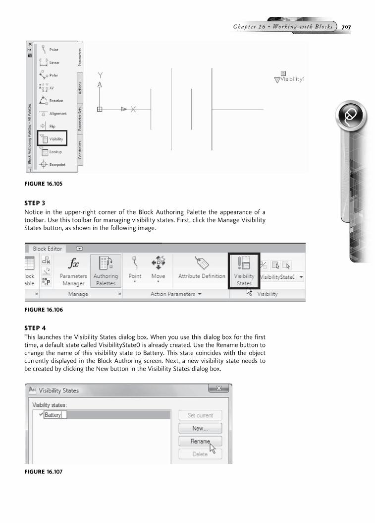
STEP 3Notice in the upper-right corner of the Block Authoring Palette the appearance of atoolbar. Use this toolbar for managing visibility states. First, click the Manage VisibilityStates button, as shown in the following image.
STEP 4This launches the Visibility States dialog box. When you use this dialog box for the firsttime, a default state called VisibilityState0 is already created. Use the Rename button tochange the name of this visibility state to Battery. This state coincides with the objectcurrently displayed in the Block Authoring screen. Next, a new visibility state needs tobe created by clicking the New button in the Visibility States dialog box.
FIGURE 16.105
FIGURE 16.106
FIGURE 16.107
Chap t e r 16 • Work in g w i t h B l o c k s 707

STEP 5This launches the New Visibility State dialog box, as shown in the following image on theleft. In the Visibility state name field, enter the name Capacitor. Also, be sure to checkthe radio button next to Hide all existing objects in new state. This will hide all objectswhen you return to the Block Editor. Click the OK button to continue.
STEP 6When you return to the Block Editor, insert the block Capacitor at an insertion point of0,0 and explode the block back into its individual objects. The objects that remain in theBlock Editor form the Capacitor visibility state.
Launch the Manage Visibility States dialog box again. Create another new visibility statecalled Circuit Breaker, and make sure Hide all existing objects in new state is selected.Insert the Circuit Breaker block at an insertion point of 0,0 and explode the block backinto its individual objects.
Repeat the procedure for creating more visibility states based on the other electricalblock symbols. Close the Block Editor and save the changes to the block.
Insert a Battery block in the drawing and test the visibility states by selecting them fromthe list, as shown in the following image on the right. If you created visibility states of allelectrical symbols, your list will be longer.
END OF CHAPTER PROBLEMS FOR CHAPTER 16Please refer to the CD that is supplied with this book and locate the file AutoCAD Tutor2010 Support Docs.pdf. In addition to extra information supplied in this chapter,end-of-chapter problems are also available to provide additional practice.
FIGURE 16.108
708 Au t oCAD 2010 Tu t o r f o r Eng in e e r i n g Graph i c s

CHAPTER
17
Working withAttributes
This chapter begins the study of how to create, display, edit, and extract attributes.Attributes consist of intelligent text data that is attached to a block. The data couldconsist of part description, part number, catalog number, and price. Whenever theblock is inserted in a drawing, you are prompted for information that, once entered,becomes attribute data. Attributes could also be associated with a title block for enter-ing such items as drawing name, who created, checked, revised, and approved thedrawing, drawing date, and drawing scale. Once included in the drawing, the attri-butes can be extracted and shared with other programs.
WHAT ARE ATTRIBUTES?An attribute may be considered a label that is attached to a block. This label is called atag and can contain any type of information that you desire. Examples of attributetags are illustrated in the following image on the left. The tags are RESISTANCE,PART_NAME, WATTAGE, and TOLERANCE. They relate to the particularsymbol they are attached to, in this case an electrical symbol of a resistor. Attributetags are placed in the drawing with the symbol. When the block, which includes thetags and symbol, is inserted, AutoCAD requests the values for the attributes. Thesame resistor with attribute values is illustrated in the following image on the right.When you create the attribute tags, you determine what information is requested, theactual prompts, and the default values for the information requested. Once the valuesare provided and inserted in the drawing, the information contained in the attributescan be displayed, extracted, and even shared with spreadsheet or database programs.
FIGURE 17.1
709

Once attributes are inserted in the drawing, the following additional tasks can beperformed on attributes:
1. Attributes can be turned on, turned off, or displayed normally through the use of theATTDISP command.
2. The individual attributes can be changed through the Enhanced Attribute Editor dia-log box, which is activated through the EATTEDIT command.
3. Attributes can be globally edited using the -ATTEDIT and find commands.4. Once edited, attributes can be extracted into tables or text files through the Data
Extraction wizard, which is activated by the DATAEXTRACTION command.5. The text file created by the attribute extraction process can be exported to a spread-
sheet or database program.
The following commands, which will be used throughout this chapter, assist in thecreation, editing, and manipulation of attributes:
ATTDEF—Activates the Attribute Definition dialog box used for the creation ofattributes
ATTDISP—Used to control the visibility of attributes in a drawing
-ATTEDIT—Used to edit attributes singly or globally; the hyphen (-) in front ofthe command activates prompts from the command line
FIND—Used to find and replace text including attribute values
BATTMAN—Activates the Block Attribute Manager dialog box, used to editattribute properties of a block definition
EATTEDIT—Activates the Enhanced Attribute Editor dialog box, used to editthe attributes of a block
EATTEXT—Activates the Attribute Extraction wizard, used to extract attributes
CREATING ATTRIBUTES THROUGH THEATTRIBUTE DEFINITION DIALOG BOXSelecting Define Attributes from the Block cascading menu on the Draw Menu Baror the Ribbon shown in the following image on the left, activates the AttributeDefinition dialog box, illustrated in the following image on the right. The followingcomponents of this dialog box will be explained in this section: Attribute Tag,Attribute Prompt, Attribute Default, and Attribute Mode.
FIGURE 17.2
710 Aut oCAD 2010 Tu t o r f o r Eng in e e r i n g Graph i c s

Attribute TagA tag is the name given to an attribute. Typical attribute tags could include PART_NAME, CATALOG_NUMBER, PRICE, DRAWING_NAME, and SCALE.The underscore is used to separate words because spaces are not allowed in tag names.
Attribute PromptThe attribute prompt is the text that appears on the text line when the block contain-ing the attribute is inserted in the drawing. If you want the prompt to be the same asthe tag name, enter a null response by leaving the Prompt field blank. If the Constantmode is specified for the attribute, the prompt area is not available.
Attribute DefaultThe attribute default is the default value displayed when the attribute is inserted inthe drawing. This value can be accepted or a new value entered as desired. The attri-bute value is handled differently if the attribute mode selected is Constant or Preset.
Attribute ModesInvisible—This mode is used to determine whether the label is invisible whenthe block containing the attribute is inserted in the drawing. If you later want tomake the attribute visible, you can use the ATTDISP command.
Constant—Use this mode to give every attribute the same value. This mightbe very useful when the attribute value is not subject to change. However, if youdesignate an attribute to contain a constant value, it is difficult to change itlater in the design process.
Verify—Use this mode to verify that every value is correct. This is accomplishedby prompting the user twice for the attribute value.
Reset—This allows for the presetting of values that can be changed. However,you are not prompted to enter the attribute value when inserting a block. Theattribute values are automatically set to their default values.
Lock Position—This mode locks the location of the attribute located inside ofthe block reference. When unlocked, the attribute can be moved relative to therest of the block using grips.
Multiple lines—Specifies that the attribute value can contain multiple linesof text.
NOTEThe effects caused by invoking the Verify and Preset modes are apparent only when theATTDIA system variable is off (the Enter Attributes dialog box is not displayed). When en-tering data at the command prompt, you will be asked twice for data that is to be verifiedand you will not be asked at all to supply data for attributes that are preset.
SYSTEM VARIABLES THAT CONTROL ATTRIBUTESATTREQDetermines whether the INSERT command uses default attribute settings duringinsertion of blocks. The following settings can be used:
0 No attribute values are requested; all attributes are set to their default values.
1 Turns on prompts or a dialog box for attribute values, as specified by attdia.
Command: ATTREQ
Enter new value for ATTREQ <1>:
Chap t e r 17 • Work in g w i t h A t t r i b u t e s 711

ATTMODEControls the display of attributes. The following settings can be used:
0 Off: Makes all attributes invisible.
1 Normal: Retains current visibility of each attribute; visible attributes aredisplayed, invisible attributes are not.
On: Makes all attributes visible.
Command: ATTMODE
Enter new value for ATTMODE <1>:
ATTDIAControls whether the INSERT command uses a dialog box for attribute value entry.The following settings can be used:
0 Issues prompts on the command line.
1 Initiates a dialog box for attribute value entry.
Command: ATTDIA
Enter new value for ATTDIA <1>:
TUTORIAL EXERCISE: B TITLE BLOCK.DWG
PurposeThis tutorial is designed to assign attributes to a title block. The completed drawing isillustrated in the previous image.
System SettingsBecause the drawings B Title Block and 17_Pulley Section are provided on the CD, all unitsand drawing limits have already been set.
FIGURE 17.3
712 Aut oCAD 2010 Tu t o r f o r Eng in e e r i n g Graph i c s

LayersAll layers have already been created for this drawing.
Suggested CommandsOpen the drawing B Title Block. Using the Attribute Definition dialog box (activatedthrough the attdef command), assign attributes consisting of the following tag names:DRAWING_NAME, DRAWN_BY, CHECKED_BY, APPROVED_BY, DATE, and SCALE. Savethis drawing file with its default name. Open the drawing 17_Pulley Section, insert thetitle block in this drawing, and answer the attribute prompts designed to complete the titleblock information.
STEP 1Open the drawing B Title Block and observe the title block area, shown in the followingimage. Various point objects are present to guide you in the placement of the attributeinformation. All points are located on the layer Points.
STEP 2Activate the Attribute Definition dialog box, as shown in the following image on the left.Leave all items unchecked in the Mode area of this dialog box with the exception of Lockposition. In the Attribute area, make the following changes: Enter DRAWING_NAME inthe Tag field. In the Prompt field, enter: What is the name of the drawing? In the Defaultfield, enter UNNAMED. In the Text Settings area, change the Justification to Middle andthe Height to 0.25 units. When finished, click the OK button. This returns you to yourdrawing. Using OSNAP-Node, pick the point at “A,” as shown in the following image inthe upper right. The DRAWING_NAME tag is added to the title block area, as shown inthe following image in the lower right.
FIGURE 17.4
Chap t e r 17 • Work in g w i t h A t t r i b u t e s 713

STEP 3To define the next attribute, activate the Attribute Definition dialog box, as shown in thefollowing image on the left. Leave all items unchecked in the Mode area of this dialog boxexcept for Lock position. In the Attribute area, make the following changes: EnterDRAWN_BY in the Tag field. In the Prompt field, enter: Who created this drawing? Inthe Default field, enter UNNAMED. In the Text Settings area, verify that Justification isset to Left, and change the Height to 0.12 units. When finished, click the OK button.This returns you to your drawing. Using OSNAP-Node, pick the point at “B,” as shown inthe following image in the upper right. The DRAWN_BY tag is added to the title blockarea, as shown in the following image in the lower right.
STEP 4Activate the Attribute Definition dialog box, as shown in the following image on the left.Leave all items unchecked in the Mode area of this dialog box except for Lock position. Inthe Attribute area, make the following changes: Enter CHECKED_BY in the Tag field. Inthe Prompt field, enter: Who will be checking this drawing? In the Default field, enterCHIEF DESIGNER. In the Text Settings area, verify that Justification is set to Left andthe Height is 0.12 units. When finished, click the OK button. This returns you to yourdrawing. Using OSNAP-Node, pick the point at “C,” as shown in the following image onthe upper right. The CHECKED_BY tag is added to the title block area, as shown in thefollowing image on the lower right.
FIGURE 17.5
FIGURE 17.6
714 Aut oCAD 2010 Tu t o r f o r Eng in e e r i n g Graph i c s

STEP 5Activate the Attribute Definition dialog box, as shown in the following image on the left.Leave all items unchecked in the Mode area of this dialog box except for Lock position. Inthe Attribute area, make the following changes: Enter APPROVED_BY in the Tag field. Inthe Prompt field, enter: Who will be approving this drawing? In the Default field, enterCHIEF ENGINEER. In the Text Settings area, verify that Justification is set to Left andthe Height is 0.12 units. When finished, click the OK button. This returns you to yourdrawing. Using OSNAP-Node, pick the point at “D,” as shown in the following image inthe upper right. The APPROVED_BY tag is added to the title block area, as shown in thefollowing image in the lower right.
STEP 6Activate the Attribute Definition dialog box, as shown in the following image on the left.Leave all items unchecked in the Mode area of this dialog box except for Lock position. Inthe Attribute area, make the following changes: Enter DATE in the Tag field. In thePrompt field, enter: When was this drawing completed? In the Default field, enterUNDATED. In the Text Settings area, verify that Justification is set to Left and the Heightis 0.12 units. When finished, click the OK button. This returns you to your drawing. UsingOSNAP-Node, pick the point at “E,” as shown in the following image in the upper right.The DATE tag is added to the title block area, as shown in the following image in thelower left.
FIGURE 17.7
FIGURE 17.8
Chap t e r 17 • Work in g w i t h A t t r i b u t e s 715

STEP 7Activate the Attribute Definition dialog box, as shown in the following image on the left.Leave all items unchecked in the Mode area of this dialog box except for Lock position. Inthe Attribute area, make the following changes: Enter SCALE in the Tag field. In thePrompt field, enter: What is the scale of this drawing? In the Default field, enter 1 5 1. Inthe Text Settings area, verify that Justification is set to Left and the Height is 0.12 units.When finished, click the OK button. This returns you to your drawing. Using OSNAP-Node, pick the point at “F,” as shown in the following image in the upper right. The SCALEtag is added to the title block area, as shown in the following image in the lower right.
You have now completed creating the attributes for the title block; turn off the Pointslayer. Close and save the changes to this drawing with its default name.
STEP 8To test the attributes and see how they function in a drawing, first open the drawing file17_Pulley Section. Notice that this image is viewed from inside a Layout (or Paper Space).The current page setup is based on the DWF6-ePlot.pc3 file, with the current sheet size asANSI Expand B (17.00 � 11.00 inches). The viewport that holds the two views of the Pul-ley has the No Plot state assigned in the Layer Properties Manager dialog box. You couldturn the Viewports layer off to hide the viewport if you prefer. You will now insert thetitle block with attributes in this drawing.
FIGURE 17.9
FIGURE 17.10
716 Aut oCAD 2010 Tu t o r f o r Eng in e e r i n g Graph i c s

Verify that the system variable ATTDIA is set to 1 (This can be typed in from thekeyboard). This allows you to enter your attribute values through the use of a dialogbox. Make the Title Block layer current and activate the Insert Block dialog box. Browsefor the Title Block drawing just created. Clear the Specify On-screen checkbox in the In-sertion point area. This automatically places the title block at the 0,0,0 location of thelayout, in the lower-left corner of the printable area indicators. Click OK. Before the titleblock can be placed, you must first fill in the boxes in the Edit Attributes dialog box, illus-trated in the following image (if this dialog box does not appear and you are prompted forvalues at the command line, it is because ATTDIA is set to 0). Complete all boxes; enterappropriate names and initials as directed.
NOTEPressing the TAB key is a quick way of moving from one box to another while inside anydialog box.
The completed drawing with title block and attributes inserted is illustrated in the follow-ing image.
FIGURE 17.11
Chap t e r 17 • Work in g w i t h A t t r i b u t e s 717
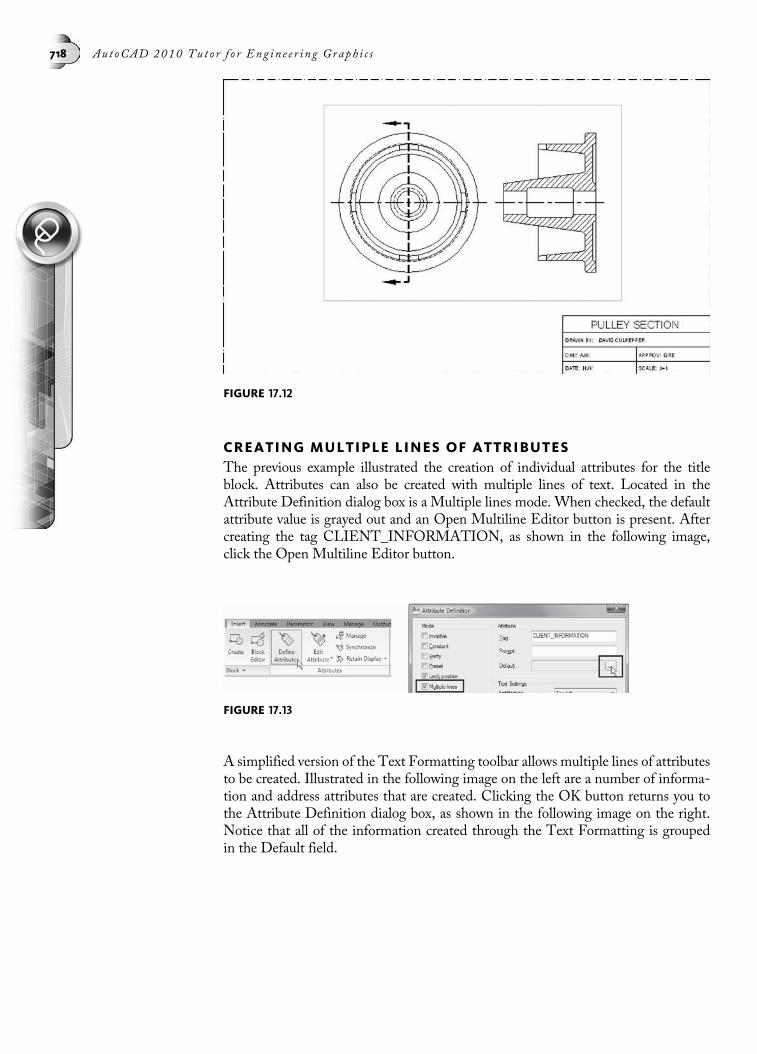
CREATING MULTIPLE LINES OF ATTRIBUTESThe previous example illustrated the creation of individual attributes for the titleblock. Attributes can also be created with multiple lines of text. Located in theAttribute Definition dialog box is a Multiple lines mode. When checked, the defaultattribute value is grayed out and an Open Multiline Editor button is present. Aftercreating the tag CLIENT_INFORMATION, as shown in the following image,click the Open Multiline Editor button.
A simplified version of the Text Formatting toolbar allows multiple lines of attributesto be created. Illustrated in the following image on the left are a number of informa-tion and address attributes that are created. Clicking the OK button returns you tothe Attribute Definition dialog box, as shown in the following image on the right.Notice that all of the information created through the Text Formatting is groupedin the Default field.
FIGURE 17.12
FIGURE 17.13
718 Aut oCAD 2010 Tu t o r f o r Eng in e e r i n g Graph i c s

After creating the multiple line attribute, the attribute tag is grouped with geometryand a new block definition is created, as shown in the following image that includesthe multiple line attribute.
When inserting the block containing the multiple line attribute, all lines of the attri-bute display as shown in the following image on the left. When an insertion pointis specified for the block, the Edit Attributes dialog box displays as shown in the fol-lowing image on the right. To change the various attribute fields, click the OpenMultiline Editor button.
FIGURE 17.15
FIGURE 17.16
FIGURE 17.14
Chap t e r 17 • Work in g w i t h A t t r i b u t e s 719

When the Text Formatting toolbar displays in the following image on the left,replace each field such as CLIENT NAME and CLIENT ADDRESS, with actualnames and locations, as shown in the following image on the right.
FIELDS AND ATTRIBUTESWhen defining attributes for a specific drawing object such as a title block, the attri-bute value can be converted into a field, as shown in the following image. In this fig-ure, the attribute tag (PROJECT_NAME) and prompt (What is the project name?)are created using conventional methods. Before entering a default value, click theInsert field button. This displays the Field dialog box. In this figure, the SheetSetfield category is being used to assign a description property called Project Name.
When you work with attribute values as fields, the actual default entry is illustrated,as shown in the following image. In this example, #### was inserted into this cellfrom the Field dialog box in the previous figure. When a title block that containsthis attribute is inserted into a drawing, you will be prompted to enter a new valuefor the PROJECT_NAME tag.
FIGURE 17.17
FIGURE 17.18
FIGURE 17.19
720 Aut oCAD 2010 Tu t o r f o r Eng in e e r i n g Graph i c s
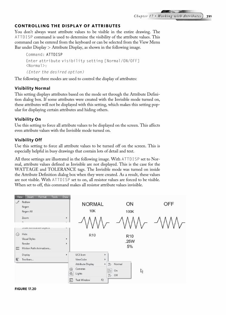
CONTROLLING THE DISPLAY OF ATTRIBUTESYou don’t always want attribute values to be visible in the entire drawing. TheATTDISP command is used to determine the visibility of the attribute values. Thiscommand can be entered from the keyboard or can be selected from the View MenuBar under Display > Attribute Display, as shown in the following image.
Command: ATTDISP
Enter attribute visibility setting [Normal/ON/OFF]<Normal>:
(Enter the desired option)
The following three modes are used to control the display of attributes:
Visibility NormalThis setting displays attributes based on the mode set through the Attribute Defini-tion dialog box. If some attributes were created with the Invisible mode turned on,these attributes will not be displayed with this setting, which makes this setting pop-ular for displaying certain attributes and hiding others.
Visibility OnUse this setting to force all attribute values to be displayed on the screen. This affectseven attribute values with the Invisible mode turned on.
Visibility OffUse this setting to force all attribute values to be turned off on the screen. This isespecially helpful in busy drawings that contain lots of detail and text.
All three settings are illustrated in the following image. With ATTDISP set to Nor-mal, attribute values defined as Invisible are not displayed. This is the case for theWATTAGE and TOLERANCE tags. The Invisible mode was turned on insidethe Attribute Definition dialog box when they were created. As a result, these valuesare not visible. With ATTDISP set to on, all resistor values are forced to be visible.When set to off, this command makes all resistor attribute values invisible.
FIGURE 17.20
Chap t e r 17 • Work in g w i t h A t t r i b u t e s 721

EDITING ATTRIBUTESA number of attribute tools in the form of dialog boxes are available to edit or makemodifications on attributes. Two commonly used tools are the Enhanced AttributeEditor dialog box and the Block Attribute Manager dialog box. The Enhanced At-tribute Editor dialog box can be displayed by selecting Object from theModifyMenuBar, followed by Attribute, and then Single, as shown in the following image. Thesetools can also be selected from the Modify II toolbar or from the Ribbon, also shownin the following image.
The following table gives a brief description of the Attribute modification toolsavailable.
Button Tool Command Function
Edit Attribute EATTEDIT Launches a dialog box designedto edit the attributes in a blockreference
Block AttributeManager
BATTMAN Launches a dialog box used formanaging attributes for blocksin the current drawing
SynchronizeAttributes
ATTSYNC Updates all instances of theselected block with the cur-rently defined attributeproperties
Data Extraction EATTEXT Exports the attributes found ina block reference out to a tableor external file
THE ENHANCED ATTRIBUTE EDITOR DIALOG BOXClick the Edit Attribute button that is found on the Ribbon to display the EnhancedAttribute Editor dialog box, as shown in the following image. This dialog box canalso be activated by entering EATTEDIT at the command prompt. In the image, theDryer block was selected. Notice that the attribute value is based on the selected tag.The value can then be modified in the Value field. To change to a different tag, selectit with your cursor. Notice that this dialog box has three tabs. The Attribute tab al-lows you to select the attribute tag that will be edited.
FIGURE 17.21
722 Aut oCAD 2010 Tu t o r f o r Eng in e e r i n g Graph i c s

NOTEDouble-clicking a block containing attribute values also launches the Enhanced AttributeEditor dialog box, illustrated in the previous image.
Clicking the Text Options tab displays the dialog box illustrated in the following im-age on the left. Use this area to change the properties of the text associated with theattribute tag selected, such as text style, justification, height, rotation, and so on.Once the changes are made, click the Apply button.
Clicking the Properties tab displays the dialog box illustrated in the following imageon the right. Use this area to change properties such as layer, color, lineweight, and soon. When you have completed the changes to the attribute, click the Apply button.
All three tabs of the Enhanced Attribute Editor dialog box have a Select block buttonvisible in the upper-right corner of each dialog box. Once you have edited a block, usethis button to select a different block for editing, if desired.
FIGURE 17.22
FIGURE 17.23
Chap t e r 17 • Work in g w i t h A t t r i b u t e s 723
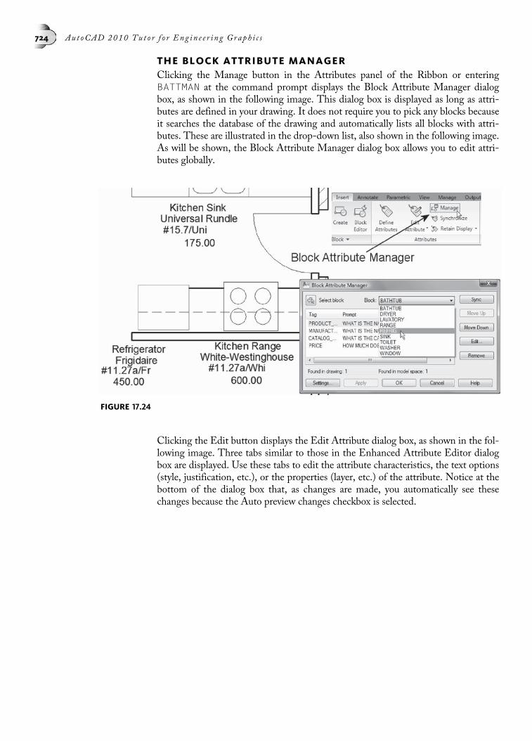
THE BLOCK ATTRIBUTE MANAGERClicking the Manage button in the Attributes panel of the Ribbon or enteringBATTMAN at the command prompt displays the Block Attribute Manager dialogbox, as shown in the following image. This dialog box is displayed as long as attri-butes are defined in your drawing. It does not require you to pick any blocks becauseit searches the database of the drawing and automatically lists all blocks with attri-butes. These are illustrated in the drop-down list, also shown in the following image.As will be shown, the Block Attribute Manager dialog box allows you to edit attri-butes globally.
Clicking the Edit button displays the Edit Attribute dialog box, as shown in the fol-lowing image. Three tabs similar to those in the Enhanced Attribute Editor dialogbox are displayed. Use these tabs to edit the attribute characteristics, the text options(style, justification, etc.), or the properties (layer, etc.) of the attribute. Notice at thebottom of the dialog box that, as changes are made, you automatically see thesechanges because the Auto preview changes checkbox is selected.
FIGURE 17.24
724 Aut oCAD 2010 Tu t o r f o r Eng in e e r i n g Graph i c s
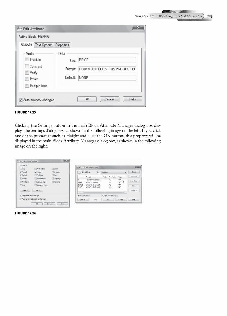
Clicking the Settings button in the main Block Attribute Manager dialog box dis-plays the Settings dialog box, as shown in the following image on the left. If you clickone of the properties such as Height and click the OK button, this property will bedisplayed in the main Block Attribute Manager dialog box, as shown in the followingimage on the right.
FIGURE 17.26
FIGURE 17.25
Chap t e r 17 • Work in g w i t h A t t r i b u t e s 725

TUTORIAL EXERCISE: 17_BLOCK ATTRIB MGR.DWG
PurposeThis tutorial is designed to modify the properties of all attributes with the Block AttributeManager dialog box, using the drawing illustrated in the previous image.
System SettingsAll units and drawing limits have already been set. Attributes have also been assigned tothe resistor block symbols.
LayersAll layers have already been created for this drawing.
Suggested CommandsThe Block Attribute Manager dialog box will be used to turn the Invisible mode on for anumber of attribute values. These changes will be automatically seen as they are made.
STEP 1Open the drawing file 17_Block Attrib Mgr, as shown in the previous image. The followingattribute tags need to have their Invisible modifier turned on: TYPE, TOLERANCE, andWATTAGE. Activate the Block Attribute Manager dialog box (BATTMAN command), asshown in the following image, and select the TYPE tag. Then click the Edit button.
FIGURE 17.27
FIGURE 17.28
726 Aut oCAD 2010 Tu t o r f o r Eng in e e r i n g Graph i c s

STEP 2This takes you to the Edit Attribute dialog box, as shown in the following image. In theAttribute tab, place a check next to the Invisible mode and click the OK button. Noticethat the changes are global and take place automatically. The attribute value WIREWOUNDis no longer visible for any of the resistor blocks.
STEP 3Turn the Invisible mode on for the TOLERANCE and WATTAGE tags. Your display should ap-pear similar to the following image, with all attributed tags invisible except for PART_NAME,and RESISTANCE.
FIGURE 17.30
FIGURE 17.29
Chap t e r 17 • Work in g w i t h A t t r i b u t e s 727

EDITING ATTRIBUTE VALUES GLOBALLYGlobal editing is used to edit multiple attributes at one time. The criteria you specifywill limit the set of attributes selected for editing. While the BATTMAN commandprovided a method to edit attribute properties, the FIND command can help youglobally edit specific attribute values.
Choose this command from the Edit Menu Bar, as shown in the following image onthe left. Clicking Find will display the Find and Replace dialog box as shown in thefollowing image on the right.
NOTE To ensure the FIND command will edit block attribute values, expand the Find and Replacedialog box and verify that a check is placed next to the block attribute value.
Let us examine how this process of globally editing attributes works through the Findand Replace dialog box. In the following image, suppose the tolerance value of 5%needs to be changed to 10% on all blocks containing this attribute value. You couldaccomplish this by editing the attributes one at a time. However, this could be timeconsuming especially if the edit affects a large number of attributes. A more produc-tive method would be to edit the group of attributes globally through the Find andReplace dialog box. Follow the examples below for accomplishing this task.
FIGURE 17.32
FIGURE 17.31
728 Aut oCAD 2010 Tu t o r f o r Eng in e e r i n g Graph i c s
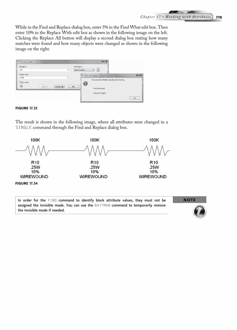
While in the Find and Replace dialog box, enter 5% in the FindWhat edit box. Thenenter 10% in the Replace With edit box as shown in the following image on the left.Clicking the Replace All button will display a second dialog box stating how manymatches were found and how many objects were changed as shown in the followingimage on the right.
The result is shown in the following image, where all attributes were changed in aSINGLE command through the Find and Replace dialog box.
NOTEIn order for the FIND command to identify block attribute values, they must not beassigned the Invisible mode. You can use the BATTMAN command to temporarily removethe Invisible mode if needed.
FIGURE 17.33
FIGURE 17.34
Chap t e r 17 • Work in g w i t h A t t r i b u t e s 729

TUTORIAL EXERCISE: 17_COMPUTERS.DWG
PurposeThis tutorial is designed to globally edit attribute values using the FIND command on thegroup of computers in the previous image.
System SettingsOpen the drawing 17_Computers. All units and drawing limits have already been set.Attributes have also been assigned to various computer components.
LayersAll layers have already been created for this drawing.
Suggested CommandsUtilize the FIND command to remove all dollar signs from the COST attribute values.This editing operation would be necessary if you needed to change the data in theCOST box from character to numeric values for an extraction operation (extracting attri-bute data will be discussed in more detail later in this chapter).
STEP 1Open the drawing 17_Computers. The following image shows an enlarged view of two ofthe computer workstations. For each workstation, $400 needs to be changed to 400, and$1300 needs to be changed to 1300. In other words, the dollar sign needs to be removedfrom all values for each workstation.
FIGURE 17.36
FIGURE 17.35
730 Aut oCAD 2010 Tu t o r f o r Eng in e e r i n g Graph i c s

STEP 2Launch the Find and Replace dialog box and enter $ in the Find What edit box. Then leavethe Replace With edit box empty as shown in the following image on the left. Clickingthe Replace All button will display a second dialog box stating how many matches werefound (16) and how many objects were changed (16) as shown in the following image onthe right.
The results are illustrated in the following image, with all dollar signs removed from allattribute values through the Find and Replace dialog box.
NOTEThe -ATTEDIT command is also available at the command line to globally edit all attributevalues and remove all dollar signs from all blocks. Pick this command from the Modify MenuBar by clicking on Object followed by Attribute and then Global. The command sequence islisted as follows:
Command: -ATTEDIT
Edit attributes one at a time? [Yes/No] <Y>: N (For No)
Performing global editing of attribute values.
Edit only attributes visible on screen? [Yes/No] <Y>:(Press ENTER to accept this default)
Enter block name specification <*>: (Press ENTER to acceptthis default)
Enter attribute tag specification <*>: COST
Enter attribute value specification <*>: (Press ENTER toaccept this default)
FIGURE 17.37
FIGURE 17.38
Chap t e r 17 • Work in g w i t h A t t r i b u t e s 731

Select Attributes: (Select all attributes using a windowselection box)
Select Attributes: (Press ENTER)
16 attributes selected.
Enter string to change: $
Enter new string: (Press ENTER; this removes the dollarsign from all attribute values)
REDEFINING ATTRIBUTESIf more sweeping changes need to be made to attributes, a mechanism exists that allowsyou to redefine the attribute tag information globally. You follow a process similar toredefining a block, and the attribute values are also affected. A few examples of whyyou would want to redefine attributes might be to change their mode status (Invisible,Constant, etc.), change the name of a tag, reword a prompt, change a value to some-thing completely different, add a new attribute tag, or delete an existing tag entirely.
Any new attributes assigned to existing block references will use their default values.Old attributes in the new block definition retain their old values. If you delete an at-tribute tag, AutoCAD deletes any old attributes that are not included in the newblock definition.
Exploding a Block with AttributesBefore redefining an attribute, you should first copy an existing block with attributesand explode it. This returns the block to its individual objects and return the attributevalues to their original tag information. The following image shows a kitchen sinkwith attribute values on the left and, on the right, the same sink but this time withattribute tags. The EXPLODE command was used on the right block to return theattribute values to their tags.
Using the Properties Palette to Edit Attribute TagsA useful tool in making changes to attribute information is the Properties Palette. Forexample, clicking the CATALOG_NO. tag and then activating the PropertiesPalette, shown in the following image, allows you to make changes to the attribute
FIGURE 17.39
732 Aut oCAD 2010 Tu t o r f o r Eng in e e r i n g Graph i c s
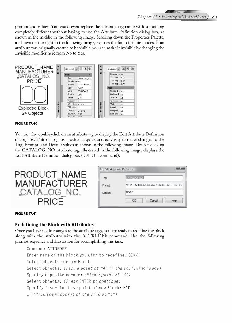
prompt and values. You could even replace the attribute tag name with somethingcompletely different without having to use the Attribute Definition dialog box, asshown in the middle in the following image. Scrolling down the Properties Palette,as shown on the right in the following image, exposes the four attribute modes. If anattribute was originally created to be visible, you can make it invisible by changing theInvisible modifier here from No to Yes.
You can also double-click on an attribute tag to display the Edit Attribute Definitiondialog box. This dialog box provides a quick and easy way to make changes to theTag, Prompt, and Default values as shown in the following image. Double-clickingthe CATALOG_NO. attribute tag, illustrated in the following image, displays theEdit Attribute Definition dialog box (DDEDIT command).
Redefining the Block with AttributesOnce you have made changes to the attribute tags, you are ready to redefine the blockalong with the attributes with the ATTREDEF command. Use the followingprompt sequence and illustration for accomplishing this task.
Command: ATTREDEF
Enter name of the block you wish to redefine: SINK
Select objects for new Block…
Select objects: (Pick a point at “A” in the following image)
Specify opposite corner: (Pick a point at “B”)
Select objects: (Press ENTER to continue)
Specify insertion base point of new Block: MID
of (Pick the midpoint of the sink at “C”)
FIGURE 17.40
FIGURE 17.41
Chap t e r 17 • Work in g w i t h A t t r i b u t e s 733

TUTORIAL EXERCISE: 17_RESISTORS.DWG
PurposeThis tutorial is designed to redefine attribute tags and update existing attribute values, asshown in the previous image.
System SettingsAll units and drawing limits have already been set. Attributes have also been assigned tocomputer components.
LayersAll layers have already been created for this drawing.
Suggested CommandsThe DDEDIT command will be used to edit various characteristics of attributes.
STEP 1Open the drawing file 17_Resistors. In the following image a series of resistors is arrangedin a partial circuit design. A number of changes need to be made to the original attributedefinitions. Once the changes are made, the block and attributes will be redefined and allthe blocks will automatically be updated.
FIGURE 17.42
FIGURE 17.43
734 Aut oCAD 2010 Tu t o r f o r Eng in e e r i n g Graph i c s

STEP 2Copy one of the resistor symbols to a blank part of your screen. Then explode this block.This should break the block down into individual objects and return the attribute valuesto their tags, as shown in the following image on the left.
STEP 3In this step, the tag TYPE needs to be replaced with a new tag. This also means creat-ing a new prompt and default value. Double-click the TYPE tag to display the EditAttribute Definition dialog box, as shown in the following image, and change the Tagfrom TYPE to SUPPLIER. In the Prompt field, change the existing prompt to SupplierName? In the Default field, change WIREWOUND to LABTRONICS, INC, as shown inthe following image. When finished, click the OK button to accept the changes anddismiss the dialog box.
FIGURE 17.44
FIGURE 17.45
Chap t e r 17 • Work in g w i t h A t t r i b u t e s 735

STEP 4After these changes are made to the exploded block, the ATTREDEF command will beused to redefine the block and automatically update all resistor blocks to their new valuesand states. Activate the ATTREDEF command. Enter RESISTOR as the name of the blockto redefine. Select the block and attributes, as shown in the following image on the left.Pick the new insertion point at “C”; as the drawing regenerates, all blocks are updated tothe new attribute values, as shown in the following image on the right.
Command: ATTREDEF
Enter name of the block you wish to redefine: RESISTOR
Select objects for new Block…
Select objects: (Pick a point at “A” in the following image)
Specify opposite corner: (Pick a point at “B”)
16 found
Select objects: (Press ENTER to continue)
Specify insertion base point of new Block: End (For ObjectSnap Endpoint mode)
of (Pick the endpoint of the resistor at “C”)
FIGURE 17.46
FIGURE 17.47
736 Aut oCAD 2010 Tu t o r f o r Eng in e e r i n g Graph i c s

EXTRACTING ATTRIBUTESOnce attributes have been created, displayed, and edited, one additional step wouldbe to extract attributes out to a file. The attributes can then be imported into Micro-soft Excel or even brought into an existing AutoCAD drawing as a table object. Thisprocess is handled through the Attribute Extraction wizard, which is activated byselecting Attribute Extraction from the Tools Menu Bar, or Modify II Toolbar, asshown in the following image.
Clicking the Data Extraction toolbar button or entering EATTEXT at the commandprompt activates the Data Extraction wizard, shown in the following image. Use thiswizard to step you through the attribute extraction process. You can start with atemplate or an extraction file, if you have previously created one. The templates aresaved with a BLK extension and the extraction files with an EXT extension. Eachextraction you create will be saved and can be reused at any time to extract the latestinformation. You will be able to individually select the attributes as well as specificblock information to extract. You can preview the extraction file, save the template,and export the results in either TXT (tab-separated file), CSV (comma separated),XLS (Microsoft Excel), or MDB (Microsoft Access) format or extract the resultsinto an AutoCAD table object.
FIGURE 17.48
FIGURE 17.49
Chap t e r 17 • Work in g w i t h A t t r i b u t e s 737
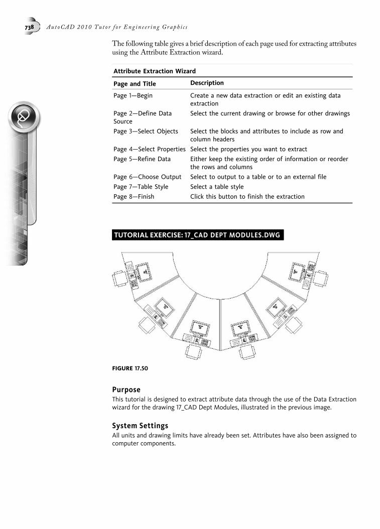
The following table gives a brief description of each page used for extracting attributesusing the Attribute Extraction wizard.
Attribute Extraction Wizard
Page and Title Description
Page 1—Begin Create a new data extraction or edit an existing dataextraction
Page 2—Define DataSource
Select the current drawing or browse for other drawings
Page 3—Select Objects Select the blocks and attributes to include as row andcolumn headers
Page 4—Select Properties Select the properties you want to extract
Page 5—Refine Data Either keep the existing order of information or reorderthe rows and columns
Page 6—Choose Output Select to output to a table or to an external file
Page 7—Table Style Select a table style
Page 8—Finish Click this button to finish the extraction
TUTORIAL EXERCISE: 17_CAD DEPT MODULES.DWG
PurposeThis tutorial is designed to extract attribute data through the use of the Data Extractionwizard for the drawing 17_CAD Dept Modules, illustrated in the previous image.
System SettingsAll units and drawing limits have already been set. Attributes have also been assigned tocomputer components.
FIGURE 17.50
738 Aut oCAD 2010 Tu t o r f o r Eng in e e r i n g Graph i c s

LayersAll layers have already been created for this drawing.
Suggested CommandsThis drawing appears inside a layout that has already been created. A table consisting ofthe extracted attributes will be inserted into this layout. Follow the steps provided by theData Extraction wizard to extract the attributes out to an AutoCAD table.
STEP 1Open the drawing file 17_CAD Dept Modules.dwg. Activate the Data Extraction wizard, asshown in the following image, by clicking Attribute Extraction from the Tools Menu Bar,as shown on the left. You will create a new data extraction. Click the Next button to con-tinue to the next step.
When the Save Data Extraction As dialog box appears as in the following image, enter thename of the data extraction file as CAD Dept Modules and select an appropriate folder inthe Save in drop-down list. When finished, click the Save button.
STEP 2In this next step, you pick the data source from which the attributes will be extracted.When the Define Data Source dialog box appears, verify that Drawings/Sheet set ispicked and that the Include current drawing box is checked as shown in the followingimage. Click the Next > button to continue.
FIGURE 17.51
FIGURE 17.52
Chap t e r 17 • Work in g w i t h A t t r i b u t e s 739

STEP 3When the Select Objects dialog box displays, verify that the Display all object types boxis not checked and that the Display blocks with attributes only box is checked at thebottom of the dialog box as shown in the following image. When the three items displayat the top of this dialog box, remove the check from the box next to Architectural Title.The remaining two items, CPU and Monitor, should remain checked. Click the Next >button to continue.
STEP 4When the Select Properties dialog box appears, clear all of the checks from the followingboxes on the right side of the dialog box as shown in the following image: 3D Visualiza-tion, Drawing, General, Geometry, and Misc. The only Category filter checked should bethe box next to Attribute. Also, verify that all three properties on the left side of the dia-log box, COST, MANUFACTURER, and PRODUCT_NAME, are checked. Click the Next >button to continue.
FIGURE 17.53
FIGURE 17.54
740 Aut oCAD 2010 Tu t o r f o r Eng in e e r i n g Graph i c s

STEP 5When the Refine Data dialog box appears, keep the display of all information as is. Thisdialog box allows you to reorder, hide, and sort the columns in order to display the infor-mation in a different format. A button located in the lower-right corner of this dialog boxallows you to create an external data link. Click the Next > button to continue.
STEP 6When the Choose Output dialog box displays, place a check in the box next to Insert dataextraction table into drawing, as shown in the following image. This creates an AutoCADtable that displays in the current drawing. Click the Next > button to continue.
FIGURE 17.55
FIGURE 17.56
FIGURE 17.57
Chap t e r 17 • Work in g w i t h A t t r i b u t e s 741

STEP 7This next dialog box deals with the components of the table that the attributes will beextracted to. In the following image, you need to enter a title for the table. In this exer-cise, the title of this table will be ATTRIBUTE EXTRACTION RESULTS. You can also selecta table style. In this exercise, a table style called Attributes was already created. Thistable also displays in the dialog box, as shown in the following image on the right.
STEP 8The final dialog box states that if you extract the attributes to a table, you will beprompted for an insertion point after you click the Finish button. If you are creatingexternal files, these will be created when clicking the Finish button.
STEP 9Clicking the Finish button in the previous step brings you back into the drawing editor.You will be prompted to insert the table; do so in a convenient location of the drawing,as shown in the following image. In this image, notice that the Count, Block Name, COST,MANUFACTURER, and PRODUCT_NAME were all extracted.
FIGURE 17.58
FIGURE 17.59
FIGURE 17.60
742 Aut oCAD 2010 Tu t o r f o r Eng in e e r i n g Graph i c s

CHAPTER
18Working with ExternalReferences and RasterImage and DWF Files
This chapter begins the study of External References and how they differ fromblocks. When changes are made to a drawing that has been externally referencedinto another drawing, these changes are updated automatically. There is no need toredefine the external reference in the same way blocks are redefined. When thesharing of data is important, the ETRANSMIT command is used to collect all supportfiles that make up a drawing. This guarantees to the individual reviewing the draw-ing that all support files come with the drawing. Working with raster images is alsodiscussed in this chapter. Raster images can be attached to a drawing file for presen-tation purposes. The brightness, contrast, and fade factor of the images can also beadjusted. To help you control the order in which images display in your drawing,the DRAWORDER command will be explained.
COMPARING EXTERNAL REFERENCES AND BLOCKSYou have already seen in Chapter 16 how easy and popular it is to insert blocks anddrawing files into other drawing files. One advantage in performing these insertionsis a smaller file size, which results because all objects connected with each block aregrouped into a single object. It is only when blocks are exploded that the drawing sizeonce again increases because the objects that made up the block have been separatedinto their individual objects. Another advantage of blocks is their ability to be rede-fined in a drawing.
External references are similar to blocks in that they are considered one object. How-ever, external references are attached to the drawing file, whereas blocks are insertedin the drawing. This attachment actually sets up a relationship between the currentdrawing file and the external referenced drawing. For example, take a floor plan fileand externally reference it into a current drawing file. All objects associated withthe floor plan are brought in, including their current layer and linetype qualities.With the floor plan acting as a guide, such items as electrical symbols, furniture, anddimensions can be added to the floor plan and saved to the current drawing file. Nowa design change needs to be made to the floor plan. Open the floor plan, stretch a fewdoors and walls to new locations, and save the file. The next time the drawing holdingthe electrical symbols and furniture arrangement is opened, the changes to the floor
743

plan are made automatically to the current drawing file. This is one of the primaryadvantages of external references over blocks. Also, even though blocks are knownto reduce file size, using external references reduces the file size even more thanusing blocks. One disadvantage of an external reference is that items such as layersand other blocks that belong to the external reference can be viewed but have limitedcapabilities for manipulation.
CHOOSING EXTERNAL REFERENCE COMMANDSThe XREF (XR is the alias) command activates a palette that allows you to attach andcontrol external references in a drawing. This command can be accessed through theMenu Bar, Ribbon, or Reference toolbar as shown in the following image.
Whichever method you use, the External References palette displays, as shown inthe following image. In this image, the drawing file 8th floor is listed at the top ofthis palette. Underneath this file are a number of additional files dealing with thefurniture, hvac, lighting, plan, plumbing, and power; these files represent externalreferences that were attached to the 8th floor drawing file.
FIGURE 18.1
FIGURE 18.2
744 Aut oCAD 2010 Tu t o r f o r Eng in e e r i n g Graph i c s

The lower portion of the External References palette illustrated in the previous imagehas a Details heading. Clicking the Details button displays the information about theselected external reference, as shown in the following image on the left. In this exam-ple, the 8th floor hvac external reference is selected and has various items such asstatus, file size, type, and date, to name a few listed. Clicking the Preview button dis-plays a preview of the selected external reference, as shown in the following image onthe right.
Located in the upper-left corner of the External References palette are buttons thatare used for attaching or reloading external references. Clicking the button locatedon the left, as shown in the following image, displays three different attach modes.Attach DWG activates the Select Reference File dialog box, used for selecting anexisting drawing file to merge into the current drawing. Attach Image activates theSelect Image File dialog box, used for selecting a raster image for merging intothe current drawing. Attach DWF activates the Select DWF File dialog box, usedfor selecting a DWF (Drawing Web Format) file for merging into the current draw-ing. Attach DGN activates the Select DGN File dialog box, used for importingMicroStation® DGN drawing files into DWG files.
When changes to original drawing files that are referenced into the current drawingoccur, click Refresh to update the information located in the External Referencespalette. You can also choose Reload All References as a means of updating yourcurrent drawing to any changes that have occurred to the external references in thedrawing.
External references can also be attached and reloaded by right-clicking on the palettearea and activating a shortcut menu, as shown in the following image on the left.Once the External References palette is populated with various references, select
FIGURE 18.3
FIGURE 18.4
Chap t e r 18 • Work i ng w i t h Ex t e r na l R e f e r e n c e s and Ra s t e r Imag e and DWF Fi l e s 745
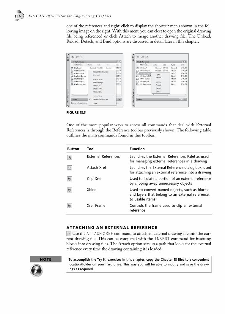
one of the references and right-click to display the shortcut menu shown in the fol-lowing image on the right. With this menu you can elect to open the original drawingfile being referenced or click Attach to merge another drawing file. The Unload,Reload, Detach, and Bind options are discussed in detail later in this chapter.
One of the more popular ways to access all commands that deal with ExternalReferences is through the Reference toolbar previously shown. The following tableoutlines the main commands found in this toolbar.
Button Tool Function
External References Launches the External References Palette, usedfor managing external references in a drawing
Attach Xref Launches the External Reference dialog box, usedfor attaching an external reference into a drawing
Clip Xref Used to isolate a portion of an external referenceby clipping away unnecessary objects
Xbind Used to convert named objects, such as blocksand layers that belong to an external reference,to usable items
Xref Frame Controls the frame used to clip an externalreference
ATTACHING AN EXTERNAL REFERENCEUse the ATTACH XREF command to attach an external drawing file into the cur-
rent drawing file. This can be compared with the INSERT command for insertingblocks into drawing files. The Attach option sets up a path that looks for the externalreference every time the drawing containing it is loaded.
NOTE To accomplish the Try It! exercises in this chapter, copy the Chapter 18 files to a convenientlocation/folder on your hard drive. This way you will be able to modify and save the draw-ings as required.
FIGURE 18.5
746 Aut oCAD 2010 Tu t o r f o r Eng in e e r i n g Graph i c s
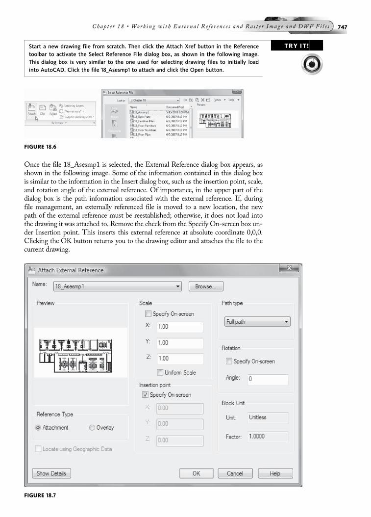
TRY IT!Start a new drawing file from scratch. Then click the Attach Xref button in the Referencetoolbar to activate the Select Reference File dialog box, as shown in the following image.This dialog box is very similar to the one used for selecting drawing files to initially loadinto AutoCAD. Click the file 18_Asesmp1 to attach and click the Open button.
Once the file 18_Asesmp1 is selected, the External Reference dialog box appears, asshown in the following image. Some of the information contained in this dialog boxis similar to the information in the Insert dialog box, such as the insertion point, scale,and rotation angle of the external reference. Of importance, in the upper part of thedialog box is the path information associated with the external reference. If, duringfile management, an externally referenced file is moved to a new location, the newpath of the external reference must be reestablished; otherwise, it does not load intothe drawing it was attached to. Remove the check from the Specify On-screen box un-der Insertion point. This inserts this external reference at absolute coordinate 0,0,0.Clicking the OK button returns you to the drawing editor and attaches the file to thecurrent drawing.
FIGURE 18.6
FIGURE 18.7
Chap t e r 18 • Work i ng w i t h Ex t e r na l R e f e r e n c e s and Ra s t e r Imag e and DWF Fi l e s 747

Since you will not see the floor plan on the small drawing sheet, perform a ZOOM-All. Your results should appear similar to the illustration in the following image.
With the external reference attached to the drawing file, layers and blocks that belongto the external reference are displayed in a unique way. Illustrated in the followingimage are the current layers that are part of the drawing. However, notice how a num-ber of layers begin with the same name (18_Asesmp1); also, what appears to be avertical bar separates 18_Asesmp1 from the names of the layers. Actually, the verticalbar represents the Pipe symbol on the keyboard, and it designates that the layersbelong to the external reference, namely 18_Asesmp1. These layers can be turnedoff, can be frozen, or can even have the color changed. However, you cannot makethese layers current for drawing because they belong to the external reference.
FIGURE 18.8
FIGURE 18.9
748 Aut oCAD 2010 Tu t o r f o r Eng in e e r i n g Graph i c s
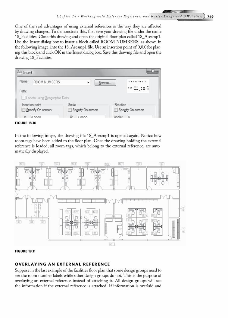
One of the real advantages of using external references is the way they are affectedby drawing changes. To demonstrate this, first save your drawing file under the name18_Facilities. Close this drawing and open the original floor plan called 18_Asesmp1.Use the Insert dialog box to insert a block called ROOM NUMBERS, as shown inthe following image, into the 18_Asesmp1 file. Use an insertion point of 0,0,0 for plac-ing this block and click OK in the Insert dialog box. Save this drawing file and open thedrawing 18_Facilities.
In the following image, the drawing file 18_Asesmp1 is opened again. Notice howroom tags have been added to the floor plan. Once the drawing holding the externalreference is loaded, all room tags, which belong to the external reference, are auto-matically displayed.
OVERLAYING AN EXTERNAL REFERENCESuppose in the last example of the facilities floor plan that some design groups need tosee the room number labels while other design groups do not. This is the purpose ofoverlaying an external reference instead of attaching it. All design groups will seethe information if the external reference is attached. If information is overlaid and
FIGURE 18.10
FIGURE 18.11
Chap t e r 18 • Work i ng w i t h Ex t e r na l R e f e r e n c e s and Ra s t e r Imag e and DWF Fi l e s 749

the entire drawing is externally referenced, the overlaid information does not display;it’s as if it is invisible. This option is illustrated in the next Try It! exercise.
TRY IT! Open the drawing 18_Floor Plan. Then use the External Reference dialog box, shown in thefollowing image, to attach the file 18_Floor Furniture (the steps for accomplishing thiswere demonstrated in the previous Try It! exercise). Use an insertion point of 0,0,0 and besure the reference type is Attachment.
Your display should be similar to the illustration in the following image. You want alldesign groups to view this information.
FIGURE 18.12
FIGURE 18.13
750 Aut oCAD 2010 Tu t o r f o r Eng in e e r i n g Graph i c s
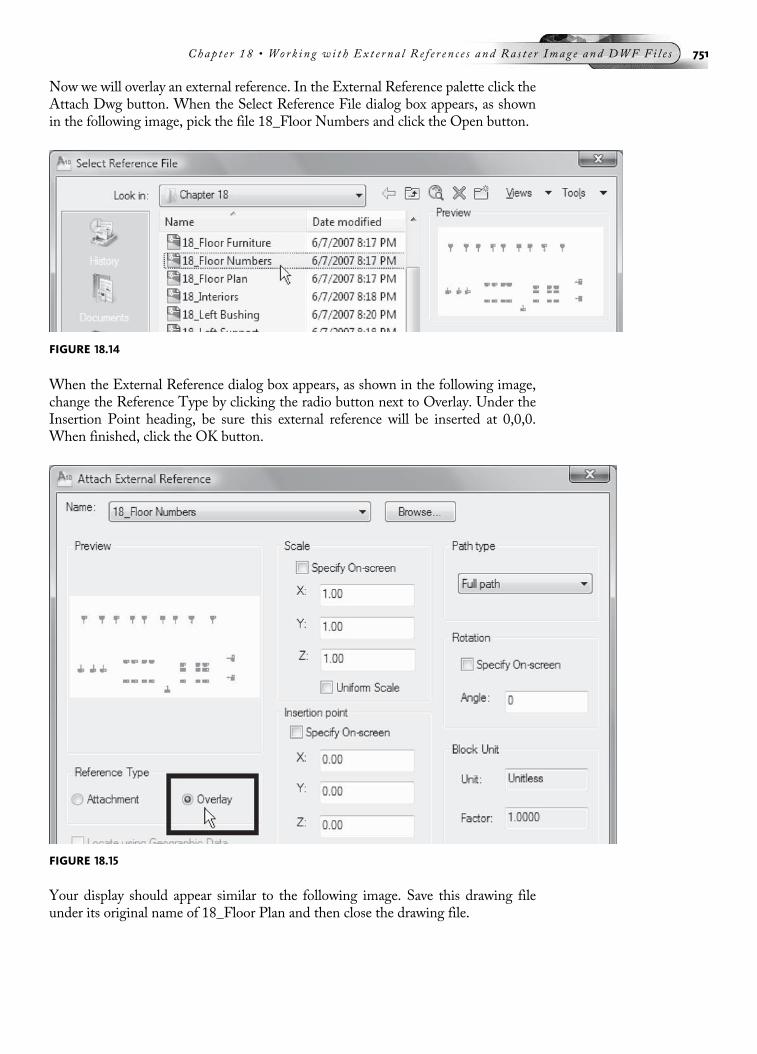
Now we will overlay an external reference. In the External Reference palette click theAttach Dwg button. When the Select Reference File dialog box appears, as shownin the following image, pick the file 18_Floor Numbers and click the Open button.
When the External Reference dialog box appears, as shown in the following image,change the Reference Type by clicking the radio button next to Overlay. Under theInsertion Point heading, be sure this external reference will be inserted at 0,0,0.When finished, click the OK button.
Your display should appear similar to the following image. Save this drawing fileunder its original name of 18_Floor Plan and then close the drawing file.
FIGURE 18.14
FIGURE 18.15
Chap t e r 18 • Work i ng w i t h Ex t e r na l R e f e r e n c e s and Ra s t e r Imag e and DWF Fi l e s 751
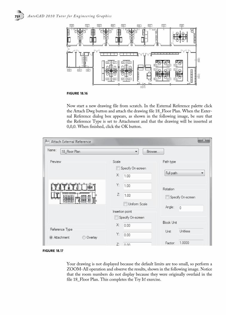
Now start a new drawing file from scratch. In the External Reference palette clickthe Attach Dwg button and attach the drawing file 18_Floor Plan. When the Exter-nal Reference dialog box appears, as shown in the following image, be sure thatthe Reference Type is set to Attachment and that the drawing will be inserted at0,0,0. When finished, click the OK button.
Your drawing is not displayed because the default limits are too small, so perform aZOOM-All operation and observe the results, shown in the following image. Noticethat the room numbers do not display because they were originally overlaid in thefile 18_Floor Plan. This completes the Try It! exercise.
FIGURE 18.16
FIGURE 18.17
752 Aut oCAD 2010 Tu t o r f o r Eng in e e r i n g Graph i c s

THE XBIND COMMANDEarlier, it was mentioned that layers belonging to external references cannot be
used in the drawing they were externally referenced into. The same is true with blocksthat were inserted into the drawing. When blocks are listed, the name of the externalreference is given first, with the Pipe symbol following, and finally the actual nameof the block, as in the example 18_Asesmp1|DESK2 where DESK2 is the blockand 10_Asesmp1 is the external reference. As with layers, these blocks cannot beused in the drawing because of the presence of the Pipesymbol, which is not sup-ported in the name of the block. There is a way, however, to convert a block or layerinto a usable object through the XBIND command.
TRY IT!Open the drawing file 18_Facilities Plan. Then select the XBIND command from the Refer-ence toolbar, as shown in the following image. This activates the Xbind dialog box, whichlists the external reference 18_ASESMP1. Expand the listing of all named objects, such asblocks and layers associated with the external reference. Then expand the Block headingto list all individual blocks associated with the external reference, as shown in the followingimage.
Click the block 18_Asesmp1|DESK2 in the listing on the left; then click the Add ->button. This moves the block name over to the right under the listing of Definitionsto Bind, as shown in the following image. Do the same for 18_Asesmp1|DESK3and 18_Asesmp1|DESK4. When finished adding these items, click the OK buttonto bind the blocks to the current drawing file.
FIGURE 18.18
FIGURE 18.19
Chap t e r 18 • Work i ng w i t h Ex t e r na l R e f e r e n c e s and Ra s t e r Imag e and DWF Fi l e s 753

Test to see that new blocks have in fact been bound to the current drawing file. Activatethe Insert dialog box, click the Name drop-down list box, and notice the display of theblocks, as shown in the following image. The three symbols just bound from the exter-nal reference still have the name of the external reference, namely, 18_Asesmp1. How-ever, instead of the Pipe symbol separating the name of the external reference and blocknames, the characters $0$ are now used. This is what makes the blocks valid in thedrawing. Now these three blocks can be inserted in the drawing file even though theyused to belong only to the external reference 18_Asesmp1.
IN-PLACE REFERENCE EDITINGIn-Place Reference Editing allows you to edit a reference drawing from the currentdrawing, which is externally referencing it. You then save the changes back to theoriginal drawing file. This becomes an efficient way of making a change to a drawingfile from an externally referenced file.
TRY IT! Open the drawing file 18_Pulley Assembly, shown in the following image. Both holes locatedin the Base Plate, Left Support, and Right Support need to be stretched 0.20 units to theleft and right. This will center the holes along the Left and Right Supports. Since all imagesthat make up the Pulley Assembly are external references, the In-Place Reference Editingfeature will be illustrated.
FIGURE 18.21
FIGURE 18.22
FIGURE 18.20
754 Aut oCAD 2010 Tu t o r f o r Eng in e e r i n g Graph i c s
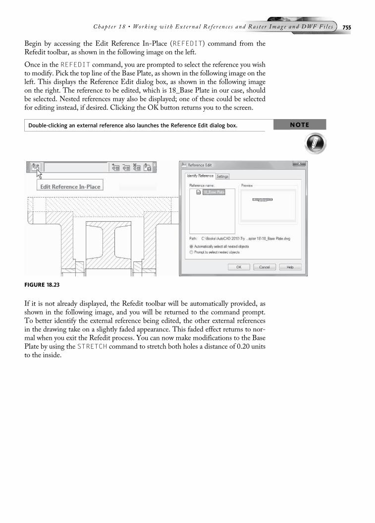
Begin by accessing the Edit Reference In-Place (REFEDIT) command from theRefedit toolbar, as shown in the following image on the left.
Once in the REFEDIT command, you are prompted to select the reference you wishto modify. Pick the top line of the Base Plate, as shown in the following image on theleft. This displays the Reference Edit dialog box, as shown in the following imageon the right. The reference to be edited, which is 18_Base Plate in our case, shouldbe selected. Nested references may also be displayed; one of these could be selectedfor editing instead, if desired. Clicking the OK button returns you to the screen.
NOTEDouble-clicking an external reference also launches the Reference Edit dialog box.
If it is not already displayed, the Refedit toolbar will be automatically provided, asshown in the following image, and you will be returned to the command prompt.To better identify the external reference being edited, the other external referencesin the drawing take on a slightly faded appearance. This faded effect returns to nor-mal when you exit the Refedit process. You can now make modifications to the BasePlate by using the STRETCH command to stretch both holes a distance of 0.20 unitsto the inside.
FIGURE 18.23
Chap t e r 18 • Work i ng w i t h Ex t e r na l R e f e r e n c e s and Ra s t e r Imag e and DWF Fi l e s 755
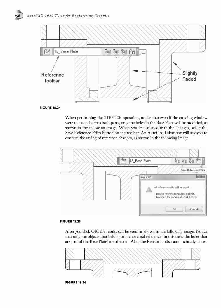
When performing the STRETCH operation, notice that even if the crossing windowwere to extend across both parts, only the holes in the Base Plate will be modified, asshown in the following image. When you are satisfied with the changes, select theSave Reference Edits button on the toolbar. An AutoCAD alert box will ask you toconfirm the saving of reference changes, as shown in the following image.
After you click OK, the results can be seen, as shown in the following image. Noticethat only the objects that belong to the external reference (in this case, the holes thatare part of the Base Plate) are affected. Also, the Refedit toolbar automatically closes.
FIGURE 18.24
FIGURE 18.25
FIGURE 18.26
756 Aut oCAD 2010 Tu t o r f o r Eng in e e r i n g Graph i c s

Perform the same series of steps using In-Place Reference Editing separately for the Leftand Right supports. Stretch the hole located on the Left Support a distance of 0.20 unitsto the right. Stretch the hole located on the Right Support a distance of 0.20 units to theleft. The final results of this In-Place Reference Editing Try It! exercise are displayed inthe following image.
BINDING AN EXTERNAL REFERENCEBinding an external reference to a drawing makes the external reference a permanentpart of the drawing and no longer an externally referenced file. In actuality, the exter-nal reference is converted into a block object. To bind the entire database of the Xrefdrawing, including all its xref-dependent named objects such as blocks, dimensionstyles, layers, linetypes, and text styles, use the Bind option of the External Referencepalette. Since binding an external reference breaks the link with the original drawingfile, this becomes a very popular technique at the end of a project when archiving finaldrawing files is important.
To bind an external reference, click the External References button located in theReference toolbar to activate the External References palette. Select the external ref-erence that you want to bind to the current drawing, right-click, and pick Bind fromthe menu, as shown in the following image on the left. This option activates the BindXrefs dialog box, illustrated in the following image on the right. Two options areavailable inside this dialog box: Bind and Insert.
The Bind option binds to the current drawing file all blocks, layers, dimension styles,and so on that belonged to an external reference. After you perform this operation,layers can be made current and blocks inserted in the drawing. For example, a typicalblock definition belonging to an external reference is listed in the symbol table asXREFname|-BLOCKname. Once the external reference is bound, all block definitionsare converted to XREFname$0$BLOCKname. In the layer display in the followingimage, the referenced layers were converted to usable layers with the Bind option.
FIGURE 18.28
FIGURE 18.27
Chap t e r 18 • Work i ng w i t h Ex t e r na l R e f e r e n c e s and Ra s t e r Imag e and DWF Fi l e s 757
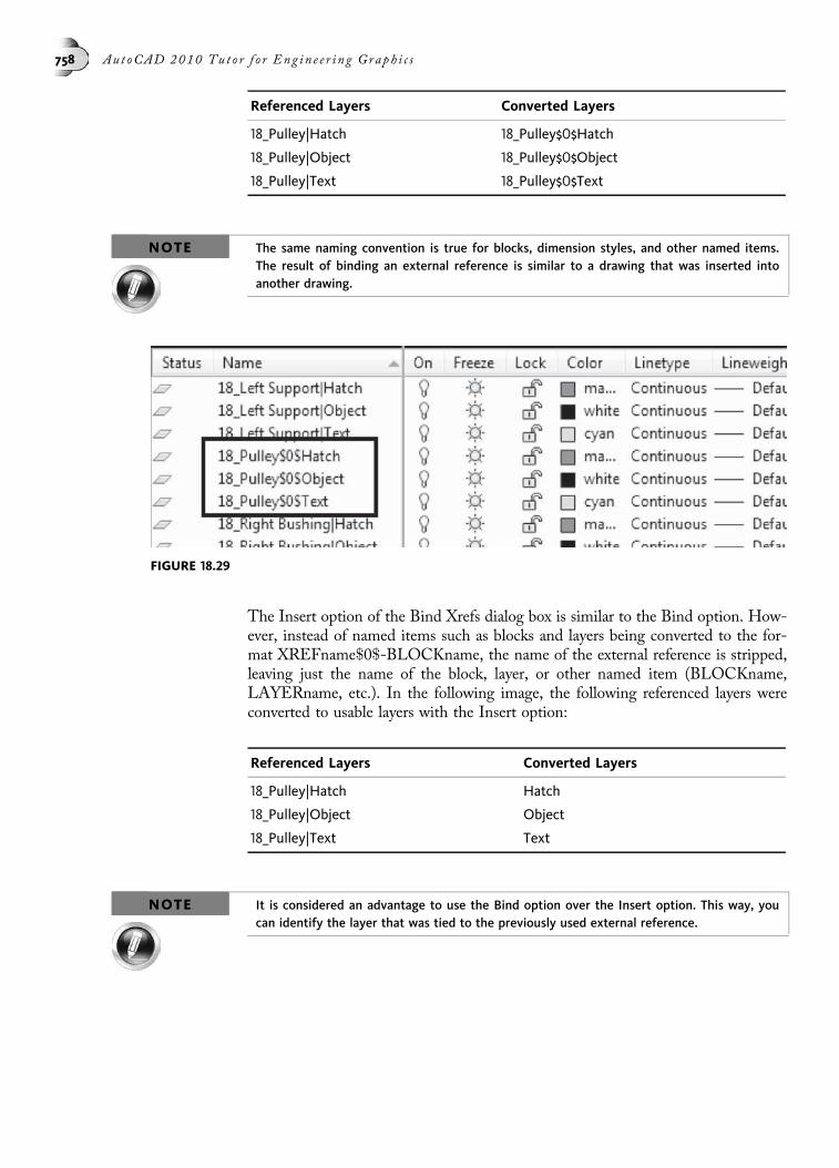
Referenced Layers Converted Layers
18_Pulley|Hatch 18_Pulley$0$Hatch
18_Pulley|Object 18_Pulley$0$Object
18_Pulley|Text 18_Pulley$0$Text
NOTE The same naming convention is true for blocks, dimension styles, and other named items.The result of binding an external reference is similar to a drawing that was inserted intoanother drawing.
The Insert option of the Bind Xrefs dialog box is similar to the Bind option. How-ever, instead of named items such as blocks and layers being converted to the for-mat XREFname$0$-BLOCKname, the name of the external reference is stripped,leaving just the name of the block, layer, or other named item (BLOCKname,LAYERname, etc.). In the following image, the following referenced layers wereconverted to usable layers with the Insert option:
Referenced Layers Converted Layers
18_Pulley|Hatch Hatch
18_Pulley|Object Object
18_Pulley|Text Text
NOTE It is considered an advantage to use the Bind option over the Insert option. This way, youcan identify the layer that was tied to the previously used external reference.
FIGURE 18.29
758 Aut oCAD 2010 Tu t o r f o r Eng in e e r i n g Graph i c s

CLIPPING AN EXTERNAL REFERENCESince attaching an external reference displays the entire reference file, you have
the option of displaying a portion of the file. This is accomplished by clipping theexternal reference with the XCLIP command. Choose this command from eitherthe Reference toolbar or theModify >Clip >XrefMenu Bar, as shown in the follow-ing image.
This operation is very useful when you want to emphasize a particular portion of yourexternal reference file. Clipping boundaries include polylines in the form of rectan-gles, regular polygonal shapes, or even irregular polyline shapes. All polylines mustform closed shapes. Also, clipping can take two forms, namely Outside and Insidemodes. With the Outside mode, objects outside of the clipping boundary are hidden.With the Inside mode, objects inside of the clipping boundary are hidden.
TRY IT!Open the drawing file 18_Facilities Plan. Follow the illustration in the following imageon the left and the command prompt sequence below for performing an outside clippingoperation.
Command: XCLIP
Select objects: (Pick the external reference)
Select objects: (Press ENTER to continue)
Enter clipping option
[ON/OFF/Clipdepth/Delete/generate Polyline/New boundary]<New>: N (For New)
FIGURE 18.31
FIGURE 18.30
Chap t e r 18 • Work i ng w i t h Ex t e r na l R e f e r e n c e s and Ra s t e r Imag e and DWF Fi l e s 759

Outside mode - Objects outside boundary will be hidden.
Specify clipping boundary or select invert option:
[Select polyline/Polygonal/Rectangular/Invert clip]<Rectangular>: (Press ENTER)
Specify first corner: (Pick a point at “A,” as shown in thefollowing image on the left)
Specify opposite corner: (Pick a point at “B”)
The results are displayed in the following image on the right. If you want to return theclipped image to the full external reference, use the XCLIP command and use theOFF clipping option. This temporarily turns off the clipping frame. To permanentlyremove the clipping frame, use the Delete clipping option.
The following image illustrates the results of clipping an external reference based onInside mode. In this example, the objects defined inside of the clipping boundaryare removed.
Command: XCLIP
Select objects: (Pick the external reference in the previousimage)
Select objects: (Press ENTER to continue)
Enter clipping option
[ON/OFF/Clipdepth/Delete/generate Polyline/New boundary]<New>: N (For New)
Outside mode - Objects outside boundary will be hidden.
Specify clipping boundary or select invert option:
[Select polyline/Polygonal/Rectangular/Invert clip]<Rectangular>: I (For Invert clip)
Inside mode - Objects inside boundary will be hidden.
Specify clipping boundary or select invert option:
[Select polyline/Polygonal/Rectangular/Invert clip]<Rectangular>: (Press ENTER)
Specify first corner: (Pick a point at “A,” as shown in theprevious image)
Specify opposite corner: (Pick a point at “B”)
FIGURE 18.32
760 Aut oCAD 2010 Tu t o r f o r Eng in e e r i n g Graph i c s

OTHER OPTIONS OF THE EXTERNAL REFERENCES PALETTEThe following additional options of the External References palette will now bediscussed, using the following image as a guide.
UnloadUnload is similar to the Detach option, with the exception that the external referenceis not permanently removed from the database of the drawing file. When an externalreference is unloaded, it is still listed in the External References palette, as shown inthe following image. Notice that an arrow (facing down) is displayed to signify theunloaded status. Since this option suppresses the external reference from any drawingregenerations, it is used as a productivity technique. Reload the external referencewhen you want it returned to the screen.
FIGURE 18.34
FIGURE 18.33
Chap t e r 18 • Work i ng w i t h Ex t e r na l R e f e r e n c e s and Ra s t e r Imag e and DWF Fi l e s 761
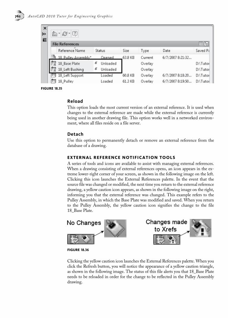
ReloadThis option loads the most current version of an external reference. It is used whenchanges to the external reference are made while the external reference is currentlybeing used in another drawing file. This option works well in a networked environ-ment, where all files reside on a file server.
DetachUse this option to permanently detach or remove an external reference from thedatabase of a drawing.
EXTERNAL REFERENCE NOTIFICATION TOOLSA series of tools and icons are available to assist with managing external references.When a drawing consisting of external references opens, an icon appears in the ex-treme lower-right corner of your screen, as shown in the following image on the left.Clicking this icon launches the External References palette. In the event that thesource file was changed or modified, the next time you return to the external referencedrawing, a yellow caution icon appears, as shown in the following image on the right,informing you that the external reference was changed. This example refers to thePulley Assembly, in which the Base Plate was modified and saved. When you returnto the Pulley Assembly, the yellow caution icon signifies the change to the file18_Base Plate.
Clicking the yellow caution icon launches the External References palette. When youclick the Refresh button, you will notice the appearance of a yellow caution triangle,as shown in the following image. The status of this file alerts you that 18_Base Plateneeds to be reloaded in order for the change to be reflected in the Pulley Assemblydrawing.
FIGURE 18.36
FIGURE 18.35
762 Aut oCAD 2010 Tu t o r f o r Eng in e e r i n g Graph i c s
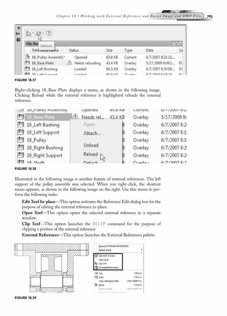
Right-clicking 18_Base Plate displays a menu, as shown in the following image.Clicking Reload while the external reference is highlighted reloads the externalreference.
Illustrated in the following image is another feature of external references. The leftsupport of the pulley assembly was selected. When you right-click, the shortcutmenu appears, as shown in the following image on the right. Use this menu to per-form the following tasks:
Edit Xref In-place—This option activates the Reference Edit dialog box for thepurpose of editing the external reference in-place.
Open Xref—This option opens the selected external reference in a separatewindow.
Clip Xref—This option launches the XCLIP command for the purpose ofclipping a portion of the external reference
External References—This option launches the External References palette.
FIGURE 18.38
FIGURE 18.37
FIGURE 18.39
Chap t e r 18 • Work i ng w i t h Ex t e r na l R e f e r e n c e s and Ra s t e r Imag e and DWF Fi l e s 763

USING ETRANSMITETransmit is an AutoCAD utility that is helpful in reading the database of yourdrawing and listing all support files needed. Once these files are identified, you canhave this utility gather all files into one zip file. You can then copy these files to a diskor CD, or transmit the files over the Internet. Clicking eTransmit…, located in theFile Menu Bar shown in the following image on the left, displays the Create Trans-mittal dialog box, as shown in the following image in the middle. Notice in the FilesTree tab a listing of all support files grouped by their specific category. For instance,an External References category exists. Clicking the “þ” sign lists all external refer-ences set to be transmitted.
Clicking the Files Table tab, as shown in the following image on the right, displays alist of all files that will be included in the transmittal set.
When you are finished examining all the support files, clicking the OK button takesyou to the Specify Zip File dialog box. It is here that you enter a file name. All supportfiles listed under the Files Tree tab will be grouped into a single zip file for easy shar-ing with other individuals or companies.
WORKING WITH RASTER IMAGESRaster images in the form of JPG, GIF, TIF, and so on can easily be merged withyour vector-based AutoCAD drawings. The addition of raster images can give anew dimension to your drawings. Typical examples of raster images are digital photo-graphs of an elevation of a house or an isometric view of a machine part.Whatever theapplication, working with raster images is very similar to what was just covered withexternal references. You attach the raster image to your drawing file. Once it is partof your drawing, additional tools are available to manipulate and fine-tune the imagefor better results. To attach a raster image to a drawing, you can use the ExternalReferences palette (Attach Image button), the Insert Menu Bar (click Raster ImageReference, as shown in the following image), or the Reference toolbar (click theAttach Image button). The Reference toolbar also contains a number of tools formanipulating raster images, as shown in the following image.
FIGURE 18.40
764 Aut oCAD 2010 Tu t o r f o r Eng in e e r i n g Graph i c s
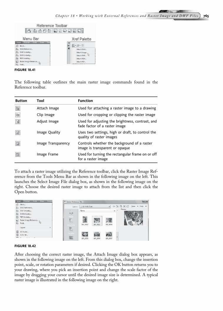
The following table outlines the main raster image commands found in theReference toolbar.
Button Tool Function
Attach Image Used for attaching a raster image to a drawing
Clip Image Used for cropping or clipping the raster image
Adjust Image Used for adjusting the brightness, contrast, andfade factor of a raster image
Image Quality Uses two settings, high or draft, to control thequality of raster images
Image Transparency Controls whether the background of a rasterimage is transparent or opaque
Image Frame Used for turning the rectangular frame on or offfor a raster image
To attach a raster image utilizing the Reference toolbar, click the Raster Image Ref-erence from the Tools Menu Bar as shown in the following image on the left. Thislaunches the Select Image File dialog box, as shown in the following image on theright. Choose the desired raster image to attach from the list and then click theOpen button.
After choosing the correct raster image, the Attach Image dialog box appears, asshown in the following image on the left. From this dialog box, change the insertionpoint, scale, or rotation parameters if desired. Clicking the OK button returns you toyour drawing, where you pick an insertion point and change the scale factor of theimage by dragging your cursor until the desired image size is determined. A typicalraster image is illustrated in the following image on the right.
FIGURE 18.42
FIGURE 18.41
Chap t e r 18 • Work i ng w i t h Ex t e r na l R e f e r e n c e s and Ra s t e r Imag e and DWF Fi l e s 765

To manage all images in a drawing, click the External References button located inthe Reference toolbar. The same dialog box used for managing external referencesis used for managing image files, as shown in the following image.
TRY IT! Begin this exercise on working with raster images by opening the drawing file 18_Linkage,illustrated in the following image. In this exercise a raster image will be attached and placedin the blank area to the right of the two-view drawing.
FIGURE 18.43
FIGURE 18.44
766 Aut oCAD 2010 Tu t o r f o r Eng in e e r i n g Graph i c s

Click the Attach Image button located in the Reference toolbar. When the SelectImage File dialog box appears, click the file Linkage1.jpg. Then click the Openbutton.
When the Image dialog box appears, as shown in the following image, leave alldefault settings. You will be specifying the insertion point on the drawing screen.Click the OK button to continue.
FIGURE 18.46
FIGURE 18.45
Chap t e r 18 • Work i ng w i t h Ex t e r na l R e f e r e n c e s and Ra s t e r Imag e and DWF Fi l e s 767

Once back in the drawing file, pick a point anchoring the lower-left corner of thegraphic, as shown in the following image. Now move your cursor in an upward rightdirection to scale the image as necessary. Pick a second point at a convenient locationto display the image.
As the image displays on your screen, you can adjust its size very easily. Click the edgeof the image (the image frame) and notice the grips appearing at the four corners ofthe image. Clicking a grip and then moving your cursor increases or decreases theimage’s size, as shown in the following image.
FIGURE 18.48
FIGURE 18.47
768 Aut oCAD 2010 Tu t o r f o r Eng in e e r i n g Graph i c s

From the Reference toolbar shown in the following image, identify the Adjust Imagebutton and click it. Clicking the edge of the raster image frame displays the ImageAdjust dialog box, as shown in the following image. Adjust the Brightness, Contrast,and Fade settings and notice that each of these affects the image previewed to theright of this dialog box. You can easily return to the original image by clicking theReset button in the lower-left corner of this dialog box.
Clicking the OK button in the Image Adjust dialog box returns you to the drawing.The final results are illustrated in the following image, with the vector drawing andraster image sharing the same layout.
FIGURE 18.49
FIGURE 18.50
Chap t e r 18 • Work i ng w i t h Ex t e r na l R e f e r e n c e s and Ra s t e r Imag e and DWF Fi l e s 769
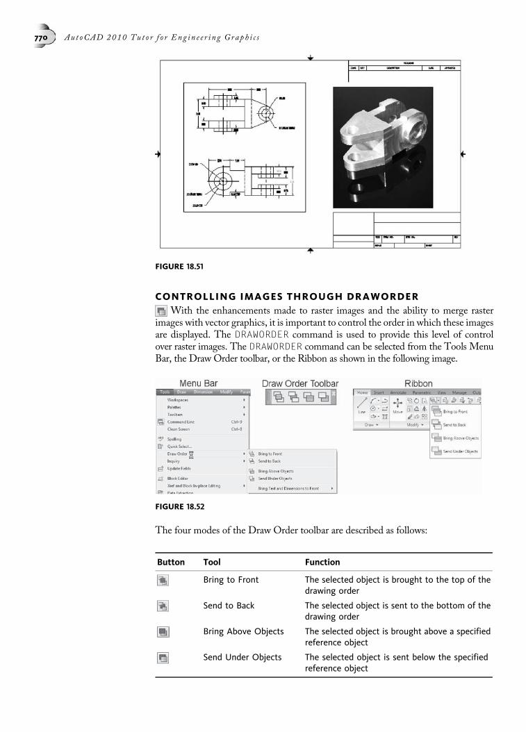
CONTROLLING IMAGES THROUGH DRAWORDERWith the enhancements made to raster images and the ability to merge raster
images with vector graphics, it is important to control the order in which these imagesare displayed. The DRAWORDER command is used to provide this level of controlover raster images. The DRAWORDER command can be selected from the Tools MenuBar, the Draw Order toolbar, or the Ribbon as shown in the following image.
The four modes of the Draw Order toolbar are described as follows:
Button Tool Function
Bring to Front The selected object is brought to the top of thedrawing order
Send to Back The selected object is sent to the bottom of thedrawing order
Bring Above Objects The selected object is brought above a specifiedreference object
Send Under Objects The selected object is sent below the specifiedreference object
FIGURE 18.51
FIGURE 18.52
770 Aut oCAD 2010 Tu t o r f o r Eng in e e r i n g Graph i c s

The following illustration displays three images, two of which are partially hiddendue to the size of the large middle image. We really want both small images to bevisible and have the larger middle image sent to the back of the image arrangement.
To correct the problem, select the Bring to Front tool. Both small images are selectedas the objects to bring to the top of the drawing order, and the results are illustratedin the following image. Both smaller images are now at the top of the drawing orderand can be viewed in full.
FIGURE 18.54
FIGURE 18.53
Chap t e r 18 • Work i ng w i t h Ex t e r na l R e f e r e n c e s and Ra s t e r Imag e and DWF Fi l e s 771

TUTORIAL EXERCISE: EXTERNAL REFERENCES
PurposeThis tutorial is designed to use the office floor plan to create an interior plan consisting ofvarious interior symbols such as desks, chairs, shelves, and plants. The office floor planwill be attached to another drawing file through the XREF command.
System SettingsSince these drawings are provided on the CD, all system settings have been made.
LayersThe creation of layers is not necessary because layers already exist for both drawing filesyou will be working on.
Suggested CommandsBegin this tutorial by opening the drawing 18_Office.Dwg, which is located on the CD, andviewing its layers and internal block definitions. Then open the drawing 18_Interiors.Dwg,also located on the CD, and view its layers and internal blocks. The file 18_Office.Dwg willthen be attached to 18_Interiors.Dwg. Once this is accomplished, chairs, desks, shelves,and plants will be inserted in the office floor plan for laying out the office furniture. Once18_Interiors.Dwg is saved, a design change needs to be made to the original office plan;open 18_Office.Dwg and stretch a few doors to new locations. Save this file and open18_Interiors.Dwg; notice how the changes to the doors are automatically made. The Xbinddialog box will also be shown as a means for making a block that had previously belongedto an external reference usable in the file 18_Interiors.Dwg.
STEP 1Open 18_Office.Dwg, which can be found on the CD, and observe a simple floor plan con-sisting of three rooms, as shown in the following image on the left. Furniture will be laidout using the floor plan as a template.
STEP 2While in 18_Office.Dwg, use the Layer Properties Manager palette and observe the layersthat exist in the drawing for such items as doors, walls, and floor, as shown in the follow-ing image on the right. These layers will appear differently once the office plan is at-tached to another drawing through the XREF command.
FIGURE 18.55
772 Aut oCAD 2010 Tu t o r f o r Eng in e e r i n g Graph i c s

STEP 3While in the office plan, activate the Insert dialog box through the INSERT command. Attimes, this dialog box is useful for displaying all valid blocks in a drawing. Clicking theName drop-down list displays the results shown in the following image. Two blocks arecurrently defined in this drawing; as with the layers, once the office plan is merged intoanother drawing through the XREF command, these block names will change. When youhave finished viewing the defined blocks, close 18_Office.Dwg.
STEP 4This next step involves opening 18_Interiors.Dwg, also found on the CD, and looking at thecurrent layers found in this drawing. Once this drawing is open, use the Layer PropertiesManager palette to observe that layers exist in this drawing for such items as floor andfurniture, as shown in the following image.
STEP 5As with the office plan, activate the Insert dialog box through the INSERT command toview the blocks internal to the drawing, as shown in the following image. The four blockslisted consist of various furniture items and will be used to lay out the interior plan.
FIGURE 18.57
FIGURE 18.58
FIGURE 18.56
Chap t e r 18 • Work i ng w i t h Ex t e r na l R e f e r e n c e s and Ra s t e r Imag e and DWF Fi l e s 773
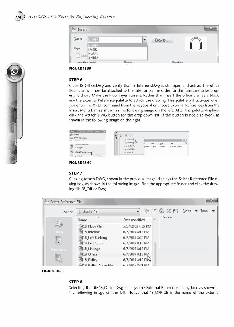
STEP 6Close 18_Office.Dwg and verify that 18_Interiors.Dwg is still open and active. The officefloor plan will now be attached to the interior plan in order for the furniture to be prop-erly laid out. Make the Floor layer current. Rather than insert the office plan as a block,use the External Reference palette to attach the drawing. This palette will activate whenyou enter the XREF command from the keyboard or choose External References from theInsert Menu Bar, as shown in the following image on the left. After the palette displays,click the Attach DWG button (or the drop-down list, if the button is not displayed), asshown in the following image on the right.
STEP 7Clicking Attach DWG, shown in the previous image, displays the Select Reference File di-alog box, as shown in the following image. Find the appropriate folder and click the draw-ing file 18_Office.Dwg.
STEP 8Selecting the file 18_Office.Dwg displays the External Reference dialog box, as shown inthe following image on the left. Notice that 18_OFFICE is the name of the external
FIGURE 18.60
FIGURE 18.61
FIGURE 18.59
774 Aut oCAD 2010 Tu t o r f o r Eng in e e r i n g Graph i c s

reference file chosen for attachment in the current drawing. Verify that the ReferenceType is an attachment. If selected, remove the checkmarks from the Specify On-screenboxes for the Insertion point, Scale, and Rotation. In the External Reference dialog box,click the OK button to attach 18_Office.Dwg to 18_Interiors.Dwg.
The floor plan is now attached to the Interiors drawing at the insertion point 0,0, asshown in the following image on the right.
With the floor plan attached to the interiors drawing, notice how both drawings appear inthe External References palette, as shown in the following image. When you have fin-ished studying the information located in this palette, you can dismiss the palette fromthe screen by clicking the “X” located in the upper-left corner.
STEP 9Once again, activate the Layer Properties Manager palette, paying close attention to thedisplay of the layers. Using the following image as a guide, you can see the familiar layersof Floor and Furniture. However, notice the group of layers beginning with 18_Office; thelayers actually belonging to the external reference file have the designation of XREF|LAYER. For example, the layer 18_Office|DOORS represents a layer located in the file18_Office.Dwg that holds all door symbols. The “|,” or Pipe symbol, is used to separatethe name of the external reference from the layer. The layers belonging to the externalreference file may be turned on or off, locked, or even frozen. However, these layers can-not be made current for drawing on.
FIGURE 18.62
FIGURE 18.63
Chap t e r 18 • Work i ng w i t h Ex t e r na l R e f e r e n c e s and Ra s t e r Imag e and DWF Fi l e s 775

STEP 10Make the Furniture layer current and begin inserting the desk, chair, shelf, and plant sym-bols in the drawing using the INSERT command or through the DesignCenter. The exter-nal reference file 18_OFFICE is to be used as a guide throughout this layout. It is notimportant that your drawing match exactly the image shown in the following image onthe left. After positioning all symbols in the floor plan, save your drawing under its origi-nal name of 18_Interiors.Dwg but do not close the file.
Even with the interior drawing file still open, make the original drawing file, 18_Office.Dwg,current by opening this file, and make the following modifications: stretch all threedoors as indicated to new locations and mirror one of the doors so it is positioned closerto the wall; stretch the wall opening over to the other end of the room, as shown in thefollowing image on the right. Finally, save these changes under the original name of18_Office.Dwg and close the file.
STEP 11After you close the office plan, your display returns to the interiors plan. At this point,nothing in the drawing will appear to have changed. However, notice in the lower-rightcorner of your display screen a tray of buttons. One of these buttons (Manage Xrefs)deals specifically with external reference files. Once the office plan is changed and saved,a Manage Xrefs button appears in this portion of your screen. It is also displayed in thefollowing image on the left. Right-clicking this button displays two options. One ofthe options allows you to reload all external reference files. Click this option and noticethe effects on the floor plan, illustrated on the left of the following image, where changesto the office plan are now reflected in the interiors drawing.
FIGURE 18.65
FIGURE 18.64
776 Aut oCAD 2010 Tu t o r f o r Eng in e e r i n g Graph i c s

In this case, observe how some of the furniture is now in the way of the doorways. If theoffice plan had been inserted in the interiors drawing as a block, these changes would nothave occurred this easily.
Because of the changes in the door openings, edit the drawing by moving the office fur-niture to better locations. The illustration in the following image on the right can be usedas a guide, although your drawing may appear slightly different.
STEP 12A door needs to be added to an opening in one of the walls of the office plan. However,the door symbol belongs to the externally referenced file 18_Office.Dwg. The door blockis defined as 18_Office|DOOR; the “|” character is not valid in the naming of the blockand, therefore, cannot be used in the current drawing. The block must first be bound tothe current drawing before it can be used. Use the XBIND command to make the exter-nal reference’s Door block available in the 18_Interiors.Dwg. This command can be se-lected from the Reference toolbar, as shown in the following image, which displays theXbind dialog box. While in this dialog box, click the “þ” symbol next to the file 18_Officeand then click the “þ” symbol next to Block. This displays all blocks that belong to theexternal reference.
STEP 13Clicking 18_OFFICE|DOOR followed by the Add -> button, as shown in the previous im-age, moves the block of the door to the Definitions to Bind area in the following image.Click OK to dismiss the dialog box; the door symbol is now a valid block that can beinserted in the drawing.
FIGURE 18.66
FIGURE 18.67
Chap t e r 18 • Work i ng w i t h Ex t e r na l R e f e r e n c e s and Ra s t e r Imag e and DWF Fi l e s 777

STEP 14Activate the Insert dialog box through the INSERT command, click the Name drop-downlist, and notice the name of the door, as shown in the following image on the left. It isnow listed as 18_Office$0$DOOR; the “|” character was replaced by the “$0$,” makingthe block valid in the current drawing. This is AutoCAD’s standard way of convertingblocks that belong to external references to blocks that can be used in the current draw-ing file. This same procedure works on layers belonging to external references as well.
STEP 15Make the Floor layer current and insert the door symbol into the open gap, as shown inthe following image on the right, to complete the drawing.
FIGURE 18.69
FIGURE 18.68
778 Aut oCAD 2010 Tu t o r f o r Eng in e e r i n g Graph i c s

CHAPTER
19
Advanced LayoutTechniques
This chapter is a continuation of Chapter 14, “Working with Drawing Layouts.”First, we will demonstrate how multiple images of the same drawing file can be laidout at different scales. This demonstration will include a number of layering anddimensioning techniques to achieve success. This chapter continues by demonstrat-ing how to create and manage annotation scales. Arranging multiple details of differ-ent drawing files in the same layout will also be demonstrated.
ARRANGING DIFFERENT VIEWS OF THE SAME DRAWINGThis chapter begins immediately with a tutorial exercise designed to lay out twoviews of the same drawing in the same layout. Both images will be scaled at differentvalues inside their respective veiwports. Follow the next series of steps for creatingthis type of layout.
779

TUTORIAL EXERCISE: 19_ROOF PLAN.DWG
PurposeThis tutorial exercise is designed to lay out the two architectural views displayed in theprevious image in the Layout mode (Paper Space). The two views consist of an overall anda detailed view of a roof plan.
System SettingsOpen an existing drawing called 19_Roof Plan. Keep all default settings for the units andlimits of the drawing.
LayersLayers have already been created for this drawing.
Suggested CommandsA new viewport will be created to house a detail view of the roof plan. Dimensions willalso be added to this viewport. However, the Dimension scale setting of the drawingneeds to be set to “Scale dimension to layout.” This will enable the scale of the dimen-sions in the new viewport to match those dimensions in the main roof plan viewport.
STEP 1Open the drawing file 19_Roof Plan. Create a new viewport, as shown in the followingimage. This viewport should be long and narrow to accommodate the detail. Notice thatwhen you are creating the viewport, the entire image zooms to the extents of the view-port. This is normal and you will arrange the detail in the next series of steps.
FIGURE 19.1
780 Aut oCAD 2010 Tu t o r f o r Eng in e e r i n g Graph i c s

STEP 2Double-click inside the new viewport to make it active. Then pan the area of the roof planso it appears similar to the following image. When applying a scale to this viewport, it iseasier to see the results if the image you are detailing is approximately in the middle ofthe viewport. If it is not, it may be difficult to locate the area of the detail.
FIGURE 19.2
FIGURE 19.3
Chap t e r 19 • Advan c e d La y ou t T e c hn i q u e s 781
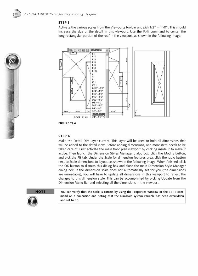
STEP 3Activate the various scales from the Viewports toolbar and pick 1/2 00 ¼ 1 0-0 00. This shouldincrease the size of the detail in this viewport. Use the PAN command to center thelong rectangular portion of the roof in the viewport, as shown in the following image.
STEP 4Make the Detail Dim layer current. This layer will be used to hold all dimensions thatwill be added to the detail view. Before adding dimensions, one more item needs to betaken care of. First activate the main floor plan viewport by clicking inside it to make itactive. Then launch the Dimension Styles Manager dialog box, click the Modify button,and pick the Fit tab. Under the Scale for dimension features area, click the radio buttonnext to Scale dimensions to layout, as shown in the following image. When finished, clickthe OK button to dismiss this dialog box and close the main Dimension Style Managerdialog box. If the dimension scale does not automatically set for you (the dimensionsare unreadable), you will have to update all dimensions in this viewport to reflect thechanges to this dimension style. This can be accomplished by picking Update from theDimension Menu Bar and selecting all the dimensions in the viewport.
NOTE You can verify that the scale is correct by using the Properties Window or the LIST com-mand on a dimension and noting that the Dimscale system variable has been overriddenand set to 96.
FIGURE 19.4
782 Aut oCAD 2010 Tu t o r f o r Eng in e e r i n g Graph i c s

STEP 5Activate the viewport containing the roof detail and place the linear dimensions as shownin the following image. Notice that the sizes of these dimensions exactly match thosein the main floor plan. The scale of the viewport, which we set earlier to 1/2 00 ¼ 1 0-0 00,sets the scale of the dimensions. This occurs automatically because the “Scale dimensionsto layout” button was selected, as shown in the previous step. You should also noticethat as these dimensions are placed in the detail, they also appear in the main floor planviewport, as shown in the following image.
STEP 6Activate the main floor plan viewport by clicking inside it. Then launch the Layer PropertiesManager palette. Identify the Dim Detail layer and freeze it in the current viewport byclicking the button as shown in the following image. This action will freeze the Dim Detaillayer in the main floor plan viewport while keeping the layer visible in the detail viewport.
FIGURE 19.5
FIGURE 19.6
Chap t e r 19 • Advan c e d La y ou t T e c hn i q u e s 783
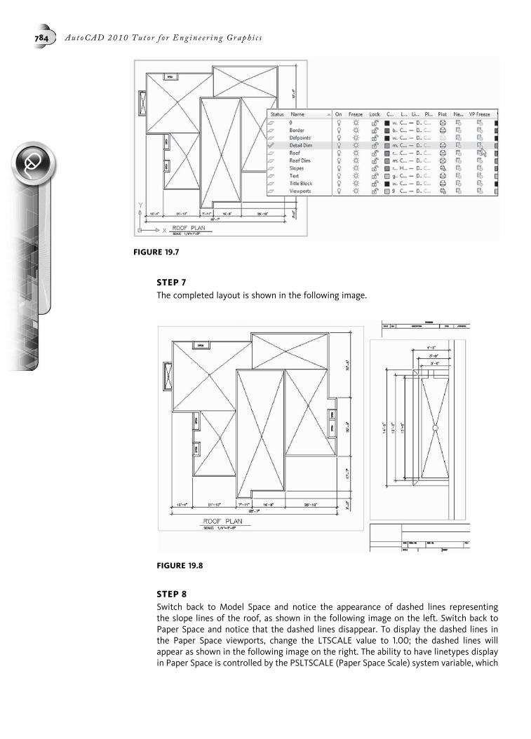
STEP 7The completed layout is shown in the following image.
STEP 8Switch back to Model Space and notice the appearance of dashed lines representingthe slope lines of the roof, as shown in the following image on the left. Switch back toPaper Space and notice that the dashed lines disappear. To display the dashed lines inthe Paper Space viewports, change the LTSCALE value to 1.00; the dashed lines willappear as shown in the following image on the right. The ability to have linetypes displayin Paper Space is controlled by the PSLTSCALE (Paper Space Scale) system variable, which
FIGURE 19.7
FIGURE 19.8
784 Aut oCAD 2010 Tu t o r f o r Eng in e e r i n g Graph i c s
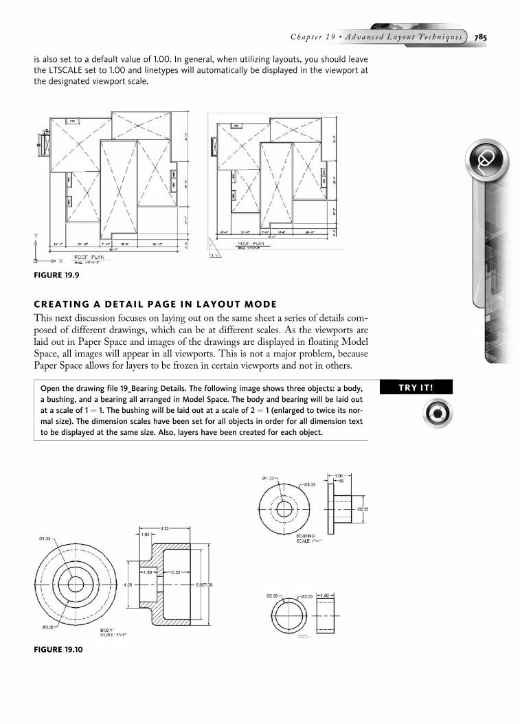
is also set to a default value of 1.00. In general, when utilizing layouts, you should leavethe LTSCALE set to 1.00 and linetypes will automatically be displayed in the viewport atthe designated viewport scale.
CREATING A DETAIL PAGE IN LAYOUT MODEThis next discussion focuses on laying out on the same sheet a series of details com-posed of different drawings, which can be at different scales. As the viewports arelaid out in Paper Space and images of the drawings are displayed in floating ModelSpace, all images will appear in all viewports. This is not a major problem, becausePaper Space allows for layers to be frozen in certain viewports and not in others.
TRY IT!Open the drawing file 19_Bearing Details. The following image shows three objects: a body,a bushing, and a bearing all arranged in Model Space. The body and bearing will be laid outat a scale of 1 ¼ 1. The bushing will be laid out at a scale of 2 ¼ 1 (enlarged to twice its nor-mal size). The dimension scales have been set for all objects in order for all dimension textto be displayed at the same size. Also, layers have been created for each object.
FIGURE 19.9
FIGURE 19.10
Chap t e r 19 • Advan c e d La y ou t T e c hn i q u e s 785

The following items have already been added to this drawing:
• A Vports layer was created. This layer holds all viewport information, and whenthe drawing is completed can be frozen or turned off.
• In Layout mode, an ANSI D-size sheet was selected for Page Setup.
• A D-size title block was inserted onto the Title Block layer.
Click the layout name ANSI-D. Except for the title block, the drawing sheet isempty. Using the Single Viewport tool located in the Viewports toolbar, create threeviewports, as shown in the following image. The exact size of these viewports is notimportant at this time since you will have to adjust them at the end of the exercise.When creating these viewports, notice that all three objects (body, bearing, and bush-ing) appear in all three viewports. You will now freeze layers inside these viewportsin order to show a different part in each viewport.
Begin the process of isolating one part per viewport by making the large viewport onthe left active by double-clicking inside it. You will notice the viewport taking onthe familiar thick border appearance, and the UCS icon is present in the lower-leftcorner of the viewport, as shown in the following image on the left. Then activatethe Layer Properties Manager palette. All layers that begin with Body need to bevisible in this viewport. Pick all layers that begin with Bearing and Bushing andfreeze these layers only in this viewport, as shown in the following image on theright.
NOTE To select multiple layers at one time, hold down the CTRL key as you select each layername.
FIGURE 19.11
786 Aut oCAD 2010 Tu t o r f o r Eng in e e r i n g Graph i c s

Next, click inside the viewport located in the upper-right corner to make it active, asshown in the following image on the left. Activate the Layer Properties Managerpalette. All layers that begin with Bearing need to be visible in this viewport. Pickall layers that begin with Body and Bushing and freeze these layers only in this view-port, as shown in the following image on the right.
NOTETo select all the layers at one time, select the first layer (Body-Center) then hold down theSHIFT key as you select the last layer name (Bushing-Object).
Finally, click inside the viewport located in the lower-right corner to make it active,as shown in the following image on the left. Activate the Layer Properties Managerpalette. All layers that begin with Bushing need to be visible in this viewport. Pickall layers that begin with Body and Bearing and freeze these layers only in this viewport,as shown in the following image on the right.
FIGURE 19.12
FIGURE 19.13
Chap t e r 19 • Advan c e d La y ou t T e c hn i q u e s 787

When finished, each viewport should contain a different part file. Items dealing withthe part body are visible in the large viewport on the left. The bearing views are visiblein the upper-right viewport and the bushing views are visible in the lower-right view-port. One other step is needed to better organize your work. Click in each port andpan each image so it appears centered in each viewport, as shown in the followingimage. Return to Paper Space by double-clicking outside the viewports.
Each image will now be scaled to each viewport. Be sure the Viewports toolbar isvisible somewhere on the display screen. Two of the viewports share the same scalefactor. Click the edge of the two viewports to highlight them as shown in the fol-lowing image. Then select the scale 1:1 from the Viewports toolbar to scale the bodyand bearing views to their respective viewports, as shown in the following image.Press ESC to remove the grips.
FIGURE 19.14
FIGURE 19.15
788 Aut oCAD 2010 Tu t o r f o r Eng in e e r i n g Graph i c s
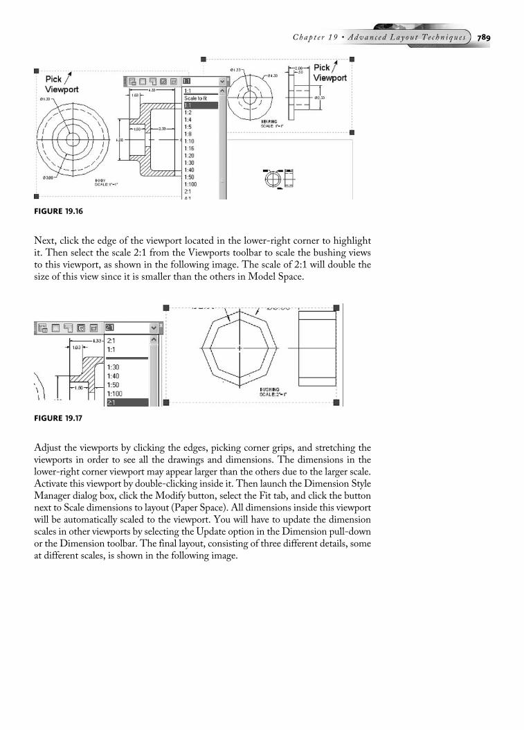
Next, click the edge of the viewport located in the lower-right corner to highlightit. Then select the scale 2:1 from the Viewports toolbar to scale the bushing viewsto this viewport, as shown in the following image. The scale of 2:1 will double thesize of this view since it is smaller than the others in Model Space.
Adjust the viewports by clicking the edges, picking corner grips, and stretching theviewports in order to see all the drawings and dimensions. The dimensions in thelower-right corner viewport may appear larger than the others due to the larger scale.Activate this viewport by double-clicking inside it. Then launch the Dimension StyleManager dialog box, click the Modify button, select the Fit tab, and click the buttonnext to Scale dimensions to layout (Paper Space). All dimensions inside this viewportwill be automatically scaled to the viewport. You will have to update the dimensionscales in other viewports by selecting the Update option in the Dimension pull-downor the Dimension toolbar. The final layout, consisting of three different details, someat different scales, is shown in the following image.
FIGURE 19.16
FIGURE 19.17
Chap t e r 19 • Advan c e d La y ou t T e c hn i q u e s 789

A good test is to perform a Plot Preview on this drawing. Notice in the followingimage the absence of any viewports. This is due to the No Plot setting being appliedto the VPORTS layer.
ADDITIONAL VIEWPORT CREATION METHODSWhen constructing viewports, you are not limited to rectangular or square shapes.Although you have been using the Scale drop-down list box in the Viewports toolbar,as shown in the following image, to scale the image inside the viewport, other buttonsare available and act on the shape of the viewport. You can clip an existing viewportto reflect a different shape, convert an existing closed object into a viewport, constructa multisided closed or polygonal viewport, or display the Viewports dialog box (youhave already constructed a single viewport in a previous exercise).
FIGURE 19.18
FIGURE 19.19
790 Aut oCAD 2010 Tu t o r f o r Eng in e e r i n g Graph i c s

Refer to the following table for a brief description of the extra commands available inthe Viewports toolbar.
Button Command Description
VPORTS Displays the Viewports dialog box
VPORTS Single Creates a single viewport
VPORTS Polygonal Used for creating a polygonalviewport
VPORTS Object Converts existing object into aviewport
VCLIP Used for clipping an existingviewport
TRY IT!Open the drawing file 19_Floor Viewports. Notice that Vports is the current layer. You willconvert the large rectangular viewport into a polygonal viewport by a clipping operation.First click the Clip Existing Viewport button. Pick the rectangular viewport and begin pick-ing points to construct a polygonal viewport around the perimeter of the floor plan dimen-sions, as shown in the following image. You can turn ORTHO on to assist with thisoperation. It is not critical that all lines are orthogonal (horizontal or vertical). The followingcommand sequence will also aid with this operation.
Command: VPCLIP
Select viewport to clip: (Select the rectangular viewport)
Select clipping object or [Polygonal] <Polygonal>: (PressENTER)
Specify start point: (Pick at “A”)
Specify next point or [Arc/Length/Undo]: (Pick at “B”)
Specify next point or [Arc/Close/Length/Undo]: (Pick at “C”)
Specify next point or [Arc/Close/Length/Undo]: (Pick at “D”)
Specify next point or [Arc/Close/Length/Undo]: (Pick at “E”)
Specify next point or [Arc/Close/Length/Undo]: (Pick at “F”)
Specify next point or [Arc/Close/Length/Undo]: C (To closethe shape)
FIGURE 19.20
Chap t e r 19 • Advan c e d La y ou t T e c hn i q u e s 791
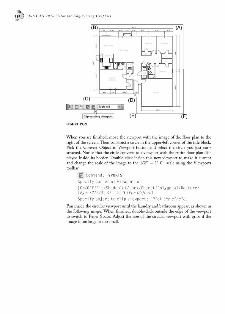
When you are finished, move the viewport with the image of the floor plan to theright of the screen. Then construct a circle in the upper-left corner of the title block.Pick the Convert Object to Viewport button and select the circle you just con-structed. Notice that the circle converts to a viewport with the entire floor plan dis-played inside its border. Double-click inside this new viewport to make it currentand change the scale of the image to the 1/2 00 ¼ 1 0-0 00 scale using the Viewportstoolbar.
Command: -VPORTS
Specify corner of viewport or
[ON/OFF/Fit/Shadeplot/Lock/Object/Polygonal/Restore/LAyer/2/3/4] <Fit>: O (For Object)
Specify object to clip viewport: (Pick the circle)
Pan inside the circular viewport until the laundry and bathroom appear, as shown inthe following image. When finished, double-click outside the edge of the viewportto switch to Paper Space. Adjust the size of the circular viewport with grips if theimage is too large or too small.
FIGURE 19.21
792 Aut oCAD 2010 Tu t o r f o r Eng in e e r i n g Graph i c s

Click the Polygonal Viewport button and construct a multisided viewport similarto the one located in the following image. Close the shape and do not be concernedthat a few lines may not be orthogonal.
Command: -VPORTS
Specify corner of viewport or
[ON/OFF/Fit/Shadeplot/Lock/Object/Polygonal/Restore/LAyer/2/3/4] <Fit>: P (For Polygonal)
Specify start point: (Pick at “A”)
Specify next point or [Arc/Length/Undo]: (Pick at “B”)
Specify next point or [Arc/Close/Length/Undo]: (Pick at “C”)
Specify next point or [Arc/Close/Length/Undo]: (Pick at “D”)
Specify next point or [Arc/Close/Length/Undo]: (Pick at “E”)
Specify next point or [Arc/Close/Length/Undo]: (Pick at “F”)
Specify next point or [Arc/Close/Length/Undo]: C (To closethe shape)
Regenerating model.
As the image of the floor plan appears in this new viewport, double-click insidethe new viewport to make it current. Scale the image inside the viewport to the scale3/8 00 ¼ 1 00 00. Pan until the kitchen area and master bathroom are visible. Yourdisplay should appear similar to the following image.
FIGURE 19.22
Chap t e r 19 • Advan c e d La y ou t T e c hn i q u e s 793

Double-click outside this viewport to return to Paper Space. Make any final adjust-ments to viewports using grips. When finished, turn off the Vports layer. Yourdisplay should appear similar to the following image.
FIGURE 19.23
FIGURE 19.24
794 Aut oCAD 2010 Tu t o r f o r Eng in e e r i n g Graph i c s

ROTATING VIEWPORTSViewports along with the view inside can easily be rotated using the traditionalROTATE command. You must first however activate the VPROTATEASSOCsystem variable before performing the rotation operation. This system variable mustbe entered in from the Command prompt and the spelling must be exact. The follow-ing image on the left represents a rectangular viewport with a land plat arrangedinside. When using the ROTATE command on the viewport, the results are dis-played in the following image in the middle. At a rotation angle of 30 degrees, theviewport rotates but the image inside does not. This is because VPROTATEASSOCis turned off or is set to 0 (zero). To rotate the viewport and the image inside, turnVPROTATEASSOC on or set it to 1. The results are displayed in the followingimage on the right with the viewport and image rotating to 30 degrees.
MATCHING THE PROPERTIES OF VIEWPORTSIn Chapter 7, the MATCHPROP (Match Properties) command was introduced as ameans of transferring all or selected properties from a source object to a series of des-tination objects. In addition to transferring layer information, dimension styles, hatchproperties, and text styles from one object to another, you can also transfer viewportinformation from a source viewport to other viewports. Information such as viewportlayer and the viewport scale are a few of the properties to transfer to other viewports.When you enter the MATCHPROP command and select the Settings option, the dia-log box in the following image will appear. When transferring viewport properties, besure the Viewport option of this dialog box is checked.
FIGURE 19.25
FIGURE 19.26
Chap t e r 19 • Advan c e d La y ou t T e c hn i q u e s 795

TRY IT! Open the drawing file 19_Matchprop Viewports, as shown in the following image. This draw-ing consists of four viewports holding different object types. The object in the first viewport(labeled “A” in the following image) is already scaled to 1 ¼ 1. All other viewports do notbelong to the Viewports layer. They are all scaled differently. These three viewports needto have the same properties as the first; namely, all viewports need to belong to the View-ports layer and all images inside all viewports need to be scaled to 1 ¼ 1. Rather thanperform these operations on each individual viewport, the MATCHPROP command will beused to accomplish this task.
Command: MA (For MATCHPROP)
Select source object: (Pick the edge of Viewport “A”)
Current active settings: Color Layer Ltype Ltscale Line-weight Thickness
PlotStyle Dim Text Hatch Polyline Viewport Table MaterialShadow display
Multileader
Select destination object(s) or [Settings]: (Pick the edge ofViewport “B”)
Select destination object(s) or [Settings]: (Pick the edge ofViewport “C”)
Select destination object(s) or [Settings]: (Pick the edge ofViewport “D”)
Select destination object(s) or [Settings]: (Press ENTER toexit this command)
The results are illustrated in the following image. All viewports share the same layerand are scaled to 1 ¼ 1 after using the matchprop command.
FIGURE 19.27
796 Aut oCAD 2010 Tu t o r f o r Eng in e e r i n g Graph i c s
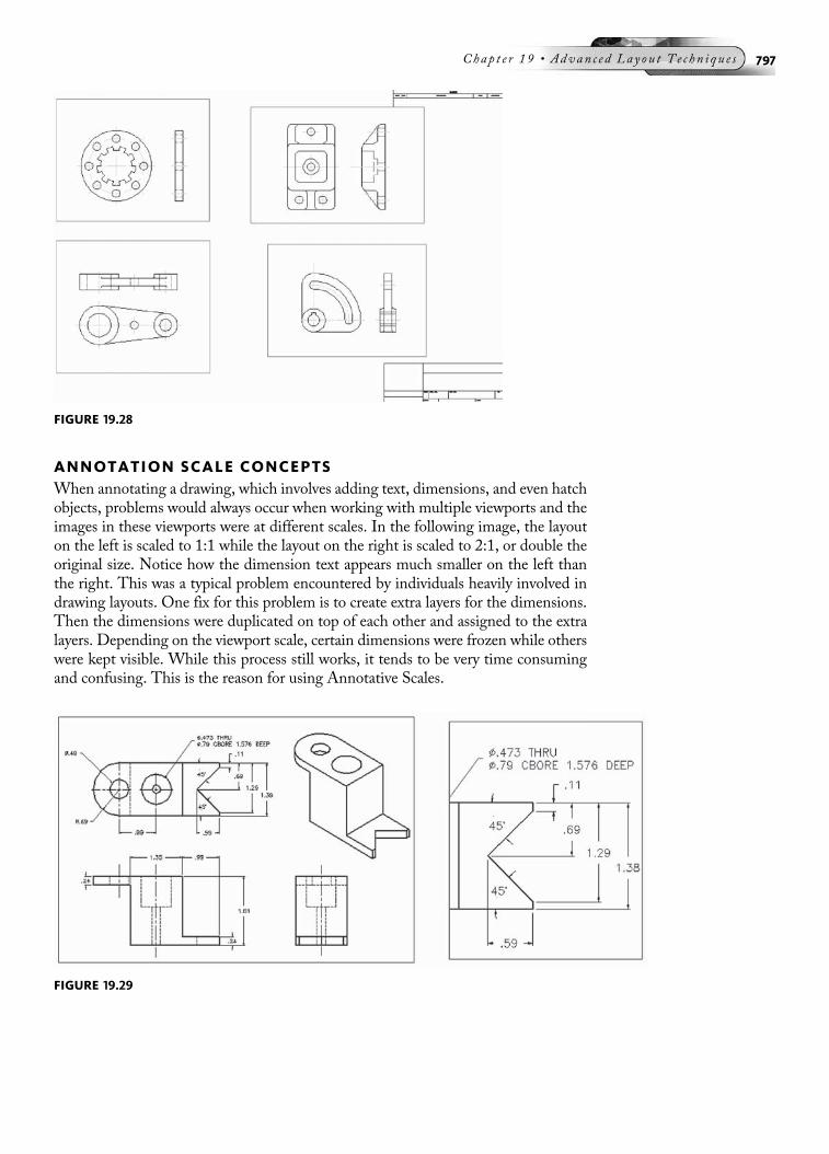
ANNOTATION SCALE CONCEPTSWhen annotating a drawing, which involves adding text, dimensions, and even hatchobjects, problems would always occur when working with multiple viewports and theimages in these viewports were at different scales. In the following image, the layouton the left is scaled to 1:1 while the layout on the right is scaled to 2:1, or double theoriginal size. Notice how the dimension text appears much smaller on the left thanthe right. This was a typical problem encountered by individuals heavily involved indrawing layouts. One fix for this problem is to create extra layers for the dimensions.Then the dimensions were duplicated on top of each other and assigned to the extralayers. Depending on the viewport scale, certain dimensions were frozen while otherswere kept visible. While this process still works, it tends to be very time consumingand confusing. This is the reason for using Annotative Scales.
FIGURE 19.28
FIGURE 19.29
Chap t e r 19 • Advan c e d La y ou t T e c hn i q u e s 797
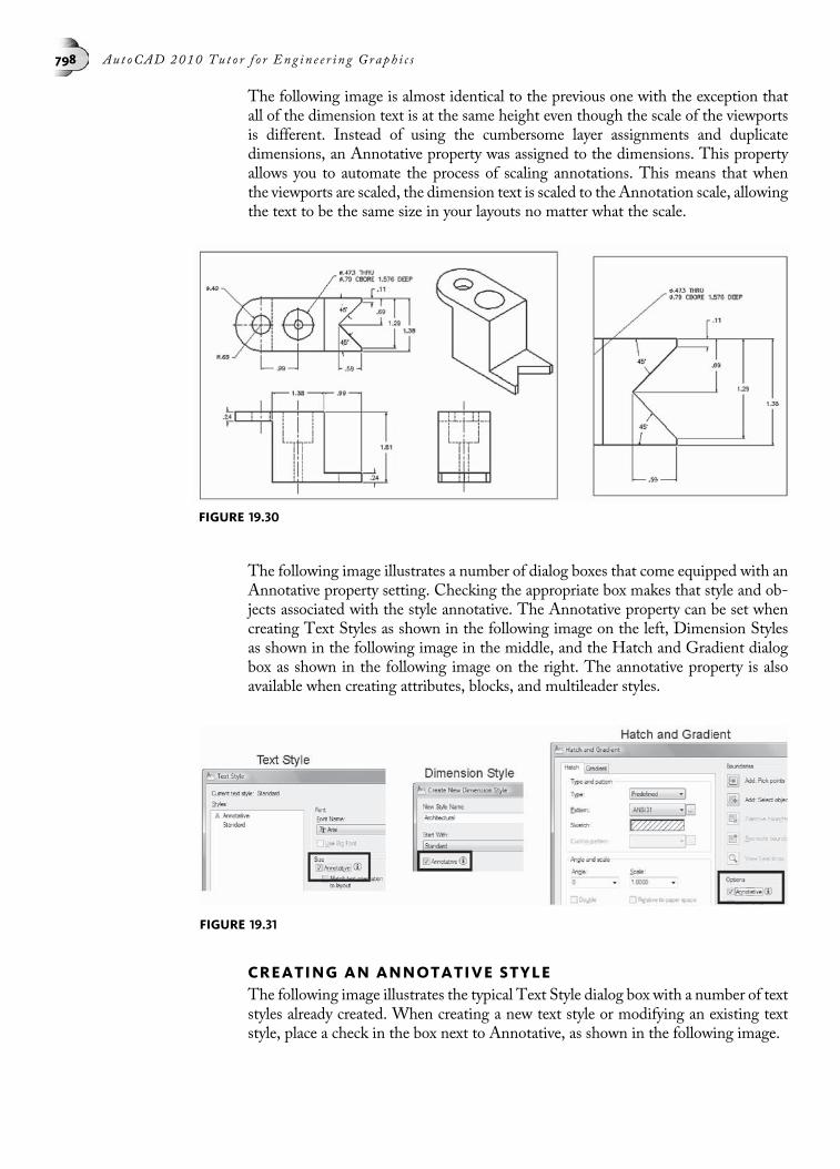
The following image is almost identical to the previous one with the exception thatall of the dimension text is at the same height even though the scale of the viewportsis different. Instead of using the cumbersome layer assignments and duplicatedimensions, an Annotative property was assigned to the dimensions. This propertyallows you to automate the process of scaling annotations. This means that whenthe viewports are scaled, the dimension text is scaled to the Annotation scale, allowingthe text to be the same size in your layouts no matter what the scale.
The following image illustrates a number of dialog boxes that come equipped with anAnnotative property setting. Checking the appropriate box makes that style and ob-jects associated with the style annotative. The Annotative property can be set whencreating Text Styles as shown in the following image on the left, Dimension Stylesas shown in the following image in the middle, and the Hatch and Gradient dialogbox as shown in the following image on the right. The annotative property is alsoavailable when creating attributes, blocks, and multileader styles.
CREATING AN ANNOTATIVE STYLEThe following image illustrates the typical Text Style dialog box with a number of textstyles already created. When creating a new text style or modifying an existing textstyle, place a check in the box next to Annotative, as shown in the following image.
FIGURE 19.30
FIGURE 19.31
798 Aut oCAD 2010 Tu t o r f o r Eng in e e r i n g Graph i c s

Annotative styles can be distinguished from traditional styles by a scale icon thatappears next to the styles name, as shown in the following image. In this image,notice the scale icon present in Dimension Style Manager and the MultileaderStyle Manager.
The following image illustrates an mtext object that was created under the controlof an Annotative text style. When you hover your cursor over this text object, theAnnotative icon appears as shown in the following image. This provides a quickway of identifying annotative text compared with regular, traditional text.
ANNOTATIVE SCALING TECHNIQUESWhile in model space, set the Annotation scale to the appropriate scale for yourdrawing (1 1/2 00 ¼ 1 00 00) as shown in the following image on the left. Any annotativetext or dimensions placed in the drawing will be automatically sized per the scalespecified. While in a drawing layout, you select the edge or activate a viewport andthe status bar displays VP (Viewport) Scale. Selecting the VP Scale, as shown in thefollowing image on the right, displays a list of scales that are identical to those usedin the Viewports toolbar. Once the scale is selected, the image in the viewport zoomsto the size required by the scale and any annotative dimensions or text will appearcorrectly sized in the layout.
FIGURE 19.32
FIGURE 19.33
FIGURE 19.34
Chap t e r 19 • Advan c e d La y ou t T e c hn i q u e s 799

NOTE Do not use the Viewports toolbar, as shown in the following image on the left, to scale view-ports when utilizing annotation scales. Use the status bar Viewport Scale button only, asshown in the following image on the right, to ensure proper automatic scaling and viewingof annotative objects.
VIEWING CONTROLS FOR ANNOTATIVE SCALESLocated in the Status bar are two additional buttons used for controlling how anno-tative scales are viewed in the current viewport. The two buttons are “AnnotationVisibility” and “Automatically add scales to annotative objects when the annotationscale changes.”
The Annotation Visibility button, as shown in the following image, is either on oroff. When Annotation Visibility is turned off in a layout, only annotative objectsthat use or match the current scale display. This means that if you change the VPScale to a different value, the annotation objects may disappear from the screen.This setting prevents you from having to freeze dimensions, text, and hatching inviewports where they would appear at the wrong size.
When Annotation Visibility is turned on in a layout, all annotative objects that useall scales will display.
FIGURE 19.35
FIGURE 19.36
FIGURE 19.37
800 Aut oCAD 2010 Tu t o r f o r Eng in e e r i n g Graph i c s
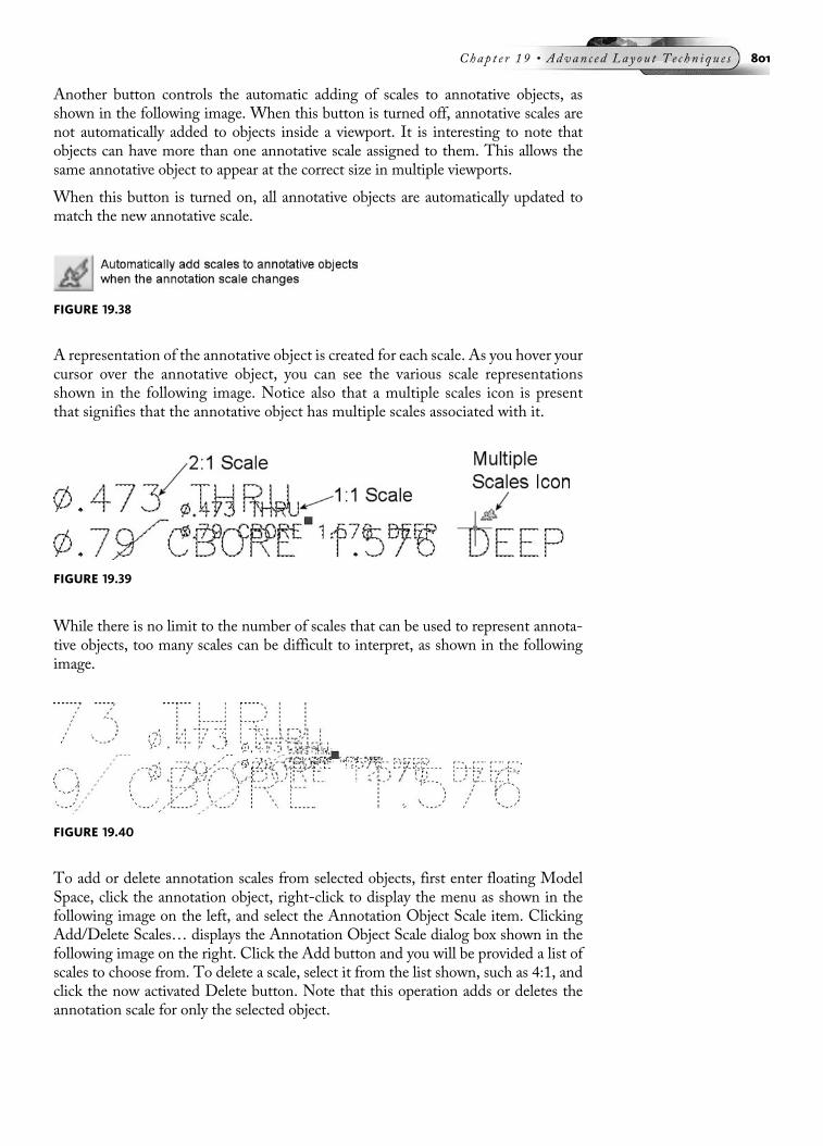
Another button controls the automatic adding of scales to annotative objects, asshown in the following image. When this button is turned off, annotative scales arenot automatically added to objects inside a viewport. It is interesting to note thatobjects can have more than one annotative scale assigned to them. This allows thesame annotative object to appear at the correct size in multiple viewports.
When this button is turned on, all annotative objects are automatically updated tomatch the new annotative scale.
A representation of the annotative object is created for each scale. As you hover yourcursor over the annotative object, you can see the various scale representationsshown in the following image. Notice also that a multiple scales icon is presentthat signifies that the annotative object has multiple scales associated with it.
While there is no limit to the number of scales that can be used to represent annota-tive objects, too many scales can be difficult to interpret, as shown in the followingimage.
To add or delete annotation scales from selected objects, first enter floating ModelSpace, click the annotation object, right-click to display the menu as shown in thefollowing image on the left, and select the Annotation Object Scale item. ClickingAdd/Delete Scales… displays the Annotation Object Scale dialog box shown in thefollowing image on the right. Click the Add button and you will be provided a list ofscales to choose from. To delete a scale, select it from the list shown, such as 4:1, andclick the now activated Delete button. Note that this operation adds or deletes theannotation scale for only the selected object.
FIGURE 19.38
FIGURE 19.39
FIGURE 19.40
Chap t e r 19 • Advan c e d La y ou t T e c hn i q u e s 801

NOTE The Annotation Object Scale dialog box can also be accessed by entering OBJECTSCALEwhen you are prompted to select the annotative objects.
Yet another method of activating the Annotation Object Scale dialog box is illus-trated in the following image. In this example, an annotative dimension was firstselected; then the Properties Palette was displayed as shown in the following imageon the left. Notice under the Misc heading the Annotative category and the 2:1scale field. Clicking on this field displays three dots or ellipses. Clicking the ellipsesbutton launches the Annotation Object Scale dialog box. Clicking the Add… buttondisplays the list of scales to add to the selected annotation object.
NOTE To delete an annotation scale from the list for all annotation objects, enter the OBJECTSCALEcommand. At the Select Annotation Objects prompt, enter All to select all annotationobjects. When the list of scales appears in the Annotation Object Scale dialog box, pickthe scale from this list to delete.
ANNOTATIVE LINETYPE SCALINGThe following Try It! exercise demonstrates how Annotative scale controls thescale of linetypes displayed in both Model and Paper Space. The system variableMSLTSCALE should be set to a value of 1 in order for the linetypes to displayproperly in Model Space. The default value is 1 but it may be set to 0 in older draw-ings. The system variable PSLTSCALE should also be set to a value of 1 in orderfor the linetypes to display properly in Paper Space.
FIGURE 19.41
FIGURE 19.42
802 Aut oCAD 2010 Tu t o r f o r Eng in e e r i n g Graph i c s

TRY IT!Open the drawing 19_Land Plat. The drawing opens up in Model Space as shown in the fol-lowing image on the left. Also, the current value of LTSCALE (Linetype Scale) is 1.00. Sincethis drawing will be plotted at a scale of 1:30, the land plat outline is too large to view thelinetypes. You could zoom in to a segment of the plat; however, even in this magnified viewthe number of short and long dashes is numerous. This problem, however, is fixed whenswitching to the Paper Space layout. Here, as shown in the following image on the right,the linetypes are properly scaled thanks to the Paper Space linetype scaling function beingturn on (PSLTSCALE ¼ 1) by default.
Switch back to Model Space by clicking the Model tab and change the LTSCALEvalue from 1.00 to 30.00. The results are displayed in the following image on the leftwith the linetypes representing the outline of the property being visible. Then clickthe layout tab and observe the results shown in the following image on the right. Evenwith Paper Space linetype scaling turned on, the LTSCALE value affects the PaperSpace image where the linetype scale value is too large to display the linetypes. Inother words, you either display the linetypes in the Model tab or the Layout tab butnot both.
The solution to this dilemma of the scaling of linetypes is illustrated in the followingimage. Return to Model Space by selecting the Model tab and set the LTSCALEback to 1.00. In the status bar set the Annotation Scale to 1:30 and perform aREGEN, as illustrated in the following image on the left. The linetype scale appearscorrect thanks to the Model Space linetype scale being turned on (MSLTSCALE ¼1). When you are switching to the Layout tab, the linetypes are still visible in
FIGURE 19.43
FIGURE 19.44
Chap t e r 19 • Advan c e d La y ou t T e c hn i q u e s 803
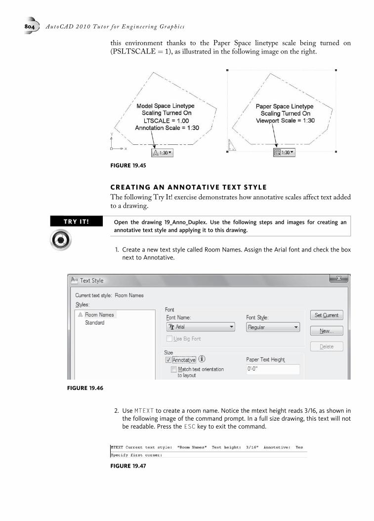
this environment thanks to the Paper Space linetype scale being turned on(PSLTSCALE ¼ 1), as illustrated in the following image on the right.
CREATING AN ANNOTATIVE TEXT STYLEThe following Try It! exercise demonstrates how annotative scales affect text addedto a drawing.
TRY IT! Open the drawing 19_Anno_Duplex. Use the following steps and images for creating anannotative text style and applying it to this drawing.
1. Create a new text style called Room Names. Assign the Arial font and check the boxnext to Annotative.
2. Use MTEXT to create a room name. Notice the mtext height reads 3/16, as shown inthe following image of the command prompt. In a full size drawing, this text will notbe readable. Press the ESC key to exit the command.
FIGURE 19.45
FIGURE 19.46
FIGURE 19.47
804 Aut oCAD 2010 Tu t o r f o r Eng in e e r i n g Graph i c s

3. While still in Model Space, change the current Annotation Scale to ¼ 00 ¼ 1 0-0 00 asshown in the following image on the left.
Reenter the MTEXT command and notice that the height of the text has changed to9 5/8 00 based on the current annotation scale. Add the text BEDROOM 1 to theroom and exit the Text Formatting toolbar. Hover your cursor over the text andnotice the appearance of the scale icon signifying that this text is considered anannotative object, as shown in the following image on the right.
4. Continue using MTEXT to add names to all of the remaining rooms of the duplex, asshown in the following image.
5. Switch to the B-Size (DWF6) layout. None of the room names display. This isbecause an annotative scale has not been set for this viewport. Click the edge ofthe viewport and change the VP Scale to ¼ 00 ¼ 1 0-0 00, as shown in the followingimage on the left.
Notice that the image inside of the viewport changes to reflect the current scale.Also, the text reappears since it matches the original annotative scale of ¼ 00 ¼ 1 0-0 00,as shown in the following image on the right.
FIGURE 19.48
FIGURE 19.49
Chap t e r 19 • Advan c e d La y ou t T e c hn i q u e s 805

6. Set the “Automatically add scales to annotative objects when the annotation scalechanges” button to on, as shown in the following image on the left.
Click the edge of the viewport and change the scale of the viewport to 3/16 00 ¼ 1 0-0 00,as shown in the following image on the right. Even though the floor plan inside of theviewport is smaller, the size of the text is the same as with the previous scale.
7. Switch back to Model Space by clicking the Model tab. Click one of the text objectsand hover your cursor over this object. Looking carefully at the selected text; twotext objects actually appear, one smaller than the other. The two text objects reflectthe larger and smaller annotative scales that were used on the viewport back in thelayout.
FIGURE 19.50
FIGURE 19.51
FIGURE 19.52
806 Aut oCAD 2010 Tu t o r f o r Eng in e e r i n g Graph i c s

8. With the text object still selected, activate the Properties Palette and observe theinformation contained under the Text heading, as shown in the following image onthe left.
9. Click inside the Annotation Scale field. When the three dots (ellipses) appear,click these, as shown in the following image on the left, and select the text objectagain; then press the ENTER key to launch the Annotation Object Scale dialog box.The two annotation scales should be listed as shown in the following image on theright. Click the Cancel button when you are finished.
10. Switch back to the B-Size (DWF6) layout and turn off the “Automatically add scales toannotative objects when the annotation scale changes” button and verify that theAnnotation Visibility button is turned off, as shown in the following image.Typically, these buttons should remain off in a layout when working with annotationscales so that annotative objects will only appear in the viewports they are correctlysized for and you will not be continuously creating scales every time you change aviewport scale.
FIGURE 19.53
FIGURE 19.54
FIGURE 19.55
Chap t e r 19 • Advan c e d La y ou t T e c hn i q u e s 807
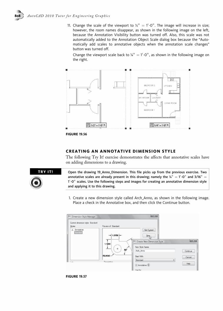
11. Change the scale of the viewport to ½ 00 ¼ 1 0-0 00. The image will increase in size;however, the room names disappear, as shown in the following image on the left,because the Annotation Visibility button was turned off. Also, this scale was notautomatically added to the Annotation Object Scale dialog box because the “Auto-matically add scales to annotative objects when the annotation scale changes”button was turned off.
Change the viewport scale back to ¼ 00 ¼ 1 0-0 00, as shown in the following image onthe right.
CREATING AN ANNOTATIVE DIMENSION STYLEThe following Try It! exercise demonstrates the affects that annotative scales haveon adding dimensions to a drawing.
TRY IT! Open the drawing 19_Anno_Dimension. This file picks up from the previous exercise. Twoannotative scales are already present in this drawing; namely the ¼ 00 ¼ 1 0-0 00 and 3/16 00 ¼1 0-0 00 scales. Use the following steps and images for creating an annotative dimension styleand applying it to this drawing.
1. Create a new dimension style called Arch_Anno, as shown in the following image.Place a check in the Annotative box, and then click the Continue button.
FIGURE 19.56
FIGURE 19.57
808 Aut oCAD 2010 Tu t o r f o r Eng in e e r i n g Graph i c s

2. Use the table below for making changes while inside of the Dimension StylesManager dialog box.
Dimension Styles Dialog Box
Tab Setting Change To
Symbols and Arrows Arrowheads Architectural Tick
Symbols and Arrows Arrow Size 1/8 00
Text Text Height 1/8 00
Text Text Placement – Vertical Above
Text Text Alignment Align with dimension line
Primary Units Unit Format Architectural
Primary Units Precision 0 0-0 00
Verify in the Fit tab that the Annotative box is checked in the Scale for dimensionarea, as shown in the following image. After making changes to the dimension set-tings, click the OK button.
3. When you return back to the main Dimension Styles Manager dialog box, notice theArch_Anno dimension style present in the list. Notice also the appearance of thescale icon next to this dimension style name, signifying that all dimensions in thisstyle will be controlled by the annotative scale feature. Click the Close button toexit the Dimension Styles Manager dialog box and continue with this exercise.
FIGURE 19.58
FIGURE 19.59
Chap t e r 19 • Advan c e d La y ou t T e c hn i q u e s 809

4. With the Annotation Scale already set to ¼ 00 ¼ 1 0-0 00 in Model Space, begin placinglinear and continue dimensions in the various locations of the floor plan, as shown inthe following image on the left.
Switch to the B-Size (DWF6) layout. Observe that the all dimensions are visible basedon the current annotation scale of ¼ 00 ¼ 1 0-0 00 matching the VP Scale, as shown inthe following image on the right.
5. Turn on the Automatically add scales button, as shown in the following image.
6. Change the VP Scale to 3/16 00 ¼ 1 0-0 00, as shown in the following image on the left.Notice in this image that as the image of the floor plan gets smaller, the dimensionsremain their original plotting height of 1/8 00.Turn the Automatically add scales button back off and switch the VP Scale back to¼ 00 ¼ 1 0-0 00, as shown in the following image on the right.
FIGURE 19.60
FIGURE 19.61
FIGURE 19.62
810 Aut oCAD 2010 Tu t o r f o r Eng in e e r i n g Graph i c s

WORKING WITH ANNOTATIVE HATCHINGThe following Try It! exercise demonstrates how annotative scales affect how anobject is crosshatched when using the Hatch and Gradient dialog box.
TRY IT!Open the drawing 19_Anno_Hatch. This file picks up from the previous exercise. Two anno-tative scales are already present in this drawing, namely the ¼ 00 ¼ 1 0-0 00 and 3/16 00 ¼ 1 0-0 00
scales. Dimensions are also present in this drawing. Use the following steps and images forworking with annotative hatching in this drawing.
1. Activate the Boundary Hatch dialog box. Change the hatch pattern scale to 48, asshown in the following image on the left. Also place a check next to Annotative toturn on Annotative scaling of the hatch pattern, as shown in the following image onthe right.
2. Click the Pick Points button and select all internal areas that represent the floor plan,as shown in the following image on the left. When you return back to the boundaryhatch dialog box, click the OK button to place the hatch pattern as shown in thefollowing image on the right.
3. Switch to the B-Size (DWF6) layout and notice that the hatch pattern is visible basedon the current Viewport and Annotation scales of ¼ 00 ¼ 1 0-0 00, as shown in thefollowing image.
FIGURE 19.63
FIGURE 19.64
Chap t e r 19 • Advan c e d La y ou t T e c hn i q u e s 811

4. Change the VP Scale to 3/16 00 ¼ 1 0-0 00. Notice that as the image of the floor plan getssmaller, the hatch pattern disappears because the hatch scale does not match theviewport scale. Turn the Annotation visibility button on to see the hatching butnotice that the hatch is incorrectly sized for this viewport scale, as shown in thefollowing image.
FIGURE 19.65
FIGURE 19.66
812 Aut oCAD 2010 Tu t o r f o r Eng in e e r i n g Graph i c s

TUTORIAL EXERCISE: 19_ARCHITECTURAL DETAILS.DWG
PurposeThis tutorial exercise is designed to lay out three architectural details, displayed in theprevious image, in the Layout mode (Paper Space). The three details consist of a floorplan, cornice detail, and foundation detail.
System SettingsOpen an existing drawing called 19_Architectural Details. Keep all default settings forthe units and limits of the drawing.
LayersLayers have already been created for this drawing.
Suggested CommandsAn existing drawing will be used to create a new layout. This layout will hold threeviewports displaying three different architectural details at different scales. The Layoutwizard will be used to create the initial layout in Paper Space. Additional viewportswill be added to hold the remaining details. Annotation scales will be used to scale thedetails relative to their individual viewports. Grips will be used to adjust the viewports.A plot preview will be performed to observe the images floating on the drawing sheet.
STEP 1Open the drawing 19_Architectural Details.Dwg. Notice the floor plan and the two smalldetails. The three architectural images will need to be arranged in separate viewportswith separate scales. The floor plan will need to be laid out at a scale of 1/4 00 ¼ 1 0-0 00;the cornice detail at 3 00 ¼ 1 0-0 00 and the foundation detail at 1 ½ 00 ¼ 1 0-0 00.
FIGURE 19.67
Chap t e r 19 • Advan c e d La y ou t T e c hn i q u e s 813

STEP 2While in Model Space, change the Annotation Scale to ¼ 00 ¼ 1 0-0 00, as shown in thefollowing image.
STEP 3Change to the Text layer and add the room names to the floor plan using the followingimage as a guide. Use the MTEXT command and a height of .20 for all room names. TheText Style “Titles” is already created and is set to Annotative, as shown in the followingimage.
FIGURE 19.68
FIGURE 19.69
814 Aut oCAD 2010 Tu t o r f o r Eng in e e r i n g Graph i c s

STEP 4Change the layer to Dimensions. Add all dimensions to the floor plan using the followingimage as a guide. The Dimension Style “Architectural” is already created and set to Anno-tative, as shown in the following image.
STEP 5Activate the Create Layout wizard by clicking on the Tools Menu Bar followed by Wizards,as shown in the following image on the left. When the Create Layout dialog box appears,change the name of the layout to Detail Sheet, as shown in the following image on
FIGURE 19.70
FIGURE 19.71
Chap t e r 19 • Advan c e d La y ou t T e c hn i q u e s 815

the right. Continue inside this wizard by making the following changes in the additionaldialog boxes that appear:
• Printer—Select DWF6 ePlot.pc3 device from the list of available printers.
• Paper Size—Select ARCH expanded D (36.00 � 24.00 Inches).
• Orientation—Verify that Landscape is the current setting in this dialog box.
• Title Block—From the available list, pick Architectural Title Block.dwg.
• Define Viewports—Verify that Single is set for the Viewport Setup. Use the defaultScale to Fit listing in the Viewport scale field.
• Pick Location—Click the Select Location button. This returns you momentarily tothe drawing editor. Pick two points at “A” and “B” as the corners of the viewport,as shown in the following image.
• Finish—Click the Finish button to exit the wizard and return to the drawing editor.
FIGURE 19.72
FIGURE 19.73
816 Aut oCAD 2010 Tu t o r f o r Eng in e e r i n g Graph i c s

STEP 6Create two additional viewports using the Single Viewport button, located in the View-ports toolbar as shown in the following image. Construct the first viewport from “A” to“B” and the second viewport from “C” to “D.” These locations are approximate. Noticethat the images of all the details appear in both viewports.
STEP 7Click the edge of all three viewports and notice in the Layer Control box the name ofthe layer. Clicking the down arrow and selecting the Viewports layer changes all threeviewports to this layer, as shown in the following image.
STEP 8Click the edge of the large viewport and change the VP Scale to ¼ 00 ¼ 1 0-0 00, as shown inthe following image.
FIGURE 19.74
FIGURE 19.75
Chap t e r 19 • Advan c e d La y ou t T e c hn i q u e s 817

STEP 9Double-click inside the upper-right viewport to make it current. Pan the image of theCornice approximately to the middle of the top viewport. It is helpful to perform this stepon small details that are about to be scaled. Sometimes images get lost in the viewport ifthis step is not performed.
STEP 10Change the VP Scale of this image to 3 00 ¼ 1 0-0 00, as shown in the following image. Theresults of this operation are illustrated in the following image. You may have to pan theimage in order to center it better inside the viewport.
FIGURE 19.76
FIGURE 19.77
818 Aut oCAD 2010 Tu t o r f o r Eng in e e r i n g Graph i c s

STEP 11Perform the same operations on the bottom-right viewport in order to scale the founda-tion detail inside the viewport. Click inside this viewport to make it current. Pan theimage of the Foundation detail approximately to the middle of the bottom viewport.
STEP 12Change the VP Scale of this image to 1-1/2 00 ¼ 1 0-0 00, as shown in the following image. Theresults of this operation are illustrated in the following image. You may have to pan theimage in order to better position it inside the viewport. Note that this detail favorsthe left side of the viewport; you will need this room to label various parts of the detailusing multileaders in a later step.
FIGURE 19.78
FIGURE 19.79
Chap t e r 19 • Advan c e d La y ou t T e c hn i q u e s 819

STEP 13Switch back to Paper Space. Click the edges of all three viewports and click the Lockbutton, as shown in the following image. This prevents any accidental scaling of the imagesif you have to enter floating Model Space. Notice also that the VP Scale reads VARIES. Thisis because all three viewports were selected and the scales of each viewport are different.
STEP 14Change to the Text layer. Double-click inside the large viewport to activate floatingModel Space. Use the MTEXT command and a text height of .30 to place the title of thisimage (FLOOR PLAN) and the scale (¼ 00 ¼ 1 0-0 00) as shown in the following image. Thesize of the text is scaled and visible since the text style was set to Annotative.
FIGURE 19.80
FIGURE 19.81
820 Aut oCAD 2010 Tu t o r f o r Eng in e e r i n g Graph i c s

STEP 15Click inside of the viewport containing the cornice detail to make it active and use theMTEXT command and a text height of .30 to place the title of this image and the scale,as shown in the following image on the left. Click inside the viewport containing thefoundation detail to make it active and use the MTEXT command to place the title ofthis image and the scale as shown in the following image on the right.
STEP 16Verify that the foundation plan is still the active viewport; the User Coordinate Systemicon should be visible. You will label various elements that make up the foundation detailwith multileaders. Notice in the following image on the left that a multileader style isalready created and set to Annotative. Then choose the MLEADER command from theDimension Menu Bar or the Ribbon, also shown in the following image on the left. Placethe following multileader notes: INSULATION, FINISHED FLOOR, CONCRETE SLAB,GRAVEL, CONCRETE PIER, and FOOTING as shown in the following image on the right.
FIGURE 19.82
FIGURE 19.83
Chap t e r 19 • Advan c e d La y ou t T e c hn i q u e s 821

STEP 17Switch back to Paper Space and perform a plot preview. Your display should appearsimilar to the following image.
NOTE You could also add crosshatching to the walls of the floor plan. To do this, click the Modeltab to return to Model Space. Activate the Hatch and Gradient dialog box. Use the ANSI31hatch pattern and change the scale of the pattern to 48. Also place a check in the box nextto Annotative.
FIGURE 19.84
FIGURE 19.85
822 Aut oCAD 2010 Tu t o r f o r Eng in e e r i n g Graph i c s

CHAPTER
20
Solid ModelingFundamentals
Solid models are mathematical models of actual objects that can be analyzed throughthe calculation of such items as mass properties, center of gravity, surface area, mo-ments of inertia, and much more. Before solid models are built, various options of theUCS command need to be understood. The use and creation of visual styles are alsodiscussed in this chapter. The solid model starts the true design process by definingobjects as a series of primitives. Boxes, cones, cylinders, spheres, and wedges are allexamples of primitives. These building blocks are then joined together or subtractedfrom each other through modify commands. Intermediate solid modeling commandssuch as EXTRUDE, REVOLVE, SWEEP, and LOFT are discussed in this chapter, aswell as the ability to create a spiral or helix object. Fillets and chamfers can be createdto give the solid model a more realistic appearance and functionality.
WORKING IN THE 3D MODELING WORKSPACEAs a means of allowing you to work in a dedicated custom, task-orientated environ-ment, predefined workspaces are already created in AutoCAD. These workspacesconsist of menus, toolbars, and palettes that are organized around a specific task.When you select a workspace, only those menus, toolbars, and palettes that relatedirectly to the task are displayed.
The workspaces can be found by picking the Workspaces toolbar as shown in thefollowing image on the left or from the status bar located at the bottom of the displayscreen, as shown in the following image on the right. Of these workspaces, you willfind it productive to use 3D Modeling throughout this chapter in the book.
823

The 3D Modeling WorkspaceClicking on the 3D Modeling workspace in the previous image changes yourAutoCAD screen to appear similar to the following image. In this image, your screencontains only 3D-related menus and palettes.
NOTE In addition to the Ribbon, the tool palette also displays when you activate the 3D Modelingworkspace. The tool palette has been turned off in the following image.
When you make changes to your drawing display (such as moving, hiding, or display-ing a toolbar or a tool palette group) and you want to preserve the display settings forfuture use, you can save the current settings to a workspace.
The Ribbon of the 3D Modeling workspace consists of buttons and controls usedprimarily for 3D modeling, 3D navigation, controlling lights, controlling visualstyles, creating and applying materials, and producing renderings as shown in the fol-lowing image. The use of the Ribbon eliminates the need to display numerous tool-bars, which tend to clutter up your screen. This enables you to have more screen realestate for constructing your 3D models. When you activate the 3D Modeling work-space, the Ribbon automatically displays. The Ribbon can also be displayed in anyworkspace by clicking the Tools Menu Bar, followed by Palettes, and then Ribbon.
When the Ribbon first displays, the Home tab is active. At this point, the followingpanels are available based on the 3D Modeling workspace; 3D Modeling, Draw,Solid Editing, Modify, View, Layers, Properties, and Utilities, as shown in thefollowing image.
The Render Tab of the RibbonAnother helpful tab used for working in a 3D environment is the Visualize tab.Clicking on the Visualize tab of the Ribbon will expose the following panels; VisualStyles, Edge Effects, Lights, Sun, Time & Location, and Materials, as shown in thefollowing image.
FIGURE 20.1
FIGURE 20.2
824 Aut oCAD 2010 Tu t o r f o r Eng in e e r i n g Graph i c s
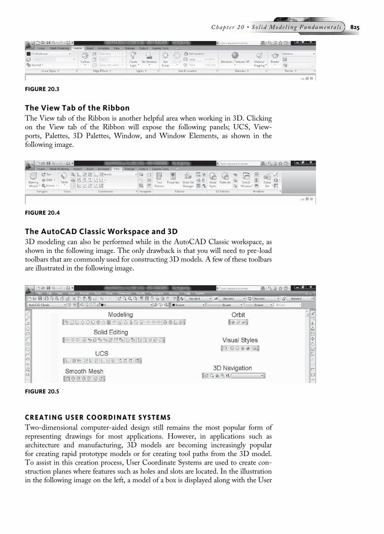
The View Tab of the RibbonThe View tab of the Ribbon is another helpful area when working in 3D. Clickingon the View tab of the Ribbon will expose the following panels; UCS, View-ports, Palettes, 3D Palettes, Window, and Window Elements, as shown in thefollowing image.
The AutoCAD Classic Workspace and 3D3D modeling can also be performed while in the AutoCAD Classic workspace, asshown in the following image. The only drawback is that you will need to pre-loadtoolbars that are commonly used for constructing 3D models. A few of these toolbarsare illustrated in the following image.
CREATING USER COORDINATE SYSTEMSTwo-dimensional computer-aided design still remains the most popular form ofrepresenting drawings for most applications. However, in applications such asarchitecture and manufacturing, 3D models are becoming increasingly popularfor creating rapid prototype models or for creating tool paths from the 3D model.To assist in this creation process, User Coordinate Systems are used to create con-struction planes where features such as holes and slots are located. In the illustrationin the following image on the left, a model of a box is displayed along with the User
FIGURE 20.3
FIGURE 20.4
FIGURE 20.5
Chap t e r 20 • So l i d Mod e l i n g Fundamen t a l s 825
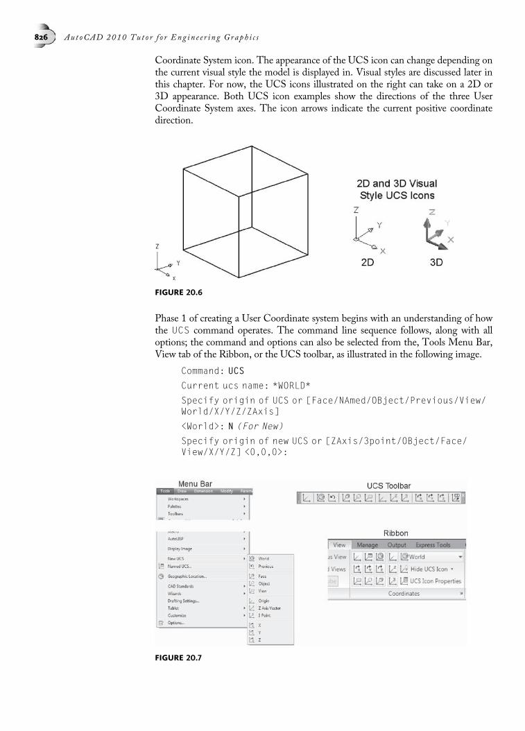
Coordinate System icon. The appearance of the UCS icon can change depending onthe current visual style the model is displayed in. Visual styles are discussed later inthis chapter. For now, the UCS icons illustrated on the right can take on a 2D or3D appearance. Both UCS icon examples show the directions of the three UserCoordinate System axes. The icon arrows indicate the current positive coordinatedirection.
Phase 1 of creating a User Coordinate system begins with an understanding of howthe UCS command operates. The command line sequence follows, along with alloptions; the command and options can also be selected from the, Tools Menu Bar,View tab of the Ribbon, or the UCS toolbar, as illustrated in the following image.
Command: UCS
Current ucs name: *WORLD*
Specify origin of UCS or [Face/NAmed/OBject/Previous/View/World/X/Y/Z/ZAxis]
<World>: N (For New)
Specify origin of new UCS or [ZAxis/3point/OBject/Face/View/X/Y/Z] <0,0,0>:
FIGURE 20.6
FIGURE 20.7
826 Aut oCAD 2010 Tu t o r f o r Eng in e e r i n g Graph i c s
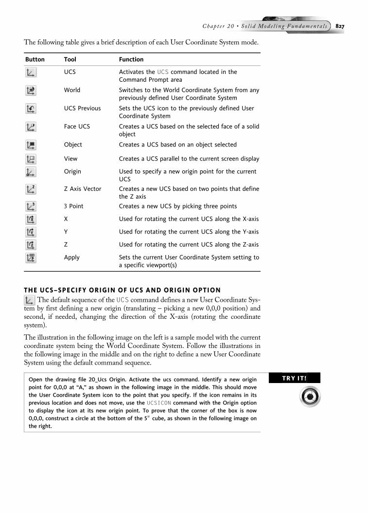
The following table gives a brief description of each User Coordinate System mode.
Button Tool Function
UCS Activates the UCS command located in theCommand Prompt area
World Switches to the World Coordinate System from anypreviously defined User Coordinate System
UCS Previous Sets the UCS icon to the previously defined UserCoordinate System
Face UCS Creates a UCS based on the selected face of a solidobject
Object Creates a UCS based on an object selected
View Creates a UCS parallel to the current screen display
Origin Used to specify a new origin point for the currentUCS
Z Axis Vector Creates a new UCS based on two points that definethe Z axis
3 Point Creates a new UCS by picking three points
X Used for rotating the current UCS along the X-axis
Y Used for rotating the current UCS along the Y-axis
Z Used for rotating the current UCS along the Z-axis
Apply Sets the current User Coordinate System setting toa specific viewport(s)
THE UCS–SPECIFY ORIGIN OF UCS AND ORIGIN OPTIONThe default sequence of the UCS command defines a new User Coordinate Sys-
tem by first defining a new origin (translating – picking a new 0,0,0 position) andsecond, if needed, changing the direction of the X-axis (rotating the coordinatesystem).
The illustration in the following image on the left is a sample model with the currentcoordinate system being the World Coordinate System. Follow the illustrations inthe following image in the middle and on the right to define a new User CoordinateSystem using the default command sequence.
TRY IT!Open the drawing file 20_Ucs Origin. Activate the ucs command. Identify a new originpoint for 0,0,0 at “A,” as shown in the following image in the middle. This should movethe User Coordinate System icon to the point that you specify. If the icon remains in itsprevious location and does not move, use the UCSICON command with the Origin optionto display the icon at its new origin point. To prove that the corner of the box is now0,0,0, construct a circle at the bottom of the 5 00 cube, as shown in the following image onthe right.
Chap t e r 20 • So l i d Mod e l i n g Fundamen t a l s 827

Command: UCS
Current ucs name: *WORLD*
Specify origin of UCS or [Face/NAmed/OBject/Previous/View/World/X/Y/Z/ZAxis]
<World>: End
of (Select the endpoint of the line at “A”)
Specify point on X-axis or <Accept>: (Press ENTER to acceptsince you do not want to rotate the coordinate system)
Command: C (For CIRCLE)
Specify center point for circle or [3P/2P/Ttr (tan tanradius)]: 2.5,2.5,0
Specify radius of circle or [Diameter]: 2
Notice a small “plus” at the corner of the User Coordinate System icon (see the illus-tration in the following image on the right). This indicates that the UCS icon is dis-played at the origin (0,0,0). A small box, as shown in the following image on the left,indicates that the icon is displaced at the World Coordinate System (WCS).
It is also important to note that the circle shown in the following image on the right isa 2D object and can only be drawn in or parallel to the XY plane (for example, thebottom or top of the box). To draw a circle in the side of the box, we will need tonot only move (translate) our coordinate system but rotate it as well.
Another popular method of changing the UCS origin is provided through the Originoption. This option is available through the UCS toolbar, Ribbon, and Tools MenuBar. It allows you select a new 0,0,0 position but does not provide any prompts forrotating the coordinate system. The Origin option is not listed in the commandprompts but can be entered as shown below.
Command: UCS
Current ucs name: *WORLD*
Specify origin of UCS or [Face/NAmed/OBject/Previous/View/World/X/Y/Z/ZAxis]
<World>: O (For Origin)
Specify new origin point <0,0,0>: (Pick desired point)
FIGURE 20.8
828 Aut oCAD 2010 Tu t o r f o r Eng in e e r i n g Graph i c s

THE UCS–3POINT OPTIONUse the 3point option of the UCS command to specify a new User Coordinate
System by identifying an origin and new directions of its positive X- and Y-axes(translate and rotate). This option, like the Origin option, is not listed in the com-mand sequence but can be entered anyway. The option is displayed in the UCS tool-bar, Ribbon, and Tools Menu Bar (New UCS).
TRY IT!Open the drawing file 20_Ucs 3p. The illustration in the following image on the left showsa 3D cube in the World Coordinate System. To construct objects on the front panel, firstdefine a new User Coordinate System parallel to the front. Use the following commandsequence to accomplish this task.
Command: UCS
Current ucs name: *WORLD*
Specify origin of UCS or [Face/NAmed/OBject/Previous/View/World/X/Y/Z/ZAxis]
<World>: 3 (For 3point)
Specify new origin point <0,0,0>: End
of (Select the endpoint of the model at “A” as shown in themiddle of the following image)
Specify point on positive portion of X-axis <>: End
of (Select the endpoint of the model at “B”)
Specify point on positive-Y portion of the UCS XY plane <>:End
of (Select the endpoint of the model at “C”)
With the Y-axis in the vertical position and the X-axis in the horizontal position, anytype of object can be constructed along this plane, such as the lines shown in the fol-lowing image on the right.
TRY IT!Open the drawing file 20_Incline. The 3point method of defining a new User CoordinateSystem is quite useful in the example shown in the following image, where a UCS needs tobe aligned with the inclined plane. Use the intersection at “A” as the origin of the new UCS,the intersection at “B” as the direction of the positive X-axis, and the intersection at “C” asthe direction of the positive Y-axis.
FIGURE 20.9
Chap t e r 20 • So l i d Mod e l i n g Fundamen t a l s 829

THE UCS–X/Y/Z ROTATION OPTIONSUsing the X/Y/Z rotation options rotates the current user coordinate around
the specific axis. Select the X, Y, or Z option to establish the axis that will act asthe pivot; a prompt appears asking for the rotation angle about the pivot axis. Theright-hand rule is used to determine the positive direction of rotation around anaxis. Think of the right hand gripping the pivot axis with the thumb pointing inthe positive X, Y, or Z direction. The curling of the fingers on the right hand deter-mines the positive direction of rotation. The following image illustrates positiverotation about each axis. By viewing down the selected axis, the positive rotation isseen to be counterclockwise.
TRY IT! Open the drawing file 20_Ucs Rotate. Given the cube shown in the following image on theleft in the World Coordinate System, the X option of the UCS command will be used tostand the icon straight up by entering a 90° rotation value, as in the following promptsequence.
Command: UCS
Current ucs name: *NO NAME*
Specify origin of UCS or [Face/NAmed/OBject/Previous/View/World/X/Y/Z/ZAxis]
<World>: X
Specify rotation angle about X-axis <90>: (Press ENTER toaccept 90° of rotation)
FIGURE 20.10
FIGURE 20.11
830 Aut oCAD 2010 Tu t o r f o r Eng in e e r i n g Graph i c s

The X-axis is used as the pivot of rotation; entering a value of 90° rotates the icon thedesired degrees in the counterclockwise direction, as shown in the following image onthe right.
THE UCS–OBJECT OPTIONAnother option for defining a new User Coordinate System is to select an object
and have the User Coordinate System align to that object (translate and rotate).
TRY IT!Open the drawing file 20_Ucs Object. Given the 3D cube shown in the following image onthe left, use the following command sequence and the illustration on the right to constructthe circle on the proper plane.
Command: UCS
Current ucs name: *WORLD*
Specify origin of UCS or [Face/NAmed/OBject/Previous/View/World/X/Y/Z/ZAxis]
<World>: OB (For Object)
Select object to align UCS: (Select the circle shown in thefollowing image on the right)
The type of object selected determines the alignment (translation and rotation) of theUser Coordinate System. In the case of the circle, the center of the circle becomes theorigin of the User Coordinate System. The point where the circle was selected be-comes the point through which the positive X-axis aligns. Other types of objectsthat can be selected include arcs, dimensions, lines, points, plines, solids, traces,3dfaces, text, and blocks.
FIGURE 20.12
FIGURE 20.13
Chap t e r 20 • So l i d Mod e l i n g Fundamen t a l s 831

THE UCS–FACE OPTIONThe Face option of the UCS command allows you to establish a new coordinate
system aligned to the selected face of a solid object.
TRY IT! Open the drawing file 20_Ucs Face. Given the current User Coordinate System, as shown inthe following image on the left, and a solid box, follow the command sequence below toalign the User Coordinate System with the Face option.
Command: UCS
Current ucs name: *WORLD*
Specify origin of UCS or [Face/NAmed/OBject/Previous/View/World/X/Y/Z/ZAxis]
<World>: F (For Face)
Select face of solid object: (Select the edge of the modelat point “A,” as shown in the following image on the right –select the edge near the corner that you want as the origin)
Enter an option [Next/Xflip/Yflip] <accept>: (Press ENTERto accept the UCS position)
THE UCS–VIEW OPTIONThe View option of the UCS command allows you to establish a new coordinate
system where the XY plane is perpendicular to the current screen viewing direction;in other words, it is parallel to the display screen.
TRY IT! Open the drawing file 20_Ucs View. Given the current User Coordinate System, as shown inthe following image on the left, follow the prompts below along with the illustration on theright to align the User Coordinate System with the View option.
Command: UCS
Current ucs name: *WORLD*
Specify origin of UCS or [Face/NAmed/OBject/Previous/View/World/X/Y/Z/ZAxis]
<World>: V (For View)
The results are displayed in the following image on the right, with the User Coordi-nate System aligned parallel to the display screen.
FIGURE 20.14
832 Aut oCAD 2010 Tu t o r f o r Eng in e e r i n g Graph i c s
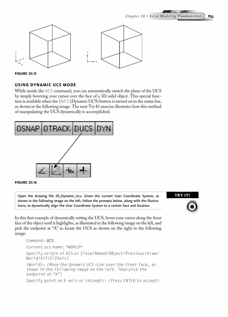
USING DYNAMIC UCS MODEWhile inside the UCS command, you can automatically switch the plane of the UCSby simply hovering your cursor over the face of a 3D solid object. This special func-tion is available when the DUCS (Dynamic UCS) button is turned on in the status bar,as shown in the following image. The next Try It! exercise illustrates how this methodof manipulating the UCS dynamically is accomplished.
TRY IT!Open the drawing file 20_Dynamic_Ucs. Given the current User Coordinate System, asshown in the following image on the left, follow the prompts below, along with the illustra-tions, to dynamically align the User Coordinate System to a certain face and location.
In this first example of dynamically setting the UCS, hover your cursor along the frontface of the object until it highlights, as illustrated in the following image on the left, andpick the endpoint at “A” to locate the UCS as shown on the right in the followingimage.
Command: UCS
Current ucs name: *WORLD*
Specify origin of UCS or [Face/NAmed/OBject/Previous/View/World/X/Y/Z/ZAxis]
<World>: (Move the Dynamic UCS icon over the front face, asshown in the following image on the left. Then pick theendpoint at “A”)
Specify point on X-axis or <Accept>: (Press ENTER to accept)
FIGURE 20.15
FIGURE 20.16
Chap t e r 20 • So l i d Mod e l i n g Fundamen t a l s 833
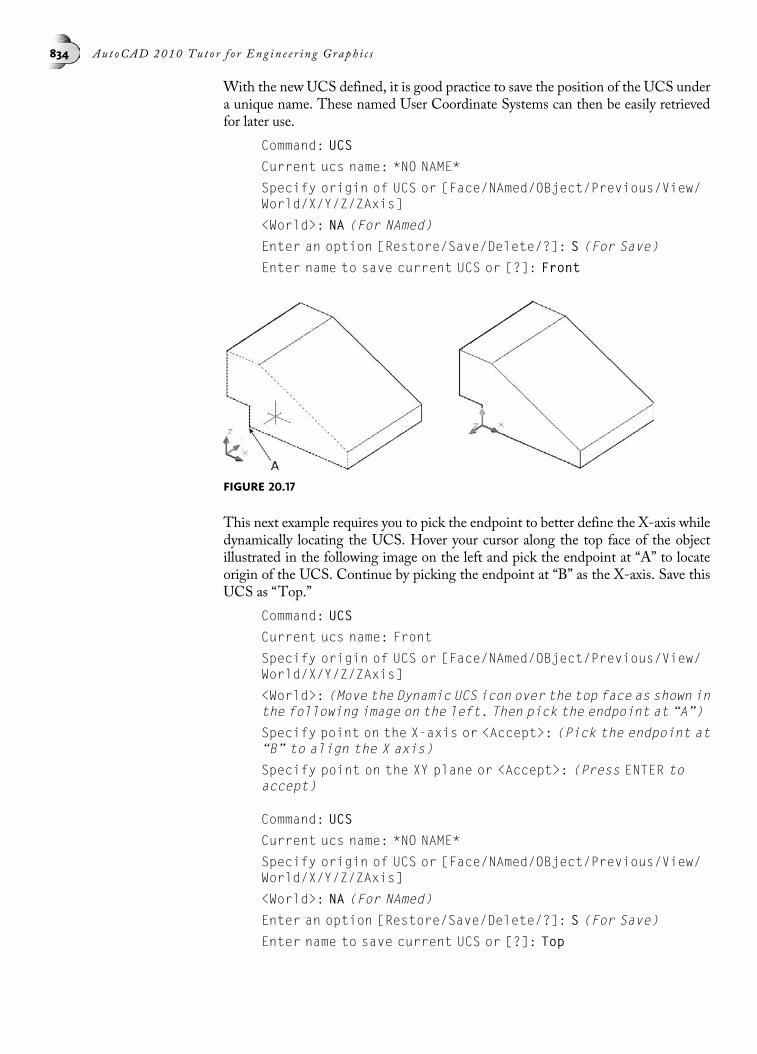
With the new UCS defined, it is good practice to save the position of the UCS undera unique name. These named User Coordinate Systems can then be easily retrievedfor later use.
Command: UCS
Current ucs name: *NO NAME*
Specify origin of UCS or [Face/NAmed/OBject/Previous/View/World/X/Y/Z/ZAxis]
<World>: NA (For NAmed)
Enter an option [Restore/Save/Delete/?]: S (For Save)
Enter name to save current UCS or [?]: Front
This next example requires you to pick the endpoint to better define the X-axis whiledynamically locating the UCS. Hover your cursor along the top face of the objectillustrated in the following image on the left and pick the endpoint at “A” to locateorigin of the UCS. Continue by picking the endpoint at “B” as the X-axis. Save thisUCS as “Top.”
Command: UCS
Current ucs name: Front
Specify origin of UCS or [Face/NAmed/OBject/Previous/View/World/X/Y/Z/ZAxis]
<World>: (Move the Dynamic UCS icon over the top face as shown inthe following image on the left. Then pick the endpoint at “A”)
Specify point on the X-axis or <Accept>: (Pick the endpoint at“B” to align the X axis)
Specify point on the XY plane or <Accept>: (Press ENTER toaccept)
Command: UCS
Current ucs name: *NO NAME*
Specify origin of UCS or [Face/NAmed/OBject/Previous/View/World/X/Y/Z/ZAxis]
<World>: NA (For NAmed)
Enter an option [Restore/Save/Delete/?]: S (For Save)
Enter name to save current UCS or [?]: Top
FIGURE 20.17
834 Aut oCAD 2010 Tu t o r f o r Eng in e e r i n g Graph i c s
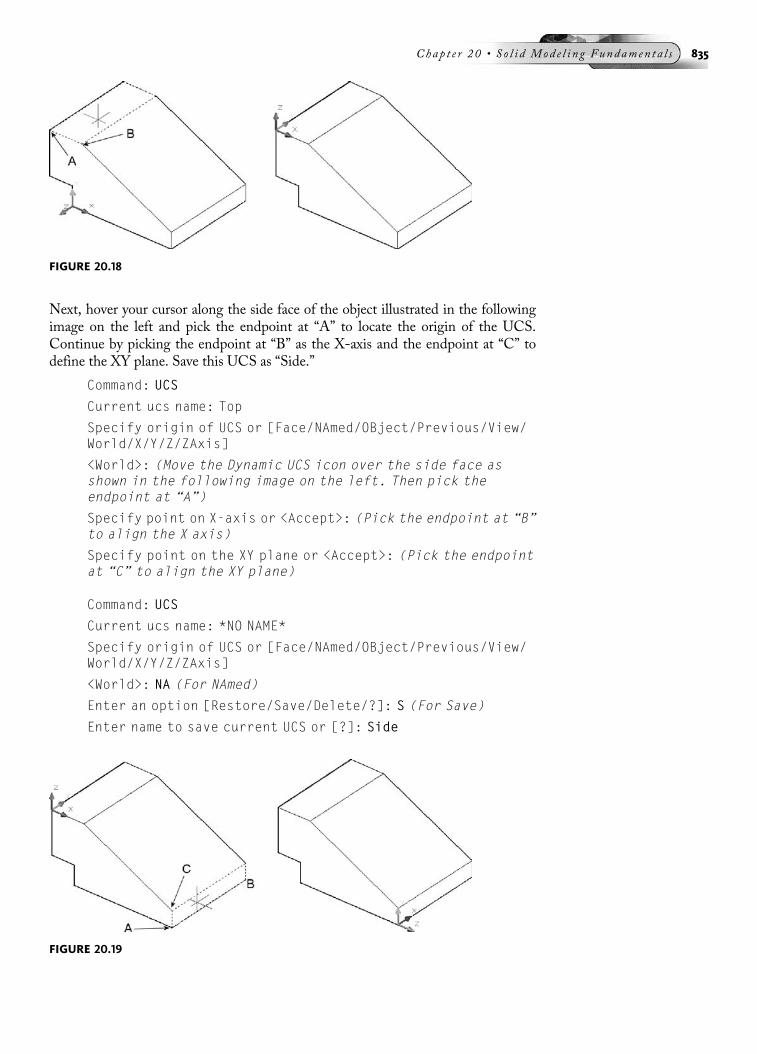
Next, hover your cursor along the side face of the object illustrated in the followingimage on the left and pick the endpoint at “A” to locate the origin of the UCS.Continue by picking the endpoint at “B” as the X-axis and the endpoint at “C” todefine the XY plane. Save this UCS as “Side.”
Command: UCS
Current ucs name: Top
Specify origin of UCS or [Face/NAmed/OBject/Previous/View/World/X/Y/Z/ZAxis]
<World>: (Move the Dynamic UCS icon over the side face asshown in the following image on the left. Then pick theendpoint at “A”)
Specify point on X-axis or <Accept>: (Pick the endpoint at “B”to align the X axis)
Specify point on the XY plane or <Accept>: (Pick the endpointat “C” to align the XY plane)
Command: UCS
Current ucs name: *NO NAME*
Specify origin of UCS or [Face/NAmed/OBject/Previous/View/World/X/Y/Z/ZAxis]
<World>: NA (For NAmed)
Enter an option [Restore/Save/Delete/?]: S (For Save)
Enter name to save current UCS or [?]: Side
FIGURE 20.18
FIGURE 20.19
Chap t e r 20 • So l i d Mod e l i n g Fundamen t a l s 835

Finally, hover your cursor along the inclined face of the object illustrated in thefollowing image on the left and pick the endpoint at “A” to locate the origin of theUCS. Continue by picking the endpoint at “B” as the X axis and the endpoint at “C”to define the XY plane. Save this UCS as “Auxiliary.”
Command: UCS
Current ucs name: Side
Specify origin of UCS or [Face/NAmed/OBject/Previous/View/World/X/Y/Z/ZAxis]
<World>: (Move the Dynamic UCS icon over the inclined face asshown in the following image on the left. Then pick theendpoint at “A”)
Specify point on X-axis or <Accept>: (Pick the endpoint at “B”to align the X axis)
Specify point on the XY plane or <Accept>: (Pick the endpointat “C” to align the XY plane)
Command: UCS
Current ucs name: *NO NAME*
Specify origin of UCS or [Face/NAmed/OBject/Previous/View/World/X/Y/Z/ZAxis]
<World>: NA (For NAmed)
Enter an option [Restore/Save/Delete/?]: S (For Save)
Enter name to save current UCS or [?]: Auxiliary
USING THE UCS DIALOG BOXAs stated earlier, considerable drawing time can be saved by assigning a name toa User Coordinate System once it has been created. Once numerous User Coordi-nate Systems have been defined in a drawing, using their names instead ofre-creating each coordinate system easily restores them. You can accomplish thison the command line by using the Save and Restore options of the UCS command.A method of retrieving previously saved User Coordinate Systems is to chooseNamed UCS from the Tools Menu Bar illustrated in the following image on theleft (the UCSMAN command). This displays the UCS dialog box, as shown in thefollowing image in the middle, with the Named UCSs tab selected. All User Coor-dinate Systems previously defined in the drawing are listed here. To make one ofthese coordinate systems current, highlight the desired UCS name and select the
FIGURE 20.20
836 Aut oCAD 2010 Tu t o r f o r Eng in e e r i n g Graph i c s

Set Current button, as shown in the following image in the middle. A named UCScan also be made current by simply double-clicking it. To define (save) a coordinatesystem you must have first translated and rotated the UCS into a desired new posi-tion; then use the dialog box to select the “Unnamed” UCS and rename it. TheUCS dialog box provides a quick method of restoring previously defined coordinatesystems without entering them at the keyboard.
Clicking on the Orthographic UCSs tab of the UCS dialog box allows you to rotatethe User Coordinate System so that the XY plane is parallel and oriented to one of thesix orthographic views: Front, Top, Back, Right Side, Left Side, and Bottom asshown in the following image on the right.
Another technique for quickly changing from one named UCS to another isillustrated in the following image. The ViewCube, which will be discussed later inthis chapter, has a down arrow next to WCS (World Coordinate System). Clickingon this button displays all named user coordinate systems defined in the model.Clicking on one of these named coordinate systems will switch you to that coordi-nate system.
CONTROLLING THE DISPLAY OF THE UCS ICONThe display of the UCS icon is controlled by clicking on View in the Menu Barfollowed by Display and UCS Icon. By default, the icon is turned on. If you wantto turn it off, click the On icon. The square box around the icon in the menu will
FIGURE 20.21
FIGURE 20.22
Chap t e r 20 • So l i d Mod e l i n g Fundamen t a l s 837
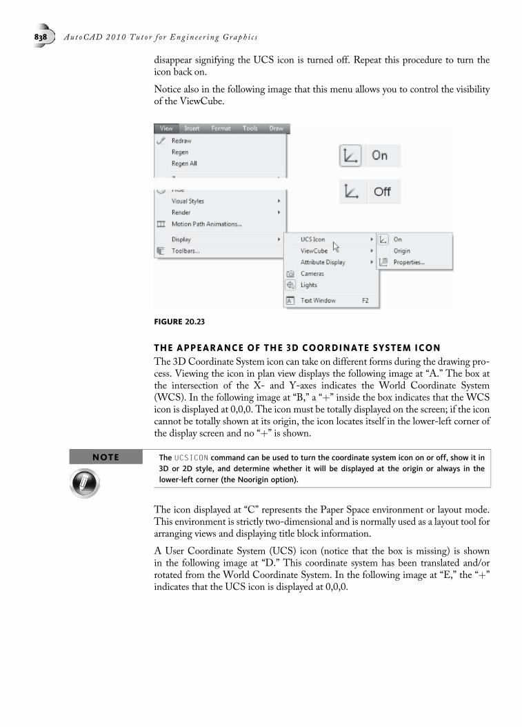
disappear signifying the UCS icon is turned off. Repeat this procedure to turn theicon back on.
Notice also in the following image that this menu allows you to control the visibilityof the ViewCube.
THE APPEARANCE OF THE 3D COORDINATE SYSTEM ICONThe 3D Coordinate System icon can take on different forms during the drawing pro-cess. Viewing the icon in plan view displays the following image at “A.” The box atthe intersection of the X- and Y-axes indicates the World Coordinate System(WCS). In the following image at “B,” a “þ” inside the box indicates that the WCSicon is displayed at 0,0,0. The icon must be totally displayed on the screen; if the iconcannot be totally shown at its origin, the icon locates itself in the lower-left corner ofthe display screen and no “þ” is shown.
NOTE The UCSICON command can be used to turn the coordinate system icon on or off, show it in3D or 2D style, and determine whether it will be displayed at the origin or always in thelower-left corner (the Noorigin option).
The icon displayed at “C” represents the Paper Space environment or layout mode.This environment is strictly two-dimensional and is normally used as a layout tool forarranging views and displaying title block information.
A User Coordinate System (UCS) icon (notice that the box is missing) is shownin the following image at “D.” This coordinate system has been translated and/orrotated from the World Coordinate System. In the following image at “E,” the “þ”indicates that the UCS icon is displayed at 0,0,0.
FIGURE 20.23
838 Aut oCAD 2010 Tu t o r f o r Eng in e e r i n g Graph i c s
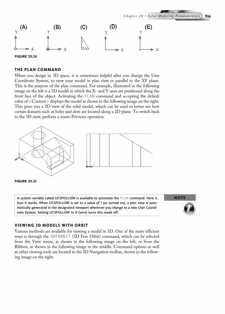
THE PLAN COMMANDWhen you design in 3D space, it is sometimes helpful after you change the UserCoordinate System, to view your model in plan view or parallel to the XY plane.This is the purpose of the plan command. For example, illustrated in the followingimage on the left is a 3D model in which the X- and Y-axes are positioned along thefront face of the object. Activating the PLAN command and accepting the defaultvalue of<Current> displays the model as shown in the following image on the right.This gives you a 2D view of the solid model, which can be used to better see howcertain features such as holes and slots are located along a 2D plane. To switch backto the 3D view, perform a zoom-Previous operation.
NOTEA system variable called UCSFOLLOW is available to automate the PLAN command. Here ishow it works. When UCSFOLLOW is set to a value of 1 (or turned on), a plan view is auto-matically generated in the designated viewport whenever you change to a new User Coordi-nate System. Setting UCSFOLLOW to 0 (zero) turns this mode off.
VIEWING 3D MODELS WITH ORBITVarious methods are available for viewing a model in 3D. One of the more efficientways is through the 3DFORBIT (3D Free Orbit) command, which can be selectedfrom the View menu, as shown in the following image on the left, or from theRibbon, as shown in the following image in the middle. Command options as wellas other viewing tools are located in the 3D Navigation toolbar, shown in the follow-ing image on the right.
FIGURE 20.24
FIGURE 20.25
Chap t e r 20 • So l i d Mod e l i n g Fundamen t a l s 839
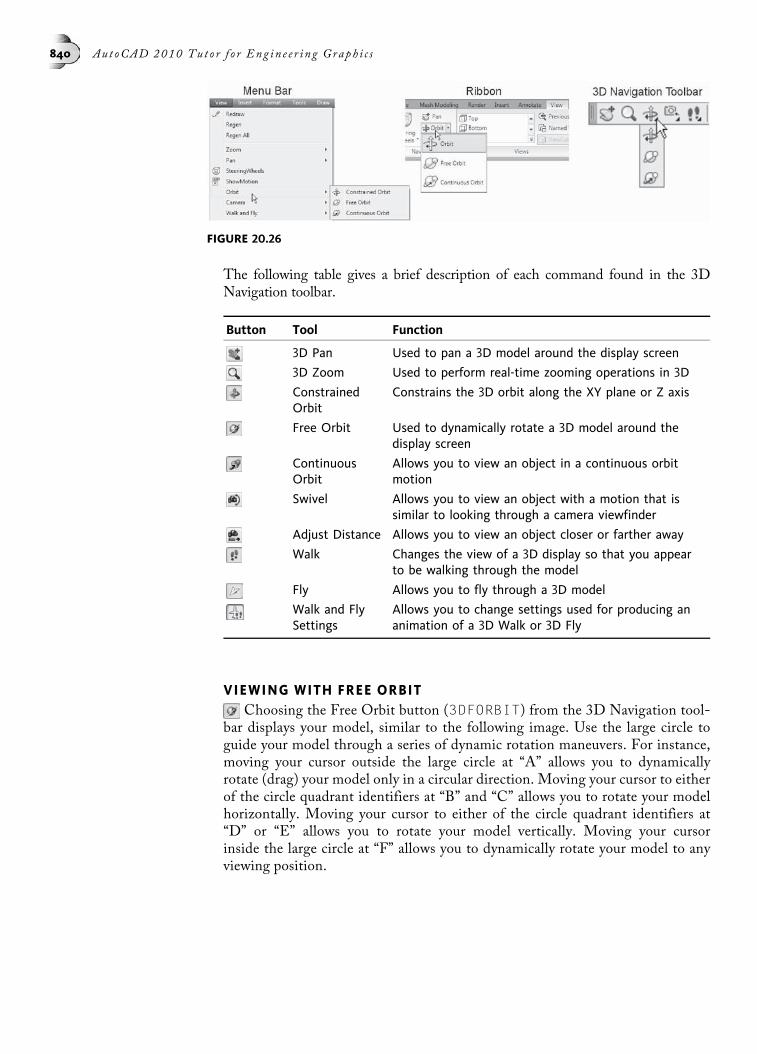
The following table gives a brief description of each command found in the 3DNavigation toolbar.
Button Tool Function
3D Pan Used to pan a 3D model around the display screen
3D Zoom Used to perform real-time zooming operations in 3D
ConstrainedOrbit
Constrains the 3D orbit along the XY plane or Z axis
Free Orbit Used to dynamically rotate a 3D model around thedisplay screen
ContinuousOrbit
Allows you to view an object in a continuous orbitmotion
Swivel Allows you to view an object with a motion that issimilar to looking through a camera viewfinder
Adjust Distance Allows you to view an object closer or farther away
Walk Changes the view of a 3D display so that you appearto be walking through the model
Fly Allows you to fly through a 3D model
Walk and FlySettings
Allows you to change settings used for producing ananimation of a 3D Walk or 3D Fly
VIEWING WITH FREE ORBITChoosing the Free Orbit button (3DFORBIT) from the 3D Navigation tool-
bar displays your model, similar to the following image. Use the large circle toguide your model through a series of dynamic rotation maneuvers. For instance,moving your cursor outside the large circle at “A” allows you to dynamicallyrotate (drag) your model only in a circular direction. Moving your cursor to eitherof the circle quadrant identifiers at “B” and “C” allows you to rotate your modelhorizontally. Moving your cursor to either of the circle quadrant identifiers at“D” or “E” allows you to rotate your model vertically. Moving your cursorinside the large circle at “F” allows you to dynamically rotate your model to anyviewing position.
FIGURE 20.26
840 Aut oCAD 2010 Tu t o r f o r Eng in e e r i n g Graph i c s
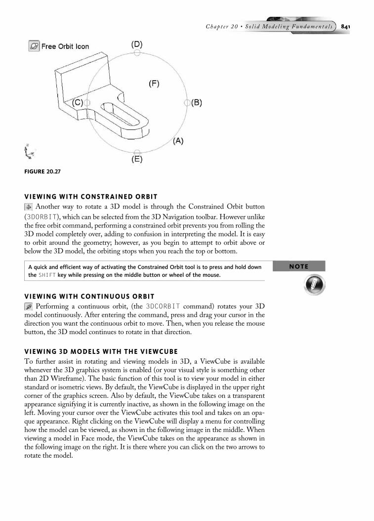
VIEWING WITH CONSTRAINED ORBITAnother way to rotate a 3D model is through the Constrained Orbit button
(3DORBIT), which can be selected from the 3D Navigation toolbar. However unlikethe free orbit command, performing a constrained orbit prevents you from rolling the3D model completely over, adding to confusion in interpreting the model. It is easyto orbit around the geometry; however, as you begin to attempt to orbit above orbelow the 3D model, the orbiting stops when you reach the top or bottom.
NOTEA quick and efficient way of activating the Constrained Orbit tool is to press and hold downthe SHIFT key while pressing on the middle button or wheel of the mouse.
VIEWING WITH CONTINUOUS ORBITPerforming a continuous orbit, (the 3DCORBIT command) rotates your 3D
model continuously. After entering the command, press and drag your cursor in thedirection you want the continuous orbit to move. Then, when you release the mousebutton, the 3D model continues to rotate in that direction.
VIEWING 3D MODELS WITH THE VIEWCUBETo further assist in rotating and viewing models in 3D, a ViewCube is availablewhenever the 3D graphics system is enabled (or your visual style is something otherthan 2D Wireframe). The basic function of this tool is to view your model in eitherstandard or isometric views. By default, the ViewCube is displayed in the upper rightcorner of the graphics screen. Also by default, the ViewCube takes on a transparentappearance signifying it is currently inactive, as shown in the following image on theleft. Moving your cursor over the ViewCube activates this tool and takes on an opa-que appearance. Right clicking on the ViewCube will display a menu for controllinghow the model can be viewed, as shown in the following image in the middle. Whenviewing a model in Face mode, the ViewCube takes on the appearance as shown inthe following image on the right. It is there where you can click on the two arrows torotate the model.
FIGURE 20.27
Chap t e r 20 • So l i d Mod e l i n g Fundamen t a l s 841

NOTE The ViewCube is designed to display when the current setting in the SHADEMODEcommand or Visual Styles Manager is set to a value other than 2D.
Clicking on ViewCube Settings, as shown in the previous image, displays the View-Cube Settings dialog box as shown in the following image. You can control theopacity level of the ViewCube in addition to its size and on-screen position.
Various viewing modes are available through the ViewCube depending on whatpart of the ViewCube is picked. These modes are all displayed in the followingimage. For example, clicking on one of the corners of the ViewCube will displaya model in an isometric mode. If you want to view a model orthogonally, then oneof the six face-viewing modes would work. The edge pivot mode pivots a modelalong a selected edge. Once in an orthogonal view, such as a Top View, rotationarrows display that allow you to rotate or swivel a model. To return back to thedefault view of a model, click on the house icon signifying the home position.
FIGURE 20.29
FIGURE 20.28
842 Aut oCAD 2010 Tu t o r f o r Eng in e e r i n g Graph i c s

An example of how the ViewCube operates is illustrated in the following image. Youcan either click on one of the box corners to get a standard isometric view, or pressand hold down the mouse on a corner. In this case, moving the mouse will rotatethe model dynamically as shown in the following image.
An example of displaying a model in its default location is illustrated in the followingimage. No matter how your model is currently displayed, you can always return themodel to its default location by clicking on the Home icon whenever the ViewCubeis displayed.
FIGURE 20.30
FIGURE 20.31
FIGURE 20.32
Chap t e r 20 • So l i d Mod e l i n g Fundamen t a l s 843
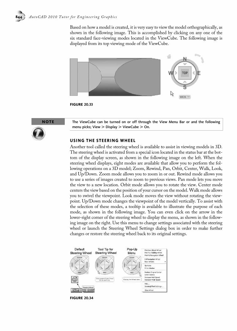
Based on how a model is created, it is very easy to view the model orthographically, asshown in the following image. This is accomplished by clicking on any one of thesix standard face-viewing modes located in the ViewCube. The following image isdisplayed from its top viewing mode of the ViewCube.
NOTE The ViewCube can be turned on or off through the View Menu Bar or and the followingmenu picks; View . Display . ViewCube . On.
USING THE STEERING WHEELAnother tool called the steering wheel is available to assist in viewing models in 3D.The steering wheel is activated from a special icon located in the status bar at the bot-tom of the display screen, as shown in the following image on the left. When thesteering wheel displays, eight modes are available that allow you to perform the fol-lowing operations on a 3D model; Zoom, Rewind, Pan, Orbit, Center, Walk, Look,and Up/Down. Zoom mode allows you to zoom in or out. Rewind mode allows youto use a series of images created to zoom to previous views. Pan mode lets you movethe view to a new location. Orbit mode allows you to rotate the view. Center modecenters the view based on the position of your cursor on the model.Walk mode allowsyou to swivel the viewpoint. Look mode moves the view without rotating the view-point. Up/Down mode changes the viewpoint of the model vertically. To assist withthe selection of these modes, a tooltip is available to illustrate the purpose of eachmode, as shown in the following image. You can even click on the arrow in thelower-right corner of the steering wheel to display the menu, as shown in the follow-ing image on the right. Use this menu to change settings associated with the steeringwheel or launch the Steering Wheel Settings dialog box in order to make furtherchanges or restore the steering wheel back to its original settings.
FIGURE 20.33
FIGURE 20.34
844 Aut oCAD 2010 Tu t o r f o r Eng in e e r i n g Graph i c s
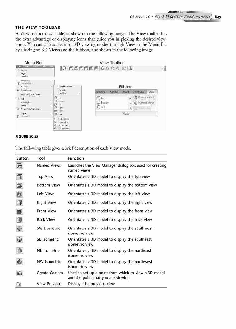
THE VIEW TOOLBARA View toolbar is available, as shown in the following image. The View toolbar hasthe extra advantage of displaying icons that guide you in picking the desired view-point. You can also access most 3D viewing modes through View in the Menu Barby clicking on 3D Views and the Ribbon, also shown in the following image.
The following table gives a brief description of each View mode.
Button Tool Function
Named Views Launches the View Manager dialog box used for creatingnamed views
Top View Orientates a 3D model to display the top view
Bottom View Orientates a 3D model to display the bottom view
Left View Orientates a 3D model to display the left view
Right View Orientates a 3D model to display the right view
Front View Orientates a 3D model to display the front view
Back View Orientates a 3D model to display the back view
SW Isometric Orientates a 3D model to display the southwestisometric view
SE Isometric Orientates a 3D model to display the southeastisometric view
NE Isometric Orientates a 3D model to display the northeastisometric view
NW Isometric Orientates a 3D model to display the northwestisometric view
Create Camera Used to set up a point from which to view a 3D modeland the point that you are viewing
View Previous Displays the previous view
FIGURE 20.35
Chap t e r 20 • So l i d Mod e l i n g Fundamen t a l s 845

SHADING SOLID MODELSVarious shading modes are available to help you better visualize the solid model youare constructing. Access the five shading modes by choosing Visual Styles from theView Menu Bar, as shown in the following image, or by clicking a button on theVisual Styles toolbar. An area is also available in the Ribbon for working with visualstyles, as shown in the following image on the right.
The following table gives a brief description of each visual style mode.
Options of the SHADEMODE Command
Button Visual Style Description
2D Wireframe Displays the 3D model as a series of lines and arcs thatrepresent boundaries
3D Wireframe Displays the 3D model that is similar in appearance tothe 2D option; the UCS icon appears as a color shadedimage
3D Hidden Displays the 3D model with hidden edges removed
Realistic Shades the objects and smooths the edges betweenpolygon faces; if materials are attached to the model,they will display when this visual style is chosen
Conceptual This mode also shades the objects and smooths theedges between polygon faces; however, the shadingtransitions between cool and warm colors
Manage VisualStyles
Launches the Visual Styles Manager palette, used forcreating new visual styles and applying existing visualstyles to a 3D model
The following image illustrates all five visual styles and how they affect the appear-ance of a 3D solid model.
FIGURE 20.36
846 Aut oCAD 2010 Tu t o r f o r Eng in e e r i n g Graph i c s
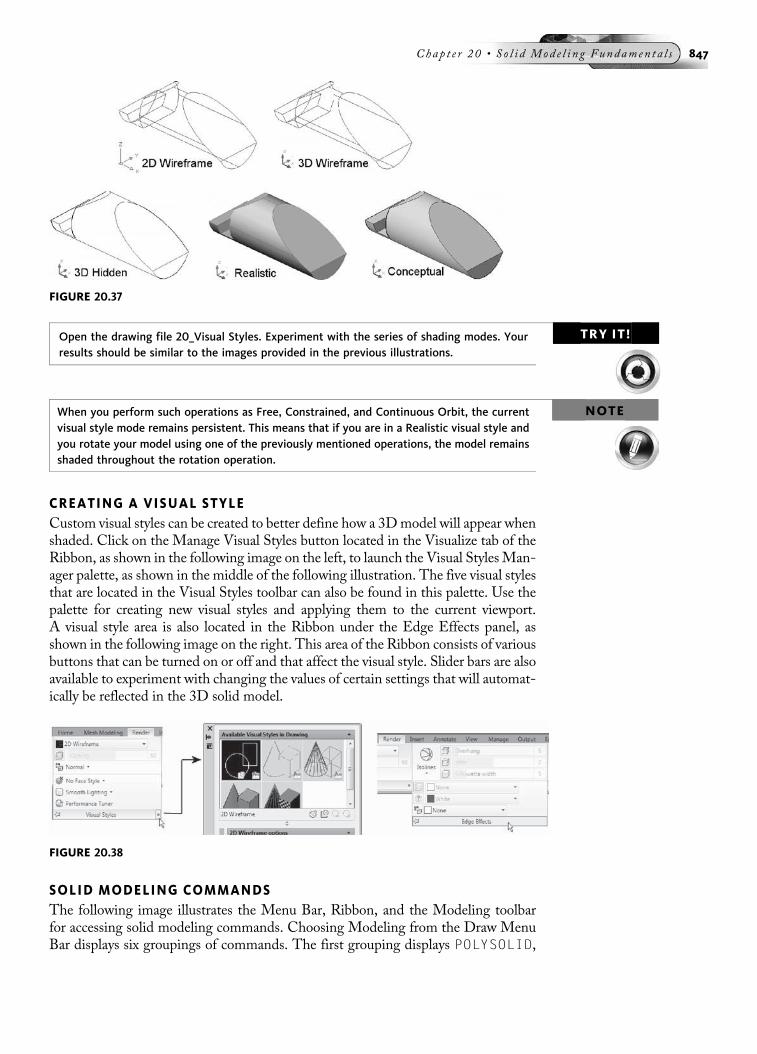
TRY IT!Open the drawing file 20_Visual Styles. Experiment with the series of shading modes. Yourresults should be similar to the images provided in the previous illustrations.
NOTEWhen you perform such operations as Free, Constrained, and Continuous Orbit, the currentvisual style mode remains persistent. This means that if you are in a Realistic visual style andyou rotate your model using one of the previously mentioned operations, the model remainsshaded throughout the rotation operation.
CREATING A VISUAL STYLECustom visual styles can be created to better define how a 3Dmodel will appear whenshaded. Click on the Manage Visual Styles button located in the Visualize tab of theRibbon, as shown in the following image on the left, to launch the Visual StylesMan-ager palette, as shown in the middle of the following illustration. The five visual stylesthat are located in the Visual Styles toolbar can also be found in this palette. Use thepalette for creating new visual styles and applying them to the current viewport.A visual style area is also located in the Ribbon under the Edge Effects panel, asshown in the following image on the right. This area of the Ribbon consists of variousbuttons that can be turned on or off and that affect the visual style. Slider bars are alsoavailable to experiment with changing the values of certain settings that will automat-ically be reflected in the 3D solid model.
SOLID MODELING COMMANDSThe following image illustrates the Menu Bar, Ribbon, and the Modeling toolbarfor accessing solid modeling commands. Choosing Modeling from the Draw MenuBar displays six groupings of commands. The first grouping displays POLYSOLID,
FIGURE 20.37
FIGURE 20.38
Chap t e r 20 • So l i d Mod e l i n g Fundamen t a l s 847

BOX, SPHERE, CYLINDER, CONE, WEDGE, TORUS, and PYRAMID, which areconsidered the building blocks of the solid model and are used to construct basic“primitives.” The second grouping displays the PLANESURF command, designed tocreate a planar surface between two closed shapes or through two diagonal points.The third grouping displays the “sweep” commands – EXTRUDE, REVOLVE, SWEEP,and LOFT – which provide an additional way to construct solid models. Polylineoutlines or circles can be extruded (swept) to a thickness that you designate. You canalso revolve (sweep) other polyline outlines about an axis. The fourth grouping ofsolid modeling commands enables you to create a section plane in order to look atthe interior of a solid model. The fifth grouping displays a set of commands thatcreate or manipulate mesh surfaces. Commands include SOLID, 3DFACE, 3DMESH,EDGE, REVSURF, TABSURF, RULESURF, and EDGESURF. The last grouping,Setup, displays three commands designed to extract orthographic views from a solidmodel. The three commands are SOLDRAW, SOLVIEW, and SOLPROF. Many ofthese same solid modeling commands can be accessed from the Modeling toolbarand Ribbon, as shown in the following image.
The following table gives a brief description of each command located in the Model-ing toolbar.
Button Tool Shortcut Function
Polysolid POLYSOLID Creates a solid shape based on adirection, width and height of the solid
Box BOX Creates a solid box
Wedge WE Creates a solid wedge
Cone CONE Creates a solid cone
Sphere SPHERE Creates a solid sphere
Cylinder CYL Creates a solid cylinder
Torus TOR Creates a solid torus
Pyramid PYR Creates a solid pyramid
FIGURE 20.39
848 Aut oCAD 2010 Tu t o r f o r Eng in e e r i n g Graph i c s

Button Tool Shortcut Function
Helix HELIX Creates a 2D or 3D helix
Planar Surface PLANESURF Creates a planar surface
Extrude EXT Creates a solid by extruding a 2Dprofile
Presspull PRESSPULL Presses or pulls closed areas resultingin a solid shape or a void in a solid
Sweep SWEEP Creates a solid based on a profile anda path
Revolve REV Creates a solid by revolving a 2Dprofile about an axis of rotation
Loft LOFT Creates a lofted solid based on a seriesof cross-section shapes
Union UNI Joins two or more solids together
Subtraction SU Removes one or more solids froma source solid shape
Intersect INT Extracts the common volume sharedby two or more solid shapes
3D Move 3DMOVE Moves objects a specified distance ina specified direction based on theposition of a move grip tool
3D Rotate 3DROTATE Revolves objects around a base pointbased on the rotate grip tool
3D Align 3DALIGN Aligns objects with other objects in2D and 3D
3D Array 3DARRAY Creates patterns of objects along theX, Y, and Z axes
CREATING SOLID PRIMITIVESSeven different commands are available for creating 3D solids in basic geometricshapes; namely boxes, wedges, cylinders, cones, spheres, tori (donut-shaped objects),and pyramids as shown in the following image. These solid shapes are often calledprimitives because they are used as building blocks for more complex solid models.They are seldom useful by themselves, but these primitives can be combined andmodified into a wide variety of geometric shapes. The following command sequencesallow you to practice creating one example of each primitive.
TRY IT!Open the drawing file 20_Primitive_Examples which represents a drawing void of anyobjects. Follow the next series of seven prompts to create each primitive illustrated in thefollowing image.
Chap t e r 20 • So l i d Mod e l i n g Fundamen t a l s 849

Creating Box PrimitivesBox primitives consist of brick-shaped solid objects. They have six rectangular sides,which are either perpendicular or parallel to one another. Boxes are probably the mostoften used primitive, as many of the objects that are modeled are made up of rectan-gles and squares. There are many ways of creating boxes; the following promptsequence illustrates the length option for creating a box (see the previous imageat “A”).
Command: BOX
Specify first corner or [Center]: 4.00,9.00
Specify other corner or [Cube/Length]: L (For Length)
Specify length <5.0000>: 3.00 (point your cursor in thepositive X direction)
Specify width <2.0000>: 2.00 (point your cursor in thepositive Y direction)
Specify height or [2Point] <1.0000>: 4.00 (point your cursorin the positive Z direction)
Creating Wedge PrimitivesWedges are like boxes that have been sliced diagonally edge to edge. They have a totalof five sides, three of which are rectangular, two that are triangular. The top rectan-gular side slopes down in the X direction. The two sides opposite this sloping side areperpendicular to each other. The bottom rectangular surface is on the XY plane. Thefollowing prompt sequence illustrates the length option for creating a wedge (see theprevious image at “B”).
Command: WE (For WEDGE)
Specify first corner or [Center]: 8.00,9.00
Specify other corner or [Cube/Length]: L (For Length)
Specify length <5.0000>: 3.00 (point your cursor in thepositive X direction)
Specify width <2.0000>: 2.00 (point your cursor in thepositive Y direction)
FIGURE 20.40
850 Aut oCAD 2010 Tu t o r f o r Eng in e e r i n g Graph i c s

Specify height or [2Point] <3.0000>: 4.00 (point your cursorin the positive Z direction)
Creating Cylinder PrimitivesCylinders are probably the second most often used primitive. Cylinders can be cre-ated as either circular or elliptical. The following prompt sequence illustrates thediameter option for creating a cylinder (see the previous image at “C”).
Command: CYL (For CYLINDER)
Specify center point of base or [3P/2P/Ttr/Elliptical]:14.00,10.00
Specify base radius or [Diameter] <1.5000>: D (For Diameter)
Specify diameter <3.0000>: 2.00
Specify height or [2Point/Axis endpoint] <4.0000>: 4.00(point your cursor in the positive Z direction)
Creating Cone PrimitivesCone primitives are closely related to cylinders. They have the same round or ellipticalcross section; but they taper either to a point or a specified height with different radiusforming a truncated cone. The following prompt sequence illustrates the radiusoption for creating a cone (see the previous image at “D”).
Command: CONE
Specify center point of base or [3P/2P/Ttr/Elliptical]:17.00,10.00
Specify base radius or [Diameter] <1.0000>: 1.00
Specify height or [2Point/Axis endpoint/Top radius]<4.0000>: 4.00 (point your cursor in the positive Zdirection)
Creating Sphere PrimitivesCreating spheres is the most straightforward process in creating primitives. Specifythe sphere’s center point and then specify either the radius or diameter of the sphere.The following prompt sequence illustrates the diameter option for creating a sphere(see the previous image at “E”).
Command: SPHERE
Specify center point or [3P/2P/Ttr]: 6.00,6.00
Specify radius or [Diameter] <2.0000>: D (For Diameter)
Specify diameter <4.0000>: 3.00
Creating a Torus PrimitiveAlthough the torus is not often needed, it is the most interesting and flexible of theseven primitive solids. The basic shape of a torus is that of a donut, but it can alsotake on a football shape. To be made properly, this primitive requires a torus radiusvalue and a tube radius value, as shown in the following image. The following promptsequence illustrates creating a torus (see the previous image at “F”).
Chap t e r 20 • So l i d Mod e l i n g Fundamen t a l s 851

Command: TOR (For TORUS)
Specify center point or [3P/2P/Ttr]: 10.00,6.00
Specify radius or [Diameter] <1.5000>: 1.50
Specify tube radius or [2Point/Diameter]: .25
Creating Pyramid PrimitivesSolid pyramids actually have similar prompts used for creating cylinders with theexception that the base of the pyramid consists of edges and are noncircular in shape.The following prompt sequence illustrates the creation of a pyramid (see the previousimage at “G”).
Command: PYR (For PYRAMID)
4 sides Circumscribed
Specify center point of base or [Edge/Sides]: 14.00,6.00
Specify base radius or [Inscribed] <1.5000>: 1.50 (point yourcursor in the positive X direction)
Specify height or [2Point/Axis endpoint/Top radius]<4.0000>: 4.00 (point your cursor in the positiveZ direction)
USING BOOLEAN OPERATIONS ON SOLID PRIMITIVESTo combine one or more primitives to form a composite solid, a Boolean operation isperformed. Boolean operations must act on at least a pair of primitives, regions, orsolids. These operations in the form of commands are located in the Modify MenuBar under Solids Editing. They can also be selected from the Solids Editing panel ofthe Ribbon, theModeling toolbar, or Solid Editing toolbar. Boolean operations allowyou to add two or more objects together, subtract a single object or group of objectsfrom another, or find the overlapping volume – in other words, form the solid commonto both primitives. Displayed in the following image are the UNION, SUBTRACT, andINTERSECT commands that you use to perform these Boolean operations.
FIGURE 20.41
852 Aut oCAD 2010 Tu t o r f o r Eng in e e r i n g Graph i c s
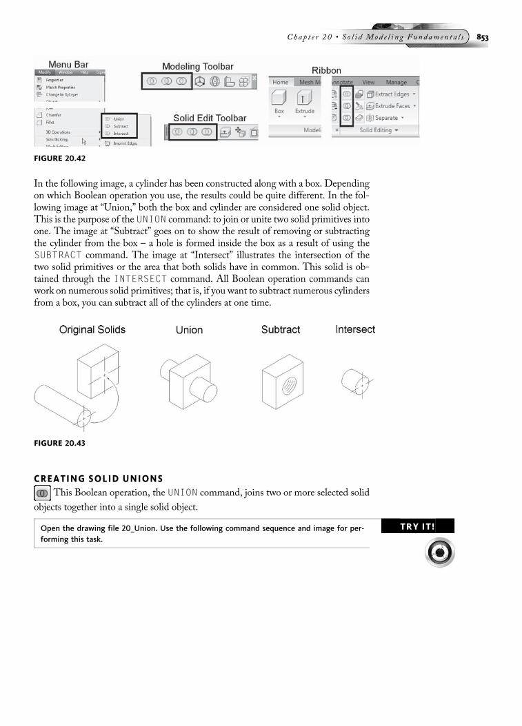
In the following image, a cylinder has been constructed along with a box. Dependingon which Boolean operation you use, the results could be quite different. In the fol-lowing image at “Union,” both the box and cylinder are considered one solid object.This is the purpose of the UNION command: to join or unite two solid primitives intoone. The image at “Subtract” goes on to show the result of removing or subtractingthe cylinder from the box – a hole is formed inside the box as a result of using theSUBTRACT command. The image at “Intersect” illustrates the intersection of thetwo solid primitives or the area that both solids have in common. This solid is ob-tained through the INTERSECT command. All Boolean operation commands canwork on numerous solid primitives; that is, if you want to subtract numerous cylindersfrom a box, you can subtract all of the cylinders at one time.
CREATING SOLID UNIONSThis Boolean operation, the UNION command, joins two or more selected solid
objects together into a single solid object.
TRY IT!Open the drawing file 20_Union. Use the following command sequence and image for per-forming this task.
FIGURE 20.42
FIGURE 20.43
Chap t e r 20 • So l i d Mod e l i n g Fundamen t a l s 853
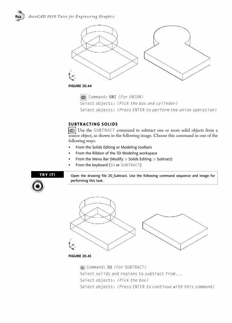
Command: UNI (For UNION)
Select objects: (Pick the box and cylinder)
Select objects: (Press ENTER to perform the union operation)
SUBTRACTING SOLIDSUse the SUBTRACT command to subtract one or more solid objects from a
source object, as shown in the following image. Choose this command in one of thefollowing ways:
• From the Solids Editing or Modeling toolbars
• From the Ribbon of the 3D Modeling workspace
• From the Menu Bar (Modify > Solids Editing > Subtract)
• From the keyboard (SU or SUBTRACT)
TRY IT! Open the drawing file 20_Subtract. Use the following command sequence and image forperforming this task.
Command: SU (For SUBTRACT)
Select solids and regions to subtract from...
Select objects: (Pick the box)
Select objects: (Press ENTER to continue with this command)
FIGURE 20.44
FIGURE 20.45
854 Aut oCAD 2010 Tu t o r f o r Eng in e e r i n g Graph i c s

Select solids and regions to subtract...
Select objects: (Pick the cylinder)
Select objects: (Press ENTER to perform the subtractionoperation)
CREATING INTERSECTIONSUse the INTERSECT command to find the solid common to a group of selected
solid objects, as shown in the following image. Choose this command in one of thefollowing ways:
• From the Solids Editing or Modeling toolbars
• From the Ribbon of the 3D Modeling workspace
• From the Menu Bar (Modify > Solids Editing > Intersect)
• From the Keyboard (IN or INTERSECT)
TRY IT!Open the drawing file 20_Intersection. Use the following command sequence and image forperforming this task.
Command: IN (For INTERSECT)
Select objects: (Pick the box and cylinder)
Select objects: (Press ENTER to perform the intersectionoperation)
3D Applications of Unioning SolidsThe following image shows an object consisting of one horizontal solid box, two ver-tical solid boxes, and two extruded semicircular shapes. All primitives have beenpositioned with the MOVE command. To join all solid primitives into one solid object,use the UNION command. The order of selection of these solids for this command isnot important.
TRY IT!Open the drawing file 20_3D App Union. Use the following prompts and image for perform-ing these tasks.
FIGURE 20.46
Chap t e r 20 • So l i d Mod e l i n g Fundamen t a l s 855

Command: UNI (For UNION)
Select objects: (Pick your screen at “A”)
Select objects: (Pick your screen at “B”)
Select objects: (Press ENTER to perform the union operation)
3D Applications of Moving SolidsUsing the same problem from the previous example, let us now add a hole in the cen-ter of the base. The cylinder will be created through the cylinder command. It willthen be moved to the exact center of the base. You can use the MOVE command alongwith the OSNAP-Tracking mode to accomplish this. Tracking mode automaticallyactivates the ORTHO mode when it is in use. See the following image.
Command: CYL (For CYLINDER)
Specify center point of base or [3P/2P/Ttr/Elliptical]:3.00,3.00
Specify base radius or [Diameter]: 0.75
Specify height or [2Point/Axis endpoint]: 0.25
Command: M (For MOVE)
Select objects: (Select the cylinder at “A”)
Select objects: (Press ENTER to continue with this command)
Specify base point or [Displacement] <Displacement>: Cen
of (Select the bottom of the cylinder at “A”)
Specify second point or <use first point as displacement>:M2P (To activate Midpoint between two points)
First tracking point: Mid
of (Select the midpoint of the bottom of the base at “B”)
Next point (Press ENTER to end tracking): Mid
of (Select the midpoint of the bottom of the base at “C”)
Next point (Press ENTER to end tracking): (Press ENTER to endtracking and perform the move operation)
FIGURE 20.47
856 Aut oCAD 2010 Tu t o r f o r Eng in e e r i n g Graph i c s

3D Applications of Subtracting SolidsNow that the solid cylinder is in position, use the SUBTRACT command to removethe cylinder from the base of the main solid and create a hole in the base, as shown inthe following image.
Command: SU (For SUBTRACT)
Select solids and regions to subtract from...
Select objects: (Select the main solid as source at “A”)
Select objects: (Press ENTER to continue with this command)
Select solids and regions to subtract...
Select objects: (Select the cylinder at “B”)
Select objects: (Press ENTER to perform the subtractionoperation)
Command: HIDE (For hidden line removal view)
Command: RE (For REGEN to return to wireframe view)
CREATING INTERSECTIONSIntersections remain one of the most misunderstood concepts to grasp in solidmodeling. However, once you become comfortable with this concept, it can be oneof the more powerful solid modeling tools available. Creating an intersection involvescreating a solid model from the common volumes of two or more overlapping solids.The objects labeled “A” and “B” in the following image represent existing solid mod-els. These models are then moved to overlap each other as shown at “C” in the
FIGURE 20.48
FIGURE 20.49
Chap t e r 20 • So l i d Mod e l i n g Fundamen t a l s 857

following image. After creating the intersection, the nonoverlapping portions of themodel are removed leaving the solid model as shown at “D” in the following image.
TRY IT! Open the drawing file 20_Int1. In the following image, the object at “C” represents thefinished model. Look at the sequence beginning at “A” to see how to prepare the solidprimitives for an Intersection operation. Two separate 3D Solid objects are created at “A.”One object represents a block that has been filleted along with the placement of a holedrilled through. The other object represents the U-shaped extrusion. With both objectsmodeled, they are moved on top of each other at “B.” The OSNAP-Midpoint was used toaccomplish this. Finally, the INTERSECT command is used to find the common volumeshared by both objects; namely the illustration at “C.”
TRY IT! Open the drawing file 20_Int2. The object in the following image is another example of howthe INTERSECT command may be applied to a solid model. For the results at “B” to beobtained from a cylinder that has numerous cuts, the cylinder is first created as a separatemodel. Then the cuts are made in another model at “A.” Again, both models are movedtogether (use the Quadrant and Midpoint OSNAP modes), and then the INTERSECT com-mand is used to achieve the results at “B.” Before undertaking any solid model, first analyzehow the model is to be constructed. Using intersections can create dramatic results, whichwould normally require numerous union and subtraction operations.
FIGURE 20.50
FIGURE 20.51
858 Aut oCAD 2010 Tu t o r f o r Eng in e e r i n g Graph i c s

CREATING SOLID EXTRUSIONSThe EXTRUDE command creates a solid by extrusion. Choose this command in
one of the following ways:
• From the Modeling Toolbar
• From the Ribbon of the 3D Modeling workspace
• From the Menu Bar (Draw > Modeling > Extrude)
• From the keyboard (EXT or EXTRUDE)
Only regions or closed, single-entity objects such as circles and closed polylines can beextruded into a solid. Other options of the EXTRUDE command include the follow-ing: Extrude by Direction, in which you specify two points that determine the lengthand direction of the extrusion; Extrude by Path, in which the extrusion is createdbased on a path that consists of a predefined object; and Extrude by Taper Angle, inwhich a tapered extrusion is created based on an angle value between �90 and þ90.
Use the following prompts to construct a solid extrusion of the closed polyline objectin the following image. For the height of the extrusion, you can enter a numeric valueor you can specify the distance by picking two points on the display screen.
TRY IT!Open the drawing file 20_Extrude1. Use the following command sequence and image forperforming this task.
Command: EXT (For EXTRUDE)
Current wire frame density: ISOLINES=4
Select objects to extrude: (Select the polyline objectat “A”)
Select objects to extrude: (Press ENTER to continue withthis command)
Specify height of extrusion or [Direction/Path/Taperangle]: 1.00
FIGURE 20.52
Chap t e r 20 • So l i d Mod e l i n g Fundamen t a l s 859

You can create an optional taper along with the extrusion by utilizing the Taper angleoption provided.
TRY IT! Open the drawing file 20_Extrude2. Use the following command sequence and image forperforming this task.
Command: EXT (For EXTRUDE)
Current wire frame density: ISOLINES=4
Select objects to extrude: (Select the polyline object at “B”in the following image)
Select objects to extrude: (Press ENTER to continue with thiscommand)
Specify height of extrusion or [Direction/Path/Taperangle]: T (For Taper angle)
Specify angle of taper for extrusion <0>: 15
Specify height of extrusion or [Direction/Path/Taperangle]: 1.00
You can also create a solid extrusion by selecting a path to be followed by the objectbeing extruded. Typical paths include regular and elliptical arcs, 2D and 3D poly-lines, or splines. The extruded pipe in the following image was created using the fol-lowing steps: First the polyline path was created. Then, a new User CoordinateSystem was established through the UCS command along with the Z-axis option;the new UCS was positioned at the end of the polyline with the Z-axis extendingalong the polyline. A circle was constructed with its center point at the end of thepolyline. Finally, the circle was extruded along the polyline path.
TRY IT! Open the drawing file 20_Extrude Pipe. Use the following command sequence and image forperforming this task.
FIGURE 20.53
FIGURE 20.54
860 Aut oCAD 2010 Tu t o r f o r Eng in e e r i n g Graph i c s

Command: EXT (For EXTRUDE)
Current wire frame density: ISOLINES=4
Select objects to extrude: (Select the small circle as theobject to extrude)
Select objects to extrude: (Press ENTER to continue)
Specify height of extrusion or [Direction/Path/Taperangle]: P (For Path)
Select extrusion path or [Taper angle]: (Select the polylineobject representing the path)
Extruding an Existing FaceOnce a solid object is created, existing faces of the model can be used as profiles tofurther extrude shapes. Illustrated in the following image on the left is a wedge-shaped 3D model. After entering the EXTRUDE command, press and hold downthe CTRL key and select the inclined face. You can either enter a value or drag yourcursor to define the height of the extrusion, as shown in the following image in themiddle. The results are shown in the following image on the right. The new extrudedshape created from the inclined face is considered a separate solid object. If bothshapes need to be considered one, use the UNION command and select both extrudedboxes to join them as one solid.
TRY IT!Open the drawing file 20_Extrude Face. Use the following command sequence and imagefor performing an extrusion on an existing face.
Command: EXT (For EXTRUDE)
Current wire frame density: ISOLINES=4
Select objects to extrude: (Press and hold down the CTRL keyand select the inclined face as shown in the following imageon the left)
Select objects to extrude: (Press ENTER to continue)
Specify height of extrusion or [Direction/Path/Taperangle]: 5.00
FIGURE 20.55
FIGURE 20.56
Chap t e r 20 • So l i d Mod e l i n g Fundamen t a l s 861

CREATING REVOLVED SOLIDSThe REVOLVE command creates a solid by revolving an object about an axis of
revolution. Choose this command in one of the following ways:
• From the Modeling Toolbar
• From the Ribbon of the 3D Modeling workspace
• From the Menu Bar (Draw > Modeling > Revolve)
• From the keyboard (REV or REVOLVE)
Only regions or closed, single-entity objects such as polylines, polygons, circles, ellip-ses, and 3D polylines can be revolved to create a solid. If a group of objects is not inthe form of a single entity, group them together using the PEDIT command or createa closed polyline/region with the BOUNDARY command. The following image repre-sents a revolved 3D Solid object.
TRY IT! Open the drawing file 20_Revolve1. Many practical applications require creating a compos-ite solid from primitives and extrusions. The CYLINDER command was used to constructthe cylindrical primitive and the REVOLVE command was used to create the revolved solid.Use the following command sequence on the objects as illustrated in the following image onthe left for creating a revolved solid.
Command: REV (For REVOLVE)
Current wire frame density: ISOLINES=4
Select objects to revolve: (Select profile “A” as the objectto revolve)
Select objects to revolve: (Press ENTER to continue with thiscommand)
Specify axis start point or define axis by [Object/X/Y/Z]<Object>: O (For Object)
Select an object: (Select line “B”)
Specify angle of revolution or [STart angle] <360>: (PressENTER to accept the default and perform the revolvingoperation)
Use the Center option of OSNAP along with the MOVE command to position therevolved solid inside the cylinder as shown in the following image on the right.
Command: M (For MOVE)
Select objects: (Select the revolved solid in the followingimage)
Select objects: (Press ENTER to continue with this command)
Specify base point or [Displacement] <Displacement>: Cen
of (Select the center of the revolved solid at “C”)
Specify second point or <use first point as displacement>:Cen
of (Select the center of the cylinder at “D”)
862 Aut oCAD 2010 Tu t o r f o r Eng in e e r i n g Graph i c s

Once the revolved solid is positioned inside the cylinder, use the SUBTRACT com-mand to subtract the revolved solid from the cylinder, as shown in the following im-age. Use the HIDE command to perform a hidden line removal at “B” to check thatthe solid is correct (this would be difficult to interpret in wireframe mode).
Command: SU (For SUBTRACT)
Select solids and regions to subtract from ...
Select objects: (Select the cylinder as source)
Select objects: (Press ENTER to continue with this command)
Select solids and regions to subtract ...
Select objects: (Select the revolved solid)
Select objects: (Press ENTER to perform the subtractionoperation)
Command: HI (For HIDE)
NOTEAs with the EXTRUDE command, you can also revolve an existing face of a 3D model tocreate a revolved feature of a 3D model.
CREATING A SOLID BY SWEEPINGThe SWEEP command creates a solid by sweeping a profile along an open
or closed 2D or 3D path. The result is a solid in the shape of the specified profilealong the specified path. If the sweep profile is closed, a solid is created. If the sweep
FIGURE 20.57
FIGURE 20.58
Chap t e r 20 • So l i d Mod e l i n g Fundamen t a l s 863

profile is open, a swept surface is created. Choose this command in one of thefollowing ways:
• From the Modeling toolbar
• From the Ribbon of the 3D Modeling workspace
• From the Menu Bar (Draw > Modeling > Sweep)
• From the keyboard (SWEEP)
TRY IT! Open the drawing file 20_Sweep. Use the following command sequence and image forperforming this task.
Illustrated in the following image on the left is an example of the geometry required tocreate a swept solid. Circles “A” and “B” represent profiles, while arc “C” representsthe path of the sweep. Notice in this illustration that the circles do not have to beconnected to the path; however, both circles must be constructed in the same planein order for both to be included in the sweep operation. Use the following commandsequence for creating a swept solid. The results of this operation are illustrated in thefollowing image on the right.
Command: SWEEP
Current wire frame density: ISOLINES=4
Select objects to sweep: (Pick circles “A” and “B”)
Select objects to sweep: (Press ENTER to continue)
Select sweep path or [Alignment/Base point/Scale/Twist]:(Pick arc “C”)
Illustrated on the left is the shaded solution to sweeping two circles along a path con-sisting of an arc. Notice, however, that an opening is not created in the shape; instead,the inner swept shape is surrounded by the outer swept shape. Both swept shapes areconsidered individual objects. To create the opening, subtract the inner shape fromthe outer shape using the SUBTRACT command. The results are illustrated in thefollowing image on the right.
FIGURE 20.59
864 Aut oCAD 2010 Tu t o r f o r Eng in e e r i n g Graph i c s

Command: SU (For SUBTRACT)
Select solids and regions to subtract from:
Select objects: (Select the outer sweep shape)
Select objects: (Press ENTER)
Select solids and regions to subtract...
Select objects: (Select the inner sweep shape)
Select objects: (Press ENTER to perform the subtraction)
CREATING A SOLID BY LOFTINGThe LOFT command creates a solid based on a series of cross sections. These cross
sections define the shape of the solid. If the cross sections are open, a surface loft iscreated. If the cross sections are closed, a solid loft is created. When you are perform-ing lofting operations, at least two cross sections must be created. Choose this com-mand in one of the following ways:
• From the Modeling toolbar
• From the Ribbon of the 3D Modeling workspace
• From the Menu Bar (Draw > Modeling > Loft)
• From the keyboard (LOFT)
The following image illustrates a lofting operation based on open spline-shaped ob-jects. In the illustration on the left, the cross sections of the plastic bottle are selectedindividually and in order starting with the left of the bottle and ending with the pro-file on the right of the bottle. The results are illustrated in the following image on theright, with a surface that is generated from the open profiles.
Command: LOFT
Select cross sections in lofting order: (Select all crosssections from the rear to the front)
Select cross sections in lofting order: (Press ENTER tocontinue)
Enter an option [Guides/Path/Cross sections only] <Crosssections only>: G (For Guides)
Select guide curves: (Select both guide curves)
Select guide curves: (Press ENTER to create the loft)
FIGURE 20.60
Chap t e r 20 • So l i d Mod e l i n g Fundamen t a l s 865
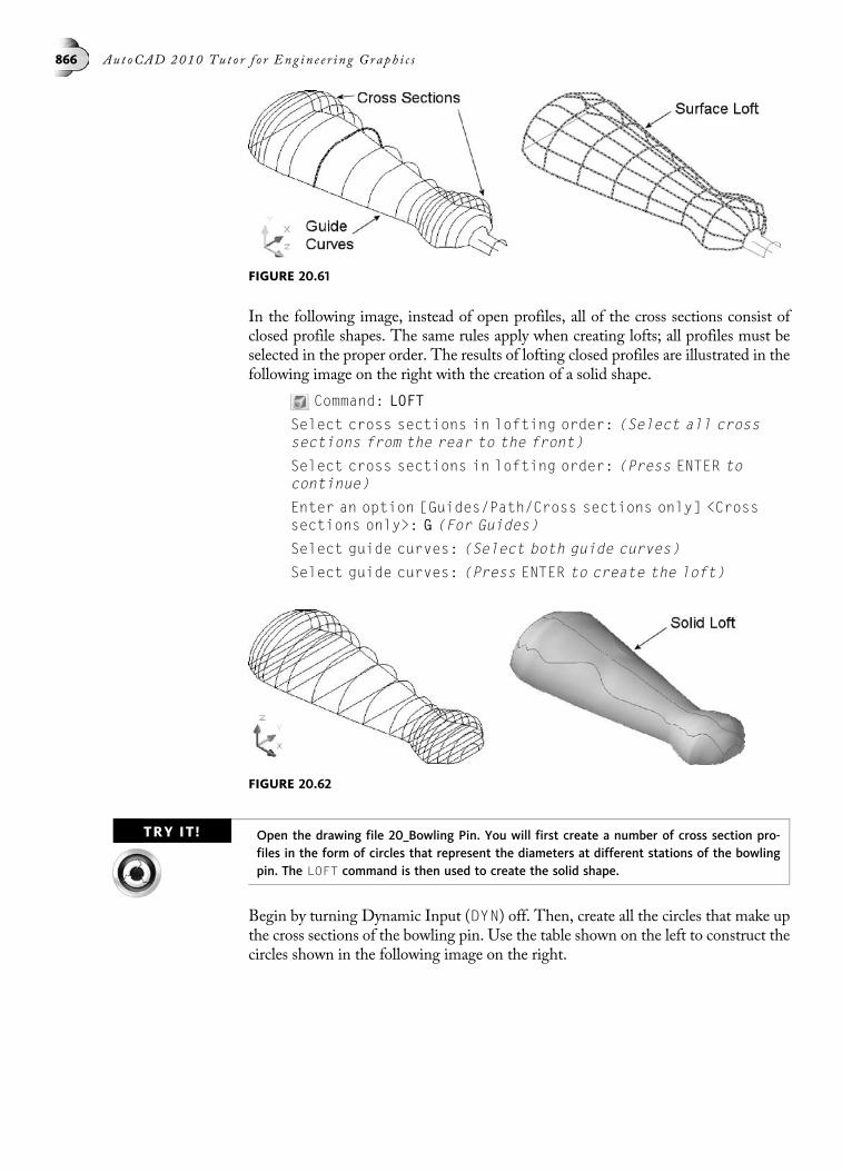
In the following image, instead of open profiles, all of the cross sections consist ofclosed profile shapes. The same rules apply when creating lofts; all profiles must beselected in the proper order. The results of lofting closed profiles are illustrated in thefollowing image on the right with the creation of a solid shape.
Command: LOFT
Select cross sections in lofting order: (Select all crosssections from the rear to the front)
Select cross sections in lofting order: (Press ENTER tocontinue)
Enter an option [Guides/Path/Cross sections only] <Crosssections only>: G (For Guides)
Select guide curves: (Select both guide curves)
Select guide curves: (Press ENTER to create the loft)
TRY IT! Open the drawing file 20_Bowling Pin. You will first create a number of cross section pro-files in the form of circles that represent the diameters at different stations of the bowlingpin. The LOFT command is then used to create the solid shape.
Begin by turning Dynamic Input (DYN) off. Then, create all the circles that make upthe cross sections of the bowling pin. Use the table shown on the left to construct thecircles shown in the following image on the right.
FIGURE 20.61
FIGURE 20.62
866 Aut oCAD 2010 Tu t o r f o r Eng in e e r i n g Graph i c s

With all profiles created, activate the LOFT command and pick the cross sections ofthe bowling pin beginning with the bottom circle and working your way up to thetop circle. When the Loft Settings dialog box appears, as shown in the followingimage on the left, verify that Smooth Fit is selected and click the OK buttonto produce the loft that is illustrated in wireframe mode in the middle of thefollowing image.
Command: LOFT
Select cross sections in lofting order: (Select the six crosssections of the bowling pin in order)
Select cross sections in lofting order: (Press ENTER tocontinue)
Enter an option [Guides/Path/Cross sections only] <Crosssections only>: (Press ENTER to accept this default value)
Enter an option [Guides/Path/Cross sections only] <Crosssections only>: (Press ENTER to perform the loft)
To complete the bowling pin, use the FILLET command to round off the topmostcircle of the bowling pin. Then view the results by clicking on the Realistic or Con-ceptual visual style. Your display should appear similar to the illustration as shown inthe following image on the right.
Command: F (For FILLET)
Current settings: Mode = TRIM, Radius = 0.00
Select first object or [Undo/Polyline/Radius/Trim/Multiple]: R (For Radius)
Specify fillet radius <0.00>: 0.50
Select first object or [Undo/Polyline/Radius/Trim/Multiple]: (Pick the edge of the upper circle)
Enter fillet radius <0.50>: (Press ENTER to accept thisvalue)
Select an edge or [Chain/Radius]: (Press ENTER to perform thefillet operation)
1 edge(s) selected for fillet.
FIGURE 20.63
Chap t e r 20 • So l i d Mod e l i n g Fundamen t a l s 867

CREATING A HELIXThe HELIX command creates a 2D or 3D spiral object. Choose this command in
one of the following ways:
• From the Modeling toolbar
• From the Ribbon of the 3D Modeling workspace (expand the 3D Modeling panel)
• From the Menu Bar (Draw > Modeling > Helix)
• From the keyboard (HELIX)
TRY IT! Open the drawing file 20_Helix. Use the following command sequences and images for cre-ating a 2D, 3D, and spiral helix.
Using the table below, experiment with the following command prompts forconstructing a 2D helix, 3D helix, and 3D spiral, as shown in the following imageson the left.
FIGURE 20.64
868 Aut oCAD 2010 Tu t o r f o r Eng in e e r i n g Graph i c s

Helix Type Helix Command Prompt
Use the following command prompt sequence to createa 2D Helix:
Command: HELIX
Number of turns = 3.0000 Twist = CCW
Specify center point of base: 0,0,0
Specify base radius or [Diameter] <1.0000>:1.00
Specify top radius or [Diameter] <1.0000>: 0
Specify helix height or [Axis endpoint/Turns/turn Height/tWist] <1.0000>: T
Enter number of turns <3.0000>: 6
Specify helix height or [Axis endpoint/Turns/turn Height/tWist] <1.0000>: 0
Use the following command prompt sequence to createa 3D Helix:
Command: HELIX
Number of turns = 3.0000 Twist = CCW
Specify center point of base: 0,0,0
Specify base radius or [Diameter] <1.0000>: 3
Specify top radius or [Diameter] <3.0000>:
Specify helix height or [Axis endpoint/Turns/turn Height/tWist] <1.0000>: T
Enter number of turns <3.0000>: 6
Specify helix height or [Axis endpoint/Turns/turn Height/tWist] <1.0000>: 2
Use the following command prompt sequence to createa 3D Spiral:
Command: HELIX
Number of turns = 3.0000 Twist = CCW
Specify center point of base: 0,0,0
Specify base radius or [Diameter] <1.0000>: 5
Specify top radius or [Diameter] <5.0000>: 2
Specify helix height or [Axis endpoint/Turns/turn Height/tWist] <1.0000>: T
Enter number of turns <3.0000>: 6
Specify helix height or [Axis endpoint/Turns/turn Height/tWist] <1.0000>: 10
FIGURE 20.65
Chap t e r 20 • So l i d Mod e l i n g Fundamen t a l s 869

HELIX APPLICATIONSTypically, a wireframe model of a helix does not fully define how an object like aspring should look. It would be beneficial to show the spring as a thin wire wrappingaround a cylinder to form the helical shape. To produce this type of object, use thewireframe of a circle as the object to sweep around the helix to produce the spring.
TRY IT! Open the drawing file 20_Helix Spring. A helix is already created, along with small circularprofile. With the helix as a path and the circle as the object to sweep, use the followingcommand prompt and images to create a spring.
Command: SWEEP
Current wire frame density: ISOLINES=4
Select objects to sweep: (Select the small circle)
Select objects to sweep: (Press ENTER to continue)
Select sweep path or [Alignment/Base point/Scale/Twist]:(Select the helix)
CREATING POLYSOLIDSA polysolid is created in a fashion similar to the one used to create a polyline. ThePOLYSOLID command is used to create this type of object. Choose this commandin one of the following ways:
• From the Modeling toolbar
• From the Ribbon of the 3D Modeling workspace
• From the Menu Bar (Draw > Modeling > Polysolid)
• From the keyboard (POLYSOLID)
You pick points and can use the direct distance mode of entry to designate the dis-tances of the polysolid, as shown in the following image on the left, where a width hasbeen entered. The main difference between polysolids and polylines is that you candesignate the height of a polysolid. In this way, polysolids are ideal for creating suchitems as walls in your model, as shown in the following image on the right.
FIGURE 20.66
870 Aut oCAD 2010 Tu t o r f o r Eng in e e r i n g Graph i c s

Polysolids can also be created from existing 2D geometry such as lines, polylines,arcs, and even circles. Illustrated in the following image on the left is a 2D polylinethat has had fillets applied to a number of corners. Activating the POLYSOLIDcommand and selecting the polyline changes the appearance of the object to matchthe illustration, as shown in the following image in the middle. Here a widthhas been automatically applied to the polysolid. When the polysolid is viewedin 3D using the SE Isometric, the polysolid is displayed with a height, as shownin the following image on the right.
Command: POLYSOLID
Specify start point or [Object/Height/Width/Justify]<Object>: (Press ENTER to accept Object)
Select object: (Pick the polyline object as shown in thefollowing image on the left)
TRY IT!Open the drawing file 20_Polysolid Walls. Use the following command sequence and imageto construct the 3D walls using the POLYSOLID command.
Command: POLYSOLID
Specify start point or [Object/Height/Width/Justify]<Object>: H (For Height)
Specify height <0 0-4 00>: 8 0
Specify start point or [Object/Height/Width/Justify]<Object>: W (For Width)
Specify width <0 0-0 1/4 00>: 4
Specify start point or [Object/Height/Width/Justify]<Object>: (Pick a point in the lower-left corner of thedisplay screen)
FIGURE 20.67
FIGURE 20.68
Chap t e r 20 • So l i d Mod e l i n g Fundamen t a l s 871

Specify next point or [Arc/Undo]: (Move your cursor to theright and enter 30 0)
Specify next point or [Arc/Undo]: (Move your cursor up andenter 10 0)
Specify next point or [Arc/Close/Undo]: (Move your cursorto the left and enter 5 0)
Specify next point or [Arc/Close/Undo]: (Move your cursorup and enter 5 0)
Specify next point or [Arc/Close/Undo]: (Move your cursorto the left and enter 25 0)
Specify next point or [Arc/Close/Undo]: C (For Close)
When finished, rotate your model using the SE Isometric view or the 3DFORBIT(3D Free Orbit) command to view the results.
FILLETING SOLID MODELSFilleting of simple or complex objects is easily handled with the FILLET com-
mand. This is the same command as the one used to create a 2D fillet.
TRY IT! Open the drawing file 20_Tee Fillet. Use the following prompt sequence and image for per-forming this task.
FIGURE 20.69
FIGURE 20.70
872 Aut oCAD 2010 Tu t o r f o r Eng in e e r i n g Graph i c s

Command: F (For FILLET)
Current settings: Mode = TRIM, Radius = 0.5000
Select first object or [Undo/Polyline/Radius/Trim/Multiple]: (Select the edge at “A,” which represents theintersection of both cylinders)
Enter fillet radius <0.5000>: 0.25
Select an edge or [Chain/Radius]: (Press ENTER to perform thefillet operation)
1 edge(s) selected for fillet.
TRY IT!Open the drawing file 20_Slab Fillet. A group of objects with a series of edges can befilleted with the Chain option of the FILLET command. Use the following promptsequence and image for performing this task.
Command: F (For FILLET)
Current settings: Mode = TRIM, Radius = 0.5000
Select first object or [Undo/Polyline/Radius/Trim/Multiple]: (Select the edge at “A”)
Enter fillet radius <0.5000>: (Press ENTER to accept thedefault value)
Select an edge or [Chain/Radius]: C (For chain mode)
Select an edge chain or [Edge/Radius]: (Select edge “A”again; notice how the selection is chained until it reachesan abrupt corner)
Select an edge chain or [Edge/Radius]: (Select the edge at “B”)
Select an edge chain or [Edge/Radius]: (Press ENTER whenfinished selecting all edges to perform the fillet operation)
10 edge(s) selected for fillet.
CHAMFERING SOLID MODELSJust as the FILLET command uses the Chain mode to group a series of edges
together, the CHAMFER command uses the Loop option to perform the same typeof operation.
FIGURE 20.71
Chap t e r 20 • So l i d Mod e l i n g Fundamen t a l s 873

TRY IT! Open the drawing file 20_Slab Chamfer. Use the following prompt sequence and image forperforming this task.
Command: CHA (For CHAMFER)
(TRIM mode) Current chamfer Dist1 = 0.5000, Dist2 = 0.5000
Select first line or [Undo/Polyline/Distance/Angle/Trim/mEthod/Multiple]: (Pick the edge at “A”)
Base surface selection...
Enter surface selection option [Next/OK (current)] <OK>: N(This option selects the other surface shared by edge “A”;the top surface should highlight. If not, use this optionagain)
Enter surface selection option [Next/OK (current)] <OK>:(Press ENTER to accept the top surface)
Specify base surface chamfer distance <0.5000>: (Press ENTERto accept the default)
Specify other surface chamfer distance <0.5000>: (PressENTER to accept the default)
Select an edge or [Loop]: L (To loop all edges together intoone)
Select an edge loop or [Edge]: (Pick any top edge; notice thatthe loop option does not stop at abrupt corners)
Select an edge loop or [Edge]: (Press ENTER to perform thechamfering operation)
OBTAINING MASS PROPERTIES OF A SOLID MODELThe MASSPROP command calculates the mass properties of a solid model.
Choose this command in one of the following ways:
• From the Inquiry toolbar
• From the Ribbon of the 3D Modeling workspace (Tools tab – Inquiry panel)
• From the Menu Bar (Tools > Inquiry > Region/Mass Properties)
• From the keyboard (MASSPROP)
FIGURE 20.72
874 Aut oCAD 2010 Tu t o r f o r Eng in e e r i n g Graph i c s

TRY IT!Open the drawing file 20_Tee Massprop. Use the MASSPROP command to calculate themass properties of a selected solid, as shown in the following image. All calculations arebased on the current position of the User Coordinate System. You will be given the optionof writing this information to a file if desired.
Command: MASSPROP
Select objects: (Select the model)
Select objects: (Press ENTER to continue with this command)
SYSTEM VARIABLES THAT AFFECT SOLID MODELSSystem variables are available to control the appearance of your solid model when-ever you perform shading or hidden line removal operations. Three in particular areuseful: ISOLINES, FACETRES, and DISPSILH. The following text describeseach system variable in detail.
The ISOLINES (Isometric Lines) System VariableTessellation refers to the lines that are displayed on any curved surface, such as thoseshown in the following image, to help you visualize the surface. Tessellation linesare automatically formed when you construct solid primitives such as cylinders andcones. These lines are also calculated when you perform solid modeling operationssuch as SUBTRACT and UNION.
FIGURE 20.73
Chap t e r 20 • So l i d Mod e l i n g Fundamen t a l s 875

The number of tessellation lines per curved object is controlled by the system variablecalled ISOLINES. By default, this variable is set to a value of 4. The following imageshows the results of setting this variable to other values, such as 9 and 20. Afterthe isolines have been changed, regenerate the screen to view the results. The morelines used to describe a curved surface, the more accurate the surface will look inwireframe mode; however, it will take longer to process screen regenerations.
TRY IT! Open the drawing file 20_Tee Isolines. Experiment by changing the ISOLINES system vari-able to numerous values. Perform a drawing regeneration using the REGEN command eachtime that you change the number of isolines.
The FACETRES (Facet Resolution) System VariableWhen you perform hidden line removals on solid objects, the results are similarto those displayed in the following image. The curved surfaces are now displayedas flat triangular surfaces (faces), and the display of these faces is controlled by theFACETRES system variable. The cylinder with FACETRES set to 0.50 processesmuch more quickly than the cylinder with FACETRES set to 2, because there arefewer surfaces to process in such operations as hidden line removals. However, theimage with FACETRES set to a large value (as high as 10) shows a more definedcircle. The default value for FACETRES is 0.50, which seems adequate for mostapplications.
FIGURE 20.74
FIGURE 20.75
876 Aut oCAD 2010 Tu t o r f o r Eng in e e r i n g Graph i c s
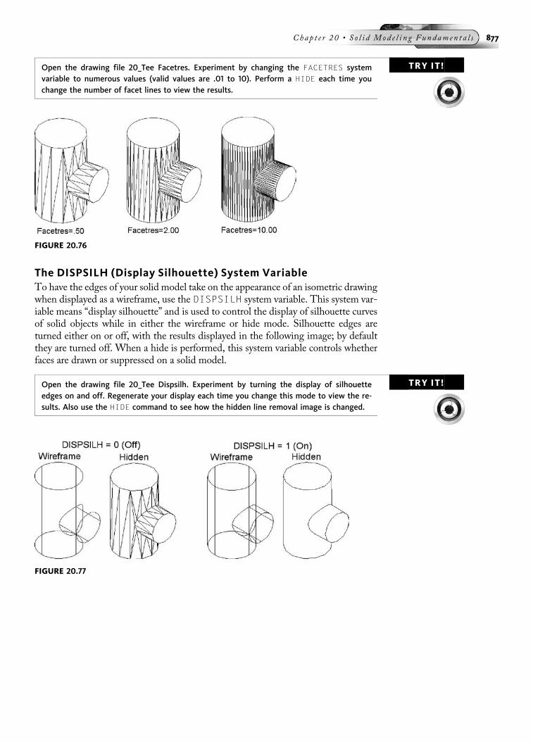
TRY IT!Open the drawing file 20_Tee Facetres. Experiment by changing the FACETRES systemvariable to numerous values (valid values are .01 to 10). Perform a HIDE each time youchange the number of facet lines to view the results.
The DISPSILH (Display Silhouette) System VariableTo have the edges of your solid model take on the appearance of an isometric drawingwhen displayed as a wireframe, use the DISPSILH system variable. This system var-iable means “display silhouette” and is used to control the display of silhouette curvesof solid objects while in either the wireframe or hide mode. Silhouette edges areturned either on or off, with the results displayed in the following image; by defaultthey are turned off. When a hide is performed, this system variable controls whetherfaces are drawn or suppressed on a solid model.
TRY IT!Open the drawing file 20_Tee Dispsilh. Experiment by turning the display of silhouetteedges on and off. Regenerate your display each time you change this mode to view the re-sults. Also use the HIDE command to see how the hidden line removal image is changed.
FIGURE 20.76
FIGURE 20.77
Chap t e r 20 • So l i d Mod e l i n g Fundamen t a l s 877
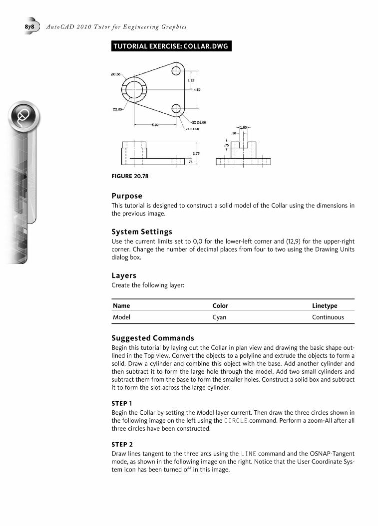
TUTORIAL EXERCISE: COLLAR.DWG
PurposeThis tutorial is designed to construct a solid model of the Collar using the dimensions inthe previous image.
System SettingsUse the current limits set to 0,0 for the lower-left corner and (12,9) for the upper-rightcorner. Change the number of decimal places from four to two using the Drawing Unitsdialog box.
LayersCreate the following layer:
Name Color Linetype
Model Cyan Continuous
Suggested CommandsBegin this tutorial by laying out the Collar in plan view and drawing the basic shape out-lined in the Top view. Convert the objects to a polyline and extrude the objects to form asolid. Draw a cylinder and combine this object with the base. Add another cylinder andthen subtract it to form the large hole through the model. Add two small cylinders andsubtract them from the base to form the smaller holes. Construct a solid box and subtractit to form the slot across the large cylinder.
STEP 1Begin the Collar by setting the Model layer current. Then draw the three circles shown inthe following image on the left using the CIRCLE command. Perform a zoom-All after allthree circles have been constructed.
STEP 2Draw lines tangent to the three arcs using the LINE command and the OSNAP-Tangentmode, as shown in the following image on the right. Notice that the User Coordinate Sys-tem icon has been turned off in this image.
FIGURE 20.78
878 Aut oCAD 2010 Tu t o r f o r Eng in e e r i n g Graph i c s

STEP 3Use the TRIM command to trim the circles. When prompted to select the cutting edgeobject, press ENTER; this makes cutting edges out of all objects in the drawing. Performthis trimming operation so your display appears similar to the illustration in the followingimage on the left.
STEP 4Prepare to construct the base by viewing the object in 3D. Select a viewpoint by choosing3D Views from the View Menu Bar and then choosing SE Isometric. Your display shouldappear similar to the illustration in the following image on the right.
STEP 5Convert all objects to a polyline using the Join option of the PEDIT command, as shownin the following image on the left.
STEP 6Use the EXTRUDE command to extrude the base to a thickness of 0.75 units, as shown inthe following image on the right.
FIGURE 20.79
FIGURE 20.80
FIGURE 20.81
Chap t e r 20 • So l i d Mod e l i n g Fundamen t a l s 879

STEP 7Turn off Dynamic UCS on the status bar. Create a cylinder using the CYLINDERcommand. Begin the center point of the cylinder at 0,0,0, with a diameter of 3.00 unitsand a height of 2.75 units. You may have to perform a ZOOM-All to display the entiremodel, as shown in the following image on the left.
STEP 8Merge the cylinder just created with the extruded base using the UNION command, asshown in the following image on the right.
STEP 9Use the CYLINDER command to create a 2.00-unit-diameter cylinder representing athrough hole, as shown in the following image on the left. The height of the cylinder is2.75 units, with the center point at 0,0,0.
STEP 10To cut the hole through the outer cylinder, use the SUBTRACT command. Select the baseas the source object; select the inner cylinder as the object to subtract. Use the HIDEcommand to view the results, as shown in the following image on the right.
STEP 11Use the REGEN command to regenerate your screen and return to Wireframe mode.Begin placing the two small drill holes (1.00 diameter and .75 high) in the base usingthe CYLINDER command. Use the OSNAP-Center mode to place each cylinder at thecenter of arcs “A” and “B,” as shown in the following image on the left.
FIGURE 20.82
FIGURE 20.83
880 Aut oCAD 2010 Tu t o r f o r Eng in e e r i n g Graph i c s

STEP 12Subtract both 1.00-diameter cylinders from the base of the model using the SUBTRACTcommand. Use the HIDE command to view the results, as shown in the following imageon the right.
STEP 13Begin constructing the rectangular slot that will pass through the two cylinders. Use theBOX command and Center option to accomplish this. Locate the center of the box at0,0,2.75 and make the box 4 units long, 1 unit wide, and 1.50 units high (using the Centeroption) as shown in the following image.
STEP 14Use the SUBTRACT command to subtract the rectangular box from the solid model, asshown in the following image on the left.
STEP 15Change the facet resolution to a higher value using the FACETRES system variable and avalue of 5. Then perform a hidden line removal to see the appearance of the completedmodel, as shown in the following image on the right.
FIGURE 20.84
FIGURE 20.85
Chap t e r 20 • So l i d Mod e l i n g Fundamen t a l s 881

TUTORIAL EXERCISE: VACUUM ATTACHMEN.DWG
PurposeThis tutorial is designed to construct a solid model of the vacuum cleaner attachmentusing the Loft tool.
System SettingsUse the current limits, which are set to 0,0 for the lower-left corner and (12,9) for theupper-right corner. Change the number of decimal places from four to two using theDrawing Units dialog box.
LayersCreate the following layer:
Name Color Linetype
Model Cyan Continuous
Suggested CommandsBegin this tutorial by laying out a slot shape and circle. Next move the midpoint of thebottom of the slot to 0,0,0 and then copy it to 0,0,2. Move the bottom quadrant of thecircle to 0,0,3.5 and then copy it to 0,0,5. These steps form the four cross sections usedfor creating the loft.
FIGURE 20.86
FIGURE 20.87
882 Aut oCAD 2010 Tu t o r f o r Eng in e e r i n g Graph i c s

STEP 1First create a new drawing file. Then, begin the construction of this 3D model byconstructing 2D geometry that will define the final shape of the vacuum cleaner attach-ment. Use the PLINE command to construct the slot shape as a closed polyline usingthe dimensions shown in the following image on the left. Then construct the circle using thediameter dimension shown in the following image on the right.
STEP 2Switch to SE Isometric viewing, as shown in the following image. This viewing positioncan be found by selecting View from the Menu Bar, then selecting 3D Views. Before con-tinuing, be sure that Dynamic Input is turned off for this segment. Next, move the slotshape from the midpoint of the bottom line to point 0,0,0.
STEP 3With the slot moved to the correct position, use the COPY command to create a duplicateshape of the slot using a base point of 0,0,0 and a second point at 0,0,2. When finished,your display should appear similar to the following image.
FIGURE 20.88
FIGURE 20.89
Chap t e r 20 • So l i d Mod e l i n g Fundamen t a l s 883

STEP 4You will next move the circle. Enter the MOVE command and pick the base point of themove using the bottom quadrant of the circle, as shown in the following image on theright. For the second point of displacement, enter the coordinate value of 0,0,3.5 fromthe keyboard.
STEP 5With the circle moved to the correct location, use the COPY command to duplicate thiscircle. Copy this circle from the bottom quadrant to a second point located at 0,0,5, asshown in the following image on the left. When finished, your display should appear sim-ilar to the illustration in the following image on the right. These form the four cross-sectional shapes that make up the vacuum cleaner attachment.
FIGURE 20.90
FIGURE 20.91
884 Aut oCAD 2010 Tu t o r f o r Eng in e e r i n g Graph i c s
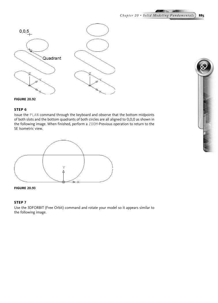
STEP 6Issue the PLAN command through the keyboard and observe that the bottom midpointsof both slots and the bottom quadrants of both circles are all aligned to 0,0,0 as shown inthe following image. When finished, perform a ZOOM-Previous operation to return to theSE Isometric view.
STEP 7Use the 3DFORBIT (Free Orbit) command and rotate your model so it appears similar tothe following image.
FIGURE 20.92
FIGURE 20.93
Chap t e r 20 • So l i d Mod e l i n g Fundamen t a l s 885
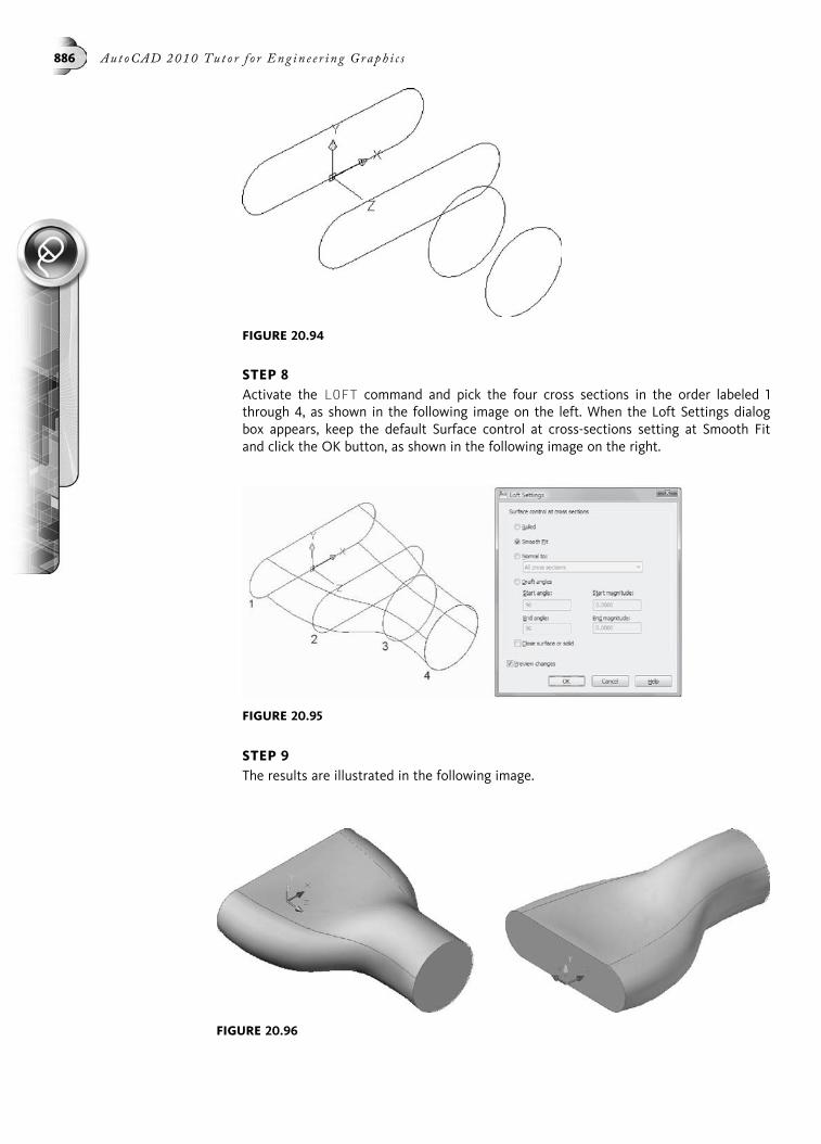
STEP 8Activate the LOFT command and pick the four cross sections in the order labeled 1through 4, as shown in the following image on the left. When the Loft Settings dialogbox appears, keep the default Surface control at cross-sections setting at Smooth Fitand click the OK button, as shown in the following image on the right.
STEP 9The results are illustrated in the following image.
FIGURE 20.95
FIGURE 20.96
FIGURE 20.94
886 Aut oCAD 2010 Tu t o r f o r Eng in e e r i n g Graph i c s
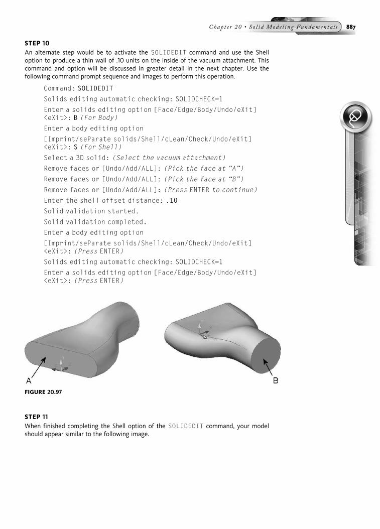
STEP 10An alternate step would be to activate the SOLIDEDIT command and use the Shelloption to produce a thin wall of .10 units on the inside of the vacuum attachment. Thiscommand and option will be discussed in greater detail in the next chapter. Use thefollowing command prompt sequence and images to perform this operation.
Command: SOLIDEDIT
Solids editing automatic checking: SOLIDCHECK=1
Enter a solids editing option [Face/Edge/Body/Undo/eXit]<eXit>: B (For Body)
Enter a body editing option
[Imprint/seParate solids/Shell/cLean/Check/Undo/eXit]<eXit>: S (For Shell)
Select a 3D solid: (Select the vacuum attachment)
Remove faces or [Undo/Add/ALL]: (Pick the face at “A”)
Remove faces or [Undo/Add/ALL]: (Pick the face at “B”)
Remove faces or [Undo/Add/ALL]: (Press ENTER to continue)
Enter the shell offset distance: .10
Solid validation started.
Solid validation completed.
Enter a body editing option
[Imprint/seParate solids/Shell/cLean/Check/Undo/eXit]<eXit>: (Press ENTER)
Solids editing automatic checking: SOLIDCHECK=1
Enter a solids editing option [Face/Edge/Body/Undo/eXit]<eXit>: (Press ENTER)
STEP 11When finished completing the Shell option of the SOLIDEDIT command, your modelshould appear similar to the following image.
FIGURE 20.97
Chap t e r 20 • So l i d Mod e l i n g Fundamen t a l s 887

END OF CHAPTER PROBLEMS FOR CHAPTER 20Please refer to the CD that is supplied with this book and locate the file AutoCADTutor 2010 Support Docs.pdf. In addition to extra information supplied in this chapter,end-of-chapter problems are also available to provide additional practice.
FIGURE 20.98
888 Aut oCAD 2010 Tu t o r f o r Eng in e e r i n g Graph i c s

CHAPTER
21Concept Modeling,
Editing Solids,andMeshModeling
This chapter begins with the study of creating concept models using a press-and-pulldrag method. The use of subshapes for editing solid models is discussed, as is the useof grips for editing solids. Once a solid model is created, various methods are availableto edit the model. The methods discussed in this chapter include the following 3Doperation commands: (3DMOVE, 3DROTATE, 3DALIGN, MIRROR3D, and ARRAY3D).Also included in this chapter is a segment on using the many options of theSOLIDEDIT command. Various 3D models will be opened and used to illustratethese commands and options. A segment on mesh modeling is also included.
CONCEPTUAL MODELINGChapter 20 dealt with the basics of creating solid primitives and how to join, subtract,or intersect these shapes to form complex solid models. Sometimes you do not needthe regimented procedures outlined in the previous chapter to get your point acrossabout a specific product you have in mind. You can simply create a concept solidmodel by dragging shapes together to form your idea. Various concept-modelingtechniques will be explained in the next segment of this chapter.
Dragging Basic Solid ShapesConstructing a 3D model with a concept in mind is easier than ever. Where exactdistances are not important, the following image illustrates the construction of a solidblock using the BOX command. First view your model in one of the many 3D viewingpositions, such as SE (Southeast) Isometric. Next enter the BOX command and pickfirst and second corner points for the box on the screen, as shown in the followingimage on the left. When prompted for the height of the box, move your cursor upand notice the box increasing in height, as shown in the following image on the right.Click to locate the height, BOX command. All solid primitives can be constructedusing this technique.
889

TRY IT! Open the drawing file 21_Concept_Box. This drawing file does not contain any objects. Also,it is already set up to be viewed in the Southeast Isometric position (SE Iso). Activatethe BOX command, pick two points to define the first and second corner points of the rect-angular base, and move your cursor up and pick to define the height of the box. You couldalso experiment using this technique for creating cylinders, pyramids, spheres, cones,wedges, and a torus. When finished, exit this drawing without saving any changes.
Using Dynamic UCS to Construct on FacesOnce a basic shape is created, it is very easy to create a second shape on an existingface with Dynamic UCS (DUCS) mode. Here is how it works. In the followingimage, a cylinder will be constructed on one of the faces. Turn on DUCS (locatedin the status bar), activate the CYLINDER command, and when prompted for thebase or center point, hover your cursor over the face, as shown in the following imageon the left. The face highlights (the edge appears dashed) to indicate that it has beenacquired. The Dynamic UCS cursor adjusts itself to this face by aligning the XYplane parallel to the face. When you click a point on this face for the start of the cyl-inder, the UCS icon changes to reflect this change and the base of the cylinder can beseen, as shown in the following image in the middle. Pick a point to specify theradius. To specify the height of the cylinder, simply drag your cursor away from theface and you will notice the cylinder taking shape, as shown in the following image onthe right. Clicking a point defines the height and exit the CYLINDER command.
FIGURE 21.1
FIGURE 21.2
890 Aut oCAD 2010 Tu t o r f o r Eng in e e r i n g Graph i c s

TRY IT!Open the drawing file 21_Concept_Cylinder. Issue the CYLINDER command and, for the baseor center point, hover your cursor over the front face in the previous image and pick apoint. The UCS changes to reflect this new position. Move your cursor until you see the cir-cle forming on the face and pick to define the radius of the cylinder. When prompted forthe height, move your cursor forward and notice the cylinder taking shape. Pick to definethe cylinder height and to exit the command.
When the cylinder is created, it is considered an individual object separate from thesolid block, as shown in the following image on the left. After the primitives are con-structed, the UNION command is used to join all primitives together as a single solidobject, as shown in the following image on the right.
USING GRIPS TO MODIFY SOLID MODELSWhenever a solid primitive is selected when no command is active, grips are dis-played, as with all types of objects that make up a drawing. The grips that appearon solid primitives, as shown in the following image, range in shape from squares toarrows. You can perform an edit operation by selecting either the square or arrowshapes. The type of editing that occurs depends on the type of grip selected.
FIGURE 21.3
FIGURE 21.4
Chap t e r 21 • Con c e p t Mod e l i n g , Ed i t i n g S o l i d s , and Me s h Mod e l i n g 891

Key Grip LocationsThe difference between the square and arrow grips is illustrated in the followingimage of a solid box primitive. The square grip located in the center of a primitiveallows you to change the location of the solid. Square grips displayed at the corner(vertex) locations of a primitive allow you to resize the base shape. The arrows locatedalong the edges of the rectangular base allow each individual side to be modified.Arrow grips that point vertically also appear in the middle of the top and bottom facesof the box primitive. These grips allow you to change the height of the primitive.
Grip Editing a ConeThe previous image outlined the various types of grips that display on a box primitive.The grips that appear on cylinders, pyramids, cones, and spheres have similar editingcapabilities. The following Try It! exercise illustrates the effects of editing certain ar-row grips on a cone.
TRY IT! Open the drawing file 21_GripEdit_Cone. Click the cone and the grips appear, as shown inthe following image on the left. Click the arrow grip at “A” and stretch the base of thecone in to match the object illustrated in the following image on the right. Next, click thearrow grip at “B” (not the grip that points up) and stretch this grip away from the cone tocreate a top surface similar to the object illustrated in the following image on the right. Ex-periment further with grips on the cone by clicking the top grip, which points up, andstretch the cone (now referred to as a frustrum) up.
FIGURE 21.5
FIGURE 21.6
892 Aut oCAD 2010 Tu t o r f o r Eng in e e r i n g Graph i c s

Editing with Grips and Dynamic InputYou have already seen how easy it is to select grips that belong to a solid primitive andstretch the grips to change the shape of the primitive. This next Try It! exercise dealswith grip editing of primitives that make up a solid model in an accurate manner. Toaccomplish this, Dynamic Input must be turned on.
TRY IT!Open the drawing file 21_GripEdit_Shape01. This 3D model consists of three separate primi-tives, namely, two boxes and one cylinder. The height of the cylinder needs to be lowered.To accomplish this, click the cylinder and observe the positions of the grips and numeric va-lues, as shown in the following image on the left. The total height of 6.0000 needs to bechanged to 3.50 units. Click the arrow grip at the top of the cylinder that is pointing up,press the TAB key to highlight the overall height value of 6.0000, and change this value to3.50. Pressing ENTER to accept this new value lowers the cylinder, as shown in the followingimage on the right. Feel free to experiment with both boxes by either increasing or decreas-ing their heights using this grip-editing method.
MANIPULATING SUBOBJECTSA subobject is any part of a solid. It could be a face, an edge, or a vertex (corner). Thefollowing image illustrates a 3D box and pyramid. Pressing the CTRL key allows youto select a subobject. Notice in this illustration that each subobject selected has a gripassociated with it. If you accidentally select a subobject, press CTRL + SHIFT and pickit again to deselect it.
FIGURE 21.7
FIGURE 21.8
Chap t e r 21 • Con c e p t Mod e l i n g , Ed i t i n g S o l i d s , and Me s h Mod e l i n g 893
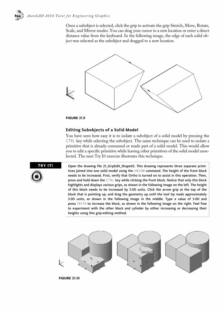
Once a subobject is selected, click the grip to activate the grip Stretch, Move, Rotate,Scale, and Mirror modes. You can drag your cursor to a new location or enter a directdistance value from the keyboard. In the following image, the edge of each solid ob-ject was selected as the subobject and dragged to a new location.
Editing Subobjects of a Solid ModelYou have seen how easy it is to isolate a subobject of a solid model by pressing theCTRL key while selecting the subobject. The same technique can be used to isolate aprimitive that is already consumed or made part of a solid model. This would allowyou to edit a specific primitive while leaving other primitives of the solid model unse-lected. The next Try It! exercise illustrates this technique.
TRY IT! Open the drawing file 21_GripEdit_Shape02. This drawing represents three separate primi-tives joined into one solid model using the UNION command. The height of the front blockneeds to be increased. First, verify that Ortho is turned on to assist in this operation. Then,press and hold down the CTRL key while clicking the front block. Notice that only this blockhighlights and displays various grips, as shown in the following image on the left. The heightof this block needs to be increased by 3.00 units. Click the arrow grip at the top of theblock that is pointing up, and drag the geometry up until the tool tip reads approximately3.00 units, as shown in the following image in the middle. Type a value of 3.00 andpress ENTER to increase the block, as shown in the following image on the right. Feel freeto experiment with the other block and cylinder by either increasing or decreasing theirheights using this grip-editing method.
FIGURE 21.9
FIGURE 21.10
894 Aut oCAD 2010 Tu t o r f o r Eng in e e r i n g Graph i c s

ADDING EDGES AND FACES TO A SOLID MODELWhen building solid models, use the UNION, SUBTRACT, and INTERSECT commandsas the primary means of joining, removing, or creating a solid that is common to twointersecting primitives. You can also imprint regular objects such as lines, circles, orpolylines—for example, the line segment shown in the following image on the left—directly onto the face of a solid model. This line, once imprinted, becomes part of thesolid and in our case divides the top face into two faces. Then, using the subobjecttechnique, we can change the shape of the solid model. The command used to per-form this operation is IMPRINT, which can be found in the Ribbon (Solid Edit panel)or the Solids Editing toolbar, as shown in the following image on the right.
Command: IMPRINT
Select a 3D solid: (Select the 3D solid model)
Select an object to imprint: (Pick the line segmentconstructed across the top surface of the solid model)
Delete the source object [Yes/No] <N>: Y (For Yes)
Select an object to imprint: (Press ENTER to perform thisoperation and exit the command)
After the imprint operation is performed on the line segment, this object becomespart of the solid model. When the imprinted line is selected as a subobject, the griplocated on the line can be selected and dragged up or down, as shown in the followingimage. The results can dramatically change the shape of the solid model.
FIGURE 21.11
FIGURE 21.12
Chap t e r 21 • Con c e p t Mod e l i n g , Ed i t i n g S o l i d s , and Me s h Mod e l i n g 895

TRY IT! Open the drawing file 21_Imprint_Roof. First, verify that ortho is turned on to assist in thisoperation. Issue the imprint command, select the solid block, as shown in the following im-age on the left, and pick the single line segment as the object to imprint. Next, press andhold down the CTRL key while clicking the imprinted line. Notice that only this line high-lights and displays a grip at its midpoint, as shown in the middle of the following image.Pick this grip, slowly move your cursor up, and notice the creation of the roof peak. Youcould also move your cursor down to create a V-shaped object.
PRESSING AND PULLING BOUNDING AREASAn additional technique used for constructing solid models is available to speed upthe construction and modification processes. The technique is called pressing andpulling, which can be accessed by picking the PRESSPULL command from the Rib-bon or the Modeling toolbar, as shown in the following image. Any closed area thatcan be hatched can be manipulated using the PRESSPULL command.
TRY IT! Open the drawing file 21_PressPull_Shapes. Activate the PRESSPULL command from theRibbon, pick inside of the circular shape, as shown in the following image on the left, moveyour cursor up, and enter a value of 6 units. Activate the PRESSPULL command again, pickinside of the closed block shape, as shown in the following image in the middle, move yourcursor up, and enter a value of 4 units. Use the PRESSPULL command one more time onthe remaining closed block shape, as shown in the following image on the right, move yourcursor up, and enter a value of 2 units. Performing this task results in the creation of threeseparate solid shapes. Use the UNION command to join all shapes into one 3D solid model.
FIGURE 21.13
FIGURE 21.14
896 Aut oCAD 2010 Tu t o r f o r Eng in e e r i n g Graph i c s

Another technique to activate the press-and-pull feature is to press and hold theCTRL + ALT keys, and then pick the area. You can perform the operation the sameway as using the PRESSPULL command from the Ribbon. The next Try It! exerciseillustrates this technique.
TRY IT!Open the drawing file 21_PressPull_Hole. Press and hold down the CTRL + ALT keys and pickinside of the circular shape, as shown in the following image on the left. Moving your cursorup creates the cylinder, as shown in the following image on the right.
Undo the previous operation, activate press and pull by pressing and holding downthe CTRL + ALT keys, and pick inside of the circular shape, as shown in the followingimage on the left. However, instead of moving your cursor up to form a cylinder, dragyour cursor down into the thin block to perform a subtraction operation and create ahole in the block.
FIGURE 21.15
FIGURE 21.16
FIGURE 21.17
Chap t e r 21 • Con c e p t Mod e l i n g , Ed i t i n g S o l i d s , and Me s h Mod e l i n g 897

TRY IT! Open the drawing file 21_PressPull Plan. Press and hold down the CTRL + ALT keys whilepicking inside of the bounding area created by the inner and outer lines, as shown in thefollowing image on the left. Move your cursor up and enter a value of 8 0 to construct a solidmodel of the walls, as shown in the following image on the right.
TRY IT! Open the drawing file 21_PressPull Openings. Press and hold down the CTRL + ALT keyswhile picking inside of one of the rectangles that signify a door or window opening. Moveyour cursor into the wall and pick inside of the model to create the opening. Use this tech-nique for the other openings as well.
USING PRESS AND PULL ON BLOCKSPressing and pulling to create solid shapes is not just limited to closed shapes such asrectangles, circles, or polylines. The press-and-pull feature can also be used on blockobjects. In some cases, depending on how you use the press-and-pull feature, it ispossible to convert the 2D block into a 3D solid model. The next Try It! exerciseillustrates this.
TRY IT! Open the drawing file 21_PressPull_Bed. All objects that describe this 2D bed are made up ofa single block. You will use the PRESSPULL command to highlight certain closed boundaryareas and pull the area to a new height. In this way, PRESSPULL is used to convert a 2Dobject into a 3D model.
Activate the PRESSPULL command, move your cursor inside the area, as shown inthe following image on the left, and press and hold down the left mouse button asyou move your cursor up. When you let go of the mouse button, type a value of 12
FIGURE 21.18
FIGURE 21.19
898 Aut oCAD 2010 Tu t o r f o r Eng in e e r i n g Graph i c s

to extrude this area a distance of 12 units up, as shown in the following image onthe right.
Command: PRESSPULL
Click inside bounded areas to press or pull. (Move your cursorover the area, as shown in the following image on the left.Press and hold down the mouse button and pull in an upwarddirection. Let go of the mouse button, enter a value of 12in the designated field, and press ENTER when finished)
1 loop extracted.
1 Region created.
12 (Value entered)
Activate the PRESSPULL command, move your cursor inside the small triangulararea, as shown in the following image on the left, and press and hold down the leftmouse button as you move your cursor up. When you let go of the mouse button,type a value of 12.5 to extrude this area a distance of 12.5 units up, as shown in thefollowing image on the right.
Command: PRESSPULL
Click inside bounded areas to press or pull. (Move your cursorover the triangular, area, as shown in the following image onthe left. Press and hold down the mouse button and pull in anupward direction. Let go of the mouse button, enter a value of12.5 in the designated field, and press ENTER when finished)
1 loop extracted.
1 Region created.
12.5 (Value entered)
FIGURE 21.20
FIGURE 21.21
Chap t e r 21 • Con c e p t Mod e l i n g , Ed i t i n g S o l i d s , and Me s h Mod e l i n g 899
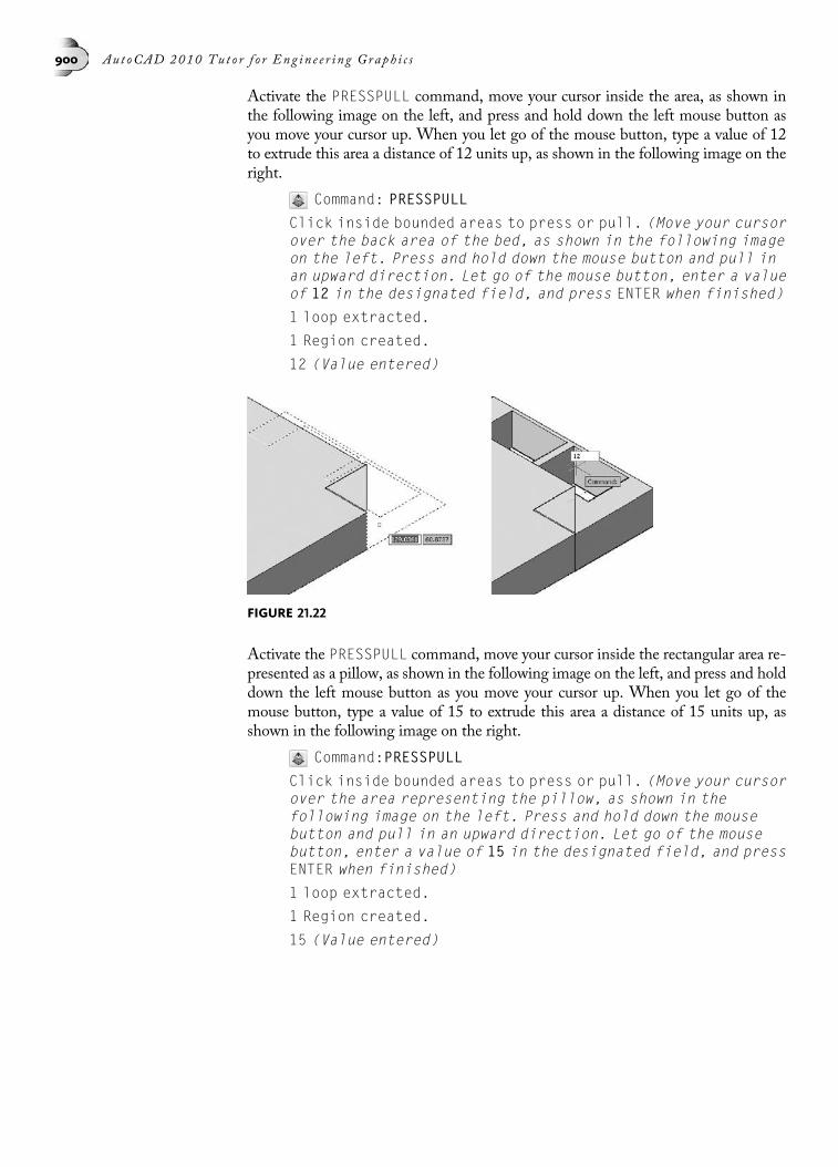
Activate the PRESSPULL command, move your cursor inside the area, as shown inthe following image on the left, and press and hold down the left mouse button asyou move your cursor up. When you let go of the mouse button, type a value of 12to extrude this area a distance of 12 units up, as shown in the following image on theright.
Command: PRESSPULL
Click inside bounded areas to press or pull. (Move your cursorover the back area of the bed, as shown in the following imageon the left. Press and hold down the mouse button and pull inan upward direction. Let go of the mouse button, enter a valueof 12 in the designated field, and press ENTER when finished)
1 loop extracted.
1 Region created.
12 (Value entered)
Activate the PRESSPULL command, move your cursor inside the rectangular area re-presented as a pillow, as shown in the following image on the left, and press and holddown the left mouse button as you move your cursor up. When you let go of themouse button, type a value of 15 to extrude this area a distance of 15 units up, asshown in the following image on the right.
Command:PRESSPULL
Click inside bounded areas to press or pull. (Move your cursorover the area representing the pillow, as shown in thefollowing image on the left. Press and hold down the mousebutton and pull in an upward direction. Let go of the mousebutton, enter a value of 15 in the designated field, and pressENTER when finished)
1 loop extracted.
1 Region created.
15 (Value entered)
FIGURE 21.22
900 Aut oCAD 2010 Tu t o r f o r Eng in e e r i n g Graph i c s

Perform the same press-and-pull operation on the second pillow. Extrude this shapea value of 15 units, as shown in the following image on the left. Since the 3D objectscreated by the press-and-pull operations are all considered individual primitives, usethe UNION command to join all primitives into a single 3D solid model. An alternatestep would be to use the FILLET command to round off all corners and edges of thebed and pillows, as shown in the following image on the right.
ADDITIONAL METHODS FOR EDITING SOLID MODELSAdditional methods are available to edit the solid model. These methods include the 3DOperation commands (3DMOVE, 3DALIGN, 3DROTATE, MIRROR3D, and 3DARRAY)and the SOLIDEDIT command, all illustrated in the following image. Various 3Ddrawings will be opened and used to illustrate these commands.
FIGURE 21.23
FIGURE 21.24
FIGURE 21.25
Chap t e r 21 • Con c e p t Mod e l i n g , Ed i t i n g S o l i d s , and Me s h Mod e l i n g 901

MOVING OBJECTS IN 3DTo assist in the positioning of objects in a 3 dimensional environment, the 3DMOVEtool is available. Choose this command from the Ribbon or Menu Bar as shown inthe following image or from one of the following methods:
• From the Modify panel located in the Ribbon (3D Modeling Workspace)
• From the Menu Bar (Modify > 3D Operations > 3DMove)
• From the keyboard (3DMOVE)
This tool displays the 3D move gizmo as shown in the following image, which dis-plays an axis for the purpose of moving objects a specified direction and distance.When using this command, you can select either objects or subobjects to move. Toselect subobjects, press and hold down the CTRL key as you select. After you pressENTER to signify that you are done with the selection process, the 3D move gizmodisplays attached to your cursor.
Pick any convenient point to utilize as the base point for the move. Object snapmodes can be used to accomplish this task if desired. You then move your cursorover one of the three axis handles to define the direction of the move. As you hoverover one of the handles, it turns yellow and a direction vector displays. Click this axishandle to lock in the direction vector. Then enter a value to move the solid model ormove your cursor along the direction vector, as shown in the following image, andpick a location to move.
FIGURE 21.26
FIGURE 21.27
902 Aut oCAD 2010 Tu t o r f o r Eng in e e r i n g Graph i c s

ALIGNING OBJECTS IN 3DUse the 3DALIGN command to specify up to three points to define the source plane ofone 3D solid model, followed by up to three points to define the destination planewhere the first solid model will be moved or aligned to. Choose this command fromone of the following:
• From the Modify panel located in the Ribbon (3D Modeling Workspace)
• From the Menu Bar (Modify > 3D Operations > 3DAlign)
• From the keyboard (3DALIGN)
When you specify points, the first source point is referred to as the base point. Thispoint is always moved to the first destination point. Selecting second and third sourceor destination points results in the 3D solid model being rotated into position.
TRY IT!Open the drawing file 21_3DAlign. The objects in the following image on the right need tobe positioned or aligned to form the assembled object shown in the small isometric view inthis image. At this point, it is unclear at what angle the objects are currently rotated. Whenyou use the 3DALIGN command, it is not necessary to know this information. Rather, youline up source points with destination points. When the three sets of points are identified,the object moves and rotates into position. The first source point acts as a base point for amove operation. The first destination point acts as a base point for rotation operations. Thesecond and third sets of source and destination points establish the direction and amountof rotation required to align the objects.
FIGURE 21.28
Chap t e r 21 • Con c e p t Mod e l i n g , Ed i t i n g S o l i d s , and Me s h Mod e l i n g 903

Follow the prompt sequence below and the illustration in the following image foraligning the hole plate with the bottom base. The first destination point acts as abase point to which the cylinder locates.
Command: 3DALIGN
Select objects: (Select the object with the hole)
Select objects: (Press ENTER to continue)
Specify source plane and orientation . . .
Specify base point or [Copy]: (Select the endpoint at “A”)
Specify second point or [Continue] <C>: (Select the endpointat “B”)
Specify third point or [Continue] <C>: (Select the endpointat “C”)
Specify destination plane and orientation . . .
Specify first destination point: (Select the endpoint at “D”)
Specify second destination point or [eXit] <X>: (Select theendpoint at “E”)
Specify third destination point or [eXit] <X>: (Select theendpoint at “F”)
FIGURE 21.29
FIGURE 21.30
904 Aut oCAD 2010 Tu t o r f o r Eng in e e r i n g Graph i c s
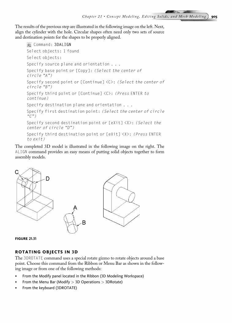
The results of the previous step are illustrated in the following image on the left. Next,align the cylinder with the hole. Circular shapes often need only two sets of sourceand destination points for the shapes to be properly aligned.
Command: 3DALIGN
Select objects: 1 found
Select objects:
Specify source plane and orientation . . .
Specify base point or [Copy]: (Select the center ofcircle “A”)
Specify second point or [Continue] <C>: (Select the center ofcircle “B”)
Specify third point or [Continue] <C>: (Press ENTER tocontinue)
Specify destination plane and orientation . . .
Specify first destination point: (Select the center of circle“C”)
Specify second destination point or [eXit] <X>: (Select thecenter of circle “D”)
Specify third destination point or [eXit] <X>: (Press ENTERto exit)
The completed 3D model is illustrated in the following image on the right. TheALIGN command provides an easy means of putting solid objects together to formassembly models.
ROTATING OBJECTS IN 3DThe 3DROTATE command uses a special rotate gizmo to rotate objects around a basepoint. Choose this command from the Ribbon or Menu Bar as shown in the follow-ing image or from one of the following methods:
• From the Modify panel located in the Ribbon (3D Modeling Workspace)
• From the Menu Bar (Modify > 3D Operations > 3DRotate)
• From the keyboard (3DROTATE)
FIGURE 21.31
Chap t e r 21 • Con c e p t Mod e l i n g , Ed i t i n g S o l i d s , and Me s h Mod e l i n g 905

After you select the object or objects to rotate, you are prompted to pick a base point,which will act as the pivot point of the rotation. After you pick this base point, the 3Drotate gizmo appears, as shown in the following image. You then hover your cursorover an axis handle until it turns yellow and an axis vector appears. If this axis is cor-rect, click it to establish the axis of rotation. Then enter the start and end angles toperform the rotation.
TRY IT! Open the drawing 21_3DRot. In the following image, a base containing a slot needs to bejoined with the two rectangular boxes to form a back and side. First select box “A” as theobject to rotate in 3D. You will be prompted to define the base point of rotation. Next youwill be prompted to choose a rotation axis by picking the appropriate axis handle on thegizmo. This axis will serve as a pivot point where the rotation occurs. Entering a negativeangle of 90° rotates the box in the counterclockwise direction (as you would look down theY-axis). Negative angles rotate in the clockwise direction. An easy way to remember the ro-tation direction is to use the right-hand rule. Point your thumb in the axis direction andyour fingers will curl in the positive rotation direction.
Command: 3DROTATE
Current positive angle in UCS: ANGDIR=counterclockwiseANGBASE=0
Select objects: (Select box “A”)
Select objects: (Press ENTER to continue)
Specify base point: (Pick the endpoint at “A”)
FIGURE 21.32
FIGURE 21.33
906 Aut oCAD 2010 Tu t o r f o r Eng in e e r i n g Graph i c s

Pick a rotation axis: (When the rotate gizmo appears, hover onthe axis handle until the proper axis appears, as shown in thefollowing image; then pick with the cursor)
Specify angle start point: (Pick the endpoint at “A”)
Specify angle end point: -90
Next, the second box, as shown in the following image, is rotated 90° after the properrotation axis is selected.
Command: 3DROTATE
Current positive angle in UCS: ANGDIR=counterclockwiseANGBASE=0
Select objects: (Select box “A”)
Select objects: (Press ENTER to continue)
Specify base point: (Pick the endpoint at “A”)
Pick a rotation axis: (When the rotate gizmo appears, clickthe axis handle until the proper axis appears, as shown in thefollowing image; then pick this axis with the cursor)
Specify angle start point: (Pick the endpoint at “A”)
Specify angle end point: 90
FIGURE 21.34
Chap t e r 21 • Con c e p t Mod e l i n g , Ed i t i n g S o l i d s , and Me s h Mod e l i n g 907
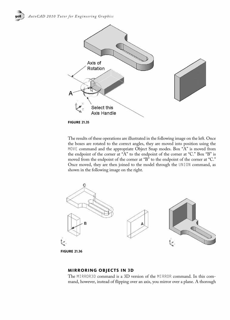
The results of these operations are illustrated in the following image on the left. Oncethe boxes are rotated to the correct angles, they are moved into position using theMOVE command and the appropriate Object Snap modes. Box “A” is moved fromthe endpoint of the corner at “A” to the endpoint of the corner at “C.” Box “B” ismoved from the endpoint of the corner at “B” to the endpoint of the corner at “C.”Once moved, they are then joined to the model through the UNION command, asshown in the following image on the right.
MIRRORING OBJECTS IN 3DThe MIRROR3D command is a 3D version of the MIRROR command. In this com-mand, however, instead of flipping over an axis, you mirror over a plane. A thorough
FIGURE 21.35
FIGURE 21.36
908 Aut oCAD 2010 Tu t o r f o r Eng in e e r i n g Graph i c s
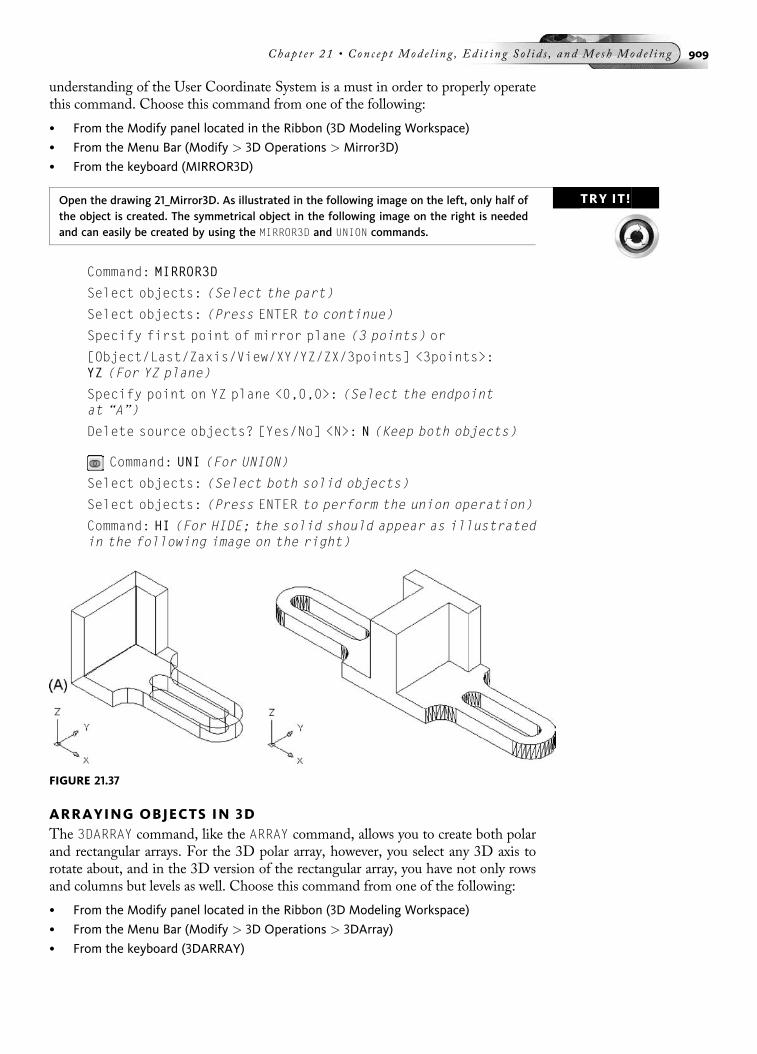
understanding of the User Coordinate System is a must in order to properly operatethis command. Choose this command from one of the following:
• From the Modify panel located in the Ribbon (3D Modeling Workspace)
• From the Menu Bar (Modify > 3D Operations > Mirror3D)
• From the keyboard (MIRROR3D)
TRY IT!Open the drawing 21_Mirror3D. As illustrated in the following image on the left, only half ofthe object is created. The symmetrical object in the following image on the right is neededand can easily be created by using the MIRROR3D and UNION commands.
Command: MIRROR3D
Select objects: (Select the part)
Select objects: (Press ENTER to continue)
Specify first point of mirror plane (3 points) or
[Object/Last/Zaxis/View/XY/YZ/ZX/3points] <3points>:YZ (For YZ plane)
Specify point on YZ plane <0,0,0>: (Select the endpointat “A”)
Delete source objects? [Yes/No] <N>: N (Keep both objects)
Command: UNI (For UNION)
Select objects: (Select both solid objects)
Select objects: (Press ENTER to perform the union operation)
Command: HI (For HIDE; the solid should appear as illustratedin the following image on the right)
ARRAYING OBJECTS IN 3DThe 3DARRAY command, like the ARRAY command, allows you to create both polarand rectangular arrays. For the 3D polar array, however, you select any 3D axis torotate about, and in the 3D version of the rectangular array, you have not only rowsand columns but levels as well. Choose this command from one of the following:
• From the Modify panel located in the Ribbon (3D Modeling Workspace)
• From the Menu Bar (Modify > 3D Operations > 3DArray)
• From the keyboard (3DARRAY)
FIGURE 21.37
Chap t e r 21 • Con c e p t Mod e l i n g , Ed i t i n g S o l i d s , and Me s h Mod e l i n g 909

TRY IT! Open the drawing 21_3DArray. As illustrated in the following image on the left, six armsneed to be arrayed around the hub in the center. To accomplish this we will perform a polararray about an axis running through the hub. We will rotate throughout a full 360°.
NOTE If you perform a polar array at an angle other than 360°, take note of the direction in whichyou select the axis because this will affect the direction of rotation (right-hand rule).
Command: 3A (For 3DARRAY)
Select objects: (Select the Arm “A”)
Select objects: (Press ENTER to continue)
Enter the type of array [Rectangular/Polar] <R>: P (ForPolar)
Enter the number of items in the array: 6
Specify the angle to fill (+=ccw, -=cw) <360>: (Press ENTER toaccept the default)
Rotate arrayed objects? [Yes/No] <Y>: Y
Specify center point of array: Cen
of (Specify the center of the back hub circle at “B”)
Specify second point on axis of rotation: Cen
of (Specify the center of the front hub circle at “C”)
Command: UNI (For UNION)
Select objects: (Select the six arms and the hub)
Select objects: (Press ENTER to perform the union operation)
Command: HI (For HIDE, the solid should appear as illustratedin the following image on the right)
Command: RE (For REGEN; this will convert the image back towireframe mode)
FIGURE 21.38
910 Aut oCAD 2010 Tu t o r f o r Eng in e e r i n g Graph i c s
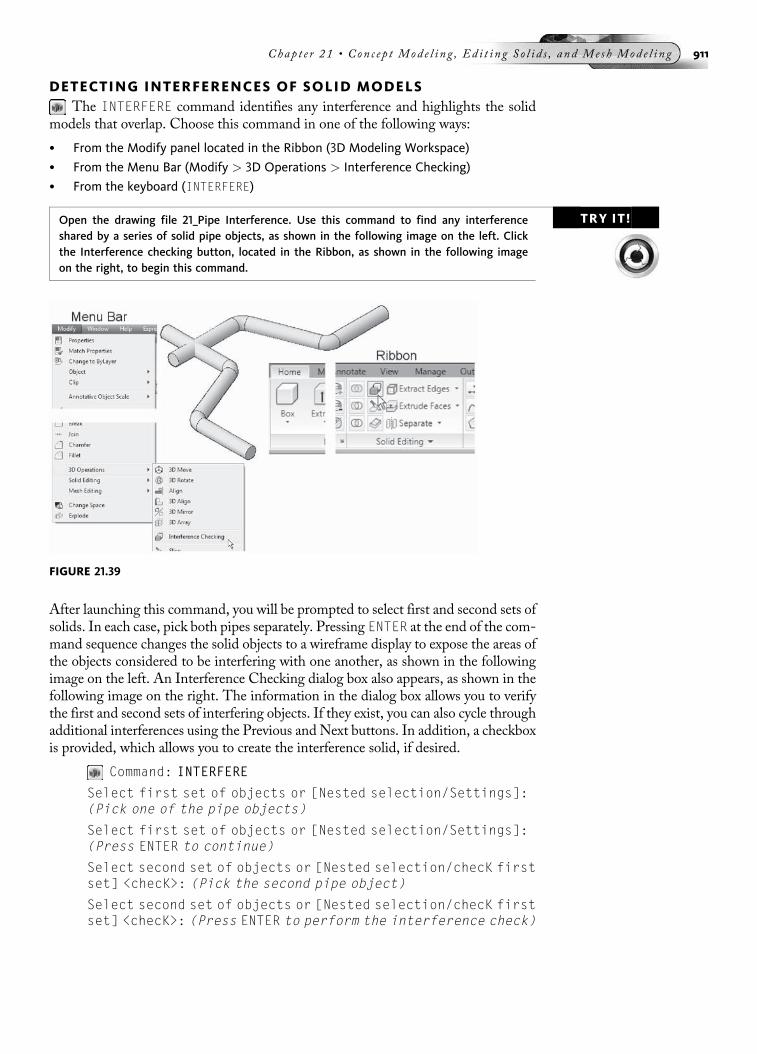
DETECTING INTERFERENCES OF SOLID MODELSThe INTERFERE command identifies any interference and highlights the solid
models that overlap. Choose this command in one of the following ways:
• From the Modify panel located in the Ribbon (3D Modeling Workspace)
• From the Menu Bar (Modify > 3D Operations > Interference Checking)
• From the keyboard (INTERFERE)
TRY IT!Open the drawing file 21_Pipe Interference. Use this command to find any interferenceshared by a series of solid pipe objects, as shown in the following image on the left. Clickthe Interference checking button, located in the Ribbon, as shown in the following imageon the right, to begin this command.
After launching this command, you will be prompted to select first and second sets ofsolids. In each case, pick both pipes separately. Pressing ENTER at the end of the com-mand sequence changes the solid objects to a wireframe display to expose the areas ofthe objects considered to be interfering with one another, as shown in the followingimage on the left. An Interference Checking dialog box also appears, as shown in thefollowing image on the right. The information in the dialog box allows you to verifythe first and second sets of interfering objects. If they exist, you can also cycle throughadditional interferences using the Previous and Next buttons. In addition, a checkboxis provided, which allows you to create the interference solid, if desired.
Command: INTERFERE
Select first set of objects or [Nested selection/Settings]:(Pick one of the pipe objects)
Select first set of objects or [Nested selection/Settings]:(Press ENTER to continue)
Select second set of objects or [Nested selection/checK firstset] <checK>: (Pick the second pipe object)
Select second set of objects or [Nested selection/checK firstset] <checK>: (Press ENTER to perform the interference check)
FIGURE 21.39
Chap t e r 21 • Con c e p t Mod e l i n g , Ed i t i n g S o l i d s , and Me s h Mod e l i n g 911

SLICING SOLID MODELSYet another way of cutting sections in 3D solid models is through the SLICE
command. This command creates new solids from the existing ones that are sliced.You can also retain one or both halves of the sliced solid. Slicing a solid requires sometype of cutting plane. The default method of creating this plane is by picking twopoints. You can also define the cutting plane or surface by specifying three points,by picking a surface, by using another object, or by basing the cutting plane line onthe current positions of the XY, YZ, or ZX planes.
Choose the SLICE command in one of the following ways:
• From the Modify panel located in the Ribbon (3D Modeling Workspace)
• From the Menu Bar (Modify > 3D Operations > Slice)
• From the keyboard (SL or SLICE)
TRY IT! Open the drawing file 21_Tee Slice. This command is similar to the SECTION commandexcept that the solid model is actually cut or sliced at a plane that you define. In the exam-ple in the following image on the left, this plane is defined by the User Coordinate System.Before the slice is made, you also have the option of keeping either one or both halves ofthe object. The MOVE command is used to separate both halves, as shown in the followingimage on the right.
Command: SL (For SLICE)
Select objects: (Select the solid object)
Select objects: (Press ENTER to continue with this command)
Specify first point on slicing plane by [Object/Zaxis/View/XY/YZ/ZX/3points] <3points>: XY
Specify a point on XY-plane <0,0,0>: (Press ENTER to acceptthis default value)
FIGURE 21.40
912 Aut oCAD 2010 Tu t o r f o r Eng in e e r i n g Graph i c s

Specify a point on desired side of the plane or [keep Bothsides]: B (To keep both sides)
Slicing a Solid with a SurfaceA solid object can also be sliced by a surface. A surface is created by performing a 3Doperation such as extrusion or revolution on an open object. Once the surface is cre-ated, it is positioned inside of the 3D solid model, where a slicing operation is per-formed. The next Try It! exercise illustrates the use of this technique.
TRY IT!Open the drawing file 21_Surface Flow. You will first extrude a spline to create a surface.The surface will then be used to slice a solid block. You will keep the bottom portion ofthe solid.
Before slicing the solid block, first extrude the spline object, as shown in the followingimage on the left, a distance equal to the depth of the block (from “A” to “B”). Sincethe spline represents an open shape, the result of performing this operation is the cre-ation of a surface instead of a solid, as shown in the following image on the right.
Command: EXT (For EXTRUDE)
Current wire frame density: ISOLINES=4
Select objects to extrude: (Pick the spline object)
Select objects to extrude: (Press ENTER to continue)
Specify height of extrusion or [Direction/Path/Taperangle]: D (For Direction)
Specify start point of direction: (Pick the endpoint at “A”)
Specify end point of direction: (Pick the endpoint at “B”)
FIGURE 21.41
FIGURE 21.42
Chap t e r 21 • Con c e p t Mod e l i n g , Ed i t i n g S o l i d s , and Me s h Mod e l i n g 913

With the newly created surface positioned inside of the solid block, issue the SLICEcommand. Pick the solid block as the object to slice and select the surface as the slic-ing plane, as shown in the following image on the left. You will also be prompted toselect the portion of the solid to keep. Here is where you pick the bottom of the solid,as shown in the following image on the left.
Command: SL (For SLICE)
Select objects to slice: (Pick the solid block)
Select objects to slice: (Press ENTER to continue)
Specify start point of slicing plane or [planar
Object/Surface/Zaxis/View/XY/YZ/ZX/3points] <3points>: S(For Surface)
Select a surface: (Pick the surface, as shown in the followingimage on the left)
Select solid to keep or [keep Both sides] <Both>: (Pick thebottom of the solid)
The results are displayed in the following image on the right, with the solid blockbeing cut by the surface.
Terrain ModelingA unique type of solid model can be created when a model is sliced by a surface cre-ated using a lofting operation. In the following image, four different splines have beenapplied to the edge faces of a solid block. Using the LOFT command, two splines areselected as cross sections and the other two splines as guides or rails. Once this spe-cialized surface is created, slice the solid block using the surface and keep the lowerportion of the model.
TRY IT! Open the drawing file 21_Terrain. You will create a lofted surface by selecting the two crosssections and the two guide curves, as shown in the following image on the left. The resultsare displayed in the following image on the right, with a complex surface being createdfrom the loft operation.
Command: LOFT
Select cross-sections in lofting order: (Select crosssection #1)
Select cross-sections in lofting order: (Select crosssection #2)
FIGURE 21.43
914 Aut oCAD 2010 Tu t o r f o r Eng in e e r i n g Graph i c s

Select cross-sections in lofting order: (Press ENTER tocontinue)
Enter an option [Guides/Path/Cross-sections only] <Cross-sections only>: G (For Guides)
Select guide curves: (Select guide curve #1)
Select guide curves: (Select guide curve #2)
Select guide curves: (Press ENTER to create the surface)
With the surface created, activate the slice command, pick the solid block as the ob-ject to slice, select the surface as the slicing plane, and, finally, pick the lower portionof the solid as the portion to keep, as shown in the following image on the left. Theresults are illustrated in the following image on the right.
Command: SL (For SLICE)
Select objects to slice: (Select the solid block)
Select objects to slice: (Press ENTER to continue)
Specify start point of slicing plane or [planar
Object/Surface/Zaxis/View/XY/YZ/ZX/3points] <3points>:S (For Surface)
Select a surface: (Select the surface)
Select solid to keep or [keep Both sides] <Both>: (Pick thelower portion of the solid block)
FIGURE 21.44
FIGURE 21.45
Chap t e r 21 • Con c e p t Mod e l i n g , Ed i t i n g S o l i d s , and Me s h Mod e l i n g 915

EDITING SOLID FEATURESOnce features such as holes, slots, and extrusions are constructed in a solid model,the time may come to make changes to these features. This is the function of theSOLIDEDIT command. This command contains numerous options, which can be se-lected from the Ribbon, as shown in the following image. You could also chooseSolids Editing from the Modify Menu Bar. The menus are arranged in three group-ings, namely, Face, Edge, and Body editing. These groupings are discussed in thepages that follow. Also, it is recommended that instead of entering the SOLIDEDITcommand at the command prompt, you use the Ribbon or Menu Bar to performediting operations. This eliminates a number of steps and make it easier to locatethe appropriate option under the correct grouping.
The following table gives a brief description of each mode for performing solid edit-ing operations.
Button Tool Function
Extrude Faces Used for lengthening or shortening faces on asolid
Move Faces Used for moving a solid shape to a new location
Offset Faces Used for offsetting faces at a specified distanceon a solid
Delete Faces Used for removing faces and fillets from a solid
Rotate Faces Used for rotating faces on a selected solid
Taper Faces Used for tapering selected faces of a solid at adraft angle along a vector direction
Copy Faces Used for copying selected faces of a solid. Thesecopied faces can take the form of regions orbodies
Color Faces Used for assigning unique colors to individualfaces
Copy Edges Used to copy edges from a solid. These newedges are often used to create new solids.
Color Edges Used for assigning unique colors to individualsolid edges
FIGURE 21.46
916 Aut oCAD 2010 Tu t o r f o r Eng in e e r i n g Graph i c s

Button Tool Function
Imprint Used for adding construction geometry to asolid model
Clean Used to remove imprints from a solid
Separate Used to separate a solid into multiple parts aslong as those parts do not intersect at any point.Solids sometimes act as a single entity eventhough they appear to be separate solids (un-ioning solids together that do not touch or re-moving part of a solid so that the remainingpieces do not touch).
Shell Used to create a thin wall in a solid model
Check Used to prove a solid is valid
EXTRUDING (FACE EDITING)Faces may be lengthened or shortened through the Extrude option of the
SOLIDEDIT command. A positive distance extrudes the face in the direction of itsnormal. A negative distance extrudes the face in the opposite direction.
TRY IT!Open the drawing file 21_Extrude. In the following image, the highlighted face at “A” needsto be decreased in height.
NOTEYou will achieve better results when selecting a face for the SOLIDEDIT command if youpick on the inside of the face rather than on the edge of the face.
Command: SOLIDEDIT
Solids editing automatic checking: SOLIDCHECK=1
Enter a solids editing option [Face/Edge/Body/Undo/eXit]<eXit>: F (For Face)
Enter a face editing option
[Extrude/Move/Rotate/Offset/Taper/Delete/Copy/coLor/mA-terial/Undo/eXit] <eXit>: E (For Extrude)
Select faces or [Undo/Remove]: (Select the face inside thearea represented by “A”)
Select faces or [Undo/Remove/ALL]: (Press ENTER to continue)
Specify height of extrusion or [Path]: -10.00
Specify angle of taper for extrusion <0>: (Press ENTER)
Solid validation started.
Solid validation completed.
Enter a face editing option
[Extrude/Move/Rotate/Offset/Taper/Delete/Copy/coLor/mAterial/Undo/eXit] <eXit>: (Press ENTER)
Solids editing automatic checking: SOLIDCHECK=1
Chap t e r 21 • Con c e p t Mod e l i n g , Ed i t i n g S o l i d s , and Me s h Mod e l i n g 917

Enter a solids editing option [Face/Edge/Body/Undo/eXit]<eXit>: (Press ENTER)
The result is illustrated in the following image at “B.”
MOVING (FACE EDITING)
TRY IT! Open the drawing 21_Move. The object in the following image illustrates two intersectingcylinders. The two horizontal cylinders need to be moved 1 unit up from their current loca-tion. The cylinders are first selected at “A” and “B” through the SOLIDEDIT command alongwith the Move option.
Command: SOLIDEDIT
Solids editing automatic checking: SOLIDCHECK=1
Enter a solids editing option [Face/Edge/Body/Undo/eXit]<eXit>: F (For Face)
Enter a face editing option
[Extrude/Move/Rotate/Offset/Taper/Delete/Copy/coLor/mAterial/Undo/eXit] <eXit>: M (For Move)
Select faces or [Undo/Remove]: (Select both highlightedfaces at “A” and “B”)
Select faces or [Undo/Remove/ALL]: (Press ENTER to continue)
Specify a base point or displacement: (Pick any point on thescreen)
Specify a second point of displacement: @0,0,1
Solid validation started.
Solid validation completed.
Enter a face editing option
[Extrude/Move/Rotate/Offset/Taper/Delete/Copy/coLor/mAterial/Undo/eXit] <eXit>: (Press ENTER)
Solids editing automatic checking: SOLIDCHECK=1
Enter a solids editing option [Face/Edge/Body/Undo/eXit]<eXit>: (Press ENTER)
The results are illustrated in the following image on the right.
FIGURE 21.47
918 Aut oCAD 2010 Tu t o r f o r Eng in e e r i n g Graph i c s
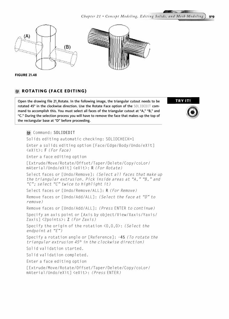
ROTATING (FACE EDITING)
TRY IT!Open the drawing file 21_Rotate. In the following image, the triangular cutout needs to berotated 45° in the clockwise direction. Use the Rotate Face option of the SOLIDEDIT com-mand to accomplish this. You must select all faces of the triangular cutout at “A,” “B,” and“C.” During the selection process you will have to remove the face that makes up the top ofthe rectangular base at “D” before proceeding.
Command: SOLIDEDIT
Solids editing automatic checking: SOLIDCHECK=1
Enter a solids editing option [Face/Edge/Body/Undo/eXit]<eXit>: F (For Face)
Enter a face editing option
[Extrude/Move/Rotate/Offset/Taper/Delete/Copy/coLor/mAterial/Undo/eXit] <eXit>: R (For Rotate)
Select faces or [Undo/Remove]: (Select all faces that make upthe triangular extrusion. Pick inside areas at “A,” “B,” and“C”; select “C” twice to highlight it)
Select faces or [Undo/Remove/ALL]: R (For Remove)
Remove faces or [Undo/Add/ALL]: (Select the face at “D” toremove)
Remove faces or [Undo/Add/ALL]: (Press ENTER to continue)
Specify an axis point or [Axis by object/View/Xaxis/Yaxis/Zaxis] <2points>: Z (For Zaxis)
Specify the origin of the rotation <0,0,0>: (Select theendpoint at “E”)
Specify a rotation angle or [Reference]: -45 (To rotate thetriangular extrusion 45° in the clockwise direction)
Solid validation started.
Solid validation completed.
Enter a face editing option
[Extrude/Move/Rotate/Offset/Taper/Delete/Copy/coLor/mAterial/Undo/eXit] <eXit>: (Press ENTER)
FIGURE 21.48
Chap t e r 21 • Con c e p t Mod e l i n g , Ed i t i n g S o l i d s , and Me s h Mod e l i n g 919
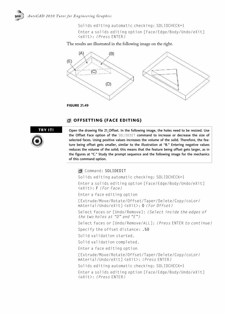
Solids editing automatic checking: SOLIDCHECK=1
Enter a solids editing option [Face/Edge/Body/Undo/eXit]<eXit>: (Press ENTER)
The results are illustrated in the following image on the right.
OFFSETTING (FACE EDITING)
TRY IT! Open the drawing file 21_Offset. In the following image, the holes need to be resized. Usethe Offset Face option of the SOLIDEDIT command to increase or decrease the size ofselected faces. Using positive values increases the volume of the solid. Therefore, the fea-ture being offset gets smaller, similar to the illustration at “B.” Entering negative valuesreduces the volume of the solid; this means that the feature being offset gets larger, as inthe figures at “C.” Study the prompt sequence and the following image for the mechanicsof this command option.
Command: SOLIDEDIT
Solids editing automatic checking: SOLIDCHECK=1
Enter a solids editing option [Face/Edge/Body/Undo/eXit]<eXit>: F (For Face)
Enter a face editing option
[Extrude/Move/Rotate/Offset/Taper/Delete/Copy/coLor/mAterial/Undo/eXit] <eXit>: O (For Offset)
Select faces or [Undo/Remove]: (Select inside the edges ofthe two holes at “D” and “E”)
Select faces or [Undo/Remove/ALL]: (Press ENTER to continue)
Specify the offset distance: .50
Solid validation started.
Solid validation completed.
Enter a face editing option
[Extrude/Move/Rotate/Offset/Taper/Delete/Copy/coLor/mAterial/Undo/eXit] <eXit>: (Press ENTER)
Solids editing automatic checking: SOLIDCHECK=1
Enter a solids editing option [Face/Edge/Body/Undo/eXit]<eXit>: (Press ENTER)
FIGURE 21.49
920 Aut oCAD 2010 Tu t o r f o r Eng in e e r i n g Graph i c s
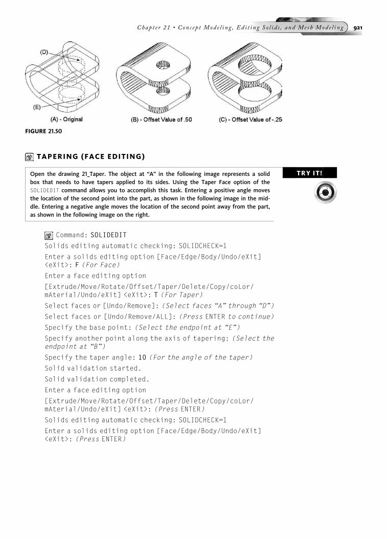
TAPERING (FACE EDITING)
TRY IT!Open the drawing 21_Taper. The object at “A” in the following image represents a solidbox that needs to have tapers applied to its sides. Using the Taper Face option of theSOLIDEDIT command allows you to accomplish this task. Entering a positive angle movesthe location of the second point into the part, as shown in the following image in the mid-dle. Entering a negative angle moves the location of the second point away from the part,as shown in the following image on the right.
Command: SOLIDEDIT
Solids editing automatic checking: SOLIDCHECK=1
Enter a solids editing option [Face/Edge/Body/Undo/eXit]<eXit>: F (For Face)
Enter a face editing option
[Extrude/Move/Rotate/Offset/Taper/Delete/Copy/coLor/mAterial/Undo/eXit] <eXit>: T (For Taper)
Select faces or [Undo/Remove]: (Select faces “A” through “D”)
Select faces or [Undo/Remove/ALL]: (Press ENTER to continue)
Specify the base point: (Select the endpoint at “E”)
Specify another point along the axis of tapering: (Select theendpoint at “B”)
Specify the taper angle: 10 (For the angle of the taper)
Solid validation started.
Solid validation completed.
Enter a face editing option
[Extrude/Move/Rotate/Offset/Taper/Delete/Copy/coLor/mAterial/Undo/eXit] <eXit>: (Press ENTER)
Solids editing automatic checking: SOLIDCHECK=1
Enter a solids editing option [Face/Edge/Body/Undo/eXit]<eXit>: (Press ENTER)
FIGURE 21.50
Chap t e r 21 • Con c e p t Mod e l i n g , Ed i t i n g S o l i d s , and Me s h Mod e l i n g 921

DELETING (FACE EDITING)Faces can be erased through the Delete Face option of the SOLIDEDIT command.
TRY IT! Open the drawing file 21_Delete. In the following image, select the hole at “A” as the face toerase.
Command: SOLIDEDIT
Solids editing automatic checking: SOLIDCHECK=1
Enter a solids editing option [Face/Edge/Body/Undo/eXit]<eXit>: F (For Face)
Enter a face editing option
[Extrude/Move/Rotate/Offset/Taper/Delete/Copy/coLor/mAterial/Undo/eXit] <eXit>: D (For Delete)
Select faces or [Undo/Remove]: (Select inside the holeat “A”)
Select faces or [Undo/Remove/ALL]: (Press ENTER to continue)
Solid validation started.
Solid validation completed.
Enter a face editing option
[Extrude/Move/Rotate/Offset/Taper/Delete/Copy/coLor/mAterial/Undo/eXit] <eXit>: (Press ENTER)
Solids editing automatic checking: SOLIDCHECK=1
Enter a solids editing option [Face/Edge/Body/Undo/eXit]<eXit>: (Press ENTER)
The results are illustrated in the following image on the right.
FIGURE 21.51
FIGURE 21.52
922 Aut oCAD 2010 Tu t o r f o r Eng in e e r i n g Graph i c s

COPYING (FACE EDITING)You can copy a face for use in the creation of another solid model using the Copy Faceoption of the SOLIDEDIT command.
TRY IT!Open the drawing file 21_Copy. In the following image, the solid model at “A” will be usedto create a region from the face at “B.” While in the command, select the face by picking inthe area at “B.” Notice that all objects making up the face, such as the rectangle and circles,are highlighted. Picking a base point and second point copies the face at “C.” The resultingobject at “C” is actually a region. The region could be exploded back into individual linesand circles, which could then be used to create a new object. A region can also be extrudedby using the EXTRUDE command to create another solid model such as the one illustrated inthe following image on the right.
Command: SOLIDEDIT
Solids editing automatic checking: SOLIDCHECK=1
Enter a solids editing option [Face/Edge/Body/Undo/eXit]<eXit>: F (For Face)
Enter a face editing option
[Extrude/Move/Rotate/Offset/Taper/Delete/Copy/coLor/mAterial/Undo/eXit] <eXit>: C (For Copy)
Select faces or [Undo/Remove]: (Select the top face inarea “B”)
Select faces or [Undo/Remove/ALL]: (Press ENTER to continue)
Specify a base point or displacement: (Pick a point to copyfrom)
Specify a second point of displacement: (Pick a point tocopy to)
Enter a face editing option
[Extrude/Move/Rotate/Offset/Taper/Delete/Copy/coLor/mAterial/Undo/eXit] <eXit>: (Press ENTER)
Solids editing automatic checking: SOLIDCHECK=1
Enter a solids editing option [Face/Edge/Body/Undo/eXit]<eXit>: (Press ENTER)
FIGURE 21.53
Chap t e r 21 • Con c e p t Mod e l i n g , Ed i t i n g S o l i d s , and Me s h Mod e l i n g 923

IMPRINTING (BODY EDITING)An interesting and powerful method of adding construction geometry to a solidmodel is though the process of imprinting.
TRY IT! Open the drawing file 21_Imprint. In the following image at “A,” a box along with slot isalready modeled in 3D. A line was constructed from the midpoints of the top surface ofthe solid model. The SOLIDEDIT command will be used to imprint this line to the model,which results in dividing the top surface into two faces.
Command: SOLIDEDIT
Solids editing automatic checking: SOLIDCHECK=1
Enter a solids editing option [Face/Edge/Body/Undo/eXit]<eXit>: B (For Body)
Enter a body editing option
[Imprint/seParate solids/Shell/cLean/Check/Undo/eXit]<eXit>: I (For Imprint)
Select a 3D solid: (Select the solid model)
Select an object to imprint: (Select line “B”)
Delete the source object [Yes/No] <N>: Y (For Yes; this erasesthe line)
Select an object to imprint: (Press ENTER to complete theimprint operation)
Enter a body editing option
[Imprint/seParate solids/Shell/cLean/Check/Undo/eXit]<eXit>: (Press ENTER)
Solids editing automatic checking: SOLIDCHECK=1
Enter a solids editing option [Face/Edge/Body/Undo/eXit]<eXit>: (Press ENTER)
The segments of the lines that come in contact with the 3D solid remain on thepart’s surface. However, these are no longer line segments; rather, these lines nowbelong to the part. The lines actually separate the top surface into two faces.
Use the Extrude Face option of the SOLIDEDIT command on one of the newlycreated faces at “C” and increase the face in height by an extra 1.50 units. The resultsare illustrated in the following image on the right.
FIGURE 21.54
924 Aut oCAD 2010 Tu t o r f o r Eng in e e r i n g Graph i c s

SEPARATING SOLIDS (BODY EDITING)Sometimes when performing union and subtraction operations on solid models, youcan end up with models that do not actually touch (intersect) but act as a single object.The Separating Solids option of the SOLIDEDIT command is used to correct thiscondition.
TRY IT!Open the drawing file 21_Separate. In the following image, the model at “A” is about to besliced in half with a thin box created at the center of the circle and spanning the depth ofthe rectangular shelf.
Use the SUBTRACT command and subtract the rectangular box from the solid object.After you subtract the box, pick the solid at “B” and notice that both halves of theobject highlight even though they appear separate. To convert the single solid modelinto two separate models, use the SOLIDEDIT command followed by the Body andSeparate options.
Command: SOLIDEDIT
Solids editing automatic checking: SOLIDCHECK=1
Enter a solids editing option [Face/Edge/Body/Undo/eXit]<eXit>: B (For Body)
Enter a body editing option
[Imprint/seParate solids/Shell/cLean/Check/Undo/eXit]<eXit>: P (For Separate)
Select a 3D solid: (Pick the solid model at “B”)
Enter a body editing option
[Imprint/seParate solids/Shell/cLean/Check/Undo/eXit]<eXit>: (Press ENTER)
Solids editing automatic checking: SOLIDCHECK=1
Enter a solids editing option [Face/Edge/Body/Undo/eXit]<eXit>: (Press ENTER)
This action separates the single model into two. When you select the model in thefollowing image at “C,” only one half highlights.
SHELLING (BODY EDITING)Shelling is the process of constructing a thin wall inside or outside of a solid model.Positive thickness produces the thin wall inside; negative values for thickness producethe thin wall outside. This wall thickness remains constant throughout the entiremodel. Faces may be removed during the shelling operation to create an opening.
FIGURE 21.55
Chap t e r 21 • Con c e p t Mod e l i n g , Ed i t i n g S o l i d s , and Me s h Mod e l i n g 925
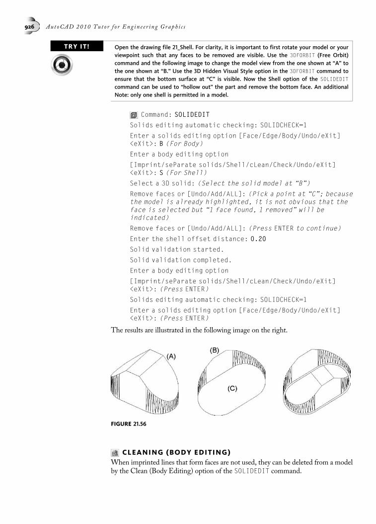
TRY IT! Open the drawing file 21_Shell. For clarity, it is important to first rotate your model or yourviewpoint such that any faces to be removed are visible. Use the 3DFORBIT (Free Orbit)command and the following image to change the model view from the one shown at “A” tothe one shown at “B.” Use the 3D Hidden Visual Style option in the 3DFORBIT command toensure that the bottom surface at “C” is visible. Now the Shell option of the SOLIDEDITcommand can be used to “hollow out” the part and remove the bottom face. An additionalNote: only one shell is permitted in a model.
Command: SOLIDEDIT
Solids editing automatic checking: SOLIDCHECK=1
Enter a solids editing option [Face/Edge/Body/Undo/eXit]<eXit>: B (For Body)
Enter a body editing option
[Imprint/seParate solids/Shell/cLean/Check/Undo/eXit]<eXit>: S (For Shell)
Select a 3D solid: (Select the solid model at “B”)
Remove faces or [Undo/Add/ALL]: (Pick a point at “C”; becausethe model is already highlighted, it is not obvious that theface is selected but “1 face found, 1 removed” will beindicated)
Remove faces or [Undo/Add/ALL]: (Press ENTER to continue)
Enter the shell offset distance: 0.20
Solid validation started.
Solid validation completed.
Enter a body editing option
[Imprint/seParate solids/Shell/cLean/Check/Undo/eXit]<eXit>: (Press ENTER)
Solids editing automatic checking: SOLIDCHECK=1
Enter a solids editing option [Face/Edge/Body/Undo/eXit]<eXit>: (Press ENTER)
The results are illustrated in the following image on the right.
CLEANING (BODY EDITING)When imprinted lines that form faces are not used, they can be deleted from a modelby the Clean (Body Editing) option of the SOLIDEDIT command.
FIGURE 21.56
926 Aut oCAD 2010 Tu t o r f o r Eng in e e r i n g Graph i c s
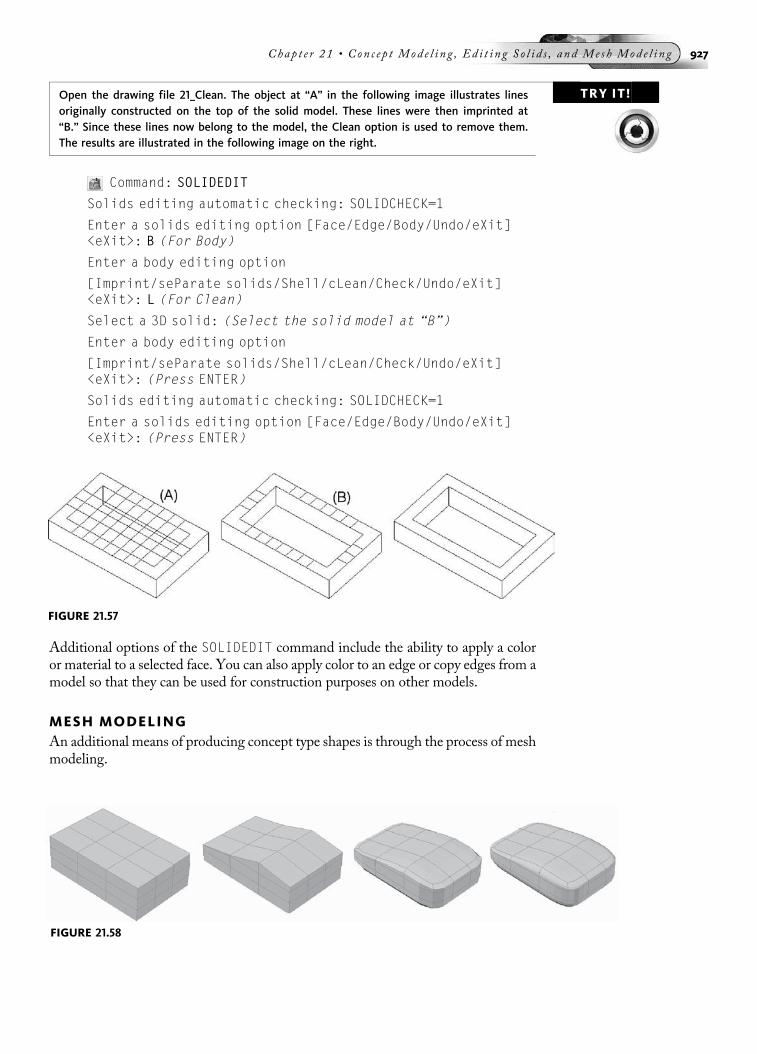
TRY IT!Open the drawing file 21_Clean. The object at “A” in the following image illustrates linesoriginally constructed on the top of the solid model. These lines were then imprinted at“B.” Since these lines now belong to the model, the Clean option is used to remove them.The results are illustrated in the following image on the right.
Command: SOLIDEDIT
Solids editing automatic checking: SOLIDCHECK=1
Enter a solids editing option [Face/Edge/Body/Undo/eXit]<eXit>: B (For Body)
Enter a body editing option
[Imprint/seParate solids/Shell/cLean/Check/Undo/eXit]<eXit>: L (For Clean)
Select a 3D solid: (Select the solid model at “B”)
Enter a body editing option
[Imprint/seParate solids/Shell/cLean/Check/Undo/eXit]<eXit>: (Press ENTER)
Solids editing automatic checking: SOLIDCHECK=1
Enter a solids editing option [Face/Edge/Body/Undo/eXit]<eXit>: (Press ENTER)
Additional options of the SOLIDEDIT command include the ability to apply a coloror material to a selected face. You can also apply color to an edge or copy edges from amodel so that they can be used for construction purposes on other models.
MESH MODELINGAn additional means of producing concept type shapes is through the process of meshmodeling.
FIGURE 21.57
FIGURE 21.58
Chap t e r 21 • Con c e p t Mod e l i n g , Ed i t i n g S o l i d s , and Me s h Mod e l i n g 927

When in the 3D Modeling workspace, the Ribbon displays a dedicated MeshModeling tab. Clicking on this tab displays all mesh modeling commands asshown in the following image.
Some of the most basic of functions when producing mesh models is to begin byconstructing a primitive shape. These shapes are similar to the solid model primitivesalready covered in Chapter 20.
An example of constructing a mesh model of a mesh box is illustrated in the fol-lowing image. You identify 2 points in the X and Y directions as shown in thefollowing image on the left. You then drag to get the 3rd direction as shown inthe following image on the right. While in the BOX command, you can switch toLength mode which will allow you to enter the length, width and height of themodel. Notice in the previous image the number of tesselation lines created inthe length, width, and height directions; these values are automatically applied tothe mesh model being created.
Command: MESH
Current smoothness level is set to: 0
Enter an option [Box/ConeCYlinderPyramidSphereWedgeTorusSEttings]<Box>: Box
Specify first corner or [Center]: (Pick a corner point)
Specify other corner or [Cube/Length]: (Pick the other cornerpoint)
Specify height or [2Point]: (Drag or enter a value for theheight)
FIGURE 21.59
FIGURE 21.60
928 Aut oCAD 2010 Tu t o r f o r Eng in e e r i n g Graph i c s

Face and Gizmo ToolsWhen making changes or editing a mesh model, it is important sometimes to pick aface and at other times to pick an edge. To make it easier to pick faces or edges, aspecial Subobject panel is available in the Mesh Modeling tab of the Ribbon. Click-ing the down arrow in Face will display a drop down menu that allows you to pickon faces, vertices, or edges as shown in the following image in the middle. Anothersubobject tool to use with dragging faces or edges of mesh models to new location isshown in the following image on the right. Here, you switch from different gizmos toeither move, rotate, or scale mesh model faces or edges.
Working with SubobjectsAfter a mesh model is created, it can easily be edited to form an entirely differentshape. This is due to the number of subobjects that make up the mesh model. Typicalsubobjects have already been mentioned such as faces and edges. To illustrate howthis works, the three top front faces need to be dropped down to a predefined level.To select the three faces of the mesh model, hold down the CTRL key and pick allthree faces as shown in the following image on the left. You will notice the appearanceof the default gizmo, namely Move. Move your cursor to the Z axis and an axis linewill appear in the following image in the middle. At this point, you can drag yourcursor up or down. As you perform this you will dynamically see the model changing.In the following image on the right, the three faces were moved or dragged down.You can also enter an exact value when perform this operation.
FIGURE 21.61
FIGURE 21.62
Chap t e r 21 • Con c e p t Mod e l i n g , Ed i t i n g S o l i d s , and Me s h Mod e l i n g 929
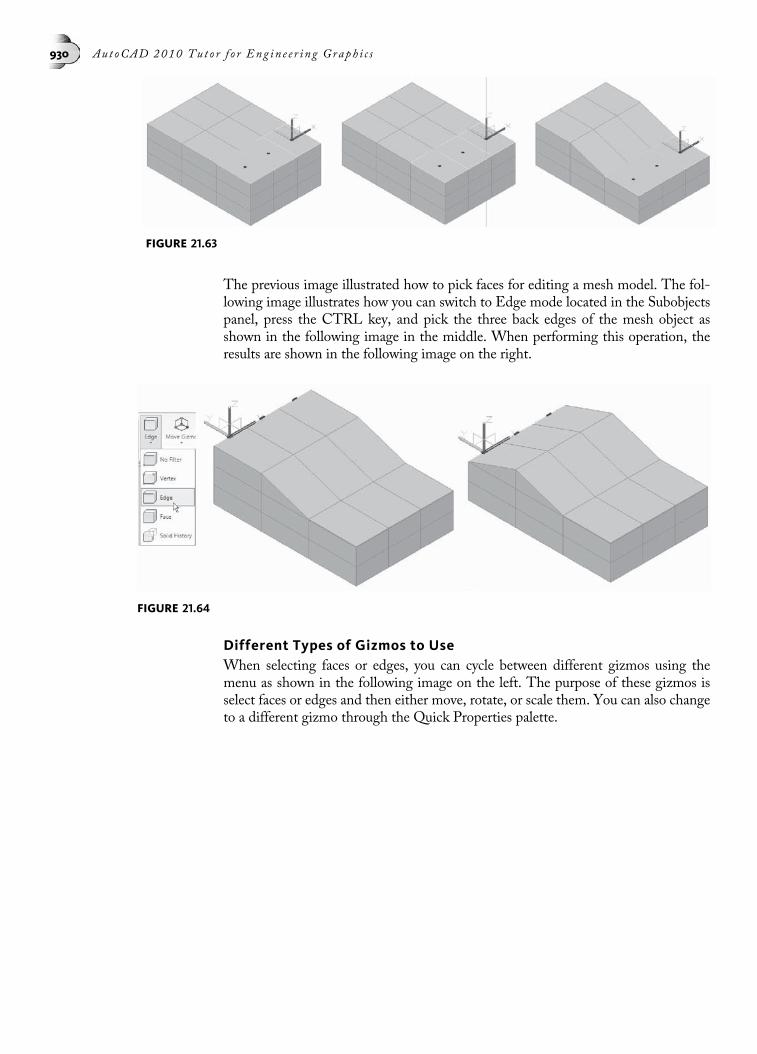
The previous image illustrated how to pick faces for editing a mesh model. The fol-lowing image illustrates how you can switch to Edge mode located in the Subobjectspanel, press the CTRL key, and pick the three back edges of the mesh object asshown in the following image in the middle. When performing this operation, theresults are shown in the following image on the right.
Different Types of Gizmos to UseWhen selecting faces or edges, you can cycle between different gizmos using themenu as shown in the following image on the left. The purpose of these gizmos isselect faces or edges and then either move, rotate, or scale them. You can also changeto a different gizmo through the Quick Properties palette.
FIGURE 21.63
FIGURE 21.64
930 Aut oCAD 2010 Tu t o r f o r Eng in e e r i n g Graph i c s

Smoothing a Mesh ModelOnce a mesh model is created as in the following image on the left, you can easilysmooth the model using a number of techniques. The example in the following imagein the middle shows the initial affects of making all mesh model edges smooth. In thefollowing image on the right, this object displays the highest level of smoothness.
One area of controlling the smoothness of a mesh model is through the Quick Prop-erties palette as shown in the following image. Clicking on the mesh model displaysthis palette. Clicking on Smoothness displays the drop down menu that allows you tochange to four different levels of smoothness. It must be pointed out that for complexmesh models, the Level 4 smoothness may result in a slower than normal processingspeed. It is for this reason that as you experiment with various smoothness values, youchoose Level I or II.
Also located in the following image is the Ribbon that displays three additionalsmoothness modes; namely Smooth More, Smooth Less, and Refine Mesh. If nosmoothness is applied to a mesh model and you click on the Smooth More button,a Level I smoothness is applied.
FIGURE 21.65
FIGURE 21.66
Chap t e r 21 • Con c e p t Mod e l i n g , Ed i t i n g S o l i d s , and Me s h Mod e l i n g 931
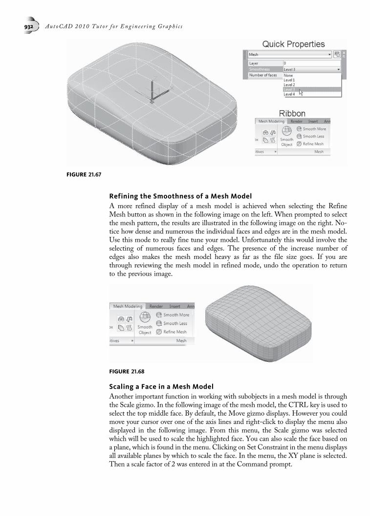
Refining the Smoothness of a Mesh ModelA more refined display of a mesh model is achieved when selecting the RefineMesh button as shown in the following image on the left. When prompted to selectthe mesh pattern, the results are illustrated in the following image on the right. No-tice how dense and numerous the individual faces and edges are in the mesh model.Use this mode to really fine tune your model. Unfortunately this would involve theselecting of numerous faces and edges. The presence of the increase number ofedges also makes the mesh model heavy as far as the file size goes. If you arethrough reviewing the mesh model in refined mode, undo the operation to returnto the previous image.
Scaling a Face in a Mesh ModelAnother important function in working with subobjects in a mesh model is throughthe Scale gizmo. In the following image of the mesh model, the CTRL key is used toselect the top middle face. By default, the Move gizmo displays. However you couldmove your cursor over one of the axis lines and right-click to display the menu alsodisplayed in the following image. From this menu, the Scale gizmo was selectedwhich will be used to scale the highlighted face. You can also scale the face based ona plane, which is found in the menu. Clicking on Set Constraint in the menu displaysall available planes by which to scale the face. In the menu, the XY plane is selected.Then a scale factor of 2 was entered in at the Command prompt.
FIGURE 21.67
FIGURE 21.68
932 Aut oCAD 2010 Tu t o r f o r Eng in e e r i n g Graph i c s

The following image of the mesh model shows how the selected face was scaled bya factor of 2 along the XY plane. This may not be enough to make the face appear asa square. For this reason, another scale operation will be performed based on theY axis and a scale factor of 1.25.
Extruding a Face in a Mesh ModelOnce the surface in the previous image was scaled to form an approximate square,you can extrude the face up or down to form the two shapes as formed in the follow-ing image. In the following image on the right, an extrude distance of 1 was appliedto the face.
FIGURE 21.69
FIGURE 21.70
Chap t e r 21 • Con c e p t Mod e l i n g , Ed i t i n g S o l i d s , and Me s h Mod e l i n g 933

Creating a Crease in a Mesh ModelA useful in mesh modeling is to convert the edges of an extruded face into edges. Inthe following example, the image on the left has a number of rounded edgeshighlighted. The results of creating a crease are illustrated on the right where theedges can form a circular cylindrical shape.
Converting a Mesh Model into a Solid ModelA mesh model can be easily converted into a solid model. You first decide thesmooth method to use from the list in the Ribbon as shown in the following image.After the smooth method is defined, click the Convert to Solid command in theRibbon and select the mesh model in the following image on the left. The resultsare shown in the following image on the right.
FIGURE 21.71
FIGURE 21.72
934 Aut oCAD 2010 Tu t o r f o r Eng in e e r i n g Graph i c s

With a solid model, a circle was constructed in the top face of the cylinder. A secondcylinder was created and subtracted to form the hole as shown in the following imageon the right.
TUTORIAL EXERCISE: 21_3DROTATE.DWG
PurposeThis tutorial exercise is designed to use the 3DROTATE command to rotate the objectsinto position before creating unions or performing subtractions, as shown in the follow-ing image.
FIGURE 21.73
FIGURE 21.74
Chap t e r 21 • Con c e p t Mod e l i n g , Ed i t i n g S o l i d s , and Me s h Mod e l i n g 935

System SettingsThe drawing units, limits, grid, and snap values are already set for this drawing. Check tosee that the following Object Snap modes are already set: Endpoint, Center, Intersection,and Extension. Also check to see that OSNAP is turned on. These are located in the bot-tom status bar.
LayersMake sure the current layer is Model.
Suggested CommandsOpen the drawing file 21_3DRotate.dwg.
Use the 3DROTATE command to rotate the sides to the proper angle before they aremoved into place and joined. The cylinders are also rotated and moved into place beforebeing subtracted from the base and sides to create holes.
STEP 1Use the MOVE command to position the center of the large cylinder “A” in the middle ofthe base, between “B” and “C,” as identified in the following image. Use the OSNAP-m2poption (midpoint between two points) to accomplish this.
FIGURE 21.75
FIGURE 21.76
936 Aut oCAD 2010 Tu t o r f o r Eng in e e r i n g Graph i c s
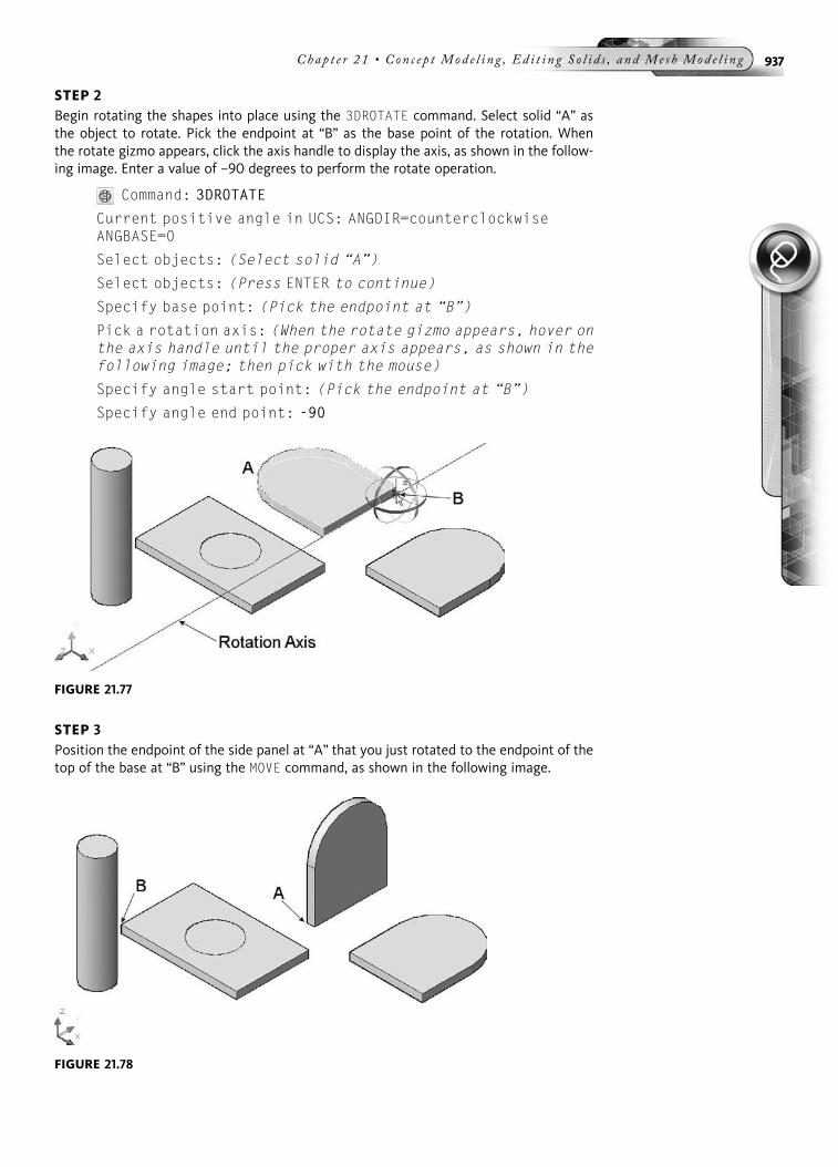
STEP 2Begin rotating the shapes into place using the 3DROTATE command. Select solid “A” asthe object to rotate. Pick the endpoint at “B” as the base point of the rotation. Whenthe rotate gizmo appears, click the axis handle to display the axis, as shown in the follow-ing image. Enter a value of –90 degrees to perform the rotate operation.
Command: 3DROTATE
Current positive angle in UCS: ANGDIR=counterclockwiseANGBASE=0
Select objects: (Select solid “A”)
Select objects: (Press ENTER to continue)
Specify base point: (Pick the endpoint at “B”)
Pick a rotation axis: (When the rotate gizmo appears, hover onthe axis handle until the proper axis appears, as shown in thefollowing image; then pick with the mouse)
Specify angle start point: (Pick the endpoint at “B”)
Specify angle end point: -90
STEP 3Position the endpoint of the side panel at “A” that you just rotated to the endpoint of thetop of the base at “B” using the MOVE command, as shown in the following image.
FIGURE 21.77
FIGURE 21.78
Chap t e r 21 • Con c e p t Mod e l i n g , Ed i t i n g S o l i d s , and Me s h Mod e l i n g 937

STEP 4Now rotate the second side panel into position. This will take two steps to accomplish.
First, rotate the panel 90° using the rotation axis, as shown in the following image.
Command: 3DROTATE
Current positive angle in UCS: ANGDIR=counterclockwiseANGBASE=0
Select objects: (Select the other side panel)
Select objects: (Press ENTER to continue)
Specify base point: (Pick the endpoint at “A”)
Pick a rotation axis: (When the rotate gizmo appears, hover onthe axis handle until the proper axis appears, as shown in thefollowing image; then pick with the cursor)
Specify angle start point: (Pick the endpoint at “A”)
Specify angle end point: 90
STEP 5Now rotate the same panel −90° using the rotation axis, as shown in the following image.
Command: 3DROTATE
Current positive angle in UCS: ANGDIR=counterclockwiseANGBASE=0
Select objects: (Select the same side panel)
Select objects: (Press ENTER to continue)
Specify base point: (Pick the endpoint at “A”)
Pick a rotation axis: (When the rotate gizmo appears, hover onthe axis handle until the proper axis appears, as shown in thefollowing image; then pick with the cursor)
Specify angle start point: (Pick the endpoint at “A”)
Specify angle end point: -90
FIGURE 21.79
938 Aut oCAD 2010 Tu t o r f o r Eng in e e r i n g Graph i c s
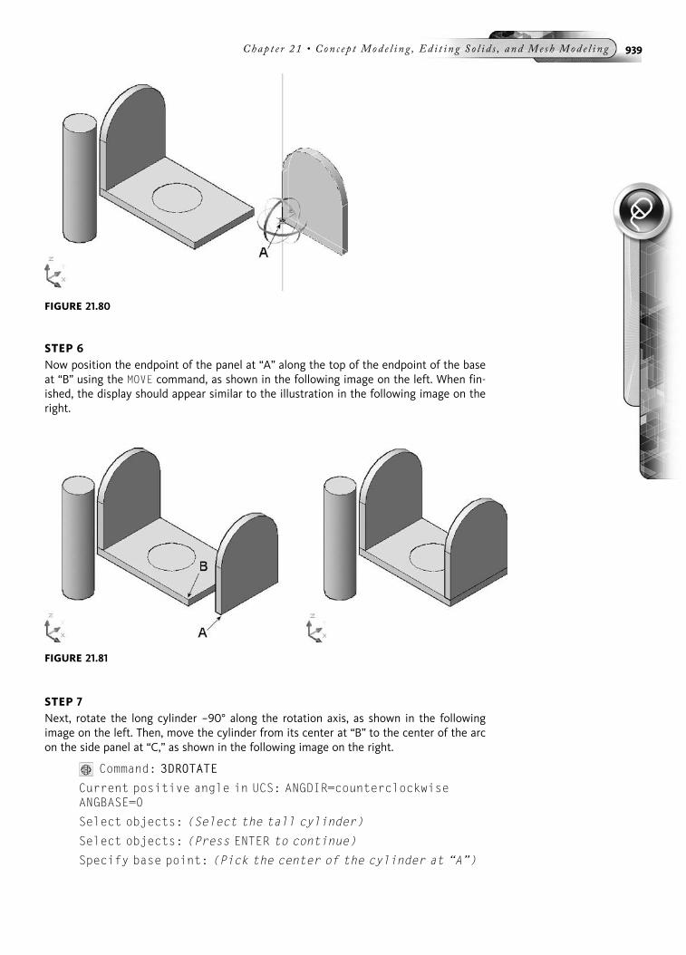
STEP 6Now position the endpoint of the panel at “A” along the top of the endpoint of the baseat “B” using the MOVE command, as shown in the following image on the left. When fin-ished, the display should appear similar to the illustration in the following image on theright.
STEP 7Next, rotate the long cylinder −90° along the rotation axis, as shown in the followingimage on the left. Then, move the cylinder from its center at “B” to the center of the arcon the side panel at “C,” as shown in the following image on the right.
Command: 3DROTATE
Current positive angle in UCS: ANGDIR=counterclockwiseANGBASE=0
Select objects: (Select the tall cylinder)
Select objects: (Press ENTER to continue)
Specify base point: (Pick the center of the cylinder at “A”)
FIGURE 21.80
FIGURE 21.81
Chap t e r 21 • Con c e p t Mod e l i n g , Ed i t i n g S o l i d s , and Me s h Mod e l i n g 939

Pick a rotation axis: (When the rotate gizmo appears, clickthe axis handle until the proper axis appears, as shown in thefollowing image; then pick this axis with the cursor)
Specify angle start point: (Pick the center of the cylinderat “A”)
Specify angle end point: -90
STEP 8Finally, use the SUBTRACT command to subtract the two cylinders from the three platesusing the following prompt sequence and illustration in the following image on the left.The side panels will automatically be unioned to the base when you complete this com-mand. The completed object is displayed in the following image on the right. The ALIGNcommand could also have been used to rotate and move the extruded shapes into theirproper positions.
Command: SU (For SUBTRACT) (can be selected from the MenuBar[Modify > Solids Editing > Subtract])
Select solids and regions to subtract from
Select objects: (Select the two side panels and the base)
Select objects: (Press ENTER to continue)
Select solids and regions to subtract.
Select objects: (Select the two cylinders to subtract)
Select objects: (Press ENTER to perform the union/subtraction operations)
FIGURE 21.82
940 Aut oCAD 2010 Tu t o r f o r Eng in e e r i n g Graph i c s
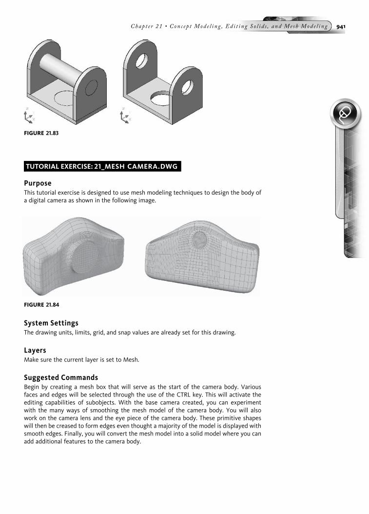
TUTORIAL EXERCISE: 21_MESH CAMERA.DWG
PurposeThis tutorial exercise is designed to use mesh modeling techniques to design the body ofa digital camera as shown in the following image.
System SettingsThe drawing units, limits, grid, and snap values are already set for this drawing.
LayersMake sure the current layer is set to Mesh.
Suggested CommandsBegin by creating a mesh box that will serve as the start of the camera body. Variousfaces and edges will be selected through the use of the CTRL key. This will activate theediting capabilities of subobjects. With the base camera created, you can experimentwith the many ways of smoothing the mesh model of the camera body. You will alsowork on the camera lens and the eye piece of the camera body. These primitive shapeswill then be creased to form edges even thought a majority of the model is displayed withsmooth edges. Finally, you will convert the mesh model into a solid model where you canadd additional features to the camera body.
FIGURE 21.83
FIGURE 21.84
Chap t e r 21 • Con c e p t Mod e l i n g , Ed i t i n g S o l i d s , and Me s h Mod e l i n g 941

STEP 1Open the drawing 21_Mesh Camera. Before creating the mesh model of the camera body,first examine the options available to you regarding the individual primitives used tomodel. Clicking the arrow located in the Primitives panel of the Ribbon as shown in thefollowing image on the left will activate the Mesh Primitive Options dialog box as shownin the following image on the right. Notice the various primitives that are contained inthis dialog box such as box, cylinder, cone, and wedge to name a few. In the dialog box,the box object is highlighted. Notice in the dialog box the number of Tesselation Divi-sions for the box. Verify that the Length is set to 5, the Width set to 3, and the Height isset to 3. You will also notice a preview of the box based on the Tesselation Divisions. Clickthe OK button to exit this dialog box.
STEP 2Click the Mesh Box button located on the Ribbon as shown in the following image on theleft. Then create a mesh box by first specifying the corner point of 10,10. For the othercorner, type L for Length at the command prompt. This will allow you to create themesh box by length, width, and height. Next, move your cursor until the angle readoutreads 0° and a value of 180 as shown in the following image on the left. Continue movingyour cursor, this time in the Y direction and enter a value of 40, which represents thewidth. Finally move your cursor in the Z direction and enter a value of 80 for the heightto complete the creation of the mesh box as shown in the following image on the right.
Command: _.MESH
Current smoothness level is set to : 0
Enter an option [Box/Cone/CYlinder/Pyramid/Sphere/Wedge/Torus/SEttings] <Box>:
_BOX
Specify first corner or [Center]: 10,10
Specify other corner or [Cube/Length]: L
Specify length <180.0000>: 180
Specify width <40.0000>: 40
Specify height or [2Point] <80.0000>: 80
FIGURE 21.85
942 Aut oCAD 2010 Tu t o r f o r Eng in e e r i n g Graph i c s

STEP 3You will now select a number of subobjects and, with the aid of the 3D move gizmo,stretch the faces vertically at a distance of 20. First, hold down the CTRL key and pickthe three top middle faces as shown in the following image on the left. When the 3Dmove gizmo appears, move your cursor until the Z axis appears. Then press and holddown the left mouse button while dragging the faces vertically. While dragging, enter avalue of 20 and press ENTER to drag the three faces 30 mm up as shown in the followingimage on the right.
STEP 4Next, you will stretch the edges of the mesh box instead of its faces. Do better accom-plish this, change the selection filter to Edge that is found under the Subobjects panel ofthe Ribbon as shown in the following image on the left. Remember . . . you should be inthe 3D Modeling workspace in order to properly access the correct commands. Afterswitching to the Edge selection filter, hold down the CTRL key while selecting the threevertical edges as shown in the following image in the middle. When the 3D move gizmo
FIGURE 21.86
FIGURE 21.87
Chap t e r 21 • Con c e p t Mod e l i n g , Ed i t i n g S o l i d s , and Me s h Mod e l i n g 943

appears, move your cursor until the Y axis appears. Press and drag these three edgestoward you while entering a value of 20. Pressing ENTER will stretch these edges 20 mmas shown in the following image on the right.
STEP 5While still in the Edge selection filter, hold down the CTRL key while selecting the threehorizontal edges as shown in the following image on the left. When the 3D move gizmoappears, move your cursor until the Z axis appears. Press and drag these three edgesdown while entering a value of 10. Pressing ENTER will stretch these edges 10 mm asshown in the following image on the right.
STEP 6At this point your model of the camera body should appear similar to the following imageon the left. Unfortunately, most digital camera bodies do not consist of sharp edges. Thisis due to a setting that allows you to control the smoothness of the camera body. Pickingon any edge of the camera body will display the Quick Properties palette as shown in thefollowing image on the right. The Smoothness setting can range from None to Level 4.Presently, your model is displayed with no smoothness. To change to a different level,follow the next step.
FIGURE 21.88
FIGURE 21.89
944 Aut oCAD 2010 Tu t o r f o r Eng in e e r i n g Graph i c s

STEP 7To resemble a more realistic camera body, click on the Smooth More button under theMesh Modeling tab of the Ribbon as shown in the following image on the left. Clickingonce on this button has the same affects as setting the Smoothness to Level 1 in theQuick Properties palette also shown in the following image on the left. Either of theseactions results in the following image on the right. Notice all edges are now smooth.Experiment on this model by changing to the levels 2, 3, and 4.
STEP 8You can generate more mesh faces by clicking on the Refine Mesh button as shown in thefollowing image on the left. Clicking on the object will produce the mesh pattern asshown in the following image on the right. As this command adds more faces to themesh model, it also could make the model heavy and slow to respond depending on theamount of RAM in your system. When you are finished observing the refined mesh pat-tern of faces, use the UNDO command to undo the refined mesh operation and return tothe Level 2 smoothness.
FIGURE 21.90
FIGURE 21.91
Chap t e r 21 • Con c e p t Mod e l i n g , Ed i t i n g S o l i d s , and Me s h Mod e l i n g 945

STEP 9Next, hold down the CTRL key while selecting the three curved faces as shown in the fol-lowing image on the left. Then move your cursor over the move gizmo, slide over to theZ axis, and stretch the three curving edges down at a distance of 20 mm. the resultsare shown in the following image on the right.
STEP 10Next, create the opening where the lens will go. Change the selection type to Face mode.Hold down the CTRL key and select the middle face. Then right-click anywhere on themove gizmo and choose Scale from the menu. Right-click on the move gizmo again andthis time, click Set Constraint from the menu followed by the ZX plane. This is the planethe selected face will be scaled by. Entering a scale factor of 1.50 will display your modelas shown in the following image on the right.
FIGURE 21.92
FIGURE 21.93
946 Aut oCAD 2010 Tu t o r f o r Eng in e e r i n g Graph i c s
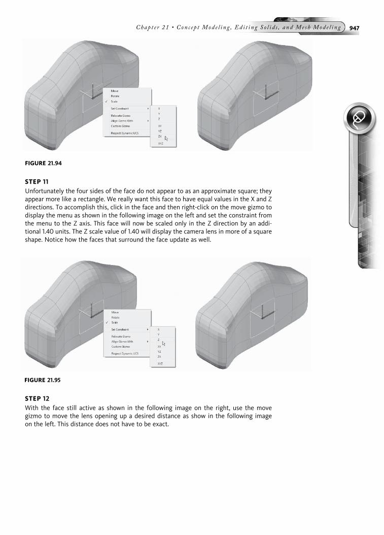
STEP 11Unfortunately the four sides of the face do not appear to as an approximate square; theyappear more like a rectangle. We really want this face to have equal values in the X and Zdirections. To accomplish this, click in the face and then right-click on the move gizmo todisplay the menu as shown in the following image on the left and set the constraint fromthe menu to the Z axis. This face will now be scaled only in the Z direction by an addi-tional 1.40 units. The Z scale value of 1.40 will display the camera lens in more of a squareshape. Notice how the faces that surround the face update as well.
STEP 12With the face still active as shown in the following image on the right, use the movegizmo to move the lens opening up a desired distance as show in the following imageon the left. This distance does not have to be exact.
FIGURE 21.94
FIGURE 21.95
Chap t e r 21 • Con c e p t Mod e l i n g , Ed i t i n g S o l i d s , and Me s h Mod e l i n g 947

STEP 13Click on the Extrude Face command fromMesh Edit panel of the Ribbon, select the squareface you have been working on, and drag the lens opening out as shown in the followingimage on the left. You could also have directed the extrusion inside of the part to create ahole or void. Keep dragging the face out and enter a distance of 10 mm. Your mesh modelof the camera body should appear similar to the following image on the right.
STEP 14The next task is to rotate the mesh model to the back as shown in the following image forthe purpose of creating the eye piece.
FIGURE 21.96
FIGURE 21.97
948 Aut oCAD 2010 Tu t o r f o r Eng in e e r i n g Graph i c s

STEP 15As with the camera lens, press and hold down the CTRL key while selecting the face.Right-click on the gizmo and pick Scale from the menu as shown in the following imageon the left. Right-click a second time on the gizmo, select Set Constraint from the menu,and scale this face based on the XZ plane. Enter a scale factor distance of .50 mm to re-duce the size of this face. Right-click again on the gizmo and change the Set Constraintaxis to the X axis. Then scale this face out in the X direction by a distance of 1.30mm. Usethe Extrude Mesh command to extrude this face out by a distance of 2mm.
FIGURE 21.98
FIGURE 21.99
Chap t e r 21 • Con c e p t Mod e l i n g , Ed i t i n g S o l i d s , and Me s h Mod e l i n g 949
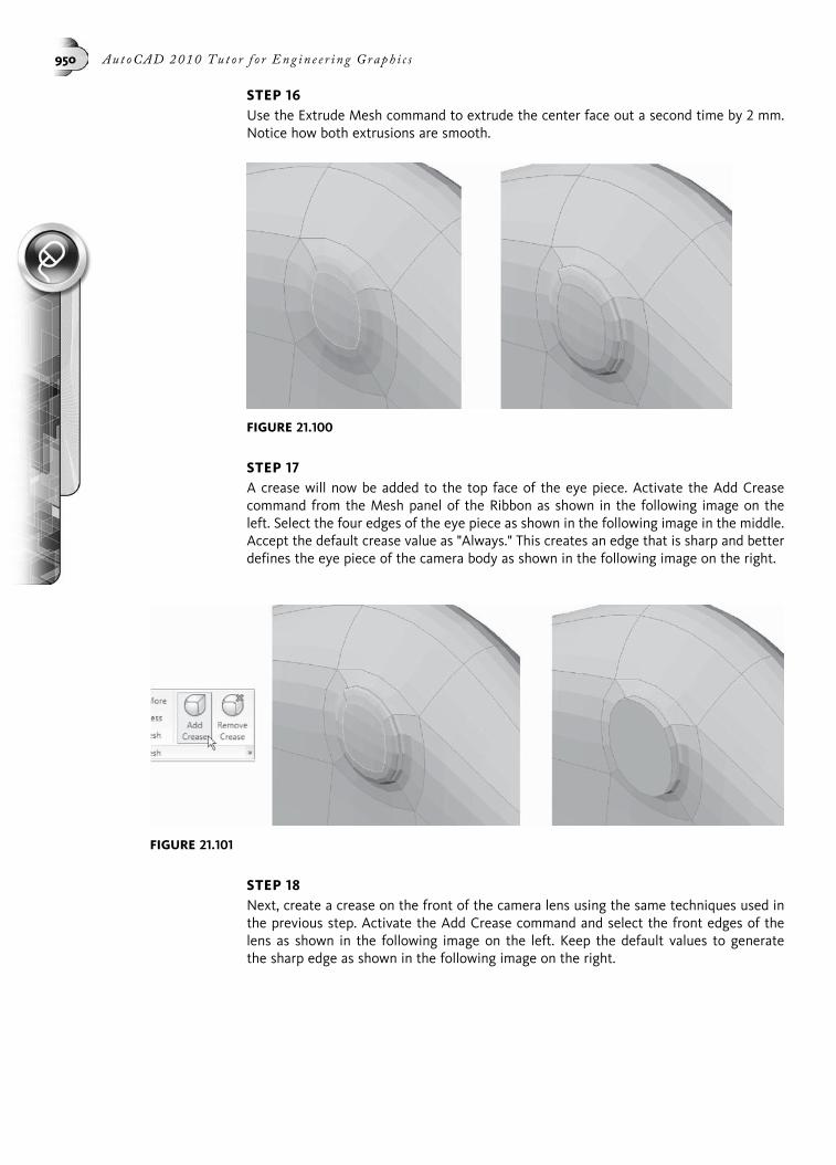
STEP 16Use the Extrude Mesh command to extrude the center face out a second time by 2 mm.Notice how both extrusions are smooth.
STEP 17A crease will now be added to the top face of the eye piece. Activate the Add Creasecommand from the Mesh panel of the Ribbon as shown in the following image on theleft. Select the four edges of the eye piece as shown in the following image in the middle.Accept the default crease value as "Always." This creates an edge that is sharp and betterdefines the eye piece of the camera body as shown in the following image on the right.
STEP 18Next, create a crease on the front of the camera lens using the same techniques used inthe previous step. Activate the Add Crease command and select the front edges of thelens as shown in the following image on the left. Keep the default values to generatethe sharp edge as shown in the following image on the right.
FIGURE 21.100
FIGURE 21.101
950 Aut oCAD 2010 Tu t o r f o r Eng in e e r i n g Graph i c s

STEP 19The results are shown in the following image. The camera lens displays edges as shown inthe following image on the left. The eye piece also has edges and are displayed in thefollowing image on the right.
STEP 20Once the mesh model has been created, it will now be converted into a solid model usingthe Convert to Solid command as shown in the following image. When prompted to se-lect the model to convert, click anywhere on the mesh model of the camera body asshown in the following image on the left. The results are illustrated in the following im-age on the right. Once the camera body is converted into a solid, you can now use thetraditional solid modeling commands to add or subtract features.
FIGURE 21.102
FIGURE 21.103
Chap t e r 21 • Con c e p t Mod e l i n g , Ed i t i n g S o l i d s , and Me s h Mod e l i n g 951

END OF CHAPTER PROBLEMS FOR CHAPTER 21Please refer to the CD that is supplied with this book and locate the file AutoCAD Tutor2010 Support Docs.pdf. In addition to extra information supplied in this chapter, end-of-chapter problems are also available to provide additional practice.
FIGURE 21.104
952 Aut oCAD 2010 Tu t o r f o r Eng in e e r i n g Graph i c s

CHAPTER
22Creating 2D
Multiview Drawingsfrom a Solid Model
One of the advantages of creating a 3D image in the form of a solid model is theability to use the data of the solid model numerous times for other purposes. The pur-pose of this chapter is to generate 2D multiview drawings from the solid model. Twocommands are used together to perform this operation: SOLVIEW and SOLDRAW. TheSOLVIEW command is used to create a layout for the 2D views. This command auto-matically creates layers used to organize visible lines, hidden lines, and dimensions.The SOLDRAW command draws the requested views on the specific layers that werecreated by the SOLVIEW command (this includes the drawing of hidden lines toshow hidden features, and even hatching if a section is requested).
Included in the layout of 2D multiview projections will be the creation of ortho-graphic, auxiliary, section, and isometric views for a drawing. Also explained will bethe FLATSHOT command, used to create 2D views that are saved as blocks. A tutorialis available at the end of this chapter to demonstrate how to dimension orthographicviews that are laid out with the SOLVIEW and SOLDRAW commands.
THE SOLVIEW AND SOLDRAW COMMANDSOnce you create the solid model, you can lay out and draw the necessary 2D viewsusing a number of Modeling Setup commands. Choosing Modeling from the DrawMenu Bar and then Setup, as shown in the following image, exposes the Drawing(SOLDRAW), View (SOLVIEW), and Profile (SOLPROF) commands. Only SOLDRAWand SOLVIEW will be discussed in this chapter. These commands can also be accessedby clicking on the Home tab and then the 3D Modeling panel of the Ribbon, asshown in the following image on the right.
953

Once the SOLVIEW command is entered, the display screen automatically switches tothe first layout or Paper Space environment. Using SOLVIEW lays out a view based onresponses to a series of prompts, depending on the type of view you want to create.Usually, the initial view that you lay out serves as the starting point for other orthog-onal views and is based on the current User Coordinate System. This needs to be de-termined before you begin this command. Once an initial view is created, it is veryeasy to create Orthographic, Auxiliary, Section, and even Isometric views.
As SOLVIEW is used as a layout tool, the images of the views created are still simplyplan views of the original solid model. In other words, after you lay out a view, it doesnot contain any 2D features, such as hidden lines. As shown in the previous image,clicking Drawing activates the SOLDRAW command, which is used to actually createthe 2D profiles once it has been laid out through the SOLVIEW command.
TRY IT! Open the drawing file 22_Solview. Before using the SOLVIEW command, study the illustra-tion of this solid model, as shown at “A” in the following image. In particular, pay closeattention to the position of the User Coordinate System icon. The current position of theUser Coordinate System will start the creation process of the base view of the 2D drawing.
TIP Before you start using the SOLVIEW command, remember to load the Hidden linetype. Thisautomatically assigns this linetype to any new layer that requires hidden lines for the draw-ing mode. If the linetype is not loaded at this point, it must be manually assigned later toeach layer that contains hidden lines through the Layer Properties Manager palette.
Activating SOLVIEW automatically switches the display to the layout or Paper Spaceenvironment. Since this is the first view to be laid out, the UCS option will be used tocreate the view based on the current User Coordinate System. The view produced issimilar to looking down the Z-axis of the UCS icon. A scale value may be entered forthe view. For the View Center, click anywhere on the screen and notice the view be-ing constructed. You can pick numerous times on the screen until the view is in adesired location. The placement of this first view is very important because otherviews will most likely be positioned from this one. When this step is completed, pressENTER to place the view. Next, you are prompted to construct a viewport around theview. Remember to make this viewport large enough for dimensions to fit inside.Once the view is given a name, it is laid out similar to the illustration at “B” in thefollowing image.
FIGURE 22.1
954 Aut oCAD 2010 Tu t o r f o r Eng in e e r i n g Graph i c s

Command: SOLVIEW
Enter an option [Ucs/Ortho/Auxiliary/Section]: U (For Ucs)
Enter an option [Named/World/?/Current] <Current>: (PressENTER)
Enter view scale <1.0000>: (Press ENTER)
Specify view center: (Pick a point near the center of thescreen to display the view; keep picking until the view isin the desired location)
Specify view center <specify viewport>: (Press ENTER toplace the view)
Specify first corner of viewport: (Pick a point at “D”)
Specify opposite corner of viewport: (Pick a point at “E”)
Enter view name: FRONT
Enter an option [Ucs/Ortho/Auxiliary/Section]: (Press ENTERto exit this command)
Once the view has been laid out through the SOLVIEW command, use SOLDRAW toactually draw the view in two dimensions. The Hidden linetype was loaded for youin this drawing and since it was loaded prior to using the SOLVIEW command, hiddenlines will automatically be assigned to layers that contain hidden line information.The result of using the SOLDRAW command is shown at “C” in the following image.You are no longer looking at a 3D solid model but at a 2D drawing created by thiscommand.
Command: SOLDRAW
(If in Model Space, you are switched to Paper Space)
Select viewports to draw.
Select objects: (Pick anywhere on the viewport at “C” inthe following image)
Select objects: (Press ENTER to perform the Soldrawoperation)
One solid selected.
The use of layers in 2D-view layout is so important that when you run the SOLVIEWcommand, the layers shown in the following image are created automatically. With
FIGURE 22.2
Chap t e r 22 • Cr e a t i n g 2D Mu l t i v i ew Draw ing s f r om a So l i d Mod e l 955

the exception ofModel and 0, the layers that begin with “FRONT” and the VPORTSlayer were all created by the SOLVIEW command. The FRONT-DIM layer is designedto hold dimension information for the Front view. FRONT-HID holds all hiddenlines information for the Front view; FRONT-VIS holds all visible line informationfor the Front view. All Paper Space viewports are placed on the VPORTS layer.The Model layer has automatically been frozen in the current viewport to hide the3D model and show the 2D visible and hidden lines.
In order for the view shown in the following image on the left to be dimensionedin model space, three operations must be performed. First, double-click inside theFront view to be sure it is the current floating Model Space viewport. Next, makeFRONT-DIM the current layer. Finally, if it is not already positioned correctly, setthe User Coordinate System to the current view using the View option of the UCScommand. The UCS icon should be similar to the illustration in the following imageon the left (you should be looking straight down the Z-axis). Now add all dimensionsto the view using conventional dimensioning commands with the aid of Object Snapmodes.When you work on adding dimensions to another view, the same three opera-tions must be made in the new view: make the viewport active by double-clickinginside it, make the appropriate dimension layer current, and update the UCS, if nec-essary, to the current view with the View option.
When you draw the views using the SOLDRAW command and then add the dimen-sions, switching back to the solid model by clicking the Model tab displays the illus-tration shown in the following image on the right. In addition to the solid model ofthe object, the constructed 2D view and dimensions are also displayed. All drawnviews from Paper Space display with the model. To view just the solid model youwould have to use the Layer Properties Manager palette along with the Freeze optionand freeze all drawing-related layers.
TIP Any changes made to the solid model will not update the drawing views. If changes aremade, you must erase the previous views and run SOLVIEW and SOLDRAW again to generatea new set of views.
FIGURE 22.3
956 Aut oCAD 2010 Tu t o r f o r Eng in e e r i n g Graph i c s

CREATING ORTHOGRAPHIC VIEWSOnce the first view is created, orthographic views can easily be created with the Orthooption of the SOLVIEW command.
TRY IT!Open the drawing file 22_Ortho. Notice that you are in a layout and a Front view is alreadycreated. Follow the command prompt sequence below to create two orthographic views.When finished, your drawing should appear similar to the following image.
Command: SOLVIEW
Enter an option [Ucs/Ortho/Auxiliary/Section]: O (For Ortho)
Specify side of viewport to project: (Select the top of theviewport at “A”—a midpoint Osnap will be automaticallyprovided)
Specify view center: (Pick a point above the front view tolocate the top view)
Specify view center <specify viewport>: (Press ENTER toplace the view)
Specify first corner of viewport: (Pick a point at “B”)
Specify opposite corner of viewport: (Pick a point at “C”)
Enter view name: TOP
Enter an option [Ucs/Ortho/Auxiliary/Section]: O (ForOrtho)
Specify side of viewport to project: (Select the right sideof the viewport at “D”)
Specify view center: (Pick a point to the right of the frontview to locate the right side view)
Specify view center <specify viewport>: (Press ENTER toplace the view)
Specify first corner of viewport: (Pick a point at “E”)
Specify opposite corner of viewport: (Pick a point at “F”)
Enter view name: R_SIDE
Enter an option [Ucs/Ortho/Auxiliary/Section]: (Press ENTERto exit this command)
FIGURE 22.4
Chap t e r 22 • Cr e a t i n g 2D Mu l t i v i ew Draw ing s f r om a So l i d Mod e l 957

Running the SOLDRAW command on the three views displays the illustration shownin the following image. Notice the appearance of the hidden lines in all views. TheVPORTS layer is turned off to display only the three views.
Command: SOLDRAW
Select viewports to draw.
Select objects: (Select the three viewports that contain theFront, Top, and Right Side view information)
Select objects: (Press ENTER to perform the Soldrawoperation)
CREATING AN AUXILIARY VIEWIn the illustration in the following image on the left, the true size and shape of theinclined surface containing the large counterbore hole cannot be shown with thestandard orthographic view. An auxiliary view must be used to properly showthese features.
FIGURE 22.5
FIGURE 22.6
958 Aut oCAD 2010 Tu t o r f o r Eng in e e r i n g Graph i c s

TRY IT!Open the drawing file 22_Auxiliary. From the 3D model in the following image use theSOLVIEW command to create a Front view based on the current User Coordinate System.The results are shown in the following image on the right.
Command: SOLVIEW
Enter an option [Ucs/Ortho/Auxiliary/Section]: U (For Ucs)
Enter an option [Named/World/?/Current] <Current>: (PressENTER)
Enter view scale <1.0000>: (Press ENTER)
Specify view center: (Pick a point to locate the view, asshown in the following image on the right)
Specify view center <specify viewport>: (Press ENTER to placethe view)
Specify first corner of viewport: (Pick a point at “A”)
Specify opposite corner of viewport: (Pick a point at “B”)
Enter view name: FRONT
Enter an option [Ucs/Ortho/Auxiliary/Section]: (Press ENTERto exit this command)
TIPNormally you do not end the SOLVIEW command after each view is laid out. Once you finishcreating a view you simply enter the appropriate option (Ucs, Ortho, Auxiliary, or Section)and create the next one. This process can continue until all necessary views are provided.
Now begin the process of constructing an auxiliary view, as shown in the followingimage on the left. After selecting the Auxiliary option of the SOLVIEW command,click the endpoints at “A” and “B” to establish the edge of the surface to view. Pick apoint at “C” to indicate the side from which to view the auxiliary view. Notice how thePaper Space icon tilts perpendicular to the edge of the auxiliary view. Pick a locationfor the auxiliary view and establish a viewport. The result is illustrated in the followingimage in the middle.
Command: SOLVIEW
Enter an option [Ucs/Ortho/Auxiliary/Section]: A (ForAuxiliary)
FIGURE 22.7
Chap t e r 22 • Cr e a t i n g 2D Mu l t i v i ew Draw ing s f r om a So l i d Mod e l 959

Specify first point of inclined plane: End
of (Pick the endpoint at “A”)
Specify second point of inclined plane: End
of (Pick the endpoint at “B”)
Specify side to view from: (Pick a point inside of theviewport at “C”)
Specify view center: (Pick a point to locate the view, asshown in the following image in the middle)
Specify view center <specify viewport>: (Press ENTER to placethe view)
Specify first corner of viewport: (Pick a point at “D”)
Specify opposite corner of viewport: (Pick a point at “E”)
Enter view name: AUXILIARY
Enter an option [Ucs/Ortho/Auxiliary/Section]: (Press ENTERto exit this command)
Run the SOLDRAW command and turn off the VPORTS layer. The finished result isillustrated in the following image on the right. Hidden lines display only because thislinetype was previously loaded.
CREATING A SECTION VIEWThe SOLVIEW and SOLDRAW commands can also be used to create a full section viewof an object. This process automatically creates section lines and place them on a layer(*-HAT) for you.
TRY IT! Open the drawing file 22_Section. From the model illustrated in the following image onthe left, create a Top view based on the current User Coordinate System, as shown in thefollowing image on the right.
Command: SOLVIEW
Regenerating layout.
Enter an option [Ucs/Ortho/Auxiliary/Section]: U (For Ucs)
Enter an option [Named/World/?/Current] <Current>:(Press ENTER)
FIGURE 22.8
960 Aut oCAD 2010 Tu t o r f o r Eng in e e r i n g Graph i c s

Enter view scale <1.0000>: (Press ENTER)
Specify view center: (Pick a point to locate the view, asshown in the following image on the right)
Specify view center <specify viewport>: (Press ENTER to placethe view)
Specify first corner of viewport: (Pick a point at “A”)
Specify opposite corner of viewport: (Pick a point at “B”)
Enter view name: TOP
Enter an option [Ucs/Ortho/Auxiliary/Section]: (Press ENTERto exit this command)
Begin the process of creating the section. You must first establish the cutting planeline in the Top view, as shown in the following image on the left. After the cuttingplane line is drawn, select the side from which to view the section. Then locate thesection view. This is similar to the process of placing an auxiliary view.
Command: SOLVIEW
Enter an option [Ucs/Ortho/Auxiliary/Section]: S (ForSection)
Specify first point of cutting plane: Qua
of (Pick a point at “A”)
Specify second point of cutting plane: (Turn Ortho on, picka point at “B”)
Specify side to view from: (Pick a point inside of theviewport at “C”)
Enter view scale <1.0000>: (Press ENTER)
Specify view center: (Pick a point below the top view tolocate the view, as shown in the following image on the right)
Specify view center <specify viewport>: (Press ENTER toplace the view)
Specify first corner of viewport: (Pick a point at “D”)
Specify opposite corner of viewport: (Pick a point at “E”)
FIGURE 22.9
Chap t e r 22 • Cr e a t i n g 2D Mu l t i v i ew Draw ing s f r om a So l i d Mod e l 961
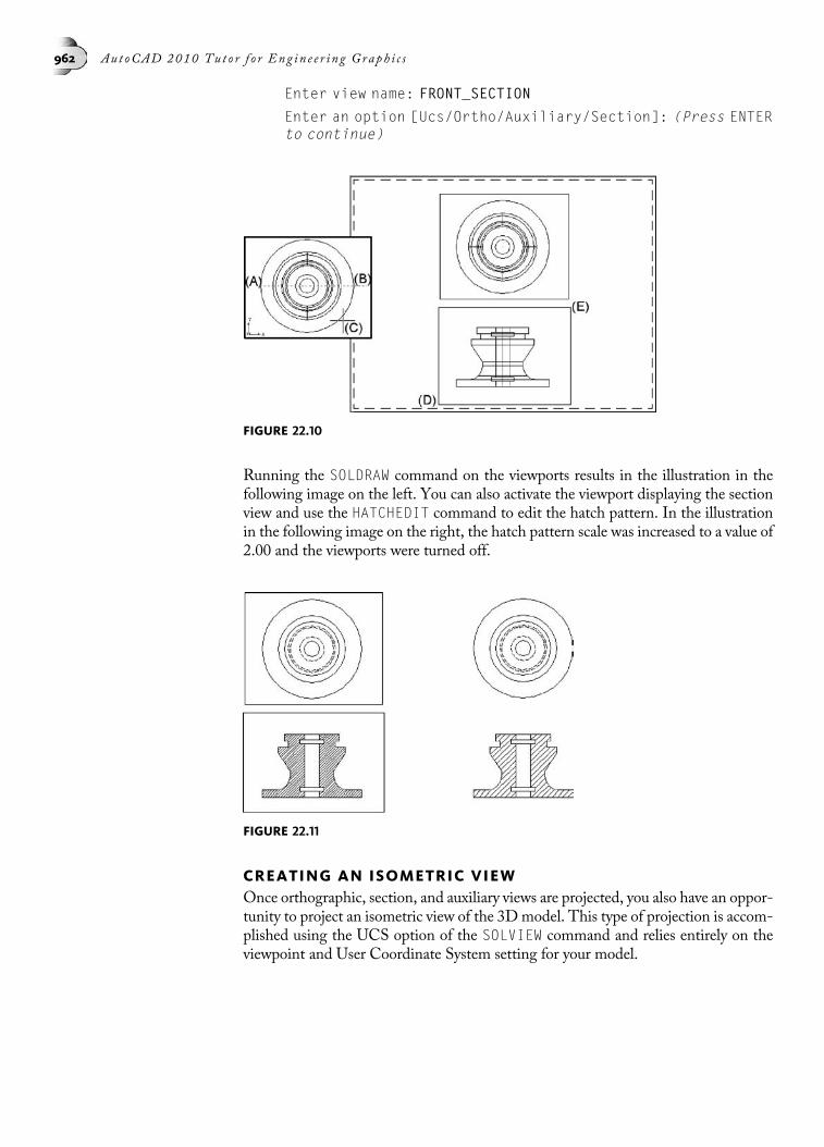
Enter view name: FRONT_SECTION
Enter an option [Ucs/Ortho/Auxiliary/Section]: (Press ENTERto continue)
Running the SOLDRAW command on the viewports results in the illustration in thefollowing image on the left. You can also activate the viewport displaying the sectionview and use the HATCHEDIT command to edit the hatch pattern. In the illustrationin the following image on the right, the hatch pattern scale was increased to a value of2.00 and the viewports were turned off.
CREATING AN ISOMETRIC VIEWOnce orthographic, section, and auxiliary views are projected, you also have an oppor-tunity to project an isometric view of the 3Dmodel. This type of projection is accom-plished using the UCS option of the SOLVIEW command and relies entirely on theviewpoint and User Coordinate System setting for your model.
FIGURE 22.10
FIGURE 22.11
962 Aut oCAD 2010 Tu t o r f o r Eng in e e r i n g Graph i c s
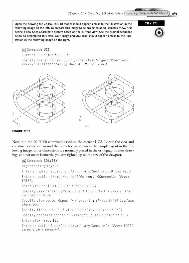
TRY IT!Open the drawing file 22_Iso. This 3D model should appear similar to the illustration in thefollowing image on the left. To prepare this image to be projected as an isometric view, firstdefine a new User Coordinate System based on the current view. See the prompt sequencebelow to accomplish this task. Your image and UCS icon should appear similar to the illus-tration in the following image on the right.
Command: UCS
Current UCS name: *WORLD*
Specify origin of new UCS or [Face/NAmed/OBject/Previous/View/World/X/Y/Z/ZAxis] <World>: V (For View)
Next, run the SOLVIEW command based on the current UCS. Locate the view andconstruct a viewport around the isometric, as shown in the sample layout in the fol-lowing image. Since dimensions are normally placed in the orthographic view draw-ings and not on an isometric, you can tighten up on the size of the viewport.
Command: SOLVIEW
Regenerating layout.
Enter an option [Ucs/Ortho/Auxiliary/Section]: U (For Ucs)
Enter an option [Named/World/?/Current] <Current>: (PressENTER)
Enter view scale <1.0000>: (Press ENTER)
Specify view center: (Pick a point to locate the view in thefollowing image)
Specify view center <specify viewport>: (Press ENTER to placethe view)
Specify first corner of viewport: (Pick a point at “A”)
Specify opposite corner of viewport: (Pick a point at “B”)
Enter view name: ISO
Enter an option [Ucs/Ortho/Auxiliary/Section]: (Press ENTERto exit this command)
FIGURE 22.12
Chap t e r 22 • Cr e a t i n g 2D Mu l t i v i ew Draw ing s f r om a So l i d Mod e l 963

Running the SOLDRAW command on the isometric results in visible lines as well ashidden lines being displayed, as shown in the following image on the left. Generally,hidden lines are not displayed in an isometric view. The layer called ISO-HID, whichwas created by SOLVIEW, contains the hidden lines for the isometric drawing. Use theLayer Properties Manager palette to turn off this layer. The results of this operationare illustrated in the following image on the right.
EXTRACTING 2D VIEWS WITH FLATSHOTThe FLATSHOT command is used to create a quick 2D view of a 3D solid modelbased on the current view. First align your view of the 3D solid and Flatshot projectsan object onto the XY plane. The object created is in the form of a block and can beinserted and modified if necessary, since the block consists of 2D geometry. ChooseFlatshot from the Section panel of the Ribbon, as shown in the following image.
FIGURE 22.13
FIGURE 22.14
FIGURE 22.15
964 Aut oCAD 2010 Tu t o r f o r Eng in e e r i n g Graph i c s

Begin the process of creating a flattened 2D view from a 3D solid model by firstaligning the screen for the view that you want captured. Illustrated in the followingimage on the left is a 3D solid model that is currently being viewed in the Front di-rection. Notice also the alignment of the XY plane; Flatshot will project the geometryto this plane.
When you activate the FLATSHOT command, the dialog box illustrated in the follow-ing image on the right displays. The Destination area is used for inserting a new blockor replacing an existing block. You can even export the geometry to a file with thefamiliar DWG extension that can be read directly by AutoCAD.
The Foreground lines area allows you to change the color and linetype of the linesconsidered visible.
In the Obscured lines area, you have the option of showing or not showing theselines. Obscured lines are considered invisible to the view and should be assigned theHIDDEN linetype if showing this geometry.
After clicking the Create button, you will be prompted to insert the block based onthe view. In the following image, the object on the left is the original 3D solid model,and the object on the right is the 2D block generated by the Flatshot operation. Anisometric view is used in this image to illustrate the results performed by Flatshot.
It was pointed out that Flatshot creates a block. However, during the creation pro-cess, you are never asked to input the name of the block. This is because Flatshot
FIGURE 22.16
FIGURE 22.17
Chap t e r 22 • Cr e a t i n g 2D Mu l t i v i ew Draw ing s f r om a So l i d Mod e l 965
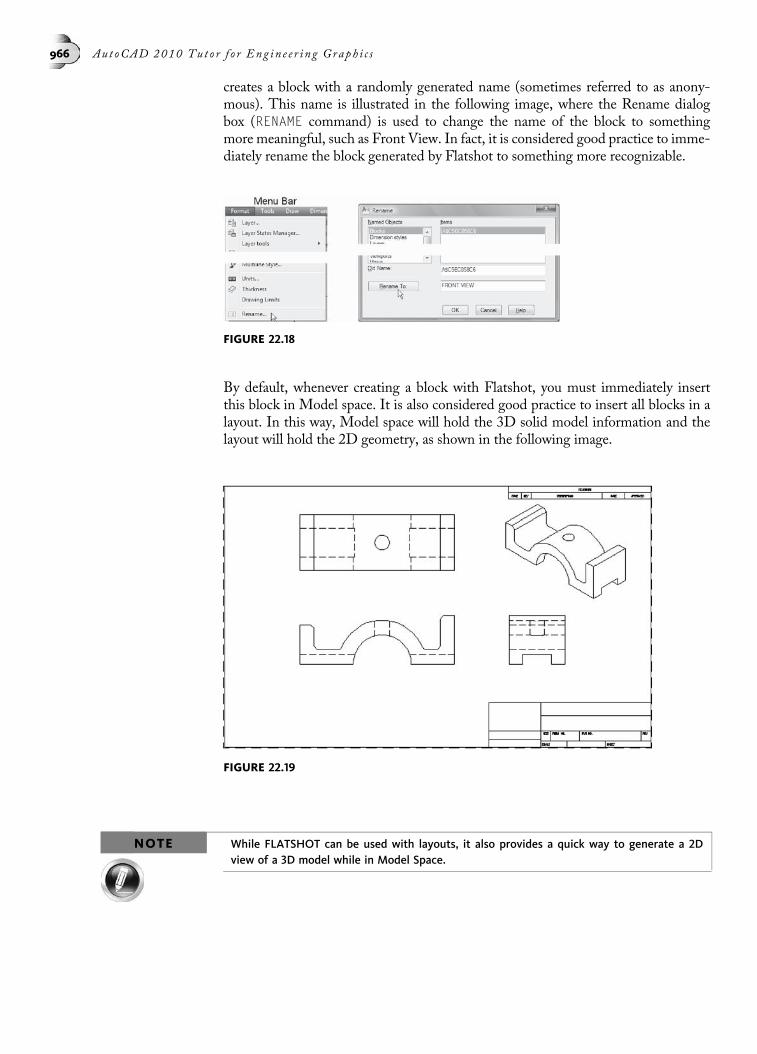
creates a block with a randomly generated name (sometimes referred to as anony-mous). This name is illustrated in the following image, where the Rename dialogbox (RENAME command) is used to change the name of the block to somethingmore meaningful, such as Front View. In fact, it is considered good practice to imme-diately rename the block generated by Flatshot to something more recognizable.
By default, whenever creating a block with Flatshot, you must immediately insertthis block in Model space. It is also considered good practice to insert all blocks in alayout. In this way, Model space will hold the 3D solid model information and thelayout will hold the 2D geometry, as shown in the following image.
NOTE While FLATSHOT can be used with layouts, it also provides a quick way to generate a 2Dview of a 3D model while in Model Space.
FIGURE 22.18
FIGURE 22.19
966 Aut oCAD 2010 Tu t o r f o r Eng in e e r i n g Graph i c s

TUTORIAL EXERCISE: 22_SOLID DIMENSION.DWG
PurposeThis tutorial exercise is designed to add dimensions to a solid model that has had itsviews extracted using the SOLVIEW and SOLDRAW commands, as shown in the previousimage.
System SettingsDrawing and dimension settings have already been changed for this drawing.
LayersLayers have already been created for this tutorial exercise.
Suggested CommandsIn this tutorial you will activate the front viewport of the 22_Solid Dimension drawing andmake the Front-DIM layer current. Then add dimensions to the Front view. As thesedimensions are placed in the Front view, the dimensions do not appear in the otherviews. This is because the SOLVIEW command automatically creates layers and thenfreezes those layers in the appropriate viewports. Next, activate the top viewport, makethe Top-DIM layer current, and add dimensions to the Top view. Finally, activate the rightside viewport, make the Right Side-DIM layer current, and add the remaining dimensionsto the Right Side views.
STEP 1Begin this tutorial by opening the drawing 22_Solid Dimension. Your display shouldappear similar to the following image. Viewports have already been created and lockedin this drawing. A locked viewport means that as you activate the viewport and acciden-tally zoom, the image inside of the viewport does not zoom; rather, the entire drawing isaffected by the zoom operation. Centerline layers have also been created and correspondto the three viewports. Centerlines have already been placed in their respective views.
FIGURE 22.20
Chap t e r 22 • Cr e a t i n g 2D Mu l t i v i ew Draw ing s f r om a So l i d Mod e l 967
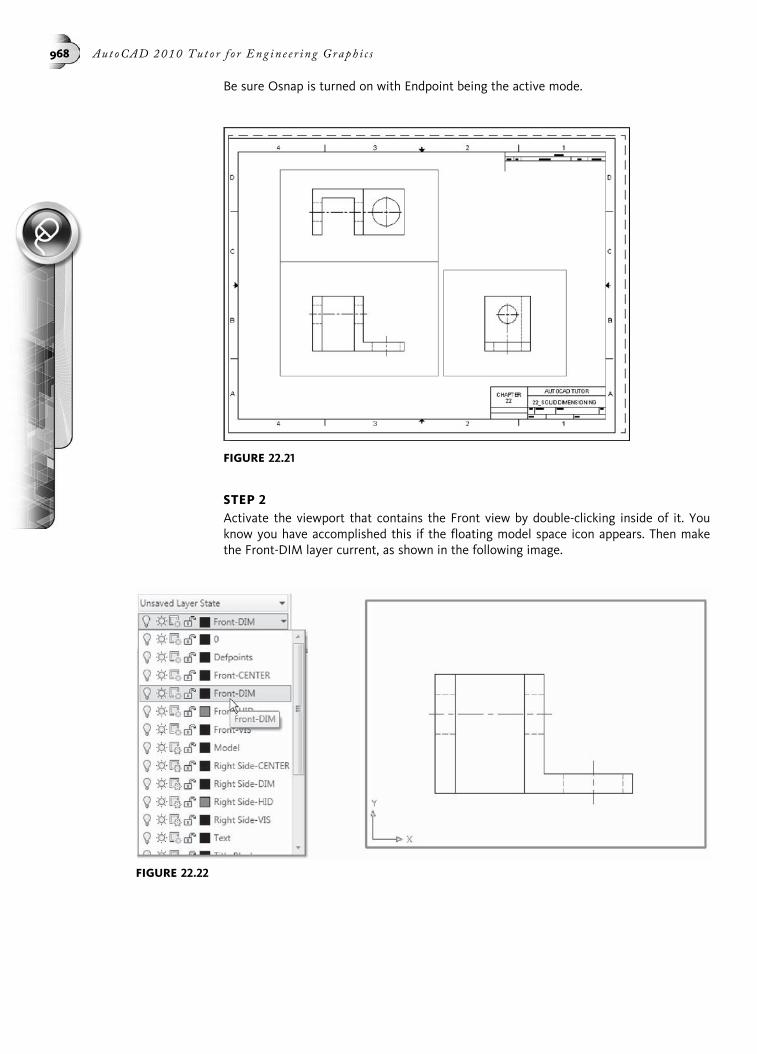
Be sure Osnap is turned on with Endpoint being the active mode.
STEP 2Activate the viewport that contains the Front view by double-clicking inside of it. Youknow you have accomplished this if the floating model space icon appears. Then makethe Front-DIM layer current, as shown in the following image.
FIGURE 22.21
FIGURE 22.22
968 Aut oCAD 2010 Tu t o r f o r Eng in e e r i n g Graph i c s

STEP 3Most of the layers displayed in the Layer Control box were created by the SOLVIEW com-mand. Notice how they correspond to a particular viewport. For example, study the fol-lowing table regarding the layer names dealing with the front viewport:
Layer Name Purpose
Front-CENTER Centerlines
Front-DIM Dimension lines
Front-HID Hidden lines
Front-VIS Visual (Object) lines
Notice the Layer Front-DIM in the following image. Because the viewport holdingthe Front view is current, this layer is thawed, meaning the dimensions placed in thisviewport will be visible. Notice that the other dimension layers (Right Side-DIM andTop-DIM) are frozen. The SOLVIEW command automatically sets up the dimension layersto be visible in the current viewport and frozen in the other viewports.
STEP 4Add the two dimensions to the Front view, as shown in the following image. Linear andbaseline dimension commands could be used to create these dimensions. Grips can beused to stretch the text of the 0.50 dimension so that it is located in the middle of theextension lines.
FIGURE 22.23
Chap t e r 22 • Cr e a t i n g 2D Mu l t i v i ew Draw ing s f r om a So l i d Mod e l 969
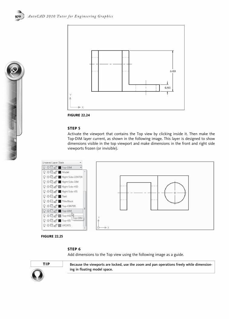
STEP 5Activate the viewport that contains the Top view by clicking inside it. Then make theTop-DIM layer current, as shown in the following image. This layer is designed to showdimensions visible in the top viewport and make dimensions in the front and right sideviewports frozen (or invisible).
STEP 6Add dimensions to the Top view using the following image as a guide.
TIP Because the viewports are locked, use the zoom and pan operations freely while dimension-ing in floating model space.
FIGURE 22.24
FIGURE 22.25
970 Aut oCAD 2010 Tu t o r f o r Eng in e e r i n g Graph i c s

STEP 7Activate the viewport that contains the Right Side view by clicking inside the viewport.Then make the Right Side-DIM layer current, as shown in the following image. This layeris designed to make dimensions visible in the right side viewport and make dimensions inthe front and top viewports frozen (or invisible).
STEP 8Add dimensions to the Right Side view using the following image as a guide. Edit thediameter dimension text to reflect two holes. Use the DDEDIT command to accomplishthis. When the Text Formatting dialog box appears, type “2X” and click the OK button.
FIGURE 22.26
FIGURE 22.27
Chap t e r 22 • Cr e a t i n g 2D Mu l t i v i ew Draw ing s f r om a So l i d Mod e l 971
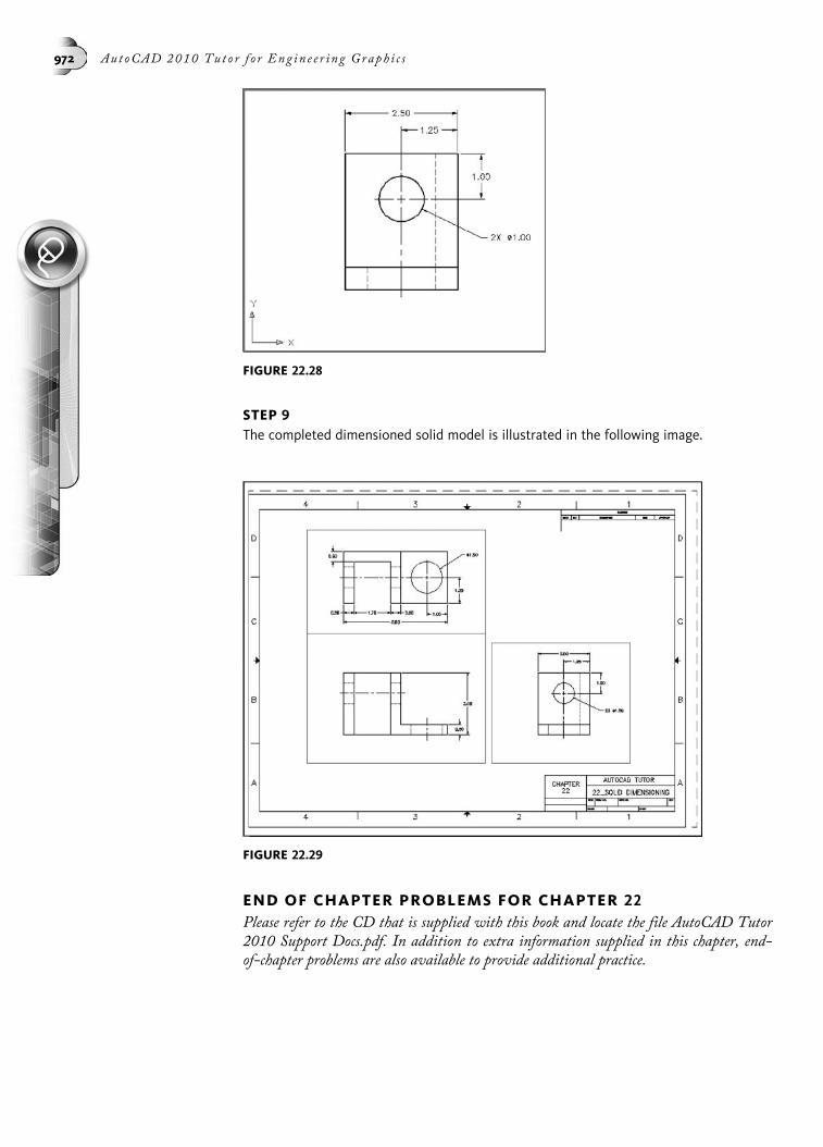
STEP 9The completed dimensioned solid model is illustrated in the following image.
END OF CHAPTER PROBLEMS FOR CHAPTER 22Please refer to the CD that is supplied with this book and locate the file AutoCAD Tutor2010 Support Docs.pdf. In addition to extra information supplied in this chapter, end-of-chapter problems are also available to provide additional practice.
FIGURE 22.28
FIGURE 22.29
972 Aut oCAD 2010 Tu t o r f o r Eng in e e r i n g Graph i c s

CHAPTER
23
Producing RenderingsandMotion Studies
This chapter introduces you to renderings in AutoCAD and how to produce realisticrenderings of 3D models. The heart of the rendering operation is the controls foundin the Ribbon. Adding lights will be the next topic of discussion.With this importantfeature you produce unlimited special effects, depending on the location and intensityof the lights. The Point, Distant, and Spotlights features are discussed, as is the abil-ity to simulate sunlight. You will be able to attach materials to your models to provideadditional realism. Materials can be selected from a library available in AutoCAD, oryou can even make your own materials. You will be shown how to walk and flythrough a 3D model. You will also be given instruction on how to make a motionpath animation of a 3D model.
AN INTRODUCTION TO RENDERINGSEngineering and architectural drawings are able to pack a vast amount of informationinto a 2D outline drawing supplemented with dimensions, some symbols, and a fewterse notes. However, training, experience, and sometimes imagination are requiredto interpret them, and many people would rather see a realistic picture of the object.Actually, realistic pictures of a 3D model are more than just a visual aid for the un-trained. They can help everyone visualize and appreciate a design, and can sometimeseven reveal design flaws and errors.
Shaded, realistic pictures of 3D models are called renderings. Until recently, theywere made with colored pencils and pens or with paintbrushes and airbrushes. Nowthey are often made with computers, and AutoCAD comes with a rendering programthat is automatically installed by the typical AutoCAD installation and is ready foryour use. The following image shows, for comparison, the solid model of a bracketin its wireframe form, as it looks when the HIDE command has been invoked, andwhen it is rendered.
This chapter is designed to give you an overview on how to create pleasing, photore-alistic renderings of your 3D models.
973

The following image displays numerous ways of accessing rendering commands.Clicking View in the Menu Bar, followed by Render, displays a number of toolsused for rendering, as shown in the following image on the left. The Render toolbar,also shown in the following image, is another convenient way to access renderingcommands. The Render tab of the Ribbon (3D Modeling workspace), shown in thefollowing image on the right, can also be used to access light, material, and renderingcommands.
The following table gives a brief description of each rendering tool.
Button Tool Function
Hide Performs a hidden line removal on a 3D model
Render Switches to the Render window, where a truerendering of the 3D model is performed
Lights Contains six additional buttons used for control-ling lights in a 3D model
Light List Displays the Lights in Model palette used formanaging lights that already exist in a 3D model
Materials Displays the Materials palette, used for creatingand applying materials to a 3D model
FIGURE 23.2
FIGURE 23.1
974 Au t oCAD 2010 Tu t o r f o r Eng in e e r i n g Graph i c s

Button Tool Function
Planar Mapping Contains four additional buttons, used for map-ping materials to planar, box, cylindrical, andspherical surfaces
RenderEnvironment
Displays the Rendering Environment dialog boxthat is used mainly for controlling the amount offog applied to a 3D model
Advanced RenderSettings
Displays the Advanced Rendering Settings palette,used for making changes to various renderingsettings
AN OVERVIEW OF PRODUCING RENDERINGSThe object illustrated in the following image consists of a 3D model that has a Real-istic visual style applied. The color of the model comes from the color set through theLayer Properties Manager. After a series of lights are placed in a 3Dmodel, and whenmaterials have been applied, the next step in the rendering process is to decide howaccurate a rendering to make.
As shown in the following image of the Ribbon, the Render tab displays differentrendering modes, or presets, as they are called. These presets range fromDraft to Pre-sentation and control the quality of the final rendered image. For example, when youperform a rendering in draft mode, the processing speed of the rendering is very fast;however, the quality of the rendering is very poor. This render preset is used, for ex-ample, to perform a quick rendering when you are unsure about the positioning oflights. When you are pleased with the lighting in the 3D model, you can switch to ahigher render preset, such as High or Presentation. These modes process the render-ing very slowly; however, the quality is photo-realistic. To perform a rendering, clickthe Render button, as shown in the following image. Also included in the Ribbon areareas that control lighting and materials.
FIGURE 23.3
Chap t e r 23 • Produ c i n g Rend e r in g s and Mo t i on S tud i e s 975

Clicking the Render button, as shown in the previous image, switches your screen tothe render window, as shown in the following image. Notice the shadows that are castto the base of the 3D model. Shadow effects are one of many special rendering toolsused to make a 3Dmodel appear more realistic. Illustrated on the right of the render-ing window is an area used for viewing information regarding the rendered image.Also, when you produce a number of renderings, they are saved in a list at the bottomof the rendering window.
As mentioned earlier, the following image displays the results of performing a Draftversus Presentation rendering. In the draft image, notice that the edges of the modeldo not look as sharp as they do in the presentation model. Also, the draft image doesnot apply shadows when being rendered. All these factors speed up the rendering ofthe draft image; however, the quality of the image suffers.
FIGURE 23.4
FIGURE 23.5
976 Au t oCAD 2010 Tu t o r f o r Eng in e e r i n g Graph i c s
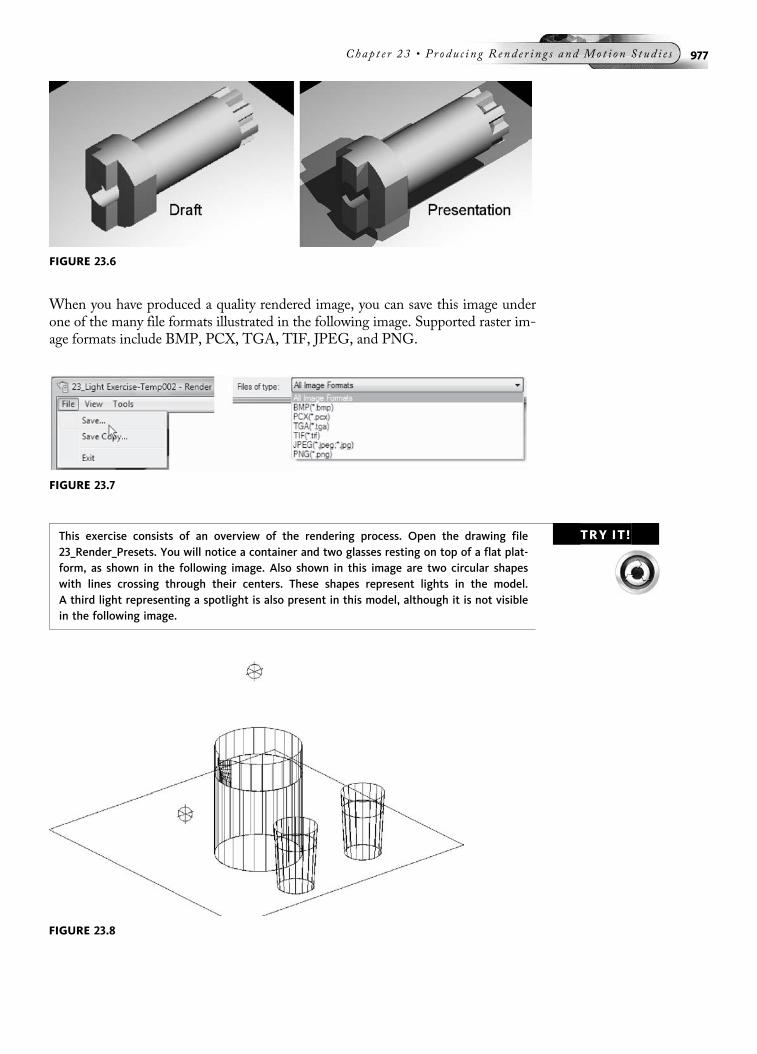
When you have produced a quality rendered image, you can save this image underone of the many file formats illustrated in the following image. Supported raster im-age formats include BMP, PCX, TGA, TIF, JPEG, and PNG.
TRY IT!This exercise consists of an overview of the rendering process. Open the drawing file23_Render_Presets. You will notice a container and two glasses resting on top of a flat plat-form, as shown in the following image. Also shown in this image are two circular shapeswith lines crossing through their centers. These shapes represent lights in the model.A third light representing a spotlight is also present in this model, although it is not visiblein the following image.
FIGURE 23.6
FIGURE 23.7
FIGURE 23.8
Chap t e r 23 • Produ c i n g Rend e r in g s and Mo t i on S tud i e s 977

Activate the 3D Modeling workspace, click on the Render tab, and click the Renderbutton found in the Render panel. The results are illustrated on the following image,with materials, lights, and a background being part of the rendered scheme. Notice inthe Render panel the presence of Medium. This represents one of the many renderpresets used to control the quality of the rendered image.
To see how the Render Preset value affects the rendered image, change the renderpreset in the panel from Medium to Draft and click on the Render button, as shownin the following image. Notice that the quality of the rendered image looks choppy;also, shadows are lost. However, the Draft Render Preset is always useful when test-ing out the lighting of the rendered scene. The processing time of this preset is veryfast compared to other render presets, although the quality of the Draft Render Presetdoes not look very appealing.
FIGURE 23.9
FIGURE 23.10
978 Au t oCAD 2010 Tu t o r f o r Eng in e e r i n g Graph i c s

In the previous image, the lighting looks too bright and overpowering in the renderedimage. To edit the intensity of existing lights, click the Lights Arrow button, locatedin the Lights panel of the Ribbon, as shown in the following image on the left. Thislaunches the Lights in Model palette, as shown in the middle of the following image.Double-clicking Pointlight1 launches the Properties palette for that light, as shownin the following image on the right. Locate the Intensity factor under the Generalcategory and change the default intensity value of 1.00 to a new value of 0.50. Thisreduces the intensity of this light by half. Perform this same operation on Pointlight2and Spotlight1 by changing their intensities from 1.00 to 0.50.
After changing the intensity of each light in the model, change the render preset fromDraft to High in the Ribbon and then click the Render button. The results are dis-played in the following image, with the lights being less intense and the shadows be-ing more pronounced.
Next, click theMaterials Arrow button, located under theMaterials panel of the Rib-bon, as shown in the following image on the left. The Materials palette displays allmaterials created in the model. Clicking the material displays the properties of thismaterial, as shown in the following image on the right. We will experiment morewith materials later in this chapter. This concludes the exercise.
FIGURE 23.11
FIGURE 23.12
Chap t e r 23 • Produ c i n g Rend e r in g s and Mo t i on S tud i e s 979
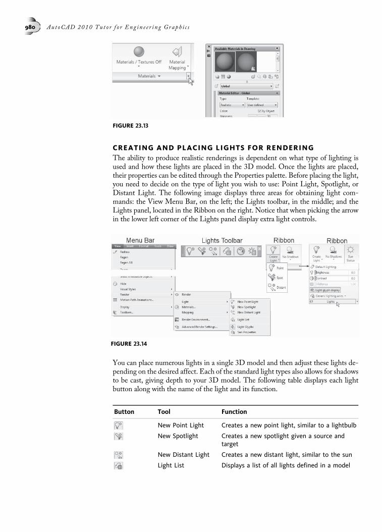
CREATING AND PLACING LIGHTS FOR RENDERINGThe ability to produce realistic renderings is dependent on what type of lighting isused and how these lights are placed in the 3D model. Once the lights are placed,their properties can be edited through the Properties palette. Before placing the light,you need to decide on the type of light you wish to use: Point Light, Spotlight, orDistant Light. The following image displays three areas for obtaining light com-mands: the View Menu Bar, on the left; the Lights toolbar, in the middle; and theLights panel, located in the Ribbon on the right. Notice that when picking the arrowin the lower left corner of the Lights panel display extra light controls.
You can place numerous lights in a single 3D model and then adjust these lights de-pending on the desired affect. Each of the standard light types also allows for shadowsto be cast, giving depth to your 3D model. The following table displays each lightbutton along with the name of the light and its function.
Button Tool Function
New Point Light Creates a new point light, similar to a lightbulb
New Spotlight Creates a new spotlight given a source andtarget
New Distant Light Creates a new distant light, similar to the sun
Light List Displays a list of all lights defined in a model
FIGURE 23.13
FIGURE 23.14
980 Au t oCAD 2010 Tu t o r f o r Eng in e e r i n g Graph i c s

Button Tool Function
Geographic Location Displays a dialog box that allows you to select ageographic location from which to calculate thesun angle
Sun Properties Displays the Sun Properties palette, which al-lows you to make changes to the properties ofthe sun
The Geographic Location button is unique in that it allows you to control the posi-tion of the sun depending on a location, as shown in the following image. Clicking onthe Geographic Location button in the Lights toolbar launches the dialog box on theleft. It is here where you determine the geographic location from a kml or kmz file,from Google Earth, or entering location values. Clicking on the Location Values areadisplays the Geographic Location dialog box as shown in the following image in themiddle. Clicking the Use Map button in this dialog box displays regional maps of theworld as shown in the following image on the right, which allow you to produce sunstudies based on these locations.
A number of lights are also available through theTool Palette which is activated fromthe View tab of the Ribbon, as shown in the following image on the left. Five lightcategories are available to give your renderings amore realistic appearance.One of thecategories deals with generic lights, as shown in the following image on the right.Through this category, you can drag and drop point, spot, and distant lights into your3D model. The remaining categories of lights are classified as photometric.
FIGURE 23.15
Chap t e r 23 • Produ c i n g Rend e r in g s and Mo t i on S tud i e s 981
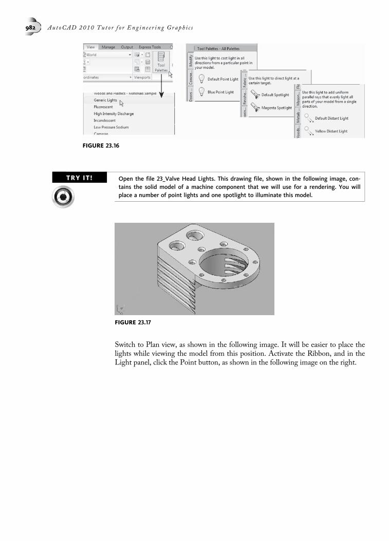
TRY IT! Open the file 23_Valve Head Lights. This drawing file, shown in the following image, con-tains the solid model of a machine component that we will use for a rendering. You willplace a number of point lights and one spotlight to illuminate this model.
Switch to Plan view, as shown in the following image. It will be easier to place thelights while viewing the model from this position. Activate the Ribbon, and in theLight panel, click the Point button, as shown in the following image on the right.
FIGURE 23.17
FIGURE 23.16
982 Au t oCAD 2010 Tu t o r f o r Eng in e e r i n g Graph i c s
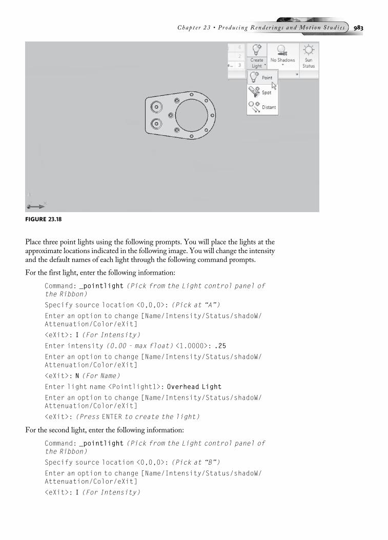
Place three point lights using the following prompts. You will place the lights at theapproximate locations indicated in the following image. You will change the intensityand the default names of each light through the following command prompts.
For the first light, enter the following information:
Command: _pointlight (Pick from the Light control panel ofthe Ribbon)
Specify source location <0,0,0>: (Pick at “A”)
Enter an option to change [Name/Intensity/Status/shadoW/Attenuation/Color/eXit]
<eXit>: I (For Intensity)
Enter intensity (0.00 - max float) <1.0000>: .25
Enter an option to change [Name/Intensity/Status/shadoW/Attenuation/Color/eXit]
<eXit>: N (For Name)
Enter light name <Pointlight1>: Overhead Light
Enter an option to change [Name/Intensity/Status/shadoW/Attenuation/Color/eXit]
<eXit>: (Press ENTER to create the light)
For the second light, enter the following information:
Command: _pointlight (Pick from the Light control panel ofthe Ribbon)
Specify source location <0,0,0>: (Pick at “B”)
Enter an option to change [Name/Intensity/Status/shadoW/Attenuation/Color/eXit]
<eXit>: I (For Intensity)
FIGURE 23.18
Chap t e r 23 • Produ c i n g Rend e r in g s and Mo t i on S tud i e s 983
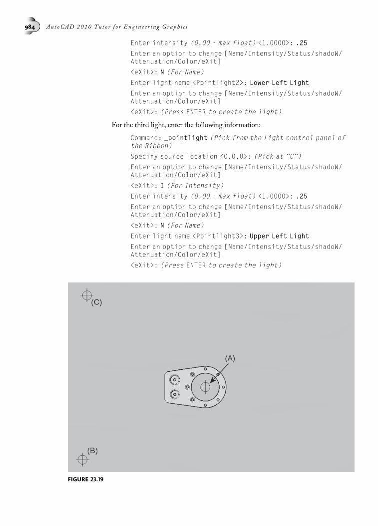
Enter intensity (0.00 - max float) <1.0000>: .25
Enter an option to change [Name/Intensity/Status/shadoW/Attenuation/Color/eXit]
<eXit>: N (For Name)
Enter light name <Pointlight2>: Lower Left Light
Enter an option to change [Name/Intensity/Status/shadoW/Attenuation/Color/eXit]
<eXit>: (Press ENTER to create the light)
For the third light, enter the following information:
Command: _pointlight (Pick from the Light control panel ofthe Ribbon)
Specify source location <0,0,0>: (Pick at “C”)
Enter an option to change [Name/Intensity/Status/shadoW/Attenuation/Color/eXit]
<eXit>: I (For Intensity)
Enter intensity (0.00 - max float) <1.0000>: .25
Enter an option to change [Name/Intensity/Status/shadoW/Attenuation/Color/eXit]
<eXit>: N (For Name)
Enter light name <Pointlight3>: Upper Left Light
Enter an option to change [Name/Intensity/Status/shadoW/Attenuation/Color/eXit]
<eXit>: (Press ENTER to create the light)
FIGURE 23.19
984 Au t oCAD 2010 Tu t o r f o r Eng in e e r i n g Graph i c s
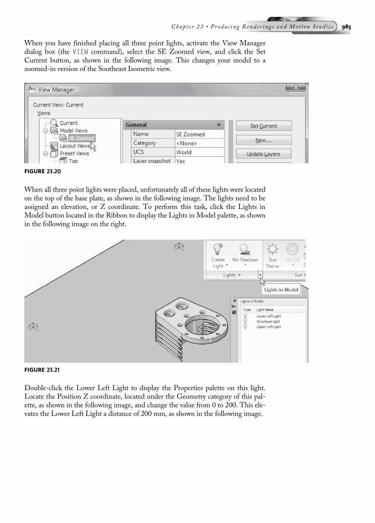
When you have finished placing all three point lights, activate the View Managerdialog box (the VIEW command), select the SE Zoomed view, and click the SetCurrent button, as shown in the following image. This changes your model to azoomed-in version of the Southeast Isometric view.
When all three point lights were placed, unfortunately all of these lights were locatedon the top of the base plate, as shown in the following image. The lights need to beassigned an elevation, or Z coordinate. To perform this task, click the Lights inModel button located in the Ribbon to display the Lights in Model palette, as shownin the following image on the right.
Double-click the Lower Left Light to display the Properties palette on this light.Locate the Position Z coordinate, located under the Geometry category of this pal-ette, as shown in the following image, and change the value from 0 to 200. This ele-vates the Lower Left Light a distance of 200 mm, as shown in the following image.
FIGURE 23.20
FIGURE 23.21
Chap t e r 23 • Produ c i n g Rend e r in g s and Mo t i on S tud i e s 985
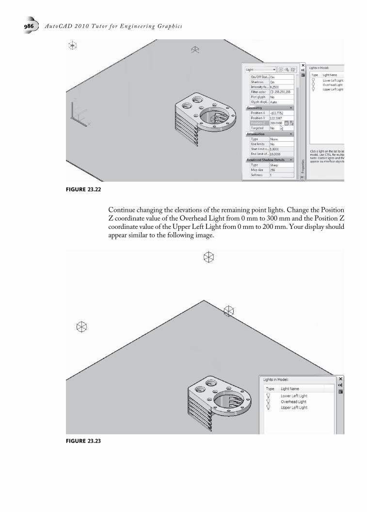
Continue changing the elevations of the remaining point lights. Change the PositionZ coordinate value of the Overhead Light from 0 mm to 300 mm and the Position Zcoordinate value of the Upper Left Light from 0mm to 200 mm. Your display shouldappear similar to the following image.
FIGURE 23.22
FIGURE 23.23
986 Au t oCAD 2010 Tu t o r f o r Eng in e e r i n g Graph i c s

Next, place a spotlight into the 3D model by clicking the Spot button, as shown inthe following image on the right. Place the source for the spotlight at the approximatelocation at “A” and the spotlight target at the center of the bottom of the valve head at“B,” as shown in the following image.
Command: spotlight (Pick from the Light control panel of theRibbon)
Specify source location <0,0,0>: (Pick the approximatelocation for the spotlight at “A”)
Specify target location <0,0,-10>: (Pick the bottom center ofthe valve head at “B”)
Enter an option to change
[Name/Intensity/Status/Hotspot/Falloff/shadoW/Attenuation/Color/eXit] <eXit>: I (For Intensity)
Enter intensity (0.00 - max float) <1.0000>: .50
Enter an option to change
[Name/Intensity/Status/Hotspot/Falloff/shadoW/Attenuation/Color/eXit] <eXit>: N (For Name)
Enter light name <Spotlight5>: Spotlight
Enter an option to change
[Name/Intensity/Status/Hotspot/Falloff/shadoW/Attenuation/Color/eXit] <eXit>: (Press ENTER to createthe light)
As with the point lights, the source of the spotlight is located at an elevation of 0 andneeds to be changed to a different height. Double-click the spotlight icon to displaythe Properties palette, and change the Position Z coordinate value to 200 mm, asshown in the following image on the right.
FIGURE 23.24
Chap t e r 23 • Produ c i n g Rend e r in g s and Mo t i on S tud i e s 987
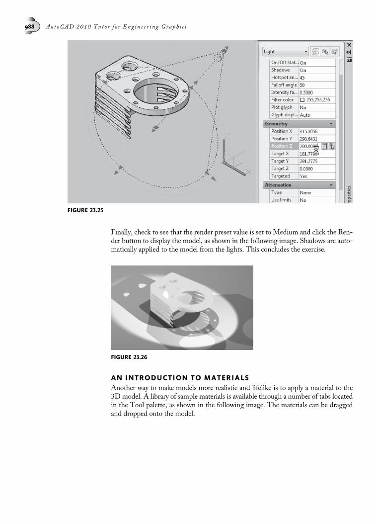
Finally, check to see that the render preset value is set to Medium and click the Ren-der button to display the model, as shown in the following image. Shadows are auto-matically applied to the model from the lights. This concludes the exercise.
AN INTRODUCTION TO MATERIALSAnother way to make models more realistic and lifelike is to apply a material to the3D model. A library of sample materials is available through a number of tabs locatedin the Tool palette, as shown in the following image. The materials can be draggedand dropped onto the model.
FIGURE 23.25
FIGURE 23.26
988 Au t oCAD 2010 Tu t o r f o r Eng in e e r i n g Graph i c s
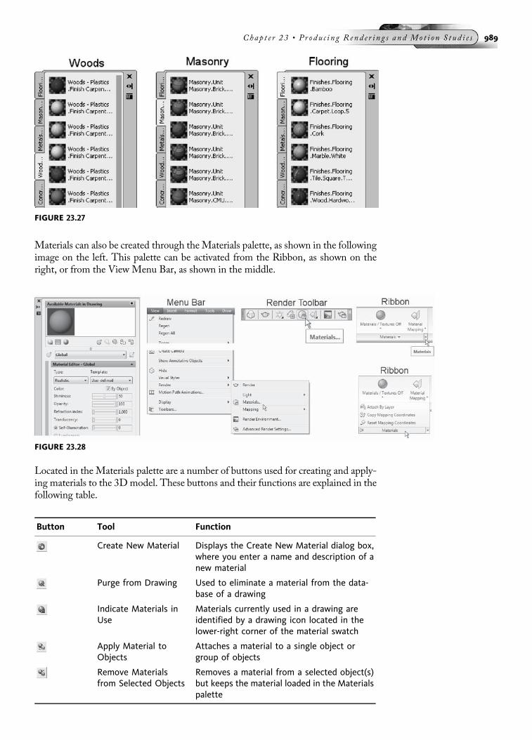
Materials can also be created through theMaterials palette, as shown in the followingimage on the left. This palette can be activated from the Ribbon, as shown on theright, or from the View Menu Bar, as shown in the middle.
Located in the Materials palette are a number of buttons used for creating and apply-ing materials to the 3Dmodel. These buttons and their functions are explained in thefollowing table.
Button Tool Function
Create New Material Displays the Create New Material dialog box,where you enter a name and description of anew material
Purge from Drawing Used to eliminate a material from the data-base of a drawing
Indicate Materials inUse
Materials currently used in a drawing areidentified by a drawing icon located in thelower-right corner of the material swatch
Apply Material toObjects
Attaches a material to a single object orgroup of objects
Remove Materialsfrom Selected Objects
Removes a material from a selected object(s)but keeps the material loaded in the Materialspalette
FIGURE 23.27
FIGURE 23.28
Chap t e r 23 • Produ c i n g Rend e r in g s and Mo t i on S tud i e s 989

Before a material can be applied to a model, it must first be loaded. One method ofaccomplishing this is to drag the material from the Tool palette, as shown in the fol-lowing image on the right, and drop it anywhere in the drawing. The material thenappears in the Materials palette, as shown in the following image on the left.
The Create New Material button in the Materials palette allows you to create yourown custom materials. For creating materials, a number of templates are available,as shown in the following image on the left. These templates already have propertiesset, depending on the purpose of the material. For instance, for theMirror template, anumber of settings have already been made to ensure that the material reflectscorrectly. As you create materials, you can further modify these settings, as shown inthe following image on the right. Clicking on the Diffuse area allows you to changethe color of the material. You can also control such properties as shininess, translu-cency, and opacity in this palette.
FIGURE 23.29
FIGURE 23.30
990 Au t oCAD 2010 Tu t o r f o r Eng in e e r i n g Graph i c s
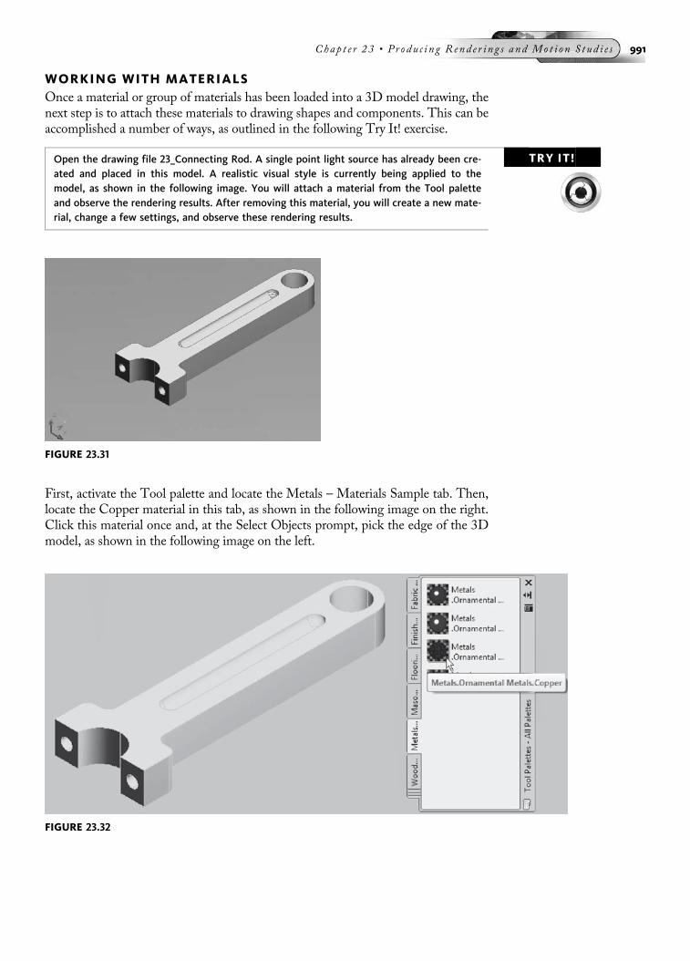
WORKING WITH MATERIALSOnce a material or group of materials has been loaded into a 3D model drawing, thenext step is to attach these materials to drawing shapes and components. This can beaccomplished a number of ways, as outlined in the following Try It! exercise.
TRY IT!Open the drawing file 23_Connecting Rod. A single point light source has already been cre-ated and placed in this model. A realistic visual style is currently being applied to themodel, as shown in the following image. You will attach a material from the Tool paletteand observe the rendering results. After removing this material, you will create a new mate-rial, change a few settings, and observe these rendering results.
First, activate the Tool palette and locate the Metals – Materials Sample tab. Then,locate the Copper material in this tab, as shown in the following image on the right.Click this material once and, at the Select Objects prompt, pick the edge of the 3Dmodel, as shown in the following image on the left.
FIGURE 23.31
FIGURE 23.32
Chap t e r 23 • Produ c i n g Rend e r in g s and Mo t i on S tud i e s 991

Since you are in a realistic visual style, materials and textures are automatically turnedon through the Materials panel located under the Materials tab of the Ribbon, asshown in the following image. The results of applying the copper material to themodel are also shown in the following image.
Before producing the rendering of this object, activate the Materials Editor by click-ing the Materials button located in the Ribbon, as shown in the following image onthe left. While inside the Materials Editor, change the Shininess to a value of 50.Click the radio button next to the Self-Illumination value to turn this mode on andchange its value to 50, as shown in the following image on the right.
To display shadows, perform a rendering with the rendering style set to Medium.The results of performing the rendering are shown in the following image. In addi-tion to the copper material being applied, shadows are cast along a flat surface fromthe existing light source.
FIGURE 23.33
FIGURE 23.34
992 Au t oCAD 2010 Tu t o r f o r Eng in e e r i n g Graph i c s

Before continuing to the next material, click the Remove Materials from SelectedObjects button as shown in the following image on the left in the Materials paletteand pick the edge of the model to remove this material from the model but not fromthe Materials palette. Notice how the original realistic color replaces the copper coloras shown in the following image on the right.
To create a new material, click the Create New Material button, as shown in the fol-lowing image on the left. When the Create New Material dialog box appears, enterthe name Red Metal, as shown in the following image on the right. Click OK.
FIGURE 23.35
FIGURE 23.36
FIGURE 23.37
Chap t e r 23 • Produ c i n g Rend e r in g s and Mo t i on S tud i e s 993

Keep the default template set to Realistic and click the Color box, as shown in thefollowing image on the left, to change the color of the material. When the SelectColor dialog box appears, change to the Index Color tab and change the color to theone shown in the following image on the right. Click the OK button to accept thematerial and return to the Materials palette.
When you return to theMaterials palette, click the ApplyMaterial to Objects button,as shown in the following image on the left. At the Select objects prompt, select the3D model shown in the following image on the right.
Producing a rendering of the 3D model with the new material should result in animage similar to the following image. When finished, exit the rendering mode andreturn to the 3D model.
FIGURE 23.38
FIGURE 23.39
994 Au t oCAD 2010 Tu t o r f o r Eng in e e r i n g Graph i c s

While still using the red metal material, expand the Material Editor to expose theOpacity heading, and change the value to 20 by sliding the bar, as shown in the fol-lowing image on the left. The material will update to reflect this change in opacity,which will change the material to include a degree of transparency.
Producing a new rendering displays the model, as shown in the following image,complete with transparent material and shadows. This concludes the exercise.
FIGURE 23.40
FIGURE 23.41
Chap t e r 23 • Produ c i n g Rend e r in g s and Mo t i on S tud i e s 995
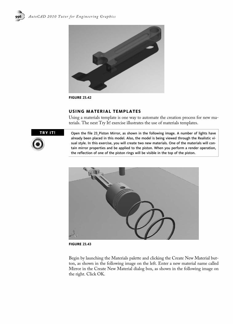
USING MATERIAL TEMPLATESUsing a materials template is one way to automate the creation process for new ma-terials. The next Try It! exercise illustrates the use of materials templates.
TRY IT! Open the file 23_Piston Mirror, as shown in the following image. A number of lights havealready been placed in this model. Also, the model is being viewed through the Realistic vi-sual style. In this exercise, you will create two new materials. One of the materials will con-tain mirror properties and be applied to the piston. When you perform a render operation,the reflection of one of the piston rings will be visible in the top of the piston.
Begin by launching the Materials palette and clicking the Create New Material but-ton, as shown in the following image on the left. Enter a new material name calledMirror in the Create New Material dialog box, as shown in the following image onthe right. Click OK.
FIGURE 23.42
FIGURE 23.43
996 Au t oCAD 2010 Tu t o r f o r Eng in e e r i n g Graph i c s
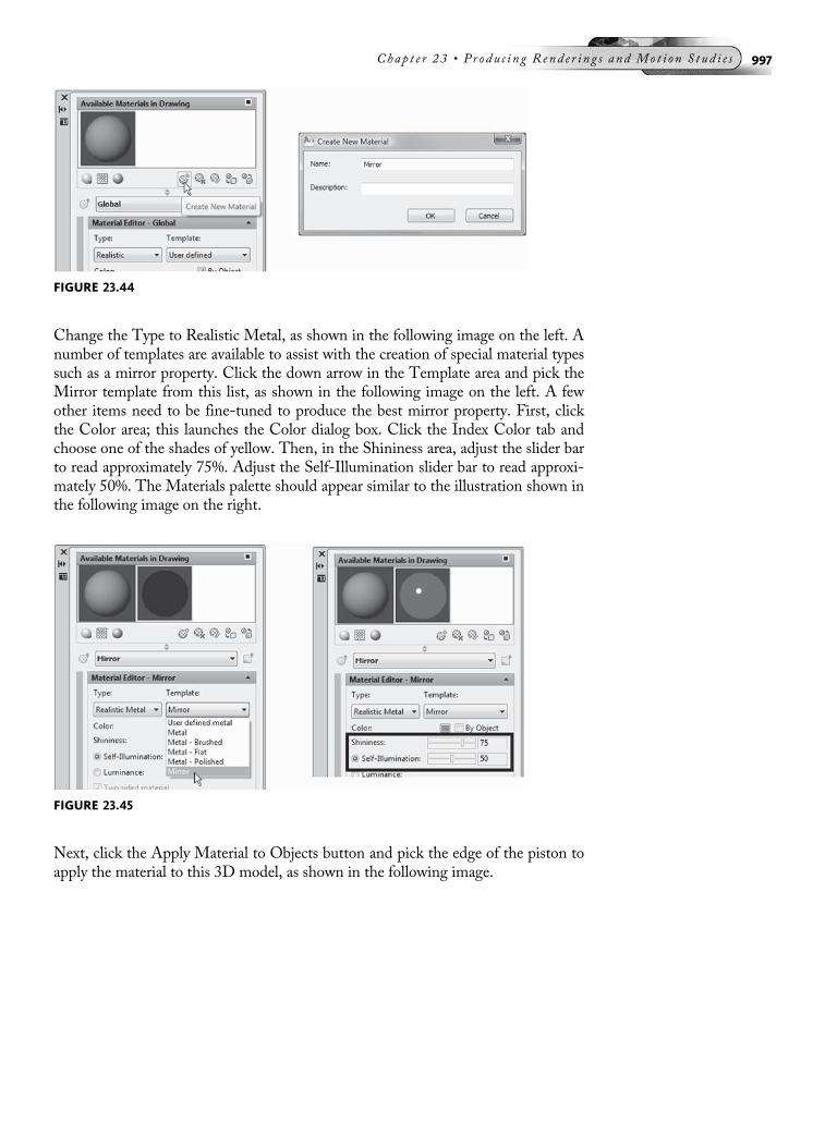
Change the Type to Realistic Metal, as shown in the following image on the left. Anumber of templates are available to assist with the creation of special material typessuch as a mirror property. Click the down arrow in the Template area and pick theMirror template from this list, as shown in the following image on the left. A fewother items need to be fine-tuned to produce the best mirror property. First, clickthe Color area; this launches the Color dialog box. Click the Index Color tab andchoose one of the shades of yellow. Then, in the Shininess area, adjust the slider barto read approximately 75%. Adjust the Self-Illumination slider bar to read approxi-mately 50%. The Materials palette should appear similar to the illustration shown inthe following image on the right.
Next, click the Apply Material to Objects button and pick the edge of the piston toapply the material to this 3D model, as shown in the following image.
FIGURE 23.44
FIGURE 23.45
Chap t e r 23 • Produ c i n g Rend e r in g s and Mo t i on S tud i e s 997

Test the mirror property by performing a render with the render style set to Medium.Notice in the following image that the piston ring and shadows are visible in the pis-ton due to the mirror material.
Create another material called Piston Support Parts, as shown in the followingimage. This material will be applied to the remainder of the parts that form thepiston assembly.
FIGURE 23.46
FIGURE 23.47
998 Au t oCAD 2010 Tu t o r f o r Eng in e e r i n g Graph i c s

Keep the default material Type set to Realistic. Click on the Color area and changethe color of this material to a different shade of green.When finished, click the ApplyMaterial to Objects button and pick the remainder of the piston parts, as shown inthe following image. (Leave the main piston set to the mirror material.)
Perform another rendering test. Your image should appear similar to the followingimage. This concludes the exercise.
FIGURE 23.48
FIGURE 23.49
Chap t e r 23 • Produ c i n g Rend e r in g s and Mo t i on S tud i e s 999

ASSIGNING MATERIALS BY LAYEROne way to render detailed reflections is to use ray tracing, which gives the most real-istic reflections. We can create our own material with attributes that will take advan-tage of this type of rendering.
TRY IT! Open the file 23_Interior Materials, as shown in the following image. You will drag and dropexisting materials from the Tool palette into the drawing. You will then assign these materi-als to specific layers and perform the rendering. Lights have already been created for thisexercise.
Activate the Materials palette and notice that two materials have already been createdin this drawing. The first material, shown in the following image on the left, is a fab-ric color designed to be applied to the chair. The second material, shown in the fol-lowing image on the right, is a paint color to be applied to the walls of the 3D model.
FIGURE 23.50
FIGURE 23.51
1000 Au t oCAD 2010 Tu t o r f o r Eng in e e r i n g Graph i c s

All other materials will be obtained from the Tool palette. You will be dragging anddropping a number of materials into a blank area of your drawing. This drag-and-drop action will load the materials into the drawing for your use. You will beselecting materials from three tabs located in this palette. The first set of materialswill be loaded from the Doors and Windows Materials Library, as shown in the fol-lowing image on the left. You will have to move your cursor over a material and leaveit stationary in order for the whole material name to be displayed. Locate the firstmaterial, Doors –Windows.Door Hardware.Chrome.Satin, as shown in the follow-ing image on the right. Press and hold down your mouse button over this material,drag the material icon into your drawing, and drop it to load it.
Continue loading the following materials located in the appropriate tabs using thetable below as a guide:
Materials Sample Tool Palette Tab Material
Doors and Windows Doors – Windows.DoorHardware.Chrome.Satin
Doors and Windows Doors – Windows.Glazing.Glass.Mirrored
Doors and Windows Doors – Windows.Wood Doors.Ash
Flooring Finishes.Flooring.Wood.Hardwood.1
Woods and Plastics Wood – Plastics.Finish Carpentry.WoodCherry
Woods and Plastics Wood – Plastics.Finish Carpentry.WoodWalnut
Woods and Plastics Wood – Plastics.Finish Carpentry.WoodSpruce
FIGURE 23.52
FIGURE 23.53
Chap t e r 23 • Produ c i n g Rend e r in g s and Mo t i on S tud i e s 1001

When you have finished loading all materials, you can check the status of the load byclicking theMaterials button, located in the Ribbon, as shown in the following imageon the left. This launches the Materials palette and displays all materials that can beapplied to 3D models in the drawing, as shown in the following image on the right.
The next step is to assign a material to a layer. From the Ribbon, click the Attach ByLayer button, as shown in the following image on the left. This launches the Mate-rial Attachment Options dialog box, as shown in the following image on the right.Now you will drag a material located in the left column of the dialog box and drop itonto a layer located in the right column of the dialog box. In this example, theChrome.Satin material has been dropped onto the Door Knob layer.
Using the following image as a guide, continue assigning materials to layers by drag-ging and dropping the materials onto the appropriate layers.
FIGURE 23.54
FIGURE 23.55
1002 Au t oCAD 2010 Tu t o r f o r Eng in e e r i n g Graph i c s
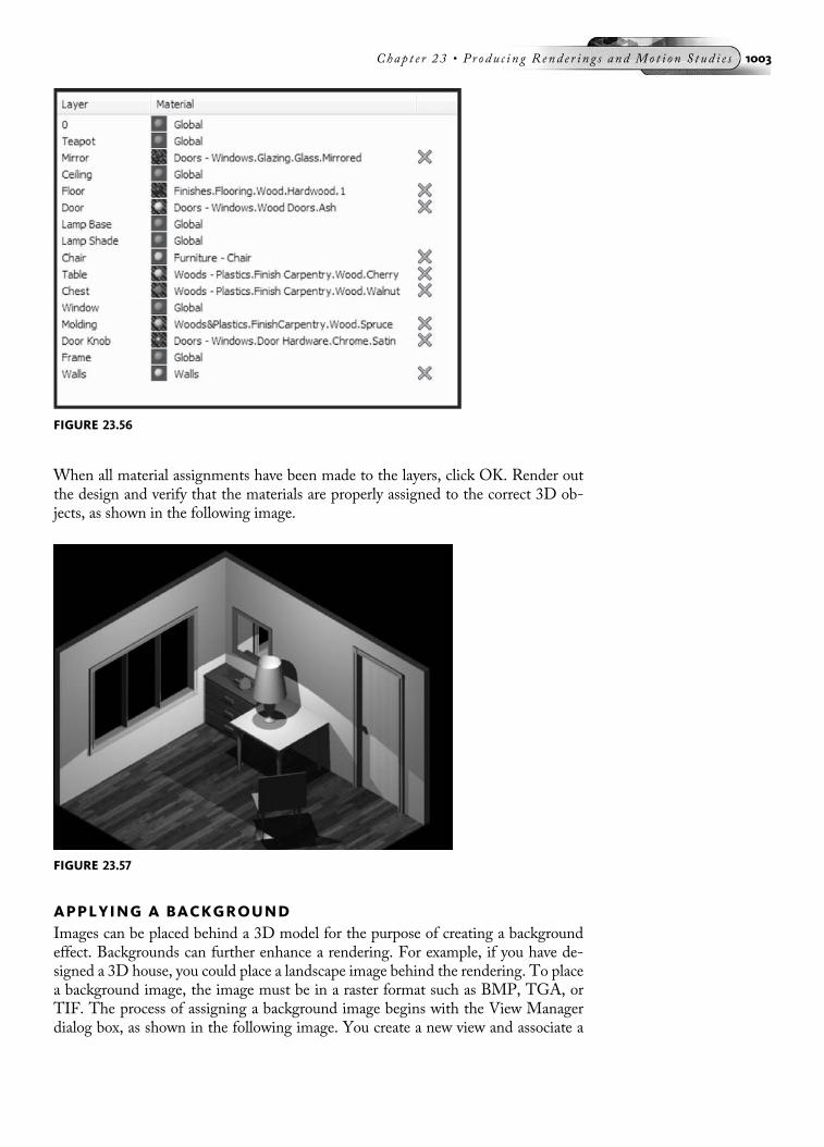
When all material assignments have been made to the layers, click OK. Render outthe design and verify that the materials are properly assigned to the correct 3D ob-jects, as shown in the following image.
APPLYING A BACKGROUNDImages can be placed behind a 3D model for the purpose of creating a backgroundeffect. Backgrounds can further enhance a rendering. For example, if you have de-signed a 3D house, you could place a landscape image behind the rendering. To placea background image, the image must be in a raster format such as BMP, TGA, orTIF. The process of assigning a background image begins with the View Managerdialog box, as shown in the following image. You create a new view and associate a
FIGURE 23.56
FIGURE 23.57
Chap t e r 23 • Produ c i n g Rend e r in g s and Mo t i on S tud i e s 1003

background with the view. In the following image, the New button is picked, whichlaunches the New View dialog box. Enter a new name for the view and place a checkin the box next to Override default background. This launches the Background dialogbox, where you can pick a background from three different types.
These background types are explained as follows.
Solid – A solid background means that AutoCAD replaces the default white (orblack) background of the drawing screen with another color. You choose thecolor from the Colors section of the dialog box.
Gradient – A gradient means that the color changes from one end of the screento the other, such as from red at the bottom to light blue at the top (to simulate asunset). AutoCAD gives you three ways to control a linear gradient – look care-fully: they are tucked into the lower-right corner. Horizon specifies where thelower color ends; a value closer to 0 moves the lower color lower down. WhenHeight is set to 0, you get a two-color gradient; any other value gives you athree-color gradient. Rotation rotates the gradient.
Image – You select a raster image for the background. The image can be in BMP(Bitmap), GIF, PNG, TGA (Targa), TIF (Tagged Image File Format), JPG(JPEG File Interchange Format), or PCX (PC Paintbrush) format.
TRY IT! Open the drawing file 23_Piston Background. The Realistic visual style is applied to thismodel, as shown in the following image. Also applied are four point lights. A special mirrormaterial is attached to the sphere.
FIGURE 23.58
1004 Au t oCAD 2010 Tu t o r f o r Eng in e e r i n g Graph i c s

Begin by performing a render using the Medium rendering style. Your image shouldappear similar to the following image, in which the reflections of various piston partsappear in the sphere due to its mirror property. All that is missing is a backgroundthat will be applied to the 3D models.
All visual style and rendering backgrounds are controlled in the ViewManager dialogbox, as shown in the following image. Begin the selection of a background by clickingthe New button.
FIGURE 23.59
FIGURE 23.60
FIGURE 23.61
Chap t e r 23 • Produ c i n g Rend e r in g s and Mo t i on S tud i e s 1005

Youmust first create a new view and then assign a background to this view.When theNew View/Shot Properties dialog box appears, as shown in the following image onthe left, enter a name for the view, such as Sky Background. In the background area,click on the default field and pick Image, as shown in the following image on the left.This launches the Background dialog box shown in the following image on the right.Click the Browse button to search for valid image files.
Once you click the Browse button in the Background dialog box, the Select File dia-log box appears, as shown in the following image. Locate the folder in which thechapter 23 Try It! exercises are located. From this list, find sky.tga, select it, and clickthe Open button.
This takes you to theBackgrounddialog box again.The sky graphic appears small butcentered on the sheet, as shown in the following image on the left. To control thedisplay of this file in the final rendering, click the Adjust Image button to launch theAdjustBackground Imagedialog box and change the Image position to Stretch.Thisshouldmake the sky graphic fill the entire screen, as shown in the following image onthe right.
FIGURE 23.62
FIGURE 23.63
1006 Au t oCAD 2010 Tu t o r f o r Eng in e e r i n g Graph i c s

Click the OK buttons in the Adjust Background Image and Background dialog boxesto return to the View Manager dialog box, where the Sky Background is now part ofthe Views list. Click the Set Current button to make this view current in the drawingand click the OK button to dismiss this dialog box.
Perform a render using the Medium rendering style and notice the results, as shownin the following image. With the image applied, it appears that the flat base sheet isfloating in air. Also, since the sphere still has the mirror material property, the sky isreflected here in addition to the piston parts. This concludes the exercise.
FIGURE 23.64
FIGURE 23.65
Chap t e r 23 • Produ c i n g Rend e r in g s and Mo t i on S tud i e s 1007

WALKING AND FLYING THROUGH A MODELTo further aid with visualization of a 3D model, walking and flying actions can besimulated through the 3DWALK and 3DFLY commands. Both can be selected fromthe View Menu Bar, as shown in the following image on the left. When walkingthrough a 3Dmodel, you travel along the XY plane. When flying through the model,you move the cursor to look over the top of the model.
When you first activate the 3DWALK command, a warning dialog box appears asshown in the following image on the right stating that you must be in Perspectivemode to walk or fly through your model. Click the Change button to enter Perspec-tive mode.
When you first enter the walk or fly mode, a Position Locator palette appears, asshown in the following image on the left. It gives you an overall view of the positionof the camera and target in relation to the 3D model. You can drag on the cameralocation inside the preview pane of the Position Locator to change its position. Youcan also change the target as you adjust the viewing points of the 3D model. Right-clicking displays the shortcut menu, as shown in the following image. Use thismenu for changing to various modes that assist in the rotating of the model.
FIGURE 23.67
FIGURE 23.66
1008 Au t oCAD 2010 Tu t o r f o r Eng in e e r i n g Graph i c s

ANIMATING THE PATH OF A CAMERAThe ability to walk or fly through a model has just been discussed. This last segmentwill concentrate on creating a motion path animation by which a camera can follow apredefined polyline path to view the contents of a 3D model. Clicking Motion PathAnimations, found under the View Menu Bar shown in the following image on theleft, launches the Motion Path Animation dialog box shown in the following imageon the right. You select the path for the camera and target in addition to changing thenumber of frames per second and the number of frames that will make up theanimation.
After making changes to the Motion Path Animation dialog box, you have the op-portunity to preview the animation before actually creating it. A sample animationpreview is shown in the following image. You can even see the relative position thecamera is in as it passes through the 3D model along the polyline path. After the pre-view is finished, clicking the OK button in the main Motion Path Animation dialogbox creates the animation and writes the results out to a dedicated file format. Sup-ported formats include AVI,MOV,MPG, andWMV. Depending on the resolutionand number of frames, this process could take a long time. However, it gives you thecapability of creating an animation using any kind of 3D model.
FIGURE 23.68
FIGURE 23.69
Chap t e r 23 • Produ c i n g Rend e r in g s and Mo t i on S tud i e s 1009
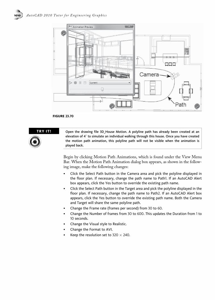
TRY IT! Open the drawing file 3D_House Motion. A polyline path has already been created at anelevation of 4 0 to simulate an individual walking through this house. Once you have createdthe motion path animation, this polyline path will not be visible when the animation isplayed back.
Begin by clicking Motion Path Animations, which is found under the View MenuBar. When the Motion Path Animation dialog box appears, as shown in the follow-ing image, make the following changes:
• Click the Select Path button in the Camera area and pick the polyline displayed inthe floor plan. If necessary, change the path name to Path1. If an AutoCAD Alertbox appears, click the Yes button to override the existing path name.
• Click the Select Path button in the Target area and pick the polyline displayed in thefloor plan. If necessary, change the path name to Path2. If an AutoCAD Alert boxappears, click the Yes button to override the existing path name. Both the Cameraand Target will share the same polyline path.
• Change the Frame rate (frames per second) from 30 to 60.
• Change the Number of frames from 30 to 600. This updates the Duration from 1 to10 seconds.
• Change the Visual style to Realistic.
• Change the Format to AVI.
• Keep the resolution set to 320 � 240.
FIGURE 23.70
1010 Au t oCAD 2010 Tu t o r f o r Eng in e e r i n g Graph i c s

When you have finished making these changes, click the Preview button to previewthe results of the motion animation. Play the animation preview as many times as youlike. Once you close the preview, you will return to the Motion Path Animation dia-log box. Click the OK button and enter the name of the AVI file as House MotionStudy. Clicking the OK button in this dialog box begins the processing of the indi-vidual frames that will make up the animation. The total processing time to producethe animation should be between 5 and 10 minutes.
When finished, launch one of the many Windows Media Player applications andplay the AVI file. This concludes the exercise.
TUTORIAL EXERCISE: SUNLIGHT STUDY
PurposeThis tutorial is designed to simulate sunlight on a specific day and time, and to observethe shadows that are cast by the house.
FIGURE 23.71
FIGURE 23.72
Chap t e r 23 • Produ c i n g Rend e r in g s and Mo t i on S tud i e s 1011

System SettingsSince this drawing is provided on the CD-ROM, all system settings have already beenmade.
LayersThe creation of layers is not necessary.
Suggested CommandsBegin this tutorial by opening up the drawing 23_House Plan Rendering, as shown in theprevious image. You will be performing a study based on the current location of thehouse and the position of the sun on a certain date, time, and geographic location.Shadow casting will be utilized to create a more realistic study.
STEP 1Make the 3D Modeling workspace current. With the Ribbon active, locate the Sun & Loca-tion panel and click the Sun Status button, as shown in the following image on the left, toturn on the sun. A dialog box appears, informing you that you cannot display sunlight ifthe default lighting mode is turned on and asking you whether you want to turn off de-fault lighting. Click the area as shown in the following image on the right to accept therecommended setting to turn off the default lighting.
STEP 2Next, click the Sun button, located in the Ribbon shown in the following image on theleft, to display the Sun Properties palette shown in the following image on the right. Inthis palette, you can change various properties that deal with the sun, such as shadows,date, time, azimuth, altitude, and source vector of the sun.
FIGURE 23.73
1012 Au t oCAD 2010 Tu t o r f o r Eng in e e r i n g Graph i c s

STEP 3Click the launch Geographic Location button, as shown in the following image on the left,to change the location of the 3D model. When the Define Geographic Location dialog boxappears, as shown in the following image on the right, click on the area to enter the loca-tion values.
STEP 4When the Geographic Location dialog box appears, click on the Use Map button, asshown in the following image on the left. This will launch the Location Picker dialog boxas shown in the following image on the right. Click the coast of South Carolina and checkto see that Charleston, SC, appears. You could also use the Nearest City drop-down list toselect the desired location. Other maps from throughout the world also are available.When you are satisfied with the location, click the OK button to leave the Location Pickerand Geographic Location dialog boxes.
FIGURE 23.74
FIGURE 23.75
Chap t e r 23 • Produ c i n g Rend e r in g s and Mo t i on S tud i e s 1013

STEP 5A dialog box appears, informing you that the time zone has been automatically updatedwith the change in the geographic location. Click the area of this dialog box shown in thefollowing image to accept updated time zone.
STEP 6Next you will change the date and time to perform a sun study when the sun is posi-tioned on a fall day. Click the Date area in the Sun Properties palette, click the threedots (ellipses), and change the date to October 18, 2008, as shown in the followingimage.
FIGURE 23.76
FIGURE 23.77
1014 Au t oCAD 2010 Tu t o r f o r Eng in e e r i n g Graph i c s

STEP 7Then, click on the Time area. When an arrow appears, click it to display a number of timesof day in 15-minute increments, and click on 11:00 AM, as shown in the following imageon the left. When you perform this change, the date and time information is also updatedin the Ribbon, as shown in the following image on the right.
STEP 8Clicking the Render button in the Ribbon will render the house, as shown in the followingimage. The shadows cast by the house reflect the time of 11:00 AM in mid-October inCharleston, South Carolina, in the United States.
FIGURE 23.78
FIGURE 23.79
FIGURE 23.80
Chap t e r 23 • Produ c i n g Rend e r in g s and Mo t i on S tud i e s 1015
.DWG file type, 16
.PC3 extension, 620@ symbol, 212 Points mode, 21124-bit color, 782D Drafting & Annotation
workspace, 1, 3, 10, 12–13,258–259
2D helix, 8692D profiles, 9542D viewsextracting, 964–966layers, 955–956solid model, 839
3 Points Arc mode, 205–2063 Points mode, 2103Daligning objects, 903–905arraying objects, 909–910mirroring objects, 908–909moving objects, 902rotating objects, 905–908
3D applications, 855–8573D Coordinate System icon, 8383D helix, 8693D Modeling workspace, 1,
823–824, 928, 9783D modelsAutoCAD Classic workspace,
825backgrounds, 1003–1007concepts, 889continuous orbit, 840default view, 842dynamic rotation maneuvers,
840Face mode, 841face-viewing modes, 842flying action, 1008hiding, 956isometric mode, 842lights, 975, 980–988materials, 975, 979, 988–995motion path animation,
1009–1011orthogonal mode, 842Plan view, 982Realistic visual style, 973, 975renderings, 973–975
rotating, 840–841shadow effects, 976Southeast Isometric view, 985spotlight, 987steering wheel, 844ViewCube viewing, 841–844viewing, 839–840, 844–845walking action, 1008
3D move gizmo, 9023D Operation commands, 9013D rotate tutorial exercise,
935–9403D solid model
defining source plan, 903–905quick 2D view, 964–966
3D spiral, 8693D Views command, 8453D-related menus, 8243D-related palettes, 8243DALIGN command, 903–9053DARRAY command, 909–9103DCORBIT command, 8403DFLY command, 10083DFORBIT (3D Free Orbit)
command, 839, 9263DMOVE tool, 9023DROTATE command, 905–9083DWALK command, 1008
AAbsolute Coordinate mode, 43Acad.Dwt (inches) template file,
101ACAD.LIN file, 79Acadiso.Dwt (millimeters)
template file, 101ACI (AutoCAD Color Index)
colors, 78acquired points, 38–39actions
dynamic blocks, 678–682parameter point associatingwith, 690
renaming, 683viewing recent, 9
Add mode, 514Add Parameter Properties dialog
box, 693
Add Plot Style Table dialog box,630
Add Plot Style Table-Begin dialogbox, 631
Add Plot Style Table-File Namedialog box, 631
Add Plot Style Table-Pick PlotStyle Table dialog box, 631
Add Plotter-Begin dialog box,620
Add Plotter-Finish dialog box, 621Add Plotter-Import PCP or PC2
dialog box, 621Add Plotter-Introduction Page
dialog box, 620Add Plotter-Plotter Model dialog
box, 620Add Plotter-Plotter Name dialog
box, 621Add Plotter-Ports dialog box, 621Add Scale dialog box, 585Add Sheets icon, 635Add-A-Plot Style Table Wizard,
630Add/Delete Scales command, 801ADDCLOSE command, 662Adjust Background Image dialog
box, 1006Adjust Image command, 765advanced functions, 327Alert icon, 681Aligned Dimensioning mode,
414–415Alignment Parameter tool, 685Alignment Parameters, 684–686Allow Docking command, 668alternate units, 480–482angle dimensions, 21angle units, 478anglesacross sharp corner, 154–157bisecting with Xlines, 235chamfering by, 155dimensioning, 433–434drawing exercise, 189–194hatch pattern manipulation, 394measuring, 66, 520–521viewing, 313XY plane, 519–520
1016

angular dimensions, spacing,423–424
animation, 1009, 1011Annotation Object Scale dialog
box, 801–802Annotation Scale, 7, 803Annotation Scales, 801annotationslinetype scaling, 802–804multileaders, 429–433scaling, 797–799
Annotative dimensions style,458, 476
annotative objects, 800–801Annotative property, 798Annotative scales, 797–798dimensions, 808–810hatching, 811–812scale of linetypes, 802text, 804–808viewing controls, 800–802
annotative styles, 798–799ANSI-D layout, 786ANSI31 pattern, 394Application Menu, 1, 8–9Arc command, 205Arc Length symbol, 444architectural details tutorial
exercise, 815–822architectural dimension tutorial
exercise, 505–510architectural drawings, 595–596Architectural units, 66architectural values, 66–67Architecture discipline, 3arcs, 205–208, 421, 555arc tangent to, 212–214arc tangent to two, 214–215center marks, 466–467continuing, 207dimensioning, 421–422,
426–427equality, 556–557length dimension, 467line tangent to, 216–217radius, 521radius dimension, 426segments, 168snapping to, 25–26
areacircles, 512–513fields, 516–518polylines, 512–513shapes, 511–512, 514–515
AREA command, 514
Array Action and dynamic blocks,689–691
ARRAY command, 170Array dialog box, 170–172, 174arraying objects in 3D, 909–910arrays, 170, 909–910arrow grips, 892associative dimensions, 179, 486,
604–605associative hatch patterns,
395–397associativity and dimensions,
484–486Attach Image command, 765Attach Image dialog box, 765ATTACH XREF command,
746ATTDEF command, 710ATTDIA system variable, 712ATTDISP command, 710–711,
721ATTEDIT command, 710ATTMODE system variable,
712ATTREDEF command, 733ATTREQ system variable, 711attribute default, 711Attribute Definition dialog box,
710–711, 718Attribute Extraction command,
737Attribute Extraction wizard, 710,
737–738attribute modes, 711attribute prompt, 711attribute tags, 709–711, 732–733attributes, 709–712blocks and, 732–733displaying, 721editing, 722–725extracting, 737–738fields and, 720globally editing, 728–729multiple lines, 718–720properties, 723properties of text, 723redefining, 732–733
Auto Constrain command,558–559
Auto-Hide command, 77, 668AutoCAD 2000, 51AutoCAD 2004, 51AutoCAD alert dialog box, 52AutoCAD Classic workspace, 1,
583
3D modeling, 825hiding layout and Model tabs,
587–588Layout1 tab, 579multiline text, 258–259switching workspaces, 3toolbars, 2, 10, 13
AutoCAD Command AliasEditor, 15
AutoCAD Create Layout wizard,594–595
AutoCAD display screen, 7AutoCAD drawing session, 52AutoCAD Help Topics dialog
box, 6AutoCAD, communicating with,
7–8Autodesk Design Review viewer,
639Autofill, 280–281AutoFit function, 660automatic ZOOM-Window
mode, 112AutoStack Properties dialog box,
257Auxiliary User Coordinate System,
836auxiliary viewsconstructing, 369–370creation, 958–960curved surface, 374–377infinite lines, 369offsets, 372–373removing excess lines, 373splines, 377transferring distances,
372–373xlines, 371–372
AVI format, 1009axiscoordinates, 42positive rotation about, 830
BBack orthographic view, 837Background dialog box, 1004,
1006backgrounds and 3D models,
1003–1007base pointrotating, 906stretching, 178
base point of displacement, 143,438
I nd e x 1017
base shape, resizing, 892baseline dimensions, 417–421, 462Baseline mode, 420Basic Stud Sizes Lookup parameter,
693Basic Stud Sizes parameter, 692Basic tolerance, 483BATTMAN command, 710, 724beveled edges, 155BHATCH command, 385–386Bind command, 757Bind Xrefs dialog box, 757–758BLK extension, 737block attrib tutorial exercise,
726–727Block Attribute Manager dialog
box, 710, 722, 724–725Block Authoring command, 675Block Authoring editor, 690Block Authoring environment,
683, 688Block Authoring palette, 678Block Authoring Palettes, 685,
689–680, 693–694Block command, 592, 645–646,
659Block Definition dialog box,
646–648Block Editor, 655, 674Block Properties Table dialog box,
696Block Reference object type, 323block tables, dynamic, 694–696blocks, 27, 644–645advantages, 743attribute tags, 709–710base point, 647center, 647copying, 667cutting, 667deleting, 667description, 647–648DesignCenter and, 661–663,
665displaying, 664DIVIDE command, 657drag and drop, 665dynamic, 644, 673–696equally spaced distances, 657exploding, 185, 649, 652, 732extending, 651–652external references and,
743–744Flatshot, 965–966full size, 660–661
global, 647grids, 661grips, 306inserting, 648–650, 657–658,743
insertion point, 645, 647labels, 709–710Layer 0, 660libraries, 662local, 646–648MEASURE command,657–658
merging into drawing file, 646multileaders, 433naming, 645, 647organizing, 662–663, 666pressing and pulling, 898–901previewing, 647properties, 667–668redefining, 654–656, 733renaming, 658, 667rotating, 645, 650scaling, 648, 650, 659–661Tool Palette, 666trimming, 651unused data, 652–654usable objects, 753–754
Blocks icon, 664BMP format, 977, 1004Boolean operations, 852–853border, 72Bottom orthographic view, 837boundaries, 164, 207–209BOUNDARY command,
207–209Boundary Creation dialog box,
207bounding areas, pressing and
pulling, 896–898BOX command, 850, 889, 928box primitives, 850boxes, 850bracket tutorial exercise, 377–383Break at Point tool, 168BREAK command, 166–169brick pattern, 400Bring Above Objects mode, 770Bring to Front mode, 770–771bulleting text, 256–257
CC-level tutorial exercise, 524–528
checking accuracy, 528–529solutions to questions, 529–534
CAD department modules tutorialexercise, 738–742
calligraphy revision cloud,231–232
camera body tutorial exercise,941–952
cameras, animating path,1009–1011
Cartesian coordinate system, 41cells, 278, 280–281Center layer, 357Center linetype, 463Center mode, 25, 32, 844center pointarcs, 207–208display based on, 114–115
centerline, 72CFG file, 630CHAMFER command, 154chamfering, 154–157corners, 228solid models, 873–874
Change to Current Layercommand, 94
Character Map dialog box, 445character mapping, 444–445Chrome.Satin material, 1002Circle Balloons multileader style,
493, 494CIRCLE command, 7, 18, 45,
3512 Points mode, 2113 Points mode, 210Diameter mode, 46options, 8, 210–218Radius mode, 46
CIRCLE-TTR (Tangent-Tangent-Radius) command,211–216
circlesarc segments, 168area, 512–513break points, 168center marks, 466–467center point, 421centerpoint, 555constructing, 45–47converting to viewport, 792Diameter mode, 46dimensioning, 421–422Dynamic Input mode, 47dynamic radius, 47equalilty, 556–557filled-in, 219line tangent to, 216–217
1018 I nd e x
quadrants, 30radius, 521Radius mode, 46snapping to center, 25tangent points, 217–218
circular array, 170circular viewports, 792Classic theme, 640Clean Screen tool, 7cleaning solid model, 926–927Clip Image command, 765Clip Xref command, 763clipping external references,
759–760, 763CLOSE command, 52, 672CLOSEALL command, 672closed shapes, 207–209closed, single-entity objects, 859,
862Coincident constraint, 547,
551–552collar tutorial exercise, 878–881collinear, 187color books, 79Color dialog box, 997Color state, 74Color-Dependent plot style table,
629–635colors, 78–79dimension lines, 461grips, 305layers, 74lines, 965materials, 990, 994plot style tables, 632properties, 632–633unselected grips, 305
Column Settings dialog box, 262columnsgrips, 262resizing, 280tables, 277text, 261–263
Command Alias Editor command,15
command aliases, 14–15command line, 7Command prompt, 7–8, 130–131Command-Mode shortcut menu,
14commandsaccessing, 9–10, 13drawing, 18execution process, 7geometric constraints, 543
options, 21previously used, 14solid modeling, 847–849Tool Palette, 667–668undoing and redoing, 188viewing sequence, 6
composite solid, 852–853computers tutorial exercise,
730–732Concentric constraints, 555conceptual modeling, 889–890CONE command, 851cone primitives, 851cones, 851, 892Confirm Purge dialog box, 653Constant mode, 711Constrained Orbit command,
840Constraint Parameters, 694–696Constraint Settings dialog box,
546constraints, 545–547, 558–559construction geometry, 924construction lines, 227, 235Continue mode, 207continued dimensions, 416,
418–421Continuous mode, 418–419controls, changing, 13Convert to Solid command,
934–935Coordinate Display mode, 4–5coordinate modes, 43–44coordinate systems, 832angle measurements based on,37
translated and/or rotated, 838coordinates, 21, 41–42COPY command, 145, 158, 667Copy Objects to New Layer
command, 95–96COPYBASE command, 673COPYCLIP command, 673copying and flipping objects, 175copying objects, 145–146corners, 150–154, 158coupler tutorial exercise, 402–405creases in mesh models, 934Create Layout command, 594Create Layout-Begin dialog box,
594Create New Dimension Style
dialog box, 459, 487Create New Material dialog box,
993
Create New Multileader Styledialog box, 493
Create New Table Style dialogbox, 283
Create Transmittal dialog box, 764Create Web Page dialog box, 638cross sections, 865–867crosshatching, managing,
385–386crossing boxescorners to dimension to, 418items changing length, 178multiple, 164trimming, 161–162
Crossing mode, 162crossing polygons selection sets,
129Crossing selection mode, 312crossing windows, 127–128, 438CTB (Color Dependent) plot
style, 630CTB extension, 631Current Layer mode, 160current layers, 85, 87cursor menus, 14curved surface, constructing true
size, 374–377curves, 232–233, 555–556custom materials, 990custom visual styles, 847Customize command, 668Customize dialog box, 668Cut command, 667CUTCLIP command, 673cutting edges, 160–162cutting plane, 71–72, 912, 961cycling through objects, 130CYLINDER command, 851,
890–891cylinders, 851
Ddatabase, reading, 764DATAEXTRACTION
command, 710Date & Time category, 275datum dimensioning, 435DDEDIT command, 266–268Decimal units, 66Deep or Depth symbol, 444Default AutoCAD workspaces, 4default plotters, 619default prompt, 7Default shortcut menu, 14
I nd e x 1019

Deferred Tangent mode, 31Define Attributes command, 710Delete command, 545, 598, 667Delete Layers dialog box, 101Delete Tool Palette command,
668delta XYZ coordinate, 519Description state, 75DesignCenter, 644, 661–665DesignCenter command, 661, 662Detach command, 762detail page, 785–790Deviation tolerance, 483dialog boxes, 13diameter dimensions, 421–423, 447DIMASSOC system variable,
484, 604DIMBASELINE command, 417,
462DIMBREAK command, 467DIMCENTER command, 354,
357DIMCONTINUE command, 416DIMDIAMETER command,
435DIMEDIT command, 438–440dimension arrowsflipping, 441moving outside extension lines,
474–475Dimension Break command, 424dimension commands, 411–414dimension constraints, 547Dimension Input, 71dimension lines, 72–73arrowhead terminator, 465–466breaking, 467colors, 461drawn between extension lines,
477lineweight, 461parallel to distance, 414–415spacing, 461suppression, 462visibility, 461
Dimension property, 334–335Dimension Style command, 457Dimension Style Manager, 799Dimension Style Manager dialog
box, 424, 457–460, 476,489–490, 789
dimension styles, 458–460dimension types, 486–488modifying, 491–492overriding, 489–490
dimension symbols, 444–445dimension text, 72, 470–472
emphasizing, 469extension lines, 474–475height, 469horizontally justifying, 477placing, 475–476prefix or suffix, 479
Dimension toolbar, 491dimension types, 486–488dimension units, 478–479dimension views tutorial exercise,
455–457Dimensional constraints, 543,
548, 559–561dimensional relationships, 559dimensioning
angles, 433–434arcs, 421–422circles, 421–422datum, 435diameter or radius, 421–423objects in Model Space, 604slots, 434–435
dimensions, 186aligning, 414–415alternate units, 480–482Annotative property, 798annotative scales, 808–810arcs, 426–427associative, 179base or starting point, 417baseline, 417breaks, 424calculating, 420–421changing, 560–562checking distance, 425continue, 416controlling associativity,484–486
dynamic blocks, 682editing, 438–444exploding, 185–186, 484fractions, 470geometric, 441–443grips, 445–447grouping, 416horizontal, 412–413inspection, 425–426jog lines, 426–427layout scale, 604linear, 412–413linetypes, 463lining up, 446machine tool applications, 437
manipulating, 186Model Space, 578modify commands, 438moving and rotating text,
439next to each other, 416nonassociative, 484ordinate, 435–437previewing, 459properties, 334–335reassociating, 485–487repositioning, 440rotating, 438scaling, 7, 476, 789spacing, 423–424stretching, 179, 446text, 438, 446tolerances, 482–483updating, 438User Coordinate System (UCS),
435values, 427vertical, 413viewports, 605–606views, 956width and height, 561–562
DIMEX tutorial exercise,495–504
DIMJOGGED command, 426DIMLINEAR command,
412–413, 415, 605DIMORDINATE command,
436Direct Distance mode, 21–22, 33,
178, 310Direction Control dialog box, 66disciplines, 3displaybased on center point,
114–115returning to previous, 117
Display command, 837Display Model and Layout tabs
command, 597Display tools, 7DISPSILH (Display Silhouette)
system variable, 877distance dimensions, 21Distance parameter, 683, 686distances, viewing, 313Distant Light, 980DIVIDE command, 224–225,
236, 657dividing objects into equal spaces,
224–225
1020 I nd e x

dockingDesignCenter, 662toolbars, 11
document controls, 8–9documents, viewing recent, 9DONUT command, 219donuts, 219door symbol, 688Door Width parameter, 688Doors and Windows Materials
Library, 1001double-clicking objects, 331Draft preset, 978Draft rendering, 975–976Drafting Settings dialog box,
32–38, 70–71drag and drop, 665dragging solid shapes, 889–890draw commands, 204–205Draw panel, 18Draw toolbar, 10–11drawing area, displaying, 115drawing Cartesian coordinates,
41–42drawing commands, 18drawing editor, 524, 647drawing filesexternal references, 743,
746–749formats, 51opening, 8, 609saving, 50–51
Drawing Interchange Format(.dxf), 51
Drawing Limits command, 68Drawing Properties command,
276Drawing Properties dialog box,
276drawing screen, 68drawing session, exiting, 52drawing sheets, 635–637Drawing Standard (.dws), 51Drawing Template (.dwt), 51drawing units, 65–66Drawing Units dialog box, 13,
65–66, 519drawingsannotation scale, 7components, 644–645different views, 779–785displaying, 114–115, 579external references, 757–758Front view, 350–357grids, 68–69
information on, 524layers, 602layout mode, 636limits, 68lines, 71–72lines vs polylines, 547–548listing layers, 96locating, 17magnifying, 110–112, 116Model Space, 580named objects, 652one-view, 350–351opening, 16–18organizing, 72–73panning, 119pin images, 609positioning tables, 278previewing, 607–609raster images, 764reading database, 764realworld units, 579, 660reducing, 110–112renaming, 51Right Side view, 352, 355–357scale, 580Side view, 352speeding up, 74starting new, 15–16switching between, 607–609text height, 580three-view, 355–357title block information, 580Top view, 352–357two-view, 352–354viewing with Zoom command,110–112
writing to file, 648zooming, 114
DRAWORDER command,770–771
Driver Info dialog box, 620DTEXT command, 249,
263–265, 266, 272DUCS mode, 5DWF (Drawing Web Format),
581, 637, 639DWF devices, 619DWFx format, 639DWG to PDF devices, 619DYN mode, 5Dynamic Block Editor, 678dynamic block tables, 694–696dynamic blocks, 655, 666action items, 674actions, 678–682
adding, 684–686Alignment parameters,
684–686angle offset, 686–689Array Action, 689–691assignments, 674creation, 673–696dimensions, 682Excel spreadsheet, 696flipping, 676grips, 674, 677input properties, 691–694Lookup parameters, 691–694parameters, 674, 678–682scale, 686–689stretching, 676tables, 691–694Tool Palette, 674Visibility States, 676width, 679, 689–691
dynamic dimensions, 21dynamic electrical list tutorial
exercise, 705–708Dynamic Inputactivating, 8controlling, 71grips, 893lines, 20–21polylines, 49
Dynamic Input (DYN) mode, 4,47
Dynamic Prompts, 71dynamic radius, 47dynamic switch plate tutorial
exercise, 701–704Dynamic Text mode, 263Dynamic UCS (DUCS) mode, 4,
833–836, 890
EEATTEDIT command, 710, 722EATTEXT command, 710edge faces and splines, 914Edge mode, 930edgesmesh objects, 929–930smoothing, 931solid models, 895–896
Edit Attribute Definition dialogbox, 733
Edit Attributes dialog box, 719,724
Edit Block Definitions dialog box,674, 678, 683, 688
I nd e x 1021

Edit Reference In-Placecommand, 755
Edit Scale dialog box, 585Edit Scale List dialog box, 585Edit Text dialog box, 331Edit Xref In-place command, 763Electrical Plan (2) layout, 598Electrical Plan layout, 598,
600–601electrical schematic tutorial
exercise, 697–700elevation, 985–987elevation tutorial exercise,
406–410ELLIPSE command, 220–222ellipses, 220–222Enable j-drop dialog box, 640enclosed circles, 512–513enclosed polylines, 512–513enclosed shapes, 511–512Endpoint (End) mode, 23, 25–26,
32endpoints and arcs, 207–208Engineering units, 66Enhanced Attribute Editor dialog
box, 710, 722–723Equal constraints, 543, 556–557ERASE command, 15, 49–50,
235, 396erasing objects, 49–50ETransmit utility, 764Excel spreadsheets, 282, 696Exit command, 52exiting AutoCAD drawing
session, 52EXPLODE command, 185, 186,
484, 652, 732–733explodingblocks, 185, 649dimensions, 185–186, 484objects, 185polylines, 185
Express Menu Bar, 15EXT extension, 737EXTEND command, 163–166,
236, 353, 651–652Extended Intersection (Int) mode,
28extendingmultiple objects, 164–165objects, 163–166piping diagram exercise, 166
Extension (Ext) mode, 26, 32, 41extension lines, 72, 462–463breaking, 467
fixed length, 464rotating, 440
extension paths, 40Extents mode, 623External Reference commands,
744–746, 763External Reference dialog box,
747, 751–752external reference drawings,
754–757external references
advantages, 744attaching, 745–749binding, 757–758clipping, 759–760, 763comparing with blocks,743–744
disadvantages, 744drawing changes, 749drawing files, 743editing in-place, 763notification tools, 762–763opening in separate window,763
overlaying, 749–752reloading, 745, 762removing, 762unloading, 761
External References palette,744–746, 751–752, 757,761–762
external references tutorialexercise, 772–778
extracting2D views, 964–966attributes, 737–738
extraction files, 737EXTRUDE command, 859–861extruding faces, 861, 917–918,
933extrusions, 859–861
FFace mode, 841face-viewing modes, 842faces
constructing shape on, 890–891copying, 923deleting, 922displaying, 876–877editing, 917–918extruding, 861, 917–918mesh model, 929, 932–933moving, 918
offsetting, 920rotating, 919–920solid models, 895–896tapering, 921tools, 929
FACETRES (Facet Resolution)system variable, 876–877
feet symbol (`), 66fences selection sets, 128FIELD command, 275Field dialog box, 275, 517, 720Field-Calc tutorial exercise,
535–542fields, 274–276area calculations, 516–518attributes and, 720
file formats, 977files, 17, 51fill patterns, 394–395filled-in dots, 219FILLET command, 150–153,
159, 212, 351, 867,872–873
filleting, 151–153, 872–873filletscorners, 151–152, 228creation, 150–154radius, 150
filters and layers, 73Find and Replace dialog box,
728–729FIND command, 710, 728Finish dialog box, 631first break point, 167first view placement, 954fit curves, generating from
polylines, 182Fix constraints, 557fixed length extension lines, 464fixture tutorial exercise, 447–455Flatshot and blocks, 965–966FLATSHOT command,
964–966Flip Arrow command, 441Flip Grips, 676flippingdimension arrows, 441dynamic blocks, 676
floating Model Space, 583–584,600, 606
floating Model Space viewport,585–586, 956
Floor Plan (2) layout, 597–598Floor Plan layout, 597–598, 600flying action, 1008
1022 I nd e x

folders and global blocks, 662–663fonts, 251, 267, 273formatted HTML page, 637formatting fractional text, 257Foundation Plan layout, 598Four Views layout, 622, 638Four Views with Details web page,
638Fractional units, 66fractions, 257, 470Free Orbit command, 840Freeze Object’s Layer command,
97Freeze state, 74From (Fro) mode, 26–27Front orthographic view, 837Front User Coordinate System,
834FRONT view, 123Front view, 350–357, 638, 641,
956, 959FRONT-DIM layer, 956FRONT-HID layer, 956FRONT-VIS layer, 956function keys, 6Furniture Plan layout, 598fuzz factor, 184
Ggap tolerance and hatch patterns,
399gasket drawing exercise, 194–198GDT (geometric tolerancing)
symbols, 442–443GDT font, 445gear arm tutorial exercise, 237–243General Notes style, 273Generate Images dialog box, 642generic lights, 981Geographic Location dialog box,
981geometric constraints, 543–545,
548, 695–696geometric dimensioning, toleran-
cing, 441–443Geometric Tolerance dialog box,
442geometrylimits on, 559Model Space, 578
GIF format, 1004gizmos, 929–930global blocks, 647, 650,
662–663
gradient backgrounds, 1004gradient hatch patterns,
390–391graphic cursor, 1GRID command, 68Grid mode, 4, 5grids, 68–70, 661controlling, 70
grip objects, 309grips, 130, 304–306angles and distances, 313arrow grips, 892changing values, 313color, 305columns, 262cones, 892diameter and radius dimensions,447
dimensions, 445–447dynamic blocks, 674, 677dynamic input and editing, 893edit command mode, 307enabling, 306Hover mode, 313hovering color, 305MIRROR mode, 311–312MOVE/COPY mode,310–311
multiline text objects, 262–263Multiple Copy modes, 315Multiple ROTATE mode,314
Offset Snap Locations mode,315–317
ROTATE mode, 312–313Rotate-Copy-Snap Locationmode, 316
scale mode, 309–310selecting multiple, 309selection limit, 306settings, 305shortcut menu, 308size, 305solid models, 891–893square grips, 892STRETCH mode, 309, 446subobjects, 893–894tables, 280tips, 306types, 306viewports, 591
groupingdimensions, 416objects, 523
groups and layers, 73
HHatch and Gradient dialog box,
385–387, 389–390,393–395, 398, 400–401, 606,811
Hatch Edit dialog box, 390, 397Hatch Pattern Palette, 13, 387hatch patterns, 13advanced techniques, 398–399angle manipulation, 394associative, 395–397editing, 397–398floating Model Space, 606gap tolerance, 399gradient, 390–391Ignore boundary style, 399large areas, 393listing, 387–388Normal boundary style, 399object snaps, 401organizing, 666origin point, 400Outer boundary style, 399placing, 400, 667previewing, 387, 392properties, 401scaling, 393, 606–607selecting, 387–388solid fill, 389symbol meanings, 391–392trimming, 394–395
Hatch property, 336HATCHEDIT command,
397–398hatchesannotative scales, 811–812managing, 385–386matching properties, 336–337
Header cells, 284helix, 868–270HELIX command, 868–869Hidden layerlineweights, 626Top view, 354
hidden lines, 72, 629–630Hidden linetype, 79–80, 182–183,
954–955, 965HIDDEN2 linetype, 80HIDDENX2 linetype, 80HIDE command, 863Hide Layout and Model tabs
command, 587High preset, 979Horizontal constraints, 548–549
I nd e x 1023

horizontal dimensions, 412–413Horizontal mode, 235Hover mode, 313HSL (Hue, Saturation, and
Luminance) model, 78HTML pages, 637HVAC tutorial exercise,
610–618
Iicon menus, 13ID (Identify) command, 522Ignore boundary style, 399Image Adjust dialog box, 769Image dialog box, 767Image Frame command, 765Image Quality command, 765Image Transparency command,
765imagesbackgrounds, 1004formats, 1004panning, 585viewports, 785, 788–789
Import Text command, 259importing text, 259–260IMPRINT command, 895imprintinglines, 926–927objects, 895solid model, 924
In-Place Reference Editing,754–757
inches symbol ("), 66Increment value set, 682–684indenting paragraphs, 251,
255, 261InfoCenter, 1Initial Setup Workspace, 1, 3Insert (Ins) modes, 27Insert a Block in a Table Cell
dialog box, 659Insert bar, 264Insert Block command, 665Insert Column Break (ALT þ
ENTER) keyboard shortcut,262
INSERT command, 648, 659,711–712
Insert dialog box, 592, 648, 650,665, 747, 754
Insert Field command, 275Insert Table dialog box, 277insertion point, 27
Inside mode, 759inspection dimensions, 425–426INTERFERE command, 911Interference Checking dialog box,
911interferences, 911Internet Explorer 7, 639INTERSECT command,
852–853, 855, 858, 895Intersection mode, 32intersections, 27–28, 857–858Invisible mode, 711ISO view, 123ISO-HID layer, 964Isolate Object’s Layer command, 95ISOLINES (Isometric Lines)
system variable, 875–876isometric mode, 842isometric view, 962–964Isoplane modes, 6
Jjog dimension, 426, 427, 468JOIN command, 187joining
objects, 187polylines, 184
Joystick Pan mode, 112JPEG format, 977JPG format, 637, 639, 1004justifying multiline text, 254JUSTIFYTEXT command,
269–270
LLAYCUR command, 94Layer 0 and blocks, 660Layer command, 73Layer Control box, 328–330Layer Delete command, 100Layer Filter Properties dialog box,
89layer filters, 89layer groups, 90Layer previous command, 86Layer Properties Manager dialog
box, 80, 90Layer Properties Manager palette,
7, 80, 85, 87, 91, 596,600–602, 626, 628, 786–787,964
auto-hiding, 77Freeze option, 956
information in, 604List View pane, 73–75Tree View pane, 73
Layer States Manager, 91Layer Tools command, 92Layer Walk command, 96layers, 72–732D-view layout, 955–956advanced tools, 89–101based on layer, 87changing, 93clearing all, 87colors, 74, 78–79, 602converting to usable object,
753–754copying objects, 95–96creation, 73–76current, 74, 85, 87, 160deleting, 77, 96deleting objects, 100–101descriptive names, 75–76displaying, 602filters, 73freezing, 84, 97, 600, 785–790grouping settings, 91groups, 73information, 600isolating, 95linetypes, 75, 79–80, 602lineweights, 75, 80–81listing, 73, 96locked, 74, 83–84, 99managing, 73–75materials, 1000–1003merging, 99–100moving objects between, 319,
328–330multiple layouts, 600–601naming, 74not plotting, 596objects, 74plotting, 75polyline objects, 208properties, 84–85renaming, 75–76restoring, 95right-click support, 87selecting, 87states, 73–75, 84, 91–92thawed, 84turning on and off, 84, 86, 96undoing changes, 86unlocking, 74, 84, 99viewing information, 87viewports, 593
1024 I nd e x

Layers II toolbar, 92Layers toolbar, 10–11LAYISO command, 95LAYMCH command, 93LAYMCUR command, 86layout environment, 579Layout mode, 578, 623, 838detail page, 785–790drawings plotted from,
622–624, 636Layout tabs, 597Layout1 command, 581Layout1 tab, 588–589layoutsarchitectural drawings, 595–596associative dimensions,
604–605creation, 588–594, 608deleting, 598features, 580layers, 600–601Model Space, 579multiple, 597–599notes, 579pin images, 608plotting, 582, 622–624, 636previewing, 607–608publishing, 608renaming, 598reordering, 598scale, 590setting up page, 581–583sheet size, 580special effects, 601switching between, 607–608title block information, 579viewports, 580, 583, 586–588wizard creation, 594–595
leader lines, 428–429Leader Settings dialog box, 429leaders, 428–429, 465–466Left Side orthographic view,
837Length mode, 928LENGTHEN command, 186lengthening objects, 186–187lettered lists, 257Level I modify commands, 143level tutorial exercise, 563–569library of sample materials, 988light commands, 980lights3D models, 975creation, 980–988Distant Light, 980
generic, 981intensity, 979photometric, 981placing, 980–988Plan view, 982point lights, 980, 983–984rendering, 980–988Spotlight, 980Tool Palette, 981
Lights in Model palette, 979, 985LIMITS command, 43, 68, 114Limits tolerance, 483LINE command, 15, 18–20, 23,
35, 216, 218, 353, 355Line object type, 323line segmentsdimension constraints, 547Direct Distance mode, 22drawing, 547equality, 556–557feedback, 20–21merging, 187picking up at last point, 20Polar Tracking angle, 37
Line Weight (LWT) mode, 4Linear Dimensioning mode, 412linear dimensionsdimension commands,412–414
multiplier for distances,479–480
Paper Space, 605rotated, 415
linear gradients, 1004Linear Jog dimension tool, 427Linear parameter, 689Linear Parameter (Stud Width)
parameter, 692Linear Parameter tool, 679lines, 71–72Absolute Coordinate mode, 43angle dimensions, 21architectural values, 66–67arcs, 211–213, 216–217circles, 216–217Collienear constraints, 553–554colors, 965combining coordinate modes,44
constructing, 19–21curves, 555–556Direct Distance mode, 21–22direction drawn, 21–22distance dimensions, 21dynamic dimensions, 21
Dynamic Input, 20–21interpretation of angles when
measuring, 520linetypes, 965measuring, 519–520objects, 31–32offsetting, 158parallel, 30Relative Coordinate mode, 43removing previously drawn, 19snapping to endpoints, 25–26
Linetype command, 82Linetype Manager dialog
box, 82Linetype state, 75linetypes, 79–80, 965annotative scaling, 802–804dimensions, 463layers, 75multiplier for distances, 87–88polyline vertex to vertex,
182–183preloading, 82scaling, 82, 87–88, 803
Lineweight command, 81, 627Lineweight dialog box, 80Lineweight Settings dialog box,
81, 627Lineweight state, 75lineweights, 80–81Color Dependent plot style
table, 635dimension lines, 461enhancing plots, 625–629Hidden layer, 626hidden lines, 629–630layers, 75Object layer, 626Paper Space, 627Preview mode, 628scale, 627Title Block layer, 626
LIST command, 523lists, 255–257Load or Reload Linetypes dialog
box, 79, 82local blocks, 646–648locating drawings, 17Lock Object’s Layer command,
99Lock Position mode, 711Lock state, 74locked layers, 83–84locked objects, 83, 557locked viewports, 586
I nd e x 1025
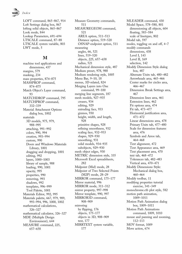
LOFT command, 865–867, 914Loft Settings dialog box, 867lofting solid objects, 865–867Look mode, 844Lookup Parameters, 691–694LTSCALE command, 87–88LTSCALE system variable, 803LWT mode, 5
Mmachine tool applications and
dimensions, 437margins, 579masking, 234mass properties, 874–875MASSPROP command,
874–875Match Object’s Layer command,
93MATCHDROP command, 795MATCHPROP command,
332–339Material Attachment Options
dialog box, 1002materials3D models, 975, 979,
988–995attaching, 991–992colors, 990, 994creation, 993–994custom, 990Doors and Windows Materials
Library, 1001dragging and dropping, 1001editing, 992layers, 1000–1003library of sample, 988loading, 990, 1001opacity, 995properties, 990removing, 993shadows, 992templates, 996–999Tool Palette, 1001
Materials Editor, 992, 995Materials palette, 667, 979, 989,
993–994, 996, 1000, 1002mathematical calculations,
326–327mathematical calculator, 326–327MDE (Multiple Design
Environment), 644MEASURE command, 225,
657–658
Measure Geometry commands,511
MEASUREGEOM command,521
AREA option, 511–513Distance option, 519–520OSNAP-endpoint option, 511
measuringangles, 66, 521lines, 519–520objects, 225, 657–658radius, 521
Mechanical dimension style, 487Medium preset, 978, 988Medium rendering style, 1005Menu Bar, 9–10, 18menus, 3D-related, 824Merging Layers into One
command, 99–100merging line segments, 187mesh models, 927–935
creases, 934editing, 929extruding face, 933gizmos, 930height, width, and length,928
primitive shapes, 928refining smoothness, 932scaling face, 932–933shapes, 929–930smoothing, 931solid models, 934–935subobjects, 929–930
mesh object edges, 930METRIC dimension style, 335Microsoft Excel spreadsheets,
282Midpoint (Mid) mode, 28Midpoint of Two Selected Points
(M2P) mode, 28–29MIRROR command, 175–177Mirror material, 996MIRROR mode, 311–312mirror property, 997–998Mirror template, 990, 997MIRROR3D command,
908–909mirroring
by flipping, 176objects, 175–177objects in 3D, 908–909text, 177
MIRRTEXT system variable,177
MLEADER command, 430Model Space, 578–580, 801dimensioning all objects, 604floating, 583–584scale of linetypes, 802
Model tab, 597modes, toggling on and off, 4–7modify commandsdimensions, 438Level I, 143Level II, 169selection, 142
Modify Dimension Style dialogbox, 487
Alternate Units tab, 480–482Arrowheads area, 465–466Center marks for circles area,
466–467Dimension Break Settings area,
467Dimension lines area, 461Extension lines, 462Fit options area, 474Fit tab, 473–477Horizontal justification area,
471–472Linear dimensions area, 478Primary Units tab, 477–480Scale for dimension features
area, 476Symbols and Arros tab,
464–468Text alignment, 472Text Appearance area, 469Text placement area, 470text tab, 468–472Tolerances tab, 482–483Vertical area, 470–471
Modify Dimensions Style:Mechanical dialog box,460–464
Modify toolbar, 11modifyng properties tutorial
exercise, 341–349monochrome.ctb plot style, 582motion path animation,
1009–1011Motion Path Animation dialog
box, 1009–1011Motion Path Animations
command, 1009, 1010mouse and panning and zooming,
112–113MOV format, 1009Move action, 674
1026 I nd e x

MOVE command, 143–144, 209,396, 593, 856, 862
Move gizmo, 929MOVE mode, 310, 316–317MOVE/COPY mode, 310–311movingobjects, 143–145press-and-drag, 145solids in 3D applications,
856MPG format, 1009MSLTSCALE system variable,
802–803MTEXT command, 249–253,
266, 272, 444Multileader Style command, 492Multileader Style Manager,
492–494, 799multileader styles, 492–494multileaders, 429–433multiline text, 250–2532D Drafting and Annotation
workspace, 258–259AutoCAD Classic workspace,
258–259bulleting, 256–257columns, 261–263editing, 267fields, 275–276height, 257identifying, 255indents, 251justifying, 254numbering, 256–257Ribbon, 258–259symbols, 260tabs, 251user-defined box, 250width, 257
Multiline Text command, 259Multiline Text Editor, 251–252,
257, 260, 266, 429, 445multiline text objects, 262–263Multiple Copy modes, 145, 315multiple crossing windows,
179–180Multiple Design Environment,
671multiple drawings, 671–673multiple editing polylines,
184–185multiple filleting, 152multiple layouts, 597–599Multiple lines mode, 711, 718multisided viewports, 793–794
NName and Expression format, 560Name format, 560Name state, 74named objects, 652–653Named plot styles, 630Named UCS command, 836named views, 120–124Named Views command, 120Nearest (Nea) mode, 29nested items, purging, 653NEW command, 15New Dimension Style: Mechani-
cal dialog box, 459New Dimension Style: Mechani-
cal: Leader dialog box, 488New Group Filter command, 90New Material dialog box, 996New Page Setup dialog box, 581,
589New Palette command, 668New Property Filter command, 89New Text Style dialog box, 273New View dialog box, 1004New View/Shot Properties dialog
box, 121–122, 1006New VP Freeze state, 75Node (Nod) mode, 29nodes, snapping to, 29nonassociative dimensions,
484–486Normal boundary style, 399notes, scaling, 580numbered lists, 257numbering text, 256–257
Oobject grip modes, 306–317object grips, 304–306Object layer, 354, 626object lines, 71–72Object Scale command, 801object segments, 207Object Selection Cycling
command, 130Object Snap Extension mode, 40Object Snap From mode, 26Object Snap Intersection mode, 26object snaps, 401objectsaligning, 831, 903–905arraying in 3D, 909–910break point, 167
breaking, 166–169constraints, 558–559copying, 95–96, 145–146,
157–160, 310–311, 673copying and flipping, 175cutting, 161, 673cycling through, 130deselecting, 130displaying, 664dividing into equal spaces, 224double-clicking, 331erasing, 49–50exploding, 185extending, 163–166freezing and thawing, 74imprinting, 895information about, 319, 326,
523joining, 181, 187layers, 93–94, 100–101leader, 429lengthening, 186–187lines tangent to, 31–32locking, 23–24, 74, 83, 557masking, 234measuring, 225, 657–658mirroring, 175–177, 311–312,
908–909moving, 143–145, 309, 319,
328–330, 902moving and copying, 316–317offsetting, 157–160, 375–376partially deleting segment,
166–169pasting, 673point of displacement, 143polylines, 183, 514pre-highlights, 126pre-selecting, 130–131properties, 318, 332–340proportionally, 147–148rectangular or circular patterns,
170reference edge, 417rotating, 148–150, 312–313,
905–908rotating and copying,
314–316scaling, 146–148, 309–310selecting, 50, 126–128selecting tutorial exercise,
132–141selection sets, 125–129sharp corners, 150snapping, 27–28, 30
I nd e x 1027

objects (continued )stretching, 177–180temporary path extending from,
26trimming, 160–163zooming, 117
obscured lines, 965OFFSET command, 159–160,
183, 351, 353, 355, 370,372–373
offset snap location mode,315–316
Offset Snap Locations mode,316–317
offsets, 26–27, 158–159,159–160, 372–373
offsettingby distance, 158–159faces, 920lines, 158objects, 157–160polyline objects, 183through point, 157–158
ogee curve, 236–237On/Off state, 74One View Drawing icon, 589one-view drawings, 350–351opacity, 995OPEN command, 16, 671Open dialog box, 609Open Documents command, 17Open Xref command, 763operations, undoing and redoing,
188Options command, 3, 305Options dialog box, 3, 8, 14,
305, 401Orbit mode, 844Ordered List icon, 17Ordered List Panel, 17–18ordinate dimensions, 435–437Ordinate mode, 420–421origins, 43, 827–829ORTHO mode, 4, 5, 34, 175,
436, 856Ortho_Drawings.ctb plot style, 631orthogonal drawings, 235orthogonal lines, 33orthogonal mode, 842orthographic block tutorial
exercise, 358–360orthographic views, 957–958Orthographic Views layout, 629OSNAP (Object Snap) modes,
4–5, 23–25, 956
continuously running, 32–33Deferred Tangent mode, 31Endpoint (End) mode, 25–26entering at keyboard, 32Extended Intersection (Int)mode, 28
Extension (Ext) mode, 26From (Fro) mode, 26–27Insert (Ins) modes, 27Intersection (Int) mode, 27Midpoint (Mid) mode, 28Midpoint of Two SelectedPoints (M2P) mode, 28–29
Nearest (Nea) mode, 29Node (Nod) mode, 29Object Snap Tracking(OTRACK) mode, 38–39
Parallel (Par) mode, 30Perpendicular (Per) mode, 30Quadrant (Qua) mode, 30reactivating, 33selecting from shortcut menu,32
Tangent (Tan) mode, 31–32OSNAP command, 862OSNAP-Center mode, 522OSNAP-Insert mode, 522OSNAP-Midpoint mode, 522OSNAP-Node mode, 522OSNAP-Tangent mode, 211, 217OSNAP-Tracking mode, 856OTRACK (Object Snap
Tracking) mode, 4, 5, 38–39Outer boundary style, 399Outside mode, 759OVERALL style, 492OVERALL view, 123Overhead Light, 986overshoots, 209
PPage Setup dialgo box, 621Page Setup dialog box, 581, 589Page Setup Manager, 581, 583,
589–590Page Setup Manager command,
581, 589pages, 581–583palettes, 13
3D-related, 824transparency controls, 670
PAN command, 119, 585panning
drawings, 119
images, 585mouse, 112–113
paper sizes, 581–582, 623Paper Space, 578, 583, 788, 838architectural drawings, 595frozen layers, 785hatch pattern, 606–607linear dimensions, 605linetype scaling, 803linetypes, 802lineweights, 627multiple layouts, 597–599plotting from layout, 622–624scaling image to, 584–585title block, 592
Paper Space viewports, 956Paragraph dialog box, 261paragraphs, 254–255, 261Parallel (Par) mode, 30Parallel constraints, 549–551parallel lines, 30, 153Parameter and Action item, 678parameters, 543, 560–562dynamic blocks, 678–682endpoint, 679renaming, 683starting point, 679value set properties, 682–684
Parameters Manager command,560
Parameters Manager dialog box,696
Parameters Manager palette,561–562
parameters tutorial exercise,570–576
parts, variations on, 694–696Paste Special command, 282Paste Special dialog box, 282PASTEBLOCK command, 673PASTECLIP command, 673pattern1 tutorial exercise, 243–248PC2 files, 621, 630PC3 format, 621PCP files, 621, 630PCX format, 977, 1004PDF documents, 619PEDIT command, 180, 181–184,
207, 208, 512, 514pen assignments, 621Perpendicular (Per) mode, 30Perpendicular Alignment
Parameter, 685–686Perpendicular constraints,
549–551
1028 I nd e x

perpendicular projector lines, 371phantom lines, 72PHANTOM linetype, 79photometric lights, 981pickadd button, 326Piston Support Parts material,
998–999pivot axis rotation angle, 830–831pivot point, 906PLAN command, 839Plan view, 982PLINE command, 18, 47–48, 512Plot command, 622plot devices, 589Plot dialog box, 580, 621–624,
628, 634Plot state, 75plot style, 581, 630Plot Style Manager command, 630Plot Style state, 75Plot Style Table Editor dialog box,
632Plot style tables, 582, 623plot style tables, 629–635plot styles, 75, 623, 630Plot Styles dialog box, 630, 633plots, enhancing with lineweights,
625–629plotted scale layouts, 582plotter documentation, 620Plotter Manager command, 619plotter manufacturer, 620plotterschoosing, 581configuring, 619–622verifying, 634
Plotters program group, 619, 622plottinginformation, 621layers, 75layouts, 622–624, 636multiple copies, 623orientation, 623paper size, 623previewing, 624
Plotting the Display mode, 623PNG format, 637, 639, 977, 1004POINT command, 223Point Light, 980point lights, 983–986point of displacement, 143, 178Point Style command, 223Point Style dialog box, 223–225,
236Pointer Input, 71
pointsabsolute coordinate listing, 522acquired, 38–39creation, 223identifying location, 223setting style, 223shape, 224size, 224snapping, 28–29, 223style, 224
polar arrays, 170, 173–174,909–910
Polar Coordinate mode, 43–44polar coordinates, 21, 43–44, 178polar distance, 36POLAR mode, 5, 34polar snaprelative polar angle, 37–38setting value, 35–37
Polar Tracking mode, 4, 33–35POLYGON command, 226polygons, 226–227polyline objectsarc segments in sequence,230–232
dividing into equal segments,224
offsetting, 183Polyline property, 337–338polylinesarea, 512–513as single object, 47chamfering, 156constructing, 47–49curve generation, 181–182dimensional constraints, 548Dynamic Input, 49editing, 180–185exploding, 185filleting, 153fit curves, 182geometric constraints, 548joining, 181, 184linetype generation of, 182–183multiple editing, 184–185properties, 337–338rounding corners, 153splines, 181–182width, 47, 180
POLYSOLIDcommand, 870–872polysolids, 870–872Position Locator palette, 1008pre-existing workspaces, 4pre-highlights, 126pre-selecting objects, 130–131
precision drawing Cartesiancoordinates, 41–42
predefined workspaces, 823preloading linetypes, 82Presentation rendering, 976presets, 975press-and-drag copying, 146press-and-drag moving, 145pressing and pullingblocks, 898–901bounding areas, 896–898
PRESSPULL command,896–901
Preview and Post dialog box,642–643
Preview model, 628
previewinganimation, 1009, 1011blocks, 647dimensions, 459drawings, 607–609hatch patterns, 387plotting, 624rectangular pattern, 171web pages, 642
primary dimension units, 478primitivesbox primitives, 850changing height, 892composite solid, 852–853cone primitives, 851creation, 849–852cylinder primitives, 851editing, 894intersection, 853, 855joining or uniting, 853–854mesh models, 928pyramid primitives, 852removing or subtracting,
853–855sphere primitives, 851torus primitives, 851–852wedge primitives, 850–851
printable area, 579printed drawings appearance, 582propertiesattributes, 723Block Reference object type,
323blocks, 667–668colors, 632–633hatch patterns, 401Layer Control box, 328–330Line object type, 323
I nd e x 1029

properties (continued )listing, 321–322matching, 332–340materials, 990modifying, 318, 321–322selection set, 322–325viewports, 795–796
Properties command, 667–668, 683Properties Palette, 318–320,
324–325, 326, 331, 683, 686,688–689, 692, 732–733, 802,979, 985
Properties toolbar, 11, 85Properties Window, 492Property Lookup Table dialog
box, 693Property Settings dialog box, 333PSLTSCALE system variable, 802Publish command, 635Publish dialog box, 635–637Publish to the Web utility,
637–643Publish to Web command, 638Publish to Web wizard, 638publishingmultiple drawing sheets,
635–637to the Web, 637–643
Pump Assembly tutorial exercise,285–294
PURGE command, 653Purge dialog box, 653PYRAMID command, 852pyramid primitives, 852pyramids, 852
QQDIM command, 418–421QLEADER command, 428–429,
444QNEW command, 15, 16QSAVE command, 50, 51QSELECT (Quick Select)
command, 131–132Quadrant (Qua) mode, 30quadrants, 30Quick Access Toolbar, 1, 12Quick Properties (QP) mode, 4–6Quick Properties command,
331–322Quick Properties palette, 321, 930Quick Select dialog box, 131–132,
323–325, 329, 330Quick Set command, 322
Quick View Drawings, 607, 609Quick View Layouts, 589, 607–608Quick View Layouts and
Drawings, 7Quick View Layouts command,
581Quick View tool, 607–608QuickCalc command, 326QuickCalc dialog box, 327
RR14 format, 51radius, 150–151radius dimensions, 421–423, 447Radius mode, 46raster image formats, 977raster images, 764–770ray construction line, 227ray tracing, 1000real time zooming, 113Realistic template, 994Realistic visual style, 975Realtime mode, 113Realtime PAN command, 113Realtime PAN mode, 112Realtime ZOOM command, 113reassociating dimensions, 485–487Recent Actions command, 17Recent Actions panel, 9Recent Documents command, 17Recent Documents mode, 9RECTANG command, 228–230rectangles, 228–230rectangular arrays, 170–173,
909–910rectangular coordinate system, 41rectangular pattern, previewing,
171Red Metal material, 993REDO command, 188redoing operations, 188Refedit toolbar, 755–756reference edge, 417Reference Edit dialog box, 755,
763reference point, 26–27Reference toolbar, 764–766Refine Mesh command, 932Refine Mesh mode, 931REGEN command, 803regions, 859, 862regular polygon, 226–227Relative Coordinate mode, 43relative coordinates, 21, 43
relative polar angle, 37–38Reload command, 762Remove All command, 636Remove Viewport Overrides
command, 602RENAME command, 658Rename command, 667Rename dialog box, 966Rename Tool Palette command,
668renamingblocks, 658drawings, 51
Render panel, 978render window, 976rendered images, 977rendering commands, 974rendering modes, 975renderings, 973–9753D Modeling workspace, 978backgrounds, 1003draft mode, 975lights, 980–988listing, 976Medium rendering style, 992,
1005overview producing, 975–979presets, 975quality, 975shadow effects, 976
Reset mode, 711resistors tutorial exercise, 734–736REVCLOUD command,
230–232Reverse curve, 236–237reverse selection set, 132revision cloud, 230–232REVOLVE command, 862–863revolving solid object about axis,
862–863Rewind mode, 844RGB (Red, Green, and Blue)
model, 78Ribbon3D Modeling panel, 9533D Modeling workspace, 824accessing commands, 1basic drawing tools, 18display modes, 12Materials panel, 979Mesh Modeling tab, 928–929multiline text, 258–259Render tab, 975View tab, 825Visualize tab, 824
1030 I nd e x
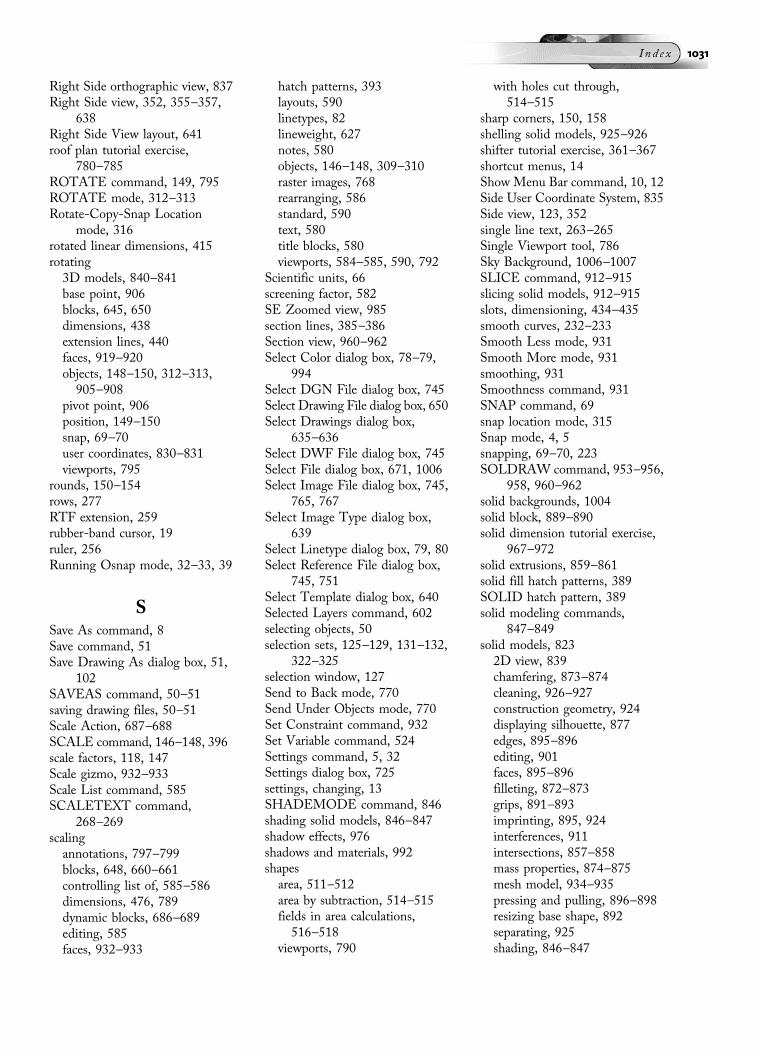
Right Side orthographic view, 837Right Side view, 352, 355–357,
638Right Side View layout, 641roof plan tutorial exercise,
780–785ROTATE command, 149, 795ROTATE mode, 312–313Rotate-Copy-Snap Location
mode, 316rotated linear dimensions, 415rotating3D models, 840–841base point, 906blocks, 645, 650dimensions, 438extension lines, 440faces, 919–920objects, 148–150, 312–313,
905–908pivot point, 906position, 149–150snap, 69–70user coordinates, 830–831viewports, 795
rounds, 150–154rows, 277RTF extension, 259rubber-band cursor, 19ruler, 256Running Osnap mode, 32–33, 39
SSave As command, 8Save command, 51Save Drawing As dialog box, 51,
102SAVEAS command, 50–51saving drawing files, 50–51Scale Action, 687–688SCALE command, 146–148, 396scale factors, 118, 147Scale gizmo, 932–933Scale List command, 585SCALETEXT command,
268–269scalingannotations, 797–799blocks, 648, 660–661controlling list of, 585–586dimensions, 476, 789dynamic blocks, 686–689editing, 585faces, 932–933
hatch patterns, 393layouts, 590linetypes, 82lineweight, 627notes, 580objects, 146–148, 309–310raster images, 768rearranging, 586standard, 590text, 580title blocks, 580viewports, 584–585, 590, 792
Scientific units, 66screening factor, 582SE Zoomed view, 985section lines, 385–386Section view, 960–962Select Color dialog box, 78–79,
994Select DGN File dialog box, 745Select Drawing File dialog box, 650Select Drawings dialog box,
635–636Select DWF File dialog box, 745Select File dialog box, 671, 1006Select Image File dialog box, 745,
765, 767Select Image Type dialog box,
639Select Linetype dialog box, 79, 80Select Reference File dialog box,
745, 751Select Template dialog box, 640Selected Layers command, 602selecting objects, 50selection sets, 125–129, 131–132,
322–325selection window, 127Send to Back mode, 770Send Under Objects mode, 770Set Constraint command, 932Set Variable command, 524Settings command, 5, 32Settings dialog box, 725settings, changing, 13SHADEMODE command, 846shading solid models, 846–847shadow effects, 976shadows and materials, 992shapesarea, 511–512area by subtraction, 514–515fields in area calculations,516–518
viewports, 790
with holes cut through,514–515
sharp corners, 150, 158shelling solid models, 925–926shifter tutorial exercise, 361–367shortcut menus, 14Show Menu Bar command, 10, 12Side User Coordinate System, 835Side view, 123, 352single line text, 263–265Single Viewport tool, 786Sky Background, 1006–1007SLICE command, 912–915slicing solid models, 912–915slots, dimensioning, 434–435smooth curves, 232–233Smooth Less mode, 931Smooth More mode, 931smoothing, 931Smoothness command, 931SNAP command, 69snap location mode, 315Snap mode, 4, 5snapping, 69–70, 223SOLDRAW command, 953–956,
958, 960–962solid backgrounds, 1004solid block, 889–890solid dimension tutorial exercise,
967–972solid extrusions, 859–861solid fill hatch patterns, 389SOLID hatch pattern, 389solid modeling commands,
847–849solid models, 8232D view, 839chamfering, 873–874cleaning, 926–927construction geometry, 924displaying silhouette, 877edges, 895–896editing, 901faces, 895–896filleting, 872–873grips, 891–893imprinting, 895, 924interferences, 911intersections, 857–858mass properties, 874–875mesh model, 934–935pressing and pulling, 896–898resizing base shape, 892separating, 925shading, 846–847
I nd e x 1031

solid models (continued )shelling, 925–926slicing, 912–915system variables, 875–877terrain modeling, 914–915viewing, 956
solid objectsbased on cross sections,
865–867coordinate system, 832creation from solids, 912–915cutting plane, 912dragging, 889–890editing features, 916–917extruding face, 861hidden line removals, 876–877lofting, 865–867revolving about axis, 862–863sliced by surface, 913–914subobjects, 893–894sweeping, 863–865unioning, 855–856
solid primitivesBoolean operations, 852–853creation, 849–852moving, 856subtracting from, 857tessellation lines, 875–876unioning, 855–856
SOLIDEDIT command, 916Clean (Body Editing) option,
926–927Copy Face option, 923Delete Face option, 922Extrude Face option, 924Extrude option, 917–918Move option, 918Offset Face option, 920Rotate Face option, 919–920Separating Solids option, 925Shell option, 926Taper Face option, 921
SOLVIEW command, 953–956,959–962
Southeast Isometric view, 985spacing dimensions, 423–424Specify Zip File dialog box, 764SPELL command, 271spell-checking text, 270–271SPHERE command, 851spheres, 851SPLINE command, 232–233, 377splinescontinuous segment, 232creation, 232–233
edge faces, 914generating from polylines,181–182
leader lines, 429Spotlight, 980, 987Staggered mode, 419–420STANDARDdimension style, 335standard scales, 590STANDARD style, 273Standard style, 458Standard toolbar, 10–11, 13states and layers, 73–75, 91–92status bar, 4–7, 583Status Bar menu tool, 7Status command, 524Status state, 74STB (Named) plot style, 630steering wheel, 844Steering Wheel Settings dialog
box, 844Stretch Action, 674, 680, 688, 690Stretch Action (Stretch Right)
parameter, 692STRETCH command, 177–180,
396, 438Stretch Grip, 676Stretch icon, 681STRETCH mode, 309, 446stretching, 177–180
dimension text, 446dynamic blocks, 676viewports, 585
STYLE command, 272–274styles
changing, 274overriding dimension style,489–490
tables, 282text, 251, 272–274
Styles toolbar, 11, 274Subobject panel, 929subobjects
grips, 893–894mesh models, 929–930
SUBTRACT command,852–855, 857, 863–864, 895,925
Subtract mode, 514subtracting
inner shape from outer shape,864
solids, 857sun, 981sunlight study tutorial exercise,
1011–1015
surface, 913–914SWEEP command, 863–865sweep profile, 863–864swept solid, 863–865Symbol dialog box, 442–443symbols, 260, 442–443Symmetrical tolerance, 483system variableschanges to, 524controlling attributes, 711–712solid models, 875–877
TTABLE command, 277–278Table property, 339Table Ribbon, 28–279Table Style dialog box, 283table summations tutorial exercise,
299–303table tutorial exercise, 295–298Table Width parameter, 683–684,
689–690tablesautofilling cells, 280–281blocks and, 659–660cells, 278columns, 277, 280creation, 277–281dynamic blocks, 691–694grips, 280manipulating, 279merging cells, 279–280Microsoft Excel spreadsheets,
282modifying, 280moving, 280positioning, 278properties, 339–340rows, 277styles, 282text, 255title, 278
Tablet mode, 6tabs, 251, 255–256Tangent (Tan) mode, 31–32Tangent constraints, 555–556tapering faces, 921template files, 101–107templates, 737, 990, 996–999Temporary Tracking Point tool,
40–41temporary tracking points, 40–41terrain modeling, 914–915tessellation lines, 875–876
1032 I nd e x

textannotative scales, 804–808autofilling, 281backwards and unreadable, 177bulleting, 256–257columns, 261–263controls, 252–253dimensions, 438editing, 266–268fields, 274–276fonts, 251, 267globally modifying, 268–270height, 251, 264identifying, 255importing, 259–260JIS (Japan International
Standard), 470leaders, 429linetypes, 80lists, 255–257mirroring, 177multileaders, 433multiline, 250–253numbering, 256–257paragraphs, 261properties, 335rotation angle, 264RTF extension, 259scaling, 7, 580single line, 263–265spell-checking, 270–271start point, 264stretching, 446styles, 251, 272–274symbols, 260tables, 255tabs, 255–256TXT extension, 259
text commands, 249–250Text Editor Ribbon, 251–253, 257Text Formatting dialog box, 254Text Formatting toolbar, 718, 720text objects, 268–269Text property, 335–336Text Style dialog box, 273TGA format, 977, 1004Thaw state, 74themes, 640thick lineweights, 80–81third-party color books, 79three-view drawings, 355–357through point, 157–158tick marks, 683–684TIF format, 977, 1004tile drawing exercise, 199–202
Time command, 524Title Block layer, 626title block tutorial exercise,
712–717title blocks, 580, 592Title cells, 284titles for tables, 278TOLERANCE style, 492tolerances, 441–443, 482–483Tool Palette, 2, 13, 644, 666–669disciplines, 3dynamic blocks, 674inserting blocks, 666–670lights, 981listing, 667materials, 1001Metals - Materials Sample tab,991
opaqueness, 670Tool Palettes command, 13Tool Properties dialog box, 668Toolbar Unlocking tool, 7toolbars, 2, 10–12Tools menu, 15tools, accessing, 8tooltips, 34Top orthographic view, 837Top User Coordinate System, 834Top view, 123, 352–357, 961Top View layout, 638, 641torus, 851–852TORUS command, 852Tracking mode, 856tracking paths, 33–35, 40tracking points, 40–41Transparency command, 668, 670Transparency dialog box, 668,
670Tree View, 663–664trigonometric functions, 327TRIM command, 160–163,
165–166, 211–215, 217, 237,351, 353–354, 395, 651
trimmingcrossing box, 161–162fill patterns, 394–395floor plan exercise, 163individual cutting edges, 160objects, 160–163selecting all objects, 161
true colors, 78Turn Object’s Layer Off
command, 98two-view drawings, 352–354TXT extension, 259
UUCS (User Coordinate System),
420alignment (translation and
rotation), 831automatically switching plane
of, 833–836creation, 825–827current view, 956default command sequence,
827–828defining X-axis while dynami-
cally locating, 834dimension calculations, 435listing, 836naming position, 834–836origin, 827–828, 829renaming, 837retrieving previously saved,
836–837rotating, 837saving, 837views, 954X- and Y-axes (translate and
rotate), 829UCS (User Coordinate System)
icon, 578–579, 583–584,825–826, 837–838
UCS command, 8253point option, 829Dynamic UCS mode, 833–836Face option, 832Object option, 831Origin option, 436, 827–828Restore option, 836Save option, 836View option, 832, 956X/Y/Z rotation options,
830–831UCS dialog box, 836–837UCS Icon command, 837UCSFOLLOW system variable,
839UCSICON command, 579,
827–828UNDO command, 188undoing operations, 188Unicode Character Mapping
dialog box, 444UNION command, 852–853,
855–856, 861, 891, 895unioning solids, 855–856Unisolate Object’s Layer
command, 95
I nd e x 1033

Units command, 65units, converting, 327Unload command, 761Unlock Object’s Layer command,
99Unlock state, 74unselected grips color, 305Up/Down mode, 844Update Fields command, 276updating fields, 276user coordinates, 830–831user-defined color books, 79user-defined viewports, 580
Vvacuum attachment tutorial
exercise, 882–888Value format, 560value set properties, 682–684VCLIP command, 791Verify mode, 711Vertical constraints, 548–549vertical dimensions, 413View Center, 954VIEW command, 985View Manager dialog box,
120–124, 985, 1003, 1005,1007
View Options command, 668View Options dialog box, 668View toolbar, 845ViewCube, 837, 841–844ViewCube Settings command, 842ViewCube Settings dialog box, 842Viewport Overrides, 602Viewport property, 338–339viewportscircles, 792color, linetype, or lineweight
overrides, 602creation, 786, 790–794dimensions, 605–606freezing layers, 600grips, 591image scaled to, 590images, 785images scaled to, 788–789layer tools affecting, 601–604layers, 593, 785–790layouts, 580, 583locking, 586matching properties, 338–339,
795–796maximizing, 586–588
Model Space, 580moving, 593multiple, 580multisided, 793–794not plotting, 593resizing, 591rotating, 795scaling, 476, 584–585, 590, 792shapes, 790stretching, 585user-defined, 580views, 954
Viewports dialog box, 790Viewports layer, 593Viewports toolbar, 790views
associating backgrounds, 1004auxiliary, 368–372, 958–960based on responses to prompts,954
correct set, 352different, 779–785dimensions, 956drawing in two dimensions, 955features, 356isometric, 962–964naming, 954orthographic, 957–958placement, 954scale value, 954section, 960–962space between, 355transferring distances, 372–373User Coordinate Systems, 954viewports, 954
Visibility Normal mode, 721Visibility Off mode, 721Visibility On mode, 721Visibility states, 676visual Object Snaps, 304visual styles, 823, 846–847Visual Styles Manager palette,
847Visual Styles toolbar, 846VP (Viewport) Scale, 799VPMAX command, 586VPORTS command, 791VPORTS layer, 956, 958VPROTATEASSOC system
variable, 795
WWalk mode, 844walking action, 1008
WBLOCK command, 646–648WCS (World Coordinate
System), 828, 838web pages, 638–642web template, 640Web, publishing to, 637–643WEDGE command, 850wedges, 850–851Window selection mode, 312Window/Crossing selection mode,
312windows, selecting objects by,
127WIPEOUT command, 234wipeout frames, 234WMV format, 1009Workspace Switching icon, 3Workspace Switching tool, 7workspaces, 1, 3–4, 823Workspaces toolbar, 3, 10, 823
XX, Y coordinates, 42X-axis, 831XBIND command, 753XCLIP command, 759–760,
763XLINE command, 235, 369,
371, 374Xlines, 235, 369, 371–372XREF command, 744XY plane, 519–520, 832, 839
ZZOOM command, 10, 110–119Zoom toolbar, 110ZOOM-All command, 68ZOOM-Extents appearance,
584ZOOM-Previous command,
117zoomingautomatically, 118–119drawing limits, 114–115extents of image, 115magnifying area of drawing,
116mouse, 112–113objects, 117real time, 113returning to previous display,
117scale factors, 118
1034 I nd e x