Australian Water Resources Assessment 2012 - Bureau of ...
777
Australian Water Resources Assessment 2012
-
Upload
khangminh22 -
Category
Documents
-
view
1 -
download
0
Transcript of Australian Water Resources Assessment 2012 - Bureau of ...

Australian Water Resources Assessment 2012

Published by the Bureau of Meteorology
GPO Box 1289, Melbourne VIC 3001 Tel: (03) 9669 4000 Fax: (03) 9669 4699 Email: [email protected] Website: www.bom.gov.au
The report, a summary document and other information about the Australian Water Resources Assessment 2012 are available at: www.bom.gov.au/water/awra/2012
The Bureau of Meteorology welcomes feedback on this report.
Find out more about the Bureau of Meteorology’s Water Information role at: www.bom.gov.au/water
ISBN: 978 0 642 70641 6
With the exception of logos and certain third party material, the Australian Water Resources Assessment 2012 is licensed under the Creative Commons Australia Attribution 3.0 Licence.
© Commonwealth of Australia 2013
Photographs © Individual copyright holders 2013
Attribution for third party material included in the 2012 Assessment is available here: www.bom.gov.au/water/awra/2012/copyright.shtml
Cover image and above: Larnebarramul Swamp, Victoria | Alison Pouliot
ContentsForeword
1 Introd uction
2 National overview
3 North East Coast
4 South East Coast (NSW)
5 South East Coast (Victoria)
6 Tasmania
7 Murray–Darling Basin
8 South Australian Gulf
9 South Western Plateau
10 South West Coast
11 Pilbara–Gascoyne
12 North Western Plateau
13 Tanami – Timor Sea Coast
14 Lake Eyre Basin
15 Carpentaria Coast
Technical supplement
Ref erences
1Australian Water Resources Assessment 2012

2 Australian Water Resources Assessment 2012
IntroductionForeword
Foreword
The Commonwealth Water Act 2007 created a number of additional functions for the Bureau of Meteorology (the Bureau), including the provision of ‘regular reports on the status of Australia’s water resources and patterns of usage of those resources’.
The Australian Water Resources Assessment 2012 (the 2012 Assessment) is the second of these reports. It presents assessments of Australia’s water resources and climatic conditions in 2011–12 and discusses regional variability and trends in water resources and patterns of water use over seasons, years and decades. It extends the content presented in the first assessment report (2010 Assessment) by including additional information about streamflow salinity, land use, population, soil types, physiographic regions, rainfall zones and rainfall deficits.
The Bureau’s water resources assessments are repeated on a regular basis (currently every two years), with a focus on consistency in reporting of particular streams of modelled and measured water resources data. The 2012 Assessment is intended to assist understanding of the impact and sustainability of current water management practices and inform the design of water resource policies and plans. This will support the goals of the National Water Initiative and contribute to the water reform agenda.
The 2012 Assessment uses data provided from organisations across the country and research outputs of the Bureau’s Water Information Research and Development Alliance with CSIRO. It has required significant effort from a large number of people and I am proud of the dedication and professionalism of the teams involved.
Graham Hawke
Deputy Director Environment and Research Division Bureau of Meteorology
September 2013

Introduction1. Introduction 4
1.1 Background ....................................................... 4
1.2 Scope and purpose ........................................... 4
1.3 Focal questions .................................................. 5
1.4 Assessment approach ....................................... 6
1.4.1 Reporting units ....................................... 6
1.4.2 Reporting period ..................................... 7
1.4.3 Landscape water balance ....................... 7
1.4.4 Mapped rainfall data ............................... 8
1.4.5 National landscape water
balance modelling ................................... 8
1.4.6 Percentiles, deciles and anomalies .......... 9
1.4.7 Flood classification analyses ................. 11
1.4.8 Trend analyses ..................................... 11
1.4.9 Site-based anomaly and
time-series analyses ............................. 11
1.5 Quality control and review: Who was involved? 14
1.6 Terminology ..................................................... 14
1.7 Future reports .................................................. 14

4 Australian Water Resources Assessment 2012
Introduction
1. Introduction1.1 Background
The Commonwealth Water Act 2007 gave the Bureau of Meteorology (the Bureau) responsibility for compiling and delivering comprehensive water information across Australia. This includes conducting timely, rigorous and independent assessments of the status of Australia’s water resources.
The Bureau’s first national water resources assessment was published in 2011 for the 2009–10 year (July 2009–June 2010). It built on earlier assessments undertaken by various Australian Government agencies and partners at irregular intervals over the last 50 years, each with a slightly different purpose and approach.
The Bureau’s water resources assessments are undertaken at regional and national spatial scales and time scales ranging from months to decades. These reports are intended to assist assessment of the impact and sustainability of current water management practices and inform the design of future water resource plans, supporting the goals of the National Water Initiative and contributing to the water reform debate.
The Bureau’s water resources assessments provide:
1. consistency in reporting across the nation and over time, enabling spatial and temporal comparisons of water resources by end users;
2. free access to water information via the web;
3. comparable information at regional and national scales;
4. a high level of transparency about the information and data used, and the modelling and analysis techniques employed;
5. scientifically robust analyses of changes in water availability, quality, and use over time-scales of months to decades; and
6. a presentation of Australia’s water resources without reference to jurisdictional boundaries.
1.2 Scopeandpurpose
The Australian Water Resources Assessment 2012 (the 2012 Assessment) presents assessments of Australia’s climate and water resources over the 2011–12 year (July 2011–June 2012). It discusses regional variability and trends in water resources and patterns of water use over recent seasons, years and decades, using currently accessible data.
The 2012 Assessment is focused on aspects of national and regional water availability rather than water allocation, trading or quality (though salinity of surface streamflow and groundwater is included). Water use is addressed for various selected urban centres and irrigation schemes.
The 2012 Assessment includes the:
• Introduction;
• National Overview;
• 13 regional assessments;
• Glossary;
• Technical Supplement; and
• References.
A summary report and the data used to develop the figures is available from the Bureau’s website.
The National Overview provides a continent-wide assessment of climate and water flows and stores across Australia in 2011–12. This includes national landscape water balance model outputs for the year, including rainfall, evapotranspiration, landscape water yield and change in soil moisture, as well as consideration of changes in surface water storage in each region. The National Overview examines important Australian climate drivers and their impact on rainfall over the year. It also provides an overview of urban and agricultural water use in 2011–12 for selected areas. Information on relevant nationally significant weather and flooding experienced in 2011–12 is also presented.
The regional chapters highlight changes in water availability and use in 13 regions that cover the Australian continent and Tasmania. Analyses presented include climate impacts on water resources over 2011–12 and also in recent decades (1980–2012). Modelled regional spatial data and time series data from selected monitoring sites provide more detail at particular locations.
With each assessment the same sites are used for data analysis. As new data becomes available the data used in analyses is updated for these selected sites. This allows clear comparisons to be made between assessments.

5Australian Water Resources Assessment 2012
Finally, the Technical Supplement provides background on the landscape water balance modelling techniques, methods, the data and the analyses used to generate information in the report.
Information and data provided in the 2012 Assessment reflect the quantity and quality of data currently available for analysis. It is expected that as data supplied to the Bureau under the Water Act and the Water Regulations 2008 are further stored, standardised and quality assured by the Bureau, analysis and reporting will be enhanced. Feedback from users will also be used to improve future reports in terms of methods used, interpretation and content.
1.3 Focalquestions
The 2012 Assessment aims to provide information to help address a variety of questions at a range of spatial and temporal scales subject to the availability of appropriate data. The scales vary from national in the National Overview to regional and local in subsequent chapters. Time scales also vary depending on the data used and the intent of the
analysis. The types of questions addressed include:
1. Which ocean and atmospheric circulation patterns influenced rainfall in different parts of the country in 2011–12? (section 9 in the National Overview).
2. How much of the rainfall received in 2011–12 ended up in rivers and groundwater and how does this compare with the past? (section 3 in the National Overview; section 4 in the regional chapters)
3. Was there any significant flooding or dry periods in 2011–12 as a result of particular weather conditions? (section 11 in the National Overview; section 5 in the regional chapters)
4. How much of the rainfall received in 2011–12 was evaporated or used by plants and how does this compare with the past? (section 3 in the National Overview; section 4 in the regional chapters)
5. How moist were soil profiles across the country in 2011–12 and how does this compare with the past? (section 4 in the National Overview; section 7 of the regional chapters)
6. Are there any regional trends evident in seasonal rainfall, evapotranspiration, soil moisture, landscape water yield or groundwater levels? (sections 4, 5 and 7 in the regional chapters)
7. How do seasonal inflows to and outflows from selected nationally significant wetlands vary from year to year and are they changing? (section 5 in the regional chapters)
Tyto wetlands, near Townsville | Andrew Rankin (Queensland Image Gallery)

6 Australian Water Resources Assessment 2012
Introduction
8. Where does the water for cities and irrigation areas come from and is this changing? (sections 6 and 7 in the regional chapters)
9. What seasonal to decadal patterns and trends are evident in water storage inflows and volumes, and in groundwater levels, particularly in relation to rainfall? (sections 5, 6 and 7 in the regional chapters)
10. How does water use in cities and irrigation areas vary from year to year, particularly in relation to water availability? (sections 6 and 7 in the regional chapters)
1.4 Assessmentapproach
The techniques used to produce the 2012 Assessment are explained in this section. The descriptions provide context to the information presented in the regional chapters.
Further information about the methods used to derive and analyse water and climate data is provided in the Technical Supplement.
1.4.1 Reporting units
The 2012 Assessment report is structured around 13 regions covering the Australian continent and Tasmania that are based on drainage division boundaries (Figure 1.1).
Drainage divisions represent the catchments of major surface water drainage systems, generally comprising a number of river basins. Drainage divisions provide a scientifically robust framework for assessing hydrological flows in the landscape while also allowing information to be presented and discussed in broadly identifiable biophysical regional and climatic contexts.
In Australia, 12 drainage divisions were first defined in the 1960s by the Australian Water Resources Council and the boundaries were formally published in the 1990s (Hutchinson and Dowling 1991). They were recently modified by the Bureau and its research partners at Geoscience Australia and the Australian National University, based on the most current topographical data. This dataset is described in the Geofabric Product Guide (The Bureau 2013b).
In the new drainage divisions, the South East Coast has been split into two regions to distinguish New South Wales coastal river basins from Victorian and
Figure1.1 2012Assessmentreportingregions

7Australian Water Resources Assessment 2012
Figure1.2 Waterbalancetermsreportedoninthe2012Assessment
GroundwaterextractionsGroundwater
extractions
Desalination
Recycling
Surface waterdiversion
Soilmoisture
Base flow
Transpiration Evaporation
Rainfall
Surface water storage
Agricultural water use
Surface waterdiversion
Surfacerunoff
Streamflow
Inflows towetlands
Urbanwater use
Groundwaterlevels
southeastern South Australian coastal river basins (Figure 1.1), to further establish a manageable heterogeneity within and between reporting units.
Within the reporting regions shown in Figure 1.1, various time-series analyses and reporting techniques have been applied depending on the availability of data. Analysis and reporting units at the sub-regional level include hydrological units (surface catchments and groundwater aquifers), water management and planning areas, water supply systems and monitoring sites or clusters of sites (for example, stream gauges on tributaries flowing into a reservoir).
1.4.2 Reporting period
The data and information presented focuses on the 12 months from July 2011 to June 2012 and/or months and seasons therein. Time-series analyses are restricted to consideration of data from 1980, in order to place the 2011–12 period in the context of the variability and trends in recent decades, with the exception of the landscape water balance flows, which are related to the rainfall data and generated model results from 1911 onwards.
Trends in groundwater levels for major aquifers in the regions are reported for the past five years (2007–08 to 2011–12).
1.4.3 Landscape water balance
Water balances are used as a consistent and repeatable means of reporting on water availability. A water balance has a number of standard variables:
• inflows, for example, rainfall;
• outflows, for example, evaporation, transpiration, run-off; and
• change in storage, for example, soil moisture.
Key terms used in the 2012 Assessment are presented in Figure 1.2. The spatially dispersed landscape water flow components, besides rainfall, include:
• Evapotranspiration: the combination of modelled evaporation from the soil and modelled transpiration from vegetation.
• Landscape water yield: the sum of modelled surface run-off and groundwater discharge to surface waters. This approximates streamflow at monthly to annual time scales in high rainfall areas and areas with steep slopes. It is an indication of potential water availability, especially groundwater, in low rainfall or topographically low profile areas.
Together with soil moisture, these are the only terms that are assessed through the use of a landscape water balance model. All other terms are assessed through the use of measured data.

8 Australian Water Resources Assessment 2012
Introduction
1.4.4 Mapped rainfall data
This 2012 Assessment uses daily rainfall data to drive the landscape water balance model. National daily rainfall grids were generated using rainfall station data from a network of persistent, high-quality sites managed by the Bureau. The grid resolution is constrained by the density of the network of rainfall stations across Australia, and is approximately 5 km x 5 km (0.05° grid).
For monthly and annual aggregate rainfall information presented on the Bureau website and in other Bureau products (for example, the National Water Account), the Bureau applies a post processing analysis method. This analysis uses rainfall ratios (daily rainfall divided by monthly averages) to incorporate the general influence of topography on prevailing weather systems, which is reflected in the monthly averages (Jones et al. 2009). The analysis provides an objective estimate of rainfall in each grid square and thus enables useful estimates of rainfall in areas with few rainfall stations, such as Central Australia. This accounts for small differences in the rainfall information shown in the 2012 Assessment as compared to other Bureau products.
Areas where rainfall interpolation was assessed to be unreliable have been marked in the maps to assist the reader in identifying the relevance of the spatial information. More detail is provided in the Technical Supplement (section data and analysis).
1.4.5 National landscape water balance modelling
A newly developed nationally consistent landscape water balance model, the Australian Water Resources Assessment Modelling System (AWRAMS) was used to generate estimates of landscape water flows and stores across the country in the 2012 Assessment. The AWRAMS was developed for the Bureau’s water-reporting purposes through the Water Information Research and Development Alliance between the Bureau and CSIRO. The purpose of the AWRAMS is to provide up-to-date, credible, accurate and relevant information about the history, present state and future trajectory of the water balance in Australia to inform water resources management policy. The 2012 Assessment is the first in its series that uses a nationally consistent landscape water balance model.
The landscape water component of the AWRAMS is referred to as AWRA-L and simulates water stores and flows in the landscape: the vegetation, soil and local catchment groundwater systems (van Dijk 2010). AWRA-L incorporates a catchment water balance that takes account of vegetation ecohydrology and phenology. AWRA-L is a national, distributed model and runs at a daily time-step. Figure 1.3 shows a schematic representation of the components (inputs, stores, flows and outputs) of the AWRA-L model.
Figure1.3 Schematicrepresentationofinputs,outputs,flowsandstoresintheAWRA-Llandscapewaterbalancemodel

9Australian Water Resources Assessment 2012
AWRA-L simulates water stores and flows on the landscape based on the following principles:
• Net rainfall is determined after accounting for interception and direct evaporation losses.
• Run-off occurs from the surface top soil through saturation or infiltration excess processes.
• Soil moisture storage and fluxes are described in three soil layers: surface top soil, shallow, and deep soil. They include evaporation, transpiration and drainage processes. Root uptake of water occurs from both the shallow and deep soil layers.
• Groundwater balance typically comprises drainage from the deep soil layer, capillary upward flow, discharge into streams and change in storage.
AWRA-L was run nationally on a 0.05° grid (approximately 5 km x 5 km), consistent with the resolution of available climate data required as input to the model.
For the 2012 Assessment, the model was used to derive estimates of monthly and annual landscape evapotranspiration and water yield for each grid cell. These estimates don’t include estimates of the impact of surface water bodies or human activities such as irrigation. Estimates of landscape water yield were produced by taking the total of modelled surface run-off and groundwater discharge estimates. The model was also used to provide estimates of changes in the soil moisture store over 2011–12.
The 2012 Assessment differs from the 2010 Assessment in that an improved calibration of the AWRA-L model was used in analyses in the 2012 report. The 2010 Assessment used combined outputs of the Waterdyn and AWRA-L models. The combined model outputs were not required for the 2012 Assessment as the new calibration has resulted in a more satisfactory representation of the landscape water flows (see Technical Supplement for more information on the model choice). The annual and seasonal patterns in total flows given in the regional chapters of the 2012 report supersede those in the 2010 report.
1.4.6 Percentiles, deciles and anomalies
National rainfall and landscape water balance analysis outputs are presented in the form of monthly and annual totals for the 2011–12 water year in conjunction with their decile rankings when compared with the historical record.
Percentiles and deciles show the ranking of the observations or estimated water balance terms for the year relative to all values in the historical record. They provide a clear indication of above or below average estimates relative to the long-term record.
The advantage of presenting percentiles and deciles in addition to absolute values is that a given estimate may vary considerably at different locations due to variations in climate and landscape characteristics whereas percentiles and deciles express this variability relative to the long-term average at a particular location.
As observations and, in particular, estimated model outputs can be imprecise both spatially and temporally, it is more credible to give relative indications of spatial and temporal differences and trends.
Using these statistical tools to relate current year data relative to history avoids putting undue emphasis on the absolute difference between years.
Calculation of percentiles, deciles values and variability in climate datasets held by the Bureau typically use all years of record to best describe pronounced conditions in these datasets.
For example, to calculate the ‘wettest month on record’, data from all years in the record are required; however, limitations in the temporal and spatial extent, as well as the quality of data, also have a bearing on the most appropriate reference period.
With this in mind, the 101-year period from July 1911–June 2012 was used to calculate percentiles and deciles for rainfall and modelled landscape water balance terms.

10 Australian Water Resources Assessment 2012
Introduction
Box1.1 Decilesandpercentiles
Deciles and percentiles are forms of descriptive statistics widely used in science to provide an easily interpretable and standardised summary of the position, or scale, of a value, measurement or observation relative to the full distribution of the long-term record.
A decile represents any of the nine values that divide a ranked dataset into ten groups with equal frequencies, so that each part represents a tenth of the record. Percentiles simply split the data into 100 equal parts; therefore, a decile is the aggregation of a set of ten percentiles.
If the graph presented in the figure below is assumed to represent the ordered distribution of a long-term record of observations (for example annual rainfall totals), then:
• Decile 1 (D1) is the highest value of the first (lowest) grouping; therefore in 10% of the years on record the annual rainfall total did not exceed the D1 value. This is equivalent to the 10th percentile value.
• Decile 9 (D9) is the highest value of the ninth (highest) grouping; therefore in 10% of the years on record the annual rainfall total exceeded the D9 value. This is equivalent to the 90th percentile value.
• The median, or decile 5 (D5), is that value which marks the level dividing the ordered dataset in half, that is, the midpoint of the ordered annual rainfall totals. This median value is equivalent to the 50th percentile value.
• This example also illustrates the classification of decile ranges used in this report to define values relative to the average (median) range that is within the ‘average’ range, ‘above / below average’ or ‘very much above / below average’. For example, Decile range 10 is the grouping of values that exceed Decile 9.

11Australian Water Resources Assessment 2012
1.4.7 Flood classification analyses
National and regional flood peak analyses for the 2011–12 period are presented. The Bureau definitions of minor, moderate and major flooding are defined on a State-by-State basis in consultation with stakeholders for key monitoring sites based on impacts on infrastructure and properties (see www.bom.gov.au/water/awid/index.shtml for the definitions of the flood classes).
A national analysis in the National Overview shows locations where peak river levels exceeded the major flood threshold during 2011–12. Flood maps are also provided in the regional chapters presenting all key flood gauging sites within each region and the maximum flood level that occurred during 2011–12.
1.4.8 Trend analyses
Climate and landscape water balance analysis for the regional scale (chapters 3–15) is the same as that used at the national scale. However, spatial trend analyses are also included at the regional scale. Trend values were determined from a linear or straight line fit using ordinary least square regression. Trend maps enable comparisons of how rainfall and other water balance terms have changed in different regions of Australia over time.
These trend maps need to be interpreted with caution. Readers are advised to interpret the trend maps in the context of the accompanying time-series. For example, a calculated trend could be due to a relatively rapid ‘step’ change, with the remainder of the series showing no trend. Spatial surfaces such as rainfall are based on point observations and, therefore, the removal or addition of a station in the network can affect the temporal analysis (particularly if it is located in an area with significant topographical influence) and may introduce an artificial ‘step change’.
The maps aim to provide a very simple spatial assessment of the general direction and, to a limited degree, the scale or magnitude of the fitted linear trends in the climate and landscape water balance time-series. The significance of estimated trends is often low as is presented in the regional trend analyses. The trend estimates are constrained by the assumptions associated with the statistical analysis that are described in the Technical Supplement.
The trend map values should not be used to imply future rates or directions of change. Due to the complex interactions between natural and human
drivers of climate change and variability, the climate of any location is always changing. Future rates of change will depend on how these drivers interact in the future, which will not necessarily be the same as in the past.
1.4.9 Site-based anomaly and time-series analyses
Water data from a wide range of organisations across Australia are currently being received by the Bureau (under the Water Act and Water Regulations 2008). This includes data and information on:
• climate (including rainfall);
• streamflow;
• surface storage levels and volumes;
• groundwater;
• agricultural water supply and use;
• water allocations and trade;
• urban water supply and use;
• urban water restrictions; and
• water quality.
At the time of publication, only a subset of data pertaining to these categories had been received, stored and checked by the Bureau and made available for analysis and presentation in this report. This included datasets on climate, streamflow and surface storage, and selected datasets related to groundwater, urban and irrigation water supply and use.
The location of monitoring sites for rainfall, streamflow, storage volumes, flood heights and groundwater level and salinity addressed in this report are shown in figures 1.4 and 1.5. A total of 292 river gauges, 315 flow salinity gauges, 25 wetland gauges, approximately 3,000 rainfall stations, 13,644 groundwater bores, 280 storages and 1,244 flood sites have been used in this report.
Where possible, selected sites, stations and datasets were identified to help present temporal variability in water availability and use around the country over the past 12 months in comparison to the past three decades.
Seasonal and annual discharges at selected river monitoring sites for 2011–12 are compared to the deciles of the datasets at these sites for the years following 1980. Variation of the annual river salinity at selected river monitoring sites for 2011–12 is also presented.

12 Australian Water Resources Assessment 2012
Introduction
Figure1.4 Locationof(a)rainfallstations,and(b)rivergaugesselectedforanalysisinthisreport

13Australian Water Resources Assessment 2012
Figure1.5 Locationof(a)groundwaterbores,and(b)surfacewaterstoragesselectedforanalysisinthisreport

14 Australian Water Resources Assessment 2012
Introduction
At river monitoring sites important for describing wetland inflows or outflows, decile ranges for each month were determined based on the monthly flows from 1980 onwards. Results for daily distribution of streamflow decile rankings over time are also presented.
Water quality, particularly river water salinity levels for 2011–12, were plotted for selected river salinity monitoring sites in selected regions where sufficient suitable data were available for this report.
Groundwater level and electrical conductivity readings over the past 20 years were plotted for monitoring bores in selected groundwater management units in regions where suitable data were available for this report.
Urban and irrigation water supply and use level and trends for the major cities and irrigation district within the region were presented where suitable data were available for this report.
1.5 Qualitycontrolandreview:Whowasinvolved?
Specialist reviewers comprising water domain and regional experts were invited to review the report before publication. These specialists, both from within and external to the Bureau, have expertise in a variety of fields, including hydrology, climatology and water resources modelling.
These reviewers were requested to examine the report with the aim of improving its quality and credibility by evaluating:
• the suitability of data used;
• the validity and robustness of the methods used;
• the appropriateness and presentation of figures and tables;
• the extent to which information is accurate, clear, complete and unbiased;
• whether information is presented within a proper context;
• the clarity of conclusions and findings;
• the extent to which conclusions are unambiguous and supported by results;
• whether any important issues or data were omitted; and
• the overall quality, style and presentation of the material.
Overall, comments and suggestions were received from over 40 reviewers. Stakeholder comments and suggestions that were not able to be implemented in this report will be considered in the evaluation process for future water information products and water resources assessments.
1.6 Terminology
In addition to definitions in the Bureau’s Australian Water Information Dictionary (see www.bom.gov.au/water/awid/index.shtml), additional frequently and consistently used terminology in this report is defined as follows:
Verymuchaboveaverage
Values are among the highest 10% of the time-series in question (10th decile range).
Aboveaverage Values lie above the highest 30% (70th percentile) but below the highest 10% (90th percentile) of the time-series in question (8th and 9th decile ranges).
Average Values lie between the 30th percentile and the 70th percentile of the time-series in question (4th to 7th decile ranges).
Belowaverage Values lie above the lowest 10% (10th percentile) but below the lowest 30% (30th percentile) of the time-series in question (2nd and 3rd decile ranges).
Verymuchbelowaverage
Values are among the lowest 10% of the time-series in question (1st decile range).
1.7 Futurereports
The Bureau’s water resources assessments will develop over time as the availability and quality of data and modelling systems improve and as analytical and reporting methods are automated. Future reports will benefit from greater access to a range of water information progressively being stored and delivered through the Australian Water Resources Information System: www.bom.gov.au/water/about/wip/awris.shtml
Monitoring sites will be added as the coverage of the report is expanded and as additional information becomes available. In particular, it is anticipated that analysis and reporting of groundwater and water quality will be increasingly evident in future reports as data availability improves.

2 NationalOverview...................................................... 2
2.1 Introduction........................................................ 2
2.2 Nationalkeyfindings.......................................... 3
2.3 Landscapewaterflows...................................... 5
2.3.1 Rainfall.................................................... 6
2.3.2 Evapotranspiration.................................. 9
2.3.3 Landscapewateryield.......................... 12
2.4 Soilmoisture.................................................... 15
2.5 Surfacewaterstorage...................................... 16
2.6 Groundwaterlevels.......................................... 17
2.7 Urbanwateruse............................................. 18
2.8 Agriculturalwateruse....................................... 19
2.9 Driversofclimaticconditions............................ 20
2.10Notablerainfallperiods..................................... 24
2.11Majorfloodevents.......................................... 26
2.12Regionalwaterresourcesassessments............ 27
NationalOverview

2 Australian Water Resources Assessment 2012
IntroductionNational Overview
2 NationalOverview
Figure 2.1 2012 Assessment reporting regions
2.1 Introduction
This chapter of the Australian Water Resources Assessment 2012 (the 2012 Assessment) presents an assessment of climatic conditions and water flows, stores and use in the Australian landscape during 2011–12. It provides an overview at the national scale and discusses the variations in water availability and use between the reporting regions (see Figure 2.1).
The assessment presents an overview of rainfall and landscape water balance terms for the year including evapotranspiration, landscape water yield, and change in soil moisture. It also considers changes in surface water storage, use, and supply in the regions.
The important drivers of climatic conditions in Australia are also examined and their impact on rainfall over the year is evaluated. Information on notable rainfall and flood events experienced during 2011–12 is presented.
Long-term average annual rainfall across Australia varies from less than 300 mm per year in central
Australia to over 4,000 mm per year in parts of far northern Queensland. Of this rainfall, about 85–95% evaporates directly from the land surface or from the upper soil layer or is transpired by plants into the atmosphere. These two processes are collectively referred to as evapotranspiration. The remaining water (5–10%) finds its way into streams and other surface water features like storages and wetlands, or drains below the soil root zone into groundwater aquifers that may subsequently discharge to surface water features.
The proportion of rainfall used by vegetation depends on soil type and depth, vegetation type and condition and the stage of the growth cycle of the vegetation. Annual crops and pasture use less water than perennial vegetation, such as trees, primarily due to their shallower root systems and the reduced interception of water by leaves and branches.
The processes mentioned above are represented conceptually in the landscape water balance model used in this report (see Introduction for a description of the AWRA-L model) to provide estimates of the dominant water balance components.

3Australian Water Resources Assessment 2012
2.2 National key findings
Climate drivers
The Australian climatic condition during 2011–12 was characterised by a moderately strong La Niña event.
The year started with neutral conditions in the Pacific. This followed the very strong La Niña event of 2010–11, which decayed to neutral conditions by the beginning of the 2011–12. During July–September 2011, average to below average rainfall was recorded over much of the country.
A La Niña developed again in spring 2011 with markedly above average rainfall across most of the country. The La Niña event was declared over in late March 2012 and, after Australia’s third wettest March on record, below average rainfall was seen over large areas of the country for the remainder of the 2011–12 period.
For more information on the drivers of Australian climatic conditions in 2011–12, see section 2.9.
Landscape water flows
The year 2011–12 began with wet soil moisture conditions throughout most of the country, except for southwest Australia. Total annual rainfall for 2011–12 was 33% above the long-term average for 1911–2012, most of which fell between November 2011 and March 2012. This increased the soil moisture substantially, particularly across the southeast of the country. With elevated water availability in most regions, evapotranspiration was 30% above the long-term average and landscape water yield was 57% above the long-term average.
The Pilbara–Gascoyne and South West Coast regions had low soil moisture conditions at the start of the year. The above average rainfall for these regions during 2011–12 substantially elevated the soil moisture conditions for Pilbara–Gascoyne region; however, in the South West Coast region soil moisture conditions increased only marginally. In this region, soils were dry and remained well below long-term average levels as evapotranspiration processes reduced much of the absorbed rainwater. As a result, landscape water yield remained below average in this region.
Surface water
The relatively high landscape water yield of 2011–12 contributed to above average streamflow in large parts of the country. Many surface water storages
received substantial inflows, causing the total water in major storages to increase from 75% at the end of 2010–11 to 83% at the end of June 2012. Increases were particularly significant in the Murray–Darling Basin and Tasmania, as well as in the storages supplying drinking water to Sydney in the South East Coast (NSW) region.
Despite the below average landscape water yield in the South West Coast, the total accessible volume of water held in surface water storages increased as a result of greater inputs of desalinated water and above average coastal rainfall in the first half of 2011–12 in this region.
Groundwater
Rising trends in groundwater levels were present in most of the selected aquifers within the North East Coast, South East Coast (Victoria) and Murray–Darling Basin regions. This reflects the high rates of recharge to groundwater due to the average to above average rainfall, streamflow and soil moisture in 2010–11 and 2011–12.
Trends in groundwater levels in the South Australian Gulf region were more variable, reflecting the local groundwater extraction and rainfall.
Urban and agricultural water use
Urban water consumption in 2011–12 remained consistent with that of the previous year for all State and Territory capitals considered in this assessment. Total urban water use in 2011–12 was 1,530 GL, a rise of just 1% from 1,513 GL in 2010–11.
Irrigation water use increased since 2010–11, but did not reached the 2005–06 levels.
Major rainfall and flooding
Widespread flooding occurred as the wet La Niña-influenced summer period (November 2011–April 2012) brought high rainfall particularly to the South East Coast (NSW) and Murray–Darling Basin regions. Major rainfall events in November 2011, January and March 2012 caused widespread flooding in parts of the South East Coast (NSW), Murray–Darling Basin, North East Coast and Lake Eyre Basin regions.
A localised rainfall event in June 2012 caused extensive flooding in eastern parts of the South East Coast (Victoria) region.
Table 2.1 gives an overview of the key components of the information in this chapter.

4 Australian Water Resources Assessment 2012
IntroductionNational Overview
Table 2.1 Key information on national water flows, stores and use indicators for 2011–12
Landscape water flows
Evapo-transpiration
Landscapewater yield
Rainfall
Region average Difference from 1911–2012 long-term annual mean
Decile ranking with respect to the 1911–2012 record
567 mm +33% 10th—very much above average
483 mm +30% 10th—very much above average
83 mm +57% 10th—very much above average
Mean annual soil moisture (decile ranking with respect to the 1911–2012 record averaged over Australia)
2011–12 2010–11
10th—very much above average 10th—very much above average
Surface water storage (comprising about 94% of the region’s total capacity of all major storages)
Total accessible capacity
30 June 2012 30 June 2011 Change
accessible volume
% of total capacity
accessible volume
% of total capacity
accessible volume
% of total capacity
79,700 GL 66,300 GL 83% 60,100 GL 75% +6,200 GL +8%
Urban water use (for all State and Territory capitals, excluding Hobart due to data unavailability)
Total use in 2011–12 Total use in 2010–11 Change
1,530 GL 1,513 GL 17 GL (+1%)

5Australian Water Resources Assessment 2012
2.3 Landscape water flows
Table 2.2 gives an overview of the regions' average annual totals of the three water balance components (rainfall, evapotranspiration and landscape water yield) for 2011–12 and their percentile rankings with respect to the 1911–2012 record. The values on the left side of the table show how the regions relate to each other in absolute terms for the year 2011–12. Values to the right show how 2011–12 compares to the reference period 1911–2012.
For most regions the annual rainfall was approximately equal to the annual evapotranspiration and landscape water yield combined; however, in two regions (the South Western Plateau and Pilbara–Gascoyne) the total evapotranspiration exceeded the rainfall. In these two regions, soil moisture levels at the beginning of the year were above average due to high rainfall during the preceding months.
The regional totals for 2011–12 are all ranked above median, except for the landscape water yield in the South West Coast region. With relatively low soil
moisture levels at the start of the year in this region, the above average rainfall in the first half of the year was largely absorbed by the soil. For the rest of 2011–12, landscape water yield in this region was generally low.
The Murray–Darling Basin region had the highest ranked rainfall and landscape water yield of all regions in 2011–12. This was the third highest estimate of landscape water yield on record for this region and contributed to a substantial increase in total water volume in the storages across the region (see section 2.5).
Rainfall in Tasmania was the highest of all regions though this was close to average for the region, itself. Annual rainfall in Tasmania is normally higher than for the other regions.
Similarly, the landscape water flows in the South Western Plateau region were lower than those for the other regions. The flows were, however, relatively high in 2011–12 with respect to the long-term record.
Table 2.2 Average rainfall, evapotranspiration and landscape water yield as well as its percentile ranking in 2011–12 by region, with highest (blue) and lowest (red) values shown
Region Region average in 2011–12 (mm) Percentile ranking with respect to the 1911–2012 record
Rainfall Evapo-transpiration
Landscape water yield
Rainfall Evapo-transpiration
Landscape water yield
North East Coast 1,041 814 223 84 87 83
South East Coast (NSW) 1,265 919 352 87 89 92
South East Coast (Victoria) 842 648 180 88 64 97
Tasmania 1,396 769 632 62 72 54
Murray–Darling Basin 651 559 65 95 93 97
South Australian Gulf 331 306 9 74 70 53
South Western Plateau 256 268 6 89 94 92
South West Coast 499 455 28 77 86 32
Pilbara–Gascoyne 338 341 19 82 89 91
North Western Plateau 319 291 26 91 92 90
Tanami – Timor Sea Coast 754 646 142 90 94 87
Lake Eyre Basin 337 327 25 88 93 93
Carpentaria Coast 992 775 237 89 95 87

6 Australian Water Resources Assessment 2012
IntroductionNational Overview
2.3.1 Rainfall
Average Australian rainfall for 2011–12 is estimated to be 567 mm, which is 33% above the estimated national long-term average of 426 mm (calculated from July 1911 –June 2012). Large areas of the country received very much above average rainfall although these areas are not the areas with the highest rainfall totals (Figure 2.2).
Close to 50% of the Murray–Darling Basin region received very much above average rainfall in 2011–12.
In contrast, the Wimmera and Mallee areas in the southwest of this region received relatively low rainfall.
Towards the south of the continent, the Limestone Coast areas in South Australia, the South East Coast (Victoria), particularly the Barwon coastal area in southwestern Victoria, also received below average rainfall. Most of Tasmania, the Nullabor Plain in the southwest and the west coast of Western Australia experienced average rainfall.
Figure 2.2 (a) Annual total rainfall in 2011–12, and (b) its decile range with respect to the 1911–2012 record

7Australian Water Resources Assessment 2012
Figure 2.3 shows the monthly rainfall totals for 2011–12 and Figure 2.4 shows the monthly rainfall decile ranking of 2011–12 with respect to the 1911–2012 record. The first three months of the 2011–12 year showed a varying pattern of both above average and below average rainfall. From October 2011 onwards very much above average rainfall prevailed over large parts of the country as a La Niña event was established in the Pacific Ocean (see Section 2.9 for a description of the major drivers of Australian climate). This period of widespread above average rainfall continued until March 2012 when a relatively dry period ensued, predominantly across the southern half of Australia. In June 2012 most of the country returned to average rainfall conditions with the exception of some areas in the northeast and southwest which received above average rainfall.
The South West Coast, South Australian Gulf, South East Coast (Victoria) and Tasmania regions mostly received average rainfall during July–September 2011. Following this period, the South West Coast region had above average rainfall, with the fifth highest monthly rainfall total on record for October. Above average sea surface temperatures were evident in the Indian Ocean during spring 2011, which generated many thunderstorms over the whole of Western Australia. From November 2011–April 2012 the southern regions, except Tasmania, all experienced above average rainfall. From October–December 2011 the South West Coast region had the highest rainfall on record. During May–June 2012 average rainfalls occurred in these regions, with only the South East Coast (Victoria) experiencing above average rainfall, including the sixth wettest June on record.
The regions with summer dominant rainfall (that is, Tanami – Timor Sea Coast, Carpentaria Coast, North East Coast and South East Coast [NSW]) also received above average rainfall over the November 2011–April 2012 period. March 2012 recorded the third highest March rainfall on record for the Carpentaria Coast region, fourth highest for the North East Coast region, and seventh highest for the Tanami – Timor Sea Coast region.
The arid regions (that is, the Pilbara–Gascoyne, North Western Plateau, South Western Plateau, and Lake Eyre Basin) and extensive parts of the Murray–Darling Basin region experienced above average to very much above average rainfall in the summer period (November 2011–April 2012). The Murray–Darling Basin region had its third highest rainfall total on record for the period November 2011 –April 2012. All these regions had one or more of these months ranking in the top five monthly rainfall events. For the Murray–Darling Basin region, the months of November and December 2011, and January, February and March 2012, were all in the top ten monthly rainfalls. Rainfall during July–October 2011 was average for the eastern regions and above average for the western regions. During May–June 2012, rainfall was also average for the eastern regions, but generally below average for the more western regions. For example, rainfall in May 2012 was the sixth lowest May rainfall on record for the Pilbara–Gascoyne region.

8 Australian Water Resources Assessment 2012
IntroductionNational Overview
Figure 2.3 Monthly rainfall totals for 2011–12
Figure 2.4 Monthly rainfall deciles for 2011–12 with respect to the 1911–2012 record

9Australian Water Resources Assessment 2012
2.3.2 Evapotranspiration
Average Australian evapotranspiration for 2011–12 is estimated to be 486 mm, which is 32% above the estimated national long-term average of 368 mm (calculated from July 1911–June 2012). Large areas of the country experienced very much above average evapotranspiration, particularly in the inland areas of the continent where water availability is normally
limited and evapotranspiration is generally lower than in the coastal areas (Figure 2.5).
Exceptions to this pattern were in several areas along the west and south coast and along the north east coast. As with rainfall (section 2.3.1), low evapotranspiration occurred in the western part of the South East Coast (Victoria) region and in the southwestern tip of the South West Coast region. Evapotranspiration was close to average in Tasmania.
Figure 2.5 (a) Modelled annual total evapotranspiration in 2011–12, and (b) and its decile range with respect to the 1911–2012 record

10 Australian Water Resources Assessment 2012
IntroductionNational Overview
Figure 2.6 Modelled monthly evapotranspiration totals for 2011–12
Figure 2.6 shows modelled monthly evapotranspiration for 2011–12 which is highest during the months of November 2011 through to March 2012. This is strongly related to the temperature and the above average rainfall during this period as identified in subsection 2.3.1. For some months, even the arid areas in the centre of the country experienced evapotranspiration rates of more than 25 mm per month (effectively reaching 1 mm per day).
Figure 2.7 shows the modelled monthly evapotranspiration decile ranking of 2011–12 with respect to the 1911–2012 record. Throughout 2011–12, evapotranspiration was very much above average in different parts of the country for several months. November, December 2011 and March 2012 stand out as months with extensive areas experiencing very much above average evapotranspiration. The North Western Plateau, South Western Plateau and Tanami – Timor Sea Coast regions experienced their highest November evapotranspiration on record. In addition, the South West Coast and Pilbara–Gascoyne regions experienced their second highest November evapotranspiration on record. The South West Coast region also experienced their highest evapotranspiration on record for December while the Murray–Darling Basin region experienced their third highest evapotranspiration on record for December.
Evapotranspiration was also particularly high for the Murray–Darling Basin, South Australian Gulf and Lake Eyre Basin regions during March 2012.
Despite the general pattern of above average evapotranspiration throughout 2011–12, some regions had prolonged periods of below average evapotranspiration. Most affected was the South West Coast region, where evapotranspiration was consistently below average for the last four months of 2011–12. This is in contrast to the first half of the year, which had the highest evapotranspiration on record for this region. In May 2012, many of the southern and western regions recorded below average evapotranspiration. This is directly associated with the shortage of rainfall for this month and the previous month (see Figure 2.4).
An interesting feature of the northern regions is that evapotranspiration is normally highest during the months of January and February. The average to below average evapotranspiration in these regions during January and February 2012 reflects the rainfall pattern (see Figure 2.4).
In the northern regions, the evapotranspiration is normally highest during the months of January and February. Interestingly, in January and February 2012 the evapotranspiration was average to below average, similar to the rainfall pattern (see Figure 2.4).

11Australian Water Resources Assessment 2012
Figure 2.7 Modelled monthly evapotranspiration deciles for 2011–12 with respect to the 1911–2012 record

12 Australian Water Resources Assessment 2012
IntroductionNational Overview
2.3.3 Landscape water yield
Average Australian landscape water yield for 2011–12 is estimated to be 87 mm, which is 56% above the estimated national long-term average of 56 mm (calculated from July 1911 – June 2012). Large areas of the country had very much above average landscape water yield, although mostly this was in areas where total landscape water yield itself was low (Figure 2.8).
Landscape water yield was very much above average across most of the Murray–Darling Basin region. In contrast, landscape water yield was relatively low for the South West Coast region.
Decile rankings along the north coast of the country were average to above average with only some areas within the highest decile ranking. Landscape water yield was generally average throughout Tasmania.
Figure 2.8 (a) Modelled annual total landscape water yield in 2011–12, and (b) its decile range with respect to the 1911–2012 record

13Australian Water Resources Assessment 2012
Monthly modelled landscape water yield, shown in Figure 2.9, indicates that for large parts of the centre of the country total landscape water yield remained below 1 mm per month throughout most of 2011–12 including large portions of the South West Coast, Pilbara–Gascoyne, North Western Plateau, South Western Plateau, South Australian Gulf, Lake Eyre Basin regions and even some areas of the Murray–Darling Basin region. Notable landscape water yield occurs consistently throughout the year only in the South East Coast (Victoria), South East Coast (NSW), and Tasmania regions. Conversely, particularly low landscape water yield occurs during the dry season in the northern regions.
Figure 2.10 shows the modelled monthly landscape water yield decile rankings. During 2011–12, very much above average landscape water yields were experienced during each month in many regions. Very much above average landscape water yields were experienced in November 2011 and March 2012 for more than 50% of the country. Very much above average landscape water yield also occurred throughout most of the year in the arid regions in the centre and west of the country; however, as can be seen from Figure 2.9, the landscape water yield for these areas did not exceed 5 mm. The frequently above average landscape water yield during most months in these regions distinguishes the year from previous years.
In contrast, landscape water yields were below average in the southwest of the country. From July–September 2011 and from March–May 2012, the South West Coast region in particular had below average landscape water yield, with the latter period having the eighth lowest landscape water yields on record (1911–2012).
The southeast of the country was most affected by widespread rainfall. In March, landscape water yield was the highest on record for both the Murray–Darling Basin region as well as the South East Coast (Victoria) region. The month had also the third highest on record landscape water yield for the North East Coast region. November 2011– March 2012 as a whole had the second highest landscape on record water yield for the Murray–Darling Basin region, fourth highest on record for the South East Coast (NSW) region and sixth highest on record for the South East Coast (Victoria) region.
In January 2012, two tropical cyclones affected the Pilbara–Gascoyne region and provided it with almost half its average annual rainfall. As a result, landscape water yields were the highest on record for the month. The North Western Plateau region also experienced the fifth highest landscape water yield on record.
The only region without any top-ten months of highest landscape water yield for 2011–12 was Tasmania.

14 Australian Water Resources Assessment 2012
IntroductionNational Overview
Figure 2.9 Modelled monthly landscape water yield totals for 2011–12
Figure 2.10 Modelled monthly landscape water yield deciles for 2011–12 with respect to the 1911–2012 record

15Australian Water Resources Assessment 2012
Figure 2.11 Decile rankings of modelled annual average soil moisture for 2011–12 with respect to the 1911–2012 record
2.4 Soil moisture
The AWRA-L landscape water balance model derives soil moisture volumes at daily time steps. The model conceptualisation of soil water storage and transfer processes is relatively simple. Since the modelled outputs are not verified against local soil moisture measurements, they are presented in relative terms only.
Figure 2.11 shows the decile ranking of the 2011–12 modelled annual average soil moisture with respect to the 1911–2012 period.
In 2011–12, soil moisture volumes were very much above average in most regions of the country, with the exception being the South West Coast region. Very low soil moisture volumes were experienced in this region at the start of the year. Even the relatively high rainfall during the year (Figure 2.2) could not lift the overall soil moisture to average levels.
The large areas of very much above average soil moisture volumes cover many important agricultural areas. For the regions in the highly cultivated southeast of the country, soil moisture was high.
The soil moisture deciles of Figure 2.11 correspond mostly to the landscape water yield deciles of Figure 2.8. This is because of the way the flow processes correlate with each other in the model. Both rainfall infiltration excess (that is, rainfall that is not infiltrating into the soil) and groundwater discharge are dependent on soil moisture levels. The model is designed so that with higher soil moisture levels both infiltration excess and deep percolation into the groundwater system becomes higher. Both processes generate higher landscape water yield.
As there is a temporal variability in soil moisture volumes, an additional monthly analysis is presented separately for each region (see the regional chapters).

16 Australian Water Resources Assessment 2012
IntroductionNational Overview
2.5 Surface water storage
The total volume of water stored in major public water storages in Australia at the end of 2011–12 was at 83% of their total accessible capacity. This represents an 8% increase on the previous year (Table 2.3). The increase is largely due to storage volume increases in the Tasmania and Murray–Darling Basin regions.
Surface water storage in the South Australian Gulf, Carpentaria Coast, Pilbara–Gascoyne and Tanami – Timor Sea Coast regions decreased over this period. The changes in the Tanami – Timor Sea Coast region (mainly Lake Argyle) and the Carpentaria Coast region (Lake Julius) are negligible in comparison to their total storage volumes, especially as the storage volumes were close to full capacity.
After substantial increases in storage volumes in most regions during 2010–11, storage volumes continued to rise during 2011–12. Storage volumes
in the eastern regions, which had not reached full capacity the previous year, increased substantially. The highest relative increase in storage volume occurred in the South East Coast (NSW) region, where the Warragamba storage reached full capacity and spilled on several occasions during the year. The Warragamba storage accounts for more than 50% of the total storage capacity in the region.
While landscape water yield for the year was average and locally below average in the South West Coast region, the volume of water in surface storage in this region increased from 22% of accessible volume to 32% of accessible volume. This was as a result of a number of significant coastal rainfall events (in July, August and September 2011) and the steady provision of other sources of water (such as groundwater and desalinated water).
Water restrictions in metropolitan areas also contributed to the observed increase in surface water storage in the South West Coast region.
Table 2.3 Change in surface water storage over 2011–12 by region
Region Accessible volume in storage (GL) % of total accessible capacity
30 June 2011
30 June 2012
Difference 30 June 2011
30 June 2012
Difference
North East Coast 9,135 9,301 +166 96 98 +2
South East Coast (NSW) 3,049 3,658 +609 79 95 +16
South East Coast (Victoria)
1,078 1,346 +268 57 71 +14
Tasmania 13,576 15,672 +2,096 61 71 +10
Murray–Darling Basin 22,006 25,230 +3,224 73 84 +11
South Australian Gulf 135 96 – 39 69 49 – 20
South Western Plateau1 — — — — — —
South West Coast 210 309 +99 22 32 +10
Pilbara–Gascoyne 62 36 – 26 98 57 – 41
North Western Plateau2 — — — — — —
Tanami – Timor Sea Coast
10,710 10,549 – 161 100 98 – 2
Lake Eyre Basin3 — — — — — —
Carpentaria Coast 93 92 – 1 94 93 – 1
Total Australia 60,054 66,289 +6,235 75 83 +8
1 –2 No major public storages exist in the South Western Plateau, North Western Plateau, and Lake Eyre Basin regions.

17Australian Water Resources Assessment 2012
2.6 Groundwater levelsA complete national overview of groundwater availability cannot be presented in this report due to the limited amount of quality-controlled data available in a suitable form at this time.
Nationally-significant groundwater systems in Western Australia, the Northern Territory and Tasmania have not been assessed. They are expected to be reported on in future assessments. No analysis has been attempted for aquifers of the Great Artesian Basin (GAB) in this report; however, the CSIRO has recently led a GAB Water Resource Assessment (Smerdon et al. 2012). Interested readers are referred to the reports of this study.
The status of groundwater levels was evaluated in a number of aquifers in four regions where data were available. The data is presented as linear
trends for the period of 2007–08 to 2011–12. The trends in groundwater levels within large aquifers are categorised as decreasing, increasing, stable or variable for each 20 km x 20 km grid (for the Murray–Darling Basin and South East Coast [Victoria] regions), and for 5 km x 5 km grid (for intermediate to local flow systems within smaller aquifers in the North East Coast and South Australian Gulf regions).
The available results are summarised in Table 2.4. The maps on the right present the location and spatial distribution of the aquifers identified for trend analysis in the four regions. Colours used to represent aquifers in the maps correspond to colours in the first column of the table; note that some aquifers overlie others and are shown with hatching.More details on aquifer extent and location are given in the groundwater status section of the regional chapters.
Table 2.4 Groundwater level trends for the 2007–08 to 2011–12 period
North East Coast
Region aquifers Trend
Alluvial and Tertiary basalts rising &
Murray–Darling Basin
Region aquifers Trend
Condamine alluvial rising &
Condamine basalts rising &
Narrabri and Gunnedah stable or rising "&
Cowra and Lachlan rising &
Shepparton no prevalent trend
Calivil declining (
Murray Group stable "
Renmark no prevalent trend
South East Coast (Victoria)
Region aquifers Trend
Quarternary and upper Tertiary rising &
Upper middle and lower middle Tertiary stable or rising "&
Lower Tertiary no prevalent trend
South Australian Gulf
Region aquifers Trend
Adelaide Plains watertable rising &
Tertiary aquifer (T1) declining (
Tertiary aquifer (T2) rising &
McLaren Vale watertable stable "
Port Willunga stable or declining "(
Maslin Sands no prevalent trend

18 Australian Water Resources Assessment 2012
IntroductionNational Overview
2.7 Urban water use
Average water consumption per property for the nation along with a number of major cities is presented in Figure 2.12.
Water conservation and demand management have seen a reduction in the nation’s urban water consumption over the past six years. Significantly above average rainfalls in many parts of Australia over the past two years has seen increased water storage levels and an easing of water restrictions across much of the country. The exception is southwest Western Australia, including Perth, which continued to experience low rainfall.
Capital city urban water consumption continued to fall with the exception of the southeast where above average rainfalls and increased water storage volumes has seen a shift in consumer behaviour and a rise in urban water consumption.
While continuing its downward trend, Perth remains the highest urban user of water on a per property basis.
Total urban water supplied to the capital cities increased by 1.4% from 2010–11 to 2011–12, with increases in the total amount supplied observed in Melbourne, Perth, Adelaide and Canberra.
In 2011–12 residential water use accounted nationally for 63% of the total volume supplied to urban areas. Commercial, municipal and industrial uses comprised 25% and the remaining 12% was attributed to uses categorised as 'other' (National Water Commission, 2013).
Figure 2.12 Total urban water supplied per property from 2006–07 to 2011–12 (Brisbane, Darwin and Hobart have been excluded from the individual and capital city analysis due to data unavailability)
Average of 44 water utilities included in NPR 2011–12
Source: National Performance Report 2011–12
Canberra
Adelaide
Sydney
Melbourne
Perth
Average of above 5 cities

19Australian Water Resources Assessment 2012
Figure 2.13 presents the volume of water sourced from major supply sources for each capital city. With the exception of Perth, surface water continues to be the major source of supply. With ongoing drought in southwest Western Australia, groundwater usage and desalination are increasing to meet the cities' needs.
On a per property basis, residential recycled water use continued on its flat trend in 2011–12. At 22 kL per connected property, it remains consistent with 2009–10 and 2010–11 figures of 22 and 21 kL per connected property.
2.8 Agricultural water use
Average agricultural water use in Australia between 2005–06 and 2010–11 was 8,232 GL (Australian Bureau of Statistics 2011a), 90% of which (7,400 GL) was used for irrigation of crops and pasture. Annual water use for irrigation over the 2010–11 period was 6,645 GL. The highest use of water for irrigation occurred in New South Wales (2,745 GL), which also
showed the greatest reduction in irrigation water use between 2005–06 and 2007–08 at the peak of the drought. Victoria and Queensland showed notable decreases in total irrigation water use during the same period. The Northern Territory used the lowest irrigation volume (22 GL in 2010–11) of any Australian State or Territory (data of the State's irrigation water use for 2011–12 was not available at the time of preparing the report). Figure 2.14 compares water use for irrigation between the Murray–Darling Basin region and the rest of Australia. In 2005–06, irrigation water use in the Murray–Darling Basin was more than double that of the rest of the country, but by 2007–08 water use in this basin was approximately equal to the rest of Australia. Water allocation and use has increased gradually since. Although the proportion of water use in the basin compared to the rest of Australia during the last two years was the same as that in 2005–06, the total water use had not increased as such.
Figure 2.13 Sources of water supplied in capital cities, 2011–12 (National Water Commission 2011a, 2013)
Figure 2.14 Irrigation water use between 2005–06 and 2011–2012

20 Australian Water Resources Assessment 2012
IntroductionNational Overview
2.9 Drivers of climatic conditions
There are a number of broad-scale influences on the climate of Australia. The climate observed in Australia during 2011–12 can be largely explained by variations in two of the main drivers: conditions in the tropical Pacific Ocean and the eastern Indian Ocean. Tropical Pacific climate indicators include the Southern Oscillation Index (SOI), trade winds, cloudiness and sea temperatures. Of these two drivers, the La Niña conditions that established in the Tropical Pacific by October 2011 dominated Australian rainfall patterns. See Box 2.1 for more on the influence of Pacific Ocean temperatures on rainfall in Australia.
In the first half of 2011 a positive SOI and the corresponding strong La Niña conditions brought very much above average rainfall to most of Australia. These conditions receded in later months and much of the country recorded average to below average rainfall for the months July–September (Figure 2.15).
A La Niña developed again in spring 2011, causing above average rainfall across large parts of the country. To the northwest of Australia, the Indian Ocean Diopole (IOD) index was positive from August–November 2011, peaking at 0.9 °C in late
August 2011 (Figure 2.16). This may have moderated the above average rainfall, especially in southeastern Australia; however, spring generally had above average rainfall over large parts of Australia, with large parts of Western Australia receiving very much above average rainfall. Averaged over Australia as a whole, spring 2011 was in Australia’s top-ten wettest springs on record. See Box 2.2 for more on the influence of Indian Ocean temperatures on rainfall in Australia.
The positive SOI declined at the start of autumn to be in the neutral range by the end of autumn. During March 2012, much of northern and eastern Australia recorded average to very much above average rainfall (Australia’s third wettest March on record). Conditions then turned drier as the La Niña waned. Averaged as a whole, autumn was still wetter than average across Australia, largely due to the very wet March.
More information on the drivers of climatic conditions in Australia can be found on the Bureau’s website at: www.bom.gov.au/lam/climate/levelthree/analclim/analclim.html and at: www.bom.gov.au/water/newEvents/presentations/ncwbriefings/index.shtml
StormovertheapproachtoCanberraAirport|NathanCampbell

21Australian Water Resources Assessment 2012
Figure 2.15 Southern Oscillation Index monthly time-series from July 2007 –June 2012 (data available at: www.bom.gov.au/climate/enso/indices.shtml)
Figure 2.16 Indian Ocean Dipole index time-series from July 2007 –June 2012 (data available at: www.bom.gov.au/climate/enso/indices.shtml)

22 Australian Water Resources Assessment 2012
IntroductionNational Overview
Much of the variability in Australia’s climate is connected with the atmospheric phenomenon called the Southern Oscillation, a major see-saw of air pressure and rainfall patterns between the Australian/Indonesian region and the eastern tropical Pacific. The Southern Oscillation Index (SOI) is calculated from the monthly mean air pressure difference between Tahiti and Darwin and provides a simple measure of the strength and phase of the Southern Oscillation and Walker Circulation.
The typical Walker Circulation patterns shown in the first panel of the schematic has an SOI close to zero (that is, the Southern Oscillation is close to the long-term average, or neutral, state). Positive values of the SOI are associated with stronger than average Pacific trade winds blowing from east to west and warmer sea temperatures to the north of Australia. Together these give a high probability that eastern and northern Australia will be wetter than normal.
During El Niño episodes, the Walker Circulation weakens, seas around Australia cool, and slackened trade winds feed less moisture into the Australian/southeast Asian region (bottom panel of schematic). Air pressure is higher over Australia and lower over the central Pacific in line with this shift in the Walker Circulation, and the SOI becomes persistently negative (for example, below – 7). Under these conditions, there is a high probability that eastern and northern Australia will be drier than normal. In addition to its effect on rainfall, the El Niño phenomenon also has a strong influence on temperatures over Australia. During winter/spring, El Niño events tend to be associated with warmer than normal daytime temperatures. Conversely, reduced cloudiness means that the air tends to cool very rapidly at night, often leading to widespread and severe frosts.
When the Pacific trade winds and Walker Circulation are stronger than average, the eastern Pacific Ocean is cooler than normal and the SOI is usually persistently positive. This enhancement of the Walker Circulation, also called La Niña, often brings widespread rain and flooding to Australia.
The effect of La Niña on Australian rainfall patterns is generally more widespread than that of El Niño. During La Niña phases, temperatures tend to be below normal, particularly over the northern and eastern parts of Australia. The cooling is strongest during the October–March period.
For more information, see: www.bom.gov.au/watl/about-weather-and-climate/australian-climate-influences.shtml?bookmark=enso
Box 2.1 The Southern Oscillation and El Niño / La Niña
The three phases of the Southern Oscillation and Walker Circulation patterns

23Australian Water Resources Assessment 2012
Box 2.2 The Indian Ocean Dipole
The Indian Ocean Dipole (IOD) is a coupled oceanic and atmospheric phenomenon in the equatorial Indian Ocean that affects the climatic conditions in Australia and other countries that surround the Indian Ocean basin.
The IOD is commonly measured by an index that is the difference in sea surface temperature (SST) between the western and eastern equatorial Indian Ocean. The images below show the east and west poles of the IOD and the phases the index can be in.
A negative IOD period is characterised by warmer than normal water in the tropical eastern Indian Ocean and cooler than normal water in the tropical western Indian Ocean. A negative IOD SST pattern can be associated with an increase in rainfall over parts of southern Australia.
A positive IOD phase is characterised by cooler than normal water in the tropical eastern Indian Ocean and warmer than normal water in the tropical western Indian Ocean. A positive IOD SST pattern can be associated with a decrease in rainfall over parts of central and southern Australia.
For more information see: www.bom.gov.au/climate/IOD/about_IOD.shtml
The three phases of the Indian Ocean Dipole (IOD)

24 Australian Water Resources Assessment 2012
IntroductionNational Overview
2.10 Notable rainfall periods
The wet La Niña-influenced summer period (November 2011–April 2012) brought high rainfall, particularly to the South East Coast (NSW) and Murray–Darling Basin regions.
A slow-moving trough brought heavy rainfall in the north of the Murray–Darling Basin region and throughout South East Coast (NSW) region in late November 2011 (Figure 2.17). Rainfall totals were highest on record for a few areas in the northeast of the Murray–Darling Basin region. These heavy rainfalls caused major flooding to occur in some rivers which continued into December.
A major summer rainfall event occurred in late January 2012 which mainly impacted rivers in the north of the South East Coast (NSW) and Murray–Darling Basin regions and the south of the North East Coast region (Figure 2.18). Heavy rainfall continued into February, particularly in the northeast of the Murray–Darling Basin region. A near-stationary trough produced daily rainfall totals up to 200 mm in some areas.
Figure 2.19 shows a major rainfall event, caused by a slow moving low pressure trough, which happened in early March 2012. The Murray–Darling Basin recorded its wettest seven-day period for any month. The Murrumbidgee River basin received seven-day rainfall totals that were double the previous highest on record (> 200 mm). It resulted not only in high river levels and local flooding in rivers across large areas of the region, but large areas of the Tanami – Timor Sea Coast, Lake Eyre Basin and the south of South East Coast (NSW) regions were also affected.
In the north, three tropical cyclones (Grant, Heidi and Iggy) passed through the north and western parts of the Australian continent in December 2011 through to February 2012. Tropical cyclone Grant crossed the northern part of the Northern Territory in late December 2011, producing heavy rainfall near the town of Katherine. The highest rainfall total was 385 mm, measured at Edith Falls Ridge on 27 December 2011. Tropical cyclone Heidi made landfall on the Pilbara coast near Port Hedland in mid-January 2012. Tropical cyclone Iggy briefly affected the coast of Western Australia in the Pilbara and Kimberley areas in late January and early February 2012.
Figure 2.17 Rainfall that contributed to flooding in the Murray–Darling Basin and South East Coast (NSW) regions in late November and early December 2011

25Australian Water Resources Assessment 2012
Figure 2.19 Rainfall that contributed to flooding in Tanami – Timor Sea Coast, Lake Eyre Basin, Murray–Darling Basin and South East Coast (NSW) regions in early March 2012
Figure 2.18 Rainfall that contributed to flooding in South East Coast (NSW), Murray–Darling Basin and North East Coast regions in late January 2012

26 Australian Water Resources Assessment 2012
IntroductionNational Overview
Figure 2.20 Major floods in 2011–12, as monitored by the Bureau’s Flood Forecasting and Warning Service
2.11 Major flood events
Major floods are events that cause large infrastructural disturbance and extensive inundation of rural or urban areas. Following on from a very wet preceding year, Australia experienced more widespread major flood events during 2011–12 than typically occurs. This was predominantly in rivers in the eastern part of the country (Figure 2.20).
Heavy rainfall in August generated floods in the northeast part of the Tasmania region. The resulting highly saturated soils caused many landslides.
In the northeast part of the Murray–Darling Basin region, floods were recorded in the Gwydir and Namoi river basins in November 2011.
In these two basins, the floodwaters moved downstream during December 2011 and, with additional high rainfall at the end of January 2012, many rivers in the Darling River basin experienced flooding through to April 2012.
The coastal rivers of the North East Coast region flooded during March. During this month in the Murray–Darling Basin region, a large rainfall event caused widespread flooding, particularly in the Lachlan and Murrumbidgee rivers.
The South East Coast (Victoria) region experienced major floods in June 2012 that were the result of a rare local rainfall event. Most of the east of the region received rainfall of over 100 mm on 5 June, resulting in a rapid rise in river levels and flash flooding.

27Australian Water Resources Assessment 2012
2.12 Regional water resources assessments
Chapters 3–15 detail assessments of water availability and use at regional scales. Within each reporting region, patterns, variability and trends in water availability and use are considered.
Topics addressed include the impacts of the climatic condition on water resources over 2011–12 and between 1980 and 2012.
The report focuses on presentation of annual to decadal trends in water resources and over monthly and seasonal periods.
Particular consideration is given to describing the hydrological state of rivers within each region during 2011–12 and over recent years. Groundwater resources are also described where data were available. Water availability and use in selected cities and irrigation areas is also presented. Information is conveyed in general descriptions of each region and the results of analysis are presented in graphs, tables and diagrams.
Modelled landscape water balance data provide a spatially explicit regional perspective, and data from selected monitoring sites give more detail at particular locations.

North East Coast3 North East Coast ....................................................... 2
3.1 Introduction ........................................................ 2
3.2 Key information .................................................. 3
3.3 Description of the region .................................... 4
3.3.1 Physiographic characteristics.................. 6
3.3.2 Elevation ................................................. 7
3.3.3 Slopes .................................................... 8
3.3.4 Soil types ................................................ 9
3.3.5 Land use ............................................. 11
3.3.6 Population distribution .......................... 12
3.3.7 Rainfall zones ....................................... 13
3.3.8 Rainfall deficit ....................................... 14
3.4 Landscape water flows ................................... 15
3.4.1 Rainfall .................................................. 16
3.4.2 Evapotranspiration ................................ 19
3.4.3 Landscape water yield ......................... 22
3.5 Surface water and groundwater ....................... 25
3.5.1 Rivers ................................................... 25
3.5.2 Streamflow volumes ............................. 27
3.5.3 Streamflow salinity ................................ 27
3.5.4 Flooding ............................................... 30
3.5.5 Storage systems ................................... 32
3.5.6 Wetlands ............................................. 34
3.5.7 Hydrogeology ....................................... 40
3.5.8 Watertable salinity ................................. 40
3.5.9 Groundwater management units ........... 40
3.5.10 Groundwater status of
selected aquifers .................................. 44
3.6 Water for cities and towns ................................ 48
3.6.1 Urban centres ....................................... 48
3.6.2 Sources of water supply ....................... 50
3.6.3 Southeast Queensland ......................... 50
3.7 Water for agriculture ......................................... 58
3.7.1 Soil moisture ......................................... 58
3.7.2 Irrigation water ...................................... 59
3.7.3 Irrigation areas ...................................... 59
3.7.4 Burdekin River Irrigation Area ................ 62

North East Coast
2 Australian Water Resources Assessment 2012
3 North East Coast3.1 Introduction
ThischapterexamineswaterresourcesintheNorthEastCoastregionin2011–12andoverrecentdecades.Itstartswithsummaryinformationonthestatusofwaterflows,storesanduse.Thisisfollowedbydescriptiveinformationincludingthephysiographiccharacteristics,soiltypes,population,landuseandclimateoftheregion.
Spatialandtemporalpatternsinlandscapewaterflowsarepresented,andsurfaceandgroundwaterresourcesexamined.Thechapterconcludeswithareviewofthewatersituationforurbancentresandirrigationareas.TheTechnicalSupplementdetailsthesourcesandmethodsusedindevelopingthediagramsandmaps.

3Australian Water Resources Assessment 2012
3.2 Keyinformation
Table3.1givesanoverviewofthekeycomponentsofthedataandinformationinthischapter.
Table 3.1 Key information on water flows, stores and use in the North East Coast region
Landscape water flows
Evapo-transpiration
Landscapewater yield
Rainfall
Regionaverage Differencefrom1911–2012long-termannual
mean
Decilerankingwithrespecttothe1911–2012record
1,041mm +22% 9th—aboveaverage
814mm +18% 9th—aboveaverage
223mm +42% 9th—aboveaverage
Streamflow (at selected gauges)
Annualtotalflow: Predominantlyaveragetoaboveaverageflowthroughouttheregion
Salinity: Annualmedianelectricalconductivitypredominantlybelow1,000μS/cmthroughouttheregion
Flooding: Majorfloodsinmanypartsoftheregion
Surface water storage (comprising about 92% of the region’s total capacity of all major storages)
Totalaccessiblecapacity
30June2012 30June2011 Change
accessiblevolume
%oftotalcapacity
accessiblevolume
%oftotalcapacity
accessiblevolume
%oftotalcapacity
9,516GL 9,301GL 98% 9,135GL 96% +166GL +2%
Wetlands inflow patterns (for selected wetlands)
BowlingGreenBay: Averageflowsthroughouttheyear,butverymuchaboveaverageflowsinMarch
FitzroyRiverfloodplain: VerymuchaboveaverageflowsduringFebruaryandMarch2012
GreatSandyStrait: VerymuchaboveaverageflowsovertheJanuarytoMarch2012period
MoretonBay: VerymuchaboveaverageflowsinJanuaryandMarch2012
Groundwater (in selected aquifers)
Levels: Predominantlyrisingtrendsintheselectedwatertableaquifersoverthe2007–08to2011–12period
Salinity: Scatteredareasofsalinegroundwater(≥3,000mg/L)throughouttheregion
Urban water use (Brisbane and Gold Coast)
Totalusein2011–12 Totalusein2010–11 Change Restrictions
176GL 180GL –4GL(–2%) PermanentWaterConservationMeasures
Annual mean soil moisture (model estimates)
Spatialpatterns: Predominantlyaboveaverageannualmeansoilmoisturewithlargeinlandareasofverymuchaboveaveragesoilmoisture
Temporalpatternsinregionalaverage:
Aboveaveragetoverymuchaboveaveragesoilmoisturethroughouttheyear

North East Coast
4 Australian Water Resources Assessment 2012
Tropical landscape with tree ferns and rain forest, Queensland Tablelands | Dirk Ercken, Dreamstime
3.3 Descriptionoftheregion
TheNorthEastCoastregionisa451,000km²areainQueenslandsurroundedbytheGreatDividingRangeinthewest,theCoralSeaintheeast,TorresStraitinthenorthandtheQueensland–NewSouthWalesborderinthesouth.
Riverbasinsintheregionvaryinsizefrom400–143,000km².MajorriverbasinsincludetheBurdekin,Fitzroy,Burnett,Brisbane,MaryandJohnstone,Mulgrave,Barron,Daintree,BloomfieldandNormanby.
ThelargestriverbasinsaretheBurdekinandtheFitzroy(Figure3.1),whichtogethercomprise64%oftheGreatBarrierReefcatchmentareaandimpactupontheoffshorereef’secosystemsthroughdischargesofsedimentsandnutrients.
TheregionincludessomeofthemosttopographicallydiverseterraininAustralia,includinghighaltitudesassociatedwithcoastalrangesandtablelandsandaretreatingescarpmentwithoutcropsonthecoastalalluvialplains.ThehighestmountainsinQueenslandandthehighestrainfallareasinAustraliaarenorthofInnisfail.Subsections3.3.1–3.3.4givemoredetailonthephysicalcharacteristicsoftheregion.
Withapopulationinexcessof4millionpeopletheregionishometojustover19%ofallAustraliansand92%ofallQueenslandresidents(AustralianBureauofStatistics[ABS]2011b).MajorpopulationcentreswithintheregionincludeBrisbane,theGold
CoastandtheSunshineCoastaswellastheregionalcentresofHerveyBay,Bundaberg,Gladstone,Rockhampton,Mackay,TownsvilleandCairns(Figure3.1).Furtherdiscussionoftheregion’spopulationdistributionandurbancentrescanbefoundinsubsection3.3.6andsection3.6respectively.
Mostoftheregionoutsidetheurbancentresisusedforgrazing.Inthenorththisoccursonnativerangelandswithfewermanagementinputsandpastureimprovementthanoccurinthesouthernriverbasins.Drylandandirrigatedagricultureaccountsforapproximately0.4%ofthelanduseofthearea.Areasofintensivelandusesuchasinurbanareasaccountfor0.2%ofthearea.Section3.7hasmoreinformationonagriculturalactivities.
Theregion’sclimateissubtropicaltotropicalwithhot,wetsummersandcooler,drywinters.Themonsoonalsummerrainfallismorepredictableinthenorththaninthesouth.Subsections3.3.7and3.3.8provideinformationontherainfallpatternsacrosstheregion.
Alargeareaofoutcroppingfracturedbasementrockdominatesthehydrogeologyoftheregion.Thegroundwatersystemsinfracturedrocktypicallyofferrestrictedlow-volumegroundwaterresources.Incontrast,largegroundwaterresourcesarelocalisedinalluvialvalleysystemsandcoastalsanddeposits.Thestatusofsurfacewaterandgroundwaterispresentedinsection3.5.

5Australian Water Resources Assessment 2012
Figure 3.1 The North East Coast region

North East Coast
6 Australian Water Resources Assessment 2012
Figure 3.2 Physiographic provinces of the North East Coast region
3.3.1 Physiographiccharacteristics
Figure3.2isaphysiographicmapindicatingareaswithsimilarlandformevolutionaryhistories(Painetal.2011).Thesearerelatedtosimilargeologyandclimaticimpactsdefiningtheextentoferosionprocesses.
Theareashavedistinctphysicalcharacteristicsthatinfluencehydrologicalprocesses.
TheNorthEastCoastregionhasfourphysiographicprovinces.Thesearedescribedinthefollowinglistwiththeproportionoftheregiontheycovershowninbrackets.
• BurdekinUplands(21%):mixtureofhills,plateausandplainswiththehighlandschieflyongraniteandmetamorphicrockswithsomeyoungbasalticplateaus;
• FitzroyUplands(43%):mixtureofhills,plateausandplainswithhighlandsofsandstone,basalt,graniteandmetamorphicrocks;
• NewEngland–MoretonUplands(23%):sandstoneandigneoushighlandswithsedimentaryandmetamorphiclowlands;and
• PeninsularUplands(13%):mixtureofhills,plateausandplainswithhighlandsofsandstoneaswellasvolcanic,graniticandmetamorphicrocks.

7Australian Water Resources Assessment 2012
Figure 3.3 Ground surface elevations in the North East Coast region
3.3.2 Elevation
Figure3.3presentsgroundsurfaceelevationsintheNorthEastCoastregion.InformationwasobtainedfromtheGeoscienceAustraliawebsite(www.ga.gov.au/topographic-mapping/digital-elevation-data.html).
TheNorthEastCoastregionhasaverydiversetopographyandincludeshighaltitudesassociatedwithcoastalrangesandtablelands,andaretreatingescarpmentwithresidualoutliersonthecoastalalluvialplains.
TheregioncontainsmanymountainsfrompartoftheGreatDividingRange.Italsocontainslargeplateausandlow-lyingcoastalareas.
ThehighestmountainsintheregioncanbefoundsouthofCairns,withpeaksreachingaltitudesof1,600mabovesealevel.
Furthersouth,thepeaksofvariouscoastalmountainrangesformwaterdividesbetweenthesmallercoastalriverbasinsandthefewinlandriverbasins.
ThecrestoftheGreatDividingRangeformsthewesternborderoftheregion.Altitudesonthisboundaryvaryfromlessthan200mtomorethan1,200m.

North East Coast
8 Australian Water Resources Assessment 2012
Figure 3.4 Surface slopes in the North East Coast region
3.3.3 Slopes
Table3.2summarisestheproportionsofslopeclassesfortheregionwhileFigure3.4showsthespatialdistributionofthesurfaceslopes.Areaswithsteepslopesprovidehigherrun-offgeneratingpotentialthanflatareas.TheNorthEastCoastregionhashighslopevariabilitywithlargerexpansesofsteeperslopesthanmostotherpartsofAustralia.Theslopeswerederivedfromtheelevationinformationusedintheprevioussection.
Table 3.2 Proportions of slope classes for the region
Slopeclass(%) 0–0.5 0.5–1 1–5 >5
Proportionofregion(%) 19.0 16.4 43.8 20.8
Slopesareparticularlysteepalongthecoastalescarpment.Riversinboththenorthandsouthoftheregionoftenhaveflashfloodingunderhighintensityrainfall.TheJanuary2011floodintheBrisbaneRiverandMarch2012floodintheHaughtonRiverareexamplesofsuchevents.
Furtherinland,slopesarerathergentle(Figure3.4).Atsomelocationslargelakeshaveformed,bothnaturallyaswellasthroughtheconstructionofdamsforwatersupply.
Intheflattercoastalareasmanylargerriversformextensivefloodplains.Theseareoftenidentifiedaswetlandareasofconservationsignificance.

9Australian Water Resources Assessment 2012
Figure 3.5 Soil types in the North East Coast region
3.3.4 Soiltypes
Soilsplayanimportantroleinthehydrologicalcyclebydistributingwaterthatreachestheground.Watercanbetransportedtoriversandlakesviathesoilsurfaceasrun-offorenterthesoilandprovidewaterforplantgrowthaswellascontributingtogroundwaterrecharge.
Thenatureofthesehydrologicalpathwaysandthesuitabilityofthesoilsforagriculturalpurposesareinfluencedbysoiltypesandtheircharacteristics.
SoiltypeinformationwasobtainedfromtheAustralianSoilResourceSystemwebsite(www.asris.csiro.au).
Figures3.5–3.6showthedistributionofsoiltypeswithintheNorthEastCoastregion.About80%ofthelandsurfaceiscoveredbyfivesoiltypes,namelysodosols,kandosols,kertosols,tenosolsandchromosols.Withtheexceptionofvertosols,thesesoilsarewidespreadacrosstheregion,arelowinfertilityandaremostlyusedforgrazing,drylandagriculture,horticultureandforestry.
Soiltypeswithcleartexturecontrastsinthisregionaresodosolsandchromosols.Thesesoilscanhaveapropensitytobecomewaterlogged.
Sodosolshaveimpermeable,sodicsubsoilduetoelevatedsodiumconcentrations.Theyaresusceptibletodrylandsalinityaswellaserosionifvegetationisremoved.Chromosolsalsohaveanimpermeablesubsoilthatisnotstronglysodicoracidic.
Vertosols,onlydistributedthroughthemiddlepartoftheregion,aresoilswithahighclaycontent.Thesearebrown,greyorblacksoilswithlargewater-holdingcapacity,butcandeveloplargecrackswhendrying.Theyarehighlyfertileandself-mulching.
Soilswithlittleornochangesinsoiltextureintheregionarekandosolsandtenosols.Kandosolsareusuallyred,yellowandgreymassiveearthysoilswithalowwater-holdingcapacity;however,awiderangeofcropscanbegrownonthemwhererainfallishighorirrigationisavailable.Similarly,tenosolshaveaweakprofiledevelopment.Theiragriculturaluseislimitedduetotheirlowwater-holdingcapacityandtheiroftenshalloworstonymaterial.Soiltypeswithsmallareacoverageintheregionarerudosols,dermosols,ferrosols,hydrosols,kurosols,andpodosols(1–6%).

North East Coast
10 Australian Water Resources Assessment 2012
Figure 3.6 Soil type distribution in the North East Coast region

11Australian Water Resources Assessment 2012
Figure 3.7 Land use distribution in the North East Coast
Figure 3.8 Land use in the North East Coast region
3.3.5 Landuse
MostoftheNorthEastCoastregionisusedforgrazing.Inthenorththisoccursonnativerangelandswithfewermanagementinputsandpastureimprovementsthaninsouthernriverbasins.
Figure3.7presentslanduseintheregion.Drylandandirrigatedagricultureaccountforapproximately
4%oflanduse,whileintensivelandusessuchasthatofurbanareasaccountfor1%oftheregion(informationfromdata.daff.gov.au/anrdl/metadata_files/pa_luav4g9abl07811a00.xml).
AsseeninFigure3.8natureconservationareas,suchasthoseonCapeYorkareanimportantpartofthelandcoverinthenorth,wherethelargestareasofunspoiltrainforestsinAustraliacanbefound.

North East Coast
12 Australian Water Resources Assessment 2012
Figure 3.9 Population density and distribution in the North East Coast region
3.3.6 Populationdistribution
Figure3.9showsthepopulationdensityanddistributionintheNorthEastCoastregion.Urbanareasaccountforlessthan1%ofthetotallandareaofthisregion.SouthEastQueensland,whichincludesBrisbane,GoldCoast,andtheSunshineCoast,isthemostheavilyurbanisedandpopulatedareaandconstitutesover65%oftheregion'stotalpopulation.
Agriculture,fishing,miningandtourismarethemajordriversforthemanypopulationcentresinthe
northandlargelyalongthecoastalfringes,estuariesandalluvialplainsoftheregion.CoalminingintheBowenbasininthecentraleasternpartoftheregionhasbeenamajordriverformanysmallinlandtownsaswellasthelargercoastalregionalcitiesthatlieonoradjacenttoitseasternboundary(Gladstone,RockhamptonandMackay).
Furthernorth,thecoastalcitiesofTownsvilleandCairnsprovidethefocalpointsforthemajorpopulationconcentrationsoftheregion’snorthernpopulation.

13Australian Water Resources Assessment 2012
Figure 3.10 Rainfall zones in the North East Coast region
3.3.7 Rainfallzones
Figure3.10representsmedianrainfallzonesintheNorthEastCoastregion,whichhasasubtropicaltotropicalclimateandreceivesmostofitsrainfallinsummer.Medianrainfallexceeds350mmthroughouttheregion.
Thenorthernhalfoftheregionreceivessummerdominantrainfallwithamarkedwetsummeranddrywinteraswellmedianrainfalldecreasingwestwards
fromover1,200mmperannumalongthecoasttobetween350mmand650mminland.
Thesouthernpartoftheregionhasasummerrainfallseason(wetsummerandlowwinterrainfall)withlocalisedareasalongthecoastnorthofBrisbanehavingaverageannualrainfallsofover1,200mm.Formoreinformationonthisandotherclimateclassifications,visittheBureauofMeteorology's(theBureau's)climatewebsite:www.bom.gov.au/jsp/ncc/climate_averages/climate-classifications

North East Coast
14 Australian Water Resources Assessment 2012
Figure 3.11 Rainfall deficit distribution in the North East Coast region
3.3.8 Rainfalldeficit
Therainfalldeficitindicator,thatis,rainfallminuspotentialevapotranspiration,givesageneralimpressionaboutwhichpartsoftheregionarelikelytoexperiencemoisturedeficitsovertheperiodofayear.TheNorthEastCoasthasadistinctrainfalldeficitpattern.
AsshowninFigure3.11,seriousdeficitscanbeexpectedinlargepartsoftheinlandareaswherethemajorlanduseisgrazing.
Alongthecoast,someareasexperienceabundantwaterovertheyear.RiverscarrythiswatertotheCoralSeaandareanimportantsourceoffreshwaterformanyestuarinewetlands.
Formoreinformationonrainfallandevapotranspiration,seetheBureau’smapsofaverageconditions:www.bom.gov.au/climate/averages/maps.shtml

15Australian Water Resources Assessment 2012
Figure 3.12 Landscape water flows in 2011–12 compared with the long-term record (July 1911– June 2012) for the North East Coast region
3.4 Landscapewaterflows
Thissectionpresentsanalysesofthespatialandtemporalvariationoflandscapewaterflows(rainfall,evapotranspirationandlandscapewateryield)acrosstheNorthEastCoastregionin2011–12.Nationalrainfallgridsweregeneratedusingdatafromanetworkofpersistent,high-qualityrainfallstationsmanagedbytheBureau.
Figure3.12showstheregionhasahighlyseasonalrainfallpatternwithawetperiodfromDecember–MarchandaparticularlydryperiodfromJuly–September.Evapotranspirationinthedryperiodgenerallyexceedsrainfall.Afterthewetperiodthesoilsnormallycontainmoisturethatisavailableforevapotranspiration.
Themonthlylandscapewateryieldhistoryfortheregionshowsastablepatternofverylowyieldinthedryperiod.Itgraduallyincreasesduringsummermonthsandsubsidesduringautumn.
The2011–12yearwasrelativelywet,particularlybetweenDecember2011andMarch2012,whenrainfallwasmuchgreaterthanthehistoricmedian.AnactivemonsooninthenorthoftheregioncontributedtoparticularlyhighrainfalltotalsforMarch2012.
Withwetsoilconditionspresentatthestartoftheyear,evapotranspirationrateswerehigherthanrainfallratesforthefirstfivemonthsof2011–12.WiththeexceptionofJanuary2012,evapotranspirationratesremainedabovethe75thpercentilefortherestoftheyearasaresultofthehigherthanusualrainfallinmostpartsoftheregion.
Thelandscapewateryieldfor2011–12closelyfollowedthehistoricpatternwiththeexceptionofMarch2012,whenveryhighrainfallgeneratedamuchhigherlandscapewateryieldthanthehistoricaverage.

North East Coast
16 Australian Water Resources Assessment 2012
Figure 3.13 Spatial distribution of (a) annual rainfall in 2011–12, and (b) their decile rankings over the 1911–2012 period for the North East Coast region
3.4.1 Rainfall
RainfallfortheNorthEastCoastregionfor2011–12isestimatedtobe1,041mm.Thisis22%abovetheregion’slong-termaverage(July1911–June2012)of853mm.Figure3.13ashowsthatthehighestrainfalloccurredalongthecoastalareaswithannualtotalsexceeding2,400mminmanyareasfor2011–12.Themajorityoftheinlandareashadrainfallrangingfrom600–900mmfor2011–12.However,insomeareasalongthewesternborder,rainfallexceeded900mm.
Rainfalldecilesfor2011–12indicateaveragetoaboveaveragerainfallfortheentireregion(Figure3.13b).Mostoftheinlandpartsoftheregionreceivedaboveaveragerainfallwithsomepartsinthewestreceivingverymuchaboveaveragerainfall.ThesoutherncoastalareanorthofBrisbane,includingFraserIsland,alsoreceivedverymuchaboveaveragerainfall.

17Australian Water Resources Assessment 2012
Figure 3.14 Time-series of (a) annual rainfall, and (b) five-year retrospective moving averages for the summer (November–April) and winter (May–October) periods for the North East Coast region
Rainfall variability in the recent past
Figure3.14ashowsannualrainfallfortheregionfromJuly1980onwards.Overthis32-yearperiodtheannualaveragewas851mm,varyingfrom551mm(1992–93)to1,586mm(2010–11).Temporalvariabilityandseasonalpatternssince1980arepresentedinFigure3.14b.Thegraphsindicatethepresenceofcyclicalpatternstypicaloftheregion’sannualrainfalloverthese32years,whichare
particularlynoticeableinthesummerperiod.ThispatterniscloselylinkedtotheoccurrenceofElNiñoandLaNiñaperiodsandcorrelateswellwiththeSouthernOscillationIndex(seeNationalOverviewchapter).
AstrongLaNiñaperiodtypicallydeliversaboveaveragerainfalltothisregion,whichisclearlyhighlightedbytherecent2010–11LaNiñaperiod.

North East Coast
18 Australian Water Resources Assessment 2012
Figure 3.15 Spatial distribution of (a) trends in annual rainfall from 1980– 2012, and (b) their statistical significance at 90% (weak) and 95% (strong) confidence levels for the North East Coast region
Recent trends in rainfall
Figure3.15apresentsthespatialdistributionofthetrendsinannualrainfallforJuly1980–June2012.Thesearederivedfromlinearregressionanalysesonthetime-seriesofeachmodelgridcell.ThestatisticalsignificanceofthetrendsisprovidedinFigure3.15b.
Figure3.15ashowsthatsince1980astrongincreaseinrainfallhasoccurredinlargepartsoftheregion
particularlytowardsthenorth.Thesetrendsarestronglysignificantin22%oftheregion(Figure3.15b).
ThetrendsarelargelyaresultofthecyclicrainfallpatternshowninFigure3.14andtheparticularlyhighrainfallofthepasttwoyears.

19Australian Water Resources Assessment 2012
Figure 3.16 Spatial distribution of (a) modelled annual evapotranspiration in 2011–12, and (b) their decile rankings over the 1911–2012 period for the North East Coast region
3.4.2 Evapotranspiration
ModelledannualevapotranspirationfortheNorthEastCoastregionfor2011–12isestimatedtobe814mm.Thisis18%abovetheregion’slong-term(July1911–June2012)averageof692mm.
Figure3.16ashowsthatspatialdistributionofannualevapotranspirationin2011–12issimilartothatofrainfallFigure3.13a.Evapotranspirationratesarehighestalongthecoastwithannualtotals
exceeding1,200mminsomeareasfor2011–12.Evapotranspirationaveragedaround750mmfortheinlandpartsoftheregion.
Figure3.16bshowsthatevapotranspirationdecilesfor2011–12indicateaboveaverageorverymuchaboveaveragetotalsacrossmostoftheregion.Thiscoincideswiththeverymuchaboveaveragerainfallobservedlargelyalongthewesternborder(Figure3.15b).Mostcoastalareasareestimatedtohavehadaverageevapotranspiration.

North East Coast
20 Australian Water Resources Assessment 2012
Figure 3.17 Time-series of (a) annual evapotranspiration, and (b) five-year retrospective moving averages for the summer (November–April) and winter (May–October) periods for the North East Coast region
Evapotranspiration variability in the recent past
Figure3.17ashowsannualevapotranspirationfortheregionfromJuly1980onwards.Overthis32-yearperiodtheannualevapotranspirationaveragewas682mm,varyingfrom477mm(1992–93)to1,054mm(2010–11).Temporalvariabilityandseasonalpatternssince1980arepresentedinFigure3.17b.
Summerperiodsshowedconsistentlyhigherevapotranspirationratesthanthewinterperiod.
Thehighertemperaturesandthehigherrainfallamountsduringtheseperiodscontributetothis.Comparedwiththeseasonalrainfall(Figure3.14b),thecyclicaltime-seriesofseasonalevapotranspirationislesspronounced(Figure3.17b).

21Australian Water Resources Assessment 2012
Figure 3.18 Spatial distribution of (a) trends in annual evapotranspiration from 1980–2012, and (b) their statistical significance at 90% (weak) and 95% (strong) confidence levels for the North East Coast region
Recent trends in evapotranspiration
Figure3.18apresentsthespatialdistributionofthetrendsinmodelledannualevapotranspirationfor1980–2012.Thesearederivedfromlinearregressionanalysesonthetime-seriesofeachmodelgridcell.ThestatisticalsignificanceofthetrendsisprovidedinFigure3.18b.
Figure3.18ashowsthatsince1980trendsaremostlyrisinginthecentralnorthernpartoftheregion.Inthesouth,thetrendsaremoreneutraltoweaklyfalling.
AsshowninFigure3.18b,thetrendsaregenerallyonlystatisticallysignificantinsomeinlandpartsoftheregion.Inthesouthoftheregionthefallingtrendshavenostatisticalsignificance.
Asevapotranspirationisdrivenbytheavailabilityofmoisture,thetrendsarerelatedtothecyclicpatternintherainfallshowninFigure3.14andtheparticularlyhighrainfallof2010–11and2011–12.

North East Coast
22 Australian Water Resources Assessment 2012
Figure 3.19 Spatial distribution of (a) modelled annual landscape water yield in 2011–12, and (b) their decile rankings over the 1911–2012 period for the North East Coast region
3.4.3 Landscapewateryield
ModelledlandscapewateryieldfortheNorthEastCoastregionfor2011–12isestimatedtobe223mm.Thisis42%abovetheregion’slong-term(July1911–June2012)averageof157mm.
Figure3.19ashowsthespatialdistributionoflandscapewateryieldfor2011–12,whichissimilartothatshowninFigure3.14a,annualrainfalldistribution.Thisisaresultofrainfallintensityandvolumebeingthedominantdriversforgeneratinglandscapewateryield.
Thehighestlandscapewateryieldsin2011–12areobservedinareasalongthemid-northandsouthcoast,locallyexceeding1,200mm.Fortherestoftheregion,thelandscapewateryielddidnotexceed400mm.
Figure3.19bisthedecile-rankingmapfor2011–12andshowsaveragetoverymuchaboveaveragelandscapewateryields.
Aboveaveragewateryieldsarefoundacrossmuchoftheinlandareas,withverymuchaboveaverageyieldsalongthewesternborder,aswellasalongthesoutherncoast.

23Australian Water Resources Assessment 2012
Figure 3.20 Time-series of (a) annual landscape water yield, and (b) five-year retrospective moving averages for the summer (November–April) and winter (May–October) periods for the North East Coast region
Landscape water yield variability in the recent past
Figure3.20ashowsannuallandscapewateryieldfortheNorthEastCoastregionfromJuly1980onwards.Overthis32-yearperiod,annuallandscapewateryieldwas162mm,varyingfrom58mm(2001–02)to481mm(2010–11).
Temporalvariabilityandseasonalpatternssince1980arepresentedinFigure3.20b.
AsshowninFigure3.20b,landscapewateryieldisconsistentlyhigherduringthesummerperiodcomparedtothewinterperiod.
Thesummerperiod’saveragealsoexhibitsagreaterinter-annualandcyclicalvariabilitydrivenbytheregion’srainfalldynamics.

North East Coast
24 Australian Water Resources Assessment 2012
Figure 3.21 Spatial distribution of (a) trends in annual landscape water yield from 1980– 2012, and (b) their statistical significance at 90% (weak) and 95% (strong) confidence levels for the North East Coast region
Recent trends in landscape water yield
Figure3.21apresentsthespatialdistributionofthetrendsinmodelledannuallandscapewateryieldfor1980–2012.Thesearederivedfromlinearregressionanalysesonthetime-seriesofeachmodelgridcell.ThestatisticalsignificanceofthetrendsisprovidedinFigure3.21b.
Figure3.21ashowsthatsince1980risingtrendsoccuralongthecoast,particularlyinareaswhere
annualrainfallnormallyexceeds1,200mm.Intheinlandpartoftheregion,weakerrisingtrendsoccur.
Figure3.21bshowsstronglysignificanttrendsoccurmainlyintheinlandpartsoftheregion.Thehighlandscapewateryieldsbetween2007–08and2011–12(Figure3.20a)contributedappreciablytotheserisingtrends.

25Australian Water Resources Assessment 2012
The Fitzroy River, east of Rockhampton | John Casey, Dreamstime
3.5 Surfacewaterandgroundwater
ThissectionexaminessurfacewaterandgroundwaterresourcesintheNorthEastCoastregionin2011–12.Ananalysisofrivers,wetlandsandwaterstoragesarediscussedtoillustratethestateoftheregion’ssurfacewaterresources.Theregion’swatertableaquifersandsalinityaredescribedandthegroundwaterstatusisillustratedbyshowingchangesingroundwaterlevelsatselectedsites.
3.5.1 Rivers
AlltheriversinthisregiondraintotheCoralSeawithmanyoftherivershavingoutflowsthatcanimpactontheGreatBarrierReef.
Figure3.22showsthe45riverbasinsintheregion,whichvaryinsizefrom400–143,000km2.
Manyoftherivershavehighsummerflowswithrelativelylongperiodsofloworzeroflowsinwinter,especiallytothemid-northoftheregion.Streamsinthesoutheastoftheregiongenerallyflowallyearroundbutstillshowdistinctseasonalvariation.
TheBurdekinandtheFitzroyriversareamongstthelargestAustralianriversintermsoftheirtotalflowvolumes.TheBurdekinRiverisasouth-flowingephemeralriverwhichoftendriestojustaseriesofdisconnectedwaterholes,andrunsover300kmbeforeturningeasttothesea.
ThelowerreachesoftheFitzroyRiverareperennialbutalargeproportionofthetributariesinthecatchmentareephemeral.
ThelowerBurdekin,NogoaandMackenzieriversrunthroughhighlymodifiedcatchments.TheBurnettRiverbasinisthethirdlargestbasinintheregion.

North East Coast
26 Australian Water Resources Assessment 2012
Figure 3.22 Rivers and catchments in the North East Coast region

27Australian Water Resources Assessment 2012
3.5.2 Streamflowvolumes
Figure3.23presentsananalysisofflowsat46monitoringsitesduring2011–12relativetoannualflowsfortheperiodfromJuly1980–July2012.Monitoringsiteswithrelativelylongrecordsacross20geographicallyrepresentativeriverswereselected(seeTechnicalSupplementfordetails).
Theannualflowsfor2011–12arecolour-codedaccordingtothedecilerankateachsiteoverthe1980–2012period.TheflowsgenerallyreflectthemostlyaveragetoaboveaveragemodelledlandscapewateryieldresultsshowninFigure3.19b.
Highrun-off,generatedintheupstreamreachesoftherivers,causedaboveaveragetoverymuchaboveaverageflowsinmanyriversinthecentralpartoftheNorthEastCoastregion.
Verymuchaboveaverageflowswereobservedatfivemonitoringsiteslocatedonriversinthewest:thenorthJohnstoneRiverinthecentralnorthandtheGregoryRiverinthesoutheastoftheregion.
Aboveaveragetotalflowswererecordedat23monitoringsites.Theseweremainlylocatedontheriverstothesouth,somecentrallylocatedrivers,andinsomeriverbasinstothecentralnorthoftheregion.
Averageflowsoccurredat17sitesintheregionthatwereontheriversinthesouthwestandfarsouthoftheregion,andamongriverbasinsinthecentralnorthandfarnorthoftheregion.
Therewasonlyonebelowaverageflowrecordedforthe46monitoringsitesexaminedacrosstheregion.ThiswasontheNormanbyRiverinthenorth.
AsshowninFigure3.23,decilesinthesummer(November2011–April2012)wereverysimilartototalannualflowsfor2011–12.Thisisnotsurprisinggiventhatthegreatestvolumeofflowsintheregion,particularlyinthecentralnorth,occurredoverthesummermonths.Thereareafewmonitoringsitesthatdidnotshowthispattern,suchastherelativelylowflowsobservedinthesummerperiodontheStewartRiverinthefarnorthoftheregion.
3.5.3 Streamflowsalinity
Figure3.24showsananalysisofstreamflowsalinityfor2011–12at79monitoringsitesthroughouttheNorthEastCoastregion.Monitoringsiteswithatleastafive-yeardatarecordwereselectedforanalysis.Theresultsareshownaselectricalconductivity(EC,μS/cm).ThisisacommonlyusedsurrogateforthemeasurementofwatersalinityinAustralia.StandardEClevelsfordifferentapplications,suchasfordrinkingwaterortypesofirrigationareprovidedintheTechnicalSupplement.ThemedianannualECvaluesareshownascolouredcircles.ThecirclesizedepictsthevariabilityinannualEC,shownasthecoefficientofvariation(CV),beingthestandarddeviationdividedbythemean.
ThemedianECvaluesformostoftheselectedmonitoringsitesfallintherange0–1,000μS/cm,anamountthatissuitableformostirrigationuses.SomeresultsforsmallriversandcreeksintheFitzroyRiverbasinandtheLoganRiverbasinfalloutsidethisrange(seeFigure3.24).Ofthe79monitoringsites,53%hadmedianECvaluesbelow500μS/cmand33%werebetween500–1,000μS/cm.Only14%ofthemonitoringsiteshadamedianECabove1,500μS/cm.
Riverswithhigher(>1,000μS/cm)mediansalinitiesalloccurinthesouthernhalfoftheregion.Theyaretypicallyassociatedwithlowannualflows.Medianstreamsalinitywasabove2,000μS/cmatthreeofthe79monitoringsites.ThesewerefromonemonitoringsiteontheDeeRiverthatisatributaryoftheDawsonRiver,andtwocreeksintheFitzroyRiverbasin.HighsalinityintheDeeRiverisinfluencedbythedecommissionedMountMorgangoldmine,fromwhichleachatesentertheDeeRiver.
ThesalinityCVvaluesvarywidelyacrosstheNorthEastCoastregion.TheCVishighatafewmonitoringsitesinthesouthandnorthwest,andintheDeeRiverintheeast.Incontrast,theCVisrelativelylowformostriversinthesouth,northeast,andcentralpartsoftheregion.TheCVofsalinityistypicallyrelatedtothevariabilityinannualflowatthemonitoringsite.

North East Coast
28 Australian Water Resources Assessment 2012
Figure 3.23 Average annual and summer period flow volumes of selected gauges for 2011–12 and their decile rankings over the 1980–2012 period in the North East Coast region

29Australian Water Resources Assessment 2012
Figure 3.24 Salinity as electrical conductivity and its associated coefficient of variation for 2011–12 in the North East Coast region

North East Coast
30 Australian Water Resources Assessment 2012
Ofthe79monitoringsites,27%hadacoefficientofvariationbelow20%;67%ofthesiteshadCVbetween20%and60%;andonly6%ofthesiteshadCVabove60%.ThesewereontheSuttorRiverintheBurdekinRiverbasininthecentreoftheregion,DeeRiverinthecentraleastandPurgaCreekintheBrisbaneRiverbasininthesouthoftheregion.
Streamsalinityvariationwasabove80%atoneofthe79monitoringsites.ThiswasontheSuttorRiverintheBurdekinRiverbasininthecentreoftheregion.
3.5.4 Flooding
FloodsintheNorthEastCoastregionaremainlycausedbytworainfalltypes.Thesearelocalisedhighintensityrainfall(forexample,thunderstorms)orprolongedperiodsofrainfall(forexample,frontalrainfall,monsoon,tropicalstorms).Whilethefirstrainfalltypeoftenresultsinlocalisedflashflooding,theprolongedrainfallcancausesustainedfloodsoverlargeareas.
Theregionhasaseasonalpatternofrainfall,withmostrainfalloccurringinsummer,inwhichbothrainfalltypesoccurfrequently.
Figure3.25showsthelocationswheretheBureaumonitorsriverlevelsintheregionaspartofitsfloodforecastingservices.Thehighestfloodlevels
experiencedduring2011–12areshownintermsofthefloodclassificationlevelsestablishedinconsultationwithemergencymanagementandlocalagenciestodescribefloodimpactsateachlocation(seeTechnicalSupplement).
Alargenumberofmajorfloodsoccurredin2011–12(Figure3.25).InlargeriverstothecentralwestoftheregionmajorfloodswereobservedduringJanuaryandFebruary2012.TheprolongedrainfallinthelastweekofJanuaryresultedinhighwaterlevelsinthesoutherntributariesoftheBurdekinRiverandmostoftheupstreamtributariesoftheFitzroyRiver.
TheprolongedJanuaryrainfallalsoimpactedtheriversaroundBrisbaneinthesouthernpartoftheregion.AlthoughnotassevereastheJanuary2011floods,someareasintheBrisbaneandLoganriverbasinsexperiencedmajorflooding;howevertheimpactsinsuburbanBrisbaneandsurroundswerelessseverewithonlyminortomoderateflooding.
InMarch,themonsooninthenorthernpartoftheregiondeliveredlargeamountsofrainfalltothecoastalareasofnorthQueensland.Majorfloodingoccurredinmanysmallrivers.FloodingalsooccurredfurthersouthinsomeriversbetweenBrisbaneandRockhampton,whererainfallforthismonthwasupto400mm.

31Australian Water Resources Assessment 2012
Figure 3.25 Flood occurrence in 2011–12 for the North East Coast region, with each dot representing a river level monitoring station and the colour of the dot representing the highest flood class measured

North East Coast
32 Australian Water Resources Assessment 2012
Table 3.3 Major public storage systems in the region as identified in the Bureau’s water storage website (August 2012), with ‘non-allocated’ accounting for the storages not allocated to a particular system
System name System type System capacity Accessible volume at 30 June 2011 Accessible volume 30 June 2012
Brisbane urban 2,220GL 1,882GL—85% 2,093GL—94%
BurdekinHaughton rural 1,868GL 1,866GL—100% 1,868GL—100%
NagoaMackenzie rural 1,305GL 1,296GL—99% 1,297GL—99%
Bundaberg rural 909GL 908GL—100% 906GL—100%
Proserpine rural 490GL 490GL—100% 480GL—100%
MareebaDimbulah rural 438GL 433GL—99% 437GL—99%
BoyneTarong rural 196GL 195GL—100% 196GL—100%
UpperBurnett rural 187GL 182GL—97% 182GL—97%
Callide rural 148GL 140GL—95% 105GL—71%
Pioneer rural 147GL 146GL—99% 146GL—99%
BarkerBarambah rural 134GL 134GL—100% 134GL—100%
BowenBroken rural 116GL 115GL—99% 116GL—100%
ThreeMoonCreek rural 88GL 88GL—100% 88GL—100%
Warrillvalley rural 86GL 83GL—97% 82GL—95%
Eton rural 62GL 61GL—98% 62GL—100%
Maryriver rural 56GL 56GL—100% 56GL—100%
Loganriver rural 44GL 44GL—100% 44GL—100%
Non-allocated — 1,022GL 1,016GL—99% 1,009GL—99%
Total 9,516 GL 9,135 GL—96% 9,301 GL—98%
3.5.5 Storagesystems
Thereareover100major,publicly-ownedwaterstoragesintheNorthEastCoastregionwithatotalaccessiblecapacityinexcessof10,400GL.
TheBureau’swaterstorageinformation(asatAugust2012)coversapproximately92%oftheregion’spubliclyownedstoragecapacity.Storagessupply17irrigationareasaswellasthecityofBrisbane.
Table3.3givesasummaryofthemajorstoragesystemstogetherwithanoverviewofthestoragelevelsattheendof2010–11andtheendof2011–12.ThelocationofallthesystemsandassociatedstoragesareshowninFigure3.26.
Totalaccessiblestorageintheregionforthe2011–12yearincreasedmarginally,withmoststoragesclosetofullcapacity.ThemajorincreasewasintheBrisbanesystem,wherevolumeswentupfrom85to94%.TheonlysubstantialdropinstoragelevelswasintheCallidesystem.
MoredetailsontheBrisbaneandBurdekinHaughtonsystemsisprovidedinthe‘Waterforcitesandtowns’and‘Waterforagriculture'sectionsinthischapter.
FurtherinformationonthepastandpresentvolumesofthestoragesystemsandtheindividualstoragescanbefoundontheBureau’swaterstoragewebsite:water.bom.gov.au/waterstorage/awris/

33Australian Water Resources Assessment 2012
Figure 3.26 Storage systems in the North East Coast region (information extracted from the Bureau of Meteorology's water storage website in August 2012)

North East Coast
34 Australian Water Resources Assessment 2012
Woodhouse Lagoon | NQ Dry Topics
3.5.6 Wetlands
Important wetlands
AsseeninFigure3.27,therearealargenumberofwetlandsofnationalandinternationalimportanceintheNorthEastCoastregionthatencompassawidediversityofwetlandtypes,fromcoastalfloodplainstohigheraltitudefreshwaterstreamsandwaterfalls.ThewetlandscreateamosaicoftemporallyandspatiallydynamichabitatswithinthispartofAustralia.Themostspatiallyextensivewetlandtypesintheregionareartificialfreshwaterstoragesandthemarine-influencedcoastalflatsandmangroves.
Theartificialwetlands,despitebeingconstructedfromdammedwatercoursesforurbanandruralwatersupplyandfloodretardationpurposes,providerecreationalandecosystemvaluessuchasaquatichabitatforanumberofimportantfloraandfaunaspecies.Thebrackishtosalinecoastalwetlandsinthisregionprovideecosystemservicessuchasmangroveandsalt-marshhabitataswellasactingasfiltersreducingsedimentdischargestotheGreatBarrierReef.
Inflows to selected wetlands
Thestateofthebiodiversityinawetlandislinkedtothewaywaterisstoredwithintheareaandthetemporalvariabilityofinflows.Ananalysisofhistoricandrecentinflowsintowetlandsformsaninformativepictureofpotentialchanges.
Threeinternationally-recognisedRamsarwetlandsites(BowlingGreenBay,GreatSandyStraitandMoretonBay)andonenationally-listedfreshwaterwetland(theSouthernFitzroyRiverwetlandcomplex)wereselectedforhydrologicalanalysisofmajorinflows.Moreinformationabouttheregion'swetlandsisavailablefromtheAustralian Directory of Important Wetlands(www.environment.gov.au/water/topics/wetlands/database/diwa.html)
Sevenupstreammonitoringgaugeswereselectedtoenabletheanalysesandinterpretationofinflowstothesefourwetlands.Thegaugesusedintheanalysesaretheclosestupstreamgaugesthathavelargelycontinuousdischargerecordssince1980.
Thoughtheanalysesdonotcapturethetotalinflows,theyareindicativeofthetemporalpatternsoffreshwatersurfaceflowstothesewetlands.

35Australian Water Resources Assessment 2012
Figure 3.27 Location of important wetlands in the North East Coast region

North East Coast
36 Australian Water Resources Assessment 2012
Bowling Green Bay
WetlandscentredonBowlingGreenBay,southofTownsville,formoneoftropicalAustralia’slargestandmostdiversecoastalwetlands.Thewetlandsaremostlycoastalplainscoveredintidalmudflats,mangroveforestandsaltmarshes.Riverchannelsandfreshwatermarshesalsoformpartofthislargewetlandcomplex.
DailydischargedataforthemonitoringgaugesontheHaughtonRiveratPowerlineandontheBarrattaCreekatNorthcotehavebeencombinedtoprovideatemporalpatternoffreshwaterinflowsintoBowlingGreenBay(Figure3.28).
Figure3.29presentsanoverviewofthedistributionofdailystreamflowdecilerankingsfortheperiodbetween1980and2012.Thedataisfairlysparseuntil1987.ThereafteronecanseeapatternofwetperiodsinblueofvaryinglengthusuallybetweenNovemberandMay.From2008–09therehasbeenanincreaseinthelengthoftheperiodofverymuchaboveaverageflows.
Figure3.30comparesmonthlydischargesfrom2011–12withtheflowstatisticsfrom1980onwards.TheMarch2012flowswellexceededtheninthdecileofthe32-yearrecordandcontributedasubstantialamountoffreshwatertoBowlingGreenBay.
Figure 3.28 Location of the monitoring sites in relation to Bowling Green Bay
Figure 3.29 Daily flows of the Haughton River at Powerline and on the Barratta Creek at Northcote between 1980 and 2012, ranked in decile classes
Figure 3.30 Combined monthly flows at Haughton River and Barratta Creek from 2011–12 compared with the 1980–2012 decile rankings

37Australian Water Resources Assessment 2012
Southern Fitzroy River floodplain complex
TheFitzroycatchmentisthesecondlargestintheregion,atnearly150,000km2,andisdominatedbyagricultureandminingincludingcoalmining.Inter-tidalwetlandsarepresentparticularlyaroundthelowerreachesoftheriverandsouthofthemouth.Thesewetlandstypicallyconsistofextensivesaltpansfringedbymangroves.
DailydischargedataforthemonitoringgaugeontheFitzroyRiveratTheGapprovidesatemporalpatternoffreshwaterinflowsintothesouthernFitzroyRiverfloodplaincomplex(Figure3.31).
Figure3.32presentsanoverviewofthedistributionofdailystreamflowdecilerankingsfortheperiodbetween1980and2012.From1994onwards,flowsweregenerallyverymuchbelowaverageduringthedryperiod,exceptforthelasttwoyears.Additionally,therewereextendedperiodsofverymuchaboveaverageflowsduringthewetmonthsof2009–10to2011–12.
Figure3.33comparesmonthlydischargesfrom2011–12withtheflowstatisticsfrom1980onwards.TheFebruaryandMarch2012flowscontributedasubstantialamountoffreshwatertothefloodplaincomplex.
Figure 3.32 Daily flows of the Fitzroy River at The Gap between 1980 and 2012, ranked in decile classes
Figure 3.31 Location of the monitoring site in relation to the southern Fitzroy River floodplain complex
Figure 3.33 Monthly flows at the Fitzroy River monitoring site at The Gap from 2011–12 compared with its 1980–2012 decile rankings.

North East Coast
38 Australian Water Resources Assessment 2012
Great Sandy Strait
TheGreatSandyStraitisenclosedbetweentheAustralianmainlandandFraserIsland.TheMaryRiverentersthestraitatRiverHeads.TheStraitisacomplexlandscapeofmangroves,sandbanks,inter-tidalsand,mudislands,saltmarshesandseagrassbeds.Itformsanimportanthabitatforbreedingfish,crustaceans,dugongs,dolphinsandmarineturtles.
DailydischargedataforthemonitoringgaugeontheMaryRiveratMiva(seeFigure3.34)provideatemporalpatternoffreshwaterinflowsintotheGreatSandyStrait.
Figure3.35presentsanoverviewofthedistributionofdailystreamflowdecilerankingsfortheperiodbetween1980and2012.Anirregularpatternofhighandlowflowsoccursthroughoutmostyears.Therewereextendedperiodsofverymuchaboveaverageflowsduringthewetmonthsof2010–2012.Extendedperiodsofverymuchbelowaverageflowsoccurredduring2002–03to2006–07.
Figure3.36comparesmonthlydischargesfrom2011–12withtheflowstatisticsfrom1980onwards.TheJanuary–March2012flowswellexceededtheninthdecileofthe32-yearrecordandcontributedasubstantialamountoffreshwatertothewetland.
Figure 3.36 Monthly flows at the Mary River monitoring site at Miva from 2011–12 compared with its 1980–2012 decile rankings
Figure 3.34 Location of the monitoring site in relation to the Great Sandy Strait
Figure 3.35 Daily flows of the Mary River at Miva between 1980 and 2012, ranked in decile classes

39Australian Water Resources Assessment 2012
Moreton Bay
Becauseoftheexistenceofaseriesofoff-shorebarrierislandsthatrestricttheflowofoceanicwater,MoretonBayactssimilartoalagoon.Thewetlandsinthebayrangefromperchedfreshwaterlakesandsedgeswampsontheoffshoresandislands,tointer-tidalmudflats,marshes,sandflatsandmangrovesontheshoresofthebay’sislandsandthemainland.ThemajorriversflowingintothebaypassthroughBrisbane.
DailydischargedataforthemonitoringgaugesontheBrisbane,LoganandNerangrivers(Figure3.37)havebeencombinedtoprovideatemporalpatternoffreshwaterinflowsintoMoretonBay.
Figure3.38presentsanoverviewofthedistributionofdailystreamflowdecilerankingsfortheperiodbetween1980and2012,rankedindecileclasses.TheWivenhoeDamintheBrisbaneRiverwascompletedin1985andfromthenonwardsflowsintheriverbecameincreasinglyregulated.Prolongedperiodsofverymuchbelowaverageinflowstothebayoccurredbetween2006–07and2010–11.TheBrisbanefloodsofDecember2010brokethispattern.
Figure3.39comparesmonthlydischargesfromJune2011–March2012withtheflowfrom1980onwards.DatawasnotavailablebeyondMarch2012.TheMarch2012flowscontributedasubstantialamountoffreshwatertothewetland.
Figure 3.37 Location of the monitoring sites in relation to Moreton Bay
Figure 3.38 Combined daily flows of Brisbane, Logan and Nerang rivers between 1980 and 2012, ranked in decile classes
Figure 3.39 Combined monthly flows of Brisbane, Logan and Nerang rivers from 2011–12 compared with the 1980–2012 decile rankings

North East Coast
40 Australian Water Resources Assessment 2012
3.5.7 Hydrogeology
AsseeninFigure3.40,theNorthEastCoastregionisdominatedbyfracturedrockgroundwatersystemsthatprovidealow-volumegroundwaterresource.Greaterresourcepotentialisassociatedwiththefollowingaquifergroups:
• Surficialsedimentaquifer(porousmedia—unconsolidated);
• Tertiarybasaltaquifer(fracturedrock);and• Mesozoicsedimentaquifer
(porousmedia—consolidated).
Figure3.40showsthatsedimentsoftheGreatArtesianBasin,whichisoneofAustralia’slargestandmostsignificantgroundwaterbasins,arepresentalongthewesternborderoftheregion;however,thesesedimentsarenotextensiveintheNorthEastCoastregion.
3.5.8 Watertablesalinity
Figure3.41showstheclassificationofwatertableaquifersasfresh(totaldissolvedsolids(TDS)<3,000mg/L)orsaline(TDS≥3,000mg/L).Thesalinitywasinterpolatedfromboreslessthan40mdeepusingthelong-termaveragegroundwatersalinityforallbores.Mostpartsoftheregionhavefreshgroundwater.Saltygroundwateroccursinlocalisedareasinthecentralhighlandsandthecoast.
3.5.9 Groundwatermanagementunits
InQueensland,anumberofgroundwaterareashavebeenestablishedbytheStategovernmenttoprotectundergroundwaterresources.
AgroundwaterareainQueenslandisanareaidentifiedintheWaterRegulation2002asawaterresourceplanorawildriverdeclaration.Withintheseareasauthorisationisrequiredtoaccessgroundwaterorconstructworkstotakegroundwaterforcertainpurposes.
ThegroundwatermanagementunitswithintheregionarepresentedinFigure3.42.ThisdatasetisextractedfromtheBureau’sInterimGroundwaterGeodatabaseascompiledin2009(currentlyunderrevision).
Mostgroundwatermanagementunitsarerelativelysmallinarea.Inlargeareas,groundwaterresourcesareusedoutsideofgroundwatermanagementunits(unincorporatedareas).Thispatternofgroundwaterusereflectsthehydrogeologyintheregion,whichisdominatedbyalargeareaofoutcroppingfracturedbasementrocktypicallyofferingrestrictedlow-volumegroundwaterresources.
Incontrast,significantgroundwaterresourcesarelocalisedinalluvialvalleysystemsandcoastalsanddeposits.

41Australian Water Resources Assessment 2012
Figure 3.40 Watertable aquifers of the North East Coast region, data extracted from the Groundwater Cartography of the Australian Hydrological Geospatial Fabric (Bureau of Meteorology 2012)

North East Coast
42 Australian Water Resources Assessment 2012
Figure 3.41 Watertable salinity classes in the North East Coast region; data extracted from the Groundwater Cartography of the Australian Hydrological Geospatial Fabric (Bureau of Meteorology 2012)

43Australian Water Resources Assessment 2012
Figure 3.42 Groundwater management units in the North East Coast region, data extracted from the National Groundwater Information System (Bureau of Meteorology 2013)

North East Coast
44 Australian Water Resources Assessment 2012
3.5.10Groundwaterstatusofselectedaquifers
ThestatusofgroundwaterlevelsisanalysedateachborethroughouttheNorthEastCoastregion.Thisassessmentevaluatestrendsingroundwaterlevelsoverthefive-yearperiod2007–08to2011–12.
Thetrendsingroundwaterlevelsoverthefiveyearsareinvestigatedusinga5kmx5kmgridacrossdatarichareasusuallyassociatedwiththemajorgroundwatermanagementunits(seeFigure3.42).Thisscalereflectsthemostlylocaltointermediateflowsystemofthealluvialandtertiarybasaltsaquifersintheregion.
Thelineartrendingroundwaterlevelsforagridcellisassessedas:
• decreasing(wheremorethan60%oftheboreshaveanegativetrendinlevelslowerthan–0.1m/year);
• stable(wheremorethan60%oftheboreshaveatrendlowerthan0.1m/yearandhigherthan–0.1m/year);
• increasing(wheremorethan60%oftheboreshaveapositivetrendinlevelshigherthan0.1m/year);and
• variable(wherethereisnodominanttrendingroundwaterlevelsamongsttheboreswithinagridcell).
Exampleborehydrographsarepresentedforeachsub-regionovertheentirerecordlengthandtrendsarediscussedwithafocusonthe2007–08to2011–12period.Theselectedborehydrographsrepresentmostlyboreswithhighdatadensitythatwereusedinthe2010Assessment.
Northern aquifers
ThemapinFigure3.43illustratesthespatialandtemporaltrendsingroundwaterlevelsinthemajoralluvialaquifersalongthecoast(showninbrown)andinthemaininlandbasaltaquifer(showninpink),overthe2007–08to2011–12period,inthenorthoftheregion.Manyofthegridcellsshowarisingtrendwithaminorityofcellsshowingastabletrend.
SelectedBore1showsastabletrendwhilebores2and3showarisingtrendingroundwaterlevelsoverthelastfiveyears.Thisreflectsthelocalgroundwateruseandtherisingtrendinrainfallforthenorthernpartoftheregion.IrrigationintheBurdekinirrigationareamayalsobeaffectinggroundwaterlevelsinBore2.Groundwaterlevelsinthelastfiveyearsarewithintheshallowestlevelsonrecord.
Central aquifers
ThemapinFigure3.44illustratesthespatialandtemporaltrendsingroundwaterlevelsinthemajoralluvial(showninbrown)andbasaltaquifers(showninpink),overthe2007–08to2011–12period,inthecentralareaoftheregion.Manyofthegridcellsshoweitherarisingorstabletrend.
SelectedBore4showsarisingtrendingroundwaterlevelsovertheanalysisperiod.TheBore4hydrographissimilarinnaturetothebehaviourofgroundwaterlevelsinthenortherncoastalaquifers.Bores5and6,locatedintheinlandalluviumoftheCallidegroundwatermanagementunit,showanincreaseingroundwaterlevelfromend2010toearly2011incontrasttothelong-termdecliningtrendsuggestingrecenthighrechargetogroundwater.Thisreflectsthehighrainfallandfloodingthatoccurredsince2010.
Southern aquifers
ThemapinFigure3.45illustratesthespatialandtemporaltrendsingroundwaterlevelsinthemajoralluvial(showninbrown)andbasalt(showninpink)aquifersinlandandalongthecoast,overthe2007–08to2011–12period.Manyofthegridcellsshowarisingtrendwithaminorityofcellsshowingastabletrend.
Selectedbores7,8and9showarisingtrendingroundwaterlevelsovertheanalysisperiod,especiallyinBore9,representingtheLockyervalleyalluviumaquifer;thisisincontrasttothelong-termdecliningtrend.Itsuggestsrecenthighrechargetogroundwater,reflectingthehighrainfallandfloodingsince2010.

45Australian Water Resources Assessment 2012
Figure 3.43 Spatial distribution of trends in groundwater levels for the surficial sediments and tertiary basalt aquifers in the northern North East Coast region for 2007–08 to 2011–12 with selected hydrographs showing groundwater levels

North East Coast
46 Australian Water Resources Assessment 2012
Figure 3.44 Spatial distribution of trends in groundwater levels for the surficial sediments and tertiary basalt aquifers in the central North East Coast region for 2007–08 to 2011–12 with selected hydrographs showing groundwater levels

47Australian Water Resources Assessment 2012
Figure 3.45 Spatial distribution of trends in groundwater levels for the surficial sediments and tertiary basalt aquifers in the southern North East Coast region for 2007–08 to 2011–12 with selected hydrographs showing groundwater levels

North East Coast
48 Australian Water Resources Assessment 2012
3.6 Waterforcitiesandtowns
ThissectionexaminesurbanwaterintheNorthEastCoastregionin2011–12.Thelargeurbancentresintheregion,theirwatersupplysystemsandwaterstoragesituationsarebrieflydescribed.Themainurbanisedarea,southeastQueensland,isaddressedinmoredetailandthehistoryofwaterrestrictionsoverrecentyearsisdiscussed.AbreakdownisprovidedforwaterobtainedforanddeliveredtoBrisbaneandtheGoldCoast.
3.6.1 Urbancentres
StraddlingtheBrisbaneRiver,thecityofBrisbaneisthelargestcityintheregionandwithapopulationofover1.8millionpeopleitisthethirdlargestinAustralia.TheSunshineCoastandGoldCoast,totherespectivenorthandsouthofBrisbane,arehometoafurther743,000people.
Outsideoftheheavilypopulatedsoutheastcoast,theregionhasalargenumberofurbancentresandtowns.Inparticular,anumberofcoastalcitiesthatsupportadjoiningareaswithintheregion.
Cairnsisthenorthernmostandsecondlargestofthesecities.FromnorthtosouthbetweenCairnsandBrisbanethesecitiesincludeTownsville,thelargestregionalcityoutsideofsoutheastQueensland,Mackay,Rockhampton,GladstoneandBundaburg.Thesecities,alongwithBrisbane,TheGoldCoastandtheSunshineCoastareshowninFigure3.46inconjunctionwiththeirpopulationranges.
Table3.4summarisesthemajorurbancentresoftheregionwithpopulationsofover25,000peopleandprovidesinformationonthepopulation,surroundingriverbasinandsignificantwaterstoragesforeachof
themajorurbancentres.
Table 3.4 Cities and their water supply sources in the North East Coast region
City Population1 River basin Major supply sources
Brisbane 1,874,000 BrisbaneRiver Wivenhoe,SomersetandNorthPinereservoirs(partofSEQWaterGrid)
TheGoldCoast 534,000 SouthCoast Hinzereservoir(partofSEQWaterGrid)
TheSunshineCoast 209,000 MaryRiver LakeMacdonald,BaroonPocket,EwenMaddock,CooloolabinandWappareservoirs
Townsville 158,000 RossRiver RossRiverandPalumareservoirs
Cairns 134,000 Mulgrave–RussellRivers
TinarooFallsandCopperlodereservoirs
Mackay 74,000 PioneerRiver TeemburraandKinchantreservoirs
Rockhampton 62,000 FitzroyRiver FitzroyRiverBarrageandEdenBannWeir
Bundaberg 50,000 BurnettRiver BenAndersonBarrage,NedChurchwardWeir,ParadiseandFredHaighreservoirs
HerveyBay 49,000 MaryRiver LakeLenthall
Gladstone 32,000 CalliopeRiver AwoongaReservoir
1 Australian Bureau of Statistics (2011b)

49Australian Water Resources Assessment 2012
Figure 3.46 Population range of major urban centres in the North East Coast region

North East Coast
50 Australian Water Resources Assessment 2012
3.6.2 Sourcesofwatersupply
Surfacewateristhemajorsourceofsupplyforthecitiesandtownsoftheregion.Ithasover70majorwaterstorages,eachwithacapacityofover1GL,thatsupplyacombinationofurban,agricultural,industrialandminingdemands.
SupplyingBrisbaneandsurroundingpopulations,Wivenhoeisarguablythemostwellknownsurfacewaterstorageintheregion;however,withrespecttosizeitranksthirdbehindFairbairnandBurdekinFalls.Thelatter,beingthelargestsurfacewaterstorageintheregion,suppliesbothirrigationandurbandemands,includingthoseoftheCityofTownsville.
Figure3.47showsmajorsurfacewaterstoragesintheregion,includingWivenhoeandBurdekinFalls,thatarepartlyinuseforurbanwatersupply.
Inadditiontosurfacewaterstoragestheregionutilisesdirectriverextractions(includingextractionsofupstreamstoragereleases),groundwater,desalination,recycledwater,andharvestedstormandrainwatertosupplyitsurbandemands.
3.6.3 SoutheastQueensland
SoutheastQueensland(SEQ)isservicedbywhatisarguablythemostcomplexwatersupplysysteminAustralia.KnownastheSEQWaterGrid,thesupplyareaitcoversisabout22,000km2,extending240kmfromtheShireofNoosainthenorthtotheGoldCoastandtheNewSouthWalesborderinthesouth.ItencompassesthetenlocalgovernmentareasofBrisbane,theGoldCoast,Ipswich,LockyerValley,Logan,MoretonBay,Redland,ScenicRim,SomersetandtheSunshineCoast.
Newinstitutionalarrangementsforthemanagementandoperationoftheregion’swaterservicescameintoeffecton1January2013.SevenseparateauthoritiesandutilitiesarecollectivelyresponsiblefortheSEQWaterGridandarecomprisedofabulkwaterauthority(Seqwater),anetworkcontrollerforbulksupplies(LinkWater)awatergridoperator(SEQWaterGridManager),anoperatorfortheregion’sdesalinationandrecycledwaterplants(SecureWater),andthreeretailsuppliers(UnityWater,QueenslandUrbanUtilitiesandAllconnexWater).
Seqwaterisresponsibleforthecollectionandstorageofsurfacewater,extractionofgroundwater,operationofthedesalinationfacilitiesandthearea’sWesternCorridorRecycledWaterScheme.Inaddition,Seqwateristhecatchmentmanagerforthearea'ssurfacewaterandgroundwatersupplycatchments.
LinkWateroperatesandmaintainsthebulkwatersupplynetworkandisresponsibleforthetransportationofwatersuppliestotreatmentplantsandbetweenstorages.
AstheownerofurbanwaterentitlementsintheSEQregiontheSEQWaterGridManageroperatestheSEQWaterGridtosupplythecouncil-ownedretailauthoritiesandindustrywithpotablewater.
SecureWateroperatestheGoldCoastdesalinationplantandtheWesternCorridorRecycledWaterScheme.
Theregion'surbanwaterutilitiesareUnityWater(MoretonBayandSunshineCoast),QueenslandUrbanUtilities(Brisbane,ScenicRim,Ipswich,SomersetandtheLockyerValley)andAllconnexWater(GoldCoast,LoganandRedland).Inadditiontotheprovisionofwatersupplyservicestheseutilitiesareresponsibleforthecollectionandtreatmentofwastewater.

51Australian Water Resources Assessment 2012
Figure 3.47 Urban supply storages in the North East Coast region

North East Coast
52 Australian Water Resources Assessment 2012
Supply system
Theregion'swatersuppliesaredrawnfromacomplexnetworkofsurfacewaterstorages,watertreatmentplants,groundwaterborefieldsandrecycledanddesalinatedwaterplants.
Overtenmajorsurfacewaterstorages,includingWivenhoe,SomersetandNorthPine,aseriesofsmallstoragesandweirs,theStradbrokeIslandandBribieIslandborefields,theTugandesalinationplant,theWesternCorridorRecycledWaterSchemeandacomplexnetworkofpipes,servicereservoirs,pumpstationsandtreatmentplantsmakeuptheSEQWaterGrid.
Figure3.48outlinesthemajorwaterinfrastructureinsoutheastQueenslandandillustratesurbanflowpathwaysbetweenlocalgovernmentandothermaincustomers.
Somewaterisexportedtocostumersbeyondthissystem,thelargestbeingtheTarongPowerStation.
Storage volumes
Incombination,theWivenhoe,Hinze,SomersetandNorthPinestoragesprovideover90%ofthetotalaccessiblesurfacewaterstorageforSEQ,withWivenhoecontributingoverhalfofthistotal.
Figure3.49presentsthetotalaccessiblevolumeheldinthesestoragesoverthepast18years(1984–2012)andclearlyillustratestheimpactsofthemillenniumdroughtwithstorageslevelsreachingcriticallylowlevelsin2008.Ashiftinclimaticconditionsin2009andaseriesofwetteryears,includingAustralia’swettesttwo-yearperiodonrecordin2010and2011,sawstoragelevelsrecoverfromtheirhistoriclows.Continuedgoodrainfallintheregion'scatchmentshasseenstoragelevelsmaintainedatornearcapacitythroughout2011–12.
TheobservedstepchangeintheaccessiblevolumesoftheHinzestorageisexplainedbyanincreaseinthestorage’stotalcapacity.ComingintoeffectinDecember2011,theHinzeDamwasraisedtoincreasethetotalaccessiblestoragefrom161GLto311GL.

53Australian Water Resources Assessment 2012
Figure 3.48 Water supply schematic for southeast Queensland
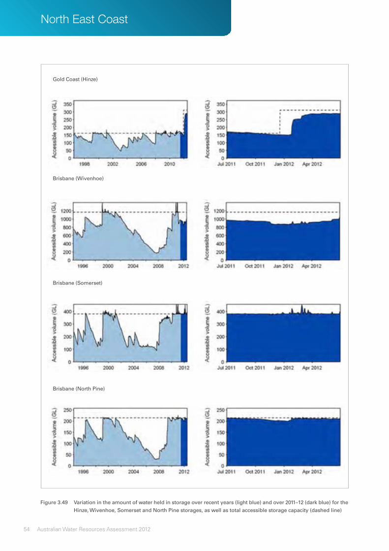
North East Coast
54 Australian Water Resources Assessment 2012
Figure 3.49 Variation in the amount of water held in storage over recent years (light blue) and over 2011–12 (dark blue) for the Hinze, Wivenhoe, Somerset and North Pine storages, as well as total accessible storage capacity (dashed line)
Gold Coast (Hinze)
Brisbane (Wivenhoe)
Brisbane (Somerset)
Brisbane (North Pine)

55Australian Water Resources Assessment 2012
Water restrictions
Followingitsformationon1January2013,SeqwaterhastakenoverthewatersecurityandefficiencyresponsibilitiespreviouslyperformedbytheQueenslandWaterCommission.
Waterrestrictionshavebeeninplacesince2005,andappliedthroughoutSEQ,excludingRedland,SunshineCoastCouncilandToowoombauntilDecember2009.TheyareshownwiththecombinedstoragelevelsinFigure3.50.
Between2005and2008combinedstoragelevelssteadilydecreasedresultingintheintroductionofmorestringentwaterrestrictions.
Permanentwaterconservationmeasures(PWCM)wereintroducedinDecember2009acrosssoutheastQueenslandincludingtheSunshineCoast.Althoughthecombinedstoragelevelremainedabove80%during2011–12,PWCMremainedinplace.Thesemeasuresencouragedtheuseofamaximumof200litresperpersonperday.
Figure 3.50 Urban water restriction levels across southeast Queensland since 2005 shown against the combined accessible water volume of Wivenhoe, Somerset and North Pine storages
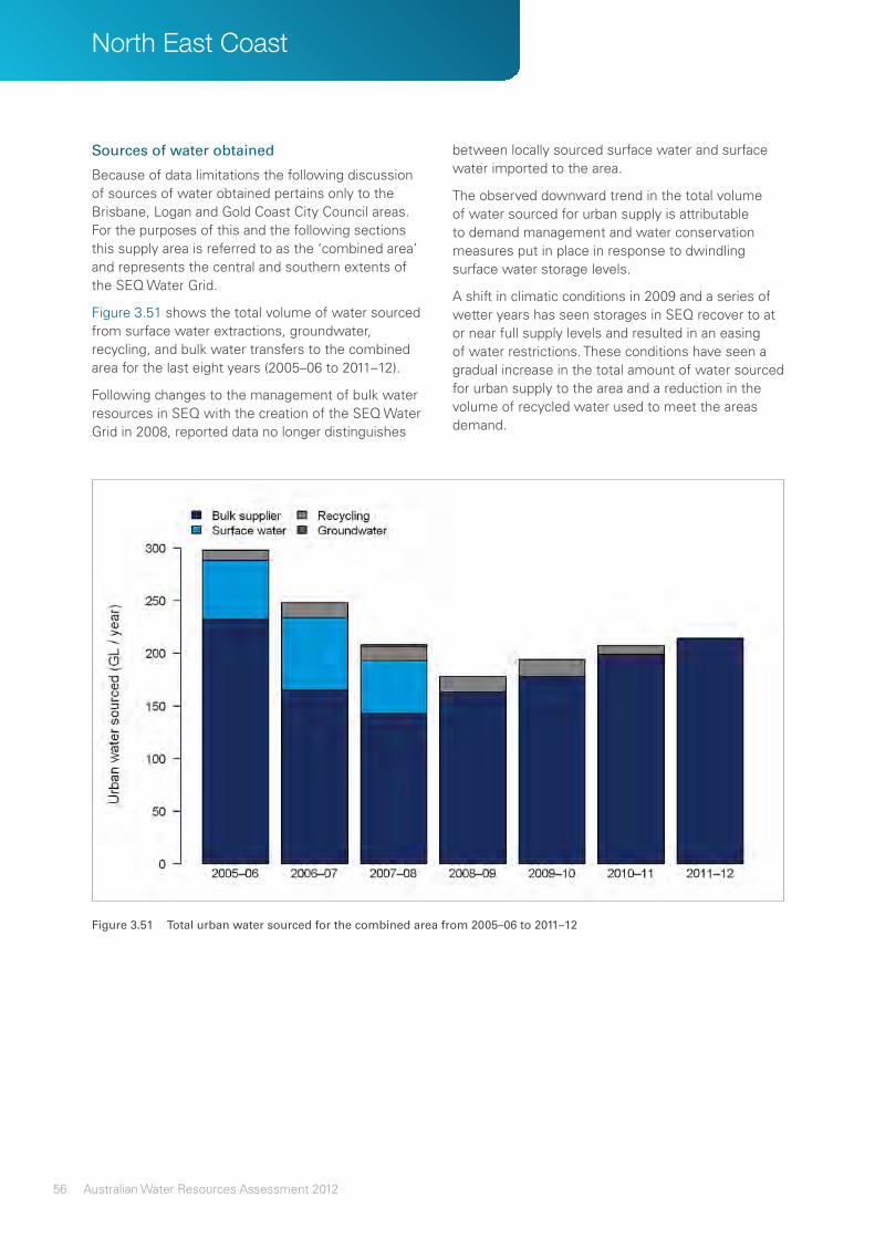
North East Coast
56 Australian Water Resources Assessment 2012
Sources of water obtained
BecauseofdatalimitationsthefollowingdiscussionofsourcesofwaterobtainedpertainsonlytotheBrisbane,LoganandGoldCoastCityCouncilareas.Forthepurposesofthisandthefollowingsectionsthissupplyareaisreferredtoasthe‘combinedarea’andrepresentsthecentralandsouthernextentsoftheSEQWaterGrid.
Figure3.51showsthetotalvolumeofwatersourcedfromsurfacewaterextractions,groundwater,recycling,andbulkwatertransferstothecombinedareaforthelasteightyears(2005–06to2011–12).
FollowingchangestothemanagementofbulkwaterresourcesinSEQwiththecreationoftheSEQWaterGridin2008,reporteddatanolongerdistinguishes
betweenlocallysourcedsurfacewaterandsurfacewaterimportedtothearea.
Theobserveddownwardtrendinthetotalvolumeofwatersourcedforurbansupplyisattributabletodemandmanagementandwaterconservationmeasuresputinplaceinresponsetodwindlingsurfacewaterstoragelevels.
Ashiftinclimaticconditionsin2009andaseriesofwetteryearshasseenstoragesinSEQrecovertoatornearfullsupplylevelsandresultedinaneasingofwaterrestrictions.Theseconditionshaveseenagradualincreaseinthetotalamountofwatersourcedforurbansupplytotheareaandareductioninthevolumeofrecycledwaterusedtomeettheareasdemand.
Figure 3.51 Total urban water sourced for the combined area from 2005–06 to 2011–12

57Australian Water Resources Assessment 2012
Categories of water delivered
Asinthepreviousdiscussionthissectionreportsonwaterusageforthe‘combinedarea’comprisingBrisbane,LoganandGoldcoastcouncils.
Figure3.52showsthetotalvolumeofwaterdeliveredtoresidential,commercial,municipal,industrial,andotherconsumers,suchasnurseries,parks,gardensandcemetaries,inthecombinedarea.
Totalwatersuppliedwas220GLin2005–06thatthendecreasedfortwoconsecutiveyearsduetowaterrestrictions.Between2007–08and2009–10,
totalwatersuppliedincreasedslightlyduetotheeasingofwaterrestrictionsandthereintroductionofoutdoorwatering.Thetotalvolumeofwatersuppliedtourbancustomersin2011–12was176GL.Recentwateruseislowcomparedtothatin2005–06.
Averagetotalresidentialwaterconsumptionofthecombinedareain2011–12was297ML/dor158litresperpersonperday(L/p/d).Theresidentialsectoraccountedfor62%oftotalpotablewaterconsumption(similartothepreviousyearwhenresidentialconsumptionwasestimatedtobe59%).Thecommercial,municipalandindustrialsectorsaccountedfor26%ofurbanwaterconsumption.
Figure 3.52 Total urban water supplied to the combined area from 2005–06 to 2011–12

North East Coast
58 Australian Water Resources Assessment 2012
3.7 Waterforagriculture
ThissectiondescribesthewatersituationforagricultureintheNorthEastCoastregionduringthe2011–12yearcomparedwiththepast.Soilmoistureconditionsarepresentedandimportantirrigationareasareidentified.TheBurdekinirrigationareaisdescribedinmoredetailandinformationisprovidedregardingsurfacewaterstorageandgroundwater.
3.7.1 Soilmoisture
Sincemodelestimatesofsoilmoisturestoragevolumesarebasedonasimpleconceptualrepresentationofsoilwaterstorageandtransferprocessesaveragedovera5kmx5kmgridcell,theyarenotsuitableforcomparisonwithlocallymeasuredsoilmoisturevolumes.Thisanalysis,therefore,presentsarelativecomparisononly,identifyinghowmodelledsoilmoisturevolumesof2011–12relatetomodelledsoilmoisturevolumesofthe1911–2012period,expressedindecilerankings.
Figure3.53givesanoverviewofthedecilerankingofmodelledannualaveragesoilmoisturefor2011–12withrespecttothe1911–2012period.Itshowsthatthemajorityoftheregionhadaboveaverageorverymuchaboveaveragesoilmoistureconditions.Thelatterconditionsweremoreprominentinthewesternpastoralandcroppingareasoftheregionwhereverymuchaboveaveragerainfallsoccurredinthatperiod.
AboveaveragesoilmoistureconditionsintheregionweredominantinthewetmonthsofNovember2011–March2012(Figure3.54).Soilmoistureremainedverymuchaboveaverageinallothermonthsoftheyear.Itcreatedbeneficialwaterconditionsfordrylandcroppingacrosstheinlandandwesternpartsoftheregionwhicharenormallydrier.
Figure 3.53 Deciles rankings of annual average soil moisture for 2011–12 with respect to the 1911–2012 period for the North East Coast region
Figure 3.54 Decile ranking of the monthly soil moisture conditions during the 2011–12 period with respect to the 1911–2012 period in the North East Coast region

59Australian Water Resources Assessment 2012
3.7.2 Irrigationwater
TheDepartmentofEnergyandWaterSupply,establishedinApril2012,providespolicyandregulationforthedeliveryofwatertoQueensland.
SunWaterisagovernment-ownedcorporation,whichisthemainsupplierofbulkwater,bulkwaterstorageanddeliveryofservicesforregionalQueensland.Inthesoutheast,Seqwaterprovidesbulkwatersupplyandservicestoaround1,000ruralcommunitiesinfivewatersupplyschemesintheUpperMary,Logan,CentralBrisbane,WarrillvalleyandLockyervalleyareas.
Acomparisonofwateruseinirrigatedcatchmentsbynaturalresourcemanagement(NRM)regionsintheregionovertheperiod2005–06to2010–11isshowninFigure3.55.Figure3.56showsthemapofthewateruseperNRMregionin2010–11.
AswiththepreviousyearsBurdekinhadthehighestirrigationwaterconsumptionamongotherNRM
regions,butthewateruseduringthe2010–11inallregionshaddroppedduetoincreasedavailabilityofwaterthroughrainfall.Atthetimeofwritingthereportdatawasnotavailablefor2011–12.
TheBurdekinRiverIrrigationAreaisdescribedinmoredetailinsubsection3.7.4
3.7.3 Irrigationareas
MostoftheNorthEastCoastregionisusedforgrazing.Drylandandirrigatedagricultureaccountforonly0.4%ofthelanduseoftheregion.Thegreatestareaofdrylandagriculture,1.8millionhectares,islocatedintheFitzroyRiverbasin.
AsshowninFigure3.57,thelargestirrigationareasarelocatedintheBrisbane,Mary,Burnett,BurrumandKolanriverbasinsinthesouth;theFitzroy,PlaneCreekandPioneerriverbasinsinthecentreoftheregion;andtheHaughtonandBurdekinriverbasinsinthenorth.
Figure 3.55 Total annual irrigation water use for 2005–06 to 2010–11 for natural resource management regions in the North East Coast region (ABS 2006–2010; 2011a)

North East Coast
60 Australian Water Resources Assessment 2012
Figure 3.56 Annual irrigation water use (GL) per natural resource management region for 2010–11 in the North East Coast region (ABS 2011a)

61Australian Water Resources Assessment 2012
Figure 3.57 Irrigation areas in the North East Coast region

North East Coast
62 Australian Water Resources Assessment 2012
3.7.4 BurdekinRiverIrrigationArea
TheBurdekinRiverbasinislocatedinthedrytropicsontheNorthEastCoastregion,coveringatotalcatchmentareaofapproximately133,000km2.
Thebasin’sassetsincludewater,biodiversity,nationalparks,grazing,fertilesoilandcrops(Figure3.58).
TheLowerBurdekininthebasinisthelargestirrigationareainnorthernAustralia,predominantlygrowingsugarcane.Thispartoftheregioncanreceivemorethan300daysofsunshineeachyear,whichisaprimaryreasonforthehighlyproductiveagriculturalsector.Thiscanbetempered,however,bythetraditionalwetseason,whichrunsfromNovember–MarcheachyearwiththewettestmonthstypicallybeingJanuaryandFebruary.
LowerBurdekincomprisestwoschemes:theBurdekinRiverDelta,andtheBurdekin–HaughtonWaterSupplyScheme.
TheBurdekinDeltadownstreamoftheBurdekinRiverisagroundwater-dominatedscheme,with
morethan35,000haofirrigatedsugarcaneandothercrops.Thissystemoverliesmajorgroundwatersupplies.
TheBurdekin–HaughtonWaterSupplySchemeissurfacewaterdominatedandreceivessignificantvolumesofwaterfromBurdekinFallsstorage.Groundwatersuppliessupplementirrigation.
BurdekinFallsontheBurdekinRiverisoneofthelargestsurfacewaterstoragesinQueenslandcovering22,000haandissuppliedbyanupstreamcatchmentareaofapproximately120,000km2.ThetotalaccessiblestoragecapacityofBurdekinFallsis1,850GL.
TotalwaterdeliveryintheBurdekin–Haughtonschemein2011–12was455GL,whichwas41percentofthewateravailabletothescheme(SunWater2012).
Forthepurposeofthisreport,theBurdekinRiverIrrigationAreawasselectedasanexampleofgroundwateruseforirrigationintheNorthEastCoastregion.
Figure 3.58 Burdekin River Irrigation Area

63Australian Water Resources Assessment 2012
Surface water storage inflows
Thehighlyseasonalrainfallpatternoftheregion,whichischaracteristicofthetropicsofnorthernAustralia,ishighlightedbythehistoricalstreamflowdischargerecordsofgaugingstationsontheSuttorRiveratStAnns,CapeRiveratTaemasandBurdekinRiveratSellheim(Figure3.59).
TheseasonalrainfallpatternislinkedtotheElNiñoSouthernOscillation,tropicalcyclonesandmonsoonalactivity.
ThemajorityoftherecordeddischargeinthethreecatchmentsupstreamofBurdekinFallsfortheperiod1980–2012occurredduringthemonthsofJanuarythroughtotheendofMarch,whichisthewetseasonintheregion.
Thedischargehydrographsof2011–12showalaginpeakflowcomparedwiththehistoricalpatterns.Thisisconsistentwiththeoverallpatternofrainfallintheregion;showinggradualascentwithapeakinMarchthatsubsidesafterwards.
Figure 3.59 Monthly inflows to Burdekin Falls for 2011–12 with respect to the 1980–2012 decile rankings

North East Coast
64 Australian Water Resources Assessment 2012
Surface water storage volumes
DespitethelargestoragecapacityofBurdekinFalls,thesignificantseasonaldischargefromtheupstreamcatchmentshasresultedinanalmostperiodicspillingofthedameverywetseasonsinceconstruction(Figure3.60).Inwetyears,thespillingcancontinueformonths.In2011–12,thedamoverflowedfromJanuary2012andcontinuedtospillinJune2012.
BetweenJanuaryandJune2012,morethan29,000MLofwaterpassedoverthespillway.Thefullstorageandwetweatherconditionsensured100%ofwaterallocationswereavailabletolocalirrigators.
Local hydrogeology
IrrigationareasintheBurdekinRiverDeltaareunderlainbyarelativelyshallowwatertable.LowerBurdekinWatermanagesagroundwater-dominatedirrigationsystemdownstreamandeastofMountKelly(Figure3.61).Morethan1,400groundwaterpumpsareinoperationapplying10–40ML/ha/yrtocrops(McMahonetal.2002).Thisisequivalentto1,000–4,000mm/year.
Thewatersourceusedforirrigation(groundwaterorsurfacewater)dependsonproximitytotheriverorirrigationchannelsandongroundwatersalinityandyield.
Thecoastalfloodplainismostlyunconfinedandhasupto100mofsedimentsoverlyingthebasement.TheshallowgroundwaterinthissystemisindirecthydraulicconnectionwiththeBurdekinRiver.
Typically,duringthedryseason,groundwaterelevationishigherthansurfacewaterlevelsintheriverupstreamoftheRocksweirallowinggroundwaterdischargeintotheriver.Duringoccasionalhighflowsinthewetseason,thedirectionofflowisreversedallowingsurfacewatertorechargegroundwater(LenahanandBristow2010).Thisactivityindicatesahighconnectivitybetweensurfacewaterandgroundwater.
Lateralgroundwaterflowisnortherlytowardsthecoast.However,groundwaterpumpingcauseslargefluctuationsingroundwaterlevelsthatcanchangethelocalgroundwaterflowdirection.
Figure 3.60 Variation in the amount of water held in storage over recent years (light blue) and over 2011–12 (dark blue) for Burdekin Falls storage, as well as total accessible storage capacity (dashed line)

65Australian Water Resources Assessment 2012
Figure 3.61 The Burdekin River Irrigation Area showing the location of groundwater bore sites, river gauge and rain gauge

North East Coast
66 Australian Water Resources Assessment 2012
Influences on shallow groundwater
Figure3.62showsthefluctuationsinshallowgroundwaterlevelsatselectedsites.From2003groundwaterlevelsshowarisingtrend.
Figure3.62alsoillustratesthedriversofthegroundwaterlevelbycomparingfluctuationinshallowgroundwaterlevelswiththemonthlycumulativerainfallresidualatAyrandthemonthlydischargeoftheBurdekinRiveratClare(Figure3.62).ThelocationofgaugesandboresisshowninFigure3.61.
Periodsinwhichthecumulativerainfallresidualcurverisesindicatewetterthanaverageconditions.Periodswithafallingtrendindicatedrierthanaverageconditions.
Figure3.62bshowsadrierthanaverageperiodupto2007,followedbyawetterthanaverageperiod.
Bothrainfallandstreamflowappeartobedriversforgroundwaterlevels.Peaksinstreamflowandintherainfallresidualcurvecorrespondtopeaksingroundwater.Thereare,however,someinconsistenciesbetweentherainfallandgroundwaterlevelcycles.Forexample,groundwaterlevelsstartrisingin1995and2003eventhoughtherainfallresidualmasscurveisstillfalling.
Figure 3.62 Comparison of shallow groundwater levels recorded at nested bore sites with rainfall and streamflow in the Burdekin River Irrigation Area to June 2012, showing (a) top panel: Bore 11910262 pipe D (red), Bore 12000202 pipe D (blue), Bore 11900162 pipe D (yellow); (b) cumulative rainfall residual mass at Ayr, Station 33002; and (c) lower panel: Burdekin River discharge at Clare, Station 120006B)

67Australian Water Resources Assessment 2012
Groundwater level
Groundwaterlevelmeasurementisanimportantsourceofinformationabouthydrologicalandanthropogenicinfluencesonthegroundwaterinanarea,includingrecharge.
Figure3.63presentsgroundwaterlevelsrecordedinboresofdifferentdepthatthesamesite,anestedboresite,intheLowerBurdekinarea.Groundwaterlevelfluctuationsaresimilaratalldepthsindicatingthatdeeperandshallowergroundwaterishydraulicallyconnected.Verticalgroundwatergradientsaremostlydownwardindicatingpossibilityofflowfromthewatertabletothedeepestpartoftheaquifer.
Figure3.64(a)showsthemediangroundwaterdepthsintheuppergroundwateraquiferintheBurdekinRiverDeltain2011–12;Figure3.64(b)
showsthedecileranksof2011–12mediangroundwaterlevelscomparedtoannualmediangroundwaterlevelsinthelast22years(1990–2012).
Ingeneral,intheupperaquifer,groundwaterlevelsvaryfromquiteshallownearthecoasttodeeperthan10mfurtherinland.Mediangroundwaterdepthsintheupperaquiferin2011–12aremostlyabovetheaverageofrecordedlevelswithintheirrigationareaandareamixofaboveaverageandbelowaveragenortheastoftheirrigationareas.
AsshowninFigure3.65(a),groundwaterlevelsintheloweraquiferaregenerallybetweenoneandfivemetersbelowthesurface.Mediangroundwaterlevelsintheloweraquiferin2011–12aremostlyabovetheaverageofrecordedlevelsofthelast22yearsFigure3.65(b).
Figure 3.63 Groundwater levels between 2007 and 2012 recorded at selected nested bore sites in the Lower Burdekin area, depth of the screen interval increases from pipe D (shallow) to pipe A (deep)

North East Coast
68 Australian Water Resources Assessment 2012
Figure 3.64 (a) Upper aquifer median groundwater depths for the Burdekin River Delta in 2011–12, and (b) decile ranks of depth in 2011–12 compared to the 1990–2012 period. Deciles 1–3 are shown as below average (greater depth below surface), deciles 4–7 as average and deciles 8–10 as above average

69Australian Water Resources Assessment 2012
Figure 3.65 (a) Lower aquifer median groundwater depths for the Burdekin River Delta in 2011–12, and (b) decile ranks of depth in 2011–12 compared to the 1990–2012 period. Deciles 1–3 are shown as below average (greater depth below surface), deciles 4–7 as average and deciles 8–10 as above

North East Coast
70 Australian Water Resources Assessment 2012
Groundwater salinity
Sincethe1960s,whentheQueenslandGovernmentcommencedregularmonitoringofgroundwaterquality,anincreaseinsalinityhasbeenreportedatmanysites.TwomainissueslinkedtodegradinggroundwaterqualityhighlightedbyLenahanandBristow(2010)are:
• anincreaseingroundwatersalinitybeyondirrigatedcroptolerancelevelreducingthegroundwaterresourcevolumeavailableforirrigation;and
• ecosystemsindeclineduetogreaterinfluxofsolutesfromtheaquifersintothesurfacewaterandultimatelyintotheGreatBarrierReef.
Increasinggroundwatersalinityatsomelocationsiscausedbyinfluencesonthehydrologicalcycle,suchaslandclearingandirrigation,whichmobilisesubsurfacesolutestores.
Increasesingroundwaterpumpingcanresultinseawaterintrusionorupwardmovementofdeepersaltygroundwater.Incontrast,decreasinggroundwatersalinitiesintheshallowsystemcanresultfromdilutionbyirrigationdrainageorleakagefromtheriver.
Figure3.66showsgroundwatersalinity,expressedinunitsofelectricalconductivity,atfourdepthsforeachofthreenestedboresitesinthelowerBurdekinRiverDelta(forborelocations,seeFigure3.61).
Groundwatersalinityinthedeepboresisusuallyveryhighcomparedtotheshallowbores.Atthesenestedsites,theshallowgroundwatersalinityismorethananorderofmagnitudelowerthansalinityindeeperbores.
Figure3.66alsoshowsthatgroundwatersalinityatthesesiteshasbeenrelativelystablesince2007.Ingeneralgroundwatersalinityisslowtochange.
Figure3.67andFigure3.68showthemediangroundwatersalinitiesintheupperandlowergroundwateraquifersin2011–12andtherankingofthesesalinitiescomparedto22-yearannualaveragesforthe1990–2012period.
TheBurdekinRiverDeltagroundwaterintheupperaquiferissaltierinthenorth,inthesoutheastnearthecoastandclosetothebedrockoutcropsinthesouth.Mediangroundwatersalinitiesintheupperaquiferin2011–12donotshowanyconsistenttrendfromthelong-termaverages.
Intheloweraquifer,saltygroundwaterappearstodefinethedistancefromthecoastwhereseawaterintrusionmayhaveoccurred.Mediangroundwatersalinitiesintheloweraquiferin2011–12againdonotshowanyconsistenttrendfromthelong-termaverage.
Figure 3.66 Groundwater salinity recorded at selected nested bore sites in the lower Burdekin area between 2007 and 2012, with depth of the screen increasing from pipe D (shallow) to pipe A (deep)

71Australian Water Resources Assessment 2012
Figure 3.67 (a) Upper aquifer median groundwater salinity for the Burdekin River Delta in 2011–12, and (b) groundwater salinity in 2011–12 compared to the 1990–2012 period. Deciles 1–3 are shown as below average (greater depth below surface), 4–7 as average and deciles 8–10 as above average

North East Coast
72 Australian Water Resources Assessment 2012
Figure 3.68 (a) Lower aquifer median groundwater salinity for the Burdekin River Delta in 2011–12, and (b) groundwater salinity in 2011–12 compared to the 1990–2012 period. Deciles 1–3 are shown as below average (greater depth below surface), deciles 4–7 as average and deciles 8–10 as above average

South East Coast (NSW)4 South East Coast (NSW) ............................................ 2
4.1 Introduction ........................................................ 2
4.2 Key information .................................................. 3
4.3 Description of the region .................................... 4
4.3.1 Physiographic characteristics.................. 6
4.3.2 Elevation ................................................. 7
4.3.3 Slopes .................................................... 8
4.3.4 Soil types ................................................ 9
4.3.5 Land use .............................................. 11
4.3.6 Population distribution .......................... 13
4.3.7 Rainfall zones ....................................... 14
4.3.8 Rainfall deficit ....................................... 15
4.4 Landscape water flows .................................... 16
4.4.1 Rainfall .................................................. 17
4.4.2 Evapotranspiration ................................ 20
4.5 Surface water and groundwater ....................... 26
4.5.1 Rivers ................................................... 26
4.5.2 Streamflow volumes ............................. 28
4.5.3 Streamflow salinity ................................ 28
4.5.4 Flooding ............................................... 31
4.5.5 Storage systems ................................... 33
4.5.6 Wetlands .............................................. 33
4.5.7 Hydrogeology ....................................... 37
4.5.8 Watertable salinity ................................. 37
4.5.9 Groundwater management units ........... 37
4.6 Water for cities and towns ................................ 42
4.6.1 Urban centres ....................................... 42
4.6.2 Sources of water supply ....................... 44
4.6.3 Greater Sydney ..................................... 46
4.7 Water for agriculture ......................................... 53
4.7.1 Soil moisture ......................................... 53
4.7.2 Irrigation water ...................................... 54
4.7.3 Irrigation areas ...................................... 56
4.7.4 Hunter River basin ................................ 58

2 Australian Water Resources Assessment 2012
South East Coast (NSW)
4.1 Introduction
This chapter examines water resources in the South East Coast (NSW) region in 2011–12 and over recent decades. It starts with summary information on the status of water flows, stores and use. This is followed by descriptive information for the region including the physiographic characteristics, soil types, population, land use and climate.
Spatial and temporal patterns in landscape water flows are presented as well as an examination of the surface and groundwater resources. The chapter concludes with a review of the water situation for urban centres and irrigation areas. The data sources and methods used in developing the diagrams and maps are listed in the Technical Supplement.
4 South East Coast (NSW)

3Australian Water Resources Assessment 2012
4.2 Keyinformation
Table 4.1 gives an overview of the key components of the data and information in this chapter
Table4.1 Keyinformationonwaterflows,storesanduseintheSouthEastCoast(NSW)region
Landscapewaterflows
Evapo-transpiration
Landscapewater yield
Rainfall
Region average Difference from 1911–2012 long-term annual mean
Decile ranking with respect to the 1911–2012 record
1,265 mm +25% 9th—above average
919 mm +12% 9th—above average
352 mm +84% 10th—very much above average
Streamflow(atselectedgauges)
Annual totals:
Above average flow throughout the region, locally very much above average
Salinity: Annual median electrical conductivity predominantly below 1,000 μS/cm (Hunter River basin only)
Flooding: Minor to moderate flooding in many rivers, locally major flooding in the north
Surfacewaterstorage(comprisingabout83%oftheregion’stotalcapacityofallmajorstorages)
Total accessible capacity
30 June 2012 30 June 2011 Change
accessible volume
% of total capacity
accessible volume
% of total capacity
accessible volume
% of total capacity
3,853 GL 3,658 GL 95% 3,049 GL 79% +609 GL +16%
Wetlandsinflowpatterns(forselectedwetlands)
Hunter Estuary wetlands: Above average flows throughout the year, with particularly high flows in November, February and March
Groundwater(inselectedaquifers)
Salinity: Scattered areas of saline groundwater (≥3,000 mg/L), particularly in coastal aquifers
Urbanwateruse(Sydney)
Total use in 2011–12 Total use in 2010–11
Change Restrictions
528 GL 544 GL – 16 GL ( – 3%) Water Wise Rules
Annualmeansoilmoisture(modelestimates)
Spatial patterns: Very much above average soil moisture levels in the centre and north of the region, above average in the south
Temporal patterns in regional average:
Above average to very much above average regional average soil moisture throughout the year

4 Australian Water Resources Assessment 2012
South East Coast (NSW)
4.3 Descriptionoftheregion
The South East Coast (NSW) region covers all of coastal New South Wales, and has a total area of 129,500 km². The western and eastern boundaries of the region are defined by the Great Dividing Range and the coast. The northern boundary is defined as the New South Wales–Queensland border, and the southern boundary reflects the dividing line between the Towamba and East Gippsland river basins.
The southern part of the region has extensive forested headwaters, large areas of national park and state forest, important wetlands, river estuaries and fresh water swamps. The main catchments are those of the Shoalhaven, Clyde, Deua, Tuross, Bega and Towamba rivers. Subsections 4.3.1–4.3.4 give more detail on physical characteristics of the region.
The region has a population of over 6 million people, just under one third of Australia’s total population (Australian Bureau of Statistics [ABS] 2011b), and includes Australia’s largest and most densely populated city, Sydney.
Figure 4.1 highlights the major population centres in the region. These include Newcastle, the Central Coast and Wollongong, Further discussion of the region’s population distribution and urban centres can be found in subsections 4.3.6 and 4.6 respectively.
Nature conservation is the main feature of the region (44%) followed by dryland pasture (37%). In the north of the region, subtropical cropping is common, and a mix of irrigated and dryland cropping is practised depending on the frequency of rainfall. In the mid-coast area, irrigated agriculture
is common and mostly occurs in the Hunter River basin. Irrigation concerns mainly wine grapes and dairy pasture. In the south of the region, irrigation of broadacre and dairy farming enterprises occurs in the Hawkesbury–Nepean and Bega river basins. Section 4.7 has more information on the region’s agricultural activities.
The region has a warm temperate climate with a moderate and generally reliable rainfall due to the presence of the Great Dividing Range. The proximity of the coast moderates weather extremes. Subsections 4.3.7 and 4.3.8 provide more information on the rainfall patterns and deficits across the region.
The Clarence River is the largest in the region in terms of annual discharge into the sea (Figure 4.1). The Hawkesbury and Hunter river basins are similar in size and form two important systems in the region in terms of urban and irrigation water supply.
Groundwater systems in the region that generally provide good potential for extraction include:
• Surficial sediment aquifer (porous media— unconsolidated);
• Tertiary basalt aquifer (fractured rock); and
• Mesozoic sediment aquifer (porous media—consolidated).
A more detailed description of the surface water and groundwater status in the region is given in section 4.5.

5Australian Water Resources Assessment 2012
Figure4.1 MajorriversandurbancentresintheSouthEastCoast(NSW)region

6 Australian Water Resources Assessment 2012
South East Coast (NSW)
4.3.1 Physiographiccharacteristics
The physiographic map in Figure 4.2 shows areas with similar landform evolutionary histories (Pain et al. 2011). These can be related back to similar geology and climatic impacts which define the extent of erosion processes. The areas have distinct physical characteristics that can influence hydrological processes.
The South East Coast (NSW) region has three physiographic provinces, namely:
• Kosciuszkan Uplands (13%): dissected high uplands on various resistant rocks, with isolated high plains;
• Macquarie Uplands (34%): deeply dissected sandstone plateaus over most of the area with rolling basalt uplands and sandstone cliffs in the northwest; and
• New England–Moreton Uplands (53%): dissected plateau margin on igneous and metamorphic rocks with coastal lowlands on weak sedimentary rocks, with littoral and alluvial plains.
Figure4.2 PhysiographicprovincesoftheSouthEastCoast(NSW)region

7Australian Water Resources Assessment 2012
4.3.2 Elevation
The western border of the South East Coast (NSW) region is clearly defined by the crest of the Great Dividing Range. The crest runs almost parallel with the coastline, with the exception of the western borders of the Hunter River basin.
As shown in Figure 4.3, the region contains many mountain ranges that belong to the Great Dividing Range (information was obtained from the Geoscience Australia website, www.ga.gov.au/topographic-mapping/digital-elevation-data.html). It also contains some plateaus and an almost continuous stretch of low-lying coastal areas.
The highest mountains in the region can be found west of Coffs Harbour, with peaks reaching altitudes of 1,500 m above sea level.
The crest of the Great Dividing Range forms the western border of the region, all the way from the north to the south. Altitudes on this crest line vary between less than 600 m at the western part of the Hunter River basin to more than 1,200 m in both the north and the south.
Figure4.3 GroundsurfaceelevationsintheSouthEastCoast(NSW)region

8 Australian Water Resources Assessment 2012
South East Coast (NSW)
4.3.3 Slopes
Areas with steep slopes provide higher run-off generating potential than flat areas. Table 4.2 shows the extent of steep slopes in the South East Coast (NSW) region. This is greater than for other regions in mainland Australia. The slopes were derived from the elevation information used in the previous section.
Table4.2 Proportionsofslopeclassesfortheregion
Slopeclass(%) 0–0.5 0.5–1 1–5 >5
Proportion of region (%)
4.9 4.5 29.9 60.7
The steep slopes in Figure 4.4 in particular show the wide escarpments of the western plateau. The eastern part of the plateau forms most of the water divide of the river basins. In fact, the highest peaks of the Great Dividing Range in this region are not necessarily located on the border of the region.
The steep slopes of the Great Dividing Range only come close to the coast around Sydney and Coffs Harbour. Also, the coastal plains of the south coast are relatively narrow.
Due to the steep slopes in the region, rivers rapidly accumulate run-off. As a consequence, high intensity rainfall often cause flash flooding in the narrow flat coastal strip. Recent years have provided clear examples of such flood in the region.
Figure4.4 SurfaceslopesintheSouthEastCoast(NSW)region

9Australian Water Resources Assessment 2012
4.3.4 Soiltypes
Soils play an important role in the hydrological cycle by distributing water that reaches the ground. Water can be transported to rivers and lakes via the soil surface as run-off or enter the soil and provide water for plant growth as well as contributing to groundwater recharge.
The nature of these hydrological pathways and the suitability of the soils for agricultural purposes are influenced by soil types and their characteristics. Soil type information was obtained from the Australian Soil Resource Information System website (www.asris.csiro.au).
About 87% of the South East Coast (NSW) region is covered by five soil types, namely kandosols, dermosols, kurosols, sodosols and tenosols (Figure 4.5 and Figure 4.6).
Kandosols are structureless soils and are often very deep (up to three metres or more). They do not have a strongly contrasting texture and do not contain carbonate throughout their profile. They are low in chemical fertility and are well drained. With only moderate water-holding capacity compared with other soil types, they only have low to moderate agricultural potential. In this region, they are mostly present in pastures and areas used for nature conservation.
Soils with higher agricultural potential and moderate to high chemical fertility are dermosols. These soils are mostly present in the northern and southern
parts of the region. They are well structured and have a high water-holding capacity, and they are mostly present in areas used for forestry and nature conservation.
Another soil type common in this region is kurosol. Soils of this type are strongly acidic (pH < 5.5) and have an abrupt increase in clay in the soil profile. Their use for agriculture is limited due to low chemical fertility and low water-holding capacity. Kurosols are mostly present in improved dairy pastures and areas used for forestry.
Sodosols are widely distributed across the region and have low agricultural potential due to a low nutrient status and low permeability. They present a clear change in texture as the clay and sodium content increases with depth. This can cause soil dispersion and instability which can give rise to a high risk of erosion (tunnel and gully erosion) as well as dryland salinity.
In the central to northern part of the region, tenosols are the common soil type. They have a weak profile development and, due to their low chemical fertility and water-holding capacity, limited agricultural potential.
The other soil types that have minimal representation in the South East Coast (NSW) region are chromosols, vertosols, hydrosols, ferrosols, podosols and rudosols (0.5–4%).
Figure4.5 SoiltypesintheSouthEastCoast(NSW)region

10 Australian Water Resources Assessment 2012
South East Coast (NSW)
Figure4.6 SoiltypedistributionintheSouthEastCoast(NSW)region

11Australian Water Resources Assessment 2012
4.3.5 Landuse
Figure 4.7 presents land use in the South East Coast (NSW) region (data from data.daff.gov.au/anrdl/metadata_files/pa_luav4g9abl07811a00.xml).The main feature of the region is nature conservation (44%) followed by dryland pasture (38%).
In the north of the region, subtropical cropping is common and a mix of irrigated and dryland cropping is practised depending on the reliability of rainfall.
In the mid-coast area, irrigated agriculture is common and mostly occurs in the Hunter River basin. This mainly consists of wine grapes and dairy pasture (Figure 4.8).
In the south of the region, irrigation of broadacre and dairy farming enterprises occurs in the Hawkesbury–Nepean and Bega river basins.
Figure4.7 LanduseinSouthEastCoast(NSW)region

12 Australian Water Resources Assessment 2012
South East Coast (NSW)
Figure4.8 LandusedistributionintheSouthEastCoast(NSW)region

13Australian Water Resources Assessment 2012
4.3.6 Populationdistribution
The South East Coast (NSW) region has over 6 million people which constitutes almost 33 % of all Australians (ABS 2011b). The most densely populated areas are along the coastal fringes (Figure 4.9).
Sydney is Australia’s largest and most densely populated city. Other major urban areas such as Newcastle, the Central Coast and Wollongong are located in a narrow coastal strip in the north and south of Sydney.
Newcastle and Wollongong have strong links with mining and heavy industries such as steel production.
In the Hunter Valley, agricultural and mining are major drivers for a number of small urban centres.
The coastal centres of Port Macquarie, Coffs Harbour, Ballina and Byron Bay are supported by large agricultural production, tourism, fisheries and mining. In the north, Taree, Kempsey, Grafton and Lismore support large agricultural districts, mostly located adjacent to major rivers. Armidale is a major population centre near the western boundary of the region.
South of Wollongong and the Illawarra district agriculture, fisheries and tourism are key drivers for population centres.
Figure4.9 PopulationdensityanddistributionintheSouthEastCoast(NSW)region

14 Australian Water Resources Assessment 2012
South East Coast (NSW)
4.3.7 Rainfallzones
The South East Coast (NSW) region has a warm temperate climate with moderate and generally reliable rainfall due to the presence of the Great Dividing Range in the west. The proximity of the coast moderates weather extremes. Median rainfall exceeds 350 mm throughout the region (Figure 4.10).
The northern half of the region has summer dominant rainfall, with median rainfall remaining high but decreasing westwards from patches with over 1,200 mm per year along the coast to between 650 mm and 1,200 mm inland.
The southern part of the region has a mixture of summer dominant rainfall amongst more uniform rainfall zones. The coastal mountains and plateaus are a major influence on the rainfall patterns that cause substantial climatic differences on a small spatial scale.
For more information on this and other climate classifications, visit the Bureau of Meteorology’s (the Bureau’s) climate website: bom.gov.au/jsp/ncc/climate_averages/climate-classifications/index.jsp
Figure4.10 RainfallzonesintheSouthEastCoast(NSW)region

15Australian Water Resources Assessment 2012
4.3.8 Rainfalldeficit
The rainfall deficit indicator, that is, rainfall minus potential evapotranspiration, gives a general impression about which parts of the region are likely to experience moisture deficits over the period of a year. The South East Coast (NSW) has a distinct rainfall deficit pattern.
Most inland areas experience a deficit of water over the year (Figure 4.11). Substantial deficits can be expected in the Hunter River basin. This basin contains major irrigation areas that must rely on surface water storages to supply enough water to the crops.
Along the coast, many areas experience an abundance of water over the year. In these areas, the land cover is mainly dominated by forests (either production forests or subtropical rainforests).
For more information on the rainfall and evapotranspiration data, see the Bureau’s maps of average conditions: www.bom.gov.au/climate/averages/maps.shtml
Figure4.11 RainfalldeficitdistributionfortheSouthEastCoast(NSW)region

16 Australian Water Resources Assessment 2012
South East Coast (NSW)
4.4 Landscapewaterflows
This section presents analyses of the spatial and temporal variation of landscape water flows (rainfall, evapotranspiration and landscape water yield) across the South East Coast (NSW) region in 2011–12. National rainfall grids were generated using data from a network of persistent, high-quality rainfall stations managed by the Bureau. Evapotranspiration and landscape water yields were derived using the landscape water balance component of the Australian Water Resources Assessment System (Van Dijk 2010). These methods and associated output uncertainties are discussed in Introduction and addressed in more detail in the Technical Supplement.
Figure 4.12 shows the region has a seasonal rainfall pattern with a wetter summer and a drier winter period. Average monthly evapotranspiration totals generally follow those of rainfall. The region’s monthly landscape water yield history shows a pattern of low yield in the period September–December, which increases during January–March and remains higher throughout April–July.
The 2011–12 year was a relatively wet year throughout. Rainfall was only below the historic median in May 2012. The wet La Niña-influenced summer period (November 2011–April 2012) contributed to particularly high monthly rainfall.
Evapotranspiration also remained above the historic median throughout the year. The monthly totals mainly stayed between the 50th and 90th percentile of the historic records.
The monthly landscape water yield for 2011–12 exceeded the 75th percentile in the first ten months of the year, only returning back to historic median levels in May 2012, due to the relatively low rainfall in that month. February and March, in particular, had very much above average high landscape water yields that coincided with the many floods that occurred in the region’s north (early February) and in the central and southern parts of the region (early March).
Figure4.12 Landscapewaterflowsin2011–12comparedwiththelong-termrecord(July1911–June2012)fortheSouthEastCoast(NSW)region

17Australian Water Resources Assessment 2012
4.4.1 Rainfall
Rainfall for the South East Coast (NSW) region for 2011–12 is estimated to be 1,265 mm. This is 25% above the region’s long-term average (July 1911–June 2012) of 1,013 mm. Figure 4.13a shows that the highest rainfall occurred adjacent to the coast with annual totals exceeding 1,800 mm in many areas for 2011–12, especially in the north. The majority of the inland areas had rainfall ranging between 600 mm and 1,200 mm for 2011–12.
Rainfall deciles for 2011–12 indicate above average rainfall for the majority of the region over the course of the year (Figure 4.13b). Some inland areas in the region’s north received average rainfall. Very much above average rainfall was recorded in the uphill areas of the central west, including large parts of the Blue Mountains, and in the coastal zone surrounding Sydney.
Figure4.13 Spatialdistributionof(a)annualrainfallin2011–12and(b)theirdecilerankingsoverthe1911–2012periodfortheSouthEastCoast(NSW)region

18 Australian Water Resources Assessment 2012
South East Coast (NSW)
Rainfallvariabilityintherecentpast
Figure 4.14a shows annual rainfall for the region from July 1980 onwards. Over this 32-year period the annual average was 1,014 mm, varying from 772 mm (2002–03) to 1,508 mm (1988–89). Temporal variability and seasonal patterns since 1980 are presented in Figure 4.14b.
Figure 4.14a also indicates the presence of cyclical patterns in annual rainfall over these 32 years. The pattern is apparent in the summer and winter periods’ moving averages (Figure 4.14b), although the pattern is less evident in the summer period than it is for the winter period.
Figure4.14 Time-seriesof(a)annualrainfall,and(b)five-yearretrospectivemovingaveragesforthesummer(November–April)andwinter(May–October)periodsfortheSouthEastCoast(NSW)region

19Australian Water Resources Assessment 2012
Recenttrendsinrainfall
Figure 4.15a presents the spatial distribution of the trends in annual rainfall for July 1980–June 2012. These are derived from linear regression analyses on the time-series of each model grid cell. The statistical significance of the trends is provided in Figure 4.15b.
Figure 4.15a shows that since 1980 a strong increase in rainfall has occurred in large parts of the north of the region. In contrast, the south has a pattern of predominantly decreasing rainfall.
Figure 4.15b, however, indicates that with the exception of some relatively small areas in the northern half of the region the trends are not statistically significant.
Figure4.15 Spatialdistributionof(a)trendsinannualrainfallfrom1980–2012,and(b)theirstatisticalsignificanceat90%(weak)and95%(strong)confidencelevelsfortheSouthEastCoast(NSW)region

20 Australian Water Resources Assessment 2012
South East Coast (NSW)
4.4.2 Evapotranspiration
Modelled annual evapotranspiration for the South East Coast (NSW) region for 2011–12 is estimated to be 919 mm. This is 12% above the region’s long-term (July 1911– June 2012) average of 819 mm. The spatial distribution of annual evapotranspiration in 2011–12 (Figure 4.16a) shows a west–east gradient of increasing totals. Evapotranspiration was highest along the north coast with annual totals exceeding 1,200 mm in some areas for 2011–12.
Evapotranspiration deciles for 2011–12 indicate above average totals across most of the region (Figure 4.16b) with very much above average totals along the Sydney and central coast and more to the north. The high evapotranspiration was possible due to the high rainfall (Figure 4.13b) and the resulting high wetness levels of the soils.
Figure4.16 Spatialdistributionof(a)modelledannualevapotranspirationin2011–12,and(b)theirdecilerankingsoverthe1911–2012periodfortheSouthEastCoast(NSW)region

21Australian Water Resources Assessment 2012
Evapotranspirationvariabilityintherecentpast
Figure 4.17a shows annual evapotranspiration for the region from July 1980 onwards. Over this 32-year period the annual evapotranspiration average was 814 mm, varying from 636 mm (2002–03) to 964 mm (1988–89). Temporal variability and seasonal patterns (over the summer and winter periods) since 1980 are presented in Figure 4.17b.
Summer periods showed consistently higher evapotranspiration than the winter period. The higher temperatures and the higher rainfall amounts during these periods contribute to this. Compared with the seasonal rainfall (Figure 4.14b), the cyclical time-series of seasonal evapotranspiration is less pronounced (Figure 4.17b).
Figure4.17 Time-seriesof(a)annualevapotranspiration,and(b)five-yearretrospectivemovingaveragesforthesummer(November–April)andwinter(May–October)periodsfortheSouthEastCoast(NSW)region

22 Australian Water Resources Assessment 2012
South East Coast (NSW)
Recenttrendsinevapotranspiration
Figure 4.18a presents the spatial distribution of the trends in modelled annual evapotranspiration for 1980–2012. These are derived from linear regression analyses on the time-series of each model grid cell. The statistical significance of the trends is provided in Figure 4.18b.
Figure 4.18a shows that since 1980 trends are weakly positive in the central northern part of the region. In the south and the far north, the trends are mostly neutral to weakly falling.
As shown in Figure 4.18b, the trends are generally only statistically significant in small parts of the region where trends are generally showing increasing evapotranspiration. In most of the area, however, the trends have no statistical significance.
Figure4.18 Spatialdistributionof(a)trendsinannualevapotranspirationfrom1980–2012,and(b)theirstatisticalsignificanceat90%(weak)and95%(strong)confidencelevelsfortheSouthEastCoast(NSW)region

23Australian Water Resources Assessment 2012
4.4.3 Landscapewateryield
Modelled landscape water yield for the South East Coast (NSW) region for 2011–12 is estimated to be 352 mm. This is 84% above the region’s long-term (July 1911–June 2012) average of 191 mm.
Figure 4.19a shows the spatial distribution of landscape water yield for 2011–12. The highest landscape water yields are observed in areas adjacent to the coast, locally exceeding 900 mm.
The landscape water yield was substantially lower inland, with some areas not exceeding 50 mm (especially in the Hunter Valley).
The decile-ranking map for 2011–12 (Figure 4.19b) shows above average landscape water yields throughout the region. Some areas recorded very much above average landscape water yield, partly reflecting the pattern of rainfall deciles in Figure 4.13b.
Figure4.19 Spatialdistributionof(a)modelledannuallandscapewateryieldin2011–12,and(b)theirdecilerankingsoverthe1911–2012periodfortheSouthEastCoast(NSW)region

24 Australian Water Resources Assessment 2012
South East Coast (NSW)
Landscapewateryieldvariabilityintherecentpast
Figure 4.20a shows annual landscape water yield for the South East Coast (NSW) region from July 1980 onwards. Over this 32-year period, average annual landscape water yield was 193 mm, varying from 82 mm (1992–93) to 441 mm (1988–89). Temporal variability and seasonal patterns (over the summer and winter periods) since 1980 are presented in Figure 4.20b.
Landscape water yield is equally distributed between the summer and winter periods. This is a result of higher landscape water yields in the south in the winter period, and in the north in the summer period.
Both periods show a distinct inter-annual cyclic variability driven by the region’s rainfall dynamics (see Figure 4.14b).
Figure4.20 Time-seriesof(a)annuallandscapewateryieldand(b)five-yearretrospectivemovingaveragesforthesummer(November–April)andwinter(May–October)periodsfortheSouthEastCoast(NSW)region

25Australian Water Resources Assessment 2012
Recenttrendsinlandscapewateryield
Figure 4.21a shows the spatial distribution of the trends in modelled annual landscape water yield for 1980–2012. These are derived from linear regression analyses on the time-series of each model grid cell. The statistical significance of the trends is provided in Figure 4.21b.
Figure 4.21a shows that since 1980, trends are rising in the central northern part of the region. In the south and the far north the trends are mostly neutral to weakly falling.
As shown in Figure 4.21b, the trends are generally only statistically significant in some central northern parts of the region, where trends are generally showing increasing landscape water yield. In most of the area, however, the trends have no statistical significance. A minor exception can be found in the Moruya River basin in the south, where a strongly significant falling trend is identified.
Figure4.21 Spatialdistributionof(a)trendsinannuallandscapewateryieldfrom1980–2012,and(b)theirstatisticalsignificanceat90%(weak)and95%(strong)confidencelevelsfortheSouthEastCoast(NSW)region

26 Australian Water Resources Assessment 2012
South East Coast (NSW)
4.5 Surfacewaterandgroundwater
This section examines surface water and groundwater resources in the South East Coast (NSW) region in 2011–12. Rivers, wetlands and storages are discussed to illustrate the state of the region’s surface water resources.
The region’s watertable aquifers and salinity are described. No data was available at the Bureau in a suitable format for a detailed analysis of individual aquifers.
4.5.1 Rivers
There are 20 river basins in the South East Coast (NSW) region, varying in size from 500–22,000 km2 (Figure 4.22).
The Clarence River is the largest in the region in terms of annual discharge into the sea. The Hawkesbury and Hunter rivers are two important systems in the region in terms of urban and irrigation water supply.
The rivers are all perennial, although in times of drought some may almost stop flowing. River flows in the region generally show distinct seasonal variations.
Hawkesbury River at Little Wobby, New South Wales | Catherine Marshall

27Australian Water Resources Assessment 2012
Figure4.22 RiversandcatchmentsintheSouthEastCoast(NSW)region

28 Australian Water Resources Assessment 2012
South East Coast (NSW)
4.5.2 Streamflowvolumes
Figure 4.23 presents an analysis of flows at 31 monitoring sites during 2011–12 relative to annual flows for the period from July 1980–July 2012. Monitoring sites with relatively long records across 15 geographically representative river catchments were selected (see Technical Supplement for details). The annual flows for 2011–12 are colour-coded according to the decile rank at each site over the 1980–2012 period.
The flows from monitoring gauges generally reflect the mostly above average to very much above average modelled landscape water yield results shown in Figure 4.19b.
High run-off, generated in the upstream reaches of the rivers, caused above average to very much above average flows in all rivers. Very much above average flows were observed at five sites located on rivers in the northwest, central east and south of the region. Above average total flows were recorded at 26 monitoring sites distributed across the entire region.
Flow deciles for summer (November 2011–April 2012) are similar to total annual flows for 2011–12 as shown in Figure 4 23. This is not surprising given that the greatest volume of flows in the region, particularly in the north and some areas in the south, occurs over the summer months. While flows in the region’s centre and central north were above average over the year, flows in most of these rivers were relatively high over the summer period. There are a few monitoring sites that did not show this pattern, such as low flows observed in the summer period on the Hunter River in the centre of the region.
4.5.3 Streamflowsalinity
Figure 4.24 presents an analysis of streamflow salinity for 2011–12 at 20 monitoring sites in the region. The sites with at least a five-year data record were selected for analysis. The results are presented as electrical conductivity (EC, μS/cm at 25 °C). This is a commonly used surrogate for the measurement of water salinity in Australia. Standard EC levels for different applications, such as for drinking water or types of irrigation, are provided in the Technical Supplement. The median annual EC values are shown as coloured circles. The size of the circle depicts the variability in annual EC, shown as the coefficient of variation (CV), being the standard deviation divided by the mean. Stream salinity data were only available in the Hunter River basin.
The median EC values for most of the selected monitoring sites in the main rivers fall in the range 0–1,000 μS/cm, an amount that is suitable for most irrigation uses. Some creeks in the Hunter River basin fall outside of this range (see Figure 4.24).
Of the 20 monitoring sites, 40% had median EC values below 500 μS/cm, and 45% were between 500–1,000 μS/cm. Only 5% of the monitoring sites had a median EC above 1,500 μS/cm. The higher median salinities all occurred in the centre and central west of the Hunter River basin.
Stream salinity was above 2,000 μS/cm at only one of the 20 monitoring sites. This was in Bayswater Creek at Liddell in the Hunter River basin. High salinity in the Bayswater Creek is due to saline discharges from coal mining, and wastewater from power generation (Environmental Protection Agency 2001) and saline groundwater input in the river.
The CV was relatively low for the most of the sites. The CV in EC is typically related to the variability in annual flow at the monitoring site.
Of the 20 monitoring sites, 10% of them had a CV below 20%, and 90% of the sites had a CV between 20% and 60%. These monitoring sites were located on the Hunter River basin towards the central part of the region.

29Australian Water Resources Assessment 2012
Figure4.23 Averageannualandsummerperiodflowvolumesatselectedsitesfor2011–12andtheirdecilerankingsoverthe1980–2012periodintheSouthEastCoast(NSW)region

30 Australian Water Resources Assessment 2012
South East Coast (NSW)
Figure4.24 Salinityaselectricalconductivityanditsassociatedcoefficientofvariationfor2011–12intheSouthEastCoast(NSW)region

31Australian Water Resources Assessment 2012
4.5.4 Flooding
Floods can be caused by either localised high intensity rainfall, for example thunderstorms, or prolonged periods of heavy rainfall, for example, during frontal rainfall, monsoon, and tropical storms. While the first rainfall type often results in localised flash flooding, the prolonged rainfall can cause sustained floods spreading over larger areas.
Floods in the region are particularly common in the north of the South East Coast (NSW) region. Most of the region’s south has a uniform rainfall pattern while the northern part receives the majority of rainfall during summer. Both types of rainfall can occur across the region, with heavy rainfalls often associated with easterly troughs and frontal systems.
Figure 4.25 shows selected locations where the Bureau is monitoring river levels as part of its flood forecasting service and the highest level reached during the year is expressed in terms of flood classification level. These classification levels are established in consultation with emergency management and local agencies and are further described in the Technical Supplement.
A three-day period of torrential rainfall along the north coast of New South Wales produced totals of about 500 mm of rain from 23–27 January 2012, causing significant flooding in some of the northern rivers. Major flooding occurred along the Tweed River, with approximately 4,200 people evacuated from this area. Rain also led to localised landslides in some areas.
Minor to moderate flooding also occurred along several other rivers, isolating more than 12,000 people in areas including Goodooga, Bellingen, Thora, Darkwood, Upper Macleay, Mullumbimby and the Brunswick and Clarence valleys. On 1 February 2012, natural disasters were declared in 11 local government areas in the north of the region as a result of the flooding. The damage due to this flooding was assessed to be several million dollars.
Bellingen River Floods | Greg McLagan

32 Australian Water Resources Assessment 2012
South East Coast (NSW)
Figure4.25 Floodoccurrencein2011–12fortheSouthEastCoast(NSW)region,witheachdotrepresentingariverlevelmonitoringstationandthecolourofthedotrepresentingthehighestfloodclassmeasured

33Australian Water Resources Assessment 2012
4.5.5 Storagesystems
There are approximately 50 major publicly owned storages in the South East Coast (NSW) region with a total capacity in excess of 4,600 GL. The Bureau’s water storage information includes approximately 83% of the region’s publicly owned storage capacity.
Storages in the region supply the irrigation areas in the Hunter Valley as well as the city of Sydney. Table 4.3 gives a summary of the region’s major storage systems together with an overview of the storage levels at the end of 2010–11 and 2011-12. The location of all the systems and associated storages are shown in Figure 4.26.
Table 4.3 indicates that the above average rainfall upstream of most storages has resulted in a substantial increase in the accessible volumes region-wide. The Sydney supply storages, especially, have received large amounts of water, with Sydney’s largest storage, Warragamba, spilling in March, April and June. The Hunter storages reached full supply level in November 2011 and have been full since. More details on the Sydney and Hunter systems is provided in subsections 4.6–4.7.
Further information on the past and present volumes of the storage systems and the individual storages can be found on the Bureau’s water storage website: water.bom.gov.au/waterstorage/awris/
4.5.6 Wetlands
Importantwetlands
There are a large number of wetlands of national and international importance in the South East Coast (NSW) region (Figure 4.27). Most of these are coastal wetlands of various types, including salt and freshwater marshes, mangrove forests, reed beds, lakes and lagoons.
The region is the most densely populated region in Australia. As a consequence, most wetlands are impacted by human activities upstream of the wetland or in the wetland area itself. The coastal estuaries and lakes are important refuges for many migrating and threatened bird species as well as many types of fish and amphibians, including several threatened species of frogs.
Inflowstoselectedwetlands
The state of the biodiversity in a wetland is linked to the way water is stored within the area and the temporal variability of inflows. An analysis of historic and recent inflows into wetlands forms an informative picture of potential changes.
One internationally recognised Ramsar wetland site (Hunter Estuary wetlands) was selected for hydrological analysis of major inflows.
More information about the region’s wetlands is available from the Australian Directory of Important Wetlands (www.environment.gov.au/water/topics/wetlands/database/diwa.html).
Two upstream stream monitoring gauges were selected to enable the analyses and interpretation of inflows to these wetlands. The gauges used in the analyses are the closest upstream gauges that have largely continuous discharge records since 1980. Although the analyses do not capture the total inflows, they are indicative of the temporal patterns of freshwater surface flows to these wetlands.
Table4.3 MajorpublicstoragesystemsintheregionasidentifiedintheBureau’swaterstorageinformation(August2012),with‘non-allocated’accountingforthestoragesnotallocatedtoaparticularsystem
Systemname Systemtype Systemcapacity Accessiblevolumeat30June2011
Accessiblevolumeat30June2012
Sydney urban 2, 582 GL 1,973 GL—76% 2,496 GL—97%
Hunter rural 1,031 GL 965 GL—94% 1,026 GL—100%
Non-allocated — 240 GL 111 GL—46% 137 GL—57%
Total 3,853GL 3,049GL—79% 3,658GL—95%

34 Australian Water Resources Assessment 2012
South East Coast (NSW)
Figure4.26 StoragesystemsintheSouthEastCoast(NSW)region;informationextractedfromtheBureau’swaterstorageinformationwebsiteinAugust2012

35Australian Water Resources Assessment 2012
Figure4.27 LocationofimportantwetlandsintheSouthEastCoast(NSW)region

36 Australian Water Resources Assessment 2012
South East Coast (NSW)
HunterEstuarywetlands
The Hunter Estuary wetlands are downstream of one of the most intensely irrigated areas of the region. The Hunter River and its tributaries contain a number of dams that catch much of the streamflow. Also, the wetlands themselves are impacted by human activities as the surrounding river branches are frequently dredged and are progressively controlled by flood mitigation structures.
Daily discharge data for the monitoring gauges on the Hunter River at Greta and on the Patterson River at Gostwyck have been combined to provide a temporal pattern of freshwater inflows into Hunter Estuary wetlands (Figure 4.28).
Figure4.29 CombineddailyflowsoftheHunterandPattersonriversbetween1980–81and2011–12,rankedin decileclasses
Figure4.28 LocationofthemonitoringsiteinrelationtotheHunterEstuarywetlands
Figure4.30 CombinedmonthlyflowsoftheHunterandPattersonriversfrom2011–12comparedwiththeJuly1980—June2012decilerankings
Figure 4.29 presents an overview of the distribution of daily streamflow decile rankings. With the absence of a distinct rainfall season, the flow pattern is qutie heterogeneous. Some years appear to have less flow than others, but no clear indication can be found that points towards a change in flow regime for the Hunter Estuary wetlands.
Figure 4.30 compares monthly discharges from 2011–12 with the statistics of flows from July 1980 onwards. The November, February and March flows exceeded the ninth decile of the 32-year record and contributed a substantial amount of freshwater to the Hunter Estuary wetlands.

37Australian Water Resources Assessment 2012
4.5.7 Hydrogeology
The hydrogeology of the South East Coast (NSW) region is dominated by a large area of outcropping fractured basement rock. Aquifer systems in fractured rock typically offer restricted low-volume groundwater resources. Productive groundwater resources are localised in alluvial valley and coastal sand aquifers.
The watertable aquifers present in the region are shown in Figure 4.31. Groundwater systems in the region that generally provide more potential for extraction include:
• Surficial sediment aquifer (porous media —unconsolidated); and
• Tertiary basalt aquifer (fractured rock).
4.5.8 Watertablesalinity
Figure 4.32 shows a classification of the watertable aquifer as either fresh (total dissolved solids [TDS] < 3,000 mg/L) or saline (TDS ≥ 3,000 mg/L) according to salinity levels.
As shown in the figure, quality-assured salinity data are not available for most of the region. Where data are available, as in the central part of the region southwest, west and northwest of Sydney, groundwater is generally fresh. Areas with known high salinity values in the region are relatively small in area.
4.5.9 Groundwatermanagementunits
Groundwater management units within the region are key features that control the extraction of groundwater through planning mechanisms. Figure 4.33 shows large groundwater management units located within the fractured and consolidated sedimentary rocks that typically provide low-volume groundwater resources. In contrast, the smaller units represent local coastal sand, alluvial valley or tertiary basal aquifers which are usually better yielding aquifers.
The Tomago Sandbeds unit (no. 5 in Figure 4.33) within coastal sand aquifers in the eastern part of the region is important as it provides 20% of the drinking water supply to the Hunter area.

38 Australian Water Resources Assessment 2012
South East Coast (NSW)
Figure4.31 WatertableaquifersoftheSouthEastCoast(NSW)region;dataextractedfromtheGroundwaterCartographyoftheAustralianHydrologicalGeospatialFabric(BureauofMeteorology2012)

39Australian Water Resources Assessment 2012
Figure4.32 WatertablesalinityclassesintheSouthEastCoast(NSW)region;dataextractedfromtheGroundwaterCartographyoftheAustralianHydrologicalGeospatialFabric(BureauofMeteorology2012)

40 Australian Water Resources Assessment 2012
South East Coast (NSW)
Figure4.33 GroundwatermanagementunitsintheSouthEastCoast(NSW)region;dataextractedfromtheNationalGroundwaterInformationSystem(BureauofMeteorology2013)

41Australian Water Resources Assessment 2012
LegendtoFigure4.33 GroundwatermanagementunitsintheSouthEastCoast(NSW)region;dataextractedfromtheNationalGroundwaterInformationSystem(BureauofMeteorology2013)

42 Australian Water Resources Assessment 2012
South East Coast (NSW)
4.6 Waterforcitiesandtowns
This section examines the urban water situation in the South East Coast (NSW) region in 2011–12. The large urban centres in the region, their water supply systems and the storage situations are briefly described. The analysis includes the most populous city in Australia, Sydney, and for this centre further details are provided on the water supply system, storage volumes, water sources and water delivered.
4.6.1 Urbancentres
Sydney is the most populous city in Australia. It is located on Australia’s southeast coast. As of June 2012, the metropolitan area had a population of 3.9 million people (ABS 2011b). Sydney’s urban area is in a coastal basin, which is bordered by the Pacific Ocean to the east, the Blue Mountains to the west, the Hawkesbury River to the north, and the Royal National Park to the south.
Newcastle, situated 162 km north of Sydney, has a population of just over 300,000 people and is the second most populated city in region.
The Central Coast is a peri-urban area located north of Sydney and south of Lake Macquarie. It has a population of 298,000 and is the third largest urban area in the region. The Central Coast is generally considered to include the area bounded by the Hawkesbury River in the south, the Watagan Mountains in the west and the southern end of Lake Macquarie in the north. It is reported to be growing at 1% per year.
Wollongong, located in the Illawarra district, has a population of 246,000 people. It is a coastal city that lies on the narrow strip between the Illawarra Escarpment and the Tasman Sea. It is situated 80 km south of Sydney.
Outside of its two major cities, the region has a large number of other ‘regional’ urban centres and towns. These, along with Sydney, Newcastle, the Central Coast and Wollongong, are shown Figure 4.34 in conjunction with their population ranges.
Sydney CBD | Malcolm Watson

43Australian Water Resources Assessment 2012
Figure4.34 PopulationrangeofurbancentresintheSouthEastCoast(NSW)region

44 Australian Water Resources Assessment 2012
South East Coast (NSW)
The major urban centres of the region, with populations of over 25,000 people, are summarised in Table 4.4. This table provides information on the population, surrounding river basin and significant water storages for each of the major urban centres.
4.6.2 Sourcesofwatersupply
All major cities and towns in the region are predominantly supplied with drinking water coming from surface water storages, or in some cases from direct river extractions, partly fed by upstream storage releases.
The region is home to over 20 major surface water storages that supply its many cities and towns. This includes the major Sydney metropolitan storage, Warragamba. With a total accessible storage capacity of over 2,000 GL it provides almost 85% of Sydney’s total surface water storage.
Major surface water storages, predominantly used for urban water supply, are shown in Figure 4.35.
In addition to surface water storages, the region utilises direct river extractions, including extractions of upstream storage releases, groundwater, desalination, recycled water, and harvested stormwater and rainwater to supply the urban demands of the region.
Groundwater extractions form a reliable source of supply in the region and are an important source of water for Newcastle and the Port Stephens area.
Recycled water is an important source of water in the region, in particular in Sydney where dedicated recycling schemes such as Rouse Hill operate to provide ‘third pipe’ recycled water to consumers.
Table4.4 MajorurbancentresandtheirwatersupplysourcesintheSouthEastCoast(NSW)region
City Population1 Riverbasin Majorsupplysources
Sydney 3,908,000 Hawkesbury River Warragamba (Lake Burragorang)Upper Nepean storages (Cataract, Avon, Cordeaux and Nepean)Shoalhaven system storages (Wingecarribee, Fitzroy Falls, Tallowa [Lake Yarrunga] and Bendeela Pondage)Woronora storageBlue Mountains storages (Lower Cascade, Middle Cascade, Upper Cascade, Lake Medlow and Lake Greaves)Lake OberonProspect Reservoir
Newcastle 308,000 Hunter River Grahamstown and Chichester storages, Tomago Sandbeds
Central Coast 298,000 Macquarie–Tuggerah Lakes Mangrove Creek, Mardi and Mooney Mooney storages
Wollongong 246,000 Wollongong Coast Avon storage
Maitland 67,000 Hunter River Grahamstown and Chichester storages, Tomago Sandbeds
Coffs Harbour 45,500 Clarence River Bellinger River
Karangi storage, Orara River
Port Macquarie 41,500 Hastings River Port Macquarie and Cowarra off-creek storages
Nowra–Bomaderry 28,000 Shoalhaven River Shoalhaven River with water released from Lake Yarrunga (Tallowa)
Lismore 27,500 Richmond River Rocky Creek storage1AustralianBureauofStatistics(2011b)

45Australian Water Resources Assessment 2012
Figure4.35 UrbansupplystoragesintheSouthEastCoast(NSW)region

46 Australian Water Resources Assessment 2012
South East Coast (NSW)
4.6.3 GreaterSydney
Sydney, with a built up area of 4,000 km2, is one of the largest cities in the world. The urban centres of Sydney and Wollongong account for nearly 60% of the population of New South Wales and are part of the Greater Sydney area, which also includes the Blue Mountains. Greater Sydney is the urban water supply reporting area addressed in this subsection.
The State Government-owned Sydney Water Corporation, Sydney Water, is the urban water utility that supplies Greater Sydney. It services a population of 3.9 million people. Sydney Water operates the bulk water supply and distribution systems, wastewater collection system and drainage assets.
Water supplies are mainly sourced from catchment areas occupying approximately 16,000 km², managed by the Sydney Catchment Authority (SCA).
Supplysystems
Sydney’s water supply catchments include the Warragamba, Upper Nepean, Blue Mountains, Woronora and Shoalhaven river basins, which provide water for Sydney’s storages as well as for the Southern Highlands and Shoalhaven areas. Parts of these water supply catchments are protected to help maintain water quality and provide habitat for a variety of rare and endangered flora and fauna.
The Fish River Water Supply Scheme, originating in Oberon, supplements Sydney’s water supply by providing water to the Blue Mountains area. Water from Tallowa (Lake Yarrunga), Fitzroy Falls and Wingecarribee storages is used to supply local communities and supplement SCA water storages during drought (NSW Government 2011b).
While water from the storages provide most of Greater Sydney’s drinking water needs, the 2006 Metropolitan Water Plan (New South Wales Government 2006) introduced measures to diversify Sydney’s water supply through water recycling and desalination. Recycled water has become important in securing supply for the residential, commercial and industrial needs of Sydney.
The major water components of the water supply system for the Greater Sydney area is shown in Figure 4 36. Sydney is known to have one of the highest per capita water storage capacities in the world (NSW Government 2011c). The inter-connected network represents a complex urban water system and includes a total of 21 storages that can hold more than 2,500 GL of water. Water taken from the Hawkesbury River is used to supply Richmond–Windsor. The water supply for Wollongong is sourced from the Avon storage.
Figure 4.36 also shows the water treatment plants and the treated water delivery systems for the Greater Sydney area. Water sourced from the storage network, the Hawkesbury River and the Kurnell desalination plant is treated and delivered to customers by Sydney Water. The water supply system includes ten water treatment plants and a network of about 21,000 km of water mains (National Water Commission 2011a). Most of the water is treated at privately owned water filtration plants operating under contract to Sydney Water.
The major surface water storage in the network, Warragamba, collects water from the Wollondilly and Coxs rivers. Its catchments cover an area of 9,000 km2. It is the largest urban water storage in Australia and accounts for about 80% of water supplies to Greater Sydney (SCA 2011b).
The storages of the Upper Nepean collect water from the catchments of the Cataract, Cordeaux, Avon and Nepean rivers. The catchments of the Upper Nepean lie in one of the highest rainfall areas in New South Wales. Together with the Shoalhaven River basin, they provide more reliable inflows than the Warragamba catchments. The Upper Nepean transfer system can provide the equivalent of 30% of Sydney’s water supply (NSW Government 2010b). Upper Canal, a 64-km long combination of open channels, tunnels and aqueducts, transfers water from Upper Nepean storages to the Prospect water filtration plant.

47Australian Water Resources Assessment 2012
Figure4.36 WatersupplyschematicforGreaterSydney

48 Australian Water Resources Assessment 2012
South East Coast (NSW)
The Blue Mountains storage system comprises three small catchments feeding six storages that provide water for the Blue Mountains region. Water can also be sourced from the Fish River Water Supply Scheme (SCA 2011a). Due to a continuing water shortage in the Oberon and surrounding regions, this scheme has not recently been used to supply the Blue Mountains.
Woronora storage, the water supply source for the Sutherland Shire in Sydney’s southeast, collects water from the Woronora River catchment.
The Shoalhaven system in the south, which includes the storages of Wingecarribee, Fitzroy Falls, Bendeela Pondage and Tallowa, is an integral part of Sydney’s water supply system. The Shoalhaven system serves as a dual-purpose water supply and hydro-electric power generation scheme. Since the 1970s, Sydney and the Illawarra have relied on water pumped from Tallowa on the Shoalhaven River to supplement water supplies in times of drought. The system can provide around 30% of supply to the Greater Sydney region. Water is transferred using the river system to provide additional water into Warragamba (Lake Burragorang) or the upper Nepean storages (NSW Government 2010b).
The Kurnell desalination plant was constructed in response to low water storage inflows from 2000 onwards and began supplying water to Sydney in
January 2010. When operating at full capacity, the desalination plant can produce 90 GL of water per year, enough water to supply up to 15% of Sydney’s current water needs. Water from the desalination plant is distributed to approximately 1.5 million people across the Sydney central business district, inner west, eastern suburbs, south Sydney, as well as parts of the Sutherland Shire.
In addition to water sourced from surface water and desalination, water recycling is an important source for securing water for residential, commercial and industrial needs. Sydney Water operates 17 recycled water schemes including Australia’s largest recycled water scheme at Rouse Hill. The Wollongong recycled water scheme supplies water for industrial and irrigation use. The remaining recycled water schemes mainly supply agricultural areas and sports fields.
Storagevolumes
Figure 4.37 shows the total accessible storage volumes for Sydney’s major storage, Warragamba and three of the four upper Nepean storages over the period 1989–90 to 2011–12. These plots clearly illustrate the significant draw down to critical levels during the latter stages of the Millennium Drought and the dramatic recovery to near full supply levels during the above average rainfall years post 2009–10.

49Australian Water Resources Assessment 2012
Figure4.37 Variationintheamountofwaterheldinstorageoverrecentyears(lightblue)andover2011–12(darkblue)forSydney’smajorstorage,Warragamba,andthreeofthefourupperNepeanstorages,aswellastotalaccessiblestoragecapacity(dashedline).
Warragamba
Avon
Cordeaux
Cataract

50 Australian Water Resources Assessment 2012
South East Coast (NSW)
Waterrestrictions
Figure 4.38 shows the accessible storage volume and the water restrictions implemented for Sydney in recent years. Water restrictions are used as a measure to reduce the demand on water supplies. On 1 November 1994, mandatory water restrictions were introduced for Sydney in response to a decreasing accessible volume at Warragamba. Above average rainfall during 1995 led to an increase in storage volume, and on 16 October 1996 the restrictions were lifted.
During 2002, Sydney experienced one of the worst periods of drought on record. Surface water storage levels began to decline rapidly and, as a strategy to reduce water consumption, voluntary water restrictions were introduced in Sydney in November 2002 (Sydney Water Corporation 2010). Despite this, the volume of water in Warragamba continued to decrease under the ongoing drought conditions.
With the total combined storage volume of Sydney’s supply network falling below 60% of its capacity, Sydney Water introduced mandatory water restrictions level 1 at the beginning of October 2003.
When Sydney’s total storage volume dropped below 50% of capacity, mandatory water restrictions were elevated on 1 June 2004 to level 2. Water restrictions were elevated to level 3 on 1 June 2005 when the total storage volume dropped below 40% of capacity.
In May 2007, Warragamba reached the lowest water level in recent years. Above average rainfall increased storage volumes to about 60% of its accessible storage capacity. As a consequence, Level 3 water restrictions were eased out by June 2008.
Combined storage volumes remained at around 60% over the following 12 months and water restrictions were replaced by ‘Water Wise Rules’ in June 2009 to encourage continued water saving. Water Wise Rules have remained in place since then as storage levels have continued to rise to near full capacity during early 2012.
Figure4.38 WaterrestrictionsintheGreaterSydneyarea

51Australian Water Resources Assessment 2012
Sourcesofwaterobtained
Figure 4.39 shows the total volume of water sourced from surface water, recycling, and desalination by Sydney Water from 2006–07 to 2011–12 (National Water Commission 2011a). The volume sourced from surface water includes water received from the bulk supplier (SCA) and surface water taken from the Hawkesbury River for supply to Richmond–Windsor.
The total volume of water sourced in 2011–12 was 495 GL. Over the past five years, the highest volume of water sourced, 517 GL, was in 2006–07. The following year annual volumes decreased to 491 GL in 2007–08 and 506 GL in 2008–09. This decrease can be attributed to, in part, the easing of water restrictions from June 2008.
The main source of water supply for the Greater Sydney region is surface water, which ranged from 97% of the total water sourced in 2006–07 to 81% in 2010–11. The decrease in surface water sourced coincides with an increase in desalination water supplied.
The Kurnell desalination plant was commissioned in January 2010. Water sourced from desalination accounted for 3.9% of total water sourced in 2009–10. The share of desalinated water increased to 15% for the 2010–11 year and 12% for 2011–12 year.
Water from recycling comprises a small yet significant component of water sourced, ranging from 1.5% in 2006–07 to 2.1% in 2010–11. In 2011–12, water sourced from recycling accounted for 2.7%.
Figure4.39 TotalurbanwatersourcedfortheGreaterSydneyareafrom2006–07to2011–12

52 Australian Water Resources Assessment 2012
South East Coast (NSW)
Categoriesofwaterdelivered
Figure 4.40 shows the total volume of water delivered to residential, commercial, municipal and industrial consumers in the Greater Sydney region from 2006–07 to 2011–12 (National Water Commission 2012). The total volume of water delivered to the residential sector in 2011–12 accounted for 61% of total potable water consumption.
Total water supplied has gradually increased since the 2007–08 year and was highest in 2010–11 at 544 GL. While residential and commercial use has remained consistent over the last three years, there has been a significant growth in water supplied for other uses.
Based on the data obtained from the National Performance Reports (National Water Commission 2012), the average water supplied by Sydney Water, per property for residential use was estimated to be 196 kL from 2006–07 to 2011–12. The maximum residential water use per property was 205 kL in 2009–10 and the minimum was 182 kL in 2007–08.
Figure4.40 TotalurbanwatersuppliedtotheGreaterSydneyareafrom2006–07to2011–12

53Australian Water Resources Assessment 2012
4.7 Waterforagriculture
This section describes the water situation for agriculture in the South East Coast (NSW) region in 2011–12. Soil moisture conditions are presented and important irrigation areas are identified. The Hunter River irrigation area is described in more detail and information is provided regarding surface storage.
4.7.1 Soilmoisture
Since model estimates of soil moisture storage volumes are based on a simple conceptual representation of soil water storage and transfer processes averaged over a 5 km x 5 km grid cell, they are not suitable to compare with locally measured soil moisture volumes. This analysis therefore presents a relative comparison only, identifying how modelled soil moisture volumes of 2011–12 relate to those of the 1911–2012 period, expressed in decile rankings.
The above average rainfall in the region during 2011–12 favoured wet conditions in the soils, which ranked as very much above the long-term average for most areas. In the southern parts, the soils were generally at above average conditions (Figure 4.41).
Temporal variation of the decile rankings show very much above average soil moisture conditions for most of 2011–12 (Figure 4.42). This was a result of the high rainfall in the region, which sustained the wet conditions in the soil.
Figure4.42 Decilerankingofthemonthlysoilmoistureconditionsduringthe2011–12periodintheSouthEastCoast(NSW)region
Figure4.41 Decilesrankingsofthesoilmoistureoverthe1911–2012periodintheSouthEastCoast(NSW)region

54 Australian Water Resources Assessment 2012
South East Coast (NSW)
4.7.2 Irrigationwater
Irrigation water use in the region between 2005–06 and 2010–11 is shown in Figure 4.43 and Figure 4.44 by natural resource management (NRM) region. Data for the 2011–12 year was not available at the time of preparing this report.
The data show that the highest irrigation water use occurs in the regulated Hunter River basin, followed by the Hawkesbury–Nepean river basin.
Figure 4.44 shows the variation in the irrigation water use during the 2010–11 year. The Hunter River basin with 86 GL was the major consumer of irrigation water.
In the next section, the Hunter River basin is used as an example for water resource conditions and irrigated agriculture in 2011–12.
Figure4.43 Totalannualirrigationwaterusefor2005–06to2010–11fornaturalresourcemanagementregionsintheSouthEastCoast(NSW)region(ABS2006–10;2011a)
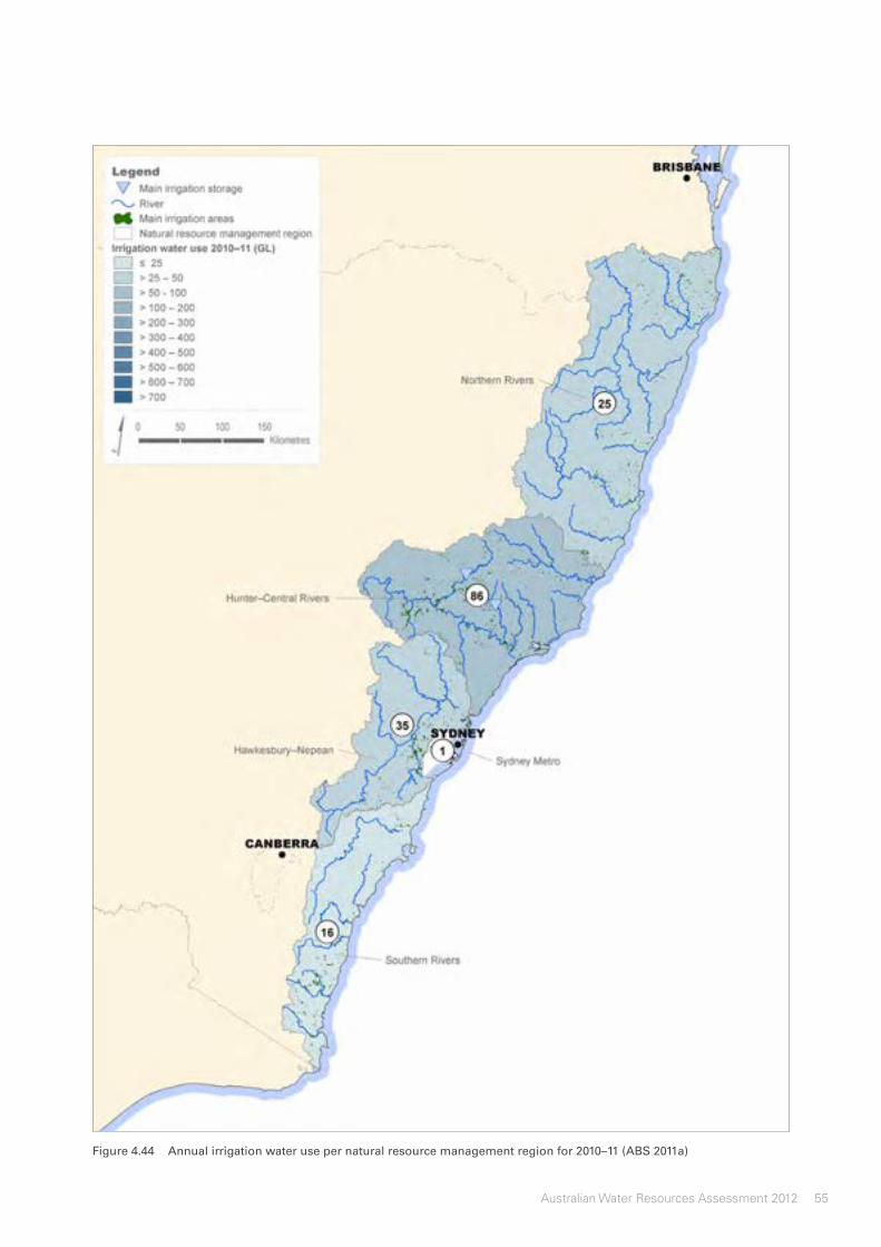
55Australian Water Resources Assessment 2012
Figure4.44 Annualirrigationwaterusepernaturalresourcemanagementregionfor2010–11(ABS2011a)

56 Australian Water Resources Assessment 2012
South East Coast (NSW)
4.7.3 Irrigationareas
In the subtropical north, where dairy is the largest industry, irrigation is necessary during spring and early summer. Mild winters and warm hot summers in the north are conducive also to avocado, banana, citrus and other fruit production.
In the mid-coast catchments, wine grapes and dairy pasture are the two most important irrigated industries. In these areas, most of the licences for irrigation are located in the Hunter catchment (Figure 4.45) along the Williams and Goulburn rivers and Wollombi Brook (Hope 2003b).
The southern coast has extensive forested headwaters, wetlands, river estuaries and freshwater swamps. Irrigated agriculture occurs mainly in the Hawkesbury–Nepean and Bega river basins (Hope 2003c). Dairy production is the main industry followed by vegetables and floriculture.
Unregulated rivers are the major source of water for the irrigation industry in most parts of the region. Irrigation from farm storages is widespread and provides a level of security during droughts. Irrigation from groundwater is very limited (Hope 2003a).
The Hunter River basin irrigation areas are described in more detail in subsection 4.7.4.
Hunter Valley vineyards, New South Wales | Christopher Howey (Dreamstime)

57Australian Water Resources Assessment 2012
Figure4.45 TheHunterRiverbasinintheSouthEastCoast(NSW)region

58 Australian Water Resources Assessment 2012
South East Coast (NSW)
4.7.4 HunterRiverbasin
The Hunter River drains the largest coastal catchment in New South Wales (22,000 km2) and provides the only regulated water supplies in the mid-coast part of the South East Coast (NSW) region (Figure 4.46).
The Hunter River basin contains approximately 80% of the irrigated area in the mid-coast. Irrigation is used to grow pasture and lucerne for dairy farms. Vineyards are the second most important irrigated
enterprise in the river basin and are located along the Goulburn River and Wollombi Brook. The river basin also supports a diversity of other agricultural activities, such as beef cattle, dairy, poultry, wool and sheep, cereal crops and horse and cattle studs.
Most of the water in the Hunter Valley irrigation area comes from the north-eastern part of the catchment. Water is controlled by three storages: Glenbawn, Lake St Clair, behind Glennies Creek dam, and Lostock.
Figure4.46 IrrigatedareasintheHunterRiverbasin

59Australian Water Resources Assessment 2012
Glenbawn storage, with an accessible capacity of 750 GL plus 120 GL for flood control, is located behind the largest earth-filled dam in Australia. It regulates flows in the Hunter River downstream of Maitland. The storage has an area of 26 km2 with a maximum depth of 85 m. It provides water for towns, stock, irrigation, industry and environmental flows.
Glenbawn is operated in conjunction with Glennies Creek storage. The latter has an accessible storage capacity of 283 GL with surface and catchment areas of 15 km2 and 233 km2, respectively. It supplies water for the town of Singleton as well as for irrigation, stock and industries such as coal mining (State Water Corporation 2011).
The Hunter Regulated River Water Sharing Plan contains rules for how water is shared between the environment and water users with different categories of licences. The plan establishes a long-term average annual extraction limit estimated as 217 GL per year, out of an annual natural average flow estimated at 1,042 GL (New South Wales Department of Water and Energy 2009). This ensures a minimum level of flow in the Hunter River at Liddell, just upstream of the Glennies Creek junction, and Greta (near the end of the regulated river system).
The plan also establishes water reserves (or environmental contingency allowances) of 20 GL per year in both Glenbawn and Glennies Creek. The rules for how water is shared between extractive users are set by the plan.
The Hunter regulated river water source is divided into three management zones and five supplementary water reaches for the management of extractions by supplementary water access licences. An actual volumetric allocation scheme was introduced in 1981 which is based on 6 ML/ha. In most years, water allocation for general security use was 100% or more.
Surfacewaterstorageinflows
In 2011–12, the flows in the catchments upstream of the Glenbawn storage were at medium to high levels compared with their historic record. The maximum flows at the Hunter River occurred in February that coincided with the high incidents of rainfall in the region (Figure 4.47). The flows gradually declined during spring and early summer, with a sudden rise during February following the rainfall pattern in the region.
Figure4.47 MonthlydischargehydrographscomparedtodischargedecilesofHunterRiveratBelltrees,representinginflowsintoGlenbawn

60 Australian Water Resources Assessment 2012
South East Coast (NSW)
Surfacewaterstoragevolumes
Combined inflows to the Glenbawn and Glennies Creek storages and total regulated water use in the Hunter region since 1985 are shown in Figure 4.48. The inverse relationship between the two indicates diversions increased in drought years in response to greater irrigation water demand. The combined
inflows to Glenbawn and Glennies Creek in 2011–12 were much above the average (184 GL).
The storage volume for both the Glenbawn and Glennies Creek storages remained at 100% of their accessible capacity for most parts of the year (Figure 4.49).
Figure4.49 Variationintheamountofwaterheldinstorageoverrecentyears(lightblue)andover2011–12(darkblue)for GlenbawnandGlenniesCreekstorages,aswellastotalaccessiblestoragecapacity(dashedline)
Figure4.48 CombinedinflowstotheGlenbawnandGlenniesCreekstoragesandtotalregulatedwateruseintheHunterregionbetween1985–86and2011–2012
Glenbawn
Glennies Creek

South East Coast (Victoria)5 South East Coast (Victoria) ......................................... 2
5.1 Introduction ........................................................ 2
5.2 Key information .................................................. 3
5.3 Description of the region .................................... 4
5.3.1 Physiographic characteristics.................. 6
5.3.2 Elevation ................................................. 7
5.3.3 Slopes .................................................... 8
5.3.4 Soil types ............................................... 9
5.3.5 Land use .............................................. 11
5.3.6 Population distribution .......................... 12
5.3.7 Rainfall zones ....................................... 13
5.3.8 Rainfall deficit ....................................... 14
5.4 Landscape water flows ................................... 15
5.4.1 Rainfall .................................................. 16
5.4.2 Evapotranspiration ................................ 19
5.4.3 Landscape water yield ......................... 22
5.5 Surface water and groundwater ....................... 25
5.5.1 Rivers ................................................... 25
5.5.2 Streamflow volumes ............................. 26
5.5.3 Streamflow salinity ................................ 27
5.5.4 Flooding ............................................... 28
5.5.5 Storage systems ................................... 29
5.5.6 Wetlands .............................................. 31
5.5.7 Hydrogeology ....................................... 35
5.5.8 Watertable salinity ................................. 35
5.5.9 Groundwater management units ........... 35
5.5.10 Status of selected aquifers .................... 39
5.6 Water for cities and towns ................................ 43
5.6.1 Urban centres ....................................... 43
5.6.2 Sources of water supply ....................... 45
5.6.3 Melbourne ............................................ 46
5.7 Water for agriculture ......................................... 51
5.7.1 Soil moisture ......................................... 51
5.7.2 Irrigation water ...................................... 52
5.7.3 Irrigation areas ...................................... 54
5.7.4 Werribee and Bacchus Marsh
irrigation districts................................... 55
5.7.5 Macalister Irrigation District ................... 56

2 Australian Water Resources Assessment 2012
South East Coast (Victoria)
5.1 Introduction
This chapter examines water resources in the South East Coast (Victoria) in 2011–12 and over recent decades. It starts with summary information on the status of water flows, stores and use. This is followed by descriptive information for the region including the physiographic characteristics, soil types, population, land use and climate.
Spatial and temporal patterns in landscape water flows are presented as well an examination of the surface water and groundwater resources. The chapter concludes with a review of the water situation for urban centres and irrigation areas. The data sources and methods used in developing the diagrams and maps are listed in the Technical Supplement.
5 South East Coast (Victoria)

3Australian Water Resources Assessment 2012
5.2 Keyinformation
Table 5.1 gives an overview of the key components of the data and information in this chapter.
Table5.1 Keyinformationonwaterflows,storesanduseintheSouthEastCoast(Victoria)region
Landscapewaterflows
Evapo-transpiration
Landscapewater yield
Rainfall
Region average Difference from 1911–2012 long-term annual mean
Decile ranking with respect to the 1911–2012 record
842 mm +14% 9th—above average
648 mm +3% 7th —average
180 mm +68% 10th—very much above average
Streamflow(atselectedgauges)
Annual total flow:
Very much above average flow in the eastern half of the region, predominantly average in the western rivers
Salinity: Annual median electrical conductivity below 1000 μS/cm in the few gauges in the east and many rivers in the west with higher than 2000 μS/cm
Flooding: Major flooding in the eastern rivers in June 2012
Surfacewaterstorage(comprisingabout73%oftheregion’stotalcapacityofallmajorstorages)
Total accessible capacity
30 June 2012 30 June 2011 Change
accessible volume
% of total capacity
accessible volume
% of total capacity
accessible volume
% of total capacity
1,907 GL 1,346 GL 71% 1,078 GL 57% +268 GL +14%
Wetlandsinflowpatterns(forselectedwetlands)
Western District Lakes: Below average flows, particularly in the wet season (August to October)
Gippsland Lakes: Very much above average flows for much of the year
Reedy Lake–Lake Connewarre:
Predominantly average flows, with high flows in June 2012
Groundwater(inselectedaquifers)
Levels: Variable groundwater levels in the various aquifers throughout the region
Salinity: Large areas of saline groundwater (≥3,000 mg/L), particularly in the eastern aquifers
Urbanwateruse(Melbourne)
Total use in 2011–12 Total use in 2010–11
Change Restrictions
361 GL 343 GL +18 GL (+5%) Eased to Stage 1
Annualmeansoilmoisture(modelestimates)
Spatial patterns: Above average soil moisture levels in the east, predominantly average in the west
Temporal patterns in regional average:
Above average in July 2011, dropping to average between October 2011 and February 2012, then returning to above average in March 2012
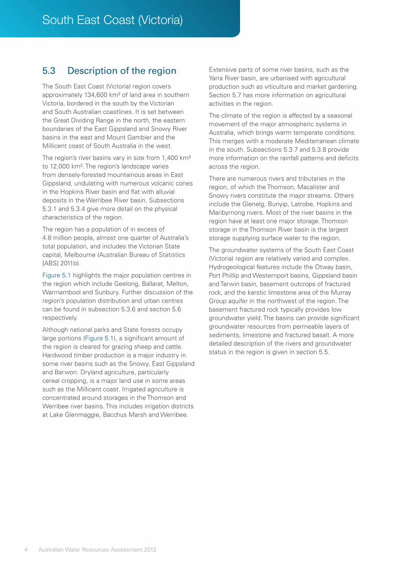
4 Australian Water Resources Assessment 2012
South East Coast (Victoria)
5.3 Descriptionoftheregion
The South East Coast (Victoria) region covers approximately 134,600 km² of land area in southern Victoria, bordered in the south by the Victorian and South Australian coastlines. It is set between the Great Dividing Range in the north, the eastern boundaries of the East Gippsland and Snowy River basins in the east and Mount Gambier and the Millicent coast of South Australia in the west.
The region’s river basins vary in size from 1,400 km² to 12,000 km². The region’s landscape varies from densely-forested mountainous areas in East Gippsland, undulating with numerous volcanic cones in the Hopkins River basin and flat with alluvial deposits in the Werribee River basin. Subsections 5.3.1 and 5.3.4 give more detail on the physical characteristics of the region.
The region has a population of in excess of 4.8 million people, almost one quarter of Australia’s total population, and includes the Victorian State capital, Melbourne (Australian Bureau of Statistics [ABS] 2011b).
Figure 5.1 highlights the major population centres in the region which include Geelong, Ballarat, Melton, Warrnambool and Sunbury. Further discussion of the region’s population distribution and urban centres can be found in subsection 5.3.6 and section 5.6 respectively.
Although national parks and State forests occupy large portions (Figure 5.1), a significant amount of the region is cleared for grazing sheep and cattle. Hardwood timber production is a major industry in some river basins such as the Snowy, East Gippsland and Barwon. Dryland agriculture, particularly cereal cropping, is a major land use in some areas such as the Millicent coast. Irrigated agriculture is concentrated around storages in the Thomson and Werribee river basins. This includes irrigation districts at Lake Glenmaggie, Bacchus Marsh and Werribee.
Extensive parts of some river basins, such as the Yarra River basin, are urbanised with agricultural production such as viticulture and market gardening. Section 5.7 has more information on agricultural activities in the region.
The climate of the region is affected by a seasonal movement of the major atmospheric systems in Australia, which brings warm temperate conditions. This merges with a moderate Mediterranean climate in the south. Subsections 5.3.7 and 5.3.8 provide more information on the rainfall patterns and deficits across the region.
There are numerous rivers and tributaries in the region, of which the Thomson, Macalister and Snowy rivers constitute the major streams. Others include the Glenelg, Bunyip, Latrobe, Hopkins and Maribyrnong rivers. Most of the river basins in the region have at least one major storage. Thomson storage in the Thomson River basin is the largest storage supplying surface water to the region.
The groundwater systems of the South East Coast (Victoria) region are relatively varied and complex. Hydrogeological features include the Otway basin, Port Phillip and Westernport basins, Gippsland basin and Tarwin basin, basement outcrops of fractured rock, and the karstic limestone area of the Murray Group aquifer in the northwest of the region. The basement fractured rock typically provides low groundwater yield. The basins can provide significant groundwater resources from permeable layers of sediments, limestone and fractured basalt. A more detailed description of the rivers and groundwater status in the region is given in section 5.5.

5Australian Water Resources Assessment 2012
Figure5.1 MajorriversandurbancentresintheSouthEastCoast(Victoria)region
Yarra River, Melbourne | MoMorad (iStockphoto)

6 Australian Water Resources Assessment 2012
South East Coast (Victoria)
5.3.1 Physiographiccharacteristics
The physiographic map in Figure 5.2 shows areas with similar landform evolutionary histories (Pain et al 2011). These can be related back to similar geology and climatic impacts which define the extent of erosion processes. The areas have distinct physical characteristics that can influence hydrological processes. The South East Coast (Victoria) region has two physiographic provinces, the Kosciuszkan Uplands and the Murray Lowlands.
The Kosciuszkan Uplands province occupies 73% of the region and has undulating upland plains with some tabular basalt relief and granitic rock outcrops
in the northeast. The central portion comprises dissected high plateaus on various resistant rocks, with isolated high plains. The south coast has sandstone and granite hills with terraced plains on weak sedimentary and basalt rocks. The northwest has moderately high plateaus and ridges.
The Murray Lowlands province occupies 27% of the area and, in the southeast, has parallel dune limestone ridges with intervening swamps, closed karst depressions and young volcanoes. In the northeast there are aeolian and alluvial sand plains, minor low sandstone ridges. In the northwest there are coastal barriers, lagoons and calcareous dunes.
Figure5.2 PhysiographicprovincesoftheSouthEastCoast(Victoria)region

7Australian Water Resources Assessment 2012
5.3.2 Elevation
Figure 5.3 presents the topography in the South East Coast (Victoria) region, which varies from alpine mountains in the northeast to low-lying coastal zones. The northwest is called the Limestone Coast and includes large plains lined by rows of sand hills parallel to the coast.
Information was obtained from the Geoscience Australia website (www.ga.gov.au/topographic-mapping/digital-elevation-data.html). The region contains the most southern part of the Great Dividing Range on the Australian mainland. It includes some
of the highest mountains in the Great Dividing Range, including Australia’s highest mainland mountain, Mount Kosciuszko.
To the west, the tilted sandstone formations of the Grampians form a north–south orientated series of parallel ridges, reaching altitudes of over 800 m. Only the southern parts of these ridges are located in the region.
The crest of the Great Dividing Range forms the northwest border of the region. Moving to the west, the altitude of the water divide that forms the border of the region gradually reduces to less than 100 m in the far west.
Figure5.3 GroundsurfaceelevationsintheSouthEastCoast(Victoria)region

8 Australian Water Resources Assessment 2012
South East Coast (Victoria)
5.3.3 Slopes
Areas with steep slopes provide higher run-off generating potential than flat areas. The South East Coast (Victoria) region has high variability in slopes (Table 5.2), with generally large areas of steeper slopes in relation to the rest of Australia. The slopes were derived from the elevation information used in the previous section.
Table5.2 Proportionsofslopeclassesfortheregion
Slopeclass(%)
0–0.5 0.5–1 1–5 >5
Proportion of region (%)
27.4 15.3 30.1 27.2
Particularly in the northeast, the slopes in the Great Dividing Range are steep. Streamflow runs quickly into the many storages located in the area. South of this area, in the flat coastal areas, rivers form floodplains and coastal lakes (Figure 5.4).
To the west of Melbourne, many inland areas are rather flat. Water does not run off into large rivers, but rather forms small lakes and swamps. This landscape is even more distinct in the Limestone Coast, where the many swamps and lakes needed to be drained to transform the land into exploitable farmland.
Figure5.4 SurfaceslopesintheSouthEastCoast(Victoria)region

9Australian Water Resources Assessment 2012
5.3.4 Soiltypes
Soils play an important role in the hydrological cycle by distributing water that reaches the ground. Water can be transported to rivers and lakes via the soil surface as run-off or enter the soil and provide water for plant growth as well as contributing to groundwater recharge. The nature of these hydrological pathways and the suitability of the soils for agricultural purposes are influenced by soil types and their characteristics. Soil type information was obtained from the Australian Soil Resource Information System website (www.asris.csiro.au).
About 83% of the South East Coast (Victoria) region is covered by five soil types, namely sodosols, chromosols, tenosols, dermosols and vertosols (Figure 5.5 and Figure 5.6).
The most common and widely spread soils for this region are sodosols (38%). They are characterised by an abrupt increase of clay as well as sodium with depth leading to dispersion and instability. Sodosols are prone to erosion, especially tunnel and gully erosion as well as dryland salinity. Due to the high sodicity and low permeability they have a low agricultural potential.
Chromosols are mainly found in the eastern part of the region, but also to some extent in the central western part of this region. Similarly to sodosols,
chromosols have an abrupt increase in clay content in the soil profile. They have moderate chemical fertility, water-holding capacity and a moderate agricultural potential often used for wheat cropping as well as for grazing. Soil acidification and soil structural decline may occur on these soils.
Dermosols also have moderate and partly high agricultural potential due to their moderate chemical fertility, well structured and high water-holding capacity. They are widely spread in the central and eastern parts of the region.
In the central to northern parts of the region tenosols are also common soil types. They have a weak profile development and with a low chemical fertility and water-holding capacity their agricultural potential is low.
Vertosols, soils with high clay contents throughout the profile are mainly found in western parts and to a small extent in central parts of the region. They have tendencies for soil cracks when dry and swelling during wetting, are highly fertile and have a large water-holding capacity. They, however, require a significant amount of water before it becomes available to plants.
Other soil types with small area coverage in this region are kurosols, podosols, ferrosols, rudosols, calcarosols as well as kandosols (Figure 5.6).
Figure5.5 SoiltypesintheSouthEastCoast(Victoria)region

10 Australian Water Resources Assessment 2012
South East Coast (Victoria)
Figure5.6 SoiltypedistributionintheSouthEastCoast(Victoria)region

11Australian Water Resources Assessment 2012
5.3.5 Landuse
National parks and State forests occupy large portions of the region, although the majority of the region is cleared for grazing sheep and cattle. Figure 5.7 presents land use in the regions (information from data.daff.gov.au/anrdl/metadata_files/pa_luav4g9abl07811a00.xml). Hardwood timber production is a major industry in some river basins such as the Snowy, East Gippsland and Barwon river basins (Figure 5.8).
Dryland cropping such as cereals is scattered across the South East Coast (Victoria) region, mostly in the western part of the region.
Irrigation districts at Lake Glenmaggie, Bacchus Marsh and Werribee are the largest irrigated areas in the region. Viticulture and market gardening can be found in the Yarra district.
Figure5.7 LandusedistributionintheSouthEastCoast(Victoria)region
Figure5.8 LanduseintheSouthEastCoast(Victoria)region

12 Australian Water Resources Assessment 2012
South East Coast (Victoria)
5.3.6 Populationdistribution
The South East Coast (Victoria) region has a population of just over 4.8 million people, with the largest concentrations located through its central corridor, and southern coastal areas. In particular the areas adjacent to Port Phillip and Westernport bays, which include the cities of Geelong, Melbourne and Frankston, are the most densely populated areas in the region. Figure 5.9 shows the spatial distribution of population density based on data from the Australian Bureau of Statistics [ABS 2011b].
Beyond the many towns dotted along the coastal fringe, the populations of the western and eastern extents of the region are clustered around centres supporting the major agriculture districts as well as mining and forestry. Ballarat, in the central north and Warrnambool in the coastal west are two major non-metropolitan cities in the region.
Figure5.9 PopulationdensityanddistributionintheSouthEastCoast(Victoria)region

13Australian Water Resources Assessment 2012
5.3.7 Rainfallzones
The climate of the region is affected by a seasonal movement of the major atmospheric systems in Australia that brings warm temperate conditions. This merges with a moderate Mediterranean climate in the south.
This region receives most of its rainfall in winter. Median rainfall exceeds 250 mm throughout (Figure 5.10).
In the centre of the region, median annual rainfall is reasonably high (>800 mm) and is generally uniform
throughout the year. The western half of the region receives winter dominant rainfall, ranging from 250 mm in the northwest to over 800 mm in the east.The mountainous eastern part of the region receives a more uniform rainfall pattern over the year. Median rainfall amounts are moderate (500–800 mm) to high (>800 mm).
For more information on this and other climate classifications, visit the Bureau of Meteorology’s (the Bureau’s) climate website www.bom.gov.au/jsp/ncc/climate_averages/climate-classifications/index.jsp
Figure5.10 RainfallzonesintheSouthEastCoast(Victoria)region

14 Australian Water Resources Assessment 2012
South East Coast (Victoria)
5.3.8 Rainfalldeficit
The rainfall deficit indicator, that is, rainfall minus potential evapotranspiration, gives a general impression about which parts of the region are likely to experience moisture deficits over the period of a year. The South East Coast (Victoria) region has a distinct rainfall deficit pattern.
Serious deficits can be expected in areas in the northwest. This area is mainly in use for dryland crop growing and pasture. Dryland crop growers in this area often face serious risks of water shortage. More centrally, rainfall deficits are less substantial.
Along the northeast border, most areas receive an abundance of water over the year (Figure 5.11). Rivers carry this water to the major storages in the region, which form a reliable source of water for the irrigation areas along the coast where slight deficits normally occur. They also form the major source of water for the city of Melbourne.
For more information on rainfall and evapotranspiration data, see the Bureau’s maps of average conditions: www.bom.gov.au/climate/averages/maps.shtml
Figure5.11 RainfalldeficitdistributionintheSouthEastCoast(Victoria)region

15Australian Water Resources Assessment 2012
5.4 Landscapewaterflows
This section presents analyses of the spatial and temporal variation of landscape water flows (rainfall, evapotranspiration and landscape water yield) across the South East Coast (Victoria) region in 2011–12. National rainfall grids were generated using data from a network of persistent, high-quality rainfall stations managed by the Bureau. Evapotranspiration and landscape water yields were derived using the landscape water balance component of the Australian Water Resources Assessment System (Van Dijk 2010). These methods and associated output uncertainties are discussed in the Introduction and addressed in more detail in the Technical Supplement.
Figure 5.12 shows that the region has a seasonal rainfall pattern with a wetter winter and a drier summer period. Average monthly evapotranspiration totals show a different pattern from those of rainfall, particularly in the period between April and August. In this colder and wetter part of the year the energy availability for generating evapotranspiration is low. In spring, the energy levels increase and
evapotranspiration normally exceeds rainfall. In summer, water availability becomes the limiting factor in large parts of the region. From March onwards, the evapotranspiration is limited by energy availability again. The monthly landscape water yield history for the region shows a pattern similar to rainfall.
The 2011–12 year was a year with high variability in all of the landscape water flows. Rainfall exceeded the 90th percentile in March and June 2012, but also had six months recording below median rainfall.
Evapotranspiration in 2011–12 also shows some variability compared with the historic pattern. The majority of the variability is related to rainfall, especially for the months in which water availability is typically limiting evapotranspiration.
The monthly landscape water yield for 2011–12 exceeded the 75th percentile in seven months of the year. Two distinct periods stand out in March and June 2012, which are the highest and third highest totals for these months in the 101-year period. Many floods occurred in June, particularly in the eastern rivers.
Figure5.12 Landscapewaterflowsin2011–12comparedwiththelong-termrecord(July1911–June2012)fortheSouthEastCoast(Victoria)region

16 Australian Water Resources Assessment 2012
South East Coast (Victoria)
5.4.1 Rainfall
Rainfall for the South East Coast (Victoria) region for 2011–12 is estimated to be 842 mm. This is 14% above the region’s long-term average (July 1911–June 2012) of 737 mm. Figure 5.13a shows that the highest rainfall occurred in the mountainous east of the region with annual totals exceeding 1,800 mm in some areas. The majority of the western areas had rainfall not exceeding 900 mm for 2011–12.
Rainfall deciles for 2011–12 indicate very much above average rainfall for the majority of the east of the region over the course of the year (Figure 5.13b). In contrast, the west of the region had a distinctly dry year with large areas of below average rainfall and very much below average rainfall for the Hopkins River basin and the Victorian Volcanic Plains in the western part of the Barwon River–Lake Corangamite basin.
Figure5.13 Spatialdistributionof(a)annualrainfallin2011–12,and(b)theirdecilerankingsoverthe1911–2012periodfortheSouthEastCoast(Victoria)region

17Australian Water Resources Assessment 2012
Rainfallvariabilityintherecentpast
Figure 5.14a shows annual rainfall for the region from July 1980 onwards. Over this 32-year period the annual average was 720 mm, varying from 570 mm (2002–03) to 964 mm (2010–11). Temporal variability and seasonal patterns since 1980 are presented in Figure 5.14b.
Figure 5.14a indicates that 2010–11 produced the highest and 2011–12 the third highest rainfall totals over the past 32 years. Figure 5.14b shows that the increase in rainfall over these years mainly happened in the summer period. The five-year moving average for the winter period shows a distinctly lower average for the years between 1997 and 2012 in relation to the first part of the 32-year reference period.
Figure5.14 Time-seriesof(a)annualrainfall,and(b)five-yearretrospectivemovingaveragesforthesummer(November–April)andwinter(May–October)periodsfortheSouthEastCoast(Victoria)region

18 Australian Water Resources Assessment 2012
South East Coast (Victoria)
Recenttrendsinrainfall
Figure 5.15a presents the spatial distribution of the trends in annual rainfall for July 1980–June 2012. These are derived from linear regression analyses on the time-series of each model grid cell. The statistical significance of the trends is provided in Figure 5.15b.
Figure 5.15a shows that trends in rainfall are only moderately decreasing in some areas in the centre of the region with a general pattern of marginal change in most parts of the region.
Figure 5.15b indicates that the trends are not statistically significant with the exception of a small area in the south of the Barwon River basin, where a strongly significant falling trend is identified.
Figure5.15 Spatialdistributionof(a)trendsinannualrainfallfrom1980–2012,and(b)theirstatisticalsignificanceat90%(weak)and95%(strong)confidencelevelsfortheSouthEastCoast(Victoria)region

19Australian Water Resources Assessment 2012
Figure5.16 Spatialdistributionof(a)modelledannualevapotranspirationin2011–12and(b)theirdecilerankingsoverthe1911–2012periodfortheSouthEastCoast(Victoria)region
5.4.2 Evapotranspiration
Modelled annual evapotranspiration for the South East Coast (Victoria) region for 2011–12 is estimated to be 648 mm. This is 3% above the region’s long-term (July 1911–June 2012) average of 629 mm. Similar to the spatial patterns in rainfall (Figure 5.13a), evapotranspiration was higher in the east than in the west (Figure 5.16a).
Evapotranspiration deciles for 2011–12 indicate large areas of very much above average totals to the east of the region (Figure 5.16b). Large areas in the west experienced average evapotranspiration, with some distinct areas of below average evapotranspiration present.

20 Australian Water Resources Assessment 2012
South East Coast (Victoria)
Evapotranspirationvariabilityintherecentpast
Figure 5.17a shows annual evapotranspiration for the region from July 1980 onwards. Over this 32-year period the annual evapotranspiration average was 613 mm, varying from 470 mm (2006–07) to 733 mm (2010–11). Temporal variability and seasonal patterns since 1980 are presented in Figure 5.17b.
Annual evapotranspiration totals reflect those of rainfall, although with less variability. Summer periods only have marginally higher evapotranspiration than winter periods with no cyclic pattern identifiable. In contrast to rainfall, evapotranspiration is higher in the summer period, meaning that in the winter period, the lack of energy substantially limits evapotranspiration.
Figure5.17 Time-seriesof(a)annualevapotranspirationand(b)five-yearretrospectivemovingaveragesforthesummer(November–April)andwinter(May–October)periodsfortheSouthEastCoast(Victoria)region

21Australian Water Resources Assessment 2012
Figure5.18 Spatialdistributionof(a)trendsinannualevapotranspirationfrom1980–2012and(b)theirstatisticalsignificanceat90%(weak)and95%(strong)confidencelevelsfortheSouthEastCoast(Victoria)region
Recenttrendsinevapotranspiration
Figure 5.18a presents the spatial distribution of the trends in modelled annual evapotranspiration for 1980–2012. These are derived from linear regression analyses on the time-series of each model grid cell. The statistical significance of the trends is provided in Figure 5.18b.
Figure 5.18a shows that since 1980, trends are weakly negative in the central part of the region and variable, but mainly neutral elsewhere.
As shown in Figure 5.18b, the trends are generally only statistically significant in small parts of the region, where trends are generally showing decreasing evapotranspiration. A particular case is Phillip Island, where Figure 5.18a indicates a weakly significant positive trend. In most of the area though, the trends have no statistical significance.

22 Australian Water Resources Assessment 2012
South East Coast (Victoria)
Figure5.19 Spatialdistributionof(a)modelledannuallandscapewateryieldin2011–12and(b)theirdecilerankingsoverthe1911–2012periodfortheSouthEastCoast(Victoria)region
5.4.3 Landscapewateryield
Modelled landscape water yield for the South East Coast (Victoria) region for 2011–12 is estimated to be 180 mm. This is 68% above the region’s long-term (July 1911–June 2012) average of 107 mm.
Figure 5.19a shows the spatial distribution of landscape water yield for 2011–12.
In the mountainous east of the region, the landscape water yield relates directly to rainfall, which in turn relates closely to elevation (Figure 5.4).
The decile-ranking map for 2011–12 (Figure 5.19b) shows very much above average landscape water yields in the east. To the west, a more variable pattern is observed, with relatively higher decile rankings throughout, in comparison to the rainfall deciles in this part of the region.

23Australian Water Resources Assessment 2012
Landscapewateryieldvariabilityintherecentpast
Figure 5.20a shows annual landscape water yield for the South East Coast (Victoria) region from July 1980 onwards. Over this 32-year period, annual landscape water yield was 103 mm, varying from 51 mm (2006–07) to 180 mm (2011–12). Temporal variability and seasonal patterns since 1980 are presented in Figure 5.20b.
As most landscape water yield is generated in the east of the region, both graphs generally refer to this area only. Many of the last 15 years have seen lower than average landscape water yields, which are mainly reflected in the substantially lower landscape water yields in the winter period, shown in Figure 5.20b.
Figure5.20 Time-seriesof(a)annuallandscapewateryieldand(b)five-yearretrospectivemovingaveragesforthesummer(November–April)andwinter(May–October)periodsfortheSouthEastCoast(Victoria)region

24 Australian Water Resources Assessment 2012
South East Coast (Victoria)
Figure5.21 Spatialdistributionof(a)trendsinannuallandscapewateryieldfrom1980–2012and(b)theirstatisticalsignificanceat90%(weak)and95%(strong)confidencelevelsfortheSouthEastCoast(Victoria)region
Recenttrendsinlandscapewateryield
Figure 5.21a shows the spatial distribution of the trends in modelled annual landscape water yield for July 1980–June 2012. These are derived from linear regression analyses on the time-series of each model grid cell. The statistical significance of the trends is provided in Figure 5.21b.
Figure 5.21a shows that since 1980, trends are mostly in the neutral range between –2 and 2 mm/year.
As shown in Figure 5.21b, the trends are generally only statistically significant in some small parts scattered throughout the region. In these areas trends are mostly falling, but considering their extent, they can be local artefacts in the input data of the model, such as rainfall, temperature or solar radiation.

25Australian Water Resources Assessment 2012
5.5 Surfacewaterandgroundwater
This section examines surface water and groundwater resources in the South East Coast (Victoria) region in 2011–12. Rivers, wetlands and storages are discussed to illustrate the state of the region’s surface water resources. The region’s watertable aquifers and salinity are described and the groundwater status is illustrated by showing changes in groundwater levels at selected sites.
5.5.1 Rivers
There are 14 river basins in the South East Coast (Victoria) region, varying in size from 1,000 to 33,000 km2 (Figure 5.22).
The Thomson, Macalister and Snowy constitute the major rivers. Others include the Glenelg, Bunyip, Latrobe, Hopkins, Mitchell, Yarra and Maribyrnong rivers.
River flows in the region generally show distinct variations in time, with streamflows showing both a seasonal pattern and substantial year-on-year variability in discharge. In all areas of the region, river flows decrease during the summer and autumn months. Rivers originating from the higher mountain ranges in the Great Dividing Range generally are perennial (that is, flow for most of the year) and are fed largely by interflow or groundwater flow. Ephemeral streams in the northwest of the region usually flow only from surface run-off after heavy rain.
Figure5.22 RiversandcatchmentsintheSouthEastCoast(Victoria)region

26 Australian Water Resources Assessment 2012
South East Coast (Victoria)
5.5.2 Streamflowvolumes
Figure 5.23 presents an analysis of flows at 38 monitoring sites during 2011–12 relative to annual flows for the period from July 1980–July 2012. Monitoring sites with relatively long records across 16 geographically representative rivers were selected (see Technical Supplement for details). The annual flows for 2011–12 are colour-coded according to the decile rank at each site over the 1980–2012 period.
The flows are mostly above average in the east and mostly average in the west and are commensurate with the modelled landscape water yield results shown in Figure 5.19b.
The flows recorded in the Glenelg River are not reflected in the modelled landscape water yield results.
High run-off, generated in the upstream reaches of the rivers, caused above average to very much above average flows in many rivers in the east and southeast of the South East Coast (Victoria) region. Very much above average flows were observed at 17 monitoring site located on rivers in the eastern half of the region, which are fully reflected by the modelled landscape water yields. Above average total flows were recorded at five monitoring sites. These were mainly located on the rivers east and north of Melbourne as well as two sites in the west of the region.
Figure5.23 Averageannualandsummerperiodflowvolumesofselectedsitesfor2011–12andtheirdecilerankingsoverthe1980–2012periodintheSouthEastCoast(Victoria)region

27Australian Water Resources Assessment 2012
Average flows occurred at 15 sites in the western half of the region. This is consistent with the average landscape water yields shown in Figure 5.19b. Of the 38 monitoring sites, there was only one where below average flows were recorded in 2011–12. This one site was located on the Woady Yalock River in the central headlands west of Melbourne.
The pattern of flow deciles for the summer period (November 2011–April 2012) is similar to that for the total annual flows for 2011–12 as shown in Figure 5.23. Though the pattern is similar, the decile values are lower in many instances, such as slightly lower flows observed in the summer period of 2011–12 in the western half of the region and some rivers to the east of Melbourne.
5.5.3 Streamflowsalinity
Figure 5.24 presents an analysis of streamflow salinity for 2011–12 at 25 monitoring sites throughout the South East Coast (Victoria) region. The monitoring sites with at least a five-year data record were selected for analysis. The results are presented as electrical conductivity (EC, μS/cm at 25°C). This is a commonly used surrogate for the measurement of water salinity in Australia. Standard EC levels for different applications, such as for drinking water or types of irrigation are provided in the Technical Supplement. The median annual EC values are shown as coloured circles. The size of the circle depicts the variability in annual EC, shown as the coefficient of variation (CV), being the standard deviation divided by the mean.
Figure5.24 Salinityaselectricalconductivityanditsassociatedcoefficientofvariationfor2011–12intheSouthEastCoast(Victoria)region

28 Australian Water Resources Assessment 2012
South East Coast (Victoria)
The median EC values for 44% of the monitoring sites in the main rivers fall in the range 0–1,000 μS/cm (suitable for most irrigation uses). More than half of the rivers and creeks shown for the region fall outside of this range (Figure 5.24) and the flows are less suitable for irrigation and many aquatic ecosystems.
Of the 25 monitoring sites included in the analysis, 32% had median EC values below 500 μS/cm and 12% between 500–1,000 μS/cm. The other monitoring sites had median EC values above 1,500 μS/cm. The higher median salinities occur in the western half of the region.
Stream salinity was above 2,000 μS/cm at eight of the 25 monitoring sites. These eight monitoring sites were located on the rivers in central southwest and central west of the region. The high salinity in the western river sites particularly Glenelg, Wannon, Dundas, Hopkins rivers, and Thompson and Birregurra creeks is influenced by saline aquifers, draining of wetlands, low flows, evaporation and poor agricultural practices (Metzeling 2001).
The CV is the expected variability of a measurement of EC value, relative to the annual mean of EC. The CV is high at some monitoring sites in the central southwest, west and in the Snowy River in the northeast. The CV is relatively low in the rivers of the central southeast and Lander Creek in the southwest of the region. The CV in EC in is typically related to the variability in annual flow at the monitoring site. Of the 25 monitoring sites 16% had a CV below 20%. Eighty-four percent of the sites had a CV between 20% and 60%.
5.5.4 Flooding
Floods are mainly caused by either localised high intensity rainfall (for example, thunderstorms) or prolonged periods of heavy rainfall (for example, frontal rainfall). While the first rainfall type often results in localised flash flooding, the prolonged rainfall events can cause sustained floods over larger areas.
The west and central parts of the South East Coast (Victoria) region typically have a seasonal winter dominated rainfall pattern whereas the eastern part of this region has a more uniform rainfall distribution. Flooding however can occur at any time during the year from rainfall associated with fronts and cut-off low pressure systems. Both systems produce sustained rainfall and which can be often heavy at times, especially when these systems are slow moving. Thunderstorms can occur throughout the region.
Figure 5.25 shows locations where the Bureau monitors river levels as part of its flood forecasting service and the highest level reached during the year expressed in terms of flood classification level. These classification levels are established in consultation with emergency management and local agencies and are further described in the Technical Supplement.
A number of heavy rainfall events were recorded in this region over the period March–June 2012 causing several episodes of major flooding in the central and eastern part of this region.
Major flooding was observed for the Snowy River in March 2012. It was caused by two consecutive rain events occurring between the first to the ninth of March 2012, with a total rainfall of approximately 260 mm.
A localised, but short-lived major flooding event occurred on the Barwon River at Ricketts Marsh in the eastern part of the region. It was caused by a strong torrential rainfall event with totals of approximately 280 mm rainfall between the 3–5 June 2012.
Major to moderate flooding also occurred during this time in the eastern part of the region. Floods were caused by an intense east coast low pressure system which formed over the Tasman Sea. Rainfall totals on the 5 June 2012 exceeded 120 mm and triggered major flooding in the Latrobe, Thomson, Macalister, Mitchell and Snowy rivers damaging infrastructure and housing. A major impact of this event occurred when the bank of the Latrobe River broke and floodwaters flowed into the Yallourn open-cut coal mine with a significant interruption to its operation.
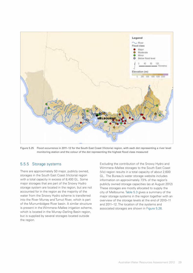
29Australian Water Resources Assessment 2012
Figure5.25 Floodoccurrencein2011–12fortheSouthEastCoast(Victoria)region,witheachdotrepresentingariverlevelmonitoringstationandthecolourofthedotrepresentingthehighestfloodclassmeasured
5.5.5 Storagesystems
There are approximately 50 major, publicly owned, storages in the South East Coast (Victoria) region with a total capacity in excess of 8,400 GL. Some major storages that are part of the Snowy Hydro storage system are located in the region, but are not accounted for in the region as the majority of the water from the Snowy Hydro scheme is transferred into the River Murray and Tumut River, which is part of the Murrumbidgee River basin. A similar structure is present in the Wimmera–Mallee irrigation scheme, which is located in the Murray–Darling Basin region, but is supplied by several storages located outside the region.
Excluding the contribution of the Snowy Hydro and Wimmera–Mallee storages to the South East Coast (Vic) region results in a total capacity of about 2,600 GL. The Bureau’s water storage website includes information on approximately 73% of the region’s publicly owned storage capacities (as at August 2012) These storages are mostly allocated to supply the city of Melbourne. Table 5.3 gives a summary of the major storage systems in the region together with an overview of the storage levels at the end of 2010–11 and 2011–12. The location of the systems and associated storages are shown in Figure 5.26.

30 Australian Water Resources Assessment 2012
South East Coast (Victoria)
Table5.3 MajorpublicstoragesystemsintheregionasidentifiedintheBureauofMeteorology’swaterstorageinformation(August2012),with‘non-allocated’accountingforthestoragesnotallocatedtoaparticularsystem
Systemname Systemtype Systemcapacity
Accessiblevolumeat30June2011
Accessiblevolumeat30June2012
Melbourne* urban 1,812 GL 1,010 GL—56% 1,268 GL—70%
Non-allocated — 95 GL 68 GL—72% 77 GL—81%
Total 1,907 GL 1,078 GL—57% 1,346 GL—71%
*TheMelbournesystemincludesThomson,whichalsohasanimportantruralsupplyfunction
Figure5.26 StoragesystemsintheSouthEastCoast(Victoria)region(informationextractedfromtheBureauofMeteorology’swaterstorageinformationinAugust2012)
During 2011–12, the Melbourne supply system storage volumes increased by 14%. In particular, the Thomson, which comprises 68% of this system, has shown a persistent rise in water levels since June 2010. For the 2011–12 year, Thomson storage volumes rose from 41% to 64% of total accessible capacity.
Further information on the past and present volumes of the storage systems and the individual storage can be found on the Bureau’s water storages website: water.bom.gov.au/waterstorage/

31Australian Water Resources Assessment 2012
Figure5.27 LocationofimportantwetlandsintheSouthEastCoast(Victoria)region
5.5.6 Wetlands
Importantwetlands
There are a large number of wetlands of national and international importance in the South East Coast (Victoria) region (Figure 5.27), encompassing several wetland types. Wetlands in the region include alpine bogs, fresh and saline lakes, coastal estuaries and bays.
The coastal lakes, lagoons and bays form the largest wetlands and attract a large number of common and threatened bird species. They also form the habitat for some rare fish and dolphins, in particular the recently-described Burrunan dolphin. The other major types of wetlands are the lakes and lagoons in the west of the region, which are mainly fed by small rivers and creeks. These provide important habitat for water birds, including a large number of duck species.
Inflowstoselectedwetlands
The state of biodiversity in a wetland is linked to the way water is stored within the area and the temporal variability of inflows. An analysis of historic and recent inflows into wetlands forms an informative picture of potential changes.
Two internationally recognised Ramsar wetland sites, Western District Lakes and Gippsland Lakes, as well as one nationally important wetland (Reedy Lake–Lake Connewarre wetland complex) were selected for hydrological analysis of major inflows. More information about the region’s wetlands is available from the Australian Directory of Important Wetlands (www.environment.gov.au/water/topics/wetlands/database/diwa.html).
Nine upstream stream monitoring gauges were selected to enable analyses and interpretation of inflows to these three wetlands. The gauges used in the analyses are the closest upstream gauges that have largely continuous discharge records since 1980. Though the analyses do not capture the total inflows, they are indicative of the temporal patterns of freshwater surface flows to these wetlands.

32 Australian Water Resources Assessment 2012
South East Coast (Victoria)
WesternDistrictLakes
The Ramsar-listed Western District Lakes form a combination of freshwater and hyper-saline lakes fed by local creeks and rivers. The wetlands are important habitats for many different species of waterbirds. Amongst the shores of the lakes, many different plant species cover vast areas of flat land.
Daily discharge data for the monitoring gauges on the Woady Yaloak River and Pirron Yallock Creek are combined to provide a temporal pattern of freshwater inflows into the Western District Lakes (Figure 5.28).
Figure5.29 CombineddailyflowsofWoadyYaloakRiverandPirronYallockCreekbetween1980and2012,rankedindecileclasses
Figure5.28 LocationofthemonitoringsitesinrelationtoWesternDistrictLakes
Figure5.30 CombinedmonthlyflowsoftheWoadyYaloakRiverandPirronYallockCreekfrom2011–12comparedwithits1980–2012decilerankings
Figure 5.29 presents an overview of the distribution of daily streamflow decile rankings. Since 1997, the normally very much above average flows in late winter and early spring have become substantially less. Additionally, the summer and autumn low flows became much more pronounced from this year onwards. The year 2010–11 was the only real exception to this pattern.
Figure 5.30 compares monthly discharges from 2011–12 with the statistics of flows from 1980 onwards. The 2011–12 flows were particularly low in the normally high flow season from August–October and failed to contribute a significant amount of freshwater to the lakes.

33Australian Water Resources Assessment 2012
GippslandLakes
The Gippsland Lakes are a Ramsar-listed complex of lakes supplied by a number of rivers. Land-use change and river regulation have reduced the original wetland dynamics substantially, but due to the large size of the complex the original biodiversity remains largely intact. The lakes are home to many water birds as well as the rare Burrunan dolphin.
Daily discharge data for the monitoring gauges on the Latrobe, Thomson, Avon, Nicholson and Tambo rivers are combined to provide a temporal pattern of freshwater inflows into the lakes (Figure 5.31).
Figure5.32 CombineddailyflowsofLatrobe,Thomson,Avon,NicholsonandTamboriversbetween1980and2012,rankedindecileclasses
Figure5.31 LocationofmonitoringsitesinrelationtotheGippslandLakes
Figure5.33 CombinedmonthlyflowsoftheLatrobe,Thomson,Avon,NicholsonandTamboriversfrom2011–12comparedwithits1980–2012decilerankings
Figure 5.32 presents an overview of the distribution of daily streamflow decile rankings. The last two years have seen much higher flows than the period 1997–08 and 2009–10. Before this flows were noticeably higher, particularly between July and December. Figure 5.33 compares monthly discharges from 2011–12 with the statistics of flows from 1980 onwards. The flows have been particularly high throughout most of the year and contributed a large amount of freshwater to the lakes.

34 Australian Water Resources Assessment 2012
South East Coast (Victoria)
ReedyLake–LakeConnewarrewetlands
The nationally recognised Reedy Lake–Lake Connewarre wetlands form a combination of freshwater swamps and shallow lakes, fed by the Barwon River. The estuary has been blocked off with a weir to prevent inflows of saline water. The lakes form the habitat for many common as well as some threatened waders and waterbird species.
Daily discharge data for the monitoring gauge on the Barwon and Moorabool rivers are combined to provide a temporal pattern of freshwater inflows into the lakes (Figure 5.34).
Figure5.35 CombineddailyflowsoftheBarwonandMooraboolriversbetween1980and2012,rankedindecileclasses
Figure5.34 LocationofthemonitoringsitesinrelationtotheReedyLake–LakeConnewarrewetlands
Figure5.36 CombinedmonthlyflowsoftheBarwonandMooraboolriversfrom2011–12comparedwiththeir1980–2012decilerankings
Figure 5.35 presents an overview of the distribution of daily streamflow decile rankings. Since 1997–98, the normally very much above average flows in late winter and early spring have become substantially less. Additionally, the summer and autumn low flows became much more pronounced from this year onwards. From 2010–11, the pre-1997–98 flow patterns returned to some extent.
Figure 5.36 compares monthly discharges from 2011–12 with the flow statistics from 1980 onwards. The 2011–12 flows were particularly low in the normally high flow season from August–October and only contributed a substantial amount of freshwater to the lakes in July 2011 and June 2012.

35Australian Water Resources Assessment 2012
5.5.7 Hydrogeology
The groundwater systems of the South East Coast (Victoria) region are varied and complex as shown in Figure 5.37. Hydrogeological features include, basement outcrops of fractured rock, sedimentary basin and the karstic limestone area of the Murray Group aquifer in southeast South Australia.
The region is bounded in the north by fractured rock groundwater systems that typically provide a low volume groundwater resource with the exception of the northwest area. In this part of the region the Murray Group aquifer provides a valuable groundwater resource.
High potential for groundwater extraction is provided by the aquifers associated with the Otway basin, Port Phillip and Westernport basins, Gippsland basin, and Tarwin basin in Southern Victoria (Southern Rural Water 2009). The volcanic basalt plains to the west of Melbourne are also a significant feature.
These aquifers are grouped in Figure 5.37 as:
• lower Tertiary aquifer (porous media—unconsolidated);
• lower mid-Tertiary aquifer (porous media—unconsolidated);
• upper mid-Tertiary aquifer (porous media—unconsolidated);
• upper Tertiary aquifer (porous media—unconsolidated); and
• upper Tertiary/Quaternary aquifer (porous media—unconsolidated).
5.5.8 Watertablesalinity
Figure 5.38 shows the classification of watertable aquifers as fresh (total dissolved solids ([TDS] < 3,000 mg/L) or saline (TDS ≥ 3,000 mg/L). Most parts of the region are considered to have fresh water. No data are available for the New South Wales part of the region, which is primarily the fractured rock of the Lachlan Fold Belt.
5.5.9 Groundwatermanagementunits
In the region, a number of groundwater areas have been established to protect underground water resources. Within these areas authorisation is required to access and/or construct works to take groundwater for certain purposes.
The groundwater management units within the region are presented in Figure 5.39. Most of the units are relatively small in area and are located near the coast, with the exception of some larger units at the western and eastern ends of the region.

36 Australian Water Resources Assessment 2012
South East Coast (Victoria)
Figure5.37 WatertableaquifersoftheSouthEastCoast(Victoria)region;dataextractedfromtheGroundwaterCartographyoftheAustralianHydrologicalGeospatialFabric(BureauofMeteorology2012)

37Australian Water Resources Assessment 2012
Figure5.38 WatertablesalinityclassesintheSouthEastCoast(Victoria)region;dataextractedfromtheGroundwaterCartographyoftheAustralianHydrologicalGeospatialFabric(BureauofMeteorology2012)

38 Australian Water Resources Assessment 2012
South East Coast (Victoria)
Figure5.39 GroundwatermanagementunitsintheSouthEastCoast(Victoria)region;dataextractedfromtheNationalGroundwaterInformationSystem(BureauofMeteorology2013).Managementunitsidentifiedbyhatchedareasarefordeeperaquifersthatmaybeconfined

39Australian Water Resources Assessment 2012
5.5.10Statusofselectedaquifers
The status of groundwater levels is analysed at each bore throughout the South East Coast (Victoria) region. The assessment of groundwater levels evaluates trends in groundwater levels over the five-year period 2007–08 to 2011–12.
The trends in groundwater levels over the last five years are investigated using a 20 km x 20 km grid across data rich areas usually associated with the major groundwater management units (see Figure 5.39). This scale reflects the mostly regional flow system of the aquifers in the region. The linear trend in levels for a grid cell is assessed as:
• decreasing (where more than 60% of the bores have a negative trend in levels lower than –0.1 m/year);
• stable (where more than 60 % of the bores have a trend lower than 0.1 m/year and higher than –0.1 m/year);
• increasing (where more than 60% of the bores have a positive trend in levels higher than 0.1 m/year); and
• variable (where there is no dominant trend in groundwater levels amongst the bores within a grid cell).
Example bore hydrographs are presented for each aquifer type over the entire record length and trends are discussed with a focus on 2007–08 to 2011–12. The hydrographs are for key bores that have been selected to assist in the analysis and reporting of groundwater trends by the Department of Sustainability and Environment across Victoria, by Southern Rural Water for the Gippsland and South West Victoria Groundwater Atlas and by the South Australian Department for Water for the Lower Limestone Coast Prescribed Wells Area.
Upperaquifers
Figure 5.40 illustrates the spatial and temporal trends in groundwater levels, over 2007–08 to 2011–12, in the upper aquifers group which includes Quaternary and upper Tertiary aquifers. This grouping is based on the National Aquifer Framework (the Bureau 2012a) that builds on the Victorian Aquifer Framework. Many of the grid cells show a rising trend with some cells showing either a variable or stable trend with only a minority of cells showing a decreasing trend.
Selected bores 1 (Gippsland basin) and 3 (Otway basin) show a rising trend in groundwater levels over the last five years. This reflects the high rainfall and floods that occurred. Overall these bores show a
long-term stable trend in groundwater levels with seasonal rises and falls which indicate good level recovery in the aquifer. Some winter peaks are more subdued in response to low rainfall. Step rises indicate groundwater response to recharge in high rainfall periods and to floods. In contrast, Bore 2 shows a declining trend until 2010 and then a sharp rising trend in groundwater levels over the last two years. This reflects the local groundwater use and the high rainfall and floods that occurred in this period.
Middleaquifers
Figure 5.41 illustrates the spatial and temporal trends in groundwater levels over 2007–08 to 2011–12, in the middle aquifers group which include upper middle and lower middle Tertiary aquifers. In the west of the region many of the grid cells show a stable trend, while in the rest of the region most of the grid cells show a rising trend with a minority of cells showing a variable or decreasing trend.
Selected bores 4 and 6 show a long-term declining trend in groundwater levels. The main factor driving this declining trend is likely to be reduced recharge. It should be noted that extraction and land use change may also contribute to localised declines. Bore 5 shows overall a stable trend. Wetter conditions during 2009–10 to 2010–11 have led to some recovery of water levels in all bores.
Loweraquifers
Figure 5.42 illustrates the spatial and temporal trends in groundwater levels, over 2007–08 to 2011–12, in the lower aquifers group which include the lower Tertiary aquifers. The grid cells do not show a clearly prevalent trend throughout the region. This probably reflects the low bore density in this aquifer group. However, there is a known long-term declining trend in the Gippsland lower Tertiary aquifer. Selected Bore 7 shows a decline in groundwater level in the late 1990s followed by a recovery in levels, and a more recent slow decline over the last five years. Bores 8 and 9 show a long- term minor declining trend. Wetter conditions during 2009–10 to 2010–2011 have not led to any substantial recovery in groundwater levels, probably due to the slow response of these deep confined groundwater systems.

40 Australian Water Resources Assessment 2012
South East Coast (Victoria)
Figure5.40 SpatialdistributionoftrendsingroundwaterlevelsfortheupperaquifersintheSouthEastCoast(Victoria)regionfor2007–12,withselectedhydrographsshowinggroundwaterlevels

41Australian Water Resources Assessment 2012
Figure5.41 SpatialdistributionoftrendsingroundwaterlevelsforthemiddleaquifersintheSouthEastCoast(Victoria)regionfor2007–12,withselectedhydrographsshowinggroundwaterlevels

42 Australian Water Resources Assessment 2012
South East Coast (Victoria)
Figure5.42 SpatialdistributionoftrendsingroundwaterlevelsfortheloweraquifersintheSouthEastCoast(Victoria)regionfor2007–12,withselectedhydrographsshowinggroundwaterlevels

43Australian Water Resources Assessment 2012
5.6 Waterforcitiesandtowns
This section examines the urban water situation in the South East Coast (Victoria) region in 2011–12. The large urban centres in the region, their water supply systems and storage situations are briefly described. The main urbanised portion, the Melbourne water supply area, is presented in detail including its water supply systems, storage position, historical and current water restrictions, water sources and supply information.
5.6.1 Urbancentres
With a population of about 3.7 million people, Melbourne is the largest and most populous city in the region and the second most populous city in Australia. The metropolitan area extends south from the city centre, along the eastern and western shorelines of Port Phillip Bay, and towards the north.
Geelong, located 75 km southwest of Melbourne, has a population of 144,000 people and is the region’s second most populous city.
Outside of its two major cities the region has a large number of other regional urban centres and towns. These, along with Melbourne and Geelong, are shown in Figure 5.43 in conjunction with their population ranges.
The major urban centres of the region with populations of over 25,000 people are summarised in Table 5.4, which provides information on the population, surrounding river basins and significant water storages for each of the major urban centres in the region.
After Geelong the most notable of the major non-metropolitan urban centres in the region are Ballarat and the Latrobe Valley.
The Latrobe Valley has a population of 125,000 people and is located to the east of Melbourne. It has four major urban centres: Warragul, Moe, Morwell, and Traralgon. Population figures for the Latrobe Valley are not included in this table.
Ballarat with a population of 86,000 people is located in the lower western plains of the Great Dividing Range, about 100 km northwest of Melbourne.
Table5.4 PopulationinmajortownsandcitiesintheSouthEastCoast(Victoria)region
City Population1 Riverbasin Majorsupplysources
Melbourne 3,707,000 Yarra, Werribee, Maribyrnong and Bunyip
Thomson, Upper Yarra, Cardinia
Geelong 144,000 Barwon Wurdee Boluc
Ballarat 86,000 Barwon Coliban storages, Lake Eppalock
Melton 46,000 Werribee Melton Reservoir
Sunbury 33,000 Maribyrnong Rosslyne Reservoir
Warrnambool 29,000 Hopkins Via pipeline from the Gellibrand River and various diversion weirs on creeks in the Great Otway National Park
Mount Gambier 25,000 Millicent Coast Blue Lake1AustralianBureauofStatistics(2011b)

44 Australian Water Resources Assessment 2012
South East Coast (Victoria)
Figure5.43 PopulationrangeofmajorurbancentresintheSouthEastCoast(Victoria)region

45Australian Water Resources Assessment 2012
5.6.2 Sourcesofwatersupply
Like much of Australia, the cities and towns of the South East Coast (Victoria) region rely on surface water as the major source of supply. The region has over 20 major water storages, each with a capacity greater than 1 GL, and the majority of these are within Victoria.
While Lake Eucumbene, located in the northwest, is the largest storage in the region and the third largest in Australia, the Thomson storage in the central north is the largest storage of the region with the primary use being for urban supply.
The Thomson primarily supplies the Melbourne metropolitan region and is the third largest water storage connected to a major city in Australia. The storage also supplies a number of small towns and, more significantly, irrigation demands across
a number of the regions irrigation districts. The Thomson, along with other major surface water storages in the region, is shown in Figure 5.44.
In addition to surface water storages the region utilises direct river extractions (including extractions of upstream storage releases), groundwater, desalination, recycled water, and harvested storm and rainwater to supply the urban demands of the region.
Groundwater extractions form a reliable source of supply in the western part of the region where surface water extractions from the Grampians and Otway Ranges catchments can be variable.
Two major wastewater treatment plants on the eastern and western extremities of metropolitan Melbourne supply significant quantities of recycled water to adjacent areas.
Figure5.44 UrbansupplystoragesintheSouthEastCoast(Victoria)region

46 Australian Water Resources Assessment 2012
South East Coast (Victoria)
5.6.3 Melbourne
The Melbourne metropolitan area is serviced by four major water corporations. These comprise three retail suppliers (City West Water, Yarra Valley Water and South East Water) and a bulk water supplier (Melbourne Water). Melbourne’s water supply and wastewater system are summarised in Figure 5.45.
Formed under Victoria’s Water Act 1989, these corporations manage Melbourne’s surface water supply catchments, storages, water treatment plants, storages and supply networks. These corporations are owned by the Victorian Government but managed by independent boards of directors.
Melbourne Water supplies bulk water to the metropolitan retailers as well as selling water to the regional urban water corporations of Western Water and Gippsland Water.
In addition to its bulk water supply role Melbourne Water operates a number of Melbourne’s wastewater treatment plants, including its two largest, the Eastern and Western treatment plants, and manages waterways and major drainage systems in the Port Phillip Bay and Westernport areas.
Yarra Valley Water is the largest of the three retail water utilities and provides water supply and sewerage services to over 1.6 million people and over 50,000 businesses in the Yarra River basin part of the Melbourne water supply area
City West Water is the second largest of the three retail water utilities in the Melbourne water supply area. It provides drinking water and recycled water services to customers in Melbourne’s central business district as well as to the inner and western suburbs, and manages sewerage and trade waste.
Figure5.45 Melbourne’smajorwatersupplyandwastewatersystem

47Australian Water Resources Assessment 2012
South East Water provides water supply services including recycled water to residents, businesses, industry and councils in Melbourne’s southeast. It manages and maintains the water and sewerage networks and some treatment plants. It also manages a network of parks as well as cultural assets, bays and waterways.
In addition to the major metropolitan suppliers, Western Water services the area within the Maribyrnong and Werribee River basins that extend into Melbourne’s Western growth area, while Gippsland Water delivers water to a small area in the southeast of Melbourne and has its major service area outside Melbourne.
Supplysystem
Melbourne’s surface water supplies are drawn from catchments that feed six main storages. These storages are Thomson, Upper Yarra, Tarago, Maroondah, O’Shannassy and Yan Yean.
In addition to these storages a further four major storages without a significant catchment area are used in the operation of the Melbourne system. These storages are Cardinia, Sugarloaf, Silvan and Greenvale.
While no longer in operation, the North South Pipeline facilitates the bidirectional transfer of water between the Goulburn River and Melbourne Water’s Sugarloaf storage.
Again, not in operation during 2011–12, the Wonthaggi desalination plant can provide potable water for Melbourne and based on current consumption is capable of supplying up to 40% of the cities potable water demand. Water supplied from the plant is transferred by pipe to Cardinia.
Storagevolumes
At approximately 60% of Melbourne’s total accessible storage capacity the Thomson plays a major role in the security of the city’s water supply. Thomson constitutes 1,068 GL of the 1,812 GL total accessible storage capacity. As such, the historical storage volume shown in Figure 5.46 provides insight into Melbourne’s surface water supply resources over the past 18 years.
Figure 5.46a shows the accessible storage volumes of Thomson from 1985–2012 and exhibits three distinct trends.
The sustained increase in the accessible storage volume between 1985 and 1990 is explained by the completion of the Thomson Dam in 1984 and the subsequent filling of the storage during successive years of good rainfall and inflows.
Below average rainfall between 1997 and 2008 saw drought conditions develop throughout much of the region. The corresponding reduction in inflows to Melbourne’s major storages saw a significant decline in the accessible storage. This trend was reflected throughout the system.
A shift in climatic conditions in 2009 and a series of wetter years (including Australia’s wettest two-year period on record in 2010–11) saw the storage level recover from their 2008 low of less than 200 GL. This filling trend is highlighted in Figure 5.46b which shows the accessible storage for Thomson for 2011–12.
Figure5.46 Variationintheamountofwaterheldinstorageoverrecentyears(lightblue)andover2011–12(darkblue)for Thomsonstorage,aswellastotalaccessiblestoragecapacity(dashedline)

48 Australian Water Resources Assessment 2012
South East Coast (Victoria)
Waterrestrictions
Drought response plans (DRPs), developed by Melbourne’s three water retailers (City West Water, South East Water and Yarra Valley Water) in consultation with Melbourne Water, are an important mechanism in the management of Melbourne’s water resources in times of shortage.
The DRPs require the three retailers and Melbourne Water to jointly prepare and publish, by 1 December each year, an annual Water Outlook for Melbourne that provides an overview of the total system storage with reference to three zones: High, Medium and Low, as well as an annual and medium term action plans which may include water restrictions.
Announcements to lift or introduce water restrictions are made by the Victorian Government based on the annual Water Outlook that considers a range of factors including storage over the Water Outlook period; past and forecast weather/climate, catchment conditions; inflows and trends in demand; as well as planned investments and actions. In times of water shortages, the urban water utilities can implement water restrictions ranging from Stage 1 (mild/alert) to Stage 4 (severe/critical).
These restriction levels and the Permanent Water Saving Rules which is a set of commonsense rules that applies all the time to ensure water efficient
practices in the community were developed following a State-wide review in 2011 by the Victorian Water Industry Association in consultation with the water industry.
Figure 5.47 shows there were no water restrictions in the Melbourne water supply area until August 2006 since the previous restrictions were lifted in March 2005. Due to the low rainfall and inflow in 2006, in September 2006 Stage 1 restrictions were introduced. This was quickly followed by Stage 2 restrictions introduced in spring 2006 and Stage 3 restrictions introduced in summer 2007. Stage 3a restrictions, which increase limitations on residential water use even further, were introduced before winter 2007.
Rainfall between 2007 and 2009 was not enough to increase water storage volumes and Stage 3a restrictions remained in place. Because of above average rainfall in the upstream sections of the supply catchments in 2009–10, water restrictions were eased to Stage 3 in April 2010. Following the above average rainfall in 2010–11 and 2011–12, the water restrictions were eased progressively, falling back to Stage 1 in December 2011.
Figure5.47 UrbanwaterrestrictionlevelsforMelbournesince2005shownagainstthecombinedaccessiblewatervolumeoftheThomson,UpperYarraandCardiniastorages

49Australian Water Resources Assessment 2012
Sourceofwaterobtained
Surface water is the main source of water supplied to the Melbourne water supply area. Figure 5.48 illustrates that over the last six years approximately 96% of bulk water delivered was derived from surface water supplies and 4% from recycled water (National Water Commission 2013).
The total volume of water supplied to Melbourne decreased from 431 GL in 2006–07 to 384 GL in 2011–12. This significant 18% reduction can be attributed to water efficiency gains, the implementation demand management strategies (including water restrictions and the installation of water efficient appliances), and the augmentation of domestic supplies with locally sourced water from storm and rainwater.
Following its broad scale introduction as a supply source in 2005–06, Melbourne has sourced approximately 14 GL of water per year from recycled water. Recycled water is supplied to consumers through various schemes operated by the water authorities. It is used to meet a broad range of end-uses that include including broad scale agriculture, market gardens and the maintenance of conservation areas and golf courses.
Once commissioned, the Wonthaggi desalination plant will provide a new source of water for Melbourne. The plant will have the capacity to meet up to 40% of Melbourne’s current demand.
Groundwater does not play a significant role in the Melbourne water supply system.
Figure5.48 TotalurbanwatersourcedfortheMelbournewatersupplyareafrom2006–07to2011–12

50 Australian Water Resources Assessment 2012
South East Coast (Victoria)
Categoriesofwaterdelivered
Figure 5.49 shows the total volume of water delivered to residential, commercial, municipal and industrial consumers by the three utilities from 2006–07 to 2011–12 financial years. Approximately 60% of the total volume supplied was for residential use and 27% for commercial, municipal and industrial use (National Water Commission 2013).
Most significantly this figure illustrates that while demand management strategies in the residential sector achieved a reduction in water consumption
(approximately 8%) the most significant savings were achieved in the commercial, industrial and municipal sectors, which collectively achieved a 16% reduction in water consumption across the 2006–07 to 2011–12 financial year period.
At individual property scale, the observed reductions in residential water consumption translate to an estimated 7 kL per year per property saving of water, with use falling from an average 148 kL per property in 2006–07 to 141 kL in 2011–12 (National Water Commission 2013).
Figure5.49 TotalurbanwatersuppliedtotheMelbournewatersupplyareafrom2006–07to2011–12

51Australian Water Resources Assessment 2012
Figure5.50 Decilesrankingsofannualaveragesoilmoisturefor2011–12withrespecttothe1911–2012periodintheSouthEastCoast(Victoria)region
5.7 Waterforagriculture
This section describes the water situation for agriculture in the South East Coast (Victoria) region in 2011–12. Soil moisture conditions are presented and important irrigation areas are identified. The Macalister, Werribee and Bacchus Marsh irrigation areas are described in more detail and information is provided regarding surface storage and groundwater.
5.7.1 Soilmoisture
Since model estimates of soil moisture storage volumes are based on a simple conceptual representation of soil water storage and transfer processes averaged over a 25 km x 25 km grid cell, they are not suitable to compare with locally measured soil moisture volumes. This analysis therefore presents a relative comparison only,
identifying how modelled soil moisture volumes of 2011–12 relate to modelled soil moisture volumes of the 1911–2012 period, expressed in decile rankings.
Soil moisture deciles for 2011–12 show very much above average conditions for most of the eastern part of the region (Figure 5.50). This was as a result of high rainfall events in the east which was in sharp contrast to the western part of the region which generally received average to very much below average rainfall during the year.
The decile ranking of monthly changes of soil moisture (Figure 5.51) shows that availability of soil moisture dropped to near average levels during the spring and summer months, partly due to very high evapotranspiration in two months of this period. The above average rainfalls that followed this period kept the soil moisture conditions at very much above average in the autumn and winter months.
Figure5.51 Decilerankingofthemonthlysoilmoistureconditionsduringthe2011–12periodintheSouthEastCoast(Victoria)region

52 Australian Water Resources Assessment 2012
South East Coast (Victoria)
5.7.2 Irrigationwater
Irrigation water use in the region between 2005–06 and 2010–11 is shown in Figure 5.52 and Figure 5.53 by natural resource management (NRM) region. The southeast (South Australia) and West Gippsland districts showed the highest irrigation water use during this period.
At the time of writing the report data was not available for 2011–12.
Water resource availability for Macalister Irrigation District in West Gippsland and Werribee and Bacchus Marsh in the Port Phillip Bay and Westernport regions are discussed in more detail in the following sections.
Figure5.52 Totalannualirrigationwaterusefor2005–06to2010–11fornaturalresourcemanagementregionsintheSouthEastCoast(Victoria)region(ABS2006–2010;2011a)
Agricultural water use in the Bacchus Marsh irrigation district, Victoria | Southern Rural Water

53Australian Water Resources Assessment 2012
Figure5.53 Annualirrigationwaterusepernaturalresourcemanagementregionfor2010–11(ABS2011b)

54 Australian Water Resources Assessment 2012
South East Coast (Victoria)
5.7.3 Irrigationareas
More than half the land in the South East Coast (Victoria) region is used for grazing sheep and cattle. Dryland cropping is concentrated in the central and western parts of the region. Hardwood timber production is a major industry in the Snowy, East Gippsland and Barwon River basins. The region contains a green triangle of more than five million hectares with the largest area of plantations in Australia including pine (softwood).
Irrigated agriculture constitutes only a small portion (0.5%) of the land use in the region (Figure 5.54). Major irrigation districts are concentrated around Lake Glenmaggie in the Thomson River basin and Bacchus Marsh and Werribee in the Werribee River basin. The most significant irrigation area in
the region is the Macalister Irrigation District that contains both irrigated pasture and horticulture. The Werribee irrigation area is important for irrigated agricultural and dairy farming. Market gardens are the dominant industry in both areas.
Water in the region is managed by the Gippsland and Southern Rural Water Corporation that delivers water to the Macalister, Werribee and Bacchus Marsh districts. These districts use about 145 GL and 330 GL from surface and groundwater each year. The storages in four major catchments, such as the Macalister, Werribee, Maribyrnong and Latrobe, are also managed by this corporation. The Werribee, Bacchus Marsh and Macalister irrigation areas are described in more detail in subsections 5.7.4–5.7.5.
Figure5.54 IrrigationareasintheSouthEastCoast(Victoria)region

55Australian Water Resources Assessment 2012
5.7.4 WerribeeandBacchusMarshirrigationdistricts
The Werribee and Bacchus Marsh irrigation districts are located in the Werribee basin that has a temperate climate with most rain in winter and spring (Figure 5.55). The combined capacity of the Werribee system storages is approximately 69 GL (Melton, Pykes Creek and Merrimu storages). This capacity is allocated between irrigation (62%) and urban (28%) water use, with the remaining 10% retained as an unallocated share.
The Werribee system has some of the highest percentages of water trading in Victoria and trading occurs across the whole system between Werribee and Bacchus Marsh irrigators and river diverters. River entitlements have been in place in the Werribee basin since 2001 as a further source of water.
Most farms in the Bacchus Marsh district have on-farm dams to store water prior to irrigation, which
provides flexibility to manage crop water demands. The Bacchus Marsh irrigation district receives its irrigation supply via a weir on the Werribee River east of Ballan as well as a second diversion weir located west of Bacchus Marsh on the Werribee River. The maximum capacity of the supply system is 105 ML/d at the Bacchus Marsh Weir, although during the millenium drought it rarely operated at flows higher than 70 ML/d.
Treated recycled water from Melbourne’s Western Treatment Plant has been available to the Werribee district irrigators since 2004. Melbourne Water supplies up to 65 ML/d of recycled water as a supplementary water source. Recycled water is mixed with river water to reduce salinity levels before it is supplied to irrigators. However, heavy rainfall, turbidity-related issues caused by wind, and algal outbreaks affect reliability of river water for mixing.
Figure5.55 TheMacalister,WerribeeandBacchusMarshirrigationdistricts

56 Australian Water Resources Assessment 2012
South East Coast (Victoria)
The following example of Pykes Creek storage shows the storage had reached full capacity in 2010 which continued for half of the 2011–12 year. The
inflows to the storage was not adequate enough to keep it full for the rest of the period (Figure 5.56).
Pykes Creek
Figure5.56 Variationintheamountofwaterheldinstorageoverrecentyears(lightblue)andover2011–12(darkblue)forthePykesCreek,aswellastotalaccessiblestoragecapacity(dashedline)
5.7.5 MacalisterIrrigationDistrict
The Macalister Irrigation District is the largest irrigation area south of the Great Dividing Range, extending from Lake Glenmaggie to near Sale along the Macalister River (Figure 5.55). The majority of the land used for irrigation is under pasture.
Lake Glenmaggie is the main source of supply for the Macalister Irrigation District, situated on the Macalister River. It covers an area of 1,760 ha and has an accessible storage capacity of 190 GL. The lake usually fills up during winter and spring and levels decline gradually during the summer months. Thomson, with an accessible storage capacity of 1,068 GL, also partially supplies the Macalister Irrigation District.
Irrigation allocations from Lake Glenmaggie each year are a function of three phases: a filling phase starting at the beginning of the irrigation season on 1 July; a spilling phase when the lake has filled (October–December); and an emptying phase when the drawdown of lake levels begins. If the dam spills, all water used from the start of the season is referred to as Spill Entitlement or off-quota and allocation use is reset to zero. The maximum volume of Spill Entitlement is 62,000 ML/yr. During the emptying phase, a high reliability water share (HRWS) and a low reliability water share (LRWS) are announced depending on the magnitude of the inflows to the storage.
There is some limited groundwater use in the Macalister Irrigation District.
Surfacewaterstorageinflows
Historically, streamflow in the Macalister River peaks during late winter and spring. The flow upstream of Lake Glenmaggie, monitored at the river gauge on the Macalister River at Stringy Bark Creek, peaked in August before it dropped to historic low levels, but maintained average to high flows afterwards. During March and July 2012 the flows were much above historic average flows (Figure 5.57). This situation coincided with a period when rainfalls exceeded the 90th percentile in the region and resulted in landscape water yields that were at historically high levels.
Figure5.57 MonthlydischargehydrographscomparedtodischargedecilesatareferencegaugeforinflowstoLakeGlenmaggie

57Australian Water Resources Assessment 2012
Figure5.58 Variationintheamountofwaterheldinstorageoverrecentyears(lightblue)andover2011–12(darkblue)fortheLakeGlenmaggiestorageaswellastotalaccessiblestoragecapacity(dashedline)
Lake Glenmaggie
All this caused the water availability from Lake Glenmaggie in 2011–12 to be at its highest on record. The seasonal allocation opened at 90% HRWS with Lake Glenmaggie spilling. The allocation increased to 100 per cent HRWS in February 2012. In addition, 15.8 GL of spill entitlement was delivered between July and December 2011.
High rainfall during February and March caused total water deliveries for the season to be 86 GL, which is below the average delivery and below delivery budget of 163 GL. (Southern Rural Water 2012).
Surfacewaterstoragevolumes
Historical data of stored water volume in Lake Glenmaggie show that storage levels reach their maximum capacity during winter and spring in each year (Figure 5.58).
High inflows into Lake Glenmaggie in 2011–12, coupled with low irrigation demand, resulted in the volume in storage remaining at 138 GL or 78% of the full capacity in May 2012 at the end of the irrigation season. This situation provided a good start for the 2012–13 season (Southern Rural Water 2012).

58 Australian Water Resources Assessment 2012
South East Coast (Victoria)
LocalHydrogeology
The Macalister Irrigation District (shown in Figure 5.59) is underlain by relatively complex groundwater systems. This is also reflected in the large number of groundwater management areas that overlay the irrigation area. There are at least five management units that regulate groundwater extraction at various depths for different aquifers.
The Boisdale Aquifer (upper middle aquifer) that occurs throughout the area provides a valuable source of water for irrigation of pasture for dairy production, vegetable cropping and stock and domestic supply. The Boisdale aquifer is underlain by the Latrobe Valley Group (lower middle and lower aquifer), grading easterly into the Balook Formation (lower middle aquifer) and the Gippsland Limestone aquifer (lower middle aquifer). Declining groundwater levels in these deeper aquifers as well as in the Boisdale aquifer is a well documented phenomenon resulting from the combined effects of offshore gas and oil extraction, dewatering of the Latrobe Valley coal mines and pumping for irrigation.
The degree of interaction between surface water and groundwater is high. The Latrobe, Thomson, Macalister and Avon are the major rivers in the area and they gain groundwater during low flow; by contrast rivers recharge the alluvial aquifers during floods (Southern Rural Water 2012). The eastern portion of the area includes Lake Wellington, Lake Victoria and Lake Reeve, which are part of the Gippsland Lake systems. The current accepted view is that groundwater discharges into the lakes as well as to the sea.
Groundwaterqualityoverview
Clearing and irrigation has significantly altered the hydrogeological regime in the irrigation area, increasing the infiltration to the shallow watertable and causing discharge of shallow saline groundwater. In addition, the recent lowering of the groundwater levels near Lake Wellington below the lake level has focused attention on the potential to draw saline water from the lake and the sea into the aquifer.
Influencesonshallowgroundwater
Fluctuations in shallow groundwater levels at selected sites are shown in Figure 5.60. To investigate the drivers of the shallow groundwater levels, fluctuations in the groundwater levels ‘(a)’ are compared to the monthly rainfall trend, shown by cumulative residuals from the historic average at Sale ‘(b)’, the monthly discharge of the Macalister River ‘(c)’ and the monthly average level of Lake Wellington ‘(d)’. Locations of gauges and bores are shown in Figure 5.59.
Periods in which the cumulative rainfall residual mass curve rises indicate wetter than average conditions. Periods with a falling trend indicate drier than average conditions.
Panel two in Figure 5.60, shows a wetter than average period up to 1996, followed by drier that average period until 2010 and since then wetter than average condition. This is reflected by groundwater levels which are lower on average after 1996 compared to before 1996 and show a rise in level at two bores after 2010.
Seasonal pumping and recovery cycles are also visible in all bores except Bore 92297. Step rises indicates groundwater response to flooding, for example in 2007. Although some of the groundwater levels show some degree of correlation with the river discharge there is no major correlation to lake levels.

59Australian Water Resources Assessment 2012
Figure5.59 TheMacalisterIrrigationDistrictshowingthelocationofgroundwaterboresites,rivergauges,lakegaugesandraingauges
A telemetered bore in Glenelg-Hopkins | Thiess Services

60 Australian Water Resources Assessment 2012
South East Coast (Victoria)
Figure5.60 (a)Comparisonofshallowgroundwaterlevelsrecordedatnestedboresiteswithrainfall,streamflowandLakeWellingtonwaterlevelsintheMacalisterIrrigationDistrict(Bore86657—yellow,Bore42095—red,Bore95486—blue,andBore92297—green;(b)cumulativerainfallresidualmassatSaleStationno.85072;(c)MacalisterRiverdischargeatGlenmaggie,Stationno.225204;and(d)LakeWellingtonlevelatBullBay,Stationno.226041.

61Australian Water Resources Assessment 2012
Figure5.61 Groundwaterlevelsbetween2007and2012recordedatselectednestedboresitesintheMacalisterIrrigationDistrict
Groundwaterlevel
Groundwater level measurements are an important source of information about hydrological and anthropological influences on the groundwater in an area, including recharge. Figure 5.61 illustrates groundwater levels recorded in bores of different depth at the same site in the Macalister Irrigation District in the last five years.
Groundwater level fluctuations in the area generally indicate upward gradients and potentially groundwater flow from the deeper aquifers (blue lines) to the shallower aquifers (red and yellow lines). However, gradients and potentially groundwater flow can be reversed during intense pumping from the lower aquifer (for example, blue line in site 1) as in 2010 and 2012. Figure 5.61 also shows in general poor connectivity between various aquifers at various depths. Groundwater levels show different patterns at different location and depth except for shallow bores 95485 and 95486.
Figure 5.62 and Figure 5.63 show the spatial distribution of depth to groundwater in bores located in the upper and middle aquifers in the Macalister Irrigation District. They also give the ranking of 2011–12 median groundwater levels compared to annual median groundwater levels in the last 22 years (1990–2012).
As shown in Figure 5.62, typically groundwater levels in the upper aquifer are mostly within 5 m of the surface. Median groundwater depth below surface in 2011–12 is typically above average or average in the southwest and in the rest of the area is average or below average.
Groundwater levels below surface in the middle aquifer vary from greater than 10 m away from Lake Wellington to above the surface (flowing artesian) near the lake (Figure 5.63). Median groundwater depth in 2011–12 is mostly below average or average, indicating that groundwater levels are the deepest or within the average of the past 22 years.
Groundwater levels from bores screened in the lower aquifer are not shown as there are not enough data available to provide a useful assessment of groundwater conditions in this aquifer.
Groundwatersalinity
At the time of writing, suitable quality controlled and assured time-series data on groundwater salinity were not available from the Australian Water Resources Information System (the Bureau of Meteorology 2011).

62 Australian Water Resources Assessment 2012
South East Coast (Victoria)
Figure5.62 (a)UpperaquifermediangroundwaterdepthfortheMacalisterIrrigationDistrictin2011–12;and(b)decilerankofdepthin2011–12comparedtothe1990–2012period.Deciles1–3areshownasbelowaverage(greaterdepthbelowsurface),deciles4–7asaverageanddeciles8–10asaboveaverage

63Australian Water Resources Assessment 2012
Figure5.63 (a)MiddleaquifermediangroundwaterdepthfortheMacalisterIrrigationDistrictin2011–12;and(b)decilerankofdepthin2011–12comparedtothe1990–2012period.Deciles1–3areshownasbelowaverage(greaterdepthbelowsurface),deciles4–7asaverageanddeciles8–10asaboveaverage

Tasmania6 Tasmania................................................................... 2
6.1 Introduction........................................................ 2
6.2 Keyinformation.................................................. 3
6.3 Descriptionoftheregion.................................... 4
6.3.1 Physiographiccharacteristics.................. 6
6.3.2 Elevation................................................. 7
6.3.3 Slopes.................................................... 8
6.3.4 Soiltypes................................................ 9
6.3.5 Landuse.............................................. 11
6.3.6 Populationdistribution.......................... 13
6.3.7 Rainfallzones....................................... 14
6.3.8 Rainfalldeficit....................................... 15
6.4 Landscapewaterflows.................................... 16
6.4.1 Rainfall.................................................. 17
6.4.2 Evapotranspiration................................ 20
6.4.3 Landscapewateryield......................... 23
6.5 Surfacewaterandgroundwater....................... 26
6.5.1 Rivers................................................... 26
6.5.2 Streamflowvolumes............................. 28
6.5.3 Streamflowsalinity................................ 28
6.5.4 Flooding............................................... 28
6.5.5 Storagesystems................................... 31
6.5.6 Wetlands.............................................. 33
6.5.7 Hydrogeology....................................... 38
6.5.8 Watertablesalinity................................ 38
6.5.9 Groundwatermanagementunits........... 38
6.6 Waterforcitiesandtowns................................ 42
6.6.1 Urbancentres....................................... 42
6.6.2 Sourcesofwatersupply....................... 44
6.6.3 GreaterHobart..................................... 44
6.7 Waterforagriculture......................................... 47
6.7.1 Soilmoisture........................................ 47
6.7.2 Irrigationwater...................................... 48
6.7.3 Irrigationareas...................................... 48
6.7.4 SouthEastandMeander
irrigationschemes................................. 51

2 Australian Water Resources Assessment 2012
Tasmania
6.1 Introduction
This chapter examines water resources in the Tasmania region in 2011–12 and over recent decades. It starts with summary information on the status of water flows, stores and use. This is followed by descriptive information for the region including the physiographic characteristics, soil types, population, land use and climate.
Spatial and temporal patterns in landscape water flows are presented as well as an examination of the surface and groundwater resources. The chapter concludes with a review of the water situation for urban centres and irrigation areas. The data sources and methods used in developing the diagrams and maps are listed in the Technical Supplement.
6 Tasmania

3Australian Water Resources Assessment 2012
6.2 Keyinformation
Table 6.1 gives an overview of the key components of the data and information in this chapter.
Table6.1 Keyinformationonwaterflows,storesanduseintheTasmaniaregion
Landscapewaterflows
Evapo-transpiration
Landscapewater yield
Rainfall
Region average Difference from 1911–2012 long-term annual mean
Decile ranking with respect to the 1911–2012 record
1,396 mm +2% 7th—average
769 mm +3% 8th—above average
632 mm +1% 6th—average
Streamflow(atselectedgauges)
Annual total flow: Predominantly average flow in the northern and southern rivers, mostly above average flow in the central east of the region
Flooding: Moderate to major floods in the central east of the region
Surfacewaterstorage(comprisingabout86%oftheregion’stotalcapacityofallmajorstorages)
Total accessible capacity
30 June 2012 30 June 2011 Change
accessible volume
% of total capacity
accessible volume
% of total capacity
accessible volume
% of total capacity
22,141 GL 15,672 GL 71% 13,576 GL 61% +2,096 GL +10%
Wetlandsinflowpatterns(forselectedwetlands)
Lower Ringarooma River: Average flows, but above average flow in August 2011
Apsley Marshes: Very much above average flows in August 2011 and above average in May and June 2012, generally average to below average flows in the other months
Moulting Lagoon: Very much above average flows in August 2011 and above average in May and June 2012, generally average flows in the other months
Groundwater(inselectedaquifers)
Salinity: Non-saline groundwater (<3,000 mg/L) in most aquifers, locally some small areas with saline (≥3,000 mg/L) groundwater in the east
Urbanwateruse(Hobart)
Total sourced in 2011–12 Total sourced in 2010–11
Change Restrictions
40 GL 42 GL – 2 GL ( – 4%) No restrictions
Annualmeansoilmoisture(modelestimates)
Spatial patterns: Predominantly average with large areas of below average in the southwest and above average soil moisture mainly in the southeast
Temporal patterns in regional average:
Above average soil moisture at the start of the year, gradually dropping to below average in January and returning to above average by June 2012

4 Australian Water Resources Assessment 2012
Tasmania
6.3 Descriptionoftheregion
The island of Tasmania is the smallest of Australia’s states with a total land size of approximately 68,000 km2. Though it is less than 1% of Australia’s surface area the region contains about 12% of Australia’s freshwater resources. It is separated from the Australian mainland by Bass Strait.
The region is largely composed of relatively fertile agricultural land, dense forests and rugged mountainous areas. The geologically and florally diverse northern regions of Tasmania include a wide variety of terrestrial, estuarine and marine ecosystems. The terrestrial ecosystems range from the vegetation and wildlife of the mountain plateaus to the wet forests and swamps of the middle elevations, the drier forests and woodlands of the lower-rainfall slopes down to the sandy hills and plains of the coast. Fertile agriculture land is also present. In the west and southwest of the region, rugged mountains, extensive forests and uninhabited coastlines are found. Subsections 6.3.1 to 6.3.4 give more detail on physical characteristics of the region.
The State-based region of Tasmania has a population of just over 0.5 million people (Australian Bureau of Statistics [ABS] 2011b). Major population centres include the State’s capital, Hobart, as well as the cities of Launceston, Devonport and Burnie.
Figure 6.1 shows the major population centres for the region, while further discussion of the region’s population distribution and urban centres can be found in subsection 6.3.6 and section 6.6 respectively.
The majority of Tasmania is under nature conservation land management (50%, see Figure 6.1). This is followed by forestry (23%) and pasture (21%). Irrigated and dryland cropping and horticulture makes up only a small portion (1.2%) of the land use. Section 6.7 has more information on agricultural activities in the region.
Tasmania has a cool temperate climate with high rainfall in the western highlands, and low rainfall in the lowlands and east. The northeast highlands also have high rainfall compared to their surrounds. Snowfall normally occurs in late winter and early spring. Subsections 6.3.7 and 6.3.8 provide more information on the rainfall types and deficits across the region.
Approximately 150,000 km of waterways, 8,800 wetlands and 94,000 water bodies exist in the region (Department of Primary Industries, Parks, Water and Environment 2009). River basins on the island vary in size from 685–11,700 km².
Tasmania has extensive groundwater resources located in igneous, sedimentary and metamorphic rocks, as well as unconsolidated sediments. The region’s hydrogeology is dominated by large areas of outcropping fractured basement rock. The groundwater systems in fractured rock typically offer restricted low to moderate volume groundwater resources. Groundwater quality and yield is highly variable. A more detailed description of the rivers and groundwater status in the region is given in section 6.5.

5Australian Water Resources Assessment 2012
Figure6.1 MajorriversandurbancentresintheTasmaniaregion

6 Australian Water Resources Assessment 2012
Tasmania
6.3.1 Physiographiccharacteristics
The physiographic map in Figure 6.2 shows areas with similar landform evolutionary histories (Pain et al. 2011). These can be related back to similar geology and climatic impacts which define the extent of erosion processes. The areas have distinct physical characteristics that can influence hydrological processes.
The Tasmania region has two large physiographic regions that account for 75% of the total area, namely:
• East Tasmanian Hills (37%): fault block hills and mountains on dolerite, sandstone, and mudstone, with coastline formed from submerged river valleys; and
• West Tasmanian Ridge (35%): ridges of folded quartzite and conglomerate, glaciated in places, parallel valleys on weaker rocks.
Four physiographic regions occupy the remaining area. They are:
• Lakes Plateau (9%): high dolerite plateau with many lakes;
• Midlands Plain (6%): lowland on weathered sediments;
• Bass Coastal Platforms (6%): low coastal platforms; and
• North West Ramp (3%): incised basalt ramp including coastal cliffs.
Figure6.2 PhysiographicprovincesoftheTasmanianregion

7Australian Water Resources Assessment 2012
6.3.2 Elevation
Figure 6.3 presents ground surface elevations in the Tasmania region. Information was obtained from the Geoscience Australia website (www.ga.gov.au/topographic-mapping/digital-elevation-data.html). The centre of Tasmania forms the highest part of the region, with peaks exceeding 1,500 m above sea level. It contains a plateau called the Central Highlands, on which a substantial number of lakes have formed.
Coastal plains are generally absent. The north coast is the most accessible, which is noticeable by the many
harbour towns along the coast. The city of Hobart is built on the flanks of the Derwent River.
Much of the western part of the island is in use for hydroelectricity generation by Hydro Tasmania. The abundance of rainfall and the presence of deep valleys form an ideal landscape for this particular industry. The area is almost totally protected under nature conservation regulations.
The three major islands north of Tasmania, that is, Flinders and Cape Barren islands to the east and in particular King Island to the west, are less mountainous.
Figure6.3 GroundsurfaceelevationsintheTasmaniaregion

8 Australian Water Resources Assessment 2012
Tasmania
6.3.3 Slopes
Table 6.2 summarises the proportions of slope classes for the region, while Figure 6.4 shows the spatial distribution for the surface slopes. Areas with steep slopes provide higher run-off generating potential than flat areas. The Tasmania region has the highest coverage of steep slopes in relation to the rest of Australia. The slopes were derived from the elevation information used in the previous section.
Table6.2Proportionsofslopeclassesfortheregion
Slopeclass(%)
0–0.5 0.5–1 1–5 >5
Proportion of region (%)
3.4 4.6 29.9 62.1
Figure 6.4 presents surface slopes in the Tasmania region. Steep slopes generally inhibit commercial use of the land other than forestry and natural conservation/recreation. This is partly why almost 75% of the land use in the region falls in these categories.
In between the steep slopes some flat areas can be noticed. Most of these are very large lakes, with the exception of the larger area in the central northeast, which are the alluvial plains of the Macquarie and South Esk rivers.
Figure6.4 SurfaceslopesintheTasmaniaregion

9Australian Water Resources Assessment 2012
6.3.4 Soiltypes
Soils play an important role in the hydrological cycle by distributing water that reaches the ground. Water can be transported to rivers and lakes via the soil surface as run-off or enter the soil and provide water for plant growth as well as contributing to groundwater recharge.
The nature of these hydrological pathways and the suitability of the soils for agricultural purposes are influenced by soil types and their characteristics. Soil type information was obtained from the Australian Soil Resource Information System website (www.asris.csiro.au).
About 85% of the Tasmania region is covered by five soil types, namely tenosols, dermosols, sodosols, kurosols as well as organosols (Figure 6.5 and Figure 6.6).
Tenosols, sodosols and kurosols soils have a low agricultural potential due to low chemical fertility and water-holding capacity.
Tenosols are distributed along the west coast as well as in central to northern parts and scattered around the east coast of the region.
Sodosols are only common in the east of the region. These soils have a strongly contrasting texture, with a relatively impermeable sodic and clay enriched subsoil. They are prone to tunnel and gully erosion due to soil dispersion and structural instability. They are also at risk of dryland salinity.
Kurosols are common in the northeast and southeast of the region. They are usually strongly acidic (pH < 5.5).
Dermosols have higher agricultural potential. They have moderate to high chemical fertility and are common in the northwest and northeast of the region. These soils are well structured and have a high water-holding capacity. They co-exist with highly fertile and well-drained ferrosols that together with the moderate climate, result in a very productive agricultural zone.
Organosols soils are rich in organic material throughout the profile and are found in the wet and forested southwest of the region.
The other soil types that have minimal representation in the region are ferrosols, chromosols, podosols and rudosols (0.5–5% of the total area).
Figure6.5 SoiltypesintheTasmaniaregion

10 Australian Water Resources Assessment 2012
Tasmania
Figure6.6 SoiltypedistributionintheTasmaniaregion

11Australian Water Resources Assessment 2012
6.3.5 Landuse
Figures 6.7 and 6.8 presents land use in the region (data from data.daff.gov.au/anrdl/metadata_files/pa_luav4g9abl07811a00.xml). The majority of the region is under nature conservation, and this is followed by forestry and pasture. Irrigated and dryland cropping and horticulture make up only a small portion of the land use.
The landscape is heavily forested and mountainous. In the north, a wide variety of terrestrial, estuarine and marine environments can be found that include:
• the vegetation and wildlife of the mountain plateaus;
• the wet forests and swamps of the middle elevations; and
• the drier forests and woodlands of the lower-rainfall slopes; and sandy coastal hills and plains.
Fertile agriculture land is also present in the north. The west and southwest of the region is covered with rugged mountains, extensive forests and uninhabited coastlines.
Figure6.7 LanduseintheTasmaniaregion

12 Australian Water Resources Assessment 2012
Tasmania
Figure6.8 LandusedistributionintheTasmaniaregion

13Australian Water Resources Assessment 2012
6.3.6 Populationdistribution
The Tasmania region, with a total population of 494,000 people, represents just over 2% of Australia’s total population. Figure 6.9 shows the spatial distribution of population density (ABS 2011b).
The region’s population is divided in two major concentrations. In the south, the population is concentrated mainly around Hobart, and in the north around the north coast that includes the major towns of Launceston, Devonport and Burnie.
Agriculture is a major driver for many communities, and Launceston, Devonport and Burnie provide important ports for exporting the produce to the Australian mainland and beyond.
The central and western districts are sparsely populated and mostly devoted to nature conservation. Mining, forestry and tourism are the major drivers for many of the more remote towns located throughout the west of the State.
Figure6.9 PopulationdensityanddistributionintheTasmaniaregion

14 Australian Water Resources Assessment 2012
Tasmania
6.3.7 Rainfallzones
Tasmania has a cool temperate climate with high rainfall and snowfall in the western highlands, and low rainfall in the lowlands and east. The northeast highlands also have high rainfall (partly as snowfall) compared to their surrounds. Median rainfall exceeds 500 mm throughout (Figure 6.10).
Median annual rainfall exceeds 1,000 mm in the west. In the southeast, the rainfall is more uniformly distributed over the year and the median annual totals are mostly below the 800 mm, with the exception of highlands in the northeast.
For more information on this and other climate classifications, visit the Bureau’s climate website: www.bom.gov.au/jsp/ncc/climate_averages/climate-classifications/index.jsp
Figure6.10 RainfallzonesintheTasmaniaregion

15Australian Water Resources Assessment 2012
6.3.8 Rainfalldeficit
The rainfall deficit indicator, that is, rainfall minus potential evapotranspiration, gives a general impression about which parts of the region are likely to experience moisture deficits over the period of a year. The Tasmania region in general has relatively limited areas of minor moisture deficit potential (Figure 6.11) in comparison to the rest of Australia.
Due to the lower temperatures and solar radiation levels, potential evapotranspiration in the region is relatively low. Hence, rainfall deficits mostly occur only in those areas where rainfall itself is a limiting factor.
In the west and central areas, the general abundance of water over the year is used to generate hydroelectricity. Hydro Tasmania uses this energy source to supply the majority of Tasmania’s electricity. Major reservoirs are located in the area.
For more information on the rainfall and evapotranspiration data, see the Bureau’s maps of average conditions: www.bom.gov.au/climate/averages/maps.shtml
Figure6.11 RainfalldeficitdistributionfortheTasmaniaregion

16 Australian Water Resources Assessment 2012
Tasmania
6.4 Landscapewaterflows
This section presents analyses of the spatial and temporal variation of landscape water flows (rainfall, evapotranspiration and landscape water yield) across the Tasmania region in 2011–12. National rainfall grids were generated using data from a network of persistent, high-quality rainfall stations managed by the Bureau. Evapotranspiration and landscape water yields were derived using the landscape water balance component of the Australian Water Resources Assessment System (Van Dijk 2010). These methods and associated output uncertainties are discussed in the Introduction and addressed in more detail in the Technical Supplement.
Figure 6.12 shows the region has a seasonal rainfall pattern with a wet winter and a drier summer period. However, in particular in this region, local anomalies can occur. The bandwidth of historic evapotranspiration data is small, which indicates that the constraint on evapotranspiration is mainly energy- driven. Evapotranspiration in the summer period occasionally exceeds rainfall, as the soils normally contain moisture available for evapotranspiration. The monthly landscape water yield history for the region shows a pattern that is closely linked to rainfall.
The 2011–12 year was relatively average, with no major extremes in the monthly rainfall exceeding the 10th–90th percentile range. There was also no dry or wet period identifiable for consecutive months.
Evapotranspiration rates were relatively high for the months of November and December. Very much above average temperatures were measured throughout the region for November, which provided additional energy for the evapotranspiration processes. For the rest of the year, the evapotranspiration closely followed the historic pattern.
As with the historic records, the landscape water yield for 2011–12 closely followed the rainfall pattern with the exception of November, when the higher rainfall was largely absorbed by the soil and consequently evaporated back to the atmosphere. The landscape water yield was consistently below average or average from September–February.
Figure6.12 Landscapewaterflowsin2011–12comparedwiththelong-termrecord(July1911–June2012)fortheTasmaniaregion

17Australian Water Resources Assessment 2012
6.4.1 Rainfall
Rainfall for the Tasmania region for 2011–12 is estimated to be 1,396 mm. This is 2% above the region’s long-term average (July 1911–June 2012) of 1,365 mm.
Figure 6.13a shows that the highest rainfall for 2011–12 occurred in the western part of the region with annual totals exceeding 2,400 mm in large areas.
Rainfall deciles for 2011–12 indicate generally average conditions, with some areas of above average rainfall in the southern and eastern coastal areas (Figure 6.13b). The Flinders and Cape Barren islands in the northeast received above average rainfall.
Figure6.13 Spatialdistributionof(a)annualrainfallin2011–12,and(b)theirdecilerankingsoverthe1911–2012periodfortheTasmaniaregion

18 Australian Water Resources Assessment 2012
Tasmania
Rainfallvariabilityintherecentpast
Figure 6.14a shows annual rainfall for the region from July 1980 onwards. Over this 32-year period the annual average was 1,311 mm, varying from 1,039 mm (2006–07) to 1,543 mm (2010–11). Temporal variability and seasonal patterns (over the summer and winter periods) since 1980 are presented in Figure 6.14b.
The graphs indicate that regional average rainfall is not very variable. The coefficient of variation (standard deviation divided by the mean) over the annual rainfall and data of Figure 6.14a is 0.11, the lowest of all regions in Australia. Both the summer and winter periods in Figure 6.14b show no signs of trends or cyclic patterns.
Figure6.14 Time-seriesof(a)annualrainfall,and(b)five-yearretrospectivemovingaveragesforthesummer(November–April)andwinter(May–October)periodsfortheTasmaniaregion

19Australian Water Resources Assessment 2012
Recenttrendsinrainfall
Figure 6.15a presents the spatial distribution of the trends in annual rainfall for July 1980–June 2012. These are derived from linear regression analyses on the time-series of each model grid cell. The statistical significance of the trends is provided in Figure 6.15b.
Figure 6.15a shows that since 1980 a strong decrease in rainfall has occurred on the southwestern coast of the region. This falling trend appears to be strongly statistically significant (Figure 6.15b), but this can be influenced by the low rain gauge density. On the other hand, a strongly significant rising trend is found in the northeast (covering the Ben Lomond National Park area) of the region.
Figure6.15 Spatialdistributionof(a)trendsinannualrainfallfrom1980–2012,and(b)theirstatisticalsignificanceat90%(weak)and95%(strong)confidencelevelsfortheTasmaniaregion

20 Australian Water Resources Assessment 2012
Tasmania
6.4.2 Evapotranspiration
Modelled annual evapotranspiration for the Tasmania region for 2011–12 is estimated to be 769 mm (Figure 6.16). This is 3% above the region’s long-term (July 1911–June 2012) average of 744 mm. The spatial distribution of annual evapotranspiration in 2011–12 (Figure 6.16) is similar to that of rainfall (Figure 6.13) and was highest along the west coast with annual totals exceeding 900 mm.
Evapotranspiration deciles for 2011–12 indicate above average or average totals across most of the region (Figure 6.16b). This spatial distribution is very different to the rainfall distribution (Figure 6.13b). The highly localised areas of very much above average evapotranspiration appearing mainly around major lakes are currently known artefacts of the model and need to be considered with care.
Figure6.16 Spatialdistributionof(a)modelledannualevapotranspirationin2011–12,and(b)theirdecilerankingsoverthe1911–2012periodfortheTasmaniaregion

21Australian Water Resources Assessment 2012
Evapotranspirationvariabilityintherecentpast
Figure 6.17a shows annual evapotranspiration for the region from July 1980 onwards. Over this 32-year period the annual evapotranspiration average was 724 mm, varying from 649 mm (2006–07) to 791 mm (1988–89). Temporal variability and seasonal patterns (over the summer and winter periods) since 1980 are presented in Figure 6.17b.
The graphs indicate that regional average evapotranspiration is even less variable than rainfall. The coefficient of variation over the annual data of Figure 6.17a is 0.06, the lowest of all regions in Australia. Both the higher summer and lower winter periods in Figure 6.17b show no obvious signs of trends or cyclic patterns.
Figure6.17 Time-seriesof(a)annualevapotranspiration,and(b)five-yearretrospectivemovingaveragesforthesummer(November–April)andwinter(May–October)periodsfortheTasmaniaregion

22 Australian Water Resources Assessment 2012
Tasmania
Recenttrendsinevapotranspiration
Figure 6.18a presents the spatial distribution of the trends in modelled annual evapotranspiration for 1980 to 2012. These are derived from linear regression analyses on the time-series of each model grid cell. The statistical significance of the trends is provided in Figure 6.18b.
Figure 6.18a shows that since 1980 trends are mostly neutral, with the exception of the southwest part of the region. Besides the same artefacts on the lakes, Figure 6.18b shows significant falling trends for only the southwest and south coast.
Figure6.18 Spatialdistributionof(a)trendsinannualevapotranspirationfrom1980–2012,and(b)theirstatisticalsignificanceat90%(weak)and95%(strong)confidencelevelsfortheTasmaniaregion

23Australian Water Resources Assessment 2012
6.4.3 Landscapewateryield
Modelled landscape water yield for the Tasmania region for 2011–12 is estimated to be 632 mm. This is just above the region’s long-term (July 1911–June 2012) average of 627 mm. Figure 6.19a shows the spatial distribution of landscape water yield for 2011–12, which is similar to that of rainfall (Figure 6.13a).
The highest landscape water yields in 2011–12 are observed along the west coast, exceeding 1,200 mm in most of the area. In contrast, the inland areas in the Midlands and the Derwent Valley had annual landscape water yield totals below 50 mm. The decile ranking map for 2011–12 (Figure 6.19b) shows mostly above average landscape water yields to the east, average landscape water yields in the centre and western part of the region and some areas of below average landscape water yield on the west coast.
Figure6.19 Spatialdistributionof(a)modelledannuallandscapewateryieldin2011–12,and(b)theirdecilerankingsoverthe1911–2012periodforTasmaniaregion

24 Australian Water Resources Assessment 2012
Tasmania
Landscapewateryieldvariabilityintherecentpast
Figure 6.20a shows annual landscape water yield for the Tasmania region from July 1980 onwards. Over this 32-year period, annual landscape water yield was 591 mm, varying from 405 mm (2006–07) to 735 mm (2010–11). Temporal variability and seasonal patterns (over the summer and winter periods) since 1980 are presented in Figure 6.20b.
The graphs indicate that regional average landscape water yield is more variable than rainfall and evaporation, but the coefficient of variation is still the lowest of all regions in Australia. Both the summer and winter period in Figure 6.20b show no signs of trends or cyclic patterns. Landscape water yield is generally high in the winter period due to the combination of higher rainfall and the lower evapotranspiration producing more saturated soils.
Figure6.20 Time-seriesof(a)annuallandscapewateryield,and(b)five-yearretrospectivemovingaveragesforthesummer(November–April)andwinter(May–October)periodsfortheTasmaniaregion

25Australian Water Resources Assessment 2012
Recenttrendsinlandscapewateryield
Figure 6.21a shows the spatial distribution of the trends in modelled annual landscape water yield for 1980–2012. These are derived from linear regression analyses on the time-series of each model grid cell. The statistical significance of the trends is provided in Figure 6.21b.
Figure 6.21a is consistent with the rainfall trends of Figure 6.15a. However, Figure 6.21b shows that the strongly significant falling trends on the southwest coast are less pronounced than those of rainfall. Conversely, the strongly significant rising trends in landscape water yield in the northeast cover a larger area than the area of significantly increased rainfall.
Figure6.21 Spatialdistributionof(a)trendsinannuallandscapewateryieldfrom1980–2012,and(b)theirstatisticalsignificanceat90%(weak)and95%(strong)confidencelevelsfortheTasmaniaregion

26 Australian Water Resources Assessment 2012
Tasmania
6.5 Surfacewaterandgroundwater
This section examines surface water and groundwater resources in the Tasmania region in 2011–12. Rivers, wetlands and storages are discussed to illustrate the state of the region’s surface water resources.
The region’s water table aquifers and salinity are described and the groundwater management units are illustrated. No data was available to the Bureau in a suitable format for a detailed analysis of individual aquifers.
6.5.1 Rivers
There are 19 river basins in the Tasmania region, varying in size from 650 to 11,000 km2 (Figure 6.22).
The main river basins within the region are the Tamar and Derwent river basins. The region includes some of the largest permanent lakes in Australia such as Lake Pedder and Lake Gordon.
Most of the major rivers are perennial except on the east coast where a variety of river types can be found. The rivers are seasonal and those fed from the highlands have increased flow during snow melt. Many rivers are fast-flowing with many rapids, dropping quickly over short distances from the source to the sea. Many, like the Gordon and Tamar, have fine estuaries before entering the ocean.
GordonRiver,Tasmania|A41cats,Dreamstime.com

27Australian Water Resources Assessment 2012
Figure6.22 RiversandcatchmentsintheTasmaniaregion

28 Australian Water Resources Assessment 2012
Tasmania
6.5.2 Streamflowvolumes
Figure 6.23 presents an analysis of flows at 25 monitoring sites during 2011–12 relative to annual flows for the period from July 1980–July 2012. Monitoring sites with relatively long flow records across 11 geographically representative river catchments were found in the north and eastern area of the region and selected for analysis. The annual flows for 2011–12 are colour-coded according to the decile ranking at each site over the 1980–2012 period.
High flows volumes are usually generated in the headwaters of rivers and their tributaries where rainfall is often relatively high. Very much above average flows were observed at three sites located on the Clyde River in the centre and the Scamander River in the northeast of the Tasmania region. Above average total flows were recorded at five monitoring sites located on the rivers in the centre and east of the region. Above average flows in these rivers were mostly generated during major rainfall events in August 2011.
Average flow occurred at 16 sites in the region that were located on the rivers in the south and most of the rivers in the north of the region. Of the 25 monitoring sites there was only one where below average flows were recorded. This site is located on the Pipers River in the north of the region.
Flow deciles in the summer (November 2011–April 2012) were very different to the total annual flows for 2011–12 as shown Figure 6.23. The main differences are the relatively low flows in the summer period in the centre and along the east coast and the relatively higher flows on the north coast. The most contrasting flow pattern can be seen in the centre of the region, especially on the Clyde River downstream of Lake Crescent (see Figure 6.23, sites with flow values of 282 and 132 ML/day). As a consequence of large winter inflows in early 2011–12, water was released for irrigation in the summer period.
6.5.3 Streamflowsalinity
Suitable streamflow salinity data were not available during this period. Therefore, streamflow salinity analysis is not included in this chapter.
6.5.4 Flooding
Floods can be caused mainly by localised high intensity rainfall (for example, during thunderstorms) or prolonged periods of heavy rainfall (for example, frontal rainfall). While the first rainfall type often results in localised flash flooding, the prolonged rainfall events can cause floods over larger areas.
While thunderstorms can occur at any time, most of the Tasmania region has a seasonal pattern of rainfall with the majority of rainfall occurring in winter. Flooding is most commonly associated with cold fronts crossing Tasmania as well as coastal low pressure systems.
Figure 6.24 shows selected locations where the Bureau is monitoring river levels as part of its flood forecasting service and the highest level reached during the year expressed in terms of flood classification level. These classification levels are established in consultation with emergency management and local agencies and are further described in the Technical Supplement.
Significant flooding occurred in the northeast of the Tasmania region following two separate periods of heavy rainfall in August 2011 causing moderate to major flooding of the South Esk and Macquarie rivers. The first event, from 7–10 August 2011, was caused by a low pressure system that slowly moved to the north of the region with a trough extending down over the northeast. Rainfall totals for the four days exceeded 100 mm at sites in the South Esk and Macquarie rivers.
The second event, from 16–19 August 2011, was another significant flooding event in the northeast. Four-day rainfall totals again exceeded 100 mm at several sites. The South Esk River reached major flood level, and the North Esk and Macquarie rivers both reached moderate flood level. Flood volumes for this event were exacerbated by already wet ground and high water levels following the earlier event.
There were landslips and several roads were closed with both events. The township of St Helens was isolated. Infrastructure damage totalled several hundred thousand dollars and flooding disrupted freight services, closing the North-South and Fingal railway lines.

29Australian Water Resources Assessment 2012
Figure6.23 Averageannualandsummerperiodflowvolumesofselectedsitesfor2011–12andtheirdecilerankingsoverthe1980–2012periodintheTasmaniaregion

30 Australian Water Resources Assessment 2012
Tasmania
Figure6.24 Floodoccurrencein2011–12fortheTasmaniaregion,witheachdotrepresentingonegaugingstationandthecolourofthedotrepresentingthehighestfloodclassmeasured

31Australian Water Resources Assessment 2012
6.5.5 Storagesystems
There are approximately 57 major publicly owned storages in the Tasmania region with a total capacity in excess of 25,700 GL. The Bureau’s water storage website provides information for more than 86% of the region’s publicly owned storage capacity (as at August 2012). Storages in the region supply ten systems used for hydro-electric power generation. They also supply the urban centre of Hobart.
Table 6.3 gives a summary of the major storage systems in the region together with an overview of the storage levels at the end of 2010–11 and 2011–12. The location of all the systems and associated storages are shown in Figure 6.25.
A mixed pattern of storage volume increases and decreases took place in the systems in 2011–12. The substantial increase in the total storage volume can mostly be ascribed to the increase in storage volume in Lake Gordon.
Since most systems are used for hydro-electrical power generation, some water release patterns are highly irregular. For example, the significant drop in volumes of the storages in the Anthony system were balanced out again in July 2012, when storage volumes were back at those volumes measured in July 2011.
Further information on the past and present volumes of the storage systems and the individual storages can be found on the Bureau’s water storage website: water.bom.gov.au/waterstorage/awris/
Table6.3 MajorpublicstoragesystemsintheregionasidentifiedintheBureau’swaterstoragewebsite(August2012),with‘non-allocated’accountingforthestoragesnotallocatedtoaparticularsystem
Systemname Systemtype Systemcapacity Accessiblevolumeat30June2011
Accessiblevolumeat30June2012
Gordon hydro 14,029 GL 8,432 GL—60% 10,527 GL—75%
South Esk—Great Lake hydro 3,619 GL 1,604 GL—44% 1,665 GL—46%
Pieman hydro 1,434 GL 1,368 GL—95% 1,179 GL—82%
Burbury hydro 1,082 GL 795 GL—73% 959 GL—89%
Upper Derwent hydro 755 GL 504 GL—67% 573 GL—76%
Nive hydro 728 GL 478 GL—66% 408 GL—56%
Mersey hydro 157 GL 102 GL—65% 86 GL—55%
Lower Derwent hydro 142 GL 120 GL—85% 115 GL—81%
Forth hydro 141 GL 130 GL—92% 128 GL—91%
Anthony hydro 36 GL 22 GL—61% 14 GL—39%
Hobart urban 3.6 GL 3.6 GL—100% 3.6 GL—100%
Non-allocated — 15 GL 15 GL—100% 14 GL—93%
Total 22,141 GL 13,576 GL—61% 15,672 GL—71%

32 Australian Water Resources Assessment 2012
Tasmania
Figure6.25 StoragesystemsintheTasmaniaregion(informationextractedfromtheBureau’swaterstoragewebsiteinAugust2012)

33Australian Water Resources Assessment 2012
6.5.6 Wetlands
Importantwetlands
There are a large number of wetlands of national and international importance in the Tasmania region (Figure 6.26), encompassing a wide diversity of wetland types, from coastal floodplains and lagoons to higher altitude freshwater streams and lakes. Dominant features in the region are the coastal lagoons. Six of the ten Ramsar-listed wetlands in the region are lagoons, each with their own characteristic biodiversity. Other dominant wetland types are river deltas and estuaries.
The coastal lagoons comprise a diverse range of seasonal and permanent marshlands, grass, forests and woodlands. They are recognised as important sites for resident and migratory birds, including some threatened bird species. The river deltas and estuaries are predominantly characterised by marshes and swamps and provide a different type of habitat for birds and plants.
Inflowstoselectedwetlands
The state of the biodiversity in a wetland is linked to the way water is stored within the area and the temporal variability of inflows. An analysis of historic and recent inflows into wetlands forms an informative picture of potential changes.
Three internationally recognised Ramsar wetland sites (Lower Ringarooma River, Moulting Lagoon and Apsley Marshes) were selected for hydrological analysis of major inflows. The Moulting Lagoon and Apsley Marshes form a linked system of wetlands, with the Apsley Marshes performing important nutrients-filtering of the Apsley River before it flows into the Moulting Lagoon. More information about the region’s wetlands is available from the Australian Directory of Important Wetlands (www.environment.gov.au/water/topics/wetlands/database/diwa.html)
Three upstream stream monitoring gauges were selected to enable the analyses and interpretation of inflows to these three wetlands. The gauges used in the analyses are the closest upstream gauges that have largely continuous discharge records since 1980. Though the analyses do not capture the total inflows, they are indicative of the temporal patterns of freshwater surface flows to these wetlands.

34 Australian Water Resources Assessment 2012
Tasmania
Figure6.26 LocationofimportantwetlandsintheTasmaniaregion

35Australian Water Resources Assessment 2012
LowerRingaroomaRiver
The Lower Ringarooma River wetlands encompass a variety of wetland types, including estuary, river and floodplain wetlands. Much of the listed wetland area has been altered from its natural state (Newall and Lloyd 2012). Mining in the 1800s and early 1900s has contributed to large scale sedimentation entering the Ringarooma River.
Daily discharge data for the monitoring gauge on the Ringarooma River at Moorina provides a temporal pattern of freshwater inflows into the Lower Ringarooma River wetlands (Figure 6.27).
Figure6.28 DailyflowsofRingaroomaRiveratMoorinabetween1980and2012,rankedindecileclasses
Figure6.27 LocationofthemonitoringsiteinrelationtotheLowerRingaroomaRiverwetlands
Figure6.29 MonthlyflowsoftheRingaroomaRivermonitoringsiteatMoorinafrom2011–12comparedwiththe1980–2012decilerankings
Figure 6.28 presents an overview of the distribution of daily streamflow decile rankings. The data provides a clear pattern of a seasonal flow regime with high flows from June up to October and low flow from December through to April. From 1999 onwards the low flows appear to be lower than before, but the wet summer of 2010–11 broke this pattern. The flows of 2011–12 were back to pre-1999 conditions.
Figure 6.29 compares monthly discharges from 2011–12 with the statistics of flows from 1980 onwards. The normally high August flows were above average in 2011–12. The remaining 2011–12 flows are close to the average flows of the past 32 years.

36 Australian Water Resources Assessment 2012
Tasmania
ApsleyMarshes
The Apsley Marshes are located in the floodplain of the Apsley River, just upstream of the Moulting Lagoon. The Apsley Marshes contain areas of woody vegetation, some salt marshes, large areas of reed and freshwater aquatic herbs. The marshes form an important habitat for some threatened bird species and support many plant and animal species considered internationally important.
Daily discharge data for the monitoring gauge on the Apsley River upstream of the Coles Bay Road bridge provides a temporal pattern of freshwater inflows into the marshes (Figure 6.30).
Figure6.31 DailyflowsofApsleyRiverupstreamofColesBayRoadbridgebetween1980and2012,rankedindecileclasses
Figure6.30 LocationofthemonitoringsitesinrelationtotheApsleyMarshes
Figure6.32 MonthlydischargesattheApsleyRivermonitoringsiteupstreamofColesBayRoadbridgefrom2011–12comparedwithits1980–2012decilerankings
Figure 6.31 presents an overview of the distribution of daily streamflow decile rankings. Although data are missing from 1992–93 to 2000–01, it can be noted that the flows have no distinct seasonal pattern. Flows can be low between November and April, but as a result of east coast lows, large rainfall events have occurred during this period that resulted in high flow peaks throughout this period for many years.
Figure 6.32 compares monthly discharges from 2011–12 with the statistics of flows from 1980 onwards. The August flows contributed a substantial amount of freshwater to the floodplain complex.

37Australian Water Resources Assessment 2012
MoultingLagoon
The Moulting Lagoon is located downstream of the Apsley Marshes on the Apsley River, but also has substantial inflows from the Swan River. The lagoon is surrounded by tidal mudflats and salt marsh that provide important feeding areas for many water bird species. The Swan River provides important inflows of freshwater to the system during peak flows.
Daily discharge data for the monitoring gauge on the Swan River at The Grange provide a temporal pattern of freshwater inflows into the lagoon (Figure 6.33).
Figure6.34 DailyflowsoftheSwanRiveratTheGrangebetween1980and2012,rankedindecileclasses
Figure6.33 LocationofthemonitoringsitesinrelationtotheMoultingLagoon
Figure6.35 MonthlyflowsattheSwanRivermonitoringsiteatTheGrangefrom2011–12comparedwithits1980–2012decilerankings
Figure 6.34 presents an overview of the distribution of daily streamflow decile rankings. The raster visualisation shows an irregular pattern of high and low flows occurring throughout most years. There were extended periods of very much below average flows during the dry years of 2007–08 and 2008–09. In general, however, flood peaks occurred frequently throughout the 32 years, providing frequent freshwater inflows into the lagoon.
Figure 6.35 compares monthly discharges from 2011–12 with the statistics of flows from 1980 onwards. The August flows well exceeded the ninth decile of the 32-year record and contributed a substantial amount of freshwater to the wetland.

38 Australian Water Resources Assessment 2012
Tasmania
6.5.7 Hydrogeology
Tasmania has extensive groundwater resources located in igneous, sedimentary and metamorphic rocks, as well as unconsolidated sediments. Groundwater quality and yield is highly variable, depending on the aquifer type, the topographic location and the rainfall.
The classification of water table aquifers based on the geology within the region is presented in Figure 6.36. Greater resource potential is associated with the following aquifer groups:
• Surficial Sediments aquifers, porous media—unconsolidated;
• Upper Tertiary aquifer, porous media—unconsolidated;
• Fractured and Karstic Rocks, local aquifers; and
• Fractured Rock aquifers.
6.5.8 Watertablesalinity
Figure 6.37 shows the salinity of the water table aquifer as fresh (total dissolved solids [TDS] < 3,000 mg/L) and saline (TDS≥ 3,000 mg/L). Data on groundwater salinity is not available for most parts of Tasmania, however, where data do exist, the water table is mainly fresh.
6.5.9 Groundwatermanagementunits
There are approximately 8,000 operating bores in Tasmania supplying water for irrigation, domestic use, town supplies, stock watering, mining and other commercial purposes. They are predominantly located in agricultural areas along the north coast, midlands, east coast and southeast.
Estimated sustainable annual groundwater yield across the state is in the order of 500–2,500 GL (Department of Infrastructure Energy and Resources 2001); however, a significant proportion is located in undeveloped terrain in the high rainfall areas of the west coast (generally reserved land).
A smaller proportion is available from aquifers in the developed areas. A number of these areas, poorly served by reliable surface water, and where the density of bores and demand on groundwater are relatively high, are currently experiencing pressure on groundwater and connected surface water resources (Sheldon 2011).
Estimated State-wide groundwater use is approximately 14% of the total current annual consumptive surface water allocation of 950 GL/year. In those parts of the State where groundwater and surface water use coincide, this ratio is significantly higher.
A regulatory framework for the management of groundwater in Tasmania is being introduced by the Department of Primary Industries, Parks, Water and Environment, through the development and implementation of policy to underpin sustainable management of connected groundwater and surface water resources. Introduction of a well-driller’s licensing system and a well works permit system occurred in October 2009, and the State’s first proclaimed groundwater area was appointed at Sassafras-Wesley Vale in August 2012 (Figure 6.38). Further groundwater areas will be considered through a formal risk assessment process likely to lead to more appointments.
While provision for active management of groundwater is made in all currently active water management plans if monitoring reveals emerging issues, a formal provision to appoint a statutory groundwater area and to licence and allocate groundwater is presently only made in the Sassafras-Wesley Vale water management plan (Department of Primary Industries, Parks, Water and Environment 2012).

39Australian Water Resources Assessment 2012
Figure6.36 WatertableaquifersoftheTasmaniaregion;dataextractedfromtheGroundwaterCartographyoftheAustralianHydrologicalGeospatialFabric(BureauofMeteorology2012)

40 Australian Water Resources Assessment 2012
Tasmania
Figure6.37 WatertablesalinityclassesoftheTasmaniaregion;dataextractedfromtheGroundwaterCartographyoftheAustralianHydrologicalGeospatialFabric(BureauofMeteorology2012)

41Australian Water Resources Assessment 2012
Figure6.38 GroundwatermanagementunitsintheTasmaniaregion;dataextractedfromtheNationalGroundwaterInformationSystem(BureauofMeteorology2013)

42 Australian Water Resources Assessment 2012
Tasmania
6.6 Waterforcitiesandtowns
This section examines urban water situation in Tasmania in 2011–12. The large urban centres in the region and their water supply systems are briefly described. The main urbanised area, Greater Hobart, is addressed in more detail.
6.6.1 Urbancentres
With over one quarter of the region’s population, Hobart is the largest city in the region; yet, with only 171,000 residents Hobart ranks just outside Australia’s top ten largest cities.
Launceston, in the north is the second largest city in the region is and has a population of 74,000 people. The city is located at the southern end of the Tamar River estuary.
Devonport, on the northwest coast, has a population of 23,000 people and supports the surrounding agricultural areas as a local commercial centre and provides a harbour for exporting the produce to the Australian mainland and beyond.
Burnie, with a population of just below 20,000, has a similar function further west on the north coast, serving the forestry industry in particular.
While its number of large urban centres is small, Tasmania is characterised by numerous small towns and communities scattered throughout its many river valleys and coastal plains Figure 6.39 shows the location and population ranges of towns and communities with populations in excess of 1000 people.
The major urban centres of the region (populations over 20,000 people) are summarised in Table 6.4. This table provides information on the population, surrounding river basin and significant water storages for each of the major urban centres.
Table6.4 CitiesandtheirwatersupplysourcesintheTasmaniaregion
City/town Population1 Riverbasin Majorsupplysources
Hobart 171,000 Derwent River, Kingston Coast
Derwent River, Mount Wellington streams, Lake Fenton
Launceston 74,000 South Esk River, North Esk River, Tamar River
North Esk River, St Patricks River, Curries River storage
Devonport 23,000 Forth River, Mersey River
Forth River and Lake Paloona
1AustralianBureauofStatistics2011b

43Australian Water Resources Assessment 2012
Figure6.39 PopulationrangeofurbancentresintheTasmaniaregion

44 Australian Water Resources Assessment 2012
Tasmania
6.6.2 Sourcesofwatersupply
With its many river valleys and high rainfall, Tasmania relies almost entirely on surface water to meet its urban supply needs.
The State has a total accessible storage capacity of over 22,000 GL, approximately one quarter of Australia’s total surface water storage capacity. Lake Gordon, in the southwest, comprises over half of the region’s total storage capacity. While the majority of this storage is used for the generation of hydro-electricity, the networks of dams, transfer channels and pipe plays an important role in the supply of the region’s urban water resources.
Urban supplies are typically drawn from river extractions from a combination of catchment inflows and storage releases. The region has a number of smaller dedicated urban storages, such as Lake Travallyn; these, however, are typically much smaller than storages used in many other regions because of the region’s reliable rainfall. Figure 6.40 shows the location of the few storages that are specifically functioning as water supply sources to the urban centres of the region.
While only playing a minor role in urban supply in the region, recycled water and groundwater are used to meet only a small proportion of the region’s demands. Harvested storm and rainwater are also used on a very local basis to supply urban demand within the region.
6.6.3 GreaterHobart
Hobart is located on the southeast coast of Tasmania on the Derwent River estuary. It occupies the foothills and low lying slopes of Mt Wellington.
Water supply and sewerage services for Hobart and the broader southern Tasmanian area are provided by the Tasmanian Water and Sewerage Corporation (Southern Region) that trades as Southern Water. The cooperation functions as both the bulk water authority and retail supplier.
SupplySystem
Water supplied to the greater Hobart area (Derwent and Kingston Coast river basins) are drawn from three primary sources, that is, the middle reaches of the Derwent River (upstream of New Norfolk), Lake Fenton/Lady Barron Creek (Mount Field in the Derwent River basin) and from several Mount Wellington streams (Hobart Water 2008).
Water sourced from the Derwent River is treated at the Bryn Estyn plant, transferred to water storages and then delivered to customers throughout Greater Hobart. Water sourced from Mount Wellington and Lake Fenton is used for supply to consumers in Hobart City and Kingborough local government areas.

45Australian Water Resources Assessment 2012
Figure6.40 UrbansupplystoragesintheTasmaniaregion

46 Australian Water Resources Assessment 2012
Tasmania
Waterrestrictions
The reliable and comparatively secure nature of water resources available for supplying the Greater Hobart area have negated the need to enforce water restrictions; however, restrictions on outdoor watering are automatically imposed during periods of total fire ban so that sufficient water is available for fire-fighting purposes (Southern Water 2012).
Storagevolumes
While the majority of the city’s water supplies are drawn from direct river extractions, Lake Fenton, in the Mount Field National Park, was constructed in 1939. The dam and transfer tunnel is capable of releasing 18 million litres of water per day into the Lady Barron Creek for transfer by pipe to Hobart’s water treatment facilities.
Sourcesofwaterobtained
The following paragraph contains data relating to the source of water to Greater Hobart from 2006–07 to 2011–12. For the period from 2006–07 to 2008–09, data was extracted from a National Performance Report (National Water Commission 2009a).
Figure 6.41 presents the total volume of water sourced from surface water for supply to Greater Hobart area. A downward trend in the water drawn is emerging with an 8% reduction over the past two years in total water supplies.
Consumption data for Greater Hobart was not available.
Figure6.41 TotalurbanwatersourcedforGreaterHobartfrom2006–07to2011–12

47Australian Water Resources Assessment 2012
6.7 Waterforagriculture
This section describes the water situation for agriculture in the Tasmania region during 2011–12 year compared with the past. Soil moisture conditions are presented and important irrigation areas are identified. The South East and Meander irrigation areas are described in more detail and information is provided regarding surface storage.
6.7.1 Soilmoisture
Since model estimates of soil moisture storage volumes are based on a simple conceptual representation of soil water storage and transfer processes averaged over a 5 x 5 km grid cell, they are not suitable to compare with locally measured soil moisture volumes. This analysis therefore presents a relative comparison only, identifying how
Figure6.42 Decilesrankingsofannualaveragesoilmoisturefor2011–12withrespecttothe1911–2012periodfortheTasmaniaregion
Figure6.43 Decilerankingofthemonthlysoilmoistureconditionsduringthe2011–12periodwithrespecttothe1911–2012intheTasmaniaregion
modelled soil moisture volumes of 2011–12 relate to modelled soil moisture volumes of the 1911–2012 period, expressed in decile rankings.
The decile ranking of soil moisture in the region indicates average and below average soil moisture conditions throughout the region in 2011–12 (Figure 6.42). The region experienced much drier conditions in the west compared with the eastern areas, which received above average rainfall in many parts of the area.
The region had above average soil moisture conditions at the start of the year, but this dropped to below average in summer, due to the combination of average rainfall and very much above average evapotranspiration in spring (Figure 6.43). Moisture levels returned back to above average in June 2012 as rainfall in the second half of the year was above average.

48 Australian Water Resources Assessment 2012
Tasmania
6.7.2 Irrigationwater
Average annual irrigation water use in the region’s three natural resource management regions over the period 2005–06 to 2010–11 is illustrated in Figure 6.44. Figure 6.45 shows the irrigation water use in each region for the year 2010–11. At the time of preparing this report, the data for 2011–12 year was not available.
The South East Irrigation Scheme (in the Coal River catchment), and Meander Irrigation District will be discussed in more detail in the following subsections.
6.7.3 Irrigationareas
Due to highly uneven rainfall distribution, the Tasmania region has a diverse range of hydrological characteristics, and as a consequence a variety of land uses is observed in the region. More than 70% of the land is covered by nature conservation and forestry. Pasture covers more than 20%. Irrigated agriculture is a developing industry in Tasmania. In spite of this, agriculture is an important component of the region’s economy, contributing to about 16% of the gross state product (Tasmanian Farmers and Graziers Association 2010). It consumes about 60% of total water use in the State (ABS 2010). Figure 6.46 shows the irrigation areas in the region.
Allocation of water resources in the region is governed by water management plans and through water licence approval processes under the State’s Water Management Act 1999. The design of policy and regulatory frameworks for allocation and sustainable use of surface and groundwater resources, as well as infrastructure construction in the region is the responsibility of the Department of Primary Industries, Parks, Water and Environment (DPIPWE).
The government-owned Hydro Tasmania is a major hydropower operator in Australia and is responsible for water management under a Special Water Licence for many major lakes and rivers in the region.
Operational service includes mechanisms to allow transfer of water for irrigation purposes and town water supply responsibilities in addition to electricity generation.
Tasmanian Irrigation is responsible for the development and operation of various irrigation schemes in the region through a public-private partnership. The Meander Irrigation District (in the Meander River catchment) is the largest scheme operated by Tasmanian Irrigation. The irrigation industry in the region is changing rapidly with a number of new schemes commencing operation.
Figure6.44 Totalannualirrigationwaterusefor2005–06to2010–11fornaturalresourcemanagementregionsintheTasmaniaregion(ABS2006-2010;2011a)

49Australian Water Resources Assessment 2012
Figure6.45 Annualirrigationwaterusepernaturalresourcemanagementregionfor2010–11(ABS2011a)

50 Australian Water Resources Assessment 2012
Tasmania
Figure6.46 IrrigationareasintheTasmaniaregion

51Australian Water Resources Assessment 2012
6.7.4 SouthEastandMeanderirrigationschemes
Figure 6.47 presents a map of the South East and Meander Valley irrigation schemes.
SouthEastIrrigationScheme
The South East Irrigation Scheme controls water distribution and usage in the Coal River catchment through stages 1 and 2 of the irrigation scheme. Stage 1 of the scheme comprises the Craigbourne storage at upper Coal River near Colebrook. Stage 2 of the scheme consists of 4,200 ha, most of which is located downstream of Craigbourne and has received regulated flows since 1986.
Craigbourne Dam was built in 1986 and the storage has an accessible capacity of 12.5 GL with a lake surface area of approximately 6.2 km2 and a catchment area of around 247 km2. The dam is built primarily for irrigation water storage, but is an important and popular fishery because of its proximity to Hobart.
In 2011–12, 12.6 GL of water was allocated to the operation of the Coal River Irrigation District (stage 1); however, only a minimal amount of 112 ML was pumped into the South East Irrigation Water District Stage 2. The urban water supplier Southern Water supplied 1.2 GL into Daisy Bank reservoir for irrigation purposes of the district (DPIPWE pers. comm.).
MeanderValleyIrrigationScheme
The Meander Valley Irrigation Scheme was established in 2007–08 (Meander Valley Council 2010). The Meander Dam (and associated Huntsman Lake) was officially operational in 2008. Huntsman Lake has a storage capacity of 43 GL. Water available for irrigation is 36 GL (Tasmanian Irrigation 2013).
In 2011–12, 4.3 GL of water was delivered for the purposes of irrigation during the operation of the Meander Valley Irrigation District (DPIPWE pers. comm.). Water delivery for irrigation in the two districts has reduced in recent years due to high rainfall inputs (Figure 6.48).
MeanderRiver,Tasmania|DennisHarding

52 Australian Water Resources Assessment 2012
Tasmania
Figure6.47 MeanderandSouthEastirrigationschemes

53Australian Water Resources Assessment 2012
Figure6.48 WateruseinMeanderandSouthEastirrigationschemesbetween1998–99and2011–12
Surfacewaterstorageinflows
The seasonal flow patterns in the Coal River, shown in Figure 6.49, show flow volumes are generally low with long periods of zero flow. The rainfall in the region is generally highest in winter and subsides during summer when evapotranspiration is at its highest. The inflows to Craigbourne were average to very much above average at the beginning of 2011–12 and dropped to almost nil afterwards before it rose again through the end of the period due to above average rainfalls that occurred in the region. The historic inflows to Huntsman Lake are much higher than that of Craigbourne, reflecting the higher rainfall in the former area. Compared with their historic average, the flow in the Meander River was average for the most part of the year.
Surfacewaterstoragevolumes
The storage volume change in the Huntsman Lake is shown in Figure 6.50, which follows the inflow pattern to the lake in Figure 6.49. The historic data shows a cyclic pattern in the availability of water in the storage that follows the seasonality of rainfall in the region.
The data for the 2011–12 year, which covers only up to February 2012, shows a gradual drop in the storage volume after winter season.

54 Australian Water Resources Assessment 2012
Tasmania
Figure6.50 Variationintheamountofwaterheldinstorageoverrecentyears(lightblue)andover2011–12(darkblue)forHuntsmanLakestorage,aswellastotalaccessiblestoragecapacity(dashedline)
Figure6.49 MonthlydischargehydrographcomparedtodischargedecilesforinflowsintoCraigbourne(CoalRiver)andHuntsmanLake(MeanderRiver)storages
Huntsman Lake

Murray–Darling Basin7. Murray–Darling Basin ................................................. 2
7.1 Introduction ........................................................ 2
7.2 Key information .................................................. 3
7.3 Description of the region .................................... 4
7.3.1 Physiographic characteristics.................. 6
7.3.2 Elevation ................................................. 7
7.3.3 Slopes .................................................... 8
7.3.4 Soil types ................................................ 9
7.3.5 Land use .............................................. 11
7.3.6 Population distribution .......................... 13
7.3.7 Rainfall zones ....................................... 14
7.3.8 Rainfall deficit ....................................... 15
7.4 Landscape water flows .................................... 16
7.4.1 Rainfall .................................................. 17
7.4.2 Evapotranspiration ............................... 20
7.4.3 Landscape water yield .......................... 23
7.5 Surface water and groundwater ....................... 26
7.5.1 Rivers ................................................... 26
7.5.2 Streamflow volumes ............................. 28
7.5.3 Streamflow salinity ................................ 28
7.5.4 Flooding ............................................... 31
7.5.5 Storage systems ................................... 33
7.5.6 Wetlands .............................................. 35
7.5.7 Hydrogeology ....................................... 41
7.5.8 Watertable salinity ................................. 41
7.5.9 Groundwater management units ........... 44
7.5.10 Status of selected aquifers .................... 48
7.6 Water for cities and towns ................................ 62
7.6.1 Urban centres ....................................... 62
7.6.2 Sources of water supply ....................... 64
7.6.3 Canberra and Queanbeyan ................... 64
7.7 Water for agriculture ......................................... 71
7.7.1 Soil moisture ......................................... 71
7.7.2 Irrigation water ...................................... 72
7.7.3 Irrigation areas ...................................... 72
7.7.4 Murray Irrigation Area ............................ 72
7.7.5 Murrumbidgee River basin .................... 76
7.7.6 Murrumbidgee Irrigation Area ................ 76
7.7.7 Coleambally Irrigation Area ................... 79

2 Australian Water Resources Assessment 2012
Murray–Darling Basin
7.1 Introduction
This chapter examines water resources in the Murray–Darling Basin region in 2011–12 and over recent decades. It starts with summary information on the status of water flows, stores and use. This is followed by descriptive information for the region including the physiographic characteristics, soil types, population, land use and climate.
Spatial and temporal patterns in landscape water flows are presented, as well as an examination of the surface and groundwater resources. The chapter concludes with a review of the water situation for urban centres and irrigation areas. The data sources and methods used in developing the diagrams and maps are listed in the Technical Supplement.
7. Murray–Darling Basin

3Australian Water Resources Assessment 2012
7.2 Keyinformation
Table 7.1 gives an overview of the key components of the data and information in this chapter.
Table7.1 Keyinformationonwaterflows,storesanduseintheMurray–DarlingBasinregion
Landscapewaterflows
Evapo-transpiration
Landscapewater yield
Rainfall
Region average Difference from 1911–2012 long-term annual mean
Decile ranking with respect to the 1911–2012 record
651 mm +40% 10th—very much above average
559 mm +29% 10th—very much above average
65 mm +110% 10th—very much above average
Streamflow(atselectedgauges)
Annual total flow:
Predominantly above average flow throughout the region and numerous stream gauges in the upper Darling River with very much above average flow
Salinity: Annual median electrical conductivity predominantly below 1,000 μS/cm throughout the region
Flooding: Major floods in the upper Darling River and in the Lachlan and Murrumbidgee rivers
Surfacewaterstorage(comprisingabout88%oftheregion’stotalcapacityofallmajorstorages)
Total accessible capacity
30 June 2012 30 June 2011 Change
accessible volume
% of total capacity
accessible volume
% of total capacity
accessible volume
% of total capacity
30,192 GL 25,230 GL 84% 22,006 GL 73% +3,224 GL +9%
Wetlandsinflowpatterns(forselectedwetlands)
Currawinya Lakes and Paroo River wetlands:
Very much above average flows in the normally wettest month of February and above average flows in December and March
Gwydir wetlands: Very much above average flows in November, December and February
Macquarie Marshes: Very much above average flows in March and April
Barmah–Millewa Forest: Very much above average flows in March, above average flows in July and August
Groundwater(inselectedaquifers)
Levels: Predominantly rising groundwater levels in the northern aquifers, variable to stable groundwater level trends in the southern aquifers
Salinity: Non-saline groundwater < 3,000 mg/L) in most aquifers in the uphill areas, mostly saline (≥3,000 mg/L) in the downhill basin aquifers
Urbanwateruse(Canberra)
Total sourced in 2011–12 Total sourced in 2010–11
Change Restrictions
44 GL 41 GL +3 GL (+7%) Permanent Water Conservation Measures
Annualmeansoilmoisture(modelestimates)
Spatial patterns: Predominantly very much above average throughout the region, with some areas of above average in the south and east of the region
Temporal patterns in regional average:
Consistently very much above average during the year
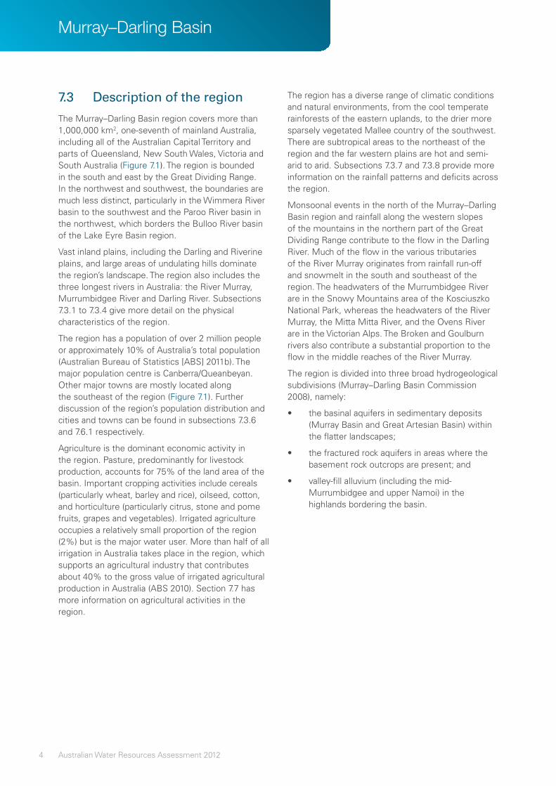
4 Australian Water Resources Assessment 2012
Murray–Darling Basin
7.3 Descriptionoftheregion
The Murray–Darling Basin region covers more than 1,000,000 km2, one-seventh of mainland Australia, including all of the Australian Capital Territory and parts of Queensland, New South Wales, Victoria and South Australia (Figure 7.1). The region is bounded in the south and east by the Great Dividing Range. In the northwest and southwest, the boundaries are much less distinct, particularly in the Wimmera River basin to the southwest and the Paroo River basin in the northwest, which borders the Bulloo River basin of the Lake Eyre Basin region.
Vast inland plains, including the Darling and Riverine plains, and large areas of undulating hills dominate the region’s landscape. The region also includes the three longest rivers in Australia: the River Murray, Murrumbidgee River and Darling River. Subsections 7.3.1 to 7.3.4 give more detail on the physical characteristics of the region.
The region has a population of over 2 million people or approximately 10% of Australia’s total population (Australian Bureau of Statistics [ABS] 2011b). The major population centre is Canberra/Queanbeyan. Other major towns are mostly located along the southeast of the region (Figure 7.1). Further discussion of the region’s population distribution and cities and towns can be found in subsections 7.3.6 and 7.6.1 respectively.
Agriculture is the dominant economic activity in the region. Pasture, predominantly for livestock production, accounts for 75% of the land area of the basin. Important cropping activities include cereals (particularly wheat, barley and rice), oilseed, cotton, and horticulture (particularly citrus, stone and pome fruits, grapes and vegetables). Irrigated agriculture occupies a relatively small proportion of the region (2%) but is the major water user. More than half of all irrigation in Australia takes place in the region, which supports an agricultural industry that contributes about 40% to the gross value of irrigated agricultural production in Australia (ABS 2010). Section 7.7 has more information on agricultural activities in the region.
The region has a diverse range of climatic conditions and natural environments, from the cool temperate rainforests of the eastern uplands, to the drier more sparsely vegetated Mallee country of the southwest. There are subtropical areas to the northeast of the region and the far western plains are hot and semi-arid to arid. Subsections 7.3.7 and 7.3.8 provide more information on the rainfall patterns and deficits across the region.
Monsoonal events in the north of the Murray–Darling Basin region and rainfall along the western slopes of the mountains in the northern part of the Great Dividing Range contribute to the flow in the Darling River. Much of the flow in the various tributaries of the River Murray originates from rainfall run-off and snowmelt in the south and southeast of the region. The headwaters of the Murrumbidgee River are in the Snowy Mountains area of the Kosciuszko National Park, whereas the headwaters of the River Murray, the Mitta Mitta River, and the Ovens River are in the Victorian Alps. The Broken and Goulburn rivers also contribute a substantial proportion to the flow in the middle reaches of the River Murray.
The region is divided into three broad hydrogeological subdivisions (Murray–Darling Basin Commission 2008), namely:
• the basinal aquifers in sedimentary deposits (Murray Basin and Great Artesian Basin) within the flatter landscapes;
• the fractured rock aquifers in areas where the basement rock outcrops are present; and
• valley-fill alluvium (including the mid-Murrumbidgee and upper Namoi) in the highlands bordering the basin.

5Australian Water Resources Assessment 2012
Figure7.1 MajorriversandurbancentresintheMurray–DarlingBasinregion

6 Australian Water Resources Assessment 2012
Murray–Darling Basin
7.3.1 Physiographic characteristics
The physiographic map in Figure 7.2 indicates areas with similar landform histories that can be related back to similar geology and climatic impacts that influence erosion processes (Pain et al. 2011). The areas have distinct physical characteristics that impact on hydrological processes.
The Murray–Darling Basin region has five major physiographic provinces, namely:
• Central Lowlands (37%): sand, clay and stony plains with low sandy hills;
• Kosciuszkan Uplands (10%): moderately high mountains and detached hills with intervening alluvial valley floors;
• New England–Moreton Uplands (7%): mainly undulating granitic plateaus and metamorphic ridges and shale lowlands; and
• Macquarie Uplands (6%): granitic and basaltic tablelands with detached hills in the west.
The remaining two provinces occupy less than 3% of the region (Gulfs Ranges and Fitzroy Uplands).
Figure7.2 PhysiographicprovincesoftheMurray–DarlingBasinregion

7Australian Water Resources Assessment 2012
7.3.2 Elevation
Most of the region’s landscape is dominated by vast inland plains and large areas of undulating hills, almost all lower than 200 m above sea level. The largest plains are the Darling Plain in the north, drained by the Darling River and its tributaries, and the Riverine Plain in the south, drained by the Murray and Murrumbidgee rivers and their tributaries.
The Murray–Darling Basin region has clear water-divide boundaries in the south and east of the region formed by the Great Dividing Range. To the northwest and southwest, the boundaries are much less distinct, due to very low topography. Elsewhere, areas of low to medium altitude determine the region’s boundaries (Figure 7.3). Information was obtained from the Geoscience Australia website (www.ga.gov.au/topographic-mapping/digital-elevation-data.html).
The region includes a large portion of the western flanks of the Great Dividing Range. It is here where most of the run-off is generated.
Figure7.3 LandsurfaceelevationsintheMurrayDarlingBasinregion

8 Australian Water Resources Assessment 2012
Murray–Darling Basin
7.3.3 Slopes
Areas with steep slopes provide higher run-off generating potential than flat areas. The Murray–Darling Basin region is generally flat, with some areas of steeper slopes along the southeast border (Table 7.2 and Figure 7.4). The slopes were derived from the elevation information used in the previous section.
Table7.2Proportionsofslopeclassesfortheregion
Slopeclass(%) 0–0.5 0.5–1 1–5 >5
Proportion of region (%)
51.4 16.2 22.7 9.7
These steep slopes provide opportunities to create large storages through the construction of relatively small dams. Major storages like Lake Hume, Lake Dartmouth and Lake Eildon now serve as an essential source of fresh water for the irrigation areas in the upper and lower River Murray.
Several large rivers flow through the flat plains of the region. In times of high flow volumes, water moves slowly and these rivers form vast floodplains over longer periods of time. When the flood waters retreat, what remains are numerous wetlands and lakes of various types that are distributed throughout the region, but are particularly prominent along the lower Darling River.
Figure7.4 SurfaceslopesintheMurray–DarlingBasinregion

9Australian Water Resources Assessment 2012
7.3.4 Soil types
Soils play an important role in the hydrological cycle by distributing water that reaches the ground. Water can be transported to rivers and lakes via the soil surface as run-off or enter the soil and provide water for plant growth as well as contributing to groundwater recharge. The nature of these hydrological pathways and the suitability of the soils for agricultural purposes are influenced by soil types and their characteristics. Soil type information was obtained from the Australian Soil Resource Information System website (www.asris.csiro.au).
About 85% of the Murray–Darling Basin region comprises four soil types, namely sodosols, kandosols, vertosols, and calcarosols (Figure 7.5).
Sodosols are widely found in the south, southcentral as well as eastern part of the region (Figure 7.6). These soils have a clear texture contrast, with a relatively impermeable, sodic and clay-enriched subsoil. Due to their soil dispersion and structural instability they are susceptible to tunnel and gully erosion as well as dryland salinity, if vegetation is cleared. Sodosols are mostly used for dryland crops and horticulture in the area.
Kandosols are dominant in the northwest of the Murray–Darling Basin region, but are also widely represented in the southeast of the region. These soils are often very deep (up to three metres or
more), but do not have a strong texture contrast and colour change, and do not contain carbonate throughout their profile. Kandosols have a low to moderate agricultural potential with moderate water-holding capacity and chemical fertility. These soils are mostly used for grazing in this region. When grazed, these soils are susceptible to surface soil degradation, such as hardsetting and crusting even under low grazing intensities.
Vertosols are stretched around the southcentral to north-central part of the region. These are brown, grey or black soils with high clay contents. They are highly fertile and have a large water-holding capacity. They, however, require a significant amount of water before it becomes available to plants. In the region they are used for dryland agriculture and horticulture.
Calcarosols are the dominate soil type in the lower parts of the region and are mostly used for dryland crops and horticulture. These soils are often shallow with low water-holding capacity. They are characterised by a high calcium carbonate content, which occurs as soft or hard white fragments, or as solid layers. They have low to moderate agricultural potential and often high salinity levels. Alkalinity and boron toxicity may cause issues.
The soil types that have minimal representation in the Murray–Darling Basin region are tenosols, rudosols, dermosols, kurosols and ferrosols (between 0.5–4% of the total area).
Figure7.5 SoiltypesintheMurray–DarlingBasinregion

10 Australian Water Resources Assessment 2012
Murray–Darling Basin
Figure7.6 SoiltypedistributionintheMurray–DarlingBasinregion

11Australian Water Resources Assessment 2012
7.3.5 Land use
Agriculture is the dominant economic activity in the Murray–Darling Basin region. Pasture, predominantly for livestock production, particularly dryland sheep and cattle production, accounts for 75% of the land area of the basin (Figure 7.7 and Figure 7.8; data from data.daff.gov.au/anrdl/metadata_files/pa_luav4g9abl07811a00.xml). Important cropping activities include cereals, oilseed, cotton, and horticulture such as fruits and vegetables.
Although irrigated agriculture occupies a relatively small portion of the region (2%), it is the major water user in the basin.
More than 60% of all irrigation in Australia takes place in the Murray–Darling Basin region. This contributes to more than 40% of the total gross value of irrigated agricultural production in Australia (ABS 2010).
In 2011–12, cotton production accounted for the largest area of irrigated land in the region. Cotton production also used the largest volume of irrigation water. Irrigation areas are located in the Murrumbidgee, Murray, Lachlan, Goulburn, Broken, Loddon and lower Murray river basins to the south of the region, and the Condamine, Border, Gwydir, Namoi and Macquarie river basins to the north of the region.
Figure7.7 LanduseintheMurray–DarlingBasinregion

12 Australian Water Resources Assessment 2012
Murray–Darling Basin
Figure7.8 LandusedistributionintheMurray–DarlingBasinregion

13Australian Water Resources Assessment 2012
7.3.6 Population distribution
The Murray–Darling Basin region has a population of over 2 million people, approximately 10% of Australia’s total population. It is home to Australia’s national capital, Canberra, which makes up 17% of the region’s total population. Figure 7.9 shows the spatial distribution of population density (ABS 2011b).
Many of the large population centres near the eastern and southern boundaries of the region provide support to the numerous agricultural districts of the basin.
These population centres are generally located in the valleys and on the alluvial plains of the many major rivers that feed the Murray–Darling River system.
Figure7.9 PopulationdensityanddistributionintheMurray–DarlingBasinregion

14 Australian Water Resources Assessment 2012
Murray–Darling Basin
7.3.7 Rainfall zones
The Murray–Darling Basin region has a large range of climatic conditions and natural environments, from the rainforests of the cool and humid eastern uplands, the temperate Mallee country of the southwest, the subtropical areas of the northeast, to the hot and dry, semi-arid and arid lands of the far western plains. Median rainfall varies throughout the region.
As the region covers a large part of the continent, the rainfall zones correspond to a number of the major climate zones of Australia (Figure 7.10).
There is a north–south pattern of summer dominant to uniform to winter dominant annual rainfall. A second pattern in the rainfall zones is the high annual total rainfall in the east contrasted with the low annual total rainfall in the west. Higher rainfall totals in the west are directly related to the presence of the Great Dividing Range in this area and its proximity to the coast.
For more information on this and other climate classifications, visit the Bureau’s climate website: www.bom.gov.au/jsp/ncc/climate_averages/climate-classifications/index.jsp
Figure7.10 RainfallzonesintheMurray–DarlingBasinregion

15Australian Water Resources Assessment 2012
7.3.8 Rainfall deficit
The rainfall deficit indicator (rainfall minus potential evapotranspiration) gives a general indication of which parts of the region are likely to experience moisture deficits over the period of a year. The Murray–Darling Basin region generally has a rather uniform pattern of substantial deficits over the whole region (Figure 7.11).
The only areas of rainfall excess are located in the southern ranges of the Great Dividing Range. It is where the major storages are located for the surface water supply of the Murrumbidgee and Murray
irrigation areas. The irrigation areas themselves are located in the – 500 to –1,000 mm deficit range. The northern irrigation areas are also reliant on surface water to a large extent, but the overall lower availability of surface water has limited the potential of intensive irrigated agriculture in these areas compared to the south of the region.
For more information on the rainfall and evapotranspiration data, see the Bureau’s maps of average conditions: www.bom.gov.au/climate/averages/maps.shtml
Figure7.11 RainfalldistributionintheMurray–DarlingBasinregion

16 Australian Water Resources Assessment 2012
Murray–Darling Basin
7.4 Landscapewaterflows
This section presents analyses of the spatial and temporal variation of landscape water flows (rainfall, evapotranspiration and landscape water yield) across the Murray–Darling Basin region in 2011–12. National rainfall grids were generated using data from a network of persistent, high-quality rainfall stations managed by the Bureau. Evapotranspiration and landscape water yields were derived using the landscape water balance component of the Australian Water Resources Assessment System (Van Dijk 2010). These methods and associated output uncertainties are discussed in the Introduction and addressed in more detail in the Technical Supplement.
Figure 7.12 shows that the region has two rainfall maxima present in the historical rainfall data. This can be attributed to a wetter summer period in the north and a wetter winter period in the south. Evapotranspiration follows a similar pattern to rainfall, although it is also related to energy availability (temperature and solar radiation), which is higher in the summer period. The monthly landscape water yield history for the region shows a stable pattern of very low yield in all months, although it moderately
increases over the July–September period.
The 2011–12 year started with four months of mostly average rainfall, which were followed by five wet months. For the remaining three months of the year rainfall was again close to average. The above average rainfall between November and March was a result of three major frontal systems, one at the end of November, one in the last week of January and a final one in late February/early March (see the National Overview chapter for more details).
Evapotranspiration in 2011–12 was generally consistent with rainfall, with close to median values for July–October, high values for November– March, returning to near median values for April–June. Despite high rainfall January recorded median evapotranspiration due to lower soil moisture levels.
The landscape water yield for 2011–12, relative to historical values, was very high for November–January and also high for February–March. The February and March peaks coincided with the end of the wet period when soil saturation levels were high.
Figure7.12 Landscapewaterflowsin2011–12comparedwiththelong-termrecord(July1911–June2012)fortheMurray–DarlingBasinregion

17Australian Water Resources Assessment 2012
7.4.1 Rainfall
Rainfall for the Murray–Darling Basin region for 2011–12 is estimated to be 651 mm. This is 40% above the region’s long-term average (July 1911–June 2012) of 465 mm.
Figure 7.13a shows that the highest rainfall occurred along the slopes of the Great Dividing Range in the east of the region, with annual totals for 2011–12 exceeding 1,200 mm in some areas.
Rainfall in the western part of the region did not exceed 600 mm for 2011–12.
Rainfall deciles for 2011–12 indicate very much above average rainfall for 48% of the region over the course of the year (Figure 7.13b). Many of the region’s irrigation areas received above and very much above average rainfall, as did the upstream catchment areas from which they extract the water. An exception to this was the Wimmera district in the southwest of the region.
Figure7.13 Spatialdistributionof(a)annualrainfallin2011–12and(b)theirdecilerankingsoverthe1911–2012periodfortheMurray–DarlingBasinregion

18 Australian Water Resources Assessment 2012
Murray–Darling Basin
Rainfallvariabilityintherecentpast
Figure 7.14a shows annual rainfall for the region from July 1980 onwards. Over this 32-year period the annual average was 482 mm, varying from 305 mm (2002–03) to 780 mm (2010–11). Temporal variability and seasonal patterns since 1980 are presented in Figure 7.14b.
Total rainfall for 2011–12 was the second highest since 1980. As can be noted from Figure 7.14b, there has been an increase in rainfall in the summer period in recent years. This is in part attributed to a strong La Niña event in 2010–11 and the return of a slightly weaker La Niña event in 2011–12.
Figure7.14 Time-seriesof(a)annualrainfalland(b)five-yearretrospectivemovingaveragesforthesummer(November–April)andwinter(May–October)periodsfortheMurray–DarlingBasinregion

19Australian Water Resources Assessment 2012
Recenttrendsinrainfall
Figure 7.15a presents the spatial distribution of the trends in annual rainfall for July 1980–June 2012. These are derived from linear regression analyses on the time-series of each model grid cell. The statistical significance of the trends is provided in Figure 7.15b.
The trend patterns indicate a decrease in rainfall for the southeastern border areas, which are areas with the highest rainfall totals.
In these areas, most of the rivers that feed the southern irrigation areas originate in the upper Murray and Murrumbidgee river basins.
The rising trends indicated as statistically significant in Figure 7.15b are largely a result of the high rainfall of the past two years.
Figure7.15 Spatialdistributionof(a)trendsinannualrainfallfrom1980–2012and(b)theirstatisticalsignificanceat90%(weak)and95%(strong)confidencelevelsfortheMurray–DarlingBasinregion

20 Australian Water Resources Assessment 2012
Murray–Darling Basin
7.4.2 Evapotranspiration
Modelled annual evapotranspiration for the Murray–Darling Basin region for 2011–12 is estimated to be 559 mm. This is 29% above the region’s long-term (July 1911–June 2012) average of 434 mm. The spatial distribution of annual evapotranspiration in 2011–12 (Figure 7.16a) is similar to that of rainfall (Figure 7.13a).
Evapotranspiration deciles for 2011–12 indicate above average or very much above average totals across most of the region (Figure 7.16b). This coincides with the very much above average rainfall observed largely along the north and centre of the region (Figure 7.13b). Evapotranspiration is normally limited by water shortage in these areas; however, the very much above average rainfall of the last two years altered this pattern.
Figure7.16 Spatialdistributionof(a)modelledannualevapotranspirationin2011–12and(b)theirdecilerankingsoverthe1911–2012periodfortheMurray–DarlingBasinregion

21Australian Water Resources Assessment 2012
Evapotranspirationvariabilityintherecentpast
Figure 7.17a shows annual evapotranspiration for the region from July 1980 onwards. Over this 32-year period the annual evapotranspiration average was 446 mm, varying from 284 mm (2002–03) to 691 mm (2010–11). Temporal variability and seasonal patterns since 1980 are presented in Figure 7.17b.
Evapotranspiration shows a similar pattern as rainfall with the highest and third highest annual totals of the last 32 years for 2010–11 and 2011–12 respectively. The greatest increase occurred in the summer period with the five-year retrospective moving average of evapotranspiration peaking much higher than in the winter period (Figure 7.17b).
Figure7.17 Time-seriesof(a)annualevapotranspirationand(b)five-yearretrospectivemovingaveragesforthesummer(November–April)andwinter(May–October)periodsfortheMurray–DarlingBasinregion

22 Australian Water Resources Assessment 2012
Murray–Darling Basin
Recenttrendsinevapotranspiration
Figure 7.18a presents the spatial distribution of the trends in modelled annual evapotranspiration for July 1980–June 2012. These are derived from linear regression analyses on the time-series of each model grid cell. The statistical significance of the trends is provided in Figure 7.18b.
Figure 7.18a shows that since 1980 trends are mostly rising in the centre and north of the region and more neutral in the rest of the region.
As shown in Figure 7.18b, the trends are generally only statistically significant in the far north and some smaller central parts of the region. In the south and northeast of the region the falling trends have no statistical significance.
As evapotranspiration is driven by the availability of moisture, the trends are related to the trend pattern in the rainfall shown in Figure 7.15a, especially with the high rainfall of the past two years.
Figure7.18 Spatialdistributionof(a)trendsinannualevapotranspirationfrom1980–2012and(b)theirstatisticalsignificanceat90%(weak)and95%(strong)confidencelevelsfortheMurray–DarlingBasinregion

23Australian Water Resources Assessment 2012
7.4.3 Landscape water yield
Modelled landscape water yield for the Murray–Darling Basin region for 2011–12 is estimated to be 65 mm. This is 110% above the region’s long-term (July 1911–June 2012) average of 31 mm. Figure 7.19a shows the spatial distribution of landscape water yield for 2011–12. Most landscape water yield is generated in the mountainous southeast of the region with large areas exceeding 400 mm.
The decile-ranking map for 2011–12 (Figure 7.19b) shows very much above average landscape water yields for 72% of the region; however, although very much above average, the largest proportion of the region remained below 50 mm of annual landscape water yield. Additionally, large parts of those areas that historically have the highest landscape water yields (the mountains in the southeast) only generated average to above average landscape water yields.
Figure7.19 Spatialdistributionof(a)modelledannuallandscapewateryieldin2011–12and(b)theirdecilerankingsoverthe1911–2012periodfortheMurray–DarlingBasinregion

24 Australian Water Resources Assessment 2012
Murray–Darling Basin
Landscapewateryieldvariabilityintherecentpast
Figure 7.20a shows annual landscape water yield for the Murray–Darling Basin region from July 1980 onwards. Over this 32-year period, annual landscape water yield was 34 mm, varying from 9 mm (2006–07) to 84 mm (2010–11). Temporal variability and seasonal patterns since 1980 are presented in Figure 7.20b.
The last two years have seen exceptionally high landscape water yield. Historically, most of the landscape water yield for the region is generated in the winter dominant rainfall areas in the southeast. It is therefore not surprising that the yields were consistently higher during the winter period compared to the summer period; however, the last two years have seen some very high intensity rainfall events in the summer period, which sparked the generation of landscape water yield throughout the whole region, including the southeast.
Figure7.20 Time-seriesof(a)annuallandscapewateryieldand(b)five-yearretrospectivemovingaveragesforthesummer(November–April)andwinter(May–October)periodsfortheMurray–DarlingBasinregion

25Australian Water Resources Assessment 2012
Recenttrendsinlandscapewateryield
Figure 7.21a shows the spatial distribution of the trends in modelled annual landscape water yield for July 1980–June 2012. These are derived from linear regression analyses on the time-series of each model grid cell. The statistical significance of the trends is provided in Figure 7.21b.
Since 1980, marginally rising trends are present over most of the region; however, they are not present in the normally high landscape water yield generating areas in the mountainous southeast.
The rising trends in landscape water yield are generally strongly significant in more extensive areas than those of rainfall and evapotranspiration. This is a consequence of the very much above average high annual totals of the last two years, which were unusual and therefore may have caused an overestimation of the trend. A more important change from a water availability point of view is that in the southeast some falling trends occurred, though these were not statistically significant.
Figure7.21 Spatialdistributionof(a)trendsinannuallandscapewateryieldfrom1980–2012and(b)theirstatisticalsignificanceat90%(weak)and95%(strong)confidencelevelsfortheMurray–DarlingBasinregion

26 Australian Water Resources Assessment 2012
Murray–Darling Basin
7.5 Surfacewaterandgroundwater
This section examines surface water and groundwater resources in the Murray–Darling Basin region in 2011–12. Rivers, wetlands and storages are discussed to illustrate the state of the region’s surface water resources. The region’s watertable aquifers are described and the groundwater status is illustrated by showing changes in groundwater levels at selected sites.
7.5.1 Rivers
There are 28 river basins in the Murray–Darling Basin region, varying in size from 1,700 to 166,000 km2 (Figure 7.22). The region is named after its two major rivers, the River Murray, which drains water from inland areas of southern New South Wales and northern Victoria, and the Darling River, which drains inland through southern Queensland and northern New South Wales. The River Murray and Darling River combine near Wentworth before discharging to the ocean via the Lower Lakes system in South Australia.
The Darling River (2,740 km), the River Murray (2,510 km) and the Murrumbidgee River (1,490 km) are the three longest rivers in Australia. Monsoonal events in the north of the basin contribute to a large portion of the flow from the north in the Darling River. The flow in the various rivers and tributaries of the River Murray originate from rainfall run-off or from snowmelt in the Great Dividing Range to the south and southeast of the region. This includes the headwaters of the River Murray and the Mitta Mitta, Kiewa, Ovens, Broken and Goulburn rivers in the Victorian Alps. The headwaters of the Murrumbidgee River lie in the Snowy Mountains area of the Kosciuszko National Park.
There are two types of rivers in the region: ephemeral and perennial. Ephemeral rivers, including the Paroo, Warrego and Culgoa rivers, generally originate in southwestern Queensland, whereas the perennial rivers usually start in the southeastern slopes of the Great Dividing Range. Ephemeral rivers in the Murray–Darling Basin region are usually slow-flowing and almost always carry notable silt loads.
Confluence of Murray and Darling rivers at Wentworth, New South Wales | Ashley Whitworth, Dreamstime

27Australian Water Resources Assessment 2012
Figure7.22 RiversandcatchmentsintheMurray–DarlingBasinregion

28 Australian Water Resources Assessment 2012
Murray–Darling Basin
7.5.2 Streamflow volumes
Figure 7.23 presents an analysis of flows at 74 monitoring sites during 2011–12 relative to annual flows for the July 1980–July 2012 period. Sites with relatively long records across 20 geographically representative rivers were selected (see Technical Supplement for details). The annual flows for 2011–12 are colour-coded according to the decile rank at each site over the 1980–2012 period.
High run-off, generated in the upstream reaches of the rivers, caused above average to very much above average flows in many rivers in the central north and east of the Murray–Darling Basin region, whereas flows to the south and southeast tended to be more variable, and were sometimes average with some below average flows (Figure 7.23).
Very much above average flows were observed at 14 monitoring sites located on rivers in the central north and some catchments in the central south of the region. Above average flows were recorded at 35 monitoring sites distributed across the Murray–Darling Basin region.
Average flows occurred at 19 sites in the region, which are mainly located on the eastern rivers and some rivers in the south of the region. Of the 74 monitoring sites, there were only six below average flows recorded across the region in 2011–12. These six monitoring sites were located on the Avoca and Loddon rivers in the south, the Macintyre Brook and the Gwydir River in the northeast, and the Mitta Mitta River in the southeast of the region.
Flow deciles in the summer (November 2011–April 2012) were very similar to total annual flows for 2011–12 as shown in Figure 7.23. This is not surprising, given that the greatest volume of flows in the Murray–Darling Basin region occurred over the summer months. While flows in the central and eastern rivers of the region were above average over 2011–12, flows in these rivers were even higher over the summer months compared with annual average conditions. There are a few monitoring sites that did not show this pattern, such as the lower flows observed in summer on the Tumut River and the River Murray downstream of the Hume Dam in the southeast of the region.
7.5.3 Streamflow salinity
Figure 7.24 presents an analysis of streamflow salinity at 142 monitoring sites throughout the Murray–Darling Basin region. Monitoring sites with at least a five-year data record were selected for analysis. The results are presented as electrical conductivity (EC), μS/cm at 25 °C). This is a commonly used surrogate for the measurement of water salinity in Australia. Standard EC levels for different applications, such as for drinking water or types of irrigation, are provided in the Technical Supplement. The median annual EC values are shown as coloured circles. The size of the circle depicts the variability in annual EC, shown as the coefficient of variation (CV), being the standard deviation divided by the mean.
The median EC values for most of the selected monitoring sites fall in the range 0–1,000 μS/cm (suitable for most irrigation uses). Of the 142 sites, 80% had median EC values below 500 μS/cm and 13% were between 500–1,000 μS/cm. Only 3% of the monitoring sites had a median EC above 1,500 μS/cm (Figure 7.24).
Stream salinity was above 2,000 μS/cm at four of the 142 monitoring sites. These were from three monitoring sites on rivers and creeks in the southwest, and Houlaghans Creek in the Murrumbidgee River basin in the southeast of the region.
The salinity CV is typically related to the variability in annual flow at the monitoring site. It is high at some monitoring sites in the central, central south and eastern rivers in the Murray–Darling Basin region, whereas it is relatively low in many of the eastern rivers and at some monitoring sites in the River Murray in the central southwest of the region.
Of the 142 sites, 25% had a CV below 20%; 75% of the sites had a CV between 20% and 60%; and the CV was above 60% at only one of the 142 monitoring sites, on the Wakool River in the central south of the region.

29Australian Water Resources Assessment 2012
Figure7.23 Averageannualandsummerperiodflowvolumesofselectedmonitoringsitesfor2011–12andtheirdecilerankingsoverthe1980–2012periodintheMurray–DarlingBasinregion

30 Australian Water Resources Assessment 2012
Murray–Darling Basin
Figure7.24 Salinityaselectricalconductivityanditsassociatedco-efficientofvariationfor2011–12intheMurray–DarlingBasinregion

31Australian Water Resources Assessment 2012
7.5.4 Flooding
Figure 7.25 presents an overview of the monitoring sites where the Bureau of Meteorology is measuring river levels in the Murray–Darling Basin region as part of the flood forecasting service. The highest river level reached during the year is expressed as one of four flood classification levels. These classification levels are established in consultation with emergency management and local agencies (see the Technical Supplement for details).
A number of major floods occurred during 2011–12 mostly in the north and southeast parts of the region. The most significant flooding occurred during November 2011–March 2012, where catchments in inland southern Queensland and the upper to mid River Murray catchments received well above average rainfall.
In late November heavy rainfalls lead to flooding in northwestern New South Wales with floodwaters moving downstream towards the west and southwest along tributaries of the Darling River.
Major floods also occurred in the northern catchments of the Condamine, Warrego and Paroo rivers during December 2011 through to February 2012 as a result of well above average rainfall in these areas.
In March 2012 high intensity, well above average rainfall in the south and west of the region resulted in major floods in the Lachlan, Murrumbidgee and the upper Murray rivers. These rivers flooded again in late June 2012. The Goulburn River and the upper and mid River Murray had a number of minor to moderate floods during much of the year.
River Murray floods, early 2012 | murrayriverguide.com.au

32 Australian Water Resources Assessment 2012
Murray–Darling Basin
Figure7.25 FloodlevelsfortheMurray–DarlingBasinregionin2011–12

33Australian Water Resources Assessment 2012
7.5.5 Storage systems
There are over 70 major publicly owned storages in the Murray–Darling Basin region. In total, the capacity of all these storages exceeds 34,000 GL. This includes the storage systems of Snowy Hydro Limited and the Grampians Wimmera–Mallee (GWMW) Corporation, which are partly located outside the region but transfer most of their water to the Murray–Darling Basin region. The Bureau’s water storage information covers more than 88% of the region’s publicly owned storage capacity (as at August 2012). Storages in the region supply 17 rural water supply systems as well as the city of Canberra.
Table 7.3 is a summary of the major water supply and associated storage systems in the region, together with an overview of the storage levels at the end of 2010–11 and 2011–12. The location of all the water supply systems and associated storages are shown in Figure 7.26.
Table 7.3 indicates that the larger systems experienced significant increases in storage volumes. This resulted in an 11% increase in total storage volume over the region. This is an important improvement in water supply security for most irrigation areas in the region. Some increases could also be partly caused by environmental water holders carrying over their allocations to be released some time in the future.
Further information on the past and present volumes of the storage systems and the individual storages can be found on the Bureau’s water storage website: water.bom.gov.au/waterstorage/awris/
Table7.3 MajorpubliclyownedstoragesystemsintheMurray–DarlingBasinregion(asatAugust2012).‘Non-allocated’meansstoragesnotallocatedtoaparticularsystem
Systemname Systemtype Systemcapacity Accessiblevolumeat30June2011
Accessiblevolumeat30June2012
Murray rural 7,441 GL 5,627 GL—76% 6,554 GL—88%
Snowy Hydro hydro /rural 5,302 GL 1,711 GL—32% 2,960 GL—56%
Goulburn rural 3,559 GL 3,056 GL—86% 3,159 GL—89%
Murrumbidgee rural 2,633 GL 2,454 GL—93% 2,485 GL—94%
Macquarie rural 1,523 GL 1,208 GL—79% 1,371 GL—90%
Gwydir rural 1,343 GL 671 GL—50% 1,282 GL—95%
Lachlan rural 1,253 GL 1,144 GL—91% 1,197 GL—96%
Namoi rural 873 GL 548 GL—63% 803 GL—92%
Wimmera–Mallee rural 662 GL 294 GL—44% 266 GL—40%
Border rivers rural 563 GL 559 GL—99% 520 GL—92%
Campaspe rural 304 GL 293 GL—96% 271 GL—89%
Loddon rural 213 GL 194 GL—91% 186 GL—87%
Canberra urban 205 GL 199 GL—97% 204 GL—100%
Upper Condamine rural 104 GL 103 GL—99% 87 GL—84%
St George rural 95 GL 94 GL—99% 91 GL—96%
Macintyre rural 69 GL 60 GL—87% 42 GL—61%
Broken rural 40 GL 40 GL—100% 40 GL—100%
Ovens rural 32 GL 23 GL—72% 24 GL—75%
Non-allocated — 3,979 GL 3,728 GL—94% 3,689 GL—93%
Total 30,192 GL 22,006 GL—73% 25,230 GL—84%

34 Australian Water Resources Assessment 2012
Murray–Darling Basin
Figure7.26 MajorwatersupplyandassociatedstoragesystemsintheMurray–DarlingBasinregion(asatAugust2012)

35Australian Water Resources Assessment 2012
7.5.6 Wetlands
Importantwetlands
There are a large number of wetlands of national and international importance in the Murray–Darling Basin region (Figure 7.27), encompassing a wide diversity of wetland types. The wetlands create a mosaic of temporally and spatially dynamic habitats within this part of Australia. The most spatially extensive wetland types in the region are river floodplains, which include lakes, swamps, lagoons and flooded forests. Another dominant type of wetland present in the region is the terminal wetland system of ephemeral rivers.
The river floodplains are particularly important for the conservation of large areas of river red gum forests as well as other woodland species. They are also important breeding grounds for threatened bird species. The swamps and lakes of the terminal wetland systems contain large areas of common reed and other water plant species that form ideal breeding and feeding grounds for many bird species as well as some rare fish species.
Inflowstoselectedwetlands
The state of the biodiversity in a wetland is linked to the way water is stored within the area and the temporal variability of inflows. An analysis of historic and recent inflows into wetlands provides an informative picture of potential changes.
Five internationally recognised Ramsar wetland sites (Currawinya Lakes, Paroo River wetlands, Gwydir wetlands, Macquarie Marshes and the Barmah Forest) were selected for hydrological analysis of major inflows. More information about the region's wetlands is available from the Australian Directory of Important Wetlands (www.environment.gov.au/water/topics/wetlands/database/diwa.html)
Four upstream monitoring sites were selected to enable analyses and interpretation of inflows to these five wetlands. The monitoring sites used in the analyses are the closest upstream monitoring sites that have suitable continuous, or almost continuous, discharge records since 1980, providing a comprehensive dataset for much of the freshwater surface-inflows to the wetlands. Though the analyses do not capture the total inflows they are indicative of the temporal patterns of flows to these wetlands.
Barmah Forest | Malcolm Watson

36 Australian Water Resources Assessment 2012
Murray–Darling Basin
Figure7.27 LocationofimportantwetlandsintheMurray–DarlingBasinregion

37Australian Water Resources Assessment 2012
CurrawinyaLakesandParooRiverwetlands
The Ramsar-listed Currawinya Lakes and Paroo River wetlands form a combination of wetlands fed by the largest free-flowing river in the region, the Paroo River (Figure 7.28). The wetlands are important nesting and feeding places for migrating birds. Since the area is semi-arid to arid, some unique flora is present amongst the permanent waterholes.
Daily flow data for the monitoring site on the Paroo River at Caiwarro provide a temporal pattern of freshwater inflows into parts of the Currawinya Lakes area and the Paroo River wetlands (Figure 7.29).
Figure7.29 DailyflowsoftheParooRiveratCaiwarrobetween1980and2012,rankedindecileclasses
Figure7.28 LocationofthemonitoringsiteinrelationtoCurrawinyaLakesandParooRiverwetlands
Figure7.30 MonthlyflowsattheParooRivermonitoringsiteatCaiwarrofrom2011–12comparedwithits1980–2012decilerankings
Figure 7.29 presents an overview of the distribution of daily streamflow decile rankings. Since 1990, above average flows from December through to March provide a reliable source of inflows into the wetlands. This pattern was only interrupted by some dry years between 2000 and 2005. Before 1990, the very much above average flows had a more irregular pattern of occurrence with more frequent periods of very much below average flows during these months.
Figure 7.30 compares monthly flows from 2011–12 with the statistics of flow statistics from 1980 onwards. The February flows well-exceeded the ninth decile of the 32-year record and contributed substantial inflows to the wetlands.

38 Australian Water Resources Assessment 2012
Murray–Darling Basin
Gwydirwetlands
The Gwydir wetlands are a terminal delta wetland complex of which a small area is Ramsar-listed (Figure 7.31). Land use change and river regulation have substantially reduced the extent of the original wetlands. The Ramsar-listed parts of the Gwydir wetlands mainly consist of grass/sedge meadows and wooded swamps and support some threatened bird species. The wetlands are important nesting and feeding places for migrating birds.
Daily flow data for the monitoring site on the Gwydir River at Pallamallawa shows the temporal pattern of inflows to the wetlands (Figure 7.32).
Figure7.32 DailyflowsoftheGwydirRiveratPallamallawabetween1980and2012,rankedindecileclasses
Figure7.31 LocationofthemonitoringsitesinrelationtotheGwydirwetlands
Figure7.33 MonthlydischargesattheGwydirRivermonitoringsiteatPallamallawafrom2011–12comparedwithits1980–2012decilerankings
Figure 7.32 presents an overview of the distribution of daily streamflow decile rankings. Although sometimes interrupted, a period of high summer flows was present between 1980 and 2003. Since the summer of 2003–04 this pattern of inflows has been interrupted for most of the eight years to 2011–12. Inflows in the summer of 2011–12 eventually reverted back to longer periods of very much above average flows.
Figure 7.33 compares monthly flows from 2011–12 with flow statistics from 1980 onwards. The November, December and February inflows well-exceeded the ninth decile of the 32-year record and contributed a substantial amount of inflows to the wetlands.

39Australian Water Resources Assessment 2012
MacquarieMarshes
The Ramsar-listed Macquarie Marshes form a combination of various wetland types, supporting a variety of habitats for various ecological communities (Figure 7.34). The marshes support river red gum woodlands, extensive reed beds and water couch marsh, all of which form large breeding grounds for many common as well as threatened bird species.
Daily flow data for the monitoring site on the Macquarie River at Warren Weir shows a temporal pattern of freshwater inflows into the marshes (Figure 7.35).
Figure7.35 DailyflowsoftheMacquarieRiveratWarrenWeirbetween1980and2012,rankedindecileclasses
Figure7.34 LocationofthemonitoringsiteinrelationtotheMacquarieMarshes
Figure7.36 MonthlydischargesattheMacquarieRivermonitoringsiteatWarrenWeirfrom2011–12comparedwithits1980–2011decilerankings
Figure 7.35 presents an overview of the distribution of daily streamflow decile rankings. From autumn 2001, flows were frequently average or below average until August 2010. Prolonged low flow periods are not unusual, but over 2000–01 to 2011–12 longer than usual periods of very much below average flows occurred.
Figure 7.36 compares monthly discharges from 2011–12 with flow statistics of flows from 1980 onwards. As can be seen, the flows for 2011–12 were particularly low during the normally high flow months of August–October.

40 Australian Water Resources Assessment 2012
Murray–Darling Basin
Barmah–MillewaForestwetlands
The Barmah–Millewa Forest wetlands are separately listed as Ramsar sites for the Victorian and New South Wales sides of the River Murray (Figure 7.37). The wetlands contain the largest river red gum forest in Australia. They depend particularly on the irregular flooding of the River Murray. The wetlands include lakes, swamps, lagoons and flooded forest and they provide habitat for a large number of bird species.
Daily flow data for the monitoring site on the River Murray at Tocumwal provides a temporal pattern of inflows into the Barmah–Millewa Forest wetlands, particularly the frequency of potential flooding (Figure 7.38).
Figure7.38 DailyflowsoftheRiverMurrayatTocumwalbetween1980and2012,rankedindecileclasses
Figure7.37 LocationofthemonitoringsiteinrelationtoBarmah–MillewaForestwetlands
Figure7.39 MonthlyflowsattheRiverMurraymonitoringsiteatTocumwalfrom2011–12comparedwithits1980–2012decilerankings
Figure 7.38 presents an overview of the distribution of daily streamflow decile rankings. In the period between 2001 and 2009 environmental flow releases from Hume Dam were undertaken to prevent large parts of the forest from drying out. In particular, between 2007 and 2009 below average flows occurred after which the usually very much above average flows of spring returned.
Figure 7.39 compares monthly flows from 2011–12 with the flow statistics from 1980 onwards. The normally highest September flows were average; however the high July, August and March flows to some extent contributed to inflows to the wetlands.

41Australian Water Resources Assessment 2012
7.5.7 Hydrogeology
As shown in the figure below (Figure 7.40), the Murray–Darling Basin region is divided into three broad hydrogeological subdivisions (Murray–Darling Basin Commission 2008), namely:
• the basinal aquifers in sedimentary deposits (Murray Basin and Great Artesian Basin) within the flatter landscapes;
• the fractured rock aquifers in areas where the basement rock outcrops (for example, Palaeozoic and pre-Cambrian Fractured Rock Aquifer); and
• valley-fill alluvium (including the Mid-Murrumbidgee and Upper Namoi) in the highlands bordering the region.
The Great Artesian Basin is the largest groundwater basin in Australia and underlies the northern portion of the region. It consists of a complex, multi-layered system of water-bearing sandstones separated by mostly shale and mudstone confining beds (Murray–Darling Basin Commission 2008). It underlies the sand and clay sequences of the Murray–Darling Basin region that were laid down over the last 50 million years. The Great Artesian Basin provides vital water resources for domestic and town water supply, for stock use by the pastoral industry, and water supplies for the operations of the mining and petroleum industries and associated communities.
The sedimentary aquifers within the region cover the main depositional areas of the Murray Geological Basin and the Darling River basin, including upstream reaches of other major rivers such as the Murrumbidgee and Lachlan rivers. The major aquifers within or at the margins of the Murray geological basin include the Shepparton, Calivil, Parilla-Loxton Sands, Murray Limestone and Renmark Group aquifers, and the upland alluvium of the Cowra and Lachlan formations. The important alluvial sediments of the Darling River basin include the Gunnedah and Narrabri aquifers.
Fractured rock aquifers occur in the highland areas around the margins of the region. In fractured rock aquifers, groundwater is stored in the fractures, joints, bedding planes and cavities of the rock mass. Although fractured rock aquifers are found over a large area, they hold a much lower groundwater volume than sedimentary aquifers. Due to the difficulty of obtaining high yields from fractured rock, the volume of groundwater extracted from any one bore and in a given area is relatively low.
7.5.8 Watertable salinity
Figure 7.41 shows the salinity of the watertable aquifer in the Murray–Darling Basin region as fresh, where (total dissolved solids [TDS] < 3,000 mg/L), or saline, where (TDS ≥ 3,000 mg/L). Generally, the shallow groundwater in the flatter alluvial plain in the region is saline, most likely due to high evapotranspiration and low rainfall recharge. In contrast, fresh groundwater resources occur at the higher elevation where rainfall recharge is higher.
Groundwater in the deeper aquifers is typically fresher than that of the watertable; often the majority of this groundwater is derived from a past wetter climatic period.
Watertable aquifer salinity levels have risen significantly since European settlement, largely due to the clearing of native vegetation, irrigation development and the consequent increase in recharge to groundwater systems (Barnett et al. 2004).

42 Australian Water Resources Assessment 2012
Murray–Darling Basin
Figure7.40 WatertableaquifersintheMurray–DarlingBasinregion;dataextractedfromtheGroundwaterCartographyoftheAustralianHydrologicalGeospatialFabric(BureauofMeteorology2012)

43Australian Water Resources Assessment 2012
Figure7.41 WatertablesalinityclassesintheMurray–DarlingBasinregion;dataextractedfromtheGroundwaterCartographyoftheAustralianHydrologicalGeospatialFabric(BureauofMeteorology2012)

44 Australian Water Resources Assessment 2012
Murray–Darling Basin
7.5.9 Groundwater management units
Total groundwater use in 2010–11 was 511 GL, which was 8% of the surface water diversion in the region decreasing from 24% in 2009–10 (Murray–Darling Basin Authority 2012b). Since 1999–2000, when groundwater reporting started, groundwater use has been steadily rising, but there was a decline in the 2010–11 reporting year. This was linked to high rainfall and wide spread floods which led to good surface water availability.
The Murray–Darling Basin Authority established long-term average sustainable diversion limits (SDL), which will come into effect in 2019, along with a range of other measures that will improve the management of water in the region. The SDL are limits on the volumes of water that can be taken for human uses (including domestic, urban, industrial and agricultural use) from both surface water and groundwater systems across the region.
The groundwater resources in the Murray–Darling Basin region have been split into 22 groundwater water resource plan (WRP) areas, which are further divided into a total of 87 SDL resource units, as shown in Figure 7.42 and Figure 7.43 (Murray–Darling Basin Authority 2012a). These include seven groundwater SDL resource units for deep groundwater that lie beneath the other 80 groundwater SDL resource units (Figure 7.43).
SDL resource unit boundaries, shown in Figure 7.42, were determined according to the types of aquifers present and the management boundaries used by the state jurisdictions. There is a volume allocated to each SDL resource unit in the draft Murray–Darling Basin plan. In some areas, there are SDL resource units that overlap one another. This occurs where SDL units have been set for discrete aquifers that overlie one another under the same area of land (Murray–Darling Basin Authority 2012a).

45Australian Water Resources Assessment 2012
Figure7.42 GroundwaterSDLresourceunitsasat31August2012(Murray-DarlingBasinAuthority2012a)

46 Australian Water Resources Assessment 2012
Murray–Darling Basin
LegendofFigure7.42GroundwaterSDLresourceunitsasat31August2012(Murray–DarlingBasinAuthority2012a)

47Australian Water Resources Assessment 2012
Figure7.43 GroundwaterSDLresourceunitslegendasat31August2012(Murray–DarlingBasinAuthority2012)

48 Australian Water Resources Assessment 2012
Murray–Darling Basin
7.5.10 Status of selected aquifers
The status of groundwater levels is analysed at each bore throughout the Murray–Darling Basin region. This assessment evaluates trends in groundwater levels over the five-year period 2007–08 to 2011–12.
The trends in groundwater levels over the last five years are investigated using a 20 km x 20 km grid across data rich areas usually associated with the major sedimentary aquifers. This scale reflects the regional flow system of the aquifers in the region.
The linear trend in groundwater levels for each grid cell is assessed as:
• decreasing (where more than 60% of the bores have a negative trend in levels lower than –0.1 m/year); stable (where the trend is lower than 0.1 m/year; and higher than – 0.1 m/year for more than 60% of the bores);
• stable (where more than 60% of the bores have a trend lower than 0.1 m/year and higher than –0.1 m/year);
• increasing (where more than 60% of the bores have a positive trend in levels higher than 0.1 m/year); and
• variable (where there is no dominant trend in groundwater levels amongst the bores within a grid cell).
Example bore hydrographs are presented for each aquifer type over the entire record length and trends are discussed with a focus on the 2007–08 to 2011–12 period. The selected hydrographs are at key bores that have been chosen to assist in the analysis and reporting of groundwater trends. Where possible, the bore hydrographs presented are for the same bores used in the Groundwater Status Report 2000 (Murray–Darling Basin Commission 2004).
Condaminealluviumaquifer
The map in Figure 7.44 illustrates the spatial and temporal trends in groundwater levels in the Condamine alluvium aquifer from 2007–08 to 2011–12. Many of the grid cells show an increasing trend in groundwater levels. In other cells, groundwater levels are variable or stable. The cells showing a variable trend indicate that, within a grid cell, no clear majority of bores has a specific trend.
For both the alluvial and basalt aquifers the increased rainfall in the last couple of years is associated with an increase in recharge in conjunction with a probable decrease in groundwater abstraction, due to surface water availability, and is the major driver of increasing groundwater levels.
The hydrographs of selected bores 1 and 2 show a clear decline in groundwater levels after 1990 and a noticeable recovery in groundwater levels after 2010; the reasons for this decline are explained in the above paragraph. Bore 3 shows an upward trend in water level for the entire period of record. This bore is located in the upper tributary of the Condamine River away from the main alluvial plain and away from major extraction bores. The long-term increasing trend is probably associated with anthropogenic factors such as land clearing.
Condaminebasaltaquifer
The map in Figure 7.45 illustrates the spatial and temporal trends in groundwater levels in the Condamine basalt aquifer from 2007–08 to 2011–12. All of the grid cells show a rising trend in groundwater levels over the past five years.
Selected bores 4 to 6 all show an increasing trend in groundwater levels. The hydrographs all have an increasing trend over the last five years. This reflects the local groundwater use and high rainfall in the past couple of years. The fluctuations in water level observed in Bore 5 are likely to be caused by seasonal groundwater extraction from nearby production bores.

49Australian Water Resources Assessment 2012
Figure7.44 SpatialdistributionoftrendsingroundwaterlevelsfortheCondaminealluviumaquiferfor2007–08to2011–12,withselectedhydrographsshowinggroundwaterlevels

50 Australian Water Resources Assessment 2012
Murray–Darling Basin
Figure7.45 SpatialdistributionoftrendsingroundwaterlevelsfortheCondaminebasaltaquiferfor2007–08to2011–12,withselectedhydrographsshowinggroundwaterlevels

51Australian Water Resources Assessment 2012
NarrabriandGunnedahaquifers
Figure 7.46 and Figure 7.47 illustrate the spatial and temporal trends in the Narrabri aquifer and the associated underlying Gunnedah aquifer respectively.
The water levels in bores within the Narrabri aquifer are generally increasing or stable, with some areas showing a variable trend within the 20 km x 20 km grid cells for the 2007–2012 period. Similarly, groundwater levels in the more permeable Gunnedah aquifer indicate an increasing or stable trend overall. There are a small number of cells that show variable or declining trends in water levels.
Bore 7 is located in the lower reaches of the Gwydir system. The hydrograph indicates an overall stable trend in groundwater level and no annual fluctuations in the groundwater level. Bore 8 is located in the lower Namoi SDL. The hydrograph shows that water levels in 2007–2012 are continuing the gradual long-term decline. Bore 9 is located in the Coxs Creek region of the upper Namoi SDL. The groundwater levels show a minor recovery after 2010 with little annual fluctuation. These two bores, which report groundwater levels for the Narrabri aquifer, are most likely to be remote from the influence of groundwater abstraction or seasonal rainfall recharge.
Bore 10 is located in the Gwydir catchment and shows a very stable water level over the entire measurement period. Similarly, Bore 11 located at the western margin of the lower Namoi groundwater management unit shows stable groundwater levels for the entire record length. These three bores, which report groundwater levels for the underlying Gunnedah aquifer, are remote from the influence of groundwater abstraction or seasonal rainfall recharge.
Bore 12 is located in the lower Namoi groundwater management unit and shows a marked seasonal fluctuation in groundwater levels indicating the influence of seasonal cycles of abstraction and recovery of groundwater levels. This bore also shows a clear recovery in groundwater levels in 2012.
CowraandLachlanaquifers
Figure 7.48 and Figure 7.49 illustrate the spatial and temporal trends in the Cowra and the underlying Lachlan aquifers respectively.
Generally the Cowra and Lachlan aquifers show increasing trends in groundwater levels within the grid cells for 2007–2012. This is in contrast to the 2010 assessment where most of the grid cells presented decreasing trends in groundwater levels for the 2005–2010 period. The change in groundwater levels trends is driven by the increased rainfall and widespread floods which occurred since 2010 that have increased groundwater recharge and decreased dependence on groundwater abstraction.
Bores 13, 14 and 15 represent groundwater levels in the Cowra Subsystem while bores 16, 17 and 18 represent groundwater levels in the Lachlan Subsystem. Bores 13 and 17, and also 15 and 18, are nested showing groundwater levels for the upper and lower aquifer at the same location. Groundwater fluctuation for these nested bores indicates a strong hydraulic connection between the Lachlan and overlying Cowra aquifers. Annual variations in groundwater level in these two aquifers are most likely due to the effects of cycles of groundwater abstraction and recovery of groundwater levels. All bores show a varying degree of declining trend in groundwater levels from 2000–2010 and a subsequent recovery in groundwater levels after 2010. This is consistent with the recent widespread flooding in the last couple of years with the break of the millennium drought.

52 Australian Water Resources Assessment 2012
Murray–Darling Basin
Figure7.46 SpatialdistributionoftrendsingroundwaterlevelsfortheNarrabriaquiferfor2007–08to2011–12,withselectedhydrographsshowinggroundwaterlevels

53Australian Water Resources Assessment 2012
Figure7.47 SpatialdistributionoftrendsingroundwaterlevelsfortheGunnedahaquiferfor2007–08to2011–12,withselectedhydrographsshowinggroundwaterlevels

54 Australian Water Resources Assessment 2012
Murray–Darling Basin
Figure7.48 SpatialdistributionoftrendsingroundwaterlevelsfortheCowraaquiferfor2007–2012,withselectedhydrographsshowinggroundwaterlevels

55Australian Water Resources Assessment 2012
Figure7.49 SpatialdistributionoftrendsingroundwaterlevelsfortheLachlanaquiferfor2007–2012,withselectedhydrographsshowinggroundwaterlevels

56 Australian Water Resources Assessment 2012
Murray–Darling Basin
Sheppartonaquifer
Figure 7.50 illustrates that groundwater levels for the Shepparton aquifer for the 2007–08 to 2011–12 period have overall an increasing trend in the southwest of the aquifer and no majority of grid cells with a distinct trend in the southeast. Bore levels most likely respond to groundwater abstraction in the main groundwater management units as well as to the recent high rainfall and floods.
Hydrographs of three bores located within the Shepparton aquifers are presented in Figure 7.50. Bore 19 is located in the Lower Murray SDL in New South Wales. The hydrograph indicates a steady increasing groundwater level overall. Bore 20 is located in the Goulburn Murray SDL in Victoria; the hydrograph indicates a stable trend in groundwater level, with a slight decline in levels since the mid 2000s and a pulse of groundwater recharge producing a marked recovery in groundwater levels after 2010. The hydrographs also illustrate that the recharge event is already starting to disperse. The hydrographs indicate that these bores are not influenced by seasonal cycles of groundwater abstraction and then recovery of levels by seasonal rainfall recharge.
Bore 21 is also located in the Goulburn Murray SDL in Victoria, close to the River Murray and major irrigation areas where groundwater abstraction is high. The hydrograph shows an annual fluctuation of water level of up to 5 m. The high amplitude of water level fluctuation is due to the effects of seasonal groundwater abstraction. There is also a decline in levels since the mid 1990s–2010 followed by a recovery in groundwater levels. This recovery is linked to recent flooding and high rainfall.
Calivilaquifer
The trend analysis illustrated in Figure 7.51 indicates that the density of bores in the Calivil aquifer with up to date groundwater level data is very poor —there are very few grid cells with a trend calculated; however, the grid cells present indicate decreasing groundwater levels in the north and no majority of grid cells with a distinct trend in the south. The decline is likely to be the result of groundwater extraction as well as the fact that recharge due to recent rainfall and floods may not have fully reached the Calivil aquifer yet.
Hydrographs of groundwater levels in three bores located near the southern and western margins in New South Wales are presented in Figure 7.51. Bore 22 is located at the western (downstream) end of the lower Murrumbidgee SDL. The hydrograph shows stable groundwater levels since 1990. Bore 23 is located near the River Murray at the western end of the lower Murray SDL in New South Wales. The water level trends over 2006–07 to 2009–10 indicate a decline, followed by a minor recovery in groundwater levels after 2010. The decline is consistent with a response to pumping further to the east in the lower Murray groundwater SDL and the low rainfall in that period; the increase in groundwater levels is consistent with recent high rainfall.
Bore 24 is located near Deniliquin in the lower Murray SDL in New South Wales. The hydrograph shows considerable fluctuation in groundwater levels due to drawdown associated with groundwater extraction during the irrigation season and subsequent recovery when the extraction ceases in winter. There is a falling trend in groundwater level from the mid-1990s followed by a recovery in groundwater levels after 2010 in response to recent high rainfall.

57Australian Water Resources Assessment 2012
Figure7.50 SpatialdistributionoftrendsingroundwaterlevelsfortheSheppartonaquiferfor2007–08to2011–12,withselectedhydrographsshowinggroundwaterlevels

58 Australian Water Resources Assessment 2012
Murray–Darling Basin
Figure7.51 SpatialdistributionoftrendsingroundwaterlevelsfortheCalivilaquiferfor2007–08to2011–12,withselectedhydrographsshowinggroundwaterlevels

59Australian Water Resources Assessment 2012
MurrayGroupaquifer
Figure 7.52 illustrates the spatial and temporal trends in the Murray Group aquifer. Note that many of the groundwater bores in the Murray Group in South Australia lie outside the Murray–Darling Basin region.
Generally the Murray Group aquifer shows stable or rising trends for the period from 2007–08 to 2011–12, showing a change from the largely decreasing trends observed for 2005–06 to 2009–10 (2010 Assessment).
Bore 25 in the Murray Group shows an annual fluctuation in the water levels, probably due to pumping at nearby wells, and has a slightly rising groundwater level since 2010. Bores 26 and 27 present a very stable groundwater level over a long period of time (Figure 7.52).
Renmarkaquifer
Figure 7.53 illustrates the spatial and temporal trends in the underlying Renmark aquifer.
The Renmark aquifer is present at depth, and groundwater observation bores are widely spaced over the large area of the aquifer. Trends generally indicate a fall in Renmark groundwater levels in the west as observed in the 2010 Assessment; the effects of increased rainfall and flooding since 2010 do not yet seem to be affecting the deep Renmark aquifer in most areas.
The hydrograph of bores 28 and 30 show a long term declining trend in groundwater levels with a recovery in levels since 2010. Annual fluctuations of water level of up to 10 m are visible in the hydrograph for Bore 28. The high amplitude of water level fluctuation is due to the effects of seasonal groundwater abstraction.
Bore 29 shows a very stable groundwater level over a long period (Figure 7.53).

60 Australian Water Resources Assessment 2012
Murray–Darling Basin
Figure7.52 SpatialdistributionoftrendsingroundwaterlevelsfortheMurrayGroupaquiferfor2007–08to2011–12,withselectedhydrographsshowinggroundwaterlevel

61Australian Water Resources Assessment 2012
Figure7.53 SpatialdistributionoftrendsingroundwaterlevelsfortheRenmarkaquiferfor2007–08to2011–12,withselectedhydrographsshowinggroundwaterlevel

62 Australian Water Resources Assessment 2012
Murray–Darling Basin
7.6 Waterforcitiesandtowns
This section examines the urban water supply situation in the Murray–Darling Basin region in 2011–12. The large urban centres in the basin, their water supply systems, and their storage situations are briefly described. The main urbanised areas, Canberra and Queanbeyan, are addressed in more detail and the history of water restrictions over recent years is discussed. A breakdown is provided for water obtained for and delivered to Canberra and Queanbeyan.
7.6.1 Urban centres
Located in the Murrumbidgee River basin in the Australian Capital Territory, Canberra, is the largest city in the region; however, with a population of 356,000 people it ranks only seventh in terms of Australia’s major cities.
The major urban centres of the region (those with populations over 25,000 people) are summarised in Table 7.4. This table provides information on the population, surrounding river basin and significant water sources for each of the major urban centres in the region.
The region, often referred to as ‘Australia’s food bowl’, supports a significant percentage of the country’s food and fibre production. As such it is home to a number of Australia largest inland centres and cities, including Tamworth, Dubbo, Wagga Wagga and Albury in New South Wales and Mildura, Bendigo and Shepparton in Victoria. These cities, along with Canberra, are shown in Figure 7.54 together with their population ranges.
Table7.4 Urbancentresandtheirwatersupplysources
City/town Population1 Riverbasin Majorsupplysources
Canberra 356,000 Murrumbidgee Cotter, Bendora, Googong and Corin storages and Murrumbidgee River
Toowoomba 94,000 Condamine–Culgoa Cooby Creek, Cressbrook and Perseverance storages
Bendigo 83,000 Loddon Lake Eppalock and Malmsbury and upper Coliban storages
Albury–Wodonga 77,000 Murray–Riverina and Kiewa
River Murray
Wagga Wagga 47,000 Murrumbidgee Murrumbidgee River and groundwater
Shepparton–Mooroopna 43,000 Goulburn–Broken Goulburn and Broken rivers
Queanbeyan 36,000 Murrumbidgee Cotter, Bendora, Googong and Corin storages and Murrumbidgee River
Tamworth 36,000 Namoi Chaffey storage
Orange 35,000 Macquarie–Bogan Suma Park and Spring Creek storages
Dubbo 32,000 Macquarie–Bogan Macquarie River and groundwater
Mildura–Buronga 33,400 Macquarie–Bogan Chifley and Winburndale storages
Bathurst 31,000 Macquarie–Bogan Chifley and Winburndale storages1AustralianBureauofStatistics(2011b)

63Australian Water Resources Assessment 2012
Figure7.54 PopulationrangeforurbancentresintheMurray–DarlingBasinregion

64 Australian Water Resources Assessment 2012
Murray–Darling Basin
7.6.2 Sources of water supply
The urban cities and towns of the region draw heavily on surface water to meet their water supply needs. This is drawn from the storages located throughout the region (see Figure 7.55). In some cases water supplies are taken by direct river extractions fed from upstream storage releases.
The region has in excess of 70 major public surface water storages, representing over 25% of the nation’s total surface water storage capacity. While much of the water stored is used for agriculture and hydroelectricity generation, it is also used to meet the demands of urban consumption.
Significantly, water stored within the region not only meets urban demands of the cities and towns located within it but also of cities and towns in the South Australian Gulf and South East Coast (Victoria) regions.
Dartmouth, Lake Eildon and Hume are, by volume, the three largest surface water storages in the region. However, in terms of urban supply the Cotter, Corin, Bendora and Googong storages play a more significant role, supplying Canberra and the neighbouring town of Queanbeyan.
Groundwater is an important source of water in the urban centres and towns not located near one of the major rivers. Also the supply of water via long pipelines has become essential for some towns, in particular Broken Hill. Recycled water continues to grow as an important source of water supply in the region.
7.6.3 Canberra and Queanbeyan
Canberra and Queanbeyan are located 150 km inland from Australia’s southeast coast and lie to the east of the Brindabella Ranges.
The water supply area is serviced by a bulk water supply and sewerage authority, ACTEW Corporation (operating as ACTEW Water), a retail utility ACTEW AGL and a local government (Queanbeyan City Council).
ACTEW Corporation is the Australian Capital Territory (ACT) Government-owned statutory body that owns and manages the Canberra water supply system. It controls surface water diversions, operates water treatment plants, maintains Canberra’s reticulation system and delivers water to Queanbeyan where water supply infrastructure is managed and maintained by Queanbeyan City Council.
In conjunction with the Australian Gaslight Company (AGL) the ACTEW Water operates the retail energy and water utility ACTEW AGL which supplies urban demands and collects sewage throughout the ACT.
Supplysystem
Figure 7.56 illustrates the major components of the Canberra and Queanbeyan urban water supply system. The key components of the system are four water storages, two water treatment plants and five wastewater treatment plants. Water is sourced from three catchments: the Cotter River catchment, the Murrumbidgee River catchment and the Queanbeyan River catchment.
Of the four major surface water storages operated by ACTEW Water, three are located on the Cotter River (Corin, Bendora and Cotter) and a forth on the Queanbeyan River (Googong). These storages provide a total accessible capacity of just over 200 GL. At nearly 120 GL, Googong presently provides over half of the area’s total storage capacity.
In addition to its surface water storages, ACTEW extracts water from the Murrumbidgee River. The Murrumbidgee pump station facilitates the transfer extraction of up to 100 ML per day.

65Australian Water Resources Assessment 2012
Figure7.55 StoragesusedforurbanwatersupplyintheMurray–DarlingBasinregion

66 Australian Water Resources Assessment 2012
Murray–Darling Basin
Figure7.56 WatersupplyschematicforCanberraandQueanbeyan

67Australian Water Resources Assessment 2012
Figure7.57 Variationintheamountofwaterheldinstorageoverrecentyears(lightblue)andover2011–12(darkblue)forCorinandGoogongstorages,aswellastotalaccessiblestoragecapacity(dashedline)
Corin
Googong
Storagevolumes
Figure 7.57 presents the total accessible volume held in Corin and Googong storages over the past 32 years (July 1980 to June 2012) and clearly illustrates the impacts of the millennium drought with storages levels, particularly in Corin, reaching critically low levels in 2007–08.
A significant drawdown of Googong can be observed in late 2003–04 and is in part explained by a need to compensate for the decreased inflows and declining storages volumes in the Cotter River system.
A shift in climatic conditions in 2009 and a series of wetter years (including Australia’s wettest two-year period on record, 2010–2011) saw the storage levels recover from their historic lows. Continued good rainfall in the region’s catchments has seen storage levels maintained at or near capacity throughout 2011–12.

68 Australian Water Resources Assessment 2012
Murray–Darling Basin
Waterrestrictions
ACTEW Water manages decisions about water restrictions for Canberra with Queanbeyan City Council applying the same decisions for Queanbeyan residents. Restrictions imposed in Canberra and Queanbeyan from 1999–2012 are shown against combined storage levels in Figure 7.58. The different stages of the restrictions are defined in the Utilities (Water Conservation) Regulation 2006 under the Utilities Act 2000 (ACT).
Until November 2002, Canberra had not experienced water restrictions since 1969. Voluntary Stage 1 water restrictions were introduced in November 2002 but were quickly replaced by mandatory Stage 1 water restrictions when storage levels dropped below 55% accessible capacity.
Stage 3 water restrictions ware introduced in October 2003 and Permanent Water Conservation Measures were introduced in March 2006.
Stage 2 water restrictions were introduced in November 2006 due to very low storage inflows. They were quickly moved to Stage 3 restrictions in December 2006 as warm and dry weather conditions persisted. Stage 3 water restrictions continued until August 2010 and were in Stage 2 until October 2010. Due to higher water levels in dams, permanent water conservation measures were introduced in November 2010 and have continued since then.
Figure7.58 UrbanwaterrestrictionlevelsforCanberraandQueanbeyansince1999shownagainstthecombinedaccessiblewatervolumeofGoogongandCorinstorages

69Australian Water Resources Assessment 2012
Sourcesofwaterobtained
Water supplied to Canberra and Queanbeyan comes from surface water and recycled water. Figure 7.59 shows the total water supplied from both sources from 2005–06 to 2011–12. During this period, the maximum volume sourced for Canberra and Queanbeyan was in 2005–06. During that year, Stage 2 water restrictions were replaced with permanent water conservation measures.
During 2006–07 and 2007–08, the volume of water supplied decreased as a result of Stage 2 and Stage 3 water restrictions being introduced. Then, during the next two years, water supplied increased slightly and again dropped in following two years.
The use of recycled water increased over the period shown in Figure 7.59, being supplied primarily for commercial, municipal and industrial uses. Recycled water use was more than doubled from 2.1 GL in 2005–06 to 4.6 GL in 2011–12.
Figure7.59 TotalurbanwatersourcedforCanberraandQueanbeyanfrom2005–06to2011–12

70 Australian Water Resources Assessment 2012
Murray–Darling Basin
Categoriesofwaterdelivered
Figure 7.60 shows the total volume of water delivered between 2005–06 and 2011–12 to residential, commercial, municipal, industrial and other customers in Canberra and Queanbeyan areas. The figure shows that water consumption dropped over the seven-year period, despite a steady population growth.
The consumption pattern is a response to the water restrictions outlined above. When restrictions were eased and replaced by Permanent Water Conservation Measures in 2005–06, the consumption
increased to 57 GL, but returned to 52 GL during 2006–07, when Stage 2 followed by Stage 3 water restrictions were introduced. During the next five-year period, the consumption was up and down due to various restriction levels and a likely change in water use habits. Residential water consumption was approximately 66%; commercial, municipal and industrial sector use was approximately 26%; and the remaining water was supplied for other uses.
Canberra and Queanbeyan’s per capita residential water use fluctuated between 202 litres/person/day (L/p/d) and 276 L/p/d during this period.
Figure7.60 TotalurbanwatersuppliedtoCanberraandQueanbeyanfrom2005–06to2011–12

71Australian Water Resources Assessment 2012
7.7 Waterforagriculture
This section describes the water situation for agriculture in the Murray–Darling Basin region in 2011–12. Soil moisture conditions are presented and important irrigation areas are identified. The Murrumbidgee, Coleambally and Murray irrigation areas are described in more detail and information is provided regarding surface water storage and groundwater.
7.7.1 Soil moisture
Since model estimates of soil moisture storage volumes are based on a simple conceptual representation of soil water storage and transfer processes averaged over a 5 km x 5 km grid cell, they are not suitable to compare with locally measured soil moisture volumes. This analysis
therefore presents a relative comparison only, identifying how modelled soil moisture volumes of 2011–12 relate to those of the 1911–2012 period, expressed in decile rankings.
Soil moisture for the majority of the Murray–Darling Basin region was above or very much above average during 2011–12 (Figure 7.61). This is explained by the high rainfall that occurred in the region that was above the 90th percentile for five consecutive months of the year.
This, combined with wet antecedent moisture conditions in the soil, resulted in very much above average soil moisture throughout the year, shown by monthly decile ranking in Figure 7.62. The prevalent wet conditions in the soil provided favourable farming opportunities in the region and reduced the requirement for irrigation.
Figure7.61 Decilesrankingsofannualaveragesoilmoisturefor2011–12withrespecttothe1911–2012periodfortheMurray–DarlingBasinregion
Figure7.62 Decilerankingofthemonthlysoilmoistureconditionsduringthe2011–12periodwithrespecttothe1911–2012periodintheMurray–DarlingBasinregion

72 Australian Water Resources Assessment 2012
Murray–Darling Basin
7.7.2 Irrigation water
A comparison of annual irrigation water use in various natural resource management areas across the Murray–Darling Basin region from 2005–06 to 2010–11 and for 2011–12 only, is shown in Figure 7.63 and Figure 7.64, respectively. The graphs indicate that the water use for 2005–06 to 2010–11 was highest in the Murrumbidgee River basin.
Water resource conditions and use in the Coleambally and Murrumbidgee irrigation areas in the Murrumbidgee River basin are considered in more detail in the following sections
7.7.3 Irrigation areas
Pasture, for dryland sheep and cattle production, accounts for 75% of the land area of the Murray–Darling Basin region. The region produces one-third of Australian food supply. About 65% of all irrigated agriculture takes place in the region. This contributes $4.4 billion (or about 38%) to the total gross value of irrigated agricultural production in Australia (ABS 2011a). Prolonged periods of drought and expansion of irrigated agriculture in the region have resulted in the increase in groundwater use.
The largest irrigation areas in the region are located in the Murrumbidgee, Murray, Lachlan, Goulburn, Broken, Loddon and Lower Murray river basins in the south of the region, and the Condamine, Border, Gwydir, Namoi and Macquarie river basins to the north of the region (Figure 7.65).
The Murrumbidgee, Coleambally and Murray irrigation areas are described in more detail in subsections 7.7.5–7.7.7.
7.7.4 Murray Irrigation Area
The Murray Irrigation Area extends from Lake Mulwala in the east to Swan Hill in the west and is composed of Berriquin, Denimein, Deniboota and Wakool districts with a total area of 750,000 ha (Figure 7.65).
Two off-takes from the Murray flow network supply water to the 2,400 landholdings of the area. These are the Mulwala Canal off-take at Lake Mulwala and Wakool Canal off-take upstream of Stevens Weir on Edward River. The Mulwala Canal extends westward and has a capacity of up to 10 GL/day (Figure 7.65).
Water is returned back to the river system through five escapes at various points: the Edward River, Perricoota, Finley, Wakool River and Yallakool Creek escapes.
Water is provided to Murray Irrigation Limited which has a bulk water entitlement of about 1,500 GL. The typical annual water use is about 850 GL.
In 2011–12, 902 GL of water was delivered to irrigators. This was more than double the amount delivered in 2010–11 and more than five times greater than that in 2009–10. The company has reported delivery losses of 176 GL (Murray Irrigation Ltd 2012). The irrigators in the area also used 470 GL of carry-over water. Rice-cropping was the major water user in the area.

73Australian Water Resources Assessment 2012
Figure7.63 Totalannualirrigationwaterusefor2005–06to2010–11fornaturalresourcemanagementregionsintheMurray–DarlingBasinregion(ABS:2006–2010;2011a)

74 Australian Water Resources Assessment 2012
Murray–Darling Basin
Figure7.64 Annualirrigationwaterusepernaturalresourcemanagementregionfor2010–11(ABS2011a)

75Australian Water Resources Assessment 2012
Figure7.65 IrrigationareasintheMurray–DarlingBasinregion

76 Australian Water Resources Assessment 2012
Murray–Darling Basin
7.7.5 Murrumbidgee River basin
The Murrumbidgee River basin is an 84,000 km2 area in the Murray–Darling Basin region with a diverse climate and distinct physical characteristics. About 17% of the area is covered by native vegetation. Land use varies from sheep and cattle grazing, conservation reserves and residential areas in the upper catchment to irrigated agriculture, horticulture, dryland cropping, grazing and forestry in the mid to lower areas of the catchment.
The Murrumbidgee River basin uses over 22% of the total surface water diverted for irrigation and urban use in the region. Over 24% of the groundwater use in the region occurs in the Murrumbidgee River basin (Murrumbidgee Catchment Management Authority 2010).
Water sharing plans define water-sharing arrangements between the environment and water users in the regulated Murrumbidgee River basin. There are a number of categories of water licences that are assigned different priorities based on the intended use of water (New South Wales Office of Water 2011). The majority of the water entitlements held within the Murrumbidgee River basin are general security entitlements. Priority is given to high security entitlements primarily used for horticultural and grape production.
An ‘Available Water Determination’ is set at the start of each financial year in terms of megalitres per share. The total number of shares held by a licence holder multiplied by the ML/share announced gives the volume of water credited to that licensee’s account, in addition to carry-over provisions.
Burrinjuck Dam is on the Murrumbidgee River and has a storage capacity of 1,000 GL. The Yass and Goodradigbee rivers flow into this dam. It is the headwater storage for the Murrumbidgee irrigation area. Built in 1928, the dam has undergone several remedial and upgrades, the last one being after the 1974 floods.
Blowering Dam on the Tumut River, which was completed in 1969, has a storage capacity of 1,600 GL. It is used for hydroelectric power generation in addition to the water being used for irrigation in the Murrumbidgee and Coleambally irrigation areas.
7.7.6 Murrumbidgee Irrigation Area
The Murrumbidgee Irrigation Area is located north of the Murrumbidgee River, between Leeton and Griffith (Figure 7.66). It occupies an area of approximately 660,000 ha (Murrumbidgee Irrigation Ltd 2011). It covers around 120,000 ha of intensive irrigation and 3,300 landholdings. The region contributes over $2.5 billion annually to the Australian economy.
Water is sourced from the Murrumbidgee River which is regulated from Burrinjuck and Blowering dams. The area is fed by two canals, the Main Canal and the Sturt Canal, diverting water from the Murrumbidgee River. The Main Canal receives water diverted at Berembed Weir to serve the Yanco, Leeton and Griffith areas and can accommodate flows of up to 6.5 GL/day. The Sturt Canal receives water diverted at Gogeldrie Weir to supply the Whitton and Benerembah areas and can accommodate flows of up to 1.7 GL/day.
There are also four drains returning water to the Murrumbidgee River on the lower eastern part of the districts, but the majority of water is being used and recirculated within the irrigation districts.
Most of the irrigation is carried out on the eastern side of the irrigation area through interconnection with the Mirrool Creek, which runs through the centre of the area. The excess water is stored in the Barren Box Swamp.
In 2011–12, a total of 855 GL was diverted for irrigation in the Murrumbidgee irrigation area, of which 753 GL was delivered to the irrigators. The area under irrigation increased by 12% compared with 2010–11 year. The water diversion and delivery also increased by 50% (Murrumbidgee Irrigation Ltd 2012).
Surfacewaterstorageinflows
Persistent rainfall during November 2011–March 2012 led to high streamflow generation, which is shown by the average to very much above above average flow in the rivers in the region (Figure 7.23). Major floods occurred in Tumut and Murrumbidgee rivers during March 2012 and the river monitoring sites upstream of Blowering and Burrinjuck registered flows which were very much above average (Figure 7.67).
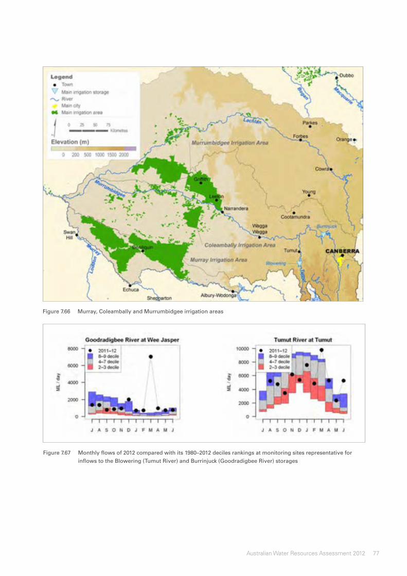
77Australian Water Resources Assessment 2012
Figure7.66 Murray,ColeamballyandMurrumbidgeeirrigationareas
Figure7.67 Monthlyflowsof2012comparedwithits1980–2012decilesrankingsatmonitoringsitesrepresentativeforinflowstotheBlowering(TumutRiver)andBurrinjuck(GoodradigbeeRiver)storages

78 Australian Water Resources Assessment 2012
Murray–Darling Basin
Figure7.68 Variationintheamountofwaterheldinstorageoverrecentyears(lightblue)andover2011–12(darkblue)forBloweringandBurrinjuckstorages,aswellastotalaccessiblestoragecapacity(dashedline)
Surfacewaterstoragevolumes
After a long drought period, water levels in the Blowering and Burrinjuck storages started to rise gradually during 2010, and maintained a close to full
capacity afterwards. There was a gradual decline in the water levels at the beginning of 2012. In March 2012, increased flows to the storages, as a result of major floods in the area, caused the water volumes to rise to almost full capacity again (Figure 7.68).
Blowering
Burrinjuck

79Australian Water Resources Assessment 2012
7.7.7 Coleambally Irrigation Area
Coleambally Irrigation Area is located in the Riverina between Darlington Point and Jerilderie and covers more than 470,000 ha of which 79,000 ha is under intensive irrigation, 42,000 ha irrigation/dry farms and the remainder receive stock and opportunistic irrigation water.
Coleambally Irrigation Limited delivers water supply to 473 farms owned by 364 business units. It also provides town supplies to the Murrumbidgee and Jerilderie Shires. They treat and supply water to the northern and southern districts of the Coleambally Irrigation Area.
Coleambally irrigation water supply is also sourced from the Murrumbidgee River. The off-take is upstream of Gogeldrie Weir. The supply system is gravity fed through a main canal at the eastern side of the irrigation area. Flow is measured through 500 regulators at 1 km intervals in a 500 km network of supply canals. Another 700 km of channels collect the drainage water from the network and are connected to three main outfalls where environmental flow is also supplied to the River Murray.
In October 2011 Burrinjuck exceeded its storage capacity (Figure 7.68) and water was released to balance inflows. This, accompanied by heavy rainfall in the area (739 mm), maximised water allocations for 2011–12 and favoured the increase in summer crop yields, which reached the highest levels in the past five years.
In 2011–12, total water diversion into the Coleambally Irrigation Area was 427 GL out of which 39 GL was channel losses and 388 GL was delivered to irrigators. Groundwater use was 37 GL. The total irrigated crop area was 68,700 ha, of which 16,700 ha was allocated to rice production (Coleambally Irrigation Co-operative Ltd 2012).
Localhydrogeology
The Coleambally Irrigation Area provides an example of groundwater use in the Murray–Darling Basin region (Figure 7.69). In 2011–12, about 10% of the total registered water used for irrigation in the Coleambally Irrigation Area was groundwater.
The Coleambally Irrigation Area is located in the eastern part of the Murray Geological Basin and overlies the lower Murrumbidgee alluvial aquifer system that starts downstream of Narrandera and consists of unconsolidated alluvial deposits of sands, silts, clays and peat. The alluvial system is comprised of three main units: the unconfined shallow Shepparton aquifer, and the confined intermediate Calivil and deep Renmark aquifers. These last two aquifers are often in hydraulic continuity.
The lowermost Renmark aquifer consists of fluvial clays, silts and gravels overlying the basaltic bedrock. In the eastern part of the Murrumbidgee catchment, the Renmark aquifer has an average thickness of about 280 m (Lawson and Webb 1998).
Overlying the Renmark aquifer are the sands of the Calivil aquifer. They were deposited by and are thickest in the ancestral drainage channels of modern-day rivers. The Calivil aquifer varies in thickness from about 50–70 m and can extend to depths greater than 150 m. Of the three regional aquifer systems, the Calivil is the most productive.
The uppermost unit is the Shepparton aquifer, which is typically 20–60 m thick. The Shepparton aquifer comprises a series of fluvio–lacustrine clays, sands and silts. These sediments are laterally discontinuous and form a highly heterogeneous unconfined aquifer system. In the Coleambally Irrigation Area, the Shepparton aquifer can be clearly divided into two parts, the Upper (0–12 m deep) and Lower Shepparton (12–60 m deep).
Recharge and discharge to and from the shallow Shepparton aquifer occurs across the area and its heterogeneity and low overall hydraulic conductivity can inhibit lateral flow. Water movement through the deep aquifers is generally from east to west; however, groundwater flow near the production bores around Darlington Point can be quite complicated. Movement occurs under gentle gradients and is therefore very slow with estimated rates of around 7–10 m/yr (Lawson and Webb 1998). Recharge to deep aquifers occurs mainly from the Murrumbidgee River downstream of Narrandera and from vertical leakage from the Shepparton aquifer.

80 Australian Water Resources Assessment 2012
Murray–Darling Basin
Figure7.69 TheColeamballyIrrigationAreawithgroundwaterboresites

81Australian Water Resources Assessment 2012
Influencesonshallowgroundwater
Prior to irrigation, watertable levels were at depths of 15–20 m; however, due to recharge to the groundwater from inefficient irrigation practices, leaky channels and recharge from rainfall, a significant proportion of the area had watertable levels within two metres of the soil surface by the late 1990s (Coleambally Irrigation Co-operative Limited 2004). These levels have since subsided due to below average rainfall and reduced surface water allocations occurring in the last ten years; however, the recent high rainfall and widespread floods have caused a minor rise in groundwater levels.
Fluctuations in groundwater levels in the Upper Shepparton aquifer are shown in Figure 7.70. No seasonal fluctuations are visible due to the fact that only one measurement per year, in September, has been plotted for consistency with recent measurement frequency. Groundwater levels are averaged between different subregions of the Coleambally Irrigation Area: Argon, Boona, Coly and Yamma.
To investigate the drivers of the shallow groundwater level trends, fluctuations in groundwater levels are compared to the monthly cumulative rainfall residual at Coleambally Irrigation Station and to the monthly discharge of the Murrumbidgee River at Darlington Point (Figure 7.70). The locations are shown in Figure 7.69.
Periods in which the cumulative rainfall residual curve rises indicate wetter than average conditions. Periods with a falling trend indicate drier than average conditions. As shown, river discharge near the off-take for irrigation and rainfall are correlated with the observed trends in groundwater levels. Some peaks in surface water discharge and in the cumulative rainfall residual mass curve correspond to peaks in groundwater.
The most striking feature is the decline in groundwater levels from 2002 to 2010 driven by reduced irrigation and drier than average conditions corresponding to the falling trend in the rainfall cumulative residual curve (and hence less recharge). Groundwater levels have recovered since 2010 consistently with the raising trend in the rainfall cumulative residual curve. The recovery is still well below the levels pre-2002.
Groundwaterlevel
Groundwater level measurements are an important source of information about hydrological and anthropological influences on groundwater in an area, including recharge. Figure 7.71 shows groundwater levels recorded at two regional nested sites within the Coleambally Irrigation Area reaching all three aquifers.
Groundwater level fluctuations at Bore 36040 are similar in the Calivil and Renmark aquifers, indicating that the two are hydraulically connected. Fluctuation in groundwater levels show the effect of pumping during the irrigation season and the subsequent recovery during the winter months when pumping ceased. No recent data is available for the Calivil aquifer but groundwater levels for the Renmark aquifer indicate recovery of groundwater levels since 2010. The Shepparton aquifer at this location (Bore 36040.1) seems disconnected from the deeper aquifers. No major recovery in groundwater levels for the Shepparton aquifer is visible at this location. Hydraulic gradient, and therefore groundwater flow, is downward. This may pose a risk to fresh groundwater at depth if the shallow groundwater is saline.
Groundwater levels at Bore 36372 show that the lower Shepparton aquifer is hydraulically connected to the Calivil aquifer and both are influenced by seasonal cycles of pumping and recovery. Groundwater levels in these two aquifers show a certain degree of recovery since 2010. The underlying Renmark aquifer shows strong effects of pumping for a short period at the end of 2009 and beginning of 2010 (Figure 7.71). Groundwater levels post-2010 have not yet recovered to pre-2010 levels and no further effects of pumping are visible. It appears that there is no hydraulic connection between the Remark and Calivil aquifers at this location. The hydraulic gradient between the Shepparton and Calivil aquifers is downward but the gradient decreases post 2010 as a result of increased recharge to groundwater in recent years.
Figures 7.72–7.75 show ranges of groundwater depth in Upper Shepparton, Lower Shepparton, Calivil and Renmark aquifers in the Coleambally Irrigation Area, and the ranking of 2011–12 median groundwater levels compared to annual median groundwater levels since 1990. The bores used are part of a network of bores that are monitored approximately annually by Coleambally Irrigation Co-operative Limited and regional bores seasonally monitored by the New South Wales Office of Water.

82 Australian Water Resources Assessment 2012
Murray–Darling Basin
Figure7.71 Groundwaterlevelsbetween2007and2012recordedatselectednestedboresites,reachingallthreeaquifers:(1)Shepparton,(2)Calivil,and(3)Renmark
Figure7.70 ComparisonofshallowgroundwaterlevelsrecordedatnestedboresiteswithrainfallandstreamflowinColeamballyirrigationsub-areas(ColeamballyIrrigationCo-operativeLimited2004,toppanel:Argon(yellow),Boona(red),Coly(blue)andYamma(green)sub-areas,middlepanel:cumulativerainfallresidualmassatColeamballyIrrigationStation74249,lowerpanel:streamflowinMurrumbidgeeRiveratDarlingtonPoint)

83Australian Water Resources Assessment 2012
Groundwater levels in the Upper Shepparton and Lower Shepparton aquifers vary from deeper than 10 m in the northeast and at the margin of the irrigation area to less than 2.5 m in the southeast of the irrigation area (Figure 7.72 and Figure 7.73). Importantly, groundwater levels are mostly deeper than 2.5 m. This indicates that the risk of groundwater salinisation of the shallow watertable is low.
The figures also show that median groundwater depths in 2011–12 are mostly below the average of recorded levels since 1990 within the irrigation area. This shows that even though wetter than average conditions occurred since 2010, recovery of groundwater levels has been small and groundwater levels are on average the deepest they have been in the past 21 years.
The sparse groundwater level data available for the regional Calivil and Renmark aquifers show that levels are all deeper than 10 m and median groundwater depths in 2011–12 are mostly at the average of recorded levels since 1990 (Figure 7.74 and Figure 7.75)
Groundwaterqualityoverview
During the 1960s, irrigation began in the Coleambally Irrigation Area with water diverted from the Murrumbidgee River upstream of Gogeldrie Weir near Darlington Point. Irrigated agriculture often leads to recharge of regional groundwater systems at rates greater than those the systems can absorb, resulting in the development of shallow watertable and causing salinity and waterlogging.
Salinity in the Calivil and Renmark aquifers is relatively low and generally increases from east near Narrandera to west around Hay along the Murrumbidgee River. In contrast, the shallow Shepparton aquifer is often very saline, especially under irrigation areas.
Irrigation induced salinity is a well known problem in many mature irrigation areas across Australia and internationally. The consequences of salinity in irrigation areas include production losses, increased production costs and damage to environmental and infrastructure assets in the region. The Coleambally Irrigation Area is experiencing such salinity problems; however, no time-series data on groundwater salinity are currently available for further analysis.
A groundwater site in the West Wimmera area, Victoria | Kate Morrison

84 Australian Water Resources Assessment 2012
Murray–Darling Basin
Figure7.72 MediangroundwaterdepthfortheupperSheppartonaquifer,(a)intheColeamballyIrrigationAreain2011–12,and(b)decileranksofdepthin2011–12comparedtothe1990–2011period.Deciles1–3areshownasbelowaverage(greaterdepthbelowsurface),deciles4–7asaverageanddeciles8–10asaboveaverage

85Australian Water Resources Assessment 2012
Figure7.73 MediangroundwaterdepthforthelowerSheppartonaquifer(a)intheColeamballyIrrigationAreain2011–12,and(b)decileranksofdepthin2011–12comparedtothe1990–2011period.Deciles1–3areshownasbelowaverage(greaterdepthbelowsurface),deciles4–7asaverageanddeciles8–10asaboveaverage

86 Australian Water Resources Assessment 2012
Murray–Darling Basin
Figure7.74 MediangroundwaterdepthforCalivilaquiferinthe(a)ColeamballyIrrigationAreain2011–12,and(b)decileranksofdepthin2011–12comparedtothe1990–2011period.Deciles1–3areshownasbelowaverage(greaterdepthbelowsurface),deciles4–7asaverageanddeciles8–10asaboveaverage

87Australian Water Resources Assessment 2012
Figure7.75 MediangroundwaterdepthforRenmarkaquifer,(a)intheColeamballyIrrigationAreain2011–12,and(b)decileranksofdepthin2011–12comparedtothe1990–2011period.Deciles1–3areshownasbelowaverage(greaterdepthbelowsurface),deciles4–7asaverageanddeciles8–10asaboveaverage

South Australian Gulf8 South Australian Gulf ................................................. 2
8.1 Introduction ........................................................ 2
8.2 Key information .................................................. 3
8.3 Description of the region .................................... 4
8.3.1 Physiographic characteristics.................. 6
8.3.2 Elevation ................................................. 7
8.3.3 Slopes .................................................... 8
8.3.4 Soil types ................................................ 9
8.3.5 Land use .............................................. 11
8.3.6 Population distribution .......................... 13
8.3.7 Rainfall zones ....................................... 14
8.3.8 Rainfall deficit ....................................... 15
8.4 Landscape water flows .................................... 16
8.4.1 Rainfall ................................................. 17
8.4.2 Evapotranspiration ................................ 20
8.4.3 Landscape water yield ......................... 23
8.5 Surface water and groundwater ....................... 26
8.5.1 Rivers ................................................... 26
8.5.2 Streamflow volumes ............................. 28
8.5.3 Streamflow salinity ................................ 28
8.5.4 Flooding ............................................... 31
8.5.5 Storage systems ................................... 31
8.5.6 Wetlands .............................................. 31
8.5.7 Hydrogeology ....................................... 35
8.5.8 Water table salinity ................................ 35
8.5.9 Groundwater management units ........... 35
8.5.10 Status of selected aquifers .................... 39
8.6 Water for cities and towns ................................ 47
8.6.1 Urban centres ....................................... 47
8.6.2 Sources of water supply ....................... 49
8.6.3 Adelaide ............................................... 49
8.7 Water for agriculture ......................................... 55
8.7.1 Soil moisture ......................................... 55
8.7.2 Irrigation water ...................................... 56
8.7.3 Irrigation areas ...................................... 56
8.7.4 McLaren Vale prescribed wells area ...... 56

2 Australian Water Resources Assessment 2012
South Australian Gulf
8.1 Introduction
This chapter examines water resources in the South Australian Gulf region in 2011–12 and over recent decades. It starts with summary information on the status of water flows, stores and use. This is followed by descriptive information for the region including the physiographic characteristics, soil types, population, land use and climate.
Spatial and temporal patterns in landscape water flows are presented as well as an examination of the surface and groundwater resources. The chapter concludes with a review of the water situation for urban centres and irrigation areas. The data sources and methods used in developing the diagrams and maps are listed in the Technical Supplement.
8 South Australian Gulf

3Australian Water Resources Assessment 2012
8.2 Keyinformation
Table 8.1 gives an overview of the key components of the data and information in this chapter.
Table8.1 Keyinformationonwaterflows,storesanduseintheSouthAustralianGulfregion
Landscapewaterflows
Evapo-transpiration
Landscapewater yield
Rainfall
Region average Difference from 1911–2012 long-term annual mean
Decile ranking with respect to the 1911–2012 record
331 mm +10% 8th —above average
306 mm +7% 8th —above average
9 mm – 10% 6th—average
Streamflow(atselectedgauges)
Annual total flow:
Highly variable pattern of high and low flow in the river gauges in the south eastern rivers
Salinity: Annual median electrical conductivity predominantly above 1,000 μS/cm in gauges in the south eastern rivers and on Kangaroo Island
Flooding: No major flooding in the monitoring gauges surrounding Adelaide
Surfacewaterstorage(comprisingabout74%oftheregion’stotalcapacityofallmajorstorages)
Total accessible capacity
30 June 2012 30 June 2011 Change
accessible volume
% of total capacity
accessible volume
% of total capacity
accessible volume
% of total capacity
197 GL 96 GL 49% 135 GL 69% – 39 GL – 20%
Groundwater(inselectedaquifers)
Levels: Variable trends in the different aquifers, predominantly falling in middle aquifers and rising in deeper aquifers
Salinity: Saline groundwater (≥3,000 mg/L) throughout most of the region with non-saline (<3,000 mg/L) areas around Adelaide and in the Flinders Ranges
Urbanwateruse(Adelaide)
Total sourced in 2011–12 Total sourced in 2010–11
Change Restrictions
138 GL 125 GL +13 GL (+10%) Water Wise Measures
Annualmeansoilmoisture(modelestimates)
Spatial patterns: Predominantly average annual mean soil moisture and very much above average soil moisture in the far north
Temporal patterns in regional average:
Average to above average soil moisture throughout the year

4 Australian Water Resources Assessment 2012
South Australian Gulf
8.3 Descriptionoftheregion
The South Australian Gulf region extends over 117,700 km2 of South Australia, surrounding the Gulf of St Vincent and Spencer Gulf, and stretching inland 300 km to the north of Spencer Gulf. To the east (at the border of the Murray–Darling Basin) the region is bounded by the western slopes of the Mount Lofty and Flinders Ranges; to the north, it is bounded by the Lake Eyre Basin; and to the west by the South Western Plateau region. The south of the region includes Kangaroo Island.
Except for the Flinders Ranges (with a highest peak of 932 m) and the Mount Lofty Ranges, the region has moderately flat terrain. Subsections 8.3.1–8.3.4 give more detail on the physical characteristics of the region.
The South Australian Gulf region has a population in excess of 1.4 million, or just over 6% of the country’s total population (Australian Bureau of Statistics [ABS] 2011b). Major population centres in the region include Adelaide, Victor Harbour, Port Pirie, Port Augusta, Whyalla and Port Lincoln (Figure 8.1). Further discussion of the region’s population distribution and urban centres can be found in subsection 8.3.6 and section 8.6 respectively.
Dryland pasture and cropping are major land uses in the region. Grazing is concentrated in the northern arid river basins such as Lake Torrens, Willochra Creek and Mambray Coast (south of Lake Torrens), and the Broughton River basin. Several river basins (Wakefield, Gawler and Broughton) have 50% or more of their area occupied by dryland agriculture. More than half of the land area devoted to nature conservation is a single reserve covering the Lake Torrens salt lake (Figure 8.1).
Other significant areas of nature conservation occur on Eyre Peninsula, Kangaroo Island, and through the Mount Lofty and Flinders Ranges. Irrigated agriculture is mostly for viticulture and wine production, the most important of which is concentrated in the Onkaparinga catchment. Section 8.7 has more information on agricultural activities in the region.
The region has a Mediterranean climate in the southeast, and a semi-arid climate inland and to the north. Rainfall mainly occurs in winter. Spring and summer rainfall can be substantial although highly variable. Subsections 8.3.7 and 8.3.8 provide more information on the rainfall patterns and deficits across the region.
There are no major permanent freshwater lakes in the South Australian Gulf region. A number of large endorheic salt lakes exist in the north, including Lake Torrens, Island Lagoon, Pernatty Lagoon, Lake Hart, Lake Gilles and Lake MacFarlane (Figure 8.1). In the south, short rivers drain into the ocean. The region has some important coastal and marine ecosystems.
The hydrogeology of the region can be partitioned into areas of surficial and underlying sediments, and areas of outcropping fractured rock. Significant groundwater resources are found in surficial sediments and the Quaternary and Tertiary aquifers that underlie them. Typically fractured rock systems offer restricted low volume groundwater resources; however, there are some parts of this region with a greater density of fractures and more substantial groundwater resource availability. A more detailed description of the rivers and groundwater status is given in section 8.5.
A view of rural Southern Australia looking north towards Flinders Range | Malcolm Watson

5Australian Water Resources Assessment 2012
Figure8.1 MajorriversandurbancentresintheSouthAustralianGulfregion

6 Australian Water Resources Assessment 2012
South Australian Gulf
8.3.1 Physiographiccharacteristics
The physiographic map in Figure 8.2 shows areas with similar landform evolutionary histories (Pain et al. 2011). These can be related back to similar geology and climatic impacts which define the extent of erosion processes. The areas have distinct physical characteristics that can influence hydrological processes. The South Australian Gulf region has two physiographic provinces, namely Eyre Peninsula and Gulfs Ranges.
The Eyre Peninsula province occupies 43% of the region and has alluvial plains and salt lakes with some dunes in the north. Moving south, this changes to rounded ranges of acid volcanic rocks and hills of metamorphic rocks followed by stable northwest–
southeast oriented longitudinal dunes, locally broken by granite hills, ridges of metamorphic rocks and plains extending as headlands and inlets along the southern coast.
The Gulfs Ranges province occupies 57% of the region and has a complex fold belt of prominent ranges in the north, chiefly quartzite with vales on weaker rocks, and in the southeast stepped fault blocks and islands, mainly of weathered metamorphic rocks with ferruginous cappings. In the northwest, there are dissected sandstone plateaus, salt lakes, alluvial and littoral plains and stabilised longitudinal dunes. In the southwest are undulating lowlands of folded crystalline and metamorphic rocks covered by calcrete and stabilised northwest–southeast longitudinal dunes.
Figure8.2 PhysiographicprovincesintheSouthAustralianGulfregion

7Australian Water Resources Assessment 2012
8.3.2 Elevation
Figure 8.3 presents ground surface elevations in the South Australian Gulf region. Information was obtained from the Geoscience website (www.ga.gov.au/topographic-mapping/digital-elevation-data.html). The region is clearly defined by the crest of the Mount Lofty Ranges in the south and the eastern ridges of the Flinders Ranges in the north. The highest point in this area is 932 m with most of the
borderline on altitudes exceeding 400 m. To the north and the west of the region, the effective water divide is less obvious.
The major mountains in the west are the Minbrie Range on Eyre Peninsula, which reach altitudes of over 400 m above sea level. The western areas contain many closed drainage areas which do not drain towards the sea. This includes the large Lake Torrens basin, which covers the majority of the north of the region.
Figure8.3 GroundsurfaceelevationsintheSouthAustralianGulfregion

8 Australian Water Resources Assessment 2012
South Australian Gulf
8.3.3 Slopes
Areas with steep slopes provide higher run-off generating potential than flat areas. The South Australian Gulf region has only some areas with steep slopes. Most of the area is rather flat (Table 8.2). The steep slopes in the map of Figure 8.4, in particular, highlight the Flinders Ranges in the east.
Table8.2Proportionsofslopeclassesfortheregion
Slopeclass(%) 0–0.5 0.5–1 1–5 >5
Proportion of region (%)
31.4 19.8 39.8 9.0
Significant slopes also exist southeast of Adelaide. The slopes were derived from the elevation information used in the previous section.
The region has a number of flat coastal plains, which, in combination with the climate and the appropriate soil conditions, have formed ideal solar salt production sites.
The flat plains in the north are mostly salt lakes, which collect the sparse run-off from their surrounding ranges. The large flat plain in the centre-north is Lake Torrens, which has only filled once in the last 150 years, as generally it is a large salty flatland.
Figure8.4 SurfaceslopesintheSouthAustralianGulfregion

9Australian Water Resources Assessment 2012
8.3.4 Soiltypes
Soils play an important role in the hydrological cycle by distributing water that reaches the ground. Water can be transported to rivers and lakes via the soil surface as run-off or enter the soil and provide water for plant growth as well as contribute to groundwater recharge. The nature of these hydrological pathways and the suitability of the soils for agricultural purposes are influenced by soil types and their characteristics. Soil type information was obtained from the Australian Soil Resource Information System website (www.asris.csiro.au).
About 88% of the South Australian Gulf region consists of four soil types, namely calcarosols, sodosols, chromosols and tenosols (Figure 8.5 and Figure 8.6).
Calcarosols are widely distributed across the region and cover about 45% of the total area. They are mainly present in areas used for pastures and to some extent for dryland agriculture. Calcarosols are characterised by a high content of calcium carbonate which occurs as soft or hard white fragments or as solid layers. These soils are often shallow and have a low water-holding capacity. They have a low to moderate agricultural potential, and salinity, alkalinity and boron toxicity may often cause problems.
Sodosols are common soils in the north and southwest and are scattered around in the southeast of the region. These soils have a strongly contrasting texture, with impermeable sodic subsoils arising from elevated sodium concentrations and clay. They are susceptible to dryland salinity as well as erosion if vegetation is removed.
Chromosols also have strongly contrasting texture, but have permeable subsoils which are not strongly acidic. They are dominant in the southeast of the region as well as on Kangaroo Island and are mostly present in pastures and areas used for dryland agriculture.
Tenosols are soils with minimal development throughout the profile. They show little or no change in texture and colour. They are often shallow or stony. These soils are low in chemical fertility and water-holding capacity and thus their agricultural potential is low. Tenosols are scattered in the central-west and in the south of the region and are mostly present in pastures and areas used for nature conservation.
The other soil types that have minimal representation in the South Australian Gulf region are rudosols, dermosol, ferrosols, hydrosols, kurosols and podosols (1–6% of the total area).
Figure8.5 SoiltypesintheSouthAustralianGulfregion

10 Australian Water Resources Assessment 2012
South Australian Gulf
Figure8.6 SoiltypedistributionintheSouthAustralianGulfregion

11Australian Water Resources Assessment 2012
8.3.5 Landuse
Dryland pasture and cropping are major land uses in the region (Figure 8.7), being often combined to varying degrees in farming operations across the region (data from data.daff.gov.au/anrdl/metadata_files/pa_luav4g9abl07811a00.xml). Grazing predominates in the northern arid river basins such as Lake Torrens, Willochra Creek and Mambray Coast (south of Lake Torrens), and the northern parts of the Broughton River basin. Several river basins (Wakefield, Gawler and Broughton) have 50% or more of their area occupied by dryland agriculture (Figure 8.7).
More than half of the land area devoted to nature conservation is a single reserve covering the Lake Torrens salt lake. Other significant areas of nature conservation occur on Eyre Peninsula, Kangaroo Island and in the Broughton River basin (Figure 8.8), and through the Mount Lofty and Flinders Ranges.
Irrigated agriculture is mostly for viticulture and wine production, the most important of which is concentrated in the Onkaparinga catchment.
Figure8.7 LanduseintheSouthAustraliaGulfregion

12 Australian Water Resources Assessment 2012
South Australian Gulf
Figure8.8 LandusedistributionintheSouthAustralianGulfregion

13Australian Water Resources Assessment 2012
8.3.6 Populationdistribution
The South Australian Gulf region has a population of greater than 1.4 million. Approximately 88% of the population is concentrated in greater Adelaide which occupies the coastal plains along the eastern edge of the Gulf of St Vincent and extends up into the Adelaide Hills (Figure 8.9).
A number of smaller coastal cities and towns are distributed along the edge of the Spencer Gulf and are driven by mining, agriculture and fisheries.
Beyond these smaller centres the remaining population is sparsely distributed throughout the western and northern parts of the region. A number of remote Indigenous communities can be found scatted throughout these parts.
Figure8.9 PopulationdensityanddistributionintheSouthAustralianGulfregion

14 Australian Water Resources Assessment 2012
South Australian Gulf
8.3.7 Rainfallzones
The region has a Mediterranean climate in the southeast and a semi-arid climate to the north. Rainfall mainly occurs in winter, though highly variable contributor to rainfall in spring through to early autumn. Median rainfall varies strongly across the region, not exceeding 800 mm throughout (Figure 8.10).
In the most northern part of the region average annual rainfall is limited to less than 200 mm.
Moving south, the annual rainfall totals increase up to levels reaching over 600 mm in the southern tip of Eyre Peninsula and Kangaroo Island.
For more information on this and other climate classifications, visit the Bureau of Meteorology’s (the Bureau’s) climate website: www.bom.gov.au/jsp/ncc/climate_averages/climate-classifications/index.jsp
Figure8.10 RainfallzonesintheSouthAustralianGulfregion

15Australian Water Resources Assessment 2012
8.3.8 Rainfalldeficit
The rainfall deficit indicator, that is, rainfall minus potential evapotranspiration, gives a general impression about which parts of the region are likely to experience moisture deficits over the period of a year. The South Australian Gulf region has a general pattern of substantial deficits in relation to this indicator (Figure 8.11).
High deficits can be expected in large parts of the northern inland areas, which include a number of ephemeral lakes. These are lakes which only get filled after major rainfall. No land cover other than grasses and shrubs is present, resulting in low density stock farming.
In the south of the region, dryland cropping and pasture for livestock are major forms of land use. The farms strongly rely on April–October rainfall for their growing season.
The city of Adelaide has some surface water storages to support the supply of water, but the general deficit in this area means the city relies on water transferred from the River Murray, particularly in summer, and since October 2011 from desalinated water.
For more information on the rainfall and evapotranspiration data, see the Bureau’s maps of average conditions: www.bom.gov.au/climate/averages/maps.shtml
Figure8.11 RainfalldeficitdistributionintheSouthAustralianGulfregion

16 Australian Water Resources Assessment 2012
South Australian Gulf
8.4 Landscapewaterflows
This section presents analyses of the spatial and temporal variation of landscape water flows (rainfall, evapotranspiration and landscape water yield) across the South Australian Gulf region in 2011–12. National rainfall grids were generated using data from a network of persistent, high-quality rainfall stations managed by the Bureau. Evapotranspiration and landscape water yields were derived using the landscape water balance component of the Australian Water Resources Assessment System (Van Dijk 2010). These methods and associated output uncertainties are discussed in the Introduction and addressed in more detail in the Technical Supplement.
Figure 8.12 shows that the region has a seasonal rainfall pattern with a predominantly wetter winter and drier summer period. Evapotranspiration generally exceeds rainfall from spring up to early summer, extracting the excess water from the soils.
The soils refill again in the wetter May–July period. The monthly landscape water yield history for the region shows a stable pattern of very low yield throughout the year.
The 2011–12 year was a relatively average year. Rainfall only exceeded the 90th percentile in the normally driest month of March, albeit only marginally.
Similar to rainfall, evapotranspiration was the highest in March. The rainfall of February and March contributed to higher than usual soil moisture, which in turn was available again for evapotranspiration. Evapotranspiration for March was third highest on record for the 1911–2012 period.
The landscape water yield for 2011–12 followed the very narrow bounds of the historic pattern. A marginally higher landscape water yield was found for March, although with no excessive volumes in absolute terms.
Figure8.12 Landscapewaterflowsin2011–12comparedwiththelong-termrecord(July1911–June2012)fortheSouthAustralianGulfregion

17Australian Water Resources Assessment 2012
8.4.1 Rainfall
Rainfall for the South Australian Gulf region for 2011–12 is estimated to be 331 mm. This is 10% above the region’s long-term average (July 1911–June 2012) of 300 mm. Figure 8.13a shows that the highest rainfall occurred along the southern coastal areas with annual totals locally exceeding 600 mm for 2011–12. The majority of the north had rainfall not exceeding 300 mm, except for the slopes of the Flinders Ranges in the east.
Rainfall deciles for 2011–12 indicate average to above average rainfall for the entire region over the course of the year (Figure 8.13b). The wetter south of the region experienced predominantly average rainfall with the exception of the far southern corner of Eyre Peninsula. In the centre and far north of the region, large areas of above average rainfall are present. As these areas are generally identified as arid, the above average areas experienced no substantially higher absolute total annual rainfall.
Figure8.13 Spatialdistributionof(a)annualrainfallin2011–12,and(b)theirdecilerankingsoverthe1911–2012periodfortheSouthAustralianGulfregion

18 Australian Water Resources Assessment 2012
South Australian Gulf
Rainfallvariabilityintherecentpast
Figure 8.14a shows annual rainfall for the region from July 1980 onwards. Over this 32-year period the annual average was 305 mm, varying from 187 mm (1982–83) to 477 mm (1992–93). Temporal variability and seasonal patterns since 1980 are presented in Figure 8.14b.
The graphs show a pattern of moderately high variability for the region, which is linked to the highly variable rainfall pattern in the arid north of the region. In Figure 8.14b, a pattern of decreasing rainfall in the winter period and increasing rainfall in the summer period is found in the most recent years. Before this, rainfall was noticeably higher in the winter period compared to the summer period.
Figure8.14 Time-seriesof(a)annualrainfall,and(b)five-yearretrospectivemovingaveragesforthesummer(November–April)andwinter(May–October)periodsfortheSouthAustralianGulfregion

19Australian Water Resources Assessment 2012
Recenttrendsinrainfall
Figure 8.15a presents the spatial distribution of the trends in annual rainfall for July 1980–June 2012. These are derived from linear regression analyses on the time-series of each model grid cell. The statistical significance of the trends is provided in Figure 8.15b.
Figure 8.15a shows that trends are mostly rising, but to an extent that is marginal. The significance map of Figure 8.15b confirms that the trends are of no statistical importance.
Figure8.15 Spatialdistributionof(a)trendsinannualrainfallfrom1980–2012,and(b)theirstatisticalsignificanceat90%(weak)and95%(strong)confidencelevelsfortheSouthAustralianGulfregion

20 Australian Water Resources Assessment 2012
South Australian Gulf
8.4.2 Evapotranspiration
Modelled annual evapotranspiration for the South Australian Gulf region for 2011–12 is estimated to be 306 mm. This is 7% above the region’s long-term (July 1911–June 2012) average of 286 mm. The spatial distribution of annual evapotranspiration in 2011–12 (Figure 8.16a) is almost identical to that of rainfall (Figure 8.13a). In this region, evapotranspiration is mostly limited to the availability of water.
Evapotranspiration deciles for 2011–12 indicate average or above average totals across most of the region (Figure 8.16b). The pattern again reflects that of rainfall (Figure 8.13b), albeit with some minor differences.
Essentially, those areas that had above average rainfall also had above average evapotranspiration. Hence, most water was returned back to the atmosphere within a short period of time.
Figure8.16 Spatialdistributionof(a)modelledannualevapotranspirationin2011–12,and(b)theirdecilerankingsoverthe1911–2012periodfortheSouthAustralianGulfregion

21Australian Water Resources Assessment 2012
Evapotranspirationvariabilityintherecentpast
Figure 8.17a shows annual evapotranspiration for the region from July 1980 onwards. Over this 32-year period the annual evapotranspiration average was 292 mm, varying from 191 mm (1982–83) to 447 mm (1992–93). Figure 8.17b presents temporal variability and seasonal patterns since 1980.
The similarity between the rainfall data of Figure 8.14 and the evapotranspiration data of Figure 8.17 is high. Evapotranspiration also shows a narrowing of the difference between the summer and winter periods over the last few years.
Figure8.17 Time-seriesof(a)annualevapotranspiration,and(b)five-yearretrospectivemovingaveragesforthesummer(November–April)andwinter(May–October)periodsfortheSouthAustralianGulfregion

22 Australian Water Resources Assessment 2012
South Australian Gulf
Recenttrendsinevapotranspiration
Figure 8.18a presents the spatial distribution of the trends in modelled annual evapotranspiration for 1980–2012. These are derived from linear regression analyses on the time-series of each model grid cell. Figure 8.18b provides the statistical significance of the trends.
Figure 8.18a shows that since 1980 trends throughout the region are within the –2 to 2 mm/year range.
As shown in Figure 8.18b, the trends are non-significant throughout the region. A major reason for this is that unlike in many other regions, the last two years were not the highest on record for the 32-year period.
Figure8.18 Spatialdistributionof(a)trendsinannualevapotranspirationfrom1980–2012,and(b)theirstatisticalsignificanceat90%(weak)and95%(strong)confidencelevelsfortheSouthAustralianGulfregion

23Australian Water Resources Assessment 2012
8.4.3 Landscapewateryield
Modelled landscape water yield for the South Australian Gulf region for 2011–12 is estimated to be 9 mm. This is 10% below the region’s long-term (July 1911–June 2012) average of 10 mm. Figure 8.19a shows the spatial distribution of landscape water yield for 2011–12. Only in the far southeast and on Kangaroo Island did some areas have landscape water yields exceeding 50 mm.
The decile ranking map for 2011–12 (Figure 8.19b) shows very much above average landscape water yield for the far north of the region. In absolute terms, however, these areas still had very low landscape water yield. In the far south some coastal areas are highlighted as very much below average landscape water yield; however, this is likely an artefact of the model calculations, which has yet to be further investigated.
Figure8.19 Spatialdistributionof(a)modelledannuallandscapewateryieldin2011–12,and(b)theirdecilerankingsoverthe1911–2012periodfortheSouthAustralianGulfregion

24 Australian Water Resources Assessment 2012
South Australian Gulf
Landscapewateryieldvariabilityintherecentpast
Figure 8.20a shows annual landscape water yield for the South Australian Gulf region from July 1980 onwards. Over this 32-year period, annual landscape water yield was 10 mm, varying from 4 mm (1982–83) to 23 mm (1992–93). Temporal variability and seasonal patterns since 1980 are presented in Figure 8.20b.
The graphs show a weak pattern of cyclic behaviour in the annual as well as summer and winter periods landscape water yield. Figure 8.20a shows that landscape water yields for some years were around 5 mm or lower, which generally means that in the arid north of the region landscape water yield was close to zero for those years.
Figure8.20 Time-seriesof(a)annuallandscapewateryieldand(b)five-yearretrospectivemovingaveragesforthesummer(November–April)andwinter(May–October)periodsfortheSouthAustralianGulfregion

25Australian Water Resources Assessment 2012
Recenttrendsinlandscapewateryield
Figure 8.21a shows the spatial distribution of the trends in modelled annual landscape water yield for 1980–2012. These are derived from linear regression analyses on the time-series of each model grid cell. The statistical significance of the trends is provided in Figure 8.21b.
Similar to rainfall and evapotranspiration, Figure 8.21a shows that since 1980 trends were within the –2 and 2 mm/year margins. With such low total annual landscape water yields involved, this is not surprising.
Figure 8.21b, however, shows some strongly significant rising trends occurring mainly in the central west of the region and in the southern part of Yorke Peninsula. In absolute terms, though, the trends do not exceed 0.2 mm/year in the central western area and 0.5 mm/year on Yorke Peninsula. The strongly significant falling trends on Kangaroo Island do not exceed –1 mm/year.
Figure8.21 Spatialdistributionof(a)trendsinannuallandscapewateryieldfrom1980to2012and(b)theirstatisticalsignificanceat90%(weak)and95%(strong)confidencelevelsfortheSouthAustralianGulfregion

26 Australian Water Resources Assessment 2012
South Australian Gulf
8.5 Surfacewaterandgroundwater
This section examines surface water and groundwater resources in the South Australian Gulf region in 2011–12. Rivers, wetlands and storages are discussed to illustrate the state of the region’s surface water resources. The region’s watertable aquifers and salinity are described and the groundwater status is illustrated by showing changes in groundwater levels at selected sites.
8.5.1 Rivers
There are 11 river basins in the South Australian Gulf region, varying in size from 154–67,000 km2 (Figure 8.22).
In the west and north, rivers are ephemeral and in the south east corner a few are perennial. There are only minor ephemeral streams in the northern half of the region.
To the southeast of the region, short rivers drain into the ocean. The perennial rivers flow off the slopes of the Mount Lofty Ranges into the Spencer Gulf. In the west, watercourses like the ephemeral Driver River flow from various low hills parallel to the coast on Eyre Peninsula. In the north, the Flinders Ranges supply most of the run-off from the east into Lake Torrens. Undulating land that averages less than 200 m above sea level, including the Andamooka Ranges, supplies the salt lake from the west.
Torrens River, Adelaide | Deqiang Pan, Dreamstime

27Australian Water Resources Assessment 2012
Figure8.22 RiversandcatchmentsintheSouthAustralianGulfregion
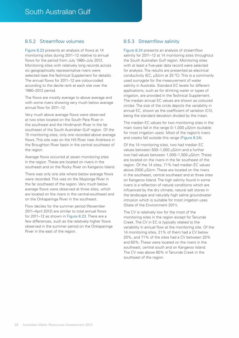
28 Australian Water Resources Assessment 2012
South Australian Gulf
8.5.2 Streamflowvolumes
Figure 8.23 presents an analysis of flows at 14 monitoring sites during 2011–12 relative to annual flows for the period from July 1980–July 2012. Monitoring sites with relatively long records across six geographically representative rivers were selected (see the Technical Supplement for details). The annual flows for 2011–12 are colour-coded according to the decile rank at each site over the 1980–2012 period.
The flows are mostly average to above average and with some rivers showing very much below average annual flow for 2011–12.
Very much above average flows were observed at two sites located on the South Para River in the southeast and the Hindmarsh River in the far southeast of the South Australian Gulf region. Of the 15 monitoring sites, only one recorded above average flows. This site was on the Hill River near Andrews in the Broughton River basin in the central southeast of the region.
Average flows occurred at seven monitoring sites in the region. These are located on rivers in the southeast and on the Rocky River on Kangaroo Island.
There was only one site where below average flows were recorded. This was on the Myponga River in the far southeast of the region. Very much below average flows were observed at three sites, which are located on the rivers in the central-southeast and on the Onkaparinga River in the southeast.
Flow deciles for the summer period (November 2011–April 2012) are similar to total annual flows for 2011–12 as shown in Figure 8.23. There are a few differences, such as the relatively higher flows observed in the summer period on the Onkaparinga River in the east of the region.
8.5.3 Streamflowsalinity
Figure 8.24 presents an analysis of streamflow salinity for 2011–12 at 14 monitoring sites throughout the South Australian Gulf region. Monitoring sites with at least a five-year data record were selected for analysis. The results are presented as electrical conductivity (EC, μS/cm at 25 ºC). This is a commonly used surrogate for the measurement of water salinity in Australia. Standard EC levels for different applications, such as for drinking water or types of irrigation, are provided in the Technical Supplement. The median annual EC values are shown as coloured circles. The size of the circle depicts the variability in annual EC, shown as the coefficient of variation (CV), being the standard deviation divided by the mean.
The median EC values for two monitoring sites in the main rivers fall in the range 0–1,000 μS/cm (suitable for most irrigation uses). Most of the region’s rivers and creeks fall outside this range (Figure 8.24).
Of the 14 monitoring sites, two had median EC values between 500–1,000 μS/cm and a further two had values between 1,000–1,500 μS/cm. These are located on the rivers in the far southeast of the region. Of the 14 sites, 71% had median EC values above 2000 μS/cm. These are located on the rivers in the southeast, central southeast and at three sites on Kangaroo Island. The high salinity found in some rivers is a reflection of natural conditions which are influenced by the dry climate, natural salt stores in the landscape and naturally high saline groundwater intrusion which is suitable for most irrigation uses (State of the Environment 2011).
The CV is relatively low for the most of the monitoring sites in the region except for Tanunda Creek. The CV in EC is typically related to the variability in annual flow at the monitoring site. Of the 14 monitoring sites, 21% of them had a CV below 20%, and 71% of the sites had a CV between 20% and 60%. These were located on the rivers in the southeast, central south and on Kangaroo Island. The CV was above 60% in Tanunda Creek in the southeast of the region.

29Australian Water Resources Assessment 2012
Figure8.23 Averageannualandsummerperiodflowvolumesofselectedsitesfor2011–12andtheirdecilerankingsoverthe1980–2012periodintheSouthAustralianGulfregion
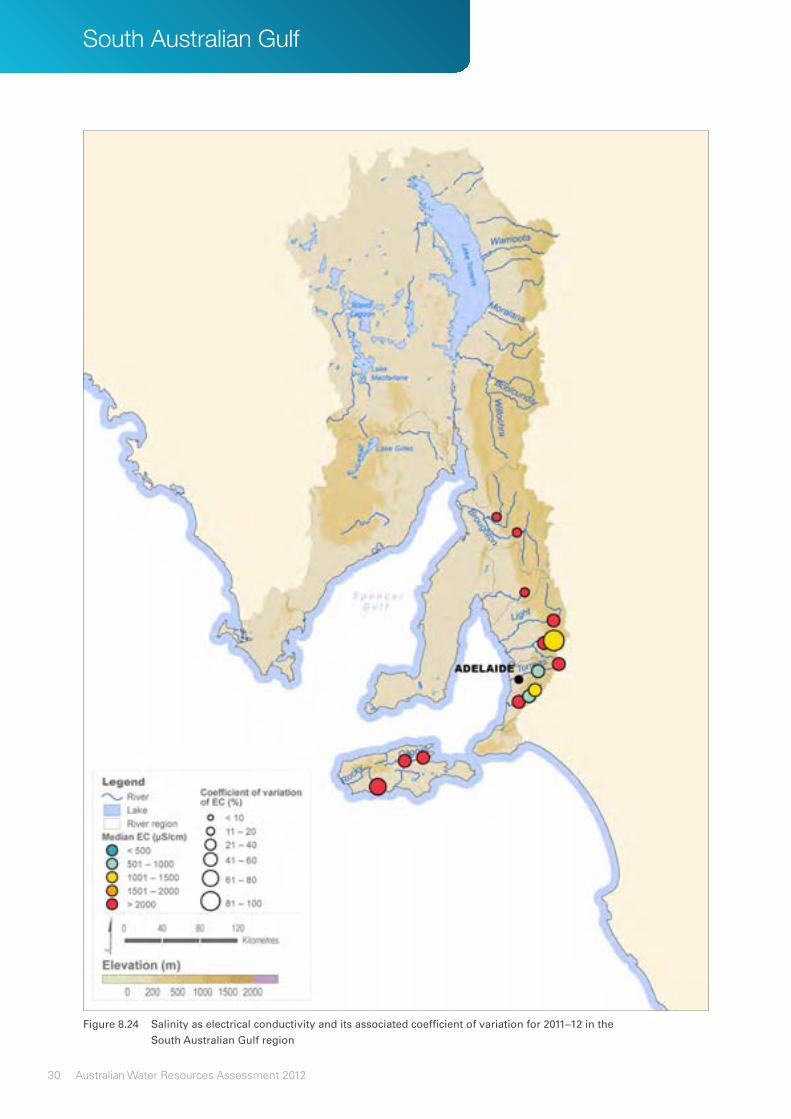
30 Australian Water Resources Assessment 2012
South Australian Gulf
Figure8.24 Salinityaselectricalconductivityanditsassociatedcoefficientofvariationfor2011–12inthe SouthAustralianGulfregion

31Australian Water Resources Assessment 2012
8.5.4 Flooding
There were no major floods recorded for the South Australian Gulf region during the reporting year. Minor flooding occurred only in local creeks in July and September 2011 and in March 2012 (Figure 8.25).
8.5.5 Storagesystems
There are approximately 16 major publicly owned storages in the South Australian Gulf region with a total capacity in excess of 268 GL. The Bureau’s water storage website includes information on approximately 74% of the region’s publicly owned storage capacities (as at August 2012)
All of the storages in the Bureau’s water storage information for this region supply the city of Adelaide, adding up to a total accessible capacity of 197 GL. At the end of 2010–11, storage levels were at 135 GL (69% of total accessible capacity), but by the end of 2011–12 this had dropped to 96 GL (49% of total accessible capacity). The location of all the systems and associated storages are shown in Figure 8.26.
The city of Adelaide is not fully dependent on storage water supply only. A large portion of the city’s water supply originates from transfers out of the River Murray, which has recently been complemented by desalinated water; however, the decrease in storage levels by 20% is not a favourable situation. This is reflected in stricter water conservation rules.
More detailed information on the Adelaide water supply system is given in subsection 8.6, Water for cities and towns. Further information on the past and present volumes of the storage systems and the individual storages can be found on the Bureau’s water storage website: water.bom.gov.au/waterstorage/awris/
8.5.6 Wetlands
There are no Ramsar-listed, internationally important wetlands in the South Australian Gulf region; however, there are a number of wetlands of national importance mentioned in the Directory of Important Wetlands in Australia (www.environment.gov.au/water/topics/wetlands/database/diwa.html). The wetlands vary from coastal tidal flats to inland ephemeral lakes and large salt lakes (Figure 8.27). No detailed assessment on the inflows of selected wetlands has been performed for this region.

32 Australian Water Resources Assessment 2012
South Australian Gulf
Figure8.25 Floodoccurrencein2011–12fortheSouthAustralianGulfregion,witheachdotrepresentingariverlevelmonitoringstationandthecolourofthedotrepresentingthehighestfloodclassmeasured

33Australian Water Resources Assessment 2012
Figure8.26 StoragesystemsintheSouthAustralianGulfregion(informationextractedfromtheBureau’swaterinformationwebsiteinAugust2012)

34 Australian Water Resources Assessment 2012
South Australian Gulf
Figure8.27 LocationofimportantwetlandsintheSouthAustralianGulfregion

35Australian Water Resources Assessment 2012
8.5.7 Hydrogeology
The hydrogeology of the South Australian Gulf region can be partitioned into areas of surficial and underlying sediments, and areas of outcropping fractured rock.
Groundwater use in the region is largest in areas with surficial sediments and underlying aquifers. Figure 8.28 shows major aquifer groups present at the watertable. Aquifer groups that provide potential for groundwater extraction (as labelled in Figure 8.2)are:
• lowermid-Tertiaryaquifer;(porousmedia—unconsolidated)
• upperTertiaryaquifer(porousmedia—unconsolidated);and
• upperTertiary/Quaternaryaquifer(porousmedia—unconsolidated).
The sediments of the Great Artesian Basin are present along the northern boundary of the region but are not dominant for water provision.
8.5.8 Watertablesalinity
Figure 8.29 shows the classification of watertable aquifers as fresh (total dissolved solids [TDS] < 3,000 mg/L) or saline (TDS ≥ 3,000 mg/L). As shown, most parts of the region are considered to have saline groundwater that is usually not suitable for irrigation. Non-saline groundwater occurs in the east of the region and in particular around the Adelaide area.
8.5.9 Groundwatermanagementunits
The groundwater management units within the region (Figure 8.30) are administrative boundaries that are used to manage the extraction of groundwater through planning mechanisms. These areas are usually created to identify a significant groundwater resource and to provide a boundary within which resource management effort can be focused. Prescription is the legal mechanism for implementing a water resource management regime in South Australia. A prescribed water resource is managed through an allocation and licensing system where the emphasis is on groundwater. These areas are known as water resources prescribed areas and prescribed wells areas within South Australia.
Groundwater management units are found in areas with significant fresh groundwater resources. These are the surficial sediments and the underlying Quaternary and Tertiary aquifers. The fractured rock systems typically offer restricted low volume groundwater resources; however, there are some parts of this region with a greater density of fractures and more substantial groundwater resources. Typically, groundwater use is high in prescribed wells areas such as McLaren Vale, the northern and central Adelaide Plains, and the southern basins.

36 Australian Water Resources Assessment 2012
South Australian Gulf
Figure8.28 WatertableaquifergroupsintheSouthAustralianGulfregion;dataextractedfromtheGroundwaterCartographyoftheAustralianHydrologicalGeospatialFabric(BureauofMeteorology2012)

37Australian Water Resources Assessment 2012
Figure8.29 WatertablesalinityclassesintheSouthAustralianGulfregion;dataextractedfromtheGroundwaterCartographyoftheAustralianHydrologicalGeospatialFabric(BureauofMeteorology2013)

38 Australian Water Resources Assessment 2012
South Australian Gulf
Figure8.30 GroundwatermanagementunitsintheSouthAustralianGulfregion;dataextractedfromtheNationalGroundwaterInformationSystem(BureauofMeteorology2013)

39Australian Water Resources Assessment 2012
8.5.10Statusofselectedaquifers
The status of groundwater levels is assessed for the Adelaide Plains and McLaren Vale aquifers which are major groundwater resources for the region. These aquifers are associated with three of the most important groundwater management units (prescribed well areas) shown in Figure 8.30. The assessment of groundwater levels evaluates trends in groundwater levels over the 2007–08 to 2011–12 period.
The trends in groundwater levels are investigated using a 5 km x 5 km grid cell across data rich areas. This scale reflects the size of the selected aquifers in the region. The linear trend in groundwater levels for a grid cell is assessed as:
• decreasing(wheremorethan60%oftheboreshaveanegativetrendinlevelslowerthan–0.1m/year);
• stable(wherethetrendislowerthan0.1m/yearandhigherthan–0.1m/yearformorethan60%ofthebores);
• increasing(wheremorethan60%oftheboreshaveapositivetrendinlevelshigherthan0.1m/year);and
• variable(wherethereisnodominanttrendingroundwaterlevelsamongsttheboreswithinagridcell).
Example bore hydrographs are presented for each aquifer over the entire record length and trends are discussed with a focus on the 2007–08 to 2011–12 period. The selected bore hydrographs represent mostly bores with high data density that were used in the 2010 Assessment. Aquifers considered:
• AdelaidePlainswatertable
• AdelaidePlainsTertiaryaquifer1(T1)
• AdelaidePlainsTertiaryaquifer2(T2)
• McLarenValewatertable
• Willunga
• Maslin.
AdelaidePlainaquifers
Figure 8.31 illustrates the spatial and temporal grid analyses of trends in groundwater levels of the Adelaide watertable over the period 2007–08 to 2011–12. Trends in groundwater levels were analysed in data-rich areas only. As shown in Figure 8.31, in the north of the aquifer groundwater levels are mostly rising. This reflects the increased groundwater recharge due to the recent high rainfall.
Selected bores 1 and 2 show variability in groundwater levels but no significant trend over the period. Peaks in water levels in these two bores represent groundwater response to infrequent recharge events. In contrast, Bore 3 shows stable levels until 2010. All bores show an increase in groundwater level after 2010 indicating recharge to groundwater during the recent high rainfall period.
Figure 8.32 illustrates the spatial and temporal grid analyses of trends in groundwater levels for the Tertiary aquifer T1 over the period 2007–08 to 2011–12. The trend analysis for the south of the aquifer indicates that groundwater levels for the past five years are either declining or variable. This is most likely in response to groundwater extraction in the southern area.
The selected hydrographs 4–6 indicate that variability in levels within a year is much larger than the inter-annual trend in levels. This illustrates the seasonal cycles of pumping and recovery of groundwater levels at the end of pumping season. All selected bores show a declining trend for the period 2007–08 to 2009–10 period and various degrees of recovery of groundwater levels, and therefore recharge, associated with higher rainfall since 2010.
Figure 8.33 illustrates the spatial and temporal grid analyses of trends in groundwater levels for the Tertiary aquifer T2 over the period 2007–08 to 2011–12. The analysis for T2 aquifer is focused in the north of the aquifer, and shows that groundwater levels for the past five years are either increasing or variable, similary to the watertable aquifer. All selected bores show declining trends for the period 2007–08 to 2009–10 and some degree of recovery thereafter.

40 Australian Water Resources Assessment 2012
South Australian Gulf
Figure8.31 SpatialdistributionoftrendsingroundwaterlevelsfortheAdelaidePlainswatertableintheSouthAustralianGulfregionfor2007–08to2011–12,withselectedhydrographsshowinggroundwaterlevels

41Australian Water Resources Assessment 2012
Figure8.32 SpatialdistributionoftrendsingroundwaterlevelsfortheAdelaidePlainsT1aquiferintheSouthAustralianGulfregionfor2007–08to2011–12,withselectedhydrographsshowinggroundwaterlevels

42 Australian Water Resources Assessment 2012
South Australian Gulf
Figure8.33 SpatialdistributionoftrendsingroundwaterlevelsfortheAdelaidePlainsT2aquiferintheSouthAustralianGulfregionfor2007–08to2011–12,withselectedhydrographsshowinggroundwaterlevels

43Australian Water Resources Assessment 2012
McLarenValeaquifers
Figure 8.34 illustrates the spatial and temporal trends in groundwater levels of the McLaren Vale watertable over the period 2007–08 to 2011–12. Grid analyses of trends in groundwater levels were carried out in data-rich areas only where three or more bores were present in a grid cell. As shown in Figure 8.34, groundwater levels are consistently stable.
The selected bores 10–12 have annual fluctuations in water levels that are most likely caused by seasonal groundwater recharge to the watertable. Hydrographs for these bores illustrate long- term relatively stable trends in water levels and, in particular, no major recharge event since 2010.
Figure 8.35 shows the grid analyses of trends in groundwater levels within the underlying Willunga aquifer, illustrating stable or declining levels for the period 2007–08 to 2011–12.This is a highly utilised aquifer and therefore the declining trends are most likely driven by groundwater extraction.
The selected bores 13–15 show continuously declining levels since the start of the records, with annual fluctuations in groundwater levels that correspond to seasonal cycles of pumping and recovery.
Figure 8.36 shows the grid analyses of trends in groundwater levels within the Maslin aquifer, indicating no prevalent trend over the period 2007–08 to 2011–12; however, no grid cells with an overall declining trend are present. This aquifer becomes unconfined in the northeast; therefore the groundwater level trends are likely to reflect the recent groundwater recharge episodes due to high rainfall.
Bores 16, 17 and 18 located at the eastern and southern ends of the Maslin Sands aquifer have stable water levels for the period 2007–08 to 2011–12 with no major recharge episode post 2010. Bore 17, located at the western end of the aquifer, shows annual fluctuations in water level that may be due to pumping from a nearby bore.

44 Australian Water Resources Assessment 2012
South Australian Gulf
Figure8.34 SpatialdistributionoftrendsingroundwaterlevelsfortheMcLarenValewatertableintheSouthAustralianGulfregionfor2007–08to2011–12,withselectedhydrographsshowinggroundwaterlevels

45Australian Water Resources Assessment 2012
Figure8.35 SpatialdistributionoftrendsingroundwaterlevelsforthePortWillungaaquiferintheSouthAustralianGulfregionfor2007–08to2011–12,withselectedhydrographsshowinggroundwaterlevels

46 Australian Water Resources Assessment 2012
South Australian Gulf
Figure8.36 SpatialdistributionoftrendsingroundwaterlevelsfortheMaslinSandsaquiferintheSouthAustralianGulfregionfor2007–08to2011–12,withselectedhydrographsshowinggroundwaterlevels

47Australian Water Resources Assessment 2012
8.6 Waterforcitiesandtowns
This section examines the urban water situation in the South Australian Gulf region in 2011–12. The large urban centres in the region, their water supply systems and storage situations are briefly described. The main urbanised area, Adelaide, is discussed in more detail in subsection 8.6.3, including the history of water restrictions over recent years.
8.6.1 Urbancentres
Adelaide is the largest city in the South Australian Gulf region and has more than 1.1 million residents. It is located north of the Fleurieu Peninsula, on the Adelaide Plains between the Gulf of St Vincent and the low-lying Mount Lofty Ranges which surround the city. Adelaide stretches 20 km from the coast to the foothills, and 90 km from Gawler at its northern extent to Sellicks Beach in the south.
Beyond Adelaide the region has four major population centres: Whyalla, Port Lincoln, Port Augusta and Port Pirie. These urban centres, along with Adelaide and other regional towns in conjunction with their population ranges, are shown in Figure 8.37.
The major urban centres of the region (populations over 10,000 people) are also summarised in Table 8.3. This table provides information on the population, surrounding river basins and significant water storages for each of the major centres.
Whyalla, with a population of just under 22,000, is the region’s second most populous city. It is a seaport located on the northeast coast of the Eyre Peninsula. The town is strongly influenced by the mining industry.
Port Lincoln is the third major town in the South Australia Gulf region and has a population of just over 14,000. It is a seaside town on Boston Bay at the southern extremity of the Eyre Peninsula. It is the largest town in the west of the region, and is located approximately 650 km from Adelaide.
Port Augusta has a population of just fewer than 14,000 and is the region’s fifth most populous town. It is a seaport and railway junction at the northern tip of the Spencer Gulf.
The population of Port Pirie is 13,800. It is also a seaport on the east coast of the Spencer Gulf, about 225 km north of Adelaide.
Table8.3 CitiesandtheirwatersupplysourcesintheSouthAustralianGulfregion
City Population1 Riverbasin Majorsupplysources
Adelaide 1,104,000 Gawler, Torrens, Onkaparinga, Myponga and Fleurieu Peninsula
Myponga, Barossa, Little Para, Kangaroo Creek, Mount Bold, Happy Valley, Hope Valley, Warren, Millbrook and South Para storages
Whyalla 21,700 Spencer Gulf River Murray (Morgan–Whyalla pipeline)
Port Lincoln 14,100 Eyre Peninsula Groundwater (Southern Basins)River Murray (Morgan–Whyalla pipeline)
Port Pirie 13,800 Mambray Coast and Broughton River
Baroota storage, River Murray (Morgan–Whyalla pipeline)
Port Augusta 13,500 Mambray Coast River Murray (Morgan–Whyalla pipeline)
1AustralianBureauofStatistics(2011b)

48 Australian Water Resources Assessment 2012
South Australian Gulf
Figure8.37 PopulationrangeofurbancentresintheSouthAustralianGulfregion

49Australian Water Resources Assessment 2012
8.6.2 Sourcesofwatersupply
While the regions’s surface water storages play an important role in the provision of its water supplies, its relatively low rainfall and long, dry summers have seen a growth in its dependence on diversions from the River Murray to meet its demands. South Australia holds an 1,850 GL-per-year entitlement to flows in the River Murray and during good rainfall years is entitled to extract an additional 3 GL per day as dilution flows.
Flows extracted from the Murray are distributed throughout the region by five bulk water transfer pipelines totalling over 650 km in length.
The Mannum–Adelaide and the Murray Bridge– Onkaparinga pipelines supply the city of Adelaide while the Swan Reach–Stockwell pipeline supplies water to townships (and farms) north of Adelaide and along its route.
The Morgan–Whyalla pipeline supplies many of the regions northern population centres and rural communities, including those of Whyalla, and Port Augusta to Woomera. At a length of 379 km, it is the longest of the five major pipelines in the region. Communities in the upper southeast of the region are supplied via the Tailem Bend–Keith pipeline. Figure 8.38 shows the major pipelines and storages in use for urban water supply.
In addition to imported and surface water storages, the region relies heavily on groundwater, recycled water and harvested storm and rainwater to supply its urban demands. In particular, South Australia has been a national leader in the use of recycled and stormwater.
8.6.3 Adelaide
The South Australia Water Corporation (SA Water) is the South Australian Government-owned statutory body that owns and manages Adelaide’s water supply systems, recycled water systems and wastewater services. SA Water controls surface water diversions, operates water treatment plants and maintains Adelaide’s reticulation system.
It supplies customers in the greater Adelaide area which includes the city of Adelaide as well as the surrounding suburbs, stretching over the Gawler, Torrens, Onkaparinga and Myponga river basins.
Watersupplysystem
Historically, the provision of a reliable and secure water supply to Adelaide has been a challenge because of its highly variable rainfall; however, the construction of a series of major pipelines supplying water from the River Murray and construction of a desalination plant have served to further ensure a reliable water supply for Adelaide.
Key components of the Adelaide water supply system include the Mannum–Adelaide and Murray Bridge–Onkaparinga pipelines, ten major storages totalling 197 GL in capacity, seven water treatment plants and twelve wastewater treatment plants. In addition, a number of privately operated bore fields supply groundwater primarily for agricultural uses. Some treated water is exported to adjacent regions for urban consumption.
The Mannum–Adelaide pipeline was the first of the pipelines built to deliver River Murray water to Adelaide. It supplies water to the Anstey Hill water treatment plant and to a number of storages.
The Murray Bridge–Onkaparinga pipeline was completed in 1973 and supplies water to the Summit Storage water treatment plant as well as releasing water into the Onkaparinga River for collection and treatment downstream.
Development of the Port Stanvac desalination plant was staged by constructing two 50 GL per year capacity plants. The first plant started production in October 2011 and the second during late 2012. Water from the desalination plant is mixed with treated surface water from the Happy Valley water treatment plant and discharged directly into Adelaide’s distribution system.
SA Water operates a number of recycled water and stormwater harvesting schemes. It also strongly promotes individual use of rainwater across the region. A number of recycled water schemes that supply treated effluent for agricultural and municipal irrigation and residential use operate within the greater Adelaide area. Several community or privately operated recycling schemes supply to viticulture and municipal applications.

50 Australian Water Resources Assessment 2012
South Australian Gulf
Figure8.38 WatersupplysystemsintheSouthAustralianGulfregion

51Australian Water Resources Assessment 2012
Storagevolumes
The Mount Bold, South Para, Kangaroo Creek and Myponga storages constitute 69% of the total Adelaide system storage. South Para serves the Northern Adelaide Plains. Kangaroo Creek is used to supply water to the northern Adelaide suburbs from Port Adelaide to the Torrens River while Mount
Bold serves the southern Adelaide suburbs from the Torrens River to the Onkaparinga River. Water from Myponga is distributed along the coast from the Onkaparinga River to Normanville. The accessible volumes of these major storages are shown individually in Figure 8.39.
Figure8.39 Variationintheamountofwaterheldinstorageoverrecentyears(lightblue)andover2011–12(darkblue)forMountBold,SouthPara,KangarooCreekandMypongastorages,aswellastotalaccessiblestoragecapacity(dashedline)
Mount Bold
Kangaroo Creek
South Para
Myponga

52 Australian Water Resources Assessment 2012
South Australian Gulf
Mount Bold is the largest storage, with a capacity of 46 GL, and it contributes approximately 20% of the total storage capacity.
The large annual fluctuation of the accessible storage shown in these figures illustrates the highly variable nature of Adelaide’s surface water resources. The figures highlight the general trend of filling during July–October and their drawdown across the drier summer period.
Extractions from the River Murray are highly dependent on the inflows to storages from their surrounding catchments. Extractions can range from 40% of the total water sourced in high rainfall years to 90% in years of very low rainfall.
Waterrestrictions
Water restriction in Adelaide and in most of the region are set by the State Government and enforced by SA Water. Restriction triggers are not solely based on the total available water in storage. Water restrictions in Adelaide are instead dependent on flows from the Mount Lofty Ranges and also on conditions in the Murray–Darling Basin, including volumes in the Hume and Dartmouth storages.
Restrictions applied to Adelaide outdoor water consumption are shown against combined storage volumes of Mount Bold, South Para, Kangaroo Creek and Myponga in Figure 8.40.
In the early 2000s, local storages, catchments and the River Murray were stressed as a result of drought conditions within the region and the Murray – Darling Basin. This saw Level 2 water restrictions introduced in July 2003 for four months. Permanent water conservation measures (PWCM) were introduced in October 2003, promoting long-term water conservation.
Figure8.40 UrbanwaterrestrictionlevelsacrossAdelaidesince2001shownagainstthecombinedaccessiblewatervolumeofMountBold,SouthPara,KangarooCreekandMypongastorages

53Australian Water Resources Assessment 2012
Enhanced level 2 restrictions were introduced in October 2006, after a record dry winter and record low inflows into the River Murray. They were quickly replaced in January 2007 by Level 3 restrictions and average annual residential water use decreased from 235 to 180 kL/property in 2006–07 to 2010–11 respectively.
An easing in water restriction levels in 2011–12 has been in part attributed to a rise in the average annual domestic water consumption of Adelaide, increasing to 195 kL/property (National Water Commission 2012).The South Australian Government imposed a temporary cessation on all outdoor watering in July 2007 which was extended through to August and September due to low winter flows. In October 2007, Adelaide residents were permitted to water for three hours per week; this was increased to five hours and then seven hours in April and May 2010 respectively.
Permanent water wise measures (WWM) were introduced on 1 December 2010 to cement water conservation across the region and to include measures to manage domestic and commercial water use.
Sourcesofwaterobtained
Figure 8.41 shows the total volume of water sourced from surface water, recycled and desalination water for supply to Adelaide (National Water Commission 2012). Demand management and water conservation measures have seen a continuing decline in the total water sourced by SA Water.
Between 2006–07 and 2011–12, the highest volume of total water sourced was 181 GL in 2006–07, which was a very dry and hot year. Over the following three years, the volume of water sourced was lower and constant as a result of demand management through water restrictions.
In 2011–12, recycled water comprised 3% of the total water sourced for Adelaide. A further 3% was sourced from desalinated water. For the remaining years shown in Figure 8.41, approximately 15% of the total water sourced was recycled water.
Figure8.41 TotalurbanwatersourcedforAdelaidefrom2006–07to2011–12

54 Australian Water Resources Assessment 2012
South Australian Gulf
Categoriesofwaterdelivered
Figure 8.42 shows the total volume of water delivered to residential, commercial, municipal, industrial and other consumers in Adelaide from 2006–07 to 2011–12. Water supply data of the last six years has been obtained from the National Water Commission’s National Performance Reports (National Water Commission 2013).
Water supply has steadily decreased from 2006–07 to 2010–11. The consumption of water increased in 2011–12 due to the lower water restrictions and above average rainfall in the region. Residential water use constitutes between 66% and 75% of Adelaide’s total water consumption. The maximum residential water use in Adelaide was during the year 2006–07 when more than 115 GL were supplied for residential use. As discussed above, water restrictions and conservation measures subsequently had a marked influence on residential water use.
The Level 2 and Level 3 restrictions introduced in 2006–07 reduced annual residential consumption to an average of 93 GL over the period 2007–08 to 2010–11. The average commercial, municipal and industrial water consumption in Adelaide during 2006–07 to 2011–12 was about 28 GL, with a maximum of more than 35 GL in 2006–07. By 2011–12, consumption by the commercial, municipal and industrial sectors fell to 26 GL with the lowest at 16 GL in 2009–10, almost half of the 2006–07 consumption.
Based on the data obtained from the National Performance Reports, the average water supply per property for residential use in Adelaide from 2006–07 to 2011–12 was estimated to be 195 kL. The maximum annual residential water use per property was 235 kL in 2006–07 and the minimum was 180 kL in 2010–11.
Figure8.42 CategoriesofwaterdeliveredtoAdelaidefrom2006–07to2011–12

55Australian Water Resources Assessment 2012
8.7 Waterforagriculture
This section describes the water situation for agriculture in the South Australian Gulf region during the 2011–12 year compared with the past. Modelled soil moisture conditions are presented and important irrigation areas are identified. The McLaren Vale Irrigation Area is described in more detail.
8.7.1 Soilmoisture
Since model estimates of soil moisture storage volumes are based on a simple conceptual representation of soil water storage and transfer processes averaged over a 5 km x 5 km grid cell, they are not suitable for comparison with locally measured soil moisture volumes. This analysis therefore presents a relative comparison only, identifying how modelled soil moisture volumes of 2011–12 relate to modelled soil moisture volumes of the 1911–2012 period, expressed in decile rankings.
Except for a narrow strip in the northern pastoral lands which had high above average soil moisture conditions, the South Australian Gulf region experienced average conditions (Figure 8.43). This follows the rainfall decile ranking during 2011–12 in the region. The similarity is more distinct for the northern and southern parts of the region.
Some irrigated lands of the southern region experienced below to very much below average soil moisture conditions (Figure 8.43).
Decile ranking of the changes in soil moisture averaged over the whole region during 2011–12 year indicates marginally above average conditions that rose in March due to historically high rainfall events, and continued during the autumn period (Figure 8.44).
Figure8.44 Decilerankingofthemonthlysoilmoistureconditionsduringthe2011–12periodintheSouthAustraliaGulfregion
Figure8.43 Decilesrankingsofannualaveragesoilmoisturefor2011–12withrespecttothe1911–2012periodfortheSouthAustralianGulfregion

56 Australian Water Resources Assessment 2012
South Australian Gulf
8.7.2 Irrigationwater
A comparison of annual irrigation water use in parts of the region for the period between 2005–06 and 2010–11 is shown by natural resource management (NRM) regions in Figure 8.45. Figure 8.46 shows the variation in annual water use between the two NRM regions in the South Australian Gulf region during 2010–11 year.
Data for the 2011–12 year was not available at the time of preparation of this report.
The McLaren Vale prescribed wells area in the Onkaparinga catchment is described in the following section as an example of irrigated agriculture water use in the region.
8.7.3 Irrigationareas
Dryland agriculture is the main agricultural activity in the South Australian Gulf region apart from grazing pasture. Viticulture and wine grape production is the main irrigated agriculture mostly in the Onkaparinga catchment (Figure 8.47). Water for these enterprises is sourced from the Mount Lofty Ranges and River Murray diversions. Mount Bold on the Onkaparinga River is the largest storage in the region with an accessible storage capacity of 46 GL.
In most years, inflows to storage are supplemented by water pumped from the River Murray via a pipeline from Murray Bridge. The majority of irrigated water use occurs in the south-eastern areas where viticulture is concentrated.
The McLaren Vale prescribed wells area is described in more detail in section 8.7.4 below.
8.7.4 McLarenValeprescribedwellsarea
The McLaren Vale prescribed wells area is located within the Onkaparinga catchment, 35 km south of Adelaide within the boundaries of the Western Mount Lofty Ranges prescribed area, and covers an area of 320 km2.
By regulation in 1998, all existing and future wells within the area were declared to be prescribed wells. Prescription is the legal mechanism for implementing a water resource management regime in South Australia. A prescribed water resource is managed through an allocation and licensing system.
The area was formed after amalgamating the Willunga Basin prescribed wells area and the Upper Willunga catchment moratorium area in 2000. The climate of the area is Mediterranean, with cool, wet winters and hot, dry summers. Annual rainfall varies from around 400 mm to around 900 mm. Irrigated viticulture accounts for more than 85% of the irrigation in the region. Orchards and other irrigated crops account for the remainder.
There are no large surface water inflows or storages in the McLaren Vale prescribed wells area. Around 75% of water used for irrigation in the McLaren Vale prescribed wells area is sourced from groundwater. Groundwater occurs in four major aquifers: the Quaternary aquifer, Port Willunga Formation aquifer, Maslin Sands aquifer and Fractured Rock aquifer.
Figure8.45 Totalannualirrigationwaterusefor2005–06to2010–11fornaturalresourcemanagementregionsintheSouthAustralianGulfregion(ABS2006–2010;2011a)

57Australian Water Resources Assessment 2012
Figure8.46 Annualirrigationwaterusepernaturalresourcemanagementregionfor2010–11(ABS2011a)

58 Australian Water Resources Assessment 2012
South Australian Gulf
Figure8.47 IrrigationareasintheSouthAustralianGulfregion

59Australian Water Resources Assessment 2012
The high cost of groundwater has encouraged the development of alternative water sources such as mains water and secondary treated water from the Christies Beach wastewater treatment plant (Government of South Australia 2000).
There is an extraction limit of 6,600 ML from groundwater. Most of the water is extracted from the Port Willunga Formation aquifer. Average allocation in McLaren Vale is 1.5 ML/ha for vines and 2.8 ML/ha for other crops.
Metered groundwater extractions in the McLaren Vale prescribed wells area for 2010–11 totalled 2,529 ML, 27% less than the previous year mostly because of above average rainfall in the region near Mount Bold (Department for Water 2011). Data for the 2011–12 year was not available at the time of preparation of this report.
Localhydrogeology
For the purpose of this report, the McLaren Vale Irrigation Area was selected as an example for the discussion of groundwater use in an irrigation area in the South Australian Gulf region.
The aquifer system in the McLaren Vale prescribed wells area (Figure 8.48) is complex but can be grouped into four aquifers listed from top to bottom: the Quaternary sediments, Willunga Formation, Maslin Sands and fractured basement rock. These aquifers are interconnected and as such, withdrawals from one aquifer will impact other aquifers. Furthermore, the aquifers are not all present at all locations in McLaren Vale.
Figure8.48 TheMcLarenValePrescribedWellsAreashowingthelocationofgroundwaterboresitesandraingauge

60 Australian Water Resources Assessment 2012
South Australian Gulf
The Willunga aquifer supplies 64% of groundwater extracted for irrigation, with the Maslin Sands and fractured basement rock aquifers supplying 20% and 16% respectively (Australian Bureau of Agricultural and Resource Economics and Sciences 2003).
The Quaternary aquifer is generally shallow and of poor quality; however, it plays an important role in supporting groundwater-dependent ecosystems such as Aldinga Scrub and by providing base flow to creeks and streams (Department of Water, Land and Biodiversity Conservation 2007).The Willunga aquifer is the most utilised groundwater resource in McLaren Vale prescribed wells area and is comprised of sand and limestone units. The Maslin Sands aquifer overlies the Fractured Rock aquifer. The aquifer is unconfined in the northeast of the area. Like the Willunga aquifer, recharge occurs via direct rainfall infiltration in unconfined areas as well as from streams and inflow from surrounding fractured rocks.
In the McLaren Vale prescribed wells area, localised cones of depression in the groundwater level due to groundwater pumping have been identified as a potential problem, particularly for saline seawater intrusion (Martin 1998; Martin and Hodgkin 2005). Stewart (2006) reported higher salinities between McLaren Vale and Blewitt Springs than in the remainder of the aquifer. This area coincides with a deflection in the potentiometric surface for the aquifer.
Groundwaterqualityoverview
Groundwater salinity increases towards the coast in the Port Willunga formation aquifer. This increase of salinity down the hydraulic gradient suggests that recharge to this aquifer is limited along the groundwater flow path. The salinity of the Maslin Sands aquifer is similar to that of the Port Willunga Formation aquifer. The salinity in the Fractured Rock aquifer is variable, but generally fresh.
Influencesonshallowgroundwater
There is often a very strong relationship observed in shallow aquifer systems between changes in groundwater levels and rainfall, which occur as a result of rapid recharge to these systems from rainfall (Department of Water, Land and Biodiversity Conservation 2007). Therefore, years of above average rainfall will result in rising groundwater levels, while years of below average rainfall will result in declining groundwater levels.
Fluctuations in the shallow groundwater levels were evaluated for the watertable aquifer at five selected sites using data between 1990 and 2012 (Figure 8.49). In Figure 8.49 fluctuation in groundwater levels are compared to the local monthly rainfall trend (location of rain gauge shown in Figure 8.48). Periods in which the cumulative rainfall residual mass curve rises indicate wetter than average conditions. Periods with a falling trend indicate drier than average conditions. Panel b in Figure 8.49 shows a wetter than average period up to 1994, followed by average rainfall conditions until 2006, then by a drier than average period up to 2009, and thereafter by average rainfall.
The figure illustrates that overall the groundwater response to trends in rainfall is prominent. It also shows that groundwater recharge in the watertable is driven by seasonal cycles in rainfall. All wells, except for one, show a decline in water level after 2006 and a minor recovery post 2009. This was as a result of below average rainfall conditions in the region from 2006 to 2009 followed by averaged rainfall (panel b in Figure 8.49). The pattern and magnitude of change in groundwater level is also influenced by the change in the pattern of extraction across the area.
Groundwaterlevel
Figure 8.50 shows ranges of groundwater depth from bores located in the three aquifers in the McLaren Vale Irrigation Area, and the ranking of 2011–12 median groundwater levels compared to annual median groundwater levels in the last 21 years (1990–2011).
As shown in Figure 8.50, typically groundwater levels in the watertable aquifer vary from very shallow 0–1 m from the surface to greater than 10 m from the surface. Median groundwater depths in 2011–12 are typically below the long-term average east of McLaren Vale town and are generally above the long-term average elsewhere.
Groundwater levels in the Willunga aquifer in 2011–12 are over all deeper than 10 m below the surface (Figure 8.51). The recorded groundwater levels are mostly below the long-term average of the past 21 years.

61Australian Water Resources Assessment 2012
In the Maslin Sands (Figure 8.52), groundwater levels in 2011–12 were also generally deep (>5 m below the surface). Overall, groundwater levels in the area increased concurrent with the expansion of irrigated land. Towards the coast, groundwater levels are below the average for the last 21 years.
Groundwatersalinity
At the time of writing, suitable quality controlled and assured time-series data on groundwater salinity were not available from the Australian Water Resources Information System (Bureau of Meteorology 2011a). Therefore, groundwater salinity status of the McLaren Vale Irrigation Area has not been analysed.
Figure8.49 (a)Groundwaterlevelsbetween1990and2012ofthewatertableaquiferatfiveboresitesintheMcLarenVale IrrigationArea,comparedwith(b)rainfallresiduals,and(c)dailyrainfallatWillunga

62 Australian Water Resources Assessment 2012
South Australian Gulf
Figure8.50 (a)Mediangroundwaterdepthbelowsurface,and(b)groundwaterleveldecilesin2011–12comparedtothe 1990–2012referenceperiodfortheMcLarenValewatertableaquifer

63Australian Water Resources Assessment 2012
Figure8.51 (a)Mediangroundwaterdepthbelowsurface,and(b)groundwaterlevelsdecilesin2011–12comparedtothe 1990–2012referenceperiodfortheWillungaaquifer

64 Australian Water Resources Assessment 2012
South Australian Gulf
Figure8.52 (a)Mediangroundwaterdepthbelowsurface,and(b)groundwaterlevelsdecilesin2011–12comparedtothe 1990–2012referenceperiodfortheMaslinSandsaquifer

South Western Plateau9. South Western Plateau .............................................. 2
9.1 Introduction ........................................................ 2
9.2 Key information .................................................. 3
9.3 Description of the region .................................... 4
9.3.1 Physiographic characteristics.................. 6
9.3.2 Elevation ................................................. 7
9.3.3 Slopes .................................................... 8
9.3.4 Soil types ................................................ 9
9.3.5 Land use .............................................. 11
9.3.6 Population distribution .......................... 12
9.3.7 Rainfall zones ....................................... 13
9.3.8 Rainfall deficit ....................................... 14
9.4 Landscape water flows .................................... 15
9.4.1 Rainfall .................................................. 16
9.4.2 Evapotranspiration ................................ 19
9.4.3 Landscape water yield .......................... 22
9.5 Surface water and groundwater ....................... 25
9.5.1 Rivers ................................................... 25
9.5.2 Flooding ............................................... 26
9.5.3 Wetlands .............................................. 26
9.5.4 Hydrogeology ....................................... 27
9.5.5 Watertable salinity ................................. 28
9.5.6 Groundwater management units ........... 29

2 Australian Water Resources Assessment 2012
South Western Plateau
9.1 Introduction
This chapter examines water resources in the South Western Plateau region in 2011–12 and over recent decades. It starts with summary information on the status of water flows, stores and use. This is followed by descriptive information for the region including the physiographic characteristics, soil types, land use, population and climate.
Spatial and temporal patterns in landscape water flows are presented as well as an examination of the surface and groundwater resources. The data sources and methods used in developing the diagrams and maps are listed in the Technical Supplement.
9. South Western Plateau

3Australian Water Resources Assessment 2012
9.2 Keyinformation
Table 9.1 gives an overview of the key components of the data and information in this chapter.
Table9.1 KeyinformationonlandscapewaterflowsandgroundwaterqualityintheSouthWesternPlateauregion
Landscapewaterflows
Evapo-transpiration
Landscapewater yield
Rainfall
Region average Difference from 1911–2012 long-term annual mean
Decile ranking with respect to the 1911–2012 record
256 mm +45% 9th—above average
268 mm +55% 10th—very much above average
6 mm +100% 10th—very much above average
Groundwater(inselectedaquifers)
Salinity: Saline groundwater (≥3000 mg/L) in the south of the region and scattered areas of saline groundwater mainly surrounding (dry) river beds and lakes in the north

4 Australian Water Resources Assessment 2012
South Western Plateau
9.3 Descriptionoftheregion
The South Western Plateau region covers 1,093,000 km2 of mostly sandy or stony desert within Western Australia, South Australia and the Northern Territory. The region borders the South Australian Gulf region to the east, Lake Eyre Basin region to the northeast, Tanami – Timor Sea Coast and North Western Plateau regions to the north, and the Pilbara–Gascoyne and South West Coast regions to the west. The Southern Ocean is the southern boundary of the region.
The region includes the Nullarbor Plain in the south and a major part of the Great Victorian Desert in the north. Vegetation is sparse with trees largely non-existent. The region is predominantly flat with some hills along the edges of the Nullarbor Plain. Subsections 9.3.1– 9.3.4 give more detail on physical characteristics of the region.
The South Western Plateau region has a population of 72,400 people that accounts for just over 0.3% of the nation’s total population (Australian Bureau of Statistics [ABS] 2011b).
Major population centres in the region include Kalgoorlie–Boulder, Esperance, Ceduna, Coolgardie, Kambalda West and Streaky Bay (Figure 9.1).
Further discussion of the region’s population distribution and urban centres can be found in Section 9.3.6.
Most of the region comprises nature conservation (Figure 9.1), including much of the Nullarbor Plain and the Great Victorian Desert. To the west and east, large areas of pasture are present, with some areas of dryland agriculture on the Eyre Peninsula (southeast) and north of Esperance (southwest).
Except for the western and eastern parts of the region, the vast area of the region is arid. Subsections 9.3.7 and 9.3.8 provide more information on the rainfall patterns and deficits across the region.
A substantial number of predominantly dry lakes are present in the west and east of the region as well as more sporadically in the north. Some small rivers discharge into the Southern Ocean surrounding Esperance in Western Australia and Ceduna in South Australia.
The hydrogeology of the region is dominated by a outcropping fractured basement rock with limited groundwater resources. There are significant groundwater resources in localised sedimentary aquifers.
The Nullabor Plain | Heidi Kaldahl

5Australian Water Resources Assessment 2012
Figure9.1 MajorriversandurbancentresintheSouthWesternPlateauregion

6 Australian Water Resources Assessment 2012
South Western Plateau
9.3.1 Physiographic characteristics
The physiographic map in Figure 9.2 shows areas with similar landform evolutionary histories (Pain et al. 2011). These can be related back to similar geology and climatic impacts which define the extent of erosion processes. The areas have distinct physical characteristics that can influence hydrological processes.
The South Western Plateau region has four such dominant physiographic provinces, namely:
• Sandland (41%): west-east longitudinal dunes, broken by low tablelands and ridges in the northwest with ferruginous plains in the north;
• Yilgarn Plateau (24%): flat to undulating plain with salt lakes;
• Nullarbor (21%): karst plain of flat-lying limestone and calcrete; and
• Eyre Peninsula (10%): alluvial plains and salt lakes with some dunes and hills of volcanic and metamorphic rocks in the south.
The remaining three provinces occupy only 4% of the region. These are:
• Central Australian Ranges: dissected sandstone, granitic and volcanic ranges with prominent escarpments; separated by sandplains with dunes of hardpan;
• Central Lowlands: silcrete capped low tablelands; and
• Pilbara: mainly alluvial lowland with hardpan and sand plains.
Figure9.2 PhysiographicprovincesoftheSouthWesternPlateauregion

7Australian Water Resources Assessment 2012
9.3.2 Elevation
The South Western Plateau region includes the Nullarbor Plain in the south and a major part of the Great Victorian Desert in the north. As seen in Figure 9.3, the region is predominantly flat with some hills along the edges of the Nullarbor Plain. Information was obtained from the Geoscience Australia website (www.ga.gov.au/topographic-mapping/digital-elevation-data.html).
The north and west of the region is part of the Western Plateau, which extends north and west to the Indian Ocean.
The highest points in the region exceed 1,200 m and are located in the northeastern Musgrave Ranges. The lowest area is the Roe Plains, a long coastal stretch of a low-lying limestone plateau.
The most eastern part of the region has no major hills and altitudes do not exceed 500 m above sea level in the Gawler Ranges. To the west, the area consists of many closed basins in between the ridges, with many dry lakes and salt plains. Altitudes in this area exceed 600 m above sea level.
Figure9.3 GroundsurfaceelevationsintheSouthWesternPlateauregion

8 Australian Water Resources Assessment 2012
South Western Plateau
9.3.3 Slopes
Areas with steep slopes provide higher run-off generating potential than flat areas. The South Western Plateau region is generally flat, with hardly any steep slopes. Figure 9.4 shows the spatial distribution of surface slopes in the region while Table 9.2 summarises the extent of the slope ranges.
Table9.2 Proportionsofslopeclassesfortheregion
Slopeclass(%) 0–0.5 0.5–1 1–5 >5
Proportion of region (%)
52.4 26.8 20.0 0.8
The steep slopes in Figure 9.4 in particular highlight the Musgrave Ranges in the north. The large Nullarbor Plain in the south is very distinctive in its flatness. Water flow is practically non-existent in this area.
The slope map also clearly shows the escarpment of the western plateau in the north and the separation between the Nullarbor Plain and the Roe Plains in the south. The slopes were derived from the elevation information used in the previous section.
The ridges to the west are particularly distinctive as well, with many flat areas in between depicting the large dry lakes and salt plains.
Figure9.4 SurfaceslopesintheSouthWesternPlateauregion

9Australian Water Resources Assessment 2012
9.3.4 Soil types
Soils play an important role in the hydrological cycle by distributing water that reaches the ground. Water can be transported to rivers and lakes via the soil surface as run-off or enter the soil and provide water for plant growth as well as contributing to groundwater recharge. The nature of these hydrological pathways and the suitability of the soilds for agricultural purposes are influenced by the soil types and their characteristics. Soil type information was obtained from the Australian Soil Resource Information System website (www.asris.csiro.au).
About 97% of the South Western Plateau region is covered by four soil types, namely tenosols, calcarosols, rudosols and kandosols (Figure 9.5 and Figure 9.6). They are mostly present in areas used for grazing or nature conservation. Among these soils tenosols and calcarosols each cover more than 30% of the region.
Tenosols, rudosols and kandosols are soils with weak and minimal development, either throughout the
profile (tenosols, rudosols) or in the upper soil profile (kandosols). They show no or little change in texture and colour and are often shallow in depth. These soils are low in chemical fertility and in water-holding capacity and thus their agricultural potential is low.
Tenosols are dominant in the north of the region and here they are found with kandosols. Tenosols are also scattered in the southeast of the region. In the east of the region, rudosols are more common Calcarosols are characterised by a high of calcium carbonate content which occurs as soft or hard white fragments or as solid layers. These soils are found along the coastline and in the eastern part of the region. The soils are often shallow and have a low water-holding capacity. They have low to moderate agricultural potential, and high salinity levels, alkalinity and boron toxicity may often cause problems.
The other soil types that have minimal representation in the South Western Plateau region include sodosols and hydrosols (0.6–3% of the total area).
Figure9.5 SoiltypesintheSouthWesternPlateauregion

10 Australian Water Resources Assessment 2012
South Western Plateau
Figure9.6 SoiltypedistributionintheSouthWesternPlateauregion

11Australian Water Resources Assessment 2012
9.3.5 Land use
As presented in Figure 9.7 and Figure 9.8, most of the region comprises nature conservation, including much of the Nullarbor Plain and the Great Victorian
Desert (data from data.daff.gov.au/anrdl/metadata_files/pa_luav4g9abl07811a00.xml). To the west and east, large areas of pasture are present with some areas of dryland agriculture on the Eyre Peninsula (southeast) and north of Esperance (southwest).
Figure9.7 LandusedistributionintheSouthWesternPlateauregion
Figure9.8 LanduseintheSouthWesternPlateauregion

12 Australian Water Resources Assessment 2012
South Western Plateau
9.3.6 Population distribution
Figure 9.9 illustrates the sparse nature of the population in the region (ABS 2011b).
The majority of the population is located near the eastern and western extremities of the region. The region is home to a number of remote Indigenous communities. Mining is the primary occupation for
the majority of the region’s sparsely distributed but permanent population centres. The mining city of Kalgoorlie–Boulder is the largest and most densely populated centre within the region and is situated in the central west, within the Western Australian State boundary. In addition to Kalgoorlie, the coastal centre of Esperance is located in the southwest of the region.
Figure9.9 PopulationdensityanddistributionintheSouthWesternPlateauregion

13Australian Water Resources Assessment 2012
9.3.7 Rainfall zones
The South Western Plateau region is the driest region in Australia. Except for the southwest and southeast of the region, which are semi-arid, the vast area in the centre is arid. With the exception of the far western coastline, median rainfall does not exceed 500 mm per year (Figure 9.10).
A large portion of the region has the lowest average annual rainfall of the continent, not exceeding 200 mm.
The winter (dominant) rainfall areas in the west and east have annual average rainfall totals of about 300 mm. In the far southeast, some consistency in winter rainfall is present, although annual average rainfall does not exceed 500 mm.
For more information on this and other climate classifications, visit the Bureau of Meteorology's (the Bureau's) climate website: www.bom.gov.au/jsp/ncc/climate_averages/climate-classifications/index.jsp
Figure9.10 RainfallzonesintheSouthWesternPlateauregion

14 Australian Water Resources Assessment 2012
South Western Plateau
9.3.8 Rainfall deficit
The rainfall deficit indicator, that is, rainfall minus potential evapotranspiration, gives a general impression about which parts of the region are likely to experience moisture deficits over the period of a year. The South Western Plateau region is highly prone to water shortages in relation to this indicator.
High deficits can be expected in large parts of the inland areas where desert vegetation prevails (Figure 9.11). For more information on the rainfall and evapotranspiration data, see the Bureau’s maps of average conditions: www.bom.gov.au/climate/averages/maps.shtml
Figure9.11 RainfalldeficitdistributionintheSouthWesternPlateauregion

15Australian Water Resources Assessment 2012
9.4 Landscapewaterflows
This section presents analyses of the spatial and temporal variation of landscape water flows (rainfall, evapotranspiration and landscape water yield) across the South Western Plateau region in 2011–12. National rainfall grids were generated using data from a network of persistent, high-quality rainfall stations managed by the Bureau. Evapotranspiration and landscape water yields were derived using the landscape water balance component of the Australian Water Resources Assessment System (Van Dijk 2010). These methods and associated output uncertainties are discussed in Introduction and addressed in more detail in the Technical Supplement.
Figure 9.12 show that the region has a highly variable historic rainfall pattern. No clear seasonality in the rainfall can be identified in the boxes of Figure 9.12. This also counts for the historic annual totals of evapotranspiration and landscape water yield. The historic pattern of evapotranspiration closely follows that of rainfall. Landscape water yield is generally close to zero for each month of the year.
It should be noted that the area has low rain gauge density, particularly in the north, and data uncertainty for the spatially interpolated rainfall data is high. Nonetheless, Figure 9.12 shows that the 2011–12 year was a relatively wet year, especially between October 2011 and January 2012. Above average sea surface temperatures were evident in the Indian Ocean during spring 2011, which generated a large number of thunderstorms over the whole of Western Australia.
Evapotranspiration closely followed the temporal pattern of rainfall. A month’s delay is noticeable in the October and November evapotranspiration in relation to rainfall, as evapotranspiration is limited to a maximum potential amount per day, based on available energy levels. Since most of the October rainfall was stored in the soil, it was directly available for evapotranspiration in November.
Throughout most of the year, landscape water yield for 2011–12 was higher than the historic monthly averages. Most of this landscape water yield occurred locally, mainly in the western part of the region.
Figure9.12 Landscapewaterflowsin2011–12comparedwiththelong-termrecord(July1911–June2012)fortheSouthWesternPlateauregion

16 Australian Water Resources Assessment 2012
South Western Plateau
9.4.1 Rainfall
Rainfall for the South Western Plateau region for 2011–12 is estimated to be 256 mm. This is 45% above the region’s long-term average (July 1911– June 2012) of 176 mm. Figure 9.13a shows that the highest rainfall occurred largely along the western borders, with annual totals exceeding 400 mm in many areas for 2011–12.
The high data uncertainty in the map indicates those areas where rain gauge density is too low to accurately capture localised rainfall, particularly in the form of thunderstorms.
Rainfall deciles for 2011–12 indicate average to above average rainfall for the entire region over the course of the year (Figure 9.13b). The pasture fields in the northwest of the region locally had very much above average rainfall.
Figure9.13 Spatialdistributionof(a)annualrainfallin2011–12and(b)theirdecilerankingsoverthe1911–2012periodfortheSouthWesternPlateauregion

17Australian Water Resources Assessment 2012
Rainfallvariabilityintherecentpast
Figure 9.14a shows annual rainfall for the region from July 1980 onwards. Over this 32-year period the annual average was 212 mm, varying from 132 mm (2007–08) to 369 mm (2010–11). Temporal variability and seasonal patterns since 1980 are presented in Figure 9.14b.
The graphs indicate a substantial increase in rainfall from 1997 onwards, especially for the summer period. Where rainfall was equally distributed between the summer and winter period in the first half of the 32-year period, summer rainfall suddenly increased to higher totals in the second half of the period.
Figure9.14 Time-seriesof(a)annualrainfall,and(b)five-yearretrospectivemovingaveragesforthesummer(November–April)andwinter(May–October)periodsfortheSouthWesternPlateauregion

18 Australian Water Resources Assessment 2012
South Western Plateau
Recenttrendsinrainfall
Figure 9.15a presents the spatial distribution of the trends in annual rainfall for July 1980–June 2012. These are derived from linear regression analyses on the time-series of each model grid cell. The statistical significance of the trends is provided in Figure 9.15b.
Figure 9.15a shows that since 1980 an increase in rainfall has occurred in most of the region, particularly in the data sparse north. Some areas with a significant rising trend are present on the Nullarbor in the centre of the region. The more cultivated southwest and southeast of the region had no change in annual rainfall since 1980.
Figure9.15 Spatialdistributionof(a)trendsinannualrainfallfrom1980–2012and(b)theirstatisticalsignificanceat90%(weak)and95%(strong)confidencelevelsfortheSouthWesternPlateauregion

19Australian Water Resources Assessment 2012
9.4.2 Evapotranspiration
Modelled annual evapotranspiration for the South Western Plateau region for 2011–12 is estimated to be 268 mm. This is 55% above the region’s long-term (July 1911–June 2012) average of 173 mm. The spatial distribution of annual evapotranspiration in 2011–12 (Figure 9.16a) is closely related to that of rainfall (Figure 9.13a).
Evapotranspiration deciles for 2011–12 indicate very much above average totals across most of the north of the region (Figure 9.16b). In the south, where the water supply through rainfall was largely average, evapotranspiration was also not able to exceed average levels.
Figure9.16 Spatialdistributionof(a)modelledannualevapotranspirationin2011–12,and(b)theirdecilerankingsoverthe1911–2012periodfortheSouthWesternPlateauregion

20 Australian Water Resources Assessment 2012
South Western Plateau
Evapotranspirationvariabilityintherecentpast
Figure 9.17a shows annual evapotranspiration for the region from July 1980 onwards. Over this 32-year period the annual evapotranspiration average was 207 mm, varying from 134 mm (1985–86) to 314 mm (2010–11). Temporal variability and seasonal patterns since 1980 are presented in Figure 9.17b.
Similar to the temporal pattern of rainfall, evapotranspiration shows an increase in annual totals after 1997, mainly occurring in the summer period. Water availability, provided by rainfall, is the only limitation to evapotranspiration in this arid region.
Figure9.17 Time-seriesof(a)annualevapotranspirationand(b)five-yearretrospectivemovingaveragesforthesummer(November–April)andwinter(May–October)periodsfortheSouthWesternPlateauregion

21Australian Water Resources Assessment 2012
Recenttrendsinevapotranspiration
Figure 9.18a presents the spatial distribution of the trends in modelled annual evapotranspiration for 1980–2012. These are derived from linear regression analyses on the time-series of each model grid cell. The statistical significance of the trends is provided in Figure 9.18b.
Figure 9.18a shows that, since 1980, trends are mostly positive in the central northern part of the region. In the south, the trends are mostly neutral.
As shown in Figure 9.18b, some statistically significant rising trends in annual evapotranspiration are present in the data sparse north and in large areas in the centre of the region. As evapotranspiration is driven by the availability of moisture, these spatial patterns are again linked to the rainfall trends of Figure 9.15.
Figure9.18 Spatialdistributionof(a)trendsinannualevapotranspirationfrom1980–2012,and(b)theirstatisticalsignificanceat90%(weak)and95%(strong)confidencelevelsfortheSouthWesternPlateauregion

22 Australian Water Resources Assessment 2012
South Western Plateau
9.4.3 Landscape water yield
Modelled landscape water yield for the South Western Plateau region for 2011–12 is estimated to be 6 mm. This is 100% above the region’s long-term (July 1911–June 2012) average of 3 mm. Figure 9.19a shows the spatial distribution of landscape water yield for 2011–12, which is similar to the annual rainfall distribution (Figure 9.13a; note the difference in the scale of the two figures).
The decile ranking map for 2011–12 (Figure 9.19b) shows above average to very much above average landscape water yields in most parts of the region. Some below average landscape water yield occurred in the southwest of the region. Throughout the area the model estimates landscape water yields which vary marginally. Only minor differences from the mean could cause areas to appear as above or below average.
Figure9.19 Spatialdistributionof(a)modelledannuallandscapewateryieldin2011–12and(b)theirdecilerankingsoverthe1911–2012periodfortheSouthWesternPlateauregion

23Australian Water Resources Assessment 2012
Landscapewateryieldvariabilityintherecentpast
Figure 9.20a shows annual landscape water yield for the South Western Plateau region from July 1980 onwards. Over this 32-year period, annual landscape water yield was 4 mm, varying from 1 mm (1985–86) to 10 mm (2010–11). Temporal variability and seasonal patterns since 1980 are presented in Figure 9.20b.
The high variability in annual landscape water yield is normal for arid areas. These areas experience only a small number of rainfall events, of which only the high intensity events have the potential to generate landscape water yield.
Landscape water yield is consistently higher during the summer period compared to the winter period, with, however, an increase in the gap between the two seasons since 1997. This again corresponds with the temporal patterns in rainfall of Figure 9.14b.
Figure9.20 Time-seriesof(a)annuallandscapewateryieldand,(b)five-yearretrospectivemovingaveragesforthesummer(November–April)andwinter(May–October)periodsfortheSouthWesternPlateauregion

24 Australian Water Resources Assessment 2012
South Western Plateau
Recenttrendsinlandscapewateryield
Figure 9.21a shows the spatial distribution of the trends in modelled annual landscape water yield for 1980– 2012. These are derived from linear regression analyses on the time-series of each model grid cell. The statistical significance of the trends is provided in Figure 9.21b.
Figure 9.21a shows that, since 1980, trends are marginal, which can be expected when applying linear regression to time-series of particularly low values.
On the other hand, Figure 9.21b shows strongly significant rising trends in landscape water yield in large parts of the region, especially in the centre. The magnitudes of the trends in these areas do not exceed 1 mm/year with most of these areas even having trends below 0.2 mm/year.
Figure9.21 Spatialdistributionof(a)trendsinannuallandscapewateryieldfrom1980–2012and(b)theirstatisticalsignificanceat90%(weak)and95%(strong)confidencelevelsfortheSouthWesternPlateauregion

25Australian Water Resources Assessment 2012
9.5 Surfacewaterandgroundwater
This section examines surface water and groundwater resources in the South Western Plateau region. Rivers and wetlands are discussed to illustrate the region’s surface water resources.
The region’s watertable aquifers and salinity are described. No data was available at the Bureau in a suitable format for a detailed analysis on individual aquifers.
Due to the absence of suitable data on river flows in this region, no analysis is performed on streamflow characteristics and wetland inflows.
There are no major public storages present in the region.
9.5.1 Rivers
There are three river basins in the South Western Plateau region, varying in size from 278,000– 496,000 km2. These river basins are Gairdner, Nullarbor and Salt Lake (Figure 9.22).
A substantial number of predominantly dry lakes are present in the west and east of the region as well as more sporadically in the north.
Some small rivers, near Esperance in Western Australia and Ceduna in South Australia, discharge to the Southern Ocean. All streams flow only after heavy rains, which may be two or three or even ten years apart.
Figure9.22 RiversandcatchmentsintheSouthWesternPlateauregion

26 Australian Water Resources Assessment 2012
South Western Plateau
9.5.2 Flooding
No major, moderate or minor floods were recorded at the two available Bureau flood monitoring sites near Esperance.
9.5.3 Wetlands
The wetlands vary from coastal floodplains and tidal flats to inland ephemeral lakes and large salt lakes. There is one Ramsar-listed, internationally important wetland present in the South Western Plateau region and a number of national important wetlands as shown in Figure 9.23.
The wetlands vary from coastal floodplains and tidal flats to inland ephemeral lakes and large salt lakes.
The Ramsar-listed Lake Warden system near Esperance consists of saline lakes and marsh areas separated from the ocean by sand dunes. It is an important habitat for water birds. More information about the region’s wetlands is available from the Australian Directory of Important Wetlands (www.environment.gov.au/water/topics/wetlands/database/diwa.html).
No detailed assessment on the inflows of selected wetlands has been performed for this region.
Figure9.23 LocationofimportantwetlandsintheSouthWesternPlateauregion

27Australian Water Resources Assessment 2012
9.5.4 Hydrogeology
The hydrogeology of the South Western Plateau region is dominated by a large area of outcropping fractured basement rock (Figure 9.24).
The groundwater systems in fractured rock typically offer restricted low volume groundwater resources. In contrast, there are significant groundwater resources in localised sedimentary aquifers.
Figure 9.24 shows a discontinuity in aquifers across the State border, which is the result of two different State-based aquifer classification systems.
Groundwater systems that provide potential for extraction are labelled as:
• Surficial sediment aquifer (porous media—unconsolidated); and
• Upper mid-Tertiary aquifer (porous media—unconsolidated).
Figure9.24 WatertableaquifersoftheSouthWesternPlateauregion;dataextractedfromtheGroundwaterCartographyoftheAustralianHydrologicalGeospatialFabric(BureauofMeteorology2012)

28 Australian Water Resources Assessment 2012
South Western Plateau
9.5.5 Watertable salinity
Figure 9.25 shows the classification of watertable aquifers as fresh (total dissolved solids [TDS] < 3,000 mg/L) or saline (TDS ≥ 3,000 mg/L) water according to watertable salinity. The discontinuity in aquifers across the State border in Figure 9.25 is the result of two different State-based aquifer salinity classification systems.
Shallow groundwater has been classified mainly as saline within South Australia and around half fresh and half saline in Western Australia; however, a clear pattern of high groundwater salinity is present in the low-lying areas, in particular in those aquifers that are mentioned as having high extraction potential.
Figure9.25 WatertablesalinityclassesoftheSouthWesternPlateauregion;dataextractedfromtheGroundwaterCartographyoftheAustralianHydrologicalGeospatialFabric(BureauofMeteorology2012)

29Australian Water Resources Assessment 2012
9.5.6 Groundwater management units
The groundwater management units within the South Western Plateau region are key features that control the extraction of groundwater through planning mechanisms.
The groundwater management units within the region are presented in Figure 9.26. This dataset is
extracted from the National Groundwater Information System (2013) which contains a collection of groundwater management units from all States.
The major management units with significant groundwater use include Goldfield, East Murchison, Nullarbor in Western Australia and Musgrave in South Australia.
Figure9.26 GroundwatermanagementunitsintheSouthWesternPlateauregion;dataextractedfromtheNationalGroundwaterInformationSystem(BureauofMeteorology2013)

South West Coast10 South West Coast ..................................................... 2
10.1 Introduction ........................................................ 2
10.2 Key information .................................................. 3
10.3 Description of region ......................................... 4
10.3.1 Physiographic characteristics.................. 6
10.3.2 Elevation ................................................. 7
10.3.3 Slopes .................................................... 8
10.3.4 Soil types ............................................... 9
10.3.5 Land use ............................................. 11
10.3.6 Population distribution .......................... 13
10.3.7 Rainfall zones ....................................... 14
10.3.8 Rainfall deficit ....................................... 15
10.4 Landscape water flows ................................... 16
10.4.1 Rainfall ................................................. 17
10.4.2 Evapotranspiration ............................... 20
10.4.3 Landscape water yield ......................... 23
10.5 Surface water and groundwater ....................... 26
10.5.1 Rivers ................................................... 26
10.5.2 Streamflow volumes ............................. 28
10.5.3 Streamflow salinity ............................... 28
10.5.4 Flooding ............................................... 31
10.5.5 Storage systems ................................... 31
10.5.6 Wetlands ............................................. 31
10.5.7 Hydrogeology ....................................... 35
10.5.8 Watertable salinity ................................. 35
10.5.9 Groundwater management units ........... 35
10.6 Water for cities and towns ................................ 39
10.6.1 Urban centres ....................................... 39
10.6.2 Sources of water supply ...................... 41
10.6.3 Perth .................................................... 41
10.7 Water for agriculture ......................................... 48
10.7.1 Soil moisture ........................................ 48
10.7.2 Irrigation water ...................................... 49
10.7.3 Irrigation areas ...................................... 49
10.7.4 Harvey Water Irrigation Area ................. 52

South West Coast
2 Australian Water Resources Assessment 2012
10 South West Coast10.1 Introduction
ThischapterexamineswaterresourcesintheSouthWestCoastregionin2011–12andoverrecentdecades.Itstartswithsummaryinformationonthestatusofwaterflows,storesanduse.Thisisfollowedbydescriptiveinformationfortheregionincludingthephysiographiccharacteristics,soiltypes,population,landuseandclimate.
Spatialandtemporalpatternsinlandscapewaterflowsarepresentedaswellasanexaminationofthesurfaceandgroundwaterresources.Thechapterconcludeswithareviewofthewatersituationforurbancentresandirrigationareas.ThedatasourcesandmethodsusedindevelopingthediagramsandmapsarelistedintheTechnicalSupplement.

3Australian Water Resources Assessment 2012
10.2 Keyinformation
Table10.1givesanoverviewofthekeycomponentsofthedataandinformationinthischapter.
Table 10.1 Key information on water flows, stores and use in the South West Coast region
Landscape water flows
Evapo-transpiration
Landscapewater yield
Rainfall
Regionaverage Differencefrom1911–2012long-termannualmean
Decilerankingwithrespecttothe1911–2012record
499mm +14% 8th—aboveaverage
455mm +15% 10th—verymuchaboveaverage
28mm -24% 4th—average
Streamflow (at selected gauges)
Annualtotalflow:
Betweenaverageandverymuchbelowaverageflowthroughouttheregion
Salinity:Annualmedianelectricalconductivitypredominantlyabove2,000μS/cminlandandlesssalineinthecoastalriversinthewest
Flooding: Sporadicminorandmoderatefloodinginthesouthwestriverbasins
Surface water storage (comprising about 92% of the region’s total capacity of all major storages)
Totalaccessiblecapacity
30June2012 30June2011 Change
accessiblevolume
%oftotalcapacity
accessiblevolume
%oftotalcapacity
accessiblevolume
%oftotalcapacity
951GL 309GL 32% 210GL 22% +99GL +10%
Groundwater (in selected aquifers)
Salinity: Non-salinegroundwater(<3000mg/L)onlyalongthesouthwestcoastlineandinscatteredareasinthenorth
Urban water use (Perth)
Totalsourcedin2011–12 Totalsourcedin2010–11
Change Restrictions
248GL 247GL +1GL EasedtoStage5inSeptember,backtoStage7
inJune
Annual mean soil moisture (model estimates)
Spatialpatterns: Predominantlyaveragetobelowaverageannualmeansoilmoisturewithlargeareasofverymuchbelowaveragesoilmoisturetotheeastandinthesouthwest
Temporalpatternsinregionalaverage:
Belowaveragesoilmoisturethroughouttheyear,onlyreachingaveragelevelsinsummer
South West Coast
4 Australian Water Resources Assessment 2012
10.3 Descriptionoftheregion
TheSouthWestCoastregioncoversapproximately326,000km²ofland.ItisboundedtothewestbytheIndianOceanandtothesouthbytheGreatAustralianBight.ThenorthernboundaryisthePilbara–GascoyneregionandtheeasternboundaryistheSouthWesternPlateauregion.
Thelandscapeoftheregionisgenerallyflatandsandyininlandareas.HigheraltitudetopographicfeaturesincludetheDarlingScarpthatformsanancientgeologicalboundarytothe30-kmwideSwanCoastalPlainalongthewestcoastandtheStirlingRangenearAlbany.TheSwanCoastalPlainconsistsofrelativelyinfertilesandysoilsandcoastaldunes;anumberofestuariesandwetlandsareseparatedfromtheseabythesedunes.Subsections10.3.1–10.3.4givemoredetailonphysicalcharacteristicsoftheregion.
Theregionhasapopulationjustover2millionpeople,whichaccountsforjustover9%ofthenation’stotalpopulation(AustralianBureauofStatistics[ABS]2011b).Figure10.1highlightsthemajorpopulationcentresintheregionthatincludesPerth,Mandurah,BunburyandAlbany.Furtherdiscussionoftheregion’spopulationdistributionandurbancentrescanbefoundinsubsection10.3.6andsection10.6respectively.
Thenorthoftheregionisdominatedbypasture,becomingamorecomplexpatternofpastureanddrylandcropstowardsthecentralandsouthernpartsoftheregion.Forestryisimportantinthewetterhigheraltitudewesternslopes,withextensiveconservationreserveareasinthispartoftheregion.Conservationshrublandandheathlandreservesarewellrepresentedinthemorearideast(Figure10.1).
Drylandandirrigatedagricultureaccountforaverysmallproportionofthelanduseinthearea.Intensivelandusessuchasurbanareasalsoaccountforsmallproportionsoftheregion.ThelargestareasofirrigatedagriculturearelocatedinthePeel–Harveyirrigationdistrict,withaconsiderableproportionofthewaterusedtoirrigatepasturefordairyandforvegetableandfruitcrops.Section10.7hasmoreinformationonagriculturalactivitiesintheregion.
Theregionhasatemperateclimatewithwarmdrysummersandcoolwinters.Mostrainfalloccursinthewestwithreducedrainfallfurtherinland.TheStirlingRangereceivesoccasionalsnowfall.Subsections10.3.7and10.3.8providemoreinformationontherainfalltypesanddeficitsacrosstheregion.
Thelongestriversarelocatedinthesouthwest,withtheAvonandBlackwoodrivershavingthelargestcatchmentareas.DuetotheraisedtopographyandorientationoftheDarlingScarp,mostofthemajorriversdraintowardstheIndianOceanbutthehighsoilpermeabilityresultsingenerallylowsurfaceflows.
Thehydrogeologyoftheregionisdominatedbyalargeareaofoutcroppingfracturedbasementrock.Thegroundwatersystemsinfracturedrocktypicallyofferarestrictedlowvolumegroundwaterresource.Significantgroundwaterresourcesare,however,availableonpartsofthecoastalplain.Approximately35–50%ofthewatersuppliedtothecityofPerthissourcedfromgroundwater.Amoredetaileddescriptionoftheriversandgroundwaterstatusintheregionisgiveninsection10.5.

5Australian Water Resources Assessment 2012
Figure 10.1 Major rivers and urban centres in the South West Coast region

South West Coast
6 Australian Water Resources Assessment 2012
Figure 10.2 Physiographic provinces of the South West Coast region
10.3.1Physiographiccharacteristics
ThephysiographicmapinFigure10.2showsareaswithsimilarlandformevolutionaryhistories(Painetal.2011).Thesecanberelatedbacktosimilargeologyandclimaticimpactswhichdefinetheextentoferosionprocesses.Theareashavedistinctphysicalcharacteristicsthatcaninfluencehydrologicalprocesses.TheSouthWestCoastregionhastwophysiographicprovinces,namelytheWesternCoastlandsandYilgarnPlateauprovinces.
TheWesternCoastlandsprovincestretchesalongthewesternsideoftheregion,occupying9%ofthearea.Inthenorthithasdissectedferruginous
plateausandhillsonsedimentaryrockswithareasofextensivecoastaldunesystems.Thecentralportionoftheregionhasduneridges(onlimestonealongthecoast)andinneralluvialplains.Inthesoutheasttherearelowmoderatelydissectedferruginousplateausondownfaultedsedimentaryrocksandaswampysouthcoastalplain.Inthesouthwestthereisanarrowgraniticridgewithcalcareousdunesanddissectedferruginousplateaus.
TheYilgarnPlateauprovincecovers91%oftheareaandislargelyflattoundulating,withsaltlakesandoccasionallowhillsofigneousandmetamorphicrock.Someareashaveferruginousbreakawaysanddunes.

7Australian Water Resources Assessment 2012
10.3.2Elevation
Figure10.3presentsgroundsurfaceelevationsintheSouthWestCoastregion.InformationwasobtainedfromtheGeoscienceAustraliawebsite(www.ga.gov.au/topographic-mapping/digital-elevation-data.html).Thelandscapeoftheregionisgenerallyflatininlandareas.HigheraltitudetopographicfeaturesincludetheDarlingRange,reachingaltitudesexceeding400mabovesealevel,andtheStirlingRange,withitshighestpeaksreachingjustover1,000mabovesealevel(Figure10.3).
TheDarlingRangeformsanancientgeologicalboundarytothe30-kmwideSwanCoastalPlainalongthewestcoast.
TheSwanCoastalPlainconsistsofrelativelyinfertilesandysoilsandcoastaldunes.Anumberofestuariesandwetlandsareseparatedfromtheseabythesedunes.
Movingfromthewesttotheeastintothevastinlandarea,altitudesgraduallyrisefromaround200mabovesealevelinthewesttoaltitudesexceeding400mabovesealevelattheeasternborderoftheregion.
Figure 10.3 Ground surface elevations in the South West Coast region

South West Coast
8 Australian Water Resources Assessment 2012
10.3.3Slopes
Areaswithsteepslopesprovidehigherrun-offgeneratingpotentialthanflatareas.TheSouthAustralianGulfregionhashardlyanyareaswithsteepslopes.Mostoftheareaisratherflat(Table10.2andFigure10.4).Theslopeswerederivedfromtheelevationinformationusedintheprevioussection.
Table 10.2 Proportions of slope classes for the region
Slope class (%) 0–0.5 0.5–1 1–5 > 5
Proportionofregion(%) 20.6 28.0 48.0 3.4
ThesteepslopesinFigure10.4inparticularhighlighttheStirlingRangeinthesouthandsomedeepervalleysintheDarlingRangewhichhavebeencutoutbyrivers.Thewesterncoastalplainsrunalongthecoastforabout400km,althoughthenorthernpartisseparatedfromtheseabyahighandwideridgeofsanddunes.
TheinlandoftheregionisnotasflatasotherinlandpartsofAustralia.Thegentleslopestheredonotinterferewithadvancedcommercialuseofland,suchasdrylandagriculture.OnthesteeperslopesoftheDarlingRange,however,forestryisadominantlanduse.
Figure 10.4 Surface slopes in the South West Coast region

9Australian Water Resources Assessment 2012
Figure 10.5 Soil types in the South West Coast region
10.3.4Soiltypes
Soilsplayanimportantroleinthehydrologicalcyclebydistributingwaterthatreachestheground.Watercanbetransportedtoriversandlakesviathesoilsurfaceasrun-offorenterthesoilandprovidewaterforplantgrowthaswellascontributingtogroundwaterrecharge.
Thenatureofthesehydrologicalpathwaysandthesuitabilityofsoilsforagriculturalpurposesareinfluencedbysoiltypesandtheircharacteristics.SoiltypeinformationwasobtainedfromtheAustralianSoilResourceInformationSystemwebsite(www.asris.csiro.au).
About86%oftheSouthWestCoastregioniscoveredbyfoursoiltypes,namelysodosols,tenosols,kandosolsandchromosols(Figure10.5andFigure10.6).
Sodosolsarethemostcommonsoilsinthisregion.Theyaredominantinthecentral-southtosoutheastoftheregion.Thesesoilshaveastronglycontrastingtexture,withimpermeablesodicsubsoilsarisingfromelevatedsodiumconcentrationsandclay.Theyaresusceptibletodrylandsalinityaswellaserosion,ifvegetationisremoved.Sodosolsareusuallylowinnutrientstatusbut,inthisregion,arepresentinareasusedfordrylandcropsandpastures.
Similarlychromosolshaveastronglycontrastingtexture,buthavepermeablesubsoilswhicharenothighinsodium.Theyhavemoderatechemicalfertility,water-holdingcapacityandagriculturalpotential.Soilacidificationandsoilstructuraldeclinemayalsooccur.Theyarecommoninthewesternpartoftheregionandaremostlypresentinpasturesandareasusedforforestryornatureconservation(Figure10.6).
Tenosolsandkandosolsaresoilswithweakandminimaldevelopmentthroughouttheprofile(tenosols)andarelessstructured(kandosols).Thesesoilsarelowinfertilityandwater-holdingcapacity,havingaweakprofiledevelopment.Theyareoftenshalloworstony.Tenosolsarecommoninthenorthernaswellasinthewesternpartoftheregionandarescatteredinthewesternpart.Kandosolsarescatteredallovertheregion.Thesesoilsareusedforforestry,pasturesandnatureconservation.
TheothersoiltypesthathaveminimalrepresentationintheSouthWestCoastregionarehydrosols,calcarosols,podosols,kurosolsandrudosols(1–5%ofthetotalarea).

South West Coast
10 Australian Water Resources Assessment 2012
Figure 10.6 Soil type distribution in the South West Coast region

11Australian Water Resources Assessment 2012
Figure 10.7 Land use in the South West Coast region
10.3.5Landuse
Figure10.7presentslanduseintheSouthWestCoastregion(datafromdata.daff.gov.au/anrdl/metadata_files/pa_luav4g9abl07811a00.xml).Muchoftheregion'snorthisdominatedbypasture,becomingamixofpastureanddrylandcropstowardsthecentralandsouthernpartsoftheregion(Figure10.8).
Forestryisamajorlandcoverinthewetter,higheraltitudesouthwesternslopes,withextensiveconservationreserveareasinthispartoftheregion.
Conservationshrublandsandheathlandreservesoccupymostofthearideastoftheregion.Irrigatedagricultureaccountsforaverysmallproportionofthelanduseofthearea.Intensivelandusessuchasurbanareasalsoaccountforsmallproportionsoftheregion.
ThelargestareasofirrigatedagricultureintheregionarelocatedinthePeel–Harveyirrigationdistrict,withaconsiderableproportionofthewaterusedtoirrigatepasturefordairyandforvegetableandfruitcrops.

South West Coast
12 Australian Water Resources Assessment 2012
Figure 10.8 Land use distribution in the South West Coast region

13Australian Water Resources Assessment 2012
10.3.6Populationdistribution
WhiletheSouthWestCoastregionoccupiesthemorepopuloussouthwesterncornerofWesternAustralia,itspopulationdensity,incontrasttotheNorthEastCoastandSouthEastCoastregions,isrelativelylow.
WiththemajorityofthepopulationresidinginPerth,theregion’spopulationcentreislocatedonitswesterncoastalfringe.ThepopulationsofPerthandsurroundingdistrictshavebeenbolsteredinrecentyearswhileprovidingsupportingservicestotherenewedandincreasedminingactivitiesintheState.
OutsideofPerth,agriculture,miningandforestryhaveplayedimportantrolesinthedistributionoftheregion’sremainingmajorpopulationcentres.ManyofthesecentresarelocatedinthesouthwesterncoastaldistrictsoftheregionandincludetheurbancentresofBunburyandAlbany.Theeasternextentsoftheregionencompassmuchofthewheatbeltdistrict,wherefarmingactivitiesplayamajorroleintheexistenceofmanytowns.
Figure10.9showsthespatialdistributionofpopulationdensityfortheregionandisbasedondatafromtheABS(2011b).
Figure 10.9 Population density and distribution of the South West Coast region

South West Coast
14 Australian Water Resources Assessment 2012
10.3.7Rainfallzones
TheSouthWestCoastregionhasatemperateclimate.Mostrainfalloccursinthesouthwestduringwinterwithreducedrainfallfurtherinland.Medianrainfallisrathervariablethroughouttheregion.
Figure10.10showsthatthenortheasterninlandpartoftheregionissemi-aridtoaridandmedianannualrainfalltotalsdonotexceed500mm.
Movingtothesouthwest,therainfallbecomesmorewinterdominantandmedianannualtotalsincreasetolevelsexceeding800mm.Especiallyinthemostsouthernareas,annualrainfalltotalsoftenexceed1,200mm.
Formoreinformationonthisandotherclimateclassifications,visittheBureauofMeteorology's(theBureau's)climatewebsite:www.bom.gov.au/jsp/ncc/climate_averages/climate-classifications/index.jsp
Figure 10.10 Rainfall zones in the South West Coast region

15Australian Water Resources Assessment 2012
10.3.8Rainfalldeficit
Therainfallminuspotentialevapotranspirationindicatorgivesageneralimpressionaboutwhereintheregionmoisturedeficitsarelikelytooccurovertheperiodofayear.TheSouthWestCoastregionhasaratheruniformpatternofsubstantialpotentialdeficitsovertheentireregion(Figure10.11).
Seriousdeficitscanbeexpectedininlandareas.Duetotheseasonalityoftherainfall,thisareaisstillwellsuitedfordrylandagriculture,whichoccursatanextensivescale.
Alongthesouthwestcoast,wherethedeficitismarginal,forestryisamajorlandusecomponent.Thefarsouthwesthassomeareasofmoistureabundancewhicharepredominantlyinusefornatureconservation,containingsomeofthetallesttreesinAustralia,includingtheKarriforests.
Formoreinformationontherainfallandevapotranspirationdata,seetheBureau'smapsofaverageconditions:www.bom.gov.au/climate/averages/maps.shtml
Figure 10.11 Rainfall deficits in the South West Coast region

South West Coast
16 Australian Water Resources Assessment 2012
Figure 10.12 Landscape water flows in 2011–12 compared with the long-term record (July 1911–June 2012) for the South West Coast region
10.4 Landscapewaterflows
Thissectionpresentsanalysesofthespatialandtemporalvariationoflandscapewaterflows(rainfall,evapotranspirationandlandscapewateryield)acrosstheSouthWestCoastregionin2011–12.Nationalrainfallgridsweregeneratedusingdatafromanetworkofpersistent,high-qualityrainfallstationsmanagedbytheBureau.EvapotranspirationandlandscapewateryieldswerederivedusingthelandscapewaterbalancecomponentoftheAustralianWaterResourcesAssessmentSystem(VanDijk2010).ThesemethodsandassociatedoutputuncertaintiesarediscussedintheIntroductionandaddressedinmoredetailintheTechnicalSupplement.
Figure10.12showsthattheregionhasahighlyseasonalrainfallpatternwithawetwinterandadrysummerperiod.Evapotranspirationfollowsthispattern,albeitwithaboutamonthdelay,therebygenerallyexceedingrainfallduringspringandsummer.Themonthlylandscapewateryieldhistoryfortheregionshowsastablepatternofverylowyieldinthedryperiod.Itmarginallyincreasesduringwintermonths.
The2011–12yearwasarelativelywetyear,withsomehighrainfallbetweenOctoberandDecember.TheDecemberrainfallwasthehighestonrecordoverthe1911–2012period.Ontheotherhand,somebelowaveragerainfalloccurredduringAprilandMay2012.
Withaboveaveragesoilmoistureconditions,duetoaboveaveragerainfallduringtheOctober–Decemberperiod,evapotranspirationwasalsorelativelyhighforthisperiod.December2011hadthehighestevapotranspirationonrecord,whereasNovemberhadthesecondhighestevapotranspirationonrecord.
Thelandscapewateryieldfor2011–12showedsomedistinctpatterns,withDecemberhavingthesecondhighestlandscapewateryieldonrecord.Ontheotherhand,theApril–Mayperiodhadthefifthlowestlandscapewateryieldonrecord;however,withverylowabsolutelandscapewateryieldoccurringintheseperiods,theabsolutedifferencefromthemeanisnothigh.

17Australian Water Resources Assessment 2012
Figure 10.13 Spatial distribution of (a) annual rainfall in 2011–12 and (b) their decile rankings over the 1911–2012 period for the South West Coast region
10.4.1Rainfall
RainfallfortheSouthWestCoastregionfor2011–12isestimatedtobe499mm.Thisis14%abovetheregion’slong-termaverage(July1911–June2012)of438mm.Figure10.13ashowsthatthehighestrainfalloccurredalongthesoutherncoastalareaswithannualtotalslocallyexceeding900mm.Therestoftheregionmostlyhadrainfallrangingbetween300and600mmfor2011–12.
Rainfalldecilesfor2011–12indicateaboveaveragerainfallformostoftheregionoverthecourseoftheyear(Figure10.13b).Mostoftheinlandpartsoftheregionreceivedaboveaveragerainfallwithsomepartsintheeastreceivingverymuchaboveaveragerainfall.ThewesterncoastalareasouthofPerthlocallyhadbelowaveragerainfall.

South West Coast
18 Australian Water Resources Assessment 2012
Figure 10.14 Time-series of (a) annual rainfall, and (b) five-year retrospective moving averages for the summer (November–April) and winter (May–October) periods for the South West Coast region
Rainfall variability in the recent past
Figure10.14ashowsannualrainfallfortheregionfromJuly1980onwards.Overthis32-yearperiodtheannualaveragewas430mm,varyingfrom340mm(2006–07)to563mm(1998–99).Temporalvariabilityandseasonalpatterns(overthesummerandwinterperiods)since1980arepresentedinFigure10.14b.
Thegraphsshowaparticularlystablepatternofannualrainfallincomparisontootherregions.Rainfallinthewinterperiodisconsistentlyhigherthaninthesummerperiod,althoughadecreaseinwinterperiodrainfallhasoccurredafter2001.Sincethen,onlythelastyearofthisperiodreachedanannualrainfalltotalthatwassubstantiallyhigherthanthe32-yearperiodaverage.

19Australian Water Resources Assessment 2012
Figure 10.15 Spatial distribution of (a) trends in annual rainfall from 1980–2012, and (b) their statistical significance at 90% (weak) and 95% (strong) confidence levels for the South West Coast region
Recent trends in rainfall
Figure10.15apresentsthespatialdistributionofthetrendsinannualrainfallforJuly1980–June2012.Thesearederivedfromlinearregressionanalysesonthetime-seriesofeachmodelgridcell.ThestatisticalsignificanceofthetrendsisprovidedinFigure10.15b.
Figure10.15ashowsthatsince1980astrongdecreaseinrainfallhasoccurredgenerallyoverthewholeofthewesterncoastalzone.
Thefallingtrendsarestronglysignificantinlargepartsofthisarea(Figure10.15b),withthepeakdecreasearoundPerth.ThishasseriouslyimpactedthesurfacewatersupplyforPerthandsurroundings(seesection10.6formoreinformationonurbanwatersupplyintheregion).

South West Coast
20 Australian Water Resources Assessment 2012
10.4.2Evapotranspiration
ModelledannualevapotranspirationfortheSouthWestCoastregionfor2011–12isestimatedtobe455mm.Thisis15%abovetheregion’slong-term(July1911–June2012)averageof397mm.Thespatialdistributionofannualevapotranspirationin2011–12(Figure10.16a)issimilartothatofrainfall(Figure10.13a).Inabsoluteterms,evapotranspirationwaspracticallyequaltorainfallinthemajorinlandpartoftheregion.
Evapotranspirationdecilesfor2011–12indicateaboveaverageorverymuchaboveaveragetotalsacrossmostoftheregion(Figure10.16b).ThiscoincideswiththespatialpatternofrainfalldecilesinFigure10.13b.Withlimitedwateravailabilityinthesouthwest,duetobelowaveragerainfall,evapotranspirationalsoremainedbelowaverageinthisarea.
Figure 10.16 Spatial distribution of (a) modelled annual evapotranspiration in 2011–12, and (b) their decile rankings over the 1911–2012 period for the South West Coast region

21Australian Water Resources Assessment 2012
Figure 10.17 Time-series of (a) annual evapotranspiration, and (b) five-year retrospective moving averages for the summer (November–April) and winter (May–October) periods for the South West Coast region
Evapotranspiration variability in the recent past
Figure10.17ashowsannualevapotranspirationfortheregionfromJuly1980onwards.Overthis32-yearperiodtheannualevapotranspirationaveragewas395mm,varyingfrom317mm(2010–11)to535mm(1999–2000).Temporalvariabilityandseasonalpatterns(overthesummerandwinterperiods)since1980arepresentedinFigure10.17b.
Despitethelowertemperaturesinthewinterperiod,evapotranspirationisconsistentlyhigherthaninthesummerperiod,duetolowerwateravailabilityduringthesummerperiod.Comparedwiththeseasonalrainfall(Figure10.14b),thetemporalpatternsofevapotranspirationarehighlysimilarandalsodisplaytheminordecreaseinevapotranspirationinthewinterperiodsince2001(Figure10.17b).

South West Coast
22 Australian Water Resources Assessment 2012
Recent trends in evapotranspiration
Figure10.18apresentsthespatialdistributionofthetrendsinmodelledannualevapotranspirationfor1980–2012.Thesearederivedfromlinearregressionanalysesonthetime-seriesofeachmodelgridcell.ThestatisticalsignificanceofthetrendsisprovidedinFigure10.18b.
Figure10.18ashowsthat,since1980,fallingtrendsareidentifiedinthewesterncoastalzone.Intheeast,largelymarginallyrisingtrendsarecalculated.
AsshowninFigure10.18b,thetrendsaregenerallyonlystatisticallysignificantinthosecoastalareaswherethetrendexceeds–2mm/year.Thespatialdistributionofthetrendsissimilartothatofrainfall.Asevapotranspirationisdrivenbytheavailabilityofmoisturecomingfromrainfall,thespatialdistributionofthetrendsandthetrendsignificancearesimilartorainfall,asshowninFigure10.15.
Figure 10.18 Spatial distribution of (a) trends in annual evapotranspiration from 1980–2012, and (b) their statistical significance at 90% (weak) and 95% (strong) confidence levels for the South West Coast region

23Australian Water Resources Assessment 2012
10.4.3Landscapewateryield
ModelledlandscapewateryieldfortheSouthWestCoastregionfor2011–12isestimatedtobe28mm.Thisis24%belowtheregion’slong-term(July1911–June2012)averageof37mm.Figure10.19ashowsthespatialdistributionoflandscapewateryieldfor2011–12,whichissimilartotheannualrainfalldistribution(Figure10.13a;notethedifferenceinthescalesbetweenthetwofigures).
Thedecile-rankingmapofFigure10.19b,however,showsaspatialpatternthatisdissimilartothosepatternsinrainfallofFigure10.13b.Themapshowsmostlyaveragetobelowaveragelandscapewateryieldsformuchlargerareasalongthecoastaswellasfurtherinland.Ithastobeacknowledgedthatmodelverificationassessmentsforthisregionidentifiedmorequestionableperformancesthaninotherregionsandresultsshouldbeinterpretedwithcare.
Figure 10.19 Spatial distribution of (a) modelled annual landscape water yield in 2011–12, and (b) their decile rankings over the 1911–2012 period for the South West Coast region

South West Coast
24 Australian Water Resources Assessment 2012
Figure 10.20 Time-series of (a) annual landscape water yield, and (b) five-year retrospective moving averages for the summer (November–April) and winter (May–October) periods for the South West Coast region
Landscape water yield variability in the recent past
Figure10.20ashowsannuallandscapewateryieldfortheSouthWestCoastregionfromJuly1980onwards.Overthis32-yearperiod,annuallandscapewateryieldwas30mm,varyingfrom11mm(2010–11)to52mm(1999–2000).Temporalvariabilityandseasonalpatterns(overthesummerandwinterperiods)since1980arepresentedinFigure10.20b.
Landscapewateryieldisconsistentlyhigherduringthewinterperiodandparticularlylowduringthesummerperiod.Thefallingtrendinlandscapewateryieldsince2001forthewinterperiodisconsistentwiththatofrainfallandevapotranspiration.

25Australian Water Resources Assessment 2012
Recent trends in landscape water yield
Figure10.21ashowsthespatialdistributionofthetrendsinmodelledannuallandscapewateryieldfor1980–2012.Thesearederivedfromlinearregressionanalysesonthetime-seriesofeachmodelgridcell.ThestatisticalsignificanceofthetrendsisprovidedinFigure10.21b.
AsshowninFigure10.21a,trendsarenegativeinthecoastalzoneandoverabandcoveringalargepartofthesouthoftheregion.Inthisband,trendsarelocallystatisticallysignificant,reachingvaluesof–0.5mm/year.Thefarnorthandfarwesthavesomeareasofsignificantrisingtrends,withtrendlineslopesupto0.5mm/year.
Figure 10.21 Spatial distribution of (a) trends in annual landscape water yield from 1980–2012, and (b) their statistical significance at 90% (weak) and 95% (strong) confidence levels for the South West Coast region

South West Coast
26 Australian Water Resources Assessment 2012
Swan River bank, Perth | BockyTandiono (iStockphoto)
10.5 Surfacewaterand groundwater
ThissectionexaminessurfacewaterandgroundwaterresourcesintheSouthWestCoastregionin2011–12.Rivers,wetlandsandstoragesarediscussedtoillustratethestateoftheregion’ssurfacewaterresources.Theregion’swatertableaquifersandsalinityaredescribed.NodatawasavailableattheBureauinasuitableformatforadetailedanalysisonindividualaquifers.
10.5.1Rivers
Thereare14riverbasinsintheSouthWestCoastregion,varyinginsizefromabout1,700–121,000km2(Figure10.22).
DuetotheelevatedtopographyandorientationoftheDarlingScarp,mostofthemajorriversdraintowardstheIndianOcean;however,thehighsoilpermeabilityintheSwanCoastalPlainresultsinsubstantiallossesofsurfacewatertogroundwater.Thenorth–southcoastaldunepatterncausesmanywatercoursestoturnabruptlyandfloweitherinasouthoranorthdirectionalongtheextensiveduneswales,oftenjoiningwithotherwatercoursesbeforedischargingtothesea.TherearealsoinlandendorheicriverbasinstotheeastoftheDarlingScarp.
Thelongestriversarelocatedinthesouthwest,withtheAvonandBlackwoodrivershavingthelargestcatchmentsareas.TheSwanRiverbecomestheAvonRiverattheDarlingScarp.Mostoftheriversareperennial,butinthenorthandwestmanyareephemeral.

27Australian Water Resources Assessment 2012
Figure 10.22 Rivers and catchments in the South West Coast region

South West Coast
28 Australian Water Resources Assessment 2012
10.5.2Streamflowvolumes
Figure10.23presentsananalysisofflowsat30monitoringsitesduring2011–12relativetoannualflowsfortheperiodfromJuly1980–July2012.Monitoringsiteswithrelativelylongrecordsacross16geographicallyrepresentativeriverswereselected(seeTechnicalSupplementfordetails).Theannualflowsfor2011–12arecolour-codedaccordingtothedecilerankateachsiteoverthe1980–2012period.
TheflowsgenerallyreflectthemostlyaveragetobelowaveragemodelledlandscapewateryieldresultsshowninFigure10.19b.AboveaverageannualflowswereobservedattwositeslocatedontheArthurandBlackwoodriversinthecentralsouthwestoftheSouthWestCoastregion.Averagetotalannualflowswereobservedat12monitoringsites,mainlylocatedontheriversinthecentralsouth,centralwest,theLockhartRiverinthecentreandtheMooreRiverinthenorthofPerth.
Belowaverageflowsoccurredat11sitesintheregionwhichwerelocatedontheriversinthewestoftheregion,especiallysurroundingPerth,andintheDeepandKalganriversinthecentralsouthoftheregion.Ofthe30monitoringsites,therewereonlyfivesitesacrosstheregionwhichrecordedverymuchbelowaverageflowsrecordedacrossthein2011–12.ThesefivemonitoringsitesweremainlylocatedontheriversinthefarsouthwestandintheHarveyRiverinthecentralwest.
Flowdecilesforthesummerperiod(November2011–April2012)aredifferenttothosefortotalannualflowsasshowninFigure10.23.Thedifferenceisthatrelativelyhigherflowsoccurredthroughouttheregioninthesummerperiod.
10.5.3Streamflowsalinity
Figure10.24presentsananalysisofstreamflowsalinityfor2011–12at28monitoringsitesthroughouttheSouthWestCoastregion.Monitoringsiteswithatleastafive-yeardatarecordwereselectedforanalysis.Theresultsarepresentedaselectricalconductivity(EC,μS/cmat25°C).ThisisacommonlyusedsurrogateforthemeasurementofwatersalinityinAustralia.StandardEClevelsfordifferentapplications,suchasfordrinkingwaterortypesofirrigationareprovidedintheTechnicalSupplement.ThemedianannualECvaluesareshownascolouredcircles.ThesizeofthecircledepictsthevariabilityinannualEC,shownasthecoefficientofvariation(CV),beingthestandarddeviationdividedbythemean.
ThemedianECvaluesforfiveofthemonitoringsitesinthemainriversfallintherange0–1,000μS/cm,suitableformostirrigationuses.MostoftheselectedmonitoringsitesintheriversandcreeksoftheregionhavemedianECvaluesoutsidethisrange(seeFigure10.24).Thisisunsuitableformostirrigationusesandformanyaquaticecosystems.Ofthe28monitoringsites,14%hadmedianECvaluesbelow500μS/cmandatonesite(4%)themedianfellintherange500–1,000μS/cm.Fortheremainderofthesites(82%),ECvalueswereabove1,500μS/cm.Mediansalinitiesvaluesaregenerallyhighertothewestoftheregion.
Streamflowsalinitywasabove2,000μS/cmat21ofthe28monitoringsites.Thesearelocatedontheriversinthesouthwest,centreandsomesitesinthecentralwestoftheregion.Highsalinityinthemonitoringsitesinthisareamaybeinfluencedbyextensivelandclearing,largenaturalstoresofsaltinthelandscape,poorirrigationpractices,salinebaseflowandevaporationduringlowflow.Naturallyoccurringsalinesoilsarealsoakeyfactorinfluencingin-streamsalinityintheregionandareassociatedwithlacustrinesedimentsofsaltlakesystems(McArthur1991).
TheCVistheexpectedvariabilityofameasurementofECvalue,relativetotheannualmeanofEC.TheCVishighatsomesitesinthecentralwestoftheregionwhereasvariabilityisrelativelylowfortheriversinthesouthwestoftheregion.TheCVinECishighlyrelatedtothevariabilityinannualflowatthemonitoringsites.Ofthe28monitoringsites,7%ofthemhadaCVbelow20%;57%ofthesiteshadaCVbetween20%and60%;and36%wereabove60%.Theseweremainlylocatedontheriversinthecentralwestandsouthwestoftheregion.TheCVwasabove80%atfiveofthe28monitoringsites.ThesewerelocatedontheriversinthecentralwestandatMobrupCreekinthecentralsouthwestoftheregion.

29Australian Water Resources Assessment 2012
Figure 10.23 Average annual and summer period flow volumes of selected sites for 2011–12 and their decile rankings over the 1980–2012 period in the South West Coast region

South West Coast
30 Australian Water Resources Assessment 2012
Figure 10.24 Salinity as electrical conductivity (μS/cm) and its associated coefficient of variation for 2011–12 in the South West Coast region

31Australian Water Resources Assessment 2012
10.5.4Flooding
TherewerenomajorfloodsintheSouthWestCoastregionduringthe2011–12year.ThelocationsofminorandmoderatefloodsareshowninFigure10.25.
10.5.5Storagesystems
Thereare21majorpubliclyownedstoragesintheSouthWestCoastregion,withatotalstoragecapacityinexcessof1,000GL.TheBureau'swaterstoragewebsiteincludesinformationonapproximately95%oftheregion'spubliclyownedstoragecapacities(asatAugust2012).Moststoragesintheregionsupplytwomajorsystems;theHarveyIrrigationAreaandtheIntegratedWaterSupplySchemewhichsupplieswatertothePerthurbanarea.
Table10.3givesasummaryofthemajorstoragesystemsintheregiontogetherwithanoverviewofthestoragelevelsattheendof2010–11and2011–12.ThelocationofallthesystemsandassociatedstoragesareshowninFigure10.26.
Thestoragesintheregioncurrentlyhaveparticularlylowvolumes,especiallyinrelationtothestoragesintheeasternpartofAustralia.Thelowerrainfalltotalsduringthewinterperiod(asfoundinFigure10.14b)haveresultedinthecatchmentupstreamofthedamstobeinaverydrystate.
Newrainfallcominginhastopartlyfillupthesesoilsfirstbeforerun-offisgenerated.Withtheaveragetoaboveaveragerainfallof2011–12intheriversupstreamofthestorages,thishaspartlybeenachieved.Togetherwiththecommissioningofaseconddesalinationplant,whichreducedthedemandsonthestoragesupply,waterlevelswereabletoriseby10%ofaccessiblecapacity.
FurtherinformationonthepastandpresentvolumesofthestoragesystemsandtheindividualstoragescanbefoundontheBureau’swaterstoragewebsite:water.bom.gov.au/waterstorage
10.5.6Wetlands
ThereareanumberofRamsar-listed,internationallyimportantwetlandsintheSouthWestCoastregionaswellasanumberofwetlandsofnationalimportancementionedintheAustralian Directory of Important Wetlands (www.environment.gov.au/water/topics/wetlands/database/diwa.html).Thewetlandsvaryfromcoastaltidalflatstoinlandephemerallakesandlargesaltlakes(Figure10.27).
Nodetailedassessmentontheinflowsofselectedwetlandshasbeenperformedforthisregion.
Table 10.3 Major public storage systems in the region as identified in the Bureau’s water storage website (August 2012), with ‘non-allocated’ accounting for the storages not allocated to a particular system
Systemname Systemtype SystemcapacityAccessiblevolumeat30June2011
Accessiblevolumeat30June2012
Perth urban 593GL 107GL—18% 139GL—23%
Harvey rural 279GL 72GL—26% 135GL—48%
Non-allocated — 79GL 30GL—38% 35GL—44%
Total 951GL 210GL—22% 309GL—32%

South West Coast
32 Australian Water Resources Assessment 2012
Figure 10.25 Flood occurrence in 2011–12 for the South West Coast region, with each dot representing one gauging station and the colour of the dot representing the highest flood class measured

33Australian Water Resources Assessment 2012
Figure 10.26 Storage systems in the South West Coast region (information extracted from the Bureau’s water information website in August 2012)

South West Coast
34 Australian Water Resources Assessment 2012
Figure 10.27 Location of important wetlands in the South West Coast region

35Australian Water Resources Assessment 2012
10.5.7Hydrogeology
Figure10.28showsthemajoraquifergroupspresentatthewatertable.Theregionisdominatedbyfracturedrockgroundwatersystemsthatmayprovidealowvolumegroundwaterresource.Groundwatersystemsthatprovidemorepotentialforextractionarelabelledas:
• Surficialsedimentaquifer(porousmedia—unconsolidated);
• Mesozoicsedimentaquifer(porousmedia—consolidated);and
• Uppertertiary/quaternaryaquifer(porousmedia—unconsolidated).
Confinedaquifersystems,underlyingsomeofthewatertableaquifersshowninthefigure,provideanimportantresourcefortheregion.MostnotablearetheLeedervilleandYarragadeeaquifersbeneaththeSwanCoastalPlain.
10.5.8Watertablesalinity
Figure10.29showstheclassificationofwatertableaquifersasfresh(totaldissolvedsolids[TDS]<3,000mg/L)orsaline(TDS≥3,000mg/L)wateraccordingtowatertablesalinity.Mostpartsoftheregionareconsideredtohavesalinegroundwater.Thecoastalregionswithusablegroundwaterresourcesarethoseidentifiedasnon-saline.
10.5.9Groundwatermanagementunits
Thehydrogeologyoftheregionisdominatedbyalargeareaofoutcroppingfracturedbasementrockwhichtypicallyoffersarestrictedlowvolumegroundwaterresource.Significantgroundwaterresourcesare,however,availableonpartsofthecoastalplain.Approximately35%to50%ofthewatersuppliedtothecityofPerthissourcedfromgroundwater.
ThegroundwatermanagementunitswithintheregionarepresentedinFigure10.30.Mostofthesmallerunitsarelocatednearthewesternboundaryoftheregion,whilethelargerunitsarelocatedintheeastandsouth.Thesizeisinverselycorrelatedtotheyieldandqualityofgroundwaterresources,thatis,largeunitstypicallyhavelowvolumeandlowquality.Infact,themajoraquiferswithintheregionincludesurficialaquifersoftheGnangaraMoundandtheunderlyingconfinedLeedervilleandYarragadeeaquifers.

South West Coast
36 Australian Water Resources Assessment 2012
Figure 10.28 Watertable aquifers of the South West Coast region; data extracted from the Groundwater Cartography of the Australian Hydrological Geospatial Fabric (Bureau of Meteorology 2012)

37Australian Water Resources Assessment 2012
Figure 10.29 Watertable salinity classes of the South West Coast region; data extracted from the Groundwater Cartography of the Australian Hydrological Geospatial Fabric (Bureau of Meteorology 2012)

South West Coast
38 Australian Water Resources Assessment 2012
Figure 10.30 Groundwater management units in the South West Coast region; data extracted from the National Groundwater Information System (Bureau of Meteorology 2013)

39Australian Water Resources Assessment 2012
10.6 Waterforcitiesandtowns
ThischapterexaminesurbanwatersupplyintheSouthWestCoastregionin2011–12andoverrecentdecades.Themainurbancentresintheregionarediscussedbriefly.Themainurbanisedportion,thePerthwatersupplyarea,ispresentedindetailincludingtheirwatersupplysystems,storageposition,historicalandcurrentwaterrestrictions,watersourcesandsupplyinformation.ThemainsourceofdataforthissectionistheNationalPerformanceReport(NationalWaterCommission[NWC]2013).
10.6.1Urbancentres
PerthisthelargesturbancentreintheSouthWestCoastregionwithapopulationofmorethan1.6millionpeople.ItincludesthesuburbancentresofJoondalupinthenorth,ArmadaleinthesoutheastandFremantle,RockinghamandMandurahalongthesouthcoast.About80%oftheregion’spopulationlivesinPerth.
OutsideofPerththeregionhastwomajorurbancentres(populationsover25,000people).TheseareBunburyandAlbany.Table10.4providesasummaryoftheirpopulation,surroundingriverbasinandsignificantwaterstorages.
Bunbury,situated175kilometressouthofPerth,hasapopulationofabout64,000.Itisaportcity,servicingthefarming,miningandtimberindustriesofthesouthwest.
ThepopulationofAlbany,locatedabout400kmsoutheastofPerth,isjustunder27,000anditisalsoaportcity.ThemainindustriesofAlbanyconsistoftourism,fishingandagriculture.
Inadditiontoitsmajorurbancentrestheregionhasanumberofsmalltowns,inparticularthroughitssouthwest.Figure10.31showstheseregionscitiesandtownsalongwiththeirpopulationranges.
Table 10.4 Cities and their water supply sources in the South West Coast region
City Population1 Riverbasin Majorsupplysource
Perth 1,630,000 SwanCoastalGroundwaterCanning,SerpentineandSouthDandalupstorages,desalination
Bunbury 64,000 PrestonRiver Groundwater
Albany 26,500 KalganRiver Groundwater
1 Australian Bureau of Statistics (2011b)

South West Coast
40 Australian Water Resources Assessment 2012
Figure 10.31. Population range of urban centres in the South West Coast region

41Australian Water Resources Assessment 2012
10.6.2Sourcesofwatersupply
UnlikemuchofAustraliatheregionasawholereliesheavilyongroundwaterfortheprovisionofitsurbanwatersupply.Whilesurfacewaterstoragesareanimportantcomponentofsupplysystems,theregion’shighlyvariablerainfallandshiftingclimaticpatternshaveseenaneedtoaugmentsupplieswithwaterfromadditionalsources.AsaresultdesalinationhasbecomeanimportantsourceofwaterforPerth.
Inthemoreremotetownstothenorthandeastoftheregion,groundwaterisoftenamajorsourceofwatersupply.TheWesternAustralianWaterCorporationhasalsoconnectedmanytownstotheirpipelinesupplynetwork,particularlyinthesoutheast.
Recycledwaterandharvestedstormandrainwatersourcesarealsousedtosupplytheurbanwaterdemandsthroughouttheregion.
10.6.3Perth
ThewatersupplysystemofPerthiscontrolledbytheWaterCorporationofWesternAustralia.Itistheprincipalsupplierofwater,wastewateranddrainageservicestohomesandbusinessesinthePerthwatersupplyarea,aswellasprovidingbulkwatertofarmsforirrigation.TheWaterCorporationmanagesPerth’sIntegratedWaterSupplyScheme(IWSS).
TheWaterCorporationalsorecycleswater,mainlyforsupplytosportingovalsandgolfcourses,butalsoforindustryandagriculture.Varioustrialsfortoppingupgroundwatersupplieswithrecycledwastewaterarealsobeingconducted,includingtheBeenyupReplenishmentTrial.
Withgrowingurbanwaterdemand,sourcesofwater,inparticularthegroundwatersystems,arebeingsubjecttosignificantstress.Tomanagegroundwaterabstractionsustainably,ecologicalwaterrequirementsandenvironmentalwaterprovisionsaredeterminedaspartofwaterallocationprocesses(WaterCorporation2008).
EnvironmentalwaterprovisionsaredeterminedbytheWesternAustralianDepartmentofWaterinaccordancewiththeprinciplesandprocessessetoutinitsEnvironmentalWaterProvisionPolicy(2000).
Theenvironmentalwaterprovisionsarethewaterregimesprovidedasaresultofthewaterallocationdecision-makingprocesses.Thisisacomprehensiveassessmentthattakesintoaccountecological,socialandeconomicimpacts.
Supply system
Perthobtainsitswatersupplyfromacombinationofgroundwater,surfacewater,desalinationandrecycledwater.TogetherthesesourcesformtheIWSS.AschematicofthisschemeisprovidedinFigure10.32.
UpuntiltwodecadesagosurfacewaterwasthemajorsourceofwaterforPerth.However,consistentlybelowaveragerainfallinthelastthreedecadeshasseengroundwaterbecomethemajorsourceofwatersupplyforurbanuse.
Withitsrelianceonthegroundwater,drawnfromtheGnangaraandJandakotmounds,anddecreasedrechargearesultofchangingclimaticconditions,Perth’swatersupplyaquiferlevelshavedeclined.Inresponsetothis,theStateGovernmenthasbegunconstructionofdesalinationplantstoprovidereliableandclimate-independentwatersupplytothePerthregion.
Thefirstdesalinationplant,inKwinana,wascompletedin2006withthecapacitytoproduce45GLperyear.Theseconddesalinationplant,inBinningup,becameoperationalinSeptember2011.TogetherthesedesalinationsourcesprovideabouthalfofthewaterneededforthePerthmetropolitanarea.
SurfacewatersuppliesforPertharedrawnfromtenmajorwaterstorageslocatedinthecatchmentstotheeastofPerth.ThesestoragesareshowninFigure10.33.Togethertheyhaveacombinedtotalaccessiblestoragecapacityof580GL.

South West Coast
42 Australian Water Resources Assessment 2012
Figure 10.32 Water supply schematic for Perth and surrounds

43Australian Water Resources Assessment 2012
Figure 10.33 Urban supply storages in the South West Coast region

South West Coast
44 Australian Water Resources Assessment 2012
Storage volumes
ThehistoricaltimeseriesoftheaccessiblevolumeofPerth’sthreemajorstorages(Serpentine,CanningandSouthDandalup)areshowninFigure10.34.Togetherthesestoragescomprisealmost60%ofPerth’stotalsurfacewaterstoragecapacity.
Thesignificantdeclineinstoragevolumesthathasresultedfromshiftingclimaticpatternsandtheresultingdecreaseinsurfacewaterrun-offcanbeclearlyobservedacrossallstorages.Inparticular,reducedwinterrainfallsanddryingcatchmentshaveplayedanimportantroleinthedeclineofthesestorages.
Figure 10.34 Variation in the amount of water held in storage for the combined area over recent years (light blue) and over 2011–12 (dark blue), as well as total accessible storage capacity (dashed line)
Serpentine
Canning
South Dandalup

45Australian Water Resources Assessment 2012
Water restrictions
WaterrestrictionsinPertharesetbytheStateGovernmentandenforcedbytheWaterCorporation.Waterrestrictionpolicy,includingrestrictionlevels,isenactedthroughWaterAgencies(WaterUse)by-lawsandlegislatedundertheWesternAustralianWater Agencies (Powers) Act 1984.
AhistoricaltimeseriesofwaterrestrictionsforPerthispresentedinFigure10.35.ThefigurehighlightsthedeclineinsurfacewaterresourcesandthesignificantrolewaterrestrictionshaveplayedinthelivesofPerthresidentsaswellasitscommercialandindustrialsectorsoverthelastdecade.
InSeptember2011,followinganincreaseinwinterrainfallandthecommissioningofPerth’sseconddesalinationplant,aneasingofrestrictionstoStage5wasallowed.However,inJune2012restrictionlevelswerebacktoStage7.
Figure 10.35 Urban water restriction levels for Perth since 1990 shown against the combined accessible water volume of Serpentine, Canning and South Dandalup storages

South West Coast
46 Australian Water Resources Assessment 2012
Sources of water obtained
GroundwatercontinuestobethemainsourceofwatersuppliedtoPerth;however,inthefuturethismaynotbethecaseduetothelowrechargeofgroundwateraquifers.Figure10.36illustratesthat,onaverage,morethan50%ofthebulkwatersourcedbytheWaterCorporationisfromgroundwater(NationalWaterCommission2011a).
Anincreaseindesalinationcapacity,asaresultoftheBinningupdesalinationplantbecomingoperationalin2011,hasseenwatersuppliedfromthissourcegrowfrom18GLin2006–07tojustover50GLin2011–12.
RecycledwatercontinuestoplayacomparativelyminorroleinPerth’surbanwatersupply.Watersuppliedfromthissourcehasexhibitedmodestgrowth,reaching6GLin2011–12,upfrom4GLin2006–07.
Despiterecordgrowth,thetotalwatersourcedforPerthwatersupplyhasremainedrelativelyconsistentovertheanalysisperiod.ThisisdirectlyattributabletodemandmanagementandwaterconservationmeasuresimplementedthroughoutPerthaswellasthebroaderarea.
Onaverage,about5GLofwaterhasbeensourcedfromrecyclingonanannualbasissince2006–07.Thiswaterissuppliedtoconsumersforarangeofactivitiesincludingtheirrigationofagriculture,vineyardsandmarketgardens.
Figure 10.36 Total urban water sourced for the Perth water supply area from 2006–07 to 2011–12

47Australian Water Resources Assessment 2012
Categories of water delivered
Figure10.37showsthetotalvolumeofwaterdeliveredtoresidential,commercial,municipalandindustrialconsumersinthePerthwatersupplyareabetween2006–07and2011–12(NWC2013).Thetotalwatersuppliedincreasedby8GLoverthisperiodfrom240–48GLduetoanincreasingpopulation.
Onaverageabout70%ofthewatersuppliedeachyearwasusedforresidentialpurposes.
Commercial,municipalandindustrialwaterusecomprisedaround20%ofthewatersuppliedwiththeremainderaccountedforbyotherwateruses.
TheaveragewatersuppliedbytheWaterCorporationperpropertyforresidentialusebetween2006–07and2011–12wasestimatedtobe269kL.Themaximumresidentialwateruseperpropertywas281kLin2006–07andtheminimumwas250kLin2011–12.
Figure 10.37 Total urban water supplied to Perth from 2006–07 to 2011–12

South West Coast
48 Australian Water Resources Assessment 2012
10.7 Waterforagriculture
ThissectiondescribesthewatersituationforagricultureintheSouthWestCoastregionin2011–12.Soilmoistureconditionsarepresentedandimportantirrigationareasareidentified.TheHarveyIrrigationAreaisdescribedinmoredetailandinformationisprovidedregardingsurfacestorageandgroundwater.
10.7.1 Soilmoisture
Sincemodelestimatesofsoilmoisturestoragevolumesarebasedonasimpleconceptualrepresentationofsoilwaterstorageandtransferprocessesaveragedovera5kmx5kmgridcell,theyarenotsuitableforcomparisonwithlocallymeasuredsoilmoisturevolumes.Thisanalysisthereforepresentsarelativecomparisononly,identifyinghowmodelledsoilmoisturevolumesof2011–12relatetomodelledsoilmoisturevolumesofthe1911–2012period,expressedindecilerankings.
Soilmoisturedistributiondecilesfortheregionindicateverydryconditionsduringtheyearforagreatportionoftheregion,asshownbythebelowaveragetoverymuchbelowaveragesoilconditions(Figure10.38).Althoughtheamountofrainfallinthe
southwestwashigherthanaverageduringspringandearlysummer,evapotranspirationthatwasaboveorverymuchabovethehistoricaverageintheregionexceededtherainfallinputs(seerecentpatternsinlandscapewaterflowssection,Figure10.12).
Thedecilerankingofchangesinsoilmoistureduringthe2011–12showsthattheregionexperiencedbelowaverageconditionsthroughoutthewholeyear.Amarginalrisewasobservedduetohighrainfallperiodsinspringandearlysummer(Figure10.39).
Figure 10.38 Deciles ranking of annual average soil moisture for 2011–12 with respect to the 1911–2012 period for the South West Coast region
Figure 10.39 Decile ranking of the monthly soil moisture conditions during the 2011–12 period in the South West Coast region

49Australian Water Resources Assessment 2012
10.7.2 Irrigationwater
Comparisonofannualirrigationwaterusebetween2005–06and2010–11acrosstheSouthWestCoastregionbynaturalresourcemanagementregions(NRM)isshowninFigure10.40.Figure10.41showsthemapofannualwateruseofthesameNRMregionsin2010–11.
Dataforthe2011–12yearperiodwasnotavailableatthetimeofpreparationofthisreport.
TheHarveyWaterIrrigationAreaisdescribedinsubsection10.7.4asanexampleofwaterusebyirrigatedagricultureintheSouthWestCoastregion.
10.7.3 Irrigationareas
MuchoftheSouthWestCoastregionisclearedforgrazinganddrylandcropping.Principallandusesincludeannualdrylandcropping(mainlywheat)andgrazing(mainlysheep).
Theregionhasatemperateclimatewithcool,wetwintersandhot,drysummers.Rainfalldeclinesrapidlyfurtherinland.Theregion’sstreamflowandgroundwaterrechargearegeneratedmostlyfromrainfallduringthecooler,wettermonthsofMay–October.
Irrigatedagricultureiscarriedoutinthemetropolitanareaandpartsofthesouthwestoftheregion.Highsalinitylevelslimitthesuitabilityofwaterresourcesforagriculturalproduction.
ThemainirrigationschemeprovidingwatertoirrigationareasinthemetropolitanandsouthwesternpartsoftheregionistheHarveyWaterIrrigationArea(Figure10.42)whichisoneofthemainirrigationschemesinWesternAustraliaaftertheOrdIrrigationScheme,bothconstitutingmorethan60%ofwaterallocationsintheState.IrrigationintheHarveyWaterIrrigationAreaismostlyforpasture,followedbyvegetablesandhorticulture.
ThePrestonValleyIrrigationCo-operativeisanotherschemeandisoperationalintheDonnybrookShirenearBunbury.
Figure 10.40 Total annual irrigation water use for 2005–06 to 2010–11 for natural resource management regions in the South West Coast region (ABS 2006–2010; 2011a)

South West Coast
50 Australian Water Resources Assessment 2012
Figure 10.41 Annual irrigation water use (GL) per natural resource management region for 2010–11 in the South West Coast region (ABS 2011a)

51Australian Water Resources Assessment 2012
Figure 10.42 Irrigation areas in the South West Coast region

South West Coast
52 Australian Water Resources Assessment 2012
10.7.4 HarveyWaterIrrigationArea
TheHarveyWaterIrrigationAreaislocatedtothewestoftheDarlingScarpontheSwanCoastalPlain(Figure10.43).ItlieswithinthePeel–HarveycatchmentthatincludestheHarvey,CollieandPrestonriverbasinscoveringanareaof3,000km2.
TheHarveyWaterIrrigationAreacoversanareaof1,000km2inthreeirrigationzones:Harvey,WaroonaandCollie.Themajorityoflandisusedfordairyfarmingandbeefproduction.Currentlyaround100km2oflandisunderpermanentirrigationfordairyfarming,beefgrazingandhorticulture,withatotalirrigableareaofapproximately300km2(HarveyWater2011).ItisWesternAustralia’sprimeirrigateddairyarea,supplyingPerthandthesouthwestwithmorethan40%ofitsmilk.
HarveyWaterisresponsibleforthewaterdeliveryinfrastructureandislicensedtodrawwaterfromDrakesBrook(LakeMoyanup),Harvey,LogueBrook(LakeBrockman),SamsonBrook(LakeKabbamup),Stirling,Waroona(LakeNavarino)andWellingtonstorages.Waterissuppliedbygravityflowfromstoragestofarmsviaanetworkofopenchannelsandpipes.Thetransfersystemisprogressivelybeingmademoreefficientbytheuseofhighdensitypiping.
Figure 10.43 Harvey Water Irrigation Area

53Australian Water Resources Assessment 2012
Surface water storage volumes
Totalvolumeforthesevenwaterstoragesintheirrigationareabetween1990and2012areshowninFigure10.44.Thetotalstoragevolumewasdrawndowntolowlevels,approximately20%ofcapacity,duringthe2002–03drought.Thedataindicatestoragetotalvolumeduring2011–12periodrecoveredfromsimilarlylowlevelsinspring2011tobeinexcessof200GLinsummer2011–12.Thisrecoverydidnotextendintothefollowingautumnduetoreducedinflowtothestorages.
TheirrigationwateruseinthethreedistrictsofCollie,HarveyandWaroonaintheHarveyirrigationareahasdroppedfromanaverageof70GLperyearsince1996tojust48GLperyearbetween2010and2012(Figure10.45).Thereductioninwateruseinrecentyearshasbeenrelatedtodeteriorationofwaterqualityandreductionindemand.
Figure 10.44 Variation in the amount of water held in seven storages supplying the Harvey Water Irrigation Area over recent years (light blue) and over 2011–12 (dark blue), as well as total accessible storage capacity (dashed line)
Figure 10.45 Water use in the three irrigation districts of the South West Coast region between 1996 and 2012

Pilbara–Gascoyne11 Pilbara–Gascoyne...................................................... 2
11.1Introduction........................................................ 2
11.2Keyinformation.................................................. 3
11.3Descriptionoftheregion.................................. 4
11.3.1Physiographiccharacteristics.................. 6
11.3.2Elevation................................................. 7
11.3.3Slopes.................................................... 8
11.3.4Soiltypes............................................... 9
11.3.5Landuse............................................. 11
11.3.6Populationdistribution.......................... 13
11.3.7Rainfallzones....................................... 14
11.3.8Rainfalldeficit....................................... 15
11.4Landscapewaterflows.................................. 16
11.4.1Rainfall.................................................. 17
11.4.2Evapotranspiration............................... 20
11.4.3Landscapewateryield......................... 23
11.5Surfacewaterandgroundwater....................... 26
11.5.1Rivers................................................... 26
11.5.2Flooding............................................... 26
11.5.3Storagesystems................................... 26
11.5.4Wetlands.............................................. 26
11.5.5Hydrogeology....................................... 30
11.5.6Watertablesalinity................................ 30
11.5.7Groundwatermanagementunits........... 30
11.6Waterforcitiesandtowns............................... 34
11.6.1Urbancentres....................................... 34
11.6.2Sourcesofwatersupply....................... 34
11.6.3Geraldton............................................. 36

Pilbara–Gascoyne
2 Australian Water Resources Assessment 2012
11Pilbara–Gascoyne11.1 Introduction
ThischapterexamineswaterresourcesinthePilbara–Gascoyneregionin2011–12andoverrecentdecades.Itstartswithsummaryinformationonthestatusofwaterflows,storesanduse.Thisisfollowedbydescriptiveinformationfortheregionincludingthephysiographiccharacteristics,soiltypes,population,landuseandclimate.
Spatialandtemporalpatternsinlandscapewaterflowsarepresentedaswellasanexaminationofthesurfaceandgroundwaterresources.Thechapterconcludeswithareviewofthewatersituationforurbancentres.ThedatasourcesandmethodsusedindevelopingthediagramsandmapsarelistedintheTechnicalSupplement.

3Australian Water Resources Assessment 2012
11.2 Keyinformation
Table11.1givesanoverviewofthekeycomponentsofthedataandinformationinthischapter.
Table 11.1 Key information on water flows, stores and use in the Pilbara–Gascoyne region
Landscape water flows
Evapo-transpiration
Landscapewater yield
Rainfall
Regionaverage Differencefrom1911–2012long-termannualmean
Decilerankingwithrespecttothe1911–2012record
338mm +29% 9th—aboveaverage
341mm +36% 9th—aboveaverage
19mm +73% 10th—verymuchaboveaverage
Streamflow (at selected gauges)
Flooding: MinorfloodinglimitedtotwogaugesinthefarnorthernriversinsinglegaugesinthemidstreampartoftheGascoyneandAshburtonrivers
Surface water storage (comprising all of the region’s major surface water storages)
Totalaccessiblecapacity
30June2012 30June2011 Change
accessiblevolume
%oftotalcapacity
accessiblevolume
%oftotalcapacity
accessiblevolume
%oftotalcapacity
63GL 36GL 57% 62GL 98% -26GL -41%
Groundwater (in selected aquifers)
Salinity: Largeareasofsalinegroundwater(≥3000mg/L)alongthecoastandinalluvialaquiferssurroundingmajorriverbeds
Urban water use (Geraldton)
Totalsourcedin2011–12 Totalsourcedin2010–11
Change Restrictions
7.8GL 8.1GL –0.3GL(-4%) PermanentWaterConservationMeasures

Pilbara–Gascoyne
4 Australian Water Resources Assessment 2012
PythonPool,Millstream–ChichesterNationalPark,WesternAustralia|TourismAustralia
11.3 Descriptionoftheregion
ThePilbara–GascoyneregionisthecentralwesterncornerofWesternAustralia.ItcoversalongcoastalsectionandadryinlandsectionborderedbytheNorthWesternPlateauandSouthWesternPlateauregionsintheeast,andtheSouthWestCoastregioninthesouth.Theregioncoversabout478,000km²oflandarea.Riverbasinareasvaryinsizefrom18,000km²to91,000km².
Theareaencompassestwomajorplateaus:thePilbaraplateauinthenorthandtheGascoyneplateauinthesoutheast.Thewesternpartoftheregionincludescoastalandinlanddunesandalluvialfloodplains,withsomelowhillsinthesouthwest.Seasonalorpersistentaridityhasresultedinlowvegetationcoverandintermittentriversystems.Subsections11.3.1–11.3.4givemoredetailonthephysicalcharacteristicsoftheregion.
ThePilbara–Gascoyneregionhasapopulationofapproximately117,000people,whichis0.5%ofthenation’stotalpopulation(AustralianBureauofStatistics[ABS]2011b).
MajorpopulationcentresareshowninFigure11.1andincludethecityofGeraldtonaswellastheregionalcentresofKarratha,PortHedland(includingSouthHedland)andCarnarvon.Furtherdiscussionoftheregion’spopulationdistributionandregionalurbancentrescanbefoundinsubsection11.3.6andsection11.6respectively.
Mostoftheregionisinarelativelynaturalstate,muchofwhichisusedforgrazing(SeeFigure11.1).
Drylandagricultureaccountsforapproximately3%ofthelanduseintheregion.Irrigationislimitedandintensivelandusessuchasurbanareasaccountfor0.03%.Section11.7hasmoreinformationonagriculturalactivitiesintheregion.
Theregionhasanaridsubtropicalclimate,withatemperateMediterraneanclimatepredominantlyoccurringinthesouth.Rainfallisgenerallylowandvariable.Irregularmonsoonalrainoccursinthenorth.Subsections11.3.7and11.3.8providemoreinformationontherainfallpatternsanddeficitsacrosstheregion.
Thegenerallyflatlandscapesensurehighrainfallinfiltrationrates.RiversaresparseanddraininternallyortowardstheIndianOcean.Themajorriversonlygeneratesubstantialamountsofflowduringandafterhighrainfallperiods.
ThehydrogeologyoftheregionisdominatedbythelargeareaofoutcroppingPalaeozoicfracturedbasementrockoflowpermeability.Thegroundwatersystemsinthisrocktypicallyofferrestrictedlowvolumegroundwaterresources.Amoredetaileddescriptionoftheriversandgroundwaterstatusintheregionisgiveninsection11.5.

5Australian Water Resources Assessment 2012
Figure 11.1 Major rivers and urban centers in the Pilbara–Gascoyne region

Pilbara–Gascoyne
6 Australian Water Resources Assessment 2012
Figure 11.2 Physiographic provinces of the Pilbara–Gascoyne region
11.3.1 Physiographiccharacteristics
ThephysiographicmapinFigure11.2showsareaswithsimilarlandformevolutionaryhistories(Painetal.2011).Thesecanberelatedbacktosimilargeologyandclimaticimpactswhichdefinetheextentoferosionprocesses.Theareashavedistinctphysicalcharacteristicsthatcaninfluencehydrologicalprocesses.ThePilbara–Gascoyneregionhasthreephysiographicprovinces,namelythePilbara,WesternCoastlandsandtheYilgarnPlateau.
ThePilbaraprovinceoccupies50%oftheregion.Inthenorthalongthecoastarefloodanddeltaicplainswithtidalflatsandsomemetamorphic,volcanicandgranitichills.Inlandfromthisaredissected
flat-toppedhillsofigneousandmetamorphicrocksinterspersedbystonyplainsongranite.Furthersoutharedissectedplateausandrangesofsandstone,quartziteandvolcanicrocks.Therearealsosomealluviallowlandswithsand,stonyandhardpanplains.
TheWesternCoastlandsprovinceoccupies29%oftheregionandcomprisesmainlyplainsofsand,stoneandcalcretewithdunes,somelowridges,plateausandhillsofsandstoneandshale.
TheYilgarnPlateauprovinceoccupies21%oftheregionandcomprisessandandhardpanplainswithoutgoingdrainageandsaltlakes,brokenbyridgesofmetamorphicrocksandgranite.

7Australian Water Resources Assessment 2012
Figure 11.3 Ground surface elevations in the Pilbara–Gascoyne region
11.3.2 Elevation
Figure11.3presentsgroundsurfaceelevationsinthePilbara–Gascoyneregion.InformationwasobtainedfromtheGeoscienceAustraliawebsite(www.ga.gov.au/topographic-mapping/digital-elevation-data.html).Theregionencompassestwomajorplateaus:thePilbaraplateauinthenorthandtheGascoyneplateauinthesoutheast.Thewesternpartoftheregionincludescoastalandinlanddunesandalluvialfloodplains,withsomelowhillsinthesouthwest.
Inthenorthoftheregion,theHamersleyRangeformadominantlandscapefeature.Peaksexceed1,200mabovesealevel,thehighestinWesternAustralia.
Thelow-lyingcoastalzonecoversalargepartoftheregionandisonlyinterceptedbytheCapeRange.Itcontainslimestoneplateausexceeding300minaltitude.
Theeasternborderoftheregionisnotanobviouswaterdivideinatopographicalsense.Manysmallerandlargerinternallydrainingbasinsexistonbothsidesoftheborder.

Pilbara–Gascoyne
8 Australian Water Resources Assessment 2012
Figure 11.4 Surface slopes in the Pilbara–Gascoyne region
11.3.3 Slopes
Areaswithsteepslopesprovidehigherrun-offgeneratingpotentialthanflatareas.ThePilbara–Gascoyneregionhasfewareaswithsteepslopes.Mostoftheareaisratherflat(Table11.2).Theslopeswerederivedfromtheelevationinformationusedintheprevioussection.
Table 11 2. Proportions of slope classes for the region
Slopeclass(%) 0–0.5 0.5–1 1–5 >5
Proportionofregion(%) 44.0 21.6 28.3 6.1
SteepslopesareparticularlyconcentratedintheHamersleyRangeinthenorth(Figure11.4).
TheflatstretchtothenorthoftherangesistheFortescueRiverandincludestheFortescueMarshwetland.
TheGascoyneplateauislocatedinthecentreoftheregion.MostofitisdrainedbytheGascoyneRiver.Slopeshaveaminorimpactonfloodinginthisregion.ItwastherainfallintensityanddurationonlythatcreatedamajorfloodinDecember2010.
Thecoastalplainsareflatandcontainmanylakesthatareseparatedfromtheseabydunes.ThemostdominantlakeisLakeMacLeod.TheextentofLakeMacLeodvariesovertimedependingontheoccasionalinflows.Itisidentifiedasanimportantwetland,butisalsoasalt-harvestingsite.

9Australian Water Resources Assessment 2012
Figure 11.5 Soil types in the Pilbara–Gascoyne region
11.3.4 Soiltypes
Soilsplayanimportantroleinthehydrologicalcyclebydistributingwaterthatreachestheground.Watercanbetransportedtoriversandlakesviathesoilsurfaceasrun-offorenterthesoilandprovidewaterforplantgrowthaswellascontributingtogroundwaterrecharge.
Thenatureofthesehydrologicalpathwaysandthesuitabilityofthesoilsforagriculturalpurposesareinfluencedbysoiltypesandtheircharacteristics.SoiltypeinformationwasobtainedfromtheAustralianSoilResourceInformationSystemwebsite(www.asris.csiro.au).
Aboutalmost90%ofthePilbara–Gascoyneregioniscoveredbythreesoiltypes,namelytenosols,sodosolsandkandosols(seeFigure11.5andFigure11.6).Amongthosemorethan40%oftheareaiscoveredbytenosols.Theyarescatteredthroughouttheentireregionandaremixedwithmostlysodosolsinthenorthandwithkandosolsinthesouthoftheregion.Thesesoilsaremostlyusedforpastoralagricultureandtosomeextentfornatureconservationintheregion.
Tenosolsaretypicallysandyandareoftenshallowindepth.Thesesoilshavelowfertilityandwater-holdingcapacityandthusareoflowagriculturalpotential.Sodosolshavecleartexturalcontrast,withimpermeable,sodicsubsoilsarisingfromelevatedsodiumconcentrationsandclay.
Theyaresusceptibletodrylandsalinityaswellaserosionifvegetationisremoved.Sodosolsareusuallylowinnutrientstatus.
Kandosolsarestructurelesssoilswhichareoftenverydeep(upto3mormore),buttheydonothaveastronglycontrastingtextureandtheydonotcontaincarbonatethroughouttheirprofile.Theyarelowinchemicalfertilityandarewell-drained.Withonlymoderatewater-holdingcapacitycomparedwithothersoiltypes,theyonlyhavelowtomoderateagriculturalpotential.
TheothersoiltypesthathaveminimalrepresentationinthePilbara–Gascoyneregionarecalcarosols,rudosols,vertosols,chromosolsandhydrosols(1–4%).

Pilbara–Gascoyne
10 Australian Water Resources Assessment 2012
Figure 11.6 Soil type distribution in the Pilbara–Gascoyne region

11Australian Water Resources Assessment 2012
Figure 11.7 Land use in the Pilbara–Gascoyne region
11.3.5 Landuse
MostofthePilbara–Gascoyneregionisinarelativelynaturalstate,muchofwhichisusedforgrazing(datafromdata.daff.gov.au/anrdl/metadata_files/pa_luav4g9abl07811a00.xml).Aridityhasresultedinlowvegetationcoverintheinlandsection.Drylandagricultureaccountsforapproximately3%oftheregion'slanduse.
Irrigationislimitedtothesoutherncoastalpartoftheregion.TheCarnarvonhorticulturaldistrictclosetotheGascoyneRiverisoneofthemostproductiveareasinWesternAustraliaforhorticulture,producingawidevarietyoffruitandvegetablecrops,particularlyoverthewintermonths.AlthoughtheGascoyneRiverismostlydry,undergroundaquifersprovideirrigationwatertothecrops.
Intensivelandusessuchasurbanareasaccountfor0.03%oftheregion(Figure11.7andFigure11.8).
BasilgrowingatoneofthemanyplantationsnearCarnarvon,WesternAustralia|GascoyneDevelopmentCommission

Pilbara–Gascoyne
12 Australian Water Resources Assessment 2012
Figure 11.8 Land use distribution in the Pilbara–Gascoyne region

13Australian Water Resources Assessment 2012
Figure 11.9 Population density and distribution in the Pilbara–Gascoyne region
11.3.6 Populationdistribution
Withapopulationrepresentingjustover0.5%ofthenation’stotalandalandareaof478,000km²(Figure11.9),Pilbara–Gascoyneisoneofthemostsparselypopulatedregions(ABS2011b).
TheregionishometoanumberofremoteIndigenouscommunities,andminingisthemostsignificantdriverfortheregion’spopulation
distribution.Permanentsettlementshavedevelopedaroundthemanyminingleasesacrosstheregion;however,thecoastalportcitiesandtownsprovidethefocalpointforthepopulation.ThecityofGeraldton,inthesouthwest,isthelargestpopulationcentreintheregion.ThenortherncoastalcentresofKarratha,DampierandPortHedland(includingSouthHedland)arecentreswithgrowingminingactivities.

Pilbara–Gascoyne
14 Australian Water Resources Assessment 2012
Figure 11.10 Rainfall zones in the Pilbara–Gascoyne region
11.3.7 Rainfallzones
Theregionhasanaridsubtropicalclimate,withatemperateMediterraneanclimatepredominantlyoccurringinthesouth.Rainfallinthenorthishighlyvariableanddependentonthepassageoftropicalcyclonesandmonsoonactivity.Elsewhere,rainfallistypicallylow.
Medianrainfalldoesnotexceed500mmandisgenerallyhighlyvariable(Figure11.10).
Mostoftheregionisclassifiedasaridbut,especiallyinthenorth,monsoonssupplyenoughraintocauseaverageannualrainfalltotalsinsomeoftheseareastoexceed400mm.
TogetherwiththeNullarborcoast,thePilbaracoastexperiencesthelowestaverageannualrainfalltotalsforcoastalareasinAustralia.EvenalongtheGascoynecoastthewinterdominantrainfalldoesnotexceedaverageannualtotalsof500mm.
Formoreinformationonthisandotherclimateclassifications,visittheBureau'sclimatewebsite:www.bom.gov.au/jsp/ncc/climate_averages/climate-classifications/index.jsp

15Australian Water Resources Assessment 2012
Figure 11.11 Rainfall deficit distribution for the Pilbara–Gascoyne region
11.3.8 Rainfalldeficit
Therainfalldeficitindicator,thatis,rainfallminuspotentialevapotranspirationindicatorgivesageneralimpressionaboutwhichpartoftheregionmoisturedeficitsarelikelytooccurovertheperiodofayear.ThePilbara–Gascoyneregionhasaratheruniformpatternofseriouspotentialdeficitsoverthewholeregion(Figure11.11).
Duetotheseasonalityoftherainfallalongthesouthcoast,thisareaisstillwell-suitedfordrylandagriculture,whichoccursatanextensivescale.
Therestoftheregioniscoveredbyeitherpasture,
sparselyinuseforstockfarming.Thenorthiscoveredbymanynationalparkandconservationlands.Afairamountofminingoccursintheregion.Therainfalldeficitsformseriouschallengestosupplythemineworkerswithfreshdrinkingwaterfromnaturalresources.
Formoreinformationontherainfallandevapotranspirationdata,seetheBureau’smapsofaverageconditions:www.bom.gov.au/climate/averages/maps.shtml

Pilbara–Gascoyne
16 Australian Water Resources Assessment 2012
Figure 11.12 Landscape water flows in 2011–12 compared with the long-term record (July 1911– June 2012) for the Pilbara–Gascoyne region
11.4 Landscapewaterflows
Thissectionpresentsanalysesofthespatialandtemporalvariationoflandscapewaterflows(rainfall,evapotranspirationandlandscapewateryield)acrossthePilbara–Gascoyneregionin2011–12.Nationalrainfallgridsweregeneratedusingdatafromanetworkofpersistent,high-qualityrainfallstationsmanagedbytheBureau.EvapotranspirationandlandscapewateryieldswerederivedusingthelandscapewaterbalancecomponentoftheAustralianWaterResourcesAssessmentSystem(VanDijk2010).ThesemethodsandassociatedoutputuncertaintiesarediscussedintheIntroductionandaddressedinmoredetailintheTechnicalSupplement.
Figure11.12showsthattheregionhasaseasonalrainfallpatternofapredominantlywetJanuary–JulyperiodandadryAugust–Decemberperiod.Evapotranspirationinthedryperiodgenerallyexceedsrainfall.Afterthewetperiodthesoilsnormallycontainplentyofmoisturethatisavailableforevapotranspiration.
Themonthlylandscapewateryieldhistoryfortheregionshowsastablepatternofverylowyieldthroughouttheyear.
The2011–12yearwasarelativelywetyear.ThemonthofJanuaryrecordedthesecondhighestregionalrainfalltotaloverthe1911–2012period.Twotropicalcycloneshittheregioninthismonth.Thefirst(Heidi)madelandfallinthenorthoftheregion.Thesecond(Iggy)alsoaffectedtheregioninthenorth.
Withwetsoilconditionspresentatthestartoftheyear,evapotranspirationrateswerehigherthanrainfallforthefirstsixmonthsof2011–12.WiththeexceptionofJanuary,MarchandJune2012,evapotranspirationratesremainedaboverainfallfortherestoftheyearasaresultofhighwateravailabilityaftertheJanuaryrainfall.
FollowingthehighJanuaryrainfall,landscapewateryieldwashighestonrecordforthismonth.Theothermonthsalsosawsomehighlandscapewateryields,butthesewerenotreallysignificantinabsoluteterms.

17Australian Water Resources Assessment 2012
Figure 11.13 Spatial distribution of (a) annual rainfall in 2011–12, and (b) their decile rankings over the 1911–2012 period for the Pilbara–Gascoyne region
11.4.1 Rainfall
RainfallforthePilbara–Gascoyneregionfor2011–12isestimatedtobe338mm.Thisis29%abovetheregion’slong-termaverage(July1911–June2012)of263mm.Figure11.13ashowsthatthehighestrainfallfor2011–12occurredinthePilbaradistrictalongthenortheastandinthefarsoutharoundGeraldton.Mostofthecoastalzonehadrainfallnotexceeding300mm,whereasinthenortheastrainfallexceeded400mmthroughout.
Rainfalldecilesfor2011–12indicateagradientofbelowaveragerainfallinthenorthwest,increasingtoverymuchaboveaverageinthecentraleastoftheregion(Figure11.13b).Mostoftheinlandpartsoftheregionreceivedaboveaveragerainfallandalongthecoastaveragerainfallgenerallyoccurred.TheverymuchaboveaveragerainfallinthecentralwestwascausedalmostentirelybytropicalcycloneHeidi.

Pilbara–Gascoyne
18 Australian Water Resources Assessment 2012
Figure 11.14 Time-series of (a) annual rainfall, and (b) five-year retrospective moving averages for the summer (November–April) and winter (May–October) periods for the Pilbara–Gascoyne region
Rainfall variability in the recent past
Figure11.14ashowsannualrainfallfortheregionfromJuly1980onwards.Overthis32-yearperiodtheannualaveragewas295mm,varyingfrom131mm(2009–10)to601mm(1998–99).Temporalvariabilityandseasonalpatternssince1980arepresentedinFigure11.14b.
Thegraphsindicateahighlyvariablepatternofannualrainfalltotalsoverthelast32years.Infact,thePilbara–Gascoyneregionhasthehighestcoefficientofvariation(standarddeviationdividedbythemean)inannualrainfallofallregions.Thismeansthatrainfallishighlyunpredictable.Itnormallydependsontheoccurrenceoflargemonsoonalortropicalstorms.

19Australian Water Resources Assessment 2012
Recent trends in rainfall
Figure11.15apresentsthespatialdistributionofthetrendsinannualrainfallforJuly1980–June2012.Thesearederivedfromlinearregressionanalysesonthetime-seriesofeachmodelgridcell.ThestatisticalsignificanceofthetrendsisprovidedinFigure11.15b.Thisanalysisindicatesthattheregionexperiencedageneralincreaseinrainfallsince1980,withtheexceptionofthefarsouthcoastwherethetrendisfalling.
However,therisingtrendsarestronglysignificantin4%oftheregiononly(Figure11.15b).Inthesouth,
onlysomesmallareasrecordedasignificantfallingtrendinrainfallsince1980.
Becauseofthehighvariabilityinrainfall,thesetrendsarehighlydependentonthereferenceperiodchosen.Sincemostofthehighrainfallyearshappenedinthesecondhalfofthereferenceperiod(seeFigure11.14),arisingtrendistobeexpected;however,thedriestyearoccurredin2009–10whichshowsthatthetrendanalysisisnotveryrelevantinthecontextofhighlyvariabletime-series.
Figure 11.15 Spatial distribution of (a) trends in annual rainfall from 1980–2012, and (b) their statistical significance at 90% (weak) and 95% (strong) confidence levels for the Pilbara–Gascoyne region

Pilbara–Gascoyne
20 Australian Water Resources Assessment 2012
11.4.2 Evapotranspiration
ModelledannualevapotranspirationforthePilbara–Gascoyneregionfor2011–12isestimatedtobe341mm.Thisis36%abovetheregion’slong-term(July1911–June2012)averageof251mm.Thespatialdistributionofannualevapotranspirationin2011–12(Figure11.16a)wassimilartothatofrainfall(Figure11.13a).
Relativelyhighsoilmoisturevolumesatthestartoftheyearallowedtheannualtotalevapotranspirationtoexceedannualtotalrainfallinlargeareasalongthenorthwestcoast.
Evapotranspirationdecilesfor2011–12indicateaboveaverageorverymuchaboveaveragetotalsacrossmostoftheregion(Figure11.16b).Thedecilelevelsoftotalannualevapotranspirationthroughouttheregionarealittlehigherthanrainfall(Figure11.13b),againcausedbytherelativelyhighsoilmoistureavailabilityatthestartoftheyear.Mostcoastalareasareestimatedtohaveaverageevapotranspiration,withsomeareashavingaboveaverageannualevapotranspiration.
Figure 11.16 Spatial distribution of (a) modelled annual evapotranspiration in 2011–12, and (b) their decile rankings over the 1911–2012 period for the Pilbara–Gascoyne region

21Australian Water Resources Assessment 2012
Figure 11.17 Time-series of (a) annual evapotranspiration, and (b) five-year retrospective moving averages for the summer (November–April) and winter (May–October) periods for the Pilbara–Gascoyne region
Evapotranspiration variability in the recent past
Figure11.17ashowsannualevapotranspirationfortheregionfromJuly1980onwards.Overthis32-yearperiodtheannualevapotranspirationaveragewas279mm,varyingfrom172mm(2009–10)to489mm(1998–99).Temporalvariabilityandseasonalpatterns(overthesummerandwinterperiods)since1980arepresentedinFigure11.17b.
Thesummerperiodshowedasuddenincreaseinevapotranspirationsince1996,followingasimilartrendinrainfall(Figure11.14b).Duetothehigherwateravailabilityinthesummerperiod,evapotranspirationwashigherthanthewinterperiodevapotranspirationonafive-yearaveragebasis.

Pilbara–Gascoyne
22 Australian Water Resources Assessment 2012
Recent trends in evapotranspiration
Figure11.18apresentsthespatialdistributionofthetrendsinmodelledannualevapotranspirationfor1980–2012.Thesearederivedfromlinearregressionanalysesonthetime-seriesofeachmodelgridcell.ThestatisticalsignificanceofthetrendsisprovidedinFigure11.18b.
Figure11.18ashowsthattrendsinevapotranspirationarealmostidenticaltothoseofrainfall(Figure11.15a).
AsshowninFigure11.18b,thetrendsaregenerallyonlystatisticallysignificantinsomeinlandpartsoftheregionaswellasaroundKarrathaandDampieronthenorthcoast;however,thetotalareaindicatedashavingastronglysignificanttrendofrisingevapotranspirationcoversonly6%oftheregion.
Figure 11.18 Spatial distribution of (a) trends in annual evapotranspiration from 1980–2012, and (b) their statistical significance at 90% (weak) and 95% (strong) confidence levels for the Pilbara–Gascoyne region

23Australian Water Resources Assessment 2012
11.4.3 Landscapewateryield
ModelledlandscapewateryieldforthePilbara–Gascoyneregionfor2011–12isestimatedtobe19mm.Thisis73%abovetheregion’slong-term(July1911–June2012)averageof11mm.Figure11.19ashowsthespatialdistributionoflandscapewateryieldfor2011–12,whichissimilartotheannualrainfalldistribution(Figure11.13a,notethedifferenceinthescaleofthetwofigures).
Thehighestlandscapewateryieldsin2011–12areobservedinthenortheastoftheregionwheretropicalcycloneHeidi madelandfallinJanuary2012.
Thedecile-rankingmapfor2011–12(Figure11.19b)showsaveragetoaboveaveragelandscapewateryields.VerymuchaboveaveragewateryieldsarefoundacrossmuchoftheGascoynearea.BelowaveragelandscapewateryieldsarefoundonlyinsomeareasaroundExmouthinthenorthwestandGeraldtoninthesouth.
Figure 11.19 Spatial distribution of (a) modelled annual landscape water yield in 2011–12, and (b) their decile rankings over the 1911–2012 period for the Pilbara–Gascoyne region

Pilbara–Gascoyne
24 Australian Water Resources Assessment 2012
Figure 11.20 Time-series of (a) annual landscape water yield, and (b) five-year retrospective moving averages for the summer (November–April) and winter (May–October) periods for the Pilbara–Gascoyne region
Landscape water yield variability in the recent past
Figure11.20ashowsannuallandscapewateryieldforthePilbara–GascoyneregionfromJuly1980onwards.Overthis32-yearperiod,annuallandscapewateryieldwas16mm,varyingfrom4mm(1982–83)to67mm(1999–2000).Temporalvariabilityandseasonalpatterns(overthesummerandwinterperiods)since1980arepresentedinFigure11.20b.
Thesuddenincreaseinrainfallinthesummerperiodsince1997hashadamajorimpactonlandscapewateryieldfortheregion.Landscapewateryieldincreasedfivefoldforthefive-yearretrospectivemovingaveragefortheyears2000–2004,andremainedsignificantlyhigherfortherestoftheperiod.

25Australian Water Resources Assessment 2012
Recent trends in landscape water yield
Figure11.21ashowsthespatialdistributionofthetrendsinmodelledannuallandscapewateryieldfor1980–2012.Thesearederivedfromlinearregressionanalysesonthetime-seriesofeachmodelgridcell.ThestatisticalsignificanceofthetrendsisprovidedinFigure11.21b.
Figure11.21ashowsthatsince1980trendsaremarginalincomparisontotherainfalltrends.Thiscanbeexpectedwhenapplyinglinearregressiontotime-seriesofparticularlylowannualtotals.
However,Figure11.21bshowsstronglysignificanttrendsoccuroveralargeareainthecentreoftheregion.Themagnitudesofthetrendsassociatedwiththisareaaremostlylimitedto0.5mm/yearintheeastand1mm/yearinthewest.Theareawithastronglysignificantrisingtrendinthenorthhasatrendof2mm/year.Theareawithafallingtrendinthesouthdoesnotappeartohaveanystatisticalsignificance.
Figure 11.21 Spatial distribution of (a) trends in annual landscape water yield from 1980–2012, and (b) their statistical significance at 90% (weak) and 95% (strong) confidence levels for the Pilbara–Gascoyne region

Pilbara–Gascoyne
26 Australian Water Resources Assessment 2012
11.5 Surfacewaterand groundwater
ThissectionexaminessurfacewaterandgroundwaterresourcesinthePilbara–Gascoyneregionin2011–12.Rivers,wetlandsandstoragesarediscussedtoillustratethestateoftheregion’ssurfacewaterresources.Theregion’swatertableaquifersandsalinityaredescribed.NodatawasavailableattheBureauinasuitableformatforadetailedanalysisonindividualaquifers.
11.5.1 Rivers
TherearenineriverbasinsinthePilbara–Gascoyneregion,varyinginsizefrom18,400to108,000km2.ThemajorbasinsaretheGascoyne,MurchisonandAshburtonriverbasins(Figure11.22).Thewatershedsareamazeofmountainscoveringalmosttheentireregionfromwhichtheriversflowinalldirections.
Riversaresparse,large,anddraininternallyortowardstheIndianOcean.Theyarerelativelyflatandstreamflowstendtoquicklyrechargealluvialaquifersthroughtheriverbeds.Riversareallseasonal,flowingonlyduringandafterheavyrains.Themajorriversgeneratesubstantialamountsofflowathighrainfallperiods.TheMurchisonRiverisabout700kmlong,originatingintheRobinsonRange450kmfromthecoast.ItmergeswiththeHope,RoderickandSandfordrivers,whichareallseasonalliketheMurchison,andflowsacrossthecoastallowlandsintotheMurchisonGorge.
Analysisofstreamflowvolumesandsalinitywasnotpossibleforthisregionduetounavailabilityofdata.
11.5.2 Flooding
TherewerenomajorfloodsonthegaugedriversinthePilbara–Gascoyneregionduring2011–12(Figure11.23).RainfallwasmainlyaboveaverageintheinlandpartsoftheregionduetotropicalcycloneHeidi,whereitdidcausesomeminorflooding.
11.5.3 Storagesystems
ThereisonlyonemajorstoragelocatedinthePilbara–Gascoyneregion,beingHarding.ThisstorageprovidesindustrialanddomesticwatertothetownsofDampier,Karratha,Wickham,Roebourne,PointSamsonandCapeLambert.Thelocationofthisstorageis20kmsouthofRoebourneontheHardingRiver.Thestoragehasanaccessiblecapacityof63GL.
Atthebeginningof2011–12Harding’sstoragevolumewasjustshortof100%at62GL,butovertheyearthisvolumedropped,reaching36GLbytheendofJune2012.Theabsenceofalargeinflowevent,ashadhappenedpreviousyears,andthecontinueduseofthewaterincombinationwiththenormallyhighevaporationlevels,causedthis41%decreaseinstoragevolume.
11.5.4 Wetlands
TherearenoRamsar-listed,internationallyimportantwetlandsinthePilbara–Gascoyneregion;however,thereareanumberofwetlandsofnationalimportancementionedintheAustralian Directory of Important Wetlands(www.environment.gov.au/water/topics/wetlands/database/diwa.html).Thewetlandsvaryfromcoastalfloodplains,lakesandtidalflatstoinlandephemerallakesandriverfloodplainsystems(Figure11.24).
Nodetailedassessmentontheinflowsofselectedwetlandshasbeenperformedforthisregion.

27Australian Water Resources Assessment 2012
Figure 11.22 Rivers and catchments in the Pilbara–Gascoyne region

Pilbara–Gascoyne
28 Australian Water Resources Assessment 2012
Figure 11.23 Flood occurrence in 2011–12 for the Pilbara–Gascoyne region

29Australian Water Resources Assessment 2012
Figure 11.24 Location of important wetlands in the Pilbara–Gascoyne region

Pilbara–Gascoyne
30 Australian Water Resources Assessment 2012
11.5.5 Hydrogeology
ThewatertableaquiferspresentintheregionaregiveninFigure11.25.ThehydrogeologyoftheregionisdominatedbythelargeareaofoutcroppingPalaeozoicfracturedbasementrockoflowpermeability.ThemaingroundwaterresourcesintheregionarecontainedintheMesozoicfracturedrockaquiferwhichcorrespondstotheCarnarvonartesianbasinandasmallpartoftheLeedervilleandYarragadeeaquifersbeneaththeSwanCoastalPlain.
TheCarnarvonartesianbasincontainstheBirdrongsandstoneaquifer,WesternAustralia'smostgeographicallyextensiveartesianaquifer.ArtesiangroundwaterfromtheBirdronghashistoricallybeenusedbythepastoralindustrybutisunderincreasingdemandfromnewdevelopmentproposals.WhiletheresourcesoftheBirdrongaquiferaresignificant,rechargeislimited.
11.5.6 Watertablesalinity
Figure11.26showstheclassificationofthegroundwaterinthewatertableaquiferasfresh(totaldissolvedsolids(TDS)<3,000mg/L)orsaline(TDS≥3,000mg/L).Asshowninthefigure,thePalaeozoicfracturedbasementisshowntohavefreshwater,whiletheMesozoicfracturedrockaquiferwhichcorrespondstotheCarnarvonartesianbasinalongthecoastalregionisidentifiedashavingmainlysalinegroundwaterwater.
However,theCarnarvonartesianbasincontainssixoverlappingmainhydrogeologicalformationswiththeprincipalaquiferbeingtheBirdrong,aportionofwhichcontainssignificantfreshgroundwaterresources.
11.5.7 Groundwatermanagementunits
Thegroundwatermanagementunitswithintheregionarekeyfeaturesthatcontroltheextractionofgroundwaterthroughplanningmechanisms.Figure11.27showsthatmajorgroundwatermanagementunitswithintheregionincludeGascoyne,EastMurchisonandPilbara.OftheseonlyGascoyneandCarnarvonareproclaimed.

31Australian Water Resources Assessment 2012
Figure 11.25 Watertable aquifers of the Pilbara–Gascoyne region; data extracted from the Groundwater Cartography of the Australian Hydrological Geospatial Fabric (Bureau of Meteorology 2012)

Pilbara–Gascoyne
32 Australian Water Resources Assessment 2012
Figure 11.26 Water table salinity classes of the Pilbara–Gascoyne region; data extracted from the Groundwater Cartography of the Australian Hydrological Geospatial Fabric (Bureau of Meteorology 2012)

33Australian Water Resources Assessment 2012
Figure 11.27 Groundwater management units in the Pilbara–Gascoyne region; data extracted from the National Groundwater Information System (Bureau of Meteorology 2013)

Pilbara–Gascoyne
34 Australian Water Resources Assessment 2012
11.6 Waterforcitiesandtowns
ThissectionexaminestheurbanwatersituationinthePilbara–Gascoyneregionin2011–12.Thelargeurbancentresintheregion,theirwatersupplysystemsandstoragesituationsarebrieflydescribed.Themaintownships,Geraldton,KarrathaandPortHedland,areaddressedinbrief.AbreakdownisprovidedforwaterobtainedforanddeliveredtoGeraldton,whichisthelargesttownintheregion.
11.6.1 Urbancentres
Geraldton,KarrathaandPortHedlandarethethreemajorurbancentresinthePilbara–Gascoyneregionwithacombinedpopulationofmorethan60,000people.Figure11.28showsthepopulationrangefortheregion.
Geraldtonisthelargestcentrewithapopulationofabout31,500people.Geraldtonisaportinthemid-westareaofWesternAustralia,locatedabout425kmnorthofPerth.Thetownisanimportantservicecentreforregionalmining,fishing,wheat,sheepandtourismindustries.
Karrathaisthesecondlargesturbancentreintheregionwithapopulationofjustunder16,500peopleandadjoinstheportofDampier.Itwasdevelopedinthelate1960stoaccommodatetheprocessingandexportationworkloadoftheHamersleyIronminingcompany.Furtherdevelopmentofthetownoccurredinthe1980stosupportthepetroleumandliquefiednaturalgasoperationsoftheNorthWestShelfVenture.
PortHedlandisthethirdmajortown,withapopulationofjustunder14,000,includingthesatellitetownofSouthHedland.PortHedlandisanaturaldeepanchorageportwhich,aswellasbeingthemainfuelandcontainerreceivalpointfortheregion,servesforshipmentoftheironorebeingminedintherangeslocatedinlandfromthetown.Othermajorresourceactivitiessupportedincludetheoffshorenaturalgasfields,salt,manganese,andlivestock.
11.6.2 Sourcesofwatersupply
TheWaterCorporationofWesternAustraliamanagestheurbanwatersupplyinthePilbara–Gascoyneregionforallthemajorurbancentres.
DomesticwatersuppliedtoGeraldtonissourcedfromgroundwater.TheaquiferthatsuppliesGeraldtonformspartoftheYarragadeeformation,avaststoreofgroundwaterthatstretchesfromAllanooka,justsouthofGeraldtoninthenorth,toAugustainthesouth.Since1967,GeraldtonhasbeensuppliedfromtheAllanookaandMtHillborefieldssituated55kmsoutheastofGeraldton.Thereare19productionboresofvariouscapacitiessupplyingGeraldton,13ofthesebeingintheAllanookaborefieldwiththeremainderatMtHill.Theboresarebetween50and150metresdeep.MtHillboresareonlyusedtohelpmeetsummerpeakdemand.
ThemajorsourceofwaterforKarrathaisgroundwaterfromtheMillstreamwellfield,locatedapproximately100kmsouthofKarratha.Thiswellfieldisareliablesourceofwater,augmentedbystoragewaterfromHarding.ThesetwosourcesofwaterareusedbytheWaterCorporationtosupplywatertotheWestPilbarawatersupplyscheme.ThisschemesupplieswatertoKarratha,Dampier,Roebourne,Wickham,PointSamson,CapeLambertandtheBurrupPeninsula.
PortHedlandandSouthHedlandaresuppliedwithdrinkingwaterviatheEastPilbaraWaterSupplyScheme.Thesystemhastwoindependentgroundwatersources,theYuleRiverandtheDeGreyRiverborefields.Thelicensedallocationfromthesourcesis13.5GLperyear.Whilethecurrentdemandontheschemeislessthanthelicensedallocation,commitmentstoindustryanddomesticgrowthwillfullyutilisethecapacityoftheschemewhentheyaretakenup.

35Australian Water Resources Assessment 2012
Figure 11.28 Population range of major urban centres in the Pilbara–Gascoyne

Pilbara–Gascoyne
36 Australian Water Resources Assessment 2012
11.6.3 Geraldton
Sources of water obtained
Figure11.29illustratesthedifferentsourcesofwaterforGeraldtonfrom2006–07to2011–12.DatawereobtainedfromtheNationalPerformanceReportfor2011–12(NationalWaterCommission2013).Onaverageabout97%ofwaterissourcedfromgroundwater.Theuseofrecycledwaterislimitedtolessthan3%.
Theuseofgroundwaterrangedfromabout9.4–7.8GLbetween2006–07and2011–12.Duetowaterrestrictionsbeinginplace,therewaslesswaterusedin2011–12comparedto2006–07whichmaybeduetoincreasedcommunityawarenessoftheneedtoconservewater.
Recycledwateruserangedbetween290and220MLin2006–07to2011–12.Figure11.29revealsadecreasingtrendofwateruse.
Figure 11.29 Total urban water sourced for Geraldton from 2006–07 to 2011–12

37Australian Water Resources Assessment 2012
Categories of water delivered
Figure11.30showsthetotalvolumeofwaterdeliveredtoresidential,commercial,municipalandindustrialconsumersinGeraldton(NationalWaterCommission2013)from2006–07to2011–12.Between62%and72%ofthewaterwassuppliedforresidentialuseandbetween23%and30%wasforcommercial,municipalandindustrialuse.Thetotalwaterusedecreasedslowlyfrom8.2GLto7.8GLbetween2006–07and2011–12largelyasaresultofwaterrestrictions.Thewaterusedforotherpurposesalsodecreasedfrom1.25GLto0.8GLfrom2009–10to2011–12.
BasedonthedatafromtheNationalPerformanceReports(NationalWaterCommission2013),theaverageresidentialwatersuppliedtoeachpropertywasestimatedtobe387kLfrom2006–07to2011–12.Themaximumresidentialwateruseperpropertywas457kLin2006–07andtheminimumwas343kLin2011–12.
Figure 11.30 Total urban water supplied to Geraldton from 2006–07 to 2011–12

North Western Plateau12 North Western Plateau ............................................... 2
12.1 Introduction ....................................................... 2
12.2 Key information .................................................. 3
12.3 Description of the region .................................... 4
12.3.1 Physiographic characteristics.................. 6
12.3.2 Elevation ................................................. 7
12.3.3 Slopes .................................................... 8
12.3.4 Soil types ............................................... 9
12.3.5 Land use ............................................. 11
12.3.6 Population distribution .......................... 13
12.3.7 Rainfall zones ...................................... 14
12.3.8 Rainfall deficit ....................................... 15
12.4 Landscape water flows ................................... 16
12.4.1 Rainfall ................................................. 17
12.4.2 Evapotranspiration ............................... 20
12.4.3 Landscape water yield ......................... 23
12.5 Surface water and groundwater ....................... 26
12.5.1 Rivers .................................................. 26
12.5.2 Flooding ............................................... 26
12.5.3 Wetlands .............................................. 26
12.5.4 Hydrogeology ...................................... 30
12.5.5 Watertable salinity ................................. 30
12.5.6 Groundwater management units ........... 30

North Western Plateau
2 Australian Water Resources Assessment 2012
12 North Western Plateau12.1 Introduction
ThischapterexamineswaterresourcesintheNorthWesternPlateauregionin2011–12andoverrecentdecades.Itstartswithsummaryinformationonthestatusofwaterflows,storesanduse.Thisisfollowedbydescriptiveinformationfortheregionincludingthephysiographiccharacteristics,soiltypes,population,landuseandclimate.
Spatialandtemporalpatternsinlandscapewaterflowsarepresentedaswellasanexaminationofthesurfaceandgroundwaterresourcestofinishthechapter.ThedatasourcesandmethodsusedindevelopingthediagramsandmapsarelistedintheTechnicalSupplement.

3Australian Water Resources Assessment 2012
12.2 Keyinformation
Table12.1givesanoverviewofthekeycomponentsofthedataandinformationinthischapter.
Table 12.1 Key information on landscape water flows, floods and groundwater quality in the North Western Plateau region
Landscape water flows
Evapo-transpiration
Landscapewater yield
Rainfall
Regionaverage Differencefrom1911–2012long-termannual
mean
Decilerankingwithrespecttothe1911–2012record
319mm +65% 10th—verymuchaboveaverage
291mm +61% 10th—verymuchaboveaverage
26mm +136% 10th—verymuchaboveaverage
Streamflow (at selected gauges)
Flooding: MajorfloodingintheDeGreyRiverbasin
Groundwater (in selected aquifers)
Salinity: Scatteredareasofsalinegroundwater(≥3000mg/L)mainlysurrounding(dry)riverbedsandlakes

North Western Plateau
4 Australian Water Resources Assessment 2012
Gibson Desert, Western Australia | Airspeed (iStockphoto)
12.3 Descriptionoftheregion
TheNorthWesternPlateauregionislocatedinnorthwestAustraliaandincludesmajorpartsoftheGreatSandyandGibsondeserts.Theregioncovers716,000km²oflandareaandonlyhassomelimitedsurfacewaterresourcespresentinthenorthernandeasternpartsoftheregion(seeFigure12.1).
Thecoastlineconsistsoftide-dominatedplainsandtidalcreeks.Drylakesarescatteredacrosstheregion,butaeolianlandformsincludingdunesandsandplainsdominatethelandscape.Subsections12.3.1–12.3.4providemoreinformationonthephysicalcharacteristicsoftheregion.
Withapopulationof13,100people,theNorthWesternPlateauishometolessthan0.1%ofthenation’stotalpopulation(AustralianBureauofStatistics[ABS]2011b).
Figure12.1showstheonlymajortownoftheregion,MarbleBar.Subsection12.3.6providessomeadditionalinformationonthepopulationanddistributionacrosstheregion.
Theareaisimportantformineralresourcesandthereareseveralminingoperationsintheregion.
Mostoftheregionisinarelativelynaturalstateand77%isassociatedwithnatureconservation.
Afurther22%oftheregionisusedforgrazing,particularlyalongthewesternandnorthernboundaries(Figure12.1).Irrigatedagricultureandurbanareasaccountforlessthan0.01%oftheregion’sarea.
Theclimateisaridandisaffectedbyerraticmonsoonalrainfall,particularlyinthenorth.Subsections12.3.7and12.3.8providemoreinformationontherainfallpatternsanddeficitsacrosstheregion.
Alltheriversintheregionareephemeralandonlyflowafteraheavyrainfall.
Thehydrogeologyisdominatedbyalargeareaofoutcroppingfracturedbasementrockinthewestandeastoftheregion.Theassociatedgroundwatersystemstypicallyofferlimitedlowvolumewaterresources.OtherimportanthydrogeologicalgroupsaretheMesozoicsedimentsthroughthecentreoftheregionandthesurficialsedimentsin-fillingpaleovalleys.Thesegroupsarelikelytooffermorereliablegroundwaterresources.Giventheirregularnatureofsurfaceflows,waterisgenerallysuppliedbygroundwater.
Amoredetaileddescriptionoftheriversandgroundwaterstatusintheregionisgiveninsubsection12.5.

5Australian Water Resources Assessment 2012
Figure 12.1 Major rivers and urban centres in the North Western Plateau region

North Western Plateau
6 Australian Water Resources Assessment 2012
Figure 12.2 Physiographic provinces of the North Western Plateau region
12.3.1Physiographiccharacteristics
ThephysiographicmapinFigure12.2showsareaswithsimilarlandformevolutionaryhistories(Painetal.2011).Thesecanberelatedbacktosimilargeologyandclimaticimpactswhichdefinetheextentoferosionprocesses,andhavedistinctphysicalcharacteristicsthatcaninfluencehydrologicalprocesses.
TheNorthWesternPlateauregionisdominatedbytheSandlandphysiographicprovincewhichoccupies73%ofitsarea.Thisprovincecomprisesmainlyeast-westlongitudinalduneswithminorsaltlakes.Therearesomesandyorstonyferruginousplainsandlowsandstonehills.Theremainingfiveprovincesoccuralongtheregion'ssouthwestandnortheastborders.
Theseprovincesare:
• Pilbara(14%):largelydissectedflat-toppedhillsofgranitic,volcanicandmetamorphicrocksinterspersedbystonyplainsongranite;
• Barkly–TanamiPlains(7%):mainlysandplainswithscatteredlowrangesandtablelandswithoccasionalgraniteandsedimentaryhills;
• YilgarnPlateau(3.5%):sand,gravelandhardpan-washplainswithsaltlakes,brokenbyridgesofmetamorphicrocksandgraniteandmesas;
• CentralAustralianRanges(2%):dunefieldsandsandplainswithsandstone,graniticandvolcanicranges,saltlakesandcalcreteplains;and
• Kimberley(0.5%):scatteredtablelands,rangesofsedimentaryrocksandplainswitheast-westlongitudinaldunes.

7Australian Water Resources Assessment 2012
Figure 12.3 Ground surface elevations in the North Western Plateau region
12.3.2Elevation
AspresentedinFigure12.3,aeolianlandforms,includingdunesandsandplains,dominatethelandscapeoftheNorthWesternPlateau.Theregionhasnosignificantmountainrangeswithinitsborder.InformationwasobtainedfromtheGeoscienceAustraliawebsite(www.ga.gov.au/topographic-mapping/digital-elevation-data.html).
Thesouthwestoftheregionhassomehigheraltitudeswithplateausexceeding600minaltitude.
TheregionhassomeofthelargestpaleodrainagesystemsinAustralia.Theycurrentlyincorporateanumberofalignedlakes.Thetopographyclearlydepictsthevalleystheserivershaveformedinthepast.
ApartfromtheDeGreyRiverinthefarwest,theregionhasnosurfacewaterflowtotheIndianOcean.Underheavyrainfall,themanyclosedriverbasinsfillupthelakesthathaveformedovertime;however,rainfallisveryunreliableandlakesarenormallydry.

North Western Plateau
8 Australian Water Resources Assessment 2012
Figure 12.4 Surface slopes in the North Western Plateau region
12.3.3Slopes
Areaswithsteepslopesprovidehigherrunoffgeneratingpotentialthanflatareaswhicharemorefavourableforverticalinfiltration.TheNorthWesternPlateauregionhasgenerallyaflattopography,withoutanydistinctslopes(Table12.2andFigure12.4).
Table 12 2. Proportions of slope classes for the region
Slopeclass(%) 0–0.5 0.5–1 1–5 >5
Proportionofregion(%) 50.6 31.7 16.9 0.8
TheslightlysteeperslopesparticularlyaroundMarbleBarinthewestprovidesomegradientforstreamflowtobegenerated(Figure12.4).TheseheadlandstreamsoccasionallyreachtheDeGreyRiver,whichflowsintotheIndianOcean.Theslopeswerederivedfromtheelevationinformationusedintheprevioussection.
Theabsenceofslopesandreliablerainfallmakesthisregionhighlyreceptiveforaeolianinfluences.Formerhillshavebeenlevelledoutbywinderosionandplainsarevastandcoveredwithsanddunes.
Apartfromthenorthernpart,theborderoftheregionisnotanaturaltopographicwaterdivide.Manysmallandlargeinternallydrainingriverbasinsexistonbothsidesoftheborderoftheinlandregion.

9Australian Water Resources Assessment 2012
Figure 12.5 Soil types in the North Western Plateau region
12.3.4Soiltypes
Soilsplayanimportantroleinthehydrologicalcyclebydistributingwaterthatreachestheground.Watercanbetransportedtoriversandlakesviathesoilsurfaceasrunofforenterthesoilandprovidewaterforplantgrowthaswellascontributingtogroundwaterrecharge.
Thenatureofthesehydrologicalpathwaysandthesuitabilityofthesoilsforagriculturalpurposesareinfluencedbysoiltypesandtheircharacteristics.SoiltypeinformationwasobtainedfromtheAustralianSoilResourceInformationSystemwebsite(www.asris.csiro.au).
About90%oftheNorthWesternPlateauareaiscoveredbythreesoiltypes,namelytenosols,rudosolsandkandosols(Figure12.5andFigure12.6).
Tenosolsandrudosolsaretypicallysandy,andshowlittlechangeintextureandcolourthroughtheprofileandareoftenshallowindepth.Tenosolsandrudosolshavelowchemicalfertilityandhavealowwater-holdingcapacity,thustheiragriculturalpotentialislow.Bothsoiltypesaremostlypresentinareasusedfornatureconservationratherthanagriculture.
Tenosolscovermorethan50%ofthetotalareaofthisregion.Theyaredominantinallpartsoftheregion,exceptforthenortheasttosoutheastwhererudosolsaredominant.
Kandosolsarestructurelesssoilswhichareoftenverydeep(uptothreemetresormore),buttheydonothaveastronglycontrastingtextureandtheydonotcontaincarbonatethroughouttheirprofile.Theyarelowinchemicalfertilityandarewell-drained,withonlymoderatewater-holdingcapacitycomparedwithothersoiltypes;thustheyonlyhavelowtomoderateagriculturalpotential.Theyaremostlyusedforgrazinginthisregion.
TheothersoiltypesthathaveminimalrepresentationintheNorthWesternPlateauregionaresodosols,calcarosols,hydrosols,vertosolsandchromosols(0.8–3%).

North Western Plateau
10 Australian Water Resources Assessment 2012
Figure 12.6 Soil type distribution in the North Western Plateau region

11Australian Water Resources Assessment 2012
Figure 12.7 Land use in the North Western Plateau region
12.3.5Landuse
AspresentedinFigure12.7andFigure12.8,mostoftheregionisinarelativelynaturalstatewith77%associatedwithnatureconservation.Afurther22%
oftheregionisusedforgrazingalongthewesternandnorthernboundaries.Irrigatedagricultureandurbanareasaccountforlessthan0.01%ofthearea(datafromdata.daff.gov.au/anrdl/metadata_files/pa_luav4g9abl07811a00.xml).

North Western Plateau
12 Australian Water Resources Assessment 2012
Figure 12.8 Land use distribution in the North Western Plateau region

13Australian Water Resources Assessment 2012
Figure 12.9 Population density and distribution in the North Western Plateau region
12.3.6Populationdistribution
Withapopulationdensityinmuchoftheregionbeingzero,theNorthWesternPlateauregionistheleastpopulatedoftheregions.ThescarcityofthepopulationisclearlyillustratedinFigure12.9(ABS2011b).
ThelargestofthepermanentpopulationcentresisMarbleBar,located200kmsouthwestofPortHedland.Miningleases,remoteIndigenouscommunitiesandanumberofsmallsettlementslocatedadjacenttomajorroadsintheregion(includingtheGreatNorthernHighwayandMarbleBarRoad)accountfortheremainingpopulation.

North Western Plateau
14 Australian Water Resources Assessment 2012
Figure 12.10 Rainfall zones in the North Western Plateau region
12.3.7Rainfallzones
Theregion’sclimateissemi-aridtoarid.Thenorthernpartisaffectedbyoccasionalmonsoonalrainfallinsummer.Medianrainfalldoesnotexceed650mmperannum(Figure12.10).
Inthenorthernpartoftheregion,rainfallisveryirregular.Relativelylowrainfallamountscanoccuroverthewetseason,duetothelimitedextentofthemonsoonandtropicaldepressions,andstormsoftenbypasstheregion.
Thearidsouthreceivesaverageannualrainfalltotalsgenerallynotexceeding300mm.Aswithmanyaridzones,rainfallisveryunreliableandhighlyvariablebetweenyears.
Formoreinformationonthisandotherclimateclassifications,visittheBureauofMeteorology's(theBureau's)climatewebsite(www.bom.gov.au/jsp/ncc/climate_averages/climate-classifications/index.jsp).

15Australian Water Resources Assessment 2012
Figure 12.11 Rainfall deficit distribution in the North Western Plateau region
12.3.8Rainfalldeficit
Therainfalldeficitindicator,thatis,rainfallminuspotentialevapotranspiration,givesageneralimpressionofwhichpartsoftheregionarelikelytoexperiencemoisturedeficitsovertheperiodofayear.TheNorthWesternPlateauregionhasauniformpatternofseriouspotentialdeficits(Figure12.11).
Mostoftheregionconsistsofdesertlandwithsomeephemeralstreamsandlakes.Themoisturedeficitsinthisareaallowsanddunesandplainstodominatethelandscape.
Inthenorth,theunreliablesupplyofrainfallandthelongdryseasoncreateaharshenvironment.MarbleBarhastheworld’slongestrecord(161consecutivedays)ofabove37.8°C.Themajorityoftheregionisdeclaredasnatureconservationland,containingsomeuniquefloraandfauna.
Formoreinformationontherainfallandevapotranspirationdata,seetheBureau’smapsofaverageconditions(www.bom.gov.au/climate/averages/maps.shtml).

North Western Plateau
16 Australian Water Resources Assessment 2012
Figure 12.12 Landscape water flows in 2011–12 compared with the long-term record (July 1911–June 2012) for the North Western Plateau region
12.4 Landscapewaterflows
Thissectionpresentsanalysesofthespatialandtemporalvariationoflandscapewaterflows(rainfall,evapotranspirationandlandscapewateryield)acrosstheNorthWesternPlateauregionin2011–12.Nationalrainfallgridsweregeneratedusingdatafromanetworkofpersistent,high-qualityrainfallstationsmanagedbytheBureau.EvapotranspirationandlandscapewateryieldswerederivedusingthelandscapewaterbalancecomponentoftheAustralianWaterResourcesAssessmentSystem(VanDijk2010).ThesemethodsandassociatedoutputuncertaintiesarediscussedintheIntroductionandaddressedinmoredetailintheTechnicalSupplement.
Figure12.12showsthattheregionhasahighlyseasonalrainfallpatternwitharelativelywetsummerandadrywinterperiod.Evapotranspirationinthedrywinterperiodgenerallyexceedsrainfall.Afterthewetperiodthesoilsnormallycontainanaboveaveragewatervolumethatisavailableforevapotranspiration.Themonthlylandscapewateryieldhistoryfortheregionshowsastablepatternofverylowyieldinthedryperiod.Itonlyincreasesmarginallyduringthesummerperiod(NovembertoApril).
The2011–12yearwasarelativelywetyear,particularlybetweenOctober2011andMarch2012,whenrainfallwasmuchhigherthanthehistoricmedian.In2011,theregionrecordedthehighestNovemberrainfallonrecord(1911–2012).Infact,theperiodbetweenOctober2011andJanuary2012wasthewettestonrecordforthisfour-monthperiod.InMarchthepassageoftropicalcycloneLuaalsocausedheavyfallsandflooding.
WithwetconditionspresentatthestartoftheyearandtheexcessofrainfallinNovemberandJanuary,evapotranspirationwasparticularlyhighthroughouttheyear.EvapotranspirationwashighestonrecordfortheNovembermonth,andsecond-highestonrecordintheOctober–Januaryperiod.
Landscapewateryieldfor2011–12startedtoincreaseinJanuary.Marchhadthehighestmonthlylandscapewateryieldfortheyear.

17Australian Water Resources Assessment 2012
Figure 12.13 Spatial distribution of (a) annual rainfall in 2011–12, and (b) their decile rankings over the 1911–2012 period for the North Western Plateau region
12.4.1Rainfall
RainfallfortheNorthWesternPlateauregionfor2011–12isestimatedtobe319mm.Thisis65%abovetheregion’slong-termaverage(July1911–June2012)of193mm.Figure12.13ashowsalargeproportionofuncertaintyofrainfalldataintheregion.Thisisduetoalowraingaugedensityandexplainsthelowrainfallinthecentreoftheregion.Forconsistencyreasons,however,thisareaincludedforcalculatingtotalsandstatistics.
Rainfallin2011–12marginallyexceeded600mmperyear,generallyintheareasthatshowverymuchaboveaveragerainfallinFigure12.13b.Fortheremainderoftheregionwithreasonabledatareliability,rainfalldecilesfor2011–12indicatepredominantlyaboveaveragerainfall.

North Western Plateau
18 Australian Water Resources Assessment 2012
Figure 12.14 Time-series of (a) annual rainfall, and (b) five-year retrospective moving averages for the summer (November–April) and winter (May–October) periods for the North Western Plateau region
Rainfall variability in the recent past
Figure12.14ashowsannualrainfallfortheregionfromJuly1980onwards.Overthis32-yearperiodtheannualaveragewas264mm,varyingfrom119mm(1989–90)to502mm(1999–2000).Temporalvariabilityandseasonalpatterns(overthesummerandwinterperiods)since1980arepresentedinFigure12.14b.
Thegraphsindicatethedependencyofannualrainfallontheamountofrainfalloccurringinthesummer
period.Rainfallinthewinterperiodisgenerallylowandrelativelystablebetweenyearswhilstrainfallinthesummerperiodishighlyvariable.Consequentlyannualrainfallishighlyvariableaswell(Figure12.14a).Infact,theNorthWesternPlateauhasthesecondhighestcoefficientofvariation(standarddeviationdividedbythemean)forannualrainfallcomparedtootherreportingregionsofAustralia,onlybehinditsneighbour,thePilbara–Gascoyneregion.
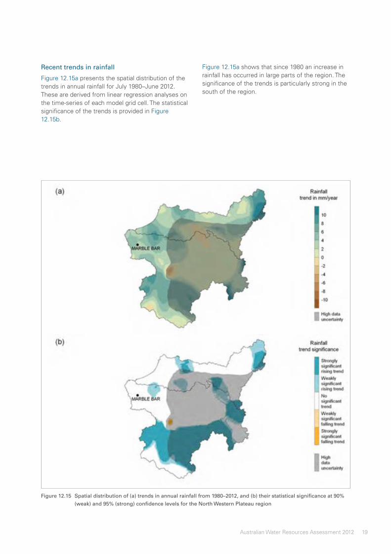
19Australian Water Resources Assessment 2012
Figure 12.15 Spatial distribution of (a) trends in annual rainfall from 1980–2012, and (b) their statistical significance at 90% (weak) and 95% (strong) confidence levels for the North Western Plateau region
Recent trends in rainfall
Figure12.15apresentsthespatialdistributionofthetrendsinannualrainfallforJuly1980–June2012.Thesearederivedfromlinearregressionanalysesonthetime-seriesofeachmodelgridcell.ThestatisticalsignificanceofthetrendsisprovidedinFigure12.15b.
Figure12.15ashowsthatsince1980anincreaseinrainfallhasoccurredinlargepartsoftheregion.Thesignificanceofthetrendsisparticularlystronginthesouthoftheregion.

North Western Plateau
20 Australian Water Resources Assessment 2012
12.4.2Evapotranspiration
ModelledannualevapotranspirationfortheNorthWesternPlateauregionfor2011–12isestimatedtobe291mm.Thisis61%abovetheregion’slong-term(July1911–June2012)averageof181mm.Thespatialdistributionandmagnitudeofannualofevapotranspirationin2011–12(Figure12.16a)issimilartothatofrainfall(Figure12.13a).
Evapotranspirationdecilesfor2011–12indicateaboveaverageorverymuchaboveaveragetotalsacrossmostoftheregion(Figure12.16b).ItalsoresemblestherainfallpatternsofFigure12.13bratherclosely,whichindicatesthatwateravailability,throughrainfall,limitstheamountofevapotranspirationoccurring.
Figure 12.16 Spatial distribution of (a) modelled annual evapotranspiration in 2011–12, and (b) their decile rankings over the 1911–2012 period for the North Western Plateau region

21Australian Water Resources Assessment 2012
Figure 12.17 Time-series of (a) annual evapotranspiration, and (b) five-year retrospective moving averages for the summer (November–April) and winter (May–October) periods for the North Western Plateau region
Evapotranspiration variability in the recent past
Figure12.17ashowsannualevapotranspirationfortheregionfromJuly1980onwards.Overthis32-yearperiodtheannualevapotranspirationaveragewas242mm,varyingfrom140mm(1985–86)to411mm(1999–2000).Temporalvariabilityandseasonalpatterns(overthesummerandwinterperiods)since1980arepresentedinFigure12.17b.
Summerperiodsshowconsistentlyhigherevapotranspirationthanthewinterperiod.Thehighertemperaturesandthehigherrainfallamountsduringtheseperiodsarethemaincontributingfactors.Comparedwithseasonalrainfall(Figure12.14b),evapotranspirationexceedstheinputofrainduringthewinterperiod.Thisisduetothehigheravailabilityofsoilmoistureaftertherelativelywetsummerperiod.

North Western Plateau
22 Australian Water Resources Assessment 2012
Recent trends in evapotranspiration
Figure12.18apresentsthespatialdistributionofthetrendsinmodelledannualevapotranspirationfor1980–2012.Thesearederivedfromlinearregressionanalysesonthetime-seriesofeachmodelgridcell.ThestatisticalsignificanceofthetrendsisprovidedinFigure12.18b.
Figure12.18ashowsthatsince1980,trendsaremostlypositivethroughouttheregion.Similarareasofstatisticalsignificance(Figure12.18b)areidentifiedascomparedtotherainfalltrendsignificanceinFigure12.15b,thoughtheareasofstatisticallysignificantevapotranspirationincreasearesomewhatlarger.
Figure 12.18 Spatial distribution of (a) trends in annual evapotranspiration from 1980–2012, and (b) their statistical significance at 90% (weak) and 95% (strong) confidence levels for the North Western Plateau region

23Australian Water Resources Assessment 2012
12.4.3Landscapewateryield
ModelledlandscapewateryieldfortheNorthWesternPlateauregionfor2011–12isestimatedtobe26mm.Thisis136%abovetheregion’slong-term(July1911–June2012)averageof11mm.Figure12.19ashowsthespatialdistributionoflandscapewateryieldfor2011–12,whichissimilartotheannualrainfalldistribution(Figure12.13a,notethedifferenceinthescaleofthelegend).
Thedecile-rankingmapfor2011–12(Figure12.19b)showsaboveaveragetoverymuchaboveaveragelandscapewateryields,similartowhatcanbeseenintherainfallpatternsofFigure12.13b.Verymuchaboveaveragewateryieldsarefoundacrossmuchofthedata-sparsesoutheast,buttheseresultsshouldbeusedwithcautionastheyaremodelresultsgeneratedwithhighlyuncertainrainfalldata.
Figure 12.19 Spatial distribution of (a) modelled annual landscape water yield in 2011–12, and (b) their decile rankings over the 1911–2012 period for the North Western Plateau region

North Western Plateau
24 Australian Water Resources Assessment 2012
Figure 12.20 Time-series of (a) annual landscape water yield, and (b) five-year retrospective moving averages for the summer (November–April) and winter (May–October) periods for the North Western Plateau region
Landscape water yield variability in the recent past
Figure12.20ashowsannuallandscapewateryieldfortheNorthWesternPlateauregionfromJuly1980onwards.Overthis32-yearperiod,annuallandscapewateryieldwas21mm,varyingfrom4mm(1989–90)to64mm(1999–2000).Temporalvariabilityandseasonalpatterns(overthesummerandwinterperiods)since1980arepresentedinFigure12.20b.
Landscapewateryieldisconsistentlyhigherduringthesummerperiodcomparedtothewinterperiod.Rainfallobviouslyisthemajorforcebehindlandscapewateryieldandthetemporalvariabilitycloselyresemblesthevariabilityinrainfall.Again,thecoefficientofvariation(standarddeviationdividedbythemean)oftheannualdataishighcomparedtomostotherregions.

25Australian Water Resources Assessment 2012
Recent trends in landscape water yield
Figure12.21ashowsthespatialdistributionofthetrendsinmodelledannuallandscapewateryieldfor1980–2012.Thesearederivedfromlinearregressionanalysesonthetime-seriesofeachmodelgridcell.ThestatisticalsignificanceofthetrendsisprovidedinFigure12.21b.
Figure12.21ashowsthatthereisnoobvioustrendinmostoftheregionwiththeexceptionofthefarnortheastwherelandscapewateryieldincreasestowardstheeasternborderoftheregion.Figure12.21bconfirmsthesignificanceofthesetrendsandshowssomestrongsignalsmainlyinthesouthwestoftheregion;however,trendshereonlyjustreach1mm/year.
Figure 12.21 Spatial distribution of (a) trends in annual landscape water yield from 1980– 2012, and (b) their statistical significance at 90% (weak) and 95% (strong) confidence levels for the North Western Plateau region

North Western Plateau
26 Australian Water Resources Assessment 2012
Birdlife on the Eighty Mile Beach, Western Australia | Gayle Partridge
12.5 Surfacewater andgroundwater
ThissectionexaminessurfacewaterandgroundwaterresourcesintheNorthWesternPlateauregionin2011–12.Riversandwetlandsarediscussedtoillustratethestateoftheregion’ssurfacewaterresources.Theregion’swatertableaquifersandsalinityaredescribed.NodatawasavailableattheBureauinasuitableformatforadetailedanalysisonindividualaquifers.
Therearenomajorstorageslocatedintheregion.
12.5.1Rivers
TherearetworiverbasinsintheNorthWesternPlateauregion.TheDeGreyRiverbasincoversanareaof477,000km2andtheSandyDesertbasinis239,000km2insize.
Theregionhassomelimitedsurfacewaterresourcespresentinthewesternpartoftheregion(Figure12.22).Thecoastlineconsistsoftide-dominatedstrandplainsandtidalcreeks.Somedrylakesarescatteredovertheregion,butaeolianlandformsincludingdunesandsandplainsdominatethelandscape.
Almostallriversareephemeral,endingupindesertcountryorsaltlakes,exceptfortheDeGreyRiverbasin.Allstreamsflowonlyafterheavyrains,whichoccurinfrequently.
12.5.2Flooding
HeavyrainfallinJanuaryassociatedwithanactivemonsoonbroughttropicalcyclonesHeidiandIggytotheregion.ThesetropicalcyclonescausedmoderatetomajorfloodingparticularlyintheShawandCoonganrivers.MajorfloodsaffectedtheNallagineandDeGreyriversinMarchwiththepassageoftropicalcycloneLua(Figure12.23).
12.5.3Wetlands
ThereisoneRamsar-listed,internationallyimportantwetlandintheNorthWesternPlateauregionandthereareanumberofwetlandsofnationalimportanceintheregionmentionedintheAustralian Directory of Important Wetlands (www.environment.gov.au/water/topics/wetlands/database/diwa.html).Thewetlandsvaryfromcoastalfloodplains,lakesandtidalflatstoinlandephemerallakesandriverfloodplainsystems(Figure12.24).
TheEightyMileBeachRamsarsitemainlyconsistsoftidalflats,whichsometimesextendupto5kminwidth.Itisahighlyimportantretreatformanyspeciesof(migrating)shorebirds.
Nodetailedassessmentontheinflowsofselectedwetlandshasbeenperformedforthisregion.

27Australian Water Resources Assessment 2012
Figure 12.22 Rivers and catchments in the North Western Plateau region

North Western Plateau
28 Australian Water Resources Assessment 2012
Figure 12.23 Flood occurrence in 2011–12 for the North Western Plateau region

29Australian Water Resources Assessment 2012
Figure 12.24 Location of important wetlands in the North Western Plateau region

North Western Plateau
30 Australian Water Resources Assessment 2012
12.5.4Hydrogeology
Thehydrogeologyisdominatedbyalargeareaofoutcroppingfracturedbasementrockinthewestandeastoftheregion.Theassociatedgroundwatersystemstypicallyofferrestrictedlowvolumewaterresources.OtherimportanthydrogeologicalgroupsaretheMesozoicsedimentsthroughthecentreoftheregionandthesurficialsedimentsin-fillingpalaeovalleys.Thesegroupsarelikelytooffermorereliablegroundwaterresources(Figure12.25).
ThewatertableaquiferspresentintheregionaregiveninFigure12.25below.Groundwatersystemsthatprovidemorepotentialforextractionarelabelledas:
• Mesozoicsedimentaquifer(porousmedia—consolidated);and
• surficialsedimentaquifer(porousmedia—unconsolidated).
12.5.5Watertablesalinity
Figure12.26showstheclassificationofwatertableaquifersasfresh(totaldissolvedsolids(TDS)<3,000mg/L)orsaline(TDS≥3,000mg/L)accordingtowatertablesalinity.Asshown,mostpartsoftheregionareconsideredtohavefreshgoundwater.Salinegroundwateroccursinlocalisedareasalongthemajordrainagelinesinthealluvialsediments.
12.5.6Groundwatermanagementunits
Thegroundwatermanagementunitswithintheregionarekeyfeaturesthatcontroltheextractionofgroundwaterthroughplanningmechanisms.Figure12.27showsthatthegroundwatermanagementunitswithintheregionincludeCanning–Kimberley,EastMurchison,GoldfieldsandPilbara.

31Australian Water Resources Assessment 2012
Figure 12.25 Watertable aquifers of the North Western Plateau region; data extracted from the Groundwater Cartography of the Australian Hydrological Geospatial Fabric (Bureau of Meteorology 2012)

North Western Plateau
32 Australian Water Resources Assessment 2012
Figure 12.26 Watertable salinity classes of the North Western Plateau region; data extracted from the Groundwater Cartography of the Australian Hydrological Geospatial Fabric (Bureau of Meteorology 2012)

33Australian Water Resources Assessment 2012
Figure 12.27 Groundwater management units in the North Western Plateau region; data extracted from the National Groundwater Information System (Bureau of Meteorology 2013)

Tanami – Timor Sea Coast13 Tanami – Timor Sea Coast ........................................ 2
13.1 Introduction ........................................................ 2
13.2 Key information .................................................. 3
13.3 Description of the region ................................... 4
13.3.1 Physiographic characteristics .................. 6
13.3.2 Elevation ................................................. 7
13.3.3 Slopes .................................................... 8
13.3.4 Soil types ............................................... 9
13.3.5 Land use ............................................. 11
13.3.6 Population distribution .......................... 13
13.3.7 Rainfall zone ......................................... 14
13.3.8 Rainfall deficit ....................................... 15
13.4 Landscape water flows ................................... 16
13.4.1 Rainfall .................................................. 17
13.4.2 Evapotranspiration ............................... 20
13.4.3 Landscape water yield ......................... 23
13.5 Surface water and groundwater ....................... 26
13.5.1 Rivers ................................................... 26
13.5.2 Streamflow volumes ............................. 28
13.5.3 Flooding ............................................... 28
13.5.4 Storage systems ................................... 31
13.5.5 Wetlands ............................................. 31
13.5.6 Hydrogeology ....................................... 34
13.5.7 Watertable salinity ................................. 34
13.5.8 Groundwater management units ........... 34
13.6 Water for cities and towns ................................ 38
13.6.1 Urban centres ....................................... 38
13.6.2 Sources of water supply ....................... 38
13.6.3 Darwin–Palmerston ............................... 38
13.7 Water for agriculture ......................................... 43
13.7.1 Soil moisture ........................................ 43
13.7.1 Irrigation areas ...................................... 44
13.7.2 Ord River Irrigation Area ....................... 44

Tanami – Timor Sea Coast
2 Australian Water Resources Assessment 2012
13 Tanami – Timor Sea Coast13.1 Introduction
ThischapterexamineswaterresourcesintheTanami–TimorSeaCoastregionin2011–12andoverrecentdecades.Itstartswithsummaryinformationonthestatusofwaterflows,storesanduse.Thisisfollowedbydescriptiveinformationfortheregionincludingthephysiographiccharacteristics,soiltypes,population,landuseandclimate.
Spatialandtemporalpatternsinlandscapewaterflowsarepresentedaswellasanexaminationofthesurfaceandgroundwaterresources.Thechapterconcludeswithareviewofthewatersituationforurbancentresandirrigationareas.ThedatasourcesandmethodsusedindevelopingthediagramsandmapsarelistedintheTechnicalSupplement.

3Australian Water Resources Assessment 2012
13.2 Keyinformation
Table13.1givesanoverviewofthekeycomponentsofthedataandinformationinthischapter.
Table 13.1 Key information on water flows, stores and use in the Tanami – Timor Sea Coast region
Landscape water flows
Evapo-transpiration
Landscapewater yield
Rainfall
Regionaverage Differencefrom1911–2012long-termannualmean
Decilerankingwithrespecttothe1911–2012record
754mm +35% 9th—aboveaverage
646mm +40% 10th—verymuchaboveaverage
142mm +53% 9th—aboveaverage
Streamflow (at selected gauges)
Annualtotalflow:
Predominantlyaveragetoaboveaverageflowinriverbasinsinthecentralnorth
Flooding: Localisedminortomoderatefloodinginthenorthernhalfoftheregion
Surface water storage (comprising about 96% of the region’s total capacity of all major storages)
Totalaccessiblecapacity
30June2012 30June2011 Change
accessiblevolume
%oftotalcapacity
accessiblevolume
%oftotalcapacity
accessiblevolume
%oftotalcapacity
10,733GL 10,549GL 98% 10,710GL 100% -161GL -2%
Groundwater (in selected aquifers)
Salinity: Non-salinegroundwater(<3000mg/L)throughouttheregion
Urban water use (Darwin)
Totalsourcedin2011–12 Totalsourcedin2010–11
Change Restrictions
35.5GL 32.3GL +3.2GL(+10%) Norestrictions
Annual mean soil moisture (model estimates)
Spatialpatterns: Predominantlyaboveaveragetoverymuchaboveaverageannualmeansoilmoisture
Temporalpatternsinregionalaverage:
Verymuchaboveaveragesoilmoisturethroughoutmostoftheyear,aboveaverageinthewetseason

Tanami – Timor Sea Coast
4 Australian Water Resources Assessment 2012
Kata Tjuta (the Olgas) | stefaniaandreetto (iStockphoto)
13.3 Descriptionoftheregion
TheTanami–TimorSeaCoastregionextendsoveralargeareaofnorthernAustraliacoveringmuchoftheNorthernTerritoryandthenorthofWesternAustralia.Theregionisapproximately1,162,000km²andincludestheOrd,Darwin,Daly,VictoriaandFitzroyriverbasins(Figure13.1).
TheregionisdominatedbytwomajordrainagesystemswithadensenetworkofnorthernriversthatdraintotheTimorSea,anddrierriversgenerallydrainingsouthtoinlandephemerallakesystems.Subsections13.3.1–13.3.4providemoreinformationonthetopographyandsoiltypes.
Withapopulationof201,500theregionishometo0.9%ofthenation’stotalpopulation(AustralianBureauofStatistics[ABS]2011b).
MajorpopulationcentresintheregionareshowninFigure13.1andincludeDarwin,Palmerston,Broome,KatherineandKununurra.Furtherdiscussionoftheregion’spopulationdistributionandurbancentrescanbefoundinsubsection13.3.6andsection13.6respectively.
Landuseintheregionmainlyconsistsofpastureandnatureconservationreserves(seesubsection13.3.5).Someofthemostwell-knownnaturallandscapefeaturesandconservationreservesinAustraliaarelocatedinthisregion,includingtheKimberley,KakaduNationalParkandUluru–KataTjutaNationalPark.
TheOrdIrrigationScheme,locatedintheOrdRivercatchmentinthefarnortheasternpartofWesternAustralia,isthelargestareaofirrigatedagricultureintheregion.Subsection13.3.5providesmoreinformationontheregion'sagriculturalactivities.
Theregionextendsacrossdistinctclimaticzonesandischaracterisedbyahumidtropicalclimatetothenorthandaverydryaridclimatetothesouth.Subsections13.3.7and13.3.8providemoreinformationontherainfallpatternsanddeficitsacrosstheregion.
Riverflowsinthetropicalnorthernclimatezoneexperiencedistinctseasonalpatterns,withapproximately90%oftheaverageannualflowoccurringinthewetseasonfromNovember–April.
ThehydrogeologyoftheregionisdominatedbytheKimberleyhardrockplateauandCanningbasinsedimentaryrocks.Inthehardrockplateau,groundwateroccursinlowbutvaluablequantitiesinfracturedrocksandsurficialriveralluvium.Substantialquantitiesofconfinedandunconfinedgroundwaterofvaryingqualityoccurinthesedimentarybasins.TheextensivegroundwaterresourcesassociatedwiththewidespreadfracturedandcavernouslimestoneoftheDalybasinareimportantfortheregion.Shallowgroundwaterisoftenofgood,lowsalinityquality,reflectingtheannualfill-and-spillcycle,andcanprovidegoodsuppliesofpotablewater.Amoredetaileddescriptionoftheriversandgroundwaterstatusintheregionisgiveninsection13.5.

5Australian Water Resources Assessment 2012
Figure 13.1 Major rivers and urban centres in the Tanami – Timor Sea Coast region

Tanami – Timor Sea Coast
6 Australian Water Resources Assessment 2012
Figure 13.2 Physiographic provinces of the Tanami – Timor Sea Coast region
13.3.1Physiographiccharacteristics
ThephysiographicmapinFigure13.2showsareaswithsimilarlandformevolutionaryhistories(Painetal.2011).Thesecanberelatedbacktosimilargeologyandclimaticimpactswhichdefinetheextentoferosionprocesses.Theareashavedistinctphysicalcharacteristicsthatinfluencehydrologicalprocesses.TheTanami–TimorSeaCoastregionhasfoursuchdominantphysiographicprovinces,namely:
• Barkly–TanamiPlains(38%):blackclay,sandandlimestoneplainsandsandstonerisesandplateaus,somewithferruginousmantlesandoccasionalgraniticandsedimentaryhills;
• NorthAustralianPlateaus(23%):dissectedbasaltic,quartziteandsandstoneplateaus(somewithlaterite-capping),roundedridgesoffoldedmetamorphicrocks,lowlandsoflimestoneandweaksedimentaryrocksincludingalluvialplains;
• Kimberley(21%):granitic,volcanicandsedimentaryranges,plateausandhillswithsomepartiallylaterisedtablelandandundulatingplains;and
• CentralAustralianRanges(13%):rangesandhillsofigneousrock,sandstoneandquartziteamongstsand,stoneandhardpanplainswithsomedunefieldsandsaltlakes.
Theremainingtwoprovincesoccupyonly5%oftheregion.Theseare:
• Sandland(4.7%):east-westlongitudinaldunesandminorsaltlakeswithsomenarrowsandstoneranges;and
• CarpentariaFall(0.3%):dissectedcoastalfall,tabularridgesgivingwayseawardstoslopingplainsandlowhills.

7Australian Water Resources Assessment 2012
Figure 13.3 Ground surface elevations in the Tanami – Timor Sea Coast region
13.3.2Elevation
Figure13.3presentsgroundsurfaceelevationsintheTanami–Timorregion.InformationwasobtainedfromtheGeoscienceAustraliawebsite(www.ga.gov.au/topographic-mapping/digital-elevation-data.html).ThetopographyoftheregionhasgeneratedtwomajordrainagesystemswiththefloodplainsofnorthernriversdrainingtotheTimorSeaandthearidzoneriversoftheTanamiDesertdrainingsouth,terminatinginephemerallakes(Figure13.3).
InthewestoftheregionmostriversoriginatefromtheKimberleyPlateau,whichhaspeaksexceeding
600mabovesealevel.Theriverstothewestandeastoftheplateaupassthroughextensivefloodplains,drainingtothesea.
Theriversinthenortheastoftheregionhavetheirheadwatersinthemanymountainrangesandplateausofthisarea,includingtheArnhemLandescarpment.Peaksinthesemountainousareasoccasionallyreach300mabovesealevel.
MoremountainousrangesarepresentintheTanamiDesertandthefarsouthoftheregionincludingtheMacDonnellRangesjustwestofAliceSprings.Somepeaksintheareaexceed1,000mabovesealevel.

Tanami – Timor Sea Coast
8 Australian Water Resources Assessment 2012
Figure 13.4 Surface slopes in the Tanami – Timor Sea Coast region
13.3.3Slopes
Areaswithsteepslopesprovidehigherrun-offgeneratingpotentialthanflatareas.TheTanami–TimorSeaCoastregionhasveryfewareaswithsteepslopes(seeTable13.2)andtheinlandareaisparticularlyflat(Figure134).Theslopeswerederivedfromtheelevationinformationusedintheprevioussection.
Table 13 2. Proportions of slope classes for the region
Slopeclass(%) 0–0.5 0.5–1 1–5 >5
Proportionofregion(%) 48.1 18.4 26.1 7.4
TherangessurroundingtheKimberleyPlateauinthenorthwesthavethesteepestslopesinthispartoftheregion.SomequitesteepslopescanalsobefoundontheescarpmentoftheArnhemLandPlateau.
Duetothelowtopographyofthearidinlandpartsoftheregion,riversneedtoreceivelargequantitiesofwaterbeforestartingtoflow.Whenthearidzoneriversdoflowinlargevolumes,theyterminateinandoccasionallyfilltheephemerallakesinthearea.
TheFitzroyRivercrossestheplainstothesouthwestoftheKimberleyPlateau.InthispartoftheregiontheFitzroyRiverhasacomplexaridfloodplainsystemofmeanderingflowpathswithanaveragewidthofaround10km.

9Australian Water Resources Assessment 2012
Figure 13.5 Soil types in the Tanami – Timor Sea Coast region
13.3.4Soiltypes
Soilsplayanimportantroleinthehydrologicalcyclebydistributingwaterthatreachestheground.Watercanbetransportedtoriversandlakesviathesoilsurfaceasrun-offorenterthesoilandprovidewaterforplantgrowthaswellascontributingtogroundwaterrecharge.
Thenatureofthesehydrologicalpathwaysandthesuitabilityofthesoilsforagriculturalpurposesareinfluencedbysoiltypesandtheircharacteristics.SoiltypeinformationwasobtainedfromtheAustralianSoilResourceInformationSystemwebsite(www.asris.csiro.au).
About90%ofthetotalTanami–TimorSeaCoastregionconsistsoffoursoiltypes,namelytenosols,rudosols,kandosolsandvertosols(Figure13.5andFigure13.6).Thesesoilsareusuallywidelydistributedacrosstheregionandaremostlyusedforgrazingandnatureconservation.
Tenosolsandrudosolsarecharacterisedbyhavingaweakandminimaldevelopment.Theyshownoorlittlechangeintextureandcolourandareoftenshallowindepth.Theyalsohavelowchemicalfertilityandhavealowwater-holdingcapacity,thus
theiragriculturalpotentialislow.Bothsoiltypesaremostlypresentinareasusedfornatureconservationratherthanforagriculture.
Kandosolsarestructurelesssoilswhichareoftenverydeep,thatis,upto3mormore.Theydonothaveastronglycontrastingtextureandtheydonotcontaincarbonatethroughouttheirprofile.Theyarelowinchemicalfertilityandarewell-drainedwithonlymoderatewaterholdingcapacitycomparedwithothersoiltypes;thustheyonlyhavelowtomoderateagriculturalpotential
VertosolsaremostlydistributedbetweenthenorthwestandnortheastoftheTanami–TimorSeaCoastregion.Vertosolsareclay-richsoilswhichtendtocrackwhendryandswellduringwetting.Theyarehighlyfertileandhavealargewater-holdingcapacity;howevertheymustholdasignificantamountofwaterbeforeitbecomesavailabletoplants.Inthisregiontheyaremostlyusedforgrazing.
TheothersoiltypesthathaveminimalrepresentationintheTanami–TimorSeaCoastregionarehydrosols,ferrosols,sodosols,chromosols,calcarosolsanddermosols(0.8–3%ofthetotalarea).

Tanami – Timor Sea Coast
10 Australian Water Resources Assessment 2012
Figure 13.6 Soil type distribution in the Tanami – Timor Sea Coast region

11Australian Water Resources Assessment 2012
Figure 13.7 Land use in the Tanami – Timor Sea Coast region
13.3.5Landuse
Landuseintheregionconsistsmainly(morethan95%)ofpastureandnaturalconservation(datafromdata.daff.gov.au/anrdl/metadata_files/pa_luav4g9abl07811a00.xml).SomeofthemostfamousnaturalattractionsinAustraliaarelocated
inthisregionincludingtheKimberleyandKakaduNationalPark.Irrigatedagriculturemakesuplessthan1%ofthelanduseintheregion,muchofwhichisconcentratedintheOrdRiverbasin(Figure13.7andFigure13.8).ThemainindustrieswithintheOrdRiverbasinareagriculture,horticulture,tourismandmining.
Ord River valley | Simon Krzic (Dreamstime)

Tanami – Timor Sea Coast
12 Australian Water Resources Assessment 2012
Figure 13.8 Land use distribution in the Tanami – Timor Sea Coast region

13Australian Water Resources Assessment 2012
Figure 13.9 Population density and distribution in the Tanami – Timor Sea Coast region
13.3.6Populationdistribution
TheTanami–TimorSeaCoastregionisoneofthemostsparselypopulatedinAustralia.Thisisdespitesomepopulatedcentresonitscoastline(Figure13.9),andanumberofsmallerirrigationandminingcentres(ABS2011b).
Darwin,locatedinthefarnorth,isthelargestcityintheregion,followedbyBroome,whichissituatedonitscoastalwesterntip.
Outsideofthemajorregionalurbancentres,miningleases,Indigenouscommunitiesandanumberofsmalltownsandsettlementslocatedadjacenttomajorroadsintheregion(includingtheStuart,KakaduandArnhemhighways)accountformuchoftheremainingpopulation.

Tanami – Timor Sea Coast
14 Australian Water Resources Assessment 2012
Figure 13.10 Rainfall zones in the Tanami – Timor Sea Coast region
13.3.7Rainfallzone
Theregionextendsacrossdistinctclimaticzonesandisdominatedbyahumidtropicalclimatetothenorthandaverydryaridclimatetothesouth.Medianrainfallisvariablethroughouttheregion(Figure13.10).
Rainfallinthenorthoftheregionissummerdominant.Monsoonalrainandtropicalcyclonesanddepressionscontributetoaverageannualrainfalltotalsexceeding1,500mminthefarnorthoftheregion.Movinginlandfromthecoast,averageannualrainfalltotalsgraduallyreduce.
Inthesouth,theregionincludesalargecomponentoftheAustraliandryinlandareawhereaverageannualrainfalldoesnotexceed400mm.
Formoreinformationonthisandotherclimateclassifications,visittheBureauofMeteorology's(theBureau's)climatewebsite:www.bom.gov.au/jsp/ncc/climate_averages/climate-classifications/index.jsp

15Australian Water Resources Assessment 2012
Figure 13.11 Rainfall deficit distribution for the Tanami – Timor Sea Coast region
13.3.8Rainfalldeficit
Therainfalldeficitindicator,thatis,rainfallminuspotentialevapotranspiration,givesageneralimpressionaboutwhichpartsoftheregionarelikelytoexperiencemoisturedeficitsovertheperiodofayear.TheTanami–TimorSeaCoastregionhasaratheruniformpatternofhighpotentialdeficitsoverthewholeregion(Figure13.11).
Duetotheseasonalityofrainfallinthenorth,withhumidwetsummersanddry,warmwinters,thereisaclearpatternofmoisturedeficitsinthedrywinterseasonandmoisturerechargeinthewetsummer
season;however,onanannualaveragebasis,thepotentialevapotranspirationexceedsrainfall.
Inthesouthernaridpartoftheregion,rainfalldeficitsarehighand,asaconsequence,vegetationdensityislow.Mostofthesouthernpartoftheregioniscoveredbypasture,sparselyusedforstockfarmingandnatureconservation.
Formoreinformationontherainfallandevapotranspirationdata,seetheBureau’smapsofaverageconditions:www.bom.gov.au/climate/averages/maps.shtml

Tanami – Timor Sea Coast
16 Australian Water Resources Assessment 2012
Figure 13.12 Landscape water flows in 2011–12 compared with the long-term record (July 1911–June 2012) for the Tanami – Timor Sea Coast region
13.4 Landscapewaterflows
Thissectionpresentsanalysesofthespatialandtemporalvariationoflandscapewaterflows(rainfall,evapotranspirationandlandscapewateryield)acrosstheTanami–TimorSeaCoastregionin2011–12.Nationalrainfallgridsweregeneratedusingdatafromanetworkofpersistent,high-qualityrainfallstationsmanagedbytheBureau.EvapotranspirationandlandscapewateryieldswerederivedusingthelandscapewaterbalancecomponentoftheAustralianWaterResourcesAssessmentSystem(VanDijk2010).ThesemethodsandassociatedoutputuncertaintiesarediscussedintheIntroductionandaddressedinmoredetailintheTechnicalSupplement.
Figure13.12showsthattheregionhasahighlyseasonalrainfallpatternwithawetsummerperiod(November–April)andadrywinterperiod(May–October).Evapotranspirationinthedryseasongenerallyexceedsrainfall.Afterthewetseasonthesoilsnormallycontainalotofmoisturethatisavailableforevapotranspiration.
Themonthlylandscapewateryieldhistoryfortheregionshowsastablepatternofverylowyieldinthedryseason.ItgraduallyincreasesduringDecemberthroughtoFebruaryandsubsidesinMarchandApril.
The2011–12yearwasarelativelywetyear,withthewetseasonstartingparticularlyearly.Anactivemonsoonintheregion'snorthcontributedtoparticularlyhighrainfalltotalsforthemonthofMarch.
WithwetsoilconditionspresentinJuly2011andaboveaverageraininOctoberandNovember,evapotranspirationwasaboveaverageforthefirstsixmonthsof2011–12.AftertheMarchrainfall,evapotranspirationagainremainedabovethe75thpercentileuntilJune2012.
Thelandscapewateryieldfor2011–12closelyfollowedthemonthlyrainfallpattern.LandscapewateryieldinMarchwasthefourthhighestonrecord(1911–2012),followingtheseventhhighest,asaconsequenceoftheseventhhighestrainfallonrecordforthatmonth.

17Australian Water Resources Assessment 2012
Figure 13.13 Spatial distribution of (a) annual rainfall in 2011–12, and (b) their decile rankings over the 1911–2012 period for the Tanami – Timor Sea Coast region
13.4.1Rainfall
RainfallfortheTanami–TimorSeaCoastregionfor2011–12isestimatedtobe754mm.Thisis35%abovetheregion’slong-termaverage(July1911–June2012)of559mm.Figure13.13ashowsthatthehighestrainfalloccurredinthetropicalnorthwithannualtotalsexceeding1,200mminmanyareasfor2011–12.TheTanamidistrictinthesouthhadrainfallnotexceeding600mm.
Thehighdatauncertaintyareasinthemapindicatethoseareaswhereraingaugedensityistoolowtoaccuratelycapturelocalisedrainfall,oftenintheformoflocalisedthunderstorms.
Rainfalldecilesfor2011–12indicateaveragetoaboveaveragerainfallfortheentireregionoverthecourseoftheyear(Figure13.13b).Scatteredthroughouttheregionareareaswithverymuchaboveaveragerainfall.

Tanami – Timor Sea Coast
18 Australian Water Resources Assessment 2012
Figure 13.14 Time-series of (a) annual rainfall, and (b) five-year retrospective moving averages for the wet summer (November–April) and dry winter (May–October) periods for the Tanami – Timor Sea Coast region
Rainfall variability in the recent past
Figure13.14ashowsannualrainfallfortheregionfromJuly1980onwards.Overthis32-yearperiodtheannualaveragewas679mm,varyingfrom362mm(1991–92)to1,236mm(2010–11).Temporalvariabilityandseasonalpatternssince1980arepresentedinFigure13.14b.
Thegraphsindicatethepresenceofarisingtrendinaveragerainfallovertheregionfrom1990onwards;however,thelastsixyearshadclosetoaveragerainfallintheregionwithonly2010–11havingexceptionallyhighrainfall.

19Australian Water Resources Assessment 2012
Figure 13.15 Spatial distribution of (a) trends in annual rainfall from 1980–2012, and (b) their statistical significance at 90% (weak) and 95% (strong) confidence levels for the Tanami – Timor Sea Coast region
Recent trends in rainfall
Figure13.15apresentsthespatialdistributionofthetrendsinannualrainfallforJuly1980–June2012.Thesearederivedfromlinearregressionanalysesonthetime-seriesofeachmodelgridcell.
ThestatisticalsignificanceofthetrendsisprovidedinFigure13.15b.
Figure13.15ashowsthatsince1980astrongincreaseinrainfallhasoccurredinlargepartsoftheregion,particularlytowardsthenorth.Someareasreachedtrendsofupto20mm/year.Thetrendsarestronglysignificantinmostoftheseareas(Figure13.15b).

Tanami – Timor Sea Coast
20 Australian Water Resources Assessment 2012
13.4.2Evapotranspiration
ModelledannualevapotranspirationfortheTanami–TimorSeaCoastregionfor2011–12isestimatedtobe646mm.Thisis40%abovetheregion’slong-term(July1911–June2012)averageof461mm.Thespatialdistributionofannualevapotranspirationin2011–12(Figure13.16a)issimilartothatofrainfall(Figure13.14a),butwithlowerannualtotalsinthenorthoftheregion.
Evapotranspirationdecilesfor2011–12indicateaboveaverageorverymuchaboveaveragetotalsacrossmostoftheregion(Figure13.16b).Thelargerareasofverymuchaboveaverageevapotranspirationincomparisontorainfallwasmadepossiblebythehighsoilmoisturelevelsatthestartoftheyear,duetorecordhighrainfallthepreviousyear,whichallowedevapotranspirationtobehigherthanaverageinthedrymonthsofJuly–September2011(seeFigure13.12).
Figure 13.16 Spatial distribution of (a) modelled annual evapotranspiration in 2011–12, and (b) their decile rankings over the 1911–2012 period for the Tanami – Timor Sea Coast region

21Australian Water Resources Assessment 2012
Figure 13.17 Time-series of (a) annual evapotranspiration, and (b) five-year retrospective moving averages for the wet summer (November–April) and dry winter (May–October) periods for the Tanami – Timor Sea Coast region
Evapotranspiration variability in the recent past
Figure13.17ashowsannualevapotranspirationfortheregionfromJuly1980onwards.Overthis32-yearperiodtheannualevapotranspirationaveragewas541mm,varyingfrom379mm(1991–92)to807mm(2010–11).Temporalvariabilityandseasonalpatternssince1980arepresentedinFigure13.17b.
Thewetperiod(November–April)showsconsistentlyhigherevapotranspirationthanthedryperiod.Evapotranspirationinthedryperiodissubstantiallyhigherthanrainfallinthisperiod(Figure13.14b),whereasevapotranspirationinthewetperiodissubstantiallylowerthanrainfallinthisperiod.

Tanami – Timor Sea Coast
22 Australian Water Resources Assessment 2012
Recent trends in evapotranspiration
Figure13.18apresentsthespatialdistributionofthetrendsinmodelledannualevapotranspirationfor1980–2012.Thesearederivedfromlinearregressionanalysesonthetime-seriesofeachmodelgridcell.ThestatisticalsignificanceofthetrendsisprovidedinFigure13.18b.
Thetrendsinevapotranspirationarerisingthroughouttheregionwithsomelocalexceptionsalongthenortherncoastline.AsshowninFigure13.18b,thetrendsarestatisticallysignificantinmostpartsoftheregion,particularlyinthoseareaswheretherisingtrendsarehigh.
Figure 13.18 Spatial distribution of (a) trends in annual evapotranspiration from 1980–2012, and (b) their statistical significance at 90% (weak) and 95% (strong) confidence levels for the Tanami – Timor Sea Coast region

23Australian Water Resources Assessment 2012
13.4.3Landscapewateryield
ModelledlandscapewateryieldfortheTanami–TimorSeaCoastregionfor2011–12isestimatedtobe142mm.Thisis53%abovetheregion’slong-term(July1911–June2012)averageof93mm.Figure13.19ashowsthespatialdistributionoflandscapewateryieldfor2011–12,whichissimilartotheannualrainfalldistribution(Figure13.13a).
Thehighestlandscapewateryieldsin2011–12areobservedinsomeareasalongthecoast,locallyexceeding600mm.InthesouthernTanamidistrictlandscapewateryielddidnotexceed50mm.
Thedecile-rankingmapfor2011–12(Figure13.19b)showsaveragetoaboveaveragelandscapewateryields,whichagainshowshighsimilaritywiththerainfalldecilemapofFigure13.13b.
Figure 13.19 Spatial distribution of (a) modelled annual landscape water yield in 2011–12, and (b) their decile rankings over the 1911–2012 period for the Tanami – Timor Sea Coast region

Tanami – Timor Sea Coast
24 Australian Water Resources Assessment 2012
Figure 13.20 Time-series of (a) annual landscape water yield, and (b) five-year retrospective moving averages for the wet summer (November–April) and dry winter (May–October) periods for the Tanami – Timor Sea Coast region
Landscape water yield variability in the recent past
Figure13.20ashowsannuallandscapewateryieldfortheTanami–TimorSeaCoastregionfromJuly1980onwards.Overthis32-yearperiod,annuallandscapewateryieldwas132mm,varyingfrom30mm(1989–90)to377mm(2010–11).Temporalvariabilityandseasonalpatternssince1980arepresentedinFigure13.20b.
Landscapewateryieldin2010–11wasverymuchaboveaverage,butevenwithoutthisexceptionalyearthegeneraltrendinregionalaverageannuallandscapewateryieldshowsarisingtrendsince1990.Thiscanbetotallyallocatedtoincreasedrainfallinthewetperiod.Inthefirsthalfofthereferenceperiod,onlythreeyearsreachedtotalannuallandscapewateryieldsthatwereabovetheperiodsaverage,albeitonlymarginally.

25Australian Water Resources Assessment 2012
Recent trends in landscape water yield
Figure13.21ashowsthespatialdistributionofthetrendsinmodelledannuallandscapewateryieldfor1980–2012.Thesearederivedfromlinearregressionanalysesonthetime-seriesofeachmodelgridcell.ThestatisticalsignificanceofthetrendsisprovidedinFigure13.21b.Figure13.21ashowsstrongrisingtrendsoccurinthenorthoftheregion.Insomeareasthesetrendsexceed16mm/year.
Aswellasthetrendsbeingstatisticallysignificantinthenorth,alargeareaofstronglysignificantrisingtrendsisalsopresentinthecentraleastoftheregion.Withmuchlowerlandscapewateryieldinthispartoftheregion,thesmallriseinannualtotalsisstillstatisticallysignificant.
Figure 13.21 Spatial distribution of (a) trends in annual landscape water yield from 1980–2012, and (b) their statistical significance at 90% (weak) and 95% (strong) confidence levels for the Tanami – Timor Sea Coast region

Tanami – Timor Sea Coast
26 Australian Water Resources Assessment 2012
Katherine Gorge | photosbyash (iStockphoto)
13.5 Surfacewaterand groundwater
ThissectionexaminessurfacewaterandgroundwaterresourcesintheTanami–TimorSeaCoastregionin2011–12.Rivers,wetlandsandstoragesarediscussedtoillustratethestateoftheregion’ssurfacewaterresources.Theregion’swatertableaquifersandsalinityaredescribed.NodatawasavailableattheBureauinasuitableformatforadetailedanalysisonindividualaquifers.
13.5.1Rivers
Thereare25riverbasinsintheTanami–TimorSeaCoastregion,varyinginsizefrom4,800to670,000km2(Figure13.22).
MajorriverbasinsoftheregionaretheOrd,Daly,Fitzroy,VictoriaandFinniss.Thetopographyoftheregiongeneratestwodominantdrainagepatterns.
ThereisacomplexnetworkoffloodplainriversthatflownorthtotheTimorSea.TheinlandVictoriaRiver–Wisocatchment,however,coverstheTanamiDesert,withseveralephemeralriversdrainingsouthwardstotemporarilyfillinlandephemerallakes,dependingonthescaleandintensityofrainfallandrun-off.
Riverflowsinthetropicalnorthernpartsoftheregionexperiencedistinctseasonalpatternswithapproximately90%oftheaverageannualdischargeoccurringinthefour-monthwetseasonfromDecember–March.Oneofthelargestrivers,theOrdRiverwithanapproximatelengthof650km,hasitsheadwatersintheDixonRangenearHill’sCreek.Theflowattheheadwatersisseasonal,buthasbecomeperennialbelowLakeArgyle.Thisisduetoagriculturaldevelopmentsinthisareaandflowmodificationsforirrigationsupply.ThelowersectionoftheOrdRiverisalargetidalestuary.
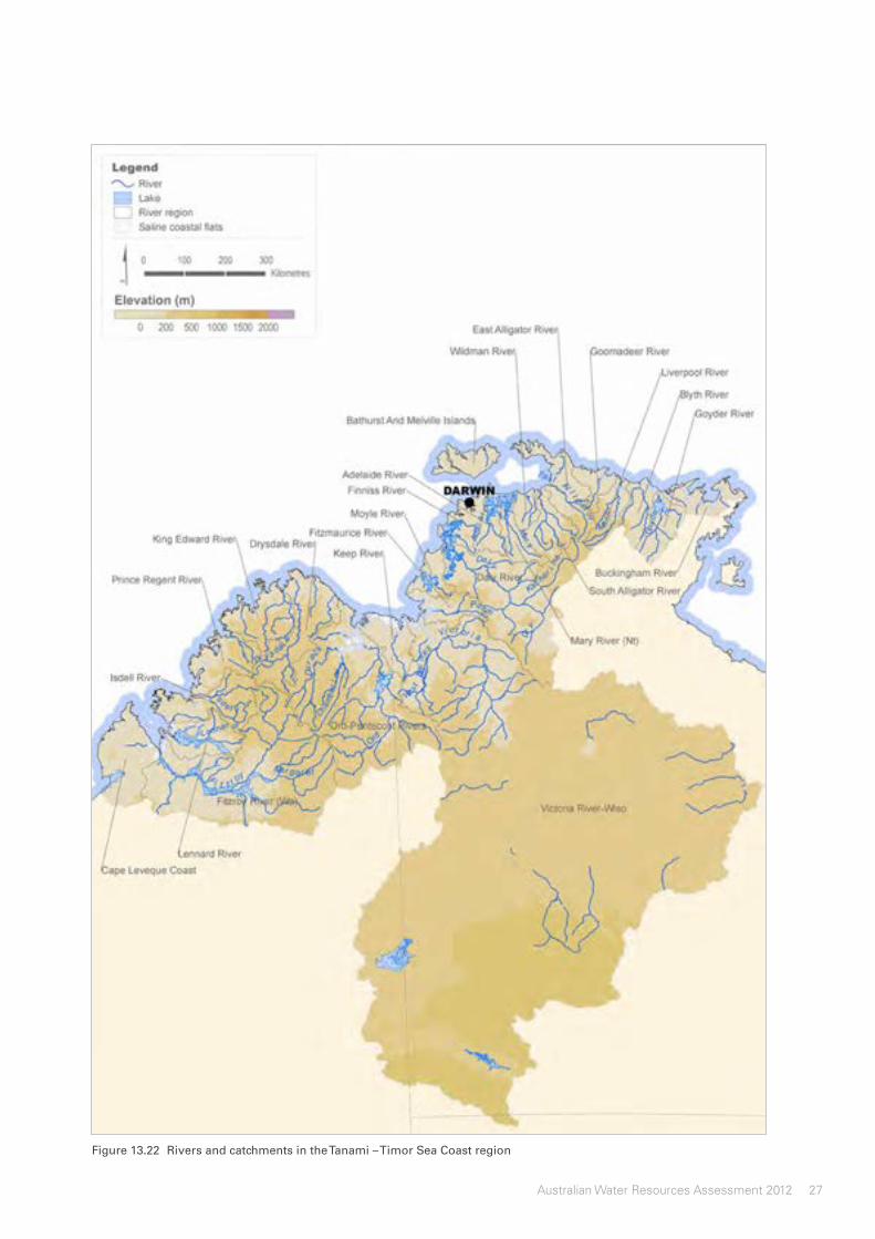
27Australian Water Resources Assessment 2012
Figure 13.22 Rivers and catchments in the Tanami – Timor Sea Coast region

Tanami – Timor Sea Coast
28 Australian Water Resources Assessment 2012
13.5.2Streamflowvolumes
RivermonitoringgaugesarerelativelysparselydistributedintheTanami–TimorSeaCoastregionduetothelowpopulation.Figure13.23presentsananalysisofflowsat13monitoringsitesduring2011–12relativetoannualflowsfortheperiodfromJuly1980–July2012.Monitoringgaugeswithrelativelylongrecordsacrossfivegeographicallyrepresentativeriverswereselected(seeTechnicalSupplementfordetails).Theannualflowsfor2011–12arecolour-codedaccordingtothedecilerankateachsiteoverthe1980–2012period.
TheflowsgenerallyreflectthemostlyaveragetoaboveaveragemodelledlandscapewateryieldresultsshowninFigure13.19b.
VerymuchaboveaverageflowswereobservedatonemonitoringsitelocatedontheDouglasRiverinthecentralnorthoftheTanami–TimorSeaCoastregion.Aboveaveragetotalflowswererecordedatthreemonitoringsites.Theseweremainlylocatedontheriversinthenorthoftheregion.
Averageflowsoccurredateightsitesintheregionwhichwerelocatedontheriversintheregion'scentralnorth.Ofthe13monitoringsites,therewasonlyonebelowaverageflowrecordedacrosstheregionin2011–12.ThisonemonitoringsitewasonRapidCreek,aflashfloodsysteminthefarnorth.
Flowdecilesinthewetseason(November2011–April2012)weresimilartototalannualflowsfor2011–12asshowninFigure13.23.WetseasonhighriverlevelsarethetypicalpatternforflowsinthispartofAustralia,especiallyintheregion'snorth.Therewereafewmonitoringsitesthatdidnotshowthisgeneralpatternofhighwetseasonflows.LowerflowsduringthisperiodwererecordedfortheKatherineandtheDouglasriversinthecentralnorthoftheregion.
Suitablesalinitydatawerenotavailableduringthisperiod.Therefore,streamflowsalinityanalysisisnotincludedinthechapter.
13.5.3Flooding
Figure13.24showsthatsomemoderatefloodingoccurredatthemonitoredrivergaugesites,associatedwithheavyrainfallsinJanuaryandMarch.ThemostsignificantfloodoccurredintheDalyRiversouthofDarwin.
Otherrivershadaminorfloodlevelmeasuredduring2011–12,butmostriversremainedbelowfloodlevels.

29Australian Water Resources Assessment 2012
Figure 13.23 Average annual and wet season (November 2011–April 2012) flow volumes at monitoring sites for 2011–12 and their decile rankings over the 1980–2012 period in the Tanami – Timor Sea Coast region

Tanami – Timor Sea Coast
30 Australian Water Resources Assessment 2012
Figure 13.24 Flood occurrence in 2011–12 for the Tanami – Timor Sea Coast region

31Australian Water Resources Assessment 2012
13.5.4Storagesystems
Therearetenmajor,publiclyowned,storagesintheTanami–TimorSeaCoastregionwithatotalstoragecapacityinexcessof11,200GL.TheBureau'swaterstoragewebsiteincludesinformationonapproximately96%oftheregion'spubliclyownedstorages(asatAugust2012).
ThemajorstoragesintheregionsupplytheOrdirrigationschemeandthecityofDarwin.Table13.3givesasummaryoftheregion'smajorstoragesystemstogetherwithanoverviewofthestoragelevelsattheendof2010–11and2011–12.Storagevolumesreflectthesituationinthemiddleofthedryseason.ThelocationofallthesystemsandassociatedstoragesareshowninFigure13.25.
LakeArgyle,themajorstorageintheOrdirrigationschemewithanaccessiblecapacityof10,400GL,isthesecondlargeststorageofAustralia,afterLakeGordoninTasmania,andistheresultofamajorplantoincreasethegenerallyabundantwaterresourcesinthenorthofthecountry.During2011–12,thestoragevolumesweremuchabovefullsupplylevelandspilling,withtheexceptionofFebruary2012andtheendofJune2012.
TheDarwinRiverstoragealsohasnowatershortageandhencethecityofDarwinhasnowaterconservationrulesinplace.Thestoragewasfilleduptofullsupplylevelduringthewetseason.
FurtherinformationonthepastandpresentvolumesofthestoragesystemsandtheindividualstoragescanbefoundontheBureau’swaterstoragewebsite(http://water.bom.gov.au/waterstorage/awris/).
13.5.5Wetlands
TherearefiveRamsar-listed,internationallyimportantwetlandsintheTanami–TimorSeaCoastregionaswellasanumberofwetlandsofnationalimportancementionedintheAustralian Directory of Important Wetlands(www.environment.gov.au/water/topics/wetlands/database/diwa.html).
Thewetlandsmainlyconsistofriverfloodplainsandestuariesaswellasinlandephemerallakes(Figure13.26).TheartificiallakesArgyleandKununurraarelistedundertheRamsarconvention.
Nodetailedassessmentontheinflowsofselectedwetlandshasbeenperformedforthisregion.
Table 13.3 Storage systems in the region as identified in the Bureau’s water storage information (August 2012), with ‘non-allocated’ accounting for the storages not allocated to a particular system
Systemname Systemtype SystemcapacityAccessiblevolumeat30June2011
Accessiblevolumeat30June2012
Ord rural 10,446GL 10,440GL—100% 10,286GL—98%
Darwin urban 285GL 268GL—94% 262GL—92%
Non-allocated — 1.8GL 1.7GL—94% 1.7GL—94%
Total 10,733GL 10,710GL—100% 10,549GL—98%

Tanami – Timor Sea Coast
32 Australian Water Resources Assessment 2012
Figure 13.25 Storage systems in the Tanami – Timor Sea Coast region (information extracted from the Bureau of Meteorology's water storage website in August 2012)

33Australian Water Resources Assessment 2012
Figure 13.26 Location of important wetlands in the Tanami – Timor Sea Coast region

Tanami – Timor Sea Coast
34 Australian Water Resources Assessment 2012
13.5.6Hydrogeology
ThewatertableaquiferspresentintheregionaregiveninFigure13.27below.ThehydrogeologyoftheregionisdominatedbytheKimberleyhardrockplateauandCanningbasinsedimentaryrocksandbytheextensiveregionalkarsticsysteminthecentral-eastpartoftheregion.Inthehardrockplateau,groundwateroccursinlesserbutvaluablequantitiesinfracturedrocksandsurficialriveralluvium.
Substantialquantitiesofconfinedandunconfinedgroundwaterofvaryingqualityoccurinthesedimentarybasins.TheextensivegroundwaterresourcesassociatedwiththewidespreadfracturedandcavernouslimestoneoftheDalybasinareveryimportantfortheregion.
Groundwatersystemsthatprovidegreatpotentialforextractionarelabelledas:
• FracturedandKarsticrocks,regionalscaleandlocalscaleaquifers;and
• Mesozoicsedimentaquifer(porousmedia—consolidated).
13.5.7Watertablesalinity
Figure13.28showstheclassificationofwatertableaquifersasfresh(totaldissolvedsolids[TDS]<3,000mg/L)orsaline(TDS≥3,000mg/L)wateraccordingtowatertablesalinity.Shallowgroundwatergenerallyhasgoodqualitythroughouttheregion,reflectingtheannualfill-and-spillcycle,andcanbeagoodsourceoflocalsupplyofpotablewater.
Inthenorthernpartoftheregion,watertablesinshallowaquifersresponddramaticallytotheseasonalrains,oftenrisingandfallingseveralmetreseachyear.Manyshallowaquifersfilltocapacityanddrainslowlytotheriversandthecoastduringthedryseason.
TheextensiveregionalaquifersoftheTindalllimestoneandOolloodolostone(intheDalyRiverbasin)areoftentheprimarysourcesofwaterthatkeeplocalstreamsflowingyear-round(CSIRO2009).
Theareaswithhighsalinityvaluesarerelativelysmall.
13.5.8Groundwatermanagementunits
Thegroundwatermanagementunitswithintheregionarekeyfeaturesthatcontroltheextractionofgroundwaterthroughplanningmechanisms.Figure13.29showsthatmostofthemajorgroundwatermanagementunitswithintheNorthernTerritoryarelocatedwithinthefracturedandkarsticrocksaquifers.InWesternAustraliathemajorgroundwatermanagementunitistheCanning–Kimberley.
MostofthepopulationintheregionisconcentratedinDarwin,Broome,KatherineandKununurra.Increasinglysurfacewater,amajorsourceofwaterforDarwinandKatherine,issupplementedbygroundwaterwhilesmallercommunitiesusuallyrelymostlyongroundwater.Inruralareas,domesticproductionboresarethemainsourcesofwater.Thepastoralindustryacrosstheregionalsousesgroundwater.IrrigatedagricultureoccurspredominantlyalongtheOrdRiverand,atasmallerscale,nearDarwinandKatherine.
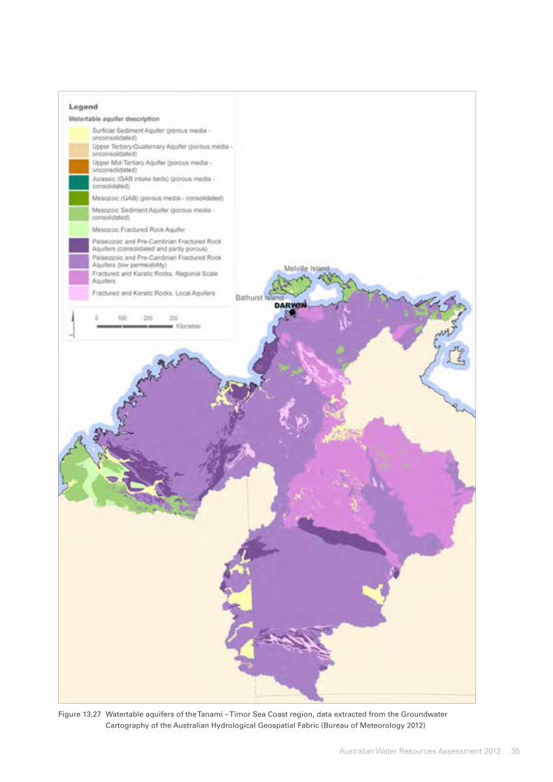
35Australian Water Resources Assessment 2012
Figure 13.27 Watertable aquifers of the Tanami – Timor Sea Coast region, data extracted from the Groundwater Cartography of the Australian Hydrological Geospatial Fabric (Bureau of Meteorology 2012)

Tanami – Timor Sea Coast
36 Australian Water Resources Assessment 2012
Figure 13.28 Watertable salinity classes in the Tanami – Timor Sea Coast region, data extracted from the Groundwater Cartography of the Australian Hydrological Geospatial Fabric (Bureau of Meteorology 2012)

37Australian Water Resources Assessment 2012
Figure 13.29 Groundwater management units in the Tanami – Timor Sea Coast region; data extracted from the National Groundwater Information System (Bureau of Meteorology 2013)

Tanami – Timor Sea Coast
38 Australian Water Resources Assessment 2012
13.6 Waterforcitiesandtowns
ThissectionexaminestheurbanwatersituationintheTanami–TimorSeaCoastregionin2011–12.Thelargeurbancentresintheregion,theirwatersupplysystemsandstoragesituationsarebrieflydescribed.Themainurbanisedarea,Darwin,isaddressedinmoredetailandabreakdownisprovidedforwaterobtainedforanddeliveredtothiscity.
13.6.1Urbancentres
Darwin,Palmerston,Broome,KatherineandKununurraarethemajorurbancentresintheTanami–TimorSeaCoastregionandareshowninFigure13.30inconjunctionwiththeirpopulationranges.
DarwinisthecapitalcityoftheNorthernTerritoryandhasapopulationof103,000people,makingitbyfarthelargestandmostpopulatedcityinthesparselypopulatedregion.ItisthesmallestoftheAustraliancapitalcities.
ThesecondlargesttownintheregionisPalmerston,aplannedsatellitecityclosetoDarwin.PalmerstonissituatednearDarwinHarbourandhasapopulationof27,700people.PalmerstonbrieflyheldinthepastthetitleofthefastestgrowingcityinAustralia.
ThethirdlargesttownintheregionisBroomewithapopulationof12,800people.Itwasbuiltonanindustryofpearlharvesting,butnowadaysresidentsaresupportedbyalargetourismindustry.
KatherineandKununurrabothhavepopulationsbelow7,000andhavemuchlessrelativegrowththanDarwinandPalmerston.
13.6.2Sourcesofwatersupply
Surfaceandgroundwaterarebothsignificantsourcesofurbanwatersuppliedintheregion.Manyoftheregion’ssmall,andinsomecasesisolatedcommunitiesrelypredominantlyongroundwatersupplies.
Theregion'sonlymajorsurfacewaterstorage,theDarwinRiverstorage,isshowninFigure13.31.ItsuppliessurfacewatertotheresidentsofDarwinandPalmerston.
GroundwaterisusedthroughouttheregionandinadditiontoaugmentingthesupplyoftheDarwinandPalmerstonareasitisthemajorsourceforwatersuppliedtothepopulationcentresofBroome,KatherineandKununurra.
ManagementofgroundwaterandsurfacewaterresourcesistheresponsibilityoftheNorthernTerritory'sDepartmentofLandResourceManagement.
RecycledwaterplaysaminorroleintheregionandisusedtomeettheirrigationneedsofanumberofsportingfacilitiesandplayingfieldsacrossDarwin.
13.6.3Darwin–Palmerston
ThePowerandWaterCorporationisownedbytheNorthernTerritoryGovernmentandsupplieswater,sewerageandpowerservicesintheNorthernTerritory,includingtheDarwinandPalmerstonareas.Withrespecttowatersupplyitoperatesasbothabulkwatersupplierandretailutility.
Darwinhasatropicalclimatewithdistinctwetanddryseasonswhichimpactsgreatlyontheavailabilityofsurfacewaterinthestoragesandrechargetothegroundwater.MostoftheannualrainfallisexperiencedfromDecember–April.Thetimingoftheonsetofregulareveningstorms,togetherwiththepresenceorabsenceofdryseasonrainfall,significantlyinfluenceswaterconsumption.

39Australian Water Resources Assessment 2012
Figure 13.30 Urban population range in the Tanami – Timor Sea Coast region

Tanami – Timor Sea Coast
40 Australian Water Resources Assessment 2012
Figure 13.31 Urban supply storages in the Tanami – Timor Sea Coast region

41Australian Water Resources Assessment 2012
Supply system
Waterissuppliedfromacombinationofsurfacewaterandgroundwatersources.MostofthiswaterissourcedfromtheDarwinRiverstorageandissupplementedfromtheHowardEastandMcMinnsborefields.
In1972,theDarwinRiverDamwasbuilttoaddressgrowingwaterneedsarisingfromtheincreasingpopulationinthesupplyarea.WiththeraisingofthedamspillwayheightinJanuary2011by1.3m,thetotalaccessiblestoragecapacityoftheDarwinRiverstorageisnow259GL.
Sources of water obtained
Figure13.32presentsthevolumesandsourcesofwatersourcedtomeetDarwin–Palmerston’surbandemand(NationalWaterCommission2013).Thedataclearlyillustratestheregion'srelianceonsurfacewater,whichtypicallycomprisesover80%ofthetotalsupplysource.
Groundwaterasasecondarysourcehasexhibitedsomegrowthoverthisperiod;however,itsextractioniscorrelatedwiththeavailablesurfacewatervolumeandhenceisrelieduponmoresignificantlyindryyears.Recycledwaterhasgrownintherecentyears,upbyalmost25%;however,thisgrowthhasbeenfromaverylowbase,andonavolumetricbasisremainslessthan1%ofthetotalwatersourcedtosupplytheregion.
Aseriesofwetteryears,includingAustralia’swettesttwo-yearperiodonrecord(2010–2011),sawanimprovementinsurfacewaterstoragelevelsandacommensuraterisenotonlyinthevolumesourcedfromsurfacewaterbutalsointhetotalvolumeextractedforurbanuse.
Figure 13.32 Total urban water sourced for Darwin from 2006–07 to 2011–12

Tanami – Timor Sea Coast
42 Australian Water Resources Assessment 2012
Categories of water delivered
Figure13.33showsthetotalvolumeofwaterdeliveredtoresidential,commercial,municipalandindustrialconsumersbythePowerandWaterCorporation(NationalWaterCommission2013).
Afteranacross-the-boardreductioninwaterconsumptionlevelsduring2010–11,aboveaveragerainfallandimprovingstoragelevelssawresidentialconsumptionreturntotheprevioushighs.BasedondataobtainedfromtheNationalPerformanceReports(NationalWaterCommission2013),theaveragewatersuppliedbythePowerandWaterCorporationforresidentialuseovertheanalysisperiodwas507kLperpropertyperyear,makingDarwinresidentssomeofthehighestresidentialwaterusersinthecountry.
Afterexhibitingadownwardtrendbetween2008–09and2010–11,waterusewasupin2011–12alongwithwatersuppliedtousersclassifiedas'other'.Thistrendisagain,inpart,explainedbytheimprovingwaterresourcesoutlookresultingfromaboveaveragerainfallsin2010and2011andimprovingwaterstoragelevelsintheDarwinRiverstorage.
Figure 13.33 Total urban water supplied to Darwin from 2006–07 to 2011–12

43Australian Water Resources Assessment 2012
13.7 Waterforagriculture
ThissectiondescribesthewatersituationforagricultureintheTanami–TimorSeaCoastregionin2011–12.Soilmoistureconditionsarepresentedandimportantirrigationareasareidentified.TheOrdRiverirrigationareaisdescribedinmoredetailandinformationisprovidedregardingsurfacestorageandgroundwater.
13.7.1 Soilmoisture
Sincemodelestimatesofsoilmoisturestoragevolumesarebasedonasimpleconceptualrepresentationofsoilwaterstorageandtransferprocessesaveragedovera5kmx5kmgridcell,theyarenotsuitableforcomparisonwithlocallymeasuredsoilmoisturevolumes.Thisanalysisthereforepresentsarelativecomparisononly,identifyinghowmodelledsoilmoisturevolumesof2011–12relatetomodelledsoilmoisturevolumesofthe1911–2012period,expressedindecilerankings.
Soilmoistureconditionsduringthe2011–12yearwereaboveaverageinmanypartsofthelandscape(Figure13.34)duetoaboveaveragerainfallfromOctoberthroughtoDecember2011.
Onlyinthemidtolatesummermonthsdidthesoilmoistureintheregiondroptoaverageandbelowaverage,butreturnedtoaboveaverageconditionsasaresultofveryhighrainfallsinMarch2012intheregion(Figure13.35).
Figure 13.34 Deciles rankings of average soil moisture over 2011–12 with respect to the 1911–2012 period in the Tanami – Timor Sea Coast region
Figure 13.35 Decile ranking of the monthly soil moisture conditions during the 2011–12 period in the Tanami – Timor Sea Coast region

Tanami – Timor Sea Coast
44 Australian Water Resources Assessment 2012
13.7.1 Irrigationareas
TheTanami–TimorSeaCoastregionextendsacrossarangeofclimaticzonesincludingahumidtropicalclimatetothenorthandaridconditionsacrossthesoutherninlandareas.Inadditiontonatureconservation,muchoftheregionispastorallands.IrrigatedagricultureisconcentratedintheOrdRiverbasin(Figure13.37).
13.7.2 OrdRiverIrrigationArea
TheOrdRiverbasinislocatedintheeastofnorthernWesternAustralia.TheOrdRiver,650kmlong,isoneofthemajorriversoftheState(Figure13.38).ThemaintributariesoftheOrdRiverincludetheNegri,WilsonandBowrivers(upstreamofLakeArgyle),andtheDunhamRiver,whichjoinstheOrdRiverdownstreamoftheKununurraDiversionDam.
TheOrdRiverirrigationareawasdevelopedin1962withtheconstructionoftheKununurraDiversionDamwhichledtotheformationofLakeKununurra.Itcomprisesapproximately13,000haofirrigablesoils.In1973theOrdDamwasbuiltthatcreatedLakeArgyle.Thissuppliedwaterforanirrigationprojectofmorethan50,000ha.In1996,thespillwaywallwasraisedby6m,whichdoubledthedam'scapacity.
ThemainindustrieswithintheOrdRiverbasinareagriculture,horticulture,tourismandmining.MeanannualrainfallintheOrdRiverbasinrangesfrom780mminthenorthto450mminthesouth.
LakeArgyle,thestoragebehindtheOrdRiverDamwithanaccessiblecapacityof10,700GL,isthelargestirrigationstorageinAustralia.TheKununurraDiversionDam,downstreamofLakeArgyle,divertswatertoirrigationareasnearKununurra(GovernmentofWesternAustraliaDepartmentofWater2010a).
WaterisreleasedfromLakeArgylethroughhydro-poweroutletsandaseriesofcontrolledreleasevalvesatthebaseofthedam.Additionalflowisreleasedthroughaspillwayplug.ThesecombinedreleasesprovideinflowintoLakeKununurrafromwhereitisdivertedtotheIvanhoePlainssystemsandthePacksaddlepumpingstations(OrdIrrigation2011).TheOrdIrrigationCooperativeprovideswateranddrainageservicestothefarmswithintheOrdRiverIrrigationArea.
ProlongeddryperiodscouldhaveamajorimpactonwatersupplyreliabilityofLakeArgyle(GovernmentofWesternAustraliaDepartmentofWater2010b);however,thelargestoragecapacityofLakeArgylebuffersthesystemagainstisolateddrieryears.Evaporationfromthesurfaceaccountsforalargecomponentoflossfromthelake.
Surface water storage volumes
DespitethelargestoragecapacityofLakeArgyle,prolongeddryperiodshaveamajorimpactonwatersupplyreliability(GovernmentofWesternAustraliaDepartmentofWater2010b).Openwaterevaporationalsoaccountsforalargecomponentoflossfromthelake.
Thehistoricdata(Figure13.36)showsthatthevolumeofwaterinthelakeregularlyexceededitstotalstoragecapacity.Thiswasalsothecasein2011–12,wherethewaterlevelinthestoragefortwoconsecutiveyearswasatoraboveitscapacityforthemostpartoftheyear.
Figure 13.36 Variation in the amount of water held in storage over recent years (light blue) and over 2011–12 (dark blue) for the Lake Argyle storage, as well as total accessible storage capacity (dashed line)

45Australian Water Resources Assessment 2012
Figure 13.37 Irrigation areas in the Tanami – Timor Sea Coast region

Tanami – Timor Sea Coast
46 Australian Water Resources Assessment 2012
Figure 13.38 The Ord River irrigation area

Lake Eyre Basin14 Lake Eyre Basin ........................................................ 2
14.1 Introduction ........................................................ 2
14.2 Key information .................................................. 3
14.3 Description of the region .................................... 4
14.3.1 Physiographic characteristics.................. 6
14.3.2 Elevation ................................................. 7
14.3.3 Slopes .................................................... 8
14.3.4 Soil types ............................................... 9
14.3.5 Land use ............................................. 11
14.3.6 Population distribution .......................... 13
14.3.7 Rainfall zones ....................................... 14
14.3.8 Rainfall deficit ....................................... 15
14.4 Landscape water flows ................................... 16
14.4.1 Rainfall .................................................. 17
14.4.2 Evapotranspiration ............................... 20
14.4.3 Landscape water yield ......................... 23
14.5 Surface water and groundwater ....................... 26
14.5.1 Rivers ................................................... 26
14.5.2 Streamflow volumes ............................. 26
14.5.3 Flooding ............................................... 29
14.5.4 Wetlands .............................................. 29
14.5.5 Hydrogeology ....................................... 32
14.5.6 Watertable salinity ................................. 32
14.5.7 Groundwater management units ........... 32

Lake Eyre Basin
2 Australian Water Resources Assessment 2012
14 Lake Eyre Basin14.1 Introduction
ThischapterexamineswaterresourcesintheLakeEyreBasinregionin2011–12andoverrecentdecades.Itstartswithsummaryinformationonthestatusofwaterflowsandstores.Thisisfollowedbydescriptiveinformationfortheregionincludingthephysiographiccharacteristics,soiltypes,population,landuseandclimate.
Spatialandtemporalpatternsinlandscapewaterflowsarepresentedaswellasanexaminationofthesurfaceandgroundwaterresources.ThedatasourcesandmethodsusedindevelopingthediagramsandmapsarelistedintheTechnicalSupplement.

3Australian Water Resources Assessment 2012
14.2 Keyinformation
Table14.1givesanoverviewofthekeycomponentsofthedataandinformationinthischapter.
Table 14.1 Key information on water flows and groundwater quality in the Lake Eyre Basin region
Landscape water flows
Evapo-transpiration
Landscapewater yield
Rainfall
Regionaverage Differencefrom1911–2012long-termannualmean
Decilerankingwithrespecttothe1911–2012record
337mm +42% 9th—aboveaverage
327mm +45% 10th—verymuchaboveaverage
25mm +150% 10th—verymuchaboveaverage
Streamflow (at selected gauges)
Annualtotalflow:
Aboveaverageflowinthreegaugesintheeast.Averageflowsononeofthegaugesinthecentre
Flooding: MajorfloodsintheupstreampartoftheCooperCreekbasin,decreasinginseveritydownstreamandsomefloodingintheDiamantinaandBulloorivers
Groundwater (in selected aquifers)
Salinity: Mostlynon-saline(<3000mg/L)groundwaterinthenorthandsaline(≥3000mg/L)inthesouth

Lake Eyre Basin
4 Australian Water Resources Assessment 2012
Lake Eyre salt lake | iTobi (iStockphoto)
14.3 Descriptionoftheregion
TheLakeEyreBasinregioncoversapproximately1.2millionkm²ofaridandsemi-aridCentralAustralia.Itrepresents17%ofthecontinentandstretches,northtosouth,fromjustbelowMountIsainQueenslandtoMarreeinSouthAustralia.Fromwesttoeast,itextendsfromAliceSpringsintheNorthernTerritorytoTamboandBlackallincentralQueensland.
Landformsintheregionmainlyconsistofplains,inlanddunes,sandplains,floodplains,andlowreliefhillsandplateaus.Highlyvariableandonaveragelowrainfallhasresultedinsparsevegetationcoverandintermittentriversystems.Subsections14.3.1–14.3.4providemoreinformationonthetopographyandsoilscover.
Withapopulationofapproximately59,000,theLakeEyreBasinaccountsforlessthan0.25%ofthenation’stotalpopulation(AustralianBureauofStatistics[ABS]2011b).
AliceSpringsisthemajorpopulationcentrealongwithanumberofremoteandregionalcentres(Figure14.1)includingCooberPedy,Birdsville,Winton,LongreachandPeterbourough.Furtherdiscussionoftheregion’spopulationdistributioncanbefoundinsubsection14.3.6.
Mostofthelandusewithintheregionisforgrazingandnatureconservation.Therearenumerousdrylakesthatformasubstantialpartoftheregion.Onlyasmallpatchinthefarsouthincludessomedrylandagriculture.
Theregion’sclimateisgenerallyquitearid,withrainfallmuchbelowpotentialevaporation.Theregionisdriestinthenortheast,butthisareadoesreceivesomemonsoonalrainand,althoughbeinghighlyvariable,itcansupplylargeamountsofwater,inparticularintotheupperreachesoftheDiamantinaandGeorginarivers.
Theregionisdividedintoseveralmajorriverbasins.ThemajorriversaretheGeorgina,Diamantina,ThomsonandBarcooriversandCooperCreek,whichflowfromcentralandwesternQueenslandintoSouthAustralia,aswellastheFinke,ToddandHughriversinCentralAustralia.ThesewaterwaysalldrainintoLakeEyre.Theriversandcreeksarecharacterisedbyhighvariabilityandunpredictabilityintheirflow,andhightransmissionlossesandverylowgradients.
ThehydrogeologyoftheregionisdominatedbythesedimentsoftheGreatArtesianBasinwithporoussandstoneaquifers.Thisgroundwaterbasinunderliestheregionfromthenortheast.ItisoneofAustralia’smostsignificantgroundwaterbasins.Thereisnotableextractionofgroundwaterforstockanddomesticpurposes.

5Australian Water Resources Assessment 2012
Figure 14.1 Major rivers and urban centres in the Lake Eyre Basin region

Lake Eyre Basin
6 Australian Water Resources Assessment 2012
Figure 14.2 Physiographic provinces of the Lake Eyre Basin region
14.3.1Physiographiccharacteristics
ThephysiographicmapinFigure14.2indicatesareaswithsimilarlandformevolutionaryhistories(Painetal.2011).Thesecanberelatedbacktosimilargeologyandclimaticimpactswhichdefinetheextentoferosionprocesses.Theareashavedistinctphysicalcharacteristicsthatcaninfluencehydrologicalprocesses.
TheLakeEyreBasinregionhasthreesuchdominantphysiographicprovinces,namely:
• CentralLowlands(72%):undulatingclayplains,sandplainswithlowsandstone,shaleandsilcretehills;
• CentralAustralianRanges(11%):rangesandhillsofigneousrock,sandstoneandquartzitesurroundedbyhardpanwashplainsandsomedunefields,sandandstonyplainsandsaltlakes;and
• Barkly–TanamiPlains(10%):blackclay,sandandlimestoneplainsandsandstonerisesandplateaussomewithferruginousmantles.
Theremainingsixprovinces(seeFigure14.2)occupyonly7%oftheregionandcontainavarietyofphysiographicfeaturesfromplainstoprominentranges.

7Australian Water Resources Assessment 2012
Figure 14.3 Ground surface elevations in the Lake Eyre Basin region
14.3.2Elevation
Figure14.3presentsgroundsurfaceelevationsintheLakeEyreBasin.InformationwasobtainedfromtheGeoscienceAustraliawebsite(www.ga.gov.au/topographic-mapping/digital-elevation-data.html).Theregionconsistsofenclosedriverbasinsastheriversdonotflowtothesea.MostoftheregiondrainsintoLakeEyre,providedenoughwaterisavailabletoreachthelake.ThelakeitselfisthelowestpointinAustralia.Thebottomofthelakeis15mbelowsealevelandtheshoresare9mbelowsealevel.
ThemajorriversthatfillLakeEyrearetheDiamantinaandGeorginarivers,whichreceivemostoftheir(monsoonal)wateronthenorthernmountainranges.
ThewatertravelsthroughChannelCountry,wherethelandformsaretypicalofdesertconditions.Theareamainlyconsistsofplains,inlanddunes,sandplains,floodplains,andlowreliefhillsandplateaus.
ThehighestmountainsintheregionarelocatedaroundAliceSprings,withpeaksexceeding1,000mabovesealevel.ThenortherntipoftheFlindersRangesinthesouthalsohassomehighpeakscloseto1,000mabovesealevel(Figure14.3).

Lake Eyre Basin
8 Australian Water Resources Assessment 2012
Figure 14.4 Surface slopes in the Lake Eyre Basin region
14.3.3Slopes
Areaswithsteepslopesprovidehigherrun-offgeneratingpotentialthanflatareas.TheLakeEyrebasinregionisgenerallyflat,withsomeminorareaswithsteephills(Table14.2andFigure14.4).Theslopeswerederivedfromtheelevationinformationusedintheprevioussection.
Table 14.2 Proportions of slope classes for the region
Slopeclass(%) 0–0.5 0.5–1 1–5 >5
Proportionofregion(%) 61.2 20.1 16.8 1.9
ThesteepslopesinthemapinparticularhighlighttheFlindersRangesinthesouthandtheMacDonnellRangesinthewest.
ThelargeareasofminorslopesinthecentreoftheregionarethesanddunesoftheSimpsonDesert.
AscanbenotedinFigure14.4,theriversintheregionrunthroughvastareaswithhardlyanygradient,whichmeansthatlargeamountsofwaterareneededtomaketheriversflow.

9Australian Water Resources Assessment 2012
Figure 14.5 Soil type in the Lake Eyre Basin region
14.3.4Soiltypes
Soilsplayanimportantroleinthehydrologicalcyclebydistributingwaterthatreachestheground.Watercanbetransportedtoriversandlakesviathesoilsurfaceasrun-offorenterthesoilandprovidewaterforplantgrowthaswellascontributingtogroundwaterrecharge.
Thenatureofthesehydrologicalpathwaysandthesuitabilityofthesoilsforagriculturalpurposesareinfluencedbysoiltypesandtheircharacteristics.SoiltypeinformationwasobtainedfromtheAustralianSoilResourceInformationSystemwebsite(www.asris.csiro.au).
About90%oftheLakeEyreBasinregioniscoveredbyfivetypesofsoil,namelyvertosols,rudosols,kandosols,sodosolsandtenosols(Figure14.5andFigure14.6).Thesoilsarecommoninareasusedforgrazingandnatureconservationinthisregion.
Vertosolsaremostlydistributedintheeasternhalfofthisregion.Theyareclayrichsoilswhichhaveatendencytocrackwhendryandswellwhilewetting.Theyarehighlyfertileandhavealargewater-holdingcapacity.Theydo,however,absorbasignificantamountofwaterbeforeanybecomesavailabletoplants.
Rudosolsaremostcommoninthewesternhalfoftheregion.Rudosolsaswellastenosols,whicharescatteredinthenorthwestandeastoftheregion,
arecharacterisedbyhavingaweakandminimaldevelopment.Theyshownoorlittlechangeintextureandcolourandareoftenshallowindepth.Tenosolsandrudosolsarelowinchemicalfertilityandinwater-holdingcapacityandthustheiragriculturalpotentialislow.
Kandosolsarestructurelesssoilswhichareoftenverydeep(uptothreemetresormore),buttheydonothaveastronglycontrastingtextureandtheydonotcontaincarbonatethroughouttheirprofile.Theyarelowinchemicalfertilityandarewell-drained;withonlymoderatewater-holdingcapacitycomparedwithothersoiltypes,thustheyonlyhavelowtomoderateagriculturalpotential.Kandosolsarescatteredacrosstheregion,exceptinthecentralpart.
Sodosolsaredominantinthecentral-westandscatteredinsmallpatchesacrossotherpartsoftheregion.Thesesoilshaveacleartexturecontrast,withanimpermeablesodicsubsoilduetoelevatedsodiumconcentrationsaswellasincreasingclaycontents.Theyaresusceptibletodrylandsalinityaswellaserosion,ifvegetationisremoved.Sodosolsareusuallylowinnutrientstatus.
TheothersoiltypesthathaveminimalrepresentationintheLakeEyreBasinregionincludedermosolsandchromosols(1–6%ofthetotalarea).

Lake Eyre Basin
10 Australian Water Resources Assessment 2012
Figure 14.6 Soil type distribution in the Lake Eyre Basin region

11Australian Water Resources Assessment 2012
Figure 14.7 Land use in the Lake Eyre Basin region
14.3.5Landuse
Figure14.7presentslanduseintheLakeEyreBasinregion.Mostofthelandisusedforgrazingandnatureconservation(datafromdata.daff.gov.au/anrdl/metadata_files/pa_luav4g9abl07811a00.xml).
Therearenumerousdrylakeswhichformasubstantialpartoftheregion.Onlyasmallpatchinthefarsouthincludessomedrylandagriculture(Figure14.8).

Lake Eyre Basin
12 Australian Water Resources Assessment 2012
Figure 14.8 Land use distribution in the Lake Eyre Basin region

13Australian Water Resources Assessment 2012
Figure 14.9 Population density and distribution in the Lake Eyre Basin region
14.3.6Populationdistribution
LakeEyreBasinregionisamongsttheleastpopulousareasinAustralia.Figure14.9showsthepopulationdensitiesfortheregionandillustratesthesparsenatureofitspopulation(ABS2011b).
ItsmajorpopulationcentreofAliceSpringsislocatednearitsboundaryinthenorthwest.Otherremotecommunitiesarelocatedonorneartheregion’sbordersinthesouthandwest.
Outsideofthemajorurbancentres,miningleases,Indigenouscommunitiesandanumberofsmalltownsandsettlementslocatedadjacenttomajorroadsaccountformuchofitsremainingpopulation.

Lake Eyre Basin
14 Australian Water Resources Assessment 2012
Figure 14.10 Rainfall zones in the Lake Eyre Basin region
14.3.7Rainfallzones
TheLakeEyreBasinregion’sclimateisaridthroughout.Theregionreceivesmonsoonalrainacrossthebasin,inparticularintheupperreachesoftheDiamantinaandGeorginarivers.Medianrainfalldoesnotexceed650mmperyearanywhereintheregion(Figure14.10).
Theregionconsistsofoneofthedriestpartsofthecontinent,withlargeareasinthecentrenotexceeding200mmofrainfallonaverage.
Thefarnortheasthasapronouncedwetseason,withannualaveragesofabout400mm.Inthefarsouth,someconsistencyinwinterrainfallispresent,althoughannualmedianrainfalldoesnotexceed500mm.
Formoreinformationonthisandotherclimateclassifications,visittheBureauofMeteorology's(theBureau's)climatewebsite:www.bom.gov.au/jsp/ncc/climate_averages/climate-classifications/index.jsp

15Australian Water Resources Assessment 2012
Figure 14.11 Rainfall deficit distribution in the Lake Eyre Basin region
14.3.8Rainfalldeficit
Therainfalldeficitindicator,thatis,rainfallminuspotentialevapotranspiration,givesageneralimpressionaboutwhichpartsoftheregionarelikelytoexperiencemoisturedeficitsovertheperiodofayear.TheLakeEyreBasinregionhasauniformpatternofveryhighpotentialdeficitsoverthewholeregion(Figure14.11),althoughrainfallishighlyvariablefromyeartoyear.
Mostoftheregionconsistsofdesertlandandephemerallakes,includingLakeEyreitself.Streamflow,oftencomingfromthenortheastasaresultofmonsoonalrainfallandtropicalstorms,
occasionallyfeedstheselakesandformslargefloodplains.
Otherthangrassesandsomeshrubsusedforsparselystockedfarming,noreallanduseoccursinthisdrylandscape.
Themoisturedeficitdoes,however,providemanyareaswithauniquefloraandfauna,mostlypreservedinthemanynatureconservationareasintheregion.
Formoreinformationontherainfallandevapotranspirationdata,seetheBureau’smapsofaverageconditions:www.bom.gov.au/climate/averages/maps.shtml

Lake Eyre Basin
16 Australian Water Resources Assessment 2012
Figure 14.12 Landscape water flows in 2011–12 compared with the long-term record (July 1911–June 2012) for the Lake Eyre Basin region
14.4 Landscapewaterflows
Thissectionpresentsanalysesofthespatialandtemporalvariationoflandscapewaterflows(rainfall,evapotranspirationandlandscapewateryield)acrosstheLakeEyreBasinregionin2011–12.Nationalrainfallgridsweregeneratedusingdatafromanetworkofpersistent,high-qualityrainfallstationsmanagedbytheBureau.EvapotranspirationandlandscapewateryieldswerederivedusingthelandscapewaterbalancecomponentoftheAustralianWaterResourcesAssessmentSystem(VanDijk2010).ThesemethodsandassociatedoutputuncertaintiesarediscussedintheIntroductionandaddressedinmoredetailintheTechnicalSupplement.
Figure14.12showsthattheLakeEyreBasinregionhasaseasonalrainfallpatternwithawetterspringtoearlyautumnandalargelydrywinterperiod.Evapotranspirationinthedrywinterperiodgenerallyexceedsrainfall.Afterthewetperiodthesoils
normallycontainplentyofmoisturethatisavailableforevapotranspiration.Themonthlylandscapewateryieldhistoryfortheregionshowsastablepatternofverylowyieldthroughouttheyear,althoughitmarginallyincreasesbetweenJanuaryandMarch.
The2011–12yearwasarelativelywetyear,withthemonthsofNovemberandMarchreceivingverymuchaboveaveragerainfall.AnactivemonsooninthenorthoftheregionandLaNiñaandwetterIndianOceaninfluencescontributedtohighrainfalltotals,particularlyforthemonthofMarch.
EvapotranspirationwasparticularlyhighinNovember,DecemberandMarch.InMarch,evapotranspirationwasthesecondhighestonrecordforthe1911–2012time-series.
Thelandscapewateryieldfor2011–12wasfifthhighestonrecordinNovemberandthirdhighestonrecordinMarch.

17Australian Water Resources Assessment 2012
Figure 14.13 Spatial distribution of (a) annual rainfall in 2011–12, and (b) their decile rankings over the 1911–2012 period for the Lake Eyre Basin region
14.4.1Rainfall
RainfallfortheLakeEyreBasinregionfor2011–12isestimatedtobe337mm.Thisis42%abovetheregion’slong-termaverage(July1911–June2012)of237mm.Figure14.13ashowsthatthehighestrainfalloccurredinthenortheastwithannualtotalsexceeding600mmin2011–12.Rainfallinthecentreoftheregiondidnotexceed200mmoverlargeareas.
Rainfalldecilesfor2011–12indicateaveragetoaboveaveragerainfallfortheentireregionoverthecourseoftheyear(Figure14.13b).Thesoutheastoftheregionreceivedverymuchaboveaveragerainfall.TheDiamantina–Georginariverbasinsinthenorthwestoftheregionreceivedpredominantlyaveragerainfallonly.

Lake Eyre Basin
18 Australian Water Resources Assessment 2012
Figure 14.14 Time-series of (a) annual rainfall, and (b) five-year retrospective moving averages for the summer (November–April) and winter (May–October) periods for the Lake Eyre Basin region
Rainfall variability in the recent past
Figure14.14ashowsannualrainfallfortheregionfromJuly1980onwards.Overthis32-yearperiodtheannualaveragewas264mm,varyingfrom156mm(2007–08)to616mm(2010–11).Temporalvariabilityandseasonalpatternssince1980arepresentedinFigure14.14b.
Thegraphsindicatethepresenceofcyclicalpatternstypicalintheregion’sannualrainfall,whichareparticularlynoticeableinthesummerperiod.ThispatterniscloselylinkedtotheSouthernOscillationIndexandtheoccurrenceofElNiñoandLaNiñaperiods(seetheNationalOverviewchapter).AstrongLaNiñaperiodtypicallydeliversaboveaveragerainfall,particularlytothenortheastoftheregion,clearlyseenintherecentverystrong2010–11LaNiñaevent.

19Australian Water Resources Assessment 2012
Figure 14.15 Spatial distribution of (a) trends in annual rainfall from 1980–2012, and (b) their statistical significance at 90% (weak) and 95% (strong) confidence levels for the Lake Eyre Basin region
Recent trends in rainfall
Figure14.15apresentsthespatialdistributionofthetrendsinannualrainfallforJuly1980–June2012.Thesearederivedfromlinearregressionanalysesonthetime-seriesofeachmodelgridcell.ThestatisticalsignificanceofthetrendsisprovidedinFigure14.15b.
Figure14.15bshowsthatsince1980anincreaseinrainfallhasoccurredinlargepartsoftheregion,particularlytowardsthenorth;however,thetrendsareonlystronglystatisticallysignificantin6%oftheregion.Thetrendsarelargelyaresultofthemulti-annualcyclicrainfallpatternshowninFigure14.14andtheparticularlyhighrainfallof2011–12.

Lake Eyre Basin
20 Australian Water Resources Assessment 2012
14.4.2Evapotranspiration
ModelledannualevapotranspirationfortheLakeEyreBasinregionfor2011–12isestimatedtobe327mm.Thisis45%abovetheregion’slong-term(July1911–June2012)averageof226mm.Thespatialdistributionofannualevapotranspirationin2011–12(Figure14.16a)issimilartothatofrainfall(Figure14.13a).
Evapotranspirationdecilesfor2011–12indicateaboveaveragetotalsacrossmostoftheregion(Figure14.16b).Around23%oftheregionevenrecordedverymuchaboveaverageevapotranspiration,scatteredthroughout.TheLakeEyredistrictinthesouthwestistheexception,wheregenerallyaverageevapotranspirationisestimated.
Figure 14.16 Spatial distribution of (a) modelled annual evapotranspiration in 2011–12, and (b) their decile rankings over the 1911–2012 period for the Lake Eyre Basin region

21Australian Water Resources Assessment 2012
Figure 14.17 Time-series of (a) annual evapotranspiration, and (b) five-year retrospective moving averages for the summer (November–April) and winter (May–October) periods for the Lake Eyre Basin region
Evapotranspiration variability in the recent past
Figure14.17ashowsannualevapotranspirationfortheregionfromJuly1980onwards.Overthis32-yearperiodtheannualevapotranspirationaveragewas250mm,varyingfrom153mm(2004–05)to543mm(2010–11).Temporalvariabilityandseasonalpatternssince1980arepresentedinFigure14.17b.
Summerperiodsshowedconsistentlyhigherevapotranspirationthanthewinterperiodduetothehighertemperaturesandthehigherrainfallinthenorthofthearea.Alsotheannualvariabilityismainlycausedduringthesummerperiod,whichagainfollowsthepatternofrainfall(Figure14.14b).

Lake Eyre Basin
22 Australian Water Resources Assessment 2012
Recent trends in evapotranspiration
Figure14.18apresentsthespatialdistributionofthetrendsinmodelledannualevapotranspirationfor1980–2012.Thesearederivedfromlinearregressionanalysesonthetime-seriesofeachmodelgridcell.ThestatisticalsignificanceofthetrendsisprovidedinFigure14.18b.
Figure14.18ashowsthatsince1980trendsaremostlyrisingwithastrongersignalinthenorthoftheregion.Figure14.18bconfirmsthatthesestrongernortherntrendsarestatisticallymoresignificant.
Figure 14.18 Spatial distribution of (a) trends in annual evapotranspiration from 1980–2012, and (b) their statistical significance at 90% (weak) and 95% (strong) confidence levels for the Lake Eyre Basin region

23Australian Water Resources Assessment 2012
14.4.3Landscapewateryield
ModelledlandscapewateryieldfortheLakeEyreBasinregionfor2011–12isestimatedtobe25mm.Thisis150%abovetheregion’slong-term(July1911–June2012)averageof10mm.Figure14.19ashowsthespatialdistributionoflandscapewateryieldfor2011–12,whichissimilartotheannualrainfalldistribution(Figure14.13a,notethedifferenceinthescalesbetweenthetwofigures).
Thedecile-rankingmapfor2011–12(Figure14.19b)showsaboveaveragetoverymuchaboveaveragelandscapewateryields.Thedecilerankingsoflandscapewateryieldaresubstantiallyhigherthanthoseofrainfallduetothehigherinitialsoilmoisturelevels,causedbythestrongwetseasonin2010–11.
Figure 14.19 Spatial distribution of (a) modelled annual landscape water yield in 2011–12, and (b) their decile rankings over the 1911–2012 period for the Lake Eyre Basin region

Lake Eyre Basin
24 Australian Water Resources Assessment 2012
Figure 14.20 Time-series of (a) annual landscape water yield, and (b) five-year retrospective moving averages for the summer (November–April) and winter (May–October) periods for the Lake Eyre Basin region
Landscape water yield variability in the recent past
Figure14.20ashowsannuallandscapewateryieldfortheLakeEyreBasinregionfromJuly1980onwards.Overthis32-yearperiod,annuallandscapewateryieldwas13mm,varyingfrom4mm(1985–86)to51mm(2010–11).Temporalvariabilityandseasonalpatternssince1980arepresentedinFigure14.20b.
LandscapewateryieldishighlyvariableintheLakeEyreBasinregionwiththesecondhighestcoefficientofvariation(standarddeviationdividedbymean)ofallregions,behindthePilbara–Gascoyneregion.Thevariabilityinlandscapewateryieldintheannualtotalsaswellasthelandscapewateryieldofthesummerperiodisdirectlyrelatedtorainfall.

25Australian Water Resources Assessment 2012
Recent trends in landscape water yield
Figure14.21ashowsthespatialdistributionofthetrendsinmodelledannuallandscapewateryieldfor1980–2012.Thesearederivedfromlinearregressionanalysesonthetime-seriesofeachmodelgridcell.ThestatisticalsignificanceofthetrendsisprovidedinFigure14.21b.
ThepatterninFigure14.20aandtheparticularlyhighpeakof2010–11makesthelandscapewateryieldtrendsstandoutasrisingthroughouttheregion,withtheexceptionoftheverylowlandscapewateryieldareaintheLakeEyredistrictinthesouthwest.Figure14.21bshowsthatinlargepartsoftheregiontrendsarestatisticallysignificant.
Figure 14.21 Spatial distribution of (a) trends in annual landscape water yield from 1980–2012, and (b) their statistical significance at 90% (weak) and 95% (strong) confidence levels for the Lake Eyre Basin region

Lake Eyre Basin
26 Australian Water Resources Assessment 2012
14.5 Surfacewaterand groundwater
ThissectionexaminessurfacewaterandgroundwaterresourcesintheLakeEyreBasinregionin2011–12.Rivers,wetlandsandstoragesarediscussedtoillustratethestateoftheregion’ssurfacewaterresources.Theregion’swatertableaquifersandsalinityaredescribed.NodatawasavailableattheBureauinasuitableformatforadetailedanalysisonindividualaquifers.
DatawasnotavailableforstreamflowsalinityintheLakeEyreBasin.
TherearenostoragesystemsintheLakeEyreBasin.
14.5.1Rivers
Theregionistheworld’slargestinternallydrainingsystemandLakeEyreisthefifthlargestterminallakeintheworld.Therearethreeriverbasinsintheregion,varyinginsizefrom106,000to699,000km2(Figure14.22).
ThemajorriversintheregionflowfromcentralandwesternQueenslandinthenortheastintoSouthAustraliainthesouth.Thesouthwestcorneroftheregion(LakeEyre)isupto15mbelowsealevelanditisthefinalreceivingareaforallmajorwatercoursesinthebasinifthefloodextentislargeenough.
Theriversandcreeksarecharacterisedbyhighvariabilityandunpredictabilityintheirflowwithhightransmissionlossesandverylowgradients.Allcreeksandriversofthebasinareephemeralwithrelativelyshortperiodsofflowfollowingrain,andoftenlongperiodswithnoflow.
14.5.2Streamflowvolumes
Figure14.23presentsananalysisofflowsatfivemonitoringsitesduring2011–12relativetoannualflowsfortheperiodfromJuly1980–July2012.Monitoringsiteswithrelativelylongrecordsacrossfourgeographicallyrepresentativeriverswereselected(seeTechnicalSupplement).Theannualriverflowsfor2011–12arecolour-codedaccordingtothedecilerankateachsiteoverthe1980–2012period.
TheflowsgenerallyreflectthemostlyaveragetoaboveaveragemodelledlandscapewateryieldresultsshowninFigure14.19b.OnlythemonitoredflowsintheDarrRiverpresentaslightlydifferentpatternofbelowaverageflows(reddotinFigure14.23).
AboveaverageflowswereobservedatthreesitesintheregionwhichwerelocatedonriversintheeastoftheLakeEyreBasinregion.Averagetotalflowswererecordedatonemonitoringsite.ThiswasontheDiamantinaRiverinthecentreoftheregion.
Flowdecilesinthesummer(November2011–April2012)wereverysimilartototalannualflowsfor2011–12asshowninFigure14.23.Thisistobeexpectedgiventhebulkofflowsintheregion,particularlyinthenortheast,occurredoverthesummerperiod.Itisalsotheconsequenceofthesummer-dominatedrainfallinthatpartoftheregion.

27Australian Water Resources Assessment 2012
Figure 14.22 Rivers and catchments in the Lake Eyre Basin region

Lake Eyre Basin
28 Australian Water Resources Assessment 2012
Figure 14.23 Average annual and summer period flow volumes of selected gauges for 2011–12 and their decile rankings over the 1980–2012 period in the Lake Eyre Basin region

29Australian Water Resources Assessment 2012
14.5.3Flooding
Figure14.24givesanoverviewofthelocationswheretheBureauismonitoringfloodlevelsintheLakeEyreBasinregionthroughtheNorthernTerritoryGovernment.TheselevelsarefurtherspecifiedintheTechnicalSupplement.
Asequenceofwetanddryspellshasbeenobservedinthelakeoveryears,whichisverymuchrelatedtotheElNiño—SouthernOscillationIndex.MajoreventsoffillingtheLakeEyreareassociatedwithrarecasesofannualrainfallinexcessof500mm.SeveralofthetributariestothelakewerefloodedduringthemonthsbetweenJanuaryandMarch2012.Inearly2012,majorfloodsoccurredintheBullooRiver.
LaterinFebruary,themaintributarytoLakeEyre,theDiamantinaRiver,wasflooded;thiswasconcurrentwithmajorfloodsinseveralsegmentsoftheBarcooRiver.SomemoderatefloodswerealsoregisteredintheThomsonandBullooriversduringFebruary.
InMarch2012andfollowingheavyrainfallsinthecatchmentalltributariesofthelakewereflooded,themostsignificantofwhichwastheDiamantinaRiverwhichhadmajorfloods.Moderatefloodsoccurredinothertributariesofthelake.InApril,thefloodsgraduallysubsidedandwerelimitedtosomemoderateandminorfloodsintheDiamantinaandThomsonrivers,respectively.
14.5.4Wetlands
TherearetwoRamsar-listed,internationallyimportantwetlandsintheLakeEyreBasinregionaswellasanumberofwetlandsofnationalimportancementionedintheAustralian Directory of Important Wetlands (www.environment.gov.au/water/topics/wetlands/database/diwa.html)
Thewetlandsmainlyconsistofephemeralriverfloodplainsandlakes(Figure14.25).Theyplayimportantrolesinthesurvivalofmanyrarespeciesofplantsandanimals.Theyalsoattractlargenumbersofcommonwaterbirdswhenthelakesandfloodplainsareflooded.
Nodetailedassessmentontheinflowsofselectedwetlandshasbeenperformedforthisregion.
Coongie Lakes wetlands | Paul Wainwright

Lake Eyre Basin
30 Australian Water Resources Assessment 2012
Figure 14.24 Flood occurrences in the Lake Eyre Basin region

31Australian Water Resources Assessment 2012
Figure 14.25 Location of important wetlands in the Lake Eyre Basin region

Lake Eyre Basin
32 Australian Water Resources Assessment 2012
14.5.5Hydrogeology
ThehydrogeologyoftheregionisdominatedbythesedimentsoftheGreatArtesianBasinwithporoussandstoneaquifers.Figure14.26showsthattheGreatArtesianBasinunderliestheregionfromthenortheast,wheretheboundariesofbothbasinscloselyapproximateeachother,andextendsthroughtothecentralandsouthwestmargins.ThisbasinisoneofAustralia’smostsignificantgroundwaterbasins.TheareasidentifiedasPalaeozoicfracturedrock(lowpermeability)inthenorthwestofthisregiontypicallyofferrestrictedlowvolumegroundwaterresources.
Incontrast,theareasidentifiedasfracturedandkarsticandPalaeozoicfracturedrock(consolidatedandpartlyporous)provideausablegroundwaterresourceinsomeparts.Theseunitsprovide95%ofthetownwatersupplyforAliceSprings.
Groundwatersystemsthatprovidemorepotentialforextractionarelabelledas:
• FracturedandKarsticRocks(regional)and(local);and
• MesozoicGAB(porousmedia—consolidated).
14.5.6Watertablesalinity
Figure14.27belowshowstheclassificationofwatertableaquifersasfresh(totaldissolvedsolids<3,000mg/L)orsaline(TDS≥3,000mg/L)wateraccordingtowatertablesalinity.Therearesmallareasofnodatarepresentedingrey.Ingeneral,groundwaterhasbeenclassifiedasmainlyfreshalongthebordersoftheNorthernTerritoryandNewSouthWales,andmainlysalineintheSouthAustralianborderarea.
14.5.7Groundwatermanagementunits
Thegroundwatermanagementunitswithintheregionarekeyfeaturesthatcontroltheextractionofgroundwaterthroughplanningmechanisms.Figure14.28showsthemajorgroundwatermanagementunitsthataresuperimposedontheGreatArtesianBasin,thatis,NorthernTerritory,GreatArtesianBasinWaterControlDistrict;SouthAustralia:FarNorthPrescribedWellsArea;Queensland:GreatArtesianBasin;NewSouthWales:GreatArtesianBasinCapRock,andtheKarsticandFracturedRocksresources,thatis,NorthernTerritory:AliceSpringsandQueensland:MountIsa.
Aerial view, Lake Eyre with water | Edstock (iStockphoto)

33Australian Water Resources Assessment 2012
Figure 14.26 Watertable aquifers of the Lake Eyre Basin region; data extracted from the Groundwater Cartography of the Australian Hydrological Geospatial Fabric (Bureau of Meteorology 2012)

Lake Eyre Basin
34 Australian Water Resources Assessment 2012
Figure 14.27 Water table salinity classes in the Lake Eyre Basin region; data extracted from the Groundwater Cartography of the Australian Hydrological Geospatial Fabric (Bureau of Meteorology 2012)

35Australian Water Resources Assessment 2012
Figure 14.28 Groundwater management units in the Lake Eyre Basin region; data extracted from the National Groundwater Information System (Bureau of Meteorology 2013)

Carpentaria Coast15 Carpentaria Coast ..................................................... 2
15.1 Introduction ....................................................... 2
15.2 Key information .................................................. 3
15.3 Description of the region ................................... 4
15.3.1 Physiographic characteristics.................. 6
15.3.2 Elevation ................................................. 7
15.3.3 Slopes .................................................... 8
15.3.4 Soil types ............................................... 9
15.3.5 Land use ............................................. 11
15.3.6 Population distribution .......................... 13
15.3.7 Rainfall zones ....................................... 14
15.3.8 Rainfall deficit ....................................... 15
15.4 Landscape water flows ................................... 16
15.4.1 Rainfall ................................................. 17
15.4.2 Evapotranspiration ............................... 20
15.4.3 Landscape water yield ......................... 23
15.5 Surface water and groundwater ....................... 26
15.5.1 Rivers ................................................... 26
15.5.2 Streamflow volumes ............................. 28
15.5.3 Streamflow salinity .............................. 28
15.5.4 Flooding ............................................... 31
15.5.5 Storage systems ................................... 31
15.5.6 Wetlands ............................................. 31
15.5.7 Hydrogeology ....................................... 35
15.5.8 Water table salinity ................................ 35
15.5.9 Groundwater management units ........... 35

Carpentaria Coast
2 Australian Water Resources Assessment 2012
15 Carpentaria Coast15.1 Introduction
ThischapterexamineswaterresourcesintheCarpentariaCoastregionin2011–12andoverrecentdecades.Itstartswithsummaryinformationonthestatusofwaterflows,storesanduse.Thisisfollowedbydescriptiveinformationfortheregion,includingthephysiographiccharacteristics,soiltypes,population,landuseandclimate.
Spatialandtemporalpatternsinlandscapewaterflowsarepresented,followedbyanexaminationofthesurfacewaterandgroundwaterresourcestofinishthechapter.ThedatasourcesandmethodsusedindevelopingthediagramsandmapsarelistedintheTechnicalSupplement.

3Australian Water Resources Assessment 2012
15.2 Keyinformation
Table15.1givesanoverviewofthekeycomponentsofthedataandinformationinthischapter.
Table 15.1 Key information on water flows and stores in the Carpentaria Coast region
Landscape water flows
Evapo-transpiration
Landscapewater yield
Rainfall
Regionaverage Differencefrom1911–2012long-termannualmean
Decilerankingwithrespecttothe1911—2012record
992mm +31% 9th—aboveaverage
775mm +30% 10th—verymuchaboveaverage
237mm +54% 9th—aboveaverage
Streamflow (at selected gauges)
Annualtotalflow:
Predominantlyaverageflow,aboveaverageflowinsomeheadwaterrivers
Salinity: Annualmedianelectricalconductivitybelow1,000μS/cm
Flooding: Minortomoderatefloodsinmostgauges,majorfloodsinsomegaugesinthesouthernandwesternrivers
Surface water storage (comprising about 24% of the region’s total capacity of all major storages)
Totalaccessiblecapacity
30June2012 30June2011 Change
accessiblevolume
%oftotalcapacity
accessiblevolume
%oftotalcapacity
accessiblevolume
%oftotalcapacity
99GL 92GL 93% 93GL 94% -1GL -1%
Groundwater (in selected aquifers)
Salinity: Non-salinegroundwater(<3000mg/L)throughouttheregionwithsomecoastalareasofsalinegroundwater(≥3000mg/L),duetoseawaterintrusion

Carpentaria Coast
4 Australian Water Resources Assessment 2012
River delta on the Gulf of Carpentaria between Weipa and Pormpuraaw, Queensland | Dr Linda Sands
15.3 Descriptionoftheregion
TheCarpentariaCoastregioncoversapproximately647,000km2.TothewestisArnhemLandandGrooteEylandt,thelargestislandintheGulfofCarpentaria.TotheeastistheCapeYorkPeninsula.
Thelandscapeisgenerallyflatandlow-lying,comprisedoffloodplains,muchofwhichdrainintothegulf.Subsections15.3.1–15.3.4providemoreinformationonthetopographyandsoilscover.
Approximately66,500peoplepermanentlyresideintheCarpentariaCoastregion.Thisaccountsforlessthan0.29%ofthenation’stotalpopulation(AustralianBureauofStatistics[ABS]2011b).Overonequarteroftheregion’spopulationisIndigenous.
InadditiontoitsmajorpopulationcentreofMountIsa,theregionhasanumberofremoteandregionaltownsthatareshowninFigure15.1.TheseincludetheregionalcentresofCloncurry,Normanton,DoomadgeeandKowanyama.Furtherdiscussionoftheregion’spopulationdistributioncanbefoundinsubsection15.3.6.
Grazingisthedominantlanduse.Therearelargeareasofnatureconservation,Indigenouslanduseandsomeforestry.Irrigatedagricultureonlyexistsonaverylocalscale,supportedbywaterfromtwomajorstorages.Thereisextensiveminingactivityintheregion.
Theclimateishotandhumidmostlyinthewetseason.ThedryseasonrunsfromaboutMay–OctoberandthemonsoonalwetseasonfromNovember–April.Subsections15.3.7and15.3.8providemoreinformationontherainfallpatternsanddeficitsacrosstheregion.
TheriversareverylargebyAustralianstandardsandcarryapproximatelyaquarterofthecontinent’stotalyearlystreamflow.Mostrivers,however,flowmainlyduringthewetseason.Therefore,perennialriversandperennialspringsintheregionareimportantsourcesofwater.
ThehydrogeologyoftheregionisdominatedbythesedimentsoftheGreatArtesianBasin,fracturedandkarsticrockinsomeareas,andsomeoutcroppingbasementrock.Amoredetaileddescriptionoftheriversandgroundwaterstatusintheregionisgiveninsection15.5.

5Australian Water Resources Assessment 2012
Figure 15.1 Major rivers and urban centres in the Carpentaria Coast region

Carpentaria Coast
6 Australian Water Resources Assessment 2012
Figure 15.2 Physiographic provinces of the Carpentaria Coast region
15.3.1Physiographiccharacteristics
ThephysiographicmapinFigure15.2indicatesareaswithsimilarlandformevolutionaryhistories(Painetal.2011).Thesecanberelatedbacktosimilargeologyandclimaticimpactswhichdefinetheextentoferosionprocesses.Theareashavedistinctphysicalcharacteristicsthatcaninfluencehydrologicalprocesses.
TheCarpentariaCoastregionhasthreesuchdominantphysiographicprovinces,namely:
• CarpentariaFall(26%):ridgesandhillswithplainsalongmuchofthecoast;rangesandlowlandsonfoldedmetamorphicrocksandgranitesintheeast;
• CarpentariaLowlands(37%):clayandsandyplainsandplateausofsandstoneorbauxiteinsomeareas;and
• PeninsularUplands(13%):sandstoneplateausandhillycountryonacidigneousandmetamorphicrocks.
Theremainingfourprovincesoccupy24%oftheregion.
• Barkly–TanamiPlains(7%):alluvialvalleys;
• CentralLowlands(7%):undulatingclayplains;
• NorthAustralianPlateaus(6%):rangesoffoldedmetamorphicrocks;and
• BurdekinUplands(4%):partlysandstoneplateauandsomeyoungbasalticplateaus;rangespredominantlyofgraniteandmetamorphicrocks.

7Australian Water Resources Assessment 2012
Figure 15.3 Land surface elevations in the Carpentaria Coast region
15.3.2Elevation
Figure15.3presentsgroundsurfaceelevationsintheCarprentariaCoastregion.InformationwasobtainedfromtheGeoscienceAustraliawebsite(www.ga.gov.au/topographic-mapping/digital-elevation-data.html).
TheeasternborderoftheregionisformedbythecrestofthenorthernpartoftheGreatDividingRange.Thehighestpeaksintheareaexceed1,200mabovesealevel.Theyarelocatedwheretheregion’sborderalmostreachestheCoralSea(Figure15.3).
Inthewesternpartoftheregion,riversoriginatefromthemainlandplateauandfromtheArnhemLandPlateauinthenorth.
Thecentrallow-lyingarea(GulfPlains)iscrossedbytheFlindersRiveranditstributaries.TheFlindersRiveroriginatesinthesoutheastoftheregionandisthelongestriverinQueensland.
BesidestheGulfPlains,theGulfofCarpentariacoastlineisawidebandoflow-lyingplains.Theriversinthisareaoftenformlargefloodplainsinthewetseason.

Carpentaria Coast
8 Australian Water Resources Assessment 2012
Figure 15.4 Surface slopes in the Carpentaria Coast region
15.3.3Slopes
Table15.2summarisestheproportionsofslopeclassesfortheregionwhileFigure15.4showsthespatialdistributionofthesurfaceslopes.Areaswithsteepslopesprovidehigherrun-offgeneratingpotentialthanflatareas.TheCarpentariaCoastregionhasfewareaswithsteepslopes.Theslopeswerederivedfromtheelevationinformationusedintheprevioussection.
Table 15.2 Proportions of slope classes for the region
Slopeclass(%) 0–0.5 0.5–1 1–5 >5
Proportionofregion(%) 49.5 16.5 28.1 5.9
ThesteepslopesinFigure15.4particularlyhighlighttherangesandtablelandescarpmentswestofCairns.Theseareareasofhighrainfall,andrun-offgeneratedinthisareamakestheMitchellRiveroneofthehighestdischargingriversinAustralia.Duetothehighvariationinrainfallduringtheyear,theriverhasaseasonalflowpattern.
Duetotheflatnessofthecentralplainintheregion(GulfPlains),theriversthatcrossitmeanderovervastareas.ThestreambedsoftheFitzroyRiveranditstributariescoverlargeareas.
InthehillsnorthofMountIsa,thevalleyswiththeirsteepslopeshavemadeitsuitablefordamconstruction.Twomajordamshavebeenconstructedhere,formingLakeMoondarraandLakeJulius.ThesestoragesprovidewaterforthelocalirrigationareasandfreshwaterforthetownofMountIsa.

9Australian Water Resources Assessment 2012
Figure 15.5 Soil types in the Carpentaria Coast region
15.3.4Soiltypes
Soilsplayanimportantroleinthehydrologicalcyclebydistributingwaterthatreachestheground.Watercanbetransportedtoriversandlakesviathesoilsurfaceasrun-offorenterthesoilandprovidewaterforplantgrowthaswellascontributingtogroundwaterrecharge.
Thenatureofthesehydrologicalpathwaysandthesuitabilityofthesoilsforagriculturalpurposesareinfluencedbysoiltypesandtheircharacteristics.SoiltypeinformationwasobtainedfromtheAustralianSoilResourceInformationSystemwebsite(www.asris.csiro.au).
About89%oftheCarpentariaCoastregionconsistsoffivesoiltypes,namelytenosols,kandosols,vertosols,rudosolsandhydrosols(Figure15.5andFigure15.6).Themajorityofthesesoilsareusedforpasturesandtosomeextentfornatureconservation.
Tenosolsaswellaskandosolsarewidelyspreadacrosstheregion.Rudosolsaremorecommoninthewesternhalfoftheregion.Rudosolsaswellastenosolsarecharacterisedbyhavingweakandminimaldevelopment.Theyshownoorlittlechangeintextureandcolourandareoftenshallowindepth.Tenosolsandrudosolsarelowinchemicalfertilityandinwater-holdingcapacityandthustheiragriculturalpotentialislow.
Kandosolsarestructurelesssoilswhichareoftenverydeep,uptothreemetresormore,buthaveneitherastrongtexturecontrastnorcarbonatethroughouttheirprofile.Theyhavealowtomoderateagriculturalpotentialwithmoderatewater-holdingcapacity,aremostlywelldrainedandhavemoderatechemicalfertility.
Vertosolsaredominantinthecentralpartofthisregion.Theyareclayrichsoilswithtendenciesforsoilcrackswhendry,andswellingduringwetting.Theyarehighlyfertileandhavealargewater-holdingcapacity.They,however,requirealargeamountofwaterbeforebecomingavailabletoplants.
Hydrosolsaremostcommonalongthenarrowcoastalplainsoftheregion,andtoagreaterextentalongtheeastcoast.Thesesoilsareseasonallywetduetohighseasonalrainfall,andarethussaturatedfortwotothreemonthsandcanalsobeinfluencedbytidalchanges.
Othersoiltypeswithsmallareacoverageintheregionarechromosols,sodosols,ferrosolsanddermosols(1–4%).

Carpentaria Coast
10 Australian Water Resources Assessment 2012
Figure 15.6 Soil type distribution in the Carpentaria Coast region

11Australian Water Resources Assessment 2012
Figure 15.7 Land use in the Carpentaria Coast region
15.3.5Landuse
Figure15.7andFigure15.8presentlanduseinformationintheCarpentariaCoastregion(datafromdata.daff.gov.au/anrdl/metadata_files/pa_luav4g9abl07811a00.xml).
TheregionispredominantlycoveredbypasturewithlargeareasalsodesignatedfornatureconservationCropping,eitherirrigatedordryland,occupiesaverysmallportionoftheregion.Mostincomeis
generatedbymining.IrrigatedagriculturearoundMountIsaonlyexistsonaverylocalscale,supportedbywaterfromthestoragesoftheJuliusandMoondarradams.
TheMareeba–DimbulahIrrigationAreaontheAthertonTablelandinthefareastoftheregionistheregion'sonlymainirrigationarea.IrrigationofsugarcaneandhorticulturalcropsoccurswithwatertakenfromLakeTinarooontheBarronRiverintheNorthEastCoastregion.
Julius Dam, Leichhardt River | Bureau of Meteorology

Carpentaria Coast
12 Australian Water Resources Assessment 2012
Figure 15.8 Land use distribution in the Carpentaria Coast region

13Australian Water Resources Assessment 2012
Figure 15.9 Population density and distribution in the Carpentaria Coast
15.3.6Populationdistribution
GivenitssizeandthenumberofpeoplepermanentlyresidingintheCarpentariaCoastregion,thepopulationdensitiesareverylowandinmanypartsapproachzero.ThisisclearlyillustratedinFigure15.9(ABS2011b).
TheminingtownofMountIsa,inthecentralsouthoftheregion,isthemajorpopulationcentreandaccountsforjustunderhalfoftheregion’spopulation.
WhilstMountIsaislocatedinland,themajorityofregionalcommunitiesarescatteredalongthecoastalfringeoftheGulfofCarpentariaandincludeanumberofremoteIndigenouscommunities.

Carpentaria Coast
14 Australian Water Resources Assessment 2012
Figure 15.10 Rainfall zones in the Carpentaria Coast region
15.3.7Rainfallzones
Theclimateishotandhumidwithtwodistinctseasonsperyear.ThedryseasonrunsfromaboutMay–SeptemberandthemonsoonalwetseasonfromOctober–April.Themajorityofrainfalloccursinathree-monthperiod.Medianrainfallexceeds350mmthroughout(Figure15.10).
Thetropicalnortheastoftheregion,CapeYork,receivesmostrainfall,withmedianrainfallexceeding1,200mmperannum.
AlongtheGulfofCarpentariacoastthemedianrainfallnormallyreacheslevelsbetween650and1,200mm.
Thesouthernpartoftheregionhasamuchdrierrainfallpatterngraduallyreachingmedianvalueslowerthan350mminthefarsouthoftheregion.
Formoreinformationonthisandotherclimateclassifications,visittheBureauofMeteorology's(theBureau's)climatewebsite:www.bom.gov.au/jsp/ncc/climate_averages/climate-classifications/index.jsp

15Australian Water Resources Assessment 2012
Figure 15.11 Rainfall deficit distribution for the Carpentaria Coast region
15.3.8Rainfalldeficit
Therainfallminuspotentialevapotranspirationindicatorgivesageneralimpressionofwhichpartsoftheregionmoisturedeficitsarelikelytooccurovertheperiodofayear.TheCarpentariaCoastregionisoneofextremesinrelationtothisindicator(Figure15.11).
Largedeficitscanbeexpectedinmostpartsoftheinlandareas.
Alongthecoast,someareasexperiencelessdistinctdeficits.TheabundanceofwaterintheheadlandsoftheMitchellRiverinthefareastoftheregionisonlyofminorimportancetostreamflowinthisriver.
Formoreinformationontherainfallandevapotranspirationdata,seetheBureau’smapsofaverageconditions:www.bom.gov.au/climate/averages/maps.shtml

Carpentaria Coast
16 Australian Water Resources Assessment 2012
Figure 15.12 Landscape water flows in 2011–12 compared with the long-term record (July 1911–June 2012) for the Carpentaria Coast region
15.4 Landscapewaterflows
Thissectionpresentsanalysesofthespatialandtemporalvariationoflandscapewaterflows(rainfall,evapotranspirationandlandscapewateryield)acrosstheCarpentariaCoastregionin2011–12.Nationalrainfallgridsweregeneratedusingdatafromanetworkofpersistent,high-qualityrainfallstationsmanagedbytheBureau.EvapotranspirationandlandscapewateryieldswerederivedusingthelandscapewaterbalancecomponentoftheAustralianWaterResourcesAssessmentSystem(VanDijk2010).ThesemethodsandassociatedoutputuncertaintiesarediscussedintheIntroductionandaddressedinmoredetailintheTechnicalSupplement.
Figure15.12showsthattheregionhasahighlyseasonalrainfallpatternwithdistinctwetanddryseasons.Evapotranspirationinthedryseasonalwaysexceedsrainfall.Afterthewetseason,thesoilsnormallycontainplentyofmoisturethatisavailableforevapotranspiration.Themonthlylandscapewateryieldhistoryfortheregionshowsastablepatternofverylowyieldinthedryseason.
Itgraduallyincreasesduringthewetseasonandsubsidesafterwards.
The2011–12yearwasarelativelywetyear,especiallyduringNovember–December2011,whenrainfallwasconsistentlyhigherthanthehistoricmedian.Additionally,anactivemonsooninthenorthoftheregioncontributedtoparticularlyhighrainfalltotalsforthemonthofMarch2012.
Withwetsoilconditionspresentatthestartoftheyear,evapotranspirationwashighforthefirstsixmonthsof2011–12.WiththeexceptionofJanuaryandFebruary2012,evapotranspirationratesremainedabovethe75thpercentilefortherestoftheyear.EvapotranspirationinJune2012wasthesecondhighestonrecord(1911–2012)forthismonth.
Thelandscapewateryieldfor2011–12closelyfollowedtherainfallpattern,withtheMarchlandscapewateryieldbeingfourthhighestonrecord.TheonlyexceptionisthemonthofFebruary,whenrainfallwasbelowaverage,buthighsoilmoisturelevels,duetothewetspring,maintainedarelativelyhighlandscapewateryield.

17Australian Water Resources Assessment 2012
Figure 15.13 Spatial distribution of (a) annual rainfall in 2011–12, and (b) their decile rankings over the 1911–2012 period for the Carpentaria Coast region
15.4.1Rainfall
RainfallfortheCarpentariaCoastregionfor2011–12isestimatedtobe992mm.Thisis31%abovetheregion’slong-termaverage(July1911–June2012)of755mm.Figure15.13ashowsthatthehighestrainfalloccurredalongtheeasterncoastalareasoftheGulfofCarpentariawithannualtotalsexceeding1,800mmin2011–12.Thewesternandsouthernpartsoftheregionhadrainfallmostlyrangingbetween600and900mm.
Rainfalldecilesfor2011–12showaveragetoverymuchaboveaveragerainfall(Figure15.13b).ThehighrainfallintheCapeYorkareaonlyresultedinaverymuchaboveaveragedecilerankinginpartsofthearea.Thesouthernpartoftheregionwasalsorelativelywet.Inthefarnorthwestandthefareast,rainfallwasaverage.IntheMitchellRiverbasin,rainfallwasbelowhistoricaverage.

Carpentaria Coast
18 Australian Water Resources Assessment 2012
Figure 15.14 Time-series of (a) annual rainfall, and (b) five-year retrospective moving averages for the wet summer (November–April) and dry winter (May–October) periods for the Carpentaria Coast region
Rainfall variability in the recent past
Figure15.14ashowsannualrainfallfortheregionfromJuly1980onwards.Overthis32-yearperiodtheannualaveragewas833mm,varyingfrom506mm(1987–88)to1,388mm(2010–11).Temporalvariabilityandseasonalpatternssince1980arepresentedinFigure15.14b.
Thegraphsindicatethattheannualvariationinrainfallisbasedonthevariationinrainfallinthewetseason(November–April)only.Thedifferencebetweenrainfallinthewinterandsummerperiods,asinFigure15.14b,isindicativeforaregionthatiscompletelydependentontheannuallyreturningmonsoontodeliverrainfall.

19Australian Water Resources Assessment 2012
Figure 15.15 Spatial distribution of (a) trends in annual rainfall from 1980– 2012, and (b) their statistical significance at 90% (weak) and 95% (strong) confidence levels for the Carpentaria Coast region
Recent trends in rainfall
Figure15.15apresentsthespatialdistributionofthetrendsinannualrainfallforJuly1980–June2012.Thesearederivedfromlinearregressionanalysesonthetime-seriesofeachmodelgridcell.
ThestatisticalsignificanceofthetrendsisprovidedinFigure15.15b.
Figure15.15ashowsthatsince1980astrongincreaseinrainfallhasoccurredinlargepartsoftheregion.Thesetrendsarestronglysignificantinmostoftheregion(Figure15.15b).Thelocalareaofdecreasingrainfallinthenortheastisremarkable,butnotstatisticallysignificant.

Carpentaria Coast
20 Australian Water Resources Assessment 2012
15.4.2Evapotranspiration
ModelledannualevapotranspirationfortheCarpentariaCoastregionfor2011–12isestimatedtobe775mm.Thisis30%abovetheregion’slong-term(July1911–June2012)averageof598mm.Thespatialdistributionofannualevapotranspirationin2011–12(Figure15.16a)issimilartothatofrainfall(Figure15.13a),butlowerinmagnitude.
Evapotranspirationdecilesfor2011–12indicateaboveaverageorverymuchaboveaveragetotalsacrossmostoftheregion(Figure15.16b).TheexceptionsarethenorthernpartofCapeYorkandintheupstreampartoftheMitchellRiverbasin.Theverymuchaboveaverageevapotranspirationalongmuchofthesouthwestislargelytheresultofthehighsoilmoistureavailabilitystartinginthepreviouswetyear2010–11.
Figure 15.16 Spatial distribution of (a) modelled annual evapotranspiration in 2011–12, and (b) their decile rankings over the 1911–2012 period for the Carpentaria Coast region

21Australian Water Resources Assessment 2012
Figure 15.17 Time-series of (a) annual evapotranspiration, and (b) five-year retrospective moving averages for the wet summer (November–April) and dry winter (May–October) period for the Carpentaria Coast region
Evapotranspiration variability in the recent past
Figure15.17ashowsannualevapotranspirationfortheregionfromJuly1980onwards.Overthis32-yearperiodtheannualevapotranspirationaveragewas634mm,varyingfrom479mm(1987–88)to935mm(2010–11).Temporalvariabilityandseasonalpatternssince1980arepresentedinFigure15.17b.
Evapotranspirationinthewetseasonismuchhigherthaninthedryseason.Thisisduetothehigherrainfallamountsandthereforewateravailabilityduringthewetseason.Duringthedryseason,evapotranspirationissubstantiallyhigherthantherainfallforthisseason(Figure15.14b).

Carpentaria Coast
22 Australian Water Resources Assessment 2012
Recent trends in evapotranspiration
Figure15.18apresentsthespatialdistributionofthetrendsinmodelledannualevapotranspirationfor1980–2012.Thesearederivedfromlinearregressionanalysesonthetime-seriesofeachmodelgridcell.ThestatisticalsignificanceofthetrendsisprovidedinFigure15.18b.
Figure15.18ashowsthatsince1980trendsarerisinginthemostoftheregionexceptforthefarnorthernpartofCapeYork.
AsshowninFigure15.18b,thetrendsaregenerallystatisticallysignificantthroughoutmostoftheregion.Themarginalandnegativetrendsinthenortharenotstatisticallysignificant.
Figure 15.18 Spatial distribution of (a) trends in annual evapotranspiration from 1980–2012, and (b) their statistical significance at 90% (weak) and 95% (strong) confidence levels for the Carpentaria Coast region

23Australian Water Resources Assessment 2012
15.4.3Landscapewateryield
ModelledlandscapewateryieldfortheCarpentariaCoastregionfor2011–12isestimatedtobe237mm.Thisis54%abovetheregion’slong-term(July1911–June2012)averageof154mm.Figure15.19ashowsthespatialdistributionoflandscapewateryieldfor2011–12,whichissimilartotheannualrainfalldistribution(Figure15.13a).
Thehighestlandscapewateryieldsin2011–12occurredinthenortheast,locallyexceeding900mm.Forthesouthandwestoftheregion,thelandscapewateryieldgenerallydidnotexceed200mmovertheyear.
Thedecile-rankingmapfor2011–12(Figure15.19b)showsthatlandscapewateryieldcloselyfollowedthepatternsofrainfalldecilesinFigure15.13b.
Figure 15.19 Spatial distribution of (a) modelled annual landscape water yield in 2011–12, and (b) their decile rankings over the 1911–2012 period for the Carpentaria Coast region

Carpentaria Coast
24 Australian Water Resources Assessment 2012
Figure 15.20 Time-series of (a) annual landscape water yield, and (b) five-year retrospective moving averages for the wet summer (November–April) and dry winter (May–October) periods for the Carpentaria Coast region
Landscape water yield variability in the recent past
Figure15.20ashowsannuallandscapewateryieldfortheCarpentariaCoastregionfromJuly1980onwards.Overthis32-yearperiod,annuallandscapewateryieldwas194mm,varyingfrom50mm(1982–83)to437mm(2010–11).Temporalvariabilityandseasonalpatternssince1980arepresentedinFigure15.20b.
Landscapewateryieldsclearlyshowsarisingtrendinannualandwetseasontotals.Inparticularthelastfiveyearshaveseenconsistentlyhighlandscapewateryields.
Dryseasonlandscapewateryieldisparticularlylowandhashadminimalcontributiontotheannualtotallandscapewateryield.

25Australian Water Resources Assessment 2012
Recent trends in landscape water yield
Figure15.21ashowsthespatialdistributionofthetrendsinmodelledannuallandscapewateryieldfor1980–2012.Thesearederivedfromlinearregressionanalysesonthetime-seriesofeachmodelgridcell.ThestatisticalsignificanceofthetrendsisprovidedinFigure15.21b.
Figure15.21ashowsthatsince1980strongrisingtrendsoccuralongthecoastlineoftheGulfofCarpentaria.Locallythesetrendsexceed14mm/year.
Figure15.21bshowsthatmostoftherisingtrendsareconfirmedtobestatisticallysignificant.AsalreadynotedinthegraphsofFigure15.20,thetrendsareveryobvious,especiallywiththeperiodofveryhighlandscapewateryieldforthelastfiveyears.
Figure 15.21 Spatial distribution of (a) trends in annual landscape water yield from 1980–2012, and (b) their statistical significance at 90% (weak) and 95% (strong) confidence levels for the Carpentaria Coast region

Carpentaria Coast
26 Australian Water Resources Assessment 2012
Boodjamulla (Lawn Hill) National Park | Wilderness Challenge Pty Ltd
15.5 Surfacewaterand groundwater
ThissectionexaminessurfacewaterandgroundwaterresourcesintheCarpentariaCoastregionin2011–12.Rivers,wetlandsandstoragesarediscussedtoillustratethestateoftheregion’ssurfacewaterresources.Theregion’swatertableaquifersandsalinityaredescribed.NodatawasavailableattheBureauinasuitableformatforadetailedanalysisonindividualaquifers.
15.5.1Rivers
Thereare23riverbasinsintheCarpentariacoastregion,varyinginsizefrom1,000to231,000km2(Figure15.22).ThefourmajorbasinsintheregionaretheFlinders–Norman,Roper,Nicholson–Leichhardt,andMitchell–Coleman.MuchoftheCarpentariaCoastregiondrainsintotheGulfofCarpentariaandcomprisesfloodplains.
Therivers,however,areverylargebyAustralianstandardsandcarryapproximatelyaquarterofthecontinent’stotalyearlystreamflow.
ThemainriversflowingnorthtotheGulfofCarpentariaaretheMitchell,Flinders,Gilbert,RoperandLeichhardt.Theseriversaregenerallybraidedandseasonallyintermittent.AfewexceptionsliketheRoperandtheGregoryareperennial.TheGilbert,Mitchell,FlindersandLeichhardtriversaretypicalofseasonalriversandtheirdischargecanvarygreatlydependingontheintensityofthemonsoon.TheLeichhardtRiverflowsnorthfromtheMountIsadistricttowardstheGulfofCarpentaria,eastofBurketown,andtheFlindersRiverrisesintheGreatDividingRange,110kmnortheastofHughendenandflowsintothegulfwestofKarumba.Mostrivers,however,flowonlyduringthewetseason.Therefore,allperennialriversandperennialspringsareimportantsourcesofwater.

27Australian Water Resources Assessment 2012
Figure 15.22 Rivers and catchments in the Carpentaria Coast region

Carpentaria Coast
28 Australian Water Resources Assessment 2012
15.5.2Streamflowvolumes
Figure15.23presentsananalysisofriverflowsat16monitoringsitesintheCarpentariaCoastregionduring2011–12relativetoannualflowsfortheJuly1980–July2012period.Siteswithrelativelylongrecordsacrosssevengeographicallyrepresentativeriverswereselected(seeTechnicalSupplement).Theannualriverflowsfor2011–12arecolour-codedaccordingtothedecilerankateachsiteoverthe1980–2012period.
TheflowsgenerallyreflectthemostlyaveragetoaboveaveragemodelledlandscapewateryieldresultsshowninFigure15.19b.
AboveaverageflowswereobservedatfivesiteslocatedonriversinthesoutheastandMcArthurRiverinthesouthwestoftheregion.Fivefurthersites,mainlylocatedontheriversinthecentraleast,theRoperRiverinthewestandtheGregoryRiverinthesouthwest,recordedaverageflows.
Ofthe16monitoringsitesacrosstheregiontherewereonlytwolocationswherebelowaverageflowswererecorded.ThesewerelocatedontheWaterhouseRiverinthewestandWalshRiverinthecentraleastoftheregion.
Flowdecilesinthewetseason(November2011–April2012)wereverysimilartototalannualflowsfor2011–12asshowninFigure15.23.Therearefewmonitoringsitesthatdidnotshowthispattern,suchasontheRoperRiverinthewestoftheregionwhichhadrelativelylowflowsinthewetseason.
15.5.3Streamflowsalinity
Figure15.24presentsananalysisofstreamflowsalinityfor2011–12atsevenmonitoringsitesthroughouttheCarpentariaCoastregion.Themonitoringsiteswithatleastafive-yeardatarecordwereselectedforanalysis.Theresultsarepresentedaselectricalconductivity(EC,μS/cmat25°C).ThisisacommonlyusedsurrogateforthemeasurementofwatersalinityinAustralia.StandardEClevelsfordifferentapplications,suchasfordrinkingwaterortypesofirrigation,areprovidedintheTechnicalSupplement.ThemedianannualECvaluesareshownascolouredcircles.ThesizeofthecircledepictsthevariabilityinannualEC,shownasthecoefficientofvariation(CV),beingthestandarddeviationdividedbythemean.
ThemedianECvaluesformostofthemonitoringsitesinthemainriversfallintherange0–1,000μS/cm,whichissuitableformostirrigationuses.Ofthesevenmonitoringsites,43%hadmedianECvaluesbelow500μS/cmand57%werebetween500–1,000μS/cm.Alittlehighersalinityoccursintheriverbasinsinthesouthoftheregion.
ThesalinityCVistheexpectedvariabilityofameasurementofEC,relativetothemeanEC.TheCVinECistypicallyrelatedtothevariabilityoftheflowatthemonitoringsites.TheCVisrelativelylowforthemostofthemonitoringsitesintheregionexceptDugaldRiverinthesouthoftheregion.Ofthesevenmonitoringsites,43%hadaCVbelow20%;43%ofthesiteshadaCVbetween20%and60%;andtheCVwasabove60%atoneofthesevenmonitoringsites.ThiswasontheDugaldRiverinthesouthoftheregion.

29Australian Water Resources Assessment 2012
Figure 15.23 Average annual and wet season (November 2011–April 2012) flow volumes of selected monitoring sites for 2011–12 and their decile rankings over the 1980–2012 period in the Carpentaria Coast region

Carpentaria Coast
30 Australian Water Resources Assessment 2012
Figure 15.24 Salinity as electrical conductivity and its associated coefficient of variation for 2011–12 in the Carpentaria Coast region

31Australian Water Resources Assessment 2012
15.5.4Flooding
Figure15.25givesanoverviewofthelocationswheretheBureauisassessesfloodlevelsintheCarpentariaCoastregionthroughtheNorthernTerritoryGovernmentaspartofitsfloodforecastingservice.TheselevelsarefurtherspecifiedintheTechnicalSupplement.
Thereweremajorfloodsintheregion,mostlyduringtheJanuary–March2012period,thatwereassociatedwithanactivemonsoonovernorthernAustraliaandtheGulfofCarpentaria.
InthelastweekofDecember2011themonsoonwasveryactiveovertheeasternhalfofNorthernAustralia.InlateJanuary2012alowformedoverwesternCapeYorkPeninsulaandmovedintothesoutheastGulfofCarpentaria.MajorfloodsoccurredintheCloncurryRiverwithothermoderatefloodsintheLeichhardtRiverandminorfloodsfurtherwestintheGregoryRiver.
InmidtolateFebruary2012alowpressuresystemproducedheavyrainfallsacrossmostoftheGulfCountryandresultedinmajorfloodsovervastpartoftheregionfromtheEinasleighRiverintheeasttotheGregoryRiverinthewest.
InearlyMarch2012moderatetoheavyrainfallaffectedthenorthtropicalcoastandcentralcoastandmajorfloodsoccurredinnortheastriverssuchasMitchellwithminorfloodinginothereasternriverssuchastheGilbertandEinasleigh.
OnemajorfloodoccurredduringApril2012inupperFlinders.Theheavyrainfallssubsidedintheregionandnofloodingoccurredafterwards.
15.5.5Storagesystems
Onestorage,LakeJulius,isreportedintheCarpentariaCoastregionbytheBureau’swaterstorageinformation.TheBureau'swaterstoragewebsiteincludesinformationonapproximately24%oftheregion'spubliclyownedstoragecapacity(asatAugust2012).StoragesnotreportedincludeLakeMoondarraandLakeMitchell.LakeJuliusprovideswatertoMountIsaandsurroundingmines.
ThelocationofLakeJuliusisshowninFigure15.26.Thestoragenormallyfillsupoverthewetseasonandslowlydropsinleveloverthedryseason.InJune2012,LakeJuliuswasfilledto93%ofitsstoragecapacity.Theloweststoragelevelwas80%ofitsstoragecapacity.
FurtherinformationonthepastandpresentvolumesofthestoragesystemsandtheindividualstoragescanbefoundontheBureau’swaterstoragewebsite:water.bom.gov.au/waterstorage/awris/
15.5.6Wetlands
TherearenoRamsar-listedinternationallyimportantwetlandsintheCarpentariaCoastregion,buttherearealargenumberofwetlandsofnationalimportancementioned(Figure15.27).MoreinformationaboutthewetlandsintheregioncanbefoundintheAustralian Directory of Important Wetlands(www.environment.gov.au/water/topics/wetlands/database/diwa.html).
Thewetlandsconsistmainlyofwidespreadtidalflatsintheestuariesofmostrivers.Theseestuariesarefloodedwithfreshwaterduringthewetseasonpeakflows,andprovidelargehabitatsforwaterbirdstofeedandbreed.
Nodetailedassessmentontheinflowsofselectedwetlandshasbeenperformedforthisregion.

Carpentaria Coast
32 Australian Water Resources Assessment 2012
Figure 15.25 Flood occurrence in 2011–12 for the Carpentaria Coast region

33Australian Water Resources Assessment 2012
Figure 15.26 Storage systems in the Carpentaria Coast region (information extracted from the Bureau’s water storage website in August 2012)

Carpentaria Coast
34 Australian Water Resources Assessment 2012
Figure 15.27 Location of important wetlands in the Carpentaria Coast region

35Australian Water Resources Assessment 2012
15.5.7Hydrogeology
ThehydrogeologyoftheregionisdominatedbythesedimentsoftheGreatArtesianBasin,fracturedandkarsticrockinsomeareas,andsomeoutcroppingbasementrock(Figure15.28).
Groundwatersystemsthatprovidemorepotentialforextractionarelabelledas:
• FracturedandKarsticRocks;and
• MesozoicGAB(porousmedia—consolidated).
TheGreatArtesianBasinisoneofAustralia’slargestandmostsignificantgroundwaterbasinswithporoussandstoneaquifersfromtheTriassic,JurassicandCretaceousperiods.Thereisasubstantialamountofextractionofgroundwaterfromthislargeresourceforstockanddomesticpurposes.
FracturedandkarsticrockoccursintheRopercatchment(intheregion’swest)andtheMountIsaareainthesouth.Inthehardrockofthebasement,substantialgroundwaterflowonlyoccursinrockfracturesandthistypeofgroundwatersystemtypicallyoffersrestrictedlowvolumegroundwaterresources.
15.5.8Watertablesalinity
Figure15.29showstheclassificationofwatertableaquifersasfresh(totaldissolvedsolids[TDS]<3,000mg/L)orsaline(TDS≥3,000mg/L)wateraccordingtowatertablesalinity.Asshowninthisfigurethereisalargeareaofnodatarepresentedingrey;however,wherethedataexistsgroundwaterismainlyfresh.
Althoughthewaterqualityofshallowaquifersisgenerallygood,theseasonalvariabilityofrainfall,andconsequentlythelevelofthewatertable,reducesthereliabilityoftheyield.
15.5.9Groundwatermanagementunits
Thegroundwatermanagementunitswithintheregionarekeyfeaturesthatcontroltheextractionofgroundwaterthroughplanningmechanisms.Figure15.30showsthatthemajorgroundwatermanagementunitwithintheNorthernTerritorycontainsthefracturedandkarsticrocksaquifersoftheDalyRoperarea.InQueenslandthemajorgroundwatermanagementunitsaretheGreatArtesianBasin,theCook,andtheMountIsa.

Carpentaria Coast
36 Australian Water Resources Assessment 2012
Figure 15.28 Watertable aquifers in the Carpentaria Coast region; data extracted from the Groundwater Cartography of the Australian Hydrological Geospatial Fabric (Bureau of Meteorology 2012)

37Australian Water Resources Assessment 2012
Figure 15.29 Watertable salinity classes in the Carpentaria Coast region; data extracted from the Groundwater Cartography of the Australian Hydrological Geospatial Fabric (Bureau of Meteorology 2012)

Carpentaria Coast
38 Australian Water Resources Assessment 2012
Figure 15.30 Groundwater management units in the Carpentaria Coast region; data extracted from the National Groundwater Information System (Bureau of Meteorology 2013)

Technical supplement 1 Introduction ........................................................ 2
2 Region boundaries ............................................. 2
3 Landscape water balance framework ................ 4
3.1 Background ............................................ 4
3.2 Measured water balance
and climatic data .................................... 5
3.3 Modelled landscape water
balance estimates ................................... 5
3.4 Model performance ................................ 7
4 Methods summaries .......................................... 9
5 Data sources and analyses .............................. 36
5.1 Data sources and selection procedures 36
5.2 Data analysis procedures ...................... 39
6 Data available with the report ........................... 46
6.5 Introduction .......................................... 46
6.6 Spatial information ................................ 46
6.7 Graphed information ............................. 46
7 Appendix ......................................................... 47

Technical supplement
2 Australian Water Resources Assessment 2012
1 Introduction
TheAustralian Water Resources Assessment 2012 (the2012Assessment)isthesecondinaseriesofreportsproducedbytheBureauofMeteorology(theBureau).ThereportpresentsassessmentsofAustralia’sclimateandwaterresourcesin2011–12(July2011–June2012)anddiscussesregionalvariabilityandtrendsinwaterresourcesandpatternsofwateruseoverrecentyearsanddecades,basedonthecurrentlyaccessibledata.
ThisTechnicalSupplementprovidessupportinginformationforthe2012Assessmentandincludes:
• Regionboundaries
• Landscapewaterbalanceframework
• Methodssummaries
• Datasourcesandanalyses
• Dataavailablewiththereport.
2 Regionboundaries
Similartothe2010Assessment,the2012Assessmentisstructuredaround13regionscoveringtheAustraliancontinent,basedondrainagedivisionboundaries.Drainagedivisionsrepresentthecatchmentsofmajorsurfacewaterdrainagesystems,generallycomprisinganumberofriverbasins.Drainagedivisionsprovideanaturalframeworkforassessinghydrologicalflowsinthelandscapewhilealsoallowinginformationtobepresentedanddiscussedinbroadlyidentifiableregionalandclimaticcontexts.
The13regionswerederivedfromtheAustralianHydrologicalGeospatialFabric(Bureau2011f).Thisisaspecialisedgeographicinformationsystemthatidentifiesthespatialrelationshipsofimportanthydrologicalfeaturessuchasrivers,lakes,reservoirs,dams,canalsandcatchments.
Hierarchically-nestedcatchmentswerederivedusinganautomateddrainageanalysisprocedurebasedonanine-seconddigitalelevationmodel(BureauofMeteorology2010c);12drainagedivisionsweredefinedatthehighestlevelofthehierarchyandwereusedasthebasisforthereportingregionsinthe2012Assessment.ThisworkbuildsonandapproximatesthedrainageboundariesdevelopedbyGeoscienceAustralia(1997)thatweretheresultofajointState,TerritoryandAustralianCommonwealthGovernmentprojecttocreateanationalspatialdatabaseofmajorhydrologicalbasins.
OneofthedrainagedivisionsdevelopedbyGeoscienceAustralia,theSouthEastCoast,wassplitintwo,usingselectedcatchmentboundariesatthesecondlevelofthehierarchy.ThisdivisionwaschosentobestapproximatetheborderbetweenNewSouthWales(NSW)andVictoria(Victoria),creatingthe'SouthEastCoast(NSW)'and'SouthEastCoast(Vic)'regions.
ThedifferencesbetweentheoriginalGeoscienceAustraliaboundariesandthoseusedinthe2012AssessmentareillustratedinFigure1.

3Australian Water Resources Assessment 2012
Figure 1 (a) Comparison of drainage division boundaries of Geoscience Australia (1997) and the 2012 Assessment regions, and (b) the subdivision of the South-East Coast drainage division into two reporting regions
(a)
(b)

Technical supplement
4 Australian Water Resources Assessment 2012
3 Landscapewaterbalance framework
3.1 Background
Theestimationofthedominantlandscapewaterflowsandstoresonanationalscaleisamajorpartofthe2012Assessment.Thisincludesinformationonprecipitation,actualevapotranspiration,soilmoistureandlandscapewateryield(comprisingrun-offandgroundwaterdischarge).Thesecomponentsarenotmeasureddirectly.TogeneratethisinformationacrossallpartsofAustralia,modellingsimulationsandspatialinterpolationtechniqueswereused.
Thischapterexplainsthereasoningforthechoiceofthemethodstoestimatethespatialandtemporalvariabilityofthesenon-measuredwaterbalancecomponents.
Considerations for choice of the methods
TheBureau’sWaterInformationServicesbranchwasformedin2008toproducevariousretrospectivewaterreportingproducts.Sincethen,BureauandCSIROstaffhavebeenworkingonestablishingsystemsandmethodstosupportthisnewrole.Twomajorinformationproductsarebeingproduced.ThesearetheAustralianWaterResourcesAssessment(www.bom.gov.au/water/awra)andtheNationalWaterAccount(www.bom.gov.au/water/nwa).
TheNationalWaterAccountcontainswateraccountingreportsfornationallysignificantregions.Itprovidesinformationonwaterstoresandflows,waterrightsandwateruse.
Bothproductsrequirecontinentalscalewaterbalanceestimation.Initialinvestigationsidentifiedtheneedforaframework,accordingtowhichthespatiallyandtemporallydistributedinformationwastobepresented.Thisconceptualwaterbalanceframework(Barratt2008)isillustratedinFigure2.Asobservationsarenotavailableforallofthesestoresandflowsatsufficientfrequencyandresolutionacrossthecontinent,asrequiredbythewaterbalancereportingterms,modelsor/estimationmethodsarerequired.
ThemethodsforestimatingcomponentsofthewaterbalancefortheAustralianWaterResourcesAssessmentandtheNationalWaterAccountarechosenaccordingtothefollowingconsiderations:
• Consistency: themethodscouldbeappliedconsistentlytobothproducts;
• Timeliness:themethodscouldbeimplementedintimeforbothproductdeadlinessubjecttoavailableBureauresources;and
• Robustness: themethodsaredemonstrablyrobustcomparedwithotheravailablemethods.
TheNationalWaterAccountpresentsadetailedannualwaterbalanceforthecomponentsasshowninFigure2,focusingonwateruseandmanageablestoragefromthesurfacewaterandgroundwaterstores.TheAustralianWaterResourcesAssessmentonlycapturesthemajorlandscapewaterflowprocesses,thatis,rainfall,actualevapotranspiration,landscapewateryieldandsoilmoisturestorage,focusingonwateravailabilityandthelandscapewaterflows.Thechoiceofmethodsforestimatingtheselandscapewaterflowsarediscussed,inturn,below.

5Australian Water Resources Assessment 2012
3.2 Measuredwaterbalanceand climaticdata
RainfallmeasurementsarerequiredforestimationofthespatialdistributionofrainfallacrossAustraliaandforinputintothewaterbalancemodel.GriddedrainfallestimatesproducedbytheBureau(Jonesetal.2009)wereused.ThedatasetwasderivedfromspatialinterpolationofavailabledailyrainfallreadingscollectedbytheBureau.
Solarradiationandtemperaturealsoserveasinputintowaterbalancemodel.DailygriddedestimatesprovidedundertheAustralianWaterAvailabilityProject(AWAP)wereused(seewww.bom.gov.au/jsp/awap/).
3.3 Modelledlandscapewater balanceestimates
The2010Assessmentincludedestimatesofactualevapotranspiration,landscapewateryield(run-offandgroundwaterdischarge)andsoilmoisturestoragefromacombinationoftwoconceptuallysimilarmodels:WaterDynandAWRA-L.The2012AssessmenthasmovedawayfromthatapproachtocontinuewithanupdatedversionoftheAWRA-Lmodelonly.TheAWRA-Lmodelversion2.0(the2010AssessmentusedAWRA-Lversion0.5)hasbeenusedtoproduceestimatesofthemajorlandscapewaterflowprocessesofactualevapotranspiration,landscapewateryieldandsoilmoisturestorage.Figure3showsadiagramoftheconceptualprocessescontainedinthismodel.
Figure 2 Water flows and stores in the conceptual water balance framework (Barratt 2008)

Technical supplement
6 Australian Water Resources Assessment 2012
ThechoiceisbasedonthefactthattheBureau,incollaborationwithCSIRO,isintheprocessofimplementingaholisticwaterbalancemodelanddataassimilationsystem(namedastheAWRASystem)whichconsistsoftheAWRA-Llandscapemodel,complementedinthefuturebyriverandgroundwatermodelcomponents(Figure4).Alreadyatthisstage,butevenmoresointhefuture,thissystemwillprovideaconsistentwaterbalanceestimationsystem,whichwillbethecornerstoneoftheAustralianWaterResourcesAssessmentandNationalWaterAccountproducts.
TheAWRAmodellingsystemwilleventuallyincludethefollowingcomponents:
• Aholisticwater balancemodel(AWRA-LRG)
• Amodel-data fusion systemtoupdateandconstrainmodelestimatesaccordingtoobservationswhereappropriate.Model-datafusionincludescalibration/
parameterisationofmodelcomponents(forexample,calibrationofarainfallrun-offmodelaccordingtostreamflowdata),assimilationofobservationstoupdatemodelstates/parameters(updatingmodelsoilstorestatesaccordingtosatelliteobservations)andotherblendingmethods(forexample,averagingdifferingmodelestimatesofrun-off).
• Abenchmarking systemtotestthatthemodelandinputdataareaccuratelyreflectingobservations.Thebenchmarkingsystemreferstoasetof(partlyorwhollyautomated)testsdesignedtoassesshowwellthesimulationsfromamodifiedsystemversion(incomparisontoaprevioussystemversion)reproduceastandardsetofobservationsfollowingastandardsetofcriteria.Thisalsoneedstoincludeongoingevaluationofsystemforcingdatawherepossible.
Figure 3 Conceptual diagram of AWRA-L model processes

7Australian Water Resources Assessment 2012
3.4 Modelperformance
TheintroductionofasophisticatedcalibrationandverificationstructureinthelastyearhaveenhancedthereliabilityoftheAWRA-LmodeloutcomeusingAWRA-Lv2.0comparedtothecombinationofmodelsthatwasusedinthe2010Assessment(thatis,averageofAWRA-Lv0.5andWaterDyn).
ThemodelcalibrationandvalidationstructureoptimisesthereprodutionofstreamflowandLeafAreaIndex(LAI).LAIisameasureofleafgrowthandisestimatedusingsatelliteimagery.TheLAIisincludedintheobjectivefunctionofthecalibrationproceduretoimprovethemodel’scapacitytoreflectvegetationgrowth.Vegetationgrowthplaysanimportantroleinthegenerationoftranspiration,whichinturnformsalargepartoftheactualevapotranspirationthatisreportedoninthe2012Assessment.
Thecalibrationofmodelparameterstooptimisestreamflowreproductionisdonetoimprovethemodel’sestimatesonlandscapewateryield.Inthecalibrationprocedure,thelandscapewateryieldtotalsofallgridcellsinthecatchmentarecombinedtoformstreamflowatthegaugingpointofacatchment.
Figure5indicatesmodelperformancesinestimatingstreamflowthroughoutAustraliawithasingle
parameterset.Theresultsofthemodelarecomparedwithpreviousversionsofthemodelaswellasthepreviouslyused(singleparameterset)WaterDynmodel.Toindicateachievablemodelperformancesapurposespecificrainfallrun-offmodel(CWYET_GR4J)isalsoincludedinthiscomparison.
Nash–Sutcliffemodelefficiencycoefficient(NSE)andtherelativebiasareusedasmeasuresofthepredictivestrengthofthesemodels(Figure5).ThehighertheNSEandthelowerthebias,thebetterthematchbetweenthemodelresultsandtheobservations.
TheCWYET_GR4JmodelresultsgiveninFigure5areestimatedonthebasisofusingcalibratedparametersetsofneighbouringcatchments.TheAWRA-Lmodelontheotherhandusesoneparametersetforthewholecountry.
Theintroductionoftheadvancedcalibrationtool(inAWRA-Lv1.0)particularlyhelpedimprovingtheAWRA-Lmodelresults.Sincethen,minorimprovementshavebeenachievedmainlythroughtheintroductionofadditionalinformation,inparticularonvegetation,fromremotelysensedproductsandsmallconceptualchangesinsomecomponentsofthemodel.
Figure 4 Australian Water Resources Assessment modelling system conceptual diagram

Technical supplement
8 Australian Water Resources Assessment 2012
Figure 5 Distribution of the Nash-Suthcliff Efficiency (NSE) scores and relative bias for monthly streamflow reproduction of 289 catchments

9Australian Water Resources Assessment 2012
4 Methodssummaries
The2012Assessmentincludesmanydifferentanalysismethods,mostofthemspecificallyfocusingonparticularcomponentsofthewaterresources(thatis,groundwater,reservoirsorstreamflow).ThesemethodswerecarefullyselectedbasedonasoundinvestigationofsimilarassessmentspreviouslyperformedinAustraliaandoverseas.
Thetablesthatfollowprovidealistofreferencesandpeerreviewsofeachofthemethodsused,soastodemonstratetheirvalidity.Foreachmethodthefollowinginformationisprovided:
• areferencetothesectioninwhichthemethodisused;
• ashortdescriptionoftheinputdatafortheanalysis;
• ashortdescriptionoftheappliedmethod;
• theresolution(temporalandspatial)oftheoutputdata;
• referencestootherworkinwhichthemethodwasapplied;and
• anexampleillustrationoftheoutput.
Inadditiontothis,informationoneachindividualreportfigurecanbefoundinthemetadataforthefigureinquestion.ThisisprovidedontheAustralianWaterResourcesAssessmentwebsite:www.bom.gov.au/water/awra/

Technical supplement
10 Australian Water Resources Assessment 2012
2012 Assessment analysis Data Method Reference / peer review
Annual and monthly national rainfall surfaces
Landscapewaterflowsin2011–12,NationalOverview,s.2.3
Description
5kmx5kmoriginalrainfallgriddataderivedusingananomaly-basedapproachapplyingtheBarnessuccessivecorrectionmethodandsmoothingsplineapproach.
Source
Bureau(NationalClimateCentre)
Description
Bureaustandardspatialclimatedatapresentationmethod.Monthlyandannualtotalrainfallgrids(July–June)presented.
Resolutionofoutput
Temporal:annual/monthly
Spatial:5kmx5kmgrid(nationalcoverage)
BureauofMeteorology2012,Annual Climate Summary 2011,www.bom.gov.au/climate/annual_sum/2011/index.shtml
Jones,DA,Wang,W,Fawcett,R2009,‘High-qualityspatialclimatedata-setsforAustralia’,Australian Meteorological and Oceanographic Journal, vol. 58,pp.233–48
Example figures

11Australian Water Resources Assessment 2012
2012 Assessment analysis Data Method Reference / peer review
Annual and monthly national modelled actual evapotranspiration surfaces
Landscapewaterflowsin2011–12,NationalOverview,s.2.3
Description
5kmx5kmactualevapotranspirationgriddata,basedonthePriestly–Taylorequation.
Source
AWRA-L2.0
Description
Bureaustandardspatialclimatedatapresentationmethod.Monthlyandannualtotalmodelledactualevapotranspirationgrids(July–June)presented.
Resolution of output
Temporal:annual/monthly
Spatial:5kmx5kmgrid(nationalcoverage)
VanDjikA2010,TheAustralianWaterResourcesAssessmentsystem,Technicalreport3,Landscapemodel,version0.5,Water for Healthy Country,CSIRONationalResearchFlagship,www.clw.csiro.au/publications/waterforahealthycountry/2010/wfhc-aus-water-resources-assessment-system.pdf
Example figures

Technical supplement
12 Australian Water Resources Assessment 2012
2012 Assessment analysis Data Method Reference / peer review
Annual and monthly national modelled landscape water yield surfaces
Landscapewaterflowsin2011–12,NationalOverview,s.2.3
Description
5kmx5kmmodelledlandscapewateryieldgriddata.
Source
AWRA-L2.0
Description
Bureaustandardspatialclimatedatapresentationmethod.Monthlyandannualtotalmodelledlandscapewateryieldgrids(July–June)presented.
Resolution of output
Temporal:annual/monthly
Spatial:5kmx5kmgrid
(nationalcoverage)
VanDjikA2010,TheAustralianWaterResourcesAssessmentsystem,Technicalreport3,Landscapemodel,version0.5,Water for Healthy Country,CSIRONationalResearchFlagship,www.clw.csiro.au/publications/waterforahealthycountry/2010/wfhc-aus-water-resources-assessment-system.pdf
Viney,NR2010,‘Acomparisonofmodellingapproachesforcontinentalstreamflowprediction’,WaterforHealthyCountry,CSIRONationalResearchFlagship,CSIRO,Canberra.
Example figures

13Australian Water Resources Assessment 2012
2012 Assessment analysis Data Method Reference / peer review
Annual and monthly national deciles (rainfall, evapotranspiration and landscape water yield)
Landscapewaterflowsin2011–12,NationalOverview,s.2.3
Description
5kmx5kmannualandmonthlydecilesgriddatageneratedforeachofthelandscapewaterflows.
Decilescalculatedfromlong-termgriddeddata(July1911–June2012).
Source
Bureau(NationalClimateCentre)and
AWRA-L2.0
Description
Bureaustandardspatialclimatedataanalysisandpresentationmethod.Monthlyandannualdecilesgrids(July–June)presentedbasedonthelong-termrecord(July1911–June2012).
Resolution of output
Temporal:annual/monthly
Spatial:5kmx5kmgrid(nationalcoverage)
BureauofMeteorology2012,Annual Climate Summary 2011,www.bom.gov.au/climate/annual_sum/2011/
BureauofMeteorology2013,Specialclimatestatements,www.bom.gov.au/climate/current/special-statements.shtml
CentreforAustralianWeatherandClimateResearch2013,www.cawcr.gov.au/publications/researchletters.php
Example figures

Technical supplement
14 Australian Water Resources Assessment 2012
2012 Assessment analysis Data Method Reference / peer review
Annual variation in national soil moisture surfaces
SoilMoisturein2011–12,NationalOverview,s.2.4
Description
5kmx5kmgriddedannualsoilmoisturevolumedata.
Decilescalculatedfromlong-termgriddeddata(July1911–June2012).
Source
AWRA-L2.0
Description
Modelledannualaveragesoilmoisturedecilesfor2011–12withrespecttothe1911–2012record
Resolution of output
Temporal:annual
Spatial:5kmx5kmgrid(nationalcoverage)
VanDjikA2010,TheAustralianWaterResourcesAssessmentsystem,Technicalreport3,Landscapemodel,version0.5,Water for Healthy Country,CSIRONationalResearchFlagship,www.clw.csiro.au/publications/waterforahealthycountry/2010/wfhc-aus-water-resources-assessment-system.pdf
Example figures

15Australian Water Resources Assessment 2012
2012 Assessment analysis Data Method Reference / peer review
Southern Oscillation Index (SOI) and Indian Ocean Dipole (IOD) time-series
DriversoftheAustralianclimaticconditionin2011–12,NationalOverview,s.2.9
Description
MonthlySouthernOscillationIndex(SOI)time-seriesdata(July2007–July2012).
WeeklyIndianOceanDipole(IOD)time-seriesdata(July2007–July2012).
Source
Bureau(NationalClimateCentre)
Description
StandardpresentationofhistoricSOIandIODtime-seriesdata.
SOIdatapresentedatmonthlyresolutionwithafive-monthbinomialweightedmean.Thefive-monthmeanformonthx=(SOIx-2+4SOIx-1+6SOIx+4SOIx+1+SOIx+2)/16
IODIndexdatapresentedatweeklyresolution.
Resolution of output
Temporal:monthly(SOI)andweekly(IOD)
BureauofMeteorology2012,‘ElNiño/LaNiño’,ENSOWrap-Up,www.bom.gov.au/climate/enso/
BureauofMeteorology2012,SOIandIODtime-series,www.bom.gov.au/climate/current/soi2.shtml,andwww.bom.gov.au/climate/enso/indices.shtml
Troup,A1965,‘Thesouthernoscillation’,Quarterly journal of Royal Meteorological Society,vol.91,pp.490–506.
Saji,NHetal.‘AdipolemodeinthetropicalIndianOcean’,Nature,vol.401,pp.360–63.
Example figures

Technical supplement
16 Australian Water Resources Assessment 2012
2012 Assessment analysis Data Method Reference / peer review
Soil types
Descriptionoftheregion,s.3oftheregionalchapters
Description
ThemapshowsthedistributionofsoiltypesasclassifiedperAustraliansoilorderclassificationsystem.
Description
ThesoiltypemapwasproducedbylinkingdigitalsoilmappingunitsoftheAtlas Australian Soil Classification(Northcoteetal.1960–1968)totheAustralianSoilClassificationsoilorderasdevelopedbyAshtonandMcKenzie(2001).The Atlas of Australian Soils wasproducedbetween1960and1968(Northcoteetal.1960–1968).
AdigitalversionoftheatlaswascreatedbytheBureauofRuralSciencein1991.
ThedatawasaccessedthroughtheASRISwebsite(ASRIS2011)
Thedigitalsoilmappingunitsareaccessibleatascaleof1:2,000,000,buttheoriginalcompilationwasatscalesfrom1:250,000to1:500,000.
Ashton,LJ,McKenzie,NJ2001,‘ConversionoftheAtlasofAustralianSoilstotheAustralianSoilClassification’,CSIROLandandWater(unpublished)
CSIRO,AustralianSoilResourceInformationSystem2012,retrieved7November2012,www.asris.csiro.au
Northcote,KHetal.1960–1968,Atlas of Australian Soils,sheets1–10(includesexplanatorydata),CSIROAustraliaandMelbourneUniversityPress,Melbourne
Example figures

17Australian Water Resources Assessment 2012
2012 Assessment analysis Data Method Reference / peer review
Monthly box plots of regional landscape water balance model flows
Landscapewaterflows,s.4oftheregionalchapters
Description
Regionallyaveragedmonthlylandscapewaterflowdata.
Datapresentedarerainfall,evapotranspirationandlandscapewateryield.
Source
Bureau(NationalClimateCentre)and
AWRA-L2.0
Description
Monthlydataforthecurrentyear(2011–12)arepresentedrelativetolong-termrecord.Monthlydistributions(boxandwhiskers)arecalculatedfromlong-termmodelrundata(July1911–June2012).
Landscapewaterflowvariablespresentedare:
• rainfall;
• actualevapotranspiration;and
• landscapewateryield.
Resolution of output
Temporal:monthly
Spatial:2012Assessmentreportingregion(spatiallyaveraged)
BureauofMeteorology2013,‘ExamplefortheinterpretationoftheBureau’sStreamflowForecasts’,www.bom.gov.au/water/ssf/forecasts.shtml#drainage=murray_darling&basin=upper_murray&catchment=Q_HUME_TOT&productType=DT_1&productGroup=data
Example figures

Technical supplement
18 Australian Water Resources Assessment 2012
2012 Assessment analysis Data Method Reference / peer review
Regional summary of annual landscape water flows (mapped annual totals and deciles)
Landscapewaterflows,s.4oftheregionalchapters
Description
5kmx5kmgriddedannuallandscapewaterflowsdata(July–June).
Decilescalculatedfromlong-termgriddeddata(July1911–June2012)
Theunderlyingdataarethesameaspresentedforthenationaloverviewlandscapewaterflowsurfacesins.2.3.
Source
Bureau(NationalClimateCentre)andAWRA-L2.0
Description
Bureaustandardspatialclimatedatapresentationmethod.Annualtotalandannualdecileslandscapewaterflowgrids(July–June)presented.
Annualdecilesgrids
(July–June)calculatedbasedonthelong-termrecord(July1911–June2012).
Landscapewaterflowvariablespresentedare:
• rainfall;
• actualevapotranspiration;and
• landscapewateryield
Resolution of output
Temporal:annual
Spatial:5kmx5kmgridforeach2012Assessmentreportingregion
BureauofMeteorology2012,Annual Climate Summary 2011,www.bom.gov.au/climate/annual_sum/2011/
Example figures

19Australian Water Resources Assessment 2012
2012 Assessment analysis Data Method Reference / peer review
Time-series of landscape water flows over the past 32 years (annual and seasonal)
Landscapewaterflows,s.4oftheregionalchapters
Description
Spatiallyaveragedmonthlyandannuallandscapewaterflowdata(July–June).Summer(November–April)andwinter(May–October)seasontotalscalculatedfrommonthlymodeloutputdata.
Source
Bureau(NationalClimateCentre)and
AWRA-L2.0
Description
Time-seriesplotofannualdatapresentedforlast32years(July1980–June2012).
Time-seriesplotofseasonalfive-yearmovingaverages(backwardlooking)datapresentedforlast32years(November1980–October2012).
Landscapewaterflowvariablespresentedare:
• rainfall;
• actualevapotranspiration;and
• landscapewateryield.
Resolution of output
Temporal:annual(July–June)andsix-monthseasons(November–AprilandMay–October)Spatial:2012Assessmentreportingregion(spatiallyaveraged)
BureauofMeterology2013,‘ExampleoftheBureau’sclimatevariabilityandchangetimeseries:Annualplot’,Australianclimatevariabilityandchange—Timeseriesgraphs,www.bom.gov.au/cgi-bin/climate/change/timeseries.cgi?graph=rain&area=aus&season=0112&ave_yr=A
BureauofMeteorology2013,‘ExampleoftheBureau’sclimatevariabilityandchangetimeseries:Seasonalplot’,Australianclimatevariabilityandchange—Timeseriesgraphs,www.bom.gov.au/cgi-bin/climate/change/timeseries.cgi?graph=rain&area=aus&season=0411&ave_yr=5
Jones,DA,Wang,W,Fawcett,R2009,‘High-qualityspatialclimatedata-setsforAustralia’,Australian Meteorological and Oceanographic Journal,vol.58,pp.233–48.
Example figures
http://www.bom.gov.au/cgi-bin/climate/change/timeseries.cgi?graph=rain&area=aus&season=0112&ave_yr=A
http://www.bom.gov.au/cgi-bin/climate/change/timeseries.cgi?graph=rain&area=aus&season=0112&ave_yr=A
http://www.bom.gov.au/cgi-bin/climate/change/timeseries.cgi?graph=rain&area=aus&season=0112&ave_yr=A
http://www.bom.gov.au/cgi-bin/climate/change/timeseries.cgi?graph=rain&area=aus&season=0112&ave_yr=A
http://www.bom.gov.au/cgi-bin/climate/change/timeseries.cgi?graph=rain&area=aus&season=0411&ave_yr=5
http://www.bom.gov.au/cgi-bin/climate/change/timeseries.cgi?graph=rain&area=aus&season=0411&ave_yr=5

Technical supplement
20 Australian Water Resources Assessment 2012
2012 Assessment analysis Data Method Reference / peer review
Regional maps trends in annual landscape water flows over the past 32 years (seasonal)
Landscapewaterflows,s.4oftheregionalchapters
Description
5kmx5kmgriddedlandscapewaterflowdata.
Trendanalysisappliedtoannualtotalsforthepast32years(1980–2012).
Source
Bureau(NationalClimateCentre)and
AWRA-L2.0
Description
Linearregressiontrendcalculatedforannualtotalsateach5kmx5kmgridcelloverthelast32years(July1980–June2012).Slopeoflinearregressionline(mm/year)reflectsthestrengthanddirectionofpotentialtrends.
Thesignificancetest(t-test)fortheslopesoftheregressionlinesat5%(stronglysignificant)and10%(weaklysignificant)wascalculated.
Resolution of output
Temporal:annual
Spatial:5kmx5kmgridforeach2012Assessmentreportingregion
BureauofMeterology2013,‘ExampleoftheBureau’sclimatevariabilityandchangetrendanalysis',www.bom.gov.au/cgi-bin/climate/change/trendmaps.cgi?map=rain&area=aus&season=1202&period=1970
Kundzewicz,ZW,Robson,AJ2004,‘Changedetectioninhydrologicalrecords—areviewofthemethodology’,Hydrological Sciences Journal/Journal des Sciences Hydrologiques,vol.49,no.1,pp.7-19
Example figures
http://www.bom.gov.au/cgi-bin/climate/change/trendmaps.cgi?map=rain&area=aus&season=1202&period=1970
http://www.bom.gov.au/cgi-bin/climate/change/trendmaps.cgi?map=rain&area=aus&season=1202&period=1970

21Australian Water Resources Assessment 2012
2012 Assessment analysis Data Method Reference / peer review
Site-based seasonal streamflow anomaly analyses
Regionalwaterresourcesassessmentsandsurfacewaterandgroundwater,s.5ofsomeregionalchapters
Description
Measuredstreamflowdischarge(ML/day).
Datacollatedforcurrentlyoperationalselectedstreamflowgaugeswithrecordsavailableforatleastthepast32years(July1980–June2012).
Source
Bureau
Description
Annualdischargeanddecilerankingofannualdischargeforthereportingyear(July2011–June2012)comparedtolong-term(July1980–June2012)annualtimeseries.
Decilerankingofsummerdischargeforthereportingyear(November2011–April2012)comparedtolong-term(November1980–April2012)seasonaltimeseries.
Resolution of output
Temporal:annual/summerseason(November–April)
Spatial:siteswithinrelevant2012Assessmentreportingregion
Marsh,T,Sanderson,F2009,UK Hydrological Review 2008,NERC/CentreforEcologyandHydrology,UnitedKingdom,www.ceh.ac.uk/data/nrfa/nhmp/annual_review/pdf/Hydrological_Review_2008.pdf
Example figures

Technical supplement
22 Australian Water Resources Assessment 2012
2012 Assessment analysis Data Method Reference / peer review
Site-based annual median with variation of streamflow salinity analyses.
Surfacewaterandgroundwater,s.5ofsomeregionalchapters
Description
Measuredelectricalconductivityofstreamflow(μS/cmat25°C).
Datacollatedforcurrentlyoperationalselectedstreamflowsalinitygaugeswithrecordsavailableforatleastthepastfiveyears(July2007–June2012).
Source
Bureau
Description
Medianofannualstreamflowsalinityforthereportingyear(July2011–June2012)arecoloured-codedrelativetotheclassificationofelectricalconductivity(EC)i.e.,<500,501–1000,1001–1500,1501–2000and>2000.
Coefficientsofvariation(standarddeviationdividedbythemean)ofannualstreamflowECforthereportingyeararedifferentsizesrelativetotheCVofECrangesi.e.,<10,11–20,21–40,41–60,61–80and81–100.
Resolution of output
Temporal:annual
Spatial:siteswithinrelevant2012Assessmentreportingregion.
Standardanalysisandpresentationofhydrologicalinformation
Example figures

23Australian Water Resources Assessment 2012
2012 Assessment analysis Data Method Reference / peer review
Decile rankings of daily streamflow
Inflowstowetlands,s.5ofsomeregionalchapters
Description
Dailystreamflowsince1980
Source
Bureau
Description
Datarankedintheirrespectivedecilecategoriesandgivenincoloursofoccurrence
Resolution of output
Temporal:daily
Koehler,R2004,Raster Based Analysis and Visualization of Hydrologic Time Series,Ph.D.dissertation,UniversityofArizona,USA,p.189
Strandhagen,E,Marcus,WA,Meacham,JE2006.‘Viewsoftherivers:representingstreamflowofthegreaterYellowstoneecosystem’,Cartographic Perspectives,no.55,Fall2006
Example figures

Technical supplement
24 Australian Water Resources Assessment 2012
2012 Assessment analysis Data Method Reference / peer review
Site-based time series of monthly flows into wetlands and into selected storages (urban / irrigation)
Surfacewaterandgroundwater,s.5ofsomeregionalchapters
Waterforcitiesandtowns,s.6ofsomeregionalchapters
Waterforagriculture,s.7ofsomeregionalchapters
Description
Measuredstreamflowdischarge(ML/day).
Datacollatedforcurrentlyoperationalselectedstreamflowgaugeswithrecordsavailableforatleastthepast32years(July1980–June2012).
Source
Bureau
Description
Graphicalpresentationofmeasuredmonthlystreamflowfor2011–12plottedagainstderivedmonthlypercentileclasses(10–30,30–70and70–90).Percentilescalculatedfrom32-year(July1980–June2012)record.
Resolution of output
Temporal:monthly
Spatial:siteswithinrelevant2012Assessmentreportingregion
Standardgraphicalpresentationofhydrologicalinformation
Example figures

25Australian Water Resources Assessment 2012
2012 Assessment analysis Data Method Reference / peer review
Regional map of groundwater salinity class
Regionalwaterresourcesassessmentsandsurfacewaterandgroundwater,s.5ofallregionalchapters
Description
Salinityclassofwatertableaquiferbasedonelectricalconductivityofgroundwater.
Datacollatedforboreslessthan40mdeepforthepast22years(July1990–June2012).
Source
Bureau(Groundwaterdatabase)
Description
InterpolatedsalinitymapusingInverseDistanceWeighting,calculatedfromaverageelectricalconductivitymeasurementsinboresoverthe22-yearperiod(July1990–June2012)presentedinclassesoflessthan3000mg/L(fresh)andmorethan3000mg/L(saline).Theboreswerealllessthan40mdeep.
Empiricalequation(below)usedtoconvertunitsofElectricalConductivity(EC)(μS/cm)toTotalDissolvedSolids(TDS)(mg/L).
TDS(mg/L)=
EC(μS/cmat25°C)x0.6
Resolution of output
Temporal:long-termaverage(22years)
Spatial:siteswithinrelevant2012Assessmentreportingregion
PeerreviewedbyseniorhydrogeologistfromQueenslandGovernmentDepartmentofNaturalResourcesandMines
DepartmentofPrimaryIndustry2011,Victoria's groundwater resource,VictorianResourcesOnline
Example figures

Technical supplement
26 Australian Water Resources Assessment 2012
2012 Assessment analysis Data Method Reference / peer review
Regional map and site-based time-series of groundwater level status
Regionalwaterresourcesassessments/Surfacewaterandgroundwater(s.3.5)
Description
Trendsingroundwaterlevelsformajoraquifersforthepastfiveyears(2007–2012).
Selectedborehydrographsreportinggroundwaterlevelsfluctuationsfortheentireperiodofrecords
Source
Bureau(Groundwaterdatabase)
Description
Lineartrend(negative,stable,positive)ingroundwateriscalculatedbasedona0.1m/yrchangeasthecriteria.Theperiodofcalculationisthelast5years.Thisisrepresentedata5-or20-kmgridresolutionas:decreasing,stable,increasing,andvariablebasedona60%majorityoftheboresineachgridsquare(atminimumdatafromthreebores).
Graphicalpresentationofvariationsandchangesingroundwaterlevelforselectedboresoverthe22-yearperiod(July1990–June2012)
Resolution of output
Temporal:5-yeartrend(2007–2012)forthemapsandlengthofrecordsforhydrographs)
Spatial:siteswithinrelevant2012Assessmentreportingregion
Murray–DarlingBasinCommission2004,Groundwater status: 1990–2000 summary report,MDB,Commission,Canberra.
Murray–DarlingBasinCommission(2008),Groundwater status: 2000–2005 technical report,MDBCommission,Canberra.
DepartmentofPrimaryIndustry2011,Victoria's groundwater resource,VictorianResourcesOnline
DepartmentofEnvironmentandPrimaryIndustries2013,Groundwaterlevelswww.water.vic.gov.au/monitoring/monthly/groundwater_levels#groundwatermaps
Example figures

27Australian Water Resources Assessment 2012
2012 Assessment analysis Data Method Reference / peer review
Site-based time-series of changes in surface water storage (urban / irrigation)
RegionalwaterresourcesassessmentsandWaterforcitiesandtowns,s.6ofsomeregionalchapters
RegionalwaterresourcesassessmentsandWaterforagriculture,s.7ofsomeregionalchapters
Description
Volumeofwaterheldinamajorstorage.
Source
Bureau’sAustralianWaterResourcesInformationSystem(AWRIS)
Description
Graphicalpresentationofobservedlong-termandreportingyearstoragedata(2011–12).Graphicalaxesrepresentdataasbothstoragelevelandpercentfull(percentofmaximumcapacity).
Resolution of output
Temporal:daily
Spatial:siteswithinrelevant2012Assessmentreportingregion
Standardpresentationofwaterstorageinformation
water.bom.gov.au/waterstorage/awris
www.bom.gov.au/water/about/publications/document/factsheet_waterstorage.pdf
Example figures

Technical supplement
28 Australian Water Resources Assessment 2012
2012 Assessment analysis Data Method Reference / peer review
Time-series of annual urban water supply by source
Waterforcitiesandtowns,s.6ofmostregionalchapters
Description
Informationabouturbanwatermanagement.
Source
NationalPerformanceReport2009–10:Urbanwaterutilities,archive,archive.nwc.gov.au/library/topic/npr/npr-2009-10-urban
Description
Plotoftotalannualwatersourcedfromsurfacewater,groundwater,recycledanddesalinationwaterforurbanconsumption.
Resolution of output
Temporal:annual(July–June)
Spatial:urbanwatersupplyareawithinrelevant2012Assessmentreportingregion
Standardgraphicalpresentationofhydrologicalinformation
Example figures

29Australian Water Resources Assessment 2012
2012 Assessment analysis Data Method Reference / peer review
Changes in urban water restrictions over time
RegionalwaterresourcesassessmentsandWaterforcitiesandtowns,s.6ofsomeregionalchapters
Description
Wateruserestrictionannouncementsindicatinglevel,commencementandterminationdates,adescriptionofwaterrestrictionlevelsandwheretheyapply.
Source
Bureau'swaterinformationdatabase
Description
Graphicalrepresentationofwaterrestrictionlevelsovertimeplottedagainstarelevantmeasureofwateravailability,thatis,waterstorage.Onlyappliedwhererestrictionsmaybedefinedrelativetoadefinedstoragelevelorotherresourceavailabilityvariable.
Resolution of output
Temporal:variable—dependentonannouncementsofchangestorestrictionlevels
Spatial:watersupplyareawithinrelevant2012Assessmentreportingregion
Standardgraphicalpresentationofhydrologicalinformation
Example figures

Technical supplement
30 Australian Water Resources Assessment 2012
2012 Assessment analysis Data Method Reference / peer review
Patterns in annual irrigation water use
Waterforagriculture,s.7ofsomeregionalchapters
Description
Annual(July–June)irrigationwaterusedatafromABSWater Use on Australian Farmsreports.DataaresummarisedatanNRMlevelforthefouryearsbetween2005–06and2010–11.
Dataforthe2011–12yearwerenotavailableatthetimeofpublication.
Source
AustralianBureauofStatistics
Description
Mappedandgraphicalrepresentationofannualirrigationwateruseforeachnaturalresourcemanagementregionwithinthereportingregion.
Resolution of output
Temporal:annual
Spatial:naturalresourcemanagementregionswithinrelevant2012Assessmentreportingregion
AustralianBureauofStatistics(ABS)2012,Water Use on Australian Farms 2010–11,ABS,Canberra,www.abs.gov.au/ausstats/[email protected]/mf/4618.0
Example figures

31Australian Water Resources Assessment 2012
2012 Assessment analysis Data Method Reference / peer review
Site-based time-series of variations in shallow groundwater levels, residual rainfall, streamflow and reservoir level
RegionalwaterresourcesassessmentsandWaterforagriculture,s.7ofsomeregionalchapters
Description
Groundwaterlevelofabore(relativetodatum)andmeasuredstreamflowdischarge(GL/month)andreservoirmonthlylevel(m).
Datacollatedforcurrentlyoperationalmonitoringboresforthepast22years(July1990–June2012).
Source
Bureau'swaterinformationdatabase
Description
Graphicalpresentationoftherelationshipbetweenmonthlyvariationsinshallowgroundwaterlevels(m),localresidualrainfall(mm/month),measuredstreamflow(GL/month)andmonthlyreservoirlevels(m).
Therainfallresidualmasscurveisbasedonthefollowingequation.
Actualrainfallformonth(x)–averagerainfallformonth(x)+thecumulativesumof(actualrainfallformonth–averagerainfallformonth)forallpreviousmonths
Resolution of output
Temporal:monthly
Spatial:siteswithinrelevant2012Assessmentreportingregion
Murray–DarlingBasinCommission2008,Groundwater Status Report 2000–2005,TechnicalReport,ed.Murray–DarlingBasinCommission,Canberra.
SouthernRuralWater2012,Gippsland Groundwater Atlas,SouthernRuralWater
www.srw.com.au/Page/Page.asp?Page_Id=689&h=-1
Example figures

Technical supplement
32 Australian Water Resources Assessment 2012
2012 Assessment analysis Data Method Reference / peer review
Site-based time-series of variations in groundwater levels at nested sites
RegionalwaterresourcesassessmentsandWaterforagriculture,s.7ofsomeregionalchapters
Description
Groundwaterlevelofabore(relativetodatum)
Datacollatedforcurrentlyoperationalmonitoringboresforthepastfiveyears(July2007–June2012).
Source
Bureau(Groundwaterdatabase)
Description
Graphicalpresentationoftherelationshipbetweenvariationsinshallowgroundwaterlevels(m)forboresscreenedindifferentaquifersatthesamelocation
Resolution of output
Temporal:groundwater—sub-annualdependingonthefrequencyofobservationfrom2007–12
Spatial:selectednestedbores
Standardanalysisandpresentationofgroundwaterlevelinformation
Example figures

33Australian Water Resources Assessment 2012
2012 Assessment analysis Data Method Reference / peer review
Site-based time-series of variations in groundwater salinity at nested sites
RegionalwaterresourcesassessmentsandWaterforagriculture,s.7ofsomeregionalchapters
Description
Groundwatersalinityofaboreaselectricalconductivity.
Datacollatedforcurrentlyoperationalmonitoringboresforthepastfiveyears(July2007–June2012).
Source
Bureau(Groundwaterdatabase)
Description
Graphicalpresentationoftherelationshipbetweenvariationsinshallowgroundwatersalinityaselectricalconductivity(μS/cm)forboresscreenedindifferentaquifersatthesamelocation
Resolution of output
Temporal:groundwater:sub-annualdependingonthefrequencyofobservationfrom2007–2012
Spatial:selectednestedbores
Standardanalysisandpresentationofgroundwatersalinityinformation
Example figures

Technical supplement
34 Australian Water Resources Assessment 2012
2012 Assessment analysis Data Method Reference / peer review
Site-based analysis of groundwater depth
RegionalwaterresourcesassessmentsandWaterforagriculture,s.7ofsomeoftheregionalchapters
Description
Groundwaterlevelofabore(relativetodatum).
Datacollatedforcurrentlyoperationalmonitoringboresforthepast20years(July1990–June2012).
Source
Bureau(Groundwaterdatabase)
Description
Standardmappresentationofcalculatedmediandepthtogroundwater(m)forthereportingyear(July2011–June2012).
Decilerankingofmediandepthtogroundwater(m)forthereportingyear(July2011–June2012)comparedtolong-term(July1980–June2012)levels.
Resolution of output
Temporal:annual(medianlevelanddecilerank)
Spatial:siteswithinrelevant2012Assessmentreportingregion
PeerreviewfromgroundwaterexpertwithintheBureau
Example figures

35Australian Water Resources Assessment 2012
2012 Assessment analysis Data Method Reference / peer review
Site-based analysis of groundwater salinity
RegionalwaterresourcesassessmentsandWaterforagriculture,s.7ofsomeregionalchapters
Description
Groundwatersalinityofaborebasedonelectricalconductivityofgroundwaterandreportedastotaldissolvedsolids(TDS)(mg/L).
Datacollatedforcurrentlyoperationalmonitoringboresforthepast22years(July1990–June2012).
Source
Bureau(Groundwaterdatabase)
Description
Standardmappresentationofcalculatedmediangroundwatersalinityto(mg/L)forthereportingyear(July2011–June2012).
Empiricalequation(below)usedtoconvertunitsofelectricalconductivity(EC)(μS/cm)toTDS(mg/L).
TDS(mg/L)=EC(μS/cmat25°C)x0.6
Decilerankingofmediangroundwatersalinity(m)forthereportingyear(July2011–June2012)comparedtolong-term(July1990–June2012)levels.
Resolution of output
Temporal:annual(medianlevelanddecilerank)
Spatial:siteswithinrelevant2012Assessmentreportingregion
PeerreviewfromgroundwaterexpertwithintheBureau
Example figures

Technical supplement
36 Australian Water Resources Assessment 2012
5 Datasourcesandanalyses
Thissectiongivesbackgroundinformationondatasources,selectionproceduresandthemethodsappliedtoproducethefiguresinthe2012Assessment.Thedataavailablefordownloadfromthewebsiteisalsodiscussed.
5.1 Datasourcesandselection procedures
Anumberofdifferentselectionprocedureswereemployedtoidentifysuitabledataforthe2012Assessment.SourcesincludedtheAustralianWaterResourcesInformationSystem(AWRIS)(Bureau2011a),therelatedwebpagesanddirectcontactwithdatacustodians.Totheextentthatdatawasavailable,carefulconsiderationwasgiventomaintainconsistencyinpresentinginformationacrossvariousstudyregions.Theproceduresadoptedforeachdatatypearediscussedbelow.
5.1.1 Estimated flows – high data uncertainty areas
TheAustralianlandscapewaterbalancemodellingusesgriddeddailyrainfalldataasaprimarymodelinputvariablealongwithanumberofgriddedmeteorologicaldatasetsforthecalculationofpotentialandactualevapotranspiration.Thesearemaximumandminimumtemperature,humidityandincomingsolarradiation.
Astheanalysisandinterpretationofthemodelresultsarebasedonthemodelrunsfora101-yearperiod(July1911–June2012),anunderstandingofthereliabilityandqualityofmodelinputdataisnecessary.Thisisparticularlyimportantforrainfalldatathatexhibithighlevelsofspatialvariability.
Jonesetal.(2009)investigatedthereliabilityoftheinterpolatedrainfallsurfacestoidentifyareasofpoorqualitydatafollowingtheexpansionoftherain-gaugenetworkbetween1990and2006.TheyreportedinterpolationfailuresaregeneratedasaresultofsparsegaugenetworksthatareparticularlyprominentinthecentralandwesterndesertsofAustralia.Theiranalysisproducedsurfacesofrainfallinterpolationreliabilityrangingfrom100%unreliable(datashowconsistentinterpolationfailure)tozeropercentunreliable,wheredataarereliablethroughouttherecordasdefinedbytheinterpolationtechniqueusedintheirwork.
Inthe2012Assessment,theareasthatweremorethan20%unreliable(orlessthan80%reliable)wereidentifiedinthemapsofthelandscapewaterbalancemodellingresults.Themajorityoftheseareas,whichareshowninFigure6,arelocatedinthecentralwestportionsofthecontinentwheretheamountofprecipitationisminimalandthustheyarehydrologicallylessactivecomparedtotherestofthelandscape.

37Australian Water Resources Assessment 2012
5.1.2 Streamflow and salinity gauge selection
Gaugeswereselectedforallrelevantriverbasinstorepresentthelowerreachesofeachbasin(thatis,toapproximatetotalbasinoutflow).Inthecaseoflargerbasins,additionalgaugeswereselectedtorepresentthemajor‘middle’and‘upper’basintributaries,toenableamonitoringofthevaryingstatusofriverflowaswaterpassesfromtheuppercatchmenttributariestothedownstreampartofthebasin.Thedataforselectedgaugesareprovidedinthedatafilesaccompanyingthereportchapters.
Gaugeswereselectedwhich:
• wereinon-goingoperationin2011–12year;
• possessedgreaterthanorequalto30yearsofdatarecord;and
• havedatarecordsavailablewithintheBureau’sdataarchives.
Streamsalinitygaugeswereselectedintermsofavailabilityandqualityofdataforriverbasins,creeksandtributariestorepresenttheregion.Anumberoffactorshavebeentakenintoconsiderationforthesiteselectionofstreamflowsalinityanalysis.
Theseincludewhether:
• gaugesareinongoingoperationandhaveahistoryofatleastfiveyearstoallowstatisticalanalysis;
• siteslocatedwherethewaterintheriverismixedandawayfromthedirectinfluenceofpointsourcepollutionsuchasdrainsandoutlets;
• recordsareofgoodqualitydata(thatis,therearelimiteddatagapsandanappropriatemeasurementfrequency);and
• datarecordsareavailablewithintheBureau’sdataarchives.
Summariesofallstreamflowandsalinitygaugesareprovidedinthedatasection.Thefollowingtableprovidesthestandardvaluesofelectricalconductivityfordifferentpurposesofuse(ANZECCandARMCANZ200b).
Figure 6 Map of high data uncertain areas which were included in the 2012 Assessment landscape water balance modelling but were highlighted in the maps generated from the modelling results

Technical supplement
38 Australian Water Resources Assessment 2012
Table 1 Standard value of electrical conductivity (ANZECC/ARMCANZ 2000b)
Purpose Typical value of EC (μS/cm)
Irrigationwater—verylowsalinityrating*
<650
Irrigationwater—lowsalinityrating*
650–1,300
Irrigationwater—mediumsalinityrating*
1,300–2,900
Irrigationwater—highsalinityrating*
2,900–5,200
Irrigationwater—extremelyhighsalinityrating*
>5,500
Drinkingwater—cattle <6,000
Drinkingwater—sheep <7,500
Drinkingwater—human 800
* This is a general guide, as the impact of saline irrigation water on crops varies greatly due to the wide range of crop tolerances to salinity, irrigation method, soil properties and growth stage of the plant.
Inselectinggaugesforthewetlandsections,theseneededtobegeographicallyclosetotheupstreamsideofthewetland(soastorepresentvariabilityinriverinflowtothewetlandsite).
Avisualqualitycheckwasperformedontherun-offhydrographstoexcludeunsuitabledatafromtheanalysis.Theseincludedtheoutliersanderroneousdataandwherelonggapsexistedinthedata.Itwasrecognisedthatsomedistinctpatternswerecausedbyhumanactions(forexample,constructionofnewweirs/damsordeviationofriverbeds)andthereforenotallunusualpatternsweretheresultofdataerrors.
5.1.3 Flood classification sites
SitesforthefloodclassificationmapswereselectedfromtheBureau’sAustralianIntegratedForecastSystemdatabase.Theselectionwasbasedontheconditionthataquantitativefloodforecastclassificationispresent(thesesitesusuallycorrespondwithpopulatedcentresandbetterqualitydata).Itmeansthatforthechosensites,riverwaterlevelsareidentified,whichrelatetoaminor,moderateormajorfloodlevel.Thedatawasqualitycheckedfordataerrorsandinconsistencies.Themapsdisplayafloodclassforeachsite,whichrepresentsthehighestoccurringclassduringtheyear.
5.1.4 Selection of water storages in urban and agricultural context
Waterstorageswereselectedbasedontheirrepresentationofthetotalsystemstorageandsystembehaviour,anduponsuitabledataavailabilityfor2011–12.
5.1.5 Selection of groundwater bores
ThesourcesofgroundwaterdatausedforanalysescarriedoutforthisreportwereobtainedfromthemaingovernmentagenciesresponsiblefordatacollectionwithinthedifferentStates.TheseagenciesaretheDepartmentofEnvironmentandResourceManagementinQueensland,theNewSouthWalesOfficeofWaterandtheDepartmentofWaterinSouthAustralia.OtherStateswerenotconsideredinthisreportas,atthetimeofwriting,suitablequalitycontrolleddatawerenotavailablefromtheBureau’sdatastores.
TherelevantaquifersforboreslocatedwithintheStateofNewSouthWalesandwithintheMurray–DarlingBasinwereidentifiedbasedontheGeographicalInformationSystemdataconnectedwiththeGroundwaterStatusReport2000–05(Murray–DarlingBasinCommission2008a).TheaquiferinformationforboreslocatedwithintheStatesofQueenslandandSouthAustraliawereobtainedeitherfromtherelevantdatabasesorreports.

39Australian Water Resources Assessment 2012
5.1.6 Natural Resource Management regions and irrigation water use
Thereare56naturalresourcemanagementregionsidentifiedforAustralia,basedoncatchmentsandbioregions.TheboundarieswereestablishedthroughagreementsbetweentheCommonwealth,StateandTerritorygovernmentsbetweenDecember2002andJune2004(www.nrm.gov.au/about/nrm/regions/).
TheirrigationwaterusefiguresavailablefromtheAustralianBureauofStatisticsandusedinthispublicationaresummarisedaccordingtonaturalresourcemanagementregions.
Theseboundariesdonotcoincidewiththoseofthe2012Assessmentreportingregionboundaries.Inareasclosetotheboundaries,populationdensitiesarerelativelylowandtheuseofthesenaturalresourcemanagementregionsprovidesafairapproximationtothe2012Assessmentregions.TheareasusedareshowninFigure7againstabackdropofthesituationintheAustralianWaterResourcesAssessmentsreportingregions.TheWimmeranaturalresourcemanagementregion,forexample,spansboththeSouthEastCoast(Victoria)
andMurray–DarlingBasinreportingregions.Inthispublication,theirrigationwaterusehasbeenreportedwheremajorityofthenaturalresourcemanagementregionhasbeeninsidethereportingregionsandnopartitioningwasattemptedinthatregard.
5.2 Dataanalysisprocedures
5.2.1 Guide to landscape flows trend analysis results
Analysisoftrendsinlandscapewaterflowtime-serieswasperformedinordertoprovideanassessmentofpotentiallong-termmovementandchangesinmodelledvariablesovertime.AsnotedbyRadziejewskiandKundzewicz(2004),manystatisticaltrendandchangetestsarenotabletodetectaweaktrendorachangethatisnotsufficientlylong,butthiscannotbeinterpretedasademonstrationoftheabsenceofchange.
Figure 7 The Australian Water Resources Assessment 2012 reporting region and natural resource management region boundaries

Technical supplement
40 Australian Water Resources Assessment 2012
TheteststatisticforlinearregressionwasusedtoestimatetrendsacrossAustraliaapplyingtheordinaryleastsquaresestimatortofitastraightlinebetweenthepointsinthetime-series.Theanalysisprovidesanestimateofwhetherwaterflowvariablesincreasedordecreasedoverthedefinedtimeperiod(32yearsinthe2012Assessment)bycalculatingthegradientofthebest-fitregressionline.
Data
Thetrendanalysiswasappliedtothefollowingnationallevellandscapeflows:
• rainfall;
• modelledevapotranspiration;and
• modelledlandscapewateryield.
Thesedatarepresentmodelledinputsoroutputsassociatedwiththelandscapewaterbalancemodelappliedforeach5x5kmmodelgridcell,givingfullcoverageofAustralia.
Linear regression
Linearregressionfitsastraightlinethroughthesetofpointsinsuchawaythatminimisesthesumofsquareofresiduals.Theresidualsarethedifferencesbetweenthepointsandthefittedline.Theobjectiveoftheanalysisistodeterminetheequationofthestraightline(givenbelow)thatwouldprovidethe‘best’fitforthedata.
Y = B0 + B1X
WhereΒ0isaconstant,Β1istheslope(alsocalledtheregressioncoefficient),Xisthevalueoftheindependentvariable(inthiscasetheyears),andYisthevalueofthedependentvariable(annualtotallandscapewaterflowvariable).Theslopecoefficient(B1)wascalculatedateachgridcellforallthreeflowvariables.
Significance of estimated regression trend
Anassessmentofthesignificanceofannualtrendswasalsocarriedoutaspartofthestatisticaltrendanalysisprocessandtheresultsofthesignificancetestswereincludedintheregionalchapters.Thetrendanalysiswascarriedouttodeterminewhetherthesechangesarestatisticallysignificant.Alinearregressiont-testwasappliedtodeterminewhethertheslopeoftheregressionlinedifferssignificantlyfromzero.Significancelevelsoffivepercentandtenpercentwerechosenforthepresentationofresults,whicharewidelyusedinstatistics.
Length of reference period
Toidentifytheimpactofthechosenreferenceperiodonthetrendsandtheirsignificance,acomparisonhasbeenconductedbetweentheperiodfrom1911–2012(101years)andfrom1980–2012(32years).Nationalmapsofthecalculatedlinearregressionslopes(inmm/year)andstatisticalsignificancearepresentedforrainfall,evapotranspirationandlandscapewateryieldinfigures8-10.
Ascanbenotedfromthefigures,acleardifferenceinthemagnitudeandsignificanceofthetrendsforthe101-yearand32-yearreferenceperiodsexists.Wherethemagnitudesofthetrendsarelargerfortheshorterreferenceperiod,theactualsignificanceofthesetrendsisless.Inshortthismeansthatthereliabilityofthe32-yeartrendanalysisislessthanthe101-yeartrendanalysis;however,therearefurtherassumptionsandlimitationsofthelinearregressionanalysisthatneedtobetakenintoconsideration.
Assumptions and limitations
Thetrendsanalysisprovidesonlyasimplifiedassessmentof(linear)trendsinlandscapemodelvariablesandshould,therefore,onlybeinterpretedasprovidinganindicationofthedirectionaltendenciesinthesevariablesoverthepast32years.Inaddition,thesignificanceofthesetrendsshouldbetakentobeindicativeasaconsequenceofthenatureofthestatisticaltestandtheinherentvariability,spatiallyandtemporally,oftheunderlyingdata.
Someoftherelevantassumptionsandlimitationsofthestatisticalanalysisareidentifiedbelow.

41Australian Water Resources Assessment 2012
Figure 8 Magnitude and significance of linear regression trends for the period of (a) 1911–2012, and (b) 1980–2012 for rainfall in Australia

Technical supplement
42 Australian Water Resources Assessment 2012
Figure 9 Magnitude and significance of linear regression trends for the period of (a) 1911–2012, and (b) 1980–2012 for evapotranspiration in Australia

43Australian Water Resources Assessment 2012
Figure 10 Magnitude and significance of linear regression trends for the period of (a) 1911–2012, and (b) 1980–2012 for landscape water yield in Australia

Technical supplement
44 Australian Water Resources Assessment 2012
Assumptions
• Trendsinseasonalandannualrainfall,modelledevapotranspirationandlandscapewateryieldareassumedtobelinearoverthepast32years.
• Thedatapointsareassumedtobeindependentwithnoserialcorrelation,thatis,noshort-termcorrelationbetweensamples.
• Themeasurementandcalculationofthedataisassumedtobeconsistentoverspaceandtime,thatis,themethodusedforthegenerationoflandscapewaterflowsurfacesisthesameoverthe32-yearperiod.
• Thedataareassumedtobenormallydistributed.Datatransformationstocompensateforundesirabledataproperties,thatis,highskewnessorstrongdeparturefromnormality,werenotapplied.
Limitations
• Onlyverylimitedexploratorydataanalysisandvisualassessmentwasappliedtothedataandthereforethedepthofunderstandingoftheunderlyingdataisalsolimited.Thelargevolumeofdatainvolvedintheanalysisandtimeandresourceconstraintsprovedhighlyprohibitiveinthefurtheranalysisandunderstandingofthedataandresultsofstatisticalanalysis.Itisacknowledgedthatwithoutarigorousexploratorydataanalysisprocess,thequality,robustnessandreliabilityoftheanalysisanditsinterpretationwillbeweakened.
• Thelinearregressiontestdoesnotidentifymorecomplexcharacteristicsoftrends.Forinstance,thisapproachdoesnotidentifybreakpointsandstepchangesinthetime-seriesorchangesintrenddirectionorperiodtrendswithinthedataperiod.
The32-yearreferenceperiodwasassumedtobesufficientfortheanalysisofstatisticaltrends.Theanalysisofmuchlongerrecords,thatis,upto101years,mayprovideamorestatisticallyrobustresult,butismainlydilutedbytheassumptionofhomogeneityinthetime-series.Thisisnotthecase,asovertime,thedensityoftherainfallandtemperaturestationshaschanged.Also,thedatainputsofsolarradiationwereonlyintroducedasameasurementforthelast40years.Asaresult,thetrendassessmentsintheregionalchapterscontainthetrendmapaswellasthetrendsignificancemap(weaktrend=10%significance,strongtrend=5%significance)toillustratethemagnitudeofrecenttrends(32-years)togetherwithanindicativemeasureofuncertaintyaboutthestatisticalsignificanceofthetrends.

45Australian Water Resources Assessment 2012
5.2.2 Guide to surface water storage information
Thissectionprovidesinformationrelatingtothewaterstoragefigurespresentedinthe2012Assessment.Thisisgeneralinformationregardingterminology,understandingstoragegraphsanddata,copyrightanddatasupplyandgeneraldataprocessing.Storagespecificinformationanddataareavailablewithinthestoragefigures’metadata.
Water storage terminology
ThefollowingtermsareusedforthewaterstoragevolumefiguresandarevisuallyexplainedbyFigure11.
• Per cent of accessible capacity:thevolumeofwaterinstorageasapercentageofaccessiblestoragecapacity.Notethatthepercentagefullmayexceed100%duetofloods.
• Accessible storage capacity: thevolumeofwaterastoragecanholdbetweentheminimumsupplylevelandfullsupplylevel,equaltototalstoragecapacityexcludingdeadstoragecapacity.Thisisusedtoreportonthecapacityofallstorages.Thesumofthiscapacityisusedtoreportonstoragesystems.
• Accessible storage volume: thevolumeofwaterstoredataparticulartimeanddate.Itexcludesthedeadstoragevolumeandhenceisthevolumeofwaterthatcanbeaccessedundernormalcircumstanceswithouttheinstallationofadditionalinfrastructure.
• Dead storage capacity:theportionofawaterstorage’scapacitythatisequaltothevolumeofwaterbelowthelevelofthelowestoutlet(theminimumsupplylevel).Thiswatercannotbeaccessedundernormaloperatingconditions.
Figure 11 Conceptual representation of a water storage

Technical supplement
46 Australian Water Resources Assessment 2012
Storagedatagraphsinthe2012Assessmentreportgiveanindicationofaccessiblestorage,excludingdeadstorage.
Themeandailyaccessiblestorageforastorageorsystemofstoragesisshownbyablackline,whichmaycontaingapswheredatafromoneormorestoragesareunavailable.Therearenogapsintheblueshadingasdatawerelinearlyinterpolatedoverthegaps.See,forexample,sourcesofwatersupplyintheSouthEastCoast(NSW)region.
Duringperiodsofhighriverfloworflood,storagescanholdmorethan100%oftheirratedcapacity.
Percentagesarecalculatedbasedontheaccessiblecapacityofthestorageasof30June2012.Therefore,thestoragevolumeinpreviousyearsmayalsoexceed100%ifthestoragecapacitydecreased.Changesinstoragecapacitycanoccurforavarietyofreasonsincludingsedimentaccumulationorchangestotheheightofthedamoroutletstructures.
6 Dataavailablewiththereport
6.5 Introduction
DatafilesareavailablefordownloadformostofthefigurescontainedinthereportfromtheBureau’swebsite:www.bom.gov.au/water/awra/2012/metadata.shtml
Readilyavailablebackgroundinformation(particularlyforthemaps)isreferencedonly,asareafewdatasetsconsideredsensitivebythedataproviders.
Onlyinformationshowninthefiguresisincludedtogetherwithitsassociatedmetadata.Theoriginaldatausedtoderivethisinformationaredescribedinthemetadata.Informationisgroupedintozipfilesassociatedwitheachchapter.PDFmetadatafilesareassociatedwiththedataforeachfigure.ForeaseofidentificationasmallJPGfileofthefigureisalsoincluded.
6.6 Spatialinformation
Therasterdatathatareprovidedwiththenationaloverviewchapterarenotrepeatedintheregionalchapters.Ashapefileofregionalboundariesisprovidedtoenableselectionofregionaldatasubsets.Legendinformationisprovidedlinkingnumericalrangestoassociatedcoloursusedinthereport.TherasterdataareprovidedinASCIIgridformat.
AllpubliclyavailablebackgroundinformationisavailablefromtheBureau’sGeofabricwebsite:www.bom.gov.au/water/geofabric/index.shtmlandGeoscienceAustralia:www.ga.gov.au/products-services/data-applications.html
SpatialinformationongroundwaterunitboundariesisnotincludedbutwillbeavailableinthenearfuturefromtheBureau’swebsite.
6.7 Graphedinformation
Thegraphedinformationinthefiguresisprovidedinzipfilesassociatedwitheachoftheindividualchapters.Informationisprovidedincsvformat.

47Australian Water Resources Assessment 2012
7 Appendix
Thedatasourcesusedindevelopingthe2012Assessmentmapsarelistedinthefollowingtable.
Type of map Data source
Overview Rivers, catchments:
BureauofMeteorologywww.bom.gov.au/water/geofabric/index.shtmlSurfacenetwork,hydrologyreportingcatchments
Cities and towns:
GeoscienceAustraliawww.ga.gov.au/products/servlet/controller?event=GEOCAT_DETAILS&catno=68695Habitation:built-upareas,placenames,populatedplaces
Roads:
GeoscienceAustraliawww.ga.gov.au/products/servlet/controller?event=GEOCAT_DETAILS&catno=68695*Transport:Roads
Land use:
DepartmentofAgricultureFisheriesandForestryhttp://adl.brs.gov.au/anrdl/metadata_files/pa_luav4g9abl07811a00.xml
(*reclassified for forestry and nature conservation)
Physiographicprovinces CSIROwww.asris.csiro.au/themes/PhysioRegions.html
Elevation GeoscienceAustraliawww.ga.gov.au/topographic-mapping/digital-elevation-data.html
Slope DerivedfromGeoscienceAustraliawww.ga.gov.au/topographic-mapping/digital-elevation-data.html
Soiltypes** CSIROwww.asris.csiro.au/index_ie.html
(**map and soil type pie chart)
Landuse*** DepartmentofAgricultureFisheriesandForestryhttp://adl.brs.gov.au/anrdl/metadata_files/pa_luav4g9abl07811a00.xml
(***mapandlandusetypepiechart)
Populationdensity AustralianBureauofStatisticswww.abs.gov.au/AUSSTATS/[email protected]/DetailsPage/3218.02011?OpenDocument
Rainfallzone BureauofMeteorologywww.bom.gov.au/climate/environ/other/seas_all.shtml
Rainfalldeficit RainfalldeficitcalculatedintheGISArcMap.Long-termaveragerainfallminuspotentialevapotranspiration(1961–1999)
Rainfall
www.bom.gov.au/jsp/ncc/climate_averages/rainfall/index.jsp
Arial evapotranspiration:
www.bom.gov.au/jsp/ncc/climate_averages/evapotranspiration/index.jsp?maptype=3&period=an#maps
Riversandcatchments BureauofMeteorologywww.bom.gov.au/water/geofabric/index.shtmlSurfacenetwork,hydrologyreportingcatchments
http://www.bom.gov.au/jsp/ncc/climate_averages/evapotranspiration/index.jsp?maptype=3&period=an#maps

Technical supplement
48 Australian Water Resources Assessment 2012
Type of map Data source
Annualandsummerstreamflow Seelistofdataprovidersatwww.bom.gov.au/water/awra/2012/copyright.shtmlandalso:
State of Victoria
www.vicwaterdata.net/vicwaterdata/data_warehouse_content.aspx?option=4
State of Tasmania
wrt.tas.gov.au/wist/ui
Electricalconductivity Seelistofdataprovidersat:www.bom.gov.au/water/awra/2012/copyright.shtmlandalso:
State of Victoria
www.vicwaterdata.net/vicwaterdata/data_warehouse_content.aspx?option=4
Flood UnpublisheddataproducedbytheBureauasdescribedat:www.bom.gov.au/water/floods/index.shtml
Storagesystems Bureau of Meteorology
www.bom.gov.au/water/geofabric/documentation.shtml
Surface cartography
Seelistofdataprovidersat:www.bom.gov.au/water/awra/2012/copyright.shtmlandalso:
State of Tasmania
www.hydro.com.au
State of South Australia
www.environment.sa.gov.au
Wetlands Department of Sustainability, Environment, Water, Population and Communities
www.environment.gov.au/water/topics/wetlands/database/index.html
Watertableaquifers Bureau of Meteorology
www.bom.gov.au/water/geofabric/index.shtmlGroundwatercartography
Salinity Bureau of Meteorology
www.bom.gov.au/water/geofabric/index.shtmlGroundwatercartography
Groundwatermanagementunits Bureau of Meteorology
NationalGroundwaterInformationSystem,GroundwaterManagementUnitsV2(unpublisheddata)
Trendsofborelocations DataasprovidedtotheBureauthroughthewaterregulations
State of New South Wales
NewSouthWalesOfficeofWater:www.water.nsw.gov.au/
State of South Australia
DepartmentofWater:www.waterconnect.sa.gov.au/Pages/Home.aspx
State of Victoria
DepartmentofSustainabilityandEnvironment:GroundwaterManagementSystemwww.vvg.org.au/cb_pages/gms.php
State of Queensland
DepartmentofNaturalResourcesandMineswww.nrm.qld.gov.au/water
Populationrange AustralianBureauofStatistics:www.abs.gov.au/AUSSTATS/[email protected]/DetailsPage/3218.02011?OpenDocument

49Australian Water Resources Assessment 2012
Type of map Data source
Urbansupplystorage Seelistofdataprovidersat:www.bom.gov.au/water/awra/2012/copyright.shtmlaswellas:
State of Tasmania
www.hydro.com.au
State of South Australia
Urbanstoragewww.environment.sa.gov.au
Geoscience Australia
www.ga.gov.au/products/servlet/controller?event=GEOCAT_DETAILS&catno=68695Utility:Pipelines
www Brisbane water supply schematic
www.seqwgm.qld.gov.au/seq-water-grid-operations/about-the-water-grid/connected-assetsaswellas:www.previous.seqwater.com.au/public/news-publications/annual-reports
Sydney water supply schematic:
www.sydneywater.com.au/SW/water-the-environment/how-we-manage-sydney-s-water/water-network/index.htm
Canberra water supply schematic
www.actew.com.au/WaterandSewerageSystems/ACTWaterSupplySystem/ACTWaterSupplyMap.aspx
Adelaide water supply schematic
www.sawater.com.au/NR/rdonlyres/D929607D-8E12-45F2-9AC9-67698E7446EF/0/ar03comp.pdf%5d
Melbourne water supply schematic
www.melbournewater.com.auwww.westernwater.com.au/aboutus/Pages/AboutUs.aspxwww.sewl.com.au/Pages/Home.aspxwww.yvw.com.au/homewww.citywestwater.com.au
Perth water supply schematic
www.water.gov.au/RegionalWaterResourcesAssessments/SpecificGeographicRegion/TabbedReports.aspx?PID=WA_SW_614x
Irrigationareas**** Department of Agriculture, Fisheries and Forestry:
adl.brs.gov.au/anrdl/metadata_files/pa_luav4g9abl07811a00.xml
(****Reclassified for irrigation areas)
Averageannualwateruse Australian Bureau of Statistics
www.abs.gov.au/AUSSTATS/[email protected]/DetailsPage/4618.02010-11?OpenDocument
http://www.actew.com.au/Water and Sewerage Systems/ACT Water Supply System/ACT Water Supply Map.aspx

Technical supplement
50 Australian Water Resources Assessment 2012
Type of map Data source
Irrigationareaswithtrendsingroundwaterbores
DataasprovidedtotheBureauthroughtheregulations
State New of South Wales
NewSouthWalesOfficeofWaterwww.water.nsw.gov.auColeamballyirrigationdistrictCICLpdfreportCnew.colyirr.com.au/?TabId=69
State of South Australia
DepartmentofWaterwww.waterconnect.sa.gov.au/Pages/Home.aspx
State of Victoria
DepartmentofSustainabilityandEnvironment:GroundwaterManagementSystemwww.vvg.org.au/cb_pages/gms.php
State of Queensland
DepartmentofNaturalResourcesandMineswww.nrm.qld.gov.au/water
Figure 12 Key for all maps
0 150 300 450Kilometres
$
Key for all mapsCity
! Town
Bore location
River
Aquifer extent
Catchment boundary
Lake
Mainland coast
No aquifer data
Region boundary
State border
Projection: Lambert_Conformal_ConicCentral_Meridian: 135.0Standard_Parallel_1: –18.0Standard_Parallel_2: –36.0
Projection:
North arrow:
True North
Scale:

ReferencesReferences....................................................................... 2
. Summary.................................................................... 2
. Chapter.1..Introduction............................................... 2
. Chapter.2..National.Overview...................................... 2
. Chapter.3..The.North.East.Coast................................ 2
. Chapter.4..The.South.East.Coast.(NSW)..................... 3
. Chapter.5..The.South.East.Coast.(Victoria)................. 4
. Chapter.6..Tasmania................................................... 5
. Chapter.7..The.Murray–Darling.Basin.......................... 6
. Chapter.8..The.South.Australian.Gulf.......................... 7
. Chapter.9..The.South.Western.Plateau....................... 8
. Chapter.10..The.South.West.Coast............................ 9
. Chapter.11..Pilbarra–Gascoyne................................ 10
. Chapter.12..The.North.Western.Plateau.................... 10
. Chapter.13..The.Tanami.–.Timor.Sea.Coast.............. 10
. Chapter.14..The.Lake.Eyre.Basin.............................. 11
. Chapter.15..The.Carpentaria.Coast.......................... 11
. Technical.Supplement............................................... 11

References
2 Australian Water Resources Assessment 2012
References
Summary Australian Bureau of Statistics 2011a, Water use on Australian farms 2010–11, www.abs.gov.au/AUSSTATS/[email protected]/DetailsPage/4618.02010–11?OpenDocument
National Water Commission 2013, National Performance Report 2011–12: Urban water utilities, NWC, Canberra, www.nwc.gov.au/publications?result_24055_result_page=2
Chapter 1. IntroductionBureau of Meteorology 2013a, About Australian Water Resources Assessments, www.bom.gov.au/water/awra/index.shtml
Bureau of Meteorology (2013b), About the Geofabric, www.bom.gov.au/water/geofabric/about.shtml
Hutchinson, MF and Dowling TI 1991, ‘A continental hydrological assessment of a new grid–based digital elevation model of Australia’, Hydrological Processes, vol. 5, pp. 45–58
Jones DA, Wang, W, and Fawcett, R 2009, ‘High–quality spatial climate data–sets for Australia’, Australian Meteorological and Oceanographic Journal, vol. 58, pp. 233–48
Van Djik A 2010, The Australian Water Resources Assessment system, Technical report 3, Landscape model, version 0.5, Water for Healthy Country, CSIRO National Research Flagship, www.clw.csiro.au/publications/waterforahealthycountry/2010/wfhc-aus-water-resources-assessment-system.pdf
Chapter 2. National OverviewAustralian Bureau of Statistics 2011a, Water use on Australian farms 2010–11, www.abs.gov.au/AUSSTATS/[email protected]/DetailsPage/4618.02010–11?OpenDocument
National Water Commission 2011a, National Performance Report 2009–10: Urban water utilities, NWC, Canberra, archive.nwc.gov.au/library/topic/npr/npr-2009-10-urban
National Water Commission 2013, National Performance Report 2011–12: Urban water utilities, NWC, Canberra, www.nwc.gov.au/publications?result_24055_result_page=2
Smerdon BD, Ransley TR, Radke BM and Kellett JR 2012, Water Resource Assessment for the Great Artesian Basin: A technical report to the Australian Government from the CSIRO Great Artesian Basin Water Resource Assessment, CSIRO Water for a Healthy Country Flagship, Australia, https://publications.csiro.au/rpr/pub?pid=csiro:EP132685
Chapter 3. The North East CoastAustralian Bureau of Statistics 2006, Water use on Australian farms 2005–06, www.abs.gov.au/AUSSTATS/[email protected]/DetailsPage/4618.02005–06?OpenDocument
Australian Bureau of Statistics 2007, Water use on Australian farms 2006–07, www.abs.gov.au/AUSSTATS/[email protected]/DetailsPage/4618.02006–07?OpenDocument
Australian Bureau of Statistics 2008, Water use on Australian farms 2007–08, www.abs.gov.au/AUSSTATS/[email protected]/DetailsPage/4618.02007–08?OpenDocument
Australian Bureau of Statistics 2009, Water use on Australian farms 2008–09, www.abs.gov.au/AUSSTATS/[email protected]/DetailsPage/4618.02008–09?OpenDocument
Australian Bureau of Statistics 2010, Water use of Australian farms 2009–10, www.abs.gov.au/AUSSTATS/[email protected]/DetailsPage/4618.02009–10?OpenDocument
Australian Bureau of Statistics 2011a, Water use on Australian farms 2010–11, www.abs.gov.au/AUSSTATS/[email protected]/DetailsPage/4618.02010–11?OpenDocument
Australian Bureau of Statistics 2011b, Regional population growth, Australia, www.abs.gov.au/ausstats/[email protected]/Previousproducts/3218.0Main%20Features12011?opendocument&tabname=Summary&prodno=3218.0&issue=2011&num=&view=

3Australian Water Resources Assessment 2012
Bureau of Meteorology 2012, Australian hydrological geospatial fabric groundwater cartography, version 2.1, www.bom.gov.au/water/geofabric/index.shtml
Bureau of Meteorology 2013, ‘National groundwater information system: Groundwater management units’, version 2 (unpublished)
Pain C, Gregory L, Wilson P, and McKenzie N 2011, The physiographic regions of Australia explanatory notes, Australian Collaborative Land Evaluation Program and National Committee on Soil and Terrain, www.clw.csiro.au/aclep/documents/PhysiographicRegions_2011.pdf
Engineers Australia 2010, Transport energy water telecommunications infrastructure report card 2010, p. 90
Lenahan, MJ and Bristow KL 2010, ‘Understanding sub–surface solute distributions and salinization mechanisms in a tropical coastal floodplain groundwater system’, Journal of Hydrology, vol. 390, pp. 131–42
McMahon, GA, Arunakumaren NJ and Bajracharya K 2002, Estimation of the groundwater budget of the Burdekin River delta aquifer, www.clw.csiro.au/lbi/publications/iahc2002-mcmahon.pdf
Sunwater 2012, Annual Report 2012, www.sunwater.com.au/about-sunwater/media-room/publications
Van Djik A 2010, The Australian Water Resources Assessment system, Technical report 3, Landscape model, version 0.5, Water for Healthy Country, CSIRO National Research Flagship, www.clw.csiro.au/publications/waterforahealthycountry/2010/wfhc-aus-water-resources-assessment-system.pdf
Chapter 4. The South East Coast (NSW)Australian Bureau of Statistics 2006, Water use on Australian farms 2005–06, www.abs.gov.au/AUSSTATS/[email protected]/DetailsPage/4618.02005–06?OpenDocument
Australian Bureau of Statistics 2007, Water use on Australian farms 2006–07, www.abs.gov.au/AUSSTATS/[email protected]/DetailsPage/4618.02006–07?OpenDocument
Australian Bureau of Statistics 2008, Water use on Australian farms 2007–08, www.abs.gov.au/AUSSTATS/[email protected]/DetailsPage/4618.02007–08?OpenDocument
Australian Bureau of Statistics 2009, Water use on Australian farms 2008–09, www.abs.gov.au/AUSSTATS/[email protected]/DetailsPage/4618.02008–09?OpenDocument
Australian Bureau of Statistics 2010, Water use of Australian farms 2009–10, www.abs.gov.au/AUSSTATS/[email protected]/DetailsPage/4618.02009–10?OpenDocument
Australian Bureau of Statistics 2011a, Water use on Australian farms 2010–11, www.abs.gov.au/AUSSTATS/[email protected]/DetailsPage/4618.02010–11?OpenDocument
Australian Bureau of Statistics 2011b, Regional population growth, Australia, www.abs.gov.au/ausstats/[email protected]/Previousproducts/3218.0Main%20Features12011?opendocument&tabname=Summary&prodno=3218.0&issue=2011&num=&view=
Bureau of Meteorology 2012, Australian hydrological geospatial fabric groundwater cartography, version 2.1, www.bom.gov.au/water/geofabric/index.shtml
Bureau of Meteorology 2013, ‘National groundwater information system: groundwater management units’, version 2 (unpublished)
Pain C, Gregory L, Wilson P, and McKenzie N 2011, The physiographic regions of Australia explanatory notes, Australian Collaborative Land Evaluation Program and National Committee on Soil and Terrain, www.clw.csiro.au/aclep/documents/PhysiographicRegions_2011.pdf
New South Wales Environment Protection Agency 2001, Proposed protection of the environment operations (Hunter River Salinity Trading Scheme) regulation 2001, www.environment.nsw.gov.au/resources/consult/EPA/hrstsris.pdf
Hope, M, 2003a, New South Wales North Coast region irrigation profile, Water Use Efficiency Advisory Unit, New South Wales Agriculture and Department of Sustainable Natural Resource, www.dpi.nsw.gov.au/__data/assets/pdf_file/0008/164375/irrigation-profile-north-coast.pdf
Hope, M, 2003b, New South Wales Mid–Coast region irrigation profile, Water Use Efficiency Advisory Unit, New South Wales Agriculture and Department of Sustainable Natural Resource,www.dpi.nsw.gov.au/__data/assets/pdf_file/0006/164373/irrigation-profile-mid-coast.pdf

References
4 Australian Water Resources Assessment 2012
Hope, M, 2003c, Sydney–South Coast region irrigation profile, Water Use Efficiency Advisory Unit, New South Wales Agriculture and Department of Sustainable Natural Resource, www.dpi.nsw.gov.au/__data/assets/pdf_file/0009/164376/irrigation-profile-south-coast.pdf
National Water Commission 2011a, National Performance Report 2009–10: urban water utilities, NWC, Canberra, www.archive.nwc.gov.au/library/bookshop/april-2011/national-performance-report-2009-10-urban-water-utilitiesw
National Water Commission 2013, National Performance Report 2011–12: Urban water utilities, NWC, Canberra. www.nwc.gov.au/publications?result_24055_result_page=2
New South Wales Department of Water and Energy 2009, Water sharing in the Hunter regulated river, Progress report 2004–2008, www.water.nsw.gov.au/ArticleDocuments/34/wsp_progressreport_hunter.pdf.aspx
New South Wales Government 2006, 2006 Metropolitan Water Plan, www.waterforlife.nsw.gov.au/sites/default/files/publication-documents/wfl-metro-water-plan-2006.pdf
New South Wales Government 2010b, Dams continue to provide a vital rain-fed source, www.waterforlife.nsw.gov.au/sites/default/files/publication-documents/3_Dams_continue_to_provide_a_vital_rain-fed_source.pdf
New South Wales Government 2011b, Shoalhaven transfer scheme, www.waterforlife.nsw.gov.au/dams/shoalhaven_transfer_scheme
New South Wales Government 2011c, Dams, www.waterforlife.nsw.gov.au/dams
New South Wales Office of Water 2011, Water resources and management overview: Murrumbidgee catchment, www.water.nsw.gov.au/Water-management/Basins-and-catchments/Murrumbidgee-catchment/Murrumbidgee-catchment
State Water Corporation (2011), Glennies Creek Dam, www.statewater.com.au/Water+Delivery/Dams/Glennies+Creek+Dam
Sydney Catchment Authority 2011a, Major SCA dams, www.sca.nsw.gov.au/dams-and-water/major-sca-dams
Sydney Catchment Authority 2011b, Warragamba Dam, www.sca.nsw.gov.au/dams-and-water/major-sca-dams/warragamba-dam
Sydney Water Corporation 2010, Annual Report 2010: Sustainability indicators: Water drawn, www.nwc.gov.au/publications/topic/nprs/urban-2011-2012
Van Djik A 2010, The Australian Water Resources Assessment system, Technical report 3, Landscape model, version 0.5, Water for Healthy Country, CSIRO National Research Flagship, www.clw.csiro.au/publications/waterforahealthycountry/2010/wfhc-aus-water-resources-assessment-system.pdf
Water for Life 2006, 'Securing Sydney's water needs', 2006 Metropolitan Water Plan, New South Wales Government, www.waterforlife.nsw.gov.au/sites/default/files/publication-documents/06mwp_chapter_2.pdf
Chapter 5. The South East Coast (Victoria)Australian Bureau of Statistics 2006, Water use on Australian farms 2005–06 www.abs.gov.au/AUSSTATS/[email protected]/DetailsPage/4618.02005–06?OpenDocument
Australian Bureau of Statistics 2007, Water use on Australian farms 2006–07 www.abs.gov.au/AUSSTATS/[email protected]/DetailsPage/4618.02006–07?OpenDocument
Australian Bureau of Statistics 2008, Water use on Australian farms 2007–08 www.abs.gov.au/AUSSTATS/[email protected]/DetailsPage/4618.02007–08?OpenDocument
Australian Bureau of Statistics 2009, Water use on Australian farms 2008–09 www.abs.gov.au/AUSSTATS/[email protected]/DetailsPage/4618.02008–09?OpenDocument
Australian Bureau of Statistics 2010, Water use on Australian farms 2009–10 www.abs.gov.au/AUSSTATS/[email protected]/DetailsPage/4618.02009–10?OpenDocument
Australian Bureau of Statistics 2011a, Water use on Australian farms 2010–11 www.abs.gov.au/AUSSTATS/[email protected]/DetailsPage/4618.02010–11?OpenDocument

5Australian Water Resources Assessment 2012
Australian Bureau of Statistics (2011b). Regional population growth, Australia, www.abs.gov.au/ausstats/[email protected]/Previousproducts/3218.0Main%20Features12011?opendocument&tabname=Summary&prodno=3218.0&issue=2011&num=&view=
Bureau of Meteorology 2011, Australian Water Resources Information System, www.bom.gov.au/water/about/wip/awris.shtml
Bureau of Meteorology 2012, Australian hydrological geospatial fabric groundwater cartography, version 2.1, www.bom.gov.au/water/geofabric/index.shtml
Bureau of Meteorology 2013, ‘National groundwater information system: Groundwater management units’, version 2 (unpublished)
Pain C, Gregory L, Wilson P, and McKenzie N 2011, The physiographic regions of Australia explanatory notes, Australian Collaborative Land Evaluation Program and National Committee on Soil and Terrain, www.clw.csiro.au/aclep/documents/PhysiographicRegions_2011.pdf
Metzeling, L. 2001, Australia–Wide Assessment of River Health: Victoria bio-assessment report, Monitoring River Heath Initiative, Technical report No. 4, Commonwealth of Australia and VIC Environment Protection Authority,
National Water Commission (NWC) 2013, National Performance Report 2011–12: Urban water utilities, NWC, Canberra, nwc.gov.au/publications?result_24055_result_page=2
Southern Rural Water 2009, Hydrogeological Mapping of Southern Victoria Report, prepared by Sinclair Knight Merz and GHD.
Southern Rural Water 2012, Gippsland groundwater atlas, SRW, www.srw.com.au/Page/Page.asp?Page_Id=689&h=-1
Van Djik A 2010, The Australian Water Resources Assessment system, Technical report 3, Landscape model, version 0.5, Water for Healthy Country, CSIRO National Research Flagship, www.clw.csiro.au/publications/waterforahealthycountry/2010/wfhc-aus-water-resources-assessment-system.pdf
Victorian Water Industry Association 2005, Victorian uniform drought water restriction guidelines, VWIA, Melbourne.
Chapter 6. TasmaniaAustralian Bureau of Statistics 2006, Water use on Australian farms 2005–06 www.abs.gov.au/AUSSTATS/[email protected]/DetailsPage/4618.02005–06?OpenDocument
Australian Bureau of Statistics 2007, Water use on Australian farms 2006–07 www.abs.gov.au/AUSSTATS/[email protected]/DetailsPage/4618.02006–07?OpenDocument
Australian Bureau of Statistics 2008, Water use on Australian farms 2007–08 www.abs.gov.au/AUSSTATS/[email protected]/DetailsPage/4618.02007–08?OpenDocument
Australian Bureau of Statistics 2009, Water use on Australian farms 2008–09 www.abs.gov.au/AUSSTATS/[email protected]/DetailsPage/4618.02008–09?OpenDocument
Australian Bureau of Statistics 2010, Water use on Australian farms 2009–10 www.abs.gov.au/AUSSTATS/[email protected]/DetailsPage/4618.02009–10?OpenDocument
Australian Bureau of Statistics 2011a, Water use on Australian farms 2010–11 www.abs.gov.au/AUSSTATS/[email protected]/DetailsPage/4618.02010–11?OpenDocument
Australian Bureau of Statistics (2011b). Regional Population Growth, Australia, www.abs.gov.au/ausstats/[email protected]/Previousproducts/3218.0Main%20Features12011?opendocument&tabname=Summary&prodno=3218.0&issue=2011&num=&view=
Bureau of Meteorology 2012, Australian hydrological geospatial fabric groundwater cartography, version 2.1, www.bom.gov.au/water/geofabric/index.shtml
Bureau of Meteorology 2013, ‘National groundwater information system: groundwater management units’, version 2 (unpublished)
Pain C, Gregory L, Wilson P, and McKenzie N 2011, The physiographic regions of Australia explanatory notes, Australian Collaborative Land Evaluation Program and National Committee on Soil and Terrain, www.clw.csiro.au/aclep/documents/PhysiographicRegions_2011.pdf

References
6 Australian Water Resources Assessment 2012
Department of Infrastructure Energy and Resources 2001, Report on groundwater in Tasmania, Background report, www.dpipwe.tas.gov.au/inter.nsf/Attachments/RPIO-4XV8UY/$FILE/groundwater.PDF
Department of Primary Industries, Parks, Water and Environment 2009, Overview of surface water in Tasmania, www.dpiw.tas.gov.au/inter.nsf/WebPages/RPIO–4Y4VHT?open
Department of Primary Industries Parks Water and Environment 2012, Sassafras Wesley Vale water management plan, Water and Marine Resources Division, Department of Primary Industries, Parks, Water and Environment, Hobart
Hobart Regional Water Authority 2008, Annual Report 2007–08, www.tasmanianirrigation.com.au/index.php/schemes/meander–valley
Meander Valley Council and Department Economic Development Tourism and Arts (2010), Meander Valley agriculture study, www.dpiw.tas.gov.au/inter.nsf/Attachments/JBAS-8MYUA9/$FILE/MVAg_Study_July_2010.pdf
National Water Commission 2009, National Performance Report 2009–10: Urban water utilities, archive, archive.nwc.gov.au/library/topic/npr/npr-2009-10-urban
Newall, PR, and Lloyd, LN, 2012, Ecological character description for the flood plain lower Ringarooma River, Lloyd Environmental Pty Ltd, project no. LE0944, Syndal, Victoria.
Sheldon, R 2011. Groundwater and surface water connectivity in Tasmania: Preliminary assessment and risk analysis, Department of Primary Industries Parks, Water and Environment, Hobart.
Southern Water 2012, Annual Report 2009–10, Southern Water, Tasmania: www.southernwatertas.com.au/News–Publications/Publications/publications
Tasmanian Farmers and Grazing Association 2010, Submission to the Tasmanian Government’s 2010–11 State budget process, www.tfga.com.au/
Tasmanian Irrigation 2013, Meander Valley, www.tasmanianirrigation.com.au/index.php/schemes/meander-valley
Van Djik A 2010, The Australian Water Resources Assessment system, Technical report 3, Landscape model, version 0.5, Water for Healthy Country, CSIRO National Research Flagship, www.clw.csiro.au/publications/waterforahealthycountry/2010/wfhc-aus-water-resources-assessment-system.pdf
Water for Life 2006, 2006 Metropolitan Water Plan, New South Wales Government, www.waterforlife.nsw.gov.au/sites/default/files/publication-documents/06mwp_chapter_6.pdf
Chapter 7. The Murray–Darling BasinACTEW 2012, Annual Report 2012, ACTEW Corporation, www.actew.com.au/News%20and%20Publications/Reports%20and%20Publications/Annual%20Reports.aspx
Australian Bureau of Statistics 2006, Water use on Australian farms 2005–06 www.abs.gov.au/AUSSTATS/[email protected]/DetailsPage/4618.02005–06?OpenDocument
Australian Bureau of Statistics 2007, Water use on Australian farms 2006–07 www.abs.gov.au/AUSSTATS/[email protected]/DetailsPage/4618.02006–07?OpenDocument
Australian Bureau of Statistics 2008, Water use on Australian farms 2007–08 www.abs.gov.au/AUSSTATS/[email protected]/DetailsPage/4618.02007–08?OpenDocument
Australian Bureau of Statistics 2009, Water use on Australian farms 2008–09 www.abs.gov.au/AUSSTATS/[email protected]/DetailsPage/4618.02008–09?OpenDocument
Australian Bureau of Statistics 2010, Water use on Australian farms 2009–10 www.abs.gov.au/AUSSTATS/[email protected]/DetailsPage/4618.02009–10?OpenDocument
Australian Bureau of Statistics 2011a, Water use on Australian farms 2010–11 www.abs.gov.au/AUSSTATS/[email protected]/DetailsPage/4618.02010–11?OpenDocument
Australian Bureau of Statistics (2011b), Regional Population Growth, Australia, www.abs.gov.au/ausstats/[email protected]/Previousproducts/3218.0Main%20Features12011?opendocument&tabname=Summary&prodno=3218.0&issue=2011&num=&view=
Barnett S, Caronsone F, Dyson P, Evans R, Hillier J, Ife D, Jensen G, Macumber P, Marvenek S, Morris M, Skelt K. and Wooley D. 2004, Murray–Darling Basin groundwater status 1990–2000, Technical report, Murray–Darling Basin Commission, www.tasmanianirrigation.com.au/index.php/schemes/meander-valley
http://www.actew.com.au/News%20and%20Publications/Reports%20and%20Publications/Annual%20Reports.aspx

7Australian Water Resources Assessment 2012
Bureau of Meteorology 2012, Australian hydrological geospatial fabric groundwater cartography, version 2.1, www.bom.gov.au/water/geofabric/index.shtml
Coleambally Irrigation Co–operative Limited 2004, Annual Environment Report 2004, new.colyirr.com.au/Environment/EnvironmentalReports/AERACR/tabid/107/Default.aspx
Coleambally Irrigation Co–operative Limited 2012, Annual Compliance Report, new.colyirr.com.au/Environment/EnvironmentalReports/AERACR/tabid/107/Default.aspx
Pain C, Gregory L, Wilson P, and McKenzie N 2011, The physiographic regions of Australia explanatory notes, Australian Collaborative Land Evaluation Program and National Committee on Soil and Terrain, www.clw.csiro.au/aclep/documents/PhysiographicRegions_2011.pdf
Geoscience Australia 2012, Longest Rivers, www.ga.gov.au/education/geoscience-basics/landforms/longest-rivers.html
Lawson, S. and Webb, E. 1998, Review of groundwater use and groundwater level behaviour in the lower Murrumbidgee Valley, Technical report no. 98/05, Department of Land and Water Conservation, Murrumbidgee region, test.dnr.nsw.gov.au/care/water/rural_water_mngmt/pdfs/gw_status_report_6.pdf
Murray Darling Basin Authority 2012a, Addendum to the proposed groundwater baseline and sustainable diversion limits, Methods report no. 62/12, MDBA, Canberra.
Murray Darling Basin Commission 2004, Groundwater Status Report 1990–2000, Summary report, MDBC, Canberra
Murray Irrigation Ltd 2012, Annual Report 2012, www.murrayirrigation.com.au/corporate/annual-reports/
Murray–Darling Basin Authority 2012b, Water Audit Monitoring Report 2010–11, Report no. 44/12, MDBA, Canberra
Murray–Darling Basin Commission 2008, Groundwater Status Report 2000–2005, Technical report, MDBC, Canberra.
Murrumbidgee Catchment Management Authority 2010, Annual Report 2010, www.mirrigation.com.au/About-Us/Annual-Reports
Murrumbidgee Irrigation Ltd 2011, Annual Report 2011, www.mirrigation.com.au/About-Us/Annual-Reports
Murrumbidgee Irrigation Limited 2012, Annual Report 2012, www.mirrigation.com.au/About-Us/Annual-Reports
New South Wales Office of Water 2011, Water resources and management overview: Murrumbidgee catchment, www.water.nsw.gov.au/ArticleDocuments/34/catchment_overview_murrumbidgee.pdf.aspx
Van Djik A 2010, The Australian Water Resources Assessment system, Technical report 3, Landscape model, version 0.5, Water for Healthy Country, CSIRO National Research Flagship, www.clw.csiro.au/publications/waterforahealthycountry/2010/wfhc-aus-water-resources-assessment-system.pdf
Chapter 8. The South Australian GulfAustralian Bureau of Agricultural and Resource Economics 2003, Groundwater allocation policies to maximise viticultural benefits. Grape and Wine Research and Development Corporation project number BAE 02/01, www.gwrdc.com.au/wp-content/uploads/2012/09/BAE0201.pdf
Australian Bureau of Statistics 2006, Water use on Australian farms 2005–06 www.abs.gov.au/AUSSTATS/[email protected]/DetailsPage/4618.02005–06?OpenDocument
Australian Bureau of Statistics 2007, Water use on Australian farms 2006–07 www.abs.gov.au/AUSSTATS/[email protected]/DetailsPage/4618.02006–07?OpenDocument
Australian Bureau of Statistics 2008, Water use on Australian farms 2007–08 www.abs.gov.au/AUSSTATS/[email protected]/DetailsPage/4618.02007–08?OpenDocument
Australian Bureau of Statistics 2009, Water use on Australian farms 2008–09 www.abs.gov.au/AUSSTATS/[email protected]/DetailsPage/4618.02008–09?OpenDocument
Australian Bureau of Statistics 2010, Water use on Australian farms 2009–10 www.abs.gov.au/AUSSTATS/[email protected]/DetailsPage/4618.02009–10?OpenDocument

References
8 Australian Water Resources Assessment 2012
Australian Bureau of Statistics 2011a, Water use on Australian farms 2010–11 www.abs.gov.au/AUSSTATS/[email protected]/DetailsPage/4618.02010–11?OpenDocument
Australian Bureau of Statistics (2011b). Regional Population Growth, Australia, viewed in March 2013, www.abs.gov.au/ausstats/[email protected]/Previousproducts/3218.0Main%20Features12011?opendocument&tabname=Summary&prodno=3218.0&issue=2011&num=&view=
Bureau of Meteorology 2011, Australian Water Resources Information System, www.bom.gov.au/water/about/wip/awris.shtml
Pain C, Gregory L, Wilson P, and McKenzie N 2011, The physiographic regions of Australia explanatory notes, Australian Collaborative Land Evaluation Program and National Committee on Soil and Terrain, www.clw.csiro.au/aclep/documents/PhysiographicRegions_2011.pdf
Department for Water Government of South Australia 2011, ‘McLaren Vale prescribed wells area (PWA’), Groundwater level and salinity status report 2011, www.groundwater.com.au/media/W1siZiIsIjIwMTM-vMDUvMjcvMThfNDVfMzhfODg3X01WX1NhbGluaXR5X1JlcG9ydF9GaW5hbC5wZGYiXV0/MV%20Salin-ity%20Report%20Final.pdf
Department of Water, Land and Biodiversity Conservation 2007, McLaren Vale prescribed wells area groundwater monitoring status report 2005, Report no. DWLBC 2006/04, www.waterconnect.sa.gov.au/Content/Publications/DEWNR/ki_dwlbc_report_2006_04.pdf
Government of South Australia 2000, Water allocation plan: McLaren Vale prescribed wells area, www.amlrnrm.sa.gov.au/LinkClick.aspx?fileticket=MdlPV0MWs-M%3D&tabid=832&mid=1541
Martin, R. 1998, Willunga basin: Status of groundwater resources 1998, Report book 98/28, Department of Mines and Energy, South Australia.
Martin, R and Hodgkin T 2005, State and condition of the Adelaide Plains sub-aquifers, Report no. DWLBC 2005/32, Department of Water, Land and Biodiversity Conservation (South Australia), Adelaide
National Water Commission (NWC) 2013, National Performance Report 2011–12: Urban water utilities, NWC, Canberra. nwc.gov.au/publications?result_24055_result_page=2
South Australia Water 2012, Desalination: Project information, www.sawater.com.au/SAWater/WhatsNew/MajorProjects/ADP_ProjectInfo.htm
South Australian Water Corporation 2010, Annual Report 2009–10, SAWC, Adelaide
Stewart, S 2006, McLaren Vale prescribed wells area groundwater monitoring status report, Report no. DWLBC 2006/04, Department of Water, Land and Biodiversity Conservation (South Australia), Adelaide
Van Djik A 2010, The Australian Water Resources Assessment system, Technical report 3, Landscape model, Version 0.5, Water for Healthy Country, CSIRO National Research Flagship, www.clw.csiro.au/publications/waterforahealthycountry/2010/wfhc-aus-water-resources-assessment-system.pdf
Chapter 9. The South Western PlateauAustralian Bureau of Statistics (2011b), Regional population growth, Australia, www.abs.gov.au/ausstats/[email protected]/Previousproducts/3218.0Main%20Features12011?opendocument&tabname=Summary&prodno=3218.0&issue=2011&num=&view=
Bureau of Meteorology 2012, Australian hydrological geospatial fabric groundwater cartography, version 2.1
Bureau of Meteorology 2013, ‘National groundwater information system: Groundwater management units’, version 2 (unpublished)
Pain C, Gregory L, Wilson P, and McKenzie N 2011, The physiographic regions of Australia explanatory notes, Australian Collaborative Land Evaluation Program and National Committee on Soil and Terrain, www.clw.csiro.au/aclep/documents/PhysiographicRegions_2011.pdf
National Water Commission (NWC) 2013, National Performance Report 2011–12: Urban water utilities, NWC, Canberra. nwc.gov.au/publications?result_24055_result_page=2
Van Djik A 2010, The Australian Water Resources Assessment system, Technical report 3, Landscape model, version 0.5, Water for Healthy Country, CSIRO National Research Flagship, www.clw.csiro.au/publications/waterforahealthycountry/2010/wfhc-aus-water-resources-assessment-system.pdf

9Australian Water Resources Assessment 2012
Chapter 10. The South West CoastAustralian Bureau of Statistics 2006, Water use on Australian farms 2005–06 www.abs.gov.au/AUSSTATS/[email protected]/DetailsPage/4618.02005–06?OpenDocument
Australian Bureau of Statistics 2007, Water use on Australian farms 2006–07 www.abs.gov.au/AUSSTATS/[email protected]/DetailsPage/4618.02006–07?OpenDocument
Australian Bureau of Statistics 2008, Water use on Australian farms 2007–08 www.abs.gov.au/AUSSTATS/[email protected]/DetailsPage/4618.02007–08?OpenDocument
Australian Bureau of Statistics 2009, Water use on Australian farms 2008–09 www.abs.gov.au/AUSSTATS/[email protected]/DetailsPage/4618.02008–09?OpenDocument
Australian Bureau of Statistics 2010, Water use on Australian farms 2009–10 www.abs.gov.au/AUSSTATS/[email protected]/DetailsPage/4618.02009–10?OpenDocument
Australian Bureau of Statistics 2011a, Water use on Australian farms 2010–11 www.abs.gov.au/AUSSTATS/[email protected]/DetailsPage/4618.02010–11?OpenDocument
Australian Bureau of Statistics (2011b), Regional population growth, Australia, www.abs.gov.au/ausstats/[email protected]/Previousproducts/3218.0Main%20Features12011?opendocument&tabname=Summary&prodno=3218.0&issue=2011&num=&view=
Bureau of Meteorology 2012, Australian hydrological geospatial fabric groundwater cartography, version 2.1, www.bom.gov.au/water/geofabric/index.shtml
Bureau of Meteorology 2013, ‘National groundwater information system: Groundwater management units’, version 2 (unpublished)
Pain C, Gregory L, Wilson P, and McKenzie N 2011, The physiographic regions of Australia explanatory notes, Australian Collaborative Land Evaluation Program and National Committee on Soil and Terrain, www.clw.csiro.au/aclep/documents/PhysiographicRegions_2011.pdf
Government of Western Australia Department of Water 2011, Irrigation, www.water.wa.gov.au/Managing+water/Irrigation/default.aspx
Harvey Water 2011, The irrigation area, www.harveywater.com.au/about_us.asp?aboutid=2
McArthur, WM 1991, Reference soils of southwestern Australia, Department of Agriculture, Perth, p. 265
National Water Commission 2011a, National performance report 2009–10: Urban water utilities, NWC, Canberra.
National Water Commission (NWC) 2013, National Performance Report 2011–12: Urban water utilities, NWC, Canberra, nwc.gov.au/publications?result_24055_result_page=2
Van Djik A 2010, The Australian Water Resources Assessment system, Technical report 3, Landscape model, version 0.5, Water for Healthy Country, CSIRO National Research Flagship, www.clw.csiro.au/publications/waterforahealthycountry/2010/wfhc-aus-water-resources-assessment-system.pdf
Water Corporation 2008, Water forever: Options for our water future,
Water Corporation 2011a, Water storage in our dams, Water Corporation, Perth.

References
10 Australian Water Resources Assessment 2012
Chapter 11. Pilbarra–GascoyneAustralian Bureau of Statistics (2011b), Regional population growth, Australia, www.abs.gov.au/ausstats/[email protected]/Previousproducts/3218.0Main%20Features12011?opendocument&tabname=Summary&prodno=3218.0&issue=2011&num=&view=
Bureau of Meteorology 2012, Australian hydrological geospatial fabric groundwater cartography, version 2.1, www.bom.gov.au/water/geofabric/index.shtml
Bureau of Meteorology 2013, ‘National groundwater information system: Groundwater management units’, version 2 (unpublished)
Pain C, Gregory L, Wilson P, and McKenzie N 2011, The physiographic regions of Australia explanatory notes, Australian Collaborative Land Evaluation Program and National Committee on Soil and Terrain, www.clw.csiro.au/aclep/documents/PhysiographicRegions_2011.pdf
Van Djik A 2010, The Australian Water Resources Assessment system, Technical report 3, Landscape model (version 0.5), Water for Healthy Country, CSIRO National Research Flagship, www.clw.csiro.au/publications/waterforahealthycountry/2010/wfhc-aus-water-resources-assessment-system.pdf
Chapter 12. The North Western PlateauAustralian Bureau of Statistics (2011b), Regional population growth, Australia, www.abs.gov.au/ausstats/[email protected]/Previousproducts/3218.0Main%20Features12011?opendocument&tabname=Summary&prodno=3218.0&issue=2011&num=&view=
Bureau of Meteorology 2012, Australian hydrological geospatial fabric groundwater cartography, version 2.1, www.bom.gov.au/water/geofabric/index.shtml
Bureau of Meteorology 2013, ‘National groundwater information system: Groundwater management units’, version 2 (unpublished)
Pain C, Gregory L, Wilson P, and McKenzie N 2011, The physiographic regions of Australia explanatory notes, Australian Collaborative Land Evaluation Program and National Committee on Soil and Terrain, www.clw.csiro.au/aclep/documents/PhysiographicRegions_2011.pdf
Van Djik A 2010, The Australian Water Resources Assessment system, Technical report 3, Landscape model, version 0.5, Water for Healthy Country, CSIRO National Research Flagship, www.clw.csiro.au/publications/waterforahealthycountry/2010/wfhc-aus-water-resources-assessment-system.pdf
Chapter 13. The Tanami – Timor Sea CoastAustralian Bureau of Statistics (2011b), Regional population growth, Australia, www.abs.gov.au/ausstats/[email protected]/Previousproducts/3218.0Main%20Features12011?opendocument&tabname=Summary&prodno=3218.0&issue=2011&num=&view=
Bureau of Meteorology 2012, Australian hydrological geospatial fabric groundwater cartography, version 2.1, www.bom.gov.au/water/geofabric/index.shtml
Bureau of Meteorology 2013, ‘National groundwater information system: Groundwater management units’, version 2 (unpublished)
Pain C, Gregory L, Wilson P, and McKenzie N 2011, The physiographic regions of Australia explanatory notes, Australian Collaborative Land Evaluation Program and National Committee on Soil and Terrain, www.clw.csiro.au/aclep/documents/PhysiographicRegions_2011.pdf
CSIRO 2009, ‘Water in northern Australia’, Summary of reports to the Australian Government from the CSIRO Northern Australia Sustainable Yields Project, CSIRO, Canberra
Government of Western Australia Department of Water 2010a, Kimberley Regional Water Plan 2010–2030: Strategic directions and actions, Department of Water, Perth
Government of Western Australia Department of Water 2010b, Reservoir simulations in the Ord River catchment, Western Australia, www.water.wa.gov.au/PublicationStore/first/93127.pdf
National Water Commission 2013, National Performance Report 2011–12: Urban water utilities, NWC, Canberra. nwc.gov.au/publications?result_24055_result_page=2

11Australian Water Resources Assessment 2012
Van Djik A 2010, The Australian Water Resources Assessment system, Technical report 3, Landscape model, version 0.5, Water for Healthy Country, CSIRO National Research Flagship, www.clw.csiro.au/publications/waterforahealthycountry/2010/wfhc-aus-water-resources-assessment-system.pdf
Chapter 14. The Lake Eyre BasinAustralian Bureau of Statistics (2011b), Regional population growth, Australia, www.abs.gov.au/ausstats/[email protected]/Previousproducts/3218.0Main%20Features12011?opendocument&tabname=Summary&prodno=3218.0&issue=2011&num=&view=
Bureau of Meteorology 2012, Australian hydrological geospatial fabric groundwater cartography, version 2.1, www.bom.gov.au/water/geofabric/index.shtml
Bureau of Meteorology 2013, ‘National groundwater information system: Groundwater management units’, version 2 (unpublished)
Pain C, Gregory L, Wilson P, and McKenzie N 2011, The physiographic regions of Australia explanatory notes, Australian Collaborative Land Evaluation Program and National Committee on Soil and Terrain, www.clw.csiro.au/aclep/documents/PhysiographicRegions_2011.pdf
Van Djik A 2010, The Australian Water Resources Assessment system, Technical report 3, Landscape model, version 0.5, Water for Healthy Country, CSIRO National Research Flagship, www.clw.csiro.au/publications/waterforahealthycountry/2010/wfhc-aus-water-resources-assessment-system.pdf
Chapter 15. The Carpentaria CoastAustralian Bureau of Statistics (2011b), Regional population growth, Australia, www.abs.gov.au/ausstats/[email protected]/Previousproducts/3218.0Main%20Features12011?opendocument&tabname=Summary&prodno=3218.0&issue=2011&num=&view=
Bureau of Meteorology 2012, Australian hydrological geospatial fabric groundwater cartography, version 2.1, www.bom.gov.au/water/geofabric/index.shtml
Bureau of Meteorology 2013, ‘National groundwater information system: Groundwater management units’, version 2 (unpublished)
Pain C, Gregory L, Wilson P, and McKenzie N 2011, The physiographic regions of Australia explanatory notes, Australian Collaborative Land Evaluation Program and National Committee on Soil and Terrain, www.clw.csiro.au/aclep/documents/PhysiographicRegions_2011.pdf
Van Djik A 2010, The Australian Water Resources Assessment system, Technical report 3, Landscape model, version 0.5, Water for Healthy Country, CSIRO National Research Flagship, www.clw.csiro.au/publications/waterforahealthycountry/2010/wfhc-aus-water-resources-assessment-system.pdf
Technical SupplementAustralian and New Zealand Environment and Conservation Council and Agriculture and Resource Management Council of Australia and New Zealand 2000, Australian and New Zealand guidelines for fresh and marine water quality, vol. 3, Primary industries: Rationale and background information, www.environment.gov.au/water/publications/quality/nwqms-guidelines-4-vol3.html
Ashton and McKenzie 2001, Conversion of the atlas of Australian soils to the Australian soil classification, CSIRO Land and Water (unpublished)
Australian Bureau of Statistics 2011b, Water use on Australian farms 2010–11, www.abs.gov.au/AUSSTATS/[email protected]/DetailsPage/4618.02010–11?OpenDocument
Barratt, D 2008, A proposed national water balance framework, Bureau of Meteorology, Canberra.
Bureau of Meteorology 2010c, Australian hydrological geospatial fabric data product specification—surface catchments, www.bom.gov.au/water/geofabric/documentation.shtml
Bureau of Meteorology 2011, Australian Water Resources Information System www.bom.gov.au/water/about/wip/awris.shtml
Bureau of Meteorology 2012, Australian hydrological geospatial fabric groundwater cartography, version 2.1, www.bom.gov.au/water/geofabric/index.shtml

References
12 Australian Water Resources Assessment 2012
Bureau of Meteorology 2012, Annual Climate Summary 2011, www.bom.gov.au/climate/annual_sum/2011/index.shtml
CSIRO, Australian Soil Resource Information System 2012, www.asris.csiro.au
E–Water (Source Rivers) 2010, Catchment water yield estimation tool, www.ewater.com.au/uploads/files/CWYET final A4.pdf
Geosciences Australia 1997, Great Artesian Basin boundary, Australian Government Department of Environment, Water, Heritage and the Arts, Canberra.
Jones DA, Wang W,& Fawcett, R . 2009, ‘High–quality spatial climate data–sets for Australia’, Australian Meteorological and Oceanographic Journal, vol. 1, vol. 58, pp. 233–48
Koehler, R 2004, ‘Raster based analysis and visualization of hydrologic time series’, Ph.D. dissertation, University of Arizona, USA, p. 189
Kundzewicz, ZW and Robson AJ 2004, ‘Change detection in hydrological records: a review of the methodology’, Hydrological Sciences Journal, vol. 49, no. 1
Marsh, T and Sanderson F 2009, Hydrological Review 2008, Natural Environment Research Council/Centre for Ecology and Hydrology, United Kingdom.
Murray Darling Basin Commission 2004, Groundwater Status Report 1990–2000, Summary report, MDBC, Canberra.
Murray Darling Basin Commission 2008a, Groundwater Status Report 2000–2005, Technical report, MDBC, Canberra.
Northcote, KH, Beckmann, GG, Bettenay, E, Churchward, HM, Van Dijk, DC, Dimmock, GM, Hubble, GD, Isbell, RF, McArthur, WM, Murtha, GG, Nicolls, KD, Paton, TR, Thompson, CH, Webb, AA, and Wright, MJ 1960–1968, Atlas of Australian soils, Sheets 1–10, with explanatory data, CSIRO Australia and Melbourne University Press, Melbourne
Radziejewski, M and Kundzewicz Z 2004, ‘Detectability of changes in hydrological records’, Hydrological Sciences Journal, vol. 49, no. 1, pp. 39–51.
Saji, NH, Goswami BN, and Vinayachandran, PN 1999, ‘A dipole mode in the tropical Indian Ocean’, Nature, vol. 401, pp. 360–63
Southern Rural Water 2012, Gippsland groundwater atlas, www.srw.com.au/Page/Page.asp?Page_Id=689&h=-1
Strandhagen, E, Marcus, WA, and Meacham, JE 2006, Views of the rivers: Representing streamflow of the greater Yellowstone ecosystem, www.geography.uoregon.edu/amarcus/Publications/Strandhagen-et-al_2006_Cart_Pers.pdf
Troup, AJ 1965, ‘The southern oscillation’, Quarterly Journal of the Royal Meteorological Society, vol. 91, pp. 490–506.
Van Djik A 2010, The Australian Water Resources Assessment system, Technical report 3, Landscape model, version 0.5, Water for Healthy Country, CSIRO National Research Flagship, www.clw.csiro.au/publications/waterforahealthycountry/2010/wfhc-aus-water-resources-assessment-system.pdf
Victorian Resources Online 2013, Monthly Water Report: Groundwater levels, www.water.vic.gov.au/monitoring/monthly/groundwater_levels#groundwatermaps
Viney, NR 2010, A comparison of modelling approaches for continental stream flow prediction, CSIRO National Research Flagships, Water for Healthy Country, Canberra.

Australian Water Resources Assessment 2012 | Summary Report
Through the Water Act 2007, the Australian Government has given the Bureau of Meteorology responsibility for compiling and delivering comprehensive water information across Australia.
For more information
Visit our website at www.bom.gov.au/water Send an email request to [email protected]