August 2021 Vol.43, No.3 - KDI Journal of Economic Policy
84
August 2021 Vol.43, No.3 Effects of Easing LTV·DTI Regulations on the Debt Structure and Credit Risk of Borrowers ······ Meeroo Kim and Yoon Hae Oh Measuring the Degree of Integration into the Global Production Network by the Decomposition of Gross Output and Imports: Korea 1970-2018 ······ Dongseok Kim An Unsuccessful Reform on the Local Public Contracts Law in Korea ······ Sunjoo Hwang
-
Upload
khangminh22 -
Category
Documents
-
view
1 -
download
0
Transcript of August 2021 Vol.43, No.3 - KDI Journal of Economic Policy

August 2021 Vol.43, No.3
August 2021 Vol.43, No.3
Effects of Easing LTV·DTI Regulations on the Debt Structure and Credit Risk of Borrowers······ Meeroo Kim and Yoon Hae Oh
Measuring the Degree of Integration into the Global Production Network by the Decomposition of Gross Output and Imports: Korea 1970-2018······ Dongseok Kim
An Unsuccessful Reform on the Local Public Contracts Law in Korea ······ Sunjoo Hwang
KDI Journal of Economic Policy
Statement of Purpose
Editorial Board
KDI Publications
Annual Fees
Sign-Up
Contact
The KDI Journal of Economic Policy (KDI JEP) is a professional journal published on a quarterly basis. The
Journal publishes papers on the academic and policy issues related to the development of Korea’s economy.
The KDI Journal of Economic Policy welcomes innovative and insightful academic papers on all areas of
economics with an emphasis on empirical analysis that contain solid policy implications. KDI JEP is published
in English starting in 2015, volume 37 number 1.
The Journal aims to disseminate research outcomes and policy recommendations not only to experts at
academia and research institutes but also to policy-makers and the general public. First published in March
1979, the original objective was to circulate ongoing- and past researches conducted in KDI, a leading
economic think-tank of South Korea. Starting in August, 2001, the Journal has accepted manuscripts from
outside in order to provide the readers more diverse perspectives on Korea’s policy initiatives. The Journal
now actively seeks and welcomes submissions by researchers at home and from abroad who have genuine
interests in the Korean economy.
The contents of papers published in KDI JEP contain personal views of the authors, and thus do not represent
the objectives of the Journal or the mission statements of KDI.
KDI Book Membership Information
• All KDI publications, with the e• Preferential invitations to special events hosted by KDI including seminars, policy discussion forums, public hearings, etc., are to be mailed.
• A 10% discount on the online purchases of additional copies of the published research monographs (printed-only)
from the KDI homepage.
• Publications include books, research monographs, policy studies, KDI policy forums, KDI FOCUS, research papers and policy-information materials.
• Three types of periodicals are available:- Monthly: KDI Monthly Economic Trends, KDI Review of the North Korean Economy, Economic Bulletin,
Narakyungje- Quarterly: KDI Journal of Economic Policy, KDI Analysis on Real Estate Market Trends
- Biannual: KDI Economic Outlook
• Individual Purchase: 100,000 KRW
• Institutional Purchase: 300,000 KRW
• You may sign up for membership via KDI homepage. Please register on the homepage by completing and submitting the registration form. Possible payment methods are as follows:- Bank-Transfer: Woori Bank, 254-012362-13-145 (account holder name: Korea Development Institute)- GIRO System: No. 6961017 (Credit Card and Mobile Payments available)
• Publication personnel in char- Tel: 82-44-550-4346 / Fax: 82-44-550-4950 / E-mail: [email protected]
• Sales Distributors- Kyobo Bookstore (Gwanghwamun Branch: Government Publications Section)- Tel: 82-2-397-3628- Yongpoong Bookstore (Jongno Branch: Policy & Economy Section)- Tel: 82-2-399-5632
Editor-in-Chief: Kim, Dongseok (Professor at KDI School) [email protected]
Managing Editor: Lee, Jinkook (Fellow at KDI) [email protected]
Administration: Park, Sejin (Research Associate at KDI) [email protected]
Editors: Choi, Yongseok (Professor at KyungHee University) [email protected]
Chun, Youngjun (Professor at HanYang University) [email protected]
Chun, Hyunbae (Professor at Sogang University) [email protected]
Chung, Wankyo (Professor at Seoul National University) [email protected]
Hahn, Chinhee (Professor at Gachon University) [email protected]
Kim, Jungwook (Fellow at KDI) [email protected]
Lee, Jongyearn (Professor at KDI School) [email protected]
Kim, Jongil (Professor at Dongguk University) [email protected]
Lee, Chulhee (Professor at Seoul National University) [email protected]
Shin, Kwanho (Professor at Korea University) [email protected]
Shin, Sukha (Professor at Sookmyung Women’s University) [email protected]
Yoon, Kyungsoo (Professor at Gachon University) [email protected]
Kim, Kwang-ho (Professor at HanYang University) [email protected]
Lee, Hangyong (Professor at HanYang University) [email protected]

KDI Journal of Economic Policy
August 2021 VOL. 43, NO. 3
Articles
Effects of Easing LTV·DTI Regulations on the Debt Structure and Credit Risk of Borrowers
Meeroo Kim and Yoon Hae Oh ·································································· 1
Measuring the Degree of Integration into the Global Production Network by the Decomposition of Gross Output and Imports: Korea 1970-2018
Dongseok Kim ·························································································· 33
An Unsuccessful Reform on the Local Public Contracts Law in Korea
Sunjoo Hwang ·························································································· 55

KDI Journal of Economic Policy 2021, 43(3):1–32 http://dx.doi.org/10.23895/kdijep.2021.43.3.1
1
Effects of Easing LTV·DTI Regulations on the Debt Structure and Credit Risk of Borrowers†
By MEEROO KIM AND YOON HAE OH*
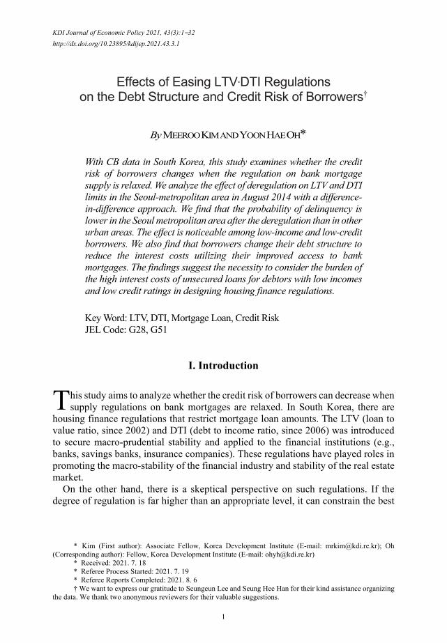
With CB data in South Korea, this study examines whether the credit risk of borrowers changes when the regulation on bank mortgage supply is relaxed. We analyze the effect of deregulation on LTV and DTI limits in the Seoul-metropolitan area in August 2014 with a difference-in-difference approach. We find that the probability of delinquency is lower in the Seoul metropolitan area after the deregulation than in other urban areas. The effect is noticeable among low-income and low-credit borrowers. We also find that borrowers change their debt structure to reduce the interest costs utilizing their improved access to bank mortgages. The findings suggest the necessity to consider the burden of the high interest costs of unsecured loans for debtors with low incomes and low credit ratings in designing housing finance regulations.
Key Word: LTV, DTI, Mortgage Loan, Credit Risk JEL Code: G28, G51
I. Introduction
his study aims to analyze whether the credit risk of borrowers can decrease when supply regulations on bank mortgages are relaxed. In South Korea, there are
housing finance regulations that restrict mortgage loan amounts. The LTV (loan to value ratio, since 2002) and DTI (debt to income ratio, since 2006) was introduced to secure macro-prudential stability and applied to the financial institutions (e.g., banks, savings banks, insurance companies). These regulations have played roles in promoting the macro-stability of the financial industry and stability of the real estate market.
On the other hand, there is a skeptical perspective on such regulations. If the degree of regulation is far higher than an appropriate level, it can constrain the best
* Kim (First author): Associate Fellow, Korea Development Institute (E-mail: [email protected]); Oh
(Corresponding author): Fellow, Korea Development Institute (E-mail: [email protected]) * Received: 2021. 7. 18 * Referee Process Started: 2021. 7. 19 * Referee Reports Completed: 2021. 8. 6 † We want to express our gratitude to Seungeun Lee and Seung Hee Han for their kind assistance organizing
the data. We thank two anonymous reviewers for their valuable suggestions.
T

2 KDI Journal of Economic Policy AUGUST 2021
source of funding, which is inexpensive and offers long-term maturity. Thus, such regulation can deteriorate the debt structure and increase the debt repayment burden. For example, in the words of the Deputy Prime Minister when relaxing the LTV and DTI ratios of bank mortgage loans in July 2014: “Total household debt will increase due to deregulation of real estate, but the credit risk will decrease as the household loan structure improves.” The rationale for this claim is that bank mortgages are the best loan product from a borrower’s standpoint. Therefore, relaxing housing finance regulations may reduce debtors’ credit risk.
Furthermore, the decreased repayment burden caused by LTV and DTI deregulation can be even more substantial for borrowers with low credit scores. There are two possible explanations for this. First, the interest rates of unsecured loans are much higher for borrowers with lower credit scores. Thus, the burden of interest by borrowers who have used unsecured loans due to LTV and DTI limits on bank mortgages would be much more significant for those with low credit ratings. Second, while variations in interest rates in bank mortgages are not notable, the interest rates of non-bank mortgages (e.g., savings banks, capital companies, and credit card companies) rise when a borrower’s credit score decreases. Accordingly, the interest expense for borrowers with low credit ratings may increase further due to LTV restrictions.
Therefore, we analyze whether the relaxation of the LTV and DTI limit on bank mortgages reduces the credit risk of borrowers and whether the effect is more substantial among low-credit borrowers with extensive CB data. To understand the detailed mechanism, we also analyze the impact of the relaxation of housing finance regulations on the share of high-cost loans (the share of loans other than bank mortgage loans) and the repayment burden (Debt Service Ratio(DSR): repayment of principal and interest of all loans relative to annual income). Finally, we assess changes in the debt structure that could reduce the repayment burden considering the reduced credit risk.
LTV limit was relaxed to 70% in all financial institutions in August 2014. Since the LTV limit in the banking sector was 50-70% in the Seoul metropolitan area and 60-70% in other regions before the deregulation, the degree of the deregulation is differential between Seoul metropolitan area and other regions. We use this differential degree of deregulation as an identification strategy based on the difference-in-difference method to find the effect of the deregulation on borrowers’ debt structure and credit risk. Since the LTV limit of bank mortgage was increased more in the Seoul metropolitan area than in other regions, borrowers in Seoul metro area are classified as a treatment group.1
According to our analysis, the probability of delinquency among borrowers in the Seoul metropolitan area is lower than in other areas. This effect was pronounced in borrowers with low incomes and low credit scores. Concerning this decline in credit risk, the debt structure of borrowers was changed, reducing their repayment burden via improved access to bank mortgage loans. This result suggests a need to vary LTV
1On the other hand, the previous LTV limits for mortgages by non-banking institutions, except for insurance
companies, were 60-85% in the Seoul metropolitan area and 70-85% in other areas. Thus, this policy can be seen as a reinforced regulation in non-banking financial institutions. However, here we focus on bank mortgage loans, which are the best loan products in terms of the interest rate, and show that the enhanced accessibility to bank mortgage can improve borrowers' credit risk.
VOL. 43 NO. 3 Effects of Easing LTV·DTI Regulations 3 on the Debt Structure and Credit Risk of Borrowers
and DTI regulations according to the characteristics of borrowers. The composition of this chapter is as follows. Section 2 introduces the literature
in this area and the housing finance regulatory policy. Section 3 provides the data and research hypotheses. Section 4 presents the estimation results. Finally, Section 5 concludes the paper with a summary and policy implications.
II. Review of LTV·DTI in the Literature
A. LTV and DTI and Major Issues
In August 2014, regulations on mortgage loans were relaxed in Seoul metropolitan area, especially in the banking sector. This was done to revitalize domestic demand and boost the housing market over concerns about the economic slowdown.
In South Korea, from the early 2000s to 2014, the LTV and DTI regulatory policies were alternately reinforced or mitigated considering the housing economy, which differs by region. LTV regulation is introduced in September 2003 in South Korea at a 60% level for speculative areas. Then, according to the condition of housing market, LTV·DTI regulations have been strengthened or mitigated. However, regulations on housing finance were eventually eased as the housing economy in some areas slowed after the 2008 global financial crisis. Since 2012, the housing market has been depressed, and the need for the deregulation of housing finance has been discussed. In May 2012, the three districts of Gangnam-gu were excluded from the list of speculative areas, and the deregulation trend continued. In 2013, LTV and DTI regulations were relaxed for first-time home buyers. In July 2014, 70% as the upper limit of the LTV ratio and 60% as the upper limit for DTI were introduced, corresponding to a significantly relaxed level of borrowing regulation compared to the previous level.
Strengthening housing finance regulations may increase borrowers’ risk of default. Table 2 shows the average interest rates and the corresponding differences between mortgage loans and unsecured loans by banking sector or non-banking sector according to the borrower’s credit score, suggesting three crucial facts important in this study, as follows:
1. For both unsecured loans and mortgages, borrowers with lower credit scores
pay higher interest rates. 2. The interest rates on unsecured loans increase rise very steeply as borrowers’
credit ratings worsen, especially in the non-banking sector. 3. In the banking sector, the mortgage interest rate does not vary according to
credit score. Still, the interest rate rises significantly when the credit score worsens in the non-banking sector.
Thus, LTV regulations of bank mortgage loans may keep some borrowers from
obtaining a sufficient amount of bank mortgages with long-term maturities and low-

4 KDI Journal of Economic Policy AUGUST 2021
TABLE 1—CHANGES IN HOUSING FINANCE REGULATIONS BEFORE AND AFTER AUGUST 2014
Before August 2014 After August 2014
Banks & Insurance company Other Non-banking All Institutions
LTV Seoul Metropolitan area 50~70% 60~85%1)
70% Other areas 60~70% 70~85%1)
DTI
Seoul 50% 50~55%2) 60%
Gyeong-gi do Incheon-si 60% 60~65%2)
Other areas none
Note: 1) Including the adjusted limit of financial co-ops (within 15%p), 2) When the housing price is less than KRW 300 million.
Source: “New Economic Policies” (Ministry of Economy and Finance, 24 July 2014).
TABLE 2—AVERAGE INTEREST RATES FOR MORTGAGES AND UNSECURED LOANS
BY INSTITUTION AND CREDIT RATING (UNIT: %)
Credit rating Bank loans interest rates Non-bank loans interest rates
Unsecured Loan
Mortgage Loan Difference Unsecured
Loans Mortgage
Loan Difference
1 (Best) 4.8 4.1 0.7 7.4 5.0 2.4 2 5.0 4.1 0.9 8.8 5.0 3.8 3 5.7 4.2 1.5 12.4 5.0 7.4 4 6.6 4.3 2.3 14.9 5.4 9.5 5 7.7 4.4 3.3 17.0 5.6 11.4 6 8.4 4.4 4.0 18.5 5.9 12.6 7 8.8 4.5 4.3 20.5 6.4 14.1 8 9.5 4.8 4.7 24.1 7.5 16.5 9 10.4 5.3 5.1 22.5 9.2 13.3
10 (Worst) 10.3 5.3 5.0 22.6 8.3 14.3
Note: As of December 2014, based on KCB credit rating.
Source: Provided by KCB, calculated using total borrower data of KCB.
interest rates. As a result, those borrowers may need to receive an additional mortgage from a non-banking institution or an unsecured loan, both of which are relatively expensive. Therefore, stronger regulations on bank mortgages can negatively impact the debt structures of those with low credit ratings. For this reason, we investigate whether the deregulation of bank mortgage loans reduces the probability of a debtor’s delinquency and whether this effect is more noticeable among borrowers with low credit scores.
B. Literature Review
This study is related to previous studies that analyzed LTV and DTI levels and
regulatory changes that affected homeownership and mortgage loans and to studies that analyze the effects of LTV and DTI levels on default outcomes. Mian and Sufi (2009) and Park (2017) are most relevant to this study in that they analyze the effects
VOL. 43 NO. 3 Effects of Easing LTV·DTI Regulations 5 on the Debt Structure and Credit Risk of Borrowers
of changes in housing finance regulations on household credit risk and debt increases. Work by Mian and Sufi (2009) is also similar to our study as they analyze the impact of US housing finance regulations on mortgage delinquency rates. However, Mian and Sufi (2009) focus on the excess supply of credit as one of the factors that caused massive defaults in the US mortgage market in 2007. This is contrary to our finding that deregulation of housing finance regulations can lower the credit risk of borrowers with low credit scores.
The distinction between Mian and Sufi (2009) and this study may be due to the discrepancy between the existing level of housing finance regulation in the US mortgage market before 2007 and the Korean housing finance market situation in 2014. In the case of the United States, there were practically no regulations corresponding to Korea's LTV and DTI limits before the global financial crisis. However, with strict LTV and DTI in South Korea, borrowers inevitably need to use unsecured and non-banking sector loans. In the Seoul metropolitan area in 2014, we find that when the LTV of banking mortgage loans was limited to 50-60%, relaxation of housing finance regulations can reduce the debt repayment burden of borrowers and thus reduce the credit risk.
Park (2017) also uses KCB’s data for each borrower and policy changes in August 2014. Park (2017) notes the necessity of monitoring the possibility that the credit risk of low-income and low-credit borrowers will increase depending on the housing market conditions in the future. On the other hand, this study shows that deregulations can reduce the debt repayment burden through debt restructuring and consequently reduce credit risk. It is also found that reducing credit risk is more pronounced among low-income and low-credit groups.
Choi, Ji, and Cho (2002) found that introducing housing finance regulations could reduce housing demand for households. Igan and Kang (2011) noted that stricter LTV DTI regulations caused a reduction in housing prices and the transaction volume.
Prior studies of the effects of LTV⋅DTI ratios on default risk include those by Ji and Choi (2007), Bang, Park, and Park (2010), Hur (2012), and Kim and Lee (2015). They use borrower-level data and show that borrowers’ higher LTV⋅DTI ratios lead to higher default probabilities. The present study is similar to these studies regarding how credit risk and borrowing structure determinants are analyzed. However, it differs from prior studies using the LTV and DTI levels of borrowers in that it utilizes policy changes that have changed LTV regulatory levels exogenously.
In addition, Jeong (2018) and Lee et al. (2014) are similar to the present study in that they analyze the delinquency factors of borrowers using large-scale borrower-unit credit information data. However, unlike this study, Jeong (2018) and Lee et al. (2014) did not directly analyze the effects of exogenous policy changes.
III. Data and Empirical Strategy
A. Data
We use data from the Korea Credit Bureau (KCB), one of Korea’s leading credit
rating companies, covering the whole Korean population. A 10% random sample of population data was provided with borrowers who take a mortgage loan between

6 KDI Journal of Economic Policy AUGUST 2021
2008 and 2018. The data covers account-level monthly information, including delinquencies, opening and maturity dates, repayment method, loan amount, monthly loan balance, and the financial institution. It covers all financial institutions including non-banks and all types of loans including unsecured loans. Thus, we can use obtain a detailed picture of all loans held by individual borrowers. The characteristics of the borrowers include the borrower’s age, occupation, residential address, DTI, income, credit score, and credit rating. We use delinquency information of 30 business days or more in any loan. We also use regional housing price trend data from the Korea Real Estate Board to control for fluctuations in regional housing prices. Specifically, the year-on-year increase in house prices one month before creating a new account is used as a control variable. This allows us to control the effects of expected price hikes in each region on our empirical results.
This study analyzes the effects of deregulation on bank mortgage loans on borrowers’ credit risk and debt structure outcomes. Therefore, it is necessary to construct a sample of borrowers who already had a mortgage loan before the deregulation. We also need to confine the sample to borrowers who used other loans due to housing finance regulations, even if they still sought additional funds in the form of bank mortgage loans. Therefore, we only analyze debtors who concurrently held bank mortgage loans and other types of loans (unsecured loans and other mortgage loans) or who held non-bank mortgage loans as of July 2014. In other words, we exclude borrowers with bank mortgage loans only among the debtors who held mortgage loans just before the deregulation. In Appendix 1, we compare the debt structure of the borrowers to be analyzed and that of total borrowers by comparing the overall loan balance for each financial sector. Also, we examine differences in the maturity structure and repayment method between the borrowers to be analyzed and all borrowers.
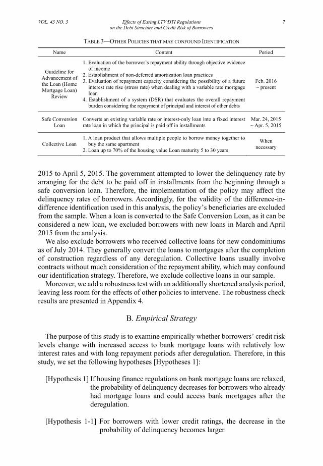
Policies regulating the housing market have been announced frequently compared to those in other areas of the economy. Table 3 shows the policies, other than LTV and DTI deregulation, which may confound our difference-in-difference identification strategy within our analysis period.
First, we analyze the sample period between January 2013 and January 2016 to exclude the effects of other policies that may confound our difference-in-difference identification based on housing finance deregulation. By limiting the sample period, we could exclude the impact of the “Guideline for the Advancement of Loan (Home Mortgage Loan) Reviews” implemented in February and May 2016. It was introduced to establish advanced credit practices focusing on the repayment capacity by reflecting the borrower’s income and debt accurately and comprehensively during the review process. As the access to an additional loan would be difficult due to this policy, the probability of delinquency can increase among debtors who already held loans. On the other hand, the total delinquency rate can also decrease as banks started to screen debtors in terms of risk more accurately. Therefore, we limited our sample period up to January 2016.
Second, we excluded several debtors from the sample. On March 24, 2015, the Financial Services Commission launched the “Safe Conversion Loan” of 2.5~2.6% per annum through 16 banks. The Safe Conversion Loan is a policy that converts an existing variable rate or interest-only loan into a fixed interest rate loan in which the principal is paid off in installments. This policy was implemented from March 24,
VOL. 43 NO. 3 Effects of Easing LTV·DTI Regulations 7 on the Debt Structure and Credit Risk of Borrowers
TABLE 3—OTHER POLICIES THAT MAY CONFOUND IDENTIFICATION
Name Content Period
Guideline for Advancement of the Loan (Home Mortgage Loan)
Review
1. Evaluation of the borrower’s repayment ability through objective evidence of income
2. Establishment of non-deferred amortization loan practices 3. Evaluation of repayment capacity considering the possibility of a future
interest rate rise (stress rate) when dealing with a variable rate mortgage loan
4. Establishment of a system (DSR) that evaluates the overall repaymentburden considering the repayment of principal and interest of other debts
Feb. 2016 ~ present
Safe Conversion Loan
Converts an existing variable rate or interest-only loan into a fixed interest rate loan in which the principal is paid off in installments
Mar. 24, 2015 ~ Apr. 5, 2015
Collective Loan 1. A loan product that allows multiple people to borrow money together to
buy the same apartment 2. Loan up to 70% of the housing value Loan maturity 5 to 30 years
When necessary
2015 to April 5, 2015. The government attempted to lower the delinquency rate by arranging for the debt to be paid off in installments from the beginning through a safe conversion loan. Therefore, the implementation of the policy may affect the delinquency rates of borrowers. Accordingly, for the validity of the difference-in-difference identification used in this analysis, the policy’s beneficiaries are excluded from the sample. When a loan is converted to the Safe Conversion Loan, as it can be considered a new loan, we excluded borrowers with new loans in March and April 2015 from the analysis.
We also exclude borrowers who received collective loans for new condominiums as of July 2014. They generally convert the loans to mortgages after the completion of construction regardless of any deregulation. Collective loans usually involve contracts without much consideration of the repayment ability, which may confound our identification strategy. Therefore, we exclude collective loans in our sample.
Moreover, we add a robustness test with an additionally shortened analysis period, leaving less room for the effects of other policies to intervene. The robustness check results are presented in Appendix 4.
B. Empirical Strategy
The purpose of this study is to examine empirically whether borrowers’ credit risk
levels change with increased access to bank mortgage loans with relatively low interest rates and with long repayment periods after deregulation. Therefore, in this study, we set the following hypotheses [Hypotheses 1]:
[Hypothesis 1] If housing finance regulations on bank mortgage loans are relaxed,
the probability of delinquency decreases for borrowers who already had mortgage loans and could access bank mortgages after the deregulation.
[Hypothesis 1-1] For borrowers with lower credit ratings, the decrease in the
probability of delinquency becomes larger.

8 KDI Journal of Economic Policy AUGUST 2021
[Hypothesis 1-2] For the borrowers with lower incomes, the decrease in the probability of delinquency becomes larger.
Deregulation also can increase the overall credit risk in the whole economy, as the
total amount of household loans may increase. However, this study only focuses on changes in the credit risk of borrowers who already had mortgage loans and whose access to bank mortgages is constrained despite the demand for additional loans. For these borrowers, improved access to bank mortgage loans may represent an opportunity to change their debt structure at a low cost and to gain a bank mortgage with a long-term maturity.
We also examine whether the extent of the reduction in credit risk is more noticeable for borrowers with worse credit ratings (Hypothesis 1-1). As shown in Table 2, the lower and worse credit score is (i.e., with a higher credit rating) related to the larger the difference in interest rates between bank mortgages and other loans. This can cause the burden of higher interest rates due to housing finance regulations for the low-credit class. Therefore, the decrease in the probability of delinquency when regulations are relaxed may be more pronounced for the low-credit class.
In addition, because incomes and credit ratings are partially related, the decrease in the credit risk is also expected to rise as income decreases. However, for some borrowers with low incomes, their asset possessions can be considerable; therefore, Hypothesis 1-2 is separately established and analyzed.
Suppose the credit risk of a borrower decreases, as in Hypothesis 1. In such a case, this may stem from the borrower converting loans with relatively high interest rates to low-interest bank mortgage loans, also converting short-term unsecured loans to long-term mortgage loans. The change in the debt structure can decrease the interest and monthly repayment burden. Therefore, we also set Hypothesis 2 to analyze whether the relaxation of housing finance regulations affects the debt structure of borrowers.
[Hypothesis 2] With the relaxation of housing finance regulations on bank
mortgages, the repayment burden of borrowers with access to bank mortgage loans is reduced.
[Hypothesis 2-1] The ratio of high-interest loans of borrowers will decrease. [Hypothesis 2-2] The ratio of repayment to the income of borrowers will decrease. To test the hypotheses, we exploit the housing financial deregulation policy of
August 2014 as an identification strategy in the differentiation-in-difference method. Before the policy, the LTV limit in the banking sector was 50-70% in the Seoul metropolitan area and 60-70% in non-metropolitan areas. However, the deregulation relaxed the LTV limit to 70% for all financial institutions in all areas. Therefore, after deregulation, the LTV limit for mortgage loans in the banking sector was further eased in the Seoul metropolitan area compared to non-metropolitan areas. Therefore, we classify residents of the Seoul metropolitan area as the treatment group, while those in non-metropolitan areas are the control group.
In order to achieve unbiased estimates of the deregulation effect through the

VOL. 43 NO. 3 Effects of Easing LTV·DTI Regulations 9 on the Debt Structure and Credit Risk of Borrowers
difference-in-difference method, the parallel trend assumption must be satisfied. In this analysis, the LTV regulation is considered to be relaxed in all areas, but the magnitude of the deregulation has been greater in the Seoul metropolitan area. Thus, we also assume that the magnitude of the deregulation would have been identical if the degree of deregulation was also identical.
For the regression analysis, we use equation (1) for the main estimation. The dependent variable ,i ty represents borrower i ’s credit risk or debt structure at period t . As dependent variables, we consider whether one of the borrower’s loan accounts was delinquent for more than 30 days within six months after a mortgage account is opened as a measure of credit risk. Note that delinquencies in this study are not limited only to mortgage loans. This measure has a value of 1 when it occurs for more than 30 days in any of the accounts held by the borrower. Regarding the change in the debt structure, we use the high-cost loan ratio (share of loans excluding bank mortgage loans among loans) and the debt service ratio (DSR) referring to the debt repayment burden relative to income. Because the occurrence of a delinquency for more than 30 days can be observed over a considerably long period, we use semiannual observations (January and July). We use monthly observations for the high-cost loan ratio and DSR.
(1) , 0 1408 1408 1408 , ,i t DD Sudo Sudo Sudo i t i ty D D D D X
Here, 1408D is a dummy variable indicating the period after August 2014, when the housing finance regulation in the Seoul metropolitan area was relaxed. SudoD is a dummy variable representing the residents of the Seoul metropolitan area at that time, who belong to the treatment group. ,i tX is a matrix that represents a group of control variables that may affect the borrower’s credit risk and debt structure. This matrix includes individual debtors’ characteristics, such as their ages, average incomes, and credit ratings, including their credit and debit card usage statistics in the previous year. In addition, macroeconomic variables such as the CD91 interest rate (monthly), consumer price index (monthly), real GDP (quarters), and real GRDP (quarter) are also included as control variables. Finally, city-level fixed effects are included in the model.
The coefficient DD in equation (1) shows the effect of the housing finance deregulation, which is a measure of whether the average value of the dependent variable has changed further in the Seoul metropolitan area compared to those in non-metropolitan areas after the event. Therefore, if there is a decrease in the credit risk and a decrease in the repayment burden of borrowers in the metropolitan area, where the extent of deregulation on housing finance was larger, a negative estimate of DD is expected, which supports Hypothesis 1.
We also find that the effects of deregulation on a delinquency outcome can differ according to income, credit score, and the existing debt structure. Thus, each sample was classified according to income and credit rating, and for each subsample we also ran estimates using equation (1). The classification criteria for low, middle and high credit ratings, the income quintile, and the existing debt structure are described in detail in Section 4.

10 KDI Journal of Economic Policy AUGUST 2021
C. Descriptive Statistics
This section examines the proportion of debtors who took out bank mortgages after deregulation in the Seoul metropolitan area. It examines whether they tend to reduce their non-bank mortgage loans or unsecured loans. In August 2014, the same deregulation took place in the banking and insurance sectors, but insurance was classified as a non-bank sector in this section. An analysis that categorized the sample into bank/insurance mortgage loans and other secured loans was also conducted. These results are very similar, and the analysis is presented in Appendix 2.
Borrowers who hold only bank mortgage loans and no unsecured loans account for the largest share in the original sample. However, they are excluded from the analysis because there is no room for improvement in the debt structure.
As of July 2014, just before the deregulation, those in category (A), who hold both bank mortgage loans and unsecured loans, accounted for 34.3% of the total. On the other hand, the proportion of borrowers who have both bank and non-bank mortgage loans at the same time was small at about 3.6%. In January 2016, a year and a half after the deregulation, the proportion of borrowers who had only bank mortgage loans without unsecured loans decreased, while the proportion of borrowers who had both bank and non-bank mortgage loans increased. In addition, the average credit rating for each debt structure classification remained similar. In sum, the proportion of borrowers who can access bank mortgage loans in the Seoul metropolitan area after the deregulation has remained relatively constant.
After deregulation, the proportion of debtors who opened bank mortgages was largest at 33.7% in the group with bank mortgage loans and unsecured loans, while this rate was 27% in the group with bank and non-bank mortgage loans at the same time. Moreover, 20-30% of borrowers in each category have increased their total loans since the deregulation. This appears to reflect that it is easy for borrowers who already had a bank mortgage to open a new mortgage loan account within the same sector after deregulation due to the characteristics of the mortgage product. Groups with unsecured loans include a higher proportion of debtors opening bank mortgage
TABLE 4—DEBT STRUCTURE OF MORTGAGE LOAN HOLDERS BEFORE AND AFTER THE DEREGULATION
(BORROWERS IN THE SEOUL METROPOLITAN AREA)
Timing of observation Jul. 2014 Jul. 2014- Jan. 2016 Jan. 2016
Debt structure (as of Jul. 2014) ProportionAvg.
Credit rating
Proportion of borrowers with new
bank mortgage Proportion
Avg. Credit rating
Only bank mortgage loans + no unsecured loans 46.7 3.3 44.0 3.3
Only bank mortgage loans + unsecured loans A 34.3 3.7 33.7 34.8 3.6
Mortgage loans from both banks and the non-bank sector
Secured loans B1 1.9 4.6 27.8 3.1 4.5
No Secured loans B2 1.7 3.6 26.6 2.7 3.6
Only non-bank mortgage loans
Secured loans C1 7.2 4.8 12.9 7.2 4.6
No Secured loans C2 8.3 3.6 10.8 8.1 3.6
Note: Borrowers with group loan in Jul 2014 and the Secure Convertible loan in Mar. 2015 are excluded.
Source: Authors’ calculation using a sample of KCB borrowers.

VOL. 43 NO. 3 Effects of Easing LTV·DTI Regulations 11 on the Debt Structure and Credit Risk of Borrowers
TABLE 5—CHANGE IN THE SHARE OF NON-BANK MORTGAGE LOANS AMONG WHOM OPENED A NEW BANK MORTGAGE ACCOUNT AFTER DEREGULATION
(UNIT: KRW 1,000, %, BORROWER IN THE SEOUL METROPOLITAN AREA)
Classification (As of Jul. 2014)
(Based on initial loan amount) (Based on loan balance)
Change Share of borrowers
who reduced non-bank mortgages
Change Share of borrowers
who reduced non-bank mortgages
Mortgage loans from both banks and the
non-bank sector
Secured loans B1 -56,226.9 45.9 -49,961.7 59.7
No Secured loans B2 -48,747.8 46.8 -38,933.26 60.4
Only non-bank mortgage loans
Secured loans C1 -106,497.9 77.7 -100,663.9 83.0
No Secured loans C2 -99,336.6 77.0 -86,547.3 82.8
Source: Authors’ calculation using a sample of KCB borrowers.
loans after the deregulation compared to other groups, which may be due to the incentive to convert high-interest-rate unsecured loans to bank mortgage loans.
Table 5 describes whether borrowers who opened a new bank mortgage account after deregulation reduced their amounts of non-bank mortgage loans. The average loan contract amount and loan balance decreased in all categories, and the average reduction amount ranged from 38 million won to 100 million won. When calculating the proportion of those who have reduced non-bank mortgage loan, in terms of the loan balance, it represents approximately 60% of those who hold bank and non-bank mortgage loans simultaneously and about 83% of those who have only non-bank mortgage loans. Therefore, among the non-bank mortgage loan holders in the metropolitan area, the proportion of those newly opening bank mortgage loans after deregulation is low, but most of them reduce the amounts of their non-bank mortgage loans, suggesting that additional borrowing in the form of bank loans improves their debt structures.
Table 6 shows the changes in unsecured loans after deregulation by borrowers who newly took out bank mortgages. The average amount of these loans increased after deregulation for the group that held bank mortgage loans and unsecured loans. However, for those who had non-bank mortgage loans, the average loan amount decreased. Calculating the share of those for whom the loan amount was reduced, we find that more than half reduced the unsecured loans in all cases. Therefore, it is
TABLE 6—AVERAGE CHANGE IN UNSECURED LOANS AMONG WHOM OPENED
NEW BANK MORTGAGE ACCOUNTS AFTER DEREGULATION (UNIT: KRW 1,000, %, BORROWER IN THE SEOUL METROPOLITAN AREA)
Classification (As of July 2014) Change in Amount of Unsecured Loans
Share of borrowers Who reduced unsecured loans
Only bank mortgage loans + unsecured loans A 1,122.90 53.82 Mortgage loans from both banks and the non-bank
sector + unsecured loans B1 -18,985.88 61.81
Only non-bank mortgage loans + unsecured loans C1 -3,463.53 59.57
Note: Borrowers who opened a new bank mortgage account between Jul. 2014 and Jan. 2016.
Source: Authors’ calculation using a sample of KCB borrowers.

12 KDI Journal of Economic Policy AUGUST 2021
believed that after the deregulation in the metropolitan area, mortgage loan holders who additionally took out bank mortgages tended to improve their debt structure. Based on these descriptive statistics, we utilized the difference-in-differences method to determine the effects of the LTV deregulation on credit risks and the debt structure of borrowers.
IV. Empirical Results
A. Impact of Deregulation on Credit Risk
This section analyzes the effect of easing housing finance regulation on the
delinquency rate exceeding 30 business days. Here, delinquency refers to an overdue record on any loan held by the borrowers, including mortgage loans, unsecured loans, and other secured loans.
Table 7 shows the effect of the housing finance deregulation on the probability of a delinquency. Because we use the difference-in-difference method, a negative estimate of the interaction term between the Seoul metropolitan area and the time dummy(after August 2014) suggests that the borrower’s credit risk decreased after the deregulation. The first column stands for estimates using the full sample, and it shows that the delinquency rate decreases by approximately 0.22%p after the deregulation. Considering that the average delinquency rate is close to 1.4%, the deregulation (increase in the LTV limit by 10-20 (%p)) decreases the delinquency rate of borrowers about 15.7%. In other words, the improvement of accessibility to bank mortgages can lower the credit risk of borrowers.
The second and third columns of Table 7 show the estimates for the subsample with a history of being overdue exceeding five days and without overdue between January 2013 and July 2014, just before the deregulation. This comparison examines the heterogeneous effects of deregulation for groups who experienced a liquidity constraint and those who did not. The deregulation reduces the delinquency rate significantly only for those who have experienced liquidity constraints before the deregulation. This suggests that the group suffering from liquidity constraints is more likely to change the debt structure after the deregulation.
Moreover, the delinquency rate tends to increase with older age, worse credit rating, higher CD rates, and lower-income. These results are sensible in expecting the effect of each factor on the probability of delinquency.2
2 TABLE 1-1. DEFAULT RATE BY CREDIT RATING GROUP Credit Rating Companies 1 2 3 4 5 6 7 8 9 10
NICE 0.05 0.16 0.34 0.51 0.7 1.82 6.29 9.79 11.87 33.03 KCB 0.06 0.11 0.22 0.56 1.31 3.47 7.88 17.79 37.12 75.43
Note: Credit ratings is calculated at the end of 2017 and default information is at the end of 2018 (one year later than 2017). The main regression analysis in Table 7 included credit rating variables from the first to fourth order terms.
According to Table 1-1, the probability of delinquency surges as the credit rating changes by one. As the nonlinear relationship between the credit rating and delinquency rate is remarkable, the high-order terms of the credit rating are included. Otherwise, when we include only the first-order term of the credit rating, the coefficient of annual income was estimated to be a positive value, somewhat insensible (in Table A5).

VOL. 43 NO. 3 Effects of Easing LTV·DTI Regulations 13 on the Debt Structure and Credit Risk of Borrowers
TABLE 7—EFFECTS OF HOUSING FINANCE DEREGULATION ON THE DELINQUENCY RATE
Sample
Variable
Dependent Variable: Experience of 30+ days Delinquency in any Loans (Dummy)
(1) Whole sample
(2) With delinquency record before the deregulation
(3) Without delinquency record
before the deregulation
Seoul Metro. Area x Afterderegulation (dummy)
-0.0022*** (0.00068)
-0.023*** (0.0046)
0.00017 (0.00035)
Seoul Metro. Area (dummy) -0.0058 (0.0074)
-0.036 (0.048)
-0.0025 (0.0037)
After deregulation (dummy) 0.0030*** (0.0010)
0.017*** (0.0067)
0.0019*** (0.00057)
Age (unit: 5 years interval) 0.000050*** (0.000015)
0.00055*** (0.00010)
-2.7e-06 (6.9e-06)
ln (income) -0.0017*** (0.00027)
0.00067 (0.0022)
-0.00026** (0.00012)
Credit rating (Level 1-10)
0.016*** (0.0023)
0.12*** (0.0088)
-0.010*** (0.0014)
1 year credit card usage amount (one million won)
-0.000088*** (6.5e-06)
-0.00023*** (0.000081)
-8.7e-06*** (1.5e-06)
1 year debit card usage amount (one million won)
0.000061** (0.000024)
-0.000017 (0.000097)
6.2e-06* (3.7e-06)
cd 91 interest rates 0.0066*** (0.0012)
0.060*** (0.0079)
-0.00089 (0.00068)
CPI (Inflation Rate) 0.00059 (0.00038)
0.0043 (0.0027)
-0.000010 (0.00016)
GRDP (regional economy) 4.6e-08 (3.0e-08)
3.2e-07 (1.9e-07)
1.2e-08 (1.5e-08)
GDP 8.4e-08*** (2.2e-08)
6.8e-07*** (1.6e-07)
1.6e-08* (8.9e-09)
Housing price growth (YoY, 1 month lag)
0.00022 (0.00015)
0.0011 (0.0010)
0.00023*** (0.000060)
Constant -0.11*** (0.034)
-1.00*** (0.25)
0.0040 (0.014)
N 719,675 89,354 630,321
R2 0.193 0.237 0.043
Note: 1) Statistical significance level: ***p<0.01, **p<0.05, *p<0.1, 2) All standard errors were calculated as Huber-White robust standard errors, 3) The metropolitan and year fixed effect and the second, third, and fourth terms of credit rating are included in the regressions but not reported, 4) This was calculated using information on a semiannual basis (January, July), and 30-day delinquency refers to a case in which more than 30 days of delinquency occur among any loans (including unsecured loans) held by the borrower within the preceding six months, 5) A group with past delinquency is composed of borrowers with a record of more than five days overdue in any loans as of July 2014, 6) The numbers of borrowers of each sample (columns (1),(2),(3)) were 206,361, 33,650 and 172,711 respectively.
As the effect of the deregulation on delinquency rate can be more pronounced for
borrowers with more severe liquidity constraints, we need to see whether borrowers with worse credit ratings are more likely to be affected by the deregulation. Thus, we perform the above analysis separately for each credit rating group. Based on the KCB credit rating at the first observation in the sample, borrowers are classified into three groups, a high-credit (1~3 in the KCB ratings), a medium-credit (4~6), and a low-credit (7~10). Note that credit rate 1 is the best rate and 10 is the worst credit

14 KDI Journal of Economic Policy AUGUST 2021
TABLE 8—NUMBER OF BORROWERS BY CREDIT RATING GROUP
Credit rating group
High-credit borrower Medium-credit borrower Low-credit borrower
Credit rating 1~3 3~4 7~10
Observations 110,873 71,295 24,193
Source: Authors’ calculation using a sample of KCB borrowers.
TABLE 9—EFFECTS OF HOUSING FINANCE DEREGULATION ON THE DELINQUENCY RATE: BY CREDIT RATING
Sample
Variable
Dependent Variable: Experience of 30+ days Delinquency in any Loans (Dummy)
(1) High-credit borrower
(Levels 1~3)
(2) Medium-credit borrower
(Levels 4~6)
(3) Low-credit borrower
(Levels 7~10)
Seoul Metro. Area x After deregulation (dummy)
-0.000048 (0.00019)
-0.0017** (0.00083)
-0.011** (0.0055)
Seoul Metro. Area (dummy) -0.0023 (0.0021)
-0.0036 (0.0081)
0.00078 (0.054)
After deregulation (dummy) 0.000021 (0.00032)
0.0020 (0.0013)
0.019** (0.0086)
N 399,049 241,261 79,365 R2 0.000 0.004 0.157
Note: 1) Statistical significance level: ***p<0.01, **p<0.05, *p<0.1, 2) All standard errors were calculated as Huber-White robust standard errors, 3) Additional explanatory variables: age, income, credit rating, credit card usage for the previous year, debit card usage for the previous year, CD interest rates, CPI, GRDP, GDP, housing price growth, constant terms, fixed effects of metropolitan cities, 4) Semiannual basis (January, July) information is utilized, and delinquency refers to an occurrence of more than 30 days overdue in any loans held by borrowers, 5) The numbers of borrowers of each sample (columns (1),(2),(3)) were 110,873, 71,295, and 24,193, respectively.
rating.3
Table 9 shows estimates of the effect of housing finance deregulation by each credit rating group. The deregulation lowers the credit risk of borrowers with poor credit ratings. When LTV of bank mortgage loans was eased by 10-20 (%p), the average delinquency rate for borrowers with the worst credit ratings decreased by about 1.1%p, showing the most significant decline. While, the average delinquency rate declined by 0.17%p for borrowers with mid-level credit ratings. The effect of the credit risk declines greater with lower credit rating when the housing finance regulation is eased. As the credit rating worsens, the reduction in the debt repayment burden becomes more significant. It is because, as suggested in Table 2, the interest rate on unsecured loans increases steeply as the credit rating worsens, especially in the non-banking sector.
Although the correlation between the credit rating and income is high, borrowers with low credit ratings and low-income groups do not necessarily show a perfect match. Therefore, we conduct the same analysis according to the income segment.4
3Table 8 shows the number of borrowers of each credit rating group. In the sample, the proportion of low-credit
borrowers is relatively small because the sample in this analysis consists only of borrowers with mortgages. 4 One of the most important factors determining a credit rating is a history of past overdue payments.

VOL. 43 NO. 3 Effects of Easing LTV·DTI Regulations 15 on the Debt Structure and Credit Risk of Borrowers
TABLE 10—DEFINITION OF INCOME SEGMENT BY NATIONAL TAX SERVICE (ATTRIBUTABLE TO 2014~16)
Income segment Tax rate segment
1 12 million won or less
2 More than 12 million won and less than 46 million won
3 More than 46 million won and less than 88 million won
4 More than 88 million won and less than 150 million won
5 More than 150 million won
TABLE 11—EFFECTS OF HOUSING FINANCE DEREGULATION ON THE DELINQUENCY RATE:
BY INCOME SEGMENT
Sample
Variable
Dependent Variable: Experience of 30+ days Delinquency in any Loans (Dummy)
(1) Income segment
1
(2) Income segment
2
(3) Income segment
3
(4) Income segment
4
(5) Income segment
5
Seoul Metro. Area x Afterderegulation (dummy)
-0.025 (0.016)
-0.0034*** (0.00096)
-0.00093 (0.00085)
-0.00016 (0.0017)
0.0028 (0.0069)
Seoul Metro. Area (dummy) -0.088 (0.12)
-0.0015 (0.010)
-0.019** (0.0093)
0.011 (0.018)
0.065 (0.089)
After deregulation (dummy) -0.0017 (0.022)
0.0049*** (0.0014)
0.00075 (0.0013)
-0.00027 (0.0025)
-0.015* (0.0087)
N 405 463,079 208,103 41,670 6,418
R2 0.166 0.194 0.197 0.128 0.216
Note: 1) Statistical significance level: ***p<0.01, **p<0.05, *p<0.1, 2) All standard errors were calculated as Huber-White robust standard errors, 3) Additional explanatory variables: age, income, credit rating, credit card usage for the previous year, debit card usage for the previous year, CD interest rates, CPI, GRDP, GDP, housing price growth, constant terms, fixed effects of metropolitan cities, 4) Semiannual basis (January, July) information is utilized, and delinquency refers to an occurrence of more than 30 days overdue in any loans held by borrowers, 5) The sample comprises borrowers holding bank mortgages with other types of loans together and borrowers holding non-bank mortgages as of July 2014, 6) The number of borrowers corresponding to each sample were 128, 138,116, 56,576, 9,986, and 1,555, respectively.
The definition of the income segment is based on the tax rate segment of the National Tax Service as of 2014. As summarized in Table 10, the first segment corresponds to borrowers with the lowest annual income. The higher number of income segment shows higher the annual income.
Table 11 shows the estimates of the regression difference-in-difference method for each income segment. The decline of delinquencies after relaxing the housing finance regulation is greater with the lower income level. In income segment 1, the coefficient estimate is prominent, but the number of observations is insufficient, resulting in a statistically insignificant estimate. In income segment 2, the decline in the delinquency rate due to the relaxation of the housing finance regulation is most noticeable. In particular, the average delinquency rate for borrowers in the second
Delinquency risk is closely linked not only to the income of the borrower but also to assets. For example, for retired borrowers in their 60s or older, the income range is estimated to be low. In contrast, the incidence of delinquency is not high due to a high level of assets and, as a result, the credit rating is often high.

16 KDI Journal of Economic Policy AUGUST 2021
TABLE 12—CHANGES IN DELINQUENCY RATES AFTER THE DEREGULATION: NEW BANK MORTGAGE ACCOUNT
Sample
Variable
Dependent Variable: Experience of 30+ days Delinquency in any Loans (Dummy)
(1) opening new bank mortgages account after the deregulation
(2) Without opening new bank mortgages account after the deregulation
After deregulation (dummy) -0.0031*** (0.00069)
0.0050*** (0.0016)
N 154,016 359,462
R2 0.020 0.224
Note: 1) Statistical significance level: ***p<0.01, **p<0.05, *p<0.1, 2) All standard errors were calculated as Huber-White robust standard errors, 3) Additional explanatory variables: age, income, credit rating, credit card usage for the previous year, debit card usage for the previous year, CD interest rates, CPI, GRDP, GDP, housing price growth, constant terms, fixed effects of metropolitan cities, 4) Semiannual basis (January, July) information is utilized, and delinquency refers to an occurrence of more than 30 days overdue in any loans held by borrowers, 5) The sample comprises borrowers holding bank mortgages with other types of loans together and borrowers holding non-bank mortgages as of July 2014.
income segment falls by 0.34%p.
We show that the housing finance deregulation in the banking sector reduces the credit risk of the borrowers, and this can be achieved by adjusting the debt structure to reduce the burden of debt repayment.
Table 12 shows the estimates of the change in the delinquency rate after the deregulation. The sample is divided into two groups that newly opened bank mortgage account after the deregulation and that did not. The delinquency rate decreased significantly for the borrowers who newly opened a mortgage loan in the banking sector. Considering that the average delinquency rate in the Seoul metropolitan area was 1.85%, this decrease in delinquencies is more than 15%. On the other hand, in the group that did not open a new bank mortgage account, the delinquency rate increased by about 0.5%p, which is a 26% change. This result suggests that borrowers may change their debt structure to reduce their debt repayment burden by using a bank mortgage loan after the housing finance deregulation. The delinquency rate may decrease consequently. In the next section, the change in the debt structure, leading to a reduction in the delinquency rate, will be examined in more detail.
Table 13 shows the estimates of the deregulation effect for each group divided by the debt structure of borrowers as of July 2014. After the deregulation, delinquency rate decreased the most with the borrowers who owned additional loans with mortgage loans. In particular, the delinquency rate decreases by 0.6%p when the housing finance regulation is eased in the group that holds non-bank mortgages and additional unsecured loans.
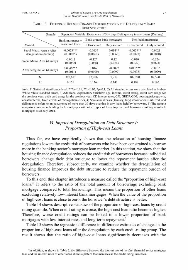
VOL. 43 NO. 3 Effects of Easing LTV·DTI Regulations 17 on the Debt Structure and Credit Risk of Borrowers
TABLE 13—EFFECTS OF HOUSING FINANCE DEREGULATION ON THE DELINQUENCY RATE: DEBT STRUCTURE
Sample
Variable
Dependent Variable: Experience of 30+ days Delinquency in any Loans (Dummy)
Bank mortgages + unsecured loans
Bank or non-bank mortgages Non-bank mortgages
+ Unsecured Only secured + Unsecured Only secured
Seoul Metro. Area x After deregulation (dummy)
-0.0023*** (0.00075)
-0.0059 (0.0061)
0.014** (0.0063)
-0.0059** (0.0027)
-0.0021 (0.0020)
Seoul Metro. Area (dummy) -0.0011 (0.0082)
-0.12* (0.068)
0.12 (0.074)
-0.020 (0.029)
-0.024 (0.023)
After deregulation (dummy) 0.0046*** (0.0011)
0.016 (0.0100)
-0.0097 (0.0097)
0.011*** (0.0038)
-0.0015 (0.0029)
N 390,617 12,706 7,712 102,220 89,580 R2 0.151 0.136 0.141 0.199 0.180
Note: 1) Statistical significance level: ***p<0.01, **p<0.05, *p<0.1, 2) All standard errors were calculated as Huber-White robust standard errors, 3) Additional explanatory variables: age, income, credit rating, credit card usage for the previous year, debit card usage for the previous year, CD interest rates, CPI, GRDP, GDP, housing price growth, constant terms, fixed effects of metropolitan cities, 4) Semiannual basis (January, July) information is utilized, and delinquency refers to an occurrence of more than 30 days overdue in any loans held by borrowers, 5) The sample comprises borrowers holding bank mortgages with other types of loans together and borrowers holding non-bank mortgages as of July 2014.
B. Impact of Deregulation on Debt Structure I:
Proportion of High-cost Loans
Thus far, we have empirically shown that the relaxation of housing finance regulations lowers the credit risk of borrowers who have been constrained to borrow more in the banking sector’s mortgage loan market. In this section, we show that the housing finance deregulation reduces the credit risk of borrowers because individual borrowers change their debt structure to lower the repayment burden after the deregulation. Therefore, subsequently, we examine whether the deregulation of housing finance improves the debt structure to reduce the repayment burden of borrowers.
To this end, this chapter introduces a measure called the “proportion of high-cost loans.” It refers to the ratio of the total amount of borrowings excluding bank mortgage compared to total borrowings. This means the proportion of other loans excluding relatively low-interest bank mortgages. When the value of the proportion of high-cost loans is close to zero, the borrower’s debt structure is better.
Table 14 shows descriptive statistics of the proportion of high-cost loans by credit rating quantile. When credit rating is worse, the high-cost loan ratio becomes higher. Therefore, worse credit ratings can be linked to a lower proportion of bank mortgages with low-interest rates and long-term repayment.5
Table 15 shows the regression difference-in-difference estimates of changes in the proportion of high-cost loans after the deregulation by each credit-rating group. The result shows that the ratio of high-cost loans significantly decreases with the
5In addition, as shown in Table 2, the difference between the interest rate of the first financial sector mortgage
loan and the interest rates of other loans shows a pattern that increases as the credit rating increases.
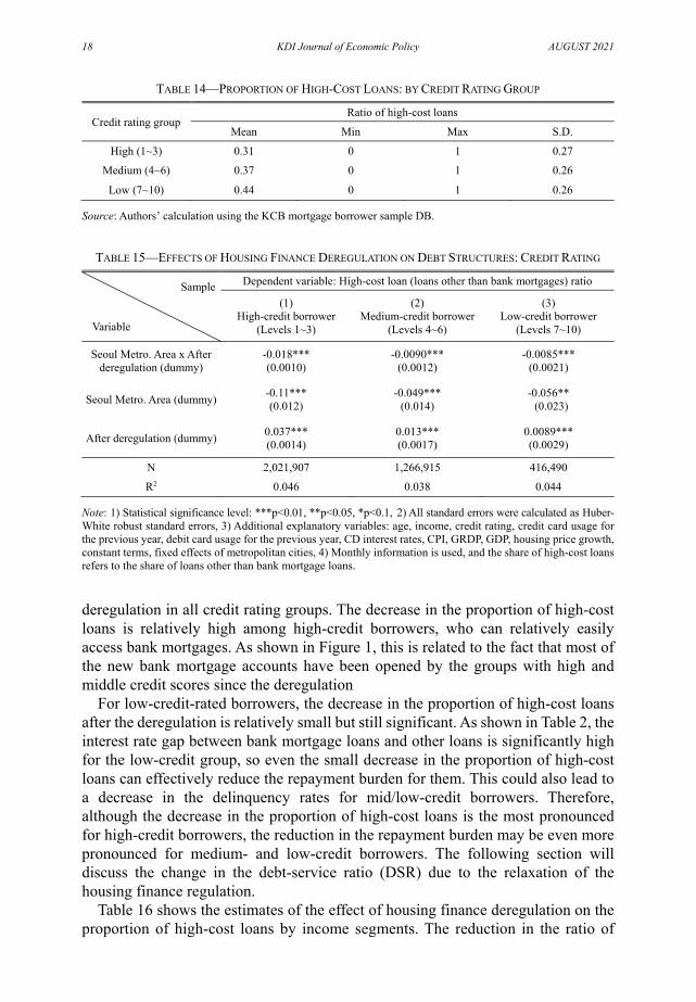
18 KDI Journal of Economic Policy AUGUST 2021
TABLE 14—PROPORTION OF HIGH-COST LOANS: BY CREDIT RATING GROUP
Credit rating groupRatio of high-cost loans
Mean Min Max S.D.
High (1~3) 0.31 0 1 0.27 Medium (4~6) 0.37 0 1 0.26
Low (7~10) 0.44 0 1 0.26
Source: Authors’ calculation using the KCB mortgage borrower sample DB.
TABLE 15—EFFECTS OF HOUSING FINANCE DEREGULATION ON DEBT STRUCTURES: CREDIT RATING
Sample
Variable
Dependent variable: High-cost loan (loans other than bank mortgages) ratio
(1) High-credit borrower
(Levels 1~3)
(2) Medium-credit borrower
(Levels 4~6)
(3) Low-credit borrower
(Levels 7~10)
Seoul Metro. Area x Afterderegulation (dummy)
-0.018*** (0.0010)
-0.0090*** (0.0012)
-0.0085*** (0.0021)
Seoul Metro. Area (dummy) -0.11*** (0.012)
-0.049*** (0.014)
-0.056** (0.023)
After deregulation (dummy) 0.037*** (0.0014)
0.013*** (0.0017)
0.0089*** (0.0029)
N 2,021,907 1,266,915 416,490 R2 0.046 0.038 0.044
Note: 1) Statistical significance level: ***p<0.01, **p<0.05, *p<0.1, 2) All standard errors were calculated as Huber-White robust standard errors, 3) Additional explanatory variables: age, income, credit rating, credit card usage for the previous year, debit card usage for the previous year, CD interest rates, CPI, GRDP, GDP, housing price growth, constant terms, fixed effects of metropolitan cities, 4) Monthly information is used, and the share of high-cost loans refers to the share of loans other than bank mortgage loans.
deregulation in all credit rating groups. The decrease in the proportion of high-cost loans is relatively high among high-credit borrowers, who can relatively easily access bank mortgages. As shown in Figure 1, this is related to the fact that most of the new bank mortgage accounts have been opened by the groups with high and middle credit scores since the deregulation
For low-credit-rated borrowers, the decrease in the proportion of high-cost loans after the deregulation is relatively small but still significant. As shown in Table 2, the interest rate gap between bank mortgage loans and other loans is significantly high for the low-credit group, so even the small decrease in the proportion of high-cost loans can effectively reduce the repayment burden for them. This could also lead to a decrease in the delinquency rates for mid/low-credit borrowers. Therefore, although the decrease in the proportion of high-cost loans is the most pronounced for high-credit borrowers, the reduction in the repayment burden may be even more pronounced for medium- and low-credit borrowers. The following section will discuss the change in the debt-service ratio (DSR) due to the relaxation of the housing finance regulation.
Table 16 shows the estimates of the effect of housing finance deregulation on the proportion of high-cost loans by income segments. The reduction in the ratio of

VOL. 43 NO. 3 Effects of Easing LTV·DTI Regulations 19 on the Debt Structure and Credit Risk of Borrowers
FIGURE 1. OPENING NEW MORTGAGE LOANS IN BANKING SECTOR
AFTER THE HOUSING FINANCE DEREGULATION: BY CREDIT RATINGS
Source: Authors’ calculation using the KCB mortgage borrower sample DB.
TABLE 16—EFFECTS OF HOUSING FINANCE DEREGULATION ON DEBT STRUCTURE:
BY INCOME SEGMENT
Sample
Variable
Dependent variable: High-cost loan (loans other than bank mortgages) ratio
(1) Income segment
1
(2) Income segment
2
(3) Income segment
3
(4) Income segment
4
(5) Income segment
5 Seoul Metro. Area x After
deregulation (dummy) -0.068** (0.030)
-0.014*** (0.00089)
-0.015*** (0.0014)
-0.0076** (0.0034)
-0.0066 (0.0096)
Seoul Metro. Area (dummy) -0.63* (0.37)
-0.10*** (0.010)
-0.034** (0.016)
-0.074* (0.041)
0.16 (0.12)
After deregulation (dummy) 0.046 (0.044)
0.026*** (0.0012)
0.026*** (0.0019)
0.018*** (0.0045)
0.028** (0.013)
N 2,123 2,383,851 1,079,240 216,417 32,934
R2 0.148 0.050 0.058 0.059 0.060
Note: 1) Statistical significance level: ***p<0.01, **p<0.05, *p<0.1, 2) All standard errors were calculated as Huber-White robust standard errors, 3) Additional explanatory variables: age, income, credit rating, credit card usage for the previous year, debit card usage for the previous year, CD interest rates, CPI, GRDP, GDP, housing price growth, constant terms, fixed effects of metropolitan cities, 4) Monthly information is used, and the share of high-cost loans refers to the share of loans other than bank mortgage loans.
Source: Authors’ calculation using the KCB mortgage borrower sample DB.
high-cost loans is the most prominent in the lowest income group (income segment 1) when the housing finance regulation is relaxed. Considering that the average proportion of high-cost loans for income segment 1 is about 39%, the proportion of high-cost loans decreases is about 17.4%. This suggests that low-income borrowers improve their debt structures to reduce their repayment burden when the housing finance regulation is eased. High-cost loans are also reduced in other income groups. Considering that the proportion of high-cost loans of borrowers other than those who belong to income segment 1 is 34-41%, the ratio of high-cost loans decreases

20 KDI Journal of Economic Policy AUGUST 2021
TABLE 17—EFFECTS OF HOUSING FINANCE DEREGULATION ON DEBT STRUCTURES: BY PREVIOUS DEBT STRUCTURE
Sample
Variable
Dependent variable: High-cost loan (loans other than bank mortgages) ratio
Bank mortgage loans
+ unsecured loans
Mortgage Loans from both Bank and Non-bank Non-bank mortgages
Unsecured loans Only secured Unsecured loans Only secured
Seoul Metro. Area x After deregulation (dummy)
-0.0053*** (0.00089)
-0.038*** (0.0042)
-0.045*** (0.0059)
-0.018*** (0.00097)
-0.020*** (0.00089)
Seoul Metro. Area (dummy)
-0.029*** (0.0100)
0.10** (0.051)
-0.030 (0.071)
0.022* (0.013)
-0.010 (0.013)
After deregulation (dummy)
0.0091*** (0.0012)
0.068*** (0.0059)
0.062*** (0.0082)
0.034*** (0.0014)
0.031*** (0.0013)
N 2,089,752 67,908 40,985 547,383 476,231
R2 0.053 0.028 0.026 0.032 0.017
Note: 1) Statistical significance level: ***p<0.01, **p<0.05, *p<0.1, 2) All standard errors were calculated as Huber-White robust standard errors, 3) Additional explanatory variables: age, income, credit rating, credit card usage for the previous year, debit card usage for the previous year, CD interest rates, CPI, GRDP, GDP, housing price growth, constant terms, fixed effects of metropolitan cities, 4) Monthly information is used, and the share of high-cost loans refers to the share of loans other than bank mortgage loans.
just about 2.5-5% for those borrowers after the deregulation. This is related to previous results showing that the decline in the delinquency rate after deregulations is prominent in the low-income group.
Table 17 shows the estimates of the effect of the housing finance deregulation on the proportion of high-cost loans for each group by debt structure before the deregulation. The ratio of high-cost loans decreased significantly in all groups after the deregulation. The decline in the proportion of high-cost loans is significant in all groups. Especially for groups with mortgage loans in both banking and non-banking sectors, the decreases in the proportion of high-cost loans were approximately 3.8%p (with unsecured loans) and 4.5%p (without unsecured loans), respectively.
Except for high-credit groups, as the interest payment burden is lower in bank mortgage loans than other loans, the lower proportion of loans other than bank mortgages can lead to a lower interest burden. We will directly examine whether the deregulation causes a lower DSR for some borrowers in the next section.
C. Impact of Deregulation on Debt Structure II:
Debt Service Ratio (DSR)
This section examines whether the debt restructuring reduced principal and interest repayment burden by measuring the debt service ratio (DSR). The DSR is the ratio of a borrower’s monthly payment of principal and interest for financial institutions to his monthly income. We showed that the proportion of high-cost loans decreased when housing finance regulations were eased, indicating that the debt structure of borrowers has changed in a way that improves their situations. Table 18 shows the basic statistics of DSR, indicating that the average DSR increases as the credit rating quantile increases; that is, the credit rating worsens. This appears to be a natural phenomenon as income decreases as the credit rating worsens while the

VOL. 43 NO. 3 Effects of Easing LTV·DTI Regulations 21 on the Debt Structure and Credit Risk of Borrowers
TABLE 18—BASIC STATISTICS OF DSR BY CREDIT RATING QUANTILE
Credit rating quantileDSR
Mean S.D. N 1 0.22 0.32 112,629 2 0.37 0.44 72,225
3 0.53 0.64 22,112
Source: Authors’ calculation using the KCB mortgage borrower sample DB.
TABLE 19—EFFECTS OF HOUSING FINANCE DEREGULATION ON THE DEBT REPAYMENT BURDEN:
BY CREDIT RATING
Sample
Variable
Dependent variable: DSR (ratio of principal and interest repayment to income) (1)
High-credit borrower (Levels 1~3)
(2) Medium-credit borrower
(Levels 4~6)
(3) Low-credit borrower
(Levels 7~10) Seoul Metro. Area x After
deregulation (dummy) -0.021*** (0.0011)
-0.029*** (0.0018)
-0.026*** (0.0047)
Seoul Metro. Area (dummy) 0.065*** (0.0023)
0.064*** (0.0036)
0.11*** (0.0091)
After deregulation of housingfinance (dummy)
0.022*** (0.0015)
0.036*** (0.0024)
0.0083 (0.0063)
N 2,737,845 1,721,619 498,407
R2 0.076 0.121 0.105
Note: 1) Statistical significance level: ***p<0.01, **p<0.05, *p<0.1, 2) All standard errors were calculated as Huber-White robust standard errors, 3) Additional explanatory variables: age, income, credit rating, credit card usage for the previous year, debit card usage for the previous year, CD interest rates, CPI, GRDP, GDP, housing price growth, constant terms, fixed effects of metropolitan cities, 4) Calculated using monthly information, the DSR is a variable provided by KCB and represents the ratio of principal and interest repayment to borrower’s income. As DSR information constructed by KCB includes the entire principal amount instead of the principal repayment at the time of delinquency, the observed value at the time of delinquency is removed.
charged loan interest rates increase.
Table 19 shows the regression difference-in-difference estimates of the change in the DSR due to the relaxation of the housing finance regulation for each credit rating quantile. The DSR decreased with the housing finance deregulation for all credit ratings. In particular, the decrease in the DSR is fairly significant in the groups with mid- and low-credit ratings. The DSR can decrease even if the total amount of loans does not decrease if borrowers reduce their proportion of high-cost loans by increasing the amount of bank mortgages. Since the interest rate gap between bank mortgages and other loans is larger with the lower credit ratings, the decrease in DSR can be more significant for the low-credit rating group when the share of high-cost loans decrease after the regulation.
Table 20 shows the estimates of difference-in-difference regression examining the changes in the DSR due to the housing finance deregulation for each income segment. What is notable is that the decrease in the DSR is most prominent in the low-income group, which is similar to the pattern of changes in the average delinquency rate.
Table 21 shows the estimates of the changes in the DSR due to deregulation
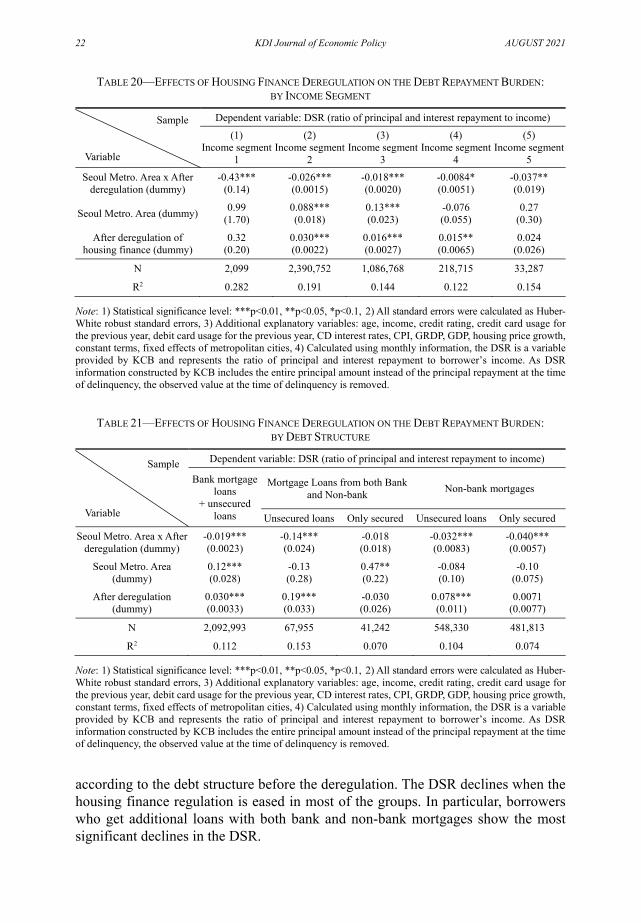
22 KDI Journal of Economic Policy AUGUST 2021
TABLE 20—EFFECTS OF HOUSING FINANCE DEREGULATION ON THE DEBT REPAYMENT BURDEN: BY INCOME SEGMENT
Sample
Variable
Dependent variable: DSR (ratio of principal and interest repayment to income) (1)
Income segment 1
(2) Income segment
2
(3) Income segment
3
(4) Income segment
4
(5) Income segment
5 Seoul Metro. Area x After
deregulation (dummy) -0.43***
(0.14) -0.026*** (0.0015)
-0.018*** (0.0020)
-0.0084* (0.0051)
-0.037** (0.019)
Seoul Metro. Area (dummy) 0.99 (1.70)
0.088*** (0.018)
0.13*** (0.023)
-0.076 (0.055)
0.27 (0.30)
After deregulation of housing finance (dummy)
0.32 (0.20)
0.030*** (0.0022)
0.016*** (0.0027)
0.015** (0.0065)
0.024 (0.026)
N 2,099 2,390,752 1,086,768 218,715 33,287
R2 0.282 0.191 0.144 0.122 0.154
Note: 1) Statistical significance level: ***p<0.01, **p<0.05, *p<0.1, 2) All standard errors were calculated as Huber-White robust standard errors, 3) Additional explanatory variables: age, income, credit rating, credit card usage for the previous year, debit card usage for the previous year, CD interest rates, CPI, GRDP, GDP, housing price growth, constant terms, fixed effects of metropolitan cities, 4) Calculated using monthly information, the DSR is a variable provided by KCB and represents the ratio of principal and interest repayment to borrower’s income. As DSR information constructed by KCB includes the entire principal amount instead of the principal repayment at the time of delinquency, the observed value at the time of delinquency is removed.
TABLE 21—EFFECTS OF HOUSING FINANCE DEREGULATION ON THE DEBT REPAYMENT BURDEN:
BY DEBT STRUCTURE
Sample
Variable
Dependent variable: DSR (ratio of principal and interest repayment to income)
Bank mortgage loans
+ unsecured loans
Mortgage Loans from both Bank and Non-bank Non-bank mortgages
Unsecured loans Only secured Unsecured loans Only secured
Seoul Metro. Area x After deregulation (dummy)
-0.019*** (0.0023)
-0.14*** (0.024)
-0.018 (0.018)
-0.032*** (0.0083)
-0.040*** (0.0057)
Seoul Metro. Area (dummy)
0.12*** (0.028)
-0.13 (0.28)
0.47** (0.22)
-0.084 (0.10)
-0.10 (0.075)
After deregulation (dummy)
0.030*** (0.0033)
0.19*** (0.033)
-0.030 (0.026)
0.078*** (0.011)
0.0071 (0.0077)
N 2,092,993 67,955 41,242 548,330 481,813
R2 0.112 0.153 0.070 0.104 0.074
Note: 1) Statistical significance level: ***p<0.01, **p<0.05, *p<0.1, 2) All standard errors were calculated as Huber-White robust standard errors, 3) Additional explanatory variables: age, income, credit rating, credit card usage for the previous year, debit card usage for the previous year, CD interest rates, CPI, GRDP, GDP, housing price growth, constant terms, fixed effects of metropolitan cities, 4) Calculated using monthly information, the DSR is a variable provided by KCB and represents the ratio of principal and interest repayment to borrower’s income. As DSR information constructed by KCB includes the entire principal amount instead of the principal repayment at the time of delinquency, the observed value at the time of delinquency is removed.
according to the debt structure before the deregulation. The DSR declines when the housing finance regulation is eased in most of the groups. In particular, borrowers who get additional loans with both bank and non-bank mortgages show the most significant declines in the DSR.
VOL. 43 NO. 3 Effects of Easing LTV·DTI Regulations 23 on the Debt Structure and Credit Risk of Borrowers
V. Conclusion
This study confirmed that when the supply regulation on LTV and DTI of bank mortgages is eased, the credit risk of borrowers can be reduced. As borrowers can improve their debt structure through the additional borrowing of bank mortgage loans, low-interest and long-term maturity.
In August 2014, financial regulations on bank mortgages were eased in South Korea, especially in Seoul metropolitan area. With the difference-in-difference method, we find that the probability of a borrower being overdue for 30 days or more decreased after the deregulation among debtors who had both bank mortgage loans and other types of high-cost loans.
The reduction in the default risk due to the LTV and DTI deregulation was prominent for borrowers with low credit scores or low incomes. This is because the interest rates gap between bank mortgages and other loans is higher for borrowers with low credit scores and low incomes than those with high credit scores and high incomes. In addition, only the group that took out new bank mortgage loans was less likely to be delinquent than before. This indicates that the reduction in the credit risk was due to the improvement of the debt structure when they took out more bank mortgages.
We also find that the proportion of high-cost loans and the burden of the repayment of principal and interest significantly decreased in Seoul metropolitan area after the deregulation. When the samples were classified by income, credit, and the existing debt structure, the debt structure was improved in all samples.
Considering our results, the relaxation of bank housing finance regulations can improve the debt structure and lessens the credit risk for some borrowers. Especially, borrowers with low credit scores and low incomes may have limited access to bank mortgages as the value of their collateral would not be sizable; therefore, the effect of improving the debt structure was not highest for them. However, for borrowers with low incomes and low credit scores, delinquency rate can be significantly reduced with only a partial improvement in the debt structure. It is because the interest rate gap between bank mortgages and other loans is significantly higher for borrowers with low credit ratings.
Because the deregulation in August of 2014 applied only to bank mortgage loans, this study examined only the effects of the deregulation of bank mortgage loans. Considering that the interest rates of mortgages are lower than those of unsecured loans, our finding cannot be applied to predict the effects of easing housing finance regulations in the entire financial sector. Also, it is not plausible to predict the impact of regulatory reinforcements based on our results, as the reinforced regulations target only new borrowers, while the deregulation affects both new and existing borrowers. However, our finding that a mortgage loan can improve the debt structure and reduce default risk is still valid when regulations are strengthened.
Stabilizing the housing market would be a fundamental policy goal when the housing market is overheated, and strengthening LTV and DTI regulations is an effective and necessary policy tool to achieve this goal. However, there may be debtors with high credit risk among those living in overheated districts. Limiting their access to low-interest rates and long-term mortgages may increase their credit

24 KDI Journal of Economic Policy AUGUST 2021
risk. Therefore, it is necessary to conduct additional studies to analyze borrowers’ credit risk changes during regulatory reinforcement, which is left as a follow-up study.
The LTV·DTI policy introduced in Korea in 2002 has played a valuable role in securing macro-prudential and real estate market price stability. However, the regulation has been understood as only stabilizing the housing market and increasing household debt. Thus, we suggest that it is necessary to pay attention to another impact of the policy by showing that the housing finance regulation policy can also affect credit risk and the debt structure depending on how it is introduced. The results of this study suggest a need to vary the level of housing finance regulation given the high levels of credit risk in some low-credit and low-income classes and general debtors when designing policies that will ease or strengthen housing finance regulations.

VOL. 43 NO. 3 Effects of Easing LTV·DTI Regulations 25 on the Debt Structure and Credit Risk of Borrowers
APPENDIX
1. Characteristic of Sample Borrowers Table A1, A2 compares the descriptive statistics of total borrowers in the KCB
dataset and borrowers in our sample. Table A1 shows the average amount of loans other than bank mortgage, and borrowers in our sample hold a higher amount of loans in unsecured loans and non-bank mortgages than the total population. This is because we exclude borrowers without any mortgages or borrowers with only bank mortgages in our sample. Table A2. shows that borrowers in our sample have slightly higher incomes and lower credit scores than total borrowers in South Korea demonstrated in the KCB dataset.
Figure A1 summarizes the loan maturity of the sample borrowers and total borrowers for each banking and non-banking sector. The figure shows that 30-year-maturity loan contracts were the most frequently assigned in the banking and non-banking sectors. Also, the maturity of the mortgage loans in the banking sector is longer than that in the non-banking sector. These features are similar in total borrowers and our sample.
Figure A2 shows the distribution of repayment methods for the bank mortgages and the non-bank mortgages. The amortization method is most common in bank mortgages, while the share of the lump-sum payment is still high in non-bank mortgages. The percentage of the lump-sum repayment is slightly higher in our
TABLE A1—COMPARISON OF TOTAL BORROWERS IN KCB DATASET AND BORROWERS IN OUR SAMPLE:
LOAN AMOUNT (UNIT: KRW 1,000)
Object Total Borrowers in KCB dataset Borrowers in our sample
(Bank mortgage + other loans or Non-bank mortgages)
Variable Average S.D. Average S.D. Unsecured
loans Bank 7,271.41 24,312.22 10,484.79 27,192.38
Non-bank sector 3,897.71 21,467.19 5,711.23 27,561.94 Non-bank mortgages 10,732.83 111,072.8 15,202.63 150,065.6
Source: Provided by KCB, calculated using total borrower data of KCB.
TABLE A2—COMPARISON OF TOTAL BORROWERS IN KCB DATASET AND BORROWERS IN OUR SAMPLE:
OTHER CHARACTERISTICS
Object Total Borrowers in KCB dataset Borrowers in our sample
(Bank mortgage + other loans or Non-bank mortgages)
Variable Average S.D. Average S.D. Age 51.29 8.81 51.28 8.43 DTI 0.26 0.39 0.35 0.73
Income (KRW 1,000) 41223.96 50434.07 43770.83 57233.5 Credit Score 825.55 135.23 800.6 147.2 Credit Rating 3.28 2.03 3.66 2.17
Delinquency rate 0.01 0.11 0.01 0.11
Source: Provided by KCB, calculated using total borrower data of KCB.

26 KDI Journal of Economic Policy AUGUST 2021
FIGURE A1. COMPARISON OF TOTAL BORROWERS IN KCB DATASET AND SAMPLE BORROWERS:
BY MORTGAGE MATURITY
Source: Provided by KCB, calculated using total borrower data of KCB.
FIGURE A2. COMPARISON OF TOTAL BORROWERS IN KCB DATASET AND SAMPLE BORROWERS:
REPAYMENT METHODS
Source: Provided by KCB, calculated using total borrower data of KCB.
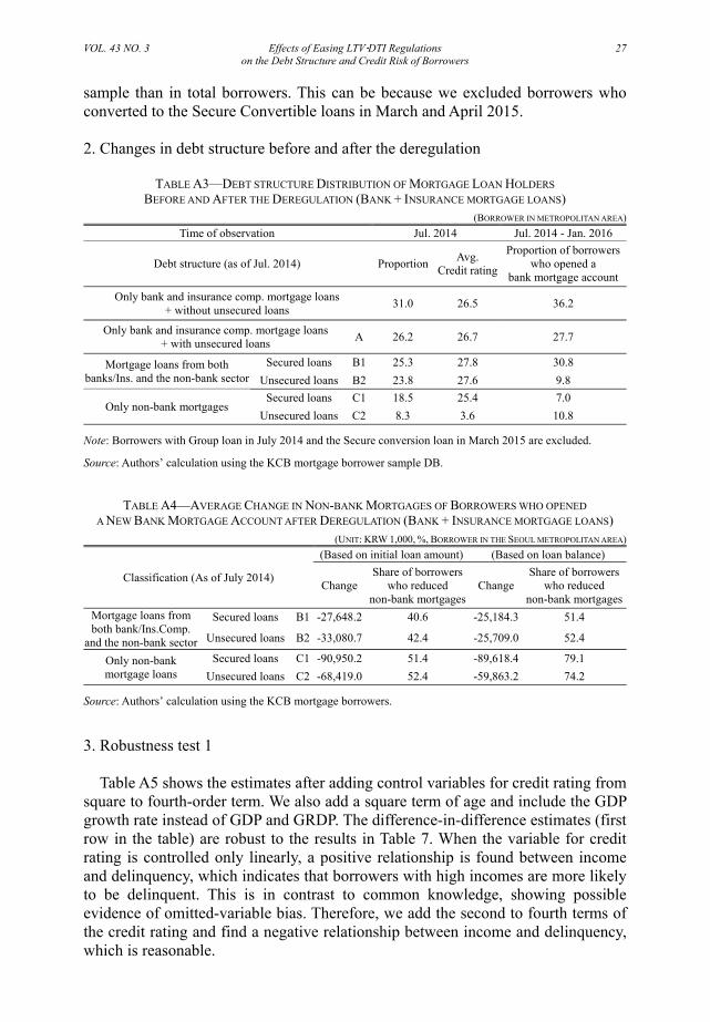
VOL. 43 NO. 3 Effects of Easing LTV·DTI Regulations 27 on the Debt Structure and Credit Risk of Borrowers
sample than in total borrowers. This can be because we excluded borrowers who converted to the Secure Convertible loans in March and April 2015.
2. Changes in debt structure before and after the deregulation
TABLE A3—DEBT STRUCTURE DISTRIBUTION OF MORTGAGE LOAN HOLDERS
BEFORE AND AFTER THE DEREGULATION (BANK + INSURANCE MORTGAGE LOANS) (BORROWER IN METROPOLITAN AREA)
Time of observation Jul. 2014 Jul. 2014 - Jan. 2016
Debt structure (as of Jul. 2014) Proportion Avg. Credit rating
Proportion of borrowers who opened a
bank mortgage account Only bank and insurance comp. mortgage loans
+ without unsecured loans 31.0 26.5 36.2
Only bank and insurance comp. mortgage loans + with unsecured loans A 26.2 26.7 27.7
Mortgage loans from both banks/Ins. and the non-bank sector
Secured loans B1 25.3 27.8 30.8 Unsecured loans B2 23.8 27.6 9.8
Only non-bank mortgages Secured loans C1 18.5 25.4 7.0
Unsecured loans C2 8.3 3.6 10.8
Note: Borrowers with Group loan in July 2014 and the Secure conversion loan in March 2015 are excluded.
Source: Authors’ calculation using the KCB mortgage borrower sample DB.
TABLE A4—AVERAGE CHANGE IN NON-BANK MORTGAGES OF BORROWERS WHO OPENED
A NEW BANK MORTGAGE ACCOUNT AFTER DEREGULATION (BANK + INSURANCE MORTGAGE LOANS) (UNIT: KRW 1,000, %, BORROWER IN THE SEOUL METROPOLITAN AREA)
Classification (As of July 2014)
(Based on initial loan amount) (Based on loan balance)
ChangeShare of borrowers
who reduced non-bank mortgages
ChangeShare of borrowers
who reduced non-bank mortgages
Mortgage loans from both bank/Ins.Comp.
and the non-bank sector
Secured loans B1 -27,648.2 40.6 -25,184.3 51.4
Unsecured loans B2 -33,080.7 42.4 -25,709.0 52.4
Only non-bank mortgage loans
Secured loans C1 -90,950.2 51.4 -89,618.4 79.1 Unsecured loans C2 -68,419.0 52.4 -59,863.2 74.2
Source: Authors’ calculation using the KCB mortgage borrowers.
3. Robustness test 1
Table A5 shows the estimates after adding control variables for credit rating from
square to fourth-order term. We also add a square term of age and include the GDP growth rate instead of GDP and GRDP. The difference-in-difference estimates (first row in the table) are robust to the results in Table 7. When the variable for credit rating is controlled only linearly, a positive relationship is found between income and delinquency, which indicates that borrowers with high incomes are more likely to be delinquent. This is in contrast to common knowledge, showing possible evidence of omitted-variable bias. Therefore, we add the second to fourth terms of the credit rating and find a negative relationship between income and delinquency, which is reasonable.

28 KDI Journal of Economic Policy AUGUST 2021
TABLE A5—EFFECT OF DEREGULATION ON THE PROBABILITY OF 30+ DELINQUENCY - ROBUSTNESS TEST
SampleVariable
Dependent variable: 30+ days delinquency (in any loan) dummy
(1) (2) (3) (4) (5)
Seoul Metro. area x After deregulation (dummy)
-0.0026*** (0.00073)
-0.0022*** (0.00070)
-0.0022*** (0.00068)
-0.0022*** (0.00068)
-0.0029*** (0.00068)
Seoul Metro. area (dummy) 0.0031 (0.0079)
-0.0068 (0.0075)
-0.0058 (0.0074)
-0.0058 (0.0074)
0.0092*** (0.00075)
After deregulation (dummy) 0.0024** (0.0011)
0.0030*** (0.0010)
0.0030*** (0.0010)
0.0030*** (0.0010)
0.00125 (0.00092)
Age (by 5 years interval)
0.00027 (0.00023)
-0.00021 (0.00022)
0.000022 (0.00022)
0.000046 (0.00022)
0.000125*** (0.000017)
Age2 (by 5 years interval)
-1.4e-06 (2.2e-06)
2.5e-06 (2.1e-06)
3.0e-07 (2.1e-06)
3.7e-08 (2.1e-06)
ln (income) 0.0052*** (0.00034)
-0.0013*** (0.00029)
-0.0017*** (0.00028)
-0.0017*** (0.00028)
0.0052*** (0.00033)
Credit rating (Level 1~10) 0.016*** (0.00016)
-0.043*** (0.00049)
0.038*** (0.00094)
0.016*** (0.0023)
0.016*** (0.00016)
Credit rating2 0.0066*** (0.000069)
-0.013*** (0.00027)
-0.0042*** (0.0010)
Credit rating3 0.0013*** (0.000022)
-0.000017 (0.00017)
Credit rating4 0.000067*** (8.9e-06)
1 year credit card usage amount(one million won)
-0.00016*** (0.000011)
-0.00012*** (8.1e-06)
-0.000086*** (6.4e-06)
-0.000088*** (6.5e-06)
-0.00016*** (0.000011)
1 year debit card usage amount (one million won)
0.00015*** (0.000039)
0.000080** (0.000032)
0.000059** (0.000024)
0.000061** (0.000024)
0.00015*** (0.000039)
cd91 interest rate 0.0061*** (0.0013)
0.0072*** (0.0012)
0.0065*** (0.0012)
0.0066*** (0.0012)
0.0053*** (0.0010)
CPI (Inflation rate) 0.00018 (0.00040)
0.00052 (0.00038)
0.00058 (0.00038)
0.00059 (0.00038)
0.00086** (0.00037)
GRDP (Regional economy) 2.3e-08 (3.2e-08)
5.0e-08* (3.0e-08)
4.6e-08 (3.0e-08)
4.6e-08 (3.0e-08)
GDP 5.5e-08** (2.3e-08)
8.9e-08*** (2.2e-08)
8.4e-08*** (2.2e-08)
8.4e-08*** (2.2e-08)
GDP growth rate 0.0011*** (0.00040)
Housing price growth (YoY, 1 month lag)
-0.000010 (0.00016)
0.00018 (0.00016)
0.00022 (0.00015)
0.00022 (0.00015)
0.00011 (0.00015)
Constant -0.16*** (0.037)
-0.038 (0.035)
-0.12*** (0.034)
-0.11*** (0.034)
-0.20*** (0.037)
N 719,675 719,675 719,675 719,675 719,675
R2 0.077 0.167 0.193 0.193 0.077
Note: 1) Statistical significance level: ***p<0.01, **p<0.05, *p<0.1, 2) All standard errors were calculated as Huber-White robust standard errors, 3) The fixed effect of metropolitan cities is included in the regression equation, but omitted, 4) This was calculated using information on a semiannual basis (January, July), and 30-day delinquency refers to a case in which more than 30 days of delinquency occur among loans (including unsecured loans) held by the borrower within the preceding six months, 5) As of July 2014, if there is more than 5 days of overdue experience (in any type of loan), it is classified as a borrower with past overdue experience, 6) The total number of borrowers for each sample was 206,361.
Source: Author’s calculations using the KCB mortgage borrower sample DB.

VOL. 43 NO. 3 Effects of Easing LTV·DTI Regulations 29 on the Debt Structure and Credit Risk of Borrowers
TABLE A6—EFFECT OF DEREGULATION ON DELINQUENCY RATE: TRIPLE-DIFFERENCE BY CREDIT RATING
Independent Variables Dependent variable: 30+ days delinquency
Seoul Metro. Area x After deregulation(dummy) x Credit rating -0.0086*** (0.00079)
Seoul Metro. Area x After deregulation (dummy) 0.011*** (0.0012)
Seoul Metro. Area (dummy) 0.0030 (0.0079)
After deregulation of housing finance (dummy) 0.0026** (0.0011)
Constant -0.15*** (0.036)
N 719,675 R2 0.078
Note: 1) Statistical significance level: ***p<0.01, **p<0.05, *p<0.1, 2) All standard errors were calculated as Huber-White robust standard errors, 3) Additional explanatory variables: age, income, credit rating, credit card usage for the previous year, debit card usage for the previous year, CD interest rates, CPI, GRDP, GDP, housing price growth rate, constant terms, fixed effects of metropolitan cities.
Source: Author’s calculations using the KCB mortgage borrower sample DB.
TABLE A7—EFFECT OF DEREGULATION: TRIPLE-DIFFERENCE BY INCOME LEVEL
Dependent Variable 30+ days delinquency High-cost loan ratio DSR Seoul Metro. Area x After deregulation
(dummy) x Income level 0.00068** (0.00033)
0.022*** (0.00041)
0.11*** (0.00093)
Seoul Metro. Area x After deregulation (dummy)
-0.0039*** (0.0012)
-0.067*** (0.0012)
-0.28*** (0.0027)
Seoul Metro. Area (dummy) -0.0058 (0.0074)
-0.079*** (0.0084)
0.085*** (0.014)
After deregulation (dummy) 0.0030*** (0.0010)
0.026*** (0.0010)
0.030*** (0.0017)
Constant -0.11*** (0.034)
-0.80*** (0.045)
3.03*** (0.076)
N 719,675 3,714,565 3,731,621 R2 0.193 0.050 0.140
Note: 1) Statistical significance level: ***p<0.01, **p<0.05, *p<0.1, 2) All standard errors were calculated as Huber-White robust standard errors, 3) Additional explanatory variables: age, income, credit rating, credit card usage for the previous year, debit card usage for the previous year, CD interest rates, CPI, GRDP, GDP, housing price growth, constant terms, fixed effects of metropolitan cities.
Source: Author’s calculations using the KCB mortgage borrower sample DB.
Table A6 shows the estimates with the triple-difference term (interaction between
the double-difference term and the credit rating dummy). The negative estimates of the triple-difference term indicate that the average delinquency rate of borrowers with poor credit ratings falls more with deregulation. This is consistent with the results shown in Table 9.
The first column in Table A7 shows the estimates by the triple-difference term (interaction between the double-difference term and the income level). The signs of estimates are all reasonable and consistent with our results in Table 10, Table 16, and Table 20.
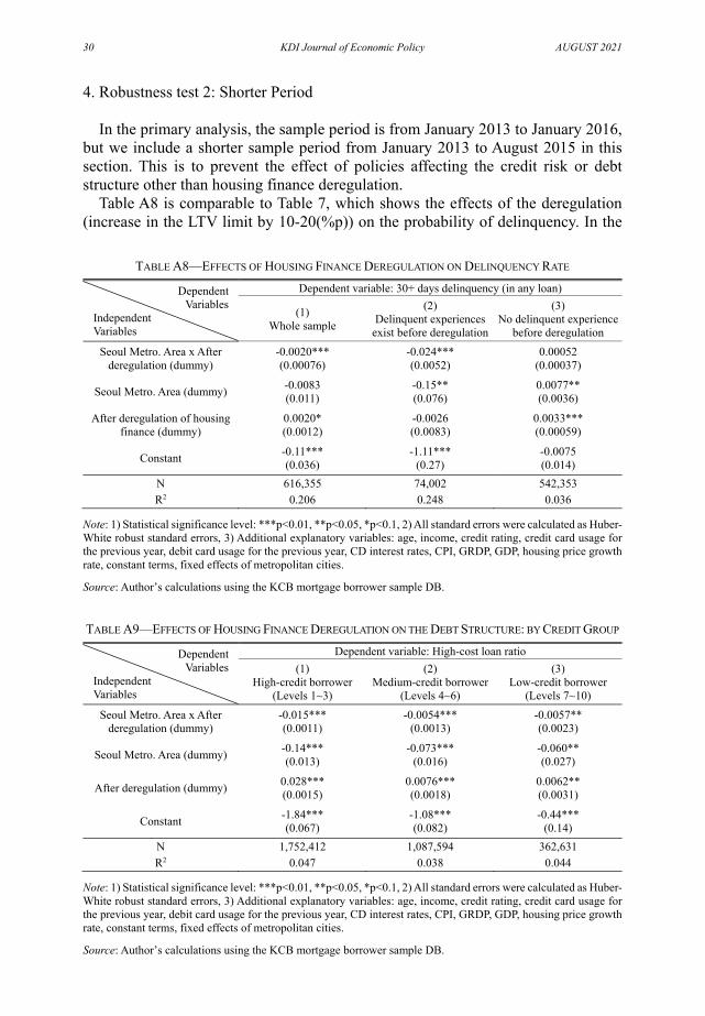
30 KDI Journal of Economic Policy AUGUST 2021
4. Robustness test 2: Shorter Period In the primary analysis, the sample period is from January 2013 to January 2016,
but we include a shorter sample period from January 2013 to August 2015 in this section. This is to prevent the effect of policies affecting the credit risk or debt structure other than housing finance deregulation.
Table A8 is comparable to Table 7, which shows the effects of the deregulation (increase in the LTV limit by 10-20(%p)) on the probability of delinquency. In the
TABLE A8—EFFECTS OF HOUSING FINANCE DEREGULATION ON DELINQUENCY RATE
Dependent Variables
Independent Variables
Dependent variable: 30+ days delinquency (in any loan)
(1) Whole sample
(2) Delinquent experiences
exist before deregulation
(3) No delinquent experience
before deregulation Seoul Metro. Area x After
deregulation (dummy) -0.0020*** (0.00076)
-0.024*** (0.0052)
0.00052 (0.00037)
Seoul Metro. Area (dummy) -0.0083 (0.011)
-0.15** (0.076)
0.0077** (0.0036)
After deregulation of housingfinance (dummy)
0.0020* (0.0012)
-0.0026 (0.0083)
0.0033*** (0.00059)
Constant -0.11*** (0.036)
-1.11*** (0.27)
-0.0075 (0.014)
N 616,355 74,002 542,353 R2 0.206 0.248 0.036
Note: 1) Statistical significance level: ***p<0.01, **p<0.05, *p<0.1, 2) All standard errors were calculated as Huber-White robust standard errors, 3) Additional explanatory variables: age, income, credit rating, credit card usage for the previous year, debit card usage for the previous year, CD interest rates, CPI, GRDP, GDP, housing price growth rate, constant terms, fixed effects of metropolitan cities.
Source: Author’s calculations using the KCB mortgage borrower sample DB.
TABLE A9—EFFECTS OF HOUSING FINANCE DEREGULATION ON THE DEBT STRUCTURE: BY CREDIT GROUP
Dependent Variables
Independent Variables
Dependent variable: High-cost loan ratio (1)
High-credit borrower (Levels 1~3)
(2) Medium-credit borrower
(Levels 4~6)
(3) Low-credit borrower
(Levels 7~10) Seoul Metro. Area x After
deregulation (dummy) -0.015*** (0.0011)
-0.0054*** (0.0013)
-0.0057** (0.0023)
Seoul Metro. Area (dummy) -0.14*** (0.013)
-0.073*** (0.016)
-0.060** (0.027)
After deregulation (dummy) 0.028*** (0.0015)
0.0076*** (0.0018)
0.0062** (0.0031)
Constant -1.84*** (0.067)
-1.08*** (0.082)
-0.44*** (0.14)
N 1,752,412 1,087,594 362,631 R2 0.047 0.038 0.044
Note: 1) Statistical significance level: ***p<0.01, **p<0.05, *p<0.1, 2) All standard errors were calculated as Huber-White robust standard errors, 3) Additional explanatory variables: age, income, credit rating, credit card usage for the previous year, debit card usage for the previous year, CD interest rates, CPI, GRDP, GDP, housing price growth rate, constant terms, fixed effects of metropolitan cities.
Source: Author’s calculations using the KCB mortgage borrower sample DB.

VOL. 43 NO. 3 Effects of Easing LTV·DTI Regulations 31 on the Debt Structure and Credit Risk of Borrowers
TABLE A10—EFFECTS OF HOUSING FINANCE DEREGULATION ON THE DEBT REPAYMENT BURDEN: CREDIT RATING GROUP
Dependent Variables
Independent Variables
Dependent variable: DSR (ratio of principal and interest repayment to income) (1)
High-credit borrower (Levels 1~3)
(2) Medium-credit borrower
(Levels 4~6)
(3) Low-credit borrower
(Levels 7~10) Seoul Metro. Area x After
deregulation (dummy) -0.019*** (0.0015)
-0.023*** (0.0024)
-0.012* (0.0061)
Seoul Metro. Area (dummy) 0.055*** (0.017)
0.083*** (0.028)
0.20*** (0.078)
After deregulation (dummy) 0.023*** (0.0020)
0.031*** (0.0033)
-0.0013 (0.0087)
Constant 1.29*** (0.089)
2.88*** (0.15)
3.87*** (0.39)
N 1,822,706 1,080,156 314,349 R2 0.073 0.117 0.109
Note: 1) Statistical significance level: ***p<0.01, **p<0.05, *p<0.1, 2) All standard errors were calculated as Huber-White robust standard errors, 3) Additional explanatory variables: age, income, credit rating, credit card usage for the previous year, debit card usage for the previous year, CD interest rates, CPI, GRDP, GDP, housing price growth rate, constant terms, fixed effects of metropolitan cities.
Source: Author’s calculations using the KCB mortgage borrower sample DB.
entire sample, delinquency rate decreases by about 0.20%p, which is a 14.2% change. This is robust to the main analysis in Table 7, showing a 15.7% change. Table A9 is comparable to Table 15, and Table A10 is comparable to Table 19. Estimates in the robustness checks in this section are all consistent to those of the main regression.
32 KDI Journal of Economic Policy AUGUST 2021
REFERENCES Bang Doowon, Saewoon Park and Yunwoo Park. 2010. “An Analysis of Default and
Prepayment in Korean Mortgage Markets,” Journal of Money & Finance, 24(4): 87-118 (in Korean).
Choi, Mackjoong, Kyuhyun Ji and Jeongrae Cho. 2002. “Empirical Analyses of the Effect of Constraint in Housing Finance,” Housing Studies Review, 10(1): 33-48 (in Korean).
Hur, Seokkyun. 2012. “The effects of DTI, LTV, and Contract Types on the Delinquency of Loans Secured by Residential Property,” Journal of Regulation Studies, 21(2): 39-77 (in Korean).
Igan, Deniz and Heedong Kang. 2011. “Do Loan-to-Value and Debt-to-Income Limits Work? Evidence from Korea,” 23 March 2011. (http://ssrn.com/abstract=1915127 or http://dx.doi.org/10.2139/ssrn.1915127).
Ji, Kyuhyun and Changgyu Choi. 2007. “Effect of LTV and Borrower`s Character for Mortgage Default in Korea -Empirical Study from 2001 to 2003-,” Journal of The Korean Regional Development Association, 19(3): 213-227. (in Korean)
Jeong, Hosung. 2018. “Default Factors for Household Loans and Financial Fragility: The Importance of Self-Employed Borrowers in Korea,” Bank of Korea WP, 2018(5): 1-38 (in Korean).
KCB. “Sample DB of Mortgage Loans Borrowers” (acquired on April 26, 2019). Kim, Moonyeun and Youngman Lee. 2015. “An Analysis on Timing and Hazard Rate of Arrears
and Default in Residential Mortgages: Focus on Cross Effect between Original DTI and LTV Ratio,” The Korea Spatial Planning Review, 87: 17-32 (in Korean).
Lee Donggull, Sungin Jun, Jaewook Chung and Dongjun Byun. 2014. “A Study of the Delinquency Decision Factors and Vulnerability of the Korean Households with Debts,” Journal of Money & Finance, 28(2): 137-178 (in Korean).
Mian, Atif and Amir Sufi. 2009. “The Consequences of Mortgage Credit Expansion: Evidence from the U.S. Mortgage Default Crisis,” The Quarterly Journal of Economics, 124(4): 1449-1496 (https://doi.org/10.1162/qjec.2009.124.4.1449).
Park Jongsang. 2017. “Who Responds to Housing Finance Deregulation? A Case Study of Korea’s 2014 Deregulation,” in Minkyu Song (ed.) Home-Backed Loans in Korea: Design of Policies and Mortgage Products, Korea Institute of Finance (in Korean).
LITERATURE IN KOREAN
김문년⋅이용만. 2015. 「주택담보대출에서 연체 및 채무불이행의 발생시기별 위험률: DTI와 LTV 비율의 교
차효과를 중심으로」, 『국토연구』, 87: 17-32.
박종상, 2017. 「주택담보대출 규제 완화가 차입자 미시구조에 미치는 영향」, 송민규 편, 『주택담보대출 리
스크 관리를 위한 규제 및 대출 상품의 설계』, KIF 연구총서 2017-01, 한국금융연구원.
방두완⋅박세운⋅박연우, 2010. 「한국 모기지시장의 채무불이행 및 조기상환 분석」, 『금융연구』, 24(4): 87-
118.
이동걸⋅전성인⋅정재욱⋅변동준, 2014. 「우리나라 가계부채의 연체결정요인 및 취약성 연구」, 『금융연구』,
28(2): 137-178.
정호성, 2018. 「가계대출 부도요인 및 금융업권별 금융취약성: 자영업 차주를 중심으로」, 『BOK 경제연
구』, 2018(5): 1-38.
지규현⋅최창규, 2007. 「Effect of LTV and Borrower`s Character for Mortgage Default in Korea -
Empirical Study from 2001 to 2003-」, 『한국지역개발학회지』, 19(3): 213-227.
최막중⋅지규현⋅조정래, 2002. 「주택금융 제약이 주택소비규모와 점유형태 선택에 미치는 영향에 관한 실
증분석」, 『주택연구』, 10(1): 33-48.
허석균, 2012. 「DTI, LTV 및 대출상환 조건이 주택담보대출의 연체율에 미치는 영향」, 『규제연구』, 21(2):
39-77.
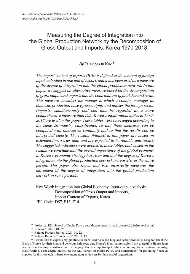
KDI Journal of Economic Policy 2021, 43(3):33–53 http://dx.doi.org/10.23895/kdijep.2021.43.3.33
33
Measuring the Degree of Integration into the Global Production Network by the Decomposition of
Gross Output and Imports: Korea 1970-2018†
By DONGSEOK KIM*
The import content of exports (ICE) is defined as the amount of foreign input embodied in one unit of export, and it has been used as a measure of the degree of integration into the global production network. In this paper, we suggest an alternative measure based on the decomposition of gross output and imports into the contributions of final demand terms. This measure considers the manner in which a country manages its domestic production base (gross output) and utilizes the foreign sector (imports) simultaneously and can thus be regarded as a more comprehensive measure than ICE. Korea’s input-output tables in 1970-2018 are used in this paper. These tables were rearranged according to the same 26-industry classification so that these measures can be computed with time-series continuity and so that the results can be interpreted clearly. The results obtained in this paper are based on extended time-series data and are expected to be reliable and robust. The suggested indicators were applied to these tables, and, based on the results we conclude that the overall importance of the global economy in Korea’s economic strategy has risen and that the degree of Korea’s integration into the global production network increased over the entire period. This paper also shows that ICE incorrectly measures the movement of the degree of integration into the global production network in some periods.
Key Word: Integration into Global Economy, Input-output Analysis, Decomposition of Gross Output and Imports, Import Content of Exports, Korea
JEL Code: D57, F13, F14
* Professor, KDI School of Public Policy and Management (E-mail: [email protected]) * Received: 2020. 10. 19 * Referee Process Started: 2020. 10. 22 * Referee Reports Completed: 2020. 12. 17 † I would like to express my gratitude to team head Kyuchae Jung and senior economist Sangdon Bu at the
Bank of Korea for their kind and generous help regarding Korea’s input-output tables. I am grateful to Hanna Jang for her outstanding assistance in rearranging Korea’s input-output tables according to a common industry classification. I am deeply grateful to the KDI School of Public Policy and Management for providing financial support for this research. I thank two anonymous reviewers for their useful suggestions.

34 KDI Journal of Economic Policy AUGUST 2021
I. Introduction
t is a widely known and extensively documented fact that export-driven economic growth has been an essential component of Korea’s growth strategy since the 1960s
(Krugman et al., 2018, pp.321-323). In Korea’s Five-Year Economic Development Plans, which served as the backbone of Korea’s economic policy in the 1960s and 1970s, export promotion was one of the ‘core’ policies facilitating rapid economic growth (Han, 2014).
Exports, along with consumption and investment, form a component of an economy’s final demand. According to demand-side economics such as demand-driven input-output analysis, the supply side is assumed to be infinitely elastic. An increase in the final demand, therefore, receives an immediate reply from the supply side, which is followed by infinitely repeated rounds of inter-industry relationships represented by intermediate inputs and demands. This process results in the increases in gross output, imports of foreign intermediate inputs, value-added and employment, which can be computed by various methodologies, for example, a demand-driven input-output analysis using the Leontief inverse matrix.
In an early economic development period with low income levels when an economy does not have sufficient final demand, exports can be a good source for increasing final demand. If a developing country succeeds in finding products with a sufficient comparative advantage in the global market, therefore, it can embark on a path of an export-led growth. The four ‘Asian Tigers’ – Korea, Taiwan, Singapore and Hong Kong – are the most well-known examples of export-led growth in the twentieth century. Figure 1 presents the exports of Korea as a percent of GDP, from which we can confirm that Korea’s exports as a percent of GDP entered a consistent growth trend in 1970s.
In fact, the world economy has witnessed a consistent increase in international trade since the mid-twentieth century. According to Maddison (2001), world exports as a percent of GDP amounted to 9.0% in 1929 but declined to 5.5% in 1950 after
FIGURE 1. EXPORTS OF KOREA AND THE WORLD (% OF GDP, 1953-2019)
Source: Bank of Korea, Maddison (2001, p.363),1 World Bank.
1World exports as a percent of GDP in 1950, 5.5%, is from Maddison (2001), and those during 1970-2019 are
from the World Bank; the shares between 1950 and 1970 were computed by linear interpolation.
0
10
20
30
40
50
60
1953 1960 1965 1970 1975 1980 1985 1990 1995 2000 2005 2010 20152019
World Korea
I

VOL. 43 NO. 3 Measuring the Degree of Integration into the Global Production Network 35 by the Decomposition of Gross Output and Imports
two world wars, at which point it began recovering, eventually exceeding 10% in the early 1970s.
Many factors have been suggested as causes of this trend, such as improved transportation and information technology, containerization, declines in transportation costs, declines in protectionism, decreases in piracy, the development of a global production network (GPN), and international fragmentation, to name a few (Weil, 2013). Most of these factors are related to one another, and it can be said that they took place simultaneously and affected one another during the second half of the 20th century.
Out of these factors, the deepening of the GPN has become so strong over the past decades that taking advantage of and realizing integration into the GPN have become essential components in the growth strategies of many countries. The purpose of this paper is to measure the degree of integration into the GPN of Korea in 1970-2018 by means of a demand-side input-output (IO) analysis.
Specifically, we will decompose gross output and imports into the contributions of individual final demand terms, that is, consumption, investment and exports. Considering that gross output and imports constitute the total supply of an economy, following the tracks of the shares of gross output and imports induced by exports will help us better understand how Korea managed its domestic production base (DPB) and utilized the foreign sector as a part of its growth strategy. This approach will also enable the measurement of the degree of integration into the GPN over the past half century.
II. Motivation and Literature
The degree of integration into the GPN can be measured in various ways. The ratio
of exports to GDP represents the degree of dependence on the foreign sector. While used in various contexts, this ratio can be regarded as a simple measure of integration into the GPN. Similarly, the ratio of total imports of products to GDP, if seldom used, can also be regarded as an alternative measure. These two ratios can be thought of as measures of dependence on the foreign sector on the demand and supply sides, respectively.
The ratio of the total trade volume, i.e., the sum of exports and imports, to GDP is frequently used as an indicator of the integration into the GPN, or the ‘openness of an economy.’ It has been used frequently as a determinant of the growth rate of the income level or total factor productivity.
In fact, the traditional way to analyze an economy’s dependence on, and utilization of, the global market was to use various indices using trade statistics. Trade statistics are type of first-hand statistics collected and published by the tariff authorities of most countries and by international organizations. Trade statistics by direction (export of import), by various product classifications (e.g., Standard International Trade Classification, Harmonized Commodity Description and Coding System), by partner countries or regions, are the major statistics long used by various institutions.
The wide availability of trade statistics has led to the development of numerous indices based on these data. A few examples are market shares in partner countries, in various regions, and in the world market; the compositions of exports and imports

36 KDI Journal of Economic Policy AUGUST 2021
by product and by partner countries; export similarity indexes that measure the degree of competition between two countries in a specific market; a revealed comparative advantage index that measures the strength of a comparative advantage of a country, as developed by Balassa, to name a few. Woo et al. (2003) evaluated Korea’s trade performance based on various trade statistics for the period of 1992-2000.
The consistent increase in international trade in goods and services has led to the development and utilization of new indicators, many of which are derived from the IO analysis. Since Wassily Leontief published the first IO tables of US in the 1940s, many countries have compiled their own IO tables and used them in various situations, mostly in forecasting the impact of final demand shocks on supply-side variables such as gross output, intermediate input, value-added, employment, and so forth. Hence, the IO analysis has been applied to export data, a component of final demand, to compute the trade performance and the degree of integration into the global economy.
Export-led growth requires additional resources. An increase in exports requires an increase in production, which, in turn, implies an increase in the service of the primary production factors, labor and capital, and in intermediate input, both domestic and imported.
An increase in the demand for labor can be met by an increase in the labor supply mostly by domestic households. Increased demand for capital, on the other hand, can be satisfied by more domestic savings. However, this is usually difficult for developing countries and is supplemented by foreign capital inflows, which can be measured by the net savings rate, or, alternatively, by net exports as a percent of GDP. See Figure 2, where the net exports graph was computed as the ratio of net exports to GDP while the net savings graph was computed as the total savings rate less the total domestic investment rate. These two ratios are connected by the national income identity S I EX M , where S , I , EX and M denote savings, investments, exports and imports, respectively.
Thirdly, an increase in the demand for imported intermediate input is met by importing these products. Lastly, an increase in the demand for domestic intermediate input must be met by producing them domestically, in other words, by an increase in gross output, which initiates the second and the subsequent rounds of the
FIGURE 2. NET EXPORTS AND NET SAVINGS OF KOREA (% OF GDP, 1970-2019)
Source: Bank of Korea.
-15
-10
-5
0
5
10
15
1970 1975 1980 1985 1990 1995 2000 2005 2010 2015 2019
Net Export Net Saving

VOL. 43 NO. 3 Measuring the Degree of Integration into the Global Production Network 37 by the Decomposition of Gross Output and Imports
production process involving almost all industries in the economy. This production process results in increases in gross output, value-added, imports and employment, all of which can be computed for individual industries and for the entire economy by means of an IO analysis. Miller et al. (2009) is the most widely used reference.
The consistently increasing trend of international trade in the 1990s and 2000s attracted the attention of a number of countries, in particular those with major shares in the world market, such as Germany, Japan, Hong Kong, Singapore, and Korea, among others. Kim (2004) observed that while Korea’s exports recorded unprecedented high growth rates, domestic demand such as consumption and investment levels were showing extremely low or even negative growth rates. Increases in exports usually have a positive chain effect on value-added and then on domestic demand with some time lag. Here, the huge gap between foreign and domestic demand levels implied a structural change.
Kim (2004) showed that the share of imported intermediate input in total intermediate input continued to decrease until the 1980s but later entered a rapidly increasing trend in early 1990s. He also showed, using an IO analysis, that the share of GDP generated by exports began to decrease in the early 1990s. He conjectured that this phenomenon may have been caused by (i) Korea’s large-scale market opening in the 1990s, (ii) the deteriorating competitiveness of Korea’s parts and components industries, (iii) the concentration of Korea’s exports on a few products that heavily depend on imported intermediate inputs, and/or (iv) by the increasing trend of ‘global sourcing.’
Loschky and Ritter (2006) were motivated by a similar observation. They observed that Germany achieved record-breaking exports of products in the mid-2000s, but, at the same time, the share of imported intermediate input in German products was also quickly increasing. They computed the share of imported input in German exports, which they called the ‘import content of exports (ICE),’ and showed that ICE increased from 31% in 1995 to 42% in 2005.2
Breda et al. (2009) interpreted ICE as a measure of ‘internationalization’ and computed the ICE of individual products and the aggregate ICE of seven European countries in 1995 and 2000. They showed that the ICE of most products in most countries increased during the period while also analyzing the various internationalization patterns of the seven countries.
As seen earlier, increases in exports lead to increases in various terms on the supply side. Out of the increases in these variables, the increases in value-added and imports add up to the increase in exports given that value-added and import equal the total final demand in a national economy. One unit of export, therefore, can be decomposed into the shares of domestic and imported intermediate inputs, or, equivalently, the shares of domestic and imported value-added. The former set represents the measures used by Kim (2004), while the latter, ICE, is used by Loschky and Ritter (2006) and Breda et al. (2009). Years earlier, Hummels et al. (2001) referred to the trend of the increasing integration of a GPN as ‘vertical specialization’ and used ICE as the measure of vertical specialization.
2Simultaneous increases in international trade and the share of imported raw materials in the exports of most countries, and many related phenomena, have been given various names, such as global outsourcing, international fragmentation of production, offshoring, vertical specialization, integration of global production network, global market integration, and a bazaar economy, among others.
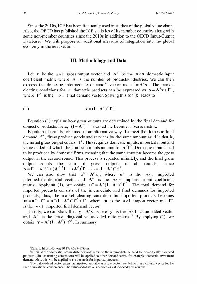
38 KDI Journal of Economic Policy AUGUST 2021
Since the 2010s, ICE has been frequently used in studies of the global value chain. Also, the OECD has published the ICE statistics of its member countries along with some non-member countries since the 2010s in addition to the OECD Input-Output Database.3 We will propose an additional measure of integration into the global economy in the next section.
III. Methodology and Data
Let x be the 1n gross output vector and dA be the n n domestic input
coefficient matrix where n is the number of products/industries. We can then express the domestic intermediate demand 4 vector as d du A x . The market clearing conditions for n domestic products can be expressed as d d x A x f , where df is the 1n final demand vector. Solving this for x leads to
(1) 1( ) .d d x I A f
Equation (1) explains how gross outputs are determined by the final demand for domestic products. Here, 1( )d I A is called the Leontief inverse matrix.
Equation (1) can be obtained in an alternative way. To meet the domestic final demand df , firms produce goods and services by the same amount as df ; that is, the initial gross output equals df . This requires domestic inputs, imported input and value-added, of which the domestic inputs amount to d dA f . Domestic inputs need to be produced by domestic firms, meaning that the same amounts become the gross output in the second round. This process is repeated infinitely, and the final gross output equals the sum of gross outputs in all rounds; hence
2 3 1( ) ( ) ( )d d d d d d d d d x f A f A f A f I A f . We can also show that m mu A x , where mu is the 1n imported
intermediate demand vector and mA is the n n imported input coefficient matrix. Applying (1), we obtain 1( )m m d d u A I A f . The total demand for imported products consists of the intermediate and final demands for imported products; thus, the market clearing condition for imported products becomes
1( )m m m d d m m u f A I A f f , where m is the 1n import vector and mf is the 1n imported final demand vector.
Thirdly, we can show that yy A x , where y is the 1n value-added vector and yA is the n n diagonal value-added ratio matrix.5 By applying (1), we obtain 1( )y d d y A I A f . In summary,
3Refer to https://doi.org/10.1787/5834f58a-en. 4In this paper, ‘domestic intermediate demand’ refers to the intermediate demand for domestically produced
products. Similar naming conventions will be applied to other demand terms, for example, domestic investment demand. Also, this will be applied to the demands for imported products.
5The value-added vector enters the input-output table as a row vector. We define it as a column vector for the sake of notational convenience. The value-added ratio is defined as value-added/gross output.

VOL. 43 NO. 3 Measuring the Degree of Integration into the Global Production Network 39 by the Decomposition of Gross Output and Imports
(2)
x d
m d m
y d
x R fm R f fy R f
where
1
1
1
( )( ) .( )
x d
m m d
y y d
R I AR A I AR A I A
Equation (2) explains how the gross outputs, imports and value-added of individual products/ industries are determined by domestic and imported final demands.
Exports form a part of domestic final demand df , therefore, the second equation in (2) indicates that the amount of imports generated by exports is mR ex , where ex is the 1n vector of exports. ICE is defined as the total imports generated by total exports divided by total exports;
(3) ICE1' ' ( )
' '
m m d
o R ex o A I A exo ex o ex
where o is the sum vector, i.e., the 1n vector of 1s. ICE is the amount of imported input embodied in the total exports and is the indicator of the integration into the GPN or of the vertical specialization used in Hummels et al. (2001), Loschky and Ritter (2006), Breda et al. (2009) and in the OECD database.
ICE can be computed also for individual products. Note from (2) that the ( , )i j th elements of xR , mR and yR denote the increases in the gross output, import and value-added of the i th product/industry when the final demand for the j th product only increases by one unit, respectively. In that case, df is an 1n vector of 0s except for the j th element being equal to 1, and (3) becomes the sum of the elements in the j th column of 1( )m m d R A I A . In consequence,
1' ' ( )m m d o R o A I A is the 1 n vector of the ICEs of individual products. It should be noted that 1' ' ( )m m d o R o A I A is the vector of the import
content of individual products not only for exports but also for consumption and investment, as the elements of ' mo R are computed under the assumption that the demand for only one product changes and because, in such a case, there is no difference among the impacts of the individual final demand terms. They do make a difference when the final demand levels for two or more products change at the same time because different products have different import contents and different final demand terms have different compositions of products. In other words, the ‘composition effect’ causes a difference in the import contents among consumption, investment and export.6
Following a similar line of reasoning, it can be seen from the third equation in (2) that the amounts of value-added generated by exports are yR ex , and the index used in Kim (2004) is the total value-added generated by total exports divided by total exports, which we will call the ‘domestic value-added content of export (DVCE).’
6This also implies that we can compute the import contents of consumption and of investment.

40 KDI Journal of Economic Policy AUGUST 2021
(4) DVCE1' ' ( ) .
' '
y y d
o R ex o A I A exo ex o ex
ICE is the amount of imported input embodied in aggregate exports, but it can also be interpreted as the amount of foreign value-added embodied in aggregate exports, as the imported input is the export for the exporting country, and export is a part of final demand. Hence, DVCE and ICE represent the amounts of domestic and foreign value-added embodied in one unit of export, respectively. Furthermore, it can easily be proved that DVCE + ICE = 1.7 We can say, in conclusion, that DVCE and ICE contain the same amount of information.
The domestic final demand consists of the consumption, investment and export of domestic products, and the imported final demand consists of the consumption and investment of imported products;
(5) ,,
d d d
m m m
f c i exf c i
where dc and di are the 1n vectors of the consumption and investment of domestic products and mc and mi denote the 1n vectors of the consumption and investment of imported products, respectively.
Using (2) and (5) together, we can decompose the aggregate gross output and imports into the contributions of individual final demand terms. We will use these decompositions when analyzing the pattern in which a country manages DPB (gross output) and utilizes the foreign sector (imports). By substituting (5) into the first two equations in (2), we obtain the decompositions of the gross outputs and imports into the contributions of the final demand terms;
(6) ,.
x d x d x
m d m d m m m
x R c R i R exm R c R i R ex c i
Finally, we pre-multiply the transpose of the sum vector to (6) and divide both sides by the left-hand sides, obtaining the decompositions of the aggregate gross output and imports into the contributions of the individual final demand terms in shares;
7 The national income identity underlies this equality. Let Y and C denote aggregate GDP and
consumption, respectively. The national income identity, Y C I EX M , can then be rewritten as Y M C I EX . The last expression implies that the sum of GDP and import equals the total final demand, leading to Y M EX . That is, when exports increase, the sum of the increases in GDP and imports equals the increase in exports.

VOL. 43 NO. 3 Measuring the Degree of Integration into the Global Production Network 41 by the Decomposition of Gross Output and Imports
(7)
' ' '1 ,' ' '
' ' ' ' '1 .' ' ' ' '
x d x d x
m d m d m m m
o R c o R i o R exo x o x o x
o R c o R i o R ex o c o io m o m o m o m o m
We then define the third terms on the right-hand sides in (7) as xex and m
ex ;
(8) ''
xxex
o R exo x
and ''
mmex
o R exo m
.
Note that xex is the share of the contribution of exports in gross output, or,
equivalently, the share of gross output generated by exports out of the total gross output. It can be interpreted as the degree to which an economy utilizes its DPB for international trade. Similarly, m
ex is the share of imports generated by exports out of total imports, and it can be interpreted as the degree to which an economy utilizes the GPN for international trade.
This paper claims that the two shares ( xex , m
ex ) provide a more comprehensive and accurate degree of integration into the GPN than ICE. Suppose m
ex increases by 10%p from 20% to 30%. This implies an increase in the share of imports generated by export, and it can be said that the country’s integration into the GPN has been strengthened. This is not valid, however, if x
ex increases by 20%p from 20% to 40% at the same time because the country operated the DPB more than it utilized the GPN in order to meet the increase in exports. In conclusion, therefore, we can say that the country’s integration into the GPN was weakened.
On the other hand, the value of ICE increases in this example, and we would conclude that the integration into the GPN is strengthened if ICE is the only measure used. This reversal transpires because ICE only considers the utilization of the GPN while the two shares ( x
ex , mex ) consider the utilization of both the DPB and GPN.
This can also be confirmed from the observation that mex equals ICE when
' 'o m o ex , i.e., when a country is in an equilibrium current account. The two shares ( x
ex , mex ) have one more advantage over ICE. As mentioned
earlier, ICEs at the product level are meaningless given that the import contents at the product level do not depend on the type of the final demand, i.e., whether the type of the final demand is exports, consumption, or investments. In other words, the terminology itself, ‘import content of exports,’ is misleading.
On the other hand, the two shares ( xex , m
ex ) are well defined at the product level. In fact, these two shares are well defined at the aggregate level and at the product level, for countries and for years, and are perfectly comparable. For example, comparisons of the degrees of integration into the GPN among countries, among products and among years are all clearly defined using these two shares.
This is possible because the two shares xex and m
ex are defined on an identical scale [0, 1]. Specifically, these two shares measure the degrees to which a country utilizes the DPB and the GPN on an identical scale and are comparable to each other. Numerous indicators have been developed to measure the extent to which a country

42 KDI Journal of Economic Policy AUGUST 2021
is open to the foreign sector and utilizes the DPB and the GPN, but we cannot directly compare the degrees with which a country utilizes the DPB and the GPN using any of these indices.
The purpose of this paper is to examine the degree of integration of Korea into the GPN during the period of 1970-2018 using the two shares ( x
ex , mex ) based on
Korea’s input-output tables. Korea’s input-output tables have been produced 34 times since 1960, but the tables since 1970 are used in this paper due to reliability and time-series continuity.
In Korea, product/industry classifications of input-output tables have been revised in the years which end with 0 or 5 and in 2003. All tables used in this paper were rearranged into tables with a common 26-industry classification. See the Appendix for the 26-industry classification table. Tables of the years for which this rearrangement is not possible were not used in this paper. Finally, the tables of 21 years were included in the analysis of this paper, while the results for only the years ending with 0 or 5 and 2018 are reported. The 2018 table is Korea’s most recent one.
IV. Results8
Three simple measures of openness are given in Figure 3. Exports and total trade
as a percent of GDP recorded a remarkable increase in the past half century. Exports accounted for only 13.8% of GDP in 1970, but they peaked at 50.8% in 2010 and then slightly declined afterwards. Total trade shows a similar pattern; it was 39.1% of GDP in 1970 but increased rapidly and approached 100.0% in 2010, after which it declined in the 2010s. We observe that both exports and imports of Korea show an M-shaped trend over the past five decades, with the first peak at around 1980 and the second at around 2010.
There was a dramatic change in the composition of Korea’s exports and imports, as shown correspondingly in Figures 4 and 5. Korea’s exports began with
FIGURE 3. MEASURES OF OPENNESS OF KOREA (% OF GDP, 1970-2018)
Source: Bank of Korea.
8Figures in this section were constructed based on the author’s computations using input-output tables and
national accounts data from the Bank of Korea.
0
20
40
60
80
100
1970 1975 1980 1985 1990 1995 2000 2005 2010 2015 2018
(Export+Import) / GDP
Export / GDP
Import / GDP
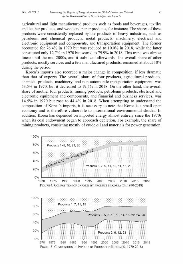
VOL. 43 NO. 3 Measuring the Degree of Integration into the Global Production Network 43 by the Decomposition of Gross Output and Imports
agricultural and light manufactured products such as foods and beverages, textiles and leather products, and wood and paper products, for instance. The shares of these products were consistently replaced by the products of heavy industries, such as petroleum and chemical products, metal products, machinery, electrical and electronic equipment and components, and transportation equipment. The former accounted for 76.4% in 1970 but was reduced to 10.0% in 2018, while the latter constituted only 12.7% in 1970 but soared to 79.9% in 2018. This trend was almost linear until the mid-2000s, and it stabilized afterwards. The overall share of other products, mostly services and a few manufactured products, remained at about 10% during the period.
Korea’s imports also recorded a major change in composition, if less dramatic than that of exports. The overall share of four products, agricultural products, chemical products, machinery, and non-automobile transportation equipment, was 53.5% in 1970, but it decreased to 19.5% in 2018. On the other hand, the overall share of another four products, mining products, petroleum products, electrical and electronic equipment and components, and financial and business services, was 14.5% in 1970 but rose to 44.4% in 2018. When attempting to understand the composition of Korea’s imports, it is necessary to note that Korea is a small open economy and is therefore vulnerable to international environmental shocks. In addition, Korea has depended on imported energy almost entirely since the 1970s when its coal endowment began to approach depletion. For example, the share of mining products, consisting mostly of crude oil and materials for power generation,
FIGURE 4. COMPOSITION OF EXPORTS BY PRODUCT IN KOREA (%, 1970-2018)
FIGURE 5. COMPOSITION OF IMPORTS BY PRODUCT IN KOREA (%, 1970-2018)
0%
20%
40%
60%
80%
100%
1970 1975 1980 1990 1995 2000 2005 2010 2015 2018
Products 6, 7, 9, 11, 12, 14, 15, 23
Products 1~5, 16, 21, 26
0%
20%
40%
60%
80%
100%
1970 1975 1980 1985 1990 1995 2000 2005 2010 2015 2018
Products 1, 7, 11, 15
Products 2, 6, 12, 23
Products 3~5, 8~10, 13, 14, 16~22, 24~26
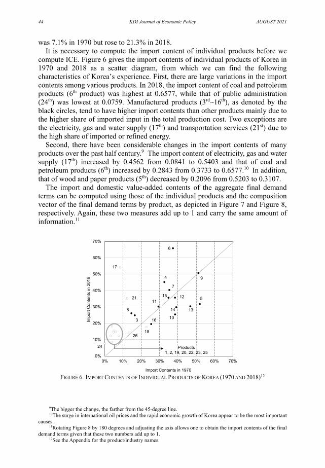
44 KDI Journal of Economic Policy AUGUST 2021
was 7.1% in 1970 but rose to 21.3% in 2018. It is necessary to compute the import content of individual products before we
compute ICE. Figure 6 gives the import contents of individual products of Korea in 1970 and 2018 as a scatter diagram, from which we can find the following characteristics of Korea’s experience. First, there are large variations in the import contents among various products. In 2018, the import content of coal and petroleum products (6th product) was highest at 0.6577, while that of public administration (24th) was lowest at 0.0759. Manufactured products (3rd~16th), as denoted by the black circles, tend to have higher import contents than other products mainly due to the higher share of imported input in the total production cost. Two exceptions are the electricity, gas and water supply (17th) and transportation services (21st) due to the high share of imported or refined energy.
Second, there have been considerable changes in the import contents of many products over the past half century.9 The import content of electricity, gas and water supply (17th) increased by 0.4562 from 0.0841 to 0.5403 and that of coal and petroleum products (6th) increased by 0.2843 from 0.3733 to 0.6577.10 In addition, that of wood and paper products (5th) decreased by 0.2096 from 0.5203 to 0.3107.
The import and domestic value-added contents of the aggregate final demand terms can be computed using those of the individual products and the composition vector of the final demand terms by product, as depicted in Figure 7 and Figure 8, respectively. Again, these two measures add up to 1 and carry the same amount of information.11
FIGURE 6. IMPORT CONTENTS OF INDIVIDUAL PRODUCTS OF KOREA (1970 AND 2018)12
9The bigger the change, the farther from the 45-degree line. 10The surge in international oil prices and the rapid economic growth of Korea appear to be the most important
causes. 11Rotating Figure 8 by 180 degrees and adjusting the axis allows one to obtain the import contents of the final
demand terms given that these two numbers add up to 1. 12See the Appendix for the product/industry names.
0%
10%
20%
30%
40%
50%
60%
70%
0% 10% 20% 30% 40% 50% 60% 70%
Impo
rt C
onte
nts
in 2
018
Import Contents in 1970
6
9
17
21 5
10
4
8 13
11
24
3
7
15 12
14
16
18
Products1, 2, 19, 20, 22, 23, 25
26
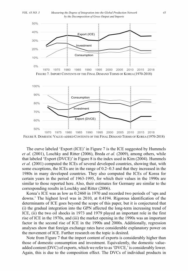
VOL. 43 NO. 3 Measuring the Degree of Integration into the Global Production Network 45 by the Decomposition of Gross Output and Imports
FIGURE 7. IMPORT CONTENTS OF THE FINAL DEMAND TERMS OF KOREA (1970-2018)
FIGURE 8. DOMESTIC VALUE-ADDED CONTENTS OF THE FINAL DEMAND TERMS OF KOREA (1970-2018)
The curve labeled ‘Export (ICE)’ in Figure 7 is the ICE suggested by Hummels
et al. (2001), Loschky and Ritter (2006), Breda et al. (2009), among others, while that labeled ‘Export (DVCE)’ in Figure 8 is the index used in Kim (2004). Hummels et al. (2001) computed the ICEs of several developed countries, showing that, with some exceptions, the ICEs are in the range of 0.2~0.3 and that they increased in the 1980s in many developed countries. They also computed the ICEs of Korea for certain years in the period of 1963-1995, for which their values in the 1990s are similar to those reported here. Also, their estimates for Germany are similar to the corresponding results in Loschky and Ritter (2006).
Korea’s ICE was as low as 0.2460 in 1970 and recorded two periods of ‘ups and downs.’ The highest level was in 2010, at 0.4194. Rigorous identification of the determinants of ICE goes beyond the scope of this paper, but it is conjectured that (i) the gradual integration into the GPN affected the long-term increasing trend of ICE, (ii) the two oil shocks in 1973 and 1979 played an important role in the first rise of ICE in the 1970s, and (iii) the market opening in the 1990s was an important factor in the second rise of ICE in the 1990s and 2000s. Additionally, regression analyses show that foreign exchange rates have considerable explanatory power on the movement of ICE. Further research on the topic is desired.
Note from Figure 7 that the import content of exports is considerably higher than those of domestic consumption and investment. Equivalently, the domestic value-added content (DVC) of exports, which we refer to as ‘DVCE,’ is considerably lower. Again, this is due to the composition effect. The DVCs of individual products in
0%
10%
20%
30%
40%
50%
1970 1975 1980 1985 1990 1995 2000 2005 2010 2015 2018
Consumption
Investment
Export (ICE)
50%
60%
70%
80%
90%
100%
1970 1975 1980 1985 1990 1995 2000 2005 2010 2015 2018
Consumption
Investment
Export (DVCE)

46 KDI Journal of Economic Policy AUGUST 2021
2018 and their rankings are given in Table 1 along with the compositions of the final demand terms by product. Also, the top five products in terms of shares are shaded. Note from Table 1 that the top five products in the composition of domestic consumption, the share of which overall amounts to 73.5%, are the products with high DVCs. On the other hand, Korea’s exports are concentrated on those products with very low DVCs, while domestic investment is positioned in the middle. This explains the gaps between the import and domestic value-added contents of consumption and exports in Figures 7 and 8.
One striking fact that can be drawn from Figure 7 and Figure 8 is that the gap has consistently widened. That is, the DVC of exports compared to the DVC of domestic demand13 has been deteriorating consistently. This could be reflecting the increasing degree of Korea’s integration into the global economy, but it is widely believed that it has been caused by the deteriorating competitiveness of Korea’s parts and components industries. This could be another reason why ICE cannot be solely regarded as the measure of global vertical specialization.
This can be indirectly confirmed by a small counterfactual experiment. Using the
TABLE 1—DOMESTIC VALUE-ADDED CONTENTS OF INDIVIDUAL PRODUCTS OF KOREA (2018)
No. Product / Industry DVC Share
value rank dc di ex
1 Agricultural, forest & fishery goods 0.8467 8 1.3% 0.1% 0.1% 2 Mined and quarried goods 0.8535 7 0.0% 0.0% 0.0% 3 Food, beverages & tobacco products 0.7513 12 4.5% 0.1% 1.0% 4 Textile and leather products 0.5485 23 1.5% 0.0% 3.3% 5 Wood and paper products 0.6830 18 0.1% 0.1% 0.5% 6 Coal and petroleum products 0.3423 26 1.4% 0.0% 7.0% 7 Chemical products 0.5968 22 0.4% 0.6% 13.0% 8 Non-metallic mineral products 0.7394 14 0.0% 0.1% 0.6% 9 Basic metal products 0.4938 24 -0.1% -0.4% 5.7% 10 Fabricated metal products 0.7463 13 0.1% 1.1% 1.6% 11 Machinery and equipment 0.6981 16 0.2% 8.3% 7.2% 12 Elec/electronic equipment & components 0.6441 21 1.7% 3.6% 30.4% 13 Precision instruments 0.6967 17 0.1% 0.9% 1.5% 14 Motor vehicles 0.7022 15 3.1% 3.9% 8.8% 15 Other transport equipment 0.6443 20 0.0% 1.6% 3.4% 16 Other manufactured products 0.8049 11 0.3% 0.8% 0.6% 17 Electricity, gas, and water supply 0.4597 25 1.7% 0.0% 0.0% 18 Construction 0.8238 9 0.0% 49.1% 0.0% 19 Wholesale and retail 0.8767 3 8.0% 2.7% 4.0% 20 Food services and accommodation 0.8191 10 7.6% 0.0% 1.3% 21 Transportation and warehousing 0.6484 19 1.8% 0.1% 4.2% 22 Communications and broadcasting 0.8548 6 1.6% 0.0% 0.2% 23 Finance, real estate & business services 0.9150 2 20.2% 11.7% 4.3% 24 Public administration and defense 0.9241 1 13.0% 0.0% 0.0% 25 Education, research and healthcare 0.8761 4 24.8% 15.3% 0.9% 26 Other services 0.8592 5 6.6% 0.4% 0.3%
13The DVC of domestic demand is the weighted average of the DVCs of domestic consumption and investment.

VOL. 43 NO. 3 Measuring the Degree of Integration into the Global Production Network 47 by the Decomposition of Gross Output and Imports
FIGURE 9. COUNTERFACTUAL: DVC OF IMPORTS OF KOREA (1970-2018)14
composition of imports by product applied to the DVCs of individual products given in Table 1, we can compute the DVC of imports, which is given in Figure 9 along with the DVC of exports. The DVC of imports can be interpreted as the amount of the hypothetical GDP if the imported products were procured domestically.
Figure 9 implies that the compositions of exports and imports were similar in 1970 in terms of the impact on the GDP, but the DVC of exports became lower than that of imports and the gap widened afterwards; in other words, exports are more concentrated on products with a lower impact on the GDP than imports, as DVC is the increase in the GDP when the final demand increases by one unit. This result does not imply that Korea’s overall international competitiveness has deteriorated but means simply that the composition of Korea’s exports has changed such that the average impact of exports on value-added decreased.
Before we compute the measure suggested in this paper, ( xex , m
ex ), it is worthwhile to review the allocation structures of domestically produced products (gross output) and imported products (total imports) separately. In other words, we will review the compositions of the total demand for domestic and imported products, as given in Figures 10 and 11, respectively.
From Figures 10 and 11, we find that gross output and imports have entirely different allocation structures, even setting aside the considerable difference in the magnitudes.15 The greatest difference lies in the shares of intermediate demand. In the domestic product markets, the share of intermediate demand has been stable at around 45% since 1980. On the other hand, it has been almost 80% on average in the imported product markets with some fluctuations. In other words, procuring intermediate inputs has been the major purpose of imports.16 Furthermore, the share of intermediate and investment demand, that is, non-consumption demand, exceeded 90% during the period of Korea’s rapid economic growth. The Korean government’s policy to restrain the consumption of imported products by high tariff rates on consumer goods in the 1970s and 1980s may have been a cause of the low share of imported consumption demand in the early decades. It was in the late 1990s when the share first exceeded 10%.
14Imports without tariffs were used in Figure 9, while imports with tariffs were used in all other tables and
figures. 15Gross output has been around 6~7 times total imports since 1970. 16The share of imported input as a percent of total input has been relatively stable in the 20~25% range.
0.55
0.60
0.65
0.70
0.75
0.80
1970 1975 1980 1985 1990 1995 2000 2005 2010 2015 2018
Export
Import

48 KDI Journal of Economic Policy AUGUST 2021
FIGURE 10. COMPOSITION OF THE TOTAL DEMAND FOR DOMESTIC PRODUCTS IN KOREA (%, 1970-2018)
FIGURE 11. COMPOSITION OF THE TOTAL DEMAND FOR IMPORTED PRODUCTS IN KOREA (%, 1970-2018)
The second difference is on the shares of investment demands. The share of capital
goods out of total imports was as high as nearly 20% in the 1970s but has decreased to less than 10% in recent years. On the other hand, the share of capital goods in the domestic product markets has long remained highly stable at around 12%. Lastly, we observe that exports as percent of the total domestic demand have increased steadily from 7.5% in 1970 to almost 20% in recent years, but this cannot be considered as a difference between the domestic and imported product markets.
The decompositions of the gross output and imports into the contributions of the final demand terms as computed by equation (7) are depicted in Figures 12 and 13, respectively, where the two shares ( x
ex , mex ) can be found at the bottom of the
corresponding charts. Gross output can be interpreted as the magnitude of the operation of DPB to serve
the three categories of the final demand: consumption, investments and exports. According to Figure 12, the share of the operation of DPB to serve the foreign demand, i.e., exports, ( x
ex ), increased steadily, from 12.6% in 1970 to 33.4% in 2010, while it has decreased slowly since 2010.
A similar trend is observed in Figure 13. Imports can be interpreted as the magnitude of the utilization of the GPN to serve the same three categories of final demand. According to Figure 13, the share of total imports to serve the export demand ( m
ex ) increased steadily, from 13.4% in 1970 to 43.3% in 2010, but has decreased slowly since 2010. In summary, the Korean economy operated the DPB and utilized the GPN to more serve export demand.
0%
20%
40%
60%
80%
100%
1970 1975 1980 1985 1990 1995 2000 2005 2010 2015 2018
Intermediate Demand
Final Demand: Consumption
Final Demand: Investment
Final Demand: Export
0%
20%
40%
60%
80%
100%
1970 1975 1980 1985 1990 1995 2000 2005 2010 2015 2018
Intermediate Demand
Final Demand: Consumption
Final Demand: Investment

VOL. 43 NO. 3 Measuring the Degree of Integration into the Global Production Network 49 by the Decomposition of Gross Output and Imports
FIGURE 12. DECOMPOSITION OF THE GROSS OUTPUT OF KOREA (1970-2018)
FIGURE 13. DECOMPOSITION OF THE IMPORTS OF KOREA (1970-2018)
Note from Figures 12 and 13 that m
ex increased more rapidly than xex . Both
shares were similar at approximately 13% in 1970 and 24~25% in 1975, but mex
began to rise more rapidly after 1980. The gap reached 6.9% in 2005, remaining at 4.9% in recent years. This implies that in order to meet the increased foreign demand, Korea utilized the GPN more than it operated the DPB, indicating that the degree to which Korea became integrated into the GPN increased during the period.
We can investigate the trend of the degree of integration into the GPN more easily using a scatter diagram of ( x
ex , mex ). It can be said that (i) the importance of
international trade increases if point ( xex , m
ex ) moves farther from the origin, and (ii) the degree of integration into the GPN increases if the line segment connecting point ( x
ex , mex ) and the origin rotates counterclockwise.
The chart on the left in Figure 14 is a scatter diagram of ( xex , m
ex ) during the period of 1970-2018. Note that point ( x
ex , mex ) moved farther from the origin and
rotated counterclockwise even though it moved closer to the origin or rotated clockwise in some periods. We conclude that the importance of international trade and the degree of integration into the GPN both increased during the period even if there were some fluctuations.
The chart on the right in Figure 14 is a plot of the fitted values of ( xex , m
ex ) from the regression of ( x
ex , mex ) using the quadratic function of time, from which the
above-mentioned trends can be more clearly observed. The values of the two shares ( x
ex , mex ) and ICE are given in Table 2, from which
0%
20%
40%
60%
80%
100%
1970 1975 1980 1985 1990 1995 2000 2005 2010 2015 2018
Export (αex )
Domestic Consumption
Domestic Investment
x
0%
20%
40%
60%
80%
100%
1970 1975 1980 1985 1990 1995 2000 2005 2010 2015 2018
Domestic Consumption
Imported Investment
Imported Consumption
Domestic Investment
Export (αex )m

50 KDI Journal of Economic Policy AUGUST 2021
FIGURE 14. SHARES OF CONTRIBUTIONS OF EXPORTS IN GROSS OUTPUT AND IMPORT, 1970-2018
TABLE 2—COMPARISON OF ( x
ex , mex ) AND ICE
(UNIT: %)
Year xex m
ex m xex ex ICE
1970 12.63 13.41 0.78 24.60 1975 24.67 24.10 -0.57 33.54 1980 26.03 27.75 1.72 36.16 1985 28.17 33.65 5.48 35.31 1990 25.05 28.30 3.25 30.84 1995 24.96 26.66 1.70 29.91 2000 31.43 36.15 4.72 36.58 2005 32.51 39.42 6.91 38.20 2010 38.67 43.28 4.61 41.94 2015 35.45 40.38 4.93 35.13 2018 33.37 38.27 4.90 35.40
we can confirm the values of the two shares ( x
ex , mex ) and ICE are given in Table 2,
from which we can confirm the advantage of the measures suggested in this paper. Note that during 1980-1985, for example, both x
ex and mex increased, and the
increment of mex (5.90%p) exceeded that of x
ex (2.13%p), meaning that the difference m x
ex ex increased by 3.76%p. In other words, the importance of the foreign sector for the Korean economy expanded, and the degree of integration into the GPN increased. During the same period, however, ICE decreased by 0.85%p, and we would incorrectly conclude that the degree of integration of Korea into the GPN decreased if we depend only on ICE. In Table 2, the shaded cells signify the periods in which the measures suggested in this paper and ICE imply a reverse direction of the degree of integration into the GPN.
As mentioned in the previous section, the two shares ( xex , m
ex ) are well defined at the product level. Figure 15 depicts the shares ( x
ex , mex ) of the two important
products with regard to the development of the Korean economy, textile and leather
10%
15%
20%
25%
30%
35%
40%
45%
10% 15% 20% 25% 30% 35% 40% 45%
αexm
αexx
Actual
10%
15%
20%
25%
30%
35%
40%
45%
10% 15% 20% 25% 30% 35% 40% 45%
1970
2018αex
m
αexx
Fitted

VOL. 43 NO. 3 Measuring the Degree of Integration into the Global Production Network 51 by the Decomposition of Gross Output and Imports
FIGURE 15. SHARES OF CONTRIBUTIONS OF EXPORTS IN GROSS OUTPUT AND IMPORTS AT THE PRODUCT LEVEL
products (T&L), and electrical and electronic equipment and components (E&E). The former was a key product in the Korean economy until the 1980s, while the latter has taken on tremendous importance in recent decades.
Note from the chart on the left in Figure 15 that (i) the share of the contribution of exports out of the total gross output ( x
ex ) of T&L peaked at 72% in the late 1980s and declined afterwards, (ii) the share in the imports ( m
ex ) also peaked at 67% in mid 1980s and then rapidly decreased, (iii) m
ex was lower than xex during the
entire period, and finally (iv) the gap widened steadily. In conclusion, the importance of T&L exports increased until 1980s and then decreased afterwards; looking at this another way, Korea has depended more on the DPB than on the GPN to meet T&L export demand, and the degree of integration into the GPN weakened steadily during the period.
Applying the same line of reasoning, we can deduce from the chart on the right in Figure 15 that the importance of E&E exports has increased consistently, that Korea has depended more on the DPB than on the GPN to meet E&E export demand, and that the degree of integration into the GPN has been stable during the period. Finally, note from Figure 15 that the gap between the two shares of T&L was smaller than that of E&E in 1970 but larger in 2018. This implies that the degree of integration into the GPN of the T&L industry was greater than that of the E&E industry, but the relative degrees of integration into the GPN reversed in the mid-1990s.
V. Conclusion
The import content of exports (ICE) was proposed as a measure of
internationalization or integration into the GPN and has been used frequently in recent studies. While it is a useful indicator and carries much information, it is not a comprehensive measure and is an incorrect measure in certain situations given that ICE reflects only the information embodied in import data.
0%
10%
20%
30%
40%
50%
60%
70%
80%
90%
1970 1980 1990 2000 2010 2018
αexm
αexx
Textile and leather products0%
10%
20%
30%
40%
50%
60%
70%
80%
90%
1970 1980 1990 2000 2010 2018
αexm
αexx
Electrical and electronic equipment & components

52 KDI Journal of Economic Policy AUGUST 2021
The purpose of this paper is to suggest an alternative indicator, which is the decompositions of gross output and imports into the contributions of the final demand terms. This can be regarded as a more comprehensive indicator in the sense that it considers the manner in which a country manages its domestic production base (gross output) and utilizes the foreign sector (import) simultaneously. In addition, it provides more comprehensive and richer information regarding the degree of integration into the GPN as it is well defined at the aggregate level, at the product level, for countries and for years, and is perfectly comparable.
The proposed indicator was applied to the input-output tables of Korea for the period of 1970-2018. Based on the results of this paper, we conclude that the overall importance of the global economy in Korea’s economic strategy has risen and that the degree of Korea’s integration into the global production network has increased consistently.
APPENDIX
TABLE A1—26-INDUSTRY CLASSIFICATION
Number Name 1 Agricultural, forest, and fishery goods 2 Mined and quarried goods 3 Food, beverages and tobacco products 4 Textile and leather products 5 Wood and paper products 6 Coal and petroleum products 7 Chemical products 8 Non-metallic mineral products 9 Basic metal products 10 Fabricated metal products 11 Machinery and equipment 12 Electrical and electronic equipment and components 13 Precision instruments 14 Motor vehicles 15 Other transport equipment 16 Other manufactured products 17 Electricity, gas, and water supply 18 Construction 19 Wholesale and retail 20 Food services and accommodation 21 Transportation and warehousing 22 Communications and broadcasting 23 Finance, insurance, real estate services and business services24 Public administration and defense 25 Education, research and healthcare services 26 Other services

VOL. 43 NO. 3 Measuring the Degree of Integration into the Global Production Network 53 by the Decomposition of Gross Output and Imports
REFERENCES Bank of Korea. “Foreign Exchange Rate Statistics” (http://ecos.bok.or.kr/, accessed in October
13, 2020). Bank of Korea. “Input-Output Tables” (http://ecos.bok.or.kr/, accessed on October 13, 2020). Bank of Korea. “National Account Statistics” (http://ecos.bok.or.kr/, accessed on October 13,
2020). Breda, Emanuele, Rita Cappariello and Roberta Zizza. 2009. “Vertical Specialisation in
Europe: Evidence from the Import Content of Exports,” in Luca Lambertini (eds.) Firm’s Objectives and Internal organization in a Global Economy, Palgrave Macmillan.
Han, Seunghee. 2014. Operation of the Economic Planning Board in the Era of High Economic Growth in Korea, 2013 Modularization of Korea’s Development Experience, Ministry of Strategy and Finance, KDI School of Public Policy and Management.
Hummels, David, Jun Ishii and Kei-Mu Yi. 2001. “The Nature and Growth of Vertical Specialization in World Trade,” Journal of International Economics, 54: 75-96.
Kim, Dongseok. 2004. “Impact of Exports on GDP: Analysis using Input-Output Tables,” KDI Economy Outlook, 21(2): 115-124 (in Korean).
Krugman, Paul R., Maurice Obstfeld and Marc J. Melitz. 2018. International Economics: Theory and Policy, 11th Edition, Pearson.
Loschky, Alexander and Liane Ritter. 2006. “Import Content of Exports,” 7th OECD International Trade Statistics Export Meeting ITS and OECD-EUROSTAT Meeting of Experts in Trade-in-Services Statistics (TIS), OECD.
Maddison, Angus. 2001. The World Economy: A Millennial Perspective, Development Centre of the Organisation for Economic Co-operation and Development.
Miller, Ronald E. and Peter D. Blair. 2009. Input-Output Analysis: Foundations and Extensions, Second Edition, Cambridge University Press.
OECD. “Import Content of Export” (https://doi.org/10.1787/5834f58a-en, accessed on October 13, 2020).
Weil, David N. 2013. Economic Growth, Third Edition, Pearson. Woo, Cheonsik, Dongseok Kim, Joonghae Suh, Moonjoong Tcha, Taehoon Youn, Hawon
Chang, Yoongyu Yoon and Kwangseok Han. 2003. Comprehensive Study of Korea’s Industrial Competitiveness, Korea Development Institute (in Korean).
World Bank. “World Development Indicators” (https://databank.worldbank.org/databases, accessed on October 13, 2020).
LITERATURE IN KOREAN
김동석. 2004. 「산업연관표를 이용한 수출의 부가가치 유발효과 분석」, 『KDI 경제전망』, 21(2): 115-124.
우천식⋅김동석⋅서중해⋅차문중⋅연태훈⋅장하원⋅윤윤규⋅한광석. 2003. 『한국의 산업경쟁력 종합연구』, 한국
개발연구원.

KDI Journal of Economic Policy 2021, 43(3):55–77 http://dx.doi.org/10.23895/kdijep.2021.43.3.55
55
An Unsuccessful Reform on the Local Public Contracts Law in Korea†
By SUNJOO HWANG*
In Korea, local governments and local agencies had to apply a version of the first price auction augmented by an ex-post screening process when they procure construction contracts. However, this first price auction had been criticized because it was felt that too much price competition could lead to poor ex-post performance in construction. In response, the existing auction method was recently replaced by a version of the average price auction with a similar screening process. This paper empirically examines the effectiveness of this reform and finds that the replacement only increases the fiscal burden of local governmental bodies without making any improvement in the ex-post performance.
Key Word: Local Government, Procurement, Average Price Auction, Screening, Price Competition, Ex-Post Performance
JEL Code: D44, H57, K12
I. Introduction
ocal public contracts procured by local governments, local-government-owned enterprises or other local agencies are very important in the national economy,
especially considering their size. As of 2019, local public contracts amounted to at least 55 trillion Korean won, representing one third of all public contracts procured by either local governmental bodies or central governmental bodies.
Therefore, relieving the fiscal burden of local governmental bodies by applying a well-designed auction format to the local public procurement process should be an important concern in the Korean economy. Traditionally, the first price auction was used in the local public procurement process in order to minimize winning bid prices. However, this approach has been heavily criticized in that too much bid price competition can result in poor ex-post performance. For instance, an inefficient
* Fellow, Korea Development Institute (E-mail: [email protected]) * Received: 2020. 12. 10 * Referee Process Started: 2020. 12. 14 * Referee Reports Completed: 2021. 2. 23 † I appreciate valuable comments of two anonymous referees. All remaining errors are my own.
L
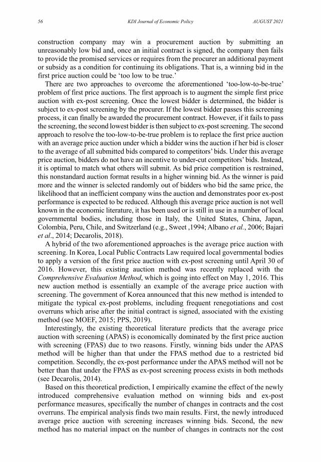
56 KDI Journal of Economic Policy AUGUST 2021
construction company may win a procurement auction by submitting an unreasonably low bid and, once an initial contract is signed, the company then fails to provide the promised services or requires from the procurer an additional payment or subsidy as a condition for continuing its obligations. That is, a winning bid in the first price auction could be ‘too low to be true.’
There are two approaches to overcome the aforementioned ‘too-low-to-be-true’ problem of first price auctions. The first approach is to augment the simple first price auction with ex-post screening. Once the lowest bidder is determined, the bidder is subject to ex-post screening by the procurer. If the lowest bidder passes this screening process, it can finally be awarded the procurement contract. However, if it fails to pass the screening, the second lowest bidder is then subject to ex-post screening. The second approach to resolve the too-low-to-be-true problem is to replace the first price auction with an average price auction under which a bidder wins the auction if her bid is closer to the average of all submitted bids compared to competitors’ bids. Under this average price auction, bidders do not have an incentive to under-cut competitors’ bids. Instead, it is optimal to match what others will submit. As bid price competition is restrained, this nonstandard auction format results in a higher winning bid. As the winner is paid more and the winner is selected randomly out of bidders who bid the same price, the likelihood that an inefficient company wins the auction and demonstrates poor ex-post performance is expected to be reduced. Although this average price auction is not well known in the economic literature, it has been used or is still in use in a number of local governmental bodies, including those in Italy, the United States, China, Japan, Colombia, Peru, Chile, and Switzerland (e.g., Sweet ,1994; Albano et al., 2006; Bajari et al., 2014; Decarolis, 2018).
A hybrid of the two aforementioned approaches is the average price auction with screening. In Korea, Local Public Contracts Law required local governmental bodies to apply a version of the first price auction with ex-post screening until April 30 of 2016. However, this existing auction method was recently replaced with the Comprehensive Evaluation Method, which is going into effect on May 1, 2016. This new auction method is essentially an example of the average price auction with screening. The government of Korea announced that this new method is intended to mitigate the typical ex-post problems, including frequent renegotiations and cost overruns which arise after the initial contract is signed, associated with the existing method (see MOEF, 2015; PPS, 2019).
Interestingly, the existing theoretical literature predicts that the average price auction with screening (APAS) is economically dominated by the first price auction with screening (FPAS) due to two reasons. Firstly, winning bids under the APAS method will be higher than that under the FPAS method due to a restricted bid competition. Secondly, the ex-post performance under the APAS method will not be better than that under the FPAS as ex-post screening process exists in both methods (see Decarolis, 2014).
Based on this theoretical prediction, I empirically examine the effect of the newly introduced comprehensive evaluation method on winning bids and ex-post performance measures, specifically the number of changes in contracts and the cost overruns. The empirical analysis finds two main results. First, the newly introduced average price auction with screening increases winning bids. Second, the new method has no material impact on the number of changes in contracts nor the cost

VOL. 43 NO. 3 An Unsuccessful Reform of the Local Public Contracts Law in Korea 57
overruns, which suggesting that neither the frequent renegotiation problem nor the cost overrun problem is resolved. These findings are consistent with the theoretical literature.
This paper is related to a number of existing studies. One of the most closely related papers is that by Decarolis (2014), which examines an Italian public procurement dataset and finds that the replacement of the existing average price auction (without screening) by a first price auction with (weak) screening in the end reduces winning bids while exacerbating the cost overrun problem. The current paper differs from Decarolis (2014) in the sense that I consider an average price auction with screening, while Decarolis (2014) considers an average price auction without screening. The aforementioned theoretic prediction that the average price auction with screening is economically dominated by the first price auction with screening holds only when the average price auction is combined with a screening process.
Kang and Kim (2017) empirically study Korean public procurement data. They consider central public contracts procured by central governmental bodies rather than local governmental bodies and examine the comprehensive examination method, which came into effect on January 1, 2016, for central public contracts. The comprehensive examination method is similar to the comprehensive evaluation method considered in this paper in that both are examples of the average price auction with screening. However, the detailed scoring rules of bid price and non-price characteristics are different. Moreover, the former is applied to central public contracts while the latter is applied to local public contracts. Without conducting a regression analysis but by comparing the average winning bid under the new method with that under the existing method, they find that winning bids increase due to the new auction method.
Kim (2012) examines the primary factors that determine a winner in the existing first price auction with screening using a Korean central public contracts dataset. He finds that almost every qualified bidder was assigned the highest possible score on non-price aspects in the screening process. This result implies that the first price auction with screening is in effect equal to a simple first price auction without screening given that the screening process cannot distinguish good from poor companies. Although Kim (2012) does not consider the average price auction with screening at all, his findings imply that even the existing first price auction with screening is not perfect. By considering this important caveat, I shall carefully discuss policy implications of the main findings of the current paper.
The current paper is also related to Spulber (1990), McAfee and McMillan (1986), and Bajari et al. (2014) in that these papers emphasize the ex-post moral hazard problem of the first price auction. Spulber (1990) and McAfee and McMillan (1986) depict the moral hazard problem theoretically, while Bajari et al. (2014) examines the problem empirically. In addition, the current paper is related to Lewis and Bajari (2011a; 2011b) in the sense that all of these empirical papers agree on the conclusion that a scoring auction that evaluates both the bid and quality of a bidder is better than a simple first price auction in the realm of public procurement.
The organization of the current paper is as follows. Section 2 reviews the institutional background of local public contracts in Korea. Section 3 provides an overview of related theoretical studies and formulates testable hypotheses based on

58 KDI Journal of Economic Policy AUGUST 2021
the theoretical predictions. Section 4 examines empirically the effect of the comprehensive evaluation method on winning bids and on ex-post performance outcomes. Finally, Section 5 draws some policy implications and presents concluding remarks.
II. Institutional Background
Local governments and local-government-owned enterprises frequently procure
contracts for construction. In Korea, these local governmental bodies must comply with the rules and regulations stipulated by the Local Public Contracts Law when they procure these contracts.
Until April 30, 2016, local governmental bodies were obliged to apply a type of first price auction augmented by an after-bid screening process when procuring construction contracts whose estimated prices are no less than 10 billion KRW.1 The procurement process consists of two phases. In the first phase, construction companies submit bids, and the lowest bidder is selected as the preferred bidder. In the second phase, the procurer screens this preferred bidder in order to assess whether this bidder is in fact capable of conducting the required construction tasks in a timely manner with a reasonable degree of quality. If the preferred bidder passes the screening, it becomes the winner and signs the contract with the procurer. However, if the preferred bidder is screened out, the procurer selects the second lowest bidder as the preferred bidder and proceeds with the screening process.
However, an amendment of the Local Public Contracts Law was passed and, therefore, a new method of procurement auction went into effect, starting on May 1, 2016. The new method is called the comprehensive evaluation method, which is basically a type of average price auction augmented by an after-bid screening process. This new method applies to almost every construction contract whose ‘estimated price’ is equal to or higher than 30 billion KRW. Under this method, construction companies submit bids. Then, the procurer evaluates the score on price (=bid) and the score on the non-price quality of each bidder and awards the contract to the bidder whose total score is the highest. Interestingly, the price score moves higher, as the difference between a bid and the average bid becomes smaller, where the average bid is the average of all submitted bids. That is, a bidder can receive the highest score on price if its bid is closer to the average bid relative to any competitor’s bid. Consequently, an optimal bidding strategy is to match what others may bid, and the worst strategy is to submit a bid lower than competitors’ bids. The scoring process for non-price quality in the new auction method is nearly identical to the screening process of the existing auction method in the sense that both processes rely on quantitative evaluations and the evaluation criteria and performance measurements are virtually identical. Accordingly, the newly introduced comprehensive evaluation method can be seen as an average price auction with screening, while the existing method is a type of first price auction with
1According to the Local Public Contracts Law, local governmental bodies must announce an ‘estimated price’
of a construction contract whenever it invites bids. This estimated price is generally different from the reserve price, which is kept secret until the opening of all submitted bids.

VOL. 43 NO. 3 An Unsuccessful Reform of the Local Public Contracts Law in Korea 59
screening. It should also be noted that this existing method still applies to construction contracts whose estimated prices are between 10 and 30 billion KRW.
According to the government of Korea, the motivation behind the replacement of the existing auction method with the comprehensive evaluation method is to mitigate ‘ex-post problems’ caused by the first price auction rule within the existing method. The Ministry of Economy and Finance (MOEF) explicitly admitted that the first price auction rule should be abandoned in order to prevent ex-post problems such as frequent renegotiations and cost overruns after the initial contract is signed (see MOEF, 2015). It has been argued that a construction company has an incentive to submit an unreasonably low bid to win the auction and then soon after strongly request a renegotiation of the terms of the contract and often threaten the procurer that continuation of construction is possible only if the procurer pays the contractor more than the initially agreed-upon amount. Another goal is to subsidize the construction industry. The Korea Public Procurement Service (PPS) announced that a primary objective of the comprehensive evaluation method is to boost the profitability of the construction industry (see PPS, 2019).
III. Theory Overview and Hypothesis Formulation
Although the first price auction is standard in economics and practice, it has been
criticized for the related trade-off between winning bids and ex-post performance (i.e., too-low-bid-to-be-true problem). According to Spulber (1990), auctions for contracts should be distinguished from auctions for goods because in the former case, a transaction does not take place immediately after the determination of a winner, and there is cost uncertainty. Given that it takes several months or years to complete the work required by a contract, a shock could attack the construction company in the meantime, possibly increasing the cost of construction. However, contracting parties cannot predict with certainty whether such a cost shock will occur when initially drawing up the contract. Due to this cost uncertainty, adverse selection, moral hazard, and the ‘winner’s curse’ could arise with auctions involving contracts. Similarly, McAfee and McMillan (1986) show that the first price auction may be feasible for awarding a contract at a low price but may also cause moral hazard of the winner ex-post. Decarolis (2018) also provides a stylized model in which a bidder gambles on the final cost of a project. In his model, the final cost is the sum of a bidder’s private cost and an added unforeseeable cost. By submitting a very low bid, an inefficient bidder can be awarded a project even if its private cost is higher than competitors. Once after the project begins, the added cost realizes as high or low. On the upside, the added cost becomes low and hence the inefficient bidder gets some return. However, on the down side, the added cost is sufficiently high that the bidder is not affordable to complete the project. In this case, the bidder will make a default on the project and hence loses nothing. In the end, inefficient bidders are awarded and could commit ex-post moral hazard under the first price auction.
In order to mitigate the aforementioned problem of an overly low bid being ‘too good to be true’ in a first price auction, one of two approaches can be utilized. The first approach is to augment a simple first price auction with ex-post screening. After selecting the lowest bidder as a preferred bidder, the procurer can determine by
60 KDI Journal of Economic Policy AUGUST 2021
screening whether the bidder can sufficiently fulfill its obligation. The second approach is to replace the first price auction with an average price auction. Decarolis (2018) and Conley and Decarolis (2016) find that winning bids under average price auctions are generally higher than those under a first price auction, as bidders could avoid price competition in order to win under the average price auction. If they lower their bids, the chance of winning also decreases. Alternatively, if they match what they believe others will bid, the odds that they will win improve. These findings suggest that the usual ex-post problem of the first price auction is less likely to occur in the average price auction given that the winning bidder is repaid more and is therefore in a better position to overcome an ex-post cost shock.
One may also consider a hybrid of the previous two approaches – the average price auction augmented by screening. The comprehensive evaluation method introduced on May 1, 2016 in the Local Public Contracts Law in Korea is such an example. However, according to Decarolis (2014), average price auctions with screening are economically dominated by first price auctions with screening. As a screening process exists under both auction formats, there is not much of a difference with regard to the ex-post problem. Therefore, the average price auction with screening worsens the financial burden of the procurer by curbing bid price competition without leading to any improvement in the ex-post performance, as opposed to the first price auction with screening.
Although the ex-post performance can be evaluated by a number of performance measures, theoretical and empirical studies in the literature emphasize the importance of cost overruns as one of the leading performance measures. The more the cost of construction increases after the initial contract period, the poorer the ex-post performance becomes. In addition, frequent renegotiations after the initial contract could also indicate poor ex-post performance. If a construction contract changes frequently, it implies that the winning bidder is not very adaptable to unforeseen changes in the construction environment, which means a lack of capability to fulfill its obligations. The government of Korea also considered frequent changes in contracts after the initial contract is signed as an example of an ex-post problem.
Based on this theoretical prediction in the comparison of the average price auction with screening and the first price auction with screening and based on the discussion of the ex-post performance measures, I can formulate the following two testable hypotheses.
Hypothesis 1: The replacement of the existing first price auction with screening
by the comprehensive evaluation method (i.e., an example of the average price auction with screening) results in an increase of the winning bid.
Hypothesis 2: The replacement of the existing first price auction with screening
by the comprehensive evaluation method does not reduce cost overruns or the frequency of changes in contracts.

VOL. 43 NO. 3 An Unsuccessful Reform of the Local Public Contracts Law in Korea 61
IV. Empirical Analysis: Price Performance
I utilize a contract-level cross-sectional dataset containing information on winning bids for 985 construction contracts procured by local governments or local- government-owned enterprises through standard competitive bidding processes during the period between May 2013 and December 2018. This period is roughly equal to the three-year window of May 1, 2016, when the new comprehensive evaluation method was introduced. The raw data is obtained from the Procurement Information Open Portal, which is operated by the Korea Public Procurement Service.2
I restrict the dataset so that it only contains construction contracts for which the ‘estimated price’ is no less than 10 billion Korean won. This is done because 10B KRW has long been considered in practice to be a threshold that distinguishes between normal-scale and small-scale construction projects. The Local Public Contracts Law also followed this convention and therefore applied a standard auction format to every construction contract whose estimated price exceeds 10B KRW but applied only a largely simplified version of the standard format to every other construction contract whose estimated price did not reach 10B KRW. However, since May 1, 2016, the comprehensive evaluation method has replaced the aforementioned standard method for any contract whose estimated price exceeds 30 billion KRW, while the existing standard method continues to be applied to every contract whose estimated price lies between 10B and 30B KRW. In this sense, I consider contracts higher than 30B KRW as a ‘treatment’ group while other contracts in the range of 10B to 30B KRW are the ‘control’ group in the following analysis.
However, it is also important to note that contracts between 10B and 30B KRW in fact form a reasonably good but not an ideal control group given that until May 1, 2016, one version of the first price auction with screening was applied to this group while another version of the first price auction with screening was applied to contracts exceeding 30B KRW. The two versions are similar in the sense that the lowest bidder is the first to be screened, but if it fails to pass the screening process, the second lowest bidder is then screened. However, in the first version, the procurement authority assesses the ability to conduct the assigned construction contract (i.e., ability screening) in the screening process, whereas in the second version, the authority assesses the appropriateness of the winning bid (i.e., bid screening) during the screening process. In the following, I provide a detailed explanation of this second version; some bidders may offer bids that are too high or too low such that they may be unable to properly conduct the assigned construction work at such low bids. For instance, a construction company may submit an unreasonably bid so low that it cannot even cover their costs. If such a company wins the auction, obviously it cannot properly conduct the required work. To prevent such an event from taking place, a procurement authority initially checks whether the winning bid lies in a predetermined safe interval. If the bid is outside of the safe interval, it is a signal that the bid is too high or too low. In such a case, the winning bidder must explain in front of a screening committee that it is still able to fulfill the
2https://data.g2b.go.kr (Final access date: Nov. 27, 2020).

62 KDI Journal of Economic Policy AUGUST 2021
required work even with this seemingly unreliable bid. The winning bidder is finally awarded the contract only if the committee determines that the explanation is reasonable enough. The gist is that ability screening in the first version and bid screening in the second share an identical goal: preventing an unreliable bidder from winning an auction by offering an unreasonably low bid. In addition, the two versions are slightly different in that the first version places a lower bound on bids, meaning that bidders are excluded if they bid lower than this bound. Although the second version does not utilize the same lower bound, the safe intervals used in the bid screening process effectively install similar lower bounds. I do not argue that the first and second versions are perfectly identical auction formats, but I assume that the two versions are at least reasonably similar. Likewise, the literature does not make an explicit distinction between first price auctions with ability screening and first price auctions with bid screening (see Bajari et al., 2014; Decarolis, 2014). The following empirical results based on the price and non-price effects of the comprehensive evaluation method obtained from the difference-in-differences estimation should be understood in this context.
Table 1 summarizes descriptive statistics of the variables of interest. The winning bid is the ratio of a winner’s bid price to the reserve price. The average winning bid of 985 construction contracts is 80.28%. A dummy variable D2016.5 equals one if the given contract is procured after May 1, 2016, and zero otherwise. Another dummy variable D30B equals one if the estimated price of the given contract is greater than or equal to 30B KRW. Of 985 contracts, 51.9% were procured after May 1, 2016, and 15.2% were contracts for which the estimated price exceeds 30B KRW. The estimated price and the reserve price are similar but not identical. The former is publicly disclosed before bidding while the latter is kept secret until all sealed bids are opened. The number of bidders is on average 182, which implies that bidding is usually very competitive.
Figure 1 compares the (within-quarter average) winning bids of the treatment group and control group. The control group consists of contracts whose estimated price is 10B to 30B KRW for which the comprehensive evaluation method is not applied. The treatment group contains contracts whose estimated price is greater than or equal to 30B KRW for which the new method has been applied since May 1, 2016. Before its experimental application, the winning bid of the treatment group is approximately 75% (as a percentage of the reserve price), which is approximately 6% below the winning bid of the control group. However, with the experimental application as described above, the winning bid of the treatment group suddenly rises above the winning bid of the control group.
I shall estimate the following empirical model:
(1) 2016.5 30 2016.5 301 2 3
B Bit it it it it it itwinning_bid D D D D X
where itwinning_bid is the winner’s bid price for contract i procured at time t as a percentage of reserve price. 2016.5
itD is a dummy variable that equals 1 if and only if the bidding process for contract i begins on or after May 1, 2016. 30B
itD is a dummy variable that equals 1 if and only if the estimated price for contract i is equal to or higher than 30 billion KRW.
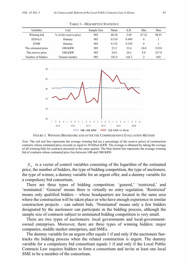
VOL. 43 NO. 3 An Unsuccessful Reform of the Local Public Contracts Law in Korea 63
TABLE 1—DESCRIPTIVE STATISTICS
Variables Unit Sample Size Mean S.D. Min Max Winning bid % of the reserve price 985 80.28 2.69 67.22 98.91
D2016.5 Dummy 985 0.519 0.499 0 1 D30B Dummy 985 0.152 0.359 0 1
The estimated price 10B KRW 985 23.5 23.6 10.0 219.0 The reserve price 10B KRW 985 24.8 24.3 8.8 227.0
Number of bidders Natural number 985 182.5 144.7 2 692
FIGURE 1. WINNING BID BEFORE AND AFTER THE COMPREHENSIVE EVALUATION METHOD
Note: The red real line represents the average winning bid (as a percentage of the reserve price) of construction contracts whose estimated price exceeds or equal to 30 billion KRW. The average is obtained by taking the average of all winning bids for contracts procured in the same quarter. The blue dotted line represents the average winning bid of contracts whose estimated price lies between 10B and 30B KRW.
itX is a vector of control variables consisting of the logarithm of the estimated price, the number of bidders, the type of bidding competition, the type of auctioneer, the type of winner, a dummy variable for an urgent offer, and a dummy variable for a compulsory bid consortium.
There are three types of bidding competition: ‘general,’ ‘restricted,’ and ‘nominated.’ ‘General’ means there is virtually no entry regulation. ‘Restricted’ means only qualified bidders – whose headquarters are located in the same area where the construction will be taken place or who have enough experience in similar construction projects – can submit bids. ‘Nominated’ means only a few bidders designated by the auctioneer can participate in the bidding process, although the sample size of contracts subject to nominated bidding competition is very small.
There are two types of auctioneers: local governments and local-government- owned enterprises. Moreover, there are three types of winning bidders: major companies, middle market enterprises, and SMEs.
The dummy variable for an urgent offer equals 1 if and only if the auctioneer fast- tracks the bidding process when the related construction is urgent. The dummy variable for a compulsory bid consortium equals 1 if and only if the Local Public Contracts Law requires bidders to form a consortium and invite at least one local SME to be a member of the consortium.

64 KDI Journal of Economic Policy AUGUST 2021
In addition, I consider a number of fixed effects, including ‘region,’ ‘construction type,’ and ‘year.’ ‘Region’ is a municipal-level variable, such as Seoul, Busan, or Gyeongi Province. ‘Construction type’ examples include civil engineering, architecture, and plants, among others.
The coefficient of interest is 1 , which measures the effect of the comprehensive evaluation method on the winning bid. Here, I examine this effect via a difference-in-differences estimation. Table 2 illustrates the difference-in-differences estimation. Recall that the new scoring method has applied contracts whose estimated prices are equal to or exceed 30B KRW since May 1, 2016. Therefore, the estimated effect of the difference in time on the winning bid for the treatment group is 1 2 , while the estimated effect of the same difference in time on the winning bid for the control group is 2 . Thus, difference-in-differences 1 measures the effect of the new method on the winning bid.
Table 3 shows the estimation results of empirical model (1) for a number of model specifications. The first three specifications are baseline specifications. The first specification ‘Simple’ is the simplest possible difference-in-differences model specification. The second specification ‘FE’ adds to ‘Simple’ the region fixed effect and construction fixed effect as additional control variables. The third specification ‘All’ adds to ‘FE’ some additional control variables including the number of bidders, the type of bidder, and the type of auctioneer.
In any of the first three baseline specifications, the estimated coefficient for the interaction term of the two dummy variables 2016.5
itD and 30BitD is positive and
significant. That is, the introduction of the comprehensive evaluation method, which is a version of the average price auction with screening, is associated with an increase in the winning bid. This positive association is statistically significant at the 1% level and is also economically significant as the magnitude is approximately 7.5%, which is meaningfully large especially in the current low-interest-rate environment. Recall from Table 1 that the average reserve price of construction contracts contained in the dataset is 24.8 billion KRW, meaning that a local government or a local-government-owned enterprise should pay on average 1.86 billion KRW more for each construction contract due to the new method. Therefore, the introduction of the new auction scoring rule significantly increases the fiscal burden borne by local governmental bodies.
The signs of the coefficient estimates of other control variables are also consistent with intuition. The winner is paid the less as the number of competing bidders grows simply because the bidding is then more competitive. In contrast, the winner is paid the more if it is not a major company but a middle-market enterprise or a SME. This presumably stems from the fact that the Local Public Contracts Law requires auctioneers to provide some privileges to non-major companies.
TABLE 2—IDENTIFICATION BY DIFFERENCE-IN-DIFFERENCE
30B KRW or More Less than 30B KRW Difference On or after May 1, 2016 1 2 3 2 1 3
Before May 1, 2016 3 0 3
Difference 1 2 2 1
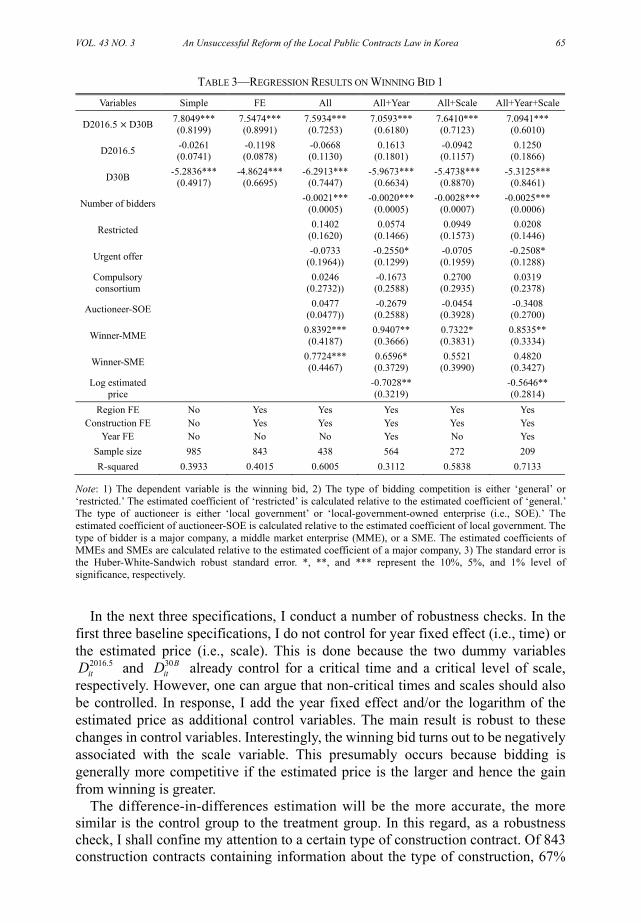
VOL. 43 NO. 3 An Unsuccessful Reform of the Local Public Contracts Law in Korea 65
TABLE 3—REGRESSION RESULTS ON WINNING BID 1
Variables Simple FE All All+Year All+Scale All+Year+Scale
D2016.5 × D30B 7.8049*** (0.8199)
7.5474*** (0.8991)
7.5934*** (0.7253)
7.0593*** (0.6180)
7.6410*** (0.7123)
7.0941*** (0.6010)
D2016.5 -0.0261 (0.0741)
-0.1198 (0.0878)
-0.0668 (0.1130)
0.1613 (0.1801)
-0.0942 (0.1157)
0.1250 (0.1866)
D30B -5.2836*** (0.4917)
-4.8624*** (0.6695)
-6.2913*** (0.7447)
-5.9673*** (0.6634)
-5.4738*** (0.8870)
-5.3125*** (0.8461)
Number of bidders -0.0021*** (0.0005)
-0.0020*** (0.0005)
-0.0028*** (0.0007)
-0.0025*** (0.0006)
Restricted 0.1402 (0.1620)
0.0574 (0.1466)
0.0949 (0.1573)
0.0208 (0.1446)
Urgent offer -0.0733 (0.1964))
-0.2550* (0.1299)
-0.0705 (0.1959)
-0.2508* (0.1288)
Compulsory consortium 0.0246
(0.2732)) -0.1673 (0.2588)
0.2700 (0.2935)
0.0319 (0.2378)
Auctioneer-SOE 0.0477 (0.0477))
-0.2679 (0.2588)
-0.0454 (0.3928)
-0.3408 (0.2700)
Winner-MME 0.8392*** (0.4187)
0.9407** (0.3666)
0.7322* (0.3831)
0.8535** (0.3334)
Winner-SME 0.7724*** (0.4467)
0.6596* (0.3729)
0.5521 (0.3990)
0.4820 (0.3427)
Log estimated price -0.7028**
(0.3219) -0.5646** (0.2814)
Region FE No Yes Yes Yes Yes Yes Construction FE No Yes Yes Yes Yes Yes
Year FE No No No Yes No Yes Sample size 985 843 438 564 272 209 R-squared 0.3933 0.4015 0.6005 0.3112 0.5838 0.7133
Note: 1) The dependent variable is the winning bid, 2) The type of bidding competition is either ‘general’ or ‘restricted.’ The estimated coefficient of ‘restricted’ is calculated relative to the estimated coefficient of ‘general.’ The type of auctioneer is either ‘local government’ or ‘local-government-owned enterprise (i.e., SOE).’ The estimated coefficient of auctioneer-SOE is calculated relative to the estimated coefficient of local government. The type of bidder is a major company, a middle market enterprise (MME), or a SME. The estimated coefficients of MMEs and SMEs are calculated relative to the estimated coefficient of a major company, 3) The standard error is the Huber-White-Sandwich robust standard error. *, **, and *** represent the 10%, 5%, and 1% level of significance, respectively.
In the next three specifications, I conduct a number of robustness checks. In the
first three baseline specifications, I do not control for year fixed effect (i.e., time) or the estimated price (i.e., scale). This is done because the two dummy variables
2016.5itD and 30B
itD already control for a critical time and a critical level of scale, respectively. However, one can argue that non-critical times and scales should also be controlled. In response, I add the year fixed effect and/or the logarithm of the estimated price as additional control variables. The main result is robust to these changes in control variables. Interestingly, the winning bid turns out to be negatively associated with the scale variable. This presumably occurs because bidding is generally more competitive if the estimated price is the larger and hence the gain from winning is greater.
The difference-in-differences estimation will be the more accurate, the more similar is the control group to the treatment group. In this regard, as a robustness check, I shall confine my attention to a certain type of construction contract. Of 843 construction contracts containing information about the type of construction, 67%

66 KDI Journal of Economic Policy AUGUST 2021
TABLE 4—REGRESSION RESULTS ON WINNING BID 2
Variables Civil- Simple Civil- All Civil-
All+Year Civil-
All+Scale Civil-
All+Year+ScaleArchitecture-
Simple D2016.5 ×
D30B 6.8808*** (1.1101)
8.4866*** (1.1429)
7.4804*** (0.8986)
8.3559*** (1.1686)
7.5976*** (0.8874)
11.2196*** (1.2218)
D2016.5 -0.1329 (0.1182)
-0.0361 (0.1307)
0.2364 (0.2745)
-0.0335 (0.1276)
0.1953 (0.2790)
-0.1045 (0.1178)
D30B -5.0700*** (0.9209)
-7.1507*** (1.1793)
-6.4658*** (1.0172)
-6.1969*** (1.1851)
-5.8762*** (1.1501)
-4.9930*** (0.6370)
Control variable Yes Yes Yes Yes Yes Yes
Log estimated price -0.8089*
(0.4324) -0.5032* (0.2982)
Region FE No Yes Yes Yes Yes No Construction
FE No Yes Yes Yes Yes No
Year FE No No Yes No Yes No Sample size 564 272 272 272 272 209 R-squared 0.3112 0.5838 0.7741 0.5911 0.7769 0.7133
Note: 1) The dependent variable is the winning bid, 2) The first five model specifications consider only civil engineering construction contracts and the last model specification considers only architecture construction contracts, 3) The row for ‘Control variable’ is marked ‘Yes’ if the number of bidders, the type of competition, the dummy variable for urgent offer, the dummy variable for compulsory consortium, the type of auctioneer, and the type of winner are all controlled. The row is marked as ‘No’ if all of these variables are not controlled, 4) The standard error is the Huber-White-Sandwich robust standard error. *, **, and *** represent the 10%, 5%, and 1% level of significance, respectively.
are civil engineering construction projects, 25% are architecture construction projects, and only less than 10% are other types of construction projects.
Table 4 shows the results when the estimation is conducted separately for civil engineering and architecture constructions. For civil engineering, which is the most important type of construction in terms of its share out of all construction projects, the comprehensive evaluation method is found to be positively associated with the winning bid, and this outcome is statistically significant at the 1% level for all five specifications. The magnitude is approximately 8%, which is roughly identical to the magnitude of 7.5% calculated for all construction projects. For architecture, which is the second most important type of construction, the new method is still positively associated with the winning bid at a strongly statistically significant level. The economic significance is even stronger as the estimated effect is 11.2% of the reserve price. However, it is important to note that this magnitude is obtained without controlling for a number of relevant variables due to the lack of sample of architecture construction contracts.
In this paper, I interpret an increase in the winning bid as a rise in the fiscal pressure on local governmental bodies. However, this interpretation is invalid if an auctioneer lowers the reserve price in response to the new auction scoring rule, simply because the auctioneer’s payment to the winner equals the product of the winning bid and the reserve price. In fact, some industry practitioners argue that local governments will cut reserve prices in order to minimize foreseeable fiscal shocks. In this regard, I examine how the reserve price changes in response to the introduction of the comprehensive evaluation method. Table 5 shows the estimation results, where the dependent variable is not the winning bid but the logarithm of the

VOL. 43 NO. 3 An Unsuccessful Reform of the Local Public Contracts Law in Korea 67
TABLE 5—REGRESSION RESULTS ON RESERVE PRICES
Variables Simple FE All All+Year All+Year+Scale
D2016.5 × D30B -0.0423 (0.0848)
0.0500 (0.0947)
0.0772 (0.1014)
0.0668 (0.1058)
0.0056 (0.0090)
D2016.5 -0.0251 (0.0207)
-0.0444* (0.0233)
-0.0379 (0.0280)
-0.0662 (0.0582)
-0.0024 (0.0064)
D30B 1.3158*** (0.0512)
1.2135*** (0.0667)
1.1256*** (0.0886)
1.1232*** (0.0894)
-0.0264*** (0.0101)
Log estimated price 0.9910*** (0.0059)
Control variables No No Yes Yes Yes Region FE No Yes Yes Yes Yes
Construction FE No Yes Yes Yes Yes Year FE No No No Yes Yes
Sample size 985 843 438 438 438 R-squared 0.6641 0.6597 0.7017 0.7019 0.9965
Note: 1) The dependent variable is the logarithm of the reserve price, 2) The row for ‘Control variable’ is marked ‘Yes’ if the number of bidders, the type of competition, the dummy variable for an urgent offer, the dummy variable for a compulsory consortium, the type of auctioneer, and the type of winner are all controlled. The row is marked as ‘No’ if all of these variables are not controlled, 3) The standard error is the Huber-White-Sandwich robust standard error. *, **, and *** represent the 10%, 5%, and 1% level of significance, respectively.
reserve price. These results show that the reserve price is not associated with the new auction scoring rule, which means a rise in the winning bid can be interpreted as an increase in the financial burden on local governments.
V. Empirical Analysis: Ex-Post Performance
The first dataset used in the previous section contains information only about what
happens on the bid opening and contract signing dates, but it does not have information about changes in contracts. Fortunately, the Procurement Information Open Portal also provides a separate dataset based on which one can trace out how an initial contract evolves over time. However, this second dataset is not ready to be used in an empirical analysis given that renegotiated contracts are not properly linked to the corresponding initial contract. I have matched each set of renegotiated contracts to their corresponding initial contract manually and generated a new contract-level cross-sectional dataset that contains the number of contract renegotiations and the amounts of cost overruns for roughly 1,337 construction contracts that were initially procured during the period between August 1, 2012, and June 30, 2020, which is a three-year and nine-month event window at around May 1, 2016. I merge this second dataset with the first dataset. However, the information pertaining to the number of bidders, urgent offers, and the type of bidder (i.e., whether it is a large company, middle-market enterprise, or a SME) cannot be utilized because there is no related identifier in the second dataset.
Table 6 provides summary statistics of the variables reflecting changes in contracts. Even if the two parties agree and sign a contract, they could afterward renegotiate over the initial contract for some reason. The number of changes (1Y) is the number of official revisions made in one year since the initial contract date.

68 KDI Journal of Economic Policy AUGUST 2021
TABLE 6—DESCRIPTIVE STATISTICS
Variables Unit Sample size Mean S.D. Min Max Number of
changes (6M) Number 1,160 0.337 0.607 0 4
Number of changes (1Y) Number 989 1.271 1.131 0 9
Number of changes (2Y) Number 644 2.967 1.836 0 11
Cost overrun (6M) % of the reserve price 1,160 -0.014 5.805 -72.361 81.098
Cost overrun (1Y) % of the reserve price 989 0.386 8.055 -60.875 86.097
Cost overrun (2Y) % of the reserve price 644 2.823 11.184 -54.889 89.694
Note: The dataset contains information about changes in contractual terms which occurred up to February 28, 2020. Therefore, it is possible to trace out changes in contractual terms six months from an initial contract date only if the initial contract date is no later than August 30, 2019. For this reason, the numbers of changes (6M) and cost overruns (6M) are calculated for each contract whose initial contract date is between January 1, 2013, and August 30, 2019, which is a three-year and four-month window relative to May 1 2016. Similarly, the numbers of changes (1Y) and cost overruns (1Y) are calculated for each contract whose initial contract date is between July 1, 2013, and February 28, 2019, which is a two-year and ten-month window relative to May 1 2016. Additionally, the numbers of changes (2Y) and cost overruns (2Y) are calculated for each contract whose initial contract date is between July 1, 2014, and February 28, 2018, representing a one-year and ten-month window relative to May 1, 2016. However, all of the regression results presented in this section are robust to this subsampling.
These changes are recorded officially and hence the related new contract overrides the initial one. A typical contract changes on average 0.337 times, 1.271 times, and 2.967 times after six months, one year, and two year from the initial contract date, respectively. The maximum number of changes made for one year is nine. Cost overrun (1Y) refers to the cumulative changes in the cost of construction which occurred one year after the initial contract date. Cost overruns are measured as a percentage of the reserve price. (The reserve price is set only once at the bid opening time.) Thus, the cost of a construction contract increases on average by 0.386% of the reserve price one year since the initial contract date and by 2.823% for two years. Although the average of the cost overrun (1Y) is relatively small, this does not mean that cost overruns are not a significant issue in public procurement. The standard deviation of the cost overrun (1Y) is 8.055, which is approximately 20 times larger than its mean. This implies that once a cost overrun arises, its magnitude is meaningfully large. Consistent with this notion, the minimum and maximum of the cost overrun (1Y) in absolute terms turn out to be very large.
In the following paragraphs, I examine whether the newly introduced comprehensive evaluation method improves the reliability of a construction contract. To this end, I use two measurements of reliability: the number of changes and the cost overruns. If these variables decrease according to the new method, it suggests an improvement in the reliability.
A. Number of Changes
Figure 2 illustrates the movement of the number of changes (1Y) before and after
May 1, 2016, when the comprehensive evaluation method was first introduced for construction contracts whose estimated prices are equal to or exceed 30B KRW. The
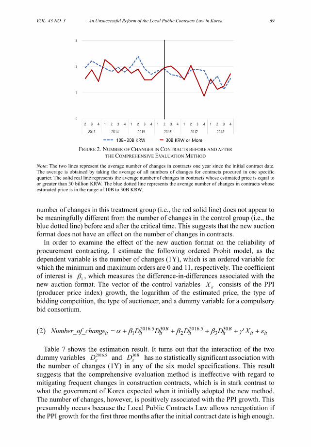
VOL. 43 NO. 3 An Unsuccessful Reform of the Local Public Contracts Law in Korea 69
FIGURE 2. NUMBER OF CHANGES IN CONTRACTS BEFORE AND AFTER
THE COMPREHENSIVE EVALUATION METHOD
Note: The two lines represent the average number of changes in contracts one year since the initial contract date. The average is obtained by taking the average of all numbers of changes for contracts procured in one specific quarter. The solid real line represents the average number of changes in contracts whose estimated price is equal to or greater than 30 billion KRW. The blue dotted line represents the average number of changes in contracts whose estimated price is in the range of 10B to 30B KRW.
number of changes in this treatment group (i.e., the red solid line) does not appear to be meaningfully different from the number of changes in the control group (i.e., the blue dotted line) before and after the critical time. This suggests that the new auction format does not have an effect on the number of changes in contracts.
In order to examine the effect of the new auction format on the reliability of procurement contracting, I estimate the following ordered Probit model, as the dependent variable is the number of changes (1Y), which is an ordered variable for which the minimum and maximum orders are 0 and 11, respectively. The coefficient of interest is 1 , which measures the difference-in-differences associated with the new auction format. The vector of the control variables itX consists of the PPI (producer price index) growth, the logarithm of the estimated price, the type of bidding competition, the type of auctioneer, and a dummy variable for a compulsory bid consortium.
(2) 2016.5 30 2016.5 301 2 3
B Bit it it it it it itNumber_of_change D D D D X
Table 7 shows the estimation result. It turns out that the interaction of the two dummy variables 2016.5
itD and 30BitD has no statistically significant association with
the number of changes (1Y) in any of the six model specifications. This result suggests that the comprehensive evaluation method is ineffective with regard to mitigating frequent changes in construction contracts, which is in stark contrast to what the government of Korea expected when it initially adopted the new method. The number of changes, however, is positively associated with the PPI growth. This presumably occurs because the Local Public Contracts Law allows renegotiation if the PPI growth for the first three months after the initial contract date is high enough.

70 KDI Journal of Economic Policy AUGUST 2021
TABLE 7—ORDERED PROBIT REGRESSION RESULTS OF NUMBER OF CHANGES 1
Variables Simple FE All All+Year All+Scale All+Year+Scale
D2016.5 × D30B -0.1190 (0.1961)
-0.2018 (0.2153)
-0.1406 (0.2097)
-0.1376 (0.2111)
-0.1277 (0.2101)
-0.1258 (0.2115)
D2016.5 0.0590 (0.0739)
0.0352 (0.0836)
-0.0360 (0.0979)
-0.2862 (0.2036)
-0.0405 (0.0979)
-0.2872 (0.2030)
D30B -0.5353*** (0.1397)
-0.5198*** (0.1657)
-0.2631 (0.1708)
-0.2574 (0.1718)
-0.0944 (0.2115)
-0.0960 (0.2140)
PPI growth 0.0648 (0.0431)
0.0862* (0.0487)
0.0625 (0.0431)
0.0842* (0.0488)
Restricted -0.1628* (0.0959)
-0.1704* (0.0959)
-0.1503 (0.0962)
-0.1588* (0.0962)
Compulsory consortium 0.1023
(0.1387) 0.0884
(0.1400) 0.0930
(0.1391) 0.0797
(0.1404)
Auctioneer-SOE -0.9837*** (0.1240)
-0.9760*** (0.1241)
-0.9808*** (0.1237)
-0.9731*** (0.1238)
Log estimated price -0.1444
(0.1080) -0.1376 (0.1088)
Region FE No Yes Yes Yes Yes Yes Construction FE No Yes Yes Yes Yes Yes
Year FE No No No Yes No Yes Sample size 989 844 844 844 844 844
Pseudo R-squared 0.0150 0.0486 0.0828 0.0850 0.0835 0.0856
Note: 1) The dependent variable is the number of changes in contracts one year since the initial contract date, 2) PPI growth is the growth rate of the producer price index during the three months after the initial contract date, 3) The type of bidding competition is either ‘general’ or ‘restricted.’ The estimated coefficient of ‘restricted’ is calculated relative to the estimated coefficient of ‘general.’ The type of auctioneer is either ‘local government’ or ‘local-government-owned enterprise (i.e., SOE).’ The estimated coefficient of auctioneer-SOE is calculated relative to the estimated coefficient of local government, 4) The standard error is the Huber-White-Sandwich robust standard error. *, **, and *** represent the 10%, 5%, and 1% level of significance, respectively.
Moreover, the dependent variable is negatively associated with the variable ‘Restricted.’ A plausible explanation here is that the initial contract is more favorable to the winning bidder if the competition is restricted as opposed to unrestricted and, hence, the winner is less likely to require renegotiation.
Below, I conduct a number of robustness checks. In the first set of robustness checks, I control for the contract size. In the baseline estimation, I place relatively small contracts for which the estimated price is 30B KRW and relatively large contracts for which the estimated price is 200B KRW into the same treatment group. Although the same set of procurement rules is applied to these two contracts, one may expect that the characteristics of these two types are quite different. As a response, I focus on a subsample which contains contracts for which the estimated price is in a small range around at 30B KRW. The first three columns in Table 8 suggest that the comprehensive evaluation method is still ineffective in reducing the number of changes in contracts.
In the second set of robustness checks, I trace out changes in contracts for different time intervals. One can argue that one year is not long enough to trace out changes in contracts fully. Others may be interested in examining changes in a shorter time interval than one year, as incomplete contracts could be renegotiated early after the initial contract date. In response, I consider the numbers of changes in contracts six

VOL. 43 NO. 3 An Unsuccessful Reform of the Local Public Contracts Law in Korea 71
TABLE 8—ORDERED PROBIT REGRESSION RESULTS OF NUMBER OF CHANGES 2
Variables Within 10B Within 15B Within 20B 6-month 1-year 2-year
D2016.5 × D30B 0.2708 (0.4707)
0.0910 (0.3412)
0.0872 (0.3073)
-0.3373 (0.2676)
-0.1406 (0.2097)
-0.2045 (0.2183)
D2016.5 0.3777 (0.2384)
0.1486 (0.1496)
-0.0194 (0.0985)
-0.0284 (0.1093)
-0.0360 (0.0979)
0.0860 (0.1187)
D30B -0.2713 (0.3389)
-0.0770 (0.2587)
-0.3051 (0.2350)
-0.0276 (0.1916)
-0.2631 (0.1708)
-0.0964 (0.1691)
Control variables Yes Yes Yes Yes Yes Yes Region FE Yes Yes Yes Yes Yes Yes
Construction FE Yes Yes Yes Yes Yes Yes Sample size 196 374 766 940 844 617
Pseudo R-squared 0.1848 0.1011 0.066 0.0778 0.0828 0.0575
Note: 1) For the first three specifications, the dependent variable is the number of changes in contracts one year since the initial contract date. The first specification considers contracts whose estimated prices are within 10B KRW relative to 30B KRW. That is, contracts with estimated prices from 20B to 40B KRW are considered. The second specification considers contracts with estimated prices within 15B KRW relative to 30B KRW. The third specification considers contracts with estimated prices within 20B KRW relative to 30B KRW, 2) For the next three specifications, the dependent variable is the number of changes in contracts six months, one year, and two years since the initial contract date, respectively, 3) The row for ‘Control variables’ is marked ‘Yes’ if PPI growth, the type of competition, the dummy variable for compulsory consortium, and the type of auctioneer are all controlled. The row is marked ‘No’ if all of these variables are not controlled, 4) The standard error is the Huber-White-Sandwich robust standard error. *, **, and *** represent the 10%, 5%, the 1% level of significance, respectively.
TABLE 9—ORDERED PROBIT REGRESSION RESULTS OF NUMBER OF CHANGES 3
Variables Civil 6-month Civil 1-year Civil 2-year Architecture 1-year Architecture 2-year
D2016.5 × D30B -0.3851 (0.3644)
-0.2809 (0.2524)
0.0407 (0.2971)
0.2120 (0.3964)
-0.5496 (0.4409)
D2016.5 -0.1820 (0.1329)
-0.0537 (0.1208)
-0.0658 (0.1471)
-0.2857 (0.2037)
0.2734 (0.2798)
D30B -0.1750 (0.2566)
-0.0703 (0.2107)
-0.2123 (0.2101)
-0.5626* (0.3397)
0.2910 (0.3634)
Control variables Yes Yes Yes Yes Yes Region FE Yes Yes Yes Yes Yes
Construction FE Yes Yes Yes Yes Yes Sample size 617 548 409 225 160
Pseudo R-squared 0.1002 0.0944 0.0314 0.0989 0.1383
Note: 1) For the first three specifications, I consider only civil engineering construction contracts. The dependent variable is the number of changes in contracts six months, one year, and two years since the initial contract date, respectively, 2) For the next two specifications, I consider only architecture construction contracts. The dependent variable is the number of changes in contracts one year and two years from the initial contract date, respectively, 3) The row for ‘Control variables’ is marked ‘Yes’ if PPI growth, the type of competition, the dummy variable for compulsory consortium, and the type of auctioneer are all controlled. The row is marked ‘No’ if all of these variables are not controlled, 4) The standard error is the Huber-White-Sandwich robust standard error. *, **, and *** represent the 10%, 5%, and 1% level of significance, respectively.
months, one year, and two years from the initial contract date. The last three columns in Table 8 show that the coefficient of interest is still insignificant.
In the third set of robustness checks, I consider two most important types of construction, civil engineering and architecture. Table 9 suggests that the comprehensive evaluation method could not effectively cause any difference in the number of changes in either type of construction contract.

72 KDI Journal of Economic Policy AUGUST 2021
B. Cost Overrun
Cost overrun is a phenomenon during which the cost of construction increases unexpectedly after an initial contract is signed. A cost overrun is more likely to arise if the winning bidder is not capable of conducting the required work or if the winner does not put much effort into completing its mission. The government of Korea predicted that the comprehensive evaluation method could reduce the cost overrun problem. To ascertain whether this expectation is realized, I estimate the following empirical model (3). The dependent variable is the cost overrun as a percentage of the reserve price. The vector of control variables itX is identical to that used in empirical model (2).
(3) 2016.5 30 2016.5 301 2 3
B Bit it it it it it itCost overrun D D D D X
Table 10 shows the estimation results for a number of model specifications. In every such specification, it turns out that the new auction format is not statistically significantly associated with the cost overrun for the period of one year since the initial contract date. That is, this suggests that using the new method is futile with regard to reducing the cost overrun problem.
TABLE 10—REGRESSION RESULTS OF COST OVERRUN 1
Variables Simple FE All All+Year All+Scale All+Year+Scale
D2016.5 × D30B -0.4272 (0.7373)
0.3411 (0.8731)
0.3211 (0.8649)
0.2795 (0.8202)
0.3473 (0.8823)
0.3023 (0.8354)
D2016.5 0.5997 (0.6089)
0.3771 (0.6678)
0.2097 (0.7487)
-3.2078* (1.6786)
0.2030 (0.7523)
-3.2098* (1.6790)
D30B -0.3959 (0.5329)
-1.1976 (0.7331)
-0.6327 (0.7174)
-0.5607 (0.6823)
-0.3445 (0.9903)
-0.2995 (0.9633)
PPI growth 0.1184 (0.3462)
0.0503 (0.3771)
0.1136 (0.3487)
0.0462 (0.3803)
Restricted -1.3087** (0.5860)
-1.1838** (0.5904)
-1.2886** (0.5950)
-1.1661* (0.5994)
Compulsory consortium 0.3076
(0.6739) 0.1241
(0.6738) 0.2925
(0.6794) 0.1105
(0.6778)
Auctioneer-SOE 1.1674** (0.5521)
1.3303** (0.5445)
1.1724** (0.5530)
1.3351** (0.5449)
Log estimated price -0.2446
(0.6560) -0.2210 (0.6530)
Region FE No Yes Yes Yes Yes Yes Construction FE No Yes Yes Yes Yes Yes
Year FE No No No Yes No Yes Sample size 989 844 844 844 844 844 R-squared 0.0021 0.0368 0.0420 0.0550 0.0421 0.0551
Note: 1) The dependent variable is the cost overrun as a percentage of the reserve price one year since the initial contract date, 2) PPI growth is the growth rate of the producer price index during the three months since the initial contract date. The type of bidding competition is either ‘general’ or ‘restricted.’ The estimated coefficient of ‘restricted’ is calculated relative to the estimated coefficient of ‘general.’ The type of auctioneer is either ‘local government’ or ‘local-government-owned enterprise (i.e., SOE).’ The estimated coefficient of auctioneer-SOE is calculated relative to the estimated coefficient of local government, 3) The standard error is the Huber-White-Sandwich robust standard error. *, **, and *** represent the 10%, 5%, and 1% level of significance, respectively.

VOL. 43 NO. 3 An Unsuccessful Reform of the Local Public Contracts Law in Korea 73
I also check the robustness of the baseline estimation result. In the first three columns in Table 11, I focus on a subsample of contracts whose estimated prices lie in small ranges around at 30B KRW. In the next three columns, I consider not the just one-year change in construction cost but also the six-month and two-year changes. In addition, I confine my attention to the two most important types of construction, i.e., civil engineering and architecture projects, as presented in Table 12. The estimation results for all of these specifications suggest that the new auction
TABLE 11—REGRESSION RESULTS OF COST OVERRUN 2
Variables Within 10B Within 15B Within 20B 6-month 1-year 2-year
D2016.5 × D30B 2.5553 (1.9845)
0.4613 (1.6627)
0.3297 (1.1909)
0.2814 (0.5332)
0.3211 (0.8649)
0.8930 (1.5474)
D2016.5 -2.7671 (1.9375)
-0.0152 (1.2935)
0.1976 (0.7609)
0.1315 (0.4721)
0.2097 (0.7487)
-0.5480 (1.4776)
D30B -1.5403 (1.1899)
-0.7166 (0.9847)
-0.4861 (0.8454)
0.0131 (0.3888)
-0.6327 (0.7174)
-0.6193 (1.3219)
Control variables Yes Yes Yes Yes Yes Yes Region FE Yes Yes Yes Yes Yes Yes
Construction FE Yes Yes Yes Yes Yes Yes Sample size 196 374 766 940 844 617 R-squared 0.1323 0.0429 0.0424 0.0236 0.0420 0.1257
Note: 1) For the first three specifications, the dependent variable is the cost overrun as a percentage of the reserve price one year since the initial contract date. The first specification considers contracts whose estimated prices are within 10B KRW relative to 30B KRW. That is, contracts with estimated prices from 20B to 40B KRW are considered. The second specification considers contracts with estimated prices within 15B KRW relative to 30B KRW. The third specification considers contracts with estimated prices within 20B KRW relative to 30B KRW, 2) For the next three specifications, the dependent variable is cost overrun as a percentage of the reserve price six months, one year, and two years since the initial contract date, respectively, 3) The row for ‘Control variables’ is marked ‘Yes’ if the PPI growth, the type of competition, the dummy variable for compulsory consortium, and the type of auctioneer are all controlled. The row is marked ‘No’ if all of these variables are not controlled, 4) The standard error is the Huber-White-Sandwich robust standard error. *, **, and *** represent the 10%, 5%, and 1% level of significance, respectively.
TABLE 12—REGRESSION RESULTS OF COST OVERRUN 3
Variables Civil 6-month Civil 1-year Civil 2-year Architecture 1-year Architecture 2-year
D2016.5 × D30B 0.3488 (0.7648)
0.5991 (1.2024)
2.2774 (2.0469)
-0.7966 (1.4991)
-1.9742 (3.1174)
D2016.5 0.0043 (0.6998)
0.0493 (0.9977)
-0.4273 (1.6475)
-0.5974 (1.4320)
0.1203 (4.0243)
D30B -0.2036 (0.5538)
-0.8916 (0.9047)
-1.1669 (1.6593)
0.0122 (1.3957)
0.3023 (3.2937)
Control variables Yes Yes Yes Yes Yes Region FE Yes Yes Yes Yes Yes
Construction FE Yes Yes Yes Yes Yes Sample size 617 548 409 225 160 R-squared 0.0310 0.0302 0.1083 0.0982 0.1906
Note: 1) For the first three specifications, I consider only civil engineering construction contracts. The dependent variable is the cost overrun as a percentage of the reserve price six months, one year, and two year since the initial contract date, respectively. For the next two specifications, I consider only architecture construction contracts. The dependent variable is cost overrun as a percentage of the reserve price one year and two years from the initial contract date, respectively, 2) The row for ‘Control variables’ is marked ‘Yes’ if PPI growth, the type of competition, the dummy variable for compulsory consortium, and the type of auctioneer are all controlled. The row is marked ‘No’ if all of these variables are not controlled, 3) The standard error is the Huber-White-Sandwich robust standard error. *, **, and *** represent the 10%, 5%, and 1% level of significance, respectively.
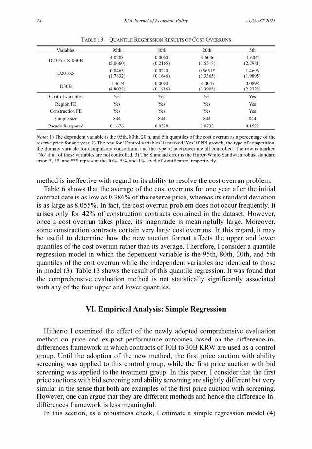
74 KDI Journal of Economic Policy AUGUST 2021
TABLE 13—QUANTILE REGRESSION RESULTS OF COST OVERRUNS
Variables 95th 80th 20th 5th
D2016.5 × D30B 4.0203 (5.0660)
0.0000 (0.2165)
-0.6046 (0.5518)
-1.6042 (2.7981)
D2016.5 0.0463 (1.7832)
0.0220 (0.1646)
0.5651* (0.3365)
1.4696 (1.9895)
D30B -1.3674 (4.8028)
0.0000 (0.1886)
-0.0047 (0.3905)
0.0898 (2.2728)
Control variables Yes Yes Yes Yes Region FE Yes Yes Yes Yes
Construction FE Yes Yes Yes Yes Sample size 844 844 844 844
Pseudo R-squared 0.1676 0.0328 0.0732 0.1522
Note: 1) The dependent variable is the 95th, 80th, 20th, and 5th quantiles of the cost overrun as a percentage of the reserve price for one year, 2) The row for ‘Control variables’ is marked ‘Yes’ if PPI growth, the type of competition, the dummy variable for compulsory consortium, and the type of auctioneer are all controlled. The row is marked ‘No’ if all of these variables are not controlled, 3) The Standard error is the Huber-White-Sandwich robust standard error. *, **, and *** represent the 10%, 5%, and 1% level of significance, respectively.
method is ineffective with regard to its ability to resolve the cost overrun problem.
Table 6 shows that the average of the cost overruns for one year after the initial contract date is as low as 0.386% of the reserve price, whereas its standard deviation is as large as 8.055%. In fact, the cost overrun problem does not occur frequently. It arises only for 42% of construction contracts contained in the dataset. However, once a cost overrun takes place, its magnitude is meaningfully large. Moreover, some construction contracts contain very large cost overruns. In this regard, it may be useful to determine how the new auction format affects the upper and lower quantiles of the cost overrun rather than its average. Therefore, I consider a quantile regression model in which the dependent variable is the 95th, 80th, 20th, and 5th quantiles of the cost overrun while the independent variables are identical to those in model (3). Table 13 shows the result of this quantile regression. It was found that the comprehensive evaluation method is not statistically significantly associated with any of the four upper and lower quantiles.
VI. Empirical Analysis: Simple Regression
Hitherto I examined the effect of the newly adopted comprehensive evaluation
method on price and ex-post performance outcomes based on the difference-in-differences framework in which contracts of 10B to 30B KRW are used as a control group. Until the adoption of the new method, the first price auction with ability screening was applied to this control group, while the first price auction with bid screening was applied to the treatment group. In this paper, I consider that the first price auctions with bid screening and ability screening are slightly different but very similar in the sense that both are examples of the first price auction with screening. However, one can argue that they are different methods and hence the difference-in-differences framework is less meaningful.
In this section, as a robustness check, I estimate a simple regression model (4)
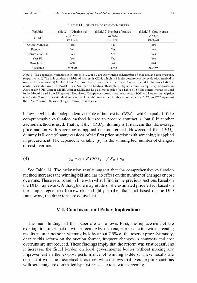
VOL. 43 NO. 3 An Unsuccessful Reform of the Local Public Contracts Law in Korea 75
TABLE 14—SIMPLE REGRESSION RESULTS
Variables (Model 1) Winning bid (Model 2) Number of change (Model 3) Cost overrun
CEM 4.9915*** (0.4494)
-0.2074 (0.1872)
-0.2786 (0.7692)
Control variables Yes Yes Yes Region FE Yes Yes Yes
Construction FE Yes Yes Yes Year FE Yes Yes Yes
Sample size 438 844 844 R-squared 0.6090 0.0845 0.0489
Note: 1) The dependent variables in the models 1, 2, and 3 are the winning bid, number of changes, and cost overruns, respectively, 2) The independent variable of interest is CEM, which is 1 if the comprehensive evaluation method is used and 0 otherwise, 3) Models 1 and 3 are simple OLS models, while model 2 is an ordered Probit model, 4) The control variables used in Model 1 are Number of bidders, Restricted, Urgent offers, Compulsory consortium, Auctioneer-SOE, Winner-MME, Winner-SME, and Log estimated price (see Table 3), 5) The control variables used in the Model 1 and 2 are PPI growth, Restricted, Compulsory consortium, Auctioneer-SOE and Log estimated price (see Tables 7 and 10), 6) Standard error is the Huber-White-Sandwich robust standard error. *, **, and *** represent the 10%, 5%, and 1% level of significance, respectively.
below in which the independent variable of interest is itCEM , which equals 1 if the comprehensive evaluation method is used to procure contract i but 0 if another auction method is used. That is, if the itCEM dummy is 1, it means that the average price auction with screening is applied in procurement. However, if the itCEM dummy is 0, one of many versions of the first price auction with screening is applied in procurement. The dependent variable ity is the winning bid, number of changes, or cost overruns.
(4) 1it it it ity CEM X
See Table 14. The estimation results suggest that the comprehensive evaluation method increases the winning bid and has no effect on the number of changes or cost overruns. These results are in line with what I find in the previous sections based on the DID framework. Although the magnitude of the estimated price effect based on the simple regression framework is slightly smaller than that based on the DID framework, the directions are equivalent.
VII. Conclusion and Policy Implications
The main findings of this paper are as follows. First, the replacement of the
existing first price auction with screening by an average price auction with screening results in an increase in winning bids by about 7.5% of the reserve price. Secondly, despite this reform on the auction format, frequent changes in contracts and cost overruns are not reduced. These findings imply that the reform was unsuccessful as it increases the fiscal burden on local governmental bodies without making any improvement in the ex-post performance of winning bidders. These results are consistent with the theoretical literature, which shows that average price auctions with screening are dominated by first price auctions with screening.

76 KDI Journal of Economic Policy AUGUST 2021
There is an important caveat to consider when interpreting the empirical results here. The results are obtained by considering contracts exceeding 30B KRW as a treatment group and contracts from 10B to 30B KRW as a control group, as first price auctions with screening were applied to both groups until May 1, 2016. However, contracts in the range of 10B to 30B KRW represent a reasonably good but not ideal control group as a first price auction with bid screening was applied to the treatment group while a first price auction with ability screening was applied to the control group until May 1, 2016. Bid screening and ability screening are not identical procedures and the control group for this reason is not ideal. However, the two screening methods are similar in that during the bid screening process, the procurement authority examines the relationship between the winning bid and the ability of the winner. That is, both bid screening and ability screening are conducted with the same objective of preventing incompetent companies from winning an auction by offering too low bid, and in this regard I believe that the control group is reasonably good. In addition, the two first price auction versions are slightly different in that the one with ability screening utilizes a single lower bound for admissible bids while the other with bid screening effectively places a number of similar lower bounds. The empirical results on the price and non-price effects of the comprehensive evaluation method obtained in this paper using the difference-in-differences estimation should be understood in this context.
The theoretical literature and this paper’s empirical findings imply that the comprehensive evaluation method should be repealed and replaced by a version of the first price auction with screening. However, this paper does not argue that we must return to the existing version of the first price auction with screening, as this method has its own serious problems. Related to this, Kim (2012) observes that under this existing method, almost every qualified bidder receives the maximum score on non-price qualities given that the existing screening process is not enough effective with regard to its ability to distinguish between efficient bidders and inefficient bidders. Therefore, this paper proposes the adoption of a new version of the first price auction with screening in which the screening process is intensified. Determining how to intensify the screening process could be an important future research agenda.

VOL. 43 NO. 3 An Unsuccessful Reform of the Local Public Contracts Law in Korea 77
REFERENCES Albano, G. L., M. Bianchi, and G. Spagnolo. 2006. “Bid Average Method in Procurement,”
Rivista di Politica Economica, 96(1): 41-62. Bajari, Patrick, Stephanie Houghton, and Steven Tadelis. 2014. “Bidding for Incomplete
Contracts: An Empirical Analysis of Adaptation Costs,” American Economic Review, 104(4): 1288-1319.
Conley, Timothy and Francesco Decarolis. 2016. “Detecting Bidders’ Groups in Collusive Auctions,” American Economic Journal: Microeconomics, 8(2): 1-38.
Decarolis, Francesco. 2014. “Awarding Price, Contract Performance, and Bids Screening: Evidence from Procurement Auctions,” American Economic Journal: Applied Economics, 6(1): 108-132.
Decarolis, Francesco. 2018. “Comparing Public Procurement Auctions,” International Economic Review, 59(2): 391-419.
Kang, Heewoo and Bitmaro Kim. 2017. A Study on Reforming Public Procurement System in Korea, Korea Institute of Public Finance (in Korean).
Kim, Jungwook. 2012. Analysis on Determinants of Winner in Public Procurement Auction, Policy Study 2012-08, KDI (in Korean).
Lewis, Gregory and Patrick Bajari. 2011a. “Procurement Contracting with Time Incentives: Theory and Evidence,” Quarterly Journal of Economics, 126(3): 1173-1211.
Lewis, Gregory and Patrick Bajari. 2011b. “Moral Hazard, Incentive Contracts and Risk: Evidence from Procurement,” NBER Working Paper Series.
McAfee, R. Preston and John McMillan. 1986. “Bidding for Contracts: A Principal-Agent Analysis,” Rand Journal of Economics, 17(3): 326-338.
MOEF (Ministry of Economy and Finance). 2015. “The First Price Auction Will Be Replaced by The Comprehensive Examination Method Since 2016,” Press Release, 29, Dec (in Korean).
PPS (Public Procurement Service). 2019. “Some Changes in the Comprehensive Examination Method Will Lead to a Rise in the Profitability in the Construction Industry,” Press Release, 29, Oct (in Korean).
Spulber, Daniel. 1990. “Auctions and Contract Enforcement,” Journal of Law, Economics, and Organizations, 6(2): 325-344.
Sweet, Justin. 1994. “Legal Aspects of Architecture, Engineering and the Construction Process,” 5th ed., West Publishing Company.
LITERATURE IN KOREAN
강희우⋅김빛마로. 2017. 『공공조달시장제도 개선방안 연구』, 한국조세재정연구원.
기획재정부. 2015. 「2016년부터 최저가낙찰제가 종합심사낙찰제로 개편─300억원 이상 공사는 가격, 공
사 수행능력, 사회적 책임을 종합 평가」, 보도자료, 2015. 12. 29.
김정욱. 2012. 『공공투자사업 입찰에서의 낙찰자 결정요인 분석』, 정책연구시리즈 2012-08, 한국개발연
구원.
조달청. 2019. 「종심제 기준개정으로 ‘건설업체 수익성’ 제고」, 보도자료, 2019. 10. 29.


KDI Journal of Economic Policy
Statement of Purpose
Editorial Board
KDI Publications
Annual Fees
Sign-Up
Contact
The KDI Journal of Economic Policy (KDI JEP) is a professional journal published on a quarterly basis. The
Journal publishes papers on the academic and policy issues related to the development of Korea’s economy.
The KDI Journal of Economic Policy welcomes innovative and insightful academic papers on all areas of
economics with an emphasis on empirical analysis that contain solid policy implications. KDI JEP is published
in English starting in 2015, volume 37 number 1.
The Journal aims to disseminate research outcomes and policy recommendations not only to experts at
academia and research institutes but also to policy-makers and the general public. First published in March
1979, the original objective was to circulate ongoing- and past researches conducted in KDI, a leading
economic think-tank of South Korea. Starting in August, 2001, the Journal has accepted manuscripts from
outside in order to provide the readers more diverse perspectives on Korea’s policy initiatives. The Journal
now actively seeks and welcomes submissions by researchers at home and from abroad who have genuine
interests in the Korean economy.
The contents of papers published in KDI JEP contain personal views of the authors, and thus do not represent
the objectives of the Journal or the mission statements of KDI.
KDI Book Membership Information
• All KDI publications, with the e• Preferential invitations to special events hosted by KDI including seminars, policy discussion forums, public hearings, etc., are to be mailed.
• A 10% discount on the online purchases of additional copies of the published research monographs (printed-only)
from the KDI homepage.
• Publications include books, research monographs, policy studies, KDI policy forums, KDI FOCUS, research papers and policy-information materials.
• Three types of periodicals are available:- Monthly: KDI Monthly Economic Trends, KDI Review of the North Korean Economy, Economic Bulletin,
Narakyungje- Quarterly: KDI Journal of Economic Policy, KDI Analysis on Real Estate Market Trends
- Biannual: KDI Economic Outlook
• Individual Purchase: 100,000 KRW
• Institutional Purchase: 300,000 KRW
• You may sign up for membership via KDI homepage. Please register on the homepage by completing and submitting the registration form. Possible payment methods are as follows:- Bank-Transfer: Woori Bank, 254-012362-13-145 (account holder name: Korea Development Institute)- GIRO System: No. 6961017 (Credit Card and Mobile Payments available)
• Publication personnel in char- Tel: 82-44-550-4346 / Fax: 82-44-550-4950 / E-mail: [email protected]
• Sales Distributors- Kyobo Bookstore (Gwanghwamun Branch: Government Publications Section)- Tel: 82-2-397-3628- Yongpoong Bookstore (Jongno Branch: Policy & Economy Section)- Tel: 82-2-399-5632
Editor-in-Chief: Kim, Dongseok (Professor at KDI School) [email protected]
Managing Editor: Lee, Jinkook (Fellow at KDI) [email protected]
Special Editor: Cho, Dongchul (Professor at KDI School) [email protected]
Administration: Park, Sejin (Research Associate at KDI) [email protected]
Editors: Choi, Yongseok (Professor at KyungHee University) [email protected]
Chun, Youngjun (Professor at HanYang University) [email protected]
Chun, Hyunbae (Professor at Sogang University) [email protected]
Chung, Wankyo (Professor at Seoul National University) [email protected]
Hahn, Chinhee (Professor at Gachon University) [email protected]
Kim, Jungwook (Fellow at KDI) [email protected]
Lee, Jongyearn (Professor at KDI School) [email protected]
Kim, Jongil (Professor at Dongguk University) [email protected]
Lee, Chulhee (Professor at Seoul National University) [email protected]
Shin, Kwanho (Professor at Korea University) [email protected]
Shin, Sukha (Professor at Sookmyung Women’s University) [email protected]
Yoon, Kyungsoo (Professor at Gachon University) [email protected]
Kim, Kwang-ho (Professor at HanYang University) [email protected]
Lee, Hangyong (Professor at HanYang University) [email protected]
August 2021 Vol.43, No.3
Registration Number 세종 바00002호Printed on August, 27, 2021Published on August, 31, 2021Published by Jang-Pyo Hong, President of KDI Printed by Good Idea Good Peoples
Price : 3,000 KRW@Korea Development Institute 2021Registered on March, 13, 1979