1

Asset Poverty in the United States, 1984−1999:Evidence from the Panel Study of Income Dynamics

Asena Caner* and Edward N. Wolff**

*Levy Economics Institute*Levy Economics Institute and New York UniversityE-mail addresses:caner@levy.org and edward.wolff@nyu.eduThe authors gratefully acknowledge financial support provided by the Ford Foundation.

2

I. INTRODUCTION

The reduction of poverty is a non-controversial goal of nearly all societies. As anyone would

agree, a fight against poverty has to start with a detailed description of poverty and the choice of

a measure to be used in the identification of the poor. The most common way of measuring

poverty is to compare the amount of resources owned by a family or a person to the minimum

amount needed to satisfy basic needs. This minimum level is usually called the poverty line or

the poverty threshold, and those remaining below the poverty line are considered poor.

Although this looks straightforward, there is no standard way of defining poverty. What

is necessary to satisfy basic needs varies across time and place, depending on the level of

development, societal norms and values. Moreover, scholars have different opinions about

which economic variables best identify the people whose resources are less than the minimally

acceptable level. So far, the typical variables of choice used to determine the poverty status of

families or individuals have been either income or consumption.

A growing part of the poverty measurement literature emphasizes that poverty is not

only a lack of income but a lack of assets as well. Assets provide an economic protection for the

hard times and enable people to invest in their future. Even low levels of asset holdings can

make a significant difference in the lives of low-income families. As stated in Shapiro and

Wolff (2001, p.6), “assets provide a stake that income alone cannot provide.” Therefore, a

poverty measure should take household wealth into consideration together with income in order

to get a better assessment of well-being. Previous research, on the contrary, took for granted

that income or consumption is sufficient to define well-being. These studies focused entirely on

income or on consumption and left the issue of asset poverty out of the picture.

On the policy front, there have been changes too. Recently, the focus of the approach to

dealing with poverty has shifted from an income-transfer policy that tries to maintain a

sufficient level of income for everyone, to an asset-based policy that aspires to increase the asset

holdings of the poor. As an example, in 1998, the Individual Development Account (IDA)

Demonstration Act was signed into law1. By this, the government promised to provide matching

funds to every dollar that a family saves and deposits to these accounts. In fact, there have

already been a number of asset-based programs, mostly structured into the tax system, which

became quite successful in creating incentives for many families to save. These include

1 http://clinton6.nara.gov/1998/10/1998-10-27-fact-sheet-on-individual-development-accounts.html

3

programs like corporate and individual retirement accounts and state-sponsored savings plans

for higher education. However, such programs have benefited the non-poor almost exclusively,

leaving families with few or no assets behind2. Assistance programs designed for the poor, until

recently, focused only on supporting a minimum level of consumption while they ignored and

even prohibited asset accumulation among the poor.

In this paper, we propose an asset poverty line, which, like the official poverty measure,

sets the minimum requirements for survival. We then estimate the size and severity of asset

poverty in the United States with respect to this asset poverty line, both for the entire population

and for various demographic and labor market groups, using the Panel Study of Income

Dynamics (PSID) data. Additionally, we provide an estimate of the impact of adding wealth to

the official poverty definition. We attempt to identify the trends in asset poverty and the

population groups that have become more or less prone to be asset-poor. We investigate the

persistence of asset poverty in the U.S. and identify the major events that are associated with the

transitions into and out of poverty.

The rest of the paper is organized as follows: Section 2 discusses the main themes in

poverty measurement research and describes how poverty is defined in the official U.S.

government statistics. It also talks about some of the shortcomings of the official measure as

well as recommendations in the literature for improvement. Section 3 provides the definition of

asset poverty used in this paper. The estimates of asset poverty are reported in section 4. Section

5 analyzes the effects of compositional changes on the overall asset poverty rates. Section 6

compares asset poverty rates in the PSID and the rates in the Survey of Consumer Finances

(SCF). Section 7 compares asset poverty rates to official poverty rates. The difference between

household-based and individual-based asset poverty rates is discussed in section 8. Section 9

looks into the composition of household portfolios. Section 10 provides descriptive statistics of

the characteristics of households in asset poverty. Section 11 performs regression analyses to

identify the trends in asset poverty. Section 12 estimates poverty rates using an alternative

measure that combines income and wealth. We talk about the persistence of poverty in section

13. The role of changes in assets and changes in debts as well as the role of major lifetime

events on the transitions into and out of asset poverty are discussed in this section. Section 14

summarizes the findings and concludes the paper.

2 See Sherraden (1991) and Shapiro and Wolff (2001).

4

II. BACKGROUND

A. Review of Poverty Measurement Research

This section reviews the literature on poverty measurement. First, we discuss the alternative

ways of setting a poverty threshold or defining the “needs.” Second, we talk about the main

ideas on how to define the “resources,” emphasizing the literature on the impacts of adding net

worth to the poverty definition. Next, we summarize the main findings of poverty duration

analyses.

There are three main ways of setting poverty lines. One could set an absolute poverty

line, a relative one or a subjective one. An absolute poverty line remains fixed over time and is

unaffected by changes in the average amount of resources available to the population. The

official poverty measure currently being used in the U.S. is an absolute measure, in that it

classifies families whose income fall below a certain level as poor. The poverty lines used by

the World Bank to estimate world-wide income poverty are also absolute measures, set at $1

and $2 per person per day (World Bank 2001). A relative measure of poverty, on the other hand,

makes the poverty line a function of the amount of resources owned by the median person or

family in the population. The poverty standards developed by the OECD and currently being

used to estimate the extent of poverty in western European and Scandinavian countries are

relative measures. They are designed to identify individuals and families living in households

with income below half of the national median for households of similar size3. Subjective

measures of poverty rely on families’ own assessment of their economic well-being to judge on

who is poor. Also known as the ‘Leyden School’ approach, the technique involves using

people’s subjective evaluations of how much income would be ‘excellent’, ‘good’ and so on to

maintain an adequate standard of living to build a national poverty line4. The poverty lines set

by these measures have the advantage of being free from the judgement of a handful of

politicians; however they are sensitive to question wording and the particular method used in

their derivation.

An important part of the problem of setting poverty lines is how to take different family

types into account. Usually, poverty lines are set for the ‘standard’ family first. In the U.S. it is

composed of two adults and two children. Then, they are adjusted for different family types by

3 See Smeeding et al. (1993) for more on poverty in Europe.4 See Hagenaars and van Praag (1985).

5

equivalence scales to account for the economies of scale in shared expenditures. Family

characteristics such as the family size, age of the head and the number of children should all be

taken into consideration in building these scales. Exactly how poverty lines should vary to

account for these characteristics is a controversial issue. Triest (1998) examines the sensitivity

of the U.S. official poverty rate to alternative equivalence scales and shows that both the level

and the trend of poverty depend on the type of scale used, so the choice of equivalence scales

matters. In fact, one characteristic of the official poverty measure in the U.S. that is subject to

criticism is the anomalous pattern of economies of scale implicit in the thresholds for families of

different size. Some alternatives have been suggested (see Short 2001, but more work is

required in this area.

The next issue is the discussion in the literature about the type of economic variables or

“resources” that should be used to identify the poor. There is some consensus among economists

that poverty is associated with the lack of “economic resources,” yet there are widely varying

perspectives on what these resources should be and how they should be measured. Usually

family income is assumed to represent the amount of resources that a family has the right to use,

as done in the official measure of poverty in the U.S. However, income may not be a very good

proxy for well-being, especially for low-income families. Incomes fluctuate over time but

families usually find a way to maintain a more or less constant level of consumption. They use

their assets or they receive non-cash benefits from government in hard times. In fact, some

researchers, such as Slesnick (1993) and Jorgenson and Slesnick (1987) have argued that

consumption is a much better measure of well-being. However, these measures also have

shortcomings, such as the sensitivity of the estimated poverty rates to the equivalence scale

used5.

An alternative definition of poverty (‘Self-Reliant poverty’), inspired by the work of

Amartya Sen, is developed by Haveman6. Here, the emphasis is on potential earnings, called

‘earnings capacity’, and not on realized earnings. The idea is that being incapable of earning

sufficient income is a more vulnerable situation than being short of cash in a given year;

therefore, poverty analysis and policy should shift its focus from low incomes to lack of basic

capabilities and should emphasize the merits of individual independence. An individual is Self-

5 Triest (1998) reports that the level of consumption poverty estimated by Jorgenson and Slesnick depends cruciallyon the equivalence scales used and that the scales they use take unreasonable values.6 Haveman and Bershadker (2001). Two prior studies that have used measures of earnings capacity are Garfinkeland Haveman (1977) and Haveman and Bershadker (1998).

6

Reliant poor if his earnings capacity is lower than that would enable him to secure a socially-

accepted minimum level of living, even if he or she worked full-time full-year, accounting for

the time lost because of poor health or disability and the cost of dependent care. Haveman and

Bershadker (2001) estimate earnings capacity using individual and family characteristics such as

age, education, marital status, region of residence and non-labor income, controlling for

selection bias. Their results are revealing. They show that both the official and the Self-Reliant

poverty rates have an upward trend in the 1975-97 period; however the official rates have a

much slower trend. This indicates that “the potential earnings of families at the bottom of the

distribution are declining at a more rapid rate than is the realization of that potential, suggesting

an increase in the utilization of earnings capacity by these working-age families.” This can be

interpreted as evidence that deterioration in the labor market opportunities for the less skilled

workers plays an important role in the upward trend in the poverty rate.

Of particular interest to this paper is the group of researchers that has called attention to

the importance of wealth in the measurement of poverty. These researchers argue that wealth is

an important dimension of well-being, therefore it should be included in the family resources

when defining poverty. Wealth gives its owner an advantage in life, “independent of the direct

financial income it provides” (Wolff 2001a) and apart from the political power it brings. It is a

source of consumption, since it can be converted into cash in times of economic stress caused by

unemployment, disability, sickness or family breakup (Wolff 2001a). Comparing income to

wealth, Oliver and Shapiro (1990) state that “income is a transitory measure and can be

consumed as quickly as it is earned, yet wealth is a more stable indicator of status or position in

society and represents stored-up purchasing power. It reflects savings and investments that can

be drawn on in times of need.” In addition, families normally enjoy consumption services from

assets such as owner-occupied housing and consumer durables. It is now very well-known that

wealth is distributed far more unevenly than income in the U.S.7. Oliver and Shapiro (1990)

show that one-third of households in the U.S. have zero or negative net financial assets;

therefore “redistributive and welfare policies based on income analyzes and levels seriously

underestimate the severity of the problems they are meant to address.”

Evidently, a poverty measure that includes wealth in the definition of family resources is

preferable to a measure based on income only. However, there are some issues that need to be

resolved. First, one has to find a way to add wealth, which is a stock variable, to income, which

7

is a flow variable. Researchers have suggested mainly two ways of doing this: converting wealth

into an income flow before adding it to family income, which is used more commonly, and

setting a joint threshold of income and wealth. The income flow generated by wealth can be

computed as a lifetime annuity that brings wealth down to zero at the end of one’s lifetime.

Alternatively, it can be assumed that the annuity flow is paid out like a bond coupon and the

principal value of wealth can be kept constant. The method used in the computation of the

annuity flow may have an effect on the results. In either case, one would expect the elderly to

benefit more from the addition of wealth to income than the non-elderly, since the elderly have

higher ratios of wealth to current income. But the lifetime annuity approach accentuates further

the advantage of the elderly, because they have shorter life expectancies.

Weisbrod and Hansen (1968) first attempted to explicitly account for wealth as well as

income in measuring poverty. Using 1962 data, a fixed $3000 poverty line and the lifetime

annuity technique, they found both a lower incidence of poverty (20 percent versus 18 percent

with 4 percent interest rate) and a younger age distribution of poor households under the

income-net worth approach than under the simple income measure. Lerman and Mikesell (1988)

added several new wrinkles to the Weisbrod-Hansen study. They used more recent data (1983

Survey of Consumer Finances (SCF)), adjusted poverty thresholds for family size and

composition, examined the overlap between the two measures and extended the analysis to

several demographic characteristics. They found an overall poverty rate of 11 percent with the

income-net worth poverty measure, compared to 13 percent with income only. They also

considered adjusting the poverty thresholds for the inclusion of wealth. Their argument for this

adjustment was that differences in the official poverty lines between elderly and non-elderly

households were partially intended to reflect differences in wealth; thus if wealth is included in

family resources the poverty lines should also be adjusted upward. They chose to calibrate their

thresholds to replicate the poverty headcount based on the official thresholds. They showed that

87 percent of the income-poor were also income-net worth-poor. However, the extended

threshold changed the composition of the poor; they found more non-elderly, renters, large

families, children and unemployed among the poor.

Wolff (1990) included a wealth dimension in the poverty measure by assuming that

households receive annuity flows of their wealth which are paid out like bond coupons. By

using data from the 1983 wave of the SCF, he found that the impact of adding wealth was to_____________________________7 Oliver and Shapiro (1990) and Wolff (2001a).

8

reduce poverty rate by about 10 percent for the full population and by more than 20 percent for

the elderly. He also analyzed the consequences of using a poverty line that is based on a joint

threshold of income and net worth. First, he defined poverty as the state of having below-

poverty income and below-median wealth. This caused a 15 percent reduction in the income

only poverty rate. Then, he considered defining poverty as having below-poverty income or

below-median wealth, which resulted in a 20 percent higher poverty rate compared to the

official rate.

Moon (1977), Crystal and Shea (1990) and Rendall and Speare (1993) focused on the

economic circumstances of the elderly and demonstrated how using raw income to estimate the

well-being of the elderly could distort the picture of poverty. Moon (1977) and Crystal and Shea

(1990) found that restricting the analysis to family incomes caused the poverty rate among

whites to be overestimated. A more comprehensive measure of poverty detected more poor

minorities than an income-only measure did. Crystal and Shea (1990) showed that the apparent

disadvantage of the elderly disappeared, once incomes were adjusted for household size,

underreporting of property income and for the annuity value of net worth. However, as both

Crystal and Shea (1990) and Rendall and Speare (1993) reported, the adjustment process did not

eliminate the inequality among the elderly. While Social Security exercised some leveling

effect, these equalizing effects were outweighed by those of pension and property income

concentrated in the hands of high-income individuals.

Ruggles and Williams (1989) and Ruggles (1990) analyzed the effects of asset holdings

on the poverty entries and spell durations, assuming that assets could be used to bring the

consumption levels of those with below-poverty incomes to the poverty line for as long as

possible. They found that over 60 percent of poverty entries remained even after asset holdings

were accounted for. By contrast, half of the observed poverty spell entries for the elderly were

eliminated. Those who did remain in poverty even when their assets were counted were the ones

who were more likely to experience very long spells; so the average spell duration increased

after the addition of assets in resources.

This takes us to another point of interest of this paper, which is the persistence of

poverty. Identifying the groups of people and families that are poor chronically versus

temporarily is important both for theoretical reasons and for making informed policy decisions.

Assuming that the causes of the two types of poverty are different, so will be their remedies.

9

Bane and Ellwood (1986) is the first study that carefully distinguishes between the “ever-poor”

and the “poor at a particular time.” Using the PSID data, the authors examined transitions into

and out of poverty to derive estimates of completed spells of poverty for the non-elderly

population. Their work showed that most of the people who are ever poor stay in poverty for a

short time, while the majority of the poor at a given time experience long spells of poverty

before they exit. To illustrate, among those who ever experienced poverty on an annual basis,

about 45 percent of poverty spells ended within one year and 70 percent within three years.

Only 12 percent of spells lasted longer than eight years. Restricting the sample to those who are

poor in a given year, only 11 percent of spells lasted for less than a year, about 25 percent lasted

for less than three years and a little more than 50 percent lasted more than eight years8. This

finding is very important, since it means that the persistence of poverty is much lower when the

analysis is based on the people that are just beginning a poverty spell than it is when one looks

at the stock of people poor at any point in time.

Bane and Ellwood (1986) helped us understand not only the extent of temporary versus

chronic poverty, but also some of the reasons why people move into and out of poverty. Among

the non-elderly population, a drop in the earnings of the family head accounts for 38 percent of

all poverty beginnings. Divorce, birth of a child or setting up an independent household

accounts for another 43 percent. Interestingly, similar events, in the reverse direction, cause

people to escape poverty, although a change in earnings or transfers play a relatively more

important role in the exit from poverty.

Although the Bane and Ellwood study reformed the understanding of poverty dynamics

in an important way, it had a major shortcoming. It focused on single spells. Stevens (1999)

extended it to analyze multiple poverty spells. She found that individuals were likely to fall back

into poverty, especially during the years just after an exit from poverty. Specifically, she

calculated that half of all individuals ending a poverty spell in a given year became poor again

within the next four years. The fact that people returned to poverty caused the average time

spent in poverty to be higher than it would be when the analysis was restricted to single spells.

This led to the conclusion that the Bane and Ellwood study understates the persistence of

poverty within the sample of those who ever entered poverty compared to poverty in the sample

of those poor at a particular time. Strikingly, Stevens’ results showed that the average time spent 8 Given the Census Bureau statistics of annual poverty of 12-14 percent, this result can be used to conclude thatabout 6 or 7 percent of the population is chronically poor, if chronic poverty is defined as being poor for at least

10

in poverty in a ten-year period is four years with more than half of blacks and about a third of

whites who ever become poor spending five or more of the ten years in poverty.

Another important finding of Stevens (1999) is that the persistence of poverty depends

on individual and family characteristics. Those living in two-parent households have the most

transient poverty. Education and race of the head play important roles, too. On average, people

living in families headed by black and less-educated males spend four out of ten years in

poverty, while those in families with white and at least high school graduate heads spend less

than two and a half out of ten years in poverty. Persistence of poverty is extremely high for

people in single-female headed households, especially for children. Poverty continues for at

least six out of ten years for between 26 and 64 percent of adults (depending on race and

education level) and for between 47 and 90 percent of children living in such households.

Ruggles and Williams (1989) critiqued the Bane and Ellwood (1986) study for its

reliance on an annual poverty measure. They cautioned that incomes usually fluctuate widely

during the year, particularly for the low-income population. For example, the 1984 poverty rate

based on annual income as measured in the Survey of Income and Program Participation (SIPP)

was 11 percent, but only 5 percent were poor in every month. In contrast, over 26 percent were

poor in at least one month. Even relatively short spells can mean substantial hardship, to the

extent that such sub-annual poverty spells are experienced by those with near-poverty incomes

and thus with limited savings. The authors observed that while there were a few cases of high-

income individuals with short spells of poverty, the typical case was a low-income individual

who lacked the resources to call upon to withstand a poverty spell.

Duration studies of poverty dynamics implicitly assumed that chronic poverty is a state

in which income is less than needs during a long and continuous period of time. This

assumption may be misleading if the time period analyzed is not representative of the lifetime

income profile of an individual. In fact, individuals can make intertemporal income transfers by

borrowing and saving. Rodgers and Rodgers (1993) attempted to correct for this by supposing

that individuals can make inter-year income transfers at realistic savings and borrowing rates.

They developed a notion of chronic poverty on the basis of a measure of permanent income

compared with permanent needs. Using the PSID data for the period since the late 1970s, they

concluded that about one-third of measured poverty in the U.S. as of 1987 could be regarded as

chronic, and that over the period they studied, “poverty not only increased, it became more_____________________________eight years.

11

chronic and less transitory in nature.” They also found that “the poorest group identified consists

of people living in families headed by African-American females without high-school diplomas,

for whom chronic poverty is about twelve times as intense as in the entire population.”

B. The Official Measure of Poverty in the U.S. and Suggestions for its Improvement

The underlying concept in the definition of the official poverty measure in the U.S. is comparing

pre-tax money income of a family to some minimum standard. The measure is based on work

done almost four decades ago by Orshansky (1965). Using 1955 nutrition data from the U.S.

Department of Agriculture, she calculated the minimum amount of money needed to feed a

family of four. At that time, except for the area of food, no definitive and accepted standards of

minimum need for major consumption items (such as housing, medical care, clothing, and

transportation) existed nor do they exist today. Since the data at that time showed that food

made up about one-third of low income families’ expenditures, she computed the poverty

threshold by multiplying the minimum food cost by a factor of three to include spending for

shelter, clothing and other necessities. Also, the threshold was adjusted for such factors as

family size, farm versus non-farm residence, age of the family head and the number of children.

To account for price changes over time, poverty lines are updated each year according to the

overall Consumer Price Index (CPI).

The establishment of an official poverty line is considered by many as the most

important contribution of the ‘War on Poverty’ to social policy. It caused a shift in the emphasis

of the federal budget from military spending toward social welfare spending. During the decade

following the declaration of the war on poverty in 1964, new programs were initiated and the

old ones were expanded. However, at the time of its establishment, the official poverty measure

was intended to be only a starting point for the development of new and more refined

methodologies, and not to be the ultimate measure. Revisions were supposed to be made in

many directions over time. Due mainly to political reasons, these expectations were not

fulfilled. Concerns about a possible increase in the poverty count and program eligibility after a

revision are cited by some observers as an explanation of why very little modification was made

in the poverty measure (Rodgers 2000). As a result, the poverty lines designed in the 1960s

remain to be the official method of estimating poverty rates today.

In the beginning of the 1990s, recognizing the importance of accurately measuring

poverty and as a response to the ongoing criticism towards the official measure, the Congress

12

asked the National Academy of Science (NAS) to convene a committee to investigate new

approaches. The report of this panel, released in Citro and Michael (1995) highlights the flaws

in the official measure and makes suggestions for its improvement. The panel puts forward a set

of “experimental poverty thresholds” and an updated “family resources” definition to be used in

the new poverty measure.

The experimental poverty thresholds proposed by the NAS panel are based on the cost of

food, clothing and shelter with a small allowance for other expenses, as opposed to only food

with a large multiplier for all other expenses as in the official measure. The panel recommends

that the poverty lines be based on actual consumer expenditure data (the Consumer Expenditure

Survey), and not on expert judgement, to account for the changes in living standards and

consumption patterns over time. The thresholds should be updated each year for the changes in

spending on food, clothing and shelter over previous three years for two-adult two-child

families, as opposed to adjusting only for changes in the price level.

As mentioned earlier, the official poverty lines were set only on the basis of food

requirements of the standard family and the lines for other family types were adjusted by

wrongly assuming that other consumption needs vary more or less in the same proportion as

food requirements. For this reason the equivalence scale implicit in the official thresholds is not

internally consistent and exhibits an irregular pattern. The NAS panel recommends that the

equivalence scale be defined explicitly and separate parameters be assigned to represent adult

equivalence and economies of scale. Another problem is that, the current measure reflects ad

hoc adjustments for single people living alone and for two-person families. It also sets lower

thresholds for the elderly than for younger people, which does not make much sense. Although

the elderly may need less food or clothing, they have higher health costs, which more than offset

the reduction in spending on food or clothing. The NAS panel agrees that the scale should

account for differences between the needs of adults and children but urges that no further

distinction be made among family members by age or other characteristics.

The panel emphasizes strongly that the consistency principle be respected, i.e. that the

definitions of poverty thresholds and family resources be made in the same terms. The official

measure has been violating this principle from the beginning, since the thresholds were defined

in terms of after-tax income data while resources were defined in before-tax terms. To solve this

problem, family resources should include not only the before-tax money income, but also the

value of in-kind benefits such as food stamps and housing subsidies. Income and payroll taxes

13

and other nondiscretionary expenses should be deducted. These include items such as child care

and other work-related expenses, child support paid to other households and out-of-pocket

medical expenses.

Finally, the panel makes some points on how to define family resources in a more

comprehensive way. The report maintains that, as expected, the practice of adding assets

directly to family income to quantify family resources can not be justified in general. It is

appropriate only when the accounting period of poverty is very short (a few months), since

spending down assets can alleviate poverty only for a short period of time. In fact, some

government programs, such as food stamps, work on this principle and allow families to qualify

for assistance if their income is low temporarily and if their asset holdings are lower than a

threshold. The panel report mentions that for longer periods (a year or longer), it is more

appropriate, instead, to define resources as disposable income from all sources, including any

income from assets, such as interest or rent, although very few income-poor people have

financial assets. Surprisingly, though, the panel does not specify clearly how the income flow

from assets should be computed.

The panelists reach a consensus on the importance of accounting for the flow of services

from owner-occupied housing, which constitutes a large part of household wealth, in order to

make consistent estimates of families’ economic resources. The motivation for this argument is

that owners with low housing costs have more of their income available for consumption of

other items. Hence, not to include imputed rent is to underestimate their income relative to their

poverty threshold. The panel reasons, however, that this task is currently not feasible due to the

lack of data to develop adequate rental imputations. Valuation of home ownership services is

marked as a priority area for further research and consideration for implementation in the

poverty measure at a later date.

III. THE DEFINITION OF ASSET POVERTY

In this paper, we adopt the definition of asset poverty in Haveman and Wolff (2001): “A

household or a person is considered to be ‘asset-poor’ if the access that they have to wealth-type

resources is insufficient to enable them to meet their ‘basic needs’ for some limited ‘period of

time’.” We specify ‘basic needs’, the ‘period of time’ and the content of ‘wealth-type

resources’, in the spirit of the study cited above, as follows:

14

1. We use four alternative wealth measures: Net worth (NW) includes the current value of all

marketable assets less the current value of all debts. Net worth minus home equity (NW-HE)

includes all items in NW except for home equity. Liquid wealth (LIQ) measures the value of

cash and other kinds of easily monetizable assets. The final measure sets an absolute

standard of $5,000 and labels all households with asset holdings below this level as asset

poor. (See the Appendix for the description of the wealth data in the Panel Study of Income

Dynamics (PSID).)

2. We set the ‘period of time’ somewhat arbitrarily, but reasonably, as three months. This is the

time period that we require the households to survive on their own by spending down their

wealth in case their income flow stopped for some reason.

3. We use the family-size conditioned poverty thresholds recently proposed by a National

Academy of Sciences panel. The panel first set the threshold for a reference family made up

of two adults and two children using Consumer Expenditure Survey data. The threshold for

the reference family was $15,998 in 1997 dollars. Then, the panel adjusted the threshold for

different family sizes and structures by using a three-parameter equivalence scale9. We

adjust poverty thresholds for inflation using CPI-U.

As an illustration of the level of these thresholds, we present an example. For the reference

family, the asset poverty threshold is $2,589 in 1984, $3,089 in 1989, $3,693 in 1994 and

$4,151 in 1999.

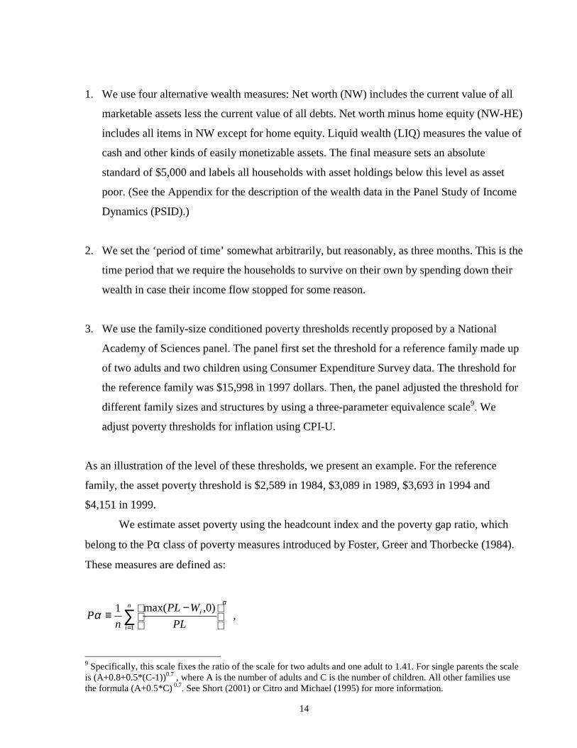
We estimate asset poverty using the headcount index and the poverty gap ratio, which

belong to the Pα class of poverty measures introduced by Foster, Greer and Thorbecke (1984).

These measures are defined as:

∑=

−

≡n

i

i

PLWPL

nP

1

)0,max(1 α

α ,

9 Specifically, this scale fixes the ratio of the scale for two adults and one adult to 1.41. For single parents the scaleis (A+0.8+0.5*(C-1))0.7 , where A is the number of adults and C is the number of children. All other families usethe formula (A+0.5*C) 0.7. See Short (2001) or Citro and Michael (1995) for more information.

15

where PL is the asset poverty line, n is the sample size, Wi is the wealth of household i and α is

the measure of inequality aversion. When α=0, the index gives a headcount, i.e., the percentage

of households in asset poverty. When α=1, the index becomes the poverty gap ratio, i.e., the

mean shortfall of wealth below the poverty line as a proportion of the poverty line.

In words, the headcount index gives us an estimate of the share of households that would

be unable to survive for three months if forced to liquidate all wealth and consume the proceeds.

The poverty gap ratio measures the amount of wealth that we would need to transfer to the

average asset-poor household to bring it to the asset poverty line.

IV. ESTIMATES OF ASSET POVERTY IN THE U.S. FROM 1984 TO 1999

A. The Evolution of Wealth in Years 1984-1999

To start with, we present some evidence on how the mean and some percentiles of household

wealth in the U.S. fared during the 15-year period that we are analyzing. Tables 1A and 1B

describe mean and some percentiles of NW, NW-HE and LIQ in the four years for which wealth

information was collected. As shown in these tables, mean household wealth, represented by

mean NW, NW-HE and LIQ, increased steadily between 1984 and 1999, although at different

growth rates. We will document later in this paper that the percentage of the population that

remained below the asset poverty threshold stayed more or less the same during this period,

despite the considerable increase in mean household wealth (see Table 1A and Table 1B).

Median net worth increased from $42,970 to $56,500 (all in 1999 dollars), or 31.48

percent between 1984 and 1999. The 25th percentile increased only slightly, from $1,600 to

$2,000. However, the top 5 percent of the distribution went up 61.24 percent from $483,120 to

$799,000 during the same period. Therefore, the lower tail of the net worth distribution

stagnated or moved to the left as the upper tail moved to the right. NW-HE showed a similar

trend. The faster progress in the upper percentiles of both NW and NW-HE relative to their

median increased the skewness of these distributions. The 10th percentile of NW and NW-HE

became more negative that is, the indebtedness of the poorest 10 percent of the Americans

increased between 1984 and 1999.

The rise in liquid asset holdings was also highly concentrated at the upper tail of the

distribution. The median value of liquid assets went up from $5,610 to $9,010 in the 1984-94

16

period, only to decline to $6,000 in 1999. By contrast, the 95th percentile of the liquid asset

distribution went up by 77 percent.

B. Changes in Asset Poverty, 1984-99

The following table shows estimates of the headcount index of asset poverty for the entire

population of households in the United States. As expected, NW yields the lowest estimates (25

percent-27 percent), as it is the most inclusive measure of wealth. Excluding home equity

increases poverty rates by almost 15 percentage points. This is consistent with the fact that

home equity is the most widely held asset category and also an important part of household

wealth in the US. It is interesting that the NW-HE and liquid asset estimates are pretty close.

This happens because only a small percentage of households own illiquid assets other than

primary residence, such as real estate (other than home) or business assets. The highest

estimates are obtained when the $5,000 threshold for liquid assets is used. Close to one half of

the population lack even a $5,000 worth of liquid asset cushion to protect them against adverse

shocks.

We also notice that there seems to be almost no trend in overall asset poverty rates in

this 15-year period. Net worth poverty increased only a bit from 1984 to 1989 and then declined

slightly from 1989 to 1999. Liquid asset poverty remained pretty much the same as well,

although it declined to its lowest level in 1994. According to the fourth measure of asset

poverty, the share of households whose liquid assets are worth at least $5,000 went up from 46.5

percent (100 percent−53.5 percent) to 53.6 percent (100 percent−46.4 percent). Since the $5,000

threshold is in current dollar terms, increases in the overall price level pushed the nominal value

of assets up in time, leaving fewer households below the threshold. Despite this good news,

there is no sign of a downward trend in liquid asset poverty between 1984 and 1999.

Table 2B presents the poverty gap ratios estimated for years 1984 to 1999 for the entire

population. As mentioned before, this index measures the mean shortfall of wealth below the

poverty line as a proportion of the poverty line. For instance, in 1984 the asset poverty line for a

reference family of two adults with two children was $2,589 ($10,356 / 4). Our estimates show

that the average net worth poor family with this family structure would need an additional

$1,592 (61.51 percent of $2,589) to move to the poverty threshold.

17

It is interesting how the stability of the headcount index gives one the false impression

that the recession in the beginning of the 1990s did not have any adverse effects on the asset-

poor. Although the share of the asset-poor stayed constant over time, the large increase in the P1

index between 1989 and 1994 suggests that the economic downturn in the beginning of the

1990s was harsh on almost one fourth of the population. It seems that the average asset-poor

household lost assets during the recession. In 1989, the asset-poor households were on average

75 percent below the poverty line, while in 1994 they were 89 percent below the poverty line, as

shown in Table 2B. To illustrate, the average (4-person) asset-poor household had $752 and

$393 net worth in 1989 and in 1994, respectively, in current dollars10.

Moreover, contrary to popular belief, asset poverty rates did not go down during the

expansion in the late 1990s. Both NW and NW-HE poverty stayed the same; liquid asset

poverty increased from 37.8 percent to 41.6 percent. The share of households with less than

$5,000 worth of liquid assets went up from 43.1 percent to 46.4 percent. During this

expansionary period, both the NW and NW-HE poverty gaps fell, although the NW-HE gap

stayed above 100 percent in 1999. As Table 3 shows, in 1999 the NW-HE-poor had negative

wealth on average, with an average non-mortgage debt of $6,999, compared to the average

value of businesses at $177, real estate at $82, and checking and saving accounts at $1,099.

Looking at the NW poverty gap we can see that it fell from 89 percent to 82 percent between

1994 and 1999; however it was still higher in 1999 in comparison to the 1980s.

Another observation worth noting is that the ordering among the P1 indices for the three

wealth measures remains the same in every year, except in 1994: the liquid asset poverty gap is

the lowest among the three, NW gap comes the second, and the NW-HE gap is the highest. The

finding that the liquid asset poverty gap is the lowest is interesting, given the previous finding

that liquid asset poverty is more widespread than NW poverty (see Tables 1A-1B). A deeper

look into the asset holdings of poor households tells us why.

In Table 3, we show the asset ownership rates as well as the mean value of each asset in

the portfolio of the asset-poor households. Comparing the last section of the table to the

previous two sections, we notice that the average liquid-asset-poor household is actually rich by

the other two measures. Such a household has $27,466 NW and $8,783 NW-HE in 1984, which

are both well above the poverty line. These households usually hold considerable amounts of

10 These figures are for the reference (2 adults, 2 children) household.

18

non-liquid assets and especially home equity, yet they have too little liquid assets to be

considered liquid asset non-poor.

Comparing the second section of Table 3 to its first section, we observe that NW-poor

households, as expected, have a very low home ownership rate at 5.35 percent. Although the

ownership rates of other assets are comparable to the rates in the other two groups, asset

holdings are very low. Items with the highest value in the portfolio of the average NW-poor

household are vehicles and debt, the remaining items are worth little. Consequently, the average

NW-poor household is NW-HE-poor and liquid asset poor as well.

In short, liquid asset poverty is very common, but the poverty gap for the liquid asset

poor is relatively small. NW-HE and liquid asset poverty rates (P0) are close. However the NW-

HE poverty gap (P1) is higher than the NW poverty gap since the NW-HE wealth measure

excludes home equity. The absence of debt in the liquid asset wealth measure creates a natural

upper limit on the poverty gap. When debt is included, wealth may take a negative value and the

poverty gap may exceed 100 percent. This actually happened in 1994 and 1999, when the debt

side of the portfolio became heavier than the asset side for the NW-HE-poor households.

Finally, we make a remark about the volatility over time of the NW and NW-HE P1

indices. Over the 1984-1999 period, the liquid asset P1 index varied very little, between 30

percent to 33 percent, as shown in Table 2B. By contrast, the NW and NW-HE P1 indices were

volatile and the latter sometimes exceeded 100 percent over the time of analysis. The estimates

in Table 3 imply that there has been a noticeable increase in the indebtedness of the asset-poor

households from the 1980s to 1990s. In the 1980s the debt holdings of the average asset-poor

household were low and comparable to its asset holdings. However, over the 1990s, both the

mortgage and non-mortgage debt of the NW and NW-HE poor jumped substantially and

exceeded their asset holdings.

C. Structure of Asset Poverty in 1999

Table 4 presents descriptive statistics on asset poverty in 1999 for various demographic and

labor market groups. Households are classified according to the age, race/ethnicity and the

education level of the head of the household, their housing tenure and family type (marital status

and presence of children).

19

Several points are worth noting:

• First, there are striking differences in asset poverty rates among the racial/ethnic groups,

regardless of the wealth measure used. Blacks are more than twice as likely to be asset-poor

than whites11. Latin Americans and the “others” are also more asset-poor than whites. Latin

Americans are closer in poverty rates to blacks whereas the residual racial group is closer to

whites. This ranking is independent of the poverty measure used. Poverty gap ratios for

racial groups display almost the same ordering as poverty rates: The severity of poverty is

the highest among blacks and the lowest among whites. Latin Americans and “others” are in

between. However, these two groups seem to be closer to blacks than to whites.

• Second, the following life-cycle pattern is evident: Both asset poverty indices decrease as

the age of the household head increases. It is also striking that NW and NW-HE poverty

gaps for the youngest (head younger than 35) are much greater than the 100 percent level,

i.e., the young poor households have negative wealth on average.

• Third, asset poverty rates (P0 indices) decrease with the education level of the household

head and this is true for every wealth measure used. There is a striking difference in asset

poverty rates of households headed by a high school dropout and a high school graduate.

Also, holding a college degree seems to matter: Households whose heads dropped out of

college are twice as likely to be asset-poor as those with college graduate heads. Asset

poverty gaps (P1 indices) decline with the education of the household head as do the P0

indices, with the exception of NW and NW-HE poverty gaps for those with some college

experience.

• Fourth, homeowners (or families who are in the process of buying their homes) are much

wealthier than renters. In 1999, the NW poverty rate among homeowners is about 6 percent,

whereas it is 67 percent among renters. Even after excluding home equity, we observe more

than twice as much asset poverty among renters as among homeowners (27 percent versus

67 percent). Furthermore, the severity of asset poverty among the poor renters is much

worse than it is among poor homeowners. The average NW or NW-HE-poor renter has

11 There is a large number of studies that have attempted to explain the black-white wealth gap. See, for instance,Gittleman and Wolff (2001).

20

negative wealth in 1999. The disparity between the homeowners and renters is sharp even

when we compare the holdings of assets unrelated to home equity, such as liquid assets.

• Fifth, looking at the decomposition according to family structure, we see that the group with

the highest rate of asset poverty is female-headed families with children. The second highest

asset poverty rate is among families with children. However, the poverty rates of these two

groups are quite far apart; families with children are half as likely to be asset-poor when

both parents are present as when the father is absent. This is exactly as we would expect to

see, considering the high unemployment rate and dependency on government assistance

among single mothers and the high living expenses families with children have to bear. The

lowest asset poverty rate among family types occurs among elderly married couples. Even

among the elderly, being married seems to be an important factor that determines wealth

holdings. Looking at the P1 indices, we see that female-headed families with children have

the highest asset poverty with poverty gaps over 100 percent, whereas the married elderly

are again the group with the lowest poverty gap.

D. Changes in Asset Poverty in Years 1984 to 1999, by Groups

1. Asset Poverty by Race, 1984 to 1999

Table 5B presents evidence on how the four racial and ethnic groups have fared in terms of asset

poverty between 1984 and 1999. By the net worth measure, whites experienced a small decline

in their asset poverty rate, from 21 percent to 19 percent. The poverty rate for blacks declined

from 56 percent in 1984 to 51 percent in 1994 and then bounced back to 55 percent in 1999. As

a result, the black-white disparity in the poverty rate went up between 1984 and 1999.12

Although this result is not robust to the measure of wealth used, we do not see any evidence for

a narrowing black-white wealth gap. P1 indices in Table 6 add the information that asset

poverty is more severe among blacks than among whites (with the exception of the NW poverty

gap in 1994). The P1 index for black NW-HE poverty is especially noteworthy: It exceeds 100

percent in all years.

12 This finding is in contrast with Haveman and Wolff (2001), who report on the basis of SCF data a large increasein asset poverty for whites relative to non-whites between 1983 and 1998.

21

The degree of variation in the asset poverty rates for Latin Americans is remarkable: We

observe 15 percentage point declines and 30 percentage point increases!13 We observe that the

Hispanic poverty rates declined during the 1984-94 period and increased during the 1994-99

period. The increases in the 1994-99 period were large enough to offset the reductions in the

previous 10-year period. Their net worth poverty rate, for instance, dropped from 46 percent to

31 percent, but climbed to 51 percent by 1999. Despite the increase in the poverty rate between

1994 and 1999, the severity of poverty declined in the same period. In fact, the P1 indices

estimated for NW and NW-HE declined throughout the 15-year period. We estimate NW

poverty gap as 203 percent, 114 percent, 94 percent and 83 percent for 1984, 1989, 1994 and

1999, respectively. The liquid asset poverty gap went down as well (from 57 percent to 33

percent), but only until 1994, after which it went up (to 64 percent).

The residual racial group, which mainly includes Asians, saw a sizeable increase in the

asset poverty rate (about 25 points) between 1984 and 1999. Poverty rates and poverty gap

ratios for this group moved upward until 1994 and downward between 1994 and 1999. The

worst time for this group was 1994, when the NW poverty rate climbed to 41 percent and the

NW poverty gap went as high as 255 percent. Some part of this trend seems to match the ups

and downs of the business cycle: This group benefited from the expansionary period of 1994-99,

and lost during the recession in the beginning of the 1990s.

2. Asset Poverty Rates by Age of the Household Head, 1984 to 1999

The decomposition of asset poverty rates by the age of the head of the household reveals an

interesting picture. Although there is no apparent common trend for all the age groups during

1984-89 and 1989-94, the 1994-99 period was characterized by an increase in asset poverty

rates for all age groups (except for the oldest) regardless of the wealth measure used. By and

large, the younger groups experienced bigger percentage point increases, and, in fact, the

youngest age group (under 25) had by far the largest increase over the 1984-1999 period. There

was an almost continuous rise in NW and NW-HE poverty gap (P1 index) for all age groups

(except for the oldest) during these 15 years. The estimates of this index remained above 100

13 We should stress that the sample shares of Latin Americans in the PSID varied considerably from one cross-section to the other as they were dropped from the sample for various reasons and included again at a later date.The characteristics of the households that were dropped and added could be very different. In short, the data do notprovide us with a stable and clear representation of Latin Americans during these 15 years.

22

percent for those younger than 35 in all four years of the analysis. Moreover, the increase in the

poverty gap was the steepest for the youngest group.

3. Asset Poverty Rates by Education of the Household Head, 1984 to 1999

Table 5D presents the changes in asset poverty rates for the four educational groups.

The 1984-89 period was the time during which all groups saw declines in asset poverty rates.

For the other two five-year periods, the results are mixed. The least educated group was

different from the others in the sense that asset poverty rates followed a U-shape, declining first

and the rising later over the 10 years from 1989 to 1999, whereas the rates for the other three

groups usually declined. From the last column in the table it is evident that all but those with

less than a high school degree enjoyed a reduction in asset poverty over the entire 1984-99

period. Among college graduates, asset poverty rates were reduced by almost half over the

period.

Table 6 presents more evidence on the disparity among the education groups. NW and

NW-HE poverty gap almost doubled for the least educated group. Although there was an

increase in the poverty gap for the other three groups, the rate of increase was not as high.

College graduates saw a decline in poverty between 1984 and 1999. However the degree of

asset poverty within this group in 1994 is quite high. The NW poverty gap in this group reached

a peak of 112 percent in 1994 and then went down to 74 percent in 1999. The NW-HE poverty

gap declined a bit for college graduates between 1984 and 1999, but it stayed above 100 percent

in all years. Looking at liquid asset poverty gaps, we notice the clear ranking by education;

among those that are liquid asset poor, the least educated ones held the lowest amount of funds

on average.

4. Asset Poverty Rates by Homeownership, 1984 to 1999

The first and possibly the most striking observation is that the gap between the homeowners and

renters is huge and persistent. As Table 5E shows, renters are more than twice as likely to be

asset poor as homeowners in all years of the analysis. However, the descriptive statistics show

no clear difference between the two groups in terms of changes in asset poverty rates.

Another observation is that there has been almost no change in liquid wealth poverty

rates as well as poverty gap ratios among homeowners in the 15 years from 1984 to 1999.

23

Although a higher percentage of them are above the $5,000 threshold, about the same

percentage of them still seem to be liquid asset poor in 1999.

The big difference in poverty rates between homeowners and renters mirror the

difference in poverty gap ratios. NW and NW-HE poverty gaps among homeowners are about

25 percent and 60 percent respectively (with the exception of year 1994), while those for renters

are greater than 100 percent at all times and close to 200 percent in 1999.

5. Asset Poverty Rates by Family Structure, 1984 to 1999

Changes in asset poverty rates for some selected family types from 1984 to 1999 are shown in

Table 5F. The most surprising result is for non-elderly female-headed families with children.

Although they have the highest rate of asset poverty by all measures of wealth, they seem to

have experienced a continuous decline in poverty over the 15-year period that we are analyzing.

However, Table 6 shows another side of the story. While the number of asset poor in this group

declined, the poverty of the asset poor increased. In 1984, the NW poor in this group held

almost zero wealth, but from 1989 onward the wealth holding of the poor became negative. The

NW-HE poverty gap was always greater than 100 percent for this group. What is worse, it

increased from 120 percent in 1984 to 176 percent in 1999.

Changes in asset poverty among the elderly show that this group is not homogenous.

Marriage is apparently an important factor that determines not only the level of but also the

trend in asset poverty. Between 1984 and 1999, asset poverty rates decreased among the married

elderly while they increased among the unmarried elderly. We see a similar picture when we

look at poverty gap ratios. The P1 index went down among the married elderly, but it went up

among the unmarried elderly. The rise in both P0 and P1 indices was the highest during the

1989-94 period, which includes a recession.

Surprisingly, childless non-elderly couples witnessed an increase in asset poverty, while

non-elderly couples with children saw a decrease. NW poverty rate among the childless couples

increased from 10 percent to 14 percent between 1984 and 1999, and thus moved closer to the

NW poverty rate of the couples with children. Comparing the trends in P1 indices for these two

groups, we see that in 1984 both the NW and NW-HE P1 indices among couples with children

were higher than the ones among childless couples. However, this difference was eliminated as

the P1 indices for childless couples increased to catch up with the P1 indices among couples

24

with children. The worst year for the asset poor in these groups was 1994 when the P1 index

generally reached its peak value (with the exception of married couples with children).

V. EFFECTS OF THE CHANGES IN POPULATION COMPOSITION ONOVERALL ASSET POVERTY RATES

The population in the United States experienced some compositional changes set off by events

such as immigration and aging during the 15 years that we analyze. Table 7 shows the changes

in the shares of the demographic and labor market groups from 1984 to 1999. Even if we held

constant the asset poverty rates within all these groups, changes in the shares by themselves

could create changes in the overall asset poverty rates. Since we do not observe any substantial

changes in total asset poverty rates in our dataset, it is interesting to see how these two sets of

factors have been interacting to keep these rates more or less the same.

In the literature, the typical way of estimating the contribution of changes in the sample

composition to the change in a statistic of interest (such as a poverty index or an index of

income distribution) is to decompose the change in the statistic using a shift-share analysis. This

technique simply breaks down the total change in the statistic into changes in the values that the

statistic takes for various groups and changes in the population shares of these groups. Formally,

a decomposable index Y can be written as,

∑=

=n

iititt sYY

1

, where itY is the value of Y for group i at time t , its is the share of group i in the

population at time t and n is the number of groups. Then, the change in Y between t and 1−t

can be approximated as ∑=

∆∆≈∆n

iititt sYY

1

, where 1−−≡∆ ttt xxx for a variable tx .

Researchers who use this technique to analyze changes in poverty or income distribution

usually find that compositional factors have only a modest impact. For instance, Gottschalk and

Danziger (1995) show that the decline in poverty from 1949 to 1969 was due entirely to

economic changes, with demographic factors working in the opposite direction. They attribute

the rise in poverty from 1973 to 1991 to the weakened effect of economic changes on poverty

rather than to any massive change in the demographic composition of the population. Freeman

(2001) carries the time frame of the same analysis forward to investigate whether the economic

boom of the 1990’s-early 2000s improved the well being of people in the bottom of the income

25

distribution. He reports that the timing of demographic changes does not coincide with the

timing of changes in unemployment, poverty and growth, and argues that the demographic story

does not explain the data.

To investigate whether the compositional changes would have had any considerable

influence on overall asset poverty rates, we apply the same technique to our case. We should

note that we are not trying to “explain” the changes in asset poverty rates, since there are only

minor changes in the overall asset poverty rates during the period of analysis. But we are trying

to determine “what would asset poverty rates have been if only the composition of the

population had changed and poverty rates within the groups had stayed the same.”

We perform the decomposition of net worth poverty for each grouping category

separately; that is, we have a total of five decompositions. This enables us to analyze the impact

of changes in the shares of racial/ethnic, age, education, homeownership and family type groups

separately. To estimate the counterfactual asset poverty rates for the later years, we keep the

poverty rates within groups constant at their 1984 levels and adjust for the changes in the

composition only. We report our estimates of counterfactual NW poverty rates in table 8,

together with the actual NW poverty rates for comparison.

The figures in Table 8 suggest that changes in the shares of groups in race/ethnicity and

family type categories had a negligible effect on the total NW poverty rate. Changes in age,

education and homeownership composition, however, had some effect. The aging of the

population would have pulled the overall NW poverty rate down to 20.34 percent in 1999, but

the increases in the poverty rates within the younger groups and the decreases within the older

groups kept the actual rate at 25.88 percent. Similarly, the increase in the homeownership rate

would have brought about a decline in the poverty rate to 21.96 percent. However this did not

actually happen, since the net worth poverty rate within both renters and homeowners increased.

The effect of increases in the education of the heads is smaller, though. Taking the educational

improvements into account and keeping the group poverty rates constant would have lowered

the overall poverty rate to 24.94 percent, which is quite close to the actual NW poverty rate.

26

VI. COMPARISON OF ASSET POVERTY RATES IN THE PSID TO THERATES IN THE SCF

Haveman and Wolff (2001) computed asset poverty rates defined in the same way for the same

time frame using another major source of wealth data, the Survey of Consumer Finances (SCF)

conducted by the Federal Reserve Board. Each wave of this survey consists of a core

representative sample combined with a high-income supplement. The design of this survey

makes it different from the PSID in two main aspects: First, it provides a much “richer” sample

of high income and therefore potentially very wealthy households. Secondly, it provides more

detail than the PSID on both assets and debts. It contains information on the current value of

pension plans, and therefore it has a more inclusive measure of wealth than the PSID.

Given that SCF oversamples high-income households and collects information on

pension wealth, one would expect the SCF estimates of asset poverty rates to be lower than the

PSID estimates. This is in fact generally true, as documented in Table 9, which presents

estimates of asset poverty rates computed by Haveman and Wolff (2001). The one overlapping

year is 1989, and the overall estimates of NW, NW-HE, and LIQ poverty rates computed using

the SCF data are lower than the corresponding rates computed from the PSID data.14 The SCF-

based poverty rates by demographic group are also generally lower than the corresponding

PSID-based poverty rates in 1989.

Though the years differ slightly (1983-1998 for the SCF data versus 1984-1999 for the

PSID data), comparisons of trends over time are still quite interesting. According to the SCF

data, the overall NW poverty rate rose by 2.3 percentage points between 1983 and 1989 and

then grew by another 0.8 percentage points over the remaining 9 years, for a total increase of 3.1

percentage points. In contrast, the comparable PSID poverty rate increased by 0.7 percentage

points from 1984 to 1989 and then dropped by 1.2 percentage points from 1989 to 1999, for a

net decline of 0.5 percentage points. The SCF-based NW-HE poverty rate showed virtually no

change from 1983 to 1998, whereas the PSID-based rate fell by 1.5 percentage points between 14 The one apparent exception is the poverty rate based on liquid assets less than $5,000. However, this is due todifferences in methodology. In Haveman and Wolff, the criterion is based on constant 1998 dollars, whereas herewe use current dollars. Another difference worth noting is that liquid wealth in the PSID incorporates “OtherSavings” (item (6) in the definition of wealth in Appendix), which includes the value of collections householdsacquire for investment purposes and equity in a trust or estate. These items are not included in liquid wealth in theHaveman and Wolff study and would not be classified as part of liquid wealth here if a detailed breakdown of“Other Savings” were available. However, only the total value of “Other Savings” is reported. The SCF has a finerdecomposition of the assets in household portfolios.

27

1984 and 1999. The SCF-based LIQ poverty rate climbed by a huge 6.5 percentage points over

the 15-year period, whereas the PSID-based rate showed virtually no change.

Results also differ by demographic characteristics. Among whites, the SCF data indicate

a significant increase in the NW poverty rate between 1983 and 1998 of 3.4 percentage points,

whereas the PSID data shows a drop of 2.4 percentage points from 1984 to 1999. In contrast, the

PSID data show virtually no change in the NW poverty rate among blacks, whereas the SCF

data indicate a drop of 2.1 percentage points among blacks and Hispanics. Moreover, according

to the SCF data, there was a sharp increase in NW poverty among blacks and Hispanics from

1983 to 1989, followed by an even greater decline from 1989 to 1998, whereas the PSID data

indicate a fall from 1984 to 1989 and then an equivalent increase from 1989 to 1999 among

blacks.

The SCF data show increases in NW poverty rates for all age groups and particularly

among the two younger (under 25 and 25-34). In contrast, the PSID calculations show increases

among the three younger age groups but no change or decreases among the older three groups.

Both surveys indicate a hefty rise in NW poverty among both home-owners and renters over

their respective 15-year intervals. On the other hand, results by family type are at variance

between the two samples.

It is hard to say whether the two sets of estimates are inconsistent or which set of

estimates is more accurate. The dates differ between the two samples. However, both 1983 to

1984 and 1998 to 1999 were years of economic growth, so that poverty rates should have fallen

between the two sets of years (and thus the changes should cancel each other out). In some

cases, the demographic categories are different for example, in the SCF data blacks and

Hispanics are combined in a single category whereas they are separated in the PSID

computations.) Generally speaking the SCF data give better estimates of household wealth since

the survey asks many more detailed questions on asset and debt holdings. However, the SCF

sample is weighted toward high income households, whereas the PSID tends to over-sample the

poor. As a result, the PSID sample may give a more accurate assessment of the wealth holdings

of low income households.

28

VII. COMPARISON OF ASSET POVERTY RATES TO OFFICAL POVERTYRATES

At this point, it is worth taking a look at how the asset poverty rates we have calculated using

PSID data compare to the official poverty rates published by the U.S. Bureau of the Census. As

we mentioned before, the unit of analysis for our asset poverty measure is the household that

is, our measure tells us what percentage of households are below the asset poverty threshold.

The official poverty rates are published both for families and for people (individuals). However,

a Census Bureau family is not an equivalent to a PSID household.15 Therefore, we choose to

base the comparison of asset poverty rates on individuals.

Table 10 presents both income-based and asset-based poverty rates. We follow the

convention of the Census Bureau when grouping people by race/ethnicity, age and gender. The

asset poverty rate for individuals is defined as the ratio of the number of individuals in asset-

poor households to the total number of individuals in the population. The race of a household

member is determined by the race of the household head. As before, we calculate poverty rates

for four different measures of wealth.

The figures in Table 10 show us that the official poverty rates for almost all of these

groups are much less than asset-based poverty rates. On average, asset poverty is two to four

times as high as income poverty. Looking at racial groups, we observe the same ranking among

groups with income poverty as we do with asset poverty, with whites having the lowest rate and

blacks having the highest among racial groups.16 Among age groups, however, income poverty

is slightly higher among the elderly than among the 18-64 year old group, while the elderly are

the least asset poor group. Classifying individuals according to gender, we observe that both

asset and income poverty rates for females are greater than the corresponding rates for males.

However, the disparity in income poverty rates seems to be greater than the disparity of asset

poverty rates.

15 The U.S. Census Bureau defines a family as a group of two people or more (one of whom is the householder)related by birth, marriage, or adoption and residing together. The PSID definition of a family unit (FU) is a groupof people living together. They are usually related by blood, marriage or adoption, but unrelated persons can be partof a FU if they are permanently living together and share both income and expenses. Obviously, the twodefinitions are not equivalent. The Census Bureau definition excludes one-person units and the PSID definitionincludes all persons living together if they share income and expenses, although they may not be related.16 This raises the issue of whether income poverty goes hand in hand with asset poverty, which we do not explorehere.

29

As expected, the official poverty rate follows the business cycle in the U.S., decreasing

in booms as incomes go up and increasing in recessions. However, there is no such trend for

asset poverty. In fact, net worth poverty seems to be moving in the opposite direction, going up

in the expansionary periods of 1984-89 and 1994-99, and going down during the recession in

the beginning of 1990’s. This might suggest that saving rates go down during booms and that

the decline in saving rates is big enough to offset the effects of an increase in the prices of the

assets already owned.

We should note that, despite the differences in their levels, both income and asset

poverty rates moved in the same direction between 1984 and 1999, that is, both poverty rates

went down. The exception is the trend in NW poverty rates. As the number of individuals in

NW-HE or LIQ-poverty declined, the number of NW-poor individuals seems to have increased.

Next, we explore why NW-poverty rates for people went up as the other rates went down.

VIII. COMPARISON OF HOUSEHOLD ASSET POVERTY TO INDIVIDUALASSET POVERTY

As shown in Table 10, the number of people in income poverty declined between 1984 and

1999, while the number in net worth poverty inclined. This trend exists for almost all of the

groups. For instance, the income poverty rate among blacks went down from 33 percent to 23

percent but their net worth poverty rate went up from 52 percent to 57 percent. Similarly, the

income poverty rate for Hispanics went down from 28 percent to 22 percent while their net

worth poverty rate went up from 37 percent to 52 percent.

We suspect that the growth of the number of individuals in NW-poverty despite the

stagnation in the number of households in NW-poverty has something to do with the changes

over time in NW poverty within households of different sizes. To explore this issue further, we

tabulate NW poverty rates for households of different sizes for all years of analysis. As shown

in Table 11A, the level of and the trend in NW poverty change by household size.

In 1984, one-person households had the highest NW poverty rate, at 36 percent, while

two-person households had the lowest rate, at 18 percent. The rates among the other household

groups lie in between the two. Checking the trends, it is noticeable that NW poverty rate among

one-person households went down from 36 percent to 33 percent between 1994 and 1999. The

rates for households that are made up of two to four persons remained almost the same. By

30

contrast, NW poverty rate among the households with five or more members went up from 26

percent in 1984 to 31 percent in 1999. The average household size in our sample stayed almost

the same (varying between 2.76 and 2.9) during the years 1984 to 1999. Therefore, these

findings suggest that the increase in NW poverty among large households and the decrease

among one-person households can explain why NW poverty rate for households stayed the same

while the rates for individuals went up.

We next check whether a similar trend exists for NW-HE poverty rates. Table 11B

displays these rates for households of different sizes. Looking at the changes over time, we

observe that during these 15 years NW-HE poverty rates remained more or less the same for

one- to three-person households and decreased for households with four or more members. So

the trend mentioned before is for NW poverty only. Since the only difference between NW and

NW-HE is, by definition, home equity, we proceed to investigate the changes in the value of this

portfolio item over time17. We would like to know if it was changes in house value or changes in

mortgage principal that caused the increase in NW poverty rates. For this purpose, we add house

value to NW-HE wealth measure. Poverty rates estimated with this measure are shown in Table

11C.

The figures in the first section of Table 11C tell us what the asset poverty rates would be if

only the house value (primary residence) were added to the NW-HE wealth measure and if the

remaining mortgage principal were assumed to be zero. All of these poverty rates are less than

both NW-HE and NW poverty rates, as they should be. Adding the house value reduces asset

poverty rates, but including the value of remaining mortgage principal takes away some of the

reduction. The second section of Table 11C shows us what percentage of this reduction is taken

away by the inclusion of mortgage principal. To illustrate, in 1984, the NW-HE poverty rate for

one-person households was 43.73 percent (Table 11B). Adding house value reduces it to 36.43

percent, while subtracting the remaining mortgage principal increases it to 36.80 percent

(Table11A). Therefore, the percentage of the reduction in the asset poverty rate that is

eliminated by subtracting the mortgage principal was 5.1 percent. By 1999, this percentage went

up to 13.8 percent. The effect has been far more pronounced for large households. For

households with five or more members, the corresponding figures are 7.3 percent in 1984 versus

27.4 percent in 1999. Evidently, the impact of mortgages on asset poverty rates has intensified

17 Home equity is defined as the value of the house minus the value of the remaining outstanding mortgageprincipal on the primary residence.

31

from year 1984 to 1999. Moreover, this increase is more visible for large households than for

small households. As a result, NW poverty rates for individuals went up between 1984 and 1999

while the same rates for households remained almost constant over the same period.

IX. THE PORTFOLIO COMPOSITION OF THE POOR

In this section we first look into the asset holdings of the entire sample of households. Following

that, we examine the portfolios of some selected income- or asset-poor groups. For each sample,

we decompose net worth into its components and we compute the share of the sample that holds

each component, as well as the mean value of the component and its share in the total net worth

of the sample. Table 12A shows the breakdown for the entire sample. In the first column we

report the percentage of households that own each wealth item in each year. The second column

shows the mean value of each item and the third column shows the share of each item in the

total wealth (net worth) of that group. Although vehicles are considered as durable consumption

goods and are not a wealth component in this paper, we include them in net worth in this

section. This is done with the purpose of displaying the degree of (or lack of) access to this

resource, which is a necessity in many parts of the country.

The figures in the table show that the home ownership rate increased from 60 percent to

67 percent during the 15-year period. Mortgage holdings followed the trend in home ownership

rate, yet the share of homeowners who also have a mortgage has remained more or less the same

(60-63 percent, not shown in the table). Although both rates went up, their wealth shares moved

in different directions. House value as a share of total net worth stayed more or less the same

(48-51 percent) until 1994, but dropped to 43 percent in 1999. On the other hand, the wealth

share of remaining mortgage principal seems to have an upward trend, with a peak in 1994.

More importantly, for the average household, mortgage debt as a share of house value climbed

from 27 percent to 37 percent between 1984 and 1999, after achieving a peak of 40 percent in

1994. This result is consistent with the observation made by Wolff (2001b), who documents that

the rising indebtedness of the middle class is due to rising mortgage debt. Such a trend may also

be a response to changing incentives, as conjectured in Hurst, Luoh and Stafford (1998). After

the tax law changes of the 1990s, mortgage interest continued to be tax-deductible, while the

ability to deduct interest payments on consumer loans was phased out. It is possible that as

32

borrowing against home equity became more attractive, new financial products emerged, which

encouraged many homeowners to refinance their mortgages and take out home equity loans.

Another point worth noting is the sharp increase of the share of stocks in the total

household net worth, from 9 percent to 20 percent during this period. In fact, the wealth share in

1999 is probably higher than the 20 percent shown in the table, since IRAs, which are asked

separately in 1999, consist of both stocks and money market funds (classified under

checking/saving), but the division is unknown. Despite this rise in equity ownership, the popular

view that corporate equity holdings have become the primary asset in the 1990’s for a broad

spectrum of American households is not true. As emphasized by Tracy, Schneider and Chan

(1999) and as obvious in Table 11A, home equity is still the major item in most households'

portfolios. The share of stocks in total wealth in the country has gone up in the 1990s. However,

this is largely due to the increased holdings of the richest households, as stock ownership is

highly skewed by wealth and income class (Wolff 2001b).

We can also see that the average value of vehicles has gone up since 1984, from $8,850

to $13,312 (in 1999 dollars). The vehicle ownership rate and the relative value of vehicles to

total net worth have stayed almost the same.

How do the asset and debt holdings of the more vulnerable groups compare to those of

the better-off groups? Are the asset-poor groups poor because of heavy debt, or is it because

they have not accumulated any assets? What types of assets do the poor own, if any? To answer

these questions, we now present some descriptive statistics of portfolio composition of some

selected asset- or income-poor groups. We contrast the asset and debt holdings of these groups

to the holdings of all remaining groups, which we call “others.” In Table 12B, the first column

for each survey year reports asset ownership rates and the second column shows the share of

each wealth item in the total wealth (net worth) of that group. These descriptive statistics reveal

a number of interesting results:

- While 60-70 percent of “others” own their homes, only about 40 percent of blacks do so.

The homeownership rate among blacks is not high, but on average this group seems to own

nothing else. House value (gross) makes 76-100 percent of net worth of an average black

household. Another observation on black families is that their vehicle ownership rate is low

compared to “others”; it is even lower than the rate among single mothers. Yet, vehicles

constitute a non-negligible share of their total wealth (14-19 percent), and it constitutes the

33

second highest wealth share, after home equity. In addition, the vehicle ownership rate went

up from 56 percent to 63 percent. Strikingly, only 45 percent of blacks have a bank account,

which makes them the group with the lowest bank account ownership rate, whereas 90

percent of “others” have an account. Similarly, stock, real estate and business ownership

rates are very low among blacks (6-11 percent, 5-8 percent and 2 percent, respectively)

compared to “others” (32-45 percent, 18-23 percent and 18-19 percent, respectively). In

addition to these, IRA ownership rate in this group is incredibly low at 8.6 percent, whereas

43 percent of “others” hold such accounts.

- It is interesting that the group of households whose heads do not have a high school degree

hold a non-negligible share of their wealth in farm or business assets; moreover, the share

has increased in time. This is true despite the fact that the business ownership rate in this

group is not very high. Home equity is an important asset for this group too, and mortgage

debt has increased relative to the gross value of homes. The IRA ownership rate of this

group is much lower than average.

- Among the elderly the sum of mortgage and non-mortgage debt makes up only 3-4 percent

of the net worth of this group. The business ownership rate is also lower among the elderly

than among the “others” group. The elderly have the highest home ownership rate (70-79

percent) and more of the elderly were homeowners in 1999 than in 1984. It is also

noteworthy how the portfolio composition of this group has changed from 1984 to 1999. In

the 1980s, the portfolios of the elderly included three main items: home, real estate and bank

accounts. Although the stock ownership rate was not low, stocks constituted a small share of

their wealth. In the 1990s, the elderly were holding a bigger percentage of their wealth in

business assets and stocks and a smaller percentage in home equity, real estate and bank

accounts.

- The portfolio composition of single-female headed families is strikingly similar to that of

black families in many ways: a very high concentration in home equity, and low business,

stock and real estate ownership rates. This similarity is expected, since single female heads

are mostly black. However, there are also differences: The percentage with and the wealth

share of non-mortgage debt is higher among single mothers then among blacks. A higher

34

percentage of single mothers own stocks, and they keep a larger share of their net worth in

stocks. The wealth share of stocks in year 1999 is especially noteworthy.

X. DETERMINING THE CHARACTERISTICS OF THE ASSET-POOR

We now turn our attention to the composition of the asset-poor part of the population with the

purpose of determining the characteristics that these households might have in common. Before

performing a regression analysis, we present some descriptive statistics.

Table 13 decomposes the asset poor part of the population into the demographic and

labor market groups that we have been looking at. For all wealth measures, we observe that the

share in asset poverty of the following households went down during the 1984-1999 period: (I)

households with white or black heads; (2) households whose heads are younger than 35; (3)

households whose heads have a high school degree or less; (4) non-elderly female-headed

households with children; and (5) renters. On the other hand, the shares in asset poverty of the

following households went up during the same period: (1) households with non-white and non-

black heads (i.e. Latin American, Asian etc.); (2) households whose heads are 35-61 years old;

(3) households whose heads are college graduates; (4) non-elderly households with no children;

and (5) homeowners (or those who are in the process of buying their homes).

To trace the independent effect of each factor on asset, we next estimate a probit model

for each survey year. In these models, all independent variables are dummy variables that

represent household characteristics. To prevent multicollinearity, the dummy variables for

whites, the 50-61 age group, the lowest education group and the unmarried non-elderly are

excluded. The dependent variable is a binary variable that takes the value of one if the

household is asset poor and zero otherwise. The model is estimated for all four measures of

asset poverty separately.

Formally, we assume that the household i is asset-poor if 0' ≥+ iix εβ , where ix is a

vector of a constant and dummy variables representing the characteristics of the household and

its head and β is the vector of coefficients on these characteristics. If we assume that iε is

normally distributed, then the probability that household i is asset-poor is )'( βixΦ , where Φ is

the cumulative normal density function.

35

Table 14 presents the marginal effects in this model estimated for the 1999 cross-section,

along with the Wald statistics of model significance and the maximized values of the log-

likelihood function. We approximate the marginal effects vector, m , by using the standard

formula, which is ββφ )(Xm ≡ , where φ is the standard normal density, X is the vector of

sample means and β is the vector of regression coefficients.

The estimates in Table 14 indicate that, relative to the excluded 50-61 age group,

households with heads that are older than 61 are less likely to belong to the asset poor group,

whereas those with heads that are younger than 50 are more likely. For instance, the 25-34 age

group is 16.2 percent more likely and the oldest group is 20.5 percent less likely to be NW-poor

than the 50-61 year old group.

The estimates also confirm that having a higher degree of education increases the

chances of having higher wealth. To illustrate, households with high school graduate heads are

21.4 percent less likely than those without a high school degree to be NW-HE-poor. Having

some college experience reduces the probability of being NW-HE-poor by another 3.1 percent

and a college degree reduces it further by 19.4 percent18. Interestingly, the effect of a college

degree is stronger when the liquid assets of the household are used as a measure of wealth. A

household with a college graduate head is 28.8 percent less likely than one with a college

dropout head to be LIQ-poor.

Race/ethnicity is another important factor that determines asset poverty. The results

indicate that, controlling for all the other factors, having a black or Latin American head

increases the chances for the household of being below the poverty threshold. The “other race”

group has a small but negative marginal effect that is, they are a bit less likely than whites to

be asset poor.

Comparing the estimates for different family types, we observe that non-elderly couples

with children, female-headed families with children and single or widowed elderly are more

likely to be asset-poor relative to the excluded group, which is the group of non-elderly singles.

Childless couples and the married elderly have negative marginal effects, i.e. they are less likely

18 The education dummies take the value of one if the household head has at least the specified degree and zero ifnot. For example, the “high school” dummy is equal to one if the head has 12 or more years of formal educationand zero otherwise. For a college graduate, all three of the education dummies are equal to one. Thus, the estimateof the coefficient on an education dummy is an estimate of the additional value of obtaining the degree, relative tothe lower degree.

36

to be asset poor. Homeownership seems to be a very important factor. Homeowners are 41.6

percent less likely to be NW-poor and about 20 percent less likely to be NW-HE or LIQ-poor

than renters.

Tables 15A through 15D report the estimated β-coefficients as well as the sample sizes,

the adjustment factors, Wald statistics of model significance, and the maximized value of the

loglikelihood function. The marginal effects in these models can be calculated by multiplying β-

coefficients by the adjustment factors.

XI. IDENTIFYING TRENDS IN ASSET POVERTY

In this section we try to find out whether any of the demographic and labor market groups have

become more or less likely to be asset-poor in time. To test for the existence of such a trend, we

test the hypothesis that the β-coefficients remain the same from one survey year to the next19.

To do this, we take advantage of the fact that the β vector is asymptotically normally

distributed. Therefore, the hypothesis that we test is 0: 120 =− ttH ββ . The test statistic is in a

standard form: Test statistic 11212 ))(( −

−−≡ sstt σββ , where 2/121

2212 )( ssss σσσ +=− , assuming that

0),cov( 21 =ss σσ 20.

Tables 15A to 15D present the β-coefficients for each year and for each wealth

definition. In these tables, we indicate whether the test statistic is positive or negative, i.e.,

whether there is an upward (U) or a downward (d) trend, and also the significance of the trend.

The test procedure reveals the following trends over the 15 years of analysis:

• Households whose heads have a high school degree displayed an upward trend relative to

those without a high school degree. Similarly, those with some college experience displayed

19 Marginal effect vectors are functions of sample means )(X , which normally change over time. In order to keepour results free of the influence of changing X , we choose to identify trends by looking at differences in β-coefficients and not in the marginal effects. The changes in β-coefficients indicate the changes in the contributionof each independent variable to the index βX . We must mention that, due to the non-linearity of the probit model,it is impossible to interpret these changes as changes in the contribution to the probability of being asset-poor.20 This test is in fact a quite conservative one due to the assumption of zero covariance between the coefficientestimates. It is possible that the coefficients are positively correlated, which would make 12 ss −σ smaller and the

test statistic larger (in absolute value), which would lead to a rejection of 0H more often.

37

an upward trend relative to high school graduates. Therefore, the incremental effect on

reducing asset poverty from having a high school degree or some college experience

declined over time. On the contrary, the incremental effect of a college degree increased,

since college graduates displayed a downward trend in their contribution to asset poverty

relative to college dropouts.

• Although the level of asset poverty among blacks remained quite high, the contribution to

asset poverty of being black relative to being white surprisingly went down. The other

racial/ethnic groups showed mixed results.

• Looking at the age effects, we observe that the 35-49 year-old group experienced an upward

trend in its contribution to asset poverty, relative to the excluded 50-61 year-old group21. All

other age groups experienced a downward trend relative to this pre-retirement group.

• We observe some unexpected trends for some family groups. Being married with children

became less important for determining asset poverty. On the other hand, childless couples

became more likely to be asset poor. Surprisingly, the contribution of being a (non-elderly)

female head with children to asset poverty went down. For households with an elderly head,

we observe a downward trend in NW-poverty. However, this is true for married elderly

only. In fact, having a single or widowed elderly head (of either sex) became a more

important factor in making a household asset poor22.

• Being “not working” contributed less to asset poverty in 1999 than in 1984.

• The propensity to be asset poor went up among homeowners, but only when asset poverty is

defined as on the basis of net worth.

To summarize, in years 1984 to 1999, heads with one or more of the following characteristics

became worse off in terms of asset poverty: Working, 35-49 years old, married without children,

white, low education, single or widowed elderly. The contribution of having a college degree to

reducing asset poverty increased. To our surprise, the importance of being black, being married

with children or being a female head with children diminished as a determinant of asset poverty.

What implications do these trends in β-coefficients have for the changes in the

probability of being asset-poor? To illustrate a few cases, we pick five fictitious household 21 This middle-age pre-retirement group was selected as the reference group due to its relatively stable asset povertyrate and population share.

38

heads and compute their probabilities of being NW-poor predicted by the probit models in years

1984 and 1999. The estimates, presented in Table 16 are interesting. Lines (1) and (2)

demonstrate the difference between an elderly married head and an elderly female head with no

husband. The household in line (1) became less likely to be NW-poor whereas the one in line

(2) became more likely. Comparing lines (2) and (3), we observe that the probability of being

poor is much smaller for homeowners than for renters, as expected. However, homeowners

faced a higher percentage increase in their likelihood of being poor; their chances increased five

times according to the probit model estimates. Lines (4) and (5) compare a black household to a

white one. Although both households experienced an increase, the percentage increase for the

black household was smaller.

XII. AN ALTERNATIVE POVERTY RATE CALCULATION

As mentioned in the beginning of this paper, the current practice of measuring poverty relies

only on the comparison of annual household income to a minimum needs threshold.

Conceptually, poverty is a state of lacking the resources to have a decent living and wealth is an

important resource both for the income it produces and for the sense of power and security it

provides. For this reason, it makes sense to make wealth a part of the poverty measure.

In this section, we suggest a combined income and net worth poverty measure. We

investigate whether the addition of a wealth dimension changes the income poverty rates and

identify the groups for which the addition has a pronounced effect.

We use the technique of adding the annuity value of wealth to income23, following

Wolff(1990). We assume that the annuity of net worth is paid out like a bond coupon, so the

capital value of net worth remains the same. The amount of annual consumption-out-of-wealth

that keeps wealth the same is )1/( rrW + , where r is the real interest rate and W is wealth. We

try three alternative interest rates: 3 percent, 5 percent and 7 percent.

Household income is defined as in the Current Population Survey (CPS). For a list of the items

included in household income, see the Appendix.

_____________________________22 For instance, for a male head who is 71 or older, β-coefficients in the NW-poverty regression for the age effectand the family type effect sum to –0.696 in 1984 and the sum declines to –0.332 in 1999.23 We should note that the way we treat wealth is not to be interpreted as a suggestion for households to annuitizetheir assets nor as an indication of the actual practice. It is just a simple and acceptable way of combining wealthand income.

39

Line (1) in Table 17A shows what the poverty rate would be if an annuity computed to

net worth were added to household income. In fact, the assets that a household owns already

produce income in the form of rent, interest and dividends; that is, this process overstates the

effect on the poverty rate of adding an annuity flow. In line (2), property income is subtracted

from the gross annuity value used above. Line (3) takes into account adding the value of

imputed rent to owner occupied housing. Gross imputed rent is estimated as the annuity flow

from the gross value of the house. Mortgage interest payments, homeowner insurance and

property taxes are subtracted from gross imputed rent to get net imputed rent. Line (4) shows the

effect of adding net imputed rent. Finally, in lines (5) and (6), gross and net values, respectively,

of the annuity to both net worth and owner occupied housing are included in the poverty

measure. Since the annuity value of the house is added twice (the first time directly and the

second time through net worth) in lines (5) and (6), these two measures of poverty are

unrealistically low.

The section on the right in Table 17A shows the combined poverty rate as a percentage

of the income poverty rate. As is apparent, the poverty rate is reduced by 20-25 percent when

the annuity value of wealth is added to household income. As expected, the degree of reduction

in poverty rate depends on the components of wealth used to compute the annuity flow as well

as the interest rate. The higher the interest rate, the lower the combined poverty rate. Strikingly,

though, even after adding the gross values of both the annuity and the imputed rent, and

assuming a 7 percent interest rate, the poverty rate is reduced to 77 percent of the income-only

level, from 11.81 percent to 9.09 percent, an only 2.72 percentage point decline. Therefore, we

do not see a substantial reduction in the overall poverty rate, which signals a low level of wealth

holdings among the low-income groups.

Table 17B reports our estimates of income plus net worth poverty rates as a percentage

of income poverty rates for various demographic groups. The last two columns of the table

show income-only poverty rates for comparison. Both of these rates are from the PSID; the first

one is based on the experimental poverty threshold and the second one is based on the official

threshold. As expected, the impact of adding the annuity flow from wealth in the poverty

measure is the strongest for groups that have the lowest asset poverty rates, such as whites, the

elderly, homeowners and college graduates. For homeowners, in particular, estimated poverty

rates are cut from 30 to almost 50 percent. For others, the impact is much smaller and even zero

for some.

40

XIII. PERSISTENCE OF POVERTY

A. The Conditional Probability of Being Poor: Descriptive Statistics

How likely is it for a household to be observed in asset poverty in two consecutive survey

years? And, has the probability of remaining poor increased or decreased between 1984 and

1999? How does asset poverty persistence compare to income poverty persistence?

Ideally, we would like to analyze the duration of poverty spells and compare the

characteristics of households that experience longer spells to the characteristics of those with

shorter spells. However, since wealth data are available only at five-year intervals, however, a

duration analysis of asset poverty is not feasible. We use the information on wealth at the end

points of each 5-year period to identify the groups that are repeatedly seen in asset poverty. It is

true that this analysis has some weaknesses, such the inability to differentiate between a

household that is poor in only the two survey years and one that is poor throughout the period.

However, the analysis is still meaningful, since the fact that the household is in poverty a second

time points out that asset poverty is not just a one-time event for that household.

Table 18 presents for both the overall population and for individual groups the

probability of a household being asset-poor in a survey year, given that the same household was

asset-poor in the previous survey year24. This probability is estimated as the number of

households who are asset poor in both years divided by the number of poor in the first year.

The estimates are based on the longitudinal sample that is restricted to households for which the

head remains the same over the five-year period. Three different longitudinal samples are used.

The figures in the table are revealing. Our previous estimates showed that in a given year

about 26 percent of the households are NW-poor. Table 18 shows that about 60 percent of those

who are asset poor in one year will still be NW-poor in five years. Combining the two pieces of

information, we can say that about 15 percent of all households are unable to escape NW-

poverty within five years. The situation gets worse when a more restrictive wealth measure is

used. About 28 percent of all households remain in NE-HE or in LIQ-poverty.

24 For example, the conditional probability of being LIQ-poor in the second survey year (t2) can be expressed as:

)()()|(11212 ttttt

LIQpoorPLIQpoorLIQpoorPLIQpoorLIQpoorP ∩≡

41

Evidently, both liquid asset (LIQ) and NW-HE poverty are more likely to carry on to the second

survey year than NW-poverty for all periods analyzed. This reminds us once again of the

importance of home equity. Many households escape NW-poverty by buying a residence but

they either do not accumulate other types of assets or can not get out of debt and therefore stay

NW-HE and LIQ-poor.

Another point worth noting is the changing persistence of asset poverty in time. We

observe that NW-poverty was hardest to move out of during the 1989-94 period. However, for

NW-HE and LIQ poverty, the 1994-99 period seems to be the worst.

For the racial/ethnic groups, we see a picture that is similar to the one-year asset poverty

rates. Whites have the lowest and blacks have the highest conditional poverty rates. For the

residual racial group the conditional NW poverty rate in 1989 is 100 percent, since there were

only a small number of observations in this group in 1984 and all of them were still in poverty

in 1989.

For age groups, the picture is different from before. We reported before that the asset

poverty rates are the lowest for the elderly and the highest for the youngest and that the poverty

rate is a decreasing function of the age of the household head. The conditional poverty rates, on

the other hand, are the lowest for the groups whose heads are between 35 and 60. The rates for

the youngest and oldest groups are higher, showing a smaller degree of wealth mobility for

these groups.

Education of the head seems to be an important determinant of the probability of staying

in poverty. College graduates have the smallest conditional probabilities. Homeowners are half

as likely to stay in NW-poverty as renters. However these two groups are not very different in

terms of NW-HE or LIQ-poverty.

Examining the persistence of asset poverty for different types of families, we notice that

families headed by the elderly and female-headed families with children have the highest chance

of staying in asset poverty. The latter group stays in poverty with about 85 percent probability.

Next, we take a look at the conditional probabilities of being income poor. As Table 19

demonstrates, these probabilities are much smaller than the conditional asset poverty rates.

Overall, an income poor household in 1984 has a 41 percent probability of being income poor

again in 1989. The lowest conditional probability estimate is for college graduates. The younger

households have more income mobility than the older ones. As expected, blacks, single mothers

and the elderly are more likely to stay in income poverty.

42

B. Determining the Role of Changes in Assets and Changes in Debt on the Transitions Intoand Out of Asset Poverty

If some households have stayed in asset poverty while others have moved out of poverty, was it

because they did not accumulate assets or because they piled up debt? For the families who have

fallen into asset poverty, was the precipitating event a loss of assets or a sudden increase in

debt?

Before we perform a formal analysis, we present some descriptive statistics. Tables 20A-

20C show the mean values of NW in the beginning and at the end of each five-year period. The

tables also show the mean values of changes in assets and debts classified by the families’

movements into and out of poverty. For example, households who were NW-poor both in 1984

and in 1989 increased their assets by $3,000 on average (1999 dollars) and increased their debt

by $3,800.

For the whole sample, we observe the following: First, households that stayed in NW-

poverty increased both their assets and their debts, and the magnitudes of these two changes

were close. Second, those who moved out of and those who stayed out of NW-poverty increased

both assets and debts too. However, the increase in their assets was much stronger than the

increase in their debts. Third, those who went into poverty saw a large decline in their assets.

To measure the effect of changes in assets and changes in debts on the transition

probabilities of moving into and out of poverty, we proceed as follows:

We divide the sample into two, based on the state of asset poverty in the beginning of

the 5-year period; poor and non-poor. For each sub-sample, we run the following probit

regression:

i

k

jjijiii dDebtAssety εββββ ++∆+∆+= ∑

=+

12210

* , .

0,0,1 *

otherwisey

y ii

>

=

The dependent variable takes the value of one if the household changes its asset poverty

status during the period. The independent variable iAsset∆ is the value of the change in assets

for household i and iDebt∆ is the change in debt. We control for the effects of household

characteristics by introducing group dummies to the regression25. The dummy variable jid takes

the value of one if household i is a member of group j and zero otherwise. There are k groups.

43

The β-coefficients of this model are estimated by running a probit regression for the two sub-

samples separately. The estimates are reported in Tables 21A and 21B.

The estimates of β-coefficients on iAsset∆ and iDebt∆ have the expected signs but are

pretty close in absolute value. For example, for the sample of households that are asset-poor in

1984, the estimates of β-coefficients on iAsset∆ and iDebt∆ are 0.0761 and - 0.0522,

respectively. In order to find out which one of these two variables has more effect on the

transition probabilities, we test the hypotheses that the β-coefficients on these variables sum to

zero, that is we test 0: 210 =− ββH . The p-values for these tests are reported in the tables.

Unfortunately, the null hypotheses are rejected in only some cases, but not in all. Therefore, we

can not say for sure which variable is the more influential one in every period that we analyze.

C. Events Associated with Movements Into and Out of Asset Poverty

Another innovation of this paper is that it investigates the correlation of movements into and out

of asset poverty with some major lifetime events. One can imagine that a change in the family

composition caused by a divorce of the head may have an impact on the wealth of that family,

since the spouse will probably move out with some assets. Similarly, a change in the health

status of the head, such as a disability that affects his ability to work, may oblige the family to

spend down its wealth26. Or, starting a new business can make the family asset-rich if the

business becomes successful. As far as we know, no research has been done on the impact of

lifetime events on asset poverty transitions.

Our analysis is based on estimating probit models that explain the movements into and

out of NW poverty. For the three five-yearly longitudinal samples (1984-89, 1989-94 and 1994-

99), we run two separate probit regressions on the probability of changing NW poverty status

the first for the NW-poor and the second for the non-poor sub-samples. For each longitudinal

sample, the first regression explains the movement out of NW poverty while the second one

explains the movement into poverty. We control for the characteristics of the household head,

_____________________________25 The same change in assets or debts can have different effects on the transition probabilities of distinct groups,since the P1 indices are not the same. For example, asset-poor blacks may require a larger increase in assets thanwhites do to move out of poverty.26 The analysis of family composition changes is somewhat limited in this paper, since the longitudinal samples arerestricted to households for which the head remains the same. The only change allowed is the movement of familymembers other than the head, such as the marriage of the head or the arrival of a new child.

44

using dummies that stand for the demographic and labor market groups. The β-coefficient

estimates and their standard errors are reported in Table 22.

All independent variables shown in this table are dummy variables. The “ended

marriage” dummy takes the value of one if the household head is married in the beginning of the

period and the marriage ends (via divorce or death) during the period, and vice versa for “got

married.” The “lost job” dummy is one if the head is working in the beginning and becomes

unemployed sometime during the period. The dummies “got retired” and “became disabled” are

one if the head is working in the beginning and retired and disabled in the end, respectively. The

dummy variables “bought home,” “lost home,” “started business,” and “closed business” are

defined with respect to the ownership status of the head in the beginning and the end of the

period. “Inheritance” is one if the head receives an inheritance during the period27. The

household has a “new child” if the number of children in the beginning is smaller than the

number of children at the end of the period and vice versa for the “child left home” dummy. The

β-coefficient estimates shown in the table reveal some interesting findings. We must stress that

while some of these estimates have the signs that one would intuitively expect to see, others

have the opposite sign. This poses some puzzles on which we speculate below.

Controlling for all other factors, we find that getting married has been a way out of NW

poverty for some and the upward trend in the β-coefficient estimates suggests that the

contribution of getting married to escaping asset poverty has increased in time. The ending of

the head’s marriage, on the other hand, increases his chances of becoming poor. Surprisingly, in

the 1994-99 sample, getting married increased the chances of a NW non-poor household falling

into poverty, although the effect is not significant. Could this be because the new spouses

brought in more debt than assets to these households? Or is it because the newly married

couples made bad investments and lost money, or refinanced the mortgage on their homes

perhaps, to pay for the wedding?

The job market experiences of the head appear to have some effect on the wealth of the

household. However the signs of the estimates are not always what we would expect to see.

Specifically, coefficient estimates for the “found job” dummy are puzzling. For the poor, the

27 For the samples 1984-89 and 1989-94, the PSID tracks only the inheritances that exceed $10,000 in amount,resulting in a censored distribution. For the 1994-99 sample, however, the actual amounts are reported and theinheritance dummy takes the value of one whenever the amount is positive. Redefining the dummy variable so thatit is one when the amount exceeds $10,000 does not change the results very much.

45

direction of the effect is ambiguous as the estimates take different signs in the samples. For the

non-poor, finding a job makes it more likely for the household head to fall below the NW-

poverty threshold. We could speculate that those who have found a job during the period were

unemployed but non-poor in the beginning, and were relying on their non-labor income or their

assets to survive. The fact that the household head has found a job might mean that he has run

down the assets and is desperate enough to take any job offered to him.

Getting retired and becoming disabled have mixed effects on the probabilities of moving

both into and out of NW-poverty. Therefore, the results do not suggest a specific direction of

correlation. As expected, buying a home has a highly significant effect on the transition out of

poverty in all samples, just as losing a home does on the transition into poverty. Interestingly,

the effectiveness of buying a home diminished in time, although it remained a significant

determinant of getting out of poverty in all NW-poor samples. For the NW non-poor, losing a

home increased in importance.

Inheritances have highly significant effects on the transition probabilities. This is very

intuitive since inheritances usually come in considerable amounts. They increase the likelihood

of escaping poverty for the poor and decrease the likelihood of falling into poverty for the non-

poor, with the exception of the “1994-99 poor” sample. The coefficient estimates for starting

and closing businesses are as expected too, with the exception of the “1989-94 non-poor”

sample. The direction and the degree of correlation between a change in the number of children

in the household and the transition probabilities are, however, uncertain.

Overall, many of these lifetime events such as changes in marital, homeownership and

business ownership status are correlated with the transition probabilities and the correlations run

in the directions that we would expect. However, some coefficient estimates create puzzles and

more research is needed to solve them.

XIV. SUMMARY AND CONCLUSION

In this paper, we argue that household wealth is important for its own sake and not only for the

income that it generates. Assets provide people with an economic protection for the hard times

and enable them to invest in their future. Distribution of political power is also closely related to

distribution of wealth. During the last two decades, the mean net worth of households in 1999

dollars climbed from $127,000 to $217,000. However, the bulk of the gains went to the upper

46

tail of the wealth distribution. Median net worth rose at a much slower rate, from $42,000 to

$56,000 in this period.

We estimate the level and the severity of asset poverty in the United States in the years

1984 to 1999. Our findings suggest that a very large percentage of the population is in asset

poverty, despite the low thresholds that we assume. About 25 percent of all households are in

NW-poverty. For comparison, the income poverty rate is around 13 percent. Excluding home

equity from the wealth measure increases the asset poverty rate to 40 percent. About 50 percent

of all households in the United States do not have even $5,000 worth of liquid assets. Moreover,

the persistence of asset poverty is very high. There is a 60 percent probability that a NW-poor

household will be NW-poor again in five years. Furthermore, despite the stability of household-

based NW poverty rate, the individual-based NW poverty rate went up, which means that there

are more people if not more households in NW-poverty in 1999 than in 1984. These findings are

alarming, since they point to a sizeable part of the population that is persistently vulnerable to

adversities, such as a job loss.

We estimate asset poverty rates for various demographic and labor market groups. We

observe that white households have lower asset poverty rates than non-whites, and that blacks

have the highest poverty rates. The NW-poverty rates for whites and blacks are 20 percent and

53 percent respectively. Poverty rates decline with the age and the education of the household

head. NW-poverty rates are approximately 75 percent for households with heads younger than

25, and 13 percent for those older than 70. Households whose heads do not have a high school

degree have about 30 percent NW-poverty while the same rate for those with college graduate

heads is around 10 percent. Homeowners have an enormous wealth advantage. Even when we

exclude home equity from the wealth measure, they are half as likely to be asset-poor as renters.

About 60 percent of female-headed households with children are NW-poor and close to 80

percent of them have less than $5,000 liquid assets. About one fifth of intact non-elderly

families with children are NW-poor.

The decomposition of household wealth shows us that about 65 percent of all households

own home equity. House value as a share of total net worth stayed more or less the same (48-51

percent) until 1994 and dropped to 43 percent in 1999, whereas the wealth share of remaining

mortgage principal has an upward trend. More importantly, for the average household, mortgage

debt as a share of house value climbed from 27 percent to 37 percent between 1984 and 1999,

achieving a peak of 40 percent in 1994. About 80 percent of all households have a bank account,

47

but only 39 percent of black households and 30 percent of female-headed households with

children do. The NW-poor households are poor because they have both low assets and high

debt, with mortgage debt exceeding non-mortgage debt on average.

It is worth mentioning that the increase in stock market wealth of the average household

is deceiving, since it is highly influenced by a small number of households that own stocks in

very large amounts. The average NW-poor household held $104 and $364 in stocks in 1984 and

in 1999, respectively. The average liquid asset-poor household held $22 and $23 in stocks in

1984 and 1999. Given that 40 percent of the households are liquid asset-poor, it is clear how

misleading the population mean can be.

The estimates of probit regressions explaining asset poverty suggest a downward trend

in the contribution to asset poverty of being a college graduate and of being a married elderly

head. To our surprise, the contribution to asset poverty of being black, being a single mother or

being married with children went down as well. The probit regression estimates indicate an

upward trend in the contribution of not having a college degree, being a 35-49 year-old

household head or being a childless non-elderly couple. The contributions of being a

homeowner to NW-poverty went up as well. Being elderly seems to have lost its advantage in

reducing the likelihood of being asset poor if the household head is not married. The finding that

the elderly who are married are less likely to be asset poor now than before, while unmarried

elderly are more likely may suggest that wealth inequality among the elderly has increased.

Given the importance of household wealth and its high concentration, we argue that it

should be included in the poverty measure in order to get a better understanding of the living

standards in the United States. Our income plus net worth poverty estimates are somewhat lower

than the rates estimated using an income-only measure. However, adding wealth to the poverty

measure makes a difference for some groups, such as the elderly, college graduates and

homeowners.

Descriptive statistics of the changes in assets and debts for households that move into

and out of asset poverty suggest that the changes in assets have a more important role than the

changes in debts on the transitions. We notice especially the large decline in assets for those

who became poor. For those who moved out of asset poverty, the role of assets was again more

pronounced than the role of debts.

We look finally at some lifetime events that might be associated with the transitions into

and out of asset poverty. Regression estimates show that many of these events such as changes

48

in marital, homeownership and business ownership status are correlated with the transition

probabilities. Moreover, the correlations run in the directions that one would expect. However,

coefficient estimates for some events are not as expected. These create puzzles and more

research is needed to solve them.

Given all this evidence, it is clear that economic and financial developments benefited

only a relatively small part of the population in the United States in the years 1984-1999. Asset

poverty rates did not go down even in the long expansionary period in the late 1990s. Given the

high persistence of asset poverty, there is a good reason to suspect that more or less the same

households stayed in asset poverty in these fifteen years. Poverty reduction policy in the United

States has so far focused exclusively on income maintenance. While government programs

created under this policy benefited many families, they did not do a very good job of making the

poor self-sufficient. The short-term focus and especially the asset limits of these programs even

made some families dependent on government assistance. These programs should be

supplemented by new ones, which provide incentives for the poor to accumulate assets. The

Individual Development Accounts introduced in 1998 is a sign of the progress made in this

endeavor.

49

REFERENCES

Bane, Mary Jo and David Ellwood. 1986. “Slipping Into and Out of Poverty: The Dynamics ofSpells.” Journal of Human Resources 21:1 (Winter): 1-23.

Brown, Charles, Greg J. Duncan and Frank Stafford. 1996. “Data Watch: The Panel Study ofIncome Dynamics.” The Journal of Economic Perspectives 10: 2: 155-68.

Citro, Constance F. and Robert T. Michael, eds. 1995. Measuring Poverty: A New Approach.Washington, D.C.: National Academy Press.

(Available also at http://www.census.gov/hhes/poverty/povmeas/toc.html)

Crystal, Stephen and Dennis Shea. 1990. “The Economic Well-Being of the Elderly.” Review ofIncome and Wealth 36: 3 (September): 227-47.

Foster, James E., Joel Greer and Erik Thorbecke. 1984. “A Class of Decomposable PovertyMeasures.” Econometrica 52: 761-66.

Freeman, Richard B. 2001. “The Rising Tide Lifts…?” National Bureau of Economics Research(NBER) Working Paper No. 8155.

Garfinkel, Irwin, and Robert Haveman (with the assistance of David Betson). 1977. EarningsCapacity, Poverty and Inequality. New York: Academic Press.

Gittleman, Maury and Edward N. Wolff. 2001. “Racial Wealth Disparities: Is the Gap Closing?”The Levy Economics Institute Working Paper No. 311.

Gottschalk, Peter and Sheldon Danziger. 1995. America Unequal. Cambridge, Massachusetts:Harvard University Press.

Hagenaars, Aldi J. M., and Bernard M. S. Van Praag. 1985. “A Synthesis of Poverty LineDefinitions.” Review of Income and Wealth 31: 2 (June): 139-54.

Haveman, Robert and Andrew Bershadker. 1998. “Self-Reliance as a Poverty Criterion: Trendsin Earnings-Capacity Poverty, 1975-92.” American Economic Review 88: 2: 342-7.

Haveman, Robert and Andrew Bershadker. 2001. “The ‘Inability to be Self-Reliant’ as anIndicator of Poverty: Trends for the U.S., 1975-97.” Review of Income and Wealth 47: 3:(September) 335-60.

Haveman, Robert and Edward N. Wolff. 2001. “Who are the Asset Poor?: Levels, Trends andComposition, 1983-1998.” Mimeo.

Hurst, Erik, Ming Ching Luoh and Frank P. Stafford. 1998. “The Wealth Dynamics ofAmerican Families, 1984-94.” Brookings Papers on Economic Activity 1: 267-337.

50

Jorgenson, Dale W., and Daniel T. Slesnick. 1987. “Aggregate Consumer Behavior andHousehold Equivalence Scales.” Journal of Business and Economic Statistics 5: 2: 219-32.

Lerman Donald L. and James J. Mikesell. 1988. “Impacts of Adding Net Worth to the PovertyDefinition.” Eastern Economic Journal XIV: 4 (October-December): 357-70.

Moon, Marilyn. 1977. The Measurement of Economic Welfare: Applications to the Aged. NewYork: Academic Press.

Oliver, Melvin L., and Thomas M. Shapiro. 1990. “Wealth of a Nation: At Least One Third ofHouseholds are Asset-Poor.” The American Journal of Economics and Sociology 49: 2(April): 129-50.

Orshansky, Mollie. 1965. “Counting the Poor: Another Look at the Poverty Profile.” SocialSecurity Bulletin 28: 1 (January): 3-29.

Rendall, Michael S., and Alden Speare Jr. 1993 “Comparing Economic Well-Being AmongElderly Americans.” Review of Income and Wealth 39: 1 (March): 1-21.

Rodgers, Harrell R. Jr. 2000. American Poverty in a New Era of Reform. New York: M.E.Sharpe.

Rodgers, Joan R., and John L. Rodgers. 1993. “Chronic Poverty in the U.S.” The Journal ofHuman Resources 28: 1 (Winter): 25-54.

Ruggles, Patricia. 1990. Drawing the Line: Alternative Poverty Measures and TheirImplications for Public Policy. Washington, D.C.: Urban Institute Press.

Ruggles, Patricia, and Roberton Williams. 1989. “Longitudinal Measures of Poverty:Accounting for Income and Assets over Time.” Review of Income and Wealth 35: 3(September): 225-44.

Shapiro, Thomas M. And Edward N. Wolff. 2001. “Introduction.” In Thomas M. Shapiro andEdward N. Wolff, eds. Assets for the Poor: Benefits of Spreading Asset Ownership. NewYork: Russell Sage Foundation.

Sherraden, Michael. 1991. Assets and the Poor: A New American Welfare Policy. New York:M. E. Sharpe.

Short, Kathleen. 2001. “Experimental Poverty Measures: 1999.” Current Population Reports.60-216. Washington, D.C.: U.S. Government Printing Office.

Slesnick, Daniel T. 1993 “Gaining Ground: Poverty in the Postwar United States.” Journal ofPolitical Economy 101: 1: 1-38.

Smeeding, Timothy M., Peter Saunders, John Coder, Stephen Jenkins, Johan Fritzell, Aldi J. M.Hagenaars, Richard Hauser, and Michael Wolfson. 1993. “Poverty, Inequality, and

51

Family Living Standards Impacts Across Seven Nations: The Effects of Non-CashSubsidies for Health, Education and Housing.” Review of Income and Wealth 39: 3(September): 229-56.

Stevens, Ann Huff. 1999. “Climbing Out of Poverty, Falling Back In: Measuring the Persistenceof Poverty Over Multiple Spells.” The Journal of Human Resources 34: 3 (Summer):557-588.

Tracy, Joseph, Henry Schneider, and Sewin Chan. 1999. “Are Stocks Overtaking Real Estate inHousehold Portfolios?” Federal Reserve Bank of New York, Current Issues inEconomics and Finance 5: 5 (April).

Triest, Robert. 1998. “Has Poverty Gotten Worse?” Journal of Economic Perspectives 12: 1(Winter): 97-114.

U.S. Census Bureau. 2000. “Historical Poverty Tables.” Current Population Survey.http://www.census.gov/hhes/income/histinc/histpovtb.html.

U.S. Census Bureau. 2000. “Definitions and Explanations.” Current Population Survey.http://www.census.gov/population/www/cps/cpsdef.html.

Weisbrod, Burton A., and Lee W. Hansen. 1968. “An Income-Net Worth Approach toMeasuring Economic Welfare.” American Economic Review 58: 5 (December): 1315-29.

Wolff, Edward N. 1990. “Wealth Holdings and Poverty Status in the United States.” Review ofIncome and Wealth 36: 2 (June): 143-65.

Wolff, Edward N. 2001a. “Recent Trends in Wealth Ownership, 1983-1998.” In Thomas M.Shapiro and Edward N. Wolff, eds. Assets for the Poor: The Benefits of Spreading AssetOwnership. New York: The Ford Foundation Series on Asset Building, Russell SageFoundation.

Wolff, Edward N. 2001b. “What Has Happened to the Wealth of the Middle Class?” C.V. StarrCenter Newsletter 17. New York: New York University.

World Bank. 2001. “Poverty Trends and Voices of the Poor: Income Poverty.”http://www.worldbank.org/poverty/data/trends/income.htm

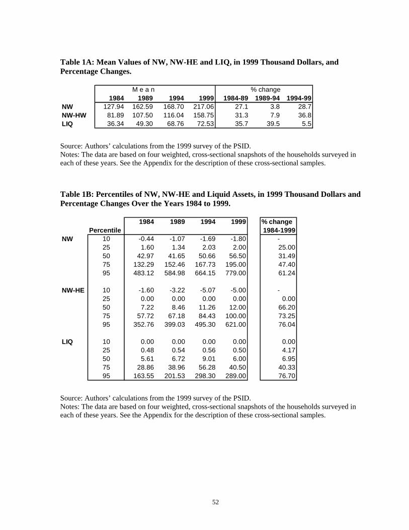
52

Table 1A: Mean Values of NW, NW-HE and LIQ, in 1999 Thousand Dollars, andPercentage Changes.

M e a n % change1984 1989 1994 1999 1984-89 1989-94 1994-99

NW 127.94 162.59 168.70 217.06 27.1 3.8 28.7NW-HW 81.89 107.50 116.04 158.75 31.3 7.9 36.8LIQ 36.34 49.30 68.76 72.53 35.7 39.5 5.5

Source: Authors’ calculations from the 1999 survey of the PSID.Notes: The data are based on four weighted, cross-sectional snapshots of the households surveyed ineach of these years. See the Appendix for the description of these cross-sectional samples.

Table 1B: Percentiles of NW, NW-HE and Liquid Assets, in 1999 Thousand Dollars andPercentage Changes Over the Years 1984 to 1999.

1984 1989 1994 1999 % changePercentile 1984-1999

NW 10 -0.44 -1.07 -1.69 -1.80 -25 1.60 1.34 2.03 2.00 25.0050 42.97 41.65 50.66 56.50 31.4975 132.29 152.46 167.73 195.00 47.4095 483.12 584.98 664.15 779.00 61.24

NW-HE 10 -1.60 -3.22 -5.07 -5.00 -25 0.00 0.00 0.00 0.00 0.0050 7.22 8.46 11.26 12.00 66.2075 57.72 67.18 84.43 100.00 73.2595 352.76 399.03 495.30 621.00 76.04

LIQ 10 0.00 0.00 0.00 0.00 0.0025 0.48 0.54 0.56 0.50 4.1750 5.61 6.72 9.01 6.00 6.9575 28.86 38.96 56.28 40.50 40.3395 163.55 201.53 298.30 289.00 76.70

Source: Authors’ calculations from the 1999 survey of the PSID.Notes: The data are based on four weighted, cross-sectional snapshots of the households surveyed ineach of these years. See the Appendix for the description of these cross-sectional samples.

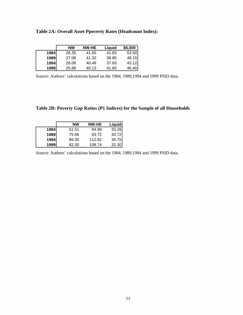
53

Table 2A: Overall Asset Ppoverty Rates (Headcount Index):

NW NW-HE Liquid $5,0001984 26.35 41.65 41.83 53.501989 27.08 41.32 38.85 48.151994 26.08 40.49 37.83 43.121999 25.88 40.13 41.65 46.40

Source: Authors’ calculations based on the 1984, 1989,1994 and 1999 PSID data.

Table 2B: Poverty Gap Ratios (P1 Indices) for the Sample of all Households

NW NW-HE Liquid1984 61.51 84.99 33.281989 75.66 93.72 30.721994 89.35 112.82 30.751999 82.30 108.74 32.30

Source: Authors’ calculations based on the 1984, 1989,1994 and 1999 PSID data.

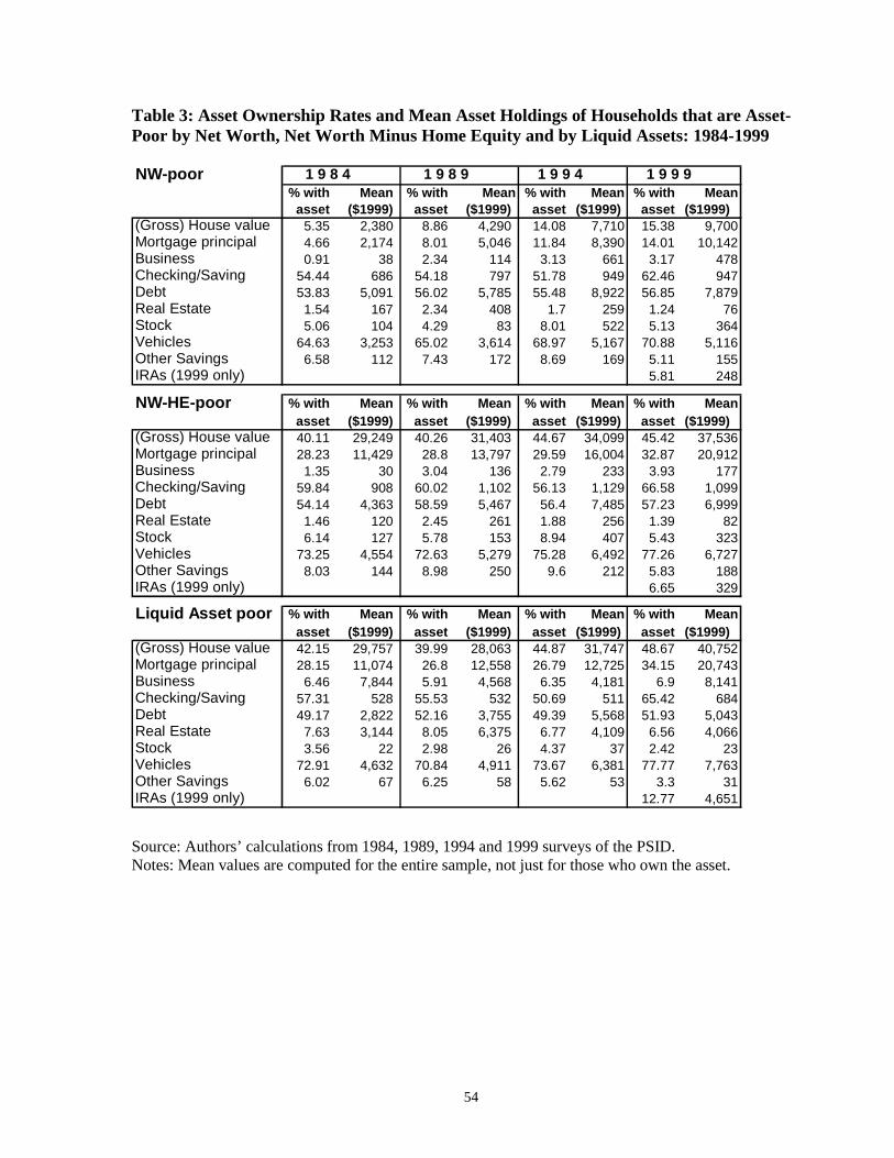
54

Table 3: Asset Ownership Rates and Mean Asset Holdings of Households that are Asset-Poor by Net Worth, Net Worth Minus Home Equity and by Liquid Assets: 1984-1999

NW-poor 1 9 8 4 1 9 8 9 1 9 9 4 1 9 9 9% with Mean % with Mean % with Mean % with Mean

asset ($1999) asset ($1999) asset ($1999) asset ($1999)(Gross) House value 5.35 2,380 8.86 4,290 14.08 7,710 15.38 9,700Mortgage principal 4.66 2,174 8.01 5,046 11.84 8,390 14.01 10,142Business 0.91 38 2.34 114 3.13 661 3.17 478Checking/Saving 54.44 686 54.18 797 51.78 949 62.46 947Debt 53.83 5,091 56.02 5,785 55.48 8,922 56.85 7,879Real Estate 1.54 167 2.34 408 1.7 259 1.24 76Stock 5.06 104 4.29 83 8.01 522 5.13 364Vehicles 64.63 3,253 65.02 3,614 68.97 5,167 70.88 5,116Other Savings 6.58 112 7.43 172 8.69 169 5.11 155IRAs (1999 only) 5.81 248

NW-HE-poor % with Mean % with Mean % with Mean % with Meanasset ($1999) asset ($1999) asset ($1999) asset ($1999)

(Gross) House value 40.11 29,249 40.26 31,403 44.67 34,099 45.42 37,536Mortgage principal 28.23 11,429 28.8 13,797 29.59 16,004 32.87 20,912Business 1.35 30 3.04 136 2.79 233 3.93 177Checking/Saving 59.84 908 60.02 1,102 56.13 1,129 66.58 1,099Debt 54.14 4,363 58.59 5,467 56.4 7,485 57.23 6,999Real Estate 1.46 120 2.45 261 1.88 256 1.39 82Stock 6.14 127 5.78 153 8.94 407 5.43 323Vehicles 73.25 4,554 72.63 5,279 75.28 6,492 77.26 6,727Other Savings 8.03 144 8.98 250 9.6 212 5.83 188IRAs (1999 only) 6.65 329

Liquid Asset poor % with Mean % with Mean % with Mean % with Meanasset ($1999) asset ($1999) asset ($1999) asset ($1999)

(Gross) House value 42.15 29,757 39.99 28,063 44.87 31,747 48.67 40,752Mortgage principal 28.15 11,074 26.8 12,558 26.79 12,725 34.15 20,743Business 6.46 7,844 5.91 4,568 6.35 4,181 6.9 8,141Checking/Saving 57.31 528 55.53 532 50.69 511 65.42 684Debt 49.17 2,822 52.16 3,755 49.39 5,568 51.93 5,043Real Estate 7.63 3,144 8.05 6,375 6.77 4,109 6.56 4,066Stock 3.56 22 2.98 26 4.37 37 2.42 23Vehicles 72.91 4,632 70.84 4,911 73.67 6,381 77.77 7,763Other Savings 6.02 67 6.25 58 5.62 53 3.3 31IRAs (1999 only) 12.77 4,651

Source: Authors’ calculations from 1984, 1989, 1994 and 1999 surveys of the PSID.Notes: Mean values are computed for the entire sample, not just for those who own the asset.

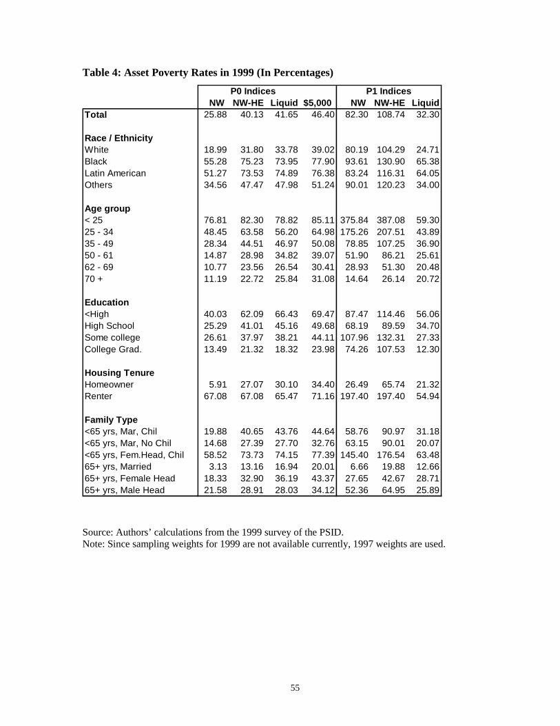
55

Table 4: Asset Poverty Rates in 1999 (In Percentages)P0 Indices P1 Indices

NW NW-HE Liquid $5,000 NW NW-HE LiquidTotal 25.88 40.13 41.65 46.40 82.30 108.74 32.30

Race / EthnicityWhite 18.99 31.80 33.78 39.02 80.19 104.29 24.71Black 55.28 75.23 73.95 77.90 93.61 130.90 65.38Latin American 51.27 73.53 74.89 76.38 83.24 116.31 64.05Others 34.56 47.47 47.98 51.24 90.01 120.23 34.00

Age group< 25 76.81 82.30 78.82 85.11 375.84 387.08 59.3025 - 34 48.45 63.58 56.20 64.98 175.26 207.51 43.8935 - 49 28.34 44.51 46.97 50.08 78.85 107.25 36.9050 - 61 14.87 28.98 34.82 39.07 51.90 86.21 25.6162 - 69 10.77 23.56 26.54 30.41 28.93 51.30 20.4870 + 11.19 22.72 25.84 31.08 14.64 26.14 20.72

Education<High 40.03 62.09 66.43 69.47 87.47 114.46 56.06High School 25.29 41.01 45.16 49.68 68.19 89.59 34.70Some college 26.61 37.97 38.21 44.11 107.96 132.31 27.33College Grad. 13.49 21.32 18.32 23.98 74.26 107.53 12.30

Housing TenureHomeowner 5.91 27.07 30.10 34.40 26.49 65.74 21.32Renter 67.08 67.08 65.47 71.16 197.40 197.40 54.94

Family Type<65 yrs, Mar, Chil 19.88 40.65 43.76 44.64 58.76 90.97 31.18<65 yrs, Mar, No Chil 14.68 27.39 27.70 32.76 63.15 90.01 20.07<65 yrs, Fem.Head, Chil 58.52 73.73 74.15 77.39 145.40 176.54 63.4865+ yrs, Married 3.13 13.16 16.94 20.01 6.66 19.88 12.6665+ yrs, Female Head 18.33 32.90 36.19 43.37 27.65 42.67 28.7165+ yrs, Male Head 21.58 28.91 28.03 34.12 52.36 64.95 25.89

Source: Authors’ calculations from the 1999 survey of the PSID.Note: Since sampling weights for 1999 are not available currently, 1997 weights are used.

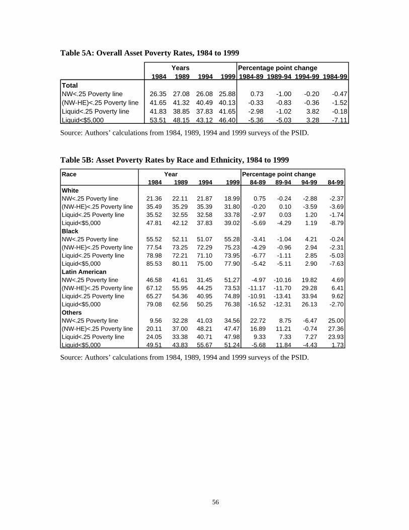
56

Table 5A: Overall Asset Poverty Rates, 1984 to 1999

Years Percentage point change1984 1989 1994 1999 1984-89 1989-94 1994-99 1984-99

TotalNW<.25 Poverty line 26.35 27.08 26.08 25.88 0.73 -1.00 -0.20 -0.47(NW-HE)<.25 Poverty line 41.65 41.32 40.49 40.13 -0.33 -0.83 -0.36 -1.52Liquid<.25 Poverty line 41.83 38.85 37.83 41.65 -2.98 -1.02 3.82 -0.18Liquid<$5,000 53.51 48.15 43.12 46.40 -5.36 -5.03 3.28 -7.11

Source: Authors’ calculations from 1984, 1989, 1994 and 1999 surveys of the PSID.

Table 5B: Asset Poverty Rates by Race and Ethnicity, 1984 to 1999

Race Year Percentage point change1984 1989 1994 1999 84-89 89-94 94-99 84-99

WhiteNW<.25 Poverty line 21.36 22.11 21.87 18.99 0.75 -0.24 -2.88 -2.37(NW-HE)<.25 Poverty line 35.49 35.29 35.39 31.80 -0.20 0.10 -3.59 -3.69Liquid<.25 Poverty line 35.52 32.55 32.58 33.78 -2.97 0.03 1.20 -1.74Liquid<$5,000 47.81 42.12 37.83 39.02 -5.69 -4.29 1.19 -8.79BlackNW<.25 Poverty line 55.52 52.11 51.07 55.28 -3.41 -1.04 4.21 -0.24(NW-HE)<.25 Poverty line 77.54 73.25 72.29 75.23 -4.29 -0.96 2.94 -2.31Liquid<.25 Poverty line 78.98 72.21 71.10 73.95 -6.77 -1.11 2.85 -5.03Liquid<$5,000 85.53 80.11 75.00 77.90 -5.42 -5.11 2.90 -7.63Latin AmericanNW<.25 Poverty line 46.58 41.61 31.45 51.27 -4.97 -10.16 19.82 4.69(NW-HE)<.25 Poverty line 67.12 55.95 44.25 73.53 -11.17 -11.70 29.28 6.41Liquid<.25 Poverty line 65.27 54.36 40.95 74.89 -10.91 -13.41 33.94 9.62Liquid<$5,000 79.08 62.56 50.25 76.38 -16.52 -12.31 26.13 -2.70OthersNW<.25 Poverty line 9.56 32.28 41.03 34.56 22.72 8.75 -6.47 25.00(NW-HE)<.25 Poverty line 20.11 37.00 48.21 47.47 16.89 11.21 -0.74 27.36Liquid<.25 Poverty line 24.05 33.38 40.71 47.98 9.33 7.33 7.27 23.93Liquid<$5,000 49.51 43.83 55.67 51.24 -5.68 11.84 -4.43 1.73

Source: Authors’ calculations from 1984, 1989, 1994 and 1999 surveys of the PSID.

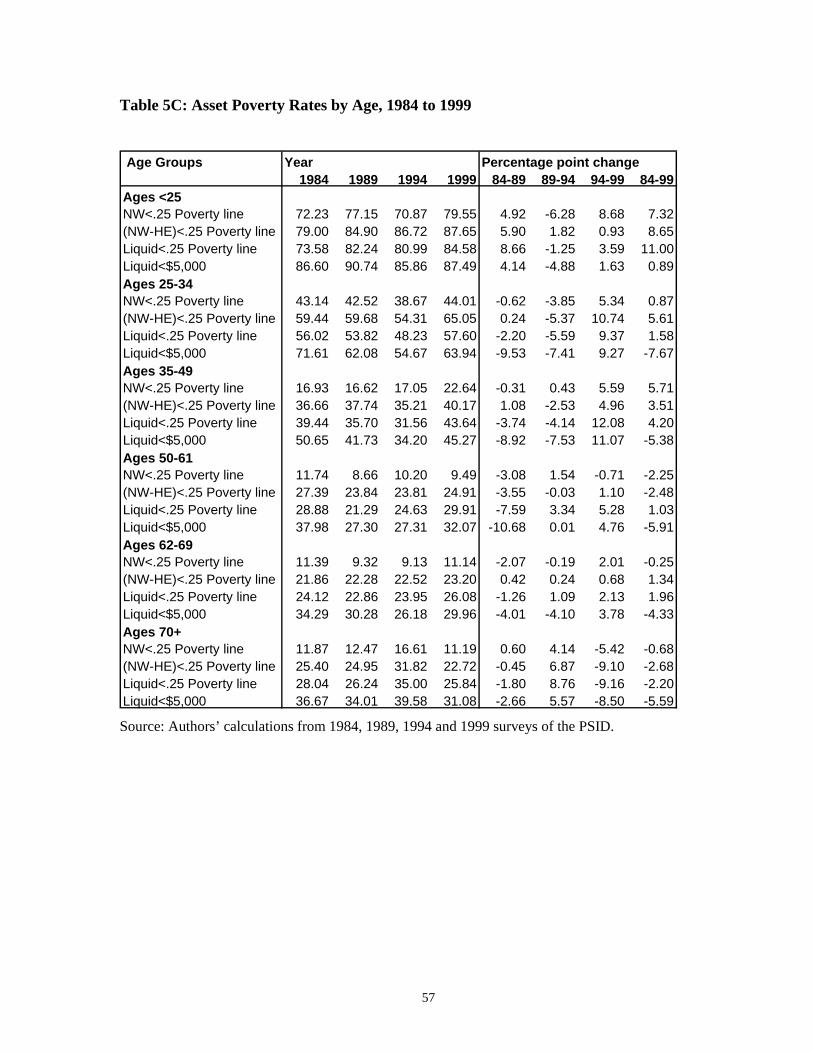
57

Table 5C: Asset Poverty Rates by Age, 1984 to 1999

Age Groups Year Percentage point change1984 1989 1994 1999 84-89 89-94 94-99 84-99

Ages <25NW<.25 Poverty line 72.23 77.15 70.87 79.55 4.92 -6.28 8.68 7.32(NW-HE)<.25 Poverty line 79.00 84.90 86.72 87.65 5.90 1.82 0.93 8.65Liquid<.25 Poverty line 73.58 82.24 80.99 84.58 8.66 -1.25 3.59 11.00Liquid<$5,000 86.60 90.74 85.86 87.49 4.14 -4.88 1.63 0.89Ages 25-34NW<.25 Poverty line 43.14 42.52 38.67 44.01 -0.62 -3.85 5.34 0.87(NW-HE)<.25 Poverty line 59.44 59.68 54.31 65.05 0.24 -5.37 10.74 5.61Liquid<.25 Poverty line 56.02 53.82 48.23 57.60 -2.20 -5.59 9.37 1.58Liquid<$5,000 71.61 62.08 54.67 63.94 -9.53 -7.41 9.27 -7.67Ages 35-49NW<.25 Poverty line 16.93 16.62 17.05 22.64 -0.31 0.43 5.59 5.71(NW-HE)<.25 Poverty line 36.66 37.74 35.21 40.17 1.08 -2.53 4.96 3.51Liquid<.25 Poverty line 39.44 35.70 31.56 43.64 -3.74 -4.14 12.08 4.20Liquid<$5,000 50.65 41.73 34.20 45.27 -8.92 -7.53 11.07 -5.38Ages 50-61NW<.25 Poverty line 11.74 8.66 10.20 9.49 -3.08 1.54 -0.71 -2.25(NW-HE)<.25 Poverty line 27.39 23.84 23.81 24.91 -3.55 -0.03 1.10 -2.48Liquid<.25 Poverty line 28.88 21.29 24.63 29.91 -7.59 3.34 5.28 1.03Liquid<$5,000 37.98 27.30 27.31 32.07 -10.68 0.01 4.76 -5.91Ages 62-69NW<.25 Poverty line 11.39 9.32 9.13 11.14 -2.07 -0.19 2.01 -0.25(NW-HE)<.25 Poverty line 21.86 22.28 22.52 23.20 0.42 0.24 0.68 1.34Liquid<.25 Poverty line 24.12 22.86 23.95 26.08 -1.26 1.09 2.13 1.96Liquid<$5,000 34.29 30.28 26.18 29.96 -4.01 -4.10 3.78 -4.33Ages 70+NW<.25 Poverty line 11.87 12.47 16.61 11.19 0.60 4.14 -5.42 -0.68(NW-HE)<.25 Poverty line 25.40 24.95 31.82 22.72 -0.45 6.87 -9.10 -2.68Liquid<.25 Poverty line 28.04 26.24 35.00 25.84 -1.80 8.76 -9.16 -2.20Liquid<$5,000 36.67 34.01 39.58 31.08 -2.66 5.57 -8.50 -5.59

Source: Authors’ calculations from 1984, 1989, 1994 and 1999 surveys of the PSID.

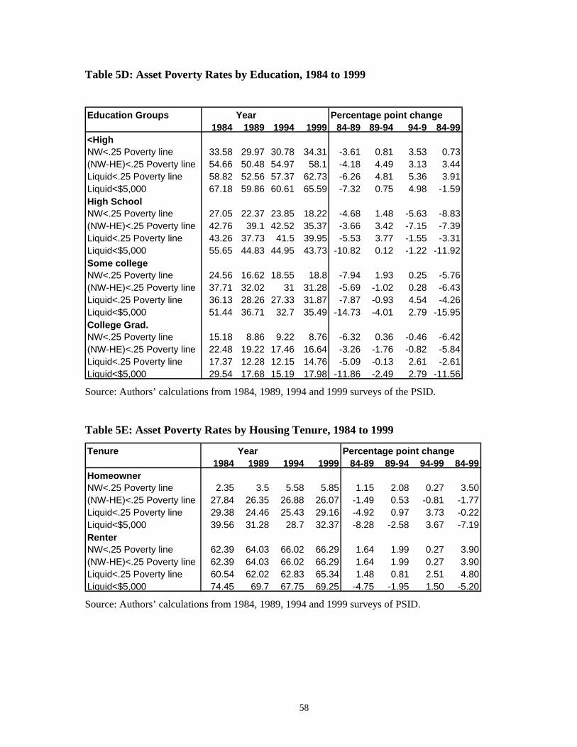
58

Table 5D: Asset Poverty Rates by Education, 1984 to 1999

Education Groups Year Percentage point change1984 1989 1994 1999 84-89 89-94 94-9 84-99

<HighNW<.25 Poverty line 33.58 29.97 30.78 34.31 -3.61 0.81 3.53 0.73(NW-HE)<.25 Poverty line 54.66 50.48 54.97 58.1 -4.18 4.49 3.13 3.44Liquid<.25 Poverty line 58.82 52.56 57.37 62.73 -6.26 4.81 5.36 3.91Liquid<$5,000 67.18 59.86 60.61 65.59 -7.32 0.75 4.98 -1.59High SchoolNW<.25 Poverty line 27.05 22.37 23.85 18.22 -4.68 1.48 -5.63 -8.83(NW-HE)<.25 Poverty line 42.76 39.1 42.52 35.37 -3.66 3.42 -7.15 -7.39Liquid<.25 Poverty line 43.26 37.73 41.5 39.95 -5.53 3.77 -1.55 -3.31Liquid<$5,000 55.65 44.83 44.95 43.73 -10.82 0.12 -1.22 -11.92Some collegeNW<.25 Poverty line 24.56 16.62 18.55 18.8 -7.94 1.93 0.25 -5.76(NW-HE)<.25 Poverty line 37.71 32.02 31 31.28 -5.69 -1.02 0.28 -6.43Liquid<.25 Poverty line 36.13 28.26 27.33 31.87 -7.87 -0.93 4.54 -4.26Liquid<$5,000 51.44 36.71 32.7 35.49 -14.73 -4.01 2.79 -15.95College Grad.NW<.25 Poverty line 15.18 8.86 9.22 8.76 -6.32 0.36 -0.46 -6.42(NW-HE)<.25 Poverty line 22.48 19.22 17.46 16.64 -3.26 -1.76 -0.82 -5.84Liquid<.25 Poverty line 17.37 12.28 12.15 14.76 -5.09 -0.13 2.61 -2.61Liquid<$5,000 29.54 17.68 15.19 17.98 -11.86 -2.49 2.79 -11.56

Source: Authors’ calculations from 1984, 1989, 1994 and 1999 surveys of the PSID.

Table 5E: Asset Poverty Rates by Housing Tenure, 1984 to 1999

Tenure Year Percentage point change1984 1989 1994 1999 84-89 89-94 94-99 84-99

HomeownerNW<.25 Poverty line 2.35 3.5 5.58 5.85 1.15 2.08 0.27 3.50(NW-HE)<.25 Poverty line 27.84 26.35 26.88 26.07 -1.49 0.53 -0.81 -1.77Liquid<.25 Poverty line 29.38 24.46 25.43 29.16 -4.92 0.97 3.73 -0.22Liquid<$5,000 39.56 31.28 28.7 32.37 -8.28 -2.58 3.67 -7.19RenterNW<.25 Poverty line 62.39 64.03 66.02 66.29 1.64 1.99 0.27 3.90(NW-HE)<.25 Poverty line 62.39 64.03 66.02 66.29 1.64 1.99 0.27 3.90Liquid<.25 Poverty line 60.54 62.02 62.83 65.34 1.48 0.81 2.51 4.80Liquid<$5,000 74.45 69.7 67.75 69.25 -4.75 -1.95 1.50 -5.20

Source: Authors’ calculations from 1984, 1989, 1994 and 1999 surveys of PSID.

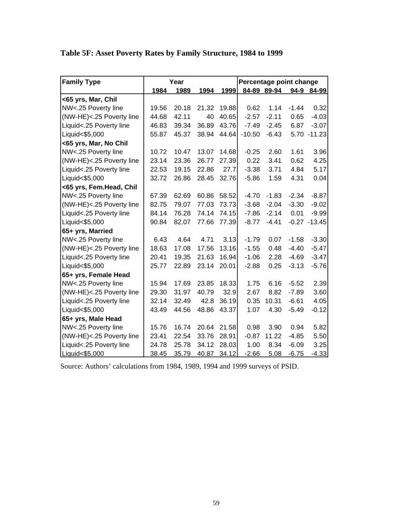
59

Table 5F: Asset Poverty Rates by Family Structure, 1984 to 1999

Family Type Year Percentage point change1984 1989 1994 1999 84-89 89-94 94-9 84-99

<65 yrs, Mar, ChilNW<.25 Poverty line 19.56 20.18 21.32 19.88 0.62 1.14 -1.44 0.32(NW-HE)<.25 Poverty line 44.68 42.11 40 40.65 -2.57 -2.11 0.65 -4.03Liquid<.25 Poverty line 46.83 39.34 36.89 43.76 -7.49 -2.45 6.87 -3.07Liquid<$5,000 55.87 45.37 38.94 44.64 -10.50 -6.43 5.70 -11.23<65 yrs, Mar, No ChilNW<.25 Poverty line 10.72 10.47 13.07 14.68 -0.25 2.60 1.61 3.96(NW-HE)<.25 Poverty line 23.14 23.36 26.77 27.39 0.22 3.41 0.62 4.25Liquid<.25 Poverty line 22.53 19.15 22.86 27.7 -3.38 3.71 4.84 5.17Liquid<$5,000 32.72 26.86 28.45 32.76 -5.86 1.59 4.31 0.04<65 yrs, Fem.Head, ChilNW<.25 Poverty line 67.39 62.69 60.86 58.52 -4.70 -1.83 -2.34 -8.87(NW-HE)<.25 Poverty line 82.75 79.07 77.03 73.73 -3.68 -2.04 -3.30 -9.02Liquid<.25 Poverty line 84.14 76.28 74.14 74.15 -7.86 -2.14 0.01 -9.99Liquid<$5,000 90.84 82.07 77.66 77.39 -8.77 -4.41 -0.27 -13.4565+ yrs, MarriedNW<.25 Poverty line 6.43 4.64 4.71 3.13 -1.79 0.07 -1.58 -3.30(NW-HE)<.25 Poverty line 18.63 17.08 17.56 13.16 -1.55 0.48 -4.40 -5.47Liquid<.25 Poverty line 20.41 19.35 21.63 16.94 -1.06 2.28 -4.69 -3.47Liquid<$5,000 25.77 22.89 23.14 20.01 -2.88 0.25 -3.13 -5.7665+ yrs, Female HeadNW<.25 Poverty line 15.94 17.69 23.85 18.33 1.75 6.16 -5.52 2.39(NW-HE)<.25 Poverty line 29.30 31.97 40.79 32.9 2.67 8.82 -7.89 3.60Liquid<.25 Poverty line 32.14 32.49 42.8 36.19 0.35 10.31 -6.61 4.05Liquid<$5,000 43.49 44.56 48.86 43.37 1.07 4.30 -5.49 -0.1265+ yrs, Male HeadNW<.25 Poverty line 15.76 16.74 20.64 21.58 0.98 3.90 0.94 5.82(NW-HE)<.25 Poverty line 23.41 22.54 33.76 28.91 -0.87 11.22 -4.85 5.50Liquid<.25 Poverty line 24.78 25.78 34.12 28.03 1.00 8.34 -6.09 3.25Liquid<$5,000 38.45 35.79 40.87 34.12 -2.66 5.08 -6.75 -4.33

Source: Authors’ calculations from 1984, 1989, 1994 and 1999 surveys of PSID.

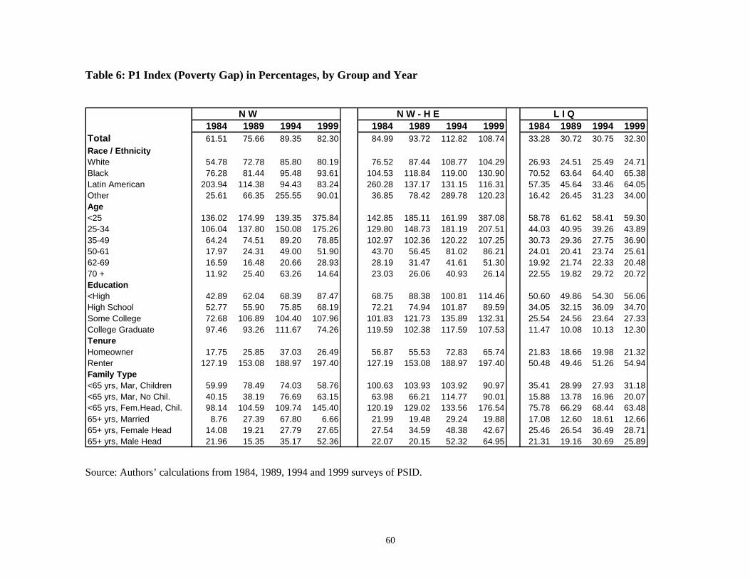
60

Table 6: P1 Index (Poverty Gap) in Percentages, by Group and Year

N W N W - H E L I Q1984 1989 1994 1999 1984 1989 1994 1999 1984 1989 1994 1999

Total 61.51 75.66 89.35 82.30 84.99 93.72 112.82 108.74 33.28 30.72 30.75 32.30Race / EthnicityWhite 54.78 72.78 85.80 80.19 76.52 87.44 108.77 104.29 26.93 24.51 25.49 24.71Black 76.28 81.44 95.48 93.61 104.53 118.84 119.00 130.90 70.52 63.64 64.40 65.38Latin American 203.94 114.38 94.43 83.24 260.28 137.17 131.15 116.31 57.35 45.64 33.46 64.05Other 25.61 66.35 255.55 90.01 36.85 78.42 289.78 120.23 16.42 26.45 31.23 34.00Age<25 136.02 174.99 139.35 375.84 142.85 185.11 161.99 387.08 58.78 61.62 58.41 59.3025-34 106.04 137.80 150.08 175.26 129.80 148.73 181.19 207.51 44.03 40.95 39.26 43.8935-49 64.24 74.51 89.20 78.85 102.97 102.36 120.22 107.25 30.73 29.36 27.75 36.9050-61 17.97 24.31 49.00 51.90 43.70 56.45 81.02 86.21 24.01 20.41 23.74 25.6162-69 16.59 16.48 20.66 28.93 28.19 31.47 41.61 51.30 19.92 21.74 22.33 20.4870 + 11.92 25.40 63.26 14.64 23.03 26.06 40.93 26.14 22.55 19.82 29.72 20.72Education<High 42.89 62.04 68.39 87.47 68.75 88.38 100.81 114.46 50.60 49.86 54.30 56.06High School 52.77 55.90 75.85 68.19 72.21 74.94 101.87 89.59 34.05 32.15 36.09 34.70Some College 72.68 106.89 104.40 107.96 101.83 121.73 135.89 132.31 25.54 24.56 23.64 27.33College Graduate 97.46 93.26 111.67 74.26 119.59 102.38 117.59 107.53 11.47 10.08 10.13 12.30TenureHomeowner 17.75 25.85 37.03 26.49 56.87 55.53 72.83 65.74 21.83 18.66 19.98 21.32Renter 127.19 153.08 188.97 197.40 127.19 153.08 188.97 197.40 50.48 49.46 51.26 54.94Family Type<65 yrs, Mar, Children 59.99 78.49 74.03 58.76 100.63 103.93 103.92 90.97 35.41 28.99 27.93 31.18<65 yrs, Mar, No Chil. 40.15 38.19 76.69 63.15 63.98 66.21 114.77 90.01 15.88 13.78 16.96 20.07<65 yrs, Fem.Head, Chil. 98.14 104.59 109.74 145.40 120.19 129.02 133.56 176.54 75.78 66.29 68.44 63.4865+ yrs, Married 8.76 27.39 67.80 6.66 21.99 19.48 29.24 19.88 17.08 12.60 18.61 12.6665+ yrs, Female Head 14.08 19.21 27.79 27.65 27.54 34.59 48.38 42.67 25.46 26.54 36.49 28.7165+ yrs, Male Head 21.96 15.35 35.17 52.36 22.07 20.15 52.32 64.95 21.31 19.16 30.69 25.89

Source: Authors’ calculations from 1984, 1989, 1994 and 1999 surveys of PSID.

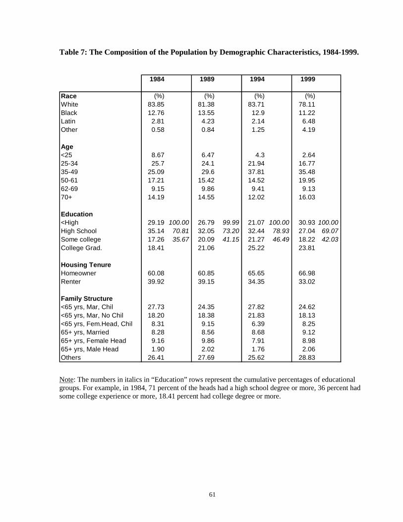
61

Table 7: The Composition of the Population by Demographic Characteristics, 1984-1999.

1984 1989 1994 1999

Race (%) (%) (%) (%)White 83.85 81.38 83.71 78.11Black 12.76 13.55 12.9 11.22Latin 2.81 4.23 2.14 6.48Other 0.58 0.84 1.25 4.19

Age<25 8.67 6.47 4.3 2.6425-34 25.7 24.1 21.94 16.7735-49 25.09 29.6 37.81 35.4850-61 17.21 15.42 14.52 19.9562-69 9.15 9.86 9.41 9.1370+ 14.19 14.55 12.02 16.03

Education<High 29.19 100.00 26.79 99.99 21.07 100.00 30.93 100.00High School 35.14 70.81 32.05 73.20 32.44 78.93 27.04 69.07Some college 17.26 35.67 20.09 41.15 21.27 46.49 18.22 42.03College Grad. 18.41 21.06 25.22 23.81

Housing TenureHomeowner 60.08 60.85 65.65 66.98Renter 39.92 39.15 34.35 33.02

Family Structure<65 yrs, Mar, Chil 27.73 24.35 27.82 24.62<65 yrs, Mar, No Chil 18.20 18.38 21.83 18.13<65 yrs, Fem.Head, Chil 8.31 9.15 6.39 8.2565+ yrs, Married 8.28 8.56 8.68 9.1265+ yrs, Female Head 9.16 9.86 7.91 8.9865+ yrs, Male Head 1.90 2.02 1.76 2.06Others 26.41 27.69 25.62 28.83

Note: The numbers in italics in “Education” rows represent the cumulative percentages of educationalgroups. For example, in 1984, 71 percent of the heads had a high school degree or more, 36 percent hadsome college experience or more, 18.41 percent had college degree or more.

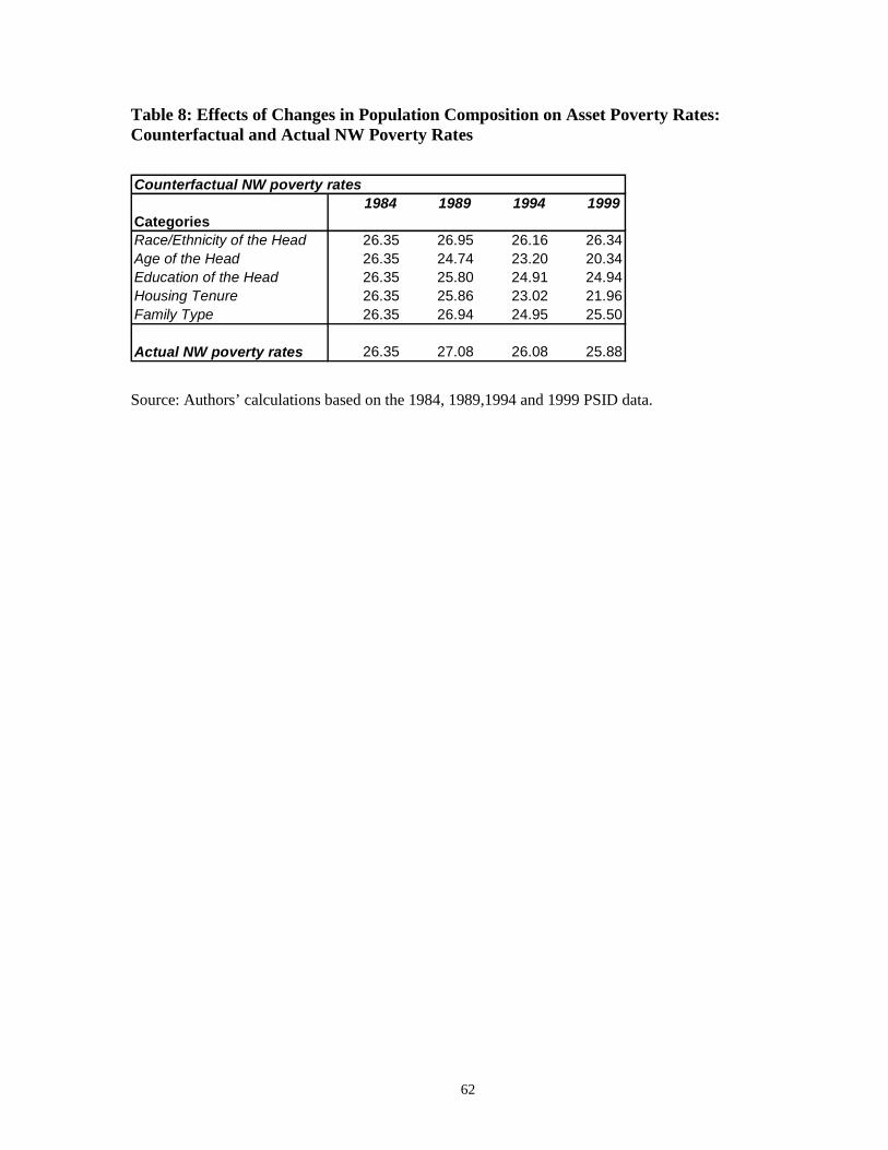
62

Table 8: Effects of Changes in Population Composition on Asset Poverty Rates:Counterfactual and Actual NW Poverty Rates

Counterfactual NW poverty rates1984 1989 1994 1999

CategoriesRace/Ethnicity of the Head 26.35 26.95 26.16 26.34Age of the Head 26.35 24.74 23.20 20.34Education of the Head 26.35 25.80 24.91 24.94Housing Tenure 26.35 25.86 23.02 21.96Family Type 26.35 26.94 24.95 25.50

Actual NW poverty rates 26.35 27.08 26.08 25.88

Source: Authors’ calculations based on the 1984, 1989,1994 and 1999 PSID data.

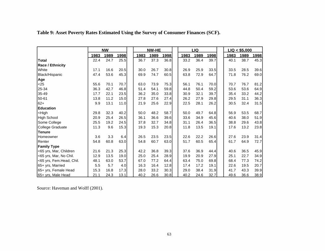
63

Table 9: Asset Poverty Rates Estimated Using the Survey of Consumer Finances (SCF).

NW NW-HE LIQ LIQ < $5,0001983 1989 1998 1983 1989 1998 1983 1989 1998 1983 1989 1998

Total 22.4 24.7 25.5 36.7 37.3 36.8 33.2 36.4 39.7 40.1 38.7 45.3Race / EthnicityWhite 17.1 16.6 20.5 30.0 26.7 30.8 26.9 25.9 33.5 33.5 28.5 39.6Black/Hispanic 47.4 53.6 45.3 69.9 74.7 60.5 63.8 72.9 64.7 71.8 76.2 69.0Age<25 55.6 70.1 70.7 63.0 73.9 75.3 56.1 76.1 70.0 70.7 76.7 81.225-34 36.3 42.7 46.8 51.4 54.1 59.8 44.8 50.4 59.2 53.6 53.6 64.935-49 17.7 22.1 23.5 36.2 35.0 33.8 30.9 32.1 39.7 35.4 33.2 44.250-61 13.8 11.2 15.0 27.8 27.6 27.4 26.2 27.9 29.8 29.5 31.1 36.362+ 9.9 13.1 11.0 21.9 25.6 22.9 22.5 28.1 26.2 30.5 32.4 31.5Education<High 29.8 32.3 40.2 50.0 48.2 58.7 50.0 49.7 64.8 56.9 53.5 68.7High School 20.9 25.4 26.5 36.1 36.6 39.6 33.6 34.9 45.6 40.6 38.0 51.9Some College 25.5 19.2 24.5 37.8 32.7 34.8 31.1 26.4 36.5 38.8 29.6 43.8College Graduate 11.3 9.6 15.3 19.3 15.3 20.8 11.8 13.5 19.1 17.6 13.2 23.8TenureHomeowner 3.6 3.3 6.4 26.5 23.5 23.5 22.6 22.2 26.6 27.6 23.9 31.4Renter 54.8 60.8 63.0 54.8 60.7 63.0 51.7 60.5 65.4 61.7 64.9 72.7Family Type<65 yrs, Mar, Children 21.6 21.3 25.3 42.2 36.8 39.3 37.6 36.9 44.4 40.6 36.5 45.9<65 yrs, Mar, No Chil. 12.9 13.5 19.0 25.0 25.4 28.9 19.9 20.9 27.9 25.1 22.7 34.9<65 yrs, Fem.Head, Chil. 48.1 63.0 53.7 67.0 77.2 64.4 63.4 75.0 69.8 68.4 77.3 74.265+ yrs, Married 5.5 5.7 4.0 16.3 16.4 12.8 17.4 17.2 19.1 22.6 19.5 20.765+ yrs, Female Head 15.3 16.8 17.3 28.0 33.2 30.3 29.0 38.4 31.9 41.7 43.3 39.965+ yrs, Male Head 21.1 24.3 13.1 40.2 26.6 30.8 40.2 24.6 32.7 49.6 36.6 38.9

Source: Haveman and Wolff (2001).

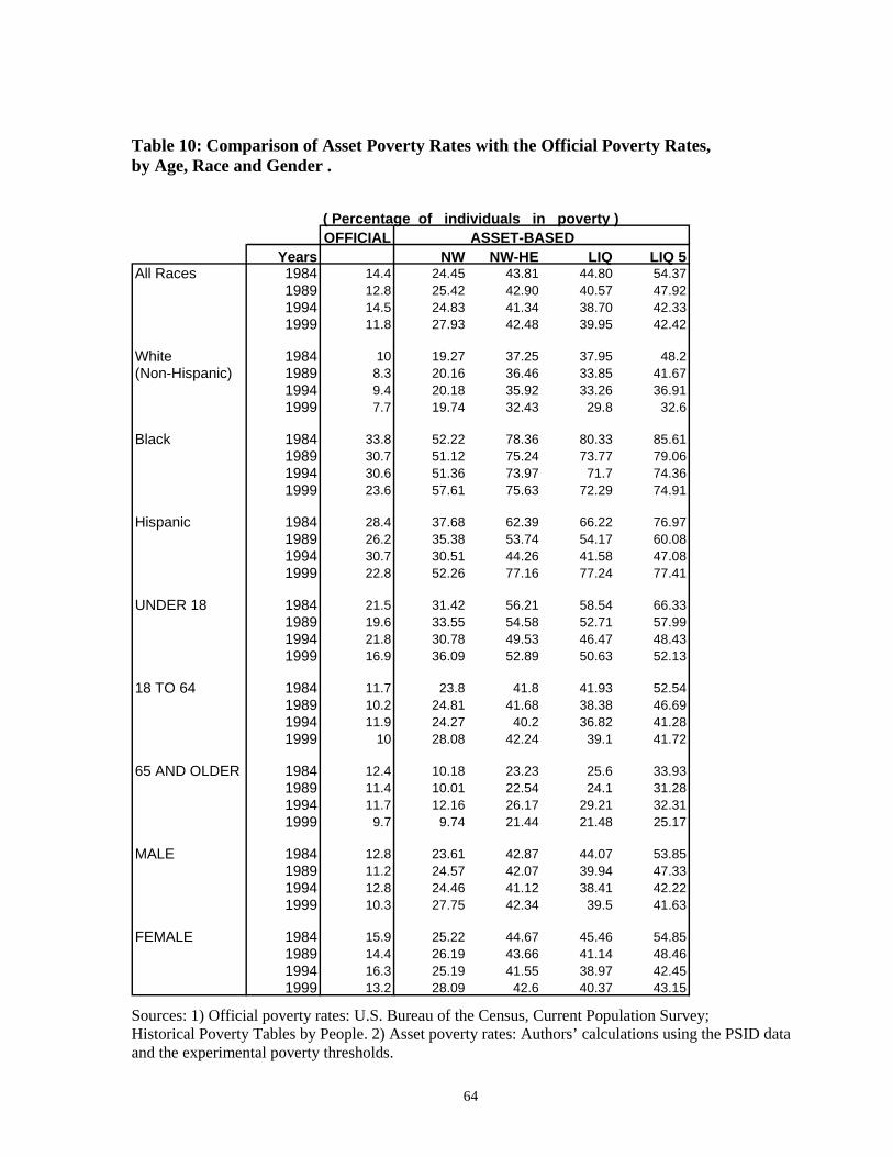
64

Table 10: Comparison of Asset Poverty Rates with the Official Poverty Rates,by Age, Race and Gender .

( Percentage of individuals in poverty )OFFICIAL ASSET-BASED

Years NW NW-HE LIQ LIQ 5All Races 1984 14.4 24.45 43.81 44.80 54.37

1989 12.8 25.42 42.90 40.57 47.921994 14.5 24.83 41.34 38.70 42.331999 11.8 27.93 42.48 39.95 42.42

White 1984 10 19.27 37.25 37.95 48.2(Non-Hispanic) 1989 8.3 20.16 36.46 33.85 41.67

1994 9.4 20.18 35.92 33.26 36.911999 7.7 19.74 32.43 29.8 32.6

Black 1984 33.8 52.22 78.36 80.33 85.611989 30.7 51.12 75.24 73.77 79.061994 30.6 51.36 73.97 71.7 74.361999 23.6 57.61 75.63 72.29 74.91

Hispanic 1984 28.4 37.68 62.39 66.22 76.971989 26.2 35.38 53.74 54.17 60.081994 30.7 30.51 44.26 41.58 47.081999 22.8 52.26 77.16 77.24 77.41

UNDER 18 1984 21.5 31.42 56.21 58.54 66.331989 19.6 33.55 54.58 52.71 57.991994 21.8 30.78 49.53 46.47 48.431999 16.9 36.09 52.89 50.63 52.13

18 TO 64 1984 11.7 23.8 41.8 41.93 52.541989 10.2 24.81 41.68 38.38 46.691994 11.9 24.27 40.2 36.82 41.281999 10 28.08 42.24 39.1 41.72

65 AND OLDER 1984 12.4 10.18 23.23 25.6 33.931989 11.4 10.01 22.54 24.1 31.281994 11.7 12.16 26.17 29.21 32.311999 9.7 9.74 21.44 21.48 25.17

MALE 1984 12.8 23.61 42.87 44.07 53.851989 11.2 24.57 42.07 39.94 47.331994 12.8 24.46 41.12 38.41 42.221999 10.3 27.75 42.34 39.5 41.63

FEMALE 1984 15.9 25.22 44.67 45.46 54.851989 14.4 26.19 43.66 41.14 48.461994 16.3 25.19 41.55 38.97 42.451999 13.2 28.09 42.6 40.37 43.15

Sources: 1) Official poverty rates: U.S. Bureau of the Census, Current Population Survey;Historical Poverty Tables by People. 2) Asset poverty rates: Authors’ calculations using the PSID dataand the experimental poverty thresholds.

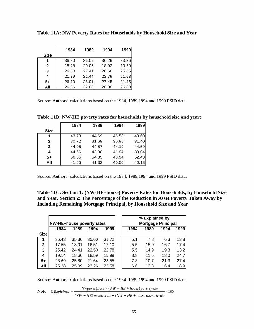
65

Table 11A: NW Poverty Rates for Households by Household Size and Year

1984 1989 1994 1999Size

1 36.80 36.09 36.29 33.362 18.28 20.06 18.92 19.593 26.50 27.41 26.68 25.654 21.39 21.44 22.79 21.68

5+ 26.10 28.91 27.45 31.45All 26.36 27.08 26.08 25.89

Source: Authors’ calculations based on the 1984, 1989,1994 and 1999 PSID data.

Table 11B: NW-HE poverty rates for households by household size and year:1984 1989 1994 1999

Size1 43.73 44.69 46.58 43.602 30.72 31.69 30.95 31.403 44.95 44.57 44.19 44.594 44.66 42.90 41.94 39.04

5+ 56.65 54.85 48.94 52.43All 41.65 41.32 40.50 40.13

Source: Authors’ calculations based on the 1984, 1989,1994 and 1999 PSID data.

Table 11C: Section 1: (NW-HE+house) Poverty Rates for Households, by Household Sizeand Year. Section 2: The Percentage of the Reduction in Asset Poverty Taken Away byIncluding Remaining Mortgage Principal, by Household Size and Year

% Explained by NW-HE+house poverty rates Mortgage Principal

1984 1989 1994 1999 1984 1989 1994 1999Size

1 36.43 35.36 35.60 31.72 5.1 7.8 6.3 13.82 17.55 18.01 16.51 17.10 5.5 15.0 16.7 17.43 25.42 24.41 22.50 22.78 5.5 14.9 19.3 13.24 19.14 18.66 18.59 15.99 8.8 11.5 18.0 24.7

5+ 23.69 25.80 21.64 23.55 7.3 10.7 21.3 27.4All 25.28 25.09 23.26 22.58 6.6 12.3 16.4 18.9

Source: Authors’ calculations based on the 1984, 1989,1994 and 1999 PSID data.

Note: 100*)()(

)(%

epovertyrathouseHENWepovertyratHENW

epovertyrathouseHENWateNWpovertyrExplained

+−−−

+−−≡

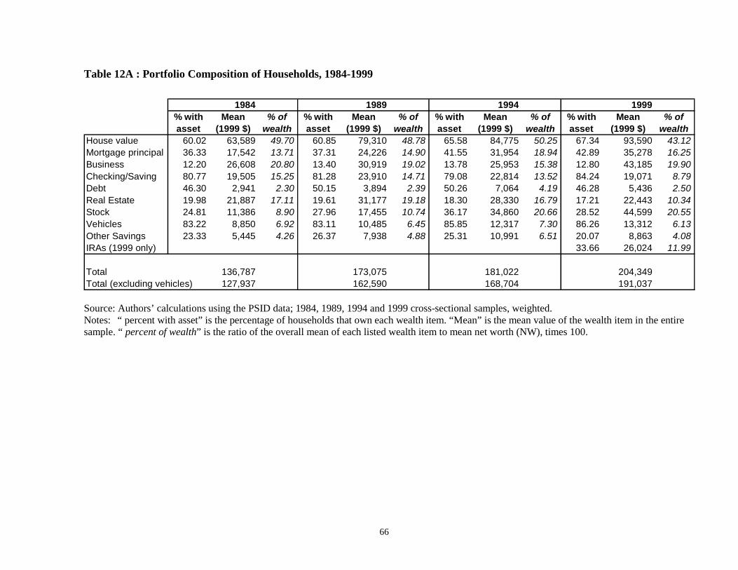
66

Table 12A : Portfolio Composition of Households, 1984-1999

1984 1989 1994 1999% with Mean % of % with Mean % of % with Mean % of % with Mean % ofasset (1999 $) wealth asset (1999 $) wealth asset (1999 $) wealth asset (1999 $) wealth

House value 60.02 63,589 49.70 60.85 79,310 48.78 65.58 84,775 50.25 67.34 93,590 43.12Mortgage principal 36.33 17,542 13.71 37.31 24,226 14.90 41.55 31,954 18.94 42.89 35,278 16.25Business 12.20 26,608 20.80 13.40 30,919 19.02 13.78 25,953 15.38 12.80 43,185 19.90Checking/Saving 80.77 19,505 15.25 81.28 23,910 14.71 79.08 22,814 13.52 84.24 19,071 8.79Debt 46.30 2,941 2.30 50.15 3,894 2.39 50.26 7,064 4.19 46.28 5,436 2.50Real Estate 19.98 21,887 17.11 19.61 31,177 19.18 18.30 28,330 16.79 17.21 22,443 10.34Stock 24.81 11,386 8.90 27.96 17,455 10.74 36.17 34,860 20.66 28.52 44,599 20.55Vehicles 83.22 8,850 6.92 83.11 10,485 6.45 85.85 12,317 7.30 86.26 13,312 6.13Other Savings 23.33 5,445 4.26 26.37 7,938 4.88 25.31 10,991 6.51 20.07 8,863 4.08IRAs (1999 only) 33.66 26,024 11.99

Total 136,787 173,075 181,022 204,349Total (excluding vehicles) 127,937 162,590 168,704 191,037

Source: Authors’ calculations using the PSID data; 1984, 1989, 1994 and 1999 cross-sectional samples, weighted.Notes: “ percent with asset” is the percentage of households that own each wealth item. “Mean” is the mean value of the wealth item in the entiresample. “ percent of wealth” is the ratio of the overall mean of each listed wealth item to mean net worth (NW), times 100.

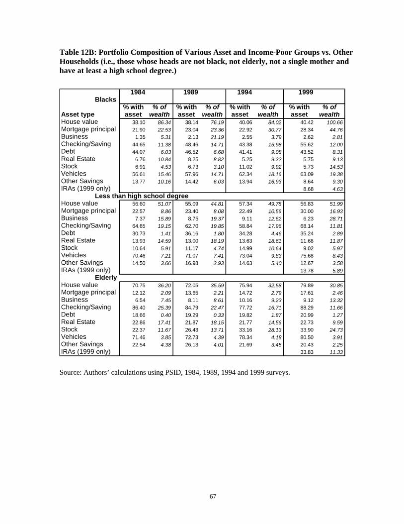
67

Table 12B: Portfolio Composition of Various Asset and Income-Poor Groups vs. OtherHouseholds (i.e., those whose heads are not black, not elderly, not a single mother andhave at least a high school degree.)

1984 1989 1994 1999Blacks

% with % of % with % of % with % of % with % ofAsset type asset wealth asset wealth asset wealth asset wealthHouse value 38.10 86.34 38.14 76.19 40.06 84.02 40.42 100.66Mortgage principal 21.90 22.53 23.04 23.36 22.92 30.77 28.34 44.76Business 1.35 5.31 2.13 21.19 2.55 3.79 2.62 2.81Checking/Saving 44.65 11.38 48.46 14.71 43.38 15.98 55.62 12.00Debt 44.07 6.03 46.52 6.68 41.41 9.08 43.52 8.31Real Estate 6.76 10.84 8.25 8.82 5.25 9.22 5.75 9.13Stock 6.91 4.53 6.73 3.10 11.02 9.92 5.73 14.53Vehicles 56.61 15.46 57.96 14.71 62.34 18.16 63.09 19.38Other Savings 13.77 10.16 14.42 6.03 13.94 16.93 8.64 9.30IRAs (1999 only) 8.68 4.63

Less than high school degreeHouse value 56.60 51.07 55.09 44.81 57.34 49.78 56.83 51.99Mortgage principal 22.57 8.86 23.40 8.08 22.49 10.56 30.00 16.93Business 7.37 15.89 8.75 19.37 9.11 12.62 6.23 28.71Checking/Saving 64.65 19.15 62.70 19.85 58.84 17.96 68.14 11.81Debt 30.73 1.41 36.16 1.80 34.28 4.46 35.24 2.89Real Estate 13.93 14.59 13.00 18.19 13.63 18.61 11.68 11.87Stock 10.64 5.91 11.17 4.74 14.99 10.64 9.02 5.97Vehicles 70.46 7.21 71.07 7.41 73.04 9.83 75.68 8.43Other Savings 14.50 3.66 16.98 2.93 14.63 5.40 12.67 3.58IRAs (1999 only) 13.78 5.89

ElderlyHouse value 70.75 36.20 72.05 35.59 75.94 32.58 79.89 30.85Mortgage principal 12.12 2.09 13.65 2.21 14.72 2.79 17.61 2.46Business 6.54 7.45 8.11 8.61 10.16 9.23 9.12 13.32Checking/Saving 86.40 25.39 84.79 22.47 77.72 16.71 88.29 11.66Debt 18.66 0.40 19.29 0.33 19.82 1.87 20.99 1.27Real Estate 22.86 17.41 21.87 18.15 21.77 14.56 22.73 9.59Stock 22.37 11.67 26.43 13.71 33.16 28.13 33.90 24.73Vehicles 71.46 3.85 72.73 4.39 78.34 4.18 80.50 3.91Other Savings 22.54 4.38 26.13 4.01 21.69 3.45 20.43 2.25IRAs (1999 only) 33.83 11.33

Source: Authors’ calculations using PSID, 1984, 1989, 1994 and 1999 surveys.

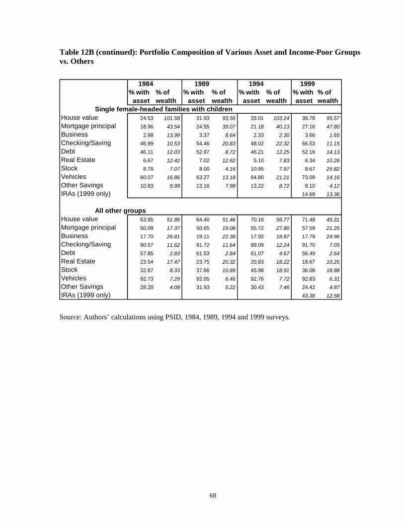
68

Table 12B (continued): Portfolio Composition of Various Asset and Income-Poor Groupsvs. Others

1984 1989 1994 1999% with % of % with % of % with % of % with % of

asset wealth asset wealth asset wealth asset wealthSingle female-headed families with children

House value 24.53 101.58 31.93 93.56 33.01 103.24 36.78 95.57Mortgage principal 18.96 43.54 24.55 39.07 21.18 40.13 27.16 47.80Business 2.98 13.99 3.37 8.64 2.33 2.30 3.66 1.65Checking/Saving 46.99 10.53 54.46 20.83 48.02 22.32 66.53 11.15Debt 46.11 12.03 52.97 8.72 46.21 12.25 52.16 14.13Real Estate 6.67 12.42 7.02 12.62 5.10 7.83 6.34 10.26Stock 8.78 7.07 8.00 4.16 10.95 7.97 8.67 25.82Vehicles 60.07 16.86 63.27 13.18 64.80 21.21 73.09 14.16Other Savings 10.83 9.99 13.16 7.98 13.22 8.72 9.10 4.12IRAs (1999 only) 14.69 13.36

All other groupsHouse value 63.95 51.89 64.40 51.46 70.16 56.77 71.48 45.31Mortgage principal 50.09 17.37 50.65 19.08 55.72 27.80 57.59 21.25Business 17.70 26.81 19.11 22.38 17.92 18.87 17.79 24.96Checking/Saving 90.57 11.62 91.72 11.64 89.09 12.24 91.70 7.05Debt 57.85 2.83 61.53 2.84 61.07 4.67 56.49 2.64Real Estate 23.54 17.47 23.75 20.32 20.83 18.22 18.67 10.25Stock 32.87 8.33 37.66 10.89 45.98 18.91 36.08 18.88Vehicles 92.73 7.29 92.05 6.46 92.76 7.72 92.83 6.31Other Savings 28.28 4.08 31.93 5.22 30.43 7.46 24.42 4.87IRAs (1999 only) 43.38 12.58

Source: Authors’ calculations using PSID, 1984, 1989, 1994 and 1999 surveys.

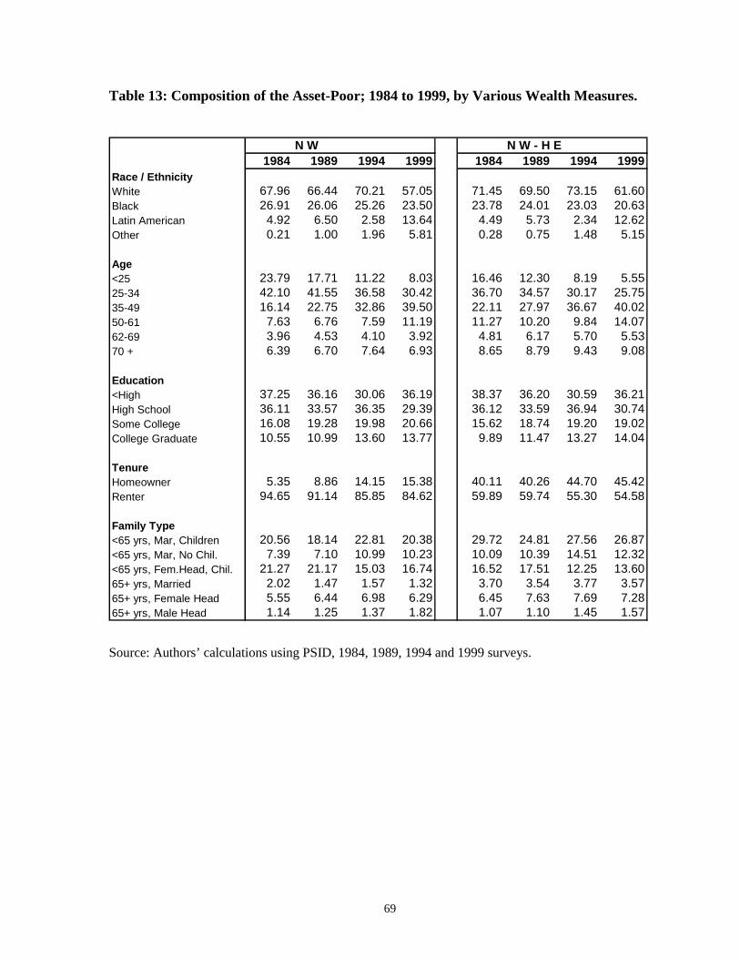
69

Table 13: Composition of the Asset-Poor; 1984 to 1999, by Various Wealth Measures.

N W N W - H E1984 1989 1994 1999 1984 1989 1994 1999

Race / EthnicityWhite 67.96 66.44 70.21 57.05 71.45 69.50 73.15 61.60Black 26.91 26.06 25.26 23.50 23.78 24.01 23.03 20.63Latin American 4.92 6.50 2.58 13.64 4.49 5.73 2.34 12.62Other 0.21 1.00 1.96 5.81 0.28 0.75 1.48 5.15

Age<25 23.79 17.71 11.22 8.03 16.46 12.30 8.19 5.5525-34 42.10 41.55 36.58 30.42 36.70 34.57 30.17 25.7535-49 16.14 22.75 32.86 39.50 22.11 27.97 36.67 40.0250-61 7.63 6.76 7.59 11.19 11.27 10.20 9.84 14.0762-69 3.96 4.53 4.10 3.92 4.81 6.17 5.70 5.5370 + 6.39 6.70 7.64 6.93 8.65 8.79 9.43 9.08

Education<High 37.25 36.16 30.06 36.19 38.37 36.20 30.59 36.21High School 36.11 33.57 36.35 29.39 36.12 33.59 36.94 30.74Some College 16.08 19.28 19.98 20.66 15.62 18.74 19.20 19.02College Graduate 10.55 10.99 13.60 13.77 9.89 11.47 13.27 14.04

TenureHomeowner 5.35 8.86 14.15 15.38 40.11 40.26 44.70 45.42Renter 94.65 91.14 85.85 84.62 59.89 59.74 55.30 54.58

Family Type<65 yrs, Mar, Children 20.56 18.14 22.81 20.38 29.72 24.81 27.56 26.87<65 yrs, Mar, No Chil. 7.39 7.10 10.99 10.23 10.09 10.39 14.51 12.32<65 yrs, Fem.Head, Chil. 21.27 21.17 15.03 16.74 16.52 17.51 12.25 13.6065+ yrs, Married 2.02 1.47 1.57 1.32 3.70 3.54 3.77 3.5765+ yrs, Female Head 5.55 6.44 6.98 6.29 6.45 7.63 7.69 7.2865+ yrs, Male Head 1.14 1.25 1.37 1.82 1.07 1.10 1.45 1.57

Source: Authors’ calculations using PSID, 1984, 1989, 1994 and 1999 surveys.

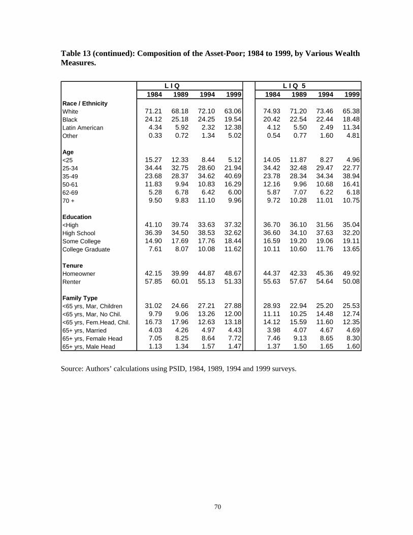
70

Table 13 (continued): Composition of the Asset-Poor; 1984 to 1999, by Various WealthMeasures.

L I Q L I Q 51984 1989 1994 1999 1984 1989 1994 1999

Race / EthnicityWhite 71.21 68.18 72.10 63.06 74.93 71.20 73.46 65.38Black 24.12 25.18 24.25 19.54 20.42 22.54 22.44 18.48Latin American 4.34 5.92 2.32 12.38 4.12 5.50 2.49 11.34Other 0.33 0.72 1.34 5.02 0.54 0.77 1.60 4.81

Age<25 15.27 12.33 8.44 5.12 14.05 11.87 8.27 4.9625-34 34.44 32.75 28.60 21.94 34.42 32.48 29.47 22.7735-49 23.68 28.37 34.62 40.69 23.78 28.34 34.34 38.9450-61 11.83 9.94 10.83 16.29 12.16 9.96 10.68 16.4162-69 5.28 6.78 6.42 6.00 5.87 7.07 6.22 6.1870 + 9.50 9.83 11.10 9.96 9.72 10.28 11.01 10.75

Education<High 41.10 39.74 33.63 37.32 36.70 36.10 31.56 35.04High School 36.39 34.50 38.53 32.62 36.60 34.10 37.63 32.20Some College 14.90 17.69 17.76 18.44 16.59 19.20 19.06 19.11College Graduate 7.61 8.07 10.08 11.62 10.11 10.60 11.76 13.65

TenureHomeowner 42.15 39.99 44.87 48.67 44.37 42.33 45.36 49.92Renter 57.85 60.01 55.13 51.33 55.63 57.67 54.64 50.08

Family Type<65 yrs, Mar, Children 31.02 24.66 27.21 27.88 28.93 22.94 25.20 25.53<65 yrs, Mar, No Chil. 9.79 9.06 13.26 12.00 11.11 10.25 14.48 12.74<65 yrs, Fem.Head, Chil. 16.73 17.96 12.63 13.18 14.12 15.59 11.60 12.3565+ yrs, Married 4.03 4.26 4.97 4.43 3.98 4.07 4.67 4.6965+ yrs, Female Head 7.05 8.25 8.64 7.72 7.46 9.13 8.65 8.3065+ yrs, Male Head 1.13 1.34 1.57 1.47 1.37 1.50 1.65 1.60

Source: Authors’ calculations using PSID, 1984, 1989, 1994 and 1999 surveys.

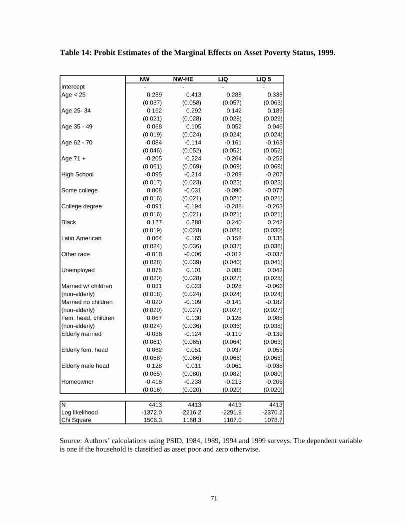
71

Table 14: Probit Estimates of the Marginal Effects on Asset Poverty Status, 1999.

NW NW-HE LIQ LIQ 5Intercept - - - -Age < 25 0.239 0.413 0.288 0.338

(0.037) (0.058) (0.057) (0.063)Age 25- 34 0.162 0.292 0.142 0.189

(0.021) (0.028) (0.028) (0.029)Age 35 - 49 0.068 0.105 0.052 0.046

(0.019) (0.024) (0.024) (0.024)Age 62 - 70 -0.084 -0.114 -0.161 -0.163

(0.046) (0.052) (0.052) (0.052)Age 71 + -0.205 -0.224 -0.264 -0.252

(0.061) (0.069) (0.069) (0.068)High School -0.095 -0.214 -0.209 -0.207

(0.017) (0.023) (0.023) (0.023)Some college 0.008 -0.031 -0.090 -0.077

(0.016) (0.021) (0.021) (0.021)College degree -0.091 -0.194 -0.288 -0.263

(0.016) (0.021) (0.021) (0.021)Black 0.127 0.288 0.240 0.242

(0.019) (0.028) (0.028) (0.030)Latin American 0.064 0.165 0.158 0.135

(0.024) (0.036) (0.037) (0.038)Other race -0.018 -0.006 -0.012 -0.037

(0.028) (0.039) (0.040) (0.041)Unemployed 0.075 0.101 0.085 0.042

(0.020) (0.028) (0.027) (0.028)Married w/ children 0.031 0.023 0.028 -0.066(non-elderly) (0.018) (0.024) (0.024) (0.024)Married no children -0.020 -0.109 -0.141 -0.182(non-elderly) (0.020) (0.027) (0.027) (0.027)Fem. head, children 0.067 0.130 0.128 0.088(non-elderly) (0.024) (0.036) (0.036) (0.038)Elderly married -0.036 -0.124 -0.110 -0.139

(0.061) (0.065) (0.064) (0.063)Elderly fem. head 0.062 0.051 0.037 0.053

(0.058) (0.066) (0.066) (0.066)Elderly male head 0.128 0.011 -0.061 -0.038

(0.065) (0.080) (0.082) (0.080)Homeowner -0.416 -0.238 -0.213 -0.206

(0.016) (0.020) (0.020) (0.020)

N 4413 4413 4413 4413Log likelihood -1372.0 -2216.2 -2291.9 -2370.2Chi Square 1506.3 1168.3 1107.0 1078.7

Source: Authors’ calculations using PSID, 1984, 1989, 1994 and 1999 surveys. The dependent variableis one if the household is classified as asset poor and zero otherwise.

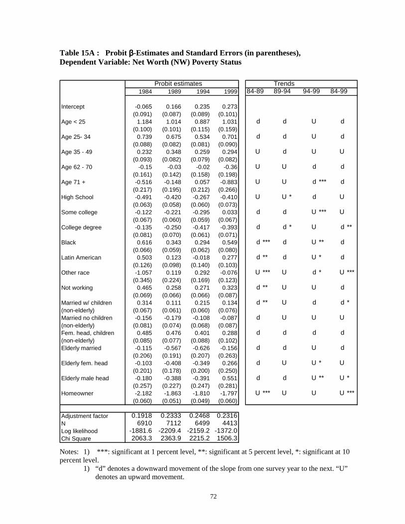
72

Table 15A : Probit ββββ-Estimates and Standard Errors (in parentheses),Dependent Variable: Net Worth (NW) Poverty Status

Probit estimates Trends1984 1989 1994 1999 84-89 89-94 94-99 84-99

Intercept -0.065 0.166 0.235 0.273(0.091) (0.087) (0.089) (0.101)

Age < 25 1.184 1.014 0.887 1.031 d d U d(0.100) (0.101) (0.115) (0.159)

Age 25- 34 0.739 0.675 0.534 0.701 d d U d(0.088) (0.082) (0.081) (0.090)

Age 35 - 49 0.232 0.348 0.259 0.294 U d U U(0.093) (0.082) (0.079) (0.082)

Age 62 - 70 -0.15 -0.03 -0.02 -0.36 U U d d(0.161) (0.142) (0.158) (0.198)

Age 71 + -0.516 -0.148 0.057 -0.883 U U d *** d(0.217) (0.195) (0.212) (0.266)

High School -0.491 -0.420 -0.267 -0.410 U U * d U(0.063) (0.058) (0.060) (0.073)

Some college -0.122 -0.221 -0.295 0.033 d d U *** U(0.067) (0.060) (0.059) (0.067)

College degree -0.135 -0.250 -0.417 -0.393 d d * U d **(0.081) (0.070) (0.061) (0.071)

Black 0.616 0.343 0.294 0.549 d *** d U ** d(0.066) (0.059) (0.062) (0.080)

Latin American 0.503 0.123 -0.018 0.277 d ** d U * d(0.126) (0.098) (0.140) (0.103)

Other race -1.057 0.119 0.292 -0.076 U *** U d * U ***(0.345) (0.224) (0.169) (0.123)

Not working 0.465 0.258 0.271 0.323 d ** U U d(0.069) (0.066) (0.066) (0.087)

Married w/ children 0.314 0.111 0.215 0.134 d ** U d d *(non-elderly) (0.067) (0.061) (0.060) (0.076)Married no children -0.156 -0.179 -0.108 -0.087 d U U U(non-elderly) (0.081) (0.074) (0.068) (0.087)Fem. head, children 0.485 0.476 0.401 0.288 d d d d(non-elderly) (0.085) (0.077) (0.088) (0.102)Elderly married -0.115 -0.567 -0.626 -0.156 d d U d

(0.206) (0.191) (0.207) (0.263)Elderly fem. head -0.103 -0.408 -0.349 0.266 d U U * U

(0.201) (0.178) (0.200) (0.250)Elderly male head -0.180 -0.388 -0.391 0.551 d d U ** U *

(0.257) (0.227) (0.247) (0.281)Homeowner -2.182 -1.863 -1.810 -1.797 U *** U U U ***

(0.060) (0.051) (0.049) (0.060)

Adjustment factor 0.1918 0.2333 0.2468 0.2316N 6910 7112 6499 4413Log likelihood -1881.6 -2209.4 -2159.2 -1372.0Chi Square 2063.3 2363.9 2215.2 1506.3

Notes: 1) ***: significant at 1 percent level, **: significant at 5 percent level, *: significant at 10percent level.

1) “d” denotes a downward movement of the slope from one survey year to the next. “U”denotes an upward movement.

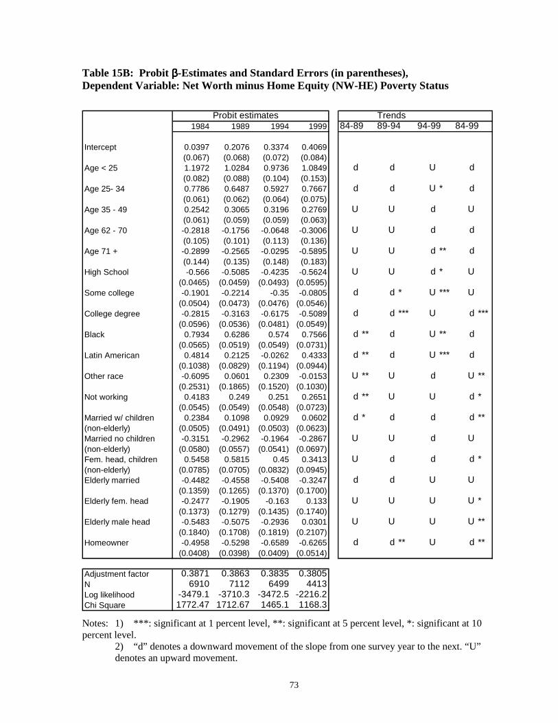
73

Table 15B: Probit ββββ-Estimates and Standard Errors (in parentheses),Dependent Variable: Net Worth minus Home Equity (NW-HE) Poverty Status

Probit estimates Trends1984 1989 1994 1999 84-89 89-94 94-99 84-99

Intercept 0.0397 0.2076 0.3374 0.4069(0.067) (0.068) (0.072) (0.084)

Age < 25 1.1972 1.0284 0.9736 1.0849 d d U d(0.082) (0.088) (0.104) (0.153)

Age 25- 34 0.7786 0.6487 0.5927 0.7667 d d U * d(0.061) (0.062) (0.064) (0.075)

Age 35 - 49 0.2542 0.3065 0.3196 0.2769 U U d U(0.061) (0.059) (0.059) (0.063)

Age 62 - 70 -0.2818 -0.1756 -0.0648 -0.3006 U U d d(0.105) (0.101) (0.113) (0.136)

Age 71 + -0.2899 -0.2565 -0.0295 -0.5895 U U d ** d(0.144) (0.135) (0.148) (0.183)

High School -0.566 -0.5085 -0.4235 -0.5624 U U d * U(0.0465) (0.0459) (0.0493) (0.0595)

Some college -0.1901 -0.2214 -0.35 -0.0805 d d * U *** U(0.0504) (0.0473) (0.0476) (0.0546)

College degree -0.2815 -0.3163 -0.6175 -0.5089 d d *** U d ***(0.0596) (0.0536) (0.0481) (0.0549)

Black 0.7934 0.6286 0.574 0.7566 d ** d U ** d(0.0565) (0.0519) (0.0549) (0.0731)

Latin American 0.4814 0.2125 -0.0262 0.4333 d ** d U *** d(0.1038) (0.0829) (0.1194) (0.0944)

Other race -0.6095 0.0601 0.2309 -0.0153 U ** U d U **(0.2531) (0.1865) (0.1520) (0.1030)

Not working 0.4183 0.249 0.251 0.2651 d ** U U d *(0.0545) (0.0549) (0.0548) (0.0723)

Married w/ children 0.2384 0.1098 0.0929 0.0602 d * d d d **(non-elderly) (0.0505) (0.0491) (0.0503) (0.0623)Married no children -0.3151 -0.2962 -0.1964 -0.2867 U U d U(non-elderly) (0.0580) (0.0557) (0.0541) (0.0697)Fem. head, children 0.5458 0.5815 0.45 0.3413 U d d d *(non-elderly) (0.0785) (0.0705) (0.0832) (0.0945)Elderly married -0.4482 -0.4558 -0.5408 -0.3247 d d U U

(0.1359) (0.1265) (0.1370) (0.1700)Elderly fem. head -0.2477 -0.1905 -0.163 0.133 U U U U *

(0.1373) (0.1279) (0.1435) (0.1740)Elderly male head -0.5483 -0.5075 -0.2936 0.0301 U U U U **

(0.1840) (0.1708) (0.1819) (0.2107)Homeowner -0.4958 -0.5298 -0.6589 -0.6265 d d ** U d **

(0.0408) (0.0398) (0.0409) (0.0514)

Adjustment factor 0.3871 0.3863 0.3835 0.3805N 6910 7112 6499 4413Log likelihood -3479.1 -3710.3 -3472.5 -2216.2Chi Square 1772.47 1712.67 1465.1 1168.3

Notes: 1) ***: significant at 1 percent level, **: significant at 5 percent level, *: significant at 10percent level.

2) “d” denotes a downward movement of the slope from one survey year to the next. “U”denotes an upward movement.

74

Table 15C : Probit ββββ-Estimates and Standard Errors (in parentheses), DependentVariable: Liquid Wealth (Liq) Poverty Status

Probit estimates Trends1984 1989 1994 1999 84-89 89-94 94-99 84-99

Intercept 0.126 0.2585 0.4166 0.6852(0.067) (0.069) (0.073) (0.084)

Age < 25 1.0151 0.9625 0.8578 0.7457 d d d d(0.081) (0.088) (0.103) (0.147)

Age 25- 34 0.6709 0.5702 0.383 0.3669 d d ** d d ***(0.062) (0.064) (0.065) (0.074)

Age 35 - 49 0.3004 0.3681 0.1327 0.1349 U d *** U d *(0.061) (0.061) (0.060) (0.062)

Age 62 - 70 -0.1683 -0.1441 -0.0899 -0.4177 U U d * d(0.103) (0.105) (0.113) (0.135)

Age 71 + -0.148 -0.2538 -0.0134 -0.6848 d U d *** d **(0.142) (0.138) (0.148) (0.178)

High School -0.668 -0.598 -0.455 -0.541 U U ** d U *(0.047) (0.046) (0.049) (0.058)

Some college -0.246 -0.308 -0.441 -0.234 d d ** U *** U(0.050) (0.048) (0.048) (0.054)

College degree -0.442 -0.505 -0.819 -0.747 d d *** U d ***(0.061) (0.057) (0.050) (0.055)

Black 0.819 0.663 0.619 0.623 d ** d U d **(0.057) (0.052) (0.055) (0.072)

Latin American 0.400 0.243 -0.044 0.410 d d * U *** U(0.102) (0.084) (0.122) (0.095)

Other race -0.421 0.065 0.156 -0.031 U U d U(0.243) (0.194) (0.157) (0.102)

Not working 0.431 0.227 0.267 0.220 d *** U d d **(0.055) (0.056) (0.055) (0.071)

Married w/ children 0.351 0.119 0.170 0.073 d *** U d d ***(non-elderly) (0.051) (0.050) (0.051) (0.062)Married no children -0.322 -0.400 -0.250 -0.365 d U * d d(non-elderly) (0.059) (0.058) (0.056) (0.069)Fem. head, children 0.655 0.545 0.483 0.333 d d d d ***(non-elderly) (0.079) (0.070) (0.083) (0.093)Elderly married -0.577 -0.356 -0.448 -0.286 U d U U

(0.134) (0.128) (0.136) (0.165)Elderly fem. head -0.362 -0.169 -0.189 0.096 U d U U **

(0.135) (0.130) (0.143) (0.171)Elderly male head -0.717 -0.387 -0.360 -0.158 U U U U **

(0.182) (0.171) (0.182) (0.212)Homeowner -0.468 -0.524 -0.630 -0.551 d d * U d

(0.041) (0.040) (0.042) (0.051)

Adjustment factor 0.3873 0.3751 0.3720 0.3859N 6910 7112 6499 4413Log likelihood -3455.1 -3556.8 -3352.4 -2291.9Chi Square 1772.4 1778.4 1505.2 1107.0

Notes: 1) ***: significant at 1 percent level, **: significant at 5 percent level, *: significant at 10 percent level.2) “d” denotes a downward movement of the slope from one survey year to the next. “U” denotes anupward movement.

75

Table 15D: Probit ββββ-Estimates and Standard Errors (in parentheses) DependentVariable: Liquid Wealth <$5,000 (Liq5) Poverty Status

Probit estimates Trends1984 1989 1994 1999 84-89 89-94 94-99 84-99

Intercept 0.6042 0.5486 0.6273 0.889(0.067) (0.068) (0.073) (0.084)

Age < 25 1.0936 1.3087 1.035 0.8522 U * d * d d(0.086) (0.098) (0.108) (0.159)

Age 25- 34 0.8092 0.7421 0.5371 0.4766 d d ** d d ***(0.061) (0.062) (0.064) (0.073)

Age 35 - 49 0.345 0.464 0.2066 0.1161 U d *** d d ***(0.059) (0.059) (0.058) (0.061)

Age 62 - 70 -0.1508 -0.1616 -0.1203 -0.4099 d U d * d(0.098) (0.101) (0.111) (0.130)

Age 71 + -0.2491 -0.3848 -0.0261 -0.6349 d U * d *** d *(0.134) (0.132) (0.145) (0.172)

High School -0.586 -0.557 -0.456 -0.522 U U d U(0.047) (0.046) (0.050) (0.059)

Some college -0.194 -0.257 -0.389 -0.194 d d ** U *** d(0.050) (0.047) (0.047) (0.053)

College degree -0.483 -0.496 -0.769 -0.663 d d *** U d **(0.057) (0.053) (0.049) (0.053)

Black 0.735 0.651 0.574 0.610 d d U d(0.063) (0.055) (0.056) (0.074)

Latin American 0.539 0.205 0.090 0.340 d ** d U d(0.114) (0.085) (0.119) (0.096)

Other race 0.080 0.054 0.435 -0.093 d U d *** d(0.231) (0.193) (0.161) (0.102)

Not working 0.337 0.166 0.216 0.107 d ** U d d ***(0.056) (0.056) (0.055) (0.069)

Married w/ children 0.012 -0.182 -0.077 -0.167 d *** U d d **(non-elderly) (0.051) (0.050) (0.051) (0.061)Married no children -0.499 -0.510 -0.312 -0.460 d U ** d * U(non-elderly) (0.056) (0.056) (0.054) (0.068)Fem. head, children 0.472 0.336 0.320 0.223 d d d d *(non-elderly) (0.090) (0.074) (0.085) (0.096)Elderly married -0.704 -0.408 -0.530 -0.349 U * d U U *

(0.126) (0.123) (0.134) (0.159)Elderly fem. head -0.346 0.037 -0.142 0.134 U ** d U U **

(0.128) (0.125) (0.141) (0.165)Elderly male head -0.571 -0.205 -0.298 -0.095 U d U U *

(0.169) (0.160) (0.178) (0.201)Homeowner -0.480 -0.491 -0.649 -0.520 d d *** U ** d

(0.041) (0.040) (0.041) (0.051)

Adjustment factor 0.3942 0.3987 0.3912 0.3971N 6910 7112 6499 4413Log likelihood -3543.7 -3682.7 -3441.3 -2370.2Chi Square 1763.12 1838.28 1575.4 1078.7

Notes: 1) ***: significant at 1 percent level, **: significant at 5 percent level, *: significant at 10 percent level.2) “d” denotes a downward movement of the slope from one survey year to the next. “U” denotes anupward movement.

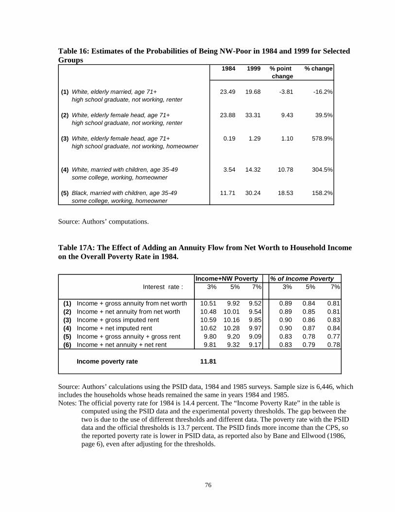
76

Table 16: Estimates of the Probabilities of Being NW-Poor in 1984 and 1999 for SelectedGroups

1984 1999 % point % changechange

(1) White, elderly married, age 71+ 23.49 19.68 -3.81 -16.2%high school graduate, not working, renter

(2) White, elderly female head, age 71+ 23.88 33.31 9.43 39.5%high school graduate, not working, renter

(3) White, elderly female head, age 71+ 0.19 1.29 1.10 578.9%high school graduate, not working, homeowner

(4) White, married with children, age 35-49 3.54 14.32 10.78 304.5%some college, working, homeowner

(5) Black, married with children, age 35-49 11.71 30.24 18.53 158.2%some college, working, homeowner

Source: Authors’ computations.

Table 17A: The Effect of Adding an Annuity Flow from Net Worth to Household Incomeon the Overall Poverty Rate in 1984.

Income+NW Poverty % of Income Poverty Interest rate : 3% 5% 7% 3% 5% 7%

(1) Income + gross annuity from net worth 10.51 9.92 9.52 0.89 0.84 0.81(2) Income + net annuity from net worth 10.48 10.01 9.54 0.89 0.85 0.81(3) Income + gross imputed rent 10.59 10.16 9.85 0.90 0.86 0.83(4) Income + net imputed rent 10.62 10.28 9.97 0.90 0.87 0.84(5) Income + gross annuity + gross rent 9.80 9.20 9.09 0.83 0.78 0.77(6) Income + net annuity + net rent 9.81 9.32 9.17 0.83 0.79 0.78

Income poverty rate 11.81

Source: Authors’ calculations using the PSID data, 1984 and 1985 surveys. Sample size is 6,446, whichincludes the households whose heads remained the same in years 1984 and 1985.Notes: The official poverty rate for 1984 is 14.4 percent. The “Income Poverty Rate” in the table is

computed using the PSID data and the experimental poverty thresholds. The gap between thetwo is due to the use of different thresholds and different data. The poverty rate with the PSIDdata and the official thresholds is 13.7 percent. The PSID finds more income than the CPS, sothe reported poverty rate is lower in PSID data, as reported also by Bane and Ellwood (1986,page 6), even after adjusting for the thresholds.

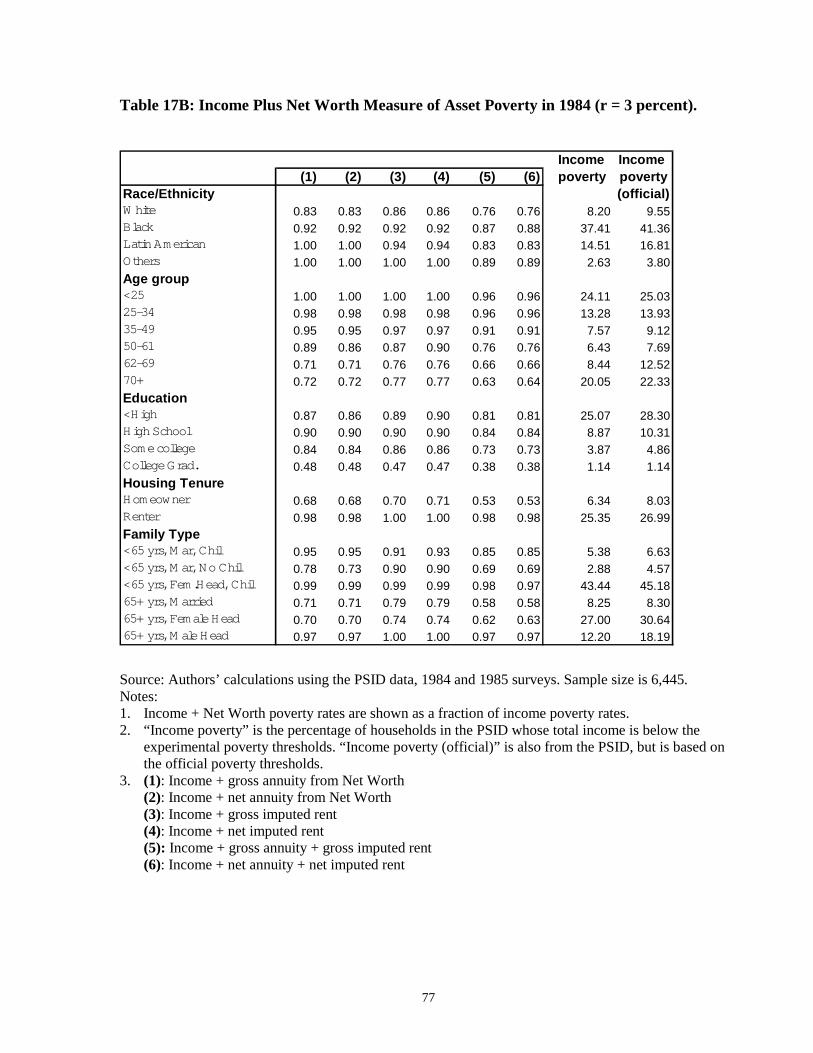
77

Table 17B: Income Plus Net Worth Measure of Asset Poverty in 1984 (r = 3 percent).

Income Income (1) (2) (3) (4) (5) (6) poverty poverty

Race/Ethnicity (official)W hite 0.83 0.83 0.86 0.86 0.76 0.76 8.20 9.55Black 0.92 0.92 0.92 0.92 0.87 0.88 37.41 41.36Latin American 1.00 1.00 0.94 0.94 0.83 0.83 14.51 16.81Others 1.00 1.00 1.00 1.00 0.89 0.89 2.63 3.80Age group<25 1.00 1.00 1.00 1.00 0.96 0.96 24.11 25.0325-34 0.98 0.98 0.98 0.98 0.96 0.96 13.28 13.9335-49 0.95 0.95 0.97 0.97 0.91 0.91 7.57 9.1250-61 0.89 0.86 0.87 0.90 0.76 0.76 6.43 7.6962-69 0.71 0.71 0.76 0.76 0.66 0.66 8.44 12.5270+ 0.72 0.72 0.77 0.77 0.63 0.64 20.05 22.33Education<High 0.87 0.86 0.89 0.90 0.81 0.81 25.07 28.30High School 0.90 0.90 0.90 0.90 0.84 0.84 8.87 10.31Some college 0.84 0.84 0.86 0.86 0.73 0.73 3.87 4.86College Grad. 0.48 0.48 0.47 0.47 0.38 0.38 1.14 1.14Housing TenureHomeowner 0.68 0.68 0.70 0.71 0.53 0.53 6.34 8.03Renter 0.98 0.98 1.00 1.00 0.98 0.98 25.35 26.99Family Type<65 yrs, M ar, Chil 0.95 0.95 0.91 0.93 0.85 0.85 5.38 6.63<65 yrs, M ar, No Chil 0.78 0.73 0.90 0.90 0.69 0.69 2.88 4.57<65 yrs, Fem.Head, Chil 0.99 0.99 0.99 0.99 0.98 0.97 43.44 45.1865+ yrs, M arried 0.71 0.71 0.79 0.79 0.58 0.58 8.25 8.3065+ yrs, Female Head 0.70 0.70 0.74 0.74 0.62 0.63 27.00 30.6465+ yrs, M ale Head 0.97 0.97 1.00 1.00 0.97 0.97 12.20 18.19

Source: Authors’ calculations using the PSID data, 1984 and 1985 surveys. Sample size is 6,445.Notes:1. Income + Net Worth poverty rates are shown as a fraction of income poverty rates.2. “Income poverty” is the percentage of households in the PSID whose total income is below the

experimental poverty thresholds. “Income poverty (official)” is also from the PSID, but is based onthe official poverty thresholds.

3. (1): Income + gross annuity from Net Worth(2): Income + net annuity from Net Worth(3): Income + gross imputed rent(4): Income + net imputed rent(5): Income + gross annuity + gross imputed rent(6): Income + net annuity + net imputed rent

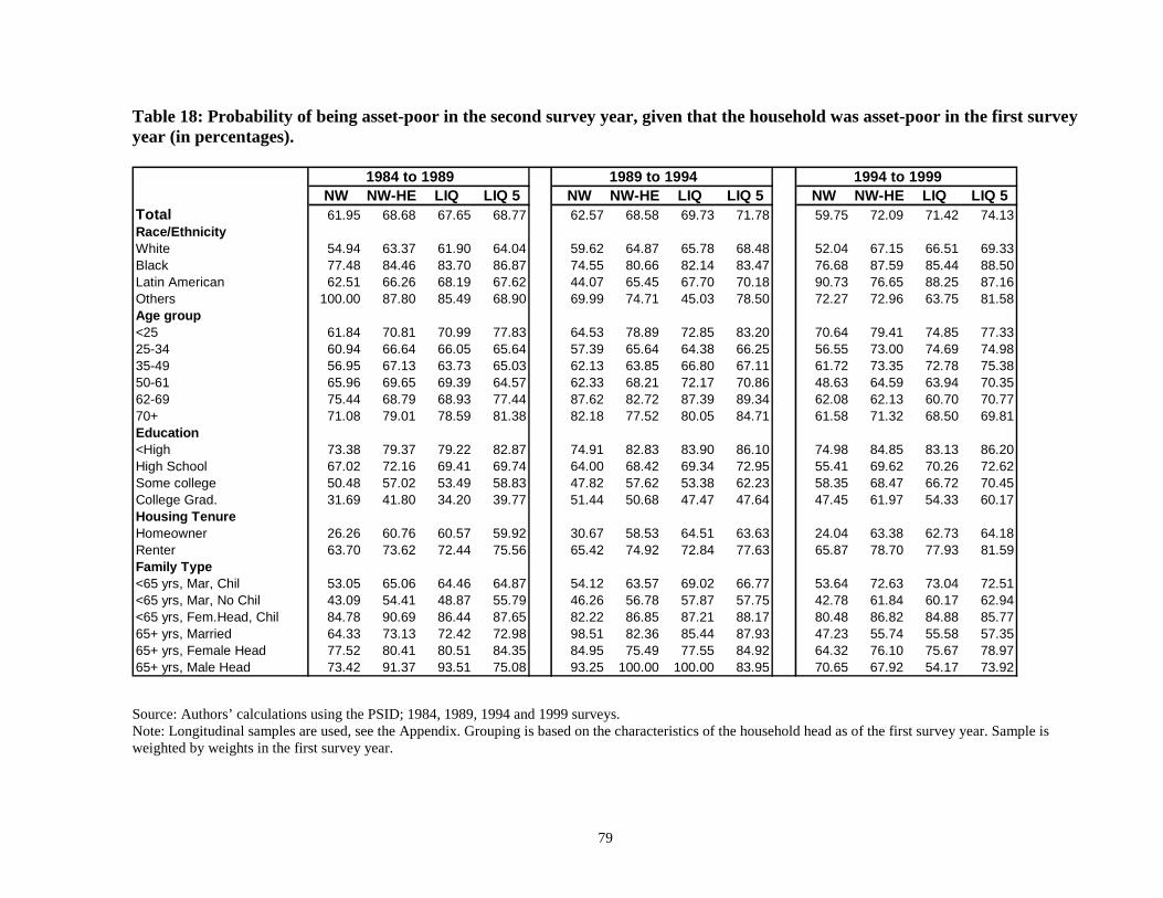
79

Table 18: Probability of being asset-poor in the second survey year, given that the household was asset-poor in the first surveyyear (in percentages).

1984 to 1989 1989 to 1994 1994 to 1999NW NW-HE LIQ LIQ 5 NW NW-HE LIQ LIQ 5 NW NW-HE LIQ LIQ 5

Total 61.95 68.68 67.65 68.77 62.57 68.58 69.73 71.78 59.75 72.09 71.42 74.13Race/EthnicityWhite 54.94 63.37 61.90 64.04 59.62 64.87 65.78 68.48 52.04 67.15 66.51 69.33Black 77.48 84.46 83.70 86.87 74.55 80.66 82.14 83.47 76.68 87.59 85.44 88.50Latin American 62.51 66.26 68.19 67.62 44.07 65.45 67.70 70.18 90.73 76.65 88.25 87.16Others 100.00 87.80 85.49 68.90 69.99 74.71 45.03 78.50 72.27 72.96 63.75 81.58Age group<25 61.84 70.81 70.99 77.83 64.53 78.89 72.85 83.20 70.64 79.41 74.85 77.3325-34 60.94 66.64 66.05 65.64 57.39 65.64 64.38 66.25 56.55 73.00 74.69 74.9835-49 56.95 67.13 63.73 65.03 62.13 63.85 66.80 67.11 61.72 73.35 72.78 75.3850-61 65.96 69.65 69.39 64.57 62.33 68.21 72.17 70.86 48.63 64.59 63.94 70.3562-69 75.44 68.79 68.93 77.44 87.62 82.72 87.39 89.34 62.08 62.13 60.70 70.7770+ 71.08 79.01 78.59 81.38 82.18 77.52 80.05 84.71 61.58 71.32 68.50 69.81Education<High 73.38 79.37 79.22 82.87 74.91 82.83 83.90 86.10 74.98 84.85 83.13 86.20High School 67.02 72.16 69.41 69.74 64.00 68.42 69.34 72.95 55.41 69.62 70.26 72.62Some college 50.48 57.02 53.49 58.83 47.82 57.62 53.38 62.23 58.35 68.47 66.72 70.45College Grad. 31.69 41.80 34.20 39.77 51.44 50.68 47.47 47.64 47.45 61.97 54.33 60.17Housing TenureHomeowner 26.26 60.76 60.57 59.92 30.67 58.53 64.51 63.63 24.04 63.38 62.73 64.18Renter 63.70 73.62 72.44 75.56 65.42 74.92 72.84 77.63 65.87 78.70 77.93 81.59Family Type<65 yrs, Mar, Chil 53.05 65.06 64.46 64.87 54.12 63.57 69.02 66.77 53.64 72.63 73.04 72.51<65 yrs, Mar, No Chil 43.09 54.41 48.87 55.79 46.26 56.78 57.87 57.75 42.78 61.84 60.17 62.94<65 yrs, Fem.Head, Chil 84.78 90.69 86.44 87.65 82.22 86.85 87.21 88.17 80.48 86.82 84.88 85.7765+ yrs, Married 64.33 73.13 72.42 72.98 98.51 82.36 85.44 87.93 47.23 55.74 55.58 57.3565+ yrs, Female Head 77.52 80.41 80.51 84.35 84.95 75.49 77.55 84.92 64.32 76.10 75.67 78.9765+ yrs, Male Head 73.42 91.37 93.51 75.08 93.25 100.00 100.00 83.95 70.65 67.92 54.17 73.92

Source: Authors’ calculations using the PSID; 1984, 1989, 1994 and 1999 surveys.Note: Longitudinal samples are used, see the Appendix. Grouping is based on the characteristics of the household head as of the first survey year. Sample isweighted by weights in the first survey year.

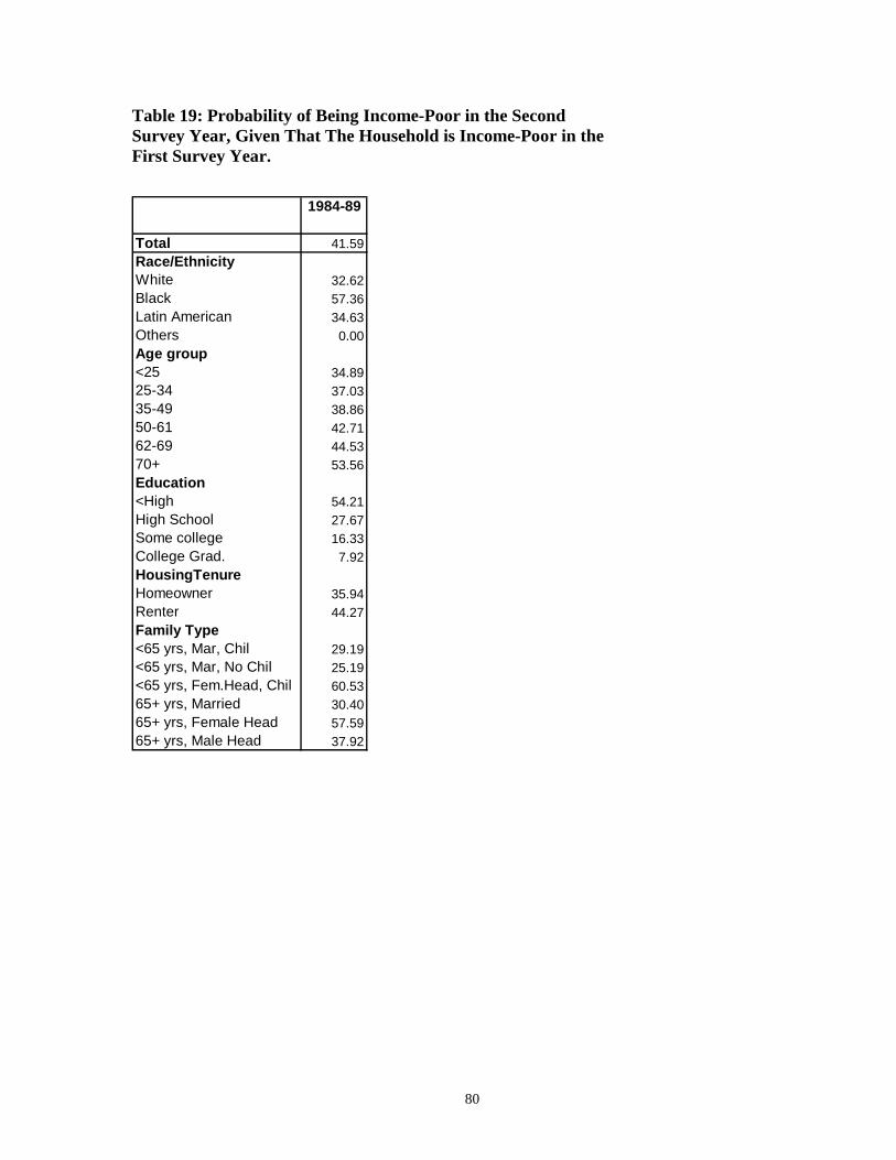
80

Table 19: Probability of Being Income-Poor in the SecondSurvey Year, Given That The Household is Income-Poor in theFirst Survey Year.

1984-89

Total 41.59Race/EthnicityWhite 32.62Black 57.36Latin American 34.63Others 0.00Age group<25 34.8925-34 37.0335-49 38.8650-61 42.7162-69 44.5370+ 53.56Education<High 54.21High School 27.67Some college 16.33College Grad. 7.92HousingTenureHomeowner 35.94Renter 44.27Family Type<65 yrs, Mar, Chil 29.19<65 yrs, Mar, No Chil 25.19<65 yrs, Fem.Head, Chil 60.5365+ yrs, Married 30.4065+ yrs, Female Head 57.5965+ yrs, Male Head 37.92

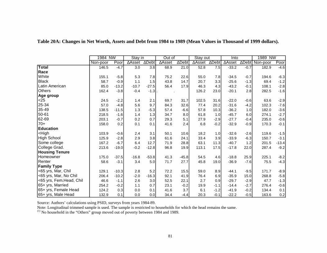
81

Table 20A: Changes in Net Worth, Assets and Debt from 1984 to 1989 (Mean Values in Thousand of 1999 dollars).

1984 NW Stay in Out of Stay out Into 1989 NW Non-poor Poor ∆Asset ∆Debt ∆Asset ∆Debt ∆Asset ∆Debt ∆Asset ∆Debt Non-poor Poor

Total 146.5 -4.7 3.0 3.8 68.9 21.0 52.8 7.5 -33.2 -0.7 182.9 -4.6RaceWhite 155.1 -5.8 5.3 7.8 75.2 22.6 55.0 7.8 -34.5 -0.7 194.6 -6.3Black 58.7 -0.9 1.1 1.5 43.8 14.7 20.7 3.3 -25.6 -1.3 69.4 -1.2Latin American 85.0 -13.2 -10.7 -27.5 56.4 17.9 46.3 4.3 -43.2 -0.1 108.1 -2.8Others 162.4 -3.8 -0.4 -1.3 . . 126.2 23.0 -20.1 2.8 282.5 -1.6Age group<25 24.5 -2.2 1.4 2.1 69.7 31.7 102.5 31.6 -22.0 -0.6 63.6 -2.925-34 57.0 -4.8 5.6 9.7 84.3 32.6 77.4 20.2 -31.6 -4.2 102.3 -7.635-49 138.5 -11.5 1.3 -5.3 57.4 -6.6 57.8 10.3 -36.2 1.0 182.0 -3.650-61 218.5 -1.6 1.4 1.3 34.7 8.0 61.8 1.0 -45.7 6.0 274.1 -2.762-69 203.1 -0.7 0.2 0.7 29.3 5.1 27.9 -2.9 -27.7 -0.4 235.0 -0.670+ 158.0 0.2 0.1 0.1 41.6 2.4 6.8 -0.2 -32.9 -0.9 170.3 -0.1Education<High 103.9 -0.6 2.4 3.1 50.1 10.6 18.2 1.0 -32.6 -2.6 119.6 -1.5High School 125.9 -2.8 2.9 3.8 61.6 24.1 33.4 3.9 -33.9 -6.3 150.7 -3.1Some college 167.2 -6.7 6.4 12.7 71.9 28.8 63.1 11.3 -40.7 1.2 201.5 -13.4College Grad. 213.6 -19.0 -0.2 -12.8 96.8 19.9 113.1 17.5 -17.8 22.0 287.4 -9.2Housing TenureHomeowner 175.0 -37.5 -16.8 -53.8 41.3 -45.8 54.5 4.6 -18.8 25.9 225.1 -8.2Renter 58.6 -3.1 3.4 5.0 71.7 27.7 45.8 19.0 -36.9 -7.6 75.5 -4.3Family Type<65 yrs, Mar, Chil 129.1 -10.3 2.8 5.2 72.2 15.5 59.0 8.9 -44.1 -9.5 171.7 -8.9<65 yrs, Mar, No Chil 206.4 -10.2 -2.0 -16.3 92.1 41.9 76.4 6.9 -35.9 15.0 268.8 -5.8<65 yrs, Fem.Head, Chil 46.6 -1.1 2.6 3.0 52.5 22.1 2.7 0.9 -29.7 -2.9 47.7 -1.365+ yrs, Married 254.2 -0.2 1.1 0.7 23.1 -0.2 19.9 -1.1 -14.4 -2.7 276.4 -0.665+ yrs, Female Head 124.2 0.3 0.0 0.1 41.6 3.7 6.1 -1.2 -41.9 -0.2 134.4 0.165+ yrs, Male Head 132.9 0.1 0.0 0.0 34.4 -4.4 20.3 -0.1 -22.2 -0.5 163.6 0.2

Source: Authors’ calculations using PSID, surveys from years 1984-89.Note: Longitudinal trimmed sample is used. The sample is restricted to households for which the head remains the same.(1) No household in the “Others” group moved out of poverty between 1984 and 1989.

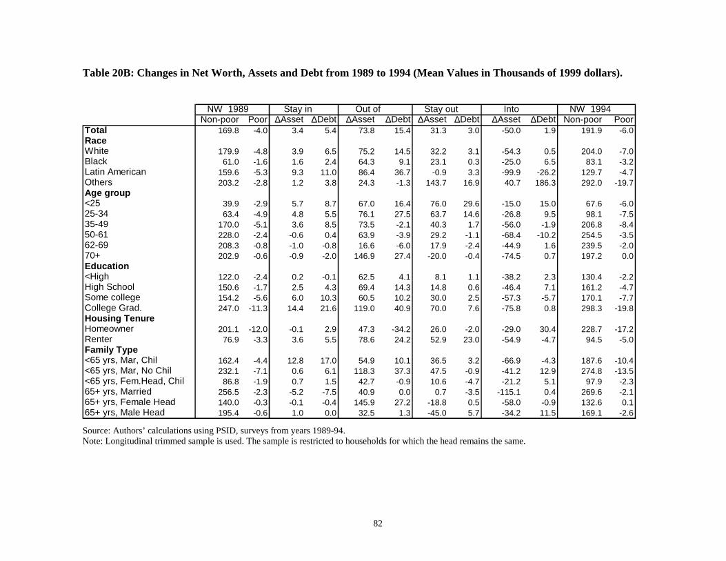
82

Table 20B: Changes in Net Worth, Assets and Debt from 1989 to 1994 (Mean Values in Thousands of 1999 dollars).

NW 1989 Stay in Out of Stay out Into NW 1994Non-poor Poor ∆Asset ∆Debt ∆Asset ∆Debt ∆Asset ∆Debt ∆Asset ∆Debt Non-poor Poor

Total 169.8 -4.0 3.4 5.4 73.8 15.4 31.3 3.0 -50.0 1.9 191.9 -6.0RaceWhite 179.9 -4.8 3.9 6.5 75.2 14.5 32.2 3.1 -54.3 0.5 204.0 -7.0Black 61.0 -1.6 1.6 2.4 64.3 9.1 23.1 0.3 -25.0 6.5 83.1 -3.2Latin American 159.6 -5.3 9.3 11.0 86.4 36.7 -0.9 3.3 -99.9 -26.2 129.7 -4.7Others 203.2 -2.8 1.2 3.8 24.3 -1.3 143.7 16.9 40.7 186.3 292.0 -19.7Age group<25 39.9 -2.9 5.7 8.7 67.0 16.4 76.0 29.6 -15.0 15.0 67.6 -6.025-34 63.4 -4.9 4.8 5.5 76.1 27.5 63.7 14.6 -26.8 9.5 98.1 -7.535-49 170.0 -5.1 3.6 8.5 73.5 -2.1 40.3 1.7 -56.0 -1.9 206.8 -8.450-61 228.0 -2.4 -0.6 0.4 63.9 -3.9 29.2 -1.1 -68.4 -10.2 254.5 -3.562-69 208.3 -0.8 -1.0 -0.8 16.6 -6.0 17.9 -2.4 -44.9 1.6 239.5 -2.070+ 202.9 -0.6 -0.9 -2.0 146.9 27.4 -20.0 -0.4 -74.5 0.7 197.2 0.0Education<High 122.0 -2.4 0.2 -0.1 62.5 4.1 8.1 1.1 -38.2 2.3 130.4 -2.2High School 150.6 -1.7 2.5 4.3 69.4 14.3 14.8 0.6 -46.4 7.1 161.2 -4.7Some college 154.2 -5.6 6.0 10.3 60.5 10.2 30.0 2.5 -57.3 -5.7 170.1 -7.7College Grad. 247.0 -11.3 14.4 21.6 119.0 40.9 70.0 7.6 -75.8 0.8 298.3 -19.8Housing TenureHomeowner 201.1 -12.0 -0.1 2.9 47.3 -34.2 26.0 -2.0 -29.0 30.4 228.7 -17.2Renter 76.9 -3.3 3.6 5.5 78.6 24.2 52.9 23.0 -54.9 -4.7 94.5 -5.0Family Type<65 yrs, Mar, Chil 162.4 -4.4 12.8 17.0 54.9 10.1 36.5 3.2 -66.9 -4.3 187.6 -10.4<65 yrs, Mar, No Chil 232.1 -7.1 0.6 6.1 118.3 37.3 47.5 -0.9 -41.2 12.9 274.8 -13.5<65 yrs, Fem.Head, Chil 86.8 -1.9 0.7 1.5 42.7 -0.9 10.6 -4.7 -21.2 5.1 97.9 -2.365+ yrs, Married 256.5 -2.3 -5.2 -7.5 40.9 0.0 0.7 -3.5 -115.1 0.4 269.6 -2.165+ yrs, Female Head 140.0 -0.3 -0.1 -0.4 145.9 27.2 -18.8 0.5 -58.0 -0.9 132.6 0.165+ yrs, Male Head 195.4 -0.6 1.0 0.0 32.5 1.3 -45.0 5.7 -34.2 11.5 169.1 -2.6

Source: Authors’ calculations using PSID, surveys from years 1989-94. Note: Longitudinal trimmed sample is used. The sample is restricted to households for which the head remains the same.

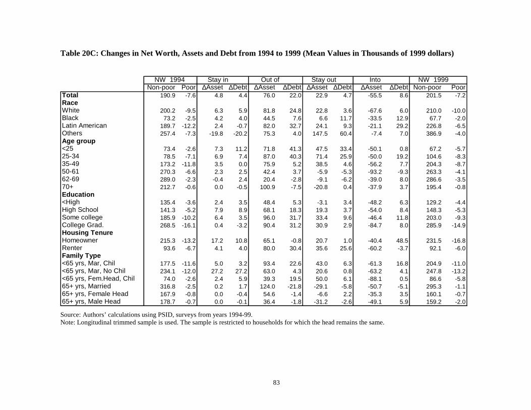
83

Table 20C: Changes in Net Worth, Assets and Debt from 1994 to 1999 (Mean Values in Thousands of 1999 dollars)

NW 1994 Stay in Out of Stay out Into NW 1999Non-poor Poor ∆Asset ∆Debt ∆Asset ∆Debt ∆Asset ∆Debt ∆Asset ∆Debt Non-poor Poor

Total 190.9 -7.6 4.8 4.4 76.0 22.0 22.9 4.7 -55.5 8.6 201.5 -7.2RaceWhite 200.2 -9.5 6.3 5.9 81.8 24.8 22.8 3.6 -67.6 6.0 210.0 -10.0Black 73.2 -2.5 4.2 4.0 44.5 7.6 6.6 11.7 -33.5 12.9 67.7 -2.0Latin American 189.7 -12.2 2.4 -0.7 82.0 32.7 24.1 9.3 -21.1 29.2 226.8 -6.5Others 257.4 -7.3 -19.8 -20.2 75.3 4.0 147.5 60.4 -7.4 7.0 386.9 -4.0Age group<25 73.4 -2.6 7.3 11.2 71.8 41.3 47.5 33.4 -50.1 0.8 67.2 -5.725-34 78.5 -7.1 6.9 7.4 87.0 40.3 71.4 25.9 -50.0 19.2 104.6 -8.335-49 173.2 -11.8 3.5 0.0 75.9 5.2 38.5 4.6 -56.2 7.7 204.3 -8.750-61 270.3 -6.6 2.3 2.5 42.4 3.7 -5.9 -5.3 -93.2 -9.3 263.3 -4.162-69 289.0 -2.3 -0.4 2.4 20.4 -2.8 -9.1 -6.2 -39.0 8.0 286.6 -3.570+ 212.7 -0.6 0.0 -0.5 100.9 -7.5 -20.8 0.4 -37.9 3.7 195.4 -0.8Education<High 135.4 -3.6 2.4 3.5 48.4 5.3 -3.1 3.4 -48.2 6.3 129.2 -4.4High School 141.3 -5.2 7.9 8.9 68.1 18.3 19.3 3.7 -54.0 8.4 148.3 -5.3Some college 185.9 -10.2 6.4 3.5 96.0 31.7 33.4 9.6 -46.4 11.8 203.0 -9.3College Grad. 268.5 -16.1 0.4 -3.2 90.4 31.2 30.9 2.9 -84.7 8.0 285.9 -14.9Housing TenureHomeowner 215.3 -13.2 17.2 10.8 65.1 -0.8 20.7 1.0 -40.4 48.5 231.5 -16.8Renter 93.6 -6.7 4.1 4.0 80.0 30.4 35.6 25.6 -60.2 -3.7 92.1 -6.0Family Type<65 yrs, Mar, Chil 177.5 -11.6 5.0 3.2 93.4 22.6 43.0 6.3 -61.3 16.8 204.9 -11.0<65 yrs, Mar, No Chil 234.1 -12.0 27.2 27.2 63.0 4.3 20.6 0.8 -63.2 4.1 247.8 -13.2<65 yrs, Fem.Head, Chil 74.0 -2.6 2.4 5.9 39.3 19.5 50.0 6.1 -88.1 0.5 86.6 -5.865+ yrs, Married 316.8 -2.5 0.2 1.7 124.0 -21.8 -29.1 -5.8 -50.7 -5.1 295.3 -1.165+ yrs, Female Head 167.9 -0.8 0.0 -0.4 54.6 -1.4 -6.6 2.2 -35.3 3.5 160.1 -0.765+ yrs, Male Head 178.7 -0.7 0.0 -0.1 36.4 -1.8 -31.2 -2.6 -49.1 5.9 159.2 -2.0

Source: Authors’ calculations using PSID, surveys from years 1994-99.Note: Longitudinal trimmed sample is used. The sample is restricted to households for which the head remains the same.

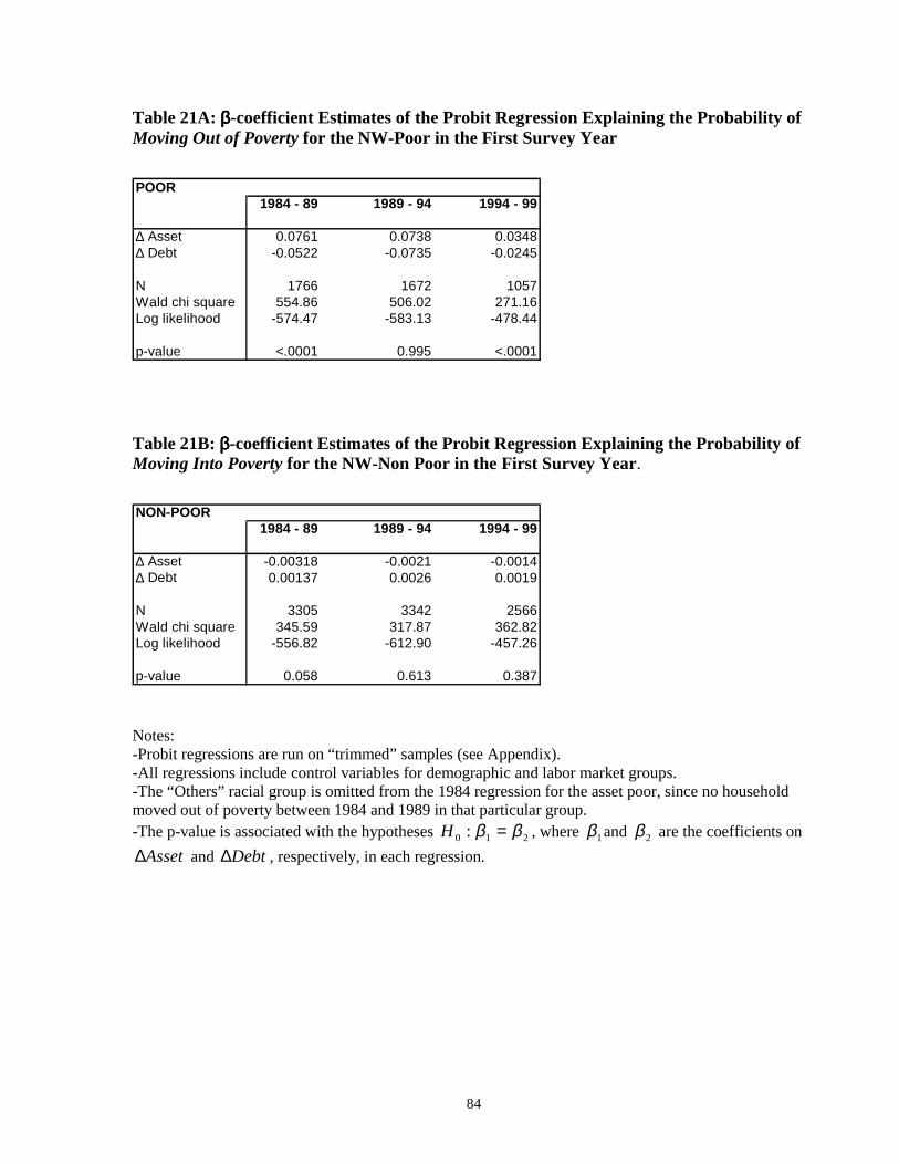
84

Table 21A: ββββ-coefficient Estimates of the Probit Regression Explaining the Probability ofMoving Out of Poverty for the NW-Poor in the First Survey Year

POOR1984 - 89 1989 - 94 1994 - 99

∆ Asset 0.0761 0.0738 0.0348∆ Debt -0.0522 -0.0735 -0.0245

N 1766 1672 1057Wald chi square 554.86 506.02 271.16Log likelihood -574.47 -583.13 -478.44

p-value <.0001 0.995 <.0001

Table 21B: ββββ-coefficient Estimates of the Probit Regression Explaining the Probability ofMoving Into Poverty for the NW-Non Poor in the First Survey Year.

NON-POOR1984 - 89 1989 - 94 1994 - 99

∆ Asset -0.00318 -0.0021 -0.0014∆ Debt 0.00137 0.0026 0.0019

N 3305 3342 2566Wald chi square 345.59 317.87 362.82Log likelihood -556.82 -612.90 -457.26

p-value 0.058 0.613 0.387

Notes:-Probit regressions are run on “trimmed” samples (see Appendix).-All regressions include control variables for demographic and labor market groups.-The “Others” racial group is omitted from the 1984 regression for the asset poor, since no householdmoved out of poverty between 1984 and 1989 in that particular group.-The p-value is associated with the hypotheses 210 : ββ =H , where 1β and 2β are the coefficients on

Asset∆ and Debt∆ , respectively, in each regression.

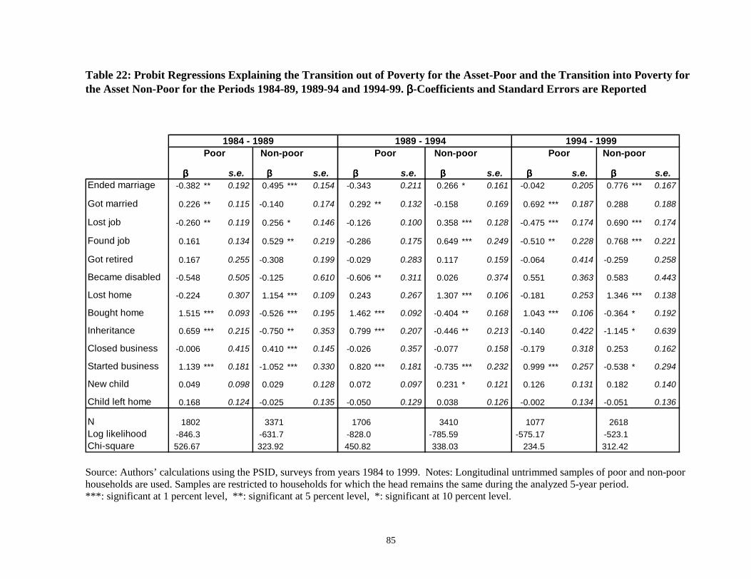
85

Table 22: Probit Regressions Explaining the Transition out of Poverty for the Asset-Poor and the Transition into Poverty forthe Asset Non-Poor for the Periods 1984-89, 1989-94 and 1994-99. ββββ-Coefficients and Standard Errors are Reported

1984 - 1989 1989 - 1994 1994 - 1999Poor Non-poor Poor Non-poor Poor Non-poor

ββββ s.e. ββββ s.e. ββββ s.e. ββββ s.e. ββββ s.e. ββββ s.e.Ended marriage -0.382 ** 0.192 0.495 *** 0.154 -0.343 0.211 0.266 * 0.161 -0.042 0.205 0.776 *** 0.167

Got married 0.226 ** 0.115 -0.140 0.174 0.292 ** 0.132 -0.158 0.169 0.692 *** 0.187 0.288 0.188

Lost job -0.260 ** 0.119 0.256 * 0.146 -0.126 0.100 0.358 *** 0.128 -0.475 *** 0.174 0.690 *** 0.174

Found job 0.161 0.134 0.529 ** 0.219 -0.286 0.175 0.649 *** 0.249 -0.510 ** 0.228 0.768 *** 0.221

Got retired 0.167 0.255 -0.308 0.199 -0.029 0.283 0.117 0.159 -0.064 0.414 -0.259 0.258

Became disabled -0.548 0.505 -0.125 0.610 -0.606 ** 0.311 0.026 0.374 0.551 0.363 0.583 0.443

Lost home -0.224 0.307 1.154 *** 0.109 0.243 0.267 1.307 *** 0.106 -0.181 0.253 1.346 *** 0.138

Bought home 1.515 *** 0.093 -0.526 *** 0.195 1.462 *** 0.092 -0.404 ** 0.168 1.043 *** 0.106 -0.364 * 0.192

Inheritance 0.659 *** 0.215 -0.750 ** 0.353 0.799 *** 0.207 -0.446 ** 0.213 -0.140 0.422 -1.145 * 0.639

Closed business -0.006 0.415 0.410 *** 0.145 -0.026 0.357 -0.077 0.158 -0.179 0.318 0.253 0.162

Started business 1.139 *** 0.181 -1.052 *** 0.330 0.820 *** 0.181 -0.735 *** 0.232 0.999 *** 0.257 -0.538 * 0.294

New child 0.049 0.098 0.029 0.128 0.072 0.097 0.231 * 0.121 0.126 0.131 0.182 0.140

Child left home 0.168 0.124 -0.025 0.135 -0.050 0.129 0.038 0.126 -0.002 0.134 -0.051 0.136

N 1802 3371 1706 3410 1077 2618Log likelihood -846.3 -631.7 -828.0 -785.59 -575.17 -523.1Chi-square 526.67 323.92 450.82 338.03 234.5 312.42

Source: Authors’ calculations using the PSID, surveys from years 1984 to 1999. Notes: Longitudinal untrimmed samples of poor and non-poorhouseholds are used. Samples are restricted to households for which the head remains the same during the analyzed 5-year period.***: significant at 1 percent level, **: significant at 5 percent level, *: significant at 10 percent level.

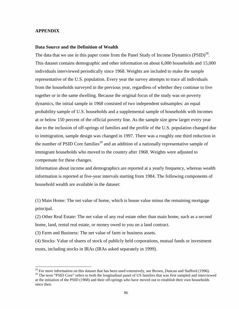
86

APPENDIX

Data Source and the Definition of Wealth

The data that we use in this paper come from the Panel Study of Income Dynamics (PSID)28.

This dataset contains demographic and other information on about 6,000 households and 15,000

individuals interviewed periodically since 1968. Weights are included to make the sample

representative of the U.S. population. Every year the survey attempts to trace all individuals

from the households surveyed in the previous year, regardless of whether they continue to live

together or in the same dwelling. Because the original focus of the study was on poverty

dynamics, the initial sample in 1968 consisted of two independent subsamples: an equal

probability sample of U.S. households and a supplemental sample of households with incomes

at or below 150 percent of the official poverty line. As the sample size grew larger every year

due to the inclusion of off-springs of families and the profile of the U.S. population changed due

to immigration, sample design was changed in 1997. There was a roughly one third reduction in

the number of PSID Core families29 and an addition of a nationally representative sample of

immigrant households who moved to the country after 1968. Weights were adjusted to

compensate for these changes.

Information about income and demographics are reported at a yearly frequency, whereas wealth

information is reported at five-year intervals starting from 1984. The following components of

household wealth are available in the dataset:

(1) Main Home: The net value of home, which is house value minus the remaining mortgage

principal.

(2) Other Real Estate: The net value of any real estate other than main home, such as a second

home, land, rental real estate, or money owed to you on a land contract.

(3) Farm and Business: The net value of farm or business assets.

(4) Stocks: Value of shares of stock of publicly held corporations, mutual funds or investment

trusts, including stocks in IRAs (IRAs asked separately in 1999).

28 For more information on this dataset that has been used extensively, see Brown, Duncan and Stafford (1996).29 The term “PSID Core” refers to both the longitudinal panel of US families that was first sampled and interviewedat the initiation of the PSID (1968) and their off-springs who have moved out to establish their own householdssince then.

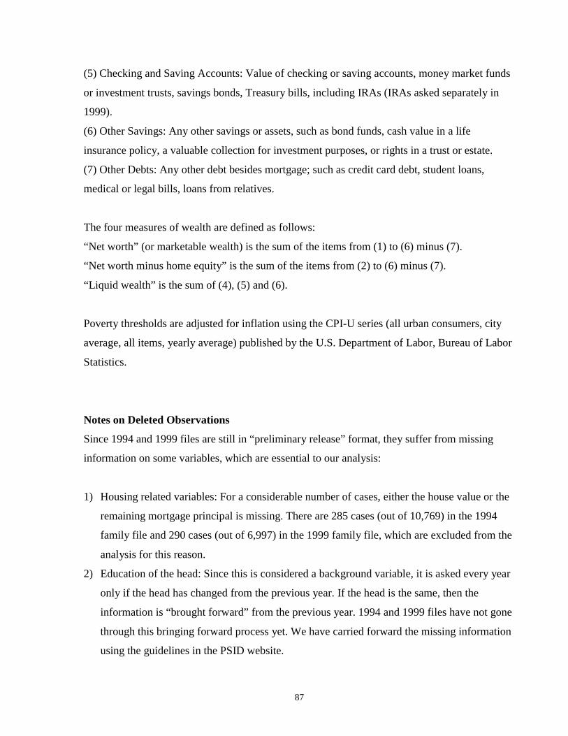
87

(5) Checking and Saving Accounts: Value of checking or saving accounts, money market funds

or investment trusts, savings bonds, Treasury bills, including IRAs (IRAs asked separately in

1999).

(6) Other Savings: Any other savings or assets, such as bond funds, cash value in a life

insurance policy, a valuable collection for investment purposes, or rights in a trust or estate.

(7) Other Debts: Any other debt besides mortgage; such as credit card debt, student loans,

medical or legal bills, loans from relatives.

The four measures of wealth are defined as follows:

“Net worth” (or marketable wealth) is the sum of the items from (1) to (6) minus (7).

“Net worth minus home equity” is the sum of the items from (2) to (6) minus (7).

“Liquid wealth” is the sum of (4), (5) and (6).

Poverty thresholds are adjusted for inflation using the CPI-U series (all urban consumers, city

average, all items, yearly average) published by the U.S. Department of Labor, Bureau of Labor

Statistics.

Notes on Deleted Observations

Since 1994 and 1999 files are still in “preliminary release” format, they suffer from missing

information on some variables, which are essential to our analysis:

1) Housing related variables: For a considerable number of cases, either the house value or the

remaining mortgage principal is missing. There are 285 cases (out of 10,769) in the 1994

family file and 290 cases (out of 6,997) in the 1999 family file, which are excluded from the

analysis for this reason.

2) Education of the head: Since this is considered a background variable, it is asked every year

only if the head has changed from the previous year. If the head is the same, then the

information is “brought forward” from the previous year. 1994 and 1999 files have not gone

through this bringing forward process yet. We have carried forward the missing information

using the guidelines in the PSID website.

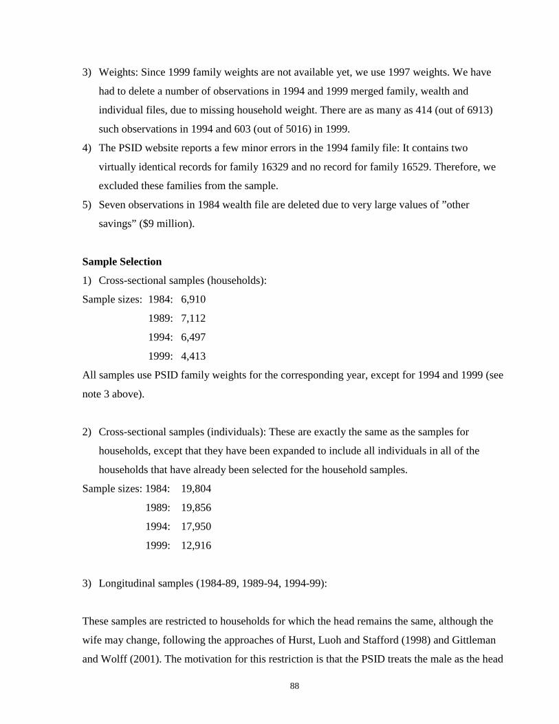
88

3) Weights: Since 1999 family weights are not available yet, we use 1997 weights. We have

had to delete a number of observations in 1994 and 1999 merged family, wealth and

individual files, due to missing household weight. There are as many as 414 (out of 6913)

such observations in 1994 and 603 (out of 5016) in 1999.

4) The PSID website reports a few minor errors in the 1994 family file: It contains two

virtually identical records for family 16329 and no record for family 16529. Therefore, we

excluded these families from the sample.

5) Seven observations in 1984 wealth file are deleted due to very large values of ”other

savings” ($9 million).

Sample Selection

1) Cross-sectional samples (households):

Sample sizes: 1984: 6,910

1989: 7,112

1994: 6,497

1999: 4,413

All samples use PSID family weights for the corresponding year, except for 1994 and 1999 (see

note 3 above).

2) Cross-sectional samples (individuals): These are exactly the same as the samples for

households, except that they have been expanded to include all individuals in all of the

households that have already been selected for the household samples.

Sample sizes: 1984: 19,804

1989: 19,856

1994: 17,950

1999: 12,916

3) Longitudinal samples (1984-89, 1989-94, 1994-99):

These samples are restricted to households for which the head remains the same, although the

wife may change, following the approaches of Hurst, Luoh and Stafford (1998) and Gittleman

and Wolff (2001). The motivation for this restriction is that the PSID treats the male as the head

89

of the household (if one is present). If a male respondent changes his marital status, the wealth

of his family is tracked both before and after the change. However, the wealth of a woman

facing similar changes is not tracked. This approach is also helpful for handling such cases as a

child leaving his parents to establish his own household. Without this restriction, the

longitudinal sample could match the new household with the parents’ household and it would be

misleading to include the wealth difference between two such households to an estimate of the

wealth accumulation pattern in the population.

Another problem is the existence of a number of observations that suffer from huge

changes in wealth between two survey years. To avoid the undue influence of these outliers, we

trim the sample by deleting the lowest and the highest percentiles of the distribution of changes

in net worth.

Longitudinal “untrimmed” sample sizes:

1984 to 1989: 5,173

1989 to 1994: 5,115

1994 to 1999: 3,694

Definition of Total Household Income

Total household income includes earnings, unemployment compensation, workers’

compensation, social security income, supplemental security income, public assistance,

veterans’ payments, survivor benefits, disability benefits, pension or retirement income, interest,

dividends, rents, royalties, periodic payment from estates and trusts, educational assistance,

alimony, child support, financial assistance from outside of the household and all other income

households receive regularly that are not included elsewhere.

This definition does not include capital gains or losses from the sale of property,

withdrawals of bank deposits, money borrowed, tax refunds, gifts and lump-sum inheritances

and insurance payments.

For more information, see the CPS website;

http://www.census.gov/population/www/cps/cpsdef.html

Filename: wp356-paper.docDirectory: P:\wrkpap\356Template: C:\Program Files\Microsoft Office\Templates\Normal.dotTitle: Total and RaceSubject:Author: canerKeywords:Comments:Creation Date: 09/23/02 4:45 PMChange Number: 3Last Saved On: 11/01/02 4:46 PMLast Saved By: Harold LaDueTotal Editing Time: 40 MinutesLast Printed On: 11/07/02 12:03 PMAs of Last Complete Printing

Number of Pages: 89Number of Words: 22,940 (approx.)Number of Characters: 114,700 (approx.)