Sensors 2008, 8, 3460-3481; DOI: 10.3390/s8053460

sensors ISSN 1424-8220

www.mdpi.org/sensors Article

Assessing the Potentialities of FORMOSAT-2 Data for Water and Crop Monitoring at Small Regional Scale in South-Eastern France

Dominique Courault 1,*, Aline Bsaibes 1, Emmanuel Kpemlie 1, Rachid Hadria 1, Olivier Hagolle 2, Olivier Marloie 1, Jean-F. Hanocq 1, Albert Olioso 1, Nadine Bertrand 1 and Véronique Desfonds 1

1 UMR 1114 INRA-UAPV EMMAH, Domaine St Paul, 84914 Avignon, France;

E-mails: courault@avignon.inra.fr; absaibes@avignon.inra.fr; ekpemlie@avignon.inra.fr

2 CNES (DCT/SI/MO) et CESBIO BPI 811, 18 avenue E.Belin, 31401 Toulouse Cedex 9, France

*Author to whom correspondence should be addresse; E-mail: courault@avignon.inra.fr;

Received: 1 February 2008 / Accepted: 20 May 2008 / Published: 23 May 2008

Abstract: Water monitoring at the scale of a small agricultural region is a key point to

insure a good crop development particularly in South-Eastern France, where extreme

climatic conditions result in long dry periods in spring and summer with very sparse

precipitation events, corresponding to a crucial period of crop development. Remote

sensing with the increasing imagery resolution is a useful tool to provide information on

plant water status over various temporal and spatial scales. The current study focussed on

assessing the potentialities of FORMOSAT-2 data, characterized by high spatial (8m pixel)

and temporal resolutions (1-3 day/time revisit), to improve crop modeling and spatial

estimation of the main land properties. Thirty cloud free images were acquired from March

to October 2006 over a small region called Crau-Camargue in SE France, while numerous

ground measurements were performed simultaneously over various crop types. We have

compared two models simulating energy transfers between soil, vegetation and atmosphere:

SEBAL and PBLs. Maps of evapotranspiration were analyzed according to the agricultural

practices at field scale. These practices were well identified from FORMOSAT-2 images,

which provided accurate input surface parameters to the SVAT models.

Keywords: FORMOSAT-2, crop monitoring, evapotranspiration, LAI, albedo, surface

temperature.

OPEN ACCESS

Sensors 2008, 8

3461

1. Introduction

Describing soil - vegetation - atmosphere transfers is of prime interest for understanding interactions

and feedbacks between vegetation and boundary layer, and assessing plant water status [1]. This is

gaining importance over these last years in the context of climatic changes, because land use evolution

can induce significant modifications of surface fluxes like evapotranspiration, and therefore result in

different irrigation strategies. The Crau-Camargue region located in South-Eastern France (Figure 1) is

an interesting study case, particularly sensitive to global changes. It is a flat region characterized by

highly contrasted humid areas, with a high diversity of crops and agricultural practices. The Crau

region is famous for irrigated meadows providing COP (Certified Origin Product) hay exported all

over the world. While the Camargue region is known for its rice fields that were initially cultivated for

soil salinity remediation purposes [2]. Significant modifications have been noticed these last 10 years.

Climatic hazards such as long and dry spring periods and heavy rains in autumn are becoming more

frequent. Consequently, the increasing water scarcity during the growing season, in addition to water

redistribution for the industrial and urban sectors, has led the authorities to restrict irrigation. Irrigated

crops like meadow, which are dominant in the Crau region, were affected by those restrictions. Other

crops such as corn, demanding large water quantity during summer period, disappear progressively of

the cultural landscape. Moreover, rice plantations in Camargue show large differences in yields (mainly

due to the various cultural practices performed in terms of sowing dates, submersion dates after sowing

and drying up dates before harvesting [2]). It is therefore important to estimate with accuracy this

surface variability, to know the real water need for each field so as to improve crop and water

management.

Remote sensing with the increasing imagery resolution is an useful tool to provide such information

on plant water status over various temporal and spatial scales [3]. Evapotranspiration (ET) may be

estimated from remote sensing data with different approaches: direct methods using thermal infrared

(TIR) data, indirect estimates using assimilation procedures combining different wavelengths to get

various input parameters [23]. However, the use of remote sensing for operational applications still

presents several problems. Water and crop monitoring requires a frequent time revisit of satellites and a

fine spatial resolution to get accurate information at the field scale. The relatively long time revisit (16

days) for satellites having a high spatial resolution such as ASTER or Landsat make their use for

operational applications often unattractive (even if they have thermal spectral bands which are used in

numerous ET models). Recent satellites such as FORMOSAT-2 offer both a high spatial and temporal

resolution, since they can revisit a same area, every day with a constant viewing angle, with a pixel of

8m (for FORMOSAT in multispectral range or 2m in black and white). This new sensor generation

characterized by repetitive acquisitions of high resolution images is very useful for monitoring land

surface dynamics. Future missions, such as Venµs [4] or Sentinel2 [42]), having similar characteristics,

are thus defined to be part of the GMES program (Global Monitoring for Environment and Security)

with larger objectives dealing on the environment surveillance (http://www.gmes.info/). However,

these last satellites do not have spectral bands in the thermal range. Several missions (conducted by

CNES: Centre National d’Etudes Spatiales, Toulouse 3w/cnes.fr: IRSUTE [56], SEXTET [34]) have

studied the interest of TIR data acquired at fine spatial and temporal resolution. Actually there is no

current satellites which have these specific configurations. Recent works explore future missions to

Sensors 2008, 8

3462

answer to this strong demand (let us mention the MISTIGRI mission conducted by the CNES). While

waiting for operational solutions, alternative approaches are proposed combining information at

different wavelengths and resolutions [56].

A heavy experimentation took place over the Crau-Camargue region in 2006, including intensive

ground measurements on different crop types, in parallel to airborne and satellite data collection. Thirty

cloudless FORMOSAT-2 images were acquired from March to October. Thermal data were taken at

fine resolution from an airborne thermal camera (3.5m) at few dates during this period (see table 1),

while ASTER and Landsat 5 images were recorded at a larger resolution.

The objectives of this study were i) to evaluate the potentialities of FORMOSAT-2 data for

mapping the main land properties, and ii) to estimate and better understand the spatial variability of

surface fluxes and microclimate over this region, using operative models requiring minimum input data

combining multi spectral data acquired at fine spatial resolution. These models are based on data

acquired in both the optical and thermal domains. The microclimate is represented here by its main

variable: air temperature which is strongly related to land surface thermal exchanges, vegetation

functioning, and to the plant growth.

Besides, let us mention that it was the first time that such remote sensing data (FORMOSAT-2) are

used for agricultural applications. The interest of the high temporal resolution was particularly

important for this study area, where irrigation was applied to different surfaces with a high frequency

(every 8-11 days over the meadows). The impact of these various agricultural practices has a great

influence on all exchanges between surface and atmosphere.

For this work, we have used different types of models, first to estimate the main biophysical

variables characterizing the various crops, and then to simulate surface fluxes and air temperature.

Section 2 presents the dataset used. The models based, either on physical or semi-empirical

relationships, are briefly described in section 3. The main results are discussed in section 4. Finally a

conclusion is made on the potentialities of FORMOSAT-2 data and the future applications.

2. Dataset

2.1. Ground measurements

The study area (centered at 2.3E 45.89N 4E 47.69N, figure 1) is characterized by various crop types.

Five representative fields were chosen for intensive ground measurements: two wheat fields sown in

winter at different dates and which evolved into bare soils around the end of June, a meadow field

flooded every 11 days, and cut three times per year, a sprinkler irrigated corn field (depending on

weather conditions), and a rice plantation, sown in April and then submerged by water during its

vegetative period with a fluctuating water level until harvesting in October.

On these five fields, meteorological measurements like rainfall, air temperature and moisture, wind

speed, global and atmospheric radiations were recorded from March to October 2006. Values were

averaged over a time step of 10 min.

Albedo was measured with albedometers (Kipp & Zonen CM7) with the same time step during all

the cultural cycle of the study fields. The Kipp sensors were calibrated to provide estimates of

incoming radiation over the whole spectrum for measurements over 300 to 3000 nm spectral band.

Sensors 2008, 8

3463

Incident radiation was measured with a pyranometer located on the center of the experimental area.

The footprints of these measurements ranged from 1000 to 3000m². Additionally, surface temperatures

were acquired all along the experiment, with KT17 Heimann radiothermometers on three locations

(wheat, meadow and rice).

For a few intensive observation periods, surface fluxes were measured during several days. 1D-

anenometers (CA27 T Campbell) were set up on the various surfaces, allowing to compute the sensible

heat flux (H). Soil heat fluxes (G) were measured using soil fluxmeters (HFT-3, REBS), put just below

the surfaces. Pyradiometers (Q7 REBS) measured net radiation (Rn). Finally, the latent heat flux (LE)

was obtained by the residual method of the energy balance:

LE=Rn-H-G. (1)

For these intensive observation periods, atmospheric profiles were also acquired according to the

weather conditions (low winds) for several days with a tethered balloon up to 200 m above the surface.

Table 1. Main measurements performed on studied fields (Ts : surface temperature - KT

17 Heimann, Ta: air temperature - thermistor 107 Campbell, q: humidity - Vaisala

capacity probe: HPMP35D, u: wind-speed - anemometer A100L2).

Measurements Wheat 1 then

stubbes

Wheat 2 then

bare soil

Irrigated meadow corn Rice

Micrometeorology

( Ta,q,u) + Albedo

Ts

Surface Fluxes

Crop height

LAI

Remote sensing

Airborne

Atmospheric

profiles

Continuous from

15/3 to 30/9

idem

8 x (2-4) days

6 dates

6 dates

30 FORMOSAT

5 flights

5 dates

Continuous from

15/3 to 30/9

/

/

6 dates

6 dates

30 FORMOSAT

5 flights

5 dates

Continuous from

15/3 to 30/9

idem

8 x (2-4) days

13 dates

13 dates

30 FORMOSAT

5 flights

5 dates

Continuous from

5/5 to 30/9

/

/

5 dates

5 dates

30 FORMOSAT

5 flights

5 dates

Continuous from

27/4 to 20/10

idem

8 x (2-4) days

7 dates

7 dates

30 FORMOSAT

5 flights

5 dates

The main development stages of the various crops were monitored by different observations and

measurements. Crop heights (hveg) were measured to estimate surface roughness (z0m=0.13 hveg) [5]

needed to simulate fluxes over different fields. Leaf Area Index (LAI) was estimated for each field by

both planimetry and hemispherical photographies. Comparisons between both methods were performed

for some dates and gave satisfactory results. We chose the second method for this study, as it was

easier to implement. For this indirect method, we used the CAN-EYE software

(http://www.avignon.inra.fr/can_eye/page5.php) developed by Weiss and Baret at INRA Avignon to

process the image series (technical report at http://www.avignon.inra.fr/can_eye/page5.php). This

software allows to obtain different surface parameters such as fCover (vegetation fraction), FAPAR

(fraction of absorbed photosynthetically active radiation) and the Effective LAI (that does not take into

account vegetation clumping effect), which are comparable to remote sensing estimations [6]. For each

study field, 40 to 60 photographies were taken along transects in cross sectional pattern, according to

the surface heterogeneity and the field size; (the temporal sampling was done according to the crop

Sensors 2008, 8

3464

development). Since LAI measurements were punctual, temporal interpolation of ground measurements

using Koetz et al. [7] model was done in order to compare them to LAI estimated from FORMOSAT-2

images (described later). Table 1 summarizes the main measurements performed during the

experiment.

2.2. Remote sensing data and image processing

Thirty cloud free FORMOSAT-2 images were acquired every 3 to 4 days during 8 months at 10:30

TU from March to October 2006, and with a constant viewing angle of 41° over the Crau-Camargue

region (Figure 1). FORMOSAT-2 is a Taiwanese high resolution satellite launched in May 2004. It

provides images (distribution by SPOT-IMAGE) with the following features: spatial resolution of 8 m

in four spectral bands centred at 488, 555, 650 and 830 nm, with a field of view of 24 km, an orbital

cycle of one day, with a constant observation angle (see table 2 in appendix for its main features). This

data set was first geolocated, registered, calibrated and the cloud and their shadows were discarded by a

CNES-Cesbio team in Toulouse according to the method described in Baillarin et al, [8]. Then the

images were corrected from atmospheric effects using the atmospheric correction method developed by

Hagolle et al. [9] based on the inversion of an atmospheric radiative transfer model.

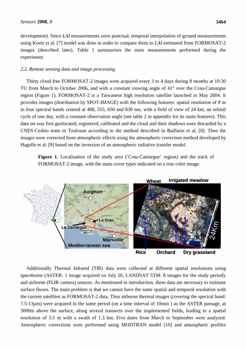
Figure 1. Localisation of the study area (‘Crau-Camargue’ region) and the track of

FORMOSAT-2 image, with the main cover types indicated on a true color image.

Additionally Thermal Infrared (TIR) data were collected at different spatial resolutions using

spaceborne (ASTER: 1 image acquired on July 26, LANDSAT 5TM: 8 images for the study period),

and airborne (FLIR camera) sensors. As mentioned in introduction, these data are necessary to estimate

surface fluxes. The main problem is that we cannot have the same spatial and temporal resolution with

the current satellites as FORMOSAT-2 data. Thus airborne thermal images (covering the spectral band:

7.5-13µm) were acquired in the same period (on a time interval of 10min ) as the ASTER passage, at

3000m above the surface, along several transects over the implemented fields, leading to a spatial

resolution of 3.5 m with a swath of 1.3 km. Five dates from March to September were analyzed.

Atmospheric corrections were performed using MODTRAN model [10] and atmospheric profiles

Mediterranean seaMarseille

Avignon

La Crau

La Camargue

Wheat Irrigated meadow

Rice Orchard Dry grassland

24K

m

Mediterranean seaMarseille

Avignon

La Crau

La Camargue

Wheat Irrigated meadow

Rice Orchard Dry grassland

24K

m

Sensors 2008, 8

3465

obtained from a tethered balloon combined to outputs of the ECMWF (European Centre for Meduim

Range Weather Forecast, 3w.ecmwf.int/index.html ) model for the highest atmospheric levels. The

TES (Temperature Emissivity Separation) algorithm [11] was used to retrieve surface radiometric

temperature from ASTER data. TES relies on the spectral variability captured from the multispectral

brightness temperatures within the 5 ASTER TIR bands at 90m spatial resolution. The estimated

precision (compared with the ground measurements) is around 0.5°C for temperature computed from

the airborne camera and in the order of 1.5°C for the ASTER data. In this paper, we only focussed on

the combination of FORMOSAT and TIR airborne data. Studies are ongoing on comparison between

ASTER and airborne TIR data.

3. Methods

3.1. Models for assessing surface fluxes and microclimate

Two models simulating the transfers between soil-vegetation and atmosphere were used: the

spatially distributed energy balance model SEBAL [12] (modified version by [14]) and the ‘Planetary

Boundary Layer Model (described in [13]). They were chosen because they rely on different

assumptions and need only few input parameters easily computed from remote sensing data. Both are

based on a single source approach which consists in considering only one surface resistance for the

combined soil-canopy system. This approach assumes that all the surfaces can be represented by one

effective value of temperature and humidity [46]. For more complex canopies, for example sunflower

or tiger bush, the two source modeling schemes propose two set of resistances to reproduce the

turbulent and radiative exchanges distinguishing soil and vegetation components within the low

atmosphere [47]. Even if this last approach seems to be more realistic, many authors have shown that a

simple but correctly calibrated single source model gave satisfactory results for describing the energy

balance compared to ill parameterized dual source models [48].

SEBAL was designed to avoid the use of micrometeorological measurements, by exploiting the

information contained in the spatial variability captured from solar and thermal remotely sensed

images. Its main characteristic relies on the determination of wet and dry surfaces on the study area. A

spatial analysis is made on the relationship between albedo (a) and surface temperature (Ts) to define a

threshold, separating evaporative and dry areas. SEBAL calculates the energy partitioning combining

physical parameterization and empirical relationships with minimum ground data, and computes wind

speed and air temperature (Ta). The latent heat flux (or evapotranspiration) is computed at the satellite

acquisition time, as the residual of the energy balance. A detailed description can been found in [12].

The main advantages of this model are that i) the key points have been validated by Jacob et al., [14];

the model was used with success for various applications [15,16, 53], and ii) it is easy to implement

and not expensive in computing time.

The second model used to estimate surface fluxes and temperatures variations over the Crau-

Camargue, was the Brunet et al. model [13], that we called here ‘PBLs’. It was initially developped

over a homogeneous surface on a daily time scale. This land-surface model consists in coupling the

simple soil-vegetation-atmosphere transfer model based on the Penman-Monteith equations, and the

planetary boundary layer (PBL) model of Tennekes and Driedonks [18]. The surface scheme is based

Sensors 2008, 8

3466

on the resolution of the energy budget. The canopy is treated as a single big leaf where the complexity

of vegetation-atmosphere interactions were reduced to a key parameter, the surface resistance (Rs)

computed with the same parametrisation used in the ISBA model described by Jacquemin and Noilhan

[19]. The formulation for Rs (derived from the Jarvis approach) depends upon both atmospheric factors

and available water in the soil (equation 2)

LAIffff

RR s

s4321

min= (2)

Where Rsmin is the minimum stomatal resistance, f1-4 are limiting factors varying from 0 to 1. They

depend on atmospheric and soil moisture conditions. They are described in detail in [19, 21]).

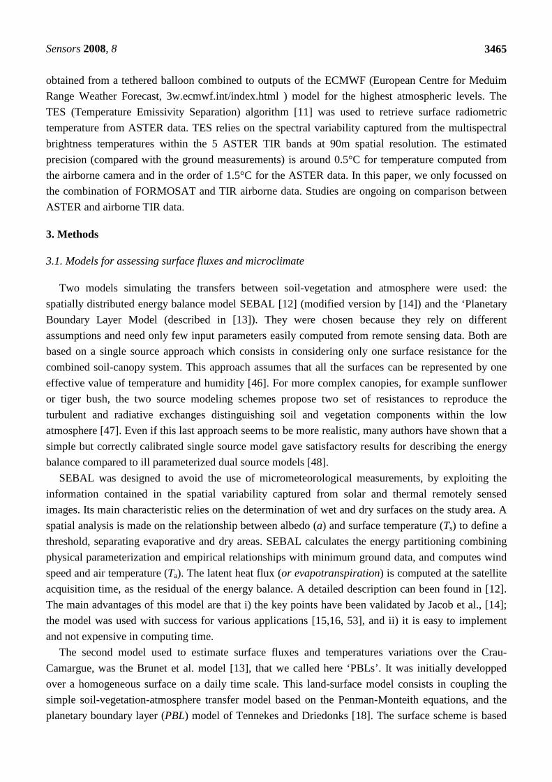
PBLs takes into account the feedbacks between surface and atmosphere via the following simple

equation:

( ) xXHXS CFFFht

X +−=∂∂ 1 (3)

Where t is time, X is air potential temperature (Tp) or air moisture (q), CFx is a term due to the

Coriolis force and FXS and FXH are the vertical fluxes at the bottom and the top of the mixed layer. FXS

correspond to the convective fluxes computed by the big leaf surface model.

As the landscape is heterogeneous, we have modified the surface scheme, in order to take into account

the surface variability, introducing a ‘tile approach’ to compute the Fx term [20, 50]. The method

consists in averaging the surface fluxes computed over each vegetation class, weighted by their percent

of surface occupation (α) according to equation 4 (Figure2).

[ ]∑ ∑ ++=n

i

n

iiiiinii GLEHR αα (4)

This tile approach requests spatially distributed variables derived from remote sensing data,

described in the next section. Other variables were also requested by the model, like the initialising

variables for the atmosphere, the daily evolution of the global radiation and windspeed. Temperature

and humidity profiles were initiated using radio-sounding measurements. Seven characteristic points

define these profiles : Tp, the potential temperature, (qs: the specific humidity) at the surface boundary

layer height (hCLS), γTp (and γqs respectively) the slopes of temperature (and humidity) evolution in the

free atmosphere, and ∆Tp (∆qs) the jump of temperature (or humidity) between free and mixed

atmosphere (figure 2). The model computes all the fluxes of the energy balance in addition to surface

temperature, air temperature (Ta) and air moisture, (q) at each time step, all along the day.

Sensors 2008, 8

3467

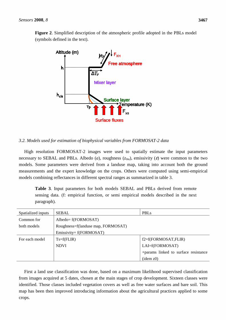
Figure 2. Simplified description of the atmospheric profile adopted in the PBLs model

(symbols defined in the text).

FXHTpγ

pT∆h

Temperature (K)

Altitude (m)

hclsSurface layer

Mixer layer

Free atmosphere

Tp

Surface fluxes

Fxs

FXHTpγ

pT∆h

Temperature (K)

Altitude (m)

hclsSurface layer

Mixer layer

Free atmosphere

Tp

FXHTpγ

pT∆h

Temperature (K)

Altitude (m)

hclsSurface layer

Mixer layer

Free atmosphere

Tp

Tpγ

pT∆h

Temperature (K)

Altitude (m)

hclsSurface layer

Mixer layer

Free atmosphere

Tp

Tpγ

pT∆

TpγTpγ

pT∆ pT∆h

Temperature (K)

Altitude (m)

hclsSurface layer

Mixer layer

Free atmosphere

Tp

hh

Temperature (K)

Altitude (m)

hclsSurface layer

Mixer layer

Free atmosphere

TpTemperature (K)

Altitude (m)

Temperature (K)

Altitude (m)

Temperature (K)Temperature (K)

Altitude (m)

hclsSurface layer

Mixer layer

Free atmosphere

Tp

hclshclsSurface layer

Mixer layer

Free atmosphere

Tp

Surface layer

Mixer layer

Free atmosphere

Surface layerSurface layer

Mixer layer

Free atmosphere

Mixer layerMixer layer

Free atmosphereFree atmosphere

TpTp

Surface fluxes

Fxs

Surface fluxesSurface fluxes

Fxs

3.2. Models used for estimation of biophysical variables from FORMOSAT-2 data

High resolution FORMOSAT-2 images were used to spatially estimate the input parameters

necessary to SEBAL and PBLs. Albedo (a), roughness (z0m), emissivity (ε) were common to the two

models. Some parameters were derived from a landuse map, taking into account both the ground

measurements and the expert knowledge on the crops. Others were computed using semi-empirical

models combining reflectances in different spectral ranges as summarized in table 3.

Table 3. Input parameters for both models SEBAL and PBLs derived from remote

sensing data. (f: empirical function, or semi empirical models described in the next

paragraph).

Spatialized inputs SEBAL PBLs

Common for

both models

Albedo= f(FORMOSAT)

Roughness=f(landuse map, FORMOSAT)

Emissivity= f(FORMOSAT)

For each model Ts=f(FLIR)

NDVI

f2=f(FORMOSAT,FLIR)

LAI=f(FORMOSAT)

+params linked to surface resistance

(idem z0)

First a land use classification was done, based on a maximum likelihood supervised classification

from images acquired at 5 dates, chosen at the main stages of crop development. Sixteen classes were

identified. Those classes included vegetation covers as well as free water surfaces and bare soil. This

map has been then improved introducing information about the agricultural practices applied to some

crops.

Sensors 2008, 8

3468

Indeed, the identification of the main cultural practices performed at the field scale, such as

irrigation, meadow cut, harvest, plowing, sowing date, is crucial for an accurate determination of the

main surface parameters. For example, the roughness map was deduced from the Brutsaert’relationship

(z0=0.13hveg), hveg being the mean height measured for each vegetation cover. The crop heights were

derived from the landuse map and expert knowledge. All the meadows were not cut at the same date.

According to the cut date and irrigation frequency, we have observed from our ground measurements

that crop height varied from 0.05 m to 0.6 m, leading to evapotranspiration values varying from 1 to 7

mm per day. Here two factors have an impact on the decrease of evapotranspiration; irrigation and LAI

decrease due to the cut. Simulations performed over irrigated meadow with a crop model (STICS,

described in [51]) clearly highlighted this large difference of evapotranspiration due to these

agricultural practices (figure 3). It is therefore important to know with accuracy the occurrence of such

main practices.

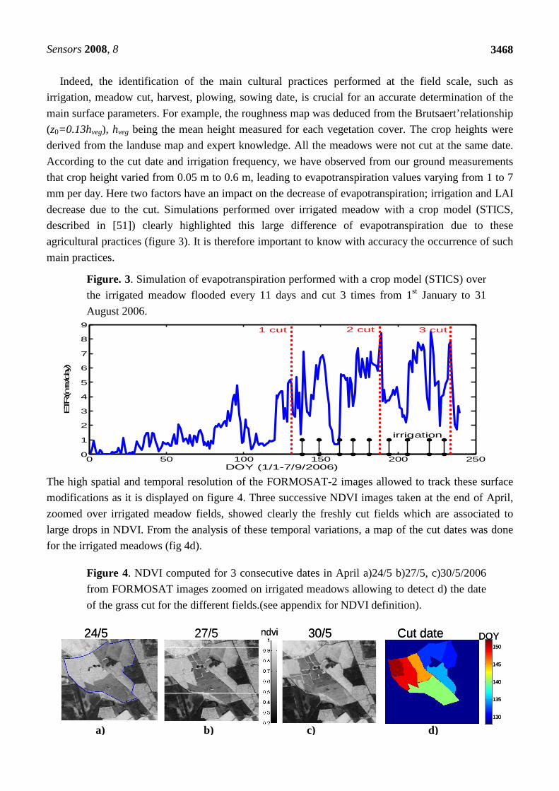
Figure. 3. Simulation of evapotranspiration performed with a crop model (STICS) over

the irrigated meadow flooded every 11 days and cut 3 times from 1st January to 31

August 2006.

0 50 100 150 200 2500

1

2

3

4

5

6

7

8

9

DOY (1/1-7/9/2006)

ETR (mm/day

)

1 cut 2 cut 3 cut

irrigation

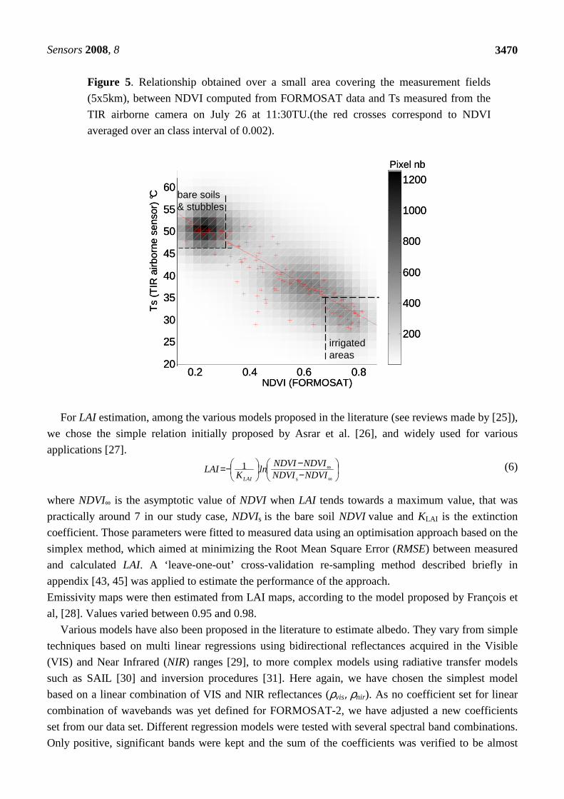
The high spatial and temporal resolution of the FORMOSAT-2 images allowed to track these surface

modifications as it is displayed on figure 4. Three successive NDVI images taken at the end of April,

zoomed over irrigated meadow fields, showed clearly the freshly cut fields which are associated to

large drops in NDVI. From the analysis of these temporal variations, a map of the cut dates was done

for the irrigated meadows (fig 4d).

Figure 4. NDVI computed for 3 consecutive dates in April a)24/5 b)27/5, c)30/5/2006

from FORMOSAT images zoomed on irrigated meadows allowing to detect d) the date

of the grass cut for the different fields.(see appendix for NDVI definition).

130

135

140

145

150

24/5 27/5 30/5 Cut date ndvi DOY

130

135

140

145

150

24/5 27/5 30/5 Cut date ndvi DOY

a) b) c) d)

Sensors 2008, 8

3469

This information has been also used to derive maps of some parameters occurring in the formulation

of the surface resistance (Rs) applied in the PBLs model (eq 2). Values for minimum resistances:

(Rsmin) were affected for each crop class according to the landuse map accounting cultural practices

performed (for example Rsmin was lower for irrigated fields than for dry crops).

Among the four limiting factors appearing in equation 2, the most important is f2 which represents the

root zone available water fraction. It varies between 0 (completely dry) and 1 (saturated). It is often

difficult to estimate with accuracy because it varies a lot spatially at regional scale and all along a

cultural cycle according to crop development stages and for different practices (such as irrigation).

Numerous studies have shown the relationships between surface temperature (Ts) and plant water

status [22, 23]. In SEBAL, Ts is an input data that indirectly informs on the spatial variability of soil

moisture at regional scale. Concerning PBLs, Ts is a model output, and two approaches exist to

estimate f2: either by forcing the model by a f2 map as accurate as possible, deduced from various

observations, or by estimating f2 through assimilation methods [24]. In a first stage, we have chosen to

force PBLs with a f2 map obtained from remote sensing data and observations. The second approach

based on an assimilation procedure to retrieve f2 is currently under study [20]. For this study, f2 was

deduced from the analysis of the thermal images acquired at fine resolution with the airborne camera,

combined with the FORMOSAT image acquired at the same date. We have assumed a negative linear

correlation between Ts and f2 with minimum Ts corresponding to a maximum f2 and inversely, a

maximum Ts corresponding to a minimum f2 (eq 5).

( )( )

( ) max2min smaxs

minssmin2max22 f

T-T

T-T.f-f f += (5)

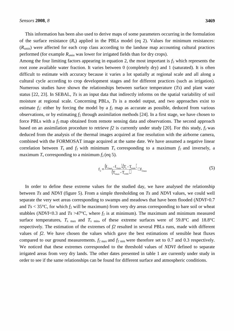
In order to define these extreme values for the studied day, we have analysed the relationship

between Ts and NDVI (figure 5). From a simple thresholding on Ts and NDVI values, we could well

separate the very wet areas corresponding to swamps and meadows that have been flooded (NDVI>0.7

and Ts < 35°C, for which f2 will be maximum) from very dry areas corresponding to bare soil or wheat

stubbles (NDVI<0.3 and Ts >47°C, where f2 is at minimum). The maximum and minimum measured

surface temperatures, Ts max and Ts min, of these extreme surfaces were of 59.8°C and 18.8°C

respectively. The estimation of the extremes of f2 resulted in several PBLs runs, made with different

values of f2. We have chosen the values which gave the best estimations of sensible heat fluxes

compared to our ground measurements. f2 max and f2 min were therefore set to 0.7 and 0.3 respectively.

We noticed that these extremes corresponded to the threshold values of NDVI defined to separate

irrigated areas from very dry lands. The other dates presented in table 1 are currently under study in

order to see if the same relationships can be found for different surface and atmospheric conditions.

Sensors 2008, 8

3470

Figure 5. Relationship obtained over a small area covering the measurement fields

(5x5km), between NDVI computed from FORMOSAT data and Ts measured from the

TIR airborne camera on July 26 at 11:30TU.(the red crosses correspond to NDVI

averaged over an class interval of 0.002).

0.2 0.4 0.6 0.820

25

30

35

40

45

50

55

60

200

400

600

800

1000

1200

irrigatedareas

NDVI (FORMOSAT)

Ts

(TIR

airb

orne

sens

or)

°CPixel nb

bare soils& stubbles

0.2 0.4 0.6 0.820

25

30

35

40

45

50

55

60

200

400

600

800

1000

1200

irrigatedareas

NDVI (FORMOSAT)

Ts

(TIR

airb

orne

sens

or)

°CPixel nb

bare soils& stubbles

For LAI estimation, among the various models proposed in the literature (see reviews made by [25]),

we chose the simple relation initially proposed by Asrar et al. [26], and widely used for various

applications [27].

−−

−=∞

∞NDVINDVINDVINDVI

ln.K

LAIsLAI

1 (6)

where NDVI∞ is the asymptotic value of NDVI when LAI tends towards a maximum value, that was

practically around 7 in our study case, NDVIs is the bare soil NDVI value and KLAI is the extinction

coefficient. Those parameters were fitted to measured data using an optimisation approach based on the

simplex method, which aimed at minimizing the Root Mean Square Error (RMSE) between measured

and calculated LAI. A ‘leave-one-out’ cross-validation re-sampling method described briefly in

appendix [43, 45] was applied to estimate the performance of the approach.

Emissivity maps were then estimated from LAI maps, according to the model proposed by François et

al, [28]. Values varied between 0.95 and 0.98.

Various models have also been proposed in the literature to estimate albedo. They vary from simple

techniques based on multi linear regressions using bidirectional reflectances acquired in the Visible

(VIS) and Near Infrared (NIR) ranges [29], to more complex models using radiative transfer models

such as SAIL [30] and inversion procedures [31]. Here again, we have chosen the simplest model

based on a linear combination of VIS and NIR reflectances (ρvis, ρnir). As no coefficient set for linear

combination of wavebands was yet defined for FORMOSAT-2, we have adjusted a new coefficients

set from our data set. Different regression models were tested with several spectral band combinations.

Only positive, significant bands were kept and the sum of the coefficients was verified to be almost

Sensors 2008, 8

3471

equal to one as suggested by Jacob et al. [32]. Finally, the best result was obtained with only two bands

in the red and near infrared ranges shown in equation 7,

NIRreda ρρ 382.0645.0 += (7)

Let us mention that different methodologies for assessing LAI and albedo (not described in this paper)

have been compared using the same data set [paper submitted 52]. We have chosen in this study only

the simplest methods which gave the better results.

4. Results - Discussion

4.1. Validation of biophysical variables

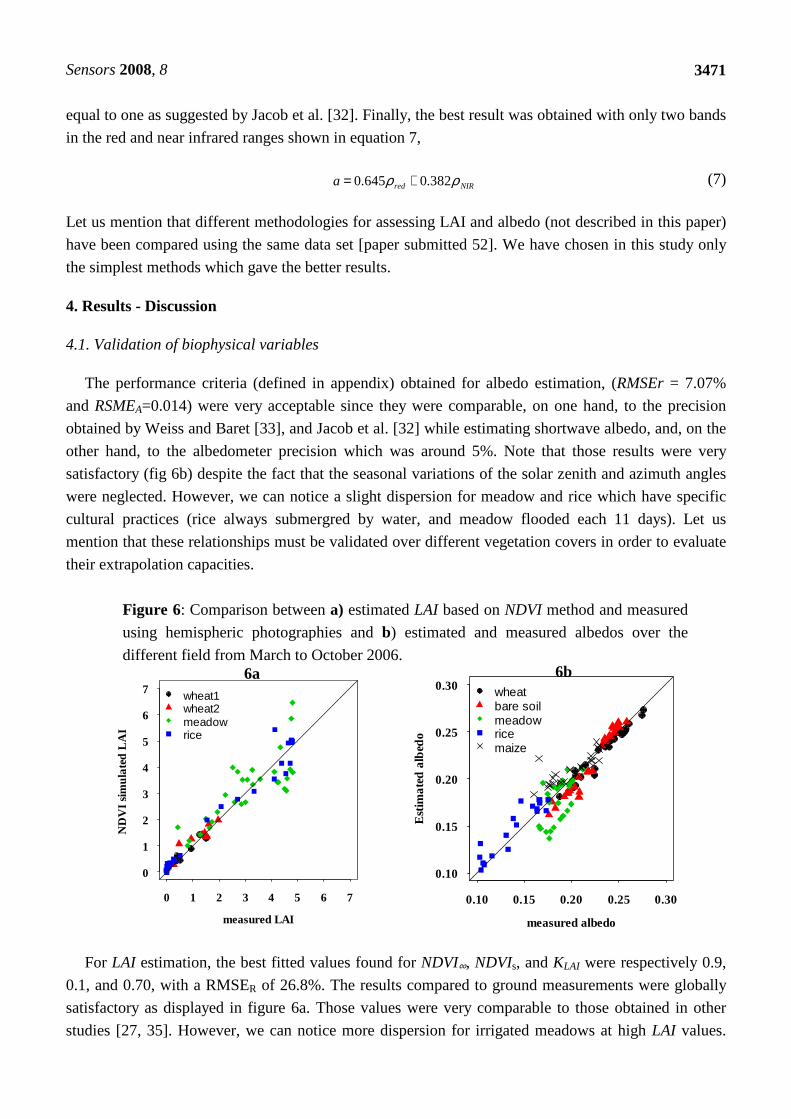
The performance criteria (defined in appendix) obtained for albedo estimation, (RMSEr = 7.07%

and RSMEA=0.014) were very acceptable since they were comparable, on one hand, to the precision

obtained by Weiss and Baret [33], and Jacob et al. [32] while estimating shortwave albedo, and, on the

other hand, to the albedometer precision which was around 5%. Note that those results were very

satisfactory (fig 6b) despite the fact that the seasonal variations of the solar zenith and azimuth angles

were neglected. However, we can notice a slight dispersion for meadow and rice which have specific

cultural practices (rice always submergred by water, and meadow flooded each 11 days). Let us

mention that these relationships must be validated over different vegetation covers in order to evaluate

their extrapolation capacities.

Figure 6: Comparison between a) estimated LAI based on NDVI method and measured

using hemispheric photographies and b) estimated and measured albedos over the

different field from March to October 2006.

0.10 0.15 0.20 0.25 0.30

0.10

0.15

0.20

0.25

0.30

measured albedo

E

stim

ate

d a

lbed

o

wheatbare soilmeadowricemaize

For LAI estimation, the best fitted values found for NDVI∞, NDVIs, and KLAI were respectively 0.9,

0.1, and 0.70, with a RMSER of 26.8%. The results compared to ground measurements were globally

satisfactory as displayed in figure 6a. Those values were very comparable to those obtained in other

studies [27, 35]. However, we can notice more dispersion for irrigated meadows at high LAI values.

0 1 2 3 4 5 6 7

0

1

2

3

4

5

6

7

measured LAI

ND

VI s

imu

late

d L

AI

wheat1wheat2meadowrice

6a 6b

Sensors 2008, 8

3472

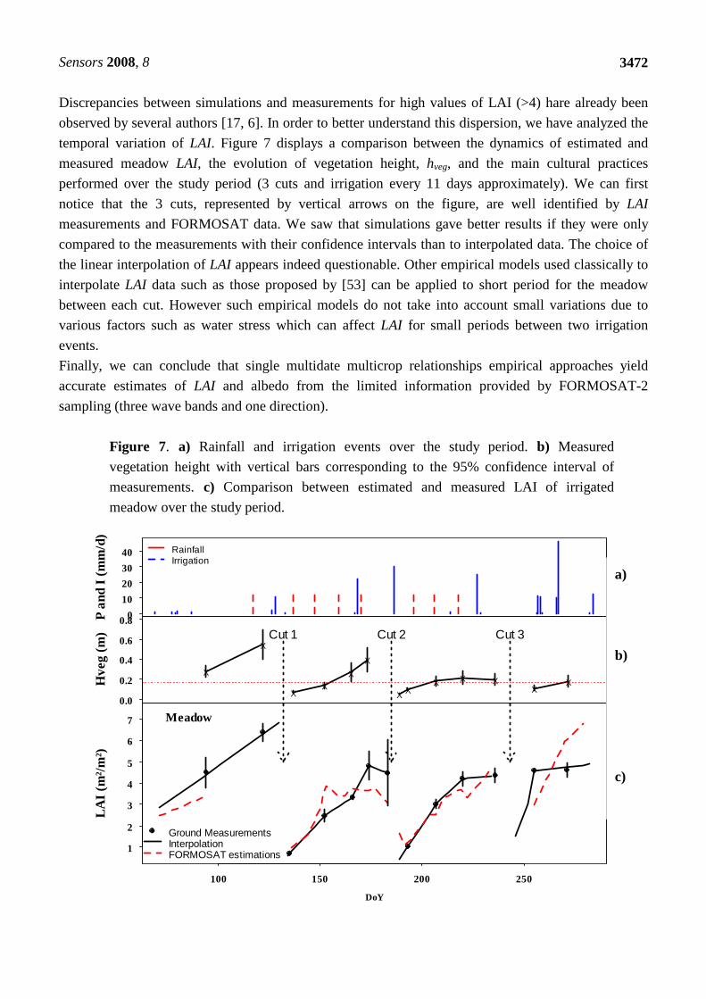
Discrepancies between simulations and measurements for high values of LAI (>4) hare already been

observed by several authors [17, 6]. In order to better understand this dispersion, we have analyzed the

temporal variation of LAI. Figure 7 displays a comparison between the dynamics of estimated and

measured meadow LAI, the evolution of vegetation height, hveg, and the main cultural practices

performed over the study period (3 cuts and irrigation every 11 days approximately). We can first

notice that the 3 cuts, represented by vertical arrows on the figure, are well identified by LAI

measurements and FORMOSAT data. We saw that simulations gave better results if they were only

compared to the measurements with their confidence intervals than to interpolated data. The choice of

the linear interpolation of LAI appears indeed questionable. Other empirical models used classically to

interpolate LAI data such as those proposed by [53] can be applied to short period for the meadow

between each cut. However such empirical models do not take into account small variations due to

various factors such as water stress which can affect LAI for small periods between two irrigation

events.

Finally, we can conclude that single multidate multicrop relationships empirical approaches yield

accurate estimates of LAI and albedo from the limited information provided by FORMOSAT-2

sampling (three wave bands and one direction).

Figure 7. a) Rainfall and irrigation events over the study period. b) Measured

vegetation height with vertical bars corresponding to the 95% confidence interval of

measurements. c) Comparison between estimated and measured LAI of irrigated

meadow over the study period.

0

10

20

30

40

P a

nd I

(mm

/d)

RainfallIrrigation

X

X

XX

X

X

X XX X X

XX

0.0

0.2

0.4

0.6

0.8

Hve

g (

m) Cut 1 Cut 2 Cut 3

100 150 200 250

1

2

3

4

5

6

7

DoY

Meadow

LAI (

m²/

m²)

Ground MeasurementsInterpolationFORMOSAT estimations

a) b) c)

Sensors 2008, 8

3473

4.2. Validation of Surface fluxes

Spatial variations of the main energy fluxes and air temperatures were simulated by both models:

SEBAL and PBLs for the July 26 2006. Comparisons were made between simulations and

measurements accounting for the footprint of the integrated flux measurements. The footprint was

computed based on the analytical solution of the diffusion equation of [36].

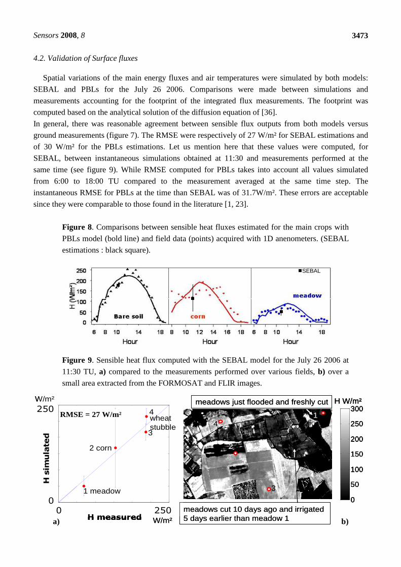
In general, there was reasonable agreement between sensible flux outputs from both models versus

ground measurements (figure 7). The RMSE were respectively of 27 W/m² for SEBAL estimations and

of 30 W/m² for the PBLs estimations. Let us mention here that these values were computed, for

SEBAL, between instantaneous simulations obtained at 11:30 and measurements performed at the

same time (see figure 9). While RMSE computed for PBLs takes into account all values simulated

from 6:00 to 18:00 TU compared to the measurement averaged at the same time step. The

instantaneous RMSE for PBLs at the time than SEBAL was of 31.7W/m². These errors are acceptable

since they were comparable to those found in the literature [1, 23].

Figure 8. Comparisons between sensible heat fluxes estimated for the main crops with

PBLs model (bold line) and field data (points) acquired with 1D anenometers. (SEBAL

estimations : black square).

SEBALSEBAL

Figure 9. Sensible heat flux computed with the SEBAL model for the July 26 2006 at

11:30 TU, a) compared to the measurements performed over various fields, b) over a

small area extracted from the FORMOSAT and FLIR images.

a) b)

-50 0 50 100 150 200 250-50

0

50

100

150

200

250

RMSE = 20.25 W/m²

H measured

H s

imul

ated

250

0

0 250H measured

H simulated

RMSE = 27 W/m²

0

50

100

150

200

250

300

1 meadow

2 corn

wheatstubble

3

2

14

H W/m²4

3

W/m²

W/m²

meadows just flooded and freshly cut

meadows cut 10 days ago and irrigated5 days earlier than meadow 1

-50 0 50 100 150 200 250-50

0

50

100

150

200

250

RMSE = 20.25 W/m²

H measured

H s

imul

ated

250

0

0 250H measured

H simulated

RMSE = 27 W/m²

0

50

100

150

200

250

300

1 meadow

2 corn

wheatstubble

3

2

14

H W/m²4

3

-50 0 50 100 150 200 250-50

0

50

100

150

200

250

RMSE = 20.25 W/m²

H measured

H s

imul

ated

250

0

0 250H measured

H simulated

RMSE = 27 W/m²

-50 0 50 100 150 200 250-50

0

50

100

150

200

250

RMSE = 20.25 W/m²

H measured

H s

imul

ated

250

0

0 250H measured

H simulated

-50 0 50 100 150 200 250-50

0

50

100

150

200

250

RMSE = 20.25 W/m²

H measured

H s

imul

ated

250

0

0 250-50 0 50 100 150 200 250

-50

0

50

100

150

200

250

RMSE = 20.25 W/m²

H measured

H s

imul

ated

250

0

0 250H measured

H simulated

RMSE = 27 W/m²

0

50

100

150

200

250

300

1 meadow

2 corn

wheatstubble

3

2

14

H W/m²4

3

W/m²

W/m²

meadows just flooded and freshly cut

meadows cut 10 days ago and irrigated5 days earlier than meadow 1

Sensors 2008, 8

3474

The simulated surface fluxes showed large spatial variations due to differences in soil moisture and

surface roughness, which were highly dependant on cultural practices performed on each field, as it is

shown in figure 9. Irrigation appeared, as expected, as the factor explaining the greatest spatial

variation. Irrigated meadows showed the lowest values for sensible heat fluxes (figure 9a), while bare

soils or wheat stubbles, which were very dry at this date, had the highest values of sensible heat flux

(250 W/m²). On Figure 9b we observed different H values for meadows due to differences in irrigation

and cut dates.

The large confidence intervals observed for the corn field (fig 9a) were essentially due to the surface

heterogeneity. Indeed, this field was sown relatively late on May 5th and was intermittently irrigated by

sprinklers depending on weather conditions. The soil was very stony at some locations, with a low

water reserve, that explained the bad development of this crop for 2006. The measurement

representativeness was therefore arguable over this corn field.

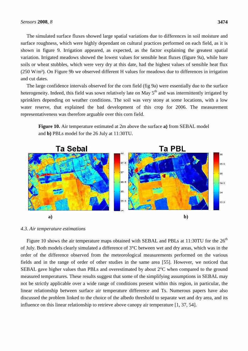
Figure 10. Air temperature estimated at 2m above the surface a) from SEBAL model

and b) PBLs model for the 26 July at 11:30TU.

a) b)

4.3. Air temperature estimations

Figure 10 shows the air temperature maps obtained with SEBAL and PBLs at 11:30TU for the 26th

of July. Both models clearly simulated a difference of 3°C between wet and dry areas, which was in the

order of the difference observed from the meteorological measurements performed on the various

fields and in the range of order of other studies in the same area [55]. However, we noticed that

SEBAL gave higher values than PBLs and overestimated by about 2°C when compared to the ground

measured temperatures. These results suggest that some of the simplifying assumptions in SEBAL may

not be strictly applicable over a wide range of conditions present within this region, in particular, the

linear relationship between surface air temperature difference and Ts. Numerous papers have also

discussed the problem linked to the choice of the albedo threshold to separate wet and dry area, and its

influence on this linear relationship to retrieve above canopy air temperature [1, 37, 54].

Sensors 2008, 8

3475

5. Summary-Conclusion

This study focussed on assessing the potentialities of FORMOSAT-2 data for water and crop

monitoring at regional scale. We have shown that the high temporal and spatial resolutions of these

new remote sensing data allowed providing accurate surface parameters that lead to satisfactory flux

simulations when used as input data in both land-surface models tested. Indeed, identification of each

crop type associated with its main cultural practices is possible (such as irrigation and cut date of

meadow for example). Roughness map can then be elaborated with more precision. The main surface

parameters characterizing the vegetation development such as LAI, or the surface radiative properties

such as albedo can be derived from these data using simple methodologies easy to implement

everywhere. The found relationships were acquired under the specific geometrical configuration of the

site, i.e. under 41° zenith view angle and solar zenith angles ranging from 25° up to 45°. Application to

other conditions may require adaptations, either using BRDF models if well calibrated over the

surfaces investigated, or replication of the whole experimental process under these new conditions.

Alternative approaches based on radiative transfer model inversion were not yet applied from this

study, and should require further efforts. However, the fact that single multidate multicrop

relationships based on empirical approaches yield accurate estimates of LAI and albedo from the

limited information provided by FORMOSAT-2 sampling (three wave bands and one direction)

indicates that this might be possible under well defined prior information.

Preliminary simulations using two different land surface models (SEBAL and PBLs) were

performed using input parameters derived from FORMOSAT-2 data, to compute surface fluxes and air

temperature above canopy. The results obtained for flux estimations were satisfactory for both models

with a slight overestimation for microclimate variables simulated with SEBAL due to simplified

assumptions used in this model. Both models were based on surface energy balance with a single

source approach. This study has shown that with minimum ancillary information, simple models could

be used for water management with quite acceptable results [53]. However, it would be required to

have remote sensing data at high spatial and temporal resolution. FORMOSAT-2 provides images

every day in four spectral bands in the visible and near infrared domains. Thermal data are also

necessary at fine resolution. Currently, there are no satellites which provide similar temporal and

spatial resolution such as FORMOSAT-2 in this spectral range. MODIS (EOS) or AVHRR (from

NOAA meteorological satellites) deliver thermal data on a daily basis but with a coarse spatial

resolution of 1km. A higher resolution was achieved by Landsat (TM: 120m, ETM: 60m), and ASTER

(90m) but the time revisit is low (16 days), and do not allow to detect for example meadow irrigation

occurring every 11 days in our region. There is currently a strong demand from the scientific

community for having thermal sensors with finer resolution, such as the former European SPECTRA

mission which yielded the Chinese SPECTLA mission (Menenti, 2005 personal communication), or

future MISTIGRI mission currently in study by CNES [34]. Meanwhile, recent works have explored

the possibility to use simultaneously various spatial resolutions [39] Different methodologies have

been proposed to disaggregate large pixels of Ts to estimate subpixel Ts combining various information

at different wavelengths [40, 41].

Sensors 2008, 8

3476

A next step for the current study will be to analyse this point which requires more investigations in

the future for operational applications, in comparing ASTER and airborne data acquired over the same

area.

Acknowledgements.

This study was part of projects financed by the MIP-PACA regions in France and by the CNES

(DAR 2006 TOSCA). The Formosat-2 images used in this paper are © NSPO (2006) and distributed

by Spot Image S.A. all rights reserved. The authors thank David Crevoisier, Erwan Fillol (students),

Frederic Jacob (IRD LISAH Montpellier) for their participation to some measurements, Jean-Claude

Mouret (UMR Innovation Monpellier) for enriched discussions about rice crops, and the farmers for

allowing us to make use of their fields. We wish also thank the two reviewers for improving this

manuscript.

Appendix

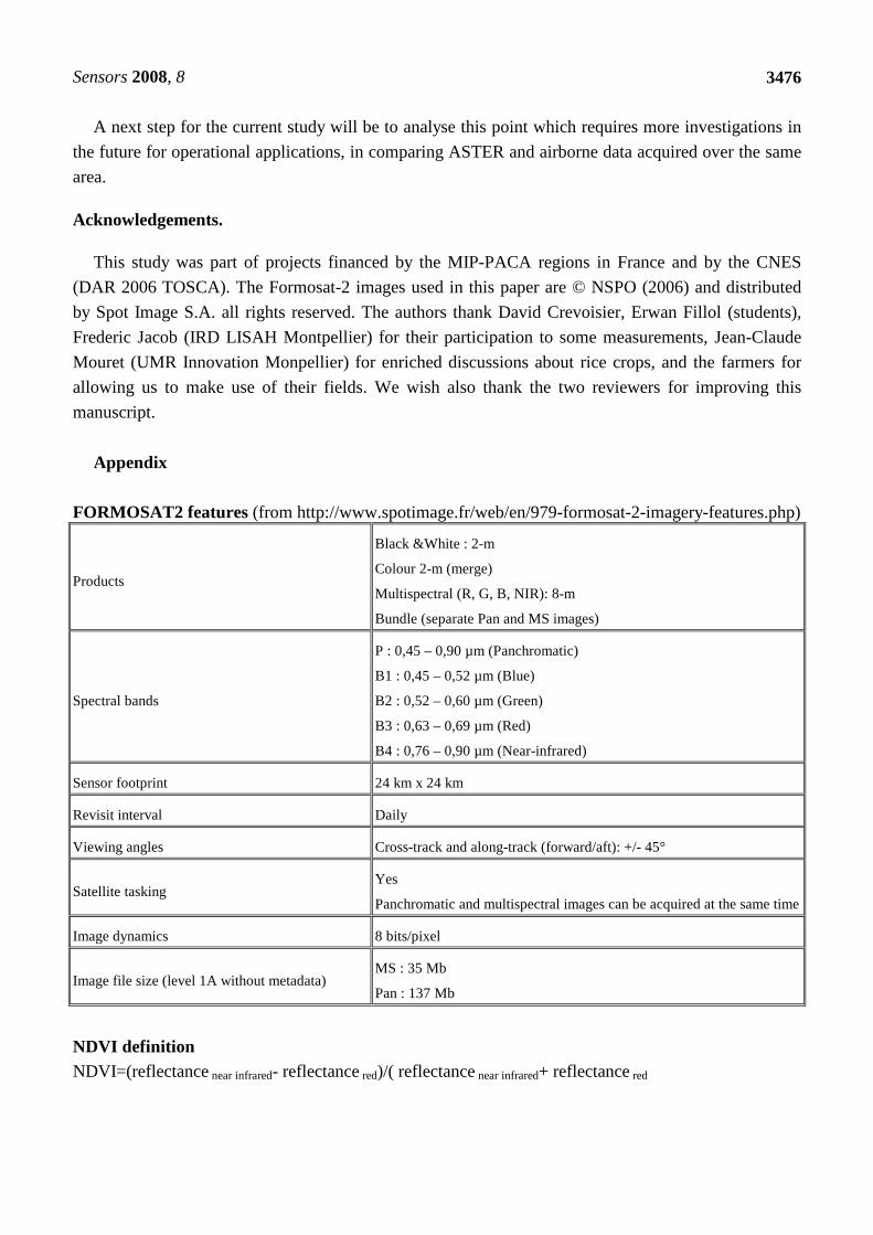
FORMOSAT2 features (from http://www.spotimage.fr/web/en/979-formosat-2-imagery-features.php)

Products

Black &White : 2-m

Colour 2-m (merge)

Multispectral (R, G, B, NIR): 8-m

Bundle (separate Pan and MS images)

Spectral bands

P : 0,45 – 0,90 µm (Panchromatic)

B1 : 0,45 – 0,52 µm (Blue)

B2 : 0,52 – 0,60 µm (Green)

B3 : 0,63 – 0,69 µm (Red)

B4 : 0,76 – 0,90 µm (Near-infrared)

Sensor footprint 24 km x 24 km

Revisit interval Daily

Viewing angles Cross-track and along-track (forward/aft): +/- 45°

Satellite tasking Yes

Panchromatic and multispectral images can be acquired at the same time

Image dynamics 8 bits/pixel

Image file size (level 1A without metadata) MS : 35 Mb

Pan : 137 Mb

NDVI definition NDVI=(reflectance near infrared- reflectance red)/( reflectance near infrared+ reflectance red

Sensors 2008, 8

3477

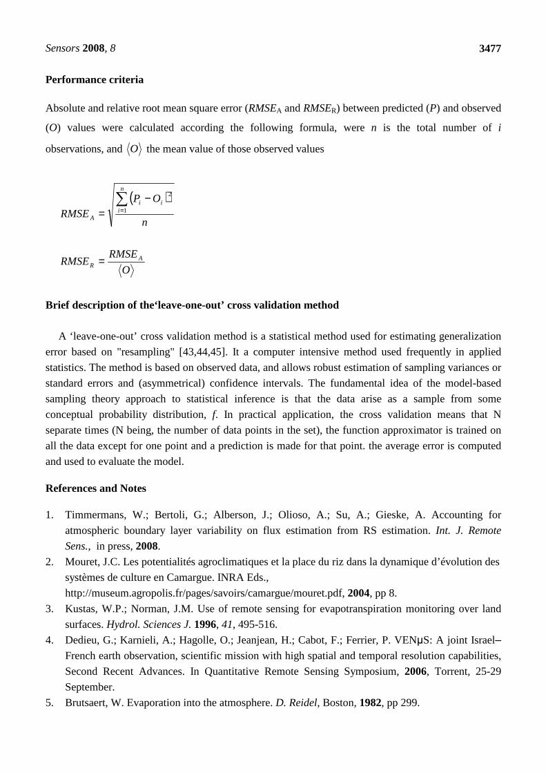
Performance criteria

Absolute and relative root mean square error (RMSEA and RMSER) between predicted (P) and observed

(O) values were calculated according the following formula, were n is the total number of i

observations, and O the mean value of those observed values

( )

O

RMSERMSE

n

OPRMSE

AR

n

iii

A

=

−=∑

=1

2

Brief description of the‘leave-one-out’ cross validation method

A ‘leave-one-out’ cross validation method is a statistical method used for estimating generalization

error based on "resampling" [43,44,45]. It a computer intensive method used frequently in applied

statistics. The method is based on observed data, and allows robust estimation of sampling variances or

standard errors and (asymmetrical) confidence intervals. The fundamental idea of the model-based

sampling theory approach to statistical inference is that the data arise as a sample from some

conceptual probability distribution, f. In practical application, the cross validation means that N

separate times (N being, the number of data points in the set), the function approximator is trained on

all the data except for one point and a prediction is made for that point. the average error is computed

and used to evaluate the model.

References and Notes

1. Timmermans, W.; Bertoli, G.; Alberson, J.; Olioso, A.; Su, A.; Gieske, A. Accounting for

atmospheric boundary layer variability on flux estimation from RS estimation. Int. J. Remote

Sens., in press, 2008. 2. Mouret, J.C. Les potentialités agroclimatiques et la place du riz dans la dynamique d’évolution des

systèmes de culture en Camargue. INRA Eds.,

http://museum.agropolis.fr/pages/savoirs/camargue/mouret.pdf, 2004, pp 8.

3. Kustas, W.P.; Norman, J.M. Use of remote sensing for evapotranspiration monitoring over land

surfaces. Hydrol. Sciences J. 1996, 41, 495-516.

4. Dedieu, G.; Karnieli, A.; Hagolle, O.; Jeanjean, H.; Cabot, F.; Ferrier, P. VENµS: A joint Israel–French earth observation, scientific mission with high spatial and temporal resolution capabilities,

Second Recent Advances. In Quantitative Remote Sensing Symposium, 2006, Torrent, 25-29

September.

5. Brutsaert, W. Evaporation into the atmosphere. D. Reidel, Boston, 1982, pp 299.

Sensors 2008, 8

3478

6. Weiss, M.; Baret, F.; Smith, G.J.; Jonckheere, I. Methods for in situ leaf area index measurement,

part II: from gap fraction to leaf area index: retrieval methods and sampling strategies. Agric.

Forest Meteorol. 2004, 121, 17-53.

7. Koetz, B.; Baret, F.; Poilve, H.; Hill, J. Use of coupled canopy structure dynamic and radiative

transfer models to estimate biophysical canopy characteristics. Remote Sens. Environ. 2005, 95,

115-124.

8. Baillarin, S.; Gleyzes, J.P.; Latry, C.; Bouillon, A.; Breton, E.; Cunin, L.; Vesco, C.; Delvit, J.M.

Validation of an automatic image orthorectification processing. IGARSS’s proceedings, 20-24

Sept., 2004, 2, 1398- 1401, ISBN: 0-7803-8742-2.

9. Hagolle, O.; Dedieu, G.; Mougenot, B.; Debaeker, V.; Duchemin, B.; Meygret, A. Correction of

aerosol effects on multitemporal images acquired with constant viewing angles: Application to

Formosat-2 images. Remote Sens. Environ. 2008, 4 (112), 1689-1701.

10. Anderson, G.; Berk, A.; Acharya, P.; Matthew, M.; Bernstein, L.; Chetwynd, J.; Dothe, H.; Adler-

Golden, S.; Ratkowski, A.; Felde, G.; Gardner, J.; Hoke, M.; Richtsmeier, S.; Pukall, B.; Mello, J.;

Jeong, L. MODTRAN 4.0: radiative transfer modeling for remote sensing. In Algorithms for

multispectral, hyperspectral and ultraspectral imagery VI: Proceedings of SPIE 2000, 176–183.

11. Gillespie, A.R.; Rokugawa, S.; Matsunaga, T.; Cothern, S.; Hook, S.J.; Kahle, A.B. A temperature

and emissivity separation algorithm for Advanced Spaceborne Thermal Emission and Reflection

radiometer (ASTER) images. IEEE Trans. Geosci. Remote Sens. 1998, 36, 113-126.

12. Bastiaanssen, W.G.M.; Menenti, M.; Feddes, R.A.; Holtslag, A.A.M.A. Remote sensing surface

energy balance algorithm for land (SEBAL) - 1. Formulation. J. Hydrology 1998, 213, 198-212.

13. Brunet, Y.; Nunez, M.; Lagouarde, J.P. A simple method for estimating regional

evapotranspiration from infrared surface-temperature data, ISPR. J. Photogrammetry Remote Sens.

1991, 46, 311-327.

14. Jacob, F.; Olioso, A.; Gu, X.; Su, B.; Seguin, B. Mapping surface fluxes using airborne visible,

near infrared, thermal infrared remote sensing data and a spatialized surface energy balance model.

Agronomie 2002, 669-680.

15. Droogers, P.; Bastiaanssen, W.G.M. Irrigation performance using hydrological and remote sensing

modeling. J. of Irr. Drainage Engineering ASCE 2002, 128, 11-18.

16. Allen, R.G.; Tasumi, M.; Morse, A.; Trezza, R. A Landsat-based energy balance and

evapotranspiration model in Western US water rights regulation and planning, Irrig. Drainage

Systems 2005, 19, 251-268.

17. Combal, B.; Baret, F.; Weiss, M.; Trubuil, A.; Macé, D.; Pragnère, A.; Myneni, R.B.; Knyazikhin,

Y.; Wang, L. Retrieval of canopy biophysical variables from bi-directional reflectance. Using prior

information to solve the ill-posed inverse problem. Remote Sens. Environ. 2002, 84, 1-15.

18. Tennekes, H.; Driedonks, A.G.M. Basic entertainment equations for the atmospheric boundary

layer. Bound. Layer Meteorol. 1981, 20, 515-531.

19. Jacquemin, B.; Noilhan, J. Sensitivity study and validation of land surface parametrization using

the Hapex-Mobilhy data set. Bound. Layer Meteorol. 1990, 52, 93-134.

Sensors 2008, 8

3479

20. Kpemlie, E.; Courault, D.; Buis, S.; Olioso, A.; Bsaibes, A. Data assimilation using remote

sensing data into SVAT model for mapping evapotranspiration and microclimate. Continental

Biosphere Vegetation and Water Cycle: Analyses and Prospects. 27-30 Aug, 2007, Paris, pp 4.

21. Courault, D.; Lagouarde, J.P.; Aloui, B. Evaporation for maritime catchment combining a

meteorological model with vegetation information and airborne surface temperatures. Agric.

Forest Meteorol. 1996, 82, 93-117.

22. Carlson, T. An Overview of the Triangle Method for Estimating Surface Evapotranspiration and

Soil Moisture from Satellite Imagery. Sensors 2007, 7, 1612-1629.

23. Courault, D.; Seguin, B.; Olioso, A. Review about estimation of evapotranspiration from remote

sensing data: from empirical to numerical modeling approach. Irrig. Drainage systems 2005, 19,

223-249.

24. Olioso, A.; Inoue, Y.; Ortega-Farias, S.; Demarty, J.; Wigneron, J.P.; Braud, I.; Jacob, F.;

Lecharpentier, P.; Ottlé, C.; Calvet, J.-C.; Brisson, N. Future directions for advanced

evapotranspiration modeling: assimilation of remote sensing data into crop simulation models and

SVAT models. Irrig. Drainage Systems 2005, 19, 377-412.

25. Baret, F.; Buis, S. Estimating canopy characteristics from remote sensing observations. Review of

methods and associated problems. 9th ISPRS symposium, Beijing, September 2005, In press in

Remote Sens. Environ., Eds. Springer. 2008. 26. Asrar, G.; Fuchs, M.; Kanemasu, E.T.; Hatfield, J.L. Estimating absorbed photosynthetic radiation

and leaf area index from spectral reflectance in wheat. Agronomy J. 1984, 76, 300-306.

27. Wilson, T.B.; Meyers, T.P. Determining vegetation indices from solar and photosynthetically

active radiation fluxes. Agric. Forest Meteorol. 2007, 144 (3-4), 160-179.

28. Francois, C.; Ottlé, C.; Prévot, L. Analytical parameterization of canopy directional emissivity and

directional radiance in the thermal infrared. Application on the retrieval of soil and foliage

temperatures using two directional measurements. Int J. Remote Sens. 1997, 18, 2587-2621.

29. Wanner, W.; Strahler, A.; Hu, B.; Lewis, P.; Muller, J.P.; Li, X.; Barker-Schaaf, C.; Barnsley, M.

Global retrieval of bidirectional reflectance and albedo over land from EOS MODIS and MISR

data: theory and algorithm. J. Geophys. Research 1997, 102 (D14), 17143-17161.

30. Verhoef, W. Light scattering by leaf layers with application to canopy reflectance modeling: The

SAIL model. Remote Sens. Environ. 1984, 16, 125-141.

31. Bacour, C.; Jacquemoud, S.; Leroy, M.; Hautecoeur, O.; Weiss, M.; Prevot, L.; Bruguier, N.;

Chauki, H. Reliability of the estimation of vegetation characteristics by inversion of three canopy

reflectance models on airborne POLDER data. Agronomie 2002, 22, 555-565.

32. Jacob, F.; Weiss, M.; Olioso, A.; French, A. Assessing the narrowband to broadband conversion to

estimate visible, near infrared and shortwave apparent albedo from airborne PolDER data.

Agronomie 2002, 22, 537-546.

33. Weiss, M.; Baret, F. Evaluation of canopy biophysical variable retrieval performances from the

accumulation of large swath satellite data. Remote Sens. Environ. 1999, 70, 293-306.

34. Jacob, F.; Schmugge, T.; Olioso, A.; French, A.N.; Courault; D.; Ogawa, K.; PetitColin, F.;

Chehbouni, G.; Pinhero, A.; Privette, G. Modeling and inversion in thermal infrared remote

Sensors 2008, 8

3480

sensing over vegetated land surface. In press in Remote Sens. Environ., Eds. Springer. 2008, 243-

295.

35. Weiss, M.; Baret, F. Validation of neutral techniques to estimate canopy biophysical variables

from remote sensing data. Agronomie 2002, 22, 133-158

36. Horst, T.W.; Weil, J.C. How far is far enough? The fetch requirements for micrometeorological

measurement of surface fluxes. J. Atmos. Oceanic Tech. 1994, 11, 1018-1025.

37. Courault, D.; Jacob, F.; Benoit, B.; Weiss, M.; Marloie, O.; Hanocq, JF.; Fillol, E.; Olioso, O.;

Dedieu, G.; Gouaux, P.; Gay, M.; French, A.N. Influence of agricultural practices on

micrometerological spatial variations at local and regional scales, 2008, in press in Int. J. Remote

Sens.

39. Kustas, W.P.; Norman, J.; Anderson, M.C.; French, A.N. Estimating subpixel surface

temperatures and energy fluxes from the vegetation index radiometric temperature relationship.

Remote Sens. Environ. 2003, 85, 429-440.

40 Anderson, M.C.; Kustas, W.P.; Norman, J.M. Upscaling and Downscaling: A regional view of the

Soil-Plant-Atmosphere Continuum. Agron. J. 2003, 95, 1408-1423.

41. Coudert, B.; Ottlé, C.; Boudevillain, B.; Guérin, C. Use of geostationary satellite thermal infrared

data to monitor surface exchanges at local scale over heterogeneous landscape: Application to

Meteosat 8 data. 2008, In press in Int. J Remote Sens.

42. Martimort, P. Sentinel-2 - the optical high-resolution mission for GMES operational services. ESA

Bulletin 2007, 131, 18 - 23.

43. Efron, B.; Tibshirani, R.J. An Introduction to the Bootstrap, London: Chapman & Hall., 1993. 44. Hjorth, J.S.U. Computer Intensive Statistical Methods Validation, Model Selection, and Bootstrap,

London: Chapman Hall., 1994, pp.

45. Efron, B.; Tibshirani, R.J. "Improvements on cross-validation: The .632+ bootstrap method" J. of

the American Statistical Association 1997, 92, 548-560.

46. Timmermans, W.; Kustas, W.P.; Anderson, M.C.; French, A.N. An intercomparaison of the

Surface Energy Balance Algorithm for Land (SEBAL) and the Two-Source Energy Balance

(TSEB) modeling schemes. Remote Sens. Environ. 2007, 108, 369-384.

47. Merlin, O.; Chehbouni, A. Different approaches in estimating heat flux using dual angle

observations of radiative surface temperature. Int J. Remote Sens. 2004, 25, 275-289.

48. Kustas, W.P. Estimates of evapotranspiration within a one-and two layer model of heat transfer

over partial vegetation cover. J. Applied Meteorol. 1990, 29, 704-715.

49. Norman JM.; Becker F. Terminology in infrared remote sensing of natural surfaces. Remote Sens.

Reviews 1995, 12, 159-173.

50. Ament, F.; Simmer, C. Improved representation of land-surface heterogeneity in a non-hydrostatic

numerical weather prediction model. Bound. Layer Meteorol. 2006, 121, 1, 153-174.

51. Brisson, N. Special Issue "Crop model STICS (Simulatuer mulTIdisciplinaire pour les Cultures

Standard)". Agronomie 2004, 24, 295-444.

52. Bsaibes, A.; Courault, D.; Baret, F.; Weiss, M.; Olioso, A.; Jacob, F.; Hagolle, O.; Marloie, O.;

Bertrand, N.; Desfond, V.; Kzemipour, F. Albedo and LAI estimates from FORMOSAT-2 data for

crop monitoring. 2008, submitted to Remote Sens. Environ.

Sensors 2008, 8

3481

53. Bastiaanssen, W.G.M.; Harshadeep, N.R. Managing scarce water resources in Asia: The nature of

the problem and can remote sensing help? Irr. and Drainage systems 2005, 131, 85-93.

54. Norman, J.M.; Anderson, M.C.; Kustas, W.P. Are single source, Remote Surface-flux models too

simple? AIP conference Proceedings of int conf on earth observation for vegetation monitoring

and water management, 10-11 November 2005, Napoli, Italy, Eds D’Urso and Moreno, 2005, 852,

170-177.

55. Courault, D.; Olioso, A.; Lagouarde, J.P.; Monestiez, P.; Allard, D. Influence des cultures sur les

variables climatiques. ECOSPACE, AIP Organisation spatiale des activités agricoles et processus

environnementaux. P. Monestiez, S. Lardon, B. Seguin Eds, Collection Science Update, INRA

Editions, Paris, 2004, 303-320.

56. Seguin, B.; Becker, F.; Phulpin, T.; Gu, X.; Guyot, G.; Kerr, Y.; King, C.; Lagouarde, J.P.; Ottlé,

C.; Stoll, M.; Tabbagh, T.; Vidal, A. IRSUTE: A minisatellite project for land surface heat flux

estimation from field to regional scale. Remote Sens. Environ. 1999, 68, 357–369.

© 2008 by the authors; licensee Molecular Diversity Preservation International, Basel, Switzerland.

This article is an open-access article distributed under the terms and conditions of the Creative

Commons Attribution license (http://creativecommons.org/licenses/by/3.0/).