Articulating the Geo-Cultural Logic of Nationalist Insurgency

Articulating the Geo-Cultural Logic of Nationalist Insurgency

Lars-Erik CedermanSwiss Federal Institute of Technology (ETH)

Center for Comparative and International Studies (CIS)Seilergraben 49

8092 Zurich Switzerland+41-1-6326759

[email protected]

Version 1.01Comments welcome!

January 13, 2004

Abstract:Logistical factors have assumed an increasingly important role in studies of civil wars. Inparticular, political economists have recently proposed models of insurgency that dependon states’ capacity to project power in rugged terrain rather than on ethnic allegiances.Yet, a large gap remains between the observed macro-level patterns and the postulatedrationalistic micro-level explanations. Aiming to reproduce similar, logistical macro-levelpatterns, this paper offers an alternative account that interprets insurgency as processes ofnationalist mobilization leading to violence when the power balance favors the peripheralcommunities over the centers. To articulate such identity-based mechanisms, I rely on acomputational model, whose cross-national output is analyzed with multivariateregressions. The computational findings suggest that the search for explanations of civilwars needs to go beyond purely rationalist conjectures.

*) Paper prepared for presentation at the workshop on “Origins and Patterns of PoliticalViolence I: Violence in Civil Wars,” to be held at the Santa Fe Institute, January 15-19,2004. I would like to thank Luc Girardin for excellent computational advice and support.

1

IntroductionAs interstate wars become less frequent, academic attention has shifted increasingly tointernal conflict. In recent years, an exciting literature on the determinants of civil warshas emerged. Political economists, relying on cross-national statistics and rational-choicemodeling, have played a prominent role in this debate. Explaining outbreaks of civil warsin materialist and logistical, rather than in cultural, terms, an important study by Fearonand Laitin (2003) interprets such conflicts as instances of armed insurgency. Whereverthe central state is weak and fails to reach the periphery due to difficult geography,rebellions become more likely. However, the authors find that the ethnic composition ofthe state in question has no impact on the likelihood of conflict.

There can me no doubt that work of this kind has advanced greatly the research frontier.Instead of sweeping generalizations based on diffuse and scattered case-study evidence,political economists have brought the phenomenon in sharper focus thus allowing for amore precise evaluation of their and others’ hypotheses. Yet, it is somewhat premature todraw definitive theoretical conclusions from these studies, because there is a considerablegap between their macro-level findings and the rationalistic micro-level mechanisms thatthey posit as explanations. As the latter remain unsupported by direct evidence, onecannot exclude alternative causal mechanisms that deviate quite radically from thesescholars’ materialist conjectures.

Several studies have appeared that take issue with the statistical interpretations proposedby Fearon and Laitin, to which I will return shortly. In this paper, however, the goal is notto question their key findings so much as to articulate alternative causal mechanisms thatbring both politics and culture back to the fore. Such a task calls for deeper and moresystemic explanations than those associated with standard methods and assumptions ofpolitical economy. Therefore, I rely on computational modeling, which is better suited totrace historical path-dependency and to capture intangible entities such as nationalidentities.

Contrary to the rationalistic reconstructions of Fearon and Laitin, I show that it ispossible to create plausible scenarios in which state strength and terrain matter, althoughthe effect is primarily mediated through geo-cultural mechanisms. The main goal is tocreate an artificial world within which peripheral insurgents manage to form coalitions,the effectiveness of which depends on inclusiveness of their shared national identity.Before creating such interactions in greater detail, however, it is necessary to “grow” acomprehensive, geo-cultural system, which includes geography, political organizations,cultural raw material, and national identities.

Based on a simple geo-cultural logic, the model generates results that are very similar tothose found in Fearon and Laitin’s theory of insurgency, both in terms of state strengthand rugged terrain. Unlike the expectations of these authors, however, the model’sinsurrectional mechanisms hinge directly on national identities, and thus indirectly on theethnic preconditions of the state in question. To confirm the power of nationalist identity-formation while controlling for materialist factors, I run multivariate regressions on themodel’s output. This analysis suggests that it is often hard, if not even impossible, toseparate political-economy interpretations from constructivist theorizing merely based onquantitative macro-level analysis.

In the following, I first review the relevant literature before introducing the four mainphases of the computational model. After having specified the model, the attention turnsto the computational main findings, followed by a section subjecting them to sensitivityanalysis. A concluding section elaborates the theoretical and empirical consequences ofthe present study.

2

The contemporary literature on civil warsThere can be no doubt about the policy relevance of civil wars. Whereas interstatewarfare has declined in recent years, intrastate conflict shows few signs of abating(Sollenberg and Wallensteen 2001; Gleditsch et al 2002). It is therefore not surprisingthat scholars, both in comparative politics and international relations, have joined forcesin a series of systematic attempts to account for why civil wars break out and why theypersist (Lake 2003). Many of the recent research activities in this area draw on theavailability of large-N data from sources such as Gurr’s Minorities at Risk project (Gurr1993) and improved, more fine-tuned measurements of internal conflict (Gleditsch et al.2002).

Marrying such quantitative tools with rational-choice modeling, political economists havebeen leading in advancing candidate explanations along rationalistic lines. These studiestend to ascribe more explanatory power to materialist factors relating to the opportunitystructure of rebellious activities than to ethnic divisions of the state in question (for areview, see Sambanis 2003). While several studies have appeared that propose variationson this theme (see e.g. Collier and Hoeffler 2002; Skaperdas 2003), a recent article byFearon and Laitin (2003) stands out as particularly well-researched and provocative.1

Contending that state strength and the logistical conditions of the rebels to a large extentdetermine the chances of civil war, Fearon and Laitin (2003, p. 75) define insurgency as“a technology of military conflict characterized by small, lightly armed bands practicingguerilla warfare from rural base areas.” Based on this definition, they “hypothesize thatfinancially, organizationally, and politically weak central governments render insurgencymore feasible and attractive due to weak local policing or inept and corrupt insurgencypractices” (pp. 75-76). Furthermore, such a logic implies that insurgency should becomeeasier to carry out in rough and mountainous terrain (see also Collier and Hoeffler 2002).

Less than a year after its publication, Fearon and Laitin’s article has already drawnconsiderable fire. Representing the state of the art in terms of methodology, it serves as auseful reference point for critiques and re-analyses. Relying on Bayesian analysis tocorrect for measurement error, Quinn, Hechter, and Wibbels (2003) confirm Fearon andLaitin’s contention that weak states are more violence prone, but cast doubt on ethnicdiversity’s alleged irrelevance. In contrast, Sambanis (2003) probes the causal reasoningof the authors based on an impressive series of case studies rather than on statistics, butcomes to similar critical conclusions. Also preoccupied with measurement error causedby Fearon and Laitin’s reliance on imperfect proxies, he shows that their postulatedmechanisms deviate from the empirical record in many of the cases. Most importantly,the political economists’ tendency to aggregate all instances of civil war into onecategory obscures the diversity of causal logics. There is no a-priori reason to believe thatthe same mechanisms explain both coups within stable borders and secessionist attempts.Indeed, disaggregation demonstrates that in wars over self-determination, ethnic cohesionamong the peripheral rebels supports collective mobilization against the centralgovernment (Sambanis and Zinn 2003). It is equally plausible that several mechanisms,rational or not, co-exist in the same civil war (Kalyvas 2003).

In his dissertation research, Kocher (2003) also uses Fearon and Laitin’s study as a pointof departure. His aim is to build a more refined theory of insurrectional civil war thatrelies more explicitly on ecological analysis. In this theory, state penetration ofgeographically remote areas is more important than sheer strength. Controlling forurbanization, Kocher finds that the standard indicators of state strength become spurious 1 See also the special issues of Journal of Conflict Resolution (2001) and the Journal of Peace Research(2002).

3

thus undermining the key interpretation advanced by Fearon and Laitin. Based onrecoded GIS-generated data, his research also indicates that internal conflict is closelylinked to difficult terrain, something that is more in line with the conventional literature.In contrast to Quinn et al. and Sambanis, however, his analysis also agrees with Fearonand Laitin in suggesting that ethnic fragmentation has no impact on civil war incidence.However, focusing on the configuration of settlement patterns, Toft (2003) anticipatesKocher’s results about urbanization in a theory that includes ethnic groups as salientactors.

What are we to make of this intriguing, if somewhat contradictory, picture? The singlemost important puzzle relates to the articulation of mechanisms. True to their rationalisticinclinations, the political economists have relied on rational-choice models as a way tobridge the micro-macro gap. Although there is obviously no complete consensus amongthese scholars as regards the postulated mechanisms, their theoretical reconstructions areinternally consistent and often elegant. Nevertheless, due to the looseness of the macro-level indicators and proxies used, and in the absence of extensive micro-level validation,it would be unwise to place too much confidence in such conjectures. In his stimulatingreview of the literature, Sambanis (2003, p. 1) sums up the situation cogently:

The gap between micro-level behavior and macro-level explanation is large. It ismagnified when micro-macro relationships are studied solely through cross-national statistical analyses. What is often lost in such studies in informationabout causal pathways that link outcomes with causes.

After all, the macro-level patterns could have been produced by radically different causalmechanisms, possibly even including the cultural ones that Fearon and Laitin choose todismiss. Therefore, it would seem reasonable to heed Sambanis’ (2003, p. 12) call urgingresearchers to “consider a wider array of micro-level theories, including how emotions,ideology, revenge, or private material interest interact to produce collective action thatculminates in a civil war.” Similarly, Quinn, Hechter, and Wibbels (2003, p. 13) insistthat their “demonstration that cultural variables are important determinants of civil strifedoes not elucidate the mechanisms that are responsible for their efficacy. Causalmechanisms of outcomes like civil war require evidence about units at a lower level ofaggregation than the state.”

Most pragmatic social scientists would have few disagreements with the thrust of thesecritiques. Yet, it remains unclear where to look for alternative theoretical theories to fillthe cultural void left open by the political economists. For sure, neither of the critiquesconsidered here offers very clear guidance as to where to look for coherent theories inwhich to embed non-materialist mechanisms. Moreover, constructivist theory has notmanaged to live up to the same high standards of internal consistency and systematicvalidation as have their rationalistic counterparts (Fearon and Laitin 2000). Beingpreoccupied with mental events rather than with macro-level processes, constructivistshave had just as great difficulties at advancing complex relational theories as do theirrationalist colleagues (McAdam, Tarrow, and Tilly 2001; Tilly 2003; Cederman 2002b;Cederman and Daase 2003).

My contention is that historical sociology goes a long way toward providing the missingconceptual pieces in the explanatory jigsaw. There are striking parallels between thecases at hand and Rokkan’s (1999) classical theory of European state-formation andnation-building. At the heart of his model is a similar center-periphery relationship as thatproposed by Fearon and Laitin (2003), and Kocher (2003). In fact, Rokkan insists that“any analysis of variations among political systems must start from notions of territory”and proceeds by specifying his three main building blocks as centers, peripheries, and

4

transactions, the latter linking the centers to the peripheries. Because transactions have torespect logistical constraints, it is necessary to study the physical, technological, military,economic, and cultural conditions of communication. Even from this brief enumeration itbecomes evident that Rokkan’s framework steers clear of the political economists’materialist reductionism. For peripherality in Rokkan’s conception means much morethan a physical struggle for power. In his more nuanced picture, peripheries arecharacterized by distance, difference, and dependence:

A periphery is located at some distance from the dominant centre or centres, andits transactions with the latter are fraught with costs. A periphery is also differentfrom the central areas on one or more scores: while the degree of distinctivenesswill vary, being to some extent a function of distances and dependence, there willinvariably be some minimum level and sense of separate identity. Finally, aperiphery is dependent upon one or more centres … in political decision-making,in cultural standardization, and in economic life (p. 115).

By stressing identity-formation, Rokkan’s account belongs to a long and prominent seriesof studies that draws the link between cultural standardization and political mobilization.In a classic study of rural France in the 19th century, E. Weber (1976) adopts a multi-dimensional perspective on a political center’s cultural penetration of the periphery withthe aid of road building, educational reforms, and other institutional mechanisms. Otherclassical accounts along similar lines include Hintze (1975), Deutsch (1953), and Gellner(1983). In addition, there are excellent, empirical studies that stress identity-formation ina regional context. Focusing on Southern Asia, Weiner’s (1978) identifies a pattern thathe refers to as the “sons of the soil,” which spawns conflicts between settlers from thecapital clashing with ethnically distinct peripheral populations.2 Likewise, there is acultural dimension in Herbst’s (2000) stimulating study of failed nation-building in thegeographical periphery of African states.

To say that nation-building is important does not mean that one has found a full-fledgedtheory. The strength of Rokkan’s system building lies at the macro level rather than at thelevel of micro-level mechanisms. Moreover, Rokkan’s research did not focus on violentconflict as much as on cleavage structures and party politics. In recent years, however,considerable conceptual progress has been made in the study of “contentious politics,”both as regards an ontological shift toward relational theorizing and an increasedepistemological stress on causal mechanisms as the key to explanation (McAdam,Tarrow, and Tilly 2001; Tilly 2003). It is in the spirit of that promising research programthat I embark on the task of articulating the geo-political logic of nationalist insurgency.For a lot of work remains until Rokkan’s sweeping generalizations and macro processescan be translated into anything that resembles operational empirical research in general,and the empirical literature on civil wars in particular. The remainder of this paper setsout to bridge this gap with computer-based tools.

A computational model of nationalist insurgencyAgent-based modeling has emerged as an increasingly popular complement toconventional, rational-choice methods. By representing distinct actors in their social (andoften spatial) context, this computational technique enables the analyst to representcomplex, macro-level processes without losing their micro-level mechanisms out of sight.Moreover, intangible concepts, such as culture and social identities, which do not easily

2 Interestingly, Fearon (2002) offers a partly inductive analysis of the duration of civil wars that confirmsthe power of Weiner’s explanation.

5

fit into a rationalistic framework, can be readily formalized and integrated into agent-based models (Cederman 1997, Chap. 3). As Ian Lustick (2000) nicely puts it:

Difficulties of amassing and manipulating collective identity data intotheoretically potent comparisons are among the reasons that agent-basedmodeling can play an important role in the elaboration, refinement, and testing ofthe kind of specific and logically connected theoretical claims that constructivistshave been faulted for not producing. Because the models are run on computersthere is no room for ambiguity in the specification of the model’s underlyingrules.

This statement describes precisely what this paper aims at, although it is important not tointerpret the reference to theory testing too literally. For while it is easy to generateunlimited amounts of “data” with a simulation model, such information should not beconfused with real-world evidence. Thus, computational modeling cannot serve as a full-fledged substitute for empirical research. Rather, agent-based models constitute artificial,and indeed simplified, worlds in which the plausibility and consistency of well-specifiedcausal mechanisms can be evaluated in a context that is more complex than that ofstandard, rationalistic modeling tools, but still much simpler than the real world. Servingas a stepping stone between micro and macro analysis, such models can help untangleinteracting mechanisms, that together generate the phenomenon to be explained. Thisperspective defines a generative research strategy that starts from such patterns andmoves backward in the search for candidate mechanisms that could generate observedoutcomes (Cederman forthcoming).

In our case, the main pattern to be reproduced is constituted by the statistical findings thatrebellions in weak states and mountainous areas are more frequent than elsewhere. Whatwould it take to construct a set of plausible, predominantly identity-based mechanismsthat generate such findings without resorting to the materialist explanations? As indicatedin the previous section, any reconstruction of this kind must specify a process of identity-formation that creates center-periphery relationships within which political actionunfolds, in some cases with civil war as the outcome.

As a minimum, such configurations feature the following building blocks:• Political organizations. The main protagonists are the sovereign states, whose

centers dominate their peripheries.• Terrain. Interaction has to proceed in a realistic space with obstacles, such as

mountains and other types of rough terrain.• Cultural map. Identity formation presupposes a multi-dimensional substrate of

cultural traits.• National identities. Nationalist behavior requires identities, which are constituted

as combinations of cultural traits.

Needless to say, a model that comprises all these components would have to be complex.In fact, no existing model combines all these properties in the same framework. Mostcomputational models of cultural politics make no distinction between culture andidentities, thus violating a fundamental tenet of constructivist theory. Typically, culture ismodeled as fixed and immutable properties influencing behavior (Epstein 2002) or asendogenous vectors whose traits all matter (Axelrod 1997, Chap. 7). Identities, however,are more selective, because only relevant culture enters the political calculus. Allowingfor such variation, Lustick’s (2000; 2002) ABIR system features endogenous identityrepertoires composed by sets of identities, but the component identities stand in nospecific relationship to each other and thus do not describe a coherent cultural space.

6

Moreover, this, and almost all other models of this type, fail to provide an explicitrepresentation for formal political organizations or terrain.

Inspired by Bremer and Mihalka’s (1977) pioneering computational research inInternational Relations, I have developed a modeling architecture, called Geosim, that isbetter suited to solve the research problem studied in this paper (Cederman 1997).3

Embedded in a dynamic state system constituted by formal political organizations, itcontains a constructivist logic that captures the culture as a tunable attribute space, withidentity mappings as schemata based on this substrate (Cederman 1997: Chap. 8; 2001;2002a). Once having generated national identities of the centers and peripheries, thesecan be brought to bear on behavior, thus avoiding cultural determinism. What is missinghere, however, is a representation of rugged terrain. The current model thus needs toincorporate a topological map beneath the cultural and political representations.Fortunately, I have already developed a module of this kind for a different purpose(Cederman 2003b). It would seem that a complex model that includes all thesedimensions would do a better job at formalizing Rokkan’s comprehensive center-periphery logic than any other existing framework.

In macro-historical theorizing, it is impossible to circumvent the question of where tostart. Strictly speaking, the contingency of world history forces us to depart from thedawn of human history. Yet, such a research design would be obviously impractical.Instead, I propose a telescoped, staged process that attempts to combine dynamics atdifferent time scales. Complex systems are known to contain processes operatingaccording to vastly different time tables (Simon 1981; Braudel 1980). While sometimeslasting for a long time, civil wars typically outpace nation-building. National identities, inturn, emerge much faster than the cultural systems within which they are situated.

In order to reduce endogeneity to manageable proportions, the staged design starts withthe most slow-moving processes and then shifts the focus to faster dynamics. As thefaster-moving phases are added, the configurations resulting from the previous phases areheld constant. This facilitates the design and calibration of the framework as well as thetracing of causal pathways unfolding during each stage.

More precisely, the current model comprises four phases, each one corresponding to adistinct set of historical processes:4

Phase I: InitializationThe first stage initializes the model by generating three of the main ontological buildingblocks, namely a state system, a representation of terrain, and a cultural landscape, allembedded within a square grid. These basic entities are parametric and result fromalgorithms that make no claims to achieving realism in terms of the dynamics of thesystem. The parametric nature allows the experimenter to retain full control over theconfiguration of each component.

First the initialization routine generates a geographic map that allocates a altitude to eachcell in the grid up from zero to maxheight = 3. Initially, a tunable number of mountainpeaks are distributed randomly across the grid. Then a diffusion process connects thesepeaks with their surrounding sites, thus creating relatively smooth mountainous terrain 3 Whereas my first models were based on Pascal, in more recent years, I have relied exclusively on Repast,the leading Java-based package for agent-based modeling in the social sciences, seehttp://repast.sourceforge.net/. This is the first of my papers that have been run in a distributed environmentdeveloped by Luc Girardin.4 The parameter values mentioned in this section are the default values, some of which will be varied in thesection on sensitivity analysis.

7

gently sloping down to the plains. Later the heights will be used as weights slowing downinteractions between the center and the periphery (see the Appendix for details).

Second, a state system, equipped with a tunable number of states, here 30, is created.Again, the algorithm starts by randomly allocating the same number of sites, from wherea recursive process proceeds by absorbing the surrounding provinces. This acceleratedprocess of geopolitical consolidation is slowed down in mountainous areas, which meansthat the state borders will respect geographical obstacles at least to some extent. Note thatthis process is a simplified and drastically compressed version of the more realistic seriesof conquest in the second phase of this model (see also Cederman 2003a).

[Figure 1 about here]

Figure 1 shows the standard 30 x 30 grid. Its cells have their own altitudes, whichtogether constitute mountain chains in gray shades, with darker shades corresponding tothe most rough areas. In this case, a large part of the grid is mountainous. On top of thisgeographic map, thirty sovereign states reside, with the black lines corresponding to theirborders and the circles to their capitals.

Finally, the initialization phase produces a cultural map that is a multi-dimensional gridallocating a symbol string to each site of the grid. The algorithm orchestrates a simulated“age of migrations”. As in the previous types of maps, this one starts with a selection ofrandom locations, this time corresponding to the homeland of each ethnic community.Each of these ethnic communities is allocated an entirely stochastic symbol string, suchas {2 3 1 4 4 2 2 2} with eight traits and four possible values. Two parameters drivethis process: the number of ethnic groups numEthnies = 5 that participated in thecultural settling of the landscape and the culturalDrift = 0.1 parameter defining thecultural differences within each tribe’s territory. This process, which is also affected bygeographic obstacles, guarantees that there will be both dialectal nuances as one movesfrom province to province as well as more abrupt ethnic cleavages representing language,or even civilizational, borders.


Instead of depicting geographical obstacles, the shading in Figure 2 portrays the culturaldifferences among the local sites. While the darker shading correspond to areascharacterized by great cultural differences, the brighter ones refer to cultural “plains” inthe cultural landscape. In our example, five randomly located ethnic groups fill the wholegrid with a trait-by-trait drift of 0.1. Overlaid on top of this cultural map is a simplifiedversion of the geographic contours, coloring all areas of altitude above one unit in brown,semi-translucent shades.

Phase II: State formation and assimilationThe next phase operates as a geo-cultural “pressure cooker” at much slower speed thanthe first phase (see the Appendix 1 for details). First, because the initial stage does notguarantee that the states are even remotely geopolitically viable, it is important to exposethem to some internal and external competition. Once unleashed, the sovereign states willstart interacting locally with their immediate territorial neighbors and with their ownprovinces. This means that both interstate wars and secession can happen, although thelatter is less likely because the would-be rebels cannot resort to nationalist coordinationas in Phase IV.

Interaction can be of two types: either the actors peacefully exist side by side or theyengage in combat. As explained in the Appendix, conflict is initiated according to a

8

simple decision rule, which depends on the local power balance between the two parties(see also Cederman 2003a). Roughly speaking, the actors play a “grim trigger” strategywith another. This means that they normally reciprocate whatever their neighbors did tothem on their respective fronts. But whenever the power balance in their favor exceeds apreset, stochastic threshold that governs the offense dominance of the system, they launchunprovoked attacks.

Assuming that interactions among states unfold as conventional battles with clearlymarked defense lines, I put the attacker’s threshold at 2.5. In internal conflict, however,the threshold is set to one, because in insurrectional fighting, it is less likely that there arefixed defense lines requiring the aggressor to be decisively superior. In these cases, onlythe provinces engage in unprovoked attacks, and then always with the aim of breakingout of the state. Yet, the capitals always fight back should there be an insurrection.

Identical stochastic criteria govern the outcome of battles. In interstate wars, a victoriousattacker is allowed to absorb the province fought over. If the defending state wins,however, the status quo results. Civil wars always end in secession if the break-awayprovince prevails, otherwise there is no change of the geopolitical map.

Rather than being driven by an advanced, trade-based economy, the system is animatedby a primitive resource metabolism based firmly on territory with some stochastic noiseadded to the extraction process. Crucially, the centers’ resource extraction declines as afunction of effective distance discounting for terrain obstacles. Even on a plain,transportation incurs cost per distance unit. In the mountains, however, moving througheach site adds a logistical penalty proportional to the altitude of the area. If the altitude isthree, for example, the effective distance ends up being three rather than one.


It is convenient to model the logistical constraints with a loss-of-strength gradient(Boulding 1963; Gilpin 1981). Figure 3 displays such a logistical curve, which slopesgently from 100 % extraction at zero distance from the capital down to 30% at largedistances. This function also governs power projection of all actors. This is especiallyimportant, because it becomes difficult for the governments to fight far away from theircapitals, especially in rugged terrain. The provinces, however, never have to worry withterrain discounting, because all of their power extraction and power projection occurs “athome.” As we will see in Phase IV, this important asymmetry helps fuel rebellions.

In addition to wars and secessions, this phase also features assimilation by the capitals totheir own cultural makeup. Note that though both the political and cultural mapsproduced by Phase I are both influenced by geographical conditions, they are not directlyconnected. Yet, throughout the ages, states have had more or less impact on their culturalmakeup of their populations. The assimilation process, introduced in the phase, proceedsby allowing each capital to assimilate one cultural trait of a province with a constantprobability per “visit” (see the Appendix). In our test run, we will let the assimilation rateassimil be 0.01 only, which means that 1000 time periods do not suffice to iron out alldifferences.


The result of geo-cultural change can be inspected in Figure 4. At the end of this period,i.e. at time step 1000, three of the smallest states in Figure 2 have disappeared leavingbehind them a few two-unit fragments. Otherwise, the state system looks very much likeit did at the beginning of the phase, thus reflecting the evolutionary stability of the

9

surviving states. In terms of culture, there are more important changes. Although the rateof assimilation is quite low in this case, the sharp “civilizational” differences have beenpartly smeared out. This can be seen clearly in the state in the lower right corner of thegrid. The capital has managed to iron out some of the cultural “ruggedness,” but far awayfrom the capital, it remains mostly intact.

Phase III: Nation-buildingOnce having created a plausible geo-cultural environment, we are ready to introducenational mobilization. Rather than treating nationalism as a constant “law”, I model thephenomenon as a macro-historical process that emerges exogenously in the entire systemat a specific point in history. This point occurs at time step 1000 and the process ofnation-building continues for another 200 time steps.

In keeping with the staged research design, I freeze all previous social configurations,including the state system and the culture map, assuming that they represent slow-movingchanges that can be treated as exogenously. This means that no interstate warfare orsecession can take place from this point. 5 Furthermore, at this point, assimilation ceasesto operate as well. This allows us to focus entirely on national identity-formation in astable geo-cultural framework.

In designing the nationalism part of the model, I have striven to stay as close as possibleto modern, constructivist theories of nationalism (Cederman 2002b). Most importantly,this modeling extension introduces a fundamental distinction between the underlyingcultural landscape and the national identities as political coalitions. Although the attributespace has an impact on identity formation, there is no one-to-one correspondencebetween culture and national identities, because only politically relevant traits count innational identity-formation.

Fortunately, there is a computational solution to this conceptual problem as well. In anattempt to formalize sets of symbol strings to be used in “schemata” representing rules,John Holland (1995) introduces wildcards (#) for those traits that could be of any value(Cederman 1997, Chap. 8; 2001; 2002a). For example, the string {4 # # 2 3 # # #}represents an identity template (see the Appendix for details). It is convenient to representnational identities in a similar way. Let us assume that nations form as “imaginedcommunities” in the public domain and that states could become members of them aslong as their culture strings match them. These constraints generate a hypotheticalfeasible set of identities to which a given actor could belong. It remains to be describedhow the actual selection occurs.

National identities are represented as distinct groups to which any state or province canbelong if the nation’s identity fits the actor’s own culture. While both capitals andprovinces are eligible members of nations, the probability of launching a nationalistmovement depends crucially on the geopolitical status of the actor in question. Thanks totheir cultural and material resources, capitals have much higher chances of founding theirown nations, but provinces may sometimes create distinct nationalist platforms inopposition to their respective capitals. The likelihood of joining an existing nation,however, is quite high, reflecting the lower difficulty of such an identity selection. Inaddition, all mobilized actors, whether provinces or capitals, attempt to recruit new

5 This simplification is strictly motivated by the research design rather than by the model’s ontology. Inreality, these geopolitical processes can be expected to be heavily influenced by the onset of nationalism(Cederman 2001; 2002a). Fortunately, the model allows for simultaneous, co-evolving processes. This is anobvious extension to which I hope to return in future research.

10

members to their identities by visiting neighboring sites, discounted by the terrainroughness. Once mobilized, an actor never loses its national identity.


Showing the grid at time 1200, at the end of the nation-building phase, Figure 5 displaysthe national identities as colored disks, complemented with a number beneath each diskcorresponding to the respective nation’s index number. It is clear that most capitals havealready become nationally mobilized. In several cases, national communities spill overstate borders. For example, three capitals shares the same nation on the right-hand side ofthe grid. The two right-most of these states have very few minorities.

Notice that nearly perfect nation-states appear in the plains. The mountainous regions, incontrast, offer less hospitable conditions to nation-builders. The state whose capitalbelongs to nation 14, for example, is clearly multi-national, because apart from fourmembers of that nation including the capital, there are also six members of nation 3 andone member of nation 22. As we will see in the next phase, such differences influence thelikelihood of civil wars.

Phase IV: Civil warFocusing on internal conflict, the final phase of the model pits provinces against capitalswhile freezing everything else, including the national identity-formation process of theprevious phase. This means that national identity configurations and the states’ outerborders have to remain intact. Culture no longer has any direct impact on the behavior ofthe model. Having ruled out interstate wars and secession, only rebellions are allowed tohappen. Whether the capital or the province prevails, the status quo results, and the rebelsare allowed to regroup.

It may seem that this exogenization unduly restricts the analysis, but it makes some sensefor the period following 1945. With the very important exceptions of imperial collapseassociated with the decolonization process and the disintegration following the end of theCold War, secession has been a relatively rare event in world politics (see e.g. Hechter1992), especially in post-colonial Africa (Herbst 1989). Likewise, as already noted, therehave been few interstate wars as well.

It is now finally time to introduce the rules governing outbreaks of civil wars. In fact, thisphase retains the mechanism that governs secession attempts in Phase II, though withoutthe geopolitical consequences. While obviously fought interactively between the centersand the peripheries, such conflicts can only be initiated by the provinces in this version ofthe model. Still, it is assumed that the capitals fight back if attacked. The previousdomestic decision-making threshold at one (rather than 2.5) operates in this phase aswell. The main difference pertains to the resource calculation of the mobilized provinces.Once belonging to a nation, a province will attempt to recruit nationalist support fromother co-national provinces within the same state. The potential rebel organizes suchrecruitment campaigns before deciding whether or not to attack the capital. Controllinghow many of the nationalists that feel obliged to help their kin, the parameter natObligdetermines the stochastic proportion of success in such cases. After adding up theresources of the potential coalition, the province in question is more likely to trigger acivil war, because thanks to nationalist solidarity, the balance can shift more decisively infavor of the periphery. With this logic in place, it is harder for the capital to “divide andrule” within its territory.

11

If the leading province decides on action, all co-national units that pledged support willmake good of their promise.6 Fighting on several fronts will force the capital toredistribute its resources, thus in many cases opening opportunities for other provinces tojoin the fray even if they do not belong to the same nation. In some cases, unmobilizedactors, who could be bandits or other opportunistic rebels, may decide that the powerbalance has shifted so much in their favor that they also want to fight the capital.

Combat then proceeds according to the same rules as in Phase II. Depending on the localpower balance for each center-periphery dyad either the capital or the province prevails.Who wins, and for how long the fighting lasts, is immaterial for the purposes of thispaper, because as already stated, all geopolitical consequences have been inhibited formethodological reasons. What matters here is whether there is fighting at all or not.


Figure 6 illustrates how all this works. At time 1239, civil wars rage in two states. Eachlocal battle is marked by a red ring. In the state whose capital belongs to nation 14 at thetop of the grid, two nation-3 provinces and two unmobilized ones have taken up armsagainst the capital. Likewise, at the bottom of the grid, the state with nation 5 as itsofficial identity has also descended into warfare. Here two nation-7 provinces have takenthe lead followed by a non-nationalist province.

This particular snapshot suggests that fighting happens predominantly in rugged terrain.Is this a recurrent pattern? To find out, we have to study the behavior of the model moresystematically. Fortunately, agent-based modeling allows us to rerun historycounterfactually as often as we want (Cederman 1997, Chap. 3), and it is to this task thatwe turn in the next section.

Replication resultsThe telescoped histories constitute artificial worlds that can be subjected to controlledexperiments. In this section, I apply standard statistical methods to the system as if itwere real. To come as close as possible to conventional methodology, cross-national (orto be correct, cross-state) data need to be collected. Then I regress the simulated conflictoutcomes on the states’ determinants to find out how well alternative explanations fare.This approach allows us to assess what quantitative analysis would have told us had themodel coincided with the real world. Note that the task of measurement is considerablyeasier in an artificial world, because there is no room for errors in a computationalmodels. Moreover, thanks to the telescoped design, endogeneity becomes moremanageable as well.

The research design is simple. For each parameter configuration, 30 runs are executed.The replications are based on ten randomly generated geographical maps with theirassociated state systems as in Figure 1. For each such configuration, the model is runwith three independently generated cultural maps.7 Measurement proceeds during PhaseIV, which lasts from time step 1200 through step 2200. The number of observationsamounts to almost 900, because there are about 30 states in each of the 30 runs(excluding unitary ones). Regressions are run on all of these observations in a pooledsample. Data for the following variables are collected for each (non-unitary) state in eachrun:

6 This is obviously a questionable assumption that needs to be endogenized (see Gates 2002).7 This is achieved through a separation of the stochastic processes, so that the cultural mechanisms rely onrandom numbers drawn from a separate generator that is seeded apart from the main seed.

12

• The dichotomous dependent variable civilwar is set to one if at least one center-periphery battle occurred within the territory of the state in question throughoutPhase IV, otherwise the variable remains zero.

• The first independent variable strength holds the resource level of each state.

• The second independent variable height measures the average altitude of the statein question based on the capital and all provinces.

• The third independent variable numnat counts the number of peripheral nationalistprovinces that are holding a different national identity than the capital (or anynational identity if the capital is unmobilized).

• The fourth independent variable natdist reveals the average terrain-correcteddistance from the capital of all the oppositional nationalist provinces if there areany, otherwise the variable is set to zero.

Whereas the two first independent variables tap materialist properties of the states, thetwo last ones capture cultural determinants relating to national identities. It is thereforepossible to separate materialist from identity-based hypotheses.

Let us start by considering what one would expect from a rationalistic perspective. Thehypothesis would be that the two first, materialist variables should be significant, whilethe cultural ones should be immaterial. After all, Fearon and Laitin (2003) find GDP percapita, interpreted as a proxy of state strength, to be a strong predictor of internal conflict.Moreover, their theory of insurgency also implies that rough terrain explains civil wars.

In opposition to this view, a relationist interpretation inspired by Rokkan would lead us toanticipate the last two variables to have a strong impact independently of the power of thematerialist ones. First of all, the stronger the nationalists are in general, the better theirchances to rebel. Note that this crude measure is not necessarily the same things as theoverall ethnic fractionalization of a state. Rather it captures the overall power of anyoppositional nationalists within a state.8 Second, as suggested by Weiner’s (1978) “sonsof the soil” mechanism, it is not merely the average ruggedness that matters, but morespecifically whether the peripheral nationalists can take advantage of rugged terrain intheir struggle against the center. Thus, the location of the groups is central in thismechanism. From this perspective, Fearon and Laitin’s (2003) explanation is too shallow,because it fails to take into account that identity-formation may also be correlated withtopological conditions, and consequently the settlement patterns assume crucial causalimportance.

[Table 1 about here]

To assess which perspective prevails in our simulations, I run multivariate logitregressions while varying natOblig, which measures the effectiveness of nationalistmobilization. Table 1 lists the results from regressions that only include the logisticalvariables strength and height. The middle panel corresponds to a 50% rate of recruitmentsuccess in the nationalist campaigns (natOblig = 0.5), which is the default value that

8 Given the specification of the model’s micro-level mechanisms, this is far from a perfect indicator of civilwar. A better one would be to measure the resources of the strongest national identity within each state. Inthis paper, I am merely focusing on the logic of nationalist mobilization rather than on nationalistcoordination (for the latter, see Cederman 1997, Chap. 8).

13

what we used in the sample run shown so far. In the upper and lower panels natOblig isset to 0.1 and 1.0 respectively. The table reveals that both variables are stronglysignificant, even though the effect of strength declines somewhat in the systems that arethe most nationalist but remains strongly significant. Purely based on this data, politicaleconomists would be forgiven for believing that their theories suffice to account for thebehavior of this model


However, this picture changes drastically when nationalist mobilization is controlled for.Table 2 makes clear that the constructivist variables numnat and natdist account for muchof the variation in conflict behavior regardless of the effectiveness of nationalistrecruitment. As would be expected, the number of peripheral nationalists numnat has astronger impact on the dependent variable the higher the value of natOblig. Thenationalists’ distance from the capital, captured by natdist, also matters strongly, thoughhere the impact declines somewhat with the effectiveness of nationalist mobilization.

Interestingly, the effect of the materialist variables remains pertinent. In fact, the strengthvariable becomes even more pertinent both in terms of its impact and its significance.The height variable, in contrast, is weakened in both respects, although it remainssignificant when nationalist mobilization becomes more effective.

In view of these findings, it is clear that statistical accounts of the system that incorporatethe right identity-related variables perform better than those that fail to do so. We alreadyknow that a lot happens in the model that cannot be reduced to materialist logistics. But isthis “meta finding” robust beyond variation in terms of natOblig ? To find out, the nextsection presents a preliminary sensitivity analysis.

Sensitivity analysisAlthough a more thorough analysis would have called for a combinatorial sweep ofparameters, this section varies one variable at a time. Thus I keep the default settings ofthe sample run illustrated in the previous section (with natOblig = 0.5). Going back tothe telescoped logic of the simulation runs, it is important to alter variables belonging toall phases. This procedure will establish confidence in the robustness of the findingsacross radically different time scales. In fact, Table 1 shows us that the cultural variablesremain significant despite one type of manipulation of Phase IV (though it may obviouslybe sensitive to changes along other dimensions). Let us now consider each of the otherphases in turn, starting with the most fundamental one.

Variations in Phase IEmpirical scholars can only dream of manipulating environmental background factors,such as terrain. Yet, in an artificial world, it is just as easy to alter the altitude and shapeof mountain chains as it is to change one individual’s behavior. Thus, the first sensitivitytest entails “lowering” and “elevating” the mountains by running simulations where themaximum height is one and five rather than three, as in the default system.


Table 3 presents the findings of this exercise. It becomes immediately obvious that thetwo cultural variables remain robust, whereas only state strength of the materialist onesholds across the test values. As would be expected, reducing the geographic obstaclesturns the height variable totally insignificant.

14

Having studied the effect of changes in the terrain, it is now time to introduce variation inthe structure of the initial cultural map. This is done along two dimensions. First, I varythe number of ethnies populating the initial grid. Second, I experiment with the rate ofcultural drift, which determines the gradual, village-to-village cleavages.



Tables 4 and 5 suggest that such variations make almost no difference. This especiallyholds for the number of ethnic groups. The default system only has five of these, so Ishow results with 10 and 20 groups. It is impossible to detect any major differencebetween these replications: all variables are still strongly significant. Much the sameapplies to Table 5, though some trends occur when cultural drift is increased from 0.05 to0.2 through the default value 0.1. It appears that the natdist variable loses some impact infavor of the height variable as the control parameter is tuned upwards, but the shift isquite small.

Variations in Phase IIHaving found the main results quite robust to alterations of Phase I, we now proceed toPhase II, where assimil, the rate of state-led cultural assimilation, plays the main role.What happens if we tune this parameter down to zero from the default value of 0.01?Will there be any change should this value be set to 1.0? Table 6 has the answers to thesequestions.


This time the behavioral output changes more as a result of the experimentalmanipulation. Given that the default value is quite low, removing assimilation mattersless than accelerating the process to its maximum speed. It should be recalled that thelatter value produces a cultural “level playing field” within the states, with virtually nodeviations from the capitals’ culture. Such flat cultural landscapes make for morehomogeneous, and thus less violent, domestic politics. As a consequence, civil warsbecome extremely rare, which helps explain the lower significance of the estimates in thiscase. Despite this fact, the cultural variables remain the most robust, but even they losesome explanatory power as the assimilation reaches its maximum value. Again, theheight variable becomes insignificant, most likely at the expense of natdist.

Variations in Phase IIIThe final step of our sensitivity analysis concerns the nation-building phase. I havechosen to control the minNumTraits parameter, which determines the national identities’“thickness.” This variable stipulates how many symbols rather than wildcards a nationalidentity needs to hold to be valid. The lower this value, the more inclusive the identity,which should make nationalist mobilization easier. Yet, this applies to both centers andperipheries, so it is not obvious what to expect.


In fact, deviations from the default value minNumTraits = 4 seem to matter little, asshown by Table 7. There is some variation in the estimates of the numnat coefficient, butthe significance remains very solid despite the changes.

It appears that the main findings are able to survive a series of robustness tests. In theabsence of a more thorough, combinatorial sensitivity analysis, I thus conclude on a

15

preliminary basis that, at least, the results are far from knife-edge. Both materialist andidentity-related variables retain their impact across the board, with a partial exception forheight, which suggests that the average ruggedness of a country may be too blunt anindicator.

ConclusionWhat are the theoretical lessons to be drawn from this paper? Given its somewhatunconventional nature, it is appropriate to start by stressing what it does not purport tosay. First, I do not claim to have refuted rationalist theories of civil wars. It deserves to bereiterated that the statistical analysis shown above relates to an artificial world, andcertainly not to real-world evidence. In fact, I offer no more micro-level validation thando most political economists, who also advance untested (but testable) theoreticalinterpretations. Second, nor do I argue that the current model offers the best formalizationof relational theories of national insurgencies. After all, this is the first model of its kind.To my knowledge, geography and identity formation have never been investigatedtogether in an integrated, dynamic model. Thus, I ask for the reader’s patience with thesometimes drastic simplifications introduced.

Indeed, it is easy to think of important extensions of the model that could bring it closerto historical sociology and the empirical record itself. One of the most urgent tasks wouldto let political and cultural boundaries co-evolve (Cederman 2002b). This can be donewithin the current computational framework (Cederman 2001; 2002a). Both qualitativeand quantitative studies have shown convincingly that ethnic conflict has a tendency tospill over state borders due to irredentism and other diffusion effects (Weiner 1971;Sambanis 2001; 2003). Yet, sometimes one step backward may mean that we can taketwo steps forward in the future. Despite this obvious loss of realism, the telescoped,phased design of the model introduces a powerful way of handling drastically differenttime scales without getting swamped by endogeneity.

Another part of the model that calls for elaboration is the behavioral interaction betweenthe center and the periphery. The current specification lets the provinces take the lead, butthis obscures an often delicate strategic “dance” going back and forth between the mainprotagonists, which features prominently counter-insurgency initiatives on the part of thecapitals. Moreover, the current design stresses opportunity structures rather than actualmotivations. Rational-choice theory offers many cues about the microfoundations ofinternal conflicts that could be integrated into the current computational framework (seee.g. Gates 2002). Nor is any claim to realism made as regards the clustering of fightinginto civil wars, the frequency and duration of which can be validated empirically. Morerealistic strategies, together with cluster-finding algorithms, could facilitate suchmeasurements, as illustrated by Cederman (2003a) in case of interstate wars.

Having stated what this study does not say, I owe the reader a few words about what Ibelieve to be the actual consequences for future research. Most importantly, I hope tohave discouraged students of civil wars from drawing too far-reaching inferences frompolitical-economy studies like Fearon and Laitin (2003). While micro-levelinterpretations of macro-level data are indispensable to most explanations, the currentpaper illustrates that such mechanisms do not have to be rationalistic in the politicaleconomists’ sense. Moreover, it should be clear that a model with a powerful geo-culturallogic as the one proposed here produces results that, at the surface, are very hard toseparate from the expectations of rationalist scholars.

More specifically, two of the Fearon and Laitin’s (2003) key variables, namely statestrength and rough terrain, seemingly vindicate their logistical theory of insurrections. If

16

properly measured, however, mechanisms of nationalist identity-formation may turn outto be correlated with materialist explanations. The computational model offers guidanceas to how these mechanisms could be disentangled conceptually. However, the crux isthat, while this is easily done in a computational model, it is much harder to carry outempirically. The political economists’ statistical controls for “nationalism theory” oftenfail to grasp the logic of these alternative perspectives, partly because the theories to berefuted are too general, and partly because the macro-level indicators are inappropriate.There is therefore an acute need for better articulated theories of nation-building.

The main goal of this paper has been start closing this gap by articulating candidatemechanisms that can be more readily exposed to empirical tests. For sure, we still havesome way to go both empirically and theoretically before a close match can be achieved,but I would submit that the current paper at least reduces the gap. Fortunately, thanks tothe considerable interest that civil wars are attracting, new data are constantly madeavailable, especially at the micro level. I have already mentioned Sambanis’ (2001)systematic series of case studies, Sambanis and Zinn’s (2003) new data base focusing oncenter-periphery interactions, and Gates and Buhaug’s (2002) efforts to use geographicdata to pinpoint the exact location of conflict. It would be very helpful if the conflictingparties could be geographically located as well, especially in relation to existingcommunication infrastructures.

Adding a new tool to our toolbox in the study of civil wars, model building of the typeintroduced by this paper will help relationist theorists sharpen their hypotheses and testempirical indicators in methodologically underdeveloped areas that have so far escapedthe grasp of conventional approaches. Fortunately, thanks to their “colonization” of theliterature on civil wars, the political economists have raised the explanatory barconsiderably. Now the main task is to prevent this methodological leap forward fromleading to premature theoretical closure. After all, much is at stake not merelyscientifically, but also in terms of policy making. While factoring in macro-processesmay seem defeatist from a policy perspective, it is more likely to lead to more realisticexpectations about what is politically feasible in the short run, and what is not. Failure tosee this difference may have serious consequences, as illustrated by the difficulties posedby “nation-building” in post-war Iraq. In an era characterized by ambitiousdemocratization projects across the globe, historical ignorance and cultural “color-blindness” are likely to worsen the problems of ethnic violence and terrorism alreadyhaunting the world’s most troubled neighborhoods.

17

Appendix: Technical notes on the modelA variable-size grid constitutes the Geosim’s core. Constituting the basic unit of theframework, a primitive actor reside permanently in each square of the grid. They cannever be destroyed, but they do expand territorially and can also lose their sovereignty asother actors come to dominate them hierarchically.

All actors, whether primitive or compound, keep track of their geopolitical context withthe help of a portfolio holding all of their current relationships. These can be of threetypes:• territorial relations point to the four territorial neighbors of each primitive actor

(north, south, west, and east).• interstate relations refer to all sovereign neighbors with which an actor interacts.• hierarchical relations specify the two-way link between provinces and capitals.

The behavior of the geopolitical base model depends crucially on these three types ofrelationship. Whereas all strategic interaction is located at the political level, territorialrelations become important as soon as structural change happens. Combat takes placelocally and results in hierarchical changes that will be described below.

The assumption that provinces retain relations only with their capitals represents a strongidealization of sovereignty in that the subordinate units cannot have political relationswith other provinces or foreign actors. This simplification rules out the possibility of civilwars among the provinces not involving the capital. Secessionist civil wars between acapital and a province can occur, however.

As in my previous models, the logic of execution is quasi-parallel with double buffering(Cederman 1997). As opposed to picking one actors at a time and giving it all the“limelight”, the process follows stages in which each actor executes code (cf. Cusack andStoll 1990). To achieve quasi-parallel execution the list of actors is scrambled each timestructural change occurs. The actors keep a memory of one step and thus make up anadvanced Markov process (though with varying transition probabilities).

In the following, technical notes will be provided on each of the four phases,supplementing the specification given in the main text:

Technical notes on Phase IThe text above describes most of the details pertaining to the initialization routines of thegeographical, political, and cultural configurations. However, a few additional notes onthe first of these are in order. First, the terrain module allocates heights to every cell inthe grid up to maxHeight = 3. The algorithm starts by creating a random selection ofmountain summits constituting a fraction propSummits = 0.05 of all unitary cells. Then arecursive algorithm is run repeatedly 20 times smoothening the height of the surroundingcells. This “brush” continues to a cell in the von Neumann neighborhood with aprobability of 0.8. For each “visit”, the algorithm sets the neighboring call to a weightedaverage 0.7 of the initial cell and its previous value. From an intuitive standpoint, thisalgorithm is similar to water flowing from the mountain peaks dragging with it soil thatleads to a smoother landscape around the summits.

Technical notes on Phase IIThe main simulation loop of Phase II contains six steps that will be presented in thefollowing. In the first phase, assimilation takes place. Second, the actors update theirresources. Third, both capitals and provinces allocate these resources to their fronts.Fourth, a decision procedure follows, during which they decide on whether to cooperateor defect in their neighbor relations. Fifth, the interaction phase determines the winner of

18

each battle, if any. Sixth, the structural change procedure carries out conquest and otherborder-changing transformations.

Step 1. AssimilationDuring each time step, with a probability of assimil = 0.01 each compound state getsthe chance to assimilate each one of its provinces. A trait of the province’s culture stringis selected randomly and set to the same value as the capital’s corresponding culturaltrait. If the traits are already the same, no change is effected.

Step 2. Resource updating As the second step in the actual simulation loop, the resource levels are updated. Thesimple “metabolism” of the system depends directly on the size of the territory controlledby each capital. It is assumed that all sites in the grid are worth one resource unit. Asovereign actor i begins the simulation loop by extracting resources from all of itsprovinces. It accumulates a share of these resources determined by a distance-dependentlogistical function dist (see Figure 3 above):

dist(d) = distOffset + (1-distOffset)/{1+(d/distThresh)^(-distSlope)}

where distOffset = 0.3 sets the flat extraction rate for long distances, and distSlope =3 the slope of the curve (higher numbers imply a steeper slope) and distThresh = 5 thethreshold value of the curve. Based on this logistic curve, the tribute gained from eachprovince is discounted in proportion to the province’s geography-corrected distance dfrom the capital. The resources of the actor res(i,t) can now be computed by addingthe non-discounted resources of the capital together with the sum of all tribute from theprovinces. Then some normally distributed noise is added, with a standard-deviationresSD = 0.02 times the resource level. Finally, the resources res(i,t) of actor i intime period t can be computed by factoring in the new resources multiplied by a fractionresChange = 0.5:

res = resUnit for all provinces j of state i do res = res + f(dist(i,j)) res(j,t) = (1-f(dist(i,j))*resUnit res = Normal(res,resSD*res) res(i,t) = (1-resChange) * res(i,t-1) + resChange * res

Step 3. Resource allocation Before the states can make any behavioral decisions, resources must be allocated to eachfront. For unitary states, there are up to four fronts, each one corresponding to a territorialrelation (those located in the corners of the grid have a few as two neighbors). Resourceallocation proceeds according to a hybrid logic. A preset share of each actor’s resourcesare considered to be fixed and have to be evenly spread to all external fronts. Yet, thisscheme lacks realism because it underestimates the strength of large actors, at least to theextent that they are capable of shifting their resources around to wherever they areneeded. The remaining part of the resources, here propMobile = 0.5, are thereforemobilized in proportion to the opponent’s strength and the previous activity on respectivefront. The current model features a simplified version of Proportional ResourceAllocation. Mobile resources are proportionally allocated to fronts that are active (i.e.where combat occurs will occur), but also for deterrent purposes in anticipation of a new

19

attack. Resources are always allocated under the assumption that no more than one newattack might happen. For example, a state with 50 mobile units could use them in the following way assumingthat its two provinces control 10 and 15 units, and three neighboring states 20, 25, and 30respectively. If the previous period featured civil war with the second province andinterstate war with second of the neighbors, these two fronts would be allocated15/(15+25) ¥ 50 = 18.75 and 25 / (15+25) ¥ 50 = 31.25. Under the assumption that onemore wars could start, the other province, and the remaining two states would beallocated respectively: 10/(15+25+10) ¥ 50 = 10, 20/(15+25+10) ¥ 50 = 20, and30/(15+25+10) ¥ 50 = 30. Formally, resource allocation for state i starts with the computation of the fixedresources for each relationship j. A preset proportion of the total resources res areevenly spread out across the n fronts:

fixedRes(i,j) = (1-propMobile) * res / n

The remaining part mobileRes = propMobile * res is allocated in proportion to theactivity and the strength of the opponents. To do this, it is necessary to calculate allresources that were targeted at actor i:

enemyRes(i) = ∑{j}{res(j,i)} The algorithm of actor i’s allocation can thus be summarized:

for all relations j do in case enemyRes(i) = 0 then [actor not under attack] res(i,j) = fixedRes(i,j)+mobileRes in case i and j were fighting in the last period then

res(i,j) = fixedRes(i,j) + r(j,i)/enemyRes(i)*mobileRes

in case i and j were not fighting the last period then res(i,j) = fixedRes(i,j)+ r(j,i)/(enemyRes(i)+r(j,i))*mobileRes

The provinces allocate all their resources to the front against the capital. Step 4. DecisionsOnce each actors has allocated resources to its external and possibly internal fronts, it isready to make decisions about future actions. This is done by recording the front-dependent decisions in the corresponding relational portfolio. Since two-level action isallowed, both sovereign states and provinces execute their algorithms in each period. Aswith resource allocation, this happens in parallel (or to be more precise in randomizedorder) without any reference to other actors’ decisions during the current time step.

All actors start by playing unforgiving “tit-for-tat” with all their neighbors, a strategy thatresembles the game-theoretic strategy “grim trigger” in conventional iterated games. Thepower-seeking aspect of the strategy relates to the second step featuring an unprovokedattack provided that no combat is already under way. First a potential victim j’ isselected.

Provinces only have one option: to attack the capital. Capitals, however, never launch anunprovoked attack against a province, but may well launch combat action against

20

external enemies. The decision to attack depends on a probabilistic criterion to which wewill return below. If an attack is approved, the aggressor chooses a battle path consistingof an agent and a target province. The target province is randomly chosen as anyprimitive actor of j* (including the capital) that borders on i. Also stochasticallyselected, the agent province is a province of i (including the capital) that borders on thetarget.

In summary, the decision algorithm for sovereign states subscribes to the following logic:

Decision-rule of sovereign state i:

for all internal and external fronts j do if i or j played D in the previous period then act(t,j) = D else act(t,j) = C [Grim Trigger]

if there is no action on any front then randomly select a neighbor state j’ with p(i,j’) do change to act(t,j’) = D [launch attack against j’] randomly select target(i,j’) and agent(i,j’)

Since provinces have only one relationship to deal with, namely that with the capital, theyuse a simpler decision-rule:

Decision-rule of province i with capital j:

if i or j played D in the previous period then act(t,j) = Delse act(t,j) = C [Grim Trigger]

if there is no action with parent j then if p(i,j) then change to act(t,j) = D [attack parent] set target(i,j)=j and agent(i,j)=i

The precise criterion for attacks p(i,j’) remains to be specified. The modelrelies on a stochastic function of logistic type in which the local power balance plays themain role:

bal(i,j’) = dist(d)*res(i,j’)/{dist(d’)*res(j’,i)} where dist(d) is the distance function described above and d and d’ the

respective distance from the capitals of i and j to the battle site. This discountingintroduces distance-dependence with respect to power projection. Hence, the probabilitycan be computed as: p(i,j’) = 1/{1+(bal(i,j’)/supTresh)^(-supSlope)} where supTresh is a system parameter specifying the threshold that has to betransgressed for the probability of an attack to reach 0.5, and supSlope a tunableparameter that determines the slope of the logistic curve, which is set to 15 for the runs

21

reported in this paper. Note that supTresh = 2.5 for interstate interactions, and supTresh= 1 for domestic conflict.

Step 5: Interaction After the decision phase, the system executes all actions and determines theconsequences in terms of the local power balance. The outcome of combat is determinedprobabilistically. If the updated local resource balance bal(i,j’) tips far enough infavor of either side, that side wins the battle. In the initial phase, the logistical probabilityfunction q(i,j’)has the same shape as the decision criterion with the same threshold setat victThresh = 2.5 and with an identical slope: victSlope = 15: q(i,j’) = 1/{1+(bal(i,j’)/victTresh)^(-victSlope)} This formula applies to attacks among capitals. In accordance with the strategic rule-of-thumb that stipulates, in interstate wars, that an attacker needs to be about three timesmore powerful than a defender to prevail, the threshold of the latter is set to1/victThresh. No such inversion is needed in civil wars because in those casesvictThresh is set to one. Each time-step of a battle can generate one of three outcomes: it may remain undecided,one or both sides could claim victory. In the first case, combat continues in the nextround due to the grim-trigger strategy in the decision phase. If the defending stateprevails, all action is discontinued. If the aggressor wins it can advance a territorial claim,which is processed in the structural change phase.

Step 6: Structural changeStructural change is defined as any change of the actors’ boundaries. The current solutionclosely follows the mechanism introduced in Cederman (1997, Chap. 4). Thus structuralchange only affects one primitive unit at a time, and can thus be seen as a matter ofterritorial combat rather than a diplomatic game at the political level.

To render the system manageable, the underlying assumption governing structural changeenforces states’ territorial contiguity in all situations. As soon as the supply lines are cutbetween a capital and a province, the latter becomes independent.

The units affected by any specific structural claim are defined by the target(i,j)province set in the decision phase:• if target(i,j) is a unitary actor, then the entire actor is absorbed into the

conquering state,• if target(i,j) is the capital province of a compound state, then the invaded state

collapses and all its provinces become sovereign,• if target(i,j) is a province of a compound state, then the province is absorbed. If,

as a consequence of this change, any of the invaded states’ other provinces becomeunreachable from the capital, these provinces regain sovereignty.

Secession works in a similar way. For each sovereign state i, the algorithm also goesthrough all of the provinces to see if any of them has raised a claim. If this is the case, theprovince becomes sovereign while retaining all its previous resources. Sometimes theindependence of a province makes other provinces unreachable from the old capital, inwhich case these provinces are made sovereign as well. By contrast, if the capitaladvances a claim in the interaction phase, no structural change occurs, but the actions andmemories are reset to C thus ending that particular secessionist attempt.

22

Technical notes on Phase IIIReflecting the distinction between culture and nations, nations are implemented asindependent computational objects with their own lists of members. A nation is born assoon as a state decides to create one. It is also possible to join or leave an already existingnation. Nations without members are deleted. A state can only be a member of one nationat a time.9

When a nation is created, its creator determines its identity based on the actor’s ownculture string. This is done stochastically by setting each of the nation’s identity trait tothe value of the creator’s corresponding cultural trait with probability probTrait = 0.2.If not set, the trait remains irrelevant and is marked by a “wildcard” #. A total number ofminNumTraits = 4 have to be specified. This procedure is repeated until at least one ofthe traits becomes relevant. For example, if the creator has the culture string {4 1 2 3 32 4 1}, valid nations include {4 # 2 3 3 # # #}, {# 1 2 3 3 2 4 1} and the wholeculture string itself. However, the identities {4 # # # # # # #} and {1 1 1 # # # ##} cannot be created, the first one because it is too short, and the second one because itdoes not fit.

An actor can join a nation if there is no incompatibility between the national identity’srelevant traits and the actor’s corresponding cultural trait. Thus, a state with culture {4 12 3 3 2 4 1} can join nations identities {# # 2 3 # # 4 1} but not {# 2 3 3 4 ## 2}. Note that a potential member does not have to be adjacent to any co-national beforejoining. Nations, as opposed to territorial states, are predominantly ideational entities thatcan span over vast spaces without there necessarily being contiguity.

Nationalist mobilization hinges on the status of the primitive unit i, which may be acapital or a province. If it is not yet mobilized, parameterized probabilistic criteria governthe creation or joining of nations. Thanks to their resources, capitals are much more likelythan other units to create new nations prCapitalCreateNation = 0.01 than provinces, inwhich case the probability is as low as prCapitalCreateNation = 0.00001. If these low-probability events do not apply, the likelihood of a units joining an existing nation (to theextent that one exists with the right fit) is very high: prJoinNation = 0.3. Should the unitin question already belong to a nation, it will attempt to recruit the immediate territorialneighbors. With probability prRecruitToNation = 0.3, the unit in question will move toan adjacent site in its VonNeumann neighborhood and invite this primitive unit to join tothe extent an identity fit exists. Here is a summary of the algorithm in pseudo code:

if i is unmobilized then if i is capital with prob. prCapitalCreateNation then i creates a new nation else if i is province with prob. prProvinceCreateNation then i creates a new nation otherwise with prob. prJoinNation i attempts to join a nationelse if i is mobilized with prob. prRecruitToNation then i attempts to recruit a territorial neighbor to its nation

Technical notes on Phase IVThis phase features modifications in the behavior of the provinces, which are now able toform nationalist coalitions with nationalist kin provinces within the same state, as long asthe capital does not belong to the same nation as the provinces in question. Nationalist 9 For the time being, mergers and splits of nations are not supported but could be easily implemented.

23

insurrections operate through a modified balancing mechanism, which facilitates theinsurrectionists’ search for a solution to the collective choice dilemma. If contemplating arebellion, a province will attempts to recruit support. The probability of any other kin-province’s accepting such an invitation is prNatOblig= 0.5.

The modified power-balance criterion for a possible attack by province i against capitalj’ is:

bal’(i,j’) = res(i,j’)/res(j’,i) if capital j’ is not in i’s nation = Sk res(k,i)/res(j’,i) if capital j’ is in i’s nation

where Sk res(k,i) are the pooled resources of the nationalist coalition. All provincesthat accepted the call make good of the pledge of fighting against the capital.

24

References

Axelrod, Robert. 1997. The Complexity of Cooperation: Agent-Based Models ofCompetition and Collaboration. Princeton: Princeton University Press.

Boulding, Kenneth E. 1963. Conflict and Defense. New York: Harper and Row.Braudel, Fernand. 1980. On History. Translated by S. Matthews. Chicago: The

University of Chicago Press.Bremer, Stuart A., and Michael Mihalka. 1977. Machiavelli in Machina: Or Politics

Among Hexagons. In Problems of World Modeling, edited by K. W. Deutsch.Boston: Ballinger.

Buhaug, Halvard, and Scott Gates. 2002. The Geography of Civil Wars. Journal of PeaceResearch 39 (4):417-433.

Cederman, Lars-Erik. 1997. Emergent Actors in World Politics: How States and NationsDevelop and Dissolve. Princeton: Princeton University Press.

Cederman, Lars-Erik. 2001. Nationalist Systems Change and its GeopoliticalConsequences. Paper presented at the Annual Convention of the American PoliticalScience Association, San Francisco.

Cederman, Lars-Erik. 2002a. Endogenizing Geopolitical Boundaries with Agent-BasedModeling. Proceedings of the National Academy 99 (suppl. 3):7796-7303.

Cederman, Lars-Erik. 2002b. Nationalism and Ethnicity. In The Handbook ofInternational Relations, edited by W. Carlsnaes, T. Risse and B. Simmons. London:Sage.

Cederman, Lars-Erik. 2003a. Modeling the Size of Wars: From Billiard Balls toSandpiles. American Political Science Review 1 (97):135-150.

Cederman, Lars-Erik. 2003b. Generating State-Size Distributions: A Geopolitical Model.Paper presented at the Agent 2003 conference on “Challenges of SocialSimulation,” University of Chicago, October 2-4.

Cederman, Lars-Erik. forthcoming. Computational Models of Social Forms: AdvancingProcess Theory. American Journal of Sociology.

Cederman, Lars-Erik, and Christopher Daase. 2003. Endogenizing Corporate Identities:The Next Step in Constructivist IR Theory. European Journal of InternationalRelations 9 (1):5-35.

Collier, Paul, and Anke Hoeffler. 2002. Greed and Grievance in Civil Wars. World Bank(November 18).

Cusack, Thomas R., and Richard Stoll. 1990. Exploring Realpolitik: ProbingInternational Relations Theory with Computer Simulation. Boulder: LynnieRienner.

Deutsch, Karl W. 1953. Nationalism and Social Communication: An Inquiry Into theFoundations of Nationality. Cambridge, Mass.: MIT Press.

Epstein, Joshua M. 2002. Modeling Civil Violence: An Agent-Based ComputationalApproach. Proceedings of the National Academy of Sciences 99 suppl. 3:7243-7250.

Fearon, James D. 2002. Why Do Some Civil Wars Last So Much Longer Than Others?Typescript, Stanford University (July 12 version).

Fearon, James D., and David D. Laitin. 2000. Violence and the Social Construction ofEthnic Identity. International Organization 54 (4):845-877.

Fearon, James D., and David D. Laitin. 2003. Ethnicity, Insurgency, and Civil War.American Political Science Review 97 (1):75-90.

Gates, Scott. 2002. Recruitment and Allegiance: The Microfoundations of Rebellion.Journal of Conflict Resolution 46 (1):111-130.

Gellner, Ernest. 1983. Nations and Nationalism. Ithaca, NY: Cornell University Press.Gilpin, Robert. 1981. War and Change in World Politics. Cambridge: Cambridge

University Press.

25

Gleditsch, Nils Petter, Peter Wallensteen, Mikael Eriksson, Margareta Sollenberg, andHåvard Strand. 2002. Armed Conflict 1946-2001: A New Dataset. Journal of PeaceResearch 39 (5):615-537.

Gurr, Ted Robert. 1993. Minorities at Risk: A Global View of Ethnopolitical Conflicts.Washinton, DC: United States Institute of Peace Press.

Hechter, Michael. 1992. The Dynamics of Secession. Acta Sociologica 35 (4):267-283.Herbst, Jeffrey. 1989. The Creation and Maintenance of National Boundaries in Africa.

International Organization 43 (4):673-692.Herbst, Jeffrey. 2000. States and Power in Africa: Comparative Lessons in Authority and

Control. Princeton: Princeton University Press.Hintze, Otto. 1975. The Formation of States and Constitutional Development: A Study in

History and Politics. In The Historical Essays of Otto Hintze, edited by F. Gilbert.New York: Oxford University Press.

Holland, John H. 1995. Hidden Order: How Adaptation Builds Complexity. Reading,Mass.: Addison-Wesley.

Kalyvas, Stathis N. 2003. The Ontology of ‘Political Violence’: Action and Identity inCivil Wars. Perspectives on Politics 1 (3):475-494.

Kocher, Matthew. 2003. Human Ecology and Civil War. Dissertation in progress, YaleUniversity.

Lake, David A. 2003. International Relations Theory and Internal Conflict: Insights fromthe Interstices. International Studies Review 5 (4):81-89.

Lustick, Ian S. 2000. Agent-Based Modelling of Collective Identity: TestingConstructivist Theory. Journal of Artificial Societies and Social Simulation 3 (1).

Lustick, Ian S. 2002. PS-I: A User-Friendly Agent-Based Modeling Platform for TestingTheories of Political Identity and Political Stability. Journal of Artificial Societiesand Social Simulation 5 (3).

McAdam, Doug, Sidney Tarrow, and Chalres Tilly. 2001. Dynamics of Contention.Cambridge: Cambridge University Press.

Quinn, Kevin, Michael Hechter, and Erik Wibbels. 2003. Ethncity, Insurgency, and CivilWar Revisited. Unpublished paper (May 6 version).

Rokkan, Stein 1999. State Formation, Nation-Building, and Mass Politics in Europe: TheTheory of Stein Rokkan. Flora, Peter, ed. Oxford: Oxford University Press.

Sambanis, Nicholas. 2001. Do Ethnic and Nonethnic Civil Wars Have the Same Causes?A Theoretical and Empirical Inquiry. Journal of Conflict Resolution 45 (3):259-282.

Sambanis, Nicholas. 2003. Expanding Economic Models of Civil Wars Using CaseStudies. Typescript, Yale University. Forthcoming in Perspectives on Politics(November 10 version).

Sambanis, Nicholas and Annalisa Zinn. 2003. “The Escalation of Self-DeterminationMovements: From Protest to Violence.” Typescript, Yale University (December 4version).

Simon, Herbert. 1981. The Sciences of the Artificial. Cambridge, MA: The MIT Press.Skaperdas, Stergios. 2003. An Economic Approach to Analyzing Civil Wars. Paper

presented at the World Bank’s workshop on “Civil Wars and Post-ConflictTransitions,” held at UC Irvine.

Sollenberg, Margareta, and Peter Wallensteen. 2001. Patterns of Major Armed Conflicts,1990-2000. In SIPRI Yearbook 2001. Armaments, Disarmament and InternationalSecurity. Oxford: Oxford University Press.

Tilly, Chalres. 2003. The Political of Collective Violence. Cambridge: CambridgeUniversity Press.

Toft, Monica Duffy. 2003. The Geography of Ethnic Violence: Identity, Interests, and theIndivisibility of Territory. Princeton: Princeton University Press.

Weber, Eugen. 1976. Peasants into Frenchmen: The Modernization of Rural France,1870-1914. Stanford: Stanford University Press.

26

Weiner, Myron. 1971. The Macedonian Syndrome: An Historical Model of InternationalRelations and Political Development. World Politics 23 (4):665-683.

Weiner, Myron. 1978. Sons of the Soil: Migration and Ethnic Conflict in India.Princeton: Princeton University Press.

27

Tables

Table 1. Logit regression of simulated data for different levels of nationalist solidarity

-> natoblig = .1

Logit estimates Number of obs = 876 LR chi2(2) = 305.30 Prob > chi2 = 0.0000Log likelihood = -376.5785 Pseudo R2 = 0.2884

------------------------------------------------------------------------------ civilwar | Coef. Std. Err. z P>|z| [95% Conf. Interval]-------------+---------------------------------------------------------------- strength | -.0123048 .0016493 -7.46 0.000 -.0155374 -.0090722 height | 1.568151 .1924044 8.15 0.000 1.191045 1.945256 _cons | -1.363476 .406206 -3.36 0.001 -2.159625 -.5673269------------------------------------------------------------------------------

_______________________________________________________________________________-> natoblig = .5



_______________________________________________________________________________-> natoblig = 1



28

Table 2. Logit regression of simulated data for different levels of nationalist solidarity

-> natoblig = .1


------------------------------------------------------------------------------ civilwar | Coef. Std. Err. z P>|z| [95% Conf. Interval]-------------+---------------------------------------------------------------- strength | -.0511133 .004643 -11.01 0.000 -.0602134 -.0420133 height | .9494634 .2462962 3.85 0.000 .4667318 1.432195 numnat | .4353315 .0464143 9.38 0.000 .3443612 .5263019 natdist | .2477629 .0265987 9.31 0.000 .1956303 .2998954 _cons | -.8146312 .5131475 -1.59 0.112 -1.820382 .1911194------------------------------------------------------------------------------

_______________________________________________________________________________-> natoblig = .5


------------------------------------------------------------------------------ civilwar | Coef. Std. Err. z P>|z| [95% Conf. Interval]-------------+---------------------------------------------------------------- strength | -.0355455 .003309 -10.74 0.000 -.0420311 -.0290599 height | 1.088768 .2466499 4.41 0.000 .6053431 1.572193 numnat | .6253982 .0533687 11.72 0.000 .5207975 .7299989 natdist | .2148597 .0229374 9.37 0.000 .1699034 .2598161 _cons | -2.219939 .5216043 -4.26 0.000 -3.242265 -1.197613------------------------------------------------------------------------------

_______________________________________________________________________________-> natoblig = 1



29

Table 3. Logit regression of simulated data for different levels of rugged terrain

-> maxheight = 1


------------------------------------------------------------------------------ civilwar | Coef. Std. Err. z P>|z| [95% Conf. Interval]-------------+---------------------------------------------------------------- strength | -.0389435 .0045478 -8.56 0.000 -.0478569 -.03003 height | -.5573395 .8879386 -0.63 0.530 -2.297667 1.182988 numnat | .5912181 .055202 10.71 0.000 .4830241 .6994121 natdist | .4012871 .0512046 7.84 0.000 .3009279 .5016463 _cons | -2.043216 .7201093 -2.84 0.005 -3.454604 -.6318279------------------------------------------------------------------------------

_______________________________________________________________________________-> maxheight = 3



_______________________________________________________________________________-> maxheight = 5


------------------------------------------------------------------------------ civilwar | Coef. Std. Err. z P>|z| [95% Conf. Interval]-------------+---------------------------------------------------------------- strength | -.0324033 .0027259 -11.89 0.000 -.037746 -.0270606 height | .5305031 .1405368 3.77 0.000 .2550561 .8059501 numnat | .5681015 .0486217 11.68 0.000 .4728047 .6633982 natdist | .1116729 .0152208 7.34 0.000 .0818408 .1415051 _cons | -.3891067 .4239674 -0.92 0.359 -1.220067 .4418541------------------------------------------------------------------------------

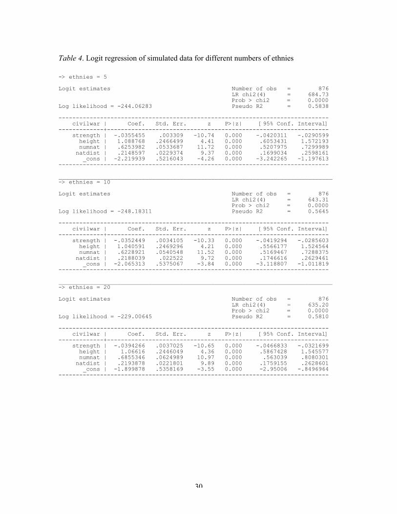
30

Table 4. Logit regression of simulated data for different numbers of ethnies

-> ethnies = 5



_______________________________________________________________________________-> ethnies = 10



_______________________________________________________________________________-> ethnies = 20


------------------------------------------------------------------------------ civilwar | Coef. Std. Err. z P>|z| [95% Conf. Interval]-------------+---------------------------------------------------------------- strength | -.0394266 .0037025 -10.65 0.000 -.0466833 -.0321699 height | 1.06616 .2446049 4.36 0.000 .5867428 1.545577 numnat | .6855346 .0624989 10.97 0.000 .563039 .8080301 natdist | .2193878 .0221801 9.89 0.000 .1759155 .2628601 _cons | -1.899878 .5358169 -3.55 0.000 -2.95006 -.8496964------------------------------------------------------------------------------

31

Table 5. Logit regression of simulated data for different levels of cultural drift

-> cultdrift = .05


------------------------------------------------------------------------------ civilwar | Coef. Std. Err. z P>|z| [95% Conf. Interval]-------------+---------------------------------------------------------------- strength | -.0351794 .0030546 -11.52 0.000 -.0411662 -.0291926 height | .5793565 .2226304 2.60 0.009 .143009 1.015704 numnat | .5988918 .0484734 12.36 0.000 .5038856 .6938979 natdist | .2279549 .0215041 10.60 0.000 .1858076 .2701021 _cons | -1.420225 .4694404 -3.03 0.002 -2.340312 -.500139------------------------------------------------------------------------------

_______________________________________________________________________________-> cultdrift = .1



_______________________________________________________________________________-> cultdrift = .2



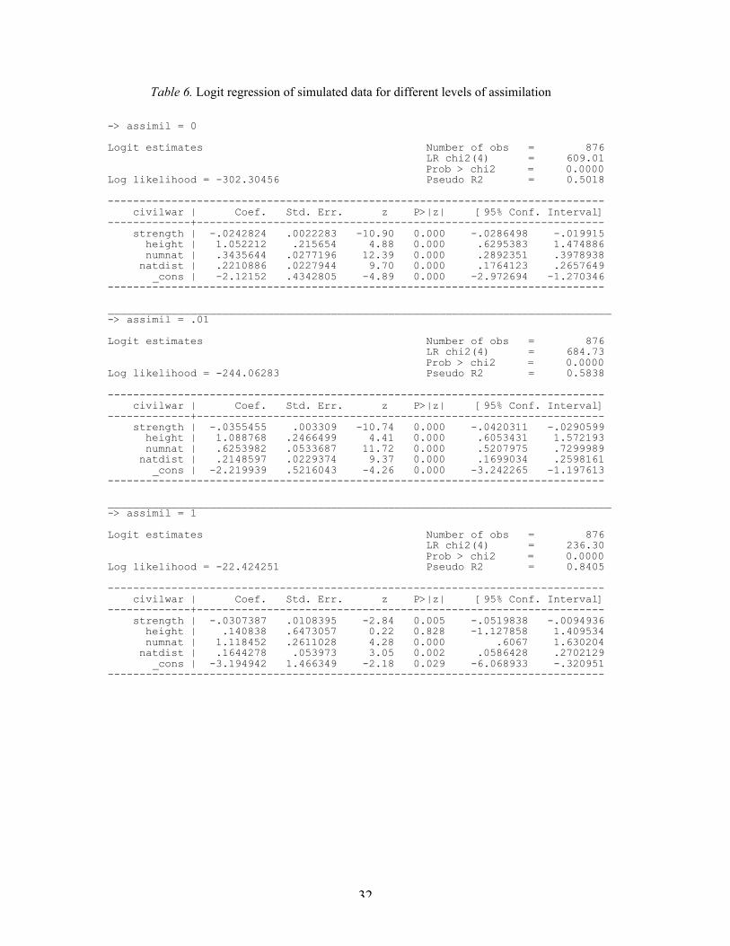
32

Table 6. Logit regression of simulated data for different levels of assimilation

-> assimil = 0



_______________________________________________________________________________-> assimil = .01



_______________________________________________________________________________-> assimil = 1


------------------------------------------------------------------------------ civilwar | Coef. Std. Err. z P>|z| [95% Conf. Interval]-------------+---------------------------------------------------------------- strength | -.0307387 .0108395 -2.84 0.005 -.0519838 -.0094936 height | .140838 .6473057 0.22 0.828 -1.127858 1.409534 numnat | 1.118452 .2611028 4.28 0.000 .6067 1.630204 natdist | .1644278 .053973 3.05 0.002 .0586428 .2702129 _cons | -3.194942 1.466349 -2.18 0.029 -6.068933 -.320951------------------------------------------------------------------------------

33

Table 7. Logit regression of simulated data for different levels of identity exclusiveness

-> mintrait = 3



_______________________________________________________________________________-> mintrait = 4



_______________________________________________________________________________-> mintrait = 5


------------------------------------------------------------------------------ civilwar | Coef. Std. Err. z P>|z| [95% Conf. Interval]-------------+---------------------------------------------------------------- strength | -.0435819 .0040276 -10.82 0.000 -.051476 -.0356879 height | 1.274015 .2512904 5.07 0.000 .7814951 1.766535 numnat | .9050021 .0783536 11.55 0.000 .7514318 1.058572 natdist | .2011718 .0218794 9.19 0.000 .158289 .2440546 _cons | -2.106222 .5412945 -3.89 0.000 -3.16714 -1.045304------------------------------------------------------------------------------

34

Figures

Figure 1. Varied terrain inhabited by 30 states at time at the end of Phase I.

35

Figure 2. A cultural map shown together with mountain contours at the end of Phase I.

36

Proportionof power

Adjusted Distance from capital

Figure 3. Terrain-adjusted loss-of-strength gradient affecting power extraction andprojection.

37

Figure 4. The system at the end of Phase II, after some consolidation and assimilation.

38

Figure 5. Mobilized populations after the end of Phase III.

39

Figure 6. Civil wars raging in two multinational states during Phase IV (see red rings).

Articulating the Geo-Cultural Logic of Nationalist Insurgency

Documents

Transcript of Articulating the Geo-Cultural Logic of Nationalist Insurgency