Aries Community Scale Biorefineries
397
California Energy Commission Clean Transportation Program FINAL PROJECT REPORT Aries Community Scale Biorefineries Optimizing Distributed Biofuel and Bioenergy Production Systems Prepared for: California Energy Commission Prepared by: Biodiesel Industries, Inc. (Biodico Sustainable Biorefineries) December 2021 |CEC-600-2021-050
-
Upload
khangminh22 -
Category
Documents
-
view
0 -
download
0
Transcript of Aries Community Scale Biorefineries

California Energy Commission Clean Transportation Program
FINAL PROJECT REPORT
Aries Community Scale Biorefineries Optimizing Distributed Biofuel and Bioenergy Production Systems
Prepared for: California Energy Commission
Prepared by: Biodiesel Industries, Inc. (Biodico Sustainable Biorefineries)
December 2021 |CEC-600-2021-050

California Energy Commission
Russell T. Teall III Russell (Trey) Teall IV Primary Author(s)
Biodico, Inc. 426 Donze Ave. Santa Barbara, CA 93101 The Biodico Website (www.biodico.com)
Agreement Number: ARV-10-024
Akasha Kaur Khalsa Commission Agreement Manager
Elizabeth John Office Manager ADVANCED FUELS AND VEHICLE TECHNOLOGIES OFFICE
Hannon Rasool Deputy Director FUELS AND TRANSPORTATION
Drew Bohan Executive Director
DISCLAIMER This report was prepared as the result of work sponsored by the California Energy Commission (CEC). It does not necessarily represent the views of the CEC, its employees, or the State of California. The CEC, the State of California, its employees, contractors, and subcontractors make no warrant, express or implied, and assume no legal liability for the information in this report; nor does any party represent that the use of this information will not infringe upon privately owned rights. This report has not been approved or disapproved by the CEC nor has the CEC passed upon the accuracy or adequacy of the information in this report.

i
ACKNOWLEDGEMENTS
Biodiesel Industries, Inc. (“Biodico”) would like to express its gratitude and appreciation to the following individuals for their contributions to the creation of this report.
California Energy Commission Agreement Managers
We have had the benefit of having our project administered by five separate Commission Agreement Managers and an Auditor, each with their particular approach to our work. Although the transition of Commission Agreement Managers has been trying at times, we appreciate the dedication, sincerity and professionalism with which they each approached this project. They are, in order of succession:
• Joanne Vinton • Michael Poe • Pilar Magaña • Phil Dyer • Phil Cazel • Akasha Kaur Khalsa
Project Collaborators
We have also had an exceptional team of collaborators on this project that have helped to make the project successful:
Biodico: JJ Rothgery, COB; Christy Teall, editor; Zac Wright and Abel Monzon, technicians; Drew Quine and Kelly Carpenter, interns Cal Poly, San Luis Obispo: Dr. Tryg Lundquist and Ruth Spierling Invensys: Derek Hook, Mike Ferguson and Mark Demick JAL Engineering: Dr. James Latty Naval Facilities Engineering & Expeditionary Warfare Center: Bruce Holden, Kyle Lawrence, Jill Lomeli, Jennie Dummer, Vern Novstrup and Chris Leksono Red Rock Ranch: John Diener, Jim Tischer and Ken Penfold UC Davis: Dr. Krassi Hristova and Tee Prattapon
ii
PREFACE
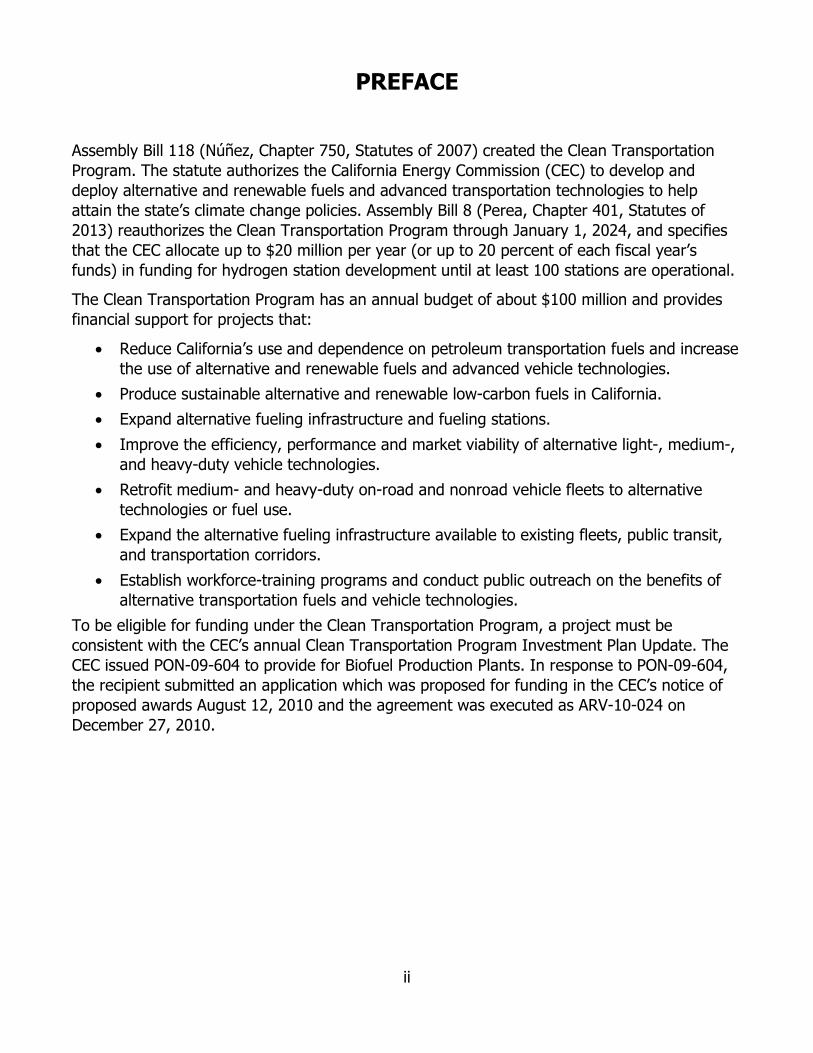
Assembly Bill 118 (Núñez, Chapter 750, Statutes of 2007) created the Clean Transportation Program. The statute authorizes the California Energy Commission (CEC) to develop and deploy alternative and renewable fuels and advanced transportation technologies to help attain the state’s climate change policies. Assembly Bill 8 (Perea, Chapter 401, Statutes of 2013) reauthorizes the Clean Transportation Program through January 1, 2024, and specifies that the CEC allocate up to $20 million per year (or up to 20 percent of each fiscal year’s funds) in funding for hydrogen station development until at least 100 stations are operational.
The Clean Transportation Program has an annual budget of about $100 million and provides financial support for projects that:
• Reduce California’s use and dependence on petroleum transportation fuels and increase the use of alternative and renewable fuels and advanced vehicle technologies.
• Produce sustainable alternative and renewable low-carbon fuels in California. • Expand alternative fueling infrastructure and fueling stations. • Improve the efficiency, performance and market viability of alternative light-, medium-,
and heavy-duty vehicle technologies. • Retrofit medium- and heavy-duty on-road and nonroad vehicle fleets to alternative
technologies or fuel use. • Expand the alternative fueling infrastructure available to existing fleets, public transit,
and transportation corridors. • Establish workforce-training programs and conduct public outreach on the benefits of
alternative transportation fuels and vehicle technologies. To be eligible for funding under the Clean Transportation Program, a project must be consistent with the CEC’s annual Clean Transportation Program Investment Plan Update. The CEC issued PON-09-604 to provide for Biofuel Production Plants. In response to PON-09-604, the recipient submitted an application which was proposed for funding in the CEC’s notice of proposed awards August 12, 2010 and the agreement was executed as ARV-10-024 on December 27, 2010.

iii
ABSTRACT
The Automated Remote Real-time Integrated Energy System: Community Scaled Bioenergy System Project investigated a single saltwater crustacean that eats saltwater algae as feedstock for biodiesel production, and biodiesel co-products as anaerobic digestion feedstock. The project also developed the methodology for biodiesel reaction monitoring in-situ and quality control by spectroscopy.
The goals of ARV-10-024 were to: (1) reduce GHG emissions by eighty percent over petroleum diesel; (2) reduce operating costs by 65 percent; and (3) improve revenues by 200 percent over conventional biodiesel production.
The objectives were to improve the economic viability and sustainability of biodiesel production systems through stable low-cost feedstock supply, reduced operating costs, reduced GHG emissions, reduced air toxics and water waste, additional revenue from renewable energy production, and incorporating stakeholder feedback.
The results of ARV-10-024 showed that (a) the biodiesel production process can be optimized through the use of byproducts to produce renewable combined heat and power, (b) effluent from anaerobic digestion and glycerin bottoms from biodiesel production can be used to enhance algaculture populations of Artemia franciscana and enhance anaerobic digestion, (c) GHG can be substantially reduced with increased sustainability bringing the carbon intensity of Artemia franciscana oil biodiesel to -1.43 gCO2e/MJ (d) feedstock costs, Capital Expenditures and Opex can be reduced and profits enhanced through Artemia franciscana, process automation and additional revenue streams, (e) distributed generation controlled by the Automated system is a worthwhile business model ready for a commercial feasibility study, (f) biodiesel batch production is much faster with spectroscopy, and (g) documentation for ARV-10-024 is valuable for technical training with complete instructions for biodiesel testing analysis and in-depth chemical content in plain English.
This is the first system of distributed biofuel and bioenergy production to have remote access and monitoring for key systems components.
Keywords: California Energy Commission, biofuel, biodiesel, biogas, anaerobic digestion, sustainability, renewable combined heat and power, greenhouse gases, algae, algaculture, process automation, brine shrimp, ARIES©.
Please use the following citation for this report: Teall, Russell T. III, Teall, Russell T. IV (Trey), Biodico Sustainable Biorefineries. 2021. ARIES
Community Scale Biorefinery. California Energy Commission. Publication Number: CEC-600-2021-050

iv
v
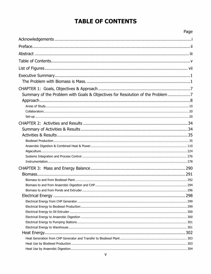
TABLE OF CONTENTS Page
Acknowledgements .............................................................................................................. i Preface ............................................................................................................................... ii Abstract ............................................................................................................................ iii Table of Contents................................................................................................................ v
List of Figures ................................................................................................................... vii Executive Summary ............................................................................................................. 1
The Problem with Biomass is Mass. ................................................................................... 1
CHAPTER 1: Goals, Objectives & Approach .......................................................................... 7 Summary of the Problem with Goals & Objectives for Resolution of the Problem .................. 7 Approach ......................................................................................................................... 8
Areas of Study ...................................................................................................................................................... 10 Collaborators ........................................................................................................................................................ 20 Set-up ................................................................................................................................................................. 20
CHAPTER 2: Activities and Results .................................................................................... 34 Summary of Activities & Results ...................................................................................... 34 Activities & Results ......................................................................................................... 35
Biodiesel Production .............................................................................................................................................. 35 Anaerobic Digestion & Combined Heat & Power ..................................................................................................... 110 Algaculture ......................................................................................................................................................... 224 Systems Integration and Process Control .............................................................................................................. 276 Instrumentation .................................................................................................................................................. 278
CHAPTER 3: Mass and Energy Balance ............................................................................ 290 Biomass ....................................................................................................................... 291
Biomass to and from Biodiesel Plant ..................................................................................................................... 292 Biomass to and from Anaerobic Digestion and CHP ................................................................................................ 294 Biomass to and from Ponds and Extruder .............................................................................................................. 296
Electrical Energy .......................................................................................................... 298 Electrical Energy from CHP Generator ................................................................................................................... 299 Electrical Energy to Biodiesel Production ............................................................................................................... 299 Electrical Energy to Oil Extruder ........................................................................................................................... 300 Electrical Energy to Anaerobic Digestion ............................................................................................................... 300 Electrical Energy to Pumping Stations ................................................................................................................... 301 Electrical Energy to Warehouse ............................................................................................................................ 301
Heat Energy ................................................................................................................. 302 Heat Generation from CHP Generator and Transfer to Biodiesel Plant ...................................................................... 303 Heat Use by Biodiesel Production ......................................................................................................................... 303 Heat Use by Anaerobic Digestion.......................................................................................................................... 304
vi
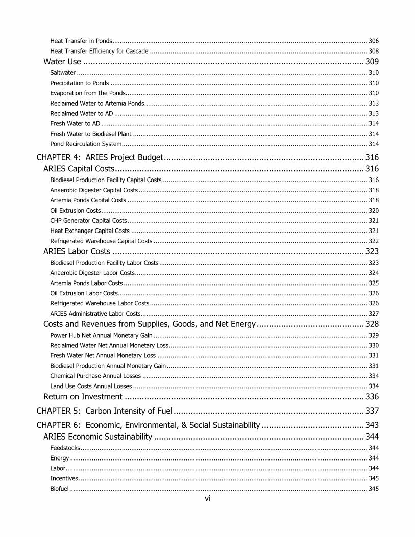
Heat Transfer in Ponds ........................................................................................................................................ 306 Heat Transfer Efficiency for Cascade .................................................................................................................... 308
Water Use ................................................................................................................... 309 Saltwater ........................................................................................................................................................... 310 Precipitation to Ponds ......................................................................................................................................... 310 Evaporation from the Ponds ................................................................................................................................. 310 Reclaimed Water to Artemia Ponds ....................................................................................................................... 313 Reclaimed Water to AD ....................................................................................................................................... 313 Fresh Water to AD .............................................................................................................................................. 314 Fresh Water to Biodiesel Plant ............................................................................................................................. 314 Pond Recirculation System ................................................................................................................................... 314
CHAPTER 4: ARIES Project Budget .................................................................................. 316 ARIES Capital Costs ...................................................................................................... 316
Biodiesel Production Facility Capital Costs ............................................................................................................. 316 Anaerobic Digester Capital Costs .......................................................................................................................... 318 Artemia Ponds Capital Costs ................................................................................................................................ 318 Oil Extrusion Costs .............................................................................................................................................. 320 CHP Generator Capital Costs ................................................................................................................................ 321 Heat Exchanger Capital Costs .............................................................................................................................. 321 Refrigerated Warehouse Capital Costs .................................................................................................................. 322
ARIES Labor Costs ....................................................................................................... 323 Biodiesel Production Facility Labor Costs ............................................................................................................... 323 Anaerobic Digester Labor Costs ............................................................................................................................ 324 Artemia Ponds Labor Costs .................................................................................................................................. 325 Oil Extrusion Labor Costs ..................................................................................................................................... 326 Refrigerated Warehouse Labor Costs .................................................................................................................... 326 ARIES Administrative Labor Costs......................................................................................................................... 327
Costs and Revenues from Supplies, Goods, and Net Energy ............................................ 328 Power Hub Net Annual Monetary Gain .................................................................................................................. 329 Reclaimed Water Net Annual Monetary Loss .......................................................................................................... 330 Fresh Water Net Annual Monetary Loss ................................................................................................................ 331 Biodiesel Production Annual Monetary Gain ........................................................................................................... 331 Chemical Purchase Annual Losses ........................................................................................................................ 334 Land Use Costs Annual Losses ............................................................................................................................. 334
Return on Investment .................................................................................................. 336
CHAPTER 5: Carbon Intensity of Fuel .............................................................................. 337
CHAPTER 6: Economic, Environmental, & Social Sustainability .......................................... 343 ARIES Economic Sustainability ...................................................................................... 344
Feedstocks ......................................................................................................................................................... 344 Energy ............................................................................................................................................................... 344 Labor ................................................................................................................................................................. 344 Incentives .......................................................................................................................................................... 345 Biofuel ............................................................................................................................................................... 345
vii
ARIES Environmental Sustainability ............................................................................... 345 Feedstocks ......................................................................................................................................................... 345 Energy ............................................................................................................................................................... 346 Labor ................................................................................................................................................................. 346 Incentives .......................................................................................................................................................... 346 Biofuel ............................................................................................................................................................... 346
ARIES Social Sustainability ............................................................................................ 347 Feedstocks ......................................................................................................................................................... 347 Labor ................................................................................................................................................................. 347 Incentives .......................................................................................................................................................... 348 Biofuel ............................................................................................................................................................... 348
CHAPTER 7: Results ....................................................................................................... 349 Observations ................................................................................................................ 353
Biodiesel Production ............................................................................................................................................ 353 Anaerobic Digestion ............................................................................................................................................ 353 Artemia Ponds .................................................................................................................................................... 353
Projections ................................................................................................................... 354 Mass and Energy Balance .................................................................................................................................... 354 Budget .............................................................................................................................................................. 354 Carbon Intensity ................................................................................................................................................. 354
Summary of Assessment ............................................................................................... 354 Assessment of Advancements and Achievement of Goals & Objectives ............................ 355
Goals Measured and Analyzed Using Economic & Environmental Pro Formas ............................................................ 355 Reduce Operating Costs by 65 percent ................................................................................................................. 357 Improve Revenues by 200 percent Over Conventional Biodiesel Production .............................................................. 359 Stakeholder Feedback ......................................................................................................................................... 359 Project Accomplishments & Projected Performance ................................................................................................ 361
CHAPTER 8: Recommendations ...................................................................................... 364 Demonstration Scale ARIES .......................................................................................... 364 Relief for Stranded AD Assets ....................................................................................... 364 Increase Biodiesel Feedstock Research .......................................................................... 365
Glossary ......................................................................................................................... 367
References ..................................................................................................................... 371
LIST OF FIGURES Page
Figure 1: Functional Components ......................................................................................... 1

viii
Figure 2: Summary of Activities ........................................................................................... 4
Figure 3: Summary of Observations & Conclusions ................................................................ 5
Figure 4: Summary of Assessment ....................................................................................... 6
Figure 5: Summary of Assessment ....................................................................................... 8
Figure 6: ARIES Functional Components ............................................................................... 9
Figure 7: Processing Feedstock to Produce Triglycerides & Oilseed Solids ............................. 10
Figure 8: Testing Times for FTIR versus GC ........................................................................ 11
Figure 9: CHP Process Flow Diagram .................................................................................. 12
Figure 10: Table 8 from Sell Report .................................................................................... 15
Figure 11: COD Calculations for "Baseline Feedstock" in Sell Report ..................................... 16
Figure 12: Demonstration of 3rd Party Prototype Scale AD Units .......................................... 17
Figure 13: Comparison of Oil Yields from DOE .................................................................... 18
Figure 14: Algae & Brine Shrimp Symbiosis & System Integration ........................................ 19
Figure 15: Part of the Project Laboratory used for Biodiesel, AD and Algaculture Testing ....... 21
Figure 16: Modular Biodiesel Production Unit ...................................................................... 22
Figure 17: MPU Producing Biodiesel and Glycerin ................................................................ 23
Figure 18: Test Calibration Screen Shot .............................................................................. 24
Figure 19: Setting up AMPTS ............................................................................................. 24
Figure 20: AMPTS Test Matrix for Five Sets of Triplicates ..................................................... 25
Figure 21: Biogas Production Rates .................................................................................... 26
Figure 22: Greenhouse Rooms ........................................................................................... 27
Figure 23: Algae Types Found in Project Aquariums and Totes ............................................ 28
Figure 24: Artemia Franciscana .......................................................................................... 28
Figure 25: Sea Salt and Artemia Franciscana ...................................................................... 29
Figure 26: Design for Above Ground Hoop Greenhouse Algaculture Raceway Ponds .............. 30
Figure 27: Comparison of Lumigrow Light Spectrum............................................................ 31
Figure 28: Invensys Hardware Panel with Programmable Logic Controls and I/O Modules ..... 32
Figure 29: Invensys System Installed and Operating at Red Rock Ranch. ............................. 33
Figure 30: Screen Capture Shot of Invensys Interface for Algaculture .................................. 33
Figure 31: Summary of Activities ........................................................................................ 34
Figure 32: ASTM Specification D6751 for Biodiesel .............................................................. 37
Figure 33: Allowable Standing Wave Configurations in Quantum Mechanics .......................... 38
ix
Figure 34: Unallowable Standing Wave Configuration .......................................................... 38
Figure 35: Carbon Dioxide as a Linear Molecule .................................................................. 39
Figure 36: Water as a Non-Linear Molecule ......................................................................... 39
Figure 37: Allowable Vibrational Modes for Water ............................................................... 40
Figure 38: Infrared Classification Schemes ......................................................................... 40
Figure 39: Analect Diamond MX FTIR Analyzer Used by Biodico ........................................... 42
Figure 40: Spectroscopy Shareware and Freeware .............................................................. 43
Figure 41: 2-D Oleic Acid Methyl Ester Diagram .................................................................. 44
Figure 42: 3-D Oleic Acid Methyl Ester ................................................................................ 44
Figure 43: Transesterification Reaction ............................................................................... 44
Figure 44: α-Linolenic Acid Methyl Ester ............................................................................. 45
Figure 45: γ-Linolenic Acid Methyl Ester ............................................................................. 45
Figure 46: Gas Chromatograph of Different Fatty Acid Profiles ............................................. 46
Figure 47: NIR Spectrogram of Canola Oil Methyl Esters Produced by Biodico at Red Rock Ranch .............................................................................................................................. 47
Figure 48: Third Party Test Results of the High Mono-Unsaturated Reference Fuel ................ 48
Figure 49: Fatty Acid Profile of Edible (not wild) Canola Oil .................................................. 49
Figure 50: ASTM D6751 Independent Lab Report ................................................................ 51
Figure 51: Oxidative Stability Report .................................................................................. 52
Figure 52: Diagrams of the Different Types of Bound Glycerin: Triglycerides, Diglycerides, and Monoglycerides ................................................................................................................. 53
Figure 53: 3-D Representation of a 1-Oleoyl 2-Linoleoyl 3-Oleoyl Triglyceride ....................... 54
Figure 54: 2-D Diagram of Glycerol (Free Glycerin) ............................................................. 54
Figure 55: 3-D Representation of Glycerol .......................................................................... 54
Figure 56: Representative Chromatograph of Biodiesel Testing Performed by ASTM Method D6584 .............................................................................................................................. 55
Figure 57: Expected Analyte Elution Times as a Ratio of Internal Standard Elution Times ...... 56
Figure 58: Diagrams of Methanol, Sodium Methylate, and Potassium Methylate .................... 58
Figure 59: 3-D Representations of Methanol, Sodium Methoxide, and Potassium Methoxide .. 58
Figure 60: Pensky Marten Closed Cup Apparatus for Flash Point .......................................... 59
Figure 61: Chromatographic Resolution of Methanol as Tested by the European Method ....... 59
Figure 62: Formation of Water in Methylate Reaction .......................................................... 60
Figure 63: Methanol Spectrogram ...................................................................................... 61

x
Figure 64: Spectrogram of 25 percent Sodium Methylate in Methanol................................... 61
Figure 65: Potentiometric Titration Definition ...................................................................... 62
Figure 66: Indicator Alcohol Titration ................................................................................. 62
Figure 67: Sodium Hydroxide Titration ............................................................................... 62
Figure 68: 2-D Diagram of Water ....................................................................................... 63
Figure 69: 3-D Representation of Water ............................................................................. 63
Figure 70: Specialized Centrifuge Vial to Test for Trace Volumes of Water ............................ 64
Figure 71: Karl Fischer Moisture Analyzer ........................................................................... 64
Figure 72: Total Moisture Content Calculation ..................................................................... 65
Figure 73: Functional Group Profile of Water ...................................................................... 66
Figure 74: Rancimat Oxidative Stability Analyzer ................................................................. 66
Figure 75: Volatile Fatty Acid Test Calculation ..................................................................... 67
Figure 76: CPA T30 Cloud Point Analyzer ............................................................................ 68
Figure 77: Cetane Analysis Motor and Example of Results ................................................... 69
Figure 78: Fatty Acid Profiles, CFPP, Cetane Number, and Oxidative Stability of Selected Oils 70
Figure 79: Relationship between Cetane and Saturation Profile ............................................ 71
Figure 80: Relationship between CFPP and Saturation Profile ............................................... 71
Figure 81: Biodiesel Testing Time per Batch ....................................................................... 73
Figure 82: General Compositional Analysis during Biodiesel Reaction .................................... 75
Figure 83: Total Amount of Samples Needed ...................................................................... 76
Figure 84: Principle Component Analysis End Points ............................................................ 77
Figure 85: mL of Reference Fuel Calculation ....................................................................... 77
Figure 86: Binary Sample Tree for FTIR Method .................................................................. 78
Figure 87: Fatty Acid Profiles of Reference Fuels ................................................................. 78
Figure 88: In-Spec FTIR Library Samples (1 of 3)................................................................ 80
Figure 89: In-Spec FTIR Library Samples (2 of 3)................................................................ 81
Figure 90: In-Spec FTIR Library Samples (3 of 3)................................................................ 82
Figure 91: Principle Component Combinations in Biodiesel Production .................................. 83
Figure 92: Percent of Sample for Each Part Calculation ........................................................ 84
Figure 93: In-Situ FTIR Matrix ........................................................................................... 87
Figure 94: Component Volumes Needed for In-Situ Test Matrix ........................................... 92
Figure 95: Fatty Acid Profile Library Samples ...................................................................... 93

xi
Figure 96: Sum of Library Fatty Acid Profile ........................................................................ 94
Figure 97: Feedstock Spectrograms by Fatty Acid Profile ..................................................... 96
Figure 98: Magnified Feedstock Spectrograms by Fatty Acid Profile ...................................... 96
Figure 99: Feedstock Spectrograms by Fatty Acid Profile # 2 ............................................... 97
Figure 100: Spectrograms of 10 Oils by Fatty Acid Profile .................................................... 97
Figure 101: Magnified Spectrograms of 10 Oils by Fatty Acid Profile ..................................... 98
Figure 102: Spectrograms of 10 Oils by Fatty Acid Profile # 2 .............................................. 98
Figure 103: Spectrograms of Bound Glycerin (Oil) and Methanol .......................................... 99
Figure 104: Spectrograms of Biodiesel with Methanol and/or Bound Glycerin ...................... 100
Figure 105: Spectrograms of Biodiesel and Free Glycerin ................................................... 100
Figure 106: Spectrograms of Free Glycerin and Methanol .................................................. 101
Figure 107: Spectrograms of Water and Methanol ............................................................. 101
Figure 108: Spectrograms of Bound Glycerin in Biodiesel ................................................... 102
Figure 109: Magnified Spectrograms of Bound Glycerin in Biodiesel ................................... 102
Figure 110: Spectrograms of Free Glycerin in Biodiesel ...................................................... 103
Figure 111: Magnified Spectrograms of Free Glycerin in Biodiesel ...................................... 103
Figure 112: Spectrograms of Free Glycerin, Methanol, and Water (Crude Glycerin) ............. 104
Figure 113: Spectrograms of Methanol in Biodiesel ........................................................... 105
Figure 114: Spectrograms of Water in Biodiesel ................................................................ 105
Figure 115: Magnified Spectrograms of Water in Biodiesel ................................................. 106
Figure 116: Spectrograms of Biodiesel with Trace Contaminants ........................................ 106
Figure 117: Magnified Spectrograms of Biodiesel with Trace Contaminants #1 ................... 107
Figure 118: Magnified Spectrograms of Biodiesel with Trace Contaminants # 2 .................. 107
Figure 119: Spectrograms of Pure Biodiesel Reference Fuels ............................................. 108
Figure 120: Ranges of Unique In-Situ Combinations .......................................................... 109
Figure 121: Glycerol as an Anaerobic Digestion Accelerant and Algaculture Nutrient ............ 110
Figure 122: Relationship between Acidogenic, Acetogenic, and Methanogenic Bacteria........ 111
Figure 123: Glycerin Compositional Analysis ..................................................................... 111
Figure 124: AMPTS Setup at Naval Base Ventura County ................................................... 112
Figure 125: AMPTS Methane Measurement Apparatus ....................................................... 113
Figure 126: Anaerobic Digestion Test Protocols ................................................................. 114
Figure 127: Visual Orientation of Test Setup ..................................................................... 114

xii
Figure 128: COD Calculation ............................................................................................ 116
Figure 129: Test Setup for Chemical Oxygen Demand ....................................................... 116
Figure 130: Ultimate Methane Yield from COD .................................................................. 117
Figure 131: Alkalinity Equation ......................................................................................... 118
Figure 132: Multimeter Setup at Naval Base Ventura County ............................................. 118
Figure 133: Multimeter Probes for Ammonia and pH Testing .............................................. 119
Figure 134: Total Solids Calculation .................................................................................. 120
Figure 135: Higher Precision, Lower Temperature, Laboratory Oven .................................. 120
Figure 136: Fixed Solids Calculation ................................................................................. 120
Figure 137: Volatile Solids Calculation .............................................................................. 121
Figure 138: Higher Temperature, Lower Precision, Muffle Furnace ..................................... 121
Figure 139: AMPTS Test Runs, Results & Multivariate Analysis ........................................... 123
Figure 140: mg of Methane Produced per Triplicate Set per Test Run ................................. 124
Figure 141: Digester Array for Glycerin and Wastewater Treatment Plant Effluent (WWTP) . 125
Figure 142: COD Data for the Glycerin and WWTP Effluent (pre) ....................................... 126
Figure 143: COD Calibration Curve for Glycerin and WWTP Effluent (pre) ........................... 127
Figure 144: COD Test Splits and Spikes for Glycerin and WWTP Effluent (pre) .................... 127
Figure 145: pH and Alkalinity for Glycerin and WWTP Effluent (pre) ................................... 128
Figure 146: Total and Volatile Solids for Glycerin and WWTP Effluent (pre) ........................ 128
Figure 147: Methane Volume per Hour for Glycerin & WWTP Effluent................................. 129
Figure 148: COD Data for Glycerin and WWTP Effluent (post) ............................................ 130
Figure 149: COD Calibration Curve for Glycerin and WWTP Effluent (post) ......................... 131
Figure 150: COD Splits and Spikes for Glycerin & WWTP Effluent (post) ............................. 131
Figure 151: pH and Alkalinity for Glycerin & WWTP Effluent (post) ..................................... 132
Figure 152: Solids for Glycerin & WWTP Effluent (post) ..................................................... 133
Figure 153: AMPTS Array for Castor Meal & Feed Manure Test #1 ..................................... 134
Figure 154: COD Results for Castor Meal and Feed Manure Test #1 (pre) .......................... 135
Figure 155: Splits and Spikes for Castor Meal & Feed Manure Test #1 (pre) ....................... 135
Figure 156: Castor Mead & Feedlot Manure Test #1 COD Calibration (pre) ......................... 136
Figure 157: pH and Alkalinity for Castor Meal & Feedlot Manure Test #1 (pre) ................... 136
Figure 158: Solids Tests by Component for Castor & Feedlot Manure (pre) ......................... 137
Figure 159: Solids Tests for Each Triplicate of Castor Meal & Feedlot Manure (pre) ............. 137
xiii
Figure 160: Cumulative Methane Produced by Castor Meal & Feedlot Manure Test #1 ........ 138
Figure 161: Total Methane Produced by Sample for Castor Meal & Feedlot Manure Test #1 139
Figure 162: COD Values for Castor & Feedlot Manure Test #1 (post) ................................. 140
Figure 163: COD Calibration Curve for Castor Meal & Feedlot Manure Test #1 (post) .......... 141
Figure 164: Splits and Spikes for Castor Meal & Feedlot Manure Test #1 (post) .................. 141
Figure 165: pH and Alkalinity for Castor Meal & Feedlot Manure Test #1 (post) .................. 142
Figure 166: Solids Data for Castor Meal & Feedlot Manure Test #1 (post) .......................... 143
Figure 167: Gas Composition by Gas Chromatography ...................................................... 144
Figure 168: Gas Composition over Time ........................................................................... 144
Figure 169: Digester Array for Castor Meal and Feedlot Manure Test #2 ............................ 145
Figure 170: COD Data for Co-Digestant Test #2 (pre) ....................................................... 146
Figure 171: Calibration Curve for Codigestant Test #2 COD (pre) ...................................... 147
Figure 172: Spikes and Splits for COD of Codigestant Test #2 (pre) ................................... 147
Figure 173: pH and Alkalinity for Co-Digestant Test #2 (pre) ............................................. 148
Figure 174: Co-Substrate Test #2 Solids (pre) .................................................................. 149
Figure 175: Methane Produced per Day by Sample for Co-Digestant Test #2 ...................... 150
Figure 176: Total Methane Produced by Sample in Co-Digestant Test #2 (pre) ................... 151
Figure 177: COD of Co-Digestant Test #2 (post) ............................................................... 152
Figure 178: COD Calibration Curve for Co-Digestant Test #2 (post) ................................... 153
Figure 179: COD Splits and Spikes for Co-Digestant Test #2 (post) .................................... 153
Figure 180: pH and Alkalinity for Co-Substrate Test #2 (post) ........................................... 154
Figure 181: Solids Data for Co-Digestant Test #2 (post) .................................................... 155
Figure 182: Digester Array for Glycerin & Dairy Test ......................................................... 156
Figure 183: COD Results from Dairy & Glycerin Test (pre) ................................................. 157
Figure 184: COD Calibration Curve for Dairy & Glycerin Test (pre) ..................................... 158
Figure 185: COD Splits and Spikes for Glycerin & Dairy (pre) ............................................. 158
Figure 186: Glycerin & Dairy pH & Alkalinity (pre) ............................................................. 159
Figure 187: Solids Data for Glycerin & Dairy Test (pre) ...................................................... 160
Figure 188: Methane Production over Time by Sample for Glycerin & Dairy ........................ 161
Figure 189: Total Methane Produced by Sample for Glycerin & Dairy .................................. 162
Figure 190: COD for Dairy & Manure (post) ...................................................................... 163
Figure 191: COD Calibration for Glycerin & Dairy (post) ..................................................... 164

xiv
Figure 192: COD Splits & Spikes for Glycerin & Dairy (post) ............................................... 164
Figure 193: pH and Alkalinity for Glycerin & Dairy (post) ................................................... 165
Figure 194: Solids for Glycerin & Dairy (post) ................................................................... 166
Figure 195: Sodium Phosphate Monobasic ........................................................................ 167
Figure 196: Sodium Phosphate Dibasic ............................................................................. 168
Figure 197: Digester Array for Glycerin & Yellow Grease Waste Test #1 ............................. 169
Figure 198: COD of Glycerin & Yellow Grease Waste (pre) ................................................. 170
Figure 199: COD Calibration Curve of Glycerin & Yellow Grease Waste (pre) ....................... 171
Figure 200: COD Splits and Spikes for Glycerin & Yellow Grease Waste (pre) ...................... 171
Figure 201: pH and Alkalinity for Glycerin & Yellow Grease Waste Test (pre) ...................... 172
Figure 202: Solids Data for Glycerin and Yellow Grease Waste (pre)................................... 173
Figure 203: Methane Production for Each Sample over Time for Glycerin & Yellow Grease Waste ............................................................................................................................ 174
Figure 204: COD of Glycerin & Yellow Grease Waste (post) ............................................... 175
Figure 205: COD Calibration Curve for Glycerin & Yellow Grease Waste (post) .................... 176
Figure 206: COD Destruction for Glycerin and Yellow Grease Waste ................................... 176
Figure 207: pH and Alkalinity for Glycerin & Yellow Grease Waste (post) ............................ 177
Figure 208: Digester Array for Glycerin & Yellow Grease Waste Test #2 ............................. 178
Figure 209: COD of Glycerin & Yellow Grease Waste Test #2 (pre) .................................... 179
Figure 210: COD Splits and Spikes Glycerin & Yellow Grease Waste Test #2 (pre) .............. 179
Figure 211: COD Calibration Curve of Glycerin & Yellow Grease Waste #2 (pre) ................. 180
Figure 212: pH and Alkalinity for Glycerin & Yellow Grease Waste Test #2 (pre) ................. 181
Figure 213: Methane Production for Each Sample over Time for Glycerin & Yellow Grease Waste Test #2 ................................................................................................................ 182
Figure 214: Methane Production by Sample per 30 Days for Glycerin & Yellow Grease Waste Test #2 .......................................................................................................................... 182
Figure 215: COD of Glycerin & Yellow Grease Waste Test #2 (post) ................................... 183
Figure 216: COD Calibration Curve for Glycerin & Yellow Grease Waste Test #2 (post) ....... 184
Figure 217: pH and Alkalinity for Glycerin & Yellow Grease Waste Test #2 (post) ............... 185
Figure 218: Digester Array for Artemia and Fish Waste Test .............................................. 187
Figure 219: Equation for Determining Sample Composition ................................................ 187
Figure 220: COD of Artemia and Fish Waste Test (pre) ..................................................... 188
Figure 221: COD Calibration Curve of Artemia and Fish Waste Test (pre) ........................... 188
xv
Figure 222: pH and Alkalinity for Artemia and Fish Waste (pre) ......................................... 189
Figure 223: Solids Data for Artemia and Fish Waste (pre) .................................................. 190
Figure 224: Total Methane Produced by Digester for Artemia and Fish Waste Test .............. 191
Figure 225: mL Methane Production over Time for Artemia and Fish Waste Test ................. 192
Figure 226: Methane from Control Samples for Artemia and Fish Waste Test ...................... 193
Figure 227: Equation Conversion Calculation..................................................................... 193
Figure 228: Percent of Total Methane by Component for Artemia and Fish Waste Test ........ 194
Figure 229: Sum Methane Produced by Component for Artemia and Fish Waste Test .......... 195
Figure 230: mL Methane Production per mL of Component for Artemia and Fish Waste Test 196
Figure 231: Total mL Methane by Component for Artemia and Fish Waste Test .................. 197
Figure 232: mL Methane Production over Time for Artemia and Fish Waste Test ................. 198
Figure 233: COD of Artemia and Fish Waste Test (post) .................................................... 199
Figure 234: COD Destruction Rate Formula....................................................................... 199
Figure 235: COD Destruction for Artemia and Fish Waste Test ........................................... 200
Figure 236: pH and Alkalinity for Artemia and Fish Waste Test (post) ................................. 201
Figure 237: Solids Data for Artemia and Fish Waste (post) ................................................ 202
Figure 238: Solids Destruction for Artemia and Fish Waste Test ......................................... 203
Figure 239: mL of Methane per mg/L COD Destruction for Artemia and Fish Waste Test ..... 204
Figure 240: mL of Methane per VS Destruction for Artemia and Fish Waste Test ................. 205
Figure 241: Changes in Energy by Component for Artemia and Fish Waste Test ................. 206
Figure 242: Calculations used in Component Analysis ........................................................ 207
Figure 243: Digester Array for Dairy Manure and Beet Stillage Co-Digestion Test ................ 209
Figure 244: COD of Components for Dairy Manure and Beet Stillage Co-Digestion Test ....... 210
Figure 245: COD of Dairy Manure and Beet Stillage Co-Digestion Test (pre) ....................... 210
Figure 246: COD Calibration Curve of Dairy Manure and Beet Stillage Co-Digestion Test (pre)...................................................................................................................................... 211
Figure 247: pH and Alkalinity for Dairy Manure and Beet Stillage Co-Digestion Test (pre) .... 212
Figure 248: Digester Wheel Clamp ................................................................................... 213
Figure 249: Total Methane Produced by Digester for Dairy Manure and Beet Stillage Co-Digestion Test................................................................................................................. 213
Figure 250: mL Methane Production over Time for Dairy Manure and Beet Stillage Co-Digestion Test ............................................................................................................................... 214
Figure 251: Equation for Positive Rate of Change .............................................................. 215
xvi
Figure 252: Percent Total Methane by Component for Dairy Manure and Beet Stillage Co-Digestion Test................................................................................................................. 216
Figure 253: Sum Methane Produced by Component for Dairy Manure and Beet Stillage Co-Digestion Test................................................................................................................. 216
Figure 254: mL Methane Production per mL of Component for Dairy Manure and Beet Stillage Co-Digestion Test ........................................................................................................... 217
Figure 255: Total mL Methane by Component for Dairy Manure and Beet Stillage Co-Digestion Test ............................................................................................................................... 218
Figure 256: Ultimate Methane Yield Predictions ................................................................. 218
Figure 257: COD of Dairy Manure and Beet Stillage Co-Digestion Test (post) ...................... 219
Figure 258: COD Destruction for Dairy Manure and Beet Stillage Co-Digestion Test ............. 220
Figure 259: pH and Alkalinity for Dairy Manure and Beet Stillage Co-Digestion Test (post) .. 221
Figure 260: Solids Data for Dairy Manure and Beet Stillage Co-Digestion (post) .................. 222
Figure 261: Calculations used in Component Analysis ........................................................ 223
Figure 262: Average Naval Base Ventura County Greenhouse pH ....................................... 228
Figure 263: Algal Density over Time for Different Salinity Levels ........................................ 228
Figure 264: Performance of Different Nutrients on Algal Population Growth ........................ 229
Figure 265: Effects of Glycerin on Algal Growth in Various Nutrient Mediums ...................... 229
Figure 266: Algal Density Resulting from Different Concentrations of Glycerin ..................... 230
Figure 266: Synthetic Nutrient Blend Use 1 ....................................................................... 231
Figure 267: Observed Relationship of Algal Density to Artemia Density............................... 232
Figure 268: Growth Rate of Algal Biomass for Different Light Cycles................................... 232
Figure 269: Increase in Algal Biomass per Increase in Light ............................................... 233
Figure 270: Increase in Artemia Biomass per Increase in Solar Energy ............................... 233
Figure 271: Total Solids Equation ..................................................................................... 234
Figure 272: Solvent Ratios for Lipid Extraction 1 ............................................................... 235
Figure 273: Solvent Ratios for Lipid Extraction 2 ............................................................... 235
Figure 274: Lipid Extraction Separations ........................................................................... 236
Figure 275: Lipid Extraction ............................................................................................. 236
Figure 276: Weight Percent of Lipids in Solution ............................................................... 237
Figure 277: Percent Lipids in Dry Artemia by Weight ......................................................... 237
Figure 278: Percent Lipids in Dry Artemia by Weight 2 ...................................................... 238
Figure 279: Polar Lipid Percentage ................................................................................... 238
xvii
Figure 280: Harvesting Variables ...................................................................................... 239
Figure 281: Harvesting Periods ........................................................................................ 240
Figure 282: Standard Deviation of Drop Samples .............................................................. 241
Figure 283: Changes in Standard Deviation by Averaged Samples ...................................... 241
Figure 284: Improved Standard Deviation of Drop Samples ............................................... 241
Figure 285: Keco Model 800 Dual Diaphragm Pump .......................................................... 242
Figure 286: Recirculation Characteristics for Discrete Chunks of Volume ............................. 243
Figure 287: Recirculation Characteristics for Continuous Flow ............................................ 243
Figure 288: General Calculation for Continuous Systems .................................................... 243
Figure 289: Table of Commonly Used Conversions ............................................................ 244
Figure 290: Tote Dimensions ........................................................................................... 244
Figure 291: Conversion from Liters to Acres ..................................................................... 245
Figure 292: Weekly Kilograms to Annual Kilograms per Acre .............................................. 245
Figure 293: Kilograms of Dry Biomass to Gallons of Artemia Oil ......................................... 245
Figure 294: Weekly Dry Biomass Yields ............................................................................ 246
Figure 295: Incremental Portion of Artemia Populations Captured by Micron Size of Harvesting Net ................................................................................................................................ 247
Figure 296: Feed Rates for Artemia Nutrient Harvesting .................................................... 249
Figure 297: Average Artemia Oil by Days between Harvests .............................................. 251
Figure 298: Algaculture Coefficients ................................................................................. 252
Figure 299: Generalized Multivariate Linear Regression Equation ....................................... 253
Figure 300: Coefficients & Variables for Linear Regression ................................................. 253
Figure 301: Multivariate Linear Regression Equation .......................................................... 253
Figure 302: Multivariate Linear Regression Data Table ...................................................... 254
Figure 303: Multivariate Polynomial Regression Coefficients Without Solar .......................... 256
Figure 304: Davis Vantage Pro2 Weather Station .............................................................. 256
Figure 305: Solar Insolation per Day for 2013 at Naval Base Ventura County ...................... 257
Figure 306: Table from Coutteau and Sorgeloos Study ...................................................... 259
Figure 307: Coutteau and Sorgeloos Unit Conversion ........................................................ 260
Figure 308: Algal Weight to Artemia Weight for Adult Populations ...................................... 260
Figure 309: Conversion Table for Gallons per Acre to Joules per Square Meter ................... 261
Figure 310: Solar Energy to Algal Biomass Conversion....................................................... 262
xviii
Figure 311: Final Coefficient Set for Multivariate Polynomial Regression ............................. 262
Figure 312: Raw Data from Regression Analysis ................................................................ 263
Figure 313: Optimum Value Calculation for Polynomial Variables ........................................ 264
Figure 314: Comparison between Greenhouse Scale Optimum Values and Laboratory Findings...................................................................................................................................... 264
Figure 315: Nutrient Coefficients and Optimum Levels ....................................................... 265
Figure 316: Artemia Oil Yields from Nutrients ................................................................... 266
Figure 317: Best Case Calculations from Established Optimum Values ................................ 267
Figure 318: Comparison of Calculated and Observed Values .............................................. 267
Figure 319: Tote Harvest Data 1 ...................................................................................... 268
Figure 320: Tote Harvest Data 2 ...................................................................................... 269
Figure 321: Tote Harvest Data 3 ...................................................................................... 270
Figure 322: Tote Harvest Data 4 ...................................................................................... 271
Figure 323: Tote Harvest Data 5 ...................................................................................... 272
Figure 324: Tote Harvest Data 6 ...................................................................................... 273
Figure 325: Projected Daily Artemia Oil per Acre for 2013 ................................................. 274
Figure 326: Monthly Artemia Oil Production per Acre ......................................................... 274
Figure 327: Optimum Effluent Demands for Artemia per Acre ............................................ 275
Figure 328: Theoretical Maximums ................................................................................... 275
Figure 329: ARIES I/O Points 1 ........................................................................................ 277
Figure 330: ARIES I/O Points 2 ........................................................................................ 278
Figure 331: ARIES Probes ................................................................................................ 279
Figure 332: ARIES Temperature Probe ............................................................................. 279
Figure 333: Transmitter for Probe Signal Conditioning ....................................................... 280
Figure 334: Float Valves for Water Level .......................................................................... 280
Figure 335: GUI Interface for Biodico Algaculture and Anaerobic Digesters ......................... 281
Figure 336: Biodico GUI for Gasifier in Online State ........................................................... 282
Figure 337: Biodico GUI for Gasifier in Offline State .......................................................... 282
Figure 338: Biodico GUI for Trend Analysis ....................................................................... 283
Figure 339: Biodico I/O GUI............................................................................................. 284
Figure 340: Amazon Web Services Cloud Management Console ......................................... 286
Figure 341: Devices and Communications protocols for SoftEther ...................................... 286
xix
Figure 342: FTIR6.IP.Demo ............................................................................................. 287
Figure 343: SoftEther VPN ............................................................................................... 287
Figure 344: Manage VPN Server “localhost” ...................................................................... 288
Figure 345: Open Remote Desktop File ............................................................................ 288
Figure 346: SoftEther VPN Client Manager ........................................................................ 289
Figure 347: Accessing Biodico on the Cloud ...................................................................... 289
Figure 348: Process Flow Diagram (PFD) for ARIES ........................................................... 290
Figure 349: Process Flow Diagram (PFD) Coding Table ...................................................... 291
Figure 350: Biomass Lines for PFD ................................................................................... 292
Figure 351: Artemia Fatty Acid Profile .............................................................................. 292
Figure 352: Biomass Weights for Biodiesel Production ....................................................... 293
Figure 353: Elemental Composition for Biodiesel Production .............................................. 293
Figure 354: Elemental Weights for Biodiesel Production ..................................................... 294
Figure 355: Elemental Weights by Percentage for Biodiesel Production ............................... 294
Figure 356: Biomass Weights for AD ................................................................................ 295
Figure 357: Elemental Composition for AD ........................................................................ 295
Figure 358: Elemental Weights for AD .............................................................................. 295
Figure 359: Elemental Weights by Percentage for AD ........................................................ 296
Figure 360: Biomass Weights for Artemia Ponds ............................................................... 296
Figure 361: Elemental Composition for Artemia Ponds ....................................................... 297
Figure 362: Elemental Weights for Artemia Ponds ............................................................. 297
Figure 363: Elemental Weights by Percentage for Artemia Ponds ....................................... 298
Figure 364: Electrical Energy Lines for PFD ....................................................................... 298
Figure 365: Electrical Energy Generation from CHP ........................................................... 299
Figure 366: Electrical Energy Use for Biodiesel Production ................................................. 299
Figure 367: Electrical Use for Extrusion ............................................................................ 300
Figure 368: Electrical Use for AD ...................................................................................... 301
Figure 369: Electrical Use for Pumping Station .................................................................. 301
Figure 370: Electricity Use for Refrigerated Warehouse ..................................................... 302
Figure 371: Heat Cascade Layout for ARIES...................................................................... 303
Figure 372: Heat Generation to Heat Exchanger ............................................................... 303
Figure 373: Heat Requirements for Biodiesel Production .................................................... 304

xx
Figure 374: Heat Increase Requirements for AD Influent ................................................... 305
Figure 375: Heat Loss for AD ........................................................................................... 306
Figure 376: Heat Transfer Balance for AD ......................................................................... 306
Figure 377: Heat Transfer for Artemia Ponds .................................................................... 308
Figure 378: Minimum Heat Cascade Efficiency for ARIES ................................................... 309
Figure 379: Water Flows for ARIES .................................................................................. 309
Figure 380: Precipitation for Five Points, CA ..................................................................... 310
Figure 381: Annual Precipitation of Southwestern US ........................................................ 311
Figure 382: Precipitation Loss by Percent for Southwestern US .......................................... 311
Figure 383: Evapotranspiration Rates for Southwestern US ................................................ 312
Figure 384: Annual Evaporation from Artemia Ponds ......................................................... 312
Figure 385: Reclaimed Water Use for Artemia Ponds ......................................................... 313
Figure 386: Reclaimed Water Use for Anaerobic Digestion ................................................. 314
Figure 387: Fresh Water Input for Biodiesel Production ..................................................... 314
Figure 388: Water Flow for Pond Recirculation System ...................................................... 315
Figure 389: Summary of Capital Expenses for ARIES ......................................................... 316
Figure 390: Biodiesel Plant Capital Expenses ..................................................................... 317
Figure 391: Time Savings from FTIR ................................................................................ 317
Figure 392: AD Capital Expenses ...................................................................................... 318
Figure 393: Artemia Pond Capital Expenses ...................................................................... 319
Figure 394: ARIES Pond Design ....................................................................................... 319
Figure 395: Data Broadcasting Hub .................................................................................. 320
Figure 396: Oil Extrusion Capital Expenses ....................................................................... 321
Figure 397: Generator Capital Expenses ........................................................................... 321
Figure 398: Heat Exchanger Capital Expenses ................................................................... 322
Figure 399: Refrigerated Warehouse Capital Expenses ...................................................... 323
Figure 400: Summary of Labor Costs for ARIES ................................................................ 323
Figure 401: Biodiesel Production Labor Costs .................................................................... 324
Figure 402: AD Labor Costs for ARIES .............................................................................. 325
Figure 403: Artemia Pond Labor Costs for ARIES .............................................................. 326
Figure 404: Oil Extrusion Labor Costs for ARIES ................................................................ 326
Figure 405: Refrigerated Warehouse Labor Costs for ARIES ............................................... 327

xxi
Figure 406: Administrative Labor Costs for ARIES ............................................................. 328
Figure 407: Supplies, Goods, and Net Energy Profile for ARIES .......................................... 329
Figure 408: Electricity Rates for Five Points Zip Code ........................................................ 329
Figure 409: Electricity Inputs for ARIES ............................................................................ 330
Figure 410: Reclaimed Water Inputs for ARIES ................................................................. 330
Figure 411: Fresh Water Inputs for ARIES ........................................................................ 331
Figure 412: Revenues from Biodiesel ................................................................................ 331
Figure 413: Artemia Composition by Weight ..................................................................... 332
Figure 414: Composition Percent of Artemia and Other Animal Feeds ................................. 332
Figure 415: Fish Meal Prices ............................................................................................ 333
Figure 416: Soybean Meal Prices ...................................................................................... 333
Figure 417: Artemia Meal Outputs from Biodiesel Production ............................................. 334
Figure 418: Major Chemical Inputs to Biodiesel Production ................................................ 334
Figure 419: Irrigated and Non-Irrigated Cropland Average Value per Acre .......................... 335
Figure 420: Crop Land Value and Cash Rental Rate ........................................................... 335
Figure 421: Land Use for ARIES ....................................................................................... 336
Figure 422: ROI for ARIES ............................................................................................... 336
Figure 423: ROI Without Meal Revenue ............................................................................ 336
Figure 424: GHG Emission Comparison ............................................................................. 338
Figure 425: Coproduct Credit for Biodiesel ........................................................................ 341
Figure 426: GHG Emissions from Biodiesel Production ....................................................... 342
Figure 427: Sustainability Summary ................................................................................. 343
Figure 428: Economic Sustainability ................................................................................. 344
Figure 429: Environmental Sustainability .......................................................................... 345
Figure 430: ULSD Displacement ....................................................................................... 347
Figure 431: Social Sustainability ....................................................................................... 347
Figure 432: Demographics ............................................................................................... 348
Figure 433: CA Diesel Taxes in Cents per Gallon ............................................................... 348
Figure 434: Total GHG Reductions from ARIES ................................................................. 349
Figure 435: Cost per Ton GHG Emissions .......................................................................... 350
Figure 436: Summary of Assessment ................................................................................ 355
Figure 437: GHG Emissions for Various Methyl Esters ........................................................ 356

xxii
Figure 438: Total GHG Reductions from ARIES ................................................................. 356
Figure 439: Cost per Ton GHG Emissions .......................................................................... 357
Figure 440: ARIES Biodiesel Cost per Gallon ..................................................................... 357
Figure 441: Traditional Biodiesel Plant Operating Costs ..................................................... 358
Figure 442: Soybean Oil Commodity Prices ....................................................................... 358
Figure 443: Biodiesel Revenues ....................................................................................... 359
Figure 444: Revenue Comparison ..................................................................................... 359
Figure 445: Summary of Outreach Activities ..................................................................... 360
Figure 446: 100,000 GPY Biodiesel MPUs .......................................................................... 361
Figure 447: W8 & AMPTS Anaerobic Digester Units ........................................................... 362
Figure 448: Differences between AD Units ........................................................................ 362
Figure 449: Performed vs Proposed Artemia Ponds ........................................................... 363
Figure 450: California Renewable Electricity Generation “Duck Curve” 2013 ........................ 364

1
EXECUTIVE SUMMARY The conventional model for fuel and energy production relies upon large centralized facilities supported by bulk access to raw materials (crude oil, coal, reservoirs, natural gas). Biomass can be better served by a distributed model.
The Problem with Biomass is Mass. Renewable biomass requires acres of feedstock production that must be harvested and delivered to the processing facility. The larger the facility, the larger the area that needs to be harvested, and the further the transportation distance. Smaller, distributed facilities can mitigate transportation costs, but they generally suffer from diseconomies of scale. The challenge is to enable the networking of distributed facilities to achieve the economies of a much larger scale facility. For biofuel to become a mainstream fuel, competitive with petroleum, biofuel production will require stable sources of local, low-cost feedstocks, value added co-products, efficient operations, exacting quality control, and a minimal environmental footprint.
The goal of ARV-10-024 was to improve the economic, social and environmental sustainability of biodiesel production. The approach is best described as the Automated Remote real-time Integrated Energy System. As shown in Figure 1, this system is composed of four functional components: (1) biodiesel production, (2) anaerobic digestion with combined heat and power, (3) algaculture, and (4) system integration and process control. Each of these components was the subject of research, demonstration and optimization as part of this project.
Figure 1: Functional Components
Illustration Credit: Biodico, Inc.
(1) Biodiesel production requires feedstocks (bio-oil), heat, and power; and generates solid and liquid byproducts in the form of glycerin bottoms, wash water, and oilseed solids.
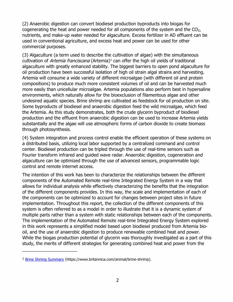
2
(2) Anaerobic digestion can convert biodiesel production byproducts into biogas for cogenerating the heat and power needed for all components of the system and the CO2, nutrients, and make-up water needed for algaculture. Excess fertilizer in AD effluent can be used in conventional agriculture, and excess heat and power can be used for other commercial purposes.
(3) Algaculture (a term used to describe the cultivation of algae) with the simultaneous cultivation of Artemia franciscana (Artemia)1 can offer the high oil yields of traditional algaculture with greatly enhanced stability. The biggest barriers to open pond algaculture for oil production have been successful isolation of high oil strain algal strains and harvesting. Artemia will consume a wide variety of different microalgae (with different oil and protein compositions) to produce much more consistent volumes of oil and can be harvested much more easily than unicellular microalgae. Artemia populations also perform best in hypersaline environments, which naturally allow for the bioexclusion of filamentous algae and other undesired aquatic species. Brine shrimp are cultivated as feedstock for oil production on site. Some byproducts of biodiesel and anaerobic digestion feed the wild microalgae, which feed the Artemia. As this study demonstrates, both the crude glycerin byproduct of biodiesel production and the effluent from anaerobic digestion can be used to increase Artemia yields substantially and the algae will use atmospheric forms of carbon dioxide to create biomass through photosynthesis.
(4) System integration and process control enable the efficient operation of these systems on a distributed basis, utilizing local labor supported by a centralized command and control center. Biodiesel production can be tripled through the use of real-time sensors such as Fourier transform infrared and guided wave radar. Anaerobic digestion, cogeneration and algaculture can be optimized through the use of advanced sensors, programmable logic control and remote internet access.
The intention of this work has been to characterize the relationships between the different components of the Automated Remote real-time Integrated Energy System in a way that allows for individual analysis while effectively characterizing the benefits that the integration of the different components provides. In this way, the scale and implementation of each of the components can be optimized to account for changes between project sites in future implementation. Throughout this report, the collection of the different components of this system is often referred to as a model in order to illustrate that it is a dynamic system of multiple parts rather than a system with static relationships between each of the components. The implementation of the Automated Remote real-time Integrated Energy System explored in this work represents a simplified model based upon biodiesel produced from Artemia bio-oil, and the use of anaerobic digestion to produce renewable combined heat and power. While the biogas production potential of glycerin was thoroughly investigated as a part of this study, the merits of different strategies for generating combined heat and power from the
1 Brine Shrimp Summary (https://www.britannica.com/animal/brine-shrimp).
3
biogas were not investigated and will factor into the development of other projects. The importance of the models, both simple and complex, is that through the use of system integration and process control it is possible to effectively implement a distributed model of biofuel and bioenergy production that is appropriate for local circumstances. As a robust and versatile energy solution, the Automated Remote real-time Integrated Energy System can also aid in the achievement of sustainable development goals such as Zero Net Energy buildings. This report describes the work that was performed to gather the information needed to characterize the scale and relationship between algaculture, anaerobic digestion, biodiesel production, real-time testing, and integrated command and control. Comparisons are drawn between algaculture bio-oil and other more traditional feedstocks in the economic projections in Chapter 3. Artemia biodiesel would be the lowest carbon intensity biofuel that is liquid at ambient temperature and pressure, having a -1.43 gCO2e/MJ carbon intensity.
Research for ARV-10-024 focused on each of the four functional groups, and can be summarized as follows (Figure 2):
1. Biodiesel production research focused on using Fourier Transform Near Infrared Spectroscopy to replace gas chromatography and several other complex and expensive pieces of analytical equipment, thus providing a real-time in-situ sensor. In order to provide functionality and accuracy, extensive calibration comparisons were made for multiple variants of biodiesel production materials. Biodico is currently working toward standardizing the method developed under ARV-10-024 with the American Oil Chemist Society, after which it can gain cross approval with the American Society for Testing and Materials in order to be able to run in lieu of sub specification ASTM D6584, free and total glycerin by gas chromatography. Once this occurs, a gas chromatography would no longer even be needed on site. Immediately though, before the approval of the method, the spectroscopy testing can replace chromatography testing for the numerous time-consuming mid-process checks that are run for quality control. This report includes a detailed technical argument for the need and validity of this method. In drawing comparisons between the Fourier method and current methods, this report discusses the purpose, the theory, and the use of the critical sub-specifications of testing D 6751 and may be useful as a primer or a training tool for biodiesel technicians.
2. Anaerobic digestion research focused on the use of biofuel byproducts, including glycerin bottoms, wash water, used cooking oil waste (food particles and water), castor meal, Artemia meal and beet stillage, to produce biogas suitable for cogeneration of on-site heat and power.
3. Algaculture research focused on the cultivation of algae with brine shrimp (Artemia franciscana) using byproducts from biodiesel production and anaerobic digestion to produce feedstock oils for biodiesel production, animal feed, and biomass for anaerobic digestion. Through this report, algaculture is often used as a coverall term to include the growth of microalgae and Artemia.
4. Systems integration and process control research focused on the use of real-time sensors, integrated with input/output ports connected to programmable logic control boards linked to a human machine interface and the internet, to enable distributed
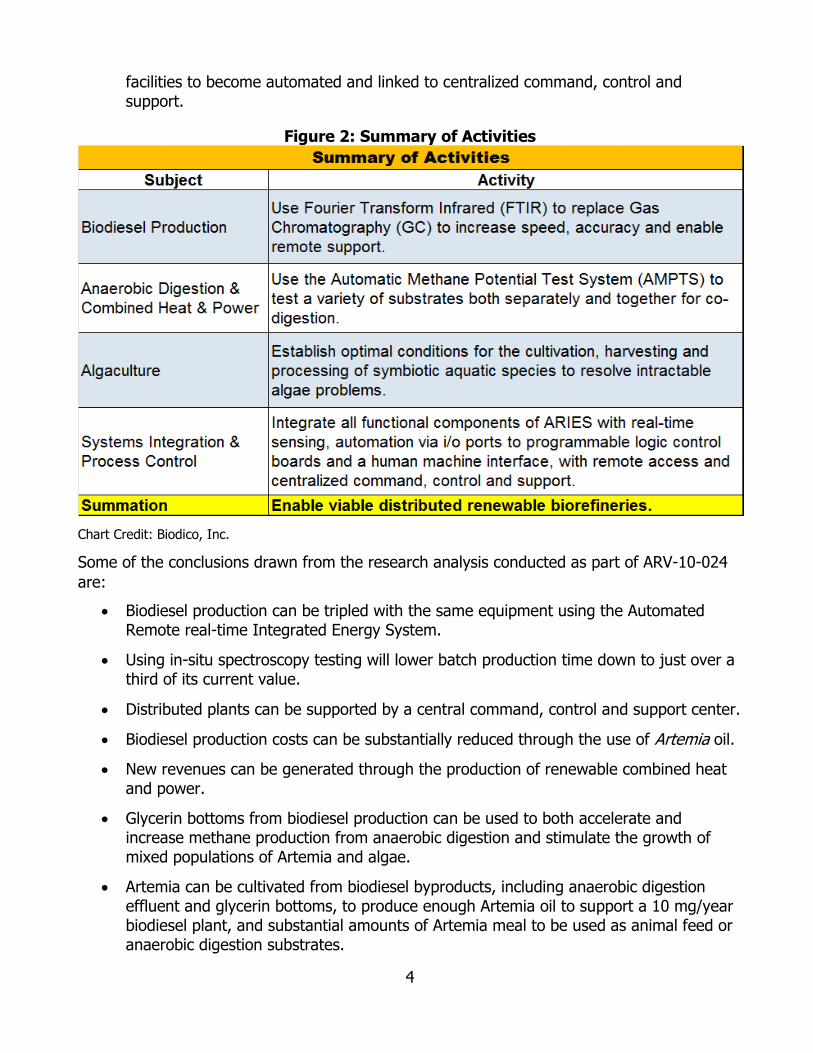
4
facilities to become automated and linked to centralized command, control and support.
Figure 2: Summary of Activities
Chart Credit: Biodico, Inc.
Some of the conclusions drawn from the research analysis conducted as part of ARV-10-024 are:
• Biodiesel production can be tripled with the same equipment using the Automated Remote real-time Integrated Energy System.
• Using in-situ spectroscopy testing will lower batch production time down to just over a third of its current value.
• Distributed plants can be supported by a central command, control and support center.
• Biodiesel production costs can be substantially reduced through the use of Artemia oil.
• New revenues can be generated through the production of renewable combined heat and power.
• Glycerin bottoms from biodiesel production can be used to both accelerate and increase methane production from anaerobic digestion and stimulate the growth of mixed populations of Artemia and algae.
• Artemia can be cultivated from biodiesel byproducts, including anaerobic digestion effluent and glycerin bottoms, to produce enough Artemia oil to support a 10 mg/year biodiesel plant, and substantial amounts of Artemia meal to be used as animal feed or anaerobic digestion substrates.
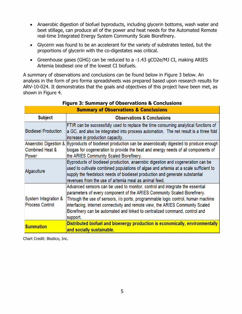
5
• Anaerobic digestion of biofuel byproducts, including glycerin bottoms, wash water and beet stillage, can produce all of the power and heat needs for the Automated Remote real-time Integrated Energy System Community Scale Biorefinery.
• Glycerin was found to be an accelerant for the variety of substrates tested, but the proportions of glycerin with the co-digestates was critical.
• Greenhouse gases (GHG) can be reduced to a -1.43 gCO2e/MJ CI, making ARIES Artemia biodiesel one of the lowest CI biofuels.
A summary of observations and conclusions can be found below in Figure 3 below. An analysis in the form of pro forma spreadsheets was prepared based upon research results for ARV-10-024. It demonstrates that the goals and objectives of this project have been met, as shown in Figure 4.
Figure 3: Summary of Observations & Conclusions
Chart Credit: Biodico, Inc.

6
Figure 4: Summary of Assessment
Chart Credit: Biodico, Inc.
Recommendations based upon the research and conclusions of ARV-10-024 are: • Demonstration of 1 percent of the Automated Remote real-time Integrated Energy
System support structure needed for the 10,000,000 per year facility at Red Rock Ranch
• Proactive protection against fraudulent misrepresentation of renewable energy in the California marketplace
• Increased biodiesel feedstock research
• Establishment of a green bank & bonds for new or expanded renewable energy project financing in California
• Exploration of additional processes to integrate into the Automated Remote real-time Integrated Energy System.
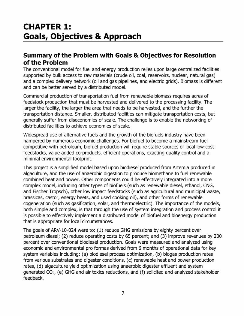
7
CHAPTER 1: Goals, Objectives & Approach
Summary of the Problem with Goals & Objectives for Resolution of the Problem The conventional model for fuel and energy production relies upon large centralized facilities supported by bulk access to raw materials (crude oil, coal, reservoirs, nuclear, natural gas) and a complex delivery network (oil and gas pipelines, and electric grids). Biomass is different and can be better served by a distributed model.
Commercial production of transportation fuel from renewable biomass requires acres of feedstock production that must be harvested and delivered to the processing facility. The larger the facility, the larger the area that needs to be harvested, and the further the transportation distance. Smaller, distributed facilities can mitigate transportation costs, but generally suffer from diseconomies of scale. The challenge is to enable the networking of distributed facilities to achieve economies of scale.
Widespread use of alternative fuels and the growth of the biofuels industry have been hampered by numerous economic challenges. For biofuel to become a mainstream fuel competitive with petroleum, biofuel production will require stable sources of local low-cost feedstocks, value added co-products, efficient operations, exacting quality control and a minimal environmental footprint.
This project is a simplified model based upon biodiesel produced from Artemia produced in algaculture, and the use of anaerobic digestion to produce biomethane to fuel renewable combined heat and power. Other components could be effectively integrated into a more complex model, including other types of biofuels (such as renewable diesel, ethanol, CNG, and Fischer Tropsch), other low impact feedstocks (such as agricultural and municipal waste, brassicas, castor, energy beets, and used cooking oil), and other forms of renewable cogeneration (such as gasification, solar, and thermoelectric). The importance of the models, both simple and complex, is that through the use of system integration and process control it is possible to effectively implement a distributed model of biofuel and bioenergy production that is appropriate for local circumstances.
The goals of ARV-10-024 were to: (1) reduce GHG emissions by eighty percent over petroleum diesel; (2) reduce operating costs by 65 percent; and (3) improve revenues by 200 percent over conventional biodiesel production. Goals were measured and analyzed using economic and environmental pro formas derived from 6 months of operational data for key system variables including: (a) biodiesel process optimization, (b) biogas production rates from various substrates and digester conditions, (c) renewable heat and power production rates, (d) algaculture yield optimization using anaerobic digester effluent and system generated CO2, (e) GHG and air toxics reductions, and (f) solicited and analyzed stakeholder feedback.
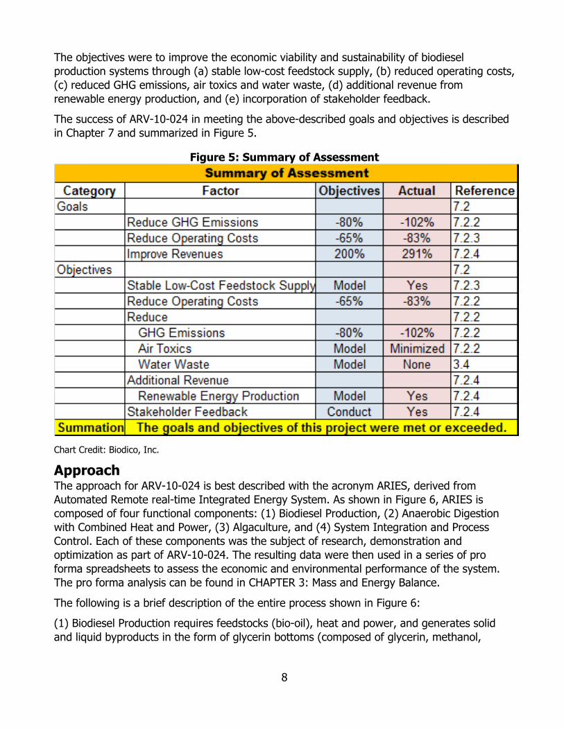
8
The objectives were to improve the economic viability and sustainability of biodiesel production systems through (a) stable low-cost feedstock supply, (b) reduced operating costs, (c) reduced GHG emissions, air toxics and water waste, (d) additional revenue from renewable energy production, and (e) incorporation of stakeholder feedback.
The success of ARV-10-024 in meeting the above-described goals and objectives is described in Chapter 7 and summarized in Figure 5.
Figure 5: Summary of Assessment
Chart Credit: Biodico, Inc.
Approach The approach for ARV-10-024 is best described with the acronym ARIES, derived from Automated Remote real-time Integrated Energy System. As shown in Figure 6, ARIES is composed of four functional components: (1) Biodiesel Production, (2) Anaerobic Digestion with Combined Heat and Power, (3) Algaculture, and (4) System Integration and Process Control. Each of these components was the subject of research, demonstration and optimization as part of ARV-10-024. The resulting data were then used in a series of pro forma spreadsheets to assess the economic and environmental performance of the system. The pro forma analysis can be found in CHAPTER 3: Mass and Energy Balance.
The following is a brief description of the entire process shown in Figure 6:
(1) Biodiesel Production requires feedstocks (bio-oil), heat and power, and generates solid and liquid byproducts in the form of glycerin bottoms (composed of glycerin, methanol,
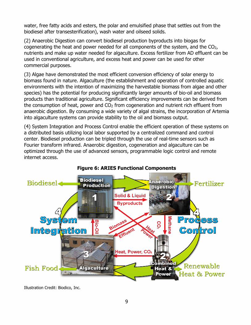
9
water, free fatty acids and esters, the polar and emulsified phase that settles out from the biodiesel after transesterification), wash water and oilseed solids.
(2) Anaerobic Digestion can convert biodiesel production byproducts into biogas for cogenerating the heat and power needed for all components of the system, and the CO2, nutrients and make up water needed for algaculture. Excess fertilizer from AD effluent can be used in conventional agriculture, and excess heat and power can be used for other commercial purposes.
(3) Algae have demonstrated the most efficient conversion efficiency of solar energy to biomass found in nature. Algaculture (the establishment and operation of controlled aquatic environments with the intention of maximizing the harvestable biomass from algae and other species) has the potential for producing significantly larger amounts of bio-oil and biomass products than traditional agriculture. Significant efficiency improvements can be derived from the consumption of heat, power and CO2 from cogeneration and nutrient rich effluent from anaerobic digestion. By consuming a wide variety of algal strains, the incorporation of Artemia into algaculture systems can provide stability to the oil and biomass output.
(4) System Integration and Process Control enable the efficient operation of these systems on a distributed basis utilizing local labor supported by a centralized command and control center. Biodiesel production can be tripled through the use of real-time sensors such as Fourier transform infrared. Anaerobic digestion, cogeneration and algaculture can be optimized through the use of advanced sensors, programmable logic control and remote internet access.
Figure 6: ARIES Functional Components
Illustration Credit: Biodico, Inc.

10
Areas of Study The following areas of study were part of ARV-10-024: Biodiesel Production Biodiesel is produced through a process called transesterification: the reaction of a triglyceride (vegetable oil or animal fat) with an alcohol (typically methanol or ethanol) in the presence of a catalyst (typically sodium or potassium hydroxide or methylate) and can occur at ambient pressure with an ideal temperature of about 140oF. The reaction sequence is composed of a series of go/no-go decisions that often require time consuming tests of up to 45 minutes each. It is possible to replace these tests with Fourier transform infrared (FTIR) and other technologies to obtain real-time process sensing that results in a substantial savings of time, which means that the same labor and equipment could potentially produce 2-3 times more biodiesel and use less reactants. Figure 7 shows workers at Biodico in front of the machine to produce triglycerides. Figure 8 compares the testing times for FTIR vs the usual gas chromatography.
Figure 7: Processing Feedstock to Produce Triglycerides & Oilseed Solids
Photo Credit: Biodico, Inc.
11
Figure 8: Testing Times for FTIR versus GC
Illustration Credit: Biodico, Inc.
Biodiesel has the potential to have a significant impact on the diesel market in California, but to be competitive it must be cost-effective and lessen the negative impacts of fossil fuels. In looking at the lifecycle of biodiesel production, every stage was examined for ways to reduce cost and enhance environmental performance. The approach for this particular area of study was to streamline the biodiesel production process by enabling real-time remote sensing to reduce labor costs and to enhance output and quality control. Conventional biodiesel production is controlled by protocols established by ASTM D6751. If biodiesel production is envisioned as a series of processes, there is a go/no-go decision point at the end of each stage. For example, the ASTM standard specifies the use of a gas chromatograph to determine if the transesterification and esterification reactions are complete and the glycerin compounds have been removed. The approach taken in the biodiesel production area was to substitute the use of gas chromatography with Fourier transform infrared. Biodico has developed a near infrared method that can perform the majority of testing needed for biodiesel production that it has dubbed QBQ-20,000. Anaerobic Digestion with Combined Heat and Power Anaerobic digestion (AD) is the microbial breakdown of certain organic materials in a low oxygen environment to produce biogas—a combination of methane and CO2. Biogas can be used as fuel in an internal combustion engine to generate combined heat and power (CHP). The cultivation of biofuel feedstocks (including Artemia among others) and biodiesel production create byproducts that have the potential to be used as substrates for AD to produce biogas for renewable cogeneration. These potential substrates include inedible oilseed extraction solids, crude glycerin bottoms and wash water. These low value substrates have the potential to produce up to 14 million kWh more renewable power and almost 14 million Btus more renewable heat energy than is needed for the entire system. This would result in a substantially lower Carbon Intensity (CI) and create substantial additional revenue streams. Crude glycerin bottoms may be used as an accelerant for digesting substrates with a long hydraulic retention time (HRT), resulting in lower capital cost for AD systems and increased biogas production.
Combined heat and power (CHP) is the simultaneous production of heat and power, usually by capturing waste heat from an engine cooling system and/or from engine exhaust. CHP is

12
substantially more efficient than producing heat and power separately. Renewable CHP is produced by CHP systems when a renewable fuel instead of a fossil fuel is used. With ARIES, renewable CHP can be used to offset the consumption of fossil fuel derived energy, reduce the CI of biodiesel production, mitigate energy costs and enhance revenues. The resulting heat and power can be used in algaculture, AD and the production of biodiesel, and any excess can be used by third parties.
The biogas resulting from anaerobic digestion can also be stored in tanks or in bladder systems to allow for changes in production rates, scheduled use in CHP to take advantage of utilities rates, and easy integration with system components that may not operate on a continuous flow basis or at the same rate as biogas production such as methane purification equipment or compression equipment. This is shown in Figure 9 showing the difference between CHP and a traditional system.
Figure 9: CHP Process Flow Diagram
Illustration Credit: Biodico, Inc.
The electricity and heat production using the glycerin bottoms produced by a 10 mmgpy biodiesel plant is 41.2 million kWh of electricity and 42.5 mmBtus of heat. This is 379 times more electricity than is needed for the biodiesel production process and over 50 percent more than what is needed for the full 10 mmgpy implementation of ARIES. The glycerin bottoms from biodiesel production are often referred to as crude glycerin or producers’ grade glycerin. Though the majority of the producers’ grade glycerin is glycerol, it contains all of the polar products and emulsified portions of the biodiesel transesterification as well as other hydrophilic compounds. It will usually contain water, saponified free fatty acids, methanol (which is often recovered by distillation), unused alkaline catalyst, and salts formed in acid-base reactions. The term glycerin in this study refers to producers’ grade glycerin that was tested for composition with the exception of the glycerol that was specifically noted as pure glycerin to compare it to producers’ grade glycerin as an algaculture feed. An easy and fairly accurate way to estimate the total amount of producers’ grade glycerin (before distillation)

13
that will result from biodiesel production is given below where VM represents methanol volume, VO represents feedstock oil volume in the reaction, VG represents the crude volume, and VB represents biodiesel volume.
The yield can vary between feedstocks (so the biodiesel out will change), some volume is added to the mixture by the catalyst, and some methanol evaporation will occur, but the relationship illustrates that whatever doesn’t stay in the biodiesel phase after the transesterification will end up leaving the reactor with the glycerin. Fuel washing and polishing after the reaction are needed to remove the polar compounds that remain solubilized in the biodiesel in order to reach the low percentages required by specification, but well over 90 percent of the methanol and the free glycerin will separate from the biodiesel before the water-wash.
The transesterification calls for a molar ratio of methanol to oil of 3:1. For triolein (the reference triglyceride used for ASTM specification testing) this gives a volume ratio of methanol to oil of roughly 12:100. Most biodiesel production processes use about twice that volume in order to account for the methanol’s affinity to the glycerin and to completely transesterify the oil. Artemia oil, taken as a weighted average of all of the fatty acids that it contains, is actually very close to triolein. The average number of carbon atoms is 18.1, as compared to triolein’s 18, and the degree of unsaturation is 1.5, as compared to triolein’s 2. The molar mass of triolein is 885.4 and the average molar mass of Artemia oil is within a quarter of a percent at 887.5.
Certain challenges in the anaerobic digestion of glycerin have been identified, including: (1) the high energy concentration of glycerin means that only low concentrations (one – five percent by volume) can be used in a digester without disrupting the balance of the microbial communities, (2) because of the high dilution rate required, there is a higher volume of digestate produced, and (3) even though the HRT may be accelerated, the Capital Expenditures and Opex for the anaerobic digestion of glycerin are similar to the costs for the anaerobic digestion of more traditional digester influents.
In comparing the results of the work performed by Biodico to previous studies, it is important to note that there are some differences in the way that glycerin quantities are reported. Many studies share Biodico’s quantification of the glycerin concentration in anaerobic digestion as a percentage of glycerin volume to digester volume (percentv/v). Other studies though, particularly regarding codigestion, refer to the glycerin as a percentage of some fixed organic loading rate (generally based on volatile solids or chemical oxygen demand). A report by Dr. Steven Sell from Iowa State University highlights the possible confusion that can come from the differences in measurement metrics.2 The paper refers to past research that had determined the toxicity level of glycerin in anaerobic digestion using the (percentv/v) unit and
2 Sell, Steven Thomas, "A scale-up procedure for substrate co-digestion in anaerobic digesters through the use of substrate characterization, BMPs, ATAs, and sub pilot-scale digesters" (2011). Graduate Theses and Dissertations. Paper 12044

14
references toxicity limits of 2percent (48), toxicity levels of 4 percent (p 50, Wollengut), survivability levels (that point to the fact that the digester didn’t crash but do not discuss optimum levels or the onset of toxicity) of 15 percent with very specific pretreatment methods used to counter the high chemical oxygen demand of glycerin (p 50, Siles). The paper also cites research showing survivability levels of glycerin by weight percentage (percent wt/wt) of 10 percent (p 50, Robra). A co-digestion study that is referenced refers to glycerin as a percentage mixed with cattle manure of 0 percent, 45 percent, 60 percent, and 100 percent, but does not give any concrete values behind the percentage (p 50, Chen). The Chen experiments tested the suitability of glycerin as a co-digestant in both batch and continuous flow digesters. The percentages referenced in the Sell paper refer to the batch portion of the Chen testing in which the organic loading rate was 3 grams of volatile solids per liter resulting in grams of volatile solids per liter from glycerin of 0, 1.35, 1.8, and 3. The glycerin used by Biodico in testing contained 755 g/L of volatile solids so the grams per liter of volatile solids used in the Chen report would equate to ( percentv/v) of 0 percent, 1.8 percent, 2.4 percent, and 4.0 percent. It is worth noting that in the continuous flow portion of the Chen experiments a mixture of 60 percent glycerin by volatile solids added to the digester at a rate of 1 g VS/L crashed the system. This would equate to a daily loading rate of (percentv/v) 0.79 percent.3 The scaling between batch systems and continuous flow systems differ between feedstocks so the information gained from the continuous monitoring that Biodico was able to perform with the AMPTS is very valuable in projecting the commercial performance of glycerin as an AD feedstock.
One of the conclusions of the Sell report is that the results of the various experiments on the anaerobic digestion of glycerin that were analyzed “demonstrate the variations in scale performance of glycerin as a co-substrate and identify some serious challenges in extrapolating bench scale assays to large-scale performance of mixed-waste anaerobic digestion systems.” From the perspective of Biodico, based on the breadth of the experiments that it has conducted and on some of the experience that it has gained through the implementation of these findings on a larger scale, the inconsistencies seems to point more toward the lack of a cohesive structure belying the group of disparate experiments in approach, goals, quantification, and qualification, than on any underlying inconsistencies in the behavior of glycerin as an anaerobic digester stand-alone or co-digested feedstock. The report does not demonstrate a clear understanding of the difference between the chemical glycerol and the glycerin byproduct of biodiesel production and introduces glycerin into the narrative by stating that “the rise in production of biodiesel in the upper Midwestern US has led to a glut of glycerin (also known as glycerol) in the region, because glycerin is a byproduct of biodiesel production” on page 49. No further clarification of these differences is given in the description of the references and the statement that “each of the preceding article results shows a lack of consistency in establishing the correct ratio for glycerin addition as a co-substrate” on page 51 combined with the brief description of the glycerin that was
3 Chen, X., R.T. Romano, R. Zhang, H.S. Kim. 2008. Anaerobic co-digestion of dairy manure and glycerin. In proceedings of 2008 American Society of Agricultural and Biological Engineering Annual International Meeting. Providence, Rhode Island.
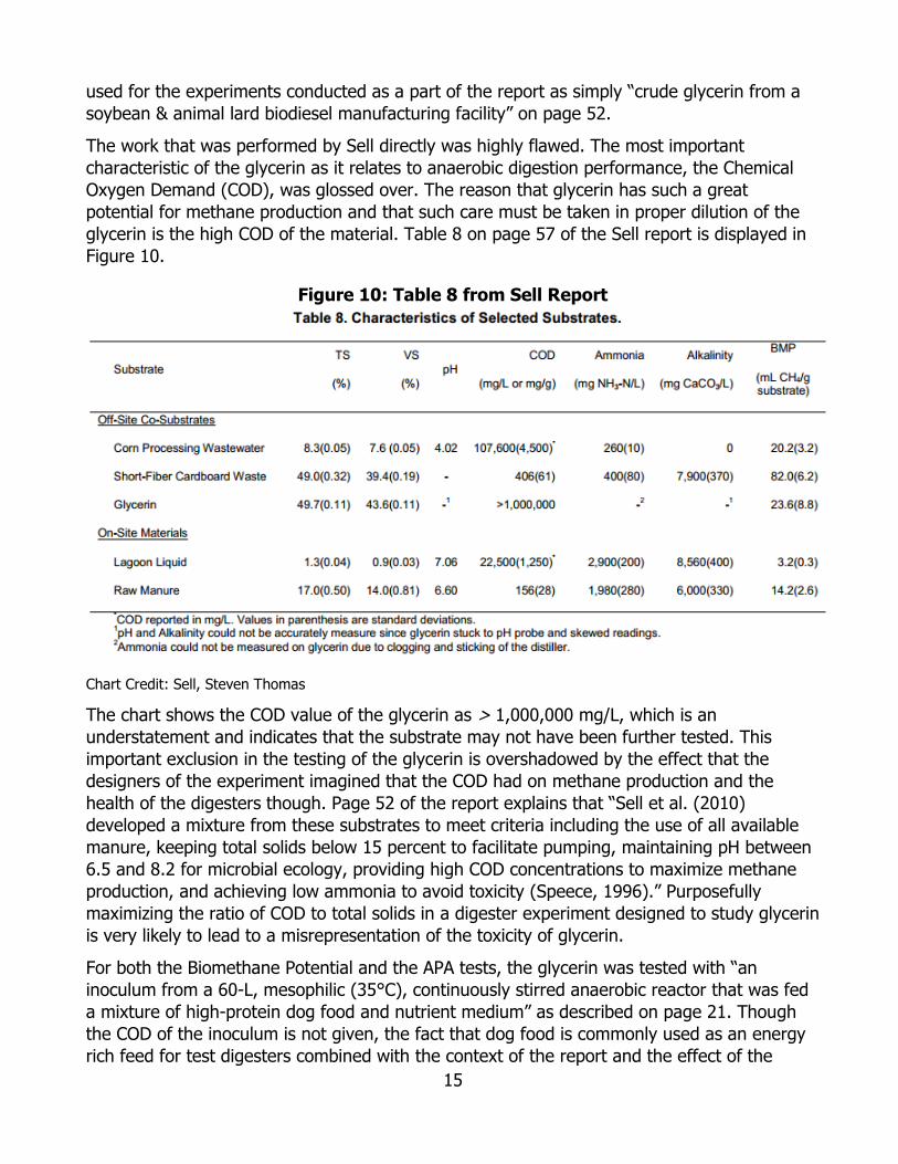
15
used for the experiments conducted as a part of the report as simply “crude glycerin from a soybean & animal lard biodiesel manufacturing facility” on page 52.
The work that was performed by Sell directly was highly flawed. The most important characteristic of the glycerin as it relates to anaerobic digestion performance, the Chemical Oxygen Demand (COD), was glossed over. The reason that glycerin has such a great potential for methane production and that such care must be taken in proper dilution of the glycerin is the high COD of the material. Table 8 on page 57 of the Sell report is displayed in Figure 10.
Figure 10: Table 8 from Sell Report
Chart Credit: Sell, Steven Thomas
The chart shows the COD value of the glycerin as > 1,000,000 mg/L, which is an understatement and indicates that the substrate may not have been further tested. This important exclusion in the testing of the glycerin is overshadowed by the effect that the designers of the experiment imagined that the COD had on methane production and the health of the digesters though. Page 52 of the report explains that “Sell et al. (2010) developed a mixture from these substrates to meet criteria including the use of all available manure, keeping total solids below 15 percent to facilitate pumping, maintaining pH between 6.5 and 8.2 for microbial ecology, providing high COD concentrations to maximize methane production, and achieving low ammonia to avoid toxicity (Speece, 1996).” Purposefully maximizing the ratio of COD to total solids in a digester experiment designed to study glycerin is very likely to lead to a misrepresentation of the toxicity of glycerin.
For both the Biomethane Potential and the APA tests, the glycerin was tested with “an inoculum from a 60-L, mesophilic (35°C), continuously stirred anaerobic reactor that was fed a mixture of high-protein dog food and nutrient medium” as described on page 21. Though the COD of the inoculum is not given, the fact that dog food is commonly used as an energy rich feed for test digesters combined with the context of the report and the effect of the
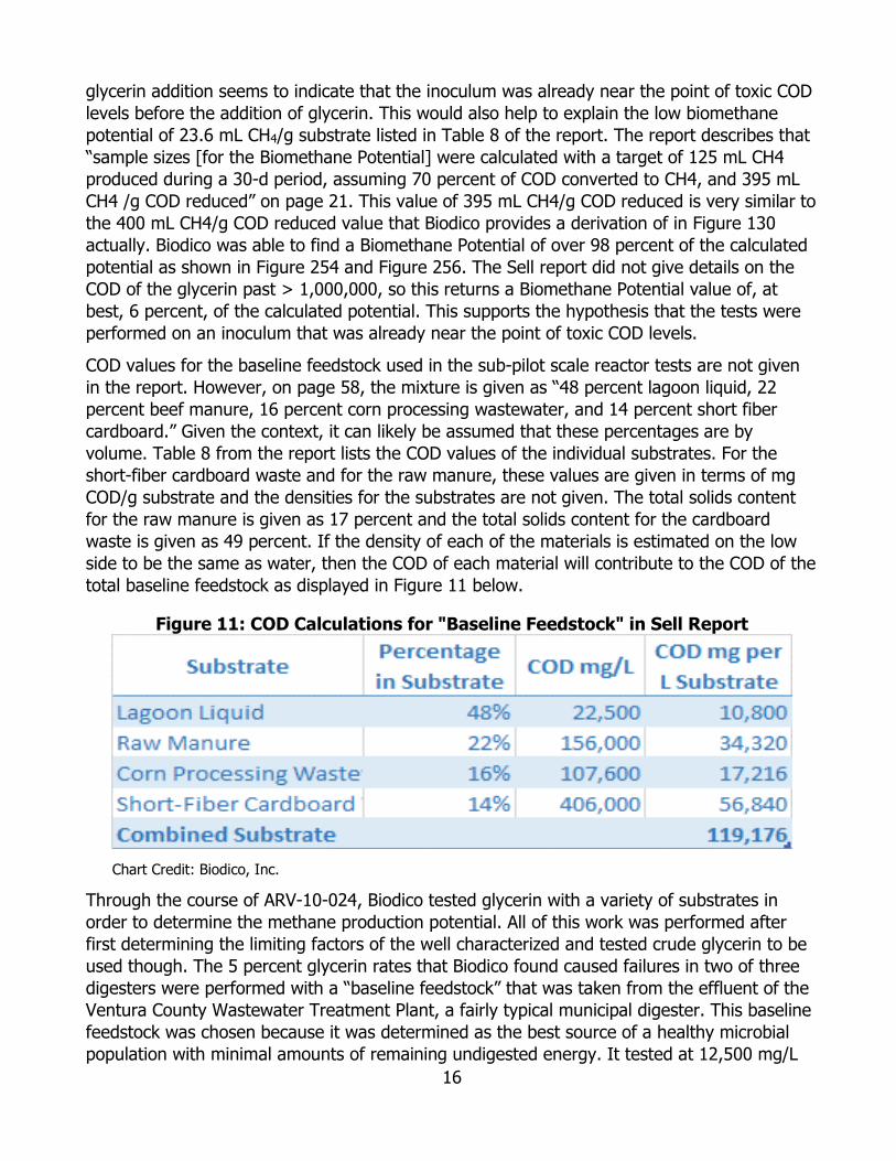
16
glycerin addition seems to indicate that the inoculum was already near the point of toxic COD levels before the addition of glycerin. This would also help to explain the low biomethane potential of 23.6 mL CH4/g substrate listed in Table 8 of the report. The report describes that “sample sizes [for the Biomethane Potential] were calculated with a target of 125 mL CH4 produced during a 30-d period, assuming 70 percent of COD converted to CH4, and 395 mL CH4 /g COD reduced” on page 21. This value of 395 mL CH4/g COD reduced is very similar to the 400 mL CH4/g COD reduced value that Biodico provides a derivation of in Figure 130 actually. Biodico was able to find a Biomethane Potential of over 98 percent of the calculated potential as shown in Figure 254 and Figure 256. The Sell report did not give details on the COD of the glycerin past > 1,000,000, so this returns a Biomethane Potential value of, at best, 6 percent, of the calculated potential. This supports the hypothesis that the tests were performed on an inoculum that was already near the point of toxic COD levels.
COD values for the baseline feedstock used in the sub-pilot scale reactor tests are not given in the report. However, on page 58, the mixture is given as “48 percent lagoon liquid, 22 percent beef manure, 16 percent corn processing wastewater, and 14 percent short fiber cardboard.” Given the context, it can likely be assumed that these percentages are by volume. Table 8 from the report lists the COD values of the individual substrates. For the short-fiber cardboard waste and for the raw manure, these values are given in terms of mg COD/g substrate and the densities for the substrates are not given. The total solids content for the raw manure is given as 17 percent and the total solids content for the cardboard waste is given as 49 percent. If the density of each of the materials is estimated on the low side to be the same as water, then the COD of each material will contribute to the COD of the total baseline feedstock as displayed in Figure 11 below.
Figure 11: COD Calculations for "Baseline Feedstock" in Sell Report
Chart Credit: Biodico, Inc.
Through the course of ARV-10-024, Biodico tested glycerin with a variety of substrates in order to determine the methane production potential. All of this work was performed after first determining the limiting factors of the well characterized and tested crude glycerin to be used though. The 5 percent glycerin rates that Biodico found caused failures in two of three digesters were performed with a “baseline feedstock” that was taken from the effluent of the Ventura County Wastewater Treatment Plant, a fairly typical municipal digester. This baseline feedstock was chosen because it was determined as the best source of a healthy microbial population with minimal amounts of remaining undigested energy. It tested at 12,500 mg/L
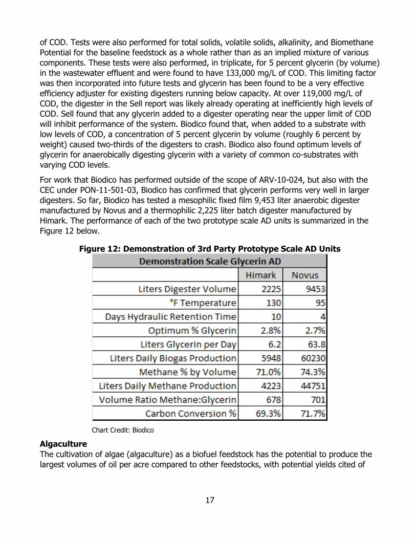
17
of COD. Tests were also performed for total solids, volatile solids, alkalinity, and Biomethane Potential for the baseline feedstock as a whole rather than as an implied mixture of various components. These tests were also performed, in triplicate, for 5 percent glycerin (by volume) in the wastewater effluent and were found to have 133,000 mg/L of COD. This limiting factor was then incorporated into future tests and glycerin has been found to be a very effective efficiency adjuster for existing digesters running below capacity. At over 119,000 mg/L of COD, the digester in the Sell report was likely already operating at inefficiently high levels of COD. Sell found that any glycerin added to a digester operating near the upper limit of COD will inhibit performance of the system. Biodico found that, when added to a substrate with low levels of COD, a concentration of 5 percent glycerin by volume (roughly 6 percent by weight) caused two-thirds of the digesters to crash. Biodico also found optimum levels of glycerin for anaerobically digesting glycerin with a variety of common co-substrates with varying COD levels.
For work that Biodico has performed outside of the scope of ARV-10-024, but also with the CEC under PON-11-501-03, Biodico has confirmed that glycerin performs very well in larger digesters. So far, Biodico has tested a mesophilic fixed film 9,453 liter anaerobic digester manufactured by Novus and a thermophilic 2,225 liter batch digester manufactured by Himark. The performance of each of the two prototype scale AD units is summarized in the Figure 12 below.
Figure 12: Demonstration of 3rd Party Prototype Scale AD Units
Chart Credit: Biodico
Algaculture The cultivation of algae (algaculture) as a biofuel feedstock has the potential to produce the largest volumes of oil per acre compared to other feedstocks, with potential yields cited of
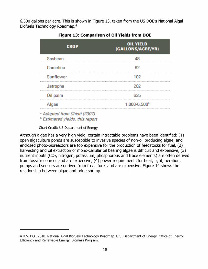
18
6,500 gallons per acre. This is shown in Figure 13, taken from the US DOE’s National Algal Biofuels Technology Roadmap.4
Figure 13: Comparison of Oil Yields from DOE
Chart Credit: US Department of Energy
Although algae has a very high yield, certain intractable problems have been identified: (1) open algaculture ponds are susceptible to invasive species of non-oil producing algae, and enclosed photo-bioreactors are too expensive for the production of feedstocks for fuel, (2) harvesting and oil extraction of mono-cellular oil bearing algae is difficult and expensive, (3) nutrient inputs (CO2, nitrogen, potassium, phosphorous and trace elements) are often derived from fossil resources and are expensive, (4) power requirements for heat, light, aeration, pumps and sensors are derived from fossil fuels and are expensive. Figure 14 shows the relationship between algae and brine shrimp.
4 U.S. DOE 2010. National Algal Biofuels Technology Roadmap. U.S. Department of Energy, Office of Energy Efficiency and Renewable Energy, Biomass Program.
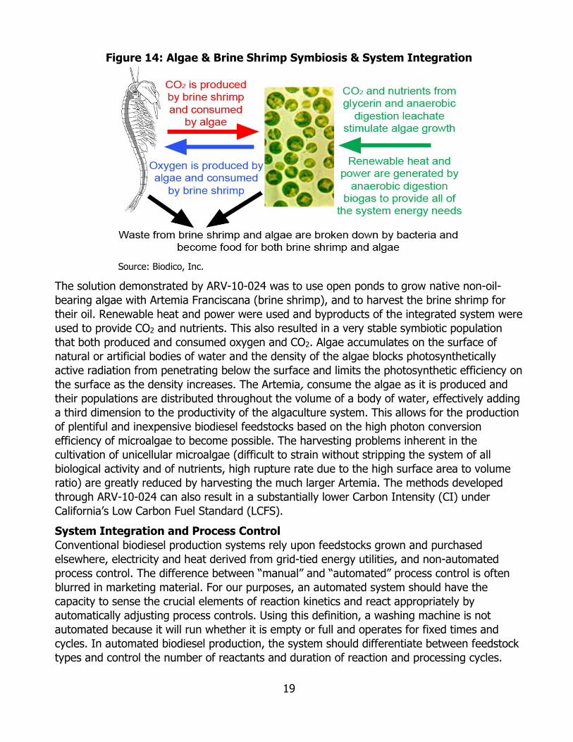
19
Figure 14: Algae & Brine Shrimp Symbiosis & System Integration
Source: Biodico, Inc.
The solution demonstrated by ARV-10-024 was to use open ponds to grow native non-oil-bearing algae with Artemia Franciscana (brine shrimp), and to harvest the brine shrimp for their oil. Renewable heat and power were used and byproducts of the integrated system were used to provide CO2 and nutrients. This also resulted in a very stable symbiotic population that both produced and consumed oxygen and CO2. Algae accumulates on the surface of natural or artificial bodies of water and the density of the algae blocks photosynthetically active radiation from penetrating below the surface and limits the photosynthetic efficiency on the surface as the density increases. The Artemia, consume the algae as it is produced and their populations are distributed throughout the volume of a body of water, effectively adding a third dimension to the productivity of the algaculture system. This allows for the production of plentiful and inexpensive biodiesel feedstocks based on the high photon conversion efficiency of microalgae to become possible. The harvesting problems inherent in the cultivation of unicellular microalgae (difficult to strain without stripping the system of all biological activity and of nutrients, high rupture rate due to the high surface area to volume ratio) are greatly reduced by harvesting the much larger Artemia. The methods developed through ARV-10-024 can also result in a substantially lower Carbon Intensity (CI) under California’s Low Carbon Fuel Standard (LCFS). System Integration and Process Control Conventional biodiesel production systems rely upon feedstocks grown and purchased elsewhere, electricity and heat derived from grid-tied energy utilities, and non-automated process control. The difference between “manual” and “automated” process control is often blurred in marketing material. For our purposes, an automated system should have the capacity to sense the crucial elements of reaction kinetics and react appropriately by automatically adjusting process controls. Using this definition, a washing machine is not automated because it will run whether it is empty or full and operates for fixed times and cycles. In automated biodiesel production, the system should differentiate between feedstock types and control the number of reactants and duration of reaction and processing cycles.
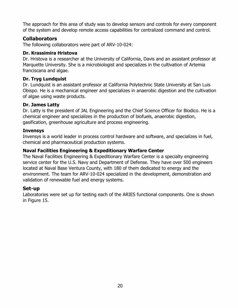
20
The approach for this area of study was to develop sensors and controls for every component of the system and develop remote access capabilities for centralized command and control.
Collaborators The following collaborators were part of ARV-10-024: Dr. Krassimira Hristova Dr. Hristova is a researcher at the University of California, Davis and an assistant professor at Marquette University. She is a microbiologist and specializes in the cultivation of Artemia franciscana and algae. Dr. Tryg Lundquist Dr. Lundquist is an assistant professor at California Polytechnic State University at San Luis Obispo. He is a mechanical engineer and specializes in anaerobic digestion and the cultivation of algae using waste products. Dr. James Latty Dr. Latty is the president of JAL Engineering and the Chief Science Officer for Biodico. He is a chemical engineer and specializes in the production of biofuels, anaerobic digestion, gasification, greenhouse agriculture and process engineering. Invensys Invensys is a world leader in process control hardware and software, and specializes in fuel, chemical and pharmaceutical production systems. Naval Facilities Engineering & Expeditionary Warfare Center The Naval Facilities Engineering & Expeditionary Warfare Center is a specialty engineering service center for the U.S. Navy and Department of Defense. They have over 500 engineers located at Naval Base Ventura County, with 180 of them dedicated to energy and the environment. The team for ARV-10-024 specialized in the development, demonstration and validation of renewable fuel and energy systems.
Set-up Laboratories were set up for testing each of the ARIES functional components. One is shown in Figure 15.
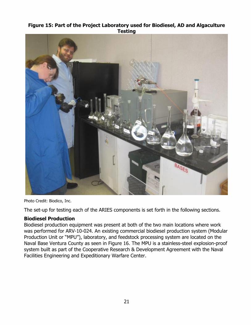
21
Figure 15: Part of the Project Laboratory used for Biodiesel, AD and Algaculture Testing
Photo Credit: Biodico, Inc.
The set-up for testing each of the ARIES components is set forth in the following sections. Biodiesel Production Biodiesel production equipment was present at both of the two main locations where work was performed for ARV-10-024. An existing commercial biodiesel production system (Modular Production Unit or “MPU”), laboratory, and feedstock processing system are located on the Naval Base Ventura County as seen in Figure 16. The MPU is a stainless-steel explosion-proof system built as part of the Cooperative Research & Development Agreement with the Naval Facilities Engineering and Expeditionary Warfare Center.
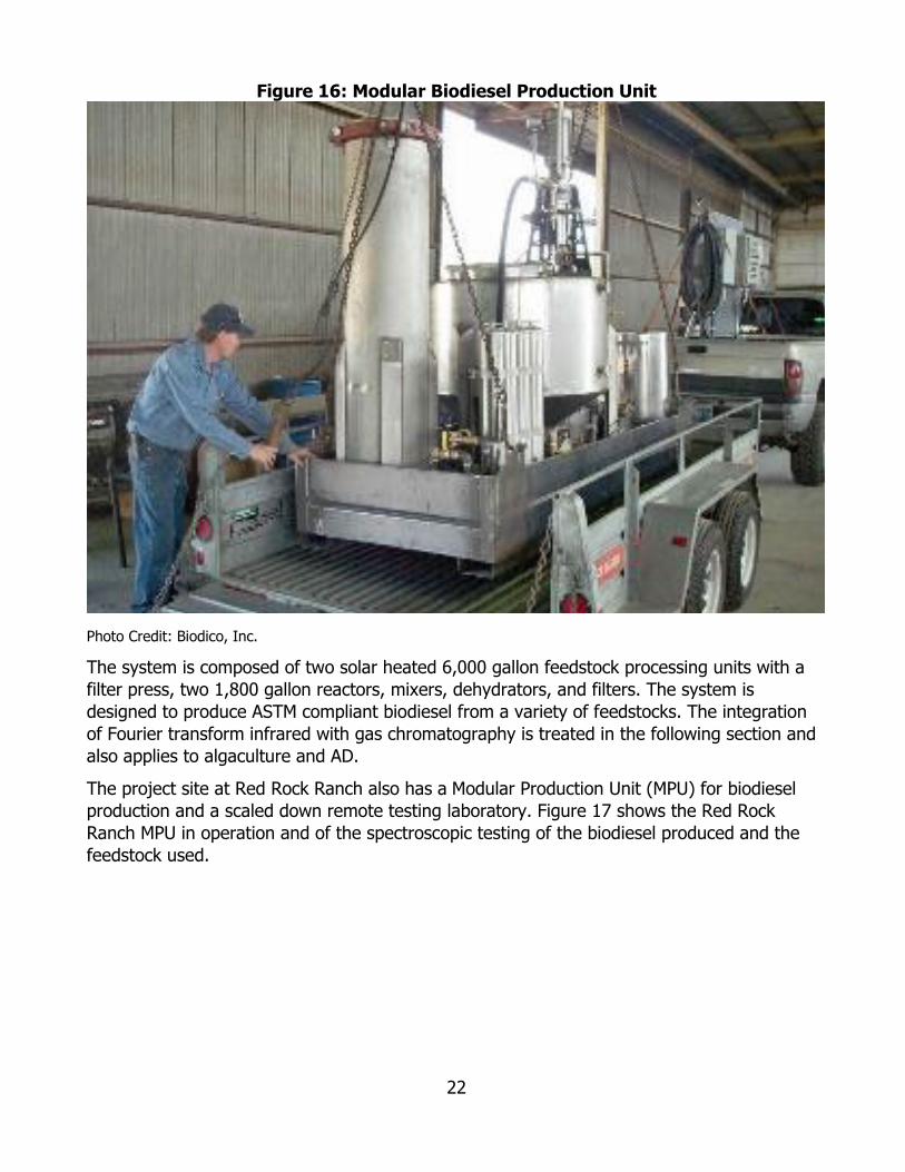
22
Figure 16: Modular Biodiesel Production Unit
Photo Credit: Biodico, Inc.
The system is composed of two solar heated 6,000 gallon feedstock processing units with a filter press, two 1,800 gallon reactors, mixers, dehydrators, and filters. The system is designed to produce ASTM compliant biodiesel from a variety of feedstocks. The integration of Fourier transform infrared with gas chromatography is treated in the following section and also applies to algaculture and AD.
The project site at Red Rock Ranch also has a Modular Production Unit (MPU) for biodiesel production and a scaled down remote testing laboratory. Figure 17 shows the Red Rock Ranch MPU in operation and of the spectroscopic testing of the biodiesel produced and the feedstock used.

23
Figure 17: MPU Producing Biodiesel and Glycerin
Photo Credit: Biodico, Inc.
The wet lab equipment at the Naval Base Ventura County is described in the Task 6 Report. For a network of commercial facilities, this volume and complexity of lab equipment is not required at each production location, but it will be part of the centralized command and control center. The laboratory capabilities at the Naval Base Ventura County are substantially greater than at Red Rock Ranch. One of the shared goals of Biodico and its private and military partners is to reduce the amount of technical expertise needed to effectively produce fuel at each location. Centralizing laboratory equipment helps in this regard.
The mechanical operation of the ARIES equipment does not require a technical background or degree in higher education. Workers with experience in agricultural machinery can be trained to operate all of the equipment comprising a full-scale ARIES unit (biodiesel production, algaculture, AD and CHP) even when English is not their primary language and with limited computer skills. Startup training usually takes three months to ensure safety, quality control and efficiency. Even interns from high school have learned to perform basic assistance functions such as weighing products accurately in a half-hour training session. Both substrates and nutrients (both are liquids) are weighed before addition to the algaculture and anaerobic digestion tanks. Records on clipboards are added to Excel files during a part of each shift by the operator. However, when this simulation becomes a commercial ARIES installation, the volume of substrates and nutrients will be pumped via automated controls into the tanks and reactors, and data logging will be kept automatically. A college graduate with engineering and laboratory skills must be available for technical support via the centralized command and control connection of ARIES to support on-site personnel, and an on-site manager with process control operating and plant management experience needs to function as the project manager.
The first priority is the calibration of the FTIR with the GC to allow for near real-time sensing of system parameters. Both the FTIR and GC are now operational and computer interconnected. A series of test calibrations were run and full calibration for biodiesel

24
production, algaculture and AD was part of Task 6 Operations. Figure 18 is a screenshot of the test calibration, while Figure 19 shows the AMPTS calibration.
Figure 18: Test Calibration Screen Shot
Chart Credit: Biodico, Inc.
Figure 19: Setting up AMPTS
Source: Biodico

25
Anaerobic Digestion and Combined Heat and Power The Automatic Methane Potential Test System (AMPTS) was used to demonstrate and evaluate the anaerobic digestion of a variety of substrates. The equipment was capable of automatically running 15 simultaneous 500ml batches with equal temperatures and agitation, collecting the gases, recording the gas production rates over an extended period of time and porting the data to the internet. Laboratory equipment necessary for preparing and testing sample substrate combination before and after AD was installed include (1) a furnace to determine volatile organic solids, (2) an oven to determine dry weight biomass, (3) chemical oxygen demand, ammonia, and pH test equipment, (4) balances for weighing samples, and (5) a dedicated computer to automatically record data and make it available via remote sensing.
The AMPTS and associated lab equipment were initially tested on a combination of sewage sludge and varying percentages of crude glycerin bottoms from biodiesel production, as indicated by Figure 20 showing five separate substrate combinations (A through E) run in triplicate. For example, one set of triplicates is A1 through A3.
Figure 20: AMPTS Test Matrix for Five Sets of Triplicates
Chart Credit: Biodico, Inc.
The system operated as designed and created a gas production log tracking each of the fifteen batches separately and in comparison, to one another for a 600 hour period as shown in Figure 21.
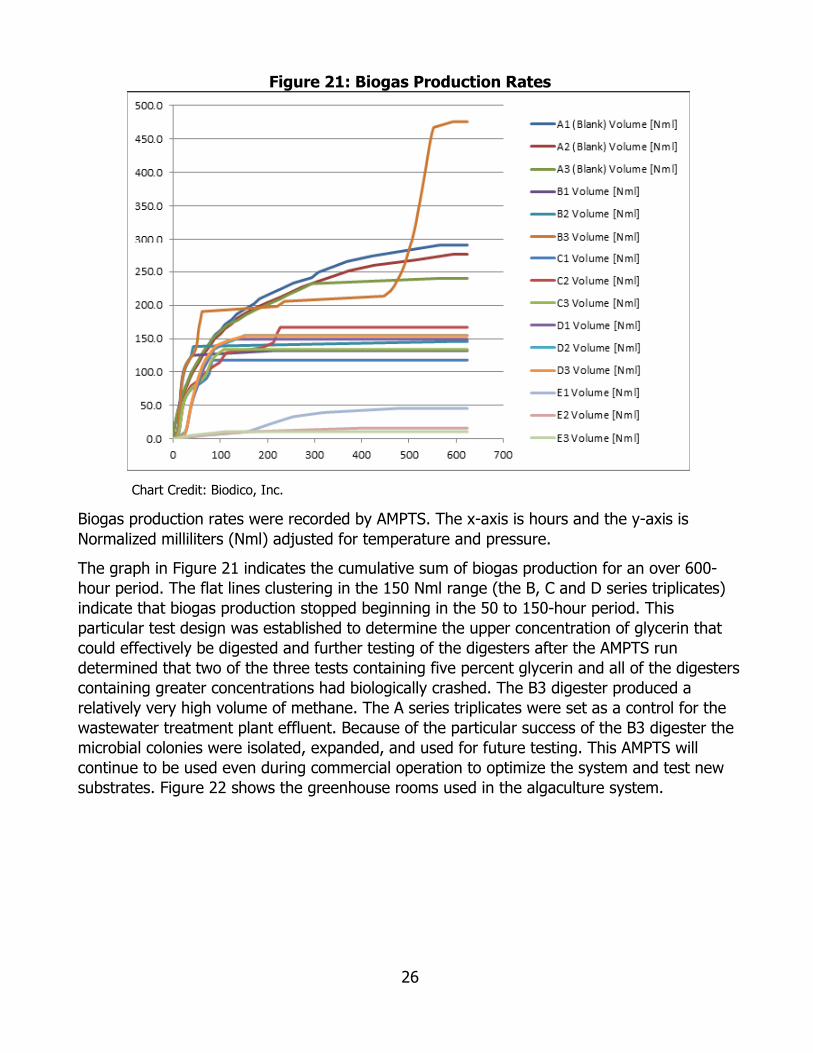
26
Figure 21: Biogas Production Rates
Chart Credit: Biodico, Inc.
Biogas production rates were recorded by AMPTS. The x-axis is hours and the y-axis is Normalized milliliters (Nml) adjusted for temperature and pressure.
The graph in Figure 21 indicates the cumulative sum of biogas production for an over 600-hour period. The flat lines clustering in the 150 Nml range (the B, C and D series triplicates) indicate that biogas production stopped beginning in the 50 to 150-hour period. This particular test design was established to determine the upper concentration of glycerin that could effectively be digested and further testing of the digesters after the AMPTS run determined that two of the three tests containing five percent glycerin and all of the digesters containing greater concentrations had biologically crashed. The B3 digester produced a relatively very high volume of methane. The A series triplicates were set as a control for the wastewater treatment plant effluent. Because of the particular success of the B3 digester the microbial colonies were isolated, expanded, and used for future testing. This AMPTS will continue to be used even during commercial operation to optimize the system and test new substrates. Figure 22 shows the greenhouse rooms used in the algaculture system.

27
Figure 22: Greenhouse Rooms
Photo Credit: Biodico, Inc.
Algaculture Aquariums & Greenhouses The algaculture system was composed of 16 ten-gallon aquariums and 16 three hundred and thirty gallon translucent International Bulk Container “totes” placed inside a four-room greenhouse as shown in Figure 22. The greenhouse rooms had secondary containment, a 12 volt photovoltaic system for power, a 12 volt pump interconnected to deliver and discharge water from each tote, a 12 volt aeration system for providing air to each tote and a low voltage LED variable spectrum grow light (red and blue light to stimulate green algae growth). A computer-connected infrared recording specific gravity meter was used to monitor temperature and salinity in each aquarium and tote. A recording weather station logged and delivered weather data to the internet at a site maintained by the Weather Channel (http://www.wunderground.com/US/CA/Port_Hueneme.html). A recording video microscope was used for population studies of species and populations. A harvest mesh net was fabricated to an optimum mesh size, a solar oven was used for dehydration of brine shrimp samples, a lab was set up for measuring moisture, oil content and weight, and an oil press was set up for extracting oil from brine shrimp and other feedstocks (to make oil for biodiesel testing and oilseed solids for AD testing). All algaculture systems were installed, integrated and operated in preparation for testing. No plumbing or electrical repairs were needed, though some minor greenhouse repairs were required. Figure 23 shows the different algae types found in the aquariums.
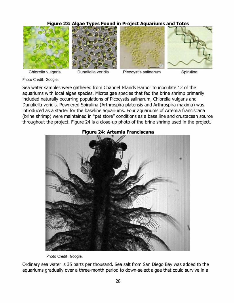
28
Figure 23: Algae Types Found in Project Aquariums and Totes
Photo Credit: Google.
Sea water samples were gathered from Channel Islands Harbor to inoculate 12 of the aquariums with local algae species. Microalgae species that fed the brine shrimp primarily included naturally occurring populations of Picocystis salinarum, Chlorella vulgaris and Dunaliella veridis. Powdered Spirulina (Arthrospira platensis and Arthrospira maxima) was introduced as a starter for the baseline aquariums. Four aquariums of Artemia franciscana (brine shrimp) were maintained in “pet store” conditions as a base line and crustacean source throughout the project. Figure 24 is a close-up photo of the brine shrimp used in the project.
Figure 24: Artemia Franciscana
Photo Credit: Google.
Ordinary sea water is 35 parts per thousand. Sea salt from San Diego Bay was added to the aquariums gradually over a three-month period to down-select algae that could survive in a
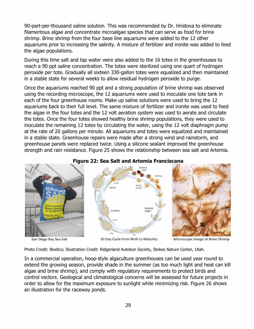
29
90-part-per-thousand saline solution. This was recommended by Dr. Hristova to eliminate filamentous algae and concentrate microalgae species that can serve as food for brine shrimp. Brine shrimp from the four base line aquariums were added to the 12 other aquariums prior to increasing the salinity. A mixture of fertilizer and ironite was added to feed the algae populations.
During this time salt and tap water were also added to the 16 totes in the greenhouses to reach a 90 ppt saline concentration. The totes were sterilized using one quart of hydrogen peroxide per tote. Gradually all sixteen 330-gallon totes were equalized and then maintained in a stable state for several weeks to allow residual hydrogen peroxide to purge.
Once the aquariums reached 90 ppt and a strong population of brine shrimp was observed using the recording microscope, the 12 aquariums were used to inoculate one tote tank in each of the four greenhouse rooms. Make up saline solutions were used to bring the 12 aquariums back to their full level. The same mixture of fertilizer and ironite was used to feed the algae in the four totes and the 12 volt aeration system was used to aerate and circulate the totes. Once the four totes showed healthy brine shrimp populations, they were used to inoculate the remaining 12 totes by circulating the water, using the 12 volt diaphragm pump at the rate of 20 gallons per minute. All aquariums and totes were equalized and maintained in a stable state. Greenhouse repairs were made after a strong wind and rainstorm, and greenhouse panels were replaced twice. Using a silicone sealant improved the greenhouse strength and rain resistance. Figure 25 shows the relationship between sea salt and Artemia.
Figure 22: Sea Salt and Artemia Franciscana
Photo Credit: Biodico; Illustration Credit: Ridgerland Autobon Society, Stokes Nature Center, Utah.
In a commercial operation, hoop-style algaculture greenhouses can be used year round to extend the growing season, provide shade in the summer (as too much light and heat can kill algae and brine shrimp), and comply with regulatory requirements to protect birds and control vectors. Geological and climatological concerns will be assessed for future projects in order to allow for the maximum exposure to sunlight while minimizing risk. Figure 26 shows an illustration for the raceway ponds.
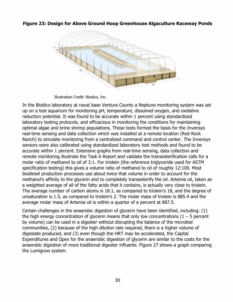
30
Figure 23: Design for Above Ground Hoop Greenhouse Algaculture Raceway Ponds
Illustration Credit: Biodico, Inc.
In the Biodico laboratory at naval base Ventura County a Neptune monitoring system was set up on a test aquarium for monitoring pH, temperature, dissolved oxygen, and oxidative reduction potential. It was found to be accurate within 1 percent using standardized laboratory testing protocols, and efficacious in monitoring the conditions for maintaining optimal algae and brine shrimp populations. These tests formed the basis for the Invensys real-time sensing and data collection which was installed at a remote location (Red Rock Ranch) to simulate monitoring from a centralized command and control center. The Invensys sensors were also calibrated using standardized laboratory test methods and found to be accurate within 1 percent. Extensive graphs from real-time sensing, data collection and remote monitoring illustrate the Task 6 Report and validate the transesterification calls for a molar ratio of methanol to oil of 3:1. For triolein (the reference triglyceride used for ASTM specification testing) this gives a volume ratio of methanol to oil of roughly 12:100. Most biodiesel production processes use about twice that volume in order to account for the methanol’s affinity to the glycerin and to completely transesterify the oil. Artemia oil, taken as a weighted average of all of the fatty acids that it contains, is actually very close to triolein. The average number of carbon atoms is 18.1, as compared to triolein’s 18, and the degree of unsaturation is 1.5, as compared to triolein’s 2. The molar mass of triolein is 885.4 and the average molar mass of Artemia oil is within a quarter of a percent at 887.5.
Certain challenges in the anaerobic digestion of glycerin have been identified, including: (1) the high energy concentration of glycerin means that only low concentrations (1 – 5 percent by volume) can be used in a digester without disrupting the balance of the microbial communities, (2) because of the high dilution rate required, there is a higher volume of digestate produced, and (3) even though the HRT may be accelerated, the Capital Expenditures and Opex for the anaerobic digestion of glycerin are similar to the costs for the anaerobic digestion of more traditional digester influents. Figure 27 shows a graph comparing the Lumigrow system.
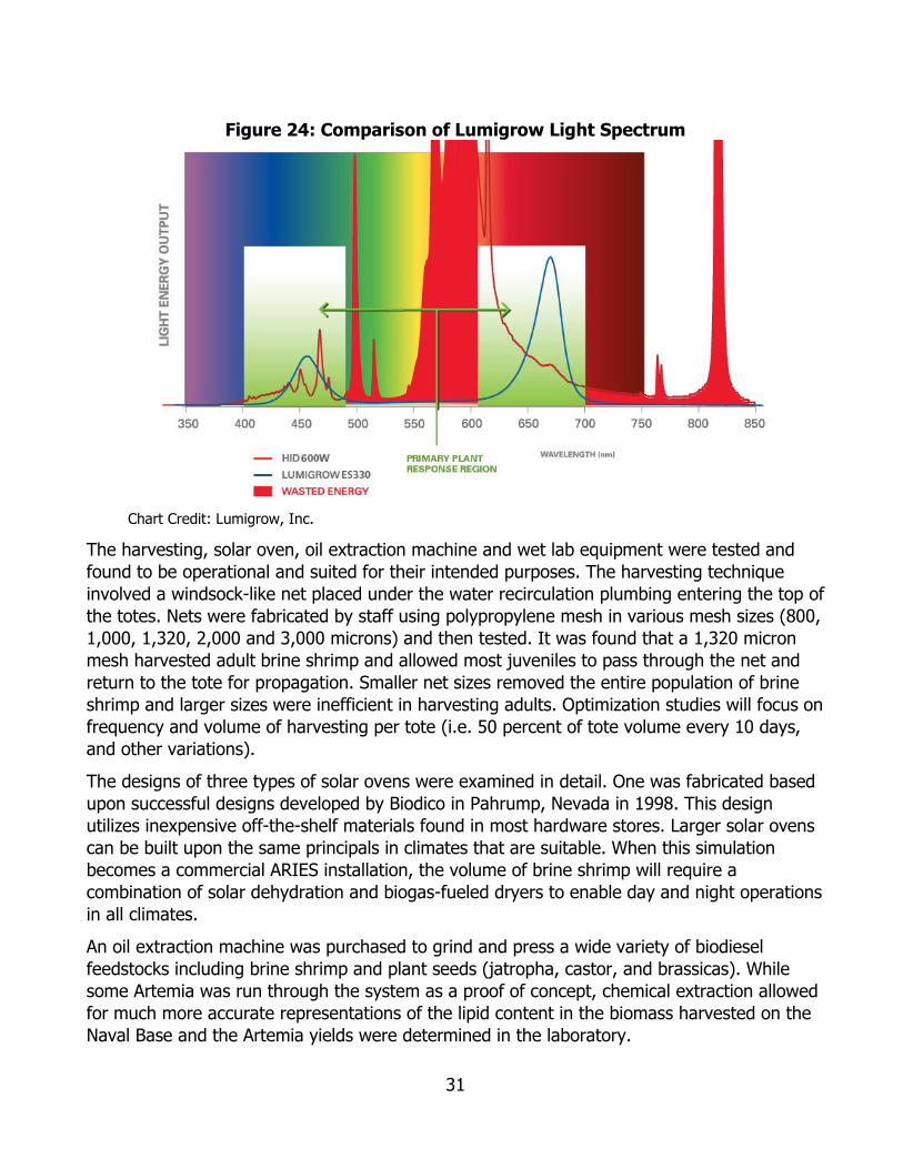
31
Figure 24: Comparison of Lumigrow Light Spectrum
Chart Credit: Lumigrow, Inc.
The harvesting, solar oven, oil extraction machine and wet lab equipment were tested and found to be operational and suited for their intended purposes. The harvesting technique involved a windsock-like net placed under the water recirculation plumbing entering the top of the totes. Nets were fabricated by staff using polypropylene mesh in various mesh sizes (800, 1,000, 1,320, 2,000 and 3,000 microns) and then tested. It was found that a 1,320 micron mesh harvested adult brine shrimp and allowed most juveniles to pass through the net and return to the tote for propagation. Smaller net sizes removed the entire population of brine shrimp and larger sizes were inefficient in harvesting adults. Optimization studies will focus on frequency and volume of harvesting per tote (i.e. 50 percent of tote volume every 10 days, and other variations).
The designs of three types of solar ovens were examined in detail. One was fabricated based upon successful designs developed by Biodico in Pahrump, Nevada in 1998. This design utilizes inexpensive off-the-shelf materials found in most hardware stores. Larger solar ovens can be built upon the same principals in climates that are suitable. When this simulation becomes a commercial ARIES installation, the volume of brine shrimp will require a combination of solar dehydration and biogas-fueled dryers to enable day and night operations in all climates.
An oil extraction machine was purchased to grind and press a wide variety of biodiesel feedstocks including brine shrimp and plant seeds (jatropha, castor, and brassicas). While some Artemia was run through the system as a proof of concept, chemical extraction allowed for much more accurate representations of the lipid content in the biomass harvested on the Naval Base and the Artemia yields were determined in the laboratory.
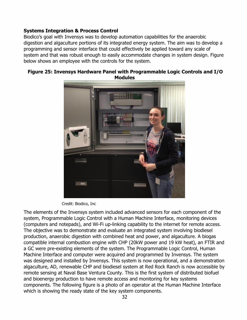
32
Systems Integration & Process Control Biodico’s goal with Invensys was to develop automation capabilities for the anaerobic digestion and algaculture portions of its integrated energy system. The aim was to develop a programming and sensor interface that could effectively be applied toward any scale of system and that was robust enough to easily accommodate changes in system design. Figure below shows an employee with the controls for the system.
Figure 25: Invensys Hardware Panel with Programmable Logic Controls and I/O Modules
Credit: Biodico, Inc
The elements of the Invensys system included advanced sensors for each component of the system, Programmable Logic Control with a Human Machine Interface, monitoring devices (computers and notepads), and Wi-Fi up-linking capability to the internet for remote access. The objective was to demonstrate and evaluate an integrated system involving biodiesel production, anaerobic digestion with combined heat and power, and algaculture. A biogas compatible internal combustion engine with CHP (20kW power and 19 kW heat), an FTIR and a GC were pre-existing elements of the system. The Programmable Logic Control, Human Machine Interface and computer were acquired and programmed by Invensys. The system was designed and installed by Invensys. This system is now operational, and a demonstration algaculture, AD, renewable CHP and biodiesel system at Red Rock Ranch is now accessible by remote sensing at Naval Base Ventura County. This is the first system of distributed biofuel and bioenergy production to have remote access and monitoring for key systems components. The following figure is a photo of an operator at the Human Machine Interface which is showing the ready state of the key system components.
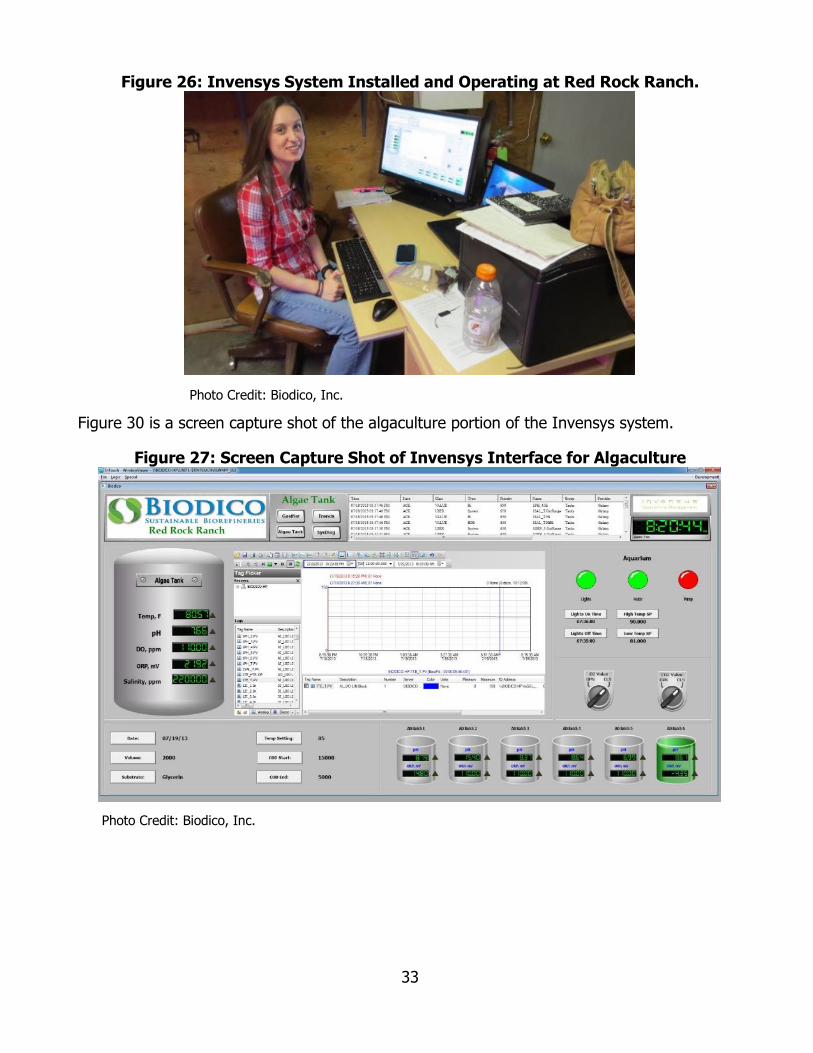
33
Figure 26: Invensys System Installed and Operating at Red Rock Ranch.
Photo Credit: Biodico, Inc.
Figure 30 is a screen capture shot of the algaculture portion of the Invensys system.
Figure 27: Screen Capture Shot of Invensys Interface for Algaculture
Photo Credit: Biodico, Inc.

34
CHAPTER 2: Activities and Results
The purpose of this chapter is to describe the activities and results of ARV-10-024. The goal was to operate all equipment as an integrated system using the actual process materials and establish a baseline.
Summary of Activities & Results All system components were operational and were run as part of an integrated system using actual process materials. The demonstration has shown that it is possible to operate a network of distributed sustainable biorefineries integrated with renewable combined heat and power by utilizing a centralized command and control center to provide remote support. The activities and results are divided into topic areas which align with the components of ARIES, as shown in Figure 31.
Figure 28: Summary of Activities
Chart Credit: Biodico, Inc.
(1) Biodiesel Production: Biodiesel and glycerin baseline times were established by tracking the test times for confirming that materials met standards set by the American Society for Testing and Materials (ASTM). ASTM method D6584 requires 15 minutes of silylation so that the analytes have different retention times in the polysiloxane column and 30 minutes of elution through the column. Test method comparisons were made between Fourier transform infrared (FTIR) and Gas Chromatography (GC). There was good correlation between the two sets of results and a more extensive library was developed to include different feedstocks and materials utilized in biodiesel production, algaculture and anaerobic digestion. It was found that FTIR is substantially faster than GC and can save significant production time, while also

35
enabling less skilled workers to operate commercial production facilities with more reliable results.
(2) Anaerobic Digestion and Combined Heat and Power: Anaerobic digestion baselines were established by running a series of tests using the AMPTS using a variety of substrates both separately and together for co-digestion. Glycerin was found to be an accelerant for the substrates tested, but the proportions of co-digestates was critical.
(3) Algaculture: Algaculture baselines were established by stabilizing the 16 laboratory aquariums, and 16 greenhouse totes with 90 ppt saline water with healthy populations of brine shrimp and algae. Optimal growth conditions, harvesting techniques, dehydration systems and oil extraction equipment were established and operated using actual process materials.
(4) Systems Integration and Process Control: Automation and remote sensing baselines were established by setting up a remote system at Red Rock Ranch which incorporates all of the key components of an ARIES sustainable biorefinery (algaculture, anaerobic digestion, renewable combined heat and power, and biodiesel production). An automation and remote sensing system was fabricated and installed by Invensys, and continues to operate and collect data for the Final Report. It was found that the Invensys system substantially improved safety, quality control and production efficiency while enabling less skilled workers to operate the equipment with support from a centralized command and control center at Biodico location at Naval Base Ventura County.
Activities & Results The activities and results are divided into topic areas which align with the components of ARIES.
Biodiesel Production The biodiesel industry in the United States has expanded significantly since its inception in 1993. At the time the United Soybean Board was trying to find a long-term market for the roughly 30 million gallons of oil per year that the member farmers were producing. There was some limited commercial biodiesel production in Europe, and the chemical reaction to transesterify fatty acid containing lipids into fatty acid methyl esters was frequently used in biochemical laboratory work. The National Biodiesel Board was founded as the trade association for the emerging U.S. biodiesel industry and members worked to develop a market for the new fuel. In order to make significant inroads into energy markets, it was crucial to gain fleet acceptance so that the fuel could be sold to organizations that were under renewable mandates. There was a relatively small contingent of early adopters, but at the time the price of biodiesel was significantly higher than the price of petroleum diesel. In 1993, the nominal price of crude oil was $19.75 per barrel and the inflation adjusted price would be $27.00. Many fleet operators, however, were faced with renewable energy mandates that required them to switch their energy consumption from petroleum to various degrees. The most common solution was to switch part of the fleet to natural gas, which required all new vehicles and new infrastructure. Even though biodiesel was more costly than petroleum diesel, it was a lot less expensive than switching to natural gas.
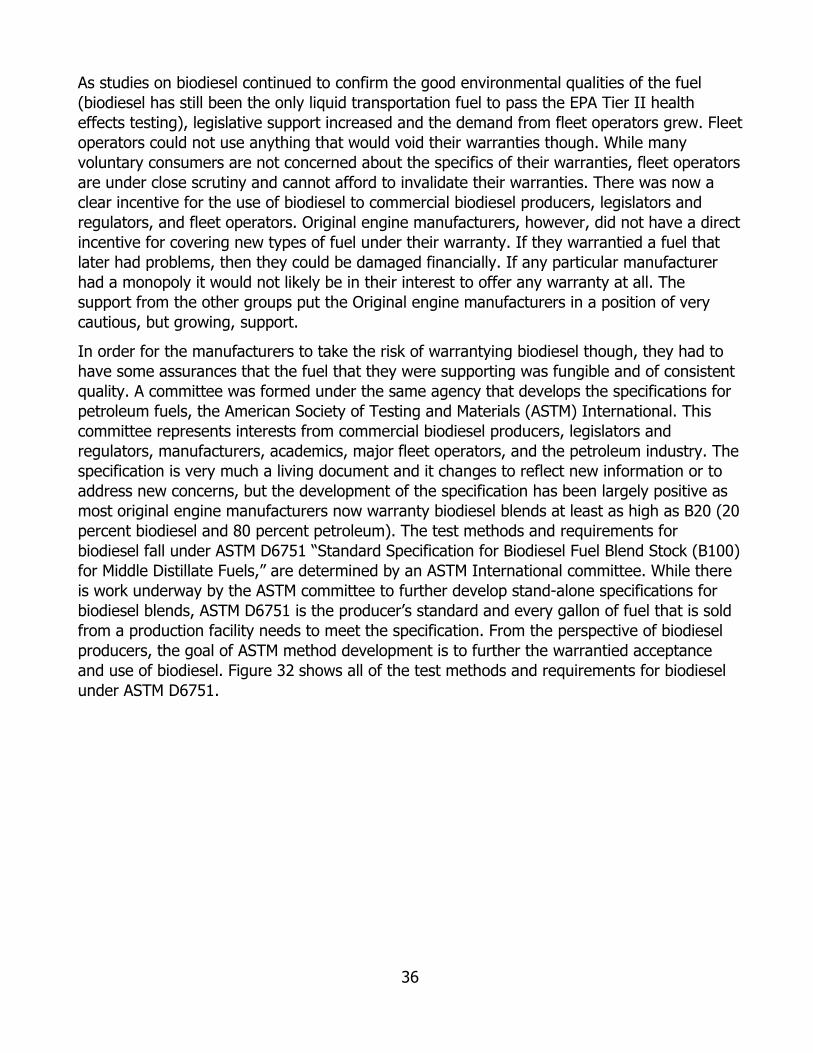
36
As studies on biodiesel continued to confirm the good environmental qualities of the fuel (biodiesel has still been the only liquid transportation fuel to pass the EPA Tier II health effects testing), legislative support increased and the demand from fleet operators grew. Fleet operators could not use anything that would void their warranties though. While many voluntary consumers are not concerned about the specifics of their warranties, fleet operators are under close scrutiny and cannot afford to invalidate their warranties. There was now a clear incentive for the use of biodiesel to commercial biodiesel producers, legislators and regulators, and fleet operators. Original engine manufacturers, however, did not have a direct incentive for covering new types of fuel under their warranty. If they warrantied a fuel that later had problems, then they could be damaged financially. If any particular manufacturer had a monopoly it would not likely be in their interest to offer any warranty at all. The support from the other groups put the Original engine manufacturers in a position of very cautious, but growing, support.
In order for the manufacturers to take the risk of warrantying biodiesel though, they had to have some assurances that the fuel that they were supporting was fungible and of consistent quality. A committee was formed under the same agency that develops the specifications for petroleum fuels, the American Society of Testing and Materials (ASTM) International. This committee represents interests from commercial biodiesel producers, legislators and regulators, manufacturers, academics, major fleet operators, and the petroleum industry. The specification is very much a living document and it changes to reflect new information or to address new concerns, but the development of the specification has been largely positive as most original engine manufacturers now warranty biodiesel blends at least as high as B20 (20 percent biodiesel and 80 percent petroleum). The test methods and requirements for biodiesel fall under ASTM D6751 “Standard Specification for Biodiesel Fuel Blend Stock (B100) for Middle Distillate Fuels,” are determined by an ASTM International committee. While there is work underway by the ASTM committee to further develop stand-alone specifications for biodiesel blends, ASTM D6751 is the producer’s standard and every gallon of fuel that is sold from a production facility needs to meet the specification. From the perspective of biodiesel producers, the goal of ASTM method development is to further the warrantied acceptance and use of biodiesel. Figure 32 shows all of the test methods and requirements for biodiesel under ASTM D6751.
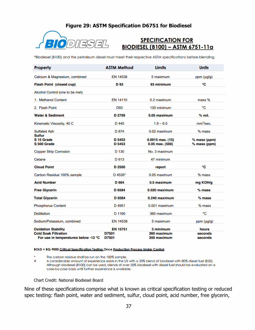
37
Figure 29: ASTM Specification D6751 for Biodiesel
Chart Credit: National Biodiesel Board
Nine of these specifications comprise what is known as critical specification testing or reduced spec testing: flash point, water and sediment, sulfur, cloud point, acid number, free glycerin,
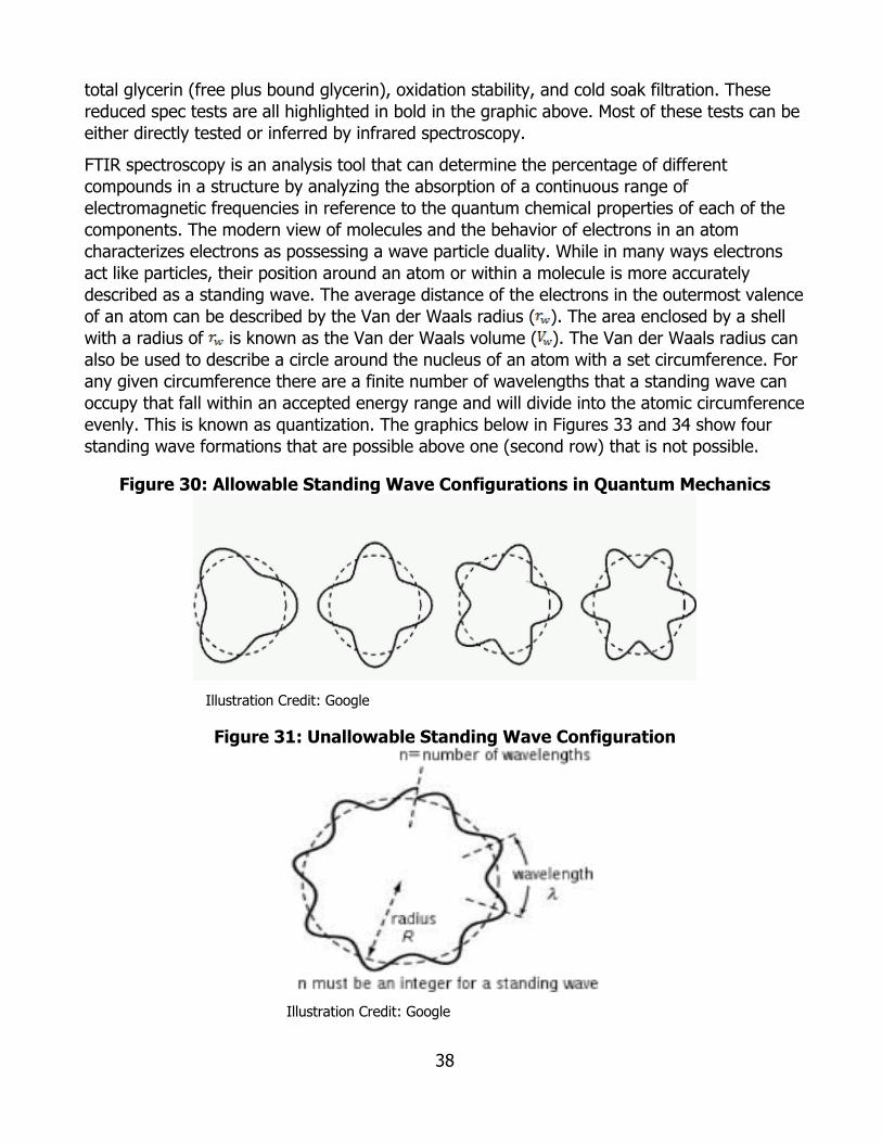
38
total glycerin (free plus bound glycerin), oxidation stability, and cold soak filtration. These reduced spec tests are all highlighted in bold in the graphic above. Most of these tests can be either directly tested or inferred by infrared spectroscopy.
FTIR spectroscopy is an analysis tool that can determine the percentage of different compounds in a structure by analyzing the absorption of a continuous range of electromagnetic frequencies in reference to the quantum chemical properties of each of the components. The modern view of molecules and the behavior of electrons in an atom characterizes electrons as possessing a wave particle duality. While in many ways electrons act like particles, their position around an atom or within a molecule is more accurately described as a standing wave. The average distance of the electrons in the outermost valence of an atom can be described by the Van der Waals radius ( ). The area enclosed by a shell with a radius of is known as the Van der Waals volume ( ). The Van der Waals radius can also be used to describe a circle around the nucleus of an atom with a set circumference. For any given circumference there are a finite number of wavelengths that a standing wave can occupy that fall within an accepted energy range and will divide into the atomic circumference evenly. This is known as quantization. The graphics below in Figures 33 and 34 show four standing wave formations that are possible above one (second row) that is not possible.
Figure 30: Allowable Standing Wave Configurations in Quantum Mechanics
Illustration Credit: Google
Figure 31: Unallowable Standing Wave Configuration
Illustration Credit: Google
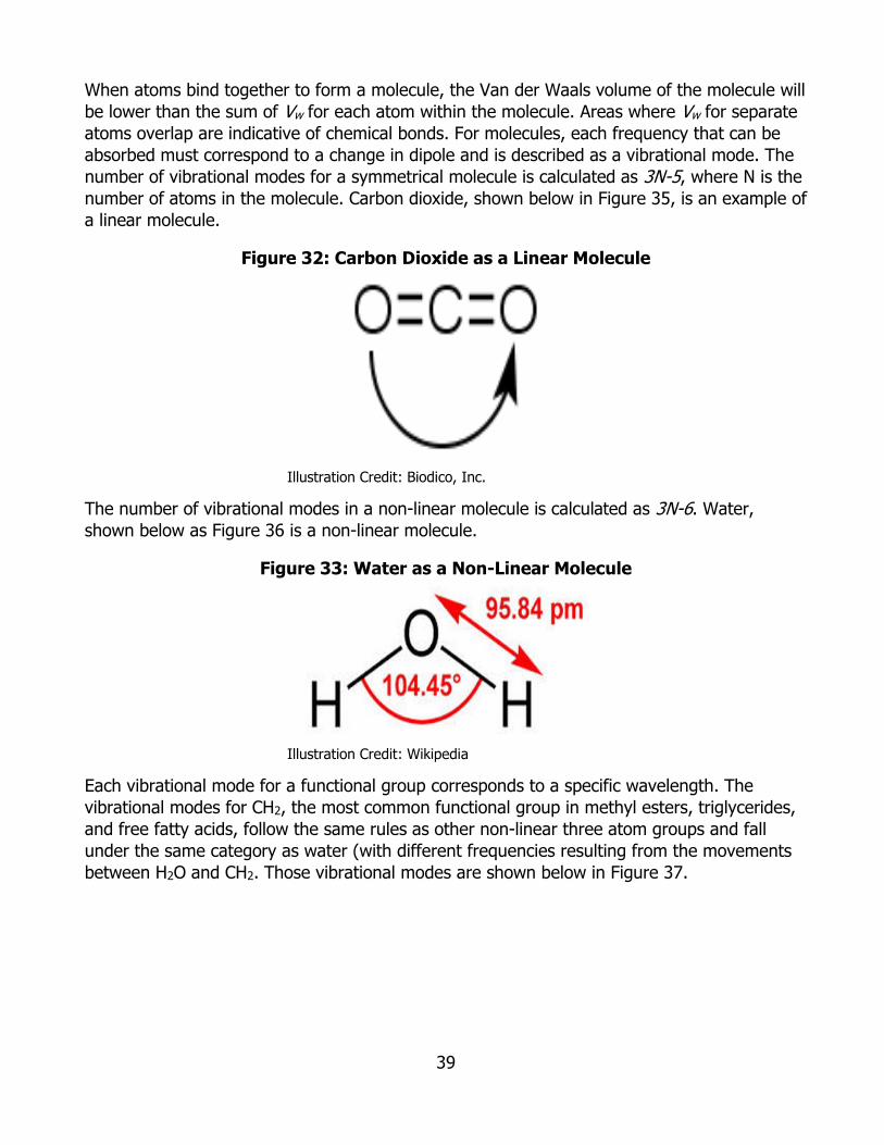
39
When atoms bind together to form a molecule, the Van der Waals volume of the molecule will be lower than the sum of Vw for each atom within the molecule. Areas where Vw for separate atoms overlap are indicative of chemical bonds. For molecules, each frequency that can be absorbed must correspond to a change in dipole and is described as a vibrational mode. The number of vibrational modes for a symmetrical molecule is calculated as 3N-5, where N is the number of atoms in the molecule. Carbon dioxide, shown below in Figure 35, is an example of a linear molecule.
Figure 32: Carbon Dioxide as a Linear Molecule
Illustration Credit: Biodico, Inc.
The number of vibrational modes in a non-linear molecule is calculated as 3N-6. Water, shown below as Figure 36 is a non-linear molecule.
Figure 33: Water as a Non-Linear Molecule
Illustration Credit: Wikipedia
Each vibrational mode for a functional group corresponds to a specific wavelength. The vibrational modes for CH2, the most common functional group in methyl esters, triglycerides, and free fatty acids, follow the same rules as other non-linear three atom groups and fall under the same category as water (with different frequencies resulting from the movements between H2O and CH2. Those vibrational modes are shown below in Figure 37.
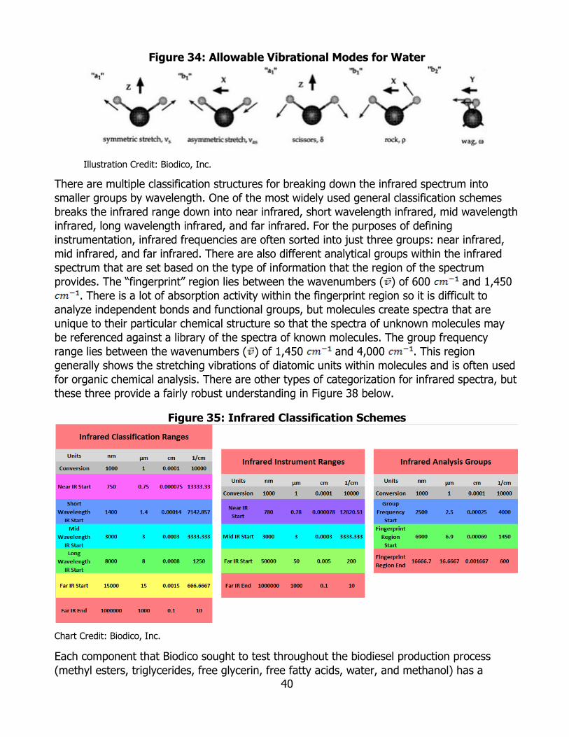
40
Figure 34: Allowable Vibrational Modes for Water
Illustration Credit: Biodico, Inc.
There are multiple classification structures for breaking down the infrared spectrum into smaller groups by wavelength. One of the most widely used general classification schemes breaks the infrared range down into near infrared, short wavelength infrared, mid wavelength infrared, long wavelength infrared, and far infrared. For the purposes of defining instrumentation, infrared frequencies are often sorted into just three groups: near infrared, mid infrared, and far infrared. There are also different analytical groups within the infrared spectrum that are set based on the type of information that the region of the spectrum provides. The “fingerprint” region lies between the wavenumbers ( ) of 600 and 1,450
. There is a lot of absorption activity within the fingerprint region so it is difficult to analyze independent bonds and functional groups, but molecules create spectra that are unique to their particular chemical structure so that the spectra of unknown molecules may be referenced against a library of the spectra of known molecules. The group frequency range lies between the wavenumbers ( ) of 1,450 and 4,000 . This region generally shows the stretching vibrations of diatomic units within molecules and is often used for organic chemical analysis. There are other types of categorization for infrared spectra, but these three provide a fairly robust understanding in Figure 38 below.
Figure 35: Infrared Classification Schemes
Chart Credit: Biodico, Inc.
Each component that Biodico sought to test throughout the biodiesel production process (methyl esters, triglycerides, free glycerin, free fatty acids, water, and methanol) has a
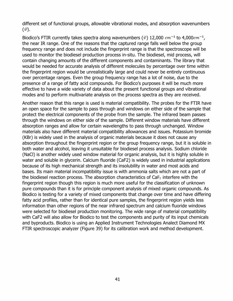
41
different set of functional groups, allowable vibrational modes, and absorption wavenumbers ( ).
Biodico’s FTIR currently takes spectra along wavenumbers ( ) 12,000 to 4,000 , the near IR range. One of the reasons that the captured range falls well below the group frequency range and does not include the fingerprint range is that the spectroscope will be used to monitor the biodiesel production process in-situ. The biodiesel, mid process, will contain changing amounts of the different components and contaminants. The library that would be needed for accurate analysis of different molecules by percentage over time within the fingerprint region would be unrealistically large and could never be entirely continuous over percentage ranges. Even the group frequency range has a lot of noise, due to the presence of a range of fatty acid compounds. For Biodico’s purposes it will be much more effective to have a wide variety of data about the present functional groups and vibrational modes and to perform multivariate analysis on the process spectra as they are received.
Another reason that this range is used is material compatibility. The probes for the FTIR have an open space for the sample to pass through and windows on either side of the sample that protect the electrical components of the probe from the sample. The infrared beam passes through the windows on either side of the sample. Different window materials have different absorption ranges and allow for certain wavelengths to pass through unchanged. Window materials also have different material compatibility allowances and issues. Potassium bromide (KBr) is widely used in the analysis of organic materials because it does not cause any absorption throughout the fingerprint region or the group frequency range, but it is soluble in both water and alcohol, leaving it unsuitable for biodiesel process analysis. Sodium chloride (NaCl) is another widely used window material for organic analysis, but it is highly soluble in water and soluble in glycerin. Calcium fluoride (CaF2) is widely used in industrial applications because of its high mechanical strength and its insolubility in water and most acids and bases. Its main material incompatibility issue is with ammonia salts which are not a part of the biodiesel reaction process. The absorption characteristics of Ca interfere with the fingerprint region though this region is much more useful for the classification of unknown pure compounds than it is for principle component analysis of mixed organic compounds. As Biodico is testing for a variety of mixed components that change over time and have differing fatty acid profiles, rather than for identical pure samples, the fingerprint region yields less information than other regions of the near infrared spectrum and calcium fluoride windows were selected for biodiesel production monitoring. The wide range of material compatibility with CaF2 will also allow for Biodico to test the components and purity of its input chemicals and byproducts. Biodico is using an Applied Instrument Technologies Analect Diamond MX FTIR spectroscopic analyzer (Figure 39) for its calibration work and method development.

42
Figure 36: Analect Diamond MX FTIR Analyzer Used by Biodico
Photo Credit: Applied Instrument Technologies
Work on spectroscopic operations, spectra analysis, and method development can be greatly aided by the use of computer software. The spectrometer came with the manufacturer’s software suite for interfacing with the machine. The software suite includes many different programs that were written specifically to perform certain functions, but the suite is primarily based around three programs that can call up the functionality of the smaller programs internally. The FX80 program is used to gather and analyze individual spectra, to perform mathematical calculations and manipulations of individual spectra, and to build libraries of different spectra. The PC80 program is used to perform real time analysis of spectroscopic inputs based on internally developed test methods. The QC80 program is used to develop test methods for the FTIR.
Between these three software programs though, there is one missing piece. After a method is developed using QC80 it needs to be plugged into a chemometrics program that will analyze all of the data points that are generated by the samples with known analyte concentrations. As new spectra enter the system every 15 seconds, each new spectra needs to be compared to the existing library of spectra so that the composition of the material that generated the active spectra can be measured. The manufacturer of the FTIR analyzer, AIT, provides a program that performs this function called CPSA (short for Constrained Principal-component Spectra Analysis). While AIT makes both CPSA and the software suite of PC80, QC80, and FX80, CPSA is run in a more isolated environment. It does not interact directly with the analyzer and the libraries are built independently of the operation of the other three programs. The PC80, FX80, and QC80 software package will also work with a variety of chemometrics programs aside from AIT. This flexibility was designed for users to be able to work with their existing libraries in the case of a switch to AIT’s analyzers from another manufacturer. Biodico is currently using the CPSA software, but has the option in the future to use a wide variety of programs without compromising the test methods that have already been built.
Biodico has also explored a variety of third-party helper software. In order to gain a fuller understanding of the quantum chemical properties of compounds and to verify the results of spectroscopic analysis, there are a number of freeware and shareware programs that perform
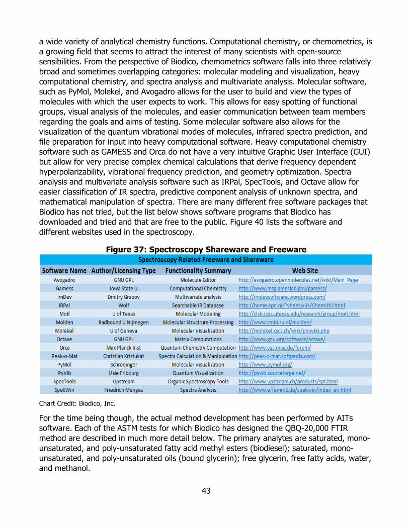
43
a wide variety of analytical chemistry functions. Computational chemistry, or chemometrics, is a growing field that seems to attract the interest of many scientists with open-source sensibilities. From the perspective of Biodico, chemometrics software falls into three relatively broad and sometimes overlapping categories: molecular modeling and visualization, heavy computational chemistry, and spectra analysis and multivariate analysis. Molecular software, such as PyMol, Molekel, and Avogadro allows for the user to build and view the types of molecules with which the user expects to work. This allows for easy spotting of functional groups, visual analysis of the molecules, and easier communication between team members regarding the goals and aims of testing. Some molecular software also allows for the visualization of the quantum vibrational modes of molecules, infrared spectra prediction, and file preparation for input into heavy computational software. Heavy computational chemistry software such as GAMESS and Orca do not have a very intuitive Graphic User Interface (GUI) but allow for very precise complex chemical calculations that derive frequency dependent hyperpolarizability, vibrational frequency prediction, and geometry optimization. Spectra analysis and multivariate analysis software such as IRPal, SpecTools, and Octave allow for easier classification of IR spectra, predictive component analysis of unknown spectra, and mathematical manipulation of spectra. There are many different free software packages that Biodico has not tried, but the list below shows software programs that Biodico has downloaded and tried and that are free to the public. Figure 40 lists the software and different websites used in the spectroscopy.
Figure 37: Spectroscopy Shareware and Freeware
Chart Credit: Biodico, Inc.
For the time being though, the actual method development has been performed by AITs software. Each of the ASTM tests for which Biodico has designed the QBQ-20,000 FTIR method are described in much more detail below. The primary analytes are saturated, mono-unsaturated, and poly-unsaturated fatty acid methyl esters (biodiesel); saturated, mono-unsaturated, and poly-unsaturated oils (bound glycerin); free glycerin, free fatty acids, water, and methanol.
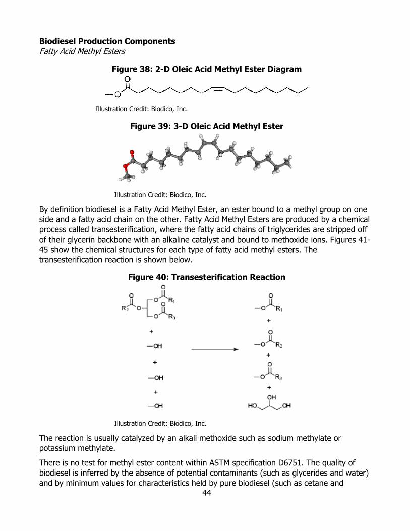
44
Biodiesel Production Components Fatty Acid Methyl Esters
Figure 38: 2-D Oleic Acid Methyl Ester Diagram
Illustration Credit: Biodico, Inc.
Figure 39: 3-D Oleic Acid Methyl Ester
Illustration Credit: Biodico, Inc.
By definition biodiesel is a Fatty Acid Methyl Ester, an ester bound to a methyl group on one side and a fatty acid chain on the other. Fatty Acid Methyl Esters are produced by a chemical process called transesterification, where the fatty acid chains of triglycerides are stripped off of their glycerin backbone with an alkaline catalyst and bound to methoxide ions. Figures 41-45 show the chemical structures for each type of fatty acid methyl esters. The transesterification reaction is shown below.
Figure 40: Transesterification Reaction
Illustration Credit: Biodico, Inc.
The reaction is usually catalyzed by an alkali methoxide such as sodium methylate or potassium methylate.
There is no test for methyl ester content within ASTM specification D6751. The quality of biodiesel is inferred by the absence of potential contaminants (such as glycerides and water) and by minimum values for characteristics held by pure biodiesel (such as cetane and
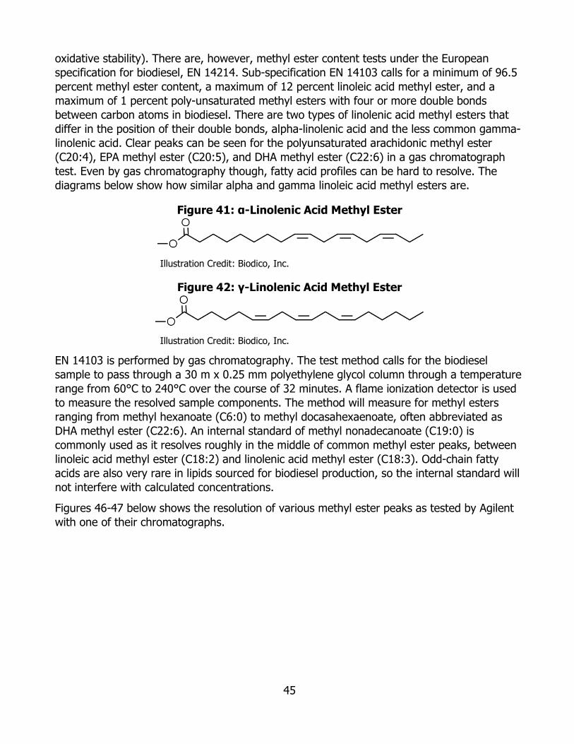
45
oxidative stability). There are, however, methyl ester content tests under the European specification for biodiesel, EN 14214. Sub-specification EN 14103 calls for a minimum of 96.5 percent methyl ester content, a maximum of 12 percent linoleic acid methyl ester, and a maximum of 1 percent poly-unsaturated methyl esters with four or more double bonds between carbon atoms in biodiesel. There are two types of linolenic acid methyl esters that differ in the position of their double bonds, alpha-linolenic acid and the less common gamma-linolenic acid. Clear peaks can be seen for the polyunsaturated arachidonic methyl ester (C20:4), EPA methyl ester (C20:5), and DHA methyl ester (C22:6) in a gas chromatograph test. Even by gas chromatography though, fatty acid profiles can be hard to resolve. The diagrams below show how similar alpha and gamma linoleic acid methyl esters are.
Figure 41: α-Linolenic Acid Methyl Ester
Illustration Credit: Biodico, Inc.
Figure 42: γ-Linolenic Acid Methyl Ester
Illustration Credit: Biodico, Inc.
EN 14103 is performed by gas chromatography. The test method calls for the biodiesel sample to pass through a 30 m x 0.25 mm polyethylene glycol column through a temperature range from 60°C to 240°C over the course of 32 minutes. A flame ionization detector is used to measure the resolved sample components. The method will measure for methyl esters ranging from methyl hexanoate (C6:0) to methyl docasahexaenoate, often abbreviated as DHA methyl ester (C22:6). An internal standard of methyl nonadecanoate (C19:0) is commonly used as it resolves roughly in the middle of common methyl ester peaks, between linoleic acid methyl ester (C18:2) and linolenic acid methyl ester (C18:3). Odd-chain fatty acids are also very rare in lipids sourced for biodiesel production, so the internal standard will not interfere with calculated concentrations.
Figures 46-47 below shows the resolution of various methyl ester peaks as tested by Agilent with one of their chromatographs.
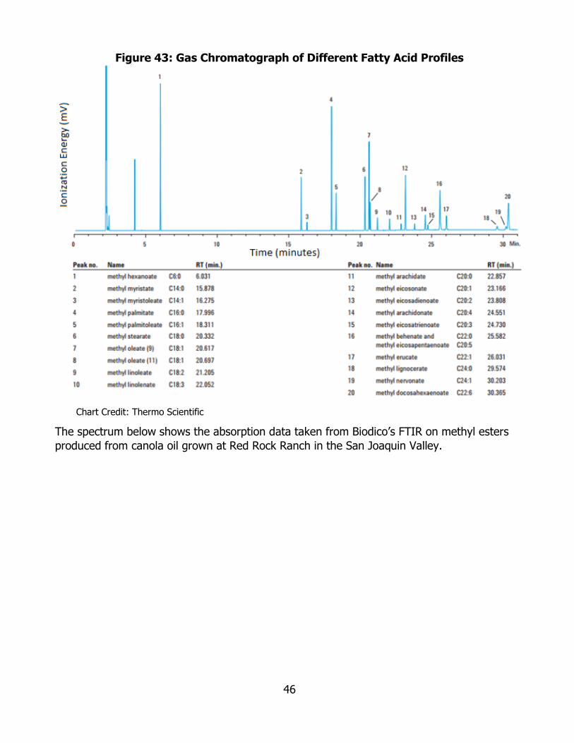
46
Figure 43: Gas Chromatograph of Different Fatty Acid Profiles
Chart Credit: Thermo Scientific
The spectrum below shows the absorption data taken from Biodico’s FTIR on methyl esters produced from canola oil grown at Red Rock Ranch in the San Joaquin Valley.
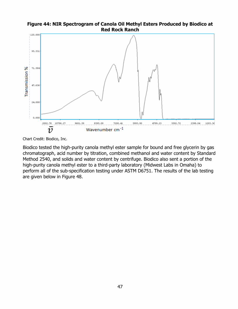
47
Figure 44: NIR Spectrogram of Canola Oil Methyl Esters Produced by Biodico at Red Rock Ranch
Chart Credit: Biodico, Inc.
Biodico tested the high-purity canola methyl ester sample for bound and free glycerin by gas chromatograph, acid number by titration, combined methanol and water content by Standard Method 2540, and solids and water content by centrifuge. Biodico also sent a portion of the high-purity canola methyl ester to a third-party laboratory (Midwest Labs in Omaha) to perform all of the sub-specification testing under ASTM D6751. The results of the lab testing are given below in Figure 48.

48
Figure 45: Third Party Test Results of the High Mono-Unsaturated Reference Fuel
Chart Credit: Biodico, Inc.
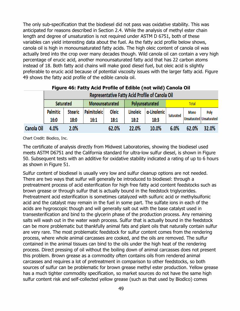
49
The only sub-specification that the biodiesel did not pass was oxidative stability. This was anticipated for reasons described in Section 2.4. While the analysis of methyl ester chain length and degree of unsaturation is not required under ASTM D 6751, both of these variables can yield interesting data about the fuel. As the fatty acid profile below shows, canola oil is high in monounsaturated fatty acids. The high oleic content of canola oil was actually bred into the crop over many decades though. Wild canola oil can contain a very high percentage of erucic acid, another monounsaturated fatty acid that has 22 carbon atoms instead of 18. Both fatty acid chains will make good diesel fuel, but oleic acid is slightly preferable to erucic acid because of potential viscosity issues with the larger fatty acid. Figure 49 shows the fatty acid profile of the edible canola oil.
Figure 46: Fatty Acid Profile of Edible (not wild) Canola Oil
Chart Credit: Biodico, Inc.
The certificate of analysis directly from Midwest Laboratories, showing the biodiesel used meets ASTM D6751 and the California standard for ultra-low sulfur diesel, is shown in Figure 50. Subsequent tests with an additive for oxidative stability indicated a rating of up to 6 hours as shown in Figure 51.
Sulfur content of biodiesel is usually very low and sulfur cleanup options are not needed. There are two ways that sulfur will generally be introduced to biodiesel: through a pretreatment process of acid esterification for high free fatty acid content feedstocks such as brown grease or through sulfur that is actually bound in the feedstock triglycerides. Pretreatment acid esterification is sometimes catalyzed with sulfuric acid or methylsulfonic acid and the catalyst may remain in the fuel in some part. The sulfate ions in each of the acids are hygroscopic though and will generally salt out with the base catalyst used in transesterification and bind to the glycerin phase of the production process. Any remaining salts will wash out in the water wash process. Sulfur that is actually bound in the feedstock can be more problematic but thankfully animal fats and plant oils that naturally contain sulfur are very rare. The most problematic feedstock for sulfur content comes from the rendering process, where whole animal carcasses are cooked, and the oils are removed. The sulfur contained in the animal tissues can bind to the oils under the high heat of the rendering process. Direct pressing of oil without the boiling down of animal carcasses does not present this problem. Brown grease as a commodity often contains oils from rendered animal carcasses and requires a lot of pretreatment in comparison to other feedstocks, so both sources of sulfur can be problematic for brown grease methyl ester production. Yellow grease has a much tighter commodity specification, so market sources do not have the same high sulfur content risk and self-collected yellow grease (such as that used by Biodico) comes
50
directly from the restaurant fryers and contains little to no sulfur. Biodico’s feedstock contains minimal sulfur and the concentration of sulfur in the biodiesel tested below was only 3.4 parts per million.
Many of the potential contaminants in the biodiesel returned tested values below detectable limits, as shown in Figure 50. These include water, sediment, methanol, sulfated ash, carbon residue, free glycerin, phosphorus, magnesium, calcium, sodium, and potassium. Biodiesel stability is directly related to the degree of unsaturation of the biodiesel feedstock and not to the chemical reactions of the production process. The required induction time for the oxidative stability index is three hours in the US and six hours in Europe. The lower induction time in the US is partly due to the wide use of soybean oil, which has a high percentage of polyunsaturated linoleic and linolenic acids. Stability additives brought Biodico’s canola (highly monounsaturated, which is inherently more stable than polyunsaturated) methyl esters above the US specification of three hours and the European specification of six hours. The biodiesel that was used for this grant was not produced with funding from this grant.
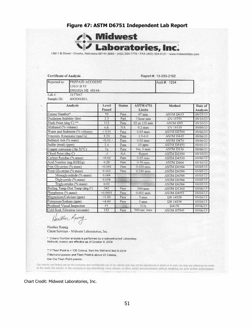
51
Figure 47: ASTM D6751 Independent Lab Report
Chart Credit: Midwest Laboratories, Inc.
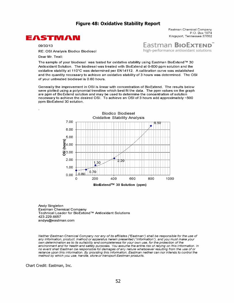
52
Figure 48: Oxidative Stability Report
Chart Credit: Eastman, Inc.
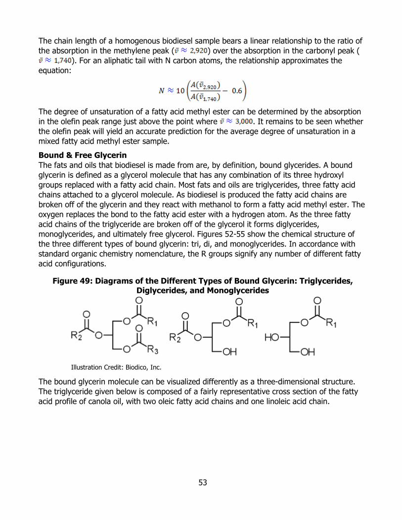
53
The chain length of a homogenous biodiesel sample bears a linear relationship to the ratio of the absorption in the methylene peak ( ) over the absorption in the carbonyl peak (
). For an aliphatic tail with N carbon atoms, the relationship approximates the equation:
The degree of unsaturation of a fatty acid methyl ester can be determined by the absorption in the olefin peak range just above the point where . It remains to be seen whether the olefin peak will yield an accurate prediction for the average degree of unsaturation in a mixed fatty acid methyl ester sample. Bound & Free Glycerin The fats and oils that biodiesel is made from are, by definition, bound glycerides. A bound glycerin is defined as a glycerol molecule that has any combination of its three hydroxyl groups replaced with a fatty acid chain. Most fats and oils are triglycerides, three fatty acid chains attached to a glycerol molecule. As biodiesel is produced the fatty acid chains are broken off of the glycerin and they react with methanol to form a fatty acid methyl ester. The oxygen replaces the bond to the fatty acid ester with a hydrogen atom. As the three fatty acid chains of the triglyceride are broken off of the glycerol it forms diglycerides, monoglycerides, and ultimately free glycerol. Figures 52-55 show the chemical structure of the three different types of bound glycerin: tri, di, and monoglycerides. In accordance with standard organic chemistry nomenclature, the R groups signify any number of different fatty acid configurations.
Figure 49: Diagrams of the Different Types of Bound Glycerin: Triglycerides, Diglycerides, and Monoglycerides
Illustration Credit: Biodico, Inc.
The bound glycerin molecule can be visualized differently as a three-dimensional structure. The triglyceride given below is composed of a fairly representative cross section of the fatty acid profile of canola oil, with two oleic fatty acid chains and one linoleic acid chain.
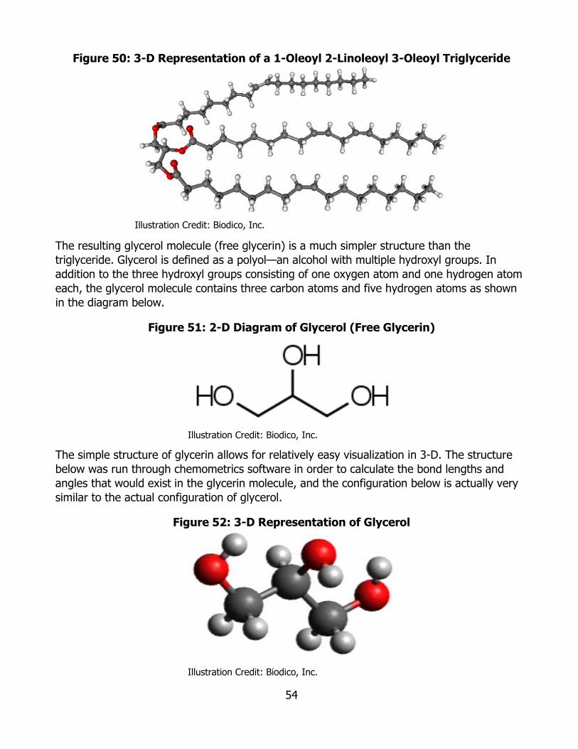
54
Figure 50: 3-D Representation of a 1-Oleoyl 2-Linoleoyl 3-Oleoyl Triglyceride
Illustration Credit: Biodico, Inc.
The resulting glycerol molecule (free glycerin) is a much simpler structure than the triglyceride. Glycerol is defined as a polyol—an alcohol with multiple hydroxyl groups. In addition to the three hydroxyl groups consisting of one oxygen atom and one hydrogen atom each, the glycerol molecule contains three carbon atoms and five hydrogen atoms as shown in the diagram below.
Figure 51: 2-D Diagram of Glycerol (Free Glycerin)
Illustration Credit: Biodico, Inc.
The simple structure of glycerin allows for relatively easy visualization in 3-D. The structure below was run through chemometrics software in order to calculate the bond lengths and angles that would exist in the glycerin molecule, and the configuration below is actually very similar to the actual configuration of glycerol.
Figure 52: 3-D Representation of Glycerol
Illustration Credit: Biodico, Inc.
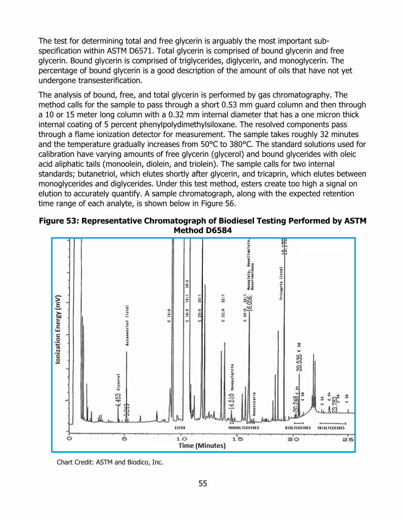
55
The test for determining total and free glycerin is arguably the most important sub-specification within ASTM D6571. Total glycerin is comprised of bound glycerin and free glycerin. Bound glycerin is comprised of triglycerides, diglycerin, and monoglycerin. The percentage of bound glycerin is a good description of the amount of oils that have not yet undergone transesterification.
The analysis of bound, free, and total glycerin is performed by gas chromatography. The method calls for the sample to pass through a short 0.53 mm guard column and then through a 10 or 15 meter long column with a 0.32 mm internal diameter that has a one micron thick internal coating of 5 percent phenylpolydimethylsiloxane. The resolved components pass through a flame ionization detector for measurement. The sample takes roughly 32 minutes and the temperature gradually increases from 50°C to 380°C. The standard solutions used for calibration have varying amounts of free glycerin (glycerol) and bound glycerides with oleic acid aliphatic tails (monoolein, diolein, and triolein). The sample calls for two internal standards; butanetriol, which elutes shortly after glycerin, and tricaprin, which elutes between monoglycerides and diglycerides. Under this test method, esters create too high a signal on elution to accurately quantify. A sample chromatograph, along with the expected retention time range of each analyte, is shown below in Figure 56.
Figure 53: Representative Chromatograph of Biodiesel Testing Performed by ASTM Method D6584
Chart Credit: ASTM and Biodico, Inc.
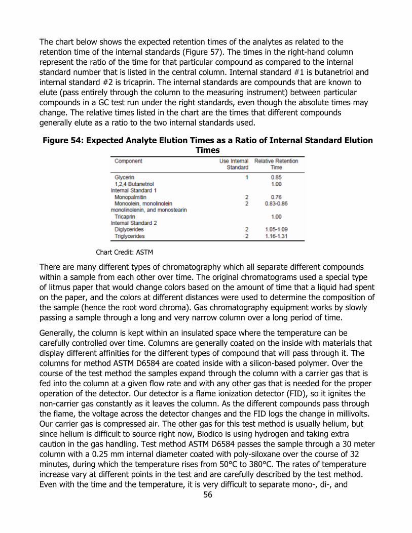
56
The chart below shows the expected retention times of the analytes as related to the retention time of the internal standards (Figure 57). The times in the right-hand column represent the ratio of the time for that particular compound as compared to the internal standard number that is listed in the central column. Internal standard #1 is butanetriol and internal standard #2 is tricaprin. The internal standards are compounds that are known to elute (pass entirely through the column to the measuring instrument) between particular compounds in a GC test run under the right standards, even though the absolute times may change. The relative times listed in the chart are the times that different compounds generally elute as a ratio to the two internal standards used.
Figure 54: Expected Analyte Elution Times as a Ratio of Internal Standard Elution Times
Chart Credit: ASTM
There are many different types of chromatography which all separate different compounds within a sample from each other over time. The original chromatograms used a special type of litmus paper that would change colors based on the amount of time that a liquid had spent on the paper, and the colors at different distances were used to determine the composition of the sample (hence the root word chroma). Gas chromatography equipment works by slowly passing a sample through a long and very narrow column over a long period of time.
Generally, the column is kept within an insulated space where the temperature can be carefully controlled over time. Columns are generally coated on the inside with materials that display different affinities for the different types of compound that will pass through it. The columns for method ASTM D6584 are coated inside with a silicon-based polymer. Over the course of the test method the samples expand through the column with a carrier gas that is fed into the column at a given flow rate and with any other gas that is needed for the proper operation of the detector. Our detector is a flame ionization detector (FID), so it ignites the non-carrier gas constantly as it leaves the column. As the different compounds pass through the flame, the voltage across the detector changes and the FID logs the change in millivolts. Our carrier gas is compressed air. The other gas for this test method is usually helium, but since helium is difficult to source right now, Biodico is using hydrogen and taking extra caution in the gas handling. Test method ASTM D6584 passes the sample through a 30 meter column with a 0.25 mm internal diameter coated with poly-siloxane over the course of 32 minutes, during which the temperature rises from 50°C to 380°C. The rates of temperature increase vary at different points in the test and are carefully described by the test method. Even with the time and the temperature, it is very difficult to separate mono-, di-, and
57
triglycerides from each other as they all mix freely in solution. The sample preparation involves the silylation of the different bound glycerides. As a part of the sample preparation N-Methyl-N-(trimethylsilyl) trifluoroacetamide (MSTFA) is mixed with the sample. This silylation attaches a trimethylsilyl ester to each point on the glycerol backbone where an ester fatty acid group is joined to the molecule. This gives the different bound glycerides different numbers of trimethylsilyl esters and hence different affinities to the poly-siloxane coating inside of the column.
The advantage of a GC is that the repeatability is very high between samples that are run on the same machine. Slight differences between the column length and the concentrations and age of the poly-siloxane inside of the column can lead to very noticeable differences between the elution times of different compounds on different machines or with different columns, and the aging can also cause differences on the same machine with the same column over time. In addition, the voltage measurement will differ between reactors and there is no real scientific link between millivolts and any particular compound. The only reason that the GC is able to identify differences is calibration; the same GC identified a known compound at that particular time with the same machine and the same column. Specifically, the only reason that the GC is able to identify concentrations by mV is that the GC identified a series of known concentrations as a part of the calibration and recorded the resulting mV and the observed mV falls somewhere inside of those values.
Internal standards are compounds known to elute between particular compounds in a GC under the right conditions, even though the relative times may change. Two internal standards—butanetriol and tricaprin—are included with the prepared GC samples.
The majority of the glycerin byproduct of biodiesel production is composed of glycerol, but it also contains water, methanol, free fatty acids, esters, and bound glycerides. Even though glycerin is hygroscopic and the fatty acid compounds are non-hygroscopic, some of the fatty acid compounds in the reaction will generally emulsify with water and hygroscopic compounds and partially solubilize in the glycerin. The impurities cause the crude glycerin byproduct to have a dark brown color rather than appearing clear like pure glycerol. Methanol Biodiesel can actually be produced from a number of different alcohols. Because of the relative abundance and low cost of methanol though, most biodiesel is a true methyl ester. If ethanol were used, for example, the resulting biodiesel would still work well but it would officially be classified as an ethyl ester and would not be a true methyl ester. In order to break the fatty acid chains in bound glycerin free from the glycerin backbones a base catalyst is used. The most common catalysts are sodium or potassium methylates. These are either purchased already blended or mixed on site. Catalysts mixed on site are usually made from combining sodium or potassium hydroxide and methanol. This produces sodium or potassium methylate but also produces water, which acts as an emulsifier between the methyl esters and the free glycerin and is not good for the reaction. Premixed methylates are generally more expensive but can lead to significant yield increases from production. The 2-D diagrams in Figure 58 represent methanol, sodium methylate, and potassium methylate.

58
Figure 55: Diagrams of Methanol, Sodium Methylate, and Potassium Methylate
Illustration Credit: Biodico, Inc.
All three chemicals are simple enough to allow for easy 3-D representation. Many different molecular visualization tools factor the atomic mass into the size of the graphically represented atoms. In looking at both sodium and potassium methylate this is particularly interesting because the differences in the molecular weights of two molecules that perform the same function is visually apparent. In the graphic below, the potassium methoxide is on the right (Figure 59).
Figure 56: 3-D Representations of Methanol, Sodium Methoxide, and Potassium Methoxide
Illustration Credit: Biodico, Inc.
There are two ASTM tests that are used to determine methanol content in a biodiesel sample: the Pensky-Marten closed cup test for flash point by ASTM D93 and methanol content by chromatography as described in EN 14110.
ASTM D93 (flash point) uses a Pensky-Marten closed cup apparatus (Figure 60). The sample is placed in a brass cup, covered, and continually stirred and heated until the methanol in the sample “flashes” with combustion. As the specification for methanol content in biodiesel is a small fraction of the total volume (0.2 percent by mass), the flash point can be difficult to observe visually. Use of an automated apparatus with electronic flash point detection is recommended. The flash point of a B100 sample must be 93°C at minimum. The test method calls for a temperature increase rate of 5°C per minute from room temperature. A typical flash point test will cover a range of about 90°C over the course of 18 minutes (without accounting for sample preparation time).

59
Figure 57: Pensky Marten Closed Cup Apparatus for Flash Point
Photo Credit: Laboratory Equipment Google
EN 14110 (methanol by GC) calls for injection of the sample into a 30 m x 0.32 mm ID column. The GC holds the temperature at 50°C for one minute, increases temperature at a linear rate of 10°C per minute for eight minutes, and holds the temperature at 130°C for half a minute. A four-point calibration curve is built by testing a reference sample with under 0.001 percent methanol and mixing and testing that reference sample with 0.01 percent methanol, 0.1 percent methanol, and 0.5 percent methanol. The retention time for methanol is between 2.5 and 3 minutes. The total runtime of the method is 9.5 minutes, and additional time is needed for sample preparation. A sample chromatograph is shown below (Figure 61).
Figure 58: Chromatographic Resolution of Methanol as Tested by the European Method
Chart Credit: Thermo Scientific
The analysis of methanol content can be more easily and more thoroughly performed by spectroscopy. The FTIR probes can be set to take a new spectrum reading every 15 seconds and the analysis of the spectrum is software based and fairly instantaneous. Methanol has

60
different functional groups than alkali metal methylates, so the difference between them can be determined.
The transesterification of lipids to fatty acid methyl esters occurs when methanol is introduced into the system along with a base catalyst. The base catalyst is generally a sodium or potassium compound. In some cases, the producer mixes an alkali metal hydroxide with methanol in order to form methylate and in some cases the producer buys sodium methylate solution that was made by mixing methoxide ions directly with sodium and diluted with methanol (generally to 25 percent or 30 percent methylate by weight). The second method is generally too dangerous to perform on-site because of the interaction of strong acids and bases. The premixed methylate costs more than the individual components needed to make the methylate. The formation of an alkali metal methylate by mixing an alkali metal hydroxide and methanol creates water though (as shown below in Figure 62), and water causes emulsifications within the biodiesel reaction and can significantly lower production yield. The higher cost of the premixed methoxide is generally less than the costs associated with lost production yields from emulsifications resulting from water in the catalyst.
Figure 59: Formation of Water in Methylate Reaction
Illustration Credit: Biodico, Inc.
FTIR spectroscopy allows for a broader data set regarding methanol than can be gained through existing ASTM and EN test methods. The data can include methanol content of biodiesel, methanol content of glycerin, catalyst content of biodiesel, catalyst content of glycerin, catalyst content of methanol, water content of methanol and catalyst. After a spectroscopy method is developed, testing takes between 15 and 30 seconds. Spectrograms for methanol and 25 percent sodium methylate dissolved in methanol are given in Figure 63.

61
Figure 60: Methanol Spectrogram
Chart Credit: Biodico, Inc.
The clear differences in the spectrograms between methanol and methylate and the ease at which they can be combined in a sample makes the determination of methylate percentage in methanol an ideal test method to gauge the function of new software or to check the reliability of hardware. As the 25 percent sodium methylate spectrogram shows in Figure 64, the addition of methylate to methanol dulls the transmission peaks and decreases the magnitude of transmission.
Figure 61: Spectrogram of 25 percent Sodium Methylate in Methanol
Chart Credit: Biodico, Inc.
Free Fatty Acids By definition, the acid number of biodiesel is the milligrams of potassium hydroxide that are required to neutralize one gram of biodiesel. The acid number of biodiesel is relatively low, with a maximum value of 0.5 . Because of the low number, many analytical chemists use automatic potentiometric titration. Potentiometric titration charts the electrical potential (E) as increasing volumes of titrant ( ) are added to the solution. The point of neutralization occurs where the rate of change in electric potential over titrant volume reaches a minimum. Where N represents the normality of potassium hydroxide in the titrant solution, E represents the electric potential, represents the volume of titrant added, and represents the volume of the analyte, the acid number, A, can be defined as shown in Figure 65.
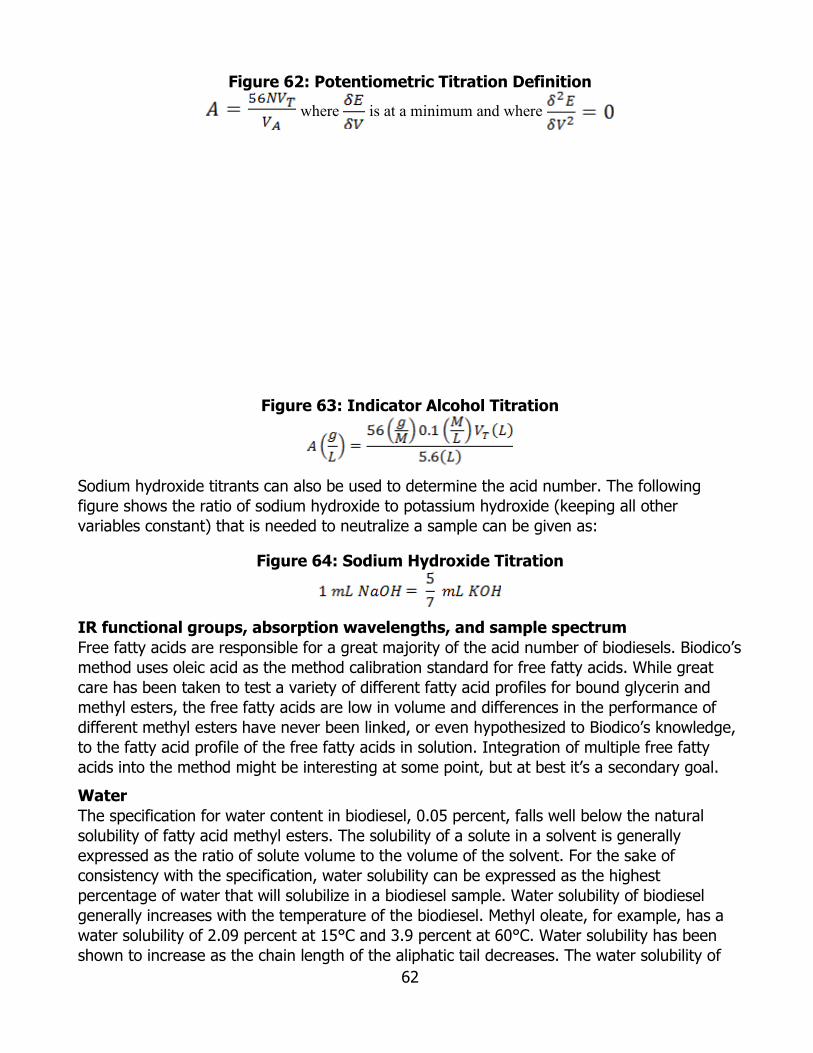
62
Figure 62: Potentiometric Titration Definition where is at a minimum and where
Figure 63: Indicator Alcohol Titration
Sodium hydroxide titrants can also be used to determine the acid number. The following figure shows the ratio of sodium hydroxide to potassium hydroxide (keeping all other variables constant) that is needed to neutralize a sample can be given as:
Figure 64: Sodium Hydroxide Titration
IR functional groups, absorption wavelengths, and sample spectrum Free fatty acids are responsible for a great majority of the acid number of biodiesels. Biodico’s method uses oleic acid as the method calibration standard for free fatty acids. While great care has been taken to test a variety of different fatty acid profiles for bound glycerin and methyl esters, the free fatty acids are low in volume and differences in the performance of different methyl esters have never been linked, or even hypothesized to Biodico’s knowledge, to the fatty acid profile of the free fatty acids in solution. Integration of multiple free fatty acids into the method might be interesting at some point, but at best it’s a secondary goal. Water The specification for water content in biodiesel, 0.05 percent, falls well below the natural solubility of fatty acid methyl esters. The solubility of a solute in a solvent is generally expressed as the ratio of solute volume to the volume of the solvent. For the sake of consistency with the specification, water solubility can be expressed as the highest percentage of water that will solubilize in a biodiesel sample. Water solubility of biodiesel generally increases with the temperature of the biodiesel. Methyl oleate, for example, has a water solubility of 2.09 percent at 15°C and 3.9 percent at 60°C. Water solubility has been shown to increase as the chain length of the aliphatic tail decreases. The water solubility of
63
methyl hexanoate ranges from 4.14 percent at 15°C to 6.28 percent at 60°C.5 Biodiesel with a high-water content can cause poor engine performance, corrosion, instability, and emulsification of impurities in the fuel, so it is important to meet the specification. The graphics below show the well-known structure of water. Even for such simple molecules though, it can be helpful to look at a visualization of the structure to predict the locations of absorption bands. Figures 68 and 69 depict this structure.
Figure 65: 2-D Diagram of Water
Illustration Credit: Biodico
Figure 66: 3-D Representation of Water
Illustration Credit: Biodico, Inc.
There are many different types of water and moisture tests for a wide variety of materials. There are two ASTM tests that apply well to biodiesel samples—ASTM D2709 and ASTM D6304. While ASTM D2709 has been incorporated into ASTM D6751 for a longer period of time, ASTM D6304 generally gives much more accurate results and, for the most part, eliminates operator errors and differences in interpretation.
ASTM D2709 calls for the biodiesel sample to be loaded into a high-speed centrifuge and spun quickly so that all of the water and sediment gather at the tip of the test tube. The accuracy of the measurement can depend greatly on the shape and capacity of the test tube. 100 mL test tubes with capillary tips (as pictured below) are generally used to measure for small amounts of solids in high volumes of liquid, and work well for ASTM D2709. After the sample is collected, the centrifuge test only takes a few minutes, but the drying process for biodiesel can take over 24 hours. Because of the need to take a manual sample for each water test, biodiesel may spend hours more in the drying process than is necessary. Figure 70 shows the centrifuge vial to test for trace for water.
5 Ind. Eng. Chem. Res. 2008, 47, 4278–4285

64
Figure 67: Specialized Centrifuge Vial to Test for Trace Volumes of Water
Photo Credit: Thermo Fisher Scientific
There are two types of Karl Fischer moisture content tests: colorimetric titration (ASTM D6304) and volumetric titration as shown in Figure 71 (ASTM D1744). The colorimetric method is generally used to test finished biodiesel, as lower percentages of water are easier to discern and there is less risk of sample interference. Karl Fischer colorimetric titration mixes an anode solution with the analyte (biodiesel). The anode solution consists of an alcohol group, a base compound, sulfur dioxide, and diatomic iodine. The iodine diatom will oxidize the sulfur dioxide for as long as there is water in the analyte. Each mole of iodine that is used in the oxidation requires a mole of water. While there are water molecules available in the analyte for the oxidation, there will be a significant amount of iodine anions that will allow for a voltage between two submersed probes. After there is no water left for the oxidation reaction, there will be an abundance of iodine diatoms rather than anions, and a sharp drop in the voltage will occur. KF titration generally only takes about five minutes, but, as with the centrifuge method, the need to take a manual sample can lead to hours of unnecessary drying time. A picture of a Karl Fischer titrator is shown below.
Figure 68: Karl Fischer Moisture Analyzer
Photo Credit: Metrohm USA, Inc.
Another type of test that is often used to determine the moisture content of a liquid sample in wastewater treatment applications is Standard Method 2540 for solids. The test method is essentially a two point gravimetric test. A metal sample tray is weighed as the tare ( ). A
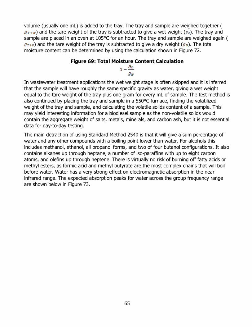
65
volume (usually one mL) is added to the tray. The tray and sample are weighed together () and the tare weight of the tray is subtracted to give a wet weight ( ). The tray and
sample are placed in an oven at 105°C for an hour. The tray and sample are weighed again () and the tare weight of the tray is subtracted to give a dry weight ( ). The total
moisture content can be determined by using the calculation shown in Figure 72.
Figure 69: Total Moisture Content Calculation
In wastewater treatment applications the wet weight stage is often skipped and it is inferred that the sample will have roughly the same specific gravity as water, giving a wet weight equal to the tare weight of the tray plus one gram for every mL of sample. The test method is also continued by placing the tray and sample in a 550°C furnace, finding the volatilized weight of the tray and sample, and calculating the volatile solids content of a sample. This may yield interesting information for a biodiesel sample as the non-volatile solids would contain the aggregate weight of salts, metals, minerals, and carbon ash, but it is not essential data for day-to-day testing.
The main detraction of using Standard Method 2540 is that it will give a sum percentage of water and any other compounds with a boiling point lower than water. For alcohols this includes methanol, ethanol, all propanol forms, and two of four butanol configurations. It also contains alkanes up through heptane, a number of iso-paraffins with up to eight carbon atoms, and olefins up through heptene. There is virtually no risk of burning off fatty acids or methyl esters, as formic acid and methyl butyrate are the most complex chains that will boil before water. Water has a very strong effect on electromagnetic absorption in the near infrared range. The expected absorption peaks for water across the group frequency range are shown below in Figure 73.

66
Figure 70: Functional Group Profile of Water
Chart Credit: Biodico, Inc.
Stability, Cold Flow, and Cetane Under ASTM D6751, the oxidation stability of biodiesel is tested according to method EN 14112. EN 14112 calls for the use of a Rancimat oxidative rancidity analyzer (Figure 74).
Figure 71: Rancimat Oxidative Stability Analyzer
Photo Credit: Metrohm USA, Inc.
The Rancimat method passes an air current over a biodiesel sample heated between 50°C and 220°C. As fatty acids volatilize, they are carried by hot air into a sample of deionized water where they solubilize and increase the conductivity of the test solution. After some amount of time ( ) the rancidification will start and there will be a sharp increase in the
67
water sample’s conductivity. Rancimat results are reported in hours as the induction time needed for the rancidification reaction. Higher induction times are indicative of greater oxidative stability, and the Rancimat induction time specification for biodiesel is three hours.
Biodico currently runs Volatile Fatty Acid tests regularly according to Standard Method 5560 C, Distillation Method for Volatile Fatty Acids. Under this method, 200 mL of sample are centrifuged and a 100 mL sample of the supernatant liquid is taken. 100 mL of deionized water and 5 mL of 1N sulfuric acid are then added to the sample. The sample is distilled in a standard distillation apparatus with a 700 mm long condenser (Biodico has found reliable results with a water-cooled Graham condenser) at a rate of roughly 5 mL per minute. The first 15 mL are discarded and the following 150 mL are collected. A representative volume of the homogenous product of distillation is then titrated with 0.1 N sodium hydroxide in a phenolphthalein indicator alcohol solution. At the point where the indicator alcohol turns pink, the Volatile Fatty Acids number (as mg volatile acids as acetic acid per liter) can be calculated as 60,000 multiplied by the mL of sodium hydroxide titrant added, multiplied by the normality of the titrant, and divided by the mL of distillate sample. This is expressed by the formula shown in Figure 75.
Figure 72: Volatile Fatty Acid Test Calculation
Photo Credit: Biodico, Inc.
The cloud point of biodiesel is defined as the temperature at which solids crystals begin to form in the biodiesel. The rate of crystallization increases after the formation of the first crystals, as new crystal structures can form around existing crystals more easily than they can in a completely liquid solution. Under ASTM D6751, the cloud point can be derived from subtests ASTM D2500 and ASTM D5773. ASTM D2500 calls for the sample to be placed in a vessel with a thermometer protruding through a stopper at the top of the vessel. The vessel is then placed in a cooled water bath. The analyst must keep a close watch on the thermometer as the test method calls for the sample to be visually inspected with every drop in temperature of 1°C. As crystallization occurs, the sample will begin to appear milky and semi-opaque. The cloud point is determined as the temperature at which this crystallization first becomes noticeable. This test can be very time consuming for analysts and the visual detection of crystallization may vary between operators, or even between tests with the same operator.
Method ASTM D5773 calls for cloud point analysis by projecting a concentrated electromagnetic beam with a frequency of 660 nm through the biodiesel sample. As crystals form in the solution, multiple phase interfaces are created. The scattered geometry of the phase interfaces within the sample combined with the creation of unordered and random refractive indexes within the sample cause the beam to scatter over a larger area than that resulting from the beam’s passage through a homogenous liquid sample. In 2005, Biodico purchased and began using a cloud point analyzer manufactured by Phase Technologies, the CPA-T30, depicted in figure 76. The CPA-T30 meets the requirements of ASTM D5773. The test takes approximately five minutes. 30 mL of biodiesel are loaded into the CPA to start the
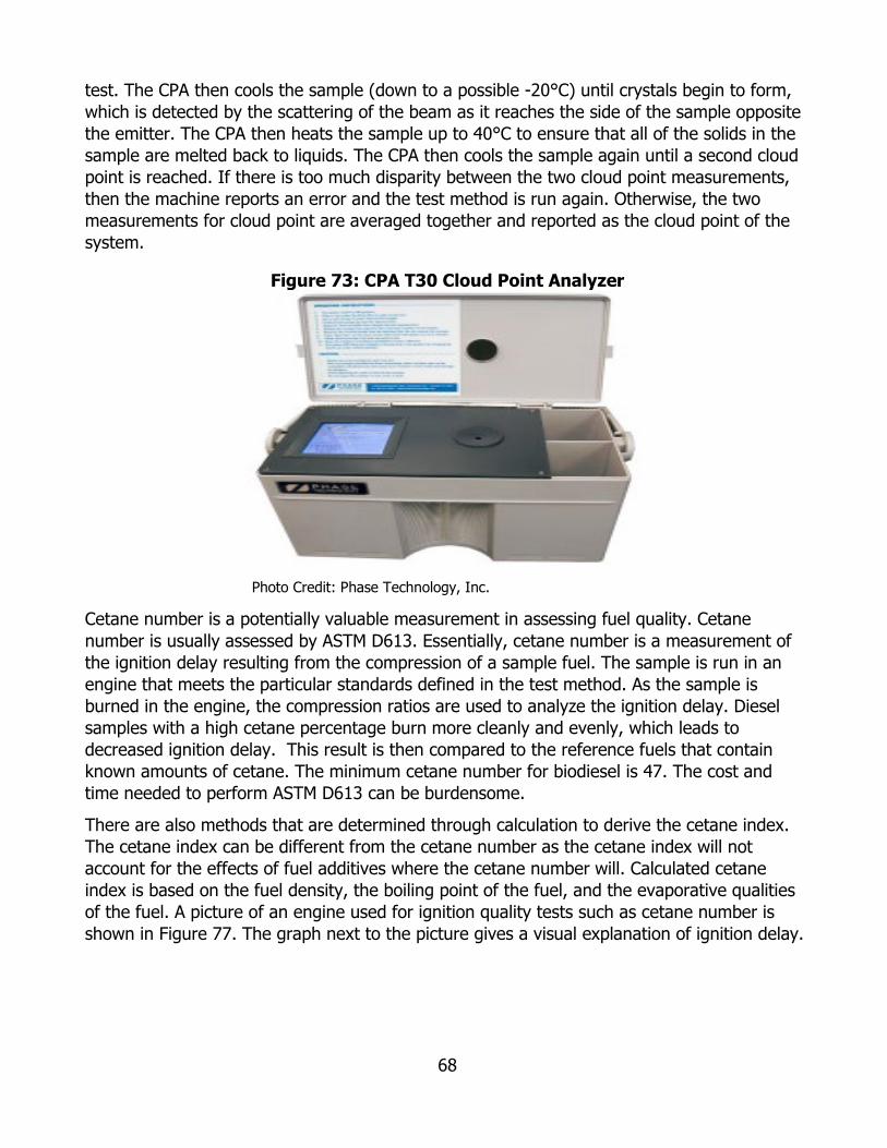
68
test. The CPA then cools the sample (down to a possible -20°C) until crystals begin to form, which is detected by the scattering of the beam as it reaches the side of the sample opposite the emitter. The CPA then heats the sample up to 40°C to ensure that all of the solids in the sample are melted back to liquids. The CPA then cools the sample again until a second cloud point is reached. If there is too much disparity between the two cloud point measurements, then the machine reports an error and the test method is run again. Otherwise, the two measurements for cloud point are averaged together and reported as the cloud point of the system.
Figure 73: CPA T30 Cloud Point Analyzer
Photo Credit: Phase Technology, Inc.
Cetane number is a potentially valuable measurement in assessing fuel quality. Cetane number is usually assessed by ASTM D613. Essentially, cetane number is a measurement of the ignition delay resulting from the compression of a sample fuel. The sample is run in an engine that meets the particular standards defined in the test method. As the sample is burned in the engine, the compression ratios are used to analyze the ignition delay. Diesel samples with a high cetane percentage burn more cleanly and evenly, which leads to decreased ignition delay. This result is then compared to the reference fuels that contain known amounts of cetane. The minimum cetane number for biodiesel is 47. The cost and time needed to perform ASTM D613 can be burdensome.
There are also methods that are determined through calculation to derive the cetane index. The cetane index can be different from the cetane number as the cetane index will not account for the effects of fuel additives where the cetane number will. Calculated cetane index is based on the fuel density, the boiling point of the fuel, and the evaporative qualities of the fuel. A picture of an engine used for ignition quality tests such as cetane number is shown in Figure 77. The graph next to the picture gives a visual explanation of ignition delay.
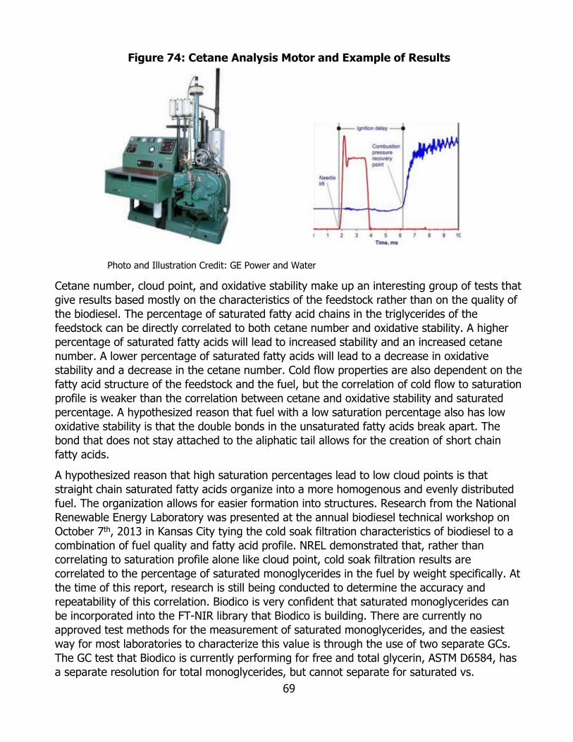
69
Figure 74: Cetane Analysis Motor and Example of Results
Photo and Illustration Credit: GE Power and Water
Cetane number, cloud point, and oxidative stability make up an interesting group of tests that give results based mostly on the characteristics of the feedstock rather than on the quality of the biodiesel. The percentage of saturated fatty acid chains in the triglycerides of the feedstock can be directly correlated to both cetane number and oxidative stability. A higher percentage of saturated fatty acids will lead to increased stability and an increased cetane number. A lower percentage of saturated fatty acids will lead to a decrease in oxidative stability and a decrease in the cetane number. Cold flow properties are also dependent on the fatty acid structure of the feedstock and the fuel, but the correlation of cold flow to saturation profile is weaker than the correlation between cetane and oxidative stability and saturated percentage. A hypothesized reason that fuel with a low saturation percentage also has low oxidative stability is that the double bonds in the unsaturated fatty acids break apart. The bond that does not stay attached to the aliphatic tail allows for the creation of short chain fatty acids.
A hypothesized reason that high saturation percentages lead to low cloud points is that straight chain saturated fatty acids organize into a more homogenous and evenly distributed fuel. The organization allows for easier formation into structures. Research from the National Renewable Energy Laboratory was presented at the annual biodiesel technical workshop on October 7th, 2013 in Kansas City tying the cold soak filtration characteristics of biodiesel to a combination of fuel quality and fatty acid profile. NREL demonstrated that, rather than correlating to saturation profile alone like cloud point, cold soak filtration results are correlated to the percentage of saturated monoglycerides in the fuel by weight specifically. At the time of this report, research is still being conducted to determine the accuracy and repeatability of this correlation. Biodico is very confident that saturated monoglycerides can be incorporated into the FT-NIR library that Biodico is building. There are currently no approved test methods for the measurement of saturated monoglycerides, and the easiest way for most laboratories to characterize this value is through the use of two separate GCs. The GC test that Biodico is currently performing for free and total glycerin, ASTM D6584, has a separate resolution for total monoglycerides, but cannot separate for saturated vs.
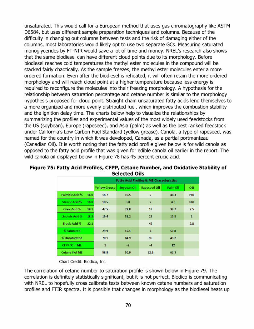
70
unsaturated. This would call for a European method that uses gas chromatography like ASTM D6584, but uses different sample preparation techniques and columns. Because of the difficulty in changing out columns between tests and the risk of damaging either of the columns, most laboratories would likely opt to use two separate GCs. Measuring saturated monoglycerides by FT-NIR would save a lot of time and money. NREL’s research also shows that the same biodiesel can have different cloud points due to its morphology. Before biodiesel reaches cold temperatures the methyl ester molecules in the compound will be stacked fairly chaotically. As the sample freezes, the methyl ester molecules enter a more ordered formation. Even after the biodiesel is reheated, it will often retain the more ordered morphology and will reach cloud point at a higher temperature because less energy is required to reconfigure the molecules into their freezing morphology. A hypothesis for the relationship between saturation percentage and cetane number is similar to the morphology hypothesis proposed for cloud point. Straight chain unsaturated fatty acids lend themselves to a more organized and more evenly distributed fuel, which improves the combustion stability and the ignition delay time. The charts below help to visualize the relationships by summarizing the profiles and experimental values of the most widely used feedstocks from the US (soybean), Europe (rapeseed), and Asia (palm) as well as the best ranked feedstock under California’s Low Carbon Fuel Standard (yellow grease). Canola, a type of rapeseed, was named for the country in which it was developed, Canada, as a partial portmanteau (Canadian Oil). It is worth noting that the fatty acid profile given below is for wild canola as opposed to the fatty acid profile that was given for edible canola oil earlier in the report. The wild canola oil displayed below in Figure 78 has 45 percent erucic acid.
Figure 75: Fatty Acid Profiles, CFPP, Cetane Number, and Oxidative Stability of Selected Oils
Chart Credit: Biodico, Inc.
The correlation of cetane number to saturation profile is shown below in Figure 79. The correlation is definitely statistically significant, but it is not perfect. Biodico is communicating with NREL to hopefully cross calibrate tests between known cetane numbers and saturation profiles and FTIR spectra. It is possible that changes in morphology as the biodiesel heats up

71
have an effect on the cetane properties in a similar fashion to the effects of morphology on cold flow.
Figure 76: Relationship between Cetane and Saturation Profile
Chart Credit: Biodico, Inc.
It should be noted that the correlation between saturation percentage and cold flow is the weakest of the three properties. Biodico is looking forward to incorporating NREL’s newest findings into its spectroscopic model. There are multiple ways to test cold flow and CFPP refers to cold filter plug point. Figure 80 reflects on this relationship between CFPP and the saturation profile.
Figure 77: Relationship between CFPP and Saturation Profile
Chart Credit: Biodico, Inc.

72
IR functional groups (C-C vs. C=C), absorption wavelengths, and sample spectrum
Saturated fatty acid aliphatic tails do not contain a double bond, unsaturated fatty acid aliphatic tails contain at least one double bond, and polyunsaturated fatty acid aliphatic tails contain at least two double bonds. The FTIR can resolve the difference between saturated and unsaturated methyl esters by the difference in their functional groups. The saturation profile’s effect on stability, cetane number, and cold flow is discussed above. Characterization of different aliphatic tail lengths gives Biodico a much better understanding of the molecular weights of the different methyl esters and average molecular weight of the compound can be achieved. Chain length has a significant effect on the viscosity of the fuel. It also helps to determine reaction efficiency by comparing the catalyst use against the molecular weight of the feedstock. This determination is also useful in allowing Biodico to quickly characterize the composition of an unknown feedstock. As California continues to explore the life cycle analyses of different feedstocks, it will be very useful to have a test method that can determine feedstock type. In fact, Biodico actually expanded its QBQ-20,000 FTIR method library from two parts to three parts to accommodate this. The fatty acid profile portion of the library incorporates the profile of both domestically and internationally available oil types that have undergone a variety of refining, from food grade, to epoxidized, to crude (non-treated) as well as several samples that were produced from Biodico’s pilot scale extrusion equipment or extracted from the Artemia.
The chart below shows the amount of time that is currently needed for the testing of each biodiesel batch (Figure 81).

73
Figure 78: Biodiesel Testing Time per Batch
Chart Credit: Biodico, Inc.
The partial notes by the chromatography tests performed under ASTM D6751 are there to indicate that the results of each of the glycerin variables all come from the same test. Even so, the test takes at least 45 minutes of waiting without any action by the analyst. The samples undergo silylation for 15 minutes before they run through the GC column for 30 minutes. Usually the test takes closer to an hour, even with a practiced analyst, and it need to be performed an average of five times for each batch. Acid number, methanol, and water also need to be tested before the final testing of the fuel takes place. After the fuel is deemed finished there are hours more of quality testing. The lines in the orange bars at the bottom of the chart show how long the tests take. The top row denotes total hours for the testing and the second orange row indicates the fastest amount of time that all the tests could theoretically be run if they were run in parallel or by multiple analysts. The right-most column indicates the amount of testing that has to be done throughout the course of the biodiesel production before the fuel is deemed finished, and the column to the left of that indicates the total amount of testing that needs to be done for any biodiesel batch, including both in-situ testing and finished specification testing. Biodico estimates that taking full advantage of the new spectroscopic method will bring their batch production time down to just over a third of
74
its current value. This effectively triples the amount of throughput that comes from the capital equipment, adds efficiency to all of the variable costs, and helps Biodico to have a whole new set of instantaneous byproduct testing techniques that were not economically feasible before. Test Plan Biodico’s FTIR method, QBQ-20,000, is encompassed by a single library, but the spectra within the library can be split into three categories. Biodico has come to refer to these categories as: in-spec, in-situ, and free fatty acid profile. The reason that the categories were originally made was that Biodico wanted to develop near infrared methods that could measure components of biodiesel fuel in real time production as well as in quick specification confirmation. The current specification for biodiesel, ASTM D 6751, along with the sub-specifications for individual components and contaminants is listed in the previous section. Biodico designed the spectroscopy to test for free glycerin, bound glycerin (and total glycerin by inference), free fatty acids, water, and methanol. Biodico also incorporated the ability to test the saturation profile of the fuel by percentage of saturated, unsaturated, and polyunsaturated aliphatic tails. This allows for Biodico to effectively predict several performance characteristics of the fuel (before it is even processed in many cases). Biodico needs to be able to see each contaminant in two different resolutions though. The different components that are used or produced in the transesterification reaction are present in the reactor at much higher concentrations than the levels of contaminants in specification testing. Essentially in a batch reactor transesterification process, the combined methanol and alkali metal methylate react very quickly with the triglycerides (oil feedstock) at the start of the reaction. The triglycerides are stripped of their fatty acid chains and the fatty acid chains bind to the alcohol groups. Where methanol is used as the alcohol group (as in the vast majority of commercial production), this produces methyl esters. The stripping of the fatty acids from the triglycerides leaves behind, in sequence, diglycerides, monoglycerides, and ultimately glycerol. The tri, di, and monoglycerides are collectively referred to as bound glycerin and the glycerol is referred to as free glycerin. The free glycerin is a polar, hydrophilic compound and will solubilize alcohols (along with any water that enters the reaction). Because of this, as the reaction progresses, the chances that the methanol and methylate will react with the bound glycerides decreases as the chances that the alcohol compounds will solubilize in the increasingly available free glycerin rises. This leads to yield curves that generally reach an asymptote into infinity and reach about 90 percent of their asymptotic value after about 10 minutes. The rates of volume change for the methyl esters (biodiesel) and free glycerin are positive. The rates of volume change for the methanol and methylate and for the bound glycerin are negative. At any given point in time the volume of alcohol compounds, bound glycerin, free glycerin, and methyl esters are roughly equal to the initial volume of bound glycerin (feedstock) and alcohol compounds (minus density changes from molecular reconfiguration and evaporative loss). For a reaction that uses 20 percent methanol and methylate by volume of feedstock (for a total volume of 120 percent the amount of feedstock), the reaction curves approximate the chart below (Figure 82).

75
Figure 79: General Compositional Analysis during Biodiesel Reaction
Chart Credit: Biodico, Inc.
In addition to confirming that biodiesel meets the appropriate specifications, Biodico will also use spectroscopy to monitor the progress of the reaction in-situ. Since the components’ volumes are much larger in-situ, Biodico really needed two resolutions in its matrix, “in-spec” and “in-situ.” To address this, Biodico set two additional points on top of the specification points for each contaminant at 33 percent and 66 percent. Even though some components do not generally reach above 33 percent in an actively mixing, homogenous reactor, there are usually impurities on both sides of the post-reaction gravimetric compound separation, and it is helpful to be able to test the purity of the free glycerin. It is also helpful to test the potential contamination of distilled methanol or of water washings.
Adding two additional points on to the “in-spec” matrix would have dramatically increased the size of the sample set from to a matrix size based on a value of (a sizable number of samples in the “in-situ” matrix do not contain methyl esters and therefore do not need to be repeated for different reference fuels). After analyzing the different possible approaches, Biodico came to the conclusion that the in-spec matrix and the in-situ matrix represent completely different times in the biodiesel process and that there is no real advantage in having samples that cross between the two matrices. For example, if a sample still has 50 percent unconverted triglycerides, there is no real advantage in knowing the free glycerin composition to an accuracy of 0.02 percent. The wider scope of the in-situ matrix will almost always be more valuable than the narrower scope of the in-spec matrix at the point where any one contaminant is somewhere within the scope of the in-situ matrix. This allowed for Biodico to essentially break the matrix up into two separate components that will operate within the same library. For the in-situ matrix a zero point was needed in addition to the 33 percent and 66 percent points, but the total amount of samples needed still reduced dramatically as the equation in Figure 83 shows.

76
Figure 80: Total Amount of Samples Needed
Photo Credit: Biodico, Inc.
As Biodico further developed the matrix, the number of repeated samples that did not have methyl ester content was found to be quite significant. This dropped the number of samples needed for the proposed matrix to 232 in-situ samples and 96 in-spec samples for a total of 328 samples.
The preparation of the samples and the development of the method were time consuming, but the time saved from 3,072 samples to 232 samples allowed for Biodico to broaden the method in a third direction that was not originally anticipated. Biodico has been performing research and development on the Naval Base Ventura County for over 10 years as part of the CRADA with the Navy. Through the course of this time period Biodico has also developed several commercial biodiesel production facilities and has worked on many international feasibility studies. As a part of this work, Biodico has tested and has produced oil samples from a wide variety of sources. Biodico usually keeps records of new or interesting oil sources and was able to add about 30 different oils to the library. In-Spec FTIR Matrix The goal of the in-spec matrix is to give the QBQ-20,000 FTIR method sufficient capabilities to determine whether a fuel meets the ASTM specification D 6751 for as many of the critical sub specifications as possible. Of the nine critical specs, Biodico can characterize seven on the FTIR. Five of the seven FTIR tests are for contaminants that are molecularly separate from the biodiesel. They include bound glycerin, free glycerin, free fatty acids, water and methanol. These can be directly detected by the library. Two of the critical specifications are dependent on the fatty acid profile of the biodiesel and the feedstock that it is made from. These two specifications are for cold flow and oxidative stability. Cetane number can also be inferred by the fatty acid profile, but it is not one of the nine critical specifications. The first step that Biodico took in developing the in-spec test matrix was to lay out a test plan for the measurable contaminants according to broadly accepted experimental recommendations for principal component analysis. The matrix includes two points for each contaminant, a high point and a low point, which are centered on the expected value. In this case, the most important value for each of the contaminants is that set by the ASTM standard. It is common for the finished biodiesel to have concentrations of any of the five contaminants that are below detectable limits so the established low point for each contaminant was 0 percent. This placed the high value for each of the contaminants at double the specification. Each of the two points was assigned a letter, A or B. The A values represent a 0 percent concentration for each of the contaminants and the B values represent a level of double the specification that is specific to the contaminant. Figure 84 below shows the corresponding percentages by weight for each of the contaminants.

77
Figure 81: Principle Component Analysis End Points
Chart Credit: Biodico, Inc.
This gives five separate letters that have a possible value of either A or B, one for each contaminant. For the sample coding system, the five letters were placed in order of least to most sensitive. In order on a sample code, the five letters represent free glycerin, water, bound glycerin, methanol, and free fatty acids. Though the specification for the bound glycerin is actually slightly lower than the specification for methanol, the higher viscosity of the bound glycerin makes it a more sensitive variable to measure. Ordering the variables by level of sensitivity was an important part of the experimental design. While meeting the specification for a biodiesel reaction is fairly straightforward, preparing ultrahigh purity biodiesel with BDL on all of the contaminants is easier to do in the lab a few liters at a time. Biodico wanted to use the same homogenously prepared ultra-high purity reference fuels for entire course of the method development, so conserving sample volume was a consideration. Only 8 mL of each sample are needed to take a spectrogram, and Biodico wanted to rinse the probe with the incoming sample once before it was tested, so 16 mL of sample was needed for each of the tests. Biodico prepared enough reference fuel for both the in-spec and in-situ matrices. (The fatty acid profiling was performed on unreacted oils.) For the in-spec test run alone, Biodico needed 512 mL of each reference fuel as shown in the equation shown in Figure 85.
Figure 82: mL of Reference Fuel Calculation
Photo Credit: Biodico, Inc.
Measuring 0.04 percent free glycerin into a 16 mL sample with any kind of accuracy would have been extremely difficult, but since half of the samples would have that concentration of glycerin, 256 mL of the reference fuel could be mixed with glycerin at the same time. This called for 102 microliters of glycerin, which was well within the precision of a micropipette. Heating the glycerin first reduced the viscosity and allowed for a very accurate measurement. In a similar vein, measuring 1 percent free fatty acids into a 16 mL sample was relatively easy and well within the precision capability of a micropipette. This meant that for each reference fuel 512 mL of sample would be measured and then split in half. One of the splits would receive a new contaminant and one would not. After the addition of each new contaminant there would be twice as many splits and new contaminants would be added to samples that were half the size. The sample tree in Figure 86 illustrates the methodology.
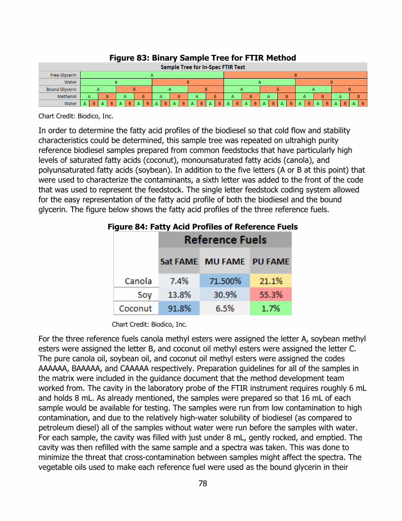
78
Figure 83: Binary Sample Tree for FTIR Method
Chart Credit: Biodico, Inc.
In order to determine the fatty acid profiles of the biodiesel so that cold flow and stability characteristics could be determined, this sample tree was repeated on ultrahigh purity reference biodiesel samples prepared from common feedstocks that have particularly high levels of saturated fatty acids (coconut), monounsaturated fatty acids (canola), and polyunsaturated fatty acids (soybean). In addition to the five letters (A or B at this point) that were used to characterize the contaminants, a sixth letter was added to the front of the code that was used to represent the feedstock. The single letter feedstock coding system allowed for the easy representation of the fatty acid profile of both the biodiesel and the bound glycerin. The figure below shows the fatty acid profiles of the three reference fuels.
Figure 84: Fatty Acid Profiles of Reference Fuels
Chart Credit: Biodico, Inc.
For the three reference fuels canola methyl esters were assigned the letter A, soybean methyl esters were assigned the letter B, and coconut oil methyl esters were assigned the letter C. The pure canola oil, soybean oil, and coconut oil methyl esters were assigned the codes AAAAAA, BAAAAA, and CAAAAA respectively. Preparation guidelines for all of the samples in the matrix were included in the guidance document that the method development team worked from. The cavity in the laboratory probe of the FTIR instrument requires roughly 6 mL and holds 8 mL. As already mentioned, the samples were prepared so that 16 mL of each sample would be available for testing. The samples were run from low contamination to high contamination, and due to the relatively high-water solubility of biodiesel (as compared to petroleum diesel) all of the samples without water were run before the samples with water. For each sample, the cavity was filled with just under 8 mL, gently rocked, and emptied. The cavity was then refilled with the same sample and a spectra was taken. This was done to minimize the threat that cross-contamination between samples might affect the spectra. The vegetable oils used to make each reference fuel were used as the bound glycerin in their

79
respective samples. The free fatty acid was a 99.5 percent purity oleic acid sourced from Acros Organics that was taken as a very common and representative fatty acid. Future research may contain a wider variety of fatty acids, but as the difference in the spectra will come from the hydroxyl groups attached to the ester, the free fatty acid profile is relatively unimportant. The methanol was 99.9 percent research grade sourced from Fisher Scientific. The water was distilled and deionized and sourced from a local pharmacy. The free glycerin was 99.5 percent USP grade glycerin sourced from a local pharmacy. The additions of the water, free fatty acids, methanol, and bound glycerin were performed with 1 microliter resolution micropipettes with a 200 microliter capacity and disposable tips. The free glycerin was added to the samples by weight with a four-point analytical scale that was calibrated by Watson Brothers in Los Angeles. Best practices were observed. The chart data in Figures 88-90 shows the final iteration of the in-spec test matrix that was used to prepare the biodiesel samples and to capture the spectra.

80
Figure 85: In-Spec FTIR Library Samples (1 of 3)
Chart Credit: Biodico, Inc.
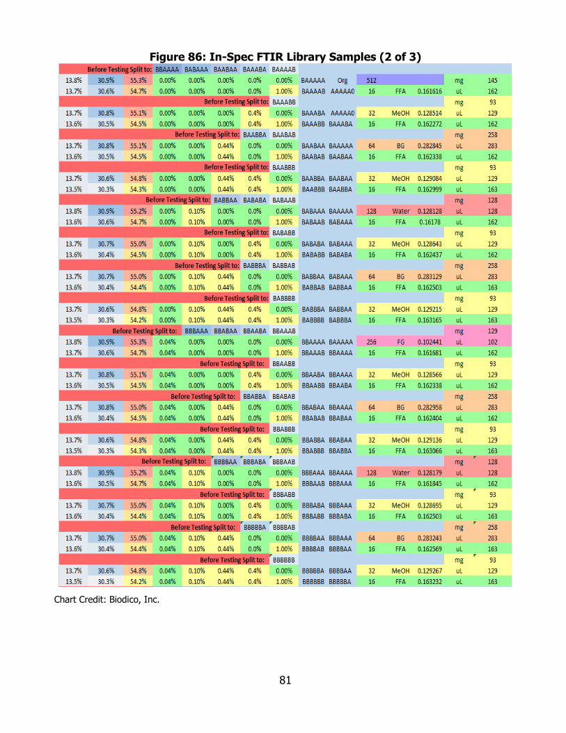
81
Figure 86: In-Spec FTIR Library Samples (2 of 3)
Chart Credit: Biodico, Inc.
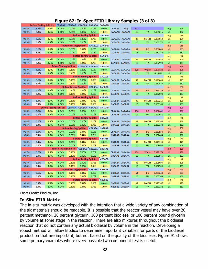
82
Figure 87: In-Spec FTIR Library Samples (3 of 3)
Chart Credit: Biodico, Inc.
In-Situ FTIR Matrix The in-situ matrix was developed with the intention that a wide variety of any combination of the six materials should be readable. It is possible that the reactor vessel may have over 20 percent methanol, 20 percent glycerin, 100 percent biodiesel or 100 percent bound glycerin by volume at some stage in the reaction. There are also mixtures throughout the biodiesel reaction that do not contain any actual biodiesel by volume in the reaction. Developing a robust method will allow Biodico to determine important variables for parts of the biodiesel production that are important, but not based on the quality of the biodiesel. Figure 91 shows some primary examples where every possible two component test is useful.
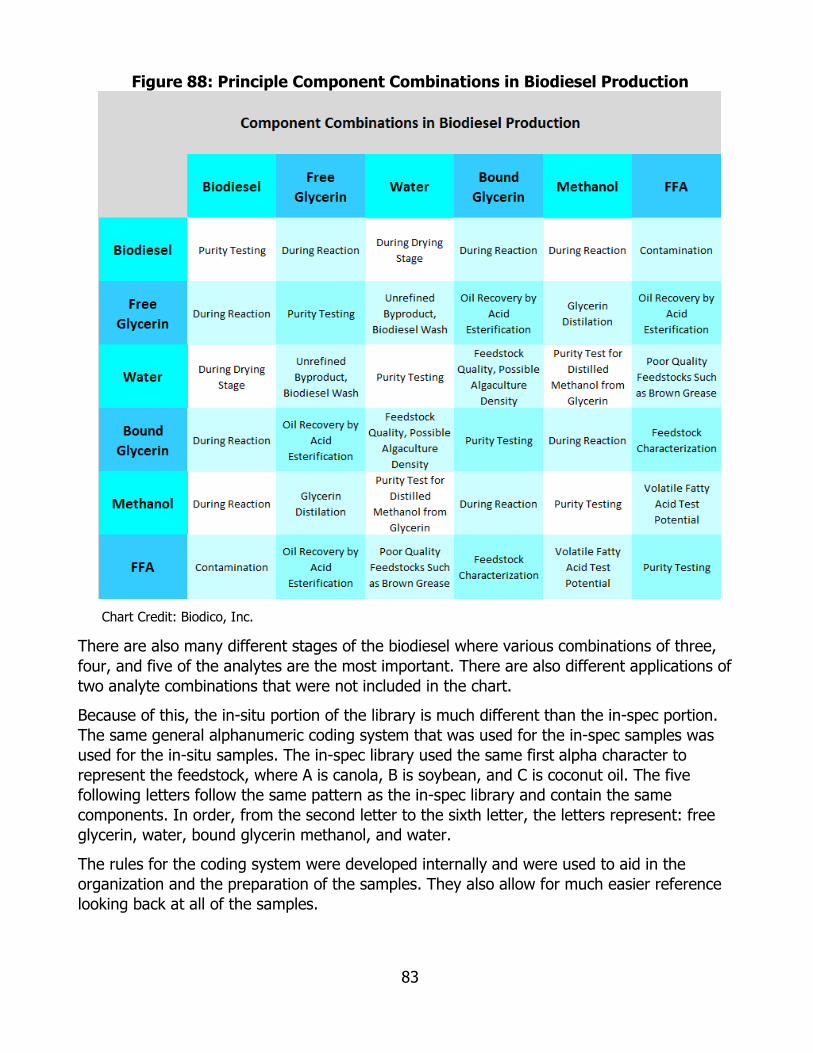
83
Figure 88: Principle Component Combinations in Biodiesel Production
Chart Credit: Biodico, Inc.
There are also many different stages of the biodiesel where various combinations of three, four, and five of the analytes are the most important. There are also different applications of two analyte combinations that were not included in the chart.
Because of this, the in-situ portion of the library is much different than the in-spec portion. The same general alphanumeric coding system that was used for the in-spec samples was used for the in-situ samples. The in-spec library used the same first alpha character to represent the feedstock, where A is canola, B is soybean, and C is coconut oil. The five following letters follow the same pattern as the in-spec library and contain the same components. In order, from the second letter to the sixth letter, the letters represent: free glycerin, water, bound glycerin methanol, and water.
The rules for the coding system were developed internally and were used to aid in the organization and the preparation of the samples. They also allow for much easier reference looking back at all of the samples.

84
• C represents one part, D represents two parts, and Z is used for samples that are 100 percent of any of the components and do not have any additional components mixed in.
• If the sum of the parts is three or less, each part represents one third of the sample by volume.
• If the total sum of the parts is two or less, ultra high purity biodiesel is used for the remaining part or parts.
• As with the in-spec test matrix, if the total sum of the parts is zero, the sample is 100 percent ultra-high purity biodiesel made from the feedstock represented by the first letter.
• If the sum of the total parts is greater than three, then the system is divided by the number of parts and the components that have a value of D have double the concentration of the components that are marked with the letter C.
As an example, if one of the parts was labeled ADCCDD the composition would be determined in the following way:
• The sample does not contain any Z values and the sample has more than zero parts, so the sample represents a mixture of components.
• Each D value represents two parts and each C value represents one part, so the total number of parts for this sample is 8.
• The total parts are greater than two, so this sample does not contain biodiesel.
• The number of parts is greater than three, so each part’s representation is indicated in Figure 92.
Figure 89: Percent of Sample for Each Part Calculation
Photo Credit: Biodico, Inc.
• The components that are marked with a D get two parts at 25 percent of the sample volume, and the components that are marked with a C get one part at 12.5 percent of the sample volume.
• For a 16 mL sample, there are four mL of free glycerin, two mL of water, two mL of bound glycerin, four mL of methanol, and four mL of free fatty acids.
The sample matrix for the in-situ portion of the library is the largest and contains 232 samples. The guidance document was prepared to minimize the man hours needed for preparation by making extra volumes for samples that could later be mixed together. For example, if a sample containing 25 percent equal parts of methanol, bound glycerin, free fatty acids, and water is called for (AACCCC), extra volumes would have been made of the sample with 50 percent methanol and 50 percent water (AADADA) and the sample with 50 percent bound glycerin and 50 percent free fatty acids (AAADAD).
85
Sample preparation with two people was much quicker than with only one person. One technician could prepare the samples and the other technician could use the computer to capture the spectra by the FTIR analyzer, log the spectra on the computer, and organize the order of sample preparation for the sample mixer. A total of five people performed the work for the method development in various two-person combinations. Having a well laid out guidance document for the testing was essential. Mixing extras of the samples that had fewer components to be used in later samples with more components proved to be inefficient though.
Since the percentages that made up the various components for the in-situ samples were much higher than for the in-spec samples, the lowest amount of sample needed was small. The highest number of parts came from the five samples that had four D values and one C value for a total of 9 parts. This meant that each part could be defined as 11 percent of the sample volume. For the larger scale measurements of the in-situ library, a 5 mL disposable tip pipette could be used to prepare most of the samples and made it a lot quicker. Mixing previous samples together to make a new sample took more time than just mixing each sample individually with the 5 mL pipette. Individual one-use samples were also much easier to organize. A large whiteboard was placed between the FTIR operator and the sample mixture, and for each new sample the FTIR operator would write the mL of each component needed for the next sample. The technician marked the sample that he was in the process of preparing to avoid confusion or mislogs.
One of the largest concerns for this testing was contamination of the samples. A small percentage of water solubilized in any of the fatty acid compounds could have a big effect on the spectra. For this reason, the samples were divided into three main categories: polar, non-polar, and mixed polarity. The mixed polarities were divided into three parts which represented the polar component that would have the largest effect on the spectra. The subcategories for mixed samples were E-H2O, E-Glycerin, and E-Methanol where the E represents emulsion. When possible, Biodico would run groups of samples with matching polarity. When the polarity changed, Biodico would rinse the probe with either heptane or methanol depending on the polarity of the sample. As with the in-spec library, each sample was prepared with enough volume to rinse the probe with 8 mL of a new sample and to refill the probe to capture the spectrogram.
Biodico was concerned that the samples with mixed polarity might not be able to read well on the analyzer. Experiments were performed using soy lecithin as an emulsifier, but in the end the mixed polarity samples returned usable spectra and the soy lecithin increased the risk of contamination between samples.
The same components that were used for the in-spec library were used for the in-situ library. Most of the measurements were performed by the 5 mL pipette with a resolution of 0.5 mL, but graduated cylinders and larger bulb pipettes were used for some samples. The accuracy of the micropipette was confirmed by measuring water into one and five mL volumetric flasks. A separate pipette tip was used for each component and great care was taken to keep them isolated to the intended component for the course of the testing.

86
The charts below show the sample matrix that was used for the in-situ sample preparation (Figure 93). Each row represents a different sample and contains the sample code, the percentages of the various components needed to make the sample, and the polarity of the sample. It is worth noting that some of the codes for the samples would have yielded identical component percentages. AAACCC and AAADDD would be the same. Each of the three components would get one part divided by a total of three parts, and each D component would get two parts divided by a total of six parts. These samples were removed from the testing matrix.
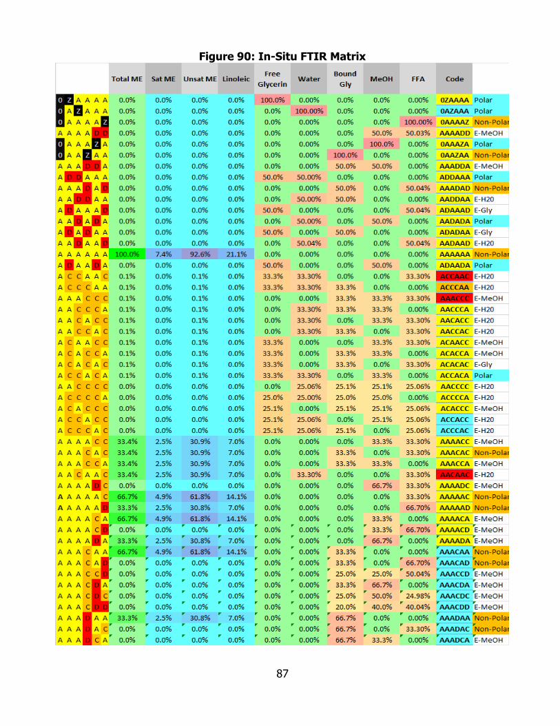
87
Figure 90: In-Situ FTIR Matrix

88
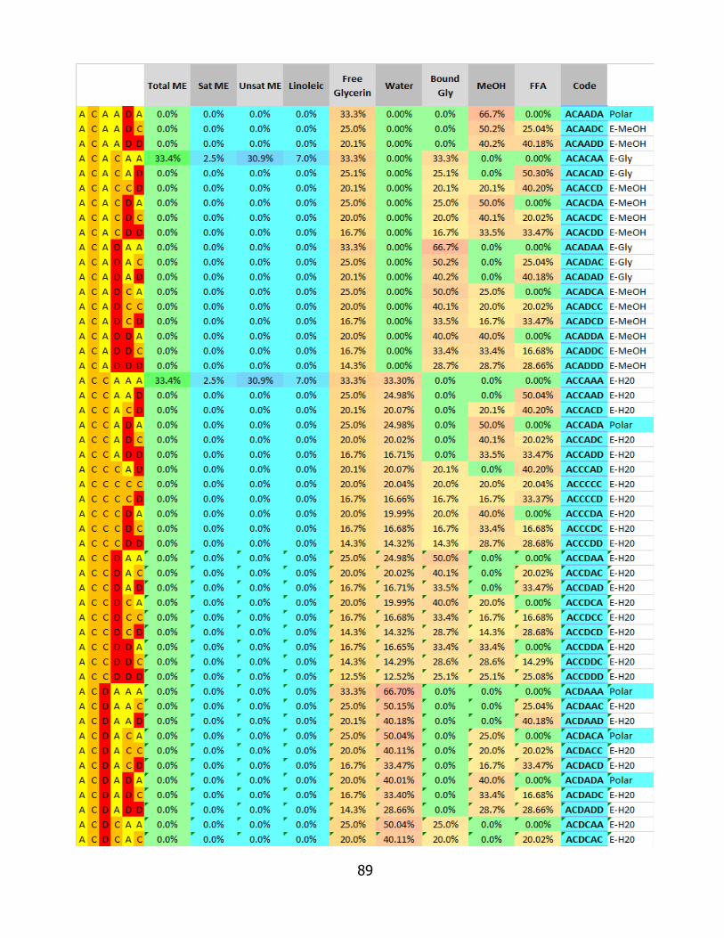
89
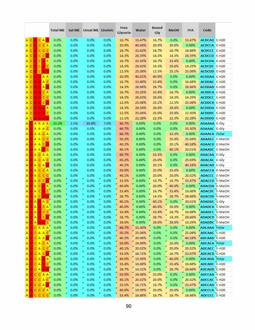
90
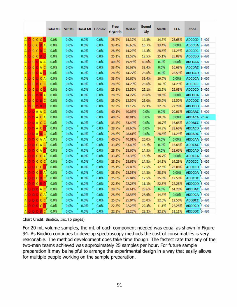
91
Chart Credit: Biodico, Inc. (6 pages)
For 20 mL volume samples, the mL of each component needed was equal as shown in Figure 94. As Biodico continues to develop spectroscopy methods the cost of consumables is very reasonable. The method development does take time though. The fastest rate that any of the two-man teams achieved was approximately 25 samples per hour. For future sample preparation it may be helpful to arrange the experimental design in a way that easily allows for multiple people working on the sample preparation.

92
Figure 91: Component Volumes Needed for In-Situ Test Matrix
Chart Credit: Biodico, Inc.
Fatty Acid Profile Matrix At the start of the QBQ-20,000 FTIR method development, Biodico did not anticipate that a section of the library would be developed for fatty acid profiles. While the sample preparation and spectra gathering was underway though, the method development team realized that the time that would be needed to capture the oil spectra would be very reasonable. The method is now much more robust and capable as a result of this inclusion.
Oil samples were named with the same conventions used in the other parts of the method. The general fatty acid profiles were taken from the product specifications directly, research performed by Biodico, research performed by other people, and various other references. For this reason, Biodico anticipates that the fatty acid profile portion of the library will continue to improve as Biodico begins operating its most recent production facility and uses the method on real world samples.
The basic profile for the fatty acid portion of the library is given in Figure 95. For many of the oil types there are multiple sources of the same oil that may differ by the method. In the chart, each oil type that was factored into the library is listed once. Two oil types that were analyzed with the rest of the samples in the fatty acid library have not yet been included in the library: Artemia oil and tall oil. The reasons for this are that the tall oil contained too many impurities to be considered a reliable reference fuel and that more independent testing of the Artemia oil’s fatty acid profile will need to be done before it is included in the reference library used to determine the profile of unknown fuels and oils. The six letter coding was used primarily for convenience in file naming, but more letters can easily be attached to the sample names as the library continues to grow.

93
Figure 92: Fatty Acid Profile Library Samples
Chart Credit: Biodico, Inc.
While the three reference fuels give excellent feedback on determining the quality of the fuel and the success of the production, all three of those fuels are fairly common, and having as many reference points as logistically possible helps the method to deliver good data for new and interesting oils. Most feedstocks have oils with carbon chains of 16 or 18. The two most common 16 carbon aliphatic tails are palmitic (16:0) and palmitoleic (16:2). The three most common 18 carbon aliphatic tails are stearic (18:0), oleic (18:1), and linoleic (18:2). The number that comes after the colon is the number of double bonds in the fatty acid. By preparing a library with a wide variety of different fatty acids, Biodico’s library is well equipped to find the characteristics of any new and promising fuel source. Figure 96 shows the sum of Library Fatty Acids’ profile.

94
Figure 93: Sum of Library Fatty Acid Profile
Chart Credit: Biodico, Inc.
One uncommon fuel that is well represented in this library is ricinoleic acid. Ricinoleic acid differs from most fatty acids in that one of the hydrogens in its aliphatic tail is substituted with a hydroxyl group. Some of the other interesting fatty acids that are included in the library are:
• Malvalic acid, which has a cyclopropenic group as part of its fatty acid chain.
• Eicosapentanoic acid (EPA), which has many double bonds and is found in many aquatic species.
• Docosahexanoic acid (DHA), which is often found in different strains of algae.
By including many of the uncommon groups, Biodico has the ability to gain a much deeper understanding of any potential feedstocks that it may wish to process. Reports & Results The three categories of test matrices—in-spec, in-situ, and Fatty Acids—all combine together to form a single library that is able to characterize the most important variables through every step of the biodiesel process. Each of the components showed good resolution against the biodiesel and against each other. The fatty acid profiles of the various fatty acid chains are also well represented, and a clear difference can be seen between the saturated, mono-unsaturated, and poly-unsaturated reference fuels. The script that Biodico wrote to use the QC80 functionality in order to collect the FTIR spectra was designed to take three spectra of every sample. Some of the samples that had mixed polarity were taken more than once so that a clearer picture emerged from the mixture of these different materials in a commercial scale reaction process. All in all, Biodico now has a library of 1,940 spectra that can be used to optimize the production of fuel at a commercial scale and that can be used to test the quality of any fuel produced. The spectroscopy method is also able to detect components in the material that are not even included in the ASTM spec, though some are included in the European spec.
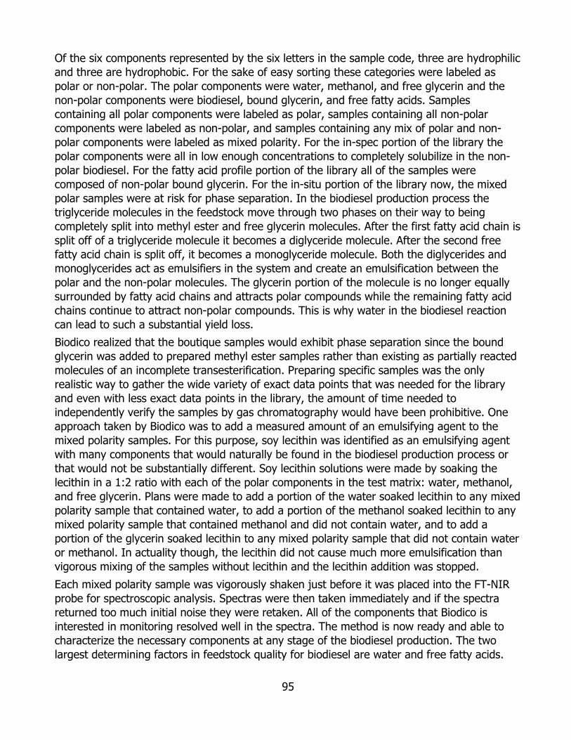
95
Of the six components represented by the six letters in the sample code, three are hydrophilic and three are hydrophobic. For the sake of easy sorting these categories were labeled as polar or non-polar. The polar components were water, methanol, and free glycerin and the non-polar components were biodiesel, bound glycerin, and free fatty acids. Samples containing all polar components were labeled as polar, samples containing all non-polar components were labeled as non-polar, and samples containing any mix of polar and non-polar components were labeled as mixed polarity. For the in-spec portion of the library the polar components were all in low enough concentrations to completely solubilize in the non-polar biodiesel. For the fatty acid profile portion of the library all of the samples were composed of non-polar bound glycerin. For the in-situ portion of the library now, the mixed polar samples were at risk for phase separation. In the biodiesel production process the triglyceride molecules in the feedstock move through two phases on their way to being completely split into methyl ester and free glycerin molecules. After the first fatty acid chain is split off of a triglyceride molecule it becomes a diglyceride molecule. After the second free fatty acid chain is split off, it becomes a monoglyceride molecule. Both the diglycerides and monoglycerides act as emulsifiers in the system and create an emulsification between the polar and the non-polar molecules. The glycerin portion of the molecule is no longer equally surrounded by fatty acid chains and attracts polar compounds while the remaining fatty acid chains continue to attract non-polar compounds. This is why water in the biodiesel reaction can lead to such a substantial yield loss. Biodico realized that the boutique samples would exhibit phase separation since the bound glycerin was added to prepared methyl ester samples rather than existing as partially reacted molecules of an incomplete transesterification. Preparing specific samples was the only realistic way to gather the wide variety of exact data points that was needed for the library and even with less exact data points in the library, the amount of time needed to independently verify the samples by gas chromatography would have been prohibitive. One approach taken by Biodico was to add a measured amount of an emulsifying agent to the mixed polarity samples. For this purpose, soy lecithin was identified as an emulsifying agent with many components that would naturally be found in the biodiesel production process or that would not be substantially different. Soy lecithin solutions were made by soaking the lecithin in a 1:2 ratio with each of the polar components in the test matrix: water, methanol, and free glycerin. Plans were made to add a portion of the water soaked lecithin to any mixed polarity sample that contained water, to add a portion of the methanol soaked lecithin to any mixed polarity sample that contained methanol and did not contain water, and to add a portion of the glycerin soaked lecithin to any mixed polarity sample that did not contain water or methanol. In actuality though, the lecithin did not cause much more emulsification than vigorous mixing of the samples without lecithin and the lecithin addition was stopped. Each mixed polarity sample was vigorously shaken just before it was placed into the FT-NIR probe for spectroscopic analysis. Spectras were then taken immediately and if the spectra returned too much initial noise they were retaken. All of the components that Biodico is interested in monitoring resolved well in the spectra. The method is now ready and able to characterize the necessary components at any stage of the biodiesel production. The two largest determining factors in feedstock quality for biodiesel are water and free fatty acids.
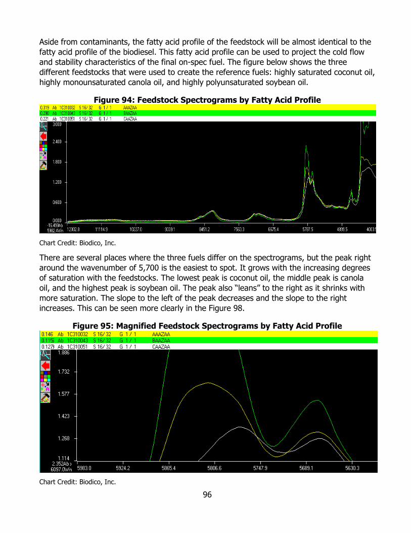
96
Aside from contaminants, the fatty acid profile of the feedstock will be almost identical to the fatty acid profile of the biodiesel. This fatty acid profile can be used to project the cold flow and stability characteristics of the final on-spec fuel. The figure below shows the three different feedstocks that were used to create the reference fuels: highly saturated coconut oil, highly monounsaturated canola oil, and highly polyunsaturated soybean oil.
Figure 94: Feedstock Spectrograms by Fatty Acid Profile
Chart Credit: Biodico, Inc.
There are several places where the three fuels differ on the spectrograms, but the peak right around the wavenumber of 5,700 is the easiest to spot. It grows with the increasing degrees of saturation with the feedstocks. The lowest peak is coconut oil, the middle peak is canola oil, and the highest peak is soybean oil. The peak also “leans” to the right as it shrinks with more saturation. The slope to the left of the peak decreases and the slope to the right increases. This can be seen more clearly in the Figure 98.
Figure 95: Magnified Feedstock Spectrograms by Fatty Acid Profile
Chart Credit: Biodico, Inc.
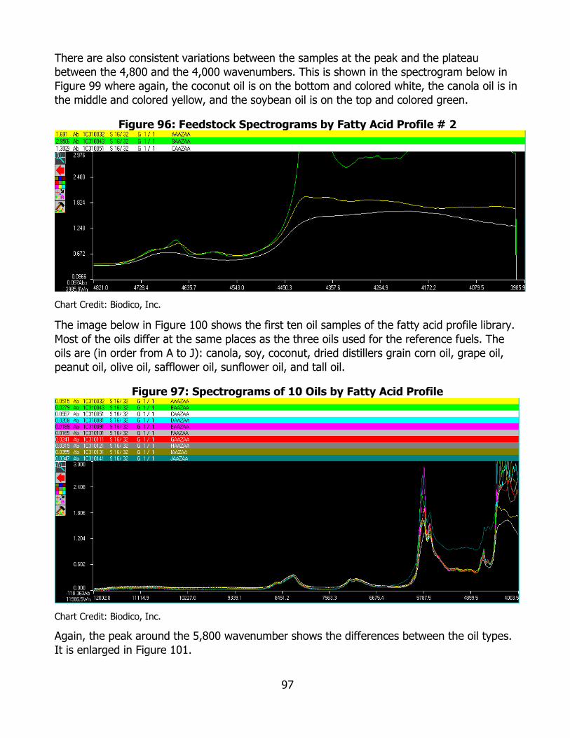
97
There are also consistent variations between the samples at the peak and the plateau between the 4,800 and the 4,000 wavenumbers. This is shown in the spectrogram below in Figure 99 where again, the coconut oil is on the bottom and colored white, the canola oil is in the middle and colored yellow, and the soybean oil is on the top and colored green.
Figure 96: Feedstock Spectrograms by Fatty Acid Profile # 2
Chart Credit: Biodico, Inc.
The image below in Figure 100 shows the first ten oil samples of the fatty acid profile library. Most of the oils differ at the same places as the three oils used for the reference fuels. The oils are (in order from A to J): canola, soy, coconut, dried distillers grain corn oil, grape oil, peanut oil, olive oil, safflower oil, sunflower oil, and tall oil.
Figure 97: Spectrograms of 10 Oils by Fatty Acid Profile
Chart Credit: Biodico, Inc.
Again, the peak around the 5,800 wavenumber shows the differences between the oil types. It is enlarged in Figure 101.

98
Figure 98: Magnified Spectrograms of 10 Oils by Fatty Acid Profile
Chart Credit: Biodico, Inc.
The different oils also show resolution in the peak and plateau range between the wavenumbers 4,800 and 4,000. This is shown in the enlarged spectrogram below in Figure 102.
Figure 99: Spectrograms of 10 Oils by Fatty Acid Profile # 2
Chart Credit: Biodico, Inc.
Once the bound glycerin is moved to the reactor for the transesterification it is reacted with methanol in the presence of an alkali methoxide and converted to biodiesel and glycerin. The image below shows a few spectra with a range of bound glycerin and methanol. The yellow line is 100 percent methanol and the green line is 100 percent bound glycerin. There are
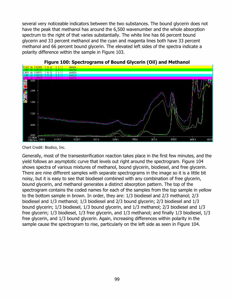
99
several very noticeable indicators between the two substances. The bound glycerin does not have the peak that methanol has around the 6,500 wavenumber and the whole absorption spectrum to the right of that varies substantially. The white line has 66 percent bound glycerin and 33 percent methanol and the cyan and magenta lines both have 33 percent methanol and 66 percent bound glycerin. The elevated left sides of the spectra indicate a polarity difference within the sample in Figure 103.
Figure 100: Spectrograms of Bound Glycerin (Oil) and Methanol
Chart Credit: Biodico, Inc.
Generally, most of the transesterification reaction takes place in the first few minutes, and the yield follows an asymptotic curve that levels out right around the spectrogram. Figure 104 shows spectra of various mixtures of methanol, bound glycerin, biodiesel, and free glycerin. There are nine different samples with separate spectrograms in the image so it is a little bit noisy, but it is easy to see that biodiesel combined with any combination of free glycerin, bound glycerin, and methanol generates a distinct absorption pattern. The top of the spectrogram contains the coded names for each of the samples from the top sample in yellow to the bottom sample in brown. In order, they are: 1/3 biodiesel and 2/3 methanol; 2/3 biodiesel and 1/3 methanol; 1/3 biodiesel and 2/3 bound glycerin; 2/3 biodiesel and 1/3 bound glycerin; 1/3 biodiesel, 1/3 bound glycerin, and 1/3 methanol; 2/3 biodiesel and 1/3 free glycerin; 1/3 biodiesel, 1/3 free glycerin, and 1/3 methanol; and finally 1/3 biodiesel, 1/3 free glycerin, and 1/3 bound glycerin. Again, increasing differences within polarity in the sample cause the spectrogram to rise, particularly on the left side as seen in Figure 104.
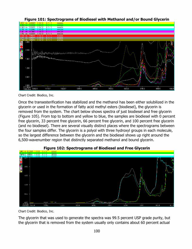
100
Figure 101: Spectrograms of Biodiesel with Methanol and/or Bound Glycerin
Chart Credit: Biodico, Inc.
Once the transesterification has stabilized and the methanol has been either solubilized in the glycerin or used in the formation of fatty acid methyl esters (biodiesel), the glycerin is removed from the system. The chart below shows spectra of just biodiesel and free glycerin (Figure 105). From top to bottom and yellow to blue, the samples are biodiesel with 0 percent free glycerin, 33 percent free glycerin, 66 percent free glycerin, and 100 percent free glycerin (and no biodiesel). There are several visually distinct places where the spectrograms between the four samples differ. The glycerin is a polyol with three hydroxyl groups in each molecule, so the largest difference between the glycerin and the biodiesel shows up right around the 6,500-wavenumber region that distinctly separated methanol and bound glycerin.
Figure 102: Spectrograms of Biodiesel and Free Glycerin
Chart Credit: Biodico, Inc.
The glycerin that was used to generate the spectra was 99.5 percent USP grade purity, but the glycerin that is removed from the system usually only contains about 60 percent actual

101
glycerin. It also contains some fatty acid compounds, methanol, and in some cases water. The methanol can be distilled out of the glycerin and reused for future reactions. The chart below shows the combinations of methanol and glycerin in the method spectrograms (Figure 106). From top to bottom and yellow to blue, the samples are free glycerin with 0 percent methanol, 33 percent methanol, 50 percent methanol, and 100 percent methanol (no glycerin).
Figure 103: Spectrograms of Free Glycerin and Methanol
Chart Credit: Biodico, Inc.
The most common problem in distilling methanol from glycerin is that water is also distilled and ends up in the recovered methanol. The chart below (Figure 107) shows spectra for methanol and water. As the ratio of water to methanol increases the rates of change in transmission between wavenumbers 7,500 and 5,000 become less dramatic and the peaks and troughs appear broader and smoother. From top to bottom and yellow to blue, the samples are methanol with 0 percent water, 33 percent water, 50 percent water, and 100 percent water (no methanol).
Figure 104: Spectrograms of Water and Methanol
Chart Credit: Biodico, Inc.
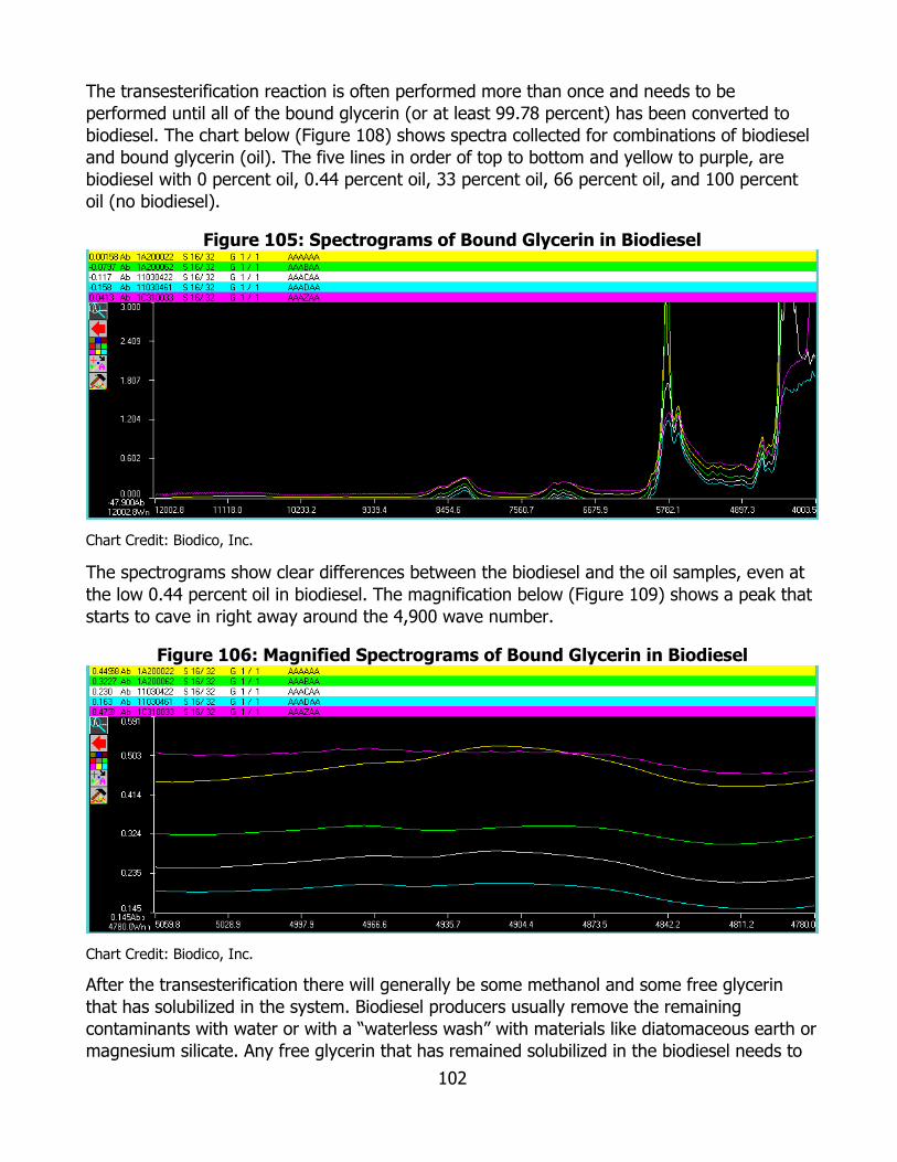
102
The transesterification reaction is often performed more than once and needs to be performed until all of the bound glycerin (or at least 99.78 percent) has been converted to biodiesel. The chart below (Figure 108) shows spectra collected for combinations of biodiesel and bound glycerin (oil). The five lines in order of top to bottom and yellow to purple, are biodiesel with 0 percent oil, 0.44 percent oil, 33 percent oil, 66 percent oil, and 100 percent oil (no biodiesel).
Figure 105: Spectrograms of Bound Glycerin in Biodiesel
Chart Credit: Biodico, Inc.
The spectrograms show clear differences between the biodiesel and the oil samples, even at the low 0.44 percent oil in biodiesel. The magnification below (Figure 109) shows a peak that starts to cave in right away around the 4,900 wave number.
Figure 106: Magnified Spectrograms of Bound Glycerin in Biodiesel
Chart Credit: Biodico, Inc.
After the transesterification there will generally be some methanol and some free glycerin that has solubilized in the system. Biodiesel producers usually remove the remaining contaminants with water or with a “waterless wash” with materials like diatomaceous earth or magnesium silicate. Any free glycerin that has remained solubilized in the biodiesel needs to

103
be removed here. The specification for free glycerin in biodiesel is a very low 0.02 percent. Thankfully biodiesel and glycerin have very different absorption properties. The chart below (Figure 110) shows biodiesel with, from top to bottom and yellow to blue, 0 percent glycerin, 0.04 percent free glycerin, 33 percent glycerin, 66 percent glycerin, and 100 percent glycerin.
Figure 107: Spectrograms of Free Glycerin in Biodiesel
Chart Credit: Biodico, Inc.
The limits of the eye fall short of chemometric computing power at this low percentage, but there are several points on the spectra where both the curve moves and its shape shifts in response to the slight addition of free glycerin. One such place is shown below (Figure 111), right around a wavenumber of 5,800. For the larger peak on the left, the biodiesel spectrogram has two small bumps which turn to one peak with only 0.04 percent free glycerin. As the glycerin concentration increases the peak continues to smooth until it is a much flatter curve for 100 percent glycerin.
Figure 108: Magnified Spectrograms of Free Glycerin in Biodiesel
Chart Credit: Biodico, Inc.

104
In the cases where water is used to wash the biodiesel, the water will often leave the system with a milky white color that indicates the presence of glycerin in the water. If the water that leaves the system is relatively clear, that is indicative that there is no free glycerin left solubilized in the biodiesel. The chart below (Figure 112) shows overlaid spectra of some of the various combinations of water, glycerin and methanol. From top to bottom and yellow to red, they are 100 percent glycerin, 100 percent water, 100 percent methanol, 50:50 glycerin and water, 50:50 glycerin and methanol, 50:50 water and methanol, and 33:33:33 for each of the three contaminants.
Figure 109: Spectrograms of Free Glycerin, Methanol, and Water (Crude Glycerin)
Chart Credit: Biodico, Inc.
The methanol has a much greater affinity to the water than to the biodiesel, but for waterless washes there can be a concern about methanol remaining in the system after the glycerin has been removed. The chart below (Figure 113) shows various combinations of biodiesel and methanol. From top to bottom and yellow to purple, the five spectra represent biodiesel with 0 percent methanol, 0.4 percent methanol, 33 percent methanol, 66 percent methanol, and 100 percent methanol (no biodiesel). As with the biodiesel spectra taken with the other contaminants, the spectrogram is responsive at the low resolutions needed for the specification.
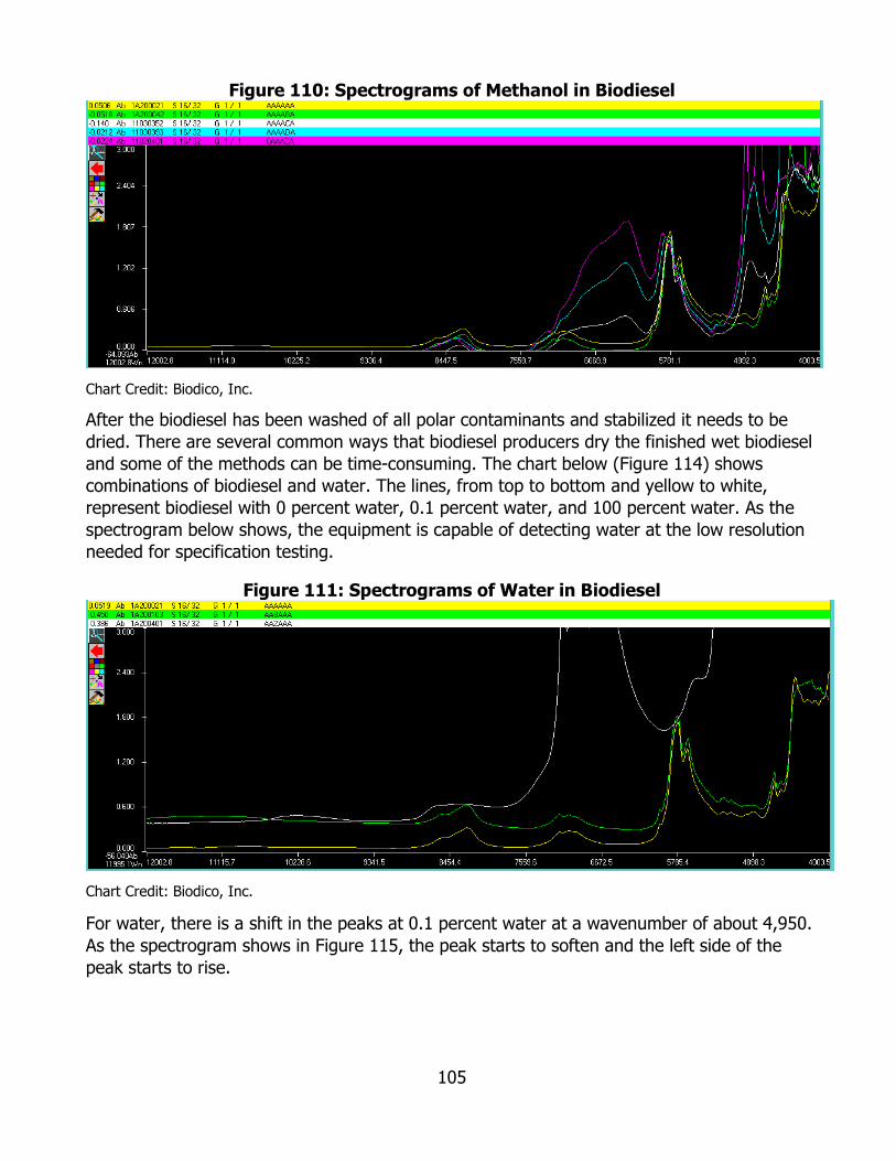
105
Figure 110: Spectrograms of Methanol in Biodiesel
Chart Credit: Biodico, Inc.
After the biodiesel has been washed of all polar contaminants and stabilized it needs to be dried. There are several common ways that biodiesel producers dry the finished wet biodiesel and some of the methods can be time-consuming. The chart below (Figure 114) shows combinations of biodiesel and water. The lines, from top to bottom and yellow to white, represent biodiesel with 0 percent water, 0.1 percent water, and 100 percent water. As the spectrogram below shows, the equipment is capable of detecting water at the low resolution needed for specification testing.
Figure 111: Spectrograms of Water in Biodiesel
Chart Credit: Biodico, Inc.
For water, there is a shift in the peaks at 0.1 percent water at a wavenumber of about 4,950. As the spectrogram shows in Figure 115, the peak starts to soften and the left side of the peak starts to rise.
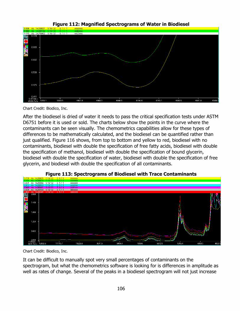
106
Figure 112: Magnified Spectrograms of Water in Biodiesel
Chart Credit: Biodico, Inc.
After the biodiesel is dried of water it needs to pass the critical specification tests under ASTM D6751 before it is used or sold. The charts below show the points in the curve where the contaminants can be seen visually. The chemometrics capabilities allow for these types of differences to be mathematically calculated, and the biodiesel can be quantified rather than just qualified. Figure 116 shows, from top to bottom and yellow to red, biodiesel with no contaminants, biodiesel with double the specification of free fatty acids, biodiesel with double the specification of methanol, biodiesel with double the specification of bound glycerin, biodiesel with double the specification of water, biodiesel with double the specification of free glycerin, and biodiesel with double the specification of all contaminants.
Figure 113: Spectrograms of Biodiesel with Trace Contaminants
Chart Credit: Biodico, Inc.
It can be difficult to manually spot very small percentages of contaminants on the spectrogram, but what the chemometrics software is looking for is differences in amplitude as well as rates of change. Several of the peaks in a biodiesel spectrogram will not just increase

107
or decrease in height but “lean” to the left or right, sharpen or smooth over, or lose or create a new bump on the side of the peak.
In the chart below (Figure 117), the peak for both the free fatty acids and the free glycerin leans more to the left and develops a new bump on the right-hand side of the peak. There is a small bump on the left-hand side of the peak that decreases with each of the contaminants except the free fatty acids (for which it seems to increase).
Figure 114: Magnified Spectrograms of Biodiesel with Trace Contaminants #1
Chart Credit: Biodico, Inc.
In Figure 118 below a bump starts to develop on the left-hand side of the left most peak for free fatty acids, methanol, and water.
Figure 115: Magnified Spectrograms of Biodiesel with Trace Contaminants # 2
Chart Credit: Biodico, Inc.
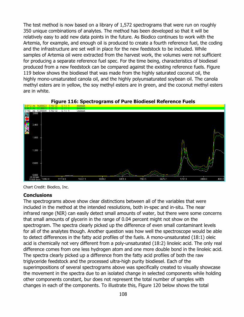
108
The test method is now based on a library of 1,572 spectrograms that were run on roughly 350 unique combinations of analytes. The method has been developed so that it will be relatively easy to add new data points in the future. As Biodico continues to work with the Artemia, for example, and enough oil is produced to create a fourth reference fuel, the coding and the infrastructure are set well in place for the new feedstock to be included. While samples of Artemia oil were extracted from the harvest work, the volumes were not sufficient for producing a separate reference fuel spec. For the time being, characteristics of biodiesel produced from a new feedstock can be compared against the existing reference fuels. Figure 119 below shows the biodiesel that was made from the highly saturated coconut oil, the highly mono-unsaturated canola oil, and the highly polyunsaturated soybean oil. The canola methyl esters are in yellow, the soy methyl esters are in green, and the coconut methyl esters are in white.
Figure 116: Spectrograms of Pure Biodiesel Reference Fuels
Chart Credit: Biodico, Inc.
Conclusions The spectrograms above show clear distinctions between all of the variables that were included in the method at the intended resolutions, both in-spec and in-situ. The near infrared range (NIR) can easily detect small amounts of water, but there were some concerns that small amounts of glycerin in the range of 0.04 percent might not show on the spectrogram. The spectra clearly picked up the difference of even small contaminant levels for all of the analytes though. Another question was how well the spectroscope would be able to detect differences in the fatty acid profiles of the fuels. A mono-unsaturated (18:1) oleic acid is chemically not very different from a poly-unsaturated (18:2) linoleic acid. The only real difference comes from one less hydrogen atom and one more double bond in the linoleic acid. The spectra clearly picked up a difference from the fatty acid profiles of both the raw triglyceride feedstock and the processed ultra-high purity biodiesel. Each of the superimpositions of several spectrograms above was specifically created to visually showcase the movement in the spectra due to an isolated change in selected components while holding other components constant, bur does not represent the total number of samples with changes in each of the components. To illustrate this, Figure 120 below shows the total

109
number of unique combinations of components that have each of the principal components within a given concentration range for the in-situ portion of the library alone.
Figure 117: Ranges of Unique In-Situ Combinations
Chart Credit: Biodico, Inc.
The speed of the testing and the responsiveness of the spectra to differences in the sample also came through very well. For each sample a total of three spectrograms were taken. The spectrograms each consisted of 16 scans. This total of 48 scans was performed in under a minute.
From this work Biodico was able to conclude that the method they have developed with an FT-NIR spectroscopic analyzer using a probe with calcium fluoride windows and measuring a wavenumber range from 12,000 to 4,000 is well equipped to take the place of the in-situ testing requirements for biodiesel, and that the method is very promising for being able to take the place of many of the final specification tests after enough cross calibration is done with the actual samples of commercial production.
The time that must be spent testing each biodiesel batch is generally higher than the time needed to actually produce the biodiesel. Of the nine critical specification tests that must be performed on a representative sample of every homogenous batch of biodiesel sold, the FT-NIR method has been designed to incorporate every test except for the cold soak filter test and sulfur. This includes free glycerin, total glycerin, acid number, cloud point, oxidative stability, moisture, and flash point. The total time needed to run all of the tests is about six hours and 45 minutes. Many of these tests require operating time for the analytical equipment though and do not require constant operator supervision. The biggest example of this is the Rancimat equipment used to measure the oxidative stability of the fuel, which requires at least three hours for fuel that meets the specification. During the Rancimat test, for example, other tests can be performed by a single lab analyst. Some tests that require time for the analytical equipment to operate are needed to inform the fuel production process and will halt the process between stages. The most relevant example of this is the gas chromatograph, which takes 45 minutes of non-operator processing time and is needed between transesterifications and some of the later production stages. When the possibility of
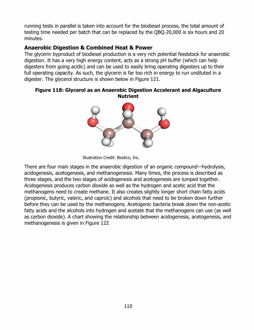
110
running tests in parallel is taken into account for the biodiesel process, the total amount of testing time needed per batch that can be replaced by the QBQ-20,000 is six hours and 20 minutes.
Anaerobic Digestion & Combined Heat & Power The glycerin byproduct of biodiesel production is a very rich potential feedstock for anaerobic digestion. It has a very high energy content, acts as a strong pH buffer (which can help digesters from going acidic) and can be used to easily bring operating digesters up to their full operating capacity. As such, the glycerin is far too rich in energy to run undiluted in a digester. The glycerol structure is shown below in Figure 121.
Figure 118: Glycerol as an Anaerobic Digestion Accelerant and Algaculture Nutrient
Illustration Credit: Biodico, Inc.
There are four main stages in the anaerobic digestion of an organic compound—hydrolysis, acidogenesis, acetogenesis, and methanogenesis. Many times, the process is described as three stages, and the two stages of acidogenesis and acetogenesis are lumped together. Acidogenesis produces carbon dioxide as well as the hydrogen and acetic acid that the methanogens need to create methane. It also creates slightly longer short chain fatty acids (propionic, butyric, valeric, and caproic) and alcohols that need to be broken down further before they can be used by the methanogens. Acetogenic bacteria break down the non-acetic fatty acids and the alcohols into hydrogen and acetate that the methanogens can use (as well as carbon dioxide). A chart showing the relationship between acidogenesis, acetogenesis, and methanogenesis is given in Figure 122.
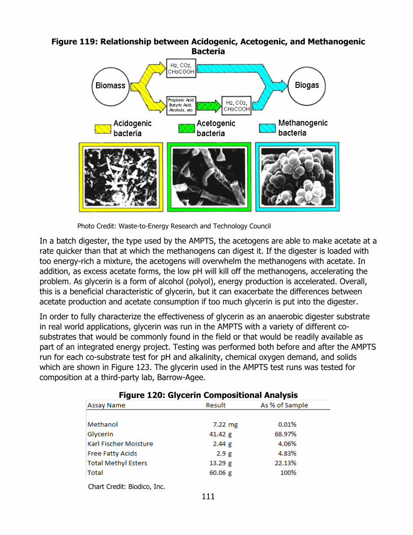
111
Figure 119: Relationship between Acidogenic, Acetogenic, and Methanogenic Bacteria
Photo Credit: Waste-to-Energy Research and Technology Council
In a batch digester, the type used by the AMPTS, the acetogens are able to make acetate at a rate quicker than that at which the methanogens can digest it. If the digester is loaded with too energy-rich a mixture, the acetogens will overwhelm the methanogens with acetate. In addition, as excess acetate forms, the low pH will kill off the methanogens, accelerating the problem. As glycerin is a form of alcohol (polyol), energy production is accelerated. Overall, this is a beneficial characteristic of glycerin, but it can exacerbate the differences between acetate production and acetate consumption if too much glycerin is put into the digester.
In order to fully characterize the effectiveness of glycerin as an anaerobic digester substrate in real world applications, glycerin was run in the AMPTS with a variety of different co-substrates that would be commonly found in the field or that would be readily available as part of an integrated energy project. Testing was performed both before and after the AMPTS run for each co-substrate test for pH and alkalinity, chemical oxygen demand, and solids which are shown in Figure 123. The glycerin used in the AMPTS test runs was tested for composition at a third-party lab, Barrow-Agee.
Figure 120: Glycerin Compositional Analysis
Chart Credit: Biodico, Inc.

112
Test Plan The AMPTS is a piece of laboratory equipment manufactured by Bioprocess Control, Inc. It is designed to accurately measure the methane output from the anaerobic digestion of multiple samples simultaneously over time. The AMPTS returns methane flow and methane volume in normalized volume to standard temperature and pressure of 0°C at 100 kPa. The density of methane at standard temperature and pressure is 0.66 kg/m3. By monitoring methane volume and flow rate over time, Biodico can more effectively monitor what is happening in the anaerobic digestion process as new substrates are introduced, combined and optimized. Each digester passes through a length of flexible plastic tubing to a 100 mL sealed Pyrex bottle filled with 80 mL of a 3 M NaOH solution and phenolphthalein. The tubing is submerged in the basic solution in order to strip the gas of carbon dioxide and other non-methane trace gases such as H2S. As the mixture in the bottle approaches saturation, the phenolphthalein turns pink (acidic). This is a fail-safe. The solution in the bottles is changed out with each test run and the solution has never turned pink (reached saturation). A second tube leads out of the fixing bottle and to the main AMPTS unit and contains pure methane (CH4). In a set of triplicate tests, one triplicate can bypass the fixing bottle while one passes through it. A comparison of the two results will show the ratio of methane and non-methane gases produced. A gas capture bag can also be used and the composition of the captured gas can be analyzed by Gas Chromatography (GC). A picture of this setup in the Biodico lab is shown below in Figure 124. The gas tank on the right is used for purging the system with nitrogen, and the adjacent furnace is used to determine the ash content and volatile solid fraction of samples.
Figure 121: AMPTS Setup at Naval Base Ventura County
Photo Credit: Biodico, Inc.

113
The main AMPTS measuring unit contains 15 hollow-bodied flippers submerged in water and hooked up to an electrical component to activate a signal recorded by a microchip portal to a lab computer and the AMPTS program. Each flipper is carefully calibrated and designed to tip upward when a threshold volume of methane enters their internal chamber and increases the buoyancy, and the programming compensates for temperature and pressure to give a normalized reading. Each of the flippers is hooked up to a separate digester in order to determine the real-time gas production of up to 15 samples at a time. Figure 125 shows a picture of the flippers is given below. One of the flippers (third flipper up from the lower right) is tipping upward due to gas flow into the system.
Figure 122: AMPTS Methane Measurement Apparatus
Photo Credit: Biodico, Inc.
As part of the AMPTS testing process the following factors are measured, as shown in Figure 126.
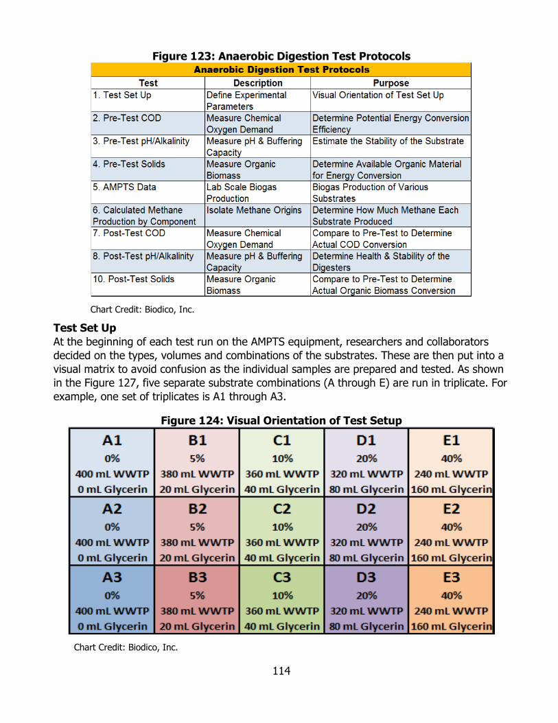
114
Figure 123: Anaerobic Digestion Test Protocols
Chart Credit: Biodico, Inc.
Test Set Up At the beginning of each test run on the AMPTS equipment, researchers and collaborators decided on the types, volumes and combinations of the substrates. These are then put into a visual matrix to avoid confusion as the individual samples are prepared and tested. As shown in the Figure 127, five separate substrate combinations (A through E) are run in triplicate. For example, one set of triplicates is A1 through A3.
Figure 124: Visual Orientation of Test Setup
Chart Credit: Biodico, Inc.
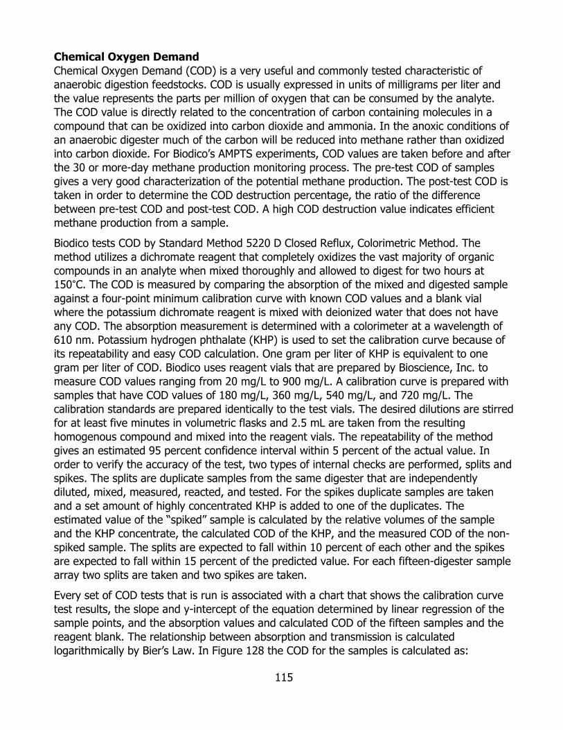
115
Chemical Oxygen Demand Chemical Oxygen Demand (COD) is a very useful and commonly tested characteristic of anaerobic digestion feedstocks. COD is usually expressed in units of milligrams per liter and the value represents the parts per million of oxygen that can be consumed by the analyte. The COD value is directly related to the concentration of carbon containing molecules in a compound that can be oxidized into carbon dioxide and ammonia. In the anoxic conditions of an anaerobic digester much of the carbon will be reduced into methane rather than oxidized into carbon dioxide. For Biodico’s AMPTS experiments, COD values are taken before and after the 30 or more-day methane production monitoring process. The pre-test COD of samples gives a very good characterization of the potential methane production. The post-test COD is taken in order to determine the COD destruction percentage, the ratio of the difference between pre-test COD and post-test COD. A high COD destruction value indicates efficient methane production from a sample.
Biodico tests COD by Standard Method 5220 D Closed Reflux, Colorimetric Method. The method utilizes a dichromate reagent that completely oxidizes the vast majority of organic compounds in an analyte when mixed thoroughly and allowed to digest for two hours at 150°C. The COD is measured by comparing the absorption of the mixed and digested sample against a four-point minimum calibration curve with known COD values and a blank vial where the potassium dichromate reagent is mixed with deionized water that does not have any COD. The absorption measurement is determined with a colorimeter at a wavelength of 610 nm. Potassium hydrogen phthalate (KHP) is used to set the calibration curve because of its repeatability and easy COD calculation. One gram per liter of KHP is equivalent to one gram per liter of COD. Biodico uses reagent vials that are prepared by Bioscience, Inc. to measure COD values ranging from 20 mg/L to 900 mg/L. A calibration curve is prepared with samples that have COD values of 180 mg/L, 360 mg/L, 540 mg/L, and 720 mg/L. The calibration standards are prepared identically to the test vials. The desired dilutions are stirred for at least five minutes in volumetric flasks and 2.5 mL are taken from the resulting homogenous compound and mixed into the reagent vials. The repeatability of the method gives an estimated 95 percent confidence interval within 5 percent of the actual value. In order to verify the accuracy of the test, two types of internal checks are performed, splits and spikes. The splits are duplicate samples from the same digester that are independently diluted, mixed, measured, reacted, and tested. For the spikes duplicate samples are taken and a set amount of highly concentrated KHP is added to one of the duplicates. The estimated value of the “spiked” sample is calculated by the relative volumes of the sample and the KHP concentrate, the calculated COD of the KHP, and the measured COD of the non-spiked sample. The splits are expected to fall within 10 percent of each other and the spikes are expected to fall within 15 percent of the predicted value. For each fifteen-digester sample array two splits are taken and two spikes are taken.
Every set of COD tests that is run is associated with a chart that shows the calibration curve test results, the slope and y-intercept of the equation determined by linear regression of the sample points, and the absorption values and calculated COD of the fifteen samples and the reagent blank. The relationship between absorption and transmission is calculated logarithmically by Bier’s Law. In Figure 128 the COD for the samples is calculated as:

116
Figure 125: COD Calculation
Photo Credit: Biodico, Inc.
The chart gives a graphical representation of the COD and the transmission of the calibration curve samples as well as the trend line that is generated by regression analysis of the calibration data points. The equation is displayed in form on the chart and the R2 value gives the coefficient of determination of the trend line. An R2 value of 100 percent means that the data points fit the trend line perfectly and lower R2 values signify less statistical correlation. Biodico generates the calibration curve with expectations that R2 will be greater than or equal to 98 percent. Figure 129 shows the test setup for chemical oxygen demand.
Figure 126: Test Setup for Chemical Oxygen Demand
Photo Credit: Biodico, Inc.
Chemical Oxygen Demand is a particularly important test metric for the determination of glycerin’s potential to create methane through anaerobic digestion. The COD of the crude glycerin byproduct of biodiesel production is very high and generally falls in the range of 2,000,000 to 2,500,000 mg/L. Most anaerobic digesters operate in a range of 20,000 to 80,000 mg/L COD and digesters become increasingly unstable toward to high end of this range. This means that proper dilution of the glycerin is essential for anaerobic digestion. It also means that the energy potential of the glycerin is very high as compared to other feedstocks.
The term ultimate methane yield is used to define the relationship between COD and methane production as 400 liters of methane per kilogram of COD that is lost in an anaerobic digestion substrate (COD destruction). Figure 130 shows the derivation.
117
Figure 127: Ultimate Methane Yield from COD
Figure Credit: Oklahoma State University
pH and Alkalinity The pH of the samples is determined by following Standard Method 4500-H+. Alkalinity is determined by following Standard Method 2320. A picture of the laboratory setup is shown in Figure 132. The pre-test pH and alkalinity are important factors in determining the survivability of healthy microbial colonies in a prepared digester sample. The healthiest digesters have a pH that is a neutral 7 pH or is a slightly alkaline pH of just above 7. As the pH of a digester falls below 7 the digester becomes increasingly less stable. Biodico has measured healthy digesters that have a low pH of almost 6 (though this is rare) but has yet to see a healthy digester with a pH value under 6. This is generally consistent with other living aquatic organisms, where neutrality is desirable and a slight alkalinity is preferred to a slight acidity. The alkalinity value represents the ability for a sample to resist changes in pH resulting from the addition of acid to a sample. The alkalinity is not solely determined by the pH. In comparing two samples, one of the samples may have a lower, more acidic pH, but a higher alkalinity value. Alkalinity is an important value because it indicates a digester’s ability to resist “going sour.” The primary limiting factor in the rate at which energy can be put into a digester is the difference between the acetogens’ ability to produce acetate and the methanogens’ ability to consume it. If too much potential energy is put into a digester, the acetate will begin to overwhelm the system and the pH of the system will begin to drop. As the pH falls, the survival of the methanogens becomes increasingly difficult. The acetate consumption and production rates can vary somewhat throughout the course of the consumption of organic material, and small drops in pH may self-correct as the methanogens have more time to adapt to the presence of more available energy in the form of acetate. At a certain point though, the acetate content in a digester will begin to kill off the methanogens and the health of the digester quickly spirals downward. The more resistance that a sample has to changes in pH, the better a chance there is that the methanogen populations will be
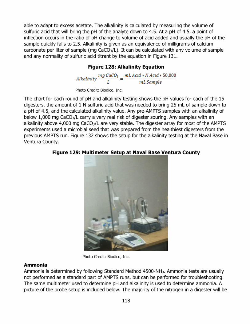
118
able to adapt to excess acetate. The alkalinity is calculated by measuring the volume of sulfuric acid that will bring the pH of the analyte down to 4.5. At a pH of 4.5, a point of inflection occurs in the ratio of pH change to volume of acid added and usually the pH of the sample quickly falls to 2.5. Alkalinity is given as an equivalence of milligrams of calcium carbonate per liter of sample (mg CaCO3/L). It can be calculated with any volume of sample and any normality of sulfuric acid titrant by the equation in Figure 131.
Figure 128: Alkalinity Equation
Photo Credit: Biodico, Inc.
The chart for each round of pH and alkalinity testing shows the pH values for each of the 15 digesters, the amount of 1 N sulfuric acid that was needed to bring 25 mL of sample down to a pH of 4.5, and the calculated alkalinity value. Any pre-AMPTS samples with an alkalinity of below 1,000 mg CaCO3/L carry a very real risk of digester souring. Any samples with an alkalinity above 4,000 mg CaCO3/L are very stable. The digester array for most of the AMPTS experiments used a microbial seed that was prepared from the healthiest digesters from the previous AMPTS run. Figure 132 shows the setup for the alkalinity testing at the Naval Base in Ventura County.
Figure 129: Multimeter Setup at Naval Base Ventura County
Photo Credit: Biodico, Inc.
Ammonia Ammonia is determined by following Standard Method 4500-NH3. Ammonia tests are usually not performed as a standard part of AMPTS runs, but can be performed for troubleshooting. The same multimeter used to determine pH and alkalinity is used to determine ammonia. A picture of the probe setup is included below. The majority of the nitrogen in a digester will be
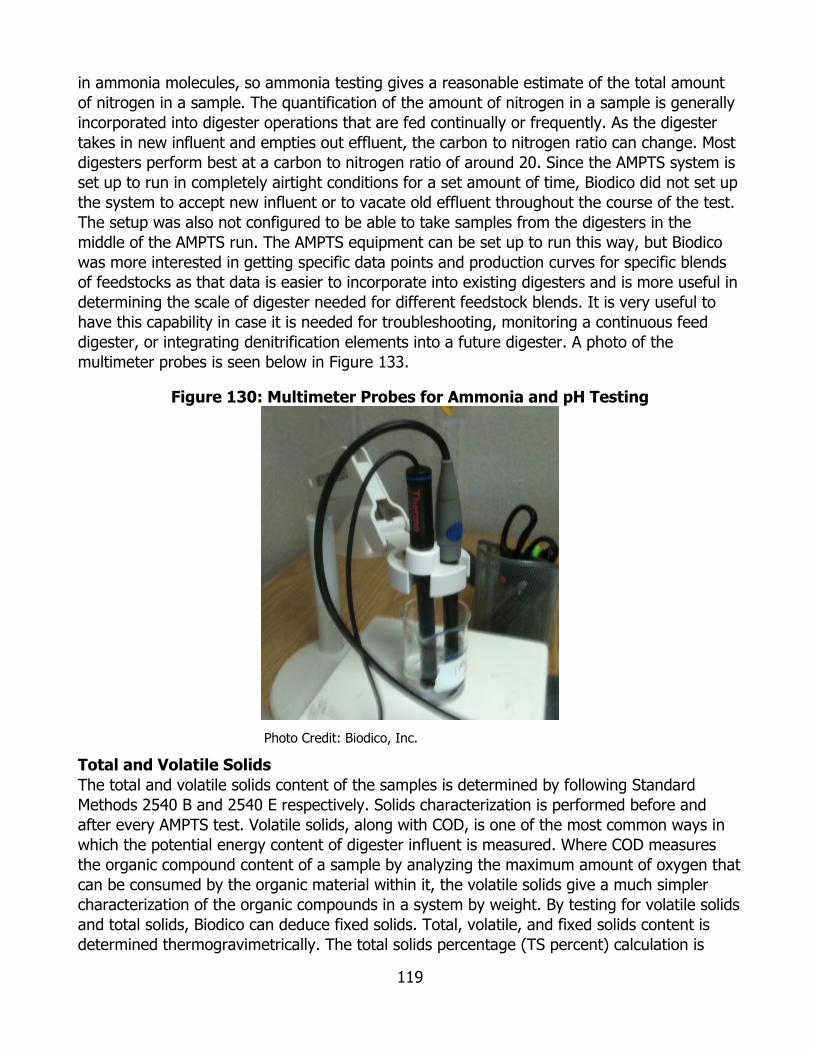
119
in ammonia molecules, so ammonia testing gives a reasonable estimate of the total amount of nitrogen in a sample. The quantification of the amount of nitrogen in a sample is generally incorporated into digester operations that are fed continually or frequently. As the digester takes in new influent and empties out effluent, the carbon to nitrogen ratio can change. Most digesters perform best at a carbon to nitrogen ratio of around 20. Since the AMPTS system is set up to run in completely airtight conditions for a set amount of time, Biodico did not set up the system to accept new influent or to vacate old effluent throughout the course of the test. The setup was also not configured to be able to take samples from the digesters in the middle of the AMPTS run. The AMPTS equipment can be set up to run this way, but Biodico was more interested in getting specific data points and production curves for specific blends of feedstocks as that data is easier to incorporate into existing digesters and is more useful in determining the scale of digester needed for different feedstock blends. It is very useful to have this capability in case it is needed for troubleshooting, monitoring a continuous feed digester, or integrating denitrification elements into a future digester. A photo of the multimeter probes is seen below in Figure 133.
Figure 130: Multimeter Probes for Ammonia and pH Testing
Photo Credit: Biodico, Inc.
Total and Volatile Solids The total and volatile solids content of the samples is determined by following Standard Methods 2540 B and 2540 E respectively. Solids characterization is performed before and after every AMPTS test. Volatile solids, along with COD, is one of the most common ways in which the potential energy content of digester influent is measured. Where COD measures the organic compound content of a sample by analyzing the maximum amount of oxygen that can be consumed by the organic material within it, the volatile solids give a much simpler characterization of the organic compounds in a system by weight. By testing for volatile solids and total solids, Biodico can deduce fixed solids. Total, volatile, and fixed solids content is determined thermogravimetrically. The total solids percentage (TS percent) calculation is

120
determined by measurements of the weight of the sample dish (tare weight, T), total sample weight (wet weight, W), and the sample weight after it is cooked in a lab oven at 105°C (dry weight, D). The calculation of total solids is calculated in Figure 134.
Figure 131: Total Solids Calculation
Photo Credit: Biodico, Inc.
The total solids are determined in an oven that has relatively low temperatures but relatively high precision. The oven is pictured below in Figure 135.
Figure 132: Higher Precision, Lower Temperature, Laboratory Oven
Photo Credit: Biodico, Inc.
After the dry weight of the sample is measured from the lab oven, the sample is placed in an oven at 550°C for fifteen minutes, cooled in a desiccator (so no moisture is reabsorbed into the sample) for 15 minutes, and the weight of the tare tray and volatilized sample (fixed weight) is taken. The portion of the sample that is left in the tray is called the fixed solids and determined by the equation in Figure 136.
Figure 133: Fixed Solids Calculation
Photo Credit: Biodico, Inc.

121
The portion of volatile solids in the total solids is determined by the equation below in Figure 137.
Figure 134: Volatile Solids Calculation
Photo Credit: Biodico, Inc.
The fixed solids samples are prepared in a muffle furnace that has high temperatures, but less precision than the lab oven. The muffle furnace is pictured below in Figure 138.
Figure 135: Higher Temperature, Lower Precision, Muffle Furnace
Photo Credit: Biodico, Inc.
Biodico also has the capability of testing for a category that is separate from volatile and fixed solids characterization, dissolved and suspended solids. Grade G4 filters are pre-cooked at 550°C and a tare weight is taken for the tray and the cooked filter (FT). The glass fiber circle is then placed in a vacuum apparatus, and the suspended solids (SS) that are caught in the filter are weighed as dry solids. The separation of total solids into two independent categories leads to a total of four categories of solids within total solids: volatile dissolved solids (VDS), volatile suspended solids, fixed dissolved solids, and fixed suspended solids. VDS essentially gives the digester an idea of potential food sources for the microbes that are not being consumed. It can be an indicator to show that the feed rate to a digester may be too high. It can also indicate inefficiency of the microbes by lack of nutrients. The most important of the
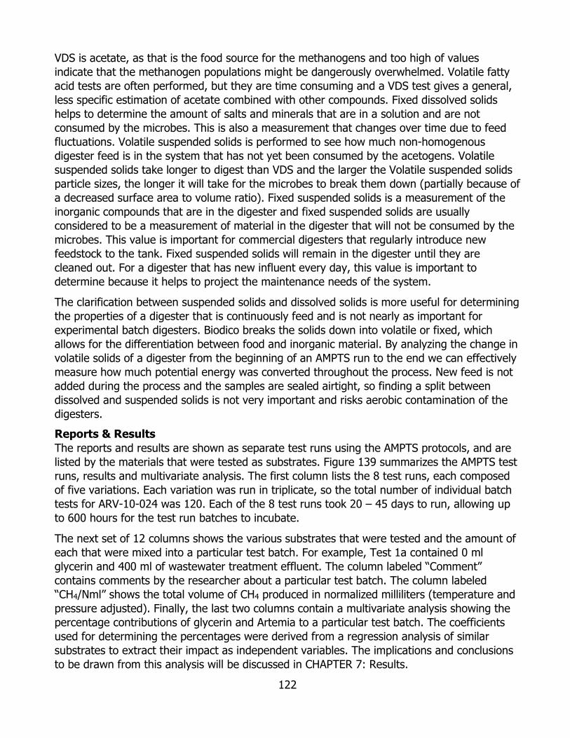
122
VDS is acetate, as that is the food source for the methanogens and too high of values indicate that the methanogen populations might be dangerously overwhelmed. Volatile fatty acid tests are often performed, but they are time consuming and a VDS test gives a general, less specific estimation of acetate combined with other compounds. Fixed dissolved solids helps to determine the amount of salts and minerals that are in a solution and are not consumed by the microbes. This is also a measurement that changes over time due to feed fluctuations. Volatile suspended solids is performed to see how much non-homogenous digester feed is in the system that has not yet been consumed by the acetogens. Volatile suspended solids take longer to digest than VDS and the larger the Volatile suspended solids particle sizes, the longer it will take for the microbes to break them down (partially because of a decreased surface area to volume ratio). Fixed suspended solids is a measurement of the inorganic compounds that are in the digester and fixed suspended solids are usually considered to be a measurement of material in the digester that will not be consumed by the microbes. This value is important for commercial digesters that regularly introduce new feedstock to the tank. Fixed suspended solids will remain in the digester until they are cleaned out. For a digester that has new influent every day, this value is important to determine because it helps to project the maintenance needs of the system.
The clarification between suspended solids and dissolved solids is more useful for determining the properties of a digester that is continuously feed and is not nearly as important for experimental batch digesters. Biodico breaks the solids down into volatile or fixed, which allows for the differentiation between food and inorganic material. By analyzing the change in volatile solids of a digester from the beginning of an AMPTS run to the end we can effectively measure how much potential energy was converted throughout the process. New feed is not added during the process and the samples are sealed airtight, so finding a split between dissolved and suspended solids is not very important and risks aerobic contamination of the digesters. Reports & Results The reports and results are shown as separate test runs using the AMPTS protocols, and are listed by the materials that were tested as substrates. Figure 139 summarizes the AMPTS test runs, results and multivariate analysis. The first column lists the 8 test runs, each composed of five variations. Each variation was run in triplicate, so the total number of individual batch tests for ARV-10-024 was 120. Each of the 8 test runs took 20 – 45 days to run, allowing up to 600 hours for the test run batches to incubate.
The next set of 12 columns shows the various substrates that were tested and the amount of each that were mixed into a particular test batch. For example, Test 1a contained 0 ml glycerin and 400 ml of wastewater treatment effluent. The column labeled “Comment” contains comments by the researcher about a particular test batch. The column labeled “CH4/Nml” shows the total volume of CH4 produced in normalized milliliters (temperature and pressure adjusted). Finally, the last two columns contain a multivariate analysis showing the percentage contributions of glycerin and Artemia to a particular test batch. The coefficients used for determining the percentages were derived from a regression analysis of similar substrates to extract their impact as independent variables. The implications and conclusions to be drawn from this analysis will be discussed in CHAPTER 7: Results.

123
Figure 136: AMPTS Test Runs, Results & Multivariate Analysis
Chart Credit: Biodico, Inc.

124
All of the methane volumes that are recorded by the AMPTS are normalized, adjusted to standard temperature and pressure. This makes it straight forward to determine the weights of methane produced since one mL of methane equals 660 μg, or 0.66 mg. The mg of methane produced from each of the triplicates from each of the test runs is given in the figure below.
Figure 137: mg of Methane Produced per Triplicate Set per Test Run
Chart Credit: Biodico, Inc.
Glycerin & Wastewater Treatment Plant Effluent In order to gain as much meaningful data about the behavior of glycerin in anaerobic digestion as possible, it was important to first determine the maximum amount of glycerin that standard populations of methanogens can tolerate. For the first AMPTS experiment four triplicate sets with exponentially increasing volumes of glycerin were mixed into wastewater sludge with active methanogen populations. A control triplicate set with no glycerin was also included. The result was five triplicate sets with 0 percent, 5 percent, 10 percent, 20 percent, and 40 percent glycerin mixed into wastewater sludge. The wastewater sludge used was a 50:50 mixed sample of anaerobic digeter sludge from the Ventura Wastewater Treatment Facility in Ventura and anaerobic digester sludge from the Hill Canyon Wastewater Treatment Facility in Camarillo. Two microbial populations were mixed together for the test in order to increase the biological diversity of the sample. Test Setup The fifteen sample array of five different concentrations of glycerin in triplicate is shown in Figure 141.
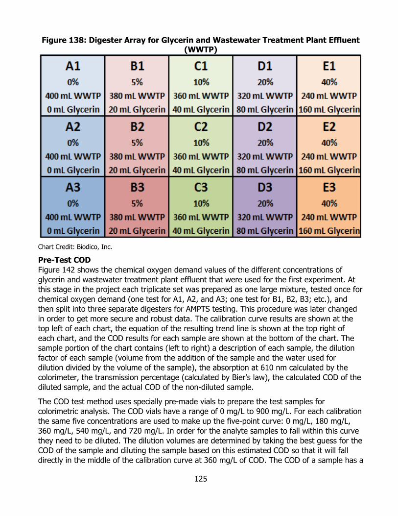
125
Figure 138: Digester Array for Glycerin and Wastewater Treatment Plant Effluent (WWTP)
Chart Credit: Biodico, Inc.
Pre-Test COD Figure 142 shows the chemical oxygen demand values of the different concentrations of glycerin and wastewater treatment plant effluent that were used for the first experiment. At this stage in the project each triplicate set was prepared as one large mixture, tested once for chemical oxygen demand (one test for A1, A2, and A3; one test for B1, B2, B3; etc.), and then split into three separate digesters for AMPTS testing. This procedure was later changed in order to get more secure and robust data. The calibration curve results are shown at the top left of each chart, the equation of the resulting trend line is shown at the top right of each chart, and the COD results for each sample are shown at the bottom of the chart. The sample portion of the chart contains (left to right) a description of each sample, the dilution factor of each sample (volume from the addition of the sample and the water used for dilution divided by the volume of the sample), the absorption at 610 nm calculated by the colorimeter, the transmission percentage (calculated by Bier’s law), the calculated COD of the diluted sample, and the actual COD of the non-diluted sample.
The COD test method uses specially pre-made vials to prepare the test samples for colorimetric analysis. The COD vials have a range of 0 mg/L to 900 mg/L. For each calibration the same five concentrations are used to make up the five-point curve: 0 mg/L, 180 mg/L, 360 mg/L, 540 mg/L, and 720 mg/L. In order for the analyte samples to fall within this curve they need to be diluted. The dilution volumes are determined by taking the best guess for the COD of the sample and diluting the sample based on this estimated COD so that it will fall directly in the middle of the calibration curve at 360 mg/L of COD. The COD of a sample has a
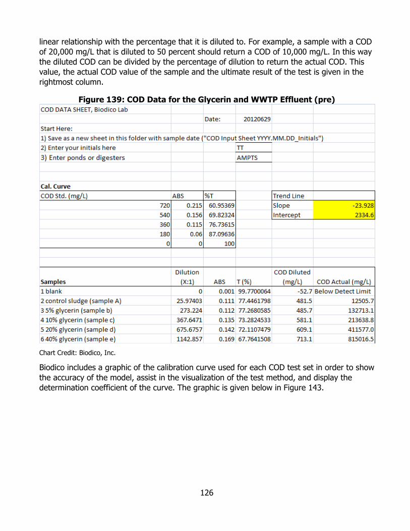
126
linear relationship with the percentage that it is diluted to. For example, a sample with a COD of 20,000 mg/L that is diluted to 50 percent should return a COD of 10,000 mg/L. In this way the diluted COD can be divided by the percentage of dilution to return the actual COD. This value, the actual COD value of the sample and the ultimate result of the test is given in the rightmost column.
Figure 139: COD Data for the Glycerin and WWTP Effluent (pre)
Chart Credit: Biodico, Inc.
Biodico includes a graphic of the calibration curve used for each COD test set in order to show the accuracy of the model, assist in the visualization of the test method, and display the determination coefficient of the curve. The graphic is given below in Figure 143.
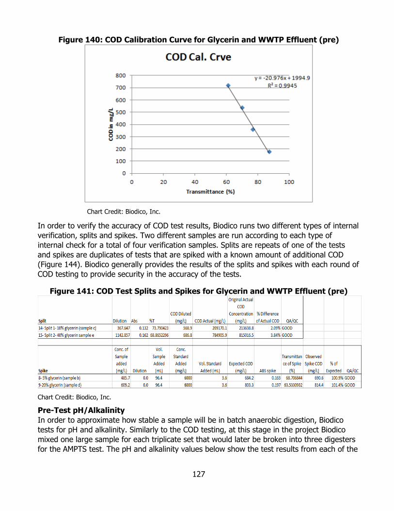
127
Figure 140: COD Calibration Curve for Glycerin and WWTP Effluent (pre)
Chart Credit: Biodico, Inc.
In order to verify the accuracy of COD test results, Biodico runs two different types of internal verification, splits and spikes. Two different samples are run according to each type of internal check for a total of four verification samples. Splits are repeats of one of the tests and spikes are duplicates of tests that are spiked with a known amount of additional COD (Figure 144). Biodico generally provides the results of the splits and spikes with each round of COD testing to provide security in the accuracy of the tests.
Figure 141: COD Test Splits and Spikes for Glycerin and WWTP Effluent (pre)
Chart Credit: Biodico, Inc.
Pre-Test pH/Alkalinity In order to approximate how stable a sample will be in batch anaerobic digestion, Biodico tests for pH and alkalinity. Similarly to the COD testing, at this stage in the project Biodico mixed one large sample for each triplicate set that would later be broken into three digesters for the AMPTS test. The pH and alkalinity values below show the test results from each of the

128
cumulatively mixed triplicate concentrations. Because this was the first AMPTS experiment, Biodico also tested the wastewater sludge in triplicate as an internal check.
Figure 142: pH and Alkalinity for Glycerin and WWTP Effluent (pre)
Chart Credit: Biodico, Inc.
Pre-Test Solids Each sample was tested for total solids content and volatile solids content both before and after the AMPTS experiment. The sample codes below may not be intuitive to the reader though. As with the other pre-AMPTS tests for glycerin and WWTP effluent, samples were taken from the blended cumulative sample that was later split into triplicate digesters. Biodico almost always tests for solids in triplicate though. The sample codes A1, A2, and A3 actually refer to triplicate tests that were taken from a combined sample that had not yet been split into three separate digesters. As Biodico’s testing protocol changed to take pre-AMPTS tests for all fifteen digesters individually, 45 different solids tests were performed. The more current labeling system contains three alphanumeric characters, two to describe the digester and one to describe the solids test triplicate. For example, E3A, E3B, and E3C later refer to triplicate tests of the last of fifteen digesters. The chart below has two alphanumeric characters, one to describe the sample and one to describe the solids test triplicate, not a separate digester (Figure 146).
Figure 143: Total and Volatile Solids for Glycerin and WWTP Effluent (pre)
Chart Credit: Biodico, Inc.
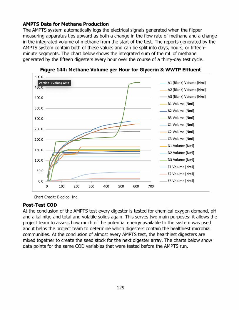
129
AMPTS Data for Methane Production The AMPTS system automatically logs the electrical signals generated when the flipper measuring apparatus tips upward as both a change in the flow rate of methane and a change in the integrated volume of methane from the start of the test. The reports generated by the AMPTS system contain both of these values and can be split into days, hours, or fifteen-minute segments. The chart below shows the integrated sum of the mL of methane generated by the fifteen digesters every hour over the course of a thirty-day test cycle.
Figure 144: Methane Volume per Hour for Glycerin & WWTP Effluent
Chart Credit: Biodico, Inc.
Post-Test COD At the conclusion of the AMPTS test every digester is tested for chemical oxygen demand, pH and alkalinity, and total and volatile solids again. This serves two main purposes: it allows the project team to assess how much of the potential energy available to the system was used and it helps the project team to determine which digesters contain the healthiest microbial communities. At the conclusion of almost every AMPTS test, the healthiest digesters are mixed together to create the seed stock for the next digester array. The charts below show data points for the same COD variables that were tested before the AMPTS run.
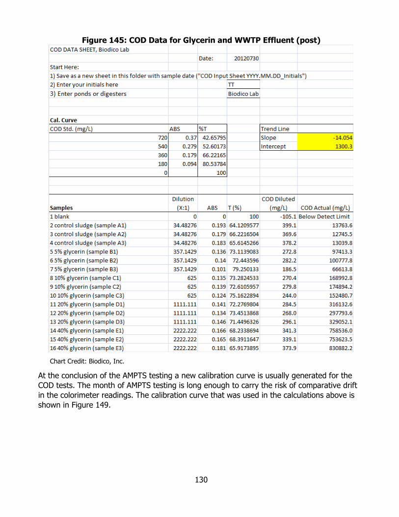
130
Figure 145: COD Data for Glycerin and WWTP Effluent (post)
Chart Credit: Biodico, Inc.
At the conclusion of the AMPTS testing a new calibration curve is usually generated for the COD tests. The month of AMPTS testing is long enough to carry the risk of comparative drift in the colorimeter readings. The calibration curve that was used in the calculations above is shown in Figure 149.
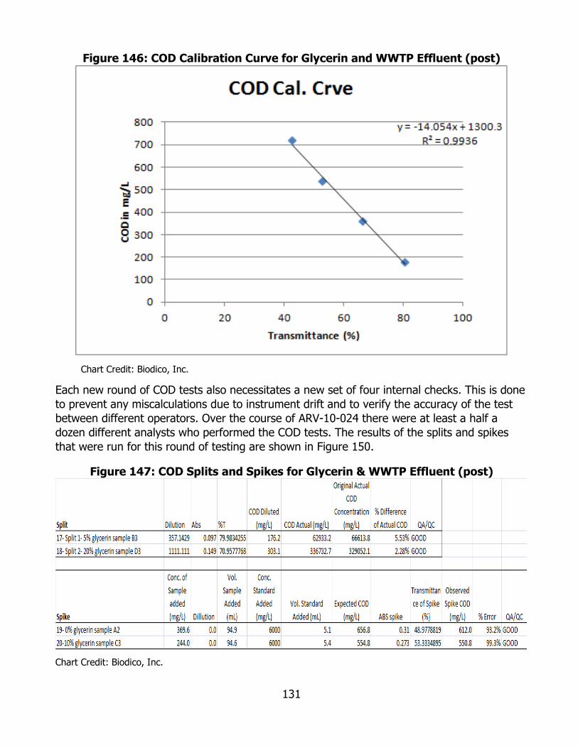
131
Figure 146: COD Calibration Curve for Glycerin and WWTP Effluent (post)
Chart Credit: Biodico, Inc.
Each new round of COD tests also necessitates a new set of four internal checks. This is done to prevent any miscalculations due to instrument drift and to verify the accuracy of the test between different operators. Over the course of ARV-10-024 there were at least a half a dozen different analysts who performed the COD tests. The results of the splits and spikes that were run for this round of testing are shown in Figure 150.
Figure 147: COD Splits and Spikes for Glycerin & WWTP Effluent (post)
Chart Credit: Biodico, Inc.
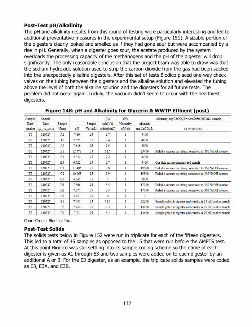
132
Post-Test pH/Alkalinity The pH and alkalinity results from this round of testing were particularly interesting and led to additional preventative measures in the experimental setup (Figure 151). A sizable portion of the digesters clearly looked and smelled as if they had gone sour but were accompanied by a rise in pH. Generally, when a digester goes sour, the acetate produced by the system overloads the processing capacity of the methanogens and the pH of the digester will drop significantly. The only reasonable conclusion that the project team was able to draw was that the sodium hydroxide solution used to strip the carbon dioxide from the gas had been sucked into the unexpectedly alkaline digesters. After this set of tests Biodico placed one-way check valves on the tubing between the digesters and the alkaline solution and elevated the tubing above the level of both the alkaline solution and the digesters for all future tests. The problem did not occur again. Luckily, the vacuum didn’t seem to occur with the healthiest digesters.
Figure 148: pH and Alkalinity for Glycerin & WWTP Effluent (post)
Chart Credit: Biodico, Inc.
Post-Test Solids The solids tests below in Figure 152 were run in triplicate for each of the fifteen digesters. This led to a total of 45 samples as opposed to the 15 that were run before the AMPTS test. At this point Biodico was still settling into its sample coding scheme so the name of each digester is given as A1 through E3 and two samples were added on to each digester by an additional A or B. For the E3 digester, as an example, the triplicate solids samples were coded as E3, E3A, and E3B.
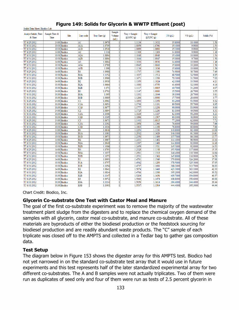
133
Figure 149: Solids for Glycerin & WWTP Effluent (post)
Chart Credit: Biodico, Inc.
Glycerin Co-substrate One Test with Castor Meal and Manure The goal of the first co-substrate experiment was to remove the majority of the wastewater treatment plant sludge from the digesters and to replace the chemical oxygen demand of the samples with all glycerin, castor meal co-substrate, and manure co-substrate. All of these materials are byproducts of either the biodiesel production or the feedstock sourcing for biodiesel production and are readily abundant waste products. The “C” sample of each triplicate was closed off to the AMPTS and collected in a Tedlar bag to gather gas composition data. Test Setup The diagram below in Figure 153 shows the digester array for this AMPTS test. Biodico had not yet narrowed in on the standard co-substrate test array that it would use in future experiments and this test represents half of the later standardized experimental array for two different co-substrates. The A and B samples were not actually triplicates. Two of them were run as duplicates of seed only and four of them were run as tests of 2.5 percent glycerin in
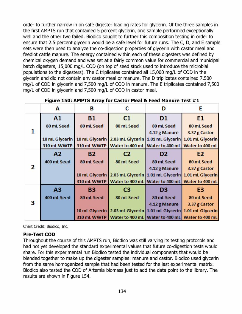
134
order to further narrow in on safe digester loading rates for glycerin. Of the three samples in the first AMPTS run that contained 5 percent glycerin, one sample performed exceptionally well and the other two failed. Biodico sought to further this composition testing in order to ensure that 2.5 percent glycerin would be a safe level for future runs. The C, D, and E sample sets were then used to analyze the co-digestion properties of glycerin with castor meal and feedlot cattle manure. The energy contained within each of these digesters was defined by chemical oxygen demand and was set at a fairly common value for commercial and municipal batch digesters, 15,000 mg/L COD (on top of seed stock used to introduce the microbial populations to the digesters). The C triplicates contained all 15,000 mg/L of COD in the glycerin and did not contain any castor meal or manure. The D triplicates contained 7,500 mg/L of COD in glycerin and 7,500 mg/L of COD in manure. The E triplicates contained 7,500 mg/L of COD in glycerin and 7,500 mg/L of COD in castor meal.
Figure 150: AMPTS Array for Castor Meal & Feed Manure Test #1
Chart Credit: Biodico, Inc.
Pre-Test COD Throughout the course of this AMPTS run, Biodico was still varying its testing protocols and had not yet developed the standard experimental values that future co-digestion tests would share. For this experimental run Biodico tested the individual components that would be blended together to make up the digester samples: manure and castor. Biodico used glycerin from the same homogenized sample that had been tested for the last experimental matrix. Biodico also tested the COD of Artemia biomass just to add the data point to the library. The results are shown in Figure 154.
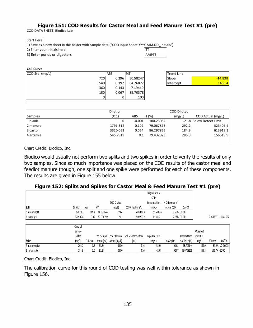
135
Figure 151: COD Results for Castor Meal and Feed Manure Test #1 (pre)
Chart Credit: Biodico, Inc.
Biodico would usually not perform two splits and two spikes in order to verify the results of only two samples. Since so much importance was placed on the COD results of the castor meal and feedlot manure though, one split and one spike were performed for each of these components. The results are given in Figure 155 below.
Figure 152: Splits and Spikes for Castor Meal & Feed Manure Test #1 (pre)
Chart Credit: Biodico, Inc.
The calibration curve for this round of COD testing was well within tolerance as shown in Figure 156.
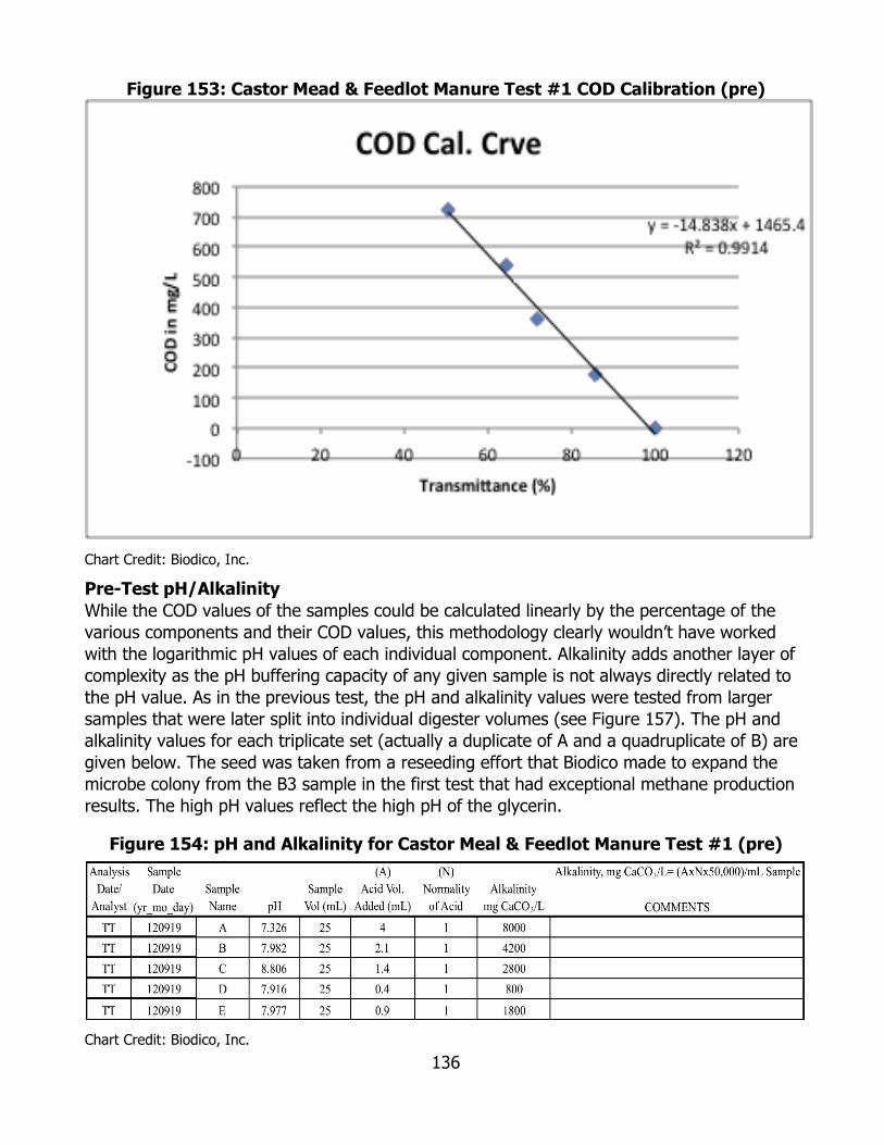
136
Figure 153: Castor Mead & Feedlot Manure Test #1 COD Calibration (pre)
Chart Credit: Biodico, Inc.
Pre-Test pH/Alkalinity While the COD values of the samples could be calculated linearly by the percentage of the various components and their COD values, this methodology clearly wouldn’t have worked with the logarithmic pH values of each individual component. Alkalinity adds another layer of complexity as the pH buffering capacity of any given sample is not always directly related to the pH value. As in the previous test, the pH and alkalinity values were tested from larger samples that were later split into individual digester volumes (see Figure 157). The pH and alkalinity values for each triplicate set (actually a duplicate of A and a quadruplicate of B) are given below. The seed was taken from a reseeding effort that Biodico made to expand the microbe colony from the B3 sample in the first test that had exceptional methane production results. The high pH values reflect the high pH of the glycerin.
Figure 154: pH and Alkalinity for Castor Meal & Feedlot Manure Test #1 (pre)
Chart Credit: Biodico, Inc.
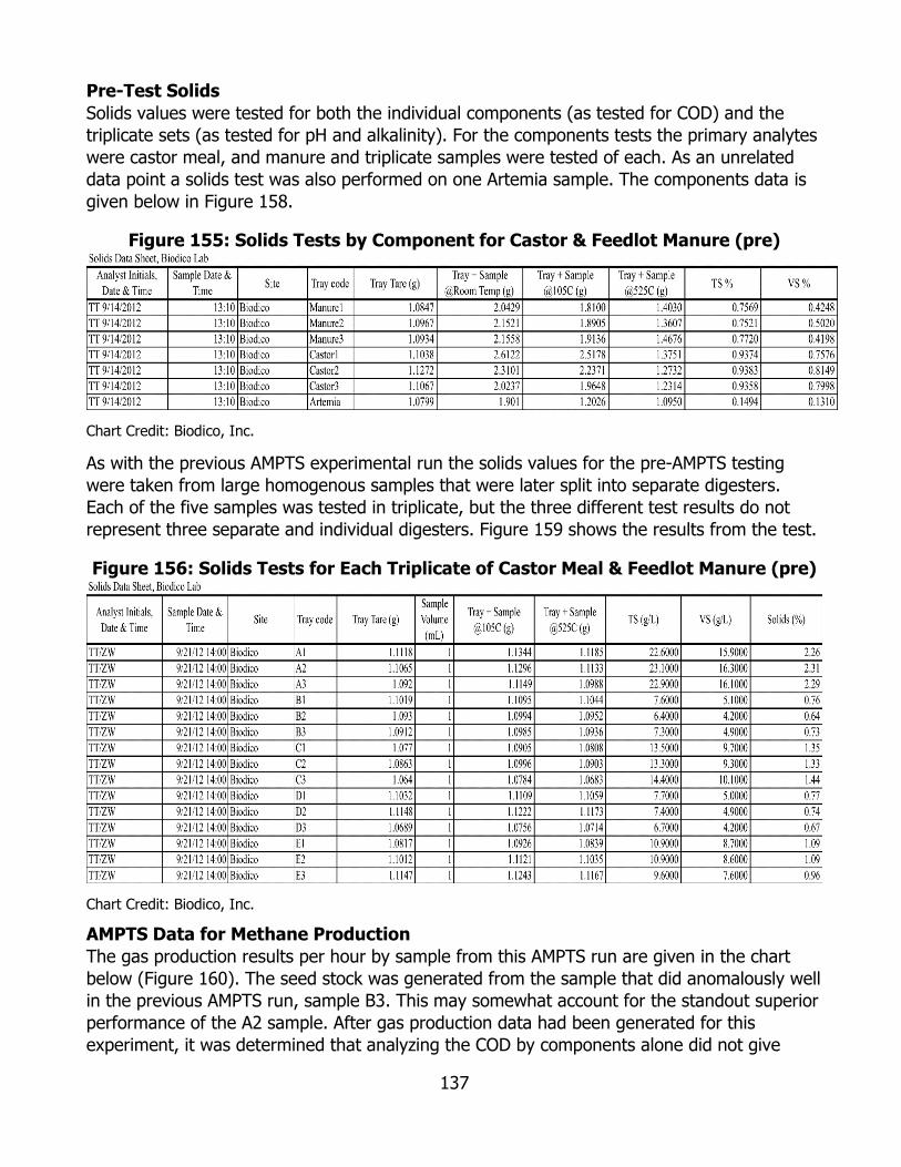
137
Pre-Test Solids Solids values were tested for both the individual components (as tested for COD) and the triplicate sets (as tested for pH and alkalinity). For the components tests the primary analytes were castor meal, and manure and triplicate samples were tested of each. As an unrelated data point a solids test was also performed on one Artemia sample. The components data is given below in Figure 158.
Figure 155: Solids Tests by Component for Castor & Feedlot Manure (pre)
Chart Credit: Biodico, Inc.
As with the previous AMPTS experimental run the solids values for the pre-AMPTS testing were taken from large homogenous samples that were later split into separate digesters. Each of the five samples was tested in triplicate, but the three different test results do not represent three separate and individual digesters. Figure 159 shows the results from the test.
Figure 156: Solids Tests for Each Triplicate of Castor Meal & Feedlot Manure (pre)
Chart Credit: Biodico, Inc.
AMPTS Data for Methane Production The gas production results per hour by sample from this AMPTS run are given in the chart below (Figure 160). The seed stock was generated from the sample that did anomalously well in the previous AMPTS run, sample B3. This may somewhat account for the standout superior performance of the A2 sample. After gas production data had been generated for this experiment, it was determined that analyzing the COD by components alone did not give

138
sufficient data to be predictive and that the energy content of the seed stock was not so small as to be negligent. One of the successes of the experiment though was that the methane volumes produced from triplicates C, D, and E were very similar. This helps to show that the energy generated from a relatively small volume of high COD glycerin can be equivalent to energy produced from significantly larger volumes of other feedstocks with lower COD values.
Figure 157: Cumulative Methane Produced by Castor Meal & Feedlot Manure Test #1
Chart Credit: Biodico, Inc.
The graphical representation of methane production from fifteen different digesters over time can be very information dense and difficult to decipher. A chart of the total volume of methane produced by each sample at the conclusion of the experiment can be much easier to interpret. For this experiment, it confirms the points discussed in relation to the chart above: the volumes of methane produced by the seed stock should not be treated as negligent and the amount of COD in the glycerin seems to give a better prediction of methane production than the volume of feedstock or volatile solids. This chart also makes it easier to see that the samples with a higher concentration of glycerin, the B samples, did not produce energy as efficiently as the other triplicate sets. The samples that had a lower concentration of glycerin and no other co-digestants, the C triplicates, performed just as well. The performance of the C triplicates was also equivalent to the performance of the co-digestant triplicates D and E that had half as much glycerin and a higher organic content from the manure and castor meal respectively. This demonstrates that short of the digester crashing there is still a range of glycerin concentrations that will produce gas and that the optimum level of glycerin is short of the level at which the digester goes sour. It is also worth noting that the COD of the feedlot

139
manure used in this test is substantially higher than the COD of dairy manure. The total methane volume snapshot is displayed in Figure 161.
Figure 158: Total Methane Produced by Sample for Castor Meal & Feedlot Manure Test #1
Chart Credit: Biodico, Inc.
Post-Test COD The COD values for each of the fifteen digesters at the conclusion of the AMPTS test are given below. Even though the B samples did not produce as much methane per weight of chemical oxygen demand, the reduction in COD throughout the course of the test was significant. The C, D, and E samples were prepared to have 15,000 mg/L of COD without taking the seed into account. On average, the digesters in these triplicate sets contained under half of that COD, including COD from seed stock, in the post-AMPTS testing. Figure 162 below shows the COD data that was collected from each of the individual digesters after the AMPTS test.
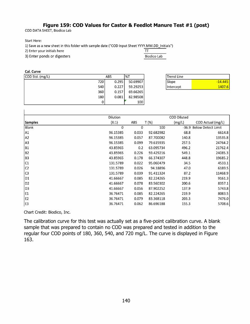
140
Figure 159: COD Values for Castor & Feedlot Manure Test #1 (post)
Chart Credit: Biodico, Inc.
The calibration curve for this test was actually set as a five-point calibration curve. A blank sample that was prepared to contain no COD was prepared and tested in addition to the regular four COD points of 180, 360, 540, and 720 mg/L. The curve is displayed in Figure 163.

141
Figure 160: COD Calibration Curve for Castor Meal & Feedlot Manure Test #1 (post)
Chart Credit: Biodico, Inc.
As with the other COD tests performed by Biodico for ARV-10-024, two splits and two spikes were taken. They both fell within acceptable margins of error from the anticipated COD values. The results of the splits and the spikes are given below in Figure 164.
Figure 161: Splits and Spikes for Castor Meal & Feedlot Manure Test #1 (post)
Chart Credit: Biodico, Inc.
Post-Test pH/Alkalinity The pH and alkalinity values that were captured at the end of this experiment almost all indicate healthy microbial communities. In general, anaerobic digester effluent that is slightly alkaline is preferable to effluent that is slightly acidic. Low pH values and/or low alkalinity values can be indicative of an energy overload to the digesters. Acetic acid that is not consumed by the methanogens will cause a decrease in pH. The slight acidity of the samples with the highest COD, A1, B1, B2, and B3, is likely a result of excess acetate. The post-AMPTS pH and alkalinity values are given in Figure 165.

142
Figure 162: pH and Alkalinity for Castor Meal & Feedlot Manure Test #1 (post)
Chart Credit: Biodico, Inc.
Post-Test Solids The solids tests on the digester samples help to characterize how much energy is going into the system before the AMPTS tests and help to characterize how much energy was not consumed by the anaerobic digestion on the way out of the AMPTS (Figure 166). The difference in these values can provide one of several different metrics to determine the digestion efficiency of different feedstock blends. Different anaerobic digesters calculate feedstock and effluent energy by a variety of different metrics and volatile solids is one of the more commonly used measurements.
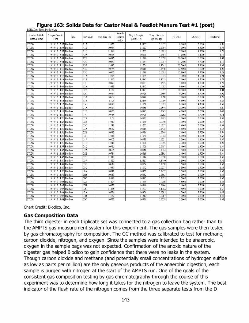
143
Figure 163: Solids Data for Castor Meal & Feedlot Manure Test #1 (post)
Chart Credit: Biodico, Inc.
Gas Composition Data The third digester in each triplicate set was connected to a gas collection bag rather than to the AMPTS gas measurement system for this experiment. The gas samples were then tested by gas chromatography for composition. The GC method was calibrated to test for methane, carbon dioxide, nitrogen, and oxygen. Since the samples were intended to be anaerobic, oxygen in the sample bags was not expected. Confirmation of the anoxic nature of the digester gas helped Biodico to gain confidence that there were no leaks in the system. Though carbon dioxide and methane (and potentially small concentrations of hydrogen sulfide as low as parts per million) are the only gaseous products of the anaerobic digestion, each sample is purged with nitrogen at the start of the AMPTS run. One of the goals of the consistent gas composition testing by gas chromatography through the course of this experiment was to determine how long it takes for the nitrogen to leave the system. The best indicator of the flush rate of the nitrogen comes from the three separate tests from the D
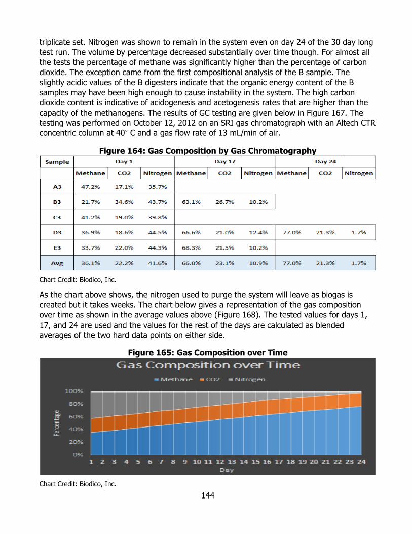
144
triplicate set. Nitrogen was shown to remain in the system even on day 24 of the 30 day long test run. The volume by percentage decreased substantially over time though. For almost all the tests the percentage of methane was significantly higher than the percentage of carbon dioxide. The exception came from the first compositional analysis of the B sample. The slightly acidic values of the B digesters indicate that the organic energy content of the B samples may have been high enough to cause instability in the system. The high carbon dioxide content is indicative of acidogenesis and acetogenesis rates that are higher than the capacity of the methanogens. The results of GC testing are given below in Figure 167. The testing was performed on October 12, 2012 on an SRI gas chromatograph with an Altech CTR concentric column at 40° C and a gas flow rate of 13 mL/min of air.
Figure 164: Gas Composition by Gas Chromatography
Chart Credit: Biodico, Inc.
As the chart above shows, the nitrogen used to purge the system will leave as biogas is created but it takes weeks. The chart below gives a representation of the gas composition over time as shown in the average values above (Figure 168). The tested values for days 1, 17, and 24 are used and the values for the rest of the days are calculated as blended averages of the two hard data points on either side.
Figure 165: Gas Composition over Time
Chart Credit: Biodico, Inc.
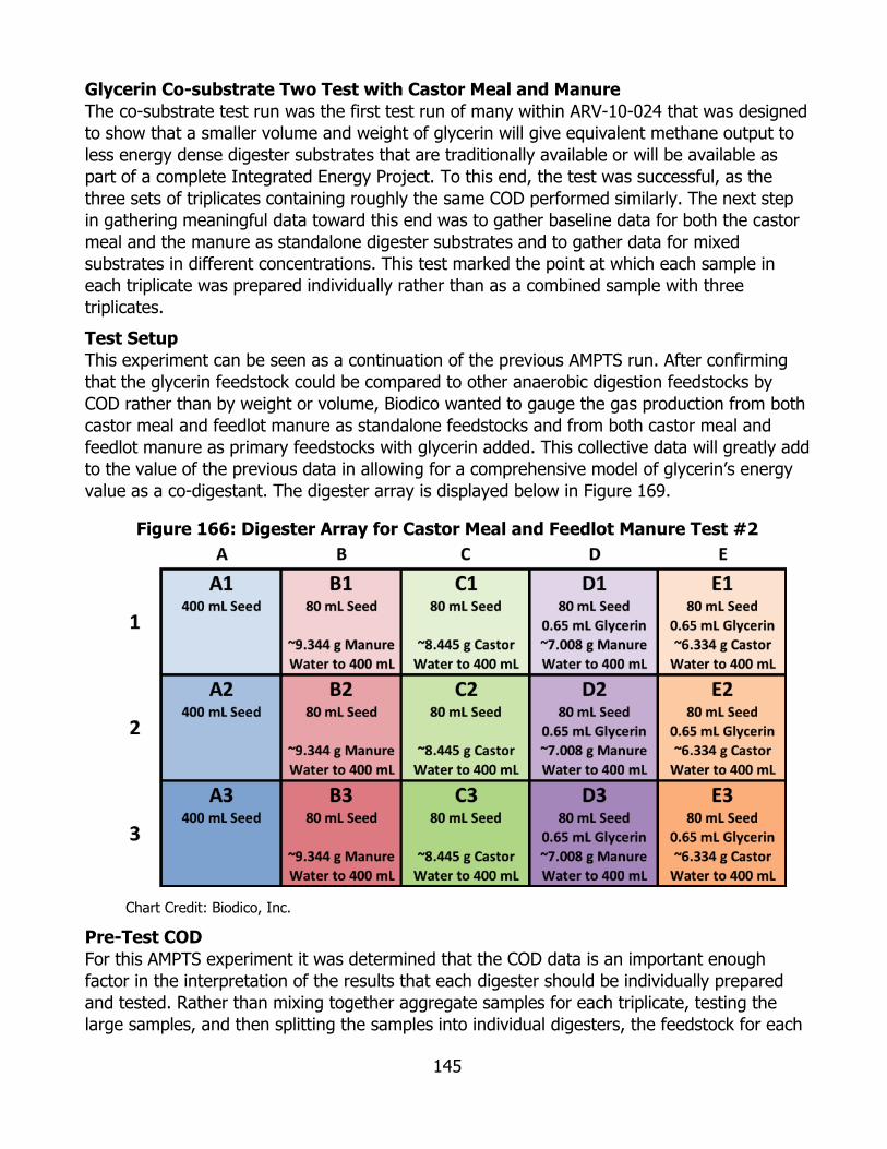
145
Glycerin Co-substrate Two Test with Castor Meal and Manure The co-substrate test run was the first test run of many within ARV-10-024 that was designed to show that a smaller volume and weight of glycerin will give equivalent methane output to less energy dense digester substrates that are traditionally available or will be available as part of a complete Integrated Energy Project. To this end, the test was successful, as the three sets of triplicates containing roughly the same COD performed similarly. The next step in gathering meaningful data toward this end was to gather baseline data for both the castor meal and the manure as standalone digester substrates and to gather data for mixed substrates in different concentrations. This test marked the point at which each sample in each triplicate was prepared individually rather than as a combined sample with three triplicates. Test Setup This experiment can be seen as a continuation of the previous AMPTS run. After confirming that the glycerin feedstock could be compared to other anaerobic digestion feedstocks by COD rather than by weight or volume, Biodico wanted to gauge the gas production from both castor meal and feedlot manure as standalone feedstocks and from both castor meal and feedlot manure as primary feedstocks with glycerin added. This collective data will greatly add to the value of the previous data in allowing for a comprehensive model of glycerin’s energy value as a co-digestant. The digester array is displayed below in Figure 169.
Figure 166: Digester Array for Castor Meal and Feedlot Manure Test #2
Chart Credit: Biodico, Inc.
Pre-Test COD For this AMPTS experiment it was determined that the COD data is an important enough factor in the interpretation of the results that each digester should be individually prepared and tested. Rather than mixing together aggregate samples for each triplicate, testing the large samples, and then splitting the samples into individual digesters, the feedstock for each
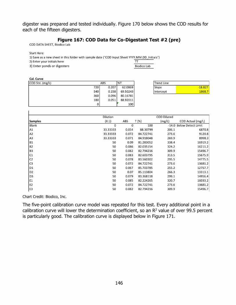
146
digester was prepared and tested individually. Figure 170 below shows the COD results for each of the fifteen digesters.
Figure 167: COD Data for Co-Digestant Test #2 (pre)
Chart Credit: Biodico, Inc.
The five-point calibration curve model was repeated for this test. Every additional point in a calibration curve will lower the determination coefficient, so an R2 value of over 99.5 percent is particularly good. The calibration curve is displayed below in Figure 171.

147
Figure 168: Calibration Curve for Codigestant Test #2 COD (pre)
Chart Credit: Biodico, Inc.
Two spikes and two splits were included in the COD test again as an internal verification means. The data is given in the figure below.
Figure 169: Spikes and Splits for COD of Codigestant Test #2 (pre)
Chart Credit: Biodico, Inc.
Pre-Test pH/Alkalinity Just as with the COD testing, this experiment marked the first time that the digesters were individually tested before the AMPTS run. The extra data for alkalinity in particular gives more confidence to the results. The alkalinity results are based on observed changes in the pH of a sample as acid is added. The sample is mixed as the acid is added and the mixing allows for increased absorption of carbon dioxide from the atmosphere. The carbon dioxide mixes with

148
salts in the sample to cause alkaline carbonate compounds like sodium and potassium bicarbonate. This causes a slight increase in the pH of the sample. By testing the alkalinity of each individual digester, the accuracy of the alkalinity results for each triplicate as a whole increase. The pre-AMPTS data for the alkalinity of the digesters in Co-Digestant Test #2 is given below in Figure 173.
Figure 170: pH and Alkalinity for Co-Digestant Test #2 (pre)
Chart Credit: Biodico, Inc.
Pre-Test Solids Just as with the pH & alkalinity and the COD tests, each individual digester was tested for solids content. Each solids test was run in triplicate, giving a total of 45 separate samples. The pre-AMPTS solids data for Co-Substrate Test #2 is given in Figure 174. As would be expected, the triplicates with higher concentrations of manure and of castor meal (B and C)

149
are higher in solids content. Somewhat counterintuitively, the samples with manure are higher in solids content than the samples with castor meal. The castor meal should have pretty minimal oil content and seed meal almost always has over 90 percent dry weight (including oil). The manure samples did have more material by weight than the castor meal samples and the moisture content of feedlot manure is significantly lower than the moisture content of dairy manure.
Figure 171: Co-Substrate Test #2 Solids (pre)
Chart Credit: Biodico, Inc.
AMPTS Data for Methane Production The cumulative methane production data for each sample over time is displayed below in Figure 175. Even though the different feedstock combinations all have different production volumes and rates of production, the results within each triplicate are consistent. Since this
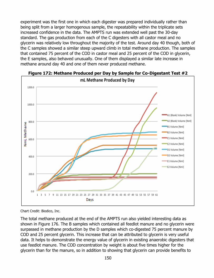
150
experiment was the first one in which each digester was prepared individually rather than being split from a larger homogenous sample, the repeatability within the triplicate sets increased confidence in the data. The AMPTS run was extended well past the 30-day standard. The gas production from each of the C digesters with all castor meal and no glycerin was relatively low throughout the majority of the test. Around day 40 though, both of the C samples showed a similar steep upward climb in total methane production. The samples that contained 75 percent of the COD in castor meal and 25 percent of the COD in glycerin, the E samples, also behaved unusually. One of them displayed a similar late increase in methane around day 40 and one of them never produced methane.
Figure 172: Methane Produced per Day by Sample for Co-Digestant Test #2
Chart Credit: Biodico, Inc.
The total methane produced at the end of the AMPTS run also yielded interesting data as shown in Figure 176. The B samples which contained all feedlot manure and no glycerin were surpassed in methane production by the D samples which co-digested 75 percent manure by COD and 25 percent glycerin. This increase that can be attributed to glycerin is very useful data. It helps to demonstrate the energy value of glycerin in existing anaerobic digesters that use feedlot manure. The COD concentration by weight is about five times higher for the glycerin than for the manure, so in addition to showing that glycerin can provide benefits to

151
existing digesters, this test also shows that the amount of glycerin needed to achieve this increase is only 20 percent of the weight of the manure that it is replacing.
Figure 173: Total Methane Produced by Sample in Co-Digestant Test #2 (pre)
Chart Credit: Biodico, Inc.
Post-Test COD The COD values for each digester after the conclusion of the AMPTS run are given below. In addition to the post-AMPTS testing, tests were performed on dairy manure in preparation for the experimental design of the next test as shown in Figure 177.
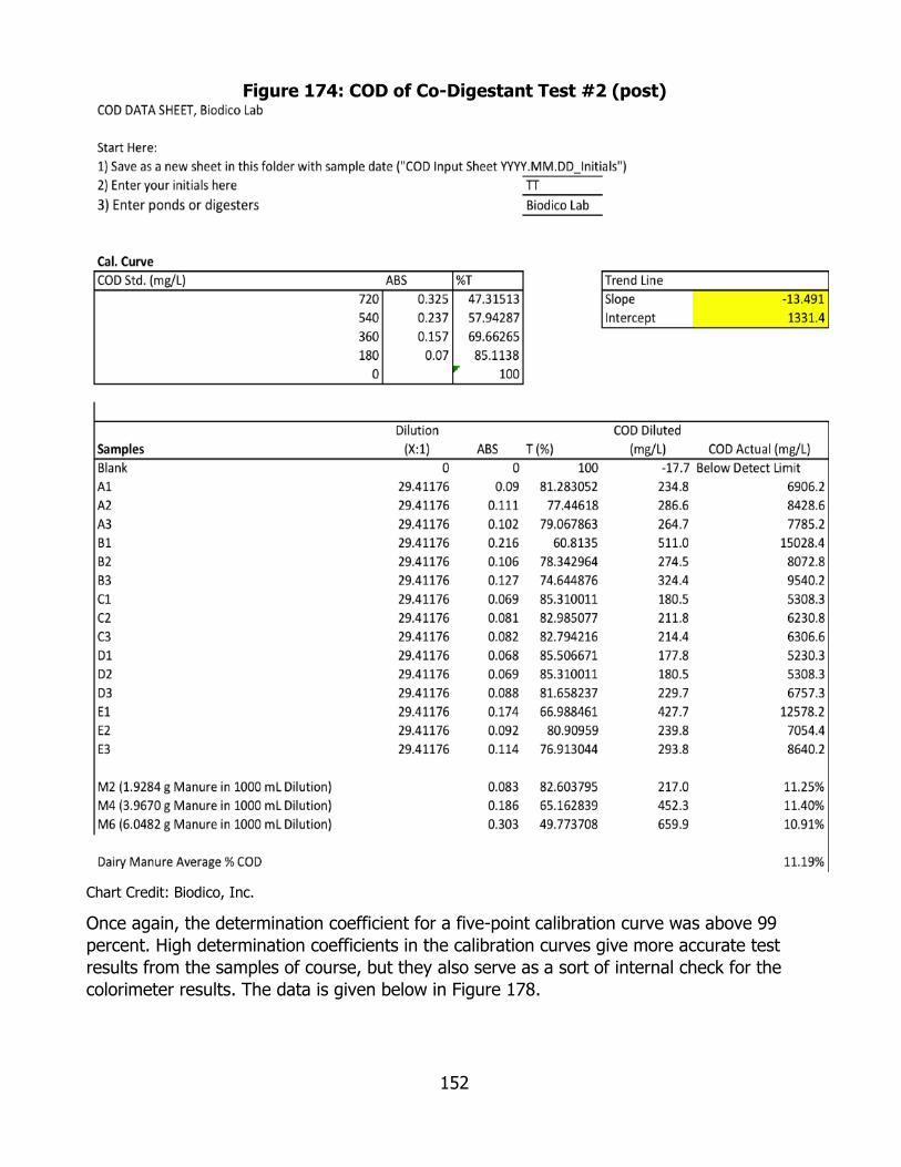
152
Figure 174: COD of Co-Digestant Test #2 (post)
Chart Credit: Biodico, Inc.
Once again, the determination coefficient for a five-point calibration curve was above 99 percent. High determination coefficients in the calibration curves give more accurate test results from the samples of course, but they also serve as a sort of internal check for the colorimeter results. The data is given below in Figure 178.
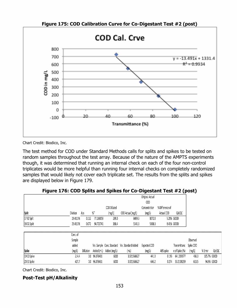
153
Figure 175: COD Calibration Curve for Co-Digestant Test #2 (post)
Chart Credit: Biodico, Inc.
The test method for COD under Standard Methods calls for splits and spikes to be tested on random samples throughout the test array. Because of the nature of the AMPTS experiments though, it was determined that running an internal check on each of the four non-control triplicates would be more helpful than running four internal checks on completely randomized samples that would likely not cover each triplicate set. The results from the splits and spikes are displayed below in Figure 179.
Figure 176: COD Splits and Spikes for Co-Digestant Test #2 (post)
Chart Credit: Biodico, Inc.
Post-Test pH/Alkalinity
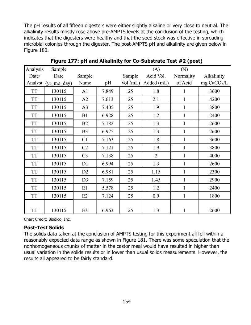
154
The pH results of all fifteen digesters were either slightly alkaline or very close to neutral. The alkalinity results mostly rose above pre-AMPTS levels at the conclusion of the testing, which indicates that the digesters were healthy and that the seed stock was effective in spreading microbial colonies through the digester. The post-AMPTS pH and alkalinity are given below in Figure 180.
Figure 177: pH and Alkalinity for Co-Substrate Test #2 (post)
Chart Credit: Biodico, Inc.
Post-Test Solids The solids data taken at the conclusion of AMPTS testing for this experiment all fell within a reasonably expected data range as shown in Figure 181. There was some speculation that the nonhomogeneous chunks of matter in the castor meal would have resulted in higher than usual variation in the solids results or in lower than usual solids measurements. However, the results all appeared to be fairly standard.

155
Figure 178: Solids Data for Co-Digestant Test #2 (post)
Chart Credit: Biodico, Inc.
Glycerin & Dairy Cattle Manure In this test, Biodico analyzed the effectiveness of glycerin as a co-digestant to dairy cattle manure. This co-substrate test was the first to be run in accordance with its developed methodology for co-substrate testing:
• Set the energy content of the samples by Chemical Oxygen Demand (COD) • Try to keep the COD of all sample sets consistent • Vary the percentages that each co-substrate contributes to the COD across the
triplicate sets (100 percent, 75 percent, and 50 percent) • For our co-substrate testing, we have used a COD of 15,000 mg/L.
Test Setup The A samples are used as a control set of all seed stock, the B samples contain 15,000 mg/L of COD from dairy manure, the C samples contain 15,000 mg/L of COD from glycerin, the D samples contain 3,750 mg/L of COD from glycerin and 11,250 mg/L of COD from dairy manure, and the E samples contain 7,500 mg/L of COD from glycerin and 7,500 mg/L of COD from dairy manure. Figure 182 shows the digester array for the current t test.
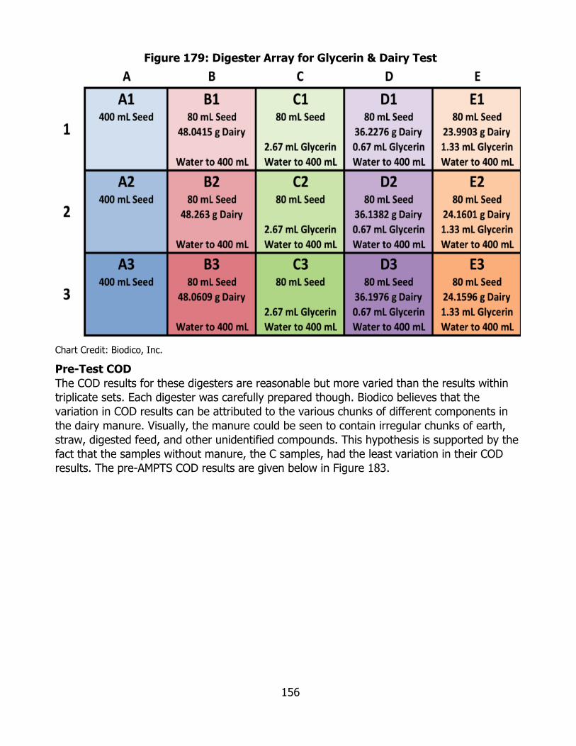
156
Figure 179: Digester Array for Glycerin & Dairy Test
Chart Credit: Biodico, Inc.
Pre-Test COD The COD results for these digesters are reasonable but more varied than the results within triplicate sets. Each digester was carefully prepared though. Biodico believes that the variation in COD results can be attributed to the various chunks of different components in the dairy manure. Visually, the manure could be seen to contain irregular chunks of earth, straw, digested feed, and other unidentified compounds. This hypothesis is supported by the fact that the samples without manure, the C samples, had the least variation in their COD results. The pre-AMPTS COD results are given below in Figure 183.
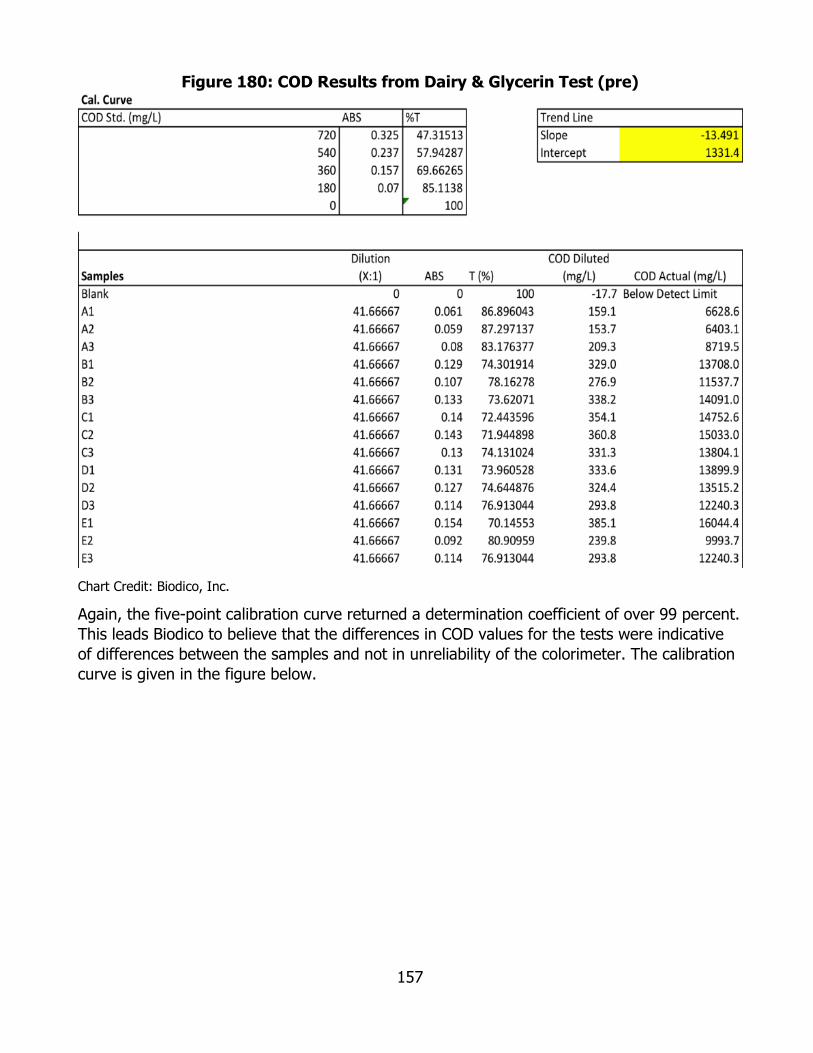
157
Figure 180: COD Results from Dairy & Glycerin Test (pre)
Chart Credit: Biodico, Inc.
Again, the five-point calibration curve returned a determination coefficient of over 99 percent. This leads Biodico to believe that the differences in COD values for the tests were indicative of differences between the samples and not in unreliability of the colorimeter. The calibration curve is given in the figure below.

158
Figure 181: COD Calibration Curve for Dairy & Glycerin Test (pre)
Chart Credit: Biodico, Inc.
The inhomogeneity of the samples was also confirmed by the results of the splits and spikes. One of the splits barely met the minimum 10 percent difference between expected values and observed values. One of the spikes failed by falling outside of the 15 percent threshold between expected values and observed values as seen in Figure 185. This was the first time for ARV-10-024 that one of the internal checks did not pass. COD data is very useful, but Biodico runs multiple tests on the digesters in order to have other characteristics of the digester feedstocks available in case one does not have as much validity as usual.
Figure 182: COD Splits and Spikes for Glycerin & Dairy (pre)
Chart Credit: Biodico, Inc.

159
Pre-Test pH/Alkalinity At the time of this test, no additional microbial colonies had been introduced to the laboratory outside of the WWTP effluent that served as the seed stock for the very first test. It was assumed that cycling out digesters from the previous test to prepare the seed for the next test could very likely lead to a nutrient deficiency. The pH and alkalinity values for this test were one of the first major indicators that the nutrient leaching process had begun. The alkalinity values of the digesters were substantially lower for this pre-AMPTS test than they had been for previous tests. Supplemental mineral nutrients that are usually present in WWTP effluent provide resistance to changes in pH, which can be observed by high alkalinity values. The pre-AMPTS pH and alkalinity tests for the glycerin and dairy experiment are given in Figure 186.
Figure 183: Glycerin & Dairy pH & Alkalinity (pre)
Chart Credit: Biodico, Inc.

160
Pre-Test Solids With the variation in COD testing for this experiment, the total and volatile solids data can be used as another metric for the consistency of the samples and for their energy content. The solids data would still be subject to variation due to inhomogeneous chunks of matter, but the samples are only one milliliter and are taken with a smaller syringe that does not draw up chunks of material as easily. In this case, the solids were consistent enough to support the previously proposed hypothesis that the high variation in COD values was a result of inhomogeneous COD samples taken and not of differences in the larger digesters themselves. The pre-AMPTS total and volatile solids data is given below in Figure 187.
Figure 184: Solids Data for Glycerin & Dairy Test (pre)
Chart Credit: Biodico, Inc.

161
AMPTS Data for Methane Production The gas production data for this test run was indicative of a lack of supplemental mineral nutrients in the system. Several of the digesters failed, and even though the total methane production from the successful digesters was somewhat consistent, the production rates followed a kind of start and stop pattern of methane production for many of the samples. The starts and stops in digesters within the triplicates did not match up in many cases either. This sort of behavior is an indicator that additional nutrients or additional buffering capacity should be added to the system. The production data is given in Figure 188 below.
Figure 185: Methane Production over Time by Sample for Glycerin & Dairy
Chart Credit: Biodico, Inc.
As always, a chart of the total gas volume produced by each sample can be helpful to isolate some characteristics. One important factor to note here is that even though the glycerin benefited the performance of manure as an anaerobic digester feed in the previous experiment, the samples with higher manure content seemed to perform better for this experiment. This is consistent with a nutrient deficiency. Cow manure has a significantly wider profile of different useful nutritional compounds. In the case of nutrient deficiency, higher volumes of manure would be better able to cover the shortfall. The total methane produced by each sample is given below in Figure 189.
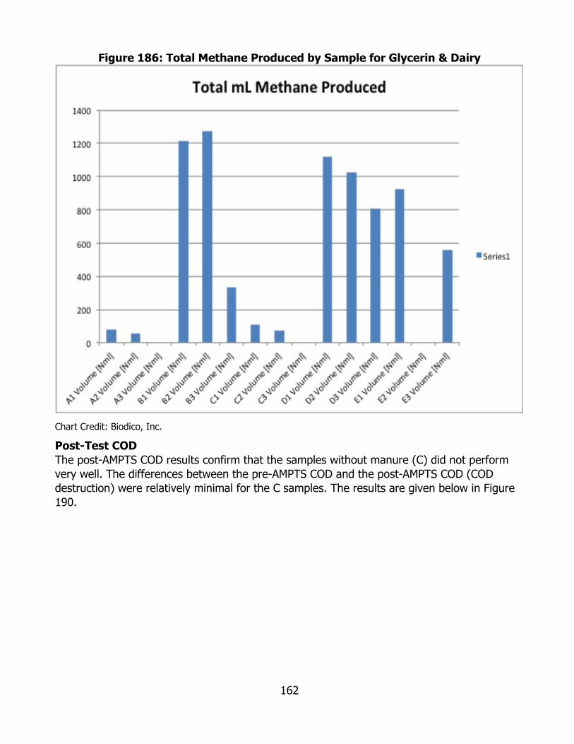
162
Figure 186: Total Methane Produced by Sample for Glycerin & Dairy
Chart Credit: Biodico, Inc.
Post-Test COD The post-AMPTS COD results confirm that the samples without manure (C) did not perform very well. The differences between the pre-AMPTS COD and the post-AMPTS COD (COD destruction) were relatively minimal for the C samples. The results are given below in Figure 190.
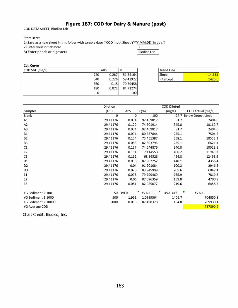
163
Figure 187: COD for Dairy & Manure (post)
Chart Credit: Biodico, Inc.
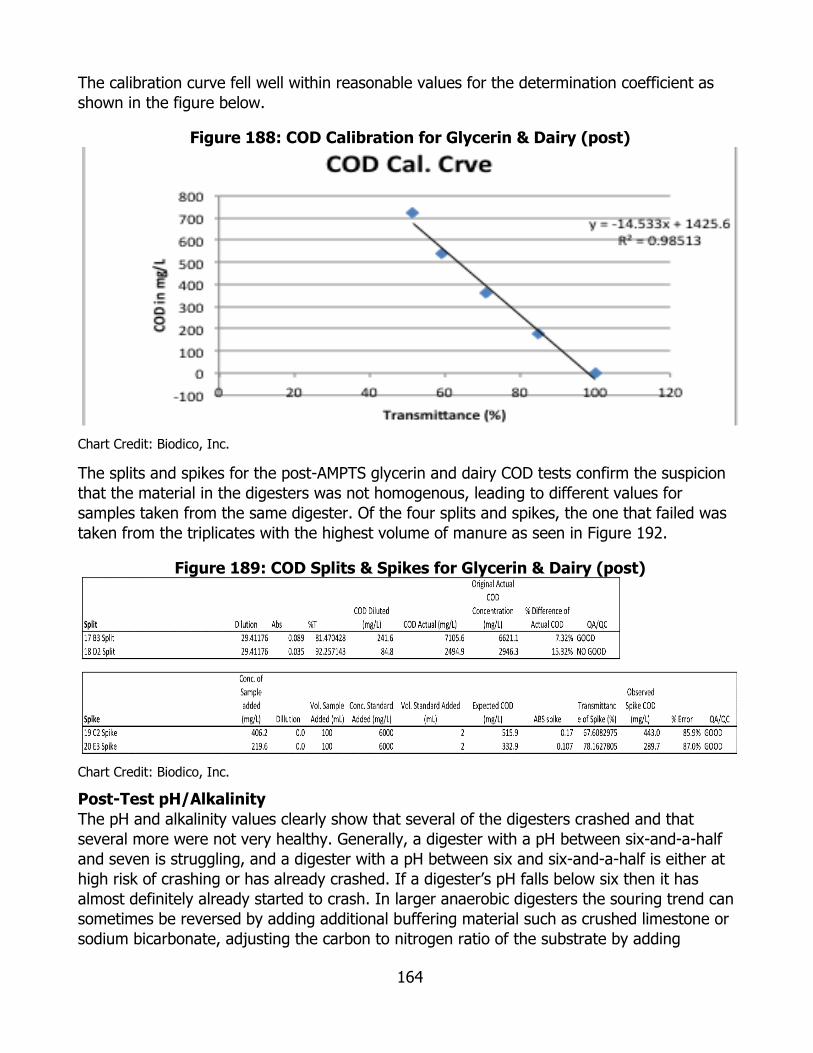
164
The calibration curve fell well within reasonable values for the determination coefficient as shown in the figure below.
Figure 188: COD Calibration for Glycerin & Dairy (post)
Chart Credit: Biodico, Inc.
The splits and spikes for the post-AMPTS glycerin and dairy COD tests confirm the suspicion that the material in the digesters was not homogenous, leading to different values for samples taken from the same digester. Of the four splits and spikes, the one that failed was taken from the triplicates with the highest volume of manure as seen in Figure 192.
Figure 189: COD Splits & Spikes for Glycerin & Dairy (post)
Chart Credit: Biodico, Inc.
Post-Test pH/Alkalinity The pH and alkalinity values clearly show that several of the digesters crashed and that several more were not very healthy. Generally, a digester with a pH between six-and-a-half and seven is struggling, and a digester with a pH between six and six-and-a-half is either at high risk of crashing or has already crashed. If a digester’s pH falls below six then it has almost definitely already started to crash. In larger anaerobic digesters the souring trend can sometimes be reversed by adding additional buffering material such as crushed limestone or sodium bicarbonate, adjusting the carbon to nitrogen ratio of the substrate by adding

165
methanol (or another compound that contains carbon and no nitrogen) or ammonia (or another compound that contains nitrogen and no carbon). The C tests in this sample crashed, but in the castor and feedlot test the same COD content of glycerin was used as a stand-alone feedstock and the digesters performed very well, creating about 400 mL of methane for every mL of glycerin. This confirms the hypothesis that the digester failures were due to nutrient leaching, as the only major difference in the two glycerin triplicates for the different AMPTS runs was that the seed for the glycerin and dairy run was further separated from the nutrient-rich WWTP effluent (in terms of how many experiments the seed had been regenerated from). Another important point to note here is that the C2 sample is very alkaline as seen in Figure 193. At the system breakdown it was confirmed that one of the check valves had deteriorated. Biodico began testing each check valve (by trying to push compressed nitrogen through the valve in reverse) before every new experimental run. No check valves have failed since, and Biodico is unsure whether the failure was attributable to material incompatibility or faulty manufacturing.
Figure 190: pH and Alkalinity for Glycerin & Dairy (post)
Chart Credit: Biodico, Inc.

166
Post-Test Solids The post-AMPTS solids tests for the glycerin and dairy experiment generally returned values within the range of reasonable expectations. The big exception was the C2 samples that vacuumed sodium hydroxide into the digesters and returned a very alkaline pH. The C2 samples had four to five times as much total solids as the C1 and C3. The ratio by which the volatile solids increased in the C2 samples was less than the total solids, returning two to three times the value for the VS. This means that most of the solids increase was in fixed solids (solids that do not volatilize at temperatures up to 550°C). Sodium hydroxide and sodium bicarbonate (that may have formed) are both fixed solids, so the solids data confirms that the C2 samples vacuumed in sodium hydroxide solution (Figure 194).
Figure 191: Solids for Glycerin & Dairy (post)
Chart Credit: Biodico, Inc.
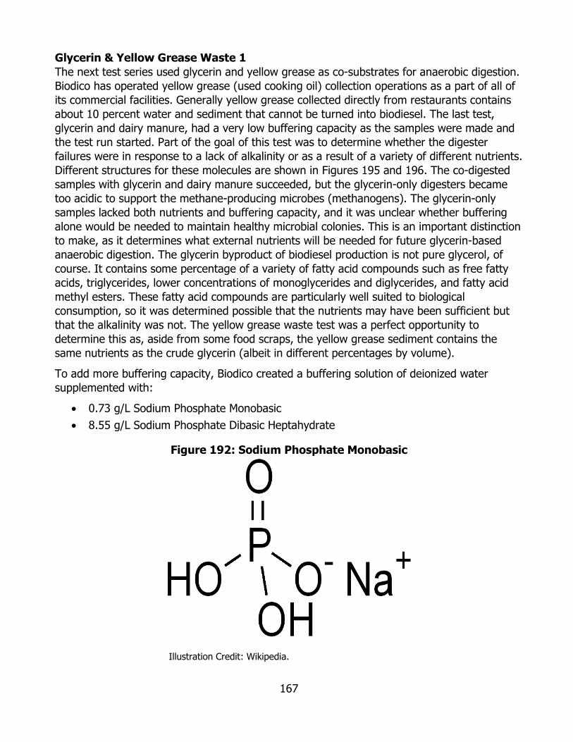
167
Glycerin & Yellow Grease Waste 1 The next test series used glycerin and yellow grease as co-substrates for anaerobic digestion. Biodico has operated yellow grease (used cooking oil) collection operations as a part of all of its commercial facilities. Generally yellow grease collected directly from restaurants contains about 10 percent water and sediment that cannot be turned into biodiesel. The last test, glycerin and dairy manure, had a very low buffering capacity as the samples were made and the test run started. Part of the goal of this test was to determine whether the digester failures were in response to a lack of alkalinity or as a result of a variety of different nutrients. Different structures for these molecules are shown in Figures 195 and 196. The co-digested samples with glycerin and dairy manure succeeded, but the glycerin-only digesters became too acidic to support the methane-producing microbes (methanogens). The glycerin-only samples lacked both nutrients and buffering capacity, and it was unclear whether buffering alone would be needed to maintain healthy microbial colonies. This is an important distinction to make, as it determines what external nutrients will be needed for future glycerin-based anaerobic digestion. The glycerin byproduct of biodiesel production is not pure glycerol, of course. It contains some percentage of a variety of fatty acid compounds such as free fatty acids, triglycerides, lower concentrations of monoglycerides and diglycerides, and fatty acid methyl esters. These fatty acid compounds are particularly well suited to biological consumption, so it was determined possible that the nutrients may have been sufficient but that the alkalinity was not. The yellow grease waste test was a perfect opportunity to determine this as, aside from some food scraps, the yellow grease sediment contains the same nutrients as the crude glycerin (albeit in different percentages by volume).
To add more buffering capacity, Biodico created a buffering solution of deionized water supplemented with:
• 0.73 g/L Sodium Phosphate Monobasic • 8.55 g/L Sodium Phosphate Dibasic Heptahydrate
Figure 192: Sodium Phosphate Monobasic
Illustration Credit: Wikipedia.
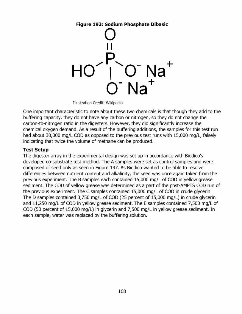
168
Figure 193: Sodium Phosphate Dibasic
Illustration Credit: Wikipedia
One important characteristic to note about these two chemicals is that though they add to the buffering capacity, they do not have any carbon or nitrogen, so they do not change the carbon-to-nitrogen ratio in the digesters. However, they did significantly increase the chemical oxygen demand. As a result of the buffering additions, the samples for this test run had about 30,000 mg/L COD as opposed to the previous test runs with 15,000 mg/L, falsely indicating that twice the volume of methane can be produced. Test Setup The digester array in the experimental design was set up in accordance with Biodico’s developed co-substrate test method. The A samples were set as control samples and were composed of seed only as seen in Figure 197. As Biodico wanted to be able to resolve differences between nutrient content and alkalinity, the seed was once again taken from the previous experiment. The B samples each contained 15,000 mg/L of COD in yellow grease sediment. The COD of yellow grease was determined as a part of the post-AMPTS COD run of the previous experiment. The C samples contained 15,000 mg/L of COD in crude glycerin. The D samples contained 3,750 mg/L of COD (25 percent of 15,000 mg/L) in crude glycerin and 11,250 mg/L of COD in yellow grease sediment. The E samples contained 7,500 mg/L of COD (50 percent of 15,000 mg/L) in glycerin and 7,500 mg/L in yellow grease sediment. In each sample, water was replaced by the buffering solution.
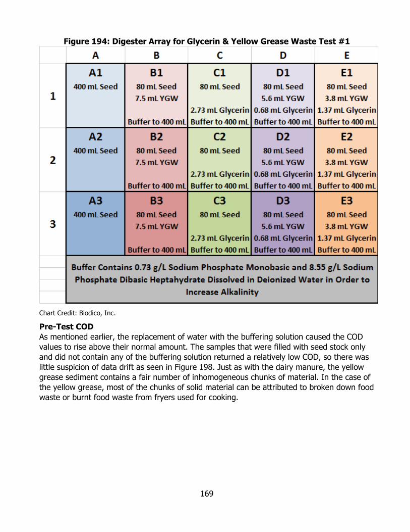
169
Figure 194: Digester Array for Glycerin & Yellow Grease Waste Test #1
Chart Credit: Biodico, Inc.
Pre-Test COD As mentioned earlier, the replacement of water with the buffering solution caused the COD values to rise above their normal amount. The samples that were filled with seed stock only and did not contain any of the buffering solution returned a relatively low COD, so there was little suspicion of data drift as seen in Figure 198. Just as with the dairy manure, the yellow grease sediment contains a fair number of inhomogeneous chunks of material. In the case of the yellow grease, most of the chunks of solid material can be attributed to broken down food waste or burnt food waste from fryers used for cooking.
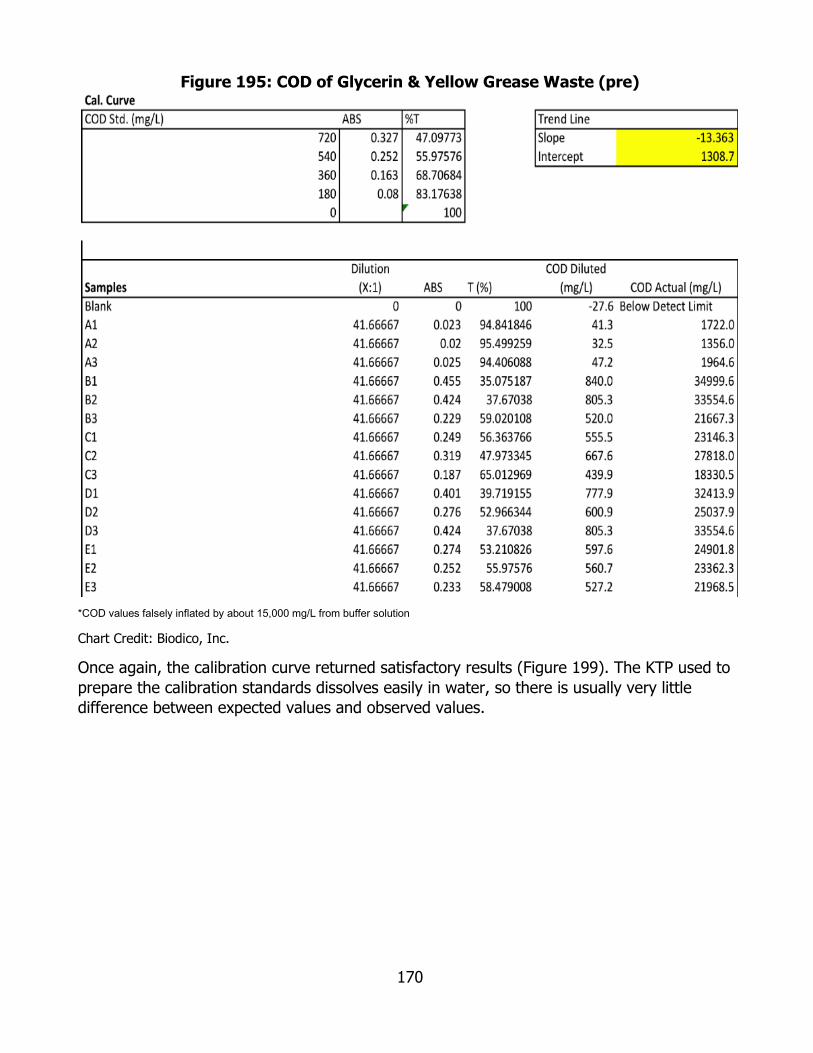
170
Figure 195: COD of Glycerin & Yellow Grease Waste (pre)
*COD values falsely inflated by about 15,000 mg/L from buffer solution
Chart Credit: Biodico, Inc.
Once again, the calibration curve returned satisfactory results (Figure 199). The KTP used to prepare the calibration standards dissolves easily in water, so there is usually very little difference between expected values and observed values.

171
Figure 196: COD Calibration Curve of Glycerin & Yellow Grease Waste (pre)
Chart Credit: Biodico, Inc.
The splits and spikes for this set of COD experiments all fell within acceptable ranges as displayed in the image below in Figure 200.
Figure 197: COD Splits and Spikes for Glycerin & Yellow Grease Waste (pre)
Chart Credit: Biodico, Inc.
Pre-Test pH/Alkalinity While the digester populations that were mixed to create the seed appeared healthy, the alkalinity was low, so a buffering solution was used in place of water. This caused the buffering capacity of the digester to increase substantially. The potassium phosphate also caused a rise in the pH, but did not cause it to become alkaline to a detrimental extent. Before the sample was mixed, a buffering solution was prepared with calcium bicarbonate (baking soda). The diluted baking soda greatly increased the alkalinity, but also caused a rise in the pH that would have risked the microbial health of the system. As previously mentioned,

172
the goal of this experimental run was to separate the low alkalinity and the lack of nutrients out as two separate possible causes of digester failure. The pH and alkalinity values after the buffer was added are given below in Figure 201. All the values indicate good digester health.
Figure 198: pH and Alkalinity for Glycerin & Yellow Grease Waste Test (pre)
Chart Credit: Biodico, Inc.
Pre-Test Solids The solids content of each of the digesters fell within the range of reasonable expectations. It should be noted that the buffering solution called for over nine grams of chemicals per liter—almost a full percentage point. The solids data is given below in Figure 202.
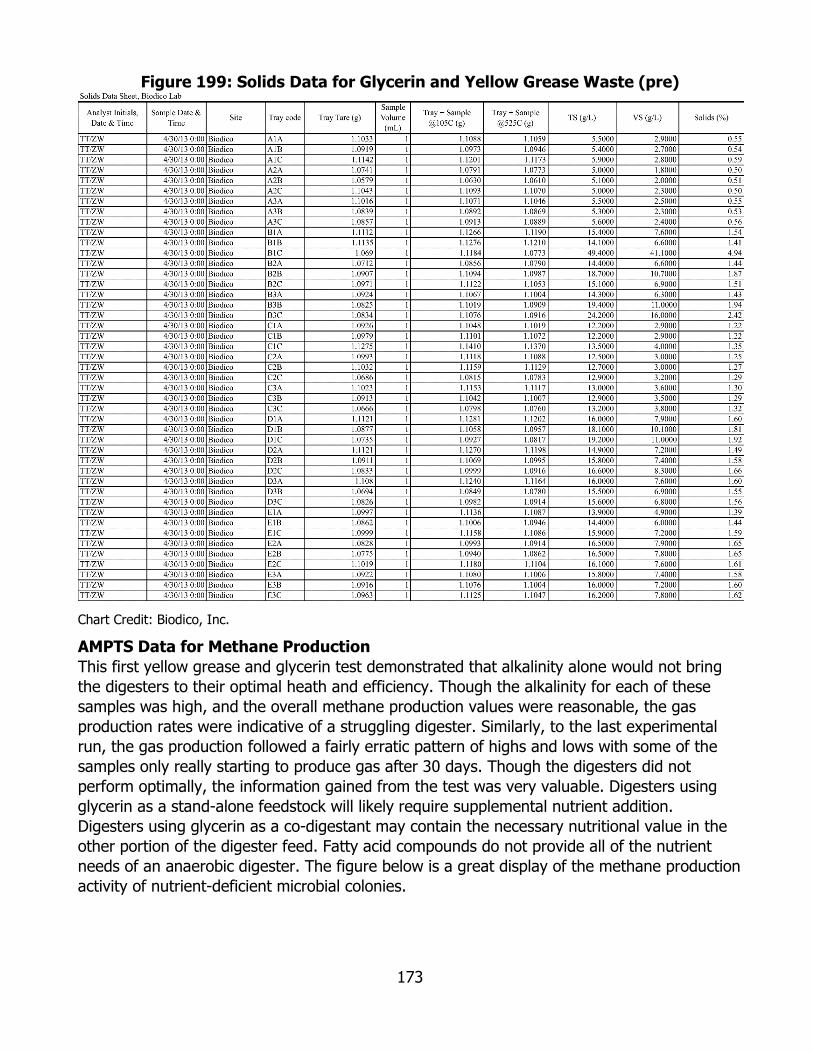
173
Figure 199: Solids Data for Glycerin and Yellow Grease Waste (pre)
Chart Credit: Biodico, Inc.
AMPTS Data for Methane Production This first yellow grease and glycerin test demonstrated that alkalinity alone would not bring the digesters to their optimal heath and efficiency. Though the alkalinity for each of these samples was high, and the overall methane production values were reasonable, the gas production rates were indicative of a struggling digester. Similarly, to the last experimental run, the gas production followed a fairly erratic pattern of highs and lows with some of the samples only really starting to produce gas after 30 days. Though the digesters did not perform optimally, the information gained from the test was very valuable. Digesters using glycerin as a stand-alone feedstock will likely require supplemental nutrient addition. Digesters using glycerin as a co-digestant may contain the necessary nutritional value in the other portion of the digester feed. Fatty acid compounds do not provide all of the nutrient needs of an anaerobic digester. The figure below is a great display of the methane production activity of nutrient-deficient microbial colonies.
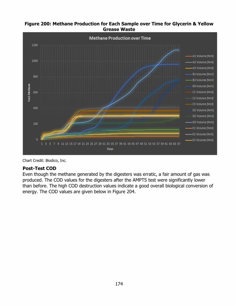
174
Figure 200: Methane Production for Each Sample over Time for Glycerin & Yellow Grease Waste
Chart Credit: Biodico, Inc.
Post-Test COD Even though the methane generated by the digesters was erratic, a fair amount of gas was produced. The COD values for the digesters after the AMPTS test were significantly lower than before. The high COD destruction values indicate a good overall biological conversion of energy. The COD values are given below in Figure 204.

175
Figure 201: COD of Glycerin & Yellow Grease Waste (post)
Chart Credit: Biodico, Inc.
In Figure 205, the determination coefficient for the calibration curve surpassed the requirements again. The fact that all of the calibration curves have been consistently accurate implies that the colorimeter continues to operate well.
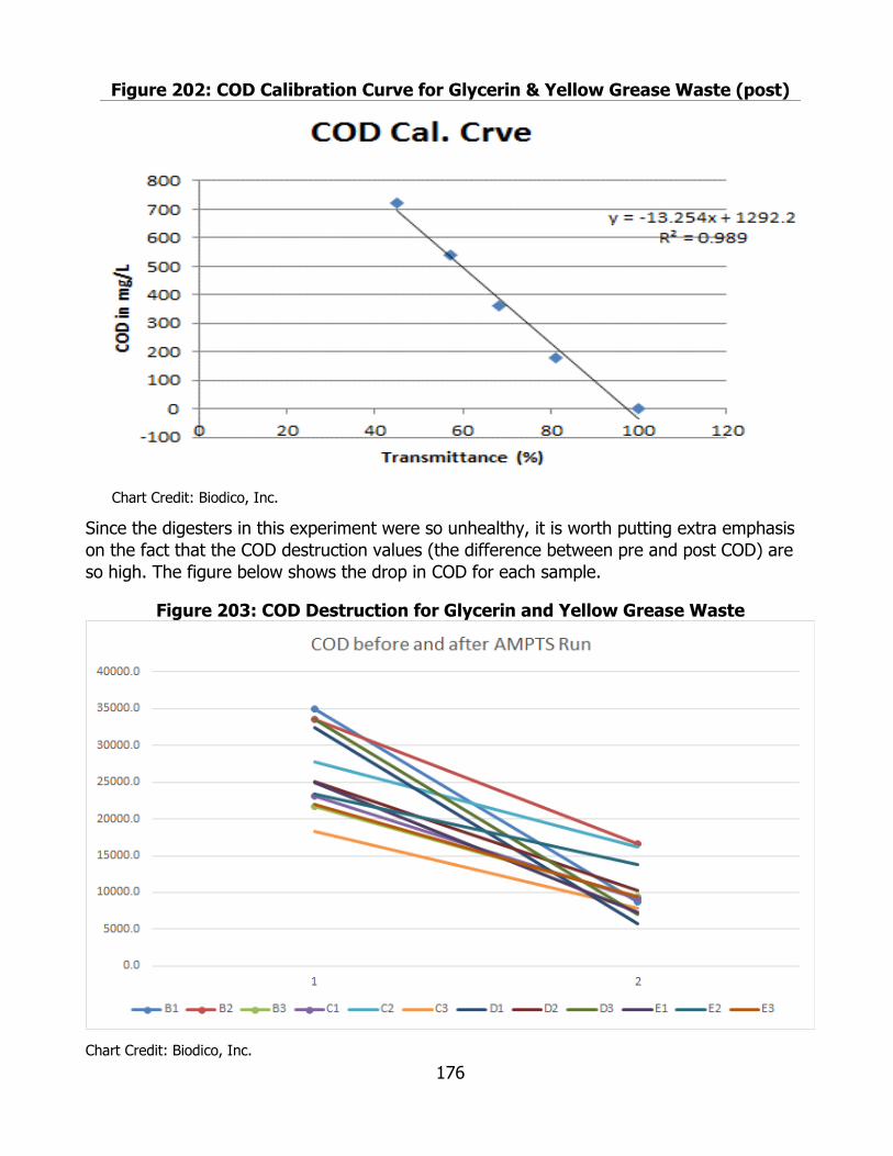
176
Figure 202: COD Calibration Curve for Glycerin & Yellow Grease Waste (post)
Chart Credit: Biodico, Inc.
Since the digesters in this experiment were so unhealthy, it is worth putting extra emphasis on the fact that the COD destruction values (the difference between pre and post COD) are so high. The figure below shows the drop in COD for each sample.
Figure 203: COD Destruction for Glycerin and Yellow Grease Waste
Chart Credit: Biodico, Inc.

177
Post-Test pH/Alkalinity The gas production curves indicated that the digesters might be in poor health and the pH data confirmed it. The pH of three of the digesters had fallen below 6 and the digesters had clearly crashed as seen in Figure 207. The remainder of the samples, aside from the controls, were acidic and had either already crashed or were just on the cusp of crashing. Amazingly though, a good volume of methane was still produced. The pH and alkalinity from this test confirmed that additional nutrients need to be added to glycerin and/or yellow grease waste. Paired with the gas production data though, the experiment also shows the large energy potential of both of these materials.
Figure 204: pH and Alkalinity for Glycerin & Yellow Grease Waste (post)
Chart Credit: Biodico, Inc.
Glycerin & Yellow Grease Waste 2 The most valuable information from the first yellow grease waste and glycerin experiment was that glycerin as an anaerobic digestion feedstock is very energy rich, but short on nutrients. Even with many digester failures though, the gas production volumes were substantial. Biodico performed another test on yellow grease waste and glycerin without any alkalinity buffers and with new seed that was collected from the Ventura County Wastewater Treatment Plant and not just prepared from the previous AMPTS test.
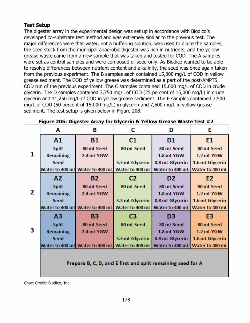
178
Test Setup The digester array in the experimental design was set up in accordance with Biodico’s developed co-substrate test method and was extremely similar to the previous test. The major differences were that water, not a buffering solution, was used to dilute the samples, the seed stock from the municipal anaerobic digester was rich in nutrients, and the yellow grease waste came from a new sample that was taken and tested for COD. The A samples were set as control samples and were composed of seed only. As Biodico wanted to be able to resolve differences between nutrient content and alkalinity, the seed was once again taken from the previous experiment. The B samples each contained 15,000 mg/L of COD in yellow grease sediment. The COD of yellow grease was determined as a part of the post-AMPTS COD run of the previous experiment. The C samples contained 15,000 mg/L of COD in crude glycerin. The D samples contained 3,750 mg/L of COD (25 percent of 15,000 mg/L) in crude glycerin and 11,250 mg/L of COD in yellow grease sediment. The E samples contained 7,500 mg/L of COD (50 percent of 15,000 mg/L) in glycerin and 7,500 mg/L in yellow grease sediment. The test setup is given below in Figure 208.
Figure 205: Digester Array for Glycerin & Yellow Grease Waste Test #2
Chart Credit: Biodico, Inc.

179
Pre-Test COD Though the same amounts of COD from glycerin and yellow grease waste were added to this experiment as were added to the previous experiment, there was no buffering solution and the COD values for all of the digesters were therefore significantly lower as shown in the chart below in Figure 209.
Figure 206: COD of Glycerin & Yellow Grease Waste Test #2 (pre)
Chart Credit: Biodico, Inc.
The calibration curve fell well within the maximum margin of error as always. A different calibration curve was used between the last experiment’s breakdown and this experiment’s setup as shown in Figure 210 and 211.
Figure 207: COD Splits and Spikes Glycerin & Yellow Grease Waste Test #2 (pre)
Chart Credit: Biodico, Inc.

180
Figure 208: COD Calibration Curve of Glycerin & Yellow Grease Waste #2 (pre)
Chart Credit: Biodico, Inc.
Pre-Test pH/Alkalinity Even though the digesters were prepared with fresh WWTP effluent that had a high alkalinity, the individual digesters returned alkalinity values that were significantly lower than the previous test, where a buffering solution was used. The chart below in Figure 212 shows the pre-AMPTS alkalinity values for glycerin and Yellow Grease Waste Test #2.
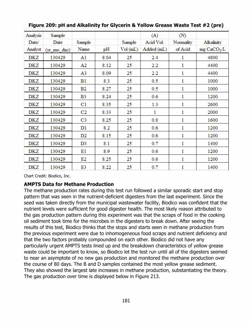
181
Figure 209: pH and Alkalinity for Glycerin & Yellow Grease Waste Test #2 (pre)
Chart Credit: Biodico, Inc.
AMPTS Data for Methane Production The methane production rates during this test run followed a similar sporadic start and stop pattern that was seen in the nutrient-deficient digesters from the last experiment. Since the seed was taken directly from the municipal wastewater facility, Biodico was confident that the nutrient levels were sufficient for good digester health. The most likely reason attributed to the gas production pattern during this experiment was that the scraps of food in the cooking oil sediment took time for the microbes in the digesters to break down. After seeing the results of this test, Biodico thinks that the stops and starts seen in methane production from the previous experiment were due to inhomogeneous food scraps and nutrient deficiency and that the two factors probably compounded on each other. Biodico did not have any particularly urgent AMPTS tests lined up and the breakdown characteristics of yellow grease waste could be important to know, so Biodico let the test run until all of the digesters seemed to near an asymptote of no new gas production and monitored the methane production over the course of 80 days. The B and D samples contained the most yellow grease sediment. They also showed the largest late increases in methane production, substantiating the theory. The gas production over time is displayed below in Figure 213.
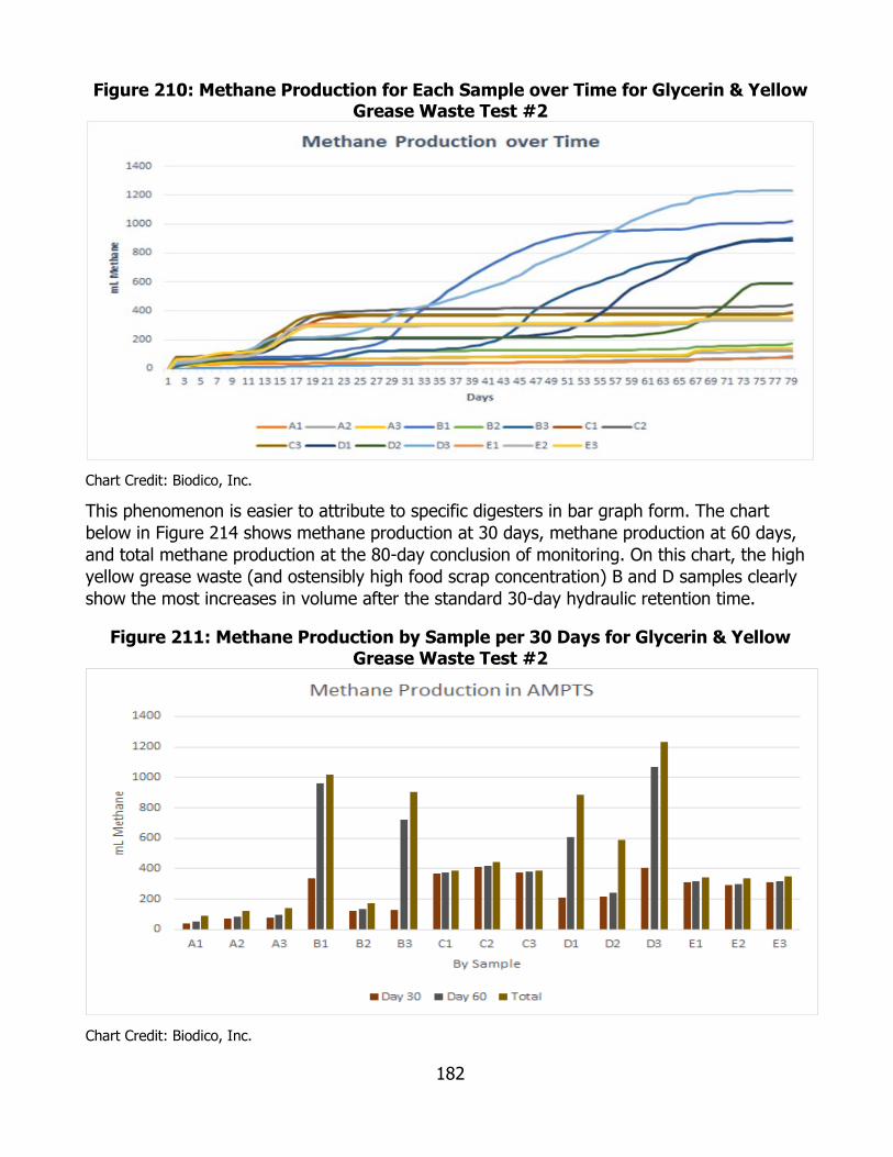
182
Figure 210: Methane Production for Each Sample over Time for Glycerin & Yellow Grease Waste Test #2
Chart Credit: Biodico, Inc.
This phenomenon is easier to attribute to specific digesters in bar graph form. The chart below in Figure 214 shows methane production at 30 days, methane production at 60 days, and total methane production at the 80-day conclusion of monitoring. On this chart, the high yellow grease waste (and ostensibly high food scrap concentration) B and D samples clearly show the most increases in volume after the standard 30-day hydraulic retention time.
Figure 211: Methane Production by Sample per 30 Days for Glycerin & Yellow Grease Waste Test #2
Chart Credit: Biodico, Inc.
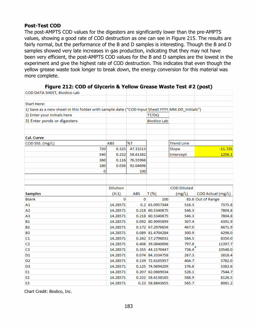
183
Post-Test COD The post-AMPTS COD values for the digesters are significantly lower than the pre-AMPTS values, showing a good rate of COD destruction as one can see in Figure 215. The results are fairly normal, but the performance of the B and D samples is interesting. Though the B and D samples showed very late increases in gas production, indicating that they may not have been very efficient, the post-AMPTS COD values for the B and D samples are the lowest in the experiment and give the highest rate of COD destruction. This indicates that even though the yellow grease waste took longer to break down, the energy conversion for this material was more complete.
Figure 212: COD of Glycerin & Yellow Grease Waste Test #2 (post)
Chart Credit: Biodico, Inc.

184
The determination coefficient for the calibration curve met the standard once again as shown in the figure below. It fell well above 99 percent, but was taken from a four-point calibration curve, so a higher correlation value is expected.
Figure 213: COD Calibration Curve for Glycerin & Yellow Grease Waste Test #2 (post)
Chart Credit: Biodico, Inc.
Post-Test pH/Alkalinity The alkalinity of the digesters, which had tested relatively low before the AMPTS test, continued to give low results (Figure 217). The pH values were all slightly alkaline though, indicating that the digesters were all in good health. This was confirmed manually by observing the look and smell of the digesters.
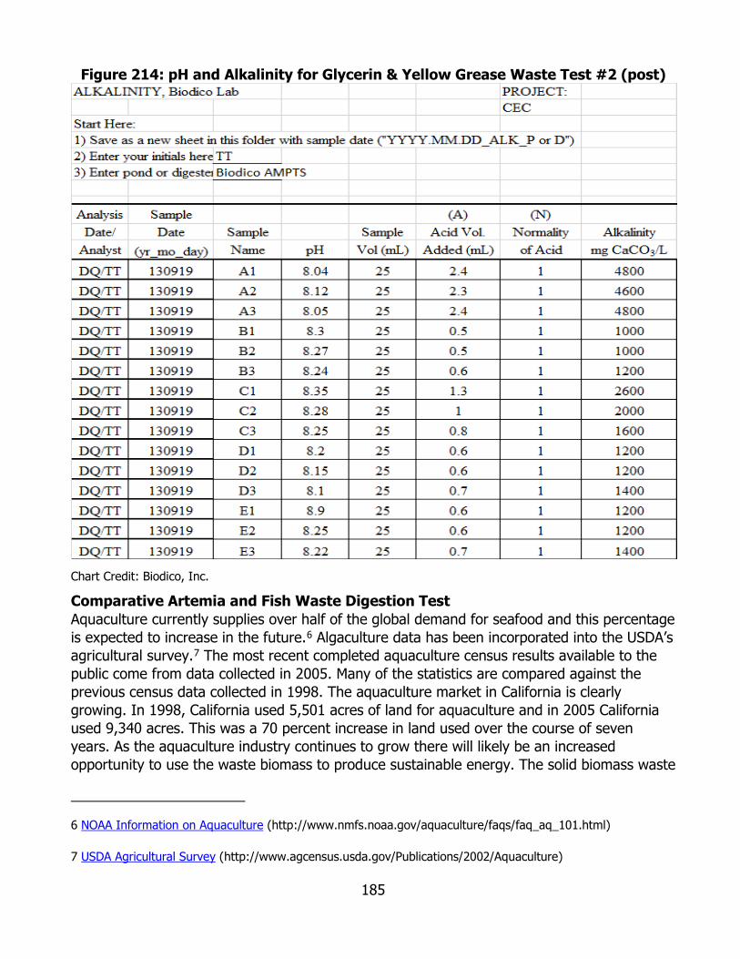
185
Figure 214: pH and Alkalinity for Glycerin & Yellow Grease Waste Test #2 (post)
Chart Credit: Biodico, Inc.
Comparative Artemia and Fish Waste Digestion Test Aquaculture currently supplies over half of the global demand for seafood and this percentage is expected to increase in the future.6 Algaculture data has been incorporated into the USDA’s agricultural survey.7 The most recent completed aquaculture census results available to the public come from data collected in 2005. Many of the statistics are compared against the previous census data collected in 1998. The aquaculture market in California is clearly growing. In 1998, California used 5,501 acres of land for aquaculture and in 2005 California used 9,340 acres. This was a 70 percent increase in land used over the course of seven years. As the aquaculture industry continues to grow there will likely be an increased opportunity to use the waste biomass to produce sustainable energy. The solid biomass waste
6 NOAA Information on Aquaculture (http://www.nmfs.noaa.gov/aquaculture/faqs/faq_aq_101.html)
7 USDA Agricultural Survey (http://www.agcensus.usda.gov/Publications/2002/Aquaculture)
186
from Artemia is high in protein and would likely not be digested directly. It is more likely that the Artemia biomass would be used to feed aquaculture systems designed for human consumption and that the resulting fish biomass would be digested, but the comparative data points are useful to better understand the energy pathway options.
Biodico compared the potential methane generation from Artemia to the methane generation from the waste streams of the largest tuna packing facility in the world—StarKist in Samoa. This experiment proved to be very useful in determining the digestion rate of both the tuna waste and the Artemia waste. The tuna waste consisted of two samples each from two separate waste streams for a total of four samples. The duplicate samples were expected to be very similar, but the two separate waste streams differed significantly in energy content. The energy concentration of the Artemia was very high, so it was necessary to dilute the samples with deionized water. The approximate COD values of the microbial seed, the low-energy StarKist waste stream, the high-energy StarKist waste stream, and the Artemia respectively are 20,000 mg/L, 3,400 mg/L, 8,000 mg/L, and 150,000 mg/L. Test Setup For this test Biodico consulted the Swedish manufacturers of the AMPTS system, Bioprocess Control. This test was not focused on co-digestion of glycerin and another analyte. The goal of this test was to characterize how well the tuna and the Artemia would work in a continuous flow digester. Bioprocess Control recommended that the samples should be mixed with the seed to a ratio based on COD. The Bioprocess Control experimental design was to mix each of the samples so that the COD from the wastewater treatment plant seed was double the COD from the different analytes (tuna and Artemia waste. This would better simulate the behavior of each of these analytes as they enter a non-batch digester. The seed was taken from the Ventura County Wastewater Treatment Plant (WWTP) and the experimental digesters were mixed on the same day as collection. As with the co-digestion experiments, each of the digesters was tested for pH and alkalinity, total and volatile solids, and COD before and after the AMPTS experiment. The test setup is displayed below in Figure 218.

187
Figure 215: Digester Array for Artemia and Fish Waste Test
Chart Credit: Biodico, Inc.
Pre-Test COD The tuna samples were prepared without any dilution to meet the 2:1 ratio for COD from seed and COD from the analyte as recommended by Bioprocess Control. The digesters mixed with the lower energy concentration waste stream (the B triplicates) ended up having a COD right around 15,000 mg/L. This was purely coincidence, but it will allow for the project team to compare the tuna waste with other digester feedstocks more easily. The higher energy concentration fish waste streams had a pre-AMPTS COD that exceeded regular energy concentrations by almost double (the C triplicates). The high concentration of WWTP seed in the C triplicates at 2:1 by COD gave the high COD digesters more biological stability, better nutrient availability, and more buffering capacity. The composition of each sample was determined by solving the equation in Figure 219.
Figure 216: Equation for Determining Sample Composition
Source: Biodico, Inc.
The COD values are displayed in Figure 220.

188
Figure 217: COD of Artemia and Fish Waste Test (pre)
Chart Credit: Biodico, Inc.
The calibration curve for the COD testing was very tight and showed a high determination coefficient of almost 99 percent (Figure 221).
Figure 218: COD Calibration Curve of Artemia and Fish Waste Test (pre)
Chart Credit: Biodico, Inc.

189
Pre-Test pH/Alkalinity When Biodico starts a test run with an unknown material, it is very helpful to determine characteristics of the analyte alone before mixing it with other samples. Biodico has been working with Artemia for a while, but the fish samples were a bit of an unknown. There was no information provided with them, so they were tested for pH and alkalinity before the AMPTS test. The values were included in the pre-AMPTS chart for future reference. One of the tuna waste streams had a slight acidity in both of the duplicate samples. The seed from the WWTP had a very high alkalinity value and added stability to all the digesters though. The pre-AMPTS data is given in Figure 222.
Figure 219: pH and Alkalinity for Artemia and Fish Waste (pre)
Chart Credit: Biodico, Inc.
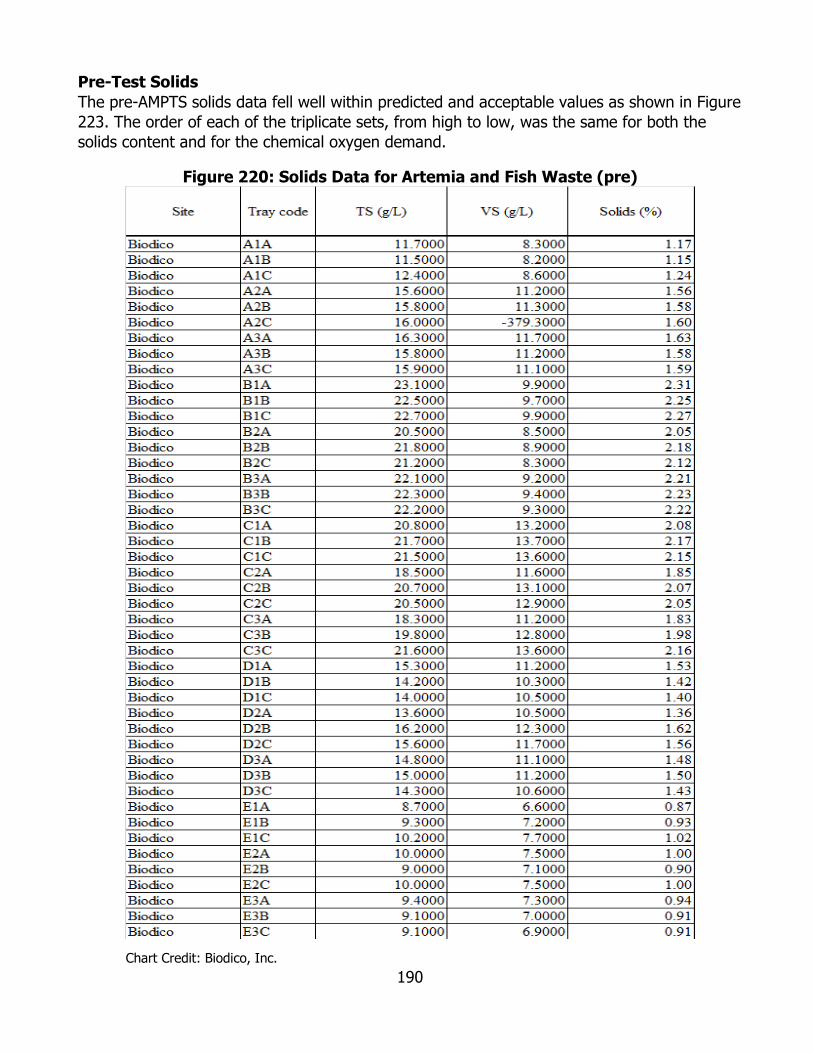
190
Pre-Test Solids The pre-AMPTS solids data fell well within predicted and acceptable values as shown in Figure 223. The order of each of the triplicate sets, from high to low, was the same for both the solids content and for the chemical oxygen demand.
Figure 220: Solids Data for Artemia and Fish Waste (pre)
Chart Credit: Biodico, Inc.

191
AMPTS Data for Methane Production The total methane volumes that were produced by each sample over the 30-day period are consistent with the amount of energy that each digester contained (Figure 224). The calibration/control triplicates are explained in the experimental setup of this report. The four remaining triplicates produced methane in the same highest to lowest order of the target and calculated pre-AMPTS COD tests. The volatile solids content did not fall in this order, but the Artemia is a more energy-rich feedstock for the digesters. Since this test was set up to test for the differences between samples, the total methane by sample is really just a jumping off point.
Figure 221: Total Methane Produced by Digester for Artemia and Fish Waste Test
Chart Credit: Biodico, Inc.
As always, it is very interesting to see how quickly different digesters produce methane and to look at the volume as an integrated flow rate over time. The chart below shows the gas production from all fifteen digesters over the 30-day test cycle. The control calibration samples in the A triplicate set were slower to produce gas than the other samples, but they continued to produce gas for a significantly longer period of time than the other samples. This is very interesting, because the other samples actually contain more of the seed sludge than the analyte (fish waste or Artemia) by COD. Since the samples with the seed only continued to produce gas after the 30-day mark and most of the analyte samples stopped producing gas at some point during the second week, it can be reasonably assumed that both analyte materials (three actually counting the two different concentrations of fish waste) acted as accelerants in the process and helped the WWTP sludge to produce gas more quickly. This is discussed more in the individual component analysis portion of the report. The methane production over time by sample is displayed in Figure 225.
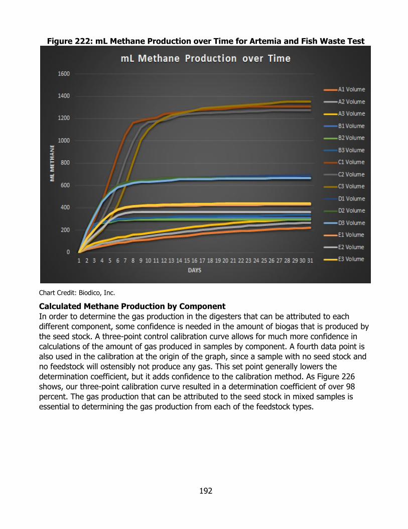
192
Figure 222: mL Methane Production over Time for Artemia and Fish Waste Test
Chart Credit: Biodico, Inc.
Calculated Methane Production by Component In order to determine the gas production in the digesters that can be attributed to each different component, some confidence is needed in the amount of biogas that is produced by the seed stock. A three-point control calibration curve allows for much more confidence in calculations of the amount of gas produced in samples by component. A fourth data point is also used in the calibration at the origin of the graph, since a sample with no seed stock and no feedstock will ostensibly not produce any gas. This set point generally lowers the determination coefficient, but it adds confidence to the calibration method. As Figure 226 shows, our three-point calibration curve resulted in a determination coefficient of over 98 percent. The gas production that can be attributed to the seed stock in mixed samples is essential to determining the gas production from each of the feedstock types.
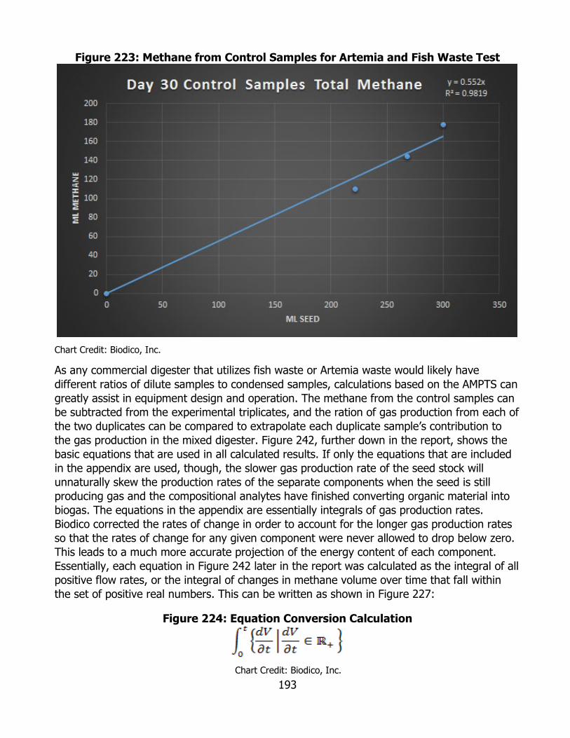
193
Figure 223: Methane from Control Samples for Artemia and Fish Waste Test
Chart Credit: Biodico, Inc.
As any commercial digester that utilizes fish waste or Artemia waste would likely have different ratios of dilute samples to condensed samples, calculations based on the AMPTS can greatly assist in equipment design and operation. The methane from the control samples can be subtracted from the experimental triplicates, and the ration of gas production from each of the two duplicates can be compared to extrapolate each duplicate sample’s contribution to the gas production in the mixed digester. Figure 242, further down in the report, shows the basic equations that are used in all calculated results. If only the equations that are included in the appendix are used, though, the slower gas production rate of the seed stock will unnaturally skew the production rates of the separate components when the seed is still producing gas and the compositional analytes have finished converting organic material into biogas. The equations in the appendix are essentially integrals of gas production rates. Biodico corrected the rates of change in order to account for the longer gas production rates so that the rates of change for any given component were never allowed to drop below zero. This leads to a much more accurate projection of the energy content of each component. Essentially, each equation in Figure 242 later in the report was calculated as the integral of all positive flow rates, or the integral of changes in methane volume over time that fall within the set of positive real numbers. This can be written as shown in Figure 227:
Figure 224: Equation Conversion Calculation
Chart Credit: Biodico, Inc.
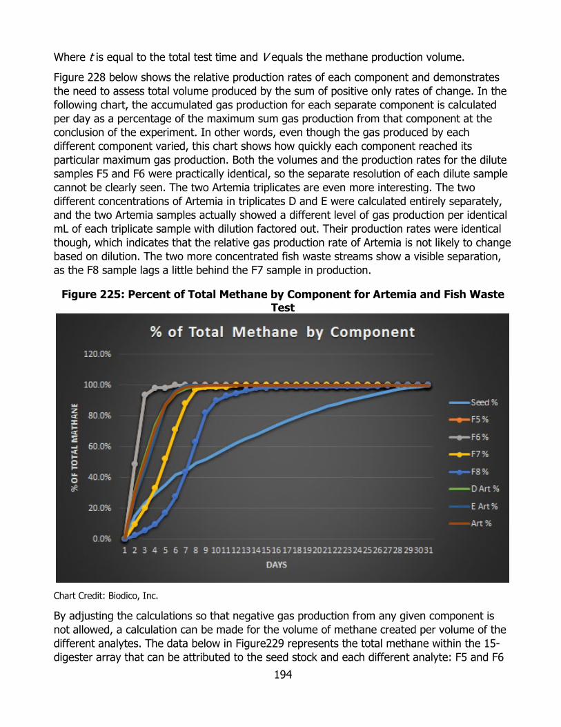
194
Where t is equal to the total test time and V equals the methane production volume.
Figure 228 below shows the relative production rates of each component and demonstrates the need to assess total volume produced by the sum of positive only rates of change. In the following chart, the accumulated gas production for each separate component is calculated per day as a percentage of the maximum sum gas production from that component at the conclusion of the experiment. In other words, even though the gas produced by each different component varied, this chart shows how quickly each component reached its particular maximum gas production. Both the volumes and the production rates for the dilute samples F5 and F6 were practically identical, so the separate resolution of each dilute sample cannot be clearly seen. The two Artemia triplicates are even more interesting. The two different concentrations of Artemia in triplicates D and E were calculated entirely separately, and the two Artemia samples actually showed a different level of gas production per identical mL of each triplicate sample with dilution factored out. Their production rates were identical though, which indicates that the relative gas production rate of Artemia is not likely to change based on dilution. The two more concentrated fish waste streams show a visible separation, as the F8 sample lags a little behind the F7 sample in production.
Figure 225: Percent of Total Methane by Component for Artemia and Fish Waste Test
Chart Credit: Biodico, Inc.
By adjusting the calculations so that negative gas production from any given component is not allowed, a calculation can be made for the volume of methane created per volume of the different analytes. The data below in Figure229 represents the total methane within the 15-digester array that can be attributed to the seed stock and each different analyte: F5 and F6
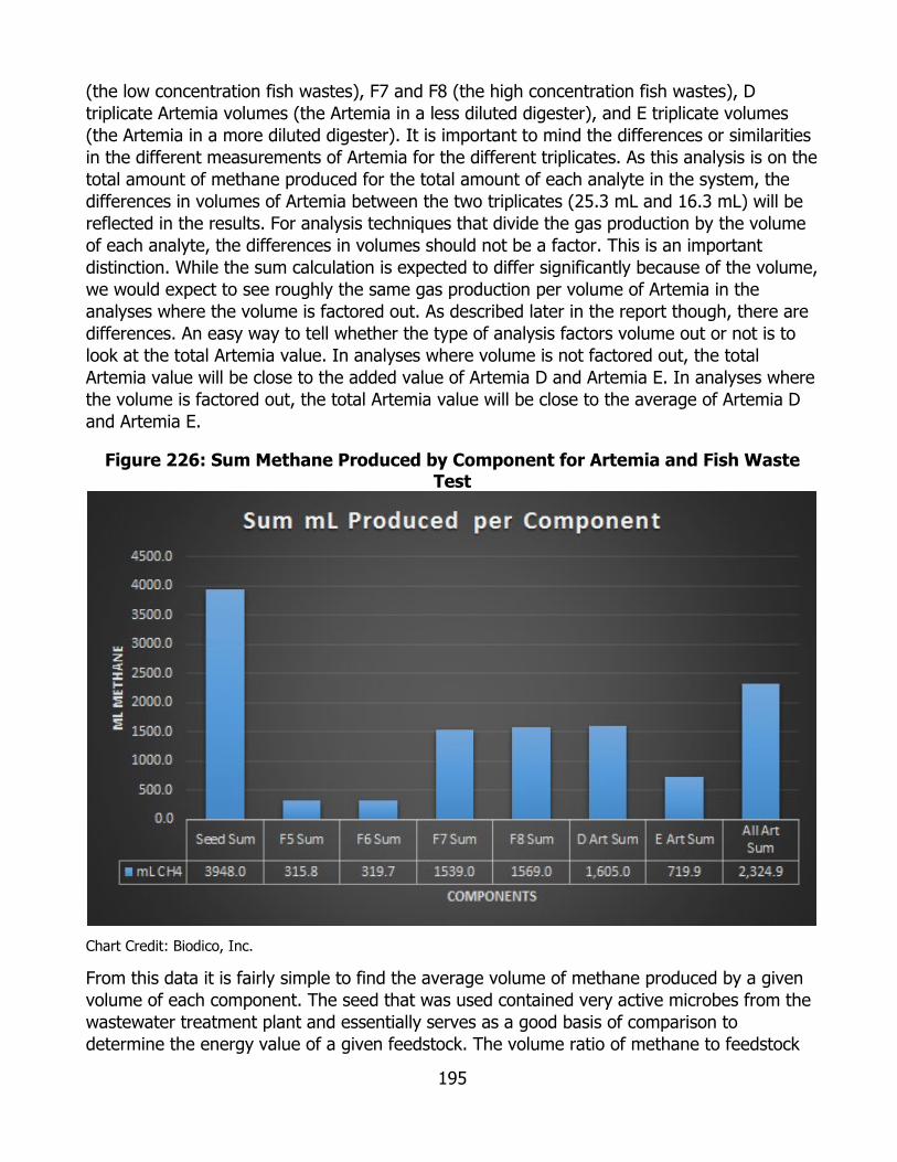
195
(the low concentration fish wastes), F7 and F8 (the high concentration fish wastes), D triplicate Artemia volumes (the Artemia in a less diluted digester), and E triplicate volumes (the Artemia in a more diluted digester). It is important to mind the differences or similarities in the different measurements of Artemia for the different triplicates. As this analysis is on the total amount of methane produced for the total amount of each analyte in the system, the differences in volumes of Artemia between the two triplicates (25.3 mL and 16.3 mL) will be reflected in the results. For analysis techniques that divide the gas production by the volume of each analyte, the differences in volumes should not be a factor. This is an important distinction. While the sum calculation is expected to differ significantly because of the volume, we would expect to see roughly the same gas production per volume of Artemia in the analyses where the volume is factored out. As described later in the report though, there are differences. An easy way to tell whether the type of analysis factors volume out or not is to look at the total Artemia value. In analyses where volume is not factored out, the total Artemia value will be close to the added value of Artemia D and Artemia E. In analyses where the volume is factored out, the total Artemia value will be close to the average of Artemia D and Artemia E.
Figure 226: Sum Methane Produced by Component for Artemia and Fish Waste Test
Chart Credit: Biodico, Inc.
From this data it is fairly simple to find the average volume of methane produced by a given volume of each component. The seed that was used contained very active microbes from the wastewater treatment plant and essentially serves as a good basis of comparison to determine the energy value of a given feedstock. The volume ratio of methane to feedstock
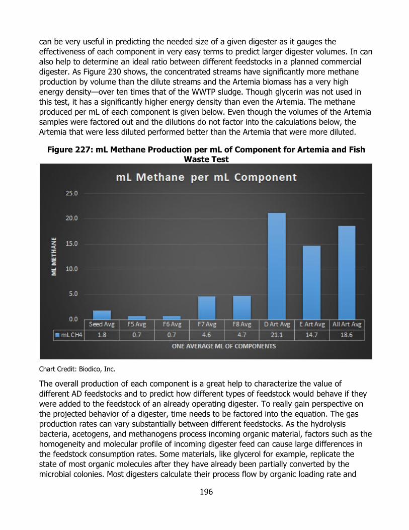
196
can be very useful in predicting the needed size of a given digester as it gauges the effectiveness of each component in very easy terms to predict larger digester volumes. In can also help to determine an ideal ratio between different feedstocks in a planned commercial digester. As Figure 230 shows, the concentrated streams have significantly more methane production by volume than the dilute streams and the Artemia biomass has a very high energy density—over ten times that of the WWTP sludge. Though glycerin was not used in this test, it has a significantly higher energy density than even the Artemia. The methane produced per mL of each component is given below. Even though the volumes of the Artemia samples were factored out and the dilutions do not factor into the calculations below, the Artemia that were less diluted performed better than the Artemia that were more diluted.
Figure 227: mL Methane Production per mL of Component for Artemia and Fish Waste Test
Chart Credit: Biodico, Inc.
The overall production of each component is a great help to characterize the value of different AD feedstocks and to predict how different types of feedstock would behave if they were added to the feedstock of an already operating digester. To really gain perspective on the projected behavior of a digester, time needs to be factored into the equation. The gas production rates can vary substantially between different feedstocks. As the hydrolysis bacteria, acetogens, and methanogens process incoming organic material, factors such as the homogeneity and molecular profile of incoming digester feed can cause large differences in the feedstock consumption rates. Some materials, like glycerol for example, replicate the state of most organic molecules after they have already been partially converted by the microbial colonies. Most digesters calculate their process flow by organic loading rate and
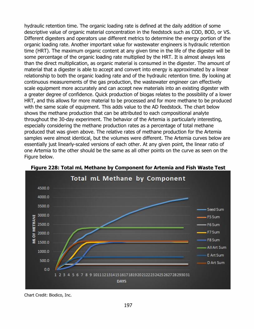
197
hydraulic retention time. The organic loading rate is defined at the daily addition of some descriptive value of organic material concentration in the feedstock such as COD, BOD, or VS. Different digesters and operators use different metrics to determine the energy portion of the organic loading rate. Another important value for wastewater engineers is hydraulic retention time (HRT). The maximum organic content at any given time in the life of the digester will be some percentage of the organic loading rate multiplied by the HRT. It is almost always less than the direct multiplication, as organic material is consumed in the digester. The amount of material that a digester is able to accept and convert into energy is approximated by a linear relationship to both the organic loading rate and of the hydraulic retention time. By looking at continuous measurements of the gas production, the wastewater engineer can effectively scale equipment more accurately and can accept new materials into an existing digester with a greater degree of confidence. Quick production of biogas relates to the possibility of a lower HRT, and this allows for more material to be processed and for more methane to be produced with the same scale of equipment. This adds value to the AD feedstock. The chart below shows the methane production that can be attributed to each compositional analyte throughout the 30-day experiment. The behavior of the Artemia is particularly interesting, especially considering the methane production rates as a percentage of total methane produced that was given above. The relative rates of methane production for the Artemia samples were almost identical, but the volumes were different. The Artemia curves below are essentially just linearly-scaled versions of each other. At any given point, the linear ratio of one Artemia to the other should be the same as all other points on the curve as seen on the Figure below.
Figure 228: Total mL Methane by Component for Artemia and Fish Waste Test
Chart Credit: Biodico, Inc.
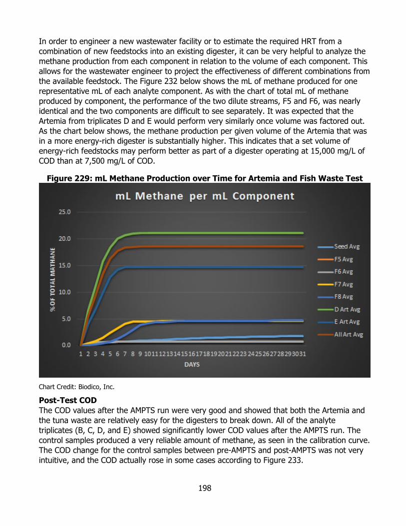
198
In order to engineer a new wastewater facility or to estimate the required HRT from a combination of new feedstocks into an existing digester, it can be very helpful to analyze the methane production from each component in relation to the volume of each component. This allows for the wastewater engineer to project the effectiveness of different combinations from the available feedstock. The Figure 232 below shows the mL of methane produced for one representative mL of each analyte component. As with the chart of total mL of methane produced by component, the performance of the two dilute streams, F5 and F6, was nearly identical and the two components are difficult to see separately. It was expected that the Artemia from triplicates D and E would perform very similarly once volume was factored out. As the chart below shows, the methane production per given volume of the Artemia that was in a more energy-rich digester is substantially higher. This indicates that a set volume of energy-rich feedstocks may perform better as part of a digester operating at 15,000 mg/L of COD than at 7,500 mg/L of COD.
Figure 229: mL Methane Production over Time for Artemia and Fish Waste Test
Chart Credit: Biodico, Inc.
Post-Test COD The COD values after the AMPTS run were very good and showed that both the Artemia and the tuna waste are relatively easy for the digesters to break down. All of the analyte triplicates (B, C, D, and E) showed significantly lower COD values after the AMPTS run. The control samples produced a very reliable amount of methane, as seen in the calibration curve. The COD change for the control samples between pre-AMPTS and post-AMPTS was not very intuitive, and the COD actually rose in some cases according to Figure 233.

199
Figure 230: COD of Artemia and Fish Waste Test (post)
Chart Credit: Biodico, Inc.
The COD values of the B samples, which had about 27,000 mg/L of COD before the test, were reduced to almost one-third of their original values. This is very promising because it shows that for tuna waste at least, a higher organic loading rate is possible. COD Destruction The COD destruction percentage provides another method that can be used in the field to see how efficiently the microbial colonies are breaking down the feedstock to ultimately create methane and carbon dioxide. Testing COD values for each digester before the AMPTS tests and after the AMPTS tests allows Biodico to determine the COD destruction in the digester. The COD destruction rate is given in Figure 234.
Figure 231: COD Destruction Rate Formula
Chart Credit: Biodico, Inc.
A graph of the COD destruction is given in Figure 235.
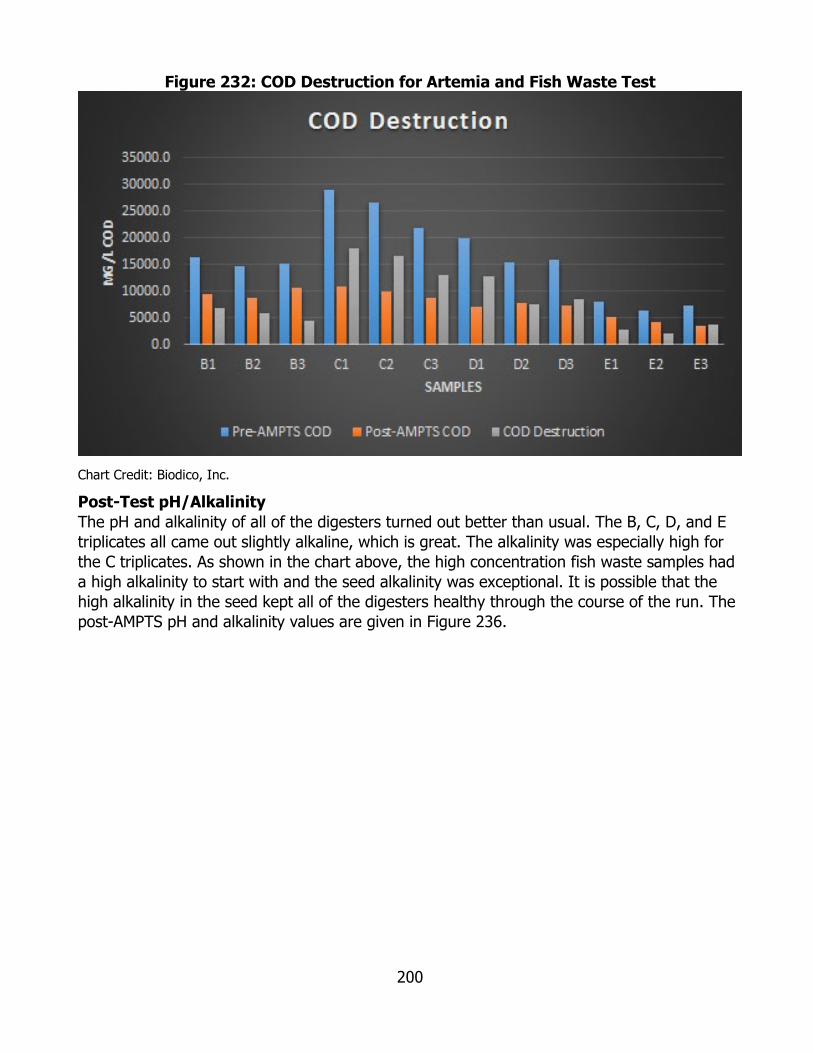
200
Figure 232: COD Destruction for Artemia and Fish Waste Test
Chart Credit: Biodico, Inc.
Post-Test pH/Alkalinity The pH and alkalinity of all of the digesters turned out better than usual. The B, C, D, and E triplicates all came out slightly alkaline, which is great. The alkalinity was especially high for the C triplicates. As shown in the chart above, the high concentration fish waste samples had a high alkalinity to start with and the seed alkalinity was exceptional. It is possible that the high alkalinity in the seed kept all of the digesters healthy through the course of the run. The post-AMPTS pH and alkalinity values are given in Figure 236.
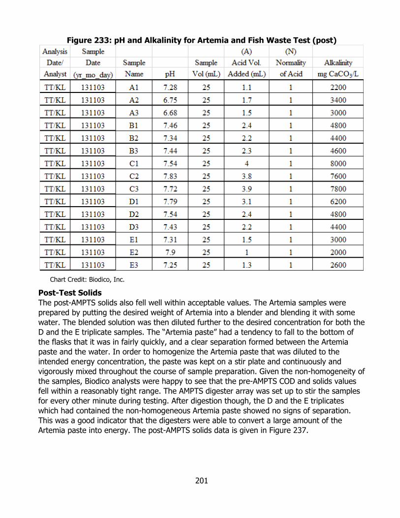
201
Figure 233: pH and Alkalinity for Artemia and Fish Waste Test (post)
Chart Credit: Biodico, Inc.
Post-Test Solids The post-AMPTS solids also fell well within acceptable values. The Artemia samples were prepared by putting the desired weight of Artemia into a blender and blending it with some water. The blended solution was then diluted further to the desired concentration for both the D and the E triplicate samples. The “Artemia paste” had a tendency to fall to the bottom of the flasks that it was in fairly quickly, and a clear separation formed between the Artemia paste and the water. In order to homogenize the Artemia paste that was diluted to the intended energy concentration, the paste was kept on a stir plate and continuously and vigorously mixed throughout the course of sample preparation. Given the non-homogeneity of the samples, Biodico analysts were happy to see that the pre-AMPTS COD and solids values fell within a reasonably tight range. The AMPTS digester array was set up to stir the samples for every other minute during testing. After digestion though, the D and the E triplicates which had contained the non-homogeneous Artemia paste showed no signs of separation. This was a good indicator that the digesters were able to convert a large amount of the Artemia paste into energy. The post-AMPTS solids data is given in Figure 237.

202
Figure 234: Solids Data for Artemia and Fish Waste (post)
Chart Credit: Biodico, Inc.
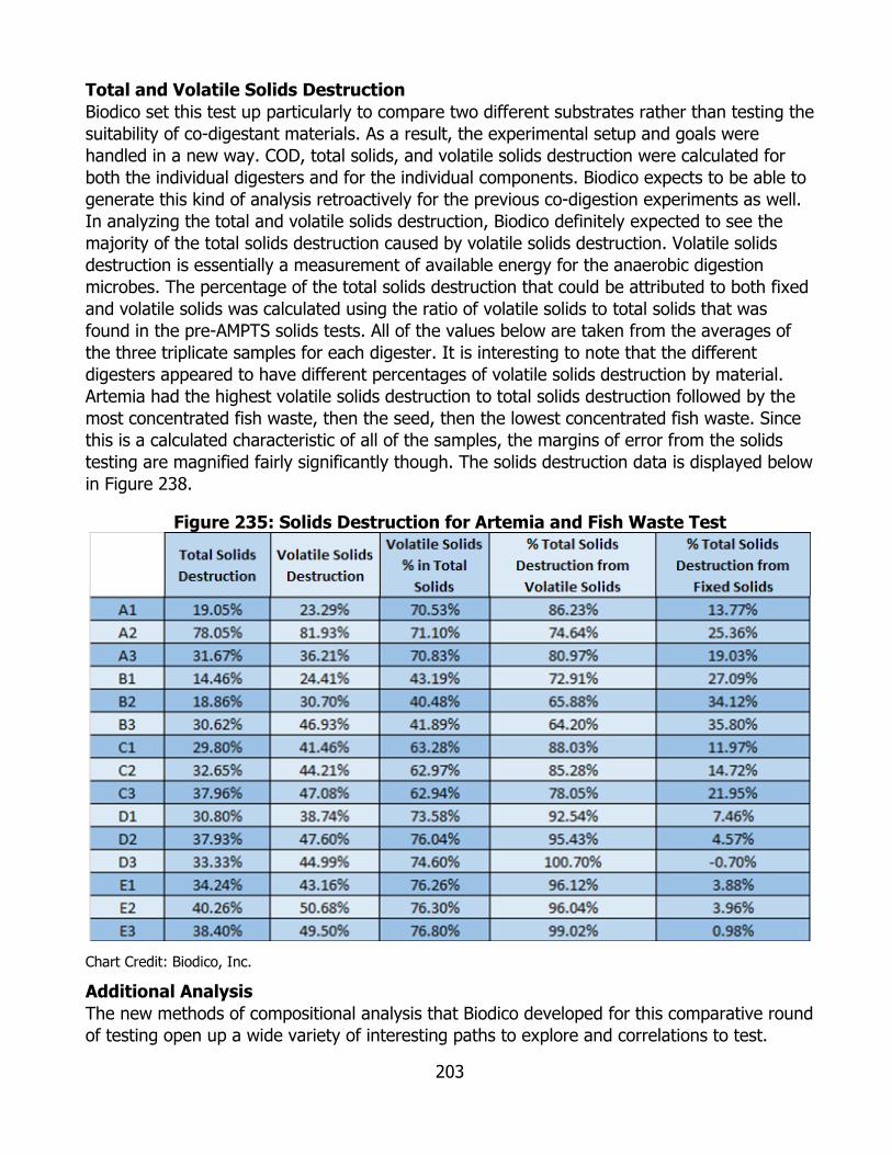
203
Total and Volatile Solids Destruction Biodico set this test up particularly to compare two different substrates rather than testing the suitability of co-digestant materials. As a result, the experimental setup and goals were handled in a new way. COD, total solids, and volatile solids destruction were calculated for both the individual digesters and for the individual components. Biodico expects to be able to generate this kind of analysis retroactively for the previous co-digestion experiments as well. In analyzing the total and volatile solids destruction, Biodico definitely expected to see the majority of the total solids destruction caused by volatile solids destruction. Volatile solids destruction is essentially a measurement of available energy for the anaerobic digestion microbes. The percentage of the total solids destruction that could be attributed to both fixed and volatile solids was calculated using the ratio of volatile solids to total solids that was found in the pre-AMPTS solids tests. All of the values below are taken from the averages of the three triplicate samples for each digester. It is interesting to note that the different digesters appeared to have different percentages of volatile solids destruction by material. Artemia had the highest volatile solids destruction to total solids destruction followed by the most concentrated fish waste, then the seed, then the lowest concentrated fish waste. Since this is a calculated characteristic of all of the samples, the margins of error from the solids testing are magnified fairly significantly though. The solids destruction data is displayed below in Figure 238.
Figure 235: Solids Destruction for Artemia and Fish Waste Test
Chart Credit: Biodico, Inc.
Additional Analysis The new methods of compositional analysis that Biodico developed for this comparative round of testing open up a wide variety of interesting paths to explore and correlations to test.

204
Throughout the course of ARV-10-024, Biodico has discussed anaerobic digester operations with a variety of municipal WWTP managers, AD researchers, AD technology providers, and other scientists. Most people in the field test for a variety of different characteristics of the feedstocks entering their digester and of the digestate that is circulating in or leaving the digester. Everybody seems to have a favorite metric to measure the energy content of the material entering their system though. This metric is usually chemical oxygen demand (COD), biological oxygen demand (BOD), or volatile solids content (VS). Biodico has now worked extensively with glycerin which is very rich in chemical oxygen demand, but not necessarily much higher in volatile solids concentrations than other feedstocks. High ratios of COD to volatile solids are also present in the used cooking oil waste that Biodico has tested (and that Biodico has as a waste stream from its cooking oil collection program) and in the Artemia that was tested for this experimental run (and that Biodico hopes to have a waste stream from in the future, albeit in a less concentrated form than the direct Artemia biomass).
With these high waste streams, Biodico has used COD as the defining factor in its experimental designs. Biodico has seen that digesters that are running glycerin that have an otherwise acceptable level of VS but a very high COD will crash. In developing the new calculations for the analyte comparison study, Biodico also implemented an easy correlation test between COD destruction and methane production. The COD destruction is given as a raw number and not as a percentage. A sample that started with a COD of 15,000 mg/L and ended with a COD of 10,000 mg/L would show a COD destruction of 5,000 mg/L and not 33.3 percent. As Figure 239 below shows, the COD destruction is not entirely predictive, but the correlation (with a determination coefficient of 71.1 percent) is significant.
Figure 236: mL of Methane per mg/L COD Destruction for Artemia and Fish Waste Test
Chart Credit: Biodico, Inc.
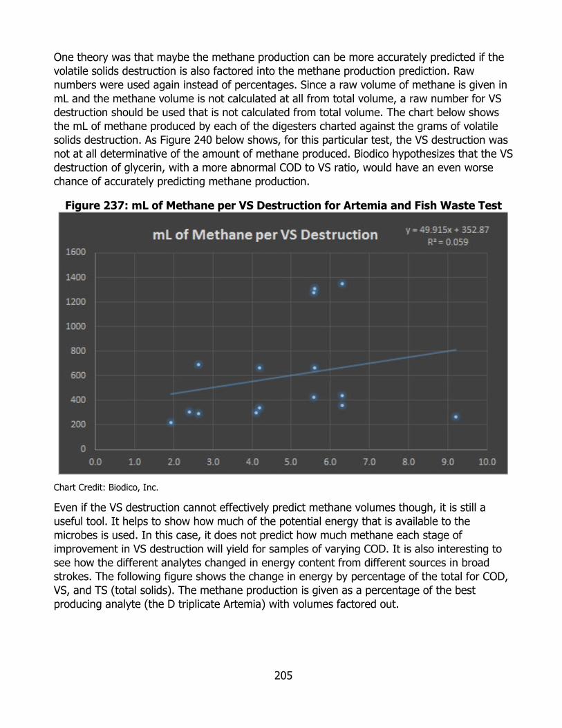
205
One theory was that maybe the methane production can be more accurately predicted if the volatile solids destruction is also factored into the methane production prediction. Raw numbers were used again instead of percentages. Since a raw volume of methane is given in mL and the methane volume is not calculated at all from total volume, a raw number for VS destruction should be used that is not calculated from total volume. The chart below shows the mL of methane produced by each of the digesters charted against the grams of volatile solids destruction. As Figure 240 below shows, for this particular test, the VS destruction was not at all determinative of the amount of methane produced. Biodico hypothesizes that the VS destruction of glycerin, with a more abnormal COD to VS ratio, would have an even worse chance of accurately predicting methane production.
Figure 237: mL of Methane per VS Destruction for Artemia and Fish Waste Test
Chart Credit: Biodico, Inc.
Even if the VS destruction cannot effectively predict methane volumes though, it is still a useful tool. It helps to show how much of the potential energy that is available to the microbes is used. In this case, it does not predict how much methane each stage of improvement in VS destruction will yield for samples of varying COD. It is also interesting to see how the different analytes changed in energy content from different sources in broad strokes. The following figure shows the change in energy by percentage of the total for COD, VS, and TS (total solids). The methane production is given as a percentage of the best producing analyte (the D triplicate Artemia) with volumes factored out.

206
Figure 238: Changes in Energy by Component for Artemia and Fish Waste Test
Chart Credit: Biodico, Inc.
Conclusions This AMPTS test was the first one that Biodico used to specifically gather performance data about the methane production performance of the individual components of each of the substrates. Though it is difficult to make broad generalizations from a sample set of only five unique digester compositions, this analysis was used for all of the AMPTS tests run after this one and a similar analysis was used retroactively to more effectively analyze the behavior of glycerin in the digesters. From this experiment in particular Biodico saw that:
• Valuable data on individual analytes can be extracted from the AMPTS test results.
• Even after volume and dilution of the samples are factored out, Artemia seems to create more methane in a 15,000 mg/L digester than in a 7,500 mg/L digester.
• Regardless of the dilution rate and the production efficiencies noted above, the methane production rate asapercentage of the total methane production for different concentrations of Artemia was nearly identical as illustrated in Figure 228.
• Both the fish waste and the Artemia waste accelerated the methane production of the WWTP sludge co-digestant.
• The COD of high energy samples has shown to be more predictive than VS in a batch digester running at mesophilic temperatures.
Calculations Used in Component Analysis
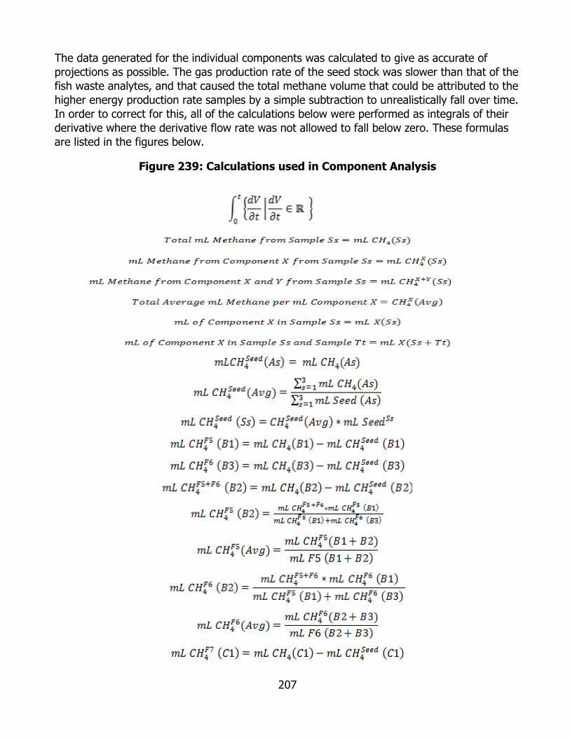
207
The data generated for the individual components was calculated to give as accurate of projections as possible. The gas production rate of the seed stock was slower than that of the fish waste analytes, and that caused the total methane volume that could be attributed to the higher energy production rate samples by a simple subtraction to unrealistically fall over time. In order to correct for this, all of the calculations below were performed as integrals of their derivative where the derivative flow rate was not allowed to fall below zero. These formulas are listed in the figures below.
Figure 239: Calculations used in Component Analysis

208
Credit: Biodico, Inc.
Dairy Manure & Beet Stillage Co-Digestion Test For this AMPTS test, Biodico sought to test its crude glycerin byproduct from biodiesel production with two different substrates. The first substrate was dairy manure that is currently being used in an anaerobic digester in the San Joaquin Valley area to actively produce methane. The second substrate is beet stillage that is a byproduct of the production of ethanol from energy beets that are currently being grown in the San Joaquin Valley. Test Setup In the previous AMPTS test, Biodico deviated from its standard experimental design and adopted an experimental design often used by the AMPTS equipment manufacturers in Sweden. The Bioprocess Control experimental design mixes each of the digesters so that the COD from the microbial seed is double the COD from the different analytes. This methodology was repeated for the latest dairy manure and beet stillage test for two primary reasons: the ratios would provide good information for starting to load glycerin into the currently operating manure digester, and sufficient data has already been generated for the behavior of glycerin and dairy manure by the other methodology. This experimental run allowed for Biodico to more fully characterize how much additional energy glycerin could provide to the existing facility. As with many previous experiments, the seed was taken from the Ventura County Wastewater Treatment Plant (WWTP) and the experimental digesters were mixed on the same day as collection.
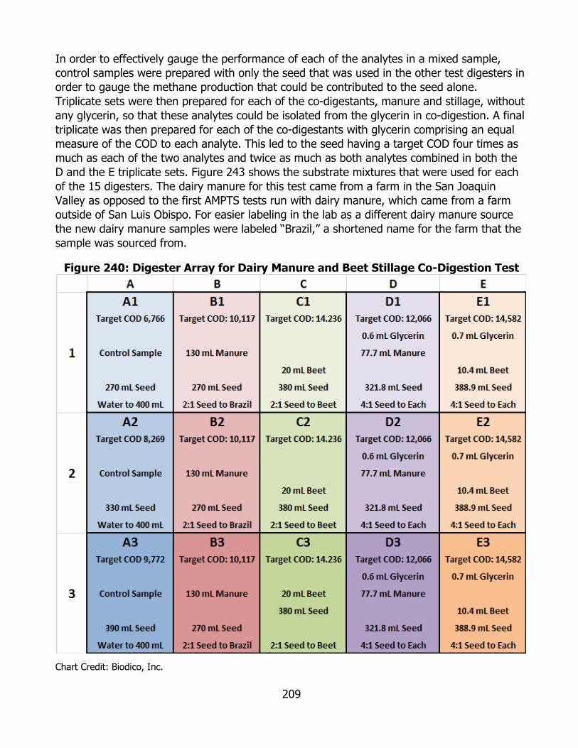
209
In order to effectively gauge the performance of each of the analytes in a mixed sample, control samples were prepared with only the seed that was used in the other test digesters in order to gauge the methane production that could be contributed to the seed alone. Triplicate sets were then prepared for each of the co-digestants, manure and stillage, without any glycerin, so that these analytes could be isolated from the glycerin in co-digestion. A final triplicate was then prepared for each of the co-digestants with glycerin comprising an equal measure of the COD to each analyte. This led to the seed having a target COD four times as much as each of the two analytes and twice as much as both analytes combined in both the D and the E triplicate sets. Figure 243 shows the substrate mixtures that were used for each of the 15 digesters. The dairy manure for this test came from a farm in the San Joaquin Valley as opposed to the first AMPTS tests run with dairy manure, which came from a farm outside of San Luis Obispo. For easier labeling in the lab as a different dairy manure source the new dairy manure samples were labeled “Brazil,” a shortened name for the farm that the sample was sourced from.
Figure 240: Digester Array for Dairy Manure and Beet Stillage Co-Digestion Test
Chart Credit: Biodico, Inc.

210
Pre-Test COD As described in the test setup subsection, the samples were prepared so that each sample would have twice the amount of COD content from the seed than it would have from the analytes. For the B and the C samples, the analytes were dairy manure and beet stillage respectively. This allowed for the methane production from each of these substrates to be effectively isolated. For the D and the E samples, the dairy manure and the beet stillage respectively were mixed with the crude glycerin byproduct of biodiesel production so that each of the analytes contributed an equal amount of COD to each digester. This meant that each of the two analytes, glycerin and dairy manure in the D samples as an example, contributed 25 percent as much COD to each digester as the seed and that the seed COD held a 2:1 ratio to the COD of the other two analytes combined. The COD of each of the starting materials was tested before the AMPTS digesters were prepared. The values were used to calculate the mixture of each digester as seen in Figure 244.
Figure 241: COD of Components for Dairy Manure and Beet Stillage Co-Digestion Test
Chart Credit: Biodico, Inc.
The initial COD values for the digesters are displayed in the figure below.
Figure 242: COD of Dairy Manure and Beet Stillage Co-Digestion Test (pre)
Chart Credit: Biodico, Inc.
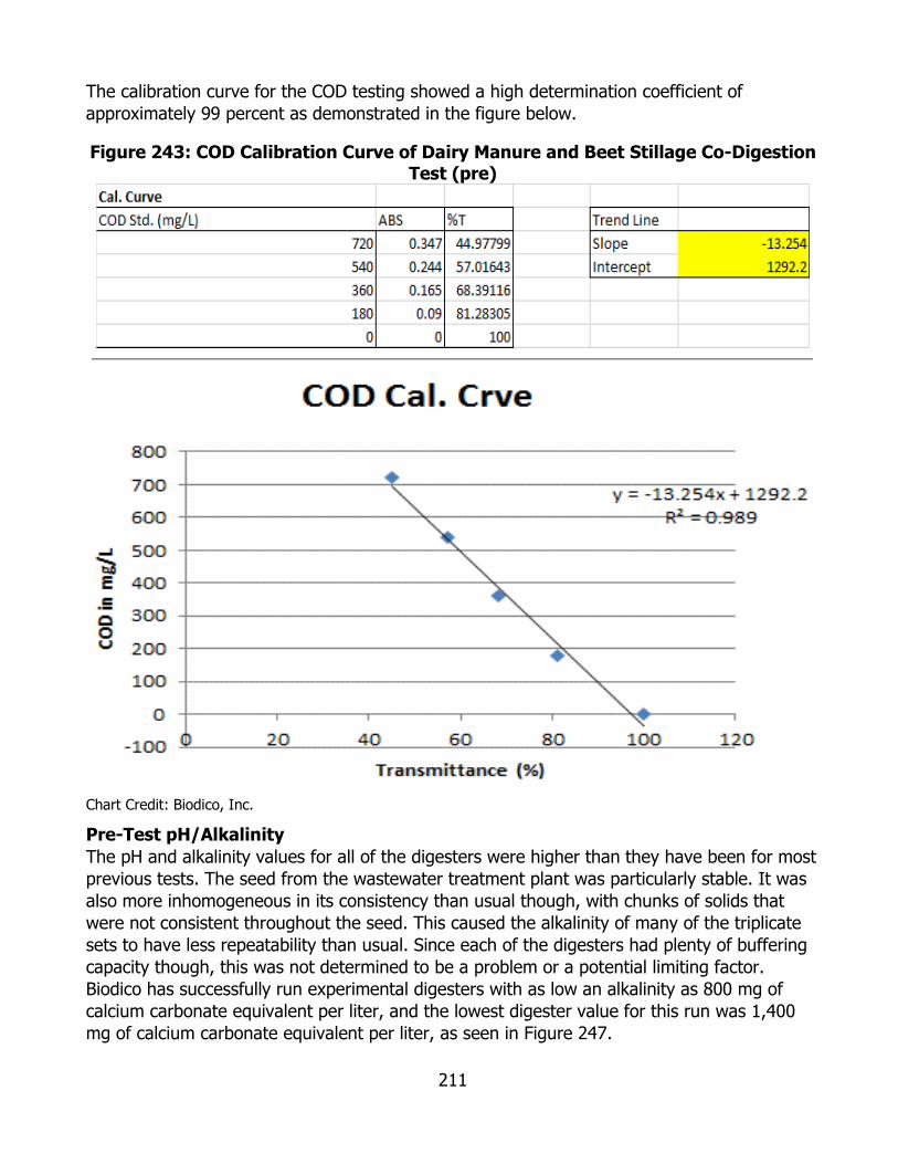
211
The calibration curve for the COD testing showed a high determination coefficient of approximately 99 percent as demonstrated in the figure below.
Figure 243: COD Calibration Curve of Dairy Manure and Beet Stillage Co-Digestion Test (pre)
Chart Credit: Biodico, Inc.
Pre-Test pH/Alkalinity The pH and alkalinity values for all of the digesters were higher than they have been for most previous tests. The seed from the wastewater treatment plant was particularly stable. It was also more inhomogeneous in its consistency than usual though, with chunks of solids that were not consistent throughout the seed. This caused the alkalinity of many of the triplicate sets to have less repeatability than usual. Since each of the digesters had plenty of buffering capacity though, this was not determined to be a problem or a potential limiting factor. Biodico has successfully run experimental digesters with as low an alkalinity as 800 mg of calcium carbonate equivalent per liter, and the lowest digester value for this run was 1,400 mg of calcium carbonate equivalent per liter, as seen in Figure 247.
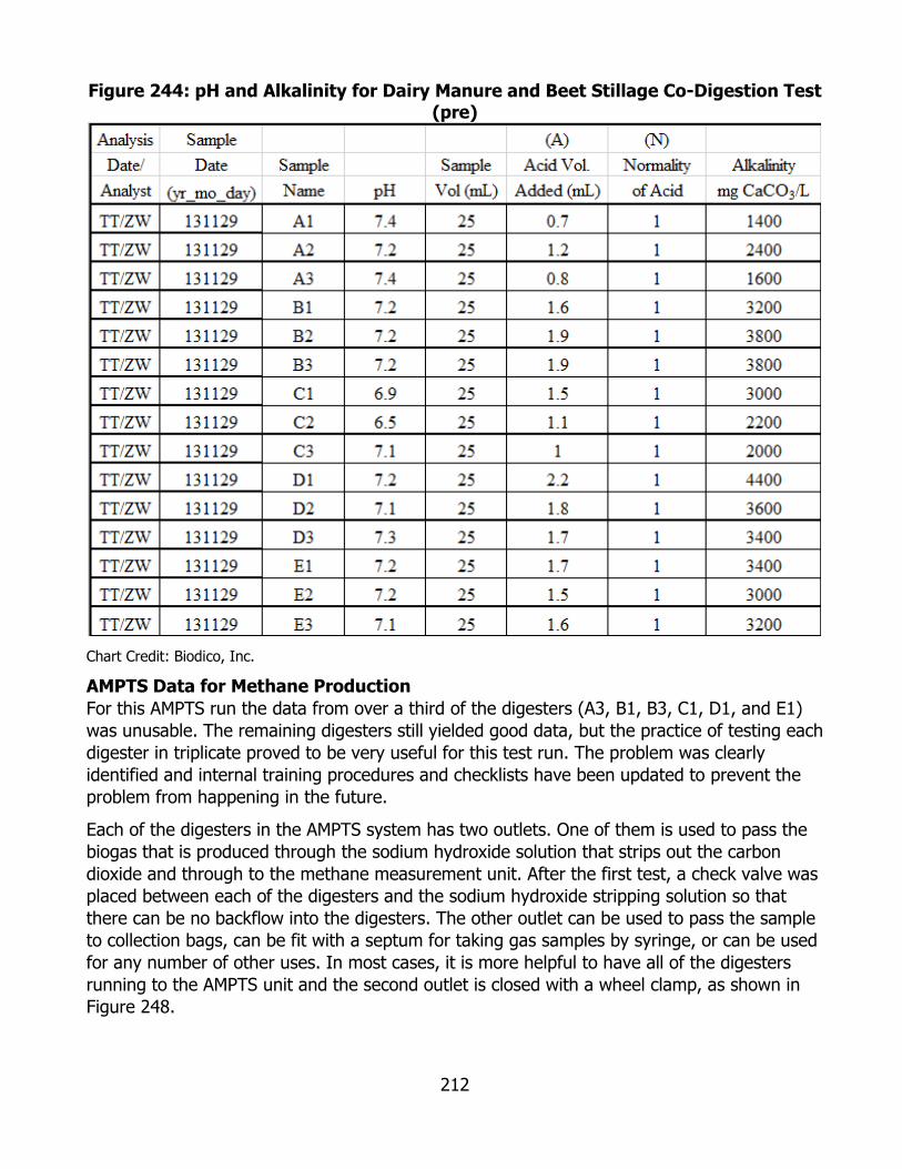
212
Figure 244: pH and Alkalinity for Dairy Manure and Beet Stillage Co-Digestion Test (pre)
Chart Credit: Biodico, Inc.
AMPTS Data for Methane Production For this AMPTS run the data from over a third of the digesters (A3, B1, B3, C1, D1, and E1) was unusable. The remaining digesters still yielded good data, but the practice of testing each digester in triplicate proved to be very useful for this test run. The problem was clearly identified and internal training procedures and checklists have been updated to prevent the problem from happening in the future.
Each of the digesters in the AMPTS system has two outlets. One of them is used to pass the biogas that is produced through the sodium hydroxide solution that strips out the carbon dioxide and through to the methane measurement unit. After the first test, a check valve was placed between each of the digesters and the sodium hydroxide stripping solution so that there can be no backflow into the digesters. The other outlet can be used to pass the sample to collection bags, can be fit with a septum for taking gas samples by syringe, or can be used for any number of other uses. In most cases, it is more helpful to have all of the digesters running to the AMPTS unit and the second outlet is closed with a wheel clamp, as shown in Figure 248.

213
Figure 245: Digester Wheel Clamp
Photo Credit: Biodico, Inc.
In this case, the digesters were set up and connected to the AMPTS system, but many of the wheel clamps were not closed tightly enough. Usually, at the point where one of the digester outlets has been connected to the check valve (preventing backflow) and one digester has been connected to a wheel clamp that has not yet been tightened (to allow for gas flow), a nitrogen tank is plumbed to the outlet with the loose wheel clamp and the system is purged in order to create anoxic conditions. The wheel clamp is then tightened with the nitrogen flow still running to seal the digester from possible oxygen contamination. Unfortunately, in this test, the valves were not tightened well and the digesters were exposed to the surrounding atmosphere.
The volume snapshot in the figure below serves as a good indicator of which digesters were affected. The contamination issue was detected part of the way through the test and fixed to the extent that it could be in the middle of the test run, but the contaminated digesters never fully recovered. For the component analysis later in this report, the contaminated digesters were removed from the data sets.
Figure 246: Total Methane Produced by Digester for Dairy Manure and Beet Stillage Co-Digestion Test
Chart Credit: Biodico, Inc.
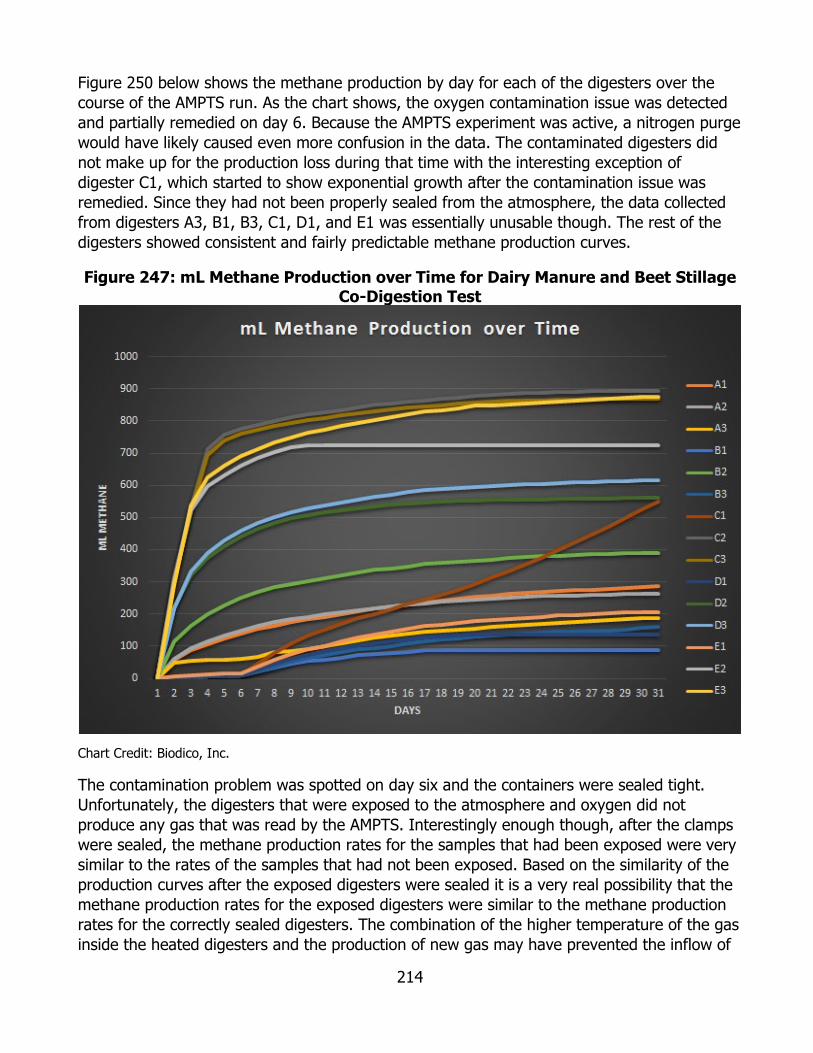
214
Figure 250 below shows the methane production by day for each of the digesters over the course of the AMPTS run. As the chart shows, the oxygen contamination issue was detected and partially remedied on day 6. Because the AMPTS experiment was active, a nitrogen purge would have likely caused even more confusion in the data. The contaminated digesters did not make up for the production loss during that time with the interesting exception of digester C1, which started to show exponential growth after the contamination issue was remedied. Since they had not been properly sealed from the atmosphere, the data collected from digesters A3, B1, B3, C1, D1, and E1 was essentially unusable though. The rest of the digesters showed consistent and fairly predictable methane production curves.
Figure 247: mL Methane Production over Time for Dairy Manure and Beet Stillage Co-Digestion Test
Chart Credit: Biodico, Inc.
The contamination problem was spotted on day six and the containers were sealed tight. Unfortunately, the digesters that were exposed to the atmosphere and oxygen did not produce any gas that was read by the AMPTS. Interestingly enough though, after the clamps were sealed, the methane production rates for the samples that had been exposed were very similar to the rates of the samples that had not been exposed. Based on the similarity of the production curves after the exposed digesters were sealed it is a very real possibility that the methane production rates for the exposed digesters were similar to the methane production rates for the correctly sealed digesters. The combination of the higher temperature of the gas inside the heated digesters and the production of new gas may have prevented the inflow of
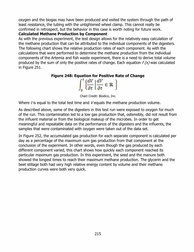
215
oxygen and the biogas may have been produced and exited the system through the path of least resistance, the tubing with the untightened wheel clamp. This cannot really be confirmed in retrospect, but the behavior in this case is worth noting for future work. Calculated Methane Production by Component As with the previous experiment, the test design allows for the relatively easy calculation of the methane production that can be attributed to the individual components of the digesters. The following chart shows the relative production rates of each component. As with the calculations that were performed to determine the methane production from the individual components of the Artemia and fish waste experiment, there is a need to derive total volume produced by the sum of only the positive rates of change. Each equation f (x) was calculated in Figure 251.
Figure 248: Equation for Positive Rate of Change
Chart Credit: Biodico, Inc.
Where t is equal to the total test time and V equals the methane production volume.
As described above, some of the digesters in this test run were exposed to oxygen for much of the run. This contamination led to a low gas production that, ostensibly, did not result from the influent material or from the biological makeup of the microbes. In order to get meaningful and repeatable data on the performance of the digesters and the influents, the samples that were contaminated with oxygen were taken out of the data set.
In Figure 252, the accumulated gas production for each separate component is calculated per day as a percentage of the maximum sum gas production from that component at the conclusion of the experiment. In other words, even though the gas produced by each different component varied, this chart shows how quickly each component reached its particular maximum gas production. In this experiment, the seed and the manure both showed the longest times to reach their maximum methane production. The glycerin and the beet stillage both had very high relative energy content by volume and their methane production curves were both very quick.
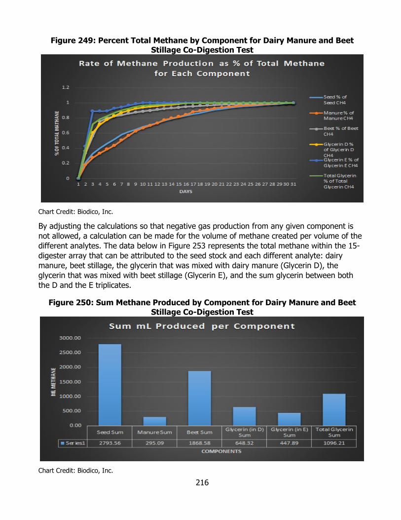
216
Figure 249: Percent Total Methane by Component for Dairy Manure and Beet Stillage Co-Digestion Test
Chart Credit: Biodico, Inc.
By adjusting the calculations so that negative gas production from any given component is not allowed, a calculation can be made for the volume of methane created per volume of the different analytes. The data below in Figure 253 represents the total methane within the 15-digester array that can be attributed to the seed stock and each different analyte: dairy manure, beet stillage, the glycerin that was mixed with dairy manure (Glycerin D), the glycerin that was mixed with beet stillage (Glycerin E), and the sum glycerin between both the D and the E triplicates.
Figure 250: Sum Methane Produced by Component for Dairy Manure and Beet Stillage Co-Digestion Test
Chart Credit: Biodico, Inc.
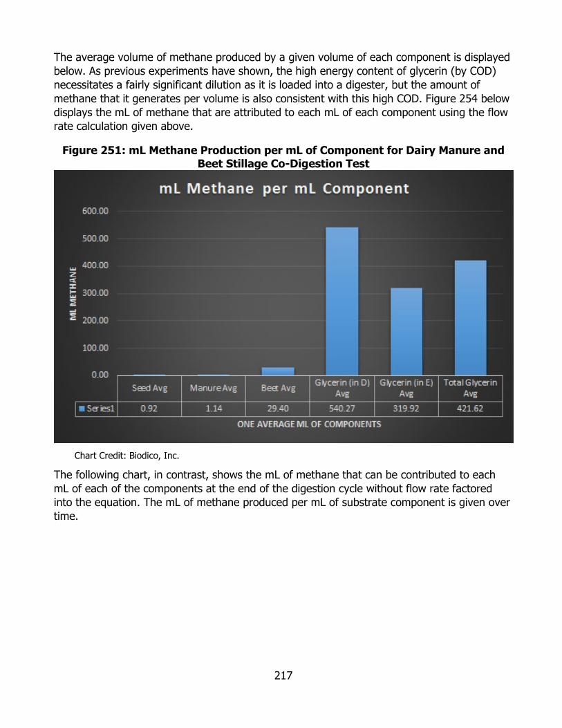
217
The average volume of methane produced by a given volume of each component is displayed below. As previous experiments have shown, the high energy content of glycerin (by COD) necessitates a fairly significant dilution as it is loaded into a digester, but the amount of methane that it generates per volume is also consistent with this high COD. Figure 254 below displays the mL of methane that are attributed to each mL of each component using the flow rate calculation given above.
Figure 251: mL Methane Production per mL of Component for Dairy Manure and Beet Stillage Co-Digestion Test
Chart Credit: Biodico, Inc.
The following chart, in contrast, shows the mL of methane that can be contributed to each mL of each of the components at the end of the digestion cycle without flow rate factored into the equation. The mL of methane produced per mL of substrate component is given over time.

218
Figure 252: Total mL Methane by Component for Dairy Manure and Beet Stillage Co-Digestion Test
Chart Credit: Biodico, Inc.
These values are consistent with the methane yield predicted by the chemical oxygen demand values of each of the components. The chart below shows the mL of methane production that are predicted per mL of each component by the ultimate methane yield (UMY) from the COD of each component. The derivation calculations for ultimate methane yield that are used in Figure 256 below are given earlier in the report in Figure 130.
Figure 253: Ultimate Methane Yield Predictions
Chart Credit: Biodico, Inc.
Post-Test COD The COD values after the AMPTS run were consistently lower than the values before the digestion. One interesting point to note is that even though several of the samples had been contaminated by oxygen, the drop-in post-test COD values was relatively uniform as seen in
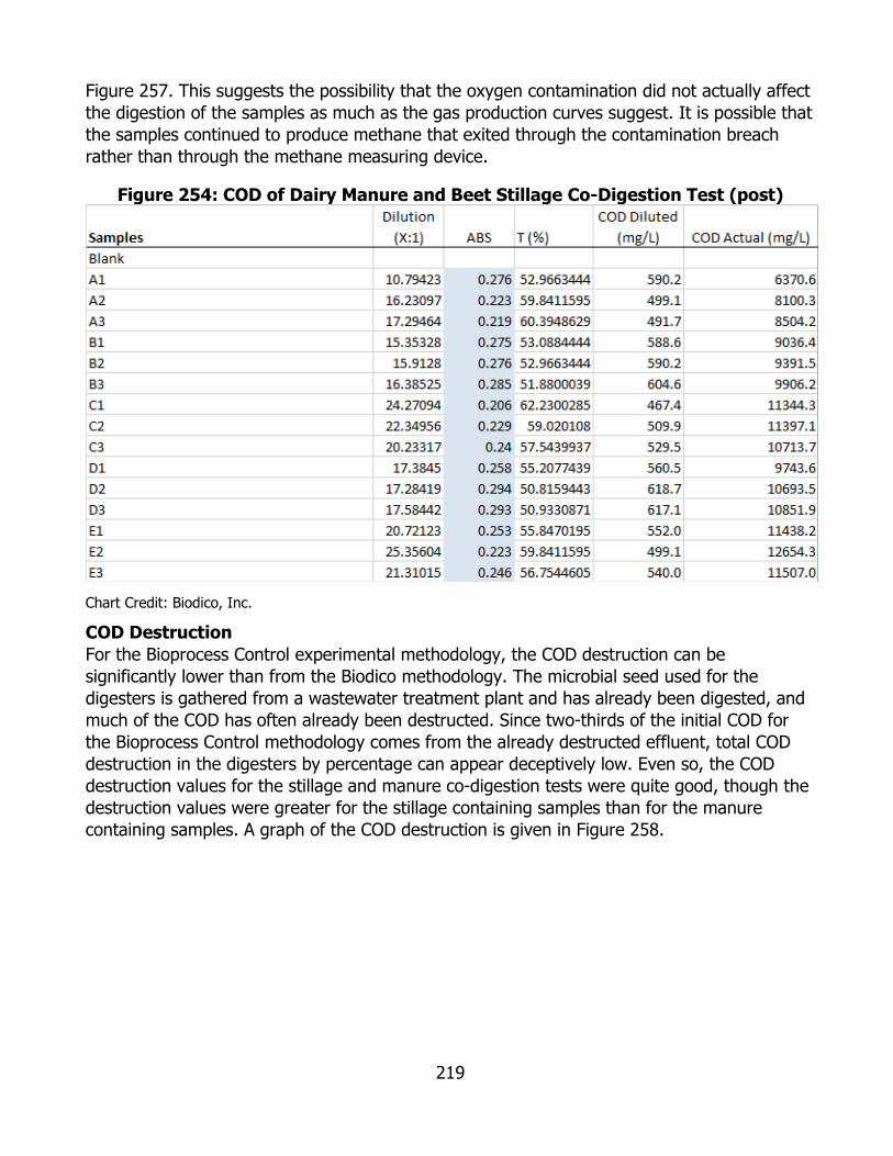
219
Figure 257. This suggests the possibility that the oxygen contamination did not actually affect the digestion of the samples as much as the gas production curves suggest. It is possible that the samples continued to produce methane that exited through the contamination breach rather than through the methane measuring device.
Figure 254: COD of Dairy Manure and Beet Stillage Co-Digestion Test (post)
Chart Credit: Biodico, Inc.
COD Destruction For the Bioprocess Control experimental methodology, the COD destruction can be significantly lower than from the Biodico methodology. The microbial seed used for the digesters is gathered from a wastewater treatment plant and has already been digested, and much of the COD has often already been destructed. Since two-thirds of the initial COD for the Bioprocess Control methodology comes from the already destructed effluent, total COD destruction in the digesters by percentage can appear deceptively low. Even so, the COD destruction values for the stillage and manure co-digestion tests were quite good, though the destruction values were greater for the stillage containing samples than for the manure containing samples. A graph of the COD destruction is given in Figure 258.
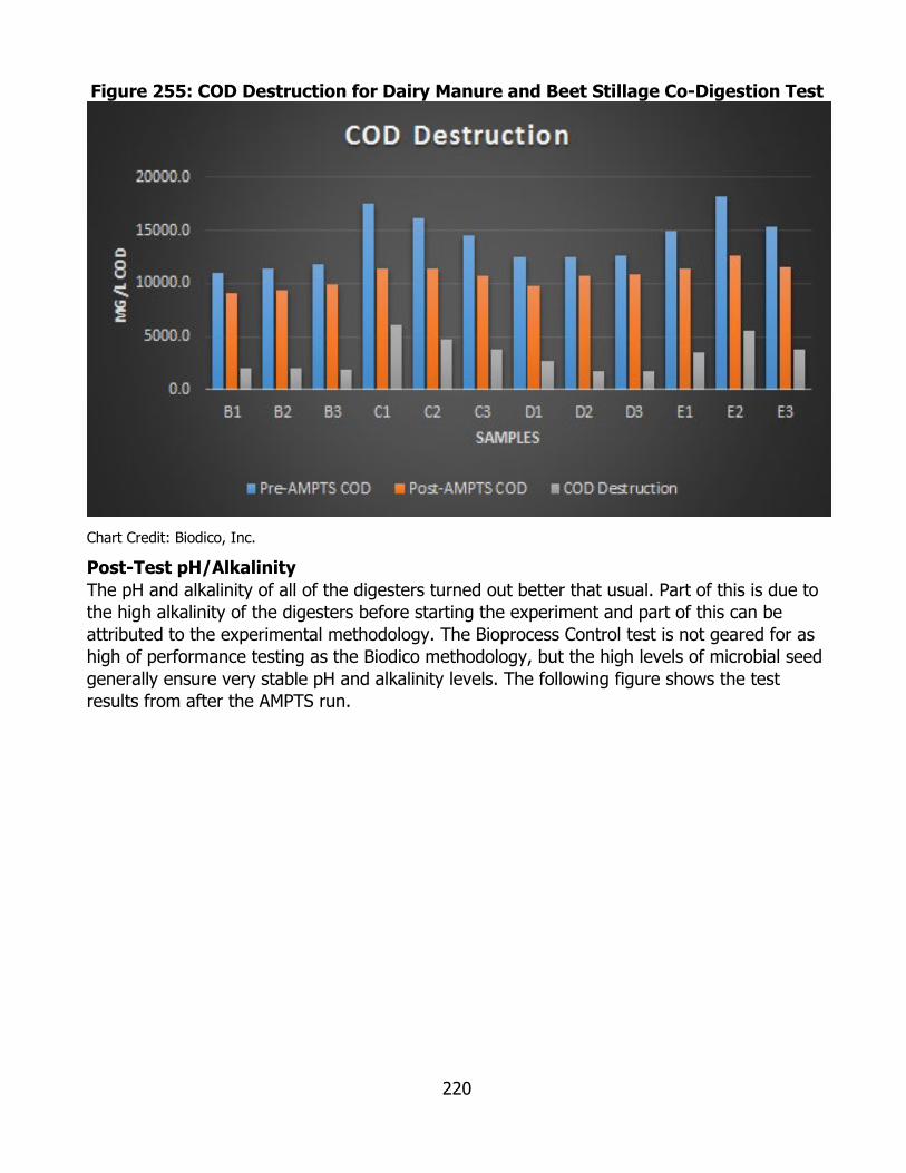
220
Figure 255: COD Destruction for Dairy Manure and Beet Stillage Co-Digestion Test
Chart Credit: Biodico, Inc.
Post-Test pH/Alkalinity The pH and alkalinity of all of the digesters turned out better that usual. Part of this is due to the high alkalinity of the digesters before starting the experiment and part of this can be attributed to the experimental methodology. The Bioprocess Control test is not geared for as high of performance testing as the Biodico methodology, but the high levels of microbial seed generally ensure very stable pH and alkalinity levels. The following figure shows the test results from after the AMPTS run.
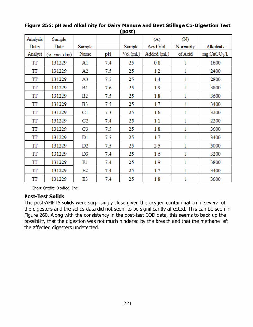
221
Figure 256: pH and Alkalinity for Dairy Manure and Beet Stillage Co-Digestion Test (post)
Chart Credit: Biodico, Inc.
Post-Test Solids The post-AMPTS solids were surprisingly close given the oxygen contamination in several of the digesters and the solids data did not seem to be significantly affected. This can be seen in Figure 260. Along with the consistency in the post-test COD data, this seems to back up the possibility that the digestion was not much hindered by the breach and that the methane left the affected digesters undetected.

222
Figure 257: Solids Data for Dairy Manure and Beet Stillage Co-Digestion (post)
Chart Credit: Biodico, Inc.

223
Conclusions Biodico has now assessed the methane potential of glycerin as a co-digestant with one of the most promising and widely used digester feedstocks in California, dairy manure, using the AMPTS equipment with two different approaches in experimental design, and has also tested the anaerobic digestion potential of another promising renewable energy byproduct, the stillage waste from ethanol production from energy beets. The results of this experiment can be summarized as:
• On average, each mL of crude glycerin yielded roughly 420 mL of methane at standard temperature and pressure (0° C at 100 kPa), or 277 mg of methane.
• In co-digestion with dairy manure, the methane production that can be attributed to glycerin is almost 500 times the amount of methane production that can be attributed to dairy manure by volume at standard temperature and pressure.
• On average, each mL of beet stillage yielded roughly 30 mL of methane at standard temperature and pressure (12.6 mg).
• Glycerin and beet stillage can effectively be co-digested to produce methane.
The relative methane production rate of more highly concentrated energy sources such as beet stillage and glycerin appear to be greater than that of lower concentrated energy sources such as dairy manure.
Calculations Used in Component Analysis As mentioned in the report, the gas production rate of the seed stock and of the manure was slower than that of the glycerin and of the beet stillage, and that caused the total methane volume that could be attributed to the more quickly producing components to unrealistically fall over time. In order to correct for this difference in ratios, all of the calculations below were performed as integrals of their derivative where the derivative flow rate was not allowed to fall below zero as seen in Figure 261 below.
Figure 258: Calculations used in Component Analysis

224
Chart Credit: Biodico, Inc.
Algaculture Arguably the largest hindrance to more rapid growth for the biodiesel industry lies in feedstock development. For almost forty years algae has been investigated as a promising high yield source of lipids. The Aquatic Species Program conducted by the DOE ran from 1976 to 1994 with a $25 million budget in order to investigate the practical possibility of growing and harvesting high oil content algal strains in order to develop sustainable energy resources. When isolated, some of the most promising strains showed a potential yield of over 5,000 gallons of lipids per acre annually (conservatively fifty times higher than oil yields of the current most common domestic biodiesel feedstock, soybean). The hurdle that the DOE found, and that still remains true to this day, is that algal strains are well adapted to the microclimate in which they are found as a result of millennia of evolution on a fairly simple organism. Algal strains that are introduced to a new environment are highly susceptible to

225
being dominated by a local varietal. While some strains of algae are very high in lipid content, the majority store most of their energy in proteins and have a relatively small oil content, and it is very likely that the propagation of a local species in algal ponds would be detrimental to the yields and the success of the project. There have been a variety of approaches to isolating high lipid algal strains, but most of them necessitate a closed system and/or photo bioreactor array that is significantly more expensive than an open pond system.
Another hurdle to the development of algaculture systems is establishing an effective harvesting method. Microalgae are unicellular and it is very difficult to harvest them without stripping the system of all other biological life or of nutrients. On a large scale the physical limitations of harvesting such small organisms can also extend into maintenance. The small pores needed to effectively harvest algae are prone to clogging and otherwise insubstantial impurities in the system can lead to problems. The microalgae also have a small surface area to volume ratio, roughly inversely linear to the diameter of the cell. This often leads to rupturing of the cell wall. Artemia are much larger and a mesh net, rather than a filter, can be used in their harvest. ARV-10-024 determined an optimum mesh opening size of 1,320 microns. Commercial Artemia harvesting operations in California’s Mono Lake have practically settled on a mesh size of approximately 1,440 microns through years of experience. Chlorella cells, as a comparison example, are usually in the range of two to ten microns in diameter and necessitate a filter with pore sizes somewhere in the order of five microns. The risk of rupturing the Artemia is, of course, also much lower. In fact, the Artemia were successfully pumped through a positive displacement dual diaphragm pump and, beyond remaining intact, had a high rate of survival.
Biodico has developed a system of Artemia franciscana (brine shrimp) cultivation that allows for lipid cultivation in an open pond system that is “algae agnostic.” Artemia are able to feed on a very wide variety of microalgal non-lipid strains without any noticeable variation in the lipid content and eventual yields of the Artemia. Biodico was first introduced to this concept eight years ago as the result of a project in the Tulare drainage district in the San Joaquin Valley where the Artemia were used to remediate an ongoing selenium contamination issue by consuming selenium-rich algae from the drainage waters and preventing bioaccumulation further up the food chain to large fish and migratory waterfowl. The Tulare project was headed by Dr. Krassimira Hristova, then of the UC Davis Land and Water Resources Department and now at Marquette University, and Biodico was approached to investigate the fuel production potential of the Artemia that were to be harvested in order to essentially remove the selenium from the food chain.8 Tests performed internally by Biodico, UC Davis, and other partners showed that the Artemia lipids were indeed suitable for fuel production. Microalgae species that fed the brine shrimp for ARV-10-024 primarily included naturally
8 Schmidt, R.; Tantoyotai, P.; Fakra, S.; Marcus, M.; Yang, S. I.; Pickering, I.; Bañuelos, G.; Hristova, K.
R., and Freeman, J. 2013. Selenium biotransformations in engineered aquatic ecosystem for bioremediation of agricultural wastewater via brine shrimp production. Env. Sci. Technol., 47: 5057–5065. online first May 2013
226
occurring populations of Picocystis salinarum, Chlorella vulgaris and Dunaliella veridis from Ventura County.
The Artemia meal also has significant value as a feed for fish in aquaculture systems and current projections tie the value of the meal to prices for Artemia as an aquaculture feed. Recent studies have shown that Artemia meal holds promise as a protein source for single stomach animals, poultry particularly, as it has a high rate of digestibility and carries less risk of disease and microbial contamination than many animal based protein sources.9 Artemia meal is also a safe feed in that it does not carry the same risk for bovine spongiform encephalopathy (mad cow disease) that mammalian bone and blood meal does. Though transmission of mad cow disease to poultry and pigs has not been a health problem, concern over potential transmission in pigs particularly has been noted. The UK has banned the use of mammalian bone and blood meal in poultry and pig feed in 1996 and the three largest fish food manufacturers have voluntarily stopped using bone and blood meal.10 This would give the meal even more value, but more studies must be conducted to take advantage of this potential opportunity. Test Plan Biodico’s goal is the knowledge that has been gained through the laboratory cultivation of Artemia to produce high density populations of Artemia in a scalable algaculture system that will give a more accurate depiction of the projected real-world behavior and yields in future commercialization of the system. A secondary goal (and one that applies to almost all of Biodico’s avenues of research) is to try to minimize the need for external inputs and to use the naturally generated byproducts of other types of sustainable energy production (biodiesel production and anaerobic digestion). Biodico constructed four greenhouses containing a total of 16 open-air 1,000 liter tanks, established stable Artemia baseline populations throughout the tanks, and set up 16 laboratory scale 40 liter aquariums. Dr. Hristova also conducted algaculture optimization studies in her labs at UC Davis and Marquette. Algae growth optimization research was also conducted by Dr. Lundquist at CalPoly. These centers were used to test various growth and harvesting scenarios to optimize production.
So far we have seen the best harvesting results with 1,320 micron mesh, glycerin neutralized with phosphoric acid as a feed, and aeration of the system with compressed air. Glycerin neutralized with chelated magnesium or sulfuric acid seems to kill off the Artemia, but does produce a very dense algal population that can be used as Artemia feed in a separate tank. Neutralized glycerin increased Artemia populations more than anaerobic digestion effluent. Both of them were far better feedstocks for the Artemia than pure glycerin (which caused a big increase in algal density but killed off most of the Artemia), untreated crude glycerin
9 A. Zarei (2013). Artemia, a New Source of Animal Protein Ingredient in Poultry Nutrition, Biomass Now - Sustainable Growth and Use, Dr. Miodrag Darko Matovic (Ed.), ISBN: 978-953-51-1105-4, InTech, DOI: 10.5772/53610. (http://www.intechopen.com/books/biomass-now-sustainable-growth-and-use/Artemia-a-new-source-of-animal-protein-ingredient-in-poultry-nutrition).
10 D. Matthews & B.C. Cooke (2003). The potential for transmissible spongiform encephalopathies in non-ruminant livestock and fish. Rev. sci. tech. Off. Int. Epiz, 2003, 22(1), 283-296
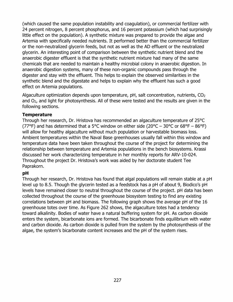
227
(which caused the same population instability and coagulation), or commercial fertilizer with 24 percent nitrogen, 8 percent phosphorus, and 16 percent potassium (which had surprisingly little effect on the population). A synthetic mixture was prepared to provide the algae and Artemia with specifically needed nutrients. It performed better than the commercial fertilizer or the non-neutralized glycerin feeds, but not as well as the AD effluent or the neutralized glycerin. An interesting point of comparison between the synthetic nutrient blend and the anaerobic digester effluent is that the synthetic nutrient mixture had many of the same chemicals that are needed to maintain a healthy microbial colony in anaerobic digestion. In anaerobic digestion systems, many of these non-organic compounds pass through the digester and stay with the effluent. This helps to explain the observed similarities in the synthetic blend and the digestate and helps to explain why the effluent has such a good effect on Artemia populations.
Algaculture optimization depends upon temperature, pH, salt concentration, nutrients, CO2 and O2, and light for photosynthesis. All of these were tested and the results are given in the following sections.
Temperature Through her research, Dr. Hristova has recommended an algaculture temperature of 25°C (77°F) and has determined that a 5°C window on either side (20°C – 30°C or 68°F – 86°F) will allow for healthy algaculture without much population or harvestable biomass loss. Ambient temperatures within the Naval Base greenhouses usually fall within this window and temperature data have been taken throughout the course of the project for determining the relationship between temperature and Artemia populations in the bench biosystems. Krassi discussed her work characterizing temperature in her monthly reports for ARV-10-024. Throughout the project Dr. Hristova’s work was aided by her doctorate student Tee Paprakorn. pH Through her research, Dr. Hristova has found that algal populations will remain stable at a pH level up to 8.5. Though the glycerin tested as a feedstock has a pH of about 9, Biodico’s pH levels have remained closer to neutral throughout the course of the project. pH data has been collected throughout the course of the greenhouse biosystem testing to find any existing correlations between pH and biomass. The following graph shows the average pH of the 16 greenhouse totes over time. As Figure 262 shows, the algaculture totes had a tendency toward alkalinity. Bodies of water have a natural buffering system for pH. As carbon dioxide enters the system, bicarbonate ions are formed. The bicarbonate finds equilibrium with water and carbon dioxide. As carbon dioxide is pulled from the system by the photosynthesis of the algae, the system’s bicarbonate content increases and the pH of the system rises.
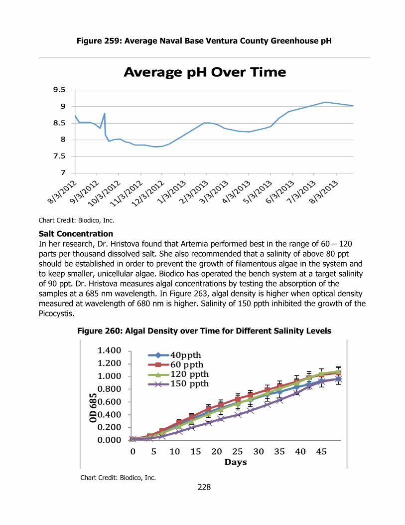
228
Figure 259: Average Naval Base Ventura County Greenhouse pH
Chart Credit: Biodico, Inc.
Salt Concentration In her research, Dr. Hristova found that Artemia performed best in the range of 60 – 120 parts per thousand dissolved salt. She also recommended that a salinity of above 80 ppt should be established in order to prevent the growth of filamentous algae in the system and to keep smaller, unicellular algae. Biodico has operated the bench system at a target salinity of 90 ppt. Dr. Hristova measures algal concentrations by testing the absorption of the samples at a 685 nm wavelength. In Figure 263, algal density is higher when optical density measured at wavelength of 680 nm is higher. Salinity of 150 ppth inhibited the growth of the Picocystis.
Figure 260: Algal Density over Time for Different Salinity Levels
Chart Credit: Biodico, Inc.

229
Nutrients Of the different carbon sources that Dr. Hristova tested throughout the course of her research, she found that glycerin performed the best in boosting algacultural yields. It is worth noting from the following chart that sodium acetate also performed well. Acetate is one of the final chemical stages of organic compounds in an anaerobic digester before they are converted into methane and carbon dioxide. Digestate leaving an anaerobic digester will very likely have between 0.5 percent and 1.0 percent acetate content as measured by volatile fatty acids. The glycerin that Krassi used for these tests was pure glycerol and not producers’ grade glycerin. Test results are given in Figure 264 below.
Figure 261: Performance of Different Nutrients on Algal Population Growth
Chart Credit: Biodico, Inc.
Dr. Hristova also found that the increased biomass yields from glycerin were present in water with and without additional nutrients. In the Figure 265 below, the baseline is given at the bottom as sample BG11. The contributions from any of the carbon sources greatly enhanced the algal growth. The doubling time given for the baseline falls about midway in the range of doubling times given for the light energy testing later in this section.
Figure 265: Effects of Glycerin on Algal Growth in Various Nutrient Mediums
Chart Credit: Biodico, Inc.
In cases where the glycerin is used to create algal growth that then in turn feeds the Artemia, Dr. Hristova found that one gram per liter of glycerin weekly will allow for the highest population density. The glycerin that Dr. Hristova used was pure glycerol rather than producers’ grade glycerol from biodiesel production and the laboratory population was thoroughly aerated. The following Figure 266 shows her results.
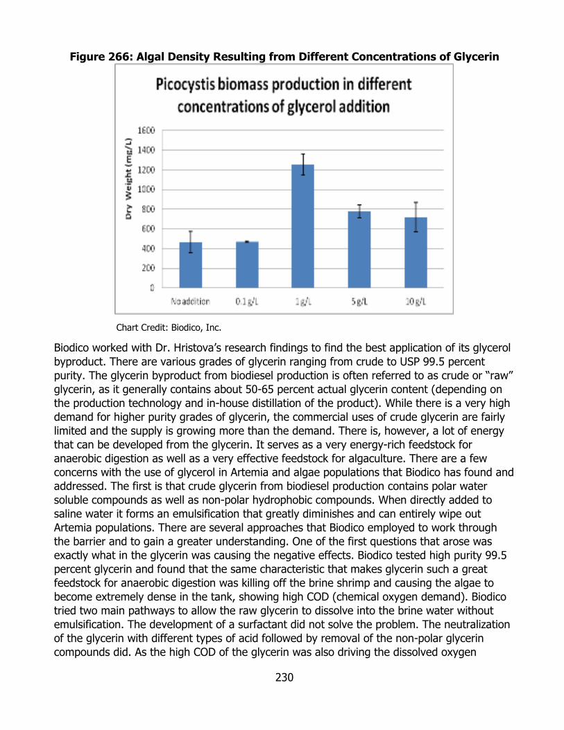
230
Figure 266: Algal Density Resulting from Different Concentrations of Glycerin
Chart Credit: Biodico, Inc.
Biodico worked with Dr. Hristova’s research findings to find the best application of its glycerol byproduct. There are various grades of glycerin ranging from crude to USP 99.5 percent purity. The glycerin byproduct from biodiesel production is often referred to as crude or “raw” glycerin, as it generally contains about 50-65 percent actual glycerin content (depending on the production technology and in-house distillation of the product). While there is a very high demand for higher purity grades of glycerin, the commercial uses of crude glycerin are fairly limited and the supply is growing more than the demand. There is, however, a lot of energy that can be developed from the glycerin. It serves as a very energy-rich feedstock for anaerobic digestion as well as a very effective feedstock for algaculture. There are a few concerns with the use of glycerol in Artemia and algae populations that Biodico has found and addressed. The first is that crude glycerin from biodiesel production contains polar water soluble compounds as well as non-polar hydrophobic compounds. When directly added to saline water it forms an emulsification that greatly diminishes and can entirely wipe out Artemia populations. There are several approaches that Biodico employed to work through the barrier and to gain a greater understanding. One of the first questions that arose was exactly what in the glycerin was causing the negative effects. Biodico tested high purity 99.5 percent glycerin and found that the same characteristic that makes glycerin such a great feedstock for anaerobic digestion was killing off the brine shrimp and causing the algae to become extremely dense in the tank, showing high COD (chemical oxygen demand). Biodico tried two main pathways to allow the raw glycerin to dissolve into the brine water without emulsification. The development of a surfactant did not solve the problem. The neutralization of the glycerin with different types of acid followed by removal of the non-polar glycerin compounds did. As the high COD of the glycerin was also driving the dissolved oxygen
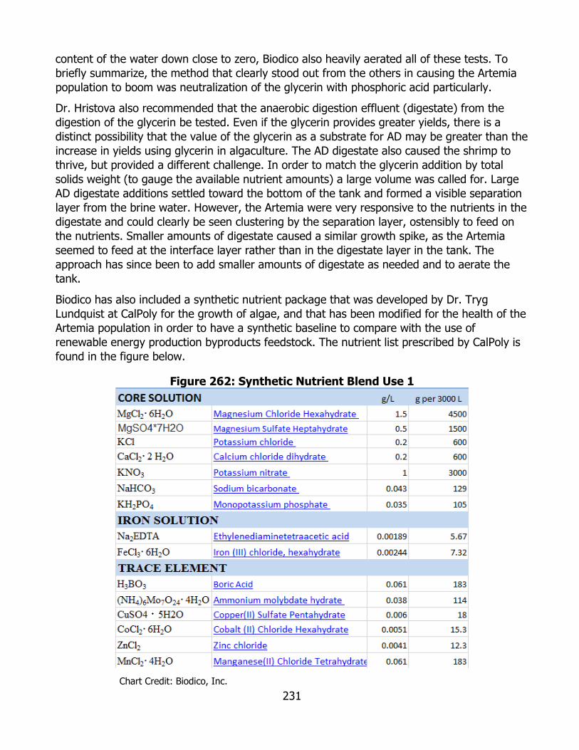
231
content of the water down close to zero, Biodico also heavily aerated all of these tests. To briefly summarize, the method that clearly stood out from the others in causing the Artemia population to boom was neutralization of the glycerin with phosphoric acid particularly.
Dr. Hristova also recommended that the anaerobic digestion effluent (digestate) from the digestion of the glycerin be tested. Even if the glycerin provides greater yields, there is a distinct possibility that the value of the glycerin as a substrate for AD may be greater than the increase in yields using glycerin in algaculture. The AD digestate also caused the shrimp to thrive, but provided a different challenge. In order to match the glycerin addition by total solids weight (to gauge the available nutrient amounts) a large volume was called for. Large AD digestate additions settled toward the bottom of the tank and formed a visible separation layer from the brine water. However, the Artemia were very responsive to the nutrients in the digestate and could clearly be seen clustering by the separation layer, ostensibly to feed on the nutrients. Smaller amounts of digestate caused a similar growth spike, as the Artemia seemed to feed at the interface layer rather than in the digestate layer in the tank. The approach has since been to add smaller amounts of digestate as needed and to aerate the tank.
Biodico has also included a synthetic nutrient package that was developed by Dr. Tryg Lundquist at CalPoly for the growth of algae, and that has been modified for the health of the Artemia population in order to have a synthetic baseline to compare with the use of renewable energy production byproducts feedstock. The nutrient list prescribed by CalPoly is found in the figure below.
Figure 262: Synthetic Nutrient Blend Use 1
Chart Credit: Biodico, Inc.
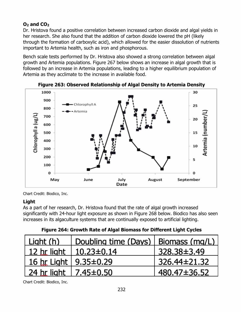
232
O2 and CO2 Dr. Hristova found a positive correlation between increased carbon dioxide and algal yields in her research. She also found that the addition of carbon dioxide lowered the pH (likely through the formation of carboxylic acid), which allowed for the easier dissolution of nutrients important to Artemia health, such as iron and phosphorous.
Bench scale tests performed by Dr. Hristova also showed a strong correlation between algal growth and Artemia populations. Figure 267 below shows an increase in algal growth that is followed by an increase in Artemia populations, leading to a higher equilibrium population of Artemia as they acclimate to the increase in available food.
Figure 263: Observed Relationship of Algal Density to Artemia Density
Chart Credit: Biodico, Inc.
Light As a part of her research, Dr. Hristova found that the rate of algal growth increased significantly with 24-hour light exposure as shown in Figure 268 below. Biodico has also seen increases in its algaculture systems that are continually exposed to artificial lighting.
Figure 264: Growth Rate of Algal Biomass for Different Light Cycles
Chart Credit: Biodico, Inc.
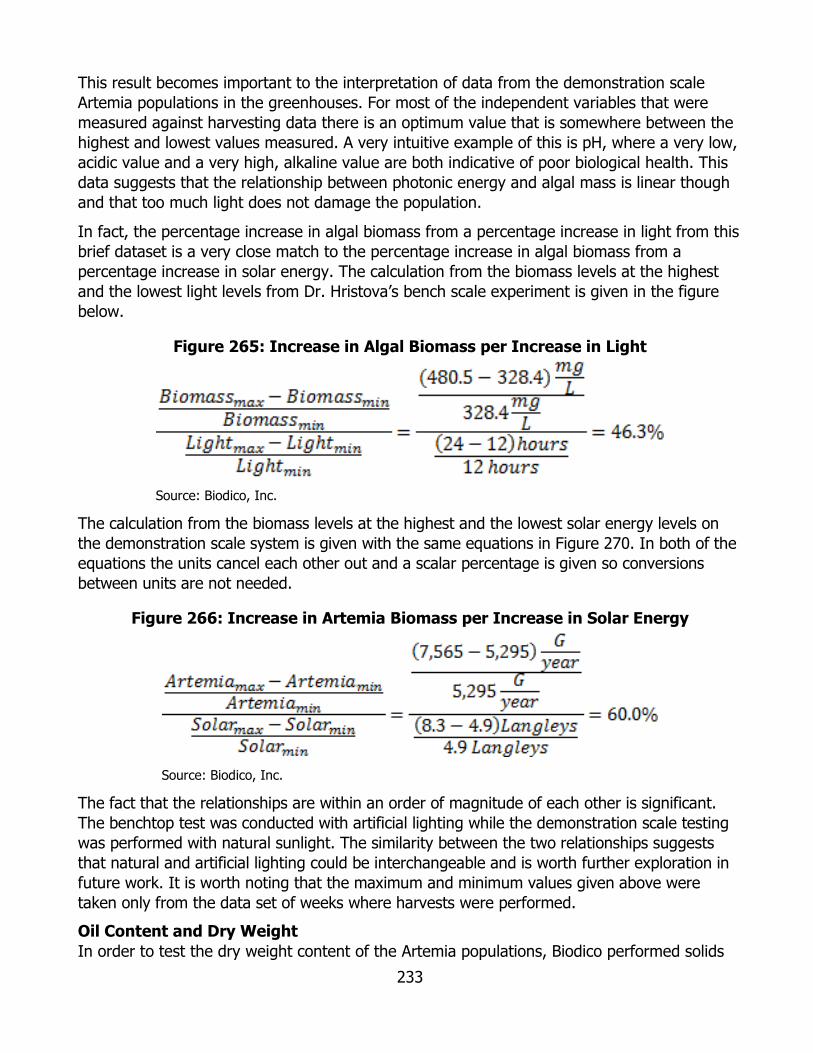
233
This result becomes important to the interpretation of data from the demonstration scale Artemia populations in the greenhouses. For most of the independent variables that were measured against harvesting data there is an optimum value that is somewhere between the highest and lowest values measured. A very intuitive example of this is pH, where a very low, acidic value and a very high, alkaline value are both indicative of poor biological health. This data suggests that the relationship between photonic energy and algal mass is linear though and that too much light does not damage the population.
In fact, the percentage increase in algal biomass from a percentage increase in light from this brief dataset is a very close match to the percentage increase in algal biomass from a percentage increase in solar energy. The calculation from the biomass levels at the highest and the lowest light levels from Dr. Hristova’s bench scale experiment is given in the figure below.
Figure 265: Increase in Algal Biomass per Increase in Light
Source: Biodico, Inc.
The calculation from the biomass levels at the highest and the lowest solar energy levels on the demonstration scale system is given with the same equations in Figure 270. In both of the equations the units cancel each other out and a scalar percentage is given so conversions between units are not needed.
Figure 266: Increase in Artemia Biomass per Increase in Solar Energy
Source: Biodico, Inc.
The fact that the relationships are within an order of magnitude of each other is significant. The benchtop test was conducted with artificial lighting while the demonstration scale testing was performed with natural sunlight. The similarity between the two relationships suggests that natural and artificial lighting could be interchangeable and is worth further exploration in future work. It is worth noting that the maximum and minimum values given above were taken only from the data set of weeks where harvests were performed. Oil Content and Dry Weight In order to test the dry weight content of the Artemia populations, Biodico performed solids
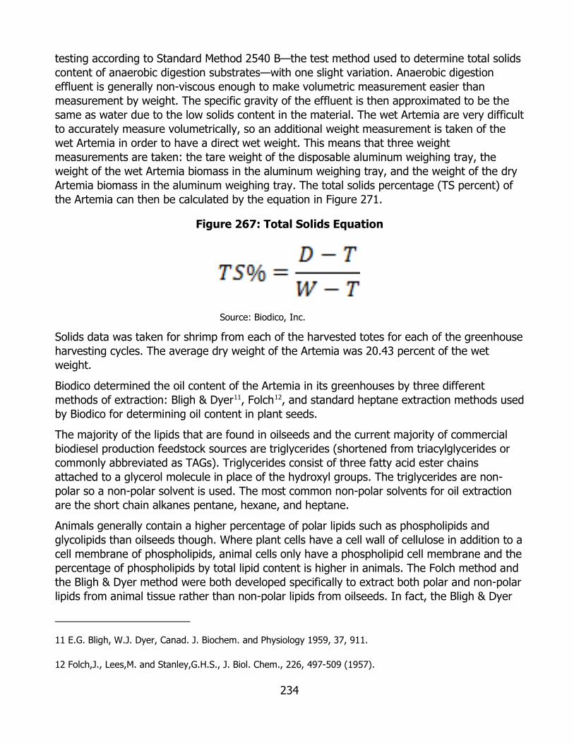
234
testing according to Standard Method 2540 B—the test method used to determine total solids content of anaerobic digestion substrates—with one slight variation. Anaerobic digestion effluent is generally non-viscous enough to make volumetric measurement easier than measurement by weight. The specific gravity of the effluent is then approximated to be the same as water due to the low solids content in the material. The wet Artemia are very difficult to accurately measure volumetrically, so an additional weight measurement is taken of the wet Artemia in order to have a direct wet weight. This means that three weight measurements are taken: the tare weight of the disposable aluminum weighing tray, the weight of the wet Artemia biomass in the aluminum weighing tray, and the weight of the dry Artemia biomass in the aluminum weighing tray. The total solids percentage (TS percent) of the Artemia can then be calculated by the equation in Figure 271.
Figure 267: Total Solids Equation
Source: Biodico, Inc.
Solids data was taken for shrimp from each of the harvested totes for each of the greenhouse harvesting cycles. The average dry weight of the Artemia was 20.43 percent of the wet weight.
Biodico determined the oil content of the Artemia in its greenhouses by three different methods of extraction: Bligh & Dyer11, Folch12, and standard heptane extraction methods used by Biodico for determining oil content in plant seeds.
The majority of the lipids that are found in oilseeds and the current majority of commercial biodiesel production feedstock sources are triglycerides (shortened from triacylglycerides or commonly abbreviated as TAGs). Triglycerides consist of three fatty acid ester chains attached to a glycerol molecule in place of the hydroxyl groups. The triglycerides are non-polar so a non-polar solvent is used. The most common non-polar solvents for oil extraction are the short chain alkanes pentane, hexane, and heptane.
Animals generally contain a higher percentage of polar lipids such as phospholipids and glycolipids than oilseeds though. Where plant cells have a cell wall of cellulose in addition to a cell membrane of phospholipids, animal cells only have a phospholipid cell membrane and the percentage of phospholipids by total lipid content is higher in animals. The Folch method and the Bligh & Dyer method were both developed specifically to extract both polar and non-polar lipids from animal tissue rather than non-polar lipids from oilseeds. In fact, the Bligh & Dyer
11 E.G. Bligh, W.J. Dyer, Canad. J. Biochem. and Physiology 1959, 37, 911.
12 Folch,J., Lees,M. and Stanley,G.H.S., J. Biol. Chem., 226, 497-509 (1957).
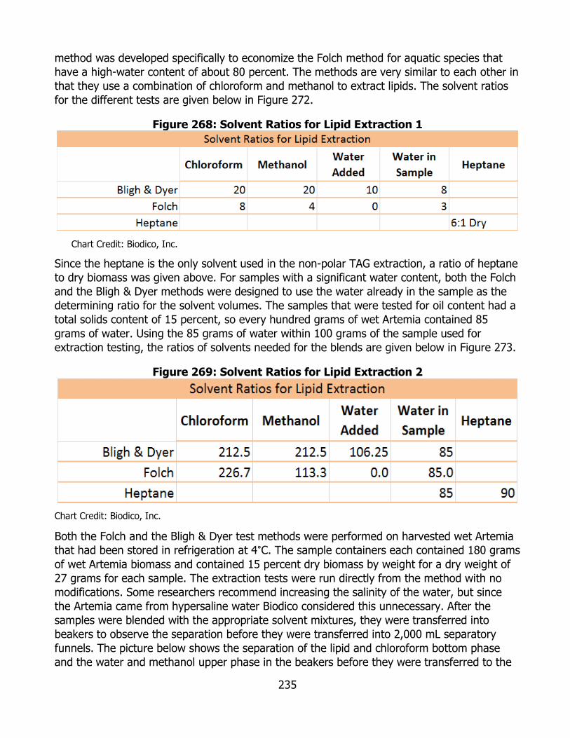
235
method was developed specifically to economize the Folch method for aquatic species that have a high-water content of about 80 percent. The methods are very similar to each other in that they use a combination of chloroform and methanol to extract lipids. The solvent ratios for the different tests are given below in Figure 272.
Figure 268: Solvent Ratios for Lipid Extraction 1
Chart Credit: Biodico, Inc.
Since the heptane is the only solvent used in the non-polar TAG extraction, a ratio of heptane to dry biomass was given above. For samples with a significant water content, both the Folch and the Bligh & Dyer methods were designed to use the water already in the sample as the determining ratio for the solvent volumes. The samples that were tested for oil content had a total solids content of 15 percent, so every hundred grams of wet Artemia contained 85 grams of water. Using the 85 grams of water within 100 grams of the sample used for extraction testing, the ratios of solvents needed for the blends are given below in Figure 273.
Figure 269: Solvent Ratios for Lipid Extraction 2
Chart Credit: Biodico, Inc.
Both the Folch and the Bligh & Dyer test methods were performed on harvested wet Artemia that had been stored in refrigeration at 4°C. The sample containers each contained 180 grams of wet Artemia biomass and contained 15 percent dry biomass by weight for a dry weight of 27 grams for each sample. The extraction tests were run directly from the method with no modifications. Some researchers recommend increasing the salinity of the water, but since the Artemia came from hypersaline water Biodico considered this unnecessary. After the samples were blended with the appropriate solvent mixtures, they were transferred into beakers to observe the separation before they were transferred into 2,000 mL separatory funnels. The picture below shows the separation of the lipid and chloroform bottom phase and the water and methanol upper phase in the beakers before they were transferred to the

236
separatory funnels (Figurre 274). The samples in the picture had not yet been filtered, so there is a clear layer of biomass between the two phases. The images are from two separate pictures and not to scale, so the perceived volumes are different.
Figure 270: Lipid Extraction Separations
Photo Credit: Biodico, Inc.
For both test methods the lipids remain in the chloroform containing bottom phase. Usually in a phase separation between a lipid containing solution and a water-containing solution, the bottom phase will contain the water and other hydrophilic compounds and the top phase will contain the lipids. For both the Folch and Bligh & Dyer methods though, the lipids solubilize in the chloroform phase and the high specific gravity of the chloroform causes the lipids to collect in the bottom phase. After the separation was confirmed, the samples were transferred to separatory funnels and allowed to separate overnight. After the separation, the lipid containing bottom phase was filtered and transferred into graduated cylinders for more accurate volumetric readings. In Figure 275 below the lipid phase of the Folch extraction is on the left and the lipid phase of the Bligh & Dyer extraction is on the right. The volumes of the two-lipid containing non-polar phases are 248 mL and 229 mL respectively.
Figure 271: Lipid Extraction
Photo Credit: Biodico, Inc.

237
A representative 10 mL sample was taken from each of the solvent/lipid solutions and the chloroform was evaporated from the sample. The calculation of the oil content in the solution is the same as the calculation of solids in AD effluent except instead of wet weight we are measuring solution weight and instead of total solids we are determining total lipids. The results of each of the thermogravimetric tests are given in Figures 276-278.
Figure 272: Weight Percent of Lipids in Solution
Chart Credit: Biodico, Inc.
As the chart above shows, the percentage of lipids in the chloroform solvent containing solution by weight are 0.99 percent for Bligh & Dyer and 0.90 percent for Folch. We can then calculate the percentage of lipids in the wet and the dry Artemia biomass with the percentage of lipids in the solution, the volume of the lipid/solvent phases, and the wet and dry weights of the original sample. The conversions are displayed below.
Figure 273: Percent Lipids in Dry Artemia by Weight
Chart Credit: Biodico, Inc.
Both the Folch and the Bligh & Dyer methods were developed to extract both polar and non-polar lipids from animal tissue. Most of Biodico’s work in the past has been based on the extraction of non-polar TAGs using a non-polar solvent. In most cases Biodico has used heptane. The use of heptane was originally established because Biodico uses heptane as a

238
dilution liquid in its gas chromatography samples to test for glycerin content in biodiesel and has a lot of experience with the chemical and how it behaves with TAGs.
Biodico performed a heptane extraction on the Artemia in order to determine the ratio of non-polar lipids to total lipids. By using a non-polar solvent on the dry biomass, the polar phospholipids were ostensibly not extracted and were not solubilized in the heptane. In order to ensure accuracy, a conservative ratio of 6:1 heptane to dry Artemia biomass by weight was used which gave a ratio of roughly 30:1 heptane to total lipids. 100 grams of dry Artemia biomass was mixed with 600 grams of heptane and left in a 1,000 separatory funnel to separate overnight. The solvent/lipid solution and biomass were then filtered, and two samples of the solution were prepared for lipid content testing. For the two samples Biodico used different solution volumes and different sizes of graduated cylinders, 10 mL and 25 mL. The results of the testing are displayed below.
Figure 274: Percent Lipids in Dry Artemia by Weight 2
Chart Credit: Biodico, Inc.
The average percentage of non-polar lipids in Artemia was then 13.75 percent. The average oil percentage returned by the Bligh & Dyer method and the Folch method was 19.67 percent. We can now define the percentage of non-polar lipids in the total Artemia lipids as:
Figure 275: Polar Lipid Percentage
Source: Biodico, Inc.
Both the polar and the non-polar lipids contain fatty acid ester chains that will produce biodiesel. Understanding the ratio of polar to non-polar lipids is useful to Biodico’s future work though as the ratio may affect several analytical and production variables.
For the purpose of extrapolating the total oil content of Artemia populations as a potential for fuel production, the chloroform solvent methods are more accurate. Their average is 19.67 percent by weight. Harvesting Biodico conducted harvesting tests between June 9th 2012 and January 3rd 2014. The harvesting was performed in the bench scale algaculture unit consisting of four interconnected greenhouses with four 330 gallon totes each for a total of 16 totes. The totes were all plumbed from the bottom outlets and through common manifolds to the inlet of a

239
dual diaphragm pump. Each tote has a butterfly valve that allows for mixing in the system to be isolated or combined and for transfer of liquid between totes. The outlet side of the pump rises roughly seven feet and is plumbed through common manifolds to provide access to each of the four greenhouses. The pipe in each greenhouse runs along three of the four walls in a horseshoe shape. Standard tee fittings provide a branch outlet to three of the four totes, and the pipe loop inside of each greenhouse terminates at the last tote. The pipes are made of PVC. The dual diaphragm pump is manufactured by Keco and circulates water in the greenhouse at roughly 20 gallons per minute.
The goals of the project were to maximize the total harvestable biomass of Artemia over time and to characterize the effects of variables of interest to the system. Biodico was interested in the effect of both dependent and independent variables on the harvestable Artemia. In this context, dependent variables are those that were not specifically changed by the experimenters in order to try to boost biomass production rates. Rather, they were tracked regularly as a part of the greenhouse operation and correlations between biomass and algae were based on the naturally occurring data. The partial exception to this would be salinity. Salinity levels were specifically targeted at 90 parts per thousand (90,000 parts per million) and were sometimes adjusted throughout the course of the experiment to hit the target. Since there was no intention to change the salinity levels dramatically in order to measure the output of Artemia growth though, the dependent descriptor for salinity is more accurate. Other dependent variables included temperature, solar energy, and pH.
The dependent variables were specifically targeted and changed in an effort to boost the biomass output of the system. The dependent variables were mesh size, feed type, and feed volume. Much more so than chemical or physical processes, biological processes can be variable and difficult to replicate. For this reason, Biodico chose to strictly limit the testing of dependent variables so that their effect could be more easily isolated and quantified. A list of the independent and dependent variables is given below in Figure 280.
Figure 276: Harvesting Variables
Chart Credit: Biodico, Inc.
Over the course of the 18-month period of greenhouse operation, 28 separate harvest tests were performed. Of these 28 weeks of harvesting data, 4 weeks were used to ensure that the system was stable and that Artemia populations had been established, 8 weeks were used to determine the ideal mesh size for long-term harvesting, 4 weeks were used to determine the
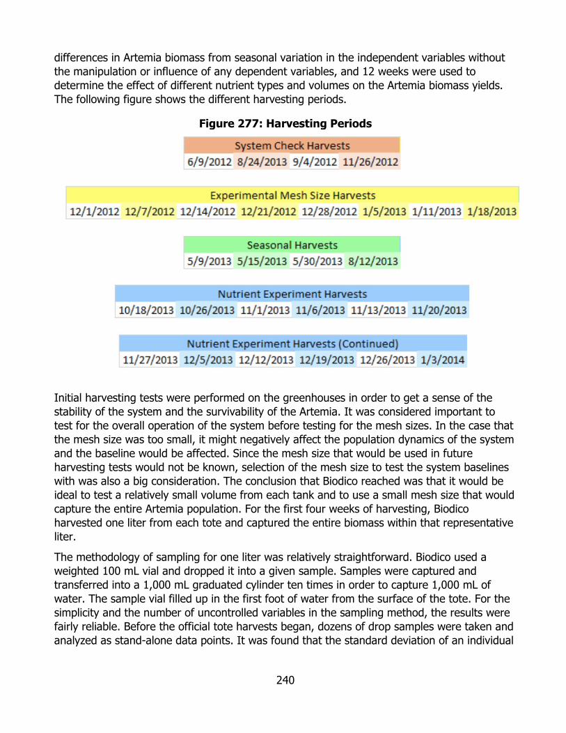
240
differences in Artemia biomass from seasonal variation in the independent variables without the manipulation or influence of any dependent variables, and 12 weeks were used to determine the effect of different nutrient types and volumes on the Artemia biomass yields. The following figure shows the different harvesting periods.
Figure 277: Harvesting Periods
Initial harvesting tests were performed on the greenhouses in order to get a sense of the stability of the system and the survivability of the Artemia. It was considered important to test for the overall operation of the system before testing for the mesh sizes. In the case that the mesh size was too small, it might negatively affect the population dynamics of the system and the baseline would be affected. Since the mesh size that would be used in future harvesting tests would not be known, selection of the mesh size to test the system baselines with was also a big consideration. The conclusion that Biodico reached was that it would be ideal to test a relatively small volume from each tank and to use a small mesh size that would capture the entire Artemia population. For the first four weeks of harvesting, Biodico harvested one liter from each tote and captured the entire biomass within that representative liter.
The methodology of sampling for one liter was relatively straightforward. Biodico used a weighted 100 mL vial and dropped it into a given sample. Samples were captured and transferred into a 1,000 mL graduated cylinder ten times in order to capture 1,000 mL of water. The sample vial filled up in the first foot of water from the surface of the tote. For the simplicity and the number of uncontrolled variables in the sampling method, the results were fairly reliable. Before the official tote harvests began, dozens of drop samples were taken and analyzed as stand-alone data points. It was found that the standard deviation of an individual
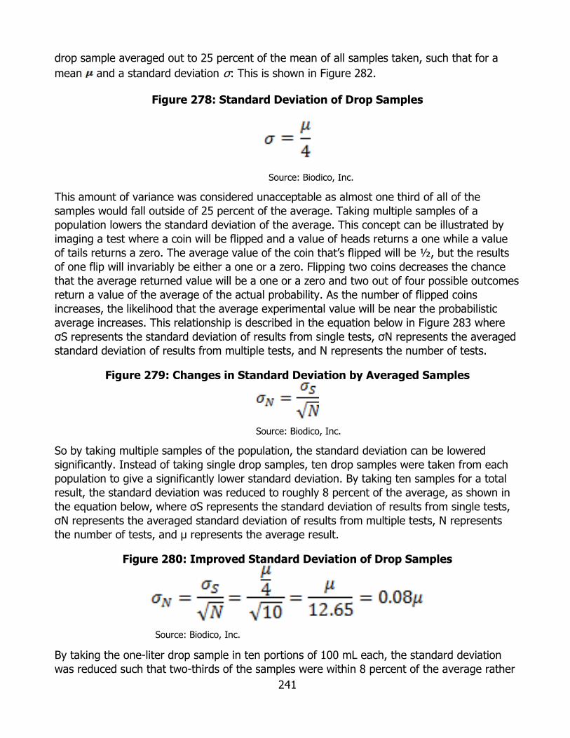
241
drop sample averaged out to 25 percent of the mean of all samples taken, such that for a mean and a standard deviation σ: This is shown in Figure 282.
Figure 278: Standard Deviation of Drop Samples
Source: Biodico, Inc.
This amount of variance was considered unacceptable as almost one third of all of the samples would fall outside of 25 percent of the average. Taking multiple samples of a population lowers the standard deviation of the average. This concept can be illustrated by imaging a test where a coin will be flipped and a value of heads returns a one while a value of tails returns a zero. The average value of the coin that’s flipped will be ½, but the results of one flip will invariably be either a one or a zero. Flipping two coins decreases the chance that the average returned value will be a one or a zero and two out of four possible outcomes return a value of the average of the actual probability. As the number of flipped coins increases, the likelihood that the average experimental value will be near the probabilistic average increases. This relationship is described in the equation below in Figure 283 where σS represents the standard deviation of results from single tests, σN represents the averaged standard deviation of results from multiple tests, and N represents the number of tests.
Figure 279: Changes in Standard Deviation by Averaged Samples
Source: Biodico, Inc.
So by taking multiple samples of the population, the standard deviation can be lowered significantly. Instead of taking single drop samples, ten drop samples were taken from each population to give a significantly lower standard deviation. By taking ten samples for a total result, the standard deviation was reduced to roughly 8 percent of the average, as shown in the equation below, where σS represents the standard deviation of results from single tests, σN represents the averaged standard deviation of results from multiple tests, N represents the number of tests, and μ represents the average result.
Figure 280: Improved Standard Deviation of Drop Samples
Source: Biodico, Inc.
By taking the one-liter drop sample in ten portions of 100 mL each, the standard deviation was reduced such that two-thirds of the samples were within 8 percent of the average rather

242
than 25 percent. For the multi-sample test method as a whole then, the biomass per liter fell within 8 percent of the mean 68 percent of the time, 16 percent of the mean 95 percent of the time, and 24 percent of the mean 99.75 percent of the time.
The rest of the harvests were performed by circulating each of the totes individually through a dual diaphragm pump. The dual diaphragm pump used by Biodico is a Keco model 800 as pictured in Figure 285.
Figure 281: Keco Model 800 Dual Diaphragm Pump
Photo Credit: KECO
A diaphragm style pump was chosen to ensure the survivability of the Artemia going through the pump. Other types of pumps, such as centrifugal pumps, would have had a very high Artemia mortality rate. The disadvantage of harvesting by continuous recirculation is that the pump speed differs substantially from the speed at which the volumes are actually recirculated. This can be illustrated by imagining a scenario where half of the tote is pumped out of the system, then put back into the system, and then half of the tote is pumped out again. Fluid engineering dictates that the dispersion of roughly homogenous liquids added to a system should be calculated as instantaneous, which given the agitation of the system is not a very unrealistic expectation. In the example above where the volume is broken into two discrete chunks, 50 percent of the volume is circulated out of the system, so 0 percent of the volume remaining in the system has passed through the pump. Then it is re-added to the system so that 50 percent of the total volume has passed through the pump. If half of the system is pumped out again then 25 percent of the fluid will have passed through the pump twice, 50 percent will have been passed through once, and 25 percent of the fluid will not have been passed through the pump. For any number of discrete chunks that the
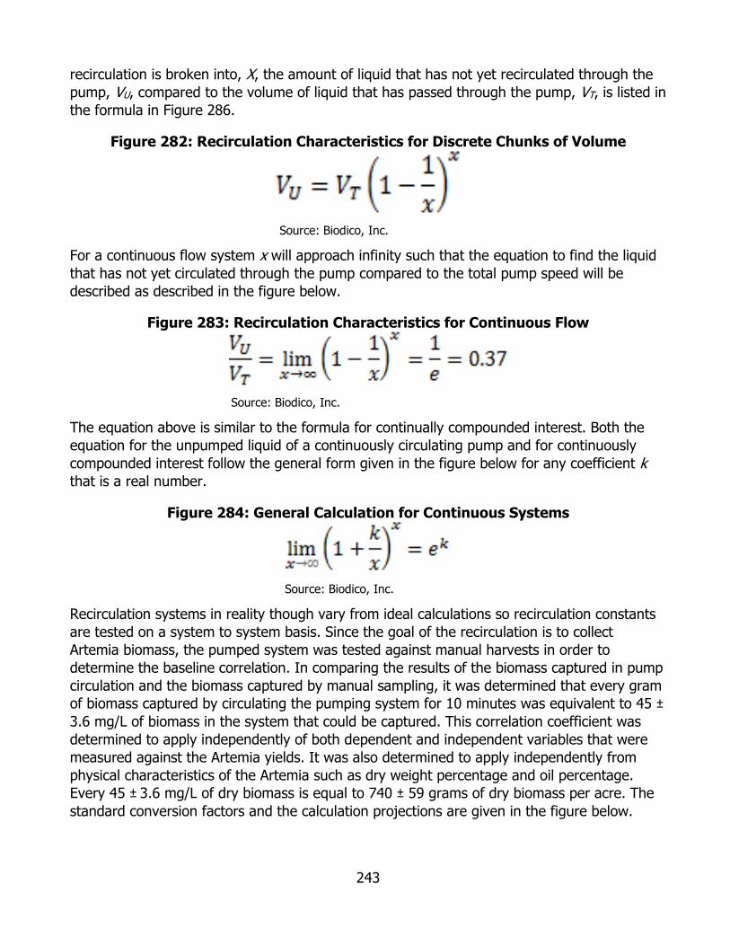
243
recirculation is broken into, X, the amount of liquid that has not yet recirculated through the pump, VU, compared to the volume of liquid that has passed through the pump, VT, is listed in the formula in Figure 286.
Figure 282: Recirculation Characteristics for Discrete Chunks of Volume
Source: Biodico, Inc.
For a continuous flow system x will approach infinity such that the equation to find the liquid that has not yet circulated through the pump compared to the total pump speed will be described as described in the figure below.
Figure 283: Recirculation Characteristics for Continuous Flow
Source: Biodico, Inc.
The equation above is similar to the formula for continually compounded interest. Both the equation for the unpumped liquid of a continuously circulating pump and for continuously compounded interest follow the general form given in the figure below for any coefficient k that is a real number.
Figure 284: General Calculation for Continuous Systems
Source: Biodico, Inc.
Recirculation systems in reality though vary from ideal calculations so recirculation constants are tested on a system to system basis. Since the goal of the recirculation is to collect Artemia biomass, the pumped system was tested against manual harvests in order to determine the baseline correlation. In comparing the results of the biomass captured in pump circulation and the biomass captured by manual sampling, it was determined that every gram of biomass captured by circulating the pumping system for 10 minutes was equivalent to 45 ± 3.6 mg/L of biomass in the system that could be captured. This correlation coefficient was determined to apply independently of both dependent and independent variables that were measured against the Artemia yields. It was also determined to apply independently from physical characteristics of the Artemia such as dry weight percentage and oil percentage. Every 45 ± 3.6 mg/L of dry biomass is equal to 740 ± 59 grams of dry biomass per acre. The standard conversion factors and the calculation projections are given in the figure below.

244
Figure 285: Table of Commonly Used Conversions
Chart Credit: Biodico, Inc.
The standard conversion factors can be used to calculate the number of tote volumes that would make up an acre. The water depth of each of the 330 gallon totes is 52 inches and the surface area is just below a square meter. All of the dimension conversions are given in Figure 290 and 291 below.
Figure 286: Tote Dimensions
Chart Credit: Biodico, Inc.
Starting with the mg of dry Artemia biomass per liter, the conversion tables above can be used to calculate the weight of dry Artemia biomass per acre that will be yielded from a given concentration per liter. The rough alignment will be shown in the next section.

245
Figure 287: Conversion from Liters to Acres
Chart Credit: Biodico, Inc.
From this the annual grams of dry biomass per acre can be calculated as follows in Figure 292.
Figure 288: Weekly Kilograms to Annual Kilograms per Acre
Chart Credit: Biodico, Inc.
Based on the oil content that was confirmed by the Bligh & Dyer test and the Folch test, the oil yield per acre can be calculated as in Figure 293.
Figure 289: Kilograms of Dry Biomass to Gallons of Artemia Oil
Chart Credit: Biodico, Inc.
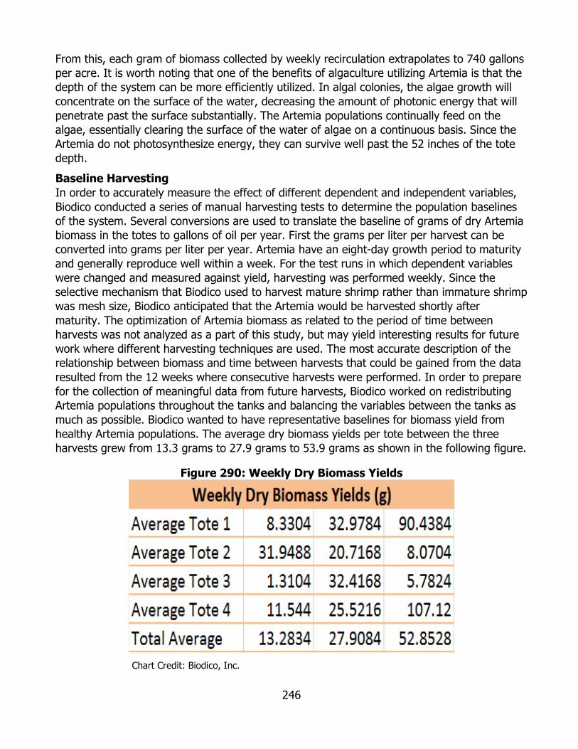
246
From this, each gram of biomass collected by weekly recirculation extrapolates to 740 gallons per acre. It is worth noting that one of the benefits of algaculture utilizing Artemia is that the depth of the system can be more efficiently utilized. In algal colonies, the algae growth will concentrate on the surface of the water, decreasing the amount of photonic energy that will penetrate past the surface substantially. The Artemia populations continually feed on the algae, essentially clearing the surface of the water of algae on a continuous basis. Since the Artemia do not photosynthesize energy, they can survive well past the 52 inches of the tote depth. Baseline Harvesting In order to accurately measure the effect of different dependent and independent variables, Biodico conducted a series of manual harvesting tests to determine the population baselines of the system. Several conversions are used to translate the baseline of grams of dry Artemia biomass in the totes to gallons of oil per year. First the grams per liter per harvest can be converted into grams per liter per year. Artemia have an eight-day growth period to maturity and generally reproduce well within a week. For the test runs in which dependent variables were changed and measured against yield, harvesting was performed weekly. Since the selective mechanism that Biodico used to harvest mature shrimp rather than immature shrimp was mesh size, Biodico anticipated that the Artemia would be harvested shortly after maturity. The optimization of Artemia biomass as related to the period of time between harvests was not analyzed as a part of this study, but may yield interesting results for future work where different harvesting techniques are used. The most accurate description of the relationship between biomass and time between harvests that could be gained from the data resulted from the 12 weeks where consecutive harvests were performed. In order to prepare for the collection of meaningful data from future harvests, Biodico worked on redistributing Artemia populations throughout the tanks and balancing the variables between the tanks as much as possible. Biodico wanted to have representative baselines for biomass yield from healthy Artemia populations. The average dry biomass yields per tote between the three harvests grew from 13.3 grams to 27.9 grams to 53.9 grams as shown in the following figure.
Figure 290: Weekly Dry Biomass Yields
Chart Credit: Biodico, Inc.

247
Mesh Test Harvesting After establishing the baselines, Biodico sought to optimize the first independent variable for the algaculture system and performed harvesting tests to determine the best technique and mesh size for the long-term survivability of the tank populations. In short, Biodico hopes to be able to harvest the adult Artemia that have reproduced while leaving the juveniles that have yet to reproduce in the tank. The mesh size that was experimentally validated by Biodico for long-term population maximums ended up falling within 10 percent of the mesh size currently used in commercial Artemia harvesting operations in Mono Lake. Biodico performed tests with 800, 1,000, 1,320, 2,000, and 3,000 micron size mesh and found the best long term sustainable harvesting resulted from the 1,320 micron mesh size. The pie chart below in Figure 295 shows the cumulative percentage of the Artemia population that was captured by each net size in decreasing microns (as a function of dry weight, not as a count of individual Artemia). For example, 22 percent of the Artemia population was captured by the 1,000 micron netting after 60 percent had already been captured by the 1,320 micron netting. Ostensibly, if only the 1,000 micron net were used, and not the 1,320 micron net, the 1,000 micron net would have captured 82 percent of the population. Rather than working as a predictive method for chance, the population spread is attributable to the different sizes that the Artemia reach as the population matures heterogeneously. Six percent of the Artemia population by mass was not captured by the smallest 800 micron size netting. Since these Artemia were the smallest in the population, this six percent by mass represents a larger percentage by count of individual Artemia.
Figure 291: Incremental Portion of Artemia Populations Captured by Micron Size of Harvesting Net
Chart Credit: Biodico, Inc.
The pie chart was compiled from bench scale tests where the entire test population could fit in laboratory containers and could be easily handled by the analyst. In order to verify the bench scale results, harvesting tests were performed on the much larger populations in the
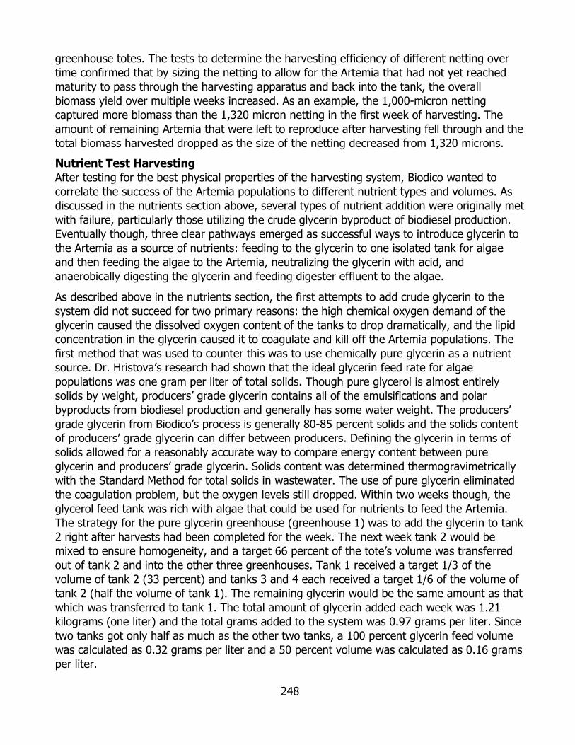
248
greenhouse totes. The tests to determine the harvesting efficiency of different netting over time confirmed that by sizing the netting to allow for the Artemia that had not yet reached maturity to pass through the harvesting apparatus and back into the tank, the overall biomass yield over multiple weeks increased. As an example, the 1,000-micron netting captured more biomass than the 1,320 micron netting in the first week of harvesting. The amount of remaining Artemia that were left to reproduce after harvesting fell through and the total biomass harvested dropped as the size of the netting decreased from 1,320 microns. Nutrient Test Harvesting After testing for the best physical properties of the harvesting system, Biodico wanted to correlate the success of the Artemia populations to different nutrient types and volumes. As discussed in the nutrients section above, several types of nutrient addition were originally met with failure, particularly those utilizing the crude glycerin byproduct of biodiesel production. Eventually though, three clear pathways emerged as successful ways to introduce glycerin to the Artemia as a source of nutrients: feeding to the glycerin to one isolated tank for algae and then feeding the algae to the Artemia, neutralizing the glycerin with acid, and anaerobically digesting the glycerin and feeding digester effluent to the algae.
As described above in the nutrients section, the first attempts to add crude glycerin to the system did not succeed for two primary reasons: the high chemical oxygen demand of the glycerin caused the dissolved oxygen content of the tanks to drop dramatically, and the lipid concentration in the glycerin caused it to coagulate and kill off the Artemia populations. The first method that was used to counter this was to use chemically pure glycerin as a nutrient source. Dr. Hristova’s research had shown that the ideal glycerin feed rate for algae populations was one gram per liter of total solids. Though pure glycerol is almost entirely solids by weight, producers’ grade glycerin contains all of the emulsifications and polar byproducts from biodiesel production and generally has some water weight. The producers’ grade glycerin from Biodico’s process is generally 80-85 percent solids and the solids content of producers’ grade glycerin can differ between producers. Defining the glycerin in terms of solids allowed for a reasonably accurate way to compare energy content between pure glycerin and producers’ grade glycerin. Solids content was determined thermogravimetrically with the Standard Method for total solids in wastewater. The use of pure glycerin eliminated the coagulation problem, but the oxygen levels still dropped. Within two weeks though, the glycerol feed tank was rich with algae that could be used for nutrients to feed the Artemia. The strategy for the pure glycerin greenhouse (greenhouse 1) was to add the glycerin to tank 2 right after harvests had been completed for the week. The next week tank 2 would be mixed to ensure homogeneity, and a target 66 percent of the tote’s volume was transferred out of tank 2 and into the other three greenhouses. Tank 1 received a target 1/3 of the volume of tank 2 (33 percent) and tanks 3 and 4 each received a target 1/6 of the volume of tank 2 (half the volume of tank 1). The remaining glycerin would be the same amount as that which was transferred to tank 1. The total amount of glycerin added each week was 1.21 kilograms (one liter) and the total grams added to the system was 0.97 grams per liter. Since two tanks got only half as much as the other two tanks, a 100 percent glycerin feed volume was calculated as 0.32 grams per liter and a 50 percent volume was calculated as 0.16 grams per liter.

249
Several different types of acid were used as glycerin neutralizing agents (sulfuric, fulvic, phosphoric) before the neutralized glycerin was fed to the Artemia populations in the laboratory aquariums. Of the different neutralized glycerin samples, the phosphoric clearly performed the best and caused the Artemia population to thrive. In order to effectively compare the acidified glycerin with the pure glycerol addition for algae feed, a 100 percent feed rate of the neutralized glycerin was calculated as 0.32 grams per liter. The acidified glycerin was fed to greenhouse number three. Tanks 9 and 10 were given 600 mL of acidified glycerin weekly, and tanks 11 and 12 were given 300 mL of acidified glycerin weekly. The acidified glycerin was prepared by stirring a 4,000 mL beaker of glycerin on a hot plate at 140°F. A pH probe was inserted into the glycerin and 10 mL of phosphoric acid was added every 30 minutes. In cases where the glycerin was too viscous to be effectively stirred magnetically, the mixture was manually stirred.
Greenhouse 2 was used to test the effects of anaerobic digester effluent on the Artemia. The use of anaerobic digestion effluent would effectively allow for biodiesel to get two consecutive uses out of any given volume of glycerin, one as a feed in the digester to create methane and one as a feed to the Artemia to create oil. The anaerobic digester effluent that was used for the algae feed was tested to have 18.4 grams of total solids per liter and the target 100 percent feed rate was 0.33 grams per liter of solids. For the two totes in greenhouse 2 at a 100 percent load rate, totes 5 and 6, six gallons of effluent was added weekly. For the two totes in greenhouse 2 at a 50 percent load rate, three gallons of effluent was added weekly.
Greenhouse four was used as a baseline for the nutrient tests. The mixture of nutrients provided to the greenhouse are described above. It is a modified mixture of what is known as Johnson’s medium. The full recommended amounts of nutrients were added to the two 100 percent feed rate totes in greenhouse 4, totes 13 and 14. Half of the recommended amounts were given to the 50 percent feed rate tanks in greenhouse 4, tanks 15 and 16.
The nutrients that were given weekly to the totes are displayed below in Figure 296.
Figure 292: Feed Rates for Artemia Nutrient Harvesting
Chart Credit: Biodico, Inc.
For the nutrient harvest tests, recirculation collections were performed for eight weeks before the addition of the nutrients without any differing factors in order to correctly account for all of the independent variables affecting the system. For the four remaining weeks of the 12-week nutrient harvest test, the feed rates were delivered as described above. The recirculation test was needed for this run because it allows for the nutrients to be mixed
250
within the isolated tanks and allows for a very repeatable methodology on a larger scale. The recirculation test did have some shortcomings though in that it drew from the bottom of tank and was refilled at the same rate that it was emptied, allowing the Artemia populations to avoid the recirculation to some extent and causing the recirculation to be generally under representative of actual populations. The recirculation harvest method was calibrated to Artemia populations by drop sampling (with each sample consisting of ten mixed depth drops to bring the standard deviation to 8 percent of the mean) in order to determine the relationship between recirculation test results and Artemia biomass. The calibration determined that every gram of dry Artemia was equivalent to 45 mg/L population density.
In finding the optimum conditions for developing Artemia biomass and creating initial extrapolations from the biomass that was harvested at the Naval Base, the research team targeted five variables that past research had shown to have a significant effect on Artemia populations: pH, temperature, solar energy, salinity, and feed. Initial harvests were performed to test for some of the physical and logistical aspects of cultivating Artemia at a pre-commercial scale, but the final 12 weeks of harvesting were performed purely to understand the effect of the five variables listed above. Salinity had been more or less stabilized throughout the system. The pH was not directly changed by the research team outside of the effect that the different feed mixtures had on the system. Greenhouses were built in order to keep the system closer to the higher temperatures recommended by Dr. Hristova’s research, but the temperatures were not directly influenced by the research team beyond that. Solar energy was also impacted by the greenhouse structure, but the effect of the enclosures was not changed or altered through the course of the harvesting. The main variable that was carefully controlled and manipulated by the research team was the feed. The research performed by Dr. Hristova had demonstrated the effectiveness of glycerin as a feed and Dr. Lundquist and his team recommended a synthetic nutrient blend to stabilize the system.
Two particular independent variables that may have an effect on biomass yields and that were not incorporated into the study are the difference between harvesting periods and the water depths of the algaculture systems. The 12 weeks of consecutive harvesting do not show a clear relationship, but the sample size is too small to prove the null hypothesis and future research would likely provide meaningful results. Throughout the course of the 12 weeks, one week marked the start of the cycle with many days since the previous harvest, one harvest was separated from the last by five days, one was separated by six days, six were separated by seven days, and three were separated by eight days. The figure below shows the relationship between the average gallons of Artemia oil per year for each harvesting week and the period of days between the harvests.
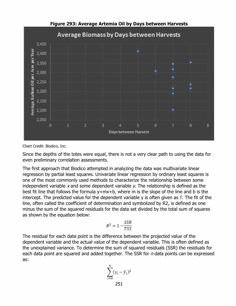
251
Figure 293: Average Artemia Oil by Days between Harvests
Chart Credit: Biodico, Inc.
Since the depths of the totes were equal, there is not a very clear path to using the data for even preliminary correlation assessments.
The first approach that Biodico attempted in analyzing the data was multivariate linear regression by partial least squares. Univariate linear regression by ordinary least squares is one of the most commonly used methods to characterize the relationship between some independent variable x and some dependent variable y. The relationship is defined as the best fit line that follows the formula y=mx+b, where m is the slope of the line and b is the intercept. The predicted value for the dependent variable y is often given as . The fit of the line, often called the coefficient of determination and symbolized by R2, is defined as one minus the sum of the squared residuals for the data set divided by the total sum of squares as shown by the equation below:
The residual for each data point is the difference between the projected value of the dependent variable and the actual value of the dependent variable. This is often defined as the unexplained variance. To determine the sum of squared residuals (SSR) the residuals for each data point are squared and added together. The SSR for n data points can be expressed as:

252
The total sum of squares (TSS) is defined as the sum of the squared total variance for each data point. The total variance is defined as the difference between the observed data point yi and the mean of all observed data points . The total variance is used to define the total sum of squares as:
The total variance can also be defined as the sum of the explained variance and the unexplained variance. The explained variance is the difference between the predicted value and the mean and the unexplained variance is the difference between the observed value and the predicted value. The relationship can be seen clearly by the equation:
Multivariate linear regression by partial least squares builds on the same basic concepts of univariate linear regression by ordinary least squares in that it defines the line of best fit as the multivariate equation that generates the lowest ratio of unexpected variance to total variance. The algorithms used to determine this fit are significantly more complicated and necessitate the use of linear algebra matrix projections and computations, but there are a number of software programs that can generate the relationships between multiple independent x variables and an independent y variable.
Figure 298 below lists the correlation coefficients for the change in dry Artemia biomass by percentage for each increase of one for solar energy (in kWh per square meter per day), temperature (in Fahrenheit), pH (on the standard 0 to 14 logarithmic scale), salinity (in parts per thousand), and nutrient feed (by grams per week). Multivariate analysis by linear regression gave some useful data but, as discussed later, the results were not ultimately very predictive of real-world performance.
Figure 294: Algaculture Coefficients
Chart Credit: Biodico, Inc.
Based on this initial analysis, the coefficients and variables for the linear regression yielded the equation listed in Figure 299.
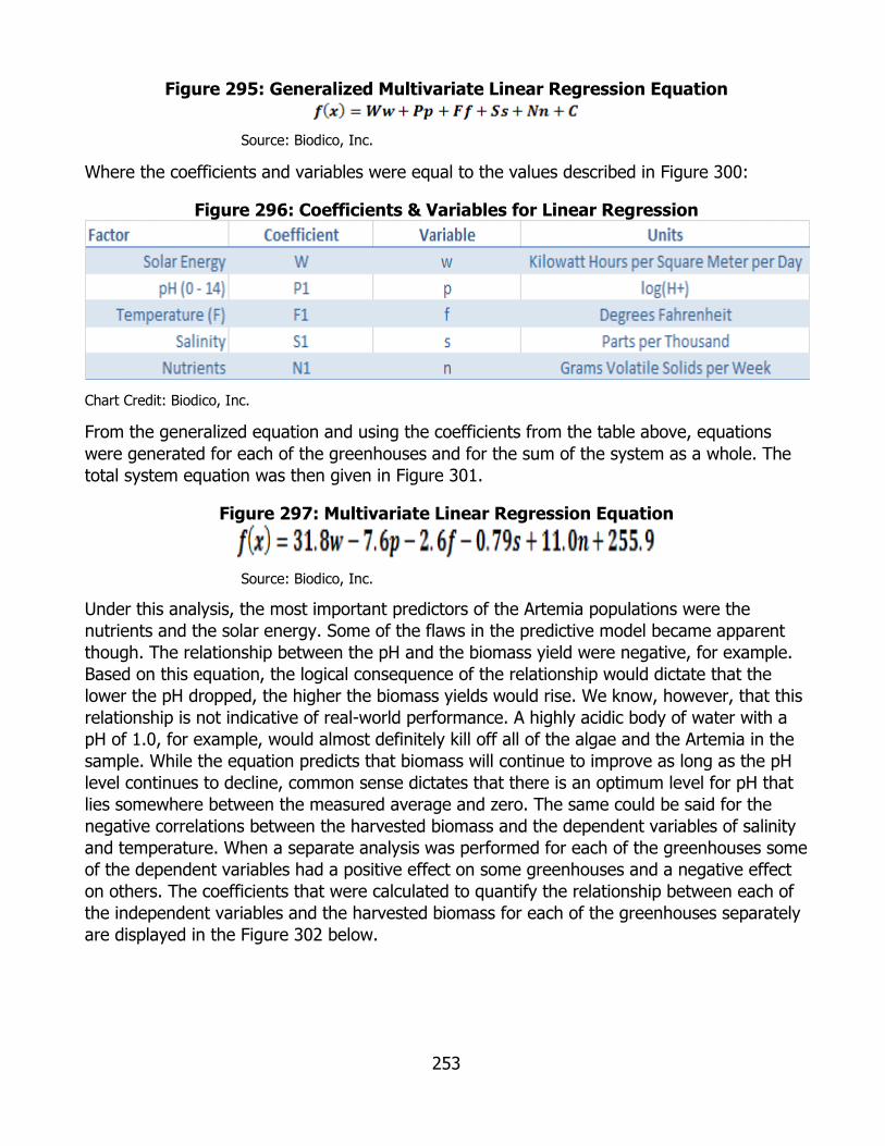
253
Figure 295: Generalized Multivariate Linear Regression Equation
Source: Biodico, Inc.
Where the coefficients and variables were equal to the values described in Figure 300:
Figure 296: Coefficients & Variables for Linear Regression
Chart Credit: Biodico, Inc.
From the generalized equation and using the coefficients from the table above, equations were generated for each of the greenhouses and for the sum of the system as a whole. The total system equation was then given in Figure 301.
Figure 297: Multivariate Linear Regression Equation
Source: Biodico, Inc.
Under this analysis, the most important predictors of the Artemia populations were the nutrients and the solar energy. Some of the flaws in the predictive model became apparent though. The relationship between the pH and the biomass yield were negative, for example. Based on this equation, the logical consequence of the relationship would dictate that the lower the pH dropped, the higher the biomass yields would rise. We know, however, that this relationship is not indicative of real-world performance. A highly acidic body of water with a pH of 1.0, for example, would almost definitely kill off all of the algae and the Artemia in the sample. While the equation predicts that biomass will continue to improve as long as the pH level continues to decline, common sense dictates that there is an optimum level for pH that lies somewhere between the measured average and zero. The same could be said for the negative correlations between the harvested biomass and the dependent variables of salinity and temperature. When a separate analysis was performed for each of the greenhouses some of the dependent variables had a positive effect on some greenhouses and a negative effect on others. The coefficients that were calculated to quantify the relationship between each of the independent variables and the harvested biomass for each of the greenhouses separately are displayed in the Figure 302 below.
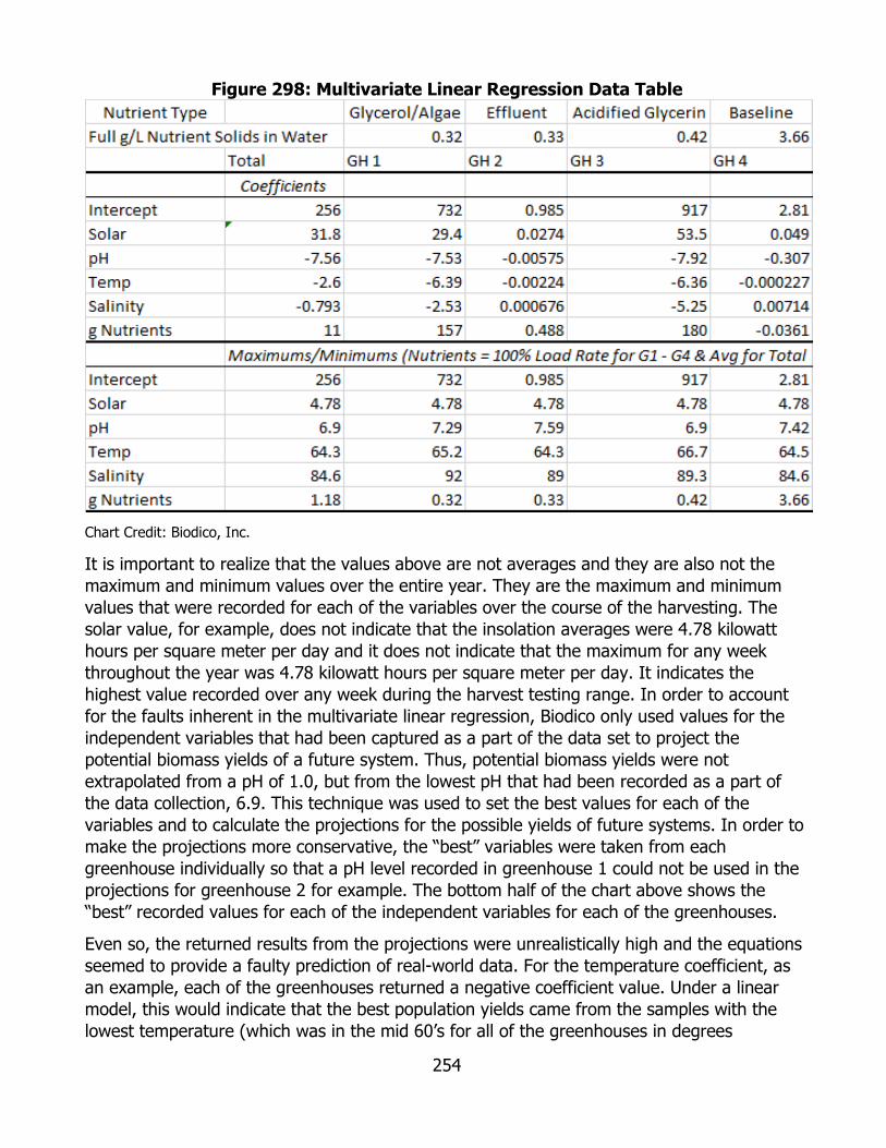
254
Figure 298: Multivariate Linear Regression Data Table
Chart Credit: Biodico, Inc.
It is important to realize that the values above are not averages and they are also not the maximum and minimum values over the entire year. They are the maximum and minimum values that were recorded for each of the variables over the course of the harvesting. The solar value, for example, does not indicate that the insolation averages were 4.78 kilowatt hours per square meter per day and it does not indicate that the maximum for any week throughout the year was 4.78 kilowatt hours per square meter per day. It indicates the highest value recorded over any week during the harvest testing range. In order to account for the faults inherent in the multivariate linear regression, Biodico only used values for the independent variables that had been captured as a part of the data set to project the potential biomass yields of a future system. Thus, potential biomass yields were not extrapolated from a pH of 1.0, but from the lowest pH that had been recorded as a part of the data collection, 6.9. This technique was used to set the best values for each of the variables and to calculate the projections for the possible yields of future systems. In order to make the projections more conservative, the “best” variables were taken from each greenhouse individually so that a pH level recorded in greenhouse 1 could not be used in the projections for greenhouse 2 for example. The bottom half of the chart above shows the “best” recorded values for each of the independent variables for each of the greenhouses.
Even so, the returned results from the projections were unrealistically high and the equations seemed to provide a faulty prediction of real-world data. For the temperature coefficient, as an example, each of the greenhouses returned a negative coefficient value. Under a linear model, this would indicate that the best population yields came from the samples with the lowest temperature (which was in the mid 60’s for all of the greenhouses in degrees
255
Fahrenheit). The laboratory research performed by Dr. Hristova showed that the Artemia populations were the healthiest and the densest at a temperature of about 86°F. Similarly, the optimum pH level had been tested as slightly alkaline in the laboratory as opposed to the slightly acidic lowest recorded value of 6.9.
After analyzing the model, Biodico concluded that for several of the variables the coefficients resulting from the linear regression analysis were more indicative of the relationship between the recorded values and the optimum values for performance than the individual recorded values and the biomass yields. Dr. Hristova’s research had found optimum levels for pH, salinity, and temperature that fell between the highest and lowest recorded points from the greenhouses.
Since these three variables can easily return values that fall above or below the optimum level, polynomial regression gives a much more description of their relationship to the harvested biomass than linear regression. The standard linear equation is:
A generalized polynomial fit curve can be given as:
Since m and x are both constants, the equation can be rewritten in standard polynomial form as:
Nutrient testing that had been performed in the aquariums prior to the larger tote harvest tests had shown that the system could be overloaded with nutrients fairly easily, particularly with glycerin. Biodico was conservative in the amounts of nutrients that were added to the populations, but still recognizes that the nutrient overload weights were relatively close to the amount of nutrients that were added and that the biomass yielded from the nutrients very likely follows a pattern of diminishing returns as the nutrient levels rise. With this in mind, even though the optimum nutrient level is expected to be higher than the maximum amount of nutrients added rather than between the highest and lowest amounts, a polynomial curve will likely be much more representative of the relationship between nutrients and biomass from Artemia.
If polynomial multivariate analysis is used in place of linear multivariate analysis, then each variable defined by a polynomial relationship will have two coefficients, one for the squared relationship and one for the linear relationship. The c values do not describe the relationship between any of the variables, so any number of c values can be combined into one variable C. Figure 303 below defines the variable and the coefficients.

256
Figure 299: Multivariate Polynomial Regression Coefficients Without Solar
Chart Credit: Biodico, Inc.
The first detail to note is that a polynomial relationship was not given to determine Artemia biomass from solar energy. Since the solar energy continued to positively contribute to the growth of the Artemia populations with no clear indication of diminishing contribution further analysis was needed to determine the best way to characterize the relationship. For the time the solar energy can be represented as Solar. Each of the other four variables was given a polynomial relationship though. This returns an equation that can be used to predict the Artemia biomass from pH, temperature, salinity, and nutrients of:
The solar values give solar energy in terms of insolation, which is a measurement of energy per area. The insolation was measured continually with a Davis Vantage Pro2TM Plus weather station, as shown in Figure 304.
Figure 300: Davis Vantage Pro2 Weather Station
Photo Credit: Davis Instruments, Inc.
The instrument returns insolation values in Langley units. Each Langley unit is equal to one thermochemical calorie per square centimeter, 41,840 joules per square meter, or 11.622 watt-hours per square meter. In order to effectively compare the data with the majority of
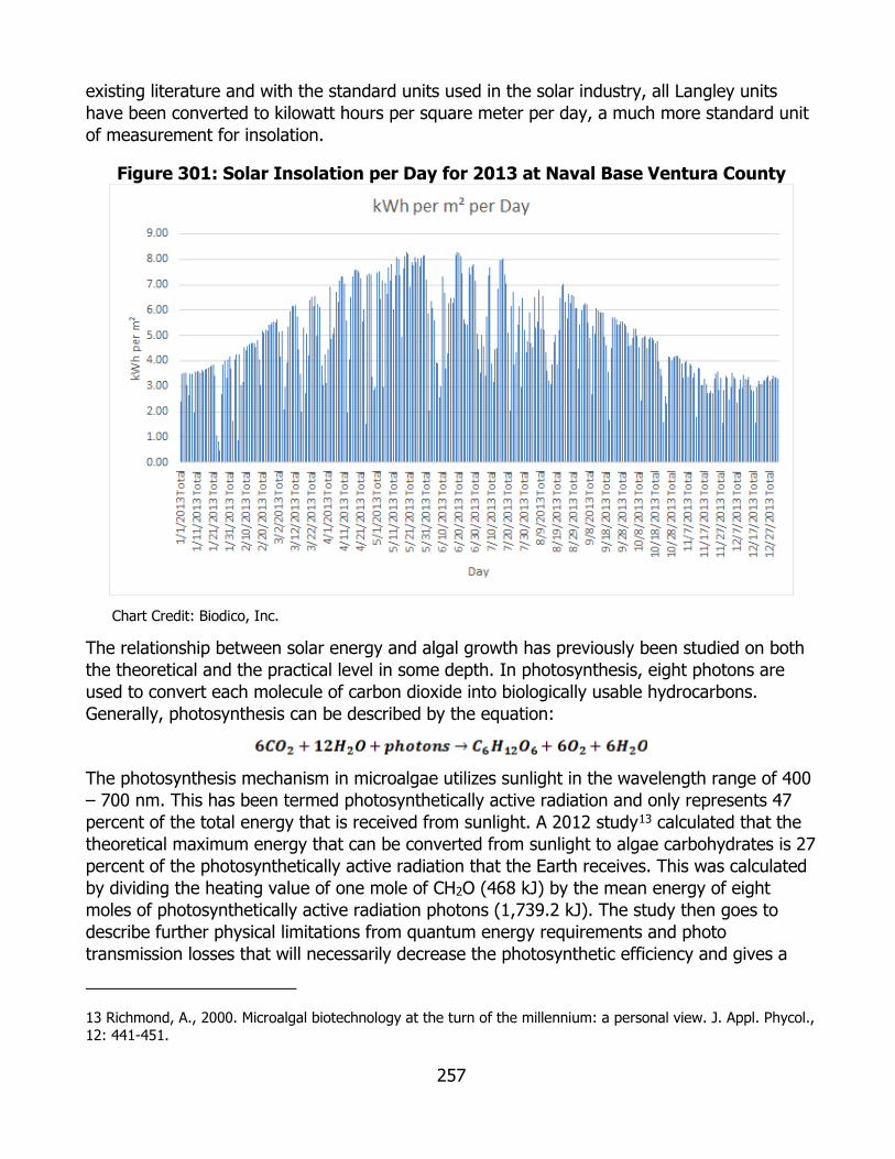
257
existing literature and with the standard units used in the solar industry, all Langley units have been converted to kilowatt hours per square meter per day, a much more standard unit of measurement for insolation.
Figure 301: Solar Insolation per Day for 2013 at Naval Base Ventura County
Chart Credit: Biodico, Inc.
The relationship between solar energy and algal growth has previously been studied on both the theoretical and the practical level in some depth. In photosynthesis, eight photons are used to convert each molecule of carbon dioxide into biologically usable hydrocarbons. Generally, photosynthesis can be described by the equation:
The photosynthesis mechanism in microalgae utilizes sunlight in the wavelength range of 400 – 700 nm. This has been termed photosynthetically active radiation and only represents 47percent of the total energy that is received from sunlight. A 2012 study13 calculated that thetheoretical maximum energy that can be converted from sunlight to algae carbohydrates is 27percent of the photosynthetically active radiation that the Earth receives. This was calculatedby dividing the heating value of one mole of CH2O (468 kJ) by the mean energy of eightmoles of photosynthetically active radiation photons (1,739.2 kJ). The study then goes todescribe further physical limitations from quantum energy requirements and phototransmission losses that will necessarily decrease the photosynthetic efficiency and gives a
13 Richmond, A., 2000. Microalgal biotechnology at the turn of the millennium: a personal view. J. Appl. Phycol., 12: 441-451.

258
maximum energy conversion of solar energy to biomass of 11.42 percent.14 The study compared this maximum conversion efficiency to a 2000 study that found the conversion efficiency of solar energy to algal biomass in nature to be 4 – 6 percent.
A 2009 study15 yielded very similar results in the theoretical conversion efficiency of total solar energy (termed full-spectrum solar energy in the paper) to algal biomass. The percentage of photosynthetically active radiation to total solar energy was given as 45.8 percent, the energy value of a mole of algal carbohydrates was given as 482.5 kJ, and the energy value of eight moles of photosynthetically active radiation photons was 1,802.4 kJ. This resulted in a maximum photon conversion efficiency of 12.25 percent as compared to 11.42 percent in the previous study. This study presented the maximum theoretical photon conversion efficiency as compared with an estimated best-case photon conversion efficiency based on real world data and compared this with previous real-world studies that had measured photon conversion efficiency. The estimated best case photon conversion efficiency factored in an estimated loss from photon transmission efficiency (which had been included in the theoretical maximum from the 2012 study as well), an estimated loss from photon utilization efficiency, and an estimated loss from biomass accumulation efficiency to give a best case photon conversion efficiency of 6.3 percent. This was compared against a 6.3 percent photon conversion efficiency based on photosynthetically active radiation for Chlorella in reduced sunlight (reduced to 22 percent)16, 2.6 – 2.7 percent photon conversion efficiency based on photosynthetically active radiation for Chlorella in full sunlight16, a highest reported efficiency of 3.7 percent for C4 crops17, a highest reported efficiency of 2.4 percent for C3 crops17, a 1 – 2 percent photon conversion efficiency for perennial grass18, and estimates of terrestrial plant conversion efficiencies of 0.1 percent15. In determining the relationship that sunlight had on the Artemia biomass growth for this study it is worth drawing attention to the Chlorella study that showed increased efficiencies from reduced sunlight. The Aquatic Species Program report19 notes on page 251 that high sunlight conversions are only observed at low
14 Sudhakar, K. and M. Premelatha, 2012. Theoretical Assessment of Algal Biomass Potential for Carbon Mitigation and Biofuel Production, Iranica Journal of Energy and the Environment 3 (3): 232-240, 2012
15 Weyer, Kristina M., Daniel R. Bush, Al Darzins, Bryan D. Wilson, 2009. Theoretical Maximum Algal Oil Production, Bioenerg. Res. (2010) 3:204-213
16 Burlew J-S (1953) Algal culture: from laboratory to pilot plant. Carnegie Institute of Washington Publication, Washington DC
17 Zhu X, Long S, Ort D (2008) What is the maximum efficiency with which photosynthesis can convert solar energy into biomass? Current Opinions Biotechnology 19:153-159
18 Heaton E-A, Dohleman F-G, Long S-P (2008) Meeting US biofuel goals with less land: the potential of Miscanthus. Glob Chang Biol 14:2000-2014
19 Sheehan, John, Terri Dunahay, John Benemann, Paul Roessler, 1998. A Look Back at the U.S. Department of Energy’s Aquatic Species Program – Biodiesel from Algae

259
sunlight intensities. Full sunlight intensities can cause the light saturation effect, where only about 10 percent of full sunlight can be effectively used by algae.
In order to effectively characterize the relationship between solar energy and Artemia biomass it is helpful to quantify the algal biomass that is represented by a given harvested biomass weight of Artemia. The following figure is taken from a study done by Coutteau and Sorgeloos in 1989 on Artemia feeding.20
Figure 302: Table from Coutteau and Sorgeloos Study
Chart Credit: Coutteau and Sorgeloos
The units used in the Sorgeloos report are somewhat counterintuitive for the purposes of this study, as shown in the subscripts. The specific growth rate is given as the natural logarithm of the differences in the Artemia weight from the start of the feeding cycle to the end of the feeding cycle. The food conversion rate is given as the total dry weight of algae that was offered to the system. For the purposes of this study we want to find the percentage of algal biomass that will be converted to Artemia biomass. Since the Artemia weight is given in terms of the natural logarithm of the difference, the actual difference is found by raising Euler’s number to the power of the given value. This number can then be divided by the difference in algal biomass to find a percentage conversion. This is done in the Figure 307. From this table,
20 Coutteau P., and Sorgeloos, P. 1989. Feeding of the brine shrimp Artemia on yeast: effect of mechanical disturbance, animal density, water quality and light intensity. In: European Aquaculture Society Spec. Publ. N° 10. Bredene, Belgium, 344 pp.
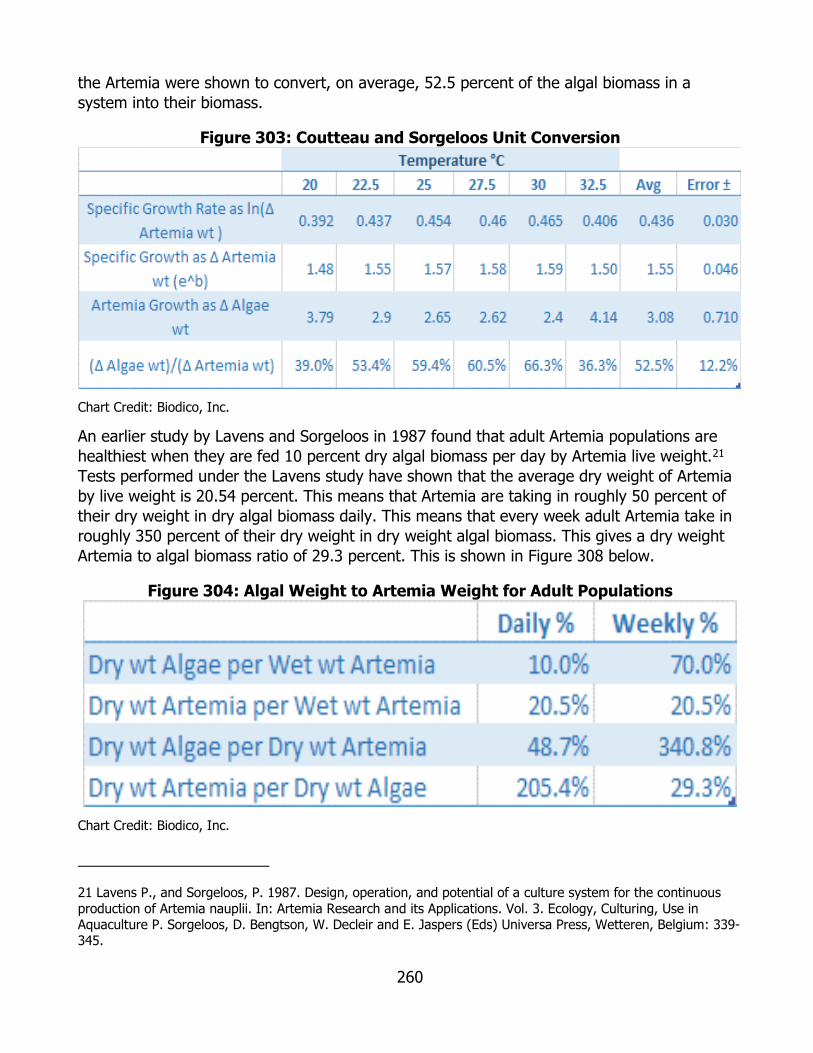
260
the Artemia were shown to convert, on average, 52.5 percent of the algal biomass in a system into their biomass.
Figure 303: Coutteau and Sorgeloos Unit Conversion
Chart Credit: Biodico, Inc.
An earlier study by Lavens and Sorgeloos in 1987 found that adult Artemia populations are healthiest when they are fed 10 percent dry algal biomass per day by Artemia live weight.21 Tests performed under the Lavens study have shown that the average dry weight of Artemia by live weight is 20.54 percent. This means that Artemia are taking in roughly 50 percent of their dry weight in dry algal biomass daily. This means that every week adult Artemia take in roughly 350 percent of their dry weight in dry weight algal biomass. This gives a dry weight Artemia to algal biomass ratio of 29.3 percent. This is shown in Figure 308 below.
Figure 304: Algal Weight to Artemia Weight for Adult Populations
Chart Credit: Biodico, Inc.
21 Lavens P., and Sorgeloos, P. 1987. Design, operation, and potential of a culture system for the continuous production of Artemia nauplii. In: Artemia Research and its Applications. Vol. 3. Ecology, Culturing, Use in Aquaculture P. Sorgeloos, D. Bengtson, W. Decleir and E. Jaspers (Eds) Universa Press, Wetteren, Belgium: 339-345.
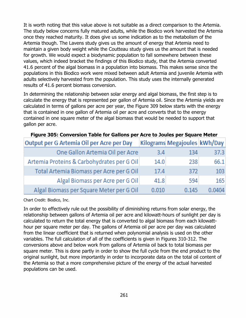
261
It is worth noting that this value above is not suitable as a direct comparison to the Artemia. The study below concerns fully matured adults, while the Biodico work harvested the Artemia once they reached maturity. It does give us some indication as to the metabolism of the Artemia though. The Lavens study gives us the amount of energy that Artemia need to maintain a given body weight while the Coutteau study gives us the amount that is needed for growth. We would expect a biodynamic population to fall somewhere between these values, which indeed bracket the findings of this Biodico study, that the Artemia converted 41.6 percent of the algal biomass in a population into biomass. This makes sense since the populations in this Biodico work were mixed between adult Artemia and juvenile Artemia with adults selectively harvested from the population. This study uses the internally generated results of 41.6 percent biomass conversion.
In determining the relationship between solar energy and algal biomass, the first step is to calculate the energy that is represented per gallon of Artemia oil. Since the Artemia yields are calculated in terms of gallons per acre per year, the Figure 309 below starts with the energy that is contained in one gallon of Artemia oil per acre and converts that to the energy contained in one square meter of the algal biomass that would be needed to support that gallon per acre.
Figure 305: Conversion Table for Gallons per Acre to Joules per Square Meter
Chart Credit: Biodico, Inc.
In order to effectively rule out the possibility of diminishing returns from solar energy, the relationship between gallons of Artemia oil per acre and kilowatt-hours of sunlight per day is calculated to return the total energy that is converted to algal biomass from each kilowatt-hour per square meter per day. The gallons of Artemia oil per acre per day was calculated from the linear coefficient that is returned when polynomial analysis is used on the other variables. The full calculation of all of the coefficients is given in Figures 310-312. The conversions above and below work from gallons of Artemia oil back to total biomass per square meter. This is done partly in order to show the full cycle from the end product to the original sunlight, but more importantly in order to incorporate data on the total oil content of the Artemia so that a more comprehensive picture of the energy of the actual harvested populations can be used.

262
Figure 306: Solar Energy to Algal Biomass Conversion
Chart Credit: Biodico, Inc.
Based on the above analysis though, the relationship between solar energy and Artemia biomass is below the threshold of diminishing returns and a linear relationship can be drawn. Based on the experimental yields of Artemia, the conversion of solar energy to algal biomass is 5.47 percent. This conversion efficiency is very consistent with previous findings by other researchers and with the conversion efficiency normally found in nature. The linear correlation of insolation (in kilowatt-hours per square meter per day) along with the polynomial correlation of the remaining factors gives the list of coefficients and variables in the following table. It is important to note that all of these variables were based off of experimental results but are not more important than the experimental results. The experimental results are more important than the math to scale up.
Figure 307: Final Coefficient Set for Multivariate Polynomial Regression
Chart Credit: Biodico, Inc.
The coefficients that were calculated for this mostly polynomial regression analysis are given below.
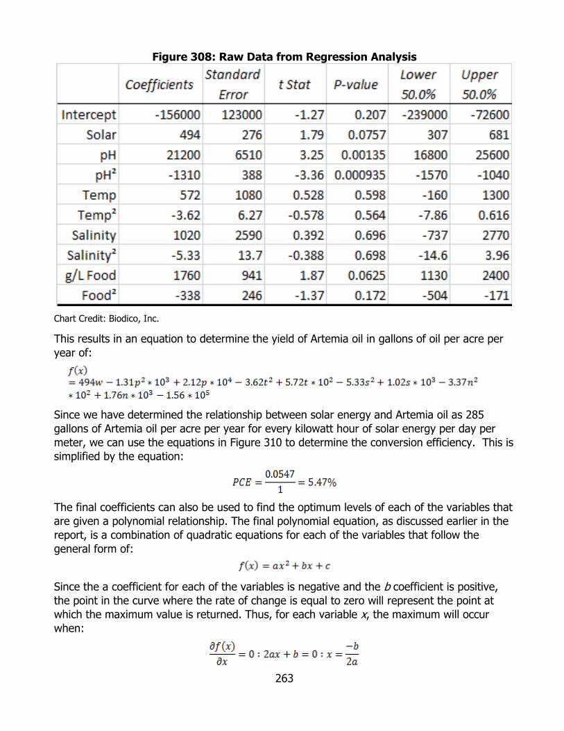
263
Figure 308: Raw Data from Regression Analysis
Chart Credit: Biodico, Inc.
This results in an equation to determine the yield of Artemia oil in gallons of oil per acre per year of:
Since we have determined the relationship between solar energy and Artemia oil as 285 gallons of Artemia oil per acre per year for every kilowatt hour of solar energy per day per meter, we can use the equations in Figure 310 to determine the conversion efficiency. This is simplified by the equation:
The final coefficients can also be used to find the optimum levels of each of the variables that are given a polynomial relationship. The final polynomial equation, as discussed earlier in the report, is a combination of quadratic equations for each of the variables that follow the general form of:
Since the a coefficient for each of the variables is negative and the b coefficient is positive, the point in the curve where the rate of change is equal to zero will represent the point at which the maximum value is returned. Thus, for each variable x, the maximum will occur when:

264
For the equation as a whole, separate partial derivatives can be used to return the optimum value for the variables. The optimum values are displayed in the figure below.
Figure 309: Optimum Value Calculation for Polynomial Variables
Chart Credit: Biodico, Inc.
The optimal values for the independent variables measured during the harvesting test that were returned by multivariate polynomial regression were very similar to the optimal values that Dr. Hristova found in her research. The table below compares the recommended levels by Dr. Hristova to the calculated optimum values from the Naval Base Ventura County work.
Figure 310: Comparison between Greenhouse Scale Optimum Values and Laboratory Findings
Chart Credit: Biodico, Inc.
The mismatch from the nutrient levels was somewhat expected since the Naval Base Ventura County greenhouses used four different types of nutrient feed. The core nutrients in particular were tough to measure against the other types of feed. The mineral nutrients contained practically no volatile solids and practically no caloric value, but the recommended total solids weight from the feed was significantly higher than that needed for the glycerin.
In order to analyze each of the nutrient types separately, the projected contribution of each of the other independent variables was subtracted from the harvest gains in order to isolate the portion of the yield that can be contributed to the feed. This gives the equation:
The coefficients found in the polynomial regression displayed above in Figure 313 can be plugged in so that the nutrient contribution for each harvest point can be calculated as:

265
The CN value for the nutrient contribution is calculated so that the minimum contribution is set at zero. Since the variable C is used to represent the intercept for the equation as a whole, the variable CN can be used to represent the intercept for the individual nutrient correlations. This intercept value can be calculated as:
A multivariate polynomial relationship can now be drawn for each of the nutrient types as:
Of the total 192 harvesting data points, there are 48 for each of the four greenhouses. Within the 48 data points there are 32 taken before the feed was added and 16 taken after. The nutrient coefficients, the optimum values, their overall contribution to the system, and the ratio of gallons of Artemia oil per acre per year over grams per liter of nutrient solids per week are given below. The first table has the coefficients and the optimum nutrient levels and the second table has the yield information.
Figure 311: Nutrient Coefficients and Optimum Levels
Chart Credit: Biodico, Inc.
The following chart shows the conversion from gallons of oil per acre per year with the nutrients at optimum levels to the oil that comes out of the system as a weight percentage of the nutrients that enter the system for each type of nutrient (one type per greenhouse) in the column on the far right. The second column from the left gives the gallons of oil per acre per year that come from each gram of nutrients per liter per week. The next column to the right shows the gallons of oil per acre per week that come from each gram of nutrients per liter per week. The next column to the right shows the gallons of oil per liter per week that come from each gram of nutrients per liter per week. The next column to the right shows the grams of oil per liter per week that come from each gram of nutrients per liter per week. Finally, this is given as a percentage.
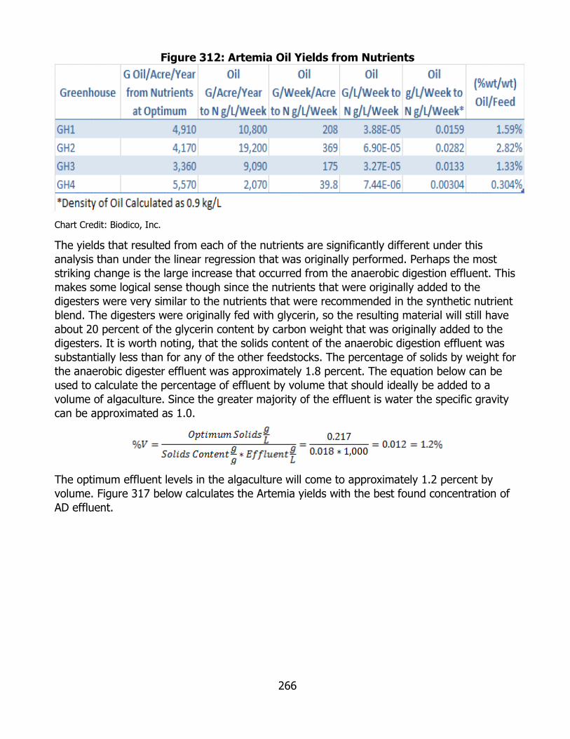
266
Figure 312: Artemia Oil Yields from Nutrients
Chart Credit: Biodico, Inc.
The yields that resulted from each of the nutrients are significantly different under this analysis than under the linear regression that was originally performed. Perhaps the most striking change is the large increase that occurred from the anaerobic digestion effluent. This makes some logical sense though since the nutrients that were originally added to the digesters were very similar to the nutrients that were recommended in the synthetic nutrient blend. The digesters were originally fed with glycerin, so the resulting material will still have about 20 percent of the glycerin content by carbon weight that was originally added to the digesters. It is worth noting, that the solids content of the anaerobic digestion effluent was substantially less than for any of the other feedstocks. The percentage of solids by weight for the anaerobic digester effluent was approximately 1.8 percent. The equation below can be used to calculate the percentage of effluent by volume that should ideally be added to a volume of algaculture. Since the greater majority of the effluent is water the specific gravity can be approximated as 1.0.
The optimum effluent levels in the algaculture will come to approximately 1.2 percent by volume. Figure 317 below calculates the Artemia yields with the best found concentration of AD effluent.

267
Figure 313: Best Case Calculations from Established Optimum Values
Chart Credit: Biodico, Inc.
The margin of error for the multivariate polynomial analysis was 924 gallons per year at a 50 percent confidence interval. Since optimum variables that match laboratory findings have been confirmed on a bench scale, future work performed on Artemia cultivation will focus on keeping the independent variables as close to optimum levels as possible rather than exploring the relationships.
Figure 318 below shows the relationships between observed average biomass harvest, the maximum biomass harvest, the calculated average, and the projected best case given the current relationships between the variables.
Figure 314: Comparison of Calculated and Observed Values
Chart Credit: Biodico, Inc.
As the chart above shows, there is significant room for improvement by more carefully controlling the independent variables of pH, salinity, and temperature. The raw data used for the original linear regression analysis and following multivariate regression analysis is given in the following Figures 319-324.

268
Figure 315: Tote Harvest Data 1
Chart Credit: Biodico, Inc.
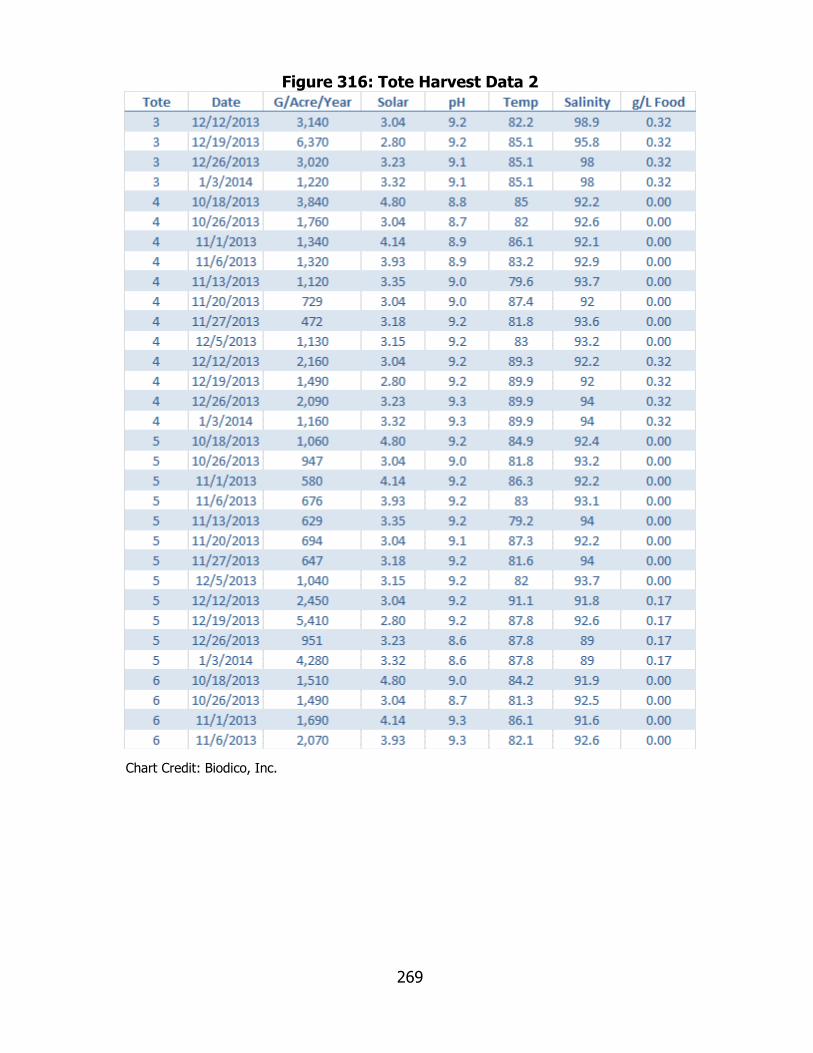
269
Figure 316: Tote Harvest Data 2
Chart Credit: Biodico, Inc.
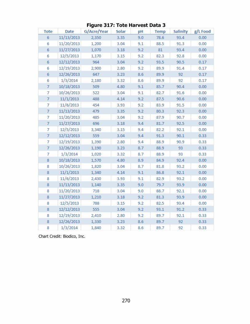
270
Figure 317: Tote Harvest Data 3
Chart Credit: Biodico, Inc.
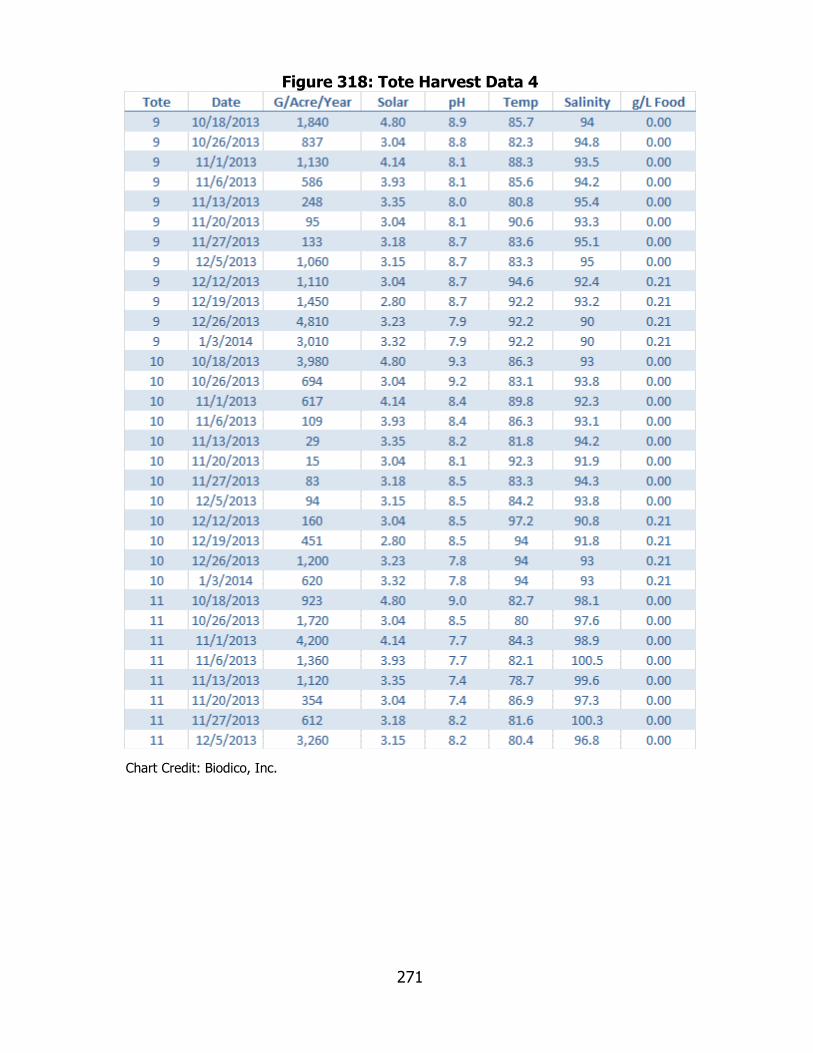
271
Figure 318: Tote Harvest Data 4
Chart Credit: Biodico, Inc.
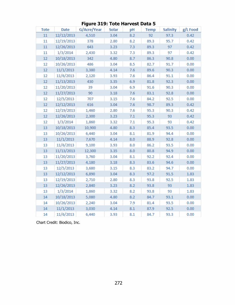
272
Figure 319: Tote Harvest Data 5
Chart Credit: Biodico, Inc.
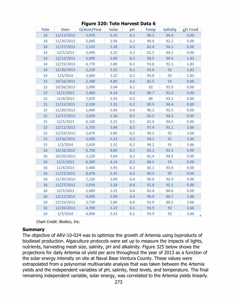
273
Figure 320: Tote Harvest Data 6
Chart Credit: Biodico, Inc.
Summary The objective of ARV-10-024 was to optimize the growth of Artemia using byproducts of biodiesel production. Algaculture protocols were set up to measure the impacts of lights, nutrients, harvesting mesh size, salinity, pH and alkalinity. Figure 325 below shows the projections for daily Artemia oil yield per acre throughout the year of 2013 as a function of the solar energy intensity on site at Naval Base Ventura County. These values were extrapolated from a polynomial multivariate analysis that was taken between the Artemia yields and the independent variables of pH, salinity, feed levels, and temperature. The final remaining independent variable, solar energy, was correlated to the Artemia yields linearly.
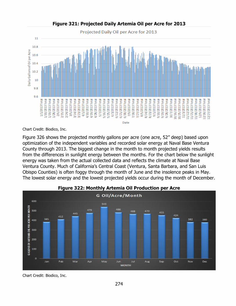
274
Figure 321: Projected Daily Artemia Oil per Acre for 2013
Chart Credit: Biodico, Inc.
Figure 326 shows the projected monthly gallons per acre (one acre, 52” deep) based upon optimization of the independent variables and recorded solar energy at Naval Base Ventura County through 2013. The biggest change in the month to month projected yields results from the differences in sunlight energy between the months. For the chart below the sunlight energy was taken from the actual collected data and reflects the climate at Naval Base Ventura County. Much of California’s Central Coast (Ventura, Santa Barbara, and San Luis Obispo Counties) is often foggy through the month of June and the insolence peaks in May. The lowest solar energy and the lowest projected yields occur during the month of December.
Figure 322: Monthly Artemia Oil Production per Acre
Chart Credit: Biodico, Inc.
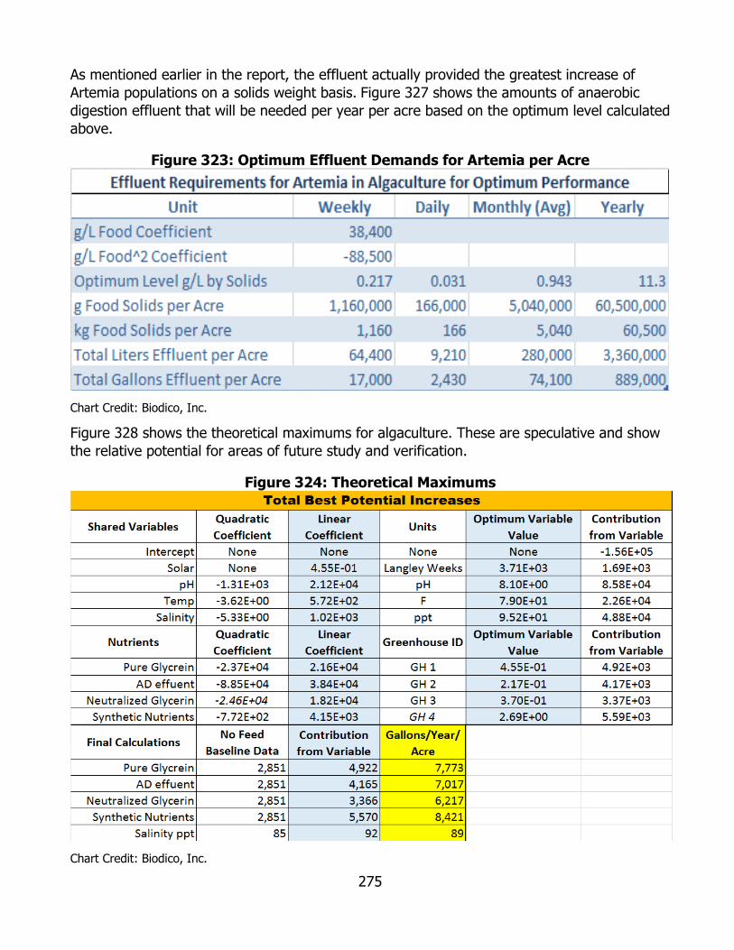
275
As mentioned earlier in the report, the effluent actually provided the greatest increase of Artemia populations on a solids weight basis. Figure 327 shows the amounts of anaerobic digestion effluent that will be needed per year per acre based on the optimum level calculated above.
Figure 323: Optimum Effluent Demands for Artemia per Acre
Chart Credit: Biodico, Inc.
Figure 328 shows the theoretical maximums for algaculture. These are speculative and show the relative potential for areas of future study and verification.
Figure 324: Theoretical Maximums
Chart Credit: Biodico, Inc.

276
Systems Integration and Process Control Biodico has designed, built and operated five commercial biodiesel production facilities throughout the world since 2000. Three of the main bottlenecks that arise in commercial biodiesel production are: sourcing feedstock, finding a viable stream for the byproducts of biodiesel, and time requirements for quality control testing. The work performed under the California Energy Commission grant ARV-10-024 included (1) the bench scale development of Artemia feedstock modules, (2) the detailed testing of the effectiveness of glycerin as both a stand-alone and a co-processed feedstock for the production of natural gas through anaerobic digestion, and (3) the use of FTIR and guided wave radar to enhance the sensing needed for quantitative and qualitative process control.
In the past, Biodico’s commercial production facilities have tied all of the electrical components of the system (pumps, heaters, etc.) together through Programmable Logic Controllers with text-based interfaces. The Programmable Logic Controls essentially served as a collection of on/off switches and did not retain any data from production. As Biodico pursues a more vertically integrated model with both feedstock development and anaerobic digestion, it will become increasingly important to have a Human Machine Interface that is visually intuitive for the user, that monitors and records key operating variables for the system, and that allows for the remote control and monitoring of the system. Invensys has developed an ARIES command unit and interface for Biodico that performs all of these functions. The ARIES system has been set up in a way that all of the probes and controls can be placed into practically any system scale. In order to facilitate easy testing of the system’s functionality and changing of the system’s configuration if needed, the ARIES system is currently hooked up to bench scale algaculture and digesters at Red Rock Ranch in West Fresno County and can be accessed easily from Naval Base Ventura County. Desired Functionality Biodico’s goal with Invensys was to develop automation capabilities for the anaerobic digestion, algaculture, and gasification portions of its integrated energy system. The aim was to develop a programming and sensor interface that can effectively be applied toward any scale of system and that is robust enough to easily accommodate changes in system design. I/O Points and Metrics Invensys sorts their input/output (I/O) points into four types: analog input, analog output (AO), digital input (DI), and digital output (DO). Analog inputs and analog outputs will accept or release a variable signal that corresponds to any real number within an established range. DIs and DOs accept or release a Boolean value defined by a binary variable (0 for off and 1 for on). Under Invensys’ hierarchy of I/O communication, racks contain cards which each contain a number of I/O points depending on their type. Biodico’s rack contains six analog input cards, three analog output cards, one DI card, and one DO card. Analog input cards each have three I/O points, analog output cards have two I/O points, digital input cards have 16 points, and digital output cards have eight output points. This gives a possibility for 18 analog input points, six analog output points, 16 DI points, and 8 DO points. Based on experience with a wide range of clients, Invensys recommended that spare I/O points be left open for each kind of I/O. Analog inputs for the algaculture include temperature, pH, dissolved oxygen, salinity, and oxidation reduction potential. Analog inputs for the anaerobic
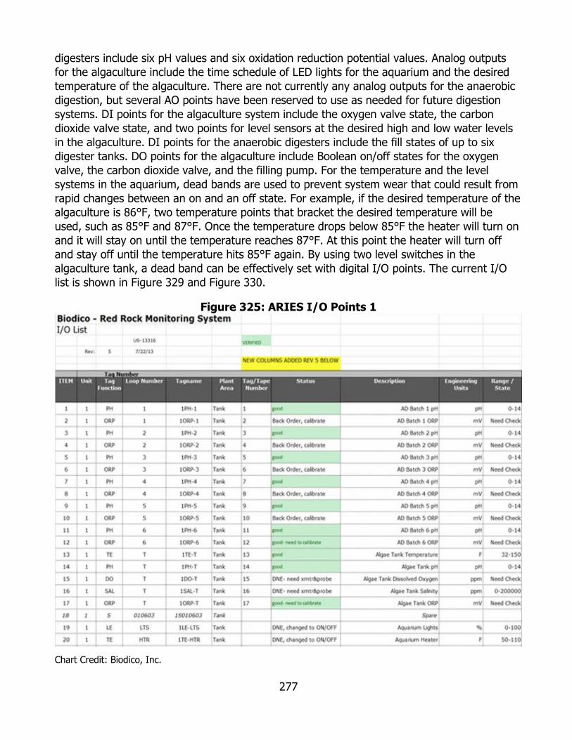
277
digesters include six pH values and six oxidation reduction potential values. Analog outputs for the algaculture include the time schedule of LED lights for the aquarium and the desired temperature of the algaculture. There are not currently any analog outputs for the anaerobic digestion, but several AO points have been reserved to use as needed for future digestion systems. DI points for the algaculture system include the oxygen valve state, the carbon dioxide valve state, and two points for level sensors at the desired high and low water levels in the algaculture. DI points for the anaerobic digesters include the fill states of up to six digester tanks. DO points for the algaculture include Boolean on/off states for the oxygen valve, the carbon dioxide valve, and the filling pump. For the temperature and the level systems in the aquarium, dead bands are used to prevent system wear that could result from rapid changes between an on and an off state. For example, if the desired temperature of the algaculture is 86°F, two temperature points that bracket the desired temperature will be used, such as 85°F and 87°F. Once the temperature drops below 85°F the heater will turn on and it will stay on until the temperature reaches 87°F. At this point the heater will turn off and stay off until the temperature hits 85°F again. By using two level switches in the algaculture tank, a dead band can be effectively set with digital I/O points. The current I/O list is shown in Figure 329 and Figure 330.
Figure 325: ARIES I/O Points 1
Chart Credit: Biodico, Inc.
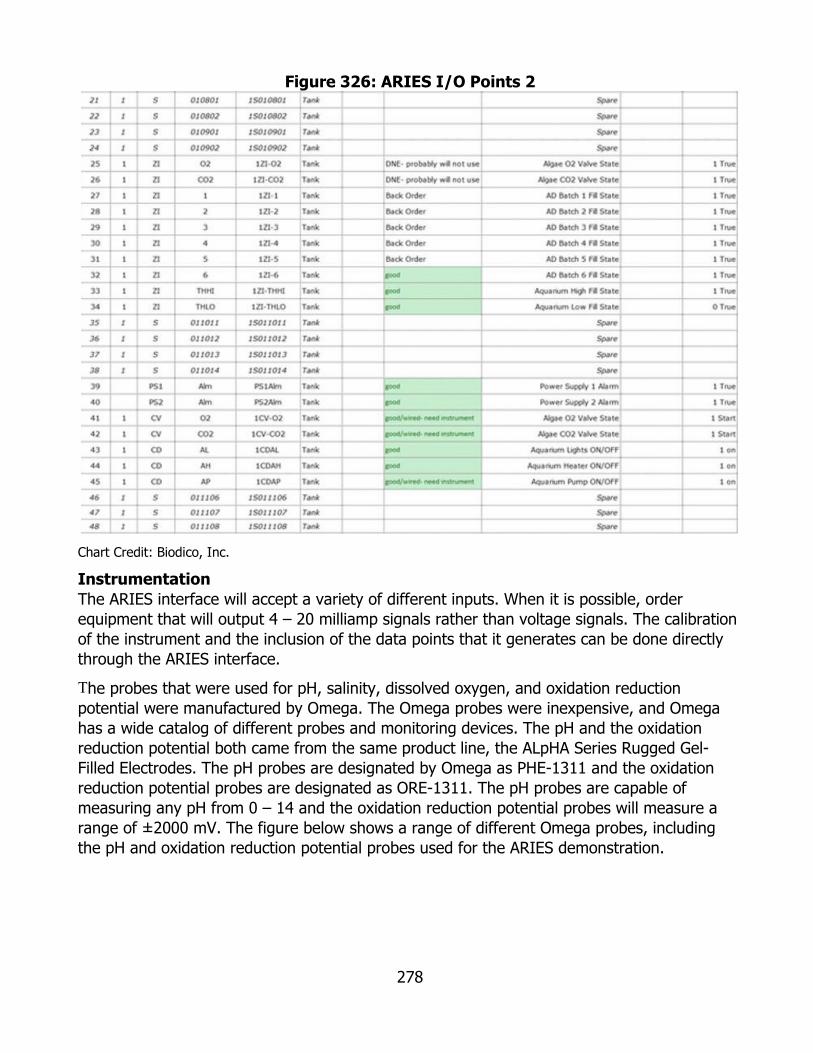
278
Figure 326: ARIES I/O Points 2
Chart Credit: Biodico, Inc.
Instrumentation The ARIES interface will accept a variety of different inputs. When it is possible, order equipment that will output 4 – 20 milliamp signals rather than voltage signals. The calibration of the instrument and the inclusion of the data points that it generates can be done directly through the ARIES interface. The probes that were used for pH, salinity, dissolved oxygen, and oxidation reduction potential were manufactured by Omega. The Omega probes were inexpensive, and Omega has a wide catalog of different probes and monitoring devices. The pH and the oxidation reduction potential both came from the same product line, the ALpHA Series Rugged Gel-Filled Electrodes. The pH probes are designated by Omega as PHE-1311 and the oxidation reduction potential probes are designated as ORE-1311. The pH probes are capable of measuring any pH from 0 – 14 and the oxidation reduction potential probes will measure a range of ±2000 mV. The figure below shows a range of different Omega probes, including the pH and oxidation reduction potential probes used for the ARIES demonstration.
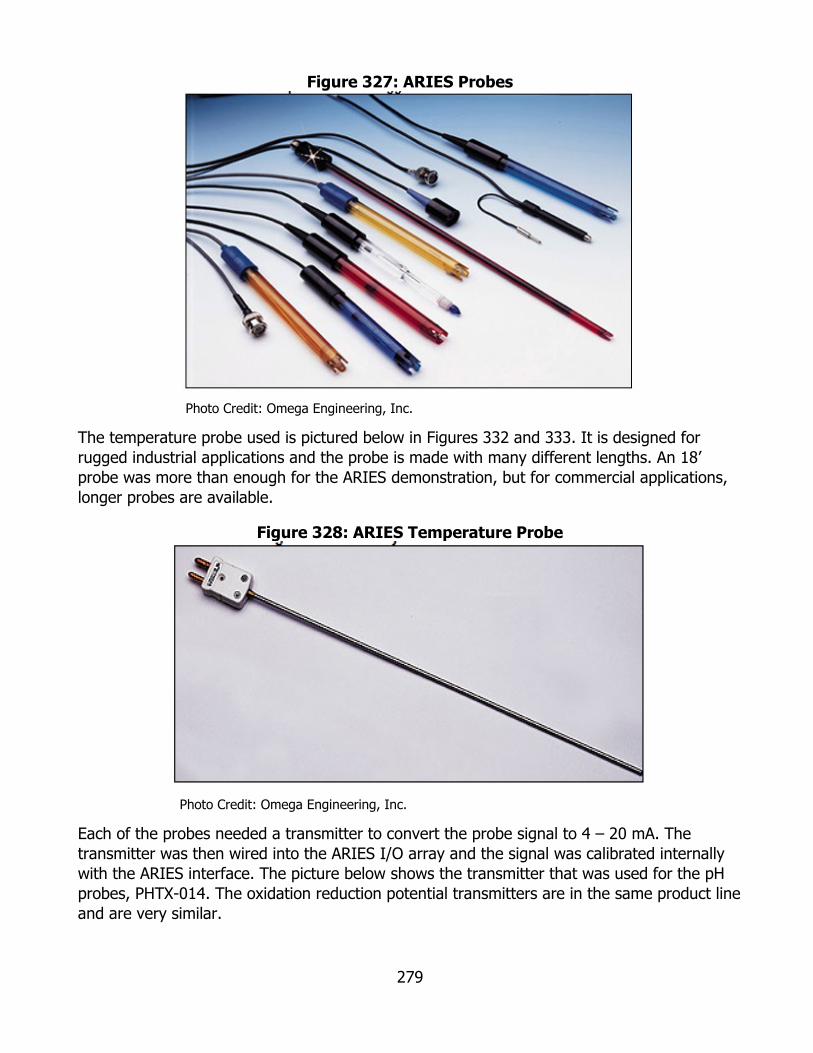
279
Figure 327: ARIES Probes
Photo Credit: Omega Engineering, Inc.
The temperature probe used is pictured below in Figures 332 and 333. It is designed for rugged industrial applications and the probe is made with many different lengths. An 18’ probe was more than enough for the ARIES demonstration, but for commercial applications, longer probes are available.
Figure 328: ARIES Temperature Probe
Photo Credit: Omega Engineering, Inc.
Each of the probes needed a transmitter to convert the probe signal to 4 – 20 mA. The transmitter was then wired into the ARIES I/O array and the signal was calibrated internally with the ARIES interface. The picture below shows the transmitter that was used for the pH probes, PHTX-014. The oxidation reduction potential transmitters are in the same product line and are very similar.
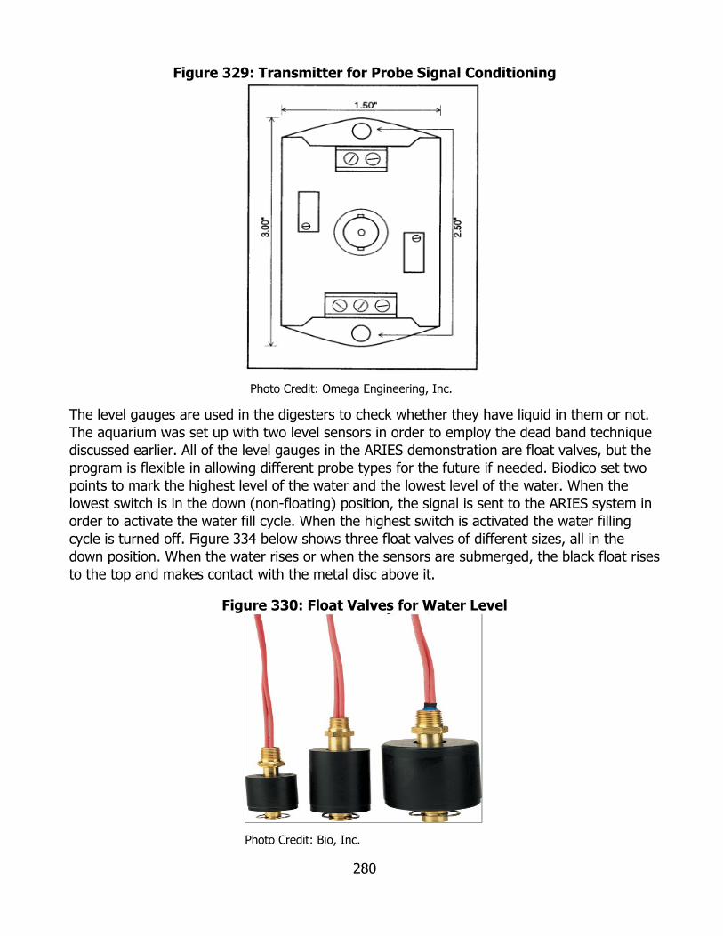
280
Figure 329: Transmitter for Probe Signal Conditioning
Photo Credit: Omega Engineering, Inc.
The level gauges are used in the digesters to check whether they have liquid in them or not. The aquarium was set up with two level sensors in order to employ the dead band technique discussed earlier. All of the level gauges in the ARIES demonstration are float valves, but the program is flexible in allowing different probe types for the future if needed. Biodico set two points to mark the highest level of the water and the lowest level of the water. When the lowest switch is in the down (non-floating) position, the signal is sent to the ARIES system in order to activate the water fill cycle. When the highest switch is activated the water filling cycle is turned off. Figure 334 below shows three float valves of different sizes, all in the down position. When the water rises or when the sensors are submerged, the black float rises to the top and makes contact with the metal disc above it.
Figure 330: Float Valves for Water Level
Photo Credit: Bio, Inc.
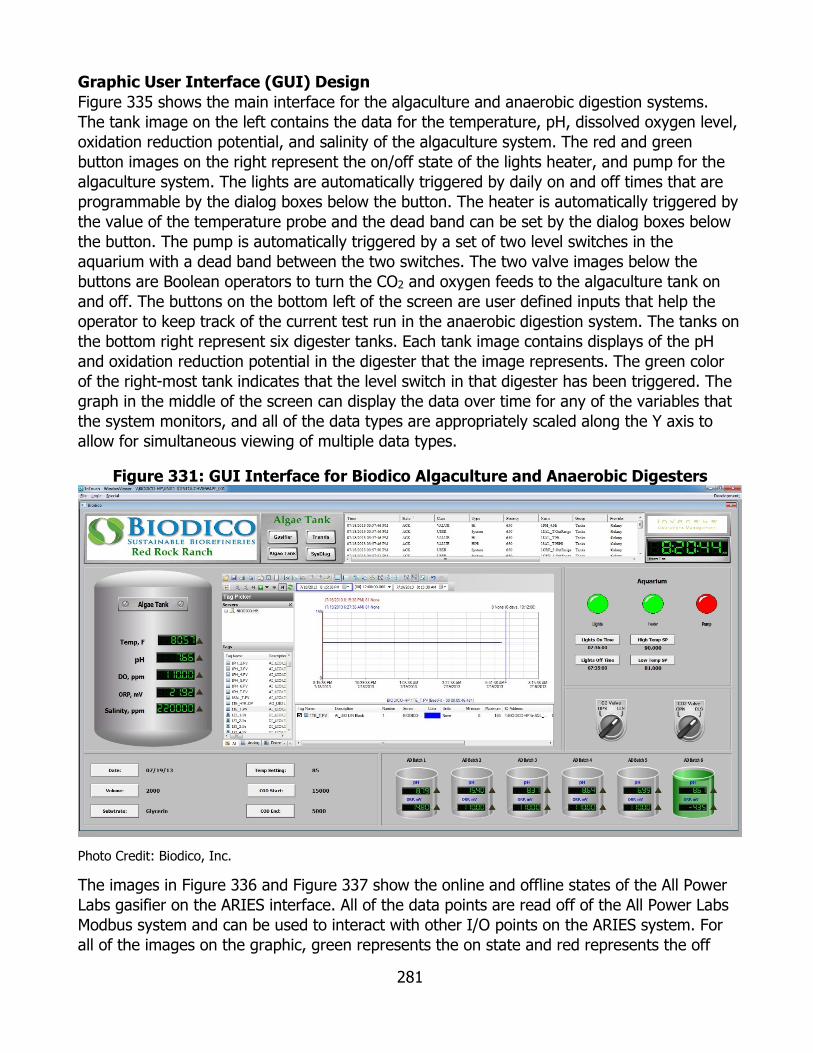
281
Graphic User Interface (GUI) Design Figure 335 shows the main interface for the algaculture and anaerobic digestion systems. The tank image on the left contains the data for the temperature, pH, dissolved oxygen level, oxidation reduction potential, and salinity of the algaculture system. The red and green button images on the right represent the on/off state of the lights heater, and pump for the algaculture system. The lights are automatically triggered by daily on and off times that are programmable by the dialog boxes below the button. The heater is automatically triggered by the value of the temperature probe and the dead band can be set by the dialog boxes below the button. The pump is automatically triggered by a set of two level switches in the aquarium with a dead band between the two switches. The two valve images below the buttons are Boolean operators to turn the CO2 and oxygen feeds to the algaculture tank on and off. The buttons on the bottom left of the screen are user defined inputs that help the operator to keep track of the current test run in the anaerobic digestion system. The tanks on the bottom right represent six digester tanks. Each tank image contains displays of the pH and oxidation reduction potential in the digester that the image represents. The green color of the right-most tank indicates that the level switch in that digester has been triggered. The graph in the middle of the screen can display the data over time for any of the variables that the system monitors, and all of the data types are appropriately scaled along the Y axis to allow for simultaneous viewing of multiple data types.
Figure 331: GUI Interface for Biodico Algaculture and Anaerobic Digesters
Photo Credit: Biodico, Inc.
The images in Figure 336 and Figure 337 show the online and offline states of the All Power Labs gasifier on the ARIES interface. All of the data points are read off of the All Power Labs Modbus system and can be used to interact with other I/O points on the ARIES system. For all of the images on the graphic, green represents the on state and red represents the off
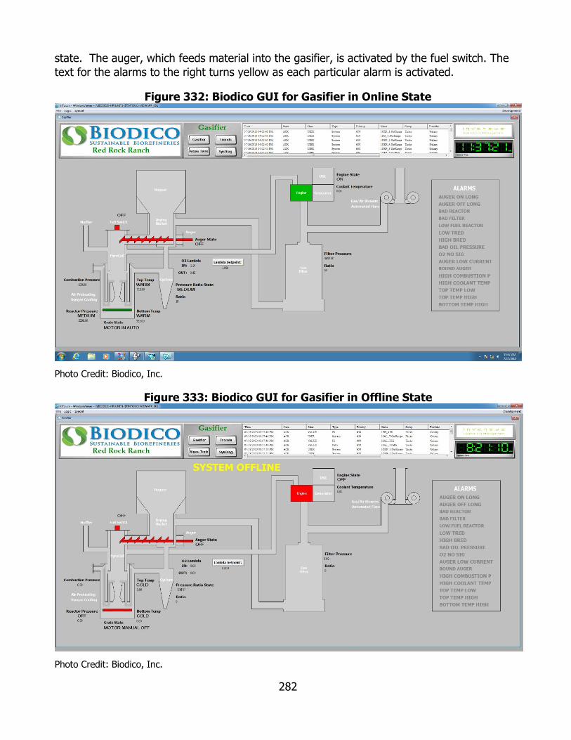
282
state. The auger, which feeds material into the gasifier, is activated by the fuel switch. The text for the alarms to the right turns yellow as each particular alarm is activated.
Figure 332: Biodico GUI for Gasifier in Online State
Photo Credit: Biodico, Inc.
Figure 333: Biodico GUI for Gasifier in Offline State
Photo Credit: Biodico, Inc.
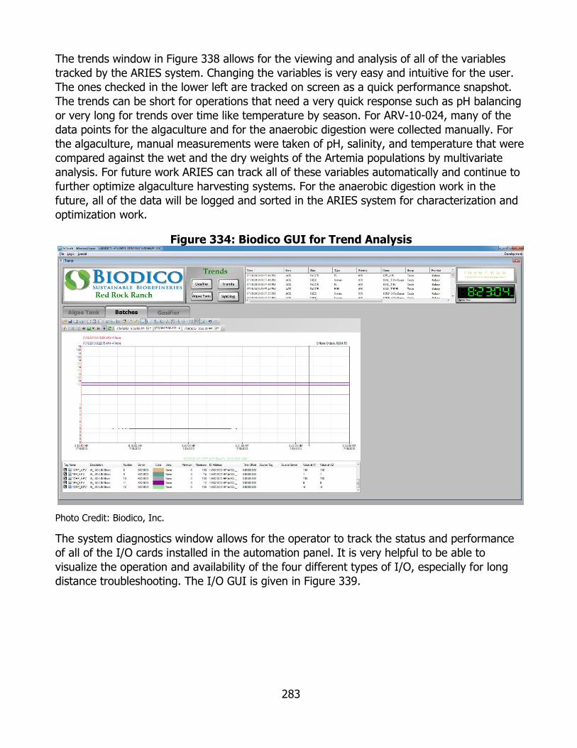
283
The trends window in Figure 338 allows for the viewing and analysis of all of the variables tracked by the ARIES system. Changing the variables is very easy and intuitive for the user. The ones checked in the lower left are tracked on screen as a quick performance snapshot. The trends can be short for operations that need a very quick response such as pH balancing or very long for trends over time like temperature by season. For ARV-10-024, many of the data points for the algaculture and for the anaerobic digestion were collected manually. For the algaculture, manual measurements were taken of pH, salinity, and temperature that were compared against the wet and the dry weights of the Artemia populations by multivariate analysis. For future work ARIES can track all of these variables automatically and continue to further optimize algaculture harvesting systems. For the anaerobic digestion work in the future, all of the data will be logged and sorted in the ARIES system for characterization and optimization work.
Figure 334: Biodico GUI for Trend Analysis
Photo Credit: Biodico, Inc.
The system diagnostics window allows for the operator to track the status and performance of all of the I/O cards installed in the automation panel. It is very helpful to be able to visualize the operation and availability of the four different types of I/O, especially for long distance troubleshooting. The I/O GUI is given in Figure 339.

284
Figure 335: Biodico I/O GUI
Photo Credit: Biodico, Inc.
Existing Modbus Interface (CHP) The gasifier uses operational variables that have already been defined by the manufacturer, All Power Labs. The All Power Labs system uses an auger to deliver feedstock from the hopper to the pyrolysis column. The char produced in pyrolysis filters through a grate that is periodically shaken to clear material through. The syngas that is produced in pyrolysis can be used in the generator engine or flared off. When the syngas is used in the engine, a filtered inlet brings in the oxygen needed for the fuel to reach optimal stoichiometry. The variables that the ARIES system reads from the gasifier Modbus include: the auger state, the feed state, the char grate state, the reactor pressure, the combustion pressure, the temperature at the top of the column, the temperature at the bottom of the column, the oxygen feed state, the gas filter pressure, and the engine state. The alarms programmed into the All Power Labs Modbus are also read by the ARIES system and can be tied into the Integrated Energy System as a whole. Future Modbus Interface Flexibility (FTIR & Guided Wave Radar) Being able to accurately assess the state of the gasifier is extremely useful in its own right, but this GUI is particularly exciting because it is flexible and robust enough to read the data from a Modbus interface that was programmed by a third party. Modbus is a commonly used communications protocol that was originally developed in California by Opto 22. Biodico has two types of probes for the FTIR analyzer. The probe that has been used to develop the QBQ-20,000 FTIR method is not designed for the lab. Biodico has two probes that are designed specifically for in-situ chemical reactions or monitoring. The probes that will be used for the analysis of biodiesel production are designed to communicate by Modbus.

285
The GUI will also be able to read data from the guided wave radar. The guided wave radar is used to detect the separation of the polar and non-polar phases at different stages of the biodiesel production: biodiesel and crude glycerin after the transesterifications and biodiesel and water after washes. Since the guided wave radar functions by specific gravity rather than polarity it can also be used to detect any layers of emulsification that may form between the biodiesel and glycerin phases of reactions. Cloud Based Data Collection and Analysis One of the goals of the ARIES system development is to be able to connect and use the data from multiple locations so that data generated at plant A can be helpful to plants B and C. For example, if the data from plant A shows that a new type of incoming oil will cause the volume of crude glycerin byproduct to change, creating more energy that can be used in the anaerobic digester, this data will be available to plants B and C and they can anticipate the changes in the mass and energy balance.
This type of data interconnectivity is essential for designing a system with FTIR analyzers at several locations. Gas chromatographs are specific to the exact operating parameters for each individual unit, and each unit needs to be internally calibrated in order to produce reliable results. GC methods can be run identically on two different units, but the calibration curves between those two units will be different and non-interchangeable. This is not true for the FTIR though. At least once every day the FTIR measures a sample with nothing but the surrounding air. This background sample is then used in the creation of the spectrogram. This keeps the spectrograms consistent and independent of atmospheric variables such as humidity, temperature, and pollution. Since there will be cross-calibrations and useful data sets for the QBQ-20,000 FTIR method generated from any production location, there needs to be an easy way to share libraries.
Biodico tried a number of ways to achieve this type of interface. TeamViewer, which is fantastic for other applications, was a bit too clunky and it made the method reliant on whatever master computer held the library files to always be running and never shut down. Oracle Virtual Machines worked decently for the first month until the Windows operating system would not run without registration. After purchasing the registration for the operating system, it continued to shut down.
Biodico then decided on a cloud networked system to store the libraries that would be more or less equally accessible from all locations. This way any new data points and method development are immediately used by any number of FTIR analyzers. A few large software and internet companies are developing their cloud service systems (Microsoft, Google), but currently Amazon has the widest variety of services and the most experience. Netflix actually runs all of their streaming media though the Amazon Web Services. The figure below shows a screenshot of the management console.
Biodico set up a cloud computer with all of the FTIR software needed to communicate with the FTIR, to capture spectra, to develop methods, to use methods, and to interpret spectra. The Amazon Web Services interface console is shown below. Biodico’s QBQ-20,000 FTIR method is currently stored on the computer (of eight total) that is highlighted in blue and reads FTIR 6. The cloud computer can be accessed by anyone who has the password.

286
Figure 336: Amazon Web Services Cloud Management Console
Photo Credit: Biodico, Inc.
In order to get the cloud-based FTIR operation computer to talk to the physical FTIR analyzer, the cloud computer has to connect to the local computer. There are several ways to do this such as port tunneling, virtual private networks, and IP forwarding. Biodico found a great freeware program called SoftEther that was developed in Japan at the University of Tsukuba. SoftEther is a very flexible and versatile program to set up virtual private networks. The following image shows the different devices and communications protocols that SoftEther can work with.
Figure 337: Devices and Communications protocols for SoftEther
Photo Credit: SoftEther

287
Setting up a virtual private network allows for the local computer to act as a gateway between the FTIR analyzer and the cloud computer that stores all of the methods and libraries and that actually sends and receives data to and from the FTIR. Essentially, any computer that has a working ethernet port, that can run a remote desktop program (one is provided with Windows that has been automatically installed), and that can run the SoftEther server can operate the FTIR analyzer. SoftEther has built in functionality for the user to create an installation script for other users that will automatically install the software and to connect it to the FTIR6 computer. The following checklist was made for a new FTIR user to access the FTIR6 (cloud) computer from their local computer. Figures 342-347 depict the steps on the computer to complete the checklist.
• Download the remote desktop file, the password file, and the key pair to the local computer.
Figure 338: FTIR6.IP.Demo
Photo Credit: Biodico, Inc.
• Run the SoftEther installation program on the local computer.
Figure 339: SoftEther VPN
Photo Credit: Biodico, Inc.
• Open the SoftEther server program on the local computer as a Virtual Private Network (VPN).
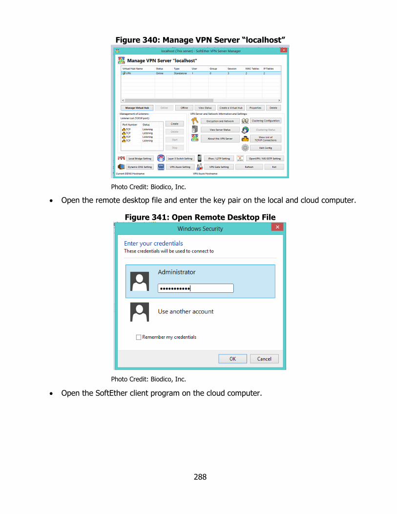
288
Figure 340: Manage VPN Server “localhost”
Photo Credit: Biodico, Inc.
• Open the remote desktop file and enter the key pair on the local and cloud computer.
Figure 341: Open Remote Desktop File
Photo Credit: Biodico, Inc.
• Open the SoftEther client program on the cloud computer.

289
Figure 342: SoftEther VPN Client Manager
Photo Credit: Biodico, Inc.
• Double click the Biodico label on SoftEther on the cloud computer.
Figure 343: Accessing Biodico on the Cloud
Photo Credit: Biodico, Inc.
After those six steps, Biodico can set up any computer as the primary Human Machine Interface to the cloud computer. At its most basic, the local, physical computer is really just a monitor and an ethernet port. As more ARIES locations are built, cloud-based data processing will help for a number of applications. The cloud-based computers run operations on their own processors, so for operations that require a heavy processing load, a temporary cloud computer can be used that will analyze the data and none of Biodico’s local, physical computers will be slowed down by the operation. As an example, Biodico as the ARIES interface will be able to more easily share data and updates for the entire network at once rather than individually. The streamlining will also allow for a better characterization of how different variables relate to the outputs of the Artemia and the anaerobic digestion systems. For the operation of the FTIR, the same library and test method will be used for everyone, and a library update will automatically be utilized by every FTIR probe within the system.
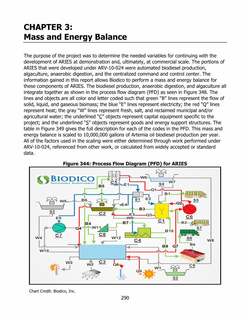
290
CHAPTER 3: Mass and Energy Balance
The purpose of the project was to determine the needed variables for continuing with the development of ARIES at demonstration and, ultimately, at commercial scale. The portions of ARIES that were developed under ARV-10-024 were automated biodiesel production, algaculture, anaerobic digestion, and the centralized command and control center. The information gained in this report allows Biodico to perform a mass and energy balance for these components of ARIES. The biodiesel production, anaerobic digestion, and algaculture all integrate together as shown in the process flow diagram (PFD) as seen in Figure 348. The lines and objects are all color and letter coded such that green “B” lines represent the flow of solid, liquid, and gaseous biomass; the blue “E” lines represent electricity; the red “Q” lines represent heat; the gray “W” lines represent fresh, salt, and reclaimed municipal and/or agricultural water; the underlined “C” objects represent capital equipment specific to the project; and the underlined “S” objects represent goods and energy support structures. The table in Figure 349 gives the full description for each of the codes in the PFD. This mass and energy balance is scaled to 10,000,000 gallons of Artemia oil biodiesel production per year. All of the factors used in the scaling were either determined through work performed under ARV-10-024, referenced from other work, or calculated from widely accepted or standard data.
Figure 344: Process Flow Diagram (PFD) for ARIES
Chart Credit: Biodico, Inc.

291
Figure 345: Process Flow Diagram (PFD) Coding Table
Chart Credit: Biodico, Inc
Biomass The green “B” lines represent liquid, solid, and gaseous biomass sources. For the purposes of this PFD, biomass refers to any organic chemical that is generated throughout the course of the process. The types of biomass during the course of the process change at many points through the facility by separation, reaction, or other means. Where electricity can always be given as kWh and heat energy can always be given as mmbtu, it is important to track the type of biomass that is generated and moved at different points in the process flow. The biomass type, the quantity, the point of origin, and the destination for each line are given in Figure 350 below. The values are given in terms of annual throughput.
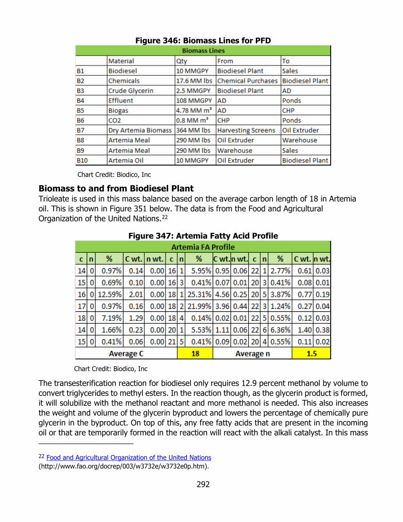
292
Figure 346: Biomass Lines for PFD
Chart Credit: Biodico, Inc
Biomass to and from Biodiesel Plant Trioleate is used in this mass balance based on the average carbon length of 18 in Artemia oil. This is shown in Figure 351 below. The data is from the Food and Agricultural Organization of the United Nations.22
Figure 347: Artemia Fatty Acid Profile
Chart Credit: Biodico, Inc
The transesterification reaction for biodiesel only requires 12.9 percent methanol by volume to convert triglycerides to methyl esters. In the reaction though, as the glycerin product is formed, it will solubilize with the methanol reactant and more methanol is needed. This also increases the weight and volume of the glycerin byproduct and lowers the percentage of chemically pure glycerin in the byproduct. On top of this, any free fatty acids that are present in the incoming oil or that are temporarily formed in the reaction will react with the alkali catalyst. In this mass
22 Food and Agricultural Organization of the United Nations (http://www.fao.org/docrep/003/w3732e/w3732e0p.htm).

293
balance sheet using triolein and sodium methylate this forms sodium oleate (soap) and water. This will emulsify the solution and cause some tri-, di-, and monoglycerides and some methyl esters to solubilize with the glycerin. This is why crude glycerin contains a high level of impurities. Based on fourteen years of commercial production at facilities built on Biodico’s patented technology in Las Vegas, Australia, Colorado, and Texas and optimization geared developmental production at Naval Base Ventura County, Biodico generates, on average, 25 percent crude glycerin from its biodiesel production. The volume, density, and weight of the compounds entering and leaving the biodiesel facility annually are given below in Figure 352.
Figure 348: Biomass Weights for Biodiesel Production
Chart Credit: Biodico, Inc
The elemental composition of all of the materials entering the facility is known. The elemental composition of the biodiesel leaving the facility is rigorously tested and also very well known. The elemental composition of each of these materials is given below in Figure 353.
Figure 349: Elemental Composition for Biodiesel Production
Chart Credit: Biodico, Inc
The glycerin is an amalgam of different compounds, as described above. Since the composition of every other compound entering or leaving the production is fairly simple though, the composition of the glycerin can be taken as the remaining material that does not leave with the biodiesel. It should be noted that some remaining impurities in the biodiesel are removed with water washes after the glycerin is removed (methanol, solubilized free glycerin, soap emulsifications, etc.) but since the water washes are going to the same destination as the glycerin (AD), all the remaining material can be put with the glycerin for
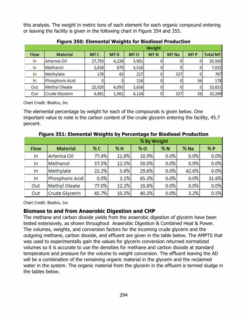
294
this analysis. The weight in metric tons of each element for each organic compound entering or leaving the facility is given in the following chart in Figure 354 and 355.
Figure 350: Elemental Weights for Biodiesel Production
Chart Credit: Biodico, Inc
The elemental percentage by weight for each of the compounds is given below. One important value to note is the carbon content of the crude glycerin entering the facility, 45.7 percent.
Figure 351: Elemental Weights by Percentage for Biodiesel Production
Chart Credit: Biodico, Inc
Biomass to and from Anaerobic Digestion and CHP The methane and carbon dioxide yields from the anaerobic digestion of glycerin have been tested extensively, as shown throughout Anaerobic Digestion & Combined Heat & Power. The volumes, weights, and conversion factors for the incoming crude glycerin and the outgoing methane, carbon dioxide, and effluent are given in the table below. The AMPTS that was used to experimentally gain the values for glycerin conversion returned normalized volumes so it is accurate to use the densities for methane and carbon dioxide at standard temperature and pressure for the volume to weight conversion. The effluent leaving the AD will be a combination of the remaining organic material in the glycerin and the reclaimed water in the system. The organic material from the glycerin in the effluent is termed sludge in the tables below.

295
Figure 352: Biomass Weights for AD
Chart Credit: Biodico, Inc
While the incoming crude glycerin and the outgoing organic portion of the glycerin, the sludge, are both amalgams of various organic compounds, the methane and carbon dioxide in the biogas have been tested by gas chromatography and are both well-known compounds. Figure 357 below gives the elemental composition of methane and carbon dioxide.
Figure 353: Elemental Composition for AD
Chart Credit: Biodico, Inc
Since the elemental balance of the crude glycerin entering the digestion and the biogas leaving the digestion are both well known, the elemental composition of the sludge leaving the anaerobic digester and entering the Artemia ponds can be calculated. The exhaust from the CHP unit will also be cycled into the Artemia ponds so the carbon dioxide portion of the biogas also enters the ponds. At the point of the CHP the methane leaves the biogas line as it is converted to electrical energy. The balances for the glycerin, carbon dioxide, methane, and sludge are shown in Figure 358.
Figure 354: Elemental Weights for AD
Chart Credit: Biodico, Inc
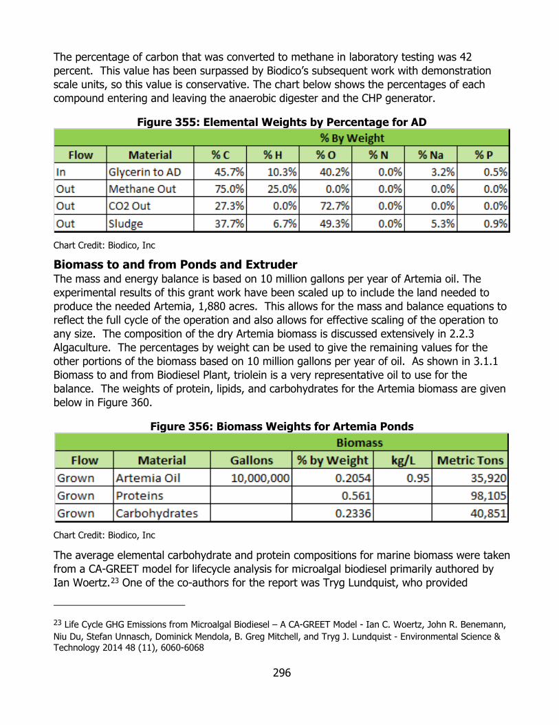
296
The percentage of carbon that was converted to methane in laboratory testing was 42 percent. This value has been surpassed by Biodico’s subsequent work with demonstration scale units, so this value is conservative. The chart below shows the percentages of each compound entering and leaving the anaerobic digester and the CHP generator.
Figure 355: Elemental Weights by Percentage for AD
Chart Credit: Biodico, Inc
Biomass to and from Ponds and Extruder The mass and energy balance is based on 10 million gallons per year of Artemia oil. The experimental results of this grant work have been scaled up to include the land needed to produce the needed Artemia, 1,880 acres. This allows for the mass and balance equations to reflect the full cycle of the operation and also allows for effective scaling of the operation to any size. The composition of the dry Artemia biomass is discussed extensively in 2.2.3 Algaculture. The percentages by weight can be used to give the remaining values for the other portions of the biomass based on 10 million gallons per year of oil. As shown in 3.1.1 Biomass to and from Biodiesel Plant, triolein is a very representative oil to use for the balance. The weights of protein, lipids, and carbohydrates for the Artemia biomass are given below in Figure 360.
Figure 356: Biomass Weights for Artemia Ponds
Chart Credit: Biodico, Inc
The average elemental carbohydrate and protein compositions for marine biomass were taken from a CA-GREET model for lifecycle analysis for microalgal biodiesel primarily authored by Ian Woertz.23 One of the co-authors for the report was Tryg Lundquist, who provided
23 Life Cycle GHG Emissions from Microalgal Biodiesel – A CA-GREET Model - Ian C. Woertz, John R. Benemann, Niu Du, Stefan Unnasch, Dominick Mendola, B. Greg Mitchell, and Tryg J. Lundquist - Environmental Science & Technology 2014 48 (11), 6060-6068
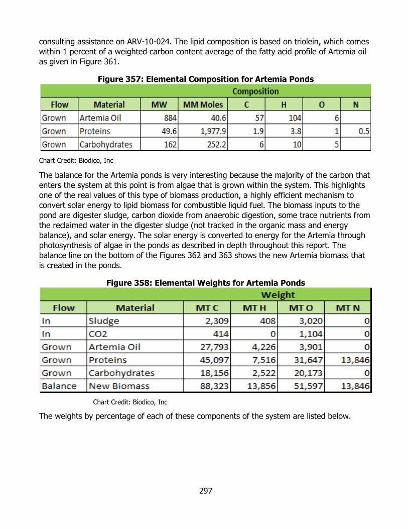
297
consulting assistance on ARV-10-024. The lipid composition is based on triolein, which comes within 1 percent of a weighted carbon content average of the fatty acid profile of Artemia oil as given in Figure 361.
Figure 357: Elemental Composition for Artemia Ponds
Chart Credit: Biodico, Inc
The balance for the Artemia ponds is very interesting because the majority of the carbon that enters the system at this point is from algae that is grown within the system. This highlights one of the real values of this type of biomass production, a highly efficient mechanism to convert solar energy to lipid biomass for combustible liquid fuel. The biomass inputs to the pond are digester sludge, carbon dioxide from anaerobic digestion, some trace nutrients from the reclaimed water in the digester sludge (not tracked in the organic mass and energy balance), and solar energy. The solar energy is converted to energy for the Artemia through photosynthesis of algae in the ponds as described in depth throughout this report. The balance line on the bottom of the Figures 362 and 363 shows the new Artemia biomass that is created in the ponds.
Figure 358: Elemental Weights for Artemia Ponds
Chart Credit: Biodico, Inc
The weights by percentage of each of these components of the system are listed below.
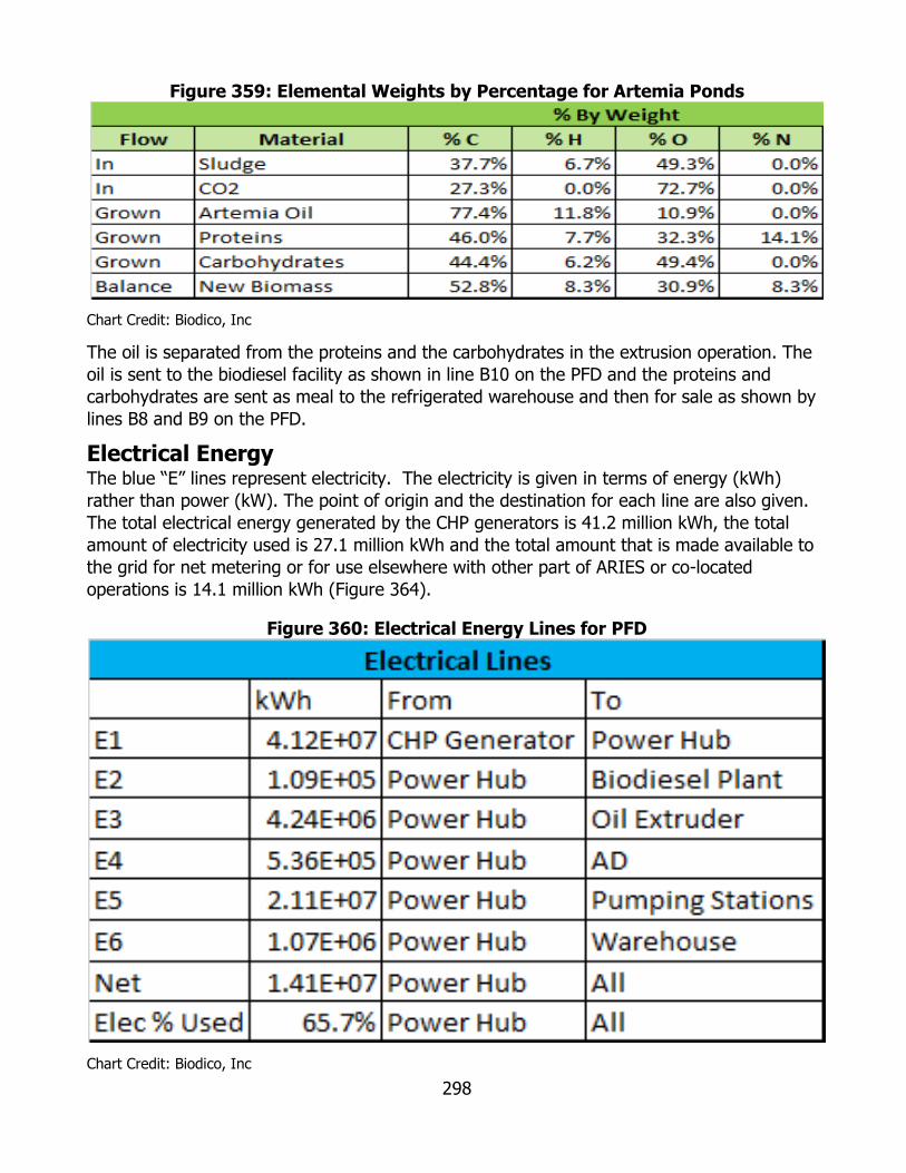
298
Figure 359: Elemental Weights by Percentage for Artemia Ponds
Chart Credit: Biodico, Inc
The oil is separated from the proteins and the carbohydrates in the extrusion operation. The oil is sent to the biodiesel facility as shown in line B10 on the PFD and the proteins and carbohydrates are sent as meal to the refrigerated warehouse and then for sale as shown by lines B8 and B9 on the PFD.
Electrical Energy The blue “E” lines represent electricity. The electricity is given in terms of energy (kWh) rather than power (kW). The point of origin and the destination for each line are also given. The total electrical energy generated by the CHP generators is 41.2 million kWh, the total amount of electricity used is 27.1 million kWh and the total amount that is made available to the grid for net metering or for use elsewhere with other part of ARIES or co-located operations is 14.1 million kWh (Figure 364).
Figure 360: Electrical Energy Lines for PFD
Chart Credit: Biodico, Inc
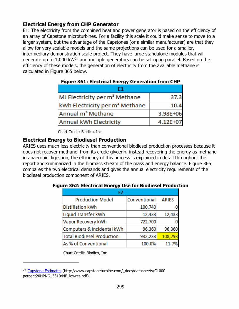
299
Electrical Energy from CHP Generator E1: The electricity from the combined heat and power generator is based on the efficiency of an array of Capstone microturbines. For a facility this scale it could make sense to move to a larger system, but the advantage of the Capstones (or a similar manufacturer) are that they allow for very scalable models and the same projections can be used for a smaller, intermediary demonstration scale project. They have large standalone modules that will generate up to 1,000 kW24 and multiple generators can be set up in parallel. Based on the efficiency of these models, the generation of electricity from the available methane is calculated in Figure 365 below.
Figure 361: Electrical Energy Generation from CHP
Chart Credit: Biodico, Inc
Electrical Energy to Biodiesel Production ARIES uses much less electricity than conventional biodiesel production processes because it does not recover methanol from its crude glycerin, instead recovering the energy as methane in anaerobic digestion, the efficiency of this process is explained in detail throughout the report and summarized in the biomass stream of the mass and energy balance. Figure 366 compares the two electrical demands and gives the annual electricity requirements of the biodiesel production component of ARIES.
Figure 362: Electrical Energy Use for Biodiesel Production
Chart Credit: Biodico, Inc
24 Capstone Estimates (http://www.capstoneturbine.com/_docs/datasheets/C1000 percent20HPNG_331044F_lowres.pdf).
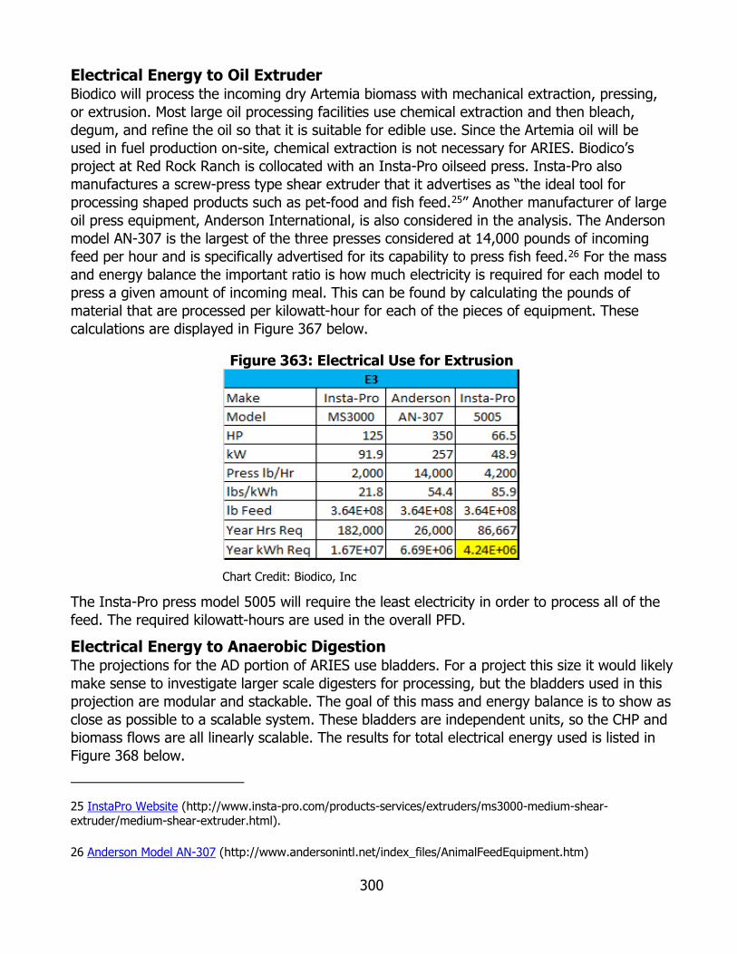
300
Electrical Energy to Oil Extruder Biodico will process the incoming dry Artemia biomass with mechanical extraction, pressing, or extrusion. Most large oil processing facilities use chemical extraction and then bleach, degum, and refine the oil so that it is suitable for edible use. Since the Artemia oil will be used in fuel production on-site, chemical extraction is not necessary for ARIES. Biodico’s project at Red Rock Ranch is collocated with an Insta-Pro oilseed press. Insta-Pro also manufactures a screw-press type shear extruder that it advertises as “the ideal tool for processing shaped products such as pet-food and fish feed.25” Another manufacturer of large oil press equipment, Anderson International, is also considered in the analysis. The Anderson model AN-307 is the largest of the three presses considered at 14,000 pounds of incoming feed per hour and is specifically advertised for its capability to press fish feed.26 For the mass and energy balance the important ratio is how much electricity is required for each model to press a given amount of incoming meal. This can be found by calculating the pounds of material that are processed per kilowatt-hour for each of the pieces of equipment. These calculations are displayed in Figure 367 below.
Figure 363: Electrical Use for Extrusion
Chart Credit: Biodico, Inc
The Insta-Pro press model 5005 will require the least electricity in order to process all of the feed. The required kilowatt-hours are used in the overall PFD.
Electrical Energy to Anaerobic Digestion The projections for the AD portion of ARIES use bladders. For a project this size it would likely make sense to investigate larger scale digesters for processing, but the bladders used in this projection are modular and stackable. The goal of this mass and energy balance is to show as close as possible to a scalable system. These bladders are independent units, so the CHP and biomass flows are all linearly scalable. The results for total electrical energy used is listed in Figure 368 below.
25 InstaPro Website (http://www.insta-pro.com/products-services/extruders/ms3000-medium-shear-extruder/medium-shear-extruder.html).
26 Anderson Model AN-307 (http://www.andersonintl.net/index_files/AnimalFeedEquipment.htm)

301
Figure 364: Electrical Use for AD
Chart Credit: Biodico, Inc
Electrical Energy to Pumping Stations The electrical demand for pumping stations per acre is based on the Woertz LCA model for algae biodiesel. The figure below converts the energy projected for influent pumping and for mixing per year into kWh per cubic meter of water. The volume of water pumped per year is based on the total hectares of the project multiplied by the acre feet multiplied by the number of cycles for pumping the volume of water per year (the number of days per year divided by the number of days per cycle). The volume of water pumped through Biodico’s circulation system for ARIES is described further in Pond Recirculation System.
Figure 365: Electrical Use for Pumping Station
Chart Credit: Biodico, Inc
Electrical Energy to Warehouse The electrical demand for refrigerated warehouse space was estimated by an equation determined through work led by Paul Singh of the UC Davis Department of Biological and Agricultural Engineering under grant funded research by the CEC’s Public Interest Energy

302
Research (PIER) program.27 The study found that the kWh per year per cubic foot of refrigerated storage volume, which was defined as specific energy consumption followed the equation below, where V is the volume in cubic feet (Figure 370).
SEC= 38.978* V -0.2275
The calculation for the cubic feet needed for refrigerated warehouse space to store and ship the meal is given in Refrigerated Warehouse Capital Costs.
Figure 366: Electricity Use for Refrigerated Warehouse
Chart Credit: Biodico, Inc
Heat Energy The red “Q” lines represent heat. The heat is given in terms of mmBtus. Since the main heating loop cascades through the different components of ARIES, the heating values for much of the system are subtracted in sequence from the original heat generated by the CHP array. The point of origin and the destination for each line are also given. The physical area that the project encompasses is fairly large, almost three square miles so some substantial heat loss through the system is definitely expected. The amount of transferable heat generated is so large though, that it will handle up to 66.2 percent loss in energy through the course of the cascade process. The effect of the cascade layout for the project is seen in Figure 371.
27 Singh, R. Paul. 2008. Benchmarking Study of the Refrigerated Warehousing Industry Sector in
California. Public Interest Energy Research (PIER) Program Contract and Research Project
Reports. California Energy Commission, PIER Program
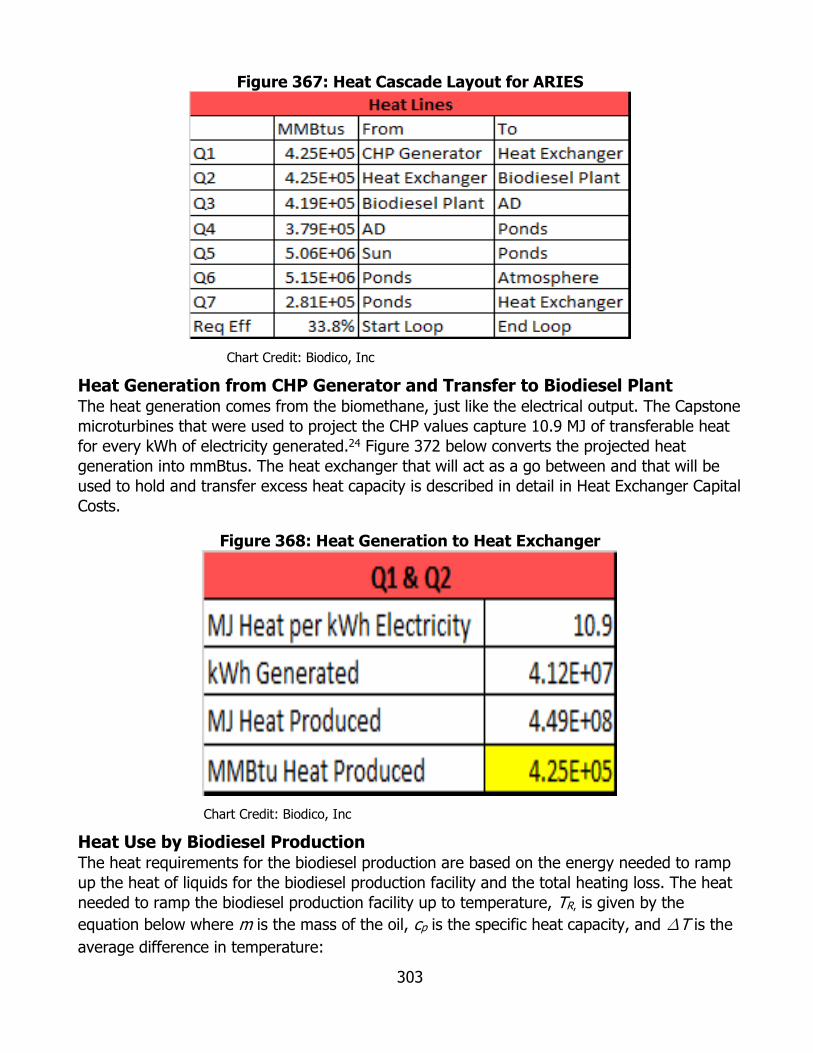
303
Figure 367: Heat Cascade Layout for ARIES
Chart Credit: Biodico, Inc
Heat Generation from CHP Generator and Transfer to Biodiesel Plant The heat generation comes from the biomethane, just like the electrical output. The Capstone microturbines that were used to project the CHP values capture 10.9 MJ of transferable heat for every kWh of electricity generated.24 Figure 372 below converts the projected heat generation into mmBtus. The heat exchanger that will act as a go between and that will be used to hold and transfer excess heat capacity is described in detail in Heat Exchanger Capital Costs.
Figure 368: Heat Generation to Heat Exchanger
Chart Credit: Biodico, Inc
Heat Use by Biodiesel Production The heat requirements for the biodiesel production are based on the energy needed to ramp up the heat of liquids for the biodiesel production facility and the total heating loss. The heat needed to ramp the biodiesel production facility up to temperature, TR, is given by the equation below where m is the mass of the oil, cp is the specific heat capacity, and ∆T is the average difference in temperature:
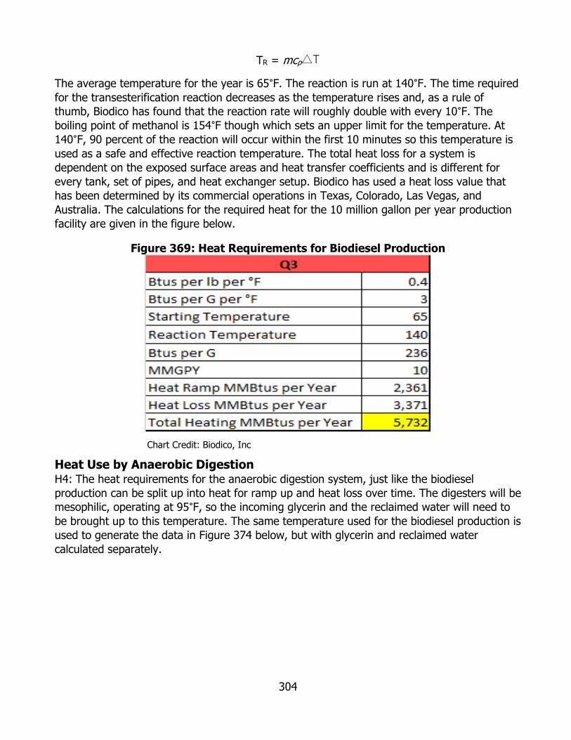
304
TR = mcp△T
The average temperature for the year is 65°F. The reaction is run at 140°F. The time required for the transesterification reaction decreases as the temperature rises and, as a rule of thumb, Biodico has found that the reaction rate will roughly double with every 10°F. The boiling point of methanol is 154°F though which sets an upper limit for the temperature. At 140°F, 90 percent of the reaction will occur within the first 10 minutes so this temperature is used as a safe and effective reaction temperature. The total heat loss for a system is dependent on the exposed surface areas and heat transfer coefficients and is different for every tank, set of pipes, and heat exchanger setup. Biodico has used a heat loss value that has been determined by its commercial operations in Texas, Colorado, Las Vegas, and Australia. The calculations for the required heat for the 10 million gallon per year production facility are given in the figure below.
Figure 369: Heat Requirements for Biodiesel Production
Chart Credit: Biodico, Inc
Heat Use by Anaerobic Digestion H4: The heat requirements for the anaerobic digestion system, just like the biodiesel production can be split up into heat for ramp up and heat loss over time. The digesters will be mesophilic, operating at 95°F, so the incoming glycerin and the reclaimed water will need to be brought up to this temperature. The same temperature used for the biodiesel production is used to generate the data in Figure 374 below, but with glycerin and reclaimed water calculated separately.

305
Figure 370: Heat Increase Requirements for AD Influent
Chart Credit: Biodico, Inc.
Since the bladders are a fairly simple design and the glycerin and water influent will stay in the same bladder until the digestion is finished and they exit the digester as effluent, the heat loss calculations are fairly straightforward. Loss in heating energy is derived from Newton’s Law of Cooling, which describes convective heat transfer. The exact mechanism of energy loss for the digesters can be most accurately described as surface heat loss due to temperature difference where energy loss per hour, EH, is described by the equation below where ks is the surface heat loss factor in Btus per hour per square foot per degree Fahrenheit, ∆T is the pond temperature subtracted by the atmospheric temperature, and A is the surface area of the pool in square feet.
The surface heat loss factor for the polyurethane bladders is 0.16. Since the outdoor heat will only rarely be above 95°F, we can take the average temperature over the year, 65°F, and multiply the average heat loss, 30°F, by the hourly heat loss. The polyurethane bladders can be generalized as a half sphere. This gives a calculation of surface area to volume of:
The volumes of the bladders are 6,000 gallons each. The conversions and calculations for the heat loss from all of the bladders over the course of the year are given in Figure 375.

306
Figure 371: Heat Loss for AD
Chart Credit: Biodico, Inc
The total heat is the sum of the heat loss and the influent temperature increase. This is shown in the following figure.
Figure 372: Heat Transfer Balance for AD
Chart Credit: Biodico, Inc
Heat Transfer in Ponds The required heating energy, ER, needed for the algaculture can be calculated by the loss in heating energy, EL, due to the surrounding atmosphere minus the gain in heating energy from the surrounding solar energy, ES, as shown in the equation below.
Since both the loss in heating energy and the solar energy fall in yearly cycles, it is necessary to sum up the total energies over the course of a year for projections. The solar energy was captured on site through the course of the project as summarized in Algaculture. The solar energy was converted to kilowatt-hours per square meter per day, so the total solar energy for the year can be calculated as:
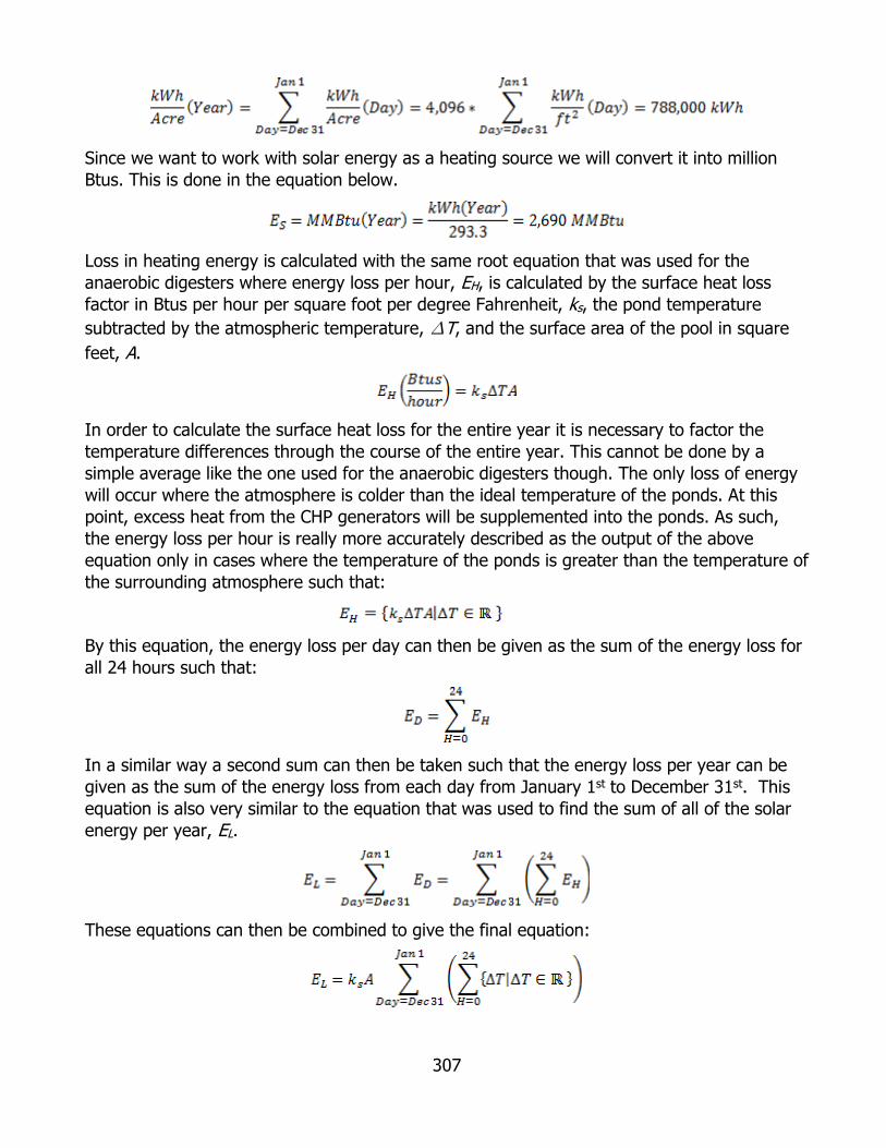
307
Since we want to work with solar energy as a heating source we will convert it into million Btus. This is done in the equation below.
Loss in heating energy is calculated with the same root equation that was used for the anaerobic digesters where energy loss per hour, EH, is calculated by the surface heat loss factor in Btus per hour per square foot per degree Fahrenheit, ks, the pond temperature subtracted by the atmospheric temperature, ∆T, and the surface area of the pool in square feet, A.
In order to calculate the surface heat loss for the entire year it is necessary to factor the temperature differences through the course of the entire year. This cannot be done by a simple average like the one used for the anaerobic digesters though. The only loss of energy will occur where the atmosphere is colder than the ideal temperature of the ponds. At this point, excess heat from the CHP generators will be supplemented into the ponds. As such, the energy loss per hour is really more accurately described as the output of the above equation only in cases where the temperature of the ponds is greater than the temperature of the surrounding atmosphere such that:
By this equation, the energy loss per day can then be given as the sum of the energy loss for all 24 hours such that:
In a similar way a second sum can then be taken such that the energy loss per year can be given as the sum of the energy loss from each day from January 1st to December 31st. This equation is also very similar to the equation that was used to find the sum of all of the solar energy per year, EL.
These equations can then be combined to give the final equation:

308
The temperatures were taken with the same instrument that was used to collect the solar energy levels. As a way to average the data, for each day throughout the year, 12 hours were estimated at the high temperature for the day and 12 hours were estimated at the low temperature. The sum for the year total of 2013 gives the result:
The average surface heat loss factor, ks, in the atmosphere is 5.5 and the number of square feet in an acre is 4,096 so the total Btu demand needed per acre of algaculture can be given as:
The required energy calculation can now be filled in with the values from the solar energy heat gain and the radiative energy heat loss as:
These calculations are all summarized in the following figure. The net heat loss, the loss from the atmosphere subtracted by the gain from the solar energy is 52 mmBtu/acre * year.
Figure 373: Heat Transfer for Artemia Ponds
Chart Credit: Biodico, Inc
Heat Transfer Efficiency for Cascade The heat circulation system will have lots of open pipes and lots of radiative heat losses. The excess heat generated ensures that the system will work as long as the losses do not exceed the heat that is generated by the system. The calculations are displayed in the figure below.

309
Figure 374: Minimum Heat Cascade Efficiency for ARIES
Chart Credit: Biodico, Inc
It is likely that the efficiency will exceed this and that the extra thermal energy can be used for co-located projects, to assist additional portions of ARIES not explored in ARV-10-024, or to be used elsewhere.
Water Use The gray “W” lines represent water. The point of origin and the destination for each line are also given. Three different water sources are listed in the following table: saltwater, fresh water, and reclaimed water. Each of these water sources can be used for different parts of ARIES. Since this PFD is designed to be used for multiple sites, some possibilities for water use are included that will not be used at Red Rock Ranch. For example, the Artemia ponds should use fresh water only as a last resort. They will thrive with saltwater or with reclaimed water. Since Red Rock Ranch is not near the ocean and since reclaimed agricultural water is readily accessible, saltwater is not used in this particular model. The pathway is worth including for sites that are near the water, such as Naval Base Ventura County. For sites where neither source is accessible an unused possibility for fresh water is also included. By that same token, this helps to distinguish water uses that would not be possible by their non-inclusion. Saltwater would not work well in the anaerobic digestion system so it is not included. Reclaimed water and fresh water both can be used, though reclaimed water is highly preferable, so they were both included. This is seen in the figure below.
Figure 375: Water Flows for ARIES
Chart Credit: Biodico, Inc
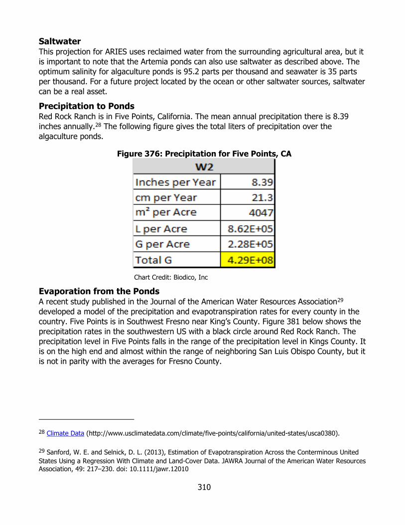
310
Saltwater This projection for ARIES uses reclaimed water from the surrounding agricultural area, but it is important to note that the Artemia ponds can also use saltwater as described above. The optimum salinity for algaculture ponds is 95.2 parts per thousand and seawater is 35 parts per thousand. For a future project located by the ocean or other saltwater sources, saltwater can be a real asset.
Precipitation to Ponds Red Rock Ranch is in Five Points, California. The mean annual precipitation there is 8.39 inches annually.28 The following figure gives the total liters of precipitation over the algaculture ponds.
Figure 376: Precipitation for Five Points, CA
Chart Credit: Biodico, Inc
Evaporation from the Ponds A recent study published in the Journal of the American Water Resources Association29 developed a model of the precipitation and evapotranspiration rates for every county in the country. Five Points is in Southwest Fresno near King’s County. Figure 381 below shows the precipitation rates in the southwestern US with a black circle around Red Rock Ranch. The precipitation level in Five Points falls in the range of the precipitation level in Kings County. It is on the high end and almost within the range of neighboring San Luis Obispo County, but it is not in parity with the averages for Fresno County.
28 Climate Data (http://www.usclimatedata.com/climate/five-points/california/united-states/usca0380).
29 Sanford, W. E. and Selnick, D. L. (2013), Estimation of Evapotranspiration Across the Conterminous United States Using a Regression With Climate and Land-Cover Data. JAWRA Journal of the American Water Resources Association, 49: 217–230. doi: 10.1111/jawr.12010

311
Figure 377: Annual Precipitation of Southwestern US
Chart Credit: Journal of the American Water Resources Association
The next chart below shows the ratio of losses by evapotranspiration to losses by precipitation for this same region. Since the precipitation values fell within the high range for Kings County, but were near the range for San Luis Obispo County, it is likely that the ratio will fall within that area. As Figure 382 below shows, the range of ratios for Kings County are the highest in the chart (1.2 to 1.29) and the ratios in all of the neighboring counties are significantly better. The evaporation loss ratio can be estimated at the low end of the range, 1.2. This would give an evaporation of 25.6 cm.
Figure 378: Precipitation Loss by Percent for Southwestern US
Chart Credit: Journal of the American Water Resources Association
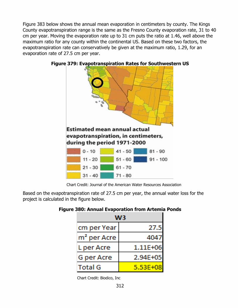
312
Figure 383 below shows the annual mean evaporation in centimeters by county. The Kings County evapotranspiration range is the same as the Fresno County evaporation rate, 31 to 40 cm per year. Moving the evaporation rate up to 31 cm puts the ratio at 1.46, well above the maximum ratio for any county within the continental US. Based on these two factors, the evapotranspiration rate can conservatively be given at the maximum ratio, 1.29, for an evaporation rate of 27.5 cm per year.
Figure 379: Evapotranspiration Rates for Southwestern US
Chart Credit: Journal of the American Water Resources Association
Based on the evapotranspiration rate of 27.5 cm per year, the annual water loss for the project is calculated in the figure below.
Figure 380: Annual Evaporation from Artemia Ponds
Chart Credit: Biodico, Inc
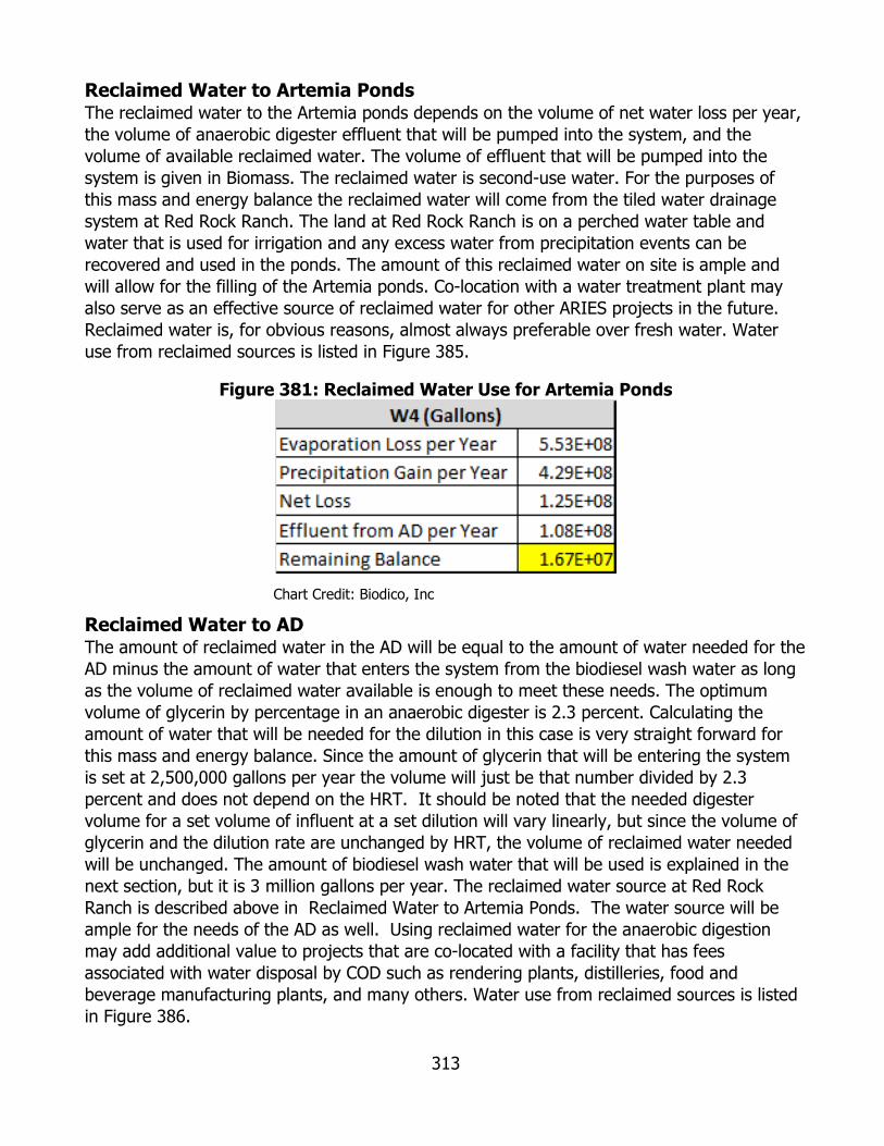
313
Reclaimed Water to Artemia Ponds The reclaimed water to the Artemia ponds depends on the volume of net water loss per year, the volume of anaerobic digester effluent that will be pumped into the system, and the volume of available reclaimed water. The volume of effluent that will be pumped into the system is given in Biomass. The reclaimed water is second-use water. For the purposes of this mass and energy balance the reclaimed water will come from the tiled water drainage system at Red Rock Ranch. The land at Red Rock Ranch is on a perched water table and water that is used for irrigation and any excess water from precipitation events can be recovered and used in the ponds. The amount of this reclaimed water on site is ample and will allow for the filling of the Artemia ponds. Co-location with a water treatment plant may also serve as an effective source of reclaimed water for other ARIES projects in the future. Reclaimed water is, for obvious reasons, almost always preferable over fresh water. Water use from reclaimed sources is listed in Figure 385.
Figure 381: Reclaimed Water Use for Artemia Ponds
Chart Credit: Biodico, Inc
Reclaimed Water to AD The amount of reclaimed water in the AD will be equal to the amount of water needed for the AD minus the amount of water that enters the system from the biodiesel wash water as long as the volume of reclaimed water available is enough to meet these needs. The optimum volume of glycerin by percentage in an anaerobic digester is 2.3 percent. Calculating the amount of water that will be needed for the dilution in this case is very straight forward for this mass and energy balance. Since the amount of glycerin that will be entering the system is set at 2,500,000 gallons per year the volume will just be that number divided by 2.3 percent and does not depend on the HRT. It should be noted that the needed digester volume for a set volume of influent at a set dilution will vary linearly, but since the volume of glycerin and the dilution rate are unchanged by HRT, the volume of reclaimed water needed will be unchanged. The amount of biodiesel wash water that will be used is explained in the next section, but it is 3 million gallons per year. The reclaimed water source at Red Rock Ranch is described above in Reclaimed Water to Artemia Ponds. The water source will be ample for the needs of the AD as well. Using reclaimed water for the anaerobic digestion may add additional value to projects that are co-located with a facility that has fees associated with water disposal by COD such as rendering plants, distilleries, food and beverage manufacturing plants, and many others. Water use from reclaimed sources is listed in Figure 386.
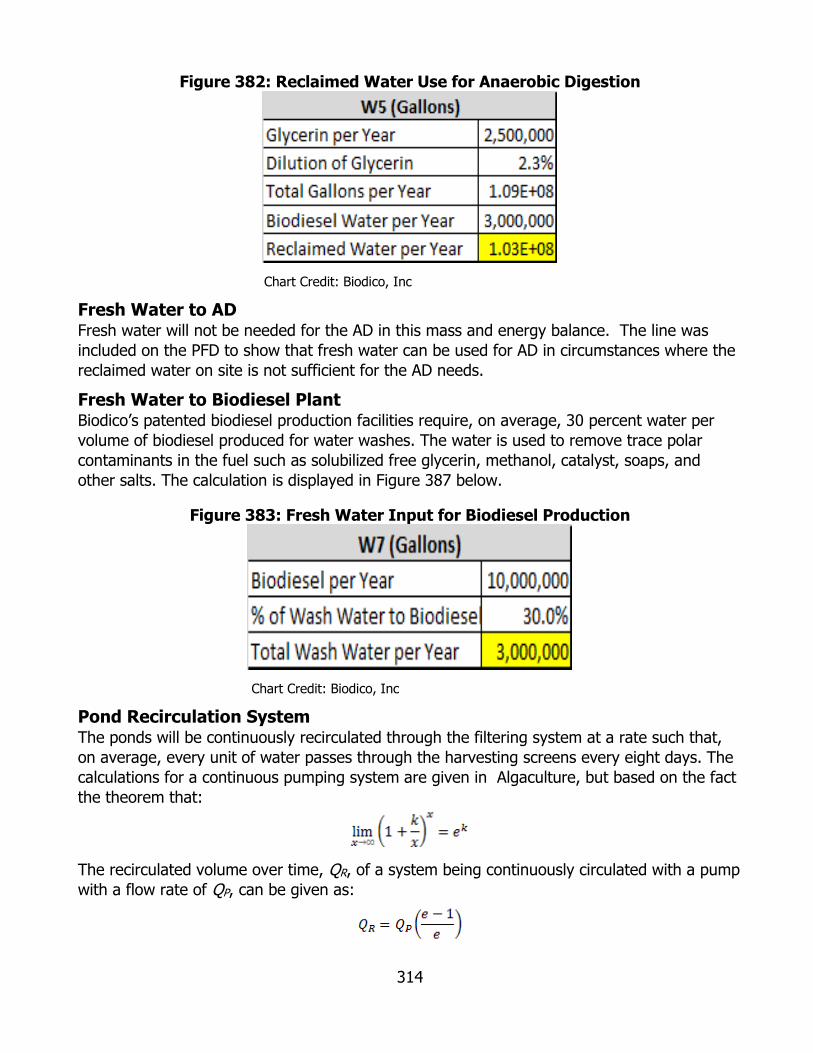
314
Figure 382: Reclaimed Water Use for Anaerobic Digestion
Chart Credit: Biodico, Inc
Fresh Water to AD Fresh water will not be needed for the AD in this mass and energy balance. The line was included on the PFD to show that fresh water can be used for AD in circumstances where the reclaimed water on site is not sufficient for the AD needs.
Fresh Water to Biodiesel Plant Biodico’s patented biodiesel production facilities require, on average, 30 percent water per volume of biodiesel produced for water washes. The water is used to remove trace polar contaminants in the fuel such as solubilized free glycerin, methanol, catalyst, soaps, and other salts. The calculation is displayed in Figure 387 below.
Figure 383: Fresh Water Input for Biodiesel Production
Chart Credit: Biodico, Inc
Pond Recirculation System The ponds will be continuously recirculated through the filtering system at a rate such that, on average, every unit of water passes through the harvesting screens every eight days. The calculations for a continuous pumping system are given in Algaculture, but based on the fact the theorem that:
The recirculated volume over time, QR, of a system being continuously circulated with a pump with a flow rate of QP, can be given as:
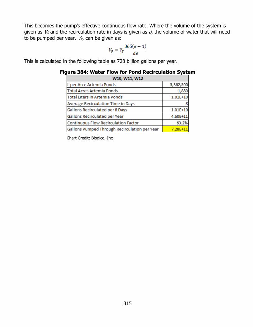
315
This becomes the pump’s effective continuous flow rate. Where the volume of the system is given as VS and the recirculation rate in days is given as d, the volume of water that will need to be pumped per year, VP, can be given as:
This is calculated in the following table as 728 billion gallons per year.
Figure 384: Water Flow for Pond Recirculation System
Chart Credit: Biodico, Inc
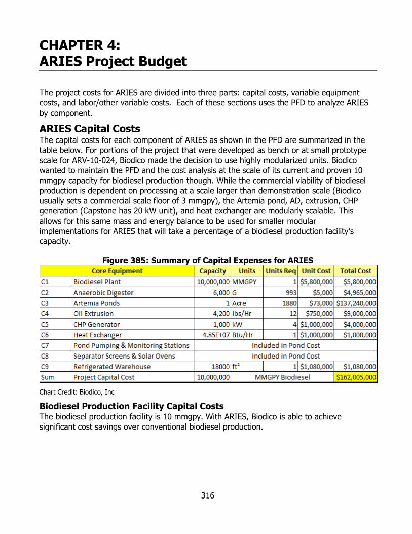
316
CHAPTER 4: ARIES Project Budget
The project costs for ARIES are divided into three parts: capital costs, variable equipment costs, and labor/other variable costs. Each of these sections uses the PFD to analyze ARIES by component.
ARIES Capital Costs The capital costs for each component of ARIES as shown in the PFD are summarized in the table below. For portions of the project that were developed as bench or at small prototype scale for ARV-10-024, Biodico made the decision to use highly modularized units. Biodico wanted to maintain the PFD and the cost analysis at the scale of its current and proven 10 mmgpy capacity for biodiesel production though. While the commercial viability of biodiesel production is dependent on processing at a scale larger than demonstration scale (Biodico usually sets a commercial scale floor of 3 mmgpy), the Artemia pond, AD, extrusion, CHP generation (Capstone has 20 kW unit), and heat exchanger are modularly scalable. This allows for this same mass and energy balance to be used for smaller modular implementations for ARIES that will take a percentage of a biodiesel production facility’s capacity.
Figure 385: Summary of Capital Expenses for ARIES
Chart Credit: Biodico, Inc
Biodiesel Production Facility Capital Costs The biodiesel production facility is 10 mmgpy. With ARIES, Biodico is able to achieve significant cost savings over conventional biodiesel production.
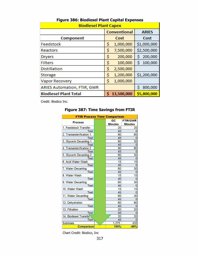
317
Figure 386: Biodiesel Plant Capital Expenses
Credit: Biodico Inc.
Figure 387: Time Savings from FTIR
Chart Credit: Biodico, Inc

318
One of the big savings is that Biodico is not distilling out methanol for recovery and reuse in the system for biodiesel production. This allows Biodico to cut out the major expense of distillation. This also cuts out a lot of energy use, which is explained further in Electrical Energy to Biodiesel Production. One of the other major saved expenses is reactor size. By using the FTIR method developed under ARV-10-024 and utilizing the Invensys developed automation protocols, Biodico will be able to triple throughput of its reactors—the biggest capital cost of a biodiesel production facility. This is because testing for the required ASTM specification must be performed before, during, and after the production cycle, which is a real bottleneck for the system. The Invensys unit allows for automated feedback to the production cycle based on the input of the FTIR. The time savings are displayed on the chart to the left. This also affects wages, which are described in Biodiesel Production Facility Labor Costs.
Anaerobic Digester Capital Costs Each modular digester fits inside a standard shipping container and holds 6,000 gallons of digester influent (glycerin and reclaimed water) not including headspace. The modular digesters include heating loops and are stackable units. This highly modularized design allows for this component of ARIES to start with a relatively small percentage of the larger, full circle integrated biorefinery and to grow incrementally to the full system. The costs for each AD unit and the cost for the whole integrated project are given in the table below.
Figure 388: AD Capital Expenses
Chart Credit: Biodico, Inc
Artemia Ponds Capital Costs The Artemia ponds are also highly modularized so that the development of the full ARIES system can proceed in steps. The study work was done in totes, but for the larger

319
implementation larger ponds with hoop greenhouse structures will be used. The costs below include pond capital costs, solar dehydrators, aeration, harvesting, and process controls and sensors. The cost per acre and the total cost for 1,880 acres are given.
Figure 389: Artemia Pond Capital Expenses
Chart Credit: Biodico, Inc
The ponds are raceway style with a hoop greenhouse to prevent unwanted contamination and interference by migratory waterfowl and other birds in the San Joaquin Valley. They contain piping for the cascading heat system and pumps for mixing and influent transfer. The quote of $45,000 was obtained by a California contractor in the San Joaquin Valley. The design is given below.
Figure 390: ARIES Pond Design
Chart Credit: Biodico, Inc

320
The controls and instrumentation are referred to as a data broadcasting hub designed to return pH and salinity and can be modified to integrate dissolved oxygen and flow meters. The probes can come from any number of manufacturers. The information is transferred as 4 – 20 mA signals to an IDEC mini- Programmable Logic Control in a water resistant steel enclosure. The IDEC mini- Programmable Logic Control then transmits the information by Modbus radio to the Invensys system where it is integrated into the automated production for the ARIES system as a whole. Biodico is currently working with Seahold under grant 11-501-03 with the CEC to install the same type of system for anaerobic digestion of a demonstration scale Upflow Anaerobic Sludge Blanket digester for glycerin. The only real difference in the system is one probe. The DHB for the Artemia ponds will have pH/temperature and salinity probes and the existing DHB for the AD has pH and oxidation reduction potential probes. A picture of the inside of the relay unit is displayed in Figure 395.
Figure 391: Data Broadcasting Hub
Chart Credit: Biodico, Inc
The system was put together by California-based Jensen Instruments. It is important to note that this mini- Programmable Logic Control is a data collection and broadcasting hub and is not intended to replace the larger Invensys unit, which is used to integrate all of the incoming data streams and inform how the Artemia ponds fit into the rest of ARIES.
Oil Extrusion Costs Three different mechanical oil extrusion units are compared in Electrical Energy to Oil Extruder. The unit selected is an Insta-Pro model 5005. 12 units will be needed to process the biomass generated in the Artemia ponds. The cost for these units is given below. These are modular units, but they are at a significantly larger capacity than the modular units for the greenhouse and anaerobic digestion. For the start of ramping up, there is an Insta-Pro model 5005 that is currently at Red Rock Ranch that can be used as the AD and pond portions of ARIES ramp up to larger scales.
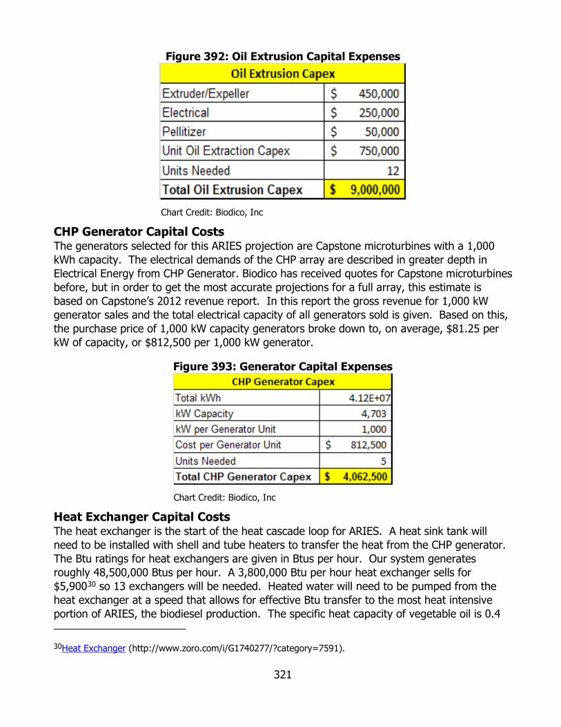
321
Figure 392: Oil Extrusion Capital Expenses
Chart Credit: Biodico, Inc
CHP Generator Capital Costs The generators selected for this ARIES projection are Capstone microturbines with a 1,000 kWh capacity. The electrical demands of the CHP array are described in greater depth in Electrical Energy from CHP Generator. Biodico has received quotes for Capstone microturbines before, but in order to get the most accurate projections for a full array, this estimate is based on Capstone’s 2012 revenue report. In this report the gross revenue for 1,000 kW generator sales and the total electrical capacity of all generators sold is given. Based on this, the purchase price of 1,000 kW capacity generators broke down to, on average, $81.25 per kW of capacity, or $812,500 per 1,000 kW generator.
Figure 393: Generator Capital Expenses
Chart Credit: Biodico, Inc
Heat Exchanger Capital Costs The heat exchanger is the start of the heat cascade loop for ARIES. A heat sink tank will need to be installed with shell and tube heaters to transfer the heat from the CHP generator. The Btu ratings for heat exchangers are given in Btus per hour. Our system generates roughly 48,500,000 Btus per hour. A 3,800,000 Btu per hour heat exchanger sells for $5,90030 so 13 exchangers will be needed. Heated water will need to be pumped from the heat exchanger at a speed that allows for effective Btu transfer to the most heat intensive portion of ARIES, the biodiesel production. The specific heat capacity of vegetable oil is 0.4
30Heat Exchanger (http://www.zoro.com/i/G1740277/?category=7591).

322
and the daily volume of oil that will need to be heated for a 330 day work year is roughly 330,000 gallons. The average temperature at Red Rock is 65°F and the required temperature for the biodiesel reaction is 140°F, for a temperature differential of 75°F. The heat exchanger needs to able to pump enough water through to heat the biodiesel to this temperature. The calculations for the heat exchange rate to the biodiesel production and the needed gallons per minute (GPM) are given below in Figure 398. The heat exchanger is scaled to have capacity for storage of 24 hours of additional heat.
Figure 394: Heat Exchanger Capital Expenses
Chart Credit: Biodico, Inc
Refrigerated Warehouse Capital Costs The refrigerated warehouse will be used to store the Artemia meal that will be sold and shipped from the facility. The warehouse will be designed to hold a week’s storage capacity. In the table below the pounds of meal per year are converted to cubic meters per week. The storage requirements for a refrigerated warehouse space are given by the Occupational Safety and Health Administration.31 The stacking configuration meets the Occupational Safety and Health Administration requirements with a margin of extra space for storage containers. The capital costs were estimated at $20 per square foot for building costs and $40 per square foot for refrigeration costs.32 The calculations are given in Figure 399.
31 OSHA Requirement (https://www.osha.gov/Publications/osha2236.pdf).
32 Capital Costs for Calculations (http://www.irr.com/_FileLibrary/Office/P484/Cold percent20Storage percent20Article.pdf).
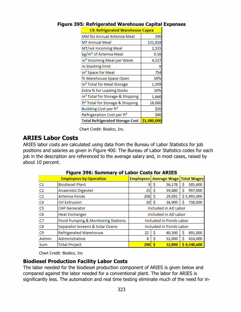
323
Figure 395: Refrigerated Warehouse Capital Expenses
Chart Credit: Biodico, Inc.
ARIES Labor Costs ARIES labor costs are calculated using data from the Bureau of Labor Statistics for job positions and salaries as given in Figure 400. The Bureau of Labor Statistics codes for each job in the description are referenced to the average salary and, in most cases, raised by about 10 percent.
Figure 396: Summary of Labor Costs for ARIES
Chart Credit: Biodico, Inc
Biodiesel Production Facility Labor Costs The labor needed for the biodiesel production component of ARIES is given below and compared against the labor needed for a conventional plant. The labor for ARIES is significantly less. The automation and real time testing eliminate much of the need for in-
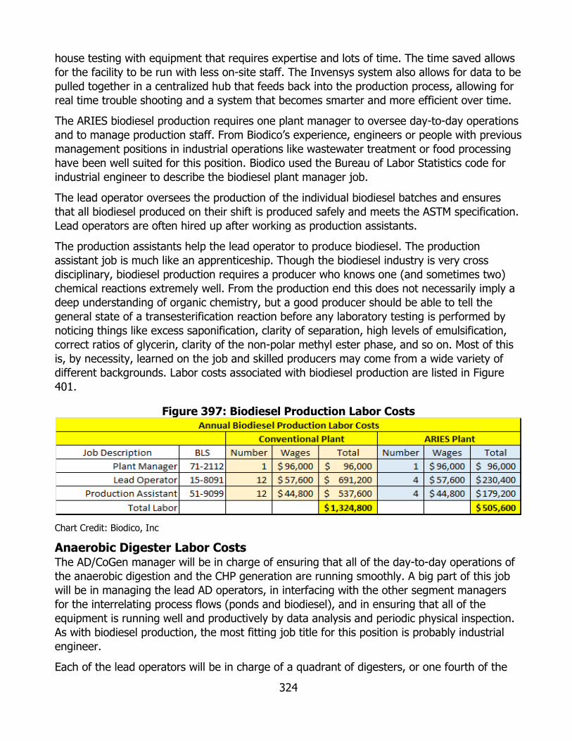
324
house testing with equipment that requires expertise and lots of time. The time saved allows for the facility to be run with less on-site staff. The Invensys system also allows for data to be pulled together in a centralized hub that feeds back into the production process, allowing for real time trouble shooting and a system that becomes smarter and more efficient over time.
The ARIES biodiesel production requires one plant manager to oversee day-to-day operations and to manage production staff. From Biodico’s experience, engineers or people with previous management positions in industrial operations like wastewater treatment or food processing have been well suited for this position. Biodico used the Bureau of Labor Statistics code for industrial engineer to describe the biodiesel plant manager job.
The lead operator oversees the production of the individual biodiesel batches and ensures that all biodiesel produced on their shift is produced safely and meets the ASTM specification. Lead operators are often hired up after working as production assistants.
The production assistants help the lead operator to produce biodiesel. The production assistant job is much like an apprenticeship. Though the biodiesel industry is very cross disciplinary, biodiesel production requires a producer who knows one (and sometimes two) chemical reactions extremely well. From the production end this does not necessarily imply a deep understanding of organic chemistry, but a good producer should be able to tell the general state of a transesterification reaction before any laboratory testing is performed by noticing things like excess saponification, clarity of separation, high levels of emulsification, correct ratios of glycerin, clarity of the non-polar methyl ester phase, and so on. Most of this is, by necessity, learned on the job and skilled producers may come from a wide variety of different backgrounds. Labor costs associated with biodiesel production are listed in Figure 401.
Figure 397: Biodiesel Production Labor Costs
Chart Credit: Biodico, Inc
Anaerobic Digester Labor Costs The AD/CoGen manager will be in charge of ensuring that all of the day-to-day operations of the anaerobic digestion and the CHP generation are running smoothly. A big part of this job will be in managing the lead AD operators, in interfacing with the other segment managers for the interrelating process flows (ponds and biodiesel), and in ensuring that all of the equipment is running well and productively by data analysis and periodic physical inspection. As with biodiesel production, the most fitting job title for this position is probably industrial engineer.
Each of the lead operators will be in charge of a quadrant of digesters, or one fourth of the

325
total digesters for the project. They will manage the individual operators, perform regular physical inspections, check that the machinery is functioning smoothly, and analyze data to distill for the AD general manager. As with biodiesel production, the lead operators will likely be promoted internally, having first-hand knowledge of the process and familiarity with the staff. AD labor costs are listed in Figure 402.
Production assistants will be in charge of monitoring the feed into the digesters, monitoring the effluent out, monitoring the gas flow, and manually tracking data where needed. This position is, for the most part, non-technical though. Willingness and hopefully eagerness to learn is the most telling factor for this position and, for the Red Rock Ranch project, most of the production assistants will likely come from an agricultural or production background, though production assistants from a wide variety of backgrounds can succeed at this job.
Figure 398: AD Labor Costs for ARIES
Chart Credit: Biodico, Inc
Artemia Ponds Labor Costs The Artemia pond harvesting operators will be in charge of monitoring the individual ponds, moving the harvesting screens into the solar ovens and transporting the dry biomass to the oil extruders. Most of the harvesting operators will likely come from agriculture backgrounds.
The harvesting equipment mechanics will be responsible for fixing any mechanical issues with parts related to the pond operation and may also be called to help with issues for other parts of ARIES. Job applicants with previous mechanic experience will be preferred for these positions.
Harvesting supervisors will be in charge of managing one octant of the ponds, or one eighth of the total ponds. The harvesting supervisors will likely be promoted internally. In addition to supervising the operators, they will be responsible for tracking the load volumes and/or weights of dry Artemia biomass from the ponds to the extruders.
The feedstock managers will work together to manage the ponds. Since this portion of the project encompasses so much area it is necessary to have two managers. The managers will also be responsible for tracking biomass production and transportation volumes and for interfacing with the managers for AD, biodiesel, extrusion, and refrigeration. Figure 403 below shows the Artemia pond labor costs for the project.

326
Figure 399: Artemia Pond Labor Costs for ARIES
Chart Credit: Biodico, Inc
Oil Extrusion Labor Costs Oil extrusion will run in two shifts, each with eight operators, one supervisor, and a mechanic. Crusher operators will be responsible for tending the machine, receiving new material as it comes in, pumping the oil over to the biodiesel plant, and sorting the meal for collection by the warehouse team. For the Red Rock Ranch project, most crusher operators will likely come from a processing background.
In addition to supervising the crushing operators, the two crusher supervisors will be in charge of interfacing with the pond, biodiesel, and warehouse supervisors and tracking and recording the material in and material out data. One supervisor will be responsible for each shift. The industrial mechanics will be on hand (one for each shift) to fix any problems that may occur with the extrusion equipment. Due to the nature of the extrusion equipment, these mechanics will be more highly trained than the mechanics at the ponds and they may be called on to fix problems with other parts of ARIES. Figure 404 lists the oil extrusion labor costs for the ARIES project.
Figure 400: Oil Extrusion Labor Costs for ARIES
Chart Credit: Biodico, Inc
Refrigerated Warehouse Labor Costs Warehouse operations will run in two shifts. The refrigerated warehouse will employ 16 movers and stockers who will be responsible for moving the meal from the extruders to the
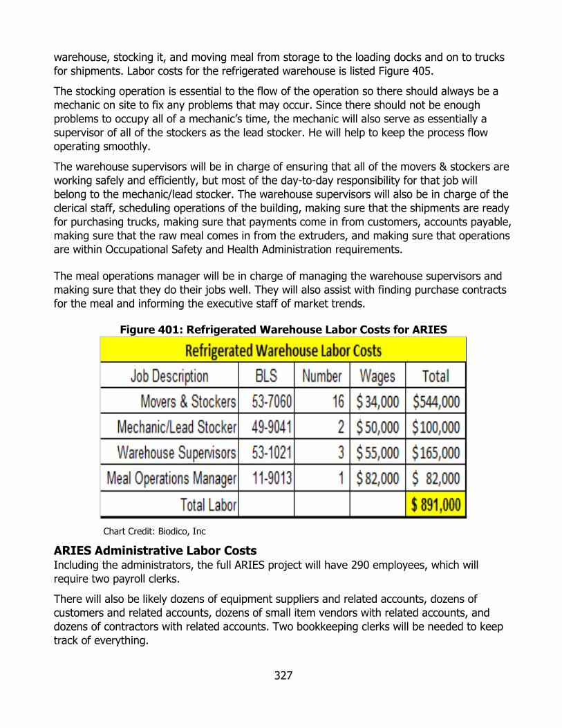
327
warehouse, stocking it, and moving meal from storage to the loading docks and on to trucks for shipments. Labor costs for the refrigerated warehouse is listed Figure 405.
The stocking operation is essential to the flow of the operation so there should always be a mechanic on site to fix any problems that may occur. Since there should not be enough problems to occupy all of a mechanic’s time, the mechanic will also serve as essentially a supervisor of all of the stockers as the lead stocker. He will help to keep the process flow operating smoothly.
The warehouse supervisors will be in charge of ensuring that all of the movers & stockers are working safely and efficiently, but most of the day-to-day responsibility for that job will belong to the mechanic/lead stocker. The warehouse supervisors will also be in charge of the clerical staff, scheduling operations of the building, making sure that the shipments are ready for purchasing trucks, making sure that payments come in from customers, accounts payable, making sure that the raw meal comes in from the extruders, and making sure that operations are within Occupational Safety and Health Administration requirements.
The meal operations manager will be in charge of managing the warehouse supervisors and making sure that they do their jobs well. They will also assist with finding purchase contracts for the meal and informing the executive staff of market trends.
Figure 401: Refrigerated Warehouse Labor Costs for ARIES
Chart Credit: Biodico, Inc
ARIES Administrative Labor Costs Including the administrators, the full ARIES project will have 290 employees, which will require two payroll clerks.
There will also be likely dozens of equipment suppliers and related accounts, dozens of customers and related accounts, dozens of small item vendors with related accounts, and dozens of contractors with related accounts. Two bookkeeping clerks will be needed to keep track of everything.
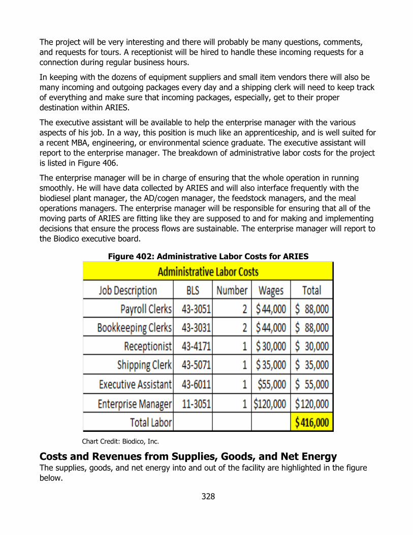
328
The project will be very interesting and there will probably be many questions, comments, and requests for tours. A receptionist will be hired to handle these incoming requests for a connection during regular business hours.
In keeping with the dozens of equipment suppliers and small item vendors there will also be many incoming and outgoing packages every day and a shipping clerk will need to keep track of everything and make sure that incoming packages, especially, get to their proper destination within ARIES.
The executive assistant will be available to help the enterprise manager with the various aspects of his job. In a way, this position is much like an apprenticeship, and is well suited for a recent MBA, engineering, or environmental science graduate. The executive assistant will report to the enterprise manager. The breakdown of administrative labor costs for the project is listed in Figure 406.
The enterprise manager will be in charge of ensuring that the whole operation in running smoothly. He will have data collected by ARIES and will also interface frequently with the biodiesel plant manager, the AD/cogen manager, the feedstock managers, and the meal operations managers. The enterprise manager will be responsible for ensuring that all of the moving parts of ARIES are fitting like they are supposed to and for making and implementing decisions that ensure the process flows are sustainable. The enterprise manager will report to the Biodico executive board.
Figure 402: Administrative Labor Costs for ARIES
Chart Credit: Biodico, Inc.
Costs and Revenues from Supplies, Goods, and Net Energy The supplies, goods, and net energy into and out of the facility are highlighted in the figure below.

329
Figure 403: Supplies, Goods, and Net Energy Profile for ARIES
Chart Credit: Biodico, Inc
Power Hub Net Annual Monetary Gain The electrical energy gains from the power hub are calculated by subtracting the power used from the power generated for the project. This is all detailed extensively in Electrical Energy. The current base rate for energy bought in Five Points, CA 93624 is $0.232, as shown in Figure 408 below.33
Figure 404: Electricity Rates for Five Points Zip Code
Chart Credit: California ISO
The price for electrical energy bought is shown as money saved in the chart below, but it does not actually factor into the net monetary gain for energy. The net monetary gain in energy is equal to the net kWh out of the facility multiplied by the estimated sale price. Power transfer agreements for renewable energy based on biomass AD have been difficult to secure for many businesses and the sale prices for net metered electricity are usually under half the rate of electricity in the area. For this projection, Biodico used a conservative $0.07 per kWh, 30 percent of the purchase price. The calculations are given in the figure below.
33 PGE Energy Estimate (https://www.chooseenergy.com/compare/93624/electricity/pge-ca/electricity-rates/)
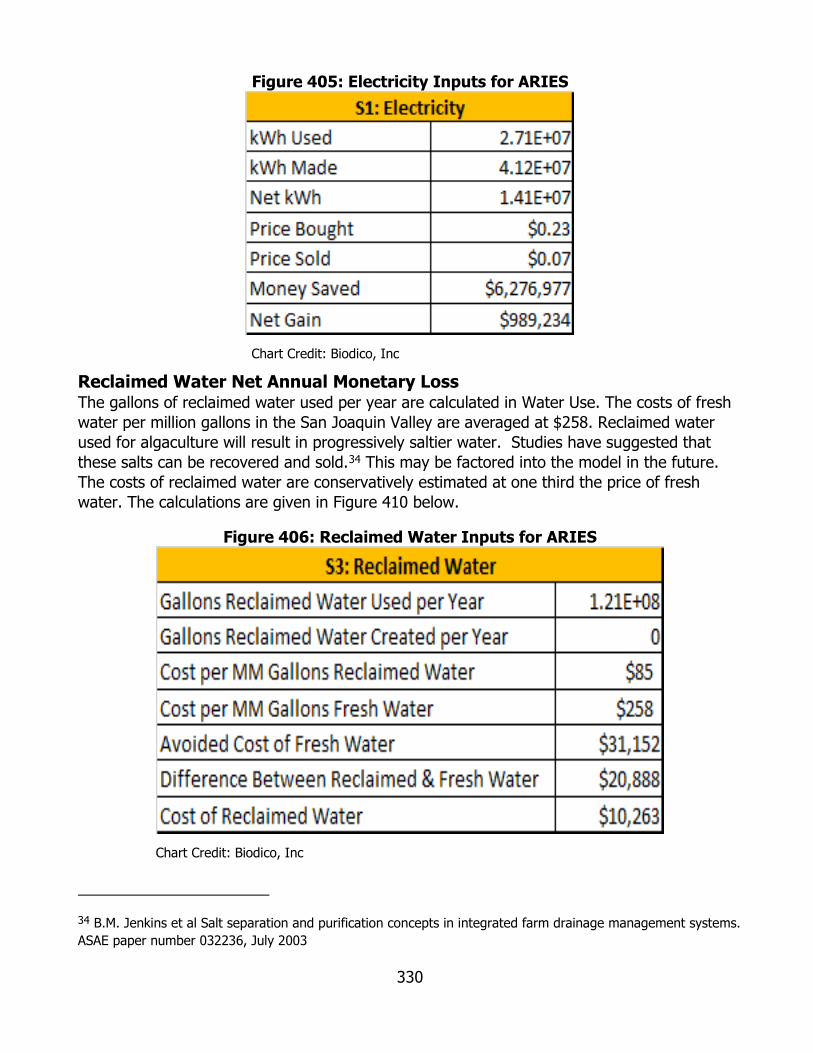
330
Figure 405: Electricity Inputs for ARIES
Chart Credit: Biodico, Inc
Reclaimed Water Net Annual Monetary Loss The gallons of reclaimed water used per year are calculated in Water Use. The costs of fresh water per million gallons in the San Joaquin Valley are averaged at $258. Reclaimed water used for algaculture will result in progressively saltier water. Studies have suggested that these salts can be recovered and sold.34 This may be factored into the model in the future. The costs of reclaimed water are conservatively estimated at one third the price of fresh water. The calculations are given in Figure 410 below.
Figure 406: Reclaimed Water Inputs for ARIES
Chart Credit: Biodico, Inc
34 B.M. Jenkins et al Salt separation and purification concepts in integrated farm drainage management systems. ASAE paper number 032236, July 2003
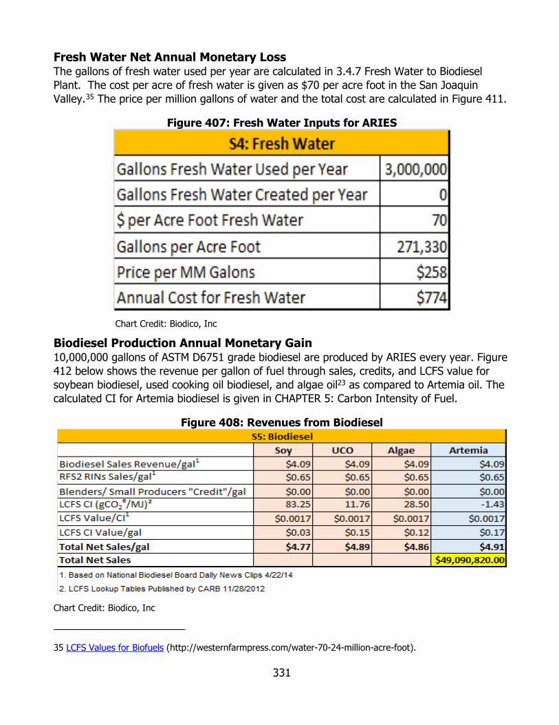
331
Fresh Water Net Annual Monetary Loss The gallons of fresh water used per year are calculated in 3.4.7 Fresh Water to Biodiesel Plant. The cost per acre of fresh water is given as $70 per acre foot in the San Joaquin Valley.35 The price per million gallons of water and the total cost are calculated in Figure 411.
Figure 407: Fresh Water Inputs for ARIES
Chart Credit: Biodico, Inc
Biodiesel Production Annual Monetary Gain 10,000,000 gallons of ASTM D6751 grade biodiesel are produced by ARIES every year. Figure 412 below shows the revenue per gallon of fuel through sales, credits, and LCFS value for soybean biodiesel, used cooking oil biodiesel, and algae oil23 as compared to Artemia oil. The calculated CI for Artemia biodiesel is given in CHAPTER 5: Carbon Intensity of Fuel.
Figure 408: Revenues from Biodiesel
Chart Credit: Biodico, Inc
35 LCFS Values for Biofuels (http://westernfarmpress.com/water-70-24-million-acre-foot).

332
Artemia Meal Annual Monetary Gain Approximately 290 million pounds of Artemia meal will leave ARIES every day. The use and nutritional value of Artemia as a fish food source has been documented for some time.36 Artemia meal is already sold as a fish food at slightly over $0.70 per pound. The protein content of the Artemia biomass is calculated in Section Biomass to and from Ponds and Extruder, but the protein content of the meal is never explicitly given. The oil, protein, and carbohydrate content of the meal is given in the figure below.
Figure 409: Artemia Composition by Weight
Chart Credit: Biodico, Inc
This protein content is similar to that of fish meal and significantly higher than that of soybean meal and most other vegetable oils. Figure 414 shows this comparison.
Figure 410: Composition Percent of Artemia and Other Animal Feeds
Chart Credit: Biodico, Inc
36 Leger, Bengston, Simpson and Sorgeloos, The Use and Nutritional Value of Artemia as a Food Source, Oceanogr. Mar. Biol. Ann. Rev., 1986, p. 521-623.

333
Fish meal prices are relatively volatile and do not seem to follow a seasonal pattern. They have both peaks and troughs in both the hot and cold months of the year. Figure 415 shows a five-year record of fish meal prices. The average of the peaks and troughs over the last five years are rising and given the trends of the last peak and trough cycles, the average of this cycle can be estimated at $1,980 per metric ton, or $0.86 per pound.
Figure 411: Fish Meal Prices
Chart Credit: www.indexmundi.com
Soybean meal prices follow the same general peaks and troughs that the fish meal prices follow, though both the prices and the volatility are decreased. Based on the last peak and trough of soybean meal prices and the current price, soybean meal is averaging around $485 per MT, or about $0.22 per pound as shown in Figure 416.
Figure 412: Soybean Meal Prices
Chart Credit: INDEXmundi
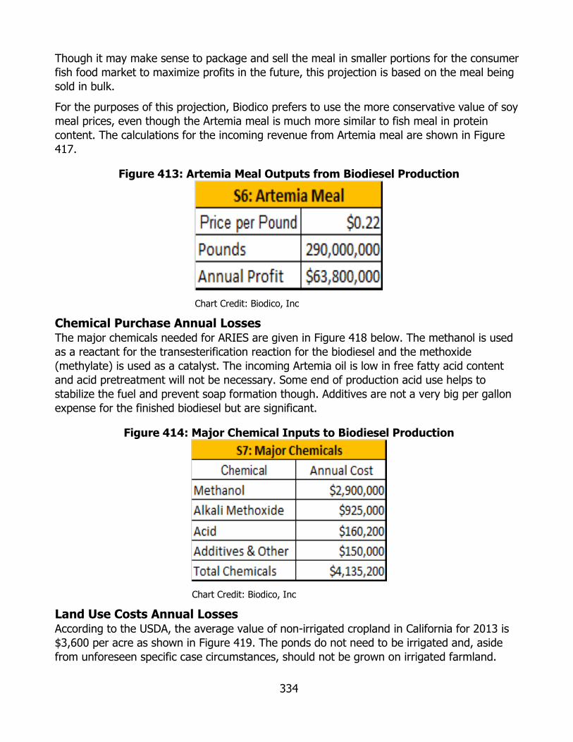
334
Though it may make sense to package and sell the meal in smaller portions for the consumer fish food market to maximize profits in the future, this projection is based on the meal being sold in bulk.
For the purposes of this projection, Biodico prefers to use the more conservative value of soy meal prices, even though the Artemia meal is much more similar to fish meal in protein content. The calculations for the incoming revenue from Artemia meal are shown in Figure 417.
Figure 413: Artemia Meal Outputs from Biodiesel Production
Chart Credit: Biodico, Inc
Chemical Purchase Annual Losses The major chemicals needed for ARIES are given in Figure 418 below. The methanol is used as a reactant for the transesterification reaction for the biodiesel and the methoxide (methylate) is used as a catalyst. The incoming Artemia oil is low in free fatty acid content and acid pretreatment will not be necessary. Some end of production acid use helps to stabilize the fuel and prevent soap formation though. Additives are not a very big per gallon expense for the finished biodiesel but are significant.
Figure 414: Major Chemical Inputs to Biodiesel Production
Chart Credit: Biodico, Inc
Land Use Costs Annual Losses According to the USDA, the average value of non-irrigated cropland in California for 2013 is $3,600 per acre as shown in Figure 419. The ponds do not need to be irrigated and, aside from unforeseen specific case circumstances, should not be grown on irrigated farmland.

335
Figure 415: Irrigated and Non-Irrigated Cropland Average Value per Acre
Chart Credit: USDA
There are various ways that an individual or organization can pay a farm owner to use their land, but for the purposes of these projections, cash rent is used. Cash rent is a flat fee paid to the land holder based on the value of the land. Generally, it is 3 – 4 percent based on the value of the land.37 The figure below shows the relationship between land value and rent for US cropland over the course of the last 10 years.
Figure 416: Crop Land Value and Cash Rental Rate
Chart Credit: USDA
37 USDA Land Estimate (http://www.extension.iastate.edu/agdm/wholefarm/html/c2-20.html)
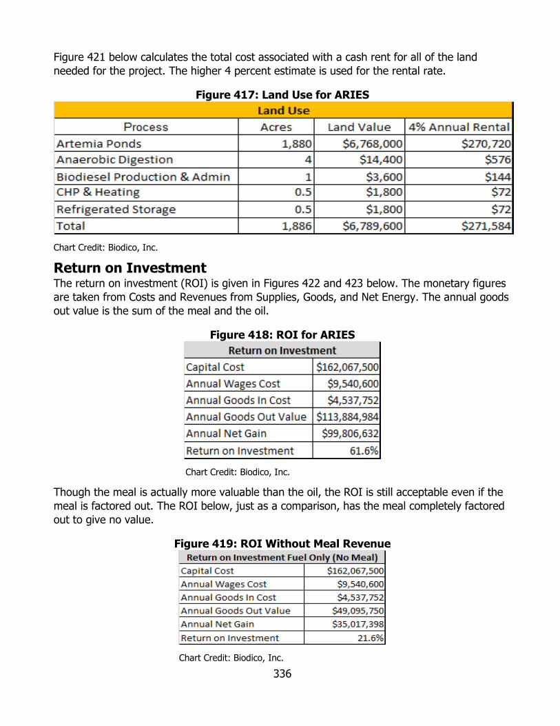
336
Figure 421 below calculates the total cost associated with a cash rent for all of the land needed for the project. The higher 4 percent estimate is used for the rental rate.
Figure 417: Land Use for ARIES
Chart Credit: Biodico, Inc.
Return on Investment The return on investment (ROI) is given in Figures 422 and 423 below. The monetary figures are taken from Costs and Revenues from Supplies, Goods, and Net Energy. The annual goods out value is the sum of the meal and the oil.
Figure 418: ROI for ARIES
Chart Credit: Biodico, Inc.
Though the meal is actually more valuable than the oil, the ROI is still acceptable even if the meal is factored out. The ROI below, just as a comparison, has the meal completely factored out to give no value.
Figure 419: ROI Without Meal Revenue
Chart Credit: Biodico, Inc.

337
CHAPTER 5: Carbon Intensity of Fuel
One of the goals of ARV-10-024 is to reduce GHG emissions by 80 percent over petroleum diesel. As shown in Figure 424, the Artemia pathway for biodiesel results in a 101 percent reduction of GHG. Biodico is currently installing a 10 million gallon per year commercial biodiesel production facility in the San Joaquin Valley that will be co-located with a sugar beet to ethanol facility. Artemia biodiesel would be the lowest CI biofuel that is liquid at ambient temperature and pressure, having a -1.43 CI for Artemia oil methyl ester biodiesel. The CI calculated here only uses methanol in the transesterification process, but future technological development allowing for the use of renewable ethanol to produce Artemia oil ethyl esters would likely result in an even lower CI.
The methodology used for this analysis is drawn from 2013 California Air Resources Board (CARB) Low Carbon Fuel Standard (LCFS) pathway analyses for determining the Carbon Intensity (CI) of various fuels using a variation of the GREET (Greenhouse gases, Regulated Emissions, and Energy use in Transportation) model. GREET is a full life-cycle model sponsored by Argonne National Laboratory (U.S. Department of Energy's Office of Energy Efficiency and Renewable Energy). It fully evaluates energy and emission impacts of advanced and new transportation fuels. The fuel cycle from well to wheel through vehicle material recovery and vehicle disposal is considered. It allows researchers and analysts to evaluate various vehicle and fuel combinations on a full fuel-cycle/vehicle-cycle basis. The unit used for comparing the CI of various fuels is grams of CO2 equivalents per megajoule.
CARB staff have already used an adapted version of GREET to define pathways for over 70 fuels. The analysis for ARV-10-024 compares California ultra-low sulfur diesel (CI = 98.03) with the pathways for biodiesel from several feedstocks. The specific pathway analysis for soy, canola, corn oil tallow and used cooking oil, along with all other pathways developed by CARB can be found on their website. In Figure 424 the values shown in light orange are taken directly from the CARB pathway analysis. The values shown in light blue are derived from a comparison to established CARB pathways. The most similar pathway to Biodico’s Artemia pathway is the pathway for Microalgae23, directly to the right of the Artemia pathway.
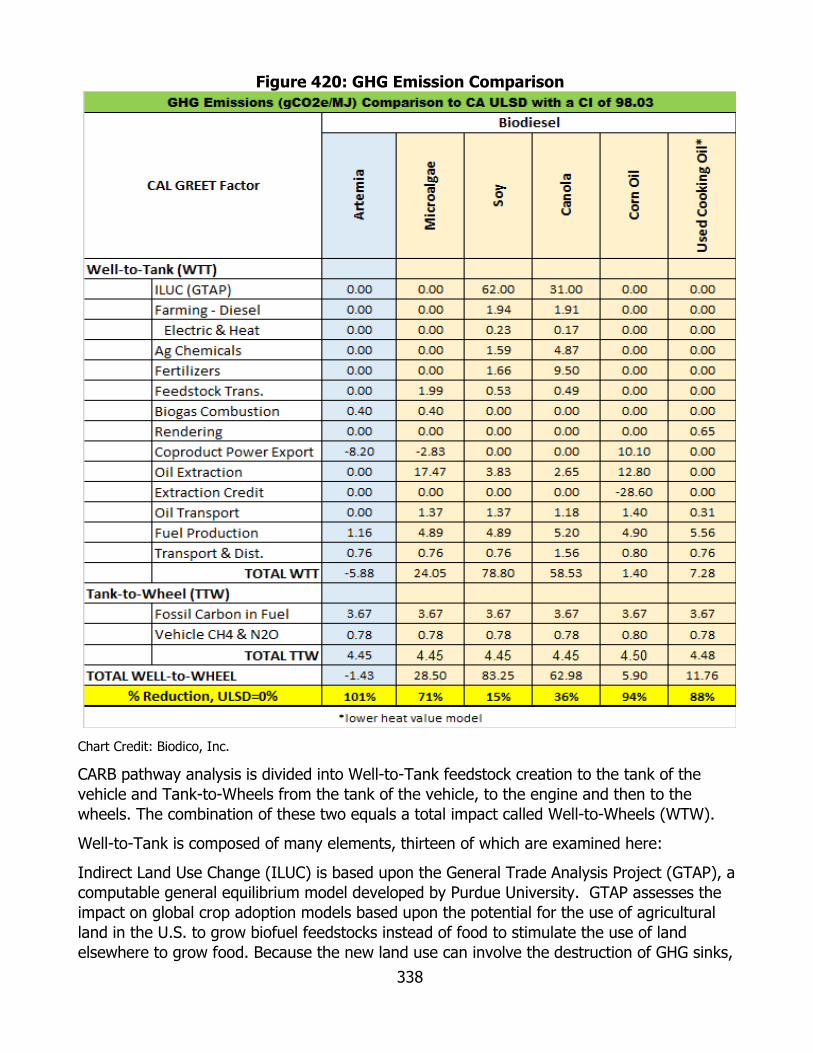
338
Figure 420: GHG Emission Comparison
Chart Credit: Biodico, Inc.
CARB pathway analysis is divided into Well-to-Tank feedstock creation to the tank of the vehicle and Tank-to-Wheels from the tank of the vehicle, to the engine and then to the wheels. The combination of these two equals a total impact called Well-to-Wheels (WTW).
Well-to-Tank is composed of many elements, thirteen of which are examined here:
Indirect Land Use Change (ILUC) is based upon the General Trade Analysis Project (GTAP), a computable general equilibrium model developed by Purdue University. GTAP assesses the impact on global crop adoption models based upon the potential for the use of agricultural land in the U.S. to grow biofuel feedstocks instead of food to stimulate the use of land elsewhere to grow food. Because the new land use can involve the destruction of GHG sinks,
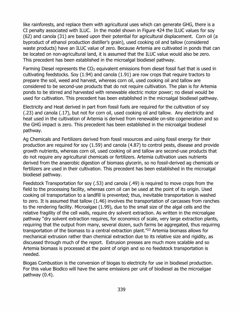
339
like rainforests, and replace them with agricultural uses which can generate GHG, there is a CI penalty associated with ILUC. In the model shown in Figure 424 the ILUC values for soy (62) and canola (31) are based upon their potential for agricultural displacement. Corn oil (a byproduct of ethanol production distiller’s grain), used cooking oil and tallow (considered waste products) have an ILUC value of zero. Because Artemia are cultivated in ponds that can be located on non-agricultural land, it is assumed that the ILUC value would also be zero. This precedent has been established in the microalgal biodiesel pathway.
Farming Diesel represents the CO2 equivalent emissions from diesel fossil fuel that is used in cultivating feedstocks. Soy (1.94) and canola (1.91) are row crops that require tractors to prepare the soil, weed and harvest, whereas corn oil, used cooking oil and tallow are considered to be second-use products that do not require cultivation. The plan is for Artemia ponds to be stirred and harvested with renewable electric motor power; no diesel would be used for cultivation. This precedent has been established in the microalgal biodiesel pathway.
Electricity and Heat derived in part from fossil fuels are required for the cultivation of soy (.23) and canola (.17), but not for corn oil, used cooking oil and tallow. Any electricity and heat used in the cultivation of Artemia is derived from renewable on-site cogeneration and so the GHG impact is zero. This precedent has been established in the microalgal biodiesel pathway.
Ag Chemicals and Fertilizers derived from fossil resources and using fossil energy for their production are required for soy (1.59) and canola (4.87) to control pests, disease and provide growth nutrients, whereas corn oil, used cooking oil and tallow are second-use products that do not require any agricultural chemicals or fertilizers. Artemia cultivation uses nutrients derived from the anaerobic digestion of biomass glycerin, so no fossil-derived ag chemicals or fertilizers are used in their cultivation. This precedent has been established in the microalgal biodiesel pathway.
Feedstock Transportation for soy (.53) and canola (.49) is required to move crops from the field to the processing facility, whereas corn oil can be used at the point of its origin. Used cooking oil transportation to a landfill is prevented; thus, inevitable transportation is washed to zero. It is assumed that tallow (1.46) involves the transportation of carcasses from ranches to the rendering facility. Microalgae (1.99), due to the small size of the algal cells and the relative fragility of the cell walls, require dry solvent extraction. As written in the microalgae pathway “dry solvent extraction requires, for economics of scale, very large extraction plants, requiring that the output from many, several dozen, such farms be aggregated, thus requiring transportation of the biomass to a central extraction plant.”23 Artemia biomass allows for mechanical extrusion rather than chemical extraction due to its relative size and rigidity, as discussed through much of the report. Extrusion presses are much more scalable and so Artemia biomass is processed at the point of origin and so no feedstock transportation is needed.
Biogas Combustion is the conversion of biogas to electricity for use in biodiesel production. For this value Biodico will have the same emissions per unit of biodiesel as the microalgae pathway (0.4).

340
Rendering is the use of heat (partially derived from fossil fuels) to separate used cooking oil (.65) and tallow (7.14) from other constituents. Artemia, soy and canola do not require rendering. The low heat value used in the chart above is the one that is usually used by biodiesel producers that collect their own material. The high heat method where “cooking” is required is the pathway used by large commercial rendering operations that take in animal carcasses, yellow grease, brown grease, and possibly other materials. At these larger, multi-use facilities the incoming oil is usually cooked through a series of tanks at 180°F, and since the yellow grease oil is sold as a commodity rather than processed into fuel on site, it is usually mixed with brown grease or very poor material to bring the free fatty acid level right up to the specification of 15 percent, helping the renderer to get a relatively high value out of the small amount of low-value brown grease that is mixed in. This material is more common for use in renewable diesel operations.
Co-product Credit is GHG accounting for the byproducts generated by the processing of feedstocks. ARB allocates the entire DDGS co-product credit to a reduction in the carbon intensity of corn ethanol; therefore, the reduced DDGS credit resulting from the removal of corn oil is an incremental addition to the corn oil carbon intensity value. There is no such co-product credit involved with soy, canola, tallow or used cooking oil. The microalgae pathway, however, has a coproduct credit based on electrical energy created onsite.23 Because of the similarity of the two pathways, Biodico uses the same coproduct credit values on a per MJ basis. In the first row of Figure 445, the microalgae J/MJ of biodiesel value gives the total joules of exported electricity divided by the total MJ of biodiesel produced. The following row gives the reduction in carbon dioxide equivalent emissions per MJ of biodiesel for the microalgae pathway. The third row gives the grams of carbon reductions per joule of coproduct energy. The fourth and fifth rows give the net kWh and GJ of electricity coproduced with 10 million gallons of biodiesel, respectively. The value of 119,500 Btus per gallon of biodiesel is a standard number for the combustible energy of biodiesel that is used to calculate the seventh row, MJ energy contained in each gallon of Artemia oil biodiesel. This is used in the following row to calculate the total amount of combustible energy in 10 million gallons of biodiesel. The net electricity produced is divided into the total combustible energy of 10 million gallons of biodiesel to give the joules of coproduct electricity per MJ of biodiesel. This value calculated in the ninth row is multiplied by the ratio from the third row to give the reduction in carbon dioxide equivalent emissions per MJ of biodiesel for the ARIES pathway. The next two rows give the total mmBtus of heat produced and the total mmBtus of heat used by ARIES. The following row gives the percentage efficiency of the heating system as 50 percent. This means that for every mmBtu captured for use in ARIES, one mmBtu will be lost to the surrounding environment. The following two rows give the net heating energy available for export from the system in mmBtus and GJ. The GJ of net heat energy are divided by the MJ of combustible energy in 10 million gallons of biodiesel to give the joules of coproduct heat energy per MJ of biodiesel. This value is multiplied by the ratio from row three to give the reduction in carbon dioxide equivalent emissions per MJ of biodiesel for the ARIES pathway. The reductions in carbon dioxide equivalent emissions from the heating and electrical energy coproducts are summed together to give the final coproduct emission reductions of -8.20 grams of carbon dioxide equivalent emissions per MJ of biodiesel.
341
Figure 421: Coproduct Credit for Biodiesel
Chart Credit: Biodico, Inc.
Oil Extraction represents the CO2 equivalent emissions from fossil energy used to extract oil from the feedstock. The CI value for soy (3.83), canola (2.65) and corn oil (12.8) is because the oil needs to be extracted from the feedstock, whereas for used cooking oil and tallow there is no extraction necessary. For microalgae (17.47), chemical extraction is needed and this adds the bulk of carbon emissions for the fuel’s CI. For Artemia, oil extraction is necessary; however, the extraction is mechanical, not chemical and all of the heat and electricity used in the process is derived from renewable cogeneration and thus does not have a negative CI.
• Extraction Credit is only assigned to corn oil because the emissions from the natural gas used to dry distillers’ grain is reduced because of the oil extraction process previously accounted for. There is no extraction credit for Artemia or the other feedstocks. This precedent has been established in the microalgal biodiesel pathway.
• • Oil Transport represents the CO2 equivalent emissions from fossil energy used to transport
the oil once it has been extracted. Since Artemia oil is extracted on-site, the oil transport CI is zero.
Fuel Production represents the CO2 equivalent emissions from the biodiesel production process. Since no external natural gas or electricity is used for the transesterification reactions, or any other portions of biodiesel production, no emissions are generated from
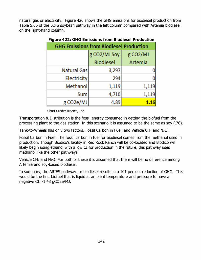
342
natural gas or electricity. Figure 426 shows the GHG emissions for biodiesel production from Table 5.06 of the LCFS soybean pathway in the left column compared with Artemia biodiesel on the right-hand column.
Figure 422: GHG Emissions from Biodiesel Production
Chart Credit: Biodico, Inc.
Transportation & Distribution is the fossil energy consumed in getting the biofuel from the processing plant to the gas station. In this scenario it is assumed to be the same as soy (.76).
Tank-to-Wheels has only two factors, Fossil Carbon in Fuel, and Vehicle CH4 and N2O.
Fossil Carbon in Fuel: The fossil carbon in fuel for biodiesel comes from the methanol used in production. Though Biodico’s facility in Red Rock Ranch will be co-located and Biodico will likely begin using ethanol with a low CI for production in the future, this pathway uses methanol like the other pathways.
Vehicle CH4 and N2O: For both of these it is assumed that there will be no difference among Artemia and soy-based biodiesel.
In summary, the ARIES pathway for biodiesel results in a 101 percent reduction of GHG. This would be the first biofuel that is liquid at ambient temperature and pressure to have a negative CI: -1.43 gCO2e/MJ.

343
CHAPTER 6: Economic, Environmental, & Social Sustainability
The sustainability summary in the table below divides the metrics of sustainability into three categories: economic sustainability, environmental sustainability, and social sustainability. Five topics are included in each of these categories: feedstock, energy, incentives, labor, and biofuel. The three categories and the topics in those categories are split apart and discussed in more detail after the figure below.
Figure 423: Sustainability Summary
Source: Biodico, Inc.
The Sustainability Best Management Practices plan for the proposed project is derived from the bioenergy crop sustainability plan developed at UC Davis through the Bioenergy Research Group (BERG)38 and the Sustainable Agriculture and Education Program (SAREP)39. SAREP and BERG provide leadership and support for scientific research and education in agricultural
38 UC Davis BioEnergy Research (http://bioenergy.ucdavis.edu/index.php).
39 Sustainable Agriculture and Education Program (http://www.sare.org/).
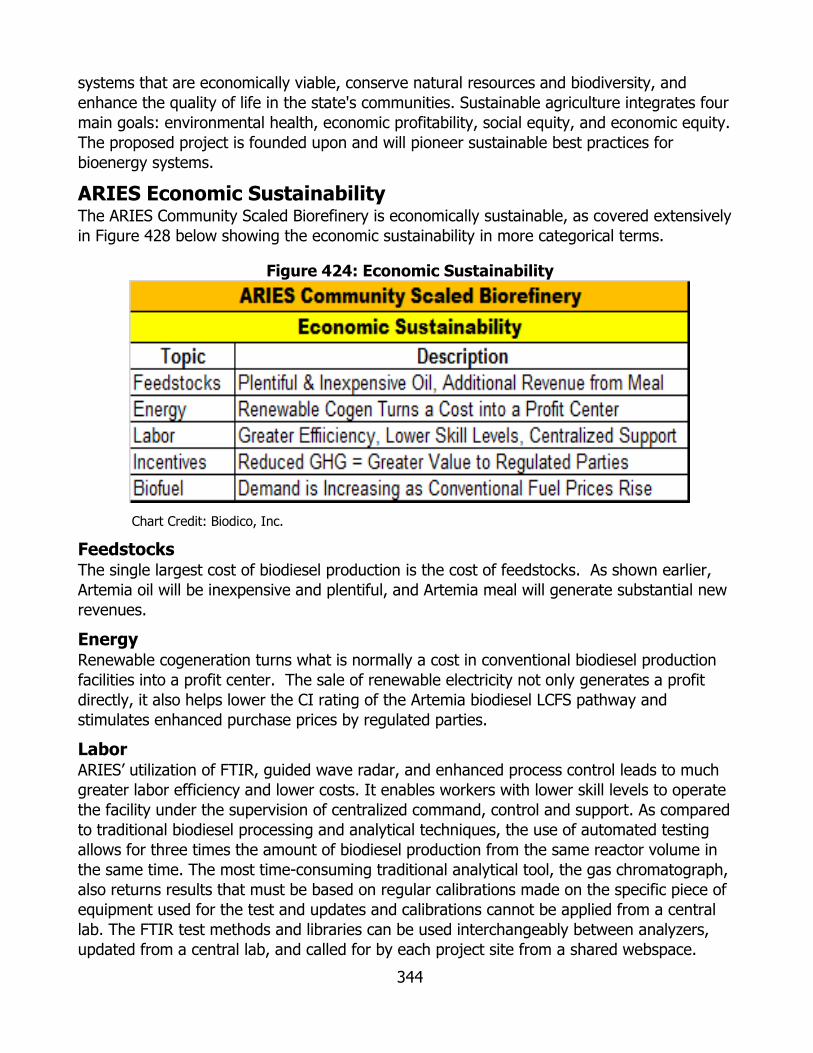
344
systems that are economically viable, conserve natural resources and biodiversity, and enhance the quality of life in the state's communities. Sustainable agriculture integrates four main goals: environmental health, economic profitability, social equity, and economic equity. The proposed project is founded upon and will pioneer sustainable best practices for bioenergy systems.
ARIES Economic Sustainability The ARIES Community Scaled Biorefinery is economically sustainable, as covered extensively in Figure 428 below showing the economic sustainability in more categorical terms.
Figure 424: Economic Sustainability
Chart Credit: Biodico, Inc.
Feedstocks The single largest cost of biodiesel production is the cost of feedstocks. As shown earlier, Artemia oil will be inexpensive and plentiful, and Artemia meal will generate substantial new revenues.
Energy Renewable cogeneration turns what is normally a cost in conventional biodiesel production facilities into a profit center. The sale of renewable electricity not only generates a profit directly, it also helps lower the CI rating of the Artemia biodiesel LCFS pathway and stimulates enhanced purchase prices by regulated parties.
Labor ARIES’ utilization of FTIR, guided wave radar, and enhanced process control leads to much greater labor efficiency and lower costs. It enables workers with lower skill levels to operate the facility under the supervision of centralized command, control and support. As compared to traditional biodiesel processing and analytical techniques, the use of automated testing allows for three times the amount of biodiesel production from the same reactor volume in the same time. The most time-consuming traditional analytical tool, the gas chromatograph, also returns results that must be based on regular calibrations made on the specific piece of equipment used for the test and updates and calibrations cannot be applied from a central lab. The FTIR test methods and libraries can be used interchangeably between analyzers, updated from a central lab, and called for by each project site from a shared webspace.

345
Incentives As described earlier, the reduced carbon footprint of the ARIES Community Scaled Biorefinery improves the CI of the biodiesel and generates greater value to regulated parties.
Biofuel The demand for fuel is increasing as the emerging economies of the world adopt western lifestyles and energy consumption patterns. Fuel prices have been steadily rising while the supply of finite fossil resources is dwindling. Biodiesel as a diesel replacement has a significant role to play, and as the concerns about health effects, global warming and energy security increase, it will have an even greater role. ARIES Environmental Sustainability The ARIES Community Scale Biorefinery is environmentally sustainable, as evidenced by the low CI and as summarized in Figure 429.
Figure 425: Environmental Sustainability
Chart Credit: Biodico, Inc.
Feedstocks On-site low ILUC feedstocks were used in ARV-10-024. Algaculture populations were established in open-air conditions in greenhouses on Naval Base Ventura County (not farmland).
This was done to model ponds that will be located on (i) non-arable land that has been contaminated by salt, selenium or both, and (ii) non-agricultural land. In fact, algae and brine shrimp were originally used for selenium bioremediation in work pioneered by Dr. Hristova. In the greenhouses the algae/Artemia were provided with CO2, nutrients from AD, and glycerin.8 Larger scale Artemia cultivation should not require any additional nutritional inputs (zero fossil Agricultural Chemicals and Fertilizers). ARV-10-024 also showed that the combined heat and power from solar cogeneration and anaerobic digestion can be sufficient for heating the growth medium and providing electricity for lights, pumps, and automated control systems. No fossil fuels were used.
The metrics listed under the LCFS are a good indicator of the sustainability of a feedstock both internally and in terms of the external energy that will be needed for the feedstock’s
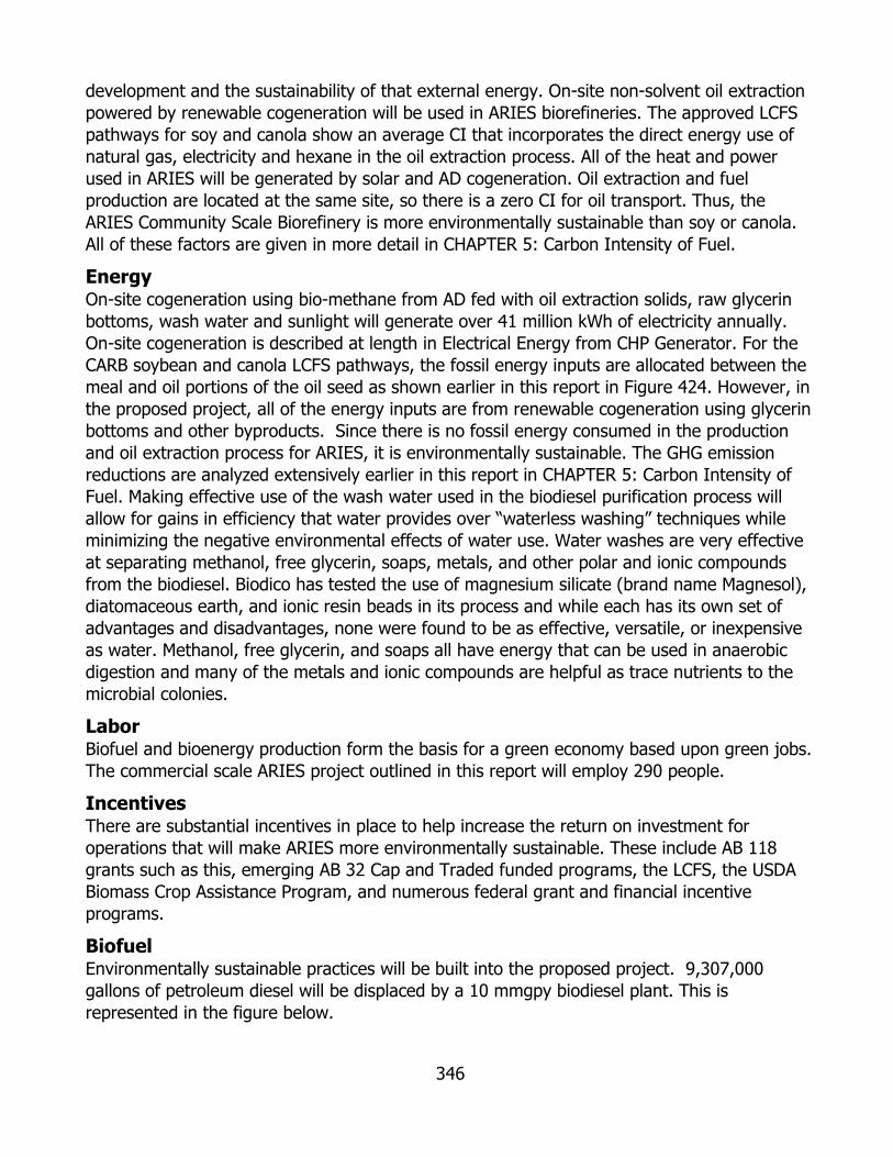
346
development and the sustainability of that external energy. On-site non-solvent oil extraction powered by renewable cogeneration will be used in ARIES biorefineries. The approved LCFS pathways for soy and canola show an average CI that incorporates the direct energy use of natural gas, electricity and hexane in the oil extraction process. All of the heat and power used in ARIES will be generated by solar and AD cogeneration. Oil extraction and fuel production are located at the same site, so there is a zero CI for oil transport. Thus, the ARIES Community Scale Biorefinery is more environmentally sustainable than soy or canola. All of these factors are given in more detail in CHAPTER 5: Carbon Intensity of Fuel.
Energy On-site cogeneration using bio-methane from AD fed with oil extraction solids, raw glycerin bottoms, wash water and sunlight will generate over 41 million kWh of electricity annually. On-site cogeneration is described at length in Electrical Energy from CHP Generator. For the CARB soybean and canola LCFS pathways, the fossil energy inputs are allocated between the meal and oil portions of the oil seed as shown earlier in this report in Figure 424. However, in the proposed project, all of the energy inputs are from renewable cogeneration using glycerin bottoms and other byproducts. Since there is no fossil energy consumed in the production and oil extraction process for ARIES, it is environmentally sustainable. The GHG emission reductions are analyzed extensively earlier in this report in CHAPTER 5: Carbon Intensity of Fuel. Making effective use of the wash water used in the biodiesel purification process will allow for gains in efficiency that water provides over “waterless washing” techniques while minimizing the negative environmental effects of water use. Water washes are very effective at separating methanol, free glycerin, soaps, metals, and other polar and ionic compounds from the biodiesel. Biodico has tested the use of magnesium silicate (brand name Magnesol), diatomaceous earth, and ionic resin beads in its process and while each has its own set of advantages and disadvantages, none were found to be as effective, versatile, or inexpensive as water. Methanol, free glycerin, and soaps all have energy that can be used in anaerobic digestion and many of the metals and ionic compounds are helpful as trace nutrients to the microbial colonies.
Labor Biofuel and bioenergy production form the basis for a green economy based upon green jobs. The commercial scale ARIES project outlined in this report will employ 290 people.
Incentives There are substantial incentives in place to help increase the return on investment for operations that will make ARIES more environmentally sustainable. These include AB 118 grants such as this, emerging AB 32 Cap and Traded funded programs, the LCFS, the USDA Biomass Crop Assistance Program, and numerous federal grant and financial incentive programs.
Biofuel Environmentally sustainable practices will be built into the proposed project. 9,307,000 gallons of petroleum diesel will be displaced by a 10 mmgpy biodiesel plant. This is represented in the figure below.
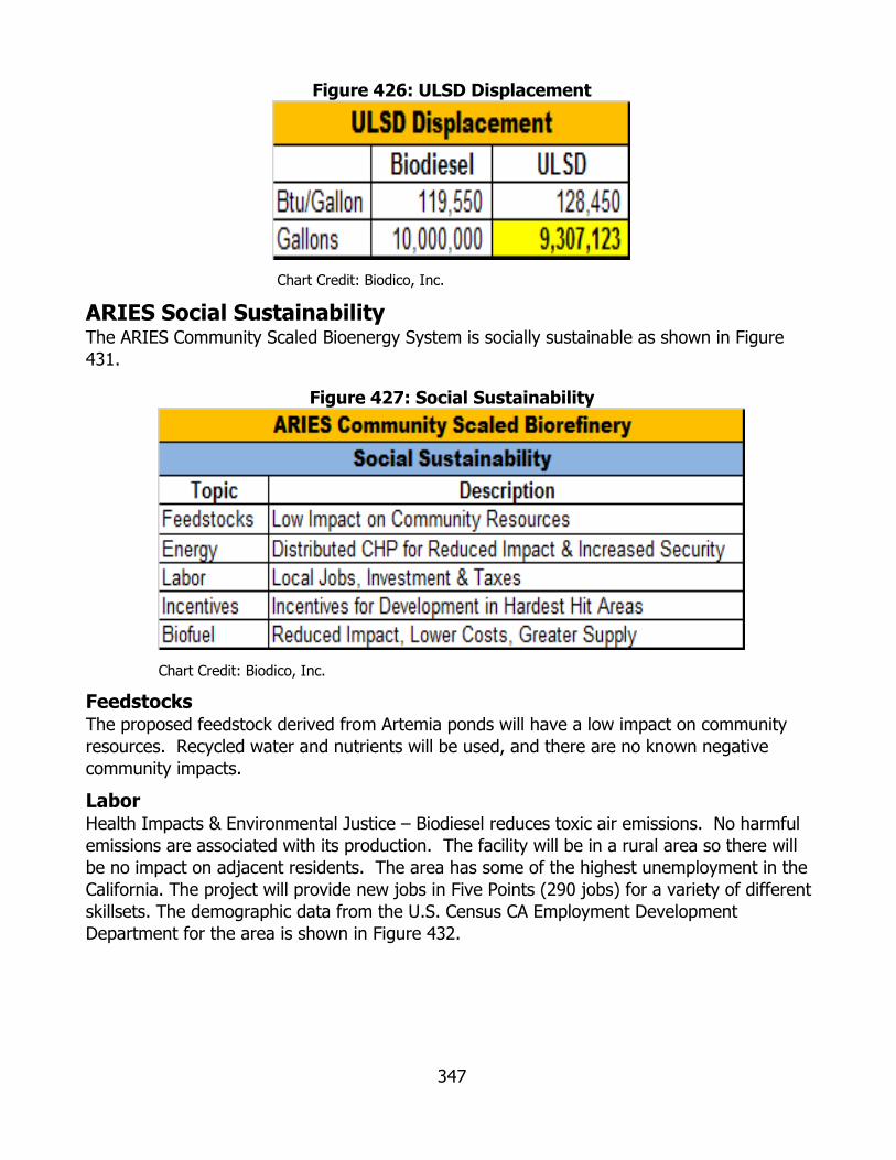
347
Figure 426: ULSD Displacement
Chart Credit: Biodico, Inc.
ARIES Social Sustainability The ARIES Community Scaled Bioenergy System is socially sustainable as shown in Figure 431.
Figure 427: Social Sustainability
Chart Credit: Biodico, Inc.
Feedstocks The proposed feedstock derived from Artemia ponds will have a low impact on community resources. Recycled water and nutrients will be used, and there are no known negative community impacts.
Labor Health Impacts & Environmental Justice – Biodiesel reduces toxic air emissions. No harmful emissions are associated with its production. The facility will be in a rural area so there will be no impact on adjacent residents. The area has some of the highest unemployment in the California. The project will provide new jobs in Five Points (290 jobs) for a variety of different skillsets. The demographic data from the U.S. Census CA Employment Development Department for the area is shown in Figure 432.
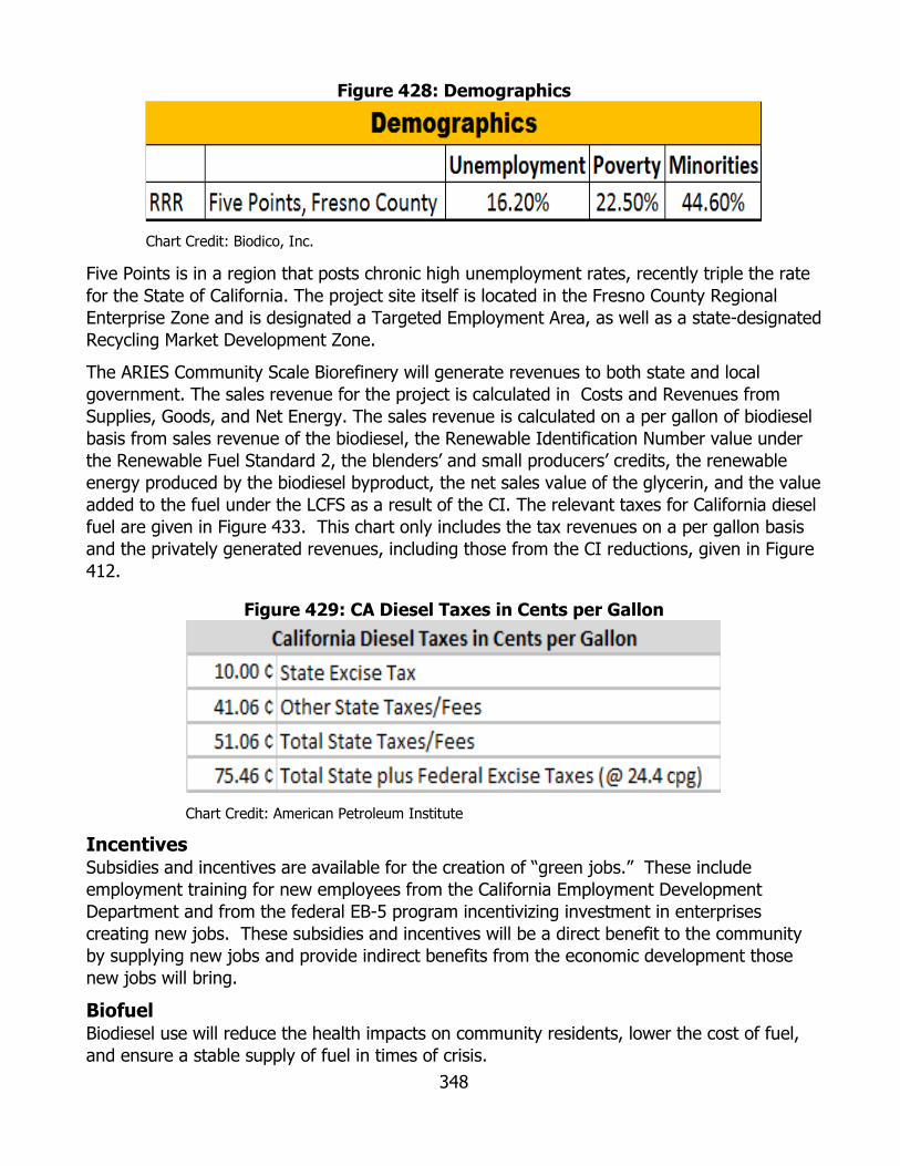
348
Figure 428: Demographics
Chart Credit: Biodico, Inc.
Five Points is in a region that posts chronic high unemployment rates, recently triple the rate for the State of California. The project site itself is located in the Fresno County Regional Enterprise Zone and is designated a Targeted Employment Area, as well as a state-designated Recycling Market Development Zone.
The ARIES Community Scale Biorefinery will generate revenues to both state and local government. The sales revenue for the project is calculated in Costs and Revenues from Supplies, Goods, and Net Energy. The sales revenue is calculated on a per gallon of biodiesel basis from sales revenue of the biodiesel, the Renewable Identification Number value under the Renewable Fuel Standard 2, the blenders’ and small producers’ credits, the renewable energy produced by the biodiesel byproduct, the net sales value of the glycerin, and the value added to the fuel under the LCFS as a result of the CI. The relevant taxes for California diesel fuel are given in Figure 433. This chart only includes the tax revenues on a per gallon basis and the privately generated revenues, including those from the CI reductions, given in Figure 412.
Figure 429: CA Diesel Taxes in Cents per Gallon
Chart Credit: American Petroleum Institute
Incentives Subsidies and incentives are available for the creation of “green jobs.” These include employment training for new employees from the California Employment Development Department and from the federal EB-5 program incentivizing investment in enterprises creating new jobs. These subsidies and incentives will be a direct benefit to the community by supplying new jobs and provide indirect benefits from the economic development those new jobs will bring.
Biofuel Biodiesel use will reduce the health impacts on community residents, lower the cost of fuel, and ensure a stable supply of fuel in times of crisis.
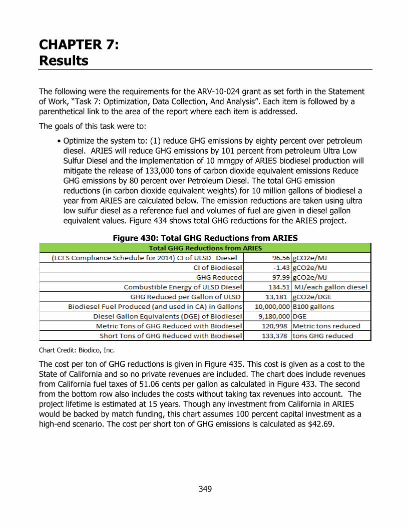
349
CHAPTER 7: Results
The following were the requirements for the ARV-10-024 grant as set forth in the Statement of Work, “Task 7: Optimization, Data Collection, And Analysis”. Each item is followed by a parenthetical link to the area of the report where each item is addressed.
The goals of this task were to:
• Optimize the system to: (1) reduce GHG emissions by eighty percent over petroleum diesel. ARIES will reduce GHG emissions by 101 percent from petroleum Ultra Low Sulfur Diesel and the implementation of 10 mmgpy of ARIES biodiesel production will mitigate the release of 133,000 tons of carbon dioxide equivalent emissions Reduce GHG emissions by 80 percent over Petroleum Diesel. The total GHG emission reductions (in carbon dioxide equivalent weights) for 10 million gallons of biodiesel a year from ARIES are calculated below. The emission reductions are taken using ultra low sulfur diesel as a reference fuel and volumes of fuel are given in diesel gallon equivalent values. Figure 434 shows total GHG reductions for the ARIES project.
Figure 430: Total GHG Reductions from ARIES
Chart Credit: Biodico, Inc.
The cost per ton of GHG reductions is given in Figure 435. This cost is given as a cost to the State of California and so no private revenues are included. The chart does include revenues from California fuel taxes of 51.06 cents per gallon as calculated in Figure 433. The second from the bottom row also includes the costs without taking tax revenues into account. The project lifetime is estimated at 15 years. Though any investment from California in ARIES would be backed by match funding, this chart assumes 100 percent capital investment as a high-end scenario. The cost per short ton of GHG emissions is calculated as $42.69.
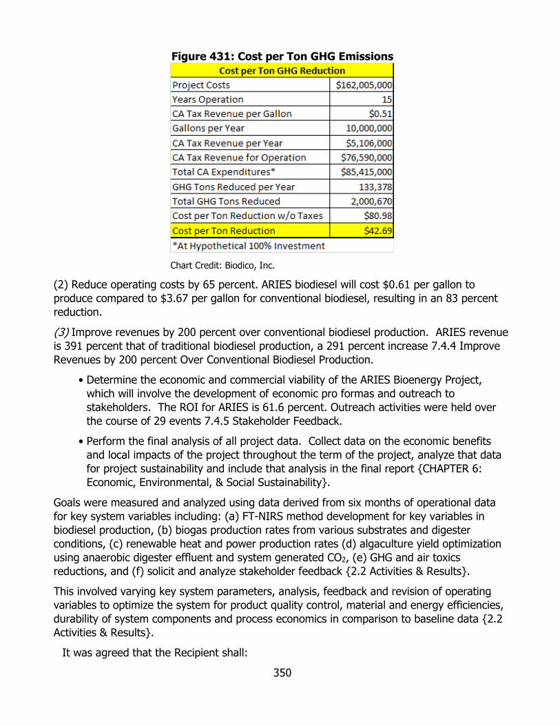
350
Figure 431: Cost per Ton GHG Emissions
Chart Credit: Biodico, Inc.
(2) Reduce operating costs by 65 percent. ARIES biodiesel will cost $0.61 per gallon to produce compared to $3.67 per gallon for conventional biodiesel, resulting in an 83 percent reduction.
(3) Improve revenues by 200 percent over conventional biodiesel production. ARIES revenue is 391 percent that of traditional biodiesel production, a 291 percent increase 7.4.4 Improve Revenues by 200 percent Over Conventional Biodiesel Production.
• Determine the economic and commercial viability of the ARIES Bioenergy Project, which will involve the development of economic pro formas and outreach to stakeholders. The ROI for ARIES is 61.6 percent. Outreach activities were held over the course of 29 events 7.4.5 Stakeholder Feedback.
• Perform the final analysis of all project data. Collect data on the economic benefits and local impacts of the project throughout the term of the project, analyze that data for project sustainability and include that analysis in the final report {CHAPTER 6: Economic, Environmental, & Social Sustainability}.
Goals were measured and analyzed using data derived from six months of operational data for key system variables including: (a) FT-NIRS method development for key variables in biodiesel production, (b) biogas production rates from various substrates and digester conditions, (c) renewable heat and power production rates (d) algaculture yield optimization using anaerobic digester effluent and system generated CO2, (e) GHG and air toxics reductions, and (f) solicit and analyze stakeholder feedback {2.2 Activities & Results}.
This involved varying key system parameters, analysis, feedback and revision of operating variables to optimize the system for product quality control, material and energy efficiencies, durability of system components and process economics in comparison to baseline data {2.2 Activities & Results}.
It was agreed that the Recipient shall:

351
• Operate the integrated energy system for a period of six months. Under the subsection of {2.2 Activities & Results}, operational data can be found for eight 15 batch AD experiments running at least 30 days each, not including time before and after each AMPTS experiment for influent and effluent tests (Figure 139); 28 weeks of harvesting of the demonstration scale Artemia populations in the greenhouses (Figure 281); and over one year each of solar insolation data collection (Figure 305), pH data collection (Figure 262), salinity data, and temperature data.
• Based upon input from project team members, vary key system parameters and analyze the results, collect feedback, revise operating parameters and compare results to the baseline and other operating scenarios. The FTIR method was developed with planned variations in the parameters of free glycerin content, bound glycerin content, water content, methanol content, free fatty acid content, and fatty acid profile in biodiesel samples. The AD work focused on the parameters of glycerin volume, co-digestant type, co-digestant volume or lack of co-digestants, COD, TS, VS, TSS, Volatile suspended solids, pH, and alkalinity. The algaculture work focused on parameters of harvesting net size, temperature, salinity, pH, solar insolation, nutrient type, and nutrient volume. The automation work collected data based on analog inputs, digital inputs, and Modbus inputs and focused on effectively bringing the different types of inputs together. This is all described in full detail in {2.2 Activities & Results}.
• Vary the key parameters to optimize the system for product quality control, material and energy efficiencies, durability of system components and process economics. The product of the FTIR work was the method, which proved very able to measure the needed variables. The product of the AD work was the methane, which was optimized to over 420 times the incoming glycerin by volume. The product of the Artemia work was the oil, which was optimized to over 5,300 gallons per acre. The product of the automation was automated collection, which was achieved for every required type of data input. This is all detailed in {2.2 Activities & Results}. The major pieces of equipment did not break through the course of the project so an expected durability minimum can only be estimated as the lifetime of the project at this point.
• Evaluate how the product from the pilot plant will comply with ASTM International standards for 100 percent biodiesel, including flash point, alcohol control (methanol content or flash point), water and sediment, kinematic viscosity, sulfated ash, copper strip corrosion, oxidation stability, sulfur, cetane number, cloud point, acid number, carbon residue, free and total glycerin, phosphorus, reduced pressure distillation temperature, atmospheric equivalent temperature, cold soak filtration, combined calcium and magnesium, and combined sodium and magnesium. {2.2.1 Biodiesel Production}
• Evaluate how the product from the pilot plant will comply with California Air Resources Board fuel requirements for sulfur. Sulfur content was independently tested at 3.4 ppm, well under the 15 ppm threshold for Ultra Low Sulfur Diesel and CARB requirements, by a verified third-party laboratory (Figure 50). This is described in more detail in {2.2.1 Biodiesel Production}

352
•Estimate gasoline and/or petroleum-based diesel fuel that will be displaced annually. This project will displaced 9,307,000 gallons of petroleum diesel annually as shown in Figure 430 and examined in detail detailed in {Chapter 3. Mass and Energy Balance}.}
• Explain how the proposed project will reduce criteria air pollutants and air toxics and reduce or avoid multimedia environmental impact, and lead to a decrease, on a life cycle basis, in emissions of water pollutants or any other substances known to damage human health or the environment. Project incorporated and achieved sustainability goals. ARIES will reduce GHG emissions by over 133,000 tons annually (Figure 434). This is detailed in {CHAPTER 5: Carbon Intensity of Fuel and 6.2 ARIES Environmental Sustainability}
• Provide a quantified estimate of the project’s carbon intensity values for life-cycle scale greenhouse gas emissions. The calculated carbon intensity is -1.43 gCO2e/MJ (Figure 424). This is detailed further in {CHAPTER 5: Carbon Intensity of Fuel}.
• Quantify any water efficiency and water use reduction measures used in the project including, but not limited to, the use of recycled or reclaimed water and the reduction or elimination of point and nonpoint source wastewater discharge. This project annually will reuse over 120 million gallons of reclaimed water. Only three million gallons of fresh water will be used, which will cascade through ARIES for three uses (Figure 379). This is detailed in {CHAPTER 3: Mass and Energy Balance and CHAPTER 5: Carbon Intensity of Fuel}.
•Describe any potential use of renewable energy or cogeneration in the project. ARIES will not have any external heat or electrical demands and will produce over 14 million kWh in excess energy and roughly 138,000 mmBtu excess heat (Figure 425). This is detailed in {Chapter 3. Mass and Energy Balance}.
• Describe any potential energy efficiency measures used in the project that would exceed Title 24 standards in Part 6 of the California Code of Regulations. The refrigerated warehouse space will fall under Section 126 of Title 24 Part 6, Mandatory Requirements for Refrigerated Warehouses, under which requirements are outlined for insulation, under slab heating, evaporators, condensers, and compressors. Beyond these requirements, incentives exist for customized HVAC motors and pumps, process cooling retrofit, refrigeration, refrigeration control, chiller, HVAC air distribution, cooling tower, HVAC, unitary AC/HP, refrigeration condenser, lighting controls and sensors, LED lighting, and induction fixtures as well as for high bay linear fluorescent lights and occupancy sensors on lights.
• Provide data on expected job creation, economic development, and increased state revenue. ARIES is expected to create 290 jobs (Figure 400). This is detailed in {4.2 ARIES Labor Costs}.
• Compare any project performance and expectations provided in the proposal to the Energy Commission with actual project performance and accomplishments. The comparisons are summarized in {CHAPTER 7: Results}.
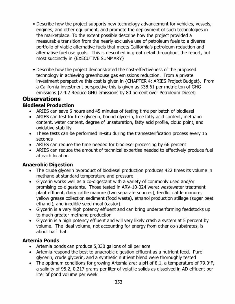
353
• Describe how the project supports new technology advancement for vehicles, vessels, engines, and other equipment, and promote the deployment of such technologies in the marketplace. To the extent possible describe how the project provided a measurable transition from the nearly exclusive use of petroleum fuels to a diverse portfolio of viable alternative fuels that meets California’s petroleum reduction and alternative fuel use goals. This is described in great detail throughout the report, but most succinctly in {EXECUTIVE SUMMARY}
• Describe how the project demonstrated the cost-effectiveness of the proposed technology in achieving greenhouse gas emissions reduction. From a private investment perspective this cost is given in {CHAPTER 4: ARIES Project Budget}. From a California investment perspective this is given as $38.61 per metric ton of GHG emissions {7.4.2 Reduce GHG emissions by 80 percent over Petroleum Diesel}
Observations Biodiesel Production
• ARIES can save 6 hours and 45 minutes of testing time per batch of biodiesel • ARIES can test for free glycerin, bound glycerin, free fatty acid content, methanol
content, water content, degree of unsaturation, fatty acid profile, cloud point, and oxidative stability
• These tests can be performed in-situ during the transesterification process every 15 seconds
• ARIES can reduce the time needed for biodiesel processing by 66 percent • ARIES can reduce the amount of technical expertise needed to effectively produce fuel
at each location
Anaerobic Digestion • The crude glycerin byproduct of biodiesel production produces 422 times its volume in
methane at standard temperature and pressure • Glycerin works well as a co-digestant with a variety of commonly used and/or
promising co-digestants. Those tested in ARV-10-024 were: wastewater treatment plant effluent, dairy cattle manure (two separate sources), feedlot cattle manure, yellow grease collection sediment (food waste), ethanol production stillage (sugar beet ethanol), and inedible seed meal (castor).
• Glycerin is a very high potency effluent and can bring underperforming feedstocks up to much greater methane production
• Glycerin is a high potency effluent and will very likely crash a system at 5 percent by volume. The ideal volume, not accounting for energy from other co-substrates, is about half that.
Artemia Ponds • Artemia ponds can produce 5,330 gallons of oil per acre • Artemia respond the best to anaerobic digestion effluent as a nutrient feed. Pure
glycerin, crude glycerin, and a synthetic nutrient blend were thoroughly tested • The optimum conditions for growing Artemia are: a pH of 8.1, a temperature of 79.0°F,
a salinity of 95.2, 0.217 grams per liter of volatile solids as dissolved in AD effluent per liter of pond volume per week

354
• The algae cultures consumed by the Artemia demonstrated a solar energy (photon) conversion efficiency of 5.47 percent
• Ponds should be covered to prevent the intrusion of local and migratory birds but may be open to the atmosphere, as the intrusion of local algae species is expected and should not prove detrimental to the Artemia populations
Projections Mass and Energy Balance
• A full scale implementation of ARIES will produce 10,000,000 gallons of biodiesel per year from internally generated Artemia oil
• ARIES will produce over 14 million kWh of electricity for export annually (41 million kWh produced total with 27 million kWh used internally)
• ARIES will produce 290 million pounds of high protein content Artemia meal annually • ARIES will use 120 million gallons of reclaimed water annually • ARIES will use three million gallons of fresh water annually • ARIES will use methanol, catalysts, acid and additives for biodiesel production • ARIES will require roughly 1,900 acres of non-irrigated farmland
Budget • A full scale implementation of ARIES will have a capital cost of roughly $162 million • ARIES will have annual labor costs of roughly $9.5 million • ARIES will employ 290 people • ARIES will have annual supply and infrastructure costs of roughly $4.5 million • ARIES will sell roughly $49 million of biodiesel annually • ARIES will sell roughly $64 million of Artemia meal annually • ARIES will have an annual net profit of $109 million • ARIES will have an ROI of 61.6 perce • Many of the components of ARIES are easily scalable
Carbon Intensity • Artemia biodiesel produced with ARIES has a total carbon intensity of -1.43 gCO2e/MJ • Artemia biodiesel produced with ARIES has a Well-to-Tank carbon intensity of -5.88
gCO2e/MJ • Artemia biodiesel produced with ARIES has a Tank-to-Wheels carbon intensity of 4.45
gCO2e/MJ
Summary of Assessment The Summary of Assessment is shown in Figure 436, and is supported by materials and data presented in more detail in section Assessment of Advancements and Achievement of Goals & Objectives.

355
Figure 432: Summary of Assessment
Chart Credit: Biodico, Inc.
Assessment of Advancements and Achievement of Goals & Objectives The Assessment of Advancements and Achievement of Goals and Objectives is divided into two parts: (1) Goals Measured and Analyzed Using Economic and Environmental Pro Formas, and (2) Objective: Improve Biodiesel Production Economic Viability and Sustainability. These two parts are somewhat overlapping because the use of pro formas in the first part by necessity includes improvements in biodiesel production economics. To avoid repetition, the second part will refer to the first part and contain a brief summary of the results.
Goals Measured and Analyzed Using Economic & Environmental Pro Formas Detailed budgets for the project are given in CHAPTER 4: ARIES Project Budget and a full review of the GHG emissions is given in CHAPTER 5: Carbon Intensity of Fuel. Reduce GHG emissions by 80 percent over Petroleum Diesel
The GHG emissions of Artemia biodiesel are calculated in detail in and CHAPTER 5: Carbon Intensity of Fuel}. In short though, Artemia biodiesel has a CI of -1.43 gCO2e/MJ as compared to soybean oil biodiesel’s CI of 83.25 gCO2e/MJ, a drop of 102 percent in overall GHG emissions. Compared to petroleum’s CI of 96.56 gCO2e/MJ, Artemia biodiesel drops GHG emissions 101 percent, which is greater than 80 percent. Figure 437 shows the GHG emissions for various methyl esters in the project.
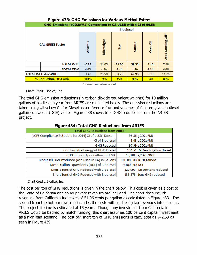
356
Figure 433: GHG Emissions for Various Methyl Esters
Chart Credit: Biodico, Inc.
The total GHG emission reductions (in carbon dioxide equivalent weights) for 10 million gallons of biodiesel a year from ARIES are calculated below. The emission reductions are taken using Ultra Low Sulfur Diesel as a reference fuel and volumes of fuel are given in diesel gallon equivalent (DGE) values. Figure 438 shows total GHG reductions from the ARIES project.
Figure 434: Total GHG Reductions from ARIES
Chart Credit: Biodico, Inc.
The cost per ton of GHG reductions is given in the chart below. This cost is given as a cost to the State of California and so no private revenues are included. The chart does include revenues from California fuel taxes of 51.06 cents per gallon as calculated in Figure 433. The second from the bottom row also includes the costs without taking tax revenues into account. The project lifetime is estimated at 15 years. Though any investment from California in ARIES would be backed by match funding, this chart assumes 100 percent capital investment as a high-end scenario. The cost per short ton of GHG emissions is calculated as $42.69 as seen in Figure 439.

357
Figure 435: Cost per Ton GHG Emissions
Chart Credit: Biodico, Inc.
Reduce Operating Costs by 65 percent The ARIES operating budget is given in detail in CHAPTER 4: ARIES Project Budget, but a summary of the costs per gallon of biodiesel is given in the figure below.
Figure 436: ARIES Biodiesel Cost per Gallon
Chart Credit: Biodico, Inc.
The operating costs for a traditional biodiesel plant operating with soybean oil are given in Figure 441.

358
Figure 437: Traditional Biodiesel Plant Operating Costs
Chart Credit: Biodico, Inc.
The feedstock costs are given in August 2014’s relatively low prices of $720 per metric ton of soybean oil. A five-year history for soybean oil is given below in Figure 442.
Figure 438: Soybean Oil Commodity Prices
Chart Credit: Biodico, Inc.
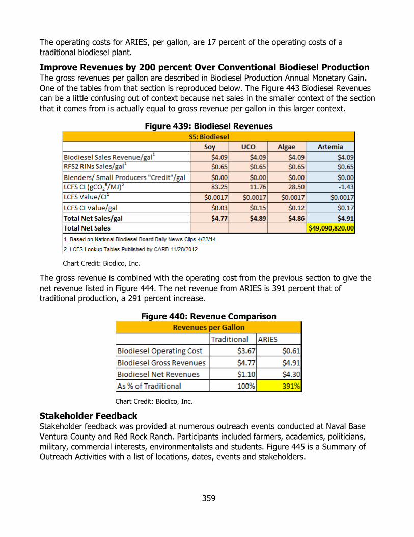
359
The operating costs for ARIES, per gallon, are 17 percent of the operating costs of a traditional biodiesel plant.
Improve Revenues by 200 percent Over Conventional Biodiesel Production The gross revenues per gallon are described in Biodiesel Production Annual Monetary Gain. One of the tables from that section is reproduced below. The Figure 443 Biodiesel Revenues can be a little confusing out of context because net sales in the smaller context of the section that it comes from is actually equal to gross revenue per gallon in this larger context.
Figure 439: Biodiesel Revenues
Chart Credit: Biodico, Inc.
The gross revenue is combined with the operating cost from the previous section to give the net revenue listed in Figure 444. The net revenue from ARIES is 391 percent that of traditional production, a 291 percent increase.
Figure 440: Revenue Comparison
Chart Credit: Biodico, Inc.
Stakeholder Feedback Stakeholder feedback was provided at numerous outreach events conducted at Naval Base Ventura County and Red Rock Ranch. Participants included farmers, academics, politicians, military, commercial interests, environmentalists and students. Figure 445 is a Summary of Outreach Activities with a list of locations, dates, events and stakeholders.

360
Figure 441: Summary of Outreach Activities
Chart Credit: Biodico, Inc.:
The principal feedback was almost universally supportive, and can be summarized along the following lines:
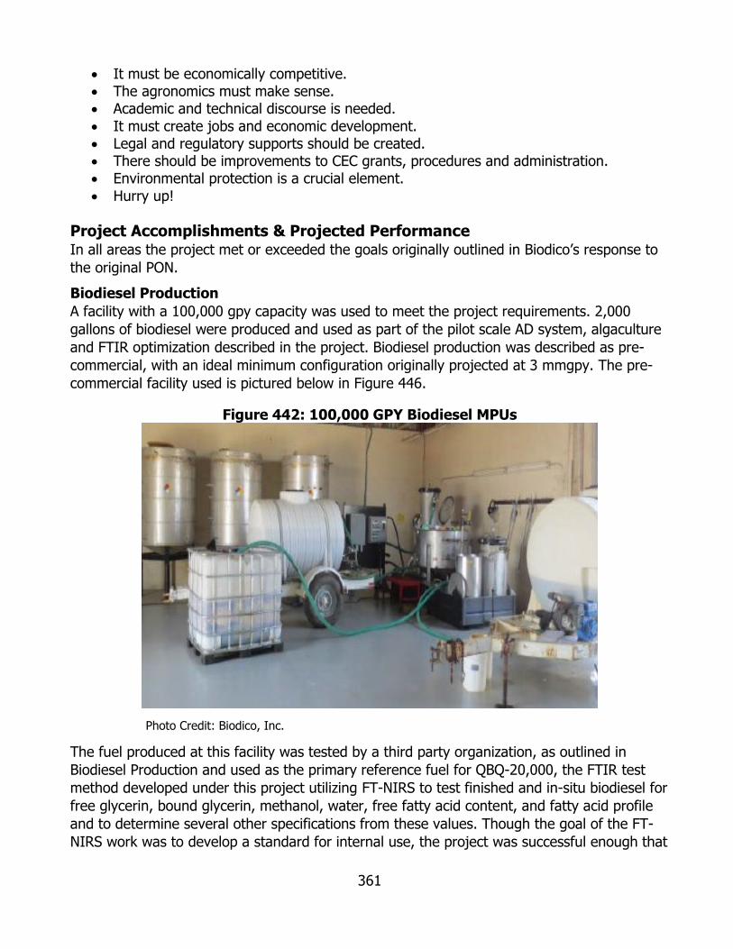
361
• It must be economically competitive. • The agronomics must make sense. • Academic and technical discourse is needed. • It must create jobs and economic development. • Legal and regulatory supports should be created. • There should be improvements to CEC grants, procedures and administration. • Environmental protection is a crucial element. • Hurry up!
Project Accomplishments & Projected Performance In all areas the project met or exceeded the goals originally outlined in Biodico’s response to the original PON. Biodiesel Production A facility with a 100,000 gpy capacity was used to meet the project requirements. 2,000 gallons of biodiesel were produced and used as part of the pilot scale AD system, algaculture and FTIR optimization described in the project. Biodiesel production was described as pre-commercial, with an ideal minimum configuration originally projected at 3 mmgpy. The pre-commercial facility used is pictured below in Figure 446.
Figure 442: 100,000 GPY Biodiesel MPUs
Photo Credit: Biodico, Inc.
The fuel produced at this facility was tested by a third party organization, as outlined in Biodiesel Production and used as the primary reference fuel for QBQ-20,000, the FTIR test method developed under this project utilizing FT-NIRS to test finished and in-situ biodiesel for free glycerin, bound glycerin, methanol, water, free fatty acid content, and fatty acid profile and to determine several other specifications from these values. Though the goal of the FT-NIRS work was to develop a standard for internal use, the project was successful enough that

362
Biodico decided to pursue specification approval with the Chemists Society,40 surpassing expectations. Anaerobic Digestion The original unit that had been included and quoted in the proposal was the Armfield W8, a unit with two five liter digesters with manual gas sampling and testing. After the approval of the project, however, Biodico found a unit that was almost identical in price and featured 15 separate 540 mL digesters and automatic gas testing, the Bioprocess Control AMPTS. The two are both pictured in Figure 447, with the Armfield W8 on the left and the Bioprocess Control AMPTS on the right.
Figure 443: W8 & AMPTS Anaerobic Digester Units
Photo Credit: Armfield & Bioprocess Control
Having 15 simultaneous digesters rather than two allowed for Biodico to run 7.5 times as many tests in the same amount of time, and the automatic gas production monitoring allowed for much more detailed characterization of the incoming feedstocks. A more complete listing of the differences between the units is given in the figure below.
Figure 444: Differences between AD Units
Chart Credit: Biodico, Inc.
40 AOCS Specification Approval (http://biodieselmagazine.com/articles/130235/in-situ-biodiesel-testing-technology-presented-at-aocs-meeting).
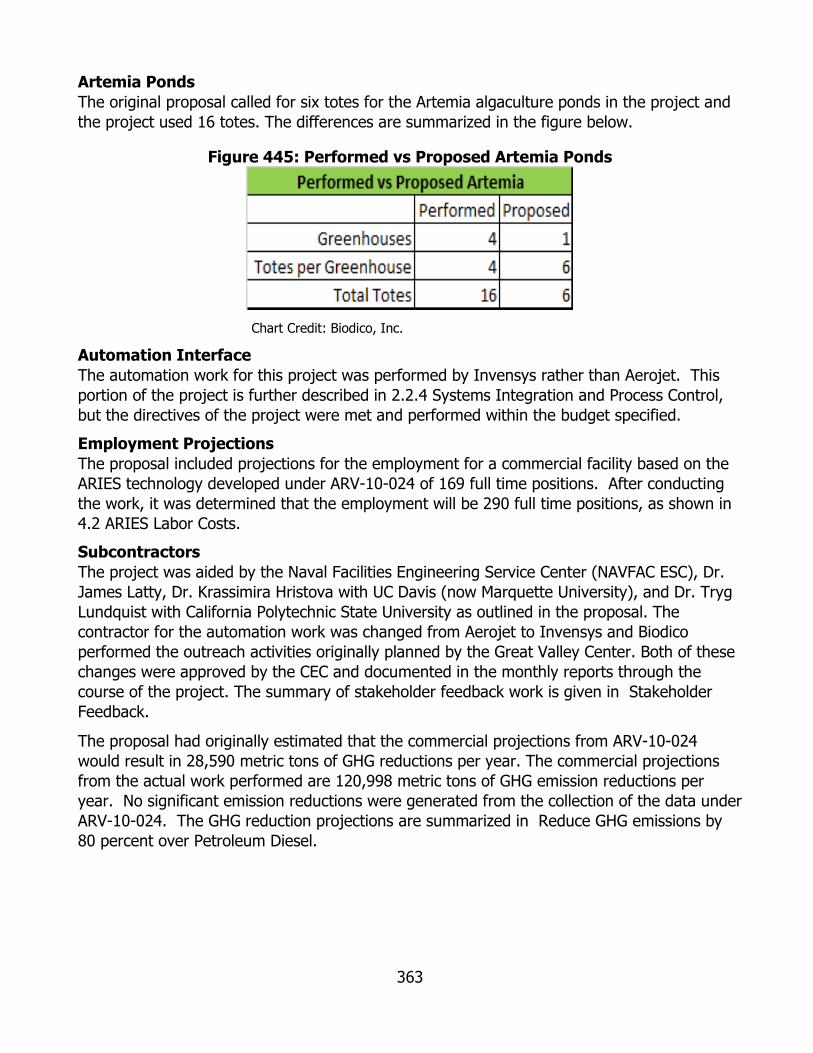
363
Artemia Ponds The original proposal called for six totes for the Artemia algaculture ponds in the project and the project used 16 totes. The differences are summarized in the figure below.
Figure 445: Performed vs Proposed Artemia Ponds
Chart Credit: Biodico, Inc.
Automation Interface The automation work for this project was performed by Invensys rather than Aerojet. This portion of the project is further described in 2.2.4 Systems Integration and Process Control, but the directives of the project were met and performed within the budget specified. Employment Projections The proposal included projections for the employment for a commercial facility based on the ARIES technology developed under ARV-10-024 of 169 full time positions. After conducting the work, it was determined that the employment will be 290 full time positions, as shown in 4.2 ARIES Labor Costs. Subcontractors The project was aided by the Naval Facilities Engineering Service Center (NAVFAC ESC), Dr. James Latty, Dr. Krassimira Hristova with UC Davis (now Marquette University), and Dr. Tryg Lundquist with California Polytechnic State University as outlined in the proposal. The contractor for the automation work was changed from Aerojet to Invensys and Biodico performed the outreach activities originally planned by the Great Valley Center. Both of these changes were approved by the CEC and documented in the monthly reports through the course of the project. The summary of stakeholder feedback work is given in Stakeholder Feedback.
The proposal had originally estimated that the commercial projections from ARV-10-024 would result in 28,590 metric tons of GHG reductions per year. The commercial projections from the actual work performed are 120,998 metric tons of GHG emission reductions per year. No significant emission reductions were generated from the collection of the data under ARV-10-024. The GHG reduction projections are summarized in Reduce GHG emissions by 80 percent over Petroleum Diesel.
364
CHAPTER 8: Recommendations
Demonstration Scale ARIES A demonstration scale implementation of ARIES should be implemented. Everything was designed to be scalable so that 1 percent, 19 acre modules of the algaculture and anaerobic digestion units can be put into place. The CHP generators that were used in the projections, Capstone 1,000 kW microturbines, are also scaled down to 65 kW units that are CARB certified. Each of these would cover about 1.4 percent of the total project capacity. The anaerobic digester bladders are completely scalable. Red Rock Ranch owns a commercial scale Instra-Pro oil extrusion unit that would cover over 10 percent of the total project needs. This oil extrusion press is co-located with a 10 mmgpy biodiesel production facility that Biodico and Red Rock Ranch plan to begin operating in November 2014. Upgrading the facility to ARIES would be a matter of programming and minor wiring work on the existing Invensys unit at Red Rock Ranch and implementing an FTIR system like the one at the naval base in Ventura County. Red Rock Ranch also owns refrigerated warehouse space that is co-located with the other facilities. Office space, laboratory space, and visiting worker dormitories have already been established at the project site. Private investment in bioenergy is usually geared toward core chemical production equipment and Biodico plans to actively seek investment to move ARIES technology past the “valley of death” between proof of concept and commercial viability. Thankfully all of the core equipment is in place, allowing this transition to occur in incremental measures.
Relief for Stranded AD Assets Power purchase agreements are very difficult for commercial AD operators to secure and from their end it often seems like the rules of the game keep changing. Publicly owned utilities feel a responsibility to their shareholders to increase profits as much as possible and to prevent their investments from losing value. Many utility companies worry about what has become known as “the duck curve” (Figure 450). The idea is that increasing renewable energy requirements are mostly based on solar, which gives a strong load to the system in the afternoon and sharply drops off in the evening. This skews the change in load rates on the utilities and strains their efficiencies (particularly due to inertia of rotating mechanical parts) and possibly equipment maintenance requirements. Biogas from AD could be a very elegant, if only very partial at today’s capacities, solution to this problem. ARIES will have continuous gas production sufficient to generate over 14 million kilowatt hours of electricity annually. For both the ramp up and the full implementation, gas can be stored in order to strategically help ease the burden highlighted by the duck curve in generating electricity between the peak hours of 4:00 and 11:00 PM.
Figure 446: California Renewable Electricity Generation “Duck Curve” 2013
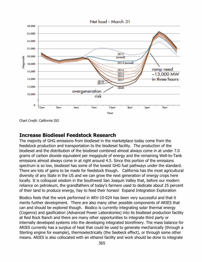
365
Chart Credit: California ISO
Increase Biodiesel Feedstock Research The majority of GHG emissions from biodiesel in the marketplace today come from the feedstock production and transportation to the biodiesel facility. The production of the biodiesel and the distribution of the biodiesel combined almost always come in at under 7.0 grams of carbon dioxide equivalent per megajoule of energy and the remaining Well-to-Tank emissions almost always come in at right around 4.5. Since this portion of the emissions spectrum is so low, biodiesel has some of the lowest GHG fuel pathways under the standard. There are lots of gains to be made for feedstock though. California has the most agricultural diversity of any State in the US and we can grow the next generation of energy crops here locally. It is colloquial wisdom in the Southwest San Joaquin Valley that, before our modern reliance on petroleum, the grandfathers of today’s farmers used to dedicate about 25 percent of their land to produce energy, hay to feed their horses! Expand Integration Exploration
Biodico feels that the work performed in ARV-10-024 has been very successful and that it merits further development. There are also many other possible components of ARIES that can and should be explored though. Biodico is currently integrating solar thermal energy (Cogenra) and gasification (Advanced Power Laboratories) into its biodiesel production facility at Red Rock Ranch and there are many other opportunities to integrate third party or internally developed systems into the developing integrated biorefinery. The mass balance for ARIES currently has a surplus of heat that could be used to generate mechanically (through a Sterling engine for example), thermoelectrically (the Seebeck effect), or through some other means. ARIES is also collocated with an ethanol facility and work should be done to integrate

366
ethyl esters into the market of methyl esters (Fatty Acid Methyl Ester biodiesel). Over 80 percent of the Tank-to-Wheels emissions (generally 3.67 of 4.45) in biodiesel come from the methanol used in production.
Per Gallon Biodiesel Incentives, Biofuels are ready to use now. Biodiesel particularly is one of very few fuel sources to have passed the EPA Tier 2 health effects testing. It can be blended with existing petroleum supplies to gradually reduce GHG emissions or to very accurately meet targeted GHG emissions Biodiesel is not classified as a hazardous material. Biodiesel is relatively safe to handle. It is non-toxic and it is a combustible liquid, not a flammable liquid. It has a track record of commercial use since 1993. Since 1993 the industry has also worked extensively with regulatory agencies, legislative organizations, Original engine manufacturers, fleet owners and operators, academia, military, and many other public and private organizations. It has done much of this through the NBB, the CBA, and the ASTM committee on biodiesel. Biodiesel has an even longer track record of successful use in Europe.

367
GLOSSARY ANAEROBIC DIGESTION (AD) — Anaerobic digestion is the natural process in which microorganisms break down organic materials. In this instance, “organic” means coming from or made of plants or animals. Anaerobic digestion happens in closed spaces where there is no air (or oxygen).41
ALTERNATIVE-FUEL VEHICLE (AFV)—A vehicle designed to operate on an alternative fuel (e.g., compressed natural gas, methane blend, electricity). The vehicle could be either a dedicated vehicle designed to operate exclusively on alternative fuel or a nondedicated vehicle designed to operate on alternative fuel and/or a traditional fuel.
AUTOMATED METHANE POTENTIAL TEST SYSTEM (AMPTS) — analytical tool preferred by scientists and engineers for conducting various anaerobic batch fermentation tests.42
AUTOMATED REMOTE REAL-TIME INTEGRATED ENERGY SYSTEM (ARIES) — is a highly automated, transportable biodiesel production unit that can be controlled from a remote location. These features ensure reliable process control and optimal production yields in a sustainable system that can be readily and widely deployed.43
AMERICAN SOCIETY FOR TESTING AND MATERIALS (ASTM)—An international standards organization that develops and publishes voluntary consensus technical standards for a wide range of materials, products, systems, and services.
CALIFORNIA AIR RESOURCES BOARD (ARB)—The "clean air agency" in the government of California whose main goals include attaining and maintaining healthy air quality, protecting the public from exposure to toxic air contaminants, and providing innovative approaches for complying with air pollution rules and regulations.
CALIFORNIA CODE OF REGULATIONS (CCR)—The official compilation and publication of the regulations adopted, amended, or repealed by state agencies pursuant to the Administrative Procedure Act (APA). Properly adopted regulations that have been filed with the Secretary of State have the force of law. The CCR is compiled into Titles and organized into Divisions containing the regulations of state agencies
CALIFORNIA ENVIRONMENTAL QUALITY ACT — (CEQA - pronounced See' quah)—Enacted in 1970 and amended through 1983, established state policy to maintain a high-quality environment in California and set up regulations to inhibit degradation of the environment.
41 Anaerobic Digestion (https://www.epa.gov/anaerobic-digestion/basic-information-about-anaerobic-digestion-ad).
42 Automated Methane Potential Test System (https://www.bioprocesscontrol.com/products/ampts-ii/)
43 ARIES System (https://www.rocket.com/article/aries-biodiesel-system-delivered-naval-base-ventura-county)
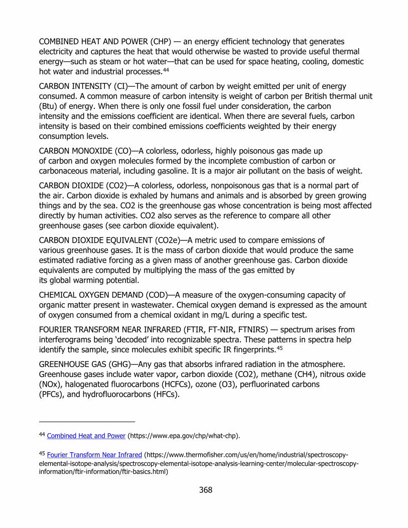
368
COMBINED HEAT AND POWER (CHP) — an energy efficient technology that generates electricity and captures the heat that would otherwise be wasted to provide useful thermal energy—such as steam or hot water—that can be used for space heating, cooling, domestic hot water and industrial processes.44
CARBON INTENSITY (CI)—The amount of carbon by weight emitted per unit of energy consumed. A common measure of carbon intensity is weight of carbon per British thermal unit (Btu) of energy. When there is only one fossil fuel under consideration, the carbon intensity and the emissions coefficient are identical. When there are several fuels, carbon intensity is based on their combined emissions coefficients weighted by their energy consumption levels.
CARBON MONOXIDE (CO)—A colorless, odorless, highly poisonous gas made up of carbon and oxygen molecules formed by the incomplete combustion of carbon or carbonaceous material, including gasoline. It is a major air pollutant on the basis of weight.
CARBON DIOXIDE (CO2)—A colorless, odorless, nonpoisonous gas that is a normal part of the air. Carbon dioxide is exhaled by humans and animals and is absorbed by green growing things and by the sea. CO2 is the greenhouse gas whose concentration is being most affected directly by human activities. CO2 also serves as the reference to compare all other greenhouse gases (see carbon dioxide equivalent).
CARBON DIOXIDE EQUIVALENT (CO2e)—A metric used to compare emissions of various greenhouse gases. It is the mass of carbon dioxide that would produce the same estimated radiative forcing as a given mass of another greenhouse gas. Carbon dioxide equivalents are computed by multiplying the mass of the gas emitted by its global warming potential.
CHEMICAL OXYGEN DEMAND (COD)—A measure of the oxygen-consuming capacity of organic matter present in wastewater. Chemical oxygen demand is expressed as the amount of oxygen consumed from a chemical oxidant in mg/L during a specific test.
FOURIER TRANSFORM NEAR INFRARED (FTIR, FT-NIR, FTNIRS) — spectrum arises from interferograms being ‘decoded’ into recognizable spectra. These patterns in spectra help identify the sample, since molecules exhibit specific IR fingerprints.45
GREENHOUSE GAS (GHG)—Any gas that absorbs infrared radiation in the atmosphere. Greenhouse gases include water vapor, carbon dioxide (CO2), methane (CH4), nitrous oxide (NOx), halogenated fluorocarbons (HCFCs), ozone (O3), perfluorinated carbons (PFCs), and hydrofluorocarbons (HFCs).
44 Combined Heat and Power (https://www.epa.gov/chp/what-chp).
45 Fourier Transform Near Infrared (https://www.thermofisher.com/us/en/home/industrial/spectroscopy-elemental-isotope-analysis/spectroscopy-elemental-isotope-analysis-learning-center/molecular-spectroscopy-information/ftir-information/ftir-basics.html)
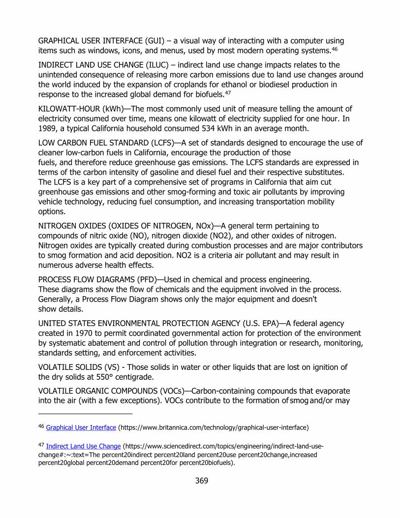
369
GRAPHICAL USER INTERFACE (GUI) – a visual way of interacting with a computer using items such as windows, icons, and menus, used by most modern operating systems.46
INDIRECT LAND USE CHANGE (ILUC) – indirect land use change impacts relates to the unintended consequence of releasing more carbon emissions due to land use changes around the world induced by the expansion of croplands for ethanol or biodiesel production in response to the increased global demand for biofuels.47
KILOWATT-HOUR (kWh)—The most commonly used unit of measure telling the amount of electricity consumed over time, means one kilowatt of electricity supplied for one hour. In 1989, a typical California household consumed 534 kWh in an average month.
LOW CARBON FUEL STANDARD (LCFS)—A set of standards designed to encourage the use of cleaner low-carbon fuels in California, encourage the production of those fuels, and therefore reduce greenhouse gas emissions. The LCFS standards are expressed in terms of the carbon intensity of gasoline and diesel fuel and their respective substitutes. The LCFS is a key part of a comprehensive set of programs in California that aim cut greenhouse gas emissions and other smog-forming and toxic air pollutants by improving vehicle technology, reducing fuel consumption, and increasing transportation mobility options.
NITROGEN OXIDES (OXIDES OF NITROGEN, NOx)—A general term pertaining to compounds of nitric oxide (NO), nitrogen dioxide (NO2), and other oxides of nitrogen. Nitrogen oxides are typically created during combustion processes and are major contributors to smog formation and acid deposition. NO2 is a criteria air pollutant and may result in numerous adverse health effects.
PROCESS FLOW DIAGRAMS (PFD)—Used in chemical and process engineering. These diagrams show the flow of chemicals and the equipment involved in the process. Generally, a Process Flow Diagram shows only the major equipment and doesn't show details.
UNITED STATES ENVIRONMENTAL PROTECTION AGENCY (U.S. EPA)—A federal agency created in 1970 to permit coordinated governmental action for protection of the environment by systematic abatement and control of pollution through integration or research, monitoring, standards setting, and enforcement activities.
VOLATILE SOLIDS (VS) - Those solids in water or other liquids that are lost on ignition of the dry solids at 550° centigrade.
VOLATILE ORGANIC COMPOUNDS (VOCs)—Carbon-containing compounds that evaporate into the air (with a few exceptions). VOCs contribute to the formation of smog and/or may
46 Graphical User Interface (https://www.britannica.com/technology/graphical-user-interface)
47 Indirect Land Use Change (https://www.sciencedirect.com/topics/engineering/indirect-land-use-change#:~:text=The percent20indirect percent20land percent20use percent20change,increased percent20global percent20demand percent20for percent20biofuels).
370
themselves be toxic. VOCs often have an odor and some examples include gasoline, alcohol and the solvents used in paints. VIRTUAL PRIVATE NETWORK (VPN) – VPN, is an encrypted connection over the Internet from a device to a network. The encrypted connection helps ensure that sensitive data is safely transmitted. It prevents unauthorized people from eavesdropping on the traffic and allows the user to conduct work remotely.48
WELL TO WHEEL (WTW)—A specific LCA (Lifecycle Assessment) used for transport fuels and vehicles. The analysis is often broken down into stages entitled "well-to-station", or "well-to-tank", and "station-to-wheel" or "tank-to-wheel", or "plug-to-wheel". The first stage, which incorporates the feedstock or fuel production and processing and fuel delivery or energy transmission, and is called the "upstream" stage, while the stage that deals with vehicle operation itself is sometimes called the "downstream" stage. The well-to-wheel analysis is commonly used to assess total energy consumption, or the energy conversion efficiency and emissions impact of marine vessels, aircraft and motor vehicles, including their carbon footprint, and the fuels used in each of these transport modes. WTW analysis is useful for reflecting the different efficiencies and emissions of energy technologies and fuels at both the upstream and downstream stages, giving a more complete picture of real emissions.
WASTEWATER TREATMENT PLANT (WWTP) – A wastewater treatment plant is a facility in which a combination of various processes (e.g., physical, chemical and biological) are used to treat industrial wastewater and remove pollutants.49
48 VPN (https://www.cisco.com/c/en/us/products/security/vpn-endpoint-security-clients/what-is-vpn.html)
49 Wastewater Treatment Plants (https://www.sciencedirect.com/topics/earth-and-planetary-sciences/waste-water-treatment-plant)
371
REFERENCES A. Zarei (2013). Artemia, a New Source of Animal Protein Ingredient in Poultry Nutrition, Biomass Now - Sustainable Growth and Use, Dr. Miodrag Darko Matovic (Ed.), ISBN: 978-953-51-1105-4, InTech, DOI: 10.5772/53610. Available from: http://www.intechopen.com/books/biomass-now-sustainable-growth-and-use/Artemia-a-new-source-of-animal-protein-ingredient-in-poultry-nutrition
Anderson International Corp. “Animal Feed Equipment.” AndersonIntl.net. http://www.andersonintl.net/index_files/AnimalFeedEquipment.htm (retrieved September 12, 2014).
Burlew J-S (1953) Algal culture: from laboratory to pilot plant. Carnegie Institute of Washington Publication, Washington DC
Chen, X., R.T. Romano, R. Zhang, H.S. Kim. 2008. Anaerobic co-digestion of dairy manure and glycerin. In proceedings of 2008 American Society of Agricultural and Biological Engineering Annual International Meeting. Providence, Rhode Island.
Coutteau P., and Sorgeloos, P. 1989. Feeding of the brine shrimp Artemia on yeast: effect of mechanical disturbance, animal density, water quality and light intensity. In: European Aquaculture Society Spec. Publ. N° 10. Bredene, Belgium, 344 pp.
B.M. Jenkins et al Salt separation and purification concepts in integrated farm drainage management systems. ASAE paper number 032236, July 2003
Capstone. “C100 Megawatt Power Package.” CapstoneTurbine.com. (http://www.capstoneturbine.com/_docs/datasheets/C1000 percent20HPNG_331044F_lowres.pdf) (retrieved September 12, 2014).
Choose Energy. “4 residential electricity plans found in 93624.” ChooseEnergy.com. (https://www.chooseenergy.com/compare/93624/electricity/pge-ca/electricity-rates/) (retrieved September 12, 2014).
Cline, Harry. “Water $70 to $2.4 million per acre foot.” WesternFarmPress.com. http://westernfarmpress.com/water-70-24-million-acre-foot (retrieved September 12, 2014).
D. Matthews & B.C. Cooke (2003). The potential for transmissible spongiform encephalopathies in non-ruminant livestock and fish. Rev. sci. tech. Off. Int. Epiz, 2003, 22(1), 283-296
Don’t, Jean, and Patrick Lavens. “Tank Production and Use of Ongrown Artemia.” FAO.org. http://www.fao.org/docrep/003/w3732e/w3732e0p.htm (retrieved September 12, 2014).
Edwards, William. “Computing a Cropland Cash Rental Rate.” IAState.edu. (http://www.extension.iastate.edu/agdm/wholefarm/html/c2-20.html) (retrieved September 12, 2014).
E.G. Bligh, W.J. Dyer, Canad. J. Biochem. and Physiology 1959, 37, 911.
Folch, J., Lees, M. and Stanley, G.H.S., J. Biol. Chem., 226, 497-509 (1957).
372
Heaton E-A, Dohleman F-G, Long S-P (2008) Meeting US biofuel goals with less land: the potential of Miscanthus. Glob Chang Biol 14:2000-2014
Ind. Eng. Chem. Res. 2008, 47, 4278–4285
Insta-Pro. “MS3000 Medium Shear Extruder.” http://www.insta-pro.com/products-services/extruders/ms3000-medium-shear-extruder/medium-shear-extruder.html (retrieved September 12, 2014).
Integra Realty Resources. “A Cost Analysis Can Be Invaluable in the Appraisal of Cold Storage Facilities.” IRR.com. (http://www.irr.com/_FileLibrary/Office/P484/Cold percent20Storage percent20Article.pdf) (retrieved September 12, 2014).
Kotrba, Ron. “In situ biodiesel testing technology presented at AOCS meeting.” BiodieselMagazine.com. http://biodieselmagazine.com/articles/130235/in-situ-biodiesel-testing-technology-presented-at-aocs-meeting (retrieved September 12, 2014).
Lavens P., and Sorgeloos, P. 1987. Design, operation, and potential of a culture system for the continuous production of Artemia nauplii. In: Artemia Research and its Applications. Vol. 3. Ecology, Culturing, Use in Aquaculture P. Sorgeloos, D. Bengtson, W. Decleir and E. Jaspers (Eds) Universal Press, Wetteren, Belgium: 339-345.
Leger, Bengston, Simpson and Sorgeloos, The Use and Nutritional Value of Artemia as a Food Source, Oceanogr. Mar. Biol. Ann. Rev., 1986, p. 521-623.
Life Cycle GHG Emissions from Microalgal Biodiesel – A CA-GREET Model - Ian C. Woertz, John R. Benemann, Niu Du, Stefan Unnasch, Dominick Mendola, B. Greg Mitchell, and Tryg J. Lundquist - Environmental Science & Technology 2014 48 (11), 6060-6068
NOAA. “Basic Questions about Aquaculture.” NOAA.gov. (http://www.nmfs.noaa.gov/aquaculture/faqs/faq_aq_101.html (retrieved September 12, 2014).
OSHA. “Materials Handling and Storage.” OSHA.gov. (https://www.osha.gov/Publications/osha2236.pdf) (retrieved September 12, 2014).
Richmond, A., 2000. Microalgal biotechnology at the turn of the millennium: a personal view. J. Appl. Phycol., 12: 441-451.
Sanford, W. E. and Selnick, D. L. (2013), Estimation of Evapotranspiration Across the Conterminous United States Using a Regression With Climate and Land-Cover Data. JAWRA Journal of the American Water Resources Association, 49: 217–230. doi: 10.1111/jawr.12010
Schmidt, R.; Tantoyotai, P.; Fakra, S.; Marcus, M.; Yang, S. I.; Pickering, I.; Bañuelos, G.; Hristova, K. R., and Freeman, J. 2013. Selenium biotransformations in engineered aquatic ecosystem for bioremediation of agricultural wastewater via brine shrimp production. Env. Sci. Technol., 47: 5057–5065. online first May 2013: dx.doi.org/10.1021/es305001n
Sell, Steven Thomas, "A scale-up procedure for substrate co-digestion in anaerobic digesters through the use of substrate characterization, BMPs, ATAs, and sub pilot-scale digesters" (2011). Graduate Theses and Dissertations.Paper 12044
373
Sheehan, John, Terri Dunahay, John Benemann, Paul Roessler, 1998. A Look Back at the U.S. Department of Energy’s Aquatic Species Program – Biodiesel from Algae
Singh, R. Paul. 2008. Benchmarking Study of the Refrigerated Warehousing Industry Sector in California. Public Interest Energy Research (PIER) Program Contract and Research Project Reports. California Energy Commission, PIER Program
Standard Xchange. “Heat Exchanger, 3,800,000, Brass.” Zoro.com. (http://www.zoro.com/i/G1740277/?category=7591) (retrieved September 12, 2014).
Sudhakar, K. and M. Premelatha, 2012. Theoretical Assessment of Algal Biomass Potential for Carbon Mitigation and Biofuel Production, Iranica Journal of Energy and the Environment 3 (3): 232-240, 2012
US Climate Data. “Climate – Five Points, California.” USClimateData.com. (http://www.usclimatedata.com/climate/five-points/california/united-states/usca0380) (retrieved September 12, 2014).
U.S. DOE 2010. National Algal Biofuels Technology Roadmap. U.S. Department of Energy, Office of Energy Efficiency and Renewable Energy, Biomass Program.
USDA. “Census of Aquaculture Publications.” USDA.gov. (http://www.agcensus.usda.gov/Publications/2002/Aquaculture) (retrieved September 12, 2014).
Weyer, Kristina M., Daniel R. Bush, Al Darzins, Bryan D. Wilson, 2009. Theoretical Maximum Algal Oil Production, Bioenergy. Res. (2010) 3:204-213
Zhu X, Long S, Ort D (2008) What is the maximum efficiency with which photosynthesis can convert solar energy into biomass? Current Opinion Biotechnology 19:153-159