Area-Identified National Crime Victimization Data

Area-Identified National Crime Victimization Survey Data:

A Resource Available Through the National Consortium on Violence Research

Brian WiersemaViolence Research GroupUniversity of Maryland

College Park, Maryland 20742-8235(301) 405-4735 (voice)

[email protected]

NCOVR Census Center Technical Paper 1Pittsburgh, Pennsylvania

Revised: January 1999

1 Support for this research was provided by the National Consortium on ViolenceResearch (NCOVR), headquartered at the Heinz School of Public Policy and Management atCarnegie Mellon University. NCOVR is supported under grant# SBR 9513040 from theNational Science Foundation in partnership with the US Department of Housing and UrbanDevelopment and the National Institute of Justice.

1

Area-Identified National Crime Victimization Survey Data:

A Resource Available Through the National Consortium on Violence Research1

National Crime Victimization Survey (NCVS) data have been publicly available for

analysis and research since the 1970's, representing an unusually long and consistent source of

high quality national data on criminal victimization. The data are collected through a stratified,

multistage cluster sample of housing units interviewed every six months over a three year period.

The content of the NCVS focuses on individual and household experiences with criminal

victimization. Over 600 variables are available in the public use files. Despite the apparent

richness of these data, the amount of information about the areas in which sampled individuals

reside is extremely limited. Research, for example, that studies the effects of neighborhood

context on individual victimization risks, has been impossible to undertake with the NCVS

because contextual area variables have been suppressed in public-use files to protect the

confidentiality of respondents and their answers.

Under a special arrangement with the U.S. Bureau of the Census (collector of the data)

and the U.S. Bureau of Justice Statistics (the survey’s sponsor), the National Consortium on

Violence Research (NCOVR) has access to secured NCVS data that include the identifying

Wiersema Area-Identified NCVS Data

2 Public-use NCVS data are available from the Inter-university Consortium for Politicaland Social Research (ICPSR) through their web site: http://www.icpsr.umich.edu/nacjd .

3 The special arrangement requires that prior to the communication of any results basedon these data, the Census Bureau must review them to assure conformity to Title 13 provisionsfor “disclosure avoidance.” The Bureau of the Census’ contact person for these issues is DavidR. Merrell. He may be reached via electronic mail at [email protected] or bytelephone at 412-268-4070.

2

information.2 Researchers who are granted access to the data become “sworn special employees”

of the U.S. Bureau of the Census which permits them to conduct research on confidential data

within a Research Data Center (RDC).3 The RDC currently housing the confidential data is

located at Carnegie Mellon University in Pittsburgh, Pennsylvania, which is also the headquarters

of NCOVR.

This document describes how the NCOVR-NCVS data differ from public-use versions, as

well as some of the survey design characteristics that may prove useful in gauging the power of

the NCOVR-NCVS data for various research purposes. The first section outlines what NCVS

data are currently available at NCOVR, their format, and the kinds of identifiers present in the

files. The second section addresses data processing issues that arise out of the phase-in/phase-out

of 1980 and 1990 sample elements which affect the 1994-1996 NCVS data. The final section

characterizes the different levels of geography in terms of sample sizes and distributions thus

providing a rough guide to the power of the sample for subnational analysis.


3

NCVS Data Presently Available

As of January 1999, the RDC at Carnegie Mellon University possessed NCVS data for

the period 1986 through 1997. Data for 1992 through 1997 are based on the redesigned survey

instrument that was formulated to produce better recall of victimization incidents by respondents

than earlier versions of the survey (see Kindermann, Lynch and Cantor, 1997, for a discussion of

the effects of the “new methods” on crime estimates). Data for 1986 through 1992 are based on

“old methods” of the NCVS meaning that the screener portion of the instrument is essentially

unchanged from the time the crime survey was first fielded. NCOVR may be able to acquire

some data from prior to 1986, but issues surrounding Census archiving formats and processing

requirements limit the amount of confidential data that can be delivered to the RDC for research.

Thus, data before 1986 are highly unlikely to become available.

Data Format

The format of the available data is ASCII, with variable-length records in a nested,

hierarchical order. ICPSR calls NCVS files in this format, “full files.” The data were not

delivered to the RDC with SAS or SPSS commands that define variable locations and widths,

nor is there a complete codebook available for the private-use data. Instead, Census has provided

the codebook for their Public-Use file and a two-page record layout for the private-use data.

Comparing the two reveals which variables are public and which contain confidential material.

The private-use file contains all variables that ICPSR includes in its archived versions of the

data, except for the ICPSR sequence number. Because most researchers who plan to use these


4

files are likely already familiar with the ICPSR formats and naming conventions, NCOVR has

created a set of SAS programs that use the ICPSR naming conventions for the public-use

variables. The remaining private use variables have been given new variable names and labels to

more completely identify them.

Confidential Variables

There are two types of variables present in the NCVS files at NCOVR that are not present

in the public use files: (1) standard geographic area identifiers, and (2) variables used in carrying

out the sampling design of the survey. The two are related because the sample design uses

Census data on the size and location of geographic areas to create the strata and clusters that

contain the housing units eventually interviewed.

1. Geographic Area Identifiers

The variables that will probably be of most use to researchers are the standard geographic

area identifiers. This is because they can be used to link the NCVS data with other data

identified by these codes. The geographic identifiers present on the file are hierarchical and can

be represented as follows:

RegionDivision

StateCounty

County subdivisionPlace

Census tract/block numbering area


5

In addition to these, codes identifying urban and metropolitan areas are available on the files.

The specific Census Bureau definitions for geographic variables on the NCOVR-NCVS files are

included in Appendix A. This appendix also includes important information regarding the

coding structure of these variables.

2. Sample Design Variables

An understanding of the NCVS sampling design is particularly important when using the

geographic subunits available in the NCOVR-NCVS data. Introductions to the survey’s sample

design and data collection procedures may be found in the ICPSR public-use file codebooks

(e.g., Bureau of Justice Statistics, 1998) or in Bureau of Justice Statistics (BJS) publications such

as the annual Criminal Victimization in the United States (e.g., Bureau of Justice Statistics,

1997). For present purposes I simply note the survey’s basic features and the variables that

represent the sampling hierarchy.

At the top level of the sampling hierarchy, known as the design’s first stage, the country

is divided into areas called Primary Sampling Units (PSUs). The PSUs are used to create strata

within which first stage selections are made. Some PSUs have such large populations that each

becomes its own stratum in the design. These are called self-representing (SR) PSUs. The

remaining PSUs (non-self-representing or NSR PSUs) are grouped into strata based on decennial

census characteristics thought to be related to criminal victimization. Such characteristics

include geographic region, principal industry, rate of population increase, and the like. Thus at

the first stage there are main two variables: PSU and STRATUM. The relationship between the


6

two is this: for SR-PSUs, there is one PSU per stratum; for NSR-PSUs, there is more than one

PSU per stratum.

Until the 1990 Census, the second stage of sampling selected “enumeration districts”

(EDs) within PSUs. Enumeration districts were geographic areas of the PSU created by the

Bureau of the Census for use in administering the decennial census. They usually followed well-

defined boundaries and on average contained about 300 households. ED’s were sampled

systematically from a geographically arranged listing with probability proportionate to their

population size. The variable identifying ED’s is called EDCODE.

Beginning with the 1990 Census (and sample designs derived from it), the concept of an

enumeration district per se became obsolete. Instead, the different types of frames within PSU’s

are arranged geographically and clusters of approximately four housing units each are

systematically selected from the sorted lists directly. The order of the lists are based on a

hierarchy of administrative units created by the Census Bureau for use in the decennial census

operation (e.g., district offices, address register areas, collection block numbers, and the like).

However for most researchers, the important sampling stages to focus on in the 1990 design are

just PSU’s and housing unit clusters (or segments, described below) within PSU’s.

In the final stage of sampling, clusters of approximately four housing units, called

segments, were selected (either within ED’s in pre-1990 designs or within PSU’s in post-1990

designs). Segments are small land areas or groups of addresses and were created from lists of

addresses compiled during the decennial census. In places where the address lists were

incomplete or inaccurate, area sampling methods were employed. About two-thirds of the


7

segments are based on address lists and are located primarily in urban areas. The remaining

segments are formed by dividing areas into small subareas and canvassing a selected subarea to

create a new list of addresses. To account for housing units constructed after the decennial

census, a separate set of segments were created from lists of new building permits. The new

construction portion of the sample is small but it increases as the decade progresses. A final

segment type is created for “special places” which are essentially group quarters such as rooming

houses and dormitories. There are several segment variables on the files. These correspond to

the different sample designs (1980 or 1990) which are discussed below.

Sampling Frame Phase-in/Phase-out

Because the NCVS is a continuous survey operation, the sampling frame upon which it is

based needs to be updated periodically. Failure to update the frame would introduce ever

increasing coverage error because newly added housing stock would have no chance of selection

in the survey. The decennial census serves as the main source of frame change information. A

new sample design for the NCVS is thus created every ten years based on the updated

information and the new sample is phased into the rotation schedule around mid-decade. In other

words, sampled units based on 1980 design information would continue in the survey through the

mid 1990's at which point information based on the 1990 census could be phased in with a new

sample design.

This has implications for merging NCVS data with other data based on census identifiers

that change definitions between censuses. Except for states and regions, virtually every other


4 Accessible via the internet at http://www.oseda.missouri.edu/plue/geocorr/index.html

5 The GeoCorr system is quite flexible and handles many different types of geography,not just census tracts.

8

geographic entity was subject to some boundary change between the 1980 and 1990 censuses.

Some of these changes might be considered trivial, such as those pertaining to counties, but for

other areas, like census tracts, the changes were fairly extensive. Merging data based on 1990

tract definitions with data based on 1980 definitions would therefore introduce considerable error

unless there was some way to make 1980 geography correspond to 1990 definitions.

In concept there are several ways to approach this problem. Perhaps the most convenient

solution is to use a powerful geographic correspondence system developed by John Blodgett of

the University of Missouri-St. Louis Urban Information Center in collaboration with the Center

for International Earth Science Information Network (CIESIN). Called MABLE/GeoCorr the

system is an interactive web-based data engine.4 In essence, the system uses data from the block

level (the MABLE or Master Area Block Level Equivalency file part) to build a set of

correspondence or correlation tables between geographic entities (the GeoCorr part) upon

request. The GeoCorr tables list the two sets of geography together with an “apportionment

factor” that is based on one of the following: (1) 1990 population size, (2) land area (km2), or (3)

1990 housing units. Thus one can determine what proportion of the 1990 tract can be distributed

among 1980 tracts (or vice versa) with this technique.5 One simply uses the allocation factor

produced by GeoCorr as weighting variable by multiplying it with 1990 census tract variables

that are to be matched with NCVS units from the 1980 sample design. NCVS units from the


9

1990 sample design obviously require no adjustment if they are to be matched with 1990 tract

data. For some geographic units (e.g., census designated places), the Census Bureau has already

performed a 1980-1990 code conversion which is reflected in the NCOVR-NCVS files. For

tracts and most other units, however, they simply attached the geographic code corresponding to

the design year (e.g., MSA codes for 1980 design units use the 1984 MSA codes and 1990 design

units use the 1993 MSA codes). In these cases, a GeoCorr type conversion of the codes would

be required to properly match external data with NCVS records.

Expressing the 1980 sample design units in terms of 1990 geographic definitions is only

the one consideration in attaching 1990 census summary data to NCVS units. Another

consideration is the missing data patterns in the NCVS matching variables. An internal Census

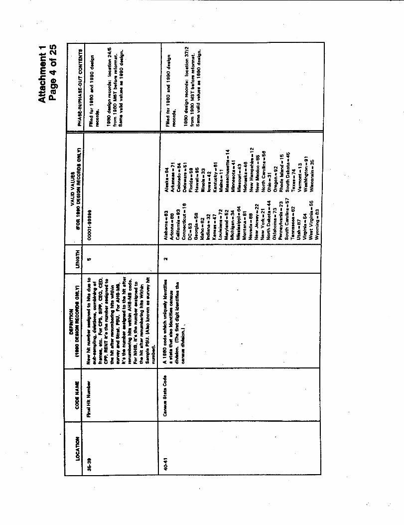
Bureau memorandum (National Crime Victimization Survey Unit Control File Information

Memorandum #9UC-G-8, dated 12/1/94, reproduced in Appendix B) outlines the contents of the

phase-in/phase-out geography in the NCVS. It indicates, for example, census tracts and block

numbering areas (BNAs) are only identified for sampled units in “old construction” frames. Any

unit in either the 1980 or 1990 sample designs that was selected from a permit frame will not

have a tract/BNA code assigned to it. Thus it cannot be matched to external data by tract/BNA

code. Since permit frame housing units comprise about 10-12% of the NCVS sample, one would

expect about 10-12% attrition in the matching procedure due to this factor. For areas larger than

tracts, no exclusions are noted in Memorandum #9UC-G-8.


10

Sample Sizes and Distributions

The NCVS is designed to produce national estimates of criminal victimization. The

sample size is large enough so that certain basic comparisons can be made with reasonable

confidence. At present, approximately 50,000 households comprise the NCVS sample. While

this may seem to be a very large set of data, it is important to understand the limits of the sample.

Once spread across the entire country, the sample is quite sparse . The following analysis is, in

part, intended to show that the geographically identified NCOVR-NCVS data are ill-suited to

produce small area estimates.

The primary purpose for making geographically identified NCVS data available is to

allow them to be enriched with other similarly identified data. While this should stimulate new

analytical models, it is important to begin with some knowledge of both the size and distribution

of the NCVS sample in terms of the various area units available on the files.

Table 1 presents basic descriptive statistics for all sampled households in the first half of

1996. It indicates, for example, that the sample contains a mean of 1141 households across the

50 U.S. states and the District of Columbia (column labeled “n”). The median number of

households per state is 796 with a mode of 80 households per state. The smallest area identified

in the NCOVR-NCVS files are census tracts. The NCVS sample contains households in 9784

different tracts in 1996 with a mean of 5.95 households per tract, and a median and mode of 4

households per tract.

The distribution of sample cases for each geographic unit is presented visually in Figure

1. On the x-axis are the percentile points of the distribution. The data are ordered from smallest


11

number of households per unit to largest number of households per unit for the following

percentiles: 0, 1, 5, 10, 25, 50, 75, 90, 95, 99, and 100.

The data in Figure 1 show the sparseness of the sample for all but the very largest units in

a specific geographic area. If one focuses on the parts of the sample with the largest populations

— for example, census designated places of population 250,000 or more—the sample contains

households in 61 places, with a mean of 164.97 households per place (SD=220.15, mode=77,

median= 111, minimum=44, maximum=1611). The same very large places contain sample that

cover 2179 census tracts with a mean of 4.62 households per tract (SD=3.37, mode=4,

median=4, minimum=1, maximum=72).

Table 1: NCVS Households by Type of Areal Unit, January-June 1996: Sample Sizes and Moments

Areal Unit n Mean SD Median Mode

State 51 1140.53 1337.23 796 80

MSA 191 242.84 251.74 178 157

County 601 96.78 117.85 69 8

MCD/CCD 3844 14.88 31.19 7 4

Place 3188 12.95 39.18 5 4

Tract 9784 5.95 7.07 4 4

When focusing on victimization incidents instead of sampled households, a similar

picture emerges except, of course, the numbers of incidents per area are smaller than the number

of households per area. Table 2 presents descriptive statistics on the numbers of victimization


6 Violent victimizations represent about a quarter of the total number of NCVS incidents.

12

incidents per areal unit for the same time period covered above for households. These include all

incidents not just violent victimizations.6 The distribution of incidents is shown in Figure 2.

Table 2: NCVS Incidents by Type of Areal Unit, January-June 1996: Sample Sizes and Moments

Areal Unit n Mean SD Median Mode

State 51 164.51 209.49 117 90

MSA 188 37.85 40.91 25 18

County 529 15.86 22.42 9 1

MCD/CCD 1950 4.24 7.80 2 1

Place 1611 4.02 8.26 2 1

Tract 4066 2.06 2.05 1 1

Again, the sparseness of the sample is the most evident feature of the data for all but the

largest subnational areal units. For example, incidents were reported in 4066 census tracts, but

the mean number of incidents per tract is 2.06 with a mode of 1 and a median of 1. The graphs in

Figure 2 are similarly flat except for the very highest end of the distribution. For places with

populations of 250,000 or more, at least one incident was reported in each of the 61 places that

contain sampled households. For these, the mean number of incidents per place (reported in a

single interview) was 28.31 (SD=28.49, mode= 26, median=23, minimum=4, maximum=177).

918 tracts located in the same largest places in the U.S. appear in the NCVS sample with at least

one incident in the first half of 1996 (mean=1.88, SD=1.75, mode=1, median=1, minimum=1,

and maximum=33).


13

Conclusions

Area-identified NCVS data represent an unprecedented opportunity to expand our

knowledge of the effects of area contexts on individual and household victimization. Data such

as those from Census Summary Tape File 3 can be merged with the NCVS that describe the areas

in which NCVS respondents live in much greater detail than has ever before been possible. To

protect the confidentiality of the identified data, all research on these files must be conducted by

researchers who become “sworn special employees” of the Census Bureau. NCOVR, BJS, and

the Census Bureau have made arrangements to provide access to these files at the Census RDC at

Carnegie Mellon University through a proposal review process that covers both the scientific

merit of the proposed research as well as the Census’ disclosure avoidance procedures.

There are many ways to make valid use of the NCOVR-NCVS data, however even a very

large sample survey has its limits. The data presented above suggest that the NCVS sample may

be rich enough to produce valid estimates for certain very large subnational areas (e.g., regions,

large states and a few very large metropolitan areas) but estimates for smaller areas would be so

imprecise as to render them useless. For other types of analyses where a reasonably large

number of units within each geographic area is important for estimation, the same caveats apply.

However, with sufficient appreciation for the design and limits of the NCVS data, a great many

new analyses can and should be conducted with the NCOVR-NCVS resources.


14

References

Bureau of Justice Statistics. (1997). Criminal Victimization in the United States, 1994. NCJ-

162126. Washington, DC: U.S. Department of Justice Office of Justice Programs.

__________. (1998). National Crime Victimization Survey, 1992-1995. [Computer file and

documentation]. Conducted by U.S. Bureau of the Census. 4th ICPSR ed. (Study 6406).

Ann Arbor, MI: Inter-university Consortium for Political and Social Research [producer

and distributor].

Kindermann, Charles, James Lynch, and David Cantor. (1997, April). Effects of the Redesign on

Victimization Estimates. (NCJ-164381). Washington, DC: Bureau of Justice Statistics.

Figure 1Distribution of Households by Type of Geographic Aggregation

15

0 1000 2000 3000 4000 5000 6000 7000

HH

s pe

r S

tate

0 10 20 30 40 50 60 70 80 90 100Percentile

States

0

500

1000

1500

2000

HH

s pe

r M

SA

0 10 20 30 40 50 60 70 80 90 100Percentile

MSAs

0

500

1000

1500

2000

HH

s pe

r C

ount

y

0 10 20 30 40 50 60 70 80 90 100Percentile

Counties

0 100 200 300 400 500 600 700

HH

s pe

r M

CD

/CC

D

0 10 20 30 40 50 60 70 80 90 100Percentile

MCD/CCDs

0

500

1000

1500

2000

HH

s pe

r P

lace

0 10 20 30 40 50 60 70 80 90 100Percentile

Places

0

50

100

150

200

HH

s pe

r T

ract

0 10 20 30 40 50 60 70 80 90 100Percentile

Tracts

Figure 2Distribution of Incidents by Type of Geographic Aggregation

16

0 200 400 600 800

1000 1200 1400

Inci

dent

s pe

r S

tate

0 10 20 30 40 50 60 70 80 90 100Percentile

States

0 50

100 150 200 250 300 350

Inci

dent

s pe

r C

ount

y

0 10 20 30 40 50 60 70 80 90 100Percentile

Counties

0 50

100 150 200 250 300 350

Inci

dent

s pe

r M

SA

0 10 20 30 40 50 60 70 80 90 100Percentile

MSAs

0 20 40 60 80

100 120 140

Inci

dent

s pe

r M

CD

/CC

D

0 10 20 30 40 50 60 70 80 90 100Percentile

MCD/CCDs

0

50

100

150

200

Inci

dent

s pe

r P

lace

0 10 20 30 40 50 60 70 80 90 100Percentile

Places

0 10 20 30 40 50 60

Inci

dent

s pe

r T

ract

0 10 20 30 40 50 60 70 80 90 100Percentile

Tracts


7 Accessible via the internet at http://www.census.gov/td/stf3/append_a.html

17

Appendix A

Census Definitions of Geographic Areas

The information in this appendix has been excerpted either wholly or in part from U.S. Bureau of

the Census technical documentation on the definition of geographic areas distributed with Census

of Population and Housing, 1990: Summary Tape File 3 on CD-ROM [machine-readable data

files] / Washington, DC: U.S. Bureau of the Census, 1992.7 Only the areas represented in the

NCOVR-NCVS files are included below.

Census Regions and Divisions

Census divisions are groupings of States that are subdivisions of the four census regions. There

are nine divisions, which the Census Bureau adopted in 1910 for the presentation of data. Census

regions are groupings of States that subdivide the United States for the presentation of data. There

are four regions--Northeast, Midwest, South, and West. Each of the four census regions is divided

into two or more census divisions. Prior to 1984, the Midwest region

was named the North Central region. From 1910, when census regions were established, through

the 1940's, there were three regions--North, South, and West.


18

States

States are the primary governmental divisions of the United States. The District of

Columbia is treated as a statistical equivalent of a State for census purposes. Each State and

equivalent is assigned a two-digit numeric Federal Information Processing Standards (FIPS) code

in alphabetical order by State name, followed by the outlying area names. Each State and

equivalent area also is assigned a two-digit census code. This code is assigned on the basis of the

geographic sequence of each State within each census division; the first digit of the code is the

code for the respective division. Puerto Rico, the Virgin Islands, and the outlying

areas of the Pacific are assigned "0" as the division code. Each State and equivalent area also is

assigned the two-letter FIPS/United States Postal Service (USPS) code.

Counties

The primary political divisions of most States are termed "counties." In Louisiana, these

divisions are known as "parishes." In Alaska, which has no counties, the county equivalents are the

organized "boroughs" and the "census areas" that are delineated for statistical purposes by the

State of Alaska and the Census Bureau. In four States (Maryland, Missouri, Nevada, and

Virginia), there are one or more cities that are independent of any county organization and thus

constitute primary divisions of their States. These cities are known as "independent cities" and are

treated as equivalent to counties for statistical purposes. That part of Yellowstone National Park

in Montana is treated as a county equivalent. The District of Columbia has no primary divisions,

and the entire area is considered equivalent to a county for statistical purposes.


19

Each county and county equivalent is assigned a three- digit FIPS code that is unique within

State. These codes are assigned in alphabetical order of county or county equivalent within State,

except for the independent cities, which follow the listing of counties.

Metropolitan Areas

The general concept of a metropolitan area (MA) is one of a large population nucleus,

together with adjacent communities that have a high degree of economic and social integration with

that nucleus. Some MA's are defined around two or more nuclei. Each MA must contain either a

place with a minimum population of 50,000 or a Census Bureau-defined urbanized area and a total

MA population of at least 100,000 (75,000 in New England). An MA comprises one or more

central counties. An MA also may include one or more outlying counties that have close economic

and social relationships with the central county. An outlying county must have a specified level of

commuting to the central counties and also must meet certain standards regarding metropolitan

character, such as population density, urban population, and population growth. In New England,

MA's are composed of cities and towns rather than whole counties.

The territory, population, and housing units in MA's are referred to as "metropolitan." The

metropolitan category is subdivided into "inside central city" and "outside central city." The

territory, population, and housing units located outside MA's are referred to as "nonmetropolitan."

The metropolitan and nonmetropolitan classification cuts across the other hierarchies; for example,

there is generally both urban and rural territory within both


20

metropolitan and nonmetropolitan areas. MA’s can be classified either as a metropolitan

statistical area (MSA) or as a consolidated metropolitan statistical area (CMSA) that is divided

into primary metropolitan statistical areas (PMSA's).

Central City. In each MSA and CMSA, the largest place and, in some cases, additional

places are designated as "central cities" under the official standards. A few PMSA's do not have

central cities. The largest central city and, in some cases, up to two additional central

cities are included in the title of the MA; there also are central cities that are not included in an

MA title. An MA central city does not include any part of that city that extends outside the MA

boundary.

Consolidated and Primary Metropolitan Statistical Area (CMSA and PMSA). If an area

that qualifies as an MA has more than one million persons, primary metropolitan statistical areas

(PMSA's) may be defined within it. PMSA's consist of a large urbanized county or cluster of

counties that demonstrates very strong internal economic and social links, in addition to close ties

to other portions of the larger area. When PMSA's are established, the larger area of which they

are component parts is designated a consolidated metropolitan statistical area (CMSA).

Metropolitan Statistical Area (MSA). Metropolitan statistical areas (MSA's) are

relatively freestanding MA's and are not closely associated with other MA's. These areas

typically are surrounded by nonmetropolitan counties.

Codes. Each metropolitan area is assigned a four-digit FIPS code, in alphabetical order

nationwide. If the fourth digit of the code is a "2," it identifies a CMSA. Additionally, there is a

separate set of two-digit codes for CMSA's, also assigned alphabetically.


21

Urbanized Areas

The Census Bureau delineates urbanized areas (UA's) to provide a better separation of

urban and rural territory, population, and housing in the vicinity of large places. A UA comprises

one or more places ("central place") and the adjacent densely settled surrounding territory ("urban

fringe") that together have a minimum of 50,000 persons. The urban fringe generally consists of

contiguous territory having a density of least 1,000 persons per square mile. The urban

fringe also includes outlying territory of such density if it was connected to the core of the

contiguous area by road and is within 1 ½ road miles of that core, or within 5 road miles of the

core but separated by water or other undevelopable territory. Other territory with a population

density of fewer than 1,000 people per square mile is included in the urban fringe if it eliminates

an enclave or closes an indentation in the boundary of the urbanized area. The population

density is determined by (1) outside of a place, one or more contiguous census blocks with a

population density of at least 1,000 persons per square mile or (2) inclusion of a place containing

census blocks that have at least 50 percent of the population of the place and a density

of at least 1,000 persons per square mile. The complete criteria are available from the Chief,

Geography Division, U.S. Bureau of the Census, Washington, DC 20233.

Urbanized Area Central Place. One or more central places function as the dominant

centers of each UA. The identification of a UA central place permits the comparison of this

dominant center with the remaining territory in the UA. There is no limit on the number of central

places, and not all central places are necessarily included in the UA title. UA central places

include: each place entirely (or partially, if the place is an extended city) within the UA that is a


22

central city of a metropolitan area (MA). If the UA does not contain an MA central city or is

located outside of an MA, the central place(s) is determined by population size.

Urbanized Area Code. The numeric code used to identify each UA is the same as the code

for the mostly encompassing MA (including CMSA and PMSA). If MA title cities represent

multiple UA's, or the UA title city does not correspond to the first name of an MA title, the Census

Bureau assigns a code based on the alphabetical sequence of the UA title in

relationship to the other UA and MA titles.

County Subdivision

County subdivisions are the primary subdivisions of counties and their equivalents for the

reporting of decennial census data. They include (1) census county divisions, (2) census subareas,

(3) minor civil divisions, and (4) unorganized territories. Each county subdivision is assigned a

three-digit census code in alphabetical order within county and a five-digit FIPS code in

alphabetical order within State.

Census County Division (CCD). Census county divisions (CCD's) are subdivisions of a

county that were delineated by the Census Bureau, in cooperation with State officials and local

census statistical areas committees, for statistical purposes. CCD's were established in 21 States

where there are no legally established minor civil divisions (MCD's), where the MCD's do not

have governmental or administrative purposes, where the boundaries of the MCD's change

frequently, and/or where the MCD's are not generally known to the public. CCD's have no legal

functions, and are not governmental units.


23

The boundaries of CCD's usually are delineated to follow visible features, and in most

cases coincide with census tract or block numbering area boundaries. The name of each CCD is

based on a place, county, or well-known local name that identifies its location. CCD's have been

established in the following 21 States: Alabama, Arizona, California, Colorado, Delaware,

Florida, Georgia, Hawaii, Idaho, Kentucky, Montana, Nevada, New Mexico, Oklahoma, Oregon,

South Carolina, Tennessee, Texas, Utah, Washington, and Wyoming. For the 1980 census, the

county subdivisions recognized for Nevada were MCD's.

Census Subarea (Alaska). Census subareas are statistical subdivisions of boroughs and

census areas (county equivalents) in Alaska. Census subareas were delineated cooperatively by

the State of Alaska and the Census Bureau. The census subareas, identified first in 1980, replaced

the various types of subdivisions used in the 1970 census.

Minor Civil Division (MCD). Minor civil divisions (MCD's) are the primary political or

administrative divisions of a county. MCD's represent many different kinds of legal entities with a

wide variety of governmental and/or administrative functions. MCD's are variously designated as

American Indian reservations, assessment districts, boroughs, election districts, gores, grants,

magisterial districts, parish governing authority districts, plantations, precincts, purchases,

supervisors' districts, towns, and townships. In some States, all or some incorporated places are

not located in any MCD and thus serve as MCD's in their own right. In other States, incorporated

places are subordinate to (part of) the MCD's in which they are located, or the pattern is

mixed--some incorporated places are independent of MCD's and others are subordinate to one or

more MCD's.


24

The Census Bureau recognizes MCD's in the following 28 States: Arkansas, Connecticut,

Illinois, Indiana, Iowa, Kansas, Louisiana, Maine, Maryland, Massachusetts, Michigan, Minnesota,

Mississippi, Missouri, Nebraska, New Hampshire, New Jersey, New York, North Carolina, North

Dakota, Ohio, Pennsylvania, Rhode Island, South Dakota, Vermont, Virginia, West Virginia, and

Wisconsin. The District of Columbia has no primary divisions, and the entire area is considered

equivalent to an MCD for statistical purposes.

The MCD's in 12 selected States (Connecticut, Maine, Massachusetts, Michigan,

Minnesota, New Hampshire, New Jersey, New York, Pennsylvania, Rhode Island, Vermont, and

Wisconsin) also serve as general-purpose local governments. The Census Bureau presents data

for these MCD's in all data products in which it provides data for places.

Unorganized Territory (unorg.). In nine States (Arkansas, Iowa, Kansas, Louisiana, Maine,

Minnesota, North Carolina, North Dakota, and South Dakota), some counties contain territory that

is not included in an MCD recognized by the Census Bureau. Each separate area of unorganized

territory in these States is recognized as one or more separate county subdivisions for census

purposes. Each unorganized territory is given a descriptive name, followed by the designation

"unorg."

Places

Places, for the reporting of decennial census data, include census designated places and

incorporated places. Each place is assigned a four-digit census code that is unique within State.

Each place is also assigned a five-digit FIPS code that is unique within State. Both the


25

census and FIPS codes are assigned based on alphabetical order within State. Consolidated cities

(see below) are assigned a one-character alphabetical census code that is unique nationwide and a

five-digit FIPS code that is unique within State.

Census Designated Place (CDP). Census designated places (CDP's) are delineated for the

decennial census as the statistical counterparts of incorporated places. CDP's comprise densely

settled concentrations of population that are identifiable by name, but are not legally incorporated

places. Their boundaries, which usually coincide with visible features or the boundary of an

adjacent incorporated place, have no legal status, nor do these places have officials elected to

serve traditional municipal functions. CDP boundaries may change with changes in the settlement

pattern; a CDP with the same name as in previous censuses does not

necessarily have the same boundaries.

Beginning with the 1950 census, the Census Bureau, in cooperation with State agencies and

local census statistical areas committees, has identified and delineated boundaries for CDP's. In

the 1990 census, the name of each such place is followed by "CDP." In the 1980 census,

"(CDP)" was used; in 1970, 1960, and 1950 censuses, these places were identified by "(U),"

meaning "unincorporated place."

To qualify as a CDP for the 1990 census, an unincorporated community must have met the

following criteria:

1. In all States except Alaska and Hawaii, the Census Bureau uses three population size criteria to

designate a CDP. These criteria are:


26

a.1,000 or more persons if outside the boundaries of an urbanized area (UA) delineated for

the 1980 census or a subsequent special census.

b. 2,500 or more persons if inside the boundaries of a UA delineated for the 1980 census

or a subsequent special census.

c. 250 or more persons if outside the boundaries of a UA delineated for the 1980 census or

a subsequent special census, and within the official boundaries of an American

Indian reservation recognized for the 1990 census.

2. In Alaska, 25 or more persons if outside a UA, and 2,500 or more persons if inside a UA

delineated for the 1980 census or a subsequent special census.

3. In Hawaii, 300 or more persons, regardless of whether the community is inside or outside a

UA.

For the 1990 census, CDP's qualified on the basis of the population counts prepared for the

1990 Postcensus Local Review Program. Because these counts were subject to change, a few

CDP's may have final population counts lower than the minimums shown above.

Hawaii is the only State with no incorporated places recognized by the Bureau of the

Census. All places shown for Hawaii in the data products are CDP's. By agreement with the State

of Hawaii, the Census Bureau does not show data separately for the city of Honolulu, which is

coextensive with Honolulu County.

Consolidated City. A consolidated government is a unit of local government for which

the functions of an incorporated place and its county or minor civil division (MCD) have merged.

The legal aspects of this action may result in both the primary incorporated place and the county or

MCD continuing to exist as legal entities, even though the county or MCD performs few


27

or no governmental functions and has few or no elected officials. Where this occurs, and where

one or more other incorporated places in the county or MCD continue to function as separate

governments, even though they have been included in the consolidated government, the primary

incorporated place is referred to as a "consolidated city."

Each consolidated city is assigned a one-character alphabetic census code. Each

consolidated city also is assigned a five-digit FIPS code that is unique within State. The

semi-independent places and the "consolidated city (remainder)" are assigned a four-digit census

code and a five-digit FIPS place code that are unique within State. Both the census and FIPS codes

are assigned based on alphabetical order within State.

Incorporated Place. Incorporated places recognized in 1990 census data products are

those reported to the Census Bureau as legally in existence on January 1, 1990 under the laws of

their respective States as cities, boroughs, towns, and villages, with the following exceptions: the

towns in the New England States, New York, and Wisconsin, and the boroughs in New York are

recognized as minor civil divisions for census purposes; the boroughs in Alaska are county

equivalents.

Census Tracts and Block Numbering Areas

Census tracts are small, relatively permanent statistical subdivisions of a county. Census

tracts are delineated for all metropolitan areas (MA's) and other densely populated counties by

local census statistical areas committees following Census Bureau guidelines (more than 3,000

census tracts have been established in 221 counties outside MA's). Six States (California,

Connecticut, Delaware, Hawaii, New Jersey, and Rhode Island) and the District of Columbia are


28

covered entirely by census tracts. Census tracts usually have between 2,500 and 8,000 persons

and, when first delineated, are designed to be homogeneous with respect to population

characteristics, economic status, and living conditions. Census tracts do not cross county

boundaries. The spatial size of census tracts varies widely depending on the density of settlement.

Census tract boundaries are delineated with the intention of being maintained over a long time so

that statistical comparisons can be made from census to census. However, physical changes in

street patterns caused by highway construction, new development, etc., may require occasional

revisions; census tracts occasionally are split due to large population growth, or combined as a

result of substantial population decline.

Census tracts are identified by a four-digit basic number and may have a two-digit suffix;

for example, 6059.02. The decimal point separating the four-digit basic tract number from the

two-digit suffix is shown in printed reports, in microfiche, and on census maps; in

machine-readable files, the decimal point is implied. Many census tracts do not have a

suffix; in such cases, the suffix field is left blank in all data products. Leading zeros in a census

tract number (for example, 002502) are shown only on machine-readable files.

Census tract numbers range from 0001 through 9499.99 and are unique within a county

(numbers in the range of 9501 through 9989.99 denote a block numbering area). The suffix .99

identifies a census tract that was populated entirely by persons aboard one or more civilian or

military ships. A "crews-of-vessels" census tract appears on census maps only as an anchor

symbol with its census tract number (and block numbers on maps showing block numbers). These

census tracts relate to the ships associated with the onshore census tract having the same four-digit


29

basic number. Suffixes in the range .80 through .98 usually identify census tracts that either were

revised or were created during the 1990 census data collection activities. Some of these revisions

may have resulted in census tracts that have extremely small land area and may have little or no

population or housing. For data analysis, such a census tract can be summarized with an adjacent

census tract.

Block numbering areas (BNA's) are small statistical subdivisions of a county for grouping

and numbering blocks in nonmetropolitan counties where local census statistical areas committees

have not established census tracts. State agencies and the Census Bureau delineated BNA's for the

1990 census, using guidelines similar to those for the delineation of census tracts. BNA's do not

cross county boundaries.

BNA's are identified by a four-digit basic number and may have a two-digit suffix; for

example, 9901.07. The decimal point separating the four-digit basic BNA number from the

two-digit suffix is shown in printed reports, in microfiche, and on census maps; in

machine-readable files, the decimal point is implied. Many BNA's do not have a suffix;

in such cases, the suffix field is left blank in all data products. BNA numbers range from 9501

through 9989.99, and are unique within a county (numbers in the range of 0001 through 9499.99

denote a census tract). The suffix .99 identifies a BNA that was populated entirely by persons

aboard one or more civilian or military ships. A "crews-of-vessels" BNA appears on census

maps only as an anchor symbol with its BNA number (and block numbers on maps showing block

numbers); the BNA relates to the ships associated with the onshore BNA's having the same


30

four-digit basic number. Suffixes in the range .80 through .98 usually identify BNA's that either

were revised or were created during the 1990 census data collection activities. Some of these

revisions produced BNA's that have extremely small land area and may have little or no

population or housing. For data analysis, such a BNA can be summarized with an adjacent BNA.


31

Appendix B

National Crime Victimization Survey Unit Control File Information

Memorandum #9UC-G-8

Area-Identified National Crime Victimization Data

Documents

Transcript of Area-Identified National Crime Victimization Data