ANALYSIS OF THE PERFORMANCE OF SELECTED AGRO-BASED COMPANIES INTHE NIGERIAN STOCK EXCHANGE

1Ayinde, I. A., 2Ayanwale, A. O. S. 1Shittu, A. M. 1Akinbode, S.O. and 1Osideinde, I. I.

1University of Agriculture, Abeokuta, Nigeria 2University ofIbadan, Nigeria

Corresponding Author: idrisayinde@gmail.com

ABSTRACT

In view of the significance and potential of the stock market toprovide the required capital for agro-based companies, a timeseries analysis of the performance of selected agricultural basedcompanies in the Nigerian Stock Exchange (NSE) was carried out.Monthly records of Volume of shares traded (VOL) as well as itsdeterminants such as Current Market Price (CMP), Dividend (DIV),Earnings Per Share (EPS), Price Earning Ratio (PER), EarningYield (EARN), and Dividend Yield (YIELD) were obtained from theNSE as an indicator of performance within a time frame of 10years (1998 – 2008). Due to the non-stationarity of the variablesunder consideration, the economic model was re–conceptualized asa Vector Auto – Regressive (VAR) system allowing for thepossibility of co– integration among the endogenous variables.Having established that more than one co–integrating vectorexisted in the data through the Johansen test, we estimated therestricted VAR using the Vector Error Correction Model (VECM)imposing normalization of VOL and PER. The result of the analysisrevealed that VOL is positively related to YIELD and CMP while itis inversely related to EARN, EPS and DIV. On the other hand PERincreases with increasing EPS and DIV but reduces with increasein EARN and CMP. Short run adjustment coefficients were generallylarge ranging from 4 months to 10 years. However, variablescoefficients were more elastic in the long run. Hence, a longterm investment in agriculture was recommended. Investors wereequally advised to play more to rules to raise their price

1

earnings ratio which has been identified as a veritable tool instock analysis.

KEY WORDS: Performance, Agro-based, Stock Exchange, Nigeria

Introduction

Arising from the nation’s practical experience in the

process of economic development and industrialization, it is now

being increasingly appreciated that agriculture constitutes the

solid and sound base upon which Nigeria’s stable, sound and

realistic economic superstructure could be erected and that its

pace of development will determine, to a very large extent, the

pace of the nation’s economic progress in the near and distant

future. Nigerian agriculture has, for too long, been starved with

the needed capital. For as long as the supply of capital to rural

activities remain scanty, talks concerning agricultural

improvement, the supply food and raw materials will continue to

be academic. The role of the agricultural sector in contributing

to economic development depends not only in creating a conducive

financial environment for the farming community alone, such

attempts must be extended to develop conditions that will enhance

the growth of the agro industrial sector which takes on the

excess that is not immediately consumed. The growth of these

industries depend to a large extent on access to finance which

can be gotten from a variety of sources, but to a large extent

from the equity shares sold on the stock exchange. The activities

2

of stock market are therefore of interest to both the consumers

and producers in planning their decisions. The performance of the

Nigerian Stock Exchange is regarded as an important indicator of

the ability of the economy to withstand shocks in monetary and

fiscal terms. This study thus attempts to give a picture of the

price, quantity and value movements of shares in selected

agricultural based companies in order to determine their

performance in the economy. In addition, Short run and Long

elasticities of performance (volume of shares traded) in response

to changes in key macroeconomic variables were duly investigated.

Theoretical and Methodological Framework

The usual approach to determining performance had been the

construction of econometric behavioural models involving relevant

variables, and the commonest approach to such models estimation

involved applications of the classical least square technique or

some variant of this to the level of the series (Greene, 1997). A

major presumption with econometric time series analysis by least

square regression is that the series are stationary: meaning that

they maintain constant means, variances and auto covariances over

time. The problem however, has been observed overtime that most

economic time series are not stationary. Furthermore, Granger and

Newbold (1974) had earlier reported that application of least

square regression to equations containing non-stationary series

results in spurious regression. They emphasised further that

3

while coefficient estimates from such model may appear to be of

correct signs and magnitudes, deeper investigations often reveal

flaws. The import of this is that standard inference procedures

do not apply to regression models that contain non-stationary

series. (Granger and Newbold, 1974)

The search for appropriate techniques for modeling economic

relations involving non-stationary series led to the emergence of

Error Correction Modeling (ECM) techniques of Engle and Granger

(1987), which permits incorporation of both the long-run and

short-run dynamics of a group of non-stationary series into

econometric models. For example, application of ECM would allow

estimation of both the short-run and long-run elasticities of

trade response, and the speed with which volume of shares traded

for example would return to its long-run equilibrium after short-

run disturbances. A major requirement for ECM, however, is the

test for cointegration, which seeks to verify whether or not a

linear combination of the non-stationary series is stationary,

and can thus describe long run or equilibrium relationships

(Engle and Granger, 1987). The problem however, has been that

multiple co-integrating relations often emerge in tests for

cointegration. This brings the identification problems of

simultaneous equation modeling into ECM such that the estimates

may not be unique nor be directly interpretable, unless some

identifying restrictions are imposed. This problem has however

been solved by more recent methodologies in co-integration and

4

ECM developed notably by Johansen (1991, 1995a,b), Johansen and

Juselius (1990, 1992, 1994), Hansen (2002), and we have what is

now known as Vector Error Correction Modeling (VECM). While co-

integration and vector error correction modeling (VECM) have

become the standard techniques for modeling economic relations

involving non-stationary time series (Hansen, 2002), only very

few applications have been undertaken in Nigeria. Thus, this

study applied the technique of co-integration and VECM in

analyzing the performance of shares of agricultural based

companies in the Nigerian Stock Exchange between 1998 and 2008.

Research Methodology

Scope and Data

The focus of this study is on three selected agricultural

based companies quoted in the Nigerian Stock Exchange (NSE). The

companies include Okomu Oil Palm PLC., Livestock Feeds PLC. and

Nestle Nigeria PLC. Okomu Oil Palm PLC was listed on the Nigerian

Stock Exchange on March 3, 1991, Livestock Feeds PLC was listed

in December 1978, while Nestle Nigeria PLC was listed on April

20, 1979. Data which was strictly time series were collected from

the NSE for a period of ten years from 1998-2008 on a monthly

basis. This resulted in a 396 data set for analysis. The data

were collected from the records of the daily official listings of

companies quoted in the NSE, information on Volume of share

traded, public quotation price, the current market price, the

5

earnings per share, price–earning ratio, and distributed

dividends of the aforementioned companies were obtained.

3.2 The Statistical Model and Estimation Procedure

The tests for statistical properties of the series were donein three stages:

(i) Test for Stationarity: this first stage of the analysis was

the test for stationarity of the individual economic series. This

test was conducted on each series using procedures for the two

variants of augmented Dickey-Fuller (ADF) tests, with one lagged

term, in EViews (Fuller, 1976).

(ii) Reconceptualisation of the Model as a Vector Autoregressive

System: having ascertained that all the series in the economic

model are non-stationary in their level, but stationary in their

first difference, it became obvious that least square technique

would not be appropriate for the estimation of the economic

model. Thus, bearing in mind the need to accommodate the

interdependence of relationships between most economic variables,

the economic model was re-conceptualised as a vector

autoregressive system (1), allowing for the possibility of

cointegration among the endogenous variables (Gujarati and

Sangeetha, 2007)

…………………………………………………...(1)

6

wherex is vector of deterministic variables, constant (C)

and/or trend;y is vector of I(1) endogenous variables – lnVOL, lnCMP,

lnDIV, lnEPS, lnPER, lnEARN, lnYIELD.B, and are matrices of coefficients to be estimated,

whilee is vector of stochastic residuals.

Terms in B give the influence of the associated deterministic

variables, while represent short-term elasticities of

response. And, where evidence of r<5 cointegrating relations

exists, by Granger causality theorem, ; in which is the

cointegrating vector (containing the long-run elasticities),

while elements of are the adjustment parameters in the vector

error correction model.

(iii) Test for Co – integration among Endogenous Variables: This

was implemented in EViews using procedures for Johansen (1992,

1995b) system based techniques. The test utilises a trace

statistic based likelihood-ratio (LR) test for the number of

cointegrating vectors in the system. In implementing the Johansen

technique however, two main issues were addressed. The first is

the choice of the optimal lag length in the VAR system, noting

that the lag length ought to be set long enough to ensure that

the residuals are white noise (EViews, 2009). Considering

limitations imposed by the data, this study stuck to the use of

one lag in the VAR. A second issue is whether deterministic7

variables such as a constant and trend should enter into the

long-run cointegrating space or the short-run model. EViews

provides facilities for conducting and comparing, cointegration

tests based on five scenarios that accommodates above

suggestions. These may be listed, from the most restrictive to

the least restrictive options, as follows:

Option A: Assumes no deterministic trend in the data, andallows no intercept nor trend in the cointegratingequation (CE) or test VAR;

Option B: Also assumes no deterministic trend in the data,and allows intercept (no trend) in the CE and nointercept in the VAR;

Option C: Allows for linear deterministic trend in the data,with intercept (no trend) in the CE and test VAR;

Option D: Allows for linear deterministic trend in the data,with intercept and trend in the CE but no trend inthe VAR;

Option E: Allows for quadratic deterministic trend in thedata, with intercept and trend in the CE and lineartrend in the VAR.

Since significant trends were not found in series in the

model (table 1), the final choice among the options was based on

application of the so-called Pantula principle (Johansen, 1992),

which permits joint test of the rank order of the long-run matrix

and the presence of deterministic components. This involved

estimating all the possible specifications, and conducting

8

Johansen's likelihood-ratio tests for the rank order of the long-

run matrix sequentially from the most restrictive to the least

restrictive specification. The first time the null hypothesis is

not rejected indicates both the rank order of the long-run matrix

and the appropriate specification for the deterministic

components (Gujarati and Sangheeta, 2007).

The final stage of the analyses, having established that more

than one cointegrating vector existed in the data, was to

estimate the restricted VAR in (1) using VECM facility in E-view

with two cointegrating restrictions imposed. The normalisation

adopted was in respect of the volume of shares traded and the

price earning ratio. This permits assessment of the long-run

influence of the dividend yield, earning yield, earnings per

share, current market price of shares, and dividend on these two

important variables.

(iv) Empirical ModelFollowing the usual approaches in literature, the long runperformance (volume traded) function adopted in this study isspecified in double logarithmic form as follows:

lnVOL = 0 + 1lnCMP + 2lnDIV + 3lnEPS + 4lnPER +

5lnEARN + 6lnYIELD + ………………………………………………………………………………….(2)

Where:

lnVOL = the logarithm of the volume traded of shares in eachmonth using volume traded at the end of each month as base value;

9

lnCMP = the logarithm of the current market price of shares usingthe current market price of shares at the end of each month asbase value;

lnDIV = the logarithm of the dividend. Dividend is also known asinterest. It is the interest on the invested capital.

Dividend (%) = Total Dividend attributable to ordinaryshare/Number of ordinary share ranking for dividend × 100%.

lnEPS = the logarithm of the earnings per share using the valuesat the end of each mont as base value;

lnPER = the logarithm of the price-earning ratio. PER indicatesthe number of years it would take for the share to earn theamount of its cost.

PER = Current Market Price /Earnings Per Share or Market Value ofShare/Total Earnings.

lnEARN = the logarithm of the earning yield. It is expressed as:

Earning Yield = earnings per share /current market price × 100%

Earnings = total earnings (profit after tax)/no. of ordinaryshare ranking for dividends.

lnYIELD = the logarithm of the dividend yield. Yield is thedividend paid by a company expressed as the percentage of thecurrent share price or calculated returns on invested capital.

Dividend Yield=dividend per share/current market price ×100%

js = are the coefficients of the jth variable in the model, while is the stochastic residual term

Results and Discussion

Unit Root and Co-integration Tests

10

The result of the Augmented Dickey-Fuller unit root tests is

summarised in table 1. The main evidence that emerged from the

ADF regressions of the unit root test is that all the variables,

except the index of dividend (lnDIV), price-earning ratio

(lnPER), and earning yield (lnEARN), had t-values that were lower

than the critical value for rejection of unit root at p<0.05 and

p<0.1, when examined at their levels. At their first difference

however, all the variables had t-coefficients greater than the

tabulated, which implied that the series are generally I (1)

series, and could not be appropriately included in their levels

in least square regressions. Thus, the appropriate modeling

technique for the performance of agricultural based companies in

the NSE would be to specify a VAR system as in 1, and since

evidence of co-integration exists, the relations was estimated by

VECM.

The results of the co – integration test for all possible

specifications supports the specification with no intercept and

no trend in the CE or VAR. An estimation of the specification in

Table 2 indicates that the null hypothesis of no co-integration

equation (CE) is rejected at 1% and 5% level of significance. The

null hypothesis of at most one CE is rejected at 1% and 5% level

of significance. However the null hypothesis of no more than two

CE could not be rejected at 1% and 5% level of significance. By

this and the specification stated by the Pantula principle, the

11

Johansen (1992, 1995a) based likelihood ratio tests revealed that

two co-integrating equations exist among the variables in the

economic model.

The Vector Error Correction Model

The normalised cointegrating vectors in the long run VECM are

presented in table 3, while table 4 presents the short run

components. The estimated coefficients in the equilibrium

performance model are quite plausible, and all variables had long

run elasticities that are consistent with economic theory. A 1%

change in dividend yield causes the volume of shares traded to

increase by about 536%, while inducing a reduction in price

earning ratio by 81%. This is expected since dividend yield

represents the financial returns on investment which after

adjustment for anticipated changes in the value of money and for

the degree of risk is the major criterion in the selection of

investment, so if the change is favourable, the share attracts

more buyers and consequently increases volume traded. As regards

price earning ratio which indicates the number of years which it

would take for the share to earn the amount of its cost, an

increase in dividend yield which leads to an increase in volume

of shares traded will expectedly result in a decrease in price

earning ratio. A 1% increase in earning yield leads to a decrease

in volume of shares traded by about 2.28% and also a decrease in

12

price earning ratio by 2.82%. This change in volume of shares

traded as a result of change in earnings is not too pronounced,

it occurs when there is a drop in the earnings of the company or

when buyers are skeptical about the financial statement of the

company even when it looks favourable. A 1% change in earnings

per share induces a decrease in volume of shares traded by about

0.44%, while increasing price earning ratio by about 3.06%. This

is so because earnings per share relate to earnings of the

company and it is necessary to examine a company’s asset

position: the real vital factor being its earning power which

provides valuable information to actual and intending

shareholders. The import of this is that a decrease in the

earnings per share will lead to a minute reduction in volume

traded and consequently increase the number of years which it

would take for the share to earn the amount of its cost. A 1%

change in current market price of shares causes an increase in

volume of shares traded by about 524%, while causing price

earning ratio to drop by about 80%; as long as there is an

increase in the volume of shares traded as a result of change in

any of the independent variables, a drop in price earning ratio

will be experienced. A 1% change in dividend decreases volume of

shares traded by about 548% while increasing price earning ratio

by about 85%.

Considering the VECM results in table 4, the variables considered

accounted for about 25.6% of the variations in the short run

13

volume traded. The adjustment coefficient for volume traded

(0.25) implies that adjustment to any disequilibrium caused by

shocks to the volume of shares traded is corrected within about

1/0.25 months (4 months). Such shocks may be due to fraudulent

acts of the company management who may send out their own

personnel to buy up the shares in such volumes as to give the

impression that the shares are doing well in the market in order

to attract unwary customers (buyers). The adjustment coefficient

for dividend yield as it affects volume traded (0.0082) implies

that adjustment to any disequilibrium caused by shocks to the

dividend yield is corrected within about 1/0.0082 months (122

months or about 10 years).

Comparing the short run and long run volume traded response

elasticities, results in this study show that the long run

effects of earning yield, earnings per share, and dividend

depreciation are generally larger (and relatively elastic) than

the short run response which is inelastic. When this result is

appraised against the background that the adjustment

coefficients in the VECM are tending more towards zero, it

becomes obvious that initial changes (reduction) in volume of

shares traded that may arise from earning yield or dividend

depreciation tend to take so many months before they steady out.

This situation has always over time been the bain of attracting

investment to the agricultural sector even in the Nigerian Stock

Exchange.

14

Summary, Conclusion and Recommendations

Modeling of performance (volume traded) of shares in the

agricultural sector of the Nigerian Stock Exchange are better

cast within the simultaneous equations frameworks, such as the

VAR or VECM, so as to appropriately incorporate the structural

interdependence among the variables. The adjustment coefficients

associated with error correction terms in the model were very

much less than zero. Thus, the variables do not adjust very

quickly to short run shocks in equilibrium performance relations,

taking about four months to ten years to adjust. This is in

agreement with happenings in the stock market towards the end of

2007 and for the better part of 2008

(www.stockmarketnigeria.com). To this effect, investors in agro

based companies are advised to engage in long term investment

rather than short term investment as the slide in the capital

market is the normal trend in the capital market, and the bearish

period will soon give way to the bullish (rise in market) times.

The agricultural sector any day provides opportunities for long

term investment. This work has drawn attention to the price

earning ratio as a veritable tool in stock analysis. This is

because happenings in the stock market towards the end of 2007

and in the year 2008 have shown that more than ever, investors

now would realize that to thread a safer path is to ‘play more to

the rules’. As such some of the basic techniques that have been

15

tested by time and established as best practice should guide

every investment decision. This would enable a healthy allocation

of financial assets for the most advantageous gains. The use of

basic mechanics of stock analysis would help in achieving that.

Now that a ‘moving with the crowd’ strategy has dealt a blow to

the undiscerning, there is the need to take on a more purposive

stance in allocation of assets, this will help to prevent over

concentration of investments in the banking and oil sectors.

REFERENCES

EViews (2009): “EViews Version 5.0 Help Topics”, EViews,Quantitative MicroSoftware.

Engle, R.F. and C.W.J. Granger (1987), “Co-integration and ErrorCorrection: Representation, Estimation, and Testing,”Econometrica 55

Fuller, W.A. (1976), Introduction to Statistical Time Series,Wiley.

Granger, C.W.J. (1969), “Investigating Causal Relations byEconometric Models and Cross-Spectral Methods,” Econometrica.

Granger, C.W.J. and P. Newbold (1974), “Spurious regressions ineconometrics”, Journal of Econometrics, 2.

Granger, C.W.J. and P. Newbold (1986), Forecasting Economic Time Series,2/e Academic Press.

Greene, William H. (1997), Econometric Analysis, 3rd edition, Prentice-Hall.

16

Gujarati D.N. and Sangheeta (2007): Basic Econometrics, TataMcGraw-Hill, 4 ed., New Dehli,

New YorkHansen, P.R. (2002), “Generalised Reduced Rank Regression”,

Economics WorkingPaper 2002-02, Brown University, http://www.econ.brown.edu/fac/Peter_Hansen/ Papers/grrr.pdf.

Johansen, S. (1988), “Statistical Analysis of Cointegrating Vectors”, Journal of Economic Dynamics and Control, 12.

Johansen, S. (1991), “Estimation and Hypothesis Testing of Cointegration Vectors in Gaussian Vector Autoregressive Models,” Econometrica, 59.

Johansen, S. (1992), "Determination of Cointegration Rank in the Presence of a LinearTrend", Oxford Bulletin of Economics and Statistics, 54.

Johansen, S. (1995a), Likelihood-based Inference in Cointegrated Vector Autoregressive Models, Oxford University Press.

Johansen, S. (1995b), “Identifying Restrictions of Linear Equations – with Applications to Simultaneous Equations and Cointegration”, Journal of Econometrics, 69

Johansen, S. and K. Juselius (1994), “Maximum LikelihoodEstimation and Inferences on Cointegration—with applicationsto the demand for money,” Oxford Bulletin of Economics and Statistics,52

The Nigerian Stock Exchange, Daily Official List (1998 - 2008)Published By the Authority of The Council of The Exchangewww.thenigerianstockexchange.com

17

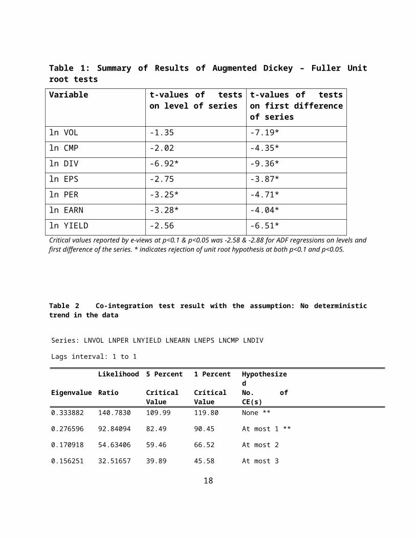
Table 1: Summary of Results of Augmented Dickey – Fuller Unitroot testsVariable t-values of tests

on level of seriest-values of testson first differenceof series

ln VOL -1.35 -7.19*ln CMP -2.02 -4.35*ln DIV -6.92* -9.36*ln EPS -2.75 -3.87*ln PER -3.25* -4.71*ln EARN -3.28* -4.04*ln YIELD -2.56 -6.51*Critical values reported by e-views at p<0.1 & p<0.05 was -2.58 & -2.88 for ADF regressions on levels andfirst difference of the series. * indicates rejection of unit root hypothesis at both p<0.1 and p<0.05.

Table 2 Co-integration test result with the assumption: No deterministictrend in the data

Series: LNVOL LNPER LNYIELD LNEARN LNEPS LNCMP LNDIV

Lags interval: 1 to 1

Likelihood 5 Percent 1 Percent Hypothesized

Eigenvalue Ratio CriticalValue

CriticalValue

No. ofCE(s)

0.333882 140.7830 109.99 119.80 None **

0.276596 92.84094 82.49 90.45 At most 1 **

0.170918 54.63406 59.46 66.52 At most 2

0.156251 32.51657 39.89 45.58 At most 3

18

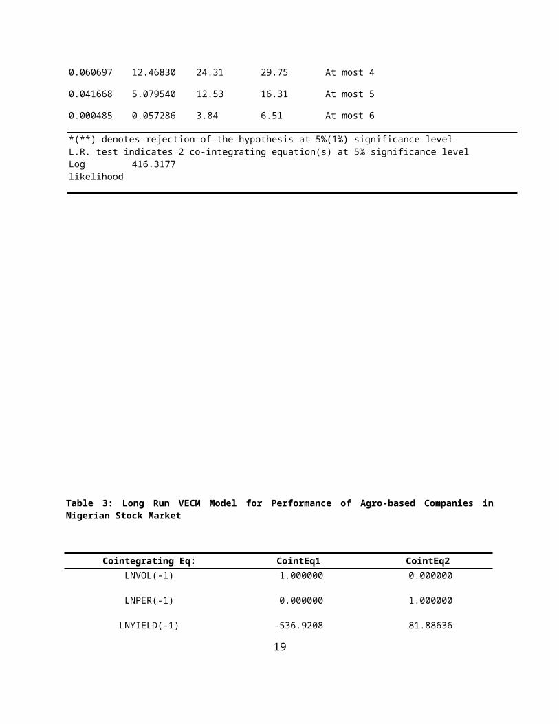
0.060697 12.46830 24.31 29.75 At most 4

0.041668 5.079540 12.53 16.31 At most 5

0.000485 0.057286 3.84 6.51 At most 6

*(**) denotes rejection of the hypothesis at 5%(1%) significance levelL.R. test indicates 2 co-integrating equation(s) at 5% significance levelLoglikelihood

416.3177

Table 3: Long Run VECM Model for Performance of Agro-based Companies inNigerian Stock Market

Cointegrating Eq: CointEq1 CointEq2LNVOL(-1) 1.000000 0.000000

LNPER(-1) 0.000000 1.000000

LNYIELD(-1) -536.9208 81.88636

19

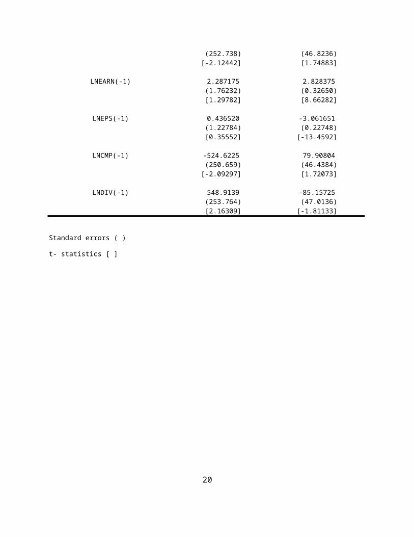
(252.738) (46.8236)[-2.12442] [1.74883]

LNEARN(-1) 2.287175 2.828375 (1.76232) (0.32650) [1.29782] [8.66282]

LNEPS(-1) 0.436520 -3.061651 (1.22784) (0.22748) [0.35552] [-13.4592]

LNCMP(-1) -524.6225 79.90804 (250.659) (46.4384)[-2.09297] [1.72073]

LNDIV(-1) 548.9139 -85.15725 (253.764) (47.0136) [2.16309] [-1.81133]

Standard errors ( )

t- statistics [ ]

20

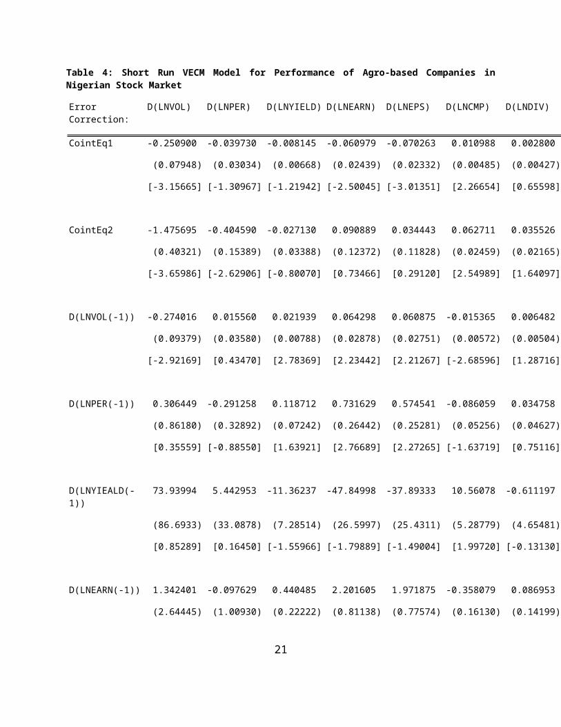
Table 4: Short Run VECM Model for Performance of Agro-based Companies inNigerian Stock Market

ErrorCorrection:

D(LNVOL) D(LNPER) D(LNYIELD) D(LNEARN) D(LNEPS) D(LNCMP) D(LNDIV)

CointEq1 -0.250900 -0.039730 -0.008145 -0.060979 -0.070263 0.010988 0.002800

(0.07948) (0.03034) (0.00668) (0.02439) (0.02332) (0.00485) (0.00427)

[-3.15665] [-1.30967] [-1.21942] [-2.50045] [-3.01351] [2.26654] [0.65598]

CointEq2 -1.475695 -0.404590 -0.027130 0.090889 0.034443 0.062711 0.035526

(0.40321) (0.15389) (0.03388) (0.12372) (0.11828) (0.02459) (0.02165)

[-3.65986] [-2.62906] [-0.80070] [0.73466] [0.29120] [2.54989] [1.64097]

D(LNVOL(-1)) -0.274016 0.015560 0.021939 0.064298 0.060875 -0.015365 0.006482

(0.09379) (0.03580) (0.00788) (0.02878) (0.02751) (0.00572) (0.00504)

[-2.92169] [0.43470] [2.78369] [2.23442] [2.21267] [-2.68596] [1.28716]

D(LNPER(-1)) 0.306449 -0.291258 0.118712 0.731629 0.574541 -0.086059 0.034758

(0.86180) (0.32892) (0.07242) (0.26442) (0.25281) (0.05256) (0.04627)

[0.35559] [-0.88550] [1.63921] [2.76689] [2.27265] [-1.63719] [0.75116]

D(LNYIEALD(-1))

73.93994 5.442953 -11.36237 -47.84998 -37.89333 10.56078 -0.611197

(86.6933) (33.0878) (7.28514) (26.5997) (25.4311) (5.28779) (4.65481)

[0.85289] [0.16450] [-1.55966] [-1.79889] [-1.49004] [1.99720] [-0.13130]

D(LNEARN(-1)) 1.342401 -0.097629 0.440485 2.201605 1.971875 -0.358079 0.086953

(2.64445) (1.00930) (0.22222) (0.81138) (0.77574) (0.16130) (0.14199)

21

ErrorCorrection:

D(LNVOL) D(LNPER) D(LNYIELD) D(LNEARN) D(LNEPS) D(LNCMP) D(LNDIV)

[0.50763] [-0.09673] [1.98218] [2.71340] [2.54193] [-2.22001] [0.61240]

D(LNEPS(-1)) -1.253764 0.341755 -0.408143 -2.142353 -1.844394 0.335829 -0.076529

(2.41009) (0.91985) (0.20253) (0.73947) (0.70699) (0.14700) (0.12940)

[-0.52021] [0.37153] [-2.01524] [-2.89713] [-2.60880] [2.28453] [-0.59139]

D(LNCMP(-1)) 71.44968 4.973180 -11.53837 -46.39127 -36.49530 10.91317 -0.435169

(86.0403) (32.8386) (7.23027) (26.3993) (25.2395) (5.24796) (4.61975)

[0.83042] [0.15144] [-1.59584] [-1.75729] [-1.44596] [2.07951] [-0.09420]

D(LNDIV(-1)) -75.46952 -5.846953 11.44163 48.53329 38.46574 -10.58164 0.667821

(87.2969) (33.3182) (7.33587) (26.7849) (25.6082) (5.32461) (4.68722)

[-0.86451] [-0.17549] [1.55968] [1.81197] [1.50209] [-1.98731] [0.14248]

R-squared 0.256468 0.210629 0.184191 0.302574 0.296780 0.291018 0.056246

Adj. R-squared

0.201896 0.152694 0.124315 0.251387 0.245167 0.238982 -0.013020

Sum sq.resides

442.5547 64.46621 3.125155 41.66272 38.08253 1.646432 1.275851

S.E.equation

2.014978 0.769047 0.169326 0.618245 0.591085 0.122902 0.108190

F-statistic 4.699688 3.635580 3.076208 5.911125 5.750155 5.592685 0.812031

Loglikelihood

-245.4256 -131.7667 46.80609 -106.0112 -100.7099 84.61763 99.66247

Akaike AIC 4.312299 2.385876 -0.640781 1.949342 1.859490 -1.281655 -1.536652

Schwarz SC 4.523622 2.597199 -0.429458 2.160665 2.070814 -1.070331 -1.325329

22

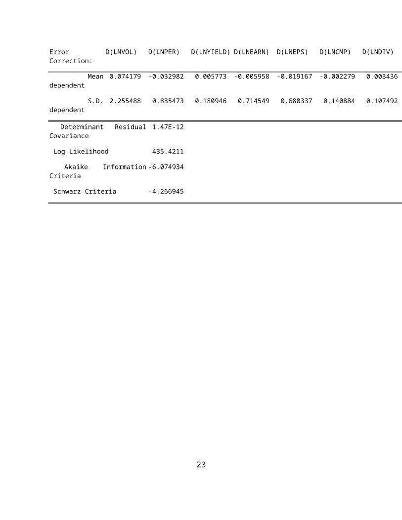
ErrorCorrection:

D(LNVOL) D(LNPER) D(LNYIELD) D(LNEARN) D(LNEPS) D(LNCMP) D(LNDIV)

Meandependent

0.074179 -0.032982 0.005773 -0.005958 -0.019167 -0.002279 0.003436

S.D.dependent

2.255488 0.835473 0.180946 0.714549 0.680337 0.140884 0.107492

Determinant ResidualCovariance

1.47E-12

Log Likelihood 435.4211

Akaike InformationCriteria

-6.074934

Schwarz Criteria -4.266945

23