Analysis of a RK/Implicit Smoother for MultigridR. C. Swanson,∗ E. Turkel† and S. Yaniv ‡

Abstract

The steady-state compressible Navier-Stokes equations are solved with a finite-volume, second-orderaccurate scheme. The equations are solved with a multigrid algorithm that uses a 3-stage Runge-Kuttascheme with an implicit preconditioner as a smoother. We analyze this smoother in which the implicitsystem is approximately inverted by a few symmetric Gauss-Seidel relaxation sweeps. The analysis forthe linear system determines the Fourier spectrum of the multigrid smoother. Improved performance ofthe algorithm based on the analysis is demonstrated by computing laminar flow in a rocket motor andturbulent flow over a wing.

1 Introduction

Multigrid algorithms with an explicit Runge-Kutta (RK) scheme and implicit residual smoothing (IRS) arethe foundation of many existing aerodynamic prediction codes. This class of methods has recently beensignificantly improved by replacing the scalar form of IRS with a matrix form. The matrix form allows alarge CFL number, resulting in faster propagation of information (enhancing multigrid efficiency since theNavier-Stokes equations contain a hyperbolic part) and reduced discrete stiffness. In this paper we analyzethis multigrid smoother (RK/implicit scheme), introduce improvements in efficiency, and demonstrate therobustness of the modified algorithm.

2 RKI Algorithm

To discretize the governing fluid dynamic equations we apply a cell-centered, finite-volume approach. Theadvection terms are approximated with three point central differencing plus numerical dissipation. A matrix-valued or Roe-type dissipation is applied such that the scheme is second order in smooth regions of the flowfield and first order in the neighborhood of shock waves. The viscous terms are discretized with a second-ordercentral difference approximation. See [1, 2] for details.

For solving the discrete equations we use the full approximation storage (FAS) multigrid algorithmdescribed in [2]. This algorithm uses full coarsening and either a V-type or W-type cycle. The operatorsfor restricting residuals and flow variables to the coarser grids are determined by a conservative residualsummation and volume weighting, respectively. Coarse grid corrections are transferred to finer grids bylinear interpolation operators. The RK scheme of the multigrid smoother has three stages with coefficients[α1, α2, α3] = [0.15, 0.4, 1.0]. The solution vector W on the q-th stage of the RK scheme is given by

W(q) = W(0) + δW(q) = W(0) − αq∆t

VLW(q−1) = W(0) − αq∆tR(q−1), (1)

where L is the complete difference operator for the system of equations, ∆t is the time step, V is the volumeof the mesh cell being considered, and R(q−1) represents the residual function for the (q − 1)-th stage. Ageneral form for the residual function can be written as

R(k) =1VLW(k) =

1V

[LcW(k) −

k∑r=0

γkr LvW(r) +k∑

r=0

γkr LdW(r)

], (2)

with Lc, Lv, and Ld denoting convective, viscous, and dissipative operators. For consistency∑

γkr = 1.The coefficients γkr are the weights of the viscous and dissipative terms on each stage, and for the 3-stagescheme,

γ00 = γ1; γ10 = 1− γ2, γ11 = γ2; γ20 = 1− γ3, γ21 = 0, γ22 = γ3. (3)∗NASA Langley Research Center, Hampton, VA 23681†School of Mathematical Sciences, Tel-Aviv University, Tel-Aviv, Israel‡Israel Military Industries Ltd. (IMI), Ramat Hasharon, Israel

When the weights [γ1, γ2, γ3] are [1.0, 1.0, 1.0], this is called standard weighting. Based upon analysis andnumerical testing we have determined that the modified weights [1.0, 0.5, 0.5] lead to improved robustnessof the smoother. In particular, the Mach number used in calculating the preconditioner needs to be cutoffto prevent a zero Mach number. The modified weights allow a lower level for these cutoffs which leads to afaster rate of convergence.

Letting Li be an implicit operator, we define the following replacement for the explicit update in Eq. (1):

δW(q)

= −αq∆t

VP LW(q−1) = −αq

∆t

VP

∑all faces

F(q−1)n S, (4)

where P is the implicit preconditioner defined by the approximate inverse L−1i , Fn is the normal flux density

vector at the cell face, and S is the area of the cell face. A first-order upwind approximation based on theRoe scheme is used for the convective derivatives in the implicit operator, which is defined by[

I + ε∆t

V∑

all faces

An S

]δW

(q)= −αq

∆t

V∑

all faces

F(q−1)n S. (5)

The matrix An is the flux Jacobian associated with Fn at a cell face, and ε is an implicit parameter.Using one-dimensional Fourier analysis and numerical testing we have found that a good choice for ε is 0.5.An approximate inverse of the implicit operator for the linear system is obtained with Gauss-Seidel (GS)relaxation. Complete discussion of the scheme is given in [3] and [4].

3 Fourier Analysis

To analyze the RK/implicit scheme we consider a finite domain with periodic boundary conditions. Wediscretize the linearized, time-dependent Navier-Stokes equations on a Cartesian grid with mf ×nf cells cov-ering the domain. For convenience, the Navier-Stokes equations are transformed from conservative variablesto primitive variables. We let Uj1,j2 denote the discrete solution vector of primitive variables that resides atthe mesh point (j1hx, j2hy). Then, the preconditioned form of Eq. 1 is Fourier transformed to obtain

U(q)k1,k2

= U(0)k1,k2

− αq∆t

VP LhU

(q−1)k1,k2

, (6)

where Lh is the linearized discrete residual operator for the primitive variables, and the transformed discretevector function

U(q)k1,k2

=1

mfnf

mf−1∑j1=0

nf−1∑j2=0

U(q)j1,j2

e−i(j1θx+j2θy), (7)

with the phase angles θx and θy, along with the corresponding wave numbers, given by

θx = 2πk1

mf, θy = 2π

k2

nf, k1 = −(

12mf − 1), · · · ,

12mf , k2 = −(

12nf − 1), · · · ,

12nf . (8)

The transformed residual operator Lh is a function of the transformed shift operators, which are defined by

Ex ≡ eiθx , Ey ≡ eiθy , −π < θx ≤ π, −π < θy ≤ π. (9)

After applying the 3-stage RK scheme with standard weighting of dissipation, we have

Un+1k1,k2

= GrkiUnk1,k2

, (10)

where the amplification matrix

Grki = I− α1PLh + α2α1(PLh)2 − α3α2α1(PLh)3,

I is the identity matrix and αq represents the product of the RK coefficient and the ratio of ∆t to V.Pierce and Giles [6] introduced a matrix preconditioner determined by the diagonal elements of the

residual function. This is equivalent to a block Jacobi preconditioner. In the RKI scheme we introduce off-diagonal terms. An approximate inverse of the resulting implicit system is obtained using a small number(usually two) of symmetric Gauss-Seidel sweeps. This method can be considered a block Gauss-Seidelpreconditioner.

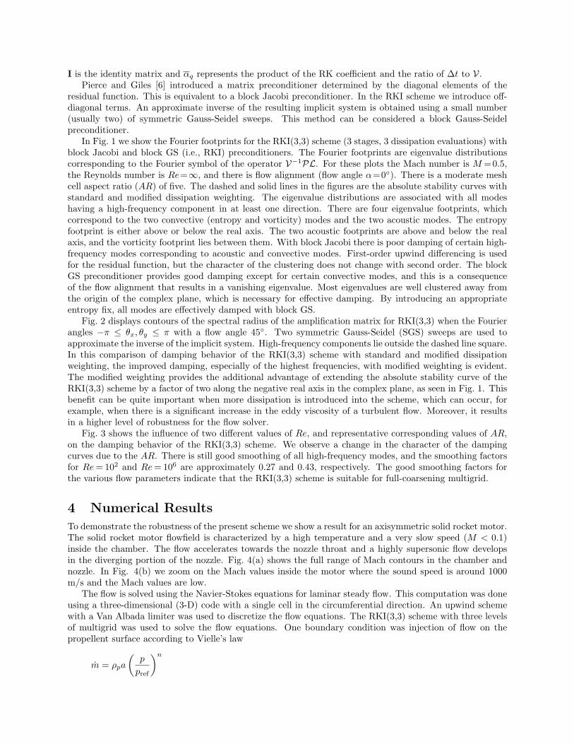
In Fig. 1 we show the Fourier footprints for the RKI(3,3) scheme (3 stages, 3 dissipation evaluations) withblock Jacobi and block GS (i.e., RKI) preconditioners. The Fourier footprints are eigenvalue distributionscorresponding to the Fourier symbol of the operator V−1PL. For these plots the Mach number is M =0.5,the Reynolds number is Re=∞, and there is flow alignment (flow angle α=0◦). There is a moderate meshcell aspect ratio (AR) of five. The dashed and solid lines in the figures are the absolute stability curves withstandard and modified dissipation weighting. The eigenvalue distributions are associated with all modeshaving a high-frequency component in at least one direction. There are four eigenvalue footprints, whichcorrespond to the two convective (entropy and vorticity) modes and the two acoustic modes. The entropyfootprint is either above or below the real axis. The two acoustic footprints are above and below the realaxis, and the vorticity footprint lies between them. With block Jacobi there is poor damping of certain high-frequency modes corresponding to acoustic and convective modes. First-order upwind differencing is usedfor the residual function, but the character of the clustering does not change with second order. The blockGS preconditioner provides good damping except for certain convective modes, and this is a consequenceof the flow alignment that results in a vanishing eigenvalue. Most eigenvalues are well clustered away fromthe origin of the complex plane, which is necessary for effective damping. By introducing an appropriateentropy fix, all modes are effectively damped with block GS.

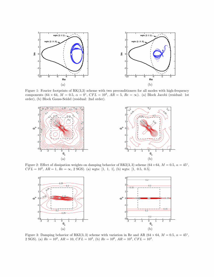
Fig. 2 displays contours of the spectral radius of the amplification matrix for RKI(3,3) when the Fourierangles −π ≤ θx, θy ≤ π with a flow angle 45◦. Two symmetric Gauss-Seidel (SGS) sweeps are used toapproximate the inverse of the implicit system. High-frequency components lie outside the dashed line square.In this comparison of damping behavior of the RKI(3,3) scheme with standard and modified dissipationweighting, the improved damping, especially of the highest frequencies, with modified weighting is evident.The modified weighting provides the additional advantage of extending the absolute stability curve of theRKI(3,3) scheme by a factor of two along the negative real axis in the complex plane, as seen in Fig. 1. Thisbenefit can be quite important when more dissipation is introduced into the scheme, which can occur, forexample, when there is a significant increase in the eddy viscosity of a turbulent flow. Moreover, it resultsin a higher level of robustness for the flow solver.

Fig. 3 shows the influence of two different values of Re, and representative corresponding values of AR,on the damping behavior of the RKI(3,3) scheme. We observe a change in the character of the dampingcurves due to the AR. There is still good smoothing of all high-frequency modes, and the smoothing factorsfor Re = 102 and Re = 106 are approximately 0.27 and 0.43, respectively. The good smoothing factors forthe various flow parameters indicate that the RKI(3,3) scheme is suitable for full-coarsening multigrid.

4 Numerical Results

To demonstrate the robustness of the present scheme we show a result for an axisymmetric solid rocket motor.The solid rocket motor flowfield is characterized by a high temperature and a very slow speed (M < 0.1)inside the chamber. The flow accelerates towards the nozzle throat and a highly supersonic flow developsin the diverging portion of the nozzle. Fig. 4(a) shows the full range of Mach contours in the chamber andnozzle. In Fig. 4(b) we zoom on the Mach values inside the motor where the sound speed is around 1000m/s and the Mach values are low.

The flow is solved using the Navier-Stokes equations for laminar steady flow. This computation was doneusing a three-dimensional (3-D) code with a single cell in the circumferential direction. An upwind schemewith a Van Albada limiter was used to discretize the flow equations. The RKI(3,3) scheme with three levelsof multigrid was used to solve the flow equations. One boundary condition was injection of flow on thepropellent surface according to Vielle’s law

m = ρpa

(p

pref

)n

where m is the injected mass flux, ρp is the propellent density, a is the burning rate, and n is the burningrate exponent. The other boundary conditions were as follows: no slip on the chamber and nozzle walls,extrapolation on the supersonic motor exit plane.

In Fig. 5 we compare the convergence behavior of the multigrid scheme using RKI(3,3) with that usingthe original (scalar) implicit residual smoothing [2]. A well converged solution is obtained with the matrixsmoother (CFL = 1000), whereas the computation with the scalar smoother (CFL = 2.5) exhibits a muchslower convergence.

To verify the effect of the new dissipation weights [1.0, 0.5, 0.5] in the RKI(3,3) scheme, we computedtransonic flow over an ONERA M6 wing with a free-stream M∞ = 0.83 and Re = 2.1158 × 107 using aBaldwin-Lomax turbulence model. A matrix-valued dissipation was used [5]. Entropy fixes were appliedto the eigenvalues of the preconditioning matrix in Eq. 5. For the entropy fix of the convective eigenvalueswe use a two-parameter function of the mesh aspect ratio. The two parameters multiply the bounds onthese eigenvalues. If these parameters are chosen too large, the convergence slows down. When they aretoo small, the scheme can become unstable. Hence, we want these parameters to be as small as possiblewithout destroying stability. Since this function is nonlinear, it cannot be modeled with the Fourier analysis.The two parameters are very dependent on the dissipation weighting used. In Table 1 we present theconvergence after 100 multigrid V-type cycles; NC means no convergence. We see that the convergencefor fixed cutoff parameters with the weights [1.0, 0.5, 0.5] is slightly better. What is more important isthat the new dissipation weights make the scheme more robust, allowing lower cutoffs which result in fasterconvergence. We have also done similar computations for two-dimensional transonic flow around the RAE2822 airfoil. The trends were the same, although the required cutoffs were slightly larger.

5 Concluding Remarks

Fourier analysis of the RKI(3,3) scheme has been considered to study the effect of various flow parameters.Using the analysis we have compared block Jacobi and block Gauss-Seidel preconditioners. The improvementof the current RK scheme, which uses block Gauss-Seidel, has been shown. The analysis has demonstratedthat this scheme has good smoothing and eigenvalue clustering properties for all high-frequency error com-ponents, making it a suitable smoother for full-coarsening multigrid. In addition, the advantages of a newweighting of dissipation, including an increased reliability of the scheme, have been discussed.

The implicit preconditioner introduced in [3], investigated and improved in [4], has been implementedin several three dimensional codes using either central-differencing with a matrix-valued dissipation or anupwind Roe scheme for the convective terms. Previously, acceleration of the convergence to a steady statehas been achieved for turbulent flows over airfoils and wings and for flows in turbomachinery. In this studywe have demonstrated that this scheme can be applied to flows inside rocket motors.

References

[1] A. Jameson, W. Schmidt, E. Turkel, Numerical solutions of the Euler equations by finite volume methodsusing Runge-Kutta time-stepping schemes, AIAA Paper 81-1259, 1981.

[2] R. C. Swanson, E. Turkel, Multistage schemes with multigrid for Euler and Navier-Stokes equations,NASA TP 3631, 1997.

[3] C.-C. Rossow, Efficient computation of compressible and incompressible flows. J. Comput. Phys. 220(2007) 879–899.

[4] R. C. Swanson, E. Turkel, C.-C. Rossow, Convergence acceleration of Runge-Kutta schemes for solvingthe Navier-Stokes equations, J. Comput. Phys. 224 (2007) 365–388.

[5] R. C. Swanson and E. Turkel, On Central Difference and Upwind Schemes, J. Comput. Phys. 101 (1992)292–306.

[6] N. A. Pierce, M. B. Giles, Preconditioned multigrid methods for compressible flow calculations onstretched meshes, J. Comput. Phys. 136 (1997) 425–445.

Re

Im

-10 -8 -6 -4 -2 0-3

-2

-1

0

1

2

3wgts: [1 1 1]

wgts: [1 .5 .5]

(a)

Re

Im

-10 -8 -6 -4 -2 0-3

-2

-1

0

1

2

3wgts: [1 1 1]

wgts: [1 .5 .5]

(b)

Figure 1: Fourier footprints of RK(3,3) scheme with two preconditioners for all modes with high-frequencycomponents (64 × 64, M = 0.5, α = 0◦, CFL = 103, AR = 5, Re = ∞). (a) Block Jacobi (residual: 1storder), (b) Block Gauss-Seidel (residual: 2nd order).

0.35 0.250.2

0.1

0.35

0.3

0.4

0.150.150.

1

0.1

0.35 0.25

0.1

0.2

0.2

0.35

0.2

0.4

0.6

0.8

0.8

θx

θ y

-3 -2 -1 0 1 2 3-3

-2

-1

0

1

2

3

(a)

0.2

0.2 0.20.250.2

5

0.20.15

0.150.2

0.6

0.8

0.8

0.4

θx

θ y

-3 -2 -1 0 1 2 3-3

-2

-1

0

1

2

3

(b)

Figure 2: Effect of dissipation weights on damping behavior of RKI(3, 3) scheme (64×64, M = 0.5, α = 45◦,CFL = 103, AR = 1, Re = ∞, 2 SGS). (a) wgts: [1, 1, 1], (b) wgts: [1, 0.5, 0.5].

0.250.2

0.15

0.25

0.20.25

0.90.15

0.4

θx

θ y

-3 -2 -1 0 1 2 3-3

-2

-1

0

1

2

3

(a)

0.2

0.2

0.2

0.2

0.15

0.15

0.250.35 0.9

θx

θ y

-3 -2 -1 0 1 2 3-3

-2

-1

0

1

2

3

(b)

Figure 3: Damping behavior of RKI(3, 3) scheme with variation in Re and AR (64× 64, M = 0.5, α = 45◦,2 SGS). (a) Re = 102, AR = 10, CFL = 103, (b) Re = 106, AR = 103, CFL = 104.

x

Y

0 0.1 0.2 0.3

-0.05

0

0.05

0.1

0.15 M2.11.71.30.90.50.1

(a)

x

Y

0 0.1 0.2 0.3

-0.05

0

0.05

0.1

0.15M0.10.080.060.040.020

(b)

Figure 4: Rocket Motor

cycles

log(err)

0 500 100010-710-610-510-410-310-210-1100101

implicit smoothingRK/implicit smoothing

Figure 5: Convergence rate for rocket motor

Dissipation Weights Cutoff Parameters Residual Conv. Rate1.0, 0.5, 0.5 .10, .20 .32710−4 .87981.0, 0.5, 0.5 .10, .10 .44510−5 .86191.0, 0.5, 0.5 .08, .05 .47210−6 .84251.0, 0.5, 0.5 .08, .04 .23010−6 .83641.0, 0.5, 0.5 .06, .04 .18210−6 .83441.0, 1.0, 1.0 .10, .20 .34810−4 .89371.0, 1.0, 1.0 .10, .10 .50010−5 .86311.0, 1.0, 1.0 .08, .05 .60410−6 .84471.0, 1.0, 1.0 .08, .04 NC1.0, 1.0, 1.0 .06, .04 NC

Table 1: Convergence for ONERA M6 wing for various dissipation weights and cutoff parameters.