Analogy-based effort estimation: a new method to discover set of analogies from dataset...

www.ietdl.org

IE

d

Published in IET SoftwareReceived on 4th August 2013Revised on 7th March 2014Accepted on 7th July 2014doi: 10.1049/iet-sen.2013.0165

T Softw., pp. 1–12oi: 10.1049/iet-sen.2013.0165

ISSN 1751-8806

Analogy-based effort estimation: a new method todiscover set of analogies from dataset characteristicsMohammad Azzeh1, Ali Bou Nassif2

1Department of Software Engineering, Applied Science University, POBOX 166, Amman, Jordan2Department of Computer Science, University of Western Ontario, London, Ontario N6A 5B9, Canada

E-mail: [email protected]

Abstract: Analogy-based effort estimation (ABE) is one of the efficient methods for software effort estimation because of itsoutstanding performance and capability of handling noisy datasets. Conventional ABE models usually use the same numberof analogies for all projects in the datasets in order to make good estimates. The authors’ claim is that using same number ofanalogies may produce overall best performance for the whole dataset but not necessarily best performance for eachindividual project. Therefore there is a need to better understand the dataset characteristics in order to discover the optimumset of analogies for each project rather than using a static k nearest projects. The authors propose a new technique based onbisecting k-medoids clustering algorithm to come up with the best set of analogies for each individual project before makingthe prediction. With bisecting k-medoids it is possible to better understand the dataset characteristic, and automatically findbest set of analogies for each test project. Performance figures of the proposed estimation method are promising and betterthan those of other regular ABE models.

1 Introduction

Analogy-based effort estimation (ABE) is simplified aprocess of finding nearest analogies based on notion ofretrieval by similarity [1–4]. It was remarked that thepredictive performance of ABE is a dataset dependentwhere each dataset requires different configurations anddesign decisions [5–8]. Recent publications reported theimportance of adjustment mechanism for generating betterestimates in ABE than null-adjustment mechanism [1, 9,10]. However, irrespective of the type of adjustmenttechnique followed, the process of discovering the best setof analogies to be used is still a key challenge.This paper focuses on the problem of how can we

automatically come up with the optimum set of analogiesfor each individual project before making the prediction?Yet, there is no reliable method that can discover such setof nearest analogies before making prediction. ConventionalABE models start with one analogy and increase thisnumber depending on the overall performance of the wholedataset then it uses the set of first k analogies that producesthe best overall performance. However, a fixed k value thatproduces overall best performance does not necessarilyprovide the best performance for each individual project,and may not be suitable for other datasets. Our claim is thatwe can avoid sticking to a fixed best performing number ofanalogies which changes from dataset to dataset or evenfrom a single project to another in the same dataset.Therefore we propose an alternative technique to tune ABEby proposing a bisecting k-medoids (BK) clusteringalgorithm. The bisecting procedure is used with k-medoids

to avoid guessing number of clusters, by recursivelyapplying the basic k-medoids algorithm and splitting eachcluster into two sub-clusters to form a binary tree ofclusters, starting from the whole dataset. This allows us todiscover the structure of dataset efficiently andautomatically come up with the best set of analogies as wellas excluding irrelevant analogies for each individual testproject. It is important to note that the discovered set ofanalogies does not necessarily include the same order ofnearest analogies as in conventional ABE.The rest of the article is structured as follows: Section 2

defines the research problem in more details. Section 3provides the related work. Section 4 the methodology wepropose to address the research problem. Section 5 presentsthe results we obtained. Section 6 presents discussion of ourresults and findings. Lastly Section 7 summarises ourconclusions and future work.

2 Research problem

Several studies in software effort estimation try to address theproblem of finding optimum number of nearest analogies tobe used by ABE [3, 5, 6, 11]. The conclusion drawn fromthese studies that using a static k value that produces overalllowest mean magnitude relative error (MMRE) does notnecessarily provide the lowest MRE value for eachindividual project, and may not be suitable for otherdatasets. This shows that every dataset has differentcharacteristics and this would have a significant impact onthe process of discovering the best set of analogies. To

1& The Institution of Engineering and Technology 2015

Fig. 1 Bar chart of k analogies for some datasets

a Albrecht datasetb Maxwell datasetc Dehasrnais dataset

www.ietdl.org

illustrate our point of view and better understand this problemwe carried out an intensive search to find the mean effortvalue of the nearest k analogies that produces lowest ‘MRE’for every single test project as shown in Fig. 1. For adataset of size n observations, the best k value can rangefrom 1 to n− 1. Since a few number of datasets wereenough to illustrate our viewpoint, we selected threedatasets that vary in the size (i.e. one small dataset(Albrecht), one medium (Maxwell) and one large(Desharnais)). Fig. 1 shows the bar chart of the bestselected k numbers for the three examined datasets, wherex-axis represents project Id in that dataset and y-axisrepresents k analogy number. It is clear that every singleproject favours different number of analogies. For examplein Albrecht dataset, Three projects (id = 3, 6 and 22)favoured k = 15 which means that the final estimates forthose project have been produced by using mean efforts of15 nearest analogies. It is clear that there is no pattern forthe process of k selection. Therefore using a fixed numberof analogies for all test projects will far from optimum andthere is provisional evidence that choosing the best set ofanalogies for each individual project is relatively subject todataset structure.

3 Related works

Software effort estimation is vital task for successful softwareproject management [12, 13]. ABE method has been widelyused for developing software effort estimation models basedupon retrieval by similarity [14–16]. The data driven ABE


method involves four primary steps [4]: (1) select k nearestanalogies using Euclidean distance function as depicted in(1). (2) Reuse efforts from the set of nearest analogies tofind out effort of the new project. (3) Adjust the retrievedefforts to bring them closer to the new project. Finally, (4)retain the estimated project in the repository for futureprediction

dxy =1

m

��∑m

i=1xi − yi( )2√

(1)

where dxy is the Euclidean distance between projects x and yacross m predictor features.In spite of ABE generates better accuracy than other

well-known prediction methods, it still requires adjustingthe retrieved estimates to reflect the structure of nearestanalogies on the final estimate [5]. Practically, the keyfactor of successful ABE method is finding the appropriatenumber of k analogies. Several researchers [7, 9, 14, 15,17] recommended using a fixed number of analogiesstarting from k = 1 and increase this number until no furtherimprovement on the accuracy can be obtained. Thisapproach is somewhat simple, but not necessarily accurate,and relies heavily on the estimator intuitions [14]. In thisdirection, Kirsopp et al. [9] proposed making predictionsfrom the k = 2 nearest cases as it was found the best valuefor their investigated datasets. They have increased theiraccuracy values with case and feature subset selectionstrategies [9]. The conclusion can be drawn from theirempirical studies is that the same k number has been usedfor all datasets irrespective of their size and feature types(i.e. numerical, categorical and ordinal features). Azzeh [14]carried out an extensive replication study on various linearand non-linear adjustment strategies used in ABE inaddition to finding the best k number for these strategies.He found that k = 1 was the most influential setting for alladjustment strategies over all datasets under investigation.On the other hand, Idri et al. [18] suggested using allprojects that fall within a certain similarity threshold. Theyproposed a fuzzy similarity approach that can select the bestanalogies for which their similarity degrees are greater thanthe predefined threshold. This approach could ignore someuseful projects which might contribute better whensimilarity between selected and unselected cases isnegligible. Also the determination of the threshold value isa challenge on its own and needs expert intuition.Another study focusing on k analogies identification in the

context of ABE is conducted by Li et al. [3]. They proposeda new model of ABE called AQUA which consists of twomain phases: learning and prediction. During the learningphase, the model attempts to learn the k analogies and bestsimilarity threshold by performing cross-validation on alltraining projects. The obtained k is then used during secondphase to make prediction for different test projects. In theirstudy Li et al. performed rigorous trials on actual andartificial datasets and they observed various effects of k values.Recently, Azzeh and Elsheikh [19] attempted to learn the k

value from the dataset characteristic. They applied thebisecting k-medoid clustering algorithm on the historicaldatasets without using adjustment techniques or featureselection. The main observation was that while there is nooptimum static k value for all datasets, there is definitely adynamic k values for each dataset. However, the proposedapproach has a significant limitation in which they used theun-weighted mean effort of the train projects of the leafcluster whose medoid is closest to the test project to

IET Softw., pp. 1–12doi: 10.1049/iet-sen.2013.0165

Fig. 2 Illustration of BK algorithm

www.ietdl.org
estimate the effort for that test project. Using such cluster doesnot ensure that all project in it are nearest analogies. In thispaper, we solve that problem by proposing a more robustapproach in which in this study we focus mainly ondiscovering the optimum set of analogies rather thanguessing only number of nearest analogies for each testproject. Further, we want to investigate that whether theobtained set of analogies works well with different kinds ofadjustment techniques. Hence we chose three well-knownadjustment techniques from the literature besides meaneffort adjustment to investigate the potential improvementsof using our model on the adjustment techniques. Thetechniques investigated in this study are:
(1) Similarity-based adjustment: This kind of adjustment aimsto calibrate the retrieved effort values based on their similaritydegrees with a target project. The general form of thistechnique involves sum of product of the normalisedaggregated similarity degrees with retrieved effort value asshown in (2). Examples, on this approach, from literatureare: AQUA [3]; FGRA [14]; and F-Analogy [18]

ex =∑k

i=1 SM(x, yi)× ei∑ki=1 SM(x, yi)

(2)

Where ex and ei are the estimated effort and effort of ithsource project, respectively. SM is the normalised similaritydegree between two projects (SM = 1− d, where d is thenormalised Euclidean distance obtained by (1)), and k is thenumber of analogies.(2) Genetic algorithm (GA)-based adjustment [15]: thisadjustment strategy uses GA to optimise the coefficient αjfor each feature distance based on minimising MMRE asshown in (3). The main challenge with this technique isthat it needs too many parameter configurations anduser interactions such as chromosome encoding, mutationand crossover which makes replication is somewhatdifficult task

ex =1

k

∑ki=1

ei +∑M

j=1aj × (fxj − fij)

( )(3)

where fxj is the jth feature value of the target project. fij is thejth feature value of the nearest project yi.(3) Neural network (NN)-based adjustment [17]: Thistechnique attempts to learn the differences between effortvalues of target project and its analogies based ondifference of their input feature values. These differencesare then converted into the amount of change that will beadded to the retrieved effort as shown in (4). The NNtraining function stops when MSE drops below thespecified threshold = 0.01, and the model is trained basedon back-propagation algorithm

ex =1

k

∑ki=1

ei + f (Sx, Sk)( )

(4)

f (Sx, Sk) is the neural network model. Sx is the featurevector of a target project and Sk is the feature matrix of thetop analogies.


4 Methodology

4.1 Proposed bisecting k-medoids algorithm

The k-medoids [20] is a clustering algorithm related to thecentroid-based algorithms which groups similar instanceswithin a dataset into N clusters known a priori [20–22]. Amedoid can be defined as the instance of a cluster, whoseaverage dissimilarity to all the instances in the cluster isminimal, that is, it is a most centrally located point in thecluster. It is more robust to noise and outliers as comparedto k-means because it minimises the sum of pairwisedissimilarities instead of the sum of squared Euclideandistances [20]. The popularity of making use of k-medoidsclustering is its ability to use arbitrary dissimilarity ordistances functions, which also makes it an appealingchoice of clustering method for software effort data assoftware effort datasets also exhibit very dissimilarcharacteristics. Since finding the suitable number of clustersis kind of guess [20] we employed bisecting procedure withk-medoids algorithm and propose BK algorithm. BK is avariant of k-medoids algorithm that can producehierarchical clustering by recursively applying the basick-medoids. It starts by considering the whole dataset to beone cluster. At each step, one cluster is selected andbisected further into two sub-clusters using the basick-medoids as shown in the hypothetical example in Fig. 2.Note that by recursively using a BK clustering procedure,the dataset can be partitioned into any given number ofclusters in which the so-obtained clusters are structured as ahierarchical binary tree. The decision whether to continueclustering or stop it depends on the comparison of variancedegree between childes and their direct parent in the tree asshown in (5). If the maximum of variance of child clustersis smaller than variance of their direct parent then clusteringis continued. Otherwise it is stopped and the parent clusteris considered as a leaf node. This criterion enables the BKto uniformly partition the dataset into homogenous clusters.To better understand the BK algorithm, we provide thepseudo code in Fig. 3

Variance = 1

n

∑n

j=1,yj[Ciyj − vi

∥∥∥ ∥∥∥2 (5)

where ||·|| is the usual Euclidean norm, yj is the jth data objectand vi is the centre of ith cluster (Ci). A smaller value of thismeasure indicates a high homogeneity (less scattering).

4.2 Proposed k-ABE methodology

The proposed k-ABE model is described by the followingsteps:


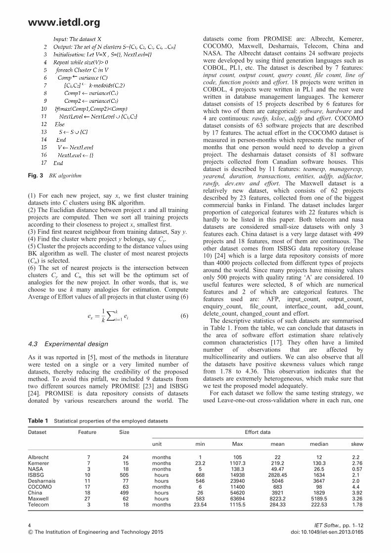
Fig. 3 BK algorithm

www.ietdl.org

(1) For each new project, say x, we first cluster trainingdatasets into C clusters using BK algorithm.(2) The Euclidian distance between project x and all trainingprojects are computed. Then we sort all training projectsaccording to their closeness to project x, smallest first.(3) Find first nearest neighbour from training dataset, Say y.(4) Find the cluster where project y belongs, say Cy.(5) Cluster the projects according to the distance values usingBK algorithm as well. The cluster of most nearest projects(Cn) is selected.(6) The set of nearest projects is the intersection betweenclusters Cy and Cn. this set will be the optimum set ofanalogies for the new project. In other words, that is, wechoose to use k many analogies for estimation. ComputeAverage of Effort values of all projects in that cluster using (6)

ex =1

k

∑k

i=1ei (6)

4.3 Experimental design

As it was reported in [5], most of the methods in literaturewere tested on a single or a very limited number ofdatasets, thereby reducing the credibility of the proposedmethod. To avoid this pitfall, we included 9 datasets fromtwo different sources namely PROMISE [23] and ISBSG[24]. PROMISE is data repository consists of datasetsdonated by various researchers around the world. The

Table 1 Statistical properties of the employed datasets

Dataset Feature Size

unit mi

Albrecht 7 24 months 1Kemerer 7 15 months 23.NASA 3 18 months 5ISBSG 10 505 hours 66Desharnais 11 77 hours 54COCOMO 17 63 months 6China 18 499 hours 26Maxwell 27 62 hours 58Telecom 3 18 months 23.5


datasets come from PROMISE are: Albrecht, Kemerer,COCOMO, Maxwell, Desharnais, Telecom, China andNASA. The Albrecht dataset contains 24 software projectswere developed by using third generation languages such asCOBOL, PL1, etc. The dataset is described by 7 features:input count, output count, query count, file count, line ofcode, function points and effort. 18 projects were written inCOBOL, 4 projects were written in PL1 and the rest werewritten in database management languages. The kemererdataset consists of 15 projects described by 6 features forwhich two of them are categorical: software, hardware and4 are continuous: rawfp, ksloc, adjfp and effort. COCOMOdataset consists of 63 software projects that are describedby 17 features. The actual effort in the COCOMO dataset ismeasured in person-months which represents the number ofmonths that one person would need to develop a givenproject. The desharnais dataset consists of 81 softwareprojects collected from Canadian software houses. Thisdataset is described by 11 features: teamexp, managerexp,yearend, duration, transactions, entities, adjfp, adjfactor,rawfp, dev.env and effort. The Maxwell dataset is arelatively new dataset, which consists of 62 projectsdescribed by 23 features, collected from one of the biggestcommercial banks in Finland. The dataset includes largerproportion of categorical features with 22 features which ishardly to be listed in this paper. Both telecom and nasadatasets are considered small-size datasets with only 3features each. China dataset is a very large dataset with 499projects and 18 features, most of them are continuous. Theother dataset comes from ISBSG data repository (release10) [24] which is a large data repository consists of morethan 4000 projects collected from different types of projectsaround the world. Since many projects have missing valuesonly 500 projects with quality rating ‘A’ are considered. 10useful features were selected, 8 of which are numericalfeatures and 2 of which are categorical features. Thefeatures used are: AFP, input_count, output_count,enquiry_count, file_count, interface_count, add_count,delete_count, changed_count and effort.The descriptive statistics of such datasets are summarised

in Table 1. From the table, we can conclude that datasets inthe area of software effort estimation share relativelycommon characteristics [17]. They often have a limitednumber of observations that are affected bymulticollinearity and outliers. We can also observe that allthe datasets have positive skewness values which rangefrom 1.78 to 4.36. This observation indicates that thedatasets are extremely heterogeneous, which make sure thatwe test the proposed model adequately.For each dataset we follow the same testing strategy, we

used Leave-one-out cross-validation where in each run, one

Effort data

n Max mean median skew

105 22 12 2.22 1107.3 219.2 130.3 2.76

138.3 49.47 26.5 0.578 14938 2828.45 1634 2.16 23940 5046 3647 2.0

11400 683 98 4.454620 3921 1829 3.92

3 63694 8223.2 5189.5 3.264 1115.5 284.33 222.53 1.78


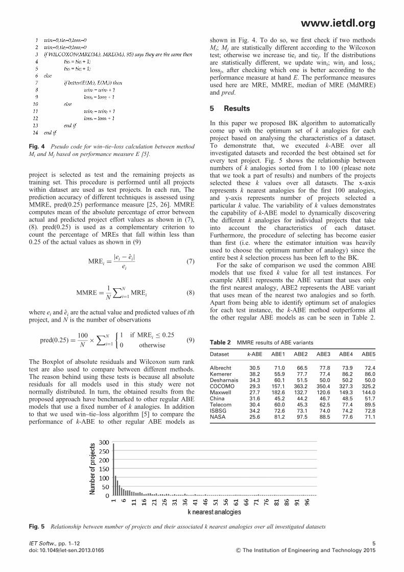
Table 2 MMRE results of ABE variants

Dataset k-ABE ABE1 ABE2 ABE3 ABE4 ABE5

Albrecht 30.5 71.0 66.5 77.8 73.9 72.4Kemerer 38.2 55.9 77.7 77.4 86.2 86.0Desharnais 34.3 60.1 51.5 50.0 50.2 50.0COCOMO 29.3 157.1 363.2 350.4 327.3 325.2Maxwell 27.7 182.6 132.7 120.6 149.3 144.0China 31.6 45.2 44.2 46.7 48.5 51.7Telecom 30.4 60.0 45.3 62.5 77.4 89.5ISBSG 34.2 72.6 73.1 74.0 74.2 72.8NASA 25.6 81.2 97.5 88.5 77.6 71.1

Fig. 4 Pseudo code for win–tie–loss calculation between methodMi and Mj based on performance measure E [5].

www.ietdl.org

project is selected as test and the remaining projects astraining set. This procedure is performed until all projectswithin dataset are used as test projects. In each run, Theprediction accuracy of different techniques is assessed usingMMRE, pred(0.25) performance measure [25, 26]. MMREcomputes mean of the absolute percentage of error betweenactual and predicted project effort values as shown in (7),(8). pred(0.25) is used as a complementary criterion tocount the percentage of MREs that fall within less than0.25 of the actual values as shown in (9)

MREi =|ei − ei|

ei(7)

MMRE = 1

N

∑N

i=1MREi (8)

where ei and ei are the actual value and predicted values of ithproject, and N is the number of observations

pred(0.25) = 100

N×

∑N

i=1

1 if MREi ≤ 0.25

0 otherwise

{(9)

The Boxplot of absolute residuals and Wilcoxon sum ranktest are also used to compare between different methods.The reason behind using these tests is because all absoluteresiduals for all models used in this study were notnormally distributed. In turn, the obtained results from theproposed approach have benchmarked to other regular ABEmodels that use a fixed number of k analogies. In additionto that we used win–tie–loss algorithm [5] to compare theperformance of k-ABE to other regular ABE models as

Fig. 5 Relationship between number of projects and their associated k


shown in Fig. 4. To do so, we first check if two methodsMi; Mj are statistically different according to the Wilcoxontest; otherwise we increase tiei and tiej. If the distributionsare statistically different, we update wini; winj and lossi;lossj, after checking which one is better according to theperformance measure at hand E. The performance measuresused here are MRE, MMRE, median of MRE (MdMRE)and pred.

5 Results

In this paper we proposed BK algorithm to automaticallycome up with the optimum set of k analogies for eachproject based on analysing the characteristics of a dataset.To demonstrate that, we executed k-ABE over allinvestigated datasets and recorded the best obtained set forevery test project. Fig. 5 shows the relationship betweennumbers of k analogies sorted from 1 to 100 (please notethat we took a part of results) and numbers of the projectsselected these k values over all datasets. The x-axisrepresents k nearest analogies for the first 100 analogies,and y-axis represents number of projects selected aparticular k value. The variability of k values demonstratesthe capability of k-ABE model to dynamically discoveringthe different k analogies for individual projects that takeinto account the characteristics of each dataset.Furthermore, the procedure of selecting has become easierthan first (i.e. where the estimator intuition was heavilyused to choose the optimum number of analogy) since theentire best k selection process has been left to the BK.For the sake of comparison we used the common ABE

models that use fixed k value for all test instances. Forexample ABE1 represents the ABE variant that uses onlythe first nearest analogy, ABE2 represents the ABE variantthat uses mean of the nearest two analogies and so forth.Apart from being able to identify optimum set of analogiesfor each test instance, the k-ABE method outperforms allthe other regular ABE models as can be seen in Table 2.

nearest analogies over all investigated datasets


Table 3 pred(0.25) results of ABE variants

Dataset k-ABE ABE1 ABE2 ABE3 ABE4 ABE5

Albrecht 41.7 29.2 33.3 33.3 37.5 41.7Kemerer 26.7 40.0 20.0 20.0 13.3 20.0Desharnais 40.3 31.2 31.2 37.7 37.7 39.0COCOMO 57.1 12.7 19.0 19.0 15.9 22.2Maxwell 56.5 9.7 19.4 17.7 14.5 17.7China 46.7 38.3 43.5 43.3 41.9 39.7Telecom 55.6 33.3 50.0 38.9 44.4 22.2ISBSG 38.8 39.6 30.7 30.9 29.7 26.5NASA 44.4 33.3 38.9 44.4 22.2 22.2

www.ietdl.org

When we look at the MMRE values, we can see that in allnine datasets, k-ABE has never been outperformed by othermethods with lowest MMRE values. This suggests thatk-ABE has attained better predictive performance valuesthan all other regular ABE models. This also shows thecapability of BK to support small-size datasets such as inKemerer and Albrecht. However, although it provedinaccurate in this study, the strategy of using fixedk-analogy may be appropriate in situations where a potentialanalogues and target project are similar in size feature andother effort drivers. On the other hand, There may be littlebasis for believing that either increasing or decreasing thek-analogies effort values of ABE models does not improvethe accuracy of the estimation. However, overall resultsfrom Tables 2 and 3 revealed that there is reasonablebelieve that using dynamic k-analogies for every test projecthas potential to improve prediction accuracy of ABE interms of pred. Concerning discontinuities in the datasetstructure, there is clear evidence that the BK technique hascapability to group similar projects together in the samecluster as appeared in the results of Maxwell, COCOMO,Kemerer and ISBSG.The variants of ABE methods are also compared using

Wilcoxon sum rank test. The results of Wilcoxon sum ranktest of absolute residuals are presented in Table 4. The solidblack square indicates that there is significance differencebetween k-ABE and the variant under investigation.Predictions based on k-ABE model presented statistically

Table 4 Wilcoxon sum rank test results between k-ABE andother ABE variants

Dataset ABE1 ABE2 ABE3 ABE4 ABE5

Albrecht – – – – –Kemerer – – – – –Desharnais ∎ ∎ ∎ ∎ ∎COCOMO ∎ ∎ ∎ ∎ ∎Maxwell ∎ ∎ ∎ ∎ ∎China ∎ ∎ ∎ ∎ ∎Telecom – – – – –ISBSG ∎ ∎ ∎ ∎NASA – – ∎ – ∎

Table 5 Win–tie–loss results of ABE variants

ABE variant win tie loss win–loss

k-ABE 108 21 6 102ABE1 64 45 26 38ABE2 21 52 62 −41ABE3 29 59 47 −18ABE4 16 39 80 −64ABE5 13 38 84 −71


significant and accurate estimations than others, confirmedby the results of MMRE as shown in Table 2. Except forsmall datasets such as Albrecht, Kemerer, Telecom andNASA, the statistical test results demonstrate that there aresignificant differences if the predictions generated by anyk-ABE and other regular ABE models. Hence it seems thatthe small datasets are the most challenging ones becausethey have relatively small number of instances and largedegree of heterogeneity between projects. This makesdifficult to obtain a cluster of sufficient number of instances.The win–tie–loss results in Table 5 shows that k-ABE

outperformed regular ABE models with win–loss = 102.Also these results are confirmed by the Boxplots ofabsolute residuals in Fig. 6 which demonstrates that k-ABEhas lowest median values and small box length than othermethods for most datasets.The obtained performance figures raised a question

concerning the efficiency of applying adjustment techniquesto k-ABE. To answer this question we carried out anempirical study on the employed datasets, using threewell-known adjustment techniques: Similarity-basedadjustment, GA-based adjustment and NN-based adjustmentin addition to the proposed BK technique. Theircorresponding k-ABE variants are denoted by k-ABESM,k-ABEGA and k-ABENN, respectively. The obtainedperformance figures in terms of MMRE and pred(0.25) arerecorded in Tables 6 and 7. In general there is nosignificant difference when applying various adjustmenttechniques than basic k-ABE. One possible reason isbecause of small number of instances in some clusters. It iswell-known that both GA and NN models need sufficientnumber of instances in order to produce good results;however this may not suitable for small datasets such asAlbrecht, Kemerer, NASA, and Telecom. In contrast, thereare little improvements on the accuracy when applyingadjustment techniques than other regular ABE models forsome datasets especially large ones.On the other hand, when comparing adjustment techniques

to the basic k-ABE model we can note that there is substantialimprovement on the accuracy for all datasets except smallones. The statistical significant test in Table 8 and win–tie–loss in Table 9 show that in general there is significancedifference between the results of k-ABE and all otheradjustment techniques: k-ABESM, k-ABEGA and k-ABENN.This suggests that the predictions generated by k-ABE aredifferent than that of other adjustment techniques.Boxplots of absolute residuals in Fig. 7 show that there is

significant difference between k-ABE and all other variantsof k-ABE. The Boxplots suggest that:

(1) All median values of k-ABE are very close to zero,indicating that the estimates were biased towards theminimum value where they have tighter spread. The medianand range of absolute residuals of k-ABE are small, whichrevealed that at least half of the predictions of k-ABE areaccurate than other variants. The box of k-ABE overlays thelower tail especially for Albrecht, COCOMO, Maxwell andChina datasets, which also presents accurate prediction.(2) Although the number of outliers for ISBSG and Chinadatasets is fairly high comparing to other datasets, they arenot extremes like other variants. This demonstrates that thek-ABE produced good prediction for such datasets.

Another important raised issue is the impact of featuresubset selection (FFS) algorithm on the structure of data,


Fig. 6 Boxplots of absolute residuals for ABE variants

www.ietdl.org

and thereby on the obtained k-values. Many research studiesin software effort estimation reported the great effect offeature selection on the prediction accuracy of ABE [4, 14].This paper also investigates whether the use of FSS


algorithm can support the proposed method to deliver betterpredication accuracy. In this paper we used brute-forcealgorithm that is implemented in ANGEL tool to identifythe best features for each dataset. It is recommended to


Table 6 MMRE results of k-ABE variants

Dataset k-ABE k-ABESM k-ABEGA k-ABENN

Albrecht 30.5 59.7 94.8 71.7Kemerer 38.2 45.7 52.8 72.6Desharnais 34.3 40.2 47.2 100.5COCOMO 29.3 73.6 70.1 118.5Maxwell 27.7 55.2 54.7 60.3China 31.6 61.4 64.6 76.0Telecom 30.4 58.4 59.8 80.4ISBSG 34.2 47.7 48.0 85.8NASA 25.6 76.7 31.8 51.9

Table 7 pred(0.25) results of k-ABE variants



Table 9 Win–tie–loss results of k-ABE variants


k-ABE 77 4 0 77k-ABESM 19 25 37 −18k-ABEGA 19 31 31 −12k-ABENN 13 20 48 −35

www.ietdl.org

re-apply the adjustment techniques using only the bestselected features. This requires applying feature subsetselection algorithm [4] prior to building variant methods ofk-ABE. Although, typically, FSS should be repeated foreach training set, it is computationally prohibitive given thelarge numbers of prediction systems to be built. Instead weperformed one FSS for each treatment of each dataset,based on a leave-one cross-validation and using ‘MMRE’.This means that the same feature subset is used for alltraining sets within a treatment and for some of thesetraining sets it will be sub-optimal. However, since aprevious study [9] has shown the optimal feature subsetvaries little with variations in the randomly sampled casespresent in the training set, this should have little impact onthe results.The performance figures in Tables 10 and 11 show that

although the number of MMRE and pred(0.25) that hasbeen improved when applying FSS is large, the MMRE andpred(0.25) differences for each method over a particulardataset are still poor. Generally, The percentage ofimprovements for k-ABE in both MMRE and pred(0.25) is83.3%, while for k-ABESM is 88.8%, for k-ABEGA is61.1%, and for k-ABENN is 77.7%. However, thesignificance tests between the k-ABE variants with all

Table 8 Wilcoxon sum rank test results between k-ABE variants

Dataset k-ABE Vs.k-ABESM

k-ABE Vs.k-ABEGA

k-ABE Vs.k-ABENN

Albrecht ∎ ∎ ∎Kemerer – – ∎Desharnais ∎ ∎ ∎COCOMO ∎ ∎ ∎Maxwell ∎ ∎ ∎China ∎ ∎ ∎Telecom – – ∎ISBSG ∎ ∎ ∎NASA ∎ – ∎


features and when using only the best features do not showsignificant differences, hence we can conclude that theproposed method works well with all features without theneed to apply features subset selection algorithms, and thiswill reduce computation cost of the whole prediction modelespecially for large datasets.To see the predictive performance of k-ABE against the

most widely used estimation methods in the literature, wecompare k-ABE with three common methods: stepwiseregression (SR); ordinary least square regression (OLS); andcategorical regression tree (CART) using the samevalidation procedure (i.e. leave-one cross-validation). Wehave chosen such estimation methods since they usedifferent strategies to make estimate. The remarkabledifference between SR and OLS is that OLS generatesregression model from all training features while SRgenerates regression model from only significant features.Since some features are skewed and not normallydistributed, it is recommended, for SR and OLS, totransform these features using log transformation such thatthey resemble more closely a normal distribution [27]. Also,all categorical attributes should be converted intoappropriate dummy variables as recommended by [27].However, all required tests such as normality tests areperformed once before running empirical validation whichresulted in a general regression model. Then, in eachvalidation iteration a different regression model thatresembles general regression model in the structure is builtbased on the training data set and then the prediction of testproject is made on training data set. Table 12 presents asample of general SR regression models.As can be seen from Table 12 that the SR model for

Desharnais dataset uses the dummy variables L1 and L2instead of the categorical variable (Dev.mode). The R2 forCOCOMO and ISBSG shows that their SR models werevery poor with only 18–21% of the variation in effort beingexplained by variation in the significant selected features.However, this is not an indicative to the worst of theirpredictive performance. On the other hand. The logtransformation is used in OLS and SR models to ensure thatthe residuals of regression models become morehomoscedastic, and follow more closely a normal

k-ABESM Vs.k-ABEGA

k-ABESM Vs.k-ABENN

k-ABEGA Vs.k-ABENN

– – –– – –– ∎ ∎– – –– – –– – –– ∎– ∎ ∎∎ – –


Fig. 7 Boxplots of absolute residuals for k-ABE variants

www.ietdl.org

distribution [8]. Tables 13 and 14 show the results from thecomparison between k-ABE and other regression models:SR, OLS, CART over all datasets. The overall resultsindicate that the k-ABE produces better performance thanregression models, but with exception to China and NASA


datasets that failed to be superior in terms of MMRE andpred(0.25).Table 15 demonstrates the sum of win, tie and loss values

that are resulted from the comparisons between k-ABE, SR,CART and OLS. Every method is compared with three


Table 10 MMRE with feature selection results for k-ABEvariants



Table 12 General regression models

Dataset SR model R2

Albrecht Effort =−16.203 + 0.06 × RawFP 0.90Kemerer Ln(Effort) =−1.057 + 0.9 × Ln(AdjFP) 0.67Desharnais Ln(Effort) = 4.4 + 0.97 × Ln(AdjFP)− 1.34 ×

L1− 1.37 × L20.77

COCOMO Ln(Effort) = 2.93− 3.813 × PCAP + 5.94 × TURN 0.18Maxwell Ln(Effort) = 633.1234 + 11.273 × Size 0.71China Ln(Effort) =−2.591 + 4.299 × Ln(AFP) + 3.151 ×

Ln(PDR_AFP)0.48

ISBSG Ln(Effort) = 5.9318 + 0.261 × Ln(AFP) + 0.066 ×Ln(ADD)

0.21

Telecom Effort = 62.594 + 1.6061 × changes 0.53NASA Ln(Effort) =−50.1815 + 34.142 × Ln(KLOC)−

0.8693 ×ME0.90

www.ietdl.org

other models, over three error measures and nine datasets,hence the maximum value that either one of the win, tie,loss statistics can attain is: 3 × 3 × 9 = 81. Note that the tievalues are in 12–25 range. Therefore they would not be soinformative as to differentiate the methods, hence weconsult to win and loss statistics. There is considerabledifference between the best and the worst methods in termson win and loss. The results show that the k-ABE is topranked method with win–loss = 37 followed by SR in thesecond place with win–loss = 8. Interestingly, OLS has theminimum number of loss over all datasets.

6 Discussion and findings

This work is an extension of our previous work presented in[19]. In the previous work, the authors tried to learn the kanalogy value using the bisecting k-medoid clusteringalgorithm on historical datasets and they found that there isno static k value for all datasets. In spite of this discovery,the previous work has several limitations. First, noadjustment techniques or feature selection methods wereused. Furthermore, the effort was estimated usingun-weighted mean trained effort of the train projects of theleaf cluster. Limitations of the previous work has beenaddressed in this extended paper by extending the previousapproach, so that the optimum k value is discovered ratherthan guessed (as in the previous paper). Moreover, in thisnew paper, we carried out research to show that thediscovered set of analogies work well with different kindsof adjustments techniques such as similarity-basedadjustment, GA-based adjustment and neural network-basedadjustment. Main findings of this paper are presented below.

6.1 Findings

Based on the obtained results and figures we can summariseour findings as follow:

Table 11 pred(0.25) results with feature selection results fork-ABE variants




Finding 1. Having seen the bar chart in Figs. 1 and 5, thereis sufficient believe that the k number of analogies is not fixedand its selection process should take into account theunderling structure of dataset as shown in Fig. 5. On theother hand, we conjecture that prior reports on discoveringk analogies were restricted to limited fixed values staringfrom 1 to 5. For example Azzeh et al. [14] found that thek = 1 was the best performer for large datasets and k = 2 and3 for small datasets. In contrast, Kirsopp et al. [9] foundk = 2 produced superior results for all employed datasets.Therefore the past believe about finding k value wasextremely subject to the human intuition.Finding 2. Using many datasets from different domains

and sources show that the proposed method has capabilityto discover their underlying data distribution andautomatically come up with optimum set of k analogies foreach individual project. The BK method works well withsmall and large datasets and those that have a lot ofdiscontinuities such as in Maxwell and COCOMO.Finding 3. Observing the impact of FSS on the BK method,

we can see that our results with FSS are not significantlydifferent than the results without FSS. Hence they aresufficiently stable to draw a conclusion that FSS is notnecessary for any variant of k-ABE as they are highlypredictive without it.Finding 4. Although regular ABE models are deprecated

by this study, the simple ABE1 with only one analogy isfound to be good choice especially for large datasets.Hence, proponents of this method might elect to exploremore intricate form than just simple ABE1.Finding 5. The top ranked method is k-ABE confirmed by

collecting win–tie–loss for each variant of ABE method asshown in Table 16. When we look at the win–tie–lossvalues in Table 4, we see that in all nine datasets, k-ABEhas the highest win− loss values. This suggests that k-ABE

Table 13 MMRE results of k-ABE variants against Regressionmodels

Dataset k-ABE SR CART OLS



Table 14 pred(0.25) results of k-ABE variants againstregression models

Dataset k-ABE SR CART OLS


Table 16 Win–tie–loss values for variants of k-ABE andmultiple k values over all datasets

Method FSS win tie loss win–loss

k-ABE no 169 40 7 162yes 174 30 12 162

k-ABESM no 51 86 79 −28yes 46 84 86 −40

k-ABEGA no 43 96 77 −34yes 48 75 93 −45

k-ABENN no 22 76 118 −96yes 21 90 105 −84

ABE1 no 68 73 75 −7yes 123 66 27 96

ABE2 no 37 123 56 −19yes 104 87 25 79

ABE3 no 39 114 63 −24yes 98 90 28 70

ABE4 no 41 93 82 −41yes 87 87 42 45

ABE5 no 52 73 91 −39yes 92 72 52 40

www.ietdl.org

has obtained lower MRE values than all other methods.Indeed, k-ABE has a loss value of 0 for eight datasets(except Maxwell dataset) and this shows that k-ABE hasnever been outperformed by any other method in alldatasets for statistically significant cases.Finding 6. Observing win–tie–loss results, we can draw a

conclusion that the adjustment techniques used in this studydo not significantly improve the performance of k-ABEvariants, hence, the basic k-ABE without adjustment is stillthe most performer model among all variants. This mayreduce the computation power needed to perform suchestimation especially when number of features and projectsis extremely large.

6.2 Threats to validity

This section presents the comments on threats to validities ofour study based on internal, external and construct validity.Internal validity is the degree to which conclusions can bedrawn with regard to configuration setup of BK algorithmincluding: (1) the identification of initial medoids of BK foreach dataset, (2) determining stopping criterion. Currently,there is no efficient method to choose initial medoids,hence we used random selection procedure. We believe thatthis decision was reasonable even though it makes thek-medoids is computationally intensive. For stoppingcriterion we preferred to use the variance performancemeasure to see when the BK should stop. Although thereare plenty of variance measures we believe that the usedmeasure is sufficient to give us indication of how instancesin the same clusters are strongly related.Concerning construct validity which assures that we are

measuring what we actually intended to measure. Althoughthere is criticism regarding the used performance measuressuch as MMRE and pred [28, 29], we do not consider thatchoice was a problem because (1) they are practical optionsfor majority of researchers [7, 30, 31], and (2) using suchmeasures enables our study to be benchmarked withprevious effort estimation studies.With regard to external validity, which is the ability to

generalise the obtained findings of our comparative studies,

Table 15 Win–tie–loss results for k-ABE and other regressionmodels


k-ABE 48 22 11 37SR 32 25 24 8CART 19 23 39 −20OLS 5 12 64 −59


we used nine datasets from two different sources to ensurethe generalisability of the obtained results. The employeddatasets contain a wide diversity of projects in terms oftheir sources, their domains and the time period they weredeveloped in. We also believe that reproducibility of resultsis an important factor for external validity. Therefore wehave purposely selected publicly available datasets.

7 Conclusions

In this paper, we presented the problem of discovering theoptimum set of analogies to be used by ABE in order tomake good software effort estimates. However, it is wellrecognised that the use of fixed number of analogies for alltest projects is not sufficient to obtain better predictiveperformance. In our paper we defined four researchquestions to address the traditional problem of tuning ABEmethods: (1) understanding the structure of data and (2)finding a technique to automatically discovering the set ofanalogies to be used for every single project. Therefore weproposed a new technique based on utilising BK clusteringalgorithm and variance degree. Therefore rather thanproposing a fixed k value a priori as the traditional ABEmethods do, what k-ABE does is starting with all thetraining samples in the dataset, learning the dataset to formBK binary tree and excluding the irrelevant analogies onthe basis of variance degree and discovering the optimumset of k analogies for each individual project. The proposedtechnique has the capability to support different size ofdatasets that have a lot of categorical features. The mainaim of utilising BK tree is to improve the predictiveperformance of ABE via: (1) building itself by discoveringthe characteristics of a particular dataset on its own and, (2)excluding outlying projects on the basis of variance degree.

8 Acknowledgments

The authors are grateful to the Applied Science University,Amman, Jordan, for the financial support granted to coverthe publication fee of this research article.


www.ietdl.org
9 References
1 Azzeh, M.: ‘A replicated assessment and comparison of adaptationtechniques for analogy-based effort estimation’, Empir. Softw. Eng.,2012, 17, (1–2), pp. 90–127

2 Keung, J., Kitchenham, B., Jeffery, D.R.: ‘Analogy-X: providingstatistical inference to analogy-based software cost estimation’, IEEETrans. Softw. Eng., 2008, 34, (4), pp. 471–484

3 Li, J.Z., Ruhe, G., Al-Emran, A., Richter, M.: ‘A flexible method forsoftware effort estimation by analogy’, Empir. Softw. Eng., 2007, 12,(1), pp. 65–106

4 Shepperd, M., Schofield, C.: ‘Estimating software project effort usinganalogies’, IEEE Trans. Softw. Eng., 1997, 23, pp. 736–743

5 Kocaguneli, E., Menzies, T., Bener, A., Keung, J.: ‘Exploiting theessential assumptions of analogy-based effort estimation’, IEEE Trans.Softw. Eng., 2011, 38, (2), pp. 425–438. ISSN: 0098–5589

6 Kocaguneli, E., Menzies, T., Bener, A., Keung, J.: ‘On the value ofensemble effort estimation’, IEEE Trans. Softw. Eng., 2011, 38, (6),pp. 1–14

7 Mendes, E., Mosley, N., Counsell, S.: ‘A replicated assessment of theuse of adaptation rules to improve Web cost estimation’. Int. Symp.on Empirical Software Engineering, 2003, pp. 100–109

8 Mendes, E., Watson, I., Triggs, C., Mosley, N., Counsell, S.: ‘Acomparative study of cost estimation models for web hypermediaapplications’, Empir. Softw. Eng., 2003, 8, pp. 163–196

9 Kirsopp, C., Mendes, E., Premraj, R., Shepperd, M.: ‘an empiricalanalysis of linear adaptation techniques for case-based prediction’. Int.Conf. on ABE, 2003, pp. 231–245

10 Shepperd, M., Cartwright, M.: ‘A replication of the use of regressiontowards the mean (R2M) as an adjustment to effort estimationmodels’. 11th IEEE Int. Software Metrics Symp. (METRICS’05),2005, p. 38

11 Azzeh, M., Marwan, A.: ‘Value of ranked voting methods for estimationby analogy’, IET Softw., 2013, 7, (4), pp. 195–202

12 González-Carrasco, I., Colomo-Palacios, R., López-Cuadrado, J.L.,Peñalvo, F.J.G.: ‘SEffEst: effort estimation in software projects usingfuzzy logic and neural networks’, Int. J. Comput. Intell. Syst., 2012, 5,(4), pp. 679–699

13 Azath, H., Wahidabanu, R.S.D.: ‘Efficient effort estimation system viz.function points and quality assurance coverage’, IET softw., 2012, 6, (4),pp. 335–341

14 Azzeh, M., Neagu, D., Cowling, P.: ‘Fuzzy grey relational analysis forsoftware effort estimation’, Empir. Softw. Eng., 2010, 15, pp. 60–90

15 Chiu, N.H., Huang, S.J.: ‘The adjusted analogy-based software effortestimation based on similarity distances’, J. Syst. Softw., 2007, 80,pp. 628–640


16 Kadoda, G., Cartwright, M., Chen, L., Shepperd, M.: ‘Experiences usingcase based reasoning to predict software project effort’. Proc. of EASE:Evaluation and Assessment in Software Engineering Conf., Keele, UK,2000

17 Li, Y.F., Xie, M., Goh, T.N.: ‘A study of the non-linear adjustment foranalogy based software cost estimation’, Empir. Softw. Eng., 2009, 14,pp. 603–643

18 Idri, A., Abran, A., Khoshgoftaar, T.: ‘Fuzzy analogy: a new approachfor software effort estimation’. 11th Int. Workshop in SoftwareMeasurements, 2001, pp. 93–101

19 Azzeh, M., Elsheikh, M.: ‘Learning best K analogies from datadistribution for case-based software effort Estimation’. In ICSEA2012, the Seventh Int. Conf. on Software Engineering Advances,2012, pp. 341–347

20 Park, H-S., Jun, C-H.: ‘A simple and fast algorithm for K-medoidsclustering’, Expert Syst. Appl., 2009, 36, (2), Part 2, pp. 3336–3341

21 Kaufman, L., Rousseeuw, P.J.: ‘Finding groups in data: an introductionto cluster analysis’ (Wiley, New York, 1990)

22 Bardsiri, V.K., Jawawi, D.N.A., Hashim, S.Z.M., Khatibi, E.:‘Increasing the accuracy of software development effort estimationusing projects clustering’, IET Softw., 2012, 6, (6), pp. 461–473

23 Boetticher, G., Menzies, T., Ostrand, T.: ‘PROMISE repository ofempirical software engineering data’ http://promisedata.org/ repository,West Virginia University, Department of Computer Science, 2012

24 ISBSG: International software benchmark and standard group, Data CDRelease 10, www.isbsg.org, 2007

25 Briand, L.C., El-Emam, K., Surmann, D., Wieczorek, I., Maxwell, K.D.:‘An assessment and comparison of common cost estimation modelingtechniques’. Proc. of the 1999 Int. Conf. on Software Engineering,1999, pp. 313–322

26 Shepperd, M., Kadoda, G.: ‘Comparing software prediction techniquesusing simulation’, IEEE Trans. Softw. Eng., 2001, 27, (11),pp. 1014–1022

27 Dejaeger, K., Verbeke, W., Martens, D., Baesens, B.: ‘Data miningtechniques for software effort estimation: a comparative study’, IEEETrans. Softw. Eng., 2012, 38, (2), pp. 375–397

28 Foss, T., Stensrud, E., Kitchenham, B., Myrtveit, I.: ‘A simulation studyof the model evaluation criterion MMRE’, IEEE Trans. Softw. Eng.,2003, 29, pp. 985–995

29 Myrtveit, I., Stensrud, E., Shepperd, M.: ‘Reliability and validity incomparative studies of software prediction models’, IEEE Trans.Softw. Eng., 2005, 31, (5), pp. 380–391

30 Jorgensen, M., Indahl, U., Sjoberg, D.: ‘Software effort estimation byanalogy and ‘regression toward the mean’, J. Syst. Softw., 2003, 68,pp. 253–262

31 Menzies, T., Chen, Z., Hihn, J., Lum, K.: ‘Selecting best practices foreffort estimation’, IEEE Trans. Softw. Eng., 2006, 32, pp. 883–895


Analogy-based effort estimation: a new method to discover set of analogies from dataset...

Documents

Transcript of Analogy-based effort estimation: a new method to discover set of analogies from dataset...