An Introduction to Game Theory.pdf - UPV/EHU

An Introduction to Game Theory

MARKET POWER AND STRATEGY

3rd Year

Degree in Economics

2021/2022

Iñaki Aguirre

Department of Economic Analysis

University of the Basque Country UPV/EHU


1

Index


Introduction.

1.1. Basic notions.

1.1.1. Extensive form games.

1.2.1. Strategic form games.

1.2. Solution concepts for non-cooperative game theory.

1.2.1. Dominance criterion.

1.2.2. Backward induction criterion.

1.2.3. Nash equilibrium.

1.2.4. Problems and refinements of Nash equilibrium.

1.3. Conclusions.


2

Introduction

The Theory of Non-Cooperative Games studies and models conflict situations among

economic agents; that is, it studies situations where the profits (gains, utility or payoffs) of

each economic agent depend not only on her own acts but also on the acts of the other agents.

We assume rational players so each player will try to maximize her profit function (utility or

payoff) given her conjectures or beliefs on how the other players are going to play. The

outcome of the game will depend on the acts of all the players.

A fundamental characteristic of non-cooperative games is that it is not possible to sign

contracts between players. That is, there is no external institution (for example, courts of

justice) capable of enforcing the agreements. In this context, co-operation among players only

arises as an equilibrium or solution proposal if the players find it in their best interest.

For each game we try to propose a “solution”, which should be a reasonable prediction of

rational behavior by players (OBJECTIVE).

We are interested in Non-Cooperative Game Theory because it is very useful in modeling and

understanding multi-personal economic problems characterized by strategic interdependency.

Consider, for instance, competition between firms in a market. Perfect competition and pure

monopoly (not threatened by entry) are special non-realistic cases. It is more frequent in real

life to find industries with not many firms (or with a lot of firms but with just a few of them

producing a large part of the total production). With few firms, competence between them is

characterized by strategic considerations: each firm takes its decisions (price, output,

advertising, etc.) taking into account or conjecturing the behavior of the others. Therefore,

competition in an oligopoly can be seen as a non-cooperative game where the firms are the

players. Many predictions or solution proposals arising from Game Theory prove very useful

in understanding competition between economic agents under strategic interaction.

Section 1 defines the main notions of Game Theory. We shall see that there are two ways of

representing a game: the extensive form and the strategic form. In Section 2 we analyze the


3

main solution concepts and their problems; in particular, we study the Nash equilibrium and

its refinements. Section 3 analyzes repeated games and, finally, Section 4 offers concluding

remarks.

1.1. Basic notions

There are two ways of representing a game: the extensive form and the strategic form. We

start by analyzing the main elements of an extensive form game.

1.1.1. Games in extensive form (dynamic or sequential games)

An extensive form game specifies:

1) The players.

2) The order of the game.

3) The choices available to each player at each turn of play (at each decision node).

4) The information held by each player at each turn of play (at each decision node).

5) The payoffs of each player as a function of the movements selected.

6) Probability distributions for movements made by nature.

An extensive form game is represented by a decision tree. A decision tree comprises nodes

and branches. There are two types of node: decision nodes and terminal nodes. We have to

assign each decision node to one player. When the decision node of a player is reached, the

player chooses a move. When a terminal node is reached, the players obtain payoffs: an

assignment of payoffs for each player.


4

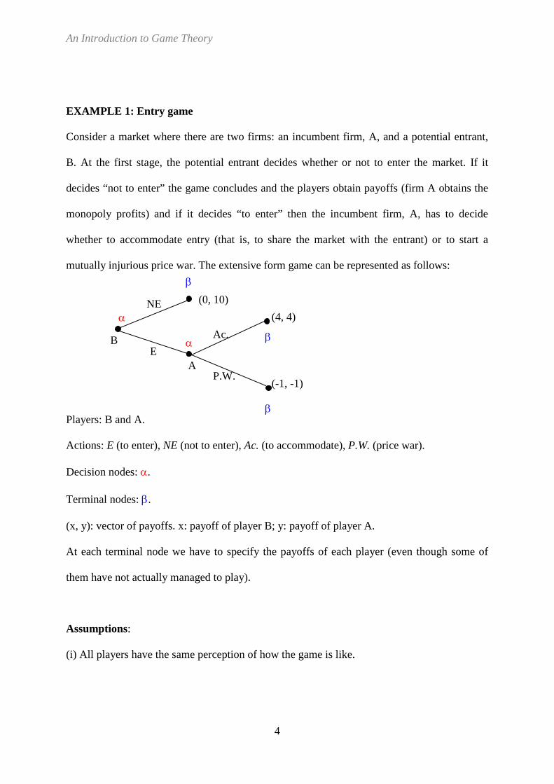
EXAMPLE 1: Entry game

Consider a market where there are two firms: an incumbent firm, A, and a potential entrant,

B. At the first stage, the potential entrant decides whether or not to enter the market. If it

decides “not to enter” the game concludes and the players obtain payoffs (firm A obtains the

monopoly profits) and if it decides “to enter” then the incumbent firm, A, has to decide

whether to accommodate entry (that is, to share the market with the entrant) or to start a

mutually injurious price war. The extensive form game can be represented as follows:

Players: B and A.

Actions: E (to enter), NE (not to enter), Ac. (to accommodate), P.W. (price war).

Decision nodes: α.

Terminal nodes: β.

(x, y): vector of payoffs. x: payoff of player B; y: payoff of player A.

At each terminal node we have to specify the payoffs of each player (even though some of

them have not actually managed to play).

Assumptions:

(i) All players have the same perception of how the game is like.

β

β α

α

(-1, -1)

(0, 10) (4, 4)

P.W.

Ac.

NE

E B

A

β


5

(ii) Complete information: each player knows the characteristics of the other players:

preferences and strategy spaces.

(iii) Perfect recall (perfect memory): each player remembers her previous behavior in the

game.

Definition 1: Information set

“The information available to each player at each one of her decision nodes”.

Game 1 Game 2

In game 1, player 2 has different information at each one of her decision nodes. At node A, if

she is called upon to play she knows that the player 1 has played I and at B she knows that

player 1 has played D. We say that these information sets are singleton sets consisting of only

one decision node. Perfect information game: a game where all the information sets are

singleton sets or, in other words, a game where all the players know everything that has

happened previously in the game. In game 2, the player 2 has the same information at both

her decision nodes. That is, the information set is composed of two decision nodes. Put

differently, player 2 does not know which of those nodes she is at. A game in which there are

information sets with two or more decision nodes is called an imperfect information game: at

A

B

(., .)

S

R

M

L

I

D 1

2

2 (., .)

(., .)

(., .)

L

2

(., .)

M

L

M I

D 1

(., .)

(., .)

(., .)


6

least one player does not observe the behavior of the other(s) at one or more of her decision

nodes.

The fact that players know the game that they are playing and the perfect recall assumption

restrict the situations where we can find information sets with two or more nodes.

Game 3 Game 4

Game 3 is poorly represented because it would not be an imperfect information game.

Assuming that player 2 knows the game, if she is called on to move and faces three

alternatives he/she would immediately deduce that the player 1 has played I. That is, the game

should be represented like game 4. Therefore, if an information set consists of two or more

nodes the number of alternatives, actions or moves at each one should be the same.

2

(., .)

I

D 1

(., .)

(., .)

(., .)

(., .)

1

(., .)

I

D 2

2 (., .) (., .)

(., .)

(., .)

1

1

1

(., .) L

b

a b

a C

(., .)

S

R

M

I

D

2

2

(., .)

(., .)

(., .)

(., .)

Game 5 Game 6

(., .) L

b

a b

a C

(., .)

S

R

M

I

D 1

2

2

(., .)

(., .)

(., .)

1

(., .)

(., .)

(., .)


7

The assumption of perfect recall avoids situations like that in game 5. When player 1 is called

on to play at her second decision node perfectly recalls her behavior at her first decision node.

The extensive form should be like that of game 6.

Definition 2: Subgame

“It is what remains to be played from a decision node with the condition that what remains to

be played does not form part of an information set with two or more decision nodes. To build

subgames we look at parts of the game tree that can be constructed without breaking any

information sets. A subgame starts at a singleton information set and all the decision nodes of

the same information set must belong to the same subgame.”

EXAMPLE 2: The Prisoner’s Dilemma

Two prisoners, 1 and 2, are being held by the police in separate cells. The police know that

the two (together) committed a crime but lack sufficient evidence to convict them. So the

police offer each of them separately the following deal: each is asked to implicate his partner.

Each prisoner can “confess” (C) or “not confess” (NC). If neither confesses then each player

goes to jail for one month. If both players confess each prisoner goes to jail for three months.

If one prisoner confesses and the other does not confess, the first player goes free while the

second goes to jail for six months.


8

- Simultaneous case: each player takes her decision with no knowledge of the decision of the

other.

PD1

There is an information set with two decision nodes. This is an imperfect information game.

There is a subgame which coincides with the proper game.

- Sequential game: the second player observes the choice made by the first.

PD2

Game PD2 is a perfect information game and there are three subgames. “In perfect

information games there are as many subgames as decision nodes”.

NC

NC

C NC

C

2

(1, 1)

C

1

(3, 0)

(0, 3)

(2, 2)

2

NC

NC

C NC

C

2

(1, 1)

C

1

(3, 0)

(0, 3)

(2, 2)


9

Definition 3: Strategy

“A player’s strategy is a complete description of what she would do if she were called on to

play at each one of her decision nodes. It needs to be specified even in those nodes not

attainable by her given the current behavior of the other player(s). It is a behavior plan or

conduct plan”.

(Examples: consumer demand, supply from a competitive firm.). It is a player’s function

which assigns an action to each of her decision nodes (or to each of her information sets). A

player’s strategy has as many components as information sets the player has.

Definition 4: Action

“A choice (decision or move) at a decision node”.

Actions are physical while strategies are conjectural.

Definition 5: Combination of strategies or strategy profile

“A specification of one strategy for each player”. The result (the payoff vector) must be

unequivocally determined.

EXAMPLE 1: The entry game

This is a perfect information game with two subgames. Each player has two strategies:

{ },BS NE E= and . Combinations of strategies: (NE, Ac.), (NE, P.W.), (E, Ac.)

and (E, P.W.).

{ }., . .AS Ac PW=


10


PD1: This is an imperfect information game with one subgame. Each player has two

strategies: { }1 ,S C NC= and { }2 ,S C NC= . Combinations of strategies: (C, C), (C, NC), (NC,

C) and (NC, NC).

PD2: This is a perfect information game with three subgames. Player 1 has two strategies

{ }1 ,S C NC= but player 2 has four strategies { }2 , , ,S CC CNC NCC NCNC= . Combinations

of strategies: (C, CC), (C, CNC), (C, NCC), (C, NCNC), (NC, CC), (NC,CNC), (NC, NCC)

and (NC, NCNC).

EXAMPLE 3

Player 1 at his/her first node has two possible actions, D and I, and two actions also at her

second: s and r. S1 = Ds, Dr, Is, Ir{ } and S2 = R, S{ }.

(4, 4)

(1, -1)

(8, 10)

(10, 0)

1 r

s

D

S

R I

1

2


11

1.1.2. Games in normal or strategic form (simultaneous or static games)

A game in normal or strategic form is described by:

1) The players.

2) The set (or space) of strategies for each player.

3) A payoff function which assigns a payoff vector to each combination of strategies.

The key element of this way of representing a game is the description of the payoffs of the

game as a function of the strategies of the players, without explaining the actions taken during

the game. In the case of two players the usual representation is a bimatrix form game where

each row corresponds to one of the strategies of one player and each column corresponds to

one strategy of the other player.



(-1, -1)

(0, 10) (4, 4)

P.W.

Ac.

NE

E B

A

P.W. Ac.

E

NE

B

A

(4, 4)

(0, 10) (0, 10)

(-1, -1)

NC

NC

C NC

C

2

(1, 1)

C

1

(3, 0)

(0, 3)

(2, 2)

NC C

NC

C

1

2

(0, 3)

(1, 1) (3, 0)

(2, 2)


12

EXAMPLE 3

Link between games in normal form and games in extensive form

a) For any game in extensive form there exists a unique corresponding game in normal form. This

is due to the game in normal form being described as a function of the strategies of the players.

b) (Problem) Different games in extensive form can have the same normal (or strategic) form.

(Example: in the prisoner’s dilemma, PD1, if we change the order of the game then the game in

extensive form also changes but the game in normal form does not change).

2

NC

NC

C NC

C

2

(1, 1)

C

1

(3, 0)

(0, 3)

(2, 2)

2 NCNC CNC

(2, 2) (0, 3)

(1, 1) (3, 0) (3, 0)

(0, 3)

(1, 1)

NCC CC

NC

C

1

(2, 2)

(4, 4)

(1, -1)

(8, 10)

(10, 0)

1 r

s

D

S

R I

1

2

Ir

Is

Dr

Ds

(8, 10) (4, 4)

(4, 4) (1, -1)

(10, 0) (10, 0) 1

2

S

(10, 0) (10, 0)

R


13

1.2. Solution concepts (criteria) for non-cooperative games

The general objective is to predict how players are going to behave when they face a particular

game. NOTE: “A solution proposal is (not a payoff vector) a combination of strategies, one for

each player, which leads to a payoff vector”. We are interested in predicting behavior, not gains.

Notation

i: Representative player, i = 1,…, n

Si : set or space of player i’s strategies.

si ∈Si : a strategy of player i.

s−i ∈S−i : a strategy or combination of strategies of the other player(s).

Πi (si ,s−i ) : the profit or payoff of player i corresponding to the combination of strategies

s ≡ (s1,s2,.....,sn) ≡ (si ,s−i ).

1.2.1. Dominance criterion

Definition 6: Dominant strategy

“A strategy is strictly dominant for a player if it leads to strictly better results (more payoff) than

any other of her strategies no matter what combination of strategies is used by the other players”.

“If ( , ) ( , ), , ;D Di i i i i i i i i i i is s s s s S s s s S− − − −Π > Π ∀ ∈ ≠ ∀ ∈ then D

is is a strictly dominant strategy for

player i”.


14


In game PD1 “confess”, C, is a (strictly) dominant strategy for each player. Independently of the

behavior of the other player the best each player can do is “confess”.

The presence of dominant strategies leads to a solution of the game. We should expect each player

to use her dominant strategy. The solution proposal for game DP1 is the combination of strategies

(C, C).

Definition 7: Strict dominance

“One strategy strictly dominates another when it leads to strictly better results (more payoff) than

the other no matter what combination of strategies is used by the other players”.

“If ( , ) ( , ), , then strictly dominates d dd d ddi i i i i i i i i is s s s s S s s− − − −Π > Π ∀ ∈ ”.

Definition 7’: (Strictly) Dominated strategy

“One strategy is strictly dominated for a player when there is another strategy which leads to

strictly better results (more payoff) no matter what combination of strategies is used by the other

players”.

“ is a strictly dominated strategy if such that ( , ) ( , ) dd d d ddi i i i i i i i i is s s s s s s S− − − −∃ Π > Π ∀ ∈ ”.

The dominance criterion consists of the iterated deletion of strictly dominated strategies.


15

EXAMPLE 4

In this game there are no dominant strategies. However, the existence of dominated strategies

allows us to propose a solution. We next apply the dominance criterion. Strategy t3 is strictly

dominated by strategy t2 so player 1 can conjecture (predict) that player 2 will never use that

strategy. Given that conjecture, which assumes rationality on the part of player 2, strategy s2 is

better than strategy s1 for player 1. Strategy s1 would be only used in the event that player 2 used

strategy t3. If player 1 thinks player 2 is rational then she assigns zero probability to the event of

player 2 playing t3. In that case, player 1 should play s2 and if player 2 is rational the best she can

do is t1. The criterion of iterated deletion of strictly dominated strategies (by eliminating

dominated strategies and by computing the reduced games) allows us to solve the game.

EXAMPLE 5

In this game there are neither dominant strategies nor (strictly) dominated strategies.

2s

3t 2t 1t 2

(-4, -2)

(2, 7) (0, 4)

(5, 5)

(4, 3) 1s

1

(5, -1)

(10, 1)

2t 1t 2

(5, 2) (10, 0) 1s

1

(2, 0) 2s


16

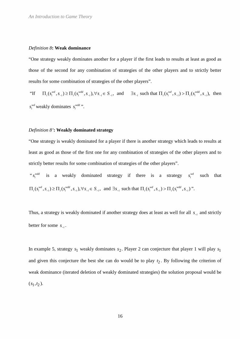
Definition 8: Weak dominance

“One strategy weakly dominates another for a player if the first leads to results at least as good as

those of the second for any combination of strategies of the other players and to strictly better

results for some combination of strategies of the other players”.

“If ( , ) ( , ), , wd wddi i i i i i i is s s s s S− − − −Π ≥ Π ∀ ∈ and such thatis−∃ ( , ) ( , ), wd wdd

i i i i i is s s s− −Π > Π then

wdis weakly dominates wdd

is ”.

Definition 8’: Weakly dominated strategy

“One strategy is weakly dominated for a player if there is another strategy which leads to results at

least as good as those of the first one for any combination of strategies of the other players and to

strictly better results for some combination of strategies of the other players”.

“ wddis is a weakly dominated strategy if there is a strategy wd

is such that

( , ) ( , ), , wd wddi i i i i i i is s s s s S− − − −Π ≥ Π ∀ ∈ and such thatis−∃ ( , ) ( , )wd wdd

i i i i i is s s s− −Π > Π ”.

Thus, a strategy is weakly dominated if another strategy does at least as well for all is− and strictly

better for some is− .

In example 5, strategy s1 weakly dominates s2. Player 2 can conjecture that player 1 will play s1

and given this conjecture the best she can do would be to play t2 . By following the criterion of

weak dominance (iterated deletion of weakly dominated strategies) the solution proposal would be

(s1, t2 ).


17

However, the criterion of weak dominance may lead to problematic results, as occurs in example 6,

or to no solution proposal as occurs in example 7 (because there are no dominant strategies, no

dominated strategies and no weakly dominated strategies).

EXAMPLE 6

EXAMPLE 7

2s

(0, 0)

(10, 100)

3t 2t 1t 2

(0, -100)

(5, 1) (4, -200) (10, 0) 1s

1

(5, 0)

3t 2t 1t 2

(10, 3)

(3, 0) (1, 3) (4, 10) 1s

1

(2, 10) 2s


18

1.2.2. Backward induction criterion

We next use the dominance criterion to analyze the extensive form. Consider example 1.


In the game in normal form, player A has a weakly dominated strategy: P.W.. Player B might

conjecture that and play E. However, player B might also have chosen NE in order to obtain a

certain payoff against the possibility of player A playing P.W..

In the game in extensive form, the solution is obtained more naturally by applying backward

induction. As she moves first, Player B may conjecture, correctly, that if she plays E then player A

(if rational) is sure to choose Ac.. Price war is therefore an incredible threat and anticipating that

player A will accommodate entry, the entrant decides to enter. By playing before A, player B may

anticipate the rational behavior of player A.

In the extensive form of the game we have more information because when player A has to move

she already knows the movement of player B.

(-1, -1)

(0, 10) (4, 4)

P.W.

Ac.

NE

E B

A

P.W. Ac.

E

NE

B

A

(4, 4)

(0, 10) (0, 10)

(-1, -1)


19

The criterion of backward induction lies in applying the criterion of iterated dominance backwards

starting from the last subgame(s). In example 1 in extensive form the criterion of backward

induction proposes the combination of strategies (E, Ac.) as a solution.

Result: In perfect information games with no ties, the criterion of backward induction leads to a

unique solution proposal.

Problems

(i) Ties.

(ii) Imperfect information. Existence of information sets with two or more nodes.

(iii) The success of backward induction is based on all conjectures about the rationality of agents

checking out exactly with independence of how long the backward path is. (It may require

unbounded rationality).

EXAMPLE 8

Backward induction does not propose a solution because in the last subgame player 1 is indifferent

between s and r. In the previous subgame, player 2 would not have a dominated action (because

she is unable to predict the behavior of player 1 in the last subgame).

(6, 1)

(5, 0)

(5, 2)

(0, 0)

1 r

s

D

S

R I

1

2


20

EXAMPLE 9

We cannot apply the criterion of backward induction.

EXAMPLE 10: Rosenthal’s (1981) centipede game

In the backward induction solution the payoffs are (1, 1). Is another rationality possible?

(0, 0)

I

D

1 r

r

s S

s

1

(2, 2)

R

2

(2, 0)

(0, 1)

(-1, 3)

(97, 100) (99, 99)

2

(1, 1)

B

D 1

(1, 4)

B

D 2 1

(0, 3)

B

D

(2, 2)

B

D 2

(98, 98)

B

D 1

(98, 101)

B

D 2 1

B

D

B

D (100, 100)


21

1.2.3. Nash equilibrium

Player i, i = 1,…, n, is characterized by:

(i) A set of strategies: Si .

(ii) A profit function, Πi (si ,s−i ) where si ∈Si and s−i ∈S−i .

Each player will try to maximize her profit (utility or payoff) function by choosing an appropriate

strategy with knowledge of the strategy space and profit functions of the other players but with no

information concerning the current strategy used by rivals. Therefore, each player must conjecture

the strategy(ies) used by her rival(s).

Definition 9: Nash equilibrium

“A combination of strategies or strategy profile s* ≡ (s1*, ...,sn

* ) constitutes a Nash equilibrium if

the result for each player is better than or equal to the result which would be obtained by playing

another strategy, with the behavior of the other players remaining constant.

s* ≡ (s1*, ...,sn

* ) is a Nash equilibrium if: Πi (si*, s−i

* ) ≥ Πi (si, s−i* ) ∀si ∈Si ,∀i,i = 1,...,n .”

At equilibrium two conditions must be satisfied:

(i) The conjectures of players concerning how their rivals are going to play must be correct.

(ii) No player has incentives to change her strategy given the strategies of the other players. This is

an element of individual rationality: do it as well as possible given what the rivals do. Put

differently, no player increases her profits by unilateral deviation.


22

Being Nash equilibrium is a necessary condition or minimum requisite for a solution proposal to be

a reasonable prediction of rational behavior by players. However, as we shall see it is not a

sufficient condition. That is, being Nash equilibrium is not in itself sufficient for a combination of

strategies to be a prediction of the outcome for a game.

Definition10: Nash equilibrium


* ) constitutes a Nash equilibrium if

each player’s strategy is a best response to the strategies actually played by her rivals.

That is, s* ≡ (s1*, ...,sn

* ) is a Nash equilibrium if:

* *( ) , 1,...,i i is BR s i i n−∈ ∀ =

where { }* ' ' * * '( ) : ( , ) ( , ), , i i i i i i i i i i i i i iBR s s S s s s s s S s s− − −= ∈ Π ≥ Π ∀ ∈ ≠ ”.

A simple way of obtaining the Nash equilibria for a game is to build the best response sets of each

player to the strategies (or combinations of strategies) of the other(s) player(s) and then look for

those combinations of strategies being mutually best responses.

EXAMPLE 11

(0, 5) (10, 2) (3, 10) c

2 i

(15, 6)

(5, 11) (20, 5)

(9, 11)

(5, 3)

j h

b

a

1 (2, 8)

1s 2s

2BR 1BR

a

c

i

h

h

i

j

b

c

a

b h


23

The strategy profile (b, h) constitutes the unique Nash equilibrium.

EXAMPLE 7

Note that the dominance criterion did not propose any solution for this game. However, the

combination of strategies (s1,t1) constitutes the unique Nash equilibrium.

3t 2t 1t 2

(10, 3)

(3, 0) (1, 3)

(0, 0)

(4, 10) 1s

1

(2, 10) 2s


24

1.2.4. Problems and refinements of the Nash equilibrium

1.2.4.1. The possibility of inefficiency

It is usual to find games where Nash equilibria are not Pareto optimal (efficient).


(C, C) is a Nash equilibrium based on dominant strategies. However, that strategy profile is the

only profile which is not Pareto optimal. In particular, there is another combination of strategies,

(NC, NC), where both players obtain greater payoffs.

1.2.4.2. Inexistence of Nash equilibrium (in pure strategies)

EXAMPLE 12

NC C

NC

C

1

2

(0, 3)

(1, 1) (3, 0)

(2, 2)

2s

NC

NC

C NC

C

2

(1, 1)

C

1

(3, 0)

(0, 3)

(2, 2)

2t 1t 2

(0, 1)

(0, 1)

(1, 0) 1s

1

(1, 0)


25

This game does not have Nash equilibria in pure strategies. However, if we allow players to use

mixed strategies (probability distributions on the space of pure strategies) the result obtained is that

“for any finite game there is always at least one mixed strategy Nash equilibrium”.

1.2.4.3. Multiplicity of Nash equilibria

We distinguish two types of games.

1.2.4.3.1. With no possibility of refinement or selection

EXAMPLE 13: The Battle of the Sexes

This game has two Nash equilibria: (M, M) and (P, P). There is a pure coordination problem.

1.2.4.3.2. With possibility of refinement or selection

a) Efficiency criterion

This criterion consists of choosing the Nash equilibrium which maximizes the payoff of players. In

general this is not a good criterion for selection.

P M

P

M

Bf

Gf

(1, 1)

(3, 2) (1, 1)

(2, 3)


26

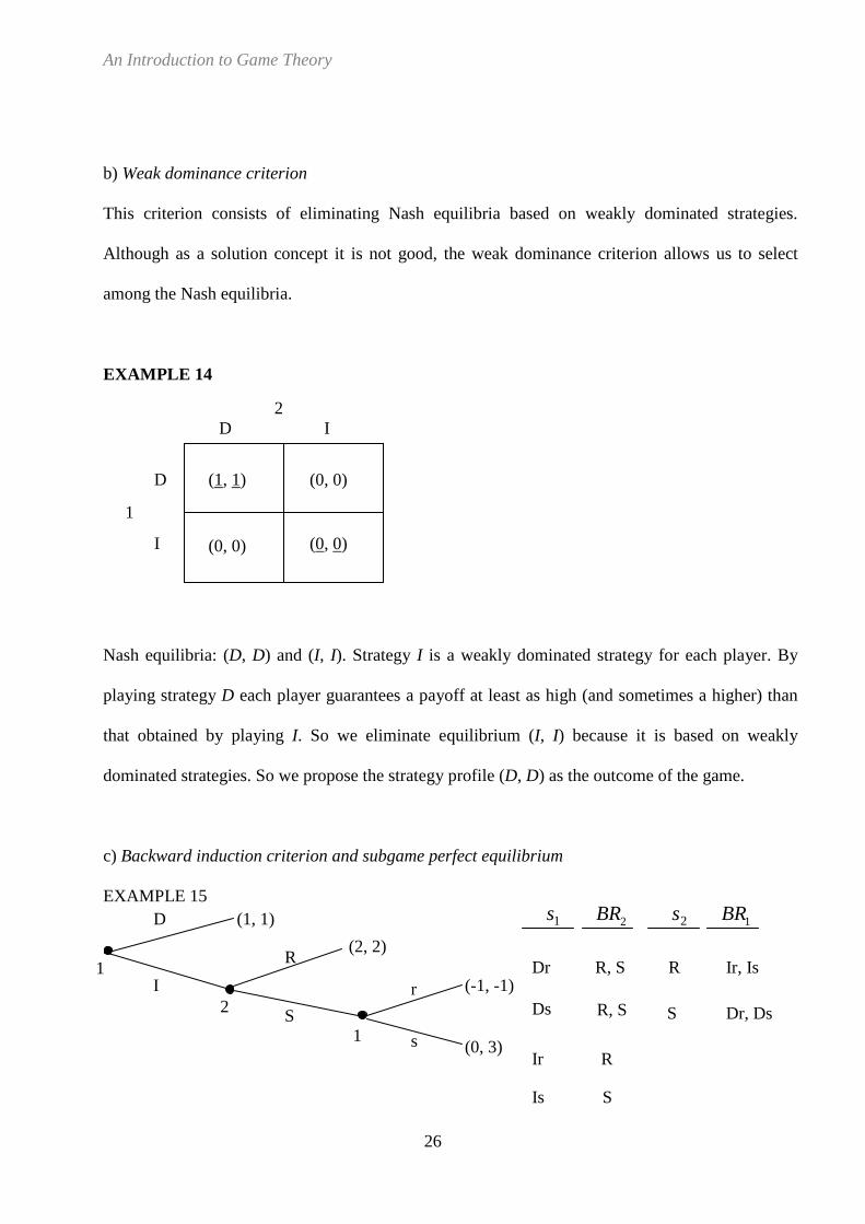
b) Weak dominance criterion

This criterion consists of eliminating Nash equilibria based on weakly dominated strategies.

Although as a solution concept it is not good, the weak dominance criterion allows us to select

among the Nash equilibria.

EXAMPLE 14

Nash equilibria: (D, D) and (I, I). Strategy I is a weakly dominated strategy for each player. By

playing strategy D each player guarantees a payoff at least as high (and sometimes a higher) than

that obtained by playing I. So we eliminate equilibrium (I, I) because it is based on weakly

dominated strategies. So we propose the strategy profile (D, D) as the outcome of the game.

c) Backward induction criterion and subgame perfect equilibrium

EXAMPLE 15

I D

I

D

1

2

(0, 0)

(1, 1) (0, 0)

(0, 0)

(2, 2)

(-1, -1)

(0, 3)

(1, 1)

1 s

r

D

S

R I

1

2

1s 2s

2BR 1BR

Dr

Ir

R, S

R

R

S

Ir, Is

Dr, Ds Ds R, S

S Is


27

There are three Nash equilibria: (Dr, S), (Ds, S) and (Ir, R). We start by looking at the efficient

profile: (Ir, R). This Nash equilibrium has a problem: at her second decision node, although it is an

unattainable given the behavior of the other player, player 1 announces that she would play r. By

threatening her with r player 1 tries to make player 2 play R and so obtain more profits. However,

that equilibrium is based on a non credible threat: if player 1 were called on to play at his/her

second node she would not choose r because it is an action (a non credible threat) dominated by s.

The refinement we are going to use consists of eliminating those equilibria based on non credible

threats (that is, based on actions dominated in one subgame). From the joint use of the notion of

Nash equilibrium and the backward induction criterion the following notion arises:

Definition 11: Subgame perfect equilibrium


* ) , which is a Nash equilibrium,

constitutes a subgame perfect equilibrium if the relevant parts of the equilibrium strategies of each

player are also an equilibrium at each of the subgames”.

In example 15 (Dr, S) and (Ir, R) are not subgame perfect equilibria. Subgame perfect equilibria

may be obtained by backward induction. We start at the last subgame. In this subgame r is a

dominated action (a non credible threat); therefore, it cannot form part of player 1’s strategy in the

subgame perfect equilibrium, so we eliminate it and compute the reduced game

(2, 2)

(-1, -1)

(0, 3)

(1, 1)

1 s

r

D

S

R I

1

2


28

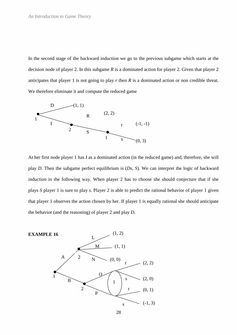
In the second stage of the backward induction we go to the previous subgame which starts at the

decision node of player 2. In this subgame R is a dominated action for player 2. Given that player 2

anticipates that player 1 is not going to play r then R is a dominated action or non credible threat.

We therefore eliminate it and compute the reduced game

At her first node player 1 has I as a dominated action (in the reduced game) and, therefore, she will

play D. Then the subgame perfect equilibrium is (Ds, S). We can interpret the logic of backward

induction in the following way. When player 2 has to choose she should conjecture that if she

plays S player 1 is sure to play s. Player 2 is able to predict the rational behavior of player 1 given

that player 1 observes the action chosen by her. If player 1 is equally rational she should anticipate

the behavior (and the reasoning) of player 2 and play D.

EXAMPLE 16

(2, 2)

(-1, -1)

(0, 3)

(1, 1)

1 s

r

D

S

R I

1

2

B

A

1

2

s

s

r P

r

1

(2, 2)

O (2, 0)

(0, 1)

(-1, 3)

2 N

L

M (1, 1)

(0, 0)

(1, 2)


29

In this game there is a multiplicity of Nash equilibria and we cannot apply backward induction

because there is a subgame with imperfect information. We shall use the definition of subgame

perfect equilibrium and we shall require that the relevant part of the equilibrium strategies to be an

equilibrium at the subgames.

At the upper subgame (the perfect information subgame) the only credible threat by player 2 is L.

At the lower subgame (the imperfect information subgame) (which starts at the lower decision

node of player 2), it is straightforward to check that the Nash equilibrium is O, r.

At her first decision node player 1 therefore has to choose between A and B anticipating that if she

chooses A then player 2 will play L and if she chooses B, then they will both play the Nash

equilibrium (of the subgame) O, r. Therefore, player 1 chooses B.

2 s

s

r P

r

1

(2, 2)

O (2, 0)

(0, 1)

(-1, 3)

B

A

1

2

2

L (1, 2)

r

1

(2, 2) O

2 N

L

M (1, 1)

(0, 0)

(1, 2)


30

Therefore, the subgame perfect equilibrium is (Br, LO): the relevant part of the equilibrium

strategies are also equilibrium at each of the subgames.

1.3. Conclusions

We have analyzed different ways of solving games, although none of them is exempt from

problems. The dominance criterion (elimination of dominated strategies) is useful in solving some

games but does not serve in others because it provides no solution proposal. The weak version of

this criterion (elimination of weakly dominated strategies) is highly useful in selecting among Nash

equilibria, especially in games in normal or strategic form. The backward induction criterion

allows solution proposals to be drawn up for games in extensive form. This criterion has the

important property that in perfect information games without ties it leads to a unique outcome. But

it also presents problems: the possibility of ties, imperfect information and unbounded rationality.

This criterion is highly useful in selecting among Nash equilibria in games in extensive form. The

joint use of the notion of Nash equilibrium and backward induction gives rise to the concept of

subgame perfect equilibrium, which is a very useful criterion for proposing solutions in many

games. Although it also presents problems (inefficiency, nonexistence and multiplicity) the notion

of the Nash equilibrium is the most general and most widely used solution criterion for solving

games. Being Nash equilibrium is considered a necessary (but not sufficient) condition for a

solution proposal to be a reasonable prediction of rational behavior by players. If, for instance, we

propose as the solution for a game a combination of strategies which is not a Nash equilibrium,

that prediction would be contradicted by the development of the game itself. At least one player

would have incentives to change her predicted strategy. In conclusion, although it presents

problems, there is quasi-unanimity that all solution proposals must at least be Nash equilibrium.


31

Basic Bibliography

Varian, H. R., 1992, Microeconomic Analysis, 3th edition, Norton. Chapter 15, sections:

introduction, 15.1, 15.2, 15.3, 15.4, 15.6, 15.7, 15.9, 15.10 and 15.11.

Complementary Bibliography

Kreps, D. M., 1994, A course in microeconomic theory, Harvester Wheatsheaf.

Tirole, J., 1990, The Theory of Industrial Organization, MIT Press.

Varian, H. R., 1998, Intermediate Microeconomics: A Modern Approach, Norton.

An Introduction to Game Theory.pdf - UPV/EHU

Documents

Transcript of An Introduction to Game Theory.pdf - UPV/EHU