Tools and Technology Article

An Evaluation of Sex-Age-Kill (SAK) Model PerformanceJOSHUA J. MILLSPAUGH,1 Department of Fisheries and Wildlife Sciences, University of Missouri, Columbia, MO 65211, USA

JOHN R. SKALSKI, School of Aquatic and Fishery Sciences, University of Washington, Box 358218, Seattle, WA 98195, USA

RICHARD L. TOWNSEND, School of Aquatic and Fishery Sciences, University of Washington, Box 358218, Seattle, WA 98195, USA

DUANE R. DIEFENBACH, United States Geological Survey, Pennsylvania Cooperative Fish and Wildlife Research Unit, Pennsylvania StateUniversity, University Park, PA 16802, USA

MARK S. BOYCE, Department of Biological Sciences, University of Alberta, Edmonton, AB T6G 2E9, Canada

LONNIE P. HANSEN, Missouri Department of Conservation, 1110 S College Avenue, Columbia, MO 65211, USA

KENT KAMMERMEYER, Kent Kammermeyer Consulting, 1565 Shoal Creek Road, Clermont, GA 30527, USA

ABSTRACT The sex-age-kill (SAK) model is widely used to estimate abundance of harvested large mammals, including white-tailed deer

(Odocoileus virginianus). Despite a long history of use, few formal evaluations of SAK performance exist. We investigated how violations of the

stable age distribution and stationary population assumption, changes to male or female harvest, stochastic effects (i.e., random fluctuations in

recruitment and survival), and sampling efforts influenced SAK estimation. When the simulated population had a stable age distribution and

k . 1, the SAK model underestimated abundance. Conversely, when k , 1, the SAK overestimated abundance. When changes to male harvest

were introduced, SAK estimates were opposite the true population trend. In contrast, SAK estimates were robust to changes in female harvest

rates. Stochastic effects caused SAK estimates to fluctuate about their equilibrium abundance, but the effect dampened as the size of the

surveyed population increased. When we considered both stochastic effects and sampling error at a deer management unit scale the resultant

abundance estimates were within 6121.9% of the true population level 95% of the time. These combined results demonstrate extreme

sensitivity to model violations and scale of analysis. Without changes to model formulation, the SAK model will be biased when k 6¼ 1.

Furthermore, any factor that alters the male harvest rate, such as changes to regulations or changes in hunter attitudes, will bias population

estimates. Sex-age-kill estimates may be precise at large spatial scales, such as the state level, but less so at the individual management unit level.

Alternative models, such as statistical age-at-harvest models, which require similar data types, might allow for more robust, broad-scale

demographic assessments. ( JOURNAL OF WILDLIFE MANAGEMENT 73(3):442–451; 2009)

DOI: 10.2193/2008-099

KEY WORDS deer, harvest, Odocoileus virginianus, population estimate, population reconstruction, sex-age-kill, white-taileddeer.

Population reconstruction methods have a long history of

use in fisheries and wildlife management. Starting 70 years

ago, wildlife managers used reconstruction techniques

extensively because data (e.g., age and sex data from hunter

harvest) were relatively inexpensive and easy to collect and

could be used in demographic assessments for large areas

(e.g., Allen 1942, Dale 1952, Petrides 1954). In addition,

calculations could be performed by hand or with simple

computer spreadsheets. Despite advances in statistical theory

and quantitative tools for estimating animal abundance

(Buckland et al. 1993, Williams et al. 2001), state agencies

continue to use population reconstruction methods as a

primary technique for broad-scale population assessments of

game species (Skalski et al. 2005).

The sex-age-kill (SAK) model of population reconstruc-

tion is used by �20 state agencies to estimate white-tailed

deer (Odocoileus virginianus) abundance (Skalski and Mill-

spaugh 2002, Millspaugh et al. 2007). The SAK model is

one variant of a large suite of reconstruction methods using

hunter harvest data and was developed by the Michigan

Department of Conservation in the late 1950s (Eberhardt

1960, Lang and Wood 1976, Skalski et al. 2005). Although

it has been used primarily to estimate white-tailed deer

abundance, variations of the SAK model have been applied

to other species, including black bears (Ursus americanus)and elk (Cervus elaphus; Bender and Spencer 1999).

Despite its widespread use, there have been few formalevaluations of the statistical properties of the SAK model(Skalski and Millspaugh 2002). Only recently have genericvariance expressions been provided and precision of thetechnique evaluated. Skalski and Millspaugh (2002) foundthat precise field data were necessary to provide a usefulestimate of population abundance. Even with intense datacollection, however, it is unclear whether SAK-modelestimates are robust to stochastic effects (i.e., fluctuationsin survival and recruitment), changes in harvest strategies, orrealistic violations of underlying assumptions of a stable agedistribution and stationary population (hereafter stable-stationary). Effective management requires biologists toconsider the utility of various analytical and samplingoptions with respect to population objectives.

Our objective was to examine SAK performance whenstochasticity and sampling error were considered and modelassumptions were violated. We evaluated the error inestimates when the stable-stationary assumption wasviolated (including general changes to population growthrate (k) and, more narrowly, to changes in male and femaleharvest rates), and under stochastic variation in modelparameters. Building on the work of Skalski and Millspaugh(2002), we examined the combined effects of sampling errorand parameter stochasticity on SAK estimation.1 E-mail: millspaughj@missouri.edu

442 The Journal of Wildlife Management � 73(3)

METHODS

Overview of SAK ModelThe following overview of the SAK model is summarizedfrom Skalski and Millspaugh (2002) and Skalski et al. (2005).The generic equation for the SAK model is as follows:

NT ¼H

MT B1þ RF=M þ RF=M � RJ=F

� �ð1Þ

whereNT ¼ estimate of total abundance;H ¼ estimated adult male harvest in year i;MT ¼ total annual mortality rate of adult males;B ¼ proportion of total male mortality due to harvest

(male recovery rate);RF=M ¼ estimated ratio of adult females to adult males in

the population;RJ=F ¼ estimated ratio of juveniles to adult females in the

population.The first factor in equation 1 estimates male abundance.

Multiplying male abundance by the female:male sex ratioestimates female abundance. The third term estimatesjuvenile abundance by the product of female abundance andthe juvenile:female ratio. This generic form of the SAKmodel (eq 1) contains no assumptions about the structure ofthe population or its dynamics over time (Skalski andMillspaugh 2002). However, to estimate some of the inputparameters, the stable-stationary assumption is often invoked.

With the stable-stationary assumption, MT can beestimated by the proportion (pYM) of 1.5-year-old malesin the adult male segment of the population (Burgoyne1981).

The Burgoyne (1981) estimator MT is based on theadditional assumption that hunter harvest provides arepresentative sample of the age structure of the malepopulation. Because most hunters are opportunistic in theirselection of deer to harvest, this assumption of representativesampling is reasonably satisfied. Additionally, RF=M can beestimated by Severinghaus and Maguire (1955) as follows:

RF=M ¼pYM

pYF

� h; ð2Þ

wherepYF ¼ proportion of 1.5-year-old females in the adult

female segment of the population;h ¼ the sex ratio of fetal males:females.Thus, the final form of the SAK model, where estimated

deer abundance during the current year (Ni) is as follows:

Ni ¼Hi

pYM B1þ pYM

pYF

� hþ pYM

pYF

� h � RJ=F

� �: ð3Þ

In addition to the stable-stationary assumption, it is assumedthat sample surveys provide unbiased estimates of the inputparameters (i.e., H, B, pYM , pYF , h, and RJ=F ) in year i.

Simulation StudiesWe used both deterministic calculations and stochasticsimulations to investigate robustness of the SAK model (eq

3) to violations of the assumptions of a stable-stationarypopulation. Specifically, we used a deterministic model toexamine effects of direct violations of the stable-stationaryassumption when k . 1 and when k , 1 and to assess howchanges in harvest regulations affect SAK performance. Weused a stochastic model to investigate effects of randomfluctuations in recruitment or survival and to assess how theSAK model performed when both sampling error andparameter stochasticity were present.

Using a deterministic 2-sex Leslie Matrix model (Leslie1945, Keyfitz and Murphy 1967), we simulated annualpopulation abundance and harvest under nonstationaryconditions, including when k . 1 and k , 1. We did notinclude stochasticity in recruitment or survival in thesecalculations. The basic deterministic model used in thesimulations began with a stable age distribution and astationary population under harvest. We used naturalsurvival rates of 0.44 for the first age classes and 0.74 forall subsequent age classes, regardless of gender. Age-specific net fecundity rates were 0.30 (¼ F0F ¼ F0M) forthe first age class and 0.55 for all subsequent age classes(i.e., F1F ¼ F2F ¼ . . . ¼ FA�1M ¼ FAM). Harvestprobabilities were 0.05 for the first age class and all adultfemale age classes. Harvest probabilities for all age (yr)class .1 males were 0.20. Population levels varieddepending on the objective of the analyses. We generatednonstable-nonstationary populations by varying �1 of thedemographic parameters as described in the Resultssection.

We computed annual abundance and harvest numbersdirectly from matrix multiplication of a 2-sex model,

M �H~ni ¼

~niþ1;

whereM ¼ Leslie 2-sex model;H ¼ harvest matrix;

~ni ¼ vector of abundance by sex and age in year i;

and where

F0F F1F . . . FAF 0 0 . . . 0S0F 00 S1F

SAF 0F0M F1M . . . FAM 0 0 . . . 0

S0M 0 . . . 00 0 S1M

SAM 0

2

66666666664

3

77777777775

�

�

h0F 0 . . . 00 h1F 0 . . . 0

0 . .. ..

.

..

.hAF

h0M

h1M

. ..

00 . . . 0 hAM

2

6666666666664

3

7777777777775

�

n0Fi

n1Fi

..

.

nAFi

n0Mi

n1Mi

..

.

nAMi

2

6666666666664

3

7777777777775

Millspaugh et al. � SAK Evaluation 443

¼

n0F ;iþ1n1F ;iþ1

nAF ;iþ1n0M ;iþ1

..

.

mAM ;iþ1

2

666666666664

3

777777777775

; ð4Þ

and whereFiF¼ net number of female offspring recruited per female

of age i (i ¼ 0, . . ., A) into the fall huntablepopulation;

FiM¼ net number of male offspring recruited per femaleof age i (i ¼ 0, . . ., A ) into the fall huntablepopulation;

SiF¼probability of annual survival from natural causes fora female of age i to iþ 1 (i¼ 0, . . ., A ) from fall tofall;

SiM ¼ probability of annual survival from natural causesfor a male of age i to iþ 1 (i¼ 0, . . ., A ) from fallto fall;

hiF ¼ probability of surviving the harvest for a female ofage i (i ¼ 0, . . ., A );

hiM¼probability of surviving the harvest for a male of agei (i ¼ 0, . . ., A );

njFi ¼ number of females of age class j ( j ¼ 0, . . ., A ) inyear i in the fall huntable population;

njMi¼number of males of age class j ( j¼0, . . ., A ) in yeari in the fall huntable population.

After multiplying through, then

n0F ;iþ1n1F ;iþ1

..

.

nAF ;iþ1n0M ;iþ1n1M ;iþ1

..

.

nAM ;iþ1

2

6666666666664

3

7777777777775

¼

XA

j¼0njFi � FjF � hjF

n0FiS0F h0F

..

.

nA�1;F ;i; SA�1;F hA�1;FXA

j¼0njFi � FjM � hjF

n0MiS0M h0M

..

.

nA�1;M ;iSA�1;M jA�1;M

2

6666666666666666664

3

7777777777777777775

: ð5Þ

In the simulation runs, we modeled age (yr) classes 0.5, 1.5,. . ., and 12.5. We simulated successive generations of deerby recursively using equation 5. We calculated annualharvest ð

~ciÞ of deer by age and sex class as the vector

~c ¼ ðI�HÞM

~ni: ð6Þ

We calculated total annual harvest (THi) as

THi ¼ 1~

0ðI�HÞM~ni ¼ 1

~

0

~c: ð7Þ

Deer recruitment and survival can be directly affected byannual changes in overwinter conditions and long-termhabitat changes. Recruitment and survival also are affectedby random chance (i.e., demographic stochasticity). These

changes in survival and recruitment affect the age and sexcomposition of the population in subsequent years. Toevaluate effects of random fluctuations in survival orrecruitment on SAK estimates, we constructed a stochastic,2-sex Leslie matrix model (Keyfitz and Murphy 1967). Thestochastic model was based on a binomial function for thenatural survival and harvest processes and a Poissonrecruitment function. We modeled harvest for a particularage and sex class as a binomial process, where

cij ;BIN�

nij ; ð1� hijÞ�; ð8Þ

wherecij ¼ harvest for age class i, gender j;nij ¼ abundance for age class i, gender j;hij ¼ probability of surviving harvest age for class i,

gender j.We modeled next year’s abundance as a binomial process

conditional on cij, where

niþ1;j ;BINðnij � cij ; SijÞ; ð9Þ

where Sij ¼ probability of surviving natural causes for ageclass i, gender j. Recruitment of age class 0.5 was based onthe expected values in equation 5, where

Eðn0jÞ ¼XA

j¼0ðniF � ciF ÞFij ¼ l0j ;

whereFij ¼ fecundity of age class i in producing gender j

offspring,niF ¼ number of age class i females,ciF ¼ number of age class i females harvested.

We then treated the number of recruited 0.5 age classindividuals in the population as a Poisson random variable,where

n0j ;Poissonðl0jÞ: ð10Þ

Using this model, we examined stochastic effects in age and sexcomposition on the SAK abundance estimator (Ni). We alsoused simulations to determine at what abundance thestochastic effects have an insignificant effect on SAK estimates.

Because covariance among vital rates is an importantcontributor to population fluctuation in deer populations(Coulson et al. 2005, Boyce et al. 2006), we performedadditional simulations that incorporated covariance betweensurvival and productivity. To induce a positive covariancebetweensurvival andproductivity, weused compoundprocessesin generating the age class data. We simulated survival to thenext age class as a compound binomial-uniform process

niþ1 ;BIN�

nt � ci; Sið1þ ekÞ�; ð11Þ

and production of juveniles as a compound Poisson-uniformprocess

n�; PXA

j¼0ðni � ciÞFið1þ ekÞ

" #

ð12Þ

444 The Journal of Wildlife Management � 73(3)

where ek is uniformly distributed U(�0.20,þ0.20) in year k.Each year, we used a new randomly generated ek that eitherincreased or decreased both survival and productivity by ek 3

100%. For example, if ek¼0.05, both the parameters Fi and Si

increased by 5% over baseline conditions that year. An ek¼�0.05 would result in Fi and Si decreasing to 95% of theirtypical value. This error structure induced a positive correlationbetween annual survival and productivity of q . 0.90. Otherdistributions and ranges for ek could be used, but this is adequatefor demonstration. We compared error in estimation, i.e.,

SEðdSAKÞ ¼ffiffiffiffiffiffiffiffiffiffiffiffiffiffiffiffiffiffiffiffidVarðdSAK

qÞ ¼

ffiffiffiffiffiffiffiffiffiffiffiffiffiffiffiffiffiffiffiffiffiffiffiffiffiffiffiffiffiffiffiffiffiffiffiffiffiffiXn

k¼1ðNSAK;k �NkÞ2

n

vuuutð13Þ

where n¼1,000 years of data simulated under 2 scenarios: 1) nocorrelation, i.e., ek ¼ 0 8k; and 2) positive correlation, ek ;

U(�0.20,þ0.20).In practice, values of pYM , pYF , and RJ=F used in the SAK

calculations are a function of both the stochastic effectsdescribed in the last section and the error in subsampling thepopulation or harvest data (Appendix). To properlycharacterize variance in SAK calculations, both sources ofuncertainty must be considered. We performed additionalsimulation studies to examine the behavior of SAK estimatesas these successive sources of variation are considered.

We conducted additional simulations where we randomlysampled harvest and population to provide estimates of ageand sex composition (i.e., pYM, pYF, and RJ=F ). For agecomposition, we randomly sampled 250 males and 250females harvested to estimate pYM and pYF . These samplinglevels are consistent with the approximately 5% samplingrate used in Wisconsin and 10% in Pennsylvania at a deermanagement unit scale (Wisconsin Department of NaturalResources [WDNR] 2001, Rosenberry et al. 2004). Inestimating RJ/F, we randomly sampled 80 females, againconsistent with typical sampling rates within a managementunit in Wisconsin (WDNR 2001, G.1). We assumed astable-stationary population of N ¼ 10,000 in the analysis.

In evaluating model performance, we calculated anestimate of the mean squared error (MSE) of N where

MSEðNÞ ¼ VarðNjN Þ þ�

EðNÞ �N�2

¼ varianceþ bias2:

In the case of a biased estimator, MSE better characterizes theactual error in the estimate. For an unbiased estimator, theMSE is the sampling variance. Across replicate simulations(n) and years (y), we calculated the MSE as follows:

!Figure 1. Population trends and corresponding sex-age-kill (SAK) modelestimates of white-tailed deer abundance (Ni) under (a) stable-stationary(stable age distribution and stationary abundance), (b) stable-nonstationary(k . 1), and (c) stable-nonstationary (k , 1) demographic conditions.Results are based on a deterministic, 2-sex Leslie matrix model. Trueabundance (solid line, ______), SAK estimates (dashed line, _ _ _ _ _) usingexact demographic data (i.e., no sampling error).

Millspaugh et al. � SAK Evaluation 445

dMSE¼ 1

n

Xn

i¼1

�Xy

j¼1Nij � Nij

2

ðy � 1Þ

�:

We varied the number of simulations (n) from 100 to 1,000

and set y ¼ 40. To standardize the error in estimationrelative to the actual abundance values, we computed a

measurement analogous to the coefficient of variation forunbiased estimates as

CE ¼

ffiffiffiffiffiffiffiffiffiffiffidMSE

p

Xn

i¼j

Xy

j¼1Nij

ny

0

@

1

A

ð14Þ

called the coefficient of error (CE). Finally, we generatedestimates of male recovery rate (B), with a CE of 10%.

RESULTS

Under stable-stationary conditions, SAK estimates trackedthe true population abundance, as expected (Fig. 1a).

However, when the population had a stable age compositionand k . 1, the SAK model underestimated Ni (Fig. 1b).Conversely, with a stable age distribution and k , 1, the

SAK overestimated Ni (Fig. 1c).

Changes to male harvest rate had an immediate and

substantial impact on SAK estimates (Fig. 2). Afterchanging male harvest rates, the SAK estimate asymptoti-cally converged to a new stable-stationary condition.However, at the time of the shift, SAK estimates werestrongly biased (Fig. 2), and this bias persisted for as long as10 years, although diminishing with each passing year.When we increased male harvest mortality, the SAKestimator underestimated actual abundance (i.e., negativebias). When we decreased male harvest mortality, the SAKestimator overestimated actual abundance (Fig. 2).

A shift in female harvest rate from 0.05 to 0.15 did notproduce the same shift in abundance estimates as maleharvest changes (Fig. 3). The SAK estimates followedabundance trends with only a slight positive bias (Fig. 3).

The stochastic effects we simulated caused the annualpopulation abundance to fluctuate about the equilibriumabundance (Fig. 4). However, random fluctuations in agecomposition (i.e., pYM , pYF , and RJ=F ) resulted in SAKabundance estimates of Ni to vary more than the populationthey were monitoring. Similar variability will be producedby environmental fluctuations in survival and fecundityabout their equilibrium values. In a population of approx-imately 50,000 deer, CE was 4.6%. As expected, aspopulation size decreased, amount of error in the SAKestimate increased. For a population of 25,000 deer, CE was8.3%, whereas for 10,000 deer, CE was 12.4%. For amanagement unit with 10,000 deer, this means thatabundance estimates were within 624.3% of the true value95% of the time when there was no sampling error. Oursimulations indicate that population sizes of 1–2 million arerequired before these stochastic effects are trivial (Fig. 5).Therefore, SAK estimates may be precise at a state level butnot at smaller, management unit levels.

Figure 2. Population trends and corresponding sex-age-kill (SAK) modelestimates of white-tailed deer abundance (Ni), followed by a 0.10 decline inmale harvest rate, followed by a 0.10 increase in male harvest rate. Resultsare based on a deterministic, 2-sex Leslie matrix model. Modeledabundance (solid line, ______) and SAK estimates (dashed line, _ _ _ _ _),based on exact demographic data (i.e., no sampling error). We generatedthe deer population using the Leslie 2-sex model under stable and stationary(k ¼ 1) conditions for the first 40 years. In year 41, we changed the maleharvest rate from a probability of 0.30 to 0.20 and it remained so for thenext 40 years (yr 41–80). During that period, the population achieved adifferent set of stable and stationary conditions. Then in year 81, wereverted the male harvest back to the original rate of 0.3. Then, thepopulation reached a new stable and stationary condition over years 81–120,the same as the original set of conditions at the beginning of the simulation.

Figure 3. Population trends and corresponding sex-age-kill (SAK) modelestimates of white-tailed deer abundance (Ni), under a stable-stationarycondition (k¼1), followed by a 0.10 increase in female harvest rate. Resultsare based on a deterministic, 2-sex Leslie matrix model. Simulatedabundance (solid line, ______), SAK estimates (dotted line, _ _ _ _ _), usingexact demographic data values (i.e., no sampling error).

446 The Journal of Wildlife Management � 73(3)

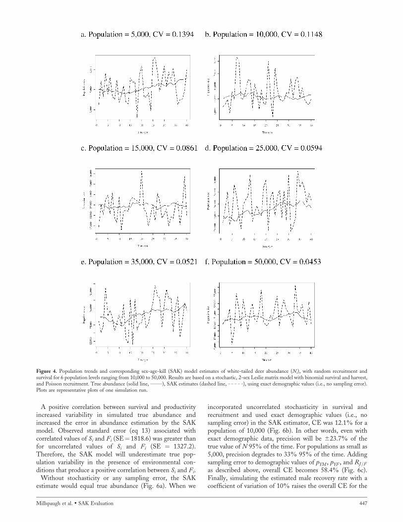
A positive correlation between survival and productivityincreased variability in simulated true abundance andincreased the error in abundance estimation by the SAKmodel. Observed standard error (eq 13) associated withcorrelated values of Si and Fi (SE¼ 1818.6) was greater thanfor uncorrelated values of Si and Fi (SE ¼ 1327.2).Therefore, the SAK model will underestimate true pop-ulation variability in the presence of environmental con-ditions that produce a positive correlation between Si and Fi.

Without stochasticity or any sampling error, the SAKestimate would equal true abundance (Fig. 6a). When we

incorporated uncorrelated stochasticity in survival andrecruitment and used exact demographic values (i.e., nosampling error) in the SAK estimator, CE was 12.1% for apopulation of 10,000 (Fig. 6b). In other words, even withexact demographic data, precision will be 623.7% of thetrue value of N 95% of the time. For populations as small as5,000, precision degrades to 33% 95% of the time. Addingsampling error to demographic values of pYM , pYF , and RJ=F

as described above, overall CE becomes 58.4% (Fig. 6c).Finally, simulating the estimated male recovery rate with acoefficient of variation of 10% raises the overall CE for the

Figure 4. Population trends and corresponding sex-age-kill (SAK) model estimates of white-tailed deer abundance (Ni), with random recruitment andsurvival for 6 population levels ranging from 10,000 to 50,000. Results are based on a stochastic, 2-sex Leslie matrix model with binomial survival and harvest,and Poisson recruitment. True abundance (solid line, ______), SAK estimates (dashed line, _ _ _ _ _), using exact demographic values (i.e., no sampling error).Plots are representative plots of one simulation run.

Millspaugh et al. � SAK Evaluation 447

SAK method to 62.2% for a population of 10,000 (Fig. 6d).Thus, with both stochastic effects and sampling error at adeer management unit level of effort, resultant abundanceestimates, Ni, were within 6121.9% of the true simulatedpopulation level 95% of the time.

DISCUSSION

The general form of the SAK model assumes a stable agedistribution and a stationary population, which is unrealisticfor many ungulate populations (e.g., Unsworth et al. 1999).Ungulate populations could meet these assumptions if therewere strong density dependence factors keeping thepopulation relatively constant (Eberhardt 2002, Owen-Smith 2006). However, in the northern range of white-tailed deer density independent factors may exert a greaterinfluence on population dynamics, and when the demo-graphic structure of a population is perturbed, thepopulation will not possess a stable age distribution(Yearsley 2004, Koons et al. 2006). Indeed, transientdynamics are different from those of a stable age distribution(Yearsley 2004, Koons et al. 2006). Furthermore, in thepresence of covariance in vital rates, there is disruption inthe stable age distribution as a consequence of transientdynamics (Yearsley 2004). This covariance structure is themost important component of the demography in ungulatepopulations, at least in the context of determining year-to-year fluctuations in population growth (Coulson et al. 2005,Boyce et al. 2006). Thus, in reality, the stable and stationaryassumptions are rarely attained. Our simulations demon-strate that violation of these assumptions results insubstantial bias on population estimates.

When assumptions cannot be met, alternative estimationmethods exist. For example, a modified SAK model for Ni

under stable-nonstationary conditions can be written as

Ni ¼Hi�

1� kð1� pYM Þ�B

1þ

�1� kð1� pYM Þ

�

�1� kð1� pYF Þ

� h

2

4

þ

�1� kð1� pYMÞ

�

�1� kð1� pYF Þ

� hRJ=F

3

5

ð15Þ

and should be considered when nonstationary conditionsexist. However, this solution requires additional data toestimate k and may possibly require levels of precision forestimates of k that are not realistically obtainable. Typically,if k is near 1 (i.e., 0.95–1.05), bias will be small. Unrealisticassumptions required in the SAK model (e.g., stable-stationary assumption) might be eliminated if auxiliary datawere collected to estimate age- and sex-specific harvest rates.However, collection of these auxiliary data is expensivebecause it requires monitoring of radiocollared deer. Statesthat have implemented harvest regulations that result indifferential harvest rates among age classes (e.g., defininglegal males as having a min. no. of antler points), such asPennsylvania, have used this approach (C. S. Rosenberry,Pennsylvania Game Commission, personal communication).

Instead, alternative estimation models that are more robustto violations of the stable-stationary assumption might beconsidered. For example, the statistical age-at-harvestmethod (Gove et al. 2002) provides a useful alternativethat does not make restrictive assumptions. These secondgeneration population reconstruction techniques holdpromise for deer population estimation (Skalski et al.2005, 2007). We encourage managers to assess the trade-off between broad-scale methods, such as SAK, and fine-scale methods, such as sightability models (Cogan andDiefenbach 1998) in light of monitoring objectives. Cost–benefit comparisons between the SAK and other populationestimation techniques would be beneficial and should beperformed. Furthermore, we encourage collaboration be-tween ecologists and computer programmers to developsoftware that makes these techniques accessible to wildlifemanagers.

Our simulations suggested that sudden shifts in harvestrates can dramatically impact SAK estimates. These changescould be driven by changes in hunter regulation, huntingconditions, and hunter attitudes. Perhaps most troublingwas our finding that SAK estimates were opposite theknown population trend when changes in the male harvestrate were introduced. Although managers have some controlover harvest rates, changes in hunter attitude and huntingstyles cause additional problems with SAK estimation givenits sensitivity to male harvest rate. Several states haveinstituted changes to deer hunting regulations that affectmale harvest rates (Bishop et al. 2005). For example, incertain management units the state of Wisconsin hasimplemented an ‘‘earn-a-buck’’ program that requires thathunters harvest an antlerless deer before being authorized toharvest an antlered deer. Also, changes in hunter attitudeacross the country (e.g., quality deer management; Miller

Figure 5. Error in sex-age-kill (SAK) estimation (e ¼ 1.96 coefficient oferror) versus population size for a simulated white-tailed deer population.This stochastic variability is based on calculating SAK values with exactdemographic values (i.e., no sampling error).

448 The Journal of Wildlife Management � 73(3)

and Marchinton 1995, Green and Stowe 2000, Collier andKrementz 2006) could alter male harvest rates and changesin harvest rates among age classes. As changes to maleharvest are introduced, use of SAK is questionable given itsreliance on the assumption of a known constant male harvestrate. Additional factors that are often uncontrollable, such aschanges in weather, induce variability in male harvest rates(Hansen et al. 1986). Thus, use of the SAK model isquestionable unless independent estimates of the malerecovery rate are available annually.

MANAGEMENT IMPLICATIONS

We recommend managers consider the following: 1) TheSAK model has unrealistic assumptions (stable-stationarypopulation) that when violated bias population estimates.Under nonstationary conditions, we have offered an

alternative form of the SAK that requires an estimate of k(eq 15); however, it requires additional data and thenecessary level of precision for estimates of k is unknown.Managers should consider whether they can meet monitor-ing objectives given the bias observed in our simulations.Managers should consider both stochastic effects andsampling error in their assessment of the utility of theSAK model. 2) Changes to male harvest bias SAKestimates. When changes to male harvest are introduced,SAK is expected to report population abundance in theopposite direction of the known population trend. Thesebiases can result in faulty management prescriptions. 3) Atsmall spatial scales, SAK estimates can be unreliable. Oursimulations suggested that SAK estimates may be precise atlarge spatial scales, such as a state level, but less so at smallerunit levels. Precise population estimation at a management

Figure 6. Population trends and corresponding sex-age-kill (SAK) model estimates of white-tailed deer abundance (Ni), under (a) deterministic stable-stationary (stable age distribution and stationary abundance) conditions; (b) stochastic stable-stationary conditions; (c) stochastic variation and sampling errorfor pYM (proportion of 1.5-yr-old M in the ad M segment of the population), pYF (proportion of 1.5-yr-old F in the ad F segment of the population), andRJ=F (estimated ratio of juv to ad F in the population); and (d) stochastic variation and sampling error for pYM , pYM , RJ=F , and B (proportion of total Mmortality due to harvest; h ¼ 1). Abundance from projection matrix model (solid line, ______) and SAK estimates (dotted line, _ _ _ _ _). CE indicatescoefficient of error.

Millspaugh et al. � SAK Evaluation 449

unit level may be unattainable given sampling error andstochastic effects. Although pooling data across manage-ment units may increase sample size and improve precisionof input data, pooling is only appropriate when demographicprocesses across pooled units are homogenous. 4) Werecommend managers consider the use of likelihood-basedpopulation reconstruction methods (e.g., Gove et al. 2002;Skalski et al. 2005, 2007) in situations where assumptionsare likely to be violated. The development of software wouldfacilitate use by managers.

ACKNOWLEDGMENTSWe are grateful to R. E. Rolley and K. Warnke (WDNR)and T. Van Deelen (University of Wisconsin-Madison) forassistance during our review of SAK use in Wisconsin. Alarge portion of our work was funded by the WDNR. Wethank G. White and one anonymous reviewer for commentsthat improved this manuscript.

LITERATURE CITED

Allen, D. L. 1942. A pheasant inventory method based upon kill recordsand sex ratios. Seventh North American Wildlife Conference 7:329–332.

Bender, L. C., and R. D. Spencer. 1999. Estimating elk population size byreconstruction from harvest data and herd ratios. Wildlife SocietyBulletin 27:636–645.

Bishop, C. J., G. C. White, D. J. Freddy, and B. E. Watkins. 2005. Effectof limited antlered harvest on mule deer sex and age ratios. WildlifeSociety Bulletin 33:662–668.

Boyce, M. S., C. V. Haridas, C. T. Lee, and the NCEAS StochasticDemography Working Group. 2006. Demography in an increasinglyuncertain world. Trends in Ecology and Evolution 21:141–148.

Buckland, S. T., D. R. Anderson, K. P. Burnham, and J. L. Laake. 1993.Distance sampling: estimating abundance of biological populations.Chapman and Hall, London, United Kingdom.

Burgoyne, G. E., Jr. 1981. Observations of a heavily exploited deerpopulation. Pages 403–413 in C. W. Fowler and T. D. Smith, editors.Dynamics of large mammal populations. John Wiley and Sons, NewYork, New York, USA.

Cogan, R. D., and D. R. Diefenbach. 1998. Effect of undercounting andmodel selection on a sightability-adjustment estimator for elk. Journal ofWildlife Management 62:269–279.

Collier, B. A., and D. G. Krementz. 2006. White-tailed deer managementpractices on private lands in Arkansas. Wildlife Society Bulletin 34:307–313.

Coulson, T., J. M. Gaillard, and M. Festa-Bianchet. 2005. Decomposingthe variation in population growth into contributions from multipledemographic rates. Journal of Animal Ecology 74:789–801.

Dale, F. H. 1952. Sex ratios in pheasant research and management. Journalof Wildlife Management 16:156–163.

Eberhardt, L. L. 1960. Estimation of vital characteristics of Michigan deerherds. Michigan Department of Conservation Game Division Report2282, East Lansing, Michigan, USA.

Eberhardt, L. L. 2002. A paradigm for population analysis of long-livedvertebrates. Ecology 83:2841–2854.

Gove, N. E., J. R. Skalski, P. Zager, and R. L. Townsend. 2002. Statisticalmodels for population reconstruction using age-at-harvest data. Journalof Wildlife Management 66:310–320.

Green, D., and J. P. Stowe, Jr. 2000. Quality deer management: ethical andsocial issues. Human Dimensions of Wildlife 5:62–71.

Hansen, L. P., C. M. Nixon, and F. Loomis. 1986. Factors affecting dailyand annual harvest of white-tailed deer in Illinois. Wildlife SocietyBulletin 14:368–376.

Keyfitz, N., and E. M. Murphy. 1967. Matrix and multiple decrement inpopulation analysis. Biometrics 23:485–503.

Koons, D. N., R. F. Rockwell, and J. B. Grand. 2006. Population

momentum: implications for wildlife management. Journal of Wildlife

Management 70:19–26.

Lang, L. M., and G. W. Wood. 1976. Manipulation of the Pennsylvaniadeer herd. Journal of Wildlife Management 4:159–166.

Leslie, P. H. 1945. On the use of matrices in certain populationmathematics. Biometrika 33:183–212.

Miller, K. V., and L. R. Marchinton. 1995. Quality whitetails: the why andhow of quality deer management. Stackpole, Mechanicsburg, Pennsylva-nia, USA.

Millspaugh, J. J., M. S. Boyce, D. R. Diefenbach, L. P. Hansen, K.

Kammermeyer, and J. R. Skalski. 2007. An evaluation of the SAK modelas applied in Wisconsin. Wisconsin Department of Natural Resources,Madison, USA.

Owen-Smith, N. 2006. Demographic determination of the shape of densitydependence for three African ungulate populations. Ecological Mono-graphs 76:93–109.

Petrides, G. A. 1954. Estimating the percentage kill in ringnecked

pheasants and other game species. Journal of Wildlife Management 18:294–297.

Rosenberry, C. S., D. R. Diefenbach, and B. D. Wallingford. 2004.Reporting-rate variability and precision of white-tailed deer harvest

estimates in Pennsylvania. Journal of Wildlife Management 68:860–869.

Severinghaus, C. W., and H. F. Maguire. 1955. Use of age compositiondata for determining sex ratios among adult deer. New York Fish and

Game Journal 2:242–246.

Skalski, J. R., and J. J. Millspaugh. 2002. Generic variance expressions,precision, and sampling optimization for the sex-age-kill model ofpopulation reconstruction. Journal of Wildlife Management 66:1308–

1316.

Skalski, J. R., K. E. Ryding, and J. J. Millspaugh. 2005. Wildlifedemography: analysis of sex, age, and count data. Elsevier Science, SanDiego, California, USA.

Skalski, J. R., R. L. Townsend, and B. A. Gilbert. 2007. Calibratingstatistical population reconstruction models using catch-effort and indexdata. Journal of Wildlife Management 71:1309–1316.

Unsworth, J. W., D. F. Pac, G. C. White, and R. M. Bartmann. 1999.

Mule deer survival in Colorado, Idaho, and Montana. Journal of WildlifeManagement 63:315–326.

Williams, B. K., J. D. Nichols, and M. J. Conroy. 2001. Analysis andmanagement of animal populations. Academic Press, San Diego,

California, USA.

Wisconsin Department of Natural Resources. 2001. Management work-book for white-tailed deer. Second edition. Wisconsin Department of

Natural Resources, Bureaus of Wildlife Management and IntegratedScience Services, Madison, USA.

Yearsley, J. M. 2004. Transient population dynamics and short-termsensitivity analysis of matrix population models. Ecological Modelling

177:245–258.

APPENDIX

The total variance associated with an estimate of theproportion of yearling males (pYM) is a function of bothsampling error and stochastic effects. Using the totalvariance law

VarðpYM Þ ¼ E2 Var1ðpYM j2Þ½ � þ Var2 E1ðpYM j2Þ½ �

where stage 1 refers to sampling the population and stage 2refers to the stochastic effects. Taking the variance in stages,

VarðpYMÞ ¼ E2PYM ð1� PYMÞ

h

NM � h

NM � 1

� �� �þ Var2 PYM½ �;

where E(pYM)¼PYM, the actual proportion of yearling malesin the male segment of the population (NM) and h is thenumber of males examined for age in the harvest.Proceeding

450 The Journal of Wildlife Management � 73(3)

VarðpYMÞ ¼ PYM �PYMð1� PYMÞ

NM

� �� P2

YM

� �

3ðNM � hÞðNM � 1Þh

� �þ PYM ð1� PYMÞ

NM

¼ PYM ð1� PYMÞh

NM � h

NM � 1

� �

þ PYMð1� PYMÞNM

1� ðNM � hÞðNM � 1Þ

� �:

The first term represents the variability associated withsampling the harvest, and the second term represents thevariability associated with stochastic effects.

Similar two-stage variance calculations are necessary forthe other variance elements in Skalski and Millspaugh(2002).

Associate Editor: White.

Millspaugh et al. � SAK Evaluation 451