GeoInformatica manuscript No.(will be inserted by the editor)

An evaluation of ontology matching

in geo-service applications

Lorenzino Vaccari · Pavel Shvaiko · Juan

Pane · Paolo Besana · Maurizio Marchese

Received: date / Accepted: date

Abstract Matching between concepts describing the meaning of services representing

heterogeneous information sources is a key operation in many application domains,

including web service coordination, data integration, peer-to-peer information sharing,

query answering, and so on. In this paper we present an evaluation of an ontology

matching approach, specifically of structure-preserving semantic matching (SPSM) so-

lution. In particular, we discuss the SPSM approach used to reduce the semantic het-

erogeneity problem among geo web services and we evaluate the SPSM solution on real

world GIS ESRI ArcWeb services. The first experiment included matching of original

web service method signatures to synthetically alterated ones. In the second experiment

we compared a manual classification of our dataset to the automatic (unsupervised)

classification produced by SPSM. The evaluation results demonstrate robustness and

good performance of the SPSM approach on a large (ca. 700 000) number of matching

tasks.

L. VaccariEuropean CommissionJoint Research CenterInstitute for Environment and SustainabilityE-mail: lorenzino.vaccari@jrc.ec.europa.eu

P. ShvaikoTasLab, Informatica Trentina Spa, ItalyE-mail: pavel.shvaiko@infotn.it

J. PaneDISI, University of Trento, ItalyE-mail: pane@disi.unitn.it

P. BesanaNeSC, University of Edimburgh, UKE-mail: pbesana@staffmail.ed.ac.uk

M. MarcheseDISI, University of Trento, ItalyE-mail: marchese@disi.unitn.it

2

1 Introduction

Geospatial semantics keep gaining an increased attention within and outside geospatial

information communities. This is driven by an overwhelming necessity to share infor-

mation between different stakeholders, such as departments in public administrations,

professionals and citizens. This necessity has formed the basis of a number initiatives, to

set up global, international, national and regional infrastructures for the collection and

dissemination of geographic data. The key initiatives include: the INfrastructure for

SPatial InfoRmation in Europe (INSPIRE) directive1, the Shared Environmental Infor-

mation System (SEIS) initiative2, the Water Information System for Europe (WISE)

system3, the Global Monitoring for Environmental and Security (GMES) initiative4

and the Global Earth Observation System of Systems (GEOSS)5. All these initiatives

are based on the integration of data held by Geographic Information Systems (GIS)

that are now being shared globally using Spatial Data Infrastructures (SDIs) [4,18,35,

32,38].

Through these initiatives, access to geographic data has radically changed in the

past decade and diverse number of geo web services became available from different

sources. The challenge is now to discover and compose distributed and heterogeneous

services, often based on locally defined semantics. Therefore, the semantic heterogeneity

problem arises when composing these services, impacting on the geographic services in-

tegration too. At present, within the Open Geospatial Consortium (OGC)6 initiatives,

a specific GeoSemantic Domain Working Group (DWG) has been created7. However,

there is no common agreement on the definition of the semantics of a geographic web

service, even with the availability of diverse general-purpose languages including: SA-

WSDL8, WSMO/WSML [44] and OWL-S [31].

In order to facilitate the composition of geographic web services and in line with the

work in [26] the web service signatures can be considered as a minimum specification

of locally defined vocabularies or, in general, locally defined (shallow) ontologies. Thus,

by using the implicit semantics of these local ontologies, we could semi-automatically

compose the web services. To do this, some off-the-shelf ontology matching systems can

be used [10]. In this paper we specifically focus on a type of ontology matching system

that maintains some structural properties of web service signatures, namely structure-

preserving semantic matching (SPSM)9, and evaluate a concrete solution proposed

in [11] on a set of ESRI10 ArcWeb services SOAP11 methods12. The SPSM solution

was successfully adopted as the matcher module in the OpenKnowledge13 EU Project

1 http://www.ec-gis.org/inspire/2 http://ec.europa.eu/environment/seis/index.htm3 http://ec.europa.eu/environment/water/index en.htm4 http://www.gmes.info/index.php?id=home5 http://www.earthobservations.org/geoss.shtml6 http://www.opengeospatial.org/7 http://www.opengeospatial.org/projects/groups/semantics8 http://www.w3.org/TR/sawsdl/9 Available as open source software at http://semanticmatching.org/

10 http://www.esri.com/11 http://en.wikipedia.org/wiki/SOAP12 http://www.arcwebservices.com/v2006/help/index.htm13 www.openk.org

3

to facilitate the semi-automatic composition of web services for an emergency response

scenario [30,55].

The main contribution of this paper includes an extensive evaluation of the SPSM

approach using ESRI ArcWeb services in various settings, in particular: we built an

evaluation dataset based on the signatures of the ArcWeb services, and we evaluated

the SPSM approach on the developed dataset. Specifically, we made two kinds of exper-

iments: (i) we matched the original signatures of the WSDL methods to synthetically

altered ones, and (ii) we compared a manual classification of a selected set of meth-

ods to the unsupervised one produced by SPSM. In the first experiment a high (over

50-60%) overall matching relevance quality (F-measure) was obtained. In the second

experiment the best F-measure values exceeded 50% for the given set of GIS meth-

ods. Since the average execution time per matching task was 43 ms, this performance

indicates that SPSM can be used for run-time matching tasks. In overall, the results

demonstrated the robustness of the SPSM approach on a large (more than 700 000)

number of matching tasks. To the best of our knowledge, this is the largest (in the

number of matching tasks) ontology matching evaluation ever made.

The structure of the rest of the paper is as follows. We discuss the related work in

Section 2. In Section 3 we outline a structure-preserving semantic matching approach

used to reduce the semantic heterogeneity problem in web service integration tasks.

Then, we provide the evaluation of the SPSM solution: in Section 4 (setup and descrip-

tion of the datasets), Section 5 (illustration of the evaluation method) and Section 6

(discussion of the evaluation results). In Section 7, we present the major conclusions

of this paper as well as future work.

2 Related work

In this section we first review advances in the GIS semantic heterogeneity management

for service integration (§2.1). Then, we briefly overview relevant ontology matching so-

lutions in artificial intelligence, semantic web and database communities (§2.2). Finally,

we discuss evaluation efforts made so far in ontology matching evaluation (§2.3).

2.1 GIS web service management

Semantic heterogeneity among geo web services is the focus of this work and considers

the contents of an information item and its intended meaning. Heterogeneity pervades

information systems because of their design and implementation differences. Semantic

heterogeneity is one of the categories of heterogeneity, which has been classified in

many different ways [5,23,24,46].

System and syntax heterogeneity among geo services is mainly approached by us-

ing the Open Geospatial Consortium (OGC) specifications. The most frequently used

are the Web Map Service (WMS)14 and the Web Feature Service (WFS)15 speci-

fications. The OGC specifications provide syntactic interoperability and cataloguing

of geographic information. Specifically, OGC has published the OGC Reference Model

14 http://www.opengeospatial.org/standards/wms15 http://www.opengeospatial.org/standards/wfs

4

(ORM)16 set of specifications, the OpenGIS Web Services Common (WS-Common) 17,

the OpenGIS Web Processing Service (WPS)18 and the Catalog Service (CAT)19 spec-

ifications. In turn, structural and semantic heterogeneity issues in GIS have been ad-

dressed in several works during the last few years, see, e.g., [7,37,49,57].

In particular, the importance of semantics in the GIS domain [28] involved an

approach to ontology based geographic information retrieval. In the case of GIS web

services, the work in [29] presented a rule-based framework (a simple top-level ontology

as well as a domain ontology) and an associated discovery and composition method

that helps service developers to create service chains from existing services. In [27], a

methodology was developed, that combines discovery, abstract composition, concrete

composition, and execution of services. In this approach, domain ontologies were used

for the different required steps in order to chain GIS web services. In [9] an approach to

the systematic composition of web services was presented. The approach was strongly

centered on the use of domain-specific ontologies and was illustrated by using a concrete

application scenario of agro-environmental planning.

A comparison between Business Process Execution Language (BPEL)20 and Web

Services Modeling Ontology (WSMO)21 approaches for geo-services has been made

in [17]. Here, semantic web service composition was developed using WSMO as an

improvement of BPEL limitations. The work in [58] proposed a toolset to compose GIS

web services using BPEL. In turn, the work in [53] combined WSMO and IRS-III22

for semantically composing GIS web services. The composition of GIS web services

was also analyzed in [6], where OWL [2], OWL-S23 and BPEL were used to give

meaning to diverse data sources and GIS processing web services. In order to chain

and discover GIS web services an OWL reasoner was applied as an inference engine

for the knowledge-base in use. A similarity-based information retrieval system has also

recently been introduced by [21]. This work proposed an architecture based on the

SIM-DL similarity theory [20] to support information retrieval operations.

In summary, most of these previous solutions employ a single ontology approach;

that is, web services are assumed to be described by concepts taken from a single

shared ontology [17,27,53]. This allows the matching problem to be reduced to a prob-

lem of reasoning within the shared ontology [25,40]. Moreover, the adoption of a shared

common ontology for geographic information communities is not practical, as the de-

velopment of a common ontology has proven to be both difficult and expensive [50].

In contrast, following the works of [1,39,51], we assume that different web services are

described using terms from different ontologies and that their behavior is described us-

ing complex terms. The problem becomes, therefore, that of matching two web service

descriptions; which, in turn, can be represented as tree-like structures [11].

16 http://www.opengeospatial.org/standards/orm17 http://www.opengeospatial.org/standards/common18 http://www.opengeospatial.org/standards/wps19 http://www.opengeospatial.org/standards/cat20 http://www.oasis-open.org/apps/group public/download.php/23974/wsbpel-v2.0-primer.pdf21 http://www.wsmo.org/22 http://technologies.kmi.open.ac.uk/irs/23 http://www.w3.org/Submission/2004/SUBM-OWL-S-20041122/

5

2.2 Ontology matching

A substantial amount of work has been done, where ontology matching is viewed as

a plausible solution to reduce semantic heterogeneity, see, for example, [36,8,47] for

recent surveys and solutions24. These solutions take advantage of various properties

of ontologies (such as labels and structures) and use techniques from different fields

(including statistics and data analysis, machine learning and linguistics). Different

solutions share some techniques, and attack similar problems, but differ in the way

they combine and exploit their results. A detailed analysis of the different techniques

in ontology matching has been given in [8].

The most similar approaches to the solution that we used in our scenario are the

ones taken in [1,39,51], where different services are assumed to be annotated with con-

cepts taken from various ontologies. The matching algorithms of previously mentioned

approaches combine the results of atomic matchers that roughly correspond to the

element level matchers25 used in our approach [15,11].

2.3 Ontology matching evaluation

The ontology matching evaluation topic has been given a chapter account in [8]. There

are several individual approaches to the evaluation of matching approaches in general,

such as [14], as well as with web services in particular see, for example, [33,39,51].

Moreover, there are some relevant projects, such as SEALS26 and initiatives, such as

the annual Ontology Alignment Evaluation Initiative (OAEI)27 [22]. The goal of the

SEALS project is to provide an independent, open, scalable, extensible and sustainable

infrastructure (the SEALS Platform) that allows the remote evaluation of semantic

technologies, thereby providing an objective comparison of the different existing se-

mantic technologies. OAEI is a coordinated international initiative that organizes the

evaluation of the increasing number of ontology matching systems. The main goal of

OAEI is to support the comparison of the systems and algorithms on the same basis

and to allow anyone to draw conclusions about the best matching strategies.

Unfortunately, the OAEI is yet to address the matching of web services. In addition,

the Semantic Web Service (SWS) challenge initiative aims to evaluate various web

service mediation approaches [42]. However, as noted by [45], the key problem with

the current evaluations of web service matching approaches is a lack of real world web

service data sets of appropriate size. For example, as from [42], the participants of SWS

were operating with 20 web services.

24 Examples of individual approaches addressing the matching problem can also be found on

http://www.ontologymatching.org

25 Element level matching techniques compute correspondences by analyzing concepts inisolation, ignoring their relationships with other concepts. In turn, structure level matchingtechniques compute correspondences by analyzing relationships between concepts consideringthe structure of each ontology.26 http://about.seals-project.eu/27 http://oaei.ontologymatching.org/2009

6

3 Structure-preserving semantic matching

In this section we first give an overview of the SPSM approach (§3.1). Then (§3.2),

we provide some technical details on the node matching part of SPSM and, finally,

describe the tree matching part of SPSM (§3.3).

3.1 An overview

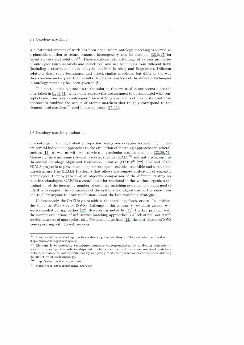
Let us suppose that we want to match a web service user description, such as: re-

questMap(Place, Format, Boundary, Vector Layers, Version), with the following web

service operation description: requestMap(Place(Position), Format, Bundary, Layers,

Edition). These descriptions can be represented as tree-like structures, respectively T1

and T2, as shown in Figure 1.

The first description requires the third argument of requestMap operation (For-

mat) to be matched to the third one (Format) of requestMap operation in the second

description. The value of Version in the first description must be passed to the sec-

ond web service operation as the Edition argument. Moreover, Boundary in T1 has

a corresponding label in T2, Bundary, which simulates errors and alterations that a

programmer could make while writing the service method signatures represented by

T2.

Fig. 1 Two web service descriptions (trees). Numbers before the labels of tree nodes are theirunique identifiers. In turn, the correspondences are expressed by arrows. By default, theirrelation is =; otherwise, these are mentioned above the arrows.

The purpose of structure-preserving semantic matching is to reduce semantic het-

erogeneity in web service user descriptions. Specifically, a semantic similarity measure

is used to estimate similarity between web service user descriptions under consider-

ation. This scenario poses additional constraints on conventional ontology matching.

In particular, we need to compute the correspondences holding among the full tree

structures and preserve certain structural properties of the trees under consideration.

Thus, the goal here is to have a structure-preserving semantic matching operation.

This operation takes two tree-like structures and produces a set of correspondences

between those nodes of the trees that correspond semantically to one another, (i) still

preserving a set of structural properties of the trees being matched, namely that func-

tions are matched to functions and variables to variables; and (ii) only in the case that

the trees are globally similar to one another, e.g., T1 is 0.71 similar to T2 according

to some measure.

The SPSM matching process is organized in two steps: (i) node matching (§3.2)

and (ii) tree matching (§3.3).

7

Node matching tackles the semantic heterogeneity problem by considering only labels

at nodes and domain specific contextual information of the trees. SPSM uses the S-

Match28 open source semantic matching system [15]. Technically, two nodes n1 and

n2 in trees T1 and T2 respectively, match if and only if: context1 R context2 holds

based on S-Match, where context1 and context2 are the concepts of the local ontologies

at nodes n1 and n2, and R represents the relation holding between the concepts of

the nodes n1 and n2, respectively. The relation R can be equivalence (=), less general

(⊑), more general (⊒) and disjointness (⊥). In particular, the key idea is that the

relations (R) between nodes are determined by (i) expressing the entities (concepts) of

the ontologies as logical formulas and (ii) reducing the matching problem to the logical

validity problem. Notice that the result of this stage is the set of correspondences that

hold between the nodes of the trees. For example, in Figure 1, that requestMap and

Version in T1 correspond to requestMap and Edition in T2, respectively.

Tree matching, in turn, exploits the results of the node matching and the structure

of the trees to find if these globally match each other. Technically, two trees T1 and

T2 approximately match if and only if there is at least one node n1i in T1 and node

n2j in T2 such that: (i) n1i matches n2j , (ii) all ancestors of n1i are matched to the

ancestors of n2j , where i = 1 . . . N1; j = 1 . . . N2;N1 and N2 are the number of nodes

in T1 and T2, respectively.

3.2 Node matching with S-Match

In this section we provide some further technical details on the node matching part of

SPSM as implemented in S-Match.

We adopted a semantic matching approach based on two key notions, namely Con-

cept of a label, which denotes the set of documents (data instances) that one would

classify under a label it encodes, and Concept at a node, which denotes the set of docu-

ments (data instances) that one would classify under a node, given that it has a certain

label and that it is in a certain position in a tree.

Consider, for example Figure 1; in what follows, “C” is used to denote concepts

of labels and concepts at nodes. Also “C1” and “C2” are used to distinguish between

concepts of labels and concepts at nodes in T1 and T2, respectively. Thus, in T1,

C1V ersion and C16 are, respectively, the concept of the label V ersion and the concept

at node 6. Finally, in order to simplify the presentation whenever it is clear from the

context, it is assumed that the formula encoding the concept of label is the label itself.

Thus, for example in T2, Edition6 is a notational equivalent of C2Edition.

The algorithm takes as inputs two tree-like structures and outputs a set of corre-

spondences in four macro steps. The first two steps represent the pre-processing phase.

The third and the fourth steps are the element level and structure level matching,

respectively.

Step 1. For all labels L in two trees, compute concepts of labels. The labels

at nodes are viewed as concise descriptions of the data that is stored under the nodes.

The meaning of a label at a node is computed by taking as input a label, by analyzing

its real-world semantics, and by returning as output a concept of the label, CL. Thus,

for example, CV ersion indicates a shift from the natural language ambiguous label

28 http://semanticmatching.org

8

V ersion to the concept CV ersion, which codifies explicitly its intended meaning, namely

the version of data. Technically, concepts of labels are codified as propositional logical

formulas [10]. For example, in this simple case, C1V ersion = 〈version, sensesWN#6〉,

where sensesWN#6 is a disjunction of six senses that WordNet [34]29 attaches to

version.

Step 2. For all nodes N in two trees, compute concepts at nodes. During this

step the meaning of the positions that the labels at nodes have in a tree is analyzed. By

doing this, concepts of labels are extended to concepts at nodes, CN . This is required to

capture the knowledge residing in the structure of a tree, namely the context in which

the given concept at label occurs. For example, in T1, by writing C5 it is meant the

concept describing the vector layers of the map request. Technically, concepts of nodes

are written in the same propositional logical language as concepts of labels. Thus,

following an access criterion semantics, the logical formula for a concept at node is

defined as a conjunction of concepts of labels located in the path from the given node

to the root. For example, C15 = RequestMap1 ⊓ V ector Layers1.

Step 3. For all pairs of labels in two trees, compute relations among atomic

concepts of labels. Relations between concepts of labels are computed with the help

of a library of several element level semantic matchers. These matchers take as input

two atomic30 concepts of labels and produce as output a semantic relation (e.g., =, ⊒)

between them. The algorithm includes some sense-based matchers, like WordNet-based

matcher, as well as string-based (syntactic) matchers, like Prefix, Suffix, Edit Distance,

Ngram. For example, Boundary = Bundary is returned by the Edit distance matcher.

Also, Version = Edition is returned by the WordNet matcher. In fact, according to

WordNet, Version is a synonym of Edition. The WordNet matcher computes equiva-

lence, more/less general, and disjointness relations. The result of this step is a matrix

of the relations holding between atomic concepts of labels of T1 and T2.

Step 4. For all pairs of nodes in two trees, compute relations among con-

cepts at nodes. During this step, initially the tree matching problem is reformulated

into a set of node matching problems. Then, each node matching problem is translated

into a propositional validity problem. Semantic relations are translated into proposi-

tional connectives: equivalence (=) into equivalence (↔), more general (⊒) and less

general (⊑) into implication (← and →, respectively), etc. The criterion for determin-

ing whether a relation holds between concepts at nodes is the fact that it is entailed

by the premises. Thus, it is necessary to prove that the following formula:

axioms −→ R(context1, context2) (1)

is valid, namely that it is true for all the truth assignments of all the propositional

variables occurring in it. context1 is the concept at node under consideration in tree 1,

while context2 is the concept at node under consideration in tree 2. R (within =, ⊑, ⊒,

⊥) is the semantic relation to be proved holding between context1 and context2. The

axioms part is the conjunction of all the relations (suitably translated) between atomic

concepts of labels mentioned in context1 and context2 (obtained as the result of Step

3). The validity of formula 1 is checked by proving that its negation is unsatisfiable by

using the standard DPLL-based SAT solver31.

29 http://wordnet.princeton.edu/30 For example, in Figure 1 all the labels are atomic (though involving multi-words), exceptrequestMap and V ector Layers, which are complex ones, see [15] for how these are handled.31 SAT4J: A satisfiability library for Java. http://www.sat4j.org/

9

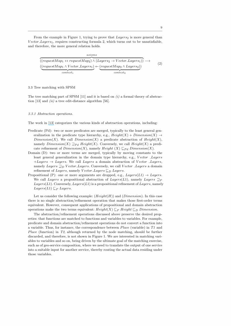
From the example in Figure 1, trying to prove that Layers2 is more general than

V ector Layers1, requires constructing formula 2, which turns out to be unsatisfiable,

and therefore, the more general relation holds.

axioms︷ ︸︸ ︷

((requestMap1 ↔ requestMap2) ∧ (Layers2 → V ector Layers1)) −→

((requestMap1 ∧ V ector Layers1)︸ ︷︷ ︸

context1

← (requestMap2 ∧ Layers2)︸ ︷︷ ︸

context2

)(2)

3.3 Tree matching with SPSM

The tree matching part of SPSM [11] and it is based on (i) a formal theory of abstrac-

tion [13] and (ii) a tree edit-distance algorithm [56].

3.3.1 Abstraction operations.

The work in [13] categorizes the various kinds of abstraction operations, including:

Predicate (Pd): two or more predicates are merged, typically to the least general gen-

eralization in the predicate type hierarchy, e.g., Height(X) + Dimension(X) →

Dimension(X). We call Dimension(X) a predicate abstraction of Height(X),

namely Dimension(X) ⊒Pd Height(X). Conversely, we call Height(X) a predi-

cate refinement of Dimension(X), namely Height (X) ⊑Pd Dimension(X).

Domain (D): two or more terms are merged, typically by moving constants to the

least general generalization in the domain type hierarchy, e.g., V ector Layers

+Layers → Layers. We call Layers a domain abstraction of V ector Layers,

namely Layers ⊒D V ector Layers. Conversely, we call V ector Layers a domain

refinement of Layers, namely V ector Layers ⊑D Layers.

Propositional (P): one or more arguments are dropped, e.g., Layers(L1) → Layers.

We call Layers a propositional abstraction of Layers(L1), namely Layers ⊒P

Layers(L1). Conversely, Layers(L1) is a propositional refinement of Layers, namely

Layers(L1) ⊑P Layers.

Let us consider the following example: (Height(H)) and (Dimension). In this case

there is no single abstraction/refinement operation that makes those first-order terms

equivalent. However, consequent applications of propositional and domain abstraction

operations make the two terms equivalent: Height(X) ⊑P Height ⊑D Dimension.

The abstraction/refinement operations discussed above preserve the desired prop-

erties: that functions are matched to functions and variables to variables. For example,

predicate and domain abstraction/refinement operations do not convert a function into

a variable. Thus, for instance, the correspondence between Place (variable) in T1 and

Place (function) in T2, although returned by the node matching, should be further

discarded, and therefore, is not shown in Figure 1. We are interested in matching vari-

ables to variables and so on, being driven by the ultimate goal of the matching exercise,

such as of geo-service composition, where we need to translate the output of one service

into a suitable input for another service, thereby routing the actual data residing under

those variables.

10

3.3.2 Global similarity measurement.

The key idea is to use abstractions / refinements because they allow the similarity

of two tree structures to be estimated through tree edit-distance operations. Tree

edit-distance is the minimum number of tree edit operations, namely node insertion,

deletion, replacement, required to transform one tree into another. The goal is to: (i)

minimize the editing cost, i.e., computation of the minimal cost composition of abstrac-

tions/refinements, (ii) allow only those tree edit operations that have their abstraction

theoretic counterparts in order to reflect semantics of the first-order terms.

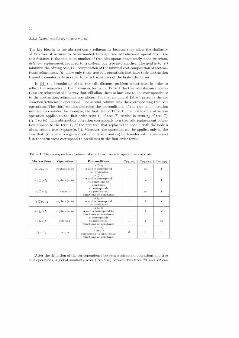
In [11] the formulation of the tree edit distance problem is restricted in order to

reflect the semantics of the first-order terms. In Table 1 the tree edit distance opera-

tions are reformulated in a way that will allow them to have one-to-one correspondence

to the abstraction/refinement operations. The first column of Table 1 presents the ab-

straction/refinement operations. The second column lists the corresponding tree edit

operations. The third column describes the preconditions of the tree edit operation

use. Let us consider, for example, the first line of Table 1. The predicate abstraction

operation applied to the first-order term t1 of tree T1 results in term t2 of tree T2(t1 ⊒Pd t2). This abstraction operation corresponds to a tree edit replacement opera-

tion applied to the term t1 of the first tree that replaces the node a with the node b

of the second tree (replace(a, b)). Moreover, the operation can be applied only in the

case that: (i) label a is a generalization of label b and (ii) both nodes with labels a and

b in the term trees correspond to predicates in the first-order terms.

Table 1 The correspondence between abstractions, tree edit operations and costs.

Abstractions Operation Preconditions CT1=T2 CT1⊑T2 CT1⊒T2

t1 ⊒Pd t2 replace(a, b)a ⊒ b;

a and b correspondto predicates

1 ∞ 1

t1 ⊒D t2 replace(a, b)

a ⊒ b;a and b correspond

to functions orconstants

1 ∞ 1

t1 ⊒P t2 insert(a)a correspondsto predicates,

functions or constants1 ∞ 1

t1 ⊑Pd t2 replace(a, b)a ⊑ b;

a and b correspondto predicates

1 1 ∞

t1 ⊑D t2 replace(a, b)a ⊑ b;

a and b correspond tofunctions or constants

1 1 ∞

t1 ⊑P t2 delete(a)a correspondsto predicates,

functions or constants1 1 ∞

t1 = t2 a = b

a = b;a and b

correspond to predicates,functions or constants

0 0 0

After the definition of the correspondence between abstraction operations and tree

edit operations, a global similarity score (TreeSim) between two trees T1 and T2 can

11

be computed as follows:

TreeSim(T1, T2) = max

0, 1−

min∑

i∈S

ni · Costi

max(N1, N2)

(3)

where, i is a set of tree edit operations, S is the set of allowed tree edit operations, ni

is the size of i, i.e., the number of i-th tree edit operation necessary to convert one tree

into the other as computed by the Tree edit-distance algorithm previously mentioned,

Costi is the cost of the i-th operation, and N1, N2 are the sizes of, respectively, T1 and

T2. Costi is defined in a way that models the semantic distance between T1 and T2.

In formula 3 the minimal edit-distance is divided by the size of the biggest tree and the

distance (denoting dissimilarity) is converted into a similarity score. Note that, when

the trees are very different, the number of tree edit distance operations can exceed the

size of the biggest tree. Thus, situations may occur where formula produces a negative

similarity value. In the SPSM implementation the negative values associated with the

measure are treated via zero substitutions. Also, when Costi is infinite (see Table 1),

TreeSim is estimated as zero.

In Table 1, SPSM assigned a unit cost to all operations that have their abstrac-

tion theoretic counterparts, while operations not allowed by definition of abstrac-

tions/refinements are assigned an infinite cost. Of course this strategy can be changed

to satisfy certain domain specific requirements. Moreover, the following three relations

between trees are considered: T1=T2, T1 ⊑ T2, and T1 ⊒ T2. The highest value of

TreeSim among T1 = T2, T1 ⊑ T2, and T1 ⊒ T2 is returned as the final similarity

score.

For the example of Figure 1, 6 node-to-node correspondences, 5 equivalence rela-

tions and 2 abstraction/refinement relations (insert(Place), replace(V ector Layers,

Layers)), were identified by the node matching algorithm. The biggest tree is T2 with

7 nodes. These are then used to compute TreeSim between T1 and T2 by exploiting

formula 3. Note that when Cost is equal to ∞ Treesim is estimated as 0. In our exam-

ple the TreeSim is 0.71 for both T1 = T2 and T1 ⊒ T2 (while it is 0 for T1 ⊑ T2 ).

The tree similarity value is used to select trees whose similarity value is greater than a

cut-off threshold. In our example the TreeSim is higher than the cut-off threshold of

0.6, and therefore, the two trees globally match as expected and the correspondences

connecting the nodes of the term trees can be further used for service composition

purposes32.

32 To obtain this result, we used a modified version of the SMatch package,release of 2010-10-09, available at http://semanticmatching.org/download.html:we set the Cost of each tree edit distance operation to 1.0 in the TreeEdit-Distance.java class, we configured the edit distance matcher threshold to 0.7(MatcherLibrary.MatcherLibrary.stringMatchers.EditDistanceOptimized.threshold =0.7 ) in the configuration file s-match-spsm-function.properties, and we config-ured the resulting matching file to show the similarity value (MappingRen-derer=it.unitn.disi.smatch.renderers.mapping.SimpleXMLMappingRenderer) in the con-figuration file s-match-spsm-function.properties.

12

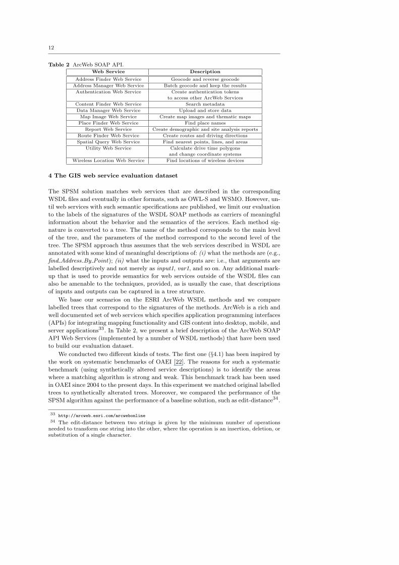
Table 2 ArcWeb SOAP API.

Web Service Description

Address Finder Web Service Geocode and reverse geocode

Address Manager Web Service Batch geocode and keep the results

Authentication Web Service Create authentication tokens

to access other ArcWeb Services

Content Finder Web Service Search metadata

Data Manager Web Service Upload and store data

Map Image Web Service Create map images and thematic maps

Place Finder Web Service Find place names

Report Web Service Create demographic and site analysis reports

Route Finder Web Service Create routes and driving directions

Spatial Query Web Service Find nearest points, lines, and areas

Utility Web Service Calculate drive time polygons

and change coordinate systems

Wireless Location Web Service Find locations of wireless devices

4 The GIS web service evaluation dataset

The SPSM solution matches web services that are described in the corresponding

WSDL files and eventually in other formats, such as OWL-S and WSMO. However, un-

til web services with such semantic specifications are published, we limit our evaluation

to the labels of the signatures of the WSDL SOAP methods as carriers of meaningful

information about the behavior and the semantics of the services. Each method sig-

nature is converted to a tree. The name of the method corresponds to the main level

of the tree, and the parameters of the method correspond to the second level of the

tree. The SPSM approach thus assumes that the web services described in WSDL are

annotated with some kind of meaningful descriptions of: (i) what the methods are (e.g.,

find Address By Point); (ii) what the inputs and outputs are: i.e., that arguments are

labelled descriptively and not merely as input1, var1, and so on. Any additional mark-

up that is used to provide semantics for web services outside of the WSDL files can

also be amenable to the techniques, provided, as is usually the case, that descriptions

of inputs and outputs can be captured in a tree structure.

We base our scenarios on the ESRI ArcWeb WSDL methods and we compare

labelled trees that correspond to the signatures of the methods. ArcWeb is a rich and

well documented set of web services which specifies application programming interfaces

(APIs) for integrating mapping functionality and GIS content into desktop, mobile, and

server applications33. In Table 2, we present a brief description of the ArcWeb SOAP

API Web Services (implemented by a number of WSDL methods) that have been used

to build our evaluation dataset.

We conducted two different kinds of tests. The first one (§4.1) has been inspired by

the work on systematic benchmarks of OAEI [22]. The reasons for such a systematic

benchmark (using synthetically altered service descriptions) is to identify the areas

where a matching algorithm is strong and weak. This benchmark track has been used

in OAEI since 2004 to the present days. In this experiment we matched original labelled

trees to synthetically alterated trees. Moreover, we compared the performance of the

SPSM algorithm against the performance of a baseline solution, such as edit-distance34.

33 http://arcweb.esri.com/arcwebonline34 The edit-distance between two strings is given by the minimum number of operationsneeded to transform one string into the other, where the operation is an insertion, deletion, orsubstitution of a single character.

13

In the second experiment (§4.2) we compared a manual classification (reference align-

ment) of our ArcWeb dataset with the unsupervised alignment produced by SPSM.

The evaluation was performed on a standard laptop Intel Centrino Core Duo CPU-

2Ghz with 2GB RAM and the Windows Vista (32bit, SP1) operating system, no ap-

plications were running except a single matching system.

4.1 The evolution scenario

Ontology and web service engineering practices suggest that often the underlying trees

to be matched are derived from one another using different kinds of operations in

order to change the syntax and the semantics of the original tree [11]. Therefore, it is

possible to compare one tree with another if it is derived from the original tree. We

evaluated SPSM following this approach in which we performed syntactic and semantic

alterations of tree nodes, with a random probability ranging in [0.1. . . 0.9]. Probability

values outside this range produce either too similar (< 0.1) or too different (> 0.9)

trees to the original ones, and hence, are out of our interest.

Initially, 80 trees were built from all the methods that implement the ESRI ArcWeb

SOAP APIs (see Table 2). Each ArcWeb Web Service corresponds to a WSDL file,

which in turn, contains the operations that implement 80 ESRI ArcWeb methods.

Some examples include:

– find Address By Point(point, address Finder Options, part),– get Distance(location1, location2, num Points, return Geometry, token, units),

– convert Map Coords To Pixel Coords(map Area, map Size, map Coords, token).

Then, 20 altered trees were automatically generated for each original tree and for each

alteration probability. Pairs, composed of the original tree and one varied tree, were

then used as input to SPSM. The alteration operations were applied to node names

being composed of labels using the following four alteration categories (the underscored

labels indicate modifications):

1. Replace a node name with an unrelated node name: the purpose of this

alteration is to check if the algorithm correctly detects unrelated concepts, thereby

resulting in a low similarity score. For example, the similarity score between two

terms, such as door and planet or between point and atom firmer, should be low.

In the implementation of these types of alterations a node name was replaced with

an unrelated node name randomly selected from a generic dictionary. We used

the Brown corpus35, a standard corpus of present-day American English36. Some

examples include:

– Original tree:

find Address By Point(point, address Finder Options, part)

– Modified tree:

find Address By Point(atom firmer, discussion, part)

35 http://icame.uib.no/brown/bcm.html36 The BROWN CORPUS contains 1 million words, so the probability of obtaining a relatedword is relatively low. If, for example, a word had 100 related terms, the probability to have arelated term is 1/10000. So we could say that the replacement is indeed with a “probabilisticallyunrelated word”.

14

2. Add or remove a label in a node name: the label of a node name was either

dropped or added. A label was dropped only if the node name contained more than

one label. The addition of a label to node names was performed randomly using

words extracted from the Brown corpus. Some examples include:

– Original tree:

find Address By Point(point,address Finder Options,part)

– Modified tree:

find By Point(toast point, address Milledgeville Finder Options, part)

3. Alter a label syntactically: This test aimed at mimicking potential misspellings

of the node labels. First we decided (randomly) whether or not to modify a node

name. Then, we randomly selected the set of labels to be modified and, for each

word, we randomly selected how to modify it using three types of alterations:

character dropped, added, or changed. The maximum number of alterations is not

greater than the total number of letters in a given word and the exact number of

changes depends on the probability of changing the letters. Some examples include:

– Original tree:

find Address By Point(point,address Finder Options,part)

– Modified tree:

finm Address By Poioat(einqt,ddress Finder Optxions,vparc)

4. Replace a label in a node name with a related one (synonyms, hyponyms,

and hypernyms): this test aimed at simulating the selection of a method whose

meaning was similar (equivalent, more general or less general) to the original one.

In the example below, find and locate are synonyms. In the implementation of these

types of alterations we used a number of generic sources including WordNet 3.0 and

Moby37. Some examples include:

– Original tree:

find Address By Point(point,address Finder Options,part)

– Modified tree:

locate Address By Point(place, address Finder Options, part)

We implemented evaluation tests to explore the robustness of the SPSM approach

towards both typical syntactic alterations (i.e., random replacements of node names,

modification of node names and misspellings) and typical semantic alterations (i.e.,

deterministic usage of synonyms, hyponyms) of node names.

4.2 The classification scenario

In this scenario, we investigated the capability of the SPSM algorithm in the unsuper-

vised aggregation of a set of meaningful-related web service methods. The evaluation

setup corresponds to a manual classification (reference alignment) of a selected set of

50 ArcWeb service methods. These 50 methods are a subset of the methods considered

in the evolution scenario (§4.1). The subset was obtained following the step 2 of the

construction procedure, which is as follows:

1. Manual classification of the set of methods conforming to the WSDL file description

of the methods.

37 http://www.mobysaurus.com

15

2. Deletion of some general (valid for all the groups) methods, for instance, get Info

(data Sources, token); which do not contribute to method-specific information of

the classification process.

3. Refinement of the classification by logically regrouping some methods, e.g., find

Place(place Name, place Finder Options, token) was grouped together with the

address finder set of methods.

Table 3 summarizes the number of operations of each group of the reference align-

ment (columns) for each original ArcWeb WSDL file (rows). We, thus, compare each

method with all the other methods in the dataset.

Table 3 Reference alignment of ArcWeb services.

GeoCoding Map Data Spatial Map Coordinate Map

and pixel manag. query image graphic transf.

routing conv. transf.

Addressfinder 4 - - - - - -

Addressmanager - 4 - - - - -Data

manager - - 12 - - - -Mapimage - 2 - - 11 - -Placefinder 1 - - - - - -Routefinder 1 - - - - - -Spatialquery - - - 3 - - -Utility 2 - - - - 5 3Wirelesslocation 2 - - - - - -

Finally, in Table 4 we summarize the following evaluation parameters: number of

methods, number of levels (tree depth), maximum and average number of nodes and

labels of the evaluation dataset.

Table 4 Summative statistics for the scenarios.

Test Number Maximum Maximum Average Maximum Average

case of WSDL number number number number number

number methods of levels of nodes of nodes of labels of labels

1 80 1 7 3.8 16 82 50 1 7 4.1 16 9

5 Evaluation method

We used standard measures such as precision, recall and F-measure to evaluate the

quality of the SPSM matching results [8]. Specifically, for both the experiments, we

based our calculation of these measures on the comparison of the correspondences

produced by a matching system (R) with the reference correspondences considered to

16

be correct (C). We also define the sets of true positives (TP), false positives (FP) and

false negatives (FN ) as, respectively, the set of the correct correspondences which have

been found, the set of the wrong correspondences which have been found and the set

of the correct correspondences which have not been found. Thus:

R = TP ∪ FP (4)

C = TP ∪ FN (5)

Precision, recall and F-measure are defined as follows:

– Precision: varies in the [0 . . . 1] range; the higher the value, the smaller the set of

false positives which have been computed. Precision is a measure of correctness and

it is computed as follows:

Precision =| TP |

| R |(6)

– Recall: varies in the [0 . . . 1] range; the higher the value, the smaller the set of true

positives which have not been computed. Recall is a measure of completeness and

it is computed as follows:

Recall =| TP |

| C |(7)

– F-measure: varies in the [0 . . . 1] range; it is global measure of the matching quality,

which increases when the matching quality increases. The version presented here

was computed as a harmonic mean of precision and recall:

F −measure =2 ∗Recall ∗ Precision

Recall + Precision(8)

5.1 The evolution scenario

Since we knew the generated tree alterations, it was possible to ‘ground truth’ the

results (or the expected similarity score, see Eq. 9), and hence, the reference results were

available for construction (see also [22]). This allowed the matching quality measures

to be computed.

Moreover, we assigned to each node a label that described the relation type with the

original node. Initially, we set the value of similarity to 1 and the value of the relation to

equivalent. Then each alteration operation, applied sequentially to each node, reduced

the similarity value and changed the relation value. The rate of the reduction and the

value of the relation were changed according to the following empirical rules38:

1. Replace a label with an unrelated label: when applied, we classified two nodes

as not related and we set the node score (Scorei in Eq. 9) to 0.

2. Add or remove a label in a node name: when applied, we reduced the current

node score (Scorei in Eq. 9) by 0.5. If the parent node was still related, we consid-

ered the initial node either more general (when the label was added) or less general

(when the label was removed) than the modified node. Some examples include:

38 The empirical rules have been designed one by one for each of the four alteration operations.The rationale behind these empirical rules is that the change rate discriminates clearly betweenthe cases. Reduction by 0.5 turned out to suffice based on some empirical preliminary testing.

17

– more general :

– Original node:

find Address By Point(part)

– Modified node (label added):

find disturbed Address By Point(part)

– less general :

– Original node:

find Address By Point(address Finder Options)

– Modified node (label removed):

find Address By Point(address Finder)

3. Alter a label syntactically: when applied, for each letter dropped, added or

changed, we empirically decreased the node score (Scorei in Eq. 9) by (0.5/(total

number of letters of the node label)). The total number of alterations is always

less than or equal to the total number of letters of the node label. We did not change

the relation value between the original node and the modified one.

4. Replace a label in a node name with a related one: when applied, if the

two nodes were related, we did not change the node score (Scorei in Eq. 9) if the

new label was a synonym. If the new label was a hypernym or a hyponym of the

original node, we changed the relation value to, respectively, less general and more

general and therefore we applied to the similarity value an empirical reduction of

0.539.

When all the alteration operations were applied, the expected similarity score (Ex-

pScore) between two trees T1 (the original one) and T2 (the modified one) that ranges

between [0 . . . 1] was computed as follows:

ExpScore(T1, T2) =

∑

i∈N

Scorei

N(9)

where i is the node number of both T1 and T2, and Scorei is the resulting similarity

value assigned to each node of T2. The expected similarity score is normalized by the

size of the biggest tree (N).

The reference correspondences, used to compute true positive and false positive

correspondences, were the altered trees whose expected similarity scores were higher

than an empirically fixed threshold (corrThresh). This empirically fixed threshold

separates the trees that a human user would, on average, consider as similar to the

original from those that are too different. Of course, this is subjective, although we

based our understanding on our previous ontology matching evaluations in the OAEI

campaigns.

We calculated the correspondences produced by the SPSM solution (R) and the

reference correspondences considered to be correct (C) as follows:

R = {T2 ∈ Res | TreeSim(T1, T2) ≥ cutoffThresh} (10)

39 The evaluation could be refined by considering the asymmetry of the similarities [54,43];since similarities are asymmetric (hypernyms are usually considered less similar to hyponymsthan the other way round), this empirical reduction could be 2-valued, depending on whetherthe relation changes to less general or more general. This line is viewed as future work.

18

C = {T2 ∈ Res | ExpScore(T1, T2) ≥ corrThresh} (11)

where ExpScore was computed for each modified tree (T2), TreeSim (see Eq. 3) was

the similarity score returned by the SPSM solution, cutoffThresh was the TreeSim

cut-off threshold and Res was, for each original tree T1, the set of the modified trees.

The set of true positive, false positive and false negative correspondences were

computed as follows:

TP = {T2 | T2 ∈ R ∧ T2 ∈ C} (12)

FP = {T2 | T2 ∈ R ∧ T2 /∈ C} (13)

FN = {T2 | T2 ∈ C ∧ T2 /∈ R} (14)

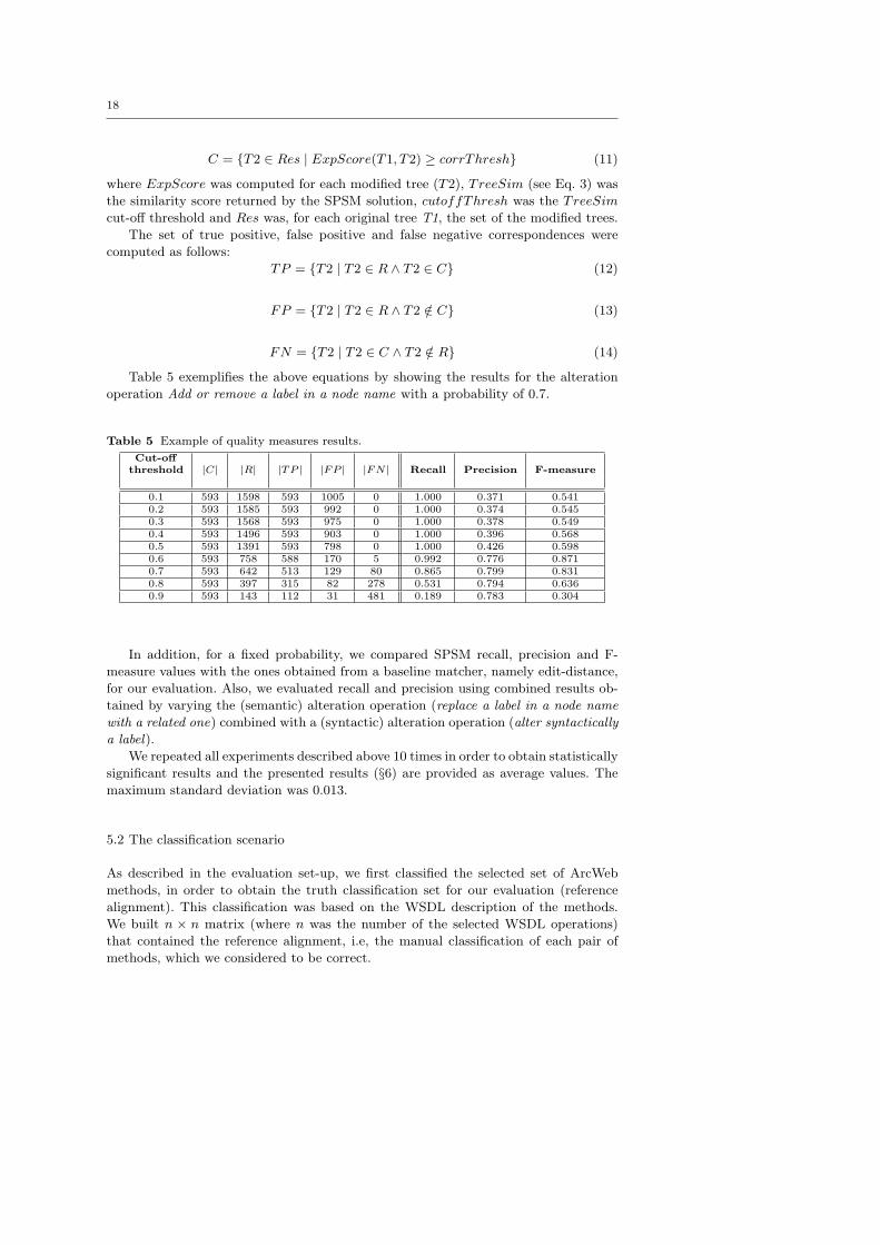
Table 5 exemplifies the above equations by showing the results for the alteration

operation Add or remove a label in a node name with a probability of 0.7.

Table 5 Example of quality measures results.

Cut-off

threshold |C| |R| |TP | |FP | |FN | Recall Precision F-measure

0.1 593 1598 593 1005 0 1.000 0.371 0.5410.2 593 1585 593 992 0 1.000 0.374 0.5450.3 593 1568 593 975 0 1.000 0.378 0.5490.4 593 1496 593 903 0 1.000 0.396 0.5680.5 593 1391 593 798 0 1.000 0.426 0.5980.6 593 758 588 170 5 0.992 0.776 0.8710.7 593 642 513 129 80 0.865 0.799 0.8310.8 593 397 315 82 278 0.531 0.794 0.6360.9 593 143 112 31 481 0.189 0.783 0.304

In addition, for a fixed probability, we compared SPSM recall, precision and F-

measure values with the ones obtained from a baseline matcher, namely edit-distance,

for our evaluation. Also, we evaluated recall and precision using combined results ob-

tained by varying the (semantic) alteration operation (replace a label in a node name

with a related one) combined with a (syntactic) alteration operation (alter syntactically

a label).

We repeated all experiments described above 10 times in order to obtain statistically

significant results and the presented results (§6) are provided as average values. The

maximum standard deviation was 0.013.

5.2 The classification scenario

As described in the evaluation set-up, we first classified the selected set of ArcWeb

methods, in order to obtain the truth classification set for our evaluation (reference

alignment). This classification was based on the WSDL description of the methods.

We built n × n matrix (where n was the number of the selected WSDL operations)

that contained the reference alignment, i.e, the manual classification of each pair of

methods, which we considered to be correct.

19

Let OP = {T1, T2, . . . , Tn} be the set of the trees that corresponds to the selected

methods. We defined the correspondences (C) considered to be correct as the subset of

the Cartesian product OP 2 = OP ×OP that corresponded to our reference alignment

(RefAlign):

C = {(Ti, Tj) ∈ OP 2|(Ti, Tj) ∈ RefAlign, 1 ≤ i ≤ n, 1 ≤ j ≤ n} (15)

In this test we compared the constructed manual classification of the selected web

service methods with those automatically obtained by the SPSM approach. Specifically:

– We compared each method signature with all the other signatures.

– We computed a similarity measure between each signature and all the other signa-

tures.

– We classified the methods depending on a given cut-off threshold.

We calculated the correspondences (R) produced by SPSM as follows:

R = {(Ti, Tj) ∈ OP 2|TreeSim(Ti, Tj) ≥ cutoffThresh, 1 ≤ i ≤ n, 1 ≤ j ≤ n} (16)

where TreeSim (see Eq. 3) was the similarity score returned by the SPSM solution

and cutoffThresh was the TreeSim cut-off threshold.

Then, we used SPSM to independently classify the same operations in an automatic

way. For each pair of methods, the SPSM algorithm returned a similarity measure

(TreeSim) that was compared to a cut-off threshold (cutoffThresh) in the range

[0.1 . . . 0.9]. If the similarity measure was higher than the cut-off threshold then the

pair was said to be similar. Finally, we compared the reference alignment with the

automatic classification performed by SPSM.

We computed recall, precision and F-measure, comparing the set of the relevant

(manual) classifications and the set of the retrieved (automatic) correspondences using

Eq. 6, 7, 8. The set of true positives (TP ) contained the pairs of methods which were

manually classified in the same group and whose similarity calculated as TreeSim was

greater than the cut-off threshold, see Eq. 17.

TP = {(Ti, Tj)|(Ti, Tj) ∈ R ∧ (Ti, Tj) ∈ C, 1 ≤ i ≤ n, 1 ≤ j ≤ n} (17)

The set of false positives (FP ) contained pairs of methods that were not manually

classified into the same group and whose (TreeSim) similarity score was greater than

the cut-off threshold, see Eq. 18.

FP = {(Ti, Tj)|(Ti, Tj) ∈ R ∧ (Ti, Tj) /∈ C, 1 ≤ i ≤ n, 1 ≤ j ≤ n} (18)

The set of false negatives (FN) contained pairs of the methods that were manually

classified into the same group but whose (TreeSim) similarity score was lower than

the cut-off threshold, see Eq. 19.

FN = {(Ti, Tj)|(Ti, Tj) ∈ C ∧ (Ti, Tj) /∈ R, 1 ≤ i ≤ n, 1 ≤ j ≤ n} (19)

For example, we manually classified the following pair of methods into the same

group:

find Address By Point(point, address Finder Options) and

find Location By Phone Number(phone Number, address Finder Options).

20

In this case, SPSM returned the TreeSim similarity score of 0.67. Then, if the

cut-off threshold was set to 0.6, the correspondence returned by SPSM would be a true

positive, and if it was set to 0.7, the correspondence returned by SPSM would be a

false negative.

6 Evaluation results

In this section we present the quality evaluation results for the evolution scenario (§6.2)

and the classification scenario (§6.2). We then present the performance evaluation

results (§6.3) and provide an evaluation summary (§6.4).

6.1 The evolution scenario

For each alteration operation, quality measures are functions of the TreeSim cut-off

threshold values. These are presented as recall, precision and F-measure 3D diagrams.

In all 3D graphs, we represent the variation of the probability of the alteration operation

on the Y axis, the used TreeSim cut-off threshold on the X axis and the resulting

measures of recall, precision and F-measure are on the Z axis. Moreover, in all reported

(the most salient) graphs, we used an empirically-fixed threshold corrThresh = 0.6.

We also investigated the variation of this empirically fixed threshold and we discuss

these results in the following subsections.

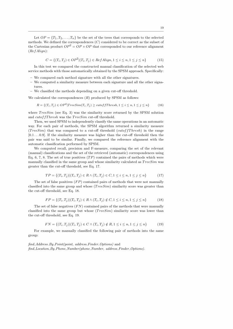
1. Replace a node name with an unrelated node name: this alteration opera-

tion replaced an entire node name with an unrelated one, randomly selected from

a thesaurus. Figures 2, 3 and 4 show the relationship between the variation of the

probability of the alteration operation, the variation of the used TreeSim cut-off

threshold and the resulting measures of recall, precision and F-measure.

Fig. 2 Recall for the Replace a node name with an unrelated one alteration.

Figures 2, 3 and 4 show that, for all probability alterations, the value of recall is

very high up to the TreeSim cut-off threshold (around 0.6), after which it drops

rapidly. Thus, we can say that, in our experiments, the SPSM approach retrieves

21

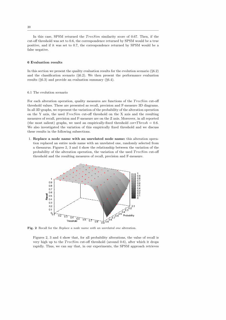
Fig. 3 Precision for the Replace a node name with an unrelated one alteration.

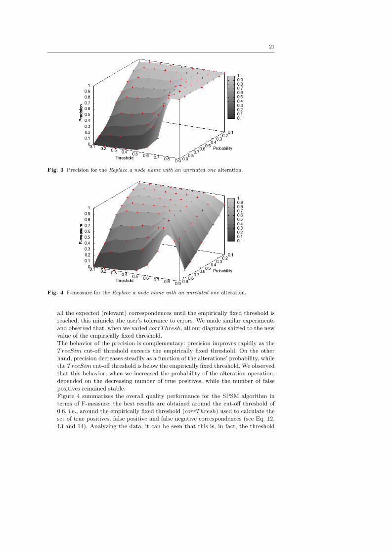
Fig. 4 F-measure for the Replace a node name with an unrelated one alteration.

all the expected (relevant) correspondences until the empirically fixed threshold is

reached, this mimicks the user’s tolerance to errors. We made similar experiments

and observed that, when we varied corrThresh, all our diagrams shifted to the new

value of the empirically fixed threshold.

The behavior of the precision is complementary: precision improves rapidly as the

TreeSim cut-off threshold exceeds the empirically fixed threshold. On the other

hand, precision decreases steadily as a function of the alterations’ probability, while

the TreeSim cut-off threshold is below the empirically fixed threshold. We observed

that this behavior, when we increased the probability of the alteration operation,

depended on the decreasing number of true positives, while the number of false

positives remained stable.

Figure 4 summarizes the overall quality performance for the SPSM algorithm in

terms of F-measure: the best results are obtained around the cut-off threshold of

0.6, i.e., around the empirically fixed threshold (corrThresh) used to calculate the

set of true positives, false positive and false negative correspondences (see Eq. 12,

13 and 14). Analyzing the data, it can be seen that this is, in fact, the threshold

22

where we can maximize the number of the true positive correspondences and min-

imize the number of the false positive correspondences. Even when the probability

of the alteration is very high, the balance between correctness and completeness

is good. For instance, at the optimal TreeSim cut-off threshold (0.6), for an al-

teration probability of 80%, the F-measure is higher than 74%. This suggests the

robustness of the SPSM approach for significant syntactic modifications in the node

names.

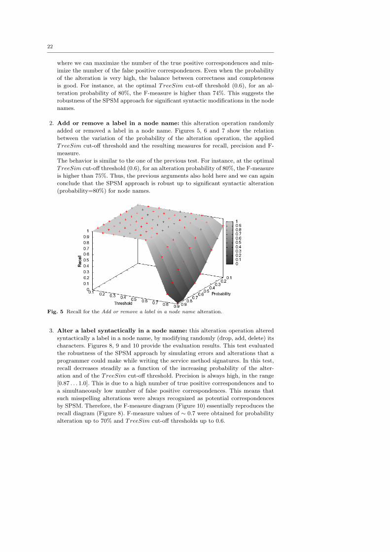
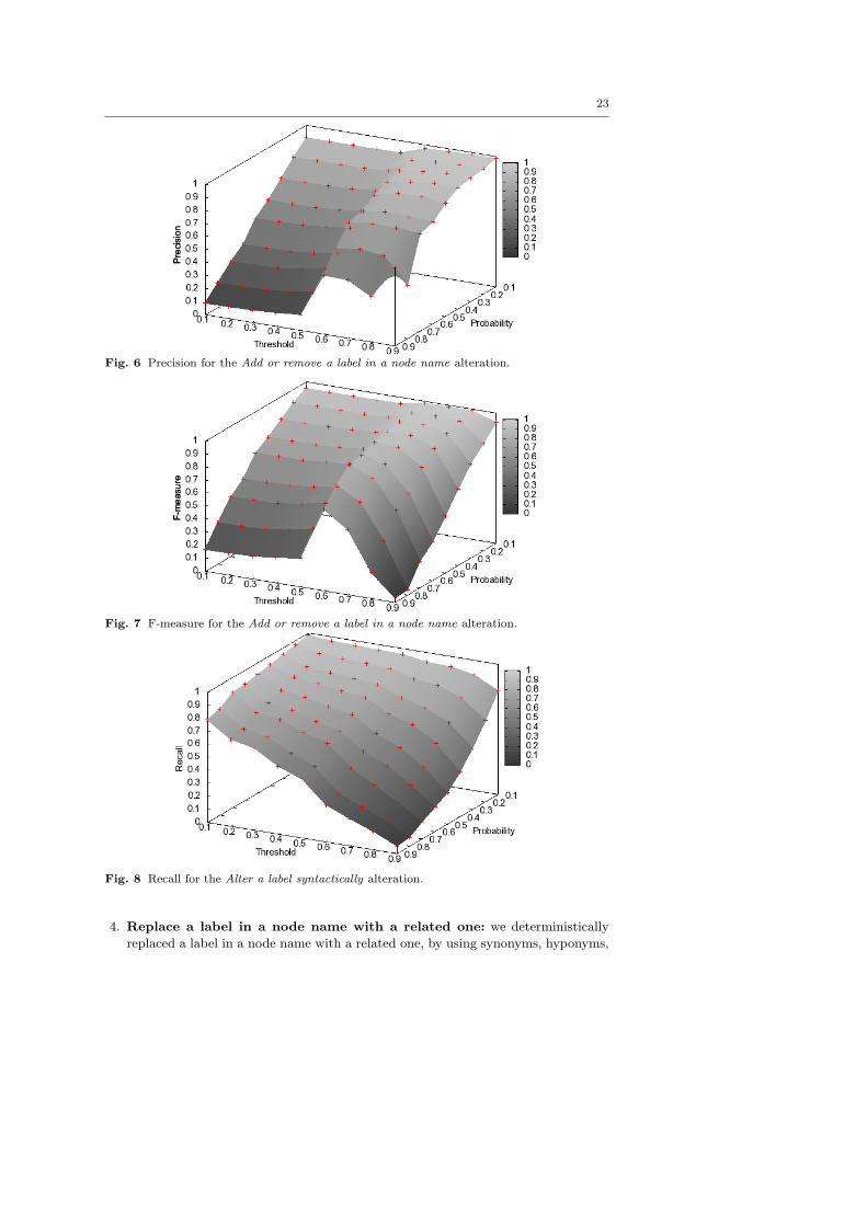
2. Add or remove a label in a node name: this alteration operation randomly

added or removed a label in a node name. Figures 5, 6 and 7 show the relation

between the variation of the probability of the alteration operation, the applied

TreeSim cut-off threshold and the resulting measures for recall, precision and F-

measure.

The behavior is similar to the one of the previous test. For instance, at the optimal

TreeSim cut-off threshold (0.6), for an alteration probability of 80%, the F-measure

is higher than 75%. Thus, the previous arguments also hold here and we can again

conclude that the SPSM approach is robust up to significant syntactic alteration

(probability=80%) for node names.

Fig. 5 Recall for the Add or remove a label in a node name alteration.

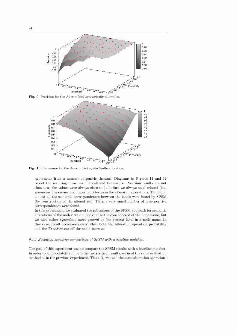
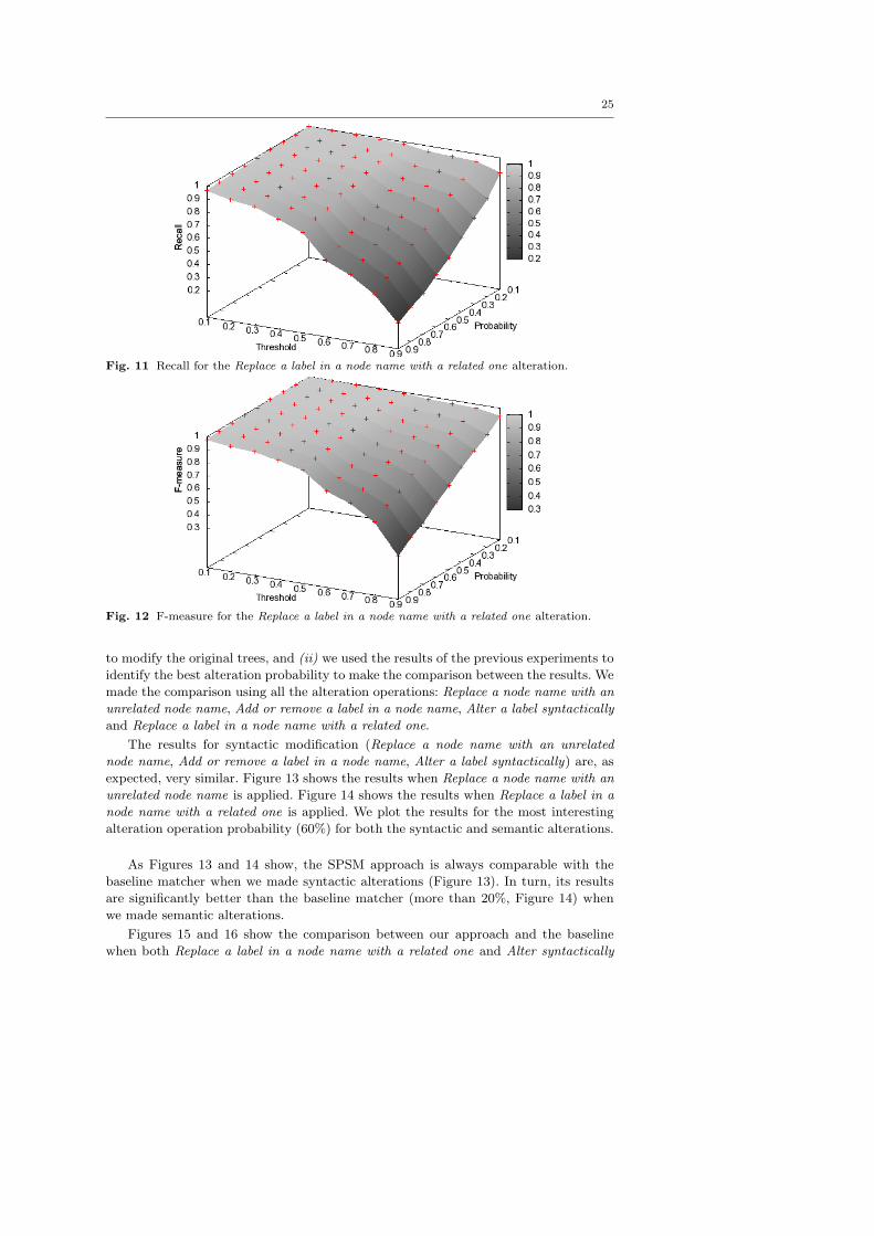
3. Alter a label syntactically in a node name: this alteration operation altered

syntactically a label in a node name, by modifying randomly (drop, add, delete) its

characters. Figures 8, 9 and 10 provide the evaluation results. This test evaluated

the robustness of the SPSM approach by simulating errors and alterations that a

programmer could make while writing the service method signatures. In this test,

recall decreases steadily as a function of the increasing probability of the alter-

ation and of the TreeSim cut-off threshold. Precision is always high, in the range

[0.87 . . . 1.0]. This is due to a high number of true positive correspondences and to

a simultaneously low number of false positive correspondences. This means that

such misspelling alterations were always recognized as potential correspondences

by SPSM. Therefore, the F-measure diagram (Figure 10) essentially reproduces the

recall diagram (Figure 8). F-measure values of ∼ 0.7 were obtained for probability

alteration up to 70% and TreeSim cut-off thresholds up to 0.6.

23

Fig. 6 Precision for the Add or remove a label in a node name alteration.

Fig. 7 F-measure for the Add or remove a label in a node name alteration.

Fig. 8 Recall for the Alter a label syntactically alteration.

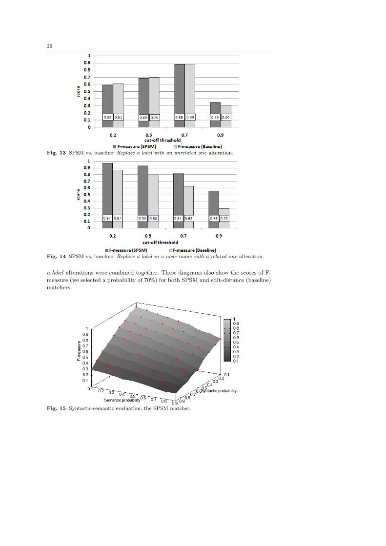
4. Replace a label in a node name with a related one: we deterministically

replaced a label in a node name with a related one, by using synonyms, hyponyms,

24

Fig. 9 Precision for the Alter a label syntactically alteration.

Fig. 10 F-measure for the Alter a label syntactically alteration.

hypernyms from a number of generic thesauri. Diagrams in Figures 11 and 12

report the resulting measures of recall and F-measure. Precision results are not

shown, as the values were always close to 1. In fact we always used related (i.e.,

synonyms, hyponyms and hypernym) terms in the alteration operations. Therefore,

almost all the semantic correspondences between the labels were found by SPSM

(by construction of the altered set). Thus, a very small number of false positive

correspondences were found.

In this experiment, we evaluated the robustness of the SPSM approach for semantic

alterations of the nodes: we did not change the core concept of the node name, but

we used either equivalent, more general or less general label in a node name. In

this case, recall decreases slowly when both the alteration operation probability

and the TreeSim cut-off threshold increase.

6.1.1 Evolution scenario: comparison of SPSM with a baseline matcher.

The goal of this experiment was to compare the SPSM results with a baseline matcher.

In order to appropriately compare the two series of results, we used the same evaluation

method as in the previous experiment. Thus: (i) we used the same alteration operations

25

Fig. 11 Recall for the Replace a label in a node name with a related one alteration.

Fig. 12 F-measure for the Replace a label in a node name with a related one alteration.

to modify the original trees, and (ii) we used the results of the previous experiments to

identify the best alteration probability to make the comparison between the results. We

made the comparison using all the alteration operations: Replace a node name with an

unrelated node name, Add or remove a label in a node name, Alter a label syntactically

and Replace a label in a node name with a related one.

The results for syntactic modification (Replace a node name with an unrelated

node name, Add or remove a label in a node name, Alter a label syntactically) are, as

expected, very similar. Figure 13 shows the results when Replace a node name with an

unrelated node name is applied. Figure 14 shows the results when Replace a label in a

node name with a related one is applied. We plot the results for the most interesting

alteration operation probability (60%) for both the syntactic and semantic alterations.

As Figures 13 and 14 show, the SPSM approach is always comparable with the

baseline matcher when we made syntactic alterations (Figure 13). In turn, its results

are significantly better than the baseline matcher (more than 20%, Figure 14) when

we made semantic alterations.

Figures 15 and 16 show the comparison between our approach and the baseline

when both Replace a label in a node name with a related one and Alter syntactically

26

Fig. 13 SPSM vs. baseline: Replace a label with an unrelated one alteration.

Fig. 14 SPSM vs. baseline: Replace a label in a node name with a related one alteration.

a label alterations were combined together. These diagrams also show the scores of F-

measure (we selected a probability of 70%) for both SPSM and edit-distance (baseline)

matchers.

Fig. 15 Syntactic-semantic evaluation: the SPSM matcher.

27

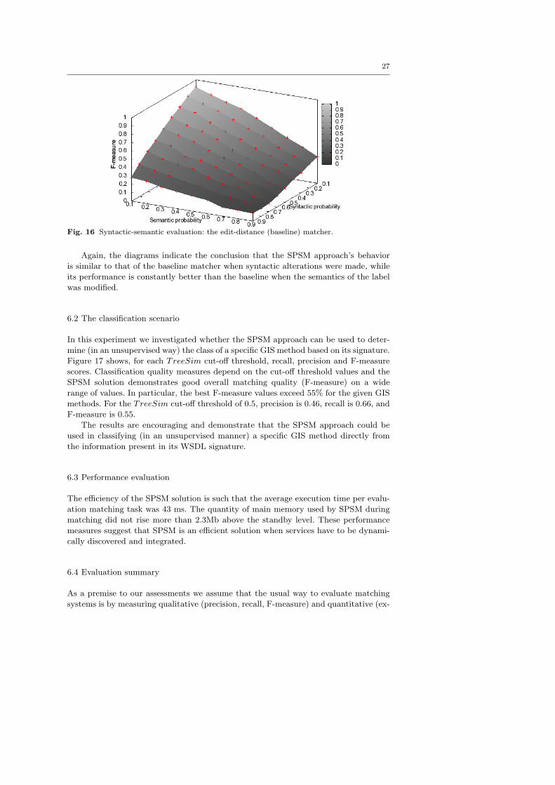
Fig. 16 Syntactic-semantic evaluation: the edit-distance (baseline) matcher.

Again, the diagrams indicate the conclusion that the SPSM approach’s behavior

is similar to that of the baseline matcher when syntactic alterations were made, while

its performance is constantly better than the baseline when the semantics of the label

was modified.

6.2 The classification scenario

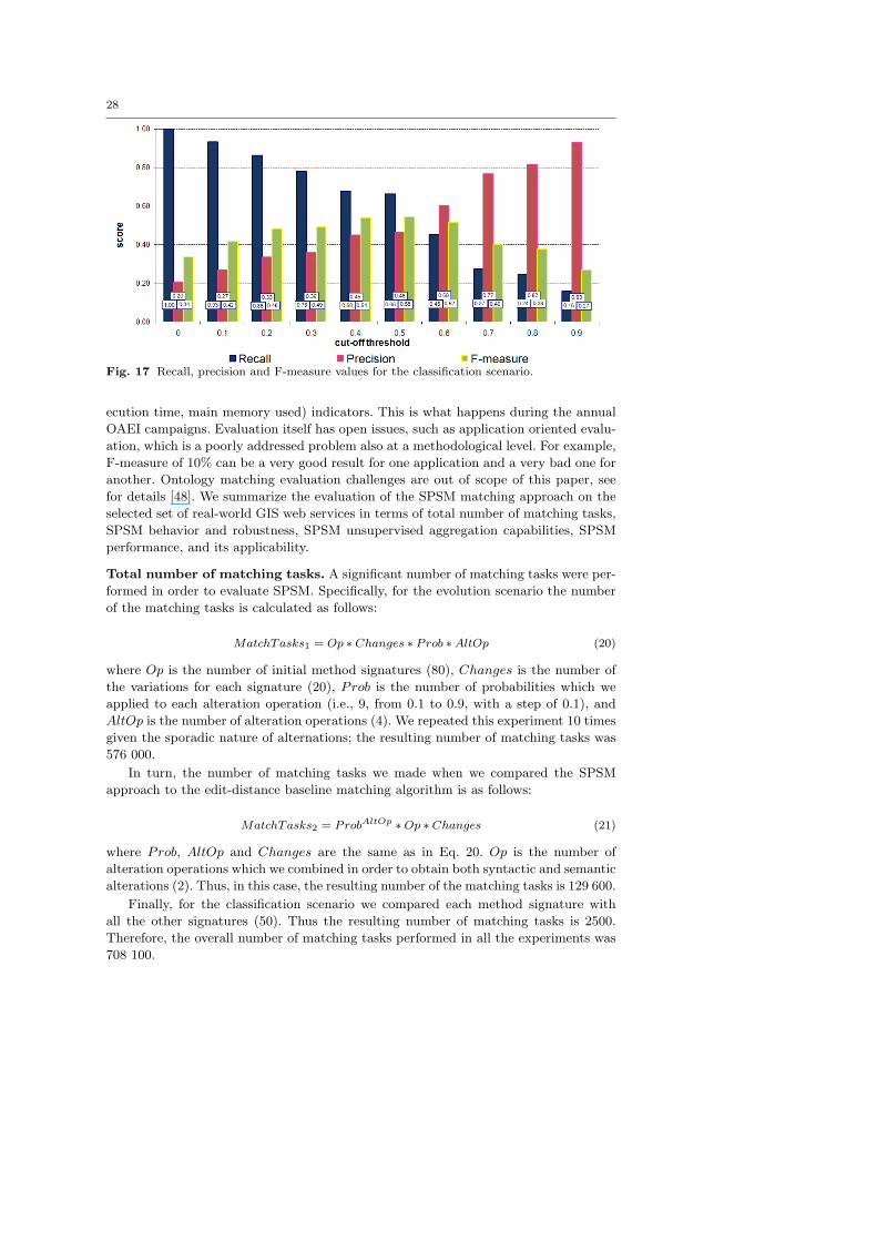
In this experiment we investigated whether the SPSM approach can be used to deter-

mine (in an unsupervised way) the class of a specific GIS method based on its signature.

Figure 17 shows, for each TreeSim cut-off threshold, recall, precision and F-measure

scores. Classification quality measures depend on the cut-off threshold values and the

SPSM solution demonstrates good overall matching quality (F-measure) on a wide

range of values. In particular, the best F-measure values exceed 55% for the given GIS

methods. For the TreeSim cut-off threshold of 0.5, precision is 0.46, recall is 0.66, and

F-measure is 0.55.

The results are encouraging and demonstrate that the SPSM approach could be

used in classifying (in an unsupervised manner) a specific GIS method directly from

the information present in its WSDL signature.

6.3 Performance evaluation

The efficiency of the SPSM solution is such that the average execution time per evalu-

ation matching task was 43 ms. The quantity of main memory used by SPSM during

matching did not rise more than 2.3Mb above the standby level. These performance

measures suggest that SPSM is an efficient solution when services have to be dynami-

cally discovered and integrated.

6.4 Evaluation summary

As a premise to our assessments we assume that the usual way to evaluate matching

systems is by measuring qualitative (precision, recall, F-measure) and quantitative (ex-

28

Fig. 17 Recall, precision and F-measure values for the classification scenario.

ecution time, main memory used) indicators. This is what happens during the annual

OAEI campaigns. Evaluation itself has open issues, such as application oriented evalu-

ation, which is a poorly addressed problem also at a methodological level. For example,

F-measure of 10% can be a very good result for one application and a very bad one for

another. Ontology matching evaluation challenges are out of scope of this paper, see

for details [48]. We summarize the evaluation of the SPSM matching approach on the

selected set of real-world GIS web services in terms of total number of matching tasks,

SPSM behavior and robustness, SPSM unsupervised aggregation capabilities, SPSM

performance, and its applicability.

Total number of matching tasks. A significant number of matching tasks were per-

formed in order to evaluate SPSM. Specifically, for the evolution scenario the number

of the matching tasks is calculated as follows:

MatchTasks1 = Op ∗ Changes ∗ Prob ∗AltOp (20)

where Op is the number of initial method signatures (80), Changes is the number of

the variations for each signature (20), Prob is the number of probabilities which we

applied to each alteration operation (i.e., 9, from 0.1 to 0.9, with a step of 0.1), and

AltOp is the number of alteration operations (4). We repeated this experiment 10 times

given the sporadic nature of alternations; the resulting number of matching tasks was

576 000.

In turn, the number of matching tasks we made when we compared the SPSM

approach to the edit-distance baseline matching algorithm is as follows:

MatchTasks2 = ProbAltOp ∗Op ∗ Changes (21)

where Prob, AltOp and Changes are the same as in Eq. 20. Op is the number of

alteration operations which we combined in order to obtain both syntactic and semantic

alterations (2). Thus, in this case, the resulting number of the matching tasks is 129 600.

Finally, for the classification scenario we compared each method signature with

all the other signatures (50). Thus the resulting number of matching tasks is 2500.

Therefore, the overall number of matching tasks performed in all the experiments was

708 100.

29

SPSM behavior and robustness. We developed evaluation tests to explore the

overall behavior and robustness of the SPSM approach for both typical syntactic and

semantic alterations of the GIS service method signatures. All experiments demon-

strated the capability of the SPSM approach to self-adapt (i.e., to provide best results)

to the empirical threshold (ExpScore) that was used in the experiments to simulate

the users’ tolerance to errors (i.e., to calculate the set of true positive, false positive

and false negative correspondences). Moreover, the results showed the robustness of the

SPSM algorithm over significant ranges of parameter variation (cut-off thresholds and

the probability of alteration operations); while maintaining relatively high (depending

on the experiment, over 50-60%) overall matching relevance quality (F-measure).

Comparison with a baseline matcher (edit-distance) showed how the SPSM ap-

proach is always comparable with the baseline when only syntactic alteration are con-

sidered, whereas SPSM results were always better (in average more than 20%) when

semantic alterations were introduced. This is exactly what one would expect, since

the SPSM approach includes a number of state-of-the-art syntactic matchers (that are

first used in the internal matching algorithm) plus a number of semantic matchers that

enter into play for the alterations in the meaning of node labels [11].

In general, based on our past experience with OAEI and evaluation of matching,

when a matching system is applied for the first time to a new domain, the F-measure

of the results is low, about 25 − 30%. In our case we have obtained a quality level of

matching results, with values of over 55% (good) and 80% (excellent). This is rarely

obtained by automatic matching systems without specific tuning. In an application

oriented setting, values of 30%, 50% should be checked as to how these actually con-

tribute to the final goal of the application in an end-to-end integration process, what

we view as future work.

SPSM unsupervised aggregation capabilities. In the classification scenario ex-

periment, we investigated how the proposed SPSM approach could be used in determin-

ing (in an unsupervised manner) the class of a specific GIS method directly from the

information present in its WSDL method signature. Classification quality measures de-

pended on the cut-off threshold values and the SPSM solution demonstrated an overall

good matching quality. In particular, the best F-measure values exceeded 55% for the

given GIS methods set. Although the results are encouraging, 45% of the GIS methods

were incorrectly classified, due to the limited information presented in the signatures.

In this case, the presence of more informative and semantically structured annota-

tion would significantly improve the automatic classification at the obvious expense of

greater designer/programmer effort.

SPSM performance. Based on all our experiments, the efficiency of the SPSM so-

lution is promising since the average execution time per matching task was 43 ms and

the quantity of main memory used was less than 2.3 Mb compared to the standby level

for 700 000 matching operations.

Applicability. A critical step in the process of reusing existing WSDL-specified ser-

vices for building web-based applications is the discovery of potentially relevant ser-

vices. Web service catalogs, like the Universal Description, Discovery, and Integration

servers, publish WSDL specifications according to categories of business activities. The

discovery of web services based on this classification method is insufficient because it

relies on the shared common-sense understanding of the application domain by the

developers who publish and consume the specified services.

30

SPSM can be used to support a more automated discovery and use of web ser-

vices. This can be achieved by distinguishing between potentially useful and possibly

irrelevant services, and by ordering the potentially useful ones according to their rele-

vance. To assess the similarity between two web services, SPSM utilizes the semantics

of their operations and we could use the SPSM approach in different stages of web

service integration: (i) during the initial phase (e.g., for the discovery of web services)

we can consider how close the similarity between two returned signatures (or between

a partial specification and a real world web service signature) is to a perfect score,

(ii) during the subsequent phase (e.g., composition or coordination of web services) we

can use the correspondences between signatures to chain input and output parameters

of the matched web services. For example, for geo-information catalogs, like the OGC

Catalogue Service, SPSM could be applied to discover and chain geo-services from cat-

alogs of geospatial information and related resources. SPSM could also be applied in

semi-supervised discovery and composition of geo-processing services which follow the

WPS specifications. These specifications include guidelines on how to publish process-

ing services that perform modeling, calculation and the elaboration of both vector and

raster geo-data.

7 Conclusions and future work

In this paper we have tackled the semantic heterogeneity problem in geo-service ap-

plications. We presented an evaluation of the structure-preserving semantic matching

approach as a practical solution to the semantic heterogeneity problem between dif-

ferent implementations of various geo-services. Specifically, we conducted an extensive

set of empirical tests to evaluate the quality and efficiency indicators of the SPSM ap-

proach. We based our tests on a set of real ArcWeb WSDL methods. The overall quality

(F-measure) of the results of the experiments is encouraging. Moreover, we obtained a

small memory footprint and good matching speed for these tasks. This suggests that

SPSM could be employed to find similar web service implementations at run-time.

Future work includes experimenting with other sources of background knowledge

used to enhance automated matching. Recent evaluations of matching systems, such as

those conducted by OAEI as well as individual evaluations in [12,14], show that lack

of background knowledge, most often domain specific, is one of the key problems of

matching systems. Various sources could be used as background knowledge, see, e.g.,

[16,52,41]. We also plan to proceed by:

– Conducting comparative evaluation, including other kinds of GIS web services (like

the ones available from the OGC specifications and the GRASS package) and with

the other available matching systems handling web services, such as in [51].

– Performing qualitative evaluation on real applications, such as matching the GEMET

thesaurus to the INSPIRE thematic classification; this includes building the corre-

sponding reference alignment (which is a time consuming exercise [14]) in order to

measure precision and recall of the matching results.

– Using different kinds of thesauri (for example, GEMET or AGROVOC) to support

multilingual matching.

– Including location related issues and topological relationships between spatial fea-

tures, thereby extending the SPSM approach.

– Adding specific geographic thesauri, such as GEMET and the INSPIRE concept

dictionary, to the reference thesaurus (WordNet).

31

– Comparing the SPSM approach to other ontology matching systems, such as COMA++

[3] and FALCON [19].

Acknowledgments. We thank Fausto Giunchiglia, Fiona McNeill, Mikalai Yatskevich and

Aliaksandr Autayeu for many fruitful discussions on the structure-preserving semantic match-

ing. This work has been partly supported by the FP6 OpenKnowledge European STREP

project (FP6-027253). The second author appreciates support from the Trentino as a Lab

(TasLab) initiative of the European Network of the Living Labs at Informatica Trentina.

References

1. R. Aggarwal, K. Verma, J. Miller, andW. Milnor. Constraint driven web service compositionin METEOR-S. In Proc. of the 1st IEEE International Conference of Services Computing(SCC), pages 23–30, 2004.

2. G. Antoniou and F. van Harmelen. Web Ontology Language: OWL. Springer, 2003.3. D. Aumuller, H.-H. Do, S. Maßmann, and E. Rahm. Schema and ontology matching withCOMA++. In Proc. 24th International Conference on Management of Data (SIGMOD),Software Demonstration, pages 906–908, 2005.

4. L. Bernard, M. Craglia, M. Gould, and W. Kuhn. Towards an SDI research agenda. In Proc.of the 11th European Commission-Geographic Information (EC-GI) and GIS Workshop,pages 147–151, 2005.

5. Y. Breitbart. Multidatabase interoperability. SIGMOD Record, 19(3):53–60, 1990.6. L. Di, P. Zhao, W. Yang, and P. Yue. Ontology-driven automatic geospatial-processingmodeling based on web-service chaining. In Proc. of the 6th Earth Science TechnologyConference (ESTC) - CDROM, 2006.

7. M. J. Egenhofer. Toward the semantic geospatial web. In Proc. of the 10th ACM Symposiumon Advances in Geographic Information Systems, pages 1–4, 2002.

8. J. Euzenat and P. Shvaiko. Ontology matching. Springer, 2007.9. R. Fileto, L. Liu, C. Pu, E. D. Assad, and C. B. Medeiros. Poesia: An ontological workflowapproach for composing web services in agriculture. The VLDB Journal, 12(4):352–367,2003.

10. F. Giunchiglia, M. Marchese, and I. Zaihrayeu. Encoding classifications into lightweightontologies. Journal of Data Semantics, VIII:57–81, 2007.

11. F. Giunchiglia, F. McNeill, M. Yatskevich, J. Pane, P. Besana, and P. Shvaiko. Approxi-mate structure-preserving semantic matching. In Proc. of the 7th Conference on Ontologies,DataBases, and Applications of Semantics (ODBASE), pages 1234–1237, 2008.

12. F. Giunchiglia, P. Shvaiko, and M. Yatskevich. Discovering missing background knowledgein ontology matching. In Proc. of the 17th European Conference on Artificial Intelligence(ECAI), pages 382–386, 2006.

13. F. Giunchiglia and T. Walsh. A theory of abstraction. Artificial Intelligence, 57(2-3):323–389, 1992.

14. F. Giunchiglia, M. Yatskevich, P. Avesani, and P. Shvaiko. A large scale dataset forthe evaluation of ontology matching systems. The Knowledge Engineering Review Journal,24(2):137–157, 2009.

15. F. Giunchiglia, M. Yatskevich, and P. Shvaiko. Semantic matching: Algorithms and im-plementation. Journal on Data Semantics, IX:1–38, 2007.

16. R. Gligorov, Z. Aleksovski, W. ten Kate, and F. van Harmelen. Using google distance toweight approximate ontology matches. In Proc. of the 16th International World Wide WebConference (WWW), pages 767–775, 2007.

17. M. Gone and S. Shade. Towards semantic composition of geospatial web services usingWSMO in comparison to BPEL. In Proc. of the 5th Geographic Information Day - YoungResearchers Forum, pages 43–63, 2007.

18. R. Groot and J. McLaughlin. Geospatial Data Infrastructure: Concepts, Cases and GoodPractice. Oxford University Press, 2000.

19. W. Hu and Y. Qu. Falcon-ao: A practical ontology matching system. Journal of WebSemantics, 6(3):237– 239, 2008.

20. K. Janowicz, C. Keßler, M. Schwarz, M. Wilkes, I. Panov, M. Espeter, and B. Baumer.Algorithm, implementation and application of the SIM-DL similarity server. GeoSpatialSemantics, LNCS 4853:128–145, 2007.

32

21. K. Janowicz, M. Wilkes, and M. Lutz. Similarity-based information retrieval and its rolewithin spatial data infrastructures. Geographic Information Science, LNCS 5266:151–167,2008.

22. A. F. Jerome Euzenat, L. Hollink, A. Isaac, C. Joslyn, V. Malaise, C. Meilicke, A. Nikolov,J. Pane, M. Sabou, F. Scharffe, P. Shvaiko, V. Spiliopoulos, H. Stuckenschmidt, O. SvabZamazal, V. Svatek, C. T. dos Santos, G. Vouros, and S. Wang. Results of the ontologyalignment evaluation initiative 2009. In Proc. of the 4th Ontology Matching (OM) Workshopat the International Semantic Web Conference (ISWC), pages 73–119, 2009.

23. V. Kashyap and A. Sheth. Semantic heterogeneity in global information systems: Therole of metadata, context and ontologies. In M. Papazoglou and G. Schlageter, editors,Cooperative Information Systems, pages 139–178. Academic Press, 1998.

24. M. Klein. Combining and relating ontologies: an analysis of problems and solutions. InProc. of the Workshop on Ontologies and Information Sharing at the International JointConference on Artificial Intelligence (IJCAI), 2001.

25. M. Klusch, B. Fries, and K. Sycara. Automated semantic web service discovery withOWLS-MX. In Proc. of the 4th International Joint Conference on Autonomous Agents andMultiagent Systems (AAMAS), pages 915–922, 2006.

26. W. Kuhn. Geospatial semantics: Why, of what, and how? Journal on Data Semantics,special issue on Semantic-based Geographical Information Systems, LNCS 3534:1–24, 2005.

27. R. Lemmens, A. Wytzisk, R. de By, C. Granell, M. Gould, and P. van Oosterom. In-tegrating semantic and syntactic descriptions to chain geographic services. IEEE InternetComputing, 10(5):42–52, 2006.

28. M. Lutz and E. Klien. Ontology-based retrieval of geographic information. InternationalJournal of Geographic Information Science, 20(3):233–260, 2006.

29. M. Lutz, R. Lucchi, A. Friis-christensen, and N. Ostlander. A rule-based descriptionframework for the composition of geographic information services. Geospatial Semantics,LNCS 4853:114–127, 2007.

30. M. Marchese, L. Vaccari, P. Shvaiko, and J. Pane. An application of approximate ontologymatching in eResponse. In Proc. of the 5th International Conference on Information Systemsfor Crisis Response and Management (ISCRAM), pages 294–304, 2008.

31. D. Martin, M. Burstein, J. Hobbs, O. Lassila, D. McDermott, S. McIlraith, S. Narayanan,M. Paolucci, B. Parsia, T. Payne, E. Sirin, N. Srinivasan, and K. Sycara. OWL-S: SemanticMarkup for Web Services. W3C Submission, 2004.

32. I. Masser. Creating Spatial Data Infrastructures. ESRI Press, 2005.33. R. Mikhaiel and E. Stroulia. Examining usage protocols for service discovery. In Proc. ofthe 4th International Conference on Service Oriented Computing (ICSOC), pages 496–502,2006.

34. G. A. Miller. Wordnet: A lexical database for english. Communications of the ACM,38(11):39–41, 1995.

35. D. Nebert. Developing Spatial Data Infrastructures. The SDI CookBook. Global SpatialData Infrastructure (GSDI), 2004.

36. N. F. Noy. Semantic integration: A survey of ontology-based approaches. SIGMOD Record,33(4):65–70, 2004.

37. T. L. Nyerges. Schema integration analysis for the development of GIS databases. Inter-national Journal of Geographical Information Systems, 3(2):153–183, 1989.

38. H. Onsrud. Research and Theory in Advancing Creating Spatial Data Infrastructure Con-cepts. ESRI Press, 2007.

39. S. Oundhakar, K. Verma, K. Sivashanmugam, A. Sheth, and J. Miller. Discovery of webservices in a multi-ontology and federated registry environment. International Journal ofWeb Services Research, 2(3):1–32, 2005.

40. M. Paolucci, T. Kawamura, T. R. Payne, and K. Sycara. Semantic matching of webservices capabilities. In Proc. of the 1st International Semantic Web Conference (ISWC),pages 333–347, 2002.

41. J. Partyka, N. Alipanah, L. Khan, B. M. Thuraisingham, and S. Shekhar. Content-basedontology matching for GIS datasets. In Proc. of the 16th International Symposium onAdvances in Geographic Information Systems (ACM-GIS), 2008.

42. C. Petrie, T. Margaria, U. Kuster, H. Lausen, and M. Zaremba. Sws challenge: Status,perspectives, and lessons learned so far. In Proc. of the 9th International Conference onEnterprise Information Systems (ICEIS), pages 447–452, 2007.

43. M. A. Rodrıguez and M. J. Egenhofer. Comparing geospatial entity classes: an asym-metric and context-dependent similarity measure. International Journal of GeographicalInformation Science, 18(3):229–256, 2004.

33

44. D. Roman, U. K. H. Lausen, J. de Bruijn, R. Lara, M. Stollberg, A. Polleres, D. Fensel,and C. Bussler. Web service modeling ontology (WSMO). Applied Ontology, 1(1):77–106,2005.

45. S. Schulte, J. Eckert, N. Repp, and R. Steinmetz. An approach to evaluate and enhance theretrieval of semantic web services. In Proc. of the 5th International Conference on ServiceSystems and Service Management, pages 237–243, 2008.

46. A. P. Sheth. Changing focus on interoperability in information systems: from systems,syntax, structure to semantics. Interoperating Geographic Information Systems, 47:5–29,1999.

47. P. Shvaiko and J. Euzenat. A survey of schema-based matching approaches. Journal onData Semantics, IV:146–171, 2005.

48. P. Shvaiko and J. Euzenat. Ten challenges for ontology matching. In Proc. 7th Interna-tional Conference on Ontologies, DataBases, and Applications of Semantics (ODBASE),pages 1163–1181, 2008.

49. B. Smith and D. M. Mark. Geographical categories: an ontological investigation. Inter-national journal of geographical information science, 15(7):591–612, 2001.

50. P. C. Smits and A. Friis-Christensen. Resource discovery in a european spatial datainfrastructure. Trans. on Knowledge and Data Engineering, 19(1):85–95, 2007.

51. E. Stroulia and Y. Wang. Structural and semantic matching for assessing web-servicesimilarity. International Journal of Cooperative Information System, 14(4):407–438, 2005.

52. Z. Syed, T. Finin, and A. Joshi. Wikipedia as an Ontology for Describing Documents. InProc. of the 2nd International Conference on Weblogs and Social Media (ICWSM), pages136–144, 2008.

53. V. Tanasescu, A. Gugliotta, J. Domingue, R. Davies, L. Gutierrez-Villarıas, M. Rowlatt,M. Richardson, and S. Stincic. A semantic web services GIS based emergency manage-ment application. In Proc. of the Workshop on Semantic Web for eGovernment at the 5thInternational Semantic Web Conference (ISWC), pages 959–966, 2006.

54. A. Tversky. Features of similarity. Psychological Review, 84(4):327–352, 1977.55. L. Vaccari, P. Shvaiko, and M. Marchese. A geo-service semantic integration in spatial datainfrastructures. International Journal of Spatial Data Infrastructures Research (IJSDIR),4:24–51, 2009.

56. G. Valiente. Algorithms on Trees and Graphs. Springer, 2002.57. M. F. Worboys and M. S. Deen. Semantic heterogeneity in distributed geographicdatabases. SIGMOD Record, 20(4):30–34, 1991.

58. P. Zhao and L. Di. Semantic web service based geospatial knowledge discovery. In Proc. ofthe International Geoscience And Remote Sensing Symposium (IGARSS), pages 3490–3493,2005.