AN ECONOMIC ANALYSIS OF PRIVATE LABEL SUPPLY

IN THE GROCERY INDUSTRY

DAVID DUNNE

A Thesis submitred in con for mi^ with the requirements for the Degree of Docror of Philosophy, F a c u l ~ of Management. University of Toronto.

@ Copyright by David Dunne 1996

National Library of Canada

Bibliothhue nationale du Canada

Acquisitions and Acquisitions et Bibliographic Services services bibliographiques

395 Wellington Street 395. rue Wellington OttawaON K 1 A O M OttawaON K1AON4 Canada Canada

The author has granted a non- L'auteur a accorde me licence non exclusive licence allowing the exclusive pennettant a la National Library of Canada to Bibliotheque nationale du Canada de reproduce, loan, distribute or sell reproduire, preter, distribuer ou copies of this thesis in microform, vendre des copies de cette thbe sous paper or electronic formats. la forme de microfiche/tilm, de

reproduction sur papier ou sur format electronique.

The author retains ownership of the L'auteur conserve la propriete du copyright in h s thesis. Neither the droit d3auteur qui protege cette these. thesis nor substantial extracts from it Ni la these ni des extraits substantiels may be printed or otherwise de celle-ci ne doivent &re imprimes reproduced without the author's ou autrement reproduits sans son permission. autorisation.

ACKNOWLEDGEMENTS

This dissertation would not have been completed without the invaluable help. encouragement and gttidance of Prof. Jack Mintz. Andy Mitchell and G a y Russell. ilny errors or omissions are mv own.

To David. Simon a ~ d Guvin for their tolerance and faith; and to Julia. for her conslancy and courage when mine faltered. I am deepbe in& bled.

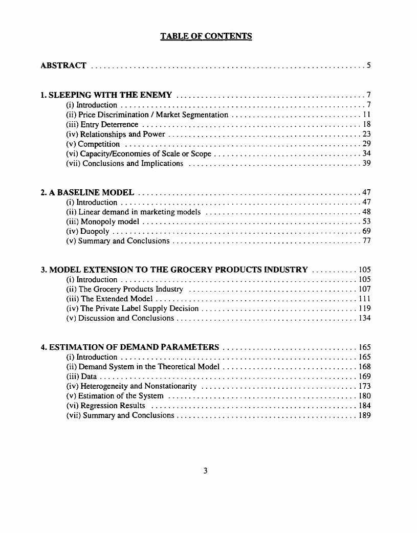
TABLE OF CONTENTS

ABSTRACT . . . . . . . . . . . . . . . . . . . . . . . . . . . . . . . . . . . . . . . . . . . . . . . . . . . . . . . . . . . . . . . . . 5

1 . SLEEPING WITH THE ENEMY .... . . . . . . . . . . . . . . . . . . . . . . . . . . . . . . . . . . . . . . . . - 7 (i)Introduction . . . . . . . . . . . . . . . . . . . . . . . . . . . . . . . . . . . . . . . . . . . . . . . . . . . . . . . . . . 7 (ii) Price Discrimination / Market Segmentation . . . . . . . . . . . . . . . . . . . . . . . . . . . . . . . 1 1

. . . . . . . . . . . . . . . . . . . . . . . . . . . . . . . . . . . . . . . . . . . . . . . . . . . . (iii)EntryDeterrence 18 (iv) Relationships and Power . . . . . . . . . . . . . . . . . . . . . . . . . . . . . . . . . . . . . . . . . . . . . . 23 (v)Competition . . . . . . . . . . . . . . . . . . . . . . . . . . . . . . . . . . . . . . . . . . . . . . . . . . . . . . . . 29 (vi) CapacityEconomies of Scale or Scope . . . . . . . . . . . . . . . . . . . . . . . . . . . . . . . . . . - 3 4 (vii) Conclusions and Implications . . . . . . . . . . . . . . . . . . . . . . . . . . . . . . . . . . . . . . . . - 3 9

2.ABASELINEMODEL . . . . . . . . . . . . . . . . . . . . . . . . . . . . . . . . . . . . . . . . . . . . . . . . . . . . . 47 (i)Introduction . . . . . . . . . . . . . . . . . . . . . . . . . . . . . . . . . . . . . . . . . . . . . . . . . . . . . . . . . 47 (ii) Linear demand in marketing models . . . . . . . . . . . . . . . . . . . . . . . . . . . . . . . . . . . . -48 (iii) Monopoly model . . . . . . . . . . . . . . . . . . . . . . . . . . . . . . . . . . . . . . . . . . . . . . . . . . . - 5 3 (iv)Duopoly . . . . . . . . . . . . . . . . . . . . . . . . . . . . . . . . . . . . . . . . . . . . . . . . . . . . . . . . . . . 69

. . . . . . . . . . . . . . . . . . . . . . . . . . . . . . . . . . . . . . . . . . . . (v) Summary and Conclusions -77

3 . MODEL EXTENSION TO THE GROCERY PRODUCTS INDUSTRY . . . . . . . . . . . 105 (i)Introduction . . . . . . . . . . . . . . . . . . . . . . . . . . . . . . . . . . . . . . . . . . . . . . . . . . . . . . . . 105

. . . . . . . . . . . . . . . . . . . . . . . . . . . . . . . . . . . . . . . . (ii) The Grocery Products Industry 107 (iii)TheExtendedModel . . . . . . . . . . . . . . . . . . . . . . . . . . . . . . . . . . . . . . . . . . . . . . . . 111 (iv) The Private Label Supply Decision . . . . . . . . . . . . . . . . . . . . . . . . . . . . . . . . . . . . . 119 (v) Discussion and Conclusions . . . . . . . . . . . . . . . . . . . . . . . . . . . . . . . . . . . . . . . . . . . 134

4 . ESTIMATION OF DEMAND PARAMETERS . . . . . . . . . . . . . . . . . . . . . . . . . . . . . . . . 165 (i)Introduction . . . . . . . . . . . . . . . . . . . . . . . . . . . . . . . . . . . . . . . . . . . . . . . . . . . . . . . . 165 (ii) Demand System in the Theoretical Model . . . . . . . . . . . . . . . . . . . . . . . . . . . . . . . . 168 (iii)Data . . . . . . . . . . . . . . . . . . . . . . . . . . . . . . . . . . . . . . . . . . . . . . . . . . . . . . . . . . . . . 169 (iv) Heterogeneity and Nonstationarity . . . . . . . . . . . . . . . . . . . . . . . . . . . . . . . . . . . . . 173 (v) Estimation of the System . . . . . . . . . . . . . . . . . . . . . . . . . . . . . . . . . . . . . . . . . . . . . 180 (vi) Regression Results . . . . . . . . . . . . . . . . . . . . . . . . . . . . . . . . . . . . . . . . . . . . . . . . . 184 (vii) Summary and Conclusions . . . . . . . . . . . . . . . . . . . . . . . . . . . . . . . . . . . . . . . . . . . 189

5 . THE MODEL IN ACTION . . . . . . . . . . . . . . . . . . . . . . . . . . . . . . . . . . . . . . . . . . . . . . . -205 (i) Introduction . . . . . . . . . . . . . . . . . . . . . . . . . . . . . . . . . . . . . . . . . . . . . . . . . . . . . . . -205 (ii) Key Assumptions of the Theoretical Model . . . . . . . . . . . . . . . . . . . . . . . . . . . . . . 208 (iii) Methodology .................................................... -221 (iv)Results ........................................................... 238 (v) Scenario Analysis . . . . . . . . . . . . . . . . . . . . . . . . . . . . . . . . . . . . . . . . . . . . . . . . . . -246 (vi) Conclusions . . . . . . . . . . . . . . . . . . . . . . . . . . . . . . . . . . . . . . . . . . . . . . . . . . . . . . -253

6 . CONCLUSIONS AND DIRECTIONS FOR FUTURE RESEARCH . . . . . . . . . . . . . . 271 (i)Summary . . . . . . . . . . . . . . . . . . . . . . . . . . . . . . . . . . . . . . . . . . . . . . . . . . . . . . . . . . 271 (ii)Contribution . . . . . . . . . . . . . . . . . . . . . . . . . . . . . . . . . . . . . . . . . . . . . . . . . . . . . . . 276 (i i i ) Limitations . . . . . . . . . . . . . . . . . . . . . . . . . . . . . . . . . . . . . . . . . . . . . . . . . . . . . . . 277 (iv) Future Research . . . . . . . . . . . . . . . . . . . . . . . . . . . . . . . . . . . . . . . . . . . . . . . . . . . -279 (v) Concluding Comment . . . . . . . . . . . . . . . . . . . . . . . . . . . . . . . . . . . . . . . . . . . . . . -289

AN ECONOMIC ANALYSIS OF PRIVATE LABEL SUPPLY

IN THE GROCERY INDUSTRY

by

DAVID DUNNE

PH.D., 1996

FACULTY OF MANAGEMENT, UNIVERSITY OF TORONTO

ABSTRACT

With private labels growing in many grocery markets, manufacturers of national brands often

find themselves in a dilemma. Private labels' gains are largely at the expense of national brands. with

the result that manufacturers can have idle capacity due to stagnating sales. Retailers. for their pan.

are paying increasing attention to product quality as they develop premium private labels in an

attempt to build store loyalty.

Supplying retailers' private labels can be attractive for national brand manufacturers.

However. there are substantial risks: the manufacturer may end up substituting low-margin private

label supply for more profitable national brand sales. As a result, some manufacturers are extremely

reluctant to consider the idea.

The attractions of private label supply include the prospect of overall gains in sales volume,

the ability to segment the market and deterrence of competitive supply. The drawbacks, on the other

hand, can include loss of margin, the possibility of starting off a price war and production

inefficiencies.

This dissertation proposes a dominant-firm model which predicts the conditions under which

a manufacturer will supply a retailer's private label. While the linear-demand basis of the model is

inherently simple, it is rich in insights about the considerations facing manufacturers in

contemplating private label supply.

The model is applied to a case study of a grocery products firm. An econometric model is

developed to develop demand functions and separate parameters are estimated to reflect

heterogeneity among consumers and nonstationarity in consumption. The parameters are entered

into a spreadsheet version of the theoretical model and results derived for this particular firm. The

spreadsheet model is used to analyze how the profitability of private label supply changes in a variety

of real-world scenarios.

It is found that private label supply is unprofitable for this firm, primarily because the

competitive fringe keeps prices and profit margins low. However, this result is very sensitive to

changes in private label costs. By contrast, changes in national brand costs or in the competing

dominant firm's strategy have little impact on the profitability of private label supply for this

manufacturer.

1. SLEEPING WITH THE ENEMY

False facrs are highly injurious to the progress of science, for they ofren endure long;

but false views, ifsupported by some evidence. do little harm, for every one takes a

sahtary pleasure in proving their falseness.

Charles Darwin:

The Descent of ,khn

f i) Introduction

"Welcome to the brutal new world of brands", declared Fortune on August Xrd, 1993. Since

April 2nd. the fateful day Philip Morris dropped the price of Marlboro in response to pressure from

discount brands. the stock of 25 of the top packaged goods manufacturers in the U.S. had lost $47.5

billion in market value.

"Marlboro Friday" forced Wall Street to recognize a trend that was already well established

in Europe. and had been emerging in the US.: the increasing vulnerability of manufacturers' brands

to retailers' private labels. With recession. improving product quality and increasing retailer power.

private labels have reached a point at which industry analysts predict that only market leaders, No.

2 brands. and private labels will be camed by retailers. "Anything below that will get squeezed right

off the shelf. It's doomsday". proclaimed one executive.

Retailers' private labels traditionally have been lower-cost. lower quality imitations of

national brands. In the dishwashing liquids category, for example, most Canadian retailers would

offer two private labels: a yellow "lemon fresh" product packed in an opaque yellow bottle. which

at a passing glance was very similar to Lever Brothers' Sunlight Liquid. the market leader; and a

green "mild" product in a transparent bottle, which looked like Colgate-Palmolive's Palmolive

Liquid. These private labels would sell for considerably less than their national brand counterparts.

but would contain a lower concentration of detergent. Since they were unadvertised. their success

depended on price comparison with national brands at the point of purchase.

Such "traditional" private label brands grew in most grocery categories through the late

1980's and the early 1990's. due to recessionary pressures on consumers. As Hoch (1 993) argues

growth cycles in private label shares can be matched quite closely to economic cycles and their

impact on consumers' incomes. Such an analysis is certainly relevant where we are talking about this

category of "traditional" private label brands.

However. another type of private label is very successful in several markets - the U.K..

Canada, and increasingly in the US. (Messinger and Narasimhan, 1995). This "premium" private

label is a retailer's brand that offers comparable quality - in some cases. superior quality - to the

equivalent national brand. usually at a slightly lower price.

The success of U.K. grocery retailers with such premium private labels has prompted

Canadian retailers to follow suit with their own. The best known of these is Loblaw's President's

Choice. but most major grocery chains have launched an equivalent line of products. President's

Choice is positioned as an upscale, high quality, innovative range of grocery products. Unlike

traditional private labels, President's Choice is advertised on television. with an emphasis on quality

rather than on price.

In addition to earning higher margins for retailers, premium private labels play a significant

part in the long-term strategies of retailers such as Loblaw's. As Crotty (1990) points out:

"Today's more sophisticated retailers use [private labels] to attract and retain

customers, to differentiate themselves from their competition. and to avoid the

inevitable and easy price-point comparison that is so easy with manufacturers' brands.

The retailer's own label is an integral part of the marketing mix; it reflects the

retailer's whole positioning in a way that manufacturers' brands never can."

In contrast to the opportunistic role played by traditional private labels, premium private

labels are strategic tools used by retailers to communicate an overall image of high quality to

consumers. For this reason. unlike traditional private labels. premium private labels should be

relatively unaffected by economic cycles.

Small wonder. then. that grocery product manufacturers are showing increasing nervousness

about the growth of private label brands in their (or rather. what were formerly their) markets.

Premium quality private labels jeopardise the national brand by offering equivalent quality at a lower

price. and can generate brand loyalty among consumers as national brands have traditionally done.

In some cases, retailers lead the race to introduce innovative new products, as exemplified by

Loblaw's introduction of "clear" soft drinks well in advance of major manufacturers.

Retailers make formidable competitors. By controlling distribution and shelf space, they have

a great deal of influence over the success or failure of manufacturers' brands. Yet often it is in

retailers' interest to place more emphasis on their own private labels than on national brands.

National brand manufacturers are thus faced with rivalry from a critical partner in their marketing

strategy.

With retailers placing greater emphasis on private labels, it is natural that manufacturers'

attention should turn to that sector and that they should consider supplying these brands themselves.

However. grocery retailers are notorious for their readiness to switch private label suppliers in search

of a bener deal, with the result that competition for such contracts is intense. Supplying retailers'

private labels often involves loss of margin, increased price sensitivity on the national brand and

disclosure of sensitive information - and ultimately, increased dependence on the retailer.

If the drawbacks to private label supply for a national brand manufacturer are so apparent.

why do some choose to do so? There are some strong arguments in favour of supply. which can be

grouped as follows:

Price Discrimination / Market Segmentofion: Manufacturers may agree to supply private

label in order to serve high and low quality consumer segments separately.

Entry Deterrence: Manufacturers may supply the private label in order to prevent a new

competitor from gaining a foothold in the market.

Relarionships and Power: Retailers may give preferential treatment to the national brands

of their private label suppliers. leaving manufacturers with little choice but to supply the

private 1abeI.

Competition: If a manufacturer does not supply a retailer's private label, a competitor may

do so, leaving the national brand vulnerable to sales losses to the private label but without

the benefits of incremental profit and some (albeit minimal) degree of control over the

private label's strategy.

Coszs and Capocity: Private labels may be supplied in order to absorb excess capacity. or to

gain economies of scale or scope.

While the topic of private label supply is highly relevant to managers. it has received little

emphasis, to date. in the academic world. Premium private labels are a relatively new development.

and their full implications for manufacturers' and retailers' strategies have yet to be recognized. The

limited existing literature on private labels focuses primarily on differences between private label

consumers and national brand consumers (a topic which has some relevance, as we shall see j. but

there is little research that considers the strategic options facing manufacturers with respect to private

label supply. This dissertation fills this gap by proposing and empirically applying an economic

model which predicts the conditions under which manufacturers will supply a retailer's private labeL

The rest of this chapter looks at the degree of suppon available in the literature for each of

the reasons for private label supply listed above. In the following chapters, a model is proposed

which takes each of these reasons into consideration: in chapter 2. a "baseline" economic model is

developed: in chapter 3. this baseline model is extended to replicate the conditions prevailing in the

grocery industry and to develop hypotheses for testing. Chapter 4 estimates demand parameters for

a manufacturer of grocery products. and chapter 5 provides model results along with simulations of

a variety of business scenarios. Chapter 6 draws overall conclusions and suggests directions for

future research.

fii) Price Discrimination / Market Segmentation

According to the price discrimination explanation. manufacturers may supply private labels

in order to appeal to two separate consumer segments with different products at different price levels.

As a result. manufacturers can raise the price of their national brands and improve their overall

profitability.

This is the thrust of Wolinsky's (1987) model. Wolinsky asks why manufacturers supply both

labelled and "unlabelled" @rivate label) products, and proposes a model to explain the phenomenon

as a form of price discrimination. He develops a duopolistic horizontal spatial model, and shows that

the manufacturers will, in equilibrium, supply the unlabelled product. Manufacturers sort out buqers

who strongly prefer their brand and charge them a higher price, while competing separately for the

business of the remaining buyers through unlabelled products. The sub-market for unlabelled serves

as a "buffer" between the two sub-markets for the labelled brands. Therefore. a change in the price

of one of the labelled products has only an indirect effect (via the sub-market for the unlabelled

product) on the sales of the other labelled brand.

Armed with this model, we might go forth and explain all manner of private label supply

arrangements - particularly those in which a manufacturer will supply a low quality private label. but

not a high quality one. The example of Pillsbury Green Giant comes to mind: this firm supplies

lower quality private label vegetables with a higher proportion of leaves and stems than its national

brand. but will not supply premium private labels.

But let's think about this a little more. The model still fails to explain why any national brand

manufacturer would ever supply a high qua@ private label for retailers to sell at a price close to.

or matching, the national brand. In supplying President's Choice, J.J. Kwinter, a manufacturer of high

quality hot dogs. can hardly be said to be price discriminating. Nor can Colonial, the supplier of

President's Choice Decadent Cookies. Wolinslq+s model does not apply to these situations because

it was not developed to deal with premium private labels. Instead. it assumes that the unlabelled

brand occupies an "intermediate" position in consumers' perceptions between the two manufactured

brands.

Furthermore, retailers do not exist in Wolinsky's model - or, at any rate. do not influence the

manufacturers' strate=. In reality. however. the proposal to launch a private label usually comes

from retailers, not manufacturers. Nonetheless, Wolinsky's contribution is to show how price

discrimination can play a part in the manufacturer's decision in some circumstances.

If manufacturers supply private labels as a means of price discrimination, then private label

consumers must somehow be different from consumers of national brands - in their quality

requirements, in their sensitivity to price. or in some other way. This is not an unreasonable idea if

we are talking about traditional private labels. which offer unambiguously lower quality and price.

However. it is less likely to apply to premium private labels whose quality is close to that of national

brands. Since existing literature starts with the premise that private labels are low quality versions

of national brands. it is audibly. if not deafeningly, silent on this aspect.

The assumption that the two groups of consumers differ is commonly held among

practitioners and researchers alike. Lal's (1990) model of trade dealing and price promotion. for

example. assumes that some consumers are "loyals" and some are "switchers". His conclusion that

manufacturers will promote their national brands in alternating periods in response to a private label

depends, in part. on the size of the switcher segment.

Similarly, Blattberg and Wisniewsk's (1 989) analysis of price competition between private

labels and national brands is a "self-selection" model which assumes a heterogeneous utility fimction

across consumers. In an analysis of scanner data in four categories of grocery products. Blattberg and

Wisniewski fmd that consumers tend to switch primarily within "price tiers" - higher-priced products

tend to gain at the expense of other higher-priced products and lower-priced products, and lower-

priced products at the expense of their lower-priced competitors.

This result seems to settle the issue. It looks as if consumers do tend to stick within their o m

"set" of brands - high- or low-priced, as the case may be. making price discrimination a potentially

viable strategy. The only problem is that the price tiers in Blattberg and Wisniewski's analysis do not

distinguish between private labels and national brands. So it would be a mistake to interpret this

research as saying that private label users stick to private labels. and national brand users stick to

national brands. With increasing private label quality. in fact. we can expect consumers to switch

between national brands and private labels to a greater extent.

The issue of differences between the two types of consumers has, however. had quite a bit

of attention in research on private labels and generics'. Uncles and Ellis (1 989). for example. in an

analysis of the U S . ground coffee market. find that purchase patterns of private labels are ven

similar to those of comparably sized national brands; most people have a repertoire. and will buy

other brands and the private labels of other chains. Just as some consumers are loyal to national

brands. some are loyal to private labels. So it seems that a "loyal" private label se-pent exists

composed largely of light users of the category. However. there is a great deal of cross-switching

between segments.

If loyal private label users tend to be light users, quality should be less important to them: the

' Adopting a definition proposed by McEnally and H a w s (1984). a generic brand is "a distributor's brand that does not include a traditional brand name on its label". Typically. generics are of lower qualih.. and price. than either national brands or private labels: if there is such a thing as a "pnvate label-prone" consumer. l i e would expect a "generics-prone" consumer to exist too. Houtver. thr. esistence of a "grnrrics-pronr." segment does nor imply that a private label segment esisrs.

less frequently they use the product, the less important is poor performance. This would fit with

Wolinsky's price discrimination model: manufacturers would supply a lower quality private label

product to capture this group of light users. They would then have more flexibility to raise prices to

heavy users, who care more about quality.

Great theory, but no cigar. The grocery products industry is replete with categories in which

light users tend to have higher, not lower, quality requirements. In laundry detergents, for example,

the heaviest users are, obviously. large families. These families spend more money annually on

detergents than any other group; if they have a chance to save some precious dollars. they will be less

concerned with getting their wash whiter than white. Smaller families that spend less on detergents

are more amenable to superior performance. Similar patterns are likely to hold for o k r categories -

such as soup. ketchup. peanut butter. etc.

This argument is supported by Murphy and Lacmiak (1979). In this consumer survey on

generic grocery products. there were strong positive associations with generic purchase by education

and by number of persons living in the household. The idea that private labels (or. at any rate.

generics) are purchased by large families is supported by this study. So Uncles and Ellis' finding does C

not appear to generalize very well beyond the coffee category. in which it is to be expected that

heavy users would be more concerned about quality.

Murphy (1978) attacks the issue of private label segmentation from another perspective:

social class. In an experimental analysis of behaviou. in the paper towels, soft drinks and laundry

detergents industries. he compares brand name and brand choice fiequency. His findings suggest that

the frequency of store brand choice increases with social class. This appears to fit with Murphy and

Lacmiak's (1979) finding that private label consumers tend to have a higher level of education. The

idea that private label consumers tend to have high levels of education is supported by Cunningham.

Hardy and Imperia (1 982). who, in a study of canned foods, find that generic buyers are generally

younger and better educated than private label or national brand buyers. Small wonder, then, that

premium private labels are successful: if private labels in general appeal to higher social classes

brands such as President's Choice offer such people higher quality than traditional private labels at

a saving compared with the national brand.

The upscale nature of private label consumers does not bode well for manufacturers wishing

to use private label as a tool for price discrimination. It seems from this research that national brand

users tend to come from lower social classes. So while they may be prepared to pay more for higher

perceived quality. their lower disposable income constrains manufacturers from raising prices too

much.

One the other hand. there is some research that suggests that there is really no difference

between private label and national brand consumers. Livesey and Lemon (1978) analyze past

research in an effort to determine the importance of socio-economic characteristics. consumer

perceptions of quality. product-specific factors, family brand preferences and preferences for more

expensive or cheaper brands - and find linle evidence of a general predisposition towards private

labels. This conclusion is supported by an empirical study across five grocery categories in the U.K.

In addition. Szymanski and Busch's (1 987) meta-analysis of 400 studies of the generics-prone

consumer fmds that perceptions of product quality, price and overall product perceptions show the

strongest correlation with the propensity to buy generics. In comparison with product perceptions.

other factors such as demographics. psychographics and shopping behaviours are only weakly related

to the purchase of generics.

Neither of these studies is flawless. Livesey and Lemon do not conduct any statistical tests.

nor do they break the sample down into sub-groups in order to determine whether private label prone

segments exist. Szymanski and Busch's paper, on the other hand. suffers from many of the classic

drawbacks of meta-analysis: specifically, collapsing of several different measures into one, and the

possibie disproportionate influence of studies with larger numbers of subjects.

Nonetheless. there is enough in these studies to raise a warning flag against the idea that

private label consumers are necessarily different, and that it is possible to discriminate between them

and national brand consurners. If there is a difference. it seems to be a slight one. and varies by

category.

Conclusions

If manufacturers supply private labels in order to price-discriminate. some segment of

consumers who are prepared to pay a premium for the national brand must exist. Researchers have

tried hard to establish whether there is a difference between private label consumers and those of

national brands. However. most studies in this area are lacking in theory. with the result that their

findings are open to several interpretations. Moreover. the statistical analysis of the empirical studies

is ofien severely limited.

There is some limited evidence that private label and generic prone consumers tend to be

more educated and have larger families than national brand consumers. However. there is also

evidence to suggest that no difference exists.

Two factors would support the idea that there is no difference: first. as private label

penetration continues to grow, difference between the two groups of consumers are likely to

disappear. The U.K. private label share of more than 30% across all food categories suggests that

it would be very difficult to distinguish private label consumers from those ofnational brands in that

country: there are probably few consumers who do not use a private label brand in some category.

Secondly, the emergence of premium quality private labels blurs the distinction between

national brands and private labels to such a degree that it is unlikely that different consumers favour

one over the other. Much of the research in this area refers to generics, and may not be extendable

to traditional private labels. let alone the premium quality private labels now available.

In the final analysis, the price discrimination explanation for private label supply is only

partly convincing. It may apply in some categories where the private label's quality is clearly much

lower than that of the national brand. But it does not seem to work for President's Choice, nor for

other premium private labels. A manufacturer supplying these brands solely on the basis of price-

discrimination would be on a short road to failure.

liii) Entrv Deterrence

Entry deterrence provides another potential explanation for private label supply: a

manufacturer supplies the private label in order to keep a potential competitor out of the market

Private label supply, the theory goes. is an easy way for a manufacturer to enter a market: the retailer.

not the manufacturer, takes most of the risks of holding inventory if the product is not successful:

shelf distribution is assured. and the manufacturer is not subject to the uncertainties of trade

promotions, slotting allowances and the host of other ways in which manufacturers can be separated

from their money.

Indeed, there are success stories of manufacturers who have entered categories through

private label supply. Con Corporation. the high-profile supplier of private label sofi drinks. grew

From humble origins by supplying private label to Loblaw. and boasted earnings of $35.4 million in

1994, up from $12.8 million in the previous year. Con is now an important competitor to Coca-Cola

and Pepsi-CoQ which were formerly, for all practical purposes. duopolists in the soft drink industry.

Would the major sofi drink manufacturers have been better off to have supplied private label

and kept Con out of the market? With 20-20 hindsight, it certainly appears this way. Brander and

Eaton's (1 984) model would also suggest that this is so. Brander and Eaton analyze firms' optimal

decisions with regard to the number of products firms produce, which products they produce and

their level of output.

Initially, they show that a monopolist would prefer to produce two products that are dis~ant

substitutes. In a duopoly, the firms may choose from four products (1,2,3.4), with product I closely

substitutable for product 2, but less so for product 3, and so on. The marker segmentation case

describes a situation where firm A produces products 1 and 2. and firm 2 produces products 3 and

4. Under a market interlacing structure. on the other hand. firm A produces products 1 and 3. and

firm B produces products 2 and 4. The product line decision is depicted in three stages: Product

Scope (how many products). Product Line (which products). and output level.

Brander and Eaton show that a monopolist would prefer to minimize cannibalization of his

existing product, and will therefore produce a distant substitute. For duopolists, Brander and Eaton

show that producing close substitutes will lead to less intense price and output competition at a later

stage. However, the threat of entry by an external competitor changes the picture: the more intense

competition produced by an interlacing structure may deter entry and be more profitable for the

incumbent firms. Eaton and Lipsey (1979) also show that a farsighted monopolist would introduce

a close substitute in a growing market before a rival.

The model has a good deal of relevance to the private label supply decision for a monopolist

and for duopolists. A low quality private label can be seen as a distant substitute for a national brand

(say. product 4 versus product I), while a high quality private label can be seen as a closer substitute

(product 3 or even product 2). Brander and Eaton's h e w o r k would suggest that a monopolist will

be willing to produce a low quality private label, but not a high quality one. On the other hand

duopolists will prefer to produce a high quality private label and "carve up" the market between them

if there are significant entry barriers. Where entry barriers are low, however, the duopolists will

prefer to intensify competition by producing low quality private labels and prevent competitors from

entering.

Applying this model to the sofi drink example, Coca-Cola and Pepsi. facing low enuy

barriers. would have preferred to follow a market interlacing strategy: one manufacturer would

supply a high quality national brand and a low quality private label (products 1 and 3) , while the

other would supply a lower quality national brand and a low quality private label (products 2 and 4).

Had there been no threat of entry. each firm would have produced a high quality national brand

(product 1 or 2) and a low quality private label (product 3 or 4).

However, Brander and Eaton's model focuses entirely on the demand side: all products are

assumed to have equal, constant marginal costs. Capital costs are assumed equal across all products

In the sofi drink example, it is quite possible that capacity and cost considerations prevented Coca-

Cola and Pepsi from embarking on private label supply, and that they effectively had little choice

but to admit a new competitor.

This is supported by media reports that Con has a substantially lower cost structure than the

major sofi drink manufacturers (Globe and Moil. 1993). In spite of the confidentiality of cost data.

we could guess that achieving comparable costs with Cott would have involved major capitalization

and re-investment on the part of Coke and Pepsi. So the rational decision for them may well have

been to allow Cott to enter.

In a similar vein. Scherer (1980) argues that entry deterrence by "product variety

proliferation" is a profitable strategy for incumbent f m s because of the fixed costs of developing

a new product. We can see private label is a means of reducing this fixed development cost. making

it more attractive for the competitor to enter. and less attractive for incumbent firms to deter entry.

The idea that a monopolist (or a cartel acting as a monopolist) will introduce a new product

to deter a competitive entr). originates in Bain's (1 954) classic work, in which he stresses the role of

product differentiation as one barrier to competitive entry. In economics literature, the phenomenon

is termed "persistence of monopoly" and is also supported by the spatial models of Schmalensee

( 1 978) and of Eaton and Lipsey (1 979). Tirole (1 992) contends that monopolies persist where

preemption of entry by introducing a new product is effective and technology is deterministic.

However. even in these conditions. a new firm may enter if it has a technological advantage over the

incumbent, if the incumbent does not have time to pre-empt the entrant. or if the incumbent does not

have complete information about the entrant. In the sofi drink example, Cott may have had a

technological advantage over Coca-Cola and Pepsi-Cola SO that it was not worth their while to deter

Cott from entering.

An example from outside the grocery industry is offered by Lele (1992) - the case of h a n a

in the microwave oven industry. Amana the dominant manufacturer. was retailers' first choice as

private label supplier, but in refusing to produce retailers' brands. allowed lower-cost Japanese

imports to enter the market. Lele argues that a firm. such as Arnana. that is competing in the high

quality segment of the market can effectively control the lower quality segment by private label

contracting. In this sense, private label supply by a dominant firm can constitute an entry barrier.

Conclusions

Brander and Eaton's model gives a credible explanation of the strategic choices facing

duopolists such as Coke and Pepsi, or Lever and Procter & Gamble. According to the model. one

of these firms should be supplying high quality private labels. and the other low quality, if there is

no great threat of entry by a competitor. If there is a threat of entry, however, both firms will produce

low quality private labels. Similarly. Arnana. the dominant firm in the microwave industry, should

have supplied a low quality private label.

But in all these cases. these firms have refused to supply any private labels at all. Either these

firms are behaving irrationally, or there is something going on here that is not being explained by

Brander and Eaton's model. There are some hints in Tirole's contingency approach to monopoly

technology. timing and information may all play a part in the decision to pre-empt a competitor.

In all likelihood, Brander and Eaton's model holds some elements of truth. In some

circumstances, it does make sense to supply private labels as an entry barrier. However. there are

several other factors at work too. Entry deterrence is a credible explanation for private label supply.

but by no means the only one.

fiv) Relationships and Power

Retailers control a scarce resource in the grocery industry - shelf space - and are becoming

increasingly sophisticated in managing it. In the US., major consumer goods companies spend as

much on trade promotion as on consumer promotions (coupons. contests, samples) and media

advertising combined (The Economist, 1992). In this environment, manufacturers may supply private

labels for positive or for negative reasons - in an attempt to further their relationship with retailers,

or because they are co-erced into doing so. In this section, we consider both perspectives and develop

some ideas about the conditions under which they might apply.

Davies (1990) sees private label supply in a positive light. arguing that private label supply

can be part of a marketing programme to retailers. "Co-marketing" of national brands and private

labels can have benefits for manufacturers:

"Supporters of co-marketing ... point to the reality that the retailer often welcomes

the possibility of sourcing [national] brands and [private label] from one supplier.

particularly where the supplier can offer an integrated marketing package"

Davies also claims that there is evidence from manufacturers who offer a mix of private label

and national brands that supplying private label can be as profitable as. or more so than, supplying

only national brands.

A Transaction Cost perspective (Williamson, 1985; Milgrom and Roberts, 1992) can be

brought to this issue. Private label supply can be seen as a way of increasing the retailer's investment

in the relationship with the manufacturer by creating specific assets which encourage the

development of longer term contractual arrangements. In this case. one important specific asset may

be the expertise developed by the manufacturer in producing the retailer's product. In order to

maintain its required quality standards, the retailer may be obliged to enter into a long-term

partnership with the manufacturer. For a manufacturer. the benefits of such an arrangement might

include, for example, the ability to raise price on his national brand. Hence a manufacturer may

supply the private label in order to increase the retailer's dependence on him'.

Other researchers see retailerlmanufacturer relationships in a more negative light

McGoldrick ( 1 984), for example, claims that private labels' ability to maintain lower prices than their

national brand counterparts is due to retailers' ability to play manufacturers off against one another:

"With overcapacity in most areas of grocery manufacturing. orders can be switched

between suppliers. different items can be produced by different manufacturers ...

sometimes one manufacturer is used in one region, another in a different area ...

Supply does not appear to be a problem in most product areas; retailers are reporting

numerous approaches from manufacturers with ideas for further generic itemsM.@. 16)

This looks more like desperation on the part of manufacturers in the face of retailers' power

to switch between suppliers. than a strategic effort to "co-market" private labels and national brands.

If manufacturers are attempting to lock retailers into long-term relationships by creating specific

assets, it seems that they are not being very successfid. The picture painted here is rather of

concentrated, powerful retailers promoting their private labels, with manufacturers following along.

gathering the available scraps as they go.

2 To avoid sexist language while maintaining balmce. I refer to the manufacturer as "he" and to the retailer as "she" throughout this dissertation.

While there are obvious differences between the textile industry and grocery products

Salmon and Cmar's (1987) study of the private label supply in textiles reaches similar conclusions.

They contend that big profits for the supplier of private label goods are unlikely, and that even

maintaining profits at a level equal to the cost of capital may be difficult due to retailers' readiness

and ability to switch suppliers.

Stern and El- Ansary (1 988) are also less than sanguine about private labels, commenting that

they are a means for the retailer to secure channel control. They argue that? if generic product

acceptance exists, the retailer can not only enter the market with her own brand. but can also play

each of the leading brand suppliers off against one another by deciding which of these brands it will

stock in order to obtain concessions.

Grocery retailers who follow this strategy of playing manufacturers off can do so because the

primary factor differentiating manufacturers from each other is cost: with few technological

differences between firms. private labels of equal quality can usually be obtained from any

manufacturer. On the other hand. retailers cannot play national brands off against one another, since

they are differentiated on the basis of quality and image.

The Economisr (1 992) expressed the risks faced by suppliers of "core" retailers. such as

Marks and Spencer and Bemetton. in European supply networks, as follows:

Private label supply can leave a manufacturer excessively dependent on one customer. The

allocation of capacity, time and energy to a private label brand can reduce the level of innovation

behind national brands, with the result that the manufacturer has few alternatives should the retailer

threaten to move to a new supplier. Hence the manufacturer finds himself caught in a web with a

powefil retailer pulling the strings.

From these two streams of research, it seems that the effect of private label supply is either

a) to make retailers more dependent on manufacturers, or b) to make manufacturers more dependent

on retailers. In the former case, power should be an incentive to supply private labels; in the latter,

it should be a disincentive. The literature suggests that there may be specific conditions in which each

scenario holds: environmental uncertainty and "marginal" national brands would favour the first

scenario, while proprietary information would favour the second.

The Transaction Con perspective would argue that retailers are more likely to enter into long-

term arrangements where environmental conditions are uncertain. & for example, demand is subject

to fluctuations, retailers' primary need may be to assure themselves of a source of supply.

Alternatively, if product quality is difficult to monitor, retailers may need to develop relationships

with suppliers who can provide credible assurances of consistently high quality. This argument

would be most convincing where a "premium" private label is concerned.

In a similar spirit, Heide and John (1988) show that small f m s in channels (in this study,

manufacturers' agents) engage in "dependence balancing" - making investments to increase the

dependence of their channel partner where they are dependent on himher. This fits with private label

supply: manufacturers, faced with a powerful retail trade, attempt to baiance their dependence on

retailers by making retailers more dependent on them for their private label. We would thus espect

manufacturers to be more prepared to supply a retailer's private label where they have some degree

of power "deficit" vis a vis the retailer.

As an example of this, McGoldrick (1 984). as outlined above, argues that private label supply

can be a costly strategy over the long term. He claims that it is the "marginal" national brands that

are at greatest risk of being delisted to make room for private labels, and that manufacturers of tkse

brands are therefore more likely to accede to a retailer's request to supply. This seems to represent

the experience of some firms in the grocery industry. E.D. Smith, the supplier of President's Choice

Bottled Sauces. has a small national bottled sauce business. Procter & Gamble. manufacturer of

several market-leading brands in household and food categories. does not supply private labels at

all. perhaps because delisting is not a credible threat.

On the other hand. manufacturers may be unwilling to supply private labels where they

perceive that they may be giving valuable information away to a retailer. The provision of

information about formulations or costs, for example, allows the retailer to approach competing

suppliers for supply. In particular. McMaster (1 987) argues that providing R&D to retailers' brands

is giving "the advantage away to a competitor - bee ... [private label] produces benefit only fiom

short-term gains". McMaster's major concern is not with the supply of low quality private labels that

cannibalize national brands to only a limited extent, but rather with high quality private labels, where

the retailer is the primary innovator.

Much of this can, however, be turned on its head. Where demand is uncertain. for example.

manufacturers may have a greater need to secure distribution outlets. Manufacturers of small brands

who supply a private label are still subject to delisting and may even be in a worse position than

before if they have given away cost information. Application of these theories to private label supply

is an uncertain science.

Conclusions

The discussion of channel power in the context of private labels is inconclusive. Although

private label supply may increase a manufacturer's power in some conditions, it can reduce it in

others.

While retailers are powerful in the grocery industry, it would appear that this power is as

likely to work against private label supply as in its favour. in the long term. supplying a private label

seems much less attractive than introducing a new national brand. and is likely to increase the

manufacturer's dependence on the retailer, rather than reduce it. By devoting plant capacity?

management time and even R & D to private labels, the manufacturer is reducing his alternatives and

linking his future with the private label contract.

The dependence can be mutual, or "balanced", in Heide and John's terms. The manufacturer

may in effect be a monopolist if none of his competitors have capacity. or refuse to supply for some

other reason. But the fact that grocery retailers carry a wide range of products means that. in most

cases. they have greater flexibility to switch than the manufacturer does.

All things considered, private label looks like a better deal for the retailer than for the

manufacturer, at least from the viewpoint of channel power. Yet there are potential benefits for

manufacturers, particularly if there are few competitors and if the product category is an important

one for the retailer. It may not be in the retailer's interest to look for the cheapest source of supply

if she is in danger of being cut off fiom supply of an important national brand, for example. The

retailer may prefer. as Davies claims, to buy the national brand and the private label from one source.

Jv) Competition

Woven into the discussions of price discrimination, entry barriers and retailer power is a set

of assumptions about the competitive environment faced by manufacturers. Schmalensee ( 1978) and

Tirole (1992) are concerned with the role of production of a second brand in the persistence of

monopoly. Wolinsky (1987) and Brander and Eaton (1994) assume that the manufacturers are

duopolists. The power of retailers over manufacturers arises fiom the nature of competition among

manufacturers for scarce resources. So manufacturers may agree to supply the private label even if

it is not in their interest to do so, if they believe their competitors will supply should they refuse.

What is uncertain is whether manufacturers will be more or less inclined to supply the private

label in different competitive environments. The purpose of this section is to consider whether the

supply of private labels can be amibuted to factors in the manufacturer's competitive environment.

To this end. a range of competitive structures - monopoly. duopoly and oligopoly -is discussed in

turn.

Monopoly

In a monopoly, we would expect that retailer power would not be a significant factor in

manufacturers' decision to supply private labels. After all. if the manufacturer refbses to supply. the

retailer has nowhere else to go.

However. the other explanations discussed so far would apply equally to monopolists as to

firms in duopolistic or oligopolistic environments. Certainly. it can be in a monopolist's interest to

price-discriminate between consumers.

Brander and Eaton's (1981) approach to multiproduct firms is to use the monopoly case as

a point of comparison with their later analysis of duopoly. They show that a monopolist who does

not anticipate competitive en- would prefer to produce two products which are distant substitutes.

In itself. this is no great surprise: a monopolist will not normally choose to cannibalize his

existing brand rather than establish a new one appealing to different consumers. Although Brander

and Eaton do not explicitly analyze the case of a monopolist who fears a competitive entry. we can

expect that. as in the duopoly case. the equilibrium will change. A monopolist who especrs a

competitor to enter with a close substitute for his product is more likely to be inclined to supply a

close substitute as a pre-emptive strategy.

Schrnalensee's argument is that a monopolist or cartel vdl supply several products if entq-

by a competitor is feared. If there is no expectation of competitive e n F . there is no need to produce

more than one product.

So it seems likely that a monopolist who anticipates entry by a competitor will be disposed

towards supplying a retailer's private label. However. a "pure" monopolist who does not anticipate

entry may still have other reasons to supply the private label.

While the monopoly case may seem unusual. it does have some representation in groceF

markets. In certain markets, such as detergents, some multinational manufacturers will refuse to

supply as a matter of worldwide corporate policy. leaving the single manufacturer who is willing to

supply. in effect. a monopolist. Whether there is a significant threat of competitive entry depends on

whether the national brand manufacturers are likely to reconsider their corporate policy. There has

been evidence of such reconsideration recently within some major packaged goods firms.

Many grocery markets consist of two dominant firms which. in effect. control the categoq'.

In such instances. a retailer may choose to "divide and conquer" in order to secure supply for her

private label at the lowest possible cost.

Wolinsky's (1987) model considers the role played by the private label in softening

competition between the duopolists. Retailers are passive in Wolinsky's worlb. so the paper suggests

why duopolists would have reasons to supply "unlabelled" products even if there were no pressure

from retailers.

In this model. each firm is concerned solely about the actions of the competing duopolist. For

categories in which entry is difficult. this seems realistic enough. However, if entry is relatively easy.

' See Chapter 3 for more details on this.

4 Rrtailcrs exist but arc assumr.li to ha\c no intlucncs on the manufacturer's stntrg?

5 1

both duopo1is:s will be looking over their shoulders in anticipation of the arrival of a third firm

Brander and Eaton show that this prospect changes the equilibrium outcome: instead of close

substitutes. the firms will produce distant substitutes. However. Brander and Eaton do not esplicitly

analyze the conditions under which the manufacturers will supply exactly two products each (as

opposed to one. three or four) - instead, they claim only that it applies to an "intermediate range" of

demand.

The key issue to consider in a duopolistic model of private label supply appears to be whether

the duopolists are reacting primarily to each other, or whether they are concerned with the possibility

of a competitive entry. In most grocery categories. for instance, there are a number of smaller firms

which can be considered a competitive "fringe". and could be seen as a potential entrant according

to Brander and Eaton's model. We would expect dominant firms to supply close substitutes to keep

the smaller firms small.

Ofigopoi'y

The oligopoly case seems v e q similar to duopoly in its essentials - the only difference is that

there are more firms. giving the retailer more options.

An interesting aspect of 01 igopoly is whether heterogeneous cornpeti tors have an equal

probability of supplying private labels. As early as 1966, Stem (1966) predicted the results of the

grow* trend in private labels: the emergence of an oligopolistic core which emphasizes R&D and

product innovation, along with "fringe" firms who will produce relatively undifferentiated private

label items. Stem argued that small firms. because of capacity limitations. may have to forego

na4onal brand production to make room for the private label. As a result. they may have to accept

lower margins and be content with producing an undifferentiated product - and. as a result. be highly

vulnerable to competitive entry. On the other hand, private labels for small manufacturers may assure

short-run survival. which is often their most meaningful goal.

This appears to mirror the soft drinks and detergents markets, although the core in these

categories, as in many others in the grocery industry, is duopolistic rather than oligopolistic. It also

agrees with the suggestion in section that smaller brands are more vulnerable to delisting. and

that their manufacturers would therefore be more amenable to private label supply. But smaller

brands are not always produced by smaller manufacturers. and "core" manufacturers of national

brands. such as Nabisco. H.J. Heinz and Scoa Paper, do supply private labels.

Where does this leave us? Perhaps it is no longer enough for a firm simply to be a supplier

of undifferentiated private labels. Premium private labels can require a great deal of R&D and

innovation. which may not be available from smaller firms. So the assumption that firms will

separate neatly between those who innovate and those who supplg. private labels is unlikely to hold

water in the fiture: private label suppliers are likely to be innovators just as their national brand

competitors are.

Research on this aspect of private label supply is remarkably thin. Based on the literature that

exists. we can identi& three main areas of concern:

Risk of supply by an existing competitor:

Risk of entry by a new competitor;

i i i Lnfluence of heterogeneity among firms.

Brander and Eaton's model showed that there is a difference between the first two: the

influence of an existing duopolistic competitor and that of a prospective third firm. The prospect of

a new entrant may also change the equilibrium in a monopoly.

Firms in a duopoly or an oligopoly may also be heterogeneous. The primary distinction is

between dominant firms and "fringe" competitors; according to Stem, fringe competitors are more

likely to supply private labels. However. there are several readily available counterexamples.

Future research needs to consider these aspects of industry structure. both as influences on

private label supply in themselves and as moderators of other influences.

lvi) Capacitv/Economies of Scale or Scope

Perhaps prii-ate label supply can be boiled down to a trivial explanation. Manufactures

supply private labels not for grandiose strategic reasons. but simply to keep machines running which

would othewise be idle.

If there is a common thread that runs through the limited literature on private label supply.

it is that private labels are primarily capacity fillers for manufacturers when sales of national brands

are soft. Stem. El-Ansary and Bronn (1 989). for example. claim that private labels command a lower

wholesale price than national brands because they are a way for manufacturers to transfer promotion

costs to the retailer. For this reason. they are appropriate as a capacity filler.

Bowersox and Cooper (1 992) agree. They comment that "... the production of the private

brand utilizes excess capacity. the cost of which would otherwise have to be absorbed by the

manufacturers' own brands." (p. 18 1 ). Firms with high fixed costs need private label production to

spread their costs over a larger volume and make their national brands more competitive.

Consider also McGoldrickls (1981) portrayal of grocery manufacturers as engaged in a

desperate search for products to fill their plants [see section @)I. Retailers seem to hold all the

cards: the growth of private labels leaves national brands vulnerable and manufacturers with spare

capacity, and retailers can readily switch between potential suppliers in search of the best price. In

effect. manufacturers are replacing national brand volume with private label vo!ume -at lower profit

margins.

Spreading fixed costs across a larger number of units can keep unit costs down: from the

economist's viewpoint. the second product can offer economies of scale or economies of scope.

Baurnol. Panzar and Willig (1982) define (product-specific) economies of scale as "the saving

resulting from increasing the output of one product. holding the quantities of other products

constant". Economies of scope. by contrast. are the "cost savings resulting from simultaneous

production of several different outputs in a single enterprise" - pairs of items like wheat and straw.

wool and mutton. and beef and hides. In general. economies of scope exist where two products s h m

factors of production.

On the face of it. economies of scope would appear to be a more appropriate concept to apply

to private label supply. However. private labels and national brands often share parts of the same

production process. Depending on the similarity of the product formulations. processing and

packaging. private labels may offer economies of scale. economies of scope - or both - if the

manufacturer has spare capacity .

In the processed vegetable industry. for instance. private label supply allows processors such

as Pillsbury Green Giant to use up materials such as stalks and leaves that would not meet the quality

standards of the national brand (the alternative would be to scrap these materials). This strategy of

supplying a lower quality private label fits neatly within the d e f ~ t i o n of economies of scope:

essentially, the private label and the national brand are complementary from a production point of

view. However. in processed meats. the production of private label hot dogs on the same production

line as the national brand allows the private label supplier to keep the fixed overhead costs of the

national brand down: this is more a case of economies of scale.

Whether the issue is one of economies of scale or of scope. we have another intuitively

reasonable explanation for private label supply. which seems to be represented in the world around

us: private labels can be used by manufacturers to absorb plant overhead.

Glemet and Mira (1 993) argue that no single strategy is appropriate in all market conditions.

Glemet and Mira position capacity-filling as an "intermediate" strategy. one among several that a

manufacturer might adopt: short of refusal to supply private labels at all. private labels can be used

opportunistically to f i l l capacity with minimal threat to the national brand. Capacity-filling is

appropriate where the national brand's distinctiveness is relatively high and where the manufacturer

has a high market share.

Davies (1 990) also takes a "contingency" approach to private label strategy. He contrasts the

different strategies adopted by packaged goods manufacturers as (i) retaining channel control by

appealing directly to the consumer. and (ii) relying on the retailer's marketing powers by offering

private label. In the first case, manufacturers invest in product innovation and heavy promotion: the

emphasis in the second is on keeping costs down. This polarization is consistent with Glemet and

Mira's claim that manufacturers commonly take a "black or white" approach -either refusing point

blank to produce any private label, or supplying whenever there is an opportunity.

However, Davies argues that an intermediate strategy is open to manufacturers. A

manufacturer could evolve packages with individual retailers that complement the retailer's own

strategic objectives. by reducing her costs or building customer loyalty to the retailer. Davies argues

for a marketing approach that takes into account retailers' needs as well as those of consumers. In

the U.K.. for example. Pedigree Petfoods works ~ l t h the giant U.K. retailer Tesco to develop the

petfoods market.

Capacity utilization and economies of scale are less important reasons for supplying private

labels than channel control. according to Davies. Glemet and Mira contend that capacity utilization

also has its place.

Perhaps the important difference between these two views is their degree of optimism about

the viability of private label supply over the long haul. In the Davies camp. private label supply

yields channel control to the retailer. which can result in excessive dependency on the retailer. The

benefits of using excess capacity must be weighed against these long-term costs.

l h s is the prevailing view held by companies such as Lever Brothers and Kellogg's - while

there are short-term benefits, private label supply carries heavy long-term costs. Interestingly, both

these firms' production processes are quite capital-intensive, at least for some of their products, so

one would expect them to be acutely aware of the costs of leaving machinery idle.

By contrast. Glemet and Mira are more positive about private label supply as a means of

using up spare capacity. Their view is more typical of firms in the meat processing industry. With

tight margins and high fixed costs, these firms compete aggressively for private label supply

contracts.

Certainly, it is difficult to understand why any manufacturer would supply private label. over

the long term. purely to obtain economies of scale or scope. Since private label tends to carry low

margins. such a manufacturer would surely be better off by developing a new national brand - even

a low quality, economy brand. One answer to this is that the costs of developing a new brand are

extremely high. and the costs and difficulty of getting it on shelf are enormous. Combined with the

fact that competition from private label keeps margins low. it may take a long time for such a

strategy to pay for itself.

Another explanation is that many manufacturers simply have a short time perspective. or. in

economic jargon. discount the future heavily. This is Stem's (1 966) argument. when he contends that

short-term survival is the most meaningful goal for smaller manufacturers.

In processed meat. keeping the plant running may be a matter of "bare bones" sunival. The

same is true of other low-margin. high-volume. high fixed cost industries.

But neither excess capacity nor economies of scale/scope rings true by itself as an

explanation for private label supply. A manufacturer with any degree of ability to see beyond today's

close of business will be concerned about which specific products should fill the plant. Other factors

will certainly come into play in this decision: loss of channel control. the costs of developing a new

national brand, future relationships with retailers and consumers' needs. among others.

There is an important issue. though. which tends to be ignored by those who claim capacity-

filling as an explanation for private label supply: with the increasing importance of premium private

labels. opportunistic strategies such as this may not be enough to keep retailers interested. As

retailers' quality demands become ever more stringent, they will be less willing to switch suppliers

in search of spare capacity. In addition. they will require the investment of R & D in development

of premium quality products - increasing fixed costs and reducing or even neutralizing whatever

economies of scale might have been available.

We are left with another partial explanation for private label supply. one which rolls off the

word processor easily. but does not stand up to closer scrutiny. Yes. capacity utilization is a factor.

but not the only one. and not always.

Jvii) ConcIusions and Implications

Grocery manufacturers face a rapidly changing environment. Across all categories monitored

by .4.C. Nielsen. private label dollar sales in Canada grew by 13% in 1993. By comparison

manufacturers' brands were stagnant. at 3% dollar growth.

Imagine the manufacturers' dilemma. If they attempt to defend their national brands. the dice

are loaded against them: their product quality is often no better than that of the private label, and

their competitor controls vital access to the final consumer. Defending national brands through

increased advertising and promotion can be expensive and risky.

Manufacturers may have spare capacity as a result of volume losses to private labels. New.

lower cost competitors may enter the market to supply retailers' brands, and erode category margins.

Retailers may hint that private label suppliers will get preferential treatment on their national brands.

Supplying private labels starts to look better and better.

But the opportunity is not without risk. Will the private label take away sales from the

national brand? Will the manufacturer become overly dependent on the retailer? Will the private

label earn a "reasonable" profit margin? Will new competitors enter anyway and undercut private

label pricing?

The discussion in this chapter has attempted to identifi the important dimensions of the

private label supply decision for a national brand manufacturer. The support for each of the

alternative explanations is summarized in Figure 1.1 :

(Figure 1. I )

This chapter has emphasized that private labels are no longer just lower quality imitations

of national brands. Increasingly. retailers are using them as tools to distinguish themselves fiom their

competitors. Accordingly. many of the old assumptions made by researchers no longer apply. Figure

1.1 makes the distinction between traditional private labels and premium private labels. and shows

that. in some cases. explanations that would have applied to traditional private label supply cannot

be assumed to apply where premium private labels are concerned.

Another issue that emerges from Figure 1.1 is that both theoretical and empirical work are

needed in the area of private label supply. Where there is theoretical support for the explanations

discussed here. it is often tangential. based on models that were never intended to apply to private

labels. The amount of empirical support for any of the theories is sadly limited.

Each of the explanations for private label supply offered by researchers turns out to capture

part of the decision, applying only in some circumstances but not in others. Manufacturers ma):

indeed supply private labels because of pressure from powerful retailers. or because of the threat of

entry by cornpetiton. or because of capacity and cost considerations. However, there is no single

model that evaluates the relative importance of these different motivations to manufacturers,

how they interact with each other. in the contemporary private label environment.

Such a model is proposed and applied in this dissertation. The considerations of private 1

and

abel

quality. costs and competitive environment are included in a game theoretic model which predicts

the conditions under which it will be profitable for a manufacturer to supply a retailer's private label.

The model is applied empirically to the case of a major manufacturer of branded grocer). products.

and its behaviour tested under a variety of conditions.

The model considers private label quality, and it is shown that it is in manufacturers' interest

to suppl!. high quality private labels which do not excessively cannibalize their national brands.

While consumers are assumed to be homogeneous. it is shown that manufacturer can take advantage

of switching between brands and. in a sense, segment the market. The entry deterrence explanation

for private label supply is analyzed by the inclusion of a competitive "fringe" which may consist of

existing or potential competitors. It is also assumed that retailers can readily switch between s

manufacturers in search of a better deal on private label supply, and that they hold some power

relative to manufacturers in this way The model also analyzes three competitive environments:

monopoly. duopoly and duopoly with a competitive fringe, and considers the implications of

economies of scale and scope.

This is the first rigorous. comprehensive model of private label supply which evaluates the

conditions under which it will be in manufacturers' interest to produce a retailer's brand. The model

fills an important gap in the growing research on private labels. and, for practitioners. points the way

towards factors that should be taken into account in this critical decision.

REFERENCES

Bain. Joe S. (1954). "Conditions of Entry and the Emergence of Monopoly". chapter in E.H.Chamberlin. ed., Monopoly and Competition and Their R e p h i o n . London: MacMillan.

Baumol. William J., John Pamar and Robert Willig (1982). Contestable Markets and the Theory of Zndusrry Structure. San Diego: Harcourt Brace Jovanovich.

Blattberg Robert C. and Kenneth i. Wisniewski (1989), "Price-Induced Patterns of Competition1', Markering Science. 8.4 (Fall). 29 1 -308.

Bowersox. Donald J. and M. Bixby Cooper (1 992). Strategic Marketing Channel Management. New York: McGraw-Hi 11.

Brander. James A. and Jonathan Eaton (1984). "Product Line Rivalry". The American Economic Review. 74, 3. 323-334.

Buueil. Robert D. and Charles C. Slater ( 1962). "Decision Theory and Marketing Management". Jozrrnal of Mwketing. July. 7- 16.

Cunudian Bzcsiness ( 1993). "Global Gourmet". July, 22-33.

Crony. Paul (1 990). "Stocking the Aisle With Private Label", Canadian Grocer. August. 16-22.

Cunningham. Isabella C.M.. Andrew P. Hardy and Giovanna Imperia 1982, "Generic Brands versus National Brands and Store Brands: A Comparison of Consumers' Preferences and Perceptions". Jozcrncd ofAh*ertising Research. 12. 5 (October/November).

Davies. Gary (1 990). "Marketing to Retailers: A Battle for Distribution?", Long Range Planning. 23.6. 101-108.

Eaton. B. Curtis and Richard G. Lipsey (1 979). "The Theory of Market preemption: The Persistence of Excess Capacity and Monopoly and Monopoly in Growing Spatial Markets". Econometrica. 46? 149- 158.

Fortlrne (1 993). "Brands: It's Thrive or Die". August 23rd, 52-56.

Glemet. Franqois and Rafael Mira (1 993). "The Brand Leader's Dilemma". The McKinsey Qzrarterly. 2. 3-15.

Globe and Mail (1993). "Private Label: Blood on Main Street. Bargains on Wall Street". May.

Heide. Jan B. and George John (1988), "The Role of Dependence Balancing in Safeguarding Transaction-Specific Assets in Conventional Channelst', Journal of Marking. 52 (January), 20-3 5.

Hoch, Stephen J. (1 993, "Private Label a Threat? Don't Believe It", Advertising Age. May 24.

Lal, Rajiv (1990), "Manufacturer Trade Deals and Retail Price Promotions". Journal of Marketing Research, XXVII (November), 428-44-

Lele. Milind M. (1 992). "The Lessons of Strategic Leverage", Journal of Business Srrare~): 13. 4. JuVAug, 3 8-45.

Livesey, F. and P. Lennon (1978). "Factors Affecting Consumerst Choice Between Manufacturer Brands and Retailer Own Labels", European Journal of Marketing, 12,2, 158-70.

McEnally. Martha R. and Jon M.Hawes (1984), "The Market for Generic Brand Grocery Products: A Review and Extension". Journul of Marketing. 48 (Winter). 75-83.

McGoldrick. Peter J. (1984). "Grocery Generics - An Extension of the Private Label Concept". European Journal of Marketing. 1 8. 1. 5-24.

McMaster. Derek (1 987). '*Own Brands and the Cookware Market". European Jozirnal of Markeiing. 2 1. 1. 83-94.

Messinger. Paul R. and Chakravarti Narasimhan. "Has Power Shifted in the G r o c e ~ Channel?". Markering Science. 14.2, 1 89-223.

Milgrom. Paul and John Roberts. 1992, Economics. Organization and Management. Englewood Cliffs. N.J.: Prentice-Hall.

Murphy. Patrick E. (1978). "The Effect of Social Class on Brand and Price Consciousness for Supermarket Products". Jotma1 of Retailing. 54. 2 (Summer). 33-42.

---------------- and Gene R. Laczniak (1 979). "Generic Supermarket Items: A Product and Consumer Analysis". Journal of Retailing. 5 5 . 2 (Summer), 3- 14.

Salmon, Walter J. and Karen A. Cmar (1987). "Private Labels are Back in Fashion", Harvard Business Review, May-June, 99- 1 06.

Scherer, F.M. (1980). Indzistriul Marker Structure and Economic Performance, Chicago: Rand McNally.

Schmalensee. R. (1978). "Entry Deterrence in the Ready-to-Eat Breakfast Cereal Industry". Bell Jownai of Economics. 9. 305-327.

Stem. Louis W. ( 1966). "The New World of Private Brands". California Management Reviewl Spring.43-50.

----------- and Adel I. El-Ansary (1988). Marketing Channels, Third Edition. Englewood Cliffs: Prentice Hall.

------ ------------ , and James R. Brown (1989), Management in Marketing Channels. Englewood Cliffs. N. J. : Prentice-Hall.

Szymanski. David M. and Paul S. Busch (1987), "Identifying the Generics-Prone Consumer: A Meta-Analysis", Journal of Markering Research. XXIV, November, 425-3 1 .

The Econornisi (1 992). "Why Networks May Fail", October I Oth, 83.

The Economist (1 993). "When smoke Got in Their Eyes". April 10th. 65-66.

Tirole. Jean (1 989). The Theory of lndzcstrial Organization. Cambridge. Mass.: The MIT Press.

Uncles. Mark and Katrina Ellis (1 989). "The Buying of Own Labels". European Jo~rrnal of Marketing. 23. 3. 57-30.

Williamson. Oliver E. (1985). The Economic Institutions of Capiralism. New York: The Free Press.

Wolinsky. Asher ( 1 987). "Brand Names and Price Discrimination". The Jozunal of hdzlstrial Economics, XXXV. March. 255-68.

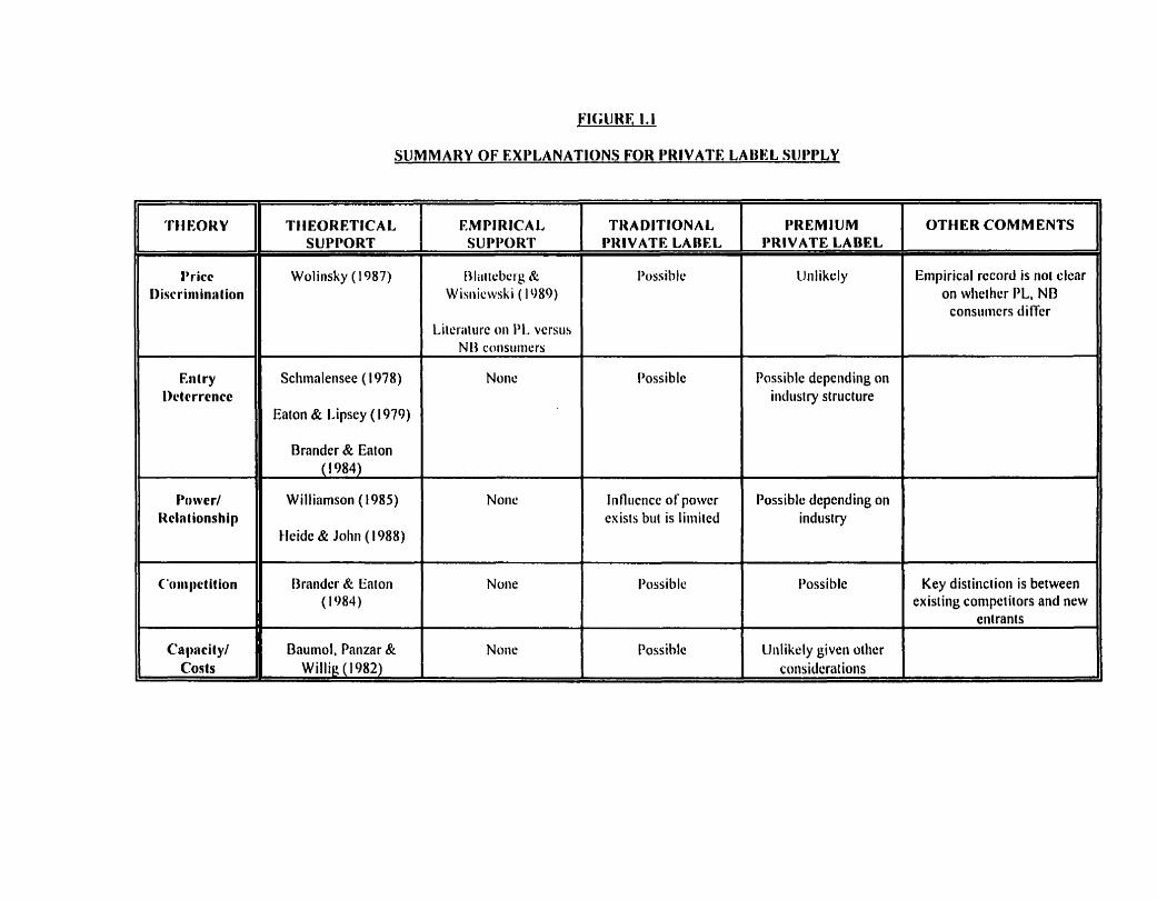
FIGURE 1.1

SUMMARY OF EXPLANATIONS FOR PRIVATE LABEL SUPPLY

THEORY TtiEORETICAL SUPPORT

EMPIRICAL SUPPORT

IDricc II Wolinsky ( 1987) I)iscrin~inalion

Nonc

13lil1tcbcrg & Wisuicwski ( 1089)

Entry 1)clcrrcnce

Schmnlensec ( 1978)

Eaton & Lipscy ( 1979)

1 ,

Capncityf Baumol, Panzar & None Willik ( I 982)

Brander & Eaton (1084)

1% w c r/ ltclalionship

Williamson ( t 985)

tleide & 501111 ( 1988)

TRADITIONAL PRIVATE LABEL

l'ossiblc

Infltrencc of power csists but i s l i~i i i ted

PREMIUM PRIVATE LABEL

U~llikely

Possible depending on industry

I'ossiblc

Possible

OTHER COMMENTS

Empirical record i s riot clcnr on wlletlwr PL, Nl3

conswlws diffcr

l'ossi blc

U~ll ikely given otller considerations

Key distinct ion is between existing compctirars and new

entrants

2. A BASELINE MODEL

Under every stone is mother stone.

Robin Skelton:

A Devious Dicfionary

Ji) Introduction

The literature review of Chapter 1 explored a variety of possible explanations for private

label supply by manufacturers. Nevertheless. there is as yet no comprehensive model that looks at

the possible strategies open to manufacturers in different conditions. The purpose of this chapter is

to develop a baseline model for extension and application to the grocery products industry.

Initially. the model is specified in a single retailer - single manufacturer world with linear

demand. Equilibrium strategies for the manufacturer and the retailer are determined. The

manufacturer's profitability with and without the private label are compared. and from this are

determined the conditions under which the manufacturer will supply the retailer's brand. This

baseline model shows that a profit-mauimizing. monopolistic manufacturer will always supply a

retailer's private label, because he will benefit from market expansion by the private label and from

allowing consumers to switch brands rather than leave the market. This model readily extends to a

situation in which the manufacturer faces multiple retailers.

In addition. this chapter explores manufacturers' propensity to supply private labels in a

duopoly. It is shown that. under some conditions. one manufacturer will supply the private label.

However. there are also some ranges of parameters under which neither manufacturer will supply.

This chapter is organized as follows. To begin, some of the literature that is relevant to the

linear-demand structure of the model is discussed; while Chapter 1 covered literature on the question

of private label supply. the purpose of discussing the literature here is to draw out issues which

concern the structure of the model itselt The baseline model and its assumptions are then specified.

and propositions are developed for a monopolistic manufacturer in section 3. The model is extended

to duopoly in section 4. The chapter concludes with a summary of the model's predictions and a

discussion of its contribution and its limitations.

{ii) Linear demand in marketinp: models

While Chapter 1 covered the literature on private label supply, the purpose of this section is

to consider literature from other streams of research that has a bearing on this model's structure. The

models discussed in this section have been developed with diEerent objectives in mind: nonetheless.

the?. are relevant because the models themselves bear similarities to that employed here. In particuiar.

these models can offer some insights into the representation of consumer demand as a linear function

of prices in a Stackelberg Framework.

In the game theoretic literature on channel structure, McGuire and Staelin's (1983) seminal

work demonstrates the role of demand substitutability in a manufacturer's decision to perform the

functions of a retailer in the channel (i.e. an integrated channel structure) rather than allow an

independent retailer to handle his product under a decentralized channel structure.

McGuire and Staelin propose a linear demand function of the form q, = I -p,+Op,. where i and

j refer to the competing manufacturers and 8 is a measure of product substitutability. Their demand

function is a rescaling of the original demand functions

q', = v S { 1 - [ P / ( W l p ' , + [Pwl-e,lp;);

q'z = (1 - m i 1 + [PW-8) lp1 , - [P/(l-Wp'd

for the products of manufacturers 1 and 2, and Or pr 1; OsW1; P20; SzO. S is a scale factor which

is equal to industry demand when the prices of both products are zero, while p represents the

absolute difference in demand between the two products - intuitively, the inherent product

"preference" for each brand.

So that demand does not increase in prices. McGuire and Staelin impose the additional

constraint 0/( 1 +8) 5 p r 1 / ( I+@. This is shown graphically in Figure 2.1. with the shaded area

representing the feasible region for p in terms of 8.

(Figure 2.1 )

As 0 increases. the feasible range for p becomes smaller and approaches 0.5 as 8 - 1 . In

other words. the absolute difference in demand becomes smaller as product substitutability increases:

two highly substitutable products will essentially split the market between them.

McGuire and Staelin's rescaled demand function, as shown in Appendix 2.1 and discussed

below, for all its simplicity and tractability, is highly restrictive. The effect of the rescaling of the

demand functions is to fix the consumer's utility and "preference" for the two products at equal

levels, i.e. to set p = 0.5 or the line AB in Figure 2.1. In other words, the products have identical

appeal to the consumer and identical own price response, but are not necessarily fully substitutable.

McGuire and Staelin's rescaled linear model is a special case of the more general demand

function assumed in this dissertation. The structure of the baseline model is also similar to that of

McGuire and Staelin - a Stackelberg framework with the manufacturer acting as leader - but there

are some significant differences.

The linear demand function used here is derived from a quadratic utility function at the

consumer level, and is more general than that proposed by McGuire and Staelin. The intercept of the

demand curve (product preference) is allowed to vary between the two products. and om-price

parameters may also differ. This captures situations in which a private label may have inferior.

similar. or even superior quality to the national brand. and may respond differently to price changes -

reflecting the distinction between traditional and premium private labels discussed in Chapter 1.

Coughkin and Wernerfelt (1989) use a more general form of linear demand function in their

discussion of this class of models of channel integration. Their demand function is p, = A - Bq, + Eq;

i.j = 1.2: i *j; EE(-B.B), which inverts to q, = [A(B+E)-Bp,-Ep,](B2-E')": ij=l.2: i=j. a generalization

of McGuire and Staelin's demand function.

Coughlan and Wernerfelt's linear demand function is consistent with that of McGuire and

Staelin. but its general form is more flexible and consistent with reasonable assumptions about

consumers' utility. However. both intercept demand and own-price response are still constrained to

be equal across the two products.

Dixit (1 979) develops a model of entry barriers with capacity constraints, and finds that two

aspects of product differentiation have distinct effects: an absolute advantage in demand for the

established firm makes competitive entry more difficult, while a lower cross-price effect facilitates

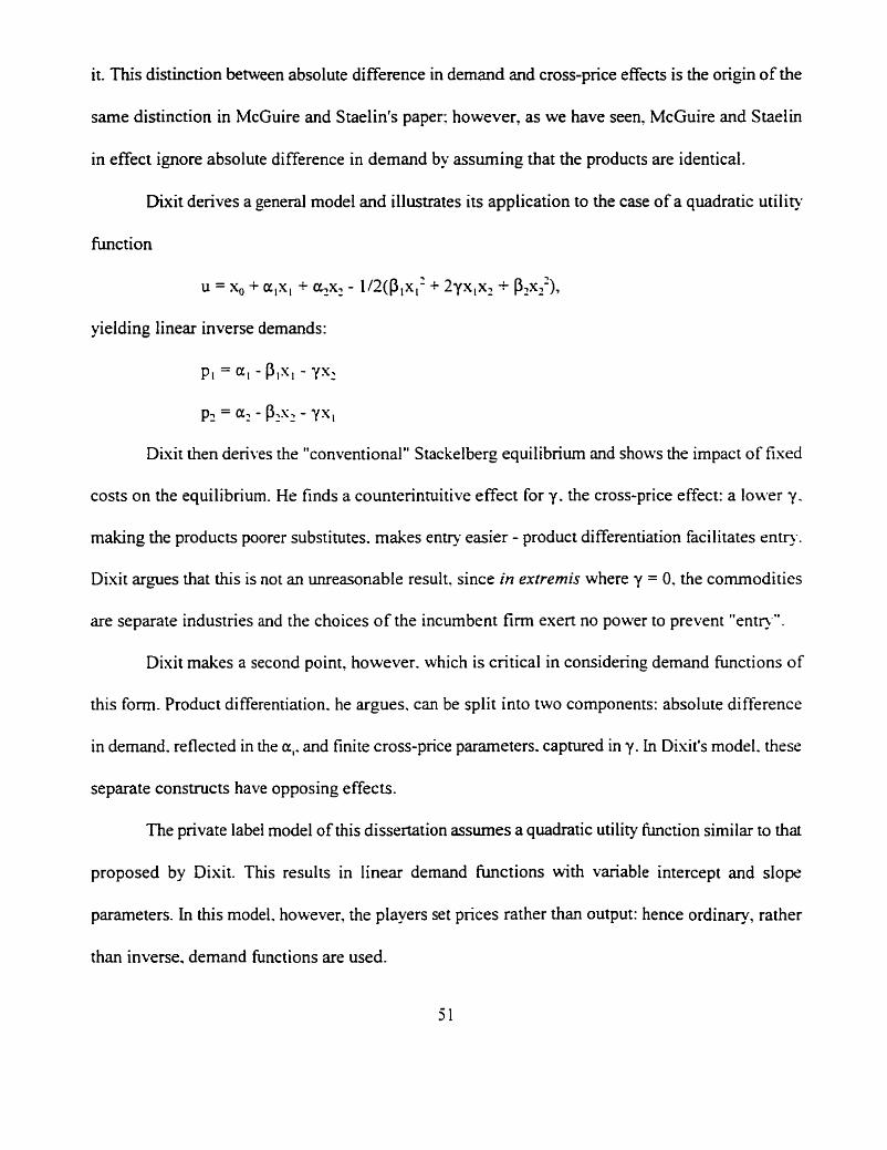
it. This distinction between absolute difference in demand and cross-price effects is the origin of the

same distinction in McGuire and Staelin's paper: however, as we have seen. McGuire and Staelin

in effect ignore absolute difference in demand by assuming that the products are identical.

Dixit derives a general model and illustrates its application to the case of a quadratic utility

function

u = x, + a,x, + a,x, - 1/2(P,x,' + 2yx,x2 + P:x?~),

yielding linear inverse demands:

pl = a, - P,s, - yx,

pZ = a, - P2s2 - yx1

Dixit then derives the "conventional" Stackelberg equilibrium and shows the impact of fixed

costs on the equilibrium. He finds a counterintuitive effect for y. the cross-price effect: a lower y.

making the products poorer substitutes. makes enny easier - product differentiation facilitates mtry.

Dixit argues that this is not an unreasonable result. since in extremis where y = 0. the commodities

are separate industries and the choices of the incumbent firm exert no power to prevent "entr). ".

Dixit makes a second point. however. which is critical in considering demand functions of

this form. Product differentiation. he argues. can be split into two components: absolute difference

in demand. reflected in the a,. and finite cross-price parameters. captured in y. In Disit's model. these

separate constructs have opposing effects.

The private label model of this dissertation assumes a quadratic utility function similar to that

proposed by Dixit. This results in linear demand Functions with variable intercept and slope

parameters. In this model. however, the players set prices rather than output: hence ordinary, rather

than inverse, demand functions are used.

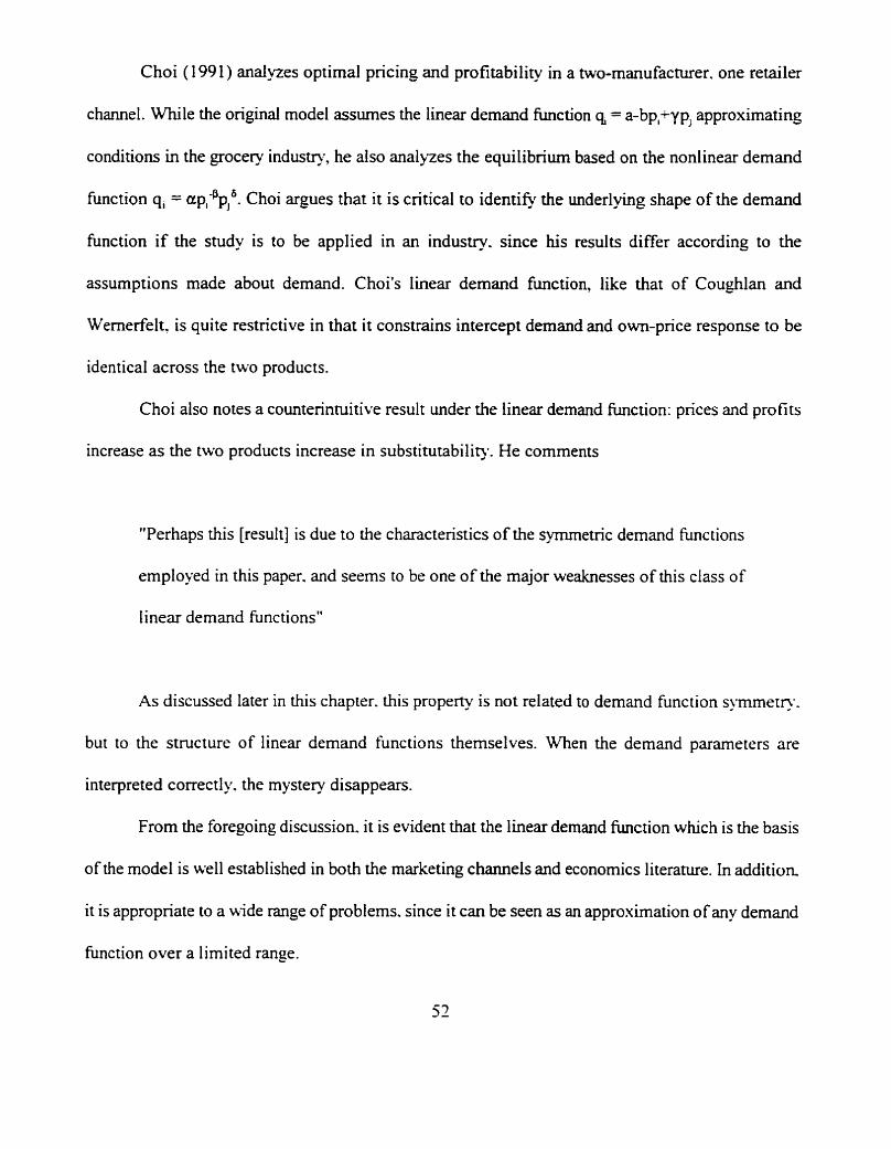
Choi (1 99 1) analyzes optimal pricing and profitability in a two-manufacturer. one retailer

channel. While the original model assumes the linear demand function q = a-bp,+yp, approximating

conditions in the grocery industry, he also analyzes the equilibrium based on the nonlinear demand

function q, = u ~ , " ~ , ~ . Choi argues that it is critical to identifv the underlying shape of the demand

function if the study is to be applied in an industq. since his results differ according to the

assumptions made about demand. Choi's linear demand function, like that of Coughlan and

Wemerfelt, is quite restrictive in that it constrains intercept demand and own-price response to be

identical across the two products.

Choi also notes a counterintuitive result under the linear demand function: prices and profits

increase as the two products increase in substitutability. He comments

"Perhaps this [result] is due to the characteristics of the symmetric demand fimctions

employed in this paper. and seems to be one of the major weaknesses of this class of

h e a r demand functions"

As discussed later in this chapter. this propert) s not related t .o demand fun ction symmetry.

but to the structure of linear demand functions themselves. When the demand parameters are

interpreted correct1 y. the mystery disappears.

From the foregoing discussion. it is evident that the linear demand function which is the basis

of the model is well established in both the marketing channels and economics literature. In addition

it is appropriate to a wide range of problems. since it can be seen as an approximation of any demand

fbnction over a limited range.

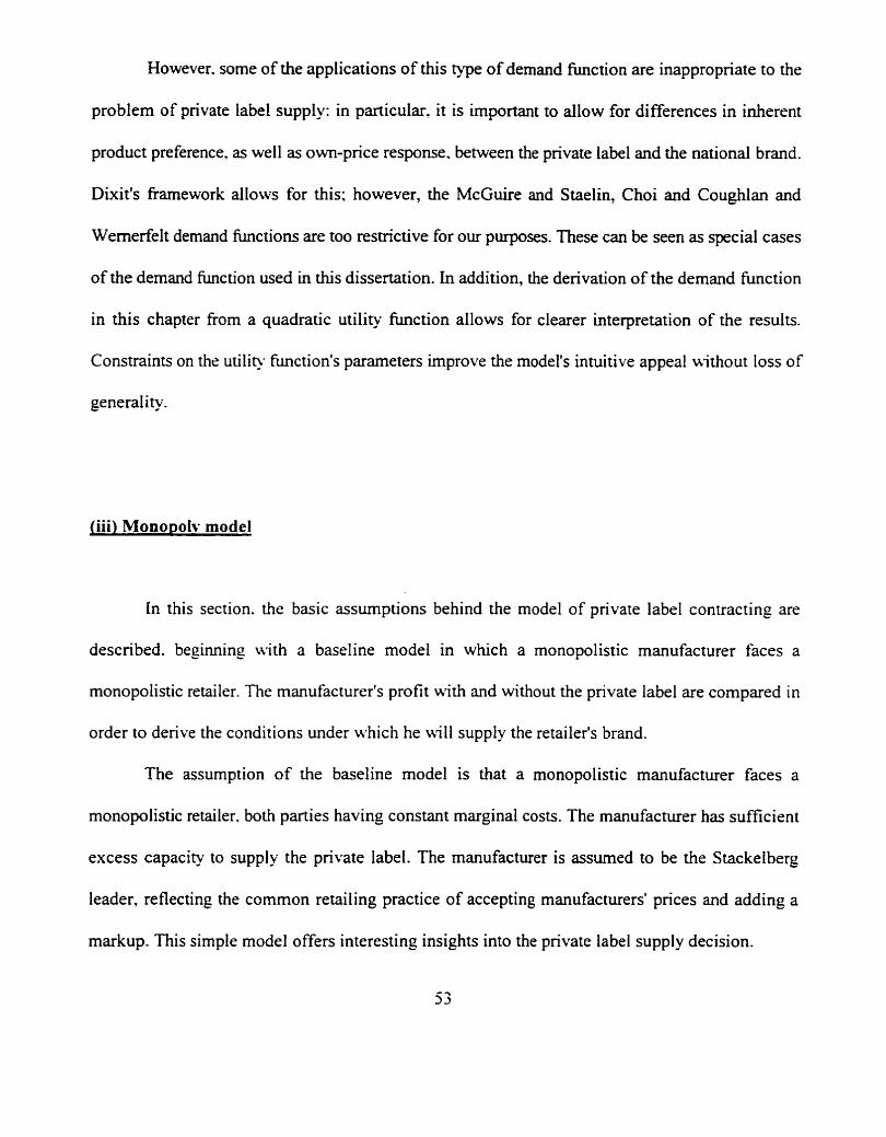
However. some of the applications of this type of demand function are inappropriate to the

problem of private label supply: in particular. it is important to allow for differences in inherent

product preference. as well as own-price response. between the private label and the national brand.

Dixit's framework allows for this: however, the McGuire and Staelin, Choi and Coughlan and

Wemerfelt demand functions are too restrictive for our purposes. These can be seen as special cases

of the demand function used in this dissertation. In addition, the derivation of the demand function

in this chapter from a quadratic utility h c t i o n allows for clearer interpretation of the results.

Constraints on the utility Function's parameters improve the model's intuitive appeal without loss of

generality.

jiii) Monopoh. model

In this section. the basic assumptions behind the model of private label contracting are

described. beginning with a baseline model in which a monopolistic manufacturer faces a

monopolistic retailer. The manufacturer's profit with and without the private label are compared in

order to derive the conditions under which he will supply the retailer's brand.

The assumption of the baseline model is that a monopolistic manufacturer faces a

monopolistic retailer. both parties having constant marginal costs. The manufacturer has sufficient

excess capacity to supply the private label. The manufacturer is assumed to be the Stackelberg

leader, reflecting the common retailing practice of accepting manufacturers' prices and adding a

markup. This simple model offers interesting insights into the private label supply decision.

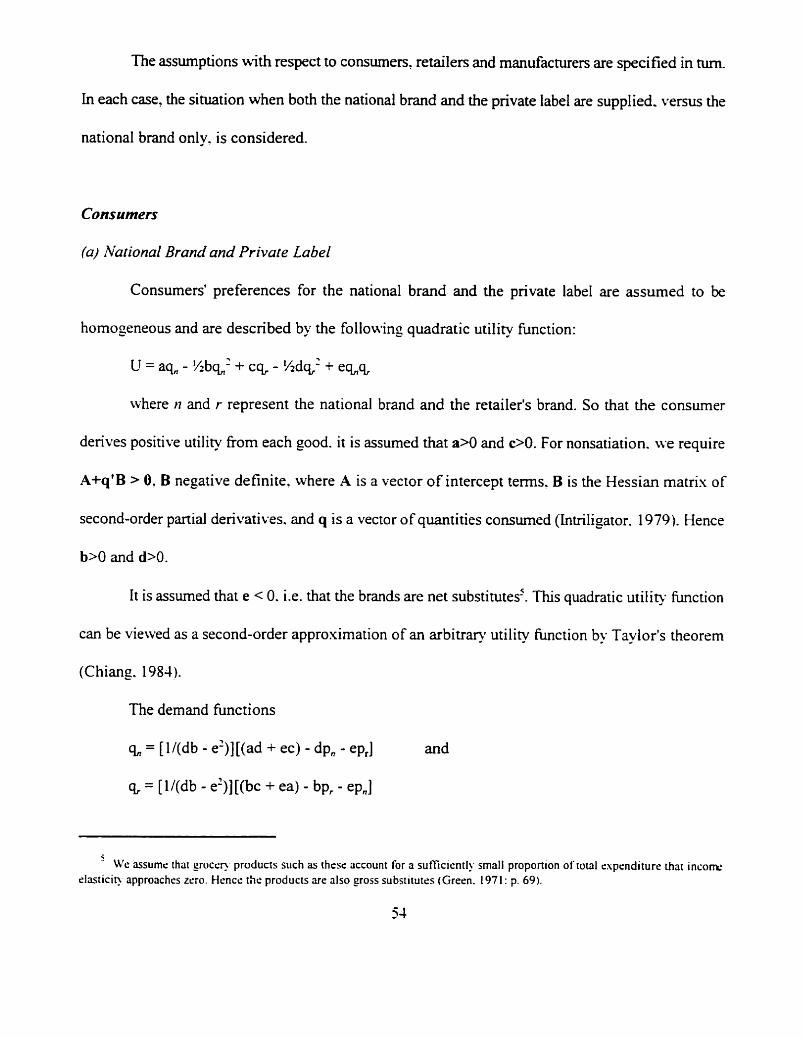
The assumptions with respect to consumers. retailers and manufacturers are specified in turn.

In each case, the situation when both the national brand and the private label are supplied. versus the

national brand only. is considered.

Consumers

(a) National Brand and Private Label

Consumers' preferences for the national brand and the private label are assumed to be

homogeneous and are described by the following quadratic utility function:

u = aq,, - %ba2 + c a - % d ~ ' + e q , , ~

where )I and r represent the national brand and the retailer's brand. So that the consumer

derives positive utility from each good. it is assumed that a>O and 00. For nonsatiation. we require

A+qlB > 0. B negative definite, where A is a vector of intercept terms. B is the Hessian matrix of

second-order partial derivatives. and q is a vector of quantities consumed (Intriligator. 1979). Hence

b>O and d>O.

It is assumed that e < 0. i.e. that the brands are net substitutes-'. This quadratic utility b c t i o n

can be viewed as a second-order approximation of an arbitrary utility h c t i o n by Taylor's theorem

(Chiang. 1984).

The demand functions

qn = [ 1 /(db - e')] [(ad + ec) - dp, - ep,] and

& = [ I /(db - el)] [(bc + ea) - bp, - ep,]

5 Wr assume that grocer\, products such as these account for a sufficientl>. small proportion of total expenditure that incom. elasticip approaches zero. Hence the products are also gross substitutes (Green. 197 1 : p. 69).

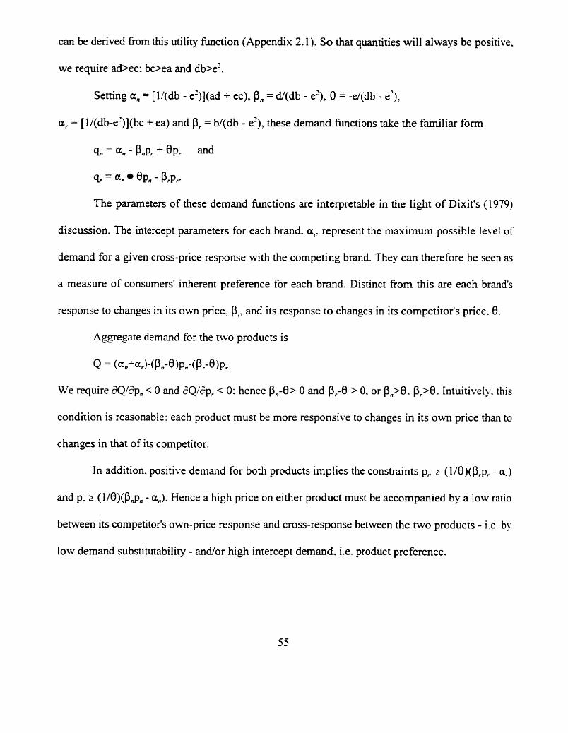
can be derived from this utility fimction (Appendix 2.1 ). So that quantities will always be positive.

we require ad>ec: bc>ea and db>e2.

Setting a, = [l/(db - e2)](ad + ec), P, = d/(db - e2), 0 = -e/(db - e'),

a, = [l/(db-e2)](bc + ea) and Pr = b/(db - e'), these demand fimctions take the familiar form

a = a n - P n p n + epr and

% = a r e ~ n - Prpr-

The parameters of these demand functions are interpretable in the light of Dixit's (1979)

discussion. The intercept parameters for each brand. a,. represent the mavimurn possible level of

demand for a given cross-price response with the competing brand. They can therefore be seen as

a measure of consumers' inherent preference for each brand. Distinct from this are each brand's

response to changes in its own price, P,, and its response to changes in its competitor's price. 0.

Aggregate demand for the two products is

Q = (an+ar)-@.-O )p,-(P;B )p,

We require dQlZp, < 0 and dQlep, < 0: hence P,,-0> 0 and Pr-0 > 0. or p,>0. pr>O. Intuitively. this

condition is reasonable: each product must be more responsive to changes in its own price than to

changes in that of its competitor.

In addition. positive demand for both products implies the constraints p, 2 (l/O)(Prp, - a,)

and pr r (~/~)(P,JJ,, - a,,). Hence a high price on either product must be accompanied by a low ratio

between its competitor's own-price response and cross-response between the two products - i.e. by

low demand substitutability - and/or high intercept demand. i .e. product preference.

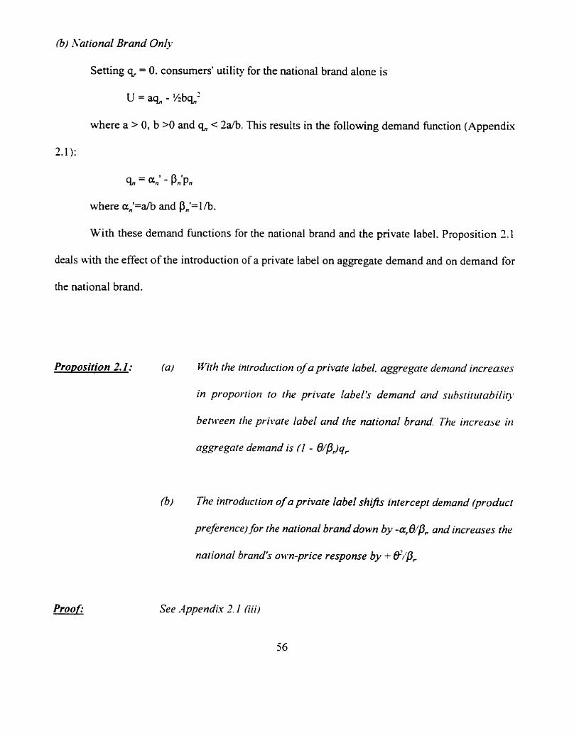
(b) Ahtional Brand Only

Setting q, = 0. consumers' utility for the national brand alone is

u = aq,, - !4ba2

where a > 0, b >O and e, < 2afb. This results in the following demand function (Appendix

Q = a n ' - Pn'pn

where anl=a/b and Pn'=llb.

With these demand functions for the national brand and the private label. Proposition 2.1

deals with the effect of the introduction of a private label on aggegate demand and on demand for

the national brand.

Proposition 2.1: (a! U'iiit the inrrodrrcriorz of u private label. aggregare denzrrr~d increases

in proporti017 to the private labelk demand and subsrirrrrabilin.

between [he private label and the national brand. The increase in

aggregate demand is ( I - O/pr)q,

(@ The introdzrction of a private label shifts intercept demand (product

preference) for the national brand down by -arO/b and increuses the

national brandk own-price response by - @ipr

Proof: See Appendix 2.1 fiiij

56

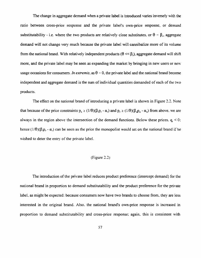
The change in aggregate demand when a private label is introduced varies inversely with the

ratio between cross-price response and the private label's own-price response. or demand

substitutability - i.e. where the two products are relatively close substitutes. or 0 - P, aggregate

demand will not change very much because the private label will cannibalize more of its volume

fiom the national brand. With relatively independent products (8 << P,), aggregate demand will shifi

more, and the private label may be seen as expanding the market by bringing in new users or new

usage occasions for consumers. In exnemis, as 0 - 0, the private label and the national brand become

independent and aggregate demand is the sum of individual quantities demanded of each of the two

products.

The effect on the national brand of introducing a private label is shown in Figure 2.2. Note

that because of the price constraints p, s (1/8)(P,pr - a,) and p, 2 (1 /B)(P$, - a3 from above. we are

always in the region above the intersection of the demand functions. Below these prices. q, < 0:

hence (1/0)(P,p, - a,) can be seen as the price the monopolist would set on the national brand if he

wished to deter the entry of the private label.

(Figure 2.2)

The introduction of the private label reduces product preference (intercept demand) for the

national brand in proportion to demand substitutability and the product preference for the private

label, as might be expected: because consumers now have two brands to choose from, they are less

interested in the original brand. Also. the

proportion to demand substitutability and

national brand's own-price response is increased in

cross-price response: again. this is consistent with

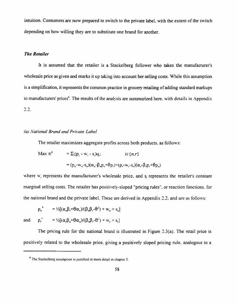
intuition. Consumers are now prepared to switch to the private label. with the extent of the switch

depending on how willing they are to substitute one brand for another.

The Retailer

It is assumed that the retailer is a Stackelberg follower who takes the manufacturer's

wholesale price as given and marks it up taking into account her selling costs. While this assumption

is a simplification. it represents the common practice in grocery retailing of adding standard markups

to manufacturers' prices6. The results of the analysis are summarized here. with details in Appendis

3 3 -.-.

(a) Nu~ional Brand and Private Label

The retailer maximizes aggregate profits across both products. as follows:

= Z,@, - w, - s,)q,: if {n ,r>

- - ( ~ , t - " n - s n ) ( a n - P n P , , + e ~ ~ ) + ( pr-wr-sr)(a; P,pr+Opn)

Max xH

where w, represents t he manufacturer's wholesale price. and 3 represents the retailer's constant

marginal selling costs. The retailer has positive1 y-sloped "pricing rules", or reaction functions. for

the national brand and the private label. These are derived in Appendix 2.1. and are as follo\vs:

Pn = K[(a,Pr+Bar)/(PnP,-8?) + wn + s,]

and P,' = Y z [ ( ~ , P , + ~ ~ , ) / ( P , P ~ - ~ ' ~ + w, + s,]

The pricing rule for the national brand is illustrated in Figure 2.3(a). The retail price is

positively related to the wholesale price. giving a positively sloped pricing rule. analogous to a

' The Swckelberr assumption is justified in more detail in chapter 5 .

58

reaction function in a Cournot/Stackelberg game in quantities. In this sense. the actions of the

manufacturer and the retailer are strategic complements (Tirole. 1988).

(Figure 2.3)

This result is consistent with Choi's (1991) finding that only half the change in the

manufacturer's wholesale price is reflected in the retail price, and the other half is absorbed by the

retailer; this is a common result for linear demand functions with constant marginal costs (Varian.

1992. p . 236-7). B y setting cr,=a, Pn=Pr and sn=O, the model reduces to Choi's model. and we end

up with identical results: p,'=l/i[a,,/(P,-O)+wnJ: pr0='/;[a,,/(Pn-O)+wrJ.

The retailer also considers the ratio between the brands' product preference and

substitutability in setting prices. The intercept of the reaction function is half the ratio of intercept

demand to the difference between own-price response and cross-price response, or between product

preference and substitutability. With inequality in the demand function parameters. both the

denominator and the numerator are moderated by the different intercept and price response terms for

the competing brand.

The perceptive reader will notice that %,'Id0 > 0 and apro/d8 > 0. This well-known result

(see, for example, Choi, 1991), that prices rise with increases in cross-price response, seems

counterintuitive. However. from eq. (6) recall that aggregate demand is Q = (an+ar)-(pn-@pa-(b

O ) p r . Hence an increase in the price of the national brand will raise aggregate demand through the

cross-price response term, 8, but reduce it through the own-price response term, Pn. Since we have

constrained the model so that P , > 0. aggregate demand will never rise due to an increase in price.

Nonetheless. an increase in 0 alone will increase aggregate demand.

The intuitive interpretation of this is that, if the national brand increases its price, some

proportion of consumers, f(P,'), will leave the market altogether and others, f(8). will switch to the

private label7. As the cross-price response term rises, the proportion of consumers that choose to stay

in the market rises. Hence the retailer who maximizes profit across both brands has more flexibility

in increasing prices as cross-price response increases; 0 can be seen as a measure of category loyalty,

or consumers' propensity to switch brands rather than leave the market.

With these prices, the retailer's derived demand for the two products is as follows, assuming

she does not purchase excess inventory:

J 4 n = %[a, - Pn(wn+sn) + 8(wr+s,)J

qJr = %[a, + &w,+s,) - P,(w,+s,)]

Since only half the change in wholesale price is passed on by the retailer. the responsiveness

of derived demand to wholesale price changes is also half that of final demand to retail prices.

(6) National Brand Only

With q, = 0. the retailer maximizes profits as follows:

With one product, the optimal retail price is

7 We have assumed that consumers are homogeneous. Hence all consumers have an equal probabilie of switching brands. but

the net result is that some wilt switch and some will not.

. Pn = %[(a,'@,') + W, + sn]

At this optimal price. the retailer will buy

4. = %[a,' - PJW, + S)J

The Manufacturer

Assume now that the retailer approaches the manufacturer with a request to supply her

private label. Under what conditions will the manufacturer agree to supply?

The manufacturer is aware of the retailer's pricing rule and derived demand and chooses his

wholesale price to maximize his profit taking these functions into account. as illustrated in Figure

X ( b ) : the manufacturer moves to the point of tangency between his isoprofit curve and the retailer's

pricing rule.

The manufacturer's profitability when he supplies both the national brand and the private

label to the retailer is compared here with his profit when supplying only the national brand.

(0) Xational Brand and Priwre Label

If the manufacturer agrees to supply the retailer's private label. his profit maximization

problem is analogous to that of the retailer:

df = Z,(w, - m,)qLi,: i~ (n,r)

where m, represents the manufacturer's constant marginal costs (= average costs). Where mn * m,.

the manufacturer can recover the difference in costs by price discriminating between private label

and national brand users.

From the retailer's problem above, derived demand is qdn = %[a,, - ~,(wn+sn) + O(wr+sr)] and

qJr = %[ar - pr(y+s,) + O(wn+sn)]. Then the manufacturer's profit can be expressed as

rLf = X(wn-m,,)[crn-~m(wn+sn)+8(wr+~r)] + l/r(wr-m,)[ar-pr(wr+sr)+8(wn+-sn)]

From this, the optimal wholesale prices are (Appendix 2.2):

I

we = 1/2[(a,Pr+8a,)/(PnP,-8') - s, + m,] and

w r = %[(~rpn+ean)l(pnPr-81) - s, + mr]

Like the retailer, the manufacturer absorbs half of any increase in costs. The other half is

passed on to the retailer. The manufacturer also takes account of intercept demand and

substitutability in the same way as the retailer. However. the manufacturer also takes account of the

retailer's selling costs: if these costs rise. the manufacturer takes account of this reduction in the

retailer's ability to pay by reducing his wholesale price by half the increase in costs. The i r

terms of the manufacturer's equilibrium wholesale prices are identical to those of the equi

retail prices. and express the ratio of product preference and demand substitutability.

The manufacturer supplies the following quantities to the retailer at these optimal prices:

4 n v = %[a, - pn(sn+m,) + O(sr+m,)] and

9r ' = %[a, + B(sn+m,,) - P,(S,+-~,)].

To simplifv notation. let c, = (s, + m,) Vi E { n r ) . At these prices and quantities. the manufacturer's

profit is as follows:

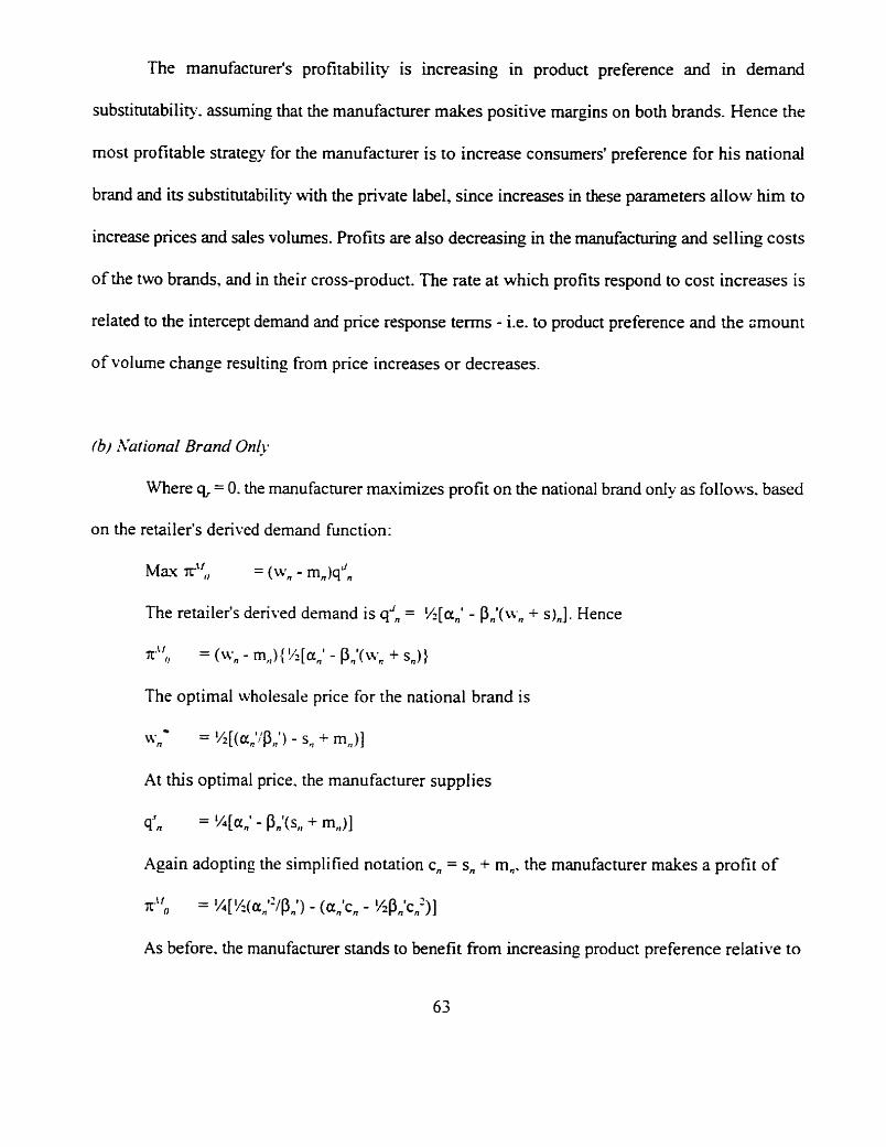
The manufacturer's profitability is increasing in product preference and in demand

substitutability. assuming that the manufacturer makes positive margins on both brands. Hence the

most profitable strategy for the manufacturer is to increase consumers' preference for his national

brand and its substitutability with the private label. since increases in these parameters allow him to

increase prices and sales volumes. Profits are also decreasing in the manufacturing and selling costs

of the two brands, and in their cross-product. The rate at which profits respond to cost increases is

related to the intercept demand and price response terms - i.e. to product preference and the moun t

of volume change resulting from price increases or decreases.

lb) hhriona[ Brand Only

Where q = 0. the manufacturer maximizes profit on the national brand only as follows. based

on the retailer's derived demand function:

Max df0 = (wn - mn)q (I ,

The retailer's derived demand is qJn = %[an' - Pnl(w, + s),].

x.i f 1) = (w, - m,J ( %[an' - Pnl(wn + s,)}

The optimal wholesale price for the national brand is

Wn - - %[(a,':pn1) - s, + m,)]

At this optimal price. the manufacturer supplies

s", = %[an1 - Pnl(s, + m,)]

Hence

Again adopting the simplified notation c, = s, + m,, the manufacturer makes a profit of

xu, = !4[%(an"iP,,') - (antn - %Pnlc~) ]

As before. the manufacturer stands to benefit from increasing product preference relative to

own-price response on the national brand.

(c) Comparison

The profitability of private label supply is derived by comparing the manufacturer's profit

under the two scenarios. i-e. by determining Ax" = df - r",:

A ~ " = 54 { %[(aiP+a:Pn+20anar)/(PnPr-82)] - [(ant, - '/zp,,c;)- (arc, - Yips,')- Ocncr] )

- !4[!4(an''@J - (aR1cR - %P,,'cn2)]

After some algebraic manipulation (see Appendix 2.3). this reduces to

~ ~ t f = ( I/8)[a,'/Pr + 2(ajpr)(ecn-Prcr) + ( '/Pr)('cn-P~r)'I

This is the profit difference for the manufacturer between supplying the private label and

supplying the national brand. It is important to recall that this takes into account not only product

preference and substitutability between the private label and the national brand. but also the shift in

the national brand's demand h c t i o n as a result of the introduction of the private label (see

Proposition 2. I ).

Where AT" is positive. the manufacturer will prefer to supply the private label along with

the national brand: where it is negative. he will prefer to supply the national brand alone. However.

as shown in Proposition 2.2. Ax-'' is ahvajr positive:

Prupusitiun 2.2: A monopolistic, projir-maximizing manufacturer who is a Stackelberg leuder

u-ill always suppiy a retailer 's privare label brand The proflubility of pr h-ate

label s o p p ! ~ depends on relative costs of the private label nnd the nurionrd

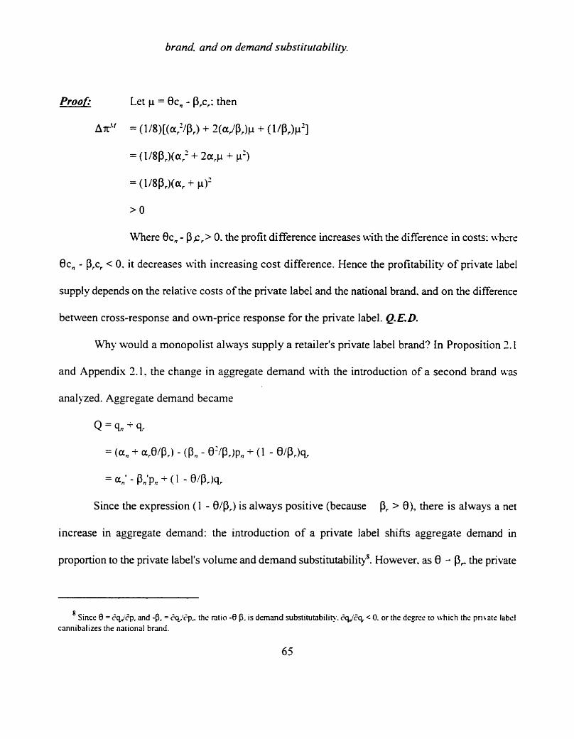
brand. and on demand substitzrtabilily.

Proafi Let p = Ocn - P,c,: then

AT" = (1 /8)[(allP,) + Z(ajp,)p + (1 /P,)cl']

Where Oc, - P ,c , > 0- the profit ( iifference increases with the difference in costs: whcrs

ec, - P,c, < 0. it decreases with increasing cost difference. Hence the profitability of private label

suppiy depends on the relative costs of the private label and the national brand. and on the difference

between cross-response and own-price response for the private label. Q.E.D.

Why would a monopolist always supply a retailer's private label brand? In Proposition 2.1

and Appendix 2.1. the change in aggregate demand with the introduction of a second brand was

analyzed. Aggregate demand became

Q = a %

= (a , + arO/P,) - (Pn - e2/Pr)pn + (1 - 843,)~

= an' - L'p, + (1 - B/P,)q,

Since the expression ( 1 - 0@,) is always positive (because P, > 0), there is always a net

increase in aggregate demand: the introduction of a private label shifts aggregate demand in

proportion to the private label's volume and demand substitutability8. However, as 8 - P, the private

8 Since 8 = Zqjep, and -9, = 6~/~3p, the ntio -0 9. IS demand subnirutabili~.. SqJSq, < 0. or the degret. to \vhich the priiats label cannibalizes the national brand.

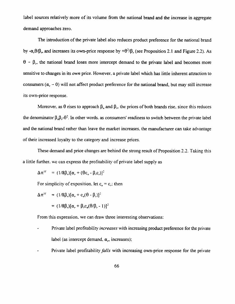
label sources relatively more of its volume from the national brand and the increase in aggregate

demand approaches zero.

The introduction of the private label also reduces product preference for the national brand

by -arO/P, and increases its own-price response by +e2/P, (see Propositicn 2.1 and Figure 2.2). As

0 - p,, the national brand loses more intercept demand to the private label and becomes more

sensitive to changes in its own price. However. a private label which has little inherent attraction to

consumers (ar - 0) will not affect product preference for the national brand, but may still increase

its OW-price response.

Moreover. as 8 rises to approach P, and P, the prices of both brands rise. since this reduces

the denominator P,Pr-0? In other words. as consumers' readiness to switch between the private label

and the national brand rather than leave the market increases. the manufacturer can take advantage

of their increased loyalty to the category and increase prices.

These demand and price changes are behind the strong result of Proposition 2.2. Taking this

a little further. we can express the profitability of private label supply as

A = (1/8P,)[a,+(8c,-P~~)] '

For simplicity of exposition. let c, = c,: then

A r " = (1 /8P , ) [~r ,+c , (~-~ , ) ] '

= ( lwPr)[ar + Prcn(B/Pr - 1 )I-'

From this expression. we can draw three interesting observations:

- Private label profitability increases with increasing product preference for the private

label (as intercept demand. a, increases):

- Private label profitability falls with increasing own-price response for the private

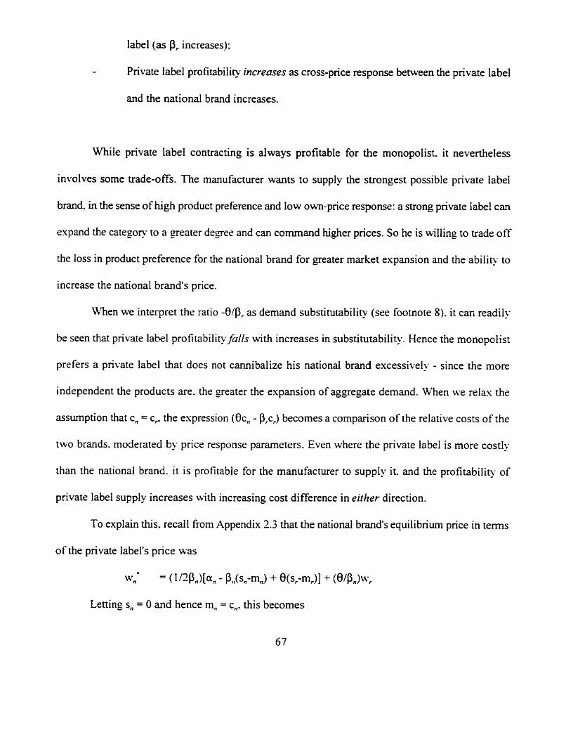
label (as Pr increases):

- Private label profitability increases as cross-price response between the private label

and the national brand increases.

While private label contracting is always profitable for the monopolist. it nevertheless

involves some trade-offs. The manufacturer wants to supply the strongest possible private label

brand. in the sense of high product preference and low own-price response: a strong private label can

expand the category to a greater degree and can command higher prices. So he is willing to trade off

the loss in product preference for the national brand for greater market expansion and the ability to

increase the national brand's price.

When we interpret the ratio -0@, as demand substitutability (see footnote 8). it can readily

be seen that private label profitability fulls with increases in substitutability. Hence the monopolist

prefers a private label that does not cannibalize his national brand excessively - since the more

independent the products are. the greater the espansion of aggregate demand. When we relas the

assumption that c, = c, the espression (Bc, - PF,) becomes a comparison of the relative costs of the

two brands. moderated by price response parameters. Even where the private label is more costly

than the national brand. it is profitable for the manufacturer to supply it. and the profitabilit). of

private label supply increases with increasing cost difference in either direction.

To explain this. recall from Appendix 2.3 that the national brand's equilibrium price in terms

of the private label's price was

w

W n = ( 1 @")[an - P,,(sn-mn) + %-mr)I + (wn)wr

Letting s, = 0 and hence m,, = cn. this becomes

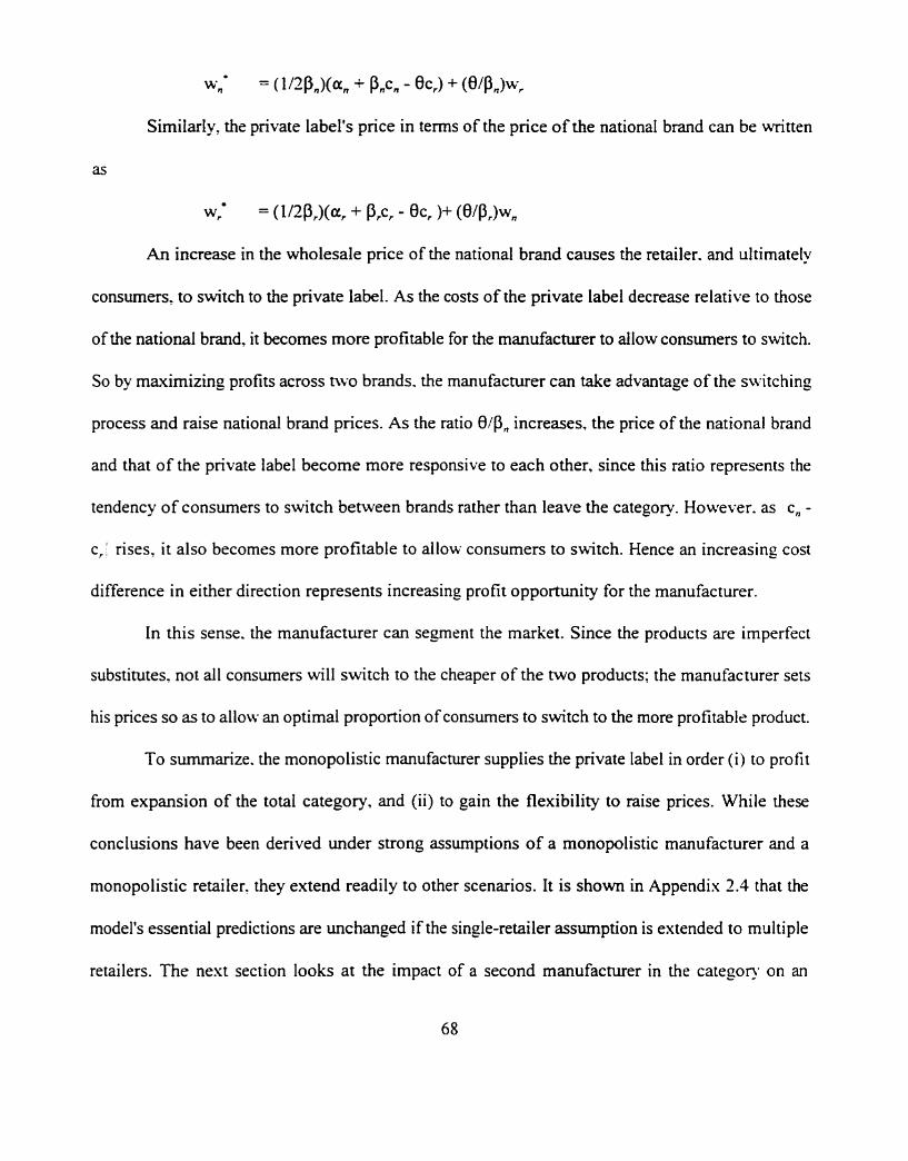
wn = ( 1/3Pn)(a, + P,F - ec,) + (e/p,)w,

Similarly, the private label's price in terms of the price of the national brand can be written

W, = (lnp,)(a, + P A - 0% )+ (0@,)w,

An increase in the wholesale price of the national brand causes the retailer. and ultimately

consumers, to switch to the private label. As the costs of the private label decrease relative to those

of the national brand, it becomes more profitable for the manufacturer to allow consumers to switch.

So by maximizing profits across two brands. the manufacturer can take advantage of the switching

process and raise national brand prices. As the ratio 8@, increases, the price of the national brand

and that of the private label become more responsive to each other, since this ratio represents the

tendency of consumers to switch between brands rather than leave the category. However. as c, -

c , rises, it also becomes more profitable to allow consumers to switch. Hence an increasing cost

difference in either direction represents increasing profit opportunity for the manufacturer.

In this sense. the manufacturer can segment the market. Since the products are imperfect

substitutes. not all consumers will switch to the cheaper of the two products: the manufacturer sets

his prices so as to allow an optimal proportion of consumers to switch to the more profitable product.

To summarize. the monopolistic manufacturer supplies the private label in order (i) to profit

from expansion of the total category. and (ii) to gain the flexibility to raise prices. While these

conclusions have been derived under strong assumptions of a monopolistic manufacturer and a

monopolistic retailer. they extend readily to other scenarios. It is shown in Appendix 1.1 that the

model's essential predictions are unchanged if the single-retailer assumption is extended to multiple

retailers. The next section looks at the impact of a second manufacturer in the category on an

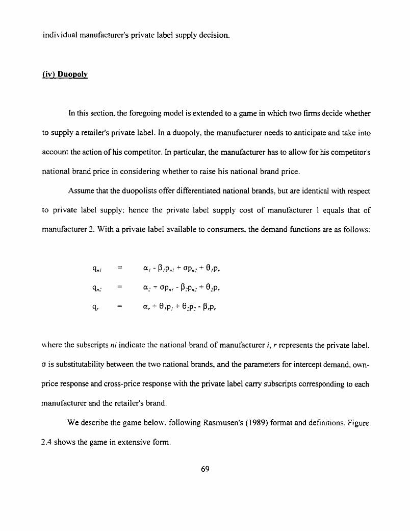
individual manufacturer's private label supply decision.

jiv) Duopolv

In this section. the foregoing model is extended to a game in which two firms decide whether

to supply a retailer's private label. In a duopoly, the manufacturer needs to anticipate and take into

account the action of his competitor. In particular, the manufacturer has to allow for his competitor's

national brand price in considering whether to raise his national brand price.

Assume that the duopolists offer differentiated national brands. but are identical with respect

to private label supply: hence the private label supply cost of manufacturer 1 equals that of

manufacturer 3. With a private label available to consumers. the demand functions are as follows:

where the subscripts ni indicate the national brand of manufacturer i, r represents the private label.

o is substitutability between the two national brands, and the parameters for intercept demand. own-

price response and cross-price response with the private label carry subscripts corresponding to each

manufacturer and the retailer's brand.

We describe the game below. following Rasmusen's ( 1 989) format and definitions. Figure

3.1 shows the game in extensive form.

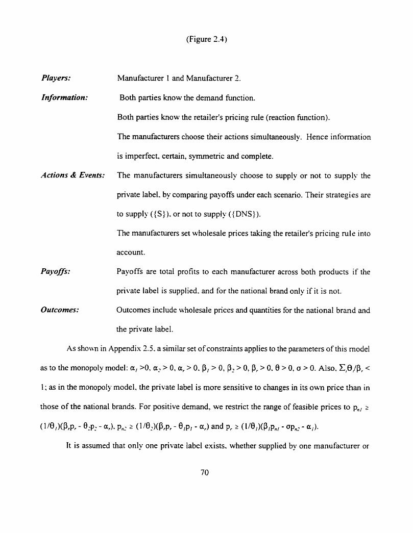
(Figure 2.1)

PIayers:

In formation:

Actions & Everrts:

Payoffs:

Outcomes:

Manufacturer I and Manufacturer 2.

Both parties know the demand function.

Both parties know the retailer's pricing rule (reaction function).

The manufacturers choose their actions simuitaneously. Hence information

is imperfect, certain, symmetric and complete.

The manufacturers simuitaneously choose to supply or not to supply the

private label. by comparing payoffs under each scenario. Their strategies are

to supply ((S)) . or not to supply ((DNS)).

The manufacturers set wholesale prices taking the retailer's pricing rule into

account.

Payoffs are total profits to each manufacturer across both products if the

private label is supplied. and for the national brand only if it is not.

Outcomes include wholesale prices and quantities for the national brand and

the private label.

As s h o w in Appendix 2.5. a similar set of constraints applies to the parameters of this model

as to the monopoly model: a, >O. a, > 0, a, > 0. P, > 0, P, > 0, P, > 0 . 0 > 0. a > 0. Also. X,O/P, <

1; as in the monopoly model. the private label is more sensitive to changes in its own price than in

those of the national brands. For positive demand. we restrict the range of feasible prices to p,, 2

(l/e/)(Prpr - 0,~: - pn, 2 ('/'?)(Prpr - elp, - and pr 2 (l/e,)(P,pn/ - op,~ - a/)-

It is assumed that only one private label exists. whether supplied by one manufacturer or

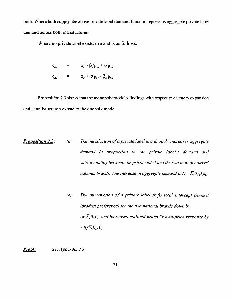
both. Where both supply. the above private label demand function represents aggregate private label

demand across both manufacturers.

Where no private label exists. demand is as follows:

Proposition 2.3 shows that the monopoly model's findings with respect to category expansion

and cannibalization extend to the duopoly model.

Proposition 2.3: /a) The infrodzrction of a private label in a duopolJ. increases aggregate

demand in proportion to the private label's demand and

sribsfitrlfubility between the private labei and the two rnanzrfactzrrers'

national brands. The increase in aggregate demand is (2 - &0;'&jq,

(bl The introdricrion of a private label shrfis total intercept demand

(prodzcct preference) for the wo national brands down by

- ar& Oipp uund increases national brand i 's own-price response by

O , ~ ' Z $ ~ J < ' ~ , .

See Appendix 2. j

As before, aggregate demand increases as a result of the introduction of the private label.

However, the benefit of this increase in aggregate demand may differ between manufacturers. As

shown in Appendix 2.5, manufacturer 1 experiences a change in demand for his national brand of

(r,O/Pr)q, - Aq,,,. where the notation A represents change. In other words, the private label's

substitution with the competing duopolist's brand reduces cannibalization of manufacturer 1's brand.

Focusing on the manufacturer's problem, we assume for this model and for the model of

chapter 3 that the retailer's selling costs for the national brand, sn, and for the private label, $, are

zero. This assumption is justified in the grocery industry by the fact that. aside from manufacturers'

unit prices, retailers' costs consist primarily of real estate rental. store personnel and store advertising

- all of which are fixed and not associated with a specific product. The costs of product-specific retail

activity. such as display and co-operative advertising. are also fixed (in the sense that they cannot

be allocated on a per unit basis) and. in any event. are largely borne by the manufacturer.

Equilibrium wholesale prices and quantities for the duopoly model are derived in Appendix

2.6. If manufacturer 1 supplies the private label taking manufacturer 2's national brand price into

account. his price for the national brand is

- wn I - x[(a,Pr+arB /)/(PIPr-0l1) + ( 0 P r + e , 0 ~ ) ~ ~ n . . . J ( P j P r - e / ~ ) + mnl]

and for the private label.

- Wr

- 1 / 2 [ ( a r P , + a / e j ) / ( P j P r - 8 j 1 ) + (a~,+P,e~)~nJ(p,Pr-e,~) + mrl

As before, the manufacturer passes on half of any cost increase to the retailer. He takes into

account the intercept demand of both his national brand and the private label, and the ratio between

cross-price response and own-price response. in setting wholesale prices. However, in this model.

he also takes into account the price of his competitor's national brand and substitutability between

the two national brands.

At these prices. he supplies the quantities

al - - %(a, - P,rn,, + elmr + own2)

% - - %(a, + O,mr + awn, - P,mr)

With both manufacturers considering whether to supply the retailer's private label. the options

open to them can be encapsulated in the normal form game shown in Figure 2.5.

(Figure 2.5)

Figure 2.6 compares the prices set by manufacturer 1 in the monopoly model and under each

of the four strategy sets of the duopoly game. The results of the duopoly model are a straightfonvard

estension of those of the monopoly model. with the additional considerations of competitive pricing

and substitution between the two national brands.

(Figure 2.6)

Where both marLufacturers supply with equal marginal costs. they become Benrand

competitors and bid each other's supply price to their marginal cost for the private label, m,. The

rerailer splits the private label contract between the two manufacturers and each makes total profits

of n,, = d,(~", - m,,).

If manufacturer 1 agrees to supply while manufacturer 2 does not, he will make positive

profits on the private label while suffering cannibalization of his national brand. His total profit will

be K': = a,(%, - m,,,) + (~(y - m,). However. if manufacturer 1 decides not to supply while

manufacturer 2 supplies. he makes I?', = q,,(w,, - m,,). Since manufacturer 2 is supplying the private

label at w, > m,. however, manufacturer I suffers less cannibalization of his national brand in this

scenario than if both supply. If neither manufacturer supplies, the payoff for each is T?', = q,,,'(w,,' -

mnt)-

We know that the payoff in Figure 2.5 to the non-supplying manufacturer from the sua t eg

set {S,DNS) or {DNS.S} is higher than that under {S,S}. Hence, if manufacturer 2 supplies.

manufacturer 1 will prefer not to supply for fear of increasing cannibalitation of his national brand

by reducing private label prices. The comparison of payoffs under (S.DNS) and {DNS-DNS J

decides the equilibrium. Where each manufacturer can gain from supplying while his competitor

does not. the Nash equilibria are {S-DNS) and {DNS.S ): one manufacturer will supply while the

other refrains from supplying. Where the opposite holds. neither manufacturer will supply.

The analysis therefore rests on determining the conditions under which

R",((S.DNS)) > x'\((DNS.DNS)) - i.e. under which one manufacturer gains by supplying. given

that his competitor does not supply. Proposition 2.4 defines these conditions.

Proposition 2.4: .An asymmetric eqttilibrizrm in which on@ one manlrfacturer supplies [he

private label becomes more likely us

li) The private label's cross-price response with national brand

i. 8,, rises;

(ii) The private label's cross-price response relative to rhr

competing manufacturer's national brand. 8,, rises:

fiiil The private label's intercept demand. a;. rises:

i The private label's own price response. P, falls.

f i j The private label's costs. rn, fall relafive 10 those of nationul

brand i.

Proofi See Appendix 2.7

Each of the parameters of the model afTects private label profitability in interaction with the

difference in manufacturer 2's national brand price between the two scenarios: if manufacturer 2

reduces his price. the effect can overpower these parameter effects and reverse manufacturer 1's

decision. From Appendix 2.7. the difference in payoffs to manufacturer 1 between supplying and not

supplying given that manufacturer 2 does not supply is

( 1 /8)0,m,(S+Twn2-m,,) + ( 1 /8)(Lr+ Vw-,,-m,)(a,-pmr+8 , m n i ~ o w n , )

- (1 /8)(8 ,/Pr)(a,+O ,m,,+8,wn,')(S+ Twn2-m,,)

+ ( 1 /8)(S+Twn,-mn,)o(wn,-w,,')

where * (a,pr+cr,8,)/(p,p,-8,'): T = (op;te,O,)/(PIP;O,'): (i = (a,P,+a,0,)/(P,pr-0 ,'): l *

= (~8,+p,0,)/(p,p;0,2): w, is manufacturer 2's national brand price when manufacturer 1 supplies

the private label: and w,,,' is manufacturer 2's national brand price when manufacturer 1 does not

supply

From the above expression. it is evident that the difference in competitive prices, (w,,-w,,')~

can change the sign of the profit difference between supplying and not supplying.

Duopolists considering supplying a retailer's private label consider similar factors to a

monopolist: substitutability. product preference for the private label and costs. Again. duopolists are

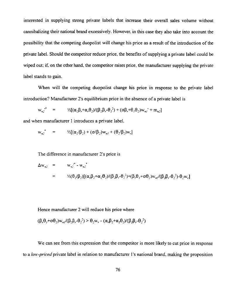
interested in supplying strong private labels that increase their overall sales volume without

cannibalizing their national brand excessively. However, in this case they also take into account the

possibility that the competing duopolist will change his price as a result of the introduction of the

private label. Should the competitor reduce price. the benefits of supplying a private label could be

wiped out: if. on the other hand, the competitor raises price, the manufacturer supplying the private

label stands to gain.

When will the competing duopolist change his price in response to the private label

introduction? Manufacturer 2's equilibrium price in the absence of a private label is

to - - M'n: %[(a,pr+are,)/(PJPr-82Z) + (opr+0,02)wn,' + m,]

and when manufacturer 1 introduces a private label.

I - \yn2 - % [ ( a J P J ) + ( o / P 2 ) ~ n , + (0ljP:)~rl

The difference in manufacturer 2's price is

Awn: = \vn;l - wn:

- - ' / . . ( 0 ~ p , ) [ ( a , p , + a ~ 8 ~ ) / ( p ~ p ~ - 8 ~ ' ) + ( ~ , 0 ,+oO,)w ~(P,P;0,')-0,w,]

We can see from this expression that the competitor is more likely to cut price in response

to a lowpriced private label in relation to manufacturer 1's national brand, making the proposition

less attractive for manufacturer 1. Manufacturer 1 is therefore more likely to be interested in a higher

priced private label which does not excessively threaten his competitor - such as a premium private

label. In other words. if the manufacturers expect to set off a price war by supplying a low-priced

private label, neither will supply.

jv) Summarv and Conclusions

The monopoly and duopoly models in this chapter provide a framework for analyzing the

questions faced by manufacturers in deciding whether to supply a retailer's private label brand.

For a monopolist. the model's conclusions are clear: it is always in his interest to supply a

retailer's private label. There are

cannibalizes the national brand:

two reasons for this: first. not all of the private label's volume

there is some category expansion. from which the monopolist

benefits. The exception to this is where product preference (intercept demand) for the private label

approaches zero. and virtually ail the private label's volume comes from the national brand.

However. even in this instance. total category demand does not decline.

The second reason for a monopolist's interest in supplying private label is that it allows him

to segment the market. It becomes profitable for the manufacturer to allow a proportion of consumers

to switch to the private label, which he can encourage by raising the price of the national brand.

To maximize the profit he derives from the private label, the monopolist needs to strengthen

the private label and minimize its costs and its substitutability with the national brand. Hence

manufacturers look for private labels with high product preference, low own-price response and low

costs, to maximize their benefits fiom both market expansion and switching between brands.

However, they will also want to minimize cannibalization of their national brands. In markets where

quality is unidimensional - i.e. where there is just one attribute consumers look for - this would seem

to be an impossible task. Strengthening the private label will necessarily move it closer in quality

to the national brand and increase cannibalization.

However. where quality is multidimensional, there can be many opportunities to develop a

high quality private label with different attributes from the national brand. The example of Loblaw's

President's Choice Bottled Sauces comes to mind: here. the product is of high quality but

differentiated fiom the supplier's brand, H.P. Sauce. It is in a manufacturer's interest to develop

private label brands of this nature which can increase demand for the category as a whole but take

away volume from the national brand onIy to a limited extent.

Retailers can take some comfort from this result. Even if a manufacturer dominates the

category. it will still be in his interest to supply a high quality private label. Moreover. he will want

the retailer's private label to have high demand from consumes and be relatively impervious to price

increases. Nonetheless, he will be concerned that the private label be as different as possible from

his own national brand - an aspect which may not accord with the retailer's objectives.

In a duopoly, the same considerations are in evidence. However, the introduction of a

national brand competitor to the model means that the manufacturer now has to anticipate the

reaction of the other duopolist to his strategy: the competitor may also bid to supply the private label,

or may change his prices in response to the launch of the retailer's brand.

A duopolist will therefore take into consideration the degree to which the private label

cannibalizes the competing duopolist's sales as opposed to his own, in addition to consumer

preference for the private label and relative costs. Segmenting the market will not be as easy for a

duopolia as a monopolist. since a change in the competitor's equilibrium price may draw consumers

away from the national brand without the compensating increase in private label demand.

Nevertheless. it is more likely that one duopolist will want to supply the private label where

it has a high degree of consumer preference and low own-price response. So once again, the idea of

supplying a "premium" private label which competes only indirectly with the national brand is likely

to appeal to both manufacturers.

The baseline models presented in this chapter provide us with some important insights into

the private label supply decision. However. simpliQing assumptions have been used to derive clear

results. In particular: the assumption of constant marginal costs suggests that manufacturers have no

economies of scale or scope. In the next chapter. a more general cost function will be incorporated

in order to determine the effect of cost changes on the private label decision.

In addition, there are few markets in the real world which can be described as pure

monopolies or pure duopolies. In the next chapter. the model will be extended to consider the effect

of other manufacturers on its predictions. In particular. a market with a "competitive fringe" will be

analyzed - a structure which is representative of many grocery categories.

REFERENCES

C hang A. C . ( 1 981). Fundamental Meihodr of Mathematical Economics, New York: McGraw-Hill.

Choi. S. Chan (1991), "Price Competition In A Channel Structure With A Common Retailer". Marketing Science. 10.4 (Fall), 271-296.

Coase, Ronald H. (1 937), "The Name Of The Firm", Econornica, 4 (Nov.), 386-405.

Coughlan, Anne T., and Birger Wemerfelt (1989), "On Credible Delegation By Oligopolists: A Discussion Of Distribution Channel Management", Management Science, 2 (Feb.). 226-239.

Dixit, A. (1 979). "A Model of Duopoly Suggesting a Theory of Entry Barriers". Bell Journal of Economics. 10. 20-32.

Dwyer. F. R.. P. H. Schurr and S. Oh ( 1 987). "Developing Buyer-Seller Relationships". Journal of Marketing. 5 1 (Apr.). 1 1-22.

Fader. P.S. and James M. Lattin. "Accounting for Heterogeneity and Nonstationarity in a Cross- sectional Model of Consumer Purchase Behavior", Marketing Science, 12,3 (Summer). 304-3 17.

Gonul. F. and K. Srinivasan (1993). "Modeling Multiple Sources of Heterogeneity in Multinomial Logit Models: Methodological and Manageiral Issues". Marketing Science, 12. 3.2 13-229.

Green. H A . John ( 1 97 1 ), Consumer Theoy. Harrnondsworth, Middx.: Penguin Books.

Intriligator, Michael D. (1 971 ) Mathematical Oprimization and Economic Theory. Englewood Cliffs. N. J. : Prentice-Hall.

McGuire. Timothy and Richard Staelin (1 983). "An Industry Equilibrium Analysis Of Downstream Vertical Integration". Marketing Science. 2. 2 (Spring). 1 6 1 - 19 1.

McNeil. I.R. (1978). "Contracts: Adjustments of Long-Term Economic Relations Under Classical. Neoclassical, and Relational Contract Law1', Northwestern Universify Low Review, 72. 854-906.

Rasmusen. Eric ( 1 989). Games and Information, Oxford: B. Blackwell.

Tirole. Jean (1 988). The Theory of Industrial Orgonizufion. Cambridge, Mass.: The MIT Press.

Varian. Hal R. (1992). Microeconomic Analysis. New York: W.W. Norton & Co.

Williamson. Oliver E. (1985). The Economic Institzrtions of Capifalism, New York: The Free Press.

APPENDICES

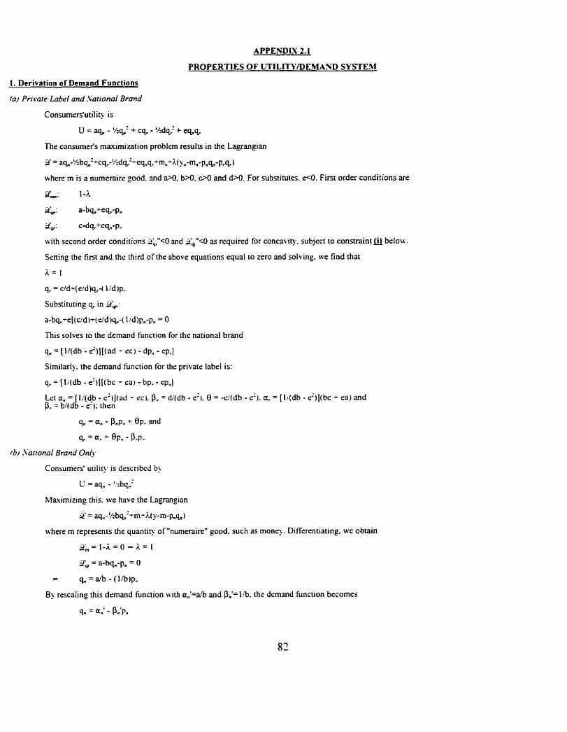
APPENDIX 2.1

PROPERTlES OF UTILITY/DEMAND SYSTEM

1. Derivation of Demand Functions

faj Privare Label and Sarional Brand

ConsumersVutilit) is

U = aq,, - '/:a' + cq, - Vide' + eq,,q,

The consumefs maximization problem results in the Lagrangian

Y = aq,-%b~'-~q,-Y:dq,'~e~~,~m,+L(~~-rn,-~,~-p,q,)

where m is a numeraire good. and a*. b>O. c>O and d>0. For substitutes. 60. First order conditions are

9,: 1 4 .

2 : a-ba+ea-p,

2': c-dq,+ea-p,

with second order conditions 2blU<O and i&"<O as required for concavip. subject to constraint a belo\v.

Setting the first and the third of the above equations equal t o zero and solving. we find that

i = l

q, = c/dt(e?'d)a-( I /d )p,

Substituting q, in ifv:

a-ba-ef(c!d )+(r/d )a-( 1 ;d)p.-pn = 0

This solves to the demand function for the national brand

q,, = [lJ(db - eZ)l[(ad - cc, -dpn - cp,]

Similarly. the demand function for the private label is:

q, = [li(db - e2)I[(bc - sa) - bp. - cp,]

Let a, = [I!(db - e2)](ad - sc]. P, = d/(db - e'). 0 = -d(db - o'). a. = [ I , (db - i ) ] ( b c ea ) and p. = bi(db - e- ); then

qn = a n - Pmp, -+ OP. and

qr = a, +- 8p, - P.p-

(6) .larional Brand On@

Consumers' utilit>. is drscribed b?

U = aq, - !,:bQnZ

blaximizing this. w e have the Lagrangian

9' = aq,-!'b~'-m-?.(y-m-p,q,)

where m represents the quantity of "numeraire" good. such as mone). DitTerentiating. we obtain

dA= 1-A =() - j. = [

9, = a-ba-p, = 0

- q ,=a /b - ( l /b )p ,

By rescaling this demand function lvirh a,'=a/b and P,'= f /b. the demand function becomes

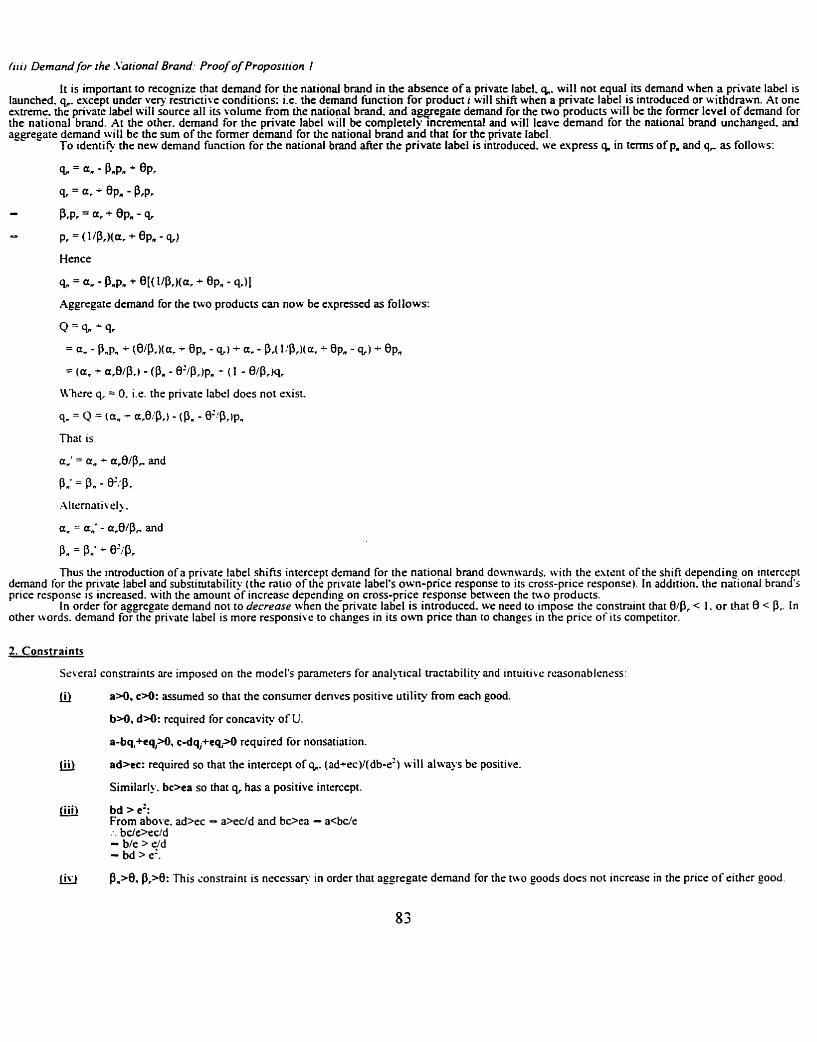
h i / Demand for rhe .Yarional Brand: Proof o/Propos;tion I

It is important to recognize that demand for the national brand in the absence of a private label. a. will not equal its demand when a private label is Iaunched. q,,. except under very restrictive conditions; i.e. the demand hnction for product i will shift when a private label is introduced or withdrawn. At one extreme. the private label will source all its volume From the national brand, and aggregate demand for the two products w11i be the former level of demand for the national brand. At the other. demand for the private label wilt be completely incremental and will leave demand for the nationaI brand unchanged. a d aggregate demand will be the sum of the former demand for the national brand and that for the private label.

To identie the new demand function for the national brand after the private label is introduced. we express q, in terms of pa and e. as follows:

Aggregate demand for the two products can now be expressed as follows:

a,' = a, - a,O/p, and

P i = on - e2:P, Xltematively.

a, = a,' - a,B/P, and

p" = p; + 0'/QI

Thus the introduction of a private label s h i b intercept demand for the national brand downwards. kvirh the rstcnt of the shift depending on interce t demand for the prlvav label and subs~itutabiliry (the ratio of the private label's own-price res onse to its cmss-price response). In addition. the national branJs price response is increased. wth the amount of incrnse de ending on crossprice response getween the two products.

In order for aggregate demand not to decrease d e n the private label is introduced. we need to im ose the constmint thar WPr < I . o r ha t 8 < P.. In other words. demand for the private label is more responsive to changes in its o m price than to changes in tEe pricc of its competitor.

2. Constraints

Scvenl consmints are imposed on the model's parameters for anaij~ical tractability and intuitive rcasonablrness:

fcl a*, c>O: assumed so that the consumer derives positive utility from each good.

b>O, d*: required for concavity of U.

a-bq,+eq,*, c-dq,+eq,* required for nonsariation.

(ii) ad>ec: required so that the intercept of q,,. (ad+ec)/(db-e') uill always be positive.

Similarly. bc>ea so that q, has a positive intercept.

(LYJ bd > e': From above. ad>ec - a>ec/d and bees - a<bc/e :. bcfe>tc/d - b/e > d d - bd > e'.

Pp8. P,>0: This constraint is necessar?. in order that aggregate demand for the two goods does not increase in the pricc o f either good

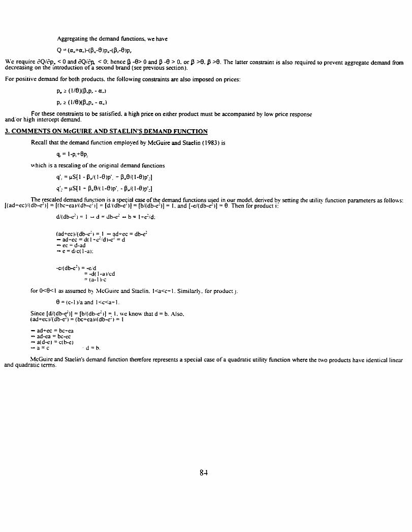
Aggregating the demand hnctions. we have

We require dQISp, < 0 and a Q i 6 ~ < 0: hence fi -0> 0 and P -8 > 0. or fl >0. fi >8. The latter constraint is also required to prevent agpegaa demand from decreasing on the lntroduct~on of a second brand (see previous section).

For positive demand for both products. the following constraints are also imposed on prices:

For these constraints to be satisfied. a high price on either product must be accompanied by low price response and'or high intercept demand.

3. COMMENTS ON McGUIRE AND STAELIN'S DEMAND FUNCTION

Recall that the demand function employed by McGuire and Staelin ( 1 983) is

which is a rescaling of the original demand functions

The cescaled demand function is a spqial case of the demand functions used in our model. derived bv setting the utility function panmeters as foIlows: I(ad-ecI4db-c-I] = [( be-ea)/(db-c- = [d'(db-e-)I = [b/(db-e')] = 1. and [-c/(db-g)] = 8. Then for product i-1

for 0<8<1 as assumed b ,LIcGuirr: and Starlin. I<a<c-1. Similarl~. for product J ;

0 = ( c - I )/a and I <c<a- 1 .

Since [d/(db-tf)~ = [b/(db-e')] 7 1. we know that d = b. Also. (ad-ec )/(db-e-) = (bc+ea )/(db-e- 1 = I

- ad+ec = bc-ea - ad-ea = bc-ec - a( d-e ) = C( b-r: ) - ;1=c - d = h .

McGuirr and Staelin's demand function therefore represents a special case of a quadratic utility function where the two products have idenrical linear and quadratic terms.

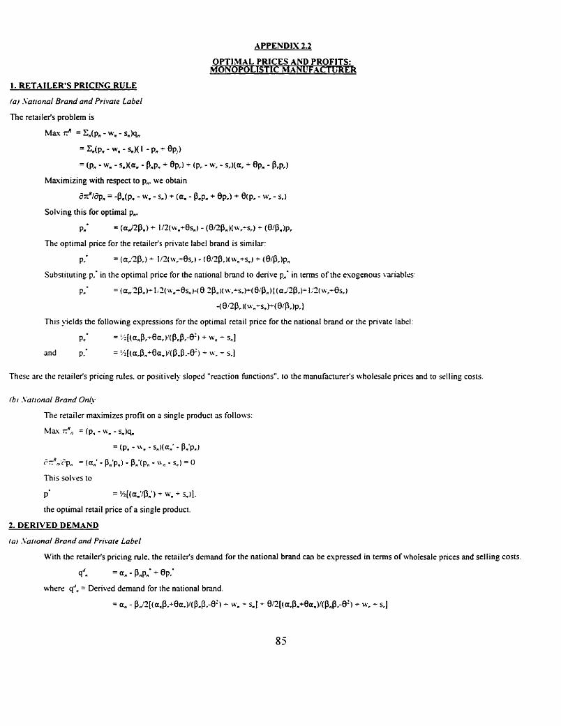
APPENDIX 2.2

OPTIMAL PRICES AND PROFITS: MONOPOLISTIC MANU'FACTURE~

The optimal price for the retailefs private label brand is similar:

PI* = (a,'2P.) + 112(ivr-8s,) - (8/2P.)( w,+s,) + (B/P,)p,

Substitutin_e p.' in the optimal price for the national brand to derive p,,' in terms of the esogenous variablrs:

PC = (a,'2P,)- t iZ(wn-0s,)-(8. ZP,~( \v, -s, ) i (0iP~){(a, 'ZP,) - I,'?( w,tes,)

-( B!2Pr lc\%+sn)i<8/P,)p, 1

This yields the following espressions for the optimal retail price for the national brand or the private label:

Pm = !/2[(anP,41a, )I(PnP,-O' + w, - s, j and p,' = !/2[(a,P,+8a,)l(PnP.-0') - iv. - 5.1

Thrsc art: the re~ailer's pricing rules. or positively sloped "reaction functions". to the manufacturer's wholesale prices and to selling costs.

fb I .Varlonal Brand On(v

The retailer maximizes profit on a single product as follo\vs:

hlax ?, = (p, - w, - sn )a

= (pn - " n - snNan' - P n ' p n )

e+,lrp, = (an1 - pntp,) - pm*(pn - Un - 5,) = 0

This soives to

P' = I/i[(a,,*/Pnl) + H;I + s,)].

the optimal retail price of a single product.

2. DERIVED DEMAND

/a) .l'ar~onal Brand and Private Label

With the retailer's pricing rule. the retailer's demand for the national brand can be espressed in terms of whoIesale prices and selling costs.

- s4 - am - Pnp,' + epr*

where q', = Derived demand for h e national brand.

= a, - P J Z [ ( ~ , P . + B ~ , ) / ( P , P . - ~ ' } - IV, - s,] + 8/2[(a,P,+8a,)/(PnQI-0') - w, - s,]

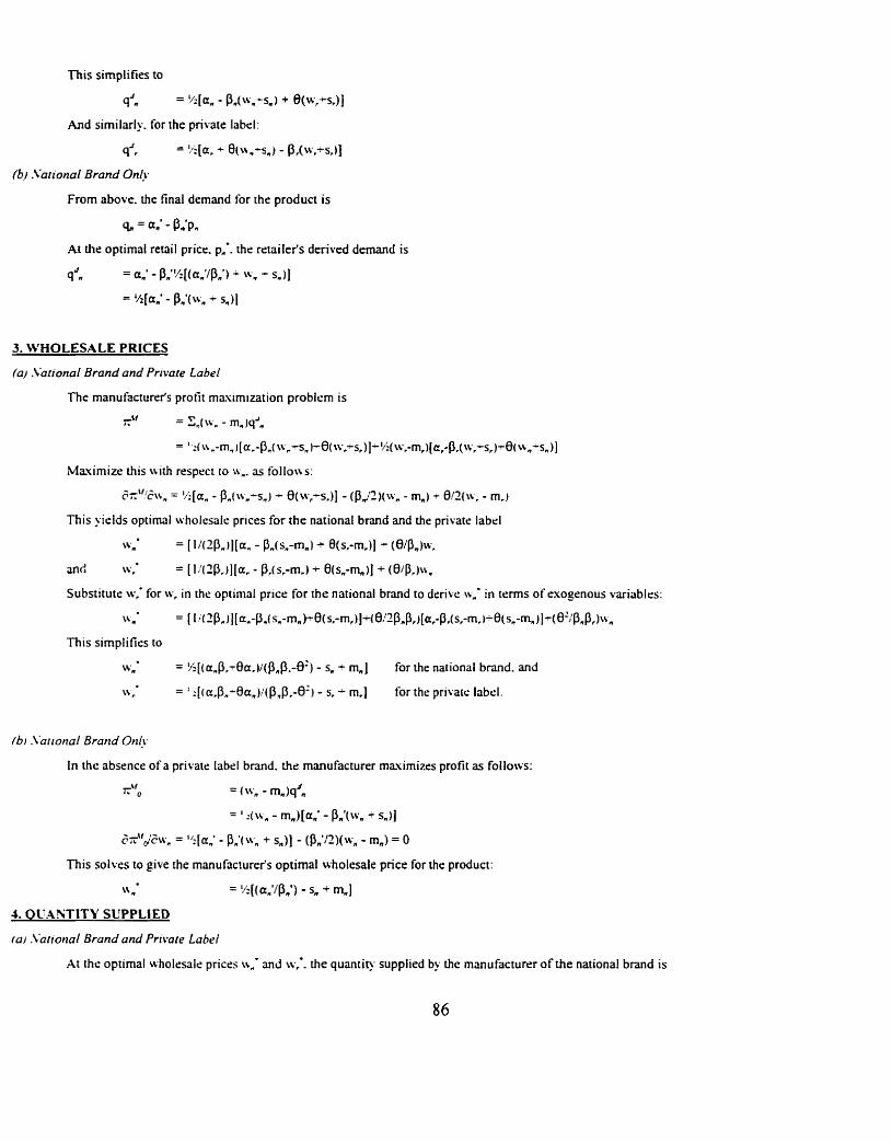
This simplifies to

s', = %[a, - Pw(~v.-s,) + 6(wP+sr)]

And similarly. for the private label:

qdr = !/:[a, + ~ ~ I V , - S ~ J - pr(~~,-s,)1 /b, .Varionai Brand Only

From above. the final demand for the product is

a = an' - Q,'p,

At the optimal retail price. p,'. the retailer's derived demand is

q d m = an1 - Pn"/2[(anf/P,') - \v, - s,)]

= %[a,* - P,'( W, f s, ) I

3. W H O L E S A L E PRICES

fa) .Varional Brand and Prrvafe Label

The manufacturer's profit maximization problcrn is

+f = S,( w, - m, )qJn

= '~\\,-m,)[a.-P,( wP-sn ~ - 8 ~ ~ v . - s , ) ~ ~ , , - s , ) ]

~Mavimizr this with respect to u.,. as follon s:

5Afl- .c\c, = %[a, - P,(\v,-s,) + 8(wr+s,)] - (PJ2)(\vn - m,) t 8/2(1~, - m,)

This ~ i e l d s optimal ~vholesalc prices for the national brand and the private label

W, - [1/(2P,)l(a, - P,ts,-rn,) + @s,-m,)] + (B/P,)w,

and \v , = [I:(?P,)][a, - PAS,-m,) + 8(s,-m,)] +- (8/P,~w,

Substitute w,' for w, in the optimal price for the national brand to derive K,' in terms of e x o p o u s variables:

- N , - [ 1 d?PJl[a,-P,( s, -m,) -8(s . -m,) ]+(8~Z~,~,~[a , -~r (sr -m,~s~-m,)~- (82~~n~, )~R

This simplifies to

we = Ij2[(anP,f0a.)/(P,P.-8') - s, + m,] for the national brand. and

\\ r = ' : [ (a ,P,~Ba,)r(~,~,-8 ' ) - S, - m.] for the private label.

/bt .\'arional Brand On/!

In the absence of a private label brand. the manufacturer rnasimizes profit as follows:

= {IV, - m,)qd,,

- I - : ( ibm - mn)[aWo - P,,'(Iv, 7 s,,)]

6ii",,/6wn = %[a: - p;(w, + s,)] - (P,'/2)(w, - m,) = 0

This solves to give the manufacturer's optimal wholesale price for the product:

N = I/Z((a,'JPWQ) - S, + m,]

4. OUANTITI' SUPPLIED

la) .\attonal Brand and Private Label

At the optimal wholesalr prices N,' and ~v,'. the quantit) supplied b! the manufacturer o f the national brand is

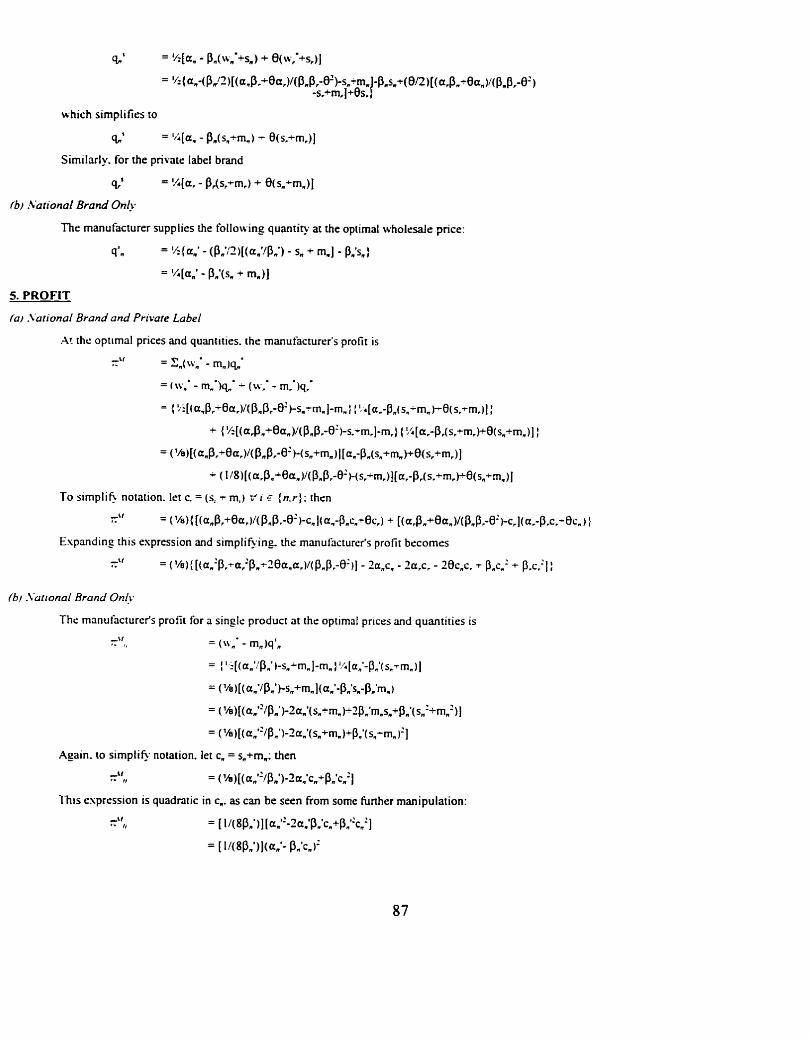
which simplifies to

a' = '';[a, - P.(s,+m,) - B(s,+~,)]

Similarly. for the private label brand

%s = %[a, - P,(s,+rn,) + O(s,+mn)I

fb) :Varionaf Brand Only

T h e manufacturer supplies the following quantity at the optimal wholesale price:

qJn = 'A{a,' - (P,,'2)[(am1/Pn') - s, + m,] - Pis,)

= %[a,' - P,,'(s, + m,)]

5. PROFIT

fa) .\brionu/ Brand and Private Label

161 .\bnonal Brand On&

Thc manufacturer's profit for a single product at the optimal prices and quantities is

Af I - I , = ( - m,, jqqn

- - r ',i[(an9:pn')-s,-m,]-m, !4[a,'-P;(s,-m,)]

= ('~>[(a,'/p,')-s,+mn](aI)'-Pn's~'m~ - - ( 1h)[(an''l~,')-2a,'(s,+m, )-2~,'rn,~,+~~'(s,'+m,')]

= ( 'h )[( an"/p,')-2a,'(s,+mn)+P,'( s,-mm )'I

Again. to simpli@ notation. let c, = s,+m,,; then

*'I .- I) = ( 1h)[(an"/Pn')-2a,,'~n+p~~n']

This expression is quadratic in c,. as can be seen from some hnher manipulation:

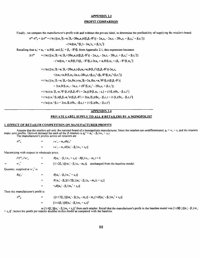
APPENDIX 2 3

PROFIT COMPARISON

Finail!.. wc compare the manufacturer's profit with and without the private label. to determine the profitability of supplying the rctailrfs brand.

r"-;r'b = Arb' = (%)( [(a,'pr+a,:p,+20a,ary(PnPr-8')] - 2a,c, - Zqc, - tOc,cr - P.cn2 + P,c,'] )

- (lh)[(a,"/P,') - 2a,'c, + Pn1cn2]

Recalling that a,' = a, - a,0/P, and P,' = P, - 8'10, from Appendis 2. I , this expression becomes

APPENDIX 2.4

PRIVATE LABEL SUPPLY T O ALL R RETAILERS BY A MONOPOLIST

1. EFFECT OF RETAILER CO!bIPETITIOX ON MANUFACTURER PROFITS

Assume h a t rhe retailers sell only the national brand of a monopolistic manufacturer. Since the retailers are undifferentiated. p, = w, - s, and the retailers make zero rofits. Derived demand for each of the R retailers is q,," = a,' - P,'(u, - s,).

1Phe manufacmrrr's profits across all retailers are

Masirnizing with respcct to wholesale. price. +Sf .-

1. (, CW', - - R[a,' - P,'(tvn + s,)] - RP,'(w, - m,) = 0

- i t '-a - - [ I!c?p,')][(ane - P.'(s, - m,)]. unchanged from the baseline model.

Quantit? supplied at n',' is

Then the manufacturer's profit is

or [li4fl.')][an:- PnV!mn + sJl' from each re@ler. Recall that the manufacturefs profit in rhr baseline model was [ l/(8P :)](a: - P :r m, + s,)]': hence his profit per retailer doubles In t h ~ s model as compared wth the baseline.

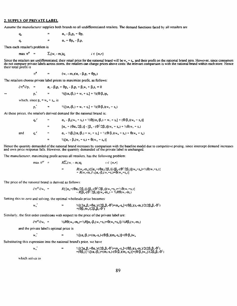
2. SUPPLY OF PRIVATE LABEL

Assume the manufacturer supplies both brands to all undifferentiated retailers. The demand Functions faced by all retailers are

d - - an - Qnpm + 0 ~ -

Then each retailefs problem is

Since the retailers are undifferentiated. their retail price for the national brand will be rr;, + s, and their profit on the national brand zero. However. since consumes do not compare private labels across stores. the retailers can charge prices above costs: the relevant comparison is with the national brand within each store. Hence their total profit is

The retailers choose private label prices to maximize profit. as follows:

At these prices. the retailefs derived demand for the national brand is:

Hence the qurtntlp demanded of the national brand.increaxs by corn a r i sy with the baseline model due to cornpetit~ve priang. since intercept demand increases and own price response falls. Horvevcr. the quantlt? demanded of t fe prlvate label is unchanged.

The manufacturer. maximizing profit across all retailers. has the following problem:

The price of the narional brand is derived as fol1o~s.s:

Sening this to zero and solving. the optimal \vholesaIe price becomes:

Similarly. the first order conditions with respect to the price of the private label are:

and the private label's optimal price is

Substituting this rspression into the national brand's price. we have

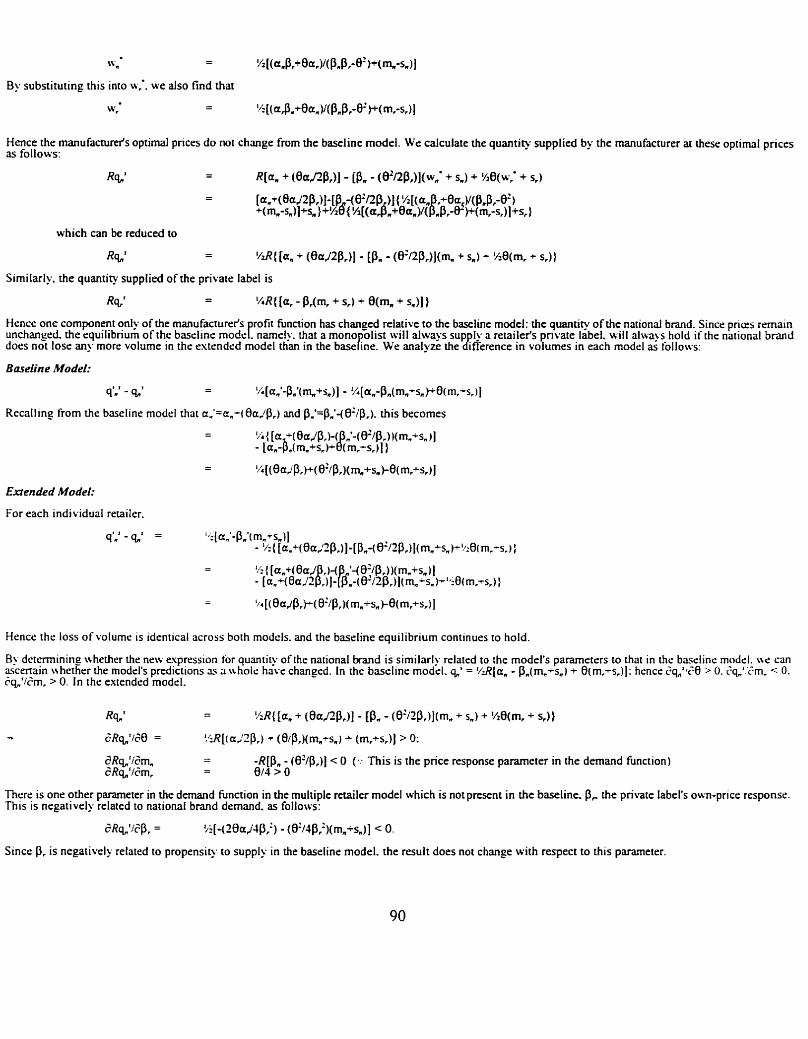
Hence the manufacturets optimal prices do not change from the baseline model. We calculate the quantity supplied by the manufacturer at these optimal prices as follows:

which can be reduced to

Ra' - - M{ [a, + (8a/2pr)] - [P, - (8'/2P,)](m, + s,) + M ( m , + s,)

Similarly. the quantity supplied of the private label is

w - - ' A 4 [a, - P m , + sr) + Qm, + s J J 1 Hence one component only of the manufacturefs rofit hnction has changed relative to the baseline model: the quantity of the national b a d . Since prics remain unchanged the equilibrium of the baseline mode! namely. that a mono &st will always sup Iy a retailer's ppnate label. will always hold if the national b m d does not lose any more volurne in the estended model than in the baxEne. We analyze the tfferencc in volumes in each rnodrl as follo\vs:

Baseline Mod&

Recalling from the baseline model that a,'=a,-( BaiP,) and &,'=Pag-(B'IP,). his becomes

Eaended Model:

For each individual retailer.

Hence the loss of volume is identical across both models. and the baseline equilibrium continues to hold.

B) determining whether the nets espresslon for quantity of the national brand is similarly related to the model's parameters to that in the baseline model. us can ascertain uhcther the model's predict~ons as a t~ holc have changed. In the baseline model. a' = '/2R[a, - p,(m,-s,) + 0(m.-s,)]: hence cqn1~ZI > 0. 2q,' 'em, < 0. sq,,'lCm, > 0. In the extended model.

a Rqn ' lZm, - - - -R[P, - (8'@,)] < 0 (.: This is the price response parameter in the demand function)

6 Rat16m, - 014 > 0

Tfier~ is one other parameter in the demand function in the multiple retailer model which is not present in the baseline. P, the private label's own-price response. This 1s negatively related to natronal brand demand. a s follows:

Since p, is negatively related to propensity to supply in the baseline model. the result does not change with respect to this parameter.

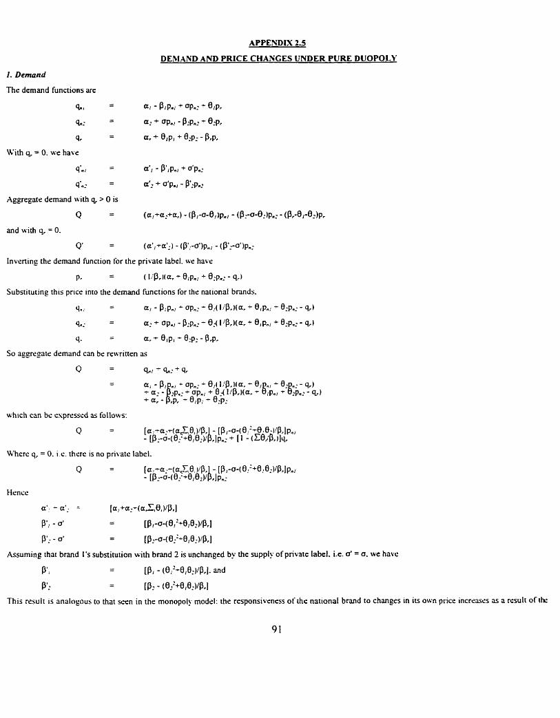
APPENDIX 2.5

DEh1AND AND PRICE CHANGES UNDER PURE DUOPOLY

1. Demand

The demand functions are

Invming the demand function for the private label. we have

Substituting this price into h e demand functions for the national brands.

- q": - a1 - P:p,, up,: - B,( liP,)(a. - Blp,: - 0,p,, - q,)

So aggregate demand can be rewritten as

which can be expressed as follows:

Where q, = 0. it.. there is no private label.

Hence

Assuming that brand 1's substitution with brand 2 is unchanged by the supply of private label. i-e. o' = a. we havc

P'1 - - [PI - (e,'+e/fl:VPrI- and

P': - - [P. - (8.2+0,0Jp.1

This result is analogous to that seen in the monopoly model: the responsiveness of ihr nationat b m d to changes in its own price increases as a result of rk

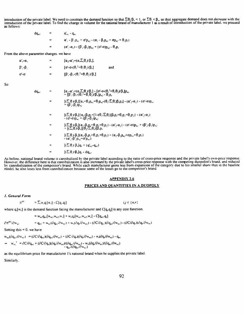
introduction of the private label. Wc need to constrain the demand function so that 10/P, < 1. or 10, c P, so that asgegate demand does not decreare with the introduction of the private label. To find the change in volume for the national brand of manufacturer 1 as a result of mtroduction of the private label. we proceed as follows:

As before. national brand volume is cannibalized by the private label according to the ratio of cross-price response and the private label's own-price response. However. the difference here is that cannibalization is also increased by the private label's cross-price res onse ivith the conpetme duopolist's brand. and reduced by cannibalization of the competitor's brand. b.hilc each manufacturer gains less from expansion of t ie categov due to his smaller share than in the baselin- model. hc also loses less from cannibalization because some of the losses go to the competitor's brand.

APPENDIX 2.6

PRICES AND QUANTITIES IN A DUOPOLY

I . General Form

where q,[w,] is the demand function facing the manufacturer and C[q.q,j is any cost fhct ion.

Setting this = 0. we have

as the equilibrium price for manufacturer 1's national brand when he suppiies the private label.

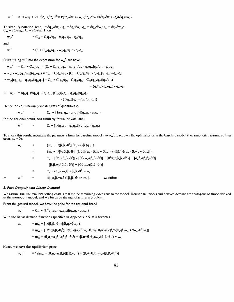
To simplifi. notation. let q,, = 6 ~ , / & v n 1 : q,, = SqJZw; q,, = dqJSw,; q,, = dq/&,,: C,, = &'6ai; C, = KGq. Then

2 Pure Duopolr with Linear Demand

LVe assume that the retailer's selling costs. s = 0 for the remaining extensions to the model. Hence retail prices and denbed demand are analogous to those derived in the monopoly model. and we focus on the manufacrurer's problem.

From the general model. we have the price for the national brand

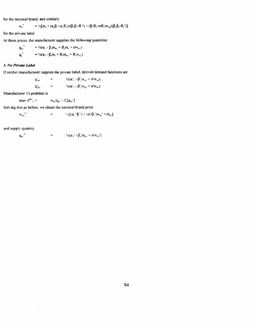
for the national brand. and similarly

w , = k[m, A (a,P,-alBl)~(P,P.-B,') - (P!B2+a01)w.~P,P,-01')]

for the private label.

At thest: prices. the manufacturer supplies the following quantities:

%' = %(a, -p lmn, - e l m , - cnv,,)

% ' = %(a, - P,m, + O,mn, - B,w,_.)

3. No Private Label

If neither manufacturer supplies the private label. derived demand functions are

q'n, - - '/z(u', - pa,\%,! ,- U1\c."_.)

q'd - - %(a': - ~ ' : L v , ~ + U'W~,)

Manufacturer 1's problem is

may z"~,) = %"mi'%,' - C[%i'\

Solving this as before. we obtain the national brand price

%% ,,'. - - ' / i [ ( a , "P: ' ) - ( f f ' /P , ' )wn~ + mml]

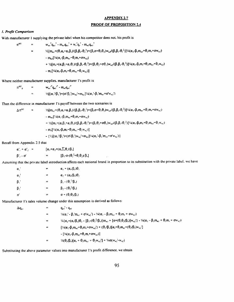
b'here neither manufacturer supplies. manufacturer 1's profit is -4f 1 - - " 0 wn1*-qn1** - mnlq";.

- - ~ ~ [ ( u ~ * / ~ , ' ~ ( u ' / ~ ' ) i v , ~ + m , , J %(a,'-p,'m,,+a'w,t)

Substituting the ahove pmmeter values into manufacturer 1's profit difference. we obtain

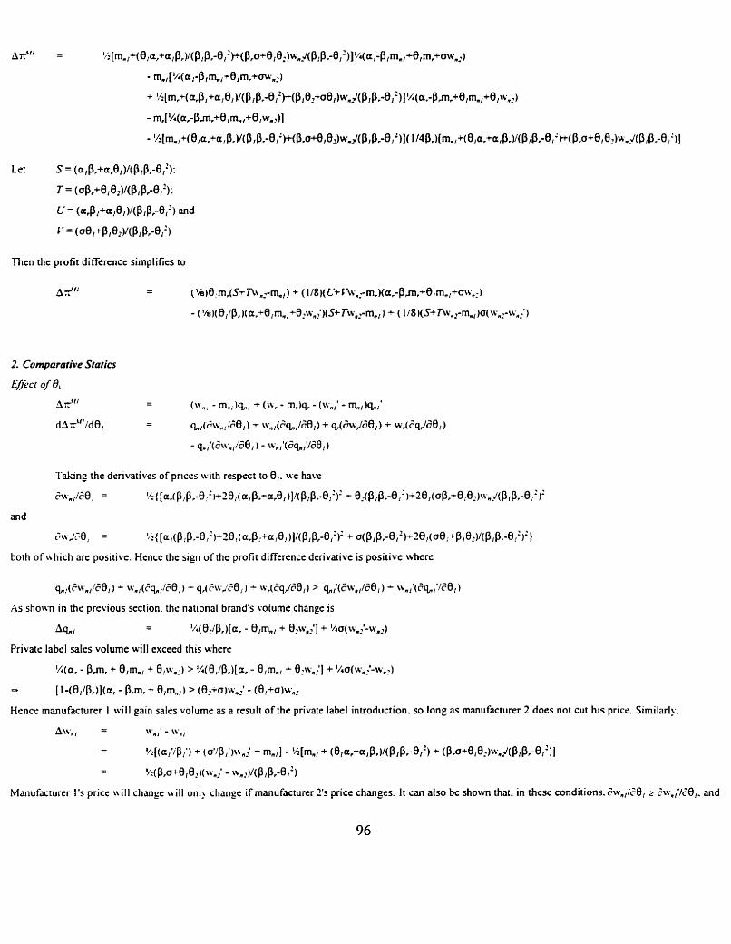
AxCt'

Let

l l e n the profit difference simplifies to

Taking the derivatives of pnces with respect to 8,. we have

GivRl/60, = ! G ( [ a . ~ ~ , ~ , - O ~ ~ r + ~ O I ( a , ~ . ~ a r O l ) ] / ~ ~ I ~ r - O I ' ) ~ - 0 . . ( ~ , ~ r - 0 1 ~ ) ~ ~ 0 1 ( o P , + 8 , 0 , ) ~ , ~ ( P I P , - 8 ~ ~ ) :

and

;\v,'a3, = ~~~{[a,(PlP.-0,')+20,(a,~,+a,0,)~/(PI~,-01')~ + a ( ~ i ~ , - 8 , ' ~ 2 ~ l ( o e , + ~ 1 0 ~ ) ~ ( ~ , ~ , - 8 ~ ' ) ~ )

both of which are pos~tive. Hence the sign of the profit difference derivative is positive where

q " / ( ~ w a 1 ~ ~ e I ) A tv"I(eqJa3; ) - qr(C?\v,'20, ) tvr(2qJc%/) > q " , ' ( ~ W ~ / l ~ 0 ~ ) W"J6qJd3/ )

As shotvn in the previous section, the national brand's volume change is

A%' - - %(0:/Pr)[ar - 8/m,, + e2\);1'] + %a(w,,'-w,,)

Private label sales volume will exceed this where

'/.(a, - Pwr + O1m,l + 8,tv,,) > %(0,/Pr)[a, - 0,m,, + 0,w,,'] + 'Aa(w,='-w,,)

[ I -@,/Pr)1(ar - Dmr +- 0,m,,) > (8,to)w,,' - (B!+a)\v,,

Hence manufacturer 1 wiil gain sales volume as a result of the private label introduction, so tong as manufacturer 2 does not cut his price. Similarly.

Awn , - - w"/' - \V"/

- - !/:[(a,*iP,') + (o'/P,')un; - m,,] - %[m,, + (81a,+a,~,)/(PIP,-~l ') + (Pra+B,O,)w,~(P,Pr-8,')j - - %(Pro+8,8,)(w,' - \v,)/(PIPr-8,')

Manufacturer 1's price tiill change ~vill only change if manufacturer 2's price changes. It can also be shown that. in these conditions.&v,,l'i;0, 2 6wn,'/60,. and

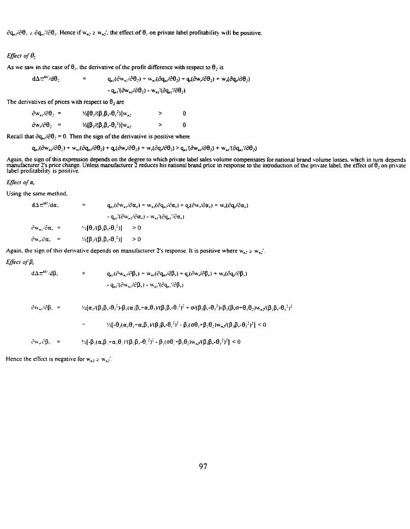
aa, /s0, 2 ;a,'/60,. Hence if w,, z \v,,'. the effect of 0, on private label profitability will be positive.

Effect of 8,

As we saw in the case of 0,. the derivative of the profit difference with respect to 0, is

The derivatives of prices with respect to 0, are

d~,~/S0, = ' / l(~ll~Plpr-e/')JwnJ > 0

ZwjSOJ = ~ I P l / < P / P r ~ e l ' ~ ] ~ ~ n ~ > O

Recall that dqJ202 = 0. Then the sign of the derivative is positive where

Again, the sign of this expression depends on the de ee to which private label sales volume compensates for national brand volume losses. wfich in turn deprnds manufacturer 2's price change. Unless manufacturer !?reduces his national brand price in response to the introduction ofthe private label. the effect of O2 on pnvae label profitabili~ is positive.

Using the same method.

Hencc the effect is negative for w,, 2 w,,'

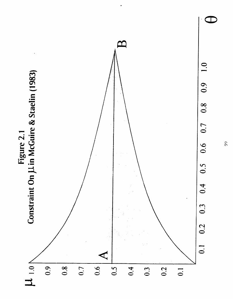
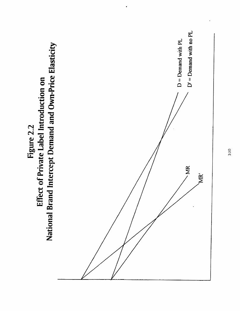
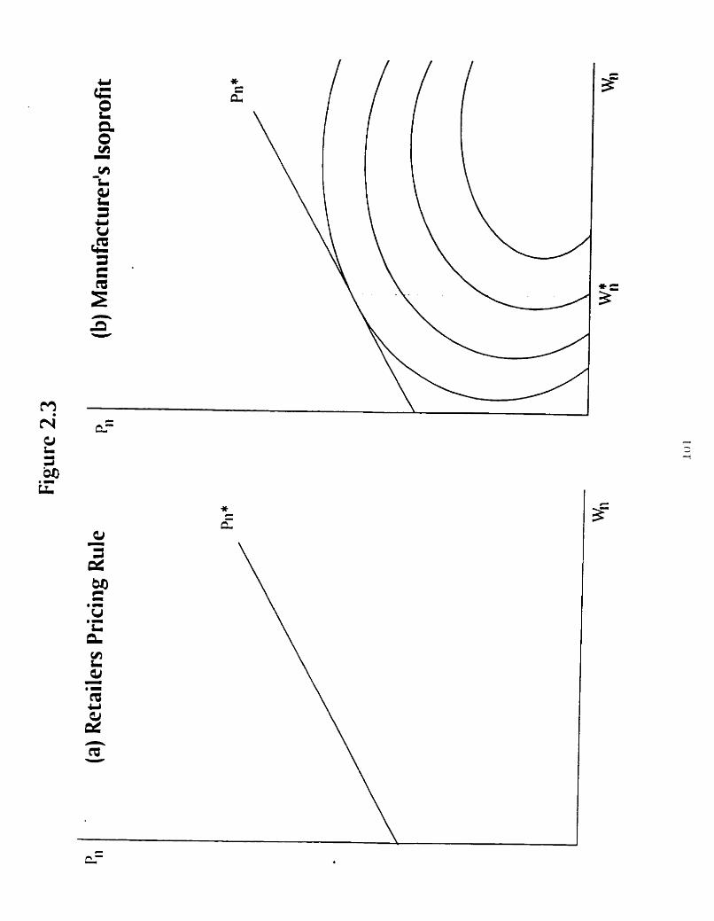
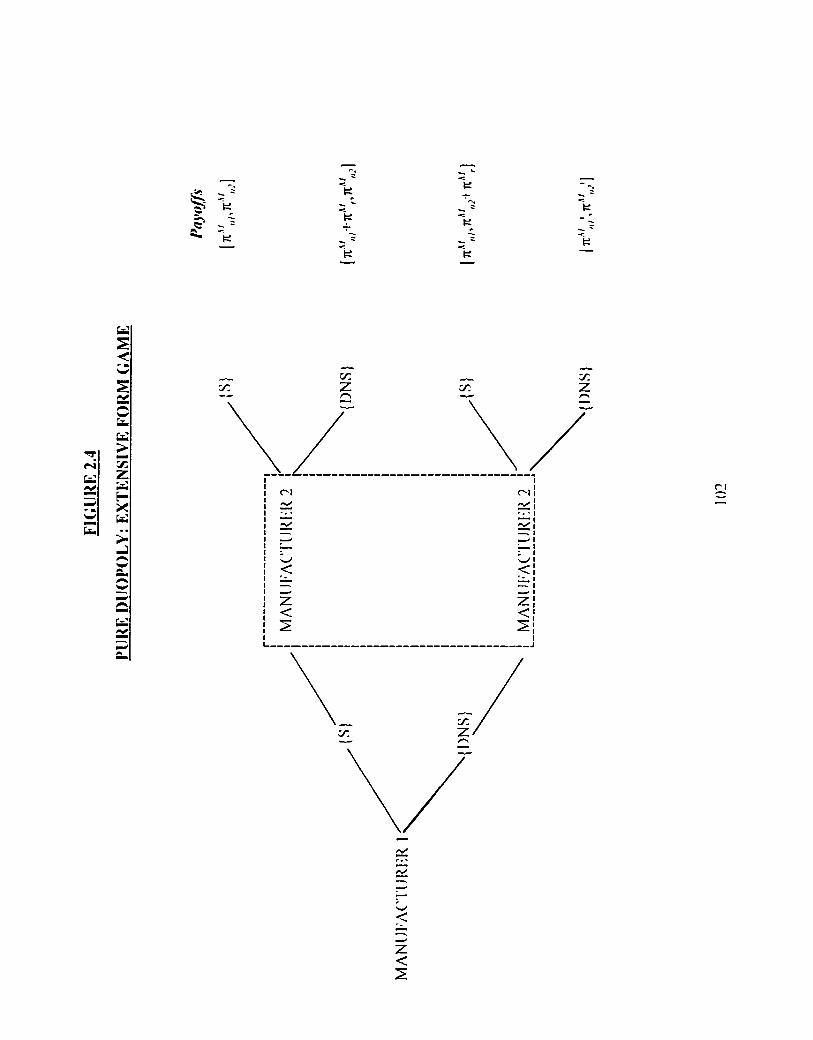
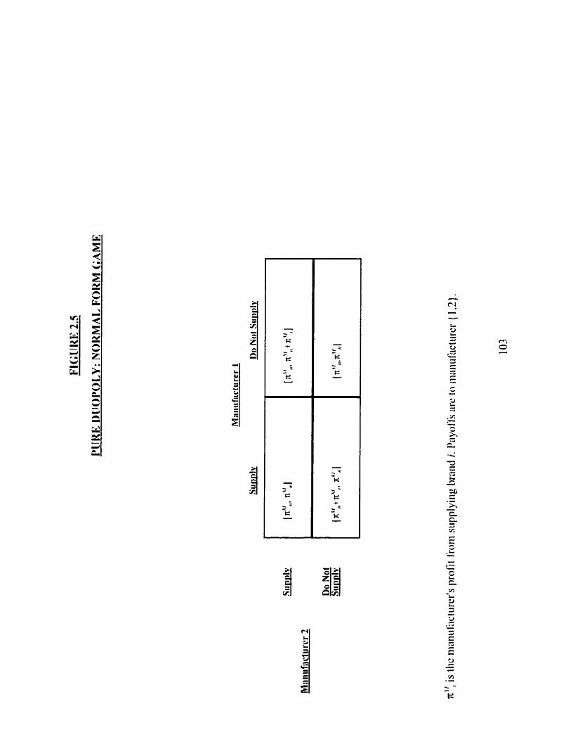
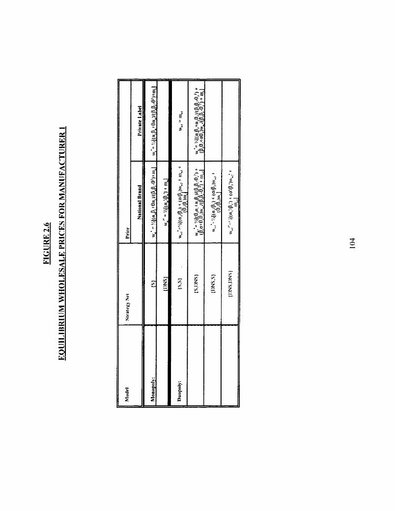
3. MODEL EXTENSION TO THE GROCERY PRODUCTS INDUSTRY

I have hardly ever known a mathematician who was capable of reasoning.

Plato:

The Republic

li) Introduction

The baseline models of chapter 2 provide us with some insight to the dimensions of the

decision to supply retailers' private labels. Nowhere is this decision more difficult than in the grocery

products industry. Faced with a growing private label sector and an increasingly sophisticated retail

trade. grocery product manufacturers are under significant pressure to supply their customers' store

brands.

As we saw in chapter 2. it is in a manufacturer's interest to supply the strongest private label

possible. but to minimize cannibalization of his national brand. For this reason. the manufacturer

prefers to supply a private label which generates a high degree of loyalty from consumers. is not too

price sensitive and expands the category rather than take too much of its sales volume from the

national brand. In addition. the private label should have low costs, so that the manufacturer can

obtain as high a profit margin as possible from those consumers who do switch.

While a monopolist will always supply a retailer's private label, a duopolist may have reasons

not to do so. If cannibalization of his national brand is too high or profit margins too low. the idea

may be unattractive. The risk of setting off a price war is an additional factor for a duopolist to

consider.

The purpose of this chapter is to derive a set of predictions. based on the model of chapter

2. which apply to the grocery products industry. To achieve this. we need to extend the baseline

model to recognize the conditions prevailing in that industry. Specifically, the market structure

should take account of the existence of a competitive sector which may supply the private label if

the leading manufacturers choose not to do so. In addition, chapter 2's assumption of constant

marginal costs will be relaved in favour of a more general cost function. in order to take account of

the effects of economies of scale and scope on the private label decision.

The extended model shows that. in addition to the demand factors considered in the baseline

models. dominant firms take into account the relative economies of scale of the private label and the

national brand. along with the dominant firm's cost advantage or disadvantage vis a vis the

competitive sector.

This chapter besins with a discussion of the grocery industry and the applicability of the

model. Section 3 extends the model in NO ways: by assuming a market structure of two duopolists

competing with each other in the presence of a group of smaller competitors. and by adopting a more

general cost function. Section 4 derives propositions under these new conditions. while Section 5 C

discusses the overall results for this model and that of chapter 2.

Jii) The Grocerv Products Industrv

The emergence and growth of suong private label brands has been one of the key trends in

the food industry in recent years. according to a survey by The Econornisf in late 1993. This trend

been particularly evident in the U.K. As shown in Figure 3.1. penetration of private labels in U.K.

grocery categories has reached 32%. a level which is closely followed by the Swiss and French

grocery markets.

(Figure 3.1 )

In Canada. private labels held a market share of 21% of all categories monitored by A.C.

Nielsen in 1993. Market shares of private labels. generics and the leading manufacturers' brands are

s h o ~ m in Appendix 3.1. It can be seen that private label share varies widely across categories. In the

Household Cleaners category. for example. private labels hold a share of only 2.5%. whereas private

label Vinegars constitute 54.6% of the market.

It is also evident from Appendix 3.1 that grocen markets tend to be relativel? concentrated.

Figure 3.2 s h o w mean shares across A.C. Nielsen categories for the top three national brands. aiong

with private label and generic brand shares. The top two national brands together account for almost

60% of the market. while the third national brand. on average. has a share under 8%. The shares of

the top two national brands and private labels together account for over 80% of grocery markets.

This panem of two dominant national brands and a relatively small third brand holds across the vast

majority of grocery categories.

(Figure 3.2)

The reason for this pattern is open to speculation; however. one plausible explanation is that

retailers are reluctant to use scarce shelf space on brands that do not generate sufficient volume. and

tend to apply a "cutoff' rule of thumb in stocking only the top two national brands in addition to their

private label.

Grocery markets are also known for their high level of channel conflict: with thousands of

products competing for limited shelf space. manufacturers find themselves devoting an ever-

increasing proportion o f their marketing budgets to trade promotion (The Econonzist. 1992). In

addition to promotional price discounts. manufacturers offer a plethora of allorvances for shelf

placement. co-operative advertising. display and volume buying.

Among manufacturers. conventional wisdom holds that large retail chains are powerful

players that can exercise monopsony power in extracting favourable terms from manufacturers.

However. there is little evidence of supranormal profits among grocery retailers. Appendix 3.2 lists

reported profit figures for food manufacturers and retailers (Globe and .Lluil. 1994). It is evident that.

while food retailers' sales revenues tend to be considerably higher than those of manufacturers. their

average five-year return on capital (unadjusted for inflation) is lower than that of their suppliers.

Retailers' power versus manufacturers derives primarily from their control of a scarce

resource. shelf space. Nevertheless. competition between the major chains is fierce. Appendix 3.3

shows the market shares of the major food retailing chains by province (Cunudiun Grocer. 1993):

it can be seen that the food retailing sector in most regions is quite fragmented. Although retailers

in the industry form buying groups to obtain better deals from manufacturers. competitive pressure

forces them to pass the bulk of these savings on to consumers. With overstoring in grocery retailing

as in other retail sectors (Stem and El-Ansaryl 1988), consumen' search costs are often minimal and

store switching is common. According to a 1991 survey by the Canadian Grocer. 45% of consumers

gave "Lower Prices" as their main reason for switching stores, followed by "More Convenient

Location" at 38%. Retailers' margins are under severe pressure. and any opportunity to obtain

concessions from manufacturers will be esploited in the interests of survival. A recent study by

Messinger and Narasimhan (1995) concludes that grocery retailers have not gained profitability at

the expense of manufacturers in the last two decades. but that both manufacturers and retailers have

experienced reductions in profitability.

The emergence of higher quality private labels in grocery markets is an indication of

increasing sophistication among grocery retailers. In Canada. following Loblaw's success with its

President's Choice range. other major retailers have followed suit with their own high quality private

label lines. However. high quality private labels have been well established in grocery retailing in

the U.K. for over I0 years. and in other retail sectors. such as apparel. for longer. High quality

private labels not oniy allow retailers to improve their margins by offering added value to consumers.

but can generate loyalty to a particular retailer by virtue of their exclusivity to that retailer. It is

interesting that those grocery retailers who have introduced high quality private labels have not

forsaken their traditional. lower quality store brands: by offering both. these retailers can appeal both

to consumers who value high quality and to those who are more concerned about price.

In summary. grocery retailers face an oligopolistic9 market in which prices are subject to

severe competitive pressure. Private labels provide them with the opportunity to increase margins

and offer consumers better value. In setting prices, the standard practice is for manufacturers to

consider competing manufacturers' prices and consumer demand. taking into account standard levels

of retail markup and prevailing levels of promotional allowances.

Manufacturers' cost structures vary widely within the industry. depending on the type of

product. Detergents manufacturing is highly capital intensive, for example. due to the need for spray

drying. A similar situation prevails in instant coffee manufacturing where freeze-drying is used

extensively. On the other hand. bottled still beverages require little processing other than mixing and

filling. However. almost all food manufacturers are affected by economies or diseconomies of scale

and scope to some degree.

The extensions to the model proposed in the remainder of this chapter reflect the conditions

described here. The typical market structure of two large firms and a group of smaller competitors

is represented by using a "dominant firm" model (Scherer. 1980). This type of model also reflects

the fact that smaller firms often enter grocery categories as private label suppliers. The cost structure

of the industq- is represented by a quadratic cost function with an interaction term to reflect

economies or diseconomies of scope. These extensions are discussed in the nest two sections. The

standard retail pricing practice of adding a markup to manufacturers' prices is modelled. as in chapter

2. by assuming that the manufacturer is a Stackelberg leader who takes the retailer's markup rule into

account in setting prices. As in the duopoly model of chapter 2. we focus on the manufacturer's

9 .At a regional level. but cornpe~irive at a local level due ro r e a d accessibilit> of stores in mcrropolitan areas and zone pricing

(set chapter 5 1.

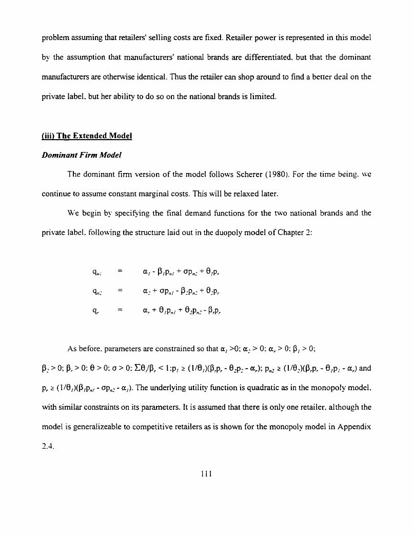
problem assuming that retailers' selling costs are fixed. Retailer power is represented in this model

by the assumption that manufacturers' national brands are differentiated. but that the dominant

manufacturers are otherwise identical. Thus the retailer can shop around to find a bener deal on the

private label. but her ability to do so on the national brands is limited.

fiii) The Extended Model

Dominant Firm Model

The dominant firm version of the model follows Scherer (1980). For the time being. we

continue to assume constant marginal costs. This will be relaxed later.

We begin by specieing the final demand functions for the two national brands and the

private label. following the structure laid out in the duopoly model of Chapter 2:

As before. parameters are constrained so that a, >O: a, > 0: a, > 0: P i 1 0;

pr r (lIB,)(f$p,, - op,, - a,). The underlying utility function is quadratic as in the monopoly model.

with similar constraints on its parameters. It is assumed that there is only one retailer. although the

model is generalizeable to competitive retailers as is shown for the monopoly model in Appendix

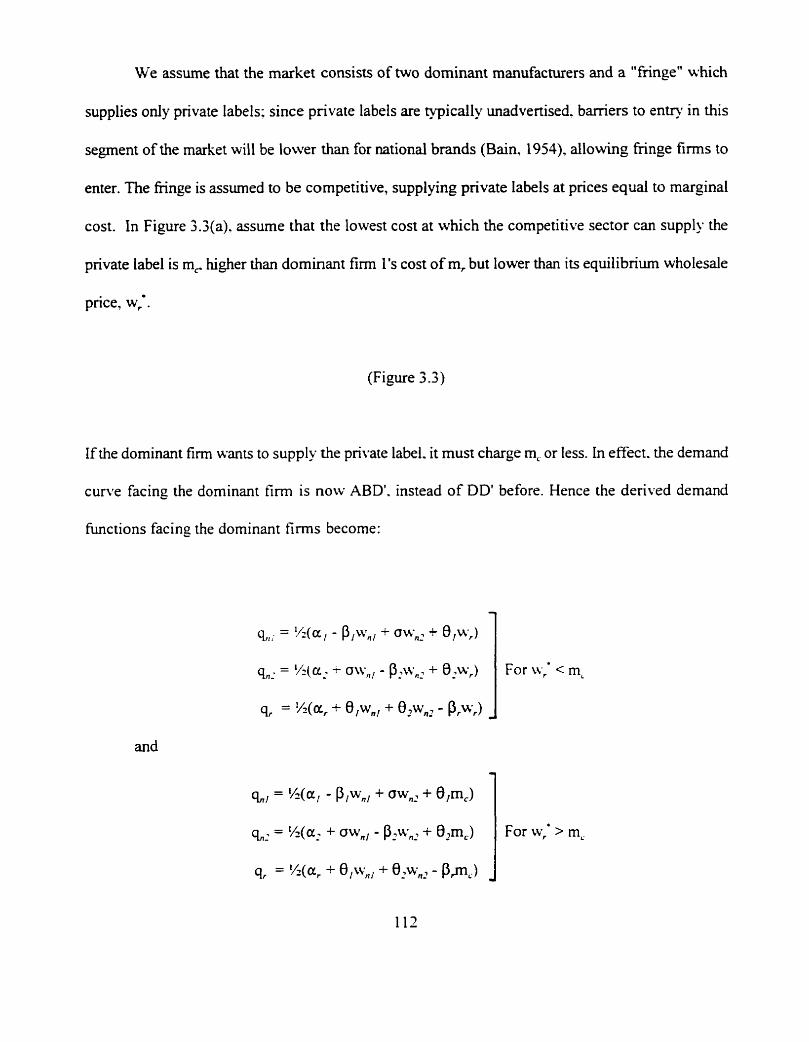
We assume that the market consists of two dominant manufacturers and a "fringe" which

supplies only private labels; since private labels are typically unadvertised. barriers to entry in this

segment of the market will be lower than for national brands (Bain. 1954), allowing fringe firms to

enter. The fringe is assumed to be competitive, supplying private labels at prices equal to marginal

cost. In Figure X(a) . assume that the lowest cost at which the competitive sector can supply the

private label is rn, higher than dominant firm 1's cost of rn, but lower than its equilibrium wholesale

price, wrm.

(Figure 3.3)

If the dominant firm wants to supply the private label. it must charge m, or less. In effect. the demand

cunre facing the dominant firm is now ABD'. instead of DD' before. Hence the derived demand

functions facing the dominant firms become:

and

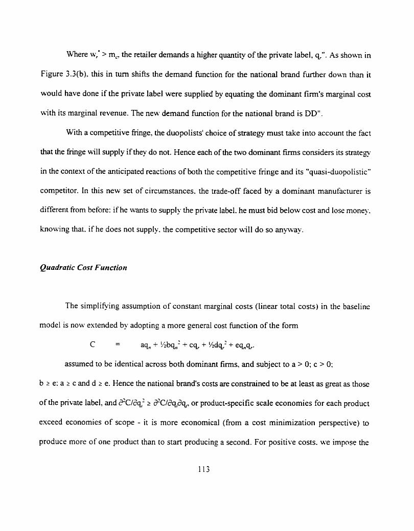
Where wrg > m, the retailer demands a higher quantity of the private label, g". As shown in

Figure 3.3(b). this in turn shifts the demand h c t i o n for the national brand M e r down than it

would have done if the private label were supplied by equating the dominant firm's marginal coa

with its marginal revenue. The new demand h c t i o n for the national brand is DD".

With a competitive fringe. the duopolists' choice of stratem must take into account the fact

that the hinge will supply if they do not. Hence each of the two dominant firms considers its strateg

in the context of the anticipated reactions of both the competitive fringe and its "quasi-duopolistic"

competitor. In this new set of circumstances. the trade-off faced by a dominant manufacturer is

different fiom before: if he wants to supply the private label. he must bid below cost and lose money.

knowing that. if he does not supply. the competitive sector will do so anyway.

Quadratic Cost Funcliotl

The simplifying as sumption of cons it marginal costs (linear tc ~tal costs) in the baseline

model is now extended by adopting a more general cost Function of the form

C - - aq, + %bq,,' + c a + %da' + eq,,a.

assumed to be identical across both dominant firms, and subject to a > 0: c > 0:

b z e: a z c and d 2 e. Hence the national brand's costs are constrained to be at least as great as those

of the private label. and 2c/zqf s a'cl~q~dq,, or product-specific scale economies for each product

exceed economies of scope - it is more economical (fiom a cost minimization perspective) to

produce more of one product than to start producing a second. For positive costs. we impose the

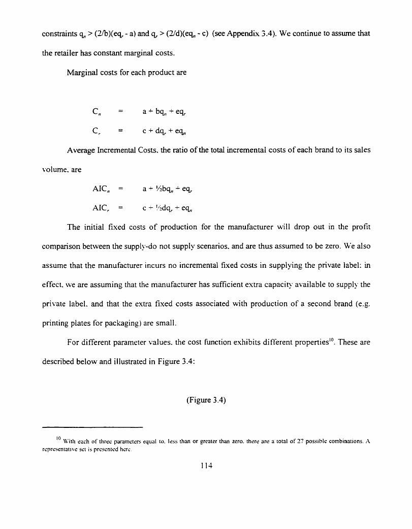
constraints > (Zb)(e% - a) and q, > (2/d)(eq,, - c ) (see Appendix 3.4). We continue to assume that

the retailer has constant marginal costs.

Marginal costs for each product are

CR - - a + b q , , + e e

c, - - c + d q , + e q ,

Average Incremental Costs. the ratio of the total incremental costs of each brand to its sales

volume. are

AIC, = a + %bq, ,+ee

AIC, = c - !/,dq - eq,

The initial fixed costs of production for the manufacturer will drop out in the profit

comparison between the supply-do not supply scenarios. and are thus assumed to be zero. We also

assume that the manufacturer incurs no incremental fixed costs in supplying the private label: in

effect. we are assuming that the manufacturer has sufficient extra capacip available to supply the

private label. and that the extra fixed costs associated with production of a second brand (e.g.

printing plates for packaging) are small.

For different parameter values. the cost function exhibits different propertiest0. These are

described below and illustrated in Figure 3.4:

(Figure 3.4)

10 K 3 h each of threc panrncrcrs equal to. less than or grcater than zero. there arc a rota1 of 27 possibls combinations. .-\

rtprcssnrarlvs set is prrsentrd hcrr.

Case l : b = d = ~ O

In this case. the cost function reduces to C = aq,, + c%. Marginal costs are constant.

equal to a for the national brand and c for the private label. Hence the baseline scenario of

constant marginal costs is a special case of this quadratic cost function.

Case 2: b>O, d>O

With positive parameters on both quadratic terms. the cost bc t i on is increasing and

strictly convex". Both the national brand and the private label exhibit decreasing product-

specific returns to scale. since Marginal Costs exceed Average Incremental Costs.

Case 3: e 4

-4 negative interaction term shifts the cost function downward with the introduction

of a second brand. Cost complementarities exist. defined as C,, < 0 and C, < 0 where the

subscripts denote the second derivatives of the cost function. Goman ( 1 985) argues that

economies of scope may arise from fised costs rather than from cost complementarities. In

this case. since fised costs are assumed to be zero, economies of scope arise entirely from

cost complementarities.

Hence this case represents a situation in which the total cost of producing two

products in one firm are lower than the costs of producing the two goods separately" (Bailey

- -

' ' A X q , > 0 and P2C/5q; > 0 for q, > 0.

12 Algebraically. C(q,.q,) c C(q.0) + C(0.q)

and Friedlaender. 1982; Baurnol. Panzar and Willig, 1982). Economies of scope arise

because of the use of shared machinery, labour or materials in production.

Case 4: b<0, d<O

In this case. the cost function for each product becomes concave and exhibits

increasing product-specific returns to scale: dC/Sq, > 0 and 2'c/eq,' < 0 for q, > 0. Average

Incremental Cosrs for each product lie above Marginal Costs.

Case 5: e>O

In contrast to Case 3. a positive interaction term represents diseconomies of scope

(cost anticomplementarities. i.e.C, > 0 and C, > 0). under which producing two products

in one firm is more costly than producing them separately.

Profit Marimization

In general. manufacturer i maximizes the objective function

As we saw in Chapter 2. a manufacturer facing a linear demand function passes on half of

any cost increase to a retailer where his marginal costs are constant. This standard result for linear

demand functions (see. for example, Varian, 1992, p.237-8) is due to the fact that the marginal

revenue function has twice the slope of the demand function and marginal cost is constant [see

Figure 3.5 (a)].

(Figure 3.5)

However. with a quadratic cost function. the result no longer holds. Consider a simplified

case of a manufacturer facing the demand function q = a-pw for a single product and having total

costs of C = aq. or constant marginal costs of MC = a. Then the manufacturer chooses the price

ti' - - %[a@ + a]

as before. and the manufacturer passes on half of any increase in cost.

If the manufacturer's total costs are C = aq + l/zbq2. marginal costs become

MC = a + bq. and the manufacturer chooses the price

\v - - (a - ap + apb)/(P2b + ZP)

Where b = 0. this reduces to the above price based on constant marginal costs. However.

where b * 0, &v;& = l/(pb+2) and &dab = ~(1-P)/(P2b+pb+4). Hence the manufacturer no longer

passes on half of cost changes as before. but will take into account the overall change in cost.

resulting from a change in one parameter.

This is shonn in Figure 3.5 (b). which shows the effect of an increase in b on the equilibrium

price. for b > 0. In contrast to the situation in which marginal costs are constant. the proponion of

cost increases which are passed on depends on the point at which marginal revenues and marginal

costs intersect - i.e. the equilibrium price and quantity, and on the rate of increase in the parameter

b.

Turning to the dominant firm model, equilibrium prices for a duopolistic manufacturer

supplying a national brand and a private label are as follows (see Appendix 5.5):

%I = ~ [ ( ~ ~ P r + ~ ~ ~ ~ ) ~ ( P ~ P ; ~ l ' ) + ( ~ P r + ~ r ~ ~ ) w , J ( P r P ; ~ ~ ' ) + C . ~ l

%do = %(a, - Picn, - O;cr + ow,,,,

for the national brand. and

. wr = %[(ar,P,+a,0, )/(p!Pr-e,')+(oe/+p,e2)wn/(p,p;e~')-cr]

Q* = %(a, - P,c, - B,c,, + OW,:)

for the private label. where C,, is the marginal cost of the national brand. and C j s the private

label's marginal cost. These prices and quantities are similar to those we have derived for the

duopoly model. However. since marginal costs are now a function of demand. the esplicit solution

for prices in term of exogenous parameters is somewhat more complex:

0 - M'n I

- %[(A,B.+ArO ,)/(BIB,-@ ,')+(CB,+O,O,)wn~(B,Br-8 ,') ]

and w; - - %[(AB,+A,O ,)/(BIB;@ ,')+(2@ l + B 1 0 2 ) ~ n ~ ( ~ , B , - 0 ,')I

where

4 - - a,+@ ,a-8 ,c)+Ka,(P b-8 ,e)-%a,@ ,d-P,e)

A r - - ar+(PpO ,a)+ !4ar(Prd-8 ,e)- %c(,(0 ,b-P,e)

BI - Pr+'/4P1(P lb-0,e)+%8,(0,d-~,e)

B r - - Pr+I/4~,(P#-B,e)+%BI(0 ,b-Pre)

0, - - 0 ,+l/40 I(P+i-Ole)+lAP ,(elb-Pre)

0, - - B,+L/482(P$-B,e)-'/20(8,b-Pre)

C - - 0+1/2u(P Ib-B 1e)-1/282(0 ,d-P ,e)

It can readily be seen that these prices are again of the same form as those of the duopoly

model. In Case 1. where b = d = e = 0, these prices reduce to the duopoly prices of the previous

chapter. Instead of passing half of any increase in marginal cost, the manufacturer takes into account

all the parameters of the cost function and relative elasticities of the two brands.

(iv) The Private Label Supplv Decision

As in chapter 2. the two dominant firms each decide whether to bid to supply the private label

and set prices, taking the retailer's pricing rule into account. Hence the strategy combinations in the

game are {B,B }. B,DNB J. {DNB,B J and [DNB,DNF3) as before. Where neither of the dominant

firms supplies. the competitive fringe does so, always setting its price equal to its marginal cost

irrespective of the dominant firms' national brand prices. The competitive fringe is thus a non-player

whose actions affect the outcome of the game between the dominant firms. but does not actively

participate. Hence the structure of the game is unchanged from that described in chapter 2 and

Figures 2.4 and 2.5. but the dominant firms' payoffs will change because of the presence of the

competitive fringe.

Assume that the competitive fringe can supply the private label at the linearly increasing

marginal cost C,(q,). In contrast to the dominant firms in the industry. capacity is readily available

in the competitive sector, where new firms can enter or exit quite readily by using inexpensive

technology or labour intensive production.

Figure 3.6 compares the cost function and profit-maximizing wholesale price of a dominant

manufacturer with an increasing and convex cost function (i.e. diseconomies of scale and no

economies of scope), with the linear cost of the fringe firms.

(Figure 3.6)

Where the competitive fringe's cost lies below the price charged by the dominant firms. the

retailer will purchase from the fringe sector. However. even if a dominant Arm's optimal price lies

above the competitive fringe's cost. it may make positive profits on the private label by pricing at the

competitive level.

Since w,' s $ (from the manufacturer's optimal prices), the manufacturer will never set

private label prices below costs. Similarly. he will not match the competitive fringe's price of C, if

it lies below his private label costs. Hence there are two interesting scenarios to consider:

w,' > C, > C; Since the retailer will not buy at w,'. the dominant manufacturers may reduce

their price to C,, since the competitive sector would otherwise supply at this

price and the dominant firms can make positive profits by doing so.

C, < w,' < C,: Dominant manufacturers may choose not to supply the private label, allowing

the competitive sector to provide it at a higher price in order to minimize

cannibalization of their national brands.

This reasoning can be applied to private label quality also: the cost to

the competitive sector of producing equivalent quality to the national brands

may be high. but they may be able to supply a lowerquality substitute at a

lower cost. So the dominant firms can limit cannibalization of their national

brands by allowing the competitive sector to supply the lower quality private

label".

For the following discussion, we refer to the normal form game in Figure 3.7, which depicts

the decision facing the two dominant firms in the same form as the duopoly game of Chapter 2. As

before. the strategies open to each of the manufacturers are to supply the retailer's private label ( (S 1)

or to refuse ((DNS)), taking into account its rival's payoffs. However, the key difference versus the

duopoly game is that in this case, if both refuse to supply, the retailer will procure her private label

from the competitive sector. One way or the other, therefore. the duopolists will face private label

competition.

(Figure 3.7)

wg>c.>c;_ 4

The wont situation for both manufacturers occurs when both supply. since they

I! In the real world. dominant manufacturers may often have technological advantages over smaller competitive firms. so thar the playing field may not appear as level as it is portrayed here. However. the cost functions in the model represent this disparity in technology since patents are rare in the grocery industry, competitive fim' cosrs lo produce an equivalenr product to that supplied by the dominant firms may be higher if they do not have equivalent technology. This is the situation in the cold breakfast cereal category. where malting technolop to produce Corn Flakes is prohibitively expensive and is owned by only one firm. KeIlo&s. Pnvate label cornflakes are not supplied by Kellogg's. but by smaller firms who are unable to match Kellogg's quality.

become Bertrand competitors and bid prices down to marginal costs: hence they make no

profit on the private label. Furthermore, their profit on the national brand is reduced relative

to the scenario in which one manufacturer supplies at C,, because the private label will

cannibalize more of its volume at this lower price.

Each manufacturer makes the same profit on the national brand when he supplies it

at C,, versus allowing the competitive sector to supply at that price. However. because C, >

C, he still makes positive profits on the private label. Hence there are two Nash equilibria:

{S,DNS }. and (DNS.S J . Only one manufacturer will supply the private label.

It can be shown that dw,'/da, > 0; awr0/t3p, < 0; dwr*/20, > 0, as in the monopoly and

duopoly models. Hence the supplying manufacturer's prices are highest, and this scenario is

most likely to occur. where consumer preference for the private label is high, private label

own-price response is low. or cross-price response between the national brand and the private

label is high. These conditions. as we have already seen in Chapter 3. favour the supply of

private labels by one manufacturer.

c-< w.' < C,i

In this situation. the manufacturers can charge their equilibrium price. However, the

presence of the competitive sector can change the outcome relative to the duopoly scenario

of Chapter 2.

As before, each manufacturer is better off not supplying if his competitor supplies.

However, it is the relative size of each individual manufacturer's payoff when he done

supplies. versus allowing the competitive sector to supply, that determines the equilibrium.

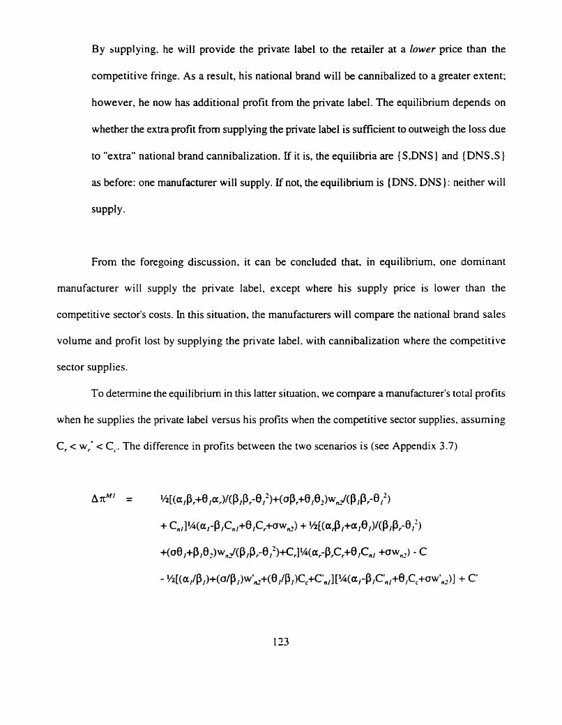
By wpplying. he will provide the private label to the retailer at a lower price than the

competitive fringe. As a result, his national brand will be cannibalized to a greater extent:

however, he now has additional profit from the private label. The equilibrium depends on

whether the extra profit from supplying the private label is suffkient to outweigh the loss due

to "extra" national brand cannibalization. If it is, the equilibria are {S.DNS } and {DNS,S }

as before: one manufacturer will supply. If not, the equilibrium is { DNS. DNS J : neither will

supply -

From the foregoing discussion, it can be concluded that, in equilibrium. one dominant

manufacturer will supply the private label, except where his supply price is lower than the

competitive sector's costs. In this situation, the manufacturers will compare the national brand sales

volume and profit lost by supplying the private label. with cannibalization where the competitive

sector supplies.

To determine the equilibrium in this latter situation, we compare a manufacturer's total profits

when he supplies the private label versus his profits when the competitive sector supplies. assuming

C , c w,' c C,. The difference in profits between the two scenarios is (see Appendix 3.7)

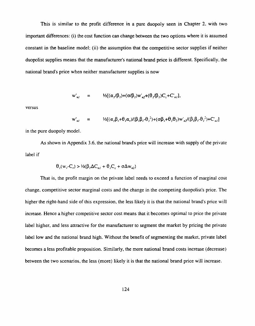
This is similar to the profit difference in a pure duopoly seen in Chapter 2. with two

important differences: (i) the cost function can change between the two options where it is assumed

constant in the baseline model: (ii) the assumption that the competitive sector supplies if neither

duopolist supplies means that the manufacturer's national brand price is different. Specifically. the

national brand's price when neither manufacturer supplies is now

versus

- w'n, - '2[(aIPr+e Iar)/(P/Pr-e / ' ) + ( ~ ~ r + ~ , ~ ~ ) w ' L ~ ( P I P r - ~ , ' ) + c ' n , l

in the pure duopoly model.

As shown in Appendix 3.6. the national brand's price will increase with supply of the private

label if

O,(W-C,) > L/2(P,ACn, + elCc + CJAW,J

That is. the profit margin on the private label needs to exceed a function of marginal cost

change, competitive sector marginal costs and the change in the competing duopolist's price. The

higher the right-hand side of this expression. the less likely i t is that the national brand's price will

increase. Hence a higher competitive sector cost means that it becomes optimal to price the private

label higher, and less attractive for the manufacturer to segment the market by pricing the private

label low and the national brand high. Without the benefit of segmenting the market. private label

becomes a less profitable proposition. Similarly, the more national brand costs increase (decrease)

between the two scenarios, the less (more) likely it is that the national brand price will increase.

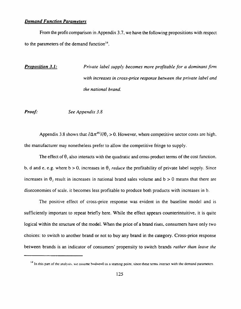
Demand Function Parameters

From the profit comparison in Appendix 3.7, we have the following propositions with respect

to the parameters of the demand functiont4.

Proposition 3.1: Private label suppfy becomes more profitable for a dominant firnl

with increases in cross-price response between the private label and

the national brand.

See Appendix 3.8

Appendix 3.8 shows that d ~ r ' ~ ' / 2 0 , > 0. However, where competitive sector costs are high.

the manufacturer may nonetheless prefer to allow the competitive fringe to supply.

The effect of 8, also interacts with the quadratic and cross-product terms of the cost function.

b. d and e. e.g. where b > 0. increases in 8, redme the profitability of private label supply. Since

increases in 8, result in increases in national brand sales volume and b > 0 means that there are

diseconomies of scale. it becomes less profitable to produce both products with increases in b.

The positive effect of cross-price response was evident in the baseline model and is

sufficiently important to repeat briefly here. While the effect appears counterintuitive, it is quite

logical within the structure of the model. When the price of a brand rises. consumers have only two

choices: to switch to another brand or not to buy any brand in the category. Cross-price response

between brands is an indicator of consumers' propensity to switch brands rather than leave the

I 4 In this pan o f the analysis. we assume tr=d=e=O as a starting point. since these terms interact with the demand parameters

125

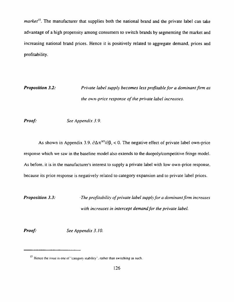
market? The manufacturer that supplies both the national brand and the private label can take

advantage of a high propensity among consumers to switch brands by segmenting the market and

increasing national brand prices. Hence it is positively related to aggregate demand, prices and

profitability.

Proposition 3.2:

Proofi

Private label supply becomes less profitable for a dominant firm as

the own-price response of the private label increases.

See Appendix 3.9.

As shown in Appendix 3.9. dAxM'/$, < 0. The negative effect of private label own-price

response which we saw in the baseline model also extends to the duopoly/competitive fringe model.

As before. it is in the manufacturer's interest to supply a private label with low own-price response.

because its price response is negatively related to category expansion and to private label prices.

Proposition 3.3: -The profitnbilih of private label suppi! for a dorninnntfirm increases

with increases in intercept demand for the private label.

Proofi See Appendix 3.10.

I5 Hence the issue is one of "category s~ability". rather than switching as such.

I26

Appendix 3.10 shows that SAr*'/aa, > 0, except where private label intercept demand

interacts with private label marginal costs. In other words. to the extent that increasing intercept

demand increases revenue, the manufacturer is better off; but increasing intercept demand can also

increase private label costs through the parameters of the cost function, which reduces the

profitability of private label supply.

Again. this effect is consistent with the baseline model. As the private label becomes a

"stronger" brand. in the sense of higher intercept demand, the dominant firms become more

interested in supplying i t themselves rather than leave it to the competitive fringe.

In summary. one manufacturer will supply the retailer's private label unless the competitive

sector's costs are much higher than the optimal prices of the dominant firms - in which case the

manufacturers' national brands will not suffer excessive cannibalization if the competitive sector is

allowed to supply - or the private label itself is unattractive. By similar intuition to that discussed in

Chapter 2, the ideal private label has high consumer demand and low own-price response. Increased

category loyalty, represented by the cross-price response parameter 8,, makes private label supply

more profitable, since higher levels of category loyalty allow the manufacturer to raise prices on the

national brand while using the private label to appeal to those consumers who switch brands.

Cost Parameters

We now turn to the role played by economies of scale and scope in a dominant

manufacturer's decision to supply the private label. Each of Cases 2-5 described in the previous

section is considered in turn.

Case 2: b M, d>O

The parameters b and d represent increasing product-specific returns to scale when positive.

and decreasing returns to scale when negative. In the case where b > 0 and d > 0, marginal costs lie

above average costs as shown in Figure 3.4(b). The following propositions are derived from the

foregoing profit comparison.

Proposition 3.4: ( a ) Where b > 0, increases in b have a positive impact on

dominant rnanttfacturers' p r o p e n s i ~ to srrpplv a rerailer's

private label.

( 6 ) Where d > 0, increases in d have a negative irnpacr on

dominant rnatzrlfacturers' propensig to sicppiy a retailer's

private label.

See Appendix 3. / I

Proposition 3.4 refers to decreasing product-specific returns to scale on the national brand

and the private label. Increases in the parameters b or d increase the responsiveness of the total cost

function to sales volume, shifting marginal cost upwards.

As b increases, the marginal costs of the national brand for a given quantity also rise.

Although the manufacturer can partly recover his costs by increasing price, recall that he will only

partly recover increases in marginal costs through increased prices. Hence it becomes relatively more

attractive for the manufacturer to consider supplying the private label.

This can be understood more fully by examining the relationship between b and private label

profitability at optimal quantities'6, from Appendix 3.1 1:

Since the manufacturer cannot supply the private label at a higher price than the competitive

sector. his national brand sales volume when he supplies the private label will be equal to or lower

than that when the competitive sector supplies. i.e. Aq,,, r 0. Applying the constraints d z e and 0,

> p,. the expression is clearly positive.

The positive impact of decreasing returns to scale on the national brand depends on the term

8,d-P,e, which expresses the comparison between private label returns to scale and economies of

scope, moderated by own-price and cross-price response. In other words, the effect interacts with the

terms of the private label's cost function. and with substitutability.

Increases in d have the opposite effect, increasing the marginal costs of the private label in

relation to that of the national brand. Private label supply thus becomes less profitable. The effect

of d is as follows:

The first term in this expression, lh(Prc-O,a)q,', represents a trade-off by the manufacturer

16 The quantity terms are evaluated 31 thc~r oprim31 Icvcls. following the Envelope Theorem.

129

of the unit costs of the two brands (the intercepts of the marginal cost function). The second term.

!h(Pre-O,b)qreq,,,'. can be seen as a comparison between national brand diseconomies of scale and

the economies of scope derived from producing both products together. The third term, lA(P,d-

8,e)qrq, represents a similar comparison for the private label.

Assume for the moment that a=c and b=d=e; then this reduces to

Since p, > 8,. the overall effect of d is negative. However, its level is influenced by the

manufacturer's comparison of the other cost terms. If national brand costs (the terms a and b) are very

high. they can outweigh the negative effect of decreasing returns to scale on the private label: in

other words, if the national brand is very expensive to produce, the private label may appear

attractive by comparison. If the national brand exhibits diseconomies of scale (b is high relative to

e ) . the private label can appear more attractive.

Case 3: e<O

The case of e < 0 represents economies of scope, where the total cost of producing both

products is less than the sum of their individual costs. The following proposition expresses their

effect in the model.

Proposition 3.5: For e c 0, increases in ie have a positive effect on manufacturers*

propemih to suppi! the private label.

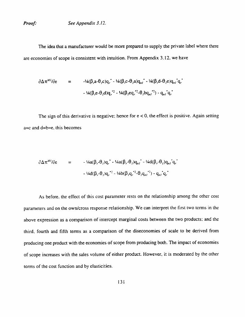
Proofi See Appendix 3.12.

The idea that a manufacturer would be more prepared to supply the priv ate lab ere there

are economies of scope is consistent with intuition. From Appendix 3.12, we have

The sign of this derivative is negative: hence for e < 0. the effect is positive. Again setting

a=c and d=b=e. this becomes

As before. the effect of this cost parameter rests on the relationship among the other cost

parameters and on the owdcross response relationship. We can interpret the first two terms in the

above expression as a comparison of intercept marginal costs between the two products: and the

third. fourth and fifth terms as a comparison of the diseconomies of scale to be derived from

producing one product with the economies of scope from producing both. The impact of economies

of scope increases with the sales volume of either product. However, it is moderated by the other

terms of the cost function and by elasticities.

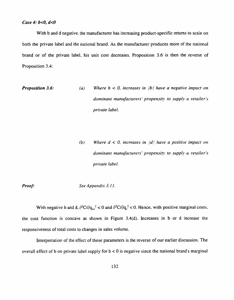
Case 4: b<O, d<O

With b and d negative. the manufacturer has increasing product-specific returns to scale on

both the private label and the national brand. As the manufacturer produces more of the national

brand or of the private label, his unit cost decreases. Proposition 3.6 is then the reverse of

Proposition 3.4:

Proposition 3.6: (a) Where b < 0, increases in / b / have a negative impact on

dominant manufacturers' propensic to s~cppiy a retailer's

private label.

(b) Wlzere d c 0. increases in jd/ haw a positive impact 012

dominant man rcfacturers ' propensin. to supply a retailer's

private label.

Proof.. See Appendix 3. I I .

With negative b and d, $C/aq,,,' < 0 and a2C/dq; c 0. Hence, with positive marginal costs.

the cost function is concave as shown in Figure 3.4(d). Increases in b or d increase the

responsiveness of total costs to changes in sales volume.

Interpretation of the effect of these parameters is the reverse of our earlier discussion. The

overall effect of b on private label supply for b c 0 is negative since the national brand's marginal

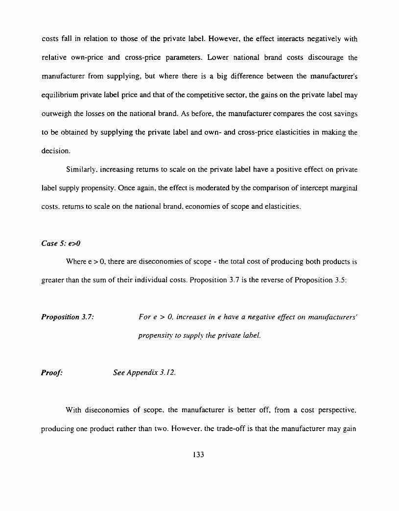
costs fall in relation to those of the private label. However, the effect interacts negatively with

relative ow n-price and cross-price parameters. Lower national brand costs discourage the

manufacturer from supplying, but where there is a big difference between the manufacturer's

equilibrium private label price and that of the competitive sector, the gains on the private label may

outweigh the losses on the national brand. As before, the manufacturer compares the cost savings

to be obtained by supplying the private label and own- and cross-price elasticities in malung the

decision.

Similarly. increasing returns to scaIe on the private label have a positive effect on private

label supply propensity. Once again, the effect is moderated by the comparison of intercept marginal

costs. returns to scale on the national brand. economies of scope and elasticities.

Case 5: e>O

Where e > 0, there are diseconomies of scope - the total cost of producing both products is

greater than the sum of their individual costs. Proposition 3.7 is the reverse of Proposition 3.5:

Proposition 3.7: For e > 0, increases in e have a negative effect on ~~~~~~~~~~~~ers'

p r o p e n s i ~ to slcpplj the private label.

Proof: See Appendix 3.12.

With diseconomies of scope. the manufacturer is better off, from a cost perspective.

producing one product rather than two. However. the trade-off is that the manufacturer may gain

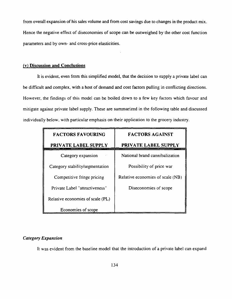
from overall expansion of his sales volume and from cost savings due to changes in the product mix.

Hence the negative effect of diseconomies of scope can be outweighed by the other cost function

parameters and by own- and cross-price elasticities.

(v) Discussion and Conclusions

It is evident, even from this simplified model, that the decision to supply a private label can

be difficult and complex, with a host of demand and cost factors pulling in conflicting directions.

However, the findings of this model can be boiled down to a few key factors which favour and

mitigate against private label supply. These are summarized in the following table and discussed

individually below, with particular emphasis on their application to the grocery industry.

FACTORS FAVOURING

PRIVATE LABEL SUPPLY

Category expansion

Category stabi l i ty/segmentation

Competitive fringe pricing

Private Label "attractiveness"

Relative economies of scale (PL)

Economies of scoDe

FACTORS AGAINST

PRIVATE LABEL SUPPLY

National brand cannibalization

Possibility of price war

Relative economies of scale (NB)

Diseconomies of scope

Category Expansion

It was evident from the baseline model that the introduction of a private label can expand

category demand. This result held consistently through the duopoly and dominant firm extensions

of the model. If a manufacturer is in a position to benefit from category expansion. his total

profitability can improve as a result of private label supply.

However. grocery categories generally are mature do not usually expand very much in

practice. In terms of the model, this means that private label intercept demand is low. and private

label own-price response and cross-response with national brands are relatively close. In other words.

there is typically little consumer loyalty to private labels: they are seen primarily as cheaper

substitutes for national brands.

For this reason. the "category expansion" explanation is less likely to hold in the grocery

industry than in other categories, although there is anecdotal evidence of firms using private labels

to develop a category: Kraft General Foods expanded its capacity and supplied private label

Puddings for this reason. In addition. the emergence of "premium" private labels is likely to result

in more category expansion.

Category Sta bility/Segm entation

The parameter 0 must be interpreted in the light of its effect on aggregate demand. Increases

in 0 result in increases in aggregate demand, and as a result, in increased prices and profitability.

While this may appear to be an artifact of this type of model, it has an intuitive interpretation.

The introduction of a private label means that consumers now have an opportunity to switch to

another brand if the price of the national brand rises. Prior to this, their only choice would have been

to purchase the national brand at the higher price or refrain from buying at all. So the introduction

of a private label increases categop i o y a l ~ among consumers. Hence increases in cross-price

response relative to own-price response can be interpreted as increases in category loyalty. or

increases in consumers' reluctance to switch away from the category.

The private label supplier benefits from this. Instead of losing consumers to a competing

category, or to a competing private label supplier, the manufacturer who supplies private labels can

profitably raise the price of his national brand since he will retain some of those consumers who

switch away.

Competitive Fringe Pricing

The amount of volume loss on the manufacturer's national brand depends. in part, on the

relative price of the private label and the national brand. If the manufacturer has lower costs than

fringe competitors. he may do better by allowing them to supply the private label at their higher cost.

This would be particularly likely if the manufacturer's profit margins on the national brand were

much higher than those on the private label. However. if his costs are close to those of the

competitive fringe, he is likely to supply.

Another way of interpreting this is that the manufacturer may have proprietary technology.

such as that owned by Kellogg's in the cereal category. which would be prohibitively expensive for

a fringe competitor. This technology allows him to produce a superior product and limit

cannibalization. He can afford to allow the competitive fringe to supply an inferior product, knowing

that it would be much more expensive for them to produce a product equivalent to his own.

Again, in spite of the anecdotes. situations such as this are the exception rather than the rule

in the grocery industry. Few grocery products have proprietary technology or are so capital intensive

as to prevent smaller competitors from producing a reasonably close substitute. In addition. fringe

private label suppliers can have lower costs than their dominant competitors. On the other hand.

some grocery manufacturers place great faith in the uniqueness of their brand's image, which fringe

competitors could only imitate at great cost.

P n'vate Label "Attractiveness"

The appeal of the private label to a potential supplier increases as product preference for the

private label increases, its own-price response falls and its cannibalization of the national brand falls.

Manufacturers would prefer private labels which generate extra sales and are not too price sensitive.

For this reason. we would expect national brand manufacturers to be more interested in

supplying "premium" private labels which do not excessiveZy cannibalize their national brands. This

pattern is evident in the case of E.D. Smith. the supplier of President's Choice bottled sauces to

Loblaw's: E.D. Smith's private label sauce business does not directly compete with its national brand.

Similarly. Cott Beverages. the much-publicized supplier of President's Choice soft drinks. has only

a small national brand. and is unlikely to be particularly worried about cannibalization: Cott's

primary concern will be with the viability of the private label itself.

Relative Economies of Scale

Product-specific economies of scale have an influence on manufacturers' preparedness to

supply private labels. However. the imponant point to bear in mind is that we are concerned with

relative economies of scale. If the national brand becomes more economical to produce with

increases in volume and the private label does not (or does to a lesser degree). the manufacturer will

be more interested in pursuing opportunities to increase his sales of the national brand, rather than

supply the private label. Conversely. product-specific economies of scale on the private label relative

to the national brand increase a manufacturer's interest in supplying.

Economies of Scope

Economies of scope, the degree to which it is cheaper to produce both products in one firm

than individually, have a positive influence on manufacturers' propensity to supply private labels.

Economies of scope are present where two products use common manufacturing facilities or raw

materials.

In the grocery industry. manufacturers regularly use private labels as "capacity fillers", which

use national brand manufacturing equipment that otherwise would be idle. Hence we would expect

that the use of common manufacturing facilities is a motivator for private label supply. In addition.

the use of common raw materials means that manufacturers can buy in bulk from suppliers and save

on costs.

National Brand Cannibalization

We have seen that manufacturers can benefit from high private labellnational brand

substitutability, since it means that consumers are more likely to continue to purchase the product

category as national brand prices rise. However, with stable markets for most grocery items,

manufacturers may not be particularly concerned about category stability, but instead about the

degree to which the private label cannibalizes their national brand. In particular, manufacturers face

the risk of becoming Bertrand competitors on private labels, a risk which does not exist for

differentiated national brands.

Substitutability is represented in the model as the degree to which the private labei responds

to changes in the national brand's price, as opposed to its own price. For this reason it is the

difference between the private label's own-price response and national brand/private label cross-price

parameter, p, - 8,. that measures substitutability.

Depending on the degree to which national brands are differentiated from private labels.

private labels will often be quite sensitive to changes in national brand prices. We can expect this

to happen particularly where the private label is a significantly cheaper imitation of the national

brand. Thus manufacturers may be more interested in supplying premium private labels that are

distinct from their national brands.

Price War

It was evident from the duopoly model of chapter Z and the dominant firm model of this

chapter that a significant consideration for a duopolist in deciding whether to supply a private label

is the possible impact of private label supply on his competitor's pricing strategy. If the competing

duopolist lowers his national brand price in response to the introduction of the private label. it may

be unprofitable to become a private label supplier. In the presence of a competitive sector with costs

higher than those of the dominant firms, the competing duopolist may also have less incentive to

reduce his national brand price if the competitive firms are allowed to supply. Thus the prospect of

sparking off a price war may turn firms away from private label supply.

The idea that private labels "devalue" a category by reducing prices overall is common among

marketing executives in grocery manufacturing firms. However, what the model suggests is that

allowing a competitive fringe to supply may help insulate the dominant firms against price

competition. if the competitive fringe's costs are sufficiently high.

The model indicates that these factors are the key driving forces behind the supply of private

label products in the grocery industry. Nonetheless, there are some limitations to the model's

generalizeability across other product categories. In other industries. for example, the assumption

that manufacturers are Stackelberg leaden who set prices taking into account retailers' markup rule

may not hold. Choi (1991). for example. has shown that a change in the assumption about

Stackelberg leadership will change prices and profits in a linear-demand based model. Such a change

may be expected to affect the equilibrium in this model also.

The model is capable of extension to future research on private labels. It can be adapted to

derive optimal retail and wholesale prices for private labels and national brands, and the optimal

price difference from the viewpoint of retailers and manufacturers. Future research should also

consider the ability of retailers to differentiate their stores by introducing a private label.

The model's insights have significant implications for marketing practitioners also. It can

readily be applied by manufacturers in considering likely competitive strategies. while retailers can

determine from it which manufacturers are likely to offer them the best deal. A particularly

interesting application would be to develop an expert system based on these theoretical foundations

which can recommend optimal strategies to manufacturers for product mix, wholesale prices and

price gaps between private labels and national brands. A full discussion of future research

possibilities is given in chapter 6 .

Having developed the theoretical model. we apply it empirically in the next two chapters. In

chapter 4. we estimate demand parameters for a grocery category; in chapter 5, we use these

parameters. along with cost estimates, to make predictions about the profitability of private label

supply for a manufacturer in the category.

Bailey and Friedlaender (1982). "Market structure and Multiproduct Industries", Journal of Economic Literature. XX (Sept.). 1 O X - 1 O48.

Bain. Joe S. (1954). "Conditions of Entry and the Emergence of Monopoly", chapter in E.H. Charnberlin, ed., Monopoly and Competition and nteir Regufation. London: MacMillan.

Baumol, William J.. John C. Panzar and Robert D. Willig (1982), Contestable Markets and the Theory of Industry Structure. San Diego, CA.: Harcourt Brace Jovanovich.

Canndiart Grocer ( 1993). "Executive Report". Maclean Hunter.

Choi. S . Chan ( 199 1 ). "Price Competition h A Channel Structure With A Common Retailer". Marketing Scierlce. 10.4 (Fall), 27 1-296.

Globe and Maif ( 1994). "Top I000 Companies". Report on Business Magazine. July.

Gormm. Ian E. ( 1985). "Conditions for Economies of Scope in the Presence of Fixed Costs". Rand Joicnzal of Economics. 16, 3 (Autumn), 43 1-436.

Kim. Sang Yong (1993). "Store Brand: A Source of Retail Power". Working Paper, Duke University.

Messinger. Paul R. and Chakravarti Narasimhan. "Has Power Shifted in the Grocery Channel?". Marketing Science. 14.2, 1 89-223.

Stem. Louis W. and Adel I. EI-Ansary ( 1988). Marketing Channels. 3rd ed., Englewood Cliffs. N.J.: Prentice-HalI.

Scherer. F.M. ( 1980). Itldusrrial Market Structure and Economic Performance. Chicago: Rand McNally.

The Econon~ist ( l992), "Procrer's Gamble". July 25th, 6 1-62.

Tirole. Jean ( 1 988). The Theon. of Industrial Organization, Cambridge. Mass.: The MIT Press.

Varian, Hal R. ( 1992). Microeconomic Analysis. New York: W.W. N orton & Co.

APPENDICES

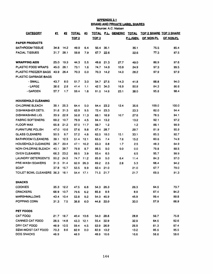
CATEGORY

PAPER PRODUCTS

BATHROOM TISSUE 34.8 14.2

FACIAL TISSUES 31.7 28.1

WRAPPING AIDS 25.0 19.3

PLASTIC F W D WRAPS 45.0 28.1

PLASTIC FREEZER BAGS 43.9 26.4

PLASTIC GARBAGE BAGS

- SMALL 43.7 8.0

- LARGE 38.6 2.8

- GARDEN 57.7 1.7

HOUSEHOLD CLEANING

CHLORINE BLEACH 39.1 25.3

DISHWASHER DETS. 31.6 31.3

DISHWASHING LIQ. 33.9 22.9

FABRIC SOFTENERS 69.2 10.7

FLOOR WAX 65.8 21.2

FURNITURE POLISH 47.0 10.6

GLASS CLEANERS 50.5 6.7

BATHROOM CLEANERS 39.1 12.3

HOUSEHOLD CLEANERS 26.7 20.4

NON-CHLORINE BLEACH 40.1 39.7

OVEN CLEANERS 66.3 23.2

LAUNDRY DETERGENTS 50.2 24.5

PRE-WASH SOAKERS 31.5 31.4

SOAP 37.8 15.7

TOILET BOWL CLEANERS 36.3 18.1

SNACKS

COOKIES 35.3 12.2

CRACKERS 68.9 10.7

MARSHMALLOWS 43.4 10.4

POPPING CORN 31.3 7.5

PET FOODS

CAT FOOD 21 -7 18.7

CANNED CAT F W D 28.5 14.8

DRY CAT FOOD 48.9 10.5

SEMJ-MOIST CAT FOOD 73.3 9.6 DOG SNACKS 48.9

4PPFNDIX 3.1

BRAND AND PRIVATE 1 ABEL SHARES Source: A.C. Nielsen

tOTAL TOTAL L GENERlC TOTAL TOP 2 SHARE TOP 3 SHARE

OF NON-PL

fl TOT& B TOTAL eb, W F R I C TOTAL TOP 2 SHARE TOP 3 SHARE

FROZEN FOOD CONFECTIONS DINNERS & ENTREES

JUICES & DRINKS ICE CREAM

- NATL - MAR - QUE

- om - ws

- ALTA

- B.C. VEGETABLES

BEVERAGES FRUIT DRINKS HOT CHOCOLATE ICED TEA MIXES INSTANT COFFEE POWDERED DRINKS REGULAR COFFEE TEA BAGS TOMATONEG JUICE COLD FLAV. DRINKS FLAV. SOFT DRINKS SPECIALTY TEA

CANNED & PKGD. FOODS

BAKED BEANS 29.6 14.4

LUNCHEON MEAT 50.4 34.1

CANNED PEARS 38.9 17.0

CANNED PINEAPPLE 32.9 22.0

CANNED SALMON 32.9 6,2

SOUP 45.9 11.9

CANNED TUNA 42.0 10.8

FLAKED MEAT 59.8 28.6

CANNED PEACHES 35.0 12.3

FRUIT COCKTAIL 40.4 11.2

SPAGHE3TI SAUCE 31.2 17.1

TOMATO PASTE 40.0 14.7

SPECIALTY VEG 33.8 5.3

CANNED VEG (TOTAL) 33.1 20.6

OF NON-PL

67.1

40.0

82.5

69.6

68.7

89.6

99.0

61.5

42.9

88.2

n . 5

51 -7 100.0

89.9

91.8

94.2

100.0

87.3

100.0

94.2 86.6

56.0

84.8

98.1

90.9

86.9

55.4

75.2

77.4

99.9

85.4

91.2

65.0

f 7 . 8 69.7

100.0

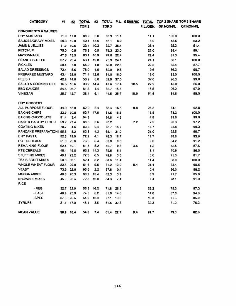
CONDIMENTS & SAUCES DRY MUSTARD 71.9 17.0

SAUCESIGRAW MIXES 20.3 19.8

JAMS 8 JELLIES 11.9 10.5

KETCHUP 75.0 0.8

MAYONNAISE 47.6 15.5

PEANUT BUTTER 37.7 25.4

PICKLES 58.4 7.8

S U D DRESSINGS 72.4 5.6

PREPARED MUSTARD 43.4 28.0

RELISH 42.9 14.0

SALAD 8 COOKING OILS 16.6 16.6

BBQ SAUCES 54.6 26.7

VINEGAR 25.7 12.7

DRY GROCERY ALL PURPOSE FLOUR 44.0 18.0

BAKING CHIPS 32.9 30.8

BAKING CHOCOLATE 91.4 3.4

CAKE 8 PASTRY FLOUR 59.2 27.4

COATING MIXES 78.7 4.6

PANCAKE PREPARATION: 55.6 8.2 DRY PASTA 52.3 19.9

HOT CEREALS 51.0 25.6

REMAINING FLOUR 62.4 19.1

RTE CEREALS 45.4 19.8

STUFFING MIXES 49.1 23.2

TEA BISCUIT MIXES 50.3 32.1

WHOLE WHEAT FLOUR 32.6 29.0

YEAST 73.6 22.0 MUFFIN MIXES 48.6 20.3

BROWNIE MIXES 45.9 26.4

RICE

- REG. 32.7 22.9

- FAST 48.9 25.9 - SPEC. 37.6 26.6

SYRUPS 31.1 17.0

MEAN VALUE 38.9 16.4

AElmamU OBE AND MAIL T O P 1000" 1994

1. PUBLIC COMPANIES

FlRM Loblaw Cos. George Weston Ltd. Oshawa Group Westfak Foods Empire Go. Metro-Richelieu Inc. Silcorp Ltd.

Al. Couche-Tard Becker Milk Co,

RETAILER MEAN

Mapte Leaf f Foods Canada Mdting Co. Corporate Foods BC Sugar Refinery Cott Corporation Schneider Corporation Dover Industries Lassonde Industries A.L. Van Houtte Canbra Foods MRRM Inc. Cobi Foods FPI Ltd. National Sea Products

MANUFACTURER MEAN

SALES Sax!

9,359,700

11.931.000

5.730.600 2585,742

2,363,312

2.n2.700 599.735

111.400

406,443

3,984,292

3.054.030 375.490

361.736

706.173

331 . S l

727.487

1 12,624

126.1 66

35.640 120.321

36.425

54.799

604.534

270.737

494.1 22

RANK 8

3

21

54

58 100

148

383 195

43

206

21 2 1 34

225 132

378 359

584

365

575 492 146

25 1

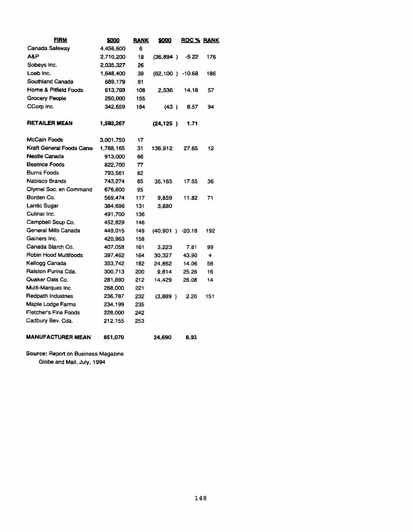
ImM Canada Safeway ABP Sobeys Inc. Loeb Inc.

Southland Canada Home & PHfield Foods Grocery People CCorp Inc.

RETAILER MEAN

McCain Foods Kraft General Foods Canar Nestle Canada Beatrice Foods Bums Foods Nabisco Brands Olyrnel Soc. en Command Borden Co. Lantic Sugar Culinar Inc. Campbell Soup Co. General Mills Canada Gainers Inc. Canada Starch Co. Robin Hood Multifoods Kellogg Canada Ralston Purina Cda. Quaker Oats Co. Multi-Marques Inc. Redpath Industries Maple Lodge Farms Fletchets Fine Foods Cadbury Bev. Cda.

MANUFACTURER MEAN

Source: Report on Business Magazine Globe and Mail. July, 1994

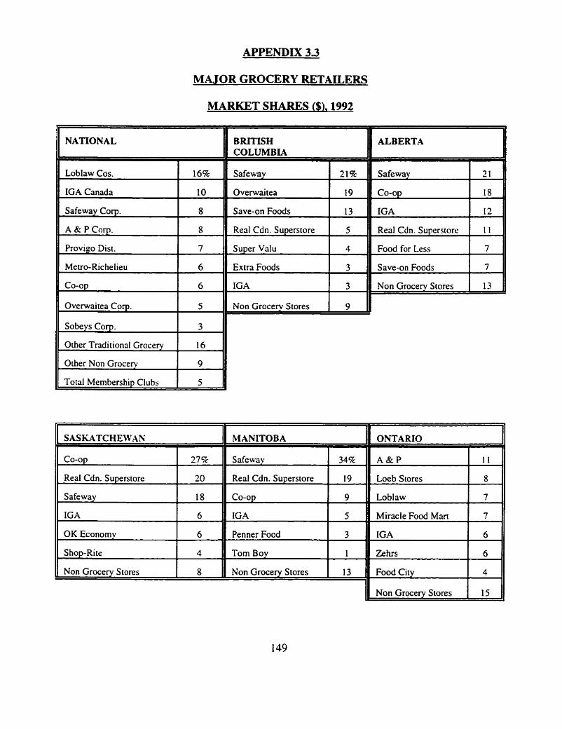
APPENDIX 3 3

MAJOR GROCERY RETAILERS

MARKET SHARJCS ($1,1992

11 NATIONAL

Loblaw Cos. I 16% I

I IGA Canada 10

Safeway Corp. 8

A tk P Corp. 8

Provigo Dist. 7

Metro-Richelieu 6

I Co-op 6

II Overwaitea Corn. I S

1, Sobeys Corp- 3

I Other Traditional Grocery 16

Other Non Grocery

BRITISH COLUMBIA

Safewa

Overwai tea

Save-on Foods

Real Cdn. Su~erstore

Extra Foods

Non Grocery Stores 1 9

ALBERTA

Real Cdn. Sunerstore I 1 1

Save-on Foods

Non Grocery Stores 13

SASKATCHEIVAN 11 MANITOBA ONTARIO

Co-op

Real Cdn. Superstore

Safeway

IG A

OK Economy

S hop-Rite

Non Grocery Stores

27%

20

18

6

6

4

8

Loblaw

Food Citv c 7

Miracle Food Man

IGA

Non Grocerv Stores I 15

_

7

6

Safeway

Real Cdn. Superstore

Co-op

IGA

Penner Food

Tom Boy

Non Grocery Stores

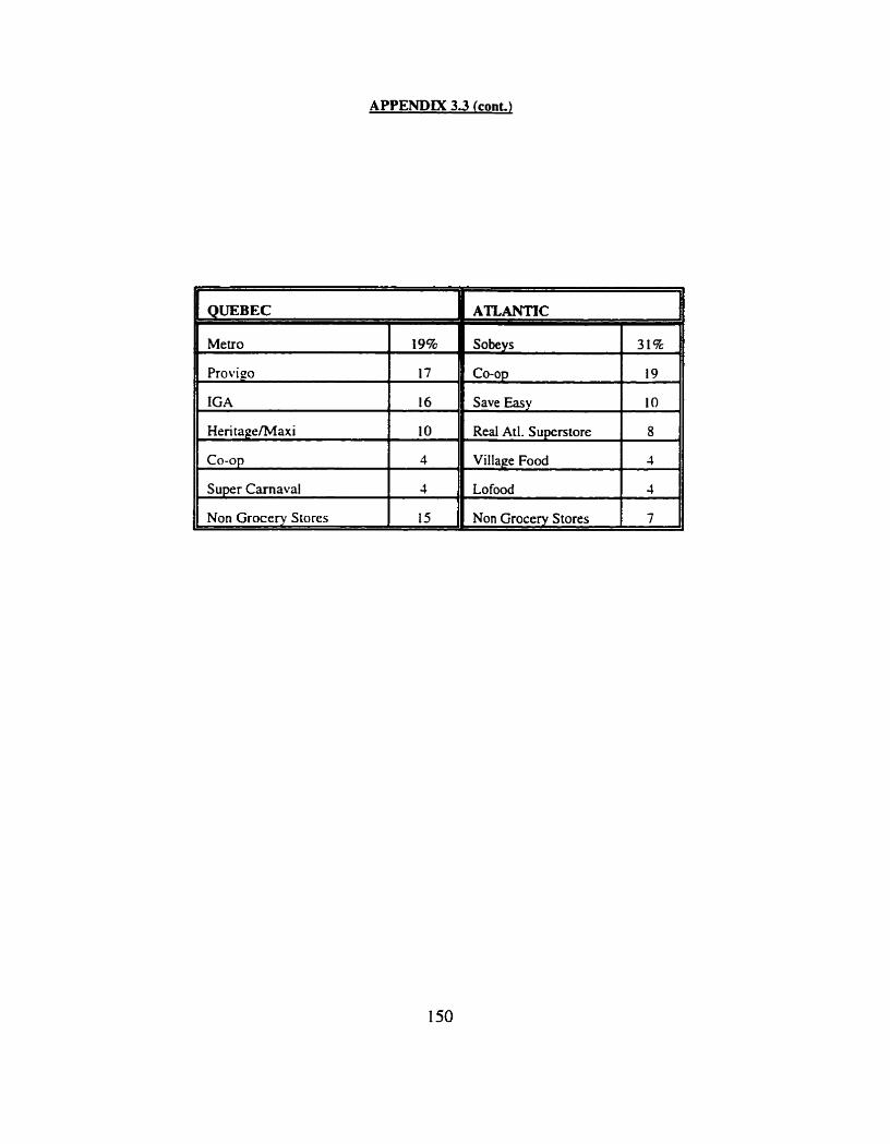
APf ENDM 3.3 (cont.1

OUEBEC

C Provieo

Non Groce N Stores

Real Atl. Su~erstore

Village Food 3

Lo food 3

Non Grocerv Stores 1 7

APPENDIX 3.4

PROPERTIES OF OUADR4TIC COST FUNCIlON

The duopoiists' cost function IS defined as

C = 3% + ~ b g ' + cq, + !4dq; + eaq,

Then rnarpnd costs are

MC, = 3 + bq, + eq,. and

MC, = c + dq, + eq,

Avn;lge Incremental Costs (Baumol. Panm and Willi 1982: Bailey and Friedlaender. 1981) are the ratio of the total incremental costs of supplyng each brand to its sales volume. In tke case of the national bmnd. this is

= a + !.ibq, + cq,

Slrnilarly. for the private label.

AIC. = c + ?/2dq, + eq,

Product-s/xc~fic econormes of scale (5.1 we represented by the ratio .UC/31C,. Where this mtio exceeds I . Mwgtnal Costs lie below Average ncremental Cosrs and returns to scdc are increasing: the reverse holds where the ratio AICfiIC, c I . Here.

AIC JMCm = ( 3 + %bqn + eq,)/(a + bq, + eqr) c I . and

AICjAlC, = (c: + "2dq, + eq,)/(c + dq, + eq,) < I .

Hence returns to scale are

- drnun~shing for the nat~onal brand where b > 0: - incrcasm~ for the nartonal brand where b c 0: - diminishing for the private label where d > 0; - increas~ng for the pnvate label where d c 0.

Economies of scope extst where thc costs of produc~ng both products wthn one firm are lower than those of producmg them In ruo separate firms. 1.r.

Hence economies of scope exist uhcre

aq, + 'nbqn' + cq, + hdq,' + eq,q, < aq, + l/2bqn1 + cq, + ldq, '

For posltive ccsts for each product. we requirc

aq, + ~ 2 b a ' > q q ,

- a + %bq, > eq,

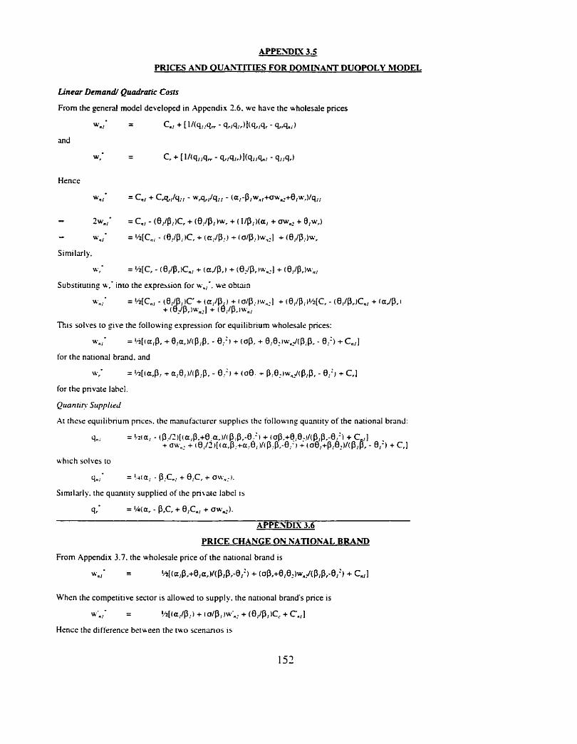
APPEhDN 3.5

PRICES AhD OUAhTITIES FOR DOMLNANT DUOPOLY MODEL

Linear Demand Quadratic Costs

From the general model developed in Appendix 2.6. we have the wholesaie prices

Hence

Quanrig Supplied

At thcse equ~iibriurn pnccs. thc manufacrurcr supplies thc foIlow~ng quantity of the national brand:

u h ~ c h solves to

Sim~lariy. the quantity supplied of the pnvate label 1s

PRICE CHANGE ON NATIOKAL BRAND

From Appendix 3.7. the wholesale price of the national brand is

W"1 - - 'h~(a,~,+O,a,)l(p,P,-&:) + ( ~ ~ , + 8 1 0 r ) w , ~ ( P l P , - ~ 1 2 ) + CnI1

When the competitive sector is allowed to supply. the narional brand's price is

%,- - - !+[(a,/P,) + ( alp, W,, + (8,lPl ICc + C'.,]

Hence the difference bctu-een the two scenarios IS

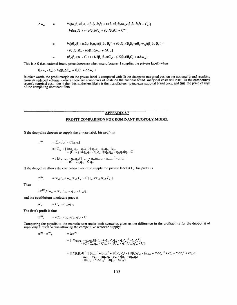
This is > 0 (i.e. national brand pnce increases when manufacturer 1 supplies the private lakl) when

In other words. the profit margin on the pnvate label is compared with (i) the chanse in mxginal cost on the nauond brand resultmg from its reduced volume - where there are economies of scale on the national brand, marginal costs will rise. (ii) the competmve sector's marginal cost - the higher this is. h e less IikeIy is the manufacturer to increase national brand price. and (ii) the price c h a n ~ c of the competing dominant firm.

APPESDIX 3.7

PROFIT COMPARISON FOR DObIINA3T DUOPOLY MODEL

If the duopolist chooses to supply the pnvare label. his profit is

I f the duopolist allows thc competltlve sector to supply the pnvate label at C,. his profit IS

and the equllibnum wholcsalr pncc 15

The firm's profit is thus

Comparin the payoffs to the manufacturer under both scenarios gives us the difference in the profitability for the duopolist of supplying fimself versus idlow~ng the comptxi~ive sector to supply:

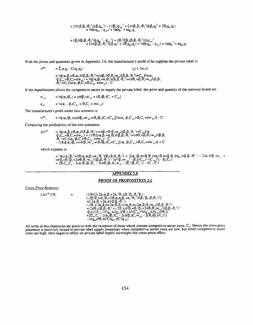
With the prices and quantities given in Appendix 3.6, the manufacturer's profit if he supplies the private label is

If the manufacrurer allows the competitive sector to supply the private label. the price and quantity of the naiional brand arc

The manufacturer's profit under this scenario is

Comparing the profirability of the two scenarios:

which expands to

APPENDlS 3.8

PROOF OF PROPOSITIOS 3.1

All trnns in [his expression arc positive with the exception of those which contain competitive sector costs. C,. Hence the cross-price panmcrer 1s sitively related to private label sup ly propensity when competitive sector costs are low: but when compctlnve sector costs are hrgr their nqauve effect on pnvae lagel supply outweighs the crorr-price effea.

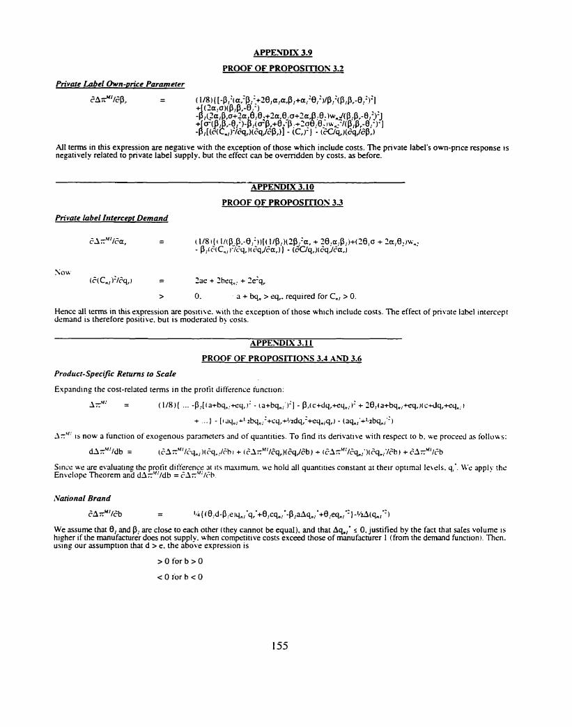
PROOF OF PROPOSITION 3 2

Pn'vde Label Own-urice Parameter

All terms in this expression are negative with the exception of those which include costs. The private label's own-pnce response rs negatively related to private label supply. but the effect can be overridden by costs. as before.

APPENDIX 3.10

PROOF OF PROPOSITIOS 3 3

Private label Intercept Demand

> 0. a + bq, > eq,. required for C,, > 0.

Hence all t e r n in this expression are posttlve. with thc exception of those wh~ch include costs. The effect of private label rntercept demand is therefore positive. but is rnoderatcd by costs.

APPENDIX 3.11

PROOF OF PROPOSITIONS 3.4 A 3 D 3.6

Product-Specific Returns to Scale

Expand~ng the cost-related terms in the protit difference function:

S~ncc we are evaluating the protit diiferenc~ ~t 11s maulmum. wc hold dl quamitres constant at t h e ~ r optimal lc~els . q,'. apply thc Envelope Theorem and dArr'"1db = ;lA;r"'/&.

We assume that 0, and p, are close to each other (they cannot be equal). and that Aq,,,. 5 0. justified by the fact that sales volume 1s higher if h e manufacturer does not supply. when competitive costs exceed those of manufacturer 1 (from the demand funct~on). Then. usmg our assumption that d > e. the above expression is

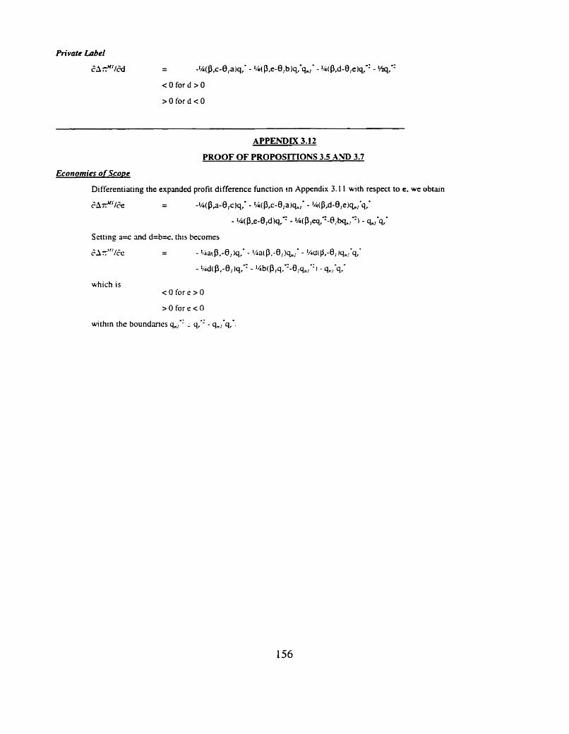
APPENDIX 3.12

PROOF OF PROPOSITIONS 3 5 AND 3.7

Economies of Scope

Differentiating the expanded profit difference function in Appendix 3.1 1 with respect to e. we obtain

- s A ;r"'l& - - l ~ ( P ~ - B , c ) q , ' - l/i(P,c-B,a)a,* - 8 4 ~ , d - 8 , e ) ~ I ' q , '

- l~(pp-fl,d)q," - lh(P,eq,c-@,bqn,? - a,'q,'

which is < O fo re>O

. - with~n the boundaries q,," - q,e: - q,, q, .

FIGURES

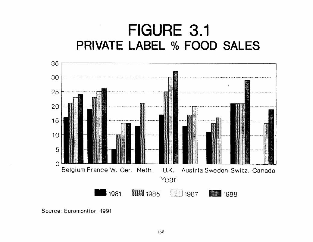
FIGURE 3.1 PRIVATE LABEL '10 FOOD SALES

Belglum France W. Ger. Nethl UIKt Austrla Sweden Swl tz. Canada

Year

Source; Euromonl tor, 1891

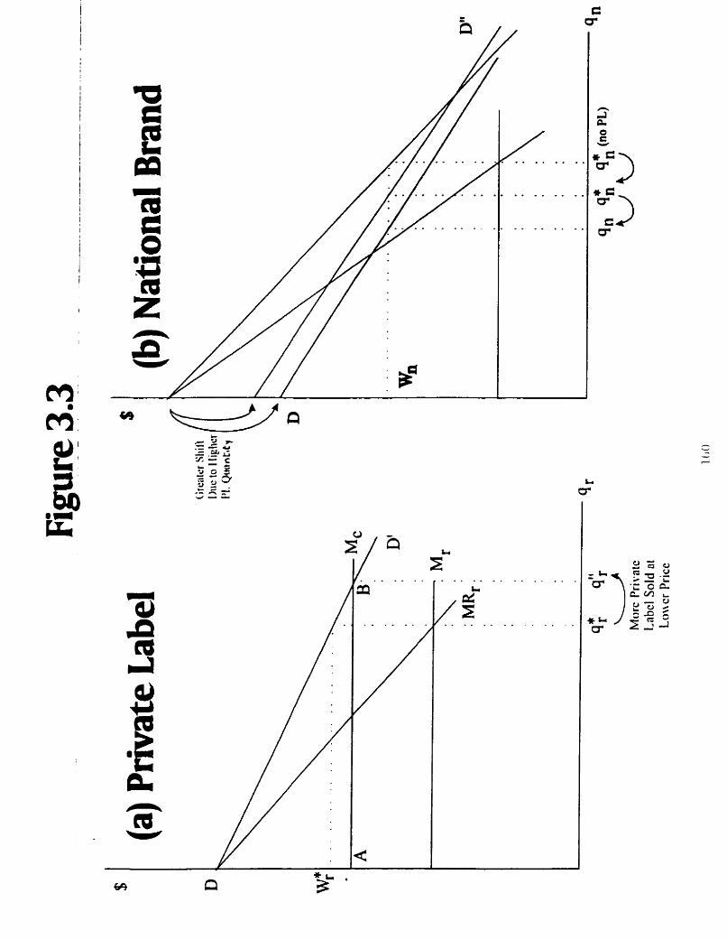
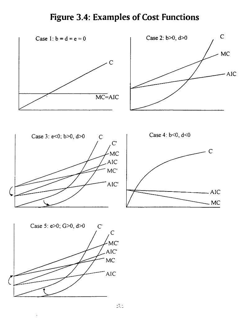
Figure 3.4: Examples of Cost Functions

Case 1: b = d = e = O

Case 3: e<O; b>O, d>O

Case 5 : e>O; G>O, d>O

Case 2: b>O, d>O

Case 4: b<O, d<O

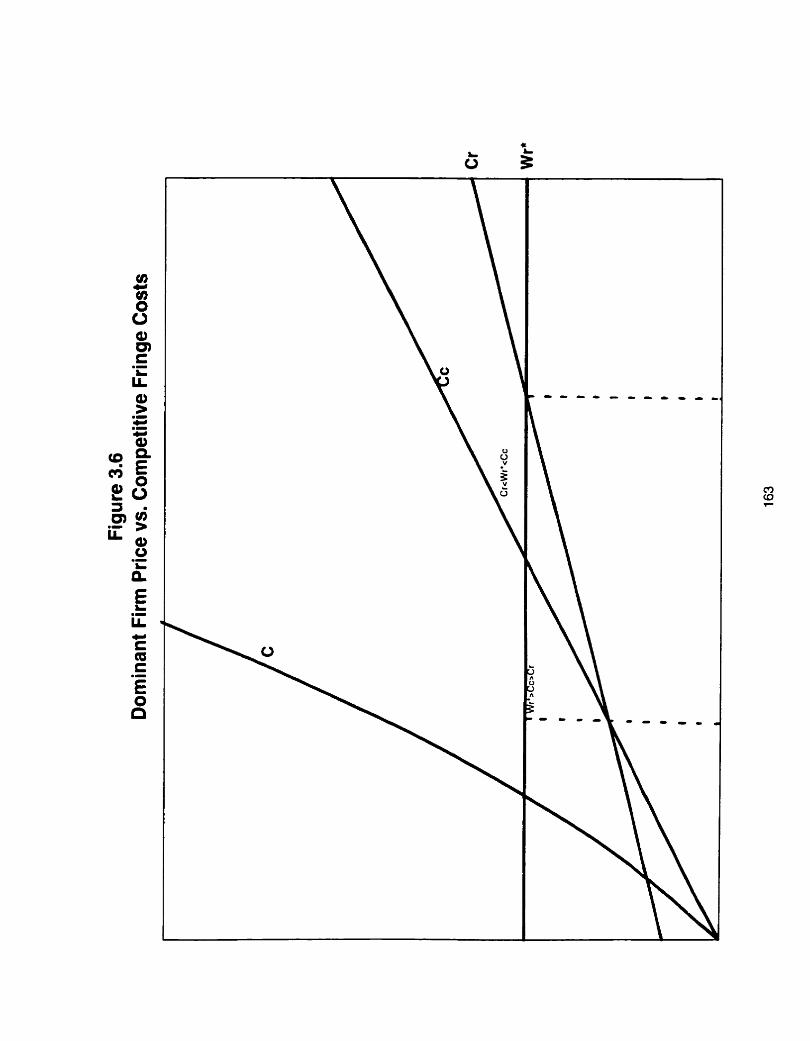
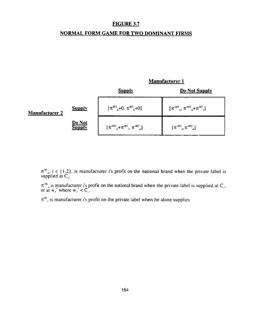
FIGURE 3.7

NORMAL FORM GAME FOR TWO DOMINANT FIRMS

Manufacturer 1

Supplv Do Not Supplv

+11 - ,,. I E { 1.2). is manufacturer i's profit on the national brand when the private label is supplied at C,.

Supplv Manufacturer 2

Do Not Gix

x"", is manufacturer i s profit on the national brand when the private label is supplied at C'.. or at w,' where w,' < C'..

x"', is manufacturer i's profit on the private label when he alone supplies

[ x ~ + o , r'f2"io] I

[TE"V l , + r w f l x14%f2n]

[nllll" X..+f2n+rLf2rJ

I

[ , p f y w .I

4. ESTIMATION OF DEMAND f ARAMETERS

A researcher can survive everything but a misprint.

Apologies to Oscar Wilde: The Chi[dre~l of the Poets

D) Introduction

The preceding two chapters specified a theoretical model of private label supply for

a national brand manufacturer. Here. we take the first step towards applying the model to data on a

category in the grocery products industry. Ultimately, our purpose is to demonstrate the model's

value as a decision tool by applying i t in a real-world context. The scenario analysis of Chapter 5

puts the model through its paces in applying it across a variety of decision environments: in this

chapter. we address some of the challenges that are raised by the need to estimate the model's

demand parameters from real data.

Towards the end of chapter 3. we summarized the key factors that favour and mitigate against

the supply of private label by a manufacturer. In particular, we saw that manufacturers look for

private labels that can expand the category with minimal cannibalization of their own national braid.

We also saw that private labels which are more elastic with respect to their own price are less

attractive to national brand manufacturers. and that the level of pricing by the competitive fringe can

also influence manufacturers' analysis of the situation. We also examined the role of costs in the

supply decision. finding that manufacturers prefer to supply the brand that offers higher economies

of scale. and that economies of scope also encourage manufacturers to supply.

The baseline model of chapter 2 dezlt with the situation facing a monopolist or duopolists.

Because refusal to supply in such industries means that the retailer is unable to market the private

label. the baseline model. in effect. analyzes the impact on incumbent national brand manufacturers

of a new private label entering the market - on the assumption that they can prevent private label

entry by refusing to supply. By contrast. the dominant manufacturer of chapter 3 has no power to

keep the private label out: if he rehses to supply, someone else will do so. Hence the manufacturer's

decision in this model is the same whether or not the private label already exists. This extended

model is therefore also appropriate to situations in which the private label is nireczdy being supplied

by a competitor, and the manufacturer is considering whether to underbid the incumbent and take

on private Iabel supply.

This was the situation facing one of the manufacturers in this grocery category": private

labels were gaining in strength. and national brand manufacturers were under pressure to take over

private label supply from the fringe sector. Market shares of the major brands are shown graphically

in Figure 4.1 :

(Figure 4.1 )

The category fits the "competitive fringe" structure described in chapter 3 well: two dominant

national brands compete against private labels, which are supplied by a competitive sector.

17 At the request of thc mnnu ficturer. d a d s of thc cmgory and the retailer are withheld and regresston panrnercrs are disguised

166

In this category. growth in private label market share has been an important issue for national

brand manufacturers. Private label suppliers go to great lengths to convince retailers to promote

private labels at the expense of national brands, providing a plethora of financial comparisons to

further their cause. National brands, for their part. have responded with data of their own and with

enriched promotional allowances for retailers to encourage featuring. One of the two dominant firms

in fact supplied private labels in the late 1970's. but more recently has taken a more combative

posture. Hence private labels are a highly topical issue. and private label supply may become a viable

strategy for one or both of the national brand manufacturers as their sales volumes decline.

Our overall goal in this chapter is to estimate demand parameters which will be used as

inputs to the theoretical model in chapter 5. To this end, we need to arrive at the most reasonable

possible estimates of demand intercepts. own-price response and cross-price response for each of

the three brands in the category. consistent with the underlying structure of the theoretical model.

These parameters will be used. along with estimates of costs. to predict the profitability of supplying

a private label for a specific manufacturer in the category.

We begin by reviewing the demand system underlying the theoretical model and its

assumptions in the next section: this is followed by a descripion of the data that will be used to

derive parameter estimates. Section (iv) considers the issues of consumer heterogeneity and

nonstationarity in consumption as they apply to this estimation process. Section (v ) specifies the

estimation procedure, section (vi) discusses the results, and section (vii) draws overall conclusions

about this phase of the analysis.

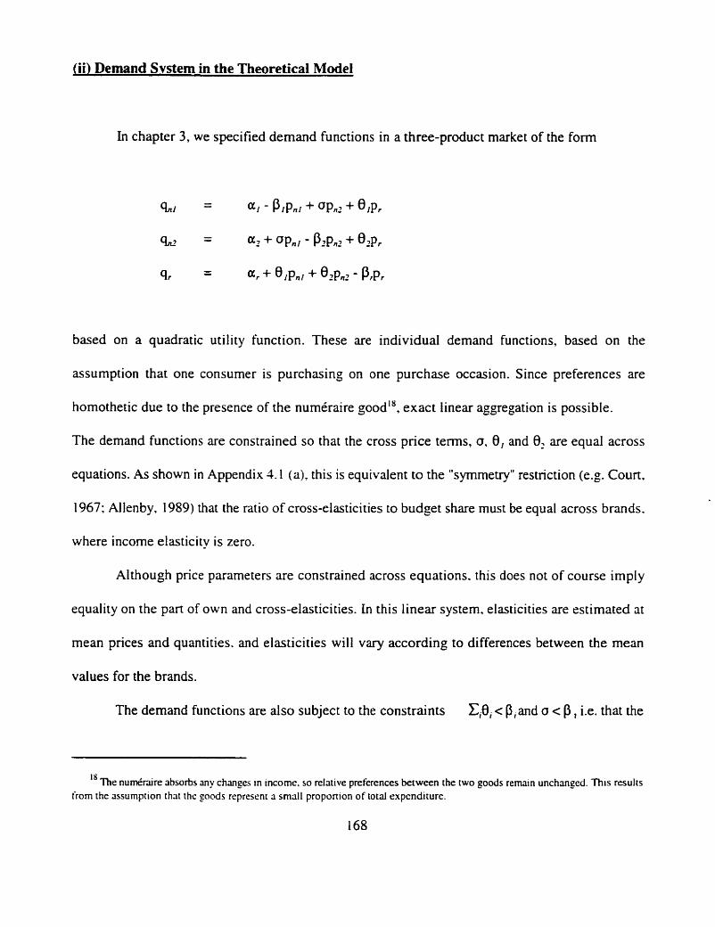
Jii) Demand Svstem in the Theoretical Model

In chapter 3, we specified demand functions in a three-product market of the form

based on a quadratic utility function. These are individual demand functions, based on the

assumption that one consumer is purchasing on one purchase occasion. Since preferences are

homothetic due to the presence of the numeraire good", exact linear aggregation is possible.

The demand functions are constrained so that the cross price terns, o, 6, and 8, are equal across

equations. As shown in Appendix 4. I (a). this is equivalent to the "symmetry" restriction ( e g Coun.

1967; Allenby, 1989) that the ratio of cross-elasticities to budget share must be equal across brands.

where income elasticity is zero.

Although price parameters are constrained across equations. this does not of course imply

equality on the pan of own and cross-elasticities. In this linear system, elasticities are estimated at

mean prices and quantities. and elasticities will vary according to differences between the mean

values for the brands.

The demand functions are also subject to the constraints &€Ii < P,and o < P , i.e. that the

'' The numinire absorbs any changes in income, so relative preferences between the two goods remain unchanged. This results from the assumption that the goods represent a small proponron of total expenditure.

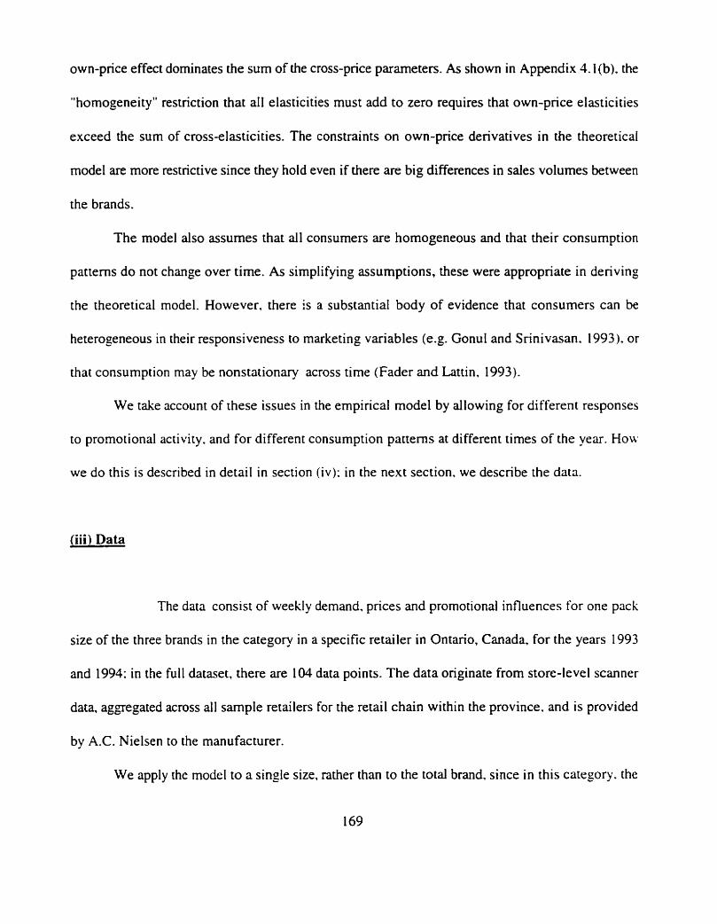
own-price effect dominates the sum of the cross-price parameters. As shown in Appendix 4.1 (b). the

"homogeneity" restriction that all elasticities must add to zero requires that own-price elasticities

exceed the sum of cross-elasticities. The constraints on own-price derivatives in the theoretical

model are more restrictive since they hold even if there are big differences in sales volumes between

the brands.

The model also assumes that all consumers are homogeneous and that their consumption

patterns do not change over time. As simplifying assumptions, these were appropriate in deriving

the theoretical model. However, there is a substantial body of evidence that consumers can be

heterogeneous in their responsiveness to marketing variables (e.g. Gonul and Srinivasan. 1993). or

that consumption may be nonstationary across time (Fader and Lattin, 1993).

We take account of these issues in the empirical model by allowing for different responses

to promotional activity. and for different consumption patterns at different times of the year. How

we do this is described in detail in section (iv): in the next section, we describe the data.

(i i i) Data

The data consist of weekly demand, prices and promotional influences for one pack

size of the three brands in the category in a specific retailer in Ontario, Canada, for the years 1993

and 1994: in the full dataset, there are 104 data points. The data originate from store-level scanner

data, aggregated across all sample retailers for the retail chain within the province. and is provided

by A.C. Nielsen to the manufacturer.

We apply the model to a single size. rather than to the total brand. since in this category. the

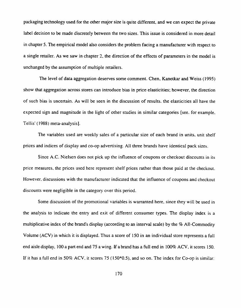
packaging technoloey used for the other major size is quite different, and we can expect the private

label decision to be made discretely between the two sizes. This issue is considered in more detail

in chapter 5. The empirical model also considers the problem facing a manufacturer with respect to

a single retailer. As we saw in chapter 2. the direction of the effects of parameters in the model is

unchanged by the assumption of multiple retailers.

The level of data aggregation deserves some comment. Chen, Kanetkar and Weiss (1 995)

show that aggregation across stores can introduce bias in price elasticities; however, the direction

of such bias is uncertain. As will be seen in the discussion of results. the elasticities all have the

expected sign and magnitude in the light of other studies in similar categories [see. for example.

Tellis* ( 1988) meta-analysis].

The variables used are weekly sales of a particular size of each brand in units. unit shelf

prices and indices of display and co-op advertising. All three brands have identical pack sizes.

Since A.C. Nielsen does not pick up the influence of coupons or checkout discounts in its

price measures. the prices used here represent shelf prices rather than those paid at the checkout.

However. discussions with the manufacturer indicated that the influence of coupons and checkout

discounts were negligible in the category over this period.

Some discussion of the promotional variables is warranted here, since they will be used in

the analysis to indicate the entry and exit of different consumer types. The display index is a

multiplicative index of the brand's display (according to an interval scale) by the % All-Commodity

Volume (ACV) in which it is displayed. Thus a score of 150 in an individual store represents a full

end aisle display. 100 a part end and 75 a wing. If a brand has a full end in 100% ACV, it scores 150.

If it has a full end in 50% ACV. it scores 75 (150*0.5), and so on. The index for Co-op is similar:

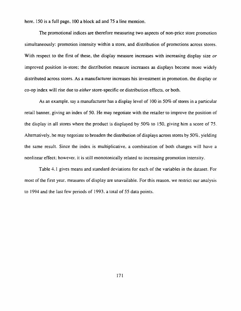
here. I50 is a full page, 100 a block ad and 75 a line mention.

The promotional indices are therefore measuring two aspects of non-price store promotion

simultaneously: promotion intensity within a store, and distribution of promotions across stores.

With respect to the first of these, the display measure increases with increasing display size or

improved position in-store: the distribution measure increases as displays become more widely

distributed across stores. As a manufacturer increases his investment in promotion. the display or

co-op index will rise due to either store-specific or distribution effects. or both.

As an example. say a manufacturer has a display level of 100 in 50% of stores in a paxticular

retail banner. giving an index of 50. He may negotiate with the retailer to improve the position of

the display in all stores where the product is displayed by 50% to 150, giving him a score of 75.

Alternatively. he may negotiate to broaden the distribution of displays across stores by 508. yielding

the same result. Since the index is multiplicative. a combination of both changes will have a

nonlinear effect: however. it is still monotonically related to increasing promotion intensity.

Table 4.1 gives means and standard deviations for each of the variables in the dataset. For

most of the first year. measures of display are unavailable. For this reason. we restrict our analysis

to 1994 and the last few periods of 1993. a total of 55 data points.

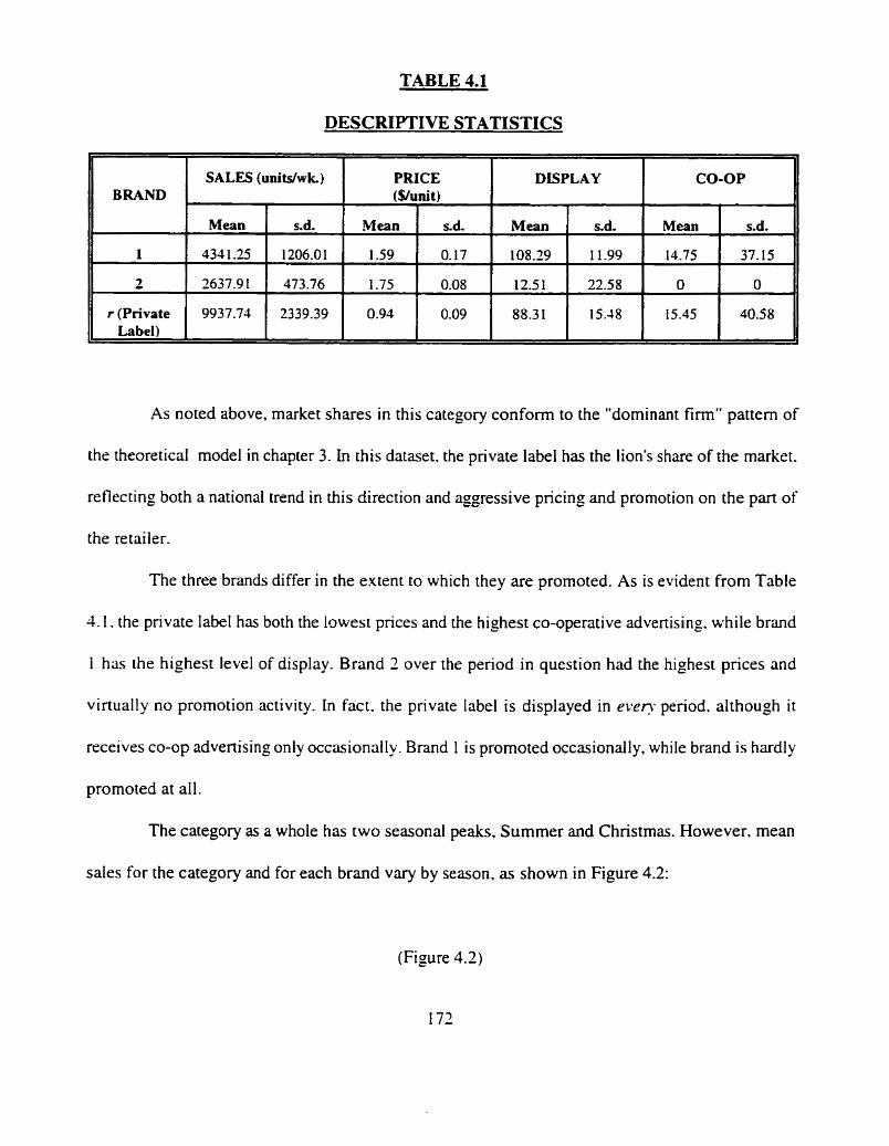
TABLE 4.1

DESCRIPTIVE STATISTICS

As noted above, market shares in this category conform to the "dominant firm" pattern of

the theoretical model in chapter 3. In this dataset. the private label has the lion's share of the market.

reflecting both a national trend in this direction and aggressive pricing and promotion on the part of

the retailer.

BRAND

1

2

r (Private Label) -

The three brands differ in the extent to which they are promoted. As is evident from Table

1.1. the private label has both the lowest prices and the highest co-operative advertising. while brand

1 has the highest level of display. Brand 2 over the period in question had the highest prices and

virtually no promotion activity. In fact. the private label is displayed in e v e n period. although it

receives co-op advertising only occasionally. Brand 1 is promoted occasionally, while brand is hardly

promoted at all.

The category as a whole has two seasonal peaks. Summer and Christmas. However. mean

sales for the category and for each brand vary by season. as shown in Figure 4.2:

(Figure 4.2)

SALES (unitdwk)

Mean

433 1.25

2637.9 I

9937.73

s.d,

1206.0 1

473.76

2339.39

PRICE ($/unit)

Mean

1.59

1.75

0.93

s.d.

0.17

0.08

0.09

DISPLAY

Mean

108.29

12.5 1

88.3 1

CO-OP

s.d.

1 1.99

22.58

15.18

Mean

14.75

0

15.45

I

s.d,

37. I5

0

40.58

In summary. this dataset offers information on demand and prices in a category which fits

the conditions assumed by the theoretical model. allowing us to estimate the parameters of the

demand functions for later use in the theoretical model. However. demand patterns in the category

suggest that promotions and seasonality may have an influence on sales of each brand. How we build

these consideration into the model is the subject of the next section.

Jiv) Heterogeneitv and Nonstationaritv

The demand functions of the theoretical model are derived from a utility function which

assumes that one consumer chooses quantities of each of the products on one purchase occasion.

given a budget constraint and preferences for all other goods. For a firm to make a decision on

private label supply, however. it needs to consider the utility functions of all potential consumers of

its products. In aggregating across consumers. however. we need to consider (i) whether all

consumers purchase according to the same demand function (heterogeneity). (ii) whether their

consumption pattern shifts with time (nonstationarity).

There is ample evidence of heterogeneity among consumers in the marketing literature.

Gonul and Srinivasan ( 1993). for example. find strong support for differences across households in

intrinsic brand utility. response to marketing variables and switching behaviour. With this and other

studies [e.g. Guadagni and Little (1983); Lattin and Bucklin (1989); Fader and Little (1992)l. there

appears to be sufficient evidence of consumer heterogeneity to prevent us from simply multiplying

the demand function of the theoretical model by the number of consumers in the market.

In this model. we assume that consumers may differ in their intrinsic brand preference

(intercept demand). own-price response and cross-price response according to whether they are

regular consumers of the category. Specifically, we assume that a core group of "regular" consumers

purchases and switches between brands in homogeneous fashion, while a second group of

"occasional" consumers moves in and out of the category in response to promotional activity. These

two groups are heteregeneous in all the parameters of their demand functions: hence they differ in

dl three of the ways identified in Gonul and Srinivasan's study.

From the literature on this subject, there are two possibilities identified by Blanberg. Briesch

and Fox (1995): that the majority of promotional volume comes from switchers within the category,

or that promotions expand the category. Blattberg et al. find conflicting results on this issue. and

suggest that the difference may depend on the potential of the category for expansion through (for

example) increased consumption. store switching. purchase acceleration or stockpiling.

Our assumption that promotions draw in occasional consumers is based on the idea that this

category is one that lends itself to expansion. The product's physical characteristics allow for easy

storage: hence consumers who use the category irregularly can purchase it on promotion and

stockpile it. In addition, nonalcoholic beverages such as this are likely to be purchased "on impulse"

by some consumers rather than as a staple item.

A further issue in empirically estimating these demand functions is the possibility that

consumers of either type may have different utility for the products at different times. As we saw

earlier, there is evidence of seasonality in this category. In our estimation of the demand functions,

we allow intercepts to shift according to seasonal differences, in response to expansion and

contraction of total or individual brand consumption. within both consumer groups, by time of year.

We formalize these ideas with the assumptions given below.

Heterogeneity

There is a groupi9 of "regular" consumers, which purchases brands according

to the demand function q,, = ai - P,p,, + op,, + 0p, in time period t .

A second group" of consumers, "occasional" consumers, enters the market

irregularly, and is specifically drawn in when there is a promotion on any of

the brands. We assume that these consumers purchase on impulse rather than

compare prices across brands - typically, they see a product on display or in

a retailer's ad. and buy accordingly. Hence their cross-price terms 0, - 0 and

o - 0. and their demand function is q,,' = a'-P,'p,,.

If there is a promotion on one of the brands. occasional consumers have some

probability of encountering it. a function of the relative intensity of the

brand's promotional activity versus that of other brands.

The above assumptions are operationalized by creating variables to indicate the prevailing conditions

in the market in a given period:

a The probability of promotional consumers seeing a promotion on brand i in

19 The demand function applies to the group as a whoie. We assume that there arc V such homogeneous consumers, a constant proportion of which. r. buys In every period. Since both Vand rare constant across periods, they simply represent a rescaling of the parameters of the individual demand functions and have been dropped from the group demand expression.

'0 The size of the occasronal segment may differ from that of the rep tar segment. Hence the demand functions shown below

should be weighted by ssgmcnt size. To keep the notatlon s~rnplc. this weightins has been omitted.

period r , given that any of the brands is being promoted, is A,,. which is in

turn a function of the intensity of promotional activity on brand i relative to

that on the other brands. Across brands, the A,,'s add to unity. Where there are

no promotions on any of the brands in a given period, A,, = 0 V i.

If there is no promotion on product i in period t , 4, = 0 and product i s

demand function is that of regular consumers only. This applies whether or

not there are promotions on other brands. While promotions on other brands

drawf occasional consumers to those brands, they do not have any effect on

the demand function for the non-promoted brand: regular consumers may still

switch between brands, however. based on price differences.

In a three-brand system such as this category. the above assumptions yield the following set

of linear demand equations in general, for brands 1.2 and r (private label) in time period t .

Gerzerul Model

0 5 A,, = {prob(i promotion seen, period t ) } i 1 : A,, = 0 where no promotion on any brand.

eke zJ,=,/l,, = 1; i E { 1.2.r}: P, > 8,; p, > a for i€ ( 1.2).

By setting A,, to specific values, we can represent different combinations of brand

promotional activity in different periods. The principal scenarios are given below.

No Promotion on Any Brand

Here. there are no occasional consumers. and demand functions refer to regular consumers

only.

The form of these equations is identical to that specified for the theoretical mode[. If there

were no promotions. this set of equations would represent the theoretical model multiplied by the

number of consumers in the market.

Promorion on Brand I Only

Occasional consumers enter the market as a result of seeing a promotion on brand 1. The

demand function for brand 1 is an amalgam of regular and occasional groups.

A,, = I; A,,=O for i = 1.

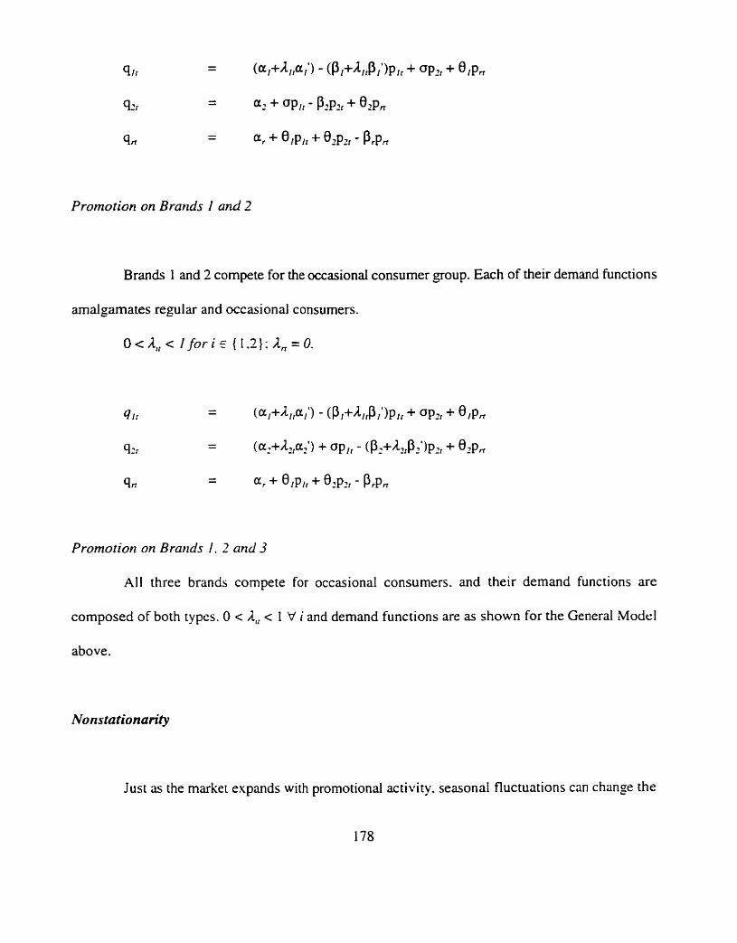
Promotion on Brartds I and 2

Brands 1 and 2 compete for the occasional consumer group. Each of their demand functions

amalgamates regular and occasional consumers.

O<Al , c I fori 5 (1.21: 1, = 0.

Promotion on Brartds I , 2 and 3

A11 three brands compete for occasional consumers. and their demand functions are

composed of both types. 0 < A,, < I V i and demand functions are as shown for the General Model

above.

Nonstationarify

Just as the market expands with promotional activity. seasonal fluctuations can change the

178

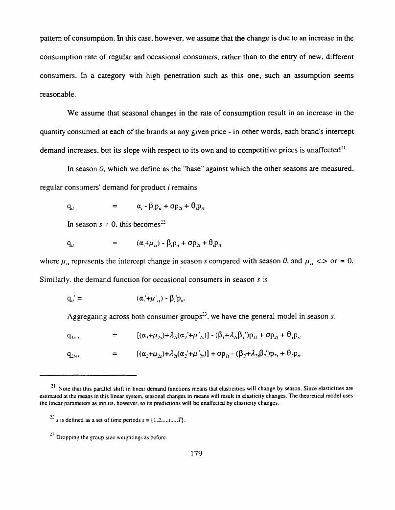
pattern of consumption. In this case. however, we assume that the change is due to an increase in the

consumption rate of regular and occasional consumers, rather than to the entry of new. different

consumers. In a category with high penetration such as this one, such an assumption seems

reasonable.

We assume that seasonal changes in the rate of consumption result in an increase in the

quantity consumed at each of the brands at any given price - in other words, each brand's intercept

demand increases, but its slope with respect to its own and to competitive prices is unaffected".

In season 0, which we define as the "base" against which the other seasons are measured.

regular consumers' demand for product i remains

911 - - a1 - P,P,~ + OP2r + ~ I P ,

In season s = 0. this becomes"

9 t* - - (a,+~ls) - PIP,, + OPI + e l ~ n

where p, represents the intercept change in season s compared with season 0. and p1., <-> or = 0-

Similarly. the demand function for occasional consumers in season s is

'I Note that this parallel shift in linear demand hnctions means that elasticities will change by season. Since elasticities are estimted at the means in this linear system. seasonal changes in means will result in elasticity changes. The theorericd model uses the linear parameters as inputs. however. so its predictions will be unaffected by elasticity changes.

-I 7 -- s is defined as a set of time periods s = ( 1 .Z ..... r ..... T).

-1 -. Dropping the group s~ze wcishtin_es as bcforc.

- %a -

K ~ ~ + P , ) + ~ K ( % ' + P ',I + 01~1, + 0 2 ~ 2 1 - ( P ; c ~ ~ ' ) P ,

where the terms a,, a,', p,, PI' . o and 8, are constant across all seasons: seasonal terms p, and p ',, vary

by season but are constant within seasons; and the promotional terms 1, vary by period.

This the model which will be estimated as outlined in the next section-

(v) Estimation of the Svstem

To estimate the system described in the last section, we need to define a variable that

measures A,,, the probability that occasional consumers will encounter a promotion on one of the

brands.

As outlined above. the dataset provides two indices which measure promotion: Co-op and

Display. weighted by distribution. One approach to the problem of identifying promotions within

the data would be to assign a dummy to each condition as previous authors (e-g. Sethuraman. 1995)

have done. However. when more than one brand is on promotion. we need to have some way of

"dividing up the spoils" - determining the relative probability of consumers seeing a particular

promotion. We could assign a value of 1.0 when one brand is promoted. 0.5 when there are two. and

so on. However. such an approach assumes that all promotions have an equal probability of being

seen. irrespective of the size or location of display, prominence of the ad. or distribution of

promotions across stores. For this reason, it is preferable to construct an index based on the available

Co-op and Display variables. As discussed in section (iii), while the scale for these variables is

arbitrary, it will be monotonically related to promotion intensity. and hence to the probability that

an "occasional" consumer will encounter a promotion on one of the brands.

We construct an index of promotional activity based on these measures. first by identifying

whether any of the brands is promoted (if not, recall that A, = 0). and then by calculating each brand's

share of promotional activity in the category. Hence there are two aspects to the measure: whether

any occasional consumers are in the market, and which promotion they are most likely to see.

To identify periods in which any brand is promoted, we define a dummy variable. D, which

equals 1 if any brand is promoted in the period in question, 0 otherwise.

Share of promotion is calculated as each brand's total promotion activity (sum of co-op and

display in dice^'^). shared to total promotion activity across all brands. Defining p,! =

(~,~+d,,)/~,(c,~+d,,). where c so -op and d=display. we have A,, = D, p, Hence A , varies between 0 and

1. with I indicating that brand i was the only brand promoted. and 0 indicating that brand i was not

promoted. or that none of the brands was promoted.

As noted earlier. data on display are not available for most of the first year: hence the above

promotion share can be used over only 55 weeks of data. As was evident from Table 4.1. brand 2 did

not have any Co-op advertising in these 55 weeks: hence its promotional activity consists of display

only. Over this time, however. at least one brand is on display in every period. making it difficult to

distinguish promoted from unpromoted periods by this measure. Hence we use Co-op on any brand

as the dummy promotion variable, Dr. In using Co-op as a measure of category promotional activity,

we are accounting for the ability of promotions to draw consumers into the category. The promotion

share variable. on the other hand. indicates which promotion consumers are most likely to encounter

once they enter the category.

'4 Sots that ~ h t s unwcightcd sum means that Display and Co-op are assumed to have the same degree o f effect on promotion tntcnsit>'.

The major flaw in this approach is that periods in which there are displays but no Co-op are

excluded as promotional periods. However, since the alternative is to recognize that at least one

brand was promoted in every period. we take the view that the presence of Co-op advenising in

addition to display indicates, at least. a more "unusual" level of promotional activity, which is more

ii kel y to attract occasional consumers.

Since seasonality is a factor in this category, we define seasonal (0.1 ) dummies for Spring,

Summer, Christmas and Winter. with Faii as the "base" season.

Based on these definitions, the model is estimated as follows:

1 SALES = [a, + p,,(SPRING) + ~,,ISUMMER) + p,,(XMAS) + p14WNTER)l + [a,'(DCOOP* 1 PSHR) + /J*~,(DCOOP* 1 PSHR*SPRING) + p ',,(DCOOP* 1 PSHR*SUMMER) + p ',,(DCOOP* 1 PSHR*XMAS ) + p*,,(DCOOP* 1 PSHR*WINTER)] + P,( I PRICE) + P',(DCOOP* 1 PSHR* 1 PRICE) + a(2PRICE ) + B!(rPRICE

?SALES = [a, + p,,(SPRING) + p,,(SUMMER) + p,?(XMAS) + p=,(WINTER)I + [a2'(DCOOP*2PSHR) + p ':,(DCOOP*2PSHR*SPRING )

+ p ',,(DCOOP*2PSHR*SUMMER) + p ',,(DCOOP*2PSHR*XbIAS 1

+ p '2,(DCOOP*2PSHR*WINTER)] + a( 1 PRICE) + P,(?PRICE) + Pe,(DCOOP*2PSHR*2PRICE) + 8,(rPRICE)

rSALES = [a, + p,,(SPRING) + pJSUMMER) + p,,(XMAS) + p,,(WINTER)] + [a,'(DCOOP*rPSHR) + p ',,(DCOOP*rPSHR*SPRING) + p',,(DCOOP*rPSHRfSUMMER) + p 'r,(DCOOP*rPSHR*XMi\S )

+ p ',(DCOOP*rPSHR*WINTER)] + 0,( 1 PRICE t + B,(YRICE) + P,(rPRICE) + P',(DCOOP*rPSHR*rPRICEt

where I SALES. 2SALES and rSALES are sales of brands I . 2 and r (Private Label) respectively:

SPRING, SUMMER, XMAS and WINTER are seasonal dummies: DCOOP is a ( 1.0 1 dummy set

at I if any brand has Co-op advenising in that period, the term D, described above. I PSHR. 2PSHR

and rPSHR are shares of total promotional activity as described above, A,,. 1PRICE. 2PRICE and

rPRICE are retail prices of the three brands.

182

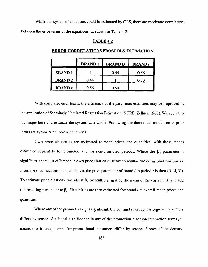
While this system of equations could be estimated by OLS, there are moderate correlations

between the error terms of the equations, as shown in Table 4.2:

TABLE 4.2

ERROR CORRELATIONS FROM OLS ESTIMATION

With correlated error terrns. the efficiency of the parameter estimates may be improved by

the application of Seemingly Unrelated Regression Estimation (SURE; Zellner. 1962). We apply this

technique here and estimate the system as a whole. Following the theoretical model. cross-price

terms are symmetrical across equations.

BRAND 1

BRAND 2

Own price elasticities are estimated at mean prices and quantities. with these means

estimated separately for promoted and for non-promoted periods. Where the P', parameter is

significant. there is a difference in own price elasticities between regular and occasional consumers.

From the specifications outlined above. the price parameter of brand i in period t is then @,+A#,).

To estimate price elasticity. we adjust P,' by multiplying it by the mean of the variable 4, and add

the resulting parameter to p,. Elasticities are then estimated for brand i at overall mean prices and

quantities.

Where any of the parameters p,, is significant, the demand intercept for regular consumers

differs by season. Statistical significance in any of the promotion * season interaction terms p ',,

BRAND1

1

0.44

means that intercept terns for promotional consumers differ by season. Slopes of the demand

I83

BRANDB

0.44

1

BRANDr

0.56

0.50

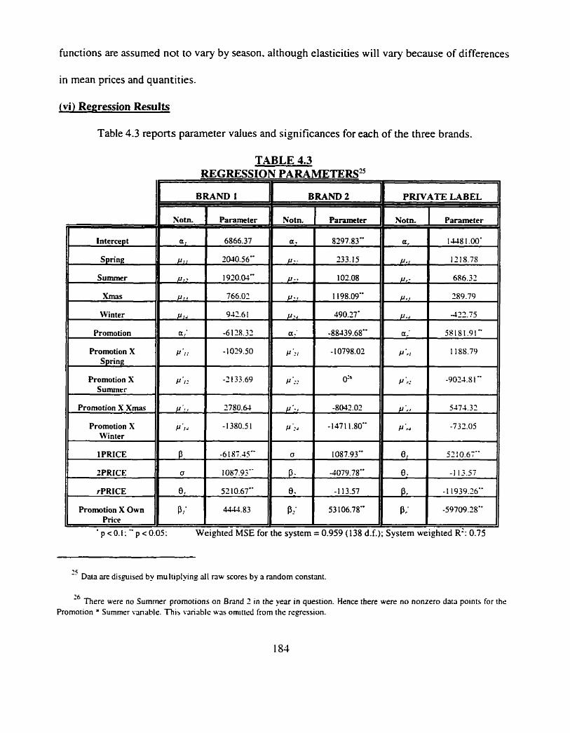
functions are assumed not to vary by season. although elasticities will vary because of differences

in mean prices and quantities.

Jvi) Regression Results

Table 4.3 reports parameter values and significances for each of the three brands.

TABLE 4.3

Interce t F Summer

Xmas

Winter

Promotion

Promotion X Spring

Promotion X Summer

Promotion X Xmas

Promotion S Winter

1 PRICE

Promotion X Own )I P"rr

BRAND 1 I

Notn I Parameter

1

Weighted

BRAND 2

25 Data are disguised by multiptying all r3w scores by a random constant.

PRIVATE LABEL ' Notn. I Parameter

rn

f.); ~vs tem

26 There were no Summer promotions on Brand 2 in the year in question. Hence there were no nonzero d313 points for the Promotion ' Summer vanable. T h ~ s variable was orn~tred from the regression.

As expected, all intercepts are positive. own price parameters negative and cross-price

parameters positive. With the exception of the cross-price term between brand 2 and the private

label, all price parameters are statistically significant at the 0.05 level. It appears from these results

that brand I substitutes with both brand 2 and private label, but that brand 2 substitutes only with

brand 1. This "price tier" pattern (Blattberg and Wisniewski, 1989) is supported by the fact that

brand 2 has the highest mean price of the three brands, brand 1 is second highest and the private label

is lowest.

Recall from the theoretical model that we constrained the parameters so that P, > &0, and

p, > o: each brand must respond to changes in its own price to a greater degree than to changes in

competitive prices. This constraint was imposed so that aggregate demand would always be

negatively related to prices. and so that prices would always be positive. These results meet this

constraint: in all cases. the own price term exceeds cross-price terns in absolute value. This was not.

however. imposed as a constraint in the estimation since empirical demand studies consistently find

that own-price elasticities exceed cross-elasticities (Blattberg, Briesch and Fox. 1995).

Since prices in this category tend to be uniform across stores within a retail chain. the data

appear to preserve the essential relationships quite well in spite of their aggregation level. While

there are promotion effects on brand 2 and the private label. the effects of promotions on brand 1

may be hidden by the aggregation level. Appendix 4.2 discusses the issue of promotion in more

detail. along with a series of diagnostic tests of the regression model.

All three brands are subject to some seasonality; however. the seasonal effects are not

consistent across brands. From this result. it would appear that not only does total consumption in

the category shift with changes in the seasons. but that brand preferences also change. In the case of

brand 2. consumption appears to peak at Christmas. while brand I increases in Spring and Summer.

While price parameters do nor vary by season. price elasticities do vary because of

differences in mean quantities and prices. Table 4.4 gives the elasticity matrix for each of the seasons

analyzed. with values that are not significant shown in parentheses:

TABLE 4.4

ELASTICITY MATRICES BY SEASON

FALL SPRING

WINTER

SUMMER

Own price elasticities on the national brands are in the neighbourhood of -2.0 to -2.5. while

cross-elasticities are lower. The magnitude of these elasticities is consistent with other studies of

186

7

r

0.89 I

(-0.03

-0.65 1

2

0.40

-2.38

(-0.0 I )

1

7

t

1

-2.15

0.6 1

0.57

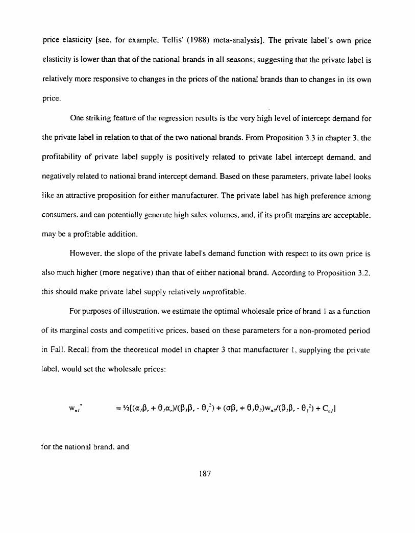
price elasticity [see. for example. Tellis' ( 1 988) meta-analysis]. The private label's own price

elasticity is lower than that of the national brands in all seasons; suggesting that the private label is

relatively more responsive to changes in the prices of the national brands than to changes in its own

price.

One striking feature of the regression results is the very high level of intercept demand for

the private label in relation to that of the two national brands. From Proposition 3.3 in chapter 3, the

profitability of private label supply is positively related to private label intercept demand. and

negatively related to national brand intercept demand. Based on these parameters. private label looks

like an attractive proposition for either manufacturer. The private label has high preference among

consumers. and can potentially generate high sales volumes. and, if its profit margins are acceptable.

may be a profitable addition.

However. the slope of the private label's demand function with respect to its own price is

also much higher (more negative) than that of either national brand. According to Proposition 3.1.

this should make private label supply relatively rcnprofitable.

For purposes of illustration. we estimate the optimal wholesale price of brand 1 as a function

of its marginal costs and competitive prices. based on these parameters for a non-promoted period

in Fall. Recall from the theoretical model in chapter 3 that manufacturer I . supplying the private

label. would set the wholesale prices:

for the national brand. and

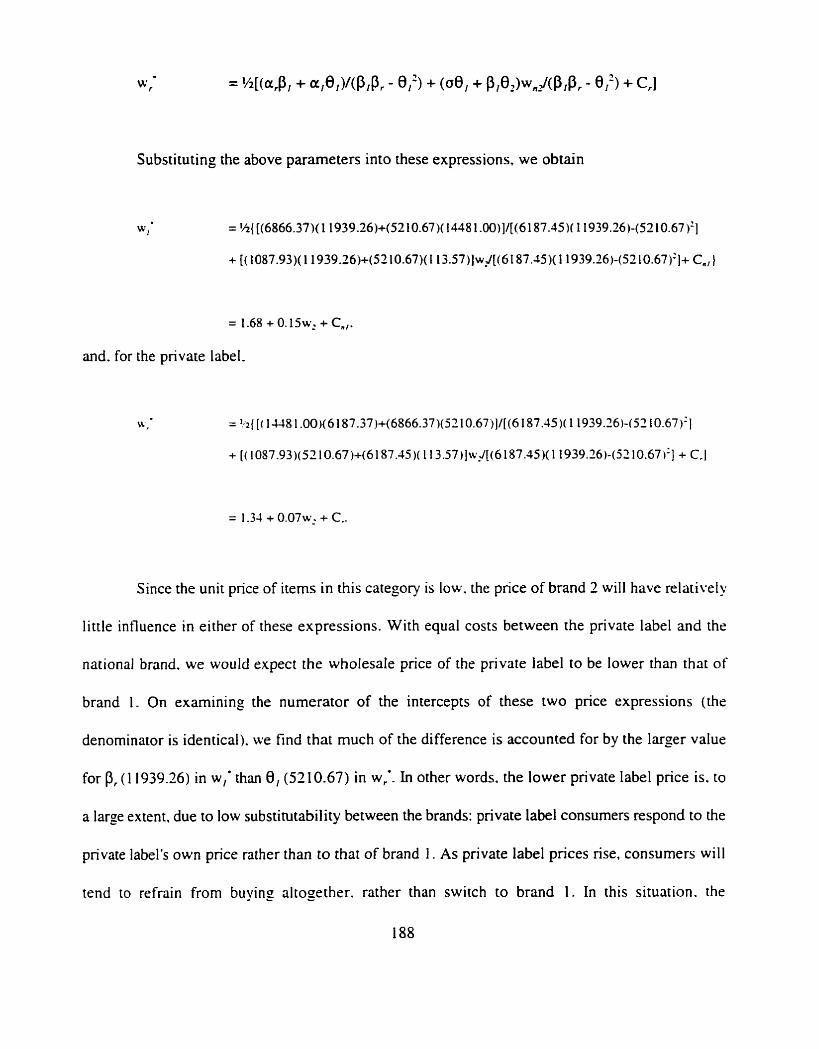
Substituting the above parameters into these expressions, we obtain

W j = 'h{ [(6866.37)(11939.26)+(5210.67)( 1448 1.00)]/[(6 187.45M I 1939.26)-(52 10.67)']

+ [( 1087.93)( 1 l939.26)+(52 lO.67)(ll3.57) jw[(6187.45)(11939.26)-(52 10.67)']+ C,, }

= 1.68 + 0 . 1 5 ~ ~ + C,,.

and. for the private label.

= 1.31 + 0 . 0 7 ~ : + C..

Since the unit price of items in this category is low. the price of brand 2 will have relatively

little influence in either of these expressions. With equal costs between the private label and the

national brand. we would expect the wholesale price of the private label to be lower than that of

brand 1. On examining the numerator of the intercepts of these two price expressions (the

denominator is identical). we find that much of the difference is accounted for by the larger value

for p, ( 1 1939.26) in w,' than 8, (5210.67) in w,'. In other words. the lower private label price is. to

a large extent, due to low substitutability between the brands: private label consumers respond to the

private label's own price rather than to that of brand 1. As private label prices rise, consumers will

tend to refrain from buying altogether. rather than switch to brand 1. In this situation. the

i 88

manufacturer maximizes his total surplus by setting a low price for the private label to capture these

consumers, and a higher price for the national brand since its demand is relatively unaffected by the

private label's price. In short. he s e p e n t s the market.

Until we estimate the full model with all parameters. including costs. however, we do not

know the net effect of these conflicting influences on private label supply profitability. This is the

subject of chapter 5. in which we use these parameters to estimate the profitability of private label

supply in a variety of business scenarios.

jvii) Sumrnarv and Conclusions

The primary purpose of this chapter has been to develop intuitively reasonable estimates of

demand parameters for input into the theoretical model. In the process of developing these estimates.

it has become clear that. in order to apply a model such as this to real-world data. we need to make

some assumptions about consumer behaviour.

Specifically. we have assumed that two types of consumers exist: "regular" consumers. who

switch between brands based on price. and "occasional" consumers. who buy the first promoted

brand they see. We have estimated separate demand functions for each of these groups. In addition.

we assumed that each of these groups' demand functions varied by season.

The results we obtain from the theoretical model - the profitability for a firm of supplying

private label - will depend on these assumptions. so we need to have some confidence that they are

reasonable.

In the case of promotions. we have assumed that occasional consumers may differ in

intercept demand and in own price parameters. but have cross-price effects that approach zero. The

origin of this assumption is the intuition that occasional consumers enter the market because they

see a retail promotion. Such consumers use relatively little of the product and will purchase enough

to last until the next promotion; the category, however. represents a small proportion of their total

erocery bill. If consumers of this type are attracted to the category by a display or switch from Y

another store because of an ad. it is reasonable to assume that they do not go to the shelf to compare

prices, but purchase on impulse, reacting only to the price of the brand on display.

A limitation of this approach is that it does not allow for the possibility that regular

consumers of the product may expand the category by switching stores. Store switching is certainly

present in this category. but it is difficult to envisage consumers switching stores on a regular basis

for an item that costs less than 52. Where a major national brand is deeply discounted, we can expect

some store switching. but for most promotions in this category. its extent is likely to be small.

The assumption that promotions draw new consumers into the category is supported by the

promotions literature, as argued earlier in this chapter. An alternative assumption would be that the

number of consumers in the category remains constant, but that regular consumers change their

behaviour in response to a promotion. There is some evidence of this in the literature. but the

evidence varies by category and is not conclusive. Given the properties of this particular product -

its ease of storage and its "impulse" nature - the assumption that promotions increase category size

by attracting occasional consumers appears reasonable.

In the case of seasonality. we have assumed that regular and occasional consumers' intercept

demands rise or fall by season, but that own and cross price terms are unaffected. In this category,

the key seasonal influences are weather and holidays. It is difficult to conceive of either of these

having a great effect on price parameters. although they certainly could affect intercept demand. The

alternative assumption, that price terms vary by season. implies that some other seasonal influence,

such as income fluctuations. affects the responsiveness of demand to prices. However, since the

products account for a small outlay in proportion to income, this appears unlikely.

The linear specification of the empirical model fits well with the linear form of the

theoretical model. This should not be taken to imply that the only way to estimate this model is

according to a linear specification, which may not be appropriate with all datasets. Earlier estimates

of this model used a log form, but did not show any material improvement in fit over the linear

version. The closer correspondence between the theoretical and empirical models and the simplicity

of the cross-elasticity constraint weighed the decision in favour of the linear version.

The results show some seasonal effects. and price effects are in the expected direction.

Promotional effects. however, are limited. This may be due to the aggregate nature of the data. which

is certainly a limitation of this empirical application.

With reasonable parameter estimates for demand, we are now in a position to move forward

with a demonstration of what the model can do in a practical situation. The next chapter shows how

these parameter estimates are entered into the model along with assumptions about costs. and

develops an analysis of several strategic scenarios.

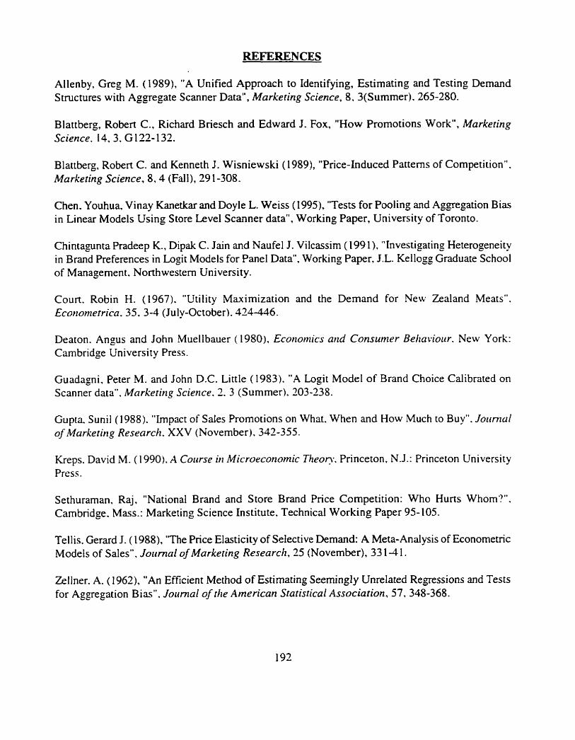
REFERENCES

Allenby, Greg M. ( 1989), "A Unified Approach to Identifying, Estimating and Testing Demand Structures with Aggregate Scanner Data", Marketing Science, 8, 3(Summer). 265-280.

Blattberg, Robert C., Richard Briesch and Edward J. Fox, "How Promotions Work", Marketing Science. 14, 3. G 122- 132.

Blattberg, Robert C. and Kenneth J. Wisniewski ( l989), "Price-Induced Patterns of Competition". Marketing Science. 8 , 4 (Fall), 29 1-308-

Chen. Youhua, Vinay Kanetkar and Doyle L. Weiss (1995). "Tests for Pooling and Aggregation Bias in Linear Models Using Store Level Scanner data", Working Paper, University of Toronto.

Chintagunta Pradeep K., Dipak C. Jain and Naufel J. Vilcassirn (199 l), "Investigating Heterogeneity in Brand Preferences in Logir Models for Panel Data", Working Paper. J.L. Kellogg Graduate School of Management. Northwestern University.

Court. Robin H. (1967). "Utility Maximization and the Demand for New Zealand Meats". Econometrics. 35. 3-4 (July-October). 42446 .

Deaton. Angus and John Muellbauer ( 1980). Econonzics and Consumer Behnviour. New York: Cambridge University Press.

Guadagni, Peter M. and John D.C. Little (1983). "A Logit Model of Brand Choice Calibrated on Scanner data". Marketing Science. 2. 3 (Summer). 203-238.

C u p . Sunil (1988). "Impact of Sales Promotions on What. When and How Much to Buy". Jounlal of Marketing Research. XXV (November). 342-355.

Kreps. David M. ( 1 990). A Corcrse in Microeconomic Theon. Princeton. N.J.: Princeton University Press.

Sethuraman. Raj. "National Brand and Store Brand Price Competition: Who Hurts Whom'?". Cambridge. Mass.: Marketing Science Institute. Technical Working Paper 95-105.

Tellis. Gerard 1. (1 988), "The Price Elasticity of Selective Demand: A Meta-Analysis of Econometric Models of Sales", Jortrnal of Marketing Research, 25 (November), 33 1-4 1.

Zellner. A. ( 1 %2), "An Efficient Method of Estimating Seemingly Unrelated Regressions and Tests for Aggregation Bias". Jortrnal of the American Statistical Association, 57, 348-368.

APPENDICES

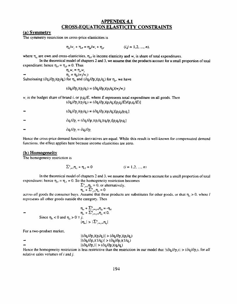
APPENDIX 4.1 CROSS-EQUATION ELASTICITY CONSTRAINTS

la) Svmmetrv The symmetry restriction on cross-price elasticities is

where q,, are own and cross-elasticities. q,, is income elasticity and w, is share of total expenditures. In the theoretical model of chapters 2 and 3. we assume that the products account for a s d I proportion of total

it*, is the budget share of brand i. or p,q/E. where E represents total expenditure on all goods. Then

- 4

.D

Hcncc th ~e cross-price demand function derivatives are equal. While this result is well-known fc functions. the effect applies here because income elasticities are zero.

r compensated demand

(b) Hornogeneitv The homogeneity restriction is

In the theoretical model of chapters 2 and 3. we assume that the products account for a small proportion of total expenditure: hence q,,. = TI,, = 0. So the homogeneity restriction becomes

~",.,q,, = 0. or alternatively. TI1 + q-,n, = 0

across all goods the consumer buys. Assume that these products are substitutes for other goods. or that qIi > 0. ~'hcrc I represents all other goods outside the category. Then

For a two-product market. I ( W + , ) ( P A ) l > (dq/W(p/q,) - I (dqj*,)( lfq,) I > (Sq/+,)( 14,)

0 I (dq/*,) l > (ZqpP,Kq/q,) Hence the homogeneity restriction is less restrictive than the restriction in our model that j (dq/Sp,) 1 > (?q/+,). for all relative sales volumes of i and j.

APPENDIX 4.2

REGRESSION DIAGNOSTICS

In this Appendix, we discuss some of the issues arising from the regression analysis in more detail.

Model Identification

In estimating the model empirically, we have found a relationship between quantity sold and prices. Although there is little likelihood of supply shocks during the 55 weeks over which the model is estimated, we need to be sure that we are estimating a demand function, rather than a series of supply functions.

One way of determining this is to consider whether there was adequate inventory to cover sales in retail stores over the period in question. U there was no supply constraint, demand would be less than supply and the quantity sold would reflect demand rather than supply.

Additional data were obtained on stockout levels from the manufacturer of brand 1. These data were derived from A.C. Nielsen's bimonthly store audit, not from the scanner database analyzed in the regressions. While these are not directly comparable with the model data. they give an indication of whether stockout levels were generally high at that time.

A.C. Nielsen-s store audit extrapolates data from a panel of stores to regional and national levels. The stockout measure is the & of All Commodity Volume in which the products was out of stock. For the package size being analyzed here, the level in ail periods in 1994 in the Ontario market was zero. Hence we can conclude that stockouts were not a major problem. and that the regression is measuring a demand function.

Exogeneity of Price

In the theoretical model. the retailer's optimal price is shown to be a function of the parameters of the demand function. However. in estimating the demand function empirically. we use price as a predictor of sales. As a result. the possibility exists that price will be correlated with the error term in the regression.

We analyze this issue by the method proposed by Hausman ( 1978): we estimate prices for each product using lagged prices and all other regressors in the system, and add these estimated prices to the regression model for each brand. The joint significance of these added predictors is a test of the null hypothesis that prices and error terms are not correlated.

Hence the model for brand 1 is

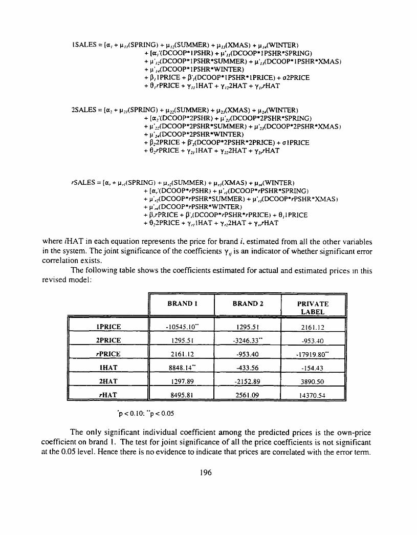
IS ALES = [aI + p,/(SPRING) + p12(SUMMER) + pI,(XMAS) + P,~(WDJTER) + [a,'(DCOOP* 1 PSHR) + p',,(DCOOP* 1 PSHR*SPRING) + p',_.(DCOOP*lPSHR*SUMMER) + p',,(DCOOP* 1 PSHR*XMAS) + p8,,(DCOOP* 1 PSHR*WINTER) + P, 1 PEUCE + P',(DCOOP* I PSHR* 1 PRICE) + a2PRICE + 0,rPRICE + y,, 1HAT + y,,2HAT + y,,rHAT

2SALES = {a2 + k,(SPRING) + p,,(SUMMER) + p,(XMAS) .t p2,(WlNTER) + [a2'(DCOOP*2PSHR) + p',,(DCOOP*2PSHR*SPRING) + p9,,(DCOOP*2PSHR*SUMMER) + p',,(DCOOP*2PSHR*XMAS )

+ p'14(DCOOP*2PSHR*WINTER) + P22PRICE + P',(DCOOP*2PSHR*2PRICE) + a 1PRTCE + 0,rPRICE + y,, IHAT + yZ22HAT + y,/HAT

SALES = [a, + p,,(SPRING) + p,JSUMMER) + p,,(XMAS) + p,(WINTER) + [a,'(DCOOP*rPSHR) + p',,(DCOOP*rPSWR*SPRING) + p',(DCOOP*rPSHR*SUMMER) + p',(DCOOP*rPSHRfXM.4S) + p',(DCOOP*rPSHR*WINTER) + PrPRICE + P1,(DCOOf *rPSHR*rPRICE) + 0,t PRICE + 6JPFUCE + yr, lHAT + y,:2HAT + y j H A T

where [HAT in each equation represents the price for brand i. estimated from all the other variables in the system. The joint significance of the coefficients y, is an indicator of whether significant error correlation exists.

The following table shows the coefficients estimated for actual and estimated prices in this revised model:

I( BRAND 1 I BRAND2 I PRIVATE (1

The only significant individual coefficient among the predicted prices is the own-price coefficient on brand 1. The test for joint significance of all the price coefficients is not significant at the 0.05 level. Hence there is no evidence to indicate that prices are correlated with the error term.

F

lPRICE

2PRICE

rPRICE

IHAT

2HAT

rHAT

- 10545.10"

1295.5 I

2161.12

8848.14"

1297.89

8495.8 1

1295.5 1

-3216.33"

-953.40

-433.56

-2 152.89

256 1 -09

LABEL

2161.12

-95 3.40

-179 19.80"

- 154.43

3890.50

11370.53

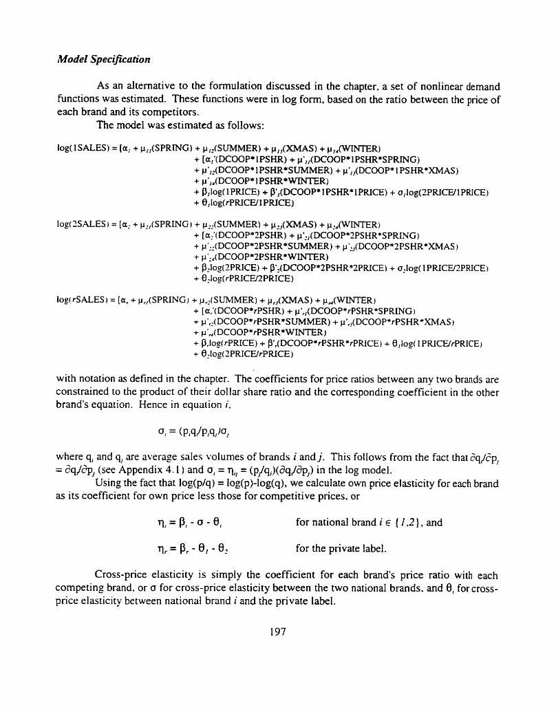
Model Specification

As an alternative to the formulation discussed in the chapter, a set of nonlinear demand hnctions was estimated. These functions were in log form, based on the ratio between the price of each brand and its competitors.

The model was estimated as follows:

log(1SALES) = [a, + p,,(SPRING) + p,,(SUMMER) + p,,(XMAS) + p,,CWINTER) + [a,'(DCOOP* 1PSHR) + p',,(DCOOP* 1 PSHR*SPRING) + p',,(DCOOP* lPSHR*SUMMER) + po1,(DCOOP* 1 PSHR*XMAS) + p',,(DCOOP* 1 PSHR*WDWXR) + p,log( 1 PRICE) + P1,(DCOOP* 1 PSHR* 1 PRICE) + ollog(2PRICU1 PRICE) + 0, Iog(rPFUCW I PRICE)

log(2SALES = [a, + p,,(SPRING) + p,,(SUMMER) + p,,(XMAS) + p,,(WINER) + [a,'(DCOOP*2PSHR) + p0,,(DCOOP*2PSHR*SPRING) + p',,(DCOOP*2PSHR*SUMMER) + p',,(DCOOP*2PSHR*XMAS ) + p',,(DCOOP*2PSHR*WINTER) + P,log(2PRICE) + P',(DCOOP*2PSHR*2PRICEb + a,log(l PRICW2PRICE) + B,log(rPRICE/2PRICE)

lo_e!rSALES) = [a, .c p,,(SPRING) + p,,(SUbIMER) + p,,(XMAS) + p , ( W N E R ) + [a,'( DCOOP*rPSHR) + p',,(DCOOP*rPSHR*SPRING ) + p',(DCOOP*rPSHR*SUMMER) + p',(DCOOP*rPSHR*XMAS) + p',(DCOOP*rPSHR*WINTER) + &log(rPRICE) + P0,(DCOOP*rPSHR*rPRICE) + 0,log( 1 PRICE/rPRICE) + e,iog(2PRICWrPRICE)

with notation as defined in the chapter. The coefficients for price ratios between any two brands are constrained to the product of their dollar share ratio and the corresponding coefficient in the other brand's equation. Hence in equation i.

where q, and q, are average sales volumes of brands i and j. This follows from the fact that dqjSp, = &@p, (see Appendix 4.1 ) and o, = q, = (p/q,)(dqjap,) in the log model.

Using the fact that log(p/q) = log(p)-log(q), we calculate own price elasticity for each brand as its coefficient for own price less those for competitive prices. or

rl, = P, - 0 - 8, for national brand i E ( I ,2 } , and

rlr= Pr- 8, - 0 2 for the private label.

Cross-price elasticity is simply the coefficient for each brand's price ratio with each competing brand. or o for cross-price elasticity between the two national brands. and 0, for cross- price elasticity between national brand i and the private label.

This model yields the following parameters:

These results are quite similar to the linear model: with only one exception, the same variables are statistically significant. The single exception is the coefficient for Summer on Private Label demand, which is significant at the 0.10 level in the linear model. but not significant here.

'k

BRAND 1 BRAND2 PRIVATE LABEL

N o h Parameter Notn. Parameter Notn. Parameter

Closer examination reveals that p=O. 1 1 for this coefficient in the log model. Elasticities, estimated according to the procedure outlined above, are

Iatercep t I

Spring r

Summer v

X m a ~

Winter r

Promotion

as follows:

BRAND I I 2 r I

I 1

a,

Plr

PI?

PI 4

P I J

(Parentheses indicate lack of sta~istical significance)

8 SO"

0.35'-

0.27"

0.15

-2.28 P:I*

a,

P ~ I

P2.q

-0.12 Promotion X Spring

-2 1 -08.

Prto

a,' ale

Plr'

8.72"

0.08

-0.06

0.33"

0.05

p r

r t

l l r ~

0.12 1

-0.28

0.15"

.. -0.50

0.49

-0.12

ar'

p24

-0.27

0.33

-0. I5

Promotion X Summer

Promotion X Xmas

Promotion X Winter

7*

P?? I

o

p 2 ~

-0.02

-0.84

0.66"

-0.24 1

-2.79'

2.85"

a,

ll 71

P r~

PI+

ll 1.'

PI !*

P P ~

0

-1 -20

-4.23"

8.93"

-0.08 I

-0.02 m

0.0 1 a

-0.35

0.58.-

,. 0.46.-

0.28

OWN PRICE

CROSS-PRICE RATIO

CROSS-PRICE RATIO

Promotion X Own Price

P - o-.

8,

P:'

PI a,

0,

PI'

- 1.7 1 .- 0.46'-

-0.1 3

12.66"

Pr

8,

8,

PI'

As in the linear model. the cross-price term between the private label and brand 2 is not significant. Generally, both own and cross-price elasticities appear lower than those derived from the linear model,

We compare the overall fit and the degree of first-order serial correlation of this log model and the linear model discussed in the body of the chapter. as follows:

"

FIT: I LINEAR LOG

System Wgt. R' 0.75 0.79

The overall fit of the log model is similar to, or slightly better than, that of the linear model. The critical values of the Durbin-Watson statistic in this case are d, = 1.78 and d, = 1.57. According to this test, the null hypothesis of no serial correlation is cannot be rejected for any of the linear submodels for each of the brands, although the test is indeterminate in the case of brand 1 (Pindyck and Rubinfeld. 198 1. p. 160). Results are similar for the log model, with the exception of brand 1. which exhibits significant serial correlation at the 5% level. In this respect, the log model fares slightly worse than the linear form.

Since the overall fit of the models and serial correlation are similar, and since the log model offers a similar pattern of results, there appears to be no reason to deviate from the linear form specified in the theoretical model. Hence further analysis is based on the linear model.

MSE 0.96 I 0.9 I

SERIAL CORR.: DW P DW P

Promotions

BRAND 1

BRAND 2 I

The results of the linear estimation of the model show limited evidence of significant effects of promotions: promotion has no effect on either the intercept or own-price coefficient of brand 1, and most Promotion X Season coefficients on each of the brands are not significant. However. promotion has a significant negative effect on the intercept of brand 2, a positive effect on its price coefficient and interacts positively with Winter seasonality. On the private label, promotion has a positive effect on the intercept, a negative effect on the price coefficient and interacts negatively with Summer seasonality.

Several reasons suggest themselves for this pattern. Recall that we defined promotion share as the sum of the brand's co-op and display indices shared to the sum of co-op and display for the category as a whole. While co-op advertising is usually co-ordinated across the chain as a whole. discussions with the manufacturer of brand 1 indicate that there can be wide variations in the level of display across stores. Stores may choose to build a larger or a smaller display. share it with

11 PRIVATE LABEL r 2.08 1 -0.08 1 1.86 1 0.00 11

1.64

2.2 1

0.17

-0.12

1.44

2.0 1

0.24

-0.04

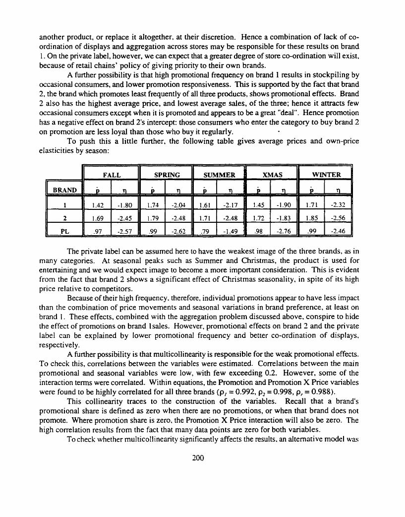
another product, or replace it altogether, at their discretion. Hence a combination of lack of co- ordination of displays and aggregation across stores may be responsible for these results on brand I . On the private label, however, we can expect that a greater degree of store coordination will exist, because of retail chains' policy of giving priority to their own brands.

A further possibility is that high promotional frequency on brand 1 results in stockpiling by occasional consumers, and lower promotion responsiveness. This is supported by the fact that brand 2, the brand which promotes least frequently of all three products, shows promotional effects. Brand 2 also has the highest average price, and lowest average sales, of the three; hence it attracts few occasional consumers except when it is promoted and appears to be a great "deal". Hence promotion has a negative effect on brand 2's intercept: those consumers who enter the category to buy brand 2 on promotion are less loyal than those who buy it regularly.

To push this a little further, the following table gives average prices and own-price elasticities by season:

SPRING SUMMER XMAS WINTER

1 1.73 -2.04 1.61 -2.17 1.45 -1.90 1.71 -2.32

2 1.79 -2.48 1.71 -2.48 1.72 -1.83 1.85 -2.56

PL .99 -2.62 -79 -1.49 -98 -2.76 -99 -2.46

The private label can be assumed here to have the weakest image of the three brands, as in many categories. At seasonal peaks such as Summer and Christmas, the product is used for entertaining and we would expect image to become a more important consideration. This is evident from the fact that brand 2 shows a significant effect of Christmas seasonality, in spite of its high price relative to competitors.

Because of their high frequency, therefore, individual promotions appear to have less impact than the combination of price movements and seasonal variations in brand preference, at least on brand I . These effects, combined with the aggregation problem discussed above, conspire to hide the effect of promotions on brand 1 sales. However, promotional effects on brand 3 and the private label can be explained by lower promotional frequency and better co-ordination of displays, respectively.

A further possibility is that multicollinearity is responsible for the weak promotional effects. To check this, correlations between the variabtes were estimated. Correlations between the main promotional and seasonal variables were low, with few exceeding 0.2. However, some of the interaction terms were correlated. Within equations, the Promotion and Promotion X Price variables were found to be highly correlated for all three brands (p, = 0.992, p, = 0.998, p, = 0.988).

This collinearity traces to the construction of the variables. Recall that a brand's promotional share is defined as zero when there are no promotions, or when that brand does not promote. Where promotion share is zero, the Promotion X Price interaction will also be zero. The high correlation results from the fact that many data points are zero for both variables.

To check whether multicollinearity significantly affects the results. an alternative model was

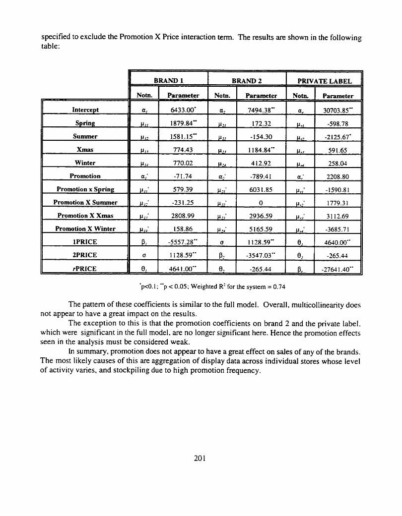
specified to exclude the Promotion X Price interaction term. The results are shown in the following table:

-p<O. 1 ; '.p < 0.05; Weighted R' for the system = 0.74

Intercept

Spring

Summer

X m a ~

Winter

Promotion

Promotion x Spring:

Promotion X Summer

Promotion X Xmas

Promotion X Winter

lPRICE

2PRICE

rPRICE *

The pattern of these coefficients is similar to the full model. Overall, multicollinearity does not appear to have a great impact on the results.

The exception to this is that the promotion coefficients on brand 2 and the private label. which were significant in the full model. are no longer significant here. Hence the promotion effects seen in the analysis must be considered weak.

In summary, promotion does not appear to have a great effect on sales of any of the brands. The most likely causes of this are aggregation of display data across individual stores whose level of activity varies, and stockpiling due to high promotion frequency.

,

BRAND 1 I BRAND 2

Notn.

a,

P I I

P I ?

P I *

P IJ

a,'

CLII

PI.!

PI!

CI 14

P 1

u

0,

PRIVATE

Notn.

a,

P r~

CL r:

P ,J

PIJ

a,'

P r / *

P .: P rj

PN - I

0,

8,

P r -

LABEL

Parameter

30703.85"

-598.78

-2 125.67'

59 1.65

258.04

2208.80

- 1590.8 1

1779.3 1

3 1 12.69

-3685.7 1

4640.00"

-265.44

-2764 1 -40'-

Parameter

6433.00'

1879.84"

1581.15"

.. 774.43

770.02

-7 I -74

579.39

-23 1.25

2808.99

158.86

-5557.28"

1 128.59.-

464 1 .0O1-

Notn.

a?

P ~ I

7 -

P? r

c 1 3

a;

P21

y y

1

Prj

p 2~

u

P 2

8,

Parameter

7494.38"

172.32

- 154.30

I 184.84"

4 12.92

-789.4 1

603 1.85

0

2936.59

5 I 65.59

1 128.59"

-3547.03"

-265 .&I

FIGURES

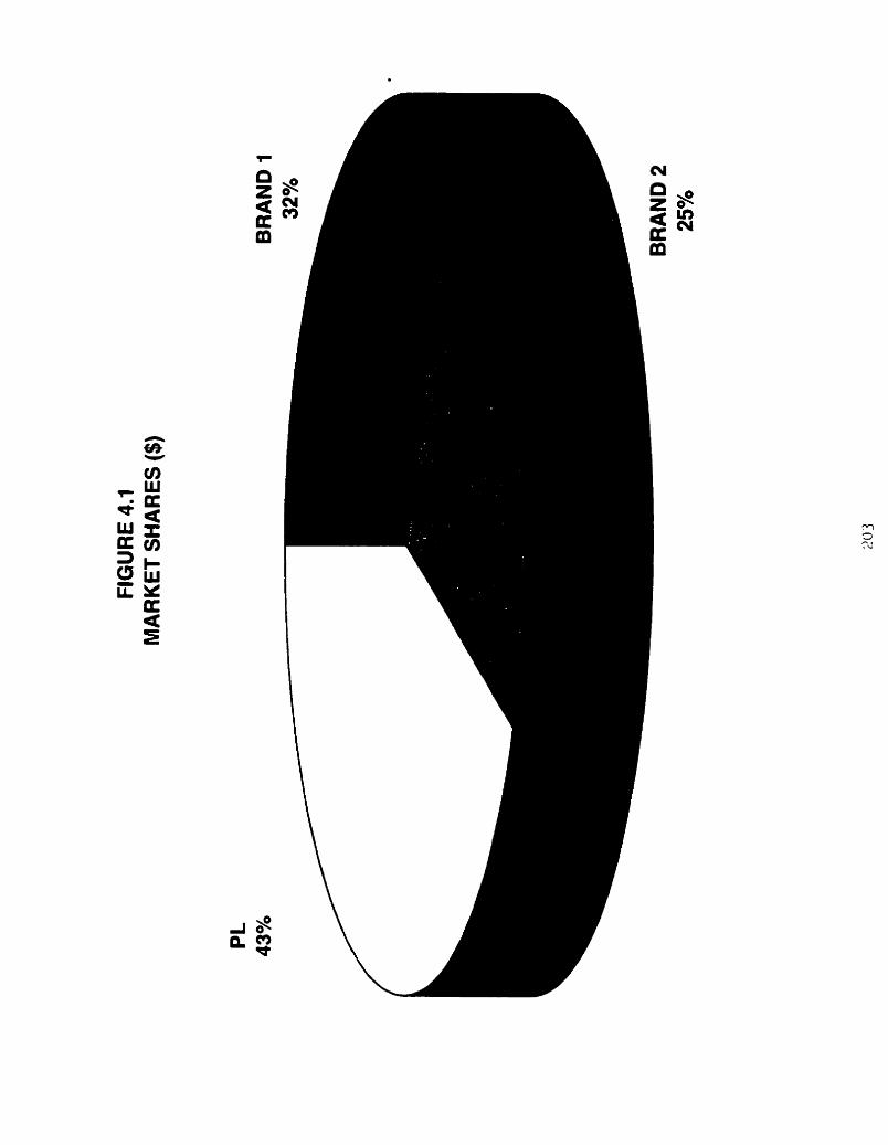
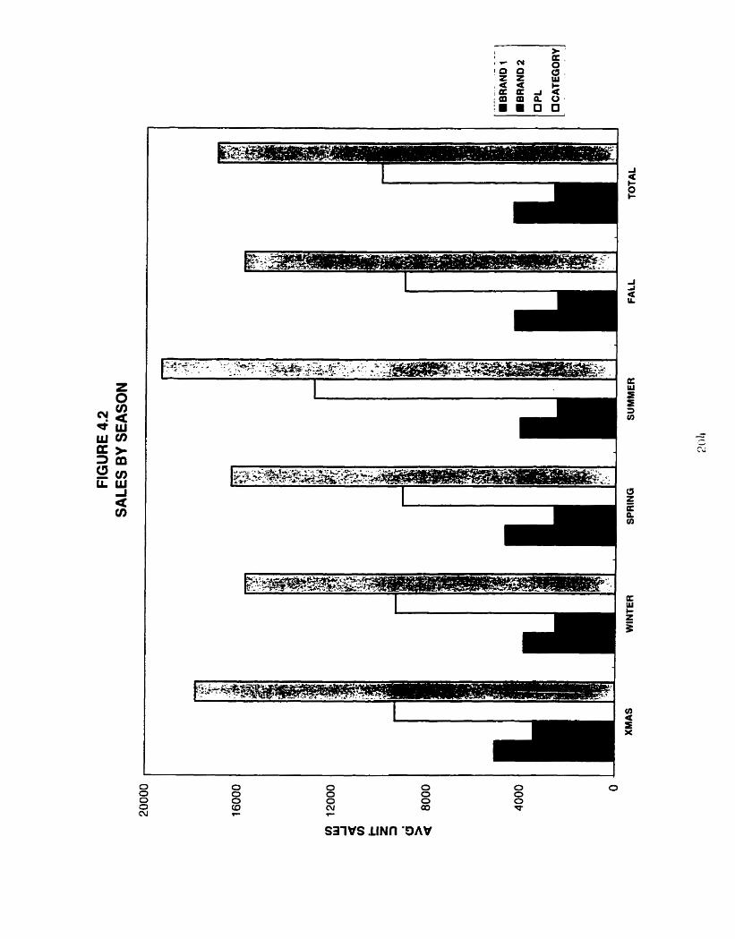
5. THE MODEL IN ACTION

To question all things; - never to turn away from any d i f i c u l ~ ; to accept no

doctrine either from ourselves or from other people without a rigid scrutiny by

negative criticism: letting no fallacy. or incoherence or confusion of thought, step

b y unperceived: above all, to insisr upon having the meaning of a word clearly

understood before using it. and he meaning of a proposition before assenting to

it: - these are the lessons we learn from ancienr dialecticians.

John Stuart Mill:

Inaugural Address as Rector, Uni~pers i~ College of St. Andrerrs

(i) Introduction

Having developed a theoretical model and estimated its parameters, we are now in a position

to apply the model to a "real world" problem: to determine the profitability of private label supply

for a manufacturer in a grocery category. In this chapter, we use the parameters derived in chapter

4 as inputs to the theoretical model. along with cost estimates.

Our objective here is to tie together the theoretical model and the empirical estimation of

its parameters. In particular, we set out to demonstrate the application of the model to a specific case

study.

In chapter 4. we took the first step in applying the model to a real-world situation by

analyzing demand data on a category of grocery products. The end result of this estimation was a set

of weekly demand functions which varied by promotional activity and by time of year.

To apply these demand functions to the manufacturer's private label supply decisioi~. we

need to develop some way of aggregating them to reflect the fact that the decision period is longer

than one week. In this chapter, we propose a method for aggregating the demand functions across

a full year that preserves the essential reiationships.

In addition. analysis of the profitability of private label supply requires some estimate of

costs as well as of demand. In this chapter, we estimate costs. in the absence of explicit data from

the manufacturer, using publicly available sources.

With estimates of annual demand functions and unit costs, we determine the profitability

of private label supply for the national brand manufacturers, deriving the equilibrium outcome for

this category. In addition. we consider how changes in the manufacturers' environment could affect

the profitability of private label supply, by simulating changes in the model's parameters.

A second goal of this chapter is to identify problems in applying the model in this specific

situation. Accordingly. the chapter begins with a discussion of the more important assumptions of

the model, their impact on the model's predictions and whether they apply in this particular case.

As a staxting point, we briefly review here the development of the model we will apply to

the case study. Recall that in chapter 3, we assumed that the manufacturers were "dominant firms",

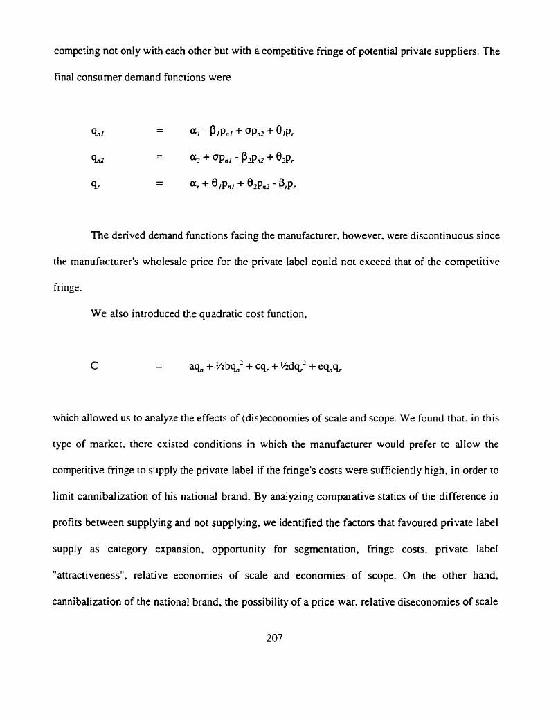
competing not only with each other but with a competitive fringe of potential private suppliers. The

final consumer demand functions were

The derived demand functions facing the manufacturer, however, were discontinuous since

the manufacturer's wholesale price for the private label could not exceed that of the competitive

fringe.

We also introduced the quadratic cost function,

which allowed us to analyze the effects of (dis)econornies of scale and scope. We found that. in this

type of market, there existed conditions in which the manufacturer would prefer to allow the

competitive fringe to supply the private label if the fringe's costs were sufficiently high, in order to

limit cannibalization of his national brand. By analyzing comparative statics of the difference in

profits between supplying and not supplying, we identified the factors that favoured private label

supply as category expansion. opportunity for segmentation, fringe costs. private label

"attractiveness", relative economies of scale and economies of scope. On the other hand.

cannibalization of the national brand, the possibility of a price war. relative diseconomies of scale

and diseconomies of scope discouraged private label supply.

This chapter is organized as follows. The next section discusses the key assumptions of the

theoretical model and their application in this specific situation. In section (iii), we propose a method

for aggregating the demand functions and derive estimates of costs. The results for this manufacturer

are then discussed in section (iv).

We analyze a series of scenarios in section (v), showing how the model can be used for

"what if' analysis based on the prevailing conditions facing a particular manufacturer.

lii) Kev Assumptions of the Theoretical Model

In this section. we consider the major underlying assumptions of the theoretical model, with

a particular interest in whether they are replicated in this case. Specifically. we discuss the following:

Manufacturer Market Structure: whether the model's assumption that the market is

composed of two dominant finns and a competitive fringe applies to this category:

Retail Market Stmcture: whether the assumption of a monopolistic retailer, or.

alternatively. competitive retailers applies here;

Stackelberg Mersh ip : whether the assumption that manufacturers are Stackelberg leaders

in this category is realistic;

One Product Category, One Size: the impact of the assumption that manufacturers have

only one size of one national brand;

Fired Costs: the exclusion of fixed costs from the analysis;

Advertising: the assumption that media advertising has no effect on either demand or costs.

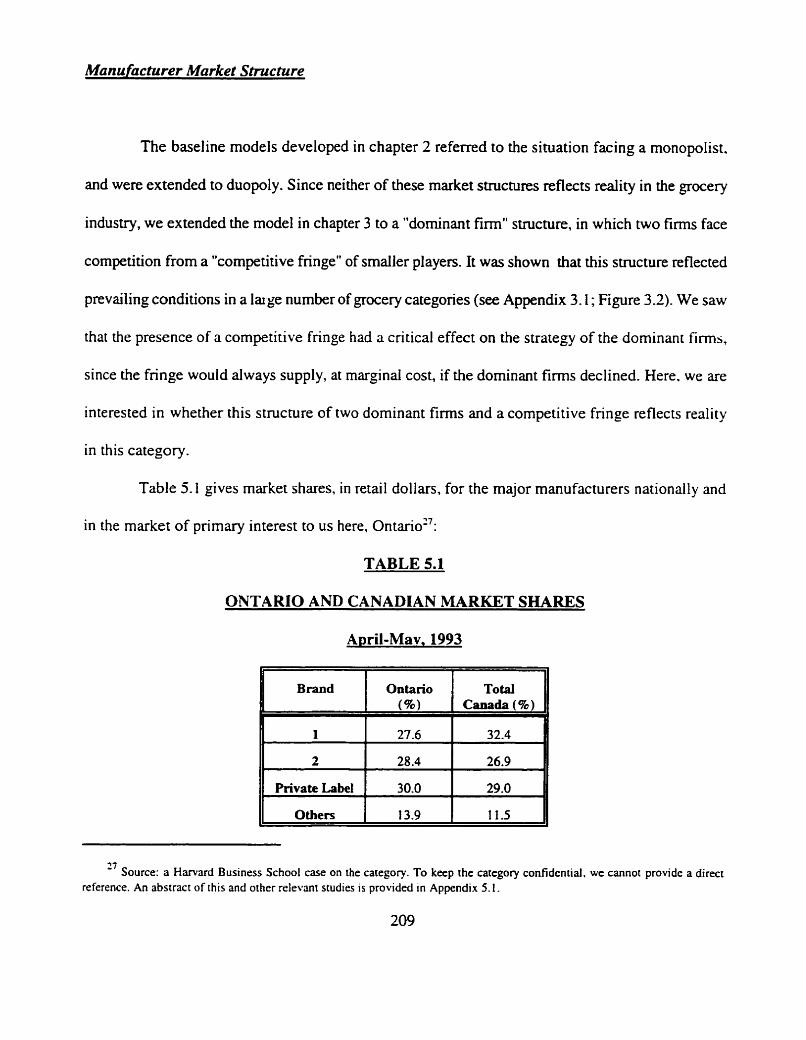
Manufacturer Market Structure

The baseline models developed in chapter 2 referred to the situation facing a monopolist.

and were extended to duopoly. Since neither of these market structures reflects reality in the grocery

industry, we extended the model in chapter 3 to a "dominant firm" structure, in which two firms face

competition from a "competitive fringe" of smaller players. It was shown that this structure reflected

prevailing conditions in a large number of grocery categories (see Appendix 3.1 ; Figure 3.2). We saw

that the presence of a competitive fringe had a critical effect on the strategy of the dominant firms.

since the fringe would always supply, at marginal cost, if the dominant firms declined. Here. we are

interested in whether this structure of two dominant firms and a competitive fringe reflects reality

in this category.

Table 5.1 gives market shares. in retail dollars, for the major manufacturers nationally and

in the market of primary interest to us here, 0ntario2':

TABLE 5.1

ONTARIO AND CANADIAN MARKET SHARES

April-Mav, 1993

I Others I 13.9 I 11.5

Brand

1

2

Private Label

I7 Source: a Harvard Business School case on the category. To keep the category confidential. we cannot provide a direct reference. An abstract of this and other relevant studies is provided in Appendix 5. I .

Ontario (W

27.6

28.4

30.0

Total Canada (9%)

32.4 I 26.9

29.0

The market share data suggest that this category fits the "dominant duopoly" structure very

well. Manufacturers 1 and 2. who supply only national brands. control approximately 60% of the

Ontario and Canadian markets. Private labels, which have been growing rapidly in this category both

in Canada and the US. account for a further 30F, with other brands taking up the remainder.

Although there is one dominant private label supplier in this category. there are several

alternative manufacturers whom retailers may approach. Retailers in the grocery industry are quite

prone to switching between private label suppliers. who are e5,entialiy undifferentiated from each

other.

On the supply side. the dominant private label manufacturer sub-contracts part of the

manufacturing process to local third parties. many of whom would be capable of producing a private

label on their own but whose local scope of operations reduces their inclination to do so. National

brand manufacturers also use third parties for their national brands. although they have moved

progressively towards ownership and control of these plants in recent years. An additional factor is

the availability of substantial excess capacity in the U.S. among both national brand manufacturers

and private label suppliers. There is sufficient excess capacity within that market to supply the entire

Canadian market. Since shipping costs are high in this category, U.S. manufacturers have not yet

moved into the Canadian market.

Although one private label supplier is dominant, then, it is forced. by the existence of

alternatives. to keep its prices low. This fits with the assumption of a competitive fringe in the

model.

Retail Market Structure

Our initial assumption in the baseline model of chapter 2 was that a monopolistic

manufacturer faced a monopolistic retailer. However, we showed in Appendix 2.4 that the

assumption of competitive retailers did not alter either the direction of the parameter effects or

manufacturers' optimal wholesale prices. In later model extensions, we therefore assumed that the

retailer was monopolistic. Hence we need to examine whether either a monopoly or a competitive

market can be said to represent grocery retailing in the Ontario market.

In the Canadian grocery industry. retailers can be considered oligopolistic on an agsregate

level: however. as shown in Appendix 3.3. the degree of concentration varies from region to region.

Table 5.2 gives the combined market share of the top two. and the top four. retailers in each region:

TABLE 5.2

TOP GROCERY RETAILER SHARES BY REGION ($), 1992

Region

National

B.C.

Alberta

Sask

Manitoba

Ontario

Quebec

Atlantic

Top Z Share ( c/c ) ,

26

40

3 9

47

53

19

3 6 - 50 I 68

Top 3 Share ( 5%)

42

58 . 62

7 I

67

66 33 1

In some regions. such as Atlantic. Manitoba and Saskatchewan, the existence of dominant

retailers is evident and the market appears oligopolistic. However, other regions are much less

concentrated and more closely approach a competitive market structure. The Ontario market. with

which we are concerned here. exhibits the lowest level of concentration of any region.

What is most relevant to the model, however, is the manner in which prices are set. Most

chain retailers set prices at a head office level, taking accortnt of local conditions. One method of

doing this is "zone pricing". whereby the retailer analyzes local competition within predetermined

areas and sets separate prices for each zone. Within metropolitan areas. stores are sufficiently

accessible to consumers that retailers are obliged to set prices that are close to. or match.

competition.

Furthermore, Canadian grocery chains are essentially undifferentiated in service terms. so

their prices do not differ greatly from those of their competitors. Numerous studies in retailing (e.g.

Wilkinson, Mason and Paksoy. 1982: Arnold. Oum and Tigert, 1983) attest to the importance of

price as a mix variable for grocery retailers: the Ontario market is no exception. as shown by the

Arnold et a1 study. From discussions with one of the national brand manufacturers. it is evident that

managers in the industry also believe that consumers are prepared to switch stores on the basis of

price differences in this category alone. The category is regularly treated as a "traffic builder" by

retailers and promotions are planned to attract consumers into the store.

There is little doubt that Ontario grocery retailers are very price competitive, as depicted by

the model. The assumption that consumers compare national brand prices across stores is supported

by this analysis.

Stackelberg Leadership

The model assumes that manufacturers are Stackelbeq leaders. taking into account retailers'

"markup rule". and competitive prices. in setting wholesale prices to the retaile?.

In reality. the process is more complex. Retailers allocate promotional "slots" (feature

periods) to brands on an annual or semi-annual basis after negotiating with manufacturers. Individual

promotions are negotiated between manufacturers and retailers, with manufacturers offering ( i )

wholesale prices and "off-invoice" allowances. (ii) co-op advertising and display support, in return

for (i) feature prices and (i i ) co-op advertising features and displays from retailers. In this negotiation

process. manufacturers attempt to minimize retail prices and maximize promotional support to

maximize total sales. Retailers maximize their profit margins and manuiacturer deals.

Normally, manufacturers will know retailers' regular and promotional markups based on past

experience. They are unlikely to h o w competitive prices with precision: however, they will certainly

be capable of estimating competitive prices within a reasonable range based on past experience.

There will necessarily be some uncertainty associated with this estimate.

The Stackelberg assumption is thus a simplification of the actual process undergone by

manufacturers and retailers in setting prices. It approximates reality in some essential ways:

manufacturers take account of retailers' normal markups in setting prices, and do so with some

estimate of competitive prices in mind. Nonetheless, its major failing is that it assumes that retailers

are price takers, and does not recognize their degree of power in the negotiation process.

2s Priccs here rcfcr to nct prices 3fit'r deal\.

One Product Cateaory, One Size

The empirical model is based on the assumption that the manufacturer produces only one

product in one size. While the firms under study here market several brands in the product category.

they market only one brand in the subcategory of concern here. and the subcategories are sufficiently

independent that switching between them is not a major factor.

The product is. however. available in more than one package size and package form.

Discussions with manufacturer I indicate that the degree of switching between package forms is

minimal. The price elasticity estimates obtained in chapter 4 are consistent with those found in

similar product categories (Tellis. 1988) which indicates that if size switching has been omitted. its

effect is not large.

Iyer and Soberman (1993). in an empirical study of two grocery categories. find that

consumers of larger sizes tend to be loyal to size rather than to brand, switching brands to find the

size they prefer instead of switching to another size within the same brand. The size analyzed in this

case is the largest in which the product is available: hence. if their results hold here. we would not

expect switchins to smaller sizes to be an imponant factor.

However. if our assumption is incorrect. the existence of a second size of the national brand

can affect either the estimate of price elasticity in the demand function, through size switching, or

the cost function, via economies or diseconomies of scope. We consider each of these possibilities

separately below. Since the effect of a second size can vary, we comment on its most likely direction

in this particular case.

Demand

The effects of multiple sizes on the demand function can be subdivided into two categories:

the empirical effect of omitting a variable from the regression, and the theoretical effect of

substitution with either the private label or the national brand.

Empirical Effect

From the empirical point of view, by omitting a variable from the regression we run the risk

of obtaining biased parameters. If the omitted variable is positively correlated with any of the

included variables, there is an upward bias in the estimated coefficient (Pindyck and Rubinfeld.

198 1. p. 129): the reverse is true if it is negatively correlated.

Although omission of the price of the second size could affect the price parameters of either

the national brand or the private label, it is most likely to affect the own-price parameter of the

national brand. The reason for this is that manufacturers in this category tend to promote all sizes

in the same period. so that there may be a positive relationship between prices of each size. Hence.

we would expect the national brand's own-price elasticity to be biased upwards. As a result. the

model's optimal national brand prices will be too low. Since the national brand's price response is

negatively related to private label profitability. upward bias in this parameter will have a negaril*~

effect on profit, causing the manufacturer to reject private label supply when he should agree to it.

Theoretical Eflect

If there is a second size which has been omitted, the manufacturer must also take its profit

into account in deciding whether to supply the private label. The effect of size switching in the

theoretical model depends on the second size's degree of substitutability with the private label and

with the first size of the national brand.

Supply of the private label by the national brand manufacturer results in a reduction in the

private label's wholesale price to the retailer, as compared with the price that would be charged by

the competitive fringe. Hence sales of a second size which substitutes with the private label will fall.

and the manufacturer's overall profit when he supplies the private label will be overstated if the

second size is omitted. Omission of size switching has apositive impact on private label profitability.

However. size substitution within the national brand is likely to be more important. Since

the national brand's price rises as a result of private label supply. sales and profits of the second size

should also rise. Hence its omission from the model will mean that the profitability of private label

supply is understated. Omission of size switching within the national brand has a negntiw effect on

private label profitability.

Since substitution within the sizes of the national brand is likely to exceed substitution with

the private label. we expect the overall effect of omission of the second size on private label

profitability to be rlegarive. In addition. substitution with a second size will reduce national brand

prices. so the model's optimal national brand prices will be too high.

Economies of Scope

The effect of a second size on costs depends on whether there are economies of scope due

to shared materials or resources with the national brand or the private label. Alternatively. there may

be diseconomies of scope due to competition for scarce resources.

If there are economies of scope between the second size and the national brand. the model

will overstate national brand costs. As a result, private label supply will look more profitable than

it should. However, another possibility is that there are economies of scope between the second size

and the private label. in which case private label costs will be overstated and private label supply will

look less profitable than it should. If there are economies of scope between the second size and both

the national brand and the private label, the overall impact will depend on which effect is dominant.

The reverse holds for diseconomies of scope: where they exist between the second size and

the national brand, private label supply will look less profitable than it should. Where there are

diseconomies of scope between the second size and the private label. the profitability of private label

supply will look too high.

Since we have assumed that the manufacturers have excess capacity available. it is most

likely that economies of scope will exist between the national brand and the second size. Hence we

expect national brand costs to be overstated. and national brand prices to be too high. The omission

of a second size has a positive overall effect on the profitability of private label supply.

In this case. the product is available in two different package forms, so that economies of

scope. if they exist. are likely to be limited to the use of common raw materials. As discussed later

in this chapter. however. there is substantial evidence that marginal costs in this size are constant.

i.e. no economies of scope exist.

In summary, we expect the omission of a second size from the model to have no effect. If

there is any effect, demand side forces would suggest that the model's prediction of private label

profitability is too low, while cost factors indicate that it is too high. The evidence suggests that the

greater effect is likely to be on the demand side. leading to downward bias in the profitability of *

private label supply.

Fixed Costs

The quadratic cost function specified in chapter 3 assumes that all costs are variable. If.

alternatively. we specified a cost function that included fixed costs. the fixed cost element would

drop our of the profit comparison so long as it was invariant bemeen optiotrs. The fixed startup costs

associated with investing in plant and equipment would not be relevant. since the manufacturer

would have to incur these anyway to produce the national brand. However. if supplying the private

label means that the manufacturer must make some fixed investment (say. in a new production line I.

this could affect private label profitability.

In the case considered here. the private label would use existing manufacturing and

distribution capacity. so there would be no plant investment involved in supplying. Similarly. RBrD

investment would be minimal. since the product would use existing formulations. However. there

can be some fixed setup costs associated with the development and printing of packaging designs

for the private labrl. These are usually not large in relation to total sales. and are often borne by the

retailer rather than the manufacturer. Lf such costs exist. they can be handled by deducting them from

the manufacturer's profit difference in favour of supplying the private label.

Advertising

Although the demand functions estimated in the empirical model include terms reflecting

temporary price promotions. they do not consider the effect of media advertising, which may vary

from week to week. The theoretical model is confined to price effects.

In our analysis. we assume that advertising levels do not change according to whether or not

the national brand manufacturer supplies the private label. Hence the demand functions will remain

unchanged between options: advertising costs are treated as fixed costs. and therefore drop out of

the comparison.

A future model could take advertising into account as an alternative strategy to private label

supply. This topic is taken up in chapter 6.

Interpretation o f Pararneters

Befare embarking on the estimation of private label profitability. we remind the reader of

the model's parameters and their interpretation. as shown in Table 5.3:

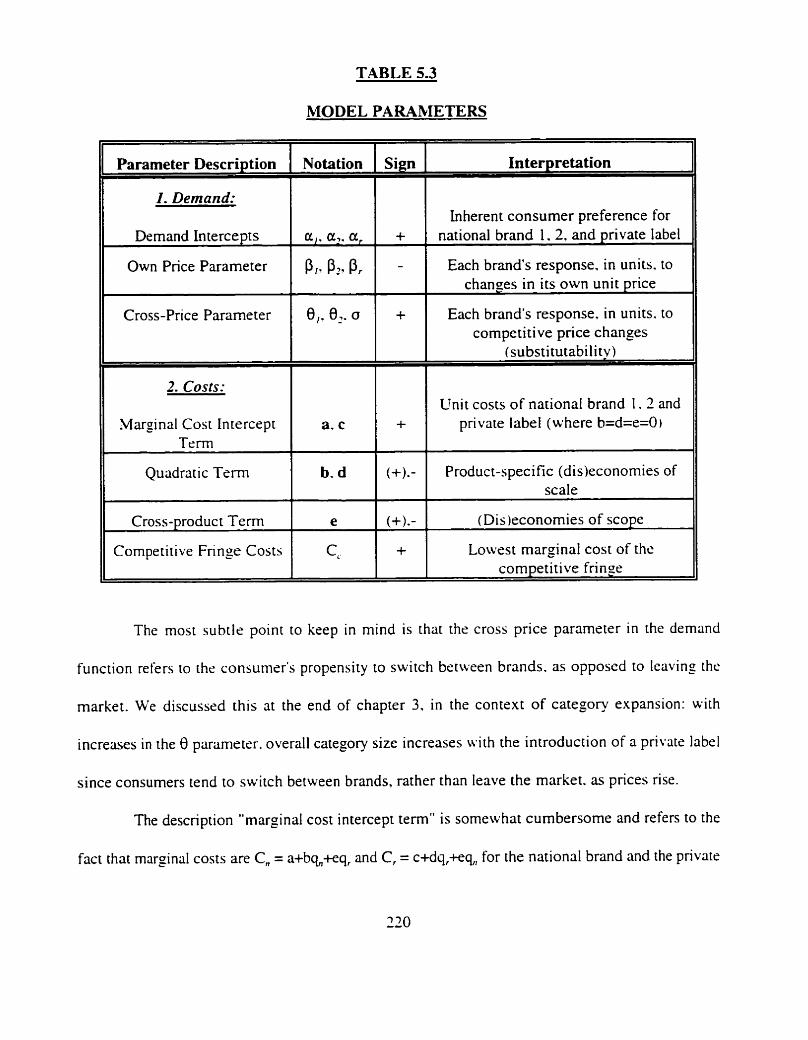
TABLE 5.3

MODEL PARAMETERS

f arameter Description Notation 1

I . Demand:

I ~ 2. costs:

Cross-Price Parameter

II Marginal Cost Intercept Term I a.c /

0,. 8,. o

11 Quadratic Term I I

Competitive Fringe Costs

Inherent consumer preference for + 1 national brand 1. 2. and private label

I

- I Each brand's response. in units. to chances in its own unit price

+

Lowest marginal cost of the com~etitive fringe

Each brand's response. in units. to competitive price changes

kubstitutabilitv)

+

The most subtle point to keep in mind is that the cross price parameter in the demand

function refers to the consumer's propensity to switch between brands. as opposed to leaving the

market. We discussed this at the end of chapter 3, in the context of category expansion: with

increases in the 0 parameter. overall category size increases with the introduction of a private label

since consumers tend to switch between brands, rather than leave the market. as prices rise.

The description "marginal cost intercept term" is somewhat cumbersome and refers to the

fact that marginal costs are C , = a+bq,,+eq, and C, = c+dq,+eq,, for the national brand and the private

Unit costs of national brand 1. 2 and private label (where b=d=e=O )

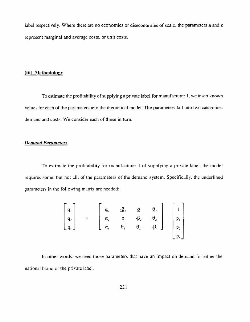
label respectively. Where there are no economies or diseconomies of scale. the parameters a and c

represent marginal and average costs. or unit costs.

To estimate the profitability of supplying a private label for manufacturer 1. we insert known

values for each of the parameters into the theoretical model. The parameters fall into two categories:

demand and costs. We consider each of these in turn.

Demand Parameters

To estimate the profitability for manufacturer I of supplying a private label. the model

requires some. but not all. of the parameters of the demand system. Specifically. the underlined

parameters in the following matrix are needed:

In other words. we need those parameters that have an impact on demand for either the

national brand or the private label.

Aggregation Across the Year

As we saw in chapter 4. the parameters of this system can vary according to whether each

brand is on promotion. or by time of year. In particular,

- intercepts vary accordins to season, promotion activity and their interaction;

- own-price terms vary according to promotion activity. but are constant across seasons:

- cross-price terms are constant across seasons and promotion activity.

In addition. we can expect prices to vary by period. so we need to decide which set of prices we are

referring to.

Since the demand parameters refer to a single week's demand. they are not useful for

decision making in any case: manufacturers in the grocery industry are not likely to fl i t in and out

of private label supply on a weekly basis. even though retailers tend to shop around for better prices

regu~arly'~. We adopt a year as the minimum decision period over which all variations in demand

are represented.

Hence we need a demand system that

( i ) Shows the responsiveness of demand to some representative pricrs over the year.

(i i) Tells us what mrnrcrl demand each brand would achieve. at a given set of prices.

and

Given the fact the intercepts and own-price terns vary from week to week. we cannot simply

multiply these terms by 53. We need to estimate their value in each week and aggregate them across

the year. With regard to prices. we take the mean price across the year as a representative price.

To illustrate the aggregation method. assume that there are only two periods and two brands.

as follows. Subscripts refer to (brand. period):

'q - I r is poss~blc. to cnblstlgc ~ndusrnc. In \ \ h ~ i h t h ~ s might happen I C . ~ . apparel I. hut t h q A r t . raw.

371) ---

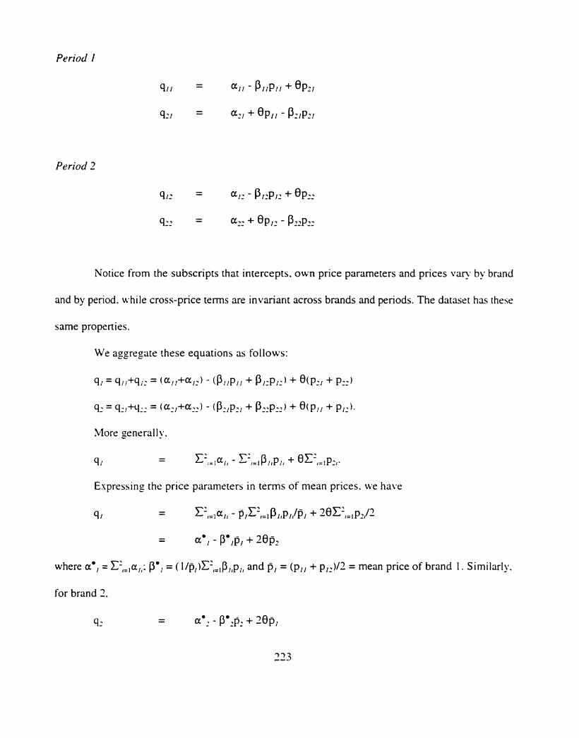
Period I

Period 2

Notice from the subscripts that intercepts. own price parameters and prices vary by brand

and by period. w-hile cross-price terms are invariant across brands and periods. The dataset has these

same properties.

We aggregate these equations as follows:

41 = q,,+q,: = ( ~ I I + ~ I ? ) - (PIIPII + PI:PI:) + O(~ : i + px )

q, = q,,+q,l = (al1+a2,) - @,,p,, + P2,p,) + @ p l j + p1J

More generally.

91 - - Z',.,a,, - L P , , p , , + e c = , p : , .

Expressing the price parameters in terms of mean prices. we have

91 - - E2,=la,l - p l ~ 2 , = i P l l ~ J ~ l + ~ ~ C L P ~ P

- - a*, - Pmlp1 + 20p2

where a', = ~',,,cr,,: p', = ( I / ~ , , , ) ~ ~ , = , P , , ~ , , and p, = (p,, + p,,)/l = mean price of brand I . Similarly.

for brand 2.

- 9: - a'. - pm,p, + 28pl

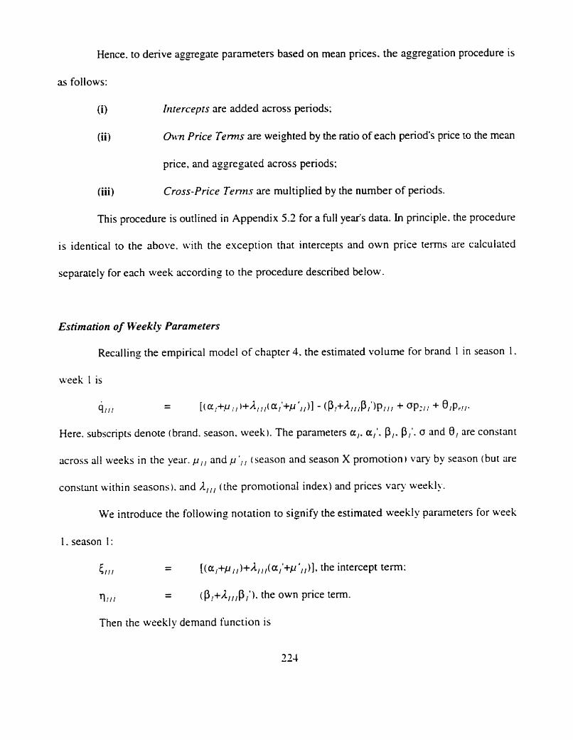
Hence. to derive aggregate parameters based on mean prices. the aggregation procedure is

as follows:

(0 bttrrcepts are added across periods;

(6) Own Price Terns are weighted by the ratio of each period's price to the mean

price. and aggregated across periods;

(iii) Cross-Price Tenrts are multiplied by the number of periods.

This procedure is outlined in Appendix 5.2 for a full year's data. In principle. the procedure

is identical to the above. with the exception that intercepts and own price terms are calculated

separately for each week according to the procedure described below.

Estimation of Weekly Parameters

Recalling the empirical model of chapter 4. the estimated volume for brand 1 in season 1.

week I is

- 1 1 I

- [W+P;, ) + L ( ~ / ' + P ' I J - @,+~,,,P, ')P/I/ + opt11 + ~ I P ~ I I .

Here. subscripts denote (brand. season. week). The parameters a,. or,'. PI. PI'. o and 8, are constant

across all weeks in the year. p,, and p ',, (season and season X promotion) vary by season (but are

constant within seasons). and (the promotional index) and prices vary werkI>.

We introduce the following notation to signify the estimated weekly parameters for week

1. season 1 :

5,1, - - ((or,+p l,)+AllI(al'+p ',,)], the intercept term:

- V l l l

- (P,+/Z,,,P,'). the own price term.

Then the weekly demand function is

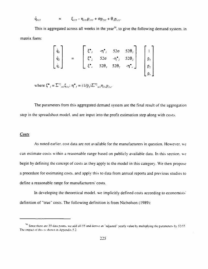
4111 - Sll, - rllllP,11 + ~ P J I I + 0 , ~ r l l -

This is aggregated across all weeks in the yea?', to give the following demand system. in

matrix form:

The parameters from this aggregated demand system are the final resuf t of the aggregation

step in the spreadsheet model. and are input into the profit estimation step along with costs.

costs - As noted earlier. cost data are not available for the manufacturers in question. Howe\fer. we

can estimate costs within a reasonable range based on publicly available data. In this section. w

besin by defining the concept of costs as they apply to the model in this category. We then propose

a procedure for estimating costs. and apply this to data from annual repons and previous studies to

define a reasonable range for manufacturers' costs.

In developing the theoretical model. we implicitly defined costs according to economist^'

definition of "true" costs. The following definition is from Nicholson ( 1989):

"The cconomic cost of any input is the payment required to keep that input in its

present employmmt. Equivalently. the economic cost of an input is the

remuneration that input would receive in its best nltemative employment." (p.309)

In essence. the difference between this definition and the accounting definition of costs lies

in the inclusion of opportunity costs.

We assume that labour markets are efficient, and that the wage paid by these manufacturers

is therefore equivalent to that paid in the best alternative employment available to workers. Similarly.

with efficient financial markets. providers of capital to these publicly-quoted firms can readily switch

to other firms or industries: hence we assume that investors do not incur opportunity costs by

investing in this industry.

Since fixed costs and sunk costs are irrelevant to the decision to supply the private label. we

exclude them from the analysis. Hence our concept of costs does not include depreciation. interest

or R gL D. The opportunity cost of applying machinery (defined as the rent the equipment would

obtain in its best alternative use) to these products can also be considered to approach zero. since the

equipment used in this category is either specialized or is readily available from other sources.

Our definition of cosrs therefore includes raw materials. labour. plant overhead and

distribution: all the direct costs that are involved in manufacturing the product and transfemng it to

the retailer. We do not include the manufiacturer's advertising or selling costs. assuming that these

are unchanged by the private label supply decision.

Functional Form

Recall that we specified a quadratic cost function for manufacturer 1 in chapter 3. as

follows:

C - - aq,, + !hbq,,,' + cq, + Vidq; + eq,,,q,.

We saw that

- where b = d = e. marginal costs are constant:

- where b > 0. there are product-specific diseconomies of scale on the national brand:

- where b c 0. there are product-specific economies of scale on the national brand:

- where d > 0. there are product-specific diseconomies of scale on the private label:

- where d c 0. there are product-specific economies of scale on the private label:

- where e > 0. there are cost anticomplementarities (diseconomies of scope). and

- where e c 0. there are cost complernentarities (economies of scope 1.

There is a substantial body of evidence to suppon an assumption of constant marginal costs

in this case. Nicholson ( t 98% reviews the empirical evidence from a variety of industries and finds

a consistent pattern: the industries studied exhibit increasing returns to scale (b c 0 in our terms J up

to some point. but constant returns to scale thereafter. There is no evidence that long-run average

costs begin to rise after some point. Hence there is a "Minimum Efficient Scale" beyond which

marginal costs are constant.

The classic meta-analysis of empirical studies on cost functions by Waiters' ( 1963) finds that

marginal costs tend to be constant in the short run. In industries other than public utilities. this

finding also applies to lonp-run marginal costs: in Walters' analysis, nearly all of the observations

were for output levels well below the "capacity" of the plants. consistent with our assumption of

excess capacity in this case.

This evidence. taken together. sugests that. in the shon run at least, marginal costs can be

regarded as constant so long as output exceeds the minimum efficient scale and falls within the

manufacturer's capacity. We apply both assumptions here. Within this category. a 199 1 econometric

study" of demand and costs also assumed constant marginal costs for analytical and mathematical

tractability. with the comment that "[tlhis choice. however. seems to be an acceptable first-order

approximation of the real cost functions in the ... industry".

Within a reasonable range of output. we can expect unit costs of raw marerials. labour and

distribution not to change a great deal: efficiencies in purchasing of raw materials tend to require

large volume increments to have a significant impact. and raw material costs are. in any event. o

small portion of total costs in this category. Assuming that capacity is available. the firms will nor

need to incur overtime and wage rates will therefore be constant: similarly. distribution rates will not

change with quantity within the range we are considering.

Hence we assume constant marginal costs for the national brand and the private label. i-r.

in the above quadratic cost function. we assume b = d = e = 0. However. we check the impact of this

assumption in some of the simulations discussed later in this chapter.

Data

As already noted. we have no explicit data on costs: hence we use publicly available sources

to derive a range within which we can be reasonably confident that costs lie. Our data sources are

as fo~lows'~:

(9 A Harvard Business School case on the category:

(ii ) A study by J.P. Morgan Securities Inc.:

(iii) A published econometric study on the category:

(iv) Annual reports of the two national brand manufacturers and the private label

suppIier.

Our procedure for analysis is summarized in the following flowchart:

RETAIL PRICES

WHOLESALE PRICES

COSTS

Starting with the retail prices in the dataset. our first step is to use the first two of the sources

named in the previous section to estimate a range of retailer markups for the category. By subtracting

these markups from retail prices. we estimate a r a n g of net wholesale prices for each manufacturer.

- -, '- SLY previous loornote. Direct retcrcnccb art' avcuded lo presene category confidentiahty. but absrrrrcts a r t glwn In A p p e n d ~ ~ 5 I

It shouid be noted that. while manufacturers* wholesale prices before promotional allowances are

available from manufacturers* price lists. net wholesale prices after such deals are not published and

must be estimated.

In step 2. we use the second two data sources to arrive at estimates of each manufacturer's

costs (raw materials. labour. plant overhead and distribution) as a percentage of the estimated

wholesale prices. From this. we calculate. in step 3. a dollar amount for unit costs.

Step I : Retailer Markups

Our purpose here is to arrive at a range of estimates of manufacturers' wholesale prices to

retailers. We achieve this by estimating the markup retailers apply to wholesale prices. and working

backwards from retail prices in the dataset to find net wholesale prices.

Retailer markups have been the subject of much discussion in this category. due to a series

of claims and counter-claims by national brand and private label suppliers. aimed at providine

support for their brands with retailers. With the growth of private labels. national brand

manufacturers are under pressure to demonsrrate that their brands are more profitable for retailers

than private labelb. in spite of the fact that retailers typically earn higher markups on the wholesale

prices of private labels than on those of national brands. Hence there has been a great deal of

discussion of relative sales volume and of which costs should be allocated to each type of brand. For

example. as we will see later in this chapter. national brand manufacturers deliver their products

direct to retailers' stores. while the private label supplier distributes to retailers' warehouses only.

Depending on the assumptions we make about the retailers' costs of internal distribution from

warehouses to stores. national brands can appear more. or less. profitable for retailers than private

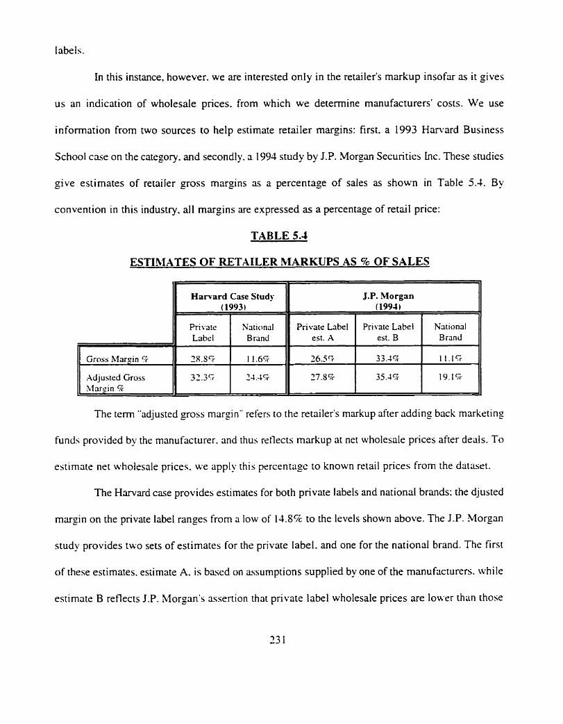
labels.

In this instance, however. we are interested only in the retailer's markup insofar as it gives

us an indication of wholesale prices. from which we determine manufacturers' costs. We use

information from two sources to help estimate retailer margins: first. a 1993 Hanrard Business

School case on the category. and secondly. a 1994 study by J.P. Morgan Securities Inc. These studies

give estimates of retailer gross margins as a percentage of sales as shown in Table 3.1. Bv

convention in this industry. all margins are expressed as a percentage of retail price:

TABLE 5.4

ESTIhlATES OF RETAILER MARKUPS AS % OF SALES

11 Haward Case Study

Private National 1 Gross Marcin ppp- 9 1 28.8% ::::: Adjusted Gross 32.35 Marcin %

The term "adjusted gross margin" refers to the retailer's markup after adding back marketing

funds provided by the manufacturer. and thus rrtlects markup at net wholesale prices after deals. To

estimate net wholesale prices. we apply this percentage to known retail prices from the dataser.

The Harvard case provides estimates for both private labels and national brands: the djusted

margin on the private label ranges from a low of 11.84 to the levels shown above. The J.P. Morgan

study provides two sets of estimates for the private label. and one for the national brand. The first

of these estimates. esiimate A. is based on assumptions supplied by one of the manufacturers. while

estimate B reflects J.P. Morgan's assertion that private label wholesale prices are lower than those

Private Label est. A

Private Label est. B

National Brand

reflected in estimate A.

We estimate manufacturers' net wholesale prices by applying these adjusted gross margins

to the retail prices in the dataset. Hence net wholesale price is (retail price)*(100 - adjusted gross

margin)/100. Since we are interested in defining a range. we take only the highest and lowest

estimates of adjusted gross margin from Table 5.1. and estimate wholesale prices in Table 5.5:

TABLE 5.5

ESTIMATED RANGE OF NET WHOLESALE PRICES

L

Net Wholesale Price

Based on the higher margins earned by retailers on the private label and on their lower retail

prices. net wholesale prices are much lower than those of national brands.

Step 2: Munu facturer Costs

Our purpose in this section is to estimate manufacturers' costs as a percentage of wholesale

price. Our data sources in this pan of the analysis are an econometric study on this category

published in 1991. and the annual reports of manufacturers 1 and 2. and the dominant private label

supplier from 199 1 to l99-l.

Brand

I

1

7

PL

1Iean Retail Price

S 1.59

S 1.74

S0.94

hlargin

High

24.1%

24.4%

35.1%

Low

S 1 20"

SI -32

50.60

LOW

19.1 '7c

19-15

14.8%

I

High

!5 1.29

S 1-42

50.80

The 199 1 study. described in Appendix 5.1. uses a full-information maximum likelihood

procedure to assess the relative performance of manufacturers' strategies based on the assumption

that the data are the equilibrium outcomes of noncooperative games in pricing and advertising. The

study analyzes the strategies of manufacturers I and 2 in the category. but does not include the

private label supplier.

In this study. manufacturers0 constant marginal costs are specified as a linear function. with

no intercept term. of prices of a key raw material. on wages and on each manufacturer's cost of

capital. Hence

where C, refers to the real average costs of manufacturer i, R represents the real price of a key raw

material common to both manufacturers. L is the real uni t cost of labour in the nondurable

manufacturing sector and CC, represents each firm's cost of capital. i.e. the firm's real bond yield.

[t should be noted that these costs do not include distribution or plant overhead.

The means of these three variables. and the parameters estimated in the study. are shown

in Table 5.6:

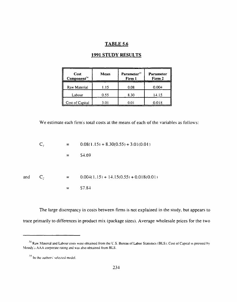
TABLE 5.6

1991 STUDY RESULTS

We estimate each tirm's total costs at the means of each of the variables as follows:

and C,

Cost Component3'

t ,

Raw Material

Labour

Cosr of Capital

The

trace primari

Paramete$' Firm 1

0.08

8.30

0.0 1

%I ean

1.15

0.55

3.0 1

large discrepancy in costs between firms is not explained in the study. but appears to

Parameter Firm 2

0.004

I4.15

0.0 1 Y

ly to differences in product mix (package sizes). Average wholesale prices for the two

-34 Raw Xlatcnd and Labour costs were obtained from the C.S. Burcau of Labor Stmsttcs (BLS 1: Cost of Cap~ral IS proxtcd h~ >food>'; AAA corporate rattng and was also obtmncd from BLS.

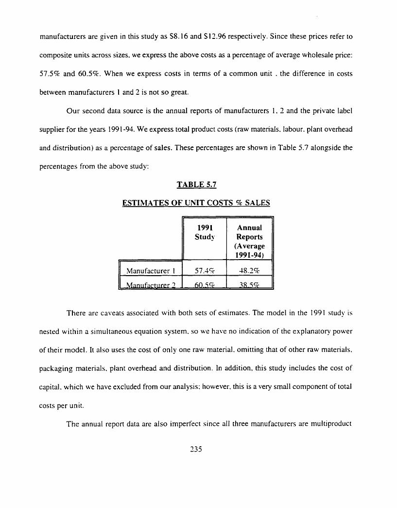
manufacturers are given in this study as S8.16 and 5 13.96 respectively. Since these prices refer to

composite units across sizes. we express the above costs as a percentage of avenge wholesale price:

57.5% and 60.54. When we express costs in terms of a common unit . the difference in costs

between manufacturers I and 2 is not so great.

Our second data source is the annual reports of manufacturers 1. 7 and the private label

supplier for the years 199 1-94. We express tgtal product costs (raw materials. labour. plant overhead

and distribution) as a percentage of sales. These percentages are shown in Table 5.7 alongside the

percentages from the above study:

TABLE 3.7

ESTIMATES OF UNIT COSTS 5% SALES

There are caveats associated with both sets of estimates. The model in the 199 1 study is

nested within a simultaneous equation system. so we have no indication of the explanatory power

of their model. It also uses the cost of only one raw material. omitting that of other raw materiais.

packaging materials. plant overhead and distribution. In addition. this study includes the cost of

capital. which we have excluded from our analysis: however. this is a very small component of total

costs per unit.

The annual report data are also imperfect since all three manufacturers are multiproduct

,Manufacturer 1

Mantlfacturer

1991 Stud?

57-45

60.57~

Annual Reports

(Average 1991-94)

18.2%

385%

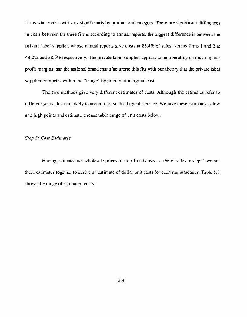
firms whose costs will vary significantly by product and category. There are significant differences

in costs between the three firms according to annual reports: the biggest difference is between the

private label supplier. whose annual reports give costs at 83.4% of sales. versus firms I and 2 at

48.28 and 38.58 respectively. The private label supplier appears to be operating on much tighter

profit margins than the national brand manufacturers; this fits with our theory that the private label

supplier competes within the "fringe" by pricing at marginal cost.

The two methods give very different estimates of costs. Although the estimates refer to

different years. this is unlikely to account for such a large difference. We take these estimates as low

and high points and estimate a reasonabIe range of unit costs below.

Step 3: Cost Estimates

Having estimated net wholesale prices in step 1 and costs as a 5% of sales in step 1. we put

these estimates togerher to derive an estimate of dollar unit costs for each manufacturer. Table 5.8

show the range of estimated costs:

TABLE 5.8

ESTIMATED RANGE OF UNIT COSTS

Manufacturer I A. Whoiesale Price (from Table 5 .5 )

B. Unit Cost 9 Sales

3Ianufacturer 2 A. Wholesale Price (from Tab le 5.5)

I

B. Unlt Cost % Sales (from Tab le 5.6)

S Unit Costs fA*B) I

f L blanufacturer Wholesale Price =

Low High

Since we have two cost Q sales estimates and two wholesale prices for each of the national

brand manufacturers. we end up with four estimates of unit costs. In the case of the private label. we

have only one cost 5 sales estimate and hence two cost estimates. We assume that the competitive

fringe sets its wholesale price equal to its cost. as specified in the theoretical model'". In analyzing

the results. we vary unit costs between the lowest and highest of the national brands' cost estimates.

shown in bold type in Table 5.8.

In summaq*. we have obtained net wholesale prices by estimating retailers' markups within

the category and applying these estimates to retail prices in the dataset. We have estimated unit costs

-16 Thc cost rmgc 01' $0.60 to $0.80 1s based on a 50.94 rctad pnsc xijusted for retaller markups of 35.45 t J.P. .\Iorgan m d

14.85 ( Han ard caw study I r c ~ ~ r l ~ t l \ t ' l >

as a percent of sales. and applied this percentage to our estimated wholesale prices to arrive at unit

costs. These costs include raw materials. labour. plant overhead and distribution: opportunity costs.

however, are not a significant component of costs in this category.

We do not have any estimate of the national brand manufacturers' cost to supply the private

label. since they do not currently do so. Since the range of private label costs is similar to that of the

national brands. we assume initially that private label and national brand costs are equal. and later

simulate changes in private label costs to find a "breakeven" cost at which the manufacturer is

indifferent between supplying and not supplying.

i iv ) Results

In this section. we discuss the results obtained when we substitute the demand parameters

for brands I . ? and the private label into the spreadsheet version of the theoretical model. along with

assumed costs and competitive prices. In addition. we show the impact of different assumptions

about costs on the outcome.

The model is quite sensitive ro the assumptions made: our starting assumptions are given

below and tfariations in costs are simulated later.

National brand unit costs. for each manufacturer. are at the mid-point of the

m n p given in the last section, i.e. a = S0.66 for manufacturer 1 and a = S0.69

for manufacturer 2.

There are no economies of scale or scope. i.e. b=d=e=O.

The competitive fringe's unit cost for the private label. C,. is equal to the mid-

point of the cost range for the private label manufacturer. i.e. C, = $0.70.

The national brand manufacturers' cost to supply the private label is also

equal to that of the national brand, i.e. c = $0.66 for manufacturer 1 and c =

0.69 for manufacturer 2.

Each competing manufacturer's price when he does not supply the private

label is equal to the mid-point of the range of his wholesale price based on

mean prices from the dataset (see Table 5.5). i.e. when we are analyzing

manufacturer 1's private label profitability. w,,: = S 1.37: when we are

analyzing manufacturer 2's private label profitability. urn, = S 1.25.

The competing manufacturer does not change price in response to supply by

a particular manufacturer.

These assumptions represent a reasonable starting point for our analysis based on the data

available. Appendix 5.3 summarizes these assumed values along with aggregated parameter values

for each of the brands. Together. these constitute the inputs to the spreadsheet model.

Table 5.9 shows the results of the analysis for manufacturer 1. assuming that manufacturer

2 does nor supply.

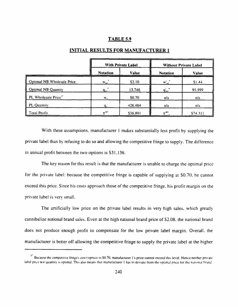
TABLE 5.9

INITIAL RESULTS FOR MANUFACTURER 1

With these assumptions. manufacturer I makes substantially less profit by supplying the

private label than by refusing to do so and allowing the competitive fringe to supply. The difference

in annual profit between the two options is S3 1.136.

The key reason for this result is that the manufacturer is unable to charge the optimal price

for the private label: because the competitive fringe is capable of supplying at $0.70. he cannot

exceed this price. Since his costs approach those of the competitive fringe. his profit margin on the

private label is very small.

The artificially low price on the private label results in very high sales. which greatly

cannibalize national brand sales. Even at the high national brand price of 52.08. the national brand

does not produce enough profit to compensatz for the low private label margin. Overall. the

manufacturer is better off allowin,o the competitive fringe to supply the private label at the higher

. - Bccauw the compcnrlw inngc's cost (=pnci.) is $0.70. mmulacturer 1's pnce cannot c.uct.cd t h ~ s level. Hence nclrhtr p n v v r

label pnit. n i v quantlt? 1s opt~mal. Th13 also mram that mmul'rtcturcr I has to dt.\ia[r from [he optlrn~l pnct: for tht. n ~ r ~ c w l hrclnc!

With Private Label Without Private Label

Value

52. I0

1 3.746

50.70

426.464

Notation

weq,.

n t ,

n/rl

n/rt

Notation

536.89 1 tiHl S73.71 I

Value

S 1.41 I

95.599

n/a 3

nka

Optimal NB Wholesale Price

Optimal NB Quantity

PL Wholesale price:'-

PL Quantity

Total Profit

w, I

9,,1

\vr

4,

r.rtf c

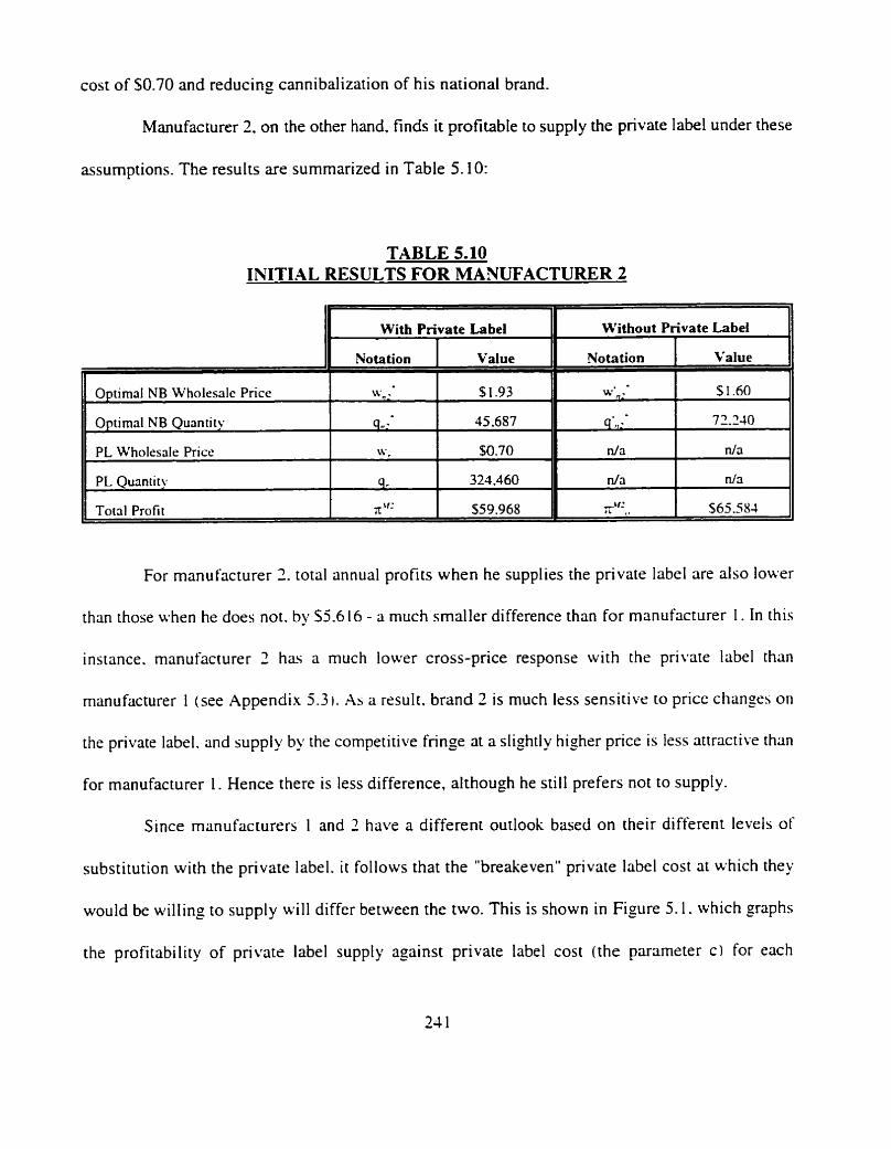
cost of 50.70 and reducing cannibalization of his national brand.

Manufacturer 2. on the other hand. finds it profitable to supply the private label under these

assumptions. The results are summarized in Table 5.10:

TABLE 5.10 INITIAL RESULTS FOR MANUFACTURER 2

II With Private Label 11 Without Private Label r 1

For manufacturer 2. total annual profits when he supplies the private label are also lower

than those when he does not. by 55.6 16 - a much smaller difference than for manufacturer I . In this

instance. manufacturer 2 has a much lower cross-price response with the private label than

manufacturer 1 (see Appendix 5.3 1. As a result. brand 2 is much less sensitive to price changes on

the private label. and supply by the competitive fringe at a slightly higher price is less attractive than

for manufacturer 1. Hence there is less difference, although he still prefers not to supply.

Since manufacturers 1 and 2 have a different outIook based on their different levels of

substitution with the private label. i t follows that the "breakeven" private label cost at which they

would be willing to supply will differ between the two. This is shown in Figure 5.1. which graphs

the profitability of private label supply against private label cost (the parameter cl for each

11 Notation Value I 3 1.93

45.687

S0.70

324.460

959.968

Optimal NB Wholesale Price

Optimal NB Quantity

PL Wholesale Price

PL Quantity

Total Profit

\v .

9":

\v ,

'Ir X.%~:

Notation 1 Value

w',.'

. - ,, --

n/a

d a

-.*I: 4~ ,,

S 1.60

72.210

n/a

n/a

565.581

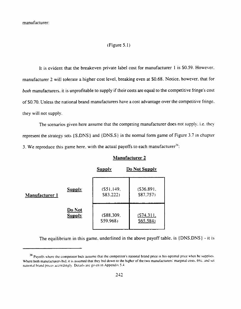
manufacturer:

( Figure 5.1 )

It is evident that the breakeven private label cost for manufacturer I is S0.59. However.

manufacturer 2 will tolerate a higher cost level, breaking even at $0.68. Notice. however. that for

both manufacturers. it is unprofitable to supply if their costs are equal to the competitive frinze's cost

of 50.70. Unless the national brand manufacturers have a cost advantage over the competitive fringe.

they will not supply.

The scenarios given here assume that the competing manufacturer does not supply. i.e. they

represent the strategy sets { S.DNS J and { DNS.S } in the normal form game of Figure 3.7 in chapter

3. We reproduce this game here. with the actual payoffs to each manufacturers:

Manufacturer 2

Supply Do Not Supplv

The equilibrium in this game. underlined in the above payoff table. is { D N S - D M } - it is

Supplv Manufacturer 1

Do Not Supplv

3"~voffs uhere the cornpetltor b ~ d s aarumr: thal the compe tmis natlonal brand pncr IS his opt~rnal pncc when he suppl~e\ Wlerc both rnmufxturer5 bld. I[ 1s assumed that they b ~ d doun to the h ~ r h c r of the two manufacturers' marginal costs. 69i. and sc; nat lon~l hrancl pnct.5 . iccorJ~ngl> Deta~lh arc g l e n rn Xppsndiv 5.4

(S5 I . 149. 5233.222)

I

($88,309. S59.968)

($36.89 1. S87.757

I

fS74.3 I 1. $65.5841

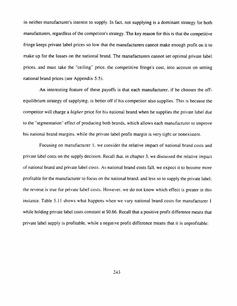
i n neither manufacturer's interest to supply. In fact. not supplying is a dominant strategy for both

manufacturers, regardless of the competitor's strategy. The key reason for this is that the competitive

fringe keeps private label prices so low that the manufacturers cannot make enough profit on it to

make up for the losses on the national brand. The manufacturers cannot set optimal private label

prices. and must take the "ceiling" price. the competitive fringe's cost. into account on setting

national brand prices (see Appendix 5.5).

An interesting feature of these payoffs is that each manufacturer. if he chooses the off-

equilibrium strategy of supplying. is better off if his competitor also supplies. This is because the

competitor will charge a higher price for his national brand when he supplies the private label due

to the "segnentation" effect of producing both brands. which allows each manufacturer to improve

his national brand margins. while the private label profit margin is very tight or nonexistent.

Focusing on manufacturer 1. we consider the relative impact of national brand costs and

private label costs on the supply decision. Recall that. in chapter 3. we discussed the relative impact

of national brand and private label costs. As national brand costs fall, we expect i t to become more

profitable for the manufacturer to focus on the national brand. and less so to supply the private label:

the reverse is true for private label costs. However. we do not know which effect is greater in this

instance. Table 5.1 1 shows what happens when we vary national brand costs for manufacturer 1

while holding private label costs constant at $0.66. Recall that a positive profit difference means that

private label supply is profitable. while a negative profit difference means that i t is unprofitable:

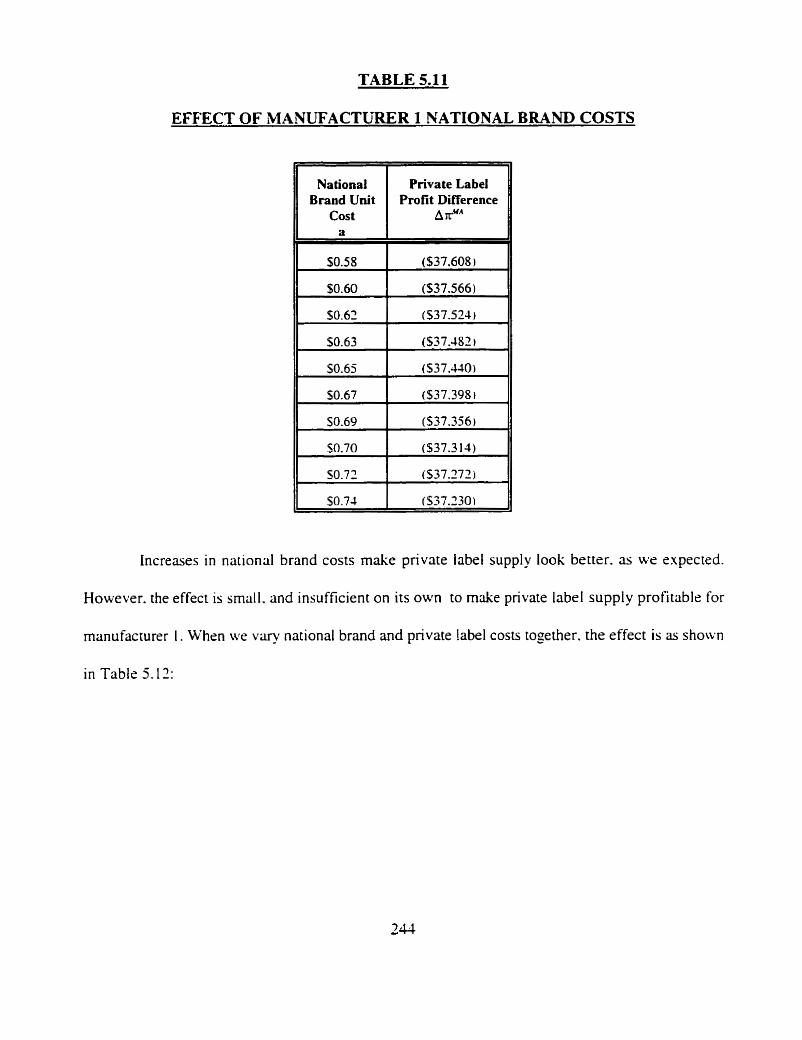
TABLE 5.1 1

EFFECT OF MANUFACTURER 1 NATIONAL BRAND COSTS

Increases in national brand costs make private label supply look better. as we expected.

However. the effect is small. and insufficient on its own to make private label supply profitable for

manufacturer 1. When we vary national brand and private label costs together. the effect is as shown

in Table 5.12:

National Brand Unit

Cost

Private Label Profit Difference

A rUA

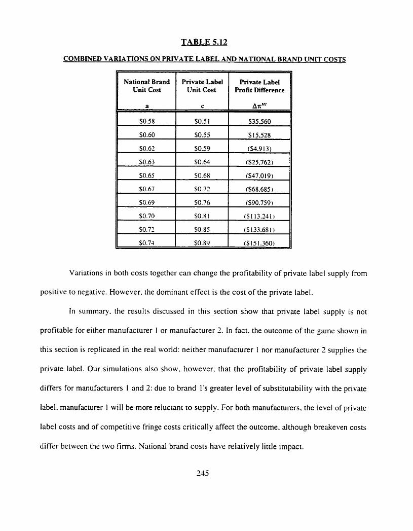
TABLE 5.12

COMBWED VARIATIONS ON PRIVATE LABEL AND NATIONAL BRAND UNIT COSTS

National Brand Private Label Private LabeI Unit Cost Unit Cost Profit Difference

Variations in both costs together can change the profitability of private label supply from

positive to negative. However. the dominant effect is the cost of the private label.

In summary. the results discussed in this section show that private label supply is not

profitable for either manufacturer I or manufacturer 2. In fact. the outcome of the game shown in

this section is replicated in the real world: neither manufacturer I nor manufacturer 2 supplies the

private label. Our simulations also show. however. that the profitability of private label supply

differs for manufacturers I and 2: due to brand 1's greater level of substitutability with the private

label. manufacturer 1 will be more reluctant to supply. For both manufacturers. the level of private

label costs and of competitive fringe costs critically affect the outcome. a1 though breakeven costs

differ between the two firms. National brand costs have relatively little impact.

While private label supply is not profitable for rhe manufacturers at present. we explore in

the next section whether it might become so if circumstances were to change. Our purpose in doing

so is both to explore realistic scenarios that might occur in this category and to illustrate the use of

the model in practice. We consider three scenarios: competitive response. type of private label and

direct store delivery. In each case, we vary the parameters of the demand and/or cost functions and

discuss their impact.

(v) Scenario Analvsis

Our purpose in this section is to illustrate the application of the model to a variety of

scenarios which represent reality in this category. In each case. we describe the situation and how

it can be represented by changes in the model's parameters. with all other parameters held at the

initial levels of the last section. We focus on the issues facing manufacturer 1 .

Competitive Actions

A significant concern for a manufacturer considering supplying a private label to a retailer

is the possibility of setting off a price war among manufacturers of national brands. In this category.

such a threat is very real. The two dominant firms see each other as their primary competition, and

are unwilling to allow each other to gain any advantage from private label supply. While increased

prices by firm 2 are a theoretical possibility (because it is in firm 1's interest to raise national brand

prices). managers in the industry argue that firm 3 is likely to reduce prices in order to discourage

private label supply by manufacturer I .

In chapter 2. we found that the possibility of a price change by a competing duopolist could

have a negative effect on the profitability of private label supply. and that such a scenario was most

likely when the price of the private label was low relative to that of the national brand. A major

concern for a duopolist would be the possibility of setting off a price war with his competitor. As

was shown in Appendix 3.7. it is also a concern for a dominant firm that the competing dominant

firm may change its national brand price in response to private label supply.

A further reaction by a competitor might be to increase his investment in promotion \s ith

the retailer. Since manufacturer 2 has a very low share of total promotions. it may weli be in his

interest to react in this way. as well as reducing price.

The model can be used to anticipate both reactions and estimate their total impact on the

profitability of private label supply for manufacturer I . We classify the possible reactions of

manufacturer 2 to private label supply by manufacturer I as mild. moderate. aggressive or hishly

aggressive by v a ~ i n g manufacturer 2's price. and by increasing his share of promotions.

The basis of our assumptions is to vary the price parameter by reducing prices by L/2 standard

deviation for each level: thus. since the standard deviation of manufacturer 2's price is 8c. a mild

response is manufacturer 2's initial price of 5 1.37 less i c . or 5 1.33, a moderate response is S 1.29.

and so on. In the case of promotions. manufacturer 2's mean promotion share from the dataset is 5%.

compared with shares of 52% for manufacturer 1 and 43% for the private label. We increase

manufacturer 2's share in increments of 10% and reduce the shares of manufacturer 1 and the private

label in proportion. Table 5.1 3 summarizes these assumptions:

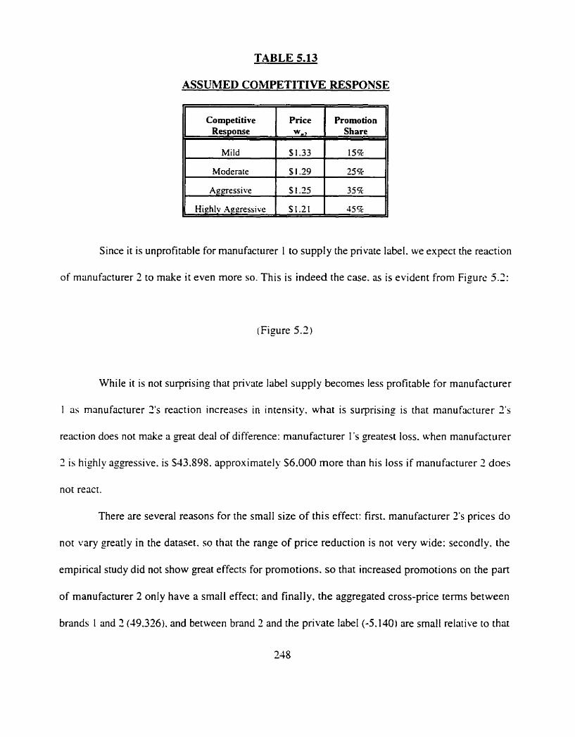
TABLE 5-13

ASSUMED COMPETITIVE RESPONSE

Competitive Price Promotion Response Share

Mild $1.33

Highly Aggressive 35% 1

Since it is unprofitable for manufacturer I to supply the private label. we expect the reaction

of manufacturer 2 to make it even more so. This is indeed the case. as is evident from Figure 5.2:

(Figure 5.2)

While it is not surprising that private label supply becomes less profitable for manufacturer

1 as manufacturer 2's reaction increases in intensity, what is surprising is that manufacturer 2's

reaction does not make a great deal of difference: manufacturer 1's greatest loss. when manufacturer

1 is highly aggressive. is $43.898. approximately $6.000 more than his loss if manufacturer 2 does

not react.

There are several reasons for the small size of this effect: first. manufacturer 2's prices do

not vary greatly in the dataset. so that the range of price reduction is not very wide: secondly. the

empirical study did not show great effects for promotions. so that increased promotions on the pan

of manufacturer 2 only have a small effect: and finally. the aggregated cross-price terms between

brands I and 7 (19.326). and between brand 2 and the private label (-5.140) are small relative to that

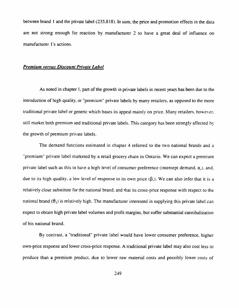
between brand I and the private label (235.8 1 8). In sum, the price and promotion effects in the data

are not strong enough for reaction by manufacturer 2 to have a great deal of influence on

manufacturer I 's actions.

Premium versus Discount Private Label

As noted in chapter 1. part of the growth in private labels in recent years has been due to the

introduction of high quality. or "premium" private labels by many retailers. as opposed to the more

traditional private label or generic which bases its appeal mainly on price. &Many retailers. however.

still market both premium and traditional private labels. This category has been strongly affected by

the growth of premium private labels.

The demand functions estimated in chapter 4 referred to the two national brands and a

"premium" private label marketed by a retail grocery chain in Ontario. We can expect a premium

private label such as this to have a high level of consumer preference (intercept demand. a,). and.

due to its high quality. a low level of response to its own price @,). We can also infer that i t is a

relatively close substitute for the national brand. and that its cross-price response with respect to the

national brand (8,) is relatively high. The manufacturer interested in supplying this private label can

expect to obtain high private label volumes and profit margins, but suffer substantial ~ ~ n i b a l i z a t i o n

of his national brand.

By contrast, a "traditional" private label would have lower consumer preference. higher

own-price response and lower cross-price response. A traditional private label may also cost less to

produce than a premium product. due to lower raw material costs and possibly lower costs of

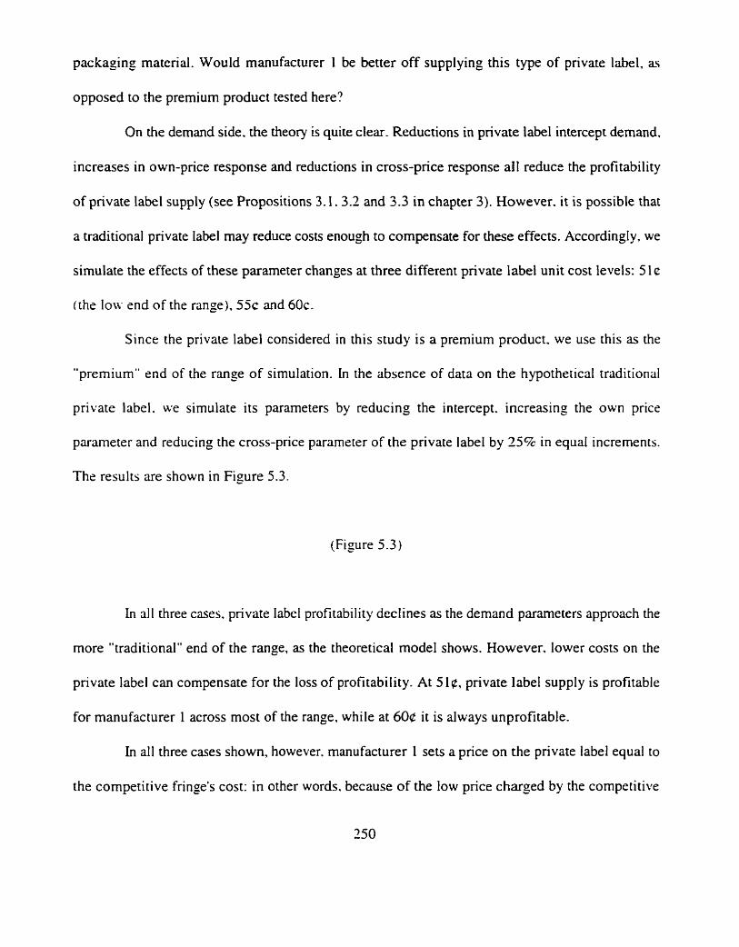
packaging material. Would manufacturer 1 be better off supplying this type of private label, as

opposed to the premium product tested here?

On the demand side. the theory is quite clear. Reductions in private label intercept demand,

increases in own-price response and reductions in cross-price response ail reduce the profitability

of private label supply (see Propositions 3.1.3.2 and 3.3 in chapter 3). However. it is possible that

a traditional private label may reduce costs enough to compensate for these effects. Accordingly, we

simulate the effects of these parameter changes at three different private label unit cost levels: 5 1 c

(the low end of the range), 5 5 ~ and 60c.

Since the private label considered in this study is a premium product. we use this as the

"premium" end of the range of simulation. In the absence of data on the hypothetical traditional

private label. we simulate its parameters by reducing the intercept. increasing the own price

parameter and reducing the cross-price parameter of the private label by 254 in equal increments.

The results are shown in Figure 5.3.

(Figure 5.3)

In all three cases. private label profitability declines as the demand parameters approach the

more "traditional" end of the range, as the theoretical model shows. However, lower costs on the

private label can compensate for the loss of profitability. At 5 Ig, private label supply is profitable

for manufacturer 1 across most of the range, while at 604 it is always unprofitable.

In all three cases shown, however. manufacturer 1 sets a price on the private label equal to

the competitive fringe's cost: in other words. because of the low price charged by the competitive

sector. he is unable to set profit-maximizing prices on the private label. or. by extension, on the

national brand (since he maximizes across both products). However, if the private label's parameters

change by extreme amounts beyond those simulated here. his optimal price falls so low that he can

beat the competitive fringe's price. In this situation, his profit margins improve, but the private label

is so inherently unattractive because of its low consumer preference and high price response that it

remains unprofitable.

Direct Store Delivery

In this category. one significant difference between the national brand manufacturers and

private label suppliers is that the former deliver their national brands direct to stores. but the latter

deliver to retailers' warehouses. The national brand manufacturers claim that their method of

distribution saves costs for retailers: at least some retailers. however. would prefer a warehouse-

delivered product at lower cost. To date. national brand manufacturers have refused to comply with

this on their national brands. Retailers are nevertheless unlikely to pay extra for a direct-delivered

private label.

This leaves national brand manufacturers with a choice of using their existing direct-to-store

distribution system for private labels as well as their national brands. or delivering to retailers'

warehouses as private label suppliers do. In the former case, the manufacturer gains economies of

scope by putting two brands through the same distribution system: in the latter. he can reduce the

unit costs of the private label. Hence there is a trade-off between unit costs and economies of scope.

This simulation considers how manufacturer 1 might make such a trade-off.

Direct store delivery costs are largely fixed: while manufacturers might consider investing

in extra DSD capacity to supply private label. this is highly unlikely since it would double unit costs.

We therefore assume that excess capacity exists. in which case the incremental costs of delivering

private label are confined to handling and some materials such as extra pallets. We assume, based

on discussions with industry experts, that these costs are small.

We simulate the savings due to warehouse delivery by reducing private label unit costs by

I c and by 2c on costs ranging from 5 5 ~ to 60e. As we saw earlier, private label supply is profitable

in this range. and we expect warehouse delivery to make it more so. as is evident when we examine

the parallel shifts in profit due to these savings in Figure 5.4:

(Figure 5.4)

The solid line in Figure 5.4 shows the effect of economies of scope. the parameter e in the

cost function. varied between 0 and -0.000000 1. At the mean volumes from the dataset, this lowest

level represents savings of approximately 44 per unit. However. since the effect of e is a function

of output. the total savings wiIl change as optimal output changes, as a result of changes in e.

From Figure 5.4. it is evident that economies of scope within this range have a limited

effect, relative to savings in unit costs. Until the savings reach the higher end of the range, the

manufacturer is better off delivering to retailers' warehouses and taking the savings in unit costs. In

other words. it takes a large increase in efficiency to offset the savings the manufacturer might obtain

if he delivered to retailers' warehouses.

This analysis. of course. does not take account of another reason why manufacturers might

prefer direct store delivery - that it gives them more control of shelf position and display. However.

this rationale disappears in the case of the private label, for two reasons: first, because retailers are

very likely to prefer to merchandise their own private label, and secondly, because it is unlikely that

truck jobbers hired by the national brand manufacturer will give the private label adequate exposure.

This raises another interesting rationale for DSD. however: the manufacturer may prefer it because

it allows him to limit the shelf exposure given to the private label, as opposed to the national brand.

In any event, a manufacturer wishing to deliver private label direct to stores will need to find

strong justification for such a decision on the basis of strategic factors. In this analysis and in the

foregoing, it has become evident that the unit costs of private label play a critical role in determining

its profitability. Warehouse delivery is one way of reducing unit costs and making private label

supply profitable.

lvi) Conclusions

Ln this chapter. we set out to learn more about the model both by identifying its limitations

and by applying it to a case study. The results provide us with interesting observations about the

model. The principal of these are outlined below.

The fundamental assumptions of the model with respect to market structure

and manufacturer-retailer interaction seem to represent reality in this category

quite well. More generally. they approximate conditions in the grocery

industry as a whole.

The major limitation of the model lies in the possibility of misspecification

of the demand function. In particular, the model does not take account of

other package sizes and advertising. The direction of bias that results from

exclusion of these factors varies,

The aggregate nature of the data (discussed in chapter 4) may lead us to

erroneous conclusions. As we saw in the simulation of competitive actions.

the lack of significant effects for competitive promotions suggests that

competitors can have little influence on the private label supply decision

This conclusion could change if store-level data showed stronger promotiona

effects.

The "dominant firm" structure of the model plays a pivotal role in the

profi tabiiity of private label supply. Because the competitive fringe's costs are

low. the national brands are heavily cannibalized if the manufacturers supply

at low costs. However, the manufacturers' ability to recover their profits

through supplying the private label is severely limited, since their price must

always be lower than the competitive fringe's cost.

The "market segmentation" effect of private label supply is an important

factor in this case. Because the manufacturer that supplies the private label

raises his national brand price, the competing national brand manufacturer

stands to gain. Hence each manufacturer is better off if his competitor

supplies the private label, whether or not he chooses to do so.

Throughout the simulations, it is clear that private label unit costs are also a

critical factor in the supply decision. This ties in with the previous

observation: with an upper bound on prices. manufacturers are unable to pass

cost increases on to the retailer and hence private label supply rapidly

becomes unprofitable with increases in costs.

It is evident both from the theoretical model and from the simulations in this

chapter that the manufacturers would be better off supplying a premium

private label than a traditional private label. In addition, delivery of private

labels direct to retailers' stores is unlikely to be justified relative to the

competitive fringe's practice of warehouse delivery.

In the case analyzed here, we applied the parameters obtained in chapter 4, along with the

most reasonable assumptions we could make about national brand and private label costs. Our

findings fit with the strategy actually followed by the manufacturers in practice: private label supply

is unprofitable. and the national brand manufacturers are better off leaving it to the competitive

sector.

In summary, the model has provided a useful perspective on the profitability of supplying

a private label for the manufacturers in this category. While it necessarily leaves out some issues.

its use as a vehicIe for simulation allows us to assess the effects of strategic changes on the

profitability of supplying private labels.

REFERENCES

Arnold, S.J.. Tae H. Oum and Douglas J. Tigert (1983). "Determinant Attributes in Retail Patronage: Seasonal. Temporal. Regional and International Comparisons". Journal of Marketing Research. 20. 149-157.

Boulding & Staelin (1993). "A Look on the Cost Side: Market Share and the Competitive Environment". Marketing Science. 12, 2(Spring), 144- 166.

Iyer. Ganesh and David Sobeman ( 1 993). "Category Market Structure: Brand Versus Size Competition". Working Paper. University of Toronto.

Nicholson, Walter, Microeconomic Theory. Orlando. Ha.: The Dryden Press.

Pindyck, R.S. and Daniel L. Rubinfeld ( 198 1 ). Econometric Models and Ecorzornic Forecasts. Nell~ York: McGraw-Hill.

Tellis. Gerard J. ( 1988). "The Price Elasticity of Selective Demand: A Meta-Analysis of Econometric Models of Sales". Jolinlal of Marketing Research. 25 (November), 33 1-4 I .

Walters. A.A. ( 1963). "Production and Cost Functions: An Econometric Survey", Econometric~r. 3 1 (Januq/April ). 1 -66.

Wilkinson. J.B.. J. Barry Mason and Christie H. Paksoy. (1982). "Assessing the Impact of Short- Term Supermarket Strategy Variables". Jorrrnnl of Marketing Research, 19, 72-86.

APPENDICES

APPENDIX 5.1

ABSTRACTS OF RELEVANT STUDIES

1. Harvard Business School Case Studv

This case study takes a close look at the situation facing the dominant private label supplier in the category in 1993. The supplier was already weil established in the Canadian market and had been making forays into the U.S. The two national brand manufacturers had reacted aggressively to the private label supplier's growth by reducing prices, and their likely reaction to the latter's ambitious plans for the U.S. market was uncertain. In addition, the private label supplier was considering expansion outside Nonh America and into other product categories. The case provides detailed historical financial data (not including unit costs), market shares, case sales by retail account, and data on international market development.

2, J.P, Morgan Studv

From the introductory section to this report:

"There has been a change in the North American corporate landscape with the emergence of strong private brand manufacturers and marketers. At the same time. traditional regional U.S. supermarket chains have come under sustained pressure not just from the recession but also from voracious new breeds of retail formats. deep discounters. clubs and supercentres. Larger, more marketing-driven chains have seized on private brand development as a survival tactic that protects retail profitability because it produces a superior gross margin mix, as well as a means of distinguishing a retailer from its less able regional competitors. Fortwolwons. it is important to determine whether private brand growth has been an unsustainable. recession-linked cyclical move:

0 If so. private brand manufacturers ... would reverse.

If so, supermarket chains would revert to an undifferentiated mass of regional sitting ducks."

The study responds to arguments made by one of the national brand manufacturers that national brands are more profitable for retailers than premium private labels. Most of these arguments are refuted using detailed data on category sales, prices and retailer costs.

3. Econometric Shrdv (1991): published in Advances in Econometrics

This paper considers a differentiated market dominated by a duopoly and focuses on some simple models of noncooperative behaviours on two strategic variables: price and advertising. The methodology explicitly recognizes the gaming nature in the econometric modeling . Specificall y, using quarterly data on the [manufacturers I & 21 markets from 1968 to 1986, the authon derive and estimate competing structural econometric models under the assumption that the data are the equilibrium outcomes of some noncooperative games in prices and advertising. The methodology presents two advantages. First. full-information estimates of the effect of advertising on market demand are obtained under specific game structures. Second. using recent model selection tests for nonnested models, the authors assess the relative performance of competing market conducts.

A later paper by the same authors, using the same data, was published in the Journal of Economics atld Management Strategy in 1 992. The abstract is as follows:

This paper proposes an empirical methodology for studying various (implicit or explicit) collusive behaviours on two strategic variables, which are price and advertising, in a differentiated market dominated by a duopoly. In addition to Nash or Stackelberg behaviours, the authors consider collusion on both variables, collusion on one variable and competition on the other. etc. Using data on the [manufacturers 1 & 21 markets from 1968 to 1986, full information maximum likeiihood estimates of cost and demand functions are obtained allowing for various collusive behaviours. The collusive hypothesis is not rejected, and the best form of colIusive behaviour is selected via nonnested testing procedures. Using the best model. Lerner indices are computed for both duopoiists to provide summary measures of market power. Finally, the approach is contrasted with the conjectural variation approach and is shown to give superior results.

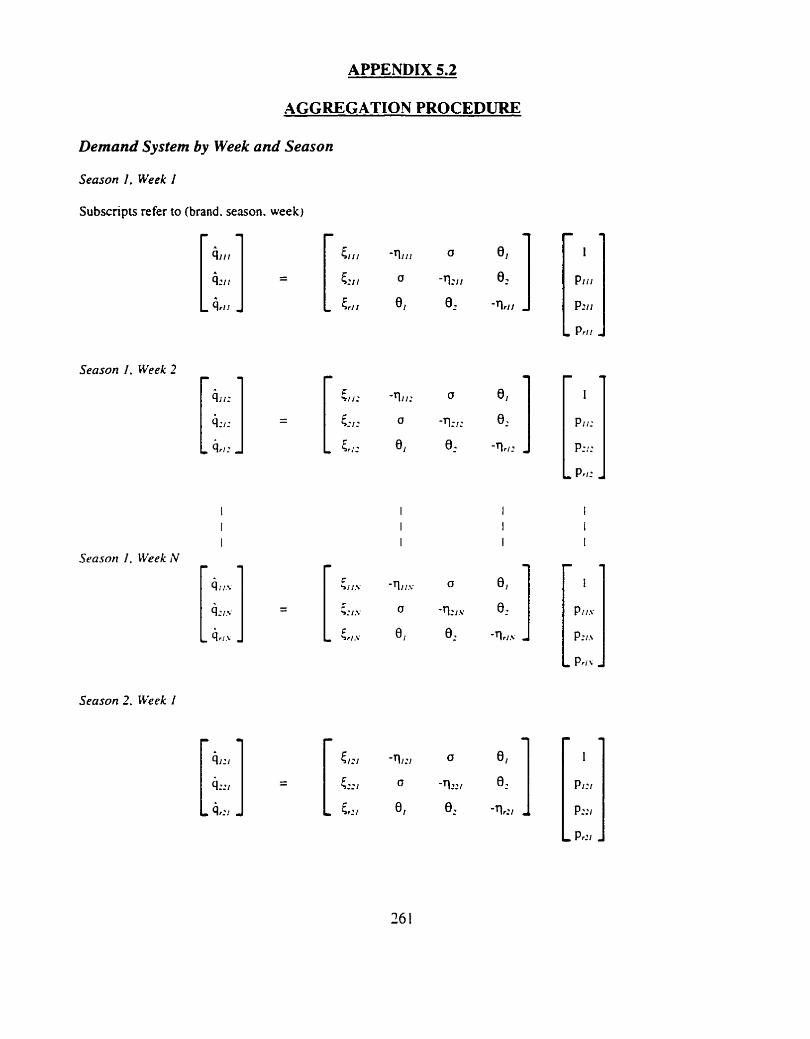
APPENDIX 5.2

AGGREGATION PROCEDURE

Demand System by Week and Season

Season I . Week I

Subscripts refer to (brand. season. week)

Season I , Week 2

Season 2. it'eek I

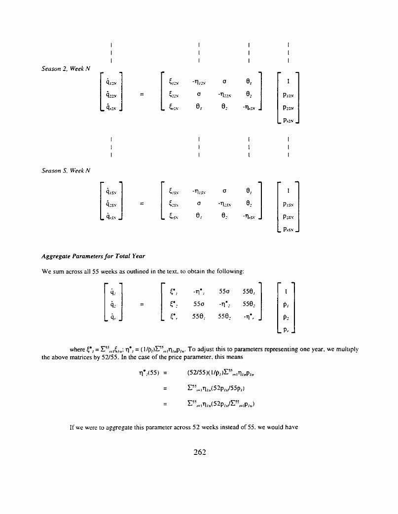
I I I

Season 2. Week N

Season S. Week N

Aggregate Parameters for Total Year

We sum across all 55 weeks as outlined in the text. to obtain the foliowing:

where c', = ~55G,5 ,x l ; qgl = ( l ~ p ~ ) ~ ~ ~ , q ~ , ~ ~ , ~ . TO adjust this to parameters representing one year. we multlply the above matrices by 52/55. In the case of the price parameter. this means

ft(S) = (5w55 ~ ~ ~ ~ ~ ~ 5 5 F ~ ~ ~ 1 1 ~ ~ 1 1

- - ~ " l , i ~ l , , ( 5 ~ p l , / 5 ~ p J J

- - C 5 5 c 1 ~ / r r ( 5 2 ~ / r l ~ 5 r = i ~ 1 5 , )

If we were to aggregate this paramercr across 53 weeks instead of 55. we would have

For these parameters to be equal.

In other words. h e proportionally reduced parameter will be unchanged from the 52-week parameter if prices change in the same proportion. .4ny difference between h e two incorporates deviations in the remaining three weeks.

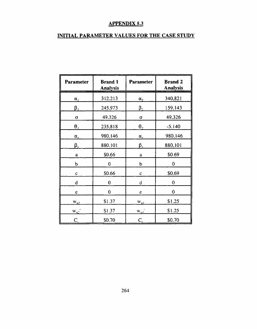
APPENDIX 5.3

INITIAL PARAMETER VALUES FOR THE CASE STUDY

,

Parameter

a,

PI o

I

8,

ar

P r

a

b

c

d

e

w,., @

w, - C,

Brand 2 Analysis

I

340,82 1

159,143

49.326

-5.140

980.146

880,lO 1 1

$0.69

0

$0.69

0

0

S 1.25

S 1.25

$0.70

Brand 1 Anaf ysis

3 12.2 13

245,973

49.326

235,8 18

980.146

880.101

$0.66

0

30.66

0

0

3 1.37

S 1.37

$0.70

Parameter

a,

PI (J

8:

a,

P r

a

b

c

d

e

w ,

W,, , C,

APPENDIX 5.4

ITERATED PRICES WHERE BOTH MANUFACTURERS BID

Where both manufacturers bid to supply the private label. we assume that they bid each other down to the greater of the two manufacturers' marginal cosb. here 69c. We start by assuming that the competitor's national price is his optimal price born the (S.DNS } and {DNS,S} stratem see. The model then computes optimal national brand prices where each manufacturer supplies: we use these prices as competitive prices in the next iteration. repeatinp the process until the prices converge.

The results of this procedure are as follows:

Iteration .

w,, W,r X, I 7c.

I

APPENDIX 5.5 NATIONAL BRAND PRICE WHERE w, IS CONSTRAINED

The competitive fringe cost C, is an upper bound on the manufacturer's private label price. Hence where the optimal private label price exceeds this cost. the manufacturer is constrained to a price of C, if he wants to supply. The same principle holds where both manufacturers bid. Here. we set private label prices at marginal costs. We then set national brand prices given these prices. instead of optimizing across both brands as before. From Appendix 3.5 to chapter 3. we have

which is. in this case

Recall that C,,, = a + bq,,(w,,') + eq,(C,). and C. = c + dq, + eq,,. Substituting these functions into w,,. we have

Rearranging terms and solving, we obtain

FIGURES

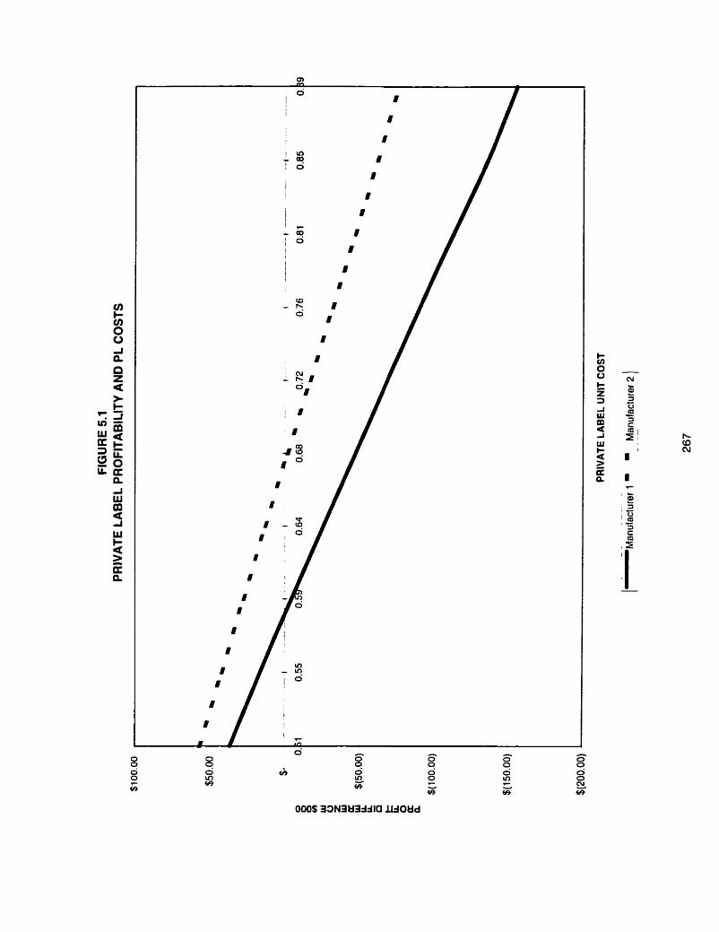
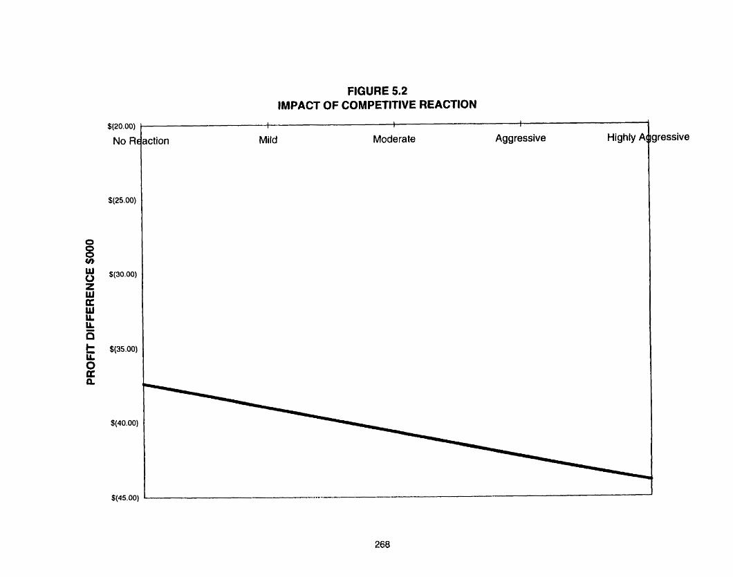
FIGURE 5.2 IMPACT OF COMPETITIVE REACTION

I 1

I 1 1 1

Mild Moderate Aggressive Highly A

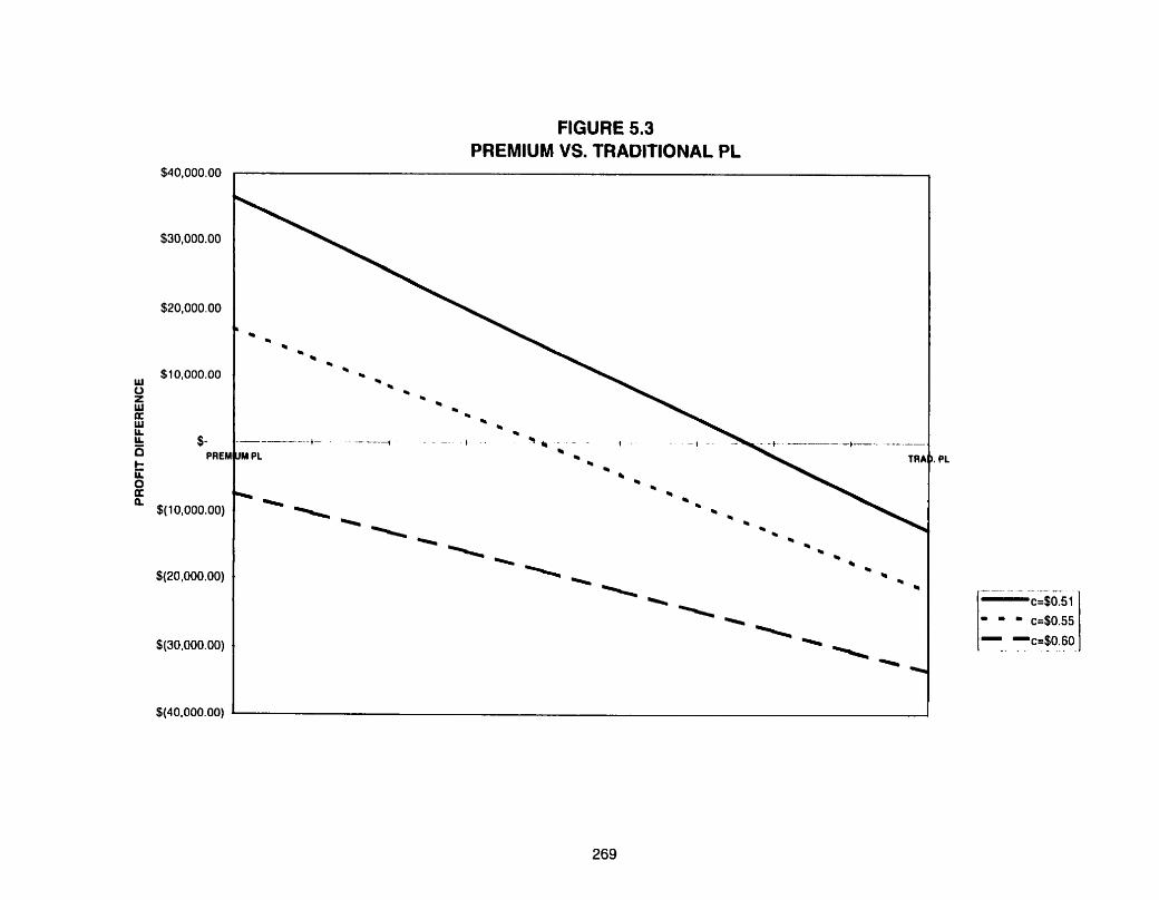
$- PREW

FIGURE 5.3 PREMIUM VS. TRADITIONAL PL

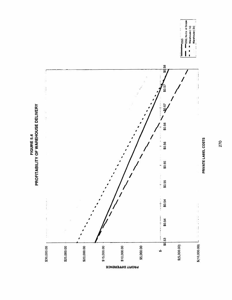
6. CONCLUSIONS AND DIRECTIONS FOR FUTURE RESEARCH

for life's not a paragraph

A~rd death i think is no parenthesis.

e.e. cummings:

Since feeling is first

li) Summarv

This dissertation has been concerned with the conditions under which it is profitable for a

manufacturer to supply a retailer's private label brand. We have focused our analysis on conditions

approximating the retail grocery industry, and have applied the model to a specific category within

that industry.

The model starts with a set of assumptions about consumer demand, industry structure.

manufacturer and retailer behaviour and costs. Optimal prices and quantities are derived. and the

profitability of private label supply determined by comparing a manufacturer's total profit when he

supplies the private label. versus when he does not supply. By analyzing the response of this

difference to each of the model's parameters, we develop predictions about the influence of

exogenous conditions on private label supply profitability. We summarized these at the end of

chapter 3. For the reader's convenience, this summary is repeated here:

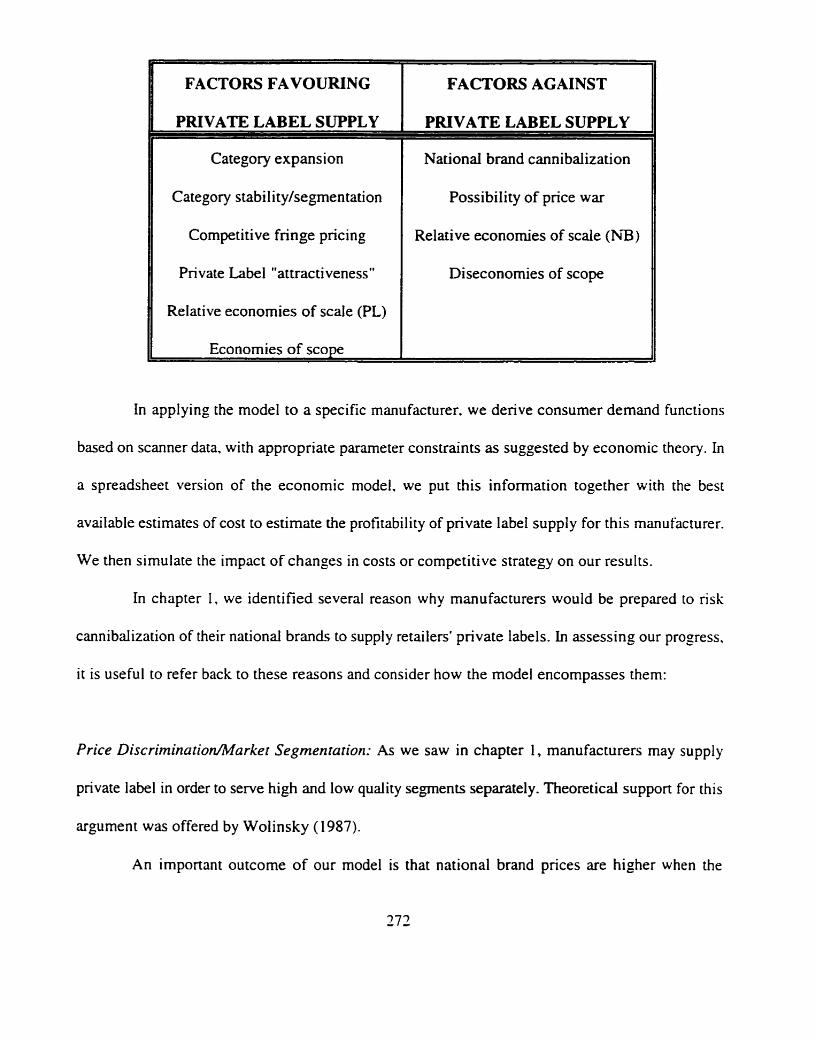
I FACTORS FAVOURING

I PRIVATE LABEL SUPPLY

Category expansion

I1 Category stability/segrnentation

Competitive fringe pricing

Private Label "attractiveness"

I Relative economies of scale (PL)

If Economies of s c o ~ e

FACTORS AGAINST

PRIVATE. LABEL SUPPLY

National brand cannibalization

Possibility of price war

Relative economies of scale (hi)

Diseconomies of scope

In applying the model to a specific manufacturer. we derive consumer demand functions

based on scanner data. with appropriate parameter constraints as suggested by economic theory. In

a spreadsheet version of the economic model, we put this information together with the best

available estimates of cost to estimate the profitability of private label supply for this manufacturer.

We then simulate the impact of changes in costs or competitive strategy on our results.

In chapter I . we identified several reason why manufacturers would be prepared to risk

cannibdization of their national brands to supply retailers' private labels. In assessing our progress.

it is useful to refer back to these reasons and consider how the model encompasses them:

Price Discrimination/Market Segmentation: As we saw in chapter 1, manufacturers may supply

private label in order to serve high and low quality segments separately. Theoretical support for this

argument was offered by Wolinsky (1987).

An important outcome of our model is that national brand prices are higher when the

manufacturer also supplies the private label. The reason for this is that the manufacturer who sells

two brands can extract some surplus from consumers of the lower-priced brand, allowing him to

raise prices on the other. Hence the model supports this explanation for private label supply.

E n m ~ Deterrence: The "entry deterrence" argument was that a manufacturer might supply a private

label in order to prevent a new competitor from gaining a foothold in the market. Schmalensee

(1978), Eaton and Lipsey (1979) and Brander and Eaton (1984) were cited as suppon for this

explanation.

In the "dominant firm" model of chapter 3 and the subsequent case application, we analyzed

a situation in which a manufacturer is faced with not only a quasi-duopolistic competitor. but also

with a competitive fringe that will supply the private label if neither dominant firm does. In order

to keep the competitive fringe out. the manufacturer has to offer a better price to the retailer for the

private label. We found support in both theoretical development and in later simulations for the idea

that. if the competitive fringe's costs are sufficiently high, it is optimal for the manufacturer to allow

entry.

Relationships and Power: We also examined the idea that retailers in the grocery industry might use

their power to force manufacturers to supply private label. However, we found that the influence of

retailer power on private label supply is extremely uncertain. In addition, a recent analysis by

Messinger and Narasimhan (1995) questions the idea that power has shifted towards retailers in the

grocery industry. There is nonetheless evidence (e-g. GlCmet and Mira, 1993) that private label

market share is associated with retailer concentration; whether this says anything about private label

supply is another matter. At best, it can be said that the jury is still out on the influence of power on

private label supply.

Retailer power is incorporated in the model in the assumption that manufacturers offer

differentiated national brands, but are undifferentiated with respect to private label supply. Hence

the retailer can readily switch from one supplier to another in search of the best price. The model

therefore asslunes that retailers are powerful with respect to the private label, but does not explicitly

analyze the influence of differing levels of retailer power on manufacturers' actions.

Competition: The competitive environment faced by a manufacturer was considered as a possible

influence in the supply of private labels: manufacturers may supply private labels in order to pre-

empt competitive actions. While there was little research on this aspect of private label supply.

Brander and Eaton (1984) did provide some support for the idea that manufacturers supplied

different products in different competitive environments.

Our model analyzed three types of competitive environment: monopoly, duopoly and two

dominant firms facing a competitive fringe. We found that. while it is always in a monopolist's

interest to supply a private label, a duopolist will take into account the likely reaction of his

competitor: should the competitor reduce price, private label supply may not be viable. A dominant

firm, on the other hand, additionally has to consider the fact that if neither he nor his competing

dominant firm supplies the private label. the competitive fringe will.

There is certainly room to analyze other competitive environments, an issue we will consider

later in this chapter. However, the existing model not only provides "baseline" conditions via the

monopoly and duopoly analysis, but examines the competitive environment that is most relevant to

the grocery industry.

CapaciiyEconornies of Scale or Scope: The idea that private labels are primarily a capacity-filler

is pervasive in channels literature, both academic and popular. In addition, putting more volume

through a plant can result in lower unit costs. if the manufacturer has declining marginal costs due

to economies of scale or scope.

The model explicitly analyzes the effect of product-specific economies of scale and

economies of scope on the profitability of privars label supply. via the inclusion of quadratic and

cross-product terms in the cost function. We find that product-specific economies of scale on the

national brand negatively affect private label supply. since the manufacturer would prefer to f i l l the

plant with more national brand volume than with private labels. Conversely. economies of scale on

the private label positively affect profitability. as do economies of scope.

The model assumes that manufacturers have the capacity to supply the private label. This

is representative of prevailing conditions in the contemporary grocery industry. where a substantial

amount of spare capacity exists. largely due to volume declines on national brands.

The model. then. includes most of the key reasons for private label supply that have been

suggested in the literature. at least insofar as they apply to the retail grocery industry. In the

remainder of this chapter, we deal with the model's contribution, its limitations and directions for

future work.

As was pointed out in chapter I , private labels are an issue of great concem to manufacturers

in the packaged g o d s industry due to their steady growth in recent years. Some manufacturers (e.0

Coca-Cola) and some academics (e.g. Hoch and Baneji. 1993) have expressed scepticism over

whether they are a major long-term concem. However, based on the evidence from European

markets, private labels can potentially capture in excess of one-third of total grocery sales. In

addition. the success of premium quality private labels at close to parity pricing to national brands

would suggest that retailers' brands are not completely a recession-related phenomenon.

With the growth of private labels, manufacturers have been under increasing pressure to

provide retailers with high-quality substitutes for their national brands. No longer are retailers

satisfied with private labels that offer the consumer low quality at a low price; increasingly, they are

insisting on products that mimic national brand quality, at lower profit margins for manufacturers.

Hence the concem among manufacturers that private labels will simply substitute low-margin sales

for high-margin sales.

The primary contribution of this dissertation. then. lies in its identification of the

microeconomic conditions that favour. and that mitigate against, the supply of private labels. In

addition, the framework proposed here is adaptable to a variety of related business issues. The

model, Furthermore, can act as a decision tool for managers who are interested in analyzing the effect

of changes in competitive strategy or environmental conditions on their decision.

liii) Limitations

The model has certain limitations which may render it less applicable in some situations.

as was discussed in chapter 5. A summary of the most important limitations is given here.

Retailers: While retailers can choose between national brands and private labels based on price and

substitutability, there are often other considerations that come into play. Because of limited shelf

space, for example. retailers may choose not to stock the national brand if its margins are too low:

on the other hand. they may give preference to the national brand of a manufacturer that supplies

their private Iabel.

The model also assumes that manufacturers are undifferentiated with respect to the private

label. While this is a reasonable approximation of reality in the grocery industry as a whole. there

may be individual situations in which some manufacturers are capable of providing a higher quality

product or some extra service such as delivery to stores. Since there are few patents in the grocery

industry, however, such differences are unlikely to be sustainable over time.

The decision to provide a private label to one retailer has also been assumed to be

independent of all other such decisions. However. one can envisage situations in which supplying

one retailer would create a "precedent" under which it would be difficult to resist demands for

private label supply from other retailers. If the private label's marginal costs are increasing or

decreasing. this could have a significant impact on the decision.

Functional Form: Both the quadratic utility function and cost function on which this model is based

are first-order approximations of any such function, and the model can therefore be seen as highly

generalizeable across different categories. However, in some situations the linear demand function

may not fit as well with the data as, for example, a log form. However, log form demand functions

are mathematically intractable in a model such as this (e.g. Choi, 1991).

One way of dealing with this is to estimate log demand hnctions where appropriate and

approximate a linear function by Taylor Series expansion around a specific point. The major

drawback to this is that even a small range on the (log) demand function is represented by an infinite

number of linear functions, and a shift in price may invalidate the results of the model. Whether this

is critical to the profitability of private label supply will vary from case to case.

Costs: The cost function given in chapter 3 represents the underlying total costs of the manufacturer.

but in reality is very difficult to estimate. Allocation of costs across business units can often hide the

true relationships between output and cost. so that the most realistic assumption. as in the case of our

simulation in chapter 5. is of constant marginal costs.

We have also assumed here that costs are exogenous to the model. while in reality they are

chosen by the manufacturer based on some production function in materials, labour and capital. For

this decision, the assumption that costs are exogenous is justifiable for an established business where

product formuiae and technology are approximately constant.

Competitive Fringe: As was demonstrated in chapter 3, the "dominant firm" framework is

descriptive of many categories in the grocery industry, including the category used for application

of the model. Smaller competitive firms. in fact, are often the key source of private label supply for

retailers (Glimet and Mira, 1993).

The most likely reason for this is that, for a small firm, supplying private label can be an

inexpensive way to enter a market. Hence national brand manufacturers may be concerned that such

firms do not grow too large and present a greater threat to their national brands. For this reason.

national brand manufacturers may prefer to deter entry by such smaller firms by supplying thc private

label.

Below the "entry-detemng price", C,, it is not in the competitive fringe's interest to supply.

While it may not be profitable for a national brand manufacturer to supply a private label at this cost.

this could change in a dynamic framework in which the competitive fringe enters and affects the

national brand manufacturer's payoffs in future periods. The widespread existence of such

competitive firms in the grocery industry would suggest. however. that this scenario does not arise

very often.

l iv) Future Research

While the limitations outlined above suggest opponunities for future work in this area. there

are, on a broader level. several directions in which research can proceed from here. Figure 6.1

provides a schematic of these areas:

(Figure 6.1 )

Extensions: The existing model can be extended in a numkr of ways both to

279

address some of the above limitations and to allow it to be generalized

beyond the scenarios discussed i ~ . this dissertation.

Differentiated Private Labels: In this model, we have assumed that national

brand manufacturers are undifferentiated from each other and from

competitive fringe suppliers. All retailers have to do is find the supplier that

can provide the cheapest product.

In some categories, however, manufacturers have different technology

or R&D resources at their disposal, so that they can supply a higher quality

product to the retailer. By doing so, they increase cannibalization of their own

product. but also raise switching costs for the retailer.

A model such as this could be accommodated within the existing

framework, but would need to be extended to a two-period sequential game

in which manufacturers bid for supply of a high-quality private label in the

first period. where the retailer's alternative is to go to the competitive fringe

for a low-quality private label. Because the retailer makes a higher profit

margin on the private label than on the national brand, he is better off with

the higher quality version which substitutes more closely with the national

brand and generates higher sales. The manufacturer evaluates his total payoff

over both periods. weighing the benefits of lower cannibalization against

those of continuing to supply the private label over two periods.

C a p a c i ~ Constrainrs: The model assumes that dl manufacturers, whether

dominant or fringe. have sufficient capacity to supply the private label. This

is a reasonable representation of prevailing conditions in the grocery industry

as a whole. In addition, the quadratic cost function assumed can be seen as

a continuous representation of capacity constraint: as a manufacturer

approaches capacity on a particular product. his parameter for diseconomies

of scale will approach infinity. However, the application of the model in other

industries, and sometimes to individual firms within the grocery industry.

may require us to represent a capacity constraint explicitly as a discontinuity

in the cost function.

Such a model would continue to assume that the competitive fringe

has unlimited capacity, but the dominant firms are constrained. so their

marginal costs increase suddenly at a certain output. Where the optimal

quantity exceeds a manufacturer's available capacity, the retailer will have to

buy private label from more than one source. In this case, the secondary

source will cannibalize the national brand to a lesser extent than the national

brand manufacturer's own label. due to its higher cost. Since the

manufacturer's private label output is less than optimal, he may be better off

allowing the competitive fringe to supply the entire quantity at its higher cost.

Dyan~ic/Seqice?ttia[ Games: The present model's treatment of private label

supply is static; however. as we saw in chapter 5. the decision period can be

as long as a year, or even longer. The issue in considering a dynamic game

is not whether manufacturers have a short-term or a long-term orientation, but

whether they have more than one opportunity to make decisions. Where

private label supply tends to move around from manufacturer to

manufacturer. this is a reasonable assumption.

As discussed previously, a dynamic framework may be most

appropriate in considering the manufacturer's interest in deterring entry by a

competitive firm. In addition, such a framework could accommodate a

scenario in which the competing dominant firm responds to a manufacturer's

supply of private label by supplying private label to a second retailer. In

arriving at a subgame perfect equilibrium strategy. the manufacturer has to

take into account cannibalization of his national brand at the second retailer

should his competitor supply in the next period39.

Alternatives to Private Label:

The existing model assumes that the manufacturer is considerins

private label supply as an alternative to doing nothing: he either supplies the

private label or he does not, holding all other strategies constant. However.

private label supply may be one of an array of strategies open to the

manufacturer. Here. we consider how some alternatives to private label

39 This idea was suggested by an expert on the soft drink industry, who a p e d that if a firm such 3s Pepsi were to supply a rctailer such as AkP. it must take into account the possibility that Coke would respond by supplying Loblaw's.

supply might be incorporated in the model.

Advertising: As an alternative to private label supply, the manufacturer can

choose to increase advertising on the national brand as a defence.

Increased advertising on the national brand would shift its demand

function outwards and may also reduce its price elasticity. To assess the

profitability of this alternative, we need to assume an advertising response

function which relates the benefits of advertising to its extra cost. In addition.

we need to derive results based on the national brand's present position on

this function. As noted in chapter 5, increased advertising will make private

label supply less profitable. Empirical application of such a model would

require data over a sufficiently broad range to determine the shape of the

advertising response function.

Promotion: In the parameter estimation of chapter 4, we empirically derived

the response to promotional activity on the manufacturer's part, assuming that

promotions draw occasional consumers into the category. Like the advertising

model, evaluation of promotion as an alternative to private label supply in a

theoretical model requires that we assume a response function. We would

expect promotion to have a more dramatic short-term effect on sales than

advertising would. However, it may also bring a quick response from the

competing dominant firm.

Product Developmenr: The strategic alternative of product development is

rich in possibilities for further modelling. The manufacturer can choose to

develop a new brand within the category, develop an improved private label

product (similar to his competitor's national brand), or develop a new brand

in another category.

This alternative can be represented by a dynamic game in which the

manufacturer invests in R&D in the first period and launches the resulting

new brand in a subsequent period. The effect of the launch depends on which

of the above strategic choices a manufacturer makes. A line extension, for

example. may cannibalize national brand volume more than a new brand.

which can be positioned to take volume from the competing dominant firm

or the private label. However. a new brand may be more costly, or more time-

consuming, to develop than a line extension. An interesting combination of

strategies woul be to supply private label in the short term, replacing it with

a new brand or line exrension when development efforts are completed.

Collrtsio~z: The dominant manufacturers may collude to keep the competitive

sector out by supplying the private label at less-than-optimal prices.

Alternatively, they may collude to allow the existence of a competitive sector

so long as it is not too threatening.

For the collusive arrangement to be sustainable, it must be optimal for

each manufacturer to uphold it. Hence we need to consider simultaneously

the payoffs to both manufacturers of supplying the private label. If the

manufacturers do supply. one would expect that private label output will be

divided between the manufacturers in some way, and the model would

determine the optimal split. This may have interesting ramifications where

it is unprofitable to supply the private label; manufacturers may want to

minimize the amount they produce, but produce just enough to prevent

retailers from going to the competitive fringe for some of their private label

needs.

Similar Problems: The model is designed specifically to compare scenarios with respect

to private label supply. but this structure can be applied to other problems. An

outline of some of the most interesting possibilities follows.

Retailer Profitabilin: As noted elsewhere, high quality private labels have

shown substantial growth as retailers grow more sophisticated. However.

many retailers market both high and low quality private labels. perhaps

segmenting the market a . we have seen manufacturers do as an outcome of

this model. In addition, some retailers place heavy emphasis on their private

labels due to higher margins than their national brand counterparts,

sometimes to the complete exclusion of some national brands.

A model of retailer profitability would consider the optimal prices and

quantities sold of each manufacturer's national brand. and of high and low

quality private labels, in the context of an oligopolistic retail market. Based

on the same manufacturer-Stackelberg structure and linear demand as

employed here. we can analyze relative profit margins and the optimal mix

of brands.

Line ErtensionsAVew Brands: The problem of launching a line extension or

a new brand bears strong similarities to the private label problem: in each

case, the manufacturer is usually concerned with making extra profit

contribution at the risk of some cannibalization.

In this case, however, the manufacturer chooses the level of

substitution with his own and competitive brands. He must trade off the

benefits he obtains from market and share expansion (which, as we saw in

chapter 2 , are closely linked with substitutability) against the risk of

cannibalizing his own sales. He thus finds an "optimal" level of

substitutability with his existing brand. As this optimal level approaches zero.

it becomes more in his interest to launch a new, independent brand.

Optimal Pricing: The present model derives optimal prices for both retailers

and manufacturers in a range of manufacturer-market structures, assuming

retailers are price takers. These can readily be extended to express optima1

prices as price differentials from other brands or private label.

An empirical application would follow a similar pattern to that

Applications:

discussed in chapters 4 and 5. demonstrating the difference in profits for a

manufacturer or a retailer between current prices and optimal prices. By

broadening the empirical application to multiple categories. we can

determine, as a whole, whether manufacturers and retailers tend to charge

optimal. less-than-optimal, or higher-than-optimal prices.

One of the interesting features of this model is that it has been

possible to turn it into a managerial tool by expressing it in spreadsheet form.

Although the spreadsheet is currently fairly rudimentary, it provided us with

a number of interesting, and useful, analyses in chapter 5.

Spreadsheet Models: The present spreadsheet model can be simplified by

linking it with some more sophisticated mathematical and graphics software.

At present. a11 calculations (cell formuias) are entered directly from the

theoretical model along with appropriate constraints expressed as if-then

conditions. This process, while user-friendly, is cumbersome from a

programming point of view. Ideally, we should be able to preserve the user-

friendliness of the system while providing more power and analytical

flexibility.

In addition, the present spreadsheet model does not do any of the

required econometric analysis. relying on parameters derived in a separate

program. In an ideal world. this should not be necessary: all we would have

to do is enter the data, and leave the program to run the regressions, extract

the parameters and simulate changes in strategic variables.

Another shortcoming of the present spreadsheet model is that a

thorough understanding of the model is required to interpret the results. The

primary reason for this is that the results can change dramatically when the

range of parameter variation takes us outside the model's constraints. A

simpler. managerially interpretable model remains a goal for the future.

Expert S-wernhVegotiation Tools: The logical extension of the spreadsheet

models outlined above is to develop an "expert" system which can accept

both verbal and numerical inputs to develop strategic recommendations. Like

the spreadsheet model. such a system would combine a statistical package

with mathematical simulation software; in this case, the user would chcose

from a number of available market structure assumptions and econometric

methods. The system would provide a report analyzing the situation in

numerical, graphical and verbal form.

One example of such an application would be a system which aids in

developing positions for negotiations with channel counterparts. With

appropriate inputs, the system would be capable of generating payoffs and

deve!oping judgements as to what would be an equilibrium strategy for each

of the parties. Over time, actual outcomes could be entered so that the system

could quantify each party's likely range of deviation from equilibrium. and

strategies could also take into account actual past behaviour.

The four broad areas for future development described here and outlined in Figure 6.1 are

not, of course, mutually exclusive. It seems realistic to consider the first two categories, Extensions

and Alternatives to Private Label Supply. as shorter term areas for exploration and the second two.

Similar Problems and Applications, as longer term opportunities.

iv) Concluding Comment

The oveniding intent in this dissertation has been to bridge the gap between academic theory

and managerial practice. To this end, we have developed a modei that uses rigorous economic theory

to derive managerially relevant conclusions and apply them empirically.

Certainly, the objective was ambitious from the start. Equally certainly, it cannot be said that

this dissertation. alone, has come close to achieving it. Nonetheless, we have made a start. In the

process, we have enhanced understanding of a particular type of managerial decision. shown how

our understanding can be put to use, and laid the groundwork for a potentially fertile stream of

research.

This dissertation is the first step on a long road.

Brander, James A. and Jonathan Eaton ( 1984), "Product Line Rivalry", The American Economic Review, 74,3,323-334.

Choi, S. Chan (1991), "Price Competition in a Channel Structure with a Common Retailer", Marketing Science, 10,4 (Fall), 27 1 -296.

Eaton. B. Curtis and Richard G. Lipsey (1979). "The Theory of Market Preemption: The Persistence of Excess Capacity and Monopoly in Growing Spatial Markets", Econornetrica, 46, 149- 158.

GlCmet, Francois and Rafael Mira (1993). "The Brand Leader's Dilemma", rite McKinsey QuarterLy, 2, 3-15.

Messinger, Paul R. and Chakravarti Narasirnhan, "Has Power Shifted in the Grocery Channel?". Marketing Science, 14,2, 1 89-223.

Schmalensee, R. (1978). "Entry Deterrence in the Ready-to-Eat Breakfast Cereal Industry", Bell Journal of Economics. 9, 305-327.

Wolinsky, Asher ( 1987), "Brand Names and Price Discrimination", The Journal of Inditstrial Economics, XXXV, March, 255-68.

Applications

Spreadsheet Models

Expert System

Negotiation Tools

FIGURE 6.1

DlRECTIONS FOR FUTURE RESEARCH

Extensions

Di ft'erentiarcd PL's

Cilpacity Con!

C7 Private Label S u ~ ~ l v Model I E E >

C

Similar Problems

Retailer PL Profitability

Line Extensions

I~npnct of New Brand

Optimal Pricing

Price Difkrcntids

"

Alternatives to PL Supply

Advert king

Promotion

Pricing

Product Development

Collusion

l MAGE EVALUATION TEST TARGET (QA-3)

APPLIED IMAGE. 1nc 1653 East Main Street - -. - Rochester. NY 14609 USA -- -- - - Phone: 71 6/482-0300 --

-7 - - F a : 71 61288-5989

O 1993. Appiied Image. Inc.. All Rtghts Reserved