An Analysis of Sequential Auctionsfor Common and Private Value Objects

Shaheen S. Fatima� Michael Wooldridge� Nicholas R. Jennings�

� Department of Computer Science,University of Liverpool, Liverpool L69 7ZF, U.K.�S.S.Fatima, M.J.Wooldridge�@csc.liv.ac.uk� School of Electronics and Computer Science,University of Southampton, Southampton SO17 1BJ, U.K.nrj@ecs.soton.ac.uk

Abstract. Sequential auctions are an important mechanism for buying/sellingmultiple objects. Existing work has studied sequential auctions for objects that areexclusively either common value or private value. However, in many real-worldcases an object has both features. Also, in such cases, the common value dependson how much each bidder values the object. Moreover, a bidder generally does notknow the true common value (since it may not know how much the other biddersvalue it). Given this, our objective is to study settings that have both common andprivate value elements by treating each bidder’s information about the commonvalue as uncertain. Each object is modelled with two signals: one for its commonvalue and the other for its private value. The auctions are conducted using Englishauction rules. For this model, we first determine equilibrium bidding strategies foreach auction in a sequence. On the basis of this equilibrium, we find the expectedselling price and the winner’s expected profit for each auction. We then showthat even if the common and private values of objects are distributed identicallyacross all objects, the selling price and the winner’s profit are not the same forall of them. We show that, in accordance with Ashenfelter’s experimental results[1], the selling price for our model can decline in later auctions. Finally, we showthat the selling prices and the winner’s expected profits in an agent-based settingcan differ from those in an all-human setting.

1 Introduction

Market-based mechanisms such as auctions are now being widely studied as a meansof buying/selling resources in multiagent systems. This uptake is occurring becauseauctions are both simple and have a number of desirable properties (typically the mostimportant of which are their ability to generate high revenues to the seller and to allo-cate resources efficiently) [19, 4, 21]. Now, in many cases the number of objects to beauctioned is greater than one. There are two types of auctions that are used for multipleobjects: combinatorial auctions [18] and sequential auctions [6, 3, 11]. The former areused when the objects for sale are available at the same time, while the latter (whichare the main focus of this paper) are used when the objects become available at differ-ent points in time. In the sequential case, the auctions are conducted at different times,

therefore a bidder may participate in more than one auction. In such a scenario, it hasbeen shown that although there is only one object being auctioned at a time, the biddingbehaviour for any individual auction strongly depends on the auctions that are yet to beconducted [6, 3]. For example, consider sequential auctions for oil exploration rights.In this scenario, the price an oil company will pay for a given area is affected not onlyby the area that is available in the current round, but also by the areas that will becomeavailable in subsequent rounds of leasing. Thus, it would be foolish for a bidder to spendall the money set aside for exploration on the first round of leasing, if potentially evenmore favourable sites are likely to be auctioned off subsequently.

Against this background, a key problem in the area is to study the strategic be-haviour of bidders in each individual auction. To date, considerable research effort hasbeen devoted to this problem, but an important shortcoming of existing work on se-quential auctions is that it focuses on objects that are either exclusively private value(different bidders value the same object differently) or exclusively common value (anobject is worth the same to all bidders) [15, 22, 17, 10, 6]. Furthermore, some of thiswork also makes the complete information assumption [17, 2]. However, most auctionsare neither exclusively private nor common value, but involve an element of both [12].Again, consider the above example of auctioning oil-drilling rights. This is, in general,treated as a common value auction. But private value differences may arise, for exam-ple, when a superior technology enables one firm to exploit the rights better than others.Also, in such cases, the common value (which is the same for all the bidders) dependson how much each bidder values the object. Moreover, generally speaking an individualbidder does not know the true common value, since it is unlikely to know how much theother bidders value it. On the other hand, the private value of a bidder is independent ofthe other bidders’ private values.

Given this, our objective is to study sequential auctions for the general case wherethere are both common and private value elements. We do this by modelling each ob-ject with a two-dimensional signal: one for its common value and the other for its pri-vate value component. Each bidder’s information about the common value is uncertain.Also, each bidder needs at most one object. The auctions are conducted using Englishauction rules. For this model, we first determine equilibrium bidding strategies for eachauction in a sequence. On the basis of this equilibrium, we find the expected sellingprice and the winner’s expected profit for each auction. We show that even if the com-mon and private values are distributed identically across all objects, the selling priceand the winner’s profit are not the same for all of them 1. Specifically, we consider anexample scenario and show that in accordance with Ashenfelter’s empirical result [1],the selling price for our model can decline in later auctions. Finally, we show that theselling prices and the winner’s expected profits in an agent-based setting differ fromthose in an all human setting. This happens because these two settings differ in terms of

1 This study is important because Ashenfelter [1] showed a declining price anomaly: in real-world sequential auctions mean sale prices for identical objects decline in later auctions. Incontrast, for objects that are exclusively common/private value, the theoretical results of Mil-grom and Weber [20, 14], and McAfee and Vincent [13] show a completely opposite effect.Our objective is therefore to show that, for our model, the selling prices can decline in laterauctions.

2

competition – an agent-based setting results in relatively higher competition (i.e., morebidders) [16].

Our paper therefore makes three important contributions to the state of the art inmulti-object auctions. First, we determine equilibrium bidding strategies for sequentialauctions that involve both common and private value elements. Second, we show that, inaccordance with Ashenfelter’s experimental results [1], the selling price can decline inlater auctions. Third, we show that the selling prices and the winner’s expected payoffsin a series of auctions in an agent-based setting can differ from those in an all-humansetting.

The remainder of the paper is organised as follows. Section 2 describes the auctionsetting. Section 3 determines equilibrium bidding strategies. In Section 4, we presentan example auction scenario to illustrate a decline in the selling price of later auctions.We also show that competition can affect the expected selling prices and the winner’sexpected profits. Section 5 provides a discussion of how our result relates with existingwork on sequential auctions. Section 6 concludes. Appendix A to C provide proofs oftheorems.

2 The sequential auctions model

Single object auctions that have both private and common value elements have beenstudied in [8]. We therefore adopt this basic model and extend it to cover the multipleobjects case. Before doing so, however, we give an overview of the basic model.

Single object. A single object auction is modelled in [8] as follows. There are � � �risk neutral bidders. The common value (��) of the object to the � bidders is equal, butinitially the bidders do not know this value. However, each bidder receives a signal thatgives an estimate of this common value. Bidder � � �� � � � � � draws an estimate (� ��)of the object’s true value (��) from the probability distribution function ���� with sup-port ���� �� �. Although different bidders may have different estimates, the true value(��) is the same for all bidders and is modelled as the average of the bidders’ signals:�� � �

�

��

��� ���. Furthermore, each bidder has a cost which is different for differentbidders and this cost is its private value. For � � �� � � � � �, let ��� denote bidder �’ssignal for this private value which is drawn from the distribution function ��� withsupport ���� �� � where �� � � and �� � �� . Cost and value signals are independentlyand identically distributed across bidders. Henceforth, we will use the term value torefer to common value and cost to refer to private value.

If bidder �wins the object and pays , it gets a utility of �������, where ������ is�’s surplus. Each bidder bids so as to maximize its utility. Note that bidder � receives twosignals (��� and ���) but its bid has to be a single number. Hence, in order to determinetheir bids, bidders need to combine the two signals into a summary statistic. This is doneas follows. For �, a one-dimensional summary signal, called �’s surplus 2, is defined as:

��� � ������ ��� (1)

2 Note that �’s true surplus is �� � ��� which is equal to ����� � ��� ��

� ��������. But since

����� � ��� depends on �’s signals while�

� �������� depends on the other bidders’ signals,

the term ‘�’s surplus’ is also used to mean ����� � ���.

3

which allows �’s optimal bids to be determined in terms of � �� (see [8] for more detailsabout the problems with two signals and why a one-dimensional surplus is required).In order to rank bidders from low to high valuations, ���� and ��� are assumed tobe log concave3. Under this assumption, the conditional expectations ���� � �� and ���� � �� are non-decreasing in �. Furthermore, ���� � �� and ���� � �� arenon-increasing in �. In other words, the bidders can be ranked from low to high valueson the basis of their surplus. We now extend this model to � � � objects.

Multiple objects4. For each of the� � � objects, the bidders’ values are independentlyand identically distributed and so are their costs. There are � distribution functions forthe common values, one for each object. Likewise, there are � distribution functionsfor the costs, one for each object. For � � �� � � � ��, let �� �� � ��� �� denote thedistribution function for the value of the �th object and � �� � ��� �� that for itscost. Thus, each bidder receives its value signal for the �th object from � � and its costsignal from � .

Furthermore, each bidder receives the cost and value signals for an auction justbefore that auction begins. The signals for the �th object are received only after the�� � �� previous auctions have been conducted. Consequently, although the biddersknow the distribution functions from which the signals are drawn, they do not know theactual signals for the �th object until the previous �� � �� auctions are over.

The � objects are sold one after another in � auctions that are conducted usingEnglish auction rules. Furthermore, each bidder can win at most one object. The winnerfor the �th object cannot participate in the remaining �� � auctions. Thus, if � agentsparticipate in the first auction, the number of agents for the �th auction is �� � � ��.For objects � � �� � � � �� and bidders � � �� � � � � �, let ��� and ��� denote the commonand private values respectively. The true common value of the �th object (denoted � �)is:

�� ��

�� � �

������

���

��� (2)

For objects � � �� � � � �� and bidders � � �� � � � � �, let ��� � ����� � ��� denote �’ssurplus for object �.

Note that the values/costs for our model are not correlated. Such correlations oc-cur across objects, if for a bidder (say �) the value/cost of object � � �� � � � �� canbe determined on the basis of �’s value/cost signal for the first object. However, inmany cases such a direct relation between the objects may not exist. Hence, we focuson the case where different objects have different distribution functions. Furthermore,although each bidder knows the distribution functions from which the values/costs aredrawn before the first auction begins, it receives its signals for an object only just before

3 Log concavity means that the natural log of the densities is concave. This restriction is metby many commonly used densities like uniform, normal, chi-square, and exponential, and itensures that optimal bids are increasing in surplus. Again see [8] for more details.

4 Our model for multiple objects is a generalisation of [3]. While [3] studies sequential auctionsfor two private value objects, we study sequential auctions for � � � objects that have bothprivate and common values.

4

the auction for that object begins. In the following section, we determine equilibriumbidding strategies for this model.

3 Equilibrium bidding strategies

The � objects are auctioned in � separate English auctions that are conducted sequen-tially. The English auction rules are as follows. The auctioneer continuously raises theprice, and bidders publicly reveal when they withdraw from the auction. Bidders whodrop out from an auction are not allowed to re-enter that auction. A bidder’s strategy forthe �th (for � � �� � � � �� � �) auctions depends on how much profit it expects to getfrom the ��� �� auctions yet to be conducted. However, since there are only� objectsthere are no more auctions after the�th one. Thus, a bidder’s strategic behaviour duringthe last auction is the same as that for a single object English auction. Equilibrium bid-ding strategies for a single object of the type described in Section 2 have been obtainedin [8]. We therefore briefly summarize these strategies and then determine equilibriumfor our � objects case.

Single object. For a single object with value ��, the equilibrium obtained in [8] is asfollows. A bidder’s strategy is described in terms of its surplus and indicates how highthe bidder should go before dropping out. Since � � �, the prices at which some biddersdrop out convey information (about the common value) to those who remain active.Suppose � bidders have dropped out at bid levels � � � � � � �. A bidder’s (say �’s)strategy is described by functions ������ � � � � ��, which specify how high it must bidgiven that � bidders have dropped out at levels � � � � � and given that its surplus is ��.The �-tuple of strategies ������ � � � � ����� with ����� defined in Equation 3, constitutesa symmetric equilibrium of the English auction.

������� � ���� � ������� � ����

������� � � � � �� ��� �

� �������� � ����

�

�

����

���

������������ �� � � � � �� � ����

� �������� � ���� (3)

where ��� is �’s surplus. The intuition for Equation 3 is as follows. Given its surplus andthe information conveyed in others’ drop out levels, the highest a bidder is willing to gois given by the expected value of the object, assuming that all other active bidders havethe same surplus. For instance, consider the bid function ������� which pertains to thecase when no bidder has dropped out yet. If all other bidders were to drop out at level������, then �’s expected payoff (�� � �� � ��� �������) would be:

�� � ��� �� �

� ���� � ����������

� ��� �� �

� ���� � ���� �� � ��� � ���

� ��� � ��

5

Using strategy ��, � remains active until it is indifferent between winning and quitting.Similar interpretations are given to �� for � � �; the only difference is that thesefunctions take into account the information conveyed in others’ drop out levels.

Let ��� denote the first order statistic of the surplus for the � bidders and let ���denote the second order statistic. � �� and ��� are obtained from the distribution functions�� and�. For the above equilibrium, it has been shown that the bidder with the highestsurplus wins and the expected selling price (denoted ����) is [8]:

���� � ���� � (4)

and the winner’s expected profit (denoted ����) is:

���� � ���� �� ���� � (5)

On the basis of the above equilibrium for a single object, we determine equilibriumfor sequential auctions for the � objects defined in Section 2 as follows.

Multiple objects. We will denote the first order statistic of the surplus for the �th (for� � �� � � � ��) auction as ������� and the second order statistic as ������� . Also, wedenote a bidder’s cumulative ex-ante expected profit from auctions � to � (where � �� � �) as �� . Finally, we denote the winner’s expected profit for the �th auction as �����. The following theorem characterises the equilibrium for � � � objects.

Theorem 1. For � � �� � � � ��, let �� � ����� � �� and let �� be defined as:

�� �

�

���

��� ���� (6)

where�� � �������� �� �������� ����� for � � �� � � � �� and��� � �. Thenthe �-tuple of strategies ������ � � � � ����� with ���� defined in Equation 7 constitutesan equilibrium for the �th (for � � �� � � � � ��� ��) auction at a stage where � biddershave dropped out:

�������� � ���� � ��� ���� � ����� ����

��

����� � �� � � � � �� ��� � �� �

�� � � ���� ���� � ����� ���� ���� � ����

�

�� � �

����

���

���� ������� � �� � � � � �� � ����

����� (7)

For the last auction, the equilibrium is as given in Equation 3 with � replaced with���� ��.

For the above equilibrium, the winner for the �th (for � � �� � � � ��) auction is thebidder with the highest surplus for that auction (see proof of Theorem 2 in the appendixfor details).

6

Theorem 2. For the �th (for � � �� � � � ��) auction, the expected selling price (denoted �����) is:

������ ����� � �������� �� ���� (8)

���� � ������ � (9)

Theorem 3. For the �th (for � � �� � � � �� � �) auction, the winner’s expected profit(denoted �����) is:

����� � �������� �� �������� � ���� (10)

and for the last auction, the winner’s expected profit is:

���� � ������ �� ������

� (11)

In the following section, we use the above equilibrium to show how the expected sellingprice and the winner’s expected profit vary from auction to auction.

4 Selling price and winner’s profit

In Section 3, we determined equilibrium for the case where the distribution function forthe value (cost) was different for different objects. In this section, our objective is toshow that even if these distribution functions are identical across objects, the expectedselling price is not the same for all objects. We present an example auction scenariowhich shows that in accordance with Ashenfelter’s empirical result [1], the selling pricefor our model can decline in later auctions. Also, since the selling prices and the win-ner’s profits depend on the number of bidders, we show that the equilibrium outcomein an agent-based setting (which has a relatively higher competition [16]), differs fromthat in an all human setting.

It must be noted that our objective here is not to provide a comprehensive study ofhow the expected selling price varies, but only to illustrate (with an example) that thereexist cases where the variation predicted by our theoretical analysis accords with theexperimental results of Ashenfelter [1].

Example auction scenario. This example in intended to show that:

- the selling price declines in later auctions (this result corresponds with Ashenfel-ter’s empirical results [1]), and

- the winner’s expected profit declines in later auctions.

In more detail, the setting for our analysis is as follows. The bidders’ values areidentically distributed across objects and so are their costs. The common values of all� objects are drawn from a single distribution function. This function (say � �� ���� ��) is used to draw the common value of the �th (� � �� � � � ��) object. Also, thereis a single distribution function (say �� � ��� ��) for the cost of the �th (� ��� � � � ��) object. As before, each bidder receives a value signal (from �) and a costsignal (from ) for an auction just before that auction begins.

7

1 2 3 4 5 6 7 8 9 1010.105

10.11

10.115

10.12

10.125

10.13

10.135

Auction

Expe

cted

sel

ling

pric

e

m=5, n=100m=7, n=100m=10, n=100

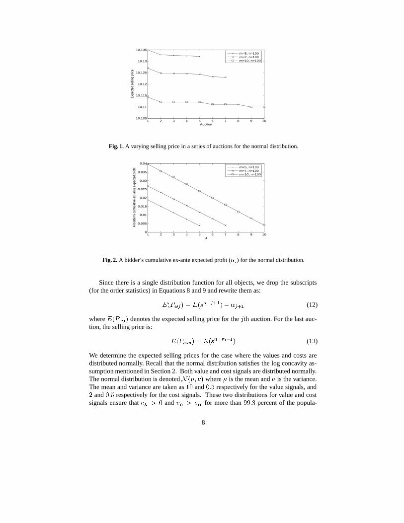
Fig. 1. A varying selling price in a series of auctions for the normal distribution.

1 2 3 4 5 6 7 8 9 100

0.005

0.01

0.015

0.02

0.025

0.03

0.035

0.04

J

A bi

dder

’s c

umul

ativ

e ex

−ant

e ex

pect

ed p

rofit m=5, n=100

m=7, n=100m=10, n=100

Fig. 2. A bidder’s cumulative ex-ante expected profit (��) for the normal distribution.

Since there is a single distribution function for all objects, we drop the subscripts(for the order statistics) in Equations 8 and 9 and rewrite them as:

����� � ��������� ���� (12)

where ����� denotes the expected selling price for the �th auction. For the last auc-tion, the selling price is:

���� � ������� (13)

We determine the expected selling prices for the case where the values and costs aredistributed normally. Recall that the normal distribution satisfies the log concavity as-sumption mentioned in Section 2. Both value and cost signals are distributed normally.The normal distribution is denoted � � !� where is the mean and ! is the variance.The mean and variance are taken as �� and �� respectively for the value signals, and� and �� respectively for the cost signals. These two distributions for value and costsignals ensure that �� � � and �� � �� for more than ���� percent of the popula-

8

1 2 3 4 5 6 7 8 9 100.0103

0.0104

0.0105

0.0106

0.0107

0.0108

0.0109

0.011

Auction

Win

ner’s

exp

ecte

d pr

ofit

m=5, n=100m=7, n=100m=10, n=100

Fig. 3. The winner’s expected profit for the normal distribution.

1 1.5 2 2.5 3 3.5 4 4.5 510.105

10.11

10.115

10.12

10.125

10.13

10.135

Auction

Expe

cted

sel

ling

pric

e m=5, n=95m=5, n=97m=5, n=100

Fig. 4. The effect of competition on the expected selling price.

tion. Since the distribution for value is ���� �� � and that for cost is ��� �� �, thedistribution for the surplus (i.e., the difference of value and cost) is ��� �� [5].

The first and second order statistics for the standard normal distribution (i.e., ��� ��)have been tabulated [9]. We use these tables to obtain the first and second order statis-tics for ��� �� as follows. Since the distributions ��� �� and ��� �� differ only intheir means, the first order statistics for ��� �� is obtained by adding � to the first or-der statistics for ��� ��. Likewise, the second order statistics for ��� �� is obtainedby adding � to the second order statistics for ��� ��. Substituting these statistics inEquations 12 and 13 we get the expected selling price for each of the � auctions.

The variation in the selling price (i.e., ��������������) for different auctions isshown in Figure 1. As shown in the figure, the expected selling price decreases from oneauction to the next. A bidder’s ex-ante probability of winning the �th auction (i.e., � � ���������) is increasing in �. A bidder’s cumulative ex-ante expected profit from auc-tions � to � (i.e., ��) is shown in Figure 2. This profit decreases from one auction to thenext. The winner’s expected profit (i.e., ����� � ��������� �������� ����)also drifts downward as shown in Figure 3.

9

1 1.5 2 2.5 3 3.5 4 4.5 50.36

0.362

0.364

0.366

0.368

0.37

0.372

0.374

0.376

0.378

0.38

Auction

Win

ner’s

exp

ecte

d pr

ofit

m=5, n=95m=5, n=97m=5, n=100

Fig. 5. The effect of competition on the winner’s expected profit.

The effect of competition. In order to study the effect of competition, we fix thenumber of objects (�) and vary the number of bidders (�) for the example scenariodescribed above. We know from Equations 12 and 13 that the expected selling pricedepends on the �������� and �� . For the normal distribution, both �������� and�� decrease with � [9]. Figure 4 is a plot of the expected selling price for different �. Asseen in the figure, an increase in the number of bidders (�) increases the selling price ofeach of the � objects. Figure 5 is a plot of the winner’s expected profit for different �.As seen in the figure, an increase in the number of bidders (�) decreases the winner’sprofit for each of the � objects. In summary, for the normal distribution, an increase incompetition (i.e., increase in �) increases the selling price and decreases the winner’sexpected profit for each individual auction in a series. Since there is more competitionin an agent-based setting than in a human setting [16], the expected selling prices arehigher for the former setting relative to the latter, while the winner’s expected profits arelower. In other words these two settings differ in terms of their equilibrium outcomes.

5 Related Work

Existing work has studied the dynamics of the selling price of objects for sequentialauctions [15, 20, 14, 3]. However, a key limitation of this work is that it focuses on ob-jects that are either exclusively private value or exclusively common value. For instance,Ortega-Reichert [15] determined the equilibrium for sequential auctions for two privatevalue objects using the first price rules. Weber [20] showed that in sequential auctionsof identical objects with risk neutral bidders who hold independent private values, theexpected selling price is the same for each auction. On the other hand, Milgrom andWeber [14] studied sequential auctions in an interdependent values model with affili-ated5 signals. They showed that expected selling prices have a tendency to drift upward.

5 Affiliation is a form of positive correlation. Let �, �, . . . , � be a set of positively corre-lated random variables. Positive correlation roughly means that if a subset of �s are large,then this makes it more likely that the remaining �s are also large.

10

This may be because earlier auctions release information about the values of objects andthereby reduce the winner’s curse problem.

In contrast to the above theoretical results, there has been some evidence in real-world sequential auctions for identical objects – for art and wine auctions in particular –that the prices tend to drift downward [1, 13]. Because the theoretical models mentionedabove predict either a stochastically constant or increasing price, this fact has beencalled the declining price anomaly. Mc Afee and Vincent [13] consider two identicalprivate value objects and using the second price sealed bid rules, they show that thedeclining price anomaly cannot be explained even if the bidders are considered to berisk averse. Furthermore, Mc Afee and Vincent acknowledge that extending their twoobject model to a general � object case is complex and they have not been able to comeup with such a generalisation. We therefore adopted the model proposed by Bernhardtand Scoones for two private value objects [3] and generalised it to � � � objects withboth common and private values. Bernhardt and Scoones [3] showed that if the numberof bidders for the first and second auctions are � and �� � �� respectively, the sellingprice can decline (by considering an example scenario). Our model is a generalizationof [3] since we consider � � � objects with both common and private values and showthe decline in price for an example setting. Although the objects we consider have bothcommon and private values, each bidder receives its signals for an auction just beforethe auction begins. In other words, during an auction, the information that bidders obtainabout the others’ value signals does not carry forward to subsequent auctions. Hence,as in the case of [3], our model too shows a decline in the selling price.

An important issue in the study of auctions with multi-dimensional signals is thatof efficiency of auctions. In general, auctions with multi-dimensional signals have beenshown to be inefficient [4]. Since our model involves two dimensional signals, we stud-ied the efficiency property in [7]. This study shows that the efficiency of auctions inan agent-based setting is higher than that in an all human setting. This is because ofthe fact that an agent based setting leads to more competition than an all human setting[16].

6 Conclusions and future work

This paper has analyzed a model for sequential auctions for objects with private andcommon values in an uncertain information setting. We first determined equilibriumstrategies for each auction in a sequence. Then we showed that even if the value and costsignals are distributed identically across objects, then in accordance with Ashenfelter’sresult [1], the expected selling price can decline in later auctions. Also, the winner’sexpected profit can decline in later auctions. We also showed that, due to differingcompetition, the equilibrium outcome in an agent-based setting differs from that in anall human setting.

There are many interesting directions for future work. First, our present focus wason determining how the expected selling price varies in a series of English auctions.However, in order to generalize our results, we intend to extend the analysis to otherauction forms. Second, we studied the case where bidders received the cost and valuesignals for an object just before the auction. In future, we will extend the analysis to the

11

case where the values and costs for the last ��� �� objects can be determined from thesignals for the first object (i.e., values and costs are perfectly correlated).

References

1. O. Ashenfelter. How auctions work for wine and art. Journal of Economic Perspectives,3(221):23–36, 1989.

2. J. P. Benoit and V. Krishna. Multiple-object auctions with budget constrained bidders. Reviewof Economic Studies, 68:155–179, 2001.

3. D. Bernhardt and D. Scoones. A note on sequential auctions. The American EconomicReview, 84(3):653–657, 1994.

4. P. Dasgupta and E. Maskin. Efficient auctions. Quarterly Journal of Economics, 115:341–388, 2000.

5. M. Dwass. Probability and Statistics. W. A. Benjamin Inc., California, 1970.6. W. Elmaghraby. The importance of ordering in sequential auctions. Management Science,

49(5):673–682, 2003.7. S. S. Fatima, M. Wooldridge, and N. R. Jennings. Sequential auctions for objects with

common and private values. In Proceedings of the Fourth International Conference on Au-tonomous Agents and Multi-Agent Systems, Utrecht, Netherlands (to appear), 2005.

8. J. K. Goeree and T. Offerman. Competitive bidding in auctions with private and commonvalues. The Economic Journal, 113(489):598–613, 2003.

9. H. L. Harter. Expected values of normal order statistics. Biometrika, 48(1/2):151–165, 1961.10. B. Katzman. A two stage sequential auction with multi-unit demands. Journal of Economic

Theory, 86:77–99, 1999.11. V. Krishna. Auction Theory. Academic Press, 2002.12. J. Laffont. Game theory and empirical economics: The case of auction data. European

Economic Review, 41:1–35, 1997.13. R. P. McAfee and D. Vincent. The declining price anomaly. Journal of Economic Theory,

60:191–212, 1993.14. P. Milgrom and R. J. Weber. A theory of auctions and competitive bidding II. In P. Klemperer,

editor, The Economic Theory of Auctions. Edward Elgar, Cheltenham, U.K, 2000.15. A. Ortega-Reichert. Models of competitive bidding under uncertainty. Technical Report 8,

Stanford University, 1968.16. E. J. Pinker, A. Seidman, and Y. Vakrat. Managing online auctions: Current business and

research issues. Management Science, 49(11):1457–1484, 2003.17. C. Pitchik and A. Schotter. Perfect equilibria in budget-constrained sequential auctions: An

experimental study. Rand Journal of Economics, 19:363–388, 1988.18. T. Sandholm and S. Suri. BOB: Improved winner determination in combinatorial auctions

and generalizations. Artificial Intelligence, 145:33–58, 2003.19. W. Vickrey. Counterspeculation, auctions and competitive sealed tenders. Journal of Fi-

nance, 16:8–37, 1961.20. R. J. Weber. Multiple-object auctions. In R. Engelbrecht-Wiggans, M. Shibik, and R. M.

Stark, editors, Auctions, bidding, and contracting: Uses and theory, pages 165–191. NewYork University Press, 1983.

21. M. P. Wellman, W. E. Walsh, P. R. Wurman, and J. K. McKie-Mason. Auction protocols fordecentralised scheduling. Games and Economic Behavior, 35:271–303, 2001.

22. R. E. Wiggans and C. M. Kahn. Multi-unit pay your-bid auctions with variable rewards.Games and Economic Behavior, 23:25–42, 1998.

12

Appendix

A Proof of Theorem 1

Proof. We consider each of the � auctions by reasoning backwards.

– �th auction. To begin, consider the �th auction for which there are ���� ��bidders. Since this is the last auction, an agent’s bidding behaviour is the same asthat for the single object case. Hence, the equilibrium for this auction is the sameas that in Equation 3 with � replaced with �� � � ��. For � � �� � � � ��, let��� denote an agent’s cumulative ex-ante expected profit from auctions � to �.Recall that although the bidders know the distribution (from which the cost andvalue signals are drawn) before the first auction begins, they draw the signals forthe �th auction only after the �� � �� earlier auctions end. Since � �� is the ex-anteexpected profit (i.e., it is computed before the bidders draw their signals for the �thauction), it is the same for all participating bidders. Thus, we will simplify notationby dropping the subscript � and denote � �� simply as �� We know from Equation 5that:

� ��

��� �� ������

�� ������ �� (14)

This is because all the ���� �� agents that participate in the �th auction haveex-ante identical chances of winning it. Note that the right hand side of Equation 14does not depend on �. In other words, since bidders receive their signals for the �thauction after the ��� ��th auction, the ex-ante expected profit for the �th auction(before the ��� ��th auction ends) is the same for all the ���� �� bidders.

– �� � ��th auction. Consider the ��� ��th auction. During this auction, a bidderbids if (�������� � �) or ( � ���������). Hence, a symmetricequilibrium for the �� � ��th auction is obtained by substituting � � � � � inEquation 7. We know from Equation 4, that the expected selling price for the singleobject case is the second order statistic of the surplus. The difference between theequilibrium bids for the single object case and the �� � ��th auction of the �objects case is � (see Equations 3 and 7). Hence, the expected selling price forthe �����th auction is ������

�� ���. This implies that the winner’s expectedprofit for the ��� ��th auction is:

�������� � �������� �� ������

�� � � (15)

– First ��� �� auctions. Consider the �th auction where � � � � �� �. We nowfind ��� � � � � ���. Since the number of bidders for the �th auction is ��� � ��and each bidder has ex-ante equal chances of winning, the probability that a bidderwins the �th (for � � �� � � � ��) auction (denoted ��) is:

�� � ����� � �� (16)

13

This implies that, for � � �� � � � ��, �� is:

�� � �� ����� ���� (17)

Generalising Equation 15 to the first ����� auctions, we get the winner’s expectedprofit ( �����) as:

����� � �������� �� �������� � ���� (18)

Consequently, a bidder’s optimal bid for the �th auction is obtained by discountingthe single object equilibrium bid by ����. Hence, we get the equilibrium bids inEquation 7.

B Proof of Theorem 2

Proof. It is important to note that for the �th (� � �� � � � ��) auction, the bids in The-orem 1 are similar to those in Equation 3 (for the single object case), except that eachbid in the former case is obtained from the corresponding bid in the latter by shiftingthe latter by the constant ����. Since ���� is the same for all participating bidders, therelative positions of bidders for each of the � auctions remains the same as that forthe corresponding single object case. Hence, for each of the � auctions, the winner isthe bidder with the highest surplus for that auction. Consequently, the expected sellingprice for the �th (for � � �� � � � �� � �) auction is ����� � �������� � � ����.For the last auction (which is similar to a single object auction), the selling price is: ���� � ������

�.

C Proof of Theorem 3

Proof. The �th auction is identical to the single object case. Hence, the expected profitfor this auction is

���� � ������ �� ������

�

Since the difference between the expected selling price for the single object case andthe �th (for � � �� � � � �� � �) auction of the � objects case is ����, the winner’sexpected profit for the �th auction is:

����� � �������� �� �������� � ����

14