AN ALTERNATIVE METHOD FOR REPRESENTING FIXED CAPITAL WITHIN A SRAFFIAN FRAMEWORK: an

exposition

Felix Ibanez. Departamento de Analisis Economico II. UNED

Mariano Matilla. Depto. de Economia Aplicada Cuantitativa I. UNED

Ruben Osuna. Departamento de Analisis Economico I. UNED

Abstract

This paper contains an exposition of the new method for representing Fixed Capital intro-

duced in Ibanez and Matilla (2004) and Ibanez, Matilla and Osuna (2004), which avoids

the machines at different stages of wear and tear being priced, by contrast to the standard

method that treats fixed capital in terms of joint production. The new method deals domi-

nantly with periodic allowance for depreciation of fixed capital stock, instead of book val-

ues, in the set of equations representing the successive production processes used by a

firm for obtaining a commodity. The lump sum of these equations is the integrated process

corresponding to this commodity, which allows the prices of marketed commodities being

determined. The resulting integrated price system associated with this new method adopts

a formal shape very similar to the standard price system corresponding to the Sraffian Cir-

culating Capital model, and, in addition, shares all the properties of the latter.

J.E.L. classification: D24.

Keywords: Fixed Capital; Sraffa; von Neumann.

1. INTRODUCTION It is common place within the literature on Fixed Capital in the Sraffian Theory of Prices, that the

general way to treat the former is to represent it in terms of joint production, wherein the same ma-

chine in successive phases of wear and tear is considered as a qualitatively differentiated commodity.

See for instance Sraffa (1960, Chap. 10), Morishima (1969, Ch. 6), Garegnani (1970), Roncaglia

(1971) (1978, pp. 36-48), Pasinetti (1973), Baldone (1974), Varri (1974), Schefold (1978)(1980) and

Kurz and Salvadori (1995, Chaps. 7 and 9), among other authors. This treatment of Fixed Capital

stems from the Classical tradition, as is reflected in Sraffa (1960, Appendix D), and, at the same time,

corresponds to the way that von Neumann (1945) tackles this topic in his pioneering contribution.

Henceforth, this method is sometimes referred to as the Torrens rule, since this latter author originally

devised the method.

This treatment of Fixed Capital is unanimously considered within this field of literature as a general

method to deal with this topic, because it allows determining, simultaneously with the price of com-

modities: i) periodic allowance for depreciation of fixed capital stock; ii) successive book values over

time for the latter; and iii) optimal truncation of economic lifespan for machines.

On the other hand, we devised another method for representing Fixed Capital introducing a slight

modification in the set of equations that materialize the standard method. As becomes clear in the two

introductory papers to this new method, Ibanez and Matilla (2004) and Ibanez, Matilla and Osuna

(2004), the sole formal difference between the Torrens rule and this new method hinges on the value

of fixed capital stock used to calculate de profit rate in each period.

In this sense, the new method, in contrast to the standard one, uses the value of fixed capital stock

when new in all cases, though modified by some parameters; instead of considering the machines at

different stages of wear and tear as differentiated commodities, in other words, instead of the latter

being priced, as the standard method requires.

Hence, from this fact it can be guessed that the new method is able to do the same things as those

pointed above for the standard one. In this sense, this paper gives an exposition of those possibilities

for the new method.

The argument featuring the new method leads to device an integrated process that results from

simple summation of the equations displaying the successive use of a fixed capital stock over time for

producing a commodity. This integrated process makes possible the prices of marketed commodities

being determined, and then, periodic allowance for depreciation and successive book values of fixed

capital stock being ascertained.

One peculiarity of this integrated process is that it entails in all cases average depreciation of fixed

capital stock over the number of periods considered, whereupon a proportional allowance for depre-

ciation for each machine separately arises in this integrated process; even though periodic allowance

for depreciation of fixed capital stock is far from being straight-line depreciation in most cases.

This paper is structured as follows. The second section is devoted to conceptual peculiarities of

Fixed Capital, as well as the Sraffian framework for the analysis. The third section contains an exposition

of the new method, focusing on allowance for depreciation and book values of fixed capital stock. The

2/27

fourth section deals with the selection of optimal truncation. Finally, we point out some concluding re-

marks.

2. FIXED CAPITAL AND ANALYTICAL FRAMEWORK Let us refer to a generic production process that obtains one single commodity. As regards Fixed Capi-

tal, the following considerations are taken into account:

a) By definition, a machine endures more than one production period. Otherwise, it is considered a

circulating capital good. Hence, machines are subject to gradual wear and tear depreciation over several

production cycles in succession, until they are scrapped and replaced by new ones. In contradistinction

to circulating capital goods, which are to be replaced at the end of a single production period for begin-

ning another one1.

b) There is no room for machines perfectly durable by means of periodic reposition of their com-

ponent parts. Otherwise, we consider that such machines consist of their different spare parts, periodi-

cally replaceable, as independent fixed capital goods. Everlasting machines have no specific entity.

Hence, physical or technical lifetime corresponding to a single machine (i.e. its maximal economic life-

time) is finite and taken for granted, in relation to the state of technological knowledge.

c) Taking as one unit of time the duration of our generic production process, the economic lifetime

of j-th machine ( production periods) used in this process is not actually a technical datum. It may vary

within the interval

jt

fjj t t ≤≤2 2, as is a parameter, depending upon commodities’ price and dis-

tributive variables value.

jt

d) The use of machines in a production process entails additional expenses over their economic

lifetime under the title of maintenance, repair and partial reposition (replacement of spare parts). Those

expenses do decisively affect to the length of machines economic lifetime.

e) Some of those expenses cannot be attributed to a single production cycle. They are to be con-

sidered as overhead expenses corresponding to the whole or part of machines economic lifetime. Not-

withstanding this, we consider them to be allocated to the period in which the payment for those ex-

penses takes place.

The longer the economic lifetime of machines is, the lesser is its periodic depreciation quota, al-

though the latter could in general be irregularly distributed over time. Notwithstanding, it normally gives

rise to larger maintenance, repair and partial reposition expenses.

Whenever such additional expenses grow up (though not necessarily in a monotonic way) as long

as machines are utilized over successive production cycles, it is said that machines have decreasing

efficiency. If such expenses are identical period after period, it is said that machines have constant

1 As obvious, to distinguish clearly fixed from circulating capital goods we do not consider the existence of

stocks for the latter in order to successive production cycles may take place without interruption.

2 stands for technical or maximum lifetime of j-th machine. fjt

3/27

efficiency. If such expenses decline, though not necessarily in a monotonic way, it is said that ma-

chines are subject to increasing efficiency over time.

Our argument is developed within a standard Sraffian framework, with features as follows:

a) Absence of joint production: each production process only obtains a positive quantity of one

commodity. We consider commodities2≥n 3. Then, each technique as a whole consists of n

production processes, one for each commodity. The first h ( nh <≤1 ) commodities are ma-

chines, the rest circulating capital goods.

b) Production processes are point/flow input-point output.

c) By definition, the duration of a production process is the time span elapsed from when the first

input is incorporated until the corresponding output is obtained. We consider that all production

processes are of the same duration; and we take the latter as one unit of time.

d) Homogeneous labor is the sole primary input.

e) Wages are paid ex post, i.e. at the end of each production process. Thus, periodic payment of

wages in each production process coincides with its duration.

f) Moreover, profit rate is referred to the unit of time that we have assumed above, as well as the

calculation of periodic allowance for depreciation for fixed capital goods.

g) Profit and wage rates are uniform over the whole economic system.

h) Machines at different stages of wear and tear are re-used within the same process that obtains

the corresponding commodity. It means that scrapped machines in a production process have no

residual value, i.e. they are not demanded by consumers, or by firms operating in other process

for obtaining a different commodity. If the contrary, joint production processes, in strict sense,

arise4.

3. THE NEW METHOD FOR REPRESENTING FIXED CAPITAL Let us focus on the production process that obtains the n-th commodity within the technique as a

whole that we are considering.

3.1 Mathematical notation a) Let us suppose that the h machines are utilized for producing the n-th commodity. Then,

stands for the economic lifetime of j-th machine, i.e. the number of production

cycles that this machine endures.

2 1,jt j≥ = … ,h

b) Let ( )1. . . , , ht lc m t t= … be the least common multiple of the h machines’ economic life-

time.

3 With only one good into consideration, there is no possibility of exchange between commodities, and so a

Market Economy is actually ruled out.

4 See Appendix 1, wherein this possibility is considered.

4/27

c) stands for the output of the n-th commodity obtained respectively in each

period. It is not necessarily constant over time due to machines’ variable efficiency in general.

1, ,jb j t= …

d) denotes a row vector of n components, the first h of which are positive, the rest zero. It

represents the number of brand-new machines of each class composing the fixed capital stock used to

produce the n-th commodity.

nk

e) stands for periodic allowance for depreciation of fixed capital stock. 1, ,j j∆ = … t

tf) denotes a row vector of n components, the first h of which are zero. The 1, ,j =ja …

1≥m remaining ones ( hnm −= ) represent the material inputs employed in successive periods to

obtain the output, as well as those inputs corresponding to maintenance, repair and partial reposition

expenses associated with the utilized machines. Thus, is not necessarily constant over time, due to

machines’ variable efficiency in general.

ja

g) stands for the input of direct labor. It also varies over time according to ma-

chines’ efficiency pattern, and may include labor input corresponding to maintenance, repair and partial

reposition expenses for machines.

1, ,jl j t= …

h) Wage rate is represented by w, and r stands for the profit rate, referred to the unit of time that

we have assumed above.

i) Let p be a column vector of n components. It stands for the price vector of marketed commodi-

ties. The first h components correspond to the price of machines when new, and the n-th component to

the price for the n-th commodity that we are considering.

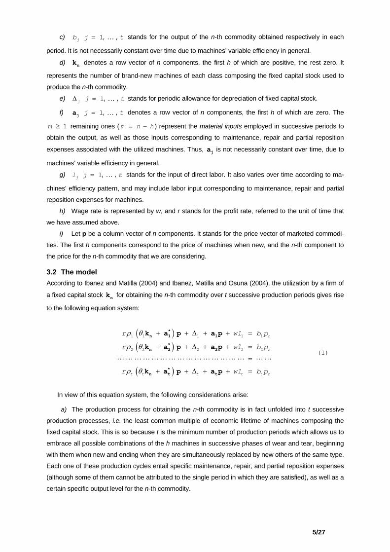
3.2 The model According to Ibanez and Matilla (2004) and Ibanez, Matilla and Osuna (2004), the utilization by a firm of

a fixed capital stock for obtaining the n-th commodity over t successive production periods gives rise

to the following equation system:

nk

( )( )

( )

1 1 1 1 1

2 2 2 2 2

n

n

t t t t t n

r w

r w

r w

ρ θ

ρ θ

ρ θ

+ + ∆ + + =

+ + ∆ + + =

=

+ + ∆ + + =

*n 1 1

*n 2 2

*n t t

k a p a p

k a p a p

k a p a p

l b p

l b p

l b p

(1)

In view of this equation system, the following considerations arise:

a) The production process for obtaining the n-th commodity is in fact unfolded into t successive

production processes, i.e. the least common multiple of economic lifetime of machines composing the

fixed capital stock. This is so because t is the minimum number of production periods which allows us to

embrace all possible combinations of the h machines in successive phases of wear and tear, beginning

with them when new and ending when they are simultaneously replaced by new others of the same type.

Each one of these production cycles entail specific maintenance, repair, and partial reposition expenses

(although some of them cannot be attributed to the single period in which they are satisfied), as well as a

certain specific output level for the n-th commodity.

5/27

Naturally, each machine is replaced 1, ,jt t j h= … times by a new other of the same type

throughout t production periods. Whenever this event may occur, it is unnecessary to resort to the free

disposal axiom. Since eventual elimination costs for scrapped machines may be incorporated either as

material inputs within aj and/or as direct labor within lj, in the corresponding equation to the production

period when this fact takes place.

b) Without loss of generality, it can be considered that these t processes take place in succession

within a firm, say, since the corresponding fixed capital stock is re-used period after period for obtaining

the n-th commodity until this stock is completely replaced at the end of t-th period.

c) Either of the equations of system (1) indicates, as is obvious, that in each period the lump sum

of profits, calculated using the value of fixed and circulating capital stock displayed in the firm’s balance

sheet at the beginning of each period, plus production costs, equals the value of the output obtained in

the corresponding production period. Naturally, costs include depreciation expense of fixed capital stock

plus costs due to consumed material inputs, and to direct labor employed in the corresponding produc-

tion period.

d) The fact of a profit rate calculated using the fixed capital stock valued as new in all periods,

though modified by parameters θ , such as appears in all equations of system (1), has been explained in

Ibanez and Matilla (2004) and Ibanez, Matilla and Osuna (2004) as follows.

Since at the end of each period depreciation expense corresponding to the fixed capital stock is

charged by the firm, this fact give rise, after net profit distribution, to an additional circulating capital. This

latter is in fact a Replacement Fund for fixed capital, to be eventually utilized to replace worn-out ma-

chines by new ones of the same type.

Notwithstanding this, the Replacement Fund, when positive, can be temporarily used as an internal

financial source for the firm: i) to adjust circulating capital required to begin a new production cycle; ii) to

create stocks of circulating capital goods. Both possibilities make that circulating capital displayed in (1),

for instance in the j-th period ( ), can differ from the material inputs consumed in the same period ( ). *ja ja

Parameters 1, ,j j tθ = … appearing at (1) are always positive. When one of them is lower than

unity in one single period, it means that the whole or part of the Replacement Fund corresponding to

preceding periods has been used to reduce firm’s liabilities, so that the available Replacement Fund is

smaller than Accumulated Depreciation of fixed capital stock at this date. Obviously, it holds that

1 1θ = .

When parameter jθ is larger than unity, it means that the Replacement Fund and Accumulated De-

preciation have become negative, due to the fixed capital stock is subject to increasing efficiency. Then,

at the beginning of j-th period, the firm has to inject the amount of the negative Replacement Fund as

additional circulating capital to begin firm’s operations.

Parameters 1, ,j j tρ = … appearing at (1) are always positive. When jρ is lower than 1, it

means that the whole or part of the Replacement Fund corresponding to preceding periods has been

invested outside the firm for rendering some positive financial revenue, which complements the revenue

obtained from selling firm’s output. When jρ is larger than 1, it means that the referred financial revenue

has become eventually negative in the j-th period.

6/27

These latter parameters have been introduced to make the firm’s rate of return, calculated from the

whole of assets displayed in the firm’s balance sheet at the beginning of each period, uniform throughout

all periods. This precisely requires distorting when necessary, according to the preceding paragraph, the

operating profit rate r in the corresponding period. Obviously, it holds that 1 1ρ = , since the firm is not

receiving any financial revenue in the first period.

In view of system (1), it is essential noting that this method for representing Fixed Capital does not

need machines at different stages of wear and tear being priced, in opposition to the Torrens rule proce-

dure.

3.3 The integrated process As one can see in (1), the production process that obtains the n-th commodity consists in fact of t pro-

duction processes by mere utilization of machines. These processes are in general different from one

another, because used machines have variable efficiency over their economic lifetime.

Thus, commodities’ price as well as distributive variables value must satisfy simultaneously all

equations of system (1), which are in general different from one another.

Hence, any linear combination of system (1) automatically holds; for instance, the one resulting

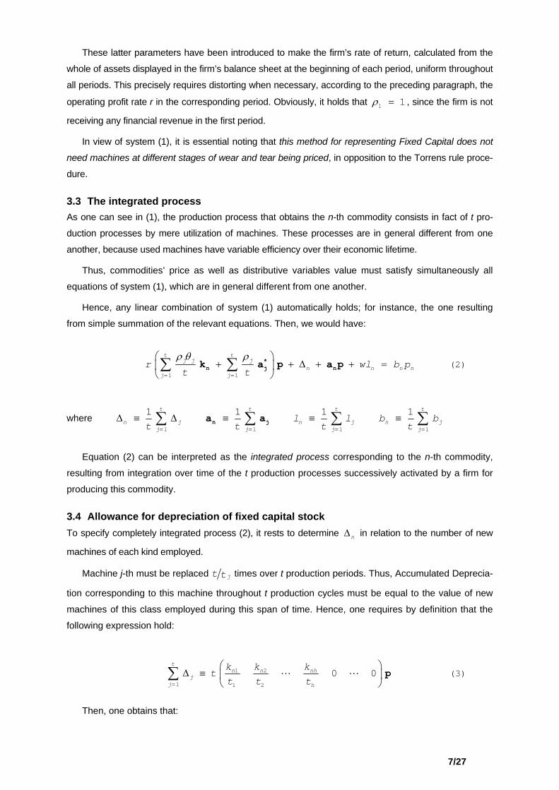
from simple summation of the relevant equations. Then, we would have:

1 1

t tj j j

n nj j

r wt t

ρ θ ρ

= =

⎛ ⎞+ + ∆ + + =⎜ ⎟

⎝ ⎠∑ ∑ *

n j nk a p a p n nl b p (2)

where 1 1 1

1 1 1t t t

n j n j nj j j

l l bt t t= = =

∆ ≡ ∆ ≡ ≡ ≡∑ ∑ ∑n ja a1

1 t

jj

bt =∑

Equation (2) can be interpreted as the integrated process corresponding to the n-th commodity,

resulting from integration over time of the t production processes successively activated by a firm for

producing this commodity.

3.4 Allowance for depreciation of fixed capital stock To specify completely integrated process (2), it rests to determine n∆ in relation to the number of new

machines of each kind employed.

Machine j-th must be replaced jt t times over t production periods. Thus, Accumulated Deprecia-

tion corresponding to this machine throughout t production cycles must be equal to the value of new

machines of this class employed during this span of time. Hence, one requires by definition that the

following expression hold:

1 2

1 1 2

0 0t

n n nhj

j h

k k kt

t t t=

⎛ ⎞∆ ≡ ⎜ ⎟

⎝ ⎠∑ p (3)

Then, one obtains that:

7/27

1 2

1 2

0 0n n nhn

h

k k kt t t

⎛ ⎞∆ = ≡⎜ ⎟

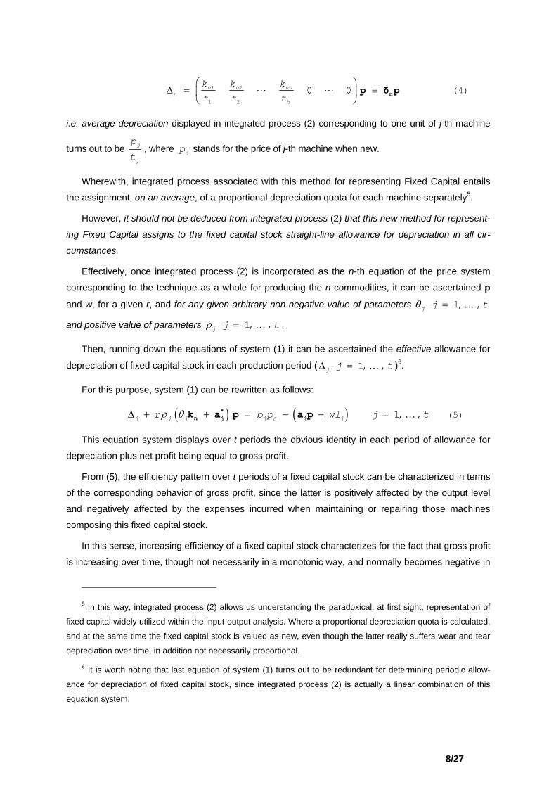
⎝ ⎠np δ p (4)

i.e. average depreciation displayed in integrated process (2) corresponding to one unit of j-th machine

turns out to be j

j

p

t, where stands for the price of j-th machine when new. jp

Wherewith, integrated process associated with this method for representing Fixed Capital entails

the assignment, on an average, of a proportional depreciation quota for each machine separately5.

However, it should not be deduced from integrated process (2) that this new method for represent-

ing Fixed Capital assigns to the fixed capital stock straight-line allowance for depreciation in all cir-

cumstances.

Effectively, once integrated process (2) is incorporated as the n-th equation of the price system

corresponding to the technique as a whole for producing the n commodities, it can be ascertained p

and w, for a given r, and for any given arbitrary non-negative value of parameters 1, ,j j tθ = …

and positive value of parameters 1, ,j j tρ = … .

Then, running down the equations of system (1) it can be ascertained the effective allowance for

depreciation of fixed capital stock in each production period ( 1, ,j j t∆ = … )6.

For this purpose, system (1) can be rewritten as follows:

( ) ( ) 1, ,j j j j n jr b p wl jρ θ∆ + + = − + =*n j jk a p a p … t

(5)

This equation system displays over t periods the obvious identity in each period of allowance for

depreciation plus net profit being equal to gross profit.

From (5), the efficiency pattern over t periods of a fixed capital stock can be characterized in terms

of the corresponding behavior of gross profit, since the latter is positively affected by the output level

and negatively affected by the expenses incurred when maintaining or repairing those machines

composing this fixed capital stock.

In this sense, increasing efficiency of a fixed capital stock characterizes for the fact that gross profit

is increasing over time, though not necessarily in a monotonic way, and normally becomes negative in

5 In this way, integrated process (2) allows us understanding the paradoxical, at first sight, representation of

fixed capital widely utilized within the input-output analysis. Where a proportional depreciation quota is calculated,

and at the same time the fixed capital stock is valued as new, even though the latter really suffers wear and tear

depreciation over time, in addition not necessarily proportional.

6 It is worth noting that last equation of system (1) turns out to be redundant for determining periodic allow-

ance for depreciation of fixed capital stock, since integrated process (2) is actually a linear combination of this

equation system.

8/27

initial periods. Thus, allowance for depreciation is also normally negative in the beginning periods.

Hence, since (3) must hold, accumulated depreciation is to be positive in ending periods, and so,

allowance for depreciation tends to be increasing over time, though not necessarily in a monotonic

way, according as gross profit increases.

In contrast, decreasing efficiency conveys that gross profit is decreasing over time, though not

necessarily in a monotonic way, and normally becomes negative in ending periods. Thus, allowance

for depreciation tends to decrease over time as to become eventually negative in ending periods.

Constant efficiency can be considered as an intervening and, at the same time, odd case with re-

spect to the two preceding ones. Gross profit is constant over time, so that allowance for depreciation

tends to be always positive.

Furthermore, one can easily deduce from (5) that all the equations are in fact identical only in the

unrealistic case of: i) machines having constant efficiency at given prices; ii) all parameters being 1;

and iii) circulating capital value being constant over time. Thus, only in this unrealistic case it

necessarily turns out that

*ja p

1, ,j n j t∆ = ∆ = … , i.e. straight-line depreciation for fixed capital stock.

However, in case of machines having variable efficiency, or parameters not all being 1, or different

circulating capital requirements over time, allowance for depreciation varies from period to period,

since some equations of (5) differ from one another.

So far, we have calculated , i.e. periodic allowance for depreciation of fixed

capital stock employed to produce the n-th commodity.

1, ,j j∆ = … t

However, although unnecessary, if one wished to determine allowance for depreciation for each ma-

chine separately, we can express periodic depreciation of fixed capital stock as follows:

1, ,j j t∆ ≡ =jδ p …

where stands for an unknown row vector of n components, the first h of which are eventually non-

zero, the rest zero; in the same way as vector has been defined in (4).

jδ

nδ

Thus, according to (5), there would be in general one equation ( jβ=jδ p ) with h unknowns (the h

components eventually non-zero of ) for each production period. That is, there would be in general t

equations available for determining unknowns. Hence, only in the trivial case of employing one

machine, its depreciation pattern over time can be automatically ascertained

jδ

ht ×7.

Notwithstanding this, the depreciation pattern of each machine separately can be ascertained in the

particular case of all machines having the same economic lifetime, despite it normally holds that

t

7 It can also be ascertained the depreciation pattern of each machine separately in the unrealistic case, con-

sidered above, of straight-line depreciation, in which it holds that 1, ,j n j∆ = ∆ = … . Then, we would

have that , where vector has been already defined in (4). 1, ,j= =j nδ δ … t nδ

9/27

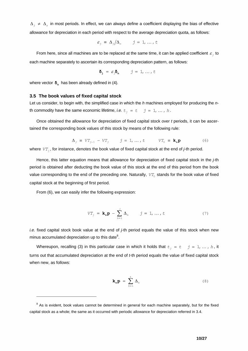
j∆ ≠ ∆n in most periods. In effect, we can always define a coefficient displaying the bias of effective

allowance for depreciation in each period with respect to the average depreciation quota, as follows:

1, ,j j n j tε ≡ ∆ ∆ = …

From here, since all machines are to be replaced at the same time, it can be applied coefficient jε to

each machine separately to ascertain its corresponding depreciation pattern, as follows:

1, ,j j tε= =j nδ δ …

where vector has been already defined in (4). nδ

3.5 The book values of fixed capital stock Let us consider, to begin with, the simplified case in which the h machines employed for producing the n-

th commodity have the same economic lifetime, i.e. 1, ,jt t j h= = … .

Once obtained the allowance for depreciation of fixed capital stock over t periods, it can be ascer-

tained the corresponding book values of this stock by means of the following rule:

(6) 1 01, ,j j jVT VT j t VT−∆ ≡ − = ≡ nk p…

where , for instance, denotes the book value of fixed capital stock at the end of j-th period. jVT

Hence, this latter equation means that allowance for depreciation of fixed capital stock in the j-th

period is obtained after deducting the book value of this stock at the end of this period from the book

value corresponding to the end of the preceding one. Naturally, stands for the book value of fixed

capital stock at the beginning of first period.

0VT

From (6), we can easily infer the following expression:

(7) 1

1, ,j

j hh

VT j t=

= − ∆ =∑nk p …

i.e. fixed capital stock book value at the end of j-th period equals the value of this stock when new

minus accumulated depreciation up to this date8.

Whereupon, recalling (3) in this particular case in which it holds that 1, ,jt t j h= = … , it

turns out that accumulated depreciation at the end of t-th period equals the value of fixed capital stock

when new, as follows:

1

t

hh=

= ∆∑nk p (8)

8 As is evident, book values cannot be determined in general for each machine separately, but for the fixed

capital stock as a whole; the same as it occurred with periodic allowance for depreciation referred in 3.4.

10/27

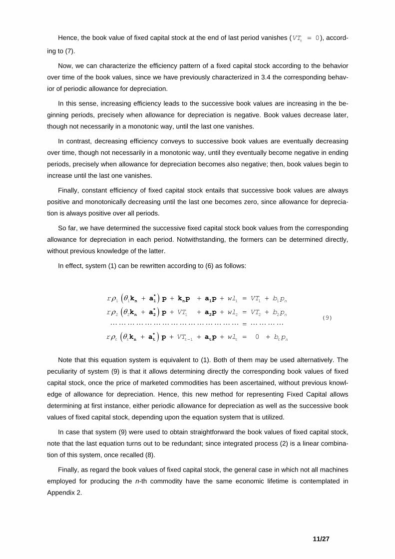
Hence, the book value of fixed capital stock at the end of last period vanishes ( ), accord-

ing to (7).

0tVT =

Now, we can characterize the efficiency pattern of a fixed capital stock according to the behavior

over time of the book values, since we have previously characterized in 3.4 the corresponding behav-

ior of periodic allowance for depreciation.

In this sense, increasing efficiency leads to the successive book values are increasing in the be-

ginning periods, precisely when allowance for depreciation is negative. Book values decrease later,

though not necessarily in a monotonic way, until the last one vanishes.

In contrast, decreasing efficiency conveys to successive book values are eventually decreasing

over time, though not necessarily in a monotonic way, until they eventually become negative in ending

periods, precisely when allowance for depreciation becomes also negative; then, book values begin to

increase until the last one vanishes.

Finally, constant efficiency of fixed capital stock entails that successive book values are always

positive and monotonically decreasing until the last one becomes zero, since allowance for deprecia-

tion is always positive over all periods.

So far, we have determined the successive fixed capital stock book values from the corresponding

allowance for depreciation in each period. Notwithstanding, the formers can be determined directly,

without previous knowledge of the latter.

In effect, system (1) can be rewritten according to (6) as follows:

( )( )

( )

1 1 1 1 1

2 2 1 2 2 2

1 0

n

n

t t t t t n

r wl

r VT wl VT

r VT wl

ρ θ

ρ θ

ρ θ −

+ + + + = +

+ + + + = +

=

+ + + + = +

*n 1 n 1

*n 2 2

*n t t

k a p k p a p

k a p a p

k a p a p

VT b p

b p

b p

(9)

Note that this equation system is equivalent to (1). Both of them may be used alternatively. The

peculiarity of system (9) is that it allows determining directly the corresponding book values of fixed

capital stock, once the price of marketed commodities has been ascertained, without previous knowl-

edge of allowance for depreciation. Hence, this new method for representing Fixed Capital allows

determining at first instance, either periodic allowance for depreciation as well as the successive book

values of fixed capital stock, depending upon the equation system that is utilized.

In case that system (9) were used to obtain straightforward the book values of fixed capital stock,

note that the last equation turns out to be redundant; since integrated process (2) is a linear combina-

tion of this system, once recalled (8).

Finally, as regard the book values of fixed capital stock, the general case in which not all machines

employed for producing the n-th commodity have the same economic lifetime is contemplated in

Appendix 2.

11/27

4. SELECTION OF OPTIMAL TRUNCATION According to (4), integrated process (2) corresponding to the n-th commodity can be rewritten as follows:

In matrix notation, we would have:

where , , and stand for the n-th row of matrices K*nK

*nA

*nB

*, A* and B*, respectively, defined below; and

is the n-th component of column vector L*nL

*, also defined below.

In the same way as that for producing the n-th commodity, it may occur that some of the h machines

into consideration could be employed for producing other commodities of our technique as a whole.

Wherewith, the corresponding integrated processes for those commodities can be obtained by applying

the same procedure.

Hence, expression (11) corresponds to the n-th equation of the following price system associated

with a technique as a whole for producing the n commodities considered from the outset:

( )1 1

t tj j j

n nj j

r wt t

ρ θ ρ

= =

⎛ ⎞+ + + + =⎜ ⎟

⎝ ⎠∑ ∑ *

n j n nk a p δ a p nl b p

*n

*

(10)

(12) r w+ + =* * *K p A p L B p

(11) * * *n n nr w+ + =K p A p L B p

In fact, price system (12) can be named integrated price system, insofar as it is composed of the in-

tegrated processes corresponding to the n commodities produced within the technique as a whole that

we are considering.

K* stands for the matrix of fixed and circulating capital stocks employed within each integrated

production process, modified by some non-negative parameters.

A* denotes the matrix of consumed material inputs. These latter include: i) average material inputs

consumed to obtain output in each industry; ii) average allowance for depreciation of fixed capital

stock; iii) average inputs related to maintenance, repair and partial reposition expenses for machines;

and iv) average inputs related to eventual elimination costs for scrapped machines.

L* stands for the vector of average direct labor input to produce the n commodities. Eventually it

may contain the average labor input corresponding to maintenance and repair of machines and elimi-

nation of scrapped ones, the same as that in the preceding paragraph.

B* denotes the output matrix. Each row represents the average bundle of commodities obtained as

output corresponding to each integrated production process. In fact, we are dealing with a diagonal

12/27

matrix, insofar as we are considering that machines have no scrap value, so that joint production is

excluded9.

Matrices K* and A*, according with their definition above, have the same zero components; hence,

the same canonical descomponibility. This is so, since for any integrated process, for instance the

corresponding to the n-th commodity, it holds that: i) parameters 1, ,j j tθ = … are non-negative

and not all zero ( 1 1θ = ); ii) parameters 1, ,j j tρ = … are all positive; iii) vectors and

have the same zero components, as obvious from (4); and iv) vectors and , then

, have the same zero components, as we argued in Ibanez, Matilla and Osuna (2004).

nk nδ

*ja 1, ,j t=ja …

na

From here, one can proceed to guarantee the existence of positive prices for marketed commodities,

associated with non-negative values for distributive variables, as though we were dealing with the famil-

iar Sraffian standard model of Circulating Capital and Simple Production. In this sense, one can guess

that in both cases the same standard assumptions are to be required for warranting positive prices. This

task will be carried out in a subsequent paper.

Integrated processes appearing in (12) have been devised by taking the economic lifetime of ma-

chines used to produce the corresponding commodity as a parameter. Nothing prevents us to select for

each value of the profit rate the optimal integrated price system; and hence, determining the optimal

truncation of machines’ economic lifetime corresponding to each integrated process.

Doing so, the conclusions that can be obtained about the behavior of machines’ economic lifetime in

an integrated process, according as profit rate varies, are identical to those already obtained by Baldone

(1974) and Schefold (1978)(1980), among others, within the standard treatment of Fixed Capital in terms

of joint production. In this sense, it is a well-known fact that a phenomenon similar to the reswitching of

techniques arises.

Moreover, it can be stated a truncation theorem for the new method, similar to those appearing in

Baldone (1974) and Schefold (1980), for the case of decreasing efficiency of fixed capital stock. Since in

this context allowance for depreciation and book values eventually become negative nearing the ending

periods of a truncation associated with a certain economic lifetime of machines.

In this sense, this theorem points out that it turns out profitable truncating the economic lifetime of

machines at the end of the period in which a negative fixed capital stock book value emerges.

This theorem requires a very simple proof in this new method, and it is contained in Appendix 4.

5. CONCLUDING REMARKS In view of (12), it is worth noting that the integrated price system corresponding to this new method for

representing Fixed Capital adopts a formal shape akin to the familiar Sraffian price system corre-

sponding to simple production and circulating capital, with processes of the same duration. The main

9 Consult Appendix 1 where machines are considered to have a positive scrap value.

13/27

difference between both referred price systems is that in the former one the stock of fixed and circulat-

ing capital differs from the flow consumed material inputs.

From here, one can guess that to warrant the price of marketed commodities being positive, asso-

ciated with non-negative values of distributive variables, the same standard assumptions are required

in both price systems. This fact reinforces Sraffa’s theory of prices, since the adoption of the new

method leads to a Fixed Capital model for price determination that is a complete and straightforward

generalization of a Circulating Capital model.

Furthermore, even those properties associated with the price system corresponding to this latter

model hold when one uses this new method for representing Fixed Capital, materialized in integrated

price system (12), whenever machines are deprived of any residual value as we are assuming so far.

Among these properties, it is to be underscored the existence of a decreasing w-r relationship, de-

pending on the numeraire, for any viable truncation, whenever the profit rate varies within an interval

ranging between zero and the maximum profit rate corresponding to the considered integrated price

system.

It does not occur when one adopts the Torrens rule. Since, as Baldone (1974), Varri (1974) and

Schefold (1978)(1980) prove, the w-r curve is necessarily decreasing in each integrated price system

if the price of “intermediate machines” (i.e. in successive phases of wear and tear) is non-negative. In

this sense, the outer envelope of w-r curves, corresponding to all possible truncations of machines’

economic lifetime within each production process, is decreasing between zero and certain maximum

profit rate. Since for each value of profit rate the optimal truncation of machines’ economic lifetime has

been selected, and this excludes, as the referred authors prove, negative prices for such “intermediate

machines”.

As we can see, this peculiarity related to the w-r curve in each integrated price system is due to the

fact that the Torrens rule always calculates the profit rate from the book value of fixed capital stock, even

if the latter becomes negative in case of decreasing efficiency. Without being aware in this latter case of

the fact that firm’s total asset value displayed in balance sheet at the beginning of each period never

becomes smaller than the value of circulating capital ( ), as we proved in Ibanez,

Matilla and Osuna (2004).

1, ,j =*ja p … t

14/27

APPENDIX 1

RESIDUAL VALUE OF MACHINES It may occur that scrapped machines in a production process for obtaining a commodity are actually

demanded by consumers, or by other firms operating in processes for obtaining other commodities,

e.g. worn-out machines that are demanded as scrap iron or second-hand machines. Even they may

be demanded by the same firm to initiate in parallel another set of production processes to obtain the

same or another commodity.

In these cases, scrapped machines in a production process are said to have a positive residual

value, i.e. a positive market price or a positive transfer value10.

These worn-out machines may be termed residual capital goods. Each one has its own market

price or transfer value, as they are considered differentiated commodities from machines brand-new

that give rise to the formers.

Let us consider the oft-referred n-th commodity. In t production periods j-th machine is replaced

jt t times. For this reason, in this span of time nj jt tk residual units of this machine are obtained.

Hence, in integrated process (2), joining bn units of the n-th commodity, must appear now as out-

put 1njnj j j , ,tkδ = = … h

residual units of j-th machine.

Market price or transfer value for each unit of these residual capital goods, as they are considered

independent and qualitatively differentiated commodities, may be denoted by . h,,=j prj …1

Let us define now the following vectors:

a) stands for a row vector with h components. It is the output vector for residual capital

goods corresponding to the n-th integrated production process. Then, it holds by definition

that:

rnδ

1rnj nj j , , hδ δ≡ = …

b) denotes a column vector with h components. It is the price vector for these residual capi-

tal goods.

rnp

Whereupon, the new integrated process for the n-th commodity, instead of (10), turns out to be

now as follows:

10 A market price for scrapped machines arises whenever the latter are demanded by other firms or by con-

sumers. Whenever the same firm demands its own scrapped machines, no market price for the latter arises but a

transfer value for each one of them, i.e. the value attributed to scrapped machines transferred to a different

production process working in parallel that is managed by the same firm.

15/27

( )1 1

t tj j j

n n nj j

r w pblt t

ρ θ ρ

= =

⎛ ⎞+ + + + =⎜ ⎟

⎝ ⎠∑ ∑ r* r

n n nn j nk a p p pδ a δ+

As can be seen, this latter equation represents a joint production, in strict sense, integrated proc-

ess. Where the output is composed of several commodities: main product and other by-products,

as residual capital goods can be considered.

nb

If within the technique as a whole there is another commodity different to the n-th one that requires

machines to be produced, the corresponding residual capital goods appear. These latter ones are to

be considered as independent and qualitatively differentiated commodities from those residual capital

goods obtained when producing the n-th commodity, even though they may stem from the same kind

of brand-new machines.

In other words, residual capital goods are treated as differentiated commodities in relation to: i) the

brand-new machines wherefrom they come, and ii) the commodity that employs these machines as

input.

Furthermore, it could be possible that residual capital goods obtained when producing a commod-

ity are employed as inputs for producing another commodity, either as scrap iron or as second-hand

machines. In this latter case, these residual capital goods are to be analytically considered as though

they were brand-new machines. However, they are to be treated as differentiated commodities from

actual brand-new machines of the same type. Hence, both types of machines (brand-new and second-

hand) can be simultaneously employed as inputs for producing any commodity within our technique as

a whole.

In such case, residual capital goods obtained in a production process from utilization as input of

second-hand machines are to be also treated as differentiated commodities. This way of proceeding

applies as many times as this phenomenon may occur. Thus, scrapped machines can be transferred

between and within processes without any analytical difficulty.

Given this, it is necessary to enlarge the number of commodities contained within our technique as

a whole, by introducing as many additional ones as residual capital goods are obtained in the whole

set of integrated processes pertaining to the technique. Such residual capital goods stem either from

actual brand-new machines as well as from other ones of second-hand.

Then, resulting new technique consists of the same number of integrated production processes as

those of the original one (n), but now the number of commodities (with their corresponding market

price or transfer value) is increased by including the corresponding residual capital goods as differen-

tiated commodities.

In this sense, redefining conveniently matrices and vectors in (12), it results a new integrated price

system, which holds the following differential features with respect to the one considered in section 4:

a) K*, A* and B* leave to be square matrices.

b) B* leaves to be a diagonal matrix. However, it retains the property of each column containing

only one positive component, i.e. each commodity is obtained within only one integrated proc-

ess.

16/27

Thus, in each integrated process is obtained one main commodity (one of the n former goods per-

taining to the original technique) and the corresponding residual capital goods as by-products, derived

from wearing as inputs of either brand-new machines as well as other ones of second-hand. Hence,

we are immersed now in the joint production framework.

17/27

APPENDIX 2

FIXED CAPITAL STOCK BOOK VALUES: The general case Let us consider now the general case in which not all machines for producing the n-th commodity have

the same economic lifetime. Preceding mathematical expressions contained in section 3.5 become a

little more complicated, but they do not vary substantially.

Firstly, since j-th machine is replaced jt t times throughout t periods, fixed capital stock book

value at the beginning of a period does not necessarily equal the corresponding book value at the end

of the preceding one. Now, one must add to the latter the value of new machines that replace those

worn out at the beginning of each period.

The value of new machines that replace those scrapped at the beginning of j-th period can be ex-

pressed as follows:

1

1,2, ,

whenever 1 ; 1 ; integer1, ,

0 otherwise

h

j ni ii

ni ni ii

ni

RE z p j t

tz k j t

t i hz

α α α

=

= =

= = + ≤ ≤=

=

∑ …

…

Obviously, in view of this mathematical expression, it holds that:

1 2 0tRE RE RE= = =

i.e. no one machine is replaced at the beginning of first period, or at the beginning of second one (all

machines endure more than one period), or at the beginning of last period (all machines are replaced

simultaneously at the end of t-th period).

In this more general context, fixed capital stock book value at the beginning of j-th period is the

lump sum of the book value at the end of the preceding one plus . For this reason, equation (6) is

to be rewritten as follows:

jRE

( )1 01, ,j j j jVT RE VT j t VT−∆ ≡ + − = ≡ nk p… (13)

i.e. allowance for depreciation in a single production period is equal to the fixed capital stock book

value at the beginning (the term within parentheses) minus the book value at the end of this period.

Hence, we can easily infer a generalization of (7):

(14) 1 1

1, ,j j

j h hh h

VT RE j t= =

⎛ ⎞= − ∆ − =⎜ ⎟

⎝ ⎠∑ ∑nk p …

where the term within parentheses means effective accumulated depreciation of fixed capital stock at

the end of j-th period, i.e. remaining accumulated depreciation after deducting the value of new ma-

chines that replace those scrapped at the beginning of the j first periods.

18/27

Whereupon, according to (14), at the end of each production period it holds that the lump sum of

fixed capital stock book value plus effective accumulated depreciation equals the value of this stock

when new. The same identity holds at the beginning of any period; since effective replacement of

some machines by new ones at this date, increases fixed capital stock book value by diminishing by

the same amount effective accumulated depreciation.

As a particularization of (14) for the t-th period, we can write:

1 1

t t

t jj j

VT RE= =

= + − j∆∑ ∑nk p

According to (3), it holds obviously that accumulated depreciation over t periods must be equal to

the value of new machines that actually replace those scrapped during this span of time. Since first

term of right hand side of last equation refers to the value of new machines that replace those

scrapped at the end of t-th period; and the second term refers to the value of new machines that

replace those scrapped at the beginning of these t periods; it turns out that as it happened in

3.5.

0tVT =

Whereupon, at the end of t-th period it holds that:

(15) 1 1

t t

j jj j

RE= =

= ∆ −∑ ∑nk p

Note that effective accumulated depreciation at this date (right hand side of this expression) equals

the value of fixed capital stock when new, since the whole fixed capital stock is scrapped and replaced

by new machines at the end of t-th period.

Finally, according to (13), system (9) can be easily generalized starting with (1), as follows:

( )( )

( )

1 1 1 1 1 1

2 2 2 1 2 2 2

1 0

n

n

t t t t t t n

r RE wl VT

r RE VT wl VT

r RE VT wl

ρ θ

ρ θ

ρ θ −

+ + + + + = +

+ + + + + = +

=

+ + + + + = +

*n 1 n 1

*n 2 2

*n t t

k a p k p a p

k a p a p

k a p a p

b p

b p

b p

(16)

Hence, integrated process (2) is obtained as a linear combination of (16), once recalled (15), by

simple summation of the relevant equations. Whereupon, last equation of (16) turns out to be redun-

dant for obtaining the successive book values of fixed capital stock, the same as it happened in 3.5.

In this latter subsection, we characterized the behavior of fixed capital stock book value over time

with respect to the efficiency pattern of this stock, when machines were assumed to have the same

economic lifetime, by resorting to the behavior of periodic allowance for depreciation previously char-

acterized in 3.4. In what follows, we intend to generalize this argument to the case contemplated in

this appendix of machines assumed to have different economic lifetime.

In this sense, there is nothing to be added characterizing increasing and decreasing efficiency with

respect to assertions contained in 3.4 and 3.5. However, it is necessary to put forward some additional

considerations characterizing constant efficiency of fixed capital stock in this more general context of

machines having different economic lifetime.

19/27

In effect, according to (14), successive book values of fixed capital stock at the end of each period,

being positive, are monotonically decreasing if effective accumulated depreciation (the term within

parentheses) is monotonically increasing. This requires that accumulated depreciation (the first com-

ponent of this term within parentheses) must grow faster than accumulated replacement of machines

at the beginning of each period (the second component of this term). Hence, according to (13), allow-

ance for depreciation becomes positive in all periods.

The converse proposition is not true in general, since positive allowance for depreciation in all pe-

riods for constant efficiency of fixed capital stock makes possible the book values at the end of each

period being not monotonically decreasing, since at the beginning of a period it becomes possible that

some machines composing the fixed capital stock have to be replaced. Whereby, being term

positive in (13), it may turn out that the book value at the end of j-th period could be larger than the

one corresponding to the end of the preceding period.

jRE

See next appendix where a characterization of constant efficiency of fixed capital stock is carried

out by resorting to the standard method for representing Fixed Capital.

20/27

APPENDIX 3

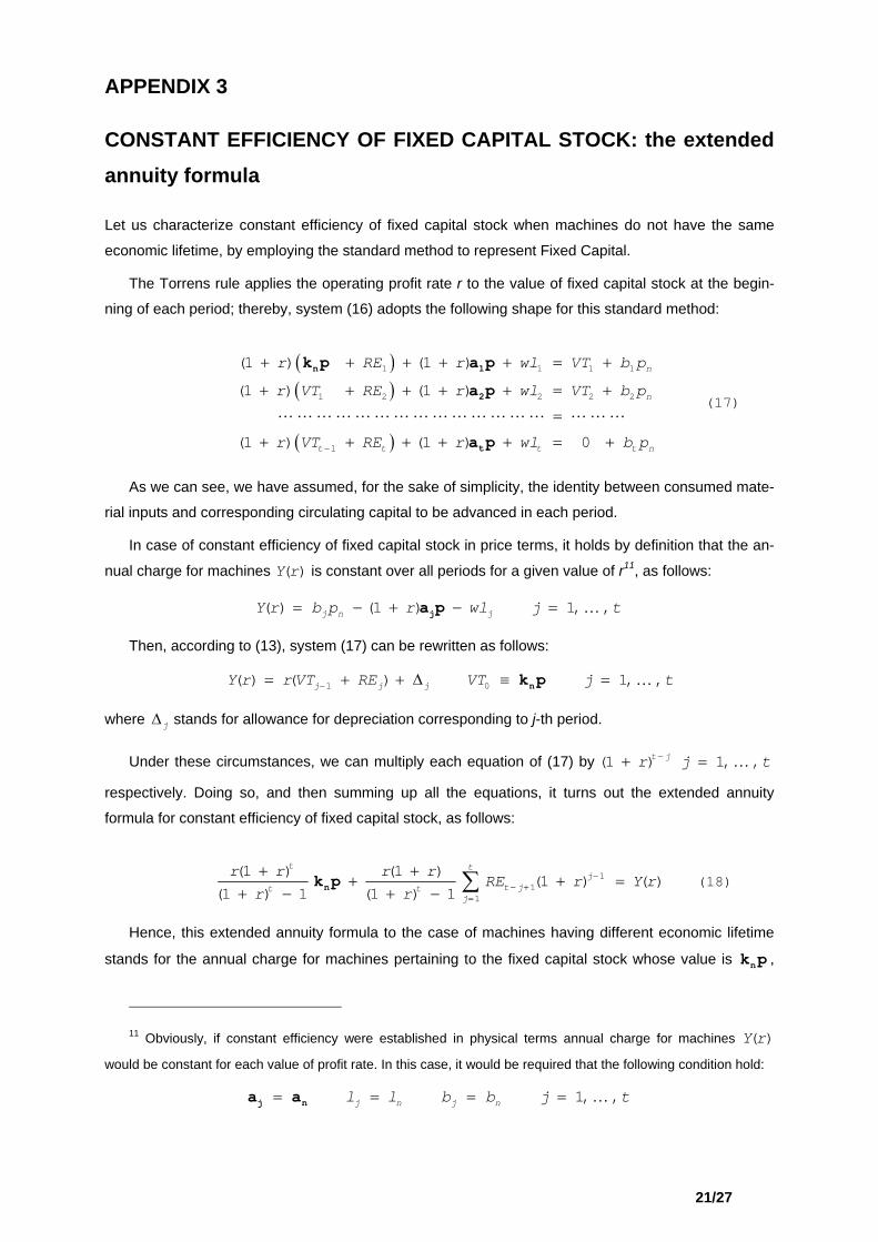
CONSTANT EFFICIENCY OF FIXED CAPITAL STOCK: the extended annuity formula

Let us characterize constant efficiency of fixed capital stock when machines do not have the same

economic lifetime, by employing the standard method to represent Fixed Capital.

The Torrens rule applies the operating profit rate r to the value of fixed capital stock at the begin-

ning of each period; thereby, system (16) adopts the following shape for this standard method:

( )( )

( )

1 1

1 2 2 2 2

1

(1 ) (1 )

(1 ) (1 )

(1 ) (1 ) 0

n

n

t t t

r RE r wl VT

r VT RE r wl VT b p

r VT RE r wl b p−

+ + + + + = +

+ + + + + = +

=

+ + + + + = +

n 1

2

t

k p a p

a p

a p

1 1

t n

b p

(17)

As we can see, we have assumed, for the sake of simplicity, the identity between consumed mate-

rial inputs and corresponding circulating capital to be advanced in each period.

In case of constant efficiency of fixed capital stock in price terms, it holds by definition that the an-

nual charge for machines is constant over all periods for a given value of r( )Y r 11, as follows:

( ) (1 ) 1, ,j n jY r b p r wl j t= − + − =ja p …

Then, according to (13), system (17) can be rewritten as follows:

1 0( ) ( ) 1, ,j j jY r r VT RE VT j t−= + + ∆ ≡ =nk p …

where stands for allowance for depreciation corresponding to j-th period. j∆

Under these circumstances, we can multiply each equation of (17) by (1

respectively. Doing so, and then summing up all the equations, it turns out the extended annuity

formula for constant efficiency of fixed capital stock, as follows:

) 1, ,t jr j−+ = … t

11

1

(1 ) (1 )(1 ) ( )

(1 ) 1 (1 ) 1

t tj

t jt tj

r r r rRE r Y r

r r−

− +=

+ ++ +

+ − + − ∑nk p = (18)

Hence, this extended annuity formula to the case of machines having different economic lifetime

stands for the annual charge for machines pertaining to the fixed capital stock whose value is , nk p

t

11 Obviously, if constant efficiency were established in physical terms annual charge for machines

would be constant for each value of profit rate. In this case, it would be required that the following condition hold:

( )Y r

1, ,j n j nl l b b j= = = =j na a …

21/27

and consists of two terms. The first one stands for the annual charge for machines over t periods

corresponding to this stock, as it is entirely replaced at the end of t-th period. The second term stands

for the annual charge for machines that belonging to this stock are periodically replaced at the begin-

ning of each of the t considered periods.

Since (17) mainly differs from (16) by the value of fixed and circulating capital stock from which the

profit rate is calculated at the beginning of each period, equations (13), (14) and (15) also apply for the

Torrens rule. Hence, characterization of constant efficiency described at the end of preceding appen-

dix is also valid when one uses the standard method to represent Fixed Capital.

Finally, it is to be underscored that in case of machines having different economic lifetime, one

cannot make the replacement fund disappear as an asset belonging to firm’s balance sheet in all

periods. Even though one is financing the fixed capital stock with total debt, and one is applying all

depreciation quotas corresponding to this stock, required being positive, to pay the principal back to

the creditors. This is so, contrasting with what happens when all machines have the same economic

lifetime, since according to (15) accumulated depreciation gives rise to a replacement fund that is

actually financing partial replacements of fixed capital stock, undertaken at the beginning of some of

the t periods, until this stock is entirely replaced at the end of the t-th period.

nk

Whereupon, the possibility of a positive replacement fund as an asset tied to the firm in one single

period causes so deep trouble to the Torrens rule, as method to represent Fixed Capital, as to make

the book value of fixed capital stock at the beginning of this period inaccurate to represent total asset

value displayed in firm’s balance sheet. This fact prevents the firm’s rate of return calculated from the

whole of assets displayed in firm’s balance sheet from being uniform in all periods, unless some

parameters similar to 1, ,j j tθ = … in (16) were used to distort the book value of fixed capital

stock at the beginning of each period, appearing in left hand side of (17) within parentheses.

22/27

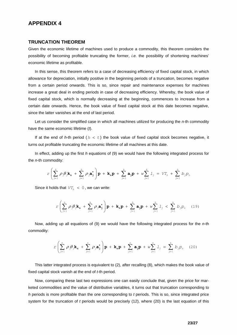
APPENDIX 4

TRUNCATION THEOREM Given the economic lifetime of machines used to produce a commodity, this theorem considers the

possibility of becoming profitable truncating the former, i.e. the possibility of shortening machines’

economic lifetime as profitable.

In this sense, this theorem refers to a case of decreasing efficiency of fixed capital stock, in which

allowance for depreciation, initially positive in the beginning periods of a truncation, becomes negative

from a certain period onwards. This is so, since repair and maintenance expenses for machines

increase a great deal in ending periods in case of decreasing efficiency. Whereby, the book value of

fixed capital stock, which is normally decreasing at the beginning, commences to increase from a

certain date onwards. Hence, the book value of fixed capital stock at this date becomes negative,

since the latter vanishes at the end of last period.

Let us consider the simplified case in which all machines utilized for producing the n-th commodity

have the same economic lifetime (t).

If at the end of h-th period (h ) the book value of fixed capital stock becomes negative, it

turns out profitable truncating the economic lifetime of all machines at this date.

t

l VT b p

l b p

l b p

<

In effect, adding up the first h equations of (9) we would have the following integrated process for

the n-th commodity:

1 1 1 1 1

h h h h h

j j j j h j nj j j j j

r wρ θ ρ= = = = =

⎛ ⎞+ + + + = +⎜ ⎟

⎝ ⎠∑ ∑ ∑ ∑ ∑*

n j n jk a p k p a p

Since it holds that , we can write: 0hVT <

(19) 1 1 1 1 1

h h h h h

j j j j j nj j j j j

r wρ θ ρ= = = = =

⎛ ⎞+ + + + <⎜ ⎟

⎝ ⎠∑ ∑ ∑ ∑ ∑*

n j n jk a p k p a p

Now, adding up all equations of (9) we would have the following integrated process for the n-th

commodity:

(20) 1 1 1 1 1

t t t t t

j j j j j nj j j j j

r wρ θ ρ= = = = =

⎛ ⎞+ + + + =⎜ ⎟

⎝ ⎠∑ ∑ ∑ ∑ ∑*

n j n jk a p k p a p

This latter integrated process is equivalent to (2), after recalling (8), which makes the book value of

fixed capital stock vanish at the end of t-th period.

Now, comparing these last two expressions one can easily conclude that, given the price for mar-

keted commodities and the value of distributive variables, it turns out that truncation corresponding to

h periods is more profitable than the one corresponding to t periods. This is so, since integrated price

system for the truncation of t periods would be precisely (12), where (20) is the last equation of this

23/27

system. At the same time, on the other hand, we would have the following integrated price system for

the truncation of h periods:

( ) ( ) ( ) ( )h h hr w+ + <* * * *K p A p L B ph

where this matrix expression consists of the same n-1 first equations as those of system (12), and of

the last one being inequality (19) instead of equation (20).

Given this, under standard assumptions, we can conclude that truncation corresponding to h peri-

ods renders a higher wage rate for each value of the profit rate than truncation corresponding to t

periods.

This result appears as obvious starting with the following particularization of (7) referred to the h-th

period:

1

h

h jj

VT=

= − ∆∑nk p

Since it holds that , we would have: 0hVT <

1

h

jj=

∆ >∑ nk p

i.e. accumulated depreciation exceeds the value of fixed capital stock brand-new at the end of h-th

period.

Hence, one can guess that it would be profitable replacing the whole fixed capital stock at this date

instead of protracting the economic lifetime of machines up to the end of t-th period.

The preceding truncation theorem can be easily extended to the more general case, contemplated

in Appendix 2, in which not all machines utilized for producing the n-th commodity have the same

economic lifetime.

In effect, adding up the first h equations of (16) we would have the following integrated process for

the n-th commodity:

1 1 1 1 1 1

h h h h h h

j j j j j h j nj j j j j j

r RE w lρ θ ρ= = = = = =

⎛ ⎞+ + + + + = +⎜ ⎟

⎝ ⎠∑ ∑ ∑ ∑ ∑ ∑*

n j n jk a p k p a p VT b p

w l b p

w l b p

Since it holds that , we can write: 0hVT <

1 1 1 1 1 1

h h h h h h

j j j j j j nj j j j j j

r REρ θ ρ= = = = = =

⎛ ⎞+ + + + + <⎜ ⎟

⎝ ⎠∑ ∑ ∑ ∑ ∑ ∑*

n j n jk a p k p a p

Now, adding up all equations of (16) we would have the following integrated process for the n-th

commodity:

1 1 1 1 1 1

t t t t h t

j j j j j j nj j j j j j

r REρ θ ρ= = = = = =

⎛ ⎞+ + + + + =⎜ ⎟

⎝ ⎠∑ ∑ ∑ ∑ ∑ ∑*

n j n jk a p k p a p

This latter integrated process is equivalent to (2), after recalling (15), which makes the book value

of fixed capital stock vanish at the end of t-th period within this more general context.

24/27

Now, comparing these two last expressions we can reach the same conclusion as earlier.

However, in this more general context where machines do not have the same economic lifetime, it

is to be additionally required that h is the least common multiple of the new economic lifetime of ma-

chines jointly used to produce the n-th commodity.

25/27

REFERENCES

Baldone, S. (1974): "Fixed Capital in Sraffa's Theoretical Scheme", in Pasinetti, L.L. (ed.) (1980),

Chap. 6, 88-137.

Bruno, M.; Burmeister, E.; Sheshinski, E. (1966): "The Nature and Implications of the Reswitching of

Techniques". Quarterly Journal of Economics, 80, 526-553.

Burmeister, E.; Dobell, A.R. (1970): Mathematical Theories of Economic Growth. MacMillan, London.

Garegnani, P. (1970): “Heterogeneous capital, the production function and the theory of distribution”.

Review of Economic Studies, 37, 407-436.

Ibanez, F.; Matilla, M. (2004): An alternative representation of fixed capital within a Sraffian frame-

work: constant efficiency. Working Paper:

http://www.uned.es/dpto-analisis-

economico2/fichprof/fibanez/working_papers/Fixed_Capital1_constant_efficiency.pdf

Ibanez, F.; Matilla, M.; Osuna, R. (2004): An alternative representation of fixed capital within a Sraffian

framework: variable efficiency. Working Paper:

http://www.uned.es/dpto-analisis-

economico2/fichprof/fibanez/working_papers/Fixed_Capital2_variable_efficiency.pdf

Kurz, H.D.; Salvadori, N. (1995): Theory of Production. A Long-Period Analysis. Cambridge University

Press, Cambridge.

Morishima, M. (1969): Theory of Economic Growth. Clarendon Press.

Pasinetti, L.L. (1973): "The Notion of Vertical Integration in Economic Analysis", in Pasinetti, L.L. (ed.)

(1980), Chap. 2, 16-43.

Pasinetti, L.L. (ed.) (1980): Essays on the Theory of Joint Production. MacMillan, London.

Roncaglia, A. (1971): "Il capitale fisso in un modello di produzione circolare". Studi Economici, 26,

232-245.

Roncaglia, A. (1978): Sraffa and the Theory of Prices. J. Wiley & Sons, New York.

Samuelson, P.A. (1983): "Durable Capital Inputs: Conditions for Price Ratios to be Invariant to Profit-

Rate Changes". Zeitschrift für Nationalökonomie, 43, 1-20.

Schefold, B. (1978): "Fixed Capital as a Joint Product". Jahrbücher für Nationalökonomie und Statistik,

415-439.

Schefold, B. (1980): "Fixed Capital as a Joint Product and the Analysis of Accumulation with Different

Forms of Technical Progress", in Pasinetti, L.L. (ed.) (1980), Chap. 7, 138-217.

26/27

Sraffa, P. (1960): Production of Commodities by means of Commodities. Cambridge University Press,

Cambridge.

Varri, P. (1974): "Prices, Rate of Profit and Life of Machines in Sraffa's Fixed-Capital Model", in Pasi-

netti, L.L. (ed.) (1980), Chap. 5, 55-87.

von Neumann, J. (1945): "A Model of General Economic Equilibrium". Review of Economic Studies,

13, 1-9.

27/27