1

An Address-light, Integrated MAC and

Routing Protocol for Wireless Sensor

Networks

Sunil Kulkarni, Aravind Iyer and Catherine RosenbergSchool of Electrical and Computer Engineering

Purdue University

West Lafayette, IN 47907, USA.

E-mail: {sunilkul,iyerav,cath }@ecn.purdue.edu

April 26, 2005 DRAFT

2

Abstract

In this paper, we propose an address-light, integrated MAC and routing protocol (abbreviated

AIMRP) for wireless sensor networks. A wireless sensor network (WSN) is characterized by a high

node density, limited energy budgets, a collaborative objective and a many-to-one communication

paradigm. Due to the broad spectrum of applications encompassed by WSNs, there is a strong

need to develop protocol solutions that are optimized for specific classes of applications. AIMRP is

a lightweight and integrated solution for WSN applications exhibiting long periods of inactivity

betweenrare eventswhich requireprompt detection and response. Owing to the many-to-one

communication paradigm, there is no need for routing capability from each node to every other

node, and hence no need forstrict per-node addressing. AIMRP utilizes this fact by employing

an address-light, tier-based routing schemewhich is integratedwith the MAC mechanism. AIMRP

uses a medium access scheme similar to that used in IEEE 802.11, but with the following important

differences: (i) it is not based on unique per-node physical addressing, and (ii) the MAC control

packets are also responsible for finding the next-hop node to relay the data. In order to curb

the energy expenditure due toidle-listening, AIMRP provides arandomizedpower-saving mode,

where nodes can shut off their radio modules when not in use, independent of one another. This

paper evaluates AIMRP through analysis and simulations, and compares it with a MAC protocol

proposed for WSNs,viz., S-MAC [13]. S-MAC is a generic MAC protocol, and not optimized for a

specific network scenario, and as the paper shows, AIMRP outperforms S-MAC for event-detection

applications, in terms of total average power consumption, while satisfying identical end-to-end

latency constraints.

Index Terms

Sensor Networks, MAC, Routing, Addressing

I. I NTRODUCTION

Recent advances in wireless communication technologies, and sophisticated techniques for

miniaturization of electronic and sensor devices, have fueled a lot of research in the area of

wireless sensor networks. Dense networks of wireless sensor devices are being deployed for

sensing or monitoring various phenomena of interest. A wireless sensor device is a ‘small’

battery-powered device, capable of sensing one or more physical quantities. In addition, it is

equipped with a limited amount of storage, and computation capabilities. A wireless sensor

network (WSN) consists of a large number of these devices, working collaboratively towards

a certain common goal. These sensor nodes communicate with each other and with one or

more sinks (or base-stations) over a wireless channel. The sink(s) is (are) responsible for

DRAFT April 26, 2005

3

collecting information from all sensor devices in the network and represents the interface of

the WSN to the outside world.

The range of applications that WSNs are envisaged to support, is tremendous, encompass-

ing military, civilian, environmental and commercial areas. Each application imposes a unique

set of goals and requirements, and also produces a different type of traffic. For instance, an

application to monitor the environmental conditions affecting crops and livestock [1], is a

data-gathering application. The traffic it generates is expected to be more or less uniform,

and the latency requirements on its data are expected to be loose. On the other hand, a sensor

network deployed to detect forest fires [1], is likely to produce data in bursts, with severe

latency constraints. Hence, a generic approach to design WSNs, will often be unable to take

advantage of any application-specific features, and sometimes may even be unsuitable for

certain applications. The danger in pursuing an application-specific approach though, is to

end up developing a different protocol for each application. Acareful examination of the

tradeoffs involved, is necessary to avoid being too generic or too specific.

To this end, it is important to be able to classify WSN applications based on their

data-delivery requirements and their traffic characteristics [14]. In particular, most of the

current WSN applications fall into one of the following five broad classesviz., (i) event

detection and reporting, (ii) monitoring and periodic reporting, (iii) sink-initiated reporting,

(iv) object detection and tracking, and (v) hybrid applications with more than one of the

above four characteristics. Our work focusses on the first class of applications, namely, event

detection and reporting. Applications which fall into this category include intruder detection

and detection of fire and hazards. These applications exhibit prolonged periods of inactivity

till the time an event of interest is detected. On detecting an event, a report of this event

has to bepromptly communicated to the sink. An event report is usually expected to carry

somelocation informationabout the event. Hence the network protocol should be designed

to satisfy the requirements of latency and location, while consuming minimal energy.

For this, we examine the following salient features of the WSNs considered in this paper:

the many-to-one communication paradigm, whereby all sensors intend to send their data to

one (or few) sink(s); the large node density that begs for sensors that are cheap to manufacture

and ready to deploy; and, the tight limitation in energy which calls for a highly optimized,

lightweight protocol stack. This impacts the protocol design for WSNs, in the following way.

In traditional communication networks, the need for modularity and interoperability, leads

to a layered protocol reference model. On the other hand, for WSNs, it is more important

April 26, 2005 DRAFT

4

to satisfy application-specific requirements, and to be energy-efficient. Hence, cross-layer

interaction or integration of protocol layers, is recommended when it can be effectively used

to reduce the protocol overhead, and to make the protocol stack lightweight.

The above discussion leads us to consider the following issues in order to design our

integrated protocol. The first is the issue of addressing. In general, there is a need for

addressing or ‘identification’ at three levels, for the purposes of (i) MAC, (ii) routing, and

(iii) location information about the data source. Strict per-node addressing is expensive in

a dense network, because not only would the size of an address be large, but also these

addresses would need to be allocated and exchanged at different layers of the protocol stack.

Allocation of addresses in a dense network, is a real problem which is often underestimated.

Our goal is to use (and even reuse) only as much addressing as is absolutely necessary. Now,

the problem of location determination in a dense WSN, is an active area of research by

itself, and is beyond the scope of this paper. In case the application requires some location

information to be associated with each event report, we assume that the required granularity

of location information is determined by some means, and isembedded in the data payload

of each packet. Hence, we only seek to reduce the bit budget of addresses used for MAC

and routing. It is clear that a further step would be to integrate all three levels of addressing.

The second issue concerns the routing protocol. Unlike in an ad hoc network, where

any node can potentially communicate with any other node, a WSN exhibits the many-

to-one communication paradigm. In addition, we assume that the sink is not required to

communicate with a particular sensor.1 These two points together imply that (i) the flow of

data originatesonly at a sensor node, and (ii) it isalwaysdestined for the sink node. Thus,

the routing protocol overhead can be reduced in two ways: firstly, the routing protocol only

needs to discover paths from each node to the sink; and secondly, since no communication

is addressed to an individual node, routing can be performed at a coarser level of addressing

than one address per node.

Thus, we can identify two major sources of wasteful energy expenditure. The first is the

overhead required for the routing and MAC protocols. This can be minimized in two ways,

namely, (i) by choosing a streamlined packet header structure, and reducing the size of each

1Clearly, if the sinkis required to communicate with a particular sensor node, then there is a need for addressing each node.

However, this is really the overhead we are trying to avoid by making this assumption. The assumption is not unreasonable

in the context of event detection applications, since we feel thatthe only reasonthe sink would need to communicate to

the sensor nodes would be for reprogramming or software updates.

DRAFT April 26, 2005

5

control field (e.g., the addressing fields) as much as possible, using integration and (ii) by

minimizing the need for non-data related information exchange. The second is idle-listening

in MAC protocols based on random access, especially in case of low traffic load. Indeed, for

event detection applications, a medium-access mechanism based on random access is more

suitable than one based on controlled access, due to the nature of the traffic generated. Hence,

an effective MAC protocol, for this class of applications, would have to be coupled with a

power-saving mechanism to minimize idle-listening. Besides, the power-saving mechanism

itself, should not impose its own overhead by requiring a lot of information exchange between

the nodes.

This paper proposes an address-light, integrated MAC and routing protocol (abbreviated

AIMRP) which seeks to address all the issues raised above. AIMRP is an integrated MAC

and routing mechanism designed specifically for WSNs which have to promptly detect and

report relatively rare events. The contributions of our work are twofold. Firstly, we design

the AIMRP protocol with the following attractive features:

• Integrated MAC and routing to minimize the protocol overhead: AIMRP organizes

the network into tiers around the sink, and routes packets by progressively forwarding

them to tiers closer to the sink. This can be readily integrated into the MAC layer.

• No per-node identification for either MAC or routing: We use short random identifiers

for MAC, on a per-transmission attempt basis, instead of physical MAC identifiers, and

per-tier addresses for routing, instead of per-node addresses.

• Power-saving modewhich requiresno coordination between the nodes: Nodes repeat-

edly shut their radio modules off when not in use, independently of one another, while

satisfying sensor-to-sink latency guarantees.

Secondly, we provide a detailed analysis for dimensioning the power-saving mode and to

compute the average energy expenditure per event report for a given event frequency, while

satisfying the latency constraints. We validate this analysis through simulations. In particular,

we show that AIMRP outperforms S-MAC [13] in terms of total average power consumption,

while satisfying identical end-to-end latency requirements.

The rest of the paper is organized as follows. In Section II, we review current work in the

area of MAC and routing for WSNs. In Section III, we introduce the principles of our address-

light, integrated MAC and routing protocol (AIMRP) for WSNs. In Section IV, we describe

in detail the working of AIMRP. Section V provides guidelines for dimensioning AIMRP

parameters, while Section VI evaluates the protocol through analysis and simulations, and

April 26, 2005 DRAFT

6

compares its performance with that of a currently proposed protocol, S-MAC [13]. Finally,

Section VII concludes the paper, and discusses possible extensions to this work.

II. RELATED WORK

Network design has traditionally followed the principle oflayering. Complex networking

functionalities are broken down and decoupled into manageable and independent levels. This

is done so as to allow interoperability, modularity, and to keep the protocols as general-

purpose as possible. Following this principle, nearly all of the research in the area of WSNs

considers the problem of medium access separate from the problem of routing, although the

need forintegratedandapplication-specificnetwork solutions has been recognized [1], [14].

One of the main approaches to MAC for WSNs, comes from its counterpart for ad hoc

networks [1], viz., the IEEE 802.11 standard. The IEEE 802.11 standard is a CSMA/CA

based protocol which is widely used in wireless LANs. Using plain 802.11 MAC for WSNs

has many drawbacks, as discussed in [4], [10], [13]. In particular, [10] shows that energy

consumption due to overhearing and idle-listening, is a major chunk of wasteful energy con-

sumption. Hence [10] suggests turning off the radio module of a node when it is “overhearing”

(i.e., listening to the transmission of a packet not addressed to it).

[13] presents a specially modified 802.11 based medium access protocol (called S-MAC),

for WSNs. In this protocol, the authors identify the following sources of energy wastage, viz.,

collision, overhearing, overheads,and idle-listening. In order to reduce energy drainage due

to idle-listening, nodes periodically sleep. Neighboring nodes form so-calledvirtual clusters

to synchronize on their sleep schedules. The sleep schedules are completely synchronized

within a cluster and are uncorrelated across clusters. The period of these sleep schedules

is determined by the end-to-end delay constraint. S-MAC also uses in-channel signaling, to

implementoverhearing avoidancefor nodes to avoid listening to long data packets not meant

for them. Finally, S-MAC appliesmessage-passingto reduce contention while transmitting

relatively long data packets.

A drawback of this protocol is that synchronizing the sleep schedules by creating virtual

clusters is a rather complex operation which produces its own overhead. Another drawback

of this protocol is that it fails to exploit the many-to-few communication paradigm in WSNs,

and does not consider the issue of addressing. In other words, S-MAC is a generic energy-

aware MAC protocol which does not cater to specific WSN applications. Our protocol tries

to improve upon these two issues for the event reporting class of applications.

DRAFT April 26, 2005

7

MAC protocols based on controlled access rather than random access have also been

proposed. For example, [2], [11], [5] study MAC protocols based on TDMA, [4], [11], [8]

on CDMA and/or FDMA. However, for the class of applications we consider, a MAC protocol

based on random access would be more appropriate than one based on controlled access.

Like in the case of MAC protocols, several routing protocols developed for ad hoc networks

have been suggested for WSNs [1]. Specifically, distance vector protocols such as Ad hoc On-

demand Distance Vector (AODV), Destination Sequenced Distance Vector (DSDV) and source

routing protocols such as Dynamic Source Routing (DSR) have been adapted for WSNs, by

optimizing for energy usage. An alternative strategy utilizing gradient-based routing, has been

proposed in [16]. But, we believe that, owing to the many-to-one communication paradigm

in WSNs, routing protocols can be further streamlined.

[5] proposes an application-specific protocol architecture for periodically routing reports

from all nodes to a distant base station. A method which uses clustering and direct transmis-

sions from cluster heads to the base station is proposed. For uniform energy consumption

across all the nodes, the responsibility of being the cluster head is rotated among all the

nodes periodically. [6] proposes a similar solution to the problem, but with two types of

nodes, sensors and cluster heads. The authors evaluate the optimum node density for these

two types of nodes, and their initial battery energies to guarantee a certain lifetime.

[12], [3] notice that for reliable routing in dense ad-hoc networks not all of the nodes

are required to be awake at the same time. In [3], nodes decide to go to sleep or to be

awake and join the forwarding backbone, depending on the local information and available

residual energy. In [12], the region is divided into virtual square grids, such that all nodes

in neighboring grids are able to communicate with each other. Only a single node remains

awake within each grid. It may be noted that putting nodes to sleeping when they cannot do

anything useful at the routing level, is a kind of integration of MAC and routing.

III. A DDRESS-LIGHT, INTEGRATED MAC AND ROUTING PROTOCOL (AIMRP):

PRINCIPLES

In this section, we introduce AIMRP, and explain its principles. AIMRP is an address-light

protocol which does not use or require the use of strict per-node identifiers or addresses. The

routing mechanism employed in AIMRP is the following. For the sake of explaining the

principle, let us assume that the WSN consists of several sensor nodes deployed in a circular

region with a single sink at the center. By means of an initial configuration phase which will

April 26, 2005 DRAFT

8

be explained later, the entire network is organized into tiers centered around the sink (refer

to Figure 1). The tiers are numbered1, 2, 3, · · · starting from the innermost tier, and are such

that a node in thenth tier can relay a message to the sink inn hops. Now at the end of

the configuration phase, the route discovery is complete, based on the rule that a node in a

given tiern only relays messages from tiers farther away from the sink than itself, i.e., tiers

n + 1, n + 2, · · ·. The routing is hop-by-hop, and at each hop the node which has the packet

indicates its tier number in the packet so that another node with a lower tier number can

receive the packet. In this way, routing can be done at the level of addressing of a tier, which

has far less overhead than having one routing address per node. The overhead required for

route discovery is also limited.

The mechanism for medium access is similar to that used in the distributed coordination

function (DCF) in IEEE 802.11, except for two important differences. First, the nodes do

not have preassigned MAC identifiers and do not use any unique addresses to communicate,

instead choosing new short random identifiers for each communication attempt. The second

difference can be explained as follows. In IEEE 802.11, theRTSmessage has two purposes:

to initiate the communication between the source and the next-hop node; and to silence all

nodes within the communication range of the source, except the next-hop node. The next-

hop node is known because of the routing protocol, before the communication is initiated.

In contrast, in AIMRP, the purpose of the analogousRTR (Request to Relay ) message

is to seeka receiver node which is closer to the sink and so the destination node is not

known beforehand. In other words, theRTR message is ananycastmessage to which any

���� ���� ���� ���

�

��

���� ��������

����

����

���� ���� ���� ���

�

����

!!

"#""#"$$ %%&& ''(())**

++,,

--..

//00 1122 3344 556

6

7788

99::

;#;;#;<< ==>> ??@@AABB

CCDD

EEFF

GGHH IIJJ KKLL MMN

N

OOPP

QQRR

S#SS#STT UUVV WWXXYYZZ

[[\\

]]^^

__`` aabb ccdd eef

f

gghh

iijj

k#kk#kll mmnn ooppqqrr

sstt

uuvv

wwxx yyzz {{|| }}~

~

����

����

�#��#��� ���� ��������

����

����

���� ���� ���� ���

�

����

����

�#��#��� ���� ��  ¡¡¢¢

££¤¤

¥¥¦¦

§§¨¨ ©©ªª ««¬¬ ­­®

®

¯¯°°

±±²²

³#³³#³´´ µµ¶¶ ··¸¸¹¹ºº

»»¼¼

½½¾¾

¿¿ÀÀ ÁÁÂÂ ÃÃÄÄ ÅÅÆ

Æ

ÇÇÈÈ

ÉÉÊÊ

Ë#ËË#ËÌÌ ÍÍÎÎ ÏÏÐÐÑÑÒÒ

ÓÓÔÔ

ÕÕÖÖ

××ØØÙÙÚÚ

ÛÛÜÜ

ÝÝÞÞ

ßßàà

á#áá#áââ ããää ååææççèè

ééêê

ëëìì

ííîî ïïðð ññòò óóô

ô

õõöö

÷÷øø

ù#ùù#ùúú ûûüü ýýþþÿÿ��

����

����

����

����

����

��

����

����

������������������

������������������������������������������������������������������������������������������

������������������������������������������������������������������������������������������

���������������������������������������������������������������������������������

���������������������������������������������������������������������������������

�����

�����

������������������������������������

������������������������������������

Base−station

Sensor Node

Fig. 1. An Illustration of Routing in AIMRP

DRAFT April 26, 2005

9

node can reply if it can relay the data according to the routing algorithm outlined above

(i.e., if its tier number is lower than the one indicated on the packet). Hence, before a node

sends aCTR(Clear to Relay ) message (analogous to theCTSmessage of IEEE 802.11),

it chooses a random back-off to avoid systematically colliding with other nodes willing to

receive and relay the data. The second difference is very important because that is how

we integrate a hop-by-hop routing functionality into the MAC protocol. Note that the only

control information necessary for this is theone-hopsource MAC and tier identifier in the

RTR message, and both theone-hopsource and next-hop MAC and tier identifiers in the

CTRmessage.

AIMRP is also equipped with a power-saving mode to curb the energy expenditure due

to idle-listening. Owing to the nature of the application that AIMRP targets, it would be

extremely wasteful to have all nodes keep their radio modules on for all time. But then if a

particular node wishes to report an event to the sink, it should find a feasible path to relay

the information to the sink, relatively quickly. In order to capture this application-specific

characteristic, AIMRP employs a power-saving mode which is subject to a constraint on

the maximum end-to-end delay that an event report can encounter. AIMRP relies on an

uncorrelated sleep-and-wake pattern at each node, to meet the latency constraint with a pre-

specified probability. Since the sleep-wake pattern at each node is independent of the other

nodes, there is no need for any additional information exchange between nodes. This is in

contrast to the sleep-and-wake algorithm proposed in S-MAC [13], but the important point

to note is that S-MAC is a generic protocol which is not designed for this particular class of

applications, i.e., event detection and reporting.

IV. AIMRP: D ESCRIPTION

In this section, we propose and describe the working of AIMRP. We consider a simple

network geometry in which nodes are distributed in a circular region of radiusL, centered

at the sink. Each node has a communication radiusR.2 We assume that an event is equally

likely to occur at any point in the region, and that only one node detects and reports this

event. Under this setting, let us define AIMRP. AIMRP involves a configuration phase and an

active phase. The configuration phase which has to be completed just after the deployment,

works as described in the following subsection.

2In practice, this sort of a ‘binary’ model of a fixed communication and interference rangeR is often unrealistic. It is

clear that a more accurate design would have to employ a more realistic channel model.

April 26, 2005 DRAFT

10

BA

Tier 2

Tier 1

Tier n

Tier n+1 Base−station

R

Sender

Next−hop nodes

nRα

(n−1)RαRα

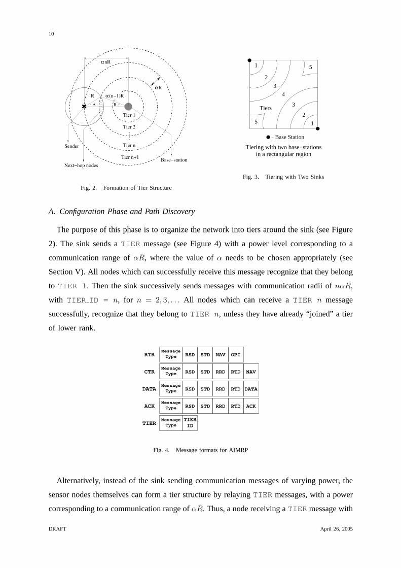
Fig. 2. Formation of Tier Structure

5

3

1

2

3

4

2

15

Tiers

in a rectangular regionTiering with two base−stations

Base Station

Fig. 3. Tiering with Two Sinks

A. Configuration Phase and Path Discovery

The purpose of this phase is to organize the network into tiers around the sink (see Figure

2). The sink sends aTIER message (see Figure 4) with a power level corresponding to a

communication range ofαR, where the value ofα needs to be chosen appropriately (see

Section V). All nodes which can successfully receive this message recognize that they belong

to TIER 1 . Then the sink successively sends messages with communication radii ofnαR,

with TIER ID = n, for n = 2, 3, . . . All nodes which can receive aTIER n message

successfully, recognize that they belong toTIER n, unless they have already “joined” a tier

of lower rank.

MessageType RSD STD RRD RTD DATA

MessageType RSD STD RRD RTD ACK

MessageType

TIERID

MessageType

MessageType

ACK

TIER

DATA

RTR

CTR

RSD STD OPI

RSD STD RRD RTD

NAV

NAV

Fig. 4. Message formats for AIMRP

Alternatively, instead of the sink sending communication messages of varying power, the

sensor nodes themselves can form a tier structure by relayingTIER messages, with a power

corresponding to a communication range ofαR. Thus, a node receiving aTIER message with

DRAFT April 26, 2005

11

TIER ID = n “joins” TIER n, unless it already belongs to a tier of lower rank. Each node

also increments theTIER ID field before forwarding theTIER message it has received. An

idea similar to this scheme has been discussed in [7]. Assuming that the radio propagation is

identical in all directions, the configuration phase will result in the formation of annular tiers

of thicknessαR centered at the sink. It is possible that owing to some obstacle or due to the

terrain, certain nodes may not find each other directly reachable via radio, even though they

are physically quite close to one another. In such cases, the shape of the tiers formed will

be dictated by the radio reachability of the nodes. In such cases, the second scheme for the

configuration phase is more robust.

The configuration phase in case there are multiple sinks, is a simple extension of what was

explained above. Consider Figure 3 which depicts a rectangular region with two sinks situated

diagonally opposite each other. For an event-reporting application, we expect the sinks to

all be connected to the outside world. Hence, it is reasonable to assume that the sinks are

indistinguishable, therefore it is irrelevant which exact sink receives the event report. Thus,

the tier rank of a node represents its distance in number of hops, from its closest sink (see

Figure 3). Thus either of the two schemes discussed above can be used for configuration.

B. Active Phase

A node in the active phase of AIMRP is always listening to the radio channel, unless it

is transmitting. It is in the so-calledListenerstate. We discuss thepower-savingfeature of

AIMRP in the next subsection, where nodes need not always listen to the radio channel. A

node remains in theListenerstate either till it detects an event or has to relay information

from some other node, and therefore hasoutstanding data to send to the sink, or till

it hears a transmission on the radio channel.

Whenever it hasoutstanding data to transmit, the node attempts tofind a next-hop

node, closer to the sink, which can relay its data. This is in contrast with IEEE 802.11 where a

node attempts to transmit to aparticular node as decided by the routing algorithm. The node

waits for a guard timetg before attempting to transmit anything. After the guard time expires

or when the channel becomes free (whichever is later), the node waits for a random listening

time tl before transmitting. The guard timetg is to ensure that nodes reliably estimate the

channel as either busy or idle. The additional random listening timetl is to prevent nodes

attempting to transmit at about the same time, from colliding. Then the node transmits a

Request To Relay (RTR) message (refer to Figure 4), which contains a randomly chosen

April 26, 2005 DRAFT

12

RSD(random source identifier), the source tier identifier (STD) i.e., itsTIER id, a NAVentry

which represents the length of the packet,3 and some optional packet information (OPI).

The RSDfield is limited to a few bits in size, and hence is much smaller than what would

be required to maintain per-node fixed MAC identifiers. It can be seen as a temporary (i.e.,

just for the sending of this message) physical node identifier. Now the node is waiting for a

Clear To Relay (CTR) message, and is in aRequestingstate.

If this RTR message is received successfully by another node with a lower tier number

(which we call the next-hop node), then that node replies to the source node. The source

node waits for a timetw in the Requestingstate before attempting to rebroadcast itsRTR

message. For each rebroadcast, the source node uses a freshly chosenRSD. This is to reduce

the possibility of two source nodes choosing the sameRSD. The next-hop node, in order to

avoid contention with other potential next-hop nodes, chooses a random back-off timetb and

listens to the channel, before it replies. This again is in contrast with 802.11 where there is

no contention between potential receiver nodes, since there is only one fixed receiver node,

as determined by the routing protocol. If during this waiting period, the next-hop node hears

either aCTR, with the correctRSDand STD, from another next-hop node or data from the

source node, it goes back into theListenerstate. Otherwise, it replies with aCTRmessage

which consists ofRSD, STD, as well as a randomly chosen receiver identifier (RRD), and the

receiver tier identifier (RTD), in addition to theNAV (see Figure 4). Now it is waiting for

data, and is in theReceiverstate.

Once thisCTR message is correctly received by the source node, aDATA and anACK

message are quickly exchanged between the source node and the next-hop node, using the

source and the next-hop node identifiers, for unambiguous identification. Detection of the loss

of a DATAor an ACKmessage is inferred through time-outs of durationtd at the receiver,

andta at the sender, respectively. On receiving the data completely, the next-hop node which

belongs to a tier closer to the sink, becomes the new source node. Thus, data is forwarded

across tiers progressively moving closer and closer to the sink. In this way, AIMRP handles

the twin problems of routing and medium access in an integrated fashion (see Figure 1).

3Note that it is possible to eliminate the use of theNAVfield. For several event detection applications, the event report

is expected to be of a fixed length, containing the time, the location and a fixed length code-word describing the event. In

such cases, assuming all packets to be of equal length, any transmission could be taken to reserve the channel for the fixed

duration of the data transmission, thereby removing the need for theNAV.

DRAFT April 26, 2005

13

TABLE I

AIMRP: PROTOCOL PARAMETERS AND THEIR FUNCTIONS

tg Guard time to reliably estimate the channel state (whether busy or idle)

tl Listening time to prevent collision of messages from nodes attempting to transmit at the same time

tb Back-off time to avoid collision ofCTRmessages with other potential next-hop nodes

Tl, Tb Upper bounds ontl and tb respectively

tw Waiting time to infer either unavailability of a next-hop node or erroneous transmission of theRTRmessage

td Waiting time to infer incorrect transmission ofDATAmessage

ta Waiting time to infer a lostACKmessage

tp Total transmission time of all protocol messages (RTR,CTR, DATAandACK)

ton On-period in power-saving mode

tσ Random sleep duration in power-saving mode (exponentially distributed with parameterσ)

tr Listening time corresponding to the highest value of theNAV to avoid collisions in power-saving mode

C. Resolution of protocol deadlocks

Since AIMRP is based on random-access, there are situations when the protocol could

potentially deadlock, unless there are provisions to prevent it. AIMRP is based closely on

IEEE 802.11, so it adopts some deadlock resolution mechanisms from 802.11. In particular,

AIMRP uses the guard timetg and the random listening timetl, in a way similar to 802.11.

It also uses the time-outstw, td andta which determine failure of an attempt at transmitting

an RTR, a DATA and anACK message respectively. Finally, it uses aNAV based virtual

carrier sensing strategy to reserve the channel for the duration of the data communication.

In contrast with 802.11 though, the receiver node in AIMRP is not pre-determined. Hence,

there is an additional random backoff timetb in order to prevent potential receiver nodes

from colliding with theirCTRmessages. Also, since random identifiers, as opposed to fixed

MAC addresses, are used, these identifiers are chosen afresh for each attemptedRTR or a

CTR. This reduces the possibility of nodes in the vicinity choosing identical identifiers and

then systematically colliding. Refer to Table I for a summary.

The state transitions based on the various protocol messages for AIMRP are illustrated in

Figure 5. Note that Figure 5 does not include transitions due to various time-outs or due to lost

messages. Although the protocol states are analogous to the states for 802.11, the important

difference is that theRTR/CTRmechanism based on randomly chosen node identifiers is used

to perform a one-hop routing as well, in addition to, organizing communication between the

two nodes, as in 802.11.

April 26, 2005 DRAFT

14

Outstanding Data

ACK

DATA

CTR

RTR Listener

RequestingReceiver

Sender

Fig. 5. States and state transitions for AIMRP

D. Path Failure and Path Repair

AIMRP is a protocol optimized for event detection and reporting. It could possibly be

deployed in hostile surroundings. Nodes following AIMRP could fail either permanently or

intermittently. Node failures could either be more or less uniform throughout the network,

or they could be concentrated in a particular area in the network. In all these scenarios, it is

important for AIMRP to maintain connectivity and continue functioning, in the best manner

possible. Now, if a given node (or set of nodes) becomes completely disconnected from the

rest of the network, then no routing algorithm will be able to find a path from the node(s)

to the sink. However, since AIMRP uses a tier-based routing algorithm, it is possible that

although a node is not disconnected, it still finds the sink unreachable, if there is no node

with a lower tier-id, in its neighborhood. This could happen if all the neighbours of a node

have higher tier-ids. In such a case, we say theTIER ID of the node is misconfigured.

In order to combat with path failures arising out of misconfiguredTIER ID s, we suggest

the following path repair strategy. Note that theTIER ID of a node, if configured correctly,

represents in some sense its distance to the sink, in number of hops. In the configuration

phase, nodes set theirTIER ID s as one greater than the lowest rankedTIER message they

receive. The rationale behind this is that they are one hop away from a node which knows its

distance to the sink. Based on this observation, we suggest the following. LetMAXTIER ID

denote an upper bound on allTIER ID s. If a node is unable to send an event report for more

than a certain number of tries,PATHREPAIR THRESH, then it reattempts the transmission

with the STDfield (see Figure 4) of itsRTRmessage set toMAXTIER ID . Now unless the

node is completely disconnected from the rest of the network, it is bound to receive aCTR

reply. On receiving this reply, the node sets itsTIER ID asRTD+1, whereRTD(see Figure

4) is theTIER ID of the replying node.

This local path repair strategy represents a good approximation to the repair strategies used

in several routing protocols such as AODV, DSDV or DSR. We note that a more fool-proof,

but expensive technique for route repair, is to re-run the configuration phase periodically.

DRAFT April 26, 2005

15

This will enable all the nodes to maintain correctly configuredTIER IDSs. In practice,

the designer can choose to deploy either of the two strategies (local repair vs. periodic

configuration) mentioned above, depending on the needs of the application.

Outstanding data

ACKDATA

CTR

RTR

ont or event detectedtσ

Requesting

Sleep

Receiver

Sender

Listener

Fig. 6. Sleep state for AIMRP with power-saving

E. Power-saving Mode

There are two major sources of wasteful energy expenditure in a WSN running a random

access MAC protocol, namely,idle-listeningand overhearing. A node is said to be in idle

mode, if its radio module is on when there is no transmission from any other node. A node

is said to be overhearing, if its radio module is on during aDATA message transmission

intended for another node. In order to reduce this energy wastage, we need a power-saving

mode for AIMRP. Previous works on power-saving schemes include PAMAS [10], S-MAC

[13] and the IEEE 802.11 power-saving mode [17]. PAMAS [10] is proposed for use in an ad

hoc wireless network of nodes communicating with an any-to-any communication paradigm.

PAMAS uses overhearing avoidance to save power. In other words, a node shuts off its

radio module during the transmission of aDATAmessage intended for another node. S-MAC

[13] and the IEEE 802.11 power-saving mode [17] use periodic duty-cycling to reduce idle-

listening. Specifically, nodes follow a scheduled cycle of on-periods when their radio modules

are on, and off-periods with the radio modules off.

In AIMRP, we take a different approach to design our power-saving mode. We propose

a completely asynchronousand randomduty-cycling scheme. The basic idea of the power-

saving mode in AIMRP is the following. We introduce a new state called theSleepstate (see

Figure 6), in which nodes shut their radio modules off (i.e., sleep). Nodes in theListenerstate

sleep from time to time, with the length of their random sleep durationtσ chosen according

to an exponential distribution with parameterσ. If a sensor node detects an event when it is in

the Sleepstate it wakes up and moves to theListenerstate immediately. Otherwise, the node

April 26, 2005 DRAFT

16

wakes up on expiry of the sleep durationtσ, remains awake for timeton, and then goes back

to sleep for a freshly chosen random sleep duration, except under certain scenarios discussed

below. The nodes remain awake for a timeton on waking up, in order to be available to other

nodes looking to relay their data closer to the sink. The on-periodton has to be dimensioned

in such a way that it enables a node to listen to at least oneRTRmessage from another node

looking to relay some data. This can be achieved by requirington ≥ tg + Tl, where tg is

the guard time, as defined earlier, andTl is an upper bound on the random listening timetl

defined earlier (refer to Table I). The timeton is smaller than aDATApacket transmission

time, tDATA (see Subsection IV-F).

In general, a node (say node A) following the power-saving mode of AIMRP needs to be

awake under the following two scenarios:

1) Either node A hasoutstanding data and is attempting to find a next-hop node

to relay the data closer to the sink,

2) Or node A is merely awake as part of the random duty-cycling, to see if another node

needs its help in relaying.

In order to explain the exact protocol behavior of a node in power-saving mode, it is useful

to consider these two scenarios separately.

Let us consider scenario 2 first. In this scenario, the default behavior of node A is the

simple duty-cycle rule stated earlier. Node A remains awake for a timeton, and then goes

to sleep again for a timetσ. However, if node A receives any protocol messages which it

can successfully decode, then it has to respond to them according to the rules of AIMRP.

For instance, if node A receives anRTRmessage from another node (say node B), with a

higher tier rank, and node A manages to be the first node to reply with aCTR to the RTR

from node B, then node A is the next-hop node for node B. In this case, node A continues

following the message exchanges according to AIMRP, and receives the data from node B.

However, if node A infers from theRTR from node B that node B has a lower tier rank

than itself, or if node A hears another node reply with aCTR to node B, or if node A

hears the preamble of aDATAmessage from node B intended to some other node, then it

will be able to conclude that it is not the next-hop relay for node B. Then, node A has to

remain silent until theDATAtransmission from node B is concluded, as dictated by theNAV

field. In this case, since the on-periodton is anyway shorter thantDATA, node A goes to sleep

immediately for a random durationtσ. We show later that the sleep durationstσ are orders

of magnitude longer than message transmission times. Hence in this scenario overhearing

DRAFT April 26, 2005

17

avoidance is actually implicit since node A goes to sleep fortDATA and much more.

Now let us consider scenario 1. The default behavior of node A in this case, is to attempt

to find a next-hop relay by transmitting anRTRmessage. However, if it hears any activity

in the radio channel, it has to respect the physical and virtual carrier sensing rules, and the

other rules of AIMRP. For instance, if it receives anRTR from another node (say node B)

with a higher tier rank than itself, it has to offer to relay the data from node B, by attempting

to send aCTRafter a random backoff. However, if node A is able to conclude that it is not

the next-hop relay for node B, then it has to remain silent until theDATAtransmission from

node B is concluded. In this case, we propose to use overhearing avoidance. So node A shuts

its radio module off until the conclusion of theDATA transmission from node B, and then

wakes up again to attempt sending its own data.

In practice, the decision of whether or not to use overhearing avoidance in scenario 1,

depends on whether it is more energy-efficient for nodes to put their radios off and bring

them up again, or to just remain awake for the entire duration of the packet transmission

(tDATA). Using the notation introduced later in Sections V and VI (refer to Table III), if

Eup + Edw ≤ PontDATA, then overhearing avoidance should be used in scenario 1. However,

due to the infrequency of event reports, it is quite unlikely that two or moreneighboring

nodessimultaneouslyhaveoutstanding data , and hence overhear one another. Hence

the difference in the power consumption between using and not using overhearing avoidance,

would be negligible. Later in Section VI, when we calculate the power consumption of

AIMRP, we do not take into account the fact that nodes use overhearing avoidance in scenario

1.

In scenario 1, one of the reasons node A could haveoutstanding data is because it

detected an event. Now node A could have been in theSleepstate when it detected the event.

In this case, node A moves immediately to theListenerstate and attempts to relay the event

report one hop closer to the sink. However, since node A has just woken up, it might have

missed theRTRor CTRof an on-going communication in its neighborhood. So it listens to

the radio channel for a timetr corresponding to the highest value of theNAVfield. This is

done to reduce the possibility of node A colliding with an on-goingDATA transmission in

the neighborhood.

Since the nodes use multi-hop relaying to send their data to the sink, they cannot put their

radio modules off indefinitely. The choice of the parameterσ which governs their sleep-

wakeup schedules is determined by the end-to-end latency required by the application. All

April 26, 2005 DRAFT

18

nodes should wake-up often enough, so that for a given node trying to send a report to the

sink, there will always be nodes available to relay the report within the specified latency

period. The dimensioning ofσ is discussed in detail in Section V.

F. Setting back-off times and timeouts

This subsection is intended as a guideline to set the widths (in number of bits) of various

subfields in each packet, and to set the values of various back-off times and timeout intervals.

In order to distinguish between different message types, we use a three bit message type field.

For the random MAC identifiers, we will need an address width of about 4 bits, while for

representing the tier number of the nodes, we will again need an address about 4 bits wide.

The NAVfield is taken to be 8 bits wide, and we assume that the data payload is 1000 bits

in size. A summary of bit widths and message sizes follows in Table II.

TABLE II

SIZES OFAIMRP MESSAGES

Field Width Message Size

Message Type 3 bits RTR 2-3 bytes

MAC or Tier identifiers 4 bits CTR 3-4 bytes

NAV 8 bits DATA ≈ 128 bytes

OPI 0-4 bits ACK 3-4 bytes

The following list explains how the different time-out intervals and back-off times are

set. These values are based on the physical characteristics of theµamps sensor nodes [9],

with a data rate of 500 kbps. Thus the total time for the transmission of all the messages

(RTR, CTR, DATA and ACK), tp = 2.2ms. The individual message transmission times are

given by tRTR = 48µs, tCTR = 64µs, tDATA = 2.0ms, andtACK = 64µs. Also, the value of the

time durationtr, defined in the previous subsection (refer to Table I) can be calculated to be

aroundtr = 2.0ms.

• tg: The value oftg is selected such that a sensor node is able to reliably estimate

the busy/idle state of the medium. This should be as small as possible and we choose

tg = 50µs.

• tl: We taketl to be uniformly distributed in[0, Tl]. The value ofTl should be chosen

such that collisions between two senders are avoided as much as possible. We choose

Tl = 500µs.

DRAFT April 26, 2005

19

• tb: Again, we taketb to be uniformly distributed in[0, Tb]. The value ofTb should be

chosen to limit the probability of collision between two active receivers which reply to

the CTRmessage. We chooseTb = 500µs.

• tw: The timeout period,tw, is used to infer either unavailability of a next-hop node

or erroneous transmission of theRTR message. Therefore,tw must be greater than

the maximum back-off timeTb for which a receiver might remain silent. We choose

tw = 600µs.

• ta, td: We chooseta = td = 50µs for inferring lost DATA or ACK messages. This is

chosen to be the same astg since that is the time it takes a node to reliably estimate a

channel.

• ton: In the power-saving mode of AIMRP, the receiver should be awake for long enough

to be able to receive anRTRmessage from some node within its transmission range, at

least once, i.e.,ton ≥ tg + Tl. We choose this value to be1100µs to allow, in the worst

case, the reception of twoRTRmessages within one active period.

V. D IMENSIONING OF AIMRP PARAMETERS

There are two protocol parameters in AIMRP that need to be dimensioned for the protocol

to work ‘best’, namely,α andσ. The first parameterα which is a measure of the width of each

tier, impacts both the connectivity of the network, as well as the average power dissipation.

In this section, we investigate howα affects the connectivity, in terms of the number of

next-hop nodes available for relaying the data, according to the tier-based routing algorithm

of AIMRP. Later in Section VI, we show that the minimum average power dissipation is

achieved atα = 0.45. The second parameterσ has to be chosen in order to guarantee an

end-to-end constraint on the latency of an event report, as specified by the application. For

the remainder of the paper, we make the assumption that the nodes are distributed randomly

and uniformly over the region with spatial densityλ nodes/m2.

A. Impact ofα on connectivity

In this subsection, we study the effect ofα on connectivity, in terms of the number of

next-hop nodes that could potentially relay data from a given node. Consider Figure 2 and

suppose that the node indicated by a cross wants to send some data to the sink. Based on

the routing algorithm used in AIMRP, the only nodes that could relay the data from this

node, would be the ones lying in the hatched region in Figure 2. The hatched region is the

April 26, 2005 DRAFT

20

region of overlap of two circles: the first one being a circle centered at the node with radius

R which is its communication range; and the other being aTIER circle centered at the sink,

with id n− 1 and radiusα(n− 1)R. Note that, we requireα to be less than unity to ensure

that any node in thenth tier is able to communicate with the(n−1)th tier. Now, irrespective

of the power-saving mechanism used, the number of nodes in this region of overlap, is a

measure of the connectivity, since eventually only a node from this region will relay the data

from the sender node.

The region of overlap shown in Figure 2 has the minimum area for all nodes inTIER

n, since the sender node is at the edge of the tier. It is easy to see that this area will be

minimized with respect ton whenn is made as small as possible, i.e., atn0 = b1/αc + 1.

This is because all nodes in tierb1/αc or lower, are within a distanceR from the sink and

hence can communicate directly with the sink. Now by thecosinerule for triangles, we have

cos A = (2n0−1)α2+12n0α

and cos B =(n2

0+(n0−1)2)α2−1

2n0(n0−1)α2 . Hence, the area of the shaded region is

given by:

A(α) = R2(A + (n0 − 1)2α2B − n0α sin A) (1)

Thus on an average the number of nodes potentially available to any sender node for relaying

its data is at leastλA(α).

Based on this calculation, the appropriate value ofλ, for a given value (or range of values)

of α, can be dimensioned. However, in this paper, we are not trying to dimension the node

density,λ, since it would be a design issue, as opposed to a protocol parameter setting. In

what follows, we simply assume that the value ofλ chosen, is large enough to provide good

connectivity irrespective of the value ofα. Later in Section VI, we find that the average

power consumed in the entire network, is minimized atα = 0.45, independent ofλ.

B. Dimensioningσ

The parameterσ is chosen based on an end-to-end latency requirement on a data message.

We consider the constraint on latency to be probabilistic. In particular, we assume that the

worst-case latency constraint is specified as a probabilistic tolerance in the following generic

form:

P(H∑

k=1

τk ≤ τ) ≥ 1− Φ (2)

DRAFT April 26, 2005

21

where τk denotes the delay encountered in thekth hop out ofH hops in total,τ denotes

the specified event report latency objective, andΦ denotes a tolerance on the probability of

achieving this latency.

In the equation above,τk denotes the delay encountered in thekth hop. In the context of

AIMRP, this delay includes the following: A sender node has to wait for a timetl + tg, and

possiblytr if it has just woken up from theSleepstate before sending anRTRmessage, a

time tb before receiving aCTRmessage, and a timetp for the actual transmission ofRTR,

CTR, DATAandACKmessages, in addition to a timetsleep which represents the delay caused

due to theSleepstate of the next-hop node. Thus, we have

τk = tr + tg + tl + tb + tp + tsleep (3)

Since in general,tsleep is expected to be much greater thantr, tg, tl, tb, andtp, we can ignore

them in (3). Thus we have

P(HA∑k=1

t(k)sleep ≤ τ) ≥ 1− Φ (4)

whereHA denotes the maximum number of hops under an AIMRP setting.

Let us now calculatetsleep. We know from the calculations above that the expected

minimum number of nodes available to relay data for any sender node is given byλA(α).

Since nodes repeatedly go to sleep independently, following an exponential distribution, the

sender node needs to wait for the first node which wakes up to relay its message. It is possible

that some next-hop nodes might already be awake, but in the worst case, all of them could be

sleeping when the sender node attempts to transmit. Since the sleep times of all theλA(α)

nodes are exponentially distributed with parameterσ and are independent, the sender node

needs to wait (in the worst case) for a random timetsleep which is exponentially distributed

with parameterσλA(α). Thus we have thatτsleep =∑HA

k=1 t(k)sleep is an Erlang distributed

random variable with parameters(HA, σλA(α)) which we write as(HA, σA) for ease of

notation. Equation (4) then rearranges to

P(τsleep > τ) =Γ(HA, σAτ)

Γ(HA)≤ Φ (5)

whereΓ(., .) is the upper incomplete Gamma function, andΓ(.) is the “complete” Gamma

function. From the geometry of the network,HA is given byHA = dL/αRe−n0 + 1, since

all nodes within tiern0 − 1 can directly communicate with the sink. Thus, given a latency

April 26, 2005 DRAFT

22

constraintτ , a toleranceΦ andα, the value ofσ required to ensure the probabilistic latency

guarantee defined as in (2), can be calculated from (5), by substituting forHA and forA(α).

Although equation (5) can be solved numerically, let us obtain an approximate closed form

expresssion forσ. Note thatτsleep is the sum overHA hops of all the one hop delaystsleep

which are independent, exponentially distributed random variables with parameterσA. Now, if

HA is large, then we can apply thecentral limit theoremand approximateτsleep by a Gaussian

random variable with mean,m = HA/σA, and standard deviation,s = (HA)12 /σA = o(HA).

Hence asHA grows larger the standard deviation,s = o(HA), can be neglected in comparison

to the mean,m = Θ(HA). Thus, we can approximateτsleep to be nearly equal to a constant,

m = HA/σA. We requireτsleep to be less than or equal to the latencyτ , and thus we have:

σ ≤ HA

λτA(α)(6)

Note that this is only anengineering approximation. However, as we observe later in Section

VI, equation (6) still gives reasonably accurate values ofσ even for HA ≈ 10 which

successfully meet the end-to-end requirement on the latency of the event reports. For a

discussion, see Section VI.

VI. PERFORMANCEANALYSIS AND SIMULATION RESULTS

In this section, we evaluate the performance of AIMRP through analysis and simulations.

In what follows, we calculate the average power consumption of a network running AIMRP

with power-saving, and compare this with the power consumption of S-MAC [13]. Then, we

provide simulation results to validate our analysis and make some observations. In comparing

AIMRP with S-MAC, we couple S-MAC with a zero-cost, optimal routing protocol. To

be precise, we assume that S-MAC is coupled with a routing protocol that imposes no

additional protocol overhead, and routes packets to the sink in the least number of hops.

Even under these favorable conditions for S-MAC, AIMRP outperforms S-MAC for event

detection applications.

In a WSN, power is consumed due to three reasons, for sensing the phenomenon of

interest, for communicating detected events to the sink via the communication protocols,

and for exchanging control information necessary for the protocols. The first component is

common to all protocols, and needs to be considered as a constant for dimensioning the initial

battery energy of the sensor nodes. In what follows, we only compare the power consumed

due to the protocol stack. Table III provides a summary of the important notation.

DRAFT April 26, 2005

23

TABLE III

SUMMARY OF IMPORTANT NOTATION

N Mean number of sensor nodes

R Communication range

L Radius of the region

T Mean duration between sensor events

τ Maximum permissible end-to-end latency on event reports

Eup, Edw Energy required to power the radio of a node on and off, respectively

Pon, Ptr Power consumption with the radio on, and with the radio transmitting, respectively

σ 1σ

is the mean sleeping interval in AIMRP

Tsw Mean sleeping interval in S-MAC

Pavg, Ereport, Ehop Average power consumption, energy consumed per event report, and energy per hop for AIMRP

P Savg, ES

report, EShop Average power consumption, energy consumed per event report, and energy per hop for S-MAC

HAavg, HA Average and maximum number of hops in AIMRP

HSavg, HS Average and maximum number of hops in S-MAC

A. Average Power Consumption in AIMRP

The power consumed in a network running AIMRP can be broken up into two components.

Firstly the network has to detect and report the events of interest. So assuming that theapriori

frequency of these events is1/T , the average power consumed for reporting these events is

given byEreport/T , whereEreport is the average energy required per report. Secondly, each

node is running the power-saving mode whereby the node sleeps, wakes up, remains awake

for a certain time and sleeps again, and so forth. Since the time with which a given node

sleeps is exponentially distributed with mean1/σ, the total average power consumed due to

this process is given byN(Eup +Edw +Ponton)σ, whereN is the number of nodes,Eup and

Edw respectively represent the energy required to power a node up and down, andPon is the

power consumption when the radio module is on. As discussed in Subsection IV-E, there are

some scenarios when a node may terminate its on-period without staying awake for a time

ton. So our analysis actually overestimates the energy consumption. Thus we have

Pavg = N(Eup + Edw + Ponton)σ +Ereport

T(7)

Now the average energy consumed per event report is given by

Ereport = EhopHAavg (8)

April 26, 2005 DRAFT

24

whereEhop is the energy consumed per hop, andHAavg is the expected number of hops that

an event report has to travel. The energy consumed in each hop on an average is given by

Ehop = tpPtr + (tr + tg + Tl

2+ Tb

2+ tp + 1

σA )Pon (9)

+(

1σAtw

)tRTRPtr + (tp + Tb

2)Pon

The first term is the energy required to transmit theRTR, CTR, DATA, andACKmessages.

As defined previously,tp represents the time required for transmitting all of these messages.

The second term is the energy consumed at the sender node due to the radio being on. The

different time durations correspond to the average values of the various terms in equation (3)

which defines thekth hop delayτk. The third term is the energy consumed by periodically

sendingRTRmessages till a receiver node wakes up from itsSleepstate. Finally, the fourth

term is the energy spent at the receiver node due to the radio being on. Note that we consider

a worst case scenario, in terms of power consumption by assuming that the nodes that are

involved in the relaying of the event report, begin doing so just at the end of their on-cycle

(ton), in the power saving mode. Since the number of nodesN is large, this upper bound for

the average power dissipation, is a good approximation.

Noting that the time the sender node waits for a receiver node to wake up, namely,1/σA,

is much larger compared to the other terms, we have

Ehop =Pon

σA=

Pon

σλA(α)≈ Ponτ

HA(10)

where the last equality follows from using the approximation in equation (6). Substituting

from (10), (8) and (6), into equation (7), and recognizing thatN = πL2λ we get the following

expression for the average power dissipation.

Pavg =πL2(Eup + Edw + Ponton)HA

τA(α)+

PonτHAavg

THA(11)

Now in order to calculateHAavg, consider the following. AIMRP routes messages from nodes

based on their tier numbers. Thus, a message originating due to an event at a node in

the nth tier, would go throughn − n0 + 1 hops before it reaches the sink. The nodes are

uniformly distributed over the region of interest with a spatial density ofλ nodes/m2, and

an event is equally likely to occur at any node in the region. The area of thenth tier is

given byπ(2n− 1)(αR)2. Hence, the probability of an event occurring in tiern is given by

(2n− 1)(αR/L)2. Thus, we have

HAavg =

∑dL/αRe−1n=n0

(n− n0 + 1

)(2n− 1)

(αRL

)2(12)

+HA(1−

(d L

αRe − 1

)2(αRL

)2)DRAFT April 26, 2005

25

where the second term accounts for the last tier. Substituting forHA, HAavg andA(α), we

can calculate the average power consumption in AIMRP from equation (11). It may be noted

that the average power dissipation turns out to be independent of the density of nodes in the

network, owing to the assumption of uniform distribution.

B. Average Power Consumption in S-MAC

First let us formulate and solve the latency constraint that needs to be satisfied when

employing S-MAC. Nodes form virtual clusters to synchronize on sleep schedules, i.e., all

nodes in a virtual cluster go to sleep and wake-up simultaneously (for details, refer to [13]).

Let us assume that sleep-and-wake schedules are of lengthTsw. Messages get routed through

a higher layer routing protocol, which we assume to beoptimal (i.e., it minimizes the number

of hops). Again we assume the latency constraint to be of the form of equation (2). Due to

the relatively long duration of the latency constraintτ , the only significant component of the

per-hop delay will be due to the sleep-and-wake cycles of sensor nodes, which gives us an

equation similar to equation (4).

P(HS∑k=1

tS−MACsleep ≤ τ) ≥ 1− Φ (13)

wheretS−MACsleep is the delay caused by the sleep-and-wake cycle of the relaying sensor nodes,

andHS is the maximum number of hops required by the routing algorithm, on top of S-MAC.

Now in S-MAC, messages get routed from one virtual cluster to another. Within a virtual

cluster, nodes sleep and wake-up simultaneously, whereas the sleep schedules of two virtual

clusters are completely uncorrelated. Thus, the delaytS−MACsleep is uniformly distributed between

0 andTsw. We can evaluateHS assuming that the routing algorithm running on top of S-

MAC routes messages in the least number of hops. Thus we haveHS = dLRe − 1, since the

message would not suffer any delay on the last hop as the sink is always awake. Then we

can solve forTsw as in [13].

Tsw ≥ 2τ

HS(14)

The average energy consumed in each hop can be calculated to be the following:

EShop = tpPtr +

(Tsw

2+ tp

)Pon + tpPon (15)

where again the first term represents the energy spent in transmitting the messages across a

distanceR, the second term represents the energy spent in keeping the radio module on at

April 26, 2005 DRAFT

26

TABLE IV

PARAMETERS FOR COMPARINGS-MAC AND AIMRP

Ptr Pon tup tdw ton

100mW 150mW 500µs 500µs 1100µs

R L T λ τ

100m 500m 6s 1/200m−2 0.6s

the sender, and the third term represents the energy spent at the receiver due to the radio

being on. Again, the componentTsw/2 is large compared to the other quantities, and so we

have the following approximation forEShop.

EShop =

PonTsw

2(16)

Hence the expected total energy consumption per report becomes

ESreport =

PonTsw

2HS

avg (17)

whereHSavg is the average number of hops that an event report may encounter. By following

steps similar to those used for calculatingHAavg, we can evaluateHS

avg as follows:

HSavg =

(L + R)(4L−R)

6RL− 1 (18)

Considering the energy consumption in waking up the nodes everyTsw time units, the

average power consumption using S-MAC can be given as

P Savg =

N(Eup + Edw + tonPon)

Tsw

+ES

report

T(19)

Substituting forTsw, ESreport andHS

avg from equations (14), (17) and (18), we can calculate

from the expression above, the average power consumption in S-MAC, with an optimal

routing protocol without accounting for the overhead due to the routing protocol.

C. Some Numerical Results

As a concrete example we consider the parameter values given in Table IV. The values of

the physical parameters of the sensor nodes are taken from [9], which contains representative

values forµamps sensor nodes. Theµamps node is designed for transmitting data upto 1

Mbps at a range of upto 100 m. We choose 500 kbps as a typical data rate. Thus, we can

evaluatetp as defined earlier to be about 2.2 ms. Using equation (5) we getσ ≈ 0.59s−1

with Φ = 0.1, while from equation (14) we getTsw ≈ 0.30s. Thus in AIMRP, nodes need to

wake up about once inE[tσ] = 1σ

= 1.7 seconds. Now in S-MAC, nodes wake up once in

DRAFT April 26, 2005

27

0.3 seconds (as opposed to once in 1.7 seconds in AIMRP) to guarantee the required delay

constraint. This clearly demonstrates the efficiency of AIMRP. The efficiency comes through

randomizing the sleep and wake cycles of all the nodes. As opposed to such randomized sleep

and wake cycles for individual nodes, S-MAC uses fully synchronized sleep and wake cycles

for nodes within a cluster and uncoordinated sleep and wake cycles for different clusters.

Now, let us compute the average power consumption, for the two protocols. For calculating

Eup andEdw, we take an approach similar to the one suggested in [9]. In particular, we take

Eup = Pontup andEdw = Pontdw. Heretup is the transceiver stabilization period. Within this

startup period, the transceiver cannot operate because the phase-locked loop (PLL) circuitry

is not locked to the carrier frequency yet. For theµamps node,tup ≈ 500µs. We also take the

time required for powering the transceiver downtdw to be 500µs. The power consumed by a

node with its radio module on,Pon, depends on whether the node is receiving or transmitting.

In the transmitting mode,Pon−tx = 81mW while in receiving modePon−rx = 180mW .

According to [9], the receiving mode has a larger power consumption because the receiving

circuitry is more complex than the transmitting circuitry. For keeping the analysis simple we

take Pon−tx = Pon−rx = Pon = 150mW . Ptr denotes the power consumption required for

transmission. We take this value to be100mW for distances of upto100m.

For these values (see Table IV), we get the following results:

Ehop = 12.64mJ Ereport = 65.22mJ Pavg = 0.74W

EShop = 23.37mJ ES

report = 65.44mJ P Savg = 4.13W

(20)

Equation (20) shows that AIMRP outperforms S-MAC, in terms of average power consump-

tion, for rare event applications.

There is one concern for using the average power consumption as a performance metric

for comparing AIMRP with S-MAC. Namely that, in our model, the sink is located at the

center of the region, and hence all the event reports are directed towards the sink. Hence,

the relaying burden on the nodes closer to the sink, is expected to be higher than that on

the nodes farther away. Thus, the nodes closer to the sink would run out of power earlier,

thereby leaving the sink disconnected from the rest of the nodes. In such cases, the right

metric for comparing two protocols, should be based on the useful lifetime of the sensor

network, starting with the same initial battery energy (see for instance, [15]). While this

observation is valid for any WSN, and affects all the currently proposed protocols for WSNs,

the use of the average power consumption, as a performance metric is justified because of the

following reason. For the application scenario we have considered (i.e., rare event detection),

April 26, 2005 DRAFT

28

the problem of non-uniform energy drainage is not so severe. In fact, we show later through

simulations that the energy consumption is nearly constant across the different tiers.

D. Simulations and Observations

In order to evaluate the performance of AIMRP and to validate the analysis above, we

have simulated AIMRP for a range of values of the parameters,T , τ , α andλ.

First we describe the simulation setting. We consider a circular region with a radiusL =

500m. We take the communication range for each sensor node to beR = 100m. The sensor

nodes are uniformly and randomly distributed in the region, with an average node density

λ = 1 node per 200m2. Sensors detect events which are equally likely to occur anywhere in

the region. The inter-event times follow an exponential distribution, with an average value

of T = 6s. The maximum tolerable sensor-to-sink latency is set asτ = 0.6s. The values

of all the other relevant parameters are as in Table IV andα is chosen to be 1/2 wherever

necessary. The value ofσ is calculated from the approximate formula in (6).

We simulate AIMRP, with the power-saving mode, according to the specifications of the

protocol described in Section IV. However, we have not implemented the channel-sensing to

determine idle/busy channel state (i.e., we assume all the transmissions are error and collision

free). This assumption is justified because the events are rare for all the combinations of

parameter values studied. For each setting of the parameters, the simulation is run for 10,000

simulation seconds. Each point on all the plots that follow represents the average of the

plotted quantity over the entire simulation run. We have observed that the difference between

the maximum and minimum values of the plotted quantity, is within5% of its average value.

We observe that AIMRP performs as expected. The average delays (in seconds) encountered

by event report messages versus the tier-id are shown in Figure 7. Also shown are the

maximum delay values encountered (in seconds). The scale for the average delays is on the

right-hand side, while that for the maximum delays is on the left-hand side. From this we

conclude that AIMRP successfully meets the specified latency guarantees (i.e. the delays are

always below0.6s). Even though, the value of the power-saving parameter,σ, is calculated

using the approximate formula in (6), we find that AIMRP is still able to meet the latency

guarantees successfully. We feel that this is due to the fact that the parameterσ is dimensioned

using (i) the smallest area of overlapA(α), and (ii) assuming that each event report may

have to go throughHA hops before it reaches the sink.

Table V lists the average power consumption per node as a function of the tier-id. The

DRAFT April 26, 2005

29

1 2 3 4 5 6 7 8 9 100

0.2

0.4

Tier Id.

Max

imum

Del

ay (

seco

nds)

Maximum Delay (seconds)

0 2 4 6 8 100

0.02

0.04

Ave

rage

Del

ay

Average Delay (seconds)

Fig. 7. Average message delay for all tiers

TABLE V

AVERAGE POWER CONSUMPTIONPER NODE VS. TIER-ID

Tier-Id Power Per Node (µW)

1 185.887

2 187.914

3 186.813

4 186.041

5 185.833

6 185.810

7 185.577

8 185.542

9 185.305

10 185.262

power consumed by different nodes is observed to be nearly independent of their tier-ids. This

is due to the fact that the energy consumption in repeatedly turning the radio on, keeping it

on for ton, and then powering it down, dominates the total energy consumption. Compared to

this, the energy required to transmit and receive messages is negligible. Since the sleep-and-

wake frequency,σ is the same for all the tiers, the energy consumed by a node is independent

of its tier-id.

To understand the effect of the parametersα, λ, τ andT , on the energy consumption of

AIMRP and S-MAC we plot the average power consumption as a function of each of these

parameters for the two protocols. In all of the plots below, the parameter on the horizontal

axis is varied as specified, while the other parameters are set as given in Table IV. The

continuous line in all the plots represents the curve obtained via analysis, using equation

April 26, 2005 DRAFT

30

0 0.2 0.4 0.6 0.8 10

1

2

3

4

5

6

α

Ave

rage

Pow

er C

onsu

mpt

ion

(W)

AIMRP AnalysisS−MAC AnalysisAIMRP Simulation

Fig. 8. Power Consumption vs.α

2 4 6 8 10x 10

−3

0

1

2

3

4

5

6

7

8

9

Ave

rage

Pow

er C

onsu

mpt

ion

(W)

λ (nodes/m2)

AIMRP AnalysisS−MAC AnalysisAIMRP Simulation

Fig. 9. Power Consumption vs.λ

(11). The simulation points for AIMRP are indicated by a ‘+’, and they are obtained, as

explained earlier, by averaging over a simulation run of 10,000 simulation seconds. The value

of α which achieves the minimum average power consumption, can be obtained numerically

from equation (11), asα = 0.5. However there is very little variation in the average power

consumption forα ∈ [0.3, 0.5].

From Figure 9, we observe that the average power consumption for S-MAC increases with

λ, while it does not change for AIMRP. This is also as expected (see (11) and (19)) because

of the following reason: as the number of nodes increases, S-MAC consumes more and more

energy due to the periodic wakeup of all clusters; while the power consumption of AIMRP

is constant since with more nodes they have to sleep and wake up less often.

0 0.1 0.2 0.3 0.4 0.5 0.6 0.70

1

2

3

4

5

6

Ave

rage

Pow

er C

onsu

mpt

ion

(W)

T (seconds)

AIMRP AnalysisS−MAC AnalysisAIMRP Simulation

Fig. 10. Power Consumption vs.T

0.01 0.02 0.03 0.04 0.050

20

40

60

80

100

120

140

160

180

τ (seconds)

Ave

rage

Pow

er C

onsu

mpt

ion

(W) AIMRP Analysis

S−MAC AnalysisAIMRP Simulation

Fig. 11. Energy Consumption vs.τ

We see from Figure 10 that for large values ofT the average power consumption of AIMRP

DRAFT April 26, 2005

31

and S-MAC remains nearly unchanged. But as T decreases (i.e., the events become more

frequent) the power consumption due to the reporting of events, starts dominating giving

a sharp increase in the average power consumption. Although AIMRP has a lower power

consumption than S-MAC for all values of T, we note that the power consumption of both

the protocols may increase rapidly due to collisions as T decreases. As the latency constraint

τ , becomes more strict (see Figure 11) we observe that AIMRP performs better than S-MAC

in terms of the average power consumption. Thus in all scenarios considered, AIMRP is a

more energy-efficient protocol than S-MAC.

VII. C ONCLUSIONS ANDEXTENSIONS

Unlike a traditional network, where individual nodes communicate with each other inde-

pendently, a WSN is deployed for a certain common objective which all nodes collaborate

to achieve. Hence the design of a WSN should be dictated by the end objectives that it seeks

to achieve, rather than any other design considerations like layering or interoperability. In

this paper, we consider a class of applications which can be described asevent detection

and reporting. We develop a simple model for this application class: namely that the events

have a certainapriori frequency of occurence, and that they can occur with equal likelihood

in the region of interest. Based on this model, we propose a protocol design (AIMRP) that

is both address-light, employing non-unique node identifiers, and integrated, by combining

the medium access and routing functionalities. With a given latency constraint on the event

report, we design a power-saving mode to reduce energy drainage due to idle-listening.

AIMRP outperforms S-MAC in terms of average power dissipation. This is, in fact, due to

the fact that S-MAC is generic and unoptimized for this application class. There are some

possible extensions to this work. The model is simplistic in the sense that it assumes that

only one node detects an event. Also there are no special provisions in the protocol to handle

a burst in the traffic. The protocol, as such, would survive although the performance could

degrade considerably.

ACKNOWLEDGEMENTS

This work was supported in part by a DARPA grant (contract no. MDA 972-02-1-0032),

and a grant from NSF (contract no. 0087266).

April 26, 2005 DRAFT

32

REFERENCES

[1] I.F. Akyildiz, W. Su, Y. Sankarasubramaniam and E. Cayirci, “Wireless Sensor Networks: A Survey”,Computer

Networks (Elsevier) Journal, pp. 393-422, March 2002.

[2] K. Arisha, M. Youssef and M. Younis, “ Energy-Aware TDMA-Based MAC for Sensor Networks”,Proceedings of the

IEEE Workshop on Integrated Management of Power Aware Communications, Computing and Networking (IMPACCT

2002), May 2002.

[3] Benjie Chen, Kyle Jamieson, Hari Balakrishnan, and Robert Morris, “SPAN: an Energy-Efficient Coordination

Algorithm for Topology Maintenance in Ad Hoc Wireless Networks”,Proceedings of the ACM/IEEE International

Conference on Mobile Computing and Networking, July 2001.

[4] Chunlong Guo, Lizhi Charlie Zhong and Jan. M. Rabaey “Low Power Distributed MAC for Ad Hoc Sensor Radio

Networks”, Proceedings of the IEEE GlobeCOM 2001, San Antonio, November 25-29, 2001.

[5] Wendi B. Heinzelman, Anantha Chandrakasan and Hari Balakrishnan, “An Application-Specific Protocol Architecture

for Wireless Microsensor Networks”,IEEE Transactions on Wireless Communication, Vol. 1, No. 4, October 2002.

[6] Vivek Mhatre, Catherine Rosenberg, Daniel Kofman, Ravi Mazumdar and Ness Shroff “A Minimum Cost Heterogenous

Sensor Network with a Lifetime Constraint”,IEEE Transactions on Mobile Computing, Submitted March 2003.

[7] Rex Min and Anantha Chandrakasan, “Energy-efficient Communication for Ad-Hoc Wireless Sensor Networks”,35th

Asilomar Conference on Signals, Systems, and Computers, Vol. 1, November 2001, pp. 139-143.

[8] Alaa Muqattash and Marwan Krunz, “Power Controlled Dual Channel (PCDC) Medium Access Protocol for Wireless

Ad Hoc Networks”, Proceedings of the IEEE INFOCOM 2003, April 2003.

[9] Eugene Shih, Seong-Hwan Cho, Nathan Ickes, Rex Min, Amit Sinha, Alice Wang, and Anantha Chandrakasan,

“Physical Layer Driven Algorithm and Protocol Design for Energy-Efficient Wireless Sensor Networks”Proceedings

of MOBICOM 2001, Rome, Italy.

[10] Suresh Singh and C.S. Raghavendra “PAMAS: Power Aware Multi-Access protocol with Signaling for Ad-Hoc

Networks”, Proceedings of the ACM/IEEE International Conference on Mobile Computing and Networking, pp. 181-

190, October 1998.

[11] Katayoun Sohrabi, Jay Gao, Vishal Ailawadhi and Gregory J. Pottie, “Protocols for Self-Organization of a Wireless

Sensor Network”,IEEE Personal Communication Magazine, Vol. 7, No. 5, October 2000, pp. 16-27.

[12] Ya Xu, John Heidemann and Deborah Estrin, “ Geography-informed Energy Conservation for Ad Hoc Routing”,

Proceedings of the ACM/IEEE International Conference on Mobile Computing and Networking, ACM. July 2001, pp.

70-84.

[13] W. Ye, J. Heidemann and D. Estrin, “An Energy-efficient MAC protocol for Wireless Sensor Networks”,Proceedings

of the IEEE INFOCOM 2002.

[14] S. Tilak, N. B. Abu-Ghazaleh and W. Heinzelman, “A Taxonomy of Wireless Sensor Network Communication

Models”, Mobile Computing and Communication Review, April 2002, Vol. 6, No. 2.

[15] V. Mhatre and C. Rosenberg, “Design Guidelines for Wireless Sensor Networks: Communication, Clustering and

Aggregation”, Ad Hoc Networks Journal, Elsevier Science, 2004, Vol. 2, Issue 1, pp 45-63

[16] Chalermek Intanagonwiwat, Ramesh Govindan and Deborah Estrin, “Directed diffusion: A Scalable and Robust

Communication Paradigm for Sensor Networks”,In Proceedings of the Sixth Annual International Conference on

Mobile Computing and Networking (MobiCOM ’00), August 2000, Boston, Massachussetts.

[17] IEEE 802 LAN/MAN Standards Committee, “Wireless LAN Medium Access Control

(MAC) and Physical Layer (PHY) Specifications”, IEEE Std. 802.11-1999 Edition, 1999.

http://standards.ieee.org/getieee802/802.11.html

DRAFT April 26, 2005