FOI-R-- 1842 --SEISSN 1650-1942

Systems Technology Scientific report

December 2005

An Accuracy Evaluation of Unstructured Node-Centred Finite

Volume Methods

Magnus Svärd, Jing Gong, Jan Nordström

FOI is an assignment-based authority under the Ministry of Defence. The core activities are research, method and technology development, as well as studies for the use of defence and security. The organization employs around 1350 people of whom around950 are researchers. This makes FOI the largest research institute in Sweden. FOI provides its customers with leading expertise in alarge number of fields such as security-policy studies and analyses in defence and security, assessment of different types of threats,systems for control and management of crises, protection against and management of hazardous substances, IT-security and thepotential of new sensors.

FOIDefence Research Agency Phone: +46 8 555 030 00 www.foi.seSystems TechnologySE-164 90 Stockholm

Fax: +46 8 555 031 00

FOI-R--1842--SE ISSN 1650-1942

Systems Technology Scientific report

December 2005

Magnus Svärd, Jing Gong, Jan Nordström

An Accuracy Evaluation of Unstructured Node-Centred Finite Volume Methods

2

Issuing organization Report number, ISRN Report type FOI – Swedish Defence Research Agency FOI-R--1842--SE Scientific report

Research area code 7. Mobility and space technology, incl materials Month year Project no. December 2005 A64019 Sub area code 73 Air vehicle technology Sub area code 2

Systems Technology SE-164 90 Stockholm

Author/s (editor/s) Project manager Magnus Svärd Jan Nordström Jing Gong Approved by Jan Nordström Monica Dahlen Sponsoring agency Department of Defence Scientifically and technically responsible Jan Nordström Report title An Accuracy Evaluation of Unstructured Node-Centred Finite Volume Methods

Abstract We analyse the accuracy properties of both first and second derivative approximations using node-centered edge-based finite volume approximations. We conclude that these schemes can only be used on special types of grids. The theoretical results are confirmed by numerical computations.

Keywords: Node-centered, Finite-Volume Method, Accuracy

Further bibliographic information Language English

ISSN 1650-1942 Pages 25 p.

Price acc. to pricelist

3

Utgivare Rapportnummer, ISRN Klassificering FOI - Totalförsvarets forskningsinstitut FOI-R--1842--SE Vetenskaplig rapport

Forskningsområde 7. Farkost- och rymdteknik, inkl material Månad, år Projektnummer December 2005 A64019 Delområde 73 Flygfarkostteknik Delområde 2

Systemteknik 164 90 Stockholm

Författare/redaktör Projektledare Magnus Svärd Jan NordströmJing Gong Godkänd av Jan Nordström Monica Dahlen Uppdragsgivare/kundbeteckning Försvarsdepartementet Tekniskt och/eller vetenskapligt ansvarig Jan NordströmRapportens titel Nogrannhets bedömning av nod-centrerade finit-volyms metoder på ostrukturerade nät.

Sammanfattning Nogrannheten hos 1:a och 2:a derivata approximationerna för nod-centrerade kant-baserade finit-volyms metoder har analyserats. Anlysen ger att dessa approximationer endast är användbara på speciella typer av nät. De teroretiska slutsatserna bekräftas av numeriska beräkningar.

Nyckelord: Nod-centrerad, Finit-volyms metod, nogrannhet

Övriga bibliografiska uppgifter Språk Engelska

ISSN 1650-1942 Antal sidor: 25 s.

Distribution enligt missiv Pris: Enligt prislista

An Accuracy Evaluation of Unstructured

Node-Centred Finite Volume Methods

Magnus Svard∗, Jing Gong†and Jan Nordstrom,‡

December 14, 2005

Abstract

Node-centred edge-based finite volume approximations are very

common in computational fluid dynamics since they are assumed to

run on structured, unstructured and even on mixed grids.

We analyse the accuracy properties of both first and second deriva-

tive approximations and conclude that these schemes can not be used

on arbitrary grids as is often assumed. For the Euler equations first-

order accuracy can be obtained if care is taken when constructing

the grid. For the Navier-Stokes equations, the grid restrictions are

so severe that these finite volume schemes have little advantage over

structured finite difference schemes. Our theoretical results are veri-

fied through extensive computations.

1 Introduction

Finite volume approximations are widely used in computational fluid dy-namics (CFD). There are several different variations of finite volume ap-proximations and one of the more popular is the node-centred edge-basedapproximation. (See [1–14].) One reason for its popularity is the simpledata structures associated with this scheme which make aerodynamic com-putations very efficient. Another is that it is assumed to run on grids made

∗Center for Turbulence Research, Building 500, Stanford University, Stanford, CA

94305-3035, USA, e-mail: svard@stanford.edu†Department of Information Technology, Uppsala University , Uppsala, Sweden.‡Department of Computational Physics, Division of Systems Technology, The Swedish

Defense Research Agency, SE-164 90 Stockholm, Sweden and Department of Information

Technology, Uppsala University , Uppsala, Sweden.

1

Figure 1: A typical CFD finite volume grid for a wing.

up of any type of elements, such as quadrilaterals or triangles in two spacedimensions or tetrahedrons, prisms etc in three dimensions. Not only is thescheme assumed to yield at least first-order accuracy on all these elementtypes but it is also assumed that a grid may mix element types. Such a gridis seen in Fig. 1. (See [15] and also [13, 16, 17] for more hybrid grids.) Thisproperty was called grid transparency in [1] and it is a crucial property sinceit greatly simplifies the task of grid generation.

In a sequence of previous articles [8, 9, 18], the present authors haveinvestigated the accuracy and stability of the edge-based finite volume ap-proximation for both hyperbolic and parabolic problems. In this paper wefocus on accuracy questions for Cauchy problems. We review and extend theanalysis of the previous papers to give a coherent view of the accuracy of theedge-based finite volume approximation.

Often, it is assumed that by only including the Laplacian part of theviscous terms, a good approximation for the Navier-Stokes equations is ob-tained and that makes it possible to construct a compact discretisation forthe viscous terms.

We will consider the scalar advection-diffusion equation as a model forthe Navier-Stokes equations,

ut + aux + buy = ǫ(uxx + uyy). (1)

This equation contains the most important terms appearing in the Navier-Stokes equations and if (1) is accurately approximated, the same is true for

2

the Navier-Stokes equations.The contents of this report are divided as follows; in Section 2 we will

present the edge-based finite volume approximations; then follow Section 3and 4 containing accuracy studies for the Laplacian approximation and theadvection equation respectively. Finally, conclusions are drawn in Section 5.

2 The Finite Volume Approximation

We begin by stressing that neither of the schemes derived below are dueto the present authors but rather standard schemes used in CFD (c.f. [1]-[13],[18],[19]).

Following the derivation in [8], we begin with one advective term andconsider equation (1) with b = ǫ = 0. The finite volume approximation isderived from the weak form of the equation,

∫∫Vi

utdxdy + a

∫∫Vi

uxdxdy = 0. (2)

Before we proceed to approximate (2) we introduce some notation. Thediscrete solution will be defined at a grid vertex (c.f Fig. 2). (That definesa node-centred scheme.) Let ri denote a grid point and let Vi be an n-sided polygon with sides dsin. Vi is defined as the volume inside the dualgrid around ri. The dual grid is in turn defined as the straight lines drawnbetween the centres of mass of the cells with ri as a vertex and the midpointsof the edges from ri, see Fig. 2. Further, dsin is defined as the sum of thelength of the “centre of mass-midpoint-centre of mass” lines passing over oneedge (see Fig. 2). We will denote the measure of the volume Vi , although itis a slight abuse of notation since the volume itself is also denoted Vi.

Further, let (uN)in denote the outward pointing derivative normal to dsin.Let rin = |ri − rn|. Finally, let Ni denote the set of indices of points beingneighbours to ri.

3

��������

������

������

����

��������

������

����

����������������������������

Vi

ri Nu( )nir

ds in

n

Figure 2: A generic 2D grid. Solid lines are the grid lines and dashed linescorresponds to the dual grid.

Now we return to equation (2). The integration is carried out over a dualvolume of size Vi for point ri (Fig. 2).

∫∫Vi

ut dxdy + a

∮∂Vi

u dy = 0 (3)

Along each dsin we approximate the solution by (un + ui)/2, where un andui are the discrete solution values at rn and ri. We obtain,

Vi(ui)t + a∑n∈Ni

ui + un

2∆yn = 0, (4)

where the sum ranges over all neighbours to ui and ∆yn is the difference iny along dsin. A similar approximation is obtained for the y-derivative.

On a rectangular grid with a smooth mapping to a Cartesian grid, thefirst derivative approximation in (4) can be proven second-order accurateusing Taylor expansions. It is also possible to prove first-order accuracy onan unstructured triangular grid (see Appendix I). This is an upper bound ofthe error and on highly regular grids the error may even be second-order.

As mentioned in the introduction, a common approximative model forthe viscous terms used in computations with the Navier-Stokes equations isto only include the Laplacian. Following the derivation in [9], assume thata = b = 0 and ǫ = 1 in equation (1) and integrate over the domain Vi. Weobtain,

∫Vi

utdv =

∫∂Vi

∂u

∂Nds, (5)

4

where Gauss’ theorem is used. N denotes the outward pointing unit normalvector such that ∂u

∂N= uN = ∇u ·N . A straightforward approximation of (5)

would be,

Vi(ut)i =∑n∈Ni

(uN)indsin. (6)

The normal derivative to dsin ((uN)in), is approximated by a central differ-ence along that edge and we obtain for an interior point ri,

Vi(ut)i =∑n∈Ni

un − ui

rnidsin. (7)

Using Taylor expansions this approximation can be shown second-order ac-curate on Cartesian grids.

3 Accuracy of Laplacian on unstructured grids

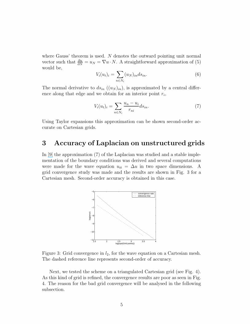
In [9] the approximation (7) of the Laplacian was studied and a stable imple-mentation of the boundary conditions was derived and several computationswere made for the wave equation utt = ∆u in two space dimensions. Agrid convergence study was made and the results are shown in Fig. 3 for aCartesian mesh. Second-order accuracy is obtained in this case.

1.5 2 2.5 3 3.5 4−11

−10

−9

−8

−7

−6

−5

log(sqrt(Grid points))

log(

erro

r)

convergence ratereference line

Figure 3: Grid convergence in l2, for the wave equation on a Cartesian mesh.The dashed reference line represents second-order of accuracy.

Next, we tested the scheme on a triangulated Cartesian grid (see Fig. 4).As this kind of grid is refined, the convergence results are poor as seen in Fig.4. The reason for the bad grid convergence will be analysed in the followingsubsection.

5

0 0.2 0.4 0.6 0.8 10

0.1

0.2

0.3

0.4

0.5

0.6

0.7

0.8

0.9

1

x

y

1.5 2 2.5 3 3.5 4−5

−4.8

−4.6

−4.4

−4.2

−4

−3.8

−3.6

−3.4

−3.2

−3

log(grid points)

log(

erro

r)

Figure 4: Left: A triangulated Cartesian mesh. Right: l2-convergence on atriangulated Cartesian mesh.

Remark A triangulated Cartesian grid is not truly an unstructured grid.But it is a good model of an unstructured grid and if the scheme is incon-sistent on such a grid it will not be consistent on an arbitrary unstructuredgrid.

3.1 Consistency Analysis

We will analyse consistency for the centre point of the grid in Fig. 5. Thescheme (7) leads to,

V1(u1)t =7∑

i=2

ui − u1

ri1

dsi1, (8)

where V1 = h2 is the area inside the dashed line. By Taylor expansions weobtain for the edge r21.

u2 − u1√2h

=u1 + hux + huy + 1

2(h2uxx + 2h2uxy + h2uyy) − u1 + O(h3)√

2h,

where the derivatives are taken at point 1. A similar derivation for edge r51

leads to,

u2 − u1√2h

ds12 +u5 − u1√

2hds15 =

h2uxx + 2h2uxy + h2uyy + O(h3)

3.

In the same manner we obtain for points edges r31, r41, r61 and r71.

u3 − u1

hds13 +

u6 − u1

hds16 =

√5

3(h2uxx + O(h3)),

u7 − u1

hds17 +

u4 − u1

hds14 =

√5

3(h2uyy + O(h3)).

6

Summing up, using (8) and V1 = h2 yield,

(u1)t =1 +

√5

3∆u +

2

3uxy + O(h),

i.e. an O(1) error. This is stated in theorem 3.1.

Theorem 3.1 On a general grid the approximation (7) of (1), with a = b =0 and ǫ = 1, is inconsistent.

����

������������

������

������������

����

������������������

����������������������������������������������������������h

a

b3

27

6 1

5 4

Figure 5: A triangular grid where the dual grid is the dashed line, b = h√

5/3and a = h

√2/3.

The theorem does not imply inconsistency on all grids. It is easily seen inthe above analysis that if the scheme consists of equilateral polygons, consis-tency is recovered. This is verified with computations on a grid with equilat-eral triangles. Again, the wave equation is considered and a grid refinementis performed. In this case the domain as well as the cells are equilateraltriangles and the grid convergence corroborates second-order accuracy. (SeeFig. 6.)

7

0 0.2 0.4 0.6 0.8 10

0.1

0.2

0.3

0.4

0.5

0.6

0.7

0.8

0.9

x

y

1 1.5 2 2.5 3 3.5 4−12

−11

−10

−9

−8

−7

−6

−5

−4

log(sqrt(grid points))

log(

erro

r)

Figure 6: Left: A mesh with equilateral triangles. Right: Convergence for thewave equation with mesh consisting of equilateral triangles. The referenceline represents second-order of accuracy.

It has been shown that the scheme works satisfactory on Cartesian as wellas equilateral triangular grids which are both equilateral polygons. In fact,the scheme will work on grids consisting of any type of equilateral polygons.In the case of equilateral triangles the domain was also chosen to be a triangle.It is not possible to alter the shape of the cell triangles near the boundarysince that would introduce errors of order 1.

The triangulated Cartesian grid used in Fig. 5 resulted in an inconsis-tent scheme. In the equilateral triangular case the scheme coincides with amass lumped finite element scheme. To show the differences between finitevolume and finite element schemes we derive the mass lumped finite elementapproximation of Laplace equation, with linear basis functions applied to thegrid in Fig. 5 and obtain,

h2(u1)t = −v4 − v3 + 4u1 − u7 − u6.

The left hand side, h2(u1)t, is the result of the mass lumping and is preciselyequal to V1(u1)t obtained with the finite volume technique. However, theright hand side coincides with the ordinary finite difference scheme on thecorresponding Cartesian grid. Compared to the finite volume case, differentweights on all the neighbouring points are obtained and especially the crossderivative contribution is cancelled since u5 and u2 do not enter the scheme.

Remark We use the wave equation in our numerical computations, sinceit is a less forgiving equation. However, also for the heat equation on atriangulated Cartesian grid, the convergence levels out (see Fig. 7).

8

1.6 1.8 2 2.2 2.4 2.6 2.8 3 3.2 3.4 3.6−5

−4.8

−4.6

−4.4

−4.2

−4

−3.8

−3.6

−3.4

−3.2

−3

log(sqrt(gridpts))

log(

erro

r)

convergence, heat eq, T=1

Figure 7: Convergence for the heat equation on a triangulated Cartesiangrid.

3.2 A Different Finite Volume Approximation

To further explore the finite volume discretisations of viscous terms we willbriefly discuss a discretisation proposed in [7] and also used in [6]. Thisdiscretisation allows for the computation of all viscous terms in the Navier-Stokes equations but it is not compact as the Laplace approximation previ-ously discussed. The scheme is basically an application of the edge-based firstderivative approximation (4) twice. In [7] it is observed that this scheme doesnot take into account the closest neighbours possibly yielding poor smoothingproperties. (Compare the second derivative approximation that is obtainedby applying a centred finite difference scheme twice.) Accordingly, they pro-pose an augmented form that also uses the neighbours.

We will analyse consistency of the first derivative applied twice withoutthis augmentation to see whether this can be used as an approximation ofthe Laplacian on more general grids. It certainly has the disadvantage thatit is wider and thus not as computationally efficient. Recalling that Ni is theneighbours of the point indexed i and denoting by (ux)i the approximationof the x-derivative at the same point we have that,

(ux)i =1

Vi

∑j∈Ni

uj + ui

2∆yj , (9)

where ∆yj is the difference (with sign) in the y direction going anti-clockwisealong dsij. If approximation (9) is carried out for point 1 in Fig. 5, we wouldobtain with V1 = h2,

(ux)1 =1

V1

∑j∈N1

uj + u1

2∆yj = ux(x1, y1) + O(h2). (10)

9

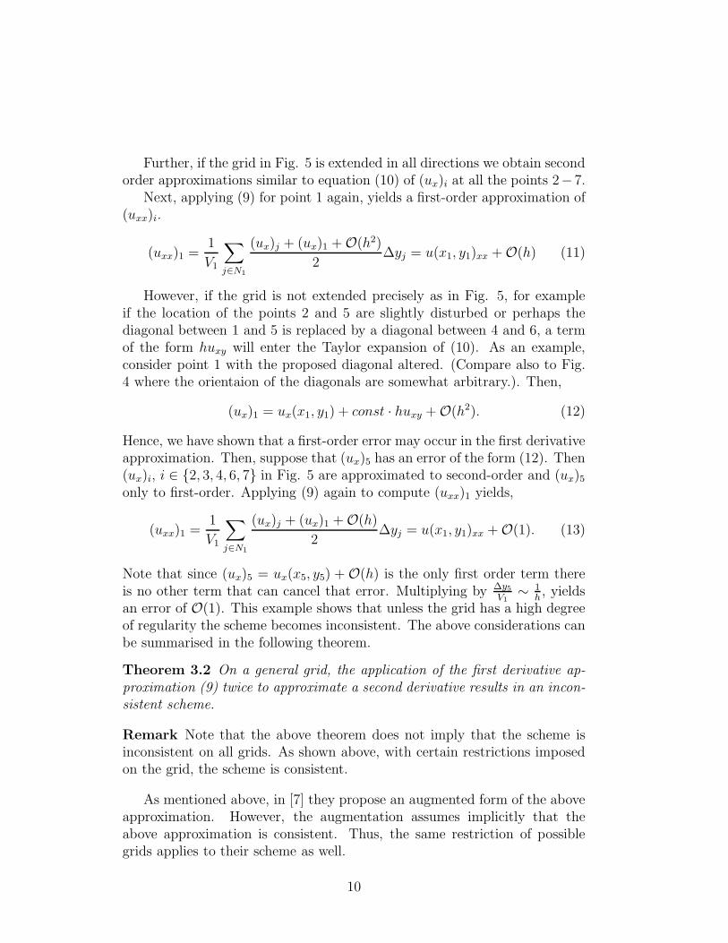
Further, if the grid in Fig. 5 is extended in all directions we obtain secondorder approximations similar to equation (10) of (ux)i at all the points 2−7.

Next, applying (9) for point 1 again, yields a first-order approximation of(uxx)i.

(uxx)1 =1

V1

∑j∈N1

(ux)j + (ux)1 + O(h2)

2∆yj = u(x1, y1)xx + O(h) (11)

However, if the grid is not extended precisely as in Fig. 5, for exampleif the location of the points 2 and 5 are slightly disturbed or perhaps thediagonal between 1 and 5 is replaced by a diagonal between 4 and 6, a termof the form huxy will enter the Taylor expansion of (10). As an example,consider point 1 with the proposed diagonal altered. (Compare also to Fig.4 where the orientaion of the diagonals are somewhat arbitrary.). Then,

(ux)1 = ux(x1, y1) + const · huxy + O(h2). (12)

Hence, we have shown that a first-order error may occur in the first derivativeapproximation. Then, suppose that (ux)5 has an error of the form (12). Then(ux)i, i ∈ {2, 3, 4, 6, 7} in Fig. 5 are approximated to second-order and (ux)5

only to first-order. Applying (9) again to compute (uxx)1 yields,

(uxx)1 =1

V1

∑j∈N1

(ux)j + (ux)1 + O(h)

2∆yj = u(x1, y1)xx + O(1). (13)

Note that since (ux)5 = ux(x5, y5) + O(h) is the only first order term thereis no other term that can cancel that error. Multiplying by ∆y5

V1

∼ 1

h, yields

an error of O(1). This example shows that unless the grid has a high degreeof regularity the scheme becomes inconsistent. The above considerations canbe summarised in the following theorem.

Theorem 3.2 On a general grid, the application of the first derivative ap-proximation (9) twice to approximate a second derivative results in an incon-sistent scheme.

Remark Note that the above theorem does not imply that the scheme isinconsistent on all grids. As shown above, with certain restrictions imposedon the grid, the scheme is consistent.

As mentioned above, in [7] they propose an augmented form of the aboveapproximation. However, the augmentation assumes implicitly that theabove approximation is consistent. Thus, the same restriction of possiblegrids applies to their scheme as well.

10

3.3 Construction of a compact Laplacian

We have now studied two common ways to compute the Laplacian on un-structured meshes and they were both inconsistent on unstructured meshes.Is it possible to construct a consistent and compact Laplacian in the finitevolume framework? The basic idea is to approximate ∂u

∂nalong the face of a

control volume. One approximation for each edge. Furthermore, the gradientof u along an edge should be added to one point and with the opposite sign tothe other point connecting to the same edge. In order to achieve that and tokeep a computational efficiency, the gradient approximation uses only pointsthat are “known” to both points at an edge. By known we mean that theyconnect via an edge. In a two-dimensional triangular grid, 4 points can beused to approximate the gradient at each edge. This can be done in variousdifferent ways, all relying on a first derivative approximation that can onlybe first-order accurate on a general grid. (As has been mentioned before andalso shown in Appendix I.) We obtain,

(∆u)i ≃1

Vi

∑n∈Ni

((uN)in + O(∆r))dsin, (14)

where ∆r is a measure of the maximum size of the edges. Unless, a cancella-tion of errors occur in the summation we will end up with a first-order error.Since, all the gradient approximations only know about the closest neighbourit is unlikely that a cancellation will occur unless the grid is highly regularwhich is precisely what we have observed.

Yet another way of viewing the construction of a Laplacian approximationis the following. The approximation could be stated as,

(∆u)i ≃ ciui +∑n∈Ni

cnun (15)

where cn are constants. If m edges connects point i we have m + 1 unknownconstants cn to determine in order to achieve a consistent approximation.Firstly, we also demand that the gradients at each edge have the oppositesign for both the points at that edge, i.e. n constraints. Secondly, if the ap-proximation is first-order accurate it must exactly differentiate the function,u = x2 + y2 +xy +x+ y + constant, i.e. 6 more constraints. In total we have5 more constraints than unknowns and we have to rely on symmetry in thegrid to fulfil all constraints.

11

4 The advection equation on mixed grids

We have already mentioned that the first derivative approximations do re-sult in at least first-order accuracy on unstructured triangular grids (see [8]and Appendix I). However, as the previous section reveals, finite volume ap-proximations of the Laplacian are not consistent on all grids, though they areassumed to be in real life computations. Hence, we go on studying a commontechnique used in CFD when constructing grids. That is to use structuredgrids in boundary layers which is changed to triangular grids outside bound-ary layers which more easily adapts to complex geometries. Throughout, thissection we will assume that ǫ = 0 in equation (1).

4.1 Consistency analysis of interface

In this case we begin by analysing the first derivative approximation at aninterface between unstructured triangles and quadrilaterals. In particular, weconsider the finite volume approximation at an interface between arbitraryunstructured triangles triangular and a Cartesian grid. (See Fig. 8)

���� ��

����

��

1C

2

3

4

5

Figure 8: An interface between triangles and squares. The dashed line marksthe dual grid.

We assume that the side of the squares have length h. This interfaceis smooth and we can derive the expected order of accuracy at the pointc. The standard way of deriving order of accuracy is to make use of Taylorexpansions. However, that becomes very complicated when unstructuredtriangles are considered. Instead, we will consider the two approximationsobtained if the grid is split along the interface. Then we formally need tospecify uc on both sides using boundary conditions, but in this case uc isgiven by the other side. First consider the finite volume approximation on

12

the control volume related to 1−2− c−5. Denote the corresponding controlvolume V C

c . (Note that the boundary of V Cc partly coincides with 2− c− 5)

The approximation (4) becomes,

V Cc (uc)t =

u1 + uc

2h + uc(−h) (16)

where c is a boundary point and the flux through the boundary is approx-imated by uc. This is a consistent treatment of the boundary (see [8]) andthe scheme is consistent.

The finite volume approximation (4) on the triangles becomes,

V tc (uc)t =

5∑i=2

ui + uc

2∆yi + uch, (17)

where V tc is the corresponding control volume related to c − 2 − 3 − 4 − 5.

(Again, it partly coincides with 2−c−5 where it precisely matches V Cc .) This

is also a consistent approximation according to [8]. Note that, V tc +V C

c = Vc.Hence, the sum of the two approximations is,

Vc(uc)x =5∑

i=2

ui + uc

2∆yi +

u1 + uc

2h =

5∑i=1

ui + uc

2∆yi. (18)

Note that, (18) is the same finite volume approximation at uc as if the schemehad been applied directly ignoring the interface. Since it is constructed fromtwo first-order approximations the sum is also at least first-order.

Since the finite volume approximation on a smooth quadrilaleral grid isalso second-order accurate we conclude that the above reasoning applies toan interface between any smooth equilateral grid and triangles.

In order to derive the global order of accuracy we will use some theoryfrom [8]. Consider the equation ut = ux + F (x) with a finite volume dis-cretisation vt = Dv + F where v denotes the vector with components vi. Dis the resulting matrix obtained by the finite volume discretisation, and Fis a forcing function. According to [8] there is an energy estimate such that‖v‖ ≤ constant(‖f‖ + ‖g‖ + ‖F‖) where f, g denotes the initial data andboundary data. ‖·‖ is the discrete l2-norm (in two space dimensions) definedby,

‖a‖2 =∑

i

a2i Vi. (19)

Then the error equation is,

et = De + T, (20)

13

where e = u − v and T is the truncation error. Note the e has zero initialand boundary data.

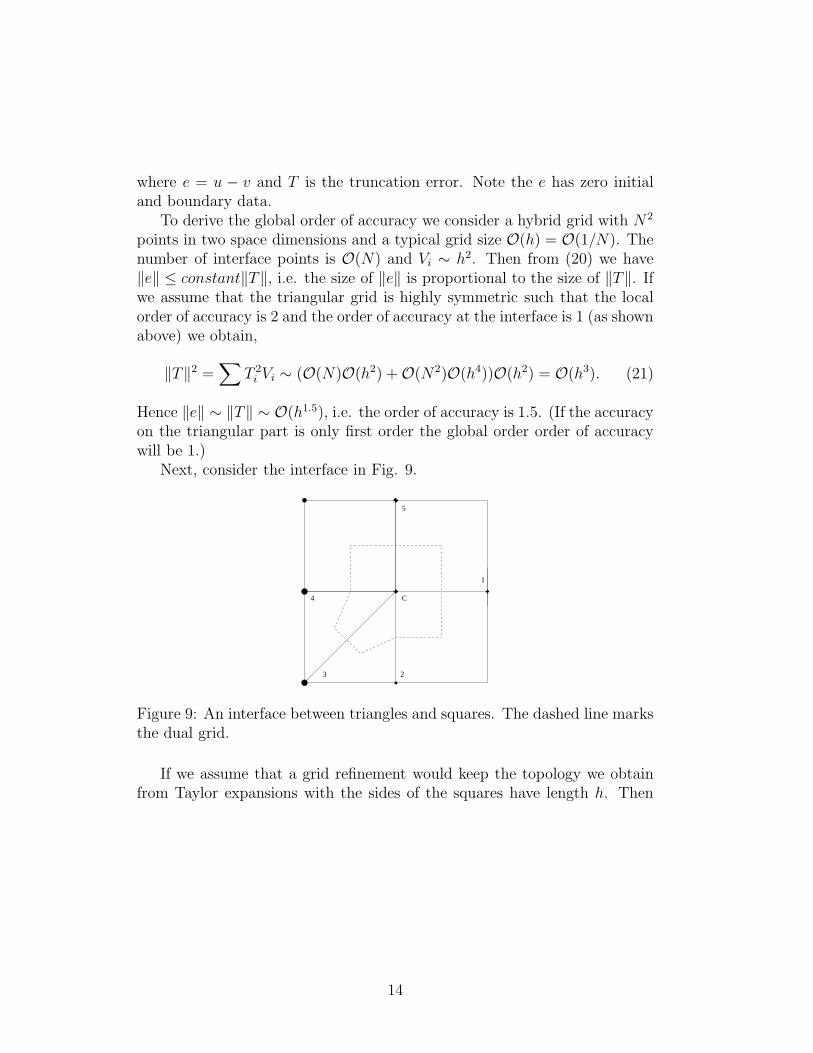
To derive the global order of accuracy we consider a hybrid grid with N2

points in two space dimensions and a typical grid size O(h) = O(1/N). Thenumber of interface points is O(N) and Vi ∼ h2. Then from (20) we have‖e‖ ≤ constant‖T‖, i.e. the size of ‖e‖ is proportional to the size of ‖T‖. Ifwe assume that the triangular grid is highly symmetric such that the localorder of accuracy is 2 and the order of accuracy at the interface is 1 (as shownabove) we obtain,

‖T‖2 =∑

T 2i Vi ∼ (O(N)O(h2) + O(N2)O(h4))O(h2) = O(h3). (21)

Hence ‖e‖ ∼ ‖T‖ ∼ O(h1.5), i.e. the order of accuracy is 1.5. (If the accuracyon the triangular part is only first order the global order order of accuracywill be 1.)

Next, consider the interface in Fig. 9.

���� ��

����

��

5

1

C

23

4

Figure 9: An interface between triangles and squares. The dashed line marksthe dual grid.

If we assume that a grid refinement would keep the topology we obtainfrom Taylor expansions with the sides of the squares have length h. Then

14

Vc = 5

6h2 and,

u1 = uc + hux +h2

2uxx + O(h2),

u2 = uc − huy +h2

2uyy + O(h2),

u3 = uc − hux − huy +h2

2(uyy + uxx + 2uxy) + O(h2),

u4 = uc − hux +h2

2uxx + O(h2),

u5 = uc + huy +h2

2uyy + O(h2),

The finite volume approximation (4) becomes,

Vcut(xc, yc) =uc + u1

2h +

uc + u2

2

h

6+

uc + u3

2

(−h)

3+

uc + u4

2

(−5h)

6=

Vcux(xc, yc) +h2

12uy(xc, yc) + O(h3). (22)

Shifting the diagonal in Fig. 9 will not improve things. In either case, wehave an O(1) error at c.

If we assume that we have an interface with a number of corners like theone above. With two space dimensions and a total number of points O(N2)there are O(N) corner points with an O(1) error. Again,we consider theerror equation and use the energy estimate derived in [8] to conclude that‖e‖ ∼ ‖T‖. To determine the size of the truncation error, assume that theorder of accuracy away from corners is 1, i.e Ti ∼ O(h) = O(1/N) at thosepoints.

‖T‖2 =∑

i

T 2i h2 ∼ O(h2)(O(N)O(1)2 + O(N2)O(1/N)2) = O(h). (23)

Then ‖T‖ ∼ O(h1/2) ∼ e, i.e the order of accuracy is 0.5.

Theorem 4.1 Consider a hybrid mesh composed of unstructured trianglesand smooth quadrilaterals with a non-smooth interface. Then the approxi-mation (4) of (1) with b = ǫ = 0 is inconsistent at the interface and theglobal order of accuracy reduces to 0.5.

Note that throughout this article we consider a model problem with twospace dimensions and we assume implicitly in Theorem 4.1 that an interfaceis one-dimensional. In general we consider an interface to be a d−1 surface in

15

q Ntot qi Nb qtot interface type2 N2 1 N 1.5 smooth,2D1 N2 1 N 1 smooth,2D2 N2 0 N 0.5 non-smooth,line,2D2 N2 0 1 1 non-smooth,point,2D2 N3 1 N2 1.5 smooth,3D1 N3 1 N2 1 smooth,3D2 N3 0 N2 0.5 non-smooth,plane,3D2 N3 0 N 1 non-smooth,line,3D2 N3 0 1 1.5 non-smooth,point,3D

Table 1: Order of accuracy for hybrid meshes. q is the lowest order ofaccuracy of the scheme away from the interface. Ntot is the total numberof points. (We assume N points in one space dimension.) qi is the order ofaccuracy at interface points. (0 meaning order 1 error.) Nb is the number ofboundary points. qtot is the resulting overall order of accuracy.

a problem with d space dimensions. One can anticipate even more restrictiveconstraints in higher-dimensional problems. If there is a disconituity at oneor many points or even along a subsapce of the interface order 1 errors willbe introduced. With the the same technique as used above to estimate thel2-norm of the truncation error we get the results displayed in Table 1 in twoand three space dimensions.

4.2 Computations

Consider, equation (1) with a = 1, b = 1 and ǫ = 0 on a two-dimensional rect-angular domain discretised by (4). The initial data is u(x, 0) = asin(4π(ax+by)) and the exact solution, u(x, t) = sin(4π(a(x− t) + b(y− t))). The exactsolution is also used as boundary data.

In Fig. 10 the convergence rate for a triangular grid is displayed. Theconvergence rate is close to 2 which is due to the fact that the grid is verysymmetric.

16

0 0.1 0.2 0.3 0.4 0.5 0.6 0.7 0.8 0.9 10

0.1

0.2

0.3

0.4

0.5

0.6

0.7

0.8

0.9

1

3 3.5 4 4.5 5 5.5 6−8

−7

−6

−5

−4

−3

−2

−1

log(sqrt(Grid points))

log(

erro

r)

convergence ratereference line

Figure 10: Left: A triangular mesh with 727 grid points. Right: Convergencerate for the advection equation on triangular meshes. The dashed referenceline represents second-order of accuracy.

We also consider a quadrilateral grid (see Figure 11) where there is asmooth mapping to a Cartesian grid. In this case we also obtain second-order accuracy. See Table 2

0 0.1 0.2 0.3 0.4 0.5 0.6 0.7 0.8 0.9 10

0.1

0.2

0.3

0.4

0.5

0.6

0.7

0.8

0.9

1

Figure 11: A smooth quadrilateral grid.

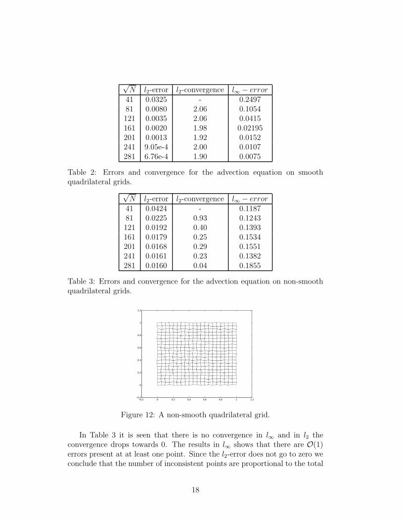
To illustrate that the smoothness is essential for quadrilateral grids weshow the convergence properties for quadrilateral grids (without stretching)with a 20% perturbation in the x- and y-direction for each node. This yieldsa sequence of non-smooth quadrilateral grids. (See Figure 12).

17

√N l2-error l2-convergence l∞ − error

41 0.0325 - 0.249781 0.0080 2.06 0.1054121 0.0035 2.06 0.0415161 0.0020 1.98 0.02195201 0.0013 1.92 0.0152241 9.05e-4 2.00 0.0107281 6.76e-4 1.90 0.0075

Table 2: Errors and convergence for the advection equation on smoothquadrilateral grids.

√N l2-error l2-convergence l∞ − error

41 0.0424 - 0.118781 0.0225 0.93 0.1243121 0.0192 0.40 0.1393161 0.0179 0.25 0.1534201 0.0168 0.29 0.1551241 0.0161 0.23 0.1382281 0.0160 0.04 0.1855

Table 3: Errors and convergence for the advection equation on non-smoothquadrilateral grids.

−0.2 0 0.2 0.4 0.6 0.8 1 1.2−0.2

0

0.2

0.4

0.6

0.8

1

1.2

Figure 12: A non-smooth quadrilateral grid.

In Table 3 it is seen that there is no convergence in l∞ and in l2 theconvergence drops towards 0. The results in l∞ shows that there are O(1)errors present at at least one point. Since the l2-error does not go to zero weconclude that the number of inconsistent points are proportional to the total

18

√N l2-error l2-convergence l∞ − error

41 0.0352 - 0.260381 0.0087 2.05 0.1035121 0.0038 2.06 0.0412161 0.0022 1.91 0.0353201 0.0014 2.04 0.0291241 0.0010 1.85 0.0246281 7.5e-4 1.87 0.0218

Table 4: Errors and convergence for the advection equation on hybrid quadri-lateral and triangular grid with smooth interface.

number of points. This is what we would expect since there are perturbationsto the nodes everywhere.

Next, we turn to mixed grids. We begin our study with the same smoothquadrilateral grid used above. The total number of points is (N + 1)2 andwe place an interface at x(N/2 + 1). This yields a smooth interface. Onone side we triangulate the grid and on the other we keep the quadrilaterals(See Figure 13). According to the previous theory this should have order ofaccuacy 1.5. The errors and convergence are displayed in Table 4 and we seethat the errors in l2 and l∞ are convergent.

0 0.1 0.2 0.3 0.4 0.5 0.6 0.7 0.8 0.9 10

0.1

0.2

0.3

0.4

0.5

0.6

0.7

0.8

0.9

1

Figure 13: A hybrid quadrilateral and triangular grid with a smooth interface.

However, as previously mentioned, it is common that the interface isnon-smooth. (See Figure 1.) An example of such an interface is displayed inFigure 14 and the convergence data given in Table 5.

19

√N l2-error l2-convergence l∞ − error

41 0.0338 - 0.132981 0.0144 1.23 0.1015121 0.0108 0.72 0.1003161 0.0091 0.60 0.0999201 0.0081 0.52 0.1004241 0.0074 0.50 0.1006281 0.0068 0.55 0.1004321 0.0064 0.46 0.1004

Table 5: Errors and convergence for the advection equation on hybrid quadri-lateral and triangular grid with non-smooth interface.

0 0.1 0.2 0.3 0.4 0.5 0.6 0.7 0.8 0.9 10

0.1

0.2

0.3

0.4

0.5

0.6

0.7

0.8

0.9

1

Figure 14: A hybrid quadrilateral and triangular grid with a non-smoothinterface.

Clearly, there are points that are non-convergent according to Table 5. Asshown above the l2-convergence should approach 0.5 which is corroboratedin Table 5.

5 Conclusions

Edge-based node-centred finite volume approximations are widely used incomputational aerodynamics for one important reason. They are assumedaccurate on unstructured grids.

In Theorem 3.1 and 3.2, we prove that discretisations of second deriva-tives with two different commonly used approximations are inconsistent onunstructured grids. However, the accuracy is recovered on grids with a highlevel of regularity. For the Laplacian approximation equilateral polygonsare required and for the first derivative approximation applied twice slightly

20

more general grids can be allowed. We conclude by showing that a compactfinite volume approximation of the Laplacian has to rely on symmetries inthe grid to be first-order accurate.

The CFD community (see for example [19]) have recognised that inboundary layers, structured grids should be used in order to obtain betteraccuracy (see Fig 1). Our analysis confirm that observation since the viscousterms are dominant in the boundary layer and those are only approximatedcorrectly on regular grids, such as rectangles and equilateral polygons.

Structured grids in boundary layers and unstructured to capture geome-tries have led us to study mixed grids for the first derivative approximation.That approximation is shown to be consistent on triangular grids and onsmooth quadrilateral grids. For mixed grids with smooth interfaces betweenthe quadrilaterals and triangles the accuracy is not degraded.

However, if the interface is non-smooth the order of accuracy drops to0.5 due to inconsistencies in the discretisation. To summarise, care has tobe taken when constructing hybrid grids. Extensive numerical experimentscorroborate our theoretical results.

21

APPENDIX

I First derivative approximation

We will show that the first derivative approximation is first order accurateon a general triangular grid. This derivation is due to [20].

Consider the grid in Fig. 15.

������

������

��

��

��

��

��1

C

2

3

4

5

Figure 15: A general triangular grid.

The approximation of ux at the centre point c is,

(ux)c =1

Vc

∑i

uc + ui

2∆yi, (24)

where V is the volume the measure of the volume of the dual grid. If thisapproximation is first order accurate it should exactly differentiate a constantand a linear function.

For a constant function u = C we have ux = 0 and,

(ux)c =C

V

∑i

∆yi = 0. (25)

Hence, the approximation is correct for a constant. Next, we turn to a linearfunction u = ax + by where a and b are constants and ux = a. Denote byr1 = (x1, y1) the position of the centre of mass for the triangle 1, 2, c and r2

for the triangle 2, 3, c etc. Then the approximation for the linear function is,

(ux)c =1

Vc

max∑i=1

axc + byc + axi + byi

2(yi − yi−1) =

1

V

max∑i=1

axi + byi

2(yi − yi−1), (26)

22

where y0 is interpreted as ymax in a cyclic manner around c. (In Fig 15max = 5.) Hence, it is always assumed assumed that we compute modulothe number of neighbours.

The y-coordinate of the centre of mass is obtained by,

yi =yi + yi+1 + yc

3. (27)

Then,

yi − yi−1 =yi + yi+1 + yc

3− yi + yi+1 + yc

3=

yi+1 − yi−1

3. (28)

Using (28) in (26) results in,

(ux)c =1

Vc

∑i

axi

2

yi+1 − yi−1

3+

byi

2

yi+1 − yi−1

3.

Note that,

max∑i=1

yi(yi+1 − yi−1) = 0.

Hence,

(ux)c =a

Vc

∑i

xiyi+1 − yi−1

6. (29)

Next, we will compute Vc. The triangle 1, 2, c has the area,

1

2|(r1 − rc) × (r2 − rc)|

where ri = (xi, yi) is the point vector at point i. With the same notation asfor ri we denote the area of traingle i, i + 1, c by Ai. Hence,

Ai =1

2((xi − xc)(yi+1 − yc) − (yi − yc)(xi+1 − xc)).

The area of the dual volume is,

Vc =∑

i

1

3Ai =

∑i

1

6((xi − xc)(yi+1 − yc) − (yi − yc)(xi+1 − xc)) =

1

6

∑i

xiyi+1 − xiyc − xcyi+1 + xcyc − (yixi+1 − ycxi+1 − yixc + ycxc) =

1

6

∑i

xiyi+1 − yixi+1 =1

6

∑i

xi(yi+1 − yi−1) (30)

23

Note that we use modulo calculations extensively which also justifies the shiftof the indices. With (30) in (29) we have,

(ux)c = a.

Hence, we have shown first order accuracy on an arbitrary triangular grid.

References

[1] A. Haselbacher, J.J. McGuirk, and G.J. Page. Finite volume discretiza-tion aspects for viscous flows on mixed unstructured grids. AIAA Jour-nal, 37(2), Feb. 1999.

[2] D.J Mavriplis. Accurate multigrid solution of the Euler equations onunstructured and adaptive meshes. AIAA Journal, 28(2), Feb. 1990.

[3] D.J Mavriplis. Multigrid strategies for viscous flow solvers on anisotropicunstructured meshes. J. Comput. Physics, 145, 1998.

[4] D.J. Mavriplis and D.W. Levy. Transonic drag prediction using an un-structured multigrid solver. Technical report, Institute for ComputerApplications in Science and Engineering, 2002.

[5] D.J. Mavriplis and V. Venkatakrishnan. A unified multigrid solver forthe Navier-Stokes equations on mixed element meshes. Technical report,Institute for Computer Applications in Science and Engineering, 1995.

[6] T. Gerhold, O. Friedrich, and J.Evans. Calculation of complex three-dimensional configurations employing the DLR-τ -Code. In AIAA paper97-0167, 1997.

[7] J.M. Weiss, J.P. Maruszewski, and W.A. Smith. Implicit solution ofpreconditioned Navier-Stokes equations using algebraic multigrid. AIAAJournal, 37(1), Jan. 1999.

[8] Jan Nordstrom, Karl Forsberg, Carl Adamsson, and Peter Eliasson. Fi-nite volume methods, unstructured meshes and strict stability for hy-perbolic problems. Applied Numerical Mathematics, 45(4), June 2003.

[9] M. Svard and J. Nordstrom. Stability of finite volume approximationsfor the laplacian operator on quadrilateral and triangular grids. AppliedNumerical Mathematics, 51(1), October 2004.

24

[10] W.K. Anderson and D.L. Bonhaus. An implicit upwind algorithm forcomputing turbulent flows on unstruxtured grids. Computers and Fluids,23(1), January 1994.

[11] E.J. Nielsen and W.K. Anderson. Recent improvements in aerodynamicdesign optimization on unstructured meshes. In AIAA-2001-0596, 2001.

[12] E.J. Nielsen, J. Lu, M. Park, and D.L. Darmofal. An implicit, exactdual adjoint solution method fo turbulent flows on unstructured grids.Computers and fluids, 33, 2004.

[13] Y. Kallinderis. A 3-D finite-volume method for the Navier-Stoekes equa-tions with adaptive hybrid grids. Applied Numerical Mathematics, 20,1996.

[14] P. Elisasson. Edge, a navier-stokes solver for unstructured grids. InProc. to Finite Volumes for Complex Applications III, pages 527–534,2002.

[15] Lars Tysell. Hybrid grid generation for complex 3d geometries. In Pro-ceedings of 7th International Conference on Numerical Grid Generationin Computational Field Simulation, Whistler,British Columbia,Canada,pages 337–346, 2000.

[16] D. Kim and H. Choi. A second-order time-accurate finite volume methodfor unsteady incompressible flow on hybrid unstructured grids. Journalof Computational Physics, 162, 2000.

[17] R.P. Koomullil, D.S. Thompson, and B.K. Soni. Iced airfoil simulationusing generalized grids. Applied Numerical Mathematics, 46, 2003.

[18] J. Gong, M. Svard, and J. Nordstrom. Artificial dissipation for strictlystable finite volume methods on unstructured meshes. In WCCM VI inconjuction with APCOM’04, Beijing, China, 2004.

[19] D.J Mavriplis. Unstructured grid techniques. Annu. Rev. Fliud. Mech.,29, 1997.

[20] Karl Forsberg. The Swedish Defence Research Agency. Private Com-munication.

25