Amidakuji: Gray Code Algorithms and Equations for Listing Ladder

Lotteries

by

Patrick Di Salvo

A Thesis

presented to

The University of Guelph

In partial fulfilment of requirements

for the degree of

Master of Science

in

Computer Science

Guelph, Ontario, Canada

c© Patrick Di Salvo, August, 2021

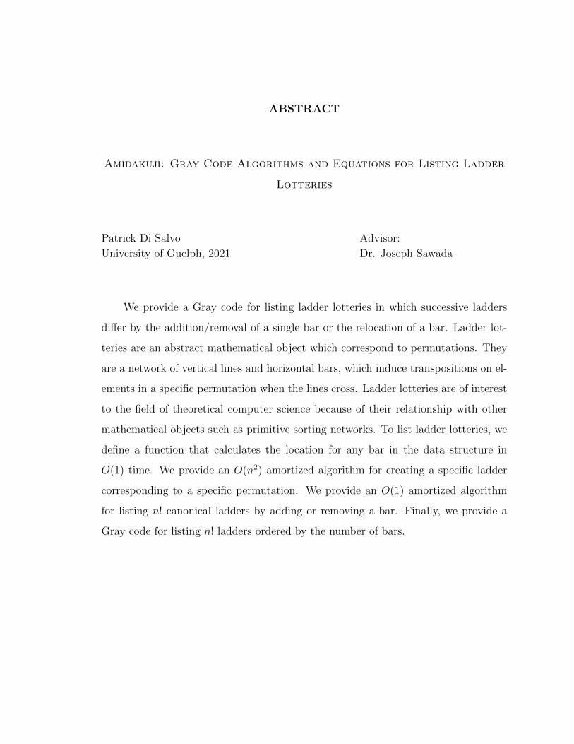
ABSTRACT

Amidakuji: Gray Code Algorithms and Equations for Listing Ladder

Lotteries

Patrick Di Salvo Advisor:

University of Guelph, 2021 Dr. Joseph Sawada

We provide a Gray code for listing ladder lotteries in which successive ladders

differ by the addition/removal of a single bar or the relocation of a bar. Ladder lot-

teries are an abstract mathematical object which correspond to permutations. They

are a network of vertical lines and horizontal bars, which induce transpositions on el-

ements in a specific permutation when the lines cross. Ladder lotteries are of interest

to the field of theoretical computer science because of their relationship with other

mathematical objects such as primitive sorting networks. To list ladder lotteries, we

define a function that calculates the location for any bar in the data structure in

O(1) time. We provide an O(n2) amortized algorithm for creating a specific ladder

corresponding to a specific permutation. We provide an O(1) amortized algorithm

for listing n! canonical ladders by adding or removing a bar. Finally, we provide a

Gray code for listing n! ladders ordered by the number of bars.

Acknowledgments

I would like to thank my advisor Dr. Joe Sawada, my second reader Dr. Charlie

Obimbo, my non-advisory committee member Dr. Steve Gismondi, the committee

chair Dr. Mark Wineberg, and the graduate assistant Jennifer Hughes for their help

with the completion of this thesis.

iii

Table of Contents

Abstract ii

Acknowledgements iii

Table of Contents iv

List of Tables vi

List of Figures vii

1 Introduction 1

1.1 Optimal Ladder Lotteries . . . . . . . . . . . . . . . . . . . . . . . . 3

1.2 Combinatorial Generation . . . . . . . . . . . . . . . . . . . . . . . . 5

1.3 Thesis Statement . . . . . . . . . . . . . . . . . . . . . . . . . . . . . 7

1.4 Contributions . . . . . . . . . . . . . . . . . . . . . . . . . . . . . . . 8

1.5 Summary of Past Known Results . . . . . . . . . . . . . . . . . . . . 8

1.6 Overview of Thesis . . . . . . . . . . . . . . . . . . . . . . . . . . . . 9

2 Background and Literature Review 11

2.1 Efficient Enumeration of Ladder Lotteries and its Application . . . . 12

2.2 Ladder Lottery Realization . . . . . . . . . . . . . . . . . . . . . . . . 14

2.3 Optimal Reconfiguration of Optimal Ladder Lotteries . . . . . . . . . 15

2.4 Coding Ladder Lotteries . . . . . . . . . . . . . . . . . . . . . . . . . 17

2.4.1 Route Based Encoding . . . . . . . . . . . . . . . . . . . . . . 17

2.4.2 Line Based Encoding . . . . . . . . . . . . . . . . . . . . . . . 18

2.4.3 Improved Line Based Encoding . . . . . . . . . . . . . . . . . 18

2.5 Enumeration, Counting, and Random Generation of

Ladder Lotteries . . . . . . . . . . . . . . . . . . . . . . . . . . . . . 20

2.5.1 Enumeration . . . . . . . . . . . . . . . . . . . . . . . . . . . 21

2.5.2 Counting . . . . . . . . . . . . . . . . . . . . . . . . . . . . . . 21

2.6 Permutations . . . . . . . . . . . . . . . . . . . . . . . . . . . . . . . 21

2.6.1 Steinhaus-Johnson-Trotter Algorithm . . . . . . . . . . . . . . 23

iv

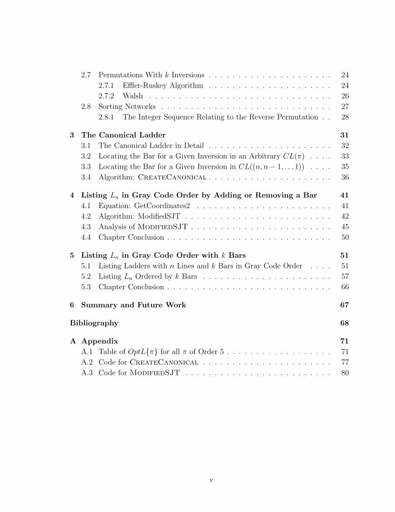
2.7 Permutations With k Inversions . . . . . . . . . . . . . . . . . . . . . 24

2.7.1 Effler-Ruskey Algorithm . . . . . . . . . . . . . . . . . . . . . 24

2.7.2 Walsh . . . . . . . . . . . . . . . . . . . . . . . . . . . . . . . 26

2.8 Sorting Networks . . . . . . . . . . . . . . . . . . . . . . . . . . . . . 27

2.8.1 The Integer Sequence Relating to the Reverse Permutation . . 28

3 The Canonical Ladder 31

3.1 The Canonical Ladder in Detail . . . . . . . . . . . . . . . . . . . . . 32

3.2 Locating the Bar for a Given Inversion in an Arbitrary CL(π) . . . . 33

3.3 Locating the Bar for a Given Inversion in CL((n, n− 1, . . . 1)) . . . . 35

3.4 Algorithm: CreateCanonical . . . . . . . . . . . . . . . . . . . . . 36

4 Listing Ln in Gray Code Order by Adding or Removing a Bar 41

4.1 Equation: GetCoordinates2 . . . . . . . . . . . . . . . . . . . . . . . 41

4.2 Algorithm: ModifiedSJT . . . . . . . . . . . . . . . . . . . . . . . . . 42

4.3 Analysis of ModifiedSJT . . . . . . . . . . . . . . . . . . . . . . . . 45

4.4 Chapter Conclusion . . . . . . . . . . . . . . . . . . . . . . . . . . . . 50

5 Listing Ln in Gray Code Order with k Bars 51

5.1 Listing Ladders with n Lines and k Bars in Gray Code Order . . . . 51

5.2 Listing Ln Ordered by k Bars . . . . . . . . . . . . . . . . . . . . . . 57

5.3 Chapter Conclusion . . . . . . . . . . . . . . . . . . . . . . . . . . . . 66

6 Summary and Future Work 67

Bibliography 68

A Appendix 71

A.1 Table of OptL{π} for all π of Order 5 . . . . . . . . . . . . . . . . . . 71

A.2 Code for CreateCanonical . . . . . . . . . . . . . . . . . . . . . . 77

A.3 Code for ModifiedSJT . . . . . . . . . . . . . . . . . . . . . . . . . 80

v

List of Tables

1.1 Table of known solutions for problems related to ladder lotteries . . . 9

2.1 Number of minimum sorting networks and |OptL{(n, n− 1, . . . , 1)}| . 29

4.1 The table with the runtimes for listing Ln using ModifiedSJT. . . . 50

5.1 Table comparing the listing of permutations with the same composition 53

A.1 Table with all 5! permutations and the corresponding size of each per-

mutation’s OptL{π} ordered by k inversions . . . . . . . . . . . . . . 71

vi

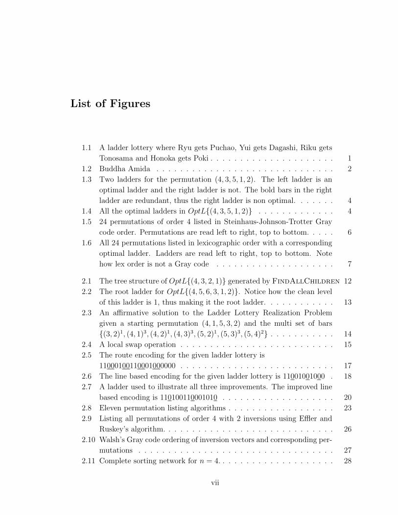
List of Figures

1.1 A ladder lottery where Ryu gets Puchao, Yui gets Dagashi, Riku gets

Tonosama and Honoka gets Poki . . . . . . . . . . . . . . . . . . . . . 1

1.2 Buddha Amida . . . . . . . . . . . . . . . . . . . . . . . . . . . . . . 2

1.3 Two ladders for the permutation (4, 3, 5, 1, 2). The left ladder is an

optimal ladder and the right ladder is not. The bold bars in the right

ladder are redundant, thus the right ladder is non optimal. . . . . . . 4

1.4 All the optimal ladders in OptL{(4, 3, 5, 1, 2)} . . . . . . . . . . . . . 4

1.5 24 permutations of order 4 listed in Steinhaus-Johnson-Trotter Gray

code order. Permutations are read left to right, top to bottom. . . . . 6

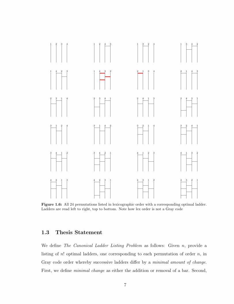
1.6 All 24 permutations listed in lexicographic order with a corresponding

optimal ladder. Ladders are read left to right, top to bottom. Note

how lex order is not a Gray code . . . . . . . . . . . . . . . . . . . . 7

2.1 The tree structure of OptL{(4, 3, 2, 1)} generated by FindAllChildren 12

2.2 The root ladder for OptL{(4, 5, 6, 3, 1, 2)}. Notice how the clean level

of this ladder is 1, thus making it the root ladder. . . . . . . . . . . . 13

2.3 An affirmative solution to the Ladder Lottery Realization Problem

given a starting permutation (4, 1, 5, 3, 2) and the multi set of bars

{(3, 2)1, (4, 1)3, (4, 2)1, (4, 3)3, (5, 2)1, (5, 3)3, (5, 4)2} . . . . . . . . . . . 14

2.4 A local swap operation . . . . . . . . . . . . . . . . . . . . . . . . . . 15

2.5 The route encoding for the given ladder lottery is

11000100110001000000 . . . . . . . . . . . . . . . . . . . . . . . . . . 17

2.6 The line based encoding for the given ladder lottery is 11001001000 . 18

2.7 A ladder used to illustrate all three improvements. The improved line

based encoding is 110100110001010 . . . . . . . . . . . . . . . . . . . 20

2.8 Eleven permutation listing algorithms . . . . . . . . . . . . . . . . . . 23

2.9 Listing all permutations of order 4 with 2 inversions using Effler and

Ruskey’s algorithm. . . . . . . . . . . . . . . . . . . . . . . . . . . . . 26

2.10 Walsh’s Gray code ordering of inversion vectors and corresponding per-

mutations . . . . . . . . . . . . . . . . . . . . . . . . . . . . . . . . . 27

2.11 Complete sorting network for n = 4. . . . . . . . . . . . . . . . . . . . 28

vii

3.1 The canonical ladder for (3, 5, 4, 1, 2). Bars (5, 4), (4, 1), (4, 2) are part

of the route of 4, but only the red bars are associated with the route

of 4. . . . . . . . . . . . . . . . . . . . . . . . . . . . . . . . . . . . . 31

3.2 The associated diagonal of 5 is in red, the associated diagonal of 4 is

in green, the associated diagonal of 3 is in blue, and the associated

diagonal of 2 is in orange. . . . . . . . . . . . . . . . . . . . . . . . . 33

3.3 Canonical ladder such that each bar or absence of a bar is calculated

using the Equation 3.1. . . . . . . . . . . . . . . . . . . . . . . . . . . 35

3.4 Canonical ladder for (6, 5, 4, 3, 2, 1). The location of each bar can be

calculated using the formula (2n− 2x+ (x− y), (x− y)) . . . . . . . 36

3.5 Canonical ladder and corresponding binary matrix. . . . . . . . . . . 38

3.6 The ordering of the state of the ladder when creating the root ladder

for (5, 7, 3, 4, 1, 2, 6) . . . . . . . . . . . . . . . . . . . . . . . . . . . . 40

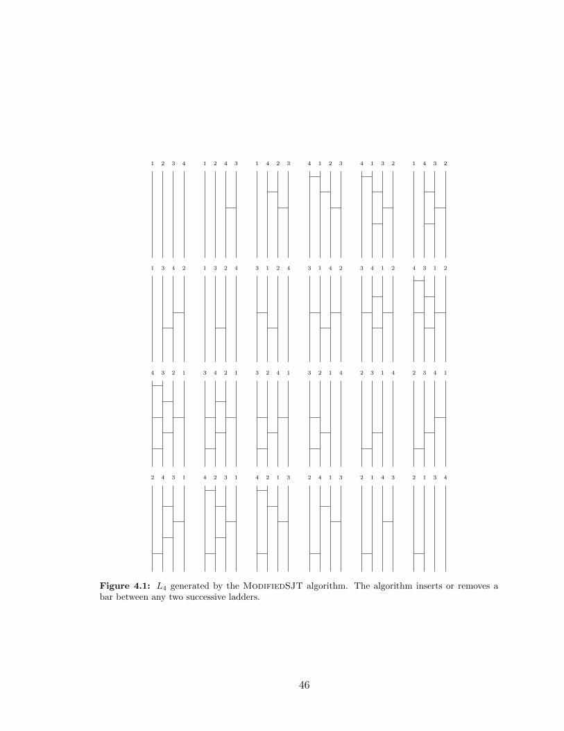
4.1 L4 generated by the ModifiedSJT algorithm. The algorithm inserts

or removes a bar between any two successive ladders. . . . . . . . . . 46

5.1 Mapping of the composition (2, 3, 1, 1) to the associated diagonals of

CL(4, 2, 5, 3, 1) . . . . . . . . . . . . . . . . . . . . . . . . . . . . . . 52

5.2 Listing L5,2 with Walsh’s Gray code on bar vector g. Ladders are read

left to right, top to bottom. g is listed above each ladder. . . . . . . . 55

5.3 Listing of L4 by k bars. For each k, successive ladders differ by the

relocation of a bar. Transitioning from the last ladder in Ln,k to the

first ladder in Ln,k+1 requires the addition of a bar. . . . . . . . . . . 58

5.4 The terminating ladder for L5,6 . . . . . . . . . . . . . . . . . . . . . 59

5.5 Ordering of g based on Conjecture 5.2.1 and the ordering of permuta-

tions corresponding to L5,4 when g is mapped to the associated diagonals. 61

viii

Chapter 1

Introduction

Amidakuji is a custom in Japan which allows for a pseudo-random assignment

of children to prizes [28]. Usually done in Japanese schools, a teacher will draw n

vertical lines, hereby known as lines, where n is the number of students in class. At

the bottom of each line will be a unique prize. At the top of each line will be the name

of one of the students. The teacher will then draw 0 or more horizontal lines, hereby

known as bars, connecting two adjacent lines. No two endpoints of two bars can be

touching. The more bars there are the more complicated (and fun) the Amidakuji is.

Each student then traces their line, and whenever they encounter an end point of a

bar along their line, they must cross the bar and continue going down the adjacent

line. The student continues tracing down the lines and crossing bars until they get to

the end of the ladder lottery. We call such a tracing for a given student a path. For

example, the path of Ryu in the ladder lottery depicted in Figure 1.1 is highlighted

in red.

Poki

Yui

Puchao

Riku

Tonosama

Honoka

Dagashi

Ryu

Figure 1.1: A ladder lottery where Ryu gets Puchao, Yui gets Dagashi, Riku gets Tonosama andHonoka gets Poki

1

The term “Amidakuji” has an interesting history. Amida is the Japanese name for

Amithaba, the supreme Buddha of the Western Paradise. Amithaba was a Buddha

from India and there was a cult based around him. The cult of Amida, otherwise

known as Amidism, believed that by worshiping Amithaba, they would enter into his

Western paradise [15]. Amidism began in India in the fourth century, made its way

to China and Korea in the fifth century, and finally came to Japan in ninth century.

Kuji is the Japanese word for lottery. Hence, the game was termed Amidakuji. In

English, Amidakuji translates to ladder lottery.

The game Amidakuji began in Japan during the Muromachi period, which spanned

from 1336 to 1573. During the Muromachi period, the game was played by having

players draw their names at the top of the lines, and at the bottom of the lines were

pieces of paper that had the amount the players were willing to bet. The pieces of

paper were folded in the shape of Amithaba’s halo [15]. In Figure 1.2 a picture of

Buddha Amithaba is provided.

Figure 1.2: Buddha Amida

An interesting property about a ladder lottery is that it is associated with a

permutation. A permutation is a unique ordering of objects. For the purposes of this

2

thesis, the objects of a permutation are 1, 2, . . . , n. A ladder lottery corresponds to a

unique permutation π when:

1. The n elements of π are listed at the top of the ladder lottery in the order that

they appear in π; one element per line of the ladder lottery.

2. At the bottom of the ladder lottery are the n elements of π in strictly ascending

order. For each element x in π, x goes down its path and ends up in the bottom

xth line.

3. Each bar in the ladder is given a label defined by two unique elements in π,

x > y, which interchange at that specific bar. We draw the label as (x, y).

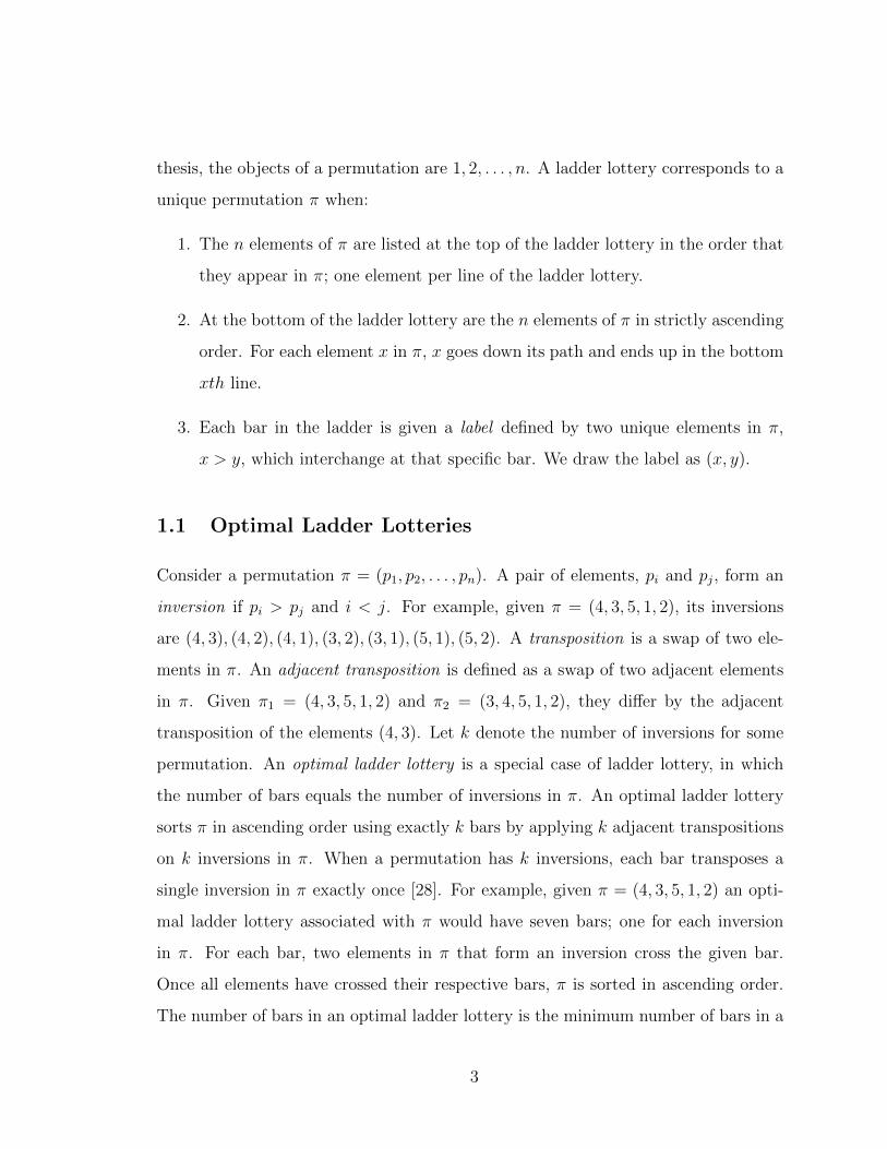
1.1 Optimal Ladder Lotteries

Consider a permutation π = (p1, p2, . . . , pn). A pair of elements, pi and pj, form an

inversion if pi > pj and i < j. For example, given π = (4, 3, 5, 1, 2), its inversions

are (4, 3), (4, 2), (4, 1), (3, 2), (3, 1), (5, 1), (5, 2). A transposition is a swap of two ele-

ments in π. An adjacent transposition is defined as a swap of two adjacent elements

in π. Given π1 = (4, 3, 5, 1, 2) and π2 = (3, 4, 5, 1, 2), they differ by the adjacent

transposition of the elements (4, 3). Let k denote the number of inversions for some

permutation. An optimal ladder lottery is a special case of ladder lottery, in which

the number of bars equals the number of inversions in π. An optimal ladder lottery

sorts π in ascending order using exactly k bars by applying k adjacent transpositions

on k inversions in π. When a permutation has k inversions, each bar transposes a

single inversion in π exactly once [28]. For example, given π = (4, 3, 5, 1, 2) an opti-

mal ladder lottery associated with π would have seven bars; one for each inversion

in π. For each bar, two elements in π that form an inversion cross the given bar.

Once all elements have crossed their respective bars, π is sorted in ascending order.

The number of bars in an optimal ladder lottery is the minimum number of bars in a

3

ladder lottery required to sort π. To see an example of two ladder lotteries associated

with π = (4, 3, 5, 1, 2), one optimal and one non-optimal, please refer to Figure 1.3.

4 3 5 1 2

1 2 3 4 5

(4, 3)

(3, 1)

(4, 1)

(3, 2)

(5, 1)

(4, 2)

(5, 2)

4 3 5 1 2

1 2 3 4 5

(4, 3)

(3, 1)

(4, 1)

(3, 2)

(5, 1)

(4, 2)

(5, 2)

(5, 2)

(5, 2)

Figure 1.3: Two ladders for the permutation (4, 3, 5, 1, 2). The left ladder is an optimal ladder andthe right ladder is not. The bold bars in the right ladder are redundant, thus the right ladder is nonoptimal.

Let OptL{π} be defined as the set of optimal ladder lotteries for a specific π. The

first discussion of OptL{π} is in the paper Efficient Enumeration of Ladder Lotteries

and its Application [28]. In this paper, the authors provide an algorithm which

generates OptL{π}; the details of the algorithm are discussed in Chapter 2. To see

OptL{(4, 3, 5, 1, 2)} please refer to Figure 1.4. Given that there are n! permutations

of order n, each of them have their own OptL{π}. In Table A.1 found in the section

A.1 of the Appendix the number of ladders in each OptL{π} of order 5 is presented.

In general, |OptL{(n, n − 1, . . . , 2, 1)}| is maximal with respect to a permutation of

order n. When n = 5, |OptL{(5, 4, 3, 2, 1)}| = 62.

4 3 5 1 2 4 3 5 1 2 4 3 5 1 2

Figure 1.4: All the optimal ladders in OptL{(4, 3, 5, 1, 2)}

4

1.2 Combinatorial Generation

Our research on ladder lotteries pertains to research in combinatorial generation.

Combinatorial generation is a subfield of theoretical computer science which lists all

instances of combinatorial objects such as permutations, combinations, sets, subsets,

graphs, and ladder lotteries [17]. Knuth describes a number of algorithms for listing

such combinatorial objects in The Art of Computer Programming, Volume 4 [13].

Gray codes are a special type of combinatorial generation in which a constant, minimal

amount of change is required to get from one object to the next. For example, a single

swap operation, a single rotation, or a single bit flip is used to get from one object

to the next. The term “Gray code” comes from the Binary Reflected code given by

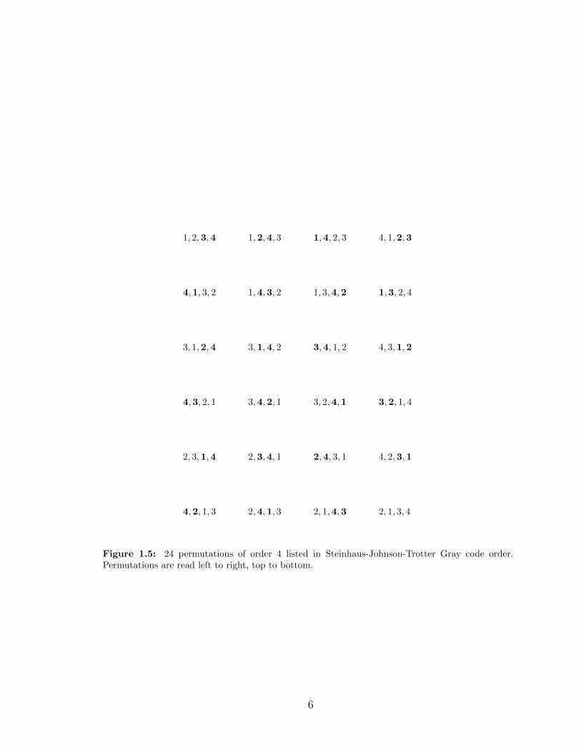
Frank Gray [9]. In Figure 1.5, all 24 permutations of order 4 are listed in Gray code

order using the Steinhaus-Johnson-Trotter Gray code.

There are many known algorithms for listing permutations of order n. Through-

out the course of this thesis, a number of such algorithms were researched [14, 4, 5,

10, 11, 7, 29, 23, 18, 2, 13]. Each of these algorithms will be reviewed in Chapter 2.

In Figure 1.6, one ladder per permutation is listed in lexicographic order; ladders are

read left to right, top to bottom. We note that the lexicographic ordering of ladders

is not a Gray code order. For example, transitioning from ladder 6 to ladder 7 in

Figure 1.6 requires four bars to be changed.

5

1, 2,3,4 1,2,4, 3 1,4, 2, 3 4, 1,2,3

4,1, 3, 2 1,4,3, 2 1, 3,4,2 1,3, 2, 4

3, 1,2,4 3,1,4, 2 3,4, 1, 2 4, 3,1,2

4,3, 2, 1 3,4,2, 1 3, 2,4,1 3,2, 1, 4

2, 3,1,4 2,3,4, 1 2,4, 3, 1 4, 2,3,1

4,2, 1, 3 2,4,1, 3 2, 1,4,3 2, 1, 3, 4

Figure 1.5: 24 permutations of order 4 listed in Steinhaus-Johnson-Trotter Gray code order.Permutations are read left to right, top to bottom.

6

1 2 3 4 1 2 4 3 1 3 2 4 1 3 4 2

1 4 2 3 1 4 3 2 2 1 3 4 2 1 4 3

2 3 1 4 2 3 4 1 2 4 1 3 2 4 3 1

3 1 2 4 3 1 4 2 3 2 1 4 3 2 4 1

3 4 1 2 3 4 2 1 4 1 2 3 4 1 3 2

4 2 1 3 4 2 3 1 4 3 1 2 4 3 2 1

Figure 1.6: All 24 permutations listed in lexicographic order with a corresponding optimal ladder.Ladders are read left to right, top to bottom. Note how lex order is not a Gray code

1.3 Thesis Statement

We define The Canonical Ladder Listing Problem as follows: Given n, provide a

listing of n! optimal ladders, one corresponding to each permutation of order n, in

Gray code order whereby successive ladders differ by a minimal amount of change.

First, we define minimal change as either the addition or removal of a bar. Second,

7

we define minimal change as moving a bar; moving a bar is the same as removing

one bar and adding a new bar. We provide a canonical ladder representation of an

optimal ladder from OptL{π} in order to translate the ladder to a data structure. By

doing so, we allow for a number of efficient solutions to solve The Canonical Ladder

Listing Problem in the form of novel equations, algorithms, and Gray codes.

1.4 Contributions

In this thesis we provide the following contributions:

1. Definition of the canonical ladder.

2. Definition of the data structure for the canonical ladder.

3. Function to calculate the location of a bar in O(1) time.

4. O(n2) algorithm to create the canonical ladder corresponding to a given per-

mutation.

5. O(1) amortized algorithm which lists n! ladders where successive ladders differ

by either a single addition of a bar or a single removal of a bar.

6. Gray code for listing ladders with n lines and k bars for some arbitrary k value

between [0 ≤ k ≤(n2

)].

7. Gray code for listing n! ladders ordered by the number of bars. Successive

ladders differ by the relocation of a bar or by the addition of a bar when tran-

sitioning from k to k + 1 bars.

1.5 Summary of Past Known Results

To the best of my knowledge, the first paper written on ladder lotteries is titled

Efficient Enumeration of Ladder Lotteries and its Application written by Yamanaka,

8

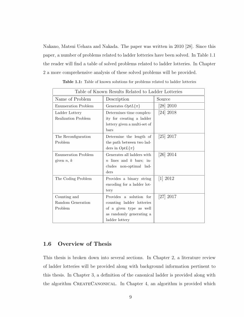
Nakano, Matsui Uehara and Nakada. The paper was written in 2010 [28]. Since this

paper, a number of problems related to ladder lotteries have been solved. In Table 1.1

the reader will find a table of solved problems related to ladder lotteries. In Chapter

2 a more comprehensive analysis of these solved problems will be provided.

Table 1.1: Table of known solutions for problems related to ladder lotteries

Table of Known Results Related to Ladder Lotteries

Name of Problem Description Source

Enumeration Problem Generates OptL{π} [28] 2010

Ladder Lottery

Realization Problem

Determines time complex-

ity for creating a ladder

lottery given a multi-set of

bars

[24] 2018

The Reconfiguration

Problem

Determine the length of

the path between two lad-

ders in OptL{π}

[25] 2017

Enumeration Problem

given n, k

Generates all ladders with

n lines and k bars; in-

cludes non-optimal lad-

ders

[26] 2014

The Coding Problem Provides a binary string

encoding for a ladder lot-

tery

[1] 2012

Counting and

Random Generation

Problem

Provides a solution for

counting ladder lotteries

of a given type as well

as randomly generating a

ladder lottery

[27] 2017

1.6 Overview of Thesis

This thesis is broken down into several sections. In Chapter 2, a literature review

of ladder lotteries will be provided along with background information pertinent to

this thesis. In Chapter 3, a definition of the canonical ladder is provided along with

the algorithm CreateCanonical. In Chapter 4, an algorithm is provided which

9

lists one optimal ladder corresponding to each permutation of order n in Gray code

order; a single bar is added or removed between successive ladders. In Chapter 5, an

algorithm for listing all ladders with n lines and k bars in Gray code order is provided.

Also in Chapter 5, we provide the algorithm for listing all n! ladders ordered by the

number of bars in Gray coder order.

10

Chapter 2

Background and Literature Review

In this chapter we will provide a more comprehensive analysis of the existing

research surrounding ladder lotteries. Let x be a ladder lottery or permutation.

Throughout this thesis a number of algorithms are presented. Many of these algo-

rithms use the following auxiliary functions:

1. Print(x): Prints x.

2. Swap(pi,pj): Swaps pi and pj which are two elements in a permutation.

3. Sort(x): Sorts x in ascending order.

4. Sorted(x): Returns true if x is sorted in ascending order, else returns false.

5. Max(x): Returns the maximum element in x.

6. Min(x): Returns the minimum element in x.

The study of ladder lotteries as mathematical objects began in 2010, in the paper

Efficient Enumeration of Ladder Lotteries and its Application, written by Matsui,

Nakada, Nakano Uehara and Yamanaka [28]. In this paper the authors present the

first algorithm for generating OptL{π} for some arbitrary permutation π. Since

this paper emerged, there have been a number of other papers written about ladder

lotteries. These papers include The Ladder Lottery Realization Problem [24], Optimal

Reconfiguration of Optimal Ladder Lotteries [25], Efficient Enumeration of all Ladder

Lotteries with K Bars [26], Coding Ladder Lotteries [1] and Enumeration, Counting,

and Random Generation of Ladder Lotteries [27]. This thesis is also heavily influenced

11

by Efficient Enumeration of Ladder Lotteries and its Application [28]. Throughout

Chapter 2, we elaborate on the aforementioned papers pertaining to ladder lotteries.

2.1 Efficient Enumeration of Ladder Lotteries and its Appli-

cation

In Efficient Enumeration of Ladder Lotteries and its Application [28], written by

Yamanaka, Nakano, Matsui, Uehara, and Nakada, the authors provide an algorithm

for generating OptL{π} for any π, in O(1) time per ladder. The authors refer to this

algorithm as FindAllChildren.

FindAllChildren was used in this thesis to generate the sample data that

aided in finding solutions for the Canonical Ladder Listing Problem. To see the

tree structure generated by FindAllChildren for OptL{(4, 3, 2, 1)} please refer to

Figure 2.1.

Figure 2.1: The tree structure of OptL{(4, 3, 2, 1)} generated by FindAllChildren

12

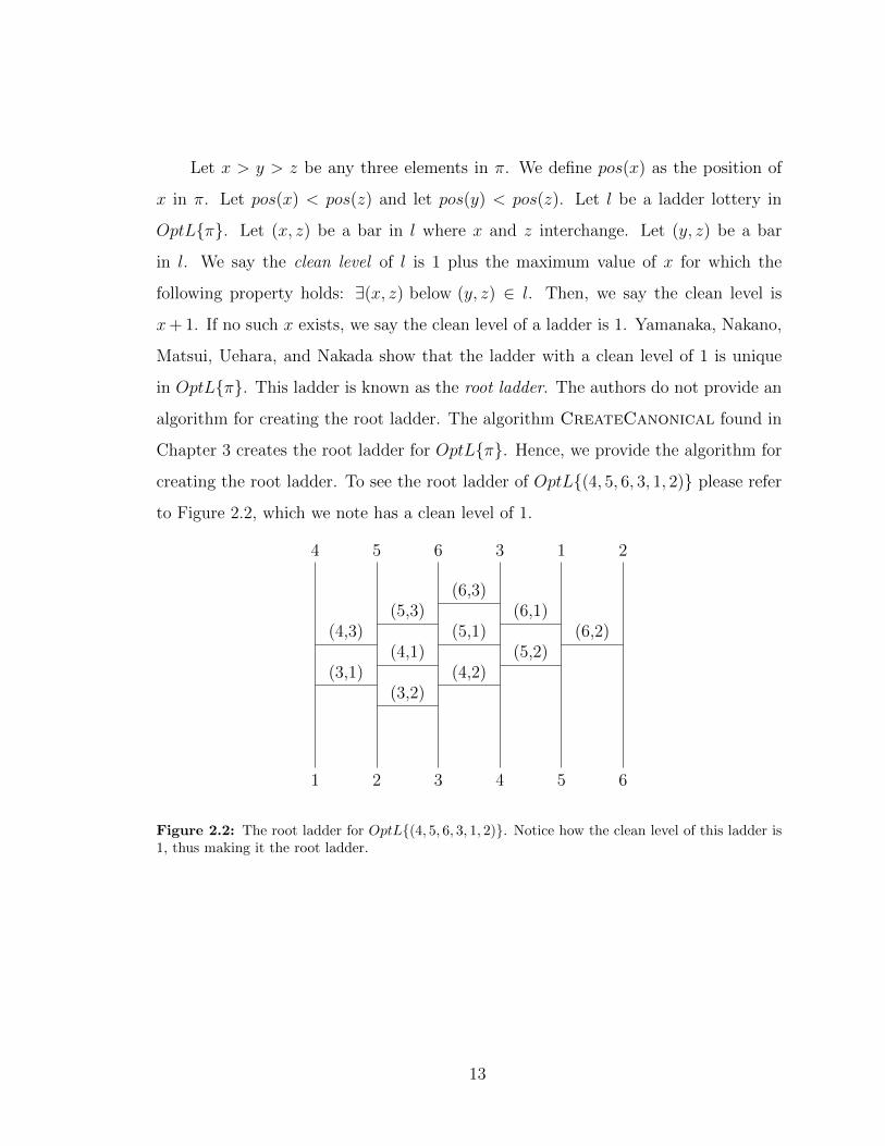
Let x > y > z be any three elements in π. We define pos(x) as the position of

x in π. Let pos(x) < pos(z) and let pos(y) < pos(z). Let l be a ladder lottery in

OptL{π}. Let (x, z) be a bar in l where x and z interchange. Let (y, z) be a bar

in l. We say the clean level of l is 1 plus the maximum value of x for which the

following property holds: ∃(x, z) below (y, z) ∈ l. Then, we say the clean level is

x+ 1. If no such x exists, we say the clean level of a ladder is 1. Yamanaka, Nakano,

Matsui, Uehara, and Nakada show that the ladder with a clean level of 1 is unique

in OptL{π}. This ladder is known as the root ladder. The authors do not provide an

algorithm for creating the root ladder. The algorithm CreateCanonical found in

Chapter 3 creates the root ladder for OptL{π}. Hence, we provide the algorithm for

creating the root ladder. To see the root ladder of OptL{(4, 5, 6, 3, 1, 2)} please refer

to Figure 2.2, which we note has a clean level of 1.

4

1

5

2

6

3

3

4

1

5

2

6

(6,3)(6,1)

(6,2)(5,3)

(5,1)(5,2)

(4,3)(4,1)

(4,2)(3,1)(3,2)

Figure 2.2: The root ladder for OptL{(4, 5, 6, 3, 1, 2)}. Notice how the clean level of this ladder is1, thus making it the root ladder.

13

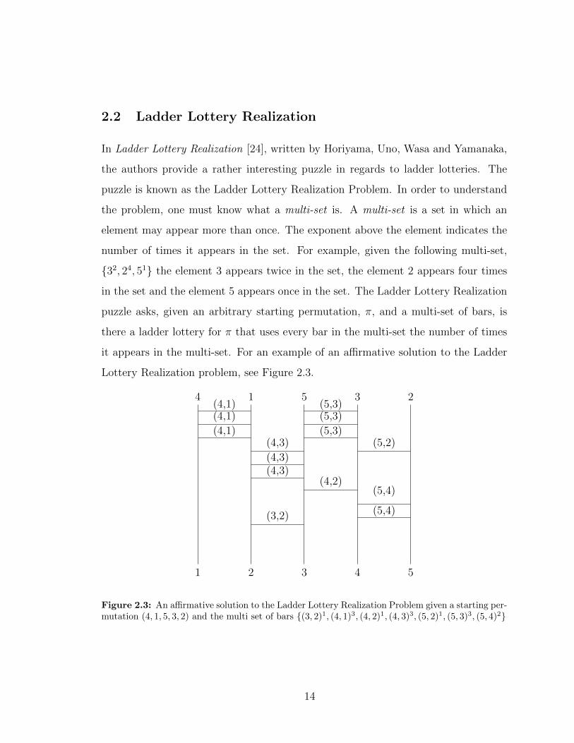
2.2 Ladder Lottery Realization

In Ladder Lottery Realization [24], written by Horiyama, Uno, Wasa and Yamanaka,

the authors provide a rather interesting puzzle in regards to ladder lotteries. The

puzzle is known as the Ladder Lottery Realization Problem. In order to understand

the problem, one must know what a multi-set is. A multi-set is a set in which an

element may appear more than once. The exponent above the element indicates the

number of times it appears in the set. For example, given the following multi-set,

{32, 24, 51} the element 3 appears twice in the set, the element 2 appears four times

in the set and the element 5 appears once in the set. The Ladder Lottery Realization

puzzle asks, given an arbitrary starting permutation, π, and a multi-set of bars, is

there a ladder lottery for π that uses every bar in the multi-set the number of times

it appears in the multi-set. For an example of an affirmative solution to the Ladder

Lottery Realization problem, see Figure 2.3.

1

4

2

1 5

3

3

4

2

5

(4,1)(4,1)

(4,1)

(5,3)(5,3)

(5,3)(4,3)

(4,3)(4,3)

(3,2)

(4,2)

(5,2)

(5,4)

(5,4)

Figure 2.3: An affirmative solution to the Ladder Lottery Realization Problem given a starting per-mutation (4, 1, 5, 3, 2) and the multi set of bars {(3, 2)1, (4, 1)3, (4, 2)1, (4, 3)3, (5, 2)1, (5, 3)3, (5, 4)2}

14

The authors prove that the Ladder Lottery Realization problem in NP-Hard by

reducing the Ladder Lottery Realization to the One-In-Three 3SAT problem, which

has already been proven to be NP-Hard. The authors note that there are two cases in

which the ladder lottery realization problem can be solved in polynomial time. These

cases include the following. First, if every bar in the multi-set appears exactly once

and every bar corresponds to an inversion, then an affirmative solution to the Ladder

Lottery Realization instance can be achieved in polynomial time. Second, if there is

an inversion in the permutation and its bar appears in the multi-set an even number

of times, then a negative solution to the Ladder Lottery Realization instance can be

achieved in polynomial time. This is because the elements that cross the bar will be

uninverted when then be inverted again. Therefore π will not be sorted by the ladder.

2.3 Optimal Reconfiguration of Optimal Ladder Lotteries

A local swap operation, corresponding to a braid relation in algebra, is a local modi-

fication of a ladder lottery demonstrated in Figure 2.4 [28].

Figure 2.4: A local swap operation

In Optimal Reconfiguration of Optimal Ladder Lotteries [25], written by Horiyama,

Wasa and Yamanaka, the authors provide a polynomial solution to the Minimal Re-

15

configuration Problem which asks, given two ladders, Li and Lm, what is the minimal

number of swap operations to perform that will transition from Li to Lm? A reverse

triple is a relation between three bars, x, y, z in two arbitrary ladders, Li, Lm, such

that if x, y, x are right swapped in Li, then they are left swapped in Lm or if they

are left swapped in Li then they are right swapped in Lm. Let an improving triple

be defined as performing a right/left swapping three bars, x, y, z, in Li such that the

result of the swap removes a reverse triple between ladders Li and Lm. The improving

triple is a symmetric relation, therefore performing a right/left swapping of the x, y, z

in Lm also results in the removal of a reverse triple between Li and Lm.

The minimal length reconfiguration sequence is the minimal number of improving

triples required to transition from Li to Lm or Lm to Li. Transitioning from Li to

Lm with the minimal length reconfiguration sequence is achieved by applying an

improving triple to each of the reverse triples between Li and Lm. That is to say,

the length of the reconfiguration sequence is equal to the number of improving triples

required to remove all reverse triples between Li and Lm.

The second contribution of this paper is that it provides a closed form formula for

the upper bound for the minimal length reconfiguration sequence for any permutation

of size n. That is to say, given some arbitrary π of order n, what is the maximum

number of swaps required for the minimal length reconfiguration sequence between

any two ladders in OptL{π}? The authors prove that there are two unique ladders in

OptL{(n, n− 1, . . . , 1)} that have the upper bound for the minimal length reconfigu-

ration sequence. These ladders are the root ladder and final ladder which is defined

as the unique ladder in OptL{π} such that ∀z < y < x : (y, z) is above (x, z) ∈ l.

The length of the reconfiguration sequence between the root ladder and final ladder

in OptL{(n, n− 1, . . . , 1)} is n(n−12

).

16

2.4 Coding Ladder Lotteries

In Coding Ladder Lotteries [1], written by Aiuchi, Yamanaka, Hirayama and Nishi-

tani, the authors provide three methods to encode ladder lotteries as binary strings.

Coding ladder lotteries as binary strings allows for a compact, computer readable,

representation of them. Although we do not apply the encodings to the results of this

thesis, we include them for completeness.

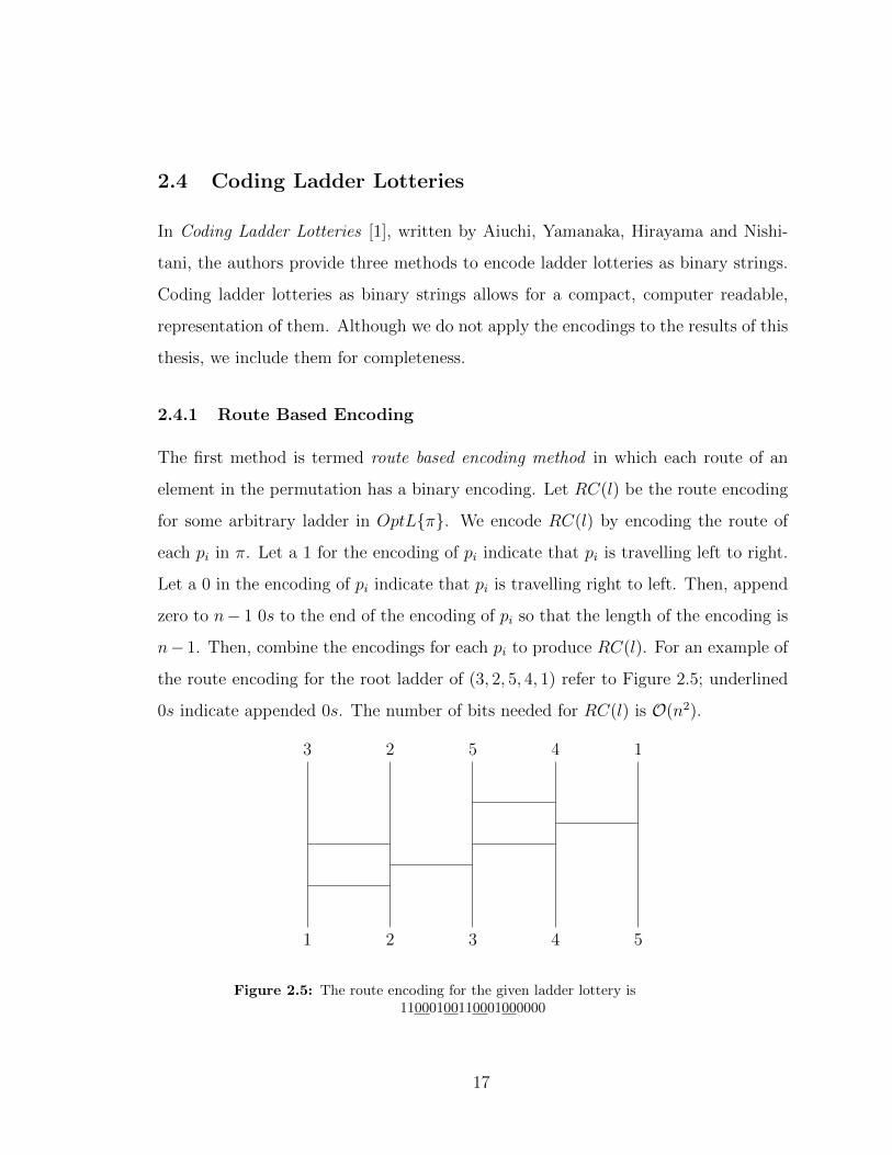
2.4.1 Route Based Encoding

The first method is termed route based encoding method in which each route of an

element in the permutation has a binary encoding. Let RC(l) be the route encoding

for some arbitrary ladder in OptL{π}. We encode RC(l) by encoding the route of

each pi in π. Let a 1 for the encoding of pi indicate that pi is travelling left to right.

Let a 0 in the encoding of pi indicate that pi is travelling right to left. Then, append

zero to n− 1 0s to the end of the encoding of pi so that the length of the encoding is

n− 1. Then, combine the encodings for each pi to produce RC(l). For an example of

the route encoding for the root ladder of (3, 2, 5, 4, 1) refer to Figure 2.5; underlined

0s indicate appended 0s. The number of bits needed for RC(l) is O(n2).

3

1

2

2

5

3

4

4

1

5

Figure 2.5: The route encoding for the given ladder lottery is11000100110001000000

17

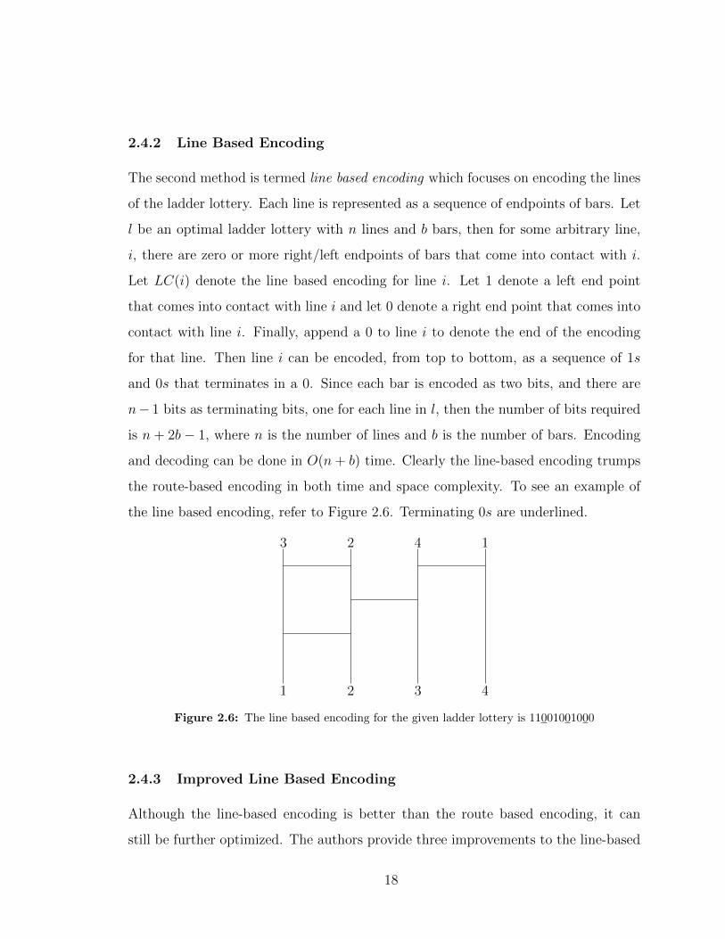
2.4.2 Line Based Encoding

The second method is termed line based encoding which focuses on encoding the lines

of the ladder lottery. Each line is represented as a sequence of endpoints of bars. Let

l be an optimal ladder lottery with n lines and b bars, then for some arbitrary line,

i, there are zero or more right/left endpoints of bars that come into contact with i.

Let LC(i) denote the line based encoding for line i. Let 1 denote a left end point

that comes into contact with line i and let 0 denote a right end point that comes into

contact with line i. Finally, append a 0 to line i to denote the end of the encoding

for that line. Then line i can be encoded, from top to bottom, as a sequence of 1s

and 0s that terminates in a 0. Since each bar is encoded as two bits, and there are

n− 1 bits as terminating bits, one for each line in l, then the number of bits required

is n + 2b− 1, where n is the number of lines and b is the number of bars. Encoding

and decoding can be done in O(n+ b) time. Clearly the line-based encoding trumps

the route-based encoding in both time and space complexity. To see an example of

the line based encoding, refer to Figure 2.6. Terminating 0s are underlined.

3 2 4 1

1 2 3 4

Figure 2.6: The line based encoding for the given ladder lottery is 11001001000

2.4.3 Improved Line Based Encoding

Although the line-based encoding is better than the route based encoding, it can

still be further optimized. The authors provide three improvements to the line-based

18

encoding.

1. The nth line has only right endpoints attached to it, therefore it actually does

not need to be encoded. Right endpoints are denoted as 0 and left endpoints

are encoded as 1, therefore the number of right endpoints for line n is equal to

the number of 1s in LC(i = n− 1).

2. Given two bars, x, y, let lx denote the left endpoint of bar x, let ly denote the

left endpoint of bar y, let rx denote the right end point of bar x and let ry

denote the right end point of bar y. Let line i be the line of lx and ly and let

line i+ 1 be the line of rx and ry. If there is not a 0 between the two 1s for lx,

ly in LCi, it is implied that there is at least one 1 between the two 0s for rx, ry

on LCi+1. Hence, one of the 1s in LC(i+ 1) can be omitted.

3. Improvement three is based off of saving some bits for right end points/0s in

LC(i = n − 1). Since line n has no left end points, then there must be some

right endpoints between any two consecutive bars connecting lines n − 1 and

line n. Knowing this, then given two bars, x and y with lx/ly on line n − 1

and rx/ry on line n, there must be at least one bar, z, with its rz between lx

and ly on line n − 1. Thus, for every 1 in LC(i = n − 1) except the last 1 a

0 must immediately proceed any 1. Since this 0 is implied, it can be removed

from LC(i = n− 1).

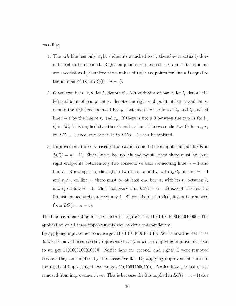
The line based encoding for the ladder in Figure 2.7 is 110101011000101010000. The

application of all three improvements can be done independently.

By applying improvement one, we get 110101011000101010. Notice how the last three

0s were removed because they represented LC(i = n). By applying improvement two

to we get 1101001100010010. Notice how the second, and eighth 1 were removed

because they are implied by the successive 0s. By applying improvement three to

the result of improvement two we get 110100110001010. Notice how the last 0 was

removed from improvement two. This is because the 0 is implied in LC(i = n−1) due

19

to the configuration between of bars connecting lines n− 1 and line n. The improved

line based encoding for the ladder in Figure 2.7 is 110100110001010.

2 1 3 4

Figure 2.7: A ladder used to illustrate all three improvements. The improved line based encodingis 110100110001010

We see that the improved line based encoding for the ladder in Figure 2.7 is

15 bits whereas the line based encoding for the same ladder is 21 bits. This is an

improvement of roughly 28.5%.

2.5 Enumeration, Counting, and Random Generation of

Ladder Lotteries

In the paper, Enumeration, Counting, and Random Generation of Ladder Lotter-

ies [27], written by Nakano and Yamanaka the authors consider the problem of enu-

meration, counting and random generation of ladder lotteries with n lines and b bars.

It is important to note that the authors considered both optimal and non-optimal

ladders for this paper. Nonetheless, the paper is still fruitful for its modelling of the

problems and insights into ladder lotteries. The authors use the line-based encoding,

LC(l) for the representation of ladders that was discussed in the previous section [1].

20

2.5.1 Enumeration

The authors denote a set of ladder lotteries with n lines and b bars as Sn,b. The

problem is how to enumerate all the ladders in Sn,b. The authors use a forest structure

to model the problem. A forest structure is a set of trees such that each tree in the

forest is disjoint union with every other tree in the forest. Consider Sn,b to be a tree

in a forest. That is to say, a union disjoint subset of all ladders with n lines and b

bars. Then Fn,b, or the forest of all Sn,b, is the union of all disjoint trees of ladders

with n lines and b bars.

2.5.2 Counting

The authors provide a method and algorithm to count all ladders with n lines and b

bars. The counting algorithm works by dividing ladders into four types of sub-ladders.

For sub-ladder, r, its type is a tuple t(n, h, p, q) where n is the number of lines, h is

the number of half bars, p is the number of unmatched end-points on line n− 1 and

q is the number of unmatched end-points on line n. From this type, the authors are

able to count all ladders with n lines and b bars.

2.6 Permutations

Ladder lotteries and permutations are intricately related to each other. The research

for The Canonical Ladder Listing Problem is highly influenced by permutation listing

algorithms. Knuth describes a number of permutation listing algorithms in The Art of

Computer Programming [14]. During the research for The Canonical Ladder Listing

Problem, twelve of these enumeration algorithms were investigated [14, 4, 5, 10, 11,

7, 29, 23, 18, 2, 13].

We define Sn as the set of all n! permutations of order n. The first algorithm

we looked at for listing Sn is the lexicographic algorithm, which orders all n! per-

mutations from smallest to largest. The lexicographic algorithm generates each per-

21

mutation with an amortized time of O(n2log(n)) [5]. The second of which is the

colexicographic algorithm which orders all n! permutations from largest to smallest.

The colexicographic algorithm generates each permutation with an amortized time

of O(n2log(n)) [4]. The third of which is Zak’s algorithm which lists Sn by reversing

a suffix in one permutation to get to the next permutation. The time complexity

of Zak’s algorithm constant amortized time [29]. The fourth of which is Heap’s al-

gorithm which is a decrease and conquer algorithm. The time complexity of Heap’s

algorithm is CAT, constant amortized time of O(1) per permutation [10]. The fifth

algorithm is the Steinhaus-Johnson-Trotter (SJT) algorithm which generates Sn by

performing adjacent swap operations on the permutation resulting in the next per-

mutation. Thus, each permutation in Sn differs from it predecessor by a single swap

operation, making SJT a Gray code [11]. To go from any two successive permuta-

tions, the time complexity is O(1) [11]. The sixth algorithm is the algorithm using

star transpositions that always swaps the first element of the permutation with some

other element. It was discovered by Gideon Ehrlich and is described as Algorithm E

in Knuth’s book [14]. The seventh algorithm is the derangement ordering in which

no two consecutive permutations have any elements in the same position. It was first

discussed by Savage in [18]. The eighth algorithm is the Single Track listing algo-

rithm. Each column in the list of permutations is a cyclic shift of the first column [2].

The computation for each successive permutation is CAT [2]. The ninth algorithm

is the Single Track Gray Code listing algorithm. The properties of the Single Track

listing algorithm hold. Furthermore, any two successive permutations differing by at

most two transpositions [2]. The tenth listing algorithm is found in Knuth’s book.

At each step, it either rotates the permutation to the left by one or swaps the first

two elements [13]. The problem as to whether such a listing algorithm exists for all

n is posed as an open problem in Knuth’s book [13]. It was solved by Sawada and

Williams in their paper A Hamiltonian Path for the Sigma-Tau Problem [19]. The

eleventh algorithm is Corbett’s algorithm which rotates a prefix of the first possible

22

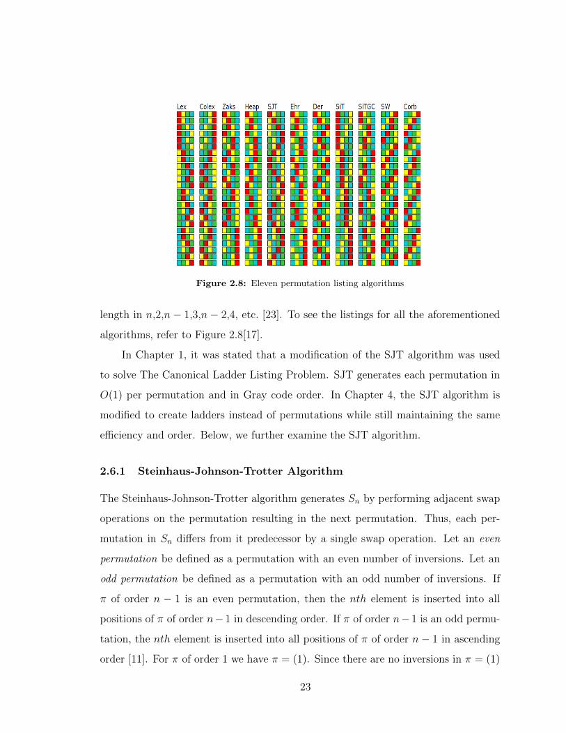
Figure 2.8: Eleven permutation listing algorithms

length in n,2,n− 1,3,n− 2,4, etc. [23]. To see the listings for all the aforementioned

algorithms, refer to Figure 2.8[17].

In Chapter 1, it was stated that a modification of the SJT algorithm was used

to solve The Canonical Ladder Listing Problem. SJT generates each permutation in

O(1) per permutation and in Gray code order. In Chapter 4, the SJT algorithm is

modified to create ladders instead of permutations while still maintaining the same

efficiency and order. Below, we further examine the SJT algorithm.

2.6.1 Steinhaus-Johnson-Trotter Algorithm

The Steinhaus-Johnson-Trotter algorithm generates Sn by performing adjacent swap

operations on the permutation resulting in the next permutation. Thus, each per-

mutation in Sn differs from it predecessor by a single swap operation. Let an even

permutation be defined as a permutation with an even number of inversions. Let an

odd permutation be defined as a permutation with an odd number of inversions. If

π of order n − 1 is an even permutation, then the nth element is inserted into all

positions of π of order n− 1 in descending order. If π of order n− 1 is an odd permu-

tation, the nth element is inserted into all positions of π of order n− 1 in ascending

order [11]. For π of order 1 we have π = (1). Since there are no inversions in π = (1)

23

it is even. Now insert 2 in all positions in π = (1) in descending order. Thus we get

(1, 2) followed by (2, 1). Since (1, 2) is an even permutation, insert 3 into all positions

in descending order resulting in (1, 2, 3), (1, 3, 2) and (3, 1, 2). Since (2, 1) is an odd

permutation, insert 3 into all permutations in ascending order resulting in (3, 2, 1),

(2, 3, 1) and (2, 1, 3).

The Steinhaus-Johnson-Trotter algorithm is a Gray code, meaning that in order

to transition between any two subsequent permutations in Sn, there is a minimal

amount of constant change required. The algorithm simply swaps two elements in

order to transition between permutations. Each recursive call creates a new per-

mutation with the exception of the initial call to the function in which n recursive

calls need to be made before the first permutation is printed. The amortized time to

transition between permutations is O(1).

2.7 Permutations With k Inversions

In the previous section we looked at permutation listings for all n! permutations. In

this section we look at listings for permutations with a given number of inversions.

Let k be the number of inversions for a given permutation of order n. Let Πn,k indicate

the number of permutations of order n with k inversions. We note that the Πn,k is

counted by the triangle of Mahonian numbers [20]. Let Sn,k denote all permutations

of order n with k inversions.

2.7.1 Effler-Ruskey Algorithm

In the paper A CAT Algorithm for Generating Permutations with a Fixed Number of

Inversions [7], written by Effler and Ruskey, the authors provide a constant amor-

tized time algorithm for generating all permutations of order n with k inversions.

The algorithm is also a BEST algorithm (backtracking ensures success at terminals),

meaning that when the algorithm backtracks, the back-tracking leads to a successful

24

Algorithm 1 Generate all permutations with k inversions

1: function KInversions(π, n, k, list)2: if n = 0 and k = 0 then3: Print(π)4: else5: for i from 1 to length of list do6: x← listi7: rank(x) gets(length of list − i) + 18: if n− rank(x) ≤ k ≤

(n−12

)+ n− rank(x) then

9: pn ← x10: k ← k − n+ rank(x)11: remove x from list12: KInversions(π, n− 1, k, list)13: insert x in list at correct position

result. We define the empty permutation of order n as an empty vector of length

n. Let the initial conditions of the algorithm be the following. Let π be the empty

permutation of order n. Let k be initialized to an integer between 0 to(n2

). Let list be

initialized to the list of n elements in strictly descending order. The algorithm works

as follows. Going left to right in the list, each element x is inserted into pn only if

inserting x into position n in π does not exceed the current number of inversions, k. If

x is inserted into π at position n then x is removed from list, a recursive call is made

and both n and k are reduced. Recursion terminates when n and k are 0 indicating

that all elements have been added to π and the correct number of inversions exist in

π. When the function returns from its recursive call, element x is placed back into

the list at its original position. To see the algorithm please refer to Algorithm 1.

Refer to Figure 2.9[7] to see an example of how the algorithm lists permutations

of order 4 with 2 inversions. Each leaf node is a unique permutation of order n with k

inversions. We note that the listing is not a Gray code ordering. For example, when

we look at the leftmost leaf node (3, 1, 2, 4) and its right sibling (2, 3, 1, 4), we note

that they differ by a prefix rotation of the elements {1, 2, 3}.

25

Figure 2.9: Listing all permutations of order 4 with 2 inversions using Effler and Ruskey’s algo-rithm.

2.7.2 Walsh

Despite the efficiency of Effler-Ruskey’s algorithm, we note that the permutations

are not listed in Gray code order. Therefore, we also look at the paper, Loop Free

Sequencing of Bounded Integer Compositions, written by Walsh [22]. Walsh provides

an algorithm for listing Sn,k in Gray code order in O(1) time per permutation. An

n part composition of a non negative integer k is an ordered n-tuple, (g1, g2 . . . , gn),

whose sum adds to k. Such a composition is said to be (m1,m2, . . . ,mn) bounded

when 0 ≤ gi ≤ mi. Let π be of order n+ 1, then we say g is an n-tuple from g1 . . . gn.

We say m is a bound on g from m1 . . .mn such that each mi = min(n + 1 − i, k)

where k is the target number of inversions. Let gi represent the number of inversions

formed by placing an element from 1 to n + 1 in π at index i in π. We note that

placing 1 at index 1 forms 0 inversions and we note that placing n + 1 at index 1

forms n inversions. g is known as the inversion vector of π, bounded by m.

Walsh lists Sn,k by incrementing some gi by 1 and decrementing some gj by

1. Let x and y be positive integers indicating offsets from an index. Incrementing

gi by 1 induces a transposition in π with pi and some element, pi+x in the suffix

pi+1 . . . pn+1, such that pi < pi+x ∧ pi+x < ∀pi+y > pi. Decrementing gj by 1 induces a

26

Figure 2.10: Walsh’s Gray code ordering of inversion vectors and corresponding permutations

transposition in π with pj and some element, pj+x in the suffix pj+1 . . . pn+1, such that

pj > pj+x ∧ pj+x > ∀pj+y < pj. We call i the first pivot j the second pivot, indicating

that the increment occurs before the decrement; each pivot is found in O(1) time. In

Figure 2.10 [22], all compositions, and permutations of order 5 with 5 inversions, are

listed in the Gray code order found in Walsh’s paper. In Chapter 5, by borrowing

from Walsh’s paper, we derive a Gray code for listing one optimal ladder for each

permutation with k inversions.

2.8 Sorting Networks

Let a wire be a horizontal line. Let a comparator be a vertical line connecting two

wires. A sorting network is a device consisting of n wires and m comparators such

that the sorting network sorts a permutation of n elements into ascending order. The

n elements are first listed to the left of each wire in the network. The elements travel

across their respective wires at the same time. When a pair of elements, traveling

through a pair of wires, encounter a comparator, the comparator swaps the elements

27

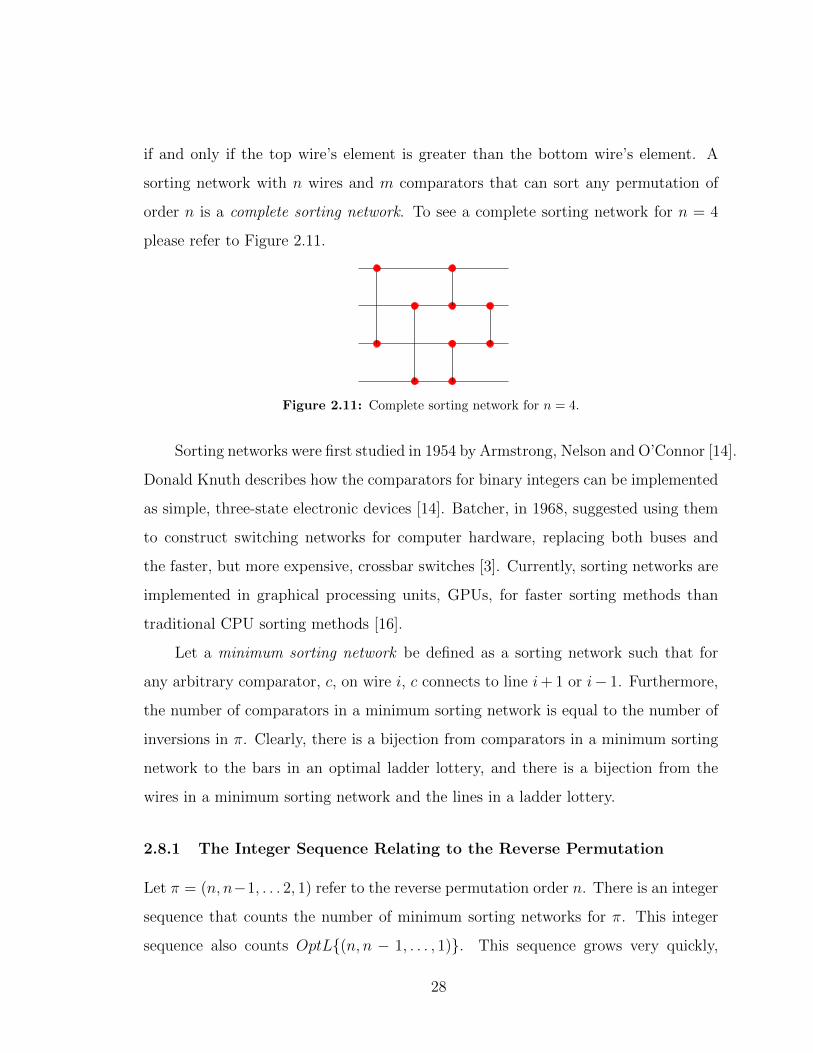
if and only if the top wire’s element is greater than the bottom wire’s element. A

sorting network with n wires and m comparators that can sort any permutation of

order n is a complete sorting network. To see a complete sorting network for n = 4

please refer to Figure 2.11.

Figure 2.11: Complete sorting network for n = 4.

Sorting networks were first studied in 1954 by Armstrong, Nelson and O’Connor [14].

Donald Knuth describes how the comparators for binary integers can be implemented

as simple, three-state electronic devices [14]. Batcher, in 1968, suggested using them

to construct switching networks for computer hardware, replacing both buses and

the faster, but more expensive, crossbar switches [3]. Currently, sorting networks are

implemented in graphical processing units, GPUs, for faster sorting methods than

traditional CPU sorting methods [16].

Let a minimum sorting network be defined as a sorting network such that for

any arbitrary comparator, c, on wire i, c connects to line i+ 1 or i− 1. Furthermore,

the number of comparators in a minimum sorting network is equal to the number of

inversions in π. Clearly, there is a bijection from comparators in a minimum sorting

network to the bars in an optimal ladder lottery, and there is a bijection from the

wires in a minimum sorting network and the lines in a ladder lottery.

2.8.1 The Integer Sequence Relating to the Reverse Permutation

Let π = (n, n−1, . . . 2, 1) refer to the reverse permutation order n. There is an integer

sequence that counts the number of minimum sorting networks for π. This integer

sequence also counts OptL{(n, n − 1, . . . , 1)}. This sequence grows very quickly,

28

Table 2.1: Number of minimum sorting networks and |OptL{(n, n− 1, . . . , 1)}|

Number of minimum sorting networks and |OptL{(n, n− 1, . . . , 1)}|N Count

1 1

2 1

3 2

4 8

5 62

6 908

7 24698

8 1232944

9 112018190

10 18410581880

11 5449192389984

12 2894710651370536

13 2752596959306389652

14 4675651520558571537540

15 14163808995580022218786390

therefore n = 15 is the largest value this integer sequence has been calculated for. To

refer to the table for this sequence please refer to Table 2.1 [21].

Dumitrescu and Mandal, in their paper New Lower Bounds For The Number of

Pseudoline Arrangements [6] published in 2018, provide the current best known lower

bound for this sequence as Tbn ∈ O(n2 − n log n). In particular, bn ≥ 0.2083n2 for

large values of n. Where bn is the bound for a given value n. In the paper, Coding and

Counting Arrangements of Pseudolines [8] by Felsner and Valtr, written in 2011, the

authors demonstrate the best known upper bound for this sequence is bn ≤ 20.657n2.

Seeing as there is yet to be a closed form solution for this sequence, new values

of n are counted by a variety of algorithms. In the paper, Efficient Enumeration of all

Ladder Lotteries and its Application [28], the authors were the first to calculate the

sequence for n = 11 with the algorithm FindAllChildren. In the paper, Counting

29

Primitive Sorting Networks by πDDs [12], written by Kawahara, Minato, Saitoh and

Yoshinaka, the authors were the first to calculate for n = 13 with a data structure

they have termed πDD.

30

Chapter 3

The Canonical Ladder

In this chapter we describe a canonical ladder for each OptL{π}. We then provide

a number of equations to calculate the location of the bar in the canonical ladder;

depending on the configuration of π, we use different equations for calculating the

location of the bar. We then define the data structure used to represent the canonical

ladder. Using the data structure, we provide an algorithm for creating the canonical

ladder for any π of order n. Lastly, we describe the listing problem in relation to the

canonical ladder. To see the canonical ladder for (3, 5, 4, 1, 2), refer to Figure 3.1.

5, 3

4, 3

3, 1

2, 1

5, 4

4, 1

3, 2

5, 1

4, 2

5, 2

3 5 4 1 2

Figure 3.1: The canonical ladder for (3, 5, 4, 1, 2). Bars (5, 4), (4, 1), (4, 2) are part of the route of4, but only the red bars are associated with the route of 4.

31

3.1 The Canonical Ladder in Detail

In this section, we fully define the canonical ladder corresponding to π. We first

define the associated terminology in order to provide a comprehensive definition of

the canonical ladder. Let the route of an element be the sequence of bars the element

travels along in order to reach its final position in the sorted permutation. The bars

are read from top to bottom. In Figure 3.1, the bars (5, 4), (4, 1) and (4, 2) compose

the route of 4. For every bar, two elements cross the bar, therefore bar association

is the association of a bar with the greater of the two elements that cross it. For

example, in Figure 3.1, element 4 has the bars (5, 4), (4, 1) and (4, 2) in its route,

however only bars (4, 1) and (4, 2) are associated with element 4. Let the absence of

a bar corresponding to two uninverted elements in π, x > y, be defined as a dashed,

horizontal line spanning across a column in the ladder. We say absence of a bar

association is the association of the absence of a bar with the greater of the two

elements that form it. For example,(5, 3) are uninverted in (3, 5, 4, 1, 2), therefore the

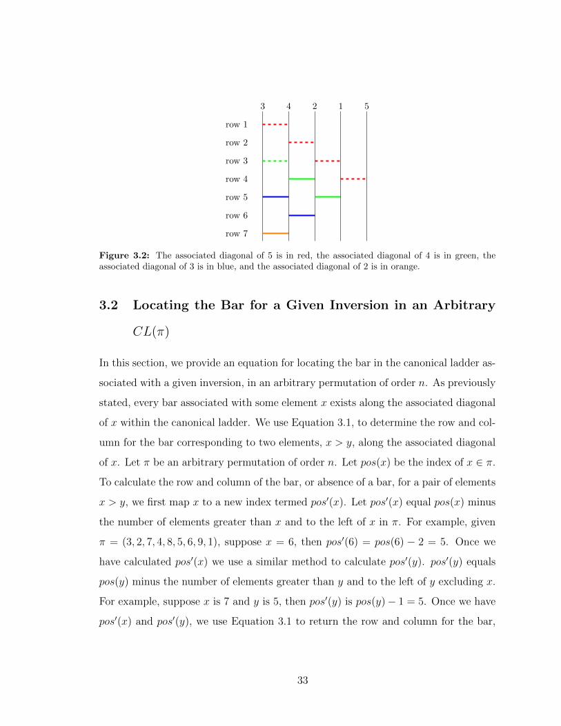
absence of the bar is associated with 5. For each element 2 ≤ x ≤ n ∈ π, we define

the associated diagonal of x as a diagonal with x − 1 row and column coordinates,

having one endpoint at (2n− 2x+ 1, 1) and the other endpoint at (2n−x− 1, x− 1).

At each row and column in the associated diagonal of x, either a bar associated with

x or the absence of a bar associated with x exists. For an example of the associated

diagonals for the ladder corresponding to (3, 4, 2, 1, 5) refer to Figure 3.2.

With the definition of the associated diagonal, we are now able to fully define the

canonical ladder as the ladder such that for each element 2 ≤ x ≤ n, each bar, and

absence of a bar, associated with x exists along the associated diagonal of x. We note

that the two aforementioned figures, Figure 3.1 and Figure 3.2, are the canonical

ladders corresponding to each of their respective permutations. We use CL(π) as

shorthand notation for ‘the canonical ladder corresponding to a permutation of order

n’.

32

row 1

row 2

row 3

row 4

row 5

row 6

row 7

3 4 2 1 5

Figure 3.2: The associated diagonal of 5 is in red, the associated diagonal of 4 is in green, theassociated diagonal of 3 is in blue, and the associated diagonal of 2 is in orange.

3.2 Locating the Bar for a Given Inversion in an Arbitrary

CL(π)

In this section, we provide an equation for locating the bar in the canonical ladder as-

sociated with a given inversion, in an arbitrary permutation of order n. As previously

stated, every bar associated with some element x exists along the associated diagonal

of x within the canonical ladder. We use Equation 3.1, to determine the row and col-

umn for the bar corresponding to two elements, x > y, along the associated diagonal

of x. Let π be an arbitrary permutation of order n. Let pos(x) be the index of x ∈ π.

To calculate the row and column of the bar, or absence of a bar, for a pair of elements

x > y, we first map x to a new index termed pos′(x). Let pos′(x) equal pos(x) minus

the number of elements greater than x and to the left of x in π. For example, given

π = (3, 2, 7, 4, 8, 5, 6, 9, 1), suppose x = 6, then pos′(6) = pos(6) − 2 = 5. Once we

have calculated pos′(x) we use a similar method to calculate pos′(y). pos′(y) equals

pos(y) minus the number of elements greater than y and to the left of y excluding x.

For example, suppose x is 7 and y is 5, then pos′(y) is pos(y)− 1 = 5. Once we have

pos′(x) and pos′(y), we use Equation 3.1 to return the row and column for the bar,

33

or absence of the bar, along the associated diagonal of x.

(row,column)=

((2n− x− 1)− (x− pos′(y)) + 1, (x− 1)− (x− pos′(y)) + 1) if pos′(x) > pos′(y)

((2n− x− 1)− (x− pos′(y)), (x− 1)− (x− pos′(y)) if pos′(y) > pos′(x)

(3.1)

Given the inversion (7, 5) ∈ (3, 2, 7, 4, 8, 5, 6, 9, 1), we calculate the row and col-

umn of the bar (7, 5) using the second case. We get row = (18− 7− 1)− (7− 5) = 8

and col = 6− (7− 5) = 4. To calculate pos′(x) and pos′(y), is linear amortized time.

Once pos′(x) and pos′(y) are calculated, returns the location in O(1) time. We can

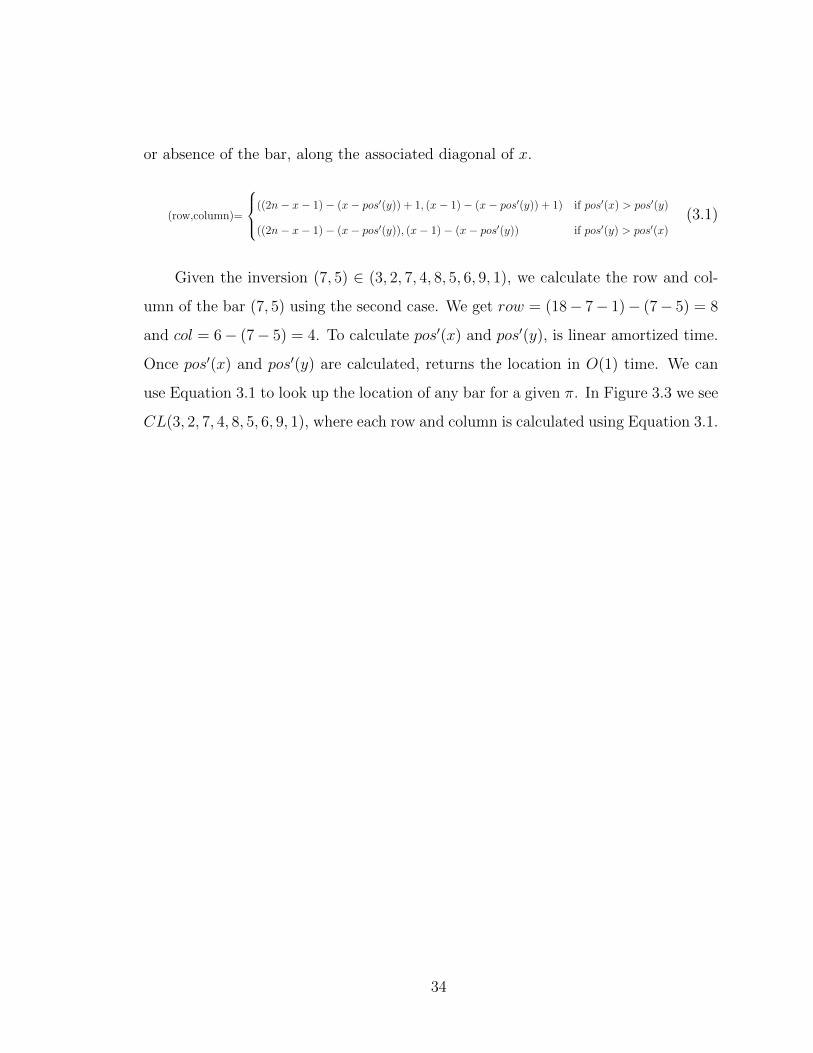
use Equation 3.1 to look up the location of any bar for a given π. In Figure 3.3 we see

CL(3, 2, 7, 4, 8, 5, 6, 9, 1), where each row and column is calculated using Equation 3.1.

34

(7, 5)

3 2 7 4 8 5 6 9 1

row1

row2

row3

row4

row5

row6

row7

row8

row9

row10

row11

row12

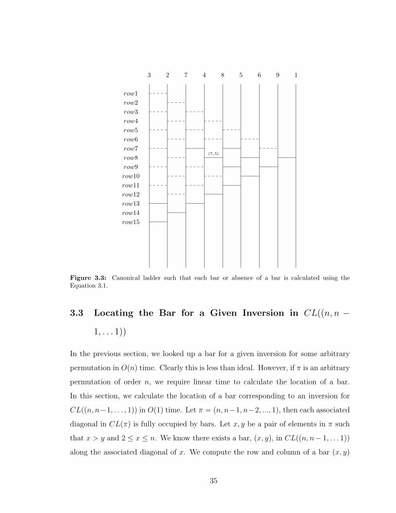
row13

row14

row15

Figure 3.3: Canonical ladder such that each bar or absence of a bar is calculated using theEquation 3.1.

3.3 Locating the Bar for a Given Inversion in CL((n, n −

1, . . . 1))

In the previous section, we looked up a bar for a given inversion for some arbitrary

permutation in O(n) time. Clearly this is less than ideal. However, if π is an arbitrary

permutation of order n, we require linear time to calculate the location of a bar.

In this section, we calculate the location of a bar corresponding to an inversion for

CL((n, n−1, . . . , 1)) in O(1) time. Let π = (n, n−1, n−2, ..., 1), then each associated

diagonal in CL(π) is fully occupied by bars. Let x, y be a pair of elements in π such

that x > y and 2 ≤ x ≤ n. We know there exists a bar, (x, y), in CL((n, n− 1, . . . 1))

along the associated diagonal of x. We compute the row and column of a bar (x, y)

35

in CL((n, n− 1, . . . 1)) in O(1) time using Equation 3.2.

(row, column) = (2n− 2x+ (x− y), (x− y)) (3.2)

For example, given π = (6, 5, 4, 3, 2, 1), bar (5, 2) is located at row 5; note that

5 = (2n−2x)+(x−y). Bar (5, 2) is also located at column 3; note that 3 = x−y. To

see the canonical ladder for (6, 5, 4, 3, 2, 1) with the corresponding bars, please refer to

Figure 3.4. We use Equation 3.2 to locate a bar when we know π = (n, n−1, . . . , 2, 1).

(6, 5)

(5, 4)

(4, 3)

(3, 2)

(2, 1)

(6, 4)

(5, 3)

(4, 2)

(3, 1)

(6, 3)

(5, 2)

(4, 1)

(6, 2)

(5, 1)

(6, 1)

6 5 4 3 2 1

row1

row2

row3

row4

row5

row6

row7

row8

row9

col1 col2 col3 col4 col5

Figure 3.4: Canonical ladder for (6, 5, 4, 3, 2, 1). The location of each bar can be calculated usingthe formula (2n− 2x+ (x− y), (x− y))

We use Equation 3.2 when possible because the calculation time is O(1) rather than

O(n).

3.4 Algorithm: CreateCanonical

In this section we provide the data structure used to represent the canonical ladder in

code. We then provide the algorithm for creating the canonical ladder corresponding

to any permutation of order n. To create the canonical ladder we must represent

36

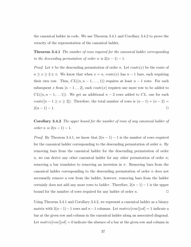
the canonical ladder in code. We use Theorem 3.4.1 and Corollary 3.4.2 to prove the

veracity of the representation of the canonical ladder.

Theorem 3.4.1 The number of rows required for the canonical ladder corresponding

to the descending permutation of order n is 2(n− 1)− 1.

Proof. Let π be the descending permutation of order n. Let route(x) be the route of

n ≥ x ≥ 2 ∈ π. We know that when x = n, route(x) has n − 1 bars, each requiring

their own row. Thus, CL((n, n − 1, . . . , 1)) requires at least n − 1 rows. For each

subsequent x from [n − 1 . . . 2], each route(x) requires one more row to be added to

CL((n, n − 1, . . . 1)). We get an additional n − 2 rows added to CL, one for each

route([n − 1 ≥ x ≥ 2]). Therefore, the total number of rows is (n − 1) + (n − 2) =

2(n− 1)− 1. 2

Corollary 3.4.2 The upper bound for the number of rows of any canonical ladder of

order n is 2(n− 1)− 1.

Proof. By Theorem 3.4.1, we know that 2(n− 1)− 1 is the number of rows required

for the canonical ladder corresponding to the descending permutation of order n. By

removing bars from the canonical ladder for the descending permutation of order

n, we can derive any other canonical ladder for any other permutation of order n;

removing a bar translates to removing an inversion in π. Removing bars from the

canonical ladder corresponding to the descending permutation of order n does not

necessarily remove a row from the ladder, however, removing bars from the ladder

certainly does not add any more rows to ladder. Therefore, 2(n− 1)− 1 is the upper

bound for the number of rows required for any ladder of order n. 2

Using Theorem 3.4.1 and Corollary 3.4.2, we represent a canonical ladder as a binary

matrix with 2(n−1)−1 rows and n−1 columns. Let matrix[row][col] = 1 indicate a

bar at the given row and column in the canonical ladder along an associated diagonal.

Let matrix[row][col] = 0 indicate the absence of a bar at the given row and column in

37

the canonical ladder along an associated diagonal. Let matrix[row][col] = − indicate

irrelevancy as to whether a 1 or 0 is at the given row and column because the row

and column do not lie on an associated diagonal. To see the canonical ladder for

(4, 2, 1, 3) and the corresponding binary matrix, refer to Figure 3.5.

4 2 1 3 1 − −− 1 −0 − 1− 0 −1 − −

Figure 3.5: Canonical ladder and corresponding binary matrix.

Using Equation 3.1, and the binary matrix representation of a ladder, we define

algorithm CreateCanonical which can be found in Algorithm 2 to create the

canonical ladder for any given permutation of order n. The initial conditions of

CreateCanonical are the following. Let ladder be the binary matrix representing

CL(π) initialized to −. Let π be an arbitrary permutation of order n. Let x be the

currently maximal element in π, initialized to n. Let GetCoordinates refer to

Equation 3.1.

Algorithm 2 The algorithm for creating the canonical ladder of OptL{π}1: function CreateCanonical(ladder, π, x)2: while x > 1 do3: pos(x)← index of x ∈ π4: for i from 1 to x do5: if i 6= pos(x) then6: (row, column)←GetCoordinates(x, pos(x), i)7: if pos(x) < i then8: ladder[row][col]← 19: else

10: ladder[row][col]← 0

11: π ← π − x12: x← x− 1

38

On each iteration of the while loop, all x − 1 1s and 0s along the associated

diagonal of the xth element are added to ladder within the for-loop. GetCoordi-

nates, which refers to Equation 3.1, returns the row and column coordinate for the

respective 1 or 0 for the pair of elements, x > y. Note that we call GetCoordinates

with the arguments (x, pos(x), i). When referring to Equation 3.1 the variables are

(x, pos′(x), pos′(y)). Prior to the next iteration of the while loop, x is removed from

π and all elements to the right of x are moved to the left by one index. Then, x is

decremented by 1. The while loop continues until x = 1. Determining pos(x) is done

in O(x) time. Removing x from π is done in O(x) time. Calculating the row and

column for each (x, y) is done in O(1) time. Overall, the algorithms complexity is

O(n2). We also note that CreateCanonical creates the ladder representation with

clean level 1. Given three elements, x > y > z and pos(x) < pos(y) < pos(z), Equa-

tion 3.1 returns a lesser row for (x, z) than for (y, z). Therefore, CreateCanonical

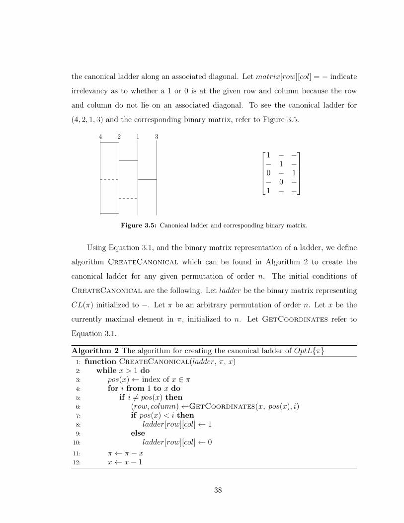
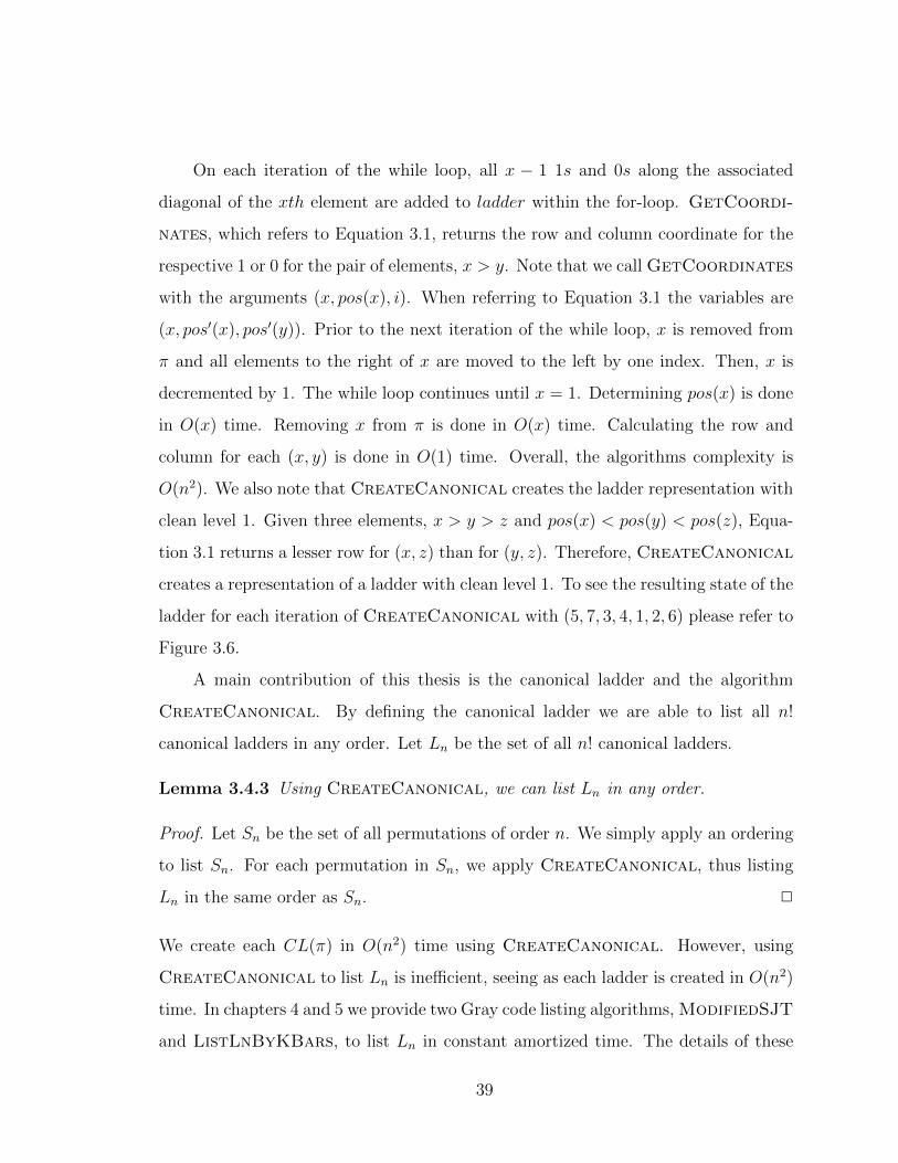
creates a representation of a ladder with clean level 1. To see the resulting state of the

ladder for each iteration of CreateCanonical with (5, 7, 3, 4, 1, 2, 6) please refer to

Figure 3.6.

A main contribution of this thesis is the canonical ladder and the algorithm

CreateCanonical. By defining the canonical ladder we are able to list all n!

canonical ladders in any order. Let Ln be the set of all n! canonical ladders.

Lemma 3.4.3 Using CreateCanonical, we can list Ln in any order.

Proof. Let Sn be the set of all permutations of order n. We simply apply an ordering

to list Sn. For each permutation in Sn, we apply CreateCanonical, thus listing

Ln in the same order as Sn. 2

We create each CL(π) in O(n2) time using CreateCanonical. However, using

CreateCanonical to list Ln is inefficient, seeing as each ladder is created in O(n2)

time. In chapters 4 and 5 we provide two Gray code listing algorithms, ModifiedSJT

and ListLnByKBars, to list Ln in constant amortized time. The details of these

39

x = 75 7 3 4 1 2 6

x = 65 7 3 4 1 2 6

x = 55 7 3 4 1 2 6

x = 45 7 3 4 1 2 6

x = 35 7 3 4 1 2 6

x = 25 7 3 4 1 2 6

Figure 3.6: The ordering of the state of the ladder when creating the root ladder for (5, 7, 3, 4, 1, 2, 6)

algorithms are found in chapters 4 and 5 respectively.

40

Chapter 4

Listing Ln in Gray Code Order by Adding or

Removing a Bar

In this chapter, we use the definition of the canonical ladder and the binary

matrix representation of the canonical ladder to list Ln in Gray code order. Recall,

a Gray code is an ordering such that successive elements in the ordering differ by a

minimal amount of change. When listing Ln, a minimal amount of change is defined

as either adding or removing a bar, or relocating a bar; relocating a bar is the same

as adding one bar and removing another. In the case of this chapter’s algorithm, we

add or remove a bar when transitioning between ladders in Ln. A key step in this

chapter is that we are able to determine the bar corresponding to an inversion in

constant time. Thus, the running time for this chapter’s algorithm is CAT.

4.1 Equation: GetCoordinates2

In the previous chapter, we described how we could list Ln using the naive approach.

However, using the naive approach is slow. In this chapter we seek to improve the

running time for listing Ln. In this section, we improve the running time by determin-

ing the location of a bar in O(1) time for a pair of adjacent elements. This allows us to

take advantage of the Steinhaus-Johnson-Trotter algorithm, which applies adjacent

transpositions to elements.

We define r, with respect to a permutation π, as a vector of order n as follows:

rx equals the number of elements less than x and to the right of x in π. We note that

41

0 ≤ rx ≤ x − 1. For example, given (3, 4, 1, 5, 6, 2), r1 = 0, r2 = 0, r3 = 2, r4 = 2,

r5 = 1 and r6 = 1. We use r to define GetCoordinates2 found in equation 4.1.

Let x > y be two elements in π such that pos(x) = pos(y) + / − 1. We are going to

apply an adjacent transposition to x and y; we need to know where to locate the 1

or 0 in the binary matrix corresponding to the elements x, y in order to flip it from

a 1 to a 0 or vice versa. Prior to the transposition of x and y, if pos(x) = pos(y)− 1

then GetCoordinates2 returns the row and column of the 1 corresponding to x

and y. If pos(x) = pos(y) + 1, then GetCoordinates2 returns the row and column

of the 0 corresponding to x and y. rx is updated accordingly by being incremented

or decremented by 1.

(row,column) =

((2n− x− 1)− rx, (x− 1)− rx) if pos(x)=pos(y)+1

((2n− x)− rx, (x)− rx) if pos(y) = pos(x)+1

(4.1)

Initially, if pos(x) = pos(y) + 1, then when we apply an adjacent transposition

between x and y, an inversion is induced in π. Therefore, rx is incremented by 1,

and the bar (x, y) gets added to the canonical ladder. Initially, if pos(x) = pos(y)− 1

then when we apply an adjacent transposition between x and y, and an inversion

gets removed from π. Therefore, rx is decremented by 1, indicating the bar (x, y)

has been removed from the canonical ladder. One of the main results of this thesis is

ModifiedSJT produces Ln in Gray code order in CAT. ModifiedSJT uses Get-

Coordinates2 and r to calculate the row and column for every 1 or 0 in the binary

matrix in O(1) time.

4.2 Algorithm: ModifiedSJT

In this section we define the algorithm ModifedSJT, using r and Equation 4.1, which

can be found in Algorithm 3. Transposing two adjacent elements in πi results in a

42

subsequent permutation πj. The transposition of the two elements results in adding or

removing a bar in CL(πi), resulting in CL(πj). The transposition of the two elements

is merely simulated in Algorithm 3, seeing as π is not an argument to the function; we

are able to calculate the location of the 1 or 0 in the binary matrix without having to

induce the transposition in π. This makes our algorithm more interesting, seeing as

we do not actually perform any swap operations on inversions. The initial conditions

of ModifiedSJT are the following: Let ladder be the binary matrix representation of

the canonical ladder such that each row and column coordinate along each associated

diagonal is initialized to 0. Let n be the maximum element. Let x be initialized to

2; x represents the current element. On each recursive call x is incremented by 1

from 2, 3 . . . n, n+ 1. Let direction be a one indexed array set to false for all indexes.

direction[x] =false implies the xth element is being adjacently transposed from right

to left. direction[x] =true implies the xth element is being transposed from left to

right. Let r be the inversion vector initialized at all indices to 0; when r is initialized

to all 0s, this means that r is the inversion vector for π = (1, 2, . . . , n− 1, n).

43

Algorithm 3 Modification of the SJT algorithm for listing Ln

1: function ModifiedSJT(n, ladder, x, direction, r)2: if x > n then3: if number of bars in ladder equals 0 then Print(ladder)

4: return5: for i from 1 to x do6: if i = 1 then7: ModifiedSJT(n, ladder, x+ 1, direction, r)8: else9: if direction[x] =false then

10: (row, column)← ((2n− x− 1)− rx, (x− 1)− rx)11: rx ← rx + 112: ladder[row][column]← 113: else14: (row, column)← ((2n− x)− rx, (x)− rx)15: rx ← rx − 116: ladder[row][column]← 0

17: Print(ladder)18: ModifiedSJT(n, ladder, x+ 1, direction)

19: if direction[x] = false then direction[x]← true20: else direction[x]← false

We use GetCoordinates2 on lines 10 and 14 of ModifiedSJT to calculate

the row and column. When direction[x] equals false we use the first case from

GetCoordinates2. When direction[x] equals true we use the second case from

GetCoordinates2 to calculate the row and column.

Given the current value of x, add or remove a bar for the route of x, then add

or remove all bars for route x + 1. Once all bars for route x + 1 have been added or

removed, proceed to add or remove the next bar from the route of x. Repeat until

all x− 1 bars have been added or removed from route x. If direction[x] is false, then

bars of x will be added to ladder from right to left, bottom to top, until no more bars

to the route of x can be added. If direction[x] is true, then bars will be removed

from ladder, left to right, top to bottom, until no more bars from the route of x

can be removed. Once all the bars for the route of x have been added or removed,

then direction[x] is negated, indicating that the opposite operation will be applied

44

to the bars of the route of x when x is next processed. On each recursive call, x is

incremented by 1. When x is greater than n, return.

4.3 Analysis of ModifiedSJT

In this section we provide a theoretical analysis of ModifiedSJT along with the

runtime for the algorithm. We have implied that ModifiedSJT produces Ln. We

note that there are two general criteria for Ln. The first, each ladder in Ln corresponds

to a unique permutation of order n. The second, each ladder in Ln is the canonical

ladder. In Lemma 4.3.1, we prove the first criteria for Ln.

Lemma 4.3.1 Each ladder produced by ModifiedSJT corresponds to a unique per-

mutation of order n

Proof. Since the algorithm is a modification of the Steinhaus-Johnson-Trotter algo-

rithm, a similar proof for the SJT algorithm can be applied to the ModifiedSJT

algorithm. Suppose we want to list all n! ladders of order n. Suppose we have all

n− 1! ladders of order n− 1, then for each ladder of order n− 1 add a new column

to the right; this results in n− 1 columns seeing as the number of columns is one less

than the number of elements. For each of the n− 1! ladders with n− 1 columns add

0 . . . n− 1 bars beginning at column n− 1 and ending at column 1. Doing so results

in (n − 1)!n = n! ladders of order n. To see an example of the proof please refer to

Figure 4.1. 2

45

1 2 3 4 1 2 4 3 1 4 2 3 4 1 2 3 4 1 3 2 1 4 3 2

1 3 4 2 1 3 2 4 3 1 2 4 3 1 4 2 3 4 1 2 4 3 1 2

4 3 2 1 3 4 2 1 3 2 4 1 3 2 1 4 2 3 1 4 2 3 4 1

2 4 3 1 4 2 3 1 4 2 1 3 2 4 1 3 2 1 4 3 2 1 3 4

Figure 4.1: L4 generated by the ModifiedSJT algorithm. The algorithm inserts or removes abar between any two successive ladders.

46

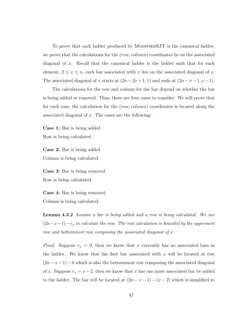
To prove that each ladder produced by ModifiedSJT is the canonical ladder,

we prove that the calculations for the (row, column) coordinates lie on the associated

diagonal of x. Recall that the canonical ladder is the ladder such that for each

element, 2 ≤ x ≤ n, each bar associated with x lies on the associated diagonal of x.

The associated diagonal of x starts at (2n− 2x+ 1, 1) and ends at (2n−x− 1, x− 1).

The calculations for the row and column for the bar depend on whether the bar

is being added or removed. Thus, there are four cases to consider. We will prove that

for each case, the calculation for the (row, column) coordinates is located along the

associated diagonal of x. The cases are the following:

Case 1: Bar is being added

Row is being calculated.

Case 2: Bar is being added

Column is being calculated.

Case 3: Bar is being removed

Row is being calculated.

Case 4: Bar is being removed.

Column is being calculated.

Lemma 4.3.2 Assume a bar is being added and a row is being calculated. We use

(2n−x−1)−rx to calculate the row. The row calculation is bounded by the uppermost

row and bottommost row composing the associated diagonal of x.

Proof. Suppose rx = 0, then we know that x currently has no associated bars in

the ladder. We know that the first bar associated with x will be located at row

(2n−x−1)−0 which is also the bottommost row composing the associated diagonal

of x. Suppose rx = x− 2, then we know that x has one more associated bar be added

to the ladder. The bar will be located at (2n− x− 1)− (x− 2) which is simplified to

47

2n−2x+ 1; 2n−2x+ 1 equals the uppermost row composing the associated diagonal

of x. 2

Lemma 4.3.3 Assume a bar is being added and a column is being calculated. We

use (x − 1) − rx to calculate the column. The column calculation is bounded by the

leftmost column and rightmost column composing the associated diagonal of x.

Proof. Suppose rx = 0, then we know that x currently has no associated bars in the

ladder. We know that the first bar associated with x will be located at (x − 1) − 0

which is also the rightmost column composing the associated diagonal of x. Suppose

rx = x − 2, then we know that x has one more associated bar to be added to the

ladder. The bar will be located at (x− 1)− (x− 2) which is simplified to 1; 1 equals

the leftmost column composing the associated diagonal of x.

2

Lemma 4.3.4 Assume a bar is being removed and a row is being calculated. We use

(2n − x) − rx to calculate the row. The row is bounded by the uppermost row and

bottommost row composing the associated diagonal of x.

Proof. Suppose rx = x − 1, then we know that x has all of its associated bars

in the canonical ladder. We calculate the row of the first bar to be removed at

(2n − x) − (x − 1) = (2n − 2x) + 1; (2n − 2x) + 1 is the uppermost row of the

associated diagonal of x. Suppose rx = 1, then we know that x only has one more bar

to be removed from the ladder. We calculate the row of the last bar to be removed

at (2n− x)− 1; 2n− x− 1 is the bottommost row of the associated diagonal of x.

2

Lemma 4.3.5 Assume a bar is being removed and a column is being calculated. We

use (x) − rx to calculate the column. The column is bounded by the leftmost column

and rightmost column composing the associated diagonal of x.

48

Proof. Suppose rx = x − 1, then we know that x has all of its associated bars in

the canonical ladder. We calculate the column of the first bar to be removed at

(x)− (x− 1) = 1; 1 is the leftmost column of the associated diagonal of x. Suppose

rx = 1, then we know x only has one more bar to be removed from the ladder. We

calculate the column of the last bar to be removed at (x)− 1; x− 1 is the rightmost

column of the associated diagonal of x. 2

Using Lemmas 4.3.1, 4.3.2, 4.3.3, 4.3.4, 4.3.5 we have shown that ModifiedSJT

produces Ln. However, we have yet to prove that ModifedSJT produces Ln in Gray

code order. We use Theorem 4.3.6 to prove that ModifiedSJT produces Ln in Gray

code order.

Theorem 4.3.6 ModifiedSJT produces Ln in Gray code order

Proof. Let li be an arbitrary ladder produced by ModifedSJT. Let j be the next lad-

der to be produced by ModifiedSJT. If li = lj plus or minus a bar, then Modified-

SJT produces Ln in Gray code order. On each iteration of the loop, direction[x] is ei-

ther true or false, but not both. When direction[x] = false, a single 1 is added to the

associated diagonal of x, indicating a bar has been added. When direction[x] = true,

a single 0 is added to the associated diagonal of x, indicating a bar has been removed.

With an addition or removal of a 1 or 0, li differs from lj by the addition or removal

of a bar. Therefore, Ln is produced by ModifedSJT in Gray code order.

2

Theorem 4.3.7 ModifiedSJT produces Ln in CAT.

Proof. The first ladder is printed in O(n) time because [2 . . . n + 1] recursive calls

are made before first ladder is printed. Each subsequent ladder deviates from its

predecessor by a single addition or removal of a bar. Calculating the location of

a 1 or 0, corresponding to a bar or absence of a bar, is done in O(1) time. Once

49

calculated, the 1 or 0 is added to li producing lj. Once li is transformed into lj, lj is

printed. 2

We calculated the runtimes for n = 1 . . . 13. The runtime is calculated without the

ladders being printed. When the ladders are printed, the runtime increases by a

substantial amount. The runtimes from n = 9 . . . n = 13 are provided in Table 4.1.

Table 4.1: The table with the runtimes for listing Ln using ModifiedSJT.

Runtimes for generating Ln in seconds

n ModifiedSJT Runtime

9 0.00

10 0.03

11 0.25

12 2.78

13 66.97

4.4 Chapter Conclusion

We have provided a CAT algorithm for listing Ln by adding or removing a bar. By

doing so, we have provided a solution to The Canonical Ladder Listing Problem. We

use Equation 4.1 and modified the Steinhaus-Johnson-Trotter algorithm in order to

create Algorithm 3. We computed the location of a bar corresponding to any pair of

adjacent elements in O(1) time.

50

Chapter 5

Listing Ln in Gray Code Order with k Bars

In this chapter we provide a Gray code for listing all ladders with k bars. We

define Ln,k as the set of all canonical ladder lotteries with n lines and exactly k bars,

where 0 ≤ k ≤(n2

). To list Ln,k, we define a mapping from associated diagonals to an

inversion vector corresponding to π. We apply this mapping to generate a Gray code

for listing Ln,k. We then provide an algorithm for listing Ln ordered by the number of

bars from 0 ≤ k ≤(n2

)in Gray code order. When listing ladders by k bars, we define

minimal change as the relocation of a bar; relocating a bar is equivalent to removing

one bar and adding another bar.

5.1 Listing Ladders with n Lines and k Bars in Gray Code

Order

In Chapter 2, we discussed Effler-Ruskey’s algorithm and Walsh’s Gray code for listing

Sn,k. In this section, we focus on Walsh’s Gray code for listing Ln,k by applying

a minimal amount of change between subsequent ladders. We relocate a bar to

transition from one ladder in Ln,k to the next ladder in Ln,k. Recall, relocating a bar

is the same as adding one bar and removing another bar.

An n part composition of a non negative integer k, is an n tuple g = (g1, g2, . . . , gn)

whose sum adds to k. We say g is the bar vector of CL(π), where π is of order n+ 1,

when we map g to a canonical ladder as follows. For each index x in g, x is mapped

to the associated diagonal of ((n+ 1)−x) + 1. Furthermore, gx equals the number of

bars along the associated diagonal of element ((n+ 1)− x) + 1. To see the mapping

51

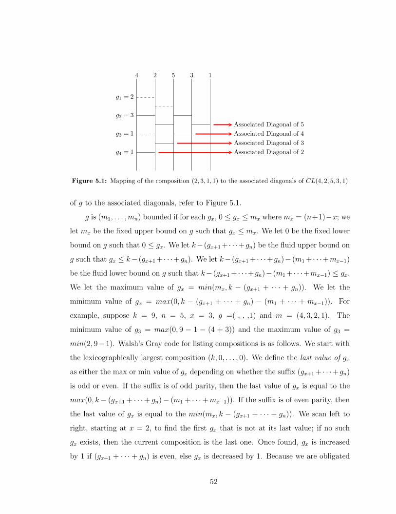
Associated Diagonal of 2

Associated Diagonal of 3

Associated Diagonal of 4

Associated Diagonal of 5

g1 = 2

g2 = 3

g3 = 1

g4 = 1

4 2 5 3 1

Figure 5.1: Mapping of the composition (2, 3, 1, 1) to the associated diagonals of CL(4, 2, 5, 3, 1)

of g to the associated diagonals, refer to Figure 5.1.

g is (m1, . . . ,mn) bounded if for each gx, 0 ≤ gx ≤ mx where mx = (n+1)−x; we

let mx be the fixed upper bound on g such that gx ≤ mx. We let 0 be the fixed lower

bound on g such that 0 ≤ gx. We let k− (gx+1 + · · ·+gn) be the fluid upper bound on

g such that gx ≤ k− (gx+1 + · · ·+gn). We let k− (gx+1 + · · ·+gn)− (m1 + · · ·+mx−1)

be the fluid lower bound on g such that k− (gx+1 + · · ·+gn)− (m1 + · · ·+mx−1) ≤ gx.

We let the maximum value of gx = min(mx, k − (gx+1 + · · · + gn)). We let the

minimum value of gx = max(0, k − (gx+1 + · · · + gn) − (m1 + · · · + mx−1)). For

example, suppose k = 9, n = 5, x = 3, g =( , , ,1) and m = (4, 3, 2, 1). The

minimum value of g3 = max(0, 9 − 1 − (4 + 3)) and the maximum value of g3 =

min(2, 9−1). Walsh’s Gray code for listing compositions is as follows. We start with

the lexicographically largest composition (k, 0, . . . , 0). We define the last value of gx

as either the max or min value of gx depending on whether the suffix (gx+1 + · · ·+gn)

is odd or even. If the suffix is of odd parity, then the last value of gx is equal to the

max(0, k− (gx+1 + · · ·+ gn)− (m1 + · · ·+mx−1)). If the suffix is of even parity, then

the last value of gx is equal to the min(mx, k − (gx+1 + · · · + gn)). We scan left to

right, starting at x = 2, to find the first gx that is not at its last value; if no such

gx exists, then the current composition is the last one. Once found, gx is increased

by 1 if (gx+1 + · · · + gn) is even, else gx is decreased by 1. Because we are obligated

52

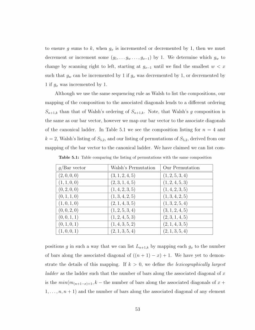
to ensure g sums to k, when gx is incremented or decremented by 1, then we must

decrement or increment some (g1, . . . gw . . . , gx−1) by 1. We determine which gw to

change by scanning right to left, starting at gx−1 until we find the smallest w < x

such that gw can be incremented by 1 if gx was decremented by 1, or decremented by

1 if gx was incremented by 1.

Although we use the same sequencing rule as Walsh to list the compositions, our

mapping of the composition to the associated diagonals lends to a different ordering

Sn+1,k than that of Walsh’s ordering of Sn+1,k. Note, that Walsh’s g composition is

the same as our bar vector, however we map our bar vector to the associate diagonals

of the canonical ladder. In Table 5.1 we see the composition listing for n = 4 and

k = 2, Walsh’s listing of S5,2, and our listing of permutations of S5,2, derived from our

mapping of the bar vector to the canonical ladder. We have claimed we can list com-

Table 5.1: Table comparing the listing of permutations with the same composition

g/Bar vector Walsh’s Permutation Our Permutation

(2, 0, 0, 0) (3, 1, 2, 4, 5) (1, 2, 5, 3, 4)

(1, 1, 0, 0) (2, 3, 1, 4, 5) (1, 2, 4, 5, 3)

(0, 2, 0, 0) (1, 4, 2, 3, 5) (1, 4, 2, 3, 5)

(0, 1, 1, 0) (1, 3, 4, 2, 5) (1, 3, 4, 2, 5)

(1, 0, 1, 0) (2, 1, 4, 3, 5) (1, 3, 2, 5, 4)

(0, 0, 2, 0) (1, 2, 5, 3, 4) (3, 1, 2, 4, 5)

(0, 0, 1, 1) (1, 2, 4, 5, 3) (2, 3, 1, 4, 5)

(0, 1, 0, 1) (1, 4, 3, 5, 2) (2, 1, 4, 3, 5)

(1, 0, 0, 1) (2, 1, 3, 5, 4) (2, 1, 3, 5, 4)

positions g in such a way that we can list Ln+1,k by mapping each gx to the number

of bars along the associated diagonal of ((n + 1) − x) + 1. We have yet to demon-

strate the details of this mapping. If k > 0, we define the lexicographically largest

ladder as the ladder such that the number of bars along the associated diagonal of x

is the min(m(n+1−x)+1, k − the number of bars along the associated diagonals of x +

1, . . . , n, n+ 1) and the number of bars along the associated diagonal of any element

53

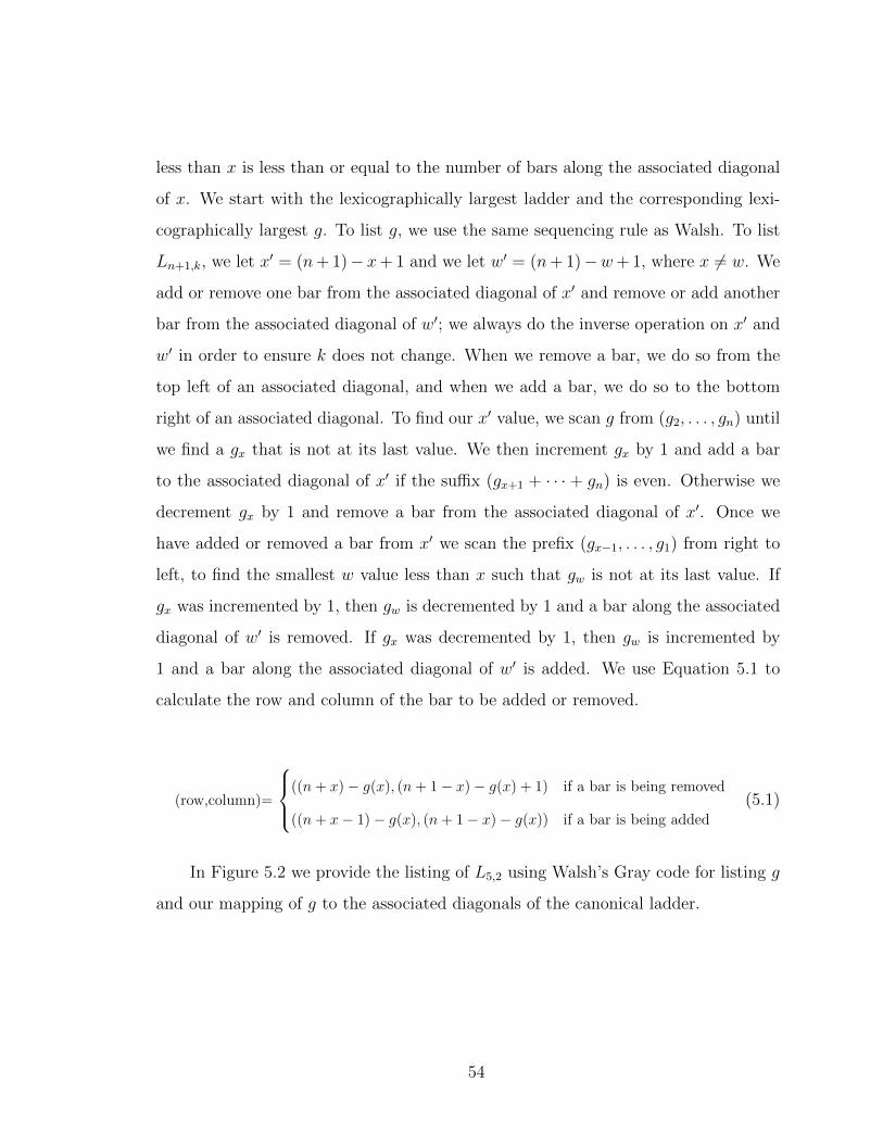
less than x is less than or equal to the number of bars along the associated diagonal

of x. We start with the lexicographically largest ladder and the corresponding lexi-

cographically largest g. To list g, we use the same sequencing rule as Walsh. To list

Ln+1,k, we let x′ = (n+ 1)− x+ 1 and we let w′ = (n+ 1)−w+ 1, where x 6= w. We

add or remove one bar from the associated diagonal of x′ and remove or add another

bar from the associated diagonal of w′; we always do the inverse operation on x′ and

w′ in order to ensure k does not change. When we remove a bar, we do so from the

top left of an associated diagonal, and when we add a bar, we do so to the bottom

right of an associated diagonal. To find our x′ value, we scan g from (g2, . . . , gn) until

we find a gx that is not at its last value. We then increment gx by 1 and add a bar

to the associated diagonal of x′ if the suffix (gx+1 + · · · + gn) is even. Otherwise we

decrement gx by 1 and remove a bar from the associated diagonal of x′. Once we

have added or removed a bar from x′ we scan the prefix (gx−1, . . . , g1) from right to

left, to find the smallest w value less than x such that gw is not at its last value. If

gx was incremented by 1, then gw is decremented by 1 and a bar along the associated

diagonal of w′ is removed. If gx was decremented by 1, then gw is incremented by

1 and a bar along the associated diagonal of w′ is added. We use Equation 5.1 to

calculate the row and column of the bar to be added or removed.

(row,column)=

((n+ x)− g(x), (n+ 1− x)− g(x) + 1) if a bar is being removed

((n+ x− 1)− g(x), (n+ 1− x)− g(x)) if a bar is being added

(5.1)

In Figure 5.2 we provide the listing of L5,2 using Walsh’s Gray code for listing g

and our mapping of g to the associated diagonals of the canonical ladder.

54

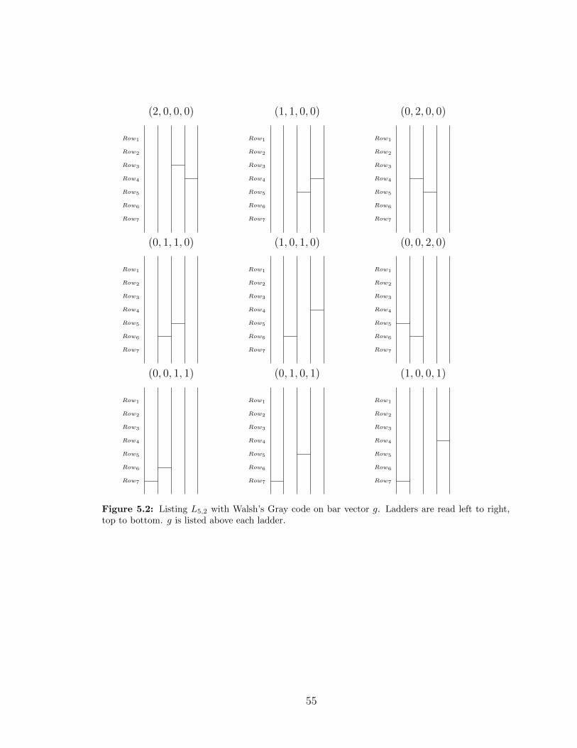
(2, 0, 0, 0)

Row1

Row2

Row3

Row4

Row5

Row6

Row7

(1, 1, 0, 0)

Row1

Row2

Row3

Row4

Row5

Row6

Row7

(0, 2, 0, 0)

Row1

Row2

Row3

Row4

Row5

Row6

Row7

(0, 1, 1, 0)

Row1

Row2

Row3

Row4

Row5

Row6

Row7

(1, 0, 1, 0)

Row1

Row2

Row3

Row4

Row5

Row6

Row7

(0, 0, 2, 0)

Row1

Row2

Row3

Row4

Row5

Row6

Row7

(0, 0, 1, 1)

Row1

Row2

Row3

Row4

Row5

Row6

Row7

(0, 1, 0, 1)

Row1

Row2

Row3

Row4

Row5

Row6

Row7

(1, 0, 0, 1)

Row1

Row2

Row3

Row4

Row5

Row6

Row7

Figure 5.2: Listing L5,2 with Walsh’s Gray code on bar vector g. Ladders are read left to right,top to bottom. g is listed above each ladder.

55

Walsh provides a loop free algorithm to list g in Gray code order [22]. His

algorithm provides the next instance of g in O(1) time by providing the x and w

indices in O(1) time. We use Walsh’s algorithm to provide the x and w value in order

to list the next canonical ladder in Ln+1,k. Walsh refers to x as pivot one and w as

pivot two. We note that x > w. We also note that gx is incremented or decremented

before gw is decremented or incremented. In Algorithm 4, termed NextLadderNK,

we list the next canonical ladder using the pivots x and w provided by Walsh’s

algorithm. The initial conditions of NextLadderNK are the following. Let x be

pivot one returned from Walsh’s algorithm. Let w be pivot two returned from Walsh’s

algorithm. Let CL be a canonical ladder with n+ 1 lines and k bars. Let increment

be a Boolean variable set to true if the pivot one is incremented and pivot two is

decremented, else increment is set to false.

Algorithm 4 Algorithm to list the next ladder in Ln+1,k

1: function NextLadderNK(x, w, CL, increment)2: if increment =true then . Add bar to ass. diag. (n+ x)− 13: (rowx, columnx)← ((n+ x− 1)− gx, (n+ 1− x)− gx)4: (roww, columnw)← ((n+ w)− gw, (n+ 1− w)− gw + 1)5: CL[rowx][columnx]← 16: CL[roww][columnw]← 07: else . Remove bar from ass. diag. (n+ x)− 18: (roww, columnw)← ((n+ w − 1)− gw, (n+ 1− w)− gw)9: (rowx, columnx)← ((n+ x)− gx, (n+ 1− x)− gx + 1)

10: CL[rowx][columnx]← 011: CL[roww][columnw]← 1

Theorem 5.1.1 NextLadderNK produces the next ladder in Ln+1,k in O(1) time.

Theorem 5.1.2 From Walsh’s paper, we know that we can attain the first and second

pivot in O(1) time. We use these pivots, x and w, to calculate the row and column

for the coordinates of the bar to add, and the coordinates of the bar to remove, in

O(1) time. 2

We use NextLadderNK as a subroutine in Algorithm 5, termed ListLNK,

56

which lists Ln,k in Gray code order. Let k be the number of bars. Let n be the number

of lines in CL. Let g be initialized to the lexicographically largest composition;

(k, 0, . . . , 0). Let m be the bound on g. We note that g and m are of order n− 1. Let

CL be the canonical ladder data structure initialized as the lexicographically largest

ladder. Let p1 and p2 be pivot one and pivot two respectively. Let increment be

a Boolean set to true if p1 is to be incremented and p2 is to be decremented, else

increment is set to false.

Algorithm 5 Algorithm for listing Ln,k

1: function ListLNK(g, m, CL, k)2: Print(CL)3: increment← true4: while g1 < m1 and g1 < k − (g2 + · · ·+ gn−1) do . while not at last g5: (p1, p2)←Walsh(g,m, . . . )6: if (gp1+1,+ . . . ,+gn−1) is even then p1← p1 + 1, p2← p2− 17: else p1← p1− 1, p2← p2 + 1

8: if g1 > m1 or g1 > k − (g2 + · · ·+ gn−1) then . surpassed last g9: g1 ← g1 − 1

10: gp1 ← gp1 + 111: return12: if (gp1+1 + · · ·+ gn−1) is even then increment← true13: else: increment← false14: NextLadderNK(p1, p2, CL, increment)15: Print(CL)

By applying Walsh’s algorithm, which returns p1 and p2 in O(1) time, we pro-

duce Ln,k in constant amortized time per ladder. We note that line 6 of the algorithm

determines the parity of the suffix; Walsh demonstrates that the parity of the suffix

can be determined in O(1) time by maintaining a number of auxiliary data struc-

tures [22].

5.2 Listing Ln Ordered by k Bars

In the previous section, we applied Walsh’s Gray code for listing Ln,k. In this section,

we further modify Walsh’s Gray code to list Ln by way of listing Ln,0 . . . Ln,k . . . Ln,(n2)

57

in Gray code order. We list Ln by way of Ln,k by first listing all ladders with exactly

k bars before we list the first ladder with k+1 bars. In Figure 5.3 we show the listing

of L4 by listing L4,0 . . . L4,k . . . L4,6.

k = 0 k = 1 k = 2 k = 3

k = 4 k = 5

k = 6

Figure 5.3: Listing of L4 by k bars. For each k, successive ladders differ by the relocation of abar. Transitioning from the last ladder in Ln,k to the first ladder in Ln,k+1 requires the addition ofa bar.

We previously defined the lexicographically largest ladder as the ladder such

that the number of bars along the associated diagonal of x is the min(m(n+1−x)+1, k−

the number of bars along the associated diagonals of x+1, . . . , n, n+1) and the num-

ber of bars along the associated diagonal of any element less than x is less than or

equal to the number of bars along the associated diagonal of x. We now define the ter-

58

minating ladder as follows. Let the first k− 1 bars compose the sub-ladder along the

associated diagonals from 3 . . . x . . . n; this sub-ladder is the lexicographically largest

sub-ladder. Bar k occupies the associated diagonal of 2. For an example of the ter-

minating ladder for L5,6, please refer to Figure 5.4. We describe the corresponding g,

termed the terminating composition g, as (k − 1, 0, . . . , 1).

Figure 5.4: The terminating ladder for L5,6

In order to list Ln by way of Ln,k, we use Walsh’s Gray code on composition g

when k is odd. When k is odd we start at the lexicographically largest g and end

at the terminating g. Therefore, our description of listing Ln,k by way of g in the

previous section still holds for odd values of k. However, when k is even we start

with the terminating g and we have to work backwards so to speak, ending at the

lexicographically largest g. We could apply Walsh’s algorithm to even instances of

k and then visit the listing in reverse order. However, doing so is slow and takes up

unnecessary space. Hence, we want to provide a CAT algorithm for listing g in the

reverse of Walsh’s ordering. We provide Conjecture 5.2.1 which describes the process

that could allow for the algorithmic implementation of the reverse ordering of Walsh’s

Gray code in CAT.

Conjecture 5.2.1 The reverse of Walsh’s Gray code can be generated in constant

amortized time. When listing g in reverse order we start from g2, scan left to right

until there exists a gx where if (gx+1,+ · · ·+, gn) is odd and there exists some minimum

1 ≤ w ≤ x− 1 such that gw that is not at its minimum value then increment gx and

decrement gw. If (gx+1+· · ·+gn) is even and there exists some minimum 1 ≤ w ≤ x−1

59

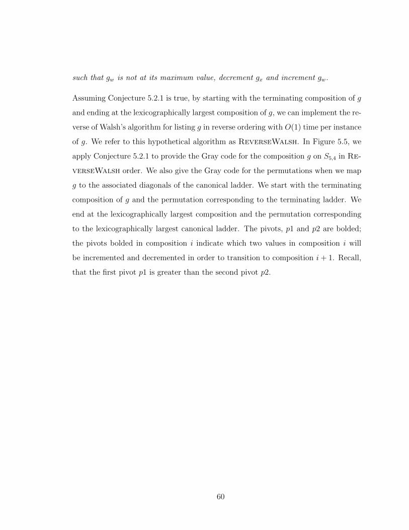
such that gw is not at its maximum value, decrement gx and increment gw.

Assuming Conjecture 5.2.1 is true, by starting with the terminating composition of g

and ending at the lexicographically largest composition of g, we can implement the re-

verse of Walsh’s algorithm for listing g in reverse ordering with O(1) time per instance

of g. We refer to this hypothetical algorithm as ReverseWalsh. In Figure 5.5, we

apply Conjecture 5.2.1 to provide the Gray code for the composition g on S5,4 in Re-

verseWalsh order. We also give the Gray code for the permutations when we map

g to the associated diagonals of the canonical ladder. We start with the terminating

composition of g and the permutation corresponding to the terminating ladder. We

end at the lexicographically largest composition and the permutation corresponding

to the lexicographically largest canonical ladder. The pivots, p1 and p2 are bolded;

the pivots bolded in composition i indicate which two values in composition i will

be incremented and decremented in order to transition to composition i+ 1. Recall,

that the first pivot p1 is greater than the second pivot p2.

60

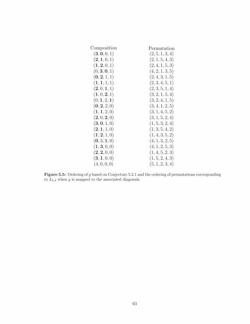
Composition Permutation(3,0, 0, 1) (2, 5, 1, 3, 4)(2,1, 0, 1) (2, 1, 5, 4, 3)(1,2, 0, 1) (2, 4, 1, 5, 3)(0,3,0, 1) (4, 2, 1, 3, 5)(0,2, 1, 1) (2, 4, 3, 1, 5)(1,1, 1, 1) (2, 3, 4, 5, 1)(2, 0,1, 1) (2, 3, 5, 1, 4)(1, 0,2, 1) (3, 2, 1, 5, 4)(0,1, 2,1) (3, 2, 4, 1, 5)(0,2, 2, 0) (3, 4, 1, 2, 5)(1,1, 2, 0) (3, 1, 4, 5, 2)(2, 0,2, 0) (3, 1, 5, 2, 4)(3,0, 1, 0) (1, 5, 3, 2, 4)(2,1, 1, 0) (1, 3, 5, 4, 2)(1,2, 1, 0) (1, 4, 3, 5, 2)(0, 3,1, 0) (4, 1, 3, 2, 5)(1,3, 0, 0) (4, 1, 2, 5, 3)(2,2, 0, 0) (1, 4, 5, 2, 3)(3,1, 0, 0) (1, 5, 2, 4, 3)(4, 0, 0, 0) (5, 1, 2, 3, 4)

Figure 5.5: Ordering of g based on Conjecture 5.2.1 and the ordering of permutations correspondingto L5,4 when g is mapped to the associated diagonals.

61

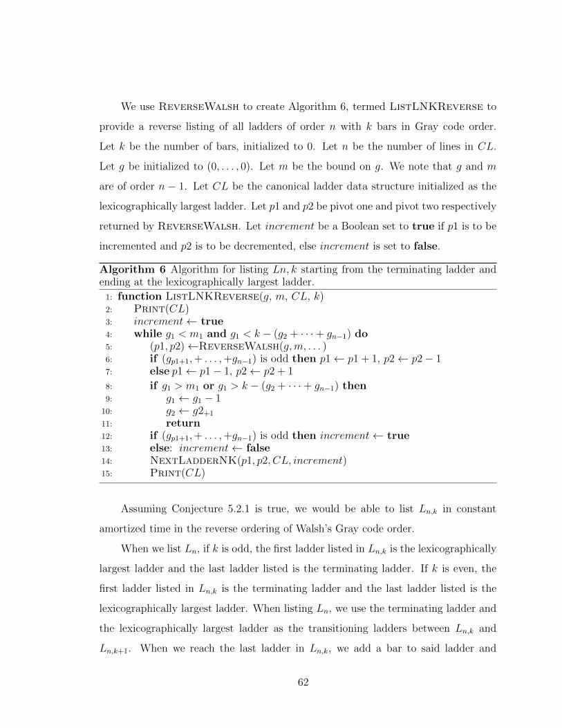
We use ReverseWalsh to create Algorithm 6, termed ListLNKReverse to

provide a reverse listing of all ladders of order n with k bars in Gray code order.

Let k be the number of bars, initialized to 0. Let n be the number of lines in CL.

Let g be initialized to (0, . . . , 0). Let m be the bound on g. We note that g and m

are of order n − 1. Let CL be the canonical ladder data structure initialized as the

lexicographically largest ladder. Let p1 and p2 be pivot one and pivot two respectively

returned by ReverseWalsh. Let increment be a Boolean set to true if p1 is to be

incremented and p2 is to be decremented, else increment is set to false.

Algorithm 6 Algorithm for listing Ln, k starting from the terminating ladder andending at the lexicographically largest ladder.

1: function ListLNKReverse(g, m, CL, k)2: Print(CL)3: increment← true4: while g1 < m1 and g1 < k − (g2 + · · ·+ gn−1) do5: (p1, p2)←ReverseWalsh(g,m, . . . )6: if (gp1+1,+ . . . ,+gn−1) is odd then p1← p1 + 1, p2← p2− 17: else p1← p1− 1, p2← p2 + 1

8: if g1 > m1 or g1 > k − (g2 + · · ·+ gn−1) then9: g1 ← g1 − 1

10: g2 ← g2+1

11: return12: if (gp1+1,+ . . . ,+gn−1) is odd then increment← true13: else: increment← false14: NextLadderNK(p1, p2, CL, increment)15: Print(CL)

Assuming Conjecture 5.2.1 is true, we would be able to list Ln,k in constant

amortized time in the reverse ordering of Walsh’s Gray code order.

When we list Ln, if k is odd, the first ladder listed in Ln,k is the lexicographically

largest ladder and the last ladder listed is the terminating ladder. If k is even, the

first ladder listed in Ln,k is the terminating ladder and the last ladder listed is the

lexicographically largest ladder. When listing Ln, we use the terminating ladder and

the lexicographically largest ladder as the transitioning ladders between Ln,k and

Ln,k+1. When we reach the last ladder in Ln,k, we add a bar to said ladder and

62

transition to the first ladder of Ln,k+1. We refer to this bar as the incrementing bar.

To calculate the coordinates of the incrementing bar when transitioning from Ln,k

to Ln,k+1, we scan g from left to right to find the smallest x value such that gx is

not at its maximum value. We then use the same formula for adding a bar found in

Equation 5.1, except we replace n with n−1 seeing as g is of order n−1 when mapping

to canonical ladders with n lines. If the last ladder of Ln,k is a terminating ladder,

when we add the incrementing bar, the first ladder of Ln,k+1 is also a terminating

ladder. If the las ladder of Ln,k is a lexicographically largest ladder, when we add the

incrementing bar, the first ladder of Ln,k+1 is also a lexicographically largest ladder.

To transition from Ln,k to Ln,k+1 we want to add the incrementing bar to the

largest associated diagonal that has room for one more bar. We know that by mapping

g to the associated diagonals, we can use m to determine the largest associated

diagonal that has room for one more bar. Based on our mapping of g to the associated

diagonals, the smallest x value in g not at its mx value corresponds to the largest

associated diagonal where we can add bar k+ 1. Let MinX be a global variable that

keeps track of the smallest x value in g that is not at its mx value. When we list g for

Ln,k, we update MinX with every transition from gi to gi+1 using Algorithm 7. Let p1

be pivot one returned by Walsh’s Gray code, let p2 be pivot two returned by Walsh’s

Gray code, let g be the current composition, let m be the upper bound on g, and let

MinX be the current smallest x value such that gx is not at its mx bound. With

63

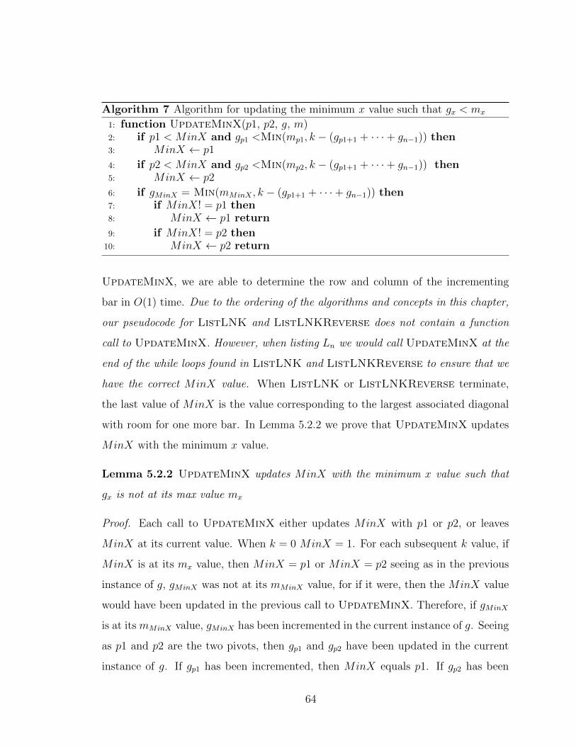
Algorithm 7 Algorithm for updating the minimum x value such that gx < mx

1: function UpdateMinX(p1, p2, g, m)2: if p1 < MinX and gp1 <Min(mp1, k − (gp1+1 + · · ·+ gn−1)) then3: MinX ← p1

4: if p2 < MinX and gp2 <Min(mp2, k − (gp1+1 + · · ·+ gn−1)) then5: MinX ← p2

6: if gMinX = Min(mMinX , k − (gp1+1 + · · ·+ gn−1)) then7: if MinX! = p1 then8: MinX ← p1 return

9: if MinX! = p2 then10: MinX ← p2 return

UpdateMinX, we are able to determine the row and column of the incrementing

bar in O(1) time. Due to the ordering of the algorithms and concepts in this chapter,

our pseudocode for ListLNK and ListLNKReverse does not contain a function

call to UpdateMinX. However, when listing Ln we would call UpdateMinX at the

end of the while loops found in ListLNK and ListLNKReverse to ensure that we

have the correct MinX value. When ListLNK or ListLNKReverse terminate,

the last value of MinX is the value corresponding to the largest associated diagonal

with room for one more bar. In Lemma 5.2.2 we prove that UpdateMinX updates

MinX with the minimum x value.

Lemma 5.2.2 UpdateMinX updates MinX with the minimum x value such that

gx is not at its max value mx

Proof. Each call to UpdateMinX either updates MinX with p1 or p2, or leaves

MinX at its current value. When k = 0 MinX = 1. For each subsequent k value, if

MinX is at its mx value, then MinX = p1 or MinX = p2 seeing as in the previous

instance of g, gMinX was not at its mMinX value, for if it were, then the MinX value

would have been updated in the previous call to UpdateMinX. Therefore, if gMinX

is at its mMinX value, gMinX has been incremented in the current instance of g. Seeing

as p1 and p2 are the two pivots, then gp1 and gp2 have been updated in the current

instance of g. If gp1 has been incremented, then MinX equals p1. If gp2 has been

64

incremented, then MinX equals p2. We replace gMinX with p1 if gMinX = mMinX

and MinX does not equal p1, or we replace MinX with p2 if gMinX = mMinX and

MinX does not equal p2. If MinX is not at its mMinX value, we replace MinX with

p1 only if gp1 is not at its mp1 value and p1 < MinX. The same goes for p2. Thus,

MinX is always equal to the smallest x value such that gMinX is not at its mx value.

2

In Algorithm 8, termed ListLnByKBars, we use the mapping of g to the

canonical ladder, ListLNK, ListLNKReverse, and UpdateMinX as subroutines

for listing Ln in Gray code order. We do so by listing Ln,0 . . . Ln,k . . . Ln,(n2)

. Let k be

initialized to 0; when k is even we call ListLNKReverse and when k is odd we call

ListLNK. Let g be of order n−1 and initialized to (0, 0, . . . , 0). Let m be the bound

on g initialized to (n − 1, n− 2, . . . 1). Let CL be initialized to the canonical ladder

corresponding the ascending permutation; i.e. the ladder with zero bars. Let MinX

be initialized to 1. Figure 5.3 shows the listing of Ln produced by ListLnByKBars.

Algorithm 8 Algorithm to list Ln by [0 . . . k . . .(n2

)] bars

1: function ListLnByKBars(g, m, k, CL, MinX)2: if k = 0 then3: Print(CL)4: ListLnByKBars(g, m, k + 1, CL, MinX)

5: if k >(n2

)then return

6: gMinX ← gMinX + 17: (r1, c1)← (((n−1)+MinX−1)−g(MinX), ((n−1)+1−MinX)−g(MinX))8: CL[r1][c1]← 19: if k is even and k > 0 then MinX ←ListLNKReverse(g, m, CL, k)

10: elseMinX ←ListLNK(g, m, CL, k)

11: ListLnByKBars(g, m, k + 1, CL, MinX)

If k is odd, we list Ln, k in accordance with Walsh’s ordering of g and if k is even

we list Ln,k in the reverse ordering of Walsh’s Gray code. When we call ListLNK

and ListLNKReverse as subroutines, we ensure that UpdateMinX is called as a

65

subroutine in these functions. By doing so, Minx is the smallest x value not at its

mx value. With the correct value for MinX, we add a bar to the largest associated

diagonal with room for the incrementing bar. We know that the maximum number of

bars is(n2

), therefore we terminate recursion when k exceeds

(n2

). ListLnByKBars

lists Ln in constant amortized time and in Gray code order.

Lemma 5.2.3 Each ladder produced by ListLnByKBars is unique.

Proof. Walsh’s Gray code lists all unique instances of g when k is odd. Each instance

of g corresponds to a unique ladder due to our mapping to the associated diagonals.

We assume that ReverseWalsh produces the reverse ordering of Walsh’s Gray code

when applied to even values of k, making all ladders for even values of k unique. When

we transition from k to k + 1 we add a bar, making the last ladder of k and the first

ladder of k + 1 unique. 2

5.3 Chapter Conclusion

We have provided a theoretical algorithm for listing Ln in Gray code order by Ln,k.

Furthermore, we would be able to do so in constant amortized time. We have provided

a second solution to The Canonical Ladder Listing Problem. What makes this solution

interesting is that we list Ln ordered by the number of bars. Our future work is as

follows:

1. Implement Walsh’s loop free algorithm

2. Prove Conjecture 5.2.1

3. Design and implement ReverseWalsh

66

Chapter 6

Summary and Future Work

In summary, we have defined the canonical ladder, designed a representation

of the canonical ladder along with equations to calculate the coordinates of the

bars in the representation, implemented an algorithm to create the canonical lad-

der, implemented a constant amortized algorithm to list Ln in Gray code order by

adding or removing a bar, designed a constant amortized algorithm to list Ln,k in

Gray code order, and designed a constant amortized algorithm to list Ln by listing

Ln,0 . . . Ln,k . . . Ln,(n2)

. The algorithms can be used to list sorting network arrange-

ments that correspond to the canonical ladders.

We are left with the following open problems:

1. Proving Conjecture 5.2.1

2. Design and implement ReverseWalsh

3. Implementing ListLNKReverse, assuming we can implement ReverseWalsh

4. Implement ListLnByKBars, assuming we can implement ListLNKReverse.

5. Continuing to work on the counting problem for the number of ladders in

OptL{π}, specifically when π = (n, n− 1, . . . , 2, 1).

67

Bibliography

[1] T. Aiuchi, K. Yamanaka, T. Hirayama, and Y. Nishitani. Coding ladder lotteries.

In Proceedings of European Workshop on Computational Geometry, pages 151–

154, 2013.

[2] J. Arndt. Matters Computational: Ideas, Algorithms, Source Code. www.jjj.de,

2010.

[3] K. E. Batcher. Sorting networks and their applications. In Proceedings of the

April 30–May 2, 1968, Spring Joint Computer Conference, AFIPS ’68 (Spring),

pages 307–314, New York, NY, USA, 1968. Association for Computing Machin-

ery.

[4] B. Bauslaugh and F. Ruskey. Generating alternating permutations lexicograph-

ically. BIT, 30:17–26, 1990.

[5] C. T. Djamegni and M. Tchuent. A cost-optimal pipeline algorithm for per-

mutation generation in lexicographic order. Journal of Parallel and Distributed

Computing, 44(2):153–159, 1997.

[6] A. Dumitrescu and R. Mandal. New lower bounds for the number of pseudoline

arrangements. SODA ’19, pages 410–425, USA, 2019. Society for Industrial and

Applied Mathematics.

[7] S. Effler and F. Ruskey. A CAT algorithm for generating permutations with a

fixed number of inversions. Information Processing Letters, 86(2):107–112, 2002.

[8] S. Felsner and P. Valtr. Coding and counting arrangements of pseudolines. Dis-

crete Comput. Geom., 46(3):405–416, Oct 2011.

[9] F. Gray. Pulse Code Communication. Bell Telephone Laboratories Incorporated,

New York USA, Serial NO 785697 edition, 1953.

[10] B. R. Heap. Permutations by Interchanges. The Computer Journal, 6(3):293–

298, 11 1963.

[11] S. M. Johnson. Generation of permutations by adjacent transposition. Mathe-

matics of Computation, 17:282–285, 1963.

68

[12] J. Kawahara, T. Saitoh, R. Yoshinaka, and M. Shin-Ichi. Couting primitive

sorting networks by πDDs. TCS-TR-A, 11(54), 2011.

[13] D. Knuth. The Art of Computer Programming, volume 4. Addison-Wesley, 2011.

[14] D. E. Knuth. The Art of Computer Programming, Volume 1 (3rd Ed.): Funda-

mental Algorithms. Addison Wesley Longman Publishing Co., Inc., USA, 1997.

[15] Louis-Frederic. Japan Encyclopedia. Belknap, 2002.

[16] J. D. Owens, M. Houston, D. Luebke, S. Green, J. E. Stone, and J. C. Phillips.

Gpu computing. Proceedings of the IEEE, 96(5):879–899, 2008.

[17] Ruskey, Mutze, Sawada, and Williams. The Combinatorial Object Server. http:

//combos.org/, 2018.

[18] C. Savage. A survey of combinatorial gray codes. SIAM Review, 39(4):605–629,

1997.

[19] J. Sawada and A. Williams. A Hamilton Path for the Sigma-Tau Problem, pages

568–575. Proceedings of the Twenty-Ninth Annual ACM-SIAM Symposium on

Discrete Algorithms, 1 2018.

[20] N. Sloane. The On-line Encyclopedia of Integer Sequences. https://oeis.org/

A008302.

[21] N. Sloane. The On-line Encyclopedia of Integer Sequences. https://oeis.org/

A006245.

[22] T. R. Walsh. Loop-free sequencing of bounded integer compositions. Journal of

Combinatorial Mathematics and Combinatorial Computing, 33:323–345, 2000.

[23] A. Williams. The greedy gray code algorithm. volume 8037, pages 525–536, 08

2013.

[24] K. Yamanaka, T. Horiyama, T. Uno, and K. Wasa. Ladder-lottery realization.

In CCCG, pages 61–67, 2018.

[25] K. Yamanaka, T. Horiyama, and K. Wasa. Optimal reconfiguration of optimal

ladder lotteries. Theoretical Computer Science, 859:57–69, 2021.

[26] K. Yamanaka and N. Shin-Ichi. Efficient enumeration of all ladder lotteries with

K bars. IEICE Transactions on Fundamentals of Electronics, Communications

and Computer Sciences, E97.A:1163–1170, 06 2014.

69

[27] K. Yamanaka and N. Shin-Ichi. Enumeration, counting, and random gener-

ation of ladder lotteries. IEICE Transactions on Information and Systems,

E100.D(3):444–451, 2017.

[28] K. Yamanaka, N. Shin-Ichi, Y. Matsui, R. Uehara, and K. Nakada. Efficient

enumeration of all ladder lotteries and its application. Theoretical Computer

Science, 411(16):1714–1722, 2010.

[29] S. Zaks. A new algorithm for generation of permutations. BIT Numerical Math-

ematics, 24(2):196–204, 1984.

70

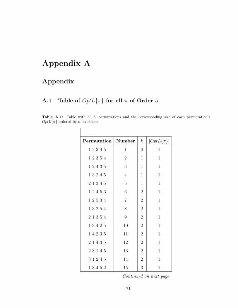
Appendix A

Appendix

A.1 Table of OptL{π} for all π of Order 5

Table A.1: Table with all 5! permutations and the corresponding size of each permutation’sOptL{π} ordered by k inversions

Permutation Number k |OptL{π}|

1 2 3 4 5 1 0 1

1 2 3 5 4 2 1 1

1 2 4 3 5 3 1 1

1 3 2 4 5 4 1 1

2 1 3 4 5 5 1 1

1 2 4 5 3 6 2 1

1 2 5 3 4 7 2 1

1 3 2 5 4 8 2 1

2 1 3 5 4 9 2 1

1 3 4 2 5 10 2 1

1 4 2 3 5 11 2 1

2 1 4 3 5 12 2 1

2 3 1 4 5 13 2 1

3 1 2 4 5 14 2 1

1 3 4 5 2 15 3 1

Continued on next page

71

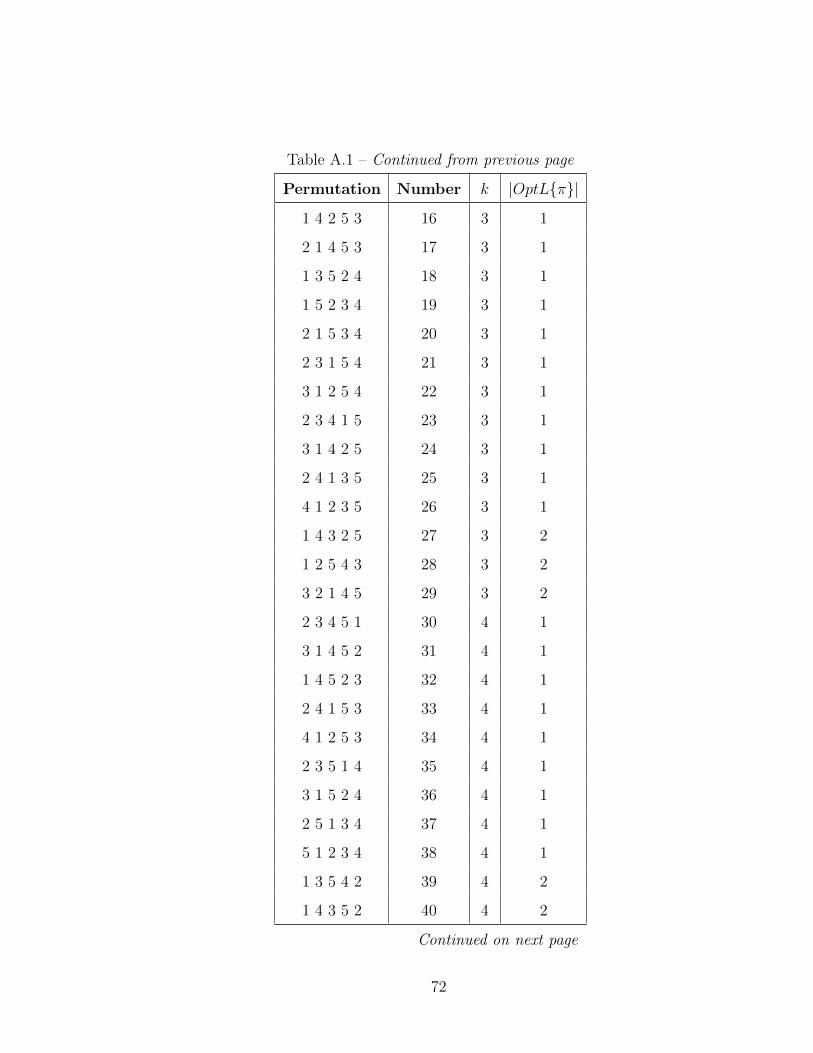
Table A.1 – Continued from previous page

Permutation Number k |OptL{π}|

1 4 2 5 3 16 3 1

2 1 4 5 3 17 3 1

1 3 5 2 4 18 3 1

1 5 2 3 4 19 3 1

2 1 5 3 4 20 3 1

2 3 1 5 4 21 3 1

3 1 2 5 4 22 3 1

2 3 4 1 5 23 3 1

3 1 4 2 5 24 3 1

2 4 1 3 5 25 3 1

4 1 2 3 5 26 3 1

1 4 3 2 5 27 3 2

1 2 5 4 3 28 3 2

3 2 1 4 5 29 3 2

2 3 4 5 1 30 4 1

3 1 4 5 2 31 4 1

1 4 5 2 3 32 4 1

2 4 1 5 3 33 4 1

4 1 2 5 3 34 4 1

2 3 5 1 4 35 4 1

3 1 5 2 4 36 4 1

2 5 1 3 4 37 4 1

5 1 2 3 4 38 4 1

1 3 5 4 2 39 4 2

1 4 3 5 2 40 4 2

Continued on next page

72

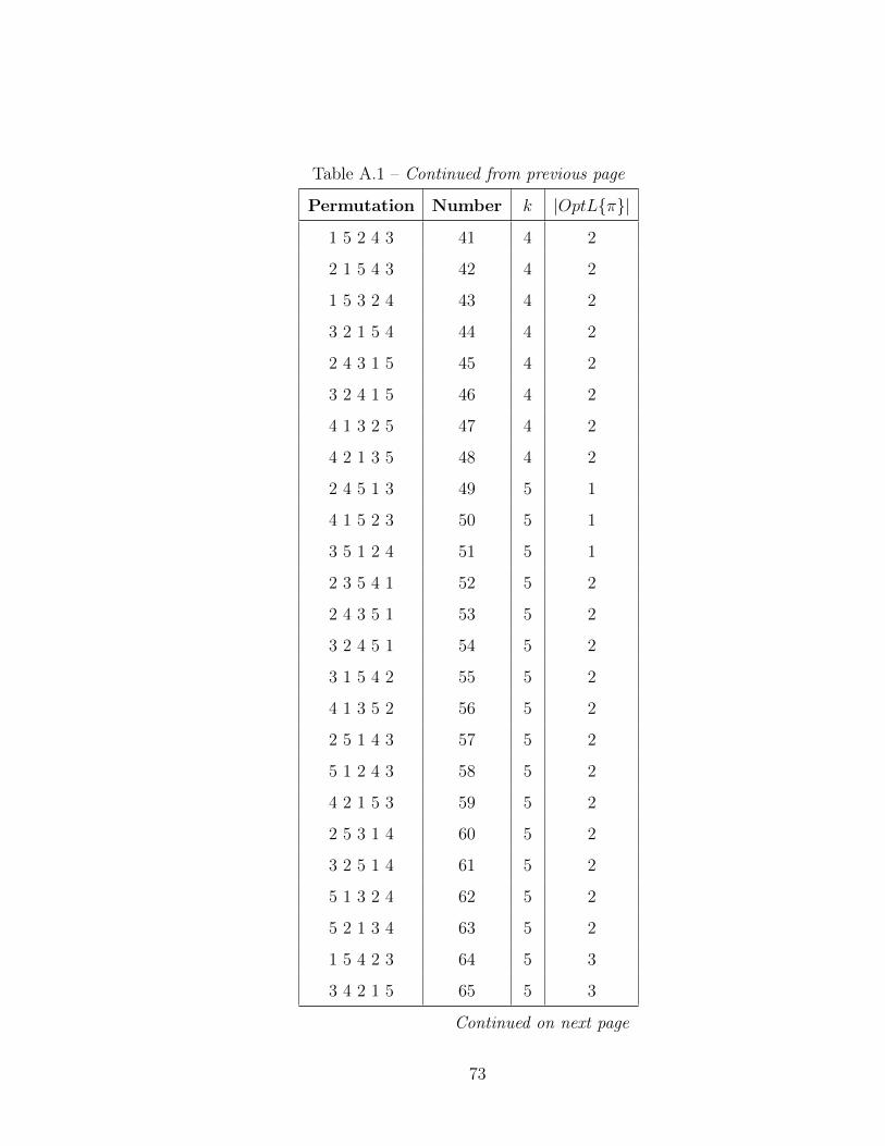
Table A.1 – Continued from previous page

Permutation Number k |OptL{π}|

1 5 2 4 3 41 4 2

2 1 5 4 3 42 4 2

1 5 3 2 4 43 4 2

3 2 1 5 4 44 4 2

2 4 3 1 5 45 4 2

3 2 4 1 5 46 4 2

4 1 3 2 5 47 4 2

4 2 1 3 5 48 4 2

2 4 5 1 3 49 5 1

4 1 5 2 3 50 5 1

3 5 1 2 4 51 5 1

2 3 5 4 1 52 5 2

2 4 3 5 1 53 5 2

3 2 4 5 1 54 5 2

3 1 5 4 2 55 5 2

4 1 3 5 2 56 5 2

2 5 1 4 3 57 5 2

5 1 2 4 3 58 5 2

4 2 1 5 3 59 5 2

2 5 3 1 4 60 5 2

3 2 5 1 4 61 5 2

5 1 3 2 4 62 5 2

5 2 1 3 4 63 5 2

1 5 4 2 3 64 5 3

3 4 2 1 5 65 5 3

Continued on next page

73

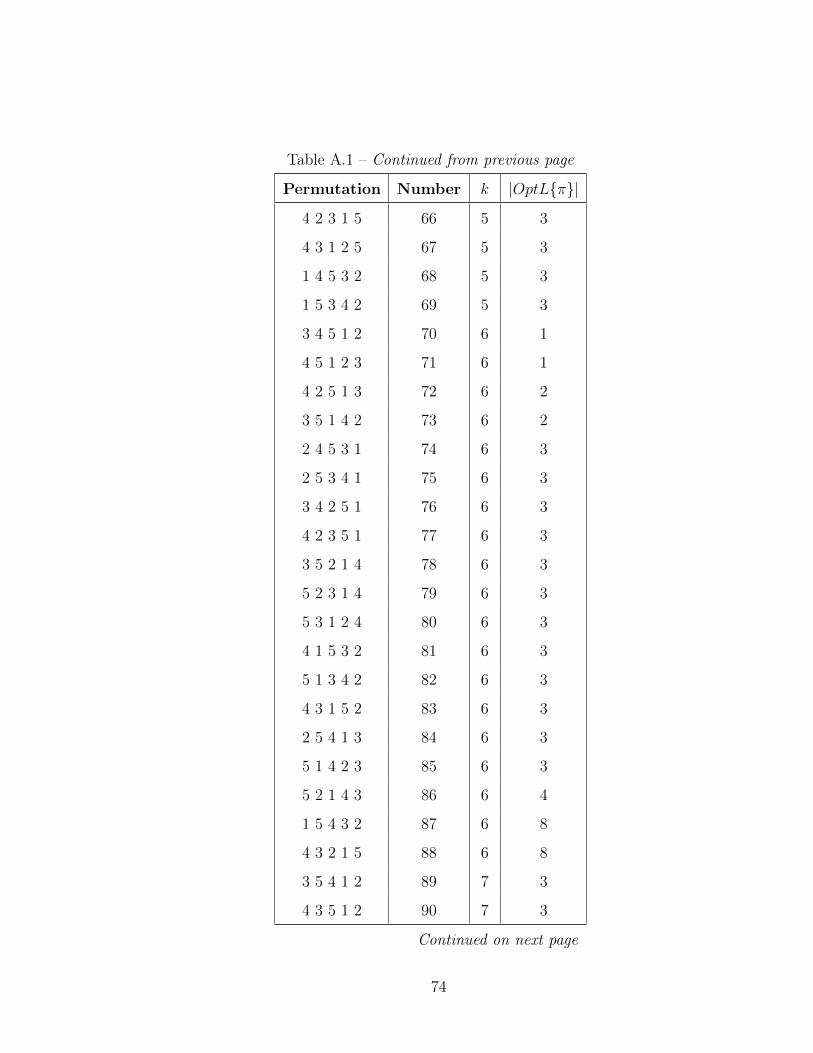
Table A.1 – Continued from previous page

Permutation Number k |OptL{π}|

4 2 3 1 5 66 5 3

4 3 1 2 5 67 5 3

1 4 5 3 2 68 5 3

1 5 3 4 2 69 5 3

3 4 5 1 2 70 6 1

4 5 1 2 3 71 6 1

4 2 5 1 3 72 6 2

3 5 1 4 2 73 6 2

2 4 5 3 1 74 6 3

2 5 3 4 1 75 6 3

3 4 2 5 1 76 6 3

4 2 3 5 1 77 6 3

3 5 2 1 4 78 6 3

5 2 3 1 4 79 6 3

5 3 1 2 4 80 6 3

4 1 5 3 2 81 6 3

5 1 3 4 2 82 6 3

4 3 1 5 2 83 6 3

2 5 4 1 3 84 6 3

5 1 4 2 3 85 6 3

5 2 1 4 3 86 6 4

1 5 4 3 2 87 6 8

4 3 2 1 5 88 6 8

3 5 4 1 2 89 7 3

4 3 5 1 2 90 7 3

Continued on next page

74

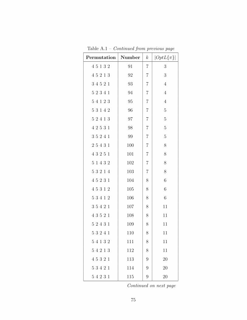
Table A.1 – Continued from previous page

Permutation Number k |OptL{π}|

4 5 1 3 2 91 7 3

4 5 2 1 3 92 7 3

3 4 5 2 1 93 7 4

5 2 3 4 1 94 7 4

5 4 1 2 3 95 7 4

5 3 1 4 2 96 7 5

5 2 4 1 3 97 7 5

4 2 5 3 1 98 7 5

3 5 2 4 1 99 7 5

2 5 4 3 1 100 7 8

4 3 2 5 1 101 7 8

5 1 4 3 2 102 7 8

5 3 2 1 4 103 7 8

4 5 2 3 1 104 8 6

4 5 3 1 2 105 8 6

5 3 4 1 2 106 8 6

3 5 4 2 1 107 8 11

4 3 5 2 1 108 8 11

5 2 4 3 1 109 8 11

5 3 2 4 1 110 8 11

5 4 1 3 2 111 8 11

5 4 2 1 3 112 8 11

4 5 3 2 1 113 9 20

5 3 4 2 1 114 9 20

5 4 2 3 1 115 9 20

Continued on next page

75

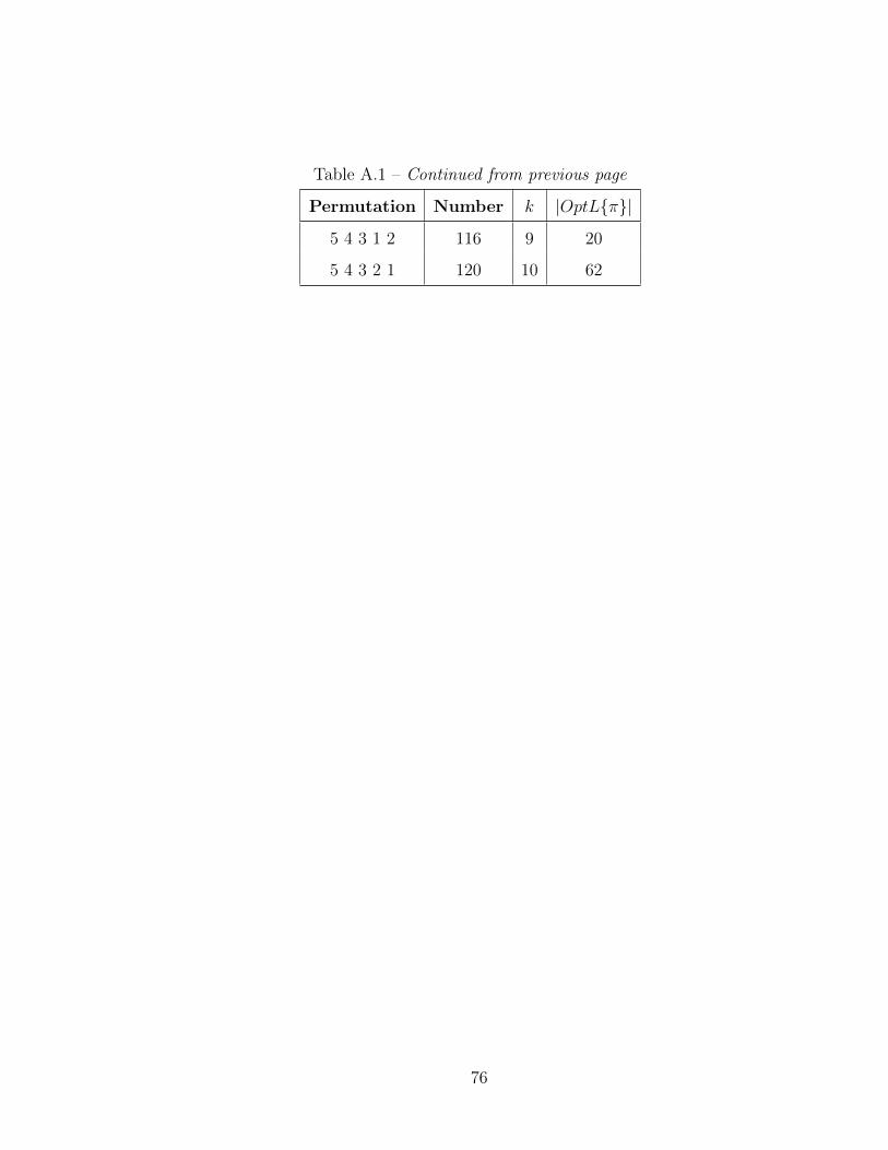
Table A.1 – Continued from previous page

Permutation Number k |OptL{π}|

5 4 3 1 2 116 9 20

5 4 3 2 1 120 10 62

76

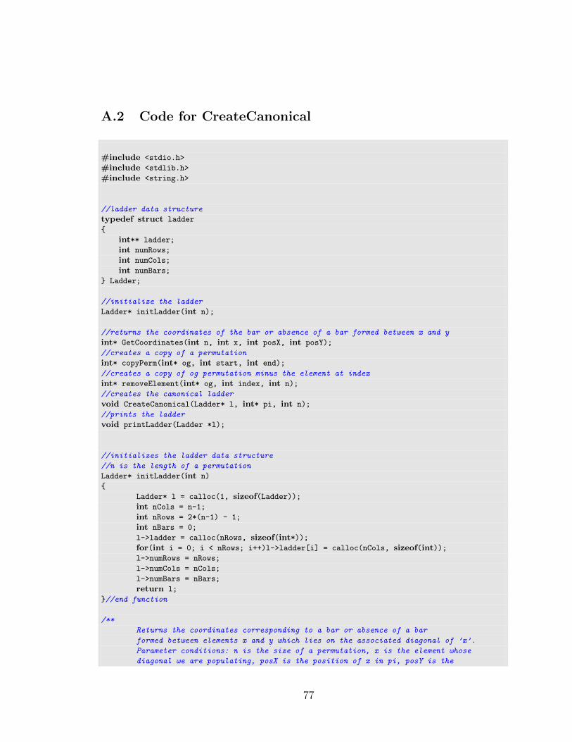
A.2 Code for CreateCanonical

#include <stdio.h>

#include <stdlib.h>

#include <string.h>

//ladder data structure

typedef struct ladder

{

int** ladder;

int numRows;

int numCols;

int numBars;

} Ladder;

//initialize the ladder

Ladder* initLadder(int n);

//returns the coordinates of the bar or absence of a bar formed between x and y

int* GetCoordinates(int n, int x, int posX, int posY);

//creates a copy of a permutation

int* copyPerm(int* og, int start, int end);

//creates a copy of og permutation minus the element at index

int* removeElement(int* og, int index, int n);

//creates the canonical ladder

void CreateCanonical(Ladder* l, int* pi, int n);

//prints the ladder

void printLadder(Ladder *l);

//initializes the ladder data structure

//n is the length of a permutation

Ladder* initLadder(int n)

{

Ladder* l = calloc(1, sizeof(Ladder));int nCols = n-1;

int nRows = 2*(n-1) - 1;

int nBars = 0;

l->ladder = calloc(nRows, sizeof(int*));for(int i = 0; i < nRows; i++)l->ladder[i] = calloc(nCols, sizeof(int));l->numRows = nRows;

l->numCols = nCols;

l->numBars = nBars;

return l;

}//end function

/**

Returns the coordinates corresponding to a bar or absence of a bar

formed between elements x and y which lies on the associated diagonal of ’x’.

Parameter conditions: n is the size of a permutation, x is the element whose

diagonal we are populating, posX is the position of x in pi, posY is the

77

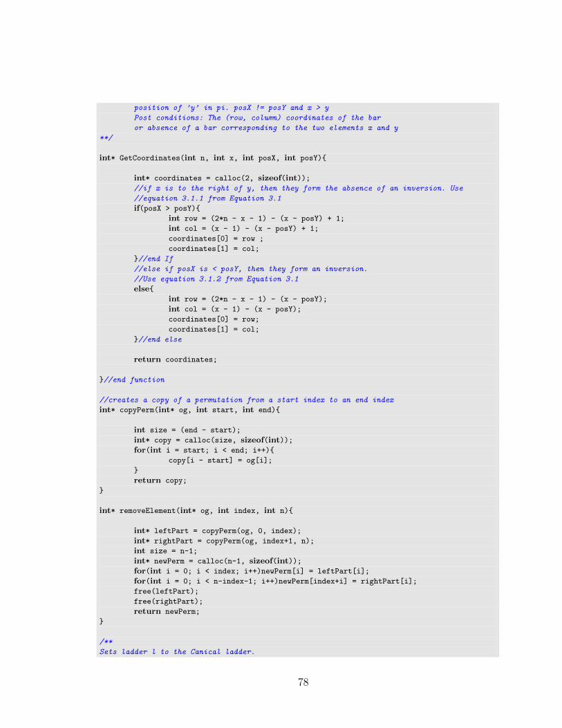
position of ’y’ in pi. posX != posY and x > y

Post conditions: The (row, column) coordinates of the bar

or absence of a bar corresponding to the two elements x and y

**/

int* GetCoordinates(int n, int x, int posX, int posY){

int* coordinates = calloc(2, sizeof(int));//if x is to the right of y, then they form the absence of an inversion. Use

//equation 3.1.1 from Equation 3.1

if(posX > posY){

int row = (2*n - x - 1) - (x - posY) + 1;

int col = (x - 1) - (x - posY) + 1;

coordinates[0] = row ;

coordinates[1] = col;

}//end If

//else if posX is < posY, then they form an inversion.

//Use equation 3.1.2 from Equation 3.1

else{int row = (2*n - x - 1) - (x - posY);

int col = (x - 1) - (x - posY);

coordinates[0] = row;

coordinates[1] = col;

}//end else

return coordinates;

}//end function

//creates a copy of a permutation from a start index to an end index

int* copyPerm(int* og, int start, int end){

int size = (end - start);

int* copy = calloc(size, sizeof(int));for(int i = start; i < end; i++){

copy[i - start] = og[i];

}

return copy;

}

int* removeElement(int* og, int index, int n){

int* leftPart = copyPerm(og, 0, index);

int* rightPart = copyPerm(og, index+1, n);

int size = n-1;

int* newPerm = calloc(n-1, sizeof(int));for(int i = 0; i < index; i++)newPerm[i] = leftPart[i];

for(int i = 0; i < n-index-1; i++)newPerm[index+i] = rightPart[i];

free(leftPart);

free(rightPart);

return newPerm;

}

/**

Sets ladder l to the Canical ladder.

78

Parameter conditions: l is created using initLadder, pi is a permutation of order n

Post conditions: l is set to the canonical ladder corresponding to pi

**/

void CreateCanonical(Ladder* l, int* pi, int n)

{

int x = n;

int* pi2 = copyPerm(pi, 0, n);

//from element x=n down to element x=2

while(x > 1)

{

int index = -1;

//get the index of element ’x’ in pi

for(int i = 0; i < x; i++){

if(pi2[i] == x){

index = i;

break;}//end if

}//end for

//populate the associated diagonal of x with 1s and 0s.

for(int i = 0; i < x; i++){

if(i != index){

int* coordinates = GetCoordinates(n, x, index, i);

int row = coordinates[0];

int col = coordinates[1];

if(i < index){

l->ladder[row][col] = 0;

}else{l->ladder[row][col] = 1;

l->numBars++;

}

}

}//end for

pi2 = removeElement(pi2, index, x);

x--;

}//end while

}

void printLadder(Ladder *l)

{

int n = l->numCols + 1;

int offset = 2*(n-1) - 1;

printf("\n\n");

for (int i = 0; i < offset; i++)

{

for (int j = 0; j < l->numCols; j++)

{

printf("|");

if (l->ladder[i][j] == 1)

printf("-----");

elseprintf(" ");

}

printf("|");

printf("\n");

79

}

}

//main for testing

int main(int argc, char* argv[])

{

//testing permutation

int pi[] = {4,1,7,2,3,6,5};

int n = 7;

Ladder* l = initLadder(n);

CreateCanonical(l, pi, n);

printLadder(l);

}

A.3 Code for ModifiedSJT

//Gets the coordinates of the row and coulumn for ModifiedSJT

int* GetCoordinatesTwo(int* rX, int n, int x, int posX, int posY);

//modified SJT algorithm for listing Ln

void ModifiedSJT(Ladder* l, int x, int n, bool* direction, int* rX);

//used in ModifiedSJT to return the location of a 1 or 0 indicating the addition or

//removal of a bar between two adjacent elements, x>y

int* GetCoordinatesTwo(int* rX, int n, int x, int posX, int posY)

{

int* coordinates = calloc(2, sizeof(int));//if posX is to the right of posY then x and y are currently

//uninverted and will be inverted. Therefore, we add a bar

//along the associated diagonal of ’x’

if(posX == posY + 1)

{

coordinates[0] = (2*n - x - 1) - (*rX)-1;

coordinates[1] = (x-1) - (*rX)-1;

(*rX)++;

}

//else if x is to the left of y by 1 position, then x and y

//are currently inverted and will become uninverted. Therefore,

//we remove a bar along the associated diagnoal of ’x’

else if(posX == posY - 1)

{

coordinates[0] = (2*n - x) - (*rX)-1;

coordinates[1] = x - (*rX)-1;

(*rX)--;

}

//else error occured

80

else{

printf("Error occurred\n");

exit(0);

}

return coordinates;

}

/**

Modify the SJT algorithm to list Ln by adding or removing a bar

**/

void ModifiedSJT(Ladder* l, int x, int n, bool* direction, int* rX)

{

if(x > n)

{

if(l->numBars == 0)printLadder(l);

return;}

for(int i = 0; i < x; i++)

{

if(i == 0)ModifiedSJT(l, x+1, n, direction, rX);

else{

//adding to the associated diagonal of x

if(direction[x-1] == false)

{

int* coordinates = GetCoordinatesTwo(&(rX[x-1]), n, x, 1, 0);

//subtract 1 for 0 index

int row = coordinates[0];

int column = coordinates[1];

l->ladder[row][column] = 1;

l->numBars++;

}

//removing a bar from the associated diagonal of x

else{int* coordinates = GetCoordinatesTwo(&(rX[x-1]), n, x, 0, 1);

int row = coordinates[0];

int column = coordinates[1];

l->ladder[row][column] = 0;

l->numBars--;

}

printLadder(l);

ModifiedSJT(l, x+1, n, direction, rX);

}

}

direction[x-1] = !(direction[x-1]);

}

81

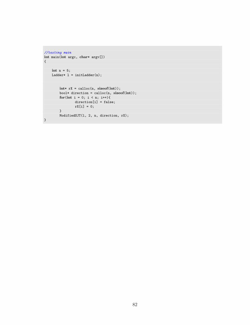
//testing main

int main(int argc, char* argv[])

{

int n = 5;

Ladder* l = initLadder(n);

int* rX = calloc(n, sizeof(int));bool* direction = calloc(n, sizeof(int));for(int i = 0; i < n; i++){

direction[i] = false;

rX[i] = 0;

}

ModifiedSJT(l, 2, n, direction, rX);

}

82