AM odel of Expertise

A Model of Expertise∗

Vijay KrishnaPenn State University

John MorganPrinceton University

May 1, 2000

Abstract

We study a model in which perfectly informed experts offer advice to adecision maker whose actions affect the welfare of all. Experts are biased andthus may wish to pull the decision maker in different directions and to differentdegrees. When the decision maker consults only a single expert, the expertwithholds substantial information from the decision maker. We ask whetherthis situation is improved by having the decision maker sequentially consult twoexperts. We Þrst show that there is no perfect Bayesian equilibrium in whichfull revelation occurs. When both experts are biased in the same direction,it is never beneÞcial to consult both. In contrast, when experts are biasedin opposite directions, it is always beneÞcial to consult both. Indeed, in thiscase full revelation may be induced in an extended debate by introducing thepossibility of rebuttal.

∗This research was supported by a grant from the National Science Foundation (SBR 9618648).We are grateful to Gene Grossman, George Mailath, Tomas Sjöström, Joel Sobel and the refereesfor sharing their expertise with us.

1

1 Introduction

The power to make decisions rarely resides in the hands of those with the necessary

specialized knowledge. Instead, decision makers often solicit experts for advice. Thus,

a division of labor has arisen between those who have the relevant expertise and those

who make use of it. The diverse range of problems confronted by decision makers,

such as corporate CEOs or political leaders, almost precludes the possibility that they

themselves are experts in all relevant Þelds and hence, the need for outside experts

naturally arises. CEOs routinely seek the advice of marketing specialists, investment

bankers and management consultants. Political leaders rely on a bevy of economic

and military advisors. Investors seek tips from stockbrokers and Þnancial advisors.

These and numerous other situations share some common features.

First, the experts dispensing advice are by no means disinterested. Experts may

attempt to inßuence the decision maker in ways that are not necessarily in the latter�s

best interests. Investment banks stand to gain from new issues and corporate mergers,

decisions about which they regularly offer advice. The political future of economic

and military advisors may be affected by the decisions on which they give counsel.

Stockbrokers are obviously interested in the investment decisions of their clients.

Second, decision makers are often bombarded with advice from numerous experts,

with possibly different agendas. Moreover, experts may strategically tailor their ad-

vice to counter that offered by other, rival, experts. For instance, hawks may choose

more extreme positions on an issue if they know that doves are also being consulted,

and vice-versa. Thus the decision maker faces the daunting task of sifting through

the mass of conßicting opinions and deciding as to the best course of action. Indeed,

this ability is routinely touted as the mark of a good leader.

In determining the size and composition of her �cabinet� of advisors, the decision

maker must carefully consider the following questions: Is it possible to extract all

information relevant to the decision from a cabinet? Is it better to actively consult

a number of advisors or only a single, well chosen, advisor? Is an advocacy system,

where the decision maker appoints experts with opposing viewpoints, helpful in de-

ciding on the correct action? How do experts with extreme views affect the advice

2

offered to the decision maker? Does it help to have an extended debate in which

experts can make counter arguments? These questions form the central focus of our

paper.

To address these questions, we use a simple model of the interplay among a single

decision maker and two perfectly informed, but interested experts. The experts offer

advice to the decision maker in order to inßuence the decision in a way that serves

their own, possibly differing, objectives. We ask how a decision maker should integrate

the opinions of experts when faced with this situation. We begin with a model where

each expert speaks only once. Speeches are made sequentially and publicly.

In our model, an expert�s preferences are parametrized by his inherent bias relative

to the decision maker. The experts may differ both in terms of how biased they are

and in which direction. They may have opposing biases: one expert may wish to pull

the decision maker to the left and the other to the right. Alternatively, they may

have like biases: both wish to pull in the same direction but possibly to differing

degrees. The absolute value of the bias parameter indicates how �loyal� an expert is

to the decision maker.

Like biases. When experts have like biases, we Þnd that the decision maker

derives no beneÞt relative to consulting only one expert, in the sense that no equi-

librium with multiple experts is superior to the most informative equilibrium with

a single expert. Moreover, ex ante all parties, including the less loyal expert, would

agree that the best course of action is for the decision maker to consult only the

more loyal expert. This implies that even with two identically informed experts all

equilibria result in some information loss.1

Opposing biases. The situation changes dramatically when experts have op-

posing biases. Now, the decision maker always derives some beneÞt from consulting

both experts relative to consulting only one. However, this conclusion holds only if

at least one of the experts is not an �extremist.� If both of the experts are extrem-

1Our results in the case of like biases concern equilibria where the action taken is a monotonic

function of the state. While non-monotonic equilibria exist, we provide sufficient conditions for all

equilibria to be monotonic.

3

ists, no information is revealed in any equilibrium � either when they are consulted

separately or in combination.2

Rebuttal. We then explore what happens when experts engage in an extended

back-and-forth debate. When experts have opposing biases, the introduction of a

rebuttal stage in the debate can result in full revelation and Þrst-best outcomes.

Extended debate does not, however, lead to full revelation when experts have like

biases.

Related Work Our basic model is closely related to the model of Crawford and

Sobel [1982] of strategic information transmission between two parties, one of whom

has information useful for the other. We depart from Crawford and Sobel [1982],

hereafter referred to as CS, in that we allow for multiple sources of information. The

additional strategic considerations that arise with multiple experts lead to technical

complications not present with a single expert. Differences between the single expert

model of CS and our model are highlighted in later sections.

Also closely related are papers by Gilligan and Krehbiel [1989] and Krishna and

Morgan [1999]. Gilligan and Krehbiel [1989] study a model where a committee con-

sisting of two �experts� with opposing biases communicate to the decision making

legislature by simultaneously submitting bills to the ßoor of the House. They argue

that the restrictive �closed rule,� which does not permit the amendment of bills sub-

mitted to the ßoor is informationally superior to the �open rule� under which bills

are freely amendable. This model differs from that in the present paper in that ex-

perts� advice is offered simultaneously and considers only the case of opposing biases.

Krishna and Morgan [1999] have reexamined the Gilligan and Krehbiel [1989] model

and shown that full informational efficiency is attainable under the open rule but not

under the closed. As we show below, full efficiency cannot be attained in our model of

sequential communication. Thus, in contrast to previous work, our paper highlights

how the informativeness of multiple experts differs depending on whether they are of

2Our results in the case of opposing biases hold generally for all equilibria, not just monotonic

equilibria.

4

like or opposing biases, as well as on the timing of the debate.

Austen-Smith [1993] also studies a model with two experts. His model differs

from ours in two regards. First, the state space is binary, as is the signal space for

each expert. Second, the experts are imperfectly informed about the state. Together,

these imply that full revelation (the expert reveals all that he knows) is possible even

with a single expert, a property that is impossible with a richer signal space. In his

model, it is sometimes the case that full revelation is possible with a single expert,

but not when two experts are consulted simultaneously. This is exactly the opposite

of the results we obtain. Also, contrary to our Þndings, Austen-Smith [1993] Þnds

that sequential consultation is superior to simultaneous consultation. In our model,

full revelation is obtainable in the simultaneous model whereas it is impossible in the

sequential model. Finally, while Austen-Smith [1993] Þnds little difference between

like and opposing biases, we Þnd that these situations are in stark contrast.

Dewatripont and Tirole [1999] examine reward schemes to induce information

gathering by �advocates.� Advocates differ from experts in that they are not inter-

ested in the decision per se but care about it only to the extent that their reward

may depend on the decision. Dewatripont and Tirole [1999] Þnd that informational

beneÞts are maximized by making each of the advocates responsible for a distinct

area and compensating them accordingly. In contrast, informational beneÞts in our

model derive solely from differences in the interests and ideologies of the experts.

Sobel [1985] and Morris [1997] study how reputational considerations affect a

single expert�s advice when the bias of the expert is uncertain. Morgan and Stocken

[1998] consider this problem in a static CS-like setting and focus on information

transmission by equity analysts. Ottaviani and Sorensen [1997] study reputational

issues with multiple experts. In their model the experts are not directly affected by

the decisions but care only about making recommendations that are validated ex post.

Banerjee and Somanathan [1998] and Friedman [1998] examine information trans-

mission in a setting in which there is a continuum of potential experts with differing

prior beliefs. Austen-Smith [1990] examines the effect of debate on voting outcomes.

In his model �expert� legislators themselves vote on legislation, so the separation

5

between the experts and the decision maker is absent. The effects of combining in-

formation provided by experts with opposing incentives has also been examined by

Shin [1994] in the context of persuasion games (see Milgrom and Roberts [1986]).

Finally, although we are not concerned with implementation per se, the problem of

how a decision maker should extract information from interested experts is related to

Baliga et al. [1997], who study abstract implementation problems where the planner

is unable to commit to a mechanism.

As is well known, models with cheap talk suffer from a plethora of equilibria

and efforts to identify some as salient has led to the development of a substantial

literature on reÞnements in this context (Matthews et al. [1991] and Farrell [1993]).

Farrell and Rabin [1996] present a concise survey. The models we consider also have

multiple equilibria; however, for the most part, our focus is on the �most informative�

equilibrium.

2 Preliminaries

In this section we sketch a simple model of decision making with multiple experts.

Rather than modelling any of the examples mentioned in the introduction explicitly,

we consider a stylized representation of the interaction among a decision maker and

experts that applies to a broad range of institutional settings. Precisely, we extend

the model of CS to a setting with multiple experts.

Consider a decision maker who takes an action y ∈ R, the utility from which

depends on some underlying state of nature θ ∈ [0, 1] which is distributed accordingto the density function f (·) . The decision maker has no information about θ, butthere are two experts each of whom observes θ.

The two experts then offer �advice� to the decision maker by sending messages

m1 ∈ [0, 1] and m2 ∈ [0, 1] , respectively. The messages are sent sequentially andpublicly. First, expert 1 offers his advice, which is heard by both the decision maker

and expert 2. Expert 2 then offers his advice, and the decision maker takes an action.

The decision maker is free to interpret the messages however she likes as well as to

6

choose any action.

In Section 6, we allow for the possibility of extending the length of the �debate.�

In particular, we study a situation where following the initial round of messages, m1

and m2, each expert offers a �rebuttal� message, r1 and r2, respectively. As in the

initial round, these messages are also sent sequentially and publicly.

The utility functions of all agents are of the form U (y, θ, bi) where bi is a parameter

which differs across agents. For the decision maker, agent 0, b0 is normalized to be 0.

We write U (y, θ) ≡ U (y, θ, 0) . For the experts, agents 1 and 2, bi 6= 0. We supposethat U is twice continuously differentiable, U11 < 0, U12 > 0, U13 > 0. Since U13 > 0,

bi is a measure of how biased expert i is, relative to the decision maker. For each

i, U (y, θ, bi) attains a maximum at some y. Since U11 < 0, the maximizing action is

unique. The biases of the two experts and the decision maker are commonly known.

These assumptions are satisÞed by �quadratic loss functions,� in which case,

U (y, θ, bi) = − (y − (θ + bi))2 . (1)

When combined with the assumption that θ is uniformly distributed on [0, 1] this is

referred to as the �uniform-quadratic� case, Þrst introduced by CS.

The multiple experts problem is divided into two cases. If both b1, b2 > 0, then

the experts are said to have like biases. If bi > 0 > bj, then the experts are said to

have opposing biases.3

DeÞne y∗ (θ) = argmaxy U (y, θ) to be the ideal action for the decision maker

when the state is θ. Similarly, y∗ (θ, bi) = argmaxy U (y, θ, bi) is the ideal action for

expert i. Since U13 > 0, bi > 0 implies that y∗ (θ, bi) > y∗ (θ); and since such an

expert always prefers a higher action than is ideal for the decision maker, we refer to

him as being right-biased. Similarly, if bi < 0 then y∗ (θ, bi) < y∗ (θ) and we refer to

such an expert as being left-biased. With quadratic loss functions, y∗ (θ, bi) = θ + bi.

A word of caution is in order. Our results fall into two categories. Some concern

the structure of equilibria of the multiple experts game and are derived under the

assumptions given above. Others concern welfare comparisons among equilibria and,

3The case where both b1, b2 < 0 is qualitatively no different from the case where both b1, b2 > 0.

7

require the same assumption as made in CS, Assumption M (p. 1444 of CS), in order

to derive unambiguous welfare results (speciÞcally, Proposition 2). This assumption,

while not so transparent, is satisÞed by the uniform-quadratic case.

3 Equilibrium with Experts

Single Expert In the single expert game studied by CS, a strategy for the

expert, µ, speciÞes the message m = µ (θ) that he sends in state θ. A strategy for the

decision maker, y, speciÞes the action y (m) that she takes following any message m

by the expert.

CS show that every Bayesian equilibrium of the single expert game has the fol-

lowing structure. There are a Þnite number of equilibrium actions y1, y2, ..., yN . The

state space is partitioned into N intervals [0, a1), [a1, a2), ... , [an−1, an), ... , [aN−1, 1]

with action yn resulting in any state θ ∈ [an−1, an). The equilibrium actions are mono-tonically increasing in the state, that is, yn−1 < yn. Finally, at every �break point�

an the following �no arbitrage� condition is satisÞed:

U (yn, an, b) = U (yn+1, an, b) . (2)

In other words, in state an the expert is indifferent between actions yn and yn+1. Since

U12 > 0, for all θ < an, the expert prefers yn to yn+1 and for all θ > an, the reverse

is true. Thus (2) serves as an incentive (or self-selection) constraint.

Multiple Experts In the multiple experts game, a pure strategy for expert 1,

µ1, speciÞes the message m1 = µ1 (θ) that he sends in state θ. A pure strategy for

expert 2, µ2, speciÞes the message m2 = µ2 (θ,m1) that he sends in state θ after

hearing message m1 from expert 1. A strategy for the decision maker, y, speciÞes

the action y (m1,m2) that she takes following messages m1 and m2. Let P (·|m1,m2)

denote the posterior beliefs on θ held by the decision maker after hearing messages

m1 and m2.

A (pure strategy) perfect Bayesian equilibrium (PBE) entails: (1) for all messages

m1 and m2, y (m1,m2) maximizes the decision maker�s expected utility given her be-

8

liefs P (·|m1,m2); (2) the beliefs P (·|m1,m2) are formed using the experts� strategies

µ1 and µ2 by applying Bayes� rule wherever possible; (3) given the decision maker�s

strategy y, for all θ and m1, µ2 (θ,m1) maximizes expert 2�s utility; and (4) given the

strategies y and µ2, for all θ, µ1 (θ) maximizes expert 1�s expected utility.4

Given a PBE, we denote by Y the outcome function that associates with every

state the resulting action. Formally, for each θ, Y (θ) = y (µ1 (θ) , µ2 (θ, µ1 (θ))) .

Denote by Y −1 (y) = {θ : Y (θ) = y} . Every Y determines an equilibrium partition ofthe state space, P = {Y −1 (y) : y is an equilibrium action}. The partition P is thena measure of the informational content of the equilibrium.

An action y is said to be rationalizable if there are some beliefs that the decision

maker could hold for which y is a best response. Clearly, an action y is rationalizable

if and only if y∗ (0) ≤ y ≤ y∗ (1) .A PBE always exists. In particular, there is always a �babbling� equilibrium in

which all messages from both experts are completely ignored by the decision maker.

Obviously, information loss is most severe in such an equilibrium. Typically, there

are also other, more informative, equilibria.

Example 1 Consider the uniform-quadratic case with b1 = 140and b2 = 1

9, so

that the experts have like biases and expert 1 is less biased than is expert 2. A PBE

for this game is depicted in Figure 1, where the states a1 = 1180, a2 =

22180, a3 =

61180and

the actions y1 = 1360, y2 =

23360, y3 =

83360, y4 =

241360.

In the Þgure, the outcome function Y is the step function depicted by the dark

lines. The dotted lines depict the experts� ideal actions y∗ (θ, bi) = θ+bi. The resulting

information partition is {[0, a1), [a1, a2), [a2, a3), [a3, 1]} . The action y1 is optimal forthe decision maker given that θ ∈ [0, a1), y2 is optimal given θ ∈ [a1, a2), etc.To see that this is an equilibrium conÞguration, notice that in state a2 expert

1 is exactly indifferent between actions y2 and y3 (In the Þgure, this indifference is

indicated by the vertical double-pointed arrow centered on a2 + b1.) Expert 1 prefers

4The formal deÞnition of a PBE requires only that the various optimality conditions hold for

almost every state and pair of messages. This would not affect any of our results.

9

r6?

r

6

?

..........................................................................

y∗(·, b2)

.................................................................

y∗(·, b1)

a1 a2 a3 θ 1

y1

y2

y3

y4

Figure 1: A PBE with Like Biases

y2 to y3 in all states θ < a2 and prefers y3 to y2 in all states θ > a2. Thus, given the

decision maker�s strategy he is willing to distinguish between states θ < a2 and states

θ > a2. Similarly, in state a3 expert 2 is indifferent between y3 and y4 and is willing

to distinguish between states θ < a3 and states θ > a3. Thus in states a2 and a3, the

CS �no arbitrage� condition (2) holds for either expert 1 or expert 2.

In state a1, however, neither expert is indifferent between y1 and y2. Indeed, expert

1 prefers y1 to y2 in state a1. (Expert 1�s ideal action is closer to y1 than y2.) Expert

2, on the other hand, prefers y2 to y1. The equilibrium calls for expert 1 to �suggest�

action y1 and for expert 2 to �agree.� Expert 2 has the option of �disagreeing� with

expert 1 and inducing action y3. Expert 2 is indifferent between y1 and y3 in state

a1 and so prefers y3 to y1 if θ > a1. Thus, even though in states just above a1, expert

1 prefers y1 to y2, were he to suggest y1, expert 2 would disagree, resulting in y3.

Since y2 is preferred to y3 by expert 1 in these states, expert 1 will not deviate.

10

Here we see how the strategic interaction of the two experts creates the possibility of

�disciplining� the experts in a manner not possible for the single expert case.5

3.1 Full Revelation

A natural question is whether the increase in discipline possible with the addition

of multiple experts can lead to full revelation. Full revelation means that for all θ,

Y (θ) = y∗ (θ) . Recall that with only a single expert, CS show that full revelation is

not a Bayesian equilibrium (BE).

With multiple experts, however, full revelation can occur in a BE. Suppose experts

have like biases and the decisionmaker holds the beliefs P (θ = min {m1,m2} |m1,m2) =

1. The associated strategy of the decision maker is then y (m1,m2) = y∗ (min {m1,m2}) .

Let expert 1 follow the strategy µ1 (θ) = θ and expert 2 follow the strategy: µ2 (θ,m1) =

θ. In state θ, both experts send messages m1 = m2 = θ, and the action is y∗ (θ) which

preferred by both experts to any action y < y∗ (θ). Reporting an mi < θ will only

decrease i�s utility whereas reporting an mi > θ will have no effect.6

The equilibrium constructed above, however, involves non-optimizing behavior on

the part of expert 2 off the equilibrium path. SpeciÞcally, in state θ ∈ [0, 1) if expert1 were to choose a message m1 = θ+ε, for ε > 0 small enough, it is no longer optimal

for expert 2 to play µ2 (θ,m1) = θ. Indeed, he is better off also deviating to m2 = m1.

Thus the full revelation BE constructed above is not a PBE. This is true in general.

Proposition 1 There does not exist a fully revealing PBE.

Proof. See Appendix.5A detailed speciÞcation of the equilibrium strategies and beliefs for this and all other examples

in the paper may be obtained from the authors.6When messages are sent simultaneously and experts have like biases, the above construction is a

fully revealing PBE. With simultaneous messages and opposing biases, Krishna and Morgan (1999)

show that full revelation is a PBE, but the construction is somewhat more involved.

11

4 Experts with Like Biases

In this section, we focus on two questions: Þrst, what is the information content

of advice offered by a given panel of like biased experts; and second, how should a

decision maker determine the composition of such a panel.

4.1 Choosing a Cabinet

To illustrate the key underlying issues, it is useful to study the example given earlier

in greater detail.

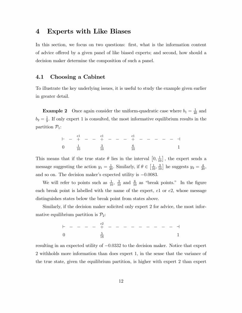
Example 2 Once again consider the uniform-quadratic case where b1 = 140and

b2 =19. If only expert 1 is consulted, the most informative equilibrium results in the

partition P1:

` − e1+ − − e1

+ − − − e1+ − − − − − a

0 110

310

610

1

This means that if the true state θ lies in the interval£0, 1

10

¤, the expert sends a

message suggesting the action y1 = 120. Similarly, if θ ∈ £ 1

10, 310

¤he suggests y2 = 4

20,

and so on. The decision maker�s expected utility is −0.0083.We will refer to points such as 1

10, 310and 6

10as �break points.� In the Þgure

each break point is labelled with the name of the expert, e1 or e2, whose message

distinguishes states below the break point from states above.

Similarly, if the decision maker solicited only expert 2 for advice, the most infor-

mative equilibrium partition is P2:

` − − − − e2+ − − − − − − − − − a

0 518

1

resulting in an expected utility of −0.0332 to the decision maker. Notice that expert2 withholds more information than does expert 1, in the sense that the variance of

the true state, given the equilibrium partition, is higher with expert 2 than expert

12

1. Intuitively, since expert 2 wishes the decision maker to choose a larger value of y

than does expert 1, he withholds more information than does expert 1.

If there were no further strategic considerations, that is neither expert knew of

the other�s existence, the decision maker could combine the reports of the two experts

to obtain the partition P1 ∧ P2:

` − e1+ − − e2

+e1+ − − − e1

+ − − − − a0 1

10518

310

610

1

which is the coarsest common reÞnement (join) of P1 and P2. The decision maker�sexpected utility is now −.0081. Thus, it seems plausible that the addition of anotherexpert, even an expert more biased than expert 1, might be helpful in overcoming

the problem of strategic information withholding.

Of course, this ignores strategic interaction among the experts. Indeed, the spec-

iÞcation above is not a PBE in the multiple experts game. What is the structure of

PBEs when the experts are aware of each other�s presence? One such equilibrium

was described in Example 1 with the following information partition.

` e1+

e1+ − − e2

+ − − − − − − − − − a0 1

18022180

61180

1

Recall that at the point θ = 1180neither expert is indifferent between y1 and y2. The

decision maker�s expected utility in this equilibrium is −.0250.A PBE with the property that expert 1 is indifferent at the Þrst point of discon-

tinuity results in the equilibrium partition Q :

` e1+

e1+ − − e2

+ − − − − − − − − − a0 1

7223180

41120

1

where expert 1 is also indifferent at the second break point and expert 2 is indifferent

at the third. This results in expected utility of −.0247 to the decision maker andis better than the equilibrium of Example 1. Intuitively, by shifting the Þrst break

point to the right, informativeness is improved since all of the other break points shift

to the right as well. Hence the resulting partition is �closer� to the most informative

13

partition with three break points; that is, where the break points are equally spaced.

Since expert 1 is not indifferent at the Þrst break point, such a rightward shift is

possible. Indeed, one can show that Q is the most informative PBE in which there

are three break points and both experts� messages are relevant. It is not possible to

have a fourth interior break point.

Comparing Q to P1 we see that the more biased expert 2 distorts the third breakpoint to the left, from 6

10to 41

120. This reduces the information content in the right-

most interval. Moreover, the leftward shift by expert 2 shifts all of the other break

points to the left; thus it also distorts expert 1�s break points to the left, from 310

down to 23180and from 1

10to 1

72. The aggregate effect of these distortions is to reduce

the expected utility of the decision maker and that of both experts.

To summarize, whenever there is a break point at which expert 1 is not indifferent,

informativeness is enhanced by shifting this break point to the right until expert 1

becomes indifferent. As a result of this shift, there is a complementary, and still

more informative, shift to the right of all of the other break points. Thus, any PBE

containing a break point where expert 2 is indifferent is detrimental. Put differently,

when experts have like biases, the decision maker can do no better than to consult

only the more loyal expert.

In coming to this conclusion, we relied essentially on two properties of any PBE.

First, that a rightward shift of one break point led to a rightward shift of all others and

this improved informativeness � this is Assumption M of CS. Second, we relied on the

fact that equilibrium partitions consisted only of intervals � that is, the equilibrium

outcome function Y (·) is monotonic in θ. We now present the main result of this

section, which shows that as long these two properties are satisÞed, the conclusion

from the example generalizes.7

Proposition 2 When experts have like biases, there is never a monotonic PBE with

both experts that is informationally superior to the most informative PBE with a single

expert.

7Although our analysis in the like bias case is conÞned to monotonic equilibria, we know of no

instance where admitting a non-monotonic equilibrium reverses the welfare comparisons.

14

Proof. See Appendix.

Despite the fact that the messages of one expert can be used to discipline the

other, in the case of monotonic equilibria with like biases, this disciplining only has

the effect of reducing informativeness. Thus, the advice of one of the experts is, at

best, redundant. The redundancy result holds regardless of whether the biases of the

two experts are close to one another or far apart.

Proposition 2 applies to monotonic PBEs. We now turn to a study of such PBEs

in the like biased case and provide some sufficient conditions for all PBEs to be

monotonic.

4.2 Monotonic Equilibria

A PBE is said to be monotonic if the corresponding outcome function Y (·) is non-decreasing. Recall that in the case of a single expert we know from CS that all

equilibria are monotonic. While the PBE constructed in Example 1 has this property,

this is not true in general when there are multiple experts.8

Monotonic equilibria must satisfy the following conditions, which are in the nature

of incentive constraints.

Lemma 1 Suppose Y is monotonic. If Y has a discontinuity at θ and

limε↓0Y (θ − ε) = y− < y+ = lim

ε↓0Y (θ + ε)

then

U¡y−, θ,min {b1, b2}

¢ ≥ U ¡y+, θ,min {b1, b2}¢ , and (3)

U¡y−, θ,max {b1, b2}

¢ ≤ U ¡y+, θ,max {b1, b2}¢ . (4)


We next show that when the experts have like biases there can be at most a Þnite

number of equilibrium actions played in any monotonic PBE.

8An example of a non-monotonic equilibrium is available from the authors.

15

Lemma 2 Suppose experts have like biases and Y is monotonic. Then there are a

Þnite number of equilibrium actions.


The intuition for Lemma 2 is that if two equilibrium actions are too close to one

another, then there will be some state where the lower action is called for, while both

experts prefer the higher action. But then the Þrst expert can deviate and send a

message inducing the higher action, conÞdent that expert 2 will follow his lead.

In the uniform-quadratic case with like biases, if the less loyal expert speaks

Þrst, then all PBE are monotonic. More generally, when b1 ≥ b2 > 0, all PBE are

monotonic as long as the following conditions are satisÞed. First, utility functions

are symmetric, that is, for all θ and k, U (y∗ (θ, bi) + k, θ, bi) = U (y∗ (θ, bi)− k, θ, bi) .Second, the utility functions satisfy non-decreasing divergence, that is, y∗ (θ, bi) −y∗ (θ) is non-decreasing in θ. Clearly, utility functions of the quadratic loss function

variety satisfy both of these conditions. Notice that the monotonicity of PBE follows

from properties of the utility functions alone and does not rely on any assumptions

on the distribution of states.

Lemma 3 Suppose utility functions are symmetric and satisfy non-decreasing diver-

gence. If b1 ≥ b2 > 0, then all PBE are monotonic.

Proof. A proof is omitted but is available from the authors.

5 Experts with Opposing Biases

A cabinet composed of two experts with like biases is no more effective than simply

consulting the more loyal expert alone. In this section, we examine whether it is

helpful to choose a cabinet where the experts have opposing biases. We begin with

an example to show that the extreme conclusion of Proposition 2 no longer holds.

16

Example 3 Consider the uniform-quadratic case with b1 = 112and b2 = − 1

12.

With expert 1 alone, the most informative partition P1 is:

` − − e1+ − − − − − a

0 13

1

Likewise, when expert 2 alone is consulted, P2 is:

` − − − − − e2+ − − a

0 23

1

In both cases, the expected utility of the decision maker is −0.028.Consider a partition equilibrium such that expert 1 reports a size 2 partition Q1

with a break at 29and expert 2 also a size 2 partition Q2 with at break at 7

9. The

information available to the decision maker Q = Q1 ∧Q2 is then a size 3 partition:

` − e1+ − − − − e2

+ − a0 2

979

1

There are strategies that support this as a PBE and have the property that, when

the decision maker hears �inconsistent� messages, he believes one or the other of the

experts. The expected utility of the decision maker in this equilibrium is −0.016.The example demonstrates that when experts have opposing biases, the decision

maker can beneÞt by consulting both experts.

To see why consulting experts with opposing biases is beneÞcial, it is useful to

consider single expert games over truncated portions of the unit interval. First,

consider a single expert game where the state space is£0, 7

9

¤. In this case, if only

expert 1 is consulted, then he can credibly convey whether or not the state lies below

θ = 29. Notice however, that if the state space were the whole unit interval, expert 1

could not himself credibly break the interval at 29. With two experts, since expert

2 is truncating the state space at 79, it is as if expert 1 is playing a truncated game,

and can credibly break the state at 29. In determining the second break point, expert

2 faces a similar truncated game where the state space is£29, 1¤. By a symmetric

argument, expert 2 is able to credibly convey whether or not the state lies above 79.

17

Notice, however, that this reasoning would not work were expert 2�s bias in the same

direction as expert 1. In that case, a break point at 79would not be credible for expert

2 in the truncated game.

By alternating break points between expert 1 and expert 2, the incentives of

expert 1 to exaggerate the state upward are mitigated by making relatively longer

intervals to the right of his break points. By the same token, the incentives of expert

2 to exaggerate downwards are mitigated by making relatively longer intervals to the

left of his break points. In the example, the interval£29, 79

¤prevents expert 1 from

exaggerating upward when θ = 29and expert 2 from exaggerating downward at θ = 7

9.

When experts have opposing biases, partition equilibria which are Pareto superior

to consulting a single expert are not atypical. In addition, consulting experts with

opposing biases also creates the possibility of �semi-revealing� equilibria. These are

equilibria where the decision maker learns the true state over a portion of the state

space. Semi-revealing equilibria are always informationally superior to consulting a

single expert. Their construction requires, however, that at least one of the experts

not be an �extremist.�

Extremists and Moderates An expert with bias bi > 0 holds extreme views

in state θ if U (y∗ (θ) , θ, bi) ≤ U (y∗ (1) , θ, bi) . Similarly, an expert with bias bj < 0holds extreme views in θ if U (y∗ (0) , θ, bj) ≥ U (y∗ (θ) , θ, bj) . If a right-biased (left-biased) expert holds extreme views in θ, then all actions that are higher (lower) than

y∗ (θ) are attractive to the expert.

An expert who holds extreme views in every state is said to be an extremist. While

an extremist will reveal no information if consulted alone, it is not the case that all

experts who reveal no information are extremists. In the uniform-quadratic case, an

expert is an extremist if |bi| ≥ 12. An expert with bias 1

2> |bi| ≥ 1

4will reveal no

information when consulted alone, but is not an extremist.

An expert who is not an extremist is amoderate. Notice, however, that every right-

biased moderate has extreme views once the state is large enough. DeÞne α (bi) < 1

to be a state such that for all θ > α (bi) a moderate expert i with bias bi > 0 holds

18

extreme views in θ and observe that

U (y∗ (α (bi)) ,α (bi) , bi) = U (y∗ (1) ,α (bi) , bi) .

Similarly, for a left-biased moderate deÞne α (bj) > 0 to be such that for all θ < α (bj)

expert j with bias bj < 0 holds extreme views in θ. Notice that for both left and

right biased experts, α (b) is a decreasing function of b. For quadratic loss functions,

α (bi) = 1− 2bi if bi > 0 and α (bj) = −2bj if bj < 0. As we shall see, states where atleast one of the experts does not hold extreme views are conducive to full revelation.

5.1 Semi-Revealing PBE

Consider the case of quadratic loss functions with b1 < 0 < b2 < 12.

Figure 2 depicts the outcome function Y associated with a semi-revealing PBE.

In this equilibrium the state is revealed when it is below 1−2b2 and not otherwise. Inequilibrium, for all θ ≤ 1−2b2, expert 1 sends the �true� messagem1 = θ and expert 2

�agrees� by sendingm2 = m1. Ifm1 < θ expert 2 sendsm2 = max (m1 + 2b2, θ + b2) .

If θ < m1 < 1− 2b2 expert 2 sends m2 = min (m1, θ + b2) . For all θ > 1− b2, expert1 suggests m1 = 1− b2 and expert 2 agrees.Following m1 ≤ 1− 2b2 and any m2, the decision maker tentatively believes that

expert 1 is telling the truth. Expert 2�s recommendation is then deemed to be �self-

serving� if under the hypothesis that 1 is telling the truth, the adoption of expert

2�s recommendation strictly beneÞts 2 relative to 1�s recommendation, that is, if and

only if U (m2,m1, b2) > U (m1,m1, b2) . Expert 2�s recommendation is adopted if and

only if it is not deemed to be self-serving. Otherwise, 1�s recommendation is adopted.

Following m1 > 1− 2b2 and any m2, the decision maker chooses y = 1− b2.It is clear that if expert 1 tells the truth, the use of the self-serving criterion

guarantees that expert 2 can do no better than to also tell the truth. If, however,

expert 1 chooses to lie and �suggest� a lower action m1 < θ expert 2 would counter

this by recommending m2 = max (m1 + 2b2, θ + b2) and this would not be deemed

self-serving. Thus any attempt by expert 1 to deviate by suggesting a lower action

will fail since expert 2 will recommend an even higher action which will be adopted.

19

¡¡¡¡¡¡¡¡¡¡¡¡¡¡¡¡¡¡¡¡¡¡

¡¡¡¡¡¡¡¡¡¡¡¡¡¡¡¡¡¡¡¡¡¡

........................................................................................

y∗(·, b2)

...................................................................

y∗(·, b1)

−b1 θ 1− 2b2 1

b2

1− b2

1

Figure 2: A PBE with Opposing Biases

Any attempt by 1 to deviate by suggesting a higher action m1 > θ will in fact lead

to the action min (m1, θ + b2) > θ.

For θ > 1−2b2, the decision maker cannot credibly apply the self-serving criterion.To see this, suppose θ > 1− 2b2 and m1 = θ − ε for some small ε. Expert 2 can dono better than to recommend max (m1 + 2b2, θ + b2) . But since this is greater than

y∗ (1) the decision maker cannot rationalize this choice even if it is not self-serving.

In other words, using expert 2 to discipline expert 1 in a state θ is only possible when

expert 2 does not hold extreme views in that state.9

9A referee pointed out if the state space was the whole real line, the same construction would

result in full revelation since, in that case, there would be no largest rationalizable action.

20

Finally, observe that the strategies of the semi-revealing equilibrium depend only

on b2 and are valid for all b1 < 0 as long as 0 < b2 < 12. The exact value of b1 plays

no role in the construction.

While the construction above was for the uniform-quadratic case, it can be readily

extended. For general utility functions and distributions of the state of nature, a

construction analogous to the one given above is a semi-revealing PBE where all

states at which expert 2 does not hold extreme views are revealed.

5.2 Choosing a Cabinet

We now show that the semi-revealing equilibrium constructed above is informationally

superior to the most informative equilibrium with a single expert of bias b2 as long

as he is a moderate.

Recall that in a semi-revealing equilibrium, all states where expert 2 does not

hold extreme views are revealed. In contrast, when expert 2 alone is consulted, CS�s

condition (2) must hold at every break point. In particular, at the last break point

aN−1, U (yN−1, aN−1, b2) = U (yN , aN−1, b2) .

We claim that aN−1 < α (b2) . If aN−1 ≥ α (b2) then, since yN−1 < y∗ (aN−1), wehave that

U (yN−1, aN−1, b2) y∗ (1) , but this is

impossible because then yN is not a rationalizable choice for the decision maker.

Since all states below aN−1 are revealed when two experts are consulted, we have

shown:

Proposition 3 When experts have opposing biases and at least one is a moderate,

there is always a PBE with both experts that is informationally superior to the most

informative PBE with a single expert.

Proposition 3 shows that whenever the more loyal expert is willing to reveal some

information on his own, the addition of a second expert with opposing bias, regardless

21

of how extreme, creates the possibility of an equilibrium that is strictly preferred by

the decision maker and both of the experts.

5.3 Extremists and the �CrossÞre Effect�

In adversarial proceedings, it is common to have individuals with extreme views

offering opinions, often as expert witnesses. As we showed above, when one of the

experts is a moderate, the addition of a second expert, regardless of his bias, is helpful.

We now turn to the case where both experts are extremists.

Proposition 4 (CrossÞre Effect) If both experts are extremists, no information is

transmitted in any PBE.


The CrossÞre Effect severely limits the information that can be garnered from

opposing extremists.10 This result highlights the essential role played by the �dis-

agreement� action in constructing the semi-revealing equilibrium. When experts are

extremists, all �disagreement� actions that are able to discipline the experts exceed

the highest rationalizable action for the decision maker (namely, y∗ (1)). Thus, there

are no beliefs that the decision maker could hold that would lead expert 2 to antici-

pate such extreme actions being taken. The inability of the decision maker to commit

to a disagreement action dramatically reduces the informativeness of the equilibrium.

Finally, we show when an extremist is paired with a moderate, a semi-revealing

equilibrium arises only if the moderate is consulted second.

Example 4 Consider the uniform-quadratic case when bi ≤ −12, 14< bj <

12.

When i = 1 and j = 2, the semi-revealing PBE constructed earlier is preferred by all

to consulting either expert singly.

Now suppose that the order of polling is reversed so that j = 1 and i = 2. In

this case, the most informative PBE involves babbling. In the case where expert 2

10The television talk show CrossÞre regularly pits an avowed right wing extremist against an

avowed left wing extremist. The debate is singularly uninformative.

22

is an extremist, it can be directly argued that any equilibrium must be monotonic

and involve only a Þnite number of actions. One can then show that one of the

experts must be indifferent at points of discontinuity. Then, since neither expert will

reveal any information when polled alone, it follows that there can be no points of

discontinuity where one of the experts is indifferent.

Thus, we have shown that both the composition of the cabinet as well as the order

of polling can have a profound impact on the information revealed in equilibrium.

6 Rebuttal

We now amend the basic model slightly to allow for rebuttal. SpeciÞcally, there is an

extended debate in which, as in the previous sections, expert 1 sends a message m1

and expert 2, having heardm1, sends a messagem2. In the rebuttal stage, Þrst expert

1 is allowed to rebut m2 by sending a second message r1 and then Þnally, expert 2 is

allowed to rebut m1 and r1 by sending a second message r2.

Opposing Biases We show that when experts have opposing biases, it is pos-

sible to obtain full revelation is an equilibrium in the game with extended debate.

This requires that there be no state in which both experts hold extreme views. This

is a fairly weak condition. For example, in the uniform-quadratic case, it is satisÞed

provided |b1|+ |b2| ≤ 12. Indeed, it is sufficient in that case that each expert be willing

to convey some information when consulted alone.

Proposition 5 Suppose that experts have opposing biases and there is no state in

which both hold extreme views. Then there exists a fully revealing PBE of the game

with rebuttal.

Without loss of generality, suppose that b1 < 0 < b2. Again, we illustrate the

construction for quadratic loss functions.

Recall that in the semi-revealing equilibrium of the previous section, all states

in which expert 2 does not hold extreme views are revealed, that is, states in the

23

interval [0, 1− 2b2]. We can construct a similar equilibrium when the order of movesis reversed so that all states in which expert 1 does not hold extreme views are

revealed, that is, states in the interval [−2b1, 1]. If, in every state θ, at least oneexpert does not hold extreme views, a fully revealing PBE can be constructed by

�patching� the two semi-revealing equilibria together.

In equilibrium, for all θ ≤ 1− 2b2, expert 1 sends m1 = θ and expert 2 agrees by

sending m2 = m1. In stage 3, expert 1 then �passes.� For all θ > 1 − b2, expert 1passes in the Þrst stage, expert 2 then tells the truth m2 = θ and expert 1 agrees in

stage 3 by sending r1 = m2. All rebuttal messages r2 by expert 2 are ignored.

Following m1 ≤ 1 − 2b2 and any m2, the decision maker applies the self-serving

criterion in deciding whether or not to adopt 2�s recommendation, as in the semi-

revealing equilibrium. If, however, expert 1 �passes� in stage 1 by recommending

m1 > 1− 2b2, then following m2 > −2b1 and any r1, the decision maker applies theself-serving criterion in deciding whether or not to adopt 1�s stage 3 recommendation,

again as in the semi-revealing equilibrium. If expert 1 passes in stage 1 and m2 ≤−2b1, the decision maker simply adopts m2.

Clearly, the decision maker is following an optimal strategy. If θ < 1 − 2b2 theargument that no deviation m1 < 1− 2b2 is proÞtable for 1 is the same as that for asemi-revealing equilibrium. If θ > −2b1 and expert 1 passes, the argument that bothexperts are optimizing is also the same as that for a semi-revealing equilibrium. If

θ ≤ −2b1 and expert 1 passes, then by sending the message m2 = min (θ + b2,−2b1)expert 2 can guarantee that his recommendation will be adopted and indeed this is

optimal. Since this is higher than θ, this deviation leaves expert 1 worse off.

Thus, there is a fully revealing PBE once the possibility of rebuttal is admitted.

Again, while the construction above was for quadratic loss functions case, it extends

in a straightforward fashion to general utility functions.11

Like Biases Extended debate and the possibility of rebuttal does not lead to

full revelation when the experts have like biases.

11The construction above shows, in fact, that it is enough that only expert 1 is allowed to rebut.

24

Proposition 6 Suppose that experts have like biases. Then there does not exist a

fully revealing PBE of the game with rebuttal.


The fact that extending the length of the debate does not lead to full revelation

in the like bias case does not rely on there being only two rounds of debate. Indeed,

the proof highlights the fact that one could add arbitrarily many rounds of (sequen-

tial) debate without affecting this result. A determination of the most informative

equilibrium with more than one round of debate is beyond the scope of this paper.

7 Other Extensions

Our assumption that both experts are perfectly informed about θ and that biases

are commonly known ensures that any improvement in information from combining

the advice of the experts arises solely from the strategic interaction. In practice,

the information of experts is neither perfect nor identical. Hence, in addition to

the strategic motives highlighted in this paper, information aggregation motives also

inßuence the composition of cabinets. Thus, our model should be thought of as

only a partial description of the problem of choosing a cabinet. Incorporating both

motives would obviously enhance the realism of the model but would obscure the

circumstances in which strategic interaction among the experts is helpful.

An alternative model is one in which experts send messages simultaneously. As

showed in Section 3, in such a model, the most informative PBE with like biases

is full revelation. Thus, the introduction of a second expert has a dramatic effect

on information transmission. We showed that this PBE does not survive when we

consider a sequential model. It also does not survive if experts� information is noisy

although a characterization of the most informative PBE with noisy information

remains an open question.

Finally, our analysis only concerns itself with cabinets consisting of two experts.

Obviously, the sequential framework we adopt is not particularly conducive to exer-

cises where more and more experts are added. Nonetheless, we believe that the basic

25

intuition that satisfying the incentive constraints of the most loyal agent leads to the

most informative equilibrium in the like bias case will carry over into the n agent

case. In the case of opposite bias, again it is the most loyal agent who determines the

length of the revealing interval in our construction of a semi-revealing equilibrium.

Thus, we expect that our construction would continue to be an equilibrium provided

that the most loyal expert does not speak Þrst. Whether this can be improved upon

by combining the information of more experts also remains an open question.

A Appendix: Proofs

Proof of Proposition 1. Suppose not. Then there is a PBE in which the state

is fully revealed and thus for all θ, the equilibrium action Y (θ) = y∗ (θ) . We Þrst

consider the case of opposing biases.

Case 1: Opposing biases. First, consider the sub-case where b1 < 0 < b2.

Let θ < 1 be such that y∗¡θ, b2

¢> y∗ (1) . Such a θ exists since b2 > 0.

Let θ ∈ ¡θ, 1¢ . Since b1 < 0 we have that y∗ (θ, b1) < y∗ (θ) . Choose a θ0 > θ closeenough to θ so that y∗ (θ0, b1) < y∗ (θ) . Suppose that m1 and m2 are the equilibrium

messages in state θ. Since the equilibrium is fully revealing, y (m1,m2) = y∗ (θ) .

Let m02 = µ2 (θ

0,m1) be expert 2�s best response to the message m1 in state θ0.

Then by deÞnition, U (y (m1,m02) , θ

0, b2) ≥ U (y (m1,m2) , θ0, b2) and since y (m1,m2) =

y∗ (θ) < y∗ (θ, b2) < y∗ (θ0, b2) , U1 (y (m1,m2) , θ0, b2) > 0 and so y (m1,m

02) ≥ y∗ (θ) .

Next observe that y (m1,m02) ≥ y∗ (θ0) . Suppose that y (m1,m

02) < y

∗ (θ0). Then

by sending the message m1 in state θ0 expert 1 can induce the action y (m1,m02) and

since y∗ (θ0, b1) < y∗ (θ) ≤ y (m1,m02) < y

∗ (θ0) this is a proÞtable deviation for 1. This

is a contradiction and so y (m1,m02) ≥ y∗ (θ0) > y∗ (θ) .

By the deÞnition of a PBE, it must be the case that the out of equilibrium action

y (m1,m02) ≤ y∗ (1) < y∗

¡θ, b2

¢.

Thus we have deduced that y∗ (θ) < y (m1,m02) < y∗ (θ, b2) . Since b2 > 0,

U (y∗ (θ) , θ, b2) < U (y (m1,m02) , θ, b2) . But this contradicts the assumption that

y∗ (θ) is an equilibrium action in state θ. Thus full revelation cannot be an equi-

26

librium.

The sub-case where b2 < 0 < b1 is treated similarly.

Case 2: Like Biases. The proof for the case of like biases is analogous. ¥

Proof of Lemma 1. In order to economize on notation, in what follows, we will

denote θ − ε by θ− and θ + ε by θ+.Case 1. b1 ≤ b2.To establish (3), suppose the contrary, that is, suppose U (y−, θ, b1) 0 small enough,

U¡Y¡θ−¢, θ−, b1

¢< U

¡Y¡θ+¢, θ−, b1

¢. (5)

Now suppose that in state θ−, expert 1 were to send the message m+1 = µ1

¡θ+¢and

let m2 be expert 2�s best response to this off-equilibrium message in state θ− so that:

U¡y¡m+1 ,m2

¢, θ−, b2

¢ ≥ U ¡y ¡m+1 ,m

+2

¢, θ−, b2

¢.

This implies that y¡m+1 ,m2

¢ ≤ y¡m+1 ,m

+2

¢since otherwise we would have that

U¡y¡m+1 ,m2

¢, θ+, b2

¢> U

¡y¡m+1 ,m

+2

¢, θ+, b2

¢contradicting the fact that Y

¡θ+¢=

y¡m+1 ,m

+2

¢is the equilibrium action in state θ+.

But now since y¡m+1 ,m2

¢ ≤ y ¡m+1 ,m

+2

¢and expert 2 weakly prefers the former

in state θ−, the fact that b1 ≤ b2 implies that expert 1 also weakly prefers the former.Thus U

¡y¡m+1 ,m2

¢, θ−, b1

¢ ≥ U ¡Y ¡θ+¢ , θ−, b1¢ and hence by (5)U¡y¡m+1 ,m2

¢, θ−, b1

¢> U

¡Y¡θ−¢, θ−, b1

¢.

Thus by sending the message m+1 in state θ

− expert 1 can induce an action that he

prefers to the equilibrium action. This is a contradiction and thus (3) holds.

To establish (4), again suppose the contrary, that is, U (y−, θ, b2) > U (y+, θ, b2) .

Then since b1 ≤ b2, U (y−, θ, b1) > U (y+, θ, b1) .Then by continuity, for small enough ε > 0,

U¡Y¡θ−¢, θ+, b1

¢> U

¡Y¡θ+¢, θ+, b1

¢and

U¡Y¡θ−¢, θ+, b2

¢> U

¡Y¡θ+¢, θ+, b2

¢.

27

Hence if in state θ+, expert 1 were to send the message m−1 = µ1

¡θ−¢expert 2 will

induce an action y¡m−1 ,m2

¢that is strictly lower than Y

¡θ+¢. This is a proÞtable

deviation for 1 and hence a contradiction. Thus (4) holds.

Case 2. b1 ≥ b2.The proof for this case is similar. If either (3) or (4) does not hold then expert 1

has a proÞtable deviation. ¥

Proof of Lemma 2. Let ε = minjminθ [y∗ (θ, bj)− y∗ (θ)] > 0.Suppose θ0 < θ00 are two states such that Y (θ0) ≡ y0 < y00 ≡ Y (θ00) . Then

there exist m01,m

02 satisfying m

01 = µ1 (θ

0), m02 = µ2 (θ

0,m01) and y (m

01,m

02) = y

0 and

similarly for the double primes. We will argue that y00 − y0 ≥ ε.Suppose that y00 − y0 < ε.Since for all θ, Y (θ) ⊆ [y∗ (0) , y∗ (1)] , there exist σ0, σ00 such that y∗ (σ0) = y0 and

y∗ (σ00) = y00. Clearly σ0 < σ00.

claim. σ0 ∈ Y −1 (y0) and σ00 ∈ Y −1 (y00) .proof of claim. Let θ = minY −1 (y0) and θ = maxY −1 (y0) . Then y∗ (θ) ≤ y0 ≤y∗¡θ¢. If y0 < y∗ (θ) then U (y0, θ) 0, for all t ∈

£θ, θ¤,

U (y0, t) y∗¡θ¢a similar argument holds.

Now since y∗ (·) is increasing, θ ≤ σ0 ≤ θ and Y (·) is monotonic, σ0 ∈ Y −1 (y0) .This establishes the claim. ¤

Now since U1 (y0,σ0) = 0, U13 > 0 implies that for j = 1, 2, U1 (y0, σ0, bj) > 0 and

since y00 − y0 < ε, U1 (y00, σ0, bj) > 0 also. Similarly, since U1 (y00,σ00) = 0, U13 > 0

implies that U1 (y00,σ00, bj) > 0 and since y0 < y00, U1 (y0, σ00, bj) > 0 also.

Now let z0 6= y00 be such that

U (y00, σ0, b2) = U (z0, σ0, b2) .

Likewise, let z00 6= y00 be such that

U (y00, σ00, b2) = U (z00,σ00, b2) .

Since U1 (y00,σ00, b2) > 0 and U11 < 0, U1 (z00,σ00, b2) < 0 and so z00 > y00. Next

since U12 > 0, U (y00,σ00, b2) z0.

28

Now in state σ0, if expert 1 sent the message m001 in lieu of m

01, then we claim that

expert 2 could do no better than sending message m002 resulting in action y

00. This is

because all actions in the interval (y00, z00) cannot be induced by expert 2 following m001

that is, there does not exist an m2 such that y (m001,m2) ∈ (y00, z00) . If there were such

a message then y00 would not be the equilibrium action in state σ00. Thus, following

m001, no action greater than y

00 is preferred by expert 2 to y00. Thus if expert 1 sends

the message m001 in state σ

0, expert 2 will respond by sending the messagem002, thereby

resulting in action y00. This deviation is then proÞtable for expert 1. ¥

Proof of Proposition 2. We give the proof for the uniform-quadratic case. How-

ever, one can show that the argument generalizes in a straightforward fashion when

Assumption M is satisÞed.

Suppose a1, a2, ..., aN−1 are points where the function Y is discontinuous. Let

a0 = 0 and a1 = 1. DeÞne b = min {b1, b2} . Lemma 1 implies that these points satisfythe system of inequalities: for n = 1, 2, ..., N − 1

(an + b)− an−1 + an2

≤ an + an+12

− (an + b)

which results in the following recursive system of inequalities:

an ≤ n

n+ 1an+1 − 2nb

Now let a1, a2, ..., aN−1 be the solution to the corresponding system of equations.

Then clearly we have that a1 ≤ a1, a2 ≤ a2, ..., aN−1 ≤ aN−1. We can now directly

apply Theorem 4 of CS. This implies that the single expert equilibrium is informa-

tionally superior. ¥

Proof of Proposition 4. Suppose, without loss of generality, that b1 < 0 < b2. We

argue that Y is constant.

Consider two states, σ and τ , such that σ < τ .

Suppose Y (σ) > Y (τ) . Then there exists a σ0 ≤ σ such that Y (σ0) = Y (σ)

and Y (σ0) ≥ y∗ (σ0) since otherwise, there are no beliefs that the decision maker

could hold that would rationalize the choice of Y (σ) . Notice that since expert 1 is

29

an extremist, then U (Y (σ0) ,σ0, b1) ≤ U (y∗ (σ0) , σ0, b1) ≤ U (y∗ (0) , σ0, b1) . In stateσ0 if expert 1 were to send the message µ1 (τ) , expert 2 will induce some action

z ≤ Y (τ) . To see this, notice that if expert 2 chose to induce an action z > Y (τ) instate σ0, then expert 2 would also prefer z to Y (τ) in state τ . Since for all z ≤ Y (τ ) ,U (z, σ0, b1) > U (Y (σ0) , σ0, b1) , this is a proÞtable deviation for 1.

Suppose Y (σ) < Y (τ) . Then there exists a τ 0 ≤ τ such that Y (τ 0) = Y (τ) andY (τ 0) ≥ y∗ (τ 0) . Since expert 1 is an extremist she prefers any action z < Y (τ 0) toY (τ 0) in state τ 0. There also exists a state σ00 ≥ σ such that Y (σ00) = Y (σ) and

Y (σ00) ≤ y∗ (σ00) . Clearly, following µ1 (σ00) , the highest inducible action by expert 2is Y (σ00) since in state σ00, all higher actions are preferred to Y (σ00) . Thus, following

the message µ1 (σ00) , expert 2 will induce some action z ≤ Y (σ00) . Since expert 1

is an extremist, all such actions are preferred to Y (τ 0) ; hence this is a proÞtable

deviation.

We have shown that Y is constant and so involves only babbling. ¥

Proof of Proposition 6. Suppose that there is fully revealing equilibrium. Then

in each state θ, the equilibrium action Y (θ) is y∗ (θ) .

Let θ0 and θ00 be two states close together such that θ0 < θ00. Suppose (m01,m

02, r

01, r

02)

and (m001,m

002, r

001 , r

002) are the equilibrium messages in the two states, respectively.

First, notice that following the messages m001, m

002 and r

001 , if z ≥ y∗ (θ00) is an

action that expert 2 can induce via his rebuttal message r2, then we must have

that U (z, θ00, b2) ≤ U (y∗ (θ00) , θ00, b2) . Since U12 > 0, this implies that U (z, θ0, b2) 0, this means that if m00

1, m002 and r

001 are sent in state θ

0,

then expert 2 cannot do better than to induce y∗ (θ00) by sending r002 .

Second, notice that following the messages m001 and m

002, if z ≥ y∗ (θ00) is an action

that expert 1 can induce (assuming that expert 2 plays his equilibrium strategy) via

his rebuttal message r1, then we must have that U (z, θ00, b1) ≤ U (y∗ (θ00) , θ00, b1) . As

before, this implies that U (z, θ0, b1) 0, this means

that if m001 and m

002 are sent in state θ

0, then expert 1 cannot do better than to induce

y∗ (θ00) by sending r001 .

Finally, notice that a similar argument shows that following m001 in state θ

0, expert

30

2 can do no better than to send m002.

Thus we have shown that if expert 1 were to send the message m001 in state θ

0, the

resulting action would be y∗ (θ00) > y∗ (θ0) . For θ0 and θ00 close to each other, this is

a proÞtable deviation for expert 1. ¥

References

[1] Austen-Smith, David, �Information Transmission in Debate,� American Journal

of Political Science, XXXIV (1990), 124-152.

[2] Austen-Smith, David, �Interested Experts and Policy Advice: Multiple Referrals

under Open Rule,� Games and Economic Behavior, V (1993), 1-43.

[3] Baliga, Sandeep, Luis Corchon and Tomas Sjöström: �The Theory of Implemen-

tation When the Planner is a Player,� Journal of Economic Theory, LXXVII

(1997), 15-33.

[4] Banerjee, Abhijit and Rohini Somanathan, �A Simple Model of Voice,� mimeo,

MIT, 1998.

[5] Crawford, Vincent and Joel Sobel, �Strategic Information Transmission,� Econo-

metrica, L (1982), pp. 1431-1451.

[6] Dewatripont, Mathias and Jean Tirole, �Advocates,� Journal of Political Econ-

omy, CVII (1999), 1-39.

[7] Farrell, Joseph, �Meaning and Credibility in Cheap Talk Games,� Games and

Economic Behavior, V (1993), 514-531.

[8] Farrell, Joseph and Matthew Rabin, �Cheap Talk,� Journal of Economic Per-

spectives, X (1996), 103-118.

[9] Friedman, Eric, �Public Debate among Experts,� mimeo, Northwestern Univer-

sity, 1998.

31

[10] Gilligan, Thomas and Keith Krehbiel, �Asymmetric Information and Legislative

Rules with a Heterogeneous Committee,� American Journal of Political Science,

XXXIII (1989), 459-490.

[11] Krishna, Vijay and John Morgan, �Asymmetric Information and Legislative

Rules: Some Amendments,� mimeo, Penn State University and Princeton Uni-

versity, 1999.

[12] Matthews, Steve, Masahiro Okuno-Fujiwara and Andrew Postlewaite, �ReÞning

Cheap Talk Equilibria,� Journal of Economic Theory, LV (1991), 247-273.

[13] Milgrom, Paul and John Roberts, �Relying on the Information of Interested

Parties,� RAND Journal of Economics, XVII (1986), 350-391.

[14] Morgan, John and Philip Stocken: �An Analysis of Stock Recommendations,�

mimeo, Princeton University, 1998.

[15] Morris, Stephen, �An Instrumental Theory of Political Correctness,� mimeo,

University of Pennsylvania, 1997.

[16] Ottaviani, Marco and Peter Sorensen, �Information Aggregation in Debate,�

mimeo, University College, London, 1997.

[17] Shin, Hyun, �The Burden of Proof in a Game of Persuasion� Journal of Economic

Theory, LXIV (1994), 253-264.

[18] Sobel, Joel, �A Theory of Credibility,� Review of Economic Studies, LII (1985),

557-573.

32

AM odel of Expertise

Documents

Transcript of AM odel of Expertise