[email protected] Alexie ALUPOAIEI, PhD E-mail

Economic Computation and Economic Cybernetics Studies and Research, Issue 2/2017, Vol. 51

_______________________________________________________________________________

5

Professor Moisă ALTĂR, PhD

E-mail: [email protected]

Alexie ALUPOAIEI, PhD


Lecturer Adam ALTĂR-SAMUEL, PhD


The Romanian – American University, Bucharest, Romania

DYNAMICS IN A NEW-KEYNESIAN MODEL WITH FINANCIAL

ACCELERATOR AND UNCERTAINTY

Abstract. Several new stylized facts were observed in the aftermath of the

recent financial crisis from the view-point of economic thinking. Here we address

some of these caveats by considering the relationship between volatility of the main

variables in a closed economy and the different stances related to the strength of

the interlinkages between real and financial sectors. In this regard we restored a

relatively simple model of New-Keynesian inspiration, extended with a financial

accelerator. As compared with other models used in the literature to investigate

the same kind of problems, we brought a slight modification from a structural

viewpoint about which we think that it could determine important implications for

the model. Relative simplicity of the model used here was assumed a priori given

that our focus was somehow on the field of practical policy analysis. Given the

before mentioned considerations, we investigated how different environments

regarding the presence of uncertainty affect the volatility of interest variables. Not

at least we studied the problem in hand separately for the cases when the short-

term interest rate is set on the base of an optimal commitment plan, respectively on

the base of simple rules..

Keywords: financial accelerator, commitment, New-Keynesian, rules,

uncertainty, volatility.

JEL Classification: E52, E58, P20

1. Introduction

The recent financial crisis, with all its features, raised a series of questions,

in both academic and decision making areas, regarding the economic thinking that

exist up to that time. One of the first question was to what extent the famous

benchmark 3-equation New-Keynesian model, as that one of Clarida, Gali and

Gertler (1999), is able to explain the real business cycle dynamics, given that there

Opinions expressed in this paper are those of the authors and should not be associated with the

institutions to which they belong.

Moisă Altăr, Alexie Alupoaiei, Adam Altăr-Samuel

______________________________________________________________

6

is no link with financial sector. In fact, this question was addressed not only for the

standard 3-equation model, regardless on the type of expectations, but also to

bigger models, the focus being on the capacity to explain the new stylized facts

brought by the crisis. In this view, afterward the crisis occurrence, an avalanche of

papers reinforced the ideas on the very high importance of financial frictions, as

it’s emphasized among other works by Bernanke and Blinder (1989), respectively

Bernanke, Gertler and Gilchrist (1999). For example, at this point we mention the

work of Gerali et al (2010), which underlined the endogenous role of financial

sector for the economic equilibrium. Cecchetti and Li (2008) and Ceccheti and

Kohler (2012) used reduced form model developed somehow ad hoc from a New-

Keynesian structure, with much less micro-foundations as in Gerali et al (2010), to

emphasize the important interlinkages between financial and real sectors. The other

question, related to the first one otherwise, was focused to whether the monetary

policy alone is able to address the issues in both real and financial sectors. For this

purpose, a series of papers such are Cecchetti and Li (2008), Ceccheti and Kohler

(2012), respectively Poutineau and Vermandel (2014) discuss about policy

measures focused distinctly on the financial developments, namely about

macroprudential policy. Not at least, another question was to what extent a central

planner endowed with a simple New-Keynesian model is able to have a full

understanding of the developments in real and financial sectors. Hansen and

Sargent (2000, 2001, 2002, 2003) and Giordani and Söderlind (2003) described

how to use Knightian uncertainty within the process of setting an optimal policy in

a macro model. On the other hand, Levin and Williams (2003), Cateau (2006) and

Söderström (2009) described how to implement a Bayesian uncertainty setting in a

New-Keynesian model. The two approaches of uncertainty admit basically that a

central planner has in fact a non-full understanding of the environment, facing

uncertainty when in his decisions.

The current paper comes to put together a part of the issues described

before in order to achieve different aims related to the understanding of business

cycle dynamics in Romanian case. The very first aim was to see the spill-overs on

the main macro variables generated by the presence of financial accelerator,

considering in this regard different degrees of interconnections between financial

and real sectors. Having set the first aim, our next step was to consider how the

presence of uncertainty within the decision making process affects the behaviour of

macro variables. For this purpose, we considered separately both Knightian and

Bayesian types of uncertainty. A third step of our work was to investigate the

relationships between different ways of setting the short-term interest rate and the

dynamics of macro variables. In this regard, we considered separately that the

central planner is using an optimal commitment based decision, respectively a

Taylor rule approach. For the optimal commitment, we considered a loss function

according to an inflation-targeting behaviour embedded also with cares on output-

gap and interest-rate developments. Therefore we assumed a no strict inflation

Dynamics in a New-Keynesian Model with Financial Accelerator and Uncertainty

7

targeting regime. In order to ensure a comparable basis, we specified a Taylor rule

with smoothness. Summing up, we analysed the unconditional volatility of the

output-gap, inflation and interest rate for each of the before mentioned

specification. Importance of our work stems from the fact that, broadly speaking,

assumed aim of a central planner is to reduce the magnitude of fluctuations during

the business cycle. In this direction, in a famous paper, Lucas (1987) raised the

issue on the welfare cost of business cycle owing to volatility. Additionally to aims

mentioned before, we were looking to underline some directions of research that

we consider very important given the new stylized facts brought by recent financial

crisis as well as given the relative scarcity of research in this field for CEE area.

Not at least, our goal was to keep the model to be relatively small, in order to be

relatively simple to be handled for policy analysis.

2. Macroeconomic model

In this section we proposed a simple model of New-Keynesian inspiration

endowed with a financial accelerator to be used in order to investigate the business

cycle dynamics and related spill-overs and interlinkages. Presence of the financial

accelerator brings several interesting implications on the interaction between real

economy and financial markets, respectively between business and financial

cycles. The model used in this paper consists in four main linear equations:

𝑦𝑡𝑔𝑎𝑝

= (1 − 𝛼) 𝑦𝑡−1𝑔𝑎𝑝

+ 𝛼𝐸𝑡[𝑦𝑡+1𝑔𝑎𝑝

] −1

𝛾(𝑖𝑡 − 𝐸𝑡[𝜋𝑡+1]) − Φ𝑙𝑡 + 𝜀𝑡

𝐷 [1]

𝜋𝑡 = (1 − 𝜆) 𝜋𝑡−1 + 𝜆𝛽𝐸𝑡[𝜋𝑡+1] + (𝛾 + 𝜏)(1 − 𝜃)(1 − 𝜃𝛽)

𝜃𝑦𝑡

𝑔𝑎𝑝

+ 𝜀𝑡𝑆

[2]

𝑖𝑡 = 𝒢𝐶,𝑅(Θ) [3]

𝑙𝑡 − 𝑖𝑡 = −𝛹𝑦𝑡𝑔𝑎𝑝

+ 𝜀𝑡𝐹 [4]

The first equation is a dynamic IS relation (or Euler equation) for the output-gap

evolution, [2] denotes the New-Keynesian Phillips curve, [3] shows the structural

way in which short-term interest rates are setting, while the last relation represents

the evolution of loan rates in economy. Parameters from [1] – [4] have the

following interpretation: (1 − 𝛼) reveals the importance of output-gap realizations

inertia (and implicitly 𝛼 shows the sensitivity to future expectations), 𝛾 is the

CRRA parameter (and therefore 1

γ is the intertemporal rate of substitution), Φ

shows the elasticity of output-gap with respect to the loan rate, 𝜆 denotes the


______________________________________________________________

8

sensitivity of inflation to future expected realization, 𝛽 is the subjective discount

factor, 𝜏 reveals the inverse elasticity of work with respect to its marginal

disutility, (1 − 𝜃) shows the probability associated to which intermediate firms

that are acting in a monopolistic market are able to change the prices they are

practicing in each moment (this mechanism is well known in the literature as a la

Calvo setup), while 𝛹denotes the elasticity of the interest rate spreads with respect

to output-gap. Stochastic part of the model is introduced through the definition of

three shocks. 𝜀𝑡𝐷 and 𝜀𝑡

𝑆that are standard demand and cost-push shocks. The third

shock 𝜀𝑡𝐹 is called a financial based shock and we will explain a bit later its

meaning.

𝒢𝐶,𝑅(Θ) could be seen here as a functional which take two forms according to the

way in which the central bank (planner ) is setting the short term rate, with Θ being

a vector of model variables and shocks. In the first case, interest rate is resulting

from the optimal response of the central planner according to a commitment

behavior. In this paper we assumed the following loss function for the central

planner:

ℒ𝑡 =1

2(𝜋𝑡

2 + ℓ𝑦(𝑦𝑡𝑔𝑎𝑝

)2

+ ℓ𝑖𝑖𝑡2)

[5]

where ℓ𝑦 and ℓ𝑖 represent the associated weights for output-gap and interest rate

in the planner’s loss function. This linear loss function reveals an inflation-

targeting behavior which departures from fully strictness as the central planner it is

also interested for realizations of the output-gap, respectively interest rate. Given

that agents are living forever, mandate of the central planner has also a dynamic

setting. Therefore, an optimization problem for the central planner is defined as:

𝒥𝑡 = 𝑚𝑖𝑛1

2𝐸𝑡 ∑ 𝛽𝑖

∞

𝑖=0

(𝜋𝑡+𝑖2 + ℓ𝑦(𝑦𝑡+𝑖

𝑔𝑎𝑝)

2+ ℓ𝑖𝑖𝑡+𝑖

2 ) [6]

subject to [1] – [4] and to the three shocks’ dynamic laws. By solving the optimal

policy [6], we will obtain a commitment based solution of the form 𝒢𝐶(Θ) for the

short interest rate. On the other hand, the central plan can use a Taylor based rule,

where the interest rate is set as a fixed reaction function to movements in inflation,

output-gap and past interest rate:

𝑖𝑡 = 𝜌𝑖𝑖𝑡−1 + (1 − 𝜌𝑖)(𝜙𝑦𝑦𝑡𝑔𝑎𝑝

+ 𝜙𝜋𝜋𝑡) [7]

with 𝜌𝑖 showing the inertia interest rates, while 𝜙𝑦 and 𝜙𝜋 represents the

sensitivities with respect to output-gap, respectively interest rate. In the primer

setting regarding Taylor rule based function no smoothness appears, but here we


9

opt for this specification in order to ensure an analogy with the formulation for ℒ𝑡

as well due to higher plausibility of such a rule given the empirics.

For the model description we provided before, in the next lines we will provide a

succinct view on its underpinnings as well on its meaning. Broadly speaking, the

model own to the well-known family of New-Keynesian, but he is expanded in

several ways to addressed different issues. First of all, the model is based on hybrid

expectations, as compared with standard model of Clarida, Gali and Gertler (1999)

which has forward-looking expectations. According to different type of

expectations, effects generated by shocks occurrence are quite different as Levin

and Williams (2003) underline. A very important extension brought to the New-

Keynesian structure of the model consist in introducing a financial accelerator in

the spirit of Bernanke, Gertler and Gilchrist(1999), which was further defined

closely to the works of Poutineau and Vermandel (2014), Cecchetti and Li (2008),

respectively Ceccheti and Kohler (2012). An noticeable difference as compared

with the three works mentioned before is that we add the a financial shocks in the

equation for interest rates spreads instead of defining an additional elasticity in

respect of capital. Our choice was motivated on the base of several reasons.

Different studies, as it’s the work of Macro-Assesment Group (2010), which

elaborated the impact study on regard on the application of Basel III provisions,

link the evolution of interest rates spreads by different other variables such are the

capital adequacy ratio, macroprudential policy, delinquency rates, housing prices,

etc. In this regard, we consider that given the model’s relative simplicity (no

external sector or risk premia or the variables mentioned before), the use of a shock

would provide a more comprehensive image on the interaction between the

business and financial cycles. More than that, the use of a shock is more plausible

given that we stress here the importance of planner’s uncertainty for the business

cycle dynamics.

3. Uncertainty in policy design

By starting from the hypothesis that the central planner has at hand the relatively

simple model presented above, this section addresses the philosophy on how to

account for uncertainty in setting the optimal related decision. Uncertainty

surrounding the central planner decisions occurs as result of a priori limitation of

the model in capturing the real business and financial dynamics, which are very

complex, non-linear and deep. Referring to this topic, it is questionable if the

presence of uncertainty within the central planner decision making process is

inversely related to the size and complexity of the used model or it is natural in the

context of impossibility to fully reveal the real dynamics. But this topic is behind

our objective here, so we turn back to the problem of interest for us in this paper.

According to Svensson (2000), we will present how to account for uncertainty


______________________________________________________________

10

within the decision making process by using a Bayesian approach, respectively a

robust control approach.

The general idea of uncertainty faced by a central planner is that true model of

economy is not known with certainty. For this reason, the central planner has to

choose from a set M of feasible models a particular one, which ensures the effects

resulted from related policy achieve a minimum or a maximum, depending on how

the costs function is set. The technical differences between Bayesian and robust

control approach will be described in the following lines. Bayesian approach

supposes the expected loss related to the central planner decisions can be defined

as:

𝐸𝑀ℒ = ∫𝑀∗𝜖𝑀ℒ(𝐹, 𝑀∗, 𝜚)𝑑𝛤 [8]

where 𝑀∗ is the true model, F is the policy function associated with Bayesian

central planner decision, 𝜚 shows the degree of risk aversion and 𝛤 denotes a

probability measures. Given the planner’ objective is to minimize the loss, he is

facing, the optimal solution in a Bayesian fashion is defined as:

𝐹𝐵(𝛤, 𝜚) = arg min𝐹𝜖ℱ

𝐸𝑀ℒ(𝐹, 𝑀∗, 𝜚) [9]

Summing up, the Bayesian central player aims to minimize the average loss across

different competing models from a finite set and with known probabilities of

occurrence. A bit later we will explain what means the concept of competing

models by showing how this approach can be practically implemented.

Robust control approach in a Hansen-Sargent sense is basically founded contrary to

the Bayesian approach. More exactly, a robust planner is aiming to minimize the

loss associated with his decisions by considering a worst-case scenario. In such a

fashion, the planner is endowed with a continuum of models around a reference

model, mentioning that it is no possible to attach a probability distribution for the

models’ occurrence. Therefore the planner is subject of Knightian uncertainty.

Robust control approach supposes the running of a two-step approach. The former

step consists in identifying the model which performs the worst:

𝑀↓(𝐹) = arg max𝑀∗𝜖𝑀

ℒ(𝐹, 𝑀∗, 𝜚) [10]

where parameters have the same interpretation as in the previous case. In the second

step, the central planner is seeking for a policy rule which minimizes the loss in

context of a the worst model:

𝐹𝑅(𝛤, 𝜚) = arg min𝐹𝜖ℱ

ℒ(𝐹, 𝑀↓, 𝜚) [11]


11

4. Practical implementation of the model with uncertainty

In this section we will describe the practical implementation of the two types of

uncertainty. For the Bayesian approach we acted in the same spirit as Levin and

William (2003), Cateau (2006) and Söderström (2009), by considering competing

models. The main idea behind this approach is that our central planner is not sure

on the real nature of expectations in economy. For this purpose it assigns equally

weights according to which the true model could have: backward-looking

expectations, forward-looking expectations or hybrid expectations. The nature of

expectations is very important, because depending on it, the effects of shocks could

be significantly different, as Levin and William (2003) underlined. We follow the

considerations formulated in Cateau (2006) and defined the following relation for

the central planner loss under a Bayesian uncertain environment:

𝒯(ℒ∗ + Ω) = ∑ 𝐸𝑀𝑖𝑝𝑀𝑖𝒯(ℒ𝑀𝑖

)

𝑀

𝑖=1

[12]

where 𝒯(ℒ) =𝑒𝜂ℒ−1

𝜂 represents a transformation function which links the loss face

by a central planner by his degree of aversion within the seeking for the true

model. So, the above relation stated that given an acceptable loss ℒ∗ and a degree

of risk aversion 𝜂, the main task is to determine a premium Ω for which the central

planner would be indifferent between achieving ℒ∗ for sure or being the

subject of uncertainty in looking for the true model. Practically we implemented the Bayesian uncertainty as following. But before to

describe how we really proceeded is important to note that as compared with Levin

and William (2003) and Cateau (2006) that resorted such an approach for a model

with rules, we used it also for the case with commitment. In the case of a model

with rules, a central planner is interested in finding the pair of parameters

{𝜌𝑖, 𝜙𝑦, 𝜙𝜋} which provides the best performance across the three models (which

means M = 3 and 𝑝𝑀𝑖= 0.33). The best performance is measuring in terms of the

ℒ𝑀𝑖, that should be as small as possible. Thus, for the optimal set of {𝜌𝑖, 𝜙𝑦, 𝜙𝜋} it

will result a minimum level of the (ℒ∗ + Ω). Therefore a Bayesian central planner

with a fashion like this one used here will minimize the sum between ℒ∗ and Ω.

Once we have the optimal pair of parameters, the unconditional variance of

variables is determined separately for each of the three models and after that are

computed expected values of the unconditional variances according to the

considered𝑝𝑀𝑖. In the same way it is possible to proceed further to compute

simulations or impulse-response functions.


______________________________________________________________

12

In the commitment case, used technology is basically the same. The main

difference stems from the way in which the short-term rate it is setting. More

exactly, we constructed the following novel in this regard. The optimal decisions

are associated with a targeting-inflation regime, which is not really strict because

the central planner is also interested by dynamics of output-gap and interest rates.

On the other hand, as a central idea of Bayesian optimal policy, the central planner

doesn’t know with certainty which is the true nature of the expectations. In such an

environment, the central planner will seek for a pair of parameters {ℓ𝑦, ℓ𝑖} in order

to get a minimum value for (ℒ∗ + Ω)in order to maintain the same ratio between

the degree of importance assigned to inflation and the degree of importance related

to the other two variables. Saying otherwise, given that operational framework is

described by an inflation-targeting regime, in these circumstances, main goal of the

central planner is to look for an optimal pair of parameters which ensure a

minimum of the size of (ℒ∗ + Ω) and which also doesn’t alter the ratio 1

ℓ𝑦+ℓ𝑖 . Of

course that it is possible to consider another way to implement the Bayesian

optimal policy under commitment, but here we focused on a plausible design

conditional on the inflation-targeting regime. From here on, the procedure is the

same as that one used for the case with rules.

For the case of Knightian uncertainty, in order to compute the unconditional

volatility of the main macro variables for the situation when the central planner is

using the optimal commitment, respectively simple rule, we use the procedures

presented in Hansen and Sargent (2000, 2001, 2002, 2003) and Giordani and

Söderlind (2003), which are based on the robust control approach. Presence of the

Knightian uncertainty within the decision making supposes a very different

technology not only by comparison with no uncertainty case, but also as compared

with the Bayesian uncertainty setup. The so well-known Hansen-Sargent robust

control is based on the following novel story that supposes the existence of a

metaphoric evil agent whose main goal is to distort the performance of a central

planner in his attempt to optimally control the economy. In this context, the central

planner is aware of the evil agent’s existence and goal and more than that the

central planner is seeking to adopt an optimal decision designed to be robust to evil

agent’s action.

Therefore, a major difference from the classical control is that under Knightian

uncertainty, the central planner is not looking for the best model, but for the model

which ensure the lowest loss in a scenario where the evil agent’s action generates

the biggest damage possible. Technically speaking, the Hansen-Sargent robust

control approach supposes the existence of a two-player zero-sum game. A major

implication determined by the presence of Knightian uncertainty is that the certain

equivalence principle is no longer valid. In these conditions, the robust-control

supposes the existence of two models: an approximating model and a worst-case

model. Firstly we will define a setting for the optimal control problem under


13

Knightian uncertainty and after that we will explain about the meaning of the two

models. By calling the standard linear-quadratic approach (LQ), a Hansen-Sargent

robust control problem can be formulated as:

min{𝑢}0

∞max{𝜔}1

∞ 𝐸0 ∑ 𝛽𝑡(𝑥𝑡

′𝑄𝑥𝑡 + 𝑢𝑡′ 𝑅𝑢𝑡 + 2𝑥𝑡

′𝑈𝑢𝑡)

∞

𝑡=0

[13]

subject to 𝑥𝑡+1 = 𝐴𝑥𝑡 + 𝐵𝑢𝑡 + 𝐶(𝜀𝑡+1 + 𝜔𝑡+1)

and 𝐸0 ∑ 𝛽𝑡𝜔𝑡+1′ 𝜔𝑡+1 ≤ 𝒮∞

𝑡=0

with 𝑄, 𝑅 and 𝑈 being weights in the LQ loss function, while 𝑥𝑡 and 𝑢𝑡 represents

the state vector, respectively the control vector. 𝐴, B and C represent matrix used to

define evolution of the state-space representation. 𝜀𝑡+1 and 𝜔𝑡+1 are two sequences

of i.i.d. shocks, with 𝜀𝑡+1 being associated to the central planner’s decisions, while

𝜔𝑡+1 denotes the vector of control for the evil agent. The second constraint show

an intertemporal measure for the distance between distorted and approximating

models, which cannot exceeds a level 𝒮that is exogenously set. When the central

planner is fully pessimist on his ability to understand the true model, then he

chooses the distorted model (worst-case model). On the other hand, in the presence

of no misspecification shocks 𝜔𝑡+1, the approximating model is the one used by

our central planner. Even in the case of no specification errors, the approximating

model doesn’t coincide with the fully rational expectations model, as the policy

rule in the former is the same with that one from distorted model1. Aim of the

robust central planner is to construct models that are as close possible to the

approximating model. Thus, 𝒮 show how much the robust central planner wishes to

avoid distorting, which means a higher value for 𝒮 coincides to a larger set of

models under consideration. An important departure from the Bayesian uncertainty

policy is that here the robust planer can choose from a continuum of model that

exists near a reference model. By inserting the last constraint in the loss function

and further by manipulation2, the optimal program becomes:

min{𝑢}0

∞max{𝜔}1

∞ 𝐸0 ∑ 𝛽𝑡(𝑦𝑡

′𝑄𝑦𝑡 + 𝑢𝑡′ 𝑅𝑢𝑡 + 2𝑦𝑡

′𝑈𝑢𝑡 − 𝜃𝜔𝑡+1′ 𝜔𝑡+1)

∞

𝑡=0

[14]

subject to 𝑦𝑡+1 = 𝐴𝑦𝑡 + 𝐵𝑢𝑡 + 𝐶(𝜀𝑡+1 + 𝜔𝑡+1)

1 For a broader discussion on the technology of robust-control approach in macroeconomics see

Hansen and Sargent (2002), as we here provide only a succinct description of the problem. 2 See Hansen and Sargent (2002) for this derivation.


______________________________________________________________

14

where 𝜃 reveals the preference of our central planner for robustness as for 𝜃 = ∞,

the optimal solution coincides with a rational expectation solution obtained in the

RE framework. By portioning the state vector in predetermined vector of variables

𝑦2,𝑡 and a vector of jump variables 𝑦2,𝑡, the following state-space form is derived:

(𝑦1,𝑡+1

𝐸𝑡𝑦2,𝑡+1) = 𝐴 (

𝑦1,𝑡

𝑦2,𝑡) + 𝐵𝑢𝑡 + 𝐶(𝜀𝑡+1 + 𝜔𝑡+1)

[15]

Optimal solution to be obtained is necessary to resort a dynamic programming

approach. Therefore the following Bellman equation will be formulated:

𝑉(𝑦) = min{𝑢}

max{𝜔}

{𝑦′𝑄𝑦 + 𝑢′𝑅𝑢 + 2𝑦′𝑈𝑢 − 𝛽𝜃𝜔′𝜔 + 𝛽𝑦∗′𝑃𝑦′} [16]

where 𝑉(𝑦) = 𝑦′𝑃𝑦 denotes the value function, with 𝑃 being an idempotent

matrix.

5. Calibration and results We investigated the unconditional volatility of the output-gap, inflation and

interest rates in the presence and absence of uncertainty, separately for the two type

of uncertainty and for the cases when the central planner is using an optimal

commitment, respectively a simple Taylor based rule. Therefore, we analyzed the

implications of financial accelerator in a number of six models. Our investigation

addressed the problem on how the modification of the interlinkages between

financial and real sector matter for dynamics of the interest variables. Basically, we

constructed two grids for the elasticity of the output-gap with respect to the loan

rates (Φ), respectively for the elasticity of interest rates spread on the output-gap

(Ψ). Considering different simultaneous scenarios on the interlinkages strength

between financial and real sectors, we were able to investigate how the

unconditional volatility is changing conditional on each state.

The general idea that we followed in calibrating the six models was to ensure

robustness to final results. For this purpose we proceeded in the following way.

Given that levels of the estimated parameters could be sensitive to the economic

structure that you assume, we tried somehow to avoid the kind of model-sensitivity

and we estimated different versions of the New-Keynesian model with hybrid

expectations and a simple Taylor Rule. The subjective discount factor was

calibrated for each time. In the first version of estimation, we reduced the Phillips

curve slope (𝛾 + 𝜏)(1−𝜃)(1−𝜃𝛽)

𝜃 to one parameter and estimated it accordingly.


15

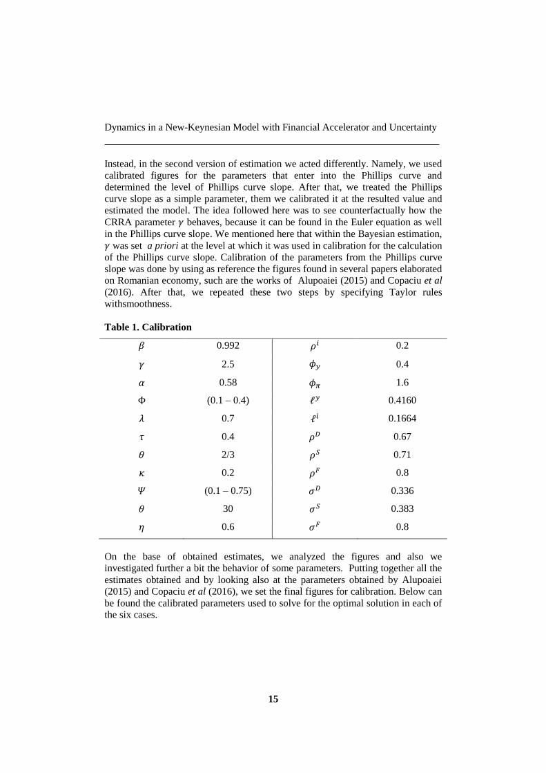
Instead, in the second version of estimation we acted differently. Namely, we used

calibrated figures for the parameters that enter into the Phillips curve and

determined the level of Phillips curve slope. After that, we treated the Phillips

curve slope as a simple parameter, them we calibrated it at the resulted value and

estimated the model. The idea followed here was to see counterfactually how the

CRRA parameter 𝛾 behaves, because it can be found in the Euler equation as well

in the Phillips curve slope. We mentioned here that within the Bayesian estimation,

𝛾 was set a priori at the level at which it was used in calibration for the calculation

of the Phillips curve slope. Calibration of the parameters from the Phillips curve

slope was done by using as reference the figures found in several papers elaborated

on Romanian economy, such are the works of Alupoaiei (2015) and Copaciu et al

(2016). After that, we repeated these two steps by specifying Taylor rules

withsmoothness.

Table 1. Calibration

𝛽 0.992 𝜌𝑖 0.2

𝛾 2.5 𝜙𝑦 0.4

𝛼 0.58 𝜙𝜋 1.6

Φ (0.1 – 0.4) ℓ𝑦 0.4160

𝜆 0.7 ℓ𝑖 0.1664

𝜏 0.4 𝜌𝐷 0.67

𝜃 2/3 𝜌𝑆 0.71

𝜅 0.2 𝜌𝐹 0.8

𝛹 (0.1 – 0.75) 𝜎𝐷 0.336

𝜃 30 𝜎𝑆 0.383

𝜂 0.6 𝜎𝐹 0.8

On the base of obtained estimates, we analyzed the figures and also we

investigated further a bit the behavior of some parameters. Putting together all the

estimates obtained and by looking also at the parameters obtained by Alupoaiei

(2015) and Copaciu et al (2016), we set the final figures for calibration. Below can

be found the calibrated parameters used to solve for the optimal solution in each of

the six cases.


______________________________________________________________

16

Once the models were calibrated accordingly, the next step consisted solving for

the optimal solution on the basis of which we obtained the unconditional variables.

Given that our work is somewhat focused on the understanding the interlinkages

between financial and real sectors, we discuss the behavior of obtained volatilities

and not necessary their levels. Plots with obtained results are reported in Annex.

Even that we have six cases, we reported results for eight models as the presence of

Knightian uncertainty supposes the existence of an approximating model,

respectively of a worst case model. Overall we would like to emphasize a non-

linear relationship between the unconditional volatility of the target variables and

the level of two elasticities. The non-linearity is observed to be pretty high in some

cases. By inspecting figures 1 – 8 we can observe that non-linearity depends a lot

on the circumstances.

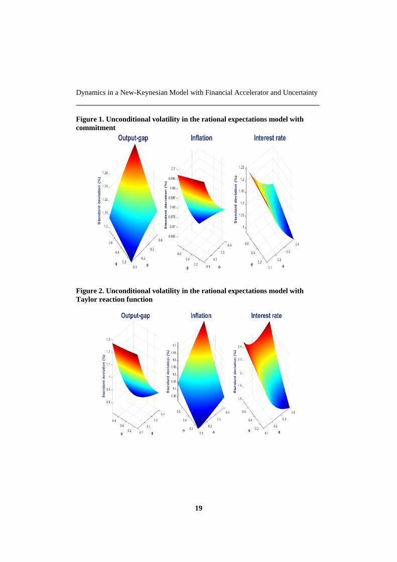
First of all we will analyze the behavior of variables’ volatility for commitment

case. In this regard we can see that volatility of the output-gap is increasing in both

elasticities, observing that volatility is much higher when the two elasticity

records high levels. Instead, for inflation case the situation is completely opposite.

By looking at the interest rate we observe that its volatility is increasing in the

output-gap elasticity with respect to the interest rates spread and is decreasing in

the interest rate elasticity with respect to the output-gap. If we look at the model

with Knightian uncertainty we can observe that inflation is increasing in Φ and Ψ

for the worst case model. Approximating and Bayesian models show the same

pattern for output-gap and inflation volatility as the standard rational expectations

model does. Looking at the volatility of interest rates, the two models obtained for

the case with Knightian uncertainty differ from the Bayesian model, respectively

the rational expectation model. An interesting observation is that for the output-

gap, obtained volatility is lower in the worst-case model as compared with the

approximating model.

For the case with simple rules we observe very different results as compared with

the commitment case. As Cecchetti and Li (2008) underlines, this could be put on

the back of an inability of the central planner to capture the real developments

within the economy when a simple rule it is used to set the short term interest rate.

Another interesting remark is that volatilities obtained with the standard rational

expectations model, respectively with the approximating and worst-case models

are very low, in comparison with the commitment case where the situation is

completely opposite.

6. Conclusion

Present work is intended to underline new lines of research by addressing

several stylized facts brought by the recent financial crisis. In this regard we

provide a normative work on the way in which the relationship between volatility

of interest variables in a closed economy and the strength of interlinkages between

financial and real sectors depends on the specified environment. More exactly, the


17

relationship that we mentioned before is very sensitive at the hypothesis on

uncertainty you set as well as the way in which the short-term interest rates is

setting-up. For this purpose we emphasized that a lot of research it is necessary

further in order to get an accurate idea on the interlinkages between financial and

real sectors. On the other hand, we showed that when a relatively small model it is

used, conclusions on the effects of financial accelerator could be relatively

sensitive to the assumed hypothesis. Not at least, our paper could be viewed as a

starting reference to address the caveats that we emphasized for the case of

emerging economies and in the context of using a relatively simple model for

policy analysis.

ACKNOWLEDGMENT:

This work was supported by a grant of the Romanian National Authority for

Scientific Research, CNCS – UEFISCDI, project number PN-II-RU-TE-2014-

2499 entitled “Coordinating Monetary and Macroprudential Policies”.

REFERENCES

[1] Alupoaiei, A.(2015), Effects of Knightian Uncertainty on the Term-Structure

of Interest Rates; Journal of Business Management and Applied Economics, Vol.

IV, Issue 3 May 2015;

[2] Bernanke, B. and Blinder, A. (1989), Credit, Money, and Aggregate

Demand; National Bureau of Economic Research Cambridge, Mass.;

[3] Bernanke, B. , Gertler, M. and Gilchrist, S. (1999), The Financial

Accelerator in a Quantitative Business Cycle Framework; Handbook of

Macroeconomics, 1 , 1341–1393;

[4]Cateau, G. (2006), Guarding against Large Policy Errors under Model

Uncertainty; Working Paper No. 2006 -13, Bank of Canada;

[5] Copaciu, M. Bulete, C. and Nalban, V. (2016), R.E.M. 2.0 A DSGE Model

with Partial Euroization Estimated for Romania; National Bank of Romania

Occasional Papers no. 21;

[6] Clarida, R., Galí, J. and Gertler, M. (1999), The Science of Monetary

Policy: A New Keynesian Perspective; Journal of Economic Literature 37, 1661–

1707;

[7] Cecchetti, S. and Kohler, M. (2012),When Capital Adequacy and Interest

Rate Policy Are Substitutes (And When They Are Not);Bank for International

Settlements, Working Paper, no. 379;


______________________________________________________________

18

[8] Cecchetti, S. and Li, L. (2008),Do Capital Adequacy Requirements Matter

for Monetary Policy?; Economic Inquiry,46 (4), 643–659;

[9] Giordani, P. and Söderlind, P. (2004), Solution of Macromodels with

Hansen-Sargent Robust Policies: Some Extensions; Journal of Economic

Dynamics & Control, 28, 2367 – 2397;

[10] Gerali, A., Neri, S., Sessa, L. and Signoretti, F. (2010), Credit and Banking

in a DSGE Model of the Euro Area; Journal of Money, Credit and Banking, 42,

107–141;

[11] Hansen, L. and Sargent, T.(2000), Wanting Robustness in

Macroeconomics; Stanford University manuscript;

[12] Hansen, L. and Sargent, T. (2001),Acknowledging Misspecification in

Macroeconomic Theory; Review of Economic Dynamics 4, 519–535;

[13] Hansen, L. and Sargent, T. (2002),Robust Control and Model Uncertainty

in Macroeconomics; Stanford University manuscript;

[14] Hansen, L. and Sargent, T. (2003),Robust Control of Forward-looking

Models; Journal of Monetary Economics 50, 581–604;

[15] Levin, A. and Williams, J. (2003),Robust Monetary Policy with Competing

Reference Models; FRBSF Working Paper 2003-10;

[16] Lucas, R. (1987), Models of Business Cycles; New York: Basil Blackwell;

[17] Macroeconomic-Assessment-Group,(2010),Assessing the Macroeconomic

Impact of the Transition to Stronger Capital and Liquidity Requirements; Final

Report, Bank for International Settlements, Basel;

[18] Söderström, U. (2009),Model Uncertainty; Mimeo;

[19] Poutineau, J. and Vermandel, G. (2014), A Primer on Macroprudential

Policy; The Journal of Economic Education 46(1):68-82;

[20] Svensson, L. (2000),Robust Control Made Simple. Mimeo.

ANNEX


19

Figure 1. Unconditional volatility in the rational expectations model with

commitment

Figure 2. Unconditional volatility in the rational expectations model with

Taylor reaction function


______________________________________________________________

20

Figure 3. Unconditional volatility in the approximating model with

commitment

Figure 4. Unconditional volatility in the approximating model with Taylor

reaction function


21

Figure 5. Unconditional volatility in the worst-case model with commitment

Figure 6. Unconditional volatility in the worst-case model with Taylor

reaction function


______________________________________________________________

22

Figure 7. Unconditional volatility in the Bayesian uncertainty model with

commitment

Figure 8. Unconditional volatility in the Bayesian uncertainty model with

Taylor reaction function

[email protected] Alexie ALUPOAIEI, PhD E-mail

Documents

Transcript of [email protected] Alexie ALUPOAIEI, PhD E-mail