ALONG THE FORWARD CURVE FOR NATURAL GAS:

UNOBSERVABLE SHOCKS

AND DYNAMIC CORRELATIONS1

Fabrizio Spargoli and Paolo Zagaglia

This version: August 15, 2007

ABSTRACT This paper studies the comovements between the daily returns of forwards on natural gas traded in the NYMEX with maturity of 1, 2 and 3 months. We identify a structural multivariate BEKK model using a recursive assumption whereby shocks to the volatility of the returns are transmitted from the short to the long section of the forward curve. We find strong evidence of spillover effects both in the conditional first and second moments. In the conditional mean, we show that the transmission mechanism operates from the longer to the shorter maturity. In terms of reduced-form conditional second moments, the shortest the maturity, the higher the volatility of the return, and the more the returns become independent from the others and follow the dynamics of the underlying commodity. The evidence from the structural second moments indicates that the longer the maturity is, the higher is the uncertainty about the returns. We also show that the higher the structural variance of a return relative to that of another return, the stronger the correlation is between the two. JEL Classification: C22, G19 Keywords: natural gas prices, forward markets, GARCH, structural VAR

1 Spargoli (corresponding author): Università Politecnica delle Marche, fspargol@mta01.univpm.it. Zagaglia: Stockholm University and European Central Bank, pzaga@ne.su.se. We are grateful to the Norwegian School of Management (BI) for providing the data. Zagaglia acknowledges the kind support of the Monetary Policy Stance Division of the European Central Bank, where this paper was finalized. The opinions expressed herein are those of the authors and do not necessarily reflect the views of the ECB.

2

Introduction

Commodity markets have lost their original purpose of trading and delivery of physical goods

nowadays. In fact, they have become the arena for investors interested in futures and forward

contracts for hedging and speculative purposes. Commodity markets carry relevant information

also for central banks, whose interest lies in understanding the financial markets determinants of

commodity prices.

In this paper, we shed light on the comovements of prices along the forward curve for

natural gas on the New York Mercantile Exchange. We consider forward prices with maturity of

one month, two months and three months and study the spillover effects both in terms of

conditional and volatility. We estimate a structural vector autoregressive model identified through

heteroskedasticity. In our framework, the process for conditional volatility follows that the

multivariate BEKK-GARCH of Engle and Kroner (1995). Our identification scheme assumes that

the conditional second moments of the variables have a recursive structure. This implies that the

second moments of the returns on the shortest maturity depend only on their own autoregressive

and innovation terms, while those on the longest maturity are a function of all the autoregressive

and innovation terms in the system. In pills, we formulate a structural BEKK-GARCH model

whose parameters are identified from the reduced-form estimates.

We find strong evidence of spillover effects for both the first and the second moments

along the forward curve. With regard to the first moments, we find that a transmission mechanism

operates from the longer to the short maturities. The results also show that the shorter the

maturity, the higher the volatility of the return is, and the more the return becomes independent

from the other returns and follows the dynamic of the underlying commodity. This consideration

holds, however, for the reduced-form moments. For what concerns the structural moments, we

find returns on the 3 months maturity display the highest volatility, which implies a large

uncertainty on the returns. We find also that the higher the structural variance of a return relative to

that of another return, the stronger the correlation is between the two.

This paper is organized as follows. In the section section, we outline our structural

GARCH model along with the identification technique. In the third section, we present the main

results. A few final remarks are in section four.

The structural GARCH model

Let us assume that the evolution of the variables can be summarized by a structural VAR model

( )t t t

Ax L xψ η= + Φ +

3

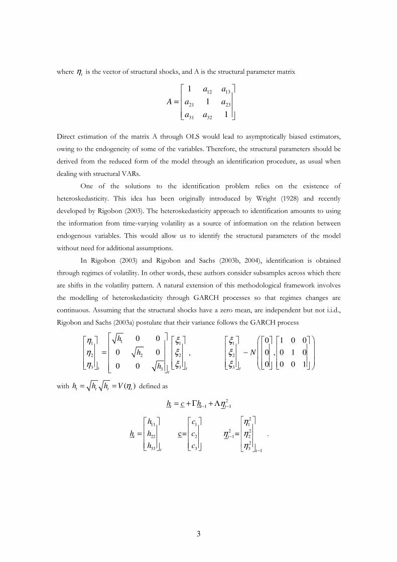
where t

η is the vector of structural shocks, and A is the structural parameter matrix

Direct estimation of the matrix A through OLS would lead to asymptotically biased estimators,

owing to the endogeneity of some of the variables. Therefore, the structural parameters should be

derived from the reduced form of the model through an identification procedure, as usual when

dealing with structural VARs.

One of the solutions to the identification problem relies on the existence of

heteroskedasticity. This idea has been originally introduced by Wright (1928) and recently

developed by Rigobon (2003). The heteroskedasticity approach to identification amounts to using

the information from time-varying volatility as a source of information on the relation between

endogenous variables. This would allow us to identify the structural parameters of the model

without need for additional assumptions.

In Rigobon (2003) and Rigobon and Sachs (2003b, 2004), identification is obtained

through regimes of volatility. In other words, these authors consider subsamples across which there

are shifts in the volatility pattern. A natural extension of this methodological framework involves

the modelling of heteroskedasticity through GARCH processes so that regimes changes are

continuous. Assuming that the structural shocks have a zero mean, are independent but not i.i.d.,

Rigobon and Sachs (2003a) postulate that their variance follows the GARCH process

11 1

2 2 2

3 33

0 0

0 0

0 0t tt

h

h

h

η ξ

η ξ

η ξ

=

,

1

2

3

0 1 0 0

0 , 0 1 0

0 0 0 1t

N

ξ

ξ

ξ

∼

with ( )t t t t

h h h V η= = defined as

2

1 1t t th c h η− −= + Γ + Λ

2

11 1 1

2 2

22 2 1 2

2

33 3 3 1

c= = t t

t t

h c

h h c

h c

η

η η

η−

−

=

.

12 13

21 23

31 32

1

1

1

a a

A a a

a a

=

4

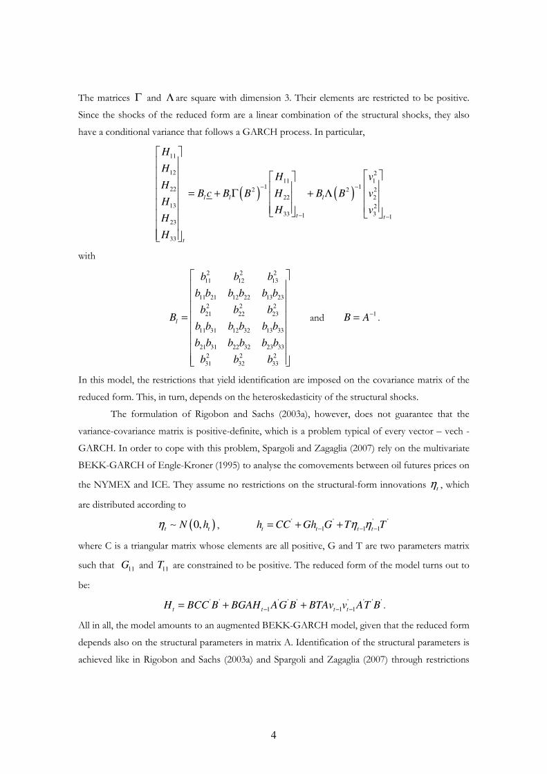
The matrices Γ and Λ are square with dimension 3. Their elements are restricted to be positive.

Since the shocks of the reduced form are a linear combination of the structural shocks, they also

have a conditional variance that follows a GARCH process. In particular,

( ) ( )

11

12 2

11 11 122 2 2 2

22 2

13 2

33 31 123

33

l l l

t t

t

H

HH v

HB c B B H B B v

HH v

H

H

− −

− −

= + Γ + Λ

with

2 2 2

11 12 13

11 21 12 22 13 23

2 2 2

21 22 23

11 31 12 32 13 33

21 31 22 32 23 33

2 2 2

31 32 33

l

b b b

b b b b b b

b b bB

b b b b b b

b b b b b b

b b b

=

and 1B A

−= .

In this model, the restrictions that yield identification are imposed on the covariance matrix of the

reduced form. This, in turn, depends on the heteroskedasticity of the structural shocks.

The formulation of Rigobon and Sachs (2003a), however, does not guarantee that the

variance-covariance matrix is positive-definite, which is a problem typical of every vector – vech -

GARCH. In order to cope with this problem, Spargoli and Zagaglia (2007) rely on the multivariate

BEKK-GARCH of Engle-Kroner (1995) to analyse the comovements between oil futures prices on

the NYMEX and ICE. They assume no restrictions on the structural-form innovations t

η , which

are distributed according to

( )0,t t

N hη ∼ , ' ' ' '

1 1 1t t t th CC Gh G T Tη η− − −= + +

where C is a triangular matrix whose elements are all positive, G and T are two parameters matrix

such that 11

G and 11

T are constrained to be positive. The reduced form of the model turns out to

be:

' ' ' ' ' ' ' ' '

1 1 1t t t tH BCC B BGAH AG B BTAv v AT B− − −= + + .

All in all, the model amounts to an augmented BEKK-GARCH model, given that the reduced form

depends also on the structural parameters in matrix A. Identification of the structural parameters is

achieved like in Rigobon and Sachs (2003a) and Spargoli and Zagaglia (2007) through restrictions

5

on the conditional variance-covariance matrix of the reduced-form innovations, that follow the

BEKK-GARCH model outlined earlier.

In this paper, the forward curve of natural gas forwards is analysed again by imposing an

identification technique on the structural GARCH model in the spirit of Rigobon (2002), which

studies the contagion effects of the 1997 Mexican crisis on Argentina, Columbia, Venezuela and

Brazil. Differently from him, however, we rely on a BEKK instead of a vech model in order to have

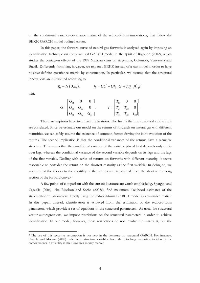
positive-definite covariance matrix by construction. In particular, we assume that the structural

innovations are distributed according to

( )0,t t

N hη ∼ , ' ' ' '

1 1 1t t t th CC Gh G T Tη η− − −= + +

with

11

21 22

31 32 33

0 0

0

G

G G G

G G G

=

,

11

21 22

31 32 33

0 0

0

T

T T T

T T T

=

.

These assumptions have two main implications. The first is that the structural innovations

are correlated. Since we estimate our model on the returns of forwards on natural gas with different

maturities, we can safely assume the existence of common factors driving the joint evolution of the

returns. The second implication is that the conditional variances of the returns have a recursive

structure. This means that the conditional variance of the variable placed first depends only on its

own lags, whereas the conditional variance of the second variable depends on its lags and the lags

of the first variable. Dealing with series of returns on forwards with different maturity, it seems

reasonable to consider the return on the shortest maturity as the first variable. In doing so, we

assume that the shocks to the volatility of the returns are transmitted from the short to the long

section of the forward curve.2

A few points of comparison with the current literature are worth emphasizing. Spargoli and

Zagaglia (2006), like Rigobon and Sachs (2003a), find maximum likelihood estimates of the

structural-form parameters directly using the reduced-form GARCH model as covariance matrix.

In this paper, instead, identification is achieved from the estimation of the reduced-form

parameters, which provide a set of equations in the structural parameters. As usual for structural

vector autoregressions, we impose restrictions on the structural parameters in order to achieve

identification. In our model, however, those restrictions do not involve the matrix A, but the

2 The use of this recursive assumption is not new in the literature on structural GARCH. For instance, Cassola and Morana (2006) order term structure variables from short to long maturities to identify the comovements in volatility in the Euro area money market.

6

conditional variances of the structural innovations. A similar technique is used in Rigobon (2002),

which derives the structural parameters of the heteroskedasticity process (both an ARCH and a

GARCH model in the vech form) from the reduced-form estimates assuming that the structural

innovations are not correlated.

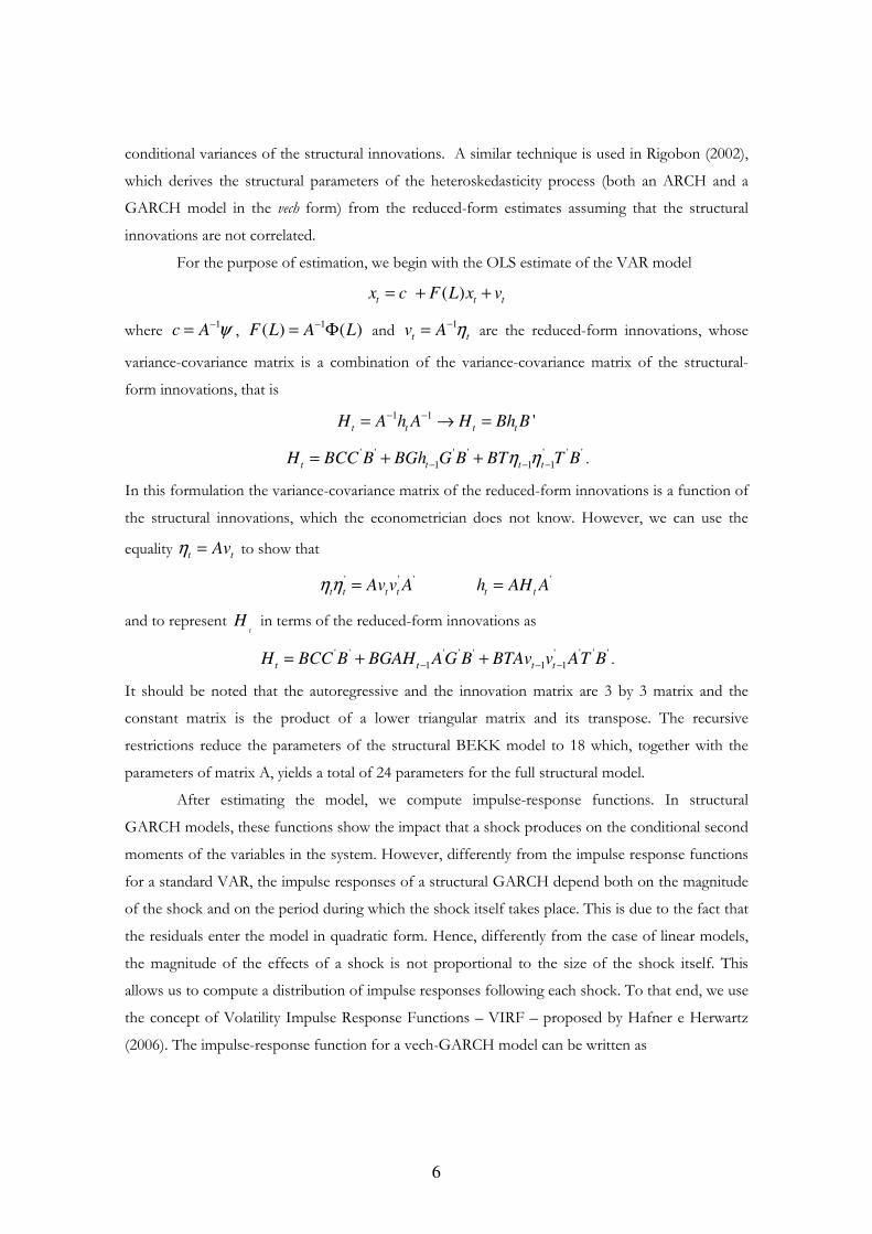
For the purpose of estimation, we begin with the OLS estimate of the VAR model

( )t t t

x c F L x v= + +

where 1c A ψ−= , 1

( ) ( )F L A L−= Φ and

1

t tv A η−= are the reduced-form innovations, whose

variance-covariance matrix is a combination of the variance-covariance matrix of the structural-

form innovations, that is

1 1'

t t t tH A h A H Bh B

− −= → =

' ' ' ' ' ' '

1 1 1t t t tH BCC B BGh G B BT T Bη η− − −= + + .

In this formulation the variance-covariance matrix of the reduced-form innovations is a function of

the structural innovations, which the econometrician does not know. However, we can use the

equality t t

Avη = to show that

' ' '

t t t tAv v Aη η =

'

t th AH A=

and to represent t

H in terms of the reduced-form innovations as

' ' ' ' ' ' ' ' '

1 1 1t t t tH BCC B BGAH AG B BTAv v AT B− − −= + + .

It should be noted that the autoregressive and the innovation matrix are 3 by 3 matrix and the

constant matrix is the product of a lower triangular matrix and its transpose. The recursive

restrictions reduce the parameters of the structural BEKK model to 18 which, together with the

parameters of matrix A, yields a total of 24 parameters for the full structural model.

After estimating the model, we compute impulse-response functions. In structural

GARCH models, these functions show the impact that a shock produces on the conditional second

moments of the variables in the system. However, differently from the impulse response functions

for a standard VAR, the impulse responses of a structural GARCH depend both on the magnitude

of the shock and on the period during which the shock itself takes place. This is due to the fact that

the residuals enter the model in quadratic form. Hence, differently from the case of linear models,

the magnitude of the effects of a shock is not proportional to the size of the shock itself. This

allows us to compute a distribution of impulse responses following each shock. To that end, we use

the concept of Volatility Impulse Response Functions – VIRF – proposed by Hafner e Herwartz

(2006). The impulse-response function for a vech-GARCH model can be written as

7

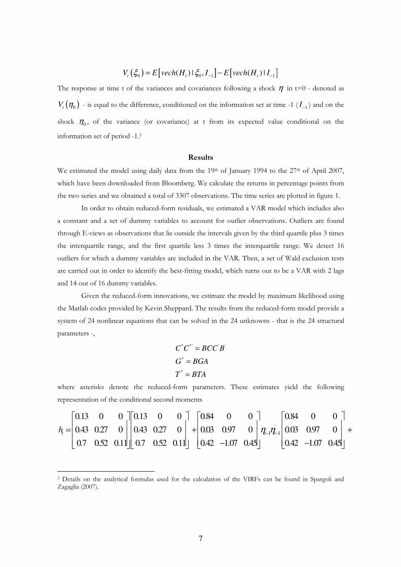
( ) [ ] [ ]0 0 1 1( ) | , ( ) |t t t

V E vech H I E vech H Iξ ξ − −= −

The response at time t of the variances and covariances following a shock η in t=0 - denoted as

( )0tV η - is equal to the difference, conditioned on the information set at time -1 (

1I− ) and on the

shock 0

η , of the variance (or covariance) at t from its expected value conditional on the

information set of period -1.3

Results

We estimated the model using daily data from the 19th of January 1994 to the 27th of April 2007,

which have been downloaded from Bloomberg. We calculate the returns in percentage points from

the two series and we obtained a total of 3307 observations. The time series are plotted in figure 1.

In order to obtain reduced-form residuals, we estimated a VAR model which includes also

a constant and a set of dummy variables to account for outlier observations. Outliers are found

through E-views as observations that lie outside the intervals given by the third quartile plus 3 times

the interquartile range, and the first quartile less 3 times the interquartile range. We detect 16

outliers for which a dummy variables are included in the VAR. Then, a set of Wald exclusion tests

are carried out in order to identify the best-fitting model, which turns out to be a VAR with 2 lags

and 14 out of 16 dummy variables.

Given the reduced-form innovations, we estimate the model by maximum likelihood using

the Matlab codes provided by Kevin Sheppard. The results from the reduced-form model provide a

system of 24 nonlinear equations that can be solved in the 24 unknowns - that is the 24 structural

parameters -,

* *' ' '

*

*

C C BCC B

G BGA

T BTA

=

=

=

where asterisks denote the reduced-form parameters. These estimates yield the following

representation of the conditional second moments

' '

'

1 1

0.13 0 0 0.13 0 0 0.84 0 0 0.84 0 0

0.43 0.27 0 0.43 0.27 0 0.03 0.97 0 0.03 0.97 0

0.7 0.52 0.11 0.7 0.52 0.11 0.42 1.07 0.45 0.42 1.07 0.45

t t th η η− −

= + + − −

3 Details on the analytical formulas used for the calculation of the VIRFs can be found in Spargoli and Zagaglia (2007).

8

'

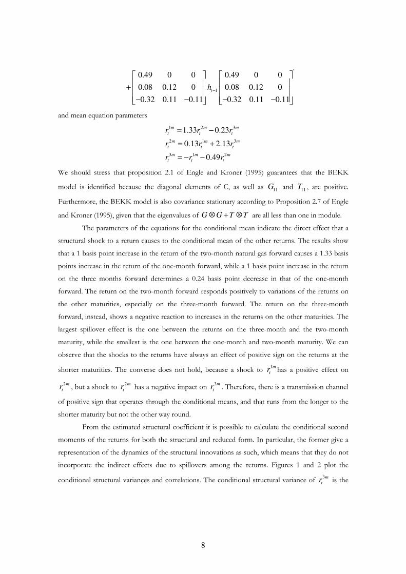
1

0.49 0 0 0.49 0 0

0.08 0.12 0 0.08 0.12 0

0.32 0.11 0.11 0.32 0.11 0.11

th −

+ − − − −

and mean equation parameters

1 2 3

2 1 3

3 1 2

1.33 0.23

0.13 2.13

0.49

m m m

t t t

m m m

t t t

m m m

t t t

r r r

r r r

r r r

= −

= +

= − −

We should stress that proposition 2.1 of Engle and Kroner (1995) guarantees that the BEKK

model is identified because the diagonal elements of C, as well as 11

G and 11

T , are positive.

Furthermore, the BEKK model is also covariance stationary according to Proposition 2.7 of Engle

and Kroner (1995), given that the eigenvalues of G G T T⊗ + ⊗ are all less than one in module.

The parameters of the equations for the conditional mean indicate the direct effect that a

structural shock to a return causes to the conditional mean of the other returns. The results show

that a 1 basis point increase in the return of the two-month natural gas forward causes a 1.33 basis

points increase in the return of the one-month forward, while a 1 basis point increase in the return

on the three months forward determines a 0.24 basis point decrease in that of the one-month

forward. The return on the two-month forward responds positively to variations of the returns on

the other maturities, especially on the three-month forward. The return on the three-month

forward, instead, shows a negative reaction to increases in the returns on the other maturities. The

largest spillover effect is the one between the returns on the three-month and the two-month

maturity, while the smallest is the one between the one-month and two-month maturity. We can

observe that the shocks to the returns have always an effect of positive sign on the returns at the

shorter maturities. The converse does not hold, because a shock to 1m

tr has a positive effect on

2m

tr , but a shock to

2m

tr has a negative impact on

3m

tr . Therefore, there is a transmission channel

of positive sign that operates through the conditional means, and that runs from the longer to the

shorter maturity but not the other way round.

From the estimated structural coefficient it is possible to calculate the conditional second

moments of the returns for both the structural and reduced form. In particular, the former give a

representation of the dynamics of the structural innovations as such, which means that they do not

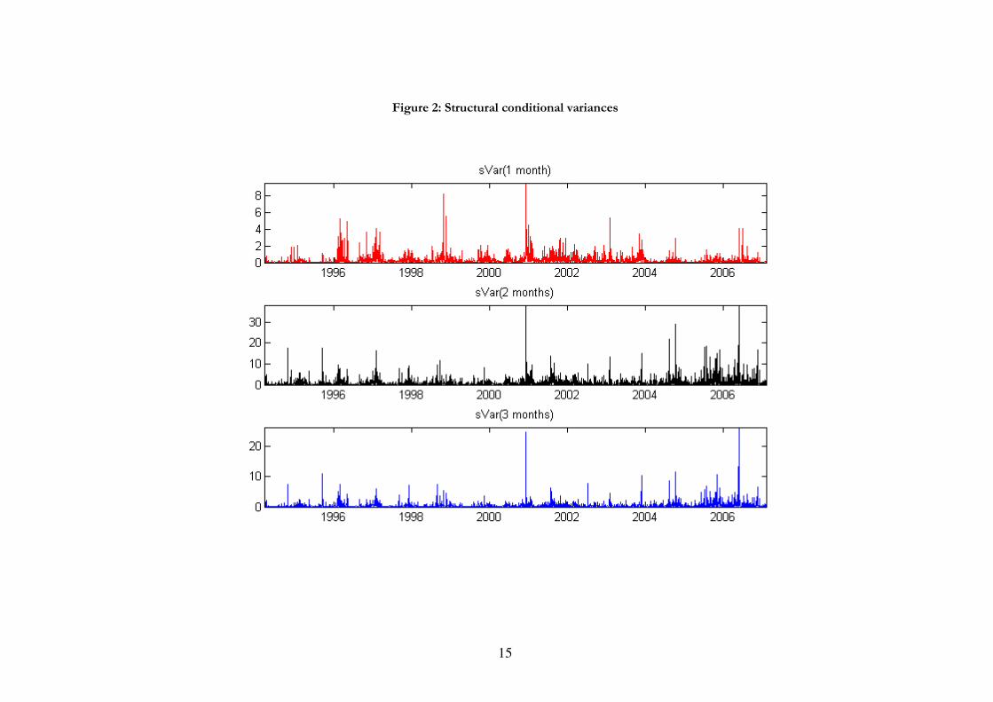
incorporate the indirect effects due to spillovers among the returns. Figures 1 and 2 plot the

conditional structural variances and correlations. The conditional structural variance of 3m

tr is the

9

highest over the sample except for its middle section, where the conditional structural variance of

1m

tr overcomes it. The conditional structural variance of

3m

tr shows frequent and high peaks, while

that of 2m

tr is the lowest over the sample. The three conditional variances show peaks at the same

points of the sample.

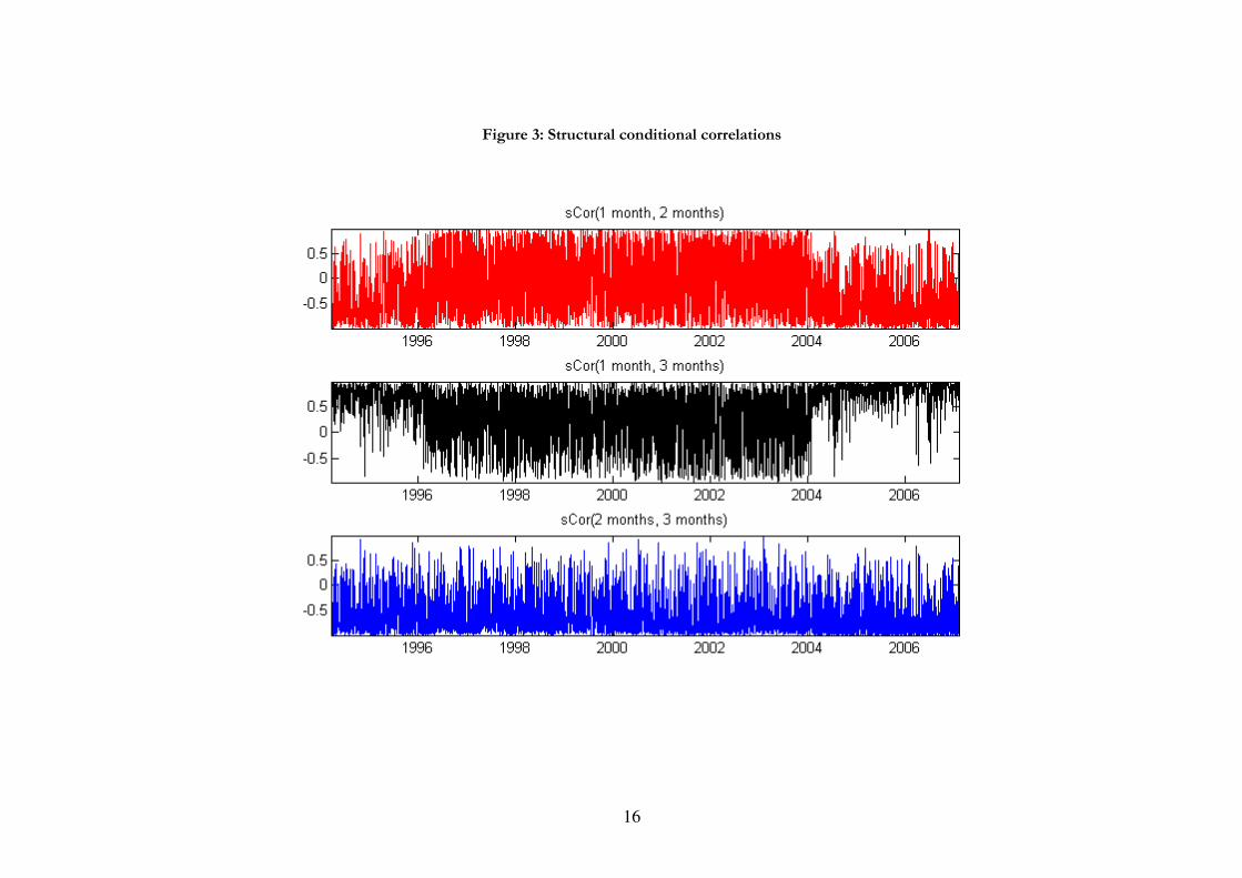
Figure 2 shows that the returns on the three maturities are strongly correlated, and that

there are frequent peaks that push the correlations to extreme levels. It is difficult to detect a

pattern in the dynamics of these conditional moments, given their frequent oscillations. However,

one can say that the structural correlation between 1m

tr and

2m

tr becomes positive, and oscillates

around 0.5, after the 500th observation. Yet, there are frequent peaks that make it negative and

reach -1. Combining the evidence from the conditional structural correlations with that on the

conditional structural variances, we can notice that is that the bigger a conditional variance at a

maturity relative to that of another maturity, the stronger the correlation is between the

corresponding returns. For example, in the period comprised between observation 0 and 500 the

correlation between 1m

tr and

2m

tr oscillates around a value between 0 and -0.5 and the structural

variance of 2m

tr is almost equal to the one of

1m

tr . In the subsequent range of observations,

however, the latter becomes much bigger than the former and, at the same time, the correlation

between the two returns oscillates around a higher mean in absolute value. The same considerations

apply also for the conditional structural correlation between 3m

tr and

1m

tr : when the conditional

structural variance of 3m

tr is bigger than

1m

tr - i.e. in the period between 0 and 500 - the correlation

is higher in absolute value than in the following period where the two structural variances are

approximately equal. This also holds for the conditional structural correlation between 2m

tr and

3m

tr . This suggests that the comovements between the returns are driven by the dynamics of the

most volatile.

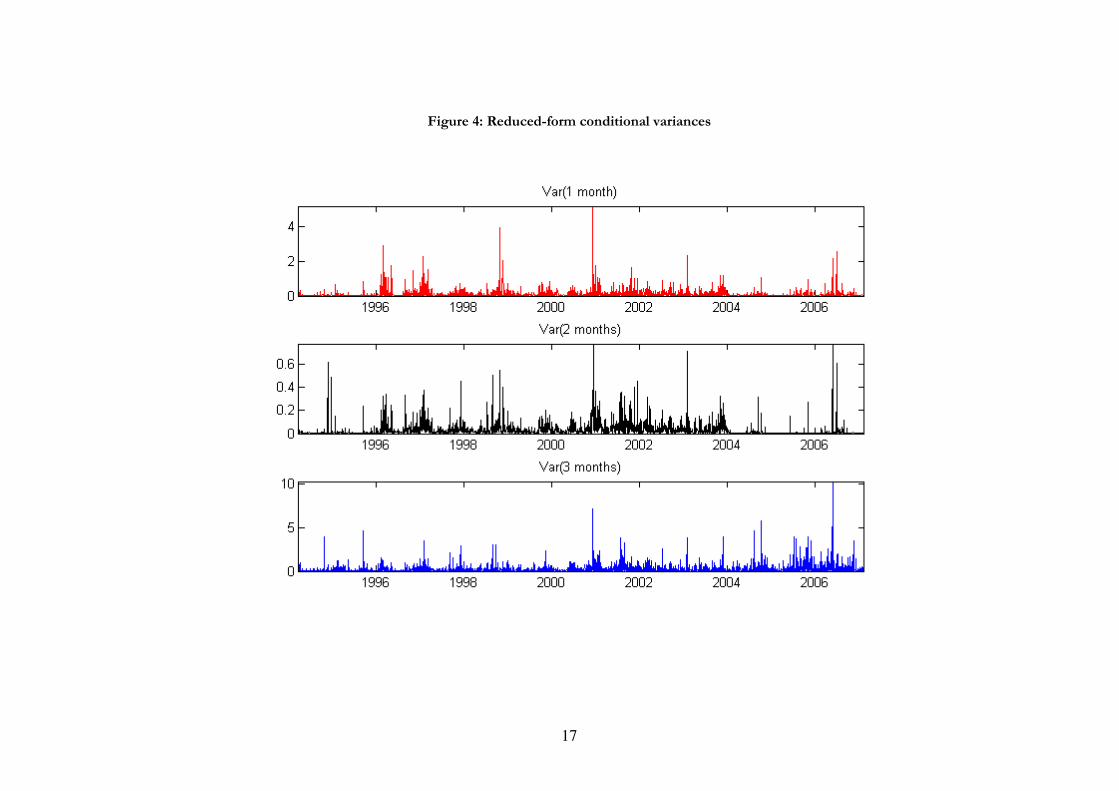
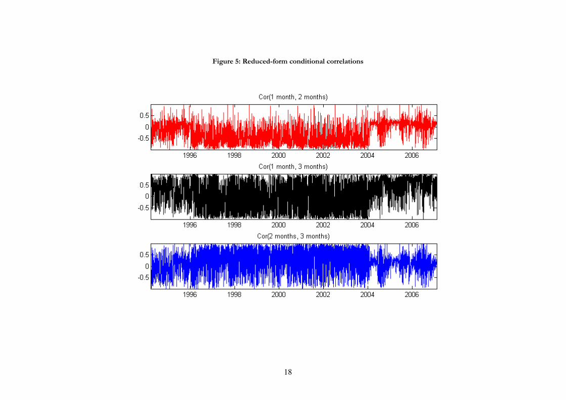
Figures 3 and 4 plot, respectively, the reduced-form conditional variances and correlations

that incorporate the linkages among the returns. The reduced-form conditional variances are

generally smaller than those of the structural form, which means that the spillovers among markets

contribute to a reduction of the volatility of structural innovations. The size of the reduced-form

conditional variances seems to be the inverse of that of the structural-form variances. This supports

the view that forward prices are more volatile for short maturities, given they are the most traded

and liquid along the maturity structure. Therefore, even if the structural conditional variance of 1m

tr

10

is the lowest over the sample, the reduced-form variance is the highest because of the spillovers and

linkages among the returns.

Figure 4 shows that the correlation between 1m

tr and

2m

tr seems to have three regimes.

The first regime goes from observation 0 to 500, when it oscillates around a mean value between

0.5 and 1. The second regime is from observation 500 to 2500, where it oscillates around a mean

value around 0. The third regime is similar to the first. The same consideration holds for the

reduced-form conditional correlation between 3m

tr and

1m

tr . This means that the return on the

shortest maturity is independent from those on the other maturities, which can be explained by the

fact that the closer the expiration date of a derivative product is, the more its price follows the price

of the underlying commodity. The reduced-form conditional correlation between 3m

tr and

2m

tr has

smaller oscillations and has a mean value comprised between 0.5 and 1. Furthermore, it is perfectly

positive in most part of the sample. These facts, together with a structural-form conditional

correlation with a negative mean value, could be interpreted as a suggestion that the two-month and

three-month maturities are held for hedging purposes.

Now we turn to the analysis of the persistence of the effects of the shocks, which we

carried out through volatility impulse responses. As explained earlier, given that GARCH are non-

linear in the innovations, the effect of a shock depends both on the size and the timing. Therefore,

our use of VIRFs is twofold. On the one hand, we can plot traditional impulse responses after a

specific shock occurred at a specific point in time. On the other hand, we can compute the

distribution of VIRFs, that is we can calculate impulse responses for each shock and then

determine their frequency. This should be done for each time horizon of the VIRF.

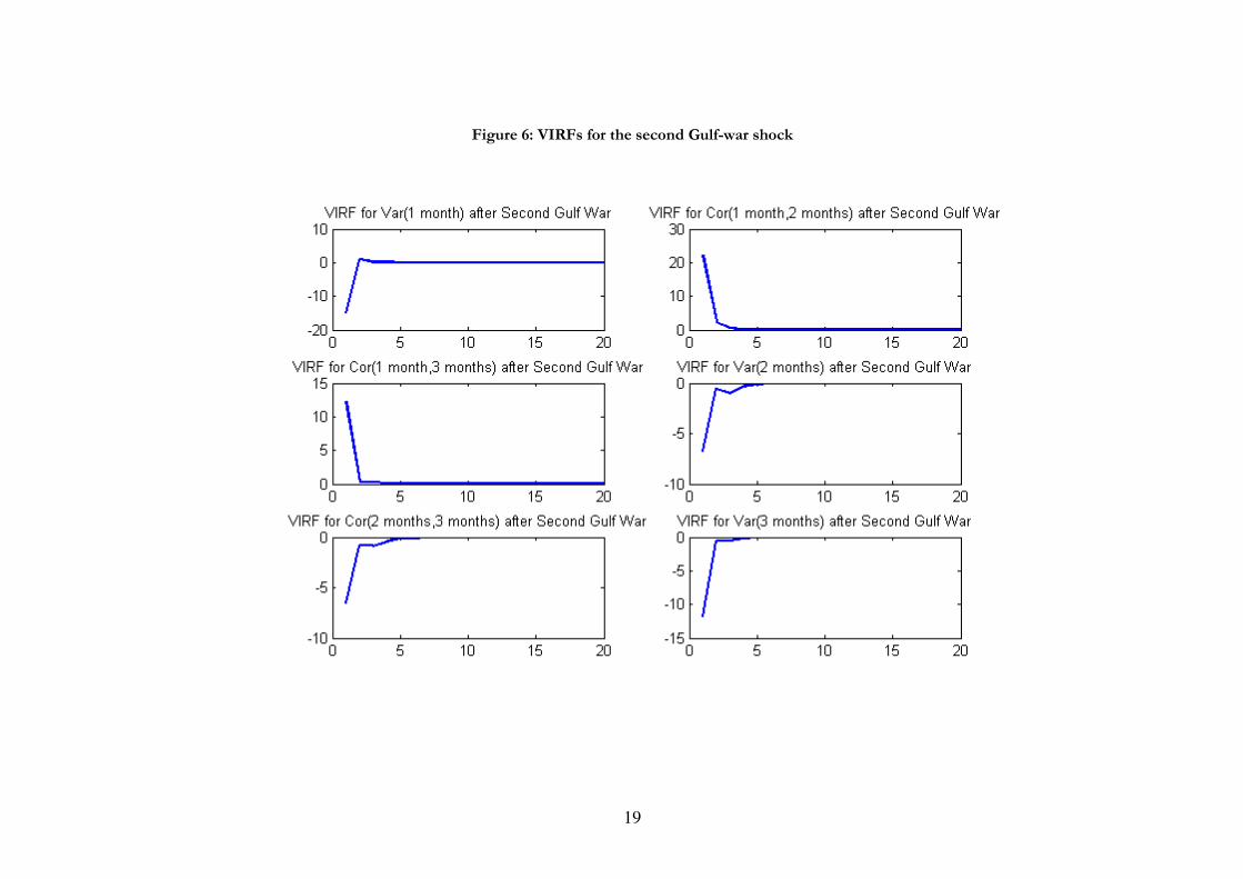
Figure 5 shows the impulse responses on a potentially significant date, namely the second

Gulf war shock, which takes place on the 20th of March 2003. The shock is absorbed very quickly,

given that the effect on all the conditional moments vanishes after 3 or 4 days. The shock has a

negative impact on the conditional variances, in particular on that of1m

tr , and on the correlation

between 3m

tr and

2m

tr while it has an impact of positive sign on the correlations between

1m

tr and

2m

tr , and on those between

3m

tr and

1m

tr . The finding about the reaction of the conditional

variance of 1m

tr confirms that the returns on the shortest maturities are more volatile. The response

of the conditional correlation shows that a shock to the returns on the one-month maturity

determines an effect of the same sign as that on the two and three-month maturity, which can be

interpreted as a transmission mechanism of volatility shocks. However, this does not hold for the

11

maturities at two and three months. This suggests that the transmission process takes place directly

from the short maturity to the rest of the forward curve.

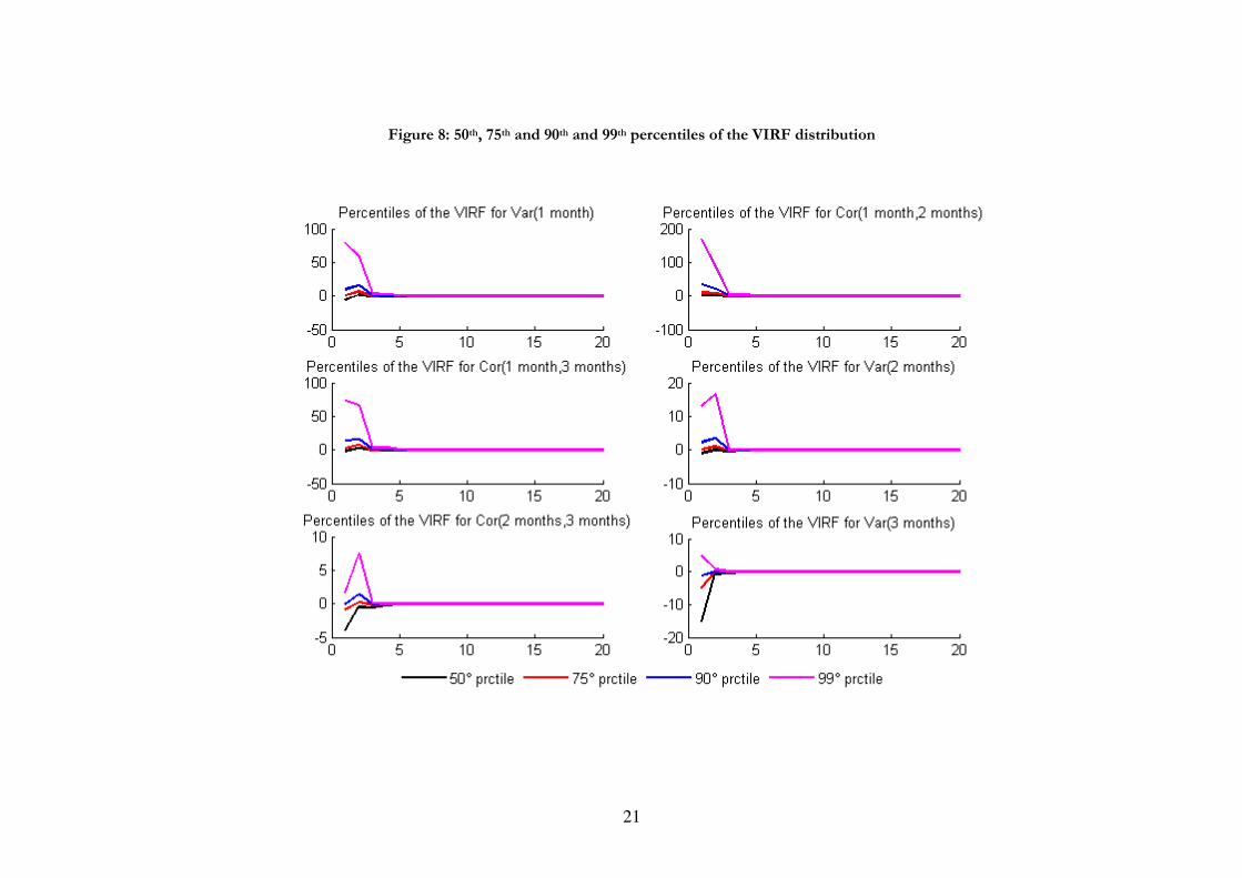
Turning to the distribution of the VIRFs, Figures 6 Figure 7 present respectively the 1st,

10th, 25th, and the 50th, 75th, 90th and 99th percentiles. At a first glance, we can again notice that the

effect of the shocks tend to absorbed very quickly, given that after 3 or 4 days all the percentiles

become close to zero. It should be noted also that the immediate impact of the shock has a great

dispersion, because the extreme percentiles of the distribution are very far from each other for all

the VIRFs. It is interesting to analyze the median of the VIRF distribution, in order to understand

whether the shocks have a positive or a negative impact on the conditional moments. From Figure

7, it is evident that the shocks exert mainly a negative impact on the conditional variance of 2m

tr

and 3m

tr and on the correlation between

2m

tr and

3m

tr , given that even the 75th percentile is

negative. As regards the other moments, the distribution of their VIRFS is symmetric because the

50th percentile is approximately zero. Therefore, the shocks generate effects of positive and negative

sign in the same proportion.

Conclusions

We study the relation between the returns on one-month, two-month and three-month maturities

of natural gas forwards traded in the New York Mercantile Exchange. We estimate a BEKK-

GARCH model (Engle and Kroner, 1995) from which we identify the parameters of a structural

model VAR model with heteroskedasticity in the structural innovations. In this way, we obtain

estimates of the spillovers among the three returns both in term of the first and second conditional

moments.

We find that the evidence about conditional second moments is in line with that

concerning forwards in general: the shorter the maturity, the higher the volatility of the return, and

the more the return becomes independent from the other returns, and follow the dynamics of the

underlying commodity price. We find also that the returns on the three-month maturity are those

with the highest volatility, which could be interpreted as a consequence of the greater uncertainty

that characterizes the factors guiding longer maturities. Another result is that the co-movement

between the returns is driven by the dynamics of the most volatile. We detect a transmission

mechanism that runs from the long to the short section of the forward curve. Finally, we also show

that the effects of the shocks on the conditional second moments have a very little persistence,

given that they vanish after 4 or 5 days.

12

References

Cassola, Nuno, and Claudio Morana, “Comovements in Volatility in the Euro Money Market”,

ECB Working Paper, No. 703, December 2006

Engle, R.obert F., and Kenneth F. Kroner, “Multivariate Simultaneous Generalized ARCH'”,

Econometric Theory, 11, 1995

Hafner, Christianam M., and Helmut Herwartz, “Volatility Impulse Responses for Multivariate

GARCH Models: An Exchange Rate Illustration”, Journal of International Money and Finance, 25(5),

2006

Rigobon, Roberto, “Identification through Heteroskedasticity”, Review of Economics and Statistics,

85(4), 2003

Rigobon, Roberto, “The Curse of non Investment Grade Countries”, Journal of Development

Economics, 69, 2002

Rigobon, Roberto, and Brian Sack, “Spillovers across U.S. Financial Markets”, unpublished manuscript,

MIT Sloan School of Management, 2003(a)

Rigobon, Roberto, and Brian Sack, “Measuring the Reaction of Monetary Policy to the Stock

Market”, Quarterly Journal of Economics, 118(2), 2003(b)

Rigobon, Roberto, and Brian Sack, “The Impact of Monetary Policy on Asset Prices”, forthcoming on

the Journal of Monetary Economics, 2004

Spargoli, Fabrizio, and Paolo Zagaglia, “The Comovements between Futures Markets for Crude

Oil: Evidence from a Structural GARCH Model”, unpublished manuscript, Stockholm University,

August 2007

Wright, Philip, The Tariff on animal and Vegetable Oils, The institute of Economics, The Macmillan

Company, New York, 1928

13

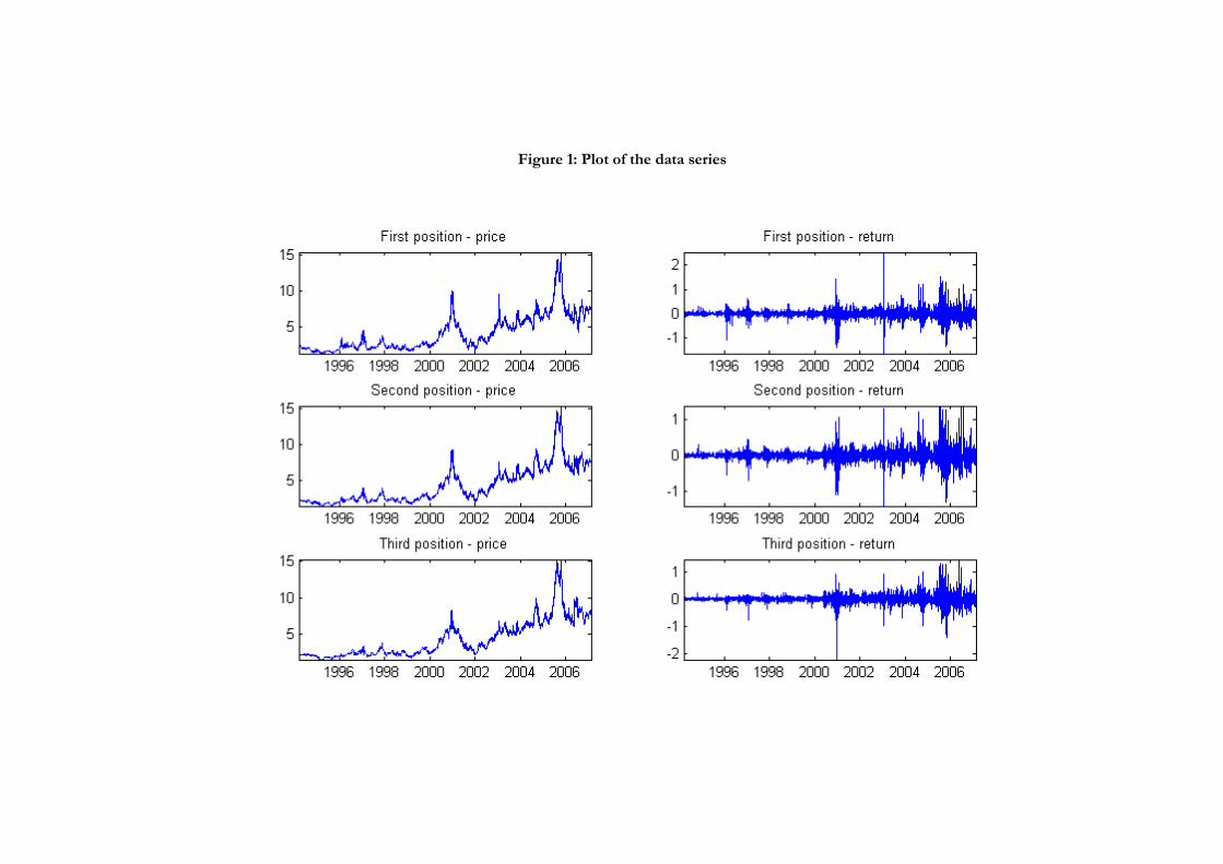
Figure 1: Plot of the data series

15

Figure 2: Structural conditional variances

16

Figure 3: Structural conditional correlations

17

Figure 4: Reduced-form conditional variances

18

Figure 5: Reduced-form conditional correlations

19

Figure 6: VIRFs for the second Gulf-war shock

20

Figure 7: 1st, 10th and 25th percentiles of the VIRF distribution

21

Figure 8: 50th, 75th and 90th and 99th percentiles of the VIRF distribution