Technical Editor: Alan Helm

Contributing Authors:Allan AndalesTroy BauderBruce BosleyJoe BrummerJessica DavisRaj KhoslaJoel Schneekloth

Layout Design:Kierra Jewell

New Options for Crop Water Use Reports from www.CoAgMet.comTroy Bauder, Joel Schneekloth, and Nolan Doesken

Irrigation season is here or quickly approaching. As you help your clients with their irrigation schedules this summer, remember that daily crop water use or evapotranspiration (ET) reports are available on the internet at www.coagmet.com. ET reports can be used to improve irrigation management and conserve limited water resources by fine-tuning irrigation timing and amount. Because ET is affected by our ever changing weather conditions, it can fluctuate daily and impact the demand for water by crops and landscapes. For example, mid-season corn water use can be as high as 0.40 inches per day when temperatures are in the mid-nineties, moderate wind, and low humidity, but will drop to half of that on cooler (low-eighties), more humid days. These changing weather conditions are measured by a network of weather stations throughout Colorado. The weather data is used to calculate and produce ET reports for several common crops. Recent revisions to this website allow users to choose up to eight crops; one or more weather stations; and adjust their planting dates to customize their reports. New for 2008 is the ability to request crop ET reports for multiple days. Precipitation from the weather station has also been added to the crop ET reports. This allows users to quickly determine a water balance for an area.

CoAgMet users now can choose the method used to calculate reference ET (ETr). The term “reference” refers to ET equations calibrated to estimate the water use of a well-watered alfalfa or grass field under a set of local weather conditions. Historically, CoAgMet has used the 1982 Kimberly Penman (KP) equation. However, the American Society of Civil Engineers Standardized Penman-Monteith (ASCE) equation is also offered as a user option. This newer equation has broad support in the literature as the more accepted equation. However, the Crop ET Access Page still defaults to the KP equation, because the crop coefficients used by CoAgMet were originally developed for this equation. Both of these equations are combination methods, meaning that they utilize temperature, wind, solar radiation and vapor pressure deficit (relative humidity) to calculate ETr. The ETr values provided are for a tall (alfalfa) reference crop.

Finally, new or recent CoAgMet users will notice that weather stations have been categorized as dryland, partially irrigated or fully irrigated. These designations describe the predominate land use in the immediate vicinity of the weather station and/or the vegetation growing around the site. The best conditions for determining ETr include station location over mowed, preferably irrigated, grass and surrounded by irrigated crops. These conditions are often difficult to find and maintain in many remote areas. Additionally, some CoAgMet stations are purposely located in areas that are predominately non-irrigated (dryland) as these stations were not intended for determining ETr. ET values from these sites will typically be higher than values from sites in fully irrigated areas. Weather stations were categorized using site characteristics as well as detailed analyses of historical weather data from each site.

Generating a crop water use reportTo generate a customized crop water use report, first, go to www.coagmet.com. Next, click

New Options for Crop Water Use Reports from www.CoAgMet.com .....1

Rocky Mountain Na-tional Park: Connection to Fertilizer Management Decisions ......................3

The Lysimeter Project at Rocky Ford ..................4

Irrigated Grazed Pastures ......................................9

Does it Pay to Fertilize Grass Hayfields with Nitrogen? ....................12

Myths of Precision Farming ......................14

on CoAgMet Crop Water Use (ET) Access or directly go to http://ccc.atmos.colostate.edu/cgi-bin/extended_etr_form.pl to get to the Crop ET Access Page. Choose the desired start date to generate an ET rate report from past data. If you need an ET report going back in time from yesterday, you can skip this step because the default date is the previous day. ET rates are based upon weather data that logs from 12:00 am to 12:00 am. Therefore, ET rates and other weather data are not available for a given date until the following day. Choose the number of days needed for your ET report. For older data, CoAgMet will use the start date you select and return ET rates forward in time for the number of days selected. For example, if you want ET rates for June 1 – 7, 2007; you select June 1, 2007 as the start date and the number 7 in the “# to do” column. If you do not change the start date from the default of yesterday, CoAgMet will return yesterday’s report and however many days you select in the “# to do” pull down list.

Crop ET Access Page Next you select the weather station(s) that will be used for the ET report. In most cases the nearest weather station (see linked map) is the best choice unless you have specific knowledge that another station is more representative of your area. If your location for ET rate is between two stations, consider using an average of both. To select multiple stations, hold down the control key and click on the stations you are interested in and CoAgMet will return data from both stations.

Finally, click on the desired crop(s) for ET rates. Select the planting date for the particular crop(s) of interest. Be aware that if crop emergence was delayed due to cool weather or other reasons, you may need to adjust the planting date back accordingly. For alfalfa, change the green-up date with each new cutting. Now, bookmark your ET output to avoid having to re-enter your preferred crop(s), station(s) and planting dates. You now can go directly to your bookmark to obtain your customized ET report.

The web site also provides a map to locate the nearest station or stations and instructions on how to use the information. We encourage you to check out this useful tool at www.coagmet.com. Keep in mind that ET-based scheduling should be periodically verified by checking soil moisture in the field with a probe or shovel. Refer to the fact sheet, Estimating Soil Moisture, 4.700 (http://www.ext.colostate.edu/pubs/crops/04700.html) for help in this process.

Example ET Report:

2

Rocky Mountain National Park: Connection to Fertilizer Management DecisionsJessica Davis, Extension Soil Specialist

What does Rocky Mountain National Park (RMNP) have to do with fertilizer choices? Knowing just two facts illuminates the link between these two realms: 1) ammonia-nitrogen can travel more than 1000 miles from its source, and 2) N deposition in the park has been climbing steadily. Atmospheric N deposition ranges from 2 to 6 lb acre-1 yr-1 in the Rocky Mountains of Colorado and Wyoming and is estimated to be increasing by about 0.3 lb N acre-1 yr-1. This may seem miniscule from an agricultural point of view, but due to the fragility of alpine ecosystems, small increases can have a big impact. The alpine areas are particularly sensitive to small increases in N deposition due to extensive areas of exposed bedrock, steep slopes, limited extent of soils and vegetation, short growing seasons, and rapid hydrologic flushing during snowmelt.

Increased N levels in RMNP can lead to measurable changes in ecosystem properties. Surface water NO3-N levels have been increasing, especially in lakes with surrounding unvegetated terrain (rocky and talus slopes). Pine trees have demonstrated greater N:P ratios in their needles with increasing elevation, and trees on the east side of the Continental Divide have higher foliar % N, along with higher N mineralization potential. In general, there is more N in the soils, plants, and lakes on the east side of the park, and these changes can impact forest and grassland productivity; algae growth, acidification, and oxygen levels of freshwaters; and biodiversity.

In response to a high level of concern among citizens living near RMNP and the National Park Service, the Colorado Department of Public Health and Environment completed an inventory to identify the primary sources of ammonia in the state of Colorado; they found that fertilizer use contributes 20% of statewide ammonia emissions. The Colorado Air Quality Control Commission recently approved a Nitrogen Deposition Reduction Plan for the Park built on the voluntary use of Best Management Practices (BMPs) to reduce ammonia emissions from agriculture. In 5 years, an evaluation will be made to decide whether a voluntary approach to N deposition reduction is working.

With these developments in mind, it is important that farmers adopt BMPs to reduce ammonia volatilization from fertilizer immediately. Volatilization reduces fertilizer use efficiency and increases costs, so there are strong incentives in place to conserve ammonia in the soil for crop uptake. So what can farmers do? Some possible BMPs include:Soil sampling to determine N application rate and avoid over-fertilizationSub-surface banding or incorporationUsing liquid urea solution instead of granular applicationChoosing controlled-release fertilizers to match N release with crop needsConsider applying urease inhibitors with urea

Using BMPs will improve fertilizer efficiency, reduce costs, and decrease both the ecological impacts of N deposition in the Rockies and the political pressure associated with the park.

3

The Lysimeter Project at Rocky Fordby Allan Andales and Abdel Berrada,

Department of Soil and Crop Sciences, Colorado State University

Rationale and Objectives

One of the recommendations that came out of the Kansas v. Colorado Arkansas River Compact litigation is for Colorado to use the American Society of Civil Engineers (ASCE) Standardized Penman-Monteith equation (PME) to estimate crop evapotranspiration (ET; also called consumptive use) in the Arkansas River Valley. The ASCE Standardized PME calculates the ET of a reference crop (ETr), which is alfalfa in Colorado. The PME uses weather data to estimate ETr and accounts for both the energy supply and the transport of water vapor away from the crop surface. Therefore, daily or more frequent measurements of net radiation, heat flow at the soil surface, air temperature, wind speed, and humidity are needed.

The ASCE standardized reference ET equation defines ETr from alfalfa (also called the tall reference) as “the ET rate from a uniform surface of dense, actively growing vegetation having specified height (50 cm or 20 inches for alfalfa) and surface resistance (to vapor transport), not short of soil water, and representing an expanse of at least 100 m (328 ft) of the same or similar vegetation.” In other states, the reference ET is that of a non-stressed grass or similar short crop that is 12 cm (5 inches) in height at full canopy and is usually denoted ETo (short reference ET).

The ET of another crop (ETc) is derived from ETr with the equation:

ETc = ETr x Kc (for well-watered crops).

The crop coefficient (Kc) varies with crop type, variety, growth stage, crop condition (plant density, health, etc.), climate, and soil wetness, among other things. When the crop is water-stressed,

ETc = ETr x Kc x Ks (for water-stressed crops).

The coefficient Ks is a soil water stress coefficient that accounts for the relative availability of soil water in the root zone. A Ks of 1.0 represents well-watered, no-stress conditions while a Ks of 0.0 represents maximum stress, with no soil water being available to the crop.

From the above equation of ETc for well-watered crops, it can be seen that the crop coefficient at any given time in the growing season is:

Thus, simultaneous measurements of ETc and ETr throughout the growing season are needed to derive local crop coefficients for different crops. Direct measurement of ET is best achieved with weighing lysimeters. Precision weighing lysimeters measure water loss from a control volume of cropped soil by tracking the change in mass (weight) of the control volume, with an accuracy of a few hundredths of a millimeter of water.

In the absence of locally generated Kc values for use with the PME, the Colorado Division of Water Resources (DWR) has been using estimates from Kimberly, ID and Bushland, TX. However, the crop growing conditions (soil, elevation, climate, etc.) in the Arkansas Valley varies greatly from the prevailing conditions in Kimberly or Bushland. In view of the recommendation to use the ASCE standardized PME for estimating crop ET in the

4

Arkansas Valley, the state of Colorado initiated the lysimeter project at Rocky Ford. The project objectives, according to Thomas Ley of DWR, are to:

1. Evaluate the performance and predictive accuracy of the ASCE Standardized PME for computing alfalfa reference crop ET for the growing conditions in southeastern Colorado, 2. Determine crop coefficients (for use with PME) for the various crops grown in the Arkansas River Valley under well-watered conditions, and,3. Determine the effects of typical local growing conditions (which may include limited irrigation, high water table conditions and irrigation with water of high salinity contents) on crop water use.

Colorado’s Attorney General requested that the Colorado Water Conservation Board (CWCB) fund the “design, installation, and operation of weighing lysimeters at the Colorado State University (CSU) Agricultural Experiment Station at Rocky Ford, Colorado”. The requested funds also cover the enhancement of a network of twelve automated weather stations (part of CoAgMet) along the Arkansas Valley, the investigation of irrigation water management in the Arkansas Valley, and the review of the changes made to the Hydrological-Institutional (H-I) Model by experts. The H-I Model has been used by the State Engineer’s Office (DWR) to determine depletions to usable water flows to Kansas.

The lysimeter project at the CSU-Arkansas Valley Research Center (AVRC) consists of one large weighing lysimeter for measuring ET of different crops (ETc) and one smaller reference lysimeter for simultaneously measuring alfalfa reference ET (ETr). The large (crop) lysimeter was installed in 2006 and the reference lysimeter is scheduled for installation in July of 2008.

CSU operates the network of twelve automated weather stations (part of CoAgMet) along the Arkansas Valley. Temperature, solar radiation, humidity, and wind speed data from these stations will be used to validate ETr estimates from the standardized PME and Kc estimates for the whole Valley.

The third objective may require additional lysimeters. It is worth noting that the effects of limited irrigation, high water table, and salinity on crop growth and water use in the Arkansas Valley have been studied by CSU scientists for several years using traditional (water balance estimates) and non-traditional (remote sensing) methods. Relatively high salt levels have been reported in the soils and waters of the Arkansas Valley (Gates et al., 2006). However, the impact of salinity on crop water use can be determined more accurately with a weighing lysimeter. Non-weighing lysimeters, which estimate ET from the volume balance of water, may be a lower cost alternative.

The installation of the crop lysimeter was completed in the fall of 2006, but some of the meteorological (weather) sensors were put in place in 2007. Consequently, it may be two to three years before Objective 1 is achieved, and several more years before usable Kc values for the major crops grown in the Arkansas Valley are available from the study. In the remainder of this article, a more detailed description of the lysimeters and current status of the project are given.

The Project Site at Rocky Ford

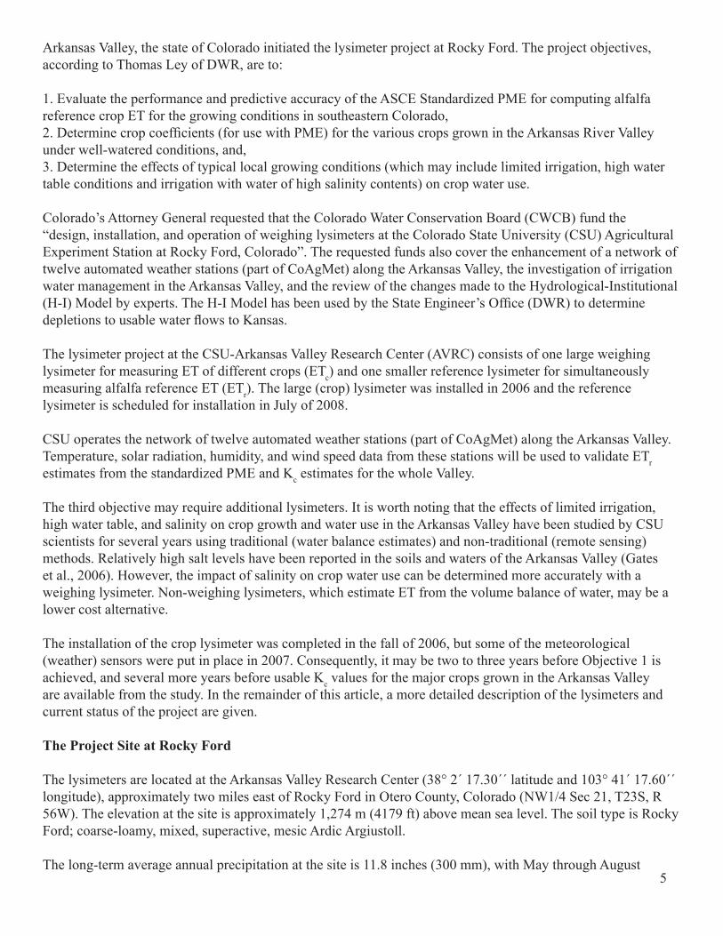
The lysimeters are located at the Arkansas Valley Research Center (38° 2´ 17.30´´ latitude and 103° 41´ 17.60´´ longitude), approximately two miles east of Rocky Ford in Otero County, Colorado (NW1/4 Sec 21, T23S, R 56W). The elevation at the site is approximately 1,274 m (4179 ft) above mean sea level. The soil type is Rocky Ford; coarse-loamy, mixed, superactive, mesic Ardic Argiustoll.

The long-term average annual precipitation at the site is 11.8 inches (300 mm), with May through August 5

having the highest rainfall. The total average annual snowfall is 23.2 inches (589 mm). The annual average minimum temperature is 36.3 °F (2.4 °C) and the annual average maximum temperature is 70.0 °F (21 °C). The last spring frost (32.5 °F or 0.3 °C) occurs on or before May 1 and the first fall frost on or before October 5 in 50% of the years; thus the average length of the growing season for warm-season crops like corn is 158 days.

The Crop and Reference Lysimeters

The crop lysimeter consists of an inner tank with dimensions of 10 ft x 10 ft surface area x 8 ft depth (3.0 m x 3.0 m x 2.4 m) and an outer containment tank. The crop lysimeter is intended for measurements of ETc for various crops grown in the Arkansas Valley. Installation and calibration of the crop lysimeter was completed in 2006. The inner tank was filled with undisturbed soil (soil monolith) from the same field where the lysimeter is located (Figure 1). Figure 2 shows the tank being lowered into its permanent location. The soil tank moves freely within the outer tank and the top edges of the two are separated by a fraction of an inch. The chamber between the two tanks houses the weighing mechanism, the drainage tanks, data loggers and has standing room for half-a-dozen people (Figure 3).

The weighing mechanism consists of a mechanical lever scale-load cell combination. The load cells are connected to a Campbell Scientific CR-7 data logger that records the weight of the inner tank plus soil every 10 seconds. The readings are given in millivolts per volt (mV/V). A thorough calibration procedure was performed in 2006 to convert the load cell output in mV/V to the weight of water in kilograms. The standard deviation of the weight measurements (accuracy) was less than 0.02%.

Water that percolates through the soil monolith is collected in two drainage tanks suspended from the scale frame that supports the soil tank, so that there is no overall weight change registered by the scale as water drains into the tanks. One tank collects water from the internal portion of the monolith and the other tank collects water from the perimeter of the monolith. The change in total weight of the soil tank (including drainage tanks) represents the amount of consumptive water use (transpiration plus evaporation from the surface of the soil monolith) by the crop. Weight changes also occur when water is added to the soil monolith by either natural precipitation or irrigation. An example of 15-minute load cell outputs and corresponding ET rates from May 5 to 6, 2008 is shown in Figure 4.

The reference lysimeter, which will provide measurements of alfalfa reference ET, is currently being assembled at the USDA-Agricultural Research Service workshop in Fort Collins, CO. Its inner tank has half the surface area of the crop lysimeter’s. Thus, the inner tank dimensions of the reference lysimeter are 5 ft x 5 ft x 8 ft (1.5 m x 1.5 m x 2.4 m). Currently, the inner tank is ready to be filled with the soil monolith (Figure 5). The welding of the outer tank is nearing completion (Figure 6). Excavation and foundation work for installation of

Figure 1. The inner tank of the crop lysimeter being pushed into the ground to acquire the soil monolith. Photo taken by Dale Straw of DWR.

Figure 2. The inner tank plus soil being lowered inside the containment tank of the crop lysimeter. Photo taken by Michael Bartolo.

Figure 3. Inside the containment tank of the crop lysimeter (west side). Photo taken by Dale Straw of DWR.

6

Figure 4: Load cell outputs and corresponding ET rates from the crop lysimeter taken every 15 minutes from May 5 to May 6, 2008. The crop lysimeter is currently planted to alfalfa. Graph by Dale Straw of DWR.

the reference lysimeter near the existing crop lysimeter is already underway. The installation of the reference lysimeter should be completed by the end of summer, 2008.

Figure 5. The inner tank of the reference lysimeter, set on a forklift. The four outer bars were temporarily attached for lifting and lowering of the inner tank during installation. Photo taken by Dale Straw of DWR.

Figure 6. The outer tank and instrument chamber of the reference lysimeter under construction at the USDA-ARS workshop in Fort Collins, CO. On the left side is the outer tank that will hold the inner tank and soil monolith. The midsection will house the weighing mechanism and data loggers, and on the right side is the access hatch. Photo taken by Dale Straw of DWR.

Instrumentation

Several instruments are located in, above, or outside the monolith. They are used to measure:

• Precipitation, wind speed and direction, minimum and maximum air temperature, barometric pressure, dew point temperature, relative humidity, and net radiation.• Incoming (from the sun) and reflected or emitted (from the ground or plants) radiation, and incoming and reflected photosynthetic active radiation (PAR)• Crop canopy temperature• Soil temperature at various depths and heat flux in or out of root zone • Soil moisture at 0- to 2.0 m in 20-cm increments with the CPN 503DR neutron probe

Calibration and Management of the Crop Lysimeter

In 2006, a calibration was performed to convert the load cell readings (mV/V) from the crop lysimeter into mass of water in kilograms. In 2007, the CPN 503DR neutron probe was calibrated to convert neutron counts, which are highly correlated with soil moisture content, into volumetric water content. The calibration procedures and results are published in Technical Bulletin 08-02 of the CSU Agricultural Experiment Station (available online at http://www.colostate.edu/Depts/AES/Pubs/pdf/tb08-2.pdf). Comparison of the soil water content inside and outside the soil monolith will be used to adjust the amount of water applied to the monolith and the amount of drainage.

7

Shortly after the installation of the crop lysimeter in 2006, the ground around it was flooded to settle the soil. Later, the ground was ripped with a Big Ox chisel plow to alleviate compaction, then plowed, disked, leveled, furrowed, and rolled. The distance between furrows is 30 inches, as is common in the Arkansas Valley. The top eight inches of the monolith were tilled with a rototiller and the beds and furrows were prepared with shovels and spades. There are three full beds in the middle and a half bed against the eastern and western edges of the monolith, and four furrows. They are aligned with the beds and furrows outside the monolith and run north-south.

The total area designated for the crop lysimeter to ensure a good fetch is 10 acres (520 ft x 840 ft), of which 6 acres were fallowed since 2005 and an adjacent 4 acres was in alfalfa since 2003. It was paramount to get all 10 acres managed uniformly, thus in early spring 2007, the area in alfalfa was sprayed with Roundup and the whole field was planted to oats on April 5, 2007 at 140 lb/acre. Oat was chosen as the first crop to be planted after the installation of the crop lysimeter because it is easy to grow and could be planted and harvested early, allowing enough time for soil preparation and the seeding and establishment of the next crop (alfalfa) before fall dormancy. The oat crop inside and outside the monolith was irrigated four times and cut for hay on June 25, 2007. Figure 7 shows the lysimeter after the oat was cut. The hay was baled on July 2, 2007 and the bales removed shortly after that.

Figure 7. View of the crop lysimeter & weather instrumentation in late June 2007. Photo taken by Michael Bartolo (CSU-AVRC).

In the latter part of July, 2007 the soil in the crop lysimeter field was again ripped, disked, and leveled. Alfalfa variety ‘Genoa’ was seeded on August 9 at 19 lb/acre and the field was then furrowed and rolled. The soil inside the monolith was prepared and seeded by hand. The number and arrangement of beds and furrows was the same as with the oat crop. Two hundred pounds of 11-52-0 per acre were broadcast on top of the hay crop on December 6, 2007.

Alfalfa establishment inside and outside the monolith was good to excellent, with the exception of a couple acres approximately 100 ft west of the crop lysimeter. In this area, alfalfa stand was spotty due to a heavy infestation of morning glory. The whole field was mowed with a brush hog on September 27-28, 2007 above the hay crop to suppress the taller weeds. That is when it became clear that approximately half of the area west of the lysimeter would have to be reseeded in the spring of 2008 to achieve a more uniform stand with the rest of the field.

Irrigation of the Soil Monolith

The alfalfa surrounding the crop lysimeter was irrigated on August 17, September 4, and October 4, 2007. Water from the irrigation canal was dispensed to each furrow with a siphon. The monolith was irrigated each time the surrounding area was. The amount of water applied was determined by subtracting the amount that flows (flow x duration) in and out of adjacent furrows, as measured by v-shaped furrow flumes. Water was pumped from the irrigation canal and applied to the monolith through a hose fitted with a flow meter and a valve. The furrows on the monolith were filled with water to simulate normal flood irrigation (Figure 8).

8

Figure 8: Water being applied to the soil monolith of the crop lysimeter. Photo taken by Michael Bartolo (CSU-AVRC).

Future Plans

The reference lysimeter will be installed in July, 2008 and seeded to alfalfa, in a field adjacent to the crop lysimeter. Alfalfa in the crop lysimeter field will be maintained for at least three more years to collect ETr data that can be compared to values from the PME; and to verify the alfalfa reference ET measurements from the reference lysimeter. Beginning in the 2008 growing season, comparisons will be made between the alfalfa ET measured from the crop lysimeter and alfalfa reference ET calculated from the ASCE standardized PME.

Reference ET will be measured with the reference lysimeter after installation, calibration, and alfalfa establishment has been completed. After the reference lysimeter has been calibrated and tested, the crop lysimeter and surrounding field will be planted to corn and other major crops in the Arkansas Valley (corn, wheat, sorghum, onions, etc.) to determine their crop coefficients. It will take at least two years of ETr and ETc data per crop to generate reliable Kc estimates.

The lysimeter project is a joint effort between CWCB, DWR, and CSU. Support has also been provided by USDA-ARS engineers and scientists in Fort Collins, CO and Bushland, TX.

For more information about the lysimeter project at AVRC, please contact Lane Simmons at lane.simmons@colostate.edu or (719) 469-5559.

Irrigated Grazed PasturesBruce Bosley

Irrigated pastures are an option to row crops or small grain farming. Grazed pastures easily complement an integrated forage and livestock operation. The forages produced in these pastures help livestock producers reduce production and feed risks. Irrigated pastures also are a good fit for limited irrigation water supply situations. Irrigated pastures can improve farm profitability and sustainability by helping producers manage risk.

Livestock producers can strengthen their operations by growing irrigated forages to meet forage demands at times when the farm’s forage needs are high or when native range or other feeds are in short supply. Irrigated cool-season grass or grass and legume pastures are highly productive during cool spring and fall or high elevation conditions. Spring forage productivity of many cool-season grasses is especially strong. Producers can take advantage of this strong forage growth rate by matching birthing times so that forage production meets the high nutritional demands of livestock during late pregnancy and early lactation. Productive fall forage will provide grazing when native range dries up or stops growing due to cooler fall weather. Fall grass production can also be stockpiled for winter feed needs. Warm-season pastures can be established to meet summer

9

livestock feed requirements. While using perennial pastures, producers find a good fit using winter annual small grains for short-season pasture (wheat, barley, & triticale).

Irrigated grass growth rates and yields throughout the growing season are presented in a Colorado Agricultural Experiment Station Technical Report: TR05-05 “Northeast Colorado Forage Comparisons” by Bosley, Schneekloth, Meyer, et.al. This report is available at: http://www.colostate.edu/Depts/AES/Pubs/pdf/tr05-05.pdf.

Livestock producers appreciate the reduction in their farm machinery requirements when they trade in equipment for planting, field preparation and cultivating, and harvesting for fences and livestock water structures. Their management consists of moving fences, water, and livestock from pasture to pasture instead of farming and maintaining equipment. They use rotational grazing systems to optimize pasture productivity and livestock gains.

With experience in managing pastures, for livestock gain, producers spend less and less time on the tractor. The most common farm equipment use is harvesting hay when spring grass growth gets ahead of livestock grazing.

Grazed cool-season pastures are a good fit for limited irrigation systems if water use can be optimized during the spring and fall growth periods and shut off during the “summer slump” growth observed with cool-season forages. Colorado State University Extension personnel are evaluating different grass species and varieties to determine their tolerance for irrigation cut-off induced drought during summer and fall months. Alfalfa has been shown to be able to withstand these induced droughts. A recent Colorado State University trial conducted in cooperation with the Northern Colorado Water Conservancy District at Berthoud compared fully irrigated alfalfa against alfalfa which was not watered after first cutting, after second cutting, or after first cutting but watered again in the fall. Figures 1 & 2 Brad Lindemayer, graduate student, and Neil Hansen, Soil & Crop Sciences faculty, conducted this study. In their two summers of data they found that while using half the irrigation water the alfalfa yielded from three quarters to 4/5ths as much as fully irrigated alfalfa. Surprisingly they found that the plant stand was denser and the forage quality of the stressed treatments exceeded that of the fully irrigated treatments. A copy of their study is available upon request.

Figure 1 Figure 2

Kentucky bluegrass, smooth and meadow brome, and other grasses have also shown good tolerance for this type of induced drought stress. CSU personnel and Extension Agents are evaluating the tolerance for varieties of orchard grass, meadow brome, tall fescue, and various wheatgrasses. We should have preliminary results completed by the end of next summer (2009).

John Deering, CSU Northern Regional Extension Economist has developed the following enterprise budget for Grazed Irrigated Pasture for Northeast Colorado. John’s also put together an analysis page for first year establishment costs.

10

Your Table 1. Performance, Price and Financial Factors Used for Cost/Return Budget

Farm Performance LevelHEAD PER ACRE Level 1 Level 2 Level 3

1.06 2.12 3.18 Average Daily Gain 2.09 1.95 1.80Head Per Acre 1.06 2.12 3.18

2. 1. Market ($/yearling) CO Sept 8th ‘07 = $116/cwt 781.76 762.70 744.09 Days on Pasture 113 113 113 2. Market ($/yearling) CO May 18th ‘07 = $131/cwt 574.24 574.24 574.24 Interest Rate on Operating Capital 6.00%

3. Cull 3. Less Death Loss ( 1.5 % of market animal value) 11.73 11.44 11.16 Purchase Weight 440 440 440

4. Other Income Purchase Price ($/cwt.) 130.51 130.51 130.51 Sale Weight (+/- 2.5%) 676 660 644

GROSS RETURN PER HEAD $195.79 $177.01 $158.69 $0.00 Sale Price ($/cwt.) 115.56 115.56 115.56GROSS RETURN PER ACRE $207.54 $375.26 $504.63 $0.00

Table 2. Production Costs ($/Acre) 5. Forage Establishment/Maintenance (5 year amortization) $32.13 $16.07 $10.71 Forage Establishment/Maintenance (5 year amortization) $34.06 6. Fencing (5 year amortization) $4.60 $2.30 $1.53 Fencing (5 year amortization) $4.88 7. Fertilizer $47.17 $23.58 $15.72 Fertilizer $50.00 8. Herbicides $0.00 $0.00 $0.00 Herbicides $0.00 9. Irrigation Energy $84.91 $42.45 $28.30 Irrigation Energy $90.0010. Sprinkler Lease $56.60 $28.30 $18.87 Sprinkler Lease $60.0011. Mineral and Salt $2.00 $2.00 $2.00 Mineral and Salt ($/Head) $2.0012. Veterinary, drugs, supplies $13.00 $13.00 $13.00 Veterinary, Drugs, Supplies ($/Head) $13.0013. Marketing Costs $3.00 $3.00 $3.00 Marketing Costs ($/Head) $3.0014. Labor $6.00 $6.00 $6.00 Labor ($/Head) $6.0015. Facility and Equipment Repairs $2.83 $1.42 $0.94 Facility and Equipment Repairs $3.0016. Professional fees (legal, accounting, etc.) $3.77 $1.89 $1.26 Professional Fees (Legal, Accounting, Etc.) $4.0017. Miscellaneous $4.72 $2.36 $1.57 Miscellaneous $5.00TOTAL OPERATING COSTS PER HEAD $260.74 $142.37 $102.91 $0.00

Table 3. Property and Ownership Costs Per Acre ($/Acre) a. 18. Depreciation on Facilities and Equipment $1.23 $0.61 $0.41 Depreciation on Facilities and Equipment 1.30

19. Interest on Facilities and Equipment $1.53 $0.76 $0.51 Interest on Facilities and Equipment 1.6220. Insurance and taxes on facilities and equipment $0.50 $0.25 $0.17 Insurance and taxes on facilities and equipment 0.5321. Interest on Purchased Livestock + 1/2 Operating costs $17.62 $16.14 $15.64 Return to Land ( % ) 5.00%TOTAL PROPERTY AND OWNERSHIP COSTS PER HEAD $20.87 $17.76 $16.73 $0.00 Land Value $1,400

TOTAL DIRECT COSTS PER HEAD $281.61 $160.13 $119.64 $0.00

NET RECEIPTS BEFORE FACTOR PAYMENTS PER HEAD ($85.81) $16.88 $39.05 $0.00 NET RECEIPTS BEFORE FACTOR PAYMENTS PER ACRE ($90.96) $35.79 $124.18 $0.00

Your Farm

INITIAL COSTS

PER ACRE

2. Machinery 20.80Fertilizer 67.40

3. Cull Herbicide 6.25

Seed 37.85Labor 7.35Misc

139.65 0.00

Livestock stocking rates on irrigated pastures have ranged from 800 lbs of live animal weight per acre to 2000 lbs depending on the productivity of the established grass or grass and legume mixture. The use of grazing cells and rotational grazing can provide for optimal forage production from the pasture grasses. Adequate water, fertilizer, and proper forage species selection are also necessary to be able to increase pasture stocking rate. The inclusion of alfalfa in a forage mix is nearly essential to be able to obtain the highest forage production and subsequent stocking rate.

You can graze alfalfa without a loss of stand using small pasture units and high stocking densities. Use enough animals to remove most top growth in less than six to 10 days. Turn animals onto the alfalfa when it is in the bud stage. Allow the alfalfa to regrow for 30 to 35 days. Reduce the chance of bloating by using poloxalene (bloat-inhibitor) blocks. Never turn hungry animals onto lush alfalfa pastures or when the forage is wet.Finally, start slow when grazing irrigated pastures. Producing high levels of forage in a perennial pasture requires experience. Livestock grazing on irrigated pastures to obtain and sustain high daily gains also takes learned management skills. It’s probably better to start by expecting to graze at 1,000 lbs of live animal weight per acre and adjust according to the plant productivity on the first year after planting. Adjust stocking rates and expectations as you learn how to increase the forage productivity and livestock cell grazing management.

11

Resources: Colorado State Fact Sheets:

• Exchanging Steers for Cow-Calf Pairs - 6.102

• Grass Growth and Response to Grazing – 6.108

• Managing Small Acreage Pastures During and After Drought – 6.112

• Pasture Management for Horses on Small Acreage – 1.627

Pasture Management from other States:• Small Pasture Management Guide for Utah: extension.usu.edu/files/agpubs/pasture.pdf• Annual Forages for Nebraska Panhandle: http://www.ianrpubs.unl.edu/epublic/live/g1527/build/g1527.pdf• Perennial Forages for Irrigated Pastures – Nebraska: http://www.ianrpubs.unl.edu/epublic/live/g1502/build/g1502.pdf• Missouri Grazing Manual: http://extension.missouri.edu/explore/manuals/m00157.htm

Does It Pay to Fertilize Grass Hayfields with Nitrogen?Dr. Joe Brummer, Forage Specialist

With the current price of nitrogen fertilizer, everyone is debating whether it will pay to fertilize their grass hayfields or not. Needless to say, it is a shock to the system to think about spending $700/ton or more for a nitrogen fertilizer source such as urea. At the present time, it seems that the price of fertilizer is changing daily. Even with the high prices, it generally does pay to fertilize with nitrogen if you need or can sell the extra hay that is produced. The reason why is because the price of hay has risen significantly in the last year or so. Therefore, it will cost you more to buy hay if you need it for your livestock or you can gross more by selling the hay if that is your business.

Several years ago, Rod Sharp, who is an Agricultural Economist based in Grand Junction, helped me put together a simple spreadsheet to calculate the economic benefits of fertilizing grass hay meadows in western Colorado. Following is an example of output from that spreadsheet when applying 80 pounds of nitrogen per acre.

Economic Impacts of Applying 80 Pounds of Nitrogen to Grass Meadow Hay in Western Colorado. Table illustrates additional income per acre with varying hay values, costs of nitrogen, and yields.

Nitrogen Use Efficiency (lbs forage per lb N)

20 25 30 35 40 45Hay Value Nitrogen Cost

Increased Yield

($/ton) ($/lb.)(Tons per Acre)

0.80 1.00 1.20 1.40 1.60 1.80 0.65 $8.00 $25.00 $42.00 $59.00 $76.00 $93.00

$120 0.75 $0.00 $17.00 $34.00 $51.00 $68.00 $85.00 0.85 -$8.00 $9.00 $26.00 $43.00 $60.00 $77.00 0.95 -$16.00 $1.00 $18.00 $35.00 $52.00 $69.00 0.65 $24.00 $45.00 $66.00 $87.00 $108.00 $129.00

$140 0.75 $16.00 $37.00 $58.00 $79.00 $100.00 $121.00 0.85 $8.00 $29.00 $50.00 $71.00 $92.00 $113.00 0.95 $0.00 $21.00 $42.00 $63.00 $84.00 $105.00 0.65 $40.00 $65.00 $90.00 $115.00 $140.00 $165.00

$160 0.75 $32.00 $57.00 $82.00 $107.00 $132.00 $157.00 0.85 $24.00 $49.00 $74.00 $99.00 $124.00 $149.00 0.95 $16.00 $41.00 $66.00 $91.00 $116.00 $141.00 0.65 $56.00 $85.00 $156.00 $143.00 $172.00 $201.00

$180 0.75 $48.00 $77.00 $148.00 $135.00 $164.00 $193.00 0.85 $40.00 $69.00 $140.00 $127.00 $156.00 $185.00 0.95 $32.00 $61.00 $132.00 $119.00 $148.00 $177.00 12

As you can see from the output, only at the lowest nitrogen use efficiency and the 2 higher costs of nitrogen per pound do you lose money fertilizing grass hayfields. The above table illustrates a number of possible scenarios where inputs such as cost per pound of actual nitrogen in the fertilizer, nitrogen use efficiency (lbs of additional forage per lb of N applied), value of hay per ton, cost of harvesting the additional hay produced, and cost of fertilizer application must be considered. These assumptions need to be adjusted to make it applicable to your individual operation.

Urea is currently selling for around $690/ton (last time I checked) which equates to about $0.75/lb ($690 ÷ 920/lbs N/ton = $0.75/lb). There are a number of factors that can affect the nitrogen use efficiency of applied nitrogen, but values will typically be between 35 and 45 lbs of additional forage per lb of nitrogen applied. These values are typical for lower elevation hayfields that have mineral soil at the surface. Higher elevation mountain meadow hayfields typically have a thick organic layer at the surface and nitrogen use efficiencies can be as low as 20 lbs of additional forage per lb of N applied. The value of grass hay can vary considerably with cow hay selling for $120 to $150/ton and horse hay in small bales selling for $180 to over $200/ton at present. Two other costs that need to be figured into the calculations are the cost to apply the fertilizer, which I put in at $8.00/ac, and the cost to put up an additional ton of hay, which I figured at $35/ton. Again, you will need to adjust these values based on your particular operation.

As an example, assume the following: (1) you apply 80 lbs of N per acre using urea which is selling for $0.75/lb ($690/ton), (2) based on previous experience, you expect a yield increase of 30 lbs of additional forage per lb of N applied or 1.2 tons/ac, (3) you anticipate that you can sell the additional hay for $140/ton, and (4) your costs for applying the fertilizer and harvesting the hay are $8/ac and $35/ton, respectively. From the table above, the additional income from fertilizing your grass hayfield on a per acre basis would be $58.

With the high cost of nitrogen fertilizers, one of the keys to stretching your fertilizer dollars is ensuring that you get the most efficient use of the fertilizer you apply. Urea is a common dry fertilizer source that is used to stimulate production of grass hayfields. It is generally one of the cheaper sources of nitrogen when figured on a cost per pound of N basis. However, the disadvantage to using urea is that it can volatilize under certain conditions. Hot, dry, windy conditions following application of urea can lead to significant losses due to volatilization of the nitrogen into the atmosphere. Application of urea on high pH soils can also lead to greater amounts of volatilization the longer it lays on the surface. Applying urea just before a rain or irrigating it into the soil as soon as possible following application are the best ways to decrease volatilization losses. Volatilization can also occur when applying liquid urea-ammonium nitrate (UAN) since this formulation is half urea. Ammonium nitrate is a better choice because it is not as susceptible to volatilization, but is becoming more difficult to find since it can be used as an explosive. Ammonium sulfate is another source of nitrogen that is not susceptible to volatilization, but it is expensive when compared on a cost per pound of nitrogen basis.

Improper management of irrigation water can also lead to losses or poor responses following nitrogen fertilizer application. Water is the number one factor that limits yield of grass hay in the western US. If the proper amount of irrigation water is not applied, then plants can become stressed which limits their response to applied nitrogen. Conversely, too much water can lead to movement of the nitrogen beyond the root zone since it is so mobile in the soil or can lead to surface runoff, especially under flood irrigated conditions.

Grass hayfields will always respond to additions of nitrogen. However, it is always good to soil test to determine if other nutrients are limiting. Phosphorus is especially important because P-deficiencies can severely limit grass response to applied nitrogen.

The final factor to take into account for improved efficiency is not to graze hayfields or meadows following

13

application of nitrogen. Grass plants are sponges for nitrogen and will quickly take up any available nitrogen once it moves into the soil. Much of this nitrogen is then quickly translocated to aboveground tissues (leaves and stems) where it can be removed by grazing animals. This will decrease responses to applied nitrogen.For further information on nitrogen fertilization or to obtain a copy of the Excel spreadsheet above, please contact Dr. Joe Brummer at 970.491.4988 or joe.brummer@colostate.edu.

14

Myths of Precision FarmingRaj Khosla, Precision Farming

Department of Soil and Crop Sciences, Colorado State University

Today’s agriculture is like every other sector of our economy; the rate of technological advancement is expanding our horizons at a pace that, just two decades ago, was unimaginable. In agriculture, new technology and innovative uses of this technology have led to numerous high-efficiency farming practices collectively known as precision farming. Unfortunately, left in the wake of such rapid advancement are people that feel alienated by the technology and therefore, in some cases, less willing to adopt it.

Precision farming is not a new branch or way of farming. Farmers already know how to grow crops and raise livestock. However, with increased globalization occurring in every sector of our economy, today’s farmer needs to produce better, greater, cheaper, and faster in order to remain viable. Precision farming can help today’s farmer meet these new challenges by applying the Right input, in the Right amount, to the Right place, at the Right time, and in the Right manner. The importance and success of precision farming lies in these five “R’s”. Whether it is labor, water, fertilizer, seed, or pesticide; all facets of farming have the potential to be better managed using precision farming. Like other sectors of our economy, opportunities abound in agriculture to take advantage of the tremendous technological advances we have witnessed as a result of the information technology boom. In today’s farming, when the input prices such as that of a basic nitrogenous fertilizer are soaring high coupled with environmental concerns, precision farming could play an even higher role. Likewise in the current market when farmers are witnessing the historically high commodity prices, it is an opportune time to get started with precision farming practices for those who have been thinking about it for a while. For those who have been taking advantage of precision farming for a while it is time take a couple of steps further, such as investment in Precision Guidance or Auto-steering systems, etc.

At first glance, some of the equipment and terminology associated with precision farming sounds foreign. Technology that was originally developed for the military is now widely available and is being used for farming (GPS, satellite imagery, etc.). Therefore, it is not surprising that some precision farming terminology is unfamiliar. For example, terms such as “auto-pilot system”, which was originally associated with airplanes, can now be heard from farming equipment dealers to describe computer guidance systems that use GPS to drive modern tractors (without a person behind the steering wheel1). Before we proceed, let’s take a moment to clarify a couple of commonly used terms in precision farming.

Spatial Variability - variability in the field that is associated with space or distance. For example, changes in soil pH across a field from 6.2 to 8.5 would be spatially variable.

Temporal Variability - variability that is associated with time. For example crop yields changing from year to year would be temporally variable.

More precision farming terminology can be found at www.precisionag.colostate.edu\terminology\

The purpose of this article is to identify and address some common myths associated with precision farming.

MYTH 1: Precision farming is grid samplingWhile it is true that grid sampling was among the first few methods that the precision farming community (i.e., early

adaptors) used to develop variability maps of crop production fields, precision farming does not rely on or even require grid sampling. What precision farming could do is precisely and accurately: (i) identify variability and its cause, (ii) quantify variability and its scale, (iii) record variability and its location, and (iv) map variability so that it can be managed. Grid soil sampling is only one such technique of quantifying variability; however, there are many other less expensive techniques available.

Grid sampling involves taking soil samples at a regular interval (4 to 10 sample for every ten acres) to determine where nutrient deficiencies are in the field. Based on the results of the grid sampling, variable-rate fertilizer recommendations 1 (As per regulation, a person is required behind the steering wheel of an auto-pilot system)

15

are made. Early on, however, it was realized that grid sampling would be too expensive to be widely adopted. To lower the costs and the amount of time and labor required for grid sampling, crop consultants began taking fewer samples per field. This caused the accuracy of the prescription maps to suffer.

Since then, much progress has been made in identifying and evaluating alternative ways of quantifying in-field variability of soil and crop parameters that influence crop yields. Currently there are several precision farming tools and techniques of varying input that do not involve grid sampling. These include, but are not limited to, site-specific management zones, remote sensing, apparent soil electrical conductivity measurements, yield mapping, and smart sampling. In fact, many of these methods were developed specifically to replace grid sampling. These methods run the gambit from low-tech and inexpensive to state-of-the-art sensors that can detect the nutrient status of a crop and vary the rate of fertilizer or other input on-the-go.

MYTH 2: Precision farming is too difficult to implementThe physical implementation of precision farming is not difficult, opening one’s mind to change; however is.

Reluctance to change is human nature. There is a steep learning curve with precision farming. But, once in place, precision farming can actually make your farming operation “easier” than it was before adopting it. Before deciding that precision farming is too difficult, consider the following benefits associated with precision farming.

• Less time in the tractor: As mentioned earlier, there are commercially-available tractor guidance systems. In fact some of these systems have been used for some time here in Eastern Colorado. One producer in Weld County that uses tractor guidance systems on his equipment says that “he has significantly reduced the amount of time spent in the cab of his tractor because over-lapping is entirely eliminated”. He also reports less physical fatigue at the end of the day.

• Lower fuel costs: Guidance systems, as pointed out above, lessen the amount of time spent in the tractor thereby lowering fuel costs. However, one does not need a tractor guidance system to lower annual fuel costs. Many of the precision fertilizer application strategies involve delaying fertilization until well after planting. For example, agronomists in Nebraska have shown that waiting until after the six-leaf crop growth stage to apply all N fertilizer does not negatively affect crop yield. Instead of using the pre-plant followed by side-dressing N application strategy, one can apply N fertilizer just at side-dressing and receive the same grain yields with half the fuel (because of fewer passes of the tractor).

• Increased fertilizer-use efficiency: Fertilizer, especially nitrogen (N), is relatively inexpensive (we are talking about prices on the average as compared to other agricultural inputs), but so are the prices being paid at the elevator. Even though N is relatively cheap (although not true based on the current N prices), it does not make sense to waste it on inefficient practices. As state above, many precision fertilizer application strategies delay fertilization. Postponing N application does two things: (1) prevents the N fertilizer from being leached below the crops rooting depth by rain and/or irrigation and (2) allows the N to be applied at a time in the crops development when the crop can most rapidly take up and use the N. Even more than delayed application, precision fertilization allows one to apply the right amount fertilizer in the right place at the right time. Every producer knows that the entire field doesn’t yield the same all the way across. There is always that area of the field that just doesn’t yield, no matter how much N and/or water are put on. Agronomists have addressed this and in doing so, have turned traditional wisdom upside down with their unique approach to fertilizer management by viewing each part of the field as a potential investment. Only those areas of the field that are sound investments (i.e., have high productivity potential) receive a high amount of input. In contrast the poor investments (i.e., areas of the field that have a low productivity potential) receive very little, if any input; why invest in something that won’t give you a return? This strategy is known as “site-specific” and has been used widely in conjunction with management zones. The bottom line of this approach is that the total amount of input to be applied to a field is redistributed such that the areas of greatest potential receive the most and visa-versa.

MYTH 3: Precision farming will not pay for itselfOne commonly held point of view is that the costs associated with adopting precision farming are excessive and

as such, many farmers don’t regard the purchase of precision farming equipment as an investment. It’s true that some of the equipment used to initiate precision farming practices is expensive (e.g., global positioning system, personal computer, application equipment, custom services, etc.). However, as a prominent agronomist from Minnesota points out that precision farming is not just the addition of new technologies, but is rather an information revolution, made possible by new

Links and Resources:

Golden Plains Area Extension: http://goldenplains.colostate.edu

Rocky Mountain Compost School: http://www.rockymountaincompostschool.info

CSU Crops Testing Programs: http://www.csucrops.com

Colorado Seed Programs: http://www.seeds.colostate.edu

We need your feedback!

Please tell us how we are doing! We would like to know what you like about the newsletter and what you

would like to see in it as well.

You can email any suggesstions or comments to:

kierra.jewell@colostate.edu

Thanks!

16

technologies that result in a higher, more precise farm management system. To this end, precision farming can be applied at with any level of technology and at any field scale. As pointed above, the five-R’s, are the most important facet of precision farming. How we deliver those five –R’s depends upon each farmer’s scale of operation and resources.

As a relatively new addition to agriculture, there have not been any long-term economic studies (> 20 years) completed as of yet. However, practitioners of precision farming from around the country have reported economic benefits. Popular magazines in particular have reported numerous success stories where precision farming made a difference on the farm and in the lives of the farmers. Producers that have used precision farming for several years have paid for the initial equipment investment through increased farm profitability and productivity. How long it takes to pay for itself will depend entirely upon how much capital was initially invested and the type and scale of the farming operation.

A recent study from Colorado State University indicated that precision farming practices can result in as much as $71 more return per acre when compared to traditional farming practices. In their study, the researchers used a method of varying N fertilizer that is based on black-and-white aerial photographs combined with the farmer’s past management experience. Other than the time required to obtain a black-and-white aerial photograph (aerial photos are free-of-charge from the Farm Service Agency or the NRCS District Conservationist) and for the farmer to identify the areas on the photograph that were high and low yielding, very little time and money was required to create a prescription nutrient map. Hence, precision farming can and does pay for itself. Like any technological tool, one needs to assess which particular tool or technique would bring about the most benefit. Again, this depends on the type and scale of the operation. A “one-size-fits-all” approach does not fit in with precision farming.

SummaryPrecision farming is here to stay. The myths related to precision farming are primarily because of a lack of readily

available information on precision farming and/or trained and skilled personnel that could lessen the steepness of the learning curve associated with precision farming. One analogy is applicable to precision farming is the advent of the combine. In the 1930s when the combine was first introduced to the farming community it was initially met with skepticism. However, today farming without a combine is unimaginable. Only time will tell if precision farming will follow suite with the combine and sustain the myths and misconceptions to flourish in the days and years to come.

Dr. Raj Khosla is an Associate Professor and Extension Specialist of Precision Agriculture at Colorado State University.

A to Z track for Practitioners

Greetings! As some of you may already know, Colorado is hosting the world’s largest and the most prestigious Precision Agriculture Conference, the 9th International Conference on Precision Agriculture to be held in Hyatt Regency Hotel in Denver Tech Center, Denver, CO from July 20th – 23rd, 2008. There will be over 300 presentations (oral and posters) from scientists, practitioners and industry personnel from over 30 countries around the world.

Keeping with the tradition of the ICPA conferences, there will be five concurrent sessions each day of the conference. One among those will be a dedicated session called “A to Z Track” which is meant especially for crop consultants, advisors, agronomists, producers, extension agents, and other practitioners.

The A to Z track will have talks from people who are considered specialist in their respective disciplines. These specialists will present talks that will be applied in nature with relevant “take home messages” for practitioners and others.

For crop consultants, advisors, producers, extension agents and other practitioners, there is reduced conference registration fee for them to attend the A to Z track portion of the conference.

The registration fees for the A to Z track are:

For one day registration (either Monday July 21st or Tuesday July 22nd) $150/dayFor all-days registration (Monday July 21st through Wednesday July 23rd noon): $300

Please go to the conference registration website http://www.icpaonline.org/2008/registration/cb_RegistrationForm_Person.php and choose A to Z track for registration.

We are in the process of putting together an excellent group of presenters for the A to Z track and will update the list of speakers on the web some time in mid-June.

For more information, please contact the conference Chairperson, Dr. Raj Khosla, Associate Professor and Extension Specialist of Precision Agriculture, Colorado State University. Email: icpa@colostate.edu.

17