Air pollution transport in the Balkan region and country-to-country pollution exchange between...

e c o l o g i c a l m o d e l l i n g 2 1 7 ( 2 0 0 8 ) 255–269

avai lab le at www.sc iencedi rec t .com

journa l homepage: www.e lsev ier .com/ locate /eco lmodel

Air pollution transport in the Balkan region andcountry-to-country pollution exchange between Romania,Bulgaria and Greece

Kostadin Ganeva,∗, Maria Prodanovab, Dimiter Syrakovb, Nikolai Milosheva

a Geophysical Institute, Bulgarian Academy of Sciences, Acad. G. Bonchev Street, Block 3, Sofia 1113, Bulgariab National Institute of Meteorology and Hydrology, Bulgarian Academy of Sciences, 66 Tzarigradsko Chausee, Sofia 1784, Bulgaria

a r t i c l e i n f o

Keywords:

Air pollution modelling

US EPA models-3 system

Ozone pollution

AOT40

NOD60

Loads

Country-to-country pollution

exchange

a b s t r a c t

US EPA Models-3 system is used for calculating the exchange of ozone pollution between

three countries in southeast Europe. For the purpose, three domains with resolution 90, 30

and 10 km are chosen in such a way that the most inner domain with dimensions 90 × 147

points covers entirely Romania, Bulgaria and Greece.

The ozone pollution levels are studied on the base of three indexes given in the EU Ozone

Directive, mainly accumulated over threshold of 40 ppb for crops (AOT40C, period May–July),

number of days with 8-h running average over 60 ppb (NOD60) and averaged daily maximum

(ADM). These parameters are calculated for every scenario and the influence of each country

emissions on the pollution of the region is estimated and commented.

Oxidized and reduced sulphur and nitrogen loads over the territories of the three countries

are also determined. The application of all scenarios gave the possibility to estimate the

contribution of every country to the S and N pollution of the others and detailed blame

matrixes to be build.

Comparison of the ozone levels model estimates with data from the EMEP monitoring

stations is made.

1

RioEZassap

to answer all these requirements by applying up-to date tools

0d

. Introduction

egional studies of the air pollution over the Balkans, includ-ng country-to-country pollution exchange, had been carriedut for quite a long time (see for example BG-EMEP (1994–1997),MEP (1998), Syrakov et al. (2002), Ganev et al. (2002, 2003),erefos et al. (1998, 2000, 2004), Chervenkov et al. (2005a,b)nd Chervenkov (2006)). These studies were focused on bothtudying some specific air pollution episodes and long-term
imulations and produced valuable knowledge and experiencebout the regional to local processes that form the air pollutionattern over Southeast Europe.
∗ Corresponding author. Tel.: +359 2 979 3708; fax: +359 2 971 3005.E-mail address: [email protected] (K. Ganev).

304-3800/$ – see front matter © 2008 Elsevier B.V. All rights reserved.oi:10.1016/j.ecolmodel.2008.06.029

© 2008 Elsevier B.V. All rights reserved.

The air pollution transport is subject to different scalephenomena, each characterized by specific atmosphericdynamics mechanisms, chemical transformations, typicaltime scales, etc. The specifics of each transport scale definea set of requirements for appropriate treatment of the pol-lutants transport and transformation processes, respectivelyfor suitable modelling tools, data bases, scenarios and timescales for air pollution evaluation. The present study attempts

and facilities.The present paper will focus on some results which give an

impression on the country-to-country (CtC) regional scale pol-

mailto:[email protected]

dx.doi.org/10.1016/j.ecolmodel.2008.06.029

i n g 2 1 7 ( 2 0 0 8 ) 255–269

FDDA amounts to adding an additional term to the prog-nostic equations that serves to “nudge” the model solutiontoward the individual observations. This significantly reduces

Table 1 – MM5 Parameterizations used in this study

Physics option Parameterization

Cloud microphysics Mixed-phase (Reisner)Cumulus parameterization GrellPlanetary boundary layer MRF PBLRadiation scheme Cloud-radiation scheme

256 e c o l o g i c a l m o d e l l

lution exchange (see also Prodanova et al. (2005a,b, 2006a,b)).The simulations performed are oriented towards solving twotasks—CtC study of ozone pollution levels in the region andCtC study of sulphur and nitrogen loads in the region.

2. Modelling tools

The US EPA Model-3 system was chosen as a modelling toolbecause it appears to be one of the most widely used modelswith proved simulation abilities. Important advantages of thissoftware are that it is free downloadable and it can be runon contemporary PCs. In the same time, this is a modellingtool of large flexibility with a range of options and possibilitiesto be used for different applications/purposes. Many researchgroups in Europe already used the Model-3 system or some ofits elements and this number are going to increase rapidly.

The system consists of three components:

• MM5 – the fifth generation PSU/NCAR Meso-meteorologicalModel MM5 – (Dudhia, 1993; Grell et al., 1994) used as mete-orological pre-processor;

• CMAQ – the Community Multiscale Air Quality SystemCMAQ – (Byun and Ching, 1999; Byun and Schere, 2006);

• SMOKE – the Sparse Matrix Operator Kernel Emissions Mod-elling System – (CEP, 2003).

Each of these models consists of number of programs thatcan be run in different schedules depending on the task tobe solved. The output of one module is input to others. Tak-ing into account that they had to be run for multiple days itoccurred that very complicated LINUX scripts were necessaryto be created. The obtained results have been visualized byseveral graphical packages – GRAPH, GRADS, PAVE, SURFER– supplemented by meta-languages for automation of draw-ing. All this presumes high experience in Linux and otherlanguages.

3. Model configuration and briefdescription of the simulations

3.1. Model domains

As far as the base meteorological data for 2000 is the NCEPglobal analysis data with 1◦ × 1◦ resolution, it was necessaryto use MM5 and CMAQ nesting capabilities as to down-scale to 10 km step for a domain over Balkans. The MM5pre-processing program TERRAIN was used to define threedomains with 90, 30 and 10 km horizontal resolution (51 × 45,79 × 61 and 160 × 103 grid points, respectively). These threenested domains (referred as D3 domain set) were chosen insuch a way that the finest resolution domain contain Bul-garia and two neighbouring Balkan countries—Romania andGreece, entirely. Lambert conformal conic projection, withtrue latitudes at 30◦N and 60◦N, and the central point with
coordinates 41.5◦N and 24◦E were chosen. Together with gridsdefinition TERRAIN specifies the raw topographic, vegetative,and soil-type data to all grid points.
The D3 model domains are shown in Fig. 1.

Fig. 1 – The three computational domains produced byTERRAIN.

3.2. MM5 simulations

First, MM5 was run on both outer grids of D3 (90 and 30 kmresolution) simultaneously with “two-way” nesting mode on.Then, after extracting the initial and boundary conditionsfrom the resulting fields for the 10-km domain, MM5 was runon the finer 10 km grid as a completely separate simulationwith “one-way” nesting mode on. In this approach, informa-tion from the 30-km grid was transferred to the 10-km domainthrough boundary conditions during the simulation, but thereis no feedback from the 10-km field up-scale to the 30-kmdomain. All simulations were made with 23 �-levels going upto 10 hPa height.

The selected physical options of MM5 are shown in Table 1.The model may be set to relax toward observed tem-

perature, wind and humidity through four-dimensional dataassimilation, known as FDDA (Stauffer and Seaman, 1990).

Shallow convection NoneVarying SST with time? YesSoil temperature model Five-layer soil modelSnow cover With effect

e c o l o g i c a l m o d e l l i n g 2 1 7 ( 2 0 0 8 ) 255–269 257

low

tTdFo

tiiFlpf

3

Cimaamc“naeaseSatts

Fig. 2 – Temperature (colored), wind and

he drift in the solution for simulations of several days or more.he NCEP dataset does not include observations, but analyzedata every 6 h in all its grid points. MM5 was configured withDDA option on as to nudge the model toward analyzed datan the 90-km grid only.

The 2000 annual simulation with MM5 was made on por-ions of 4 days. Every portion has additional 12 h that are annitial spin-up period that overlaps the last 12 h of the preced-ng run. Further on, the MM5 output was used to run CMAQ. Inig. 2, temperature and wind combined map, as well as low-evel cloud cover map for 7 June 2000, are shown. They areroduced by GRADS visualizing software. As to prepare inputor GRADS the MM5 module MM5toGRADS was used.

.3. Emission input to CMAQ

MAQ demands its emission input in specific format specify-ng time evolution of all polluters, responding to the chemical

echanism used. The usual emission inventory is made onnnual basis and many pollutants’ emissions are estimateds groups, i.e. NOx, SOx, volatile organic compounds (VOC). Iteans that preparing CMAQ emission file a number of spe-

ific estimates must be done. First of all, the individual and/orlumped” chemical species required by the chemical mecha-ism of the air quality model must be estimated from the moreggregated emissions estimates that are usually reported inmissions inventories. Organic gases emissions estimates,nd to a lesser extent SOx and NOx estimates, must be split, orpeciated, into more defined compounds in order to be prop-rly modelled for chemical transformations and deposition.econdly, time variation profiles must be over-posed on these
nnual values to account for annual, weekly and daily varia-ions. Finally, all this information must be girded – and linkedo the grid cells. The different types of sources – area (diffu-ive) sources, elevated point sources, mobile sources, biogenic
cloud coverage on June 7, 2000, 14:00.

sources – are treated in specific way. Obviously, emission mod-els are necessary as reliable emission input to the chemicaltransport models to be produced. Such a component in EPAModels-3 system is SMOKE that by the use of annually basedemission inventory produces model-ready input files contain-ing chemically, spatially and temporally resolved pollutantemissions. Unfortunately, SMOKE is highly adapted to theUS emission inventory rules, administrative division, motorfleet, etc. Many European scientific groups are working nowfor adapting SMOKE to European conditions (see Borge et al.(2008)).

In this study, CMAQ emission inputs were prepared on twosteps:

Two inventory files (for 30 and 10 km domains ofD3 set) were prepared exploiting the EMEP 50 km × 50 kmgirded inventory (Vestreng, 2001) for the entire EMEP areaand its desaggregation described in Ambelas Skjøth et al.(2002). The last detailed inventory is a true sub-grid on16.67 km × 16.67 km of the 50-km EMEP grid. The values overthe grid points of the 30-km domain were obtained by bi-linear interpolation over the 50 km EMEP inventory. The valuesfor the inner 10 km grid were obtained by bi-linear interpola-tion, again, over desaggregated 16.67-km inventory. Additionalcorrections were included for congruence between both inven-tories. These inventory files contain the annual emission ratesof five generalised pollutants—SOx, NOx, VOC, ammonia (NH3)and CO for every grid cell of both domains.

As to prepare the CMAQ emission input file, these inven-tory files were handled by a specially prepared computercode E CMAQ. Two main procedures were performed inE CMAQ. First, the pollutant groups were speciated follow-
ing the way recommended in Zlatev (1995) and Smylie etal. (1991). The final speciation to 13 compounds, requiredby CB-IV chemical mechanism of CMAQ, is presented inTable 2. The molecular weight of every compound is nec-

258 e c o l o g i c a l m o d e l l i n g

Table 2 – Speciation of “lumped” input species tospecies required by CB-IV mechanism

No. Pollutant Split factor Molecular weight

SOx (inventory as SO2)1 SO2 0.85 64.0652 SULF 0.15 96.3 NH3 17.0314 CO 28.01

NOx (inventory as NO2)5 NO2 0.15 46.0066 NO 0.85 30

VOC7 OLE 0.087306 27.748 PAR 0.56023 13.879 TOL 0.139938 97.09

10 XYL 0.09172 110.96
11 FORM 0.01242 13.8712 ALD2 0.018304 27.7413 ETH 0.105674 27.74
essary for transforming individual emission rates from1000 t/year to (mole/s) as required by CMAQ. The nextprocedure in E CMAQ is the over-posing of proper timevariation profiles (monthly, weekly and hourly). The method-ology developed in USA EPA Technology Transfer Network(http://www.epa.gov/ttn/chief/emch/temporal/index.html)was adopted. As far as in the used gridded inventory thetype of sources is not specified, some common enough areasources were chosen from the EPA source category code (SCC)classification and their profiles were averaged. The resultingprofiles were implemented. Finally, all the data, day by day,was written in the specific NetCDF format required by CMAQ.

It must be stressed that the biogenic emissions of VOC werenot estimated in E CMAQ and this fact should be taken intoconsideration when interpreting model results. This meansthat only the anthropogenic ozone is considered in the simu-lations.

3.4. CMAQ simulations

The CMAQ model requires inputs of three-dimensional grid-ded wind, temperature, humidity, cloud/precipitation, andboundary layer parameters. A meteorological database suit-able for CMAQ was generated by performing a year-long runwith MM5 as described above. From this MM5 output CMAQmeteorological input was created exploiting the newest ver-sion of the CMAQ meteorology–chemistry interface—MCIP,v2.3. During this process the computational domains decreaseby 6.5 points (boundary points) from every side (the half pointappears because the dot-points of MM5 become cross-pointsof CMAQ).

The CB-4 chemical mechanism with aqueous-phase chem-istry and EBI solver (Eulerian iterative method) was used.

The CMAQ pre-defined (default) concentration profileswere used for initial conditions over both domains at thebeginning of the simulation. The concentration fields obtained
at the end of a day’s run were used as initial condition for thenext day. Default profiles were used as boundary conditions ofthe 30-km domain during all period. The boundary conditionsfor the 10-km domain were determined through the nesting
2 1 7 ( 2 0 0 8 ) 255–269

capabilities of CMAQ. As to decrease the influence of the arti-ficial boundary conditions only the results on the inner 10-kmdomain were interpreted.

As far as the aim of this simulation is a country-to-countrystudy, i.e. to estimate the influence of pollution emissions ofeach of the three countries (Bulgaria, Romania and Greece) onthe pollution levels of the others, four emission scenarios wereprepared: basic scenario with all emission sources (scenarioAll), scenario with Bulgarian emissions set to zero (noBG),scenario with Romanian emissions set to zero (noRO) and sce-nario with Greek emissions set to zero (noGR). The respectiveemission files were produced by feeding E CMAQ by inventoryfiles with respectively modified annual emission rates. For thepurpose the basic inventory files were multiply with specificmask files containing figures between 0 and 1 reflecting thedegree of coverage of each grid cell by respective country.

CMAQ input emission files were prepared for each day ofthe period 1 May – 31 July 2000 for the two inner domains ofD3 – 30 and 10 km resolution. Every file contains 25 hourlyemission rates: from 00:00 to 24:00. A script was created forautomatic run of CMAQ on both domains for all days oneafter another using the last hour output for the previous dayas initial condition to the next day. The initial conditions ofthe first day (1 May) were prepared using the CMAQ defaultconcentration profiles.

4. Comparison of the ozone simulationswith measurements

The number of background stations monitoring the ozoneconcentration is quite limited in the region. One can obtainonly two such stations belonging to EMEP monitoring net-work that used to operate all the year 2000. These are theGreek stations GR02-Finokalia (35N20, 25E40, altitude 0 m)and GR03-Livadi (40N32, 23E15, altitude 850 m) and the sta-tion K-puszta (46N58, 19E35, altitude 125 m), located in theupper left corner of the 10-km modelling domain, in Hun-gary. All the data from these stations can be found inhttp://www.nilu.no/projects/ccc/emepdata.html.

It occurs that during all the year 2000 two more stationswere monitoring the ozone concentrations in Bulgaria in theframe of a research project (Donev et al., 1999, 2002). Thesestations are BG02-Rojen (41N40, 24E48, altitude 1700 m) andBG03-Ahtopol (41N58, 27E57, altitude 0 m). From these fourstations two are at the see shore, one is in-land (Halkidikipeninsula) and other is in the Rhodope mountain, peak Rojen.

In Figs. 3–7, the measured and modelled hourly ozone val-ues are plotted.

The first conclusion is that the CMAQ calculationsunderestimate the measurements. The possible reasons arecommented, there.

The variations of ozone values as calculated by CMAQ aremuch more regular than the measurements. The possiblereason is that one and the same mean temporal profile is over-posed on the anthropogenic emissions and that there are no
biogenic emissions. In the future different temporal profileswould be used, at least, for the sources of different SNAP cate-gories. And, of course, biogenic emissions must be accountedfor.
http://www.epa.gov/ttn/chief/emch/temporal/index.html

http://www.nilu.no/projects/ccc/emepdata.html


Fig. 3 – CMAQ ozone calculations vs. measurements—Finokalia.

Fig. 4 – CMAQ ozone calculations vs. measurements—Livadi.

tions

vdab

in

Fig. 5 – CMAQ ozone calcula

It is quite interesting that the temporal behaviour of ozonealues measured in different stations is quite different. Theyiffer not only in regularity but in the magnitude of daily andll period variations. Next, characterization of each station will
e made.
Finokalia, Greece. The diurnal variation of measured ozones quite small, less than the diurnal CMAQ calculated diur-al variations. Much bigger are the variations between the

Fig. 6 – CMAQ ozone calculations

vs. measurements—Rojen.

episodes with high and low ozone concentrations. In manysuch episodes modelled and calculated ozone values show, ifnor exact than similar variations.

Livadi, Greece. The difference between mean values of mea-
sured and calculated ozone concentration is biggest, morethan 20 ppb. The variations of measurements are quite irreg-ular that cannot be explained with the high amplitude ofdiurnal variations, only. As far as this station is quite close to
vs. measurements—Ahtopol.

260 e c o l o g i c a l m o d e l l i n g 2 1 7 ( 2 0 0 8 ) 255–269

ons v
Fig. 7 – CMAQ Ozone calculati
the big city of Thessaloniki, temporary the station is in the pol-lution plume of the town. It is worth to notice that the stationhad been working only 1 year and may be her measurementsare not very confident.

Rojen, Bulgaria. As already mentioned this is a high moun-tain station demonstrating opposite diurnal variations ofmeasured ozone concentrations. The usual behavior is day-time minimum and high concentrations in the night. As awhole, these variations are not very big (bigger than Finokaliabut less than CMAQ calculations) and some episodes can berecognized. That time no resemblance between measured andcalculated episodes can be observed.

Ahtopol, Bulgaria. Here, the mean values of calculated andmeasured ozone concentrations are almost equal. In the sametime, the measured diurnal variations are higher than calcu-lated ones. The reason is already commented.

K-puszta, Hungary. Behaviour, that is close to this ofAhtopol.

A more generalised and objective assessment of the modelbehaviour can be made from the so-called “scatter diagrams”(Fig. 8) and the calculated measured and simulated ozonemeans (C), dispersions (�), bias and normalised root meansquare error (NRMSE) (Table 3). From both diagrams and table(as well as from Figs. 3–7 as a matter of fact) it can be seenthat the dispersion of the measured ozone concentrations islarger than for the simulated ones. The bias is always negative,obviously due to the fact that no biogenic VOC emissions areincluded, i.e. the simulations reflect only the anthropogenicO3 levels.

The scatter diagrams show that almost all the points arewithin the ±50% range of deviation from the ideal case ofprecise agreement of simulated and measured O3 levels, so itcan be concluded that, as a first attempt, the Models-3 systemperformed fairly well.

Generally speaking, CMAQ produces lower concentrationsthan the measurements almost everywhere (the used mea-surement stations cover almost all the domain) with lowerdiurnal amplitude. The reason for these shortcomings is in theinput data, mainly the emission data. Nevertheless, the resultsof calculation contain valuable information about space distri-bution of surface ozone and can be used for solving differenttasks, as can be seen further.

It can also be stated that enriching the background stations
network in the region will soundly contribute to under-standing the mechanisms of regional scale transport andtransformation of pollutants over Southeast Europe and tomore reliable evaluation of CtC pollution exchange.
s. measurements—K-puszta.

5. Pollution exchange in the Balkan region

5.1. Ozone pollution levels and analysis of the CtCexchange

High ozone concentrations can cause damages on plants, ani-mals and human health. In fact, when the effects from highozone levels were studied, one should look not at the ozoneconcentrations but on some related quantities. The follow-ing four quantities are important (see European Commission(1999, 2002), Zlatev and Syrakov (2004a,b)):

AOT40C: accumulated over threshold of 40 ppb in theday-time hours during the period from May 1 to July 31 con-centrations, which are damaging crops when they exceed3000 ppb h. Further the notation AOT40 will be used for thisquantity. It is calculated as

AOT40 =N∑

i=1

max(ci − 40, 0)

where N is the number of hours in the period and ci is theozone concentration.

NOD60: number of days in which the running 8-h averageover ozone concentration exceeds at least once the criticalvalue of 60 ppb. If the limit of 60 ppb is exceeded in at least one8-h period during a given day, then the day must be classifiedas “bad”. People with asthmatic diseases have difficulties in“bad” days. Therefore, it is desirable not to have “bad” daysat all. Removing all “bad” days is a too ambitious task. Therequirement is often relaxed to the following: the number of“bad” days should not exceed 20. It turns out that in manyEuropean regions it is difficult to satisfy even this relaxedrequirement.

ADM: averaged daily maxima of the ozone concentrations.This quantity is not directly related to some particular dam-aging effects. However, it is easier to validate the modelresults when this quantity is used. The validation of themodel results related to the other quantities is difficult bothbecause many measurements may be missing at the stationsand because these quantities are very sensitive to numericalerrors.

All calculation of the three high ozone level indexes AOT40,
NOD60 and ADM is connected with great numerical instabilityand is quite sensitive to errors in measurements and/or cal-culations as shown in Zlatev and Syrakov (2004b). That is whythe direct comparison of calculated and observed indexes does


F easuK

nctl

ig. 8 – Scatter diagrams for CMAQ ozone calculations vs. m-puszta.

ot show good agreement, all the more that they are beingalculated for small period of time and limited number of sta-ions. In our calculations, a common underestimate of ozoneevels was established and there is no sense to make such com-

Table 3 – Measured and simulated ozone means (C), dispersionfor the five stations (ppb)

Station Csimulated Cmeasured �simu

Bg0002R 37.658 53.438 4.67Bg0003A 37.120 43.411 5.16Gr0002F 45.954 58.432 6.69Gr0003L 37.310 55.053 5.25HU0002R 35.466 45.972 7.28

rements for stations Ahtopol, Finokalia, Livadi and

parisons at all. Nevertheless, as far as this estimation coversall the territory it makes sense to investigate the relative influ-ences of countries in the region in the ozone pollution levelsof other countries.

s (�), bias and normalised root mean square error (NRMSE)

lated �measured Bias NRMSE

8 7.507 −15.780 0.3454 11.995 −6.291 0.3185 9.521 −12.478 0.2797 13.001 −17.743 0.3831 16.333 −10.505 0.356


e th
Fig. 9 – AOT40C values normalized by th
The calculated AOT40 fields are given in Fig. 9. As alreadymentioned they are scaled by the threshold of 3000 ppb h andtransformed in percents. It can be seen from the upper leftplot in Fig. 9, where the scaled AOT40 field obtained by the all-scenario is presented, that this index is less than the thresholdin almost all land territories. Only over western shore of theBalkan Peninsula values over 100% can be seen. In the upperright graph of Fig. 9 (scenario noBG), one can see that switch-ing off Bulgarian sources leads to considerable decrease of thisindex not only over the territory of the country itself but overthe European part of Turkey and the northern Greece. Thismeans that 30–50% of ozone pollution in these areas is due toozone precursors (NOx and VOC) emitted by Bulgarian sources.The fact that the AOT40 over Romania is almost not influencedby the elimination of Bulgarian emissions is due to the prevail-ing NW transport of air masses in the domain. From its side,
Romania contribute essentially to the ozone pollution not onlyin Bulgaria and Moldova but even in Turkey and part of north-ern Greece, as can be seen from the lower left graph in Fig. 9(scenario noRo). The last graph in Fig. 9 shows the results of
reshold of 3000 ppb h for May–July 2000.

scenario noGR. The absence of emissions over the Greek terri-tory decreases the ozone pollution mainly in the country itself.The decrease in some areas is 50–75%. Only European Turkeyis influenced in some extent by Greek NOx and VOC pollution.

Almost the same behaviour of the reciprocal pollutionbetween the three countries can be observed related to thenext ozone index—NOD. In Fig. 10, the NOD40 fields obtainedby the four scenarios are displayed. Here NOD40 – the numberof days in which the 8-h running average of ozone concen-trations overcomes 40 ppb – is shown instead of NOD60. Thereason is that because of the CMAQ underestimation of ozoneconcentrations NOD60 is quite small in almost all land, 1–2days. This does not allow making any analysis of CtC influ-ence. If Bulgarian sources are set to zero, NOD40 decreasesover all country. This decrease is higher in eastern Bulgaria,20–30 days. The same magnitude of decrease is observed in
European Turkey and northern Greece. The switch off of Roma-nian sources influences eastern Bulgaria, Turkey and NorthernGreece, while the influence of Greece is on its own territory andpartly European Turkey.


3 con

tcmfs

5a

TctioDalo

Fig. 10 – Number of days with averaged O

Similar conclusions about the geographical distribution ofhe influence of the emissions of ozone precursors of eachountry on the ozone pollution levels in the others can beade analyzing the ADM fields presented in Fig. 11. The dif-

erence is only in the degree of changes: the changes here aremall, 5–10 ppb.

.2. Sulphur and nitrogen loads in the Balkan regionnd analysis of the CtC exchange

he EMEP methodology for determining the impact of eachountry in the sulphur and nitrogen depositions over all coun-ries in the region (Bulgaria, Romania and Greece, in our case)s applied. The CMAQ output consists of three main typesf files—concentrations, dry depositions and wet depositions.
uring this simulation such files for every day of the periodre created containing hourly data for all grid points (and allevels at concentrations) for both domains—30 and 10 km res-lution. Computer code was created able to extract from the
centration over 40 ppb for May–July 2000.

CMAQ output the fields of all species that form S and N loads.The code performs the following actions:

(1) Transforms the respective hourly loads (wet and dry depo-sition) from units (kg (“respective specie”)/ha) to units(mg(N)/m2) and/or (mg(S)/m2);

(2) calculates the respective loads – wet, dry and total(total = wet + dry) deposition – according to the formulae:

Oxidized sulphur (mg(S)/m2) = SO2 + SO4

Oxidized nitrogen (mg(N)/m2)

= NO2 + NO + NO3 + N2O5

Reduced nitrogen (mg(N)/m2) = NH3


3 ma
Fig. 11 – Average daily O
(3) Accumulates the hourly loads over all 3-month period andproduces the resulting spatial distribution of;

(4) transforms the output fields in NetCDF format, whichmakes it possible to use the PAVE software for visualiza-tion;

(5) integrates the loads over given sub-domains (counties’ ter-ritories) and produces the deposition budget matrixes.

The fields of oxidized sulphur, oxidized and reduced nitro-gen, obtained for the four scenarios described above are shownin Figs. 12–14. The corresponding deposition budget matrixesare presented in Tables 4–10.

The first and most general conclusions that can be madfrom a brief view of Tables 4–10 are the following:

• The loads calculated by the long-term CMAQ simulationsare fully consistent (in terms of the order of magnitude ofdifferent deposition types) with the EMEP evaluations;

xima for May–July 2000.

• the oxidized nitrogen wet deposition is negligible in com-parison to the dry deposition. That is why, in Table 7, onlythe total deposition data are presented;

• the total deposition of oxidized sulphur is the biggest one,both as absolute value and as percents from the sulphuremissions – 348,297 t(S) and 46.627% for the whole domain,respectively (Table 6). The reduced nitrogen is next with cor-responding values of 60,182 t(N) and 34.515% (Table 10) andthe oxidized nitrogen deposition is the smallest – 10,176 t(N)and 5.836% from the total nitrogen emissions (Table 7);

• almost half of the oxidized sulphur deposition is due towet deposition (∼43% for the whole domain), while for thereduced nitrogen the contribution of the wet depositionis much less, ∼30% of the total deposition in the wholedomain.

The country-to-country pollution exchange can be fol-lowed in more details again from the tables. They present the


Fig. 12 – Total oxidized sulphur deposition (mg(S)/m2), four scenarios, May–July 2000.

Table 4 – Blame matrix for oxidized sulphur dry deposition, May–July 2000, 1000 t(S)

Table 5 – Blame matrix for oxidized sulphur wet deposition, May–July 2000, 1000 t(S)


n (m
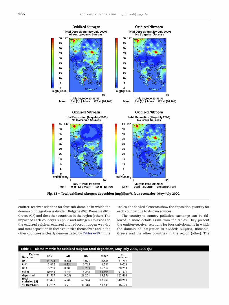
Fig. 13 – Total oxidized nitrogen depositio
emitter–receiver relations for four sub-domains in which thedomain of integration is divided: Bulgaria (BG), Romania (RO),Greece (GR) and the other countries in the region (other). The
impact of each country’s sulphur and nitrogen emissions tothe oxidized sulphur, oxidized and reduced nitrogen wet, dryand total deposition in these countries themselves and in theother countries is clearly demonstrated by Tables 4–10. In the
Table 6 – Blame matrix for oxidized sulphur total deposition, M

g(N)/m2), four scenarios, May–July 2000.

Tables, the shaded elements show the deposition quantity foreach country due to its own sources.

The country-to-country pollution exchange can be fol-
lowed in more details again from the tables. They presentthe emitter–receiver relations for four sub-domains in whichthe domain of integration is divided: Bulgaria, Romania,Greece and the other countries in the region (other). The
ay–July 2000, 1000 t(S)


n (m

itwsbts

Fig. 14 – Total reduced nitrogen depositio

mpact of each country’s sulphur and nitrogen emissionso the oxidized sulphur, oxidized and reduced nitrogenet, dry and total deposition in these countries them-

elves and in the other countries is clearly demonstratedy Tables 4–10. In the Tables, the shaded elements showhe deposition quantity for each country due to its ownources.

Table 7 – Blame matrix for oxidized nitrogen total deposition, M

g(N)/m2), four scenarios, May–July 2000.

The last three rows of the tables show, respectively thetotal quantity deposited in the country in the column head-ers, the total emitted sulphur or nitrogen for this country and
the percentage of deposited quantities from the emitted. Thelast values in the tables can be treated as the relative partof sulphur/nitrogen that remains in the domain. The percentsvaries from 5–7.5% for oxidized nitrogen to 25–35% for reduced
ay–July 2000, 1000 t(N)


Table 8 – Blame matrix for reduced nitrogen dry deposition, May–July 2000, 1000 t(N)

Table 9 – Blame matrix for reduced nitrogen wet deposition, May–July 2000, 1000 t(N)

Table 10 – Blame matrix for reduced nitrogen total deposition, May–July 2000, 1000 t(N)

nitrogen total deposition up to 34–52% for oxidized sulphurtotal deposition.

The sulphur and nitrogen loads patterns are given in detailsin Figs. 12–14. It should be noted that the big industrial sourcesand urban agglomerations impact is very well manifested,especially in the fields of total oxidized sulphur and nitrogen.

The analysis of different scenarios of switching off theemissions from Bulgaria, Greece or Romania shows (just likeTables 4–10 do), that the impact is most prominent on the sul-phur or nitrogen loads in the respective country. The impacton the neighboring countries however can also be significant.For example from Fig. 12 it can be seen that the exclusionof Bulgarian sources leads to substantial decrease of oxi-dized sulphur loads in northeast Greece and European Turkey.The exclusion of Romanian sources also leads to substantialdecrease of oxidized sulphur loads in northeast Bulgaria.

6. Conclusions

The main conclusions that can be made from this tentativestudy of the transboundary transport and transformation ofair pollutants over the Balkans for the summer of year 2000are the following:

(1) The comparison of the simulated results with measureddata from the background stations in the region showedreasonable agreement and the loads calculated by thelong-term CMAQ simulations are fully consistent (in terms

r

of the order of magnitude of different deposition types)with the EMEP evaluations, which is quite an encouragingresult.

(2) Enriching the background stations network in the regionwill soundly contribute to understand the mechanisms ofregional scale transport and transformation of pollutantsover Southeast Europe and to more reliable evaluation ofCtC pollution exchange.

(3) The emission inventories in the Balkan region need tobe significantly more detailed both in spatial resolutionand especially in temporal evolution—annual and diur-nal course. Proper evaluation of the natural biogenicemissions is also very important for reliable ozone (bothanthropogenic and biogenic) level simulations.

Acknowledgements

The present work is supported by EC through 6FP NoE ACCENT(GOCE-CT-2002-500337), IP QUANTIFY (GOGE-003893), COSTAction 728, as well as by the Bulgarian National Science Coun-cil (H3-1002/00). Deep gratitude is due to US EPA, US NCEP andEMEP for providing free-of-charge data and software.

e f e r e n c e s

Ambelas Skjøth, C., Hertel, O., Ellermann, T., 2002. Use of theACDEP trajectory model in the Danish nation-wide

g 2 1

B

B

B

B

C

C

C

C

D

D

D

E

E

E

G

G

G

e c o l o g i c a l m o d e l l i n

Background Monitoring Programme. Phys. Chem. Earth 27,1469–1477.

G-EMEP, 1994–1997. Bulgarian contribution to EMEP. AnnualReports for 1994, 1995, 1996, 1997. NIMH, EMEP/MSC-E,Sofia-Moscow.

orge, R., Lumbreras, J., Rodríguez, M.E., 2008. Development of ahigh-resolution emission inventory for Spain using theSMOKE modelling system: a case study for the years 2000 and2010. Environ. Model. Softw. 23 (8), 1026–1044.

yun, D., Ching, J., 1999. Science Algorithms of the EPA Models-3Community Multiscale Air Quality (CMAQ) Modeling System.EPA Report 600/R-99/030, Washington DC.

yun, D., Schere, K.L., 2006. Review of the governing equations,computational algorithms, and other components of theModels-3 Community Multiscale Air Quality (CMAQ) modelingsystem. Appl. Mech. Rev. 59 (March), 51–77.

EP, 2003. UNC Carolina Environmental Program, Sparse MatrixOperator Kernel Emission (SMOKE) Modeling System.University of Carolina, Carolina Environmental Programs,Research Triangle Park, North Carolina.

hervenkov, Hr., Syrakov, D., Prodanova, M., 2005a. Estimation ofthe sulphur pollution over the Balkan Region in 1995-2000. In:Incecek, S. (Ed.), Proceedings of the Third InternationalSymposium on Air Quality Management at Urban, Regionaland Global Scales. Istanbul, Turkey, September 26–30, pp.608–617.

hervenkov, Hr., Syrakov, D., Prodanova, M., 2005b. On thesulphur pollution over the Balkan Region. In: Lirkov, et, al.(Eds.), Lecture Notes in Computer Science, vol. 3743/2006Large-Scale Scientific Computing. Proceedings of the FifthInternational Conference, LSSC 2005. Springer-Verlag GmbH,Sozopol, Bulgaria, June 6–10, pp. 481–489.

hervenkov, Hr., 2006. Estimation of the exchange of sulphurpollution in the Southeast Europe. J. Environ. Protect. Ecol. 7(1), 10–18.

onev, E., Ivanova, D., Avramov, A., Zeller, K., 1999. Rankcorrelation approach to assessing influence of mountainvalley winds on ozone concentration. J. Balkan Ecol. 2, 79–85.

onev, E., Zeller, K., Avramov, A., 2002. Preliminary backgroundozone concentrations in the mountain and coastal areas ofBulgaria. Environ. Pollut. 17, 281–286.

udhia, J., 1993. A non-hydrostatic version of the PennState/NCAR Mesoscale Model: validation tests and simulationof an Atlantic cyclone and cold front. Mon. Weather Rev. 121,1493–1513.

MEP, 1998. Transboundary Acidifying Air Pollution in Europe,EMEP/MCS-W Report 1/1998. Meteorological SynthesizingCentre-West, Norwegian Meteorological Institute, Oslo,Norway, ISSN 0332-9879.

C, 1999. Ozone position paper, Directorate XI—Environment,Nuclear Safety and Civil Protection, European Commission,Brussels.

C, 2002. Directive 2002/3/EC of the European Parliament and ofthe Council of February 12, relating to ozone in ambient air.Off. J. Eur. Commun. L 67, 14–30.

anev, K., Syrakov, D., Zerefos, Ch., Prodanova, M., Dimitrova, R.,Vasaras, A., 2002. On some cases of extreme sulfur pollutionin Bulgaria or Northern Greece. Bulg. Geophys. J. 1–4,15–22.

anev, K., Dimitrova, R., Syrakov, D., Zerefos, Ch., 2003.Accounting for the mesoscale effects on the air pollution insome cases of large sulfur pollution in Bulgaria or Northern
Greece. Environ. Fluid Mech. 3, 41–53.
rell, G.A., Dudhia, J., Stauffer, D.R., 1994. A description of theFifth Generation Penn State/NCAR Mesoscale Model (MM5).NCAR Technical Note, NCAR TN-398-STR,138 pp.

7 ( 2 0 0 8 ) 255–269 269

Prodanova, M., Syrakov, D., Zlatev, Z., Slavov, K., Ganev, D.,Miloshev, N., Nikolova, E., 2005a. Estimation of ozonepollution levels in Southeast Europe Using Us Epa Models-3System. In: Incecek, S. (Ed.), Proceedings of the ThirdInternational Symposium on Air Quality Management atUrban, Regional and Local Scales, vol. I. September 26–30,Istanbul, Turkey, pp. 517–526.

Prodanova, M., Syrakov, D., Zlatev, Z., Slavov, K., Ganev, K.,Miloshev, N., Nikolova, E., 2005b. Preliminary results from theuse of MM5-CMAQ system for estimation of pollution levels insoutheast Europe. In: Fuzzi, S., Maione, M. (Eds.), Proceedingsof the First Accent Symposium on the Changing ChemicalClimate of the Atmosphere. Urbino, Italy, September 12–16,pp. 119–127.

Prodanova, M., Pérez, J., Syrakov, D., San José, R., Ganev, K.,Miloshev, N., 2006a. Exchange of Ozone Pollution betweenRomania, Bulgaria and Greece. In: Proceedings of the 26th ITMon Air Pollution Modelling and Applications, Leipzig,Germany, May 13–19, pp. 436–437.

Prodanova, M., Pérez, J., Syrakov, D., San José, R., Zlatev, Z., Ganev,K., Miloshev, N., 2006b. Preliminary estimates of US EPAModel-3 system capability for description of photochemicalpollution in Southeast Europe. In: Proceedings of the 26th ITMon Air Pollution Modelling and Applications, Leipzig,Germany, May 13–19, pp. 438–445.

Smylie, M., Fieber, J.L., Myers, T.C., Burton, S., 1991. A preliminaryexamination of the impact on emissions and ozone air qualityin Athens Greece from various hypothetical motor vehiclecontrol strategies. In: European Conference on New Fuels andClean Air, Antwerp, Belgium, June 19.

Stauffer, D.R., Seaman, N.L., 1990. Use of four-dimensional dataassimilation in a limited area mesoscale model. Part I.Experiments with synoptic data. Mon. Weather Rev. 118,1250–1277.

Syrakov, D., Prodanova, M., Ganev, K., Zerefos, Ch., Vasaras, A.,2002. Exchange of sulfur pollution between Bulgaria andGreece. Environ. Sci. Pollut. Res. 9 (5), 321–326.

Vestreng, V., 2001. Emission Data Reported to UNECE/EMEP:Evaluation of the Spatial Distribution of Emissions.Meteorological Synthesizing Centre-West, The NorwegianMeteorological Institute, Oslo, Norway, Research Note 56,EMEP/MSC-W Note 1/2001.

Zlatev, Z., 1995. Computer Treatment of Large Air PollutionModels. Kluwer Academic Publishers, Dordrecht, Boston,London.

Zlatev, Z., Syrakov, D., 2004a. A fine-resolution modelling study ofpollution levels in Bulgaria. Part 1. SOx and NOx pollution. Int.J. Environ. Pollut. 22 (1–2), 186–202.

Zlatev, Z., Syrakov, D., 2004b. A fine-resolution modelling study ofpollution levels in Bulgaria. Part 2. High ozone levels. Int. J.Environ. Pollut. 22 (1–2), 203–222.

Zerefos, Ch., Ganev, K., Syrakov, D., Vasaras, A., Tzortziou, M.,Prodanova, M., Georgieva, E., 1998. Numerical study of thetotal SO2 contents in the air column over the city ofThessaloniki. In: Bachvarova, E., Gryning, S.E. (Eds.),Proceedings of the XIII International Technical Meeting on AirPollution Modelling and its Applications. KluwerAcademic/Plenum Publ. Corp, Varna, Bulgaria, September28–October 2, pp. 175–182.

Zerefos, C., Ganev, K., Kourtidis, K., Tzortziou, M., Vasaras, A.,Syrakov, E., 2000. On the origin of SO2 above Northern Greece.Geophys. Res. Lett. 27 (3), 365–368.

Zerefos, Ch., Syrakov, D., Ganev, K., Vasaras, A., Kourtidis, K.,Tzortziou, M., Prodanova, M., Dimitrova, R., Georgieva, E.,Yordanov, D., Miloshev, N., 2004. Study of the pollutionexchange between Bulgaria and Northern Greece. Int. J.Environ. Pollut. 22 (1/2), 163–185.

Air pollution transport in the Balkan region and country-to-country pollution exchange between...

Documents

Transcript of Air pollution transport in the Balkan region and country-to-country pollution exchange between...