Adjoint-based sensitivity analysis of a mesoscale low on the mei-yu front and its implications for...

ADVANCES IN ATMOSPHERIC SCIENCES, VOL. 24, NO. 3, 2007, 435–448

Adjoint-based Sensitivity Analysis of a Mesoscale Low

on the Mei-yu Front and Its Implications

for Adaptive Observation

ZHONG Ke∗1 (� �), DONG Peiming2 (��), ZHAO Sixiong2 (��),CAI Qifa3 (��), and LAN Weiren4 (��)

1State Key Laboratory of Numerical Modeling for Atmospheric Sciences and Geophysical Fluid Dynamics (LASG),

Institute of Atmospheric Physics, Chinese Academy of Sciences, Beijing 100029

2Institute of Atmospheric Physics, Chinese Academy of Sciences, Beijing 100029

3Institute of Meteorology, PLA University of Science and Technology, Nanjing 210029

4P. O. Box 2433, Beijing 100081

(Received 8 January 2006; revised 20 July 2006)

ABSTRACT

An adjoint sensitivity analysis of one mesoscale low on the mei-yu Front is presented in this paper.The sensitivity gradient of simulation error dry energy with respect to initial analysis is calculated. Andafter verifying the ability of a tangent linear and adjoint model to describe small perturbations in thenonlinear model, the sensitivity gradient analysis is implemented in detail. The sensitivity gradient withrespect to different physical fields are not uniform in intensity, simulation error is most sensitive to thevapor mixed ratio. The localization and consistency are obvious characters of horizontal distribution of thesensitivity gradient, which is useful for the practical implementation of adaptive observation. The sensitivityregion tilts to the northwest with height increasing; the singular vector calculation proves that this tiltingcharacterizes a quick-growing structure, which denotes that using the leading singular vectors to decidethe adaptive observation region is proper. When connected with simulation of a mesoscale low on themei-yu Front, the sensitivity gradient has the following physical characters: the obvious sensitive regionis mesoscale, concentrated in the middle-upper troposphere, and locates around the key system; and thesensitivity gradient of different physical fields correlates dynamically.

Key words: adjoint sensitivity analysis, singular vector, adaptive observation, mei-yu front, mesoscale low

DOI: 10.1007/s00376-007-0435-9

1. Introduction

Mesoscale lows on the mei-yu front are often associ-ated with local storms, causing great harm to society;hence, it has always been an important component ofmesoscale meteorological research. Also, due to itssmall scale, strong intensity, and rapid growth, it isdifficult to forecast numerically (Wu and Chen, 1985;Kuo et al., 1986).

Studies in recent years have shown that small er-rors in initial conditions can induce great errors in thenumerical forecast; the initial analysis is the key to

improving the forecast precision. Therefore, researchconcerned with sensitivity analysis of the initial con-ditions, variational assimilation, Kalman filtering, en-semble forecasting, and adaptive observation, have be-come more and more important. In this paper, withimproving mesoscale low forecasts in mind, an adjointsensitivity analysis of one mesoscale low on the mei-yufront in 1999 is presented in detail.

The adjoint-based sensitivity analysis follows asthis: with the adjoint model, calculating the gradi-ent of predefined scalar cost function with respect tothe initial analysis (the cost function changed with the

∗E-mail: [email protected]

436 ADJOINT SENSITIVITY ANALYSIS OF LOW ON MEI-YU FRONT VOL. 24

forecasted state; commonly, it concerns the forecasterror), analyzing the gradient, and picking out wherethe cost function is most sensitive to the initial analy-sis (Errico and Vukicevic, 1992; Rabier et al., 1996).

The implications of sensitivity analysis are alsoconsidered in this paper. Adaptive observation hasbeen presented by European and U. S. scientists(Emanuel et al., 1995; Langland and Rohaly, 1996;Joly et al., 1997; Palmer et al., 1998; Bergot et al.,1999; Berliner et al., 1999; Bishop and Toth, 1999;Buizza and Montani, 1999; Bishop et al., 2001; Ma-jumdar et al., 2002), which adheres to the followingsteps: determining some observation points besidesthe regular observation network that has an obviouseffect on improving the initial analysis and subsequentforecast; then observing the regular and extra obser-vation network together; and finally, inputting all ob-servations in the assimilation system to produce theinitial conditions.

Although there have been many works about sen-sitivity analysis, certain features make this paper dis-tinguishable from others. Firstly, the linear assump-tion is validated before any application of the adjointmethod, which is a stepping stone for any further work;secondly, an ingredient analysis of the sensitivity gra-dient is made using singular vectors—the practical cal-culation of singular vectors proves that the sensitivitygradient is dominated by leading singular vectors, thequick-growing singular vectors; and finally, some im-plications of the sensitivity gradient to adaptive obser-vation are discussed.

The paper is organized in the following way: a briefdescription of the method of adjoint sensitivity analy-sis is illustrated in section 2; the mesoscale low on themei-yu front used in this paper is reviewed in section3; an introduction to the model and experimental con-figuration is detailed in section 4; verification of theability of the tangent and adjoint model to describesmall perturbations in the nonlinear model is in sec-tion 5; the practical sensitivity analysis is implementedin section 6; the implications of sensitivity analysis arepresented in section 7; and a discussion and concludingremarks complete the paper in section 8.

2. The adjoint sensitivity analysis methodused in this paper

The adjoint sensitivity analysis is an analysis ofsensitivity gradient. The sensitivity gradient

∂J

∂x0,a= LTP TEP (xk,f − xk,a)

is a gradient of the scalar cost function J =1/2〈P (xk,f − xk,a), P (xk,f − xk,a)〉E , where 〈 , 〉E

demonstrates the inner product defined through a pos-itively defined Hamilton matrix E, LT is the adjointmodel of the nonlinear forecast model F , P is the localprojection matrix, xk,a and xk,f are the analysis andforecast state, respectively (subscript a and f denotingthe analysis and forecast state, k indicates that thestate is at k time).

In this paper, the dry energy metric is adopted asE. The dry energy metric is demonstrated as the fol-lowing:

〈(xk,f − xk,a), (xk,f − xk,a)〉E =∫∫∫

ρc

(u2

s

2+

v2s

2+

w2s

2+

12

g2

N2

θ2s

θ2c

+

12ρ2

c

p2s

c2s

)∂pc

∂σdxdydσ ,

where us, vs, ws, θs, and ps are the difference betweenxk,f and xk,a of the west-east wind velocity, north-south wind velocity, vertical velocity, potential tem-perature, and disturbed pressure, respectively [in prac-tical calculation, θs is substituted with the differenceof temperature (ts) approximately], g is gravitationalacceleration, ρc is the density of base state, N is theBrunt-Vaisala frequency, θc is the potential tempera-ture of base state (in practical calculation, θc is sub-stituted with the base state of temperature approxi-mately), pc is reference pressure, and cs is sound ve-locity of the base state.

3. Description of the mesoscale low

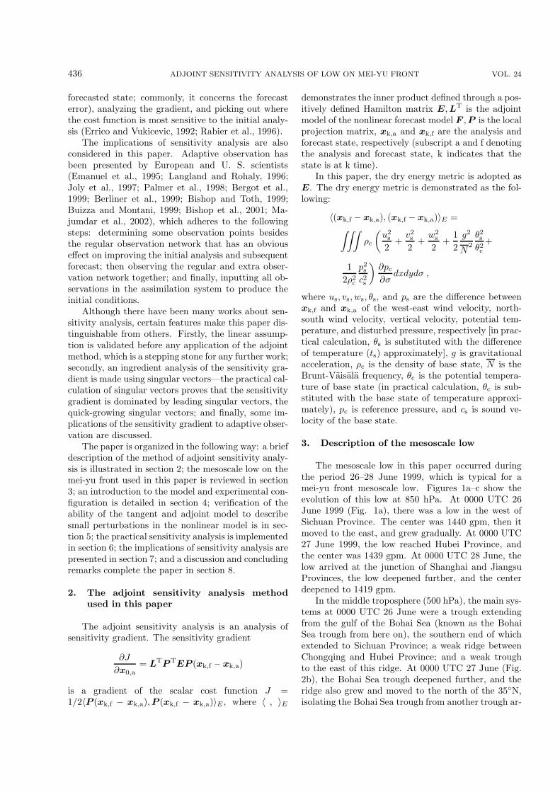
The mesoscale low in this paper occurred duringthe period 26–28 June 1999, which is typical for amei-yu front mesoscale low. Figures 1a–c show theevolution of this low at 850 hPa. At 0000 UTC 26June 1999 (Fig. 1a), there was a low in the west ofSichuan Province. The center was 1440 gpm, then itmoved to the east, and grew gradually. At 0000 UTC27 June 1999, the low reached Hubei Province, andthe center was 1439 gpm. At 0000 UTC 28 June, thelow arrived at the junction of Shanghai and JiangsuProvinces, the low deepened further, and the centerdeepened to 1419 gpm.

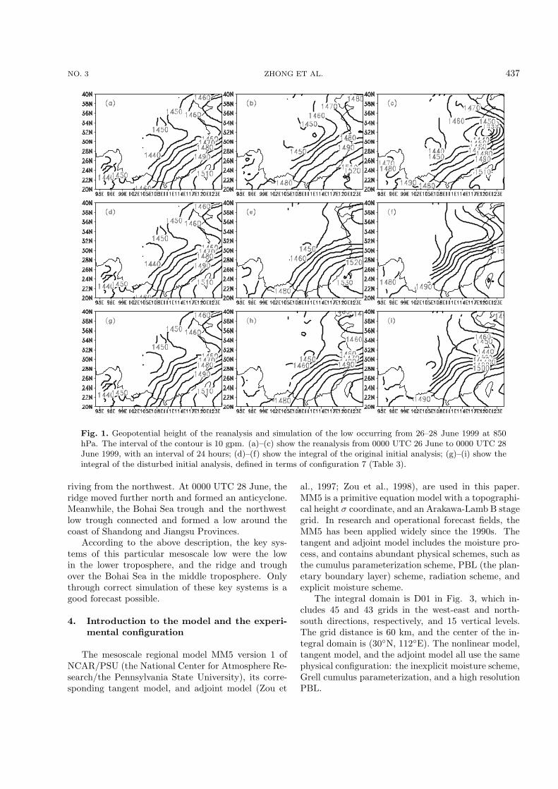
In the middle troposphere (500 hPa), the main sys-tems at 0000 UTC 26 June were a trough extendingfrom the gulf of the Bohai Sea (known as the BohaiSea trough from here on), the southern end of whichextended to Sichuan Province; a weak ridge betweenChongqing and Hubei Province; and a weak troughto the east of this ridge. At 0000 UTC 27 June (Fig.2b), the Bohai Sea trough deepened further, and theridge also grew and moved to the north of the 35◦N,isolating the Bohai Sea trough from another trough ar-

NO. 3 ZHONG ET AL. 437

Fig. 1. Geopotential height of the reanalysis and simulation of the low occurring from 26–28 June 1999 at 850hPa. The interval of the contour is 10 gpm. (a)–(c) show the reanalysis from 0000 UTC 26 June to 0000 UTC 28June 1999, with an interval of 24 hours; (d)–(f) show the integral of the original initial analysis; (g)–(i) show theintegral of the disturbed initial analysis, defined in terms of configuration 7 (Table 3).

riving from the northwest. At 0000 UTC 28 June, theridge moved further north and formed an anticyclone.Meanwhile, the Bohai Sea trough and the northwestlow trough connected and formed a low around thecoast of Shandong and Jiangsu Provinces.

According to the above description, the key sys-tems of this particular mesoscale low were the lowin the lower troposphere, and the ridge and troughover the Bohai Sea in the middle troposphere. Onlythrough correct simulation of these key systems is agood forecast possible.

4. Introduction to the model and the experi-mental configuration

The mesoscale regional model MM5 version 1 ofNCAR/PSU (the National Center for Atmosphere Re-search/the Pennsylvania State University), its corre-sponding tangent model, and adjoint model (Zou et

al., 1997; Zou et al., 1998), are used in this paper.MM5 is a primitive equation model with a topographi-cal height σ coordinate, and an Arakawa-Lamb B stagegrid. In research and operational forecast fields, theMM5 has been applied widely since the 1990s. Thetangent and adjoint model includes the moisture pro-cess, and contains abundant physical schemes, such asthe cumulus parameterization scheme, PBL (the plan-etary boundary layer) scheme, radiation scheme, andexplicit moisture scheme.

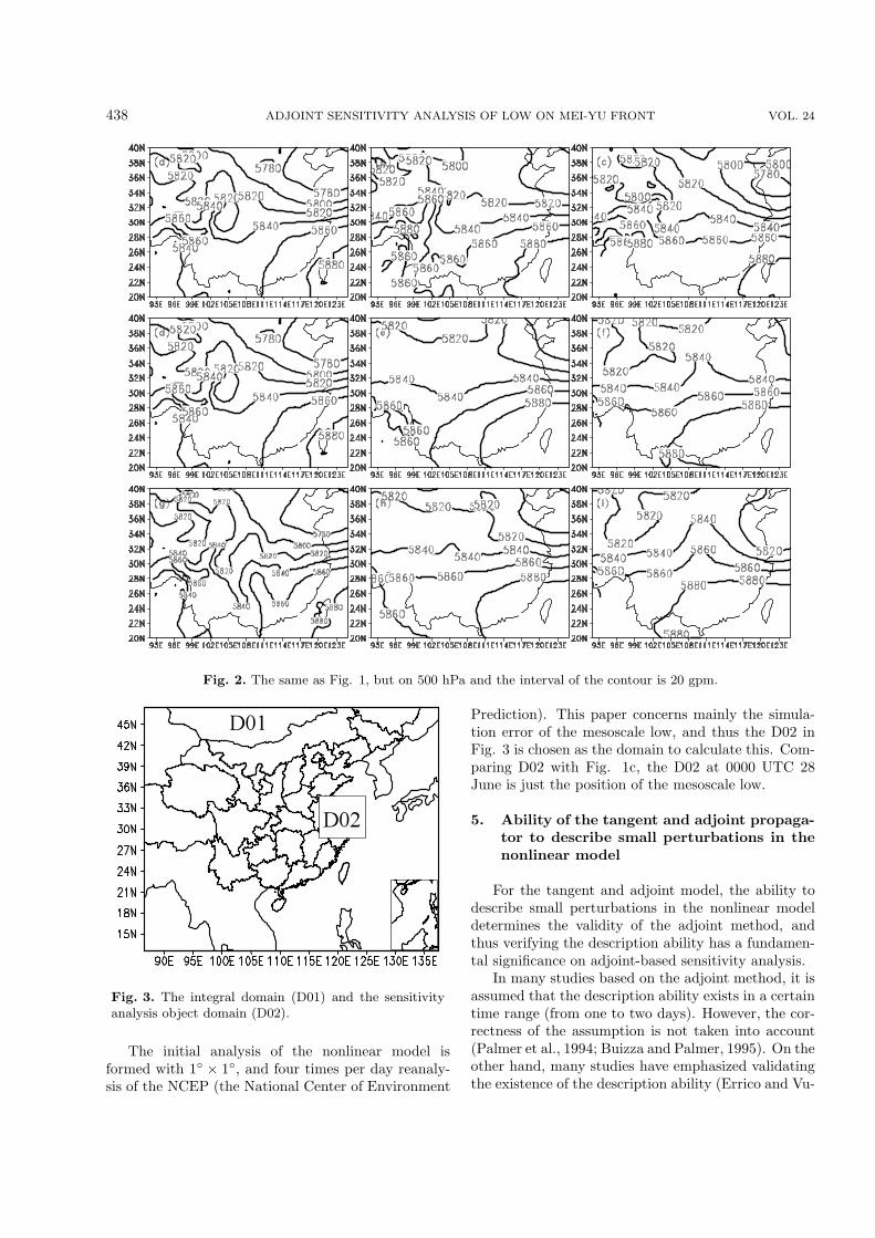
The integral domain is D01 in Fig. 3, which in-cludes 45 and 43 grids in the west-east and north-south directions, respectively, and 15 vertical levels.The grid distance is 60 km, and the center of the in-tegral domain is (30◦N, 112◦E). The nonlinear model,tangent model, and the adjoint model all use the samephysical configuration: the inexplicit moisture scheme,Grell cumulus parameterization, and a high resolutionPBL.


Fig. 2. The same as Fig. 1, but on 500 hPa and the interval of the contour is 20 gpm.

D02

D01

Fig. 3. The integral domain (D01) and the sensitivityanalysis object domain (D02).

The initial analysis of the nonlinear model isformed with 1◦ × 1◦, and four times per day reanaly-sis of the NCEP (the National Center of Environment

Prediction). This paper concerns mainly the simula-tion error of the mesoscale low, and thus the D02 inFig. 3 is chosen as the domain to calculate this. Com-paring D02 with Fig. 1c, the D02 at 0000 UTC 28June is just the position of the mesoscale low.

5. Ability of the tangent and adjoint propaga-tor to describe small perturbations in thenonlinear model

For the tangent and adjoint model, the ability todescribe small perturbations in the nonlinear modeldetermines the validity of the adjoint method, andthus verifying the description ability has a fundamen-tal significance on adjoint-based sensitivity analysis.

In many studies based on the adjoint method, it isassumed that the description ability exists in a certaintime range (from one to two days). However, the cor-rectness of the assumption is not taken into account(Palmer et al., 1994; Buizza and Palmer, 1995). On theother hand, many studies have emphasized validatingthe existence of the description ability (Errico and Vu-


Table 1. nr and lr during the integral.

Time (h)

0 6 12 18 24 30 36 42 48

nr 0.00 0.16 0.22 0.26 0.29 0.34 0.42 0.48 0.53lr 0.00 0.25 0.31 0.33 0.38 0.48 0.58 0.63 0.70

kicevic, 1992; Buizza, 1995; Gilmour and Smith, 1997;Hansen and Smith, 2000). Lorenz and Emannel (1998)conducted experiments to verify the utility of adaptiveobservation, but did not get the expected result.Hansen and Smith (2000) analyzed their experimentand determined that the failure was mainly due to theinvalidation of the linearization assumption of smallperturbations in the nonlinear model. Therefore, ver-ifying the description ability will be the first step inthis paper.

5.1 Ingredients analysis of small perturba-tions in the nonlinear model

The nonlinear component of perturbations in thenonlinear model could be quantified approximately us-ing the method of Buizza and Montani (1999), andHansen and Smith (2000).

Adding a small perturbation δx0 at initial time toform two disturbed initial analyses: x0,a,+ = x0,a +δx0 and x0,a,− = x0,a − δx0, F is integrated fromx0,a,+ and x0,a,−, at k time, and two forecasts are ob-tained: xk,f,+ = Fx0,a,+ and xk,f,- = Fx0,a,-, wheresubscript 0 shows those physical field are in initialtime, k means variables are at k time.

Introducing the following ratios:

nr =2‖O(‖δx0‖E)‖E/(‖xk,f,+ − xk,f‖E+‖xk,f,- − xk,f‖E)

and

lr =2‖L′δx0 + O(‖δx0‖E)‖E/

(‖xk,f,+ − xk,f‖E + ‖xk,f,- − xk,f‖E) ,

where

12(‖xk,f,+ − xk,f‖E + ‖xk,f,- − xk,f‖E)

represents the metric of the small perturbation in thenonlinear model approximately, nr is the ratio of thenonlinear term to the small perturbation of the non-linear model, lr is the ratio of the combination of thenonlinear term and linear part that could not be de-scribed by the tangent linear model to the small per-turbation of the nonlinear model, and O(‖δx0‖E) areterms with higher order than δx0.

With nr increasing, the linear term has more errorcompared with the small perturbation in the nonlinear

model. When there is no nonlinear term in the smallperturbation in the nonlinear model, nr = 0, whilenr = 1, meaning there is no linear term in the smallperturbation of the nonlinear model.

nr and lr in the 48-hour integral of the mesoscalelow are shown once every six hours in Table 1. nr andlr is the average of the east-west wind, south-northwind, vertical wind, temperature, vapor mixed ratio,and disturbed pressure in 15 vertical σ levels.

In Table 1, nr is not equal to 0 except at the be-ginning, which means there is a nonlinear term. Atthe same time, nr is also not equal to 1, which meansthere is a linear term. As the integration proceeds, nr

gradually increases, and the error of the linear termcompared with the small perturbation of the nonlin-ear model becomes more and more obvious.

As for lr, except at the beginning, it is not equal tonr, which means there is an indescribable linear part inthe small perturbation in the nonlinear model. As theintegral proceeds, lr increases gradually, and the de-scribable linear part tends to decrease. At any time lris greater than nr, the existence of an indescribable lin-ear part causes the error of the describable linear partcompared with the small perturbation in the nonlinearmodel more distinct. However, even after 48 hours, lris still not equal to 1, which shows that the tangentmodel has a certain ability to describe the small per-turbation in the nonlinear model.

5.2 Comparison between perturbations in thetangent linear and nonlinear models

In this section, for verifying the description abil-ity, perturbations in the tangent and nonlinear modelswill be compared directly, which is intuitive and widelyused (Errico and Vukicevic, 1992; Rabier et al., 1996).

The small perturbation of west-east wind veloc-ity (u) in the tangent linear and nonlinear models onσ = 0.81 during the integral process is listed in Fig. 4,once every 24 hours. At the start (Figs. 4a and 4d),the perturbations are all the same in the two models.At 24 hours (Figs. 4b and 4e), the central position,intensity, and distribution of two kinds of perturba-tions are still very similar; and at 48 hours (Figs. 4cand 4f), the perturbations are similar to a certain ex-tent, however there are some differences in the centralposition, and the velocity of the center of the tangentlinear model is 5 m s−1 greater than that of the non-


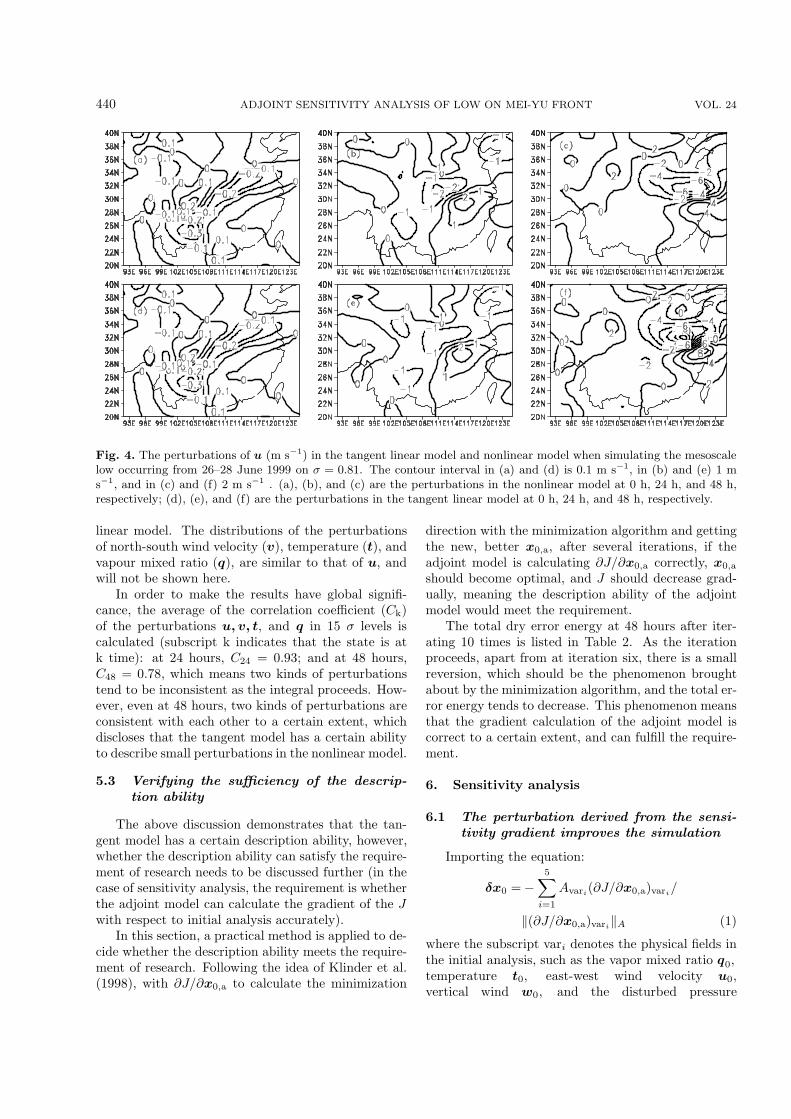
Fig. 4. The perturbations of u (m s−1) in the tangent linear model and nonlinear model when simulating the mesoscalelow occurring from 26–28 June 1999 on σ = 0.81. The contour interval in (a) and (d) is 0.1 m s−1, in (b) and (e) 1 ms−1, and in (c) and (f) 2 m s−1 . (a), (b), and (c) are the perturbations in the nonlinear model at 0 h, 24 h, and 48 h,respectively; (d), (e), and (f) are the perturbations in the tangent linear model at 0 h, 24 h, and 48 h, respectively.

linear model. The distributions of the perturbationsof north-south wind velocity (v), temperature (t), andvapour mixed ratio (q), are similar to that of u, andwill not be shown here.

In order to make the results have global signifi-cance, the average of the correlation coefficient (Ck)of the perturbations u, v, t, and q in 15 σ levels iscalculated (subscript k indicates that the state is atk time): at 24 hours, C24 = 0.93; and at 48 hours,C48 = 0.78, which means two kinds of perturbationstend to be inconsistent as the integral proceeds. How-ever, even at 48 hours, two kinds of perturbations areconsistent with each other to a certain extent, whichdiscloses that the tangent model has a certain abilityto describe small perturbations in the nonlinear model.

5.3 Verifying the sufficiency of the descrip-tion ability

The above discussion demonstrates that the tan-gent model has a certain description ability, however,whether the description ability can satisfy the require-ment of research needs to be discussed further (in thecase of sensitivity analysis, the requirement is whetherthe adjoint model can calculate the gradient of the Jwith respect to initial analysis accurately).

In this section, a practical method is applied to de-cide whether the description ability meets the require-ment of research. Following the idea of Klinder et al.(1998), with ∂J/∂x0,a to calculate the minimization

direction with the minimization algorithm and gettingthe new, better x0,a, after several iterations, if theadjoint model is calculating ∂J/∂x0,a correctly, x0,a

should become optimal, and J should decrease grad-ually, meaning the description ability of the adjointmodel would meet the requirement.

The total dry error energy at 48 hours after iter-ating 10 times is listed in Table 2. As the iterationproceeds, apart from at iteration six, there is a smallreversion, which should be the phenomenon broughtabout by the minimization algorithm, and the total er-ror energy tends to decrease. This phenomenon meansthat the gradient calculation of the adjoint model iscorrect to a certain extent, and can fulfill the require-ment.

6. Sensitivity analysis

6.1 The perturbation derived from the sensi-tivity gradient improves the simulation

Importing the equation:

δx0 = −5∑

i=1

Avari(∂J/∂x0,a)vari

/

‖(∂J/∂x0,a)vari‖A (1)

where the subscript vari denotes the physical fields inthe initial analysis, such as the vapor mixed ratio q0,temperature t0, east-west wind velocity u0,vertical wind w0, and the disturbed pressure


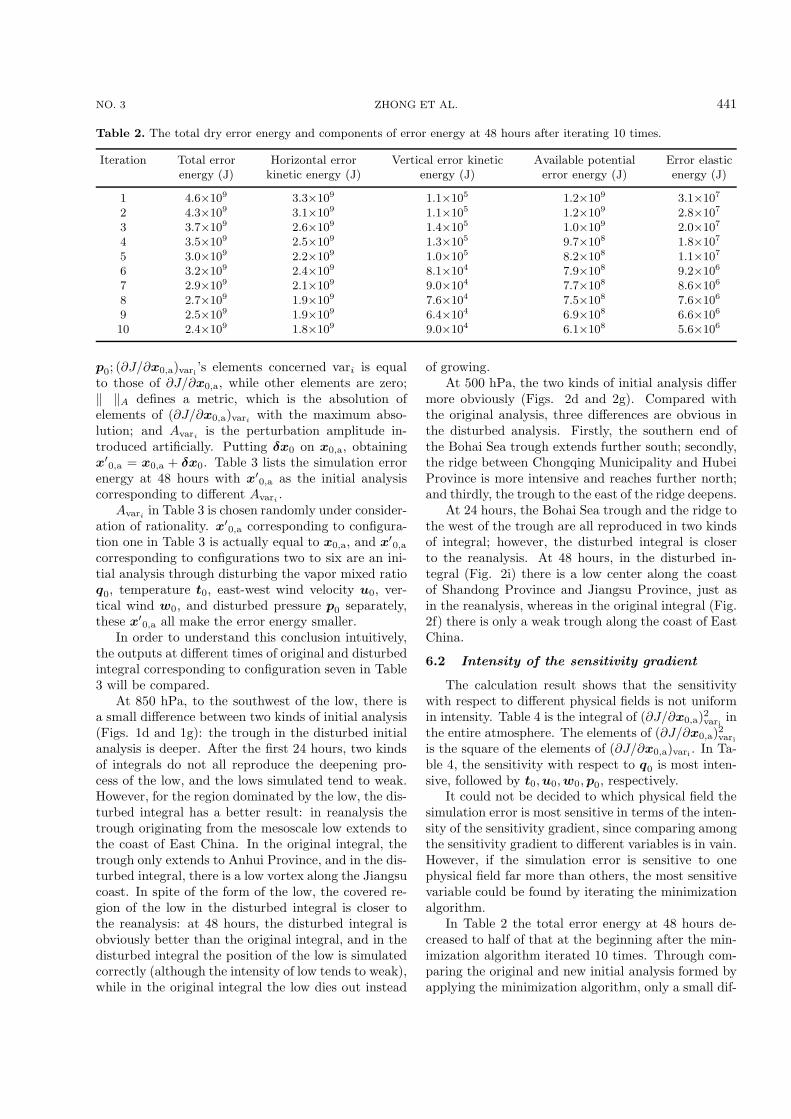
Table 2. The total dry error energy and components of error energy at 48 hours after iterating 10 times.

Iteration Total error Horizontal error Vertical error kinetic Available potential Error elasticenergy (J) kinetic energy (J) energy (J) error energy (J) energy (J)

1 4.6×109 3.3×109 1.1×105 1.2×109 3.1×107

2 4.3×109 3.1×109 1.1×105 1.2×109 2.8×107

3 3.7×109 2.6×109 1.4×105 1.0×109 2.0×107

4 3.5×109 2.5×109 1.3×105 9.7×108 1.8×107

5 3.0×109 2.2×109 1.0×105 8.2×108 1.1×107

6 3.2×109 2.4×109 8.1×104 7.9×108 9.2×106

7 2.9×109 2.1×109 9.0×104 7.7×108 8.6×106

8 2.7×109 1.9×109 7.6×104 7.5×108 7.6×106

9 2.5×109 1.9×109 6.4×104 6.9×108 6.6×106

10 2.4×109 1.8×109 9.0×104 6.1×108 5.6×106

p0; (∂J/∂x0,a)vari ’s elements concerned vari is equalto those of ∂J/∂x0,a, while other elements are zero;‖ ‖A defines a metric, which is the absolution ofelements of (∂J/∂x0,a)vari

with the maximum abso-lution; and Avari

is the perturbation amplitude in-troduced artificially. Putting δx0 on x0,a, obtainingx′

0,a = x0,a + δx0. Table 3 lists the simulation errorenergy at 48 hours with x′

0,a as the initial analysiscorresponding to different Avari

.Avari

in Table 3 is chosen randomly under consider-ation of rationality. x′

0,a corresponding to configura-tion one in Table 3 is actually equal to x0,a, and x′

0,a

corresponding to configurations two to six are an ini-tial analysis through disturbing the vapor mixed ratioq0, temperature t0, east-west wind velocity u0, ver-tical wind w0, and disturbed pressure p0 separately,these x′

0,a all make the error energy smaller.In order to understand this conclusion intuitively,

the outputs at different times of original and disturbedintegral corresponding to configuration seven in Table3 will be compared.

At 850 hPa, to the southwest of the low, there isa small difference between two kinds of initial analysis(Figs. 1d and 1g): the trough in the disturbed initialanalysis is deeper. After the first 24 hours, two kindsof integrals do not all reproduce the deepening pro-cess of the low, and the lows simulated tend to weak.However, for the region dominated by the low, the dis-turbed integral has a better result: in reanalysis thetrough originating from the mesoscale low extends tothe coast of East China. In the original integral, thetrough only extends to Anhui Province, and in the dis-turbed integral, there is a low vortex along the Jiangsucoast. In spite of the form of the low, the covered re-gion of the low in the disturbed integral is closer tothe reanalysis: at 48 hours, the disturbed integral isobviously better than the original integral, and in thedisturbed integral the position of the low is simulatedcorrectly (although the intensity of low tends to weak),while in the original integral the low dies out instead

of growing.At 500 hPa, the two kinds of initial analysis differ

more obviously (Figs. 2d and 2g). Compared withthe original analysis, three differences are obvious inthe disturbed analysis. Firstly, the southern end ofthe Bohai Sea trough extends further south; secondly,the ridge between Chongqing Municipality and HubeiProvince is more intensive and reaches further north;and thirdly, the trough to the east of the ridge deepens.

At 24 hours, the Bohai Sea trough and the ridge tothe west of the trough are all reproduced in two kindsof integral; however, the disturbed integral is closerto the reanalysis. At 48 hours, in the disturbed in-tegral (Fig. 2i) there is a low center along the coastof Shandong Province and Jiangsu Province, just asin the reanalysis, whereas in the original integral (Fig.2f) there is only a weak trough along the coast of EastChina.

6.2 Intensity of the sensitivity gradient

The calculation result shows that the sensitivitywith respect to different physical fields is not uniformin intensity. Table 4 is the integral of (∂J/∂x0,a)2vari inthe entire atmosphere. The elements of (∂J/∂x0,a)2variis the square of the elements of (∂J/∂x0,a)vari . In Ta-ble 4, the sensitivity with respect to q0 is most inten-sive, followed by t0, u0, w0, p0, respectively.

It could not be decided to which physical field thesimulation error is most sensitive in terms of the inten-sity of the sensitivity gradient, since comparing amongthe sensitivity gradient to different variables is in vain.However, if the simulation error is sensitive to onephysical field far more than others, the most sensitivevariable could be found by iterating the minimizationalgorithm.

In Table 2 the total error energy at 48 hours de-creased to half of that at the beginning after the min-imization algorithm iterated 10 times. Through com-paring the original and new initial analysis formed byapplying the minimization algorithm, only a small dif-


Table 3. Error energy at 48 hours with x′0,a as the initial analysis corresponding to different Avari .

Aq0 (kg kg−1) At0 (K) Au0 (m s−1) Aw0 (m s−1) Ap0 (Pa) Total errorenergy (J)

Configuration 1 0 0 0 0 0 4.6×109

Configuration 2 0.002 0 0 0 0 3.8×109

Configuration 3 0 4 0 0 0 3.0×109

Configuration 4 0 0 5 0 0 4.4×109

Configuration 5 0 0 0 0.02 0 4.5×109

Configuration 6 0 0 0 0 260 4.3×109

Configuration 7 0.002 2 5 0.02 260 2.9×109

Table 4. Integral of (∂J/∂x0,a)2vari

in the entire model atmosphere.

Var q0 [J2 kg2 kg−2] t0 [J2 K2 K−2] u0 [J2 m−2 s2] w0 [J2 m−2 s2] p0 (J2 Pa−2)

(∂J/∂x0,a)2vari

5×1013 − 7 × 1014 2×1010 − 2 × 1011 2×109 − 2 × 1010 3×108 − 3 × 109 3×104 − 3 × 105

ference in q0 of them is found. Other physical fieldsare almost equivalent, which means the minimizationdirection decided by the minimization algorithm is al-most consistent with −(∂J/∂x0,a)q0 , and the simula-tion error is most sensitive to the vapor field.

Although sensitivity with respect to other physicalfields is smaller than that with respect to q0, changingthe initial analysis in sensitive regions of these physicalfields still could decrease the simulation error, whichmeans that sensitivity with respect to these physicalfields also has significance to the initial analysis er-ror and should not be neglected, which is obvious inTable 3.

In addition, in Table 3 the ratio of the decreaseof error energy to the intensity of sensitivity (Table4) is not a direct ratio, which means the correct δx0

could not be obtained by choosing Avarisubjectively.

In order to obtain an optimized initial analysis throughsensitivity analysis, other methods such as the mini-mization algorithm and adaptive observation shouldbe applied.

6.3 Spatial characters of the sensitivity gradi-ent

In order to analyze the spatial characters of thesensitivity gradient distribution, Fig. 5, the contour ofthe vertical integral of (∂J/∂x0,a)2vari

of q0, t0, u0, w0,and p0 in the entire model atmosphere is plotted. InFig. 5, the sensitivity gradient with respect to w0 dis-tributes in scattered points form, while the sensitivitygradient with respect to other physical fields convergestogether, and form isolated sensitive regions. Further-more, the main sensitive regions of q0, t0, u0, and p0,almost superpose each other.

The following characterizes the vertical distribu-tion of the sensitivity gradient. Figure 6 is a verticalcross section of (∂J/∂x0,a)2q0

along the lines of Fig. 5a.

Two characteristics are obvious in Fig. 6.Firstly, the sensitivity gradient mainly concen-

trates in the upper and middle troposphere; the bot-tom of the region of obvious sensitivity gradient onlyextends to 500 hPa. This characteristic is differentfrom that of Rabier et al. (1996) and Wang and Gao(2003), who thought the sensitive regions were mainlyin the middle and lower troposphere. This differencecan probably be attributed to the difference in themodel, the cost function, the case used, and the spatialscale of the weather system. The inconsistent conclu-sions also stress the need to discuss the question moredeeply in the aim to achieve a common conclusion.

The second characteristic is that the sensitive re-gion tilts to the west-north with increasing height. Thestrong westward tilt is typical of a rapidly growing per-turbation in an ensemble forecast (Rabier et al., 1996).It is natural since the sensitivity gradient is along themost growing direction of the cost function, whereasthe following calculation will be applied to quantita-tively prove the quickly growing characteristic of thesensitivity gradient in this paper.

Introducing the equation:

∂J

∂x0,a≈ E1/2

N∑i=1

diλiz0,i

(Rabier et al., 1996; Gelaro et al., 1998), where z0,i issingular vector at initial time, λi is a singular value re-sponding to z0,i, which is the growing ratio in the sim-ulation interval and λ1 � λ2 � · · · � λN−1 � λN , di

is the coefficient of simulation error projecting to thenormalizing form of a singular vector at the terminaltime, N is the total number of singular vectors, andE is the dry energy metric matrix used for calculatingthe sensitivity gradient and singular vectors. More de-tail about the definition and calculation of a singularvector can be found in Buizza and Palmer (1995).


Fig. 5. The vertical integral of (∂J/∂x0,a)2vari

of (a) the vapor mixed ratio q0 [1011 J2 kg2 kg−2], (b) temperaturet0 [106 J2 K2 K−2], (c) east-west wind velocity u0 [105 J2 m−2 s2], (d) vertical wind w0 [104 J2 m−2 s2], and(e) disturbed pressure p0 (J2 Pa−2) in the entire model atmosphere. The contour interval of (a) is 2 × 1011

J2 kg2 kg−2, (b) is 2 × 106 J2 K2 K−2, (c) is 3 × 105 J2 m−2 s2, (d) is 2 × 104 J2 m−2 s2, and (e) is 10 J2 Pa−2.Along the line in (a) the vertical cross section in Fig. 6 is plotted.

Fig. 6. Vertical cross section of (∂J/∂x0,a)2q0

[2 × 1010

J2 kg2 kg−2] [the interval of contour 8×1010 J2 kg2 kg−2]along the line in Fig. 5a. The y-axis is pressure (hPa).

According to this equation, Rabier et al. (1996)thought that the sensitivity gradient tended to bedominated by the quickly growing perturbations. Inthis paper, 30 singular vectors are calculated to makethis clear quantitatively.

s = 〈y, y〉E , the inner product of

y = E−1 ∂J

∂x0,a− E−1/2

N∑i=1

diλiz0,i

Fig. 7. s = 〈y, y〉E (dotted line) (1010 J) and b =〈E−1∂J/∂x0,a, E

−1∂J/∂x0,a〉E (solid line) (1010 J) as afunction of N . The abscissa is the number of singularvectors, and the y-coordinate denotes the values of s andb.

about E, is calculated, where E is the dry energy met-ric. In Fig. 7, the x-axis is N , the dotted line is a curveof s changing with N , the solid line indicates

b =⟨

E−1 ∂J

∂x0,a, E−1 ∂J

∂x0,a

⟩E

.

Comparing two kinds of lines, at N=30, s/b = 0.79%,which implies that the first 30 singular vectors are


Fig. 8. E∂J/∂x0,a (m s−1) (a) and E−1/210P

i=1

diλiz0,i (m s−1) (b) of u0 at 500 hPa. The contour

interval is 15 m s−1.

Fig. 9. Initial perturbation corresponding to configuration 7 (Table 3) at 500 hPa. (a), (b), (c), and (d)correspond to

√u2 + v2 (m s−1) (horizontal wind velocity perturbation; interval of contour=0.4 m s−1),

t (K) (temperature perturbation; interval of contour=0.4 K), q (10−4 kg kg−1) (vapor mixed ratio pertur-bation; interval of contour=4× 10−4 kg kg−1), and h (gpm) (geopotential height perturbation; interval ofcontour=4 gpm), respectively.


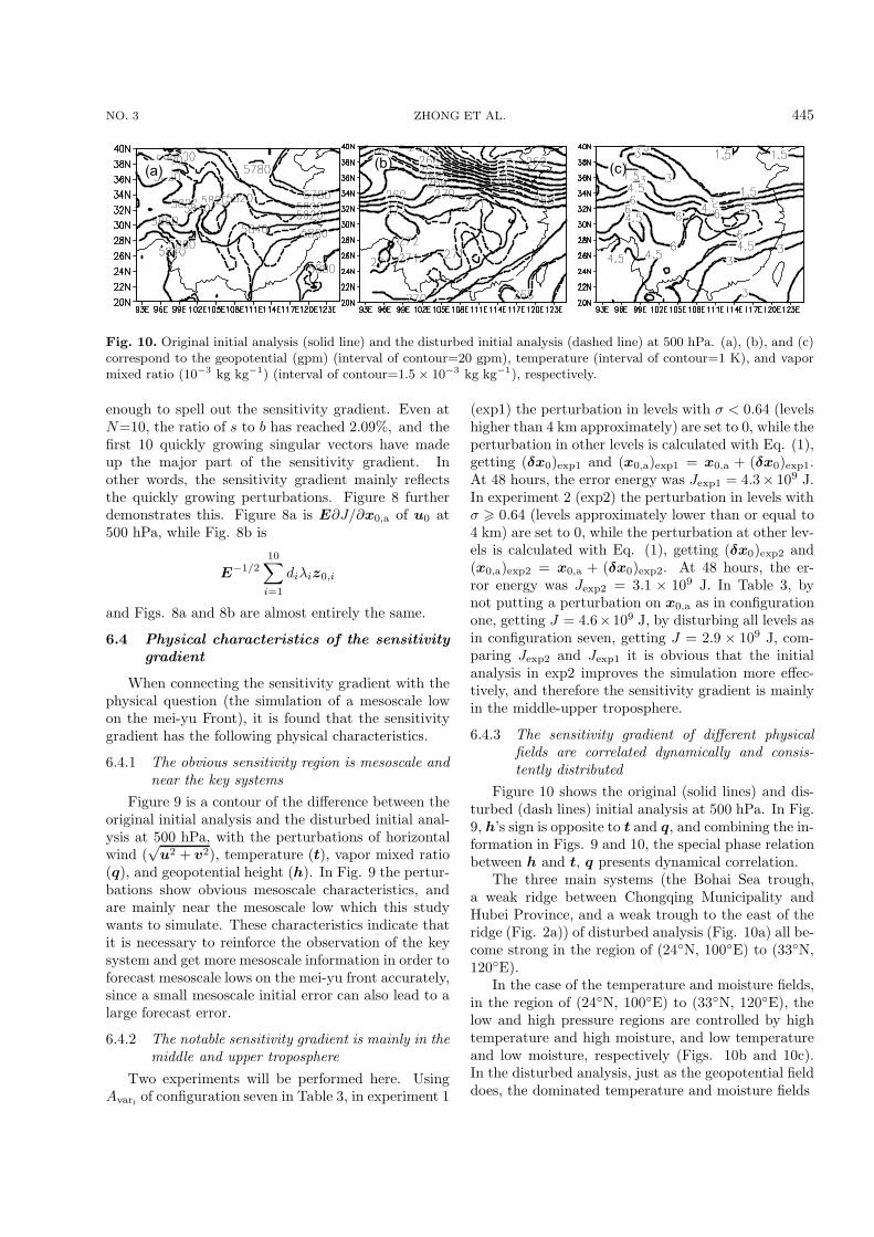
Fig. 10. Original initial analysis (solid line) and the disturbed initial analysis (dashed line) at 500 hPa. (a), (b), and (c)correspond to the geopotential (gpm) (interval of contour=20 gpm), temperature (interval of contour=1 K), and vapormixed ratio (10−3 kg kg−1) (interval of contour=1.5 × 10−3 kg kg−1), respectively.

enough to spell out the sensitivity gradient. Even atN=10, the ratio of s to b has reached 2.09%, and thefirst 10 quickly growing singular vectors have madeup the major part of the sensitivity gradient. Inother words, the sensitivity gradient mainly reflectsthe quickly growing perturbations. Figure 8 furtherdemonstrates this. Figure 8a is E∂J/∂x0,a of u0 at500 hPa, while Fig. 8b is

E−1/210∑

i=1

diλiz0,i

and Figs. 8a and 8b are almost entirely the same.

6.4 Physical characteristics of the sensitivitygradient

When connecting the sensitivity gradient with thephysical question (the simulation of a mesoscale lowon the mei-yu Front), it is found that the sensitivitygradient has the following physical characteristics.

6.4.1 The obvious sensitivity region is mesoscale andnear the key systems

Figure 9 is a contour of the difference between theoriginal initial analysis and the disturbed initial anal-ysis at 500 hPa, with the perturbations of horizontalwind (

√u2 + v2), temperature (t), vapor mixed ratio

(q), and geopotential height (h). In Fig. 9 the pertur-bations show obvious mesoscale characteristics, andare mainly near the mesoscale low which this studywants to simulate. These characteristics indicate thatit is necessary to reinforce the observation of the keysystem and get more mesoscale information in order toforecast mesoscale lows on the mei-yu front accurately,since a small mesoscale initial error can also lead to alarge forecast error.

6.4.2 The notable sensitivity gradient is mainly in themiddle and upper troposphere

Two experiments will be performed here. UsingAvari of configuration seven in Table 3, in experiment 1

(exp1) the perturbation in levels with σ < 0.64 (levelshigher than 4 km approximately) are set to 0, while theperturbation in other levels is calculated with Eq. (1),getting (δx0)exp1 and (x0,a)exp1 = x0,a + (δx0)exp1.At 48 hours, the error energy was Jexp1 = 4.3× 109 J.In experiment 2 (exp2) the perturbation in levels withσ � 0.64 (levels approximately lower than or equal to4 km) are set to 0, while the perturbation at other lev-els is calculated with Eq. (1), getting (δx0)exp2 and(x0,a)exp2 = x0,a + (δx0)exp2. At 48 hours, the er-ror energy was Jexp2 = 3.1 × 109 J. In Table 3, bynot putting a perturbation on x0,a as in configurationone, getting J = 4.6×109 J, by disturbing all levels asin configuration seven, getting J = 2.9 × 109 J, com-paring Jexp2 and Jexp1 it is obvious that the initialanalysis in exp2 improves the simulation more effec-tively, and therefore the sensitivity gradient is mainlyin the middle-upper troposphere.

6.4.3 The sensitivity gradient of different physicalfields are correlated dynamically and consis-tently distributed

Figure 10 shows the original (solid lines) and dis-turbed (dash lines) initial analysis at 500 hPa. In Fig.9, h’s sign is opposite to t and q, and combining the in-formation in Figs. 9 and 10, the special phase relationbetween h and t, q presents dynamical correlation.

The three main systems (the Bohai Sea trough,a weak ridge between Chongqing Municipality andHubei Province, and a weak trough to the east of theridge (Fig. 2a)) of disturbed analysis (Fig. 10a) all be-come strong in the region of (24◦N, 100◦E) to (33◦N,120◦E).

In the case of the temperature and moisture fields,in the region of (24◦N, 100◦E) to (33◦N, 120◦E), thelow and high pressure regions are controlled by hightemperature and high moisture, and low temperatureand low moisture, respectively (Figs. 10b and 10c).In the disturbed analysis, just as the geopotential fielddoes, the dominated temperature and moisture fields


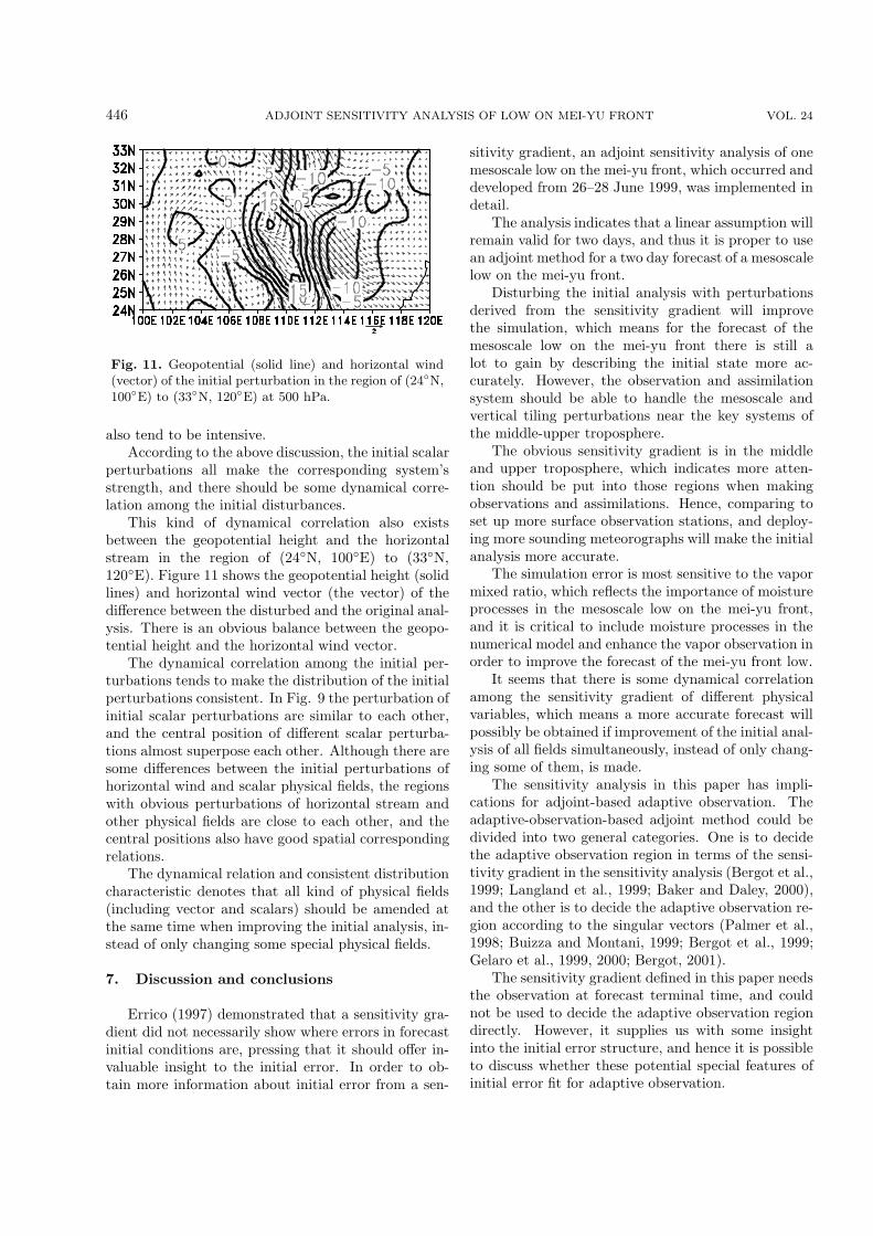
Fig. 11. Geopotential (solid line) and horizontal wind(vector) of the initial perturbation in the region of (24◦N,100◦E) to (33◦N, 120◦E) at 500 hPa.

also tend to be intensive.According to the above discussion, the initial scalar

perturbations all make the corresponding system’sstrength, and there should be some dynamical corre-lation among the initial disturbances.

This kind of dynamical correlation also existsbetween the geopotential height and the horizontalstream in the region of (24◦N, 100◦E) to (33◦N,120◦E). Figure 11 shows the geopotential height (solidlines) and horizontal wind vector (the vector) of thedifference between the disturbed and the original anal-ysis. There is an obvious balance between the geopo-tential height and the horizontal wind vector.

The dynamical correlation among the initial per-turbations tends to make the distribution of the initialperturbations consistent. In Fig. 9 the perturbation ofinitial scalar perturbations are similar to each other,and the central position of different scalar perturba-tions almost superpose each other. Although there aresome differences between the initial perturbations ofhorizontal wind and scalar physical fields, the regionswith obvious perturbations of horizontal stream andother physical fields are close to each other, and thecentral positions also have good spatial correspondingrelations.

The dynamical relation and consistent distributioncharacteristic denotes that all kind of physical fields(including vector and scalars) should be amended atthe same time when improving the initial analysis, in-stead of only changing some special physical fields.

7. Discussion and conclusions

Errico (1997) demonstrated that a sensitivity gra-dient did not necessarily show where errors in forecastinitial conditions are, pressing that it should offer in-valuable insight to the initial error. In order to ob-tain more information about initial error from a sen-

sitivity gradient, an adjoint sensitivity analysis of onemesoscale low on the mei-yu front, which occurred anddeveloped from 26–28 June 1999, was implemented indetail.

The analysis indicates that a linear assumption willremain valid for two days, and thus it is proper to usean adjoint method for a two day forecast of a mesoscalelow on the mei-yu front.

Disturbing the initial analysis with perturbationsderived from the sensitivity gradient will improvethe simulation, which means for the forecast of themesoscale low on the mei-yu front there is still alot to gain by describing the initial state more ac-curately. However, the observation and assimilationsystem should be able to handle the mesoscale andvertical tiling perturbations near the key systems ofthe middle-upper troposphere.

The obvious sensitivity gradient is in the middleand upper troposphere, which indicates more atten-tion should be put into those regions when makingobservations and assimilations. Hence, comparing toset up more surface observation stations, and deploy-ing more sounding meteorographs will make the initialanalysis more accurate.

The simulation error is most sensitive to the vapormixed ratio, which reflects the importance of moistureprocesses in the mesoscale low on the mei-yu front,and it is critical to include moisture processes in thenumerical model and enhance the vapor observation inorder to improve the forecast of the mei-yu front low.

It seems that there is some dynamical correlationamong the sensitivity gradient of different physicalvariables, which means a more accurate forecast willpossibly be obtained if improvement of the initial anal-ysis of all fields simultaneously, instead of only chang-ing some of them, is made.

The sensitivity analysis in this paper has impli-cations for adjoint-based adaptive observation. Theadaptive-observation-based adjoint method could bedivided into two general categories. One is to decidethe adaptive observation region in terms of the sensi-tivity gradient in the sensitivity analysis (Bergot et al.,1999; Langland et al., 1999; Baker and Daley, 2000),and the other is to decide the adaptive observation re-gion according to the singular vectors (Palmer et al.,1998; Buizza and Montani, 1999; Bergot et al., 1999;Gelaro et al., 1999, 2000; Bergot, 2001).

The sensitivity gradient defined in this paper needsthe observation at forecast terminal time, and couldnot be used to decide the adaptive observation regiondirectly. However, it supplies us with some insightinto the initial error structure, and hence it is possibleto discuss whether these potential special features ofinitial error fit for adaptive observation.


One requirement must be satisfied when puttingadaptive observation into practice: the extra observa-tion network should be limited to the local region, sothat the limited number plane or some other equip-ment can make observation efficient. The above dis-cussion has showed that the sensitivity gradient is lo-calized, and the sensitivity gradient distributions ofdifferent physical fields tend to be consistent. Theadaptive observation region decided by this kind ofsensitivity gradient will fulfill the requirement of adap-tive observation.

As for the singular-vector-based adaptive observa-tion, it is important to decide how many and whichsingular vectors should be used to decide the adaptiveobservation region. In this paper, the singular vectorsare calculated with the total dry energy norm, and it isfound that the sensitivity gradient is dominated by theleading singular vectors. This attribute means that itis proper and also enough to use the several leadingsingular vectors to decide the extra observation net-work in adaptive observation.

Future work will concentrate on deciding to whatextent the observation error is similar to the sensitivitygradient. Some unconventional data, such as satellitedata, will be put into the assimilation system, and thena new initial analysis will be formed. After comparingthe difference of the new and original initial analyseswith the sensitivity gradient, we could get more un-derstanding to this question.

Acknowledgements. This work was supported by

the National Natural Science Foundation of China under

Grant No. 40405020.

REFERENCES

Baker, N. L., and R. Daley, 2000: Observationand background adjoint sensitivity in the adaptiveobservation-targeting problem. Quart. J. Roy. Me-teor. Soc., 126, 1431–1454.

Bergot, T., 2001: Influence of the assimilation schemeon the efficiency of adaptive observations. Quart. J.Roy. Meteor. Soc., 127, 635–660.

Bergot, T., G.. Hello, A. Joly, and S. Malardel, 1999:Adaptive observation: a feasibility study. Mon. Wea.Rev., 127, 743–765.

Berliner, L. M., Z.-Q. Lu, and C. Snyder, 1999: Statisticaldesign for adaptive weather observations. J. Atmos.Sci., 56, 2536–2552.

Bishop, C. H., and Z. Toth, 1999: Ensemble transforma-tion and adaptive observations. J. Atmos. Sci., 56,1748–1765.

Bishop, C. H., B. J. Etherton, and S. J. Majumdar,2001: Adaptive sampling with the ensemble trans-form kalman filter. Part I: theoretical aspects. Mon.Wea. Rev., 129, 420–436.

Buizza, R., 1995: Optimal perturbation time evolutionand sensitivity of ensemble prediction to perturba-tion amplitude. Quart. J. Roy. Meteor. Soc., 121,1705–1738.

Buizza, R., and T. N. Palmer, 1995: The singular-vectorstructure of the atmospheric general circulation. J.Atmos. Sci., 52, 1434–1456.

Buizza, R., and A. Montani, 1999: Targeting observationsusing singular vector. J. Atmos. Sci., 56, 2965–2985.

Emanuel, K., and Coauthors, 1995: Report of the firstprospectus development team of the U.S. weatherresearch-program to NOAA and the NSF. Bull.Amer. Meteor. Soc., 76, 1194–1208.

Errico, R. M., 1997: What is an adjoint model. Bull.Amer. Meteor. Soc., 78, 2577–2591.

Errico, R. M., and T. Vukicevic, 1992: Sensitivity anal-ysis using an adjoint of the PSU-NCAR meso-scalModel. Mon. Wea. Rev., 120, 1644–1660.

Gelaro, R., R. Buizza, T. N. Palmer, and E. Klinker,1998: Sensitivity analysis of forecast errors and theconstruction of optimal perturbations using singularvectors. J. Atmos. Sci., 55, 1012–1037.

Gelaro, R., R. Langland, G.. D. Rohaly, and T. E. Ros-mond, 1999: An assessment of the singular vector ap-proach to targeted observations using the FASTEXdata set. Quart. J. Roy. Meteor. Soc., 125, 3299–3327.

Gelaro, R., C. A. Reynolds, R. H. Langland, and G. D.Rohaly, 2000: A predictability study using geosta-tionary satellite wind observations during NORPEX.Mon. Wea. Rev., 128, 3789–3807.

Gilmour, I., and L. A. Smith, 1997: Enlightenment inshadows. Applied Nonlinear Dynamics and Stochas-tic Systems Near the Millenium. J. B. Kadtke and A.Bulsara, Eds., American Institute of Physics, 335–340.

Hansen, J. A., and L. A. Smith, 2000: The role of oper-ational constraints in selecting supplementary obser-vations. J. Atmos. Sci., 57, 2859–2871.

Joly, A., and Coauthors, 1997: The Fronts and AtlanticStorm-Track Experiment (FASTEX): Scientific ob-jectives and experimental design. Bull. Amer. Me-teor. Soc., 78, 1917–1940.

Klinder, E., F. Rabier, and R. Gelaro, 1998: Estimationof key analysis errors using the adjoint technique.Quart. J. Roy. Meteor. Soc., 124, 1909–1933.

Kuo, Y. H., L. Cheng, and R. A. Anthes, 1986: Mesoscaleanalyses of Sichuan flood catastrophe 11–15 July1981. Mon. Wea. Rev., 114, 1984–2003.

Langland, R., and G. Rohaly, 1996: Adjoint-basedtargeting of observation for FASTEX cyclones.Preprints, Seventh Conf. on Mesoscale Process,Reading, United Kingdom, Amer. Meteor. Soc., 369–371.

Langland, R., R. Gelaro, G. D. Rohaly, and M. A.Shapiro, 1999: Targeted observations in FASTEX:Adjoint based targeting procedures and data impactexperiments in IOP/8 and IOP/8. Quart. J. Roy.Meteor. Soc., 125, 3241–3270.


Lorenz, E. N., and K. Emannel, 1998: Optimal sitesfor supplementary weather observations: Simulationwith a small model. J. Atmos. Sci., 55, 399–414.

Majumdar, S. J., C. H. Bishop, and B. J. Etherton,2002: Adaptive sampling with the ensemble trans-form Kalman filter. Part II: field program implemen-tation. Mon. Wea. Rev., 130, 1356–1369.

Palmer, T. N., R. Buizza, F. Molteni, Y. Q. Chen, and S.Corti, 1994: Singular vectors and the predictabilityof weather and climate. Philosophical Transactions:Physical Sciences and Engineering, 348, 459–475.

Palmer, T. N., R. Gelaro, J. Barkmeijer, and R. Buizza,1998: Singular vectors, metrics, and adaptive obser-vations. J. Atmos. Sci., 55, 633–653.

Rabier, F., E. Klinker, P. Courtier, and A. Hollingsworth,

1996: Sensitivity of forecast errors to initial condi-tions. Quart. J. Roy. Meteor. Soc., 122, 121–150.

Wang, Z., and K. Gao, 2003: Sensitivity experiments ofan eastward-moving southwest vortex to initial per-turbations. Adv. Atmos. Sci., 20, 638–649.

Wu, G. X., and S. J. Chen, 1985: The effect of mechan-ical forcing on the formation of a mesoscale vortex.Quart. J. Roy. Meteor. Soc., 111, 1049–1070.

Zou, X., F. Vandenberghe, M. Pondeca, and Y.-H.Kuo, 1997: Introduction to adjoint techniques andthe MM5 adjoint modeling system. NCAR/TN-435-STR, 1–107.

Zou, X., W. Huang, and Q. Xiao, 1998: A user’s guideto the MM5 adjoint modeling system. NCAR/TN-437+IA, 1–94.

Adjoint-based sensitivity analysis of a mesoscale low on the mei-yu front and its implications for...

Documents

Transcript of Adjoint-based sensitivity analysis of a mesoscale low on the mei-yu front and its implications for...