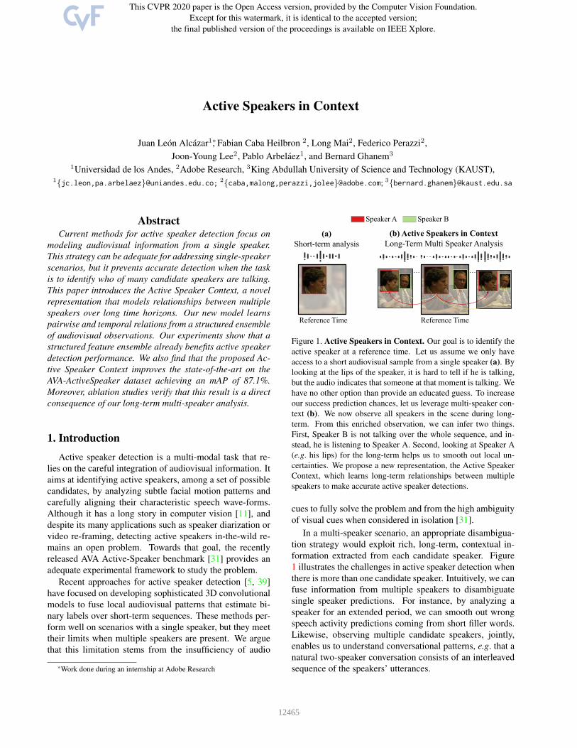
Active Speakers in Context

Juan Leon Alcazar1*, Fabian Caba Heilbron 2, Long Mai2, Federico Perazzi2,

Joon-Young Lee2, Pablo Arbelaez1, and Bernard Ghanem3

1Universidad de los Andes, 2Adobe Research, 3King Abdullah University of Science and Technology (KAUST),1{jc.leon,pa.arbelaez}@uniandes.edu.co; 2{caba,malong,perazzi,jolee}@adobe.com; 3{bernard.ghanem}@kaust.edu.sa

AbstractCurrent methods for active speaker detection focus on

modeling audiovisual information from a single speaker.

This strategy can be adequate for addressing single-speaker

scenarios, but it prevents accurate detection when the task

is to identify who of many candidate speakers are talking.

This paper introduces the Active Speaker Context, a novel

representation that models relationships between multiple

speakers over long time horizons. Our new model learns

pairwise and temporal relations from a structured ensemble

of audiovisual observations. Our experiments show that a

structured feature ensemble already benefits active speaker

detection performance. We also find that the proposed Ac-

tive Speaker Context improves the state-of-the-art on the

AVA-ActiveSpeaker dataset achieving an mAP of 87.1%.

Moreover, ablation studies verify that this result is a direct

consequence of our long-term multi-speaker analysis.

1. Introduction

Active speaker detection is a multi-modal task that re-

lies on the careful integration of audiovisual information. It

aims at identifying active speakers, among a set of possible

candidates, by analyzing subtle facial motion patterns and

carefully aligning their characteristic speech wave-forms.

Although it has a long story in computer vision [11], and

despite its many applications such as speaker diarization or

video re-framing, detecting active speakers in-the-wild re-

mains an open problem. Towards that goal, the recently

released AVA Active-Speaker benchmark [31] provides an

adequate experimental framework to study the problem.

Recent approaches for active speaker detection [5, 39]

have focused on developing sophisticated 3D convolutional

models to fuse local audiovisual patterns that estimate bi-

nary labels over short-term sequences. These methods per-

form well on scenarios with a single speaker, but they meet

their limits when multiple speakers are present. We argue

that this limitation stems from the insufficiency of audio

*Work done during an internship at Adobe Research

(a)

Short-term analysis

(b) Active Speakers in Context

Long-Term Multi Speaker Analysis

……

Reference TimeReference Time

Speaker A Speaker B

Figure 1. Active Speakers in Context. Our goal is to identify the

active speaker at a reference time. Let us assume we only have

access to a short audiovisual sample from a single speaker (a). By

looking at the lips of the speaker, it is hard to tell if he is talking,

but the audio indicates that someone at that moment is talking. We

have no other option than provide an educated guess. To increase

our success prediction chances, let us leverage multi-speaker con-

text (b). We now observe all speakers in the scene during long-

term. From this enriched observation, we can infer two things.

First, Speaker B is not talking over the whole sequence, and in-

stead, he is listening to Speaker A. Second, looking at Speaker A

(e.g. his lips) for the long-term helps us to smooth out local un-

certainties. We propose a new representation, the Active Speaker

Context, which learns long-term relationships between multiple

speakers to make accurate active speaker detections.

cues to fully solve the problem and from the high ambiguity

of visual cues when considered in isolation [31].

In a multi-speaker scenario, an appropriate disambigua-

tion strategy would exploit rich, long-term, contextual in-

formation extracted from each candidate speaker. Figure

1 illustrates the challenges in active speaker detection when

there is more than one candidate speaker. Intuitively, we can

fuse information from multiple speakers to disambiguate

single speaker predictions. For instance, by analyzing a

speaker for an extended period, we can smooth out wrong

speech activity predictions coming from short filler words.

Likewise, observing multiple candidate speakers, jointly,

enables us to understand conversational patterns, e.g. that a

natural two-speaker conversation consists of an interleaved

sequence of the speakers’ utterances.

12465

In this paper, we introduce the Active Speaker Con-

text, a novel representation that models long-term interac-

tions between multiple speakers for in-the-wild videos. Our

method estimates active speaker scores by integrating au-

diovisual cues from every speaker present in a conversation

(or scene). It leverages two-stream architectures [6, 9, 10] to

encode short-term audiovisual observations, sampled from

the speakers in the conversation, thus creating a rich con-

text ensemble. Our experiments indicate that this context,

by itself, helps improve accuracy in active speaker detec-

tion. Furthermore, we propose to refine the computed con-

text representation by learning pairwise relationships via

self-attention [33] and by modeling the temporal structure

with a sequence-to-sequence model [17]. Our model not

only improves the state-of-the-art but also exhibits robust

performance for challenging scenarios that contain multiple

speakers in the scene.

Contributions. In this work we design and validate a model

that learns audiovisual relationships among multiple speak-

ers. To this end, our work brings two contributions.1

(1) We develop a model that learns non-local relationships

between multiple speakers over long timespans (Section 3).

(2) We observe that this model improves the state-of-the-

art in the AVA-ActiveSpeaker dataset by 1.6%, and that this

improvement is a direct result of modeling long-term multi-

speaker context (Section 4).

2. Related Work

Multi-modal learning aims at fusing multiple sources of

information to establish a joint representation, which mod-

els the problem better than any single source in isolation

[27]. In the video domain, a form of modality fusion with

growing interest in the scientific community involves the

learning of joint audiovisual representations [3, 7, 19, 25,

28, 34]. This setting includes problems such as person

re-identification [20, 24, 37], audio-visual synchronization

[8, 9], speaker diarization [38], bio-metrics [25, 30], and

audio-visual source separation [3, 7, 19, 25, 28, 34]. Ac-

tive speaker detection, the problem studied in this paper,

is an specific instance of audiovisual source separation, in

which the sources are persons in a video (candidate speak-

ers), and the goal is to assign a segment of speech to an

active speaker, or none of the available sources.

Several studies have paved the way for enabling active

speaker detection using audiovisual cues [3, 4, 9, 11]. Cut-

ler and Davis pioneered the research [11] in the early 2000s.

Their work proposed a time-delayed neural network to learn

the audiovisual correlations from speech activity. Alterna-

tively, other methods [13, 32] opted for using visual infor-

mation only, especially the lips motion, to address the task.

1To enable reproducibility and promote future research, code

has been made available at: https://github.com/fuankarion/

active-speakers-context

Recently, rich alignment between audio and visual informa-

tion has been re-explored with methods that leverage audio

as supervision [3], or jointly train an audiovisual embedding

[7, 9, 26], that enables more accurate active speaker detec-

tion. Although these previous approaches were seminal to

the field, the lack of large-scale data for training and bench-

mark limited their application to in-the-wild active speaker

detection in movies or consumer videos.

To overcome the lack of diverse and in-the-wild data,

Roth et al. [31], introduced AVA-ActiveSpeaker, a large-

scale video dataset devised for the active speaker detection

task. With the release of the dataset and its baseline –a two-

stream network that learns to detect active speakers within

a multi-task setting– a few novel approaches have started

to emerge. In the AVA-ActiveSpeaker challenge of 2019,

Chung et al. [5] improved the core architecture of their

previous work [9] by adding 3D convolutions and leverag-

ing large-scale audiovisual pre-training. The submission of

Zhang et al. [39] also relied on a hybrid 3D-2D architecture,

with large-scale pre-training on two multi-modal datasets

[9, 10]. Their method achieved the best performance when

the feature embedding was refined using a contrastive loss

[15]. Both approaches improved the representation of a

single speaker, but ignored the rich contextual information

from co-occurring speaker relationships, and intrinsic tem-

poral structures that emerge from dialogues.

Our approach starts from the baseline of a two-stream

modality fusion but explores an orthogonal research direc-

tion. Instead of improving the performance of a short-term

architecture, we aim at modeling the conversational con-

text of speakers, i.e. to leverage active speaker context from

long-term inter-speaker relations. Context modeling has

been widely studied in computer vision tasks such as ob-

ject classification [23], video question answering [40], per-

son re-identification[22], or action detection [14, 36]. De-

spite the existence of many works harnessing context to im-

prove computer vision systems, our model is unique and

tailored to detect active speakers accurately. To the best of

our knowledge, our work is the first to address the task of

active speaker detection in-the-wild using contextual infor-

mation from multiple speakers.

3. Active Speakers in Context

This section describes our approach to active speaker

detection, which focuses on learning long-term and inter-

speaker relationships. At its core, our strategy estimates an

active speaker score for an individual face (target face) by

analyzing the target itself, the current audio input, and mul-

tiple faces detected at the current timestamp.

Instead of holistically encoding long time horizons and

multi-speaker interactions, our model learns relationships

following a bottom-up strategy where it first aggregates

fine-grained observations (audiovisual clips), and then maps

12466

Short-Term Encoder (STE)

STE

Ct

STE

Pairwise Refinement

W⍺ :1x1x1

Wβ :1x1x1

W𝛾 :1x1x1

Transpose

Softmax

Wδ:1x1x1

C†t

Audio

CNN

Visual

CNN

.

.

.

.

.

. Temporal Refinement

LSTM...

z1 z2 zi

Active Speaker

...

t – T/2

t + T/2

t

Tim

e

Figure 2. Active Speaker Context. Our approach first splits the video data into short clips (τ seconds) composed by a stack of face

crops and their associated audio. It encodes each of these clips using a two-stream architecture (Short-Term Encoder) to generate a low-

dimensional audiovisual encoding. Then, it stacks the high-level audiovisual features from all the clips and all the speakers sampled within

a window of size T (T > τ ) centered at a reference time t. We denote this stack of features as Ct. Then, using self-attention, our approach

refines the representation by learning a pairwise attention between all elements. Finally, an LSTM mines temporal relationships across the

refined features. This final output is our Active Speaker Context, which we use to classify speech activity of a candidate at time t.

these observations into an embedding that allows the anal-

ysis of global relations between clips. Once the individual

embeddings have been estimated, we aggregate them into a

context-rich representation which we denote as the Active

Speaker Ensemble. This ensemble is then refined to explic-

itly model pairwise relationships, and to explicitly model

long-term structures over the clips, we name this refined

ensemble the Active Speaker Context. Figure 2 presents an

overview of our approach.

3.1. Aggregating Local Video InformationOur proposal begins by analyzing audiovisual informa-

tion from short video clips. The visual information is a stack

of k consecutive face crops 2 sampled from a time interval

τ . The audio information is the raw wave-form sampled

over the same τ interval. We refer to these clips as a tuples

cs,τ = {vs, aτ}, where vs is a crop stack of a speaker s,

and aτ is the corresponding audio. For every clip cs,τ in

a video sequence, we compute an embedding us,τ using a

short-term encoder Φ(cs,τ ) whose role is twofold. First, it

creates a low-dimensional representation that fuses the au-

diovisual information. Second, it ensures that the embed-

ded representation is discriminative enough for the active

speaker detection task.

Short-term Encoder (Φ). Following recent works [6, 31,

39], we approximate Φ by means of a two-stream convo-

lutional architecture. Instead of using compute-intensive

3D convolutions as in [5, 39], we opt for 2D convolutions

in both streams. The visual stream takes as input a ten-

sor v ∈ RH×W×(3k), where H and W are the width and

height of k face crops. On the audio stream, we convert the

2Our method leverages pre-computed face tracks (consecutive face

crops) at training and testing time.

raw audio waveform into a Mel-spectrogram represented as

a ∈ RQ×P , where Q and P depend on the length of the

interval τ . On a forward pass the visual sub-network es-

timates a visual embedding uv ∈ Rdv , while the audio

sub-network computes an audio embedding ua ∈ Rda . We

compose an audiovisual feature embedding u ∈ Rd by con-

catenating the output embedding of each stream.

Structured Context Ensemble. Once the clip features

u ∈ Rd have been estimated, we proceed to assemble

these features into a set that encodes contextual informa-

tion. We denote this set as the Active Speaker Ensemble.

To construct this ensemble, we first define a long interval T

(T > τ ) centered at a reference time t, and designate one of

the speakers present at t as the reference speaker and every

other speaker is designated as context speaker.

We proceed to compute us,τ for every speaker s =1, . . . , S present at t over L different τ intervals throughout

temporal window T . This sampling scheme yields a tensor

Ct with dimensions L×S×d, where S is the total number

of speakers analyzed. Figure 3 contains a detailed example

on the sampling process.

We assemble Ct for every possible t in a video. Since

temporal structures are critical in the active speaker prob-

lem, we strictly preserve the temporal order of the sampled

features. As Ct is defined for a reference speaker, we can

generate as many ensembles Ct as speakers are present at

time t. In practice, we always locate the feature set of the

reference speaker as the first element along the S axis of

Ct. Context speakers are randomly stacked along the re-

maining positions on the S axis. This enables us to directly

supervise the label of the reference speaker regardless of the

number or order of the context speakers.

12467

Figure 3. Building Context Tensors. We build a context ensem-

ble given a reference speaker (Speaker 1 in this example), and a

reference time t. First, we define a long-term sampling window T

containing L+1 clips centered at time t, T = {0, 1, ..., t, ..., L−1, L}. We select as context speakers those that overlap with the

reference speaker at t (speakers 2 and 3). Finally, we sample clip-

level features ul throughout the whole sampling window T from

the reference speaker and all the speakers designated as context.

If the temporal span of the speaker does not entirely match the in-

terval T, we pad it with the initial or final speaker features. For

instance, Speaker 2 is absent between 0 and i, so we pad left with

ui. Similarly, for speaker 3, we pad right with uk. Notice that,

by our definition, Speakers 2 and 3 could switch positions, but

Speaker 1 must remain at the bottom of the stack.

3.2. Context RefinementAfter constructing the context ensemble Ct, we are left

with the task of classifying the speaking activity of the des-

ignated reference speaker. A naive approach would fine-

tune a fully-connected layer over Ct with binary output

classes i.e. speaking and silent. Although such a model al-

ready leverages global information beyond clips, we found

that it tends not to encode useful relationships between

speakers and their temporal patterns, which emerge from

conversational structures. This limitation inspires us to

design our novel Active Speaker Context (ASC) model.

ASC consists of two core components. First, it implements

a multi-modal self-attention mechanism to establish pair-

wise interactions between the audiovisual observations on

Ct. Second, it incorporates a long-term temporal encoder,

which exploits temporal structures in conversations.

Pairwise Refinement. We start from the multi-modal

context ensemble Ct, and model pairwise affinities between

observations in Ct regardless of their temporal order or the

speaker they belong to. We do this refinement by following

a strategy similar to Vaswani et al. [33]. We compute self-

attention over long-term sequences and across an arbitrary

number of candidate speakers.

In practice, we adapt the core idea of pair-wise atten-

tion from the non-local framework [35] to work over multi-

modal high-level features, thereby estimating a dense atten-

tion map over the full set of clips contained in the sampling

window T . We avoid using this strategy over low or mid-

level features as there is no need to relate distributed in-

formation on the spatial or temporal domains of a clip i.e.

in the active speaker detection task, meaningful informa-

tion is tightly localized on the visual (lips region) and audio

(speech snippets) domains.

We implement a self-attention module that first estimates

a pairwise affinity matrix B with dimension LS × LS and

then uses its normalized representation as weights for the

input Ct :

B = σ((Wα ∗Ct) · (Wβ ∗Ct)⊤) (1)

C†t = Wδ ∗ (B · (Wγ ∗Ct)) +Ct (2)

Where σ is a softmax operation, {Wα,Wβ ,Wγ ,Wδ} are

learnable 1 × 1 × 1 weights that adapt the channel dimen-

sions as needed, and the second term in Equation 2 (+Ct)

denotes a residual connection. The output C†t is a tensor

with identical dimensions as the input Ct (L× S × d), but

it now encodes the pairwise relationships.

Temporal Refinement. The goal of this long-term pool-

ing step is two-fold. First, to refine the weighted features

in C†t by directly attending to their temporal structure. Sec-

ond, to reduce the dimensionality of the final embedding to

d′ (d > d′), allowing us to use a smaller fully-connected

prediction layer. Given the inherent sequential structure

of the task, we implement this refinement using an LSTM

model [17]. We cast its input by squeezing the speaker and

time dimension of C†t into (L × S) × d; thus we input the

LSTM time steps ti ∈ {1, . . . , L × S}, with a feature vec-

tor zi ∈ Rd. In practice, we use a single uni-directional

LSTM unit with d′ = 128, and keep the LSTM memory as

it passes over the sequence. Thus, we create a sequence-

to-sequence mapping between tensor C†t ∈ R

(L×S)×d and

a our final Active Speaker Context representation ASCt ∈R

(L×S)×d′

.

Our final step consists of estimating the presence of

an active speaker given ASCt. We resort to a simple

fully-connected layer with binary output (active speaker and

silent). We establish the final confidence score using a soft-

max operator over the outputs and select the value of the

speaking class.

3.3. Training and Implementation Details

We use a two-stream (visual and audio) convolutional

encoder based on the Resnet-18 architecture [16] for the

Short-Term Feature extraction (STE). Following [31], we

re-purpose the video stream to accept a stack of N face

crops by replicating the weights on the input layer N times.

The audio stream input is a Mel-spectrogram calculated

from an audio snippet, which exactly matches the time in-

terval covered by the visual stack. Since Mel-spectrograms

are 2D tensors, we re-purpose the input of the audio stream

12468

to accept a L× P × 1 tensor by averaging channel-specific

weights at the input layer.

Training the Short-term Encoder We train the STE us-

ing the Pytorch library [29] for 100 epochs. We choose

the ADAM optimizer [21] with an initial learning rate of

3 × 10−4 and learning rate annealing γ = 0.1 every 40

epochs. We resize every face crop to 124×124 and per-

form random flipping and corner cropping uniformly along

the visual input stack. We drop the large-scale multi-modal

pre-training of [5], in favor of standard Imagenet [12] pre-

training for the initialization.

Since we want to favor the estimation of discrimina-

tive features on both streams, we follow the strategy pre-

sented by Roth et al. [31] and add two auxiliary supervi-

sion sources, and place them on top of both streams be-

fore the feature fusion operation, this creates two auxil-

iary loss functions La,Lv . Our final loss function is L =Lav +La+Lv . We use the standard Cross-entropy loss for

all three terms.

Training the Active Speaker Context Model We also

optimize the ASC using the Pytorch library and the ADAM

optimizer with an initial learning rate of 3×10−6 and learn-

ing rate annealing γ = 0.1 every 10 epochs. We train the

full ASC module from scratch and include batch normal-

ization layers to favor faster convergence [18]. Similar to

the STE, we use Cross-entropy loss to train ASC, but in this

scenario, the loss consists of a single term Lav .

The ASC processes a fixed number of speakers S to con-

struct Ct. Given that not every reference time t contains

the same number of speaker detections, there are three sce-

narios for J overlapping speakers and an ensemble of size

S. If J ≥ S, we randomly sample S − 1 context speakers

(one is already assigned as reference). If J < S, we se-

lect a reference, and randomly sample (with replacement)

S − 1 context speakers from the remaining J − 1 speakers.

In the extreme case where J = 1, the reference speaker is

replicated S − 1 times.

4. Experiments

This section evaluates our method’s ability to detect ac-

tive speakers in untrimmed videos. We conduct the ex-

periments using the large-scale AVA-ActiveSpeaker dataset

[31]. We divide the experiment analyses into three parts.

First, we compare our approach with the existing state-of-

the-art approaches. Then, we ablate our method and inspect

the contributions of each of its core components. Finally,

we do a performance breakdown and analyze success and

failure modes.

AVA-ActiveSpeaker dataset. The AVA-ActiveSpeaker

dataset [31] contains 297 Hollywood movies, with 133 of

those for training, 33 for validation and 131 for testing. The

dataset provides normalized bounding boxes for 5.3 million

faces (2.6M training, 0.76M validation, and 2.0M testing)

detected over 15-minute segments from each movie. These

detections occur at an approximate rate of 20fps and are

manually linked over time to produce face tracks depicting

a single identity (actor). Each face detection in the dataset is

augmented with a speaking or non-speaking attribute. Thus,

the task at inference time is to produce a confidence score

that indicates the chance of speaking for each given face

detection. In our experiments, we use the dataset official

evaluation tool, which computes the mean average preci-

sion (mAP) metric over the validation (ground-truth avail-

able) and test sets (ground-truth withheld). Unless men-

tioned otherwise, we evaluate active speaker detection on

the AVA-ActiveSpeaker validation subset.

Dataset sampling at training time. As noted by Roth et

al. [31], AVA-ActiveSpeaker has a much smaller variability

in comparison to natural image datasets with a comparable

size. For the training of the STE, we prevent over-fitting

by randomly sampling a single clip with k time contigu-

ous crops from every face track instead of densely sampling

every possible time contiguos clip of size k in the track-

let. Therefore, our epoch size correlates with the number

of face tracks rather than the number of face detections. To

train our context refinement models, we use standard dense

sampling over the training set, as we do not observe any

significant over-fitting in this stage.

4.1. Comparison with the State­of­the­art

We compare our method’s performance to the state-of-

the-art and summarize these results in Table 1. We set L =11 and S = 3 for the experiment. We report results on the

validation and testing subsets. The latter is withheld for the

AVA-ActiveSpeaker task in the ActivityNet challenge [2].

We observe that our method outperforms all existing ap-

proaches in the validation subset. This result is very fa-

vorable as the other methods rely on 3D convolutions and

large scale pre-training, while our model relies exclusively

on contextual information built from 2D models. The best

existing approach, Chung et al. [5], obtains 85.5%. Even

though their method uses a large-scale multi-modal dataset

for pre-training, our context modeling outperforms their so-

lution by 1.6%.

As Table 1 shows, our method achieves competitive re-

sults in the testing subset. Even though our model discards

3D convolutions and model ensembles [5], we rank 2nd in

the AVA-ActiveSpeaker 2019 Leaderboard3. The overall re-

sults on the AVA-ActiveSpeaker validation and testing sub-

sets validate the effectiveness of our approach. We empir-

ically demonstrate that it improves the state-of-the-art, but

a question remains. What makes our approach strong? We

answer that question next via ablation studies.

3http://activity-net.org/challenges/2019/evaluation.html

12469

Method mAP

Validation subset

Active Speakers Contex (Ours) 87.1

Chung et al. (Temporal Convolutions) [5] 85.5

Chung et al. (LSTM) [5] 85.1

Zhang et al. [39] 84.0

ActivityNet Challenge Leaderboard 2019

Naver Corporation [5] 87.8

Active Speakers Context (Ours) 86.7

University of Chinese Academy of Sciences [39] 83.5

Google Baseline [31] 82.1

Table 1. Comparison with the State-of-the-art. We report the

performance of state-of-the-art methods in the AVA Active Speak-

ers validation and testing subsets. Results in the validation set are

obtained using the official evaluation tool published by [31], test

set metrics are obtained using the the ActivityNet challenge evalu-

ation server. In the validation subset, we improve the performance

of previous approaches by 1.6%, without using large-scale multi-

modal pre-training. In the test subset, we achieve 86.7% and rank

second in the leaderboard, without using 3D convolutions, sophis-

ticated post-processing heuristics or assembling multiple models.

Context & Refinement mAP

No Context 79.5

Context + No Refinement 84.4

Context + Pairwise Refinement 85.2

Context + Pairwise Refinement + MLP 85.3

Context + Temporal Refinement 85.7

ASC 87.1

Table 2. Effect of context refinement. We ablate the contribu-

tions of our method’s core components. We begin with a baseline

that does not include any context, which achieves 79.5%. Then,

by simply leveraging context with a linear prediction layer, we

observe a significant boost of 4.9%. Additionally, we find that

adding pairwise and temporal refinement further improves the per-

formance by 0.8% and 1.3% respectively. The ASC best perfor-

mance is achieved only if both refinement steps are included.

4.2. Ablation Analysis

Does context refinement help? We first assess the effec-

tiveness of the core components of our approach. Table

2 compares the performance of the baseline, a two-stream

network (No Context) that encodes a single speaker in a

short period, a naive context prediction using a single linear

layer (Context + No Refinement), and three ablated variants

of our method, two of these variants verify the individual

contributions of the two ASC refinement steps (Context +

Pairwise Refinement and Context + Temporal Refinement),

the third (Context + Pairwise Refinement + MLP) has a two

layer perceptron which yields about the same number of pa-

rameters as the ASC, it is useful to test if the increased per-

formance derives from the increased size of the network.

While the initial assembly of the context tensor already

improves the baseline performance, our results show that

context refinement brings complementary gains. That is,

the active speaker detection task benefits not only from the

presence of additional clip information in the context, but

also profits from directly modeling speaker relationships

and temporal structures. We observe that our whole context

refinement process leads to an average of 4.73% mAP in-

crease over the context tensor and a naive prediction. These

results validate our design choice of distilling context via

the pairwise and temporal refinement modules.

Are there alternatives for temporal refinement? We

now compare our temporal refinement strategy against a

baseline strategy for temporal refinement. During the recent

ActivityNet challenge, Chung et al. [5] explored the moving

average strategy, reporting an increase of 1.3% mAP using

a median filter over prediction scores. A key difference is

that [5] processes short-term windows (0.5s), whereas we

consider windows of 2.25s. We found that smoothing long

temporal windows negatively impacts the performance of

our method. Table 3 shows that there is a negligible increase

(+0.02%) using short temporal averages, and a drastic drop

(−11.64%) using long averages.

w/o temporal + moving + moving + temporal

refinement average (0.5s) average (2.25s) refinement

85.21% +0.02% -11.64% +1.9%

Table 3. Moving average vs. temporal refinement (mAP). We

observe only marginal benefits when replacing the proposed tem-

poral smoothing step with a moving average, in fact this operation

has a large penalty when smoothing longer sampling windows.

Does context size matter? We continue the ablation by

analyzing the influence of context size on the final perfor-

mance of our method. Table 4 summarizes the two dimen-

sions of this analysis, where we vary the temporal support

(i.e. vary L from 1 to 11 clips), or alter the number of con-

text speakers (i.e. vary S from 1 to 3 speakers).

Overall, extended temporal contexts and more co-

occurring speakers at training time favor the performance

of our method. These results indicate that the proposed ap-

proach utilizes both types of context to disambiguate pre-

dictions for a single speaker. We observe a larger gap in

performance when switching between one to two speakers

(1.8% on average) than when switching between 2 and 3

(0.15% on average). This behavior might be due to the rela-

tive scarcity of samples containing more than three speakers

at training time. Regarding temporal support, we observe

gradual improvements by increasing L. However, as soon

as L reaches 11, we see diminishing returns that seem to

be correlated with the average length of face tracks in the

training subset. The context size analysis performed here

supports our central hypothesis that context from long-time

horizons and multiple-speakers is crucial for making accu-

rate active speaker detections.

12470

Temporal Number of Speakers (S)

Support (L) ↓ S = 1 S = 2 S = 3

L = 1 79.5 83.1 82.9

L = 3 83.1 84.6 85.0

L = 5 84.3 85.8 85.9

L = 7 84.9 86.4 86.6

L = 9 85.5 86.7 86.9

L = 11 85.6 87.0 87.1

Table 4. Impact of context size. We investigate the effect of dif-

ferent sizes of temporal support and the number of speakers used

to construct our context representation. To that end, We report

the mAP obtained by different context size configurations. We

observe that both types of context play a crucial role at boosting

performance. Using our longest temporal support, L = 11 (2.25

seconds), our method improves the baseline (L = 1 / S = 1)

by 6.1%. Moreover, when combined with context from multiple

speakers, i.e. L = 11 / S = 3, we achieve an additional boost of

1.5% resulting in our best performance of 87.1%. In short, our

findings reveal the importance of sampling context from long time

horizons and multiple speakers.

Sampling Distortion Type

Temporal Order Surrounding None

mAP 77.8 84.5 87.1

Table 5. Effect of context sampling distortion. We observe that

our method looses 2.6% mAP when the context speakers are ran-

domly sampled across the video. It also drastically drops (−9.3%)

when the context temporal order is scrambled. These results vali-

date the importance of sampling context for the target face within

the right surrounding and preserving its temporal order.

Does context sampling matter? We now evaluate the ef-

fect of tempering the temporal structure when construct-

ing Ct. We also assess the effectiveness of ’in-context’

speaker information, i.e. we study if sampling ’out-of-

context’ speakers degrades the performance of our ap-

proach. For the first experiment, we build Ct exactly as

outlined in Section 3.3, but randomly shuffle the temporal

sequence of all speakers except clips at reference time t. For

the second experiment we replace the context speakers with

a set of speakers sampled from a random time t′ such that

t′ 6= t. We report the results in Table 5.

Let us analyze the two sampling distortions one at a time.

First, the ablation results highlight the importance of the

temporal structure. If such a structure is altered, the effec-

tiveness of our method drops below that of the baseline to

77.8%. Second, it is also important to highlight that in-

corporating out-of-context speakers in our pipeline is worse

than using only the reference speaker (84.5% vs. 87.1%).

In other words, temporal structure and surrounding speakers

provide unique contextual cues that are difficult to replace

with random information sampled from a video.

1 2 3

Number of faces

0

20

40

60

80

100

mA

P(%

)

87.9

71.6

54.4

91.883.8

67.6

L M S

Face size

0

20

40

60

80

100

mA

P(%

)

86.4

68.3

44.9

92.2

79.0

56.2

Baseline Ours

Figure 4. Performance breakdown. We analyze the performance

of the baseline approach (w/o context) and our proposed method

(Active Speaker Context) under two different visual characteris-

tics of the samples at inference time: number of faces (left) and

face size (right). For the number of faces, we split the dataset

into three exclusive buckets: one, two, and three faces, which alto-

gether cover > 90% of the dataset. Similarly, we split the dataset

into three face sizes: Small (S), Medium (M), Large (L), corre-

sponding to face crops of width <= 64, > 64 but <= 128, and

> 128 pixels, respectively. In all scenarios, we observe that our

approach outperforms the baseline, with those gains being more

pronounced in challenging scenarios. For instance, when we com-

pare their performance for three (3) faces, our method offers a

significant boost of 13.2%. Moreover, for the hard case of small

faces (S), we achieve an improvement of 11.3% over the baseline.

4.3. Results Analysis

Performance Breakdown. Following recent works [1],

we break down our model’s and baseline performances in

terms of relevant characteristics of the AVA Active Speaker

dataset, namely number of faces and face size, which we

present in Figure 4. We also analyze the impact of noise in

speech and find that both our method and the baseline are

fairly robust to altered speech quality;

The performance breakdown for the number of faces in

Figure 4 (left) reveals the drawbacks of the baseline ap-

proach, and the benefits of ASC. We split the validation

frames into three mutually exclusive groups according to

the number of faces in the frame. For each group, we com-

pute the mAP of the baseline and our approach. Although

both follow a similar trend with performance decreasing as

the number of faces increases, our method is more resilient.

For instance, in the challenging case of three faces, our

method outperforms the baseline by 13.2%. This gain could

be due to our method leverages information from multiple

speakers at training time, making it aware of conversational

patterns and temporal structures unseen by the baseline.

Dealing with small faces is a challenge for active speaker

detection methods [31]. Figure 4 (right) presents how the

baseline and our ASC method are affected by face size.

12471

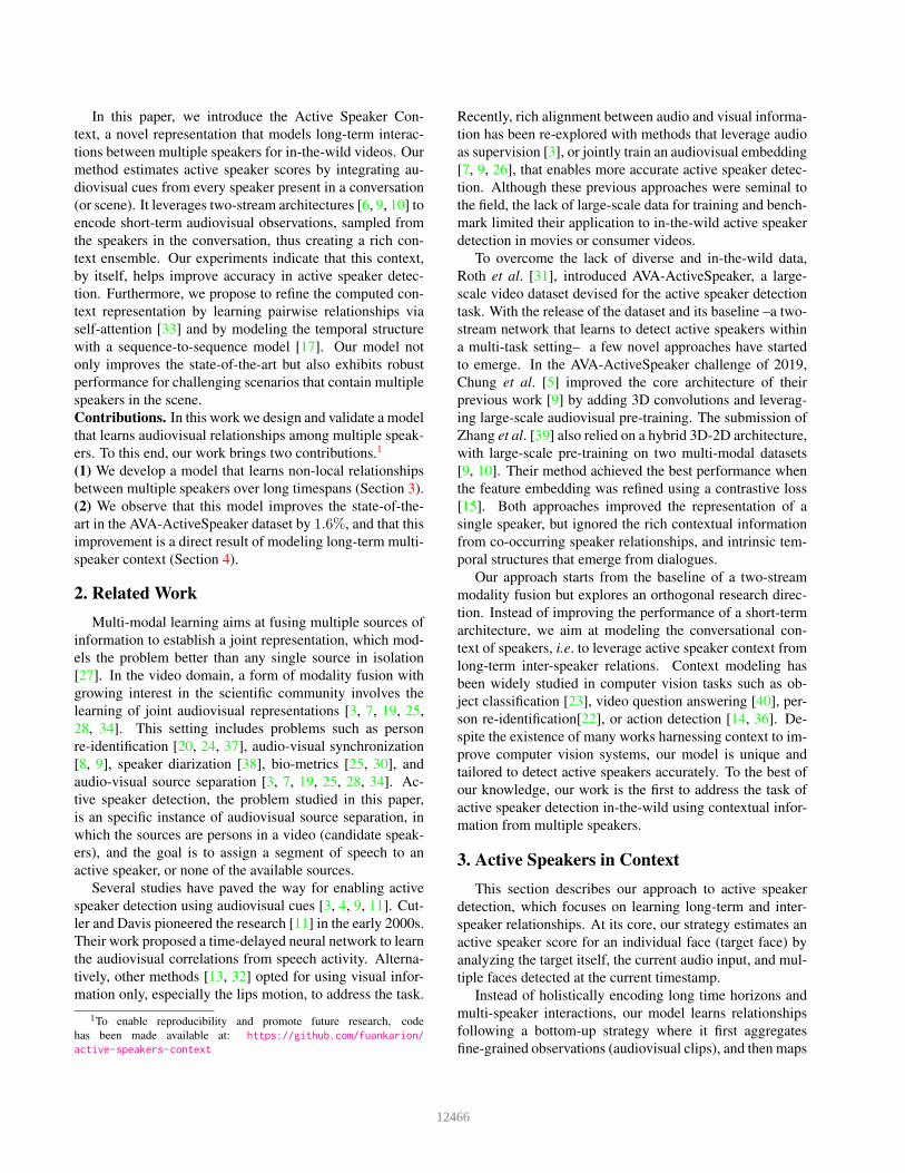
Figure 5. Qualitative results. The attention within the pairwise refinement step has some characteristic activation patterns. We highlight

the reference speaker in a yellow bounding box and represent the attention score with a heat-map growing from light-blue (no attention) to

red (the highest-attention). The first row shows a typical activation pattern for two silent speakers. The attention model focuses exclusively

on the reference speaker (highlighted in yellow) at the reference time. In the cases where there is an active speaker (second row), the

attention concentrates on the reference speaker over an extended time interval. In the third row, the reference speaker is also active, but in

this case, his facial gestures are ambiguous; thus, the attention also looks at the context speaker.

We divide the validation set into three splits: (S) small

faces with width less than 64 pixels, (M) medium faces

with width 64 and 128 pixels, and (L) large faces with

width more than 128 pixels. There is a correlation between

the performance of active speaker detection and face size.

Smaller faces are usually harder to label as active speakers.

However, our approach exhibits less performance degrada-

tion than the baseline as face size decreases. In the most

challenging case, i.e. small faces, our method outperforms

the baseline by 11.3%. We hypothesize that our method ag-

gregates information from larger faces via temporal context,

which enhances predictions for small faces.

Qualitative results. We analyze the pairwise relations

built on the matrix Ct on a model trained with only two

speakers. Figure 5 showcases three sample sequences cen-

tered at a reference time t, each containing two candidate

speakers. We highlight the reference speaker in yellow and

represent the attention score with a heat-map growing from

light-blue (no attention) to red (the highest-attention).

Overall we notice three interesting patterns. First, se-

quences labeled as silent generate very sparse activations

focusing on a specific timestamp (see top row). We hypoth-

esize that identifying the presence of speech is a much sim-

pler task than detecting the actual active speaker. Therefore,

our model reliably decides by only attending a short time

span. Second, for sequences with an active speaker, our

pairwise refinement tends to distribute the attention towards

a single speaker throughout the temporal window (see the

second row). Besides, the attention score tends to have a

higher value near the reference time and slowly decades as

it approaches the limit of the time interval. Third, we find

many cases in which our model attends to multiple speakers

in the scene. This behavior often happens when the facial

features of the reference speaker are difficult to observe or

highly ambiguous. For example, the reference speaker in

the third row is hard to see due to insufficient lighting and

face orientation in the scene. Hence, the network attends si-

multaneously to both the reference and the context speaker.

5. Conclusion

We have introduced a context-aware model for active

speaker detection that leverages cues from co-occurring

speakers and long-time horizons. We have shown that our

method outperforms the state-of-the-art in active speaker

detection, and works remarkably well in challenging sce-

narios when many candidate speakers or only small faces

are on-screen. We have mitigated existing drawbacks, and

hope our method paves the way towards more accurate ac-

tive speaker detection. Future explorations include using

speaker identities as a supervision source as well as learn-

ing to detect faces and their speech attribute jointly.

Acknowledgments. This publication is based on work sup-

ported by the King Abdullah University of Science and

Technology (KAUST) Office of Sponsored Research (OSR)

under Award No. OSR-CRG2017-3405, and by Uniandes-

DFG Grant No. P17.853122

12472

References

[1] Humam Alwassel, Fabian Caba Heilbron, Victor Escorcia,

and Bernard Ghanem. Diagnosing error in temporal action

detectors. In ECCV, 2018.[2] Fabian Caba Heilbron, Victor Escorcia, Bernard Ghanem,

and Juan Carlos Niebles. Activitynet: A large-scale video

benchmark for human activity understanding. In CVPR,

2015.[3] Punarjay Chakravarty, Sayeh Mirzaei, Tinne Tuytelaars, and

Hugo Van hamme. Who’s speaking? audio-supervised clas-

sification of active speakers in video. In International Con-

ference on Multimodal Interaction (ICMI), 2015.[4] Punarjay Chakravarty, Jeroen Zegers, Tinne Tuytelaars, et al.

Active speaker detection with audio-visual co-training. In

International Conference on Multimodal Interaction (ICMI),

2016.[5] Joon Son Chung. Naver at activitynet challenge 2019–

task b active speaker detection (ava). arXiv preprint

arXiv:1906.10555, 2019.[6] Joon Son Chung, Amir Jamaludin, and Andrew Zisserman.

You said that? arXiv preprint arXiv:1705.02966, 2017.[7] Joon Son Chung, Arsha Nagrani, and Andrew Zisserman.

Voxceleb2: Deep speaker recognition. arXiv preprint

arXiv:1806.05622, 2018.[8] Joon Son Chung, Andrew Senior, Oriol Vinyals, and Andrew

Zisserman. Lip reading sentences in the wild. In CVPR,

2017.[9] Joon Son Chung and Andrew Zisserman. Out of time: auto-

mated lip sync in the wild. In ACCV, 2016.[10] Soo-Whan Chung, Joon Son Chung, and Hong-Goo Kang.

Perfect match: Improved cross-modal embeddings for audio-

visual synchronisation. In IEEE International Conference on

Acoustics, Speech and Signal Processing (ICASSP), 2019.[11] Ross Cutler and Larry Davis. Look who’s talking: Speaker

detection using video and audio correlation. In International

Conference on Multimedia and Expo, 2000.[12] Jia Deng, Wei Dong, Richard Socher, Li-Jia Li, Kai Li,

and Li Fei-Fei. Imagenet: A large-scale hierarchical image

database. In CVPR, 2009.[13] Mark Everingham, Josef Sivic, and Andrew Zisserman. Tak-

ing the bite out of automated naming of characters in tv

video. Image and Vision Computing, 27(5):545–559, 2009.[14] Rohit Girdhar, Joao Carreira, Carl Doersch, and Andrew Zis-

serman. Video action transformer network. In CVPR, 2019.[15] Raia Hadsell, Sumit Chopra, and Yann LeCun. Dimension-

ality reduction by learning an invariant mapping. In CVPR,

2006.[16] Kaiming He, Xiangyu Zhang, Shaoqing Ren, and Jian Sun.

Deep residual learning for image recognition. In CVPR,

2016.[17] Sepp Hochreiter and Jurgen Schmidhuber. Long short-term

memory. Neural computation, 9(8):1735–1780, 1997.[18] Sergey Ioffe and Christian Szegedy. Batch normalization:

Accelerating deep network training by reducing internal co-

variate shift. arXiv preprint arXiv:1502.03167, 2015.[19] Arindam Jati and Panayiotis Georgiou. Neural predictive

coding using convolutional neural networks toward unsu-

pervised learning of speaker characteristics. IEEE/ACM

Transactions on Audio, Speech, and Language Processing,

27(10):1577–1589, 2019.[20] Changil Kim, Hijung Valentina Shin, Tae-Hyun Oh, Alexan-

dre Kaspar, Mohamed Elgharib, and Wojciech Matusik. On

learning associations of faces and voices. In ACCV, 2018.[21] D Kinga and J Ba Adam. A method for stochastic optimiza-

tion. In ICLR, 2015.[22] Jianing Li, Jingdong Wang, Qi Tian, Wen Gao, and Shiliang

Zhang. Global-local temporal representations for video per-

son re-identification. In ICCV, 2019.[23] Kevin P Murphy, Antonio Torralba, and William T Freeman.

Using the forest to see the trees: A graphical model relating

features, objects, and scenes. In NeurIPS, 2004.[24] Arsha Nagrani, Samuel Albanie, and Andrew Zisserman.

Learnable pins: Cross-modal embeddings for person iden-

tity. In ECCV, 2018.[25] Arsha Nagrani, Samuel Albanie, and Andrew Zisserman.

Seeing voices and hearing faces: Cross-modal biometric

matching. In CVPR, 2018.[26] Arsha Nagrani, Joon Son Chung, and Andrew Zisserman.

Voxceleb: a large-scale speaker identification dataset. arXiv

preprint arXiv:1706.08612, 2017.[27] Jiquan Ngiam, Aditya Khosla, Mingyu Kim, Juhan Nam,

Honglak Lee, and Andrew Y Ng. Multimodal deep learn-

ing. In ICML, 2011.[28] Andrew Owens and Alexei A Efros. Audio-visual scene

analysis with self-supervised multisensory features. In

ECCV, 2018.[29] Adam Paszke, Sam Gross, Soumith Chintala, Gregory

Chanan, Edward Yang, Zachary DeVito, Zeming Lin, Al-

ban Desmaison, Luca Antiga, and Adam Lerer. Automatic

differentiation in pytorch. In NeurIPS-Workshop, 2017.[30] Mirco Ravanelli and Yoshua Bengio. Speaker recognition

from raw waveform with sincnet. In IEEE Spoken Language

Technology Workshop (SLT), 2018.[31] Joseph Roth, Sourish Chaudhuri, Ondrej Klejch, Rad-

hika Marvin, Andrew Gallagher, Liat Kaver, Sharadh

Ramaswamy, Arkadiusz Stopczynski, Cordelia Schmid,

Zhonghua Xi, et al. Ava-activespeaker: An audio-

visual dataset for active speaker detection. arXiv preprint

arXiv:1901.01342, 2019.[32] Kate Saenko, Karen Livescu, Michael Siracusa, Kevin Wil-

son, James Glass, and Trevor Darrell. Visual speech recog-

nition with loosely synchronized feature streams. In ICCV,

2005.[33] Ashish Vaswani, Noam Shazeer, Niki Parmar, Jakob Uszko-

reit, Llion Jones, Aidan N Gomez, Łukasz Kaiser, and Illia

Polosukhin. Attention is all you need. In NeurIPS, 2017.[34] Quan Wang, Hannah Muckenhirn, Kevin Wilson, Prashant

Sridhar, Zelin Wu, John Hershey, Rif A Saurous, Ron J

Weiss, Ye Jia, and Ignacio Lopez Moreno. Voicefilter: Tar-

geted voice separation by speaker-conditioned spectrogram

masking. arXiv preprint arXiv:1810.04826, 2018.[35] Xiaolong Wang, Ross Girshick, Abhinav Gupta, and Kaim-

ing He. Non-local neural networks. In CVPR, 2018.[36] Chao-Yuan Wu, Christoph Feichtenhofer, Haoqi Fan, Kaim-

ing He, Philipp Krahenbuhl, and Ross Girshick. Long-term

feature banks for detailed video understanding. In CVPR,

2019.[37] Sarthak Yadav and Atul Rai. Learning discriminative fea-

tures for speaker identification and verification. In Inter-

12473

speech, 2018.[38] Aonan Zhang, Quan Wang, Zhenyao Zhu, John Paisley, and

Chong Wang. Fully supervised speaker diarization. In IEEE

International Conference on Acoustics, Speech and Signal

Processing (ICASSP). IEEE, 2019.[39] Yuan-Hang Zhang, Jingyun Xiao, Shuang Yang, and

Shiguang Shan. Multi-task learning for audio-visual active

speaker detection.[40] Linchao Zhu, Zhongwen Xu, Yi Yang, and Alexander G

Hauptmann. Uncovering the temporal context for video

question answering. International Journal of Computer Vi-

sion, 124(3):409–421, 2017.

12474