University of Southampton Research Repository

ePrints Soton

Copyright © and Moral Rights for this thesis are retained by the author and/or other copyright owners. A copy can be downloaded for personal non-commercial research or study, without prior permission or charge. This thesis cannot be reproduced or quoted extensively from without first obtaining permission in writing from the copyright holder/s. The content must not be changed in any way or sold commercially in any format or medium without the formal permission of the copyright holders.

When referring to this work, full bibliographic details including the author, title, awarding institution and date of the thesis must be given e.g.

AUTHOR (year of submission) "Full thesis title", University of Southampton, name of the University School or Department, PhD Thesis, pagination

http://eprints.soton.ac.uk

UNIVERSITY OF SOUTHAMPTON

FACULTY OF ENGINEERING, SCIENCE AND MATHEMATICS

School of Civil Engineering and the Environment

The behaviour of modern flexible framed structures

undergoing differential settlement

by

Gerrit Smit

Thesis for the degree of Doctor of Philosophy

August 2010

UNIVERSITY OF SOUTHAMPTON

ABSTRACT

FACULTY OF ENGINEERING, SCIENCE AND MATHEMATICS

SCHOOL OF CIVIL ENGINEERING AND THE ENVIRONMENT

Doctor of Philosophy

THE BEHAVIOUR OF MODERN FLEXIBLE FRAMED STRUCTURES

UNDERGOING DIFFERENTIAL SETTLEMENT

By Gerrit Smit

Modern office buildings are often open plan buildings with a frame consisting of flat

RC slabs, RC columns and non-load bearing internal and external partitions and

facades. These modern framed structures are more flexible than older conventional

buildings with load bearing walls and are less susceptible to differential settlement

damage. The use of conventional guidelines for differential settlement on modern

flexible framed structures may therefore be over-conservative.

The literature review of the study highlights the factors producing differential

settlement, the types of damage caused by differential settlement and conventional

guidelines for limiting differential settlement damage. Conventional guidelines

focusing on 2D structures lack provision for the 3D deformation of a structure.

To determine the behaviour of a modern flexible framed structure a numerical

experiment was performed, which consisted of the design according to British

Standards and Eurocodes of a 3D, 5-bay by 5-bay, 6 storey flat slab RC frame with pad

foundations on clay. The behaviour of the designed structure undergoing differential

settlement was then analysed by means of linear-elastic finite element analyses.

The results show firstly that it is possible to normalise structural behaviour to the soil-

structure stiffness ratio, secondly the importance of 3D deformation of the structure and

thirdly that stiffer load-displacement responses of foundations may also affect the

behaviour of the structure. A stiffer load-displacement response may occur with the

reuse of foundations.

i

Contents

1 INTRODUCTION ....................................................................................... 1

2 LITERATURE REVIEW ............................................................................ 6

2.1 Defining differential settlement .......................................................... 6

2.2 Factors producing differential settlement ........................................... 8

2.2.1 Soil variability ........................................................................ 8

2.2.2 Loads and their variability ...................................................... 9

2.2.3 Foundation load-displacement response ............................... 18

2.2.4 Structure stiffness ................................................................. 21

2.3 Difference between modern and old buildings ................................. 27

2.4 Damage to buildings ......................................................................... 30

2.4.1 Classification of damage ...................................................... 30

2.4.2 Guidelines to prevent differential settlement damage .......... 32

2.5 Conclusions ...................................................................................... 38

3 RESEARCH METHODOLOGY .............................................................. 79

3.1 Structural design ............................................................................... 80

3.1.1 Layout ................................................................................... 80

3.1.2 Structural sizing .................................................................... 81

3.2 Finite element modelling .................................................................. 83

3.2.1 Structural geometry .............................................................. 84

3.2.2 Model discretisation and element types ............................... 85

3.2.3 Material properties ................................................................ 86

3.2.4 Loading and restraints .......................................................... 86

3.3 Verification of finite element model ................................................ 87

3.4 Typical model results ....................................................................... 91

4 DISCUSSION OF ANALYSES.............................................................. 112

4.1 Normalisation of data ..................................................................... 112

4.2 Structural strength .......................................................................... 116

4.2.1 Column loads ...................................................................... 117

4.2.2 Foundation loads ................................................................ 118

4.2.3 Slab bending moment ......................................................... 121

ii

4.3 Structural deformation .................................................................... 122

4.3.1 Tilt ...................................................................................... 122

4.3.2 Deflection ........................................................................... 123

4.4 Variation in foundation-load displacement response ..................... 125

5 CONCLUSIONS AND SUGGESTIONS FOR FURTHER WORK ...... 150

5.1 Conclusions .................................................................................... 150

5.1.1 Conclusions from the literature .......................................... 150

5.1.2 Conclusions from the methodology .................................... 152

5.1.3 Conclusions from the analyses ........................................... 153

5.2 Suggestions for further work .......................................................... 156

APPENDIX A DESIGN LOADS

APPENDIX B SLAB DESIGN

APPENDIX C COLUMN DESIGN

APPENDIX D STRUCTURAL FOUNDATION DESIGN

APPENDIX E GEOTECHNICAL FOUNDATION DESIGN

REFERENCES

iii

Tables

Table 2.1: Summary of inherent variability of strength parameters (Phoon and

Kulhawy, 1999) ......................................................................................... 40

Table 2.2: Summary of inherent variability of index parameters (Phoon and

Kulhawy, 1999) ......................................................................................... 41

Table 2.3: Scale of fluctuation of some geotechnical parameters (Phoon and

Kulhawy, 1999) ......................................................................................... 42

Table 2.4: Summary of live loads ............................................................................... 43

Table 2.5: Summary of design and measured construction loads (Beeby, 2001) ....... 44

Table 2.6: Load combinations and partial factors for Ultimate Limit State

design according to British Standards Institution (BSI 8110-1: 1997) ...... 45

Table 2.7: Load combinations and partial factors for Ultimate Limit State

design according to Eurocode (EN 1990: 2002, NA to EN 1990:

2002) .......................................................................................................... 46

Table 2.8: Thermal surface temperatures (EN 1991-1-5: 2003, NA to

EN 1991-1-5: 2003) ................................................................................... 47

Table 2.9: Coefficients of linear expansion (EN 1991-1-5: 2003, EN 572-1:

2004) .......................................................................................................... 48

Table 2.10: Summary of measured and proposed loads ............................................... 49

Table 2.11: Summary of immediate to long term settlement ratios .............................. 50

Table 2.12: Effect of aggregate/cement and water/cement ratio on shrinkage ............. 51

Table 2.13: Description of buildings analysed for the Jubilee Line Extension

(Burland et al., 2001b) ............................................................................... 52

Table 2.14: Classification of visible damage to walls with particular reference to

ease of repair of plaster and brickwork or masonry (Burland et al.,

2001a) ........................................................................................................ 53

Table 2.15: Relationship between category of damage and limiting tensile strain

(Burland et al., 2001a) ............................................................................... 54

Table 3.1: Maximum element size in mesh discretisation zones ................................ 93

Table 3.2: Summary of vertical displacements ........................................................... 94

Table 3.3: Column load comparison ........................................................................... 95

Table 3.4: Optimisation of single foundation model .................................................. 96

Table 4.1: Predicted column failure at ground level due to axial load and

bending moment ...................................................................................... 128

iv

Table 4.2: Soil stiffness degradation (780 000 GPa superstructure, 13 GPa

foundations) ............................................................................................. 129

Table 4.3: Soil stiffness degradation (780 000 GPa superstructure and

foundations) ............................................................................................. 130

Table 4.4: Column loads in linear and non-linear models ........................................ 131

Table 4.5: Column tilt in structure ............................................................................ 132

Table 4.6: Deflection ratio at ground level (parallel to facade) ................................ 133

Table 4.7: Deflection ratio at ground level (diagonal to facade) .............................. 134

Table 4.8: Deflection limits based on Burland et al. (2001a) ................................... 135

Table 4.9: Column loads with soil stiffness variation at foundation B2 ................... 136

v

Figures

Figure 2.1: Definitions of ground and foundation movement (Burland et al.,

2001a) ........................................................................................................ 55

Figure 2.2: Inherent soil variability and scale of fluctuation (Phoon and

Kulhawy, 1999) ......................................................................................... 56

Figure 2.3: Load reduction factors according to area supported .................................. 57

Figure 2.4: Load reduction factors for number of floors supported ............................. 58

Figure 2.5: Load-displacement of bored piles in stiff clay (Whitaker and Cooke,

1966) .......................................................................................................... 59

Figure 2.6: Load-displacement response of various piles (De Beer et al., 1979,

Fleming, 1992) ........................................................................................... 60

Figure 2.7: Measured load distribution of the shaft and base of an under reamed

pile (Whitaker and Cooke, 1966) ............................................................... 61

Figure 2.8: Typical load settlement curves (Burland and Cooke, 1974) ...................... 62

Figure 2.9: Relation between stress/strength ratio and strain for concretes of

different strengths (Neville, 1981) ............................................................. 63

Figure 2.10: Development of strength of concrete (determined by 150 mm cubes),

stored under moist conditions (Wood, 1991) ............................................ 64

Figure 2.11: Influence of moisture condition on the modulus of elasticity at

5.5 MPa (Neville, 1981) ............................................................................ 65

Figure 2.12: Stress-strain relations for cement paste, aggregate and concrete

(Neville, 1981) ........................................................................................... 66

Figure 2.13: Relation between drying shrinkage after 2 years and modulus of

elasticity at a stress/strength ratio of 0.4 at 28 days (Neville, 1981) ......... 67

Figure 2.14: Shrinkage of concretes of fixed mix proportions but made with

different aggregates and stored in air at 21°C and a relative humidity

of 50% (Neville, 1981) .............................................................................. 68

Figure 2.15: Relation between shrinkage and time for concrete stored at different

relative humidities (Neville, 1981) ............................................................ 69

Figure 2.16: Relaxation of stress under a constant strain of 360x10-6 (Neville,

1981) .......................................................................................................... 70

Figure 2.17: Creep of concretes of fixed proportions but made with different

aggregates, loaded at the age of 28 days and stored in air at 21°C and

a relative humidity of 50% (Neville, 1981) ............................................... 71

vi

Figure 2.18: Influence of water reducing and set retarding admixtures on creep of

concrete (water/cement ratio = 0.65; age at loading = 28 days;

relative humidity of storage = 94%) (Neville, 1981) ................................. 72

Figure 2.19: Creep of concrete cured in fog for 28 days, then loaded and stored at

different humidities (Neville, 1981) .......................................................... 73

Figure 2.20: Range of creep-time curves for different concretes stored at various

relative humidities (Neville, 1981) ............................................................ 74

Figure 2.21: Circular uniform distributed load on semi-infinite mass (Poulos and

Davis, 1974)............................................................................................... 75

Figure 2.22: Cracking of a simple beam in bending and shear (Burland, 1975) ............ 76

Figure 2.23: Relationship between (∆/L)/εlim and L/H for rectangular isotropic

beams with the neutral axis at the bottom edge (Burland et al.,

2001a) ........................................................................................................ 77

Figure 2.24: Relationship between ∆/L and L/H for buildings showing various

degrees of damage (Burland et al., 1977) .................................................. 78

Figure 3.1: Building layout .......................................................................................... 97

Figure 3.2: Undrained shear strength of London Clay (Burland et al., 2001a) ............ 98

Figure 3.3: Meshed foundations on supporting soil (quarter of model shown) ........... 99

Figure 3.4: Discretisation zones ................................................................................. 100

Figure 3.5: Envelope of undrained Young’s modulus / undrained shear strength

with axial strain for London Clay (Burland et al., 2001a) ....................... 101

Figure 3.6: Vertical displacements of single bay slab supported by pinned

support ..................................................................................................... 102

Figure 3.7: Vertical displacements of a 25 bay slab .................................................. 103

Figure 3.8: Vertical displacements of the superstructure on fixed supports .............. 104

Figure 3.9: Mesh for single foundation model ........................................................... 105

Figure 3.10: Slab discretisation .................................................................................... 106

Figure 3.11: Vertical strains under pad foundations for soil with E = 50 MPa ............ 107

Figure 3.12: Vertical displacements of halfspace at foundation level ......................... 108

Figure 3.13: Vertical stresses on section through foundations and halfspace .............. 109

Figure 3.14: Vertical displacements of superstructure and halfspace surface.............. 110

Figure 3.15: Bending moments on first floor slab ....................................................... 111

Figure 4.1: Building layout ........................................................................................ 137

Figure 4.2: Ground level column loads 5 bay structure (Ec = 13 GPa) ..................... 138

Figure 4.3: Ground level column loads (Ec = 13 000 GPa) ....................................... 139

Figure 4.4: Ground level column loads 532 mm slab (Ec = 13 GPa) ........................ 140

vii

Figure 4.5: Structure normalisation ............................................................................ 141

Figure 4.6: Column strength ...................................................................................... 142

Figure 4.7: Normalised elastic foundation loads and bearing resistance ................... 143

Figure 4.8: Settlement of foundations on London Clay (Atkinson, 2000) ................. 144

Figure 4.9: Normalised soil stiffness ......................................................................... 145

Figure 4.10: Applied stress vs. settlement of foundation ............................................. 146

Figure 4.11: 2D frames for bending moment comparisons .......................................... 147

Figure 4.12: Bending moment level 1, internal span ................................................... 148

Figure 4.13: Bending moment level 1, edge span ........................................................ 149

viii

Declaration of Authorship

I, Gerrit Smit, declare that the thesis entitled “The behaviour of modern flexible framed

structures undergoing differential settlement” and the work presented in it are my own

and have been generated by me as the result of my own original research. I confirm

that:

• This work was done wholly or mainly while in candidature for a research

degree at this University;

• Where any part of this thesis has previously been submitted for a degree or any

other qualification at this University or any other institution, this has been

clearly stated;

• Where I have consulted the published work of others, this is always clearly

attributed;

• Where I have quoted from the work of others, the source is always given. With

the exception of such quotations, this thesis is entirely my own work;

• I have acknowledged all main sources of help;

• Where the thesis is based on work done by myself jointly with others, I have

made clear exactly what was done by others and what I have contributed

myself;

• None of this work has been published before submission.

Signed:

Date: 06 August 2010

ix

Acknowledgements I wish to express my appreciation to the following organisations and persons who made

this thesis possible:

• My supervisor Professor C. R. I. Clayton for his guidance and motivation

throughout this project.

• Professor S. S. J. Moy for his advice on structural aspects.

• Professor D. J. Richards for his advice on my thesis.

• Dr. J. M. Robberts for his guidance in structural design.

• School of Civil Engineering and the Environment at the University of

Southampton for financial support.

• My family, in-laws and friends who also supported me. Especially my wife,

Anli, who had to make a lot of sacrifices, as well as my Zambian friend, Ivan

Haigh, who helped to keep me sane while writing this thesis.

x

List of symbols

Symbol Descriptions

a raft radius

A area

b raft width

E Young’s modulus

Ec Young’s modulus of concrete

Er Young’s modulus of the raft

Es Young’s modulus of the soil

G shear modulus

h height

H height

I second moment of area

K relative raft stiffness

l distance

L length

n number

p stress per unit area

P total vertical load

pav average surface stress per unit area

q uniform load

r distance from raft centre

t raft thickness

α angular strain

αA area load reduction factor

αn storey load reduction factor

αT expansion coefficient

β relative rotation or angular distortion

δ differential settlement

∆ relative deflection

ε strain

v Poisson’s ratio

v’ effective Poisson’s ratio

vr Poisson’s ratio of the raft

vs Poisson’s ratio of the soil

xi

θ rotation

ρ settlement

ρt total settlement

ρu immediate settlement

ρz vertical displacement

ρ* relative bending stiffness

σz vertical pressure

ω tilt

1

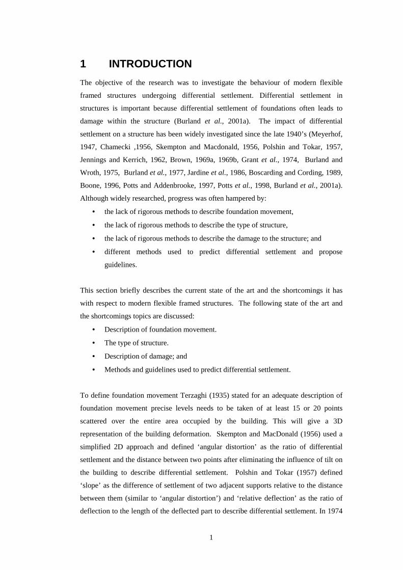
1 INTRODUCTION

The objective of the research was to investigate the behaviour of modern flexible

framed structures undergoing differential settlement. Differential settlement in

structures is important because differential settlement of foundations often leads to

damage within the structure (Burland et al., 2001a). The impact of differential

settlement on a structure has been widely investigated since the late 1940’s (Meyerhof,

1947, Chamecki ,1956, Skempton and Macdonald, 1956, Polshin and Tokar, 1957,

Jennings and Kerrich, 1962, Brown, 1969a, 1969b, Grant et al., 1974, Burland and

Wroth, 1975, Burland et al., 1977, Jardine et al., 1986, Boscarding and Cording, 1989,

Boone, 1996, Potts and Addenbrooke, 1997, Potts et al., 1998, Burland et al., 2001a).

Although widely researched, progress was often hampered by:

• the lack of rigorous methods to describe foundation movement,

• the lack of rigorous methods to describe the type of structure,

• the lack of rigorous methods to describe the damage to the structure; and

• different methods used to predict differential settlement and propose

guidelines.

This section briefly describes the current state of the art and the shortcomings it has

with respect to modern flexible framed structures. The following state of the art and

the shortcomings topics are discussed:

• Description of foundation movement.

• The type of structure.

• Description of damage; and

• Methods and guidelines used to predict differential settlement.

To define foundation movement Terzaghi (1935) stated for an adequate description of

foundation movement precise levels needs to be taken of at least 15 or 20 points

scattered over the entire area occupied by the building. This will give a 3D

representation of the building deformation. Skempton and MacDonald (1956) used a

simplified 2D approach and defined ‘angular distortion’ as the ratio of differential

settlement and the distance between two points after eliminating the influence of tilt on

the building to describe differential settlement. Polshin and Tokar (1957) defined

‘slope’ as the difference of settlement of two adjacent supports relative to the distance

between them (similar to ‘angular distortion’) and ‘relative deflection’ as the ratio of

deflection to the length of the deflected part to describe differential settlement. In 1974

2

Burland and Wroth (1975) suggested a whole set of definitions to define differential

settlements in 2D. The definitions are often used in later papers to describe differential

settlement (Burland et al., 1977, Burland et al., 2001a). These definitions have the

limitation that they only describe movement in a plane (2D) and are useful for

describing the behaviour of 2D frames and 3D buildings with minimal lateral

deformation (which is often the case with long buildings and where settlement occurs

due to tunnelling perpendicular to the building). However square buildings undergoing

differential settlement due to self weight may have significant deformation in the

corners, which is difficult to describe in 2D. The research presented in this report

investigated the behaviour of modern flexible 3D structures and the results showed that

description of deformation only in 2D is insufficient.

The type of structure influences the response to differential settlement. Skempton and

Macdonald’s (1956) guidelines were limited to traditional steel and concrete frame

buildings and structures with load bearing walls. The 1955 Building Code of the USSR

treated framed structures separately from load bearing structures with much stricter

criteria being laid down for load bearing brick buildings. Meyerhof (1956) also treated

framed panels and load bearing brick walls separately. Guidelines are often presented

in text books or design recommendations without emphasising the type of structure the

guidelines are applicable to (Burland et al., 1977). Current state of the art guidelines are

focussed on relatively stiff load bearing brick buildings. The use of these guidelines on

modern flexible framed structures may therefore be over conservative. The research

presented in this report investigated modern flexible framed structures and confirmed

that these types of buildings are less susceptible to differential settlement damage.

Damage to a structure is very subjective and depends on both the function of the

building and the reaction of the users and is difficult to quantify (Burland and Wroth,

1975). Peck et al. (1956) have shown that a certain amount of cracking is unavoidable

if the building is to be economical. Little (1969) has estimated that for a particular type

of building the cost to prevent cracking may exceed 10% of the total building cost.

Therefore it will be likely that some damage will occur and the level of acceptable

damage needs to be defined. Skempton and Macdonald (1956) divided damage into the

following 3 categories:

• ‘Structural’ involving only the frame, i.e. stanchions and beams.

• ‘Architectural’ involving only the panel walls, floors or finishes.

• Combined structural and architectural damage.

3

They also stated that architectural damage such as cracking of wall panels, is likely to

occur at smaller distortions of the building than for structural damage. This may be

true for conventional buildings, however it does not necessarily hold for modern

flexible structures. Skempton and Macdonald (1956) also note that the limits of

allowable settlement may be due to visual effects; notably the tilt or lean of a building.

Burland et al. (1977) suggested a classification system to quantify building damage

objectively. The damage classification system is based on the ease of repair of visible

damage and is based on the work of Jennings and Kerrich (1962), the UK National

Coal Board (1975) and Macleod and Littlejohn (1975). Since then it has been adopted

with only slight modifications by BRE (1981, 1990), the Institution of Structural

Engineers, London (1978, 1989, 1994, 2000) and BRE again in Freeman et al. (1994).

Burland et al. (2001a) point out that the classification system was developed for

brickwork and blockwork or stone masonry. It could be adapted for other forms of

cladding and it is not intended to apply to reinforced concrete structural elements.

These guidelines may therefore not be directly applicable to modern flexible framed

structures. The research presented in this report investigates which type of damage is

likely to occur first in modern flexible framed structures. In conventional load bearing

structures cracking of facades or infill panels is usually the limiting factor.

Initially two approaches were followed to address the impact of differential settlements

on structures. Meyerhof (1947) analysed the interaction between a 2D frame and the

soil and calculated the effect it has on the stress within the structure. Skempton and

MacDonald (1956) and Grant et al. (1974) followed an observational approach based

on case studies. They measured the differential settlement and corresponding damage

on existing buildings and suggested differential settlement limits based on the study.

The study showed that an angular distortion of greater than 1/150 will cause structural

damage and an angular distortion of greater than 1/300 will cause cracking in walls and

partitions and they recommended that angular distortions greater than 1/500 should be

avoided if it was important to avoid differential settlement damage.

In contrast Meyerhof’s (1947) frame analysis showed that a lesser angular distortion of

1/950 will cause an increase of 74% in the bending moment in the beam which was

subjected to the largest bending moment prior to differential settlement. Skempton and

MacDonald (1956) argued that an angular distortion of 1/950 did not result in damage

in the observed structures. They suggested the reason for it may be that the live loads

assumed in the design are conservative compared to the actual average loads in

4

buildings and the composite action of the frame floors and walls may reduce the

stresses and deflections within the building.

Burland and Wroth (1975) and Burland et al. (1977) used the concept of a tensile strain

limit to study the development of cracking in weightless elastic beams undergoing

deflections, which is a simplified representation of a building. Studies done by Polshin

and Tokar (1957) and Burland and Wroth (1975) showed that cracking in walls and

finishes usually results from tensile strain and that for a given material visible cracking

is associated with a reasonably well defined value of strain that is insensitive to the

mode of deformation. Boscardin and Cording (1989) associated tensile strain values

with the damage categories as proposed by Burland et al. (1977). Strain distribution

within the simple beam depends on the mode of deformation and two extreme modes of

bending only about a neutral axis and shear only were analysed. Both modes occur

simultaneously and need to be calculated to determine whether bending or diagonal

strain is limiting. Using an expression for midspan deflection of a centrally loaded

beam having both bending and shear stiffness (Timoshenko, 1957), a limiting value of

deflection can be calculated for a given tensile strain limit by taking the building length

and height, Young’s modulus and shear modulus and the position of the neutral axis

into account. Boscardin and Cording (1989) expanded the above analysis to include

horizontal strain which is associated with tunnelling.

The above method was used successfully on the Jubilee Line extension (Burland et al.,

2001a) and its simplicity is a big advantage when it comes to the analyses of structures,

however it is important to realise the simplifications and limitations of the method. The

method assumes that the deformation of the structure is predominantly 2D and that the

structure behaves like a beam. These assumptions may be true for conventional

buildings; however modern flexible framed structures may behave differently.

The advance in modern computers and modern finite element software packages allows

for the analyses of 3D models with increased complexity. Simplified 2D models may

provide valuable insight and use fewer resources; however full 3D models can include

more detail and show the shortcomings of simplified 2D models. The research

presented in this report makes use of the capability to analyse a 3D structure to

investigate the behaviour of modern flexible framed structures.

5

In recent years the need for more sustainable development has become an important

factor in the design of new buildings. In areas of frequent redevelopment the reuse of

foundations of the demolished buildings is encouraged (Chapman et al., 2001, Chow et

al., 2002, Cameron and Chapman, 2004) to save resources. However in practice old

foundations are often discarded in favour of new foundations at extra cost even when

the old foundations are located in the correct position, in good condition and capable of

withstanding the design loads. This is due to the uncertainty involved in how the

structure will behave if older preloaded foundations with a stiffer response are

combined with new foundations. Understanding the behaviour of modern flexible

structures undergoing differential settlement will pave the way for the reuse of

foundations. It will also be valuable in assessing the risk of foundation (old or new)

failure on newly constructed buildings.

The thesis first reviews and discusses the factors producing differential settlement and

the current state of the art on the behaviour of structures undergoing differential

settlement in Chapter 2. A linear-elastic model is developed and verified in Chapter 3

and typical results are presented. Chapter 4 discusses the behaviour of structures

undergoing differential settlement. The discussion is based on the results. Chapter 5

presents the conclusions of the literature review, the development of the numerical

model and the discussion of the results, as well as suggestions for future work.

6

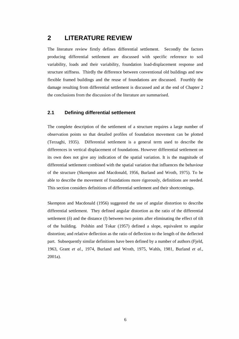
2 LITERATURE REVIEW

The literature review firstly defines differential settlement. Secondly the factors

producing differential settlement are discussed with specific reference to soil

variability, loads and their variability, foundation load-displacement response and

structure stiffness. Thirdly the difference between conventional old buildings and new

flexible framed buildings and the reuse of foundations are discussed. Fourthly the

damage resulting from differential settlement is discussed and at the end of Chapter 2

the conclusions from the discussion of the literature are summarised.

2.1 Defining differential settlement

The complete description of the settlement of a structure requires a large number of

observation points so that detailed profiles of foundation movement can be plotted

(Terzaghi, 1935). Differential settlement is a general term used to describe the

differences in vertical displacement of foundations. However differential settlement on

its own does not give any indication of the spatial variation. It is the magnitude of

differential settlement combined with the spatial variation that influences the behaviour

of the structure (Skempton and Macdonald, 1956, Burland and Wroth, 1975). To be

able to describe the movement of foundations more rigorously, definitions are needed.

This section considers definitions of differential settlement and their shortcomings.

Skempton and Macdonald (1956) suggested the use of angular distortion to describe

differential settlement. They defined angular distortion as the ratio of the differential

settlement (δ) and the distance (l) between two points after eliminating the effect of tilt

of the building. Polshin and Tokar (1957) defined a slope, equivalent to angular

distortion; and relative deflection as the ratio of deflection to the length of the deflected

part. Subsequently similar definitions have been defined by a number of authors (Fjeld,

1963, Grant et al., 1974, Burland and Wroth, 1975, Wahls, 1981, Burland et al.,

2001a).

7

Burland and Wroth (1975) proposed a consistent set of definitions based on the

displacement of a number of discrete points on the foundation of a building. The

definitions have been widely accepted, are illustrated in Figure 2.1 and defined as

follows (Burland et al., 2001a):

• Rotation or slope θ is the change in gradient of a line joining two reference

points (e.g. AB in Figure 2.1(a)).

• The angular strain α is defined in Figure 2.1(a). It is positive for upward

concavity (sagging) and negative for downward concavity (hogging).

• Relative deflection ∆ is the displacement of a point relative to the line

connecting two reference points on either side (see Figure 2.1(b)). The sign

convention is as for angular strain.

• Deflection ratio (sagging ratio or hogging ratio) is denoted by ∆/L where L is

the distance between the two reference points defining ∆. The sign convention

is as angular strain.

• Tilt ω describes the rigid body rotation of the structure or a well defined part of

it. See Figure 2.1(c).

• Relative rotation (angular distortion) β is the rotation of the line joining two

points, relative to the tilt ω. See Figure 2.1(c). It is not always straightforward

to identify the tilt and the evaluation of β can sometimes be difficult. It is also

very important not to confuse relative rotation β with angular strain α. For

these reasons Burland and Wroth (1975) preferred the use of deflection ratio

∆/L as a measure of building distortion.

The above set of definitions provides a way of describing differential settlement,

however in practice it is often difficult to know the precise deformed shape between

observation points (Burland and Wroth, 1975). Therefore care should be taken in

defining suitable observation points.

The definitions provide only a description of in plane movement and no attempt is

made to describe 3D deformation of a structure. The definitions are therefore suitable

for structures that deform primarily in plane, however 3D deformation needs to be

described for structures with 3D behaviour. Describing 3D deformation is more

complex than 2D deformation and no straightforward definitions exist.

8

2.2 Factors producing differential settlement

Differential settlement may cause damage to structures. A good understanding of

mechanisms and factors producing differential settlement will result in a better

understanding of the behaviour of the structure and will therefore allow for a more

optimal design. The following sections will discuss the impact of soil variability, loads

and their variability, foundation load-displacement response and building stiffness on

differential settlement.

2.2.1 Soil variability

This section considers soil variability, since varying stiffness and strength of soil

beneath foundations is a potential cause of differential settlement. Inherent soil

variability and the parameters describing it are considered, as are uncertainties in

measurement and transformation models of soil properties. Typical values of variation

are also discussed.

Soils are heterogeneous materials created by complex geological processes. Soil

properties vary from point to point, even in the same strata. Terzaghi (1955) discussed

how soil variability can be linked to complex depositional conditions. Fookes (1997)

discusses the value of a comprehensive geological model in understanding soil

conditions on a site, but also states that, regardless of the detail and the amount of work

involved, the geological model is unlikely to achieve the same qualitative accuracy as

the structural engineering design because of the inherent complexity and

inhomogeneity of the soil. Other researchers have investigated and quantified the

spatial variability of natural soils (Phoon and Kulhawy, 1999, Bourdeau and

Amandaray, 2005, El Gonnouni et al., 2005). Table 2.1 (Phoon and Kulhawy, 1999)

shows a summary of inherent variability of strength properties of various soils. Table

2.2 (Phoon and Kulhawy, 1999) shows inherent variability of the index parameters of

various soils. The Coefficient of Variation (COV) is the Standard Deviation

normalised to the mean soil property value. Another parameter needed to describe the

variability of soil is the distance of the variability change i.e. the scale of fluctuation.

Figure 2.2 shows the scale of fluctuation graphically. Table 2.3 (Phoon and Kulahawy,

1999) summarises vertical and horizontal fluctuations of some geotechnical properties.

From the data it is evident that the scale of fluctuation in a vertical direction is smaller

than for a horizontal fluctuation. Horizontal fluctuations typically range from 3.0 m to

80.0 m, which means within the footprint of structure, the soil properties can vary

significantly.

9

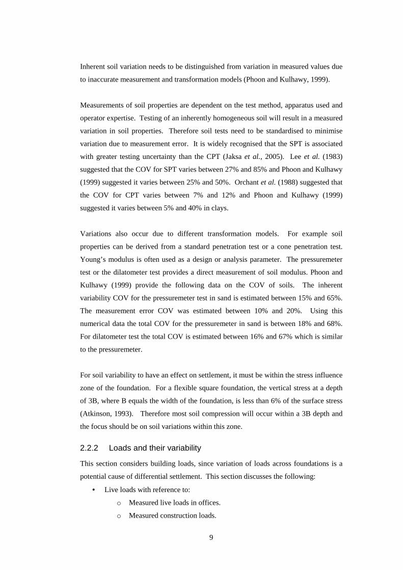
Inherent soil variation needs to be distinguished from variation in measured values due

to inaccurate measurement and transformation models (Phoon and Kulhawy, 1999).

Measurements of soil properties are dependent on the test method, apparatus used and

operator expertise. Testing of an inherently homogeneous soil will result in a measured

variation in soil properties. Therefore soil tests need to be standardised to minimise

variation due to measurement error. It is widely recognised that the SPT is associated

with greater testing uncertainty than the CPT (Jaksa et al., 2005). Lee et al. (1983)

suggested that the COV for SPT varies between 27% and 85% and Phoon and Kulhawy

(1999) suggested it varies between 25% and 50%. Orchant et al. (1988) suggested that

the COV for CPT varies between 7% and 12% and Phoon and Kulhawy (1999)

suggested it varies between 5% and 40% in clays.

Variations also occur due to different transformation models. For example soil

properties can be derived from a standard penetration test or a cone penetration test.

Young’s modulus is often used as a design or analysis parameter. The pressuremeter

test or the dilatometer test provides a direct measurement of soil modulus. Phoon and

Kulhawy (1999) provide the following data on the COV of soils. The inherent

variability COV for the pressuremeter test in sand is estimated between 15% and 65%.

The measurement error COV was estimated between 10% and 20%. Using this

numerical data the total COV for the pressuremeter in sand is between 18% and 68%.

For dilatometer test the total COV is estimated between 16% and 67% which is similar

to the pressuremeter.

For soil variability to have an effect on settlement, it must be within the stress influence

zone of the foundation. For a flexible square foundation, the vertical stress at a depth

of 3B, where B equals the width of the foundation, is less than 6% of the surface stress

(Atkinson, 1993). Therefore most soil compression will occur within a 3B depth and

the focus should be on soil variations within this zone.

2.2.2 Loads and their variability

This section considers building loads, since variation of loads across foundations is a

potential cause of differential settlement. This section discusses the following:

• Live loads with reference to:

o Measured live loads in offices.

o Measured construction loads.

10

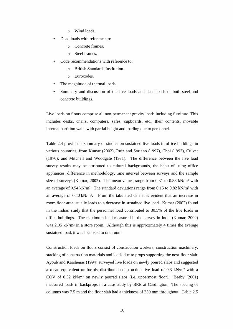
o Wind loads.

• Dead loads with reference to:

o Concrete frames.

o Steel frames.

• Code recommendations with reference to:

o British Standards Institution.

o Eurocodes.

• The magnitude of thermal loads.

• Summary and discussion of the live loads and dead loads of both steel and

concrete buildings.

Live loads on floors comprise all non-permanent gravity loads including furniture. This

includes desks, chairs, computers, safes, cupboards, etc., their contents, movable

internal partition walls with partial height and loading due to personnel.

Table 2.4 provides a summary of studies on sustained live loads in office buildings in

various countries, from Kumar (2002), Ruiz and Soriano (1997), Choi (1992), Culver

(1976); and Mitchell and Woodgate (1971). The difference between the live load

survey results may be attributed to cultural backgrounds, the habit of using office

appliances, difference in methodology, time interval between surveys and the sample

size of surveys (Kumar, 2002). The mean values range from 0.31 to 0.83 kN/m² with

an average of 0.54 kN/m². The standard deviations range from 0.15 to 0.82 kN/m² with

an average of 0.40 kN/m². From the tabulated data it is evident that an increase in

room floor area usually leads to a decrease in sustained live load. Kumar (2002) found

in the Indian study that the personnel load contributed to 30.5% of the live loads in

office buildings. The maximum load measured in the survey in India (Kumar, 2002)

was 2.05 kN/m² in a store room. Although this is approximately 4 times the average

sustained load, it was localised to one room.

Construction loads on floors consist of construction workers, construction machinery,

stacking of construction materials and loads due to props supporting the next floor slab.

Ayoub and Karshenas (1994) surveyed live loads on newly poured slabs and suggested

a mean equivalent uniformly distributed construction live load of 0.3 kN/m² with a

COV of 0.32 kN/m² on newly poured slabs (i.e. uppermost floor). Beeby (2001)

measured loads in backprops in a case study by BRE at Cardington. The spacing of

columns was 7.5 m and the floor slab had a thickness of 250 mm throughout. Table 2.5

11

is a summary of the structural design values and measured floor loads. The maximum

imposed load on a floor slab was 10.57 kN/m². The high level of load on the floor slab

is due to the load of the backprops on the slab supporting the formwork and casting of

the above slab. It is important to note that not all the floor slabs will be subjected to the

maximum live load simultaneously. As construction progresses and props are removed

live loads will change to dead loads as each floor slab supports itself.

Krishna (1995) describes the complexities in measuring wind loads on buildings. Wind

loads on buildings depend on wind strength, direction of the wind with respect to the

building, the surrounding area i.e. other buildings; and the geometry of the building.

Meecham (1992) has reported that for a hip roof, peak pressures are reduced by as

much as 50% compared with those of a gable roof. Likewise Blackmore (1988) has

reported on the effect of chamfering building edges at different angles. He has reported

that roof loads reduce with increase in chamfer angle. Reductions as high as 70% in

average load on a corner panel and 30% in overall design load are observed. It is

therefore extremely difficult to generalise average wind load and duration on buildings.

Extreme wind loads are usually of a limited duration and are often taken into account

for strength and serviceability calculations i.e. vibration of panels. Due to the short

duration it normally does not affect settlement of foundations.

Dead loads comprise all permanent gravity loads including the floors, walls, columns,

services and finishes. The dead load depends on the materials used within the

structure. A concrete structure is usually heavier than a steel structure as shown in the

following examples of typical dead loads.

A typical dead load of a concrete frame for an office building may be summarised as

follows. (Refer to Chapter 3 for details of the sizing of the elements according to the

structural design. Densities derived from BSI 6399-1: 1996.)

• A 300 mm concrete floor slab with a concrete density of 25 kN/m³ results in a

distributed load per floor of 7.50 kN/m².

• Concrete columns (2.7 m x 450 mm x 450 mm) spaced at 7.5 m centre to

centre will increase the average floor load by 0.23 kN/m².

• Combining these gives an indication of magnitude of expected dead load for

the typical concrete frame of 7.73 kN/m² per storey.

12

A typical dead load of a steel frame for an office building may be summarised as

follows. (The loads are derived from worked examples for the design of steel structures

as prepared by the Building Research Establishment, The Steel Construction Institute

and Ove Arup & Partners (Building Research Establishment, 1994)

• A raised floor on 130 mm lightweight concrete on profiled metal decking

results in a distributed load per floor of 2.70 kN/m².

• Beams (406 x 140 x 46 UB) at 2.5 m spacing in the x-direction and beams

(610 x 229 x 101 UB) at 7.5 m spacing in the y-direction results in a distributed

load per floor of 0.31 kN/m².

• Steel columns (254 x 254 x 73 UC) spaced at 7.5 m centre to centre will

increase the average floor load by 0.03 kN/m².

• Combining these gives an indication of magnitude of expected dead load for a

typical steel frame of 3.04 kN/m² per storey.

From the above examples it is evident that the typical load of a concrete frame

(7.73 kN/m² per storey) is more than twice the load of a similar steel frame (3.04 kN/m²

per storey).

The British Standards Codes and the Eurocodes are currently acceptable design codes

for the UK and the suggested design loads will therefore be compared. The current

suite of British Standards Codes, will in due course be almost entirely replaced by the

system of Eurocodes and it is expected that the replacement will be complete by about

2010 (Department for Communities and Local Government, 2006).

Eurocode 7 (EN 1997-1: 2004) offers a choice (or combination) of 4 methods for

geotechnical design:

• Using ultimate limit state design calculations for ULS and SLS.

• Using prescriptive measures. Prescriptive measures involve conventional and

generally conservative rules in the design and usually involve the application of

charts, tables and procedures that have been established from comparable

experience.

• Using tests. Designs may be based on the results of load tests; or

• Using the Observational Method. The Observational Method is a continuous,

managed, integrated process of design, construction control, monitoring and

review that enables previous modifications to be incorporated during or after

construction as appropriate.

13

The discussion of recommended Eurocodes load values will focus on the limit states

design (ULS and SLS).

The Codes recommend the following values. References to the specific codes are

British Standards Institution (BSI), Eurocodes (EU) and the UK National Annex to

Eurocode (UK).

• Structure design for Ultimate Limit State (ULS).

o Live loads (BSI 6339-1: 1996, EN 1990: 2002, NA to EN 1990: 2002,

EN 1991-1-1: 2002, NA to EN 1991-1-1: 2002, EN 1991-1-3: 2003,

NA to EN 1991-1-3: 2003).

Live loads for general use offices consist of an imposed uniform

distributed load (UDL) of 2.5 kN/m² (BSI), 1.5 to 2.0 kN/m² (EU) and

2.5 kN/m² (UK) on floors.

Movable partitions should be taken as an additional imposed UDL of

not less than 1.0 kN/m² (BS). The Eurocodes (EU and UK) distinguish

between movable partitions with different self-weights and recommend

for self weights ≤ 1.0 kN/m a UDL of 0.5 kN/m², for self weights

≤ 2.0 kN/m a UDL of 0.8 kN/m² and for self weights ≤ 3.0 kN/m a

UDL of 1.2 kN/m².

For roofs with only maintenance access, minimum UDLs of 1.5 kN/m²

(BSI), 0.4 kN/m² (EU) and 0.6 kN/m² (UK) are recommended.

Snow loads need to be considered, however recommended values are

site and structure specific and will therefore not be discussed.

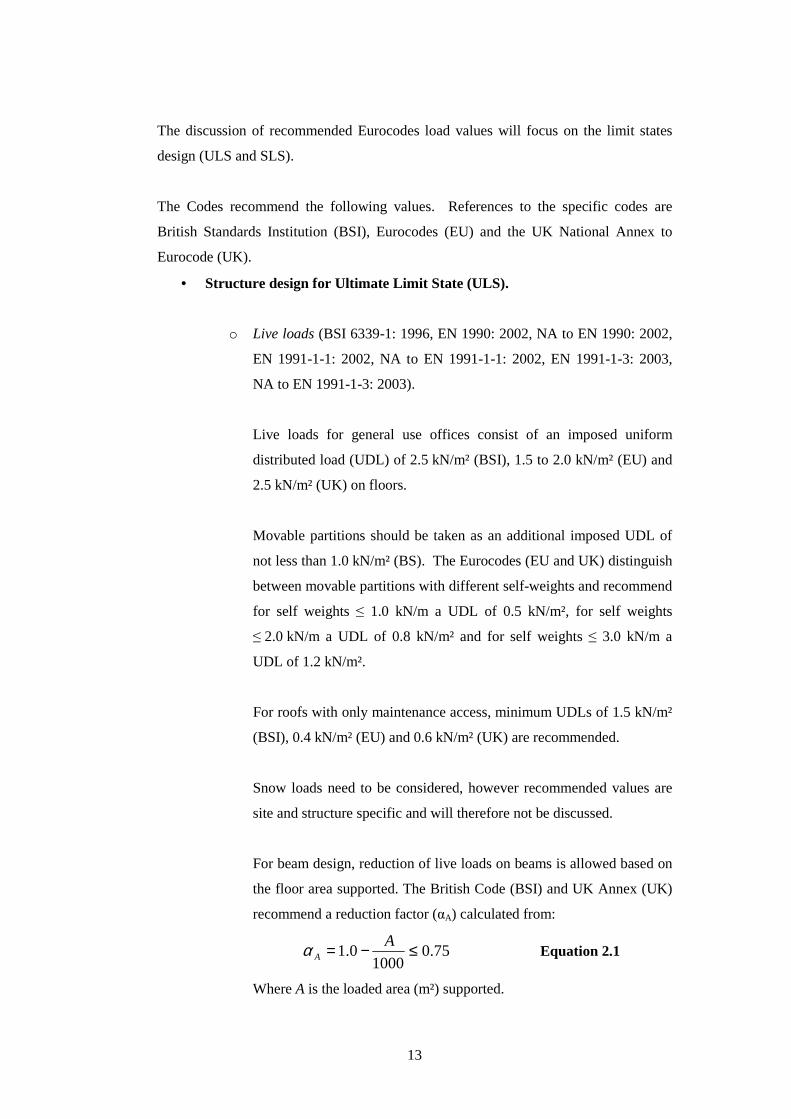
For beam design, reduction of live loads on beams is allowed based on

the floor area supported. The British Code (BSI) and UK Annex (UK)

recommend a reduction factor (αA) calculated from:

75.01000

0.1 ≤−= AAα Equation 2.1

Where A is the loaded area (m²) supported.

14

Eurocodes (EU) recommends a reduction factor (αA) calculated from:

0.110

5.0 ≤+=AAα Equation 2.2

Where A is the loaded area (m²) supported.

Figure 2.3 gives a graphical presentation of the area reduction factors.

It is evident that the load reduction factor (αA) for the Eurocodes is

approximately 20% lower than the British Standards and UK Annex

for areas above 50 m².

For column design, reduction of floor live loads is allowed based on

the number of storeys supported by the column under consideration.

The British Code (BSI) and UK Annex (UK) recommend a reduction

factor (αn) calculated from:

105.0

1056.0

5110

1.1

>=≤<=

≤≤−=

nfor

nfor

nforn

n

n

n

αα

α

Equation 2.3

Where n is the number of storeys above the loaded structural elements.

Eurocodes (EU) recommends a reduction factor (αA) calculated from:

( )

n

nn

7.022 −+=α Equation 2.4

Where n is the number of storeys (greater than 2) above the loaded

structural elements.

Figure 2.4 gives a graphical presentation of the storey reduction factors

and it is evident that the load reduction factor (αA) for the British

Standards and UK Annex is approximately 20% lower than the

Eurocodes for more than 3 floors. Combining load reduction factors

for both area and number of supported storeys should lead to a smaller

difference in predicted column live loads between the codes.

o Dead loads (BSI 6399-1: 1996, EN 1991-1-1: 2002)

Dead loads are calculated using the measured volumes and densities of

building materials used. The codes suggest densities for various

15

construction materials. Dead loads include floors, walls, columns,

services and finishes.

o Wind loads (BSI 6399-2: 1997, EN 1991-1-4: 2005)

Wind loads are building and site dependent and are influenced by

building location, altitude, topography, surrounding terrain (buildings,

trees) and building geometry.

o Partial safety factors (BSI 8110-1: 1997, EN 1990: 2002, NA to EN

1990: 2002)

Partial safety factors are applied to above loads for ULS calculations.

Combinations of partial factors according to British Standards are

summarised in Table 2.6. The Eurocodes distinguish between the

following ULS and the appropriate partial factors are summarised in

Table 2.7.

EQU: Loss of static equilibrium of the structure or any part of it

considered as a rigid body, where the strength of structural

materials and the ground are insignificant in providing

resistance.

STR: Internal failure or excessive deformation of the structure or

structural members, including footings, piles, and basement

walls, etc., where the strength of structural materials is

significant in providing resistance.

GEO: Failure or excessive deformation of the ground where strength

of soils or rock are significant in providing resistance, (e.g.

overall stability, bearing resistance of spread foundations or

pile foundations).

• Structure design for Serviceability Limit State (SLS)

o General (BSI 8110-2: 1985, EN 1990: 2002, NA to EN 1990: 2002)

For serviceability calculations the codes state that it is necessary to

make sure the assumptions made regarding loads are compatible with

the way results will be used. If a best estimate of the expected

behaviour is required then the expected or most likely values should be

16

used. However, to satisfy a serviceability limit state it may be

necessary to take a more conservative value depending on the severity

of the serviceability limit state under consideration, i.e. the

consequences of failure (with regard to serviceability limit state).

o Live loads (BSI 8110-2: 1985, EN 1990: 2002, NA to EN 1990: 2002)

Live loads should in general be the characteristic values (as calculated

for ULS, with a partial safety factor of one), however when calculating

deflections, it is necessary to determine how much of the load is

permanent and how much transitory. The British Standards suggest for

normal domestic or office occupancy, 25 % of the live load should be

considered as permanent and for structures used for storage, at least

75% should be considered permanent when the upper limit to the

deflection is being assessed.

o Dead loads (BSI 8110-2: 1985, EN 1990: 2002, NA to EN 1990: 2002)

Dead loads should be the characteristic value (as calculated for ULS,

with a partial safety factor of one).

• Foundation design according to British Standards (allowable bearing

pressure)

o Dead and live loads (BSI 8004: 1986)

Dead and live loads should be the characteristic value (as calculated for

ULS, with a partial safety factor of one). Dead load should include the

weight of foundations and any backfill above the foundations.

o Wind loads (BSI 8004: 1986)

Wind loads resulting in loads on foundations that are less than 25% of

the loadings due to dead and live loads may be ignored. Where this

ratio exceeds 25% foundations may be so proportioned that the

pressure due to combined dead, live and wind loads does not exceed

the allowable bearing pressure by more than 25%.

17

• Thermal actions

The investigation of thermal actions on buildings due to climatic and

operational temperature changes falls outside the scope of this research,

however it should be considered in the design of buildings where there is a

possibility of the ULS or SLS being exceeded due to thermal movement and/or

stresses. This section illustrates the possible effect of temperature on a

building. Eurocode 1 (EN 1991-1-5: 2003) and the UK Annex (NA to EN

1991-1-5: 2003) provide guidance on calculating temperature changes in

buildings.

The Eurocode suggests inside building temperatures of 20 °C during summer

and 25 °C during winter. Outside building temperatures depend on shade air

temperature and the type of surface. In the UK minimum shade air

temperatures range from -21 °C to -9 °C and maximum shade air temperatures

range from 26 °C to 35 °C, depending on location. Table 2.8 shows the surface

temperatures to be used for design calculations. For example, according to the

Eurocode, in the summer buildings in Southampton will experience an inside

temperature of 20 °C, while dark surfaces outside on North-East facing

elements will experience 37 °C and dark surfaces South-West or horizontal

elements 75 °C, resulting in a 55 °C temperature difference in the building.

Table 2.9 (EN 1991-1-5: 2003, EN 572-1: 2004) lists coefficients of linear

expansion for construction materials. The following example illustrates the

impact of thermal expansion on a structure. Assume a structure:

o with a thermal expansion coefficient of 10 x 10-6/°C for both the

internal frame and external facades

o located in Southampton,

o during summer; and

o dark surfaces on facades.

On West-South sides the facades will be 55 °C warmer than the internal frame.

Thermal expansion in an unrestrained 3 m facade will therefore lead to

1.65 mm differential movement of the facade with respect to the frame.

Thermal expansion in a totally restrained facade with a Young’s modulus of

70 GPa (aluminium or glass (EN 1991-1-1: 2002, EN 572-1: 2004)) will

increase the stress in the facade by 38.5 MPa.

18

It is important to note that not only the magnitude, but also the duration, of load affects

the settlement of the building. The impact of load duration on settlement will be

discussed under foundation-load displacement response.

Table 2.10 provides a summary of the measured and proposed loads as listed above.

The average of the measured live loads is 0.54 kN/m². The codes recommend

unfactored values, excluding floor area and storey reductions ranging from 1.50 kN/m²

to 4.70 kN/m². The measured loads are significantly lower than the values suggested by

the codes. The maximum load in one room measured by Kumar (2002) of 2.05 kN/m²

is within the lower end of the range of the codes’ recommended live loads. The dead

load of the concrete frame in the worked example (7.73 kN/m2) is more than twice the

load for the steel frame (3.04 kN/m2). If a short term live load of 3.00 kN/m2 is

assumed, it will be approximately 100% of the dead load of the steel frame; however it

will only be approximately 40% of the dead load of the concrete frame. The live load

on a steel framed structure is therefore a more significant part of the total load in

comparison to a concrete framed structure.

2.2.3 Foundation load-displacement response

This section considers foundation response, since varying load-settlement response is a

potential cause of differential settlement. Foundation load-displacement response

varies significantly and depends on the structural loading on the foundations, the

foundation geometry and the soil supporting the foundation. These aspects in

combination with measured load-displacement responses are discussed.

Structural loading on a foundation results in settlement of the foundation. An increase

in load (while other properties remain constant) will cause an increase in settlement;

however the stiffness will usually decrease with an increase of load as seen in the

measured load-displacement response of a number of piles in Figure 2.5 and 2.6

(Whitaker and Cooke, 1966, De Beer et al., 1979, Fleming, 1992). Load-displacement

response is also dependent on the load history, i.e. reloading on a foundation will

usually result in a stiffer load-displacement response than virgin loading (Whitaker and

Cooke, 1966). Whitaker and Cooke (1966) measured load-displacements on a number

of piles in London Clay and Figure 2.7 shows the load-displacement response of a

bored pile with an enlarged base (12 m length, 0.8 m diameter shaft and 1.7 m diameter

base). The first part of the test (until reloading) was a maintained load test with

incremental steps and the second part (after reloading) a constant rate of penetration

19

test. Although the difference in test methods may slightly influence the measured

stiffness, the data still show a significant increase in stiffness on reloading. In the range

of 1260 kN to 3620 kN the stiffness of the virgin loading was 40 kN/mm and on the

reload 385 kN/mm showing an increase in stiffness of approximately 10 times.

Therefore the increase in stiffness on reloading needs to be taken into account when

piles are being reused and combined with new piles. Reuse of piles will become more

common practice due to the drive for more sustainable development in large cities

where frequent redevelopment leads to the soil being filled with old foundations,

restricting the installation of new piles (Chapman et al., 2001, Chow et al., 2002).

The resistance of a foundation to vertical movements under loads is caused by end

bearing resistance on the horizontal contact surfaces and friction on the vertical

surfaces. Pad and raft foundations depend mainly on end bearing resistance, while the

load capacity of pile foundations are from either or a combination of end bearing and

shaft friction, depending on the type of pile. End bearing resistance in pads or rafts will

increase with settlement until the foundation fails with regard to stability (i.e. tilting).

However, damage to or unacceptable response from the superstructure due to excessive

differential settlement is likely to be the limiting factor and not the ultimate capacity of

the foundation (Chan, 1997). Two pad foundations tested on soft clay at Bothekennar

(Jardine et al., 1995, Lehane and Jardine, 2003) failed due to tilting at 160 mm and

220 mm vertical displacement respectively; however this settlement will be

unacceptable for most structures.

Whitaker and Cooke (1966) instrumented bored piles with load cells and the results

showed that shaft friction and end bearing capacity are mobilised at different rates of

settlement. Frictional resistance develops rapidly with settlement and is generally fully

mobilised when the settlement is about 0.5 % of the pile diameter. On the other hand,

base resistance is seldom fully mobilised until the pile settlement reaches 10% to 20%

of the base diameter. The shape of a bored pile load-displacement graph depends on

the relative contribution of shaft and the base (Burland and Cooke, 1974).

Figure 2.8(a) shows a typical load settlement curve for long straight shafted piles and

Figure 2.8(b) shows the behaviour of relatively short piles with large under reams.

Whitaker and Cooke (1974) measured the load distribution of the shaft and the base of

an under reamed pile. Figure 2.7 shows the results and it is evident that the skin

friction for this pile is fully mobilised at approximately 10 mm (1% of pile diameter) of

20

settlement, whereas the base load was fully mobilised at approximately 100 mm (6% of

base diameter) of settlement.

From the discussion above it is evident that a foundation load-displacement is not linear

elastic. Burland and Wroth (1975) point out that for reasonably small stress changes

overconsolidated clay behaves as an elastic material in contrast to normally

consolidated clays which deform plastic.

Foundation settlement is time dependent and the response depends on the type of

supporting soil. On sands settlement will usually occur immediately, however

collapsible sand may show significant settlement at a later stage due to a rising water

table (Wiseman and Lavie, 1983, Alawaji, 1997). In saturated fine grained soils with a

low permeability, consolidation will take place and the short and long term settlement

will differ significantly.

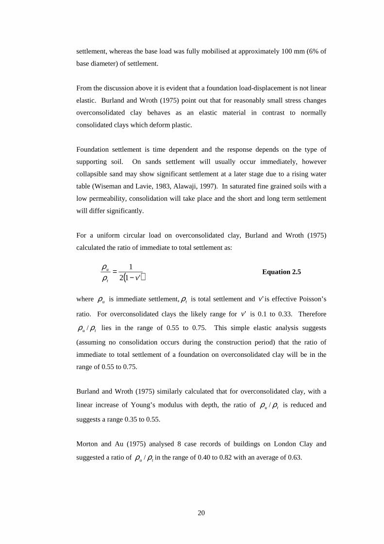
For a uniform circular load on overconsolidated clay, Burland and Wroth (1975)

calculated the ratio of immediate to total settlement as:

( )'12

1

vt

u

−=

ρρ

Equation 2.5

where uρ is immediate settlement,tρ is total settlement and 'v is effective Poisson’s

ratio. For overconsolidated clays the likely range for 'v is 0.1 to 0.33. Therefore

uρ / tρ lies in the range of 0.55 to 0.75. This simple elastic analysis suggests

(assuming no consolidation occurs during the construction period) that the ratio of

immediate to total settlement of a foundation on overconsolidated clay will be in the

range of 0.55 to 0.75.

Burland and Wroth (1975) similarly calculated that for overconsolidated clay, with a

linear increase of Young’s modulus with depth, the ratio of uρ / tρ is reduced and

suggests a range 0.35 to 0.55.

Morton and Au (1975) analysed 8 case records of buildings on London Clay and

suggested a ratio of uρ / tρ in the range of 0.40 to 0.82 with an average of 0.63.

21

Simons and Som (1970) analysed 12 case records of buildings on overconsolidated

clays and 9 case records on normally consolidated clays. For overconsolidated clay

they suggest a ratio of uρ / tρ in the range of 0.315 to 0.735 with an average of 0.575

and for normally consolidated clays a range of 0.077 to 0.212 with an average of 0.156.

Table 2.11 provides a summary of immediate to long term settlements.

2.2.4 Structure stiffness

This section discusses the structural stiffness and the factors affecting it. Structural

stiffness is determined by the stiffness of the materials used and the geometry. Firstly

the stiffness of reinforced concrete and masonry will be discussed and secondly the

effect of the geometry on the structural stiffness.

The stiffness of construction materials are strain and time dependent, however under

normal operating conditions a typical stiffness may be determined. Reinforced

concrete, masonry, dry wall partitions and glass facades are often used for construction.

Dry wall partitions and glass facades are usually fastened in such a way that the

contribution to the overall structure stiffness is insignificant and this will therefore not

be discussed. Reinforced concrete consists of reinforcement steel and concrete. The

Young’s modulus of reinforcement steel ranges from 190 to 210 GPa (Gere and

Timoshenko, 1991). British Standards Institution (BSI 8110-1:1997) suggests the use

of a steel stiffness of 200 GPa in the elastic zone. The stiffness of concrete is time

dependent and influenced (Neville, 1981) by:

• The strength of the concrete (which increases with age).

• Applied stress (which influences the strain)

• Moisture condition.

• Type of aggregate, and

• Mix ratios.

Figure 2.9 (Neville, 1981) shows the relationship between stress/strength ratio and

strain for concrete of different strengths. It is evident that stiffness decreases with an

increase of stress and that a high strength concrete has a higher stiffness than a low

strength concrete at an equivalent strain. Concrete strength increases with time as

shown in Figure 2.10 (Wood, 1991) which shows the development of strength in

150 mm concrete cubes over 20 years. Figure 2.11 (Neville, 1981) shows the influence

of the moisture condition on the modulus of elasticity at a stress of 5.5 MPa of concrete

22

at different ages. The concrete stiffness increased by 4 GPa to 5 GPa in a wet sample.

Figure 2.12 (Neville, 1981) shows the variation of stiffness between cement paste,

aggregate and concrete. The stiffness of the aggregate and cement paste is linear with

concrete being nonlinear. The stiffness of the aggregate is approximately 4 times the

stiffness of cement paste and an increase in aggregate in the mix will therefore increase

the stiffness of the concrete. A stiff aggregate can approximately double the stiffness

of the concrete in comparison to a low stiffness aggregate.

Shrinkage, creep and cracking affect the stress within the concrete member and

therefore also the stiffness of the concrete member. Table 2.12 (Neville, 1981) shows

the effect of aggregate/cement and water/cement ratio on shrinkage of concrete. An

increase in the aggregate/cement ratio leads to a decrease in shrinkage. Using an

aggregate/cement ratio of 3 instead of 7 will increase the shrinkage by 4 times. An

increase in water/cement ratio will lead to an increase in shrinkage. Using a water

cement ratio of 0.7 instead of 0.4 will approximately double the shrinkage. Figure 2.13

(Neville, 1981) shows the effect of stiffness on shrinkage. An increase in stiffness will

lead to a decrease in shrinkage. Concrete with a Young’s modulus of 35 GPa will

experience approximately half the shrinkage of a 15 GPa concrete. Figure 2.14

(Neville, 1981) shows the effect of different types of aggregate on shrinkage over time.

Using sandstone instead of quartz aggregate can double the amount of shrinkage.

Figure 2.15 (Neville, 1981) shows the effect of relative humidity on shrinkage of

concrete. A decrease in relative humidity leads to an increase of shrinkage over time.

Shrinkage for concrete typically ranges from 0 to 1.2 x 10-3.

Creep in concrete can be defined as the increase in strain under sustained stress, or as a

decrease in stress within the member under constant strain. In most structures creep

and shrinkage occur simultaneously. Creep depends on aggregate content, type of

aggregate, type of cement, applied stress, concrete strength, humidity, size of specimen,

temperature and time (Neville, 1995). Figure 2.16 (Neville, 1981) shows the effect of

creep on stress over time at a constant strain. The creep resulted in a 50% decrease in

stress within 80 days for this specific sample. Figure 2.17 (Neville, 1981) shows the

effect of aggregate type on creep. Using sandstone aggregate instead of limestone

aggregate can double the amount of creep. Figure 2.18 (Neville, 1981) shows the effect

of admixtures on the creep in concrete over time. Certain admixtures can increase

creep by up to 30%. Figure 2.19 (Neville, 1981) shows the effect of relative humidity

on creep over time. A humidity of 50% can increase creep with 150% in comparison to

23

100% humidity. Figure 2.20 (Neville, 1981) shows the range of creep-time curves for

different concretes stored at various relative humidities. Creep in concrete typically

ranges from 0 to 2000 x 10-3.

From the discussion above it is evident that the stiffness of concrete can range

significantly depending on the circumstances. The British Standards Institution (BSI

8110-2: 1985) suggest in the absence of better information the use of the following

equations to determine the Young’s modulus for serviceability limit state calculations:

28,28, 2.020 cuc fE += Equation 2.6

Where Ec.28 is the concrete modulus at 28 days in GPa and fcu,28 is concrete strength at

28 days in MPa. A class 25/30 concrete will therefore have Young’s Modulus of

26 GPa at 28 days. British Standards Institution (BSI 8110-2: 1985) suggests using the

following equation for the Young’s modulus at an age t:

( )28,,28,, 6.04.0 cutcuctc ffEE += Equation 2.7

Masonry infill in reinforced concrete frames may have a significant impact on the

stiffness of the structure. The behaviour of masonry infilled frames has been

investigated by a number of researchers. Holmes (1961), Stafford Smith (1962, 1966,

1967), and Mainstone and Weeks (1970) have conducted experimental and analytical

investigations on the lateral stiffness and strength of steel frames infilled with mortar

and concrete panels. The behaviour of masonry infilled reinforced concrete frames is

generally more complicated than of steel infilled frames and has been examined by

Kahn and Hanson (1979), Bertero and Brokken (1983), Mehrabi et al. (1996) and

Mehrabi and Shing (1997). Mehrabi et al. (1996) tested twelve 1/2-scale single-storey,

single bay frames of which eleven were infilled with masonry. The experimental

results showed that the masonry infill can significantly influence the stiffness of

reinforced concrete frames. The Young’s modulus of the eleven masonry infill panels

ranged from 3.1 to 9.6 GPa with an average of 6.7 GPa. The Young’s modulus of the

masonry is therefore approximately ¼ of the stiffness of a class 25/30 concrete at

28 days.

Differential settlement depends on both the stiffness of the structure as well as the

stiffness of the supporting soil. Theoretically the stiffness of the structure with respect

to the soil can range from perfectly flexible to perfectly rigid. A real structure’s

24

stiffness will be within the two extremes. To gain a better understanding of the

behaviour of a structure the two theoretical extremes are discussed.

Poulos and Davis (1974) provided standard elastic solutions for surface displacement

and stress due to a circular uniform load on a semi-infinite mass as shown in

Figure 2.21. Comparing settlement ratios and stress patterns for perfectly flexible and

perfectly rigid loads illustrates the behaviour of a structure at opposite extremes.

Circular loads are a simplified way to illustrate the effect of structural stiffness without

dealing with the added complexity of rectangular foundations which are present in most

structures.

The contact stress distribution under a flexible circular uniform loading is the uniform

loading whereas the contact stress distribution under a rigid circular loading

(Schiffmann and Aggarwala, 1961, cited in Poulos and Davis, 1974) can be calculated

from:

2

2

12a

r

pavz

−

=σ Equation 2.8

The vertical surface displacementzρ under a flexible circular uniform loading (Ahlvin

and Ulery, 1962, cited in Poulos and Davis, 1974) can be calculated from:

aHE

vpz

)1( 2−=ρ Equation 2.9

where H is a function of r/a. Ahlvin and Ulery provided tabulated values for H.

The vertical surface displacement under a rigid circular uniform loading (Schiffmann

and Aggarwala, 1961, cited in Poulos and Davis, 1974) can be calculated from:

aE

vpavz

)1(

2

2−= πρ Equation 2.10

Using Equations 2.8, 2.9 and 2.10, ratios of contact pressure and surface settlement

were calculated and are shown graphically in Figure 2.21. The contact stress beneath

the centre of a rigid uniform loading is 50% less than for a flexible uniform loading

with the same load and area. The contact stress at the edge of the rigid uniform

loading on an elastic halfspace is infinite. Even though a circular load on an elastic

25

halfspace is a simplification of real foundation behaviour the same trends will be seen

until the soil fails due to excessive stress. A rigid structure on a raft foundation will

therefore have higher contact pressure at the edges up to the point of soil failure.

Surface settlement due a flexible uniform loading is 19 % less at the edge and 27 %

more at the centre in comparison to that of a rigid uniform loading. The stiffness of a

structure and soil will influence the amount and distribution of differential settlement.

From Equations 2.9 and 2.10 it is evident that for a constant:

• area, settlement will increase linearly with an increase of applied stress

( pz ∝ρ ).

• applied stress, settlement will increase with an increase in area ( 2Az ∝ρ ); and

• applied total load, settlement will increase with a decrease in area

( 5.0−∝ Azρ ).

It may be argued that differential settlement may be eliminated by sizing the

foundations according to the loads carried, resulting in uniform settlement. However to

achieve this, accurate predictions of the loads within the structure and load-settlement

responses of the foundations are needed. Predicting load and load-settlement response

accurately is difficult due to the variation in load and soil conditions.

The stiffness of structures is between perfectly flexible and perfectly rigid. Brown

(1969a, 1969b) investigated the effect of raft stiffness on the behaviour of the raft. The

study was based on the numerical analyses of uniform loaded circular rafts of any

flexibility which rest on an isotropic elastic foundation layer. He found that the

behaviour of the raft depends on the soil raft stiffness ratio, and defined the relative raft

stiffness K as:

( )

3

32 .1

aE

tEK

s

rr υ−= Equation 2.11

Where Er denotes Young’s modulus of the raft, Es denotes Young’s modulus of the

foundation material, υr denotes Poisson’s ratio of the foundation material, t is the raft

thickness and a is the raft radius.

26

Fraser and Wardle (1976) defined relative raft stiffness K as:

( )( ) 32

32

.13

.14

bE

tEK

ss

rr

υυ

−−

= Equation 2.12

Where υr denotes Poisson’s ratio of the soil and b is the raft width.

Hain and Lee (1978) defined relative raft stiffness K as:

( )

4

32

3

14

aE

btEK

s

rr

πυ−

= Equation 2.13

Although Equations 2.11, 2.12 and 2.13 vary, it should be noted that results against

relative raft stiffness K are usually plotted on a log scale; therefore the Poisson’s ratio

will not have a significant impact.

In the Equation 2.13 by Hain and Lee the effect of the geometry of the raft is described

by term bt3/a4. For a complete building this term needs to describe the effective

building geometry. Potts and Addenbrooke (1997) defined relative bending stiffness ρ*

of a building as:

4

*

HE

EI

s

=ρ Equation 2.14

Where H is the half width of the building in the plane of deformation and EI the

bending stiffness of the structure. Potts and Addenbrook state that two approaches can

be taken to calculate the EI of a structure. The first approach employs the parallel axis

theorem to define the structural stiffness about the neutral axis as shown in

Equation 2.15:

)()( 2

1

hAIEEI slab

n

slabtStiffstruc += ∑ Equation 2.15

Where n is the number of storeys. This can be considered to be an overestimate of the

building stiffness as only a rigidly framed structure would approach such mode of

deformation. An alternative method was used to obtain the bending stiffness by

summing the independent EI values for each slab as shown in Equation 2.16. This

implies that the walls and columns transfer the same deformed shape to each storey.

∑=n

slabFlexstruct IEEI1

)( Equation 2.16

27

From equation 2.15 and 2.16 it is evident that stiff infill panels will have a significant

effect on the bending stiffness. Currently the bending stiffness calculations are based

on these simple assumptions. Researching the real bending stiffness of a variety of

buildings will therefore be valuable to predict accurate differential settlement behaviour

of structures.

It is important to note that most studies of the interaction between a structure and the

supporting soil assumed that the building frame is complete before loading commences.

In practice much of the loading is applied progressively during construction (Brown

and Yu, 1986). Heil (1969) and Goschy (1978) both analysed progressive loading, but

did not attempt to quantify the differences between the effect of progressive loading

and the loading of the completed frame. Brown and Yu (1986) analysed a 3-bay by

3-bay four storey steel framed office building with precast floor and roof slabs on a raft

foundation resting on a deep homogeneous linear elastic soil mass. They also analysed

a plane frame representing the midspan of the structure. Both the plane and space

frame analysis showed that the effective stiffness for interaction purposes of a building

that is loaded progressively during construction is about half the stiffness of the

completed building.

2.3 Difference between modern and old buildings

The design of modern office buildings is often significantly different from the design of

older buildings, resulting in a more flexible structure. This section discusses the case

studies of the Jubilee Line Extension with reference to the type of structure,

construction date and building stiffness. Lastly the tendency and the effect of reuse in

modern buildings are discussed.

Table 2.13 shows a summary of the descriptions of the case study buildings for the

Jubilee Line Extension (Burland et al., 2001b). The case studies provide detail

information on the type of structures. From the list it is evident that load bearing

brickwork was mostly used in the earlier buildings (1750 to 1950) and in the lower

(5-storeys or less) buildings of 1960 to 1990. The steel framed buildings date from

1900 to 1930 and one from 1978. The reinforced concrete frame buildings date from

1915 to 1990. Even though the list is limited, it shows a tendency to move away from

load bearing brick infill (especially in higher buildings) and use reinforced concrete

frames instead.

28

The case studies listed in Table 2.13 provides detailed settlement movements of the

buildings during and after the construction of the Jubilee Line Extension. The stiffness

of the building influences the settlement of the structure (Burland et al., 2001a),

however it is difficult to back analyse the building stiffness based on the settlement due

to the complex factors which also influence the settlement. These factors include:

• The size of the tunnel.

• The location of the tunnel relative to the structure.

• Tunnel construction method.

• Compensation grouting.

• Time dependency.

Settlement predictions were made for Elizabeth, Neptune, Murdoch and Clegg Houses.

Elizabeth House is a 10-storey reinforced concrete frame building constructed in the

1960s with two levels of basement and founded on a 1.4 m thick concrete raft.

Neptune, Murdoch and Clegg Houses are of similar construction, being 3-storey brick

load bearing structures.

The relative bending stiffnesses of the structures were calculated based on the relative

bending stiffness ρ* (Equation 2.14) as defined by Potts and Addenbrooke (1997).

For Elizabeth House (reinforced concrete frame) the bending stiffness of the structure

(EI ) was calculated from:

• Econcrete was assumed to be 23 x 106 kPa

• IEflexstruct was calculated based on Equation 2.16, i.e. the sum of the individual

slab stiffness and any AH2 terms (Equation 2.15) were ignored.

The calculated EI for the 10-storey reinforced concrete building is approximately

6 x 106 kN-m.

For Neptune, Murdoch and Clegg Houses the bending stiffness of the structure (EI )

was calculated from:

• Ebrick was assumed to be 7.5 x 106 kPa

• IEstiffstruct was calculated based on H3 x Ebrick where H is the height of the

building.

The calculated EI for the 3-storey load bearing brickwork building is approximately

203 x 106 kN-m.

29

From the values above it is evident that the bending stiffness of the 3-storey load

bearing brickwork building is approximately 34 times stiffer than the 10-storey

reinforced concrete building, even if the stiffness of the brickwork is approximately a

third of the concrete stiffness. Modern reinforced concrete buildings are therefore

significantly more flexible than older load bearing brickwork buildings.

Historically most structures fell in the category of load bearing brickwork structures

and research was focused on this type of structure (Skempton and MacDonald, 1956,

Polshin and Tokar, 1957, Grant et al., 1974, Burland and Wroth, 1975, Burland et al.,

2001a). Modern reinforced concrete frame structures with no infill or danger of

damage to the cladding are less susceptible to damage due to differential settlement.

Applying the stricter criteria applicable to structures with load bearing brickwork to

modern reinforced concrete framed structures may be overly conservative.

The drive for sustainable development has an impact on the design of modern

structures. Reuse of foundations reduces the consumption of resources (energy and

materials) and leads to a more sustainable development (Chapman et al., 2001, Chow

et al., 2002, Cameron and Chapman, 2004). In areas of frequent development the soil

becomes polluted with old discarded foundations, leaving no space for new

foundations. Existing services like tunnels, pipelines and cables may also affect the

availability of space for new foundations. To create space for new foundations, old

foundations need to be removed. Deep foundations, for example piles, are expensive to

remove and cause disturbance to soil. Therefore the reuse of foundations may be a

more suitable alternative.

To reuse old foundations the foundation must be suitable for supporting the new

structure. Old foundations are usually not used due to the following reasons (Chapman

et al., 2001, Chow et al., 2002, Cameron and Chapman, 2004):

• Unsuitable load capacity of the foundation.

• Unsuitable location of the foundation.

• Uncertainty of the dimensions of the foundation. Good records and in-situ

testing may eliminate it.

• Uncertainty of the integrity of the foundations. Previous loading from load

takedown calculations and non destructive testing can give valuable insight into

the integrity of foundations.

30

• Stiffer load-displacement response due to preloading.

• The belief that new foundations are better and pose less risk than old

foundations.

Knowledge of the behaviour of modern flexible framed buildings on reused

foundations in combination with new foundations will lower the risk involved in the

reuse of foundations.

2.4 Damage to buildings

Damage to buildings is very subjective and depends both on the function of the

building and the reaction of the users, and is difficult to quantify (Burland and Wroth,

1975). Burland et al. (1977) have suggested a classification system to quantify

damage. This will be discussed in more detail in the following section. Peck et al.

(1956) have also shown that a certain amount of cracking is unavoidable if the building

is to be economical. Little (1969) has estimated for a particular type of building the

cost to prevent cracking may exceed 10% of the total building cost. It is therefore

important to educate clients about possible damage management within buildings and

the impact of it on construction and running costs. It is also important to note that

damage due to movements in buildings can also be attributed to a number of factors

such as creep, shrinkage and temperature as well as movement from structural members

under working loads, rather than movement of foundations (Burland and Wroth, 1975).

2.4.1 Classification of damage

This section firstly discusses the different types of damage. Secondly a damage

classification system based on the severity of damage is presented, and lastly the

applicability to modern buildings is discussed.

Building damage can range from minor cracks to total collapse. Skempton and

Macdonald (1956) have divided building damage into 3 categories; visual appearance,

function and structural.

• Visual damage affects the appearance of structures and is usually related to

cracks or separations in panel walls, floors and finishes. Burland et al., (1977)

suggested that cracks in plaster walls greater than 0.5 mm wide and cracks in

masonry or rough concrete walls greater than 1 mm are representative of a

threshold of where damage is noticed.

31

• Functional damage affects the use of the structure and is related to jammed

doors and windows, tilting and deflection of walls and floors, extensive

cracking and falling plaster. This type of damage would require non-structural

repair to ensure full functionality of the structure.

• Structural damage affects the stability of the structure and is related to cracks

or distortions in support elements like beams, columns and load bearing walls.

Burland et al. (2001a) state that as foundation movements increase, damage to a

building will progress successively from visual damage to functional damage to

stability issues.

To quantify building damage objectively, guidelines with descriptions are needed.

Burland et al. (1977) suggested a classification system based on the work of Jennings

and Kerrich (1962), the UK National Coal Board (1975) and MacLeod and Littlejohn

(1975). Since then it has been adopted with only slight modifications by BRE (1981

and 1990), the Institution of Structural Engineers, London (1978, 1989, 1994 and 2000)

and by the Institution of Civil Engineers and BRE again in Freeman et al. (1994).

Table 2.14 shows the suggested classification system (after Burland et al., 2001a).

Burland et al. (2001a) made the following important comments regarding the

classification system:

• The classification is based on the ease of repair of the visible damage.

• The classification only relates to visible damage at a given time and not cause

or possible progression.

• The temptation to classify the damage solely on crack width must be resisted.

The ease of repair is the key factor in the classification.

• The classification was developed for brickwork or blockwork and stone

masonry and could be adapted for other forms of cladding. It is not intended to

apply to reinforced concrete structural elements.

The above classification system has been used successfully and extensively on the

Jubilee Line Extension (Burland et al., 2001a). However it is important to note the

limitations of this approach as highlighted by Burland et al. (2001a). This is aimed at

structures with load bearing walls. These structures will usually first show visual

damage, then functional damage and lastly structural damage as differential settlement

increase. Therefore maximum allowable differential settlement will be limited by

visual damage. However the design of facades and internal partitions in modern

32

framed structures often allows for movement by either leaving gaps or the connection

detail. This results in the capability to accommodate more differential settlement

without damage in comparison to older load bearing structures. This leads to the

following questions about modern open plan structures:

• How much differential settlement can the facades / partitions on modern

structures withstand without signs of damage?

• Will visible cracking or functional damage be the limiting factor?

• How much more differential settlement can a modern structure withstand in

comparison to an old structure with load bearing walls?

• Is it sensible to apply established approaches for old structures with load

bearing walls to modern open plan structures? If not, what approach needs to

be followed?

To answer these questions damage needs to be linked to differential settlement. The

following section will discuss differential settlement guidelines and the applicability to

old and modern structures.

2.4.2 Guidelines to prevent differential settlement damage

This section considers the relationship between differential settlement and damage.

Firstly, angular distortion limits to prevent damage based on a simple frame analysis

are suggested. Secondly, empirical limits based on a number of case studies are

presented and compared to each other as well as to the limits suggested by the frame

analysis. Thirdly a fundamental method linking damage to differential settlement is

presented through the use of tensile strain as a serviceability parameter and a 2D beam

analysis. These limits are compared to case studies. Lastly the limitations of the

current methods are discussed.

Meyerhof (1947) analysed a five storey three bay reinforced concrete frame and found

that an angular distortion of 1/950 caused an increase in bending moment of 74% in the

beam with the largest bending moment prior to differential settlement. A beam already

at working stress before differential settlement with a 74 % increase in bending

moment would be expected to show damage in the form of cracking.

Skempton and MacDonald (1956) however followed another approach and summarised

settlement and damage observations on 98 buildings, 40 of which showed signs of

damage. The buildings studied were mostly steel and reinforced concrete structures

33

with load bearing walls. No useable data was available for framed structures with

curtain walling and dry-construction partitions. Angular distortion was used to define

the differential settlement on buildings and was expressed as the ratio of differential

settlement δ and the distance l between two points after eliminating the effect of tilt. It

was concluded from the data that an angular distortion greater than 1/150 will cause

structural damage and an angular distortion greater than 1/300 will cause cracking in

walls and partitions. They recommended that angular distortions greater than 1/500

should be avoided if it was important to prevent differential settlement damage.

Skempton and MacDonald (1956) argued that an angular distortion of 1/950 as used by

Meyerhof (1956) in the example did not result in damage in the observed structures.

They gave the following possible explanations:

• The live loads assumed in the design are conservative compared to the actual

average loads in buildings, and

• The composite action of the frame, floors and walls may reduce the stresses

and deflections within the building.

In response to the study of Skempton and Macdonald, Meyerhof (1956) used laboratory

results of panel and load bearing brick walls failure and combined them with different

factors of safety which are based on the type of damage. He suggested angular

distortion limits of 1/300 for open frames, 1/1000 for panel walls of brick masonry and

1/2000 for load bearing walls.

Burland et al. (1977) commented on Skempton and MacDonald’s work. They

recognised it as a milestone; however, they also warned of the danger of following the

guidelines blindly, without taking the limited range of structures studied or the criteria

that were used into account. The following points were noted:

• The studies were limited to traditional steel and reinforced concrete frame

buildings and a few load bearing brick wall buildings. The direct evidence is

based on seven frame buildings of which two were damaged and seven load

bearing brick wall buildings of which only one was damaged. The remaining

data was based on indirect evidence, being where settlement damage was

reported without specifying detail or where, so far as is known, no settlement

damage had occurred. Skempton and Macdonald emphasised this, however it

is seldom emphasised in textbooks or design recommendations.

34

• The criterion used for limiting deformation is angular distortion and this

implies that damage results from shear distortion, which is not necessarily the

case.

• No classification other than ‘architectural’, ‘functional’ and ‘structural’ damage

was used to classify the damage.

• Although it is the cladding and finishes that are usually damaged, the angular

distortion values quoted are for the whole structure and not necessarily applied

to the cladding or finishes. For load bearing walls the angular distortion values

are the relevant values. However for frame buildings the cladding and finishes

may be applied after some settlement has occurred. Therefore the angular

distortion values of the facades may be significantly less than those for the

whole structure.

• The limiting values for angular distortion that leads to structural damage are for

frame buildings with structural members of average dimensions. They do not

apply to exceptionally large and stiff beams or columns where the limiting

values of angular distortion may be much less.

Grant et al. (1974) performed a similar study to that of Skempton and Macdonald

(1956) analysing 95 additional structures. The structures analysed were newer than

those analysed by Skempton and Macdonald (1956) with 68 of the 95 structures built in

the 1950’s and 1960’s. The structures analysed consisted of open frames and frames

with loadbearing walls. Their conclusions were similar to those of Skempton and

MacDonald (1956) and they suggest an angular distortion limit of 1/300 to prevent

damage.

Polshin and Tokar (1957) discussed the allowable deformation and presented the

limiting values proposed by the 1955 Building Code of the USSR. They recommend

angular distortion limits that vary from 1/500 for steel and concrete frame infilled

structures to 1/200 where there is no infill or danger of damage to the cladding. These

values are in line with those proposed by Skempton and Macdonald (1956). However

they laid down much stricter criteria for load bearing walls. For ratios of

Length/Height L/H < 3, the maximum deflection ratios ∆/L are 0.0003 and 0.0004 for

sand and soft clay respectively. For L/H > 5 the corresponding values are 0.0005 and

0.0007. Polshin and Tokar introduced two new concepts, taking the L/H ratio into

account and the use of a limiting tensile strain of 0.05% for a theoretical approach.

35

Burland and Wroth (1975), Burland et al. (1977) and Burland et al. (2001a) followed a

more fundamental approach to link damage to differential settlement. Following the

work of Polshin and Tokar (1957) they assumed that the onset of visible cracking in a

given material may be linked to a limiting tensile strain. Burland and Wroth (1975)

took as their starting point the statement that damage due to differential movement is

almost always confined to the cladding and finishes rather than the structural members

and apart from a few notable exceptions buildings will usually become unserviceable

before there is danger of structural collapse.

Drawing on the work of Mainstone (1970), Mainstone and Weeks (1971) and Burhouse

(1969), Burland and Wroth (1975) set out to determine critical tensile strains before

cracking occurs. Mainstone and Weeks reported on large scale tests of frames with

brick infill by the UK Building Research Establishment. It was observed that visible

cracking occurs at average diagonal tensile strains between 0.081% and 0.137% with a

mean of 0.081%. However, these figures are based on the measurement of

displacement of the frame. Detailed observations of the brick infill of one of the

frames indicated lower local average strains in the range of 0.05% to 0.10%. Burhouse

reported on a study of the composite action between brick walls and supporting beams.

In these tests the tensile strain at the onset of visible cracking varied from 0.038% to

0.06%. Polshin and Tokar (1957) suggested that visible cracking occurs in brick walls

at 0.05%, which seems to correlate with above results.

Boscardin and Cording (1989) analysed 17 case records of damage due to excavation

induced settlement. These case studies showed that the damage given Table 2.13 can

be broadly linked to ranges of limiting tensile strain. These ranges are tabulated in

Table 2.15.

Using a limiting tensile strain as serviceability parameter Burland and Wroth (1975),

Burland et al. (1977) and Burland et al. (2001a) used the following approach to

determine the relation between differential settlement and tensile strain. They suggest

representing a building with a rectangular beam of length L and height H. Figure 2.22

illustrates the approach. The aim is to calculate the tensile strains in the beam for a

given deflected shape and obtain the sagging or hogging ratio ∆/L at which cracking is

initiated. The distribution of strains depends on the mode of deformation. Two

extreme modes are bending only at a neutral axis at the centre (Figure 2.22c) and

shearing only (Figure 2.22d). In bending only, the maximum tensile strain occurs in the

36

extreme bottom fibre, where cracking will start. For shear only the maximum tensile

strains are inclined at 45 degrees, initiating diagonal cracking. Both modes of

deformation will usually occur simultaneously. Therefore both will need to be

calculated to determine which one is limiting.

Timoshenko (1957) gives the equation for total midspan deflection ∆ of a centrally

loaded beam having both bending and shear stiffness as:

+=∆HGL

EI

EI

PL2

3 181

48 Equation 2.17

Equation 2.17 can be rewritten in terms of the maximum extreme fibre strain εbmax as

follows:

max2

3

12 bG

E

yLH

I

t

L

Lε

×+=∆

Equation 2.18

Similarly Equation 2.17 can be rewritten for maximum diagonal strain εdmax as follows:

max

2

181 dE

G

I

hL

Lε

×+=∆

Equation 2.19

It can be shown that for a given deflection ∆ the maximum tensile strains are not very

sensitive to the precise form of loading (Burland and Wroth, 1975).

By setting εmax = εlim Equation 2.18 and 2.19 define the limiting values of ∆/L for

cracking of simple beams in bending and shear. It is evident that for a given value of

εlim the limiting value ∆/L (whichever is the lowest from Equations 2.18 and 2.19)

depends on L/H, E/G and the position of the neutral axis. Figure 2.23 shows the

relationship between ∆/L normalised by εlim and L/H for an isotropic (E/G =2.6)

rectangular beam with the neutral axis at the bottom edge. For values of L/H < 1.5 the

diagonal strains dominate, whereas for L/H >1.5 bending strains dominate.

Burland et al. (1977) compared the beam approach to damage from case studies.

Figure 2.24 show the results for frame buildings and load bearing walls. A limiting

tensile strain of 0.075% and a neutral axis at the centre were used for both cases. E/G

ratios of 12.5 and 2.5 were used respectively for the framed buildings and load bearing

walls. Also shown are an angular distortion of 1/300 and the relationship proposed by

Polshin and Tokar (1957). The beam approach is in good correlation to the case

37

studies, in spite of its simplicity. The data also shows that frame buildings can tolerate

more settlement than load bearing walls.

Boscardin and Cording (1989) included horizontal strain in the above analysis using

superposition. This will not be discussed because horizontal strains are usually

associated with tunnelling and exaction which is outside the scope of this report.

The above analyses assume that the behaviour of a 3D structure undergoing differential

settlement can be represented by a simplified 2D beam undergoing bending and shear

deformation. For damage prediction, the deformation and maximum tensile strain

within the beam are calculated and compared to known critical tensile strains for

damage in infill panels. For this method to be valid the following criteria need to be

satisfied:

• Insignificant differential settlement must occur perpendicular to the plane of

bending. This may happen where differential settlement occurs due to

tunnelling or open excavations parallel to the structure, however differential

settlement driven by the self weight of the building results in 3 dimensional

deformation of the structure.

• The complete building (including facades and partitions) is constructed before

any differential settlement occurs. This may be a justifiable assumption if the

differential settlement is caused by adjacent excavation after the completion of

the building. However, for differential settlement driven by the self weight of

the building the change of stiffness of the structure and the settlement that

occurs as construction progresses, needs to be taken into account.

• The facades and partitions are fixed to the frame and no allowance is made for

differential settlement. Gaps or brackets allowing for movement will reduce

the strain in facades and partitions.

The current state of the art as presented above gives valuable insight into damage due

to differential settlement and the works presented here can be summarised as follows:

• The frame analysis by Meyerhof (1956) resulted in a conservative angular

distortion value of 1/950 for an open frame when compared to case studies.

This is most likely due to overestimated live load and the stiffness effect of

walls and partitions in the case studies.

• Structures can be divided into 3 categories with the following suggested

angular distortion limits:

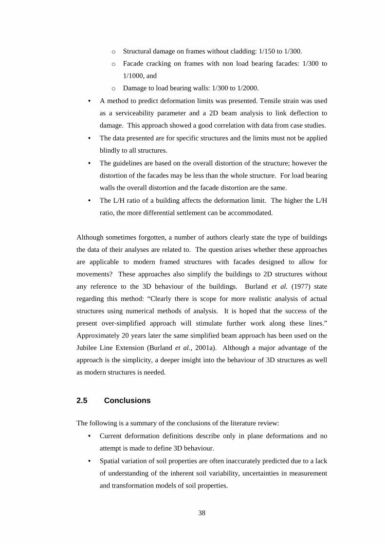
38

o Structural damage on frames without cladding: 1/150 to 1/300.

o Facade cracking on frames with non load bearing facades: 1/300 to

1/1000, and

o Damage to load bearing walls: 1/300 to 1/2000.

• A method to predict deformation limits was presented. Tensile strain was used

as a serviceability parameter and a 2D beam analysis to link deflection to

damage. This approach showed a good correlation with data from case studies.

• The data presented are for specific structures and the limits must not be applied

blindly to all structures.

• The guidelines are based on the overall distortion of the structure; however the

distortion of the facades may be less than the whole structure. For load bearing

walls the overall distortion and the facade distortion are the same.

• The L/H ratio of a building affects the deformation limit. The higher the L/H

ratio, the more differential settlement can be accommodated.

Although sometimes forgotten, a number of authors clearly state the type of buildings

the data of their analyses are related to. The question arises whether these approaches

are applicable to modern framed structures with facades designed to allow for

movements? These approaches also simplify the buildings to 2D structures without

any reference to the 3D behaviour of the buildings. Burland et al. (1977) state

regarding this method: “Clearly there is scope for more realistic analysis of actual

structures using numerical methods of analysis. It is hoped that the success of the

present over-simplified approach will stimulate further work along these lines.”

Approximately 20 years later the same simplified beam approach has been used on the

Jubilee Line Extension (Burland et al., 2001a). Although a major advantage of the

approach is the simplicity, a deeper insight into the behaviour of 3D structures as well

as modern structures is needed.

2.5 Conclusions

The following is a summary of the conclusions of the literature review:

• Current deformation definitions describe only in plane deformations and no

attempt is made to define 3D behaviour.

• Spatial variation of soil properties are often inaccurately predicted due to a lack

of understanding of the inherent soil variability, uncertainties in measurement

and transformation models of soil properties.

39

• Ultimate limit state design loads are significantly higher (up to 8 times) than

expected loads during normal use.

• Although foundation load-displacement response is non-linear, the load-

displacement behaviour of foundations loaded within the design loads on

overconsolidated clays is close to linear elastic.

• Reused foundations have been preloaded and will have a stiffer load-

displacement response than a similar new foundation. The increase in stiffness

of the load-displacement response depends on the loading and soil type.

• The ratio of immediate to total settlement of a foundation on overconsolidated

clay will be in the range of 0.35 to 0.75.

• The stiffness of a building that is loaded progressively during construction is

about half the stiffness of the completed building.

• The need exists for accurate building stiffness predictions and the

normalisation of soil-structure stiffness.

• On structures with load bearing walls, the first damage to occur due to

differential settlement will in most cases be visual damage. Structural damage

will only occur at larger differential settlements.

• The current state of the art guidelines to prevent differential settlement damage

are based on the assumption that the behaviour of the 3D structure can be

represented by a simplified 2D structure.

• The current state of the art guidelines to prevent differential settlement damage

are focussed on older, rigid, masonry infill buildings. These acknowledge that

the behaviour of flexible structures may be different and the guidelines are only

applicable to rigid structures, however minimal guidance is given on the

behaviour of 3D flexible structures.

From the literature it is evident that the current state of the art may not be applicable to

modern flexible structures. The need exists to investigate the full 3D behaviour of

modern flexible buildings with or without the reuse of foundations.

40

Table 2.1: Summary of inherent variability of strength parameters (Phoon and

Kulhawy, 1999)

Propertya Soil type No. of

data

groups

No. of tests per

group

Property value Property COV (%)

Range Mean Range Mea

n

Range Mean

Su (UC)

(kN/m2)

Fine grained 38 2-538 101 6-412 100 6-56 33

Su (UU)

(kN/m2)

Clay, silt 13 14-82 33 15-363 276 11-49 22

Su (CIUC)

(kN/m2)

Clay 10 12-86 47 130-713 405 18-42 32

Su (kN/m2)b Clay 42 24-124 48 8-638 112 6-80 32

Ø (°) Sand 7 29-136 62 35-41 37.6 5-11 9

Ø (°) Clay, silt 12 5-51 16 9-33 15.3 10-50 21

Ø (°) Clay, silt 9 - - 17-41 33.3 4-12 9

tan Ø (TC) Clay, silt 4 - - 0.24-0.69 0.509 6-46 20

tan Ø (DS) Clay, silt 3 - - - 0.615 6-46 23

tan Ø b Sand 13 6-111 45 0.65-0.92 0.744 5-14 9

a Su, undrained shear strength; Ø, effective stress friction angle; TC, triaxial compression test; UC, unconfined compression test; UU, unconsolidated-undrained triaxial compression test; CIUC, consolidated isotropic undrained triaxial compression test; DS, direct shear test.

b Laboratory test type not reported

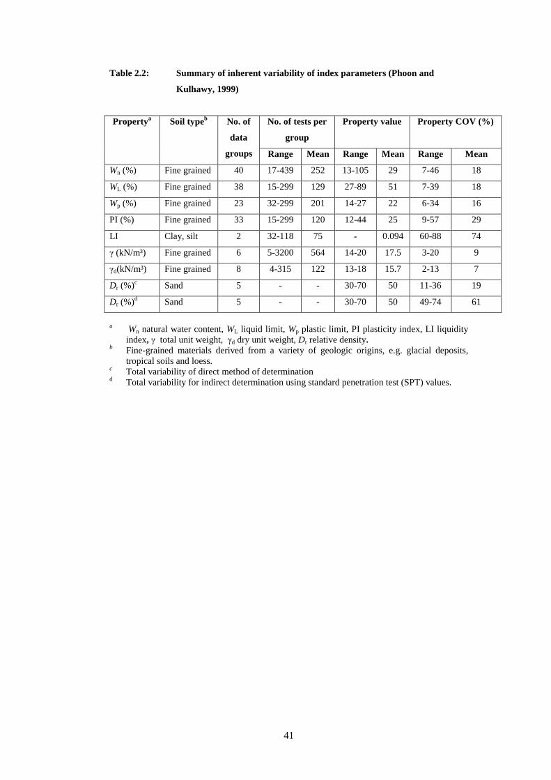
41

Table 2.2: Summary of inherent variability of index parameters (Phoon and

Kulhawy, 1999)

Propertya Soil typeb No. of

data

groups

No. of tests per

group

Property value Property COV (%)

Range Mean Range Mean Range Mean

Wn (%) Fine grained 40 17-439 252 13-105 29 7-46 18

WL (%) Fine grained 38 15-299 129 27-89 51 7-39 18

Wp (%) Fine grained 23 32-299 201 14-27 22 6-34 16

PI (%) Fine grained 33 15-299 120 12-44 25 9-57 29

LI Clay, silt 2 32-118 75 - 0.094 60-88 74

γ (kN/m³) Fine grained 6 5-3200 564 14-20 17.5 3-20 9

γd(kN/m³) Fine grained 8 4-315 122 13-18 15.7 2-13 7

Dr (%)c Sand 5 - - 30-70 50 11-36 19

Dr (%)d Sand 5 - - 30-70 50 49-74 61

a Wn natural water content, WL liquid limit, Wp plastic limit, PI plasticity index, LI liquidity index, γ total unit weight, γd dry unit weight, Dr relative density.

b Fine-grained materials derived from a variety of geologic origins, e.g. glacial deposits, tropical soils and loess.

c Total variability of direct method of determination d Total variability for indirect determination using standard penetration test (SPT) values.

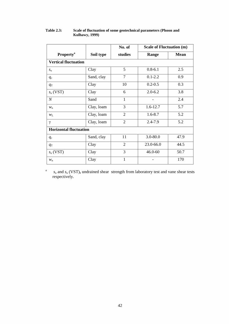
42

Table 2.3: Scale of fluctuation of some geotechnical parameters (Phoon and Kulhawy, 1999)

Propertya Soil type

No. of

studies

Scale of Fluctuation (m)

Range Mean

Vertical fluctuation

su Clay 5 0.8-6.1 2.5

qc Sand, clay 7 0.1-2.2 0.9

qT Clay 10 0.2-0.5 0.3

su (VST) Clay 6 2.0-6.2 3.8

N Sand 1 - 2.4

wn Clay, loam 3 1.6-12.7 5.7

wL Clay, loam 2 1.6-8.7 5.2

γ Clay, loam 2 2.4-7.9 5.2

Horizontal fluctuation

qc Sand, clay 11 3.0-80.0 47.9

qT Clay 2 23.0-66.0 44.5

su (VST) Clay 3 46.0-60 50.7

wn Clay 1 - 170

a su and su (VST), undrained shear strength from laboratory test and vane shear tests respectively.

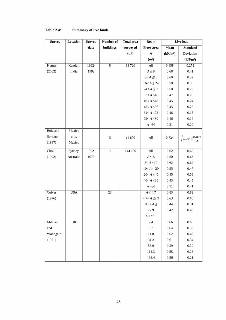
43

Table 2.4: Summary of live loads

Survey Location Survey

date

Number of

buildings

Total area

surveyed

(m²)

Room

Floor area

A

(m²)

Live load

Mean

(kN/m²)

Standard

Deviation

(kN/m²)

Kumar

(2002)

Kandur,

India

1992-

1993

8 11 720 All

A ≤ 8

8< A ≤16

16< A ≤ 24

24< A ≤32

32< A ≤40

40< A ≤48

48< A ≤56

64< A ≤72

72< A ≤80

A >80

0.458

0.68

0.60

0.50

0.50

0.47

0.45

0.45

0.46

0.46

0.31

0.278

0.41

0.32

0.36

0.29

0.26

0.24

0.25

0.15

0.19

0.20

Ruiz and

Soriano

(1997)

Mexico

city,

Mexico

5 14 890 All 0.734

A

4473.00394.0 +

Choi

(1992)

Sydney,

Australia

1972-

1979

11 144 136 All

A ≤ 5

5< A ≤10

10< A ≤ 20

20< A ≤40

40< A ≤80

A >80

0.62

0.50

0.62

0.55

0.45

0.43

0.51

0.60

0.66

0.64

0.47

0.53

0.45

0.41

Culver

(1976)

USA 23 A ≤ 4.7

4.7< A ≤9.3

9.3< A ≤

27.9

A >27.9

0.83

0.63

0.44

0.42

0.82

0.60

0.31

0.43

Mitchell

and

Woodgate

(1971)

UK 2.4

5.2

14.0

31.2

58.0

111.3

192.4

0.66

0.64

0.62

0.61

0.59

0.58

0.56

0.65

0.53

0.43

0.34

0.30

0.26

0.21

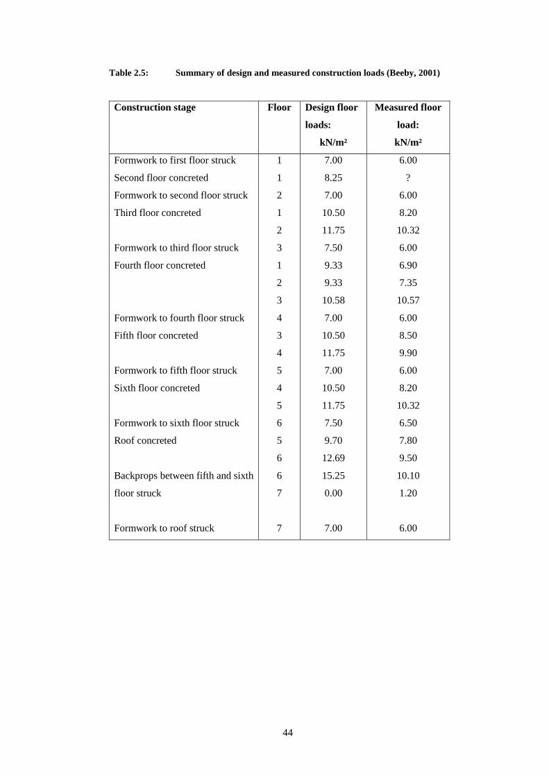
44

Table 2.5: Summary of design and measured construction loads (Beeby, 2001)

Construction stage Floor Design floor

loads:

kN/m²

Measured floor

load:

kN/m²

Formwork to first floor struck

Second floor concreted

Formwork to second floor struck

Third floor concreted

Formwork to third floor struck

Fourth floor concreted

Formwork to fourth floor struck

Fifth floor concreted

Formwork to fifth floor struck

Sixth floor concreted

Formwork to sixth floor struck

Roof concreted

Backprops between fifth and sixth

floor struck

Formwork to roof struck

1

1

2

1

2

3

1

2

3

4

3

4

5

4

5

6

5

6

6

7

7

7.00

8.25

7.00

10.50

11.75

7.50

9.33

9.33

10.58

7.00

10.50

11.75

7.00

10.50

11.75

7.50

9.70

12.69

15.25

0.00

7.00

6.00

?

6.00

8.20

10.32

6.00

6.90

7.35

10.57

6.00

8.50

9.90

6.00

8.20

10.32

6.50

7.80

9.50

10.10

1.20

6.00

45

Table 2.6: Load combinations and partial factors for Ultimate Limit State design

according to British Standards Institution (BSI 8110-1: 1997)

Load combination

Load type

Dead Live Wind

Adverse Beneficial Adverse Beneficial

Dead and live 1.4 1.0 1.6 0 -

Dead and wind 1.4 1.0 - - 1.4

Dead, live and wind 1.2 1.2 1.2 1.2 1.2

46

Table 2.7: Load combinations and partial factors for Ultimate Limit State

design according to Eurocode (EN 1990: 2002, NA to EN 1990: 2002)

Permanent action Variable action

Unfavourable Favourable Unfavourable Favourable

A) *EQU

B) *STR/GEO

C) *STR/GEO

1.05 (1.1 UK)

1.35

1.00

0.95 (0.9 UK)

1.00

1.00

1.5

1.5

1.3

0

0

0

* Notes: Static equilibrium should be verified using the design values of actions ‘A’

Design of structural members not involving geotechnical actions should be

verified using the design values of ‘B’

Design of structural members (footings, piles, etc.) involving geotechnical

actions should be verified using one of the following:

Approach 1: Applying in separate calculations design values from ‘B’

and ‘C’ to the geotechnical actions as well as the actions

on / from the structure;

Approach 2: Apply the design values of actions from ‘B’ to the

geotechnical actions as well as actions on / from the

structure;

Approach 3: Applying design values of actions from ‘C’ to the

geotechnical actions and, simultaneously, applying design

values from actions from ‘B’ to the actions on / from the

structure. UK Annex recommends Approach 1.

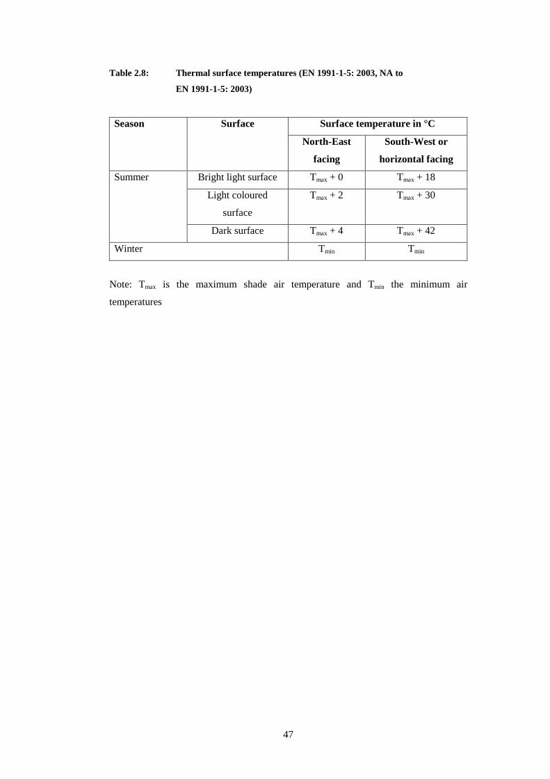
47

Table 2.8: Thermal surface temperatures (EN 1991-1-5: 2003, NA to

EN 1991-1-5: 2003)

Season Surface Surface temperature in °C

North-East

facing

South-West or

horizontal facing

Summer Bright light surface Tmax + 0 Tmax + 18

Light coloured

surface

Tmax + 2 Tmax + 30

Dark surface Tmax + 4 Tmax + 42

Winter Tmin Tmin

Note: Tmax is the maximum shade air temperature and Tmin the minimum air

temperatures

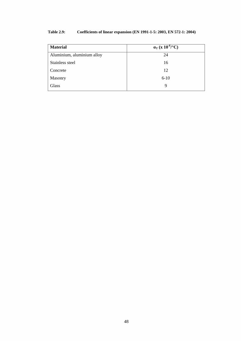
48

Table 2.9: Coefficients of linear expansion (EN 1991-1-5: 2003, EN 572-1: 2004)

Material αT (x 10-6/°C)

Aluminium, aluminium alloy

Stainless steel

Concrete

Masonry

Glass

24

16

12

6-10

9

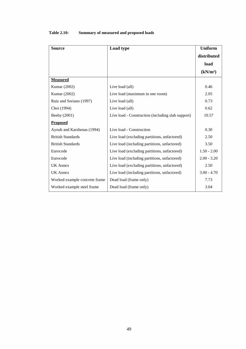
49

Table 2.10: Summary of measured and proposed loads

Source Load type Uniform

distributed

load

(kN/m²)

Measured

Kumar (2002)

Kumar (2002)

Ruiz and Soriano (1997)

Choi (1994)

Beeby (2001)

Proposed

Ayoub and Karshenas (1994)

British Standards

British Standards

Eurocode

Eurocode

UK Annex

UK Annex

Worked example concrete frame

Worked example steel frame

Live load (all)

Live load (maximum in one room)

Live load (all)

Live load (all)

Live load - Construction (including slab support)

Live load - Construction

Live load (excluding partitions, unfactored)

Live load (including partitions, unfactored)

Live load (excluding partitions, unfactored)

Live load (including partitions, unfactored)

Live load (excluding partitions, unfactored)

Live load (including partitions, unfactored)

Dead load (frame only)

Dead load (frame only)

0.46

2.05

0.73

0.62

10.57

0.30

2.50

3.50

1.50 - 2.00

2.00 - 3.20

2.50

3.00 - 4.70

7.73

3.04

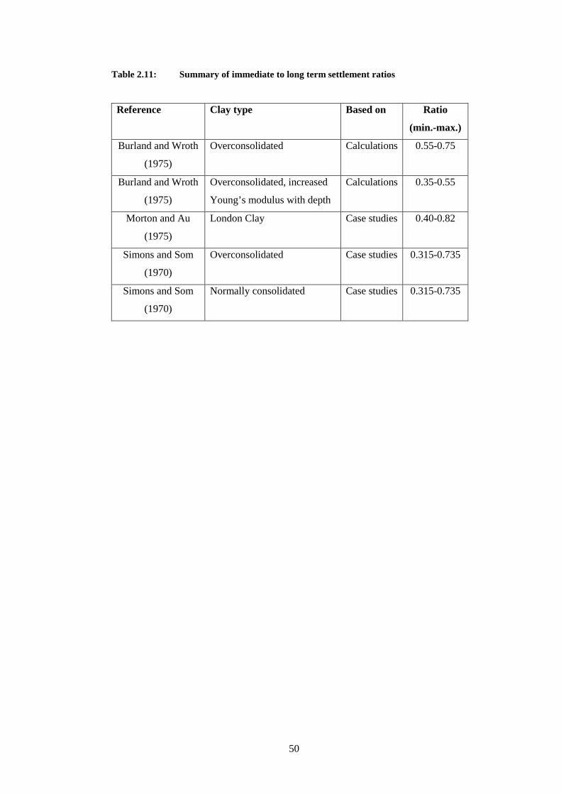
50

Table 2.11: Summary of immediate to long term settlement ratios

Reference Clay type Based on Ratio

(min.-max.)

Burland and Wroth

(1975)

Overconsolidated Calculations 0.55-0.75

Burland and Wroth

(1975)

Overconsolidated, increased

Young’s modulus with depth

Calculations 0.35-0.55

Morton and Au

(1975)

London Clay Case studies 0.40-0.82

Simons and Som

(1970)

Overconsolidated Case studies 0.315-0.735

Simons and Som

(1970)

Normally consolidated Case studies 0.315-0.735

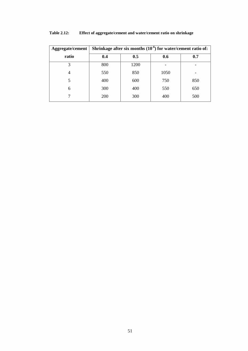
51

Table 2.12: Effect of aggregate/cement and water/cement ratio on shrinkage

Aggregate/cement

ratio

Shrinkage after six months (10-6) for water/cement ratio of:

0.4 0.5 0.6 0.7

3

4

5

6

7

800

550

400

300

200

1200

850

600

400

300

-

1050

750

550

400

-

-

850

650

500

52

Table 2.13: Description of buildings analysed for the Jubilee Line Extension (Burland

et al., 2001b)

Building Storeys Load

bearing

brickwork

Steel

frame

Reinforced

concrete

frame

Construction

date

RICS, Great George Street

128-130 Jamaica Road

London Bridge Post Office

St. Stephen’s (Clock) Tower, Palace

of Westminster

Treasury

Ritz Hotel

RAC Building

ICE, Great George Street

Telephone House

PHED, Great George Street

Murdoch, Clegg and Neptune Houses

Blick House

Fielden House

Elizabeth House

182-210 Jamaica Road

Niagara Court

Regina and Columbia Points

Tenants’ Hall and Boiler House,

Canada Estate

BT Building

RICS extension, Great George Street

Keeton’s Estate

1-7 St, Thomas Street

6

3

5

92 m

5

8

5

8

7

9

3

5

7

7 & 10

2

4

21

1

6

6

3

4

x

x

x

x

x

x

x

x

x

x

x

x

x

x

x

x

x

x

x

x

x

x

x

x

1756 & 1896

unknown,

probably early

1800s

early 1840s

1858

1898-1912

1906

1911

1912

1915

1927

1931

1950

1952

1960

1960s

1960s

1961-1962

1961-1962

mid 1970s

1978

early 1980s

late 1980s

53

Table 2.14: Classification of visible damage to walls with particular reference to

ease of repair of plaster and brickwork or masonry (Burland et al., 2001a)

Category of damage Normal degree of

severity

Description of typical damage (ease of repair is in bold type)

Note: Crack width is only one factor in assessing category of

damage and should not be used on its own as a direct measure

of it.

0

1

2

3

4

5

Negligible

Very slight

Slight

Moderate

Severe

Very severe

Hairline cracks less than about 0.1 mm wide.

Fine cracks that are easily treated during normal decoration.

Damage generally restricted to internal wall finishes. Close

inspection may reveal some cracks in external brickwork or

masonry. Typical crack widths up to 1 mm.

Cracks easily filled. Redecoration probably required.

Recurrent cracks can be masked by suitable linings. Cracks

may be visible externally and some repointing may be

required to ensure weather-tightness. Doors and windows

may stick slightly. Typical crack widths up to 5 mm.

The cracks require some opening up and can be patched by

a mason. Repointing of external brickwork and possibly a

small amount of brickwork to be replaced. Doors and

windows sticking. Service pipes may fracture. Weather

tightness often impaired. Typical crack widths are 5-15 mm or

several > 3 mm.

Extensive repair work involving breaking-out and replacing

sections of walls, especially over doors and windows.

Windows and door frames distorted, floor sloping noticeably1.

Walls leaning1 or bulging noticeably, some loss of bearing in

beams. Service pipes disrupted. Typical crack widths are 15-25

mm, but also depends on the number of cracks.

This requires a major repair job involving partial or

complete rebuilding. Beams lose bearing, walls lean badly and

require shoring. Windows broken with distortion. Danger of

instability. Typical crack widths are greater than 25 mm, but

depends on the number of cracks.

1Note: Local deviation of slope, from the horizontal or vertical, of more than 1/100 will normally be clearly visible.

Overall deviations in excess of 1/150 are undesirable.

54

Table 2.15: Relationship between category of damage and limiting tensile strain

(Burland et al., 2001a)

Category of damage Normal degree of severity Limiting tensile strain

(%)

0

1

2

3

4 to 5

Negligible

Very slight

Slight

Moderate*

Severe to very severe

0-0.05

0.05-0.075

0.075-0.15

0.15-0.3

> 0.3

*Note: Boscarding and Cording (1989) describe the damage corresponding to limiting

tensile strain in the range of 0.15 to 0.3 per cent as “moderate to severe”. However

none of these cases quoted by them exhibits severe damage for this range of strains.

There is therefore no evidence to suggest that tensile strains up to 0.3 per cent will

result in severe damage.

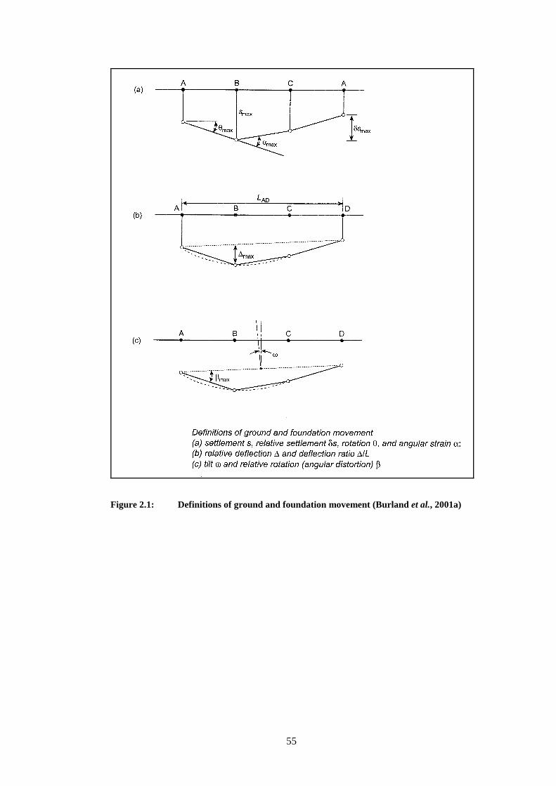
55

Figure 2.1: Definitions of ground and foundation movement (Burland et al., 2001a)

56

Figure 2.2: Inherent soil variability and scale of fluctuation (Phoon and Kulhawy,

1999)

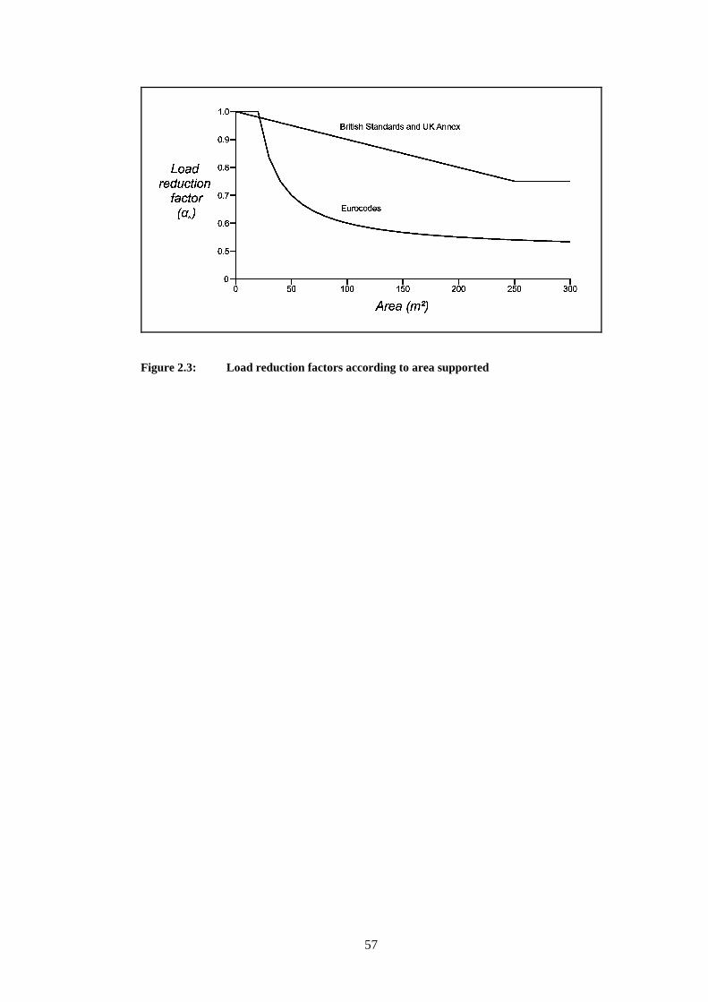
57

Figure 2.3: Load reduction factors according to area supported

58

Figure 2.4: Load reduction factors for number of floors supported

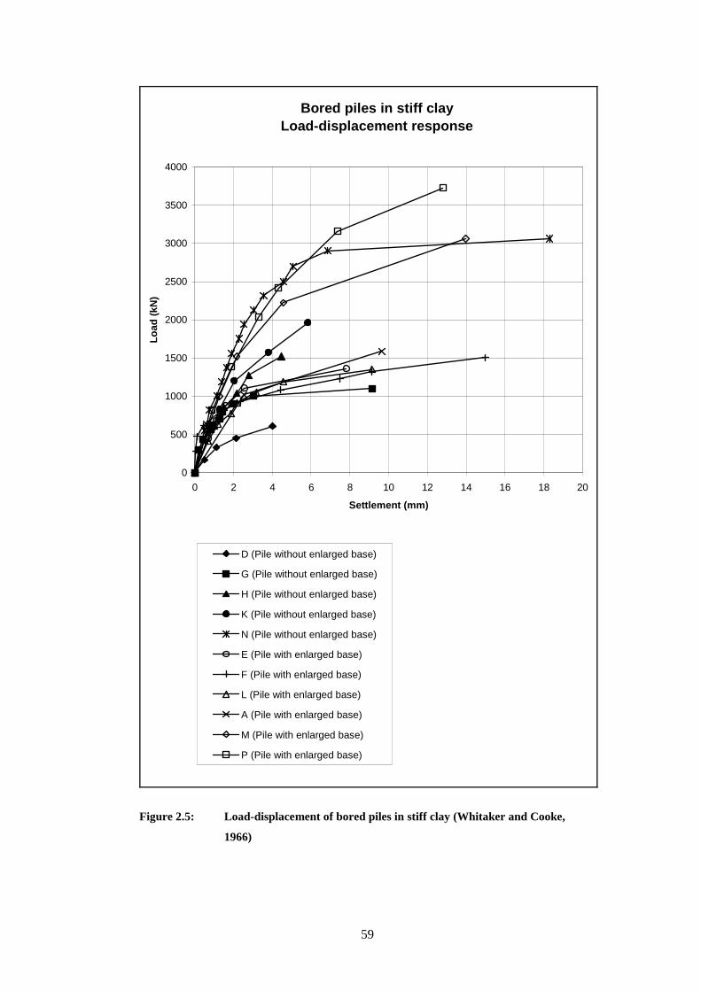
59

Bored piles in stiff clayLoad-displacement response

0

500

1000

1500

2000

2500

3000

3500

4000

0 2 4 6 8 10 12 14 16 18 20

Settlement (mm)

Lo

ad (

kN)

D (Pile without enlarged base)

G (Pile without enlarged base)

H (Pile without enlarged base)

K (Pile without enlarged base)

N (Pile without enlarged base)

E (Pile with enlarged base)

F (Pile with enlarged base)

L (Pile with enlarged base)

A (Pile with enlarged base)

M (Pile with enlarged base)

P (Pile with enlarged base)

Figure 2.5: Load-displacement of bored piles in stiff clay (Whitaker and Cooke,

1966)

60

Various piles Load-displacement response

0

500

1000

1500

2000

2500

3000

3500

4000

4500

5000

5500

6000

0 10 20 30 40 50 60 70 80 90 100 110 120

Settlement (mm)

Lo

ad (

kN)

Driven cast in place straight pile in dense sand

Driven cast in place underreamed pile in dense sand

Large diameter pile in soft chalk

750mm continious flight auger pile 27m long in silt

750mm continious flight auger pile 32m long in silt

Pile in mudstone

Figure 2.6: Load-displacement response of various piles (De Beer et al., 1979,

Fleming, 1992)

61

Figure 2.7: Measured load distribution of the shaft and base of an under reamed

pile (Whitaker and Cooke, 1966)

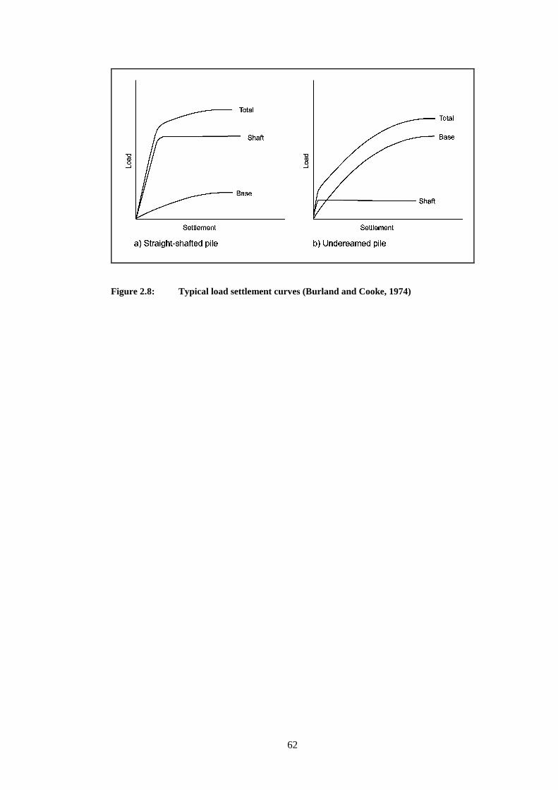
62

Figure 2.8: Typical load settlement curves (Burland and Cooke, 1974)

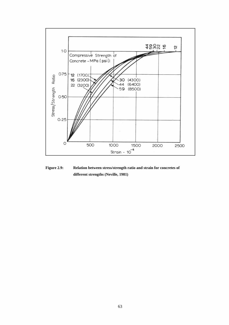
63

Figure 2.9: Relation between stress/strength ratio and strain for concretes of

different strengths (Neville, 1981)

64

Figure 2.10: Development of strength of concrete (determined by 150 mm cubes),

stored under moist conditions (Wood, 1991)

65

Figure 2.11: Influence of moisture condition on the modulus of elasticity at

5.5 MPa (Neville, 1981)

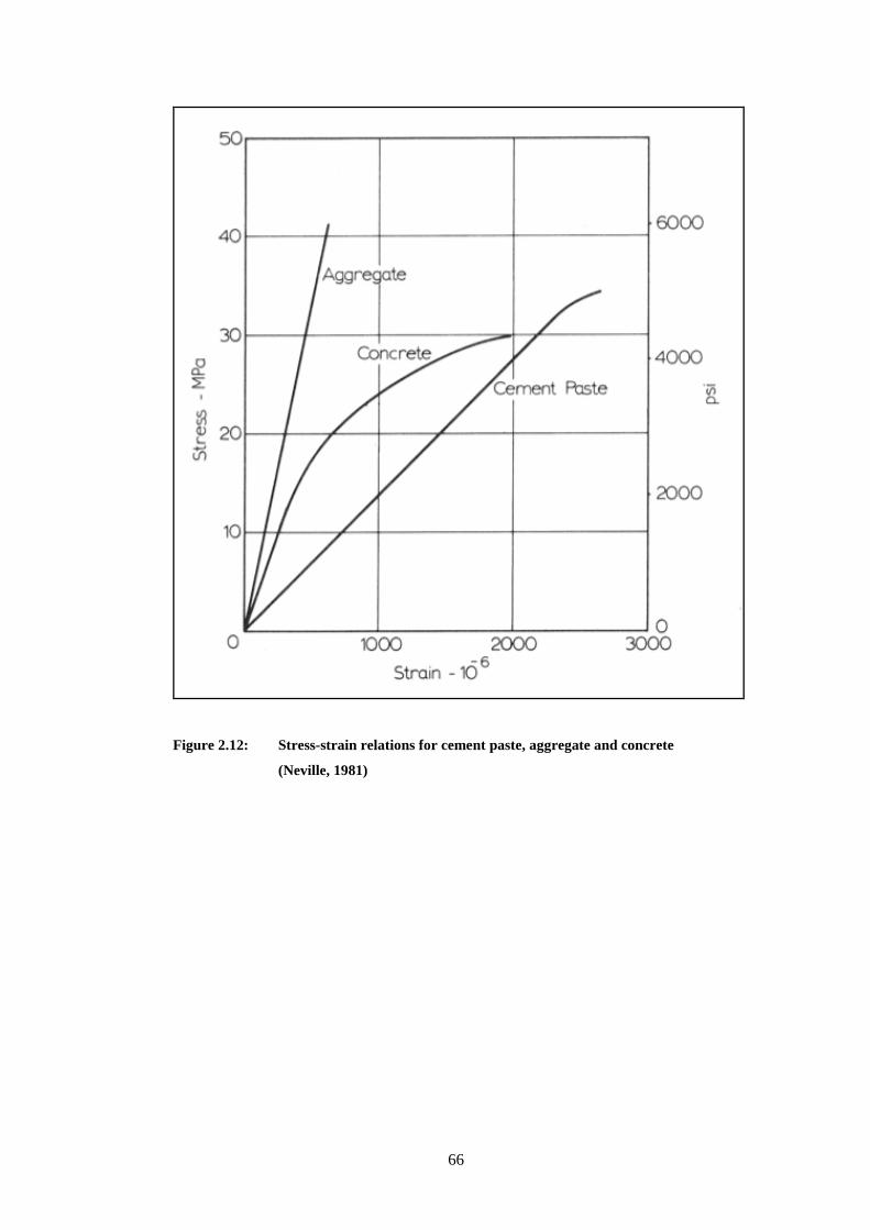
66

Figure 2.12: Stress-strain relations for cement paste, aggregate and concrete

(Neville, 1981)

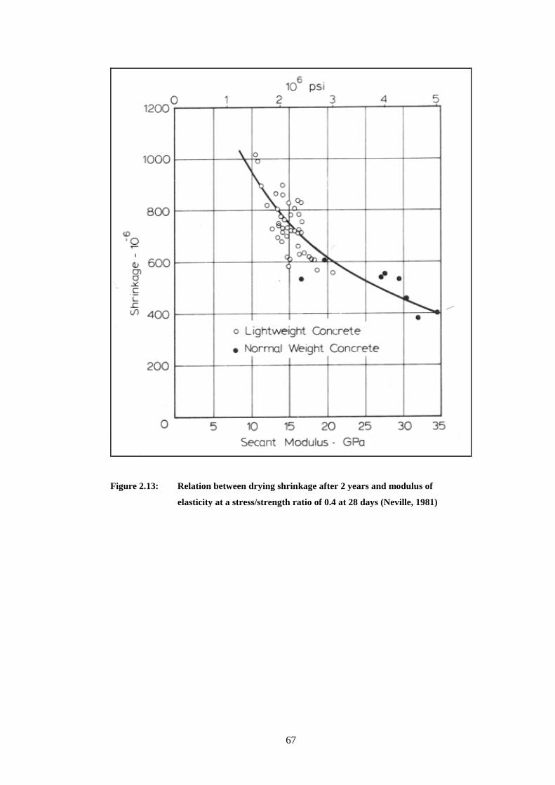
67

Figure 2.13: Relation between drying shrinkage after 2 years and modulus of

elasticity at a stress/strength ratio of 0.4 at 28 days (Neville, 1981)

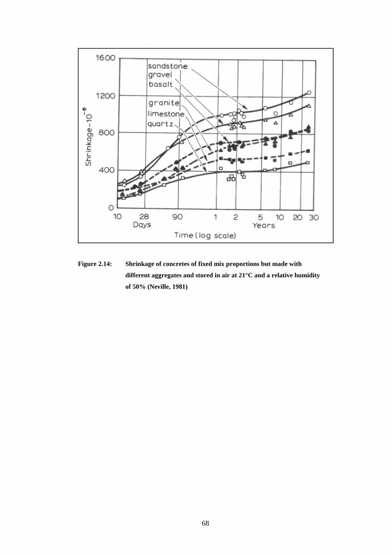
68

Figure 2.14: Shrinkage of concretes of fixed mix proportions but made with

different aggregates and stored in air at 21°C and a relative humidity

of 50% (Neville, 1981)

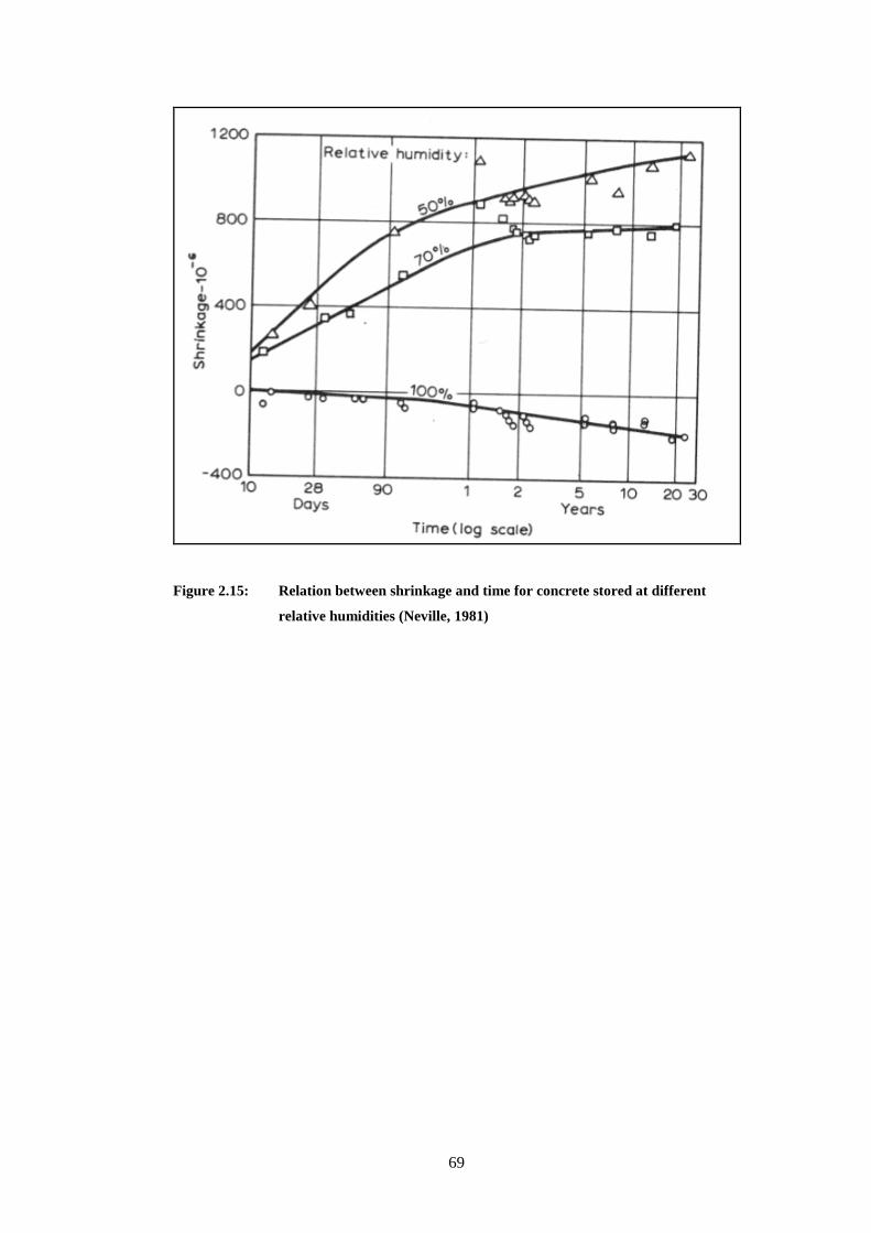
69

Figure 2.15: Relation between shrinkage and time for concrete stored at different

relative humidities (Neville, 1981)

70

Figure 2.16: Relaxation of stress under a constant strain of 360x10-6 (Neville, 1981)

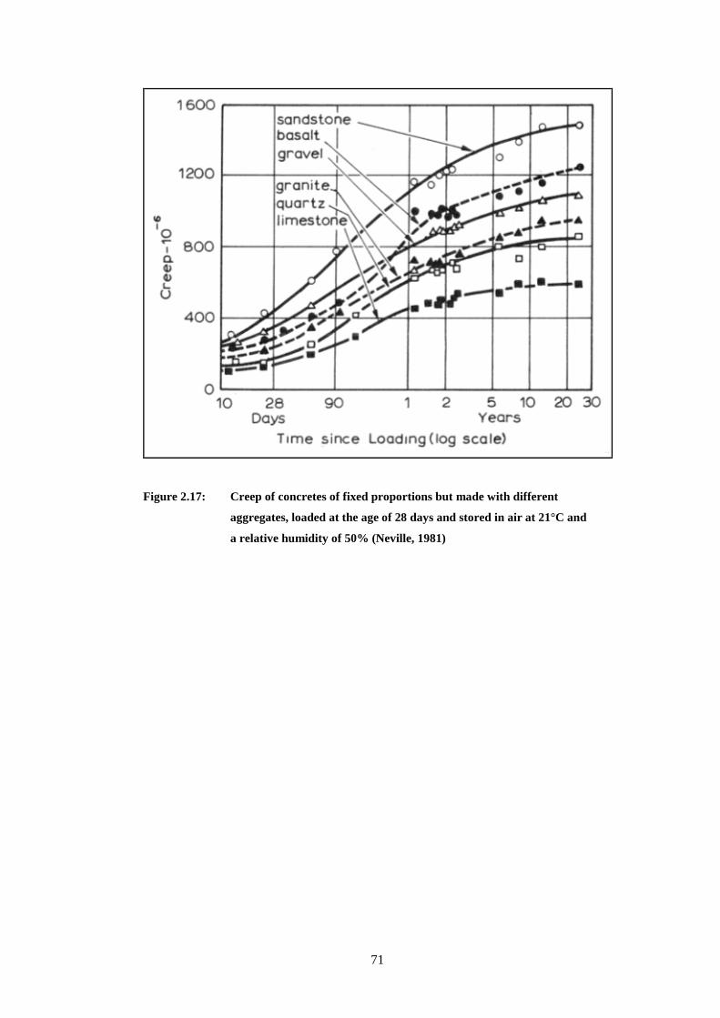
71

Figure 2.17: Creep of concretes of fixed proportions but made with different

aggregates, loaded at the age of 28 days and stored in air at 21°C and

a relative humidity of 50% (Neville, 1981)

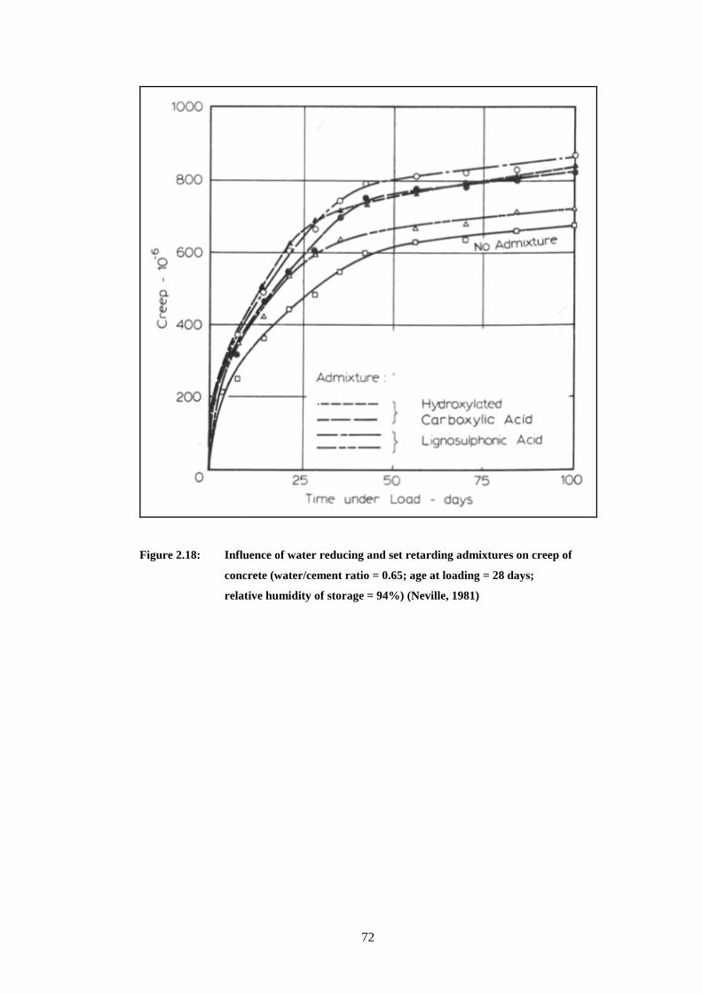
72

Figure 2.18: Influence of water reducing and set retarding admixtures on creep of

concrete (water/cement ratio = 0.65; age at loading = 28 days;

relative humidity of storage = 94%) (Neville, 1981)

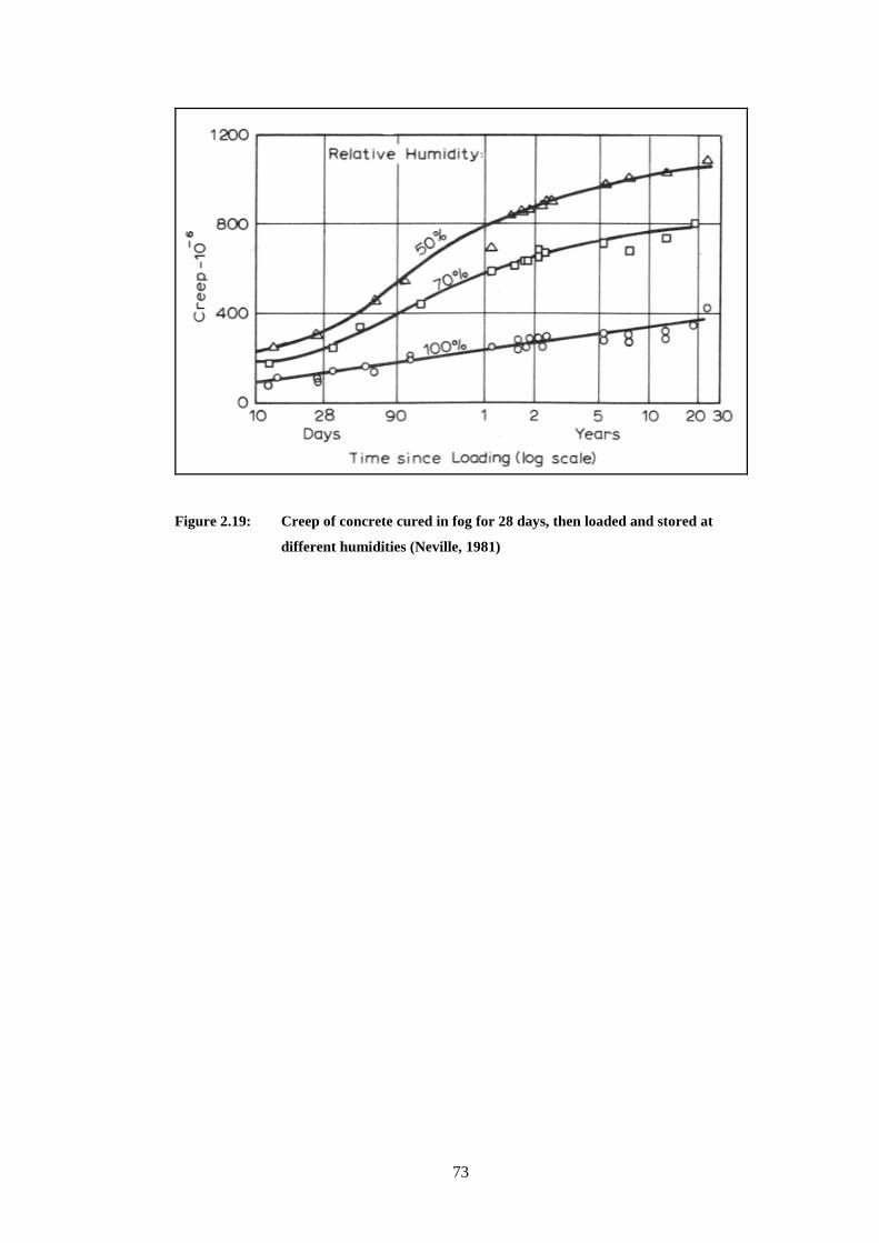
73

Figure 2.19: Creep of concrete cured in fog for 28 days, then loaded and stored at

different humidities (Neville, 1981)

74

Figure 2.20: Range of creep-time curves for different concretes stored at various

relative humidities (Neville, 1981)

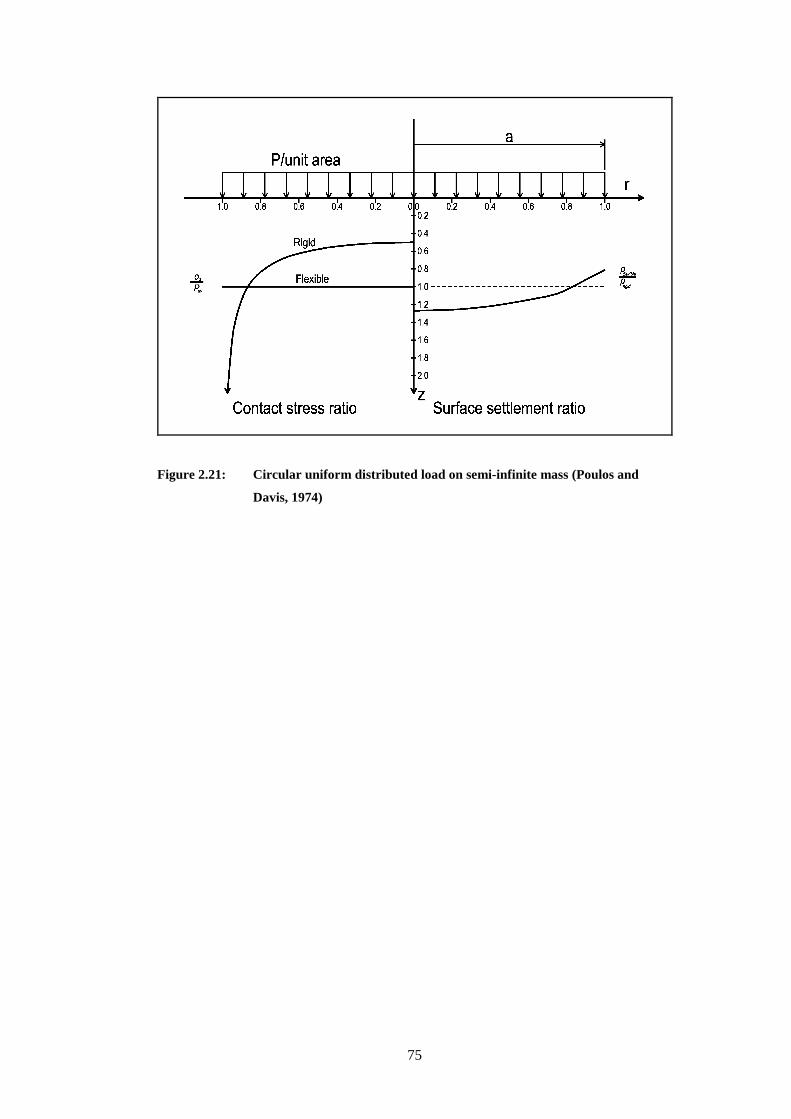
75

Figure 2.21: Circular uniform distributed load on semi-infinite mass (Poulos and

Davis, 1974)

76

Figure 2.22: Cracking of a simple beam in bending and shear (Burland, 1975)

77

Figure 2.23: Relationship between (∆/L)/εlim and L/H for rectangular isotropic

beams with the neutral axis at the bottom edge (Burland et al., 2001a)

78

Figure 2.24: Relationship between ∆/L and L/H for buildings showing various

degrees of damage (Burland et al., 1977)

79

3 RESEARCH METHODOLOGY

Finite element analysis was used to investigate the behaviour of modern flexible

framed structures undergoing differential settlement. Modern office buildings vary in

design and to minimise the numerical modelling a “typical” modern structure was

investigated. The structure investigated was a reinforced concrete structure with six

storeys and five bays in both directions, supported by pad foundations. This structure

was designed according to British Standards and Eurocode 7 to determine the member

sizes for the finite element model. Using the structural sizing from the design the finite

element model was created in phases, gradually expanding the geometry. Each phase

of the model was analysed, the behaviour verified and problems corrected before

commencing with the next phase. With the model completely built and verified the

effect of soil-structure stiffness was investigated by changing the soil or concrete

stiffness by varying the Young’s modulus of the material. The following analyses sets

were run:

• For the 5 bay structure the soil stiffness for the whole halfspace was varied

from a Young’s modulus of 100 Pa to 1 000 GPa, increasing the stiffness each

time with an order of magnitude to determine the effect of soil stiffness on

column loads, column displacements and bending moments in the slabs.

• For the 5 bay structure the Young’s modulus of the concrete was increased

from 13 GPa to 13 000 GPa to determine the effect of a stiffer structure on

column loads. 13 000 GPa is not a realistic stiffness, however it was used to

increase the superstructure stiffness without any change in the geometry. The

soil stiffness was varied as before.

• The structure geometry was reduced from 5 by 5 bays to 5 by 4 bays and

5 by 3 bays to determine the effect of structure geometry on column loads.

• The 5 by 5 bay superstructure was replaced by a slab with a bending stiffness

equivalent to the individual slabs to determine the possibility of modelling an

equivalent slab instead of the whole structure; and,

• The soil stiffness under individual pad foundations in the 5 by 5 bay structure

was varied to determine the effect of soft or hard spots under foundations.

This chapter firstly discusses the layout of the structure and presents the structural

design of the frame which was used to determine member sizes. Secondly the

80

numerical model is presented. Thirdly the verification of the model is discussed and

lastly typical results are presented. Chapter 4 contains a discussion of the analyses.

3.1 Structural design

3.1.1 Layout

To investigate the behaviour of a modern flexible frame structure the layout of the

structure under investigation needed to be defined. For a representative structure the

following assumptions were made:

• The structure was a 6 storey frame with 5 bays in each direction. This structure

was chosen to provide a sufficiently large structure to evaluate the change in

behaviour from external to internal bays and for subsequent levels. This was

also the upper limit for the number of foundations and surrounding soil which

the finite element analysis software could mesh adequately, given the computer

software that was available.

• Floor and roof slabs were reinforced flat concrete slabs, i.e. no beams. Modern

office buildings often use flat slab construction. The use of flat slabs also

simplifies the geometry of a finite element model.

• Floor spacing was 3 m centre to centre which is typical of modern buildings.

• Columns were reinforced concrete with the same dimensions throughout the

structure, i.e. sized according to the largest column load which is an internal

ground floor column. This simplified the design and the finite element

modelling.

• Column spacing was 7.5 m centre to centre which is typical for current flat slab

construction.

• External facades and internal partitions were assumed not to alter the frame

stiffness, i.e. movement was allowed between the facade or partition and frame.

• Ground floor columns were supported by individual pad foundations at 5 m

below ground level. The 5 m depth ensured enough bearing capacity on an

assumed London Clay for individual pad foundations for each column. Three

different foundation sizes were used for corner, edge and internal foundations.

• The ground floor slab was supported by the underlying soil and not connected

to the structure.

The complete structure layout was based on the above assumptions as shown in

Figure 3.1.

81

3.1.2 Structural sizing

The structure as shown in Figure 3.1 was designed according to British Standards to

determine member sizes. Eurocode 7 was used to determine the foundation footprint.

The design was based on the following characteristic loads derived from the British

Standards.

• A uniform distributed imposed floor load of 2.5 kN/m² and a concentrated

point load of 2.7 kN (BSI 6399-1: 1996).

• A uniform distributed imposed roof load of 1.5 kN/m² (BSI 6399-3: 1988).

• A horizontal uniform distributed wind load of 1.4 kN/m² (BSI 6399-2: 1997).

• A uniform distributed dead load of 0.419 kN/m² on the roof represented the

asphalt waterproofing.

• A uniform distributed dead load of 0.566 kN/m² on the floor represented the

floor finish; and

• A line load of 7.241 kN/m on the edge of each floor slab, represented facades

(BS 648: 1964).

Note the above loads were for the ultimate limit state design and the live loads were

significantly higher than the expected long term loads during the normal use of the

structure. For the subsequent finite element analysis of the behaviour of the structure

an expected uniform distributed imposed floor load of 0.5 kN/m² with no imposed roof

or wind load was used.

Design loads were calculated using combinations of partial safety factors as described

in BSI 8110-1 (1997). Appendix A shows the design load calculations. The following

partial safety factors were used:

• Adverse dead load: 1.4.

• Beneficial dead load: 1.0.

• Adverse imposed load: 1.6, and

• Beneficial imposed load was neglected.

A C25/30 concrete as suggested by the BSI 8500-1 (2006) for office buildings and

reinforcing steel with a 500 MPa tensile strength (BSI 8110-1: 1997) were used for the

design.

82

The structural design was carried out using standard design Excel spreadsheets from

RCC-2000. RCC-2000 are design spreadsheets based on BSI 8119-1 (1997) and were

published by the British Cement Association on behalf of the industry sponsors of the

Reinforced Concrete Council. The slab design calculations are shown in Appendix B

and the column design calculations in Appendix C. Flat slab and column design were

done according to BSI 8110-1 (1997).

The design showed that 300 mm flat floor slabs, a 250 mm flat roof slab and

450 mm x 450 mm columns were adequate. Although smaller columns may be used on

the higher floors, 450 mm x 450 mm columns were used throughout the structure to

simplify the design. A 200 mm ground floor slab was assumed. The ground floor slab

was not connected to the columns and was supported by the underlying soil.

The following vertical characteristic column loads at ground level were calculated for

foundation design. Live loads were reduced based on the number of floors supported

(BSI 8110-1: 1997).

• Corner columns, dead load 1 050 kN, imposed load 160 kN.

• Edge columns, dead load 1 688 kN, imposed load 321 kN, and

• Internal columns, dead load 2 636 kN, imposed load 641 kN.

The above loads in combination with the foundation footprint area were used to

calculate appropriate pad foundation thickness according to BSI 8110-1 (1997). The

design calculations are shown in Appendix D. The following foundation thicknesses

are adequate for the imposed loads.

• Corner pad, 0.50 m.

• Edge pad, 0.65 m, and

• Internal pad, 0.85 m.

Foundation footprint sizing was done according to Eurocode 7. The design calculations

are shown in Appendix E.

The undrained shear strength (Su) of the soil was assumed to be 90 kN/m² and saturated

soil bulk unit weight 20 kN/m³. The undrained shear strength was based on the data

collected by Burland et al. (2001a) on London Clay during the Jubilee Line Extension

in London as shown in Figure 3.2. They recommend a design line of Su = 50 + 8z

83

where z is the depth below the top of the London Clay. All the foundations were

founded 5 m below ground level. The following pad foundation sizes and factors of

safety regarding settlement were calculated according to Eurocode 7:

• Corner foundation 3.3 m x 3.3 m x 0.50 m thick (FOS 3.06)

• Edge foundation 4.2 m x 4.2 m x 0.65 m thick (FOS 3.02), and

• Internal foundation 5.4 m x 5.4 m x 0.85 m thick (FOS 3.04).

3.2 Finite element modelling

The LUSAS version 14.3 finite element analysis software package was used to perform

the numerical modelling. LUSAS is the trading name of Finite Element Analysis Ltd

whose headquarters are located in the UK. LUSAS is supported around the world by a

number of LUSAS regional offices as well as by a network of LUSAS Distributors.

LUSAS is a commercial package often used by structural engineers due to the ease

with which superstructures can be modelled with standard element libraries. Other

finite element analysis software packages with advanced soil models may be more

suitable for geotechnical modelling, however for this modelling the decision was made

to model the supporting halfspace as a linear elastic material, making LUSAS a suitable

package. A 2.4 GHz Intel Core2 Duo PC with a 32-bit platform and 3 GB of RAM was

used to run LUSAS.

Modelling the soil as a linear elastic material led to a significant reduction in the

computational effort to run the model. Modelling of the soil as a linear elastic material

was based on the underlying assumption that at working loads the soil mass was

behaving in a linear elastic way. To validate this assumption the linear elastic model

was compared to a model on non-linear soil; see the discussion in Chapter 4, discussion

of the analyses.

The superstructure was also modelled as a linear elastic material to reduce

computational effort. Although stress-strain behaviour in reinforced concrete within a

structure is complex and influenced by creep, shrinkage and cracking, the use of a

linear elastic material still provided valuable insight into the change of stress within the

structure, although it may not represent the actual stress within a real structure. To

validate this assumption the elastic bending moments in the slabs were compared to the

design bending moments, as discussed in Chapter 4, discussion of the analyses.

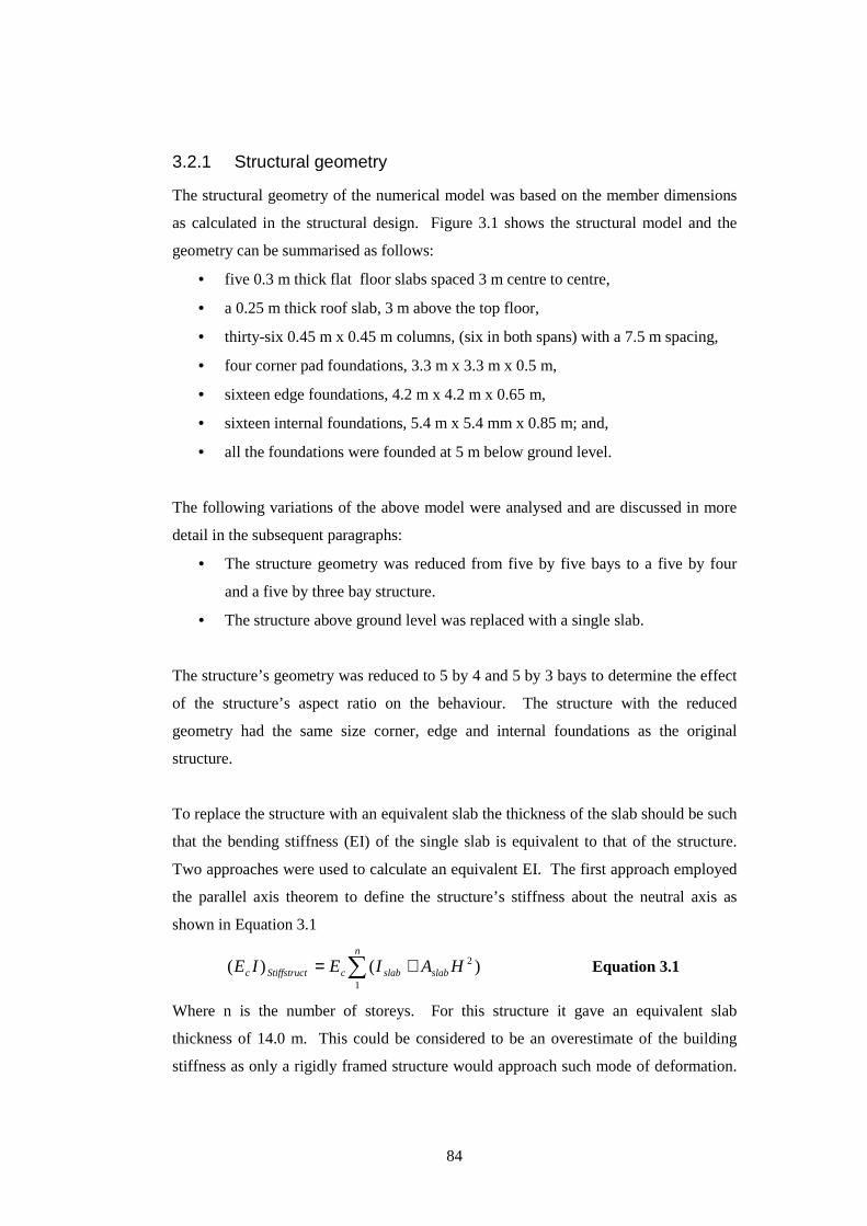
84

3.2.1 Structural geometry

The structural geometry of the numerical model was based on the member dimensions

as calculated in the structural design. Figure 3.1 shows the structural model and the

geometry can be summarised as follows:

• five 0.3 m thick flat floor slabs spaced 3 m centre to centre,

• a 0.25 m thick roof slab, 3 m above the top floor,

• thirty-six 0.45 m x 0.45 m columns, (six in both spans) with a 7.5 m spacing,

• four corner pad foundations, 3.3 m x 3.3 m x 0.5 m,

• sixteen edge foundations, 4.2 m x 4.2 m x 0.65 m,

• sixteen internal foundations, 5.4 m x 5.4 mm x 0.85 m; and,

• all the foundations were founded at 5 m below ground level.

The following variations of the above model were analysed and are discussed in more

detail in the subsequent paragraphs:

• The structure geometry was reduced from five by five bays to a five by four

and a five by three bay structure.

• The structure above ground level was replaced with a single slab.

The structure’s geometry was reduced to 5 by 4 and 5 by 3 bays to determine the effect

of the structure’s aspect ratio on the behaviour. The structure with the reduced

geometry had the same size corner, edge and internal foundations as the original

structure.

To replace the structure with an equivalent slab the thickness of the slab should be such

that the bending stiffness (EI) of the single slab is equivalent to that of the structure.

Two approaches were used to calculate an equivalent EI. The first approach employed

the parallel axis theorem to define the structure’s stiffness about the neutral axis as

shown in Equation 3.1

)()( 2

1

HAIEIE slab

n

slabctStiffstrucc += ∑ Equation 3.1

Where n is the number of storeys. For this structure it gave an equivalent slab

thickness of 14.0 m. This could be considered to be an overestimate of the building

stiffness as only a rigidly framed structure would approach such mode of deformation.

85

An alternative assumption was used to obtain the bending stiffness summing the

independent EI values for each slab as shown in Equation 3.2

∑=n

slabcFlexstructc IEIE1

)( Equation 3.2

This implied that the columns transform the same deformed shape to each storey. For

this structure it gives an equivalent slab thickness of 532 mm. This approach was used

for the plate model. The loading on the replacement slab was equal to that of the whole

structure. This was done by a distributed load to compensate for the live loads on the

slabs and the self weight of the slabs and point loads for the columns.

3.2.2 Model discretisation and element types

Columns were modelled as 3D thick beam elements with restrained translation and

rotation at end nodes. Each 3 m column and the columns below ground level (with a

length of either 4.5 m, 4.35 m or 4.15 m due to a variation in foundation thickness)

were discretised in 8 equal divisions.

The floor and roof slabs were modelled as thin shell 8 node quadrilateral elements

taking membrane and flexural deformations into account. Both translation and rotation

were restrained at nodes. Each bay was divided into 8 equal divisions in both the x and

y direction.

The foundations were modelled with 10 node tetrahedral 3D continuum elements

capable of modelling curved element boundaries. The nodes were free to rotate and

only translation was restrained. The foundations were discretised with an irregular

mesh with a maximum element size of a quarter of the foundation length. Figure 3.3

shows the mesh of foundations and the underlying soil.

The halfspace was modelled with the same 10 node tetrahedral 3D continuum elements

as for the foundations. An irregular mesh with variable element sizes was used.

Although LUSAS can vary the mesh size gradually, it was unable to mesh the model

with 36 pad foundations with a gradually variable mesh. The halfspace was therefore

divided into zones each with an assigned maximum element size. The choice of internal

zones, element sizes and boundary location is discussed in detail in Chapter 3 under the

verification of the finite element model. Figure 3.4 shows the discretisation zones and

Table 3.1 lists the maximum element size in each zone.

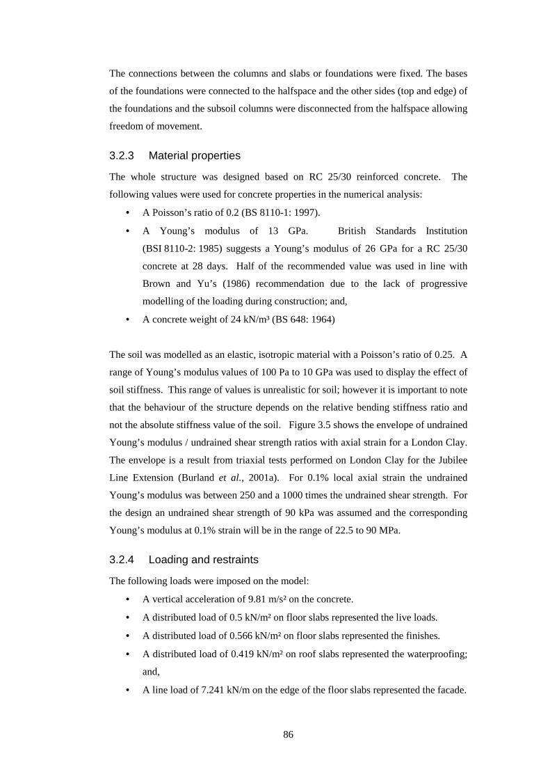
86

The connections between the columns and slabs or foundations were fixed. The bases

of the foundations were connected to the halfspace and the other sides (top and edge) of

the foundations and the subsoil columns were disconnected from the halfspace allowing

freedom of movement.

3.2.3 Material properties

The whole structure was designed based on RC 25/30 reinforced concrete. The

following values were used for concrete properties in the numerical analysis:

• A Poisson’s ratio of 0.2 (BS 8110-1: 1997).

• A Young’s modulus of 13 GPa. British Standards Institution

(BSI 8110-2: 1985) suggests a Young’s modulus of 26 GPa for a RC 25/30

concrete at 28 days. Half of the recommended value was used in line with

Brown and Yu’s (1986) recommendation due to the lack of progressive

modelling of the loading during construction; and,

• A concrete weight of 24 kN/m³ (BS 648: 1964)

The soil was modelled as an elastic, isotropic material with a Poisson’s ratio of 0.25. A

range of Young’s modulus values of 100 Pa to 10 GPa was used to display the effect of

soil stiffness. This range of values is unrealistic for soil; however it is important to note

that the behaviour of the structure depends on the relative bending stiffness ratio and

not the absolute stiffness value of the soil. Figure 3.5 shows the envelope of undrained

Young’s modulus / undrained shear strength ratios with axial strain for a London Clay.

The envelope is a result from triaxial tests performed on London Clay for the Jubilee

Line Extension (Burland et al., 2001a). For 0.1% local axial strain the undrained

Young’s modulus was between 250 and a 1000 times the undrained shear strength. For

the design an undrained shear strength of 90 kPa was assumed and the corresponding

Young’s modulus at 0.1% strain will be in the range of 22.5 to 90 MPa.

3.2.4 Loading and restraints

The following loads were imposed on the model:

• A vertical acceleration of 9.81 m/s² on the concrete.

• A distributed load of 0.5 kN/m² on floor slabs represented the live loads.

• A distributed load of 0.566 kN/m² on floor slabs represented the finishes.

• A distributed load of 0.419 kN/m² on roof slabs represented the waterproofing;

and,

• A line load of 7.241 kN/m on the edge of the floor slabs represented the facade.

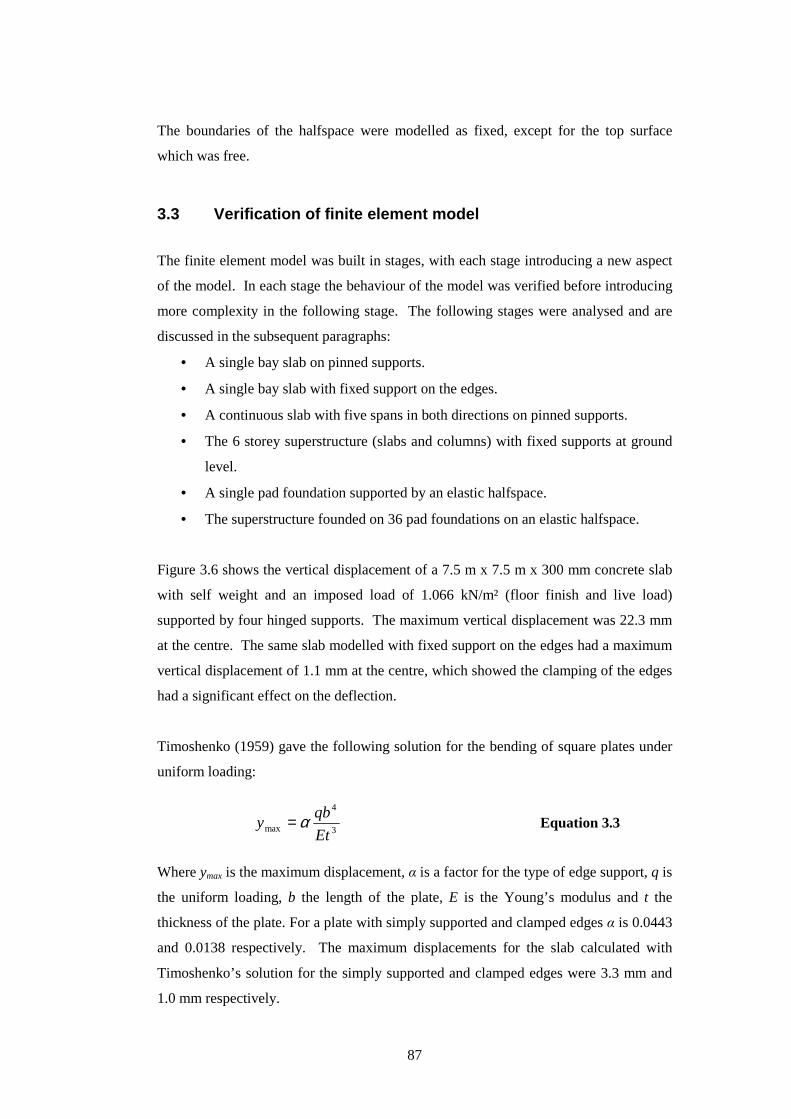
87

The boundaries of the halfspace were modelled as fixed, except for the top surface

which was free.

3.3 Verification of finite element model

The finite element model was built in stages, with each stage introducing a new aspect

of the model. In each stage the behaviour of the model was verified before introducing

more complexity in the following stage. The following stages were analysed and are

discussed in the subsequent paragraphs:

• A single bay slab on pinned supports.

• A single bay slab with fixed support on the edges.

• A continuous slab with five spans in both directions on pinned supports.

• The 6 storey superstructure (slabs and columns) with fixed supports at ground

level.

• A single pad foundation supported by an elastic halfspace.

• The superstructure founded on 36 pad foundations on an elastic halfspace.

Figure 3.6 shows the vertical displacement of a 7.5 m x 7.5 m x 300 mm concrete slab

with self weight and an imposed load of 1.066 kN/m² (floor finish and live load)

supported by four hinged supports. The maximum vertical displacement was 22.3 mm

at the centre. The same slab modelled with fixed support on the edges had a maximum

vertical displacement of 1.1 mm at the centre, which showed the clamping of the edges

had a significant effect on the deflection.

Timoshenko (1959) gave the following solution for the bending of square plates under

uniform loading:

3

4

max Et

qby α= Equation 3.3

Where ymax is the maximum displacement, α is a factor for the type of edge support, q is

the uniform loading, b the length of the plate, E is the Young’s modulus and t the

thickness of the plate. For a plate with simply supported and clamped edges α is 0.0443

and 0.0138 respectively. The maximum displacements for the slab calculated with

Timoshenko’s solution for the simply supported and clamped edges were 3.3 mm and

1.0 mm respectively.

88

The maximum displacement (1.1 mm) of the modelled slab with clamped edges

correlated well with the solution by Timoshenko (1.0 mm). The maximum

displacement on the modelled slab (22.3 mm) was significantly more than the

displacement of the slab that was simply supported on the edges (3.3 mm). This

showed that line supports reduced the displacement significantly in comparison to

pinned point supports.

Figure 3.7 shows the vertical displacement of a complete level with 25 bays on pinned

supports. Loading was the same as for the single bay except for the added line load of

7.241 kN/m at the edge of the floor slab which represented the weight of the external

facade. The maximum vertical displacement for the corner slabs was 13.8 mm. For the

edge slabs it ranged from 8.7 mm to 9.6 mm, and for the internal slabs it ranged from

3.4 mm to 5.9 mm. This clearly showed the effect adjacent bays had on the reduction of

the deflection of the slabs.

Figure 3.8 shows the vertical displacement of the complete six storey superstructure on

fixed supports at ground level. It is important to note that the top level was the roof slab

with a thickness of 250 mm with no live load and therefore the vertical displacement

will vary from a typical floor slab. The maximum vertical displacements of the top

floor level (not roof) are summarised in Table 3.2 (column 2). It is clear the vertical

displacements were significantly higher than for the single 25 bay slab (column 1).

This was due to the shortening of the columns under load. Normalising the slab

vertical displacement by subtracting the average vertical column displacement for the

specific bay gave the displacements as shown in column 3. These values correlated

well with the values of the single 25 bay slab. Column 4 gives the values of column

displacement at the top floor calculated by the assumption that each column supported

25% of each adjacent span. The values correlated well with the values from the

numerical model.

The sum of the vertical reactions at the supports in the model was within 2% of the

total load takedown determined by hand calculations. Assuming each ground level

support carried the columns above and 25% of the adjacent bays, an estimation of the

expected column loads was made. Table 3.3 shows the comparison between column

loads from the numerical model and hand calculation. All of the column loads were

within 10% of the estimated values, which shows that the model behaved as expected.

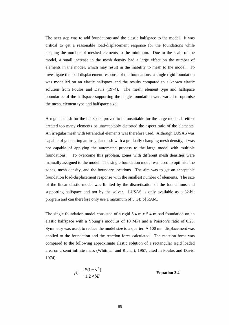
89

The next step was to add foundations and the elastic halfspace to the model. It was

critical to get a reasonable load-displacement response for the foundations while

keeping the number of meshed elements to the minimum. Due to the scale of the

model, a small increase in the mesh density had a large effect on the number of

elements in the model, which may result in the inability to mesh to the model. To

investigate the load-displacement response of the foundations, a single rigid foundation

was modelled on an elastic halfspace and the results compared to a known elastic

solution from Poulos and Davis (1974). The mesh, element type and halfspace

boundaries of the halfspace supporting the single foundation were varied to optimise

the mesh, element type and halfspace size.

A regular mesh for the halfspace proved to be unsuitable for the large model. It either

created too many elements or unacceptably distorted the aspect ratio of the elements.

An irregular mesh with tetrahedral elements was therefore used. Although LUSAS was

capable of generating an irregular mesh with a gradually changing mesh density, it was

not capable of applying the automated process to the large model with multiple

foundations. To overcome this problem, zones with different mesh densities were

manually assigned to the model. The single foundation model was used to optimise the

zones, mesh density, and the boundary locations. The aim was to get an acceptable

foundation load-displacement response with the smallest number of elements. The size

of the linear elastic model was limited by the discretisation of the foundations and

supporting halfspace and not by the solver. LUSAS is only available as a 32-bit

program and can therefore only use a maximum of 3 GB of RAM.

The single foundation model consisted of a rigid 5.4 m x 5.4 m pad foundation on an

elastic halfspace with a Young’s modulus of 10 MPa and a Poisson’s ratio of 0.25.

Symmetry was used, to reduce the model size to a quarter. A 100 mm displacement was

applied to the foundation and the reaction force calculated. The reaction force was

compared to the following approximate elastic solution of a rectangular rigid loaded

area on a semi infinite mass (Whitman and Richart, 1967, cited in Poulos and Davis,

1974):

bE

Pz ×

−=2.1

)1( 2υρ Equation 3.4

90

More than 50 model load-displacement responses were analysed to determine an

optimal model. Figure 3.9 shows the dimensions of the optimised zones with respect to

the foundation width. Table 3.4 shows the effect of halfspace size, element type and

element size on the load-displacement response. The type of halfspace element had a

significant effect on the accuracy of the solutions. A TH4 element was a 4 node

tetrahedral element and a TH10 was a 10 node tetrahedral element capable of

modelling curved boundaries. Changing from a TH4 to a TH10 element reduced the

error from 35.9% to 7.0%. An increased halfspace size and the use of a finer mesh

discretisation reduced the error. Model 2 was chosen as a basis for the discretisation of

the large model. Although this model was not the most accurate model, having a 7.0%

error, it used fewer elements than the more accurate models and therefore significantly

reduced the number of elements in the whole model. The ratios of the zone dimensions

and the element sizes from the single pad foundation were applied separately to each

foundation in the large model, as well as to the overall footprint of the building. In

overlapping areas, the finer mesh was used. The layout from Model 2 was the upper

limit with respect to elements that could be modelled successfully for the complete

geometry.

Using the above discretisation the structure with foundations on an elastic halfspace

with a Young’s modulus of 10 MPa was modelled. A comparison of the column loads

at ground level showed that the total load in the model was within 1 % of the total load

takedown. This model was used to verify the suitability of the slab discretisation and

element type. The columns loads were calculated and compared for both 4 noded and 8

noded quadrilateral elements. Each bay was divided into either 4, 8, 12, 16 or 20

divisions. Figure 3.10 shows the column loads of the models normalised to the column

load of the 12 divisions, 8 noded elements (which was used for further modelling). It

was evident that the 8 noded element resulted in more accurate predictions than the 4

noded element. With the 8 noded element the structure was insensitive to the number

of divisions with the difference in column load between 2 and 12 divisions being less

than 3%. The suitability of the column mesh was tested by comparing the ground level

column loads for 4, 8 and 12 column mesh divisions. The change of column loads

were within 0.1% of each other and therefore the difference between using 4, 8 or 12

divisions was insignificant. 8 column divisions were used for the final model.

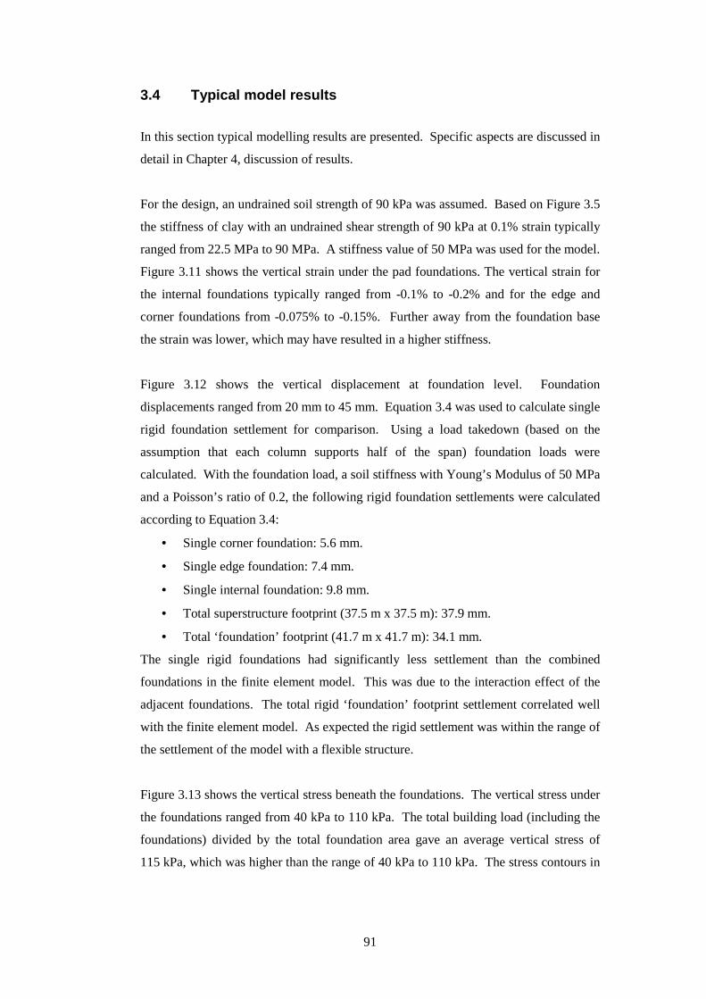
91

3.4 Typical model results

In this section typical modelling results are presented. Specific aspects are discussed in

detail in Chapter 4, discussion of results.

For the design, an undrained soil strength of 90 kPa was assumed. Based on Figure 3.5

the stiffness of clay with an undrained shear strength of 90 kPa at 0.1% strain typically

ranged from 22.5 MPa to 90 MPa. A stiffness value of 50 MPa was used for the model.

Figure 3.11 shows the vertical strain under the pad foundations. The vertical strain for

the internal foundations typically ranged from -0.1% to -0.2% and for the edge and

corner foundations from -0.075% to -0.15%. Further away from the foundation base

the strain was lower, which may have resulted in a higher stiffness.

Figure 3.12 shows the vertical displacement at foundation level. Foundation

displacements ranged from 20 mm to 45 mm. Equation 3.4 was used to calculate single

rigid foundation settlement for comparison. Using a load takedown (based on the

assumption that each column supports half of the span) foundation loads were

calculated. With the foundation load, a soil stiffness with Young’s Modulus of 50 MPa

and a Poisson’s ratio of 0.2, the following rigid foundation settlements were calculated

according to Equation 3.4:

• Single corner foundation: 5.6 mm.

• Single edge foundation: 7.4 mm.

• Single internal foundation: 9.8 mm.

• Total superstructure footprint (37.5 m x 37.5 m): 37.9 mm.

• Total ‘foundation’ footprint (41.7 m x 41.7 m): 34.1 mm.

The single rigid foundations had significantly less settlement than the combined

foundations in the finite element model. This was due to the interaction effect of the

adjacent foundations. The total rigid ‘foundation’ footprint settlement correlated well

with the finite element model. As expected the rigid settlement was within the range of

the settlement of the model with a flexible structure.

Figure 3.13 shows the vertical stress beneath the foundations. The vertical stress under

the foundations ranged from 40 kPa to 110 kPa. The total building load (including the

foundations) divided by the total foundation area gave an average vertical stress of

115 kPa, which was higher than the range of 40 kPa to 110 kPa. The stress contours in

92

this figure are ‘smoothed’ and based on averaged nodal values derived from

extrapolation of the values in the integration points.

Figure 3.14 shows the vertical displacement of the structure. The maximum vertical

displacement was 67.3 mm at the midspan of a roof slab. This displacement was due to

foundation settlement, column compression and slab deflection.

Figure 3.15 shows the pattern of the bending moment on the first floor slab. The

bending moments in the floor slabs are discussed in detail in Chapter 4, discussion of

analyses.

93

Table 3.1: Maximum element size in mesh discretisation zones

Zone Element size

1

2

3

4

5

6

0.25B

0.5B

1B

2B

4B

4B

94

Table 3.2: Summary of vertical displacements

25 bay slab

(mm)

Superstructure

top floor

(mm)

Superstructure

normalised

(mm)

Hand calculation

top floor

(mm)

Corner slab

Edge slab

Internal slab

Corner column

Edge column

Internal column

13.8

8.7-9.6

3.4-5.9

NA

NA

NA

21.6

18.2-18.4

15.2-15.7

3.0

5.5-6.1

10.0-12.5

14.7

9.6-9.9

4.4-5.1

NA

NA

NA

NA

NA

NA

3.7

6.2

10.3

95

Table 3.3: Column load comparison

Column FE Model

(kN)

Hand Calculation

(kN)

Difference

(%)

Corner

Edge

Internal

947

1632 to 1708

2763 to 3 025

1030

1702

2773

9

0 to 4

0 to -8

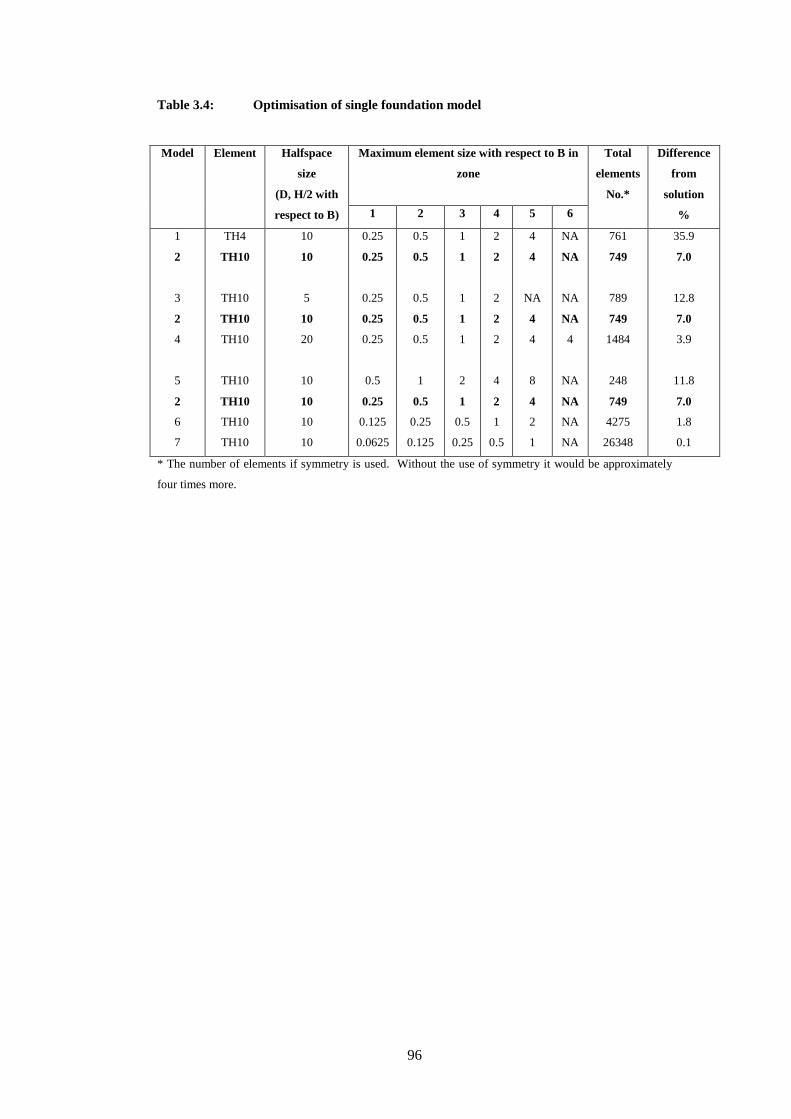
96

Table 3.4: Optimisation of single foundation model

Model Element Halfspace

size

(D, H/2 with

respect to B)

Maximum element size with respect to B in

zone

Total

elements

No.*

Difference

from

solution

% 1 2 3 4 5 6

1

2

3

2

4

5

2

6

7

TH4

TH10

TH10

TH10

TH10

TH10

TH10

TH10

TH10

10

10

5

10

20

10

10

10

10

0.25

0.25

0.25

0.25

0.25

0.5

0.25

0.125

0.0625

0.5

0.5

0.5

0.5

0.5

1

0.5

0.25

0.125

1

1

1

1

1

2

1

0.5

0.25

2

2

2

2

2

4

2

1

0.5

4

4

NA

4

4

8

4

2

1

NA

NA

NA

NA

4

NA

NA

NA

NA

761

749

789

749

1484

248

749

4275

26348

35.9

7.0

12.8

7.0

3.9

11.8

7.0

1.8

0.1

* The number of elements if symmetry is used. Without the use of symmetry it would be approximately

four times more.

97

Figure 3.1: Building layout

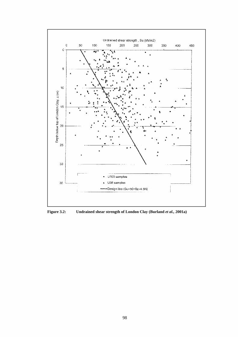
98

Figure 3.2: Undrained shear strength of London Clay (Burland et al., 2001a)

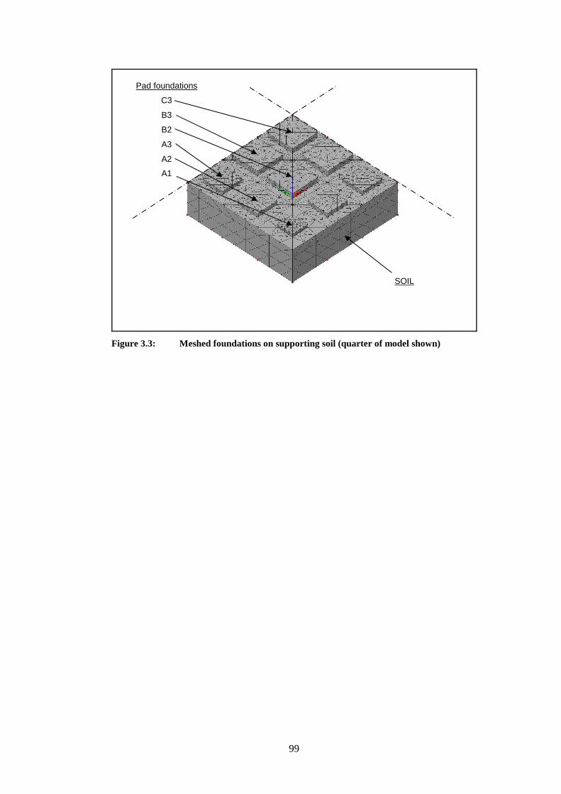
99

Figure 3.3: Meshed foundations on supporting soil (quarter of model shown)

Pad foundations

C3

B3

B2

A3

A2

A1

SOIL

100

Figure 3.4: Discretisation zones

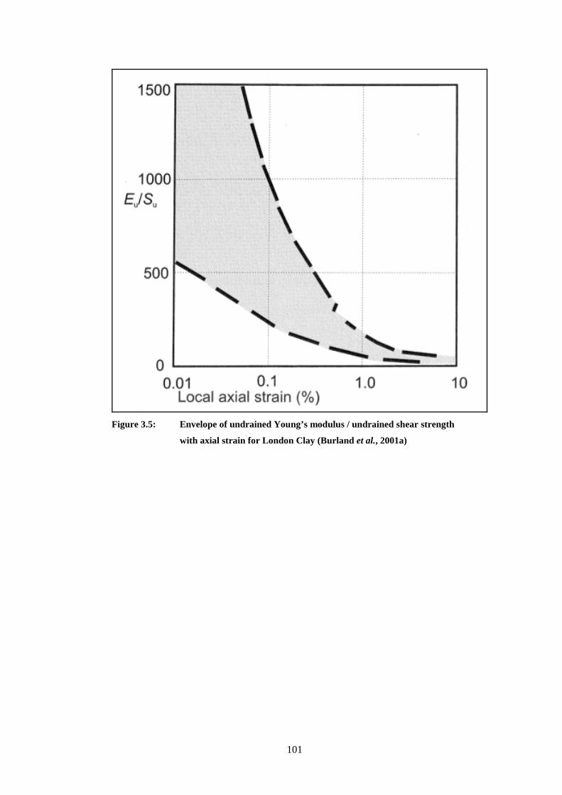
101

Figure 3.5: Envelope of undrained Young’s modulus / undrained shear strength

with axial strain for London Clay (Burland et al., 2001a)

102

Figure 3.6: Vertical displacements of single bay slab supported by pinned support

Ver

tical

dis

plac

emen

t

(m)

Hin

ge

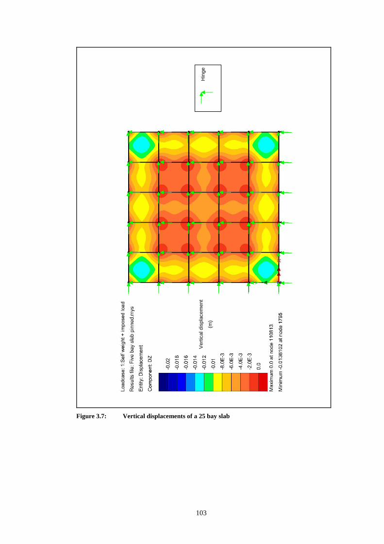
103

Figure 3.7: Vertical displacements of a 25 bay slab

Hin

ge

V

ertic

al d

ispl

acem

ent

(m)

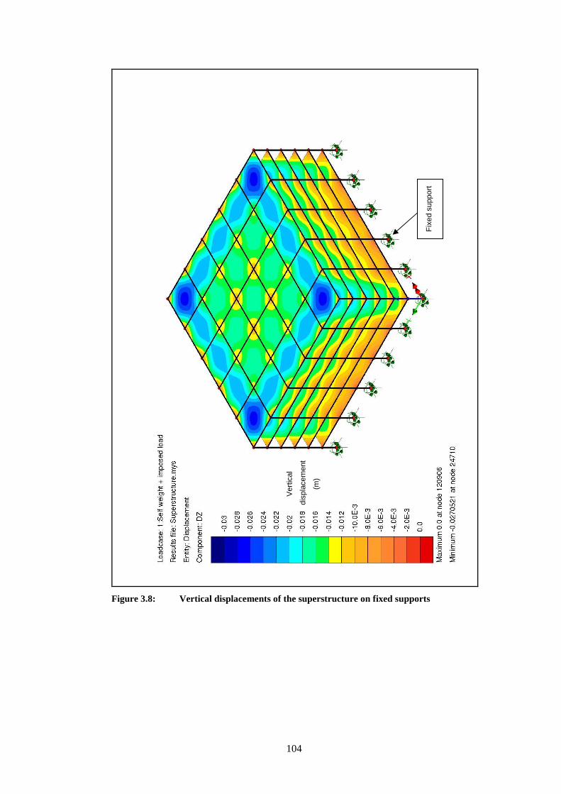
104

Figure 3.8: Vertical displacements of the superstructure on fixed supports

Ver

tical

dis

plac

emen

t

(m)

Fix

ed s

uppo

rt

105

Figure 3.9: Mesh for single foundation model

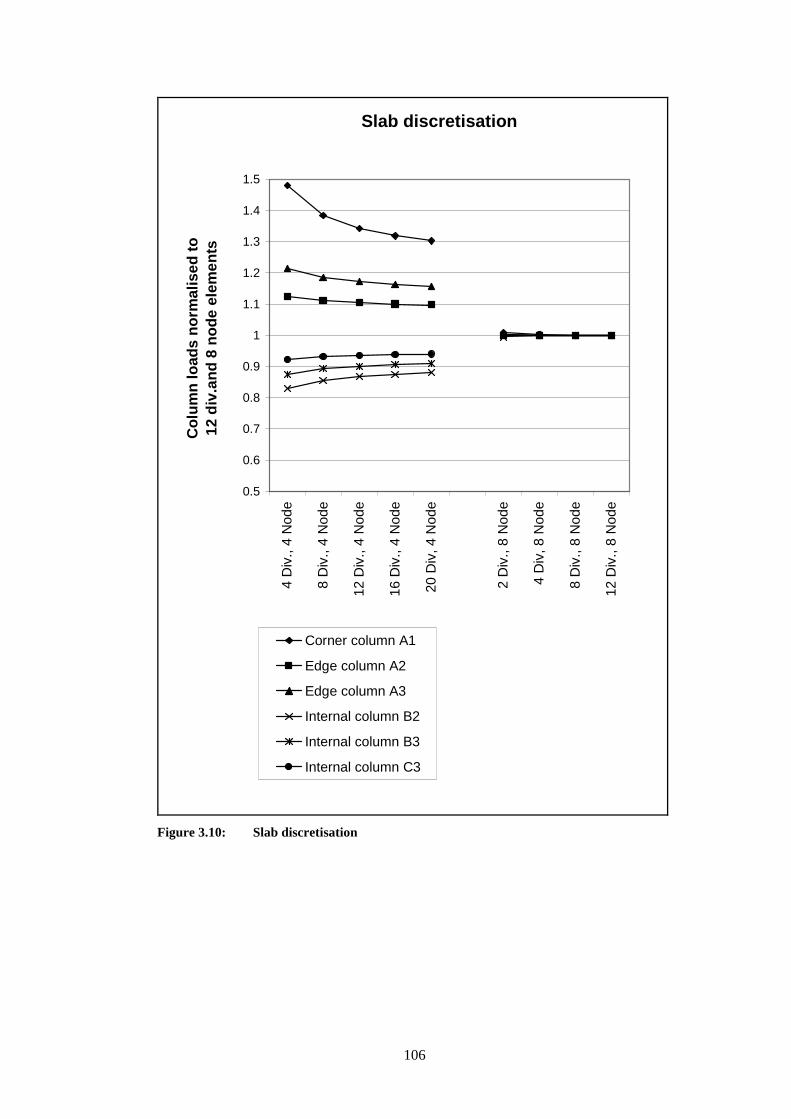
106

Slab discretisation

0.5

0.6

0.7

0.8

0.9

1

1.1

1.2

1.3

1.4

1.5

4 D

iv.,

4 N

ode

8 D

iv.,

4 N

ode

12 D

iv.,

4 N

ode

16 D

iv.,

4 N

ode

20 D

iv, 4

Nod

e

2 D

iv.,

8 N

ode

4 D

iv, 8

Nod

e

8 D

iv.,

8 N

ode

12 D

iv.,

8 N

ode

Co

lum

n lo

ads

no

rmal

ised

to

12

div

.an

d 8

no

de

elem

ents

Corner column A1

Edge column A2

Edge column A3

Internal column B2

Internal column B3

Internal column C3

Figure 3.10: Slab discretisation

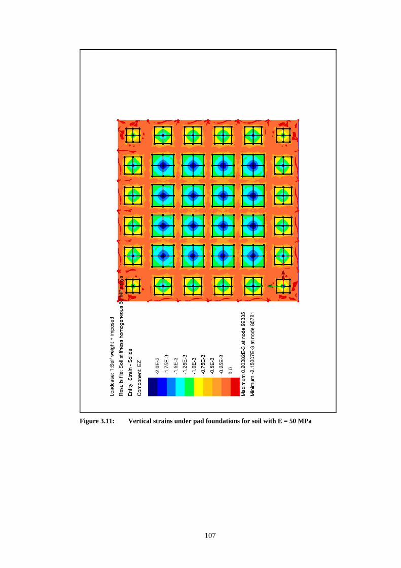
107

Figure 3.11: Vertical strains under pad foundations for soil with E = 50 MPa

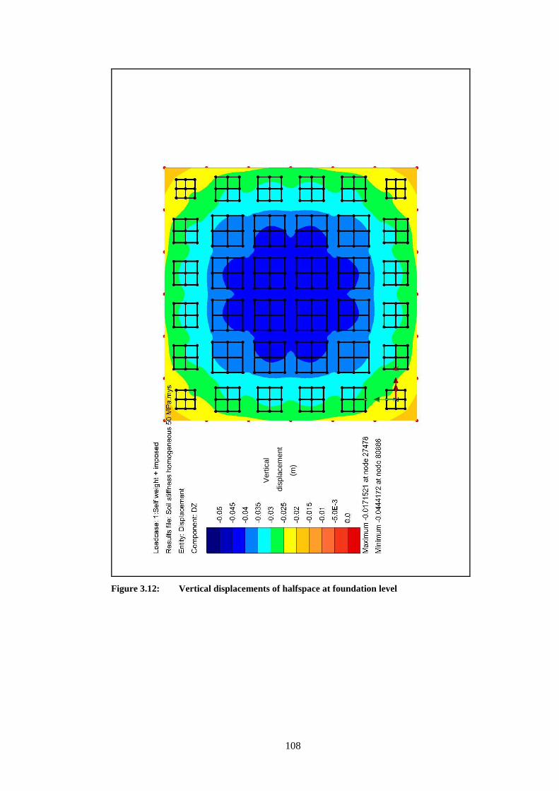
108

Figure 3.12: Vertical displacements of halfspace at foundation level

Ver

tical

dis

plac

emen

t

(m)

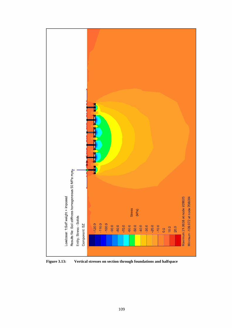
109

Figure 3.13: Vertical stresses on section through foundations and halfspace

Str

ess

(kP

a)

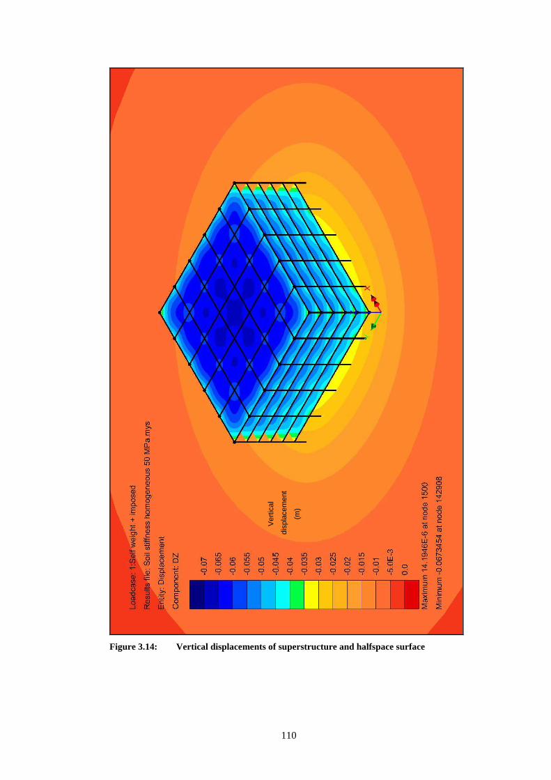
110

Figure 3.14: Vertical displacements of superstructure and halfspace surface

Ver

tical

dis

plac

emen

t

(m)

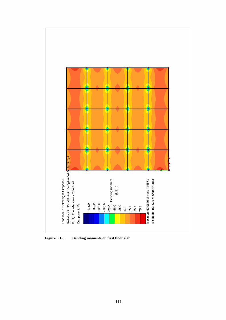
111

Figure 3.15: Bending moments on first floor slab

Ben

ding

mom

ent

(kN

.m)

112

4 DISCUSSION OF ANALYSES

This chapter discusses the results from the finite element analyses. Firstly the

normalisation of the data is discussed. The normalisation of the data allows for the data

of a limited number of models to be applied to a wider range of models, based on the

structure’s relative bending stiffness. Secondly the loads generated within the model

are compared to the strength of the materials to determine possible failure. Thirdly the

structural deformation is compared with suggested limits from the literature review.

Fourthly the effect of variation in foundation load-displacement response is discussed.

4.1 Normalisation of data

The behaviour of a structure undergoing differential settlement is determined by the

relative bending stiffness. The relative bending stiffness depends on the:

• stiffness of the building materials,

• geometry of the building,

• geometry of the foundation; and

• soil stiffness.

By normalising the relative bending stiffness the behaviour of a few specific models

can be applied to a wider range of structures, based on the relative bending stiffness.

The magnitudes of column loads at ground level were used as an indicator of the

behaviour of the structure. Due to symmetry within the structure only six column loads

needed to be used. Figure 4.1 shows the location of the columns. Column A1 is the

corner column, A2 and A3 are the two edge columns, B2, B3 and C3 are internal

columns with C3 being the nearest to the centre of the structure. Figure 4.2 shows the

column loads for the 5 bay structure with an imposed load of 0.5 kN/m² on the floors,

an imposed line load on the edges of the floor slabs of 7.241 kN/m representing the

facades, a concrete stiffness of 13 GPa and a soil stiffness that ranges from 100 Pa to

1000 GPa. The wide range of soil stiffness is unrealistic for real soils; however it

provides valuable insights into the theoretical structural behaviour. From Figure 4.2 it

is evident that the column loads at ground level are approximately constant for soil

stiffnesses larger than 100 MPa. The column loads at ground level vary for a stiffness

range from 0.01 MPa to 100 MPa. For soil stiffnesses lower than 0.01 MPa the column

loads are also constant. The change in columns loads and the ultimate strength of the

structure are discussed in detail in the following section.

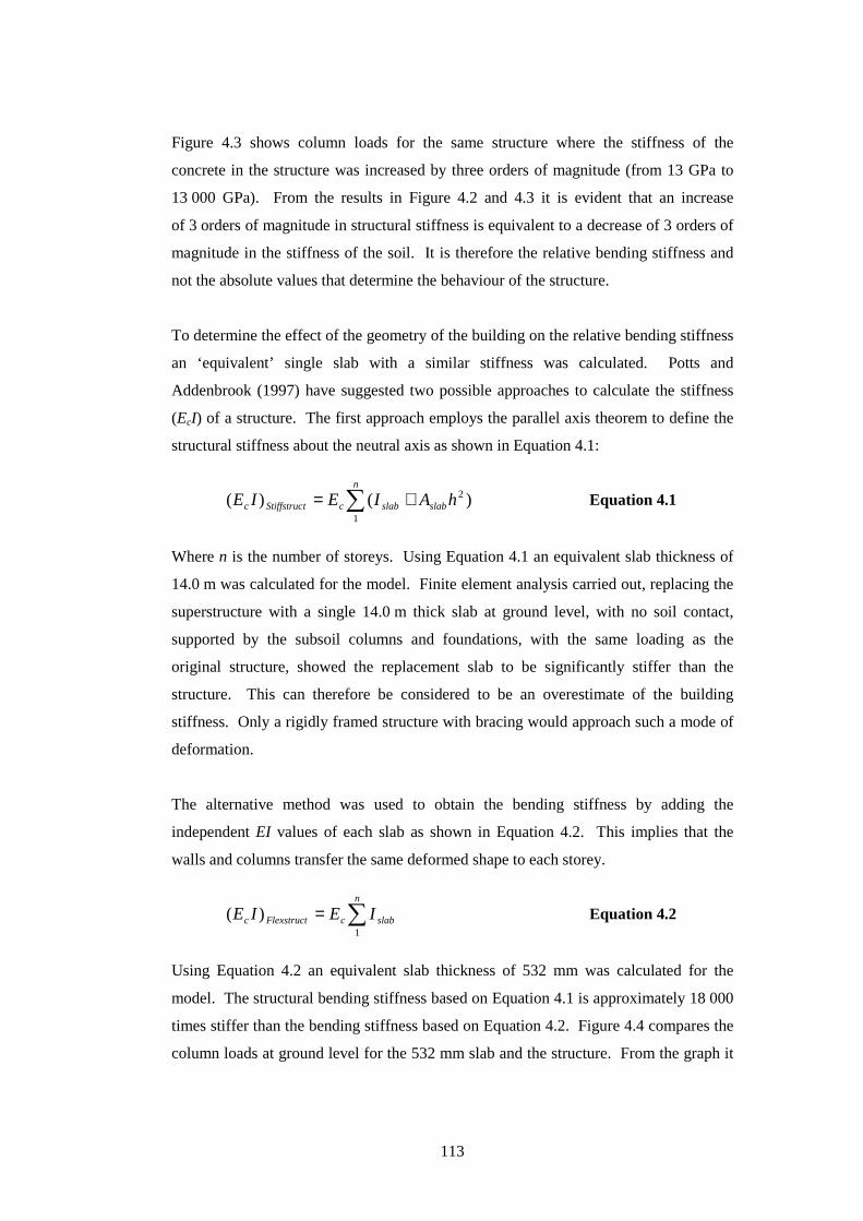
113

Figure 4.3 shows column loads for the same structure where the stiffness of the

concrete in the structure was increased by three orders of magnitude (from 13 GPa to

13 000 GPa). From the results in Figure 4.2 and 4.3 it is evident that an increase

of 3 orders of magnitude in structural stiffness is equivalent to a decrease of 3 orders of

magnitude in the stiffness of the soil. It is therefore the relative bending stiffness and

not the absolute values that determine the behaviour of the structure.

To determine the effect of the geometry of the building on the relative bending stiffness

an ‘equivalent’ single slab with a similar stiffness was calculated. Potts and

Addenbrook (1997) have suggested two possible approaches to calculate the stiffness

(EcI) of a structure. The first approach employs the parallel axis theorem to define the

structural stiffness about the neutral axis as shown in Equation 4.1:

)()( 2

1

hAIEIE slab

n

slabctStiffstrucc += ∑ Equation 4.1

Where n is the number of storeys. Using Equation 4.1 an equivalent slab thickness of

14.0 m was calculated for the model. Finite element analysis carried out, replacing the

superstructure with a single 14.0 m thick slab at ground level, with no soil contact,

supported by the subsoil columns and foundations, with the same loading as the

original structure, showed the replacement slab to be significantly stiffer than the

structure. This can therefore be considered to be an overestimate of the building

stiffness. Only a rigidly framed structure with bracing would approach such a mode of

deformation.

The alternative method was used to obtain the bending stiffness by adding the

independent EI values of each slab as shown in Equation 4.2. This implies that the

walls and columns transfer the same deformed shape to each storey.

∑=n

slabcFlexstructc IEIE1

)( Equation 4.2

Using Equation 4.2 an equivalent slab thickness of 532 mm was calculated for the

model. The structural bending stiffness based on Equation 4.1 is approximately 18 000

times stiffer than the bending stiffness based on Equation 4.2. Figure 4.4 compares the

column loads at ground level for the 532 mm slab and the structure. From the graph it

114

is evident that the stiffness of the single 532 mm slab is a good approximation of the

stiffness of the structure.

Based on a plane strain analysis (only) Potts and Addenbrooke (1997) defined relative

bending stiffness ρ* of a building as:

4

*

HE

EI

s

=ρ Equation 4.3

Where EI is the bending stiffness of the superstructure, Es is a representative soil

stiffness and H is half the width (in the plane of deformation) of the superstructure.

From the equation it is evident that for a fixed building and foundation geometry

sE

E∝*ρ which coincides with the data given in Figure 4.2 and 4.3. From Figure 4.4

it is evident that EI for this flexible structure without bracing or stiffening due to

facades can be calculated with Equation 4.2. To determine the effect of building width

a 5 bay x 4 bay and a 5 bay x 3 bay model were analysed. Both models were produced

by removing either 1 or 2 of the internal bays of the 5 bay model, which resulted in an

identical line load on the edges of the floor slabs and identical edge and corner

foundations for the structures.

Figure 4.5 shows the normalised ground level column loads of the 5, 4 and 3 bay

structures normalised using ρ* from Equation 4.3 where H is half the length of the

structure. Note that due to the formulation of ρ* the ‘stiffer soil’ is on the left of the

horizontal axis, in contrast to the previous graphs where the stiffer soil is on the right.

The column loads were normalised to the column load in the specific column without

any soil-structure interaction effect (i.e. founded on an infinitely stiff soil).

Figure 4.5 shows that the corner column loads in the linear elastic finite element model

for a ‘rigid’ structure may be up to 5 times greater than for the flexible structure. A

basic load takedown to determine column loads could be used for the flexible structure;

however a load takedown would underestimate the column loads for the linear elastic

‘rigid’ structure model. It is important to note that the results in Figure 4.5 are based on

a linear elastic model. Failure of concrete in the columns, floor slabs or soil failure

may reduce the column loads.

115

Three distinct zones of behaviour within the soil structure stiffness range can be

identified within Figure 4.5:

• Zone 1 ‘Flexible structure’ is the zone of relative bending stiffness (ρ* ) where

the structure is flexible in comparison with the soil. ρ* is typically less than

1 x 10-4 in Zone 1. The structural loads in Zone 1 can be determined without

taking differential settlement into account.

• Zone 2 ‘Intermediate structure’ is the intermediate zone where the loads in the

edge and corner columns increase and the loads in the internal columns

decrease with an increase of relative bending stiffness. ρ* typically ranges

from 1 x 10-4 to 1 x 10-1 in Zone 2.

• Zone 3 ‘Rigid structure’ is the zone of relative bending stiffness (ρ* ) where the

structure is rigid in comparison with the soil. In zone 3 the loads, stresses and

differential movements within the structure are constant, independent of the

relative bending stiffness. ρ* is typically larger than 1 x 10-1 in Zone 3.

The designed 5 bay structure on a typical London Clay with an undrained shear

strength (Su) of 90 kPa results in an approximate relative bending stiffness (ρ* )

of 2.2 x 10-6, which falls in Zone 1. This relative bending stiffness was based on a

concrete stiffness of 13 GPa, a bending stiffness based on Equation 4.2, i.e. the sum of

independent EI values of each slab and a soil stiffness of 600 MPa (the soil stiffness are

discussed in detail in section 4.2). The ‘typical’ structure modelled in this thesis by

finite element analysis will therefore behave flexibly.

The ‘typical’ structure modelled in this thesis by way of finite element analysis was

modelled without any internal walls or bracing to reduce the complexity. To

investigate the effect of a stiffer structure the concrete stiffness was increased by orders

of magnitude instead of adding internal walls and bracing.

Internal walls and bracing within structures will increase the bending stiffness of the

structure. The stiffness, location and fitment details of the walls and bracing will affect

the bending stiffness of the structure. The bending stiffness can be expected to be

between the lower bound calculated by Equation 4.2 and the upper bound calculated by

Equation 4.1. For the ‘typical’ structure modelled in this thesis the bending stiffness

calculated by Equation 4.2 is approximately 4 orders of magnitude larger than the

bending stiffness from Equation 4.1.

116

4.2 Structural strength

This section discusses the loads within the numerical linear-elastic models and

compares them to the strength of the members. The strengths of the members were then

compared to the loads from the linear-elastic model to indicate possible concrete or soil

failure.

Concrete, reinforcement steel and soil have non-linear stress-strain characteristics.

Modelling this behaviour numerically on a full scale structure is complex and requires

significant computing power; therefore a simplified linear elastic model was used to

model the behaviour of the structure.

Because linear-elastic numerical models were used to determine the effect of

differential settlement on the loads within the structure, the maximum load in the model

could be infinitely high (depending on the deformation), whereas in a real building the

material may fail, limiting the load. Under normal operating conditions the structural

members are not intended to be stressed to failure; therefore comparing the load in the

linear-elastic model to the strength gives an indication of the performance of the

structure.

The structural strength of reinforced concrete members varies and is influenced by the

strength of the individual materials and production controls. To ensure adequate

member strength the British Standards Institution (BSI 8110-1: 1997) design code

recommends the use of partial safety factors for ultimate limit state design. A

characteristic material strength is defined as the strength of the material at which less

than 5% of all possible test results are expected to fail. The characteristic material

strength is then reduced by a partial safety factor which depends on the type of material

and application to calculate design strength. For example, the characteristic strength of

reinforcement steel is divided by a factor of 1.15 and concrete in flexure or axial load

by a factor of 1.50. The same principle applies for loads. Characteristic loads are

calculated and increased by a partial safety factor depending on the load type and

application. In the design, the design load should be less than the design strength, to

ensure a safe structure. Under normal operating conditions the actual load will be

significantly less than the design load and the element strength will be higher than the

design strength.

117

The loads in the numerical models are based on expected loads and not ultimate design

loads and are therefore significantly lower. The imposed live load on the model is

0.5 kN/m² on all the floors with no roof load. In contrast the ultimate design live load

for the floor slabs ranges from 0 to 4.0 kN/m² depending on the load combination.

Dead loads on the model are the characteristic loads i.e. a partial safety factor of 1.0 in

contrast to the design dead load where a partial safety factor of 1.0 to 1.4 is used

depending on the load combination. The loads in the structure under normal operating

conditions should therefore be significantly lower than the strength of the members.

The following sections will compare the column loads, foundation loads and bending

moments in the slabs from the finite element models with the strength of the members.

4.2.1 Column loads

Column strength depends on the geometric and material properties of the column. To

simplify the design, the same column dimensions (450 mm x 450 mm) were used

throughout the structure. The column design was based on the maximum load which

occurred at an internal column at ground level. This column was used to calculate the

column strength for comparison. The column was a 450 mm x 450 mm reinforced

column with 9 Y40 reinforcement bars (3 on each side) with 40 mm cover. A 30 MPa

actual strength of the concrete was assumed. In a structure the actual concrete strength

will vary and will depend on site quality control.

A concrete column fails due to a critical combination of axial load and biaxial bending.

To calculate and present this 3-dimensional envelope is complex and therefore the

simplification as suggested in BSI 8110-1 (1997) was used. The code suggests the use

of the following equations to compare biaxial bending to uniaxial bending:

For yxxyx Mb

hMMbMhM

'

'','/'/ β+=≥ Equation 4.4

For xyyyx Mb

hMMbMhM

'

'','/'/ β+=< Equation 4.5

Where h’ and b’ are the depth of the reinforcing steel and β is a coefficient based on the

axial force on the column, the dimensions and concrete strength.

The uniaxial column strengths under combined axial load and bending moments are

shown in Figure 4.6. Table 4.1 shows the axial column loads with the equivalent

118

uniaxial bending moment derived from the biaxial bending moments and the column

loads from the model using Equations 4.4 and 4.5. As the relative bending stiffness

increased in the linear elastic model the axial loads in the corner columns increased by

approximately 5 times, the loads in the edge columns approximately doubled and the

loads in the internal columns reduced to approximately 1/3 in comparison to the

column loads within a flexible structure. The cells highlighted in grey show where the

loads from the linear elastic numerical model exceed the strength of the column. These

column loads are based on a linear elastic model, i.e. no slab or foundation failure

occurs. Yielding of foundations may protect the structure from damage to the columns.

Foundation failure is discussed in section 4.2.2. Slab failure is discussed in Section

4.2.3. From Table 4.1 it is evident that (without foundation or slab failure) column

failure may occur for a relative bending stiffness (ρ* ) higher than approximately

1.32 x 10-3 which is in Zone 2, intermediate stiffness. If the columns were sized

according to the expected loads (i.e. a corner column smaller than an internal column),

failure in the corner and edge columns may occur at a lower relative bending stiffness.

Column failure will result in moment redistribution within the structure or instability of

the structure.

4.2.2 Foundation loads

Foundation loads depend on the load-displacement response and the displacement of

the foundation. This section firstly discusses foundation loads with a linear foundation

load-displacement response and secondly foundation loads with a non-linear load

foundation response.

Figure 4.7 shows the foundation loads (not column loads at ground level) from the

linear-elastic model normalised to relative bending stiffness (ρ* ). The foundation loads

are constant in Zone 1, Flexible structure (ρ*<1 x 10-4). In Zone 2, Intermediate

stiffness (1 x 10-4 < ρ*<1 x 10-1) the loads in the corner foundation (A1) and edge

foundations (A2 and A3) increase while the loads in the internal foundations (B2, B3

and C3) decrease. In Zone 3, Rigid structure (ρ*>1 x 10-1) the foundation loads are

constant again. The load in the corner foundation is approximately 2.5 times greater in

Zone 3 than in Zone 1; however these values are based on foundations on a linear

elastic soil resulting in linear load-displacement response. Foundation failure (non-

linear load-displacement response) may reduce the loads in the foundations.

To determine the effect of non-linear load-displacement response a ‘non-linear’ model

was analysed which consisted of changing the stiffness under foundations according to

119

the settlement. For the ‘non-linear’ model, a structure with a relative bending stiffness

(ρ* ) of 1.32 x 10-1 (Zone 3, Rigid structure) was used to evaluate the effect of non-

linear load-displacement response. In Zone 3 the structure is rigid in comparison with

the soil and foundation failure may be expected. ρ* is a function of both the soil and

superstructure stiffness and for the model, firstly an appropriate soil stiffness and

secondly the superstructure stiffness were determined for a relative bending stiffness

(ρ* ) of 1.32 x 10-1.

Soil stiffness is a function of the strain within as well as the strength of the soil

(Atkinson, 2000). Figure 4.8 (Atkinson, 2000) shows the relationship between the soil

secant stiffness divided by initial soil secant stiffness vs. the foundation settlement

divided by the foundation width. The graph was based on data from settlement of

foundations on London Clay. To determine a stiffness profile for the model, a tangent

stiffness was chosen for each interval of ρ/B and the corresponding secant stiffness was

calculated (shown on Figure 4.9). The input tangent stiffnesses were changed until the

calculated secant stiffness corresponded with the secant stiffness degradation as

suggested by Atkinson (2000). With the tangent stiffness, ρ/B intervals and an initial

small strain soil stiffness a stress strain curve was calculated. Soil stiffness is related to

the soil strength (Atkinson, 2000), therefore the initial soil stiffness must be based on

the soil strength. For the designed structure an undrained soil shear strength (Cu) of

90 kPa was used. The following equation (Eurocode 7) gives the ultimate bearing

stress for a pad foundation:

qCQ uult ++= 2.1)2(π Equation 4.6

Where Qult is the ultimate bearing stress, Cu the undrained shear strength, and q the

surcharge. Assuming the surcharge (q) is approximately equal to the self weight of the

foundation and the soil above it, Qult = 6.17 Cu. For an undrained shear strength of

90 kPa, the ultimate bearing capacity is therefore 555 kPa. Figure 4.10 shows the

applied stress vs. settlement graph based on Atkinson’s stiffness degradation curve and

an initial small strain stiffness of 600 MPa. The graph shows an initial small strain

stiffness of 600 MPa, which relates to an ultimate bearing stress of approximately 555

kPa.

For a relative bending stiffness (ρ* ) of 1.32 x 10-1 and a soil stiffness of 600 MPa, a

structural stiffness (EcI) of 9.79 x 109 kN.m2 was needed. For the required structural

stiffness, the concrete stiffness (Ec) was increased instead of the second moment of

120

inertia (I). This resulted in an unrealistically high concrete stiffness (780 000 GPa),

however it is easier to change the concrete stiffness than the geometry, and it has the

same effect on the structural stiffness. The high concrete stiffness (780 000 GPa) was

assigned to the superstructure (slabs and columns) and the foundations were assigned a

normal concrete stiffness of 13 GPa.

To analyse the ‘non-linear’ model a concrete stiffness of 780 000 GPa and an initial

soil stiffness of 600 MPa were used (which relates to relative bending stiffness of (ρ* )

of 1.32 x 10-1 as shown above). Below each foundation a soil block was defined to

which an individual stiffness was assigned. The soil blocks were 7.5 m x 7.5 m wide

and 10.4 m deep (5.4 m below foundation level) to coincide with the mesh boundaries.

For the first iteration 10% of the structural load was assigned to the structure and a

600 MPa soil stiffness was assigned to the blocks and the surrounding soil. The

settlement of each foundation was extracted from the model and a new soil stiffness

calculated based from the stiffness degradation as shown in Figure 4.8. The calculated

stiffnesses were assigned to each soil block after which the model was analysed again.

These steps were repeated until the change in stiffness in each block was less than

0.1 MPa, after which the load was increased by 10% and the process repeated.

Table 4.2 shows the soil stiffness degradation with each iteration for the model with a

concrete stiffness of 780 000 GPa for the superstructure and 13 GPa for the

foundations. Table 4.3 shows the soil stiffness degradation with each iteration for the

model with a concrete stiffness of 780 000 GPa for both the superstructure and the

foundations. The final soil stiffnesses at 100% load for the model with the 13 GPa

foundations were between 75 MPa and 100 MPa (between 0.11% and 0.20% strain)

and for the model with 780 000 GPa foundations between 94 MPa and 123 MPa

(between 0.07% and 0.13% strain). The stiffer foundation resulted in less soil stiffness

degradation.

Table 4.4 shows the column loads of four models with the same relative bending

stiffness (ρ* = 1.32 x 10-1) namely:

• The ‘non-linear’ model described above with a concrete stiffness of

780 000 GPa for the superstructure and 13 GPa for the foundations.

• A linear model with a concrete stiffness of 780 000 GPa for the

superstructure and 13 GPa for the foundations.

• The ‘non-linear’ model as described above with a concrete stiffness of

780 000 GPa for both the superstructure and the foundations.

121

• A linear model with a concrete stiffness of 780 000 GPa for both the

superstructure and the foundations.

The results show that the stiffness of the foundations has an influence on the column

loads:

• The load in the corner column (A1) was reduced by 14% in the non-linear

model with a 13 GPa foundation concrete stiffness and 34% in the non-

linear model with a 780 000 GPa concrete stiffness.

• The loads in the edge columns (A2, A3) were reduced by between 1% and

4% in the non-linear model with a 13 GPa foundation concrete stiffness

and 11% in the non-linear model with a 780 000 GPa concrete stiffness.

• The loads in the internal columns (B2, B3, C3) ranged from a reduction of

5% to an increase of 9% in the non-linear model with a 13 GPa foundation

concrete stiffness and increase of between 56% and 65% in the non-linear

model with a 780 000 GPa concrete stiffness.

It is evident that the foundation and soil stiffness have a significant effect on the

column loads and yielding of foundations may protect the structure against column

failure.

4.2.3 Slab bending moment

For a ‘rigid’ structure (i.e. in Zone 3) redistribution of column loads may be possible by

bending of the slabs. Increased bending moments resulting in column load

redistribution may lead to stresses which exceed the available strength leading to

excessive deformation, shear failure or the formation of plastic hinges and structural

damage. It is therefore important to check the implied bending stresses for the finite

element analysis with the actual strength of the concrete.

For the design of the structure a simplified 2D frame analysis was used to determine the

design bending moments in the slabs. These design bending moments were compared

to the bending moments in the slabs calculated by the linear elastic 3D finite element

analysis to determine possible failure of the structure. To compare the bending

moment of the 3D finite element model with those of the design 2D frame, the 3D

model was divided into a series of 2D frames. The frames are shown in Figure 4.11.

The bending moment for the frame was calculated by averaging the bending moments

of the integration points for each row of elements perpendicular to the 2D plane.

122

Figures 4.12 and 4.13 compare the bending moment in the first floor level slab from the

linear elastic finite element analysis model with the design strength envelope. Figure

4.12 is for an internal span and Figure 4.13 for an edge span. From Figure 4.12 and

4.13 it is evident that the bending moments in a structure with a relative bending

stiffness larger than 1.32 x 10-4 fall outside the ultimate limit state load envelope, and

that cracking with load redistribution will occur within the slab which may lead to

failure of the structure. Yielding of foundations may prohibit slab failure. Slab failure

depends on the geometry and the load redistribution within the structure, however it is

most likely that the slabs will firstly fail due to unacceptable deflection, secondly

collapse due to shear failure (the plastic deformation of the reinforcing and the opening

of cracks reduce the shear resistance) and lastly collapse due to the development of

enough plastic hinges for the structure to become unstable.

4.3 Structural deformation

Excessive deformation within a structure may have an impact on the serviceability of

the structure. The following two sections compare the deformation within the finite

element model with guidelines from the literature.

4.3.1 Tilt

Excessive tilt in buildings has an impact on visual appearance and may therefore be a

limiting criterion with respect to differential settlement. The British Standards

Institution (BSI 8110-2: 1985) provides guidelines on deflection limits; however no

guidance is given for tilt. Burland et al. (2001a) note that a deviation of slope, from the

horizontal or vertical, of more than 1:100 will normally be clearly visible and overall

deviations in excess of 1:150 are undesirable.

Table 4.5 shows the maximum column tilt within each structure with respect to the

structure’s relative bending stiffness (ρ* ). The first part of the table is for the structure

with a concrete stiffness of 13 GPa on a soil with a stiffness ranging from 1 x 10-4 to

1 x 104 MPa. The second part of the table is for the structure with a concrete stiffness

of 13 000 GPa on the same soil stiffness range. A concrete stiffness of 13 000 GPa is

unrealistic, however it simulates the effect of a stiffer structure as would be the case

with bracing and internal walls. From the results in Table 4.5 it is evident that the

maximum tilt does not relate to relative bending stiffness; it is a function of both the

123

actual soil stiffness and the structure stiffness. A decrease in soil stiffness results in an

increase of tilt. A decrease of structural stiffness also results in an increase of tilt;

therefore a flexible structure is more likely to suffer from tilt.

If a maximum acceptable tilt of 1:100 is assumed (i.e. 30 mm movement on a 3 m

column), the structure with a 13 GPa concrete stiffness on a soil stiffness softer than

10 MPa may experience excessive tilt. The structure with a 13 000 GPa concrete

stiffness on a soil stiffness softer than 1 MPa may experience excessive tilt.

Spatial variation in soil stiffness may cause more tilt than what will occur on a

homogeneous soil. The above data is based on homogeneous soil stiffness.

4.3.2 Deflection

Excessive deflection has an impact on the performance of a building. Deflection within

a building is caused by deflection within each slab or by the deflection of multiple

spans due to column moment. Deflection of individual slabs is usually decreased by an

increase in the stiffness (thickness) of the slab.

The British Standards Institution (BSI 8110-2: 1985) recommends a deflection limit of

1:250 for visual appearances. To limit damage to non-structural elements (unless they

are specifically detailed to allow for deflections and then the 1:250 visual limit will be

applicable) the British Standards Institution recommends the following limits:

• 1:500 or 20 mm, whichever is the lesser, for brittle materials; and

• 1:350 or 20 mm, whichever is the lesser, for non brittle partitions or finishes.

The literature review suggested the following angular distortion (not deflection) limits:

• 1:150 to 1:300 for structural damage of frames without cladding,

• 1:300 to 1:1 000 for facade cracking of frames with non load bearing walls;

and,

• 1:300 to 1:2 000 for damage to load bearing walls.

The type of structure analysed was an open plan office with external facades detailed to

allow for deflections. Therefore the angular distortion guideline of 1:150 to 1:300

would be considered acceptable. Assuming angular distortion guidelines do not

include any tilt of the building, the deflection ratio is twice the angular distortion, i.e.

124

1:300 to 1:600. These values are stricter than the 1:250 suggested by the British

Standards.

Table 4.6 shows the deflection of sections through three adjacent foundations parallel

to the facade against soil and structure stiffness. Table 4.7 shows the deflection of

sections diagonal to the facade. Positive values show a sagging deflection and negative

values a hogging deflection. The first part of the tables is for the structure with a

concrete stiffness of 13 GPa on a soil with a stiffness ranging from 1 x 10-4 to

1 x 104 MPa. The second part of the table is for the structure with a concrete stiffness

of 13 000 GPa on the same soil stiffness range. A concrete stiffness of 13 000 GPa is

unrealistic, however it simulates the effect of a stiffer structure as would be the case

with bracing and internal walls.

From the results in Table 4.6 and Table 4.7 it is evident that the deflection ratio at

ground level does not relate to relative bending stiffness; it is a function of both the

actual soil stiffness and the structure stiffness. A decrease in soil stiffness generally

results in an increase in deflection. A decrease of structural stiffness also generally

results in an increase in deflection; therefore a flexible structure is more likely to suffer

from excessive deflection.

For the structure with a concrete stiffness of 13 GPa unacceptable deflection is likely to

occur on soil stiffnesses softer than 10 MPa. For the stiffer structure with a concrete

stiffness of 13 000 GPa unacceptable deflection is likely to occur on soil stiffnesses

softer than 0.01 MPa.

It is interesting to note that in the model with a concrete stiffness of 13 GPa and a soil

stiffness of 1 MPa the maximum deflection on the edge is 1:230, on the internal section

parallel to the edge it is less (1:183) than for the edge section and on the diagonal

section it is also less (1:134) than for the edge section. For the model with a concrete

stiffness of 13 000 GPa and a soil stiffness of 0.001 MPa the maximum deflection on

the edge is 1:702 and for the internal section parallel to the edge it is less (1:318).

These values show that the measurement of deflection on the facade of the building

(i.e. assuming that the building deformation is primarily in 2D) will result in an

underestimate of the maximum deflection. It shows the necessity to take into account

the 3D behaviour when analysing for differential settlement damage.

125

Burland et al. (2001a) suggested the use of a simplified beam model to determine the

deflection limit at which damage will occur. They used a strain limit which is linked to

a damage category as discussed in the literature review. This method is aimed at

structures with masonry load bearing walls and is not necessarily applicable to modern

open plan offices. However it is interesting to see how it compares to modern open plan

offices.

For an isotropic beam (E/G = 2.6) with the neutral axis at the bottom and an L/H ratio

of 2 (based on the structure’s geometry) the following deflection/strain ratio limit

applies (from Figure 2:22):

82.0lim

=∆ε

L Equation 4.7

Table 4.8 shows the deflection limits against damage category, based on Equation 4.7.

Refer to Table 2.13 in the literature review for the damage category description. The

last column in Table 4.6 and 4.7 shows the damage category according to Burland et al.

(2001a) guidelines. It is evident that the stiffer structure (Ec = 13 000 GPa) is more

resistant to excessive deflections.

4.4 Variation in foundation-load displacement response

The previous models which have been discussed were founded on a halfspace with

homogeneous soil stiffness. Buildings are often founded on soils with a spatial

variation of stiffness which will cause different foundation load-displacement responses

for similar foundations. This section summarises from the literature the spatial

variation of soil stiffness, the load-displacement response of piles and the effect it has

on a structure.

Phoon and Kulhawy (1999) showed that the coefficient of variation (COV) for

undrained shear strength may be up to 80%; however the typical mean COV for the

groups range from 22% to 33% (Table 2.2). It is therefore expected that the soil

stiffness may also vary in a similar order of magnitude. Phoon and Kulhawy also

showed that the horizontal fluctuation of soil properties may be as short as 3 m,

therefore it is possible to have different soil conditions under adjacent foundations.

Soft soils may cause excessive foundation settlement and hard spots beneath

foundations may cause a stiffer load-displacement response of the foundation.

126

Reused foundations often have a stiffer load-displacement response due to the

preloading from the previous structure. Whitaker and Cooke (1966) showed that the

reload load-displacement response of a pile may be ten times stiffer than the virgin

load-displacement response.

Soil stiffness can vary significantly under a structure and to fully investigate the effect

of soil variation on a structure a significant number of models need to be analysed.

Due to limited resources only two sets of models were modelled.

The first set consisted of a superstructure with a concrete stiffness of 13 GPa on a soil

with a 10 MPa stiffness (ρ* = 1.32 x 10-4). The soil stiffness under foundation B2 (see

the figure in Table 4.6 for the location of B2) was changed to 0, 1, 5, 10, 20 and

100 MPa. As discussed in the previous paragraphs the typical COV of the soil’s

stiffness will be approximately 22% to 33% with an extreme case being 80%. The

extreme case correlates with 2 MPa and 18 MPa soil stiffness for this model. The reuse

of foundations combined with new (virgin) foundations however may result in a more

significant variation of load-displacement stiffness response of up to 10 times. This

correlates to a 1 MPa and 100 MPa soil stiffness for this specific model.

The second set consisted of a superstructure with a concrete stiffness of 13 GPa on a

soil with a 100 MPa stiffness (ρ* = 1.32 x 10-5). The soil stiffness under foundation B2

was changed to 0, 10, 50, 100, 200 and 1 000 MPa. To change the stiffness below

foundation B2 a soil block which surrounded the foundation was defined to which the

new stiffness was assigned. The block was 7.5 m x 7.5 m wide (equal to the column

spacing) and 10.4 m deep (5.4 m below foundation level). The value of 10.4 m was

chosen because it coincided with a mesh boundary.

Table 4.9 shows the change in column loads at ground level compared to those

calculated for the models with homogeneous soil stiffnesses.

On the 10 MPa model (ρ* = 1.32 x 10-4) with 1 MPa stiffness below foundation B2 the

loads in the adjacent columns increased by either 36 % (internal columns) or 42 %

(edge columns) and the load in column B2 decreased by 112%, which is more than

100%, a tensile stress due to the foundation and the soil above the foundation being

supported by the superstructure and not the soil below it. Increasing the soil stiffness

127

under foundation B2 to 100 MPa increased the load on foundation B2 by 14 %. From

the results it is evident that not only softer ‘failed’ foundations, but also a harder spot

under a foundation (or stiffer foundation load-displacement response due to a reused

foundation), may have an effect on structural loads within a structure.

On the 100 MPa model (ρ* = 1.32 x 10-5) with 10 MPa stiffness below foundation B2

the loads in the adjacent columns increased by either 5 % (internal columns) or 7 %

(edge columns) and the load in column B2 decreased by 14%. Increasing the soil

stiffness under foundation B2 to 1 000 MPa increased the load on foundation B2 by

4 %. The results showed that the higher the overall stiffness of the soil, the less impact

a stiffer load-displacement response of foundation has on the structure.

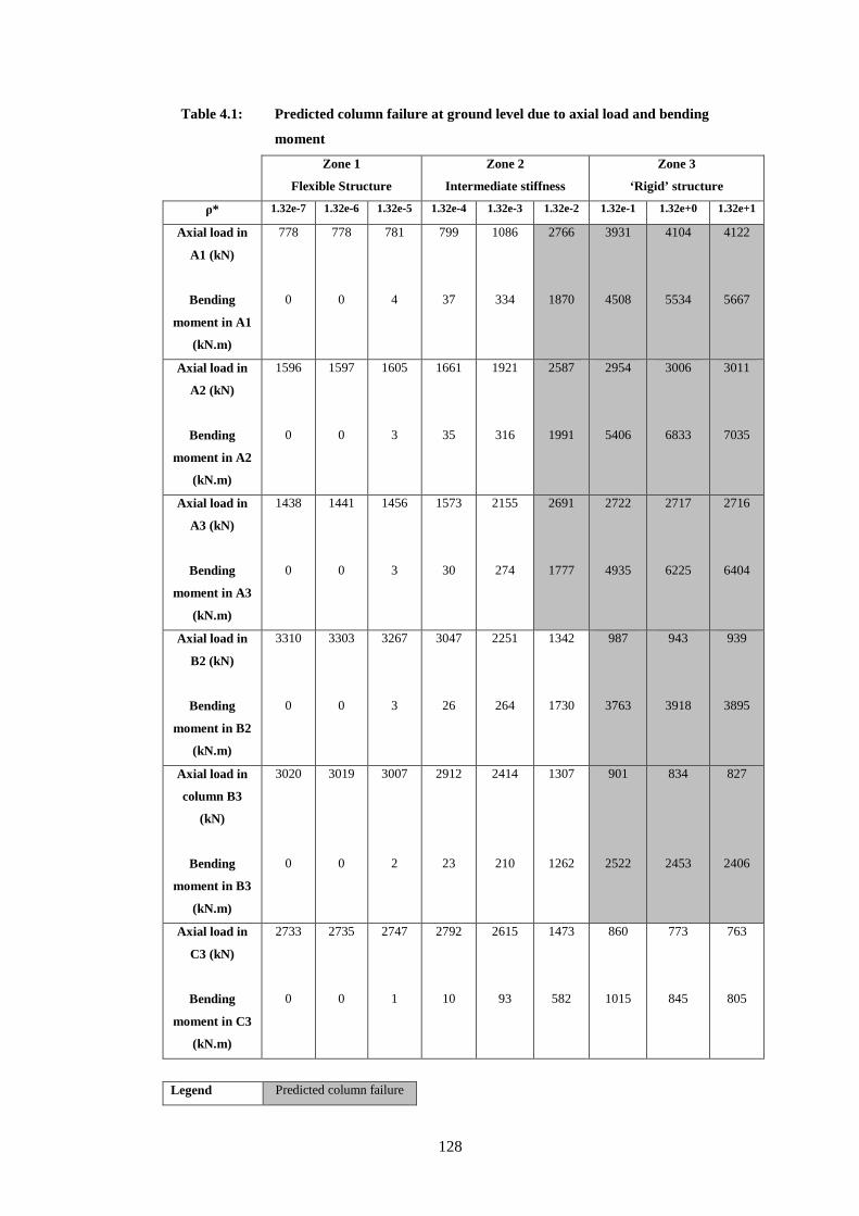
128

Table 4.1: Predicted column failure at ground level due to axial load and bending

moment

Zone 1

Flexible Structure

Zone 2

Intermediate stiffness

Zone 3

‘Rigid’ structure

ρ* 1.32e-7 1.32e-6 1.32e-5 1.32e-4 1.32e-3 1.32e-2 1.32e-1 1.32e+0 1.32e+1

Axial load in

A1 (kN)

Bending

moment in A1

(kN.m)

778

0

778

0

781

4

799

37

1086

334

2766

1870

3931

4508

4104

5534

4122

5667

Axial load in

A2 (kN)

Bending

moment in A2

(kN.m)

1596

0

1597

0

1605

3

1661

35

1921

316

2587

1991

2954

5406

3006

6833

3011

7035

Axial load in

A3 (kN)

Bending

moment in A3

(kN.m)

1438

0

1441

0

1456

3

1573

30

2155

274

2691

1777

2722

4935

2717

6225

2716

6404

Axial load in

B2 (kN)

Bending

moment in B2

(kN.m)

3310

0

3303

0

3267

3

3047

26

2251

264

1342

1730

987

3763

943

3918

939

3895

Axial load in

column B3

(kN)

Bending

moment in B3

(kN.m)

3020

0

3019

0

3007

2

2912

23

2414

210

1307

1262

901

2522

834

2453

827

2406

Axial load in

C3 (kN)

Bending

moment in C3

(kN.m)

2733

0

2735

0

2747

1

2792

10

2615

93

1473

582

860

1015

773

845

763

805

Legend Predicted column failure

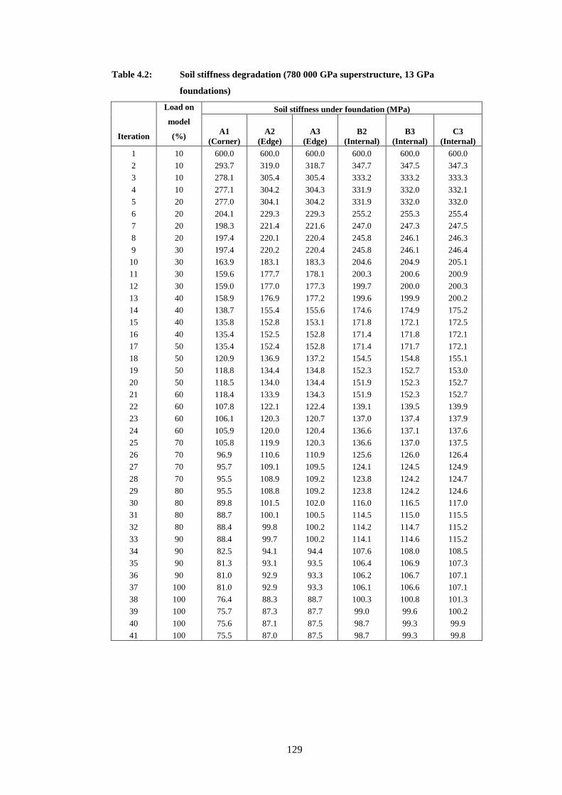
129

Table 4.2: Soil stiffness degradation (780 000 GPa superstructure, 13 GPa

foundations)

Iteration

Load on

model

(%)

Soil stiffness under foundation (MPa)

A1 (Corner)

A2 (Edge)

A3 (Edge)

B2 (Internal)

B3 (Internal)

C3 (Internal)

1 10 600.0 600.0 600.0 600.0 600.0 600.0

2 10 293.7 319.0 318.7 347.7 347.5 347.3

3 10 278.1 305.4 305.4 333.2 333.2 333.3

4 10 277.1 304.2 304.3 331.9 332.0 332.1

5 20 277.0 304.1 304.2 331.9 332.0 332.0

6 20 204.1 229.3 229.3 255.2 255.3 255.4

7 20 198.3 221.4 221.6 247.0 247.3 247.5

8 20 197.4 220.1 220.4 245.8 246.1 246.3

9 30 197.4 220.2 220.4 245.8 246.1 246.4

10 30 163.9 183.1 183.3 204.6 204.9 205.1

11 30 159.6 177.7 178.1 200.3 200.6 200.9

12 30 159.0 177.0 177.3 199.7 200.0 200.3

13 40 158.9 176.9 177.2 199.6 199.9 200.2

14 40 138.7 155.4 155.6 174.6 174.9 175.2

15 40 135.8 152.8 153.1 171.8 172.1 172.5

16 40 135.4 152.5 152.8 171.4 171.8 172.1

17 50 135.4 152.4 152.8 171.4 171.7 172.1

18 50 120.9 136.9 137.2 154.5 154.8 155.1

19 50 118.8 134.4 134.8 152.3 152.7 153.0

20 50 118.5 134.0 134.4 151.9 152.3 152.7

21 60 118.4 133.9 134.3 151.9 152.3 152.7

22 60 107.8 122.1 122.4 139.1 139.5 139.9

23 60 106.1 120.3 120.7 137.0 137.4 137.9

24 60 105.9 120.0 120.4 136.6 137.1 137.6

25 70 105.8 119.9 120.3 136.6 137.0 137.5

26 70 96.9 110.6 110.9 125.6 126.0 126.4

27 70 95.7 109.1 109.5 124.1 124.5 124.9

28 70 95.5 108.9 109.2 123.8 124.2 124.7

29 80 95.5 108.8 109.2 123.8 124.2 124.6

30 80 89.8 101.5 102.0 116.0 116.5 117.0

31 80 88.7 100.1 100.5 114.5 115.0 115.5

32 80 88.4 99.8 100.2 114.2 114.7 115.2

33 90 88.4 99.7 100.2 114.1 114.6 115.2

34 90 82.5 94.1 94.4 107.6 108.0 108.5

35 90 81.3 93.1 93.5 106.4 106.9 107.3

36 90 81.0 92.9 93.3 106.2 106.7 107.1

37 100 81.0 92.9 93.3 106.1 106.6 107.1

38 100 76.4 88.3 88.7 100.3 100.8 101.3

39 100 75.7 87.3 87.7 99.0 99.6 100.2

40 100 75.6 87.1 87.5 98.7 99.3 99.9

41 100 75.5 87.0 87.5 98.7 99.3 99.8

130

Table 4.3: Soil stiffness degradation (780 000 GPa superstructure and foundations)

Iteration

Load on

model

(%)

Soil stiffness under foundation (MPa)

A1 (Corner)

A2 (Edge)

A3 (Edge)

B2 (Internal)

B3 (Internal)

C3 (Internal)

1 10 600.0 600.0 600.0 600.0 600.0 600.0

2 10 335.0 360.8 360.0 388.7 387.9 387.2

3 10 322.6 349.4 349.0 376.6 376.2 375.9

4 10 321.6 348.5 348.2 375.7 375.3 375.0

5 20 321.5 348.5 348.1 375.6 375.2 375.0

6 20 245.3 271.8 271.5 298.6 298.3 298.1

7 20 238.4 265.1 264.9 291.5 291.4 291.4

8 20 237.7 264.3 264.2 290.7 290.6 290.6

9 30 237.7 264.2 264.1 290.6 290.5 290.5

10 30 198.2 220.7 220.6 245.9 245.9 245.8

11 30 194.0 215.1 215.2 240.3 240.4 240.5

12 30 193.4 214.5 214.5 239.7 239.8 239.9

13 40 193.3 214.4 214.5 239.6 239.7 239.9

14 40 168.9 189.1 189.2 210.8 210.9 211.1

15 40 165.7 185.3 185.5 206.8 207.1 207.3

16 40 165.2 184.7 184.9 206.1 206.4 206.7

17 50 165.1 184.6 184.8 206.0 206.3 206.6

18 50 149.1 166.4 166.6 187.3 187.5 187.8

19 50 146.6 163.8 164.1 184.0 184.4 184.8

20 50 146.2 163.4 163.6 183.5 183.9 184.3

21 60 146.1 163.3 163.6 183.4 183.8 184.2

22 60 133.0 150.2 150.4 168.6 168.9 169.3

23 60 130.6 148.1 148.4 166.3 166.7 167.1

24 60 130.2 147.7 148.0 166.0 166.3 166.7

25 70 130.1 147.6 148.0 165.9 166.3 166.7

26 70 120.8 136.6 137.0 154.2 154.5 154.8

27 70 119.0 134.6 135.0 152.4 152.8 153.2

28 70 118.7 134.2 134.6 152.1 152.5 152.9

29 80 118.6 134.1 134.5 152.0 152.4 152.8

30 80 110.5 124.9 125.2 143.1 143.3 143.7

31 80 109.1 123.4 123.8 140.8 141.4 141.9

32 80 108.8 123.1 123.4 140.4 140.9 141.5

33 90 108.8 123.1 123.4 140.4 140.9 141.5

34 90 102.4 116.2 116.6 132.0 132.5 133.1

35 90 100.9 114.6 115.1 130.2 130.8 131.4

36 90 100.6 114.3 114.8 129.8 130.4 131.0

37 100 100.5 114.2 114.7 129.7 130.3 131.0

38 100 95.2 108.4 108.8 123.3 123.7 124.2

39 100 94.2 107.2 107.6 122.1 122.6 123.1

40 100 94.0 107.0 107.4 121.8 122.3 122.8

41 100 94.0 106.9 107.3 121.8 122.3 122.8

131

Table 4.4: Column loads in linear and non-linear models

Model 1 Model 2 Model 3 Model 4 Type Non-linear Linear Non-Linear Linear

Superstructure concrete stiffness (GPa) 780 000 780 000 780 000 780 000 Foundations concrete stiffness (GPa) 13 13 780 000 780 000

Column load (kN)

A1 (Corner) 1863 2158 2595 3931 A2 (Edge) 2210 2292 2628 2954 A3 (Edge) 2091 2118 2424 2722

B2 (Internal) 2160 2285 1560 986 B3 (Internal) 2033 1988 1481 900 C3 (Internal) 1837 1692 1339 860

Change with respect

to model 2 (%) Change with respect

to model 4 (%) A1 (Corner) -14 0 -34 0 A2 (Edge) -4 0 -11 0 A3 (Edge) -1 0 -11 0

B2 (Internal) -5 0 58 0 B3 (Internal) 2 0 65 0 C3 (Internal) 9 0 56 0

132

Table 4.5: Column tilt in structure

Es

(MPa)

Ec *

(GPa)

Relative bending stiffness (ρ*) Maximum column

tilt in structure

1.00 x 104

1.00 x 103

1.00 x 102

13

13

13

Zone 1, Flexible structure

1.32 x 10-7

1.32 x 10-6

1.32 x 10-5

1:130 064

1:50 884

1:6 905

1.00 x 101

1.00 x 100

1.00 x 10-1

13

13

13

Zone 2, Intermediate stiffness

1.32 x 10-4

1.32 x 10-3

1.32 x 10-2

1:707

1:76

1:11

1.00 x 10-2

1.00 x 10-3

1.00 x 10-4

13

13

13

Zone 3, Rigid structure

1.32 x 10-1

1.32 x 100

1.32 x 101

1:3

1:0.5

1:0.05

1.00 x 104

1.00 x 103

1.00 x 102

13 000

13 000

13 000

Zone 2, Intermediate stiffness

1.32 x 10-4

1.32 x 10-3

1.32 x 10-2

1:714 420

1:76 843

1:11 775

1.00 x 101

1.00 x 100

1.00 x 10-1

1.00 x 10-2

1.00 x 10-3

1.00 x 10-4

13 000

13 000

13 000

13 000

13 000

13 000

Zone 3, Rigid structure

1.32 x 10-1

1.32 x 100

1.32 x 101

1.32 x 102

1.32 x 103

1.32 x 104

1:2 872

1:481

1:49

1:5

1:0.5

1:0.03

*Note: Second moment of area (I) is constant

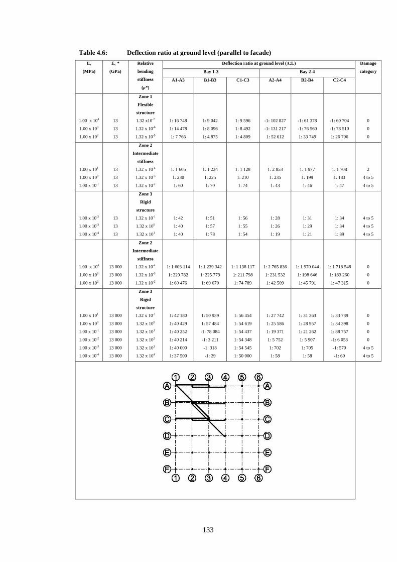
133

Table 4.6: Deflection ratio at ground level (parallel to facade)

Es

(MPa)

Ec *

(GPa)

Relative

bending

stiffness

(ρ*)

Deflection ratio at ground level (∆:L) Damage

category Bay 1-3 Bay 2-4

A1-A3 B1-B3

C1-C3 A2-A4

B2-B4

C2-C4

1.00 x 104

1.00 x 103

1.00 x 102

13

13

13

Zone 1

Flexible

structure

1.32 x10-7

1.32 x 10-6

1.32 x 10-5

1: 16 748

1: 14 478

1: 7 766

1: 9 042

1: 8 096

1: 4 875

1: 9 596

1: 8 492

1: 4 809

-1: 102 827

-1: 131 217

1: 52 612

-1: 61 378

-1: 76 560

1: 33 749

-1: 60 704

-1: 78 510

1: 26 706

0

0

0

1.00 x 101

1.00 x 100

1.00 x 10-1

13

13

13

Zone 2

Intermediate

stiffness

1.32 x 10-4

1.32 x 10-3

1.32 x 10-2

1: 1 605

1: 230

1: 60

1: 1 234

1: 225

1: 70

1: 1 128

1: 210

1: 74

1: 2 853

1: 235

1: 43

1: 1 977

1: 199

1: 46

1: 1 708

1: 183

1: 47

2

4 to 5

4 to 5

1.00 x 10-2

1.00 x 10-3

1.00 x 10-4

13

13

13

Zone 3

Rigid

structure

1.32 x 10-1

1.32 x 100

1.32 x 101

1: 42

1: 40

1: 40

1: 51

1: 57

1: 78

1: 56

1: 55

1: 54

1: 28

1: 26

1: 19

1: 31

1: 29

1: 21

1: 34

1: 34

1: 89

4 to 5

4 to 5

4 to 5

1.00 x 104

1.00 x 103

1.00 x 102

13 000

13 000

13 000

Zone 2

Intermediate

stiffness

1.32 x 10-4

1.32 x 10-3

1.32 x 10-2

1: 1 603 114

1: 229 782

1: 60 476

1: 1 239 342

1: 225 779

1: 69 670

1: 1 138 117

1: 211 798

1: 74 789

1: 2 765 836

1: 231 532

1: 42 509

1: 1 970 044

1: 198 646

1: 45 791

1: 1 718 548

1: 183 260

1: 47 315

0

0

0

1.00 x 101

1.00 x 100

1.00 x 10-1

1.00 x 10-2

1.00 x 10-3

1.00 x 10-4

13 000

13 000

13 000

13 000

13 000

13 000

Zone 3

Rigid

structure

1.32 x 10-1

1.32 x 100

1.32 x 101

1.32 x 102

1.32 x 103

1.32 x 104

1: 42 180

1: 40 429

1: 40 252

1: 40 214

1: 40 000

1: 37 500

1: 50 939

1: 57 484

-1: 78 084

-1: 3 211

-1: 318

-1: 29

1: 56 454

1: 54 619

1: 54 437

1: 54 348

1: 54 545

1: 50 000

1: 27 742

1: 25 586

1: 19 371

1: 5 752

1: 702

1: 58

1: 31 363

1: 28 957

1: 21 262

1: 5 907

1: 705

1: 58

1: 33 739

1: 34 398

1: 88 757

-1: 6 058

-1: 570

-1: 60

0

0

0

0

4 to 5

4 to 5

134

Table 4.7: Deflection ratio at ground level (diagonal to facade)

Es

(MPa)

Ec *

(GPa)

Relative

bending

stiffness

(ρ*)

Deflection ratio at ground

level

Damage

category

(taking

Table 4.5

into account)

Diagonal

A1-C3

B2-D4

1.00 x 104

1.00 x 103

1.00 x 102

13

13

13

Zone 1

Flexible

structure

1.32 x10-7

1.32 x 10-6

1.32 x 10-5

1: 7 987

1: 7153

1: 4 483

-1: 43 161

-1: 54 817

1: 21 084

0

0

0

1.00 x 101

1.00 x 100

1.00 x 10-1

13

13

13

Zone 2

Intermediate

stiffness

1.32 x 10-4

1.32 x 10-3

1.32 x 10-2

1: 1 180

1: 187

1: 43

1: 1 296

1: 135

1: 33

2

4 to 5

4 to 5

1.00 x 10-2

1.00 x 10-3

1.00 x 10-4

13

13

13

Zone 3

Rigid

structure

1.32 x 10-1

1.32 x 100

1.32 x 101

1: 28

1: 27

1: 27

1: 23

1: 22

1: 24

4 to 5

4 to 5

4 to 5

1.00 x 104

1.00 x 103

1.00 x 102

13 000

13 000

13 000

Zone 2

Intermediate

stiffness

1.32 x 10-4

1.32 x 10-3

1.32 x 10-2

1: 1 168 449

1: 185 024

1: 42 497

1:1 298 051

1: 134 805

1: 32 909

0

0

0

1.00 x 101

1.00 x 100

1.00 x 10-1

1.00 x 10-2

1.00 x 10-3

1.00 x 10-4

13 000

13 000

13 000

13 000

13 000

13 000

Zone 3

Rigid

structure

1.32 x 10-1

1.32 x 100

1.32 x 101

1.32 x 102

1.32 x 103

1.32 x 104

1: 28 428

1: 27 121

1: 26 992

1: 26 989

1: 26 852

1: 26 517

1: 22 986

1: 22 234

1: 24 258

1: 334 066

-1: 4 238

1: 2 847

0

0

0

0

4 to 5

4 to 5

135

Table 4.8: Deflection limits based on Burland et al. (2001a)

Category of

damage

Normal degree of

severity

Limiting tensile strain

(%)

Deflection limit

0

1

2

3

4 to 5

Negligible

Very slight

Slight

Moderate

Severe to very severe

0-0.05

0.05-0.075

0.075-0.15

0.15-0.3

> 0.3

1:2 439

1:1 626

1:813

1:407

136

Table 4.9: Column loads with soil stiffness variation at foundation B2

Load difference at ground level with respect to 10 MPa

soil stiffness

(%)

Soil stiffness under foundation B2 (MPa) 0 1 5 10 20 100

Soil stiffness rest of model (MPa) 10 10 10 10 10 10

Column B2

Column A2 & B1 (adjacent, edge)

Column B3 & C2 (adjacent, internal)

Column A1, A3, C1, C3 (adjacent, diagonal)

Other columns

-122

45

39

-18 to 6

-7 to 0

-112

42

36

-9 to 5

-1 to 0

-62

23

20

-5 to 3

0

0

0

0

0

0

10

-4

-3

0 to 1

0

14

-5

-4

-1 to 1

0

Load difference at ground level with respect to 100 MPa

soil stiffness

(%)

Soil stiffness under foundation B2 (MPa) 0 10 50 100 200 1000

Soil stiffness rest of model (MPa) 100 100 100 100 100 100

Column B2

Column A2 & B1 (adjacent, edge)

Column B3 & C2 (adjacent, internal)

Column A1, A3, C1, C3 (adjacent, diagonal)

Other columns

-119

55

46

-19 to 7

-7 to 0

-14

7

5

-1 to 1

-1 to 0

-2

1

1

0

0

0

0

0

0

0

2

-1

0

0

0

4

-2

-1

0

0

137

Figure 4.1: Building layout

A1 A3 A2

B3 B2

C3

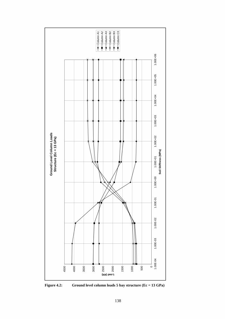
138

Figure 4.2: Ground level column loads 5 bay structure (Ec = 13 GPa)

Gro

un

d L

evel

Co

lum

n L

oad

sS

tru

ctu

re (

Ec

= 13

GP

a)

0

500

1000

1500

2000

2500

3000

3500

4000

4500 1.

00E

-04

1.00

E-0

31.

00E

-02

1.00

E-0

11.

00E

+00

1.00

E+

011.

00E

+02

1.00

E+

031.

00E

+04

1.00

E+

051.

00E

+06

So

il S

tiff

nes

s (M

Pa)

Load (kN)

Col

umn

A1

Col

umn

A2

Col

umn

A3

Col

umn

B2

Col

umn

B3

Col

umn

C3

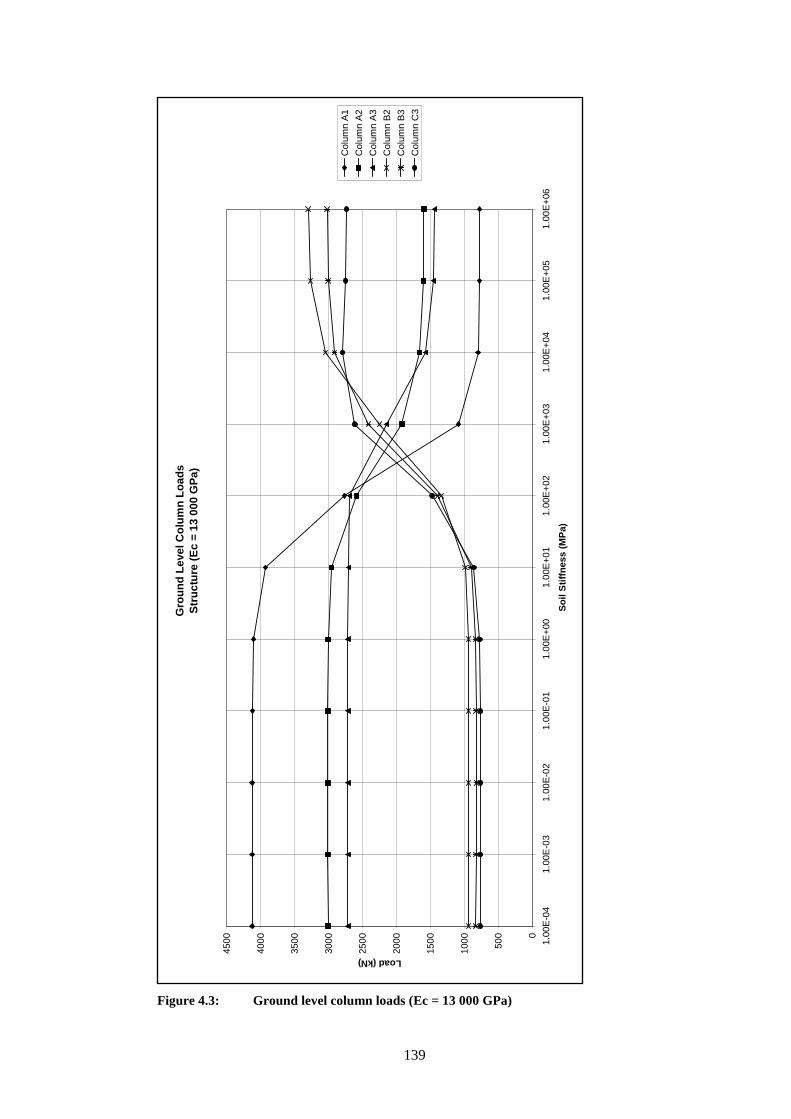
139

Figure 4.3: Ground level column loads (Ec = 13 000 GPa)

Gro

un

d L

evel

Co

lum

n L

oad

sS

tru

ctu

re (

Ec

= 13

000

GP

a)

0

500

1000

1500

2000

2500

3000

3500

4000

4500 1.

00E

-04

1.00

E-0

31.

00E

-02

1.00

E-0

11.

00E

+00

1.00

E+

011.

00E

+02

1.00

E+

031.

00E

+04

1.00

E+

051.

00E

+06

So

il S

tiff

nes

s (M

Pa)

Load (kN)

Col

umn

A1

Col

umn

A2

Col

umn

A3

Col

umn

B2

Col

umn

B3

Col

umn

C3

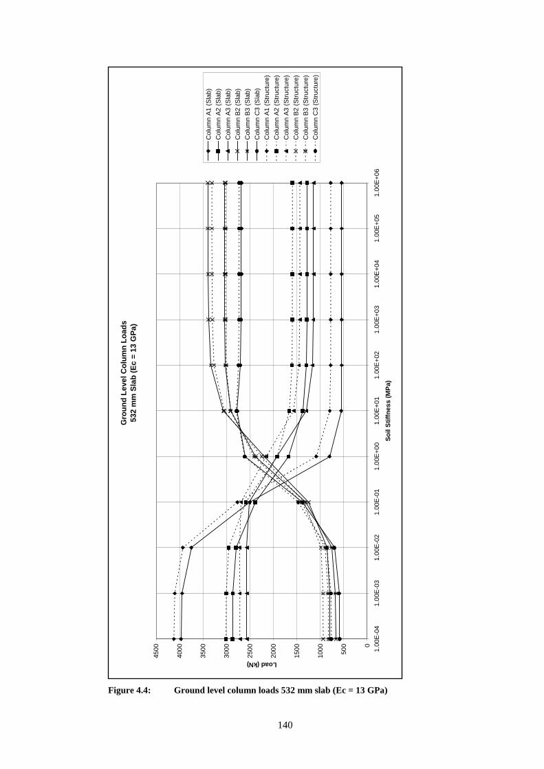
140

Figure 4.4: Ground level column loads 532 mm slab (Ec = 13 GPa)

Gro

un

d L

evel

Co

lum

n L

oad

s53

2 m

m S

lab

(E

c =

13 G

Pa)

0

500

1000

1500

2000

2500

3000

3500

4000

4500 1.

00E

-04

1.00

E-0

31.

00E

-02

1.00

E-0

11.

00E

+00

1.00

E+

011.

00E

+02

1.00

E+

031.

00E

+04

1.00

E+

051.

00E

+06

So

il S

tiff

nes

s (M

Pa)

Load (kN)

Col

umn

A1

(Sla

b)

Col

umn

A2

(Sla

b)

Col

umn

A3

(Sla

b)

Col

umn

B2

(Sla

b)

Col

umn

B3

(Sla

b)

Col

umn

C3

(Sla

b)

Col

umn

A1

(Str

uctu

re)

Col

umn

A2

(Str

uctu

re)

Col

umn

A3

(Str

uctu

re)

Col

umn

B2

(Str

uctu

re)

Col

umn

B3

(Str

uctu

re)

Col

umn

C3

(Str

uctu

re)

141

Figure 4.5: Structure normalisation

Str

uct

ure

No

rmal

isat

ion

050100

150

200

250

300

350

400

450

500

550

600 1.

E-0

71.

E-0

61.

E-0

51.

E-0

41.

E-0

31.

E-0

21.

E-0

11.

E+0

01.

E+

011.

E+0

2

No

rmal

isat

ion

fac

tor ρ

*

Column load / column load without soil-structure interaction (%)

5 B

ay C

orne

r C

olum

n A

1

5 B

ay E

dge

Col

umn

A2

5 B

ay E

dge

Col

umn

A3

5 B

ay In

tern

al C

olum

n B

2

5 B

ay In

tern

al C

olum

n B

3

5 B

ay In

tern

al C

olum

n C

3

4 B

ay C

orne

r C

olum

n A

1

4 B

ay E

dge

Col

umn

A2

4 B

ay E

dge

Col

umn

A3

4 B

ay In

tern

al C

olum

n B

2

4 B

ay In

tern

al C

olum

n B

3

4 B

ay In

tern

al C

olum

n C

3

3 B

ay C

orne

r C

olum

n A

1

3 B

ay E

dge

Col

umn

A2

3 B

ay E

dge

Col

umn

A3

3 B

ay In

tern

al C

olum

n B

2

3 B

ay In

tern

al C

olum

n B

3

3 B

ay In

tern

al C

olum

n C

3

ZO

NE

1F

lexi

ble

Str

uctu

reZ

ON

E 3

'Rig

id' S

truc

ture

ZO

NE

2In

term

edia

te S

tiffn

ess

Co

rner

co

lum

ns

Ed

ge

colu

mn

s

Inte

rnal

co

lum

ns

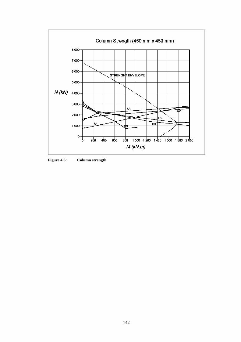
142

Figure 4.6: Column strength

143

Figure 4.7: Normalised elastic foundation loads and bearing resistance

Fo

un

dat

ion

Lo

ads

0

1000

2000

3000

4000

5000

6000

7000 1.

00E

-07

1.00

E-0

61.

00E

-05

1.00

E-0

41.

00E

-03

1.00

E-0

21.

00E

-01

1.00

E+

001.

00E

+01

1.00

E+

02

ρ*

Load (kN)

Fou

ndat

ion

A1

Fou

ndat

ion

A2

Fou

ndat

ion

A3

Fou

ndat

ion

B2

Fou

ndat

ion

B3

Fou

ndat

ion

C3

ZO

NE

1

Fle

xibl

e S

truc

ture

ZO

NE

3

'Rig

id' S

truc

ture

ZO

NE

2

Inte

rmed

iate

Stif

fnes

s

144

Figure 4.8: Settlement of foundations on London Clay (Atkinson, 2000)

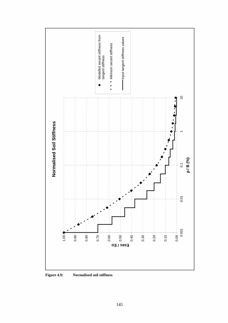
145

Figure 4.9: Normalised soil stiffness

No

rmal

ised

So

il S

tiff

nes

s

0.00

0.10

0.20

0.30

0.40

0.50

0.60

0.70

0.80

0.90

1.00

0.00

10.

010.

11

10

ρ ρ ρ ρ / B

(%

)

Esec / Eo

Mod

elle

d se

cant

stif

fnes

s fr

omta

ngen

t stif

fnes

s

Atk

inso

n se

cant

stif

fnes

s

Inpu

t tan

gent

stif

fnes

s va

lues

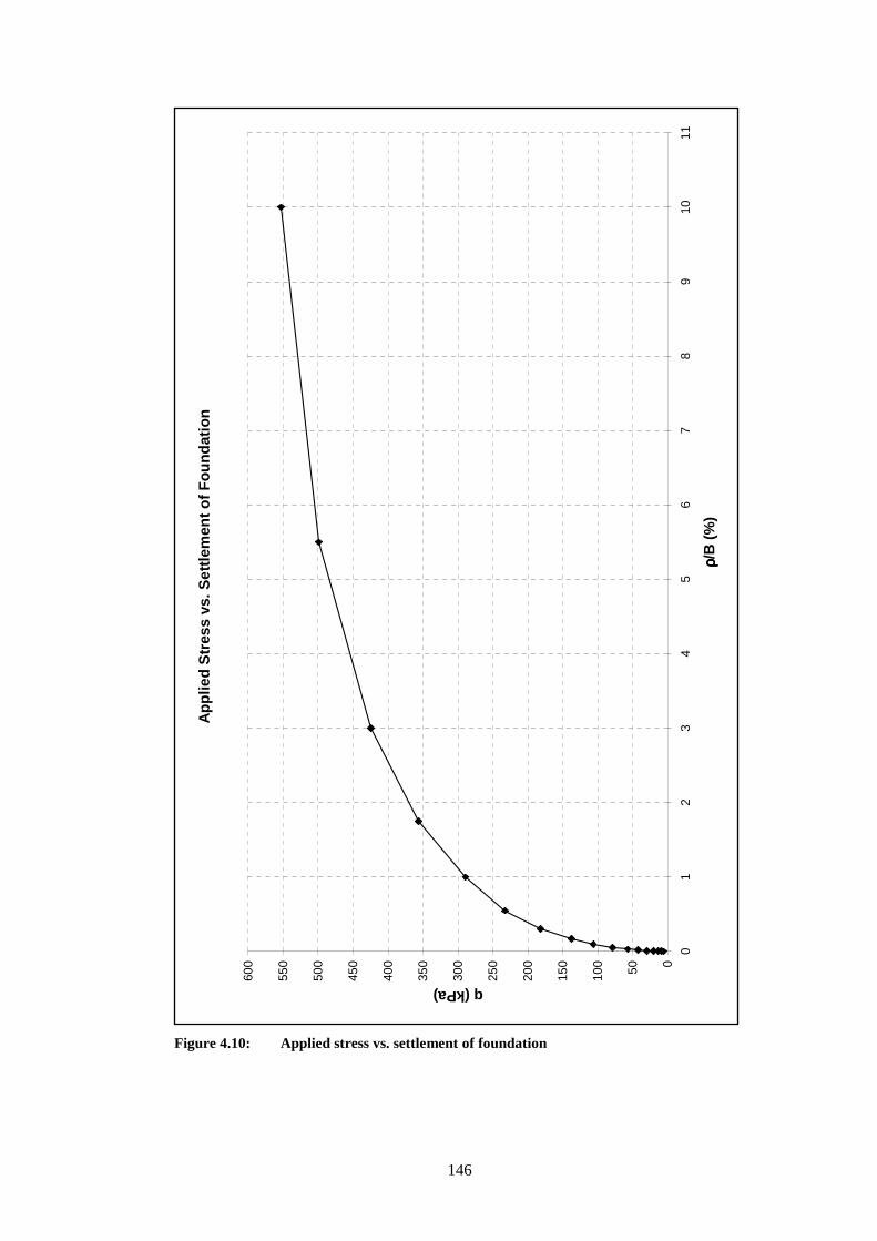
146

Figure 4.10: Applied stress vs. settlement of foundation

Ap

plie

d S

tres

s vs

. Set

tlem

ent

of

Fo

un

dat

ion

050100

150

200

250

300

350

400

450

500

550

600

01

23

45

67

89

1011

ρ ρρρ/B

(%

)

q (kPa)

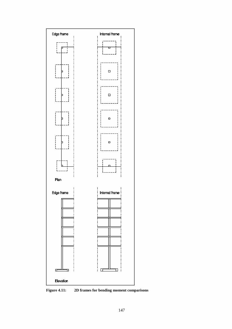
147

Figure 4.11: 2D frames for bending moment comparisons

148

Figure 4.12: Bending moment level 1, internal span

Ben

din

g M

om

ent

Lev

el 1

(In

tern

al S

pan

)

-500

0-4

800

-460

0-4

400

-420

0-4

000

-380

0-3

600

-340

0-3

200

-300

0-2

800

-260

0-2

400

-220

0-2

000

-180

0-1

600

-140

0-1

200

-100

0-8

00-6

00-4

00-2

00020

040

060

0

07.

515

Sp

an (

m)

Bending moment (kNm)

Str

engt

h bo

unda

ry

Str

engt

h bo

unda

ry

p* =

1.3

2e-6

p* =

1.3

2e-5

p* =

1.3

2e-4

p* =

1.3

2e-3

p* =

1.3

2e-2

p* =

1.3

2e-1

p* =

1.3

2e+

0

p* =

1.3

2e+

1

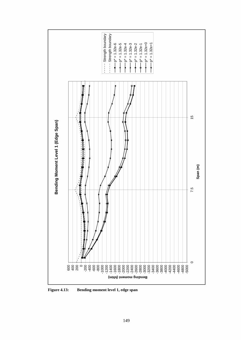
149

Figure 4.13: Bending moment level 1, edge span

Ben

din

g M

om

ent

Lev

el 1

(E

dg

e S

pan

)

-500

0-4

800

-460

0-4

400

-420

0-4

000

-380

0-3

600

-340

0-3

200

-300

0-2

800

-260

0-2

400

-220

0-2

000

-180

0-1

600

-140

0-1

200

-100

0-8

00-6

00-4

00-2

00020

040

060

0

07.

515

Sp

an (

m)

Bending moment (kNm)

Str

engt

h bo

unda

ry

Str

engt

h bo

unda

ry

p* =

1.3

2e-6

p* =

1.3

2e-5

p* =

1.3

2e-4

p* =

1.3

2e-3

p* =

1.3

2e-2

p* =

1.3

2e-1

p* =

1.3

2e+

0

p* =

1.3

2e+

1

150

5 CONCLUSIONS AND SUGGESTIONS FOR

FURTHER WORK

5.1 Conclusions

5.1.1 Conclusions from the literature

• The literature review shows that soil-structure interaction is important. Soil-

structure interaction causes transfer of loads within the structure and

deformations. Transfer of load within a structure will cause different loads to

those predicted without soil-structure interaction which may lead to structural

damage or failure. Deformations in the structure may cause visual damage i.e.

cracking of facades or partitions; loss of functionality, i.e. doors and windows

that get stuck; and unacceptable visual deformations i.e. deflected slabs and

tilting of columns (Section 1 & 2.4).

• Movements within the superstructure of a building are not always due to

differential settlement of foundations. Significant movements within the

superstructure may occur due to the movement of the members under imposed

loads and variation in temperature (Section 2.2.2 & 2.4).

• To date definitions to describe differential settlement have been defined for 2D

deformation without provision for the 3D deformation characteristics of

structures. This thesis considers the 3D nature of modern flexible framed

structures undergoing differential settlement (Section 2.1)

• The current state of the art assumes that damage to a building due to

differential settlement is confined to cladding and finishes, rather than the

structural members. This may be valid for older conventional buildings with

brick infill panels, however modern flexible framed buildings with facades that

allow for differential settlement may suffer from unacceptable aesthetical

deflections, tilting or structural damage before damage to the facades or

finishes occur (Section 2.3 & 2.4).

151

• The current state of the art assumes that the behaviour of a 3D structure

undergoing differential settlement can be represented by a simplified 2D beam

undergoing bending and shear deformation. For damage prediction, the

deformation and maximum tensile strain within the beam are calculated and

compared to known critical tensile strains for damage in infill panels. For this

method to be valid the following criteria need to be satisfied:

o Insignificant differential settlement must occur perpendicular to the

plane of bending. This may happen where differential settlement

occurs due to tunnelling or open excavations parallel to the structure,

however differential settlement driven by the self weight of the

building results in 3 dimensional deformation of the structure (Section

2.4.1).

o The complete building (including facades and partitions) is constructed

before any differential settlement occurs. This may be a justifiable

assumption if the differential settlement is caused by adjacent

excavation after the completion of the building. However, for

differential settlement driven by the self weight of the building the

change of stiffness of the structure and the settlement that occurs as

construction progresses, need to be taken into account (Section 2.4.1).

o The facades and partitions are fixed to the frame and no allowance is

made for differential settlement. Gaps or brackets allowing for

movement will reduce the strain in facades and partitions (Section

2.4.1).

o The equivalent bending and shear stiffnesses of the structure need to be

predicted. Potts and Addenbrooke (1997) calculated the bending

stiffness of the superstructure by using the parallel axis theorem, which

in their view is an overestimate of building stiffness as only a rigidly

framed structure would approach such modes of deformation. They

also suggest an alternative approach by which the bending stiffness of

the superstructure is obtained by summing the independent EI values

for each storey, which implies that the walls and columns transfer the

same deformed shape to each storey. No further guidance is given in

the literature on the stiffness of a real structure (Section 2.2.4).

152

• Extensive codes in the form of Eurocodes and British Standards exist with

guidelines on how to design a building. In contrast, there is little guidance in

the literature on how to perform a numerical analysis of a structure and its

foundations, with the aim of providing the loads, deformations, shear forces

and bending moments that will occur in reality.

5.1.2 Conclusions from the methodology

• The methodology involved the design of a structure to determine the member

sizes for the subsequent finite element analysis (Section 3.1.2).

• The design was done using British Standards and the Eurocodes. Standard

design Excel spreadsheets from RCC-2000 were used for the design.

RCC-2000 are design spreadsheets based on BSI 8119-1 (1997) and were

published by the British Cement Association on behalf of the industry sponsors

of the Reinforced Concrete Council (Section 3.1.2).

• A finite element analysis of a complete building on pad foundations was

carried out using LUSAS on a 2.4 GHz Intel Core2 Duo PC with a 32-bit

platform and 3 GB of RAM (Section 3.1.2).

• The size of the linear elastic model in LUSAS was limited by the discretisation

of the foundations and supporting halfspace and not by the solver. LUSAS is

only available as a 32-bit program and can therefore only use a maximum of

3 GB of RAM (Section 3.3).

• In the finite element model, column loads at ground level supported by a ‘rigid’

halfspace were within 10% of the load takedown, calculated assuming each

column supports half of the span. The total load from the model was within

2% of the total load from the load takedown (Section 3.3).

• To determine the optimal element type, discretisation and halfspace

boundaries, a single rigid foundation on a halfspace was modelled and the load

displacement response compared to standard elastic solutions. The load-

displacement response of a single rigid pad foundation could be calculated to

within 1% of the approximate elastic solution. However the mesh size needed

for this accuracy proved to be too fine for the complete model to work, given

the available computer resource. Reducing the accuracy of the single

foundation load-displacement ratio to within 7% allowed a usable mesh density

for the complete model (Section 3.3).

153

• The use of 10 node tetrahedral continuum elements for the foundations and

supported halfspace gave better results in LUSAS than the same number of

4 node tetrahedral continuum elements. The total number of elements that

could be discretised in the model was limited by the PC memory and was the

same for 4 and 10 node elements (Section 3.3).

• An irregular mesh with variable density proved to be more suitable than a

regular mesh for the supporting halfspace (Section 3.3).

5.1.3 Conclusions from the analyses

Normalisation of data

• For an elastic structure supported by a linear elastic soil it is possible to

normalise the relative bending stiffness with ρ* as:

4

*

HE

EI

s

=ρ

Where E is the Young’s modulus of the concrete, I is the second moment of

inertia of the structure, Es is the Young’s modulus of the soil and H is the half

length of the building (Section 4.1).

• Three distinct zones of behaviour within the relative bending stiffness range

can be identified (Section 4.1).

o Zone 1 ‘Flexible structure’ is the zone of relative bending stiffness (ρ* )

where the structure is flexible in comparison to the soil. ρ* is typically

less than 1 x 10-4 in Zone 1. Behaviour in Zone 1 can be determined

without taking soil-structure interaction into account.

o Zone 2 ‘Intermediate structure’ is the intermediate zone where the

loads, shear forces and bending moments within the structure change

as the relative bending stiffness increases. ρ* typically ranges from 1

x 10-4 to 1 x 10-1 in Zone 2.

o Zone 3 ‘Rigid structure’ is the zone of relative bending stiffness (ρ* )

where the structure is rigid in comparison to the soil. In Zone 3 the

loads, shear forces and bending moments within the structure are again

constant, independent of the relative bending stiffness, but they may be

very different from that in Zone 1. ρ* is typically larger than 1 x 10-1

in Zone 3.

154

• An equivalent slab, with a thickness resulting in a second moment of area equal

to the sum of the second moment of area of the individual slabs (around their

individual neutral axes) within the structure, exhibited a similar soil-structure

behaviour as the 6 storey structure. The equivalent slab was suspended and

supported by the subsoil columns and foundations. For this specific structure

the equivalent slab thickness was 532 mm. An alternative approach using an

equivalent slab with a thickness based on the parallel axis theorem resulted in a

slab thickness of 14.0 m which was an overestimate of the structural bending

stiffness. The bending stiffness of the alternative method is approximately

18 000 times stiffer (Section 4.1)

• The designed ‘typical’ 5 bay structure on a soil with an undrained shear

strength of 90 kPa and a subsequent Young’s modulus of 600 MPa resulted in

an approximate relative bending stiffness (ρ* ) of 2.2 x 10-6, which falls in

Zone 1. The structure will therefore behave flexibly (Section 4.1).

Structural strength

• As the relative bending stiffness increased in the linear elastic model the axial

loads in the corner columns increased by approximately 5 times, the loads in

the edge columns approximately doubled and the loads in the internal columns

reduced to approximately 1/3 in comparison to the column loads within a

flexible structure. Yielding of foundations or the structure may reduce the

column loads (Section 4.2.1)

• The linear-elastic numerical model showed the column loads exceeded the

strength of the columns where the relative bending stiffness (ρ* ) is larger than

1.32 x 10-3. Yielding of foundations may reduce the column loads and protect

against column failure (Section 4.2.1).

• Atkinson (2000) related soil strength to stiffness. A soil with an undrained

shear strength of 90 kPa will have an expected small strain stiffness of

600 MPa and an operational stiffness of between 75 and 123 MPa (between

0.07% and 0.20% strain) and this is dependent on the foundation stiffness

(Section 4.2.2).

155

• Foundation stiffness and non-linear soil stiffness influenced the column loads.

For a structure with a relative bending stiffness (ρ* ) of 1.32 x 10-1,

superstructure concrete stiffness of 780 000 GPa and soil stiffness of 600 MPa

(Section 4.2.2):

o The load in the corner column (A1) was reduced by 14% in the non-

linear model with a 13 GPa foundation concrete stiffness and 34% in

the non-linear model with a 780 000 GPa concrete stiffness.

o The loads in the edge columns (A2, A3) were reduced by between 1%

and 4% in the non-linear model with a 13 GPa foundation concrete

stiffness and 11% in the non-linear model with a 780 000 GPa

concrete stiffness.

o The loads in the internal columns (B2, B3, C3) ranged from a reduction

of 5% to an increase of 9% in the non-linear model with a 13 GPa

foundation concrete stiffness and increase of between 56% and 65% in

the non-linear model with a 780 000 GPa concrete stiffness.

• The linear-elastic numerical model showed the bending moments in the slabs

exceeded the strength of the slabs where the relative bending stiffness (ρ* ) is

larger than 1.32 x 10-4. Yielding of foundations may reduce the column loads

and protect against column failure (Section 4.2.3).

Structural deformation

• Tilt does not relate to relative bending stiffness; it is a function of both the

actual soil stiffness and the structure stiffness. A decrease in soil stiffness

results in an increase of tilt. A decrease of structural stiffness also results in an

increase of tilt, therefore a flexible structure is more likely to suffer from tilt

(Section 4.3.1).

• For structures without facades or internal partitions or where the facades and

partitions are specifically designed to allow movement, the literature suggested

deflection limits that ranged from 1:250 to 1:600 (Section 4.3.2).

• The deflection limits based on the beam model proposed by Burland et al.

(2001a) depend on the assumed class of damage and are much stricter. These

limits are applicable to masonry infill structures where damage will most likely

occur to the facades. A deflection limit of 1: 2 439 is proposed for negligible

damage. Based on this limit a relative bending stiffness of ρ* > 1 x 10-4 will

result in damage (Section 4.3.2).

156

• The researched structure deformed in 3D and the facade deflection was

significantly less than the maximum (diagonal) deflection. It is therefore

important to take the 3D deformation of a structure into account when

analysing a structure for differential settlement damage (section 4.3.2).

Variation in foundation load-displacement response

• A structure’s response to soil variation depends on the structure’s overall

relative bending stiffness (Section 4.4).

• For a relative bending stiffness of ρ* = 1.32 x 10-4, a foundation on a soil

stiffness of one order of magnitude less increased the loads in adjacent columns

between 36% and 42%. Increasing the soil stiffness under the foundation one

order of magnitude resulted in an increase of load of 14%. A foundation with a

stiffer response may therefore have an effect on foundation load. This is

significant for the reuse of foundations which have a stiffer (up to 10 times)

load-displacement response due to preloading (Section 4.4).

• For an overall relative bending stiffness of ρ* = 1.32 x 10-5, a foundation on a

soil stiffness of one order of magnitude less increased the loads in adjacent

columns between 5% and 7%. Increasing the stiffness under the foundation

one order of magnitude resulted in a maximum load variation of 4%. The

results showed that the higher the overall stiffness of the soil, the less impact a

harder spot under a foundation or a stiffer load-displacement response has on

the structure (Section 4.4).

5.2 Suggestions for further work

Suggestions for future work include:

• Model the behaviour of modern flexible framed structures on a non-linear soil

model with yielding. The presented research was based on a linear-elastic

model with a manual iteration process to show the effect of non-linear soil

response. The incorporation of non-linear soil model with yielding into the

finite element model may produce more accurate answers.

• Model the effect of single piles and pile groups (instead of pad foundations) on

the behaviour of modern flexible framed structures.

• Model the variation in soil stiffness more rigorously, i.e. investigate the effect

of spatial soil stiffness variation on the corner, edge and internal foundations.

157

• Determine and model the actual bending stiffness of concrete structures taking

into account:

o Stiffness and fitment details of the facades. Suggested facades include

glass panels, light weight concrete blocks and brickwork.

o Internal walls made out of plasterboard partitions, lightweight concrete

blocks or brickwork.

o Lift shafts and other methods of providing racking stiffness.

o Creep, shrinkage and cracking of concrete.

o The variation in stiffness during construction.

• Model the behaviour of steel framed structures and compare it to the flat slab

reinforced concrete structure.

• Model the behaviour of reinforced concrete structures with beams and compare

it to the flat slab structure.

• Model the effect of construction sequence on differential settlement, taking into

account the increase in structural stiffness and load during construction and the

time dependency of settlement. It is suggested to model the construction

sequence for both steel framed and reinforced concrete framed structures.

• Model the effect of temperature variation within steel framed and concrete

framed structures on the soil-structure interaction.

• Develop rigorous definitions to describe 3D deformations.

R-1

REFERENCES

Alawaji, H. A. (1997). Modeling of settlement and collapse of footings on sand pad

overlying collapsible soil. Proceedings of the International Conference on

Foundation Failures, Singapore, 385–392.

Atkinson, J. H. (2000). Non-linear soil stiffness in routine design. Géotechnique 50,

No.5, 487-508.

Atkinson, M. F. (1993). Structural Foundations Manual for Low-Rise Buildings.

London: E & FN Spon, 73.

Ayoub, A. H. and Karshenas, R. (1994). Survey results for concrete construction live

loads on newly poured slabs. J. Struct. Div., ASCE 120, 1543-1562.

Beeby, A. W. (2001). The forces in backprops during construction of flat slab

structures. Proc. of the Inst. of Civ. Engrs. Struct.s & Bldgs 146, Issue 3, 307-317.

Bertero, V. V., and Brokken, S (1983). Infills in seismic resistant buildings. J. Struct.

Engrg., ASCE, 109, No.6, 1337-1361.

Blackmore, P. A. (1988). Load reductions on flat roofs – The effect of edge profile. J.

Wind Eng. Ind. Aerodyn. 29, 88-89.

Boone, S. J. (1996). Ground movement related building damage. Journal of

Geotechnical Engineering 122, No.11, 886-896.

Boscardin, M. D. and Cording, E. J. (1989). Building response to excavation-induced

settlement. Journal of Geotechnical Engineering 115, No.1, 1-21.

Bourdeau, P. L. and Amandaray, J. I. (2005). Non-parametric simulation of

geotechnical variability. Géotechnique 55, No.2, 95-108.

Brown, P. T. (1969a). Numerical analyses of uniformly loaded circular rafts on elastic

layers of finite depth. Géotechnique 19, No.2, 301-306.

Brown, P. T. (1969b). Numerical analyses of uniformly loaded circular rafts on deep

elastic foundations. Géotechnique 19, No.3, 399-404.

Brown, P. T. and Yu, S. K. R. (1986). Load sequence and structure-foundation

interaction. Journal of Structural Engineering 112, No.3, 481-488.

Building Research Establishment (1994). Worked examples for the design of steel

structures. Based on BSI publication DD ENV 1993-1-1: 1992. Eurocode 3:

Design of steel structures Part 1.1 General rules and rules for buildings (together

with United Kingdom National Application Document). Watford: Building

Research Establishment.

BSI 648 (1964). Schedule of weights of building materials. London: British Standards

Institution.

R-2

BSI 6399-1 (1996). Loading for buildings – Part 1: Code of practice for dead and

imposed loads. London: British Standards Institution.

BSI 6399-2 (1997). Loading for buildings – Part 2: Code of practice for wind loads.

London: British Standards Institution.

BSI 6399-3 (1988). Loading for buildings – Part 3: Code of practice for imposed roof

loads. London: British Standards Institution

BSI 8004 (1986). Code of practice for foundations. London: British Standards

Institution.

BSI 8110-1 (1997). Structural use of concrete – Part 1: Code of practice for design

and construction. London: British Standards Institution.

BSI 8110-2 (1985). Structural use of concrete – Part 1: Code of practice for special

circumstances. London: British Standards Institution.

BSI 8500-1 (2006). Concrete – Complementary British Standard to BS EN 206-1 –

Part 1: Method of specifying and guidance for the specifier. London: British

Standards Institution.

Building Research Establishment (1981, revised 1990). Assessment of damage in low

rise buildings with particular reference to progressive foundation movements.

Digest 251, BRE, Garston.

Burhouse, P. (1969). Composite action between brick and panel walls and their

supporting beams. Proc. Instn. Civ. Engrs., 43, 175-194.

Burland, J. B. (1975). Some examples of the influence of field measurements on

foundation design and construction. Proc. 6th Regional Conf. for Africa Soil Mech.

Fdn Engng, Durban 2.

Burland, J. B., Broms, B. B. and De Mello, V. F. B. (1977). Behaviour of foundations

and structures. Proc. 9th Int. Conf. on Soil Mech. & Found. Engng., Tokyo, Vol.II,

495-546.

Burland, J. B. and Cooke, R. W. (1974). The design of bored piles in stiff clays.

Ground Engineering 7, No.4, 28-35.

Burland, J. B., Standing, J. R. and Jardine, F. M. (2001a). Building response to

tunnelling. Case studies from construction of the Jubilee Line extension, London.

Volume 1 Projects and Methods. CIRIA Special publication 200. Thomas Telford,

London.

Burland, J. B., Standing, J. R. and Jardine, F. M. (2001b). Building response to

tunnelling. Case studies from construction of the Jubilee Line extension, London.

Volume 2 Case Studies. CIRIA Special publication 200. Thomas Telford, London.

R-3

Burland, J. B. and Wroth, C. P. (1975). Settlement of buildings and associated damage.

Proc. Conf. Settlement of Structures, Cambridge, 611-654.

Cameron, G. and Chapman T. (2004). Quality assurance of bored pile foundations.

Ground Engineering 37, No.2, 35-40

Chamecki, S. (1956). Structural rigidity in calculating settlements. J. Soil Mech. &

Found. Div., ASCE 82, No. SM1, 1-9.

Chan, S. F. (1997). Causes of foundation failures. Proc. Int. Conference on foundation

failures, Singapore, 3-10.

Chapman, T., Marsh, B. and Foster, A. (2001). Foundations for the future.

Proceedings of ICE, Civil Engineering 144, Feb, 36-41.

Choi, E. C. C. (1992). Live load in office buildings point-in-time load intensity of

rooms. Proc. ICE Struct. & Build. 94, 299-306.

Chow, F. C., Chapman, T. J. P. and St. John, H. D. (2002). Reuse of existing

foundations: planning for the future. Proc. 2nd Int. Conference on Soil Structure

Interaction in Urban Civil Engineering, Zurich, 171-176.

Culver, C. G. (1976). Survey results for fire loads and live loads in office buildings.

Building Science Series 85, National Bureau of Standards, Washington DC.

De Beer, E., Lousberg, E., De Jonghe, A., Wallays, M. and Carpentier, R. (1979).

Prediction of the bearing capacity of displacement piles, penetrating into a very

dense sand layer. Proc.7th. Eur. Conf. Soil Mech., London 3, 51-59.

Department for Communities and Local Government (2006). A Designers’ Simple

Guide to BS EN 1997. Department for Communities and Local Government,

London.

El Gonnouni, M., Riou, Y. and Hicher, P. Y. (2005). Geostatistical method for

analysing soil displacement from underground urban construction. Géotechnique

55, No.2, 171-182.

EN 1990 (2002). Eurocode – Basis of structural design. London: British Standards

Institution.

EN 1991-1-1 (2002). Eurocode 1: Actions on structures – Part 1-1: General actions –

Densities, self-weight, imposed loads for buildings. London: British Standards

Institution.

EN 1991-1-3 (2003). Eurocode 1: Actions on structures – Part 1-3: General actions –

Snow loads. London: British Standards Institution.

EN 1991-1-4 (2005). Eurocode 1: Actions on structures – Part 1-4: General actions –

Wind actions. London: British Standards Institution.

R-4

EN 1991-1-5 (2003). Eurocode 1: Actions on structures – Part 1-5: General actions –

Thermal actions. London: British Standards Institution.

EN 1997-1 (2004). Eurocode 7: Geotechnical design – Part 1: General rules. London:

British Standards Institution.

EN 572-1 (2004). Glass in building – Basic soda lime silicate glass products – Part 1:

Definitions and general physical and mechanical properties. London: British

Standards Institution.

Fjeld, S. (1963). Settlement damage to a concrete-framed structure. Proc. European

Conf. Soil Mech. & Found. Engng., Wiesbaden, Vol.1, 391-399.

Fleming W. G. K. (1992). A new method for single pile settlement prediction and

analysis. Géotechnique 42, No.3, 411-425.

Fookes, P. G. (1997). First Glossop Lecture. Geology for Engineers: the Geological

Model, Prediction and Performance. Quarterly Journal of Engineering Geology,

30, 293-424.

Fraser, R. A. and Wardle, L. J. (1976). Numerical analysis of rectangular rafts on

layered foundations. Géotechnique 26, No.4, 613-630.

Freeman, T. J., Littlejohn, G. S. and Driscoll, R. M. C. (1994). Has your house got

cracks? The Institution of Civil Engineers, London, and Building Research

Establishment, Garston.

Gere, J. M. and Timoshenko, S. P. (1991). Mechanics of Mateials. Chapman and Hall,

London, 807.

Goschy, B. (1978). Soil-foundation-structure interaction. Proc. 2nd Australia-New

Zealand Conf. on Geomechanics, The Institution of Engineers, Australia, 79-82.

Grant, R., Christian, J. T. and Vanmarcke, E. H. (1974). Differential settlement of

buildings. Journal of the Geotechnical Engineering Division, ASCE 100, No.GT9,

973-991.

Hain, S. J. and Lee, I. K. (1978). The analysis of flexible raft-pile systems.

Géotechnique 28, 65-83.

Heil, H. (1969). Studies on the structural rigidity of reinforced concrete building

frames on clay. Proc. 7th Int. Conf. Soil Mech. Found. Engng., Vol.2, Mexico City,

Mexico, 115-121.

Holmes, M. (1961). Steel frames with brickwork and concrete infilling. Proc., Inst.

Civ. Engrs., 19, 473-478.

Institution of Structural Engineers (1978, 1989 and 2000). Structure-soil interaction.

A state of the art report. Revised and extended in 1989, 2nd edition August 2000,

The Institution of Structural Engineers, London.

R-5

Institution of Structural Engineers (1994). Subsidence of low rise buildings. The

Institution of Structural Engineers, London.

Jaksa, M. B., Goldsworthy, J. S., Fenton, G. A., Kaggwa, W. S., Griffits, D. V., Kuo,

Y. L. and Poulos, H. G. (2005). Towards reliable and effective site investigations.

Géotechnique 55, No.2, 109-121.

Jardine, R. J., Potts, D. M., Fourie, A. B., and Burland, J. B. (1986). Studies of the

influence of the non-linear stress-strain characteristics in soil-structure interaction.

Géotechnique 36, No.3, 377-396.

Jardine, R. J., Lehane, B. M., Smith, P. R. and Gildea, P. A. (1995). Vertical loading

experiments on rigid pad foundations at Bothkennar. Géotechnique 45, No.4, 573-

597.

Jennings, J. E. and Kerrich, J. E. (1962). The heaving of buildings and the associated

economic consequences, with particular reference to Orange Free State Goldfields.

The Civ. Engr in South Africa 5, No. 5, 55-122.

Kahn, L. F. and Hanson, R. D. (1979). Infilled walls for earthquake strengthening. J.

Struct. Div. ASCE., 105, No.2, 283-296.

Krishna, P. (1995). Wind loads on low rise buildings – A review. J. Wind Eng. Ind.

Aerodyn. 44/55, 383-396.

Kumar, S. (2002). Live loads in office buildings: point-in-time load intensity. Building

and Environment 37, 79-89.

Lee, I. K., White, W. and Ingles, O. G. (1983). Geotechnical engineering. Boston:

Pitman.

Lehane, B. M. and Jardine, R. J. (2003). Effects of long-term pre-loading on the

performance of a footing on clay. Géotechnique 53, No.8, 689-695.

Little, M. E. R. (1969). Discussion, Session 6, Proc. Symp. Design for movement in

buildings, The Concrete Society, London.

Macleod, I. A. and Littlejohn, G. S. (1975). Discussion on session 5. Proc. Conf.

Settlement of Structures, Cambridge, 792-795.

Mainstone, R. J. (1971). On the stiffness and strengths of infilled frames. Proc. Instn.

Civ. Engrs., Suppl. (IV), Paper 7360S, 57-90.

Mainstone R. J. and Weeks, G. A. (1970). The influence of a bounding frame on the

racking stiffnesses and strengths of brick walls. Proc. 2nd Int. Brick Masonry Conf.

Stoke-on-trent, 165-171.

Meecham, D. (1992). The improved performance of hip roofs in extreme winds – A

case study. J. Wind. Eng. Ind. Aerodyn. 43, 1717-1726.

R-6

Mehrabi, A. B. and Shing, P. B. (1997). Finite element modelling of masonry-infilled

RC frames. J. Struct. Eng., 123, No.5, 604-613.

Mehrabi, A. B., Shing, P. B., Schuller, M. P. and Noland, J. L. (1996). Experimental

evaluation of masonry-infilled RC frames. J. Struct. Eng., 122, No.3, 228-237.

Meyerhof, G. G. (1947). The settlement analysis of building frames. The Structural

Engineer 25, 369-409.

Meyerhof, G. G. (1956). Discussion on paper by Skempton et al.. Settlement analysis

of six structures in Chicago and London.. Proc. ICE 5, No.1, 170.

Mitchell G. R. and Woodgate R. W. (1971). A survey of floor loadings in office

buildings. CIRIA Report No. 25, London.

Morton, K. and Au, E. (1975). Settlement observations on eight structures in London.

Proc. Conf. Settlement of Structures, Cambridge, 183-203.

NA to EN 1990 (2002). UK National Annex for Eurocode 0 – Basis of structural

design. London: British Standards Institution.

NA to EN 1991-1-1 (2002). UK National Annex to Eurocode 1: Actions on structures

– Part 1-1: General actions – Densities, self-weight, imposed loads for buildings.

London: British Standards Institution.

NA to EN 1991-1-3 (2003). Eurocode 1: Actions on structures – Part 1-3: General

actions – Snow loads. London: British Standards Institution.

NA to EN 1991-1-5 (2003). Eurocode 1: Actions on structures – Part 1-5: General

actions – Thermal actions. London: British Standards Institution.

National Coal Board (1975). Subsidence Engineers Handbook. National Coal Board

Production Dept., UK.

Neville, A. M. (1981). Properties of Concrete, 3rd ed. New York: John Wiley and

Sons, 779.

Neville, A. M. (1995). Properties of Concrete, 4th ed.. London: Longman.

Orchand, C. J., Kulhawy, F. H. and Trautmann, C. H. (1988). Critical evaluation of in

situ test methods and their variability. Report EL-5507, Vol.2, Palo Alto: Electric

Power Research Institute.

Peck, R. B., Deere, D. U. and Capacete, J. L. (1956). Discussion on paper by

Skempton, A. W. and MacDonald, D. H, The allowable settlement of buildings.

Proc. Inst. Civ. Engrs. 5, Pt.III, 778-781.

Phoon, K. and Kulhawy, F. H. (1999). Characterization of geotechnical variability.

Can. Geotech. J. 36, 612-624.

Polshin, D. E. and Tokar, R. A. (1957). Maximum allowable non-uniform settlement

of structures. 4th Int. Conf. soil Mech. & Found. Engng., Vol.1, 402-405.

R-7

Potts, D. M. and Addenbrooke, T. I. (1997). A structure’s influence on tunnelling-

induced ground movements. Proceedings of ICE, Geotechnical Engineering 125,

Issue 2, 109-125.

Potts, D. M., Standing, J. R. and Addenbrooke, T. I. (1998). Interaction between

tunnelling and nearby structures. Proc. Int. Conference on Soil Structure

Interaction in Urban Civil Engineering, Darmstadt, No.4, Vol.1, 113-135.

Poulos, H.G. and Davis, E.H. (1974). Elastic Solutions for Soil and Rock Mechanics.

John Wiley and Sons, New York.

Ruiz, S. E. and Soriano, A. (1997). Design live loads for office buildings in Mexico

and the United States. Journal of Structural Engineering, ASCE 123, No.6, 816-

822.

Simons, N. E. and Som, N. N. (1970). Settlement of structures on clay, with particular

emphasis on London Clay. CIRIA Report 22.

Skempton, A. W. and Bjerrum, L. (1957). A contribution to the settlement analysis of

foundations on clay. Géotechnique 7, 168-178.

Skempton, A. W. and MacDonald, D. H. (1956). Allowable settlement of buildings.

Proc. Inst. Civ. Engrs. 5, Pt.III, 727-768.

Stafford Smith, B. (1962). Lateral stiffness of infilled frames. J. Struct. Div. ASCE, 88,

No.6, 183-199.

Stafford Smith, B. (1966). Behavior of the square infilled frames. J. Struct. Div.

ASCE, 92 No.1, 381-403.

Stafford Smith, B. (1967). Methods for predicting the lateral stiffness and strength of

multi-storey infilled frames. Build. Sci., Vol.2, Pergamon Press, Oxford, 247-257.

Terzaghi, K. (1935). The actual factor of safety in foundations. Struct. Eng. 13,

126-161.

Terzaghi. K. (1955). Influence of geologic factors on the engineering properties of

sediments. Econ. Geol. 50, 557-618.

Timoshenko, S. (1957). Strength of Materials – Part I, D van Nostrand, London.

Timoshenko, S. (1959). Theory of plates and shells, 2nd ed., Mcgraw-Hill, New York.

Wahls, H. E. (1981). Tolerable settlement of buildings. Journal of the Geotechnical

Engineering Division, ASCE 107, No.GT11, 1489-1504.

Whitaker, T. and Cooke, R. W. (1966). An investigation of the shaft and base

resistance of large bored piles in London Clay. Proc. Symp. on large bored piles,

ICE, London, 7-49.

Whitman, R. V. and Richart, F. E. (1967). Design procedures for dynamically loaded

foundations. Jnl. Soil Mech. Fndns. Divn., ASCE, 93, No. SM6, 169-193.

R-8

Wiseman, G. and Lavie, Y. (1983). Arid zone subsurface exploration and load testing.

Proceedings of the seventh Asian Regional Conference on Soil Mechanics and

Foundation Engineering, 1, Haifa, 98–104.

Wood, S. L. (1991). Evaluation of the long-term properties of concrete. ACI Mat. Jnl.,

88, No.6, 630-643.

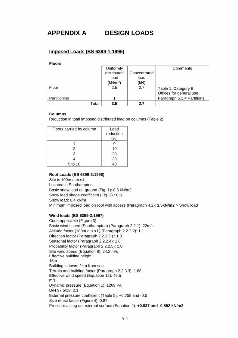
A-1

APPENDIX A DESIGN LOADS

Imposed Loads (BS 6399-1:1996)

Floors

Uniformly distributed

load Concentrated

load

Comments

(kN/m²) (kN) Floor 2.5 2.7 Table 1, Category B,

Offices for general use Partitioning 1 Paragraph 5.1.4 Partitions

Total 3.5 2.7 Columns Reduction in total imposed distributed load on columns (Table 2)

Floors carried by column Load reduction

(%) 1 0 2 10 3 20 4 30

5 to 10 40 Roof Loads (BS 6399-3:1998) Site is 100m a.m.s.l. Located in Southampton Basic snow load on ground (Fig. 1): 0.5 kN/m2 Snow load shape coefficeint (Fig. 2) : 0.8 Snow load: 0.4 kN/m Minimum imposed load on roof with access (Paragraph 4.2): 1.5kN/m2 > Snow load Wind loads (BS 6399-2:1997) Code applicable (Figure 3) Basic wind speed (Southampton) (Paragraph 2.2.1): 22m/s Altitude factor (100m a.b.s.l.) (Paragraph 2.2.2.2): 1.1 Direction factor (Paragraph 2.2.2.3.) : 1.0 Seasonal factor (Paragraph 2.2.2.4): 1.0 Probability factor (Paragraph 2.2.2.5): 1.0 Site wind speed (Equation 8): 24.2 m/s Effective building height: 18m Building in town, 2km from sea Terrain and building factor (Paragraph 2.2.3.3): 1.88 Effective wind speed (Equation 12): 45.5 m/s Dynamic pressure (Equation 1): 1269 Pa D/H 37.5/18=2.1 External pressure coefficient (Table 5): +0.758 and -0.5 Size effect factor (Figure 4): 0.87 Pressure acting on external surface (Equation 2): +0.837 and -0.552 kN/m2

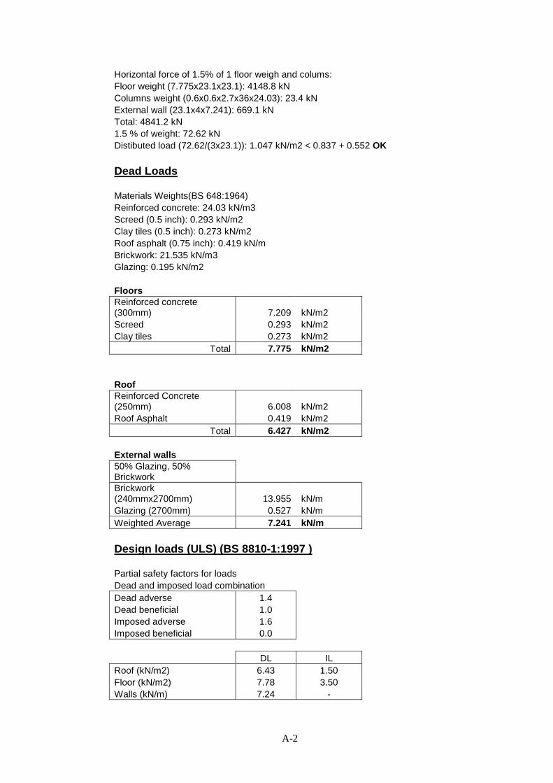
A-2

Horizontal force of 1.5% of 1 floor weigh and colums: Floor weight (7.775x23.1x23.1): 4148.8 kN Columns weight (0.6x0.6x2.7x36x24.03): 23.4 kN External wall (23.1x4x7.241): 669.1 kN Total: 4841.2 kN 1.5 % of weight: 72.62 kN Distibuted load (72.62/(3x23.1)): 1.047 kN/m2 < 0.837 + 0.552 OK

Dead Loads Materials Weights(BS 648:1964) Reinforced concrete: 24.03 kN/m3 Screed (0.5 inch): 0.293 kN/m2 Clay tiles (0.5 inch): 0.273 kN/m2 Roof asphalt (0.75 inch): 0.419 kN/m Brickwork: 21.535 kN/m3 Glazing: 0.195 kN/m2 Floors Reinforced concrete (300mm) 7.209 kN/m2 Screed 0.293 kN/m2 Clay tiles 0.273 kN/m2

Total 7.775 kN/m2 Roof Reinforced Concrete (250mm) 6.008 kN/m2 Roof Asphalt 0.419 kN/m2

Total 6.427 kN/m2 External walls 50% Glazing, 50% Brickwork Brickwork (240mmx2700mm) 13.955 kN/m Glazing (2700mm) 0.527 kN/m Weighted Average 7.241 kN/m

Design loads (ULS) (BS 8810-1:1997 ) Partial safety factors for loads Dead and imposed load combination Dead adverse 1.4 Dead beneficial 1.0 Imposed adverse 1.6 Imposed beneficial 0.0 DL IL Roof (kN/m2) 6.43 1.50 Floor (kN/m2) 7.78 3.50 Walls (kN/m) 7.24 -

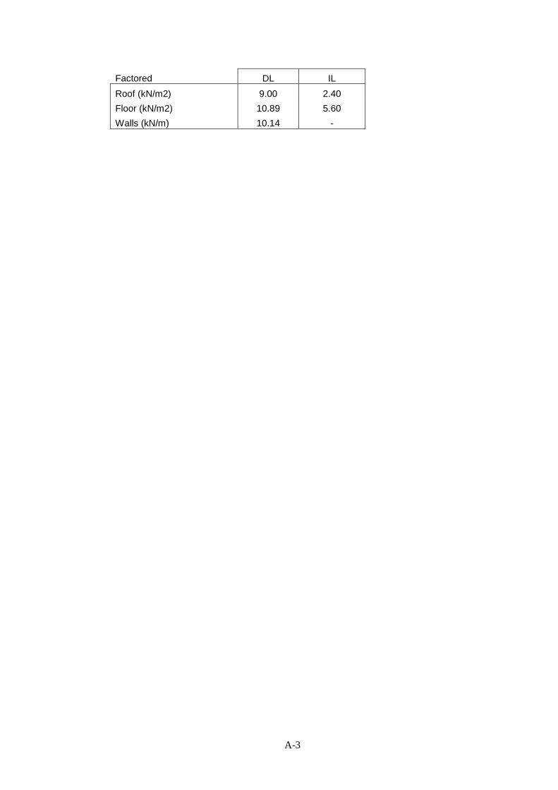
A-3

Factored DL IL

Roof (kN/m2) 9.00 2.40

Floor (kN/m2) 10.89 5.60

Walls (kN/m) 10.14 -

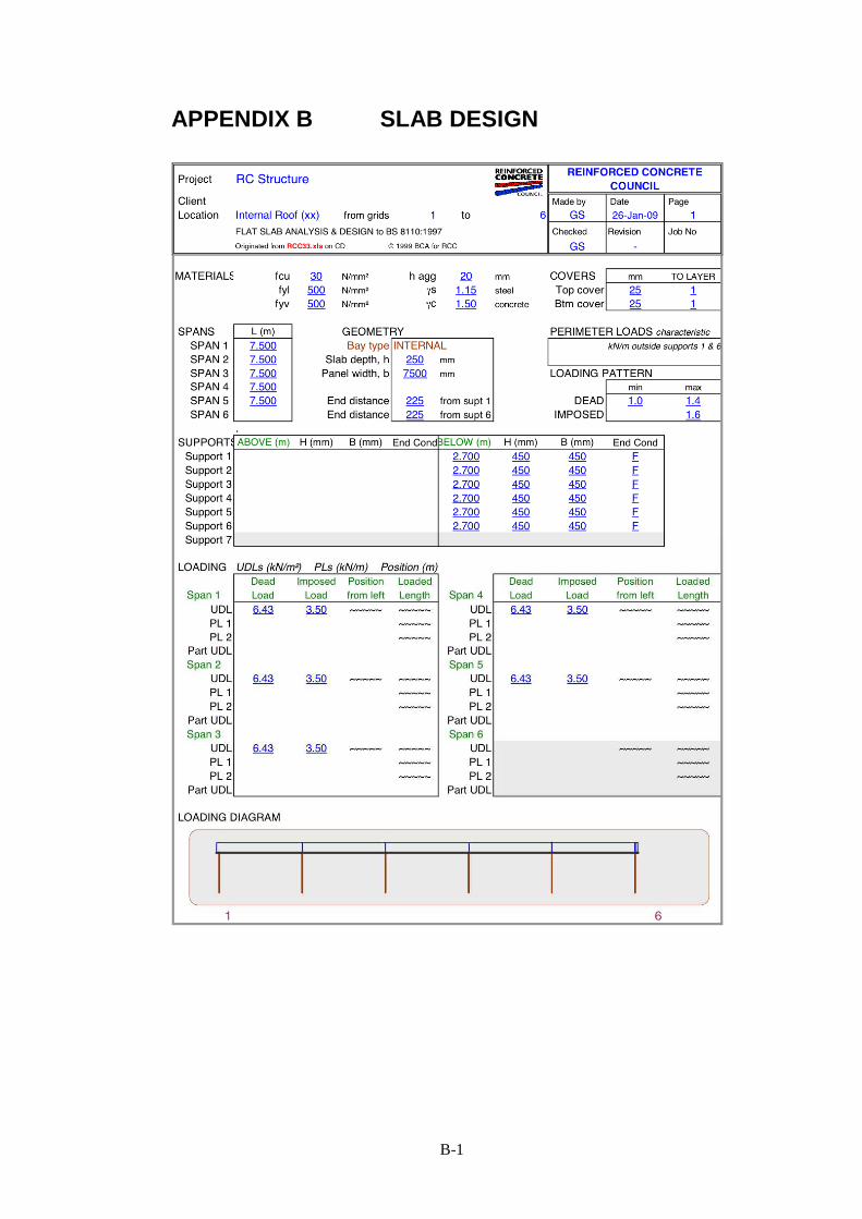
B-1

APPENDIX B SLAB DESIGN

B-2

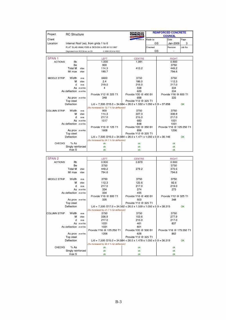
B-3

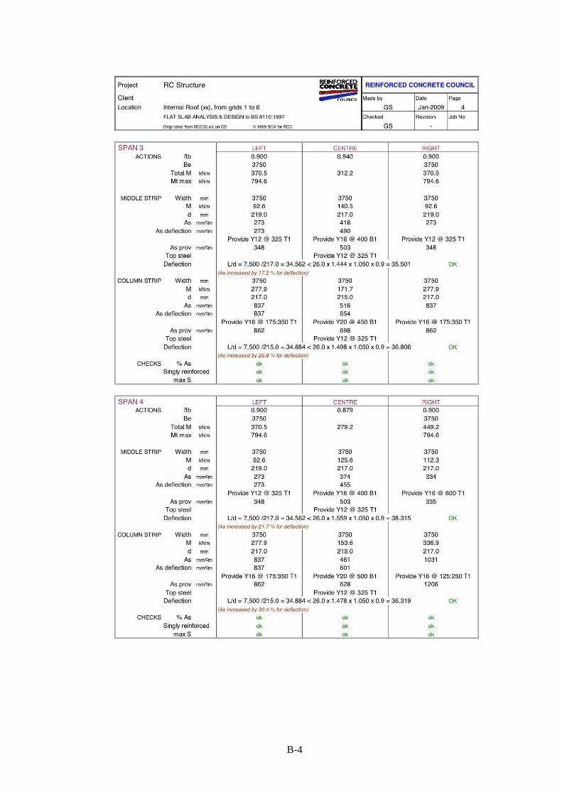
B-4

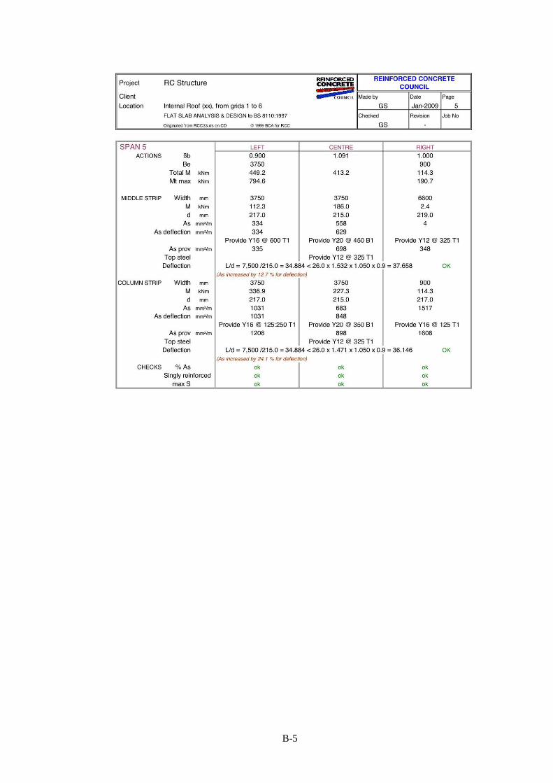
B-5

B-6

B-7

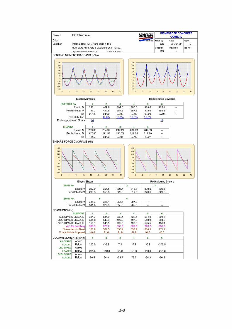
B-8

B-9

B-10

B-11

B-12

B-13

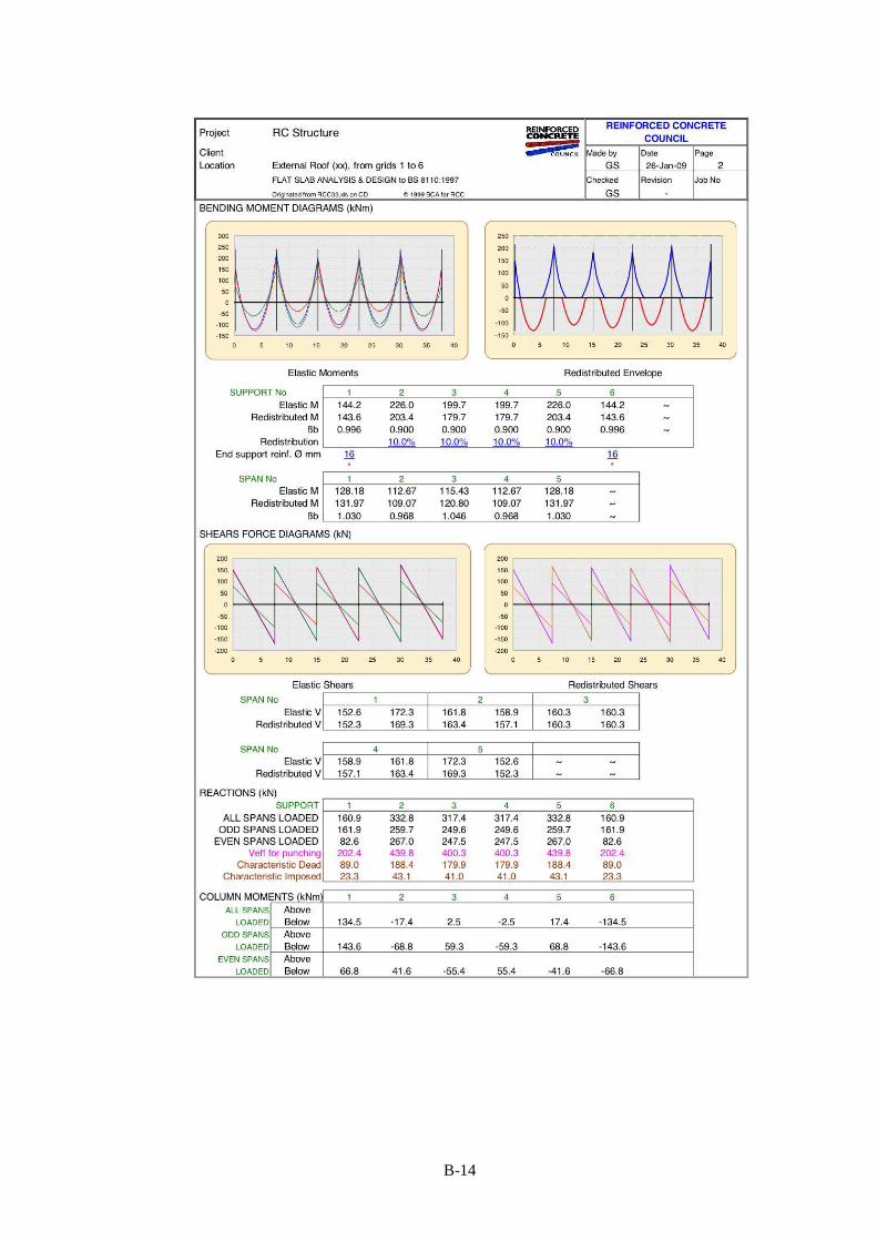
B-14

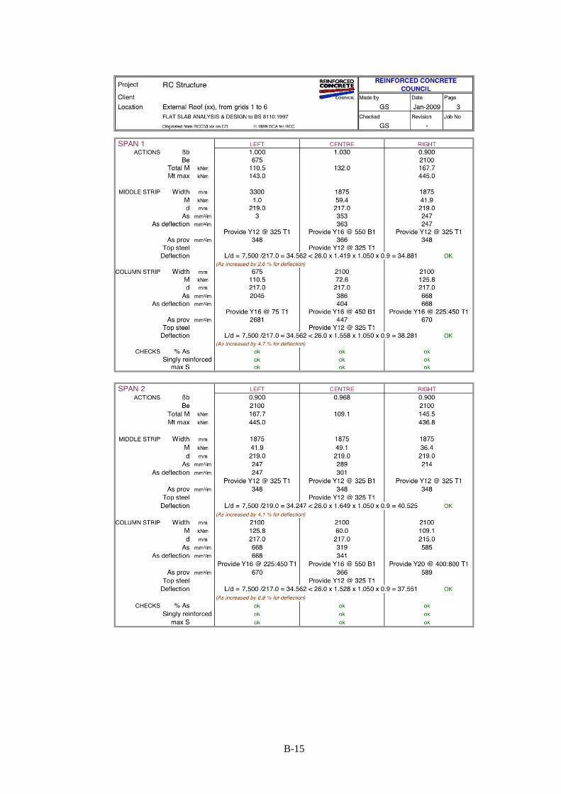
B-15

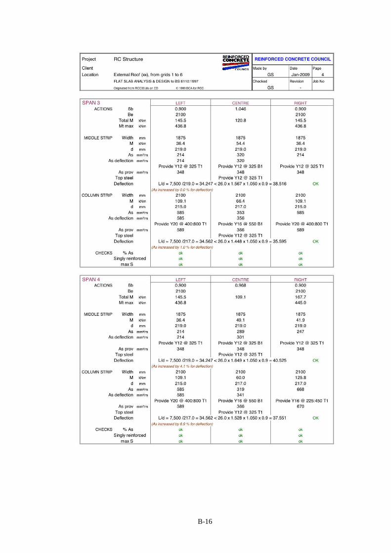
B-16

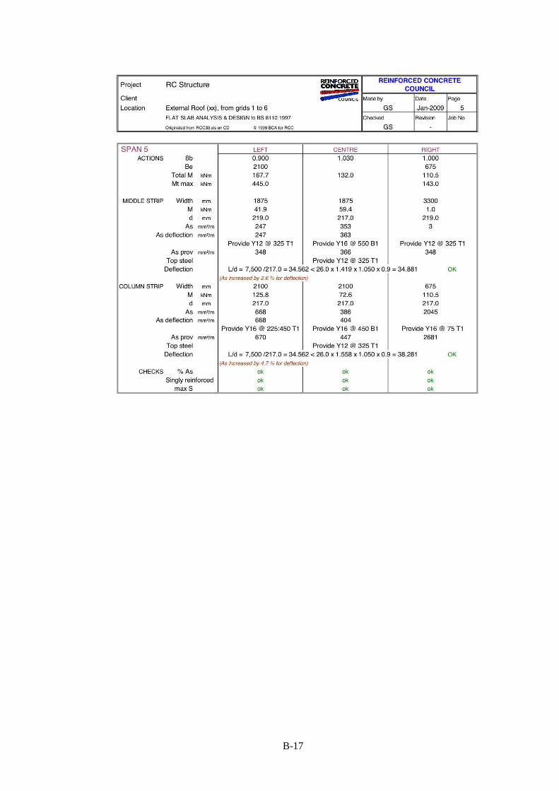
B-17

B-18

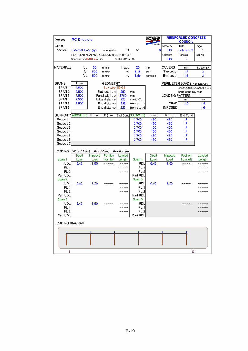
B-19

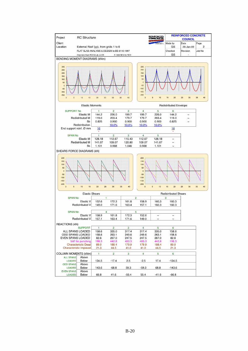
B-20

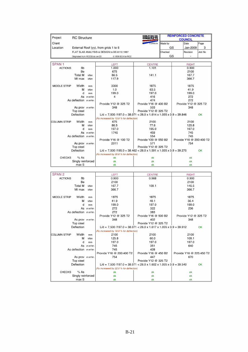
B-21

B-22

B-23

B-24

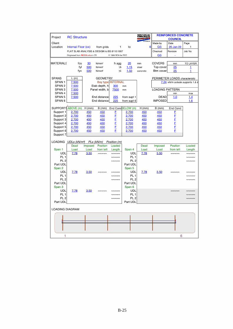
B-25

B-26

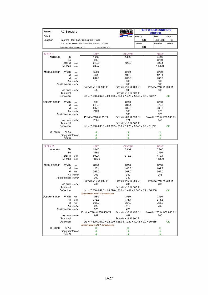
B-27

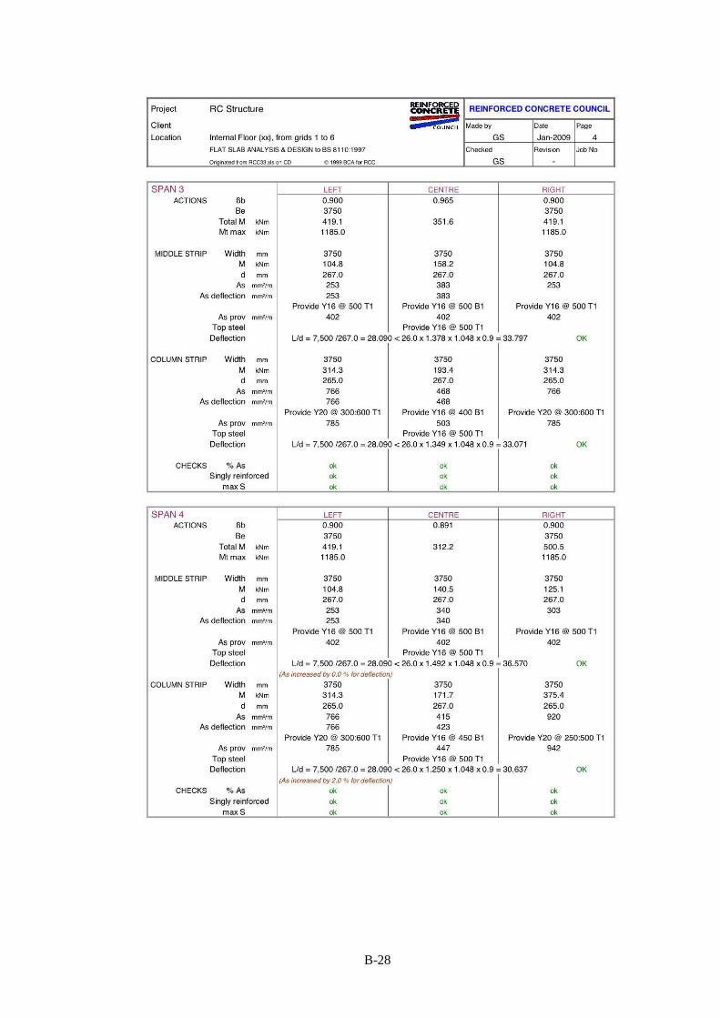
B-28

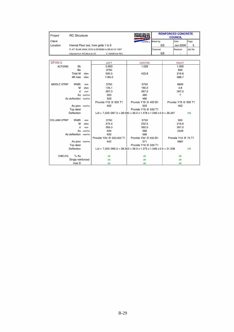
B-29

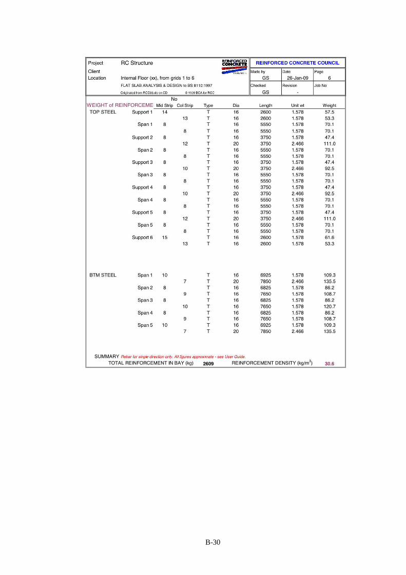
B-30

B-31

B-32

B-33

B-34

B-35

B-36

B-37

B-38

B-39

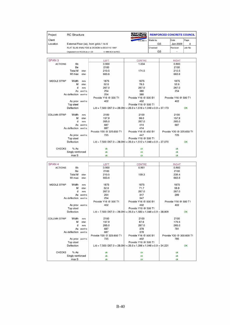
B-40

B-41

B-42

B-43

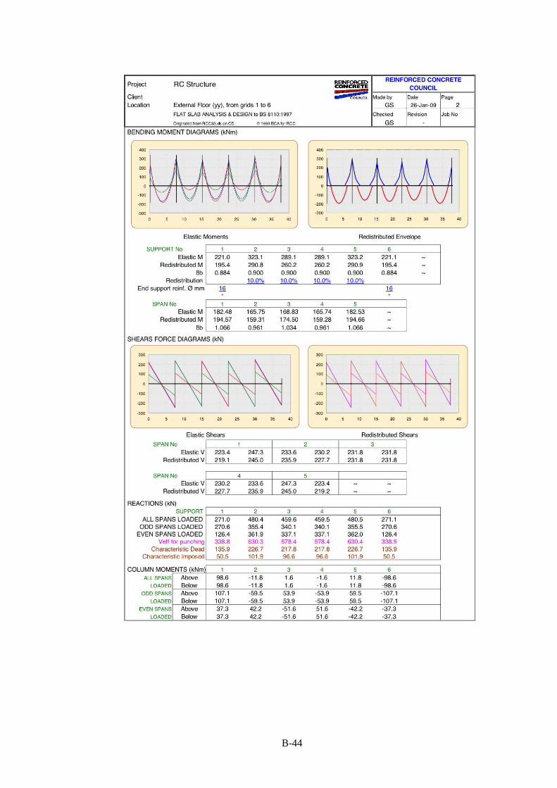
B-44

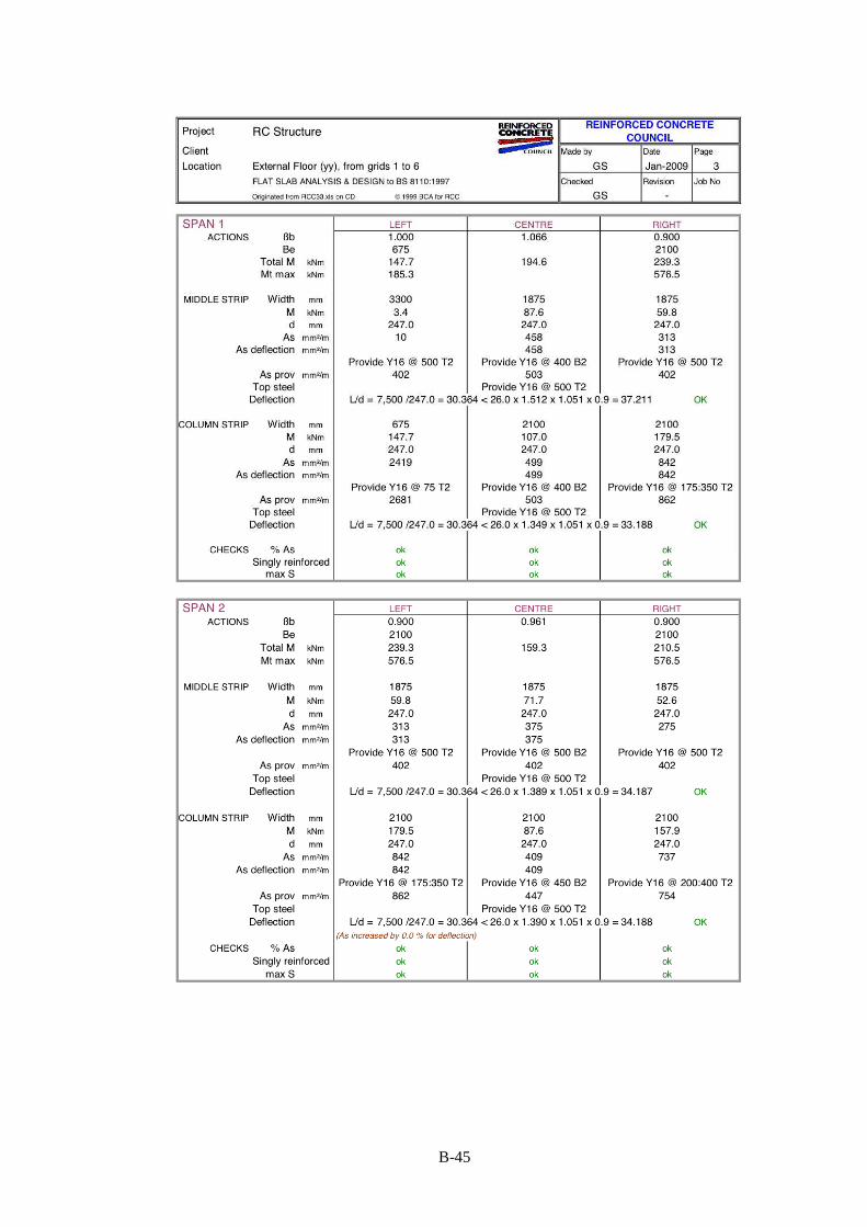
B-45

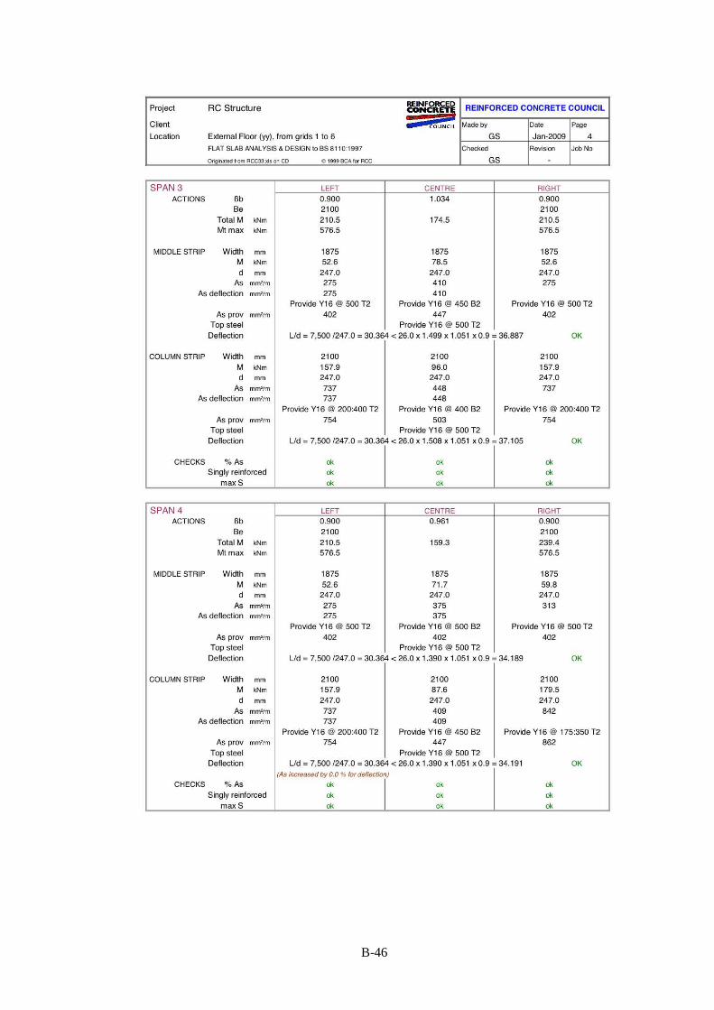
B-46

B-47

B-48

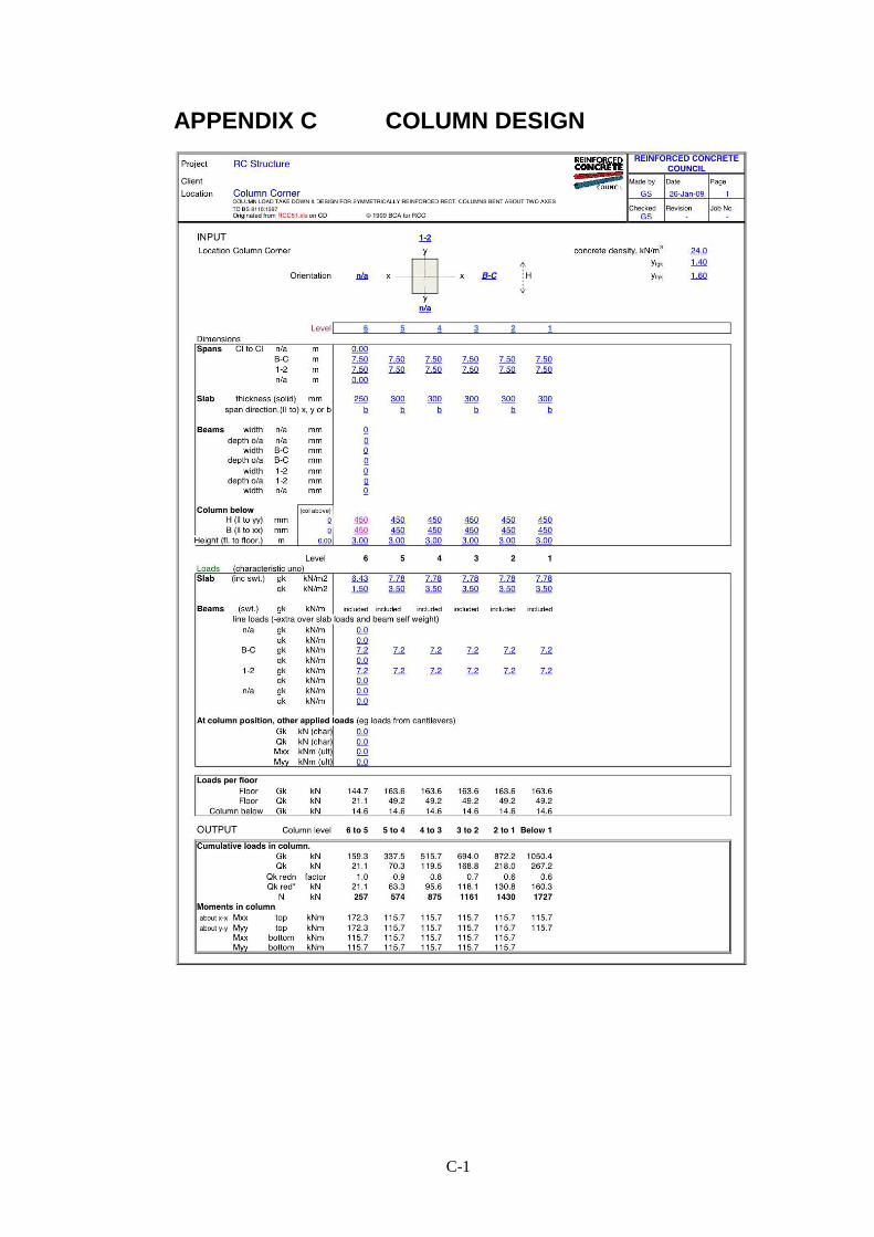
C-1

APPENDIX C COLUMN DESIGN

C-2

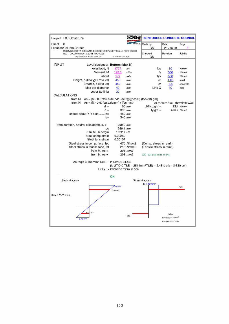
C-3

C-4

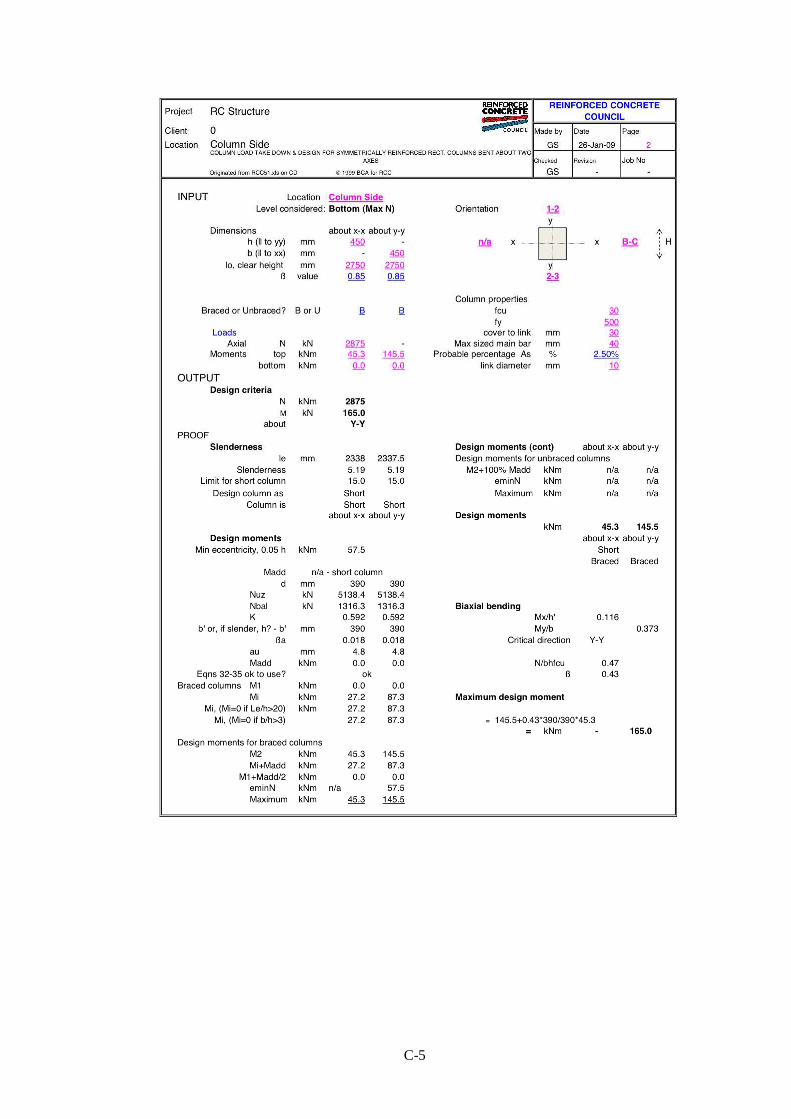
C-5

C-6

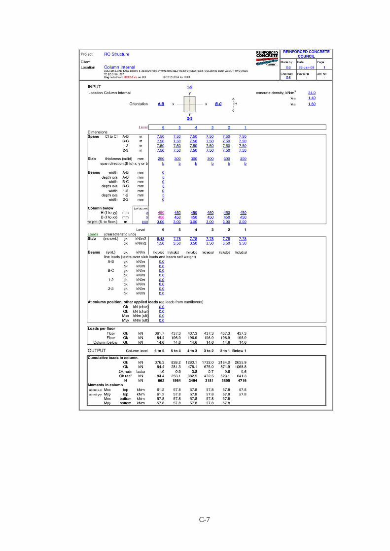
C-7

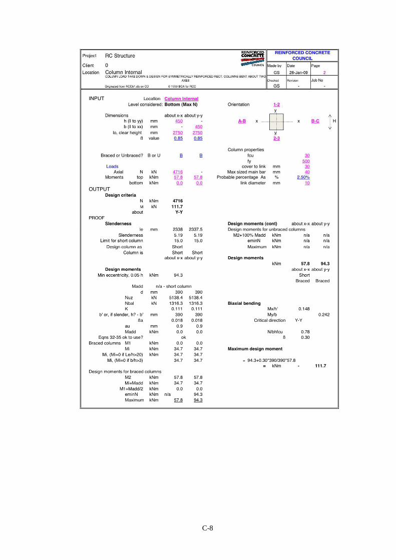
C-8

C-9

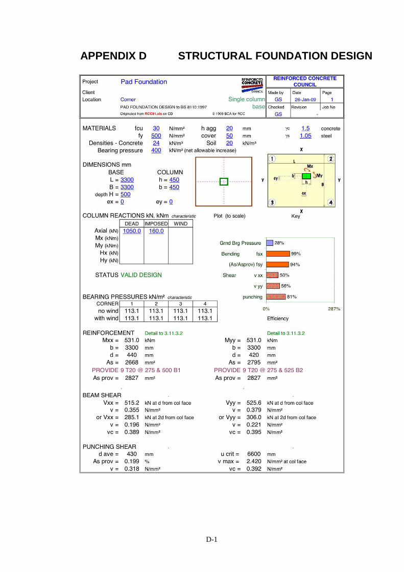
D-1

APPENDIX D STRUCTURAL FOUNDATION DESIGN

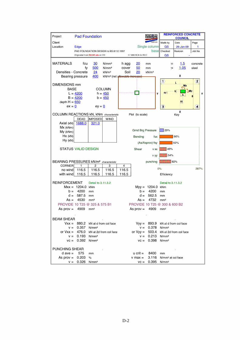
D-2

D-3

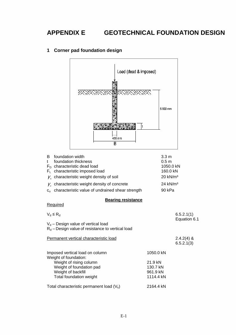
E-1

APPENDIX E GEOTECHNICAL FOUNDATION DESIGN

1 Corner pad foundation design

B foundation width 3.3 m t foundation thickness 0.5 m FD characteristic dead load 1050.0 kN FL characteristic imposed load 160.0 kN

sγ characteristic weight density of soil 20 kN/m³

cγ characteristic weight density of concrete 24 kN/m³

cu characteristic value of undrained shear strength 90 kPa

Bearing resistance Required Vd ≤ Rd 6.5.2.1(1)

Equation 6.1 Vd – Design value of vertical load

Rd – Design value of resistance to vertical load Permanent vertical characteristic load 2.4.2(4) &

6.5.2.1(3) Imposed vertical load on column 1050.0 kN Weight of foundation: Weight of rising column 21.9 kN Weight of foundation pad 130.7 kN Weight of backfill 961.9 kN Total foundation weight 1114.4 kN Total characteristic permanent load (Vk) 2164.4 kN

E-2

Variable vertical characteristic load Total characteristic variable load (VL) 160 kN Design approach 1 2.4.7.3.4.2

Analytical method 6.5.2.2

Annex D3 Undrained conditions R/A = (π +2) cusc + q Equation D1 Shape factor Square footing, sc = 1.2 Area of footing Pad 3.3 m x 3.3 m, A = 10.89 m² Bearing resistance R = 10.89 [(π + 2)1.2cu + q] Combination 1: A1, M1 and R1 2.4.7.3.4.2 Design load (A1) Vd1 = γ G x Vk + γ Q x VL Table A3 Vd1 = 1.35 x 2164.4 + 1.50 x 160 Vd1 = 3162.0 kN Design strength (M1) Table A4 Cud1 = cuk /γ cu Cud1 = 90 / 1.0 Cud1 = 90 kPa Soil surcharge, design value adjacent to footing (A1) Table A3 qd1 = qk xγ G qd1 = (5 x 20) x 1.0 qd1 = 100 kPa

Design bearing resistance (R1) Table A5 Rd1 = Rk /γ R;v Rd1 = Rk / 1.0 Rd1 = Rk Rd1 = 10.89 [(π + 2)1.2 x 90 + 100] Rd1 = 7136.1 kN Check Vd1 should be ≤ Rd1 3162.0 kN < 7136.1 kN

E-3

Footing acceptable for design approach 1, combination 1 Combination 2: A2, M2 and R1 2.4.7.3.4.2 Design load (A2) Vd2 = γ G x Vk + γ Q x VL Table A3 Vd2 = 1.0 x 2164.4 + 1.3 x 160 Vd2 = 2372.4 kN Design strength (M2) Table A4 Cud2 = cuk /γ cu Cud2 = 90 / 1.4 Cud2 = 64.3 kPa Soil surcharge, design value adjacent to footing (A2) Table A3 qd2 = qk xγ G qd2 = (5 x 20) x 1.0 qd2 = 100 kPa

Design bearing resistance (R1) Table A5 Rd2 = Rk /γ R;v Rd2 = Rk / 1.0 Rd2 = Rk Rd2 = 10.89 [(π + 2)1.2 x 64.3 + 100] Rd2 = 5408.4 kN Check Vd2 should be ≤ Rd2 2372.4 kN < 5408.4 kN Footing acceptable for design approach 1, combination 2

Settlement

Settlement using Vk ≤ Rk / 3 Vk + VL = 2324.4 kN Bearing capacity Rd1 unfactored

γ R;v = 1.0 (bearing resistance) γ G = 1.0 (surcharge) γ cu = 1.0 shear strength) Rk = Rd1 Rk = 7136.1 kN

Check Rk / (Vk + VL)= 7136.1/2324.4 = 3.07 (>3) Footing acceptable for settlement

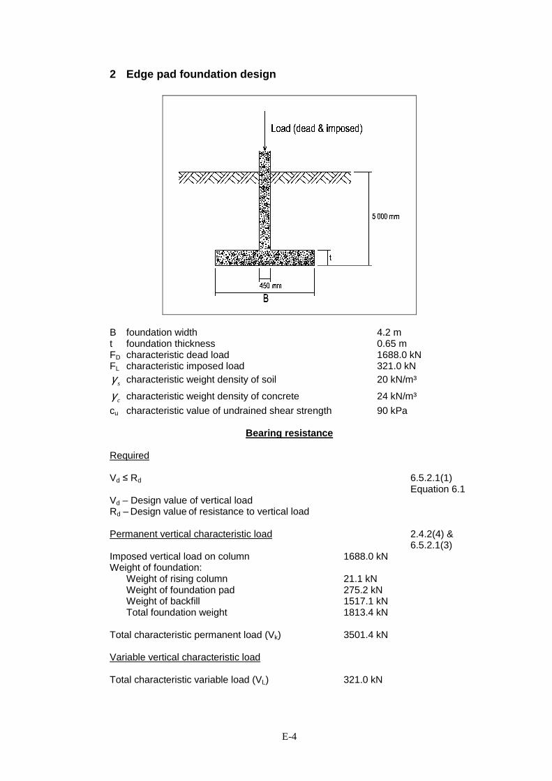
E-4

2 Edge pad foundation design

B foundation width 4.2 m t foundation thickness 0.65 m FD characteristic dead load 1688.0 kN FL characteristic imposed load 321.0 kN

sγ characteristic weight density of soil 20 kN/m³

cγ characteristic weight density of concrete 24 kN/m³

cu characteristic value of undrained shear strength 90 kPa

Bearing resistance

Required Vd ≤ Rd 6.5.2.1(1)

Equation 6.1 Vd – Design value of vertical load

Rd – Design value of resistance to vertical load Permanent vertical characteristic load 2.4.2(4) &

6.5.2.1(3) Imposed vertical load on column 1688.0 kN Weight of foundation: Weight of rising column 21.1 kN Weight of foundation pad 275.2 kN Weight of backfill 1517.1 kN Total foundation weight 1813.4 kN Total characteristic permanent load (Vk) 3501.4 kN Variable vertical characteristic load Total characteristic variable load (VL) 321.0 kN

E-5

Design approach 1 2.4.7.3.4.2 Analytical method 6.5.2.2

Annex D3 Undrained conditions R/A = (π +2) cusc + q Equation D1 Shape factor Square footing, sc = 1.2 Area of footing Pad 4.2 m x 4.2 m, A = 17.64 m² Bearing resistance R = 17.64 [(π + 2)1.2cu + q] Combination 1: A1, M1 and R1 2.4.7.3.4.2 Design load (A1) Vd1 = γ G x Vk + γ Q x VL Table A3 Vd1 = 1.35 x 3501.4 + 1.50 x 321 Vd1 = 5208.4 kN Design strength (M1) Table A4 Cud1 = cuk /γ cu Cud1 = 90 / 1.0 Cud1 = 90 kPa Soil surcharge, design value adjacent to footing (A1) Table A3 qd1 = qk xγ G qd1 = (5 x 20) x 1.0 qd1 = 100 kPa

Design bearing resistance (R1) Table A5 Rd1 = Rk /γ R;v Rd1 = Rk / 1.0 Rd1 = Rk Rd1 = 17.64 [(π + 2)1.2 x 90 + 100] Rd1 = 11559.4 kN Check Vd1 should be ≤ Rd1 5208.4 kN < 11559.4 kN Footing acceptable for design approach 1, combination 1 Combination 2: A2, M2 and R1 2.4.7.3.4.2

E-6

Design load (A2) Vd2 = γ G x Vk + γ Q x VL Table A3 Vd2 = 1.0 x 3501.4 + 1.3 x 321 Vd2 = 3918.7 kN Design strength (M2) Table A4 Cud2 = cuk /γ cu Cud2 = 90 / 1.4 Cud2 = 64.3 kPa Soil surcharge, design value adjacent to footing (A2) Table A3 qd2 = qk xγ G qd2 = (5 x 20) x 1.0 qd2 = 100 kPa

Design bearing resistance (R1) Table A5 Rd2 = Rk /γ R;v Rd2 = Rk / 1.0 Rd2 = Rk Rd2 = 17.64 [(π + 2)1.2 x 64.3 + 100] Rd2 = 8760.7 kN Check Vd2 should be ≤ Rd2 3918.7 kN < 8760.7 kN Footing acceptable for design approach 1, combination 2

Settlement

Settlement using Vk ≤ Rk / 3 Vk + VL = 38224 kN Bearing capacity Rd1 unfactored

γ R;v = 1.0 (bearing resistance) γ G = 1.0 (surcharge) γ cu = 1.0 shear strength) Rk = Rd1 Rk = 11559.4 kN

Check Rk / (Vk + VL)= 3822.4/11559.4 = 3.02 (>3) Footing acceptable for settlement

E-7

3 Internal pad foundation design

B foundation width 5.4 m t foundation thickness 0.85 m FD characteristic dead load 2636.0 kN FL characteristic imposed load 641.0 kN

sγ characteristic weight density of soil 20 kN/m³

cγ characteristic weight density of concrete 24 kN/m³

cu characteristic value of undrained shear strength 90 kPa

Bearing resistance Required Vd ≤ Rd 6.5.2.1(1)

Equation 6.1 Vd – Design value of vertical load

Rd – Design value of resistance to vertical load Permanent vertical characteristic load 2.4.2(4) &

6.5.2.1(3) Imposed vertical load on column 2636.0 kN Weight of foundation: Weight of rising column 20.2 kN Weight of foundation pad 594.9 kN Weight of backfill 2403.5 kN Total foundation weight 3018.5 kN Total characteristic permanent load (Vk) 5654.5 kN

E-8

Variable vertical characteristic load Total characteristic variable load (VL) 641.0 kN Design approach 1 2.4.7.3.4.2 Analytical method 6.5.2.2

Annex D3 Undrained conditions R/A = (π +2) cusc + q Equation D1 Shape factor Square footing, sc = 1.2 Area of footing Pad 5.4 m x 5.4 m, A = 29.16 m² Bearing resistance R = 29.16 [(π + 2)1.2cu + q] Combination 1: A1, M1 and R1 2.4.7.3.4.2 Design load (A1) Vd1 = γ G x Vk + γ Q x VL Table A3 Vd1 = 1.35 x 5654.5 + 1.50 x 641.0 Vd1 = 8595.1 kN Design strength (M1) Table A4 Cud1 = cuk /γ cu Cud1 = 90 / 1.0 Cud1 = 90 kPa Soil surcharge, design value adjacent to footing (A1) Table A3 qd1 = qk xγ G qd1 = (5 x 20) x 1.0 qd1 = 100 kPa

Design bearing resistance (R1) Table A5 Rd1 = Rk /γ R;v Rd1 = Rk / 1.0 Rd1 = Rk Rd1 = 29.16 [(π + 2)1.2 x 90 + 100] Rd1 = 19108.3 kN Check Vd1 should be ≤ Rd1 8595.1 kN < 19108.3 kN

E-9

Footing acceptable for design approach 1, combination 1 Combination 2: A2, M2 and R1 2.4.7.3.4.2 Design load (A2) Vd2 = γ G x Vk + γ Q x VL Table A3 Vd2 = 1.0 x 5654.5 + 1.3 x 641 Vd2 = 6487.8 kN Design strength (M2) Table A4 Cud2 = cuk /γ cu Cud2 = 90 / 1.4 Cud2 = 64.3 kPa Soil surcharge, design value adjacent to footing (A2) Table A3 qd2 = qk xγ G qd2 = (5 x 20) x 1.0 qd2 = 100 kPa

Design bearing resistance (R1) Table A5 Rd2 = Rk /γ R;v Rd2 = Rk / 1.0 Rd2 = Rk Rd2 = 29.16 [(π + 2)1.2 x 64.3 + 100] Rd2 = 14481.9 kN Check Vd2 should be ≤ Rd2 6487.8 kN < 14481.9 kN Footing acceptable for design approach 1, combination 2

Settlement

Settlement using Vk ≤ Rk / 3 Vk + VL = 6295.5 kN Bearing capacity Rd1 unfactored

γ R;v = 1.0 (bearing resistance) γ G = 1.0 (surcharge) γ cu = 1.0 shear strength) Rk = Rd1 Rk = 19108.3 kN

Check Rk / (Vk + VL)= 6295.5/19108.3 = 3.04 (>3) Footing acceptable for settlement