arX

iv:a

stro

-ph/

0209

241v

1 1

2 Se

p 20

02

ABS Methods and ABSPACK for Linear Systems andOptimization, a Review

Emilio Spedicato, Elena Bodon, Antonino Del PopoloDepartment of Mathematics, University of Bergamo, Bergamo

Nezam Mahdavi-Amiri,Department of Mathematics, Sharif University, Tehran

Address of person to whom send the proofs: Emilio Spedicato, Department of Math-ematics, University of Bergamo, via dei Caniana 2, 24128 Bergamo, emilio@unibg.it

Running title: A review of ABS methods

1

Abstract

ABS methods are a large class of methods, based upon the Egervary rankreducing algebraic process, first introduced in 1984 by Abaffy, Broyden andSpedicato for solving linear algebraic systems, and later extended to nonlin-ear algebraic equations, to optimization problems and other fields; softwarebased upon ABS methods is now under development. Current ABS literatureconsists of about 400 papers. ABS methods provide a unification of severalclasses of classical algorithms and more efficient new solvers for a number ofproblems. In this paper we review ABS methods for linear systems and opti-mization, from both the point of view of theory and the numerical performanceof ABSPACK.

Key Words ABS methods, linear algebraic systems, feasible directionmethods, simplex method, Diophantine equations, ABSPACK.

AMS classification 15A03, 15A06, 65F05, 65F30

1 Introduction

ABS algorithms were introduced by Abaffy, Broyden and Spedicato (1984), to solvelinear equations first in the form of the basic ABS class, later generalized as the scaledABS class. They were then applied to linear least squares, nonlinear equations andoptimization problems, see e.g. the monographs by Abaffy and Spedicato (1989)and Feng et al. (1998), or the bibliography by Spedicato et al. (2000) listing 350ABS papers. In this paper we review some of the main results obtained in the fieldof ABS methods and we provide some results on the performance of ABSPACK, aFORTRAN package based on ABS methods presently under development.

The main results obtained in almost twenty years of research in the ABS fieldcan be summarized as follows:

• ABS methods provide a unification of the field of finitely terminating methodsfor linear systems and for feasible direction methods for linearly constrainedoptimization, see sections 2 and 6; due to the several alternative formulationsof their algebra they lead to different computational implementations of thealgorithms, each one with a special feature that may be of advantage

• ABS methods provide some new methods that are better than classical onesunder several respects. For instance the implicit LX method requires the samenumber of multiplications as Gaussian elimination (which is optimal undervery general conditions) but requires less memory and does not need pivotingin general; moreover its application to the simplex method has not only a lowermemory requirement, but is cheaper in multiplications up to one order withrespect to e.g. the Forrest-Goldfarb implementation of the simplex method via

2

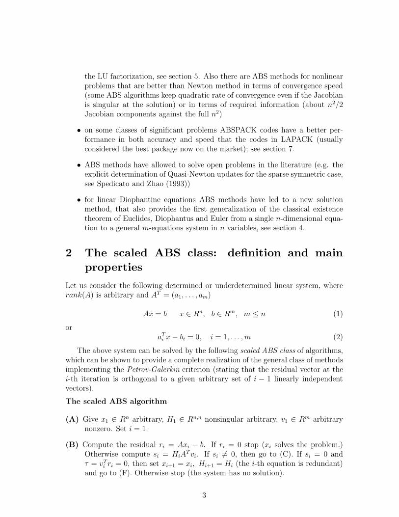
the LU factorization, see section 5. Also there are ABS methods for nonlinearproblems that are better than Newton method in terms of convergence speed(some ABS algorithms keep quadratic rate of convergence even if the Jacobianis singular at the solution) or in terms of required information (about n2/2Jacobian components against the full n2)

• on some classes of significant problems ABSPACK codes have a better per-formance in both accuracy and speed that the codes in LAPACK (usuallyconsidered the best package now on the market); see section 7.

• ABS methods have allowed to solve open problems in the literature (e.g. theexplicit determination of Quasi-Newton updates for the sparse symmetric case,see Spedicato and Zhao (1993))

• for linear Diophantine equations ABS methods have led to a new solutionmethod, that also provides the first generalization of the classical existencetheorem of Euclides, Diophantus and Euler from a single n-dimensional equa-tion to a general m-equations system in n variables, see section 4.

2 The scaled ABS class: definition and main

properties

Let us consider the following determined or underdetermined linear system, whererank(A) is arbitrary and AT = (a1, . . . , am)

Ax = b x ∈ Rn, b ∈ Rm, m ≤ n (1)

oraT

i x − bi = 0, i = 1, . . . , m (2)

The above system can be solved by the following scaled ABS class of algorithms,which can be shown to provide a complete realization of the general class of methodsimplementing the Petrov-Galerkin criterion (stating that the residual vector at thei-th iteration is orthogonal to a given arbitrary set of i − 1 linearly independentvectors).

The scaled ABS algorithm

(A) Give x1 ∈ Rn arbitrary, H1 ∈ Rn,n nonsingular arbitrary, v1 ∈ Rm arbitrarynonzero. Set i = 1.

(B) Compute the residual ri = Axi − b. If ri = 0 stop (xi solves the problem.)Otherwise compute si = HiA

T vi. If si 6= 0, then go to (C). If si = 0 andτ = vT

i ri = 0, then set xi+1 = xi, Hi+1 = Hi (the i-th equation is redundant)and go to (F). Otherwise stop (the system has no solution).

3

(C) Compute the search vector pi by

pi = HTi zi (3)

where zi ∈ Rn is arbitrary save for the condition

vTi AHT

i zi 6= 0 (4)

(D) Update the estimate of the solution by

xi+1 = xi − αipi, αi = vTi ri/v

Ti Api. (5)

(E) Update the matrix Hi by

Hi+1 = Hi − HiAT viw

Ti Hi/w

Ti HiA

T vi (6)

where wi ∈ Rn is arbitrary save for the condition

wTi HiA

T vi 6= 0. (7)

(F) If i = m, stop (xm+1 solves the system). Otherwise give vi+1 ∈ Rm arbitrarylinearly independent from v1, . . . , vi. Increment i by one and go to (B).

Matrices Hi, which are generalizations of (oblique) projection matrices, have beennamed Abaffians at the First International Conference on ABS methods (Luoyang,China, 1991). However we must recall that these matrices were used in several littleknown papers by Egervary, predating the ABS algorithms. There are alternativeformulations of the scaled ABS algorithms, e.g. using vectors instead of the squarematrix Hi, with possible advantages in storage and number of operations. For detailssee Abaffy and Spedicato (1989) and on how these formulations can be used to imbedin an ABS approach even iterative methods (including the Kaczmarz, Gauss-Seidel,ORTHOMIN, ORTHODIR etc. methods), see Spedicato and Li (2000).

The choice of the parameters H1, vi, , zi, wi determines particular methods.The basic ABS class is obtained by taking vi = ei, as the i-th unit vector in Rm.

We recall some properties of the scaled ABS class, assuming that A has full rank.

• Define Vi = (v1, . . . , vi) and Wi = (w1, . . . , wi). Then

Hi+1AT Vi = 0, HT

i+1Wi = 0 (8)

.

• The vectors HiAT vi, HT

i wi are zero if and only if ai, wi are respectively linearlydependent from a1, . . . , ai−1, w1, . . . , wi−1.

4

• Define Pi = (p1, . . . , pi) and Ai = (a1, . . . , ai). Then the implicit factorizationV T

i ATi Pi = Li holds, where Li is nonsingular lower triangular. Hence, if m = n,

one obtains a semiexplicit factorization of the inverse, with P = Pn, V =Vn, L = Ln

A−1 = PL−1V T . (9)

For several choices of V the matrix L is diagonal, hence formula (8) gives afully explicit factorization of the inverse as a byproduct of the ABS solutionof a linear system.

• The general solution of system (1) can be written as follows, with q ∈ Rn

arbitraryx = xm+1 + HT

m+1q (10)

• The Abaffian can be written in terms of the parameter matrices as

Hi+1 = H1 − H1AT Vi(W

Ti H1A

T Vi)−1W T

i H1. (11)

Letting V = Vm, W = Wm, one can show that the parameter matrices H1, V, W areadmissible (i.e. condition (7) is satisfied) iff the matrix Q = V T AHT

1 W is stronglynonsingular (i.e. it is LU factorizable). This condition can be satisfied by exchangesof the columns of V or W . If Q is strongly nonsingular and we take, as is done in allalgorithms so far considered, zi = wi, then condition (4) is also satisfied. Analysisof the conditions under which Q is not strongly nonsingular leads, when dealingwith Krylov space methods in their ABS formulation, to a characterization of thetopology of the starting points that can produce a breakdown (either a division byzero or a vanishing search direction) and to several ways of curing it, including thoseconsidered in the literature.

Three subclasses of the scaled ABS class and particular algorithms are nowrecalled.

(a) The conjugate direction subclass. This class is obtained by setting vi = pi. Itis well defined under the condition (sufficient but not necessary) that A issymmetric and positive definite. It contains the ABS versions of the Choleski,the Hestenes-Stiefel and the Lanczos algorithms. This class generates all pos-sible algorithms whose search directions are A-conjugate. If x1 = 0, the vec-tor xi+1 minimizes the energy (A-weighted Euclidean) norm of the error overSpan(p1, . . . , pi) and the solution is approached monotonically from below inthe energy norm.

(b) The orthogonally scaled subclass. This class is obtained by setting vi = Api.It is well defined if A has full column rank and remains well defined even ifm is greater than n. It contains the ABS formulation of the QR algorithm(the so called implicit QR algorithm), the GMRES and the conjugate residual

5

algorithms. The scaling vectors are orthogonal and the search vectors are AT A-conjugate. If x1 = 0, the vector xi+1 minimizes the Euclidean norm of theresidual over Span(p1, . . . , pi) and the solution is monotonically approachedfrom below in the residual norm. It can be shown that the methods in thisclass can be applied to overdetermined systems of m > n equations, where inn steps they obtain the solution in the least squares sense.

(c) The optimally stable subclass. This class is obtained by setting vi = (A−1)T pi,the inverse disappearing in the actual recursions. The search vectors in thisclass are orthogonal. If x1 = 0, then the vector xi+1 is the vector of leastEuclidean norm over Span(p1, . . . , pi) and the solution is approached mono-tonically from below in the Euclidean norm. The methods of Gram-Schmidtand of Craig belong to this subclass. The methods in this class have minimumerror growth in the approximation to the solution according to a criterion byBroyden.

3 Special algorithms in the basic ABS class

In this section we consider in more detail three specially important algorithms, thatbelong to the basic ABS class (i.e. V = I).

(A) The Huang algorithm is obtained by the choices H1 = I, zi = wi = ai. Amathematically equivalent, but numerically more stable, formulation is the socalled modified Huang algorithm (pi = Hi(Hiai) and Hi+1 = Hi − pip

Ti /pT

i pi).Huang algorithm generates search vectors that are orthogonal and identicalwith those obtained by the Gram-Schmidt procedure applied to the rows ofA. If x1 = 0, then xi+1 is the solution with least Euclidean norm of the first iequations. The solution x+ with least Euclidean norm of the whole system isapproached monotonically and from below by the sequence xi. For arbitrarystarting point the Huang algorithm generates that solution which is closest inEuclidean norm to the initial point.

(B) The implicit LU algorithm is given by the choices H1 = I, zi = wi = ei. Itis well defined iff A is regular (i.e. all principal submatrices are nonsingu-lar). Otherwise column pivoting has to be performed (or, if m = n, equationpivoting). The Abaffian has the following structure, with Ki ∈ Rn−i,i

Hi+1 =

0 0· · · · · ·0 0Ki In−i

. (12)

implying that the matrix Pi is unit upper triangular, so that the implicit fac-torization A = LP−1 is of the LU type, with units on the diagonal. The

6

algorithm requires for m = n, n3/3 multiplications plus lower order terms,the same cost of classical LU factorization or Gaussian elimination. Storagerequirement for Ki requires at most n2/4 positions, i.e. half the storage neededby Gaussian elimination and a fourth that needed by the LU factorization algo-rithm (assuming that A is not overwritten). Hence the implicit LU algorithmhas same arithmetic cost but uses less memory than the most efficient classicalmethods.

(C) The implicit LX algorithm, see Spedicato, Xia and Zhang (1997), is definedby the choices H1 = I, zi = wi = eki

, where ki is an integer, 1 ≤ ki ≤ n,such that eT

kiHiai 6= 0. By a general property of the ABS class for A with full

rank there is at least one index ki such that eTki

Hiai 6= 0. For stability reasonswe select ki such that | eT

kiHiai | is maximized. This algorithm has the same

overhead and memory requirement as the implicit LU algorithm, but does notrequire pivoting. Its computational performance is also superior and generallybetter than the performance of the classical LU factorization algorithm withrow pivoting, as available for instance in LAPACK or MATLAB, see Mirnia(1996). Therefore this algorithm can be considered as the most efficient generalpurpose linear solver not of the Strassen type.

4 Solution of linear Diophantine equations

One of the main results in the ABS field has been the derivation of ABS methodsfor linear Diophantine equations. The ABS algorithm determines if the Diophan-tine system has an integer solution, computes a particular solution and provides arepresentation of all integer solutions. It is a generalization of a method proposedby Egervary (1955) for the particular case of a homogeneous system.

Let Z be the set of all integers and consider the Diophantine linear system ofequations

Ax = b, x ∈ Zn, A ∈ Zm×n, b ∈ Zm, m ≤ n. (13)

While thousands of papers have been written concerning nonlinear, usually poly-nomial, Diophantine equations in few variables, the general linear system has at-tracted much less attention. The single linear equation in n variables was first solvedby Bertrand and Betti (1850). Egervary was probably the first author dealing witha system (albeit only the homogeneous one). Several methods for the nonhomoge-neous system have recently been proposed based mainly on reduction to canonicalforms.

We recall some results from number theory. Let a and b be integers. If there isinteger γ so that b = γa then we say that a divides b and write a|b, otherwise wewrite a6 | b. If a1, . . . , an are integers, not all being zero, then the greatest commondivisor (gcd) of these numbers is the greatest positive integer δ which divides allai, i = 1, . . . , n and we write δ = gcd(a1, . . . , an). We note that δ ≥ 1 and that

7

δ can be written as an integer linear combination of the ai, i.e. δ = zT a for somez ∈ Rn. One can show that δ is the least positive integer for which the equationa1x1 + . . . + anxn = δ has an integer solution. Now δ plays a main role in thefollowing

Fundamental Theorem of the Linear Diophantine Equation

Let a1, . . . , an and b be integer numbers. Then the Diophantine linear equation a1x1+. . . + anxn = b has integer solutions if and only if gcd(a1, . . . , an)| b. In such a caseif n > 1 then there is an infinite number of integer solutions.

In order to find the general integer solution of the Diophantine equation a1x1 + . . .+anxn = b, the main step is to solve a1x1 + . . .+anxn = δ, where δ = gcd(a1, . . . , an),for a special integer solution. There exist several algorithms for this problem. Thebasic step is the computation of δ and z, often done using the algorithm of Rosser(1941), which avoids a too rapid growth of the intermediate integers, and whichterminates in polynomial time, as shown by Schrijver (1986). The scaled ABS algo-rithm can be applied to Diophantine equations via a special choice of its parameters,originating from the following considerations and Theorems.

Suppose xi is an integer vector. Since xi+1 = xi − αipi, then xi+1 is integerif αi and pi are integers. If vT

i Api|(vTi ri), then αi is an integer. If Hi and zi are

respectively an integer matrix and an integer vector, then pi = HTi zi is also an

integer vector. Assume Hi is an integer matrix. From (6), if vTi AHT

i wi divides allthe components of HiA

T vi, then Hi+1 is an integer matrix.Conditions for the existence of an integer solution and determination of all integer

solutions of the Diophantine system are given in the following theorems, generalizingthe Fundamental Theorem, see Esmaeili, Mahdavi-Amiri and Spedicato (2001a).

Theorem 1 Let A be full rank and suppose that the Diophantine system (13)is integer solvable. Consider the Abaffians generated by the scaled ABS algorithmwith the parameter choices: H1 is unimodular (i.e. both H1 and H−1

1 are integermatrices); for i = 1, . . . , m, wi is such that wT

i HiAT vi = δi, δi = gcd(HiA

T vi).Then the following properties are true:

(a) the Abaffians generated by the algorithm are well-defined and are integer matri-ces

(b) if y is a special integer solution of the first i equations, then any integer solutionx of such equations can be written as x = y +HT

i+1q for some integer vector q.

Theorem 2 Let A be full rank and consider the sequence of matrices Hi gen-erated by the scaled ABS algorithm with parameter choices as in Theorem 1. Let x1

in the scaled ABS algorithm be an arbitrary integer vector and let zi be such thatzT

i HiAT vi = gcd(HiA

T vi). Then system (13) has integer solutions iff gcd(HiAT vi)

divides vTi ri for i = 1, . . . , m.

8

From the above theorems we obtain the following scaled ABS algorithm for Dio-phantine equations.

The ABS Algorithm for Diophantine Linear Equations

(1) Choose x1 ∈ Zn, arbitrary, H1 ∈ Zn×n, arbitrary unimodular. Let i = 1.

(2) Compute τi = vTi ri and si = HiA

T vi.

(3) If (si = 0 and τi = 0) then let xi+1 = xi, Hi+1 = Hi, ri+1 = ri and go to step(5) (the ith equation is redundant). If (si = 0 and τi 6= 0) then Stop (the ithequation and hence the system is incompatible).

(4) {si 6= 0} Compute δi = gcd(si) and pi = HTi zi, where zi ∈ Zn is an arbitrary

integer vector satisfying zTi si = δi. If δi6 |τi then Stop (the system is integerly

inconsistent), else Compute αi = τi/δi, let xi+1 = xi − αipi and update Hi by

Hi+1 = Hi−HiA

T viwT

iHi

wT

iHiAT vi

where wi ∈ Rn is an arbitrary integer vector satisfying

wTi si = δi.

(5) If i = m then Stop (xm+1 is a solution) else let i = i + 1 and go to step (2).

It follows from Theorem 1 that if there exists a solution for the system (13), thenx = xm+1 + HT

m+1q, with arbitrary q ∈ Zn, provides all solutions of (13).Egervary’s algorithm for homogeneous Diophantine systems corresponds to the

choices H1 = I, x1 = 0 and wi = zi, for all i. Egervary claimed, without proof,that any set of n − m linearly independent rows of Hm+1 form an integer basisfor the general solution of the system. Esmaeili et al. (2001a) have shown by acounterexample that Egervary’s claim is not true in general; we have also providedan analysis of conditions under which m rows in Hm+1 can be eliminated.

One can show that by special choices of the scaling parameters and by an inessen-tial modification of the update of the Abaffian it is not necessary to solve in general2m single n-dimensional Diophantine equations (to determine zi, wi), but just onesingle Diophantine equation, at the last step.

The ABS algorithm for linear Diophantine systems has been extended also tosystems of m linear inequalities (m ≤ n), where it provides an almost explicit repre-sentation of all solutions, see Esmaeili, Mahdavi-Amiri and Spedicato (2001b). Theused technique allows, in the case of m ≤ n real inequalities to find a fully explicitrepresentation of all solutions, see Esmaeili, Mahdavi-Amiri and Spedicato (2000),thereby obtaining a generalization of formula (10). Finally, the ABS approach pro-vides a new way of computing, given an integer matrix, its integer null space and,under some conditions, an integer basis of it, see Esmaeili, Mahdavi-Amiri andSpedicato (2001c).

9

5 Reformulation of the simplex method via the

implicit LX method

The implicit LX algorithm has a natural application in reformulating the simplexmethod for the LP problem in standard form:

min cT x

subject toAx = b, x ≥ 0.

The suitability of the implicit LX algorithm derives from the fact that the al-gorithm, when started with x1 = 0, generates basic type vectors xi+1, which arevertices of the polytope defined by the constraints of the LP problem if the compo-nents not identically zero are nonnegative.

The basic step of the simplex method is moving from one vertex to anotheraccording to certain rules and reducing at each step the value of cT x. The directionof movement is obtained by solving a linear system, whose coefficient matrix AB,the basic matrix, is defined by m linearly independent columns of A, called the basiccolumns. This system is usually solved via the LU factorization method or alsovia the QR factorization method. The new vertex is associated with a new basicmatrix A′

B, obtained by substituting one of the columns of AB with a column ofthe matrix AN that comprises the columns of A not belonging to AB. One hasthen to solve a new system where just one column has been changed. If the LUfactorization method is used, then the most efficient way to recompute the modifiedfactors is the steepest edge method of Forrest and Goldfarb (1992), that requiresm2 multiplications. This implementation of the simplex method has the followingstorage requirement: m2 for the LU factors and mn for the matrix A, that has tobe kept to provide the columns needed for the exchanges.

The reformulation of the simplex method via the implicit LX method, see Zhangand Xia (1995) and Spedicato, Xia and Zhang (1997), exploits the fact that in theimplicit LX method the exchange of the j-th column in AB with the k-th columnin AN corresponds to exchanging previously chosen parameters zj = wj = ejB

with new parameters zk = wk = ekB. in terms of the implied modification of the

Abaffian this operation is a special case of a general rank-one modification of theparameter matrix W = (wk1

, . . . , wkm). The modified Abaffian can be efficiently

evaluated using a general formula of Zhang (1995), without explicit use of the k-thcolumn of AN . Moreover all information needed to build the search direction (thepolytope edge) and to implement the (implicit) column exchange is contained inthe Abaffian matrix. Thus there is no need to keep the matrix A. Hence storagerequirement is only that needed in the construction and keeping of the matrix Hm+1,i.e. respectively n2/4 and n(n−m). For m close to n, such storage is about 8 timesless than in the Forrest and Goldfarb implementation of the LU method. For small m

10

storage is higher, but there is an alternative formulation of the implicit LX methodthat has a similar storage, see Spedicato and Xia (1999).

We now give the main formulas for the simplex method in the classical and inthe ABS formulation. The column in AN that substitutes a column in AB is usuallytaken as the column with least relative cost. In the ABS approach this correspondsto minimize with respect to i ∈ Nm the scalar ηi = cT HT ei. Let N∗ be the indexso chosen. The column in AB to be exchanged is often chosen with the criterionof the least edge displacement that keeps the basic variables nonnegative. Definingωi = xT ei/e

Ti HT eN∗ with x the current vertex, the above criterion is equivalent to

minimize ωi with respect to the set of indices i ∈ Bm such that

eTi HT eN∗ > 0 (14)

Notice that HT eN∗ 6= 0 and that an index i such that (14) be satisfied always exists,unless x is a solution.

The update of the Abaffian after the exchange of the obtained unit vectors isgiven by the following simple rank-one correction

H ′ = H − (HeB∗ − eB∗)e TN∗H/e T

N∗HeB∗ (15)

The displacement vector d, classically obtained by solving system ABd = −AeN∗ , isobtained at no cost by d = H T

m+1eN∗ . The relative cost vector, classically given byr = c−AT A−1

B cB, with cB comprising the components of c with indices correspondingto those of the basic columns, is given by formula r = Hm+1c.

It is easily seen that update (15) requires no more than m(n−m) multiplications.Cost is highest for m = n/2 and gets smaller as m gets smaller or closer to n. In themethod of Forrest and Goldfarb m2 multiplications are needed to update the LUfactors and again m2 to solve the system. Hence the ABS approach via formula (15)is faster for m > n/3. For m < n/3 similar costs are obtained using the alternativeformulation of the implicit LX algorithm described in Spedicato and Xia (1999). Form very close to n the advantage of the ABS formulation is essentially of one orderand such that no need is seen to develop formulas for the sparse case.

There is an ABS generalization of the simplex method based upon a modificationof the Huang algorithm which is started by a certain singular matrix, see Zhang(1997). In such generalization the solution is approached via a sequence of pointslying on the faces of the polytope. If one of such points happens to be a vertex, thenall successive iterates are vertices and the standard simplex method is reobtained.

6 ABS unification of feasible direction methods

for linearly constrained minimization

ABS methods allow a unification of feasible direction methods for linearly con-strained minimization, of which the LP problem is a special case. Let us first

11

consider the problem with only equality constraints

min f(x), x ∈ Rn

subject toAx = b, A ∈ Rm,n, m ≤ n, rank(A) = m.

Let x1 be a feasible initial point. If we consider an iteration of the form xi+1 =xi − αidi, the sequence xi consists of feasible points iff

Adi = 0 (16)

The general solution of (16) can be written using the ABS formula (10)

di = HTm+1q (17)

In (17) matrix Hm+1 depends on parameters H1, W and V and q ∈ Rn can also beseen as a parameter. Hence the general iteration generating feasible points is

xi+1 = xi − αiHTm+1q. (18)

The search vector is a descent direction if dT∇f(x) = qT Hm+1∇f(x) > 0. Thiscondition can always be satisfied by a choice of q unless Hm+1∇f(x) = 0, implying,from the structure of Null(Hm+1), that ∇f(x) = AT λ for some λ, hence that xi+1

is a KT point with λ the vector of Lagrange multipliers. If xi+1 is not a KT point,we can generate descent directions by taking

q = QHm+1∇f(x) (19)

with Q symmetric positive definite. We obtain therefore a large class of methodswith four parameter matrices (H1, W, V, Q).

Some well-known methods in the literature correspond to taking W = I in (19)and building the Abaffian as follows.

(a) The reduced gradient method of Wolfe. Hm+1 is built via the implicit LUmethod.

(b) The projection method of Rosen. Hm+1 is built via the Huang method.

(c) The Goldfarb and Idnani method. Hm+1 is built via a modification of Huangmethod where H1 is a symmetric positive definite approximation of the inverseHessian of f(x).

To deal with linear inequality constraints there are two approaches in literature.

12

• The active set method. Here the set of equality constraints is augmented withsome inequality constraints, whose selection varies in the course of the processtill the final set of active constraints is determined. Adding or cancelling asingle constraint corresponds to a rank-one correction to the matrix definingthe active set. The corresponding change in the Abaffian can be performed inorder two operations, see Zhang (1995).

• The standard form approach. Here one uses slack variables to put the problemin the following equivalent standard form

min f(x),

with the constraintsAx = b, x ≥ 0.

If x1 satisfies the above constraints, then a sequence of feasible points is generatedby the iteration

xi+1 = xi − αiβiHm+1∇f(x) (20)

where αi may be chosen by a line search along vector Hm+1∇f(x), while βi > 0 ischosen to avoid violation of the nonnegativity constraints.

If f(x) is nonlinear, then Hm+1 can usually be determined once for all at the firstiteration, since generally ∇f(x) changes from point to point, allowing the determi-nation of a new search direction. However if f(x) = cT x is linear, in which case weobtain the LP problem, then to get a new search direction we have to change Hm+1.We already observed in section 4 that the simplex method in the ABS formulationis obtained by constructing the matrix Hm+1 via the implicit LX method and ateach step modifying one of the unit vectors used to build the Abaffian. One canshow that the Karmarkar method corresponds to Abaffians built via a variation ofthe Huang algorithm, where the initial matrix is H1 = Diag(xi) and is changedat every iteration (whether the update of the Abaffian can be performed in ordertwo operations is still an open question). We expect that better methods may beobtained by exploiting all parameters available in the ABS class.

7 ABSPACK and its numerical performance

The ABSPACK project (based upon a collaboration between the University of Berg-amo, the Dalian University of Technology and the Czech Academy of Sciences) aimsat producing a mathematical package for solving linear and nonlinear systems andoptimization problems using the ABS algorithms. The project will take several yearsfor completion, in view of the substantial work needed to test the alternative waysABS methods can be implemented (via different linear algebra formulations of theprocess, different possibilities of reprojections, different possible block formulationsetc.) and of the necessity of comparing the produced software with the established

13

packages in the market (e.g. MATLAB, LINPACK, LAPACK, UFO ...). It is ex-pected that the software will be documented in a forthcoming monograph and willlbe made available to general users.

Presently FORTRAN 77 implementations have been made of several versions ofthe following ABS algorithms for solving linear systems:

1. The Huang and the modified Huang algorithms in two different linear algebraversions of the process, for solving determined, underdetermined and overde-termined systems, for a solution of least Euclidean norm

2. The implicit LU and implicit LX algorithm for determined, underdeterminedand overdetermined linear systems, for a solution of basic type

3. The implicit QR algorithm for determined, underdetermined and overdeter-mined linear systems, for a solution of basic type

4. The above algorithms for some structured problems, namely KT equationsand banded matrices.

For a full presentation of the above methods and their comparison with NAG, LA-PACK, LINPACK and UFO codes see Bodon, Spedicato and Luksan(2000a,b,c).Some results are presented at the end of this section. There the columns refer re-spectively to: the problem, the dimension, the algorithm, the relative solution error(in Euclidean norm), the relative residual error in Euclidean norm (i.e. ratio of resid-ual norm over norm of right hand side), the computed rank and the time in seconds.Computations have been performed in double precision on a Digital Alpha worksta-tion with machine zero about 10−17. All test problems have been generated withinteger entries or powers of two such that all entries are exactly represented in themachine and the right hand side can be computed exactly, so that the given solutionis an exact solution of the problem as it is represented in the machine. Compari-son is given with some LAPACK codes, including those based upon singular valuedecomposition (svd) and rank revealing QR factorization (gqr).

Analysis of all obtained results indicates:

1. Modified Huang is generally the most accurate ABS algorithm and comparesin accuracy with the best LAPACK solvers based upon singular value fac-torization and rank revealing QR factorization; also the estimated ranks areusually the same.

2. On problems where the numerical estimated rank is much less than the dimen-sion, one of the versions of modified Huang is much faster than the LAPACKcodes using SVD or rank revealing QR factorization, by even a factor morethan 100. This is due to the fact that once an equation is recognized as de-pendent it does not contribute to the general overhead in ABS algorithms.

14

3. Modified Huang is more accurate than other ABS methods and faster thanclassical methods on KT equations.

It should be noted that the performance of the considered ABS algorithms in termof time could be improved by developing block versions. ABS methods are moreoverexpected to be faster than many classical methods on vector and parallel computers,see Bodon (1993).

15

Numerical Results

RESULTS ON DETERMINED LINEAR SYSTEMS

Condition number: 0.21D+20

IDF2 2000 huang2 0.10D+01 0.69D-11 2000 262.00

IDF2 2000 mod.huang2 0.14D+01 0.96D-12 4 7.00

IDF2 2000 lu lapack 0.67D+04 0.18D-11 2000 53.00

IDF2 2000 qr lapack 0.34D+04 0.92D-12 2000 137.00

IDF2 2000 gqr lapack 0.10D+01 0.20D-14 3 226.00

IDF2 2000 lu linpack 0.67D+04 0.18D-11 2000 136.00

Condition number: 0.10D+61

IR50 1000 huang2 0.46D+00 0.33D-09 1000 36.00

IR50 1000 mod.huang2 0.46D+00 0.27D-14 772 61.00

IR50 1000 lu lapack 0.12D+04 0.12D+04 972 7.00

IR50 1000 qr lapack 0.63D+02 0.17D-12 1000 17.00

IR50 1000 gqr lapack 0.46D+00 0.42D-14 772 29.00

IR50 1000 lu linpack --- break-down ---

RESULTS ON OVERDETERMINED SYSTEMS

Condition number: 0.16D+21

IDF3 1050 950 huang7 0.32D+04 0.52D-13 950 31.00

IDF3 1050 950 mod.huang7 0.14D+04 0.20D-09 2 0.00

IDF3 1050 950 qr lapack 0.37D+13 0.83D-02 950 17.00

IDF3 1050 950 svd lapack 0.10D+01 0.24D-14 2 145.00

IDF3 1050 950 gqr lapack 0.10D+01 0.22D-14 2 27.00

Condition number: 0.63D+19

IDF3 2000 400 huang7 0.38D+04 0.35D-12 400 9.00

IDF3 2000 400 mod.huang7 0.44D+03 0.67D-12 2 0.00

IDF3 2000 400 impl.qr5 0.44D+03 0.62D-16 2 0.00

IDF3 2000 400 expl.qr 0.10D+01 0.62D-03 2 0.00

IDF3 2000 400 qr lapack 0.45D+12 0.24D-02 400 8.00

IDF3 2000 400 svd lapack 0.10D+01 0.65D-15 2 17.00

IDF3 2000 400 gqr lapack 0.10D+01 0.19D-14 2 12.00

16

RESULTS ON UNDERDETERMINED LINEAR SYSTEMS

Condition number: 0.29D+18

IDF2 400 2000 huang2 0.12D-10 0.10D-12 400 12.00

IDF2 400 2000 mod.huang2 0.36D-08 0.61D-10 3 1.00

IDF2 400 2000 qr lapack 0.29D+03 0.37D-14 400 9.00

IDF2 400 2000 svd lapack 0.43D-13 0.22D-14 3 68.00

IDF2 400 2000 gqr lapack 0.18D-13 0.24D-14 3 12.00

Condition number: 0.24D+19

IDF3 950 1050 huang2 0.00D+00 0.00D+00 950 33.00

IDF3 950 1050 mod.huang2 0.00D+00 0.00D+00 2 1.00

IDF3 950 1050 qr lapack 0.24D+03 0.56D-14 950 17.00

IDF3 950 1050 svd lapack 0.17D-14 0.92D-16 2 178.00

IDF3 950 1050 gqr lapack 0.21D-14 0.55D-15 2 26.00

RESULTS ON KT SYSTEMS

Condition number: 0.26D+21

IDF2 1000 900 mod.huang 0.55D+01 0.23D-14 16 24.00

IDF2 1000 900 impl.lu8 0.44D+13 0.21D-03 1900 18.00

IDF2 1000 900 impl.lu9 0.12D+15 0.80D-02 1900 21.00

IDF2 1000 900 lu lapack 0.25D+03 0.31D-13 1900 62.00

IDF2 1000 900 range space 0.16D+05 0.14D-11 1900 87.00

IDF2 1000 900 null space 0.89D+03 0.15D-12 1900 93.00

Condition number: 0.70D+20

IDF2 1200 600 mod.huang 0.62D+01 0.20D-14 17 36.00

IDF2 1200 600 impl.lu8 0.22D+07 0.10D-08 1800 44.00

IDF2 1200 600 impl.lu9 0.21D+06 0.56D-09 1800 33.00

IDF2 1200 600 lu lapack 0.10D+03 0.79D-14 1800 47.00

IDF2 1200 600 range space 0.11D+05 0.15D-11 1800 63.00

IDF2 1200 600 null space 0.38D+04 0.13D-12 1800 105.00

17

References

[1] Abaffy J. and Spedicato E. (1989), ABS Projection Algorithms: Mathematical Tech-niques for Linear and Nonlinear Equations, Ellis Horwood, Chichester

[2] Abaffy J., Broyden C.G. and Spedicato E. (1984), A class of direct methods for linearsystems, Numerische Mathematik 45, 361-376

[3] Bertrand I. and Betti G. (1850), Traite elementaire d’ algebre

[4] Bodon E. (1993), Numerical experiments with ABS algorithms on banded systems oflinear equations, Report CERFACS TR/PA/93/13, Toulouse

[5] Bodon E. Spedicato E. and Luksan L. (2000), Computational experience with ABSalgorithms for determined and underdetermined linear systems, Report DMSIA 00/21,University of Bergamo

[6] Bodon E. Spedicato E. and Luksan L. (2000), Computational experience with ABSalgorithms for overdetermined linear systems, Report DMSIA 00/19, University ofBergamo

[7] Bodon E. Spedicato E. and Luksan L. (2000), Computational experience with ABSalgorithms for KKT linear systems, Report DMSIA 00/20, University of Bergamo

[8] Egervary E. (1955), Aufloesung eines homogenen linearen diophantischen Gle-ichungsystems mit Hilf von Projektormatrizen, Publ. Math. Debrecen 4, 481-483

[9] Esmaeili H., Mahdavi-Amiri and Spedicato E. (2000), Explicit ABS solution of a classof linear inequality systems and LP problems, Report DMSIA 2/01, University ofBergamo, (submitted)

[10] Esmaeili H., Mahdavi-Amiri and Spedicato E. (2001a), Solution of Diophantine linearsystems via the ABS methods, Numerische Mathematik 90, 101-115

[11] Esmaeili H., Mahdavi-Amiri and Spedicato E. (2001b), ABS solution of a class of lin-ear integer inequalities and integer LP problems, Optimization Methods and Software16, 179-202

[12] Esmaeili H., Mahdavi-Amiri and Spedicato E. (2001c), Generating the integer nullspace and conditions for determination of an integer basis using the ABS algorithms,Bulletin of the Iranian Mathematical Society 27, 1-18

[13] Feng E., Xia Z. and Zhang L. (1998), Introduction to ABS methods in optimization,Dalian University Press

[14] Forrest J.J.H. and Goldfarb D. (1992), Steepest edge simplex algorithms for linearprogramming, Mathematical Programming 57, 341-374

[15] Mirnia K. (1996), Numerical experiments with iterative refinement of solutions oflinear equations by ABS methods, Report DMSIA 32/96, University of Bergamo

18

[16] Rosser J.B. (1941), A note on the linear Diophantine equation, Amer. Math. Monthly48, 662-666

[17] Schrijver A. (1986), Theory of Linear and Integer Programming, John Wiley andSons

[18] Spedicato E. and Li Z. (2000), On some classes of iterative ABS-like methods for largescale linear systems, in Recent Trends in Numerical Analysis, Nova Scientia Publ. Inc.(L. Brugnano and D. Trigiante eds.), 329-344

[19] Spedicato E. and Zhao J. (1993), Explicit general solution of the Quasi-Newton equa-tion with sparsity and symmetry, Optimization Methods and Software 2, 311-319

[20] Spedicato E., Xia Z. and Zhang L. (1997), The implicit LX method of the ABS class,Optimization Methods and Software 8, 99-110

[21] Spedicato E. and Xia Z. (1999), ABS formulation of Fletcher implicit LU method forfactorizing a matrix and solving linear equations and LP problems, Report DMSIA99/1, University of Bergamo

[22] Spedicato E., Bodon E., Del Popolo A. and Xia Z. (2000), ABS algorithms for linearsystems and optimization: a review and bibliography, Ricerca Operativa 29, 39-88

[23] Zhang L. (1995), Updating of Abaffian under perturbation in W and A, ReportDMSIA 95/15, University of Bergamo

[24] Zhang L. (1997), On an ABS algorithm with singular initial matrix and its applicationto linear programming, Optimization Methods and Software 8, 143-156

[25] Zhang L. and Xia Z. (1995), Application of the implicit LX method to linear pro-gramming, Report DMSIA 95/9, University of Bergamo

Acknowledgements Work partially supported by ex MURST 60% 2001 funds.

19