About a space-time operator in collision descriptions

May 6, 2008 15:28 WSPC/140-IJMPB 03916

International Journal of Modern Physics BVol. 22, No. 12 (2008) 1877–1897c© World Scientific Publishing Company

NEW DEVELOPMENTS IN THE STUDY OF TIME AS A

QUANTUM OBSERVABLE

V. S. OLKHOVSKY∗ and E. RECAMI†

∗Institute for Nuclear Research of NASU, Kiev-03028, Ukraine†Facolta di Ingegneria, Universita statale di Bergamo, Bergamo, Italy

and

INFN-Sezione di Milano, Milan, Italy∗[email protected]†[email protected]

Received 7 June 2007

Some results are briefly reviewed and developments are presented on the study of Time

in quantum mechanics as an observable, canonically conjugate to energy. Operatorsfor the observable Time are investigated in particle and photon quantum theory. Inparticular, this paper deals with the hermitian (more precisely, maximal hermitian, butnon-selfadjoint) operator for Time which appears: (i) for particles, in ordinary non-relativistic quantum mechanics; and (ii) for photons (i.e., in first-quantization quantumelectrodynamics).

Keywords: Time and energy as canonically conjugated quantum observables; maximalheermition operator; time-energy uncertainty relation; mean time; continuous and dis-crete energy spectra.

1. An Operator for Time in Quantum Physics for Non-Relativistic

Particles and for Photons

Almost from the birth of quantum mechanics (see, for example, Ref. 1), it is known

that Time cannot be represented by a selfadjoint operator, with the possible excep-

tion of special systems (such as an electrically charged particle in an infinite uniform

electric field).a This circumstance is known to be in contrast with the known fact

that time, as well as space, in some cases, plays the role of just a parameter, while

in some other cases, it is a physical observable, which ought to be represented by an

aThe fact that time cannot be represented by a selfadjoint operator is known to follow from thesemi-boundedness of the continuous energy spectra, which are bounded from below (usually bythe value zero). Only for an electrically charged particle in an infinite uniform electric field, andfor other very rare special systems, the continuous energy spectrum is not bounded and extendsover the whole energy axis from −∞ to ∞. It is curious that for systems with continuous energyspectra bounded from above and from below, the time operator is selfadjoint and yields a discretetime spectrum.

1877

May 6, 2008 15:28 WSPC/140-IJMPB 03916

1878 V. S. Olkhovsky & E. Recami

operator. The list of papers devoted to the problem of time in quantum mechanics

is extremely large (see, for instance, Refs. 2–30, and references therein). The same

situation had to be faced, also in quantum electrodynamics and, more in general,

in relativistic quantum field theory (see, for instance, Refs. 8, 9, 23, 24).

As for quantum mechanics, the very first articles are found to be quoted in

Refs. 2–12. A second set of papers on time in quantum physics13–30 appeared in

the nineties, stimulated mainly by the need for a consistent definition for the tun-

neling time. It is noticeable, and let us stress it right now, that this second set of

papers, however, seems to ignore Naimark’s theorem,31 which had previously con-

stituted an important (direct or indirect) basis for the results in Refs. 2–11. Let

us recall that Naimark’s theorem states31 that the non-orthogonal spectral decom-

position of an hermitian operator can be approximated by an orthogonal spectral

function (which corresponds to a selfadjoint operator), in a weak convergence with

any desired accuracy: We shall come back to such questions in the following.

Namely, in Refs. 2–6 (more details having been added in Refs. 7–9), and, inde-

pendently, in Ref. 10 and 11, it has been shown, by recourse to such an important

theorem, that, for systems with continuous energy spectra, time can be introduced

as a quantum-mechanical observable, canonically conjugate to energy. More pre-

cisely, the time operator resulted to be hermitian, even if not selfadjoint: as we are

going to see.

The main goal of the present paper is to justify shortly the association of time

with a quantum observable, by exploiting the properties of the hermitian operators

in the case of continuous energy spectra, and the properties of quasi-selfadjoint

operators in the case of discrete energy spectra.

Such a goal is conceptually connected with the more general problem of a four-

position operator, canonically conjugate to the four-momentum operator for rela-

tivistic spin-zero particles: This more general problem will be examined elsewhere,

still starting from results contained in Refs. 32–41. Also, other relevant sectors of

quantum mechanics and quantum field theory, including unstable-state decays, will

be considered elsewhere.

2. On Time as an Observable (and on the Time-Energy

Uncertainty Relation) in Non-Relativistic Quantum Mechanics,

for Systems with Continuous Energy Spectra: A Sketchy

Review

As we were saying, already in the seventies,2–11 it has been shown that, for sys-

tems with continuous energy spectra, the following simple operator, canonically

conjugate to energy, can be introduced for time:

t =

t in the (time) t-representation, (1a)

−i~ ∂

∂Ein the (energy) E-representation (1b)

May 6, 2008 15:28 WSPC/140-IJMPB 03916

New Developments in the Study of Time as a Quantum Observable 1879

which is not selfadjoint, but is hermitian, and acts on square-integrable space-time

wavepackets in representation (1a), and on their Fourier-transforms in representa-

tion (1b), once the point E = 0 is eliminated (i.e., once one deals only with moving

packets, excluding any non-moving rear tails and the cases with zero flux).b

In Refs. 2–9, the operator t (in the t-representation) had the property that any

averages over time, in the one-dimensional (1-D) scalar case, were to be obtained

by use of the following measure (or weight):

W (x, t)dt =j(x, t)dt

∫ ∞

−∞

j(x, t)dt

, (2)

where the (temporal) probability interpretation of the flux density j(x, t) corre-

sponds to the probability for a particle to pass through point x during the unit

time centered at t, when travelling in the positive x-direction. Such a measure is

not postulated, but is a direct consequence of the well-known probabilistic (spatial)

interpretation of ρ(x, t), and of the continuity relation ∂ρ(x, t)/∂t+ div j(x, t) = 0.

The quantity ρ(x, t) is, as usual, the probability of finding the considered moving

particle inside a unit space interval, centered at point x, at time t.

Quantities ρ(x, t) and j(x, t) are related to the wave function Ψ(x, t) by the usual

definitions ρ(x, t) = |Ψ(x, t)|2 and j(x, t) = Re[Ψ∗(x, t)(~/iµ)∂Ψ(x, t)/∂x]. When

the flux density j(x, t) changes its sign, the quantity W (x, t)dt is no longer positive

definite and, as it was known in Refs. 21–24, it acquires the physical meaning of a

probability density only during those partial time-intervals in which the flux den-

sity j(x, t) does keep its sign. Therefore, let us introduce the two measures,8,9,21–24

by separating the positive and the negative flux-direction values (i.e., the flux

signs):

W±(x, t)dt =j±(x, t)dt

∫ ∞

−∞

j±(x, t)dt

(2a)

with j±(x, t) = j(x, t)θ(±j).We would now like to make a useful generalization (cf. Refs. 2–9, 23, 24) of the

definitions of the averages over time 〈tn〉, with n = 1, 2, 3, . . . , for 〈f(t)〉, quantity

f(t) being any arbitrary analytic function of time; and write down, by using the

bSuch a condition is enough for operator (1a), (1b) to be an hermitian (or, more precisely, “max-

imal hermitian”) operator7–11 (see also Refs. 21–24), according to Akhiezer & Glazman’s ter-minology.43 Let us explicitly notice that, anyway, this physically reasonable boundary conditionE 6= 0 can be dispensed with, by having recourse to bi-linear operators, as shown by us inAppendix B.

May 6, 2008 15:28 WSPC/140-IJMPB 03916


weight (2), the single-valued expression

〈f(t)〉 =

∫ ∞

−∞

j(x, t)f(t)dt

∫ ∞

−∞

j(x, t)dt

=

∫ ∞

0

dE1

2[G∗(x,E)f(t)vG(x,E)vG

∗(x,E)f(t)G(x,E)]∫ ∞

0

dEv|G(x,E)|2, (3)

in which G(x,E) is the Fourier-transform of the moving 1-D wavepacket

Ψ(x, t) =

∫ ∞

0

G(x,E) exp(−iEt/~)dE =

∫ ∞

0

g(E)ϕ(x,E) exp(−iEt/~)dE (3′)

when going on from the time to the energy representation.c For free motion,

G(x,E) = g(E) exp(ikx); ϕ(x,E) = exp(ikx); and E = µ~2k2/2 = µv2/2; with

the normalization condition∫ ∞

0

v|G(x,E)|2dE =

∫ ∞

0

v|g(E)|2dE = 1

and the boundary conditions[

dng(E)

dEn

]

E=0

=

[

dng(E)

dEn

]

E=∞

= 0 , for n = 0, 1, 2, . . . (4)

Conditions (4) imply a very rapid decrease, till zero, of the flux densities near

the boundaries E = 0 and E = ∞: this complies with the actual conditions of

real experiments, and therefore they do not represent any restriction of generality

(anyway, see footnote b).

In Eq. (3), t is defined through relation (1b). One should notice that relation

(3) expresses the equivalence of the time and of the energy representations (with

their own appropriate averaging weights). This equivalence is a consequence of

the existence of the time operator. In quantum mechanics, for the time and energy

operators, it appears to hold the same formalism as for all other pairs of canonically-

conjugate observables.

For quasi-monochromatic particles, when |g(E)|2 ≈ Kδ(E − E), with K a con-

stant, Eq. (3) becomes the simpler expression

〈f(t)〉 ≡

∫ ∞

−∞

j(x, t)f(t)dt

∫ ∞

−∞

j(x, t)dt

≈

∫ ∞

−∞

ρ(x, t)f(t)dt

∫ ∞

−∞

ρ(x, t)dt

cLet us recall that in this section, we are confining ourselves to systems with continuous spectraonly.

May 6, 2008 15:28 WSPC/140-IJMPB 03916


=

∫ ∞

0

dEG∗(x,E)f(t)G(x,E)∫ ∞

0

dE|G(x,E)|2(3a)

because of the relations j(x, t) ≈ vρ(x, t) ≈ vρ(x, t).

The two canonically conjugate operators, the time operator (1) and the energy

operatord satisfy the typical commutation relation2–5,7–11,23,24

E =

E in the energy (E-) representation,

i~∂

∂tin the time (t-) representation,

(5)

[ ˆE, t] = i~ . (6)

Although up to now the Stone and von Neumann theorem25 has been interpreted

as establishing that expressions like (1) and (5) hold for selfadjoint canonically

conjugate operators only, actually that theorem is applicable to hermitian operators

too: as it has been shown, e.g., in Refs. 2–11, 23, 24 by utilizing the peculiar

mathematical properties of the “maximal hermitian” operators, described in detail

in Refs. 31–34, 43. Indeed, from Eq. (6), the uncertainty relation

∆E∆t ≥ ~/2 (7)

(where the standard deviations are ∆a =√Da, quantity Da being the variance

Da = 〈a2〉−〈a〉2; and a ≡ E, t, while 〈· · ·〉 denotes the average over t with the mea-

suresW (x, t)dt orW±(x, t)dt in the t-representationc was derived also for hermitian

operators by a straightforward generalization of the similar procedures which are

standard in the case of selfadjoint (canonically conjugate) quantities: see Refs. 2,

3, 5–11.

Moreover, relation (6) satisfies the Dirac “correspondence principle”, since the

classical Poisson brackets {q0, p0}, with q0 = t and p0 = −E, are equal to unity.44

In Ref. 7 (see also Refs. 8, 9) it was shown, as well, that the differences between the

mean times at which a wave-packet passes through a pair of points obey the Ehren-

fest correspondence principle. Namely, the Ehrenfest theorem has been suitably

generalized in Refs. 7–9.

As a consequence, one can state that, for systems with continuous energy spec-

tra, the mathematical properties43 of hermitian operators, like t in Eq. (1), are

sufficient for considering them as quantum observables: Namely, the uniqueness of

the “spectral decomposition”, also called spectral function (although such an ex-

pansion is non-orthogonal), for operators t, as well as for tn (n > 1), guarantees

the equivalence of the mean values of any analytic functions of time evaluated in

the t- or in the E-representation. In other words, such an expansion is equivalent

dThe averages over E, in the E-representation, were performed in Refs. 2–11.

May 6, 2008 15:28 WSPC/140-IJMPB 03916


to a completeness relation for the (formal) eigenfunctions of tn (n > 1), with which

any accuracy can be regarded as orthogonal, and corresponds to the actual eigen-

values of the continuous spectrum: and these approximate eigenfunctions belong

to the space of the square-integrable functions of energy E, with the boundary

conditions (4) (see the first one of Refs. 8, 9, and Refs. therein).

From this point of view, there is no practical difference between selfadjoint and

hermitian (or, more precisely, “maximal hermitian”43) operators for systems with

continuous energy spectra. Let us repeat that the mathematical properties of tn

(n > 1) are quite sufficient for considering time as a quantum-mechanical observable

(like energy, momentum, space coordinates, etc.) without having to introduce any

new physical postulates.

It is remarkable that von Neumann himself,45 before confining himself for sim-

plicity to selfadjoint operators, stressed that operators like our time t may represent

physical observables, even if they are not selfadjoint. Namely, he explicitly consid-

ered the example of the operator −i~ (∂/∂x) associated with a particle living in

the right-semispace bounded by a rigid wall located at x = 0; that operator is not

selfadjoint (it being applicable to wavepackets defined only on the positive x-axis),

but nevertheless it obviously corresponds to the x-component of the observable mo-

mentum for that particle. See Fig. 1, and Appendix A, where the whole question is

more clearly exploited and presented.

Finally, let us go back to the fact, mentioned in footnote b, that our previously

assumed boundary condition E 6= 0 can be dispensed with, by having recourse4,46,47

to the bi-linear operator

t = (−i~/2)

↔

∂

∂E(1c)

where now (f, tg) ≡ (f, (i~/2)(∂/∂E)g) + ((−i~/2)(∂/∂E)f, g). By adopting ex-

pression (1c) for the time operator, the algebraic sum of the two terms in the

Fig. 1. For a particle Q free to move in a semi-space, bounded by a rigid wall, the operator i∂/∂x

has the clear physical meaning of the particle impuse x-component even if it is not selfadjoint (cf.von Neuman,28).

May 6, 2008 15:28 WSPC/140-IJMPB 03916


right-hand-side of the last relation, as well as of (f, tf) and in∫ ∞

−∞tj(x, t)dt, re-

sults to be automatically zero at point E = 0. This question will be briefly discussed

in Appendix B.

3. On the Momentum Representation of the Time Operator

Instead of the energy-representation, with 0 < E < ∞, in Eqs. (1)–(4), one can

use the momentum k-representation (see also Refs. 10 and 11), with the advantage

that, in the continuous spectrum case, k is not bounded, −∞ < k < ∞, and the

wavepacket writes

Ψ(x, t) =

∫ ∞

−∞

dkg(k)ϕ(x, k) exp(−iEt/~) , (8)

with E = ~2k2/2µ, and k 6= 0. In such a case, the time operator (1) (acting on

L2-functions of momentum), defined over the whole axis −∞ < k < ∞, results to

be actually selfadjoint, with the boundary conditions[

dng(k)

dkn

]

k=−∞

=

[

dng(k)

dkn

]

k=∞

= 0 , n = 0, 1, 2, . . . , (9)

except for the fact that we have one more to exclude the point k = 0: an exclusion

that we know to be physically and mathematically inessential.

Let us now compare choice (8) with choice (3′). Let us first rewrite Eq. (8) as

follows:

Ψ(x, t) =

∫ ∞

0

dE(E)−1/2g((2µE)1/2/~)ϕ(x, (2µE)1/2/~) exp(−iEt/~)

+

∫ ∞

0

dE(E)−1/2g(−(2µE)1/2/~)ϕ(x,−(2µE)1/2/~) exp(−iEt/~) . (10)

If we now introduce the two-dimensional weight

g(E) = (µ/2E~2)1/4

[

g(2µE)1/2/~)

g(−(2µE)1/2/~)

]

(11)

then∫ ∞

−∞

|Ψ(x, t)|2dx =

∫ ∞

0

dE|g(E)|2 <∞ (12)

the norm being |g(E)|2 = g∗(E) · g(E) > 0.

If wavepacket (8) is travelling only in one direction, that is, g(k) ≡ g(k)ϕ(k),

then the integral∫ ∞

−∞dk transforms into the integral

∫ ∞

0dk, and the two-

dimensional vector goes on to a scalar quantity. In such a case, the boundary

conditions (4) can be replaced by relations of the same form, provided that the

replacement E → k is performed.

May 6, 2008 15:28 WSPC/140-IJMPB 03916


4. An Alternative Weight for Time Averages (in the Case of a

Particle Dwelling Inside a Certain Spatial Region)

Let us recall that the weight (2) [as well as its modifications (2a)] has the meaning

of a probability for the considered particle to pass through point x during the time

interval (t, t+ dt). Following the procedure presented in Refs. 21–24 and 8, 9 (and

Refs. therein) for the analysis of the equality∫ ∞

−∞

j(x, t)dt =

∫ ∞

−∞

|Ψ(x, t)|2dx , (13)

which evidently follows from the (one-dimensional) continuity relation, one can

easily see that an alternative, second weight

dP (x, t) ≡ Z(x, t)dx =|Ψ(x, t)|2dx

∫ ∞

−∞

|Ψ(x, t)|2dx(14)

can be adopted, possessing the meaning of probability for the particle to be “local-

ized” (or to sojourn, i.e., to dwell) inside the spatial region (x, x+dx) at the instant

t, independently from its motion properties. As a consequence, the quantity

P (x1, x2, t) =

∫ x2

x1

|Ψ(x, t)|2dx∫ ∞

−∞

|Ψ(x, t)|2dx(14a)

will have the meaning of probability for the particle to dwell inside the spatial

interval (x1, x2) at time t.

As it is known (see, for instance, Refs. 23, 24 and Refs. therein), the mean dwell

time can be written in the two equivalent forms:

〈τ(xi, xf )〉 =

∫ ∞

−∞

dt

∫ xf

xi

|Ψ(x, t)|2dx∫ ∞

−∞

jin(x, t)dt

(15a)

and

〈τ(xi , xf )〉 =

[∫ ∞

−∞

j(xf , t)tdt−∫ ∞

−∞

j(xi, t)tdt

]

∫ ∞

−∞

jin(xi, t)dt

, (15b)

where it has been taken into account, in particular, of relation (13), which follows

— as we have already seen — from the continuity equation.

Thus, in correspondence with the two measures (2) and (14), when integrating

over time, we get two different kinds of time distributions (mean values, variances,

etc.), possessing different physical meanings (which refer to the particle traversal

time in the case of measure (2), (2a), and to the particle dwelling in the case of

measure (14)). Some examples for 1-D tunneling have been put forth in Refs. 21–24.

May 6, 2008 15:28 WSPC/140-IJMPB 03916


5. Extension of the Notion of Time as a Quantum Observable for

the Case of Photons

As it is known (see, for instance, Refs. 48, 49, and also Ref. 50), in first quanti-

zation, the single-photon wave function can be probabilistically described by the

wavepacket, in the 1-D case,e

A(r, t) =

∫

k0

d3k

k0χ(k)ϕ(k, r) exp(−ik0t) , (16)

where, as usual, A(r, t) is the electromagnetic vector potential, while r = x, y, z; =

kx, ky, kz; k0 ≡ ω/c = ε/~c; and k ≡ |k| = k0. The axis x has been chosen as the

propagation direction. Let us notice that χ(k) =∑z

i=y χi(k)ei(k); with eiej =

δij ; xi, xj ≡ y, z; while χi(k) is the probability amplitude for the photon to have

momentum k and polarization ej along xj . Moreover, it is ϕ(k, r) = exp(ikxx)

in the case of plane waves; while ϕ(k, r) is a linear combination of evanescent

(decreasing) and anti-evanescent (increasing) waves in the case of “photon barriers”

(i.e., band-gap filters, or even undersized segments of waveguides for microwaves, or

frustrated total-internal-reflection regions for light, and so on). Although it is not

easy to localize a photon in the direction of its polarization,39,48 nevertheless for

1-D propagations, it is possible to use the space-time probabilistic interpretation of

Eq. (16), and define the quantity

ρem(x, t)dx =S0dx

S0dx, S0 ≡

∫∫

s0(x, y, z, t)dydz (17)

(quantity s0 = [E∗E+ H∗bfH]/4π being the energy density, while the electromag-

netic field is H∗H = rotA, and E = −(1/c)∂A/∂t) as the probability density of a

photon to be found (localized) in the spatial interval (x, x+ dx) along axis x at the

instant t; and the quantity

jem(x, t)dt =Sx(x, t)dt

∫

Sx(x, t)dt, Sx(x, t) ≡

∫∫

sx(x, y, z, t)dydz (18)

(quantity sx = cRe[E∗H]x/8π being the energy flux density) as the flux probability

density of a photon to pass through the point x during the time interval (t, t+ dt):

in full analogy with the case of the probabilistic quantities for non-relativistic par-

ticles. The justification and convenience of such definitions is self-evident when the

wavepacket group-velocity coincides with the velocity of the energy transport. For

more general cases, see Ref. 50. In particular: (i) the wavepacket (16) is quite similar

to a wavepacket for non-relativistic particles, and (ii) in analogy with conventional

non-relativistic quantum mechanics, one can define the “mean time-instant”, for a

eThe gauge condition div A = 0 is assumed.

May 6, 2008 15:28 WSPC/140-IJMPB 03916


photon (i.e., an electromagnetic wavepacket) to pass through point x, as follows:

〈t(x)〉 =

∫ ∞

−∞

t Jem,x dt =

∫ ∞

−∞

tSx(x, t)dt

∫ ∞

−∞

Sx(x, t)dt

. (19)

As a consequence [in the same way as in the case of Eqs. (1)–(2)], the form (1b)

for the time operator in the energy representation, −i~∂/∂E, is valid also for pho-

tons, with the same boundary conditions adopted in the case of particles, i.e., with

χi(0) = χi(∞) and with E = ~ckx.

The energy density s0 and energy flux-density sx satisfy the relevant continuity

equation

∂s0/∂t+ ∂sx/∂x = 0

which is Lorentz-invariant for 1-D spatial propagation.23,24,50 It appears evident,

therefore, that, even in the case of photons, one can use the same energy represen-

tation of the (maximal hermitian) time operator as for particles in nonrelativistic

quantum mechanics. So that one can verify the equivalence of the expressions for the

time standard deviations, the variances, and the mean time durations [evaluated

with the measure (18) in the case of photons processes (propagations, collisions, re-

flections, tunnelings, etc.)] in both the time and in the energy representations.23,24,50

It is also possible to introduce for photons a second (dwell-time) measure, by ex-

tending the procedure exploited for particles in Eqs. (14), (14a). In other words,

in the cases of 1-D photon propagations, time does result in a quantum observable,

even for photons.

6. Introducing the Analogue of the “Hamiltonian” for the Case of

the Time Operator: A New Hamiltonian Approach

In non-relativistic quantum mechanics, the energy operator acquires8,9 two forms:

(i) i~∂/∂t, in the time-representation, and (ii) H(pxx, . . .), in the Hamiltonian form.

The duality of these two forms can be easily seen from the Schrodinger equation:

HΨ = i~(∂Ψ/∂t). One can introduce in quantum theory a similar duality for the

case of time: Besides the general form (1b) for the time operator in the energy

representation, which is valid for any physical system (in the region of continuous

energy spectrum), one can express the time operator also in a hamiltonian form:

i.e., in terms of the coordinate and momentum operators, by having recourse to

their commutation relations (and by following Ref. 51). Thus, by the replacements{

E → H(px, x, . . .)

t→ T (px, x, . . .)(20)

and on using the commutation relation (which is similar to Eq. (6))

[H, T ] = i~ , (21)

May 6, 2008 15:28 WSPC/140-IJMPB 03916


one can obtain, given a specific Hamiltonian, the corresponding explicit expression

for T (px, x, . . .).

Indeed, this procedure can be adopted for any physical system with a known

Hamiltonian H(px, x, . . .), as we are going to see in a concrete example. By going on

from the coordinate to the momentum representation, one realizes that the formal

expressions of both the Hamiltonian-type operators H(px, x, . . .) and T (px, x, . . .)

do not change, except for a change of sign in the case of operator T (px, x, . . .).

Let us consider, as an explicit example, the simple case of a free particle whose

Hamiltonian is

H =

p2x/2µ,where px = i~

∂

∂x, in the coordinate representation, (22a)

p2x/2µ in the momentum representation (22b)

whilst, correspondingly, the Hamiltonian-type time operator, in its symmetrized

form, is written as

T =

µ

2[p−1

x x+ xp−1x ], where p−1

x =i

~

∫

dx . . . ,

in the co-ordinate representation, (23a)

−µ2

[p−1x x+ xp−1

x ], where x = i~∂

∂px,

in the momentum representation. (23b)

Incidentally, operator (23b) is equivalent to −i~∂/∂E, since E = p2x/2µ; and there-

fore it is a (maximal) hermitian operator too. Indeed, e.g., for a plane-wave of the

type exp(ikx), by applying the operator T (px, x, . . .), we obtain the same result in

both the coordinate and the momentum representation:

T exp(ikx) =x

vexp(ikx) , (24)

quantity x/v being the free-motion time (for a particle with velocity v) for travelling

the distance x.

7. Time as an Observable (and the Time-Energy Uncertainty

Relation), for Quantum-Mechanical Systems with Discrete

Energy Spectra

Following Refs. 21–24, for describing the time evolution of non-relativistic quantum

systems endowed with a purely discrete (or a continuous and discrete) spectrum,

let us now introduce wavepackets of the form

ψ(x, t) =

...∑

n=0

gnϕn(x) exp[−i(En −E0)t/~)] , (25)

where ϕn(x) are orthogonal and normalized bound states; they satisfy the equation

Hϕn(x) = Enϕn(x), quantity H being the Hamiltonian of the system, as well as

May 6, 2008 15:28 WSPC/140-IJMPB 03916


the condition...

∑

n=0

|gn|2 = 1 .

We omitted a non-significant phase factor exp(−iE0t/~), since it appears in all

terms of the sum∑...

n=0.

Let us confine ourselves only to the discrete part of the spectrum. Without

limiting the generality, we choose t = 0 as the initial time instant.

Let us first consider the simple case of those systems whose energy levels are

spaced by intervals which are multiples of a “maximum common divisor” D. Im-

portant examples of such systems are the harmonic oscillator, a particle in a rigid

box, and the spherical spinning top. For those systems, the wavepacket (25) is a

periodic function of time with period T = 2π~/D (“Poincare cycle time”). In the

t-representation, the relevant energy operator H (the Hamiltonian) is a selfadjoint

operator acting on the space of the functions ψ(x, t) periodic in time, whereas the

functions tψ(x, t), which are not periodic, do not belong to the same space. On

the contrary, in the periodic function space, the Time operator t must be itself a

periodic function of time t, even in the time-representation. This situation is quite

similar to the case of the angle, canonically conjugate to angular momentum (see,

for instance, Refs. 52, 53). Actually, in analogy with the example and results found

in Ref. 52 for the observable angle (possessing a period 2π), let us choose, instead

of time t, a periodic function of time t (possessing as period the Poincare cycle time

T = 2π~/D):

t = t− T

∞∑

n=0

Θ(t− [2n+ 1]T/2) + T

∞∑

n=0

Θ(−t− [2n+ 1]T/2) (26)

which is the so-called saw-function of t (see Fig. 2).

This choice is convenient because the periodic function (26) for the time operator

is a linear (increasing) function of time t within each Poincare interval; i.e., time

always flows forward and preserves its usual meaning of order parameter for the

system evolution.

t

Τ/2

−−−−Τ −−−−Τ/2 0 Τ/2 Τ t

– Τ/2

Fig. 2. The periodic saw-tooth function for the time operator in the case of Eq. (26).

May 6, 2008 15:28 WSPC/140-IJMPB 03916


The commutation relation of the energy and time operators, both selfadjoint,

acquires in this case (discrete energies and periodic functions of t) the form:

[E, t] = i~

{

1 − T

∞∑

n=0

δ(t− [2n+ 1]T )

}

. (27)

Let us recall (cf., e.g., Ref. 51) that a generalized form of the uncertainty relation

(∆A)2 · (∆B)2 ≥ ~2[〈N〉]2 (28)

holds for two selfadjoint operators A and B, which can be canonically conjugate to

each other through the more general commutator

[A, B] = i~N , (29)

N being a third selfadjoint operator. Then, from Eq. (27), one can easily obtain

that

(∆E)2 · (∆t)2 ≥ ~2

1 − T |ψ(T/2 + γ)|2∫ +T/2

−T/2

|ψ(t)|2dt

, (30)

where the parameter γ (it being a constant between −T/2 and +T/2) is introduced,

in order to get a single-valued integral in the right-hand-side of Eq. (27), running

over t between −T/2 and +T/2: cf. Refs. 52, 54, 55.

From Eq. (30), it follows that, when ∆E → 0 (i.e., when |gn| → δnn′), the right-

hand-side of Eq. (30) tends to zero since |ψ(t)|2 tends to a constant value. In this

case, the distribution of the instants of time at which the wavepacket passes through

point x becomes uniform (flat) within each Poincare cycle. When ∆E � D and

|ψ(T+γ)|2 � (∫ T/2

−T/2|ψ(t)|2dt)/T , the periodicity condition may become inessential

whenever ∆t � T ; in other words, the more general uncertainty relation (30)

transforms into the ordinary uncertainty relation (7) for systems with continuous

spectra.

In the energy representation, the expression for the time operator (26) becomes

a little bulky. But it is worthwhile to write it down, also for theoretical reasons. If

one evaluates the mean value 〈t(x)〉 of the time instant at which the wavepacket

passes through point x, then a long series of algebraic calculations leads to the

expression

t =i~

2

∑

n;>n

(−1)Nn−Nn′

↔

∆n′

∆n′εn(31)

where Nn = (En − E0)/D, and where bilinear operators appear once more. In

particular, now, the (finite-difference) operator↔

∆n means

An∗↔

∆n′ An ≡ An ∗ ∆n′An −An∆n′An∗ , ∆n′An ≡ An′ −An .

May 6, 2008 15:28 WSPC/140-IJMPB 03916


Eventually, one obtains

〈t(x)〉 =

∞∑

n=0

gn ∗ ϕn ∗ (x)tgnϕn(x)/

∞∑

n=0

|gnϕn(x)|2 .

Operator (31), in the simple case of two levels (n = 0, 1), acquires the simpler form

t =−i~2

↔

∆

∆ε, (31a)

while, when D ≡ E1 − E0 → 0, expression (31a) transforms into the differential

form

t =−i~2

↔

∂

∂ε, (31b)

which is quite similar to Eq. (1b), which was found (for the first time in Ref. 4) for

continuous energy spectra.

In all realistic cases, however, such as for all excited states of nuclei, atoms,

molecules, etc., the energy levels are not regularly spaced, and moreover the levels

themselves are not strictly defined because they do not correspond to discrete levels,

but rather to resonances (a circumstance that happens very frequently, at least as

a consequence of photon decays or emissions): so that not even the duration of the

Poincare cycle is exactly defined. When the resonances are large, one practically

goes back to the continuous case. By contrast, in the case of very narrow resonances,

when the level widths Γn are much smaller than the level spacings |En−En′ |, which

again correspond to many realistic systems — such as nuclei, atoms and molecules in

their low-energy excitation regimes —, we can introduce an approximate description

(with any desired degree of accuracy, even of the order Γn/|En −En′ |) in terms of

quasi-cycles with a quasi-periodic evolution: And, for sufficiently long time intervals,

the motion inside such systems can be regarded, with the same accuracy, as a

periodic motion. Then, quasi-selfadjoint time operators of the type (26) or (31)

can be introduced, and all the relevant temporal quantities defined and calculated

(always within an accuracy of the order Γn/|En −En′ |).Let us observe that, if a system has a partially continuous and a partially dis-

crete energy-spectrum, one can easily use expressions (1) for the continuous energy

spectrum, and expressions (26) and (31) for the discrete energy spectrum.

8. Conclusion, Perspectives, and Applications

8.1.

Time t, as well as space x, is known to sometimes play the role of a parameter, while

in other cases, they represent quantities which one wishes to measure, and therefore

must correspond in quantum mechanics to operators. For instance, we actually

regard time t as an observable when we have to measure flight-times, collision

durations, tunnelling times, interaction-durations, mean life-times of metastable

states, and so on (see, e.g., Refs. 7, 21–24, 60 and Refs. therein).

May 6, 2008 15:28 WSPC/140-IJMPB 03916


The (maximal) hermitian Time Operator (1b) discussed in this paper does pos-

sess a general validity, for any quantum collision or motion processes in the contin-

uum range of the energy spectrum, and both in non-relativistic quantum mechanics

and in one-dimensional quantum electrodynamics. It cannot be defined (unless one

goes on to bilinear operators) in the cases with zero fluxes or with particles at

rest: but for those cases, there are no evolution processes at all, so that the above

condition does not really imply any loss of generality. Moreover, the uniqueness

of the time operator (1b) does directly follow from the uniqueness of the Fourier-

transformation linking the time with the energy representation.

As we were saying, operator (1b) has already been rather fruitful when applied

for defining and evaluating the Tunneling Times (cf. Refs. 21–24, 50), as well as for

the time analysis of nuclear reactions (see, for instance, Refs. 7, 60, and the first

one of Refs. 8, 9).

8.2.

In the discrete range of the energy spectrum, the Time Operator assumes the form

(31) in the energy representation, and the form (26) in the time representation

(when it acts on the space of the wavepackets representing superpositions of bound

states: in full analogy with the situation for the azimuth-angle operator). Such a

Time Operator cannot be defined, however, in the case of just one bound-state,

since also in this case there is no evolution.

When one deals with overlapping resonances or with infinitesimally close lev-

els, formula (31a) transforms into formula (1b), exploited above for systems with

continuous spectra.

8.3.

The commutation relations (4) and (21), and also the uncertainty relations (7) and

(30), play exactly the same role of the analogous relations known to exist for other

pairs of canonically conjugate observables (such as coordinate x and momentum px,

in the case of Eq. (7); and as azimuth angle ϕ and angular momentum Lz, in the case

of Eq. (30)). Incidentally, relations (21) and (30) do not replace, but rather extend

(and include) the time and energy uncertainties given by Krylov and Fock.56,57

Moreover, they are consistent with the conclusions by Aharonov and Bohm.58,59

Our formalism can help attenuating the endless debates about the status of the

time-energy uncertainty relation.

8.4.

Finally, let us observe that not only the time operator, but any other quantities

corresponding to (maximal) hermitian operators (like momentum in a semi-space

with a rigid wall, and like the radial momentum in free space, both defined over a

semi-bounded axis going from 0 to ∞ only) can be regarded as quantum observables,

May 6, 2008 15:28 WSPC/140-IJMPB 03916


in the same way as the quantities to which selfadjoint operators correspond: without

the need of introducing any new physical postulates. A fortiori, the same conclusion

is valid for the quasi-selfadjoint operators, like (26) and (31), met for quasi-discrete

spectra (like for regions of very narrow resonances).

8.5.

Now, let us comment the so-called positive-operator-value-measure (POVM) ap-

proach, often used or at least discussed in the second set of papers on time in

quantum physics (for instance, in Refs. 13–20, 25–30. This approach, in general,

is well-known in the various approaches to the quantum theory of measurements

approximately from the sixties and, moeover, in Refs. 13–20, 25–30 (usually with

certain simplifications and abbreviations) and especially in [22Muga] it had been

affirmed that the generalized decomposition of unity (or POV measures) is repro-

duced from any self-adjoint extension of the time operator into the space of the

extended Hilbert space (with negative values of energy E in the left semi-axis) us-

ing the Naimark’s dilation theorem from Ref. 63. and it was realized factually only

for the simple cases like the particle free motion. However, our approach, based on

another Naimark’s theorem from Ref. 31, cited above, is much more direct, simple

and general, and at the same time non less rigorous one! Moreover, it had been pub-

lished in Refs. 2–8 (simultaneously with Refs. 10 and 11, with the same principal

idea) much earlier than Refs. 13–20, 25–30.

Acknowledgments

The authors thank L. S. Yemelyanova, L. Fraietta, A. M. Gabovich A. S. Holevo,

V. L. Lyuboshitz, V. Petrillo, G. Salesi, E. Spedicato, M. T. Vasconcelos, B. N.

Zakhariev and M. Zamboni-Rached for discussions and kind collaboration.

Appendix A. Another Example of a Non-Selfadjoint Operator

which is a Quantum Observable

After we have seen the good properties of our Time operator (1b), one might ask

himself why a time operator was not introduced in standard quantum mechanics,

even if quantum mechanics is known to associate an operator to every observable.

The reason, as we have seen, is that operator (1b) is defined as acting on the space

P of the continuous, differentiable, square-integrable functions f that satisfy the

conditions∫ ∞

0

|f |2dE <∞ ;

∫ ∞

0

|∂f/∂E|2 <∞ ;

∫ ∞

0

|f |2E2dE <∞ ,

which is a space dense45 in the Hilbert space of L2 functions defined (only) over

the interval 0 ≤ E < ∞. Therefore, operator (1b) is not selfadjoint for the fact

that P is not the space of the functions of E defined over the whole E-axis; as

May 6, 2008 15:28 WSPC/140-IJMPB 03916


a consequence, operator (1b) does not allow an (orthogonal) identity resolution.

Essentially, because of these reasons, Pauli1 rejected the use of a Time operator:

and this had the effect of practically halting studies on this subject for about forty

years.

However, as already mentioned in the text, von Neumann28 had claimed that

considering in quantum mechanics only selfadjoint operators could be too restric-

tive. To clarify this issue, let us quote an explanatory example set forth by von Neu-

mann himself. Let us consider a particle Q, free to move in a semi-space bounded

by a rigid wall (see Fig. 1). We shall then have 0 ≤ x < ∞. Consequently, the

impulse x-component of particle Q, which reads

px = −i~ ∂

∂x,

will be a non-selfadjoint but only a (maximal) hermitian operator: nevertheless, it

is an observable with an obvious physical meaning. All the same can repeated for

our Time operator (1b).

Appendix B. On the Bilinear Time Operator

With the aim of making quantum mechanics as “realistic” as possible, one may

adopt a space-time description of the collision phenomena, by introducing wave-

packets. As soon as space-time descriptions of interactions have been accepted,

one can immediately realize that, even in the framework of the usual wave-packet

formalism, a quantum operator for the observable time is operating (as it was first

noticed in Refs. 32–34). Namely, it was implicitly used for calculating the packet

time-coordinate, the flight-times, the interaction-durations, the mean-lifetimes of

metastable states, the tunnelling times, and so on (see Refs. 2, 3, 23, 24, 60, as well

as the first one of Refs. 32–34, and the last one of Refs. 21, 22). A preliminary,

heuristic inspection of the adoption of the formalism suggests the adoption of the

following operators2,3

t1 = −i~ ∂

∂Et2 = (−i~/2)

↔

∂

∂E[E ≡ Etot] (B.1)

acting on a wave-packet space which we must carefully define [because of the dif-

ferential character of these different forms of the Time Operator]. We are going to

discuss this point.

Let us consider, for simplicity, a free particle in the one-dimensional case, i.e., the

packet

F (t, x) =

∫ ∞

0

dk · F (E, k) · exp[i(kx−Et/~)] (B.2)

where E ≡ k2~

2/m0. The integral runs only over the positive values owing to the

“boundary” conditions imposed by the initial (source) and final (detector) experi-

mental devices. Notice that , in so doing, we chose as the frame of reference that one

May 6, 2008 15:28 WSPC/140-IJMPB 03916


in which source and detector are at rest: i.e., the laboratory frame. In particular,

let us consider for simplicity the case of source and detector at rest one with respect

to the other.

One can observe that the packet (average) position is always to be calculated

at a fixed time t = t; analogusly, the wave packet time-coordinate is always to

be calculated (by suitably averaging over the packet) for a position x = x along a

particular packet-propagation-ray.Therefore, in our case, we can fix a particular x =

x, and restrict ourselves to considering, instead of the packets (B.2), the functions

F (t, x) =

∫ ∞

0

dpf ′(p, x) exp(−iEt/~) =

∫

(+)

dpf(E, x) exp(−iEt/~) , (B.3)

where E ≡ Etot ≡ Ekin ≡ p2/m0; p ≡ k~; and f ′ = fdE/d|p|. Quantities F (t, x)

and f(E, x), being only functions either of t or of E, respectively, are neither wave

functions (that satisfy any Schrodinger equation), nor do they represent states in

the chronotopic or 4-momentum spaces. Let us briefly set

F ≡ F (t) ≡ F (t, x) ; f ≡ f(E) ≡ f(E, x) . (B.4a)

It is easy to go from functions F , or f , back to the “physical” wave packets, so

that one gets a one-to-one correspondence between our functions and the “physical

states”. We shall respectively call 〈〈space t〉〉 and 〈〈 spaceE〉〉 the functional spaces

of the F ’s and of the transformed functions f ’s, with the mathematical conditions

that we are going to specify. In those spaces, for example, the norms will be

‖F‖ ≡∫ ∞

−∞

|F |2dt ; ‖f‖ ≡∫ ∞

0

|f |2dE . (B.4b)

In any case, due to Eq. (B.3), the space t and the space E are representations of

the same abstract space P

F → |F 〉 ; f → |f〉 , (B.4c)

were |F 〉 ≡ |f〉. Let us now specify what has been previously said by assuming space

P to be the space of the continuous, differentiable, square-integrable functions f

that satisfy the conditions:∫ ∞

0

|f |2dE <∞ ;

∫ ∞

0

|∂f/∂E|2 <∞ ;

∫ ∞

0

|f |2E2dE <∞ , (B.5)

a space that we know to be dense45 in the Hilbert space of L2 functions defined

over the interval 0 ≤ E <∞.

Still within the framework of ordinary quantum mechanics dealing with wave

packets, let us define in the most natural way

〈t(x)〉 ≡

∫ ∞

−∞

j(x, t)tdt

∫ ∞

−∞

j(x, t)dt

=

∫ ∞

0

dE1

2[F ∗(x,E)(tv + vt)F (x,E)]

∫ ∞

0

dEv|F (x,E)|2, (B.6)

May 6, 2008 15:28 WSPC/140-IJMPB 03916


when going on from the time to the energy representation. Quantity v is the velocity

p/m0. In Eq. (B.6), quantity F (x,E) is the Fourier-transform of the moving 1-D

wave packet

Ψ(x, t) =

∫ ∞

0

F (x,E) exp(−iEt/~)dE =

∫ ∞

0

f(E)ϕ(x,E) exp(−Et/~)dE (B.7)

with the normalization condition∫ ∞

0

v|G(x,E)|2dE =

∫ ∞

0

v|g(E)|2dE = 1 ,

while the flux density

j(x, t) = Re[Ψ∗(x, t)(~/iµ)∂Ψ(x, t)/∂x] (B.8)

refers to the wave packet (B.7). In the particular case of free motions, in Eq. (B.7),

one has: F (x,E) = f(E) exp(ikx); ϕ(x,E) = exp(ikx); and E = µ~2k2/2 = µv2/2.

One can easily verify, by direct calculations, that Eq. (B.6) implies as time

operator the expression t = (−i~/2)(↔

∂ /∂E); in other words, this suggests adopting

as the Time Operator the bilinear derivation

t ≡ t2 ≡ (−i~/2)

↔

∂

∂E, (B.9)

By easy calculations, one realizes that one can also adopt the (standard) operator

t ≡ t1 ≡ −i~ ∂

∂E, (B.10)

but at the price of imposing on space P the subsidiary condition f(0, x) = 0.

In order to use in detail the bilinear derivation (B.9) as a (bilinear) operator, it

would be desirable to introduce a careful, new formalism. Here, however, we limit

ourselves for brevity’s sake at referring to Refs. 61, 62, were also the case of a

space-time, four-position operator (besides the 3-position operator) was exploited.

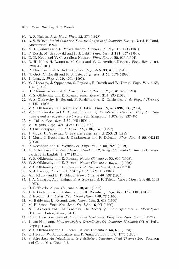
References

1. W. Pauli, General principles of quantum theory in Handbuch der Physik, ed. S.Fluegge (Springer, Berlin, 1980), p. 60.

2. V. S. Olkhovsky and E. Recami, Lett. Nuovo Cim. (1st series) 4, 1165 (1970).3. V. S. Olkhovsky, Ukrainskiy Fiz. Zhurnal [in Ukrainian and Russian] 18, 1910 (1973).4. V. S. Olkhovsky, E. Recami and A. Gerasimchuk, Nuovo Cimento A 22, 263 (1974).5. E. Recami, A time operator and the time-energy uncertainty relation, in The Uncer-

tainty Principle and Foundation of Quantum Mechanics (J. Wiley, London, 1977),pp. 21–28a.

6. E. Recami, An operator for observable time, in Proc. of the XIII Winter School inTheor. Phys., Vol. 2 (Wroclaw, 1976), pp. 251–256.

7. V. S. Olkhovsky, Sov. J. Part. Nucl. 15, 130 (1984).8. V. S. Olkhovsky, Nukleonika 35, 99 (1990).9. V. S. Olkhovsky in Mysteries, Puzzles and Paradoxes in Quantum Mechanics, ed. R.

Bonifacio (AIP, 1998), pp. 272–276.

May 6, 2008 15:28 WSPC/140-IJMPB 03916


10. A. S. Holevo, Rep. Math. Phys. 13, 379 (1978).11. A. S. Holevo, Probabilistic and Statistical Aspects of Quantum Theory (North-Holland,

Amsterdam, 1982).12. M. D. Srinivas and R. Vijayalakshmi, Pramana J. Phys. 16, 173 (1981).13. P. Busch, M. Grabowski and P. J. Lahti, Phys. Lett. A 191, 357 (1994).14. D. H. Kobe and V. C. Aguilera-Navarro, Phys. Rev. A 50, 933 (1994).15. D. H. Kobe, H. Iwamoto, M. Goto and V. C. Aguilera-Navarro, Phys. Rev. A 64,

022104 (2001).16. P. Blanchard and A. Jadczyk, Helv. Phys. Acta 69, 613 (1996).17. N. Grot, C. Rovelli and R. S. Tate, Phys. Rev. A 54, 4676 (1996).18. J. Leon, J. Phys. A 30, 4791 (1997).19. Y. Aharonov, J. Oppenhem, S. Popescu, B. Reznik and W. Unruh, Phys. Rev. A 57,

4130 (1998).20. H. Atmanspacher and A. Amann, Int. J. Theor. Phys. 37, 629 (1998).21. V. S. Olkhovsky and E. Recami, Phys. Reports 214, 339 (1992).22. V. S. Olkhovsky, E. Recami, F. Raciti and A. K. Zaichenko, J. de Phys.-I (France)

5, 1351 (1995).23. V. S. Olkhovsky, E. Recami and J. Jakiel, Phys. Reports 398, 133 (2004).24. V. S. Olkhovsky and A. Agresti, in Proc. of the Adriatico Research. Conf. On Tun-

nelling and its Implications (World Sci., Singapore, 1997), pp. 327–355.25. M. Toller, Phys. Rev. A 59, 960 (1999).26. V. Delgado, Phys. Rev. A 59, 1010 (1999).27. R. Giannitrapani, Int. J. Theor. Phys. 36, 1575 (1997).28. J. Muga, J. Papao and C. Leavens, Phys. Lett. A 253, 21 (1999).29. J. Muga, I. Egusquiza, J. Damborenea and F. Delgado, Phys. Rev. A 66, 042115

(2002).30. P. Kochanski and K. Wodkievicz, Phys. Rev. A 60, 2689 (1999).31. M. A. Naimark, Izvestiya Akademii Nauk SSSR, Seriya Matematicheskaya [in Russian,

partially in English] 4, 277 (1940).32. V. S. Olkhovsky and E. Recami, Nuovo Cimento A 53, 610 (1968).33. V. S. Olkhovsky and E. Recami, Nuovo Cimento A 63, 814 (1969).34. V. S. Olkhovsky and E. Recami, Lett. Nuovo Cim. 4, 1165 (1970).35. A. J. Kalnay, Boletin del IMAF (Cordoba) 2, 11 (1966).36. A.J. Kalnay and B. P. Toledo, Nuovo Cim. A 48, 997 (1967).37. J. A. Gallardo, A. J. Kalnay, B. A. Stec and B. P. Toledo, Nuovo Cimento A 48, 1008

(1967).38. B. P. Toledo, Nuovo Cimento A 49, 393 (1967).39. J. A. Gallardo, A. J. Kalnay and S. H. Risenberg, Phys. Rev. 158, 1484 (1967).40. E. Recami, Atti Accad. Naz. Lincei (Roma) 49, 77 (1970).41. M. Baldo and E. Recami, Lett. Nuovo Cim. 2, 613 (1969).42. M. H. Stone, Proc. Nat. Acad. Sci. USA 16, N1 (1930).43. N. I. Akhiezer and I. M. Glazman, The Theory of Linear Operators in Hilbert Space

(Pitman, Boston, Mass., 1981).44. D. ter Haar, Elements of Hamiltonian Mechanics (Pergamon Press, Oxford, 1971).45. J. von Neumann, Mathematischen Grundlagen del Quantum Mechanik (Hizzel Pub.,

Leipzig, 1932).46. V. S. Olkhovsky and E. Recami, Nuovo Cimento A 53, 610 (1968).47. E. Recami, W. A. Rodrigues and P. Smrz, Hadronic J. 6, 1773 (1983).48. S. Schweber, An Introduction to Relativistic Quantum Field Theory (Row, Peterson

and Co., 1961), Chap. 5.3.

May 6, 2008 15:28 WSPC/140-IJMPB 03916


49. A. I. Akhiezer and V. B. Berestezky, Quantum Electrodynamics [in Russian] (Fizmat-giz, Moscow, 1959).

50. V. S. Olkhovsky, E. Recami and J. Jacek, Physics Reports 398, 133 (2004).51. D. M. Rosenbaum, J .Math. Phys. 10, 1127 (1969).52. D. Judge and J. L. Levis, Phys. Lett. 5, 190 (1963).53. P. Carruthers and M. M. Nieto, Rev. Mod. Phys. 40, 411 (1968).54. A. S. Davydov, Quantum Mechanics [in Russian] (Nauka, Moscow, 1971).55. A. S. Davydov, Quantum Mechanics (Pergamon, Oxford, 1976 and 1982).56. N. S. Krylov and V. A. Fock, Sov. J. ZHETF 17, 93 (1947).57. V. A. Fock, Sov. J. ZHETF 42, 1135 (1962).58. Y. Aharonov and D. Bohm, Phys. Rev. 122, 1649 (1961).59. Y. Aharonov and D. Bohm, Phys. Rev. B 134, 1417 (1964).60. V. S. Olkhovsky, M. E. Dolinska and S. A. Omelchenko, Central European Journal of

Physics, in press (2006).61. E. Recami, W. A. Rodrigues and P. Smrz, Report INFN/BE — 83/6 (INFN, Frascati,

1983).62. E. Recami, W. A. Rodrigues and P. Smrz, Hadronic J. 6, 1773 (1983).63. M. A. Naimark, Izvestiya Akademii Nauk SSSR Seriya Matematika 7, 237 (1943).

About a space-time operator in collision descriptions

Documents

Transcript of About a space-time operator in collision descriptions