.2..3.

X

.7.

_.

,_A.a_\_T_

_..._

ytmmrmaweSnfl31IJMHmamfemSmw.mmS

mam

CADASTRALSURVEYMEASUREMENT MANAGEMENT

SYSTEM

Version 1.0dated 03/91

Documentation

Revision 7.0: //'/w 03/18/91

CMM Version 1.0 Documentati

CONTENTS

Introduction. . . . . . . . . . . . . . . . . . . . . . . . . . . . . . . . . . . . . . .

1Purpose . . . . . . . . . . . . . . . . . . . . . . . . . . . . . . . . . . . . . .

2Why is it so great? . . . . . . . . . . . . . . . . . . . . . . . . . . . . . . .

4Acknowledgements . . . . . . . . . . . . . . . . . . . . . . . . . . . . . . .

7

Chapter 2 — The PLSS Datum. . . . . . . . . . . . . . . . . . . . . . . . . . . .

8Introduction

. . . . . . . . . . . . . . . . . . . . . . . . . . . . . . . . . . . .8

The Geodetics of Cadastral Survey . . . . . . . . . . . . . . . . . . . . . .8

Manual References. . . . . . . . . . . . . . . . . . . . . . . . . . . . . . .

8PLSS Datum Defined

. . . . . . . . . . . . . . . . . . . . . . . . . . . . . .9

Forward bearing . . . . . . . . . . . . . . . . . . . . . . . . . . . . . .9

Back bearing . . . . . . . . . . . . . . . . . . . . . . . . . . . . . . . .9

MEAN bearing . . . . . . . . . . . . . . . . . . . . . . . . . . . . . . .9

Straight Lines. . . . . . . . . . . . . . . . . . . . . . . . . . . . . . . .

10Rhumb Lines

. . . . . . . . . . . . . . . . . . . . . . . . . . . . . . . .10

PLSS boundaries. . . . . . . . . . . . . . . . . . . . . . . . . . . . . .

llCoordinate Systems and the PLSS Datum

. . . . . . . . . . . . . . . . . .ll

DOUBLE PROPORTION. . . . . . . . . . . . . . . . . . . . . . . . . . .

12Cardinal Equivalents: . . . . . . . . . . . . . . . . . . . . . . . . . . .

12Cardinal offsets

. . . . . . . . . . . . . . . . . . . . . . . . . . . . . .12

Chapter 3 - Understanding Least Squares and Adjustment . . . . . . . . . . .15

Introduction. . . . . . . . . . . . . . . . . . . . . . . . . . . . . . . . . . . .

15Is There Really Such a Thing as "Unadjusted" Data?

. . . . . . . . . .16

Compass Rule Approach . . . . . . . . . . . . . . . . . . . . . . . . . . . .17

What does one need to know. . . . . . . . . . . . . . . . . . . . . . . . .

19AdditionalInformation

. . . . . . . . . . . . . . . . . . . . . . . . . . . . .21

approximations . . . . . . . . . . . . . . . . . . . . . . . . . . . . . . .22

iterations. . . . . . . . . . . . . . . . . . . . . . . . . . . . . . . . . .

22standard error . . . . . . . . . . . . . . . . . . . . . . . . . . . . . . .

22error ellipses . . . . . . . . . . . . . . . . . . . . . . . . . . . . . . . .

22robustness

. . . . . . . . . . . . . . . . . . . . . . . . . . . . . . . . . .23

Conclusions. . . . . . . . . . . . . . . . . . . . . . . . . . . . . . . . . . . .

24Dependent Resurvey . . . . . . . . . . . . . . . . . . . . . . . . . . . . . .

25TEST DATA SETS

. . . . . . . . . . . . . . . . . . . . . . . . . . . . . . .28

POST-LEAST SQUARES ANALYSIS. . . . . . . . . . . . . . . . . . .

32CONCLUSIONS

. . . . . . . . . . . . . . . . . . . . . . . . . . . . . . . . .33

Chapter 4 - Overview and Introduction to the Tool Box. . . . . . . . . . . .

35Data Input Programs . . . . . . . . . . . . . . . . . . . . . . . . . . . . . .

35Measurement Processing . . . . . . . . . . . . . . . . . . . . . . . . . . . .

35Measurement Analysis . . . . . . . . . . . . . . . . . . . . . . . . . . . . .

36PLSS datum handling computations . . . . . . . . . . . . . . . . . . . . .

38Other Programs . . . . . . . . . . . . . . . . . . . . . . . . . . . . . . . . .

39

WW ‘ CMM Ch pter - W"VV'V"‘Vpagei

CMM Version 1.0 Documentation ooge ii

FILE Naming . . . . . . . . . . . . . . . . . . . . . . . . . . . . . . . . . .40

Types of Data - Measurements:. . . . . . . . . . . . . . . . . . . . . . . .

41Other skills of value

. . . . . . . . . . . . . . . . . . . . . . . . . . . . . . .42

AdditionalProgram Documentation . . . . . . . . . . . . . . . . . . . . .42

Getting Hard Copy . . . . . . . . . . . . . . . . . . . . . . . . . . . . . . .43

Chapter 5 - Working out Example 1. . . . . . . . . . . . . . . . . . . . . . . .

45Job names . . . . . . . . . . . . . . . . . . . . . . . . . . . . . . . . . . . . .

47Cadastral Measurement Management Main Menu

. . . . . . . . . . . . .47

reduction of lines. . . . . . . . . . . . . . . . . . . . . . . . . . . . . . . .

50Azimuths

. . . . . . . . . . . . . . . . . . . . . . . . . . . . . . . . . . . . .50

GENER . . . . . . . . . . . . . . . . . . . . . . . . . . . . . . . . . . . . . .52

Creating Graphics: . . . . . . . . . . . . . . . . . . . . . . . . . . . . . . .59

VIEW. . . . . . . . . . . . . . . . . . . . . . . . . . . . . . . . . . . . . . .

59DXFLSA

. . . . . . . . . . . . . . . . . . . . . . . . . . . . . . . . . . . . .60

Finish Section Exterior data entry . . . . . . . . . . . . . . . . . . . . . .61

Running the Least Squares Analysis . . . . . . . . . . . . . . . . . . . . .68

error estimate screen . . . . . . . . . . . . . . . . . . . . . . . . . . .69

Residual Printout Limits. . . . . . . . . . . . . . . . . . . . . . . . .

71Readjust With Robusted Error Estimates

. . . . . . . . . . . . . . .72

LSAQ . . . . . . . . . . . . . . . . . . . . . . . . . . . . . . . . . . . . . . .72

Distance Residual. . . . . . . . . . . . . . . . . . . . . . . . . . . . .

75Angle residual

. . . . . . . . . . . . . . . . . . . . . . . . . . . . . . .75

a User Accountable adjustment . . . . . . . . . . . . . . . . . . . . . . . .75

BLUNDER . . . . . . . . . . . . . . . . . . . . . . . . . . . . . . . . . . . .81

Chapter 6 — Reference. . . . . . . . . . . . . . . . . . . . . . . . . . . . . . . .

89ADJUST

. . . . . . . . . . . . . . . . . . . . . . . . . . . . . . . . . . . . .89

SINGLE PROPORTION. . . . . . . . . . . . . . . . . . . . . . . . .

91DOUBLE PROPORTION

. . . . . . . . . . . . . . . . . . . . . . . .91

IRREGULAR BOUNDARY. . . . . . . . . . . . . . . . . . . . . . .

91ONE, TWO, and THREE POINT

. . . . . . . . . . . . . . . . . . .92

GRANT BOUNDARY. . . . . . . . . . . . . . . . . . . . . . . . . .

93COMPASS RULE

. . . . . . . . . . . . . . . . . . . . . . . . . . . . .94

EXAMPLES. . . . . . . . . . . . . . . . . . . . . . . . . . . . . . . .

95ARIZONA.EXE

. . . . . . . . . . . . . . . . . . . . . . . . . . . . . . . . .99

AUTOPROP.EXE . . . . . . . . . . . . . . . . . . . . . . . . . . . . . . . .99

CHECKER.EXE. . . . . . . . . . . . . . . . . . . . . . . . . . . . . . . .

105CHECKER INPUT/OUTPUT . . . . . . . . . . . . . . . . . . . . .

105CMOVE.EXE

. . . . . . . . . . . . . . . . . . . . . . . . . . . . . . . . .106

COMBIN.EXE . . . . . . . . . . . . . . . . . . . . . . . . . . . . . . . . .107

COMPAR.EXE . . . . . . . . . . . . . . . . . . . . . . . . . . . . . . . .107

CONVERT.EXE . . . . . . . . . . . . . . . . . . . . . . . . . . . . . . .107

CSTUF. . . . . . . . . . . . . . . . . . . . . . . . . . . . . . . . . . . . .

109Input Distance and Bearing Syntax Rules

. . . . . . . . . . . . . .112

"I'1- Inirodéifiii

CMM Version 1.0 Documentati

DXFLSA. . . . . . . . . . . . . . . . . . . . . . . . . . . . . . . . . . . .

114DRAW

. . . . . . . . . . . . . . . . . . . . . . . . . . . . . . . . . .114

GENER. . . . . . . . . . . . . . . . . . . . . . . . . . . . . . . . . . . . .

115Introduction

. . . . . . . . . . . . . . . . . . . . . . . . . . . . . . . .115

Detailed Explanation: . . . . . . . . . . . . . . . . . . . . . . . . . .115

look for the blunder. . . . . . . . . . . . . . . . . . . . . . . . . . .

117INREC

. . . . . . . . . . . . . . . . . . . . . . . . . . . . . . . . . . . . . .119

LOOPER. . . . . . . . . . . . . . . . . . . . . . . . . . . . . . . . . . . .

121LSAQ . . . . . . . . . . . . . . . . . . . . . . . . . . . . . . . . . . . . . .

121FILE INFORMATION:

. . . . . . . . . . . . . . . . . . . . . . . .122

INPUT DATA FILE STRUCTURE:. . . . . . . . . . . . . . . .

122LSA FileFormat:

. . . . . . . . . . . . . . . . . . . . . . . . . . . .123

Standard Error of Unit Weight . . . . . . . . . . . . . . . . . . . .125

LSSM. . . . . . . . . . . . . . . . . . . . . . . . . . . . . . . . . . . . . .

126MANAGE.EXE

. . . . . . . . . . . . . . . . . . . . . . . . . . . . . . . .126

PROJEC.EXE. . . . . . . . . . . . . . . . . . . . . . . . . . . . . . . . .

128PROPORT.EXE

. . . . . . . . . . . . . . . . . . . . . . . . . . . . . . . .128

SD.EXE. . . . . . . . . . . . . . . . . . . . . . . . . . . . . . . . . . . . .

132SECTSHOW.EXE

. . . . . . . . . . . . . . . . . . . . . . . . . . . . . . .132

SETUP.EXE. . . . . . . . . . . . . . . . . . . . . . . . . . . . . . . . . .

132SSHOT

. . . . . . . . . . . . . . . . . . . . . . . . . . . . . . . . . . . . .133

TDSLSA. . . . . . . . . . . . . . . . . . . . . . . . . . . . . . . . . . . .

133UTCOMM.EXE

. . . . . . . . . . . . . . . . . . . . . . . . . . . . . . . .133

VIEW. . . . . . . . . . . . . . . . . . . . . . . . . . . . . . . . . . . . . .

133WHATIS

. . . . . . . . . . . . . . . . . . . . . . . . . . . . . . . . . . . .134

WHATIS Dialog . . . . . . . . . . . . . . . . . . . . . . . . . . . . .135

How comers are tagged . . . . . . . . . . . . . . . . . . . . . . . .135

Appendix I -- Software Installation. . . . . . . . . . . . . . . . . . . . . . . .

137What Install does:

. . . . . . . . . . . . . . . . . . . . . . . . . . . . . . .137

INSTALL STEPS:. . . . . . . . . . . . . . . . . . . . . . . . . . . . . .

138Installing your own editor

. . . . . . . . . . . . . . . . . . . . . . . . . .139

UTCOMM - UtilitiesMenu. . . . . . . . . . . . . . . . . . . . . . . . .

139Deleting or moving CMM

. . . . . . . . . . . . . . . . . . . . . . . . . .139

Appendix 2 - Standard Comer Numbering . . . . . . . . . . . . . . . . . .140

Appendix 3 - CMM Glossary . . . . . . . . . . . . . . . . . . . . . . . . . . .143

LEAST SQUARES ANALYSIS SECTION. . . . . . . . . . . . . . .

143GEODESY / STATEPLANE COORDINATES SECTION

. . . . . .146

GENER Error message explanations . . . . . . . . . . . . . . . . . . . .148

LSAQ Error message explanations . . . . . . . . . . . . . . . . . . . . .150

r A‘!-Yr _15a¢22R%m".:R2:>*2;sr:5:::::?t=s:L::>x.:l1;£5cé5:.3$:-:€'§:::-:::> -* .'I'.'-:-:-‘-:;2-'.-.;-.-1:.‘I1.-51.;IijigIififiji:i'i:.'i§'i:.'L5v5‘/'' ~,.-.-,.-,.r,y,,'_';:.H

I Chapter 1 -

CMM Version 1.0 Documentation.'IIIII'I'I-H'>¢J €«i-JE3$§9§'QVM¢'IW3fl¢“W9WH% flZ-I«‘N'N'§'X-\1'O'H'}{\"I'I'1'1-IrI-l-C4'I>I'I'I-{'H'f'5~!-('5:-Z'}$I'l'.'IIl-I1 . I . I

. . . I . I-I-I-I .-

Introduction

What this is: This documentation and the accompanying diskette(s) are the Version1.0 release of the Cadastral Measurement Management (CMM) system. The systemhas undergone about a year of testing and evolution. CMM must still be consideredas a prototype, it takes a considerable amount of time for such a new and extensivesystem to be tested. Until recently it has not been in the hands of a great number ofusers. Primary test sites and other individuals have been involved in the ‘alpha’ and‘beta’ test releases, with the result of an easier to use, more capable and more bug freeworking release. Software development, to be effective and meet user needs, must bean evolution. In this case we are already aware of many potential improvements andnew capabilitiesthat could eventually be incorporated into the system. But it is alsoimportant to get the system into the hands of user, both to better determine the courseof the evolution, and to allow people to benefit from the capabilities that exist.

We would especially like to encourage all Cadastral personnel to try out the software.You can expect that this will not be a simple task. In addition to working withsoftware that is new and unfamiliar, there are a few other aspects of ClVlM that cantend to raise the slope of the learning curve. Many of these aspects are the result ofnecessary evils. Things thatwe have come to recognize are necessary attributes of thesystem that were needed to properly handle automated computations in PLSSretracement work.

Two of these factors thatwill be discussed at more length below are:

* Using Least Squares Analysis as a means to handle the inherent misclosurecommonly carried in BLM Cadastral surveys.

* Using State Plane coordinates as the means to dealing with the geodeticpeculiarities of the PLSS.

Some or both of these methods are new things to most of us in BLM Cadastral. Useof the CMM system will be a lot easier once the user gains some understanding ofthese two factors. This is particularly true of the Least Squares Analysis portion.With this software we have at our disposal some extremely powerful tools that havenot previously been readily available to most land surveyors. The methods andcapabilitiesare state—of-the—art for thePC. In order to effectively use the least squares‘measurementmanagement’ tool kit, you need to plunge into it and gain an understandof some of the terminology and idea behind the least squares process. Like manyaspects of surveying, in addition to reading about it here, thebest teacher is experienceand experimentationwith your actual survey data. After a whilewe hope most of youwill begin to see some of the advantages and power that are made available to youwith the least-squares capability.

I

Chapter 1 - Introduction

>.‘i-l-I-l'Z~Z-I-P2‘:-1':-N‘I-22¢}¥#*WNQh k”M'ZQWOr.

CMM Version 1.0 Documentation pageX9QWfl'G'7'5.’.‘1‘1'3P'2’b'\\'rL'§Il*l'2>€~2~Z-I-I-I-I-2-E

This system is not like a spreadsheet program, or even that much like a simple COGOpackagethatcan almost be operated withouta manual. Please take some time to readthe documentation we have to date, to ask questions of other users, and to availyourself of whatever training sessions we will be able to put together this winter.

A good and responsive way to obtain support and get questions answered after you getstarted is through the use of the Email system and the Cadastral Forum we have on

CompuServe. Using these systems is still another learning process, however once

conquered the benefits are many.

How to Proceed; The first thing we would suggest first time users of this system todo is to read through thisdocumentation until you get to the tutorial example. At thattime refer to the installation section and install the software, and then return and gothrough the example step by step. Then you may refer to the reference section andappendix for additional information on capabilitiesof the system.

What it ggg§n’t do; (as of Release 1.0 03/91)* There is no solar or polaris program. This willbeprovided in a seperate but

integrated package during the next year.

* The links to data collection included are preliminary pending user feedbackand testing.

Purpose; The purpose of CMM is to provide a first shot at a PC based CadastralComputation System, primarily for lower-48 retracement survey applications, thatwould be able to do thejob and also:

Recognize the special geodetic nature of the PLSS, the PLSS Datum

Perform themany special Cadastral Survey procedures, adjustments,requirementsand problems.

In the process of tackling these goals we have bitten off a big chunk of work, but itwas clear at the outset that if we were going to take the time to develop software forthe PC, then we should make it as capable and technically correct as possible withinthe limits allowed by existing systems as well as our knowledge of the problems.What you can expect; Softwareand automationare supposed to make your life easier,right? Maybe, but sometimes it may seem like the reverse. In this case you are likelyto encounter a pretty steep learning curve. This will be worse if you are not thatfamiliarwith using a PC and PC software. Even if that is not the case there are stilla numberof other hurdles you will have to climb in order to effectively take advantageof this system. As we continue to improve the software and documentation, and beginto provide training sessions these learning curves willbecomeless steep. Your rewardfor climbing the curve will be the ability to take advantage of many powerful

.‘.L*::;/J.1-:$fi:%fi$:& mEm$ $i§$>V&2>m1aW3fl%W&‘£$$:3%&%5‘.k.L‘:.".3R:i:I:.::>.>2-:-I:4'7:I1-'I‘E-:i:i15:2‘2‘25..‘1'-:-tliniri:i:i:i:i5'i:i:»:-'-'---'-'-'-:-I-'-:i'i:-:-3-:-5‘-2 '

CMM Chapter 1 - Introduction page 2

CMM Version 1.0 Documentation page 3- ¢K‘N'€'€4K&'W'€

. . . ‘@NK4$fi%%\\*¢5fi¢X'£-2<-I-I-I‘J('1-C'I'1'I'3'N'Z'l'2{~Z<'K7'£'€fid'~1<'1':'3'2‘::2'4'C‘FE'3'!-3~2~2{'5'€'€'€'€‘K'I"l-3'2x‘*.'*H~1'l'}'I'H‘I{'2'Vl"£

capabilitiesthat have not been available to us before.

The CMM system is modular, so that sometimes one portion of it may currently bea little inconsistent or more confusing than others, but it also means that it is not toodifficult to make improvements and advancements in the system.Some of the goals we have for continued development and evolution of CMM are:

To assure that the user interface becomes as understandable and usable aspossible.To assure that the software produces the correct technical and legal results.

That the user interface or methodologydoes not lead the user towards computingWRONG answers.

That there are methods available to verify the computations or allow for easydetection of errors.

This last item is one of some concern. One troubling aspect of automation is theabilityto quickly produce a lot of incorrect information, and because you are moreisolated from the process, not be aware of it. This is closely akin to the old GIGO(garbage in garbage out) phenomena, and is one of the corollaries to Murphy’s law.In general the computer is not a time saver, but provides powerful tools that allow auser to extend capabilitiesfurther than before.

The computer has also made it possible to mess up magnitudes more data and work,faster than you can say IBM. Keep that in mind as you work with this system on yourreal survey data. Protect you work, backup jobs and thinkbefore storing data backto copies and archives.

-.“.»g-.-.;.-5:-,5,-.-. -.,-m.,,;:6‘.;:_._:;." Introduction

CMM Version 1.0 Documentation page 4-Id-I-Z*2Z'I<£‘?fi NWNW?. . V VN*

. - ..'Z¢'§:3‘Z'l'H"r€'i'l'I-2-3-7-l".'1‘1*i'l'Z'!-Z~lr3¢2-I-H-7!‘E'Z*€<€~X-I-I-3'}-142‘£‘C<¢1~1-1‘1-H-I-l-DI-11u'Z-I1+2-I-2-'-2'3-PI-T-Z-I-Z-Z-S

Why §' it so great",

This is our first attempt at bringing a Cadastral Computation system to the PC. Whyis that special? Well, there are a lot of unique things about how we in CadastralSurvey BLM, both technically and procedurally, that make it a challenge to automate.We have a traditional manual process handed down that many in Cadastral still use.That manual process if conscientiously followed produces good and technically correctsurveys. In thinkingof automating the cadastral survey field computation processLooking at these aspects there are a few big problems we have to overcome. As westated above, this system attempts to deal with these:

+ The Geodetic aspects of the PLSS: things like true mean bearings,application of curvature to survey lines, the effects of convergency of themeridians and latitudinal arcs.

+ Special Cadastral computations: like double proportion, irregular boundaryadjustment, single proportion on latitudinal arc, etc.

What about these State Plane Coordinates?

Many of us in Cadastral Survey have a built in aversion to the word coordinate, andeven more so for the things called State Plane Coordinates. Practicioners from theprivate sector are usually amazed at this, but do not work day to day on large scalesurveys. The traditional methods allowed a pragmatic, correct and efficient methodto be applied to getting large scale Cadastral surveys done. This traditional concernabout coordinates is not withoutjustificationas we have all seen coordinate surveyingabused. A lot of this abuse occurred at the advent of electronic surveying at the sametime as electronic computation became available in the early ’70’s. People starteddoing things (it was easy) that did not represent good survey practice. Traversingbecame easy, it was especially easy if you did not have to close into anything. Theambiguity created by having two coordinates on a point was best swept under thecarpet, often adjusted away. Some people developed a belief that if they couldcompute a coordinate on a point that it was surveyed, never mind any kind of checksor analysis.The state plane coordinate systems were developed before the electronic revolution toallow the local surveyor to make use of the networkof geodetic control points that somuch money had been spent establishing. Using stations over long distances could notbe accomodated with local plane coordinate systems, and the computational tools usedby the average surveyor were minimal. Books of tables, sliderules and kurta’s. Asimple method was developed along with projection tables that had a sound geodeticprojection background, that could be used to perform geodetic computations and usethe control net, without too many corrections you could keep within 125000 of theright answer. This was pretty tight stuff at the time.

'-'- ' .B35.'<iT'/J§:£37fi$€7."o7§3".5!3.' v ’$3W”# &’%I‘£! F£§‘X~W&“£Rl-!@;‘R3'R-.-~:3:3QI-I-Si-‘i-3'32-1-112-1?5'«’a‘E‘Tb>}3T%5'9'-53%‘If-'-I-5'39‘:CMM Chapter 1 — Introduction

CMM Version 1.0 Documentation page 5. . .

Y¢ &»€N4WKfi%:~l'>N€'l-344%-I'3\i~Z'5-!§'::2-Q€<{-X~.‘\X‘£¢M¢€*1-3$(rC'€*N§-X4444-Z-5:(‘I-$'N<K'l'!'M'M‘2‘l-Z

Things are a little different today with respect to State Plane Coordinates. With thecomputer and properly designed software all corrections can be applied to survey datato obtain very high accuracies with the system. In the case of CMM, State Planecoordinates are just a means to the end of dealing with geodetics and making the leastsquares process a little easier to do. In the future this aspect may change to workdirectly with geodetics. To the user there is little difference, the answers are thesame, the software does the work.

The traditional Cadastral way to compute and handle large scale survey areas was tocompute using actual measured lines in terms of true courses defined by latitudes anddepartures (lats/deps). These lines were reported as measured by chain and solartransit. Closure was the proof of the precision of the work and the sum of a largenumber of independent distance angle and azimuth measurements. As we havemigrated away from the solar compass/transit in the last 20 years, things have gottena little more confusing.The traditional process in Cadastral Survey was good because it provided a simplemanual way to properly deal withboth the geodetic stuff and to avoid dealing with themisclosures. However it is not very susceptible to being automated. Generallyautomated systems like to use coordinates.

Coordinates and the PLSS. There are a lot of particular problems associated withusing coordinate systems in the PLSS datum that are significant. Any usefulcoordinate system will be close to orthogonal, that is north is at right angles to eastand all N-S lines are parallel. But the PLSS Datum is n_o_t that way. E—W lines arenot even straight, but are instead curves called latitudinal arcs, and N-S lines are truemeridians which converge, that is get closer together as you go north along them.Working in any projection or coordinate system while also working with PLSS datarequires some pretty good tricks to deal with those transformations. You never hadto worry about any of that with true lats/deps.A coordinate system’s north can only be the same as true north at one meridian.Almost no matter what approach you take there are complications.

If you attempt to maintain a rectangular local (non true bearing based) coordinatesystem then you will have to deal with rotating bearings to true, correcting somelines to the latitudinal arc and other problems. This can be called a basis ofbearing system, as it’s bearing may be based upon a reference azimuth at onepoint but is not corrected to true everywhere.If you attempt to use full true bearing (lat/dep) non-orthogonal,coordinate systemby adding up the curvature corrected lats and deps, then you will have to dealwith misclosure due to convergency which will cause you to have differentcoordinates for 1 point depending on how you got compute or traverse there.

55,24 ........................................................................................v.- ..................................................................................................\-.-...................; e3g:::ma:gma:::g::::&-3::z m:m:1a&3:W&%R&W¢::22C Chapter 1 - Introduction page 5

CMM Version 1.0 Documentation page 6-:-:-:»:»:»:-:-:~:-‘.-:-:40,°£

. , .

‘ 4-vac-¢<<~VM6€«$335449 Wmmn:«:u\¢€$"z¢«pt-c-9:«fines-cswt-:tuéoaoqavkvfitéwxfaéfdd-‘Acid«H-:~:»'z‘.-:»:»:::-kzazsr:-:-:-:<-:-:v:-:-:~:-:-:e:-1::-:4-I-t-2:-coo:-G-:«:-:-:-;<-:‘:-:-:-:-:-:-:-......................

To use a coordinate system base on a projection has to account for a lot ofproblems too. The PLSS system reports distances at ground elevation, whereastrue projection coordinate systems require correction of ground distances by bothan elevation and a grid scale factor to get to the grid distance. This in additionto rotating bearing to true and usually complex formula are need to figureanything.

These things make would make working between PLSS data, bearings and distances,and projection grids manually a pain in the neck. These problems can be handledtoday by not judging the problem in terms of how complex it is to handle manuallysince it is possible to deal with much of that complexity with software.

In the rest of the world coordinate systems simplify computations, it is hard to thinkabout computing without them. The traditional Cadastral manual process dealt with9_oj;1_'§_es rather than coordinates. A computation system could be developed based oncourses rather than coordinates, but this has never been done before, and would betackling a whole new computational method.

Use of a projection coordinate system also removes the computational problem ofconvergency. When we go to generate the final true line notes and plats we convertthe lines back to the PLSS datum of true mean bearings and ground distance and theconvergency reappears where it belongs. But even after eliminating that part of theproblem, the dilemma that still remains is that we cannot get very far when ourmeasurements misclose and that part of the problem results in 2, 3 or 4 coordinatesfor the same point. This is common problem we have all seen in trying to applycalculation systems and software to Cadastral work. About the only way is to keeptrack of which coordinate came from what line and only use it with computations onthatline. And we need some way to workalong latitudinal arcs. Some method wouldbe handy to allow us to get rid of this coordinate-measurementambiguity. One wayis to adjust the data.

Why is adiuging good now, whgn we have always said it’s bad?

Lgag Sgugrgs Principals; The evil word lurking in the background here isadjustment. This is another aspect of BLM Cadastral work that usually amazes theprivate survey practicioner. Traditional Cadastral dogma has also maintained thatadjustmentas well as coordinates was a bad word. Why might this be? Well, therewas good reason! The process of adjusting has a bad name becauseit is so often andso easily abused. It is easily used as a way to ‘FIX’ bad data. If you have a lot oftraverses connecting, like in a township, a network results, but simple commonadjustmentscommonly availableto the average survey practitionerhave to be looped.Aftera while some good data is being warped to some adjusted bad data and perfectlygood field work starts to become more and more a distorted figure as you progressthrough loops on loops.

‘ ‘ ‘- -*<"/'.i>‘3‘\:i'-548:!MB?!"

pag :6

CMM Version 1.0 Documentation page

..933:1923*:?N!&W"I€'€¢!3'Xtl'Xéfifififi¢\‘*I'3'23I'}~$s3'N<'Z'€~1'€~l:Z‘Z*Z-3-3‘>€-9!;-I-tn":-:~Z~3‘3‘Z-Z-€-I-2'1-Z-1'2-X

One symptom of thisproblem is how easy it is for this one loop at a time adjustmentpractice to change data more than it should. A distance you measured accurately withEDM as 1000 ft. ends up being 1000.6 ft. Lots of times the surveyor isn’t offendedby thisbecausetheprogram does not printout how much each measurement changed.But you have no choice, or do you? Is there a better way, some kind of adjustmentprocess that was intelligent, that would allow you to include all of your network atonce, not just loops hooked onto loops degrading data as you go. Is there some waythatwould allow you to define how accurate the measurements were, and then wouldlet you know if all those constraints were consistent, that is, how much eachmeasurement was required to change to meet those constraints and if there areUNACCEPTABLEerrors?

Well of course theLeast Squares process in CMMhas all of these attributes and more.Unlike the magic "ADJUST" button contained in many commercial COGO’s, leastsquares analysis is an intelligent tool that is USER ACCOUNTABLE. That is youmake estimates of your reasonable measurement errors, the process tries to meet allthe geometric constraints of your entire system simultaneously and then provides youwith data about what happened. Data that can be interpreted to tell you if yourestimates were correct, or if there was likely an unacceptableerror or blunder. Andprovides a number of other benefits.

The following pages are an explanation from an expert. After you have digested allhe has to say, we would also like to recommend that you read over another papercontained in AppendixH, that talks about theresults of this type of analysis with actualCadastral data on several large scale day-to-day Cadastral survey projects.After you have experimented with the software some you may want to review thesedocuments, as it may make more sense then.

AcknowledgementsThe production of this software owes a great deal to a large number of individualsthroughout BLM Cadastral Survey and students and staff of the University of Maine,at Orono, and the primary test site BLM Montana State Office, and the Eastern StatesOffice. It would take a page to list and give proper credit to all of these individuals,we would however like to express special thanks to Bernie Hostrop, Chief WODivision of Cadastral Surveys, through whose support and encouragement this projectwas made possible.

.................................. . *-' "' ‘I.- €:3!E-'$¥(¢«‘5t~.‘2if:2EQ~R¢:bR£:3:{<5-$‘5'.k$:fikifnfitikitkkicitifificizfififiiiit3tR3'.5tl:1:it3:1:kl:- ntroduction page

CMM Version 1.0 Documentation page 8. a ' - -.' ~- -.- '-'-" ' ' ' " " ' ' ‘ . 'G’¢'G§!9!§Wflh & @€Q&84{K’4§VH'M"d8'X'@H"1‘:h"X4'1'2e.“M$«'2'I'>X'l'1'Z€'3'X99M!.9’r7Ii&l!kVK‘K‘£V§X’II'Z'E4€¢€M'3€'§‘5¢£°Z€¢'$'I'i'3'!‘K'Z~Z'€

Chap_ter 2 - The PLSS DatumIntroduction:

,_v_.;.;.;.;.;.;,;.;¢.. ._.... . . . . ..

One of the characteristics of BLM Cadastral Surveying that strongly affects the ability toautomatefield computations is theunusual nature of thereference system in which Surveys arereported. Traditionalmethods have provided a way to work within this system without thenecessity of a thoroughunderstandingof all of it’s aspects. However thosetraditional systemsand methods do not lend themselves well to automating, and with the proliferation ofcomputing systems, it becones more and more necessary to re-examine how we measure inCadastral, and what implications that has in automating it. To the non-BLM Cadastralsurveyor, this informationshould also prove of value in understandingthe nature of the PLSSrecords and Manual procedures. In other words, in order to effectively automate we need toachieve a common understanding of how we do our job in terms of measurement techniqueand computational methods.

TheP D tum - or h ti f tr I urv

The PLSS Datum is the reference system by which the majority of the PLSS surveys aretheoreticallyreported. The data being reported on a BLM or GLO Cadastral Survey plat are,of course, bearings and distances. But bearings and distances with reference to what? Thedatum thatsurveys of thePublicLand Survey System have been reported in for over 200 yearsis discussed in various sections of the Bureau of Land Management’s current edition of TheManual ofSurveying Instructions, 1973.

Some of the Manual References you may want to review are as follows:

1-3. "Details of the plan and its methods go beyond the scope oftextbooks on surveying. The application to large—scale arearequires an understanding of the stellar and solar methods formaking observations to determine the true meridian, the treatment ofthe convergency of the meridians, the running of the true parallelsof latitude, and the conversion in the direction of lines so that atany point the angular value will be referred to the true north atthat place."2-1. "The law prescribes the chain as the unit of linearmeasure for the survey of the public lands. All returns ofmeasurements in the rectangular system are made in the truehorizontal distance in miles, chains and links...."

2-17. "The direction of each line of the public land surveys isdetermined with reference to the true meridian as defined by theaxis of the earth's rotation. Bearings are stated in terms ofangular measure referred to the true north or south."

2-19. Describes 3 Basic methods prescribed as current practice todetermine true bearings, 1) Direct Sun, star or polarisobservations; 2) Solar attachment; 3) Angles from the horizontalcontrol network. Use of the gyro-theodolite is also mentioned.

' ' ‘17k§<3«‘.’¢~'.<:2'2 %i‘o‘ WM... ‘ltfiifilt-fiZ.i'$§6(a:!e22z:.'-1-'CMM Chapter 2 - me PLSS Datum page 3

CMM Version 1.0 Documentation page 9. . . 1'%2’.‘$¢<-£9}¢¢3€-1:3‘:tiZ'WM-€"D!fl!>!39M'KN'5'>.'1?s"32>H“Z*€“)€<'fi'3'2'I-Z'Z'?:'Xr>?3->>J'2-2'2'>2'.‘ ' ' '

2-74. This entire section is very important on this issue anddescribes in detail methods for carrying forward true bearing,and defines mean bearing and many other critical concepts.".... By basic law and the Manual requirements, the directionsof all lines are stated in terms of angular measure referred tothe true north (or south) at the point of record."

2-76. Defines the solar method for laying out the true parallel oflatitude.

2-79. Contain formulas for computing Convergency of two meridians,and mentions the corrections to closure as a factor of area, and tocompute Rb, effective radius of a parallel.2-80. Describes use of the Standard Field Tables to determineconvergency.

2-81 & 82. Describe the use of M and P factors for convertingmeasurements to differences in latitude and longitude.3-87. Subdivision of Sections, refers to use of intersecting"straight lines".

5-25. Double proportion - ‘Cardinal equivalents’ to be used inreducing record, and cardinal offsets made to determine proportionedpoint.5-31. Single Proportion to allow for latitudinal curve, orcurvature.

5-36. other adjustments to allow for latitudinal curve, orcurvature.

PQS Datum Dgfined

Distancg; These and other references in theBLM and GLO Manuals make it clear that theframe of reference for distances is defined as horizontalmeasure in chains based on the U. S.Survey Foot at actual ground elevation.

Bgringsg The above Manual sections and others identify theframe of reference for directionin the PLSS as something called Mean True Bearings referenced to the true astronomicmeridian at thepoint of record.

For surveyors familiarwithbasic geodesy you will recognize that this is a geodetic datum andthat the basis of bearing changes as you go east and west since the reference meridians atdifferent eastings are not parallel but converge towards the pole.Because this is a changing reference the direction of a straight line on the ground can bedescribed with a forward bearing based on the meridian at the beginning point, or by adifferent back bearingbased on the meridian at the end point. The difference between thesetwo is equivalent to the angle of convergency of the two meridians.

If we want to accuratelydescribe how far north or west at non-cardinal line goes in a geodeticsense, we need to use the average or ‘mean’ of these two values. This mean bearing isessentially equal to the bearing of the traverse line with reference to it’s midpoint. Thus thepoint of record for determining the bearing of a straight traverse line can be said to be themeridian at the midpoint of the line.

' %$$K %S5:€ti%‘$:¢$$$:~’$:1fi$S2¢$$:5:1#$$5:°$:\i$$.<:€$:3$c‘

Datum page 9

'}".".-'.\"I'1'3‘I'?'£. . . .. $?X¢1'l§¢VM!“{V

. .

CMM Version 1.0 Documentation page 10.. N?&N'?ZMZfi-I-I4'76-D"I2:Z'2'D£<'Z‘l'Z4'2'2¢4'l’3¢¢fii".€‘f-K¢'2€<‘:'l{'3'2'D'J|¢‘2-Z-Z':‘I'Z'2<-l'l'l'.'l'L'Z‘1"Z':4‘:-Kiri-C-2-L’;-1

There are other geodetic affects thatoccur in large scale surveys, but this changing referencedirection in the PLSS datum is by far the most significant.

gtrgight Ling: Therefore, one unusual byproduct of the PLSS datum is that:

I. Straight lines on the ground are lines of constantly changing bearing.A straight line is basically what you would lay out by double centering or projecting a directline of sight. The only straight line thatdoes have a constant bearing is the meridian or northand south line. An example of a boundary thatmight be a straight line is one that is describedas a straight line running from one physical monument to another. Such a line, if reported inthe PLSS Datum would have different forward bearing and back bearing, and differentbearings at any point along it.

Another term used to describe straight lines is Great Circle. That is the line formed by theintersection of a plane which passes through the earth center and the earth’s surface. In thereal world such a line is actuallynot exactlystraight to both the ellipsoidal shape of the earthand local gravity anomalies a line you double centered would be a ‘geodesic’.

Rhumb Ling; It is also apparent from the various GLO and BLM Survey Manuals and theactual methods prescribed and used to lay out the system on the ground that most boundarylines in the PLSS are intended to be lines of constant bearing or Rhumb lines, NOT straightlines. Such lines cross every meridian at the same angle and are thus curved as viewed on theground. Therefore, another unusual byproduct of the ‘PLSS datum’ is that:

H. Lines of constant bearingappear carved on the ground.For example, the solar compass and transit were instruments that determined bearing at eachsetup, and when matched with traditional chaining, measured or laid out lines of constantbearing.The ‘Manual’ discussion of latitudinalarcs illustratesone example of a rhumb line. A parallelof latitude is a line that is due East and West in thePLSS Datum, thus one case of a line ofconstant bearing. Since it crosses each meridian at a 90 degree angle, it has a mean bearingof East or West. All lines of constant bearing in thePLSS datum except meridians will appearcurved on the ground.It also turns out that:

IH. Ihe mean bearingof any chord or sub-chord connecting any two pointsalong a PLSS rhumb line willbe the same as thebearingofthe rhumb lineitself.

Thus it is possible to lay out points on a rhumb lineby correcting traverse lines to their mean

bearing in computations.

‘mi 2-’ .' iT:BK'3$iS:itS1 Z%'3rF'i‘2\‘F!2?5!¢$f\-'3Iv'3:?-‘#232-iiU5‘-'-2%

CMM Chapter 2 - The PLSS Datum page 10

CMM Version 1.0 Documentation page 11 .

..‘ .$>1NN¢X+W% }tM3fifl#H¢WX#NMG&§W>I-I-Z-N->5’:-C-I-3+}:-2+.

.This includes standard parallels, townshipexteriors, section lines, many grant and reservation lines, some portions of state lines, etc.The effect is not necessarilylimited to E-W lines. Examples that can be seen on any map arethe largest portion of the North boundary of the U.S., and the N and S boundaries of manystates, such as Colorado, Wyoming, Kansas, etc.

§gme bgundgrifi are straight ling. This includes specifically described portions of grantor reservation boundaries, some portions of state lines. Subdivision of Section, (see Section3-87 of the Manual). There is some controversy about this, and in fact we are dealing withpretty trivial distinctions in the case of a line a mile or less in length.Examples that can be seen on a map are the diagonal portion of the East boundary ofCalifornia as well as the South boundary of California.

The amount of curvature of these lines is dependent on theproject latitude, at higher latitudes,such as in Alaska, the effect can be very great, for example the change in bearingover a mileE-W line is about 2’ 23" per mileat 70° N latitude in Alaska, or in southernArizona: 32 secs.at 32° N latitude.

Informationon the amount of curvature for different latitudes can be obtained from a numberof formulas, as well as derived from theStandgd Field Tables, also known as the Red Book,in either Table 11 - Convergency ofMeridians, Six Miles Long and Six Miles Apart..., orTable 26 - Increments of Curvature.

Note: If you apply curvature corrections to your traverses, you will in essence be surveyingas if you were using a Solar attachment, see Manual Section 2-76. For purposes of lineproportions no further corrections for latitudinal arc need be made. This is the essence ofbeing in theDatum. That is, to survey in the datum and to then apply secant or chord offsetsas described in the manual would be applying the correction twice.

Qgordinate Systgms and the PLSS Datum

If you were to try to develope and use coordinates based on the true mean bearings of yourtraverse lines, you would begin to run into some problems, why? The reason is a by productof an effect thatwe will call ‘apparent misclosure due to convergency of the meridians’. Andit results in coordinates that depend upon the path you used to compute to the point, and assuch become pretty useless as coordinates as they no longer represent in themselves a properrelation between the points.Therefore in the PLSS Datum:

IV. A theoreticallyperfect survey will appear to misclose in the PLSS datum.

The effect will be called ‘apparent misclosure due to convergency of the meridians’ and is afunction of latitude and the area of the loop closed.

Since the sum of true mean lats and deps to a point will depend on the area between the pathto the point and a true line directly to the point, the only correct answer is one obtained byrunning the straight line to the point.

CMM Version 1.0 Documentation page 12'

' ""* ' .. - -. -.-.-.- -.-.- . .*"' ' '-' '."-" "" ' .'X9fi$‘V%Q‘AV‘@&¢( .

‘3'¢$i¢'X$.§2H:3§'?-“?’.<‘$'W!3!9"-$¢'3§3’.“l'Z'l'1'2*2-7'7'2-i¢ A9¢%fifi~Z-2443':'2‘3+I‘Z-Z'€'1€'1-I-2‘1r2<~Z-1’&<- '1‘!-Z.".‘3’.'Z'2-C'I'3'Z

Coordinates systems based on mean bearingswill always have difficulty becausethe math andtrigonometric functions we are used to using are based on an orthogonal (axis are all at 90degrees to each other and straight) coordinate system, and we are dealing with a differentshaped system.

DOUBLE PRQPORTIONNow let’s look at the definition of double proportion as stated in the BLM Manual ofSurveying Instructions, 1973, which states:

"5-25. The term ‘double proportionate measurement’ is appliedto a new measurement made between four known corners, two eachon intersecting meridional and latitudinal lines, for thepurpose of relating the intersection to both.

In effect, by double proportionate measurement the recorddirections are disregarded, excepting only where there is some

acceptable supplemental survey record, some physical evidence,or testimony that may be brought into the control. Corners tothe north and south control any intermediate latitudinalposition. Corners to the east and west control the position inlongitude."ouooo

"Lengths of proportioned lines are comparable only when reducedto their cardinal equivalents. "

Qgrdingl l§_1quiv§lents; The last sentence in the above quote is one that requires some

explanation. What it means is that only the easterly components (or departures) of the E-Wcontrolling record lines are used to compute the E and W position, and only the northerlycomponents (or latitudes) of the N-S controlling record lines are used to compute the N andS position. This is different than using the line lengthsor distances on the record line.

Neglectingto correct therecord for cardinal equivalents won’t usually get you in trouble sincemost section lines in the original surveys are very near to cardinal and the correction isinsignificant. There are, however, many situations in public land surveys where this is not thecase. This situation will also occur where a retracementor subsequent GLO or BLM resurveyhas reported new measurements in the PLSS datum, and the lines are distorted.

Cardinal offsets

Ihe Manual ofSurveying Instructions, 1973 Section 5-26 describes a process for performinga double proportion. The Manual section states:

"5-26. In order to restore a lost corner of four townships,a retracement will first be made between the nearest knowncorners on the meridional line, north and south of themissing corner, and upon that line a temporary stake will beplaced at the proper proportionate distance; this willdetermine the latitude of the lost corner.

"Next, the nearest corners on the latitudinal line will beconnected, and a second point will be marked for theproportionate measurement east and west; this point willdetermine the position of the lost corner in departure (orlongitude).

1. 3‘)R$?.’5:3:’¢$$$:3:5:E€:€$:3:‘-:9m-‘.€.’-rlkié-R%‘ml(r-%!»$W!L4S:2:i:1:3:&1:5c3.- ’

CMM Chapter 2 - The l3LSS Datum* -‘@211’

CMM Version 1.0 Documentation page 13...............................................................................................................,.‘ - - .">3!WQ2‘7(I‘I'2'M!>€‘1'2‘H‘!-l‘N%¢M'M'VN'K93'ii-5'5-D»\'<2'M’€¢1!WO°N09(‘P1*2‘5‘§N-Z‘!-2'l'2¢I0'?/A-2-Z+Z'Z‘€+.

"Then, through the first temporary stake run a line east orwest, and through the second temporary stake a line north orsouth, as relative situations may determine; theintersection of these two lines will fix the position forthe restored corner."

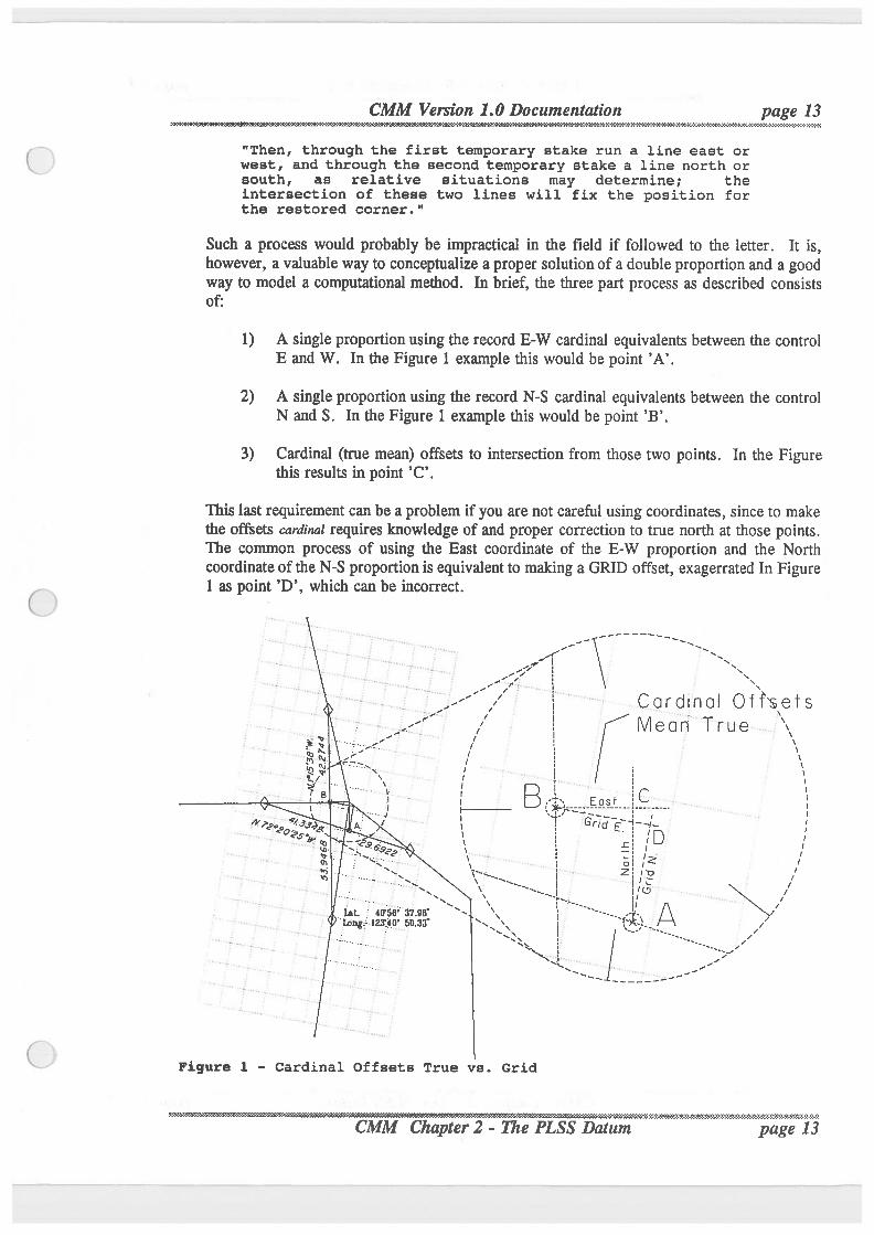
Such a process would probably be impractical in the field if followed to the letter. It is,however, a valuable way to conceptualizea proper solutionof a double proportion and a goodway to model a computational method. In brief, the three part process as described consistsof:

1) A single proportion using the record E-W cardinal equivalents between the controlE and W. In the Figure 1 example this would be point ‘A’.

2) A single proportion using the record N-S cardinal equivalents between the controlN and S. In the Figure 1 example this would be point ‘B’.

3) Cardinal (true mean) offsets to intersection from those two points. In the Figurethis results in point ‘C’.

This last requirement can be a problem if you are not careful using coordinates, since to makethe offsets cardinal requires knowledge of and proper correction to true north at those points.The common process of using the East coordinate of the E-W proportion and the Northcoordinateof the N-S proportion is equivalent to making a GRID offset, exagerrated In Figure1 as point ’D’, which can be incorrect.

Cordunol Of\fs\e’rsl\/lean: True \

\\B, East 5 C }IR ':_--1::;_:"'1'" ',“"' I9W 57*-‘~/~ I

:5 ’ ,'_: I I*5? /Z /V\\ Z; ID I’\ \‘\\ l ’ C I\\ \ \x._ ' I I0 /\\ ~~.r_ N I’, . IIlint. -' 4tr5a""37.9s' ‘ ‘ “~~~~~

-_.4‘. A I9“Ibng54zIAo'5m3f \\\‘\\ i (3§;N__ /x’

».C. \‘:§\ i. ----------

N /,’\\ ‘~>_/........

,_‘K /’

Figure 1 - Cardinal Offsets True vs. Grid

'» - %~'Y&BW&Wo#:$fl&W%- # fi%fi:i"'Y?CMM Chapte -Hatum page 13

‘(WW - OGOOONMGK

CMM Vemiap 1.0 Documentation

page 14 W'X¢D!'NN¢€*I‘NN4€>V‘5\?Q‘O'Wi'7¢$'K9<§‘(\"h?2n?0M9G'D':'0>C>PO{'0G0¢¢ONI¢66‘A¢H'b:'}§

C ,>

CMM Version 1.0 Documentation page 15.J9!H9&Z“>!3'3'Z‘E'fi1'3‘5'1-Z'Z‘l-Z'l!M'39<- #W54*?X'It3$'Wt5‘3'H:2'W'Hfi'5'M'7t'D'>3'I'1‘I'Z‘lt2->3-3-5*."t'5£'1*3-I-2'24-I

Chapter 3 - Understanding Least Squares and Adjustment

Understanding Least Squares and AdjustmentA Basic Approach for Utilization

by Ray Hintz

This is a draft copy of a paper that was preparedfor presentation at the CadastralSurvey 1990 New Technology Seminar, which was never held. Its intent is to helppeoplefeel comfortable withsome oftheprocesses which are involved in measurementmanagement. The authorthanksCorkyRodine andJeny Wahlfor theircontributionsto thispaper.

Introduction

The use of adjustment of survey measurements is obviously something the surveyingcommunity wishes could be avoided. Unfortunately we, and the instrumentation we use, arenot perfect in our measuring ability,and adjustmentis the term thathas been associated withthe procedures we use in accounting for our inconsistencies.

If an adjustment changes a measurement within an acceptable random error limit we shouldnot be concerned. The statistical difference between the adjusted and the measured quantityin this situation is negligible. A 4 second adjustment of a horizontal angle measured twicewith a 6 second least count theodolite is obviously within the expected error range of theangle. A 30 second adjustmentof thatangle could easilybe termed intolerable, and a surveyorshould not accept the adjustment. The cause of the intolerable adjustment (data entry error,field blunder, etc.) needs to be determined and the measurement corrected. The readjustmentbased upon the correction then needs to be evaluated for acceptability. One role of this paperis to explain why adjustmentcan be a valid procedure, and how to judge when it is not valid.

A large numberof thesurveying community are familiarwith the compass rule as an effectiveadjustmentprocedure for a loop traverse adjustment. Unfortunately, this approach is limitedin versatilitywhen a traverse network (series of interconnected traverses) is encountered. Aleast squares approach to adjustmentof survey data analyzes any survey networkconfigurationin the same fashion. Least squares analysis is not limited to surveying. It is an acceptedprocedure in mathematics,statistics, computer science, and a varietyof engineeringdisciplines.In most other disciplines least squares is considered a "data analysis" technique as opposed toan adjustment process. This paper will illustrate that is really an analysis technique insurveying, too. Adjustmentactuallyexists in any redundant survey network- misclosures aresimply restricted to a limited number of closing measurements in an "unadjusted" situation.While this unadjustedapproach may be a valid procedure in some cases, one would normallydesire a more uniform adjustmentprocedure since we know this is how random errors occurin our measurements. No matter what technique is used, if redundancy exists it will be shownthat adjustmentexists.

The final point to be addressed in this paper is the accepted lack of under- standing of leastsquares analysis in a large component of the surveying population. This is partially due to thelack of understandable reading material on the subject, and that it requires a computer for itto be implemented in a production environment. The personal computer revolution is a recent

' SmW$#$i'$&?$k#$$£6fl :1flfiR&%3W&3fi&6$$:5fll"I" — y’s Least Squares Paper page 15

CMM Version .0 Documentation page 1W44-1-3-1-3-3-:~:w:-:~:~:~:~:-:-:-:-:-wofisisistri-zch-at-l:-x<xk:~;-:-:~:-:1-:-:»:»:«w:a:r;-1‘:-:4:«:«1<-:-:-:-::-:-'-:-:-:4 {am-:-1-:-:-:- .-2<< - -~ - - - - - ~- -

phenomenawhich has allowed a surveyor access to least squares for survey networkanalysis,and efficient PC based software is still a difficult commodity to locate.

One does not require an in-depth understanding of linear algebra, calculus, statistics, or

computer science to become a knowledgeable user of least squares analysis. A computer,dedicated software, and a few hours of hands-on instruction and use are required. This paperdoes not replace hands-on instruction and use, but can serve as a primer for those who areunfamiliarwith this approach. This paper is directed to a user, and not to one who wishes tounderstand the mathematicswhich is beingutilized in least squares operations.

Is Ther R ll h Thin " n d' t "D "

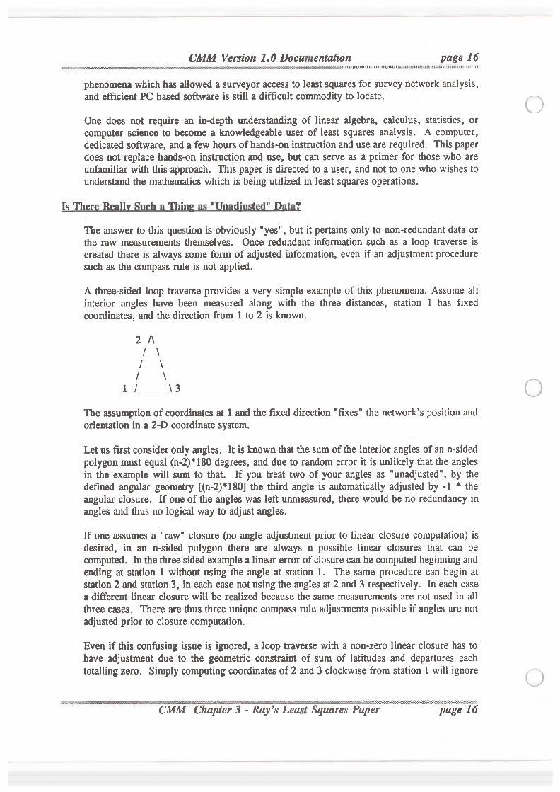
The answer to this question is obviously "yes", but it pertains only to non-redundant data orthe raw measurements themselves. Once redundant information such as a loop traverse iscreated there is always some form of adjusted information, even if an adjustmentproceduresuch as the compass mle is not applied.A three-sided loop traverse provides a very simple example of this phenomena. Assume allinterior angles have been measured along with the three distances, station 1 has fixedcoordinates, and the direction from 1 to 2 is known.

The assumption of coordinates at 1 and the fixed direction "fixes" the network'sposition andorientation in a 2-D coordinate system.

Let us first consider only angles. It is known thatthe sum of the interior angles of an n-sidedpolygon must equal (n-2)*180degrees, and due to random error it is unlikely that the anglesin the example will sum to that. If you treat two of your angles as "unadjusted", by thedefined angular geometry [(n-2)*180] the third angle is automaticallyadjusted by -1 * theangular closure. If one of the angles was left unmeasured, there would be no redundancy inangles and thus no logical way to adjust angles.If one assumes a "raw" closure (no angle adjustmentprior to linear closure computation) isdesired, in an n-sided polygon there are always n possible linear closures that can becomputed. In thethreesided example a linear error of closure can be computed beginningandending at station 1 without using the angle at station 1. The same procedure can begin atstation 2 and station 3, in each case not using the angles at 2 and 3 respectively. In each casea different linear closure will be realized becausethe same measurements are not used in allthree cases. There are thus three unique compass rule adjustmentspossible if angles are notadjusted prior to closure computation.Even if this confusing issue is ignored, a loop traverse with a non-zero linear closure has tohave adjustment due to the geometric constraint of sum of latitudes and departures eachtotalling zero. Simply computing coordinates of 2 and 3 clockwise from station 1 will ignore

-VV -W - ~ V ‘ "' Ai.'~:':1r3.-."‘-wfi-.'».'2:»':2$:‘-:1ScM:t>.Z1.‘C:i.%.‘1." ' -ea"éPaper

CMM Version 1.0 Documentation page 17.. -'l4'3’-¢'H¢'0'l"’.‘X44-1'l4Q')9I¢N"¢M'§'W’Z'€¢-“N'>24'K€}H'H'1'M€‘H‘€{¢3'€'3'I'14‘!"L'l'5'!'1'i'I'2$‘2'2

use of the angles at l and 3 and the distance from 2 to 3. This omission actually places alladjustment in these three measurements.

As stated before, one should observe if the amounts of angular and distance adjustment arewithin reasonable random error limits. If this is true, the amounts of adjustment are withinthe limits of one’s measuring abilities.If the amount of adjustmentto various measurementsis not withinacceptable limits the adjustmentprocess is indeed invalid. The source of the un-reliable measurements should be determined and corrected.

This demonstrates that if redundancy exists adjustment has to exist. Geometric constraintsprevent all measurements to remain unadjusted.

Wh n do a m Rul A r h o Tr v e Ad'us ment become Difficul

A compass rule adjustmentof a loop traverse with reasonable angular and distance closuresis a very valid procedure, and will often produce final coordinates which are very close tothose produced by a least squares adjustment. Unfortunately a loop traverse is not a highlyredundant situation. A loop traverse is also fairly weak geometrically,and can have undetectedlarger compensating errors in it. The sum of the interior angles, sum of latitudes, and sumof departures are the only geometric constraints in a loop traverse. It can also be shown bya mathematicaltechnique called error propagationthata traverse’s geometry is strongest in thedirection it "runs". A section of traverse running north-south will therefore have weakereasting and stronger northingcoordinates. Consider thenorth-southtraverse as a guitar string.It bends easier east-west than it can be stretched north- south. Now let us assume anothertraverse section is surveyed in an east- west direction and it intersects the north-southsection.If coordinates have already been computed on the north-southline (and possibly adjusted) theeast-west section will be tying into coordinates weak in easting. If you compute coordinateson the east-west section first the north-south section will be intersecting weak northingcoordinates. Least squares provides the solution to this problem.

'-MM Chapter 3 - Ray’s Least uares Paper page 17

-u"*I{-1<i'Z'I’.'Z'€.

CMM Version 1.0 Documentation page 18'-3-I-C'?,W¢’.€¢'1:t<'O-5-3-C-O".'?2i‘¢§\(‘N¢‘&$K€<£'b"/K'2<¢i(-0‘-“'¢"-4-i'2‘X*:<r>G'G¢‘£'i€'1-31W-5-I-Z-I

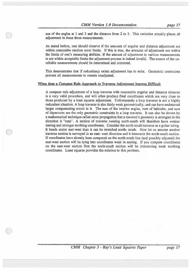
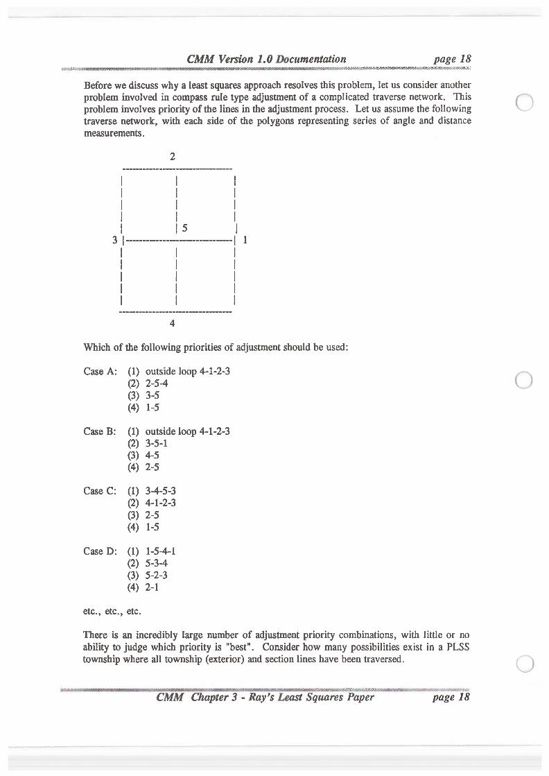
Before we discuss why a least squares approach resolves thisproblem, let us consider anotherproblem involved in compass rule type adjustmentof a complicated traverse network. Thisproblem involves priority of the lines in the adjustmentprocess. Let us assume the followingtraverse network, with each side of the polygons representing series of angle and distancemeasurements.

Which of the following priorities of adjustmentshould be used:

Case A: (1) outside loop 4-1-2-3(2) 2-5-4(3) 3-5(4) 1-5

Case B: (1) outside loop 4-1-2-3(2) 3-5-1(3) 4-5(4) 2-5

Case C: (1) 3-4-5-3(2) 4-1-2-3(3) 2-5(4) 1-5

Case D: (1) 1-5-4-1(2) 5-3-4(3) 5-2-3(4) 2-1

etc., etc., etc.

There is an incredibly large number of adjustment priority combinations, with little or no

abilityto judge which priority is "best". Consider how many possibilitiesexist in a PLSStownship where all township (exterior) and section lines have been traversed.

‘- ."»"£"5’»':S%-..~.\.---u~‘~.«"-.SR'&""""""""' -'-"Hz:-I-.5“isPaper pagewjfi

CMM Version 1.0 Documentation page 19. . WM}???-H-I'1-I“MC-Q33‘M’3'C4:€'N‘€'G:G-E’?!-34’?-M‘:-}9C-3'3‘?s‘C:}?1'2~3*H'€‘?€‘€'?€€'34-X-:'I~Z'2*7-2-2'2-1':-364'}:

A common "rule of thumb" procedure in compass rule approaches to traverse networks is toadjust the exterior of the network as one loop first, then decide on a priority approach ofadjustinginterior traverses to "fit" the adjusted exterior. This concept is often termed a rigidboundary approach. This technique is the worst possible approach thatcould be used from anelementary error propagationstandpoint. The exterior willgenerallycontain more stations thanany other loop in the network, and thus you would expect generally worse closures in it thanany smaller loops. You would thus be adjusting the component with the largest expectederror, and forcing smaller traverse sections (less propagated error) to fit it.

There is no statistically correct procedure thatdefines sequential compass rule adjustmentsofa traverse network. As opposed to a sequential procedure, least squares allows simultaneousadjustmentof any traverse networkgeometry (includingany numberof control stations). Thiswill initially seem impossible since many surveyors are not familiar with how least squaresworks, and thus a basic discussion of concepts is now required.

What dg one nfl to know to feel Comfortable about Using Least Squares Analysis?Whenever we measure somethingmore than once and average the repetitions a least squaressolution is being performed. An average minimizes the sum of the squares of the residuals.This is the underlying principle of least squares. A residual is the difference between themeasurement and its adjusted quantity (an adjusted quantity being a simple average in thiscase). The residuals have to be squared because they tend to be both positive and negative,and thus a simple summation produces zero if a simple average is being computed.Now that one realizes he or she has been using least squares all along in averaging, we nowneed to define how it applies to survey networks, and where the concept of weighting (or errorestimation) of survey measurements becomes important. Horizontal survey networks consistof measured azimuths, angles, and distances in addition to control coordinates. Least squaresadjusts all measurement types simultaneously in addition to adjusting all traverse legssimultaneously. This means relating angular quantities (azimuthsand angles) to thoseof lineardimensions (distances and coordinates). To allow this, the least squares condition is expandedto minimizing the sum of the squares of the weighted residuals. A weight is equal to onedivided by the measurement’s error estimate.

Addingthe weight into the least squares condition makes all terms in the summation unitless.As an example, a distance, its error estimate, and its residual, all have units in feet. (1/errorestimate) residual is equal to (1/feet)* feet in unit terms so the determined quantity becomesunitless. The unitless quantity can be directly compared to unitless quantities derived fromangles and azimuths.

Notice thatthe least squares conditionhas no dependency on number of traverse legs, numberof traverse connections, numberof measured azimuths, numberof control points, etc. At thistime it is also illustrated that the least squares principle can be applied to any measurementsystem in any science (not just surveying). It can also be applied to differential leveling, 3-Dtraversing, GPS vectors, or any combinationof survey measurements.

One estimates his/hererrors in various measurements using knowledgeand experience. Whilerepetition of a measurement such as an angle gives a clue to its reliability,the error estimatederived from repeated measurements does not usually take into account instrument and target

~'-' ‘ n

- y s sPaper page 19

CMM Version 1.0 Documentation pag.e_‘_‘2__0fiW¢§K%'I'3'¢'& KNfih' @.'fi£fl9.9.° "?3~?Z!Xi-Z~.‘~3'O-3*2-Z‘X~IK“!'I-Z'Ie>DOK€~2-I-I-Z-I-I'2~2'2'€'I‘i‘2€¢C"£‘1'I*X-€‘l~Z~3~2'2-:*€«K*3<<-Z~:~Z~f-1-E2-7-Z-L-1- - < I <

setup errors, some atmospheric errors, etc. In other words, the standard error computed froma series of repetitions often tends to be smaller than what a surveyor should estimate since itdoes not account for several possible error sources. An obvious example is repeated EDMmeasurements from the same instrument & target setup. Often these values will not differ bymore than 0.01 ft. but the combined error in instrument and reflector setups over theirrespective points can easilybe larger than this number.

Angle and azimuth error estimates are a function of least count of an instrument, number ofrepetitions, and stabilityof instrument setup among other factors.

An interestingoption of least squares is thatcontrol coordinates can be assigned error estimatesand allowed to adjust. If control coordinates are not to adjust, they should be given a verysmall error estimate (such as 0.001 ft.). The control coordinate can therefore be treated as a

measurement in the least squares solution.

Least squares has procedures which allow one to verify if one’s error estimates are reasonable.The first simple check is a look at all of the measurement residuals (amount of adjustmentapplied to each measurement) and see if any are outstandingly larger in magnitude (absolutevalue) than the error estimate. If all but a few are acceptable, the unacceptable ones are

obviouslypossible blunders. If a majority are outstandinglysmaller than your error estimatesyou have been pessimistic about the quality of your work, or there is very little redundancyin your work.

To scan thousandsof residuals would beextremely tedious so two "global" error computationscan be made. The first is known as a root-mean-square (RMS) error. For a particularmeasurement type, RMS error is the square root of the sum of the squared residuals, dividedby the numberof thattype of measurement. It could be thoughtof as an average residual forthat particular type of measurement. The RMS error should be near in magnitude to youraverage error estimate for a particular type of measurement.

A value which is an indicator of your error estimating abilitiesfor all types of measurements(theentire survey network) is the standard error of unit weight. To compute this quantity thesum of the squares of the weighted residuals is divided by the number of redundantmeasurements (termed number of degrees of freedom), and the square root of that computedquantity is taken. Since a residual and its respective error estimate should be near equal inmagnitude, a weighted residual tends to be near one in amount. Of course, random error sayssome will be larger than one and some smaller than one. If this is true the standard error ofunit weight will tend to be near one. A value larger than 2.5 indicates error estimates were

optimistic of blunders exist. A value less than 0.7 indicates pessimistic error estimates or

simply a lackof redundancy (thereforeno adjustmentof measurements is possible). A test canbe applied to the standard error of unit weight to statisticallyvalidate the quality of your errorestimates. A "rule-of-thumb" approach of 0.7 to 2.5 works well, too. A failure of this testindicates an invalid adjustmentdue to poor error estimates or blunders. If no blunders can befound, it is generally appropriate to change some or all of your error estimates.

Notice you can use you error estimates to "classify" different qualities of surveys within a

network, and adjust all of the network simultaneously. Least squares still preserves thegeometric constraints of sum of interior angles being (n—2)*180 degrees and sum of latitudesand departures of a loop being zero. Adjusted angles will close perfectly between adjusted

A " -3%%&W¥V%§$%&%$. -i%*AV&%3$53:$¥:Z:1::!3'}t5:F5$»'¢?3Ri5:it3:h2"esPaper page 20

CMM Version 1.0 Documentation page 21-.

'. . . .

FV-£%79W9@H¢€?n¢3'?I7'?M¢’¢¢<4!€:3~K‘W<‘W'K‘5\VE'l~Z. . . -!‘b’£'K<€-2'1IW33’I'I'Zn?M*3‘2‘.'e€'Z(€¢'Z€'?I'I'Z‘2*Z'Z“""" '.'I

azimuthmeasurements. If the data is azimuths (or bearings) and distances with no angles thesum of the interior angles constraint disappears but the latitude and departure constraintsremain. This is no different than information derived from a compass rule approach. Acompass rule adjustment actually produces residuals for all measurements, but they aregenerallynot termed residuals. The simultaneous analysis of all data on all traverse legs, withthe abilityto weight measurements using your error estimates, is the key difference.

The simultaneous approach allows the systematic distortions which result from a sequentialcompass rule approach to be eliminated. You truly obtain the "best" coordinates based on aseries of measurements and your error estimates.

Additional Information about 14-dust Sguarfi Adjustmentof Horizontal Survey Data

A brief discussion of items involved in least squares analysis of horizontal survey data willhelp users with questions like "Why do I do this?" and "What do these numbers represent?".This will be presented in a question and answer format.

(1) Why do adjustment of large networks take so long to run?

Least squares analysis of survey networks requires solution of a system of equationsequal in size to the number of unknowns. Unknowns in horizontal survey networks arethe 2-D coordinates of the stations. A 1000 station network has 2000 unknowncoordinates (1000 X, 1000 Y). This means a system of 2000 equations, 2000 unknowns(called the normal equations) needs to be solved. Even on a fast computer this is not atrivial process. As the size of the network increases the time required for the solutionincreases exponentially (i.e., a 1000 station network takes more than twice the time tosolve of a 500 station network).

(2) Why does least squares of horizontal networks require an iterative solution?

The equations used in horizontal data are "non-linear" equations. The inverse distanceand azimuth equations are examples of non-linear equations becausethey include itemssuch as square roots, squared terms, and trigonometric functions in them. A levelingnetworkproduces linear equations of the form:

Elev. B - Elev. A = meas. elev. difference + residual

There are no powers or trigonometric functions in this equation. To solve non-linearequations the equations are so-called "linearized". In doing this one creates a solutionwhich solves for updates to approximations for all unknowns. The updates are added tothe approximations, and the solution for the updates occur again (the second iteration).When the updates become "negligiblysmall" (all less than 0.005 ft. for most surveyingapplications) the solution has converged on the least squares solution for all coordinates.

M...tqa;‘é..S . .115:E£.~22Z2%>’$'£9>1'IoE-':3'.1:3:?:45‘et-’5>’$:i.'5:Q2¢.'m1:1:3$35:36:5:1tk€%:$:5Sf$:¢:Z

aper page 21

w'IC<\2\‘~Z~14':‘3¢.

CMM Version 1.0 Documentation page 22.

NfiK!0% W¥NMN¢N\\. .

» -‘.‘¢".‘:'3-1'91-3:-I-I-3'2-Z'3'X'2-M-2~Z'3."¢'l-2:1-1<Z-C-Not-299})Q<‘3-5*:-Z-2'2-2-$I(('C'l'H~¢......... .-.-. >3-I-I-I-€-:-X .¢¢{\>0~.

Sevgrgl gugtigns grigg:

(1)

(2)

(3)

(4)

How are approximationsfor all coordinates generated, and how close to theirfinaladjustedvalues do they have to be?

Conventional traverse computations are the most effective approach to approximatecoordinategeneration. Thishas been implementedfor any traverse networkconfigurationin computer program GENER of the LSAQ, etc. software package developed by theauthor. GENER performs a compass rule adjustment for all traverse routes, outputsclosure reports and residuals for all measurements from the compass rule. These serve

as excellent approximationsunless blunders exist, and are generated automaticallyfromany unordered data set.(Editors note: Current version of GENER does not use compass rule.)

How many iterations are usually required?If no blunders exist the solutionwill usually terminate in 2 iterations. The first iterationwill illustratethedifference betweenthe compass rule and least squares solution, and thesecond iteration will produce all negligibleupdates.If blunders exist a solutionwill often run more than2 iterations. There is generally littleneed to run more than 4 iterations for a data set.

What is a divergent solution?

If approximations are very poor, or substantial blunders exist, it is possible that iterationupdates will grow (diverge) instead of decrease (converge). It is important thatone looksat pre-adjustmentclosures and compass rule residuals (produced by GENER) for obviousblunders, which can be corrected, prior to running the least squares adjustment.What are the meanings ofstandard errors of coordinates and error ellipses?These quantities give the surveyor a feel for the positional reliabilityof his or herproduced coordinates. They are a functionof theproximity of the coordinates to controlstations in the network (further from control you are less confident of the positionalreliabilityof your coordinates). These error analysis results are very computationallyintensive to obtain, and thus should only be generated for large networks if trulynecessary.

A short discussion of statisticalproperties of standard errors is required to understand thiscomponent of least squares results. Least squares analysis assumes measurements aredrawn from a normal distribution. A normal distribution results in the familiarbell-shaped curve of statistics. Values of data is represented on the x axis and frequencyof occurrences on the y axis. The center of the bell shaped curve is the average.Statistics can show thatapproximately66.7% of your data falls withinthe region betweenthe average minus the standard error and the average plus the standard error.

This applies directly to standard errors of survey coordinates. If you performed the same

survey over, using the same techniques under the same conditions, you would be 66.7%

I’ '.<»‘ ma-:s:mr&m:s:::::::::m::s::;zu-::z:c.-:.:=:.*2m;*a::2r:::::-::.:::"~I CMM Chapter '-'R.ay’s Least Squares Paper 22

(5)

(6)

CMM Version 1.0 Documentation. . .

.¢¢%99We¢9'i’:¢'aW.¢t'¢,W€‘page 23

.

' fW4‘N0°¢'?.3<‘?9\?\?!i'C§!9:3.9fl$¢Q§37'¢*325'K‘I'3'I'C'¢¢<'Z‘???'I'1'€eW'€'fi‘2'1'fr:13'I'3'6'I'MO’:-2'2¢€‘5C*2‘N92'H'X4<'Z'?'W€‘9'fi‘2’a1'4'9?€€'1'0£'2'Z-3<'I4*3'2'!’Z+3'>I'M'l

confident that the new coordinate will fall within "plus or minus" the standard error ofthe first produced coordinate. Multiplying the standard error by three produces 98.6%confidence. The error ellipse produces SU - maximum error, SV - minimum error, andT - angle from north to thedirection of themaximum error direction. One will normallyfind maximum error approximately90 degrees from the direction of the traverse at thatpoint. Error ellipses provide an effective visual tool for inspecting positional accuraciesof least squares adjusted station positions.What is meant by re-weightingfor blunderdetection purposes (robustness)?Least squares can be used as an extremely effective tool in blunder detection. Oftensimply looking at residuals will isolate blunders. A technique often termed robustnessserves as a filter for bad measurements. It involves running the adjustment once withyour error estimates, then averaging the error estimate with the residual (absolute value)for a measurement. This quantity becomes the new error estimate, and the adjustmentis run again. Measurements with small "first run" residuals will get decreased errorestimates in the subsequent run, and the opposite effect occurs for measurements withlarge residuals. This will shift thebigger adjustmentsto thosemeasurements with largererror estimates. This filtering affect is very effective in blunder isolation. A weightedaverage can also be used in determining new error estimates if desired. One can robustall measurements, or only certain ones (such as angles only). The blunders should thenbe corrected and the adjustment re—processed.What is the meaning of the "Band is xx stations" which appears just prior to theadjustmentprocess itself?The equations which are being solved tend to be "sparse". Sparse means there are lotsof zero coefficients. If one can figure out where the zeros are, the station order can beswitched until the zeros are ordered in some systematic fashion. One approach tore-ordering equations or stations is bandwidth optimization. It is used by manyadjustment programs. The band is the "width" of the equations with the zero termsordered outside of thenon-zero band. A 1000 station networkwith a band of 20 stationswill solve much faster than one with a band of 100 stations. The band is a function ofredundancy and the numberof traverse leg connections. The minimum band is found inan iterative process. The total numberof terms in a banded solution is a functionof bandsize and the numberof stations. Withoutalgorithmswhich take advantage of sparsity wewould be waiting a lot longer for solutions to occur.

b&¢»k3»»fi.ww$‘».o‘2er. "};21§L"33

W$NNh ?%9

CMM Version 1.0 Documentation~)¢¢09MQ¢°O

page 24.. '€‘¢9.‘.‘J."D,0('D¢'K~X\"€‘!'30¢I€-X452‘N¢$t§O¢N~Z-2~X<~§¢{-Z-56}DI>b2'Z-2'C-X'€°2'1-I-IC-Z'\V£'I'I-.'I-5<'l'I'3":'I'€a<1i‘2-I€“¢.‘M

Conclusigm

Least squares adjustmentis a statisticallyvalid approach which can solve any survey networkconfiguration simultaneously. With efficient software, a user can become proficient at usingleast squares in a short time. Hands- on experiencewith real data sets is thebest learning toolthat exists. One should not abuse the use of least squares adjustment. A user should alwaysexamine that amounts of adjustmentto measurements are withinacceptable limits.

Least squares adjustment does not eliminate the need for preservation of our measurementinformation. It does validatewhetheror not our measurements appear reliable. "MeasurementManagement" is an integrated process with adjustment, and will undoubtedly be the topic ofanother paper such as this. Hopefully this informationwill allow hands-on experience to bea more fruitful learning procedure.

' Paper page 24

CMM Version 1.0 Documentation page 25 /wawmnmémn -:-.'.‘i»>ma-aw:-zwsH-Mrx:-:wm-:>:-:-:-:-2-:-:4‘:-ea-:-:-:—:n:r:»<n:z-:-:-:-rec-:~;:<-:~:~:-:~:-zed:-a-a-:-l:-c-9:-:¢c<»:<>>:-a-c-24>:-'.-la-a-a-a-:~:4-mam

AUTOMATION AND PRECISIONIN A CADASTRALSURVEYING ENVIRONMENT

Raymond J. HintzDepartment of Surveying Engineering

University of Maine107 Boardman Hall

Orono, Maine 04469(207) 581-2189

Corwyn J. RodineU.S. Dept. of Interior

Bureau of Land ManagementEastern States Office

350 S. Pickett St.Alexandria, VA 22304

ABSTRACT

The surveyor confronting dependent resurveys of federal lands is often working in an environmentwhich is thought to not be conducive to high levels of precision. Hillyterrain and thickvegetationlead to short sight distances and difficult instrument setups. A complete retracement of an entiretownship can easily require 2000 instrument setups. The demonstrative amount of data can alsoforce one to use non-rigorous methods of survey measurement analysis.Analysis of measurements from dependent resurveys of 4 townships, the largest requiring nearly1800 instrument setups, will be presented to illustratethatefficient field techniques, combinedwitheffective measurement analysis, can produce very reliable results. An efficient interface betweena total stationl data collector system and PC-based least squares analysis software capable ofsimultaneous adjustmentof entire townships will be demonstrated. The interface is not restrictedto any form of field procedure. Software and procedures for the quality control and maintenanceof these large data sets will also be discussed.

INTRODUCTION

One of the major elements of a dependent resurvey is the traverse data used in searching forevidence of the original and subsequent surveys. Traverse data which is lacking in quality couldresult in searching for evidence in improper locations. It also follows thatpoor traverse data willresult in proportionate measurement, the Manual of Surveying Instructions (USDI-BLM, 1973)procedure for reestablishment of lost comers, will result in a mathematicallycorrect solution in atotally inappropriate relative position.Rigorous mathematicalanalysisof surveying data has traditionallybeenrestricted to geodetic controlsurveys. The personal computer revolutionhas only recently made it possible for all land surveyorsto have data techniques such as least squares analysis at their disposal.

M'-'- N ' A M$:«'Rfiw2?)$:fi:b3bW$:3:?kR$%W'4&@;%?*-.&2Squares Test page 25 .............................................................-

.

CMM4<._«¢.;»;.;.;.;.;\~;

Version 1.0 Documentation page 26€'M¢‘N'N‘W<S('£'l'2'%'2¢<'¢'3'€‘€fi90\"Z-Z-5'K'3‘2¢€*3s‘<v3+K‘I4-E-1W’:-Z'1(-Z-2-Iv58-51€€‘H'2>Z-2'3-7

A recent joint effort betweenthe Eastern States Office of the Bureau of Land Management and theUniversity of Maine resulted in the testing of dependent resurvey measurement data in a leastsquares analysis environment. The Eastern States Office is responsible for surveys of federal landsin 31 states. The difficult surveying situations encountered range from swampland such as theFlorida Everglades to Appalachianand Ozark mountains.

It is anticipated many would question thebenefits which would be derived from statistical analysisof survey data which has been collected under very difficult field conditions. This paper hopefullywill illustrate the importance of this type of analysis, and further illustrate that it is possible toperform precise survey work in difficult field conditions. The integrationof quality field proceduresand effective mathematicalanalysis must both exist. If both do indeed exist, it will be shown that"adjustment"of survey data truly becomes analysis, as the amounts of adjustmentcan be controlledto be statistically insignificant.

EASTERN STATES OFFICE FIELD COLLECTION PROCEDURES

The Eastern States Office of BLM has beenusing total stations and data collectors for 3 years. Thedata collector system is HP-41 based and was developed in-house to specifically meet the Office’sneeds. While it presents the problem of additional field equipment, a second tripod is used with atribrach mounted prism on all foresights. The tripod, as opposed to pole, mounted prism hasproven to add a level of precision which is well worth the problems associated with carrying theadded equipment.In standard operation thebacksight is a tackmounted on a latl1. All horizontal angles are measuredonce each in the direct and reverse positions. Re-measurementoccurs if the difference between thedirect and reverse measurements if greater than 10-15 seconds (subject to setup conditions). Thedata collector stores the average horizontal angle and horizontal distance resulting from the tworepetitions.Solar/polarisobservations for azimuthdeterminationare taken approximatelyevery 30-50 setups onthe traverse covering the perimeter of the township. The number and location of the solar/polarisobservations are a function of the visibilityof the sun or star as well as terrain considerations. Asolar/polaris observation consists of 8 repetitions.One geodetic control station in the area is tied into the dependent resurvey traverse.

The cadastral computation system used by the Eastern States Office is also HP-41 based and hasbeen developed in-house. The advent of PC-based CAD produced the need for communicationbetweentheHP-41 and the computer. The same type of data transfer was used to bring the traversemeasurements into a MS—DOS environment.

'-"- ' .Z '-&3%:%1$$mifakklfifiliklkkkkit3!‘-Rfifliritit111:3:-:2€:i:2:1t2<t2C5<%¢‘l'<

Test page 26

CMM Version 1.0 Documentation page 2. ww :~w> ‘ ' ‘cox-a-:-Haw»:-»xv¢N.v.-w:-1-:4:-;:w .'-.\:-.'-:->.' :2 : : I-:v:-:-:-:-5-51+:w:ti-:-L:-H41-N¢cv:~:-H.-:r:-:«5-:»:-:-:—:-:—:«3:+c-:-:-:-1-we->2:

BASICS OF THE LEAST SQUARES ANALYSIS

Once thedependent resurvey traverse data had been transferred to thecomputer a translator programwas written to reformat the data for the least squares analysis. The least squares analysis softwarepackage used was developed by the principal author, and has evolved over the last 5 years fromcomments from a numberof users in bothprivatepracticeand governmentsurveying positions. Theobservation equation approach is used and all measurements can be automaticallyreduced to anappropriate state plane grid. An automatic coordinate generation program supplies approximatecoordinates for the least squares analysis. In addition these approximate coordinates are used togenerateunique scale factors for each distance measurementand unique convergence angles for eachmeasured azimuth. While the software allows multiple elevations to be used in the reduction to theellipsoid ("sea level" reduction), a project elevation was assigned to each data set. The use of aproject elevation mirrored the approach used in the HP-41 system.A post-adjustrnent traverse closure routine enabled calculation of conventional linear closures,angular closures, and precisions. The methodolgyused in these computations will be more fullydescribed in the presentation of these results.

-._ _

_, - '.......................................................................................................\-.--------------------------------------------------------------------------------------------------------------------------- -.-s-.v.vv'CM apter 3 - Cadastra Squares Test page 27

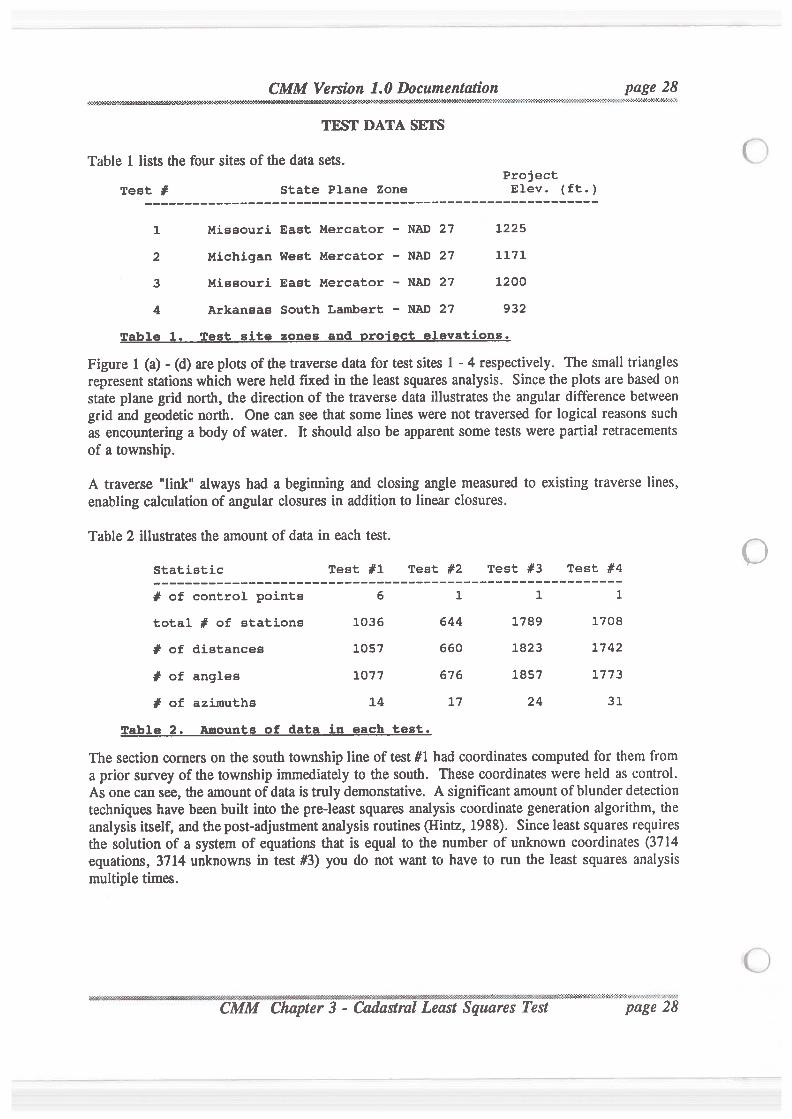
CMM Version 1.0 Documentation page 28 . .

93'?3'2-?$?fi'2'N‘i'30¢K4“2Z71-2-1'I-2‘2“>Z‘€'N'H'>X-V-}X>."‘1'O'€*!'D-GIG-C-it-Z~:':¢~$:-1-:+2-1-I-7'1‘-2-2-2-2-Z-196'»?->2-bit:-:<:-C~:

TT§{FlDA[FA.SEKTS

Table 1 lists the four sites of the data sets.Project

Test # State Plane zone Elev. (ft.)

1 Missouri East Mercator — NAD 27 1225

2 Michigan West Mercator — NAD 27 1171

3 Missouri East Mercator — NAD 27 1200

4 Arkansas South Lambert — NAD 27 932

Table 1. Test site zones and groject elevations.

Figure 1 (a) - (d) are plots of the traverse data for test sites 1 - 4 respectively. The small trianglesrepresent stations which were held fixed in the least squares analysis. Since the plots are based on

state plane grid north, the direction of the traverse data illustrates the angular difference betweengrid and geodetic north. One can see that some lines were not traversed for logical reasons suchas encountering a body of water. It should also be apparent some tests were partial retracementsof a township.A traverse "link" always had a beginning and closing angle measured to existing traverse lines,enabling calculation of angular closures in addition to linear closures.

Table 2 illustrates the amount of data in each test.

Statistic Test #1 Test #2 Test #3 Test #4

¥"SE"2S;Z2SI';SZI.Z;""""""-E——————‘I______‘I'''''''-1total # of stations 1036 644 1789 1708

# of distances 1057 660 1823 1742

# of angles 1077 676 1857 1773

# of azimuths 14 17 24 31

Table 2. Amounts of data in each test.

The section comers on the south township line of test #1 had coordinates computed for them froma prior survey of the township immediately to the south. These coordinates were held as control.As one can see, the amount of data is truly demonstative. A significant amount of blunder detectiontechniques have been built into the pre-least squares analysis coordinate generation algorithm, theanalysis itself, and thepost-adjustmentanalysis routines (Hintz, 1988). Since least squares requiresthe solution of a system of equations that is equal to the number of unknown coordinates (3714equations, 3714 unknowns in test #3) you do not want to have to run the least squares analysismultiple times.

9.1” ‘ r:‘<3."6$%>‘:i5:Z51'c3"»'2'.2$5'Z:‘55:3:2:->--5'---1--c-:.:.:::.:' ' *‘ 'kgztiostralLeast gzxitares est page

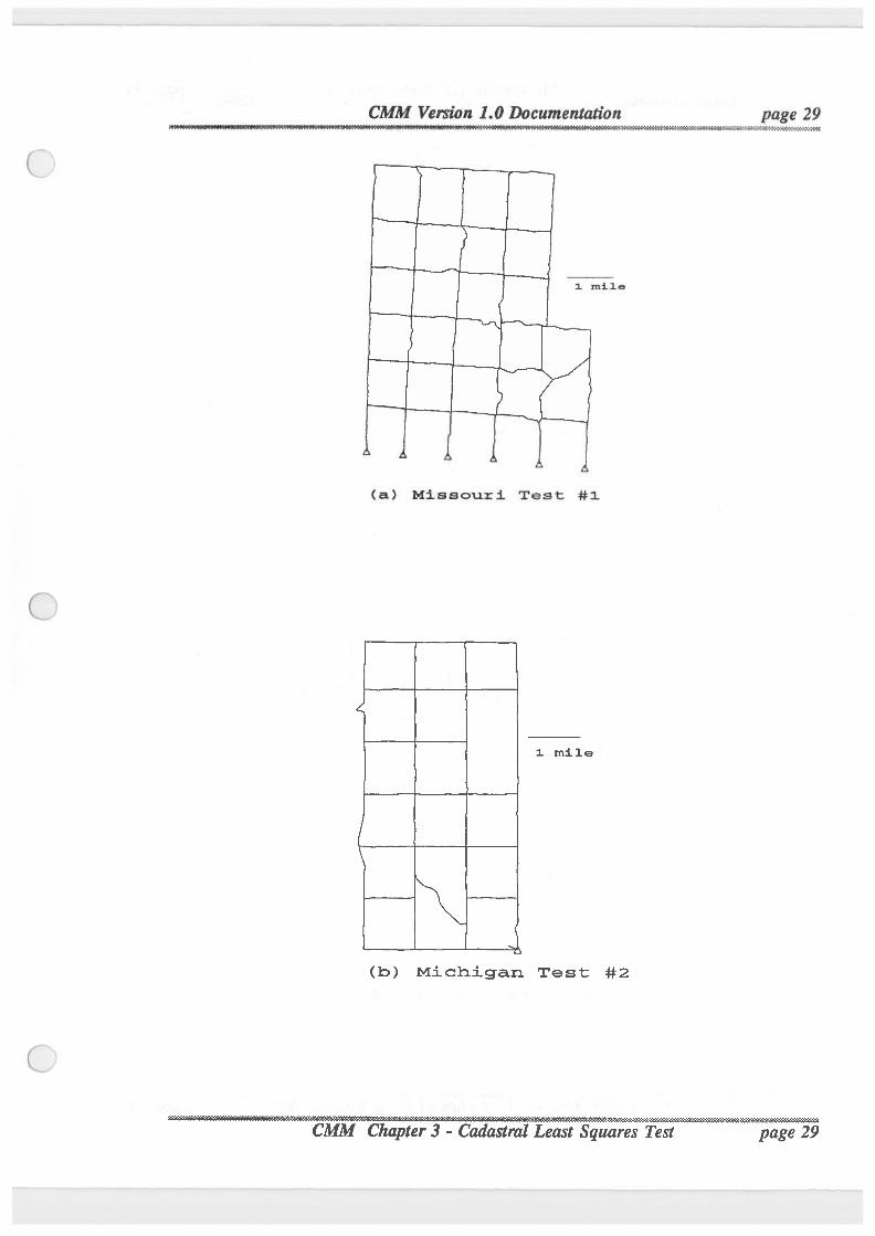
1 mile

(a) Missouri Test: #1

1 mile

(b) Michigan Test #2

CMM Version 1.0 Documentation

Test

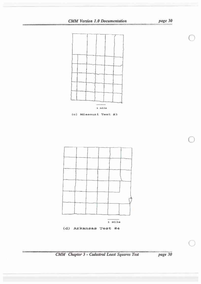
1 mile

(c) Missouri Test #3

CMM Version 1.0 Documentation

1 mile

(d) Arkansas Test #4

ést ‘ia’&ms11cb&1:3:i:i:-. . . .

_:_~'v.~’:Q.:‘a.n.-.-:-a-:-

page 30

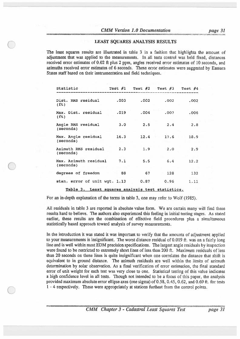
CMM Version 1.0 Documentation page 3........ . . .. . . . V . 59,99“

LEAST SQUARES ANALYSIS RESULTS

The least squares results are illustrated in table 3 in a fashion that highlights the amount ofadjustment that was applied to the measurements. In all tests control was held fixed, distancesreceived error estimates of 0.02 ft plus 2 ppm, angles received error estimates of 10 seconds, andazimuths received error estimates of 6 seconds. These error estimates were suggested by EasternStates staff based on their instrumentation and field techniques.

Statistic Test #1 Test #2 Test #3 Test #4

Dist. RMS residual .003 .002 .002 .002(ft)Max. Dist. residual .019 .004 .007 .006(ft)Angle RMS residual 3.0 2.5 2.4 2.8(seconds)Max. Angle residual 16.3 12.4 17.6 18.9(seconds)Azimuth RMS residual 2.3 1.9 2.0 2.9(seconds)Max. Azimuth residual 7.1 5.5 6.4 12.2(seconds)degrees of freedom 88 67 128 132

stan. error of unit wgt. 1.13 0.87 0.96 1.11

Table 3. Least sguares analysis test statistics.

For an in~depth explanationof the terms in table 3, one may refer to Wolf (1985).All residuals in table 3 are reported in absolute value form. We are certain many will find theseresults hard to believe. The authorsalso experienced this feeling in initial testing stages. As statedearlier, these results are the combination of effective field procedures plus a simultaneousstatisticallybased approach toward analysis of survey measurements.

In the introduction it was stated it was important to verify that the amounts of adjustment appliedto your measurements is insignificant. The worst distance residual of 0.019 ft. was on a fairly longline and is well withinmost EDM precision specifications. The largest angle residuals by inspectionwere found to be restricted to extremely short lines of less than 200 ft. Maximum residuals of lessthan 20 seconds on these lines is quite insignificant when one correlates the distance that shift isequivalent to in ground distance. The azimuth residuals are well within the limits of azimuthdetermination by solar observation. As a final verificationof error estimation, the final standarderror of unit weight for each test was very close to one. Statistical testing of this value indicatesa high confidence level in all tests. Though not intended to be a focus of this paper, the analysisprovided maximum absolute error ellipse axes (one sigma) of 0.58, 0.45, 0.62, and 0.69 ft. for tests1 - 4 respectively. These were appropriately at stations furthest from the control points.

Test page 31

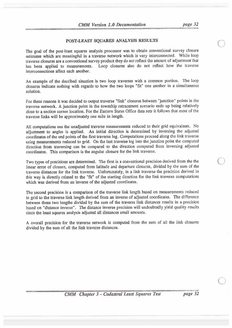
CMM Version 1.0 Documentation page 32- -

:<¢msr..w.v.~:9:-asezx-:23-:<-:¢¢:acrA4-roe-:-:-:¢ac¢cI.oc<-:<<c<<-no::u<«~o:o:4-:-:«:-:-:<-:-:->:~>:-:¢<-

POST-LEAST SQUARES ANALYSIS RESULTS

The goal of the post-least squares analysis processor was to obtain conventional survey closureestimates which are meaningful in a traverse network which is very interconnected. While looptraverse closures are a conventionalsurvey product theydo not reflect theamount of adjustmentthathas been applied to measurements. Loop closures also do not reflect how the traverseinterconnections affect each another.

An example of the decribed situation is two loop traverses with a common portion. The loopclosures indicate nothing with regards to how the two loops "fit" one another in a simultaneoussolution.

For these reasons it was decided to output traverse "link" closures between "junction" points in thetraverse network. A junction point in the township retracement scenario ends up being relativelyclose to a section corner location. For the Eastern States Office data sets it follows that most of thetraverse links will be approximatelyone mile in length.All computations use the unadjustedtraverse measurements reduced to their grid equivalents. Noadjustment to angles is applied. An initial direction is determined by inversing the adjustedcoordinates of the end points of the first traverse leg. Computations proceed along the link traverseusing measurements reduced to grid. On the last traverse leg into thejunction point the computeddirection from traversing can be compared to the direction computed from inversing adjustedcoordinates. This comparison is the angular closure for the link traverse.

Two types of precisions are determined. The first is a conventional precision derived from the thelinear error of closure, computed from latitude and departure closures, divided by the sum of thetraverse distances for the link traverse. Unfortunately, in a link traverse the precision derived inthis way is directly related to the "fit" of the starting direction for the link traverse computationswhich was derived from an inverse of the adjusted coordinates.

The second precision is a comparison of the traverse link lengthbased on measurements reducedto grid to the traverse link lengthderived from an inverse of adjusted coordinates. The differencebetween these two lengths divided by the sum of the traverse link distances results in a precisionbased on "distance inverse". The distance inverse precision will undoubtedly yield quality resultssince the least squares analysis adjusted all distances small amounts.

A overall precision for the traverse network is computed from the sum of all the link closuresdivided by the sum of all the link traverse distances.

.

7."i','6.°.".3§311\".9.i'§‘tQR«'9}-‘.'¢':~'!-'-‘-'-'53?-‘5:3: Test page 32

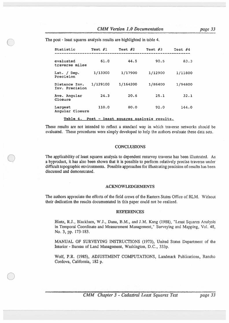
The post - least squares analysis results are highlighted in table 4.

Statistic Test #1 Test #2 Test #3 Test #4

evaluated 61.0 44.5 90.5 83.3traverse miles

Lat. / Dep. 1/13300 1/17900 1/12900 1/11800Precision

Distance Inv. 1/129100 1/164200 1/86400 1/94800Inv. Precision

Ave. Angular 24.3 20.6 25.1 32.1Closure

Largest 110.0 80.0 92.0 144.0Angular Closure

Table 4. Post — least sguares analysis results.

These results are not intended to reflect a standard way in which traverse networks should beevaluated. These procedures were simply developed to help the authorsevaluate these data sets.

CONCLUSIONS

The applicabilityof least squares analysis to dependent resurvey traverse has been illustrated. Asa byproduct, it has also been shown that it is possible to perform relatively precise traverse underdifficulttopographicenvironments. Possible approaches for illustratingprecision of results has beendiscussed and demonstrated.

ACKNOWLEDGEMENTS

The authorsappreciate the efforts of the field crews of the Eastern States Office of BLM. Withouttheir dedication the results documentated in this paper could not be realized.

REFERENCES

Hintz, R.J., Blackham, W.J., Dana, B.M., and J.M. Kang (1988), "Least Squares Analysisin Temporal Coordinate and Measurement Management," Surveying and Mapping, Vol. 48,No. 3, pp. 173-183.

MANUAL OF SURVEYING INSTRUCTIONS (1973), United States Department of theInterior - Bureau of Land Management, Washington, D.C., 333p.Wolf, P.R. (1985), ADJUSTMENT COMPUTATIONS, Landmark Publications, RanchoCordova, California, 182 p.

CMM Version 1.0 Documentation 'VWWW”:-X‘:'>3->1-3I‘:‘2-Ibi-L21’.<{-14>:-1‘:-2-i

N ~ ;:::>s2w»'a.ez'4::-;:

page 34

CMM Version 1.0 Documentation page 35. '2-2*Z1'5'$>X-2'M¢K*}NN'3H Wfi9fi€¢M¢fiV‘NM#fiZ4*2-§}%1‘XW

Qhgptgr 4 - Overview and Introduction to the T991 Bo;CMM contains many functions, many of these functions are in modular form and currentlyare actually contained in separate programs. Later on in theReference chapter there willbe a more in depth description of some of these programs, however at thispoint we wouldlike to give you a short introduction to most of these programs grouped into roughfunctional areas. This ist does not necessarly represent the order in which you might usethese program.

Data Input ProgramsGENER

GENER’s ultimate purpose is first coordinate approximation generation, which isnecessary for theLeast Squares analysisprocess. However, it's front end is designedfor manual data entry and editing of the primary measurement data.

ESOData Collection conversion for Eastern States Office data collection files. These filesmust first be transferred to the PC.

TDSLSAData Collection conversion program for the TripodData Systems (TDS) C0-0P4]data collection format. This program is preliminary.

ARIZONAData Collection conversion program for the Custom BLM C0-0P41 data collectionformat as designed by Olian Shockley. This program is preliminary.

LIETZData Collectionconversionprogram for theLIETZ SDR24 (and other) data collector.This program is preliminary.

Mggurgmgnt ProcgsingCMM

Is the command you type to get into the system. CMM is actually a DOS batch filecreated by the INSTALL program and runs MANAGE.

MANAGEIs the CMM Main Menu. Besides providing menu access to several of themeasurement functions. MANAGE allows you to create, select and define projectparameters such as State Plane Zone. It, through CMM provides access to the workhorses GENER, LSAQ, DXFLSA, your text editor and access to the CadastralUtilitiessub menu.

.......................................................~.

CMM Version 1.0 DocumentafipGENER

Discussed above under data entry, also serves as an important role in processing byproviding the basic data file for the system (the LSA file), and computing initialcoordinates and closures for the traverse data to date.

SD allows you to supply individual (rather than cross the board) error estimates.CMM and Manage prompt you for default error estimates for your measurements,such as control, azimuths (solars), angles and distances. This is important since one

frequently encounter situations where the default errors are not valid such as whenyou go thru some short shots, or unstable setups, etc.

SSHOTYou can put your sideshots into GENER along withyour other data, but they do notdo anythingto help the analysis, they cannot provide any redundancy to the systemand end up slowing the processing down for nothing. If sideshots are ALWAYSgoing to remain so (you have no intent to ever tie in the point another way), they arebest entered here. Not used much it happens.

Measurement AnglysisGENER

As above, but GENER’s closure’s are your first indicationof errors. Because of it'smethods, it caimot be relied upon for precise closure numbers, but the first largemisclosure it encountered points to problems in that loops data. Subsequent loopsmay look bad but could be okay.

BLUNDERUsed to bepart of GENER, now a standalone. BLUNDER applies a few geometricmethods to try to find angle and distance blunders. This will be added to. It’scurrent methods sometimes fail on rectangular data. So don’t believe it if it doesn’ttell you anything.

RAWA special version of GENER. This program runs your traverse data from the LSAfilewithoutadjustment. If a major blunder exists in the data it can usually be seenmore clearlyhere thanwithGENER’s report. RAW creates a VIEWable fileas wellas a report.

LSAQThe main Least Squares Analysis program. Through the process of error estimates,and looking at the results of the adjustmentcontained in the .LSA filethere is a greatdeal of informationabout large and particularly small errors. The combinationof allyour measurements and their redundancy is the key.

»€—\-,

933$“

page 37' "2W'W\

.

.. .>5’-‘5'€'€'Z-I-.‘3-.'~3'€'

CHECKERServes two purposes: First compares closing raw measurements to adjustedconnection points, and is the closest analogy to "What is the precision ratio" for thistype of system. Carefully used, CHECKER can also lead you to locate many errorsand blunders in your data. This is true because while many measurements ‘give’becauseof bad data, the line with the error will likely have the largest misclosure.

CMM Version 1.0 Documentation. . . . -Z‘W#> »8$Vfi}QX&

.

VIEWA screen graphics program that allows you to view your traverse files. This versionallows panning and zooming as well as toggling point id’s and has many otheroptions.

DXFLSA (a batch filewhich runs DRAW )Creates a graphics DXF filewhich can be viewed or exported to a CAD system andused to obtain hardcopy. Graphics can point to strange thingsthatthesystem is doingto your data when you have very large problems.

LOOPERAllows you to cut out a section of raw data from a large project and create a smallerdata set. This can be of help for two reasons. 1) to help locate errors or blundersknown to be in one area. To eliminate excess processing time recomputing good datain other areas of the project.

COMBINCombines projects. You can work separate projects or parts of projects, thenCOMBINe them into one once they are connected.

COMPARECompares two .COR coordinate files. This is useful after trying different weightingoptions, or comparing common lines between data sets to see if the real difference isof any importance.

page 37

n 1.0 Documentatw page 38W&i R‘N~'o~N'€-3'2'1'X~2iG-°.'1'l:I<'5-?»‘0¢£'3tl>vZ¢€‘fi‘°.’.'3'G'€4€¢€~1*.'-1‘*R4¢KebX€‘1-(«>2-C-&NC"'->‘.>."€-50->3‘

PLSS ggtgm hgngling QmpgtationsCSTUF

Provides a multitude of PLSS datum computations. See extensive documentation inthe Reference Section. True and/or Plane traversing, inversing, all kinds ofintersections. Can be used readily to develop search areas, one, two and 3 pointcontrol and subdivide sections, inverse to get Mean True line. AREA computationis not fully worked out yet.

INRECInrec is a very important program thatallows you to easilycreate the .REC record filethat is used by the PROPORT and AUTOPROP proportion programs. This isessentially a digital record plat upon which all proports are based and thus it is veryimportant to verify all entries are correct since all future proportions are base uponthem. It is possible to use non-standard corner naming but in general the systemfunctions best and is really designed to take advantage of theorganisational attributesof the standard numberingscheme.

WHATISAnother important program. WHA'I‘IS is the means we have to define which of thetraverse points in your project ARE to be considered or are accepted as corners, andthus to be used for proportions. It is also possible to tag each traverse point and/orcomer with attributes such as original, local etc. This does not serve any function atpresent, but may beused in the future to provide symbology with the output graphics.The programs AUTOPROP, PROPORT, SECTSHOW all use this record file forproportions.

PROPORTThe corner by corner PROPORTion program, performs single and doubleproportions geodetically correct.

AUTOPROPA wonderful program thatperforms mass proportions and even normal subdivision ofsection automatically based upon the control you have currently defined withWHA'l‘IS and the record file you have built with INREC. Primarilydeveloped toallow for generation of search areas, may be used also as a independent check onPROPORT for proportions and CSTUF for subdivision of sections.

CMOVEA program that computes comer moves andlor offsets to true line.

ADJUST

A program thatprovides for Grant boundary, Irregular boundary and Compass (non-riparian meander line) adjustments, as well as 1, 2 and 3 point control and manualversions of single and double proportions.

' r-'-J‘?&£fiW

page 38

UTCOMM

The Utilitiesmenu program. Uses the fileUTCOMM.PRGto define any number ofuser programs. This program has been enhanced to work with a broader range ofgraphics cards and the definition file it uses is customisable by the user in terms ofcolors as well as to add programs. (See installation section Appendix 1.

CONVERTGeneral purpose State Plane < -> Geodetic conversion program. The initial LeastSquares Analysis produces a geographic coordinate file, however subsequentprograms, and many of theutilitiesworkprimarilywith the .COR file, so if lat/longsare desired for those additionalpoints the .COR filecan be processed into geographiccoordinates with CONVERT.

PROJECA direct program to create a project definition file (.DEF). Normally not neededbecause the CMM-MANAGE Main Menu System performs essentially the samefunction. However, the MANAGE does not allow you to assign extreme unrealisticerror estimate values. Sometimes that is useful in searching fof blunders. PROJEChas no such limitation.

LOOKLook is a file browsing utility. CMM operation produces many report and outputfiles,many of which it is essential to examine. LOOK allows theuser to select fromamoung the files produced for the project and view (withoutedit ability)them.

TE/RUNTEA public domain text editor supplied withthe system. Associated documentation filesand configurationprograms are included with the system.

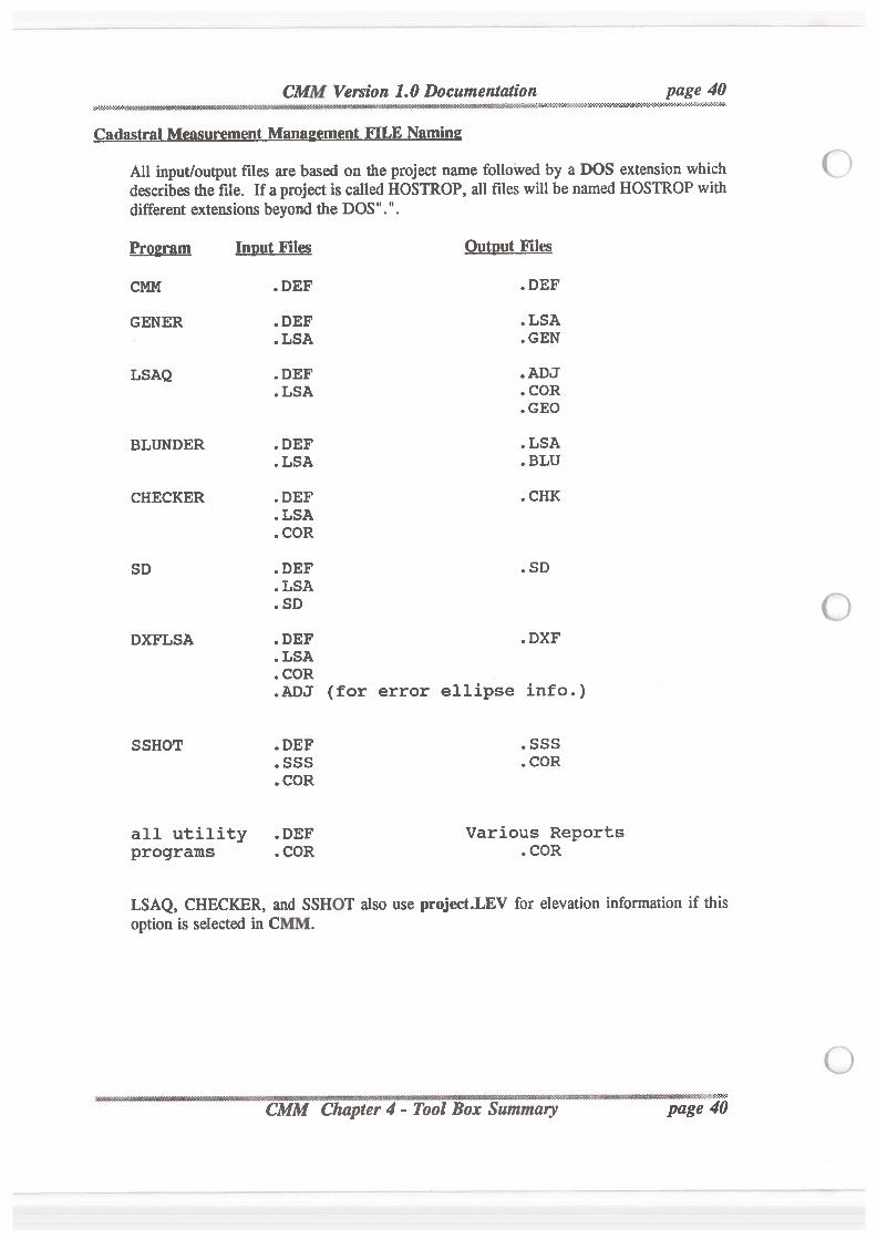
CMM Version 1.0 Docnmentqtion page 40-'-" « WRt344%W¢W¢}3fiW# ‘NN}fiW&WI-#1-#3}:-$#)2-5%.

Cggastrgl Mgggrgmgnt Mgngggmgnt FILE NgmingAll input/output files are based on the project name followed by a DOS extension whichdescribes thefile. If a project is called HOSTROP, all fileswillbe named HOSTROP withdifferent extensions beyondtheDOS"

.".

Prggmm Inpgt Filg Qgtput Files

CM .DEF .DEF

GENER .DEF .LSA.LSA .GEN

LSAQ .DEF .ADJ.LSA .COR

.GEO

BLUNDER .DEF .LSA.LSA .BLU

CHECKER .DEF .CHK.LSA.COR

SD .DEF .SD.LSA.SD 'i

DXFLSA .DEF .DXF.LSA.COR.ADJ (for error ellipse info.)

SSHOT .DEF .SSS.SSS .COR.COR

all utility .DEF Various Reportsprograms . COR . COR

LSAQ, CHECKER, and SSHOT also use project.LEV for elevation information if thisoption is selected in CMM.

CMM Version 1.0 Documentation page 41

Preliminary Details;

Tym 91' Data - Mggrgmgntgg

CMM processes measurements that are already reduced. Such as:

Mgnfl Anglg gjgh;Angles left may be entered, but they are converted to angles right.

Hgrimntgl Distgng at ground glgvgtign.Default units are feet, this can be changed withinan entry session or overridden perentry to Feet, Chains and/or Meters entry.

Other data that is required before a job can be completed are:

figggig QontrolFor at least one point on thejob site. Scaled data is adequate to allow the system toproperly compute proportions, etc. and return correct true bearings. If good controlis later tied in it can be added to thedata and theproject quicklyrerun to produce truevalues.

AzimuthQgntrglThis will usually be in the form of astronomical observations, azimuth marks ORmore than one control point on the project. Azimuths can be either true forwardazimuths, OR grid azimuths, but grid & true cannot be mixed withinone project.

Bi fa ntr"

In the future the goal we hope to have most of the field data transferred from a datacollector thatwill collect and maintain raw measurement data and create files compatiblewith CMM. This version of CMM contains a few data collection conversion programs,these are rudimentary at this time.

For many users data will have to be manually entered. This is most efficientlydone thruthe front end functions of the GENER program.

. ................................................................................................................................................................................................................................ ._........................................................_ __

CMM Chapter 4 - Too Box Summary page 41

CMM Version 1.0 Documentation page 42

Other skillggf vglgg

Kngwlfigg gf DOS - This system has made an attempt to provide a functional andunderstandable user interface. This can always use improvement and this is recognized.The system is also operating a rather complex mix of functions thatcreates quit a fewfileson your PC. For this reason a good workingknowledgeof thePC’s operating system DOSwillusually beof benefitto any user. Particular familiaritywithfilemanagement functionssuch as copying, and hard disk management functions such as creating and usingsubdirectories and changing drives are useful.

In the future there will be more job management fimctions in the system, for now it isuseful to know how to copy files so that you can get old jobs out of the working CMMdirectory, make copies for testing to protect the original data, and renaming files for someof the same reasons.

Special installation or customisation of the system also requires a moderate knowledge ofDOS.

Additignglflggram Dommgntgtign

There are several utility programs that are included with the system that can help youmanage your jobs. Documentation for these programs is contained in DOC files that are

included with the CMM system. These utilitiesare:

TE This is a basic Text Editor, informationon it’s commands is available both ina DOC fileinstalled with the system and by using the < F1 > key while in theeditor. The editor is exited withthe < F4> key, giving you theoption to save

a modified fileor exit without changes.LHARC This is a filecompression utility. This is useful for job storage as you can save

all the files associated with a job in one file, and in addition they will occupymuch less space. Documentation is contained in a DOC file installed with thesystem, and simple operational reminder is availableby typing LHARC(Enter)at the DOS prompt.

BATZEXECThis program allows you to compileDOS batch files into executable files. Thisallows then to be incorporated into the Uilities menu through theUTCOMM.PRG definition file.

KCThis is a capslock (and other) keyboard toggleutility.Documentation is suppliedin a filecalled KC.DOC.

-3

CMM Version 1.0 Documentation page 43 . . .

..‘ \‘M|3¢N'»€“3°'K'>Ct»Z¢‘3C'?3'$?'A‘¢‘5Ws‘VI‘3€‘.7.‘2{t’9€'5PD-PHI!-Z42‘3-5-2’?I-3*I-I'3':¢€‘N'I'IrI-i-DWOO-MD?!-I-¥I-I-C-30C-2'2-M‘!-P1-€'5-2-.‘¢':"D06’l'?I~?Z'2-2-1' .........~.

getting Hard gopySince files are the primary means of output for CMM, a direct method of obtaining hardcopy is not provided. In many cases the files and reports do not need to be printed, butin some cases printouts will be essential. For example a corner move report. Hard copyprovides additional assurance that what you did is documented.

Use your editor:

WordPerfect: ASCII or text files can be imported into WordPerfect and then printed.Using a wordprocessor to perform this function allows you the maximum flexibilityto document multiple files in you job, and to print to a wide variety of printerhardware.

MultiMate: same as for WordPerfect.

Other: There are a number of other editors you may use or install with the system,for example WordPerfect’s Program Editor has a print option.

DOS’s PRINT command:

Dos contains several ways to print files, one of which is the PRINT command, checkyour DOS manual for how this operates.

TEAllows sections of text to be blocked and sent to a printer.

LOOKAllows sections of text to be blocked and sent to a printer.

'I CMhapter 4 - Tol Box Sty page 43

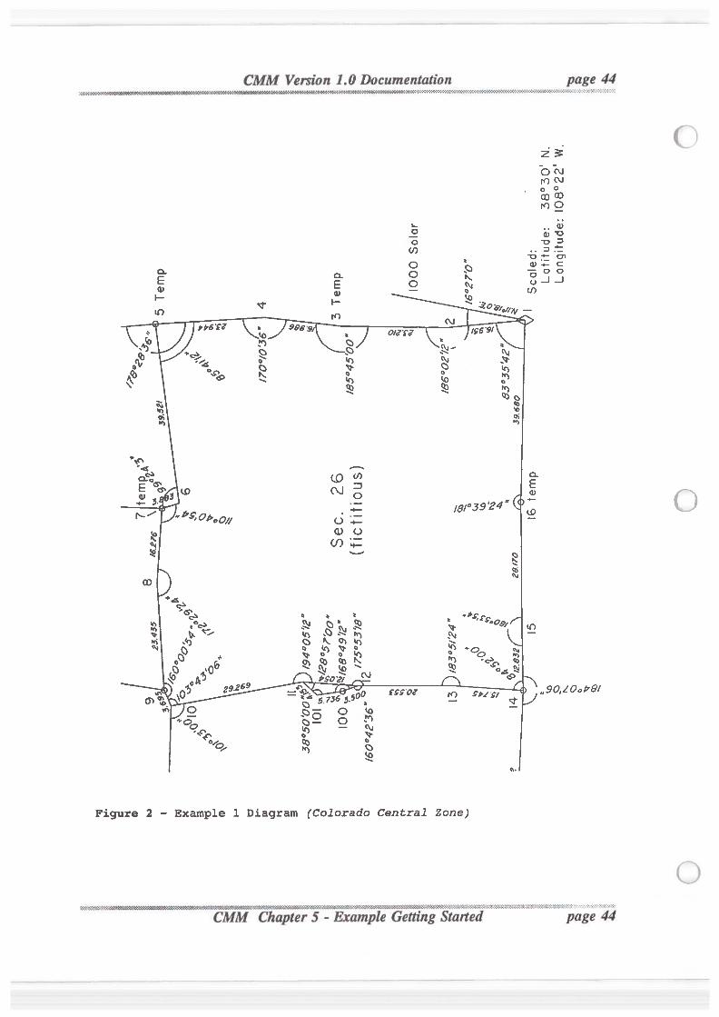
"chapter 5i3“E’§’Z”}7i}7z‘2W53”i?i'&}iW}aned

Figure 2 - Example 1 Diagram (Colorado Central Zone)

I<<#Z9§Wh 'WW€W% .

D.EQ)I-I0

Sec.26 (fictitious)

'8’-°45'00"IOOOSolar

CMM Version 1.0 Documentation

0.E0I-N‘)

/86°0276'‘"

35 §5

“J

I6temp

Scaled: Latitude:38°30'N.

Longitude:IO8°22'W.

,,.90,l0oP9/

page 4{

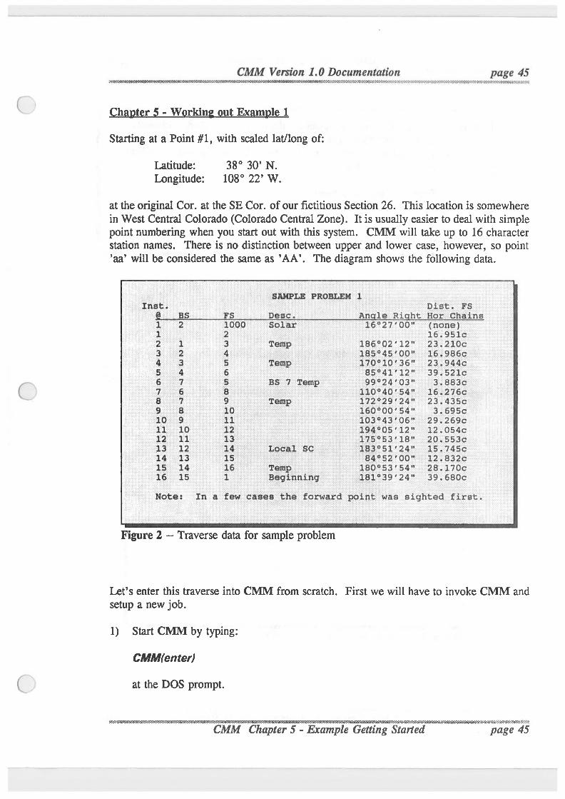
CMM Version 1.0 Documentation page 45'-:-L~:+:-o-:\><:'.«;-:-:¢:-329%-:-:-:-:-:-:-:-:-:-:-:-:-:-:-:-:-:v:-:- WISE. ' e -:-I~i-I-I-I<I{£-:41‘$034:'1'1fl'1-}1<'i‘1'I".'I'€"?3'$:¢Q'D'3'l<v1l2'2-RA:-)3-I-1-I

Chapter 5 - Working out Example 1

Starting at a Point #1, with sealed lat/long of:

Latitude: 38° 30’ N.Longitude: 108° 22’ W.

at the original Cor. at the SE Cor. of our fictitious Section 26. This location is somewherein West Central Colorado (Colorado Central Zone). It is usually easier to deal with simplepoint numbering when you start out with this system. CMM will take up to 16 characterstation names. There is no distinction between upper and lower case, however, so point’aa’ will be considered the same as ‘AA’. The diagram shows the following data.

SAMPLE PROBLEM 1Inst. Dist. FS

Q 55 E Deac. Angle Right Hor ChainsSolar 16°27'00" (nonej

16.9515-Temp 186°02'12" 23.210c

185°45'00" 16,9B6cTemp 170°10'36" 23,944c

85°41'12" 39.521cas 7 temp 99°24'03" 3.883c

110°40'54" 16.276cIemp 172°29'24" 23.435c

' 160°00'54" 3.695c103°43'06" 29.269c194°05'12" 12.054c175°53'18" 20.553c

Local sc 133°51'24" 1s.74sc84°52'00" 12.832c

Temp 180°53'54" 28.170cBeginning 181°39'24" 39.680c

\D<DU'lU\LflnIhh.I}dl-I DU!0"O112345.6739

(DE-JU\-I-hh.IBJl-INI

Note: In a few cases the forward point was sighted first.

Figure 2 -- Traverse data for sample problem

Let’s enter this traverse into CMM from scratch. First we will have to invoke CMM andsetup a new job.1) Start CMM by typing:

CMM(enter)

at the DOS prompt.

‘ ’» 5:3‘a.“-‘.§3.5".i‘.«’$:1:-‘.;:i*ltR3'.E:h'£3?27:i'i*>l‘

page 45

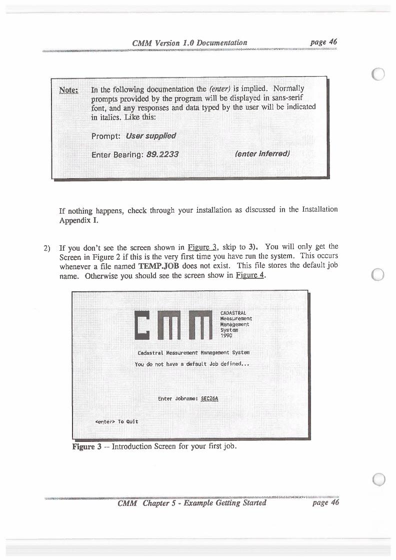
2)

CMM Version 1.0 Documentation page 46'

.

' ' ' '. .W&h‘flKfi%'& #%V9N+WW0flWEI?-N-Cniiwl4'2-24:‘:-3'!-2-5~K-Iiixfiirl-Z'ZsN4~5-E-i-KC-2-E4-3-2-Ci-('1-Z-Z-1‘1*1<-I-K-W?it-:-€€~!<-3-W-t-I-C-I-I-I-2-I-I0:-twirlJ-J-2‘:

In the following documentation the (enter) is implied. Normallyprompts provided by theprogram willbe displayed in sans—seriffont, and any responses and data typed by the user will be indicatedin italics. Like this:

Prompt: UsersuppliedEnter Bearing: 89.2233 lenter inferred)

If nothing happens, check through your installation as discussed in the InstallationAppendix I.

If you don’t see the screen shown in Figure 3, skip to 3). You will only get theScreen in Figure 2 if this is the very first time you have run the system. This occurswhenever a file named TEMP.JOB does not exist. This file stores the default jobname. Otherwise you should see the screen show in Figure 4.

CADASTRALM

‘ tleasjurement.Haneigetnent

.

System1990

Cadastral Measurement Management SystemYou do not have a default Job defined...

Enter Jobname: sEcg6A

<enter.> To Gui t

Figure 3 -— Introduction Screen for your first job.

41-). (I: .‘.::.'i-:-

- g §;;,;e&

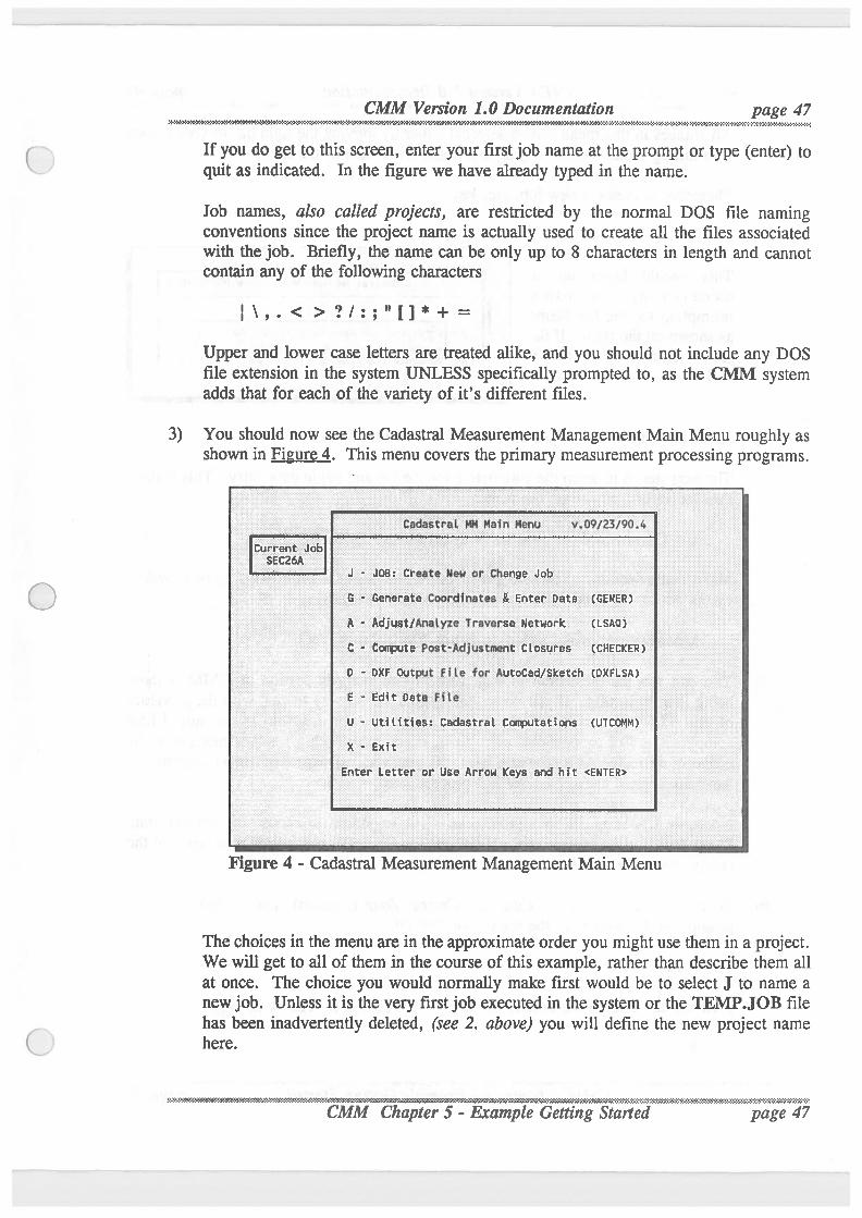
3)

CMM Version

page 47. . . . Z‘9V.¢’.'?Z'i-2-X'>W§X-}1:3:'4*1'¥D->M‘5-1'3-I->1‘ K-M-5>€M>:-1-I‘:-I-1->1-G-G-ll".-‘.¢Z-7»?-D0'?¢'2

1.0 DocumentationN9H’M*1'¢"

If you do get to this screen, enter your first job name at the prompt or type (enter) toquit as indicated. In the figure we have already typed in the name.

Job names, also called projects, are restricted by the normal DOS file namingconventions since the project name is actually used to create all the files associatedwith the job. Briefly,the name can be only up to 8 characters in length and cannotcontain any of the following characters

:\,.<>?/:;"[]*+=Upper and lower case letters are treated alike, and you should not include any DOSfileextension in the system UNLESS specifically prompted to, as the CMM systemadds that for each of the variety of it's different files.

You should now see the Cadastral Measurement Management Main Menu roughly asshown in Figure 4. This menu covers theprimary measurementprocessing programs.

Cadastral. an Main? menu ’v..o9/'23/9o.z.Current: Job

SEC26A" J - JOB: create Diet: or change Job

6 - nenerete coordinates 8. Enter abate‘ (GENER)A - Adjust/Analyzetraverse-NetworkC -‘ Coll?!‘-It? Pflsuii-ldlustment Cl~osm3,es

(LsAa)(CHECKER)

D - DXF output File for Autocagysketch (DXFLSA)E — Edit Data FileU - Utilities: Cadastral computationsX - Exit

(UTCOMM)

Enter Letter or Use. Arrow Keys and hit <ENTER>

Figure 4 - Cadastral Measurement Management Main Menu

The choices in the menu are in theapproximate order you might use them in a project.We will get to all of them in the course of this example, rather than describe them allat once. The choice you would normally make first would be to select J to name anew job. Unless it is thevery first job executed in the system or the TEMP.JOB filehas been inadvertently deleted, (see 2. above) you will define the new project namehere.

WW‘ V‘ V- -0 \'\ *fiB$%9fl W$5:&h$i$'%%SfinY ‘¢$9w£'rt$&Y¢&}#.W¢»%W5&ri -lGetting Started page 47

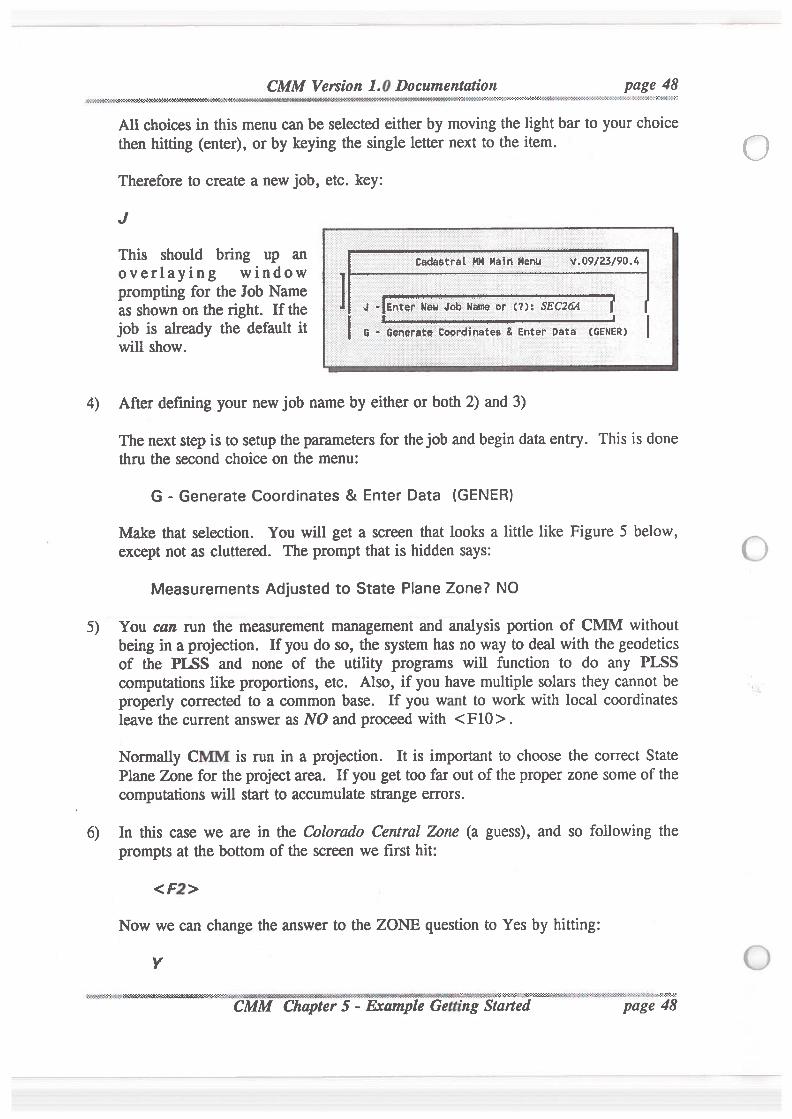
CMM Version 1.0 Documentation Wpoge'_4§« t -- ..-Me4-a-a-o-:-o-w-a-cc-:«:a:-:-2-zaz-:-:-:~:~:~:~:¢cc-:-rm’:»>;-9:-:-:r.~owc«:<«:-:~:~:-:->:¢:-.......... . . .4.-:-:9-t.VHO¢’.¢’

.. . . .“«m>:-c«-°.

All choices in this menu can be selected either by moving the light bar to your choicethen hitting (enter), or by keying the single letter next to the item.

Therefore to create a new job, etc. key:J

Th” Sm"-Id mg-

"P a"overlaying WlIld0W

.

—

.

Pfompting for the Job Name. .. . . ..

as shown on the the ...

J ' Enter NBH Job Name or (7): SECZGA

job is already the default it ‘ G -Hsenereteiilfoordinatesii Enter beta (GENER) iwill show.

4) After defining your new job name by either or both 2) and 3)

The next step is to setup theparameters for thejob and begin data entry. This is donethru the second choice on the menu:

G - Generate Coordinates & Enter Data (GENER)

Make that selection. You will get a screen that looks a little like Figure 5 below,except not as cluttered. The prompt that is hidden says:

Measurements Adjustedto State Plane Zone? NO

5) You can run the measurement management and analysis portion of CMM withoutbeing in a projection. If you do so, the system has no way to deal with the geodeticsof the PLSS and none of the utility programs will function to do any PLSScomputations like proportions, etc. Also, if you have multiple solars they cannot beproperly corrected to a common base. If you want to work with local coordinatesleave the current answer as NO and proceed with <F10>.

Normally CMM is run in a projection. It is important to choose the correct StatePlane Zone for theproject area. If you get too far out of theproper zone some of thecomputations will start to accumulate strange errors.

6) In this case we are in the Colorado Central Zone (a guess), and so following theprompts at the bottom of the screen we first hit:

<F2>

Now we can change the answer to the ZONE question to Yes by hitting:

- ~ ->'2?I.'-".-'.?«!"0S‘-2-, - - -

"-» v<'<3€'~'3!3«'§<".‘6:3:?kV$1 2?:1:~:3:¢:i:i!°'3‘.3Ei?3‘.1231Q3Sfi%'£-'3'7!-53:33!‘'§¢TExompleH

Getti g Started pag ‘iii

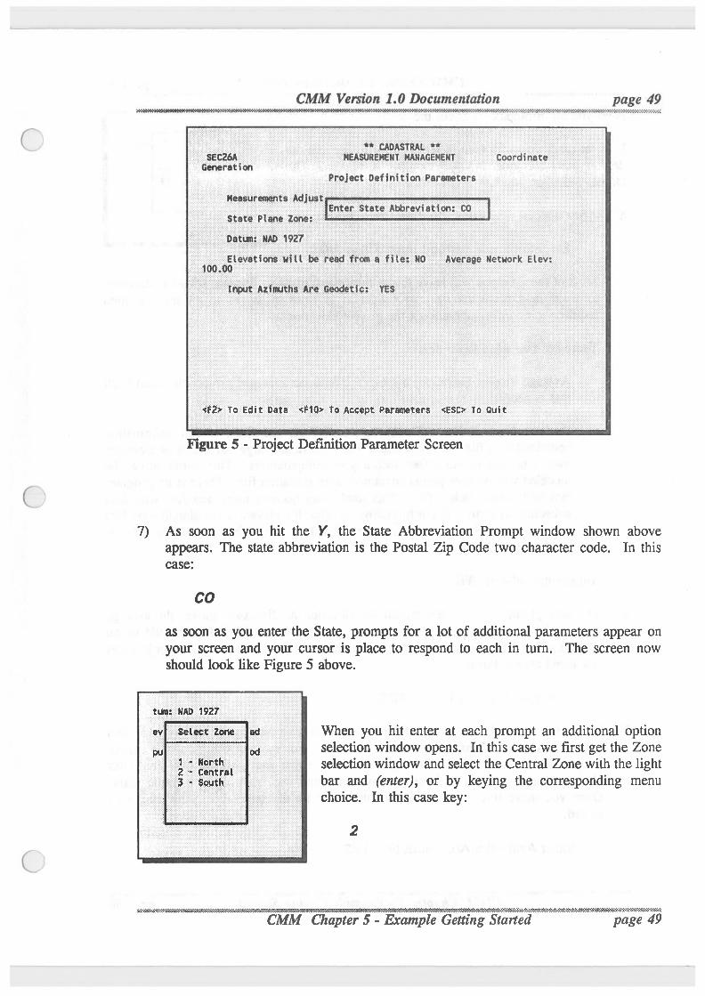
CMM Version 1.0 Documentation page 49".‘<W)'I)9KvN".*3V¥3x"£'I'I'I-1'}'1:Pk‘?H‘1'L':\E('2'Ni‘P'»PX"Kl)0:3I'?JOJ§D72-PN};v:-;v‘_\Q:a-::a¢.;¢¢-_.-_¢.;.\;.—_.;

*- caonsmu. H‘SECZGA HEASURENENT KANAGEHEHT Coordinate

GenerationProject Definition Parameters

Measurements Adjust ’-

Enter State .Abb_reviat_i_on: C0 Datum. mu: 1927'

um “Elevations will be .'read. from a file‘; ND five;-age Network Elev:

Input Azinuths are Bed:ciIéti'e.: YES

<F2> To Edit Data <F10> To Accept Parameters <ESc> To Ouit

Figure 5 - Project Definition Parameter Screen

7) As soon as you hit the Y, the State Abbreviation Prompt window shown aboveappears. The state abbreviation is the Postal Zip Code two character code. In thiscase:

C0

as soon as you enter the State, prompts for a lot of additional parameters appear on

your screen and your cursor is place to respond to each in turn. The screen nowshould look like Figure 5 above.

:ug_:_ NAD 1927ad When you hit enter at each prompt an additional option

" selection window opens. In this case we first get the Zoneselection window and select the Central Zone with the light

3 - south bar and (enter), or by keying the corresponding menuchoice. In this case key:

2 - cé.nt:'.ral

2

H CMM Chapter 5 - amV tarted page 49

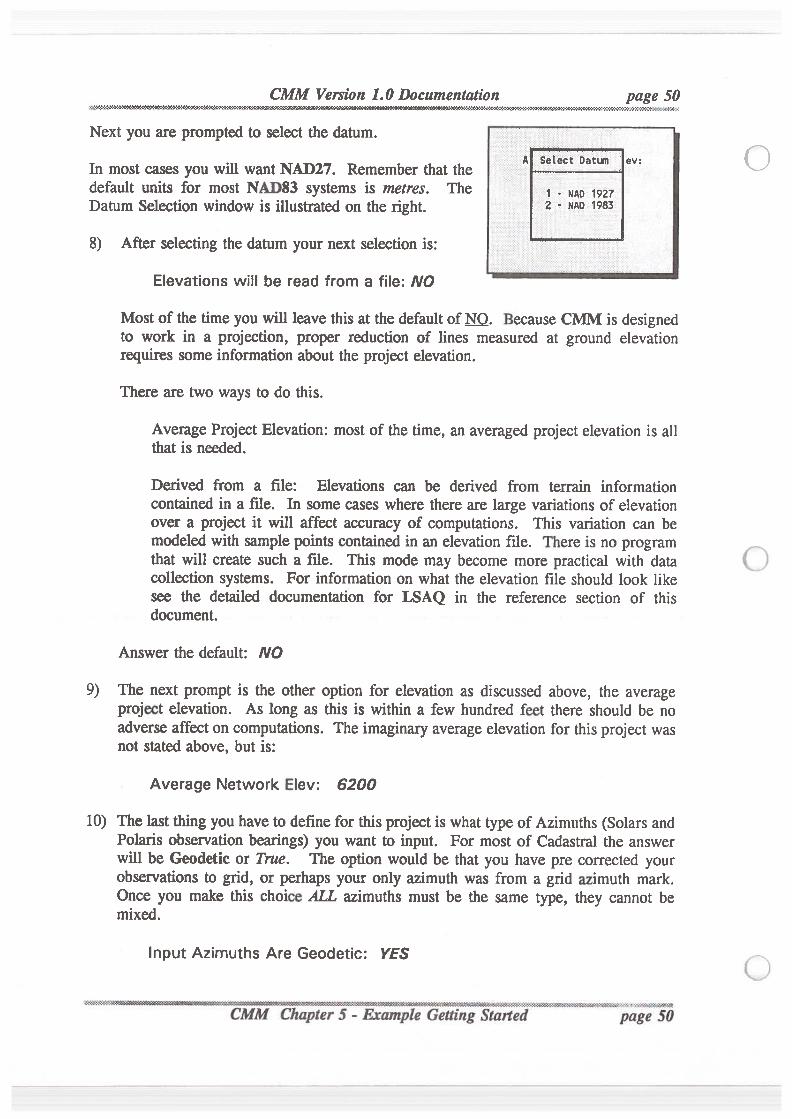
- - - - 3%KfXQ WWMW¢»’fiW44-24-3'}?!-.-9:-I-C-X-Z-C-2-M431‘:-K-2-I

CMM Version 1.0 Documentation page 50

Next you are prompted to select the datum.A‘ Select :....‘e.’..l..: jIn most cases you will want NAD27. Remember that the

default units for most NAD83 systems is metres. The 1 . "AD 1927Datum Selection window is illustrated on the right.

_

3 ' "AD 1983

8) After selecting the datum your next selection is: Elevations will be read from a file: N0

Most of the time you will leave this at the defaultof HQ. Because CMM is designedto work in a projection, proper reduction of lines measured at ground elevationrequires some information about the project elevation.

There are two ways to do this.

AverageProject Elevation: most of the time, an averaged project elevation is allthat is needed.

Derived from a file: Elevations can be derived from terrain informationcontained in a file. In some cases where there are large variations of elevationover a project it will affect accuracy of computations. This variation can bemodeled with sample points contained in an elevation file. There is no programthat will create such a file. This mode may become more practical with datacollection systems. For information on what the elevation file should look likesee the detailed documentation for LSAQ in the reference section of thisdocument.

Answer the default: N0

9) The next prompt is the other option for elevation as discussed above, the averageproject elevation. As long as this is within a few hundred feet there should be noadverse affect on computations. The imaginary average elevation for thisproject wasnot stated above, but is:

Average Network Elev: 6200

10) The last thingyou have to define for thisproject is what type of Azimuths(Solars andPolaris observation bearings) you want to input. For most of Cadastral the answerwill be Geodetic or True. The option would be that you have pre corrected yourobservations to grid, or perhaps your only azimuth was from a grid azimuth mark.Once you make this choice ALL azimuths must be the same type, they cannot bemixed.

Input AzimuthsAre Geodetic: YES

&&i: :iW&2&&k¥@kb:-'-'l‘l:--:-:.'»’I.$s-:#.'?.¢u‘r).!€'i!£

page 50

N‘

11)

12)

CMM Version 1.0 Documentation page 51WON‘X-3'3‘:-734{«VH‘*59'WH¢%Q€€‘??W'I‘???%K->2‘9T'I'0'Z'l?I'W’(’o¢'N(<*X£'XI€'C'l'Cr¢'ZW£'iv2~3'?Z-!fl'3‘:'H

Now successive entries will take you around in a circle thru the prompts. When youhave them all correct follow the information at the bottom of the screen and hit the<F10> key to accept the entries and continue.

As soon as you hit the <F10> key, the program GENER is started with the defaultproject you have just defined (set-up). GENER has 2 jobs, its ultimate goal is togenerate by any means possible coordinate estimates for all of your traverse stations.This is necessary to help out the least squares process coming up. GENER does notalways do the logical thing, or the best thing, it just gets a coordinate that should beclose. Remember it’s an estimate!!

GENER’s other big capability is that it is the primary means of manual data entry.That is entry of your traverse measurement information. The following pages containa complete dialogue of the entry of the data from the example. Comments andexplanations are shown in italics on the right side of the page. This job was enteredin such a way as to illustrate several of the options that are available.

We strongly suggest you take a zerox copy of the example diagram and/or data andfollow along closely with this dialogue.

' ' ‘,'.4-'4%->;£:-:»:-;*-‘«~oc9.‘~a29'.A'<«'u»5:c«1-5b&q5b2e.aoe'-'-5:?V ';-'2-'a''52‘!-

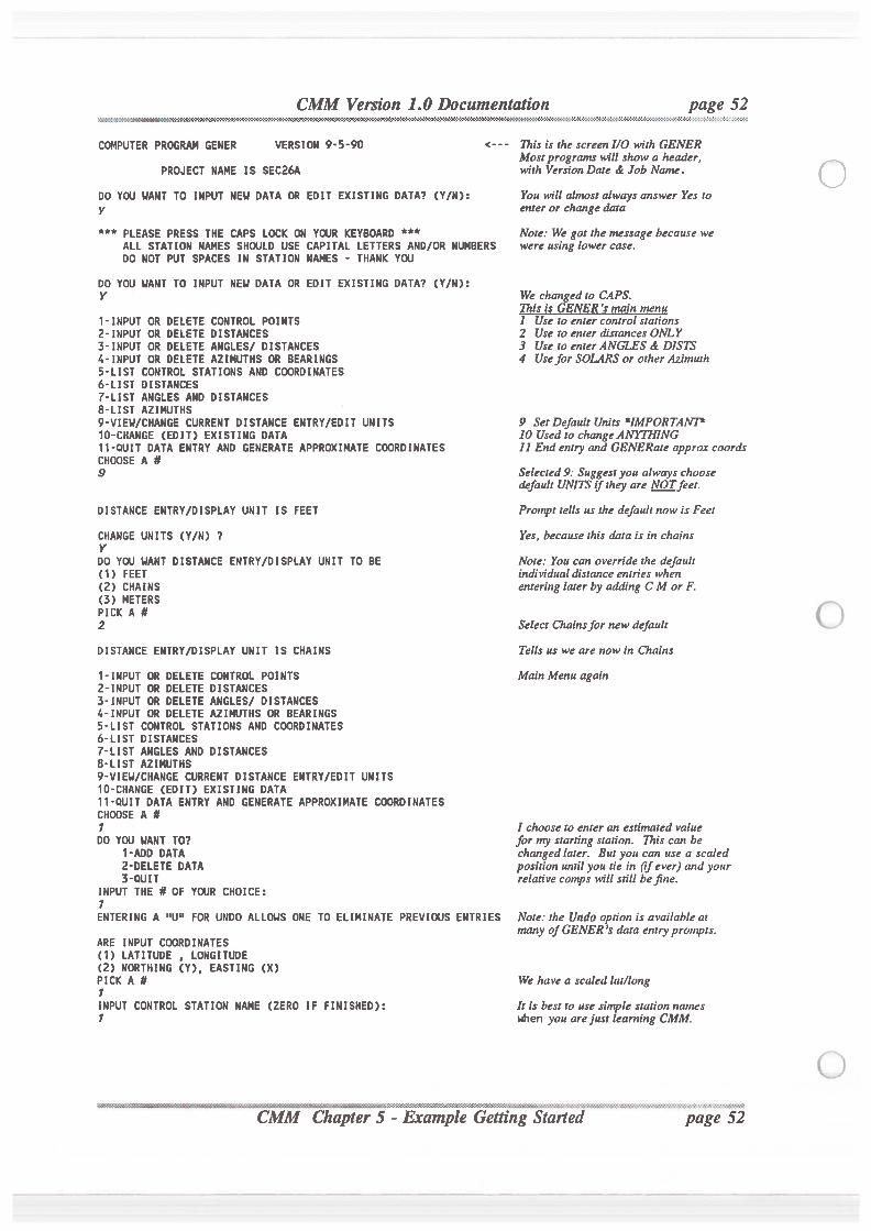
CMM Version 1.0 Documentation page 52.NWW»X ¢MNh§0NN <V»¢\W€-I-l'l'Efl-1'3‘1<’.‘€'2‘3CV3’:I'Z('X'Z¢'!'i'I'Z~J*Z'1~1¢€'€'J'l~I'I-1'1-I-M1'3 I 1-34 ‘L I . . .

‘ Ki-?li'li-:& >§%M

COMPUTER PROGRAM GENER VERSION 9-5-90 <-- - 1711': is the screen 1/0 with GENERMostprograms will show a header,

PROJECT NAME IS SEC26A with Version Date & Job Name.

DO YOU HANT T0 INPUT NEH DATA OR EDIT EXISTING DATA? (Y/N): You will almost alwaysanswer Yes toy enter or change data

*** PLEASE PRESS THE CAPS LOCK ON YOUR KEYBOARD *** Note: We got the message becauseweALL STATION NAMES SHOULD USE CAPITAL LETTERS AND/OR NUMBERS were using lowercase.DO NOT PUT SPACES IN STATION NAMES - THANK YOU

DO YOU UANT TO INPUT NEH DATA OR EDIT EXISTING DATA? (Y/N):Y We changed to CAPS.

This is GENER's main menu1-INPUT OR DELETE CONTROL POINTS 1 Use to enter control stations2-INPUT OR DELETE DISTANCES 2 Use to enter distances ONLY3-INPUT OR DELETE ANGLES] DISTANCES 3 Use to enterANGLES & DISTS4- INPUT OR DELETE AZIMUTHS OR BEARINGS 4 Use for SOLARS or otherAzimuth5-LIST CONTROL STATIONS AND COORDINATES6-LIST DISTANCES7-LIST ANGLES AND DISTANCES8-LIST AZIMUTHS9-VIEHICHANGE CURRENT DISTANCE ENTRY/EDIT UNITS 9 Set DefaultUnits ‘IMPORT/INT‘10-CHANGE (ED I T) EXISTING DATA 10 Used to change ANYTHING11-QUIT DATA ENTRY AND GENERATE APPROXIMATE COORDINATES 11 End entry and GENERate approx coardsCHOOSE A #9 Selected 9: Suggest you always choose

default UNITSif they are NOTfeet.DISTANCE ENTRY/DISPLAY UNIT IS FEET Prompt tells us the defaultnow is Feet

CHANGE UNITS (Y/N) ? Yes, becausethis data is in chainsYDO YOU HANT DISTANCE ENTRY/DISPLAY UNIT TO BE Note: You can override the default(1 ) FEET individualdistance entries when(2) CHAINS entering later by adding C M or F.(3) METERSPICK A #2 Select Chainsfor new defaultDISTANCE ENTRY/DISPLAY UNIT IS CHAINS Tells us we are now in Chains

1- INPUT OR DELETE CONTROL POINTS Main Menu again2-INPUT OR DELETE DISTANCES3-INPUT OR DELETE ANGLES] DISTANCES4-INPUT OR DELETE AZIMUTHS OR BEARINGS5-LIST CONTROL STATIONS AND COORDINATES6-LIST DISTANCES7-LIST ANGLES AND DISTANCES8-LIST AZIMUTNS9-VIEU/CHANGE CURRENT DISTANCE ENTRY/EDIT UNITS10-CHANGE (EDIT) EXISTING DATA11-QUIT DATA ENTRY AND GENERATE APPROXIMATE COORDINATESCHOOSE A it1 I choose to enter an estimated valueDO YOU HANT T0? for my starting station. This can be

1-ADD DATA changed later. But you can use a scaled2-DELETE DATA position untilyou tie in (tfever) and your3-OUIT relative comps will still befine.

INPUT THE # OF YCIJR CHOICE:1ENTERING A "U" FOR UNDO ALLOHS ONE TO ELIMINATE PREVIOUS ENTRIES Note: the Undo option is availableat

many of GENER’s data entry prompts.ARE INPUT COORDINATES(1) LATITUDE , LONGITUDE(2) NORTHING (Y), EASTING (X)PICK A # We have a scaled lat/long1INPUT CONTROL STATION NAME (ZERO IF FINISHED): It is best to use sirrple station names1 when you arejust learning CMM.

'_v-1' ‘ '%Hfi !&t-:55.’ :v'15E219333345!3'i’39'533!v$$R7C3:-'-‘C!-b‘\‘31-S359AI5%’: Example Getting Started page"‘.%§M2?

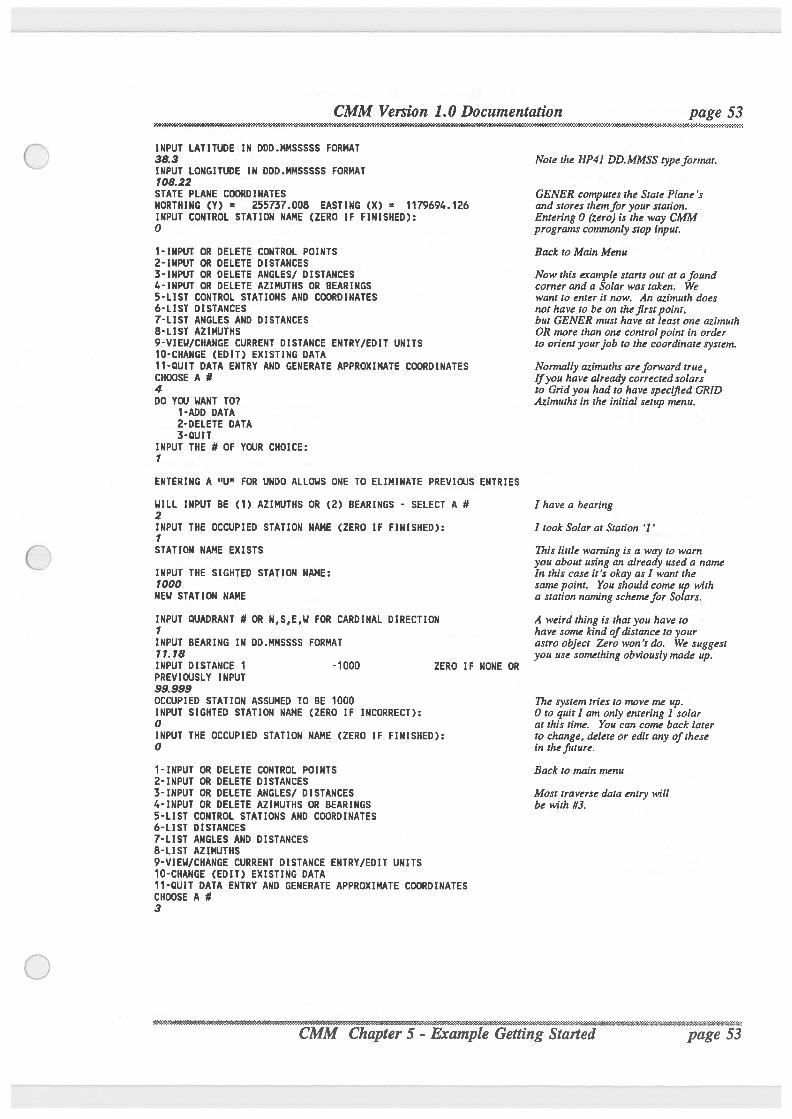
CMM Version 1.0 Documentation page 53 '

.

' AQQWWWW'7/#90“¥kXW*X'H4<’WWHhYfik '»»O%V#fi¢/#k&2£#X'S¢34

INPUT LATITUDE IN DDD.MMSSSSS FORMAT38.3 Note the HP41 DD.MMSS typeformat.INPUT LONGITUDE IN DDD.MMSSSSS FORMAT108.22STATE PLANE COORDINATES GENER computes the State Plane ’sNORTHING (Y) = 255737.008 EASTING (X) = 1179694.126 and stores themfor your station.INPUT CONTROL STATION NAME (ZERO IF FINISHED): Entering 0 (zero) is the way CMM0 programs commonly stop input.1-INPUT OR DELETE CONTROL POINTS Back to Main Menu2- INPUT OR DELETE DISTANCES3- INPUT OR DELETE ANGLESI DISTANCES Now this example starts out at it foundlo-INPUT OR DELETE AZIMUTHS OR BEARINGS comer and a Solar was taken. We5-LIST CONTROL STATIONS AND COORDINATES want to enter it now. An azimuthdoes6-LIST DISTANCES not have to be on thefirstpoint,7-LIST ANGLES AND DISTANCES but GENER must have at least one azimuth8-LIST AZIMUTHS OR more than one cantrolpoim in order9-VIEH/CHANGE CURRENT DISTANCE ENTRY/EDIT UNITS to orientyourjob to the coordinatesystem.10-CHANGE (EDIT) EXISTING DATA11-QUIT DATA ENTRY AND GENERATE APPROXIMATE COORDINATES Nommllyazimuthsareforward true,CHOOSE A it Ifyou have already corrected solars4 to Grid you had to have specified GRIDDO YOU NANT TO? Azimuthsin the initial setup menu.

‘I-ADD DATA2-DELETE DATA3-OUIT

INPUT THE # OF YOUR CHOICE:1

ENTERING A "U" FOR UNDO ALLOWS ONE TO ELIMINATE PREVIOUS ENTRIES

HILL INPUT BE (1) AZIMUTHS OR (2) BEARINGS - SELECT A # I have a bearing2INPUT THE OCCUPIED STATION NAME (ZERO IF FINISHED): I took Solar at Station '1 '

1STATION NAME EXISTS This little warning is a way to warn

you about using an already used a nameINPUT THE SIGHTED STATION NAME: In this case it's okay as I want the1000 same point. You should come up withNEH STATION NAME a station naming schemefor Solars.

INPUT OUADRANT # OR N,S,E,H FOR CARDINAL DIRECTION A weird thing is thatyouhave to1 have some kind ofdistance to yourINPUT BEARING IN DD.MMSSSS FORMAT astro object Zero won’t do. We suggest1 1. 18 you use somethingobviouslymade up.INPUT DISTANCE 1 -1000 ZERO IF NONE ORPREVIOUSLY INPUT99.999OCCUPIED STATION ASSUMED TO BE 1000 The system tries to move me up.INPUT SIGHTED STATION NAME (ZERO IF INCORRECT): 0 to quit! am only entering 1 solar0 at this time. You can come back laterINPUT THE OCCUPIED STATION NAME (ZERO IF FINISHED): to change, delete or edit any ofthese0 in thefuture.1-INPUT OR DELETE CONTROL POINTS Back to main menu2-INPUT OR DELETE DISTANCES3-INPUT OR DELETE ANGLES] DISTANCES Most traverse data entry will4-INPUT OR DELETE AZIMUTHS OR BEARINGS be with #3.5-LIST CONTROL STATIONS AND COORDINATES6-LIST DISTANCES7-LIST ANGLES AND DISTANCES8-LIST AZIMUTHS9-VIEH/CHANGE CURRENT DISTANCE ENTRY/EDIT UNITS10-CHANGE (EDIT) EXISTING DATA11-QUIT DATA ENTRY AND GENERATE APPROXIMATE COORDINATESCHOOSE A #3

; .-. ».- , -. -.-..,-.-.... ..«. ;.- -.w.-N. 2...» z.-.»»-...« '- -' '-'4'-‘-'*-W-"- Gted page 53

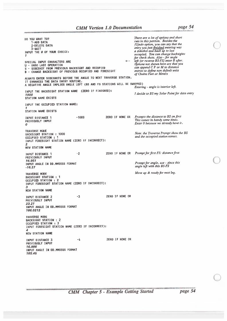
1.0 Documentation page 540I->I-I4~2~)'>2{~>2*2‘>€‘Z~1'lN2 '?A%K-Z-Z¢£<‘2'>3*Z-6-C-€A>':'X-I-I-I . Z-2-Z~

CMM Version .. . . . . . . ..

_

DO YOU HANT TO? There are a lot ofoptions and short1-ADD DATA cuts in thisportion. Besides the2-DELETE DATA (U)ndo option, you can say thatthe3-QUIT entry you just finished entering was

INPUT THE # OF YUJR CHOICE: a sideshot and back up to last1 occupied. You can change backsights

for check shots. Also - for angleSPECIAL INPUT CHARACTERS ARE <-- left (or reverse BS-FS) enter 8 afier.U - UNDO LAST OPERATION Options not shown here are thatyouS - SIDESHOT FRO! PREVIOUS BACKSIGHT AND OCCUPIED can append C F or M to distanceB - CHANGE BACKSIGHT OF PREVICXJS OCCUPIED AND FORESIGHT entries to define non defaultunits

of Chains Feet or MetersALIJAYS ENTER SIDESHOTS BEFORE THE ANGLE TO NEXT TRAVERSE STATION.IT ENHANCES THE DATA ENTRY RGJTINE.A NEGATIVE ANGLE IMPLIES ANGLE LEFT (BS AND FS STATIONS HILL BE SHAPPED)

Entering - angle is interior lefl.INPUT THE BACKSIGHT STATION NAME (ZERO IF FINISHED):1000 I decide to BS my Solar Pointfor data entrySTATI ON NAME EXISTS

INPUT THE OCCUPIED STATION NAME:1STATION NAME EXISTS

INPUT DISTANCE 1 -1000 ZERO IF NONE OR Prompts the distance to BS anjirstPREVICIJSLY INPUT This comes in handy some times.0 Enter 0 becausewe already have it.

TRAVERSE MCDEBACKSIGHT STATION : 1000 Note: the TraversePrompt show the BSOCCUPIED STATION : 1 and the occupied station names.

INPUT FORESIGHT STATION NAME (ZERO IF INCORRECT):2NEW STATION NAME

INPUT DISTANCE 1 -2 ZERO IF NONE OR Promptforfirst FS: distancefirstPREVIWSLY INPUT16.951INPUT ANGLE IN DD.MMSSSS FORMAT Promptfor angle, use - since this-16.27 angle left with thisBS-FS

TRAVERSE MIIJE Move up d’: readyfor next leg.BACKSIGHT STATION : ‘IOCCUPIED STATION : 2INPUT FORESIGHT STATION NAME (ZERO IF INCORRECT):3NEH STATION NAME

INPUT DISTANCE 2 -3 ZERO IF NONE ORPREVIOUSLY INPUT23.21INPUT ANGLE IN DD.MMSSSS FORMAT186.0212

TRAVERSE MCDEBACKSIGHT STATION : 2OCCUPIED STATION : 3INPUT FORESIGHT STATION NAME (ZERO IF INCORRECT):4NEW STATION NAME

INPUT DISTANCE 3 -4 ZERO IF NONE ORPREVIUJSLY INPUT16.988INPUT ANGLE IN DO.MMSSSS FORMAT185.45

-' ‘ Started page 54

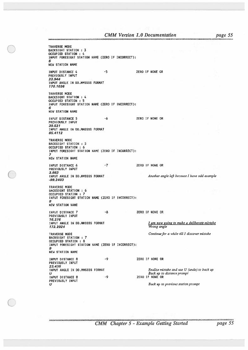
CMM Version 1.0 Documentation page 55. . . . . . . . 4 .

h A<WN«%$mfifiM¢H9&% '? W%'W%fi ......... ..

TRAVERSE MWEBACKSIGNT STATION : 3OCCUPIED STATION : 4INPUT FORESIGHT STATION NAME (ZERO IF INCORRECT):5NEH STATION NAME

INPUT DISTANCE 4 -5 ZERO IF NONE ORPREVIGJSLY INPUT23.944INPUT ANGLE IN DD.MMSSSS FORMAT170.1036

TRAVERSE MWEBACKSIGNT STATION : loOCCUPIED STATION : 5INPUT FORESIGHT STATION NAME (ZERO IF INCORRECT):6NEH STATION NAME

INPUT DISTANCE 5 -6 ZERO IF NONE ORPREVIUJSLY INPUT3.9.521INPUT ANGLE IN DD.MMSSSS FORMAT85.4112

TRAVERSE MCDEBACKSIGHT STATION . 5OCCUPIED STATION : 6INPUT FORESIGHT STATION NAME (ZERO IF INCORRECT):7NEH STATION NAME

INPUT DISTANCE 6 -7 ZERO IF NONE ORPREVIOUSLY INPUT3.883INPUT ANGLE IN DD.MMSSSS FORMAT Anotherangle lefl becauselhave odd example-99.2403

TRAVERSE MODEBACKSIGHT STATION . 6OCCUPIED STATION : 7INPUT FORESIGHT STATION NAME (ZERO IF INCORRECT):8NEH STATION NAME

INPUT DISTANCE 7 -8 ZERO IF NONE ORPREVIGJSLY INPUT16.276INPUT ANGLE IN DD.MMSSSS FORMAT I am now going to make a deliberatemistake172.2924 Wrong angleTRAVERSE NUDE Continuefor a whiletillI discover mistakeBACKSIGNT STATION . 7OCCUPIED STATION : 8INPUT FORESIGHT STATION NAME (ZERO IF INCORRECT):9NEH STATION NAME

INPUT DISTANCE 8 -9 ZERO IF NONE ORPREVIGJSLY INPUT23.435INPUT ANGLE IN DD.MMSSSS FORMAT Realize mistake and use U (undo) to back upU Back up to distancepromptINPUT DISTANCE 8 -9 ZERO IF NONE ORPREVIOUSLY INPUTU Back up to previous stationprompt

. .

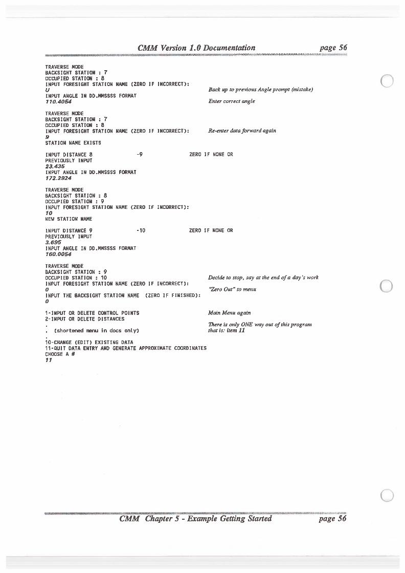
TRAVERSE MGJEBACKSIGHT STATION : 7OCCUPIED STATION : 8INPUT FORESIGHT STATION NAME (ZERO IF INCORRECT):UINPUT ANGLE IN DDJHSSSS FORMAT110.4054

TRAVERSE MCXJEBACKSIGNT STATION : 7OCCUPIED STATION : 8INPUT FORESIGHT STATION NAME (ZERO IF INCORRECT):9STATION NAME EXISTS

INPUT DISTANCE 8 -9PREVIUJSLY INPUT23.435INPUT ANGLE IN DD.MMSS$S FORMAT172.2924

TRAVERSE MCDEBACKSIGHT STATION : 8OCCUPIED STATION : 9INPUT FORESIGNT STATION NAME (ZERO IF INCORRECT):10NEH STATION NAME

CMM Version 1.0 DocumentationQQKOWSOONQOZ9300909930“{£W(45€&$~1‘7r?$"n?I|'M".t3C~3¢\I'C44WA£4-NI0(<'(e¢'9W4<e?J¢09K<¢§¢9’3€¢-W<4*i‘2«B?9.~?14-2-749:-}i-C-I-I-C-ii‘?//Kfi-Z-I-Zvi-I

Back up to previousAngleprompt (mistake)Enter correct angle

Re-enter dataforward again

ZERO IF NONE OR

INPUT DISTANCE 9 -10 ZERO IF NONE ORPREVIOUSLY INPUT3.695INPUT ANGLE IN DD.MMSSSS FORMAT160.0054

TRAVERSE MQEBACKSIGHT STATION : 9OCCUPIED STATION : 10INPUT FORESIGHT STATION NAME (ZERO IF INCORRECT):0INPUT THE BACKSIGHT STATION NAME (ZERO IF FINISHED):0

1-INPUT OR DELETE CONTROL POINTS2-INPUT OR DELETE DISTANCES

. (shortened menu in docs only)I0-CHANGE (EDIT) EXISTING DATA11-OUIT DATA ENTRY AND GENERATE APPROXIMATE COORDINATESCHOOSE A #11

..-.\ - leGettinaried

Decide to stop, say at the end ofa day '5 work

"Zero Out" to menu

Main Menu againThere is only ONE way out of thisprogramthatis: Item 11

page 56

/A-.

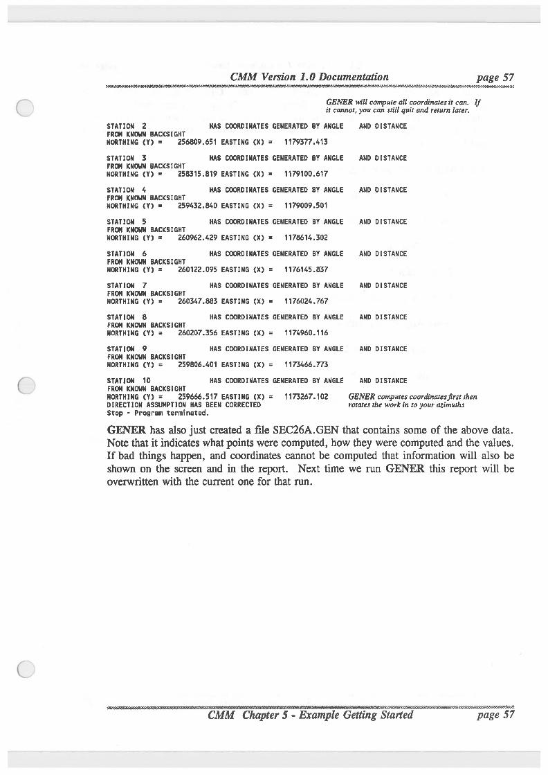
CMM Version 1.0 Documentation page 57_ rNW$WW%NéW%iK5‘%VA% #A¢WWfiK%VAwD¢>Z-2%W'%

GENER will compute all coordinates it can. Ifit cannot, you can still quit and return later.

STATION 2 HAS COORDINATES GENERATED BY ANGLE AND DISTANCEFROM KNOHN BACKSIGHTNORTHING (Y) = 256809.651 EASTING (X) = 1179377.413

STATION 3 HAS COORDINATES GENERATED BY ANGLE AND DISTANCEFROM KNOHN BACKSIGHTNORTHING (Y) = 258315.819 EASTING (X) = 1179100.617

STATION 4 HAS COORDINATES GENERATED BY ANGLE AND DISTANCEFROM KNOHN BACKSIGHTNORTHING (Y) = 259432.840 EASTING (X) = 1179009.501

STATION 5 HAS COORDINATES GENERATED BY ANGLE AND DISTANCEFROM KNOHN BACKSIGHTNORTNING (Y) = 260962.429 EASTING (X) = 1178614.302

STATION 6 HAS COORDINATES GENERATED BY ANGLE AND DISTANCEFROM KNOHN BACKSIGHTNORTHING (Y) = 260122.095 EASTING (X) = 1176145.837

STATION 7 HAS COORDINATES GENERATED BY ANGLE AND DISTANCEFROM KNOHN BACKSIGNTNORTHING (Y) = 260347.883 EASTING (X) = 1176024.767

STATION 8 HAS COORDINATES GENERATED BY ANGLE AND DISTANCEFROM KNOHN BACKSIGHTNORTHING (Y) = 260207.356 EASTING (X) = 1174960.116

STATION 9 HAS COORDINATES GENERATED BY ANGLE AND DISTANCEFROM KNOHN BACKSIGHTNORTHING (Y) = 259806.401 EASTING (X) = 1173466.773

STATION 10 HAS COORDINATES GENERATED BY ANGLE AND DISTANCEFROM KNOHN BACKSIGHTNORTHING (Y) = 259666.517 EASTING (X) = 1173267.102 GENER computes coordinatesfirst thenDIRECTION ASSUMPTION HAS BEEN CORRECTED rotates the work in to your azimuthsStop - Program terminated.

GENER has also just created a fileSEC26A.GEN that contains some of the above data.Note thatit indicates what points were computed, how they were computed and the values.If bad things happen, and coordinates cannot be computed that information will also beshown on the screen and in the report. Next time we run GENER this report will beoverwritten with the current one for that run.

....................................................................... .

CMM Chapter 5 Example Getting Started page 57

CMM Version 1.0 Documentation page 58- - - -

. M¢WO“'X0l¢%X%1¢-X':<4MWfi'W¢9“

At this point control returns to the CMM main menu. GENER has just created a filecalled SEC26A.GEN that contains the above output. The data you have entered is in thefileSEC26A.LSA, and the data that defines the project parameters you have is containedin the fileSEC26A.DEF. We will take a look at some of these fileswhen we finish a loopand have a closure.

Wh t W v ' n ' m ill '

* How to define a project* How to start data entry in GENER

* Enter Control

* Enter Azimuths

* Enter Angles and Distances

* Enter Angles Left with a -

* Correct mistakes with U (undo)* End after a days work.

* Generate approximate coordinates for work to date.

If you have been diligentlyworking through this example this is an ideal place to take abreak.

*************

"'i "

page 58

.-\_

tin

CMM Version 1.0 Documentation page 59.

‘.. .M'O'N'0W'."'I?€~€'2-O'K¢>O-.‘¢C4'X4K

hi‘

Now let’s try to get a graphic of the work to this point. Graphics provides a way to seewhat you've done which is a great aid in noticing larger errors. This is especially true ifyou are looking at your own data.

There are several ways to get graphics.First way:

Second way:

Use the utility VIEW. This program will give you a quick look at thetraverse. It has thecapabilityto pan and zoom thus allowing a good graphiclook at your job. To do this select V from the UtilitiesMenu.

Create a DXF filewith the <D> choice on the CMM main menu. DXFstands for a file format that was developed by the makers of AutoCad, andit has becomea defacto standard for interchange of graphic data between PCbased CAD systems.

There a few ways to use DXF files either to view or obtain hard copy.

1) Load the file into AutoCad with the DXFIN command, then you canview, edit, plot or printer plot the drawing. Of course not everyone hasaccess to AutoCad and plotters and such.

2) Load the fileinto AutoSketch or other basic CAD package. There are anumberof such inexpensive packages thatcan read DXF files. This can bein effective way to accomplish what we want.

3) Convert the DXF to a WPG WordPerfect 5.0 or 5.1 graphic file, thencreate a WP document graphic which can then be viewed and printed.

In this example we will just create the DXF, and bring the DXF file into thisWordPerfect Document by using the GRAPHCNV program with WP.

GRAPHCNV SEC26A.DXFSEC26A. WPG

Now:

1) Go back into CMM as earlier, then select: D

2) Follow thedialogue shown on thenext page. Note most of theresponses are

.......................\

(enter) which selects the default shown.

"$3w:w$§‘}$%?§$£&W$%$:i$ £%%%$#%W$fi$$:%WW3$$&W2Started page 59

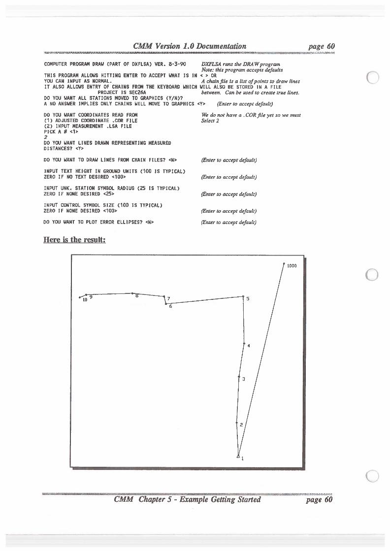
CMM Version 1.0 Documentation.DIELSA runs theDRAWprogramNote: thisprogram accept:defaults

THIS PROGRAM ALLONS HITTING ENTER TO ACCEPT NHAT IS IN < > ORYOU CAN INPUT AS NORMAL. A chainfileis a list ofpoints to draw linesIT ALSO ALLONS ENTRY OF CHAINS FRCH THE KEYBOARD HHICH HILL ALSO BE STORED IN A FILE

PROJECT IS SEC26A between. Can be used to create true lines.DO YOU HANT ALL STATIONS MOVED TO GRAPHICS (Y/N)?A ND ANSHER IMPLIES ONLY CHAINS HILL MOVE TO GRAPHICS <Y>

COMPUTER PROGRAM DRAH (PART OF DXFLSA) VER. 8-3-90

Enter to accept default)We do not have a . CORfileyet so we mustSelect 2

DO YOU HANT CUJRDINATES READ FRO!(1) ADJUSTED CWRDINATE .COR FILE(2) INPUT MEASUREMENT .LSA FILEPICK A # <1>2DO YOU HANT LINES DRAHN REPRESENTING MEASUREDDISTANCES? <Y>

DO YW HANT TO DRAU LINES FRO! CHAIN FILES? <N> Enter to acceptdefault)INPUT TEXT HEIGHT IN GROUND UNITS (100 IS TYPICAL)ZERO IF NO TEXT DESIRED <100> Enter to accept default)INPUT UNK. STATION SYMBOL RADIUS (25 IS TYPICAL)ZERO IF NONE DESIRED <25> Enter to acceptdefault)INPUT CONTROL SYMBOL SIZE (100 IS TYPICAL)ZERO IF NONE DESIRED <100> Enter to acceptdefault)DO YOU HANT TO PLOT ERROR ELLIPSES? <N> Enter to acceptdefault)

page 60 - I -w:-:-:-:—:-:-:c-:-x\e<-:o<<-

-'-‘H -§.%'.a?L‘¥:£!¥-‘.3-,$fiIn'A‘i:252\’?€‘.'«‘

page 60

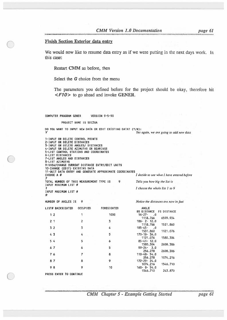
CMM Version 1.0 Documentation page 61M-WNN€'£' \W&W“-3'8‘#9398'£'}2-?I >N¢»W#»> -Vmkfii-Pflfixfififi-i>2-»€s'4-G:>O'¢':1!fl-G-X<iV.4“2!£'}'I~2¢044-I-1-2 -Z-2'2-Z-I-I-hI~l-2+}!-D-2-3‘:'i'N ‘I'3'l'l‘X'2'3'1‘I'I‘:'1'1'Z':'H'l'C'Z£'C'I'1'!'?Z'!-I‘Z'3".*73'i

Fini h cti n eri r en

We would now like to resume data entry as if we were putting in the next days work. Inthis case:

Restart CMM as before, then

Select the G choice from the menu

The parameters you defined before for the project should be okay, therefore hit<F10> to go ahead and invoke GENER.

COMPUTER PROGRAM GENER VERSION 9-5-90

PROJECT NAME IS SEC26A

DO YOU WANT TO INPUT NEH DATA OR EDIT EXISTING DATA? (Y/N):Y Yes again, we are going to add new data

1-INPUT OR DELETE CONTROL POINTS2-INPUT OR DELETE DISTANCES3-INPUT OR DELETE ANGLESI DISTANCES4-INPUT OR DELETE AZIMUTHS OR BEARINGS5-LIST CONTROL STATIONS AND COORDINATES6-LIST DISTANCES7-LIST ANGLES AND DISTANCES8-LIST AZIMUTHS9-VIEH/CHANGE CURRENT DISTANCE ENTRY/EDIT UNITS10-CHANGE (EDIT) EXISTING DATA11-OUIT DATA ENTRY AND GENERATE APPROXIMATE COORDINATESCHOOSE A # I decide to see what I have entered before7TOTAL NUMBER OF THIS MEASUREMENT TYPE IS 9 Tellsyou how big the IistisINPUT MINIMUM LIST #1 I choose the whole list 1 to 9INPUT MAXIMUM LIST #9

NUMBER OF ANGLES IS 9 Notice the distances are now in feetLIST# BACKSIGHTED OCCUPIED FORESIGHTED ANGLE

BS DISTANCE FS DISTANCE1 2 1 1000 16-27- .0

1118.766 6599.9342 1 2 3 186- 2- 12.0

1118.766 1531.8603 2 3 4 185-4S- .0

1531.860 1121.0764 3 4 5 170-10- 36.0

1121.076 1580.3045 4 5 6 85-41- 12.0

1580.304 2608.3866 7 6 5 99-24- 3.0

256.278 2608.3867 6 7 8 110-40- 54.0

256.278 1074.2168 7 8 9 172-29- 24.0

1074.216 1546.7109 8 9 10 160- 0- 54.0

1546.710 243.870PRESS ENTER TO CONTINUE

. -....... ................... .-t ----- » -------------------------------------------------. ..e. .- .CMM Chapten - Exaple Getting Started page 61

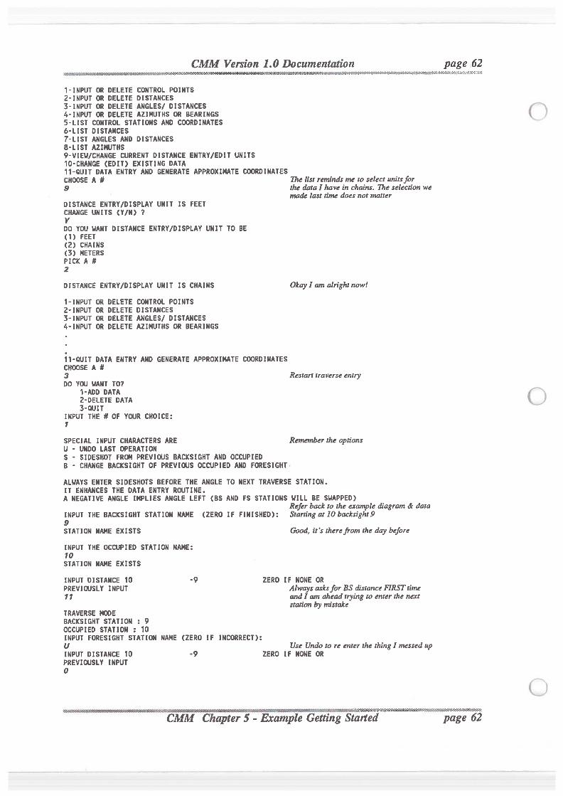
CMM Version 1.0 Documentation

1-INPUT OR DELETE CONTROL POINTS2-INPUT OR DELETE DISTANCES3-INPUT OR DELETE ANGLE$/ DISTANCES4-INPUT OR DELETE AZIMUTHS OR BEARINGS5-LIST CONTROL STATIONS AND COORDINATES6-LIST DISTANCES7-LIST ANGLES AND DISTANCES8-LIST AZIMUTHS9-VIEU/CHANGE CURRENT DISTANCE ENTRY/EDIT UNITS10-CHANGE (EDIT) EXISTING DATA11-QUIT DATA ENTRY AND GENERATE APPROXIMATE COORDINATESCHOOSE A # The list reminds me to select unitsfar9 the data I have in chains. The selection we

made last time does not matterDISTANCE ENTRY/DISPLAY UNIT IS FEETCHANGE UNITS (Y/N) 7YDO YOU HANT DISTANCE ENTRY/DISPLAY UNIT TO BE(1) FEET(2) CHAINS(3) METERSPICK A #2

DISTANCE ENTRY/DISPLAY UNIT IS CHAINS OkaylamalrightnowlI-INPUT OR DELETE CONTROL POINTS2-INPUT OR DELETE DISTANCES3-INPUT OR DELETE ANGLES] DISTANCES4-INPUT OR DELETE AZIMUTHS OR BEARINGS

‘I1-GUIT DATA ENTRY AND GENERATE APPROXIMATE COORDINATESCHOOSE A #3 Restart traverse entryDO YOU UANT TO?

1-ADD DATAZ-DELETE DATA3-QUIT

INPUT THE # OF YUJR CHOICE:1

SPECIAL INPUT CHARACTERS ARE Rememberthe optionsU - UNDO LAST OPERATIONS - SIDESHOT FRUI PREVIOUS BACKSIGHT AND OCCUPIEDB - CHANGE BACKSIGHT OF PREVICXJS OCCUPIED AND FORESIGHT

ALNAYS ENTER SIDESHOTS BEFORE THE ANGLE TO NEXT TRAVERSE STATION.IT ENHANCES THE DATA ENTRY RCAJTINE.A NEGATIVE ANGLE IMPLIES ANGLE LEFT (BS AND FS STATIONS HILL BE SHAPPED)

Refer back to the example diagram & dataINPUT THE BACKSIGHT STATION NAME (ZERO IF FINISHED): Starting at 10 backsight99STATION NAME EXISTS Good, it’: therefrom the day beforeINPUT THE OCCUPIED STATION NAME:10STATION NAME EXISTS

INPUT DISTANCE 10 -9 ZERO IF NONE ORPREVIOUSLY INPUT Alwaysasksfor BS distance FIRSTtime1 1 and I am ahead trying to enter the next

station by mistakeTRAVERSE MGJEBACKSIGHT STATION : 9OCCUPIED STATION : 1OINPUT FORESIGHT STATION NAME (ZERO IF INCORRECT):U Use Undo to re enter the thingI messed upINPUT DISTANCE 10 -9 ZERO IF NONE ORPREVIWSLY INPUT0

fl.--------- -- -. x a

C '-‘'Started

page 62

.4~a\

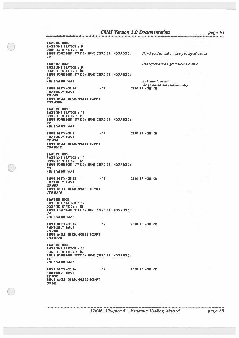
CMM Version 1.0 Documentation page 63.' 7-V-”‘}:¢!3’P.1‘X‘3‘3’."4"v'7'I'I‘:‘5‘H{

TRAVERSE MWEBACKSIGHT STATION . 9OCCUPIED STATION : 10INPUT FORESIGHT STATION NAME (ZERO IF INCORRECT): Now] goofup andput in my occupied station10

TRAVERSE HIDE It is rejected and I get a second chanceBACKSIGMT STATION : 9OCCUPIED STATION : 10INPUT FORESIGHT STATION NAME (ZERO IF INCORRECT):1 1NEH STATION NAME As it should be new

We go ahead and continue entryINPUT DISTANCE 10 -11 ZERO IF NONE ORPREVIOUSLY INPUT29.269INPUT ANGLE IN DD.MMSSSS FORMAT103.4306

TRAVERSE MCDEBACKSIGMT STATION : 10OCCUPIED STATION : 11INPUT FORESIGHT STATION NAME (ZERO IF INCORRECT):12NEH STATION NAME

INPUT DISTANCE 11 -12 ZERO IF NONE ORPREVIGJSLY INPUT12.054INPUT ANGLE IN DD.MMSSSS FORMAT194.0512

TRAVERSE MWEBACKSIGHT STATION : 11OCCUPIED STATION : 12INPUT FORESIGHT STATION NAME (ZERO IF INCORRECT):13NEH STATION NAME

INPUT DISTANCE 12 -13 ZERO IF NONE ORPREVIGJSLY INPUT20.553INPUT ANGLE IN DD.MMSSSS FORMAT175.5318

TRAVERSE MUJEBACKSIGMT STATION : 12OCCUPIED STATION : 13INPUT FORESIGHT STATION NAME (ZERO IF INCORRECT):14NEH STATION NAME

INPUT DISTANCE 13 -14 ZERO IF NONE ORPREVIIXJSLY INPUT15.745INPUT ANGLE IN DD.MMSSSS FORMAT183.5124

TRAVERSE MCDEBACKSIGHT STATION . 13OCCUPIED STATION : 14INPUT FORESIGHT STATION NAME (ZERO IF INCORRECT):15NEH STATION NAME

INPUT DISTANCE 14 -15 ZERO IF NONE ORPREVIOUSLY INPUT12.832INPUT ANGLE IN DD.MMSSSS FORMAT84.52

-. -----------------.-r vw .-A .'\.\. .- ‘\:'.'O\.'-"- - ...................................................................................._ CM Chapter 5 - Example Getting Irted I

page 63

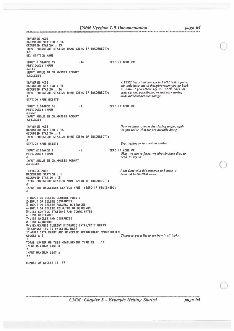
CMM Version 1.0 Documentation page 64' ‘ '##Z<$XNE9”W{'X€fiCfih\W#Wfl9fiW¢'”flm*V fiWN¢IV&Z<

TRAVERSE MODEBACKSIGHT STATION : 14OCCUPIED STATICNI : 15INPUT FORESIGNT STATION NAME (ZERO IF INCORRECT):16'NEH STATIGI NAME

INPUT DISTANCE 15 -‘I6 ZERO IF NONE ORPREVIUJSLY INPUT28.17INPUT ANGLE IN DD.MMSSSS FORMAT180.5354

TRAVERSE MUJE A VERYimportantconcept in CMM is thatpointsBACKSIGHT STATION : 15 can only have one id thereforewhen you go backOCCUPIED STATION : 16 to station 1 you MUST say so. CMM does notINPUT FORESIGNT STATION NAME (ZERO IF INCORRECT): create a new coordinate, we are only storing1 measurementsbetweenthings.STATION NAME EXISTS

INPUT DISTANCE ‘I6 -1 ZERO IF NONE ORPREVIOUSLY INPUT39.68INPUT ANGLE IN DD.MMSSSS FORMAT181.3924

Now we have to enter the closing angle, againwe just tell it what we are actuallydoing

TRAVERSE MGJEBACKSIGMT STATION . 16OCCUPIED STATION : 1INPUT FORESIGNT STATION NAME (ZERO IF INCORRECT):2STATION NAME EXISTS Yep, turning in to previous station.

INPUT DISTANCE 1 ‘Z ZERO IF NONE ORPREVIOUSLY INPUT Okay, try not toforget we already have dist, so0 Zero to say soINPUT ANGLE IN DD.MMSSSS FORMAT83.3542

I am done with this traverse so I have toZero out to GENER menu.

TRAVERSE MIXJEBACKSIGNT STATION : ‘IOCCUPIED STATION : 2INPUT FORESIGNT STATION NAME (ZERO IF INCORRECT):0INPUT THE BACKSIGHT STATION NAME (ZERO IF FINISHED):0

1-INPUT OR DELETE CONTROL POINTS2-INPUT OR DELETE DISTANCES3-INPUT OR DELETE ANGLES] DISTANCES-’o-INPUT OR DELETE AZIMUTHS OR BEARINGS5-LIST CONTROL STATIONS AND COORDINATES6-LIST DISTANCES7-LIST ANGLES AND DISTANCES8-LIST AZIMUTHS9-VIEH/CHANGE CURRENT DISTANCE ENTRY/EDIT UNITS10-CHANGE (EDIT) EXISTING DATA11-QUIT DATA ENTRY AND GENERATE APPROXIMATE COORDINATESCHOOSE A # Choose to get a list to see how it all looks7TOTAL NUMBER OF THIS MEASUREMENT TYPE IS 17INPUT MINIMUM LIST #1INPUT MAXIMUM LIST #17

NUMBER OF ANGLES IS 17

._.- a E ' };2z§é"'34~.

/\"\

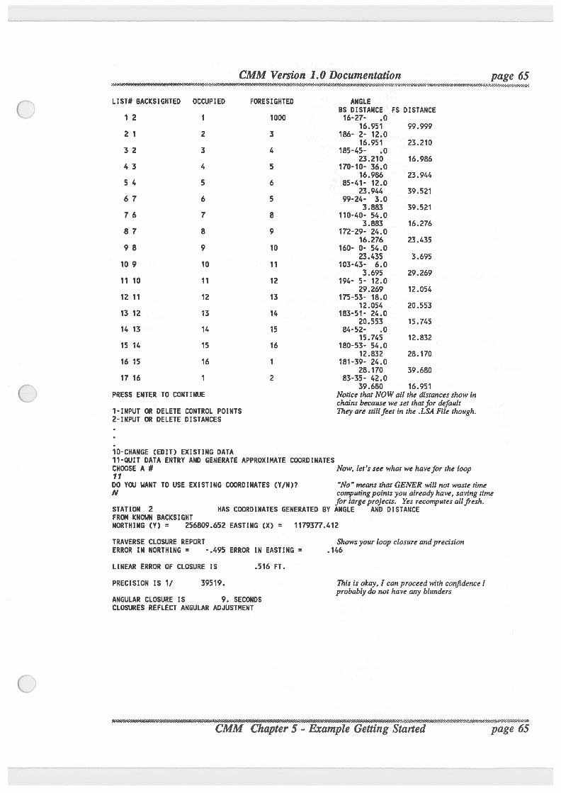
CMM Version 1.0 Documentation page 65?

. , FM-39¢}?b>?3'Z#&&Wk&X-MWOM&MN& »3W€'I'NWl'§NO’.€-X-}1~>}%‘$ A.. . . . ., .............,_.....g_....._

LIST# BACKSIGHTED OCCUPIED FORESIGHTED ANGLEBS DISTANCE FS DISTANCE

1 2 1 1000 16-27- .016.951 99.999

2 1 2 3 186- 2- 12.016.951 23.210

3 2 3 4 185-45- .023.210 16.986

4 3 4 5 170-10- 36.016.986 23.944

5 4 5 6 85-41- 12.023.944 39.521

6 7 6 5 99-24- 3.03.883 39.521

7 6 7 8 110-40- 54.03.883 16.276

8 7 8 9 172-29- 24.016.276 23.435

9 8 9 10 160- 0- 54.023.435 3.695

10 9 10 11 103-43- 6.03.695 29.269

11 10 11 12 194- 5- 12.029.269 12.054

12 11 12 13 175-53- 18.012.054 20.553

13 12 13 14 183-51- 24.020.553 15.745

14 13 14 15 84-52- .015.745 12.832

15 14 15 16 180-53- 54.012.832 28.170

16 15 16 1 181-39- 24.028.170 39.680

17 16 1 2 83-35- 42.039.680 16.951

PRESS ENTER TO CONTINUE Notice thatNOW all the distances show inchains becausewe set thatfor default

1- INPUT OR DELETE CONTROL POINTS They are stillfeet in the .LSA File though.2-INPUT OR DELETE DISTANCES

‘IO-CHANGE (EDIT) EXISTING DATA11-OUIT DATA ENTRY AND GENERATE APPROXIMATE COORDINATESCHOOSE A # Now, let's see what we havefor the loop11DO YW WANT TO USE EXISTING COORDINATES (Y/N)? "No" means thatGENER will not waste timeN computingpoints you already have, saving time

for largeprojects. Yes recomputes allfresh.STATION 2 HAS COORDINATES GENERATED BY ANGLE AND DISTANCEFRO! KNOWN BACKSIGHTNORTHING (Y) = 256809.652 EASTING (X) = 1179377.412

TRAVERSE CLOSURE REPORT Shows your loop closure andprecisionERROR IN NORTHING = ' .495 ERROR IN EASTING = .146

LINEAR ERROR OF CLOSURE IS .516 FT.

PRECISION IS 1/ 39519. This is okay, I can proceed with confidenceIprobablydo not have any blunders

ANGULAR CLOSURE IS 9. SECONDSCLOSURES REFLECT ANGULAR ADJUSTMENT

gtharted page 65 CMM Chapter 5 - mple Gettin

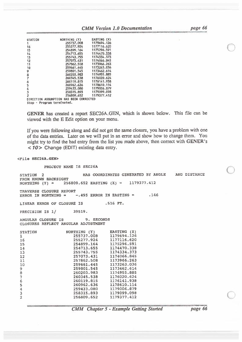
l’\)UlJ\\JlON®O-5-D-|—|-I-0-I-IUDO-Il\lUI|vL\UIO~->1-I --u 0Z NORTHING (Y)255737.008255277.924254899.164254713.655255743.755257073.431257862.508259661.445259801.545260203.983260345.538260119.815260962.636259433.080258315.893256809.652

CMM Version 1.0 Documentation

EASTING (X)1179694.1261177116.6201175296.5911174470.3381174334.3731174066.8451173966.2631173263.0361173462.6141174955.8851176020.6241176141.9381178610.1141179006.8791179099.0981179377.412

DIRECTION ASSUMPTION HAS BEEN CORRECTEDStop - Program terminated.

page 66' ' ' -

‘ ‘¢N<‘N.WW5€¢%’ fiN¢6K~?’S*K'3<'Z('€'YK€'€‘€'Z'Z‘€¢

GENER has created a report SEC26A.GEN, which is shown below. This file can beviewed with the E Edit option on your menu.

If you were following along and did not get the same closure, you have a problem with oneof the data entries. Later on we will put in an error and show how to change them. Youmight try to find the bad entry from the list you made above, then correct with GENER’s< 10> Change (EDIT) existing data entry.

<Fi1e SEC26A.GEN>

STATION 2 HAS COORDINATES GENERATED BY ANGLEFROM KNOWN BACKSIGHTNORTHING (Y) = 256809.652 EASTING (x) =

TRAVERSE CLOSURE REPORTERROR IN NORTHING

LINEAR ERROR OF CLOSURE IS

PRECISION IS 1/ANGULAR CLOSURE IS

39519.

PROJECT NAME IS SEC26A

-.495 ERROR IN EASTING =

.516 FT.

SECONDSCLOSURES REFLECT ANGULAR ADJUSTMENT

STATION11615141312

NORTHING (Y) EASTING (x)

1179377.412

255737.008 1179694.126255277.924 1177116.620254899.164 1175296.591254713.655 1174470.338255743.755 1174334.373257073.431 1174066.845257862.508 1173966.263259661.445 1173263.036259801.545 1173462.614260203.983 1174955.885260345.538 1l76020.624260119.815 1176141.938260962.636 1178610.114259433.080 1179006.879258315.893 1179099.098256809.652 1179377.412

AND DISTANCE

.146

.1‘3‘

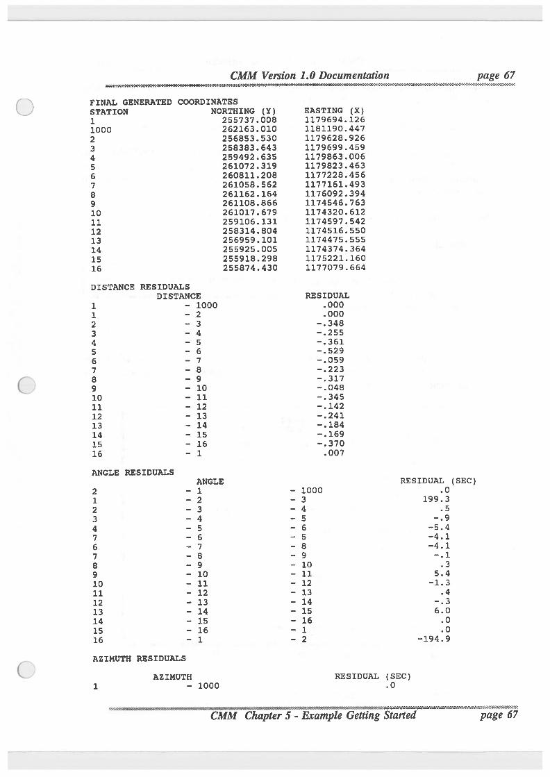
CMM Version 1.0 Doc

FINAL GENERATED COORDINATESSTATION11000omqmmnwn10111213141516

DISTANCE RESIDUALSl.D(D\lO\Ll'|ubh.|k)|-‘D-|10111213141516

ANGLE RESIDUALS\Dm\lO\\l-C>(.u|l\)b-‘I0AZIMUTH RESIDUALS

NORTHING (Y)255737.008262163.010256853.530258383.643259492.635261072.319260811.208261058.562261162.164261108.866261017.679259106.131258314.804256959.101255925.005255918.298255874.430

DISTANCE- 1000- 2- 3- 4- 5- 6- 7- 8- 9- 10- 11- 12- 13- 14- 15- 16— 1

ANGLE- 1- 2- 3— 4- 5— 6- 7- 8— 9- 10- 11- 12— 13- 14- 15- 16- 1

AZIMUTH— 1000

EASTING (X)1179694.126118119o.4471179628.9261179699.4591179863.0061179823.4631177228.4561177161.4931176o92.3941l74546.7631174320.6121174597.s421174516.55o1174475.5551174374.3641175221.16o1177o79.664

RESIDUAL.000.000

-.348-.255-.361-.529-.059-.223-.317-.048-.345—.142-.241-.184-.169-.370

.007

100034565891011121314151612

umentation. . W4'2'2'C°1-2'I'3'?!‘Hi#W¥flN'l¢%»»1'K¢# ?I'1'1'm%}&}3*:-Zfi-:°}H':-'1-Z-241-3-2-2-'2

page 67

RESIDUAL (SEC).0

199.3.5

-.9-5.4-4.1-4.1-.1

.35.4

-1.3

- - -- .\':$>‘»'a':'~:-‘$3-'."€'¢.4'f.°‘I$$3'-;’9$$9'5'}.¢t-‘.’¢':}3ge6

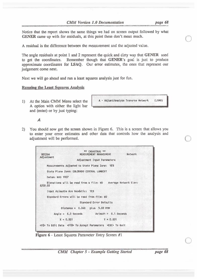
CMM Version 1.0 Documentation page 68. - 293099?‘I“€035€M95‘H‘K‘3'X'I WWI-2-V///JVWJ-7fl¢<‘X<W&P2-.4‘:

Notice that the report shows the same things we had on screen output followed by whatGENER came up with for residuals, at this point these don’t mean much.

A residual is the difference between the measurement and the adjusted value.

The angle residuals at point 1 and 2 represent the quick and dirty way that GENER usedto get the coordinates. Remember though that GENER’s goal is just to produceapproximate coordinates for LSAQ. Our error estimates, the ones that represent our

judgement come next.

Next we will go ahead and run a least squares analysis just for fun.

R i h Su An!’

A - Adjust/AnatyzeTraverse Network (LSAO)1) At the Main CMM Menu select theA option with either the light barand (enter) or by just typing:

A

2) You should now get the screen shown in Figure 6. This is a screen that allows youto enter your error estimates and other data that controls how the analysis andadjustmentwill be performed.

_

** CA.DA8IRAt *'-“

SEC_36A HEASUREHEN_T'illANA8EMEltTAdjustment

_Adjmtmen: Input’ fiarameters

Measurements Adjusted to State Kane‘ Zone: YESState Mane Zone: COLORADO CENTRAL LAMBERYDamn: NAD 1927

_

Elevations will be read from ‘a file: no Average Network Elev:$200.00

Wilt AzimlthsAre fi¢i=¢deti.c= YESstandard Errors will be read from rite: no

standard. Error 0e.f'a'ult'sDistance = 0.040 plus 5.00 PPH.

Angle = 6,0 Seconds Azimuth ‘= 0.? SecondsX is 0.001 V as 0.001

<F2> To. Edit Data <'F’lU>~ To Accept Parameters <EsC> To ouit Figure 6 - Least Squares Parameter Entry Screen #1

68

‘,.—».

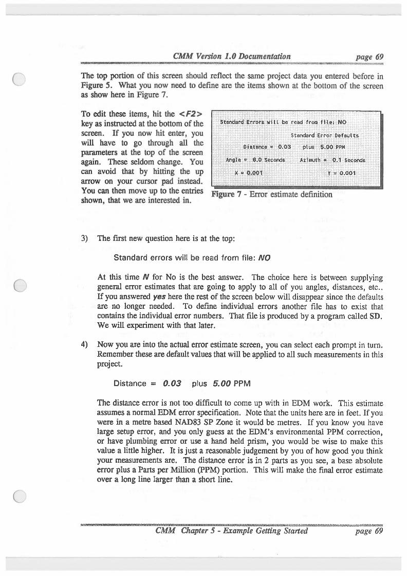
CMM Version 1.0 Documentation page 69- - - -

' I-Z-:4‘-vi-H‘!-{¢€"'.. 3¢iI0€\\36H6'Hr?~>'I-1-1-3?!-i06¢(’a>l~?>I<‘O'lH?-G-C<»I¢H¢

The top portion of this screen should reflect the same project data you entered before inFigure 5. What you now need to define are the items shown at the bottom of the screenas show here in Figure 7.

To edit these items, hit the <F2>key as instructed at thebottom of thescreen. If you now hit enter, youwill have to go through all theparameters at the top of the screenagain. These seldom change. Youcan avoid that by hitting the uparrow on your cursor pad instead.

standard‘ =,E.rr'o:.r- n¢fgults_-

alias“ -5;-hoi: rm

fiiimfifhi Q15? :$é<.=Lm'\ds .=; Q-.001‘

can men up to me ems 7 -E... W....-..i...

shown, that we are interested in.

3) The first new question here is at the top:

Standard errors will be read from file: N0

At this time N for No is the best answer. The choice here is between supplyinggeneral error estimates that are going to apply to all of you angles, distances, etc..If you answered yes here therest of the screen below will disappear since the defaultsare no longer needed. To define individual errors another file has to exist thatcontains the individualerror numbers. That fileis produced by a program called SD.We will experiment with that later.

4) Now you are into theactual error estimate screen, you can select each prompt in turn.Rememberthese are defaultvalues thatwillbeapplied to all such measurements in thisproject.

Distance = 0.03 plus 5.00 PPM

The distance error is not too difficult to come up with in EDM work. This estimateassumes a normal EDM error specification. Note that the units here are in feet. If youwere in a metre based NAD83 SP Zone it would be metres. If you know you havelarge setup error, and you only guess at the EDM’s environmental PPM correction,or have plumbing error or use a hand held prism, you would be wise to make thisvalue a litflehigher. It is just a reasonablejudgement by you of how good you thinkyour measurements are. The distance error is in 2 parts as you see, a base absoluteerror plus a Parts per Million (PPM) portion. This will make the final error estimateover a long line larger than a short line.

’ page 69

5)

6)

7)

8)

CMM Version 1.0 Documentation

Angle = 6.0 Seconds

This estimate represents how good you thinkyour angles are on the average. In thiscase I have a feeling that I can turn pretty good angles, most of the setups are good,and we have long enough sights, and the instrument is of the typical Total Station T1class.

The next value is:

Azimuth = 0.1 Seconds

This is the estimate for all your Azimuth determinations, such as Solars, Polarisobservations, etc. There are two ways to handle this. You can put in a realisticestimate. For example, the average solar is probably in the 15-20 second range, butif we only have 1 observation setting the error to 0.1 (you can’t set these to zero) willessentially hold all the Solars. You may want to experiment with both approaches.Because thisjob only has one Solar it will be held no matter what. The most logicalapproach from a statistical approach is to put in the most realistic value. The leastsquares will then use it to the degree it merits ‘averaging’ the effect of all yourobservations.

The next values represent the positional error estimates that apply to your controlpoints. They also are in the base units for the projection you are using, in this casefeet. The 0.001 values mean hold the control (so it can’t move). Rememberthat youcan have more than one control point in a job and if you choose, you can set weightson them. This may seem a little odd at first. Usually we thinkof control as absoluteand always hold it as the truth, but this is not always justified. Errors and distortionin the NAD27 networkare frequently greater than common modern survey practice.Thus holding such points fixed could distort your measurements to an unacceptabledegree. Othercontrol thatcan be weighted would be some GPS and doppler positions.Since we only have one control point, it doesn’t matter.

X = 0.001 Y = 0.001

Hitting the <F10> key accepts the data on this input screen and takes you toanother. This screen should look like Figure 8 which follows on the next page. Theseparameters control what lcind of output you will get from the Least Squares process.The first prompt:

Error Analysis: N0

This prompt could be confusing. It is NOT asking if you want error analysisperiod,but what it defines is whether you want the program to compute error ellipses. Errorellipses describe positional error information rather than measurement error

3.

9)

10)

11)

....... ._ . _,. . .

CMM Version 1.0 Documentation.”QQfiWON& #?M'¥A%¢X<<'¥AM

.

page 71.. . .... »W'.*»€~Z¢'rb3'5'€"-'1-¢'$'Z‘.".".-£'I<'1".‘¢*¢'2>€

information. There are 2 reasons to say "NO" to this. First of all, error ellipses giveyou informationabout absolute position error, and do not tell you much about relativemeasurement accuracy. In other words for what we want to do, they do not helpmuch. Error ellipse informationis always larger the farther away you go from yourcontrol. The second reason, is that this computation is intense, takes extra time andresources. LSAQ will give up even trying to compute it on large networks, and itwon't be computed anyway.

Next we have:

Residual Printout Limits:

Distance = 0.000

Angle = 0.000

Azimuth = 0.000

taking these together. The program prints out a list of the residuals, again this is thedifference between your measurement and the value that came out of the adjustment.In a large job there can be a lot of these, possibly thousands. You are generally onlyconcerned with values that are large where the least squares is telling you somethingbad may be happening. These limits are a way to limit output to only residuals overwhat you set. For example, I could say I really don’t care about residuals where theadjustment was less that 0.01 ft., and 1 second in angle and 2 seconds in azimuth.Leaving these at Zero’s will print all residuals

Next prompt is:

List Adjusted Bearings & Distances: NO

Determines whether the output reports all the bearings and distances after theadjustment. We usually say NO because the values are in GRID and don’t mean thatmuch to us anyway, besides taldng up even more room on the disk.

Next prompt:

Update Coordinate File: YES

Normally this is what you want to do, the goal of this process is to end up with thebest coordinate values for the measurements you put in. Some times you may just beexperimenting, adjusting weights, or looking for errors, and you already have anacceptable coordinate file. Saying NO would allow you to perform the computationand get the results of the analysis, but theANSWERS will not be written to you officialcoordinate .COR file.

9:-'99>'S.\‘5$$>‘ta'.'-:1‘.'-“$‘.~'‘a‘‘a'$‘;'%. hapter - aml Gettin two:-ted ’

page 71

CMM Version 1.0 Documentation ME“:-‘

.

'

12) Last prompt is:

Readjust With Robusted Error Estimates: No

page 72‘ ' ‘<"}?X‘}'3‘§°9.*3.\‘<§'L¢9'°.°'”< V“WNWD¥4%DfiWhWWW%«¢W3%WQH¢%?Z#WK4'FA<‘Z‘N'3'\§O‘l-N‘:'£iQI»1~fi';'f'3OO'>3-Z-€-I-:-I

This can be important and you may select Yes or No. We will go through a YESsession later. Also see a discussion of Robusting in Ray's explanation, and in theextra documentation in theReference Section. This is one of the many error and smallblunder detection techniques contained in CMM. For this run, we will say NO. Ifwe say yes all thatwill happen is we will get asked a question about re-adjustingwithnew weights after the program has made its first run. We can still say No there.

13) We are now ready to proceed with the Least Squares Stuff. As soon as you hit the< F10> key theprogram LSAQ will run using theproject parameters thatare storedin the SEC26A.DEF fileand the measurement data stored in the SEC26A.LSA file.The annotated screen I/O follows. LSAQ creates a complete report filewith the ADJextension, and the listing from it follow the screen dump.

COMPUTER PROGRAM LSAO VERSION 9-5-90

PROJECT NAME IS SEC26A

ALL OBSERVATIONS ARE REDUCED TO THE NAD 27 DATUMALL LISTED MEASUREMENTS HAVE BEEN REDUCED TO GRID61 COLORADO CENTRAL LAMBERTINPUT NETUORK ELEVATION IS

Tellsyou yourproject definition

6200.00 FT .

NUMBER OF CONTROL STATIONS = 1NUMBER OF DISTANCES = 17NUMBER OF ANGLES = 17NUMBER OF AZIMUTHS = 1TOTAL NUMBER OF STATIONS = 17

BANDHIDTH IS 5 STATIONSBAND IS 5 STATIONSNUMBER OF REQUIRED TERMS IN NORMAL EQUATIONS IS 397

See Ray '5 explanationto understandthis

RESULTS OF ITERATION 1

STATION NORTHING (Y) UPDATE EASTING (X) UPDATE5 -1.128 4 .105 These are the coordinate residualsfor the6 1.398 4 .398 first iteration. These are as large as they4 - .812 2.542 are becauseGENER '5 estimates are crude.1000 - .011 .0013 - .405 1.4847 1.408 4.6518 2.381 4.9792 .005 .0011 .000 .0009 3.808 5.25910 4.033 5.23116 2.432 .10615 4.134 .50511 4.128 3.44812 4.347 2.75813 4.630 1.56514 4.909 .670

STANDARD ERROR OF UNIT 1:lEIGHT= 29.727

'

~-

page 72

J»,

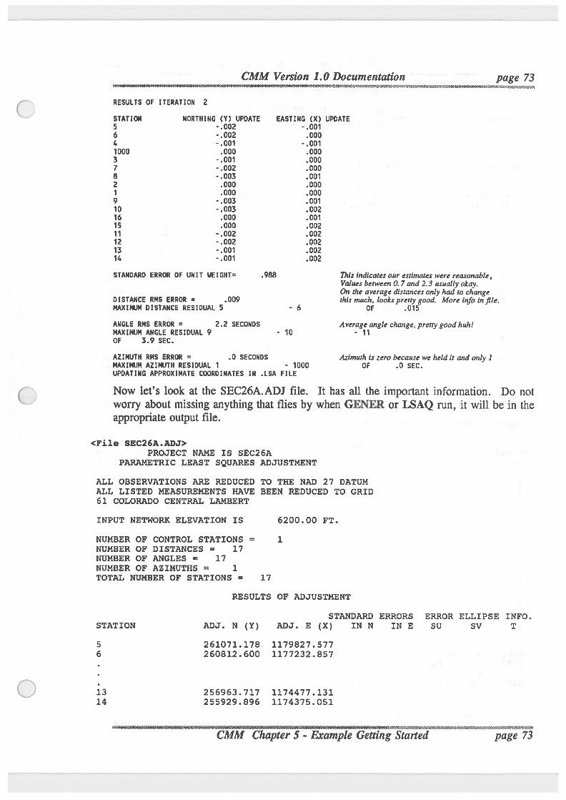
CMM Version 1.0 Documentation page 73f&§ fi>3:lW W>WV#Z%VX¢%¢>»W¢¢!-X

RESULTS OF ITERATION 2

STATION NORTNING (Y) UPDATE EASTING (X) UPDATE5 -.002 -.0016 -.002 .0006 -.001 -.0011000 .000 .0003 -.001 .0007 ~.002 .0008 -.003 .0012 .000 .0001 .000 .0009 -.003 .00110 -.003 .00216 .000 .00115 .000 .00211 -.002 .00212 -.002 .00213 -.001 .00214 -.001 .002

STANDARD ERROR OF UNIT HEIGHT= .988 This Indicatesour estimates were reasonable,Values between 0. 7 and 2.3 usually okay.On the average distances only had to change

DISTANCE RMS ERROR = .009 thismuch, lookspretty good. More info in file.MAXIMUM DISTANCE RESIDUAL 5 - 6 OF .015

ANGLE RHS ERROR = 2.2 SECONDS Averageangle change, pretty good huh!MAXIMUM ANGLE RESIDUAL 9 - 10 - 11OF 3.9 SEC.

AZIIIIUTH RMS ERROR = .0 SECONDS Azimuthis zero becausewe held it and only 1MAXIMUM AZINUTN RESIDUAL 1 - 1000 OF .0 SEC.UPDATING APPROXIMATE COORDINATES IN .LSA FILE

Now let’s look at the SEC26A.ADJ file. It has all the important information. Do notworry about missing anythingthat flies by when GENER or LSAQ run, it will be in theappropriate output file.

<Fi1e SEC26A.ADJ>PROJECT NAME IS SEC26A

PARAMETRIC LEAST SQUARES ADJUSTMENT

ALL OBSERVATIONS ARE REDUCED TO THE NAD 27 DATUMALL LISTED MEASUREMENTS HAVE BEEN REDUCED TO GRID61 COLORADO CENTRAL LAMBERT

INPUT NETWORK ELEVATION IS 6200.00 FT.

NUMBER OF CONTROL STATIONS = 1NUMBER OF DISTANCES = 17NUMBER OF ANGLES = 17NUMBER OF AZIMUTHS = 1TOTAL NUMBER OF STATIONS = 17

RESULTS OF ADJUSTMENT

STANDARD ERRORS ERROR ELLIPSE INFO.STATION ADJ. N (Y) ADJ. E (x) IN N IN E SU sv T

5 261071.178 1179827.5776 260812.600 1177232.857

13 256963.717 l174477.13114 255929.896 1174375.051

page 73 .........................................................................2 . . .. . A . , -1-.CMM Chapter 5 - amle Geg to

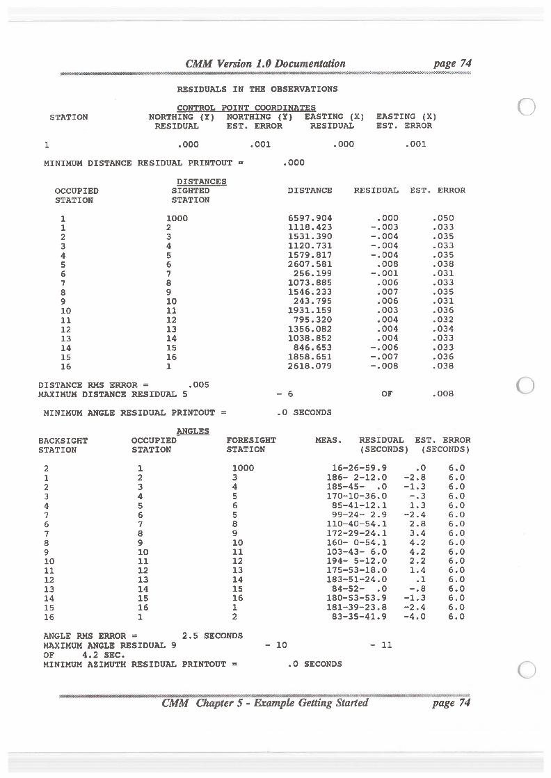
STATION

1

MINIMUM DISTANCE RESIDUAL PRINTOUT =

OCCUPIEDSTATIONI-‘I-‘D-'0-‘I-‘I-‘I-‘\Dm\lO\U'|-hhllslb-‘D-' 0\U1-hulk)!-‘O

DISTANCE RMS ERROR =

MAXIMUM DISTANCE RESIDUAL 5

MINIMUM ANGLE RESIDUAL PRINTOUT

BACKSIGHTSTATION\O®\lO\\lu§(auk)I-‘NJ

10111213141516

ANGLE RMS ERROR =

CMM Version 1.0 Documentation

RESIDUALS IN THE OBSERVATIONS

CONTROL POINT COORDINATESNORTHING (Y)

RESIDUAL

.000

NORTHING (Y)

DISTANCESSIGHTEDSTATION

O00\Dm~lO\lfl-FUNH.005

ANGLESOCCUPIEDSTATION

2.5 SECONDSMAXIMUM ANGLE RESIDUAL 9OF 4.2 SEC.MINIMUM AZIMUTH RESIDUAL PRINTOUT

EASTING (X)

page 74* . W0fi€ XM{<WR'WR'1i*3s‘¢'Z‘3¢€<¢<'3<{\9J'Z-€'Z-{vivfli

EASTING (x)EST. ERRoR RESIDUAL EST. ERROR

.001 .000 .001

.000

DISTANCE RESIDUAL EST. ERROR

6597.904 .000 .0501118.423 -.003 .0331531.390 -.004 .0351120.731 -.004 .0331579.817 —.0o4 .0352607.581 .008 .038256.199 -.001 .031

1073.885 .006 .0331546.233 .007 .035243.795 .006 .031

1931.159 .003 .036795.320 .004 .032

1356.082 .004 .0341038.852 .004 .033846.653 —.006 .033

1858.651 -.007 .0362618.079 -.008 .038

- 6 or .008

.0 SECONDS

FORESIGHT MEAS. RESIDUAL EST. ERRoRSTATION (SECONDS) (SECONDS)

1000 16-26-59.9 .0 6.03 186- 2-12.0 -2.8 6.04 185-45- .0 -1.3 6.05 170-10-36.0 -.3 6.06 85-41-12.1 1.3 6.05 99-24- 2.9 -2.4 6.08 110—40—54.1 2.8 6.09 172-29—24.1 3.4 6.010 160- 0-54.1 4.2 6.011 103-43- 6.0 4.2 6.012 194- 5—12.0 2.2 6.013 175-53-18.0 1.4 6.014 183-51-24.0 .1 6.015 84-52- .0 —.8 6.016 180-53-53.9 -1.3 6.01 181-39-23.8 -2.4 6.02 83-35-41.9 -4.0 6.0

- 10 — 11

= .0 SECONDS

.. v.

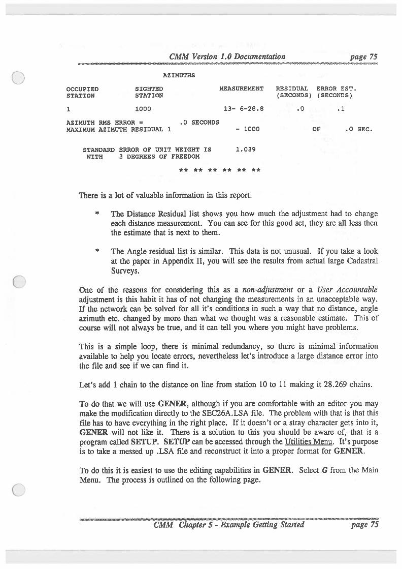
CMM Version 1.0 Documentation page 75. -'\‘F»¢3'€¢N'l-?.'6¢~3-M

AZIMUTHS

OCCUPIED SIGHTED MEASUREMENT RESIDUAL ERROR EST.STATION STATION (SECONDS) (SECONDS)1 1000 13- 6-28.8 .0 .1

AZIMUTH RMS ERROR = .0 SECONDSMAXIMUM AZIMUTH RESIDUAL 1 - 1000 OF .0 SEC.

STANDARD ERROR OF UNIT WEIGHT IS 1.039WITH 3 DEGREES OF FREEDOM

** ** ** ** ** **

There is a lot of valuable informationin this report.* The Distance Residual list shows you how much the adjustment had to change

each distance measurement. You can see for this good set, they are all less thenthe estimate that is next to them.

* The Angle residual list is similar. This data is not unusual. If you take a lookat the paper in Appendix H, you will see the results from actual large CadastralSurveys.

One of the reasons for considering this as a non-adjustment or a User Accountableadjustment is this habit it has of not changing the measurements in an unacceptable way.If the network can be solved for all it’s conditions in such a way that no distance, angleazimuth etc. changed by more than what we thought was a reasonable estimate. This ofcourse will not always be true, and it can tell you where you might have problems.This is a simple loop, there is minimal redundancy, so there is minimal informationavailable to help you locate errors, nevertheless let’s introduce a large distance error intothe fileand see if we can find it.

Let’s add 1 chain to the distance on line from station 10 to 11 making it 28.269 chains.

To do that we will use GENER, although if you are comfortable with an editor you maymake the modificationdirectly to the SEC26A.LSA file. The problem with that is that thisfilehas to have everything in the right place. If it doesn’t or a stray character gets into it,GENER will not like it. There is a solution to this you should be aware of, that is a

program called SETUP. SETUP can be accessed through theUtilitiesMenu. It’s purposeis to take a messed up .LSA fileand reconstruct it into a proper format for GENER.

To do this it is easiest to use the editing capabilitiesin GENER. Select G from the MainMenu. The process is outlined on the following page.

M ge 75

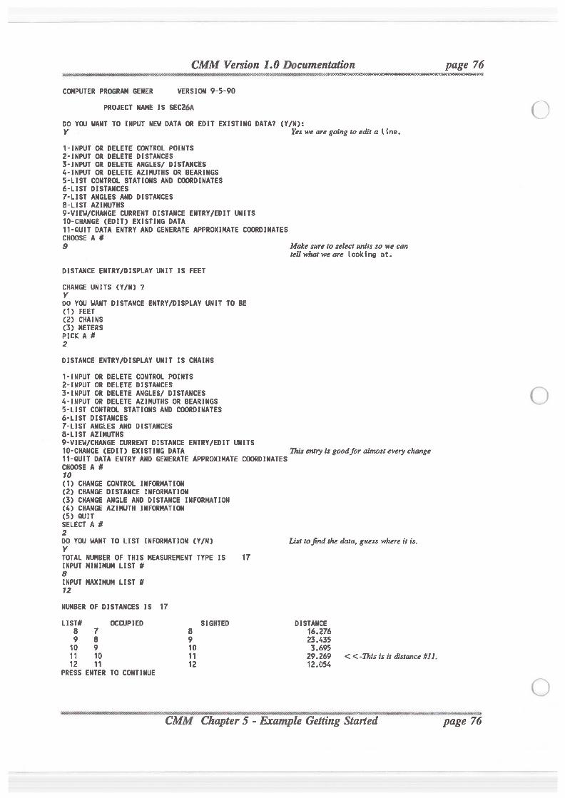
CMM Version 1.0 Documentation page 76.

A&%? %VK£#&%¢29&>N9KN¢WM9X4¢K

COMPUTER PROGRAM GENER VERSION 9-5-90

PROJECT NAME IS SEC26A

DO YOU HANT TO INPUT NEH DATA OR EDIT EXISTING DATA? (Y/N):Y Yes we are going to edit a line.

1-INPUT OR DELETE CONTROL POINTS2-INPUT OR DELETE DISTANCES3-INPUT OR DELETE ANGLES] DISTANCES4-INPUT OR DELETE AZIMUTHS OR BEARINGS5-LIST CONTROL STATIONS AND COORDINATES6-LIST DISTANCES7-LIST ANGLES AND DISTANCES8-LIST AZIMUTHS9-VIEN/CHANGE CURRENT DISTANCE ENTRY/EDIT UNITS10-CHANGE (EDIT) EXISTING DATA11-QUIT DATA ENTRY AND GENERATE APPROXIMATE COORDINATESCHOOSE A #9 Make sure to select units so we can

tell what we are looking at.

DISTANCE ENTRY/DISPLAY UNIT IS FEET

CHANGE UNITS (Y/N) 7YDO YW HANT DISTANCE ENTRY/DISPLAY UNIT TO BE(1) FEET(2) CHAINS(3) METERSPICK A #2

DISTANCE ENTRY/DISPLAY UNIT IS CHAINS

1-INPUT OR DELETE CONTROL POINTS2-INPUT OR DELETE DISTANCES3-INPUT OR DELETE ANGLESI DISTANCES4-INPUT OR DELETE AZIMUTHS OR BEARINGS5-LIST CONTROL STATIONS AND COORDINATES6-LIST DISTANCES7-LIST ANGLES AND DISTANCES8-LIST AZIIIJTHS9-VIEN/CHANGE CURRENT DISTANCE ENTRY/EDIT UNITS10-CHANGE (EDIT) EXISTING DATA This entry is gaodfar almost every change11-OUIT DATA ENTRY AND GENERATE APPROXIMATE COORDINATESCHOOSE A #10(1) CHANGE CONTROL INFORMATION(2) CHANGE DISTANCE INFORMATION(3) CHANGE ANGLE AND DISTANCE INFORMATION(4) CHANGE AZIMUTH INFORMATION(5) QUITSELECT A #2DO YOU WANT TO LIST INFORMATION (Y/N) List tofind the data, guess where it is.YTOTAL NUMBER OF THIS MEASUREMENT TYPE IS 17INPUT MINIMUM LIST #8INPUT MAXIIIM LIST #12

NUMBER OF DISTANCES IS 17

LIST# OCCUPIED SIGHTED DISTANCE8 7 8 16.2769 8 9 23.435

10 9 10 3.69511 10 11 29.269 < < -This is it distance #11.12 11 12 12.054

PRESS ENTER TO CONTINUE

"" 9' Ema

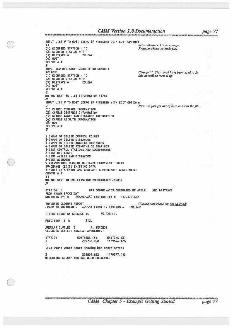
CMM Version 1.0 Documentation page 77‘

INPUT LIST # TO EDIT (ZERO IF FINISHED HITH EDIT OPTION):1 1 Select distance #11 to change(1) OCCUPIED STATION = 10 Program shows us eachpart(2) SIGHTED STATION = 11(3) DISTANCE = 29.269(4) QUITSELECT A N3INPUT NEH DISTANCE (ZERO IF NO CHANGE)28.269 Change it! This could have been used tofix(1) OCCUPIED STATION = 10 thisaswellasmessit up.(2) SIGHTED STATION = 11(3) DISTANCE = 28.269(lo) QUITSELECT A I4Do Ya! HANT TO LIST INFORMATION (Y/N)NINPUT LIST # TO EDIT (ZERO IF FINISHED HITH EDIT OPTION):0 Now, we just get out ofhere and run thefile.(1) CHANGE CONTROL INFORMATION(2) CHANGE DISTANCE INFORMATION(3) CHANGE ANGLE AND DISTANCE INFORMATION(4) CHANGE AZIMUTH INFORMATION(5) OUITSELECT A #5

1-INPUT OR DELETE CONTROL POINTSZ-INPUT OR DELETE DISTANCES3-INPUT OR DELETE ANGLES] DISTANCES4-INPUT OR DELETE AZIMUTHS OR BEARINGS5-LIST CONTROL STATIONS AND COORDINATES6-LIST DISTANCES7-LIST ANGLES AND DISTANCES8-LIST AIIMUTHS9'VIEH/CHANGE CURRENT DISTANCE ENTRY/EDIT UNITSTO-CHANGE (EDIT) EXISTING DATA11-OUIT DATA ENTRY AND GENERATE APPROXIMATE COORDINATESCHOOSE A #11DO YOU NANT TO USE EXISTING COORDINATES (Y/N)?N

STATION 2 HAS COORDINATES GENERATED BY ANGLE AND DISTANCEFROM KNOHN BACKSIGHTNORTHING (Y) = 256809.652 EASTING (X) = 1179377.lo12

TRAVERSE CLOSURE REPORT Closure now shows up not so good!ERROR IN NORTHING = 62.551 ERROR IN EASTING = -18.469

LINEAR ERROR OF CLOSURE IS 65.220 FT.

PRECISION IS 1/ 312.

ANGULAR CLOSURE IS 9. SECONDSCLOSURES REFLECT ANGULAR ADJUSTMENT

STATION NORTHING (Y) EASTING (X)1 255737.008 1179691. .126

:(ue Hon’: Haste space showing bad coordinates)2 256809.652 1179377.412DIRECTION ASSUMPTION HAS BEEN CORRECTED

w A. JV‘ « ~ ----------------------.. Chapte 5 - trte " '

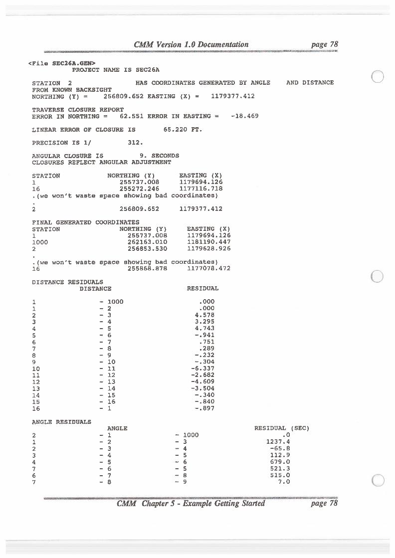
CMM Version 1.0 Documentation

<Fi1e SEC26A.GEN>PROJECT NAME IS sEc26A

STATION 2 HAS COORDINATES GENERATED BY ANGLEFROM KNOWN BACKSIGHTNORTHING (Y) = 256809.652 EASTING (X) = 1179377.412

TRAVERSE CLOSURE REPORTERROR IN NORTHING = 62.551 ERROR IN EASTING = -18.469

LINEAR ERROR OF CLOSURE IS 65.220 FT.

PRECISION IS 1/ 312.

ANGULAR CLOSURE IS 9. SECONDSCLOSURES REFLECT ANGULAR ADJUSTMENT

STATION NORTHING (Y) EASTING (x)1 255737.008 1179694.12616 255272.246 1177116.718.(we won't waste space showing bad coordinates)2 256809.652 1179377.412

FINAL GENERATED COORDINATESSTATION NORTHING (Y) EASTING (X)1 255737.008 1179694.1261000 262163.010 1181190.4472 256853.530 1179628.926

.(we won't waste space showing bad coordinates)16 255868.878 1177078.472

DISTANCE RESIDUALSDISTANCE RESIDUAL

1 - 1000 .0001 - 2 .0002 - 3 4.5783 - 4 3.2954 - 5 4.7435 - 6 —.9416 - 7 .7517 - 8 .2898 - 9 —.2329 - 10 -.30410 - 11 ~6.33711 — 12 -2.68212 - 13 -4.60913 - 14 -3.50414 - 15 —.34015 - 16 —.84016 - 1 —.897

ANGLE RESIDUALSANGLE RESIDUAL (SEC)

2 - 1 - 1000 .01 - 2 - 3 1237.42 - 3 - 4 -65.83 - 4 - 5 112.94 - 5 - 6 679.07 — 6 - 5 521.36 - 7 - 8 515.07 — 8 - 9 7.0

page 28

AND DISTANCE

nflHUOfl

8 _

9 _

10 -

11 -

12 -

13 -

14 -

15 -

16 -

AZIMUTH RESIDUALSAZIMUTH

1 _

10111213141516

1000

-10-11-12-13-14-15-16-1-2

RESIDUAL (SEC).0

-36.3-684.8

161.6-47.044.1

-758.8.7

1.8-636.5

page 79.

-. .“Mfl«WQHfiWMGK¢3WA$ #'¥Mflfi¢MM¢<fl<«WlWA

As you can see the GENER residuals have started to go bananas, there is some very smallindication that there may be a problem as the worst residual is on the distance where wemessed things up, but there is nothing definitive here, we could just as well have someangle errors. Lets go ahead and try an adjustment to see if that analysis will tell us anyIHOIC.

<Fi1e SEC26A.ADJ>PROJECT NAME IS SEC26A

PARAMETRIC LEAST SQUARES ADJUSTMENT

ALL OBSERVATIONS ARE REDUCED TO THE NAD 27 DATUMALL LISTED MEASUREMENTS HAVE BEEN REDUCED TO GRID61 COLORADO CENTRAL LAMBERT

INPUT NETWORK ELEVATION IS

NUMBER OF CONTROL SNUMBER OF DISTANCESNUMBER OF ANGLES =

NUMBER OF AZIMUTHS

TATIONS =

= 1717

= 1TOTAL NUMBER OF STATIONS =

STATIONKDHNGJQUJS-bO\Ul O C

6200.00 FT.

1

17

RESULTS OF ADJUSTMENT

ADJ. N (Y)261065.065260786.196259487.689262162.999258380.047261031.723261126.712256851.940255737.008261061.262260968.471255880.867255929.005259122.190258329.252256972.037255936.522

STANDARD ERRORS ERROR ELLIPSE INFO.ADJ. E (x)

1179812.3011l77219.8731179859.0201181190.4481179698.4831177151.4451176082.2231179629.0201179694.1261174537.6501174311.9341177079.4551175221.0091174589.7071174511.8591174474.4061174374.078

IN N IN E

apter 5 - Example$tdrted

SU SV T

page 79

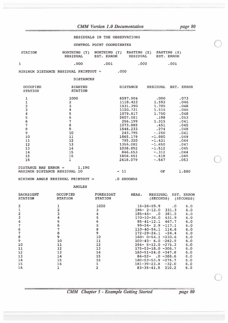
CMM Version 1.0 Documentation page 80' ...... C¢1”W9§N¢X¢>M<-?¢'3¢¢$¢¢K¢0‘M¢¢2¢$?3¢¢V£<-Z¢'1¢¢¢‘3VAOK#H

RESIDUALS IN THE OBSERVATIONS

CONTROL POINT COORDINATES

STATION NORTHING (Y) NORTHING (Y) EASTING (x) EASTING (x)RESIDUAL EST. ERROR RESIDUAL EST. ERROR

1 .000 .001 .000 .001

MINIMUM DISTANCE RESIDUAL PRINTOUT = .000

DISTANCES

OCCUPIED SIGHTED DISTANCE RESIDUAL EST. ERRORSTATION STATION

1 1000 6597.904 .000 .0731 2 1118.423 1.592 .0462 3 1531.390 1.705 .0483 4 1120.731 1.516 .0464 5 1579.817 1.750 .0485 6 2607.581 .198 .0536 7 256.199 1.315 .0417 8 1073.885 .451 .0458 9 1546.233 .274 .0489 10 243.795 -.250 .04110 11 1865.179 -1.880 .04911 12 795.320 -1.431 .04412 13 1356.082 -1.650 .04713 14 1038.852 -1.512 .04514 15 846.653 -.312 .04415 16 1858.651 —.418 .04916 1 2618.079 —.547 .053

DISTANCE RMs ERROR = 1.190MAXIMUM DIsrANcE RESIDUAL 10 - 11 OF 1.880

MINIMUM ANGLE REsIDUAL PRINTOUT = .0 sEcONDs

ANGLES

BACKSIGHT OCCUPIED FORESIGHT MEAs. RESIDUAL EST. ERRORSTATION STATION STATION (SECONDS) (SECONDS)2 1 1000 16-26-59.9 .0 6.01 2 3 186- 2-12.0 331.3 6.02 3 4 185—45- .0 381.2 6.03 4 5 170—10—36.0 431.9 6.04 5 6 85—41—12.1 467.7 6.07 6 5 99-24- 2.9 —117.1 6.06 7 8 110-40—54.1 114.6 6.07 8 9 172—29—24.1 -24.4 6.08 9 10 160- 0-54.1 -230.6 6.09 10 11 103-43- 6.0 -262.9 6.010 11 12 194- 5-12.0 -275.3 6.011 12 13 175-53-18.0 -306.7 6.012 13 14 183-51-24.0 —347.8 6.013 14 15 84—52- .0 -388.6 6.014 15 16 180-53—53.9 -276.7 6.015 16 1 181—39—23.8 -32.0 6.016 1 2 83-35-41.9 310.2 6.0

- - - 1185:... -1o(I~'\'-‘-9»'$'€A

8

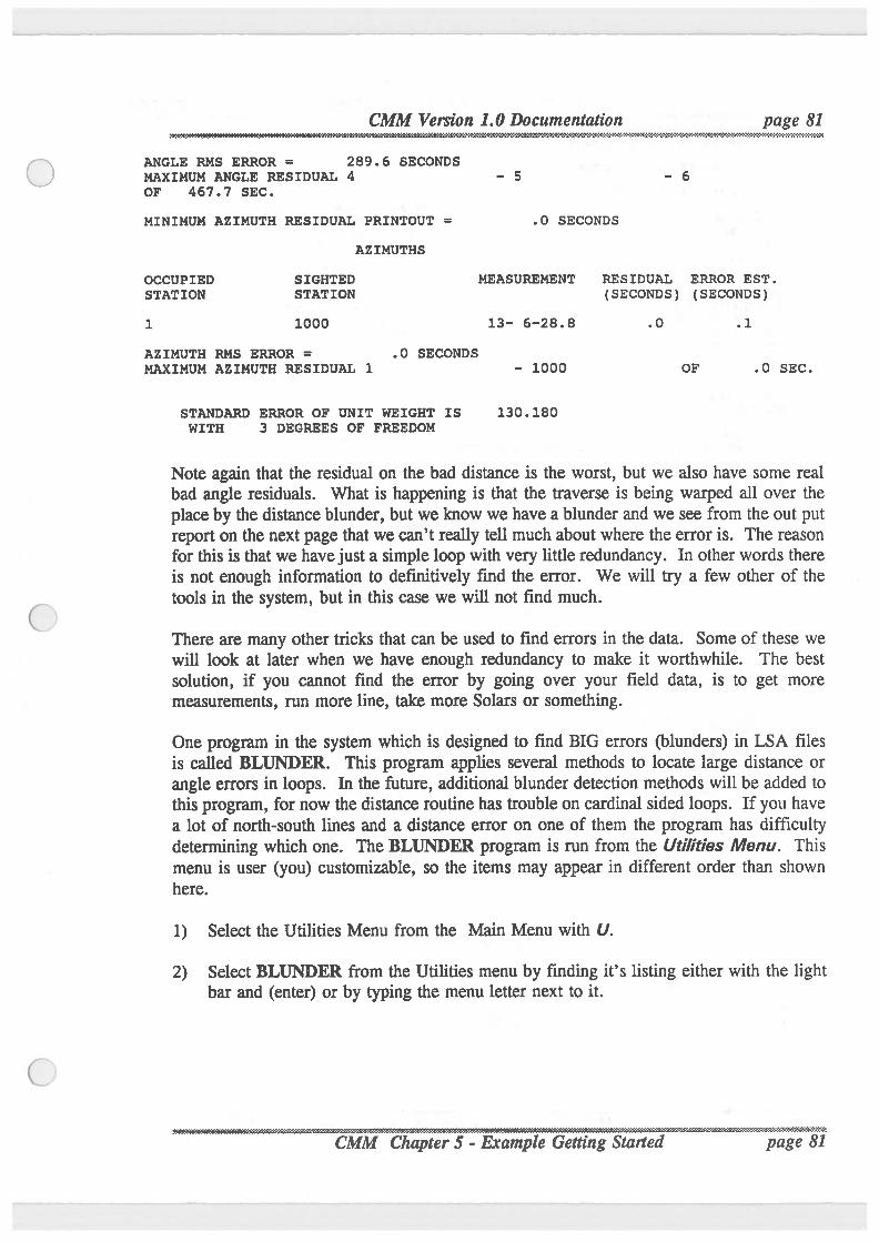
CMM Version 1. Documentation page 81. . . . . . . . . .

..

ANGLE RMS ERROR = 289.6 sEcoNDsMAXIMUM ANGLE RESIDUAL 4 — 5 — 6or 467.7 sEc.

MINIMUM AZIMUTH RESIDUAL PRINTOUT = .0 SECONDS

AZIMUTHS

OCCUPIED SIGHTED MEASUREMENT RESIDUAL ERROR EST.STATION STATION (SECONDS) (SECONDS)1 1000 13- 6-28.8 .0 .1

AZIMUTH RMs ERROR = .0 sEcoNDsMAXIMUM AZIMUTH RESIDUAL 1 — 1000 or .0 SEC.

STANDARD ERROR OF UNIT WEIGHT IS 130.180WITH 3 DEGREES OF FREEDOM

Note again that the residual on the bad distance is the worst, but we also have some realbad angle residuals. What is happening is that the traverse is being warped all over theplaceby the distance blunder, but we know we have a blunder and we see from the out putreport on the next page thatwe can’t really tell much about where the error is. The reasonfor this is thatwe have just a simple loop withvery little redundancy. In otherwords thereis not enough information to definitively find the error. We will try a few other of thetools in the system, but in this case we will not find much.

There are many other tricks that can be used to find errors in the data. Some of these wewill look at later when we have enough redundancy to make it worthwhile. The bestsolution, if you cannot find the error by going over your field data, is to get moremeasurements, run more line, take more Solars or something.One program in the system which is designed to find BIG errors (blunders) in LSA filesis called BLUNDER. This program applies several methods to locate large distance orangle errors in loops. In the future, additional blunder detection methods will be added tothisprogram, for now thedistance routine has trouble on cardinal sided loops. If you havea lot of north-south lines and a distance error on one of them the program has difficultydetermining which one. The BLUNDER program is run from the UtilitiesMenu. Thismenu is user (you) customizable, so the items may appear in different order than shownhere.

1) Select the UtilitiesMenu from the Main Menu with U.

2) Select BLUNDER from the Utilitiesmenu by finding it’s listing either with the lightbar and (enter) or by typing the menu letter next to it.

._.

_.

_...

_ _

._.

_.

_.

_.

_.,_

_.

_.

_.

_.

_._._.,.,._.

,.

_.

_.

_.

_.

_. .

_.

_.,.

_.

_.

_. . .

,.,._

.V.

_._.

_.

_.,. . .

_\,._.

_.

_.

_.

_ _.,._

._.

_., .

_ ._

CMM Version 1.0 Documentation

COMPUTER PROGRAM BLUNDER - VERSION 8-2-1990

PROJECT NAME IS SEC26A

INPUT INITIAL STATION (ZERO IF FINISHED)1POSSIBLE NEXT STATIONS

1) 10002) 23) 16

page 82J°09°°00'»M'!<'l#K-P51409090

We have to define a loop, we only have one hereAny point would do in thiscase.Theprogram is helping us define the loopsby showing whatpoints connect to 1We decide to go north

PICK TNE # ASSOCIATED HITN TNE NEXT STATION (ZERO TO QUIT)2NEXT STATIONNEXT STATIONNEXT STATIONNEXT STATIONNEXT STATION

NEXT sunouNEXT srmon

I52I83I84IS5[S6

IS 16IS 1

ANGLE BLUNDER DETECTIONANGLE NOT USED AT STA.

HITH ANGLE AT STATION 5NOT USED PRECISION IS 1/HITN ANGLE AT STATION 4NOT USED PRECISION IS 1/

RESULTING LINEAR CLOSURE65.70265.69765.68465.67065.66165.77565.77665.82265.88965.89965.90065.90865.91965.93065.89465.816

326

326

THESE ARE THE THO BEST PRECISIONSINDICATES NO ANGLE BLUNDER ISOLATED

D I STANCE BLUNDER DETECTIONDISTANCE

8 -99 -10

9 -1010 -11

10 -1111 -12

11 -1212 -13

12 -1313 -16

13 -1414 -15

CLOSURE187.580191 . 505

.32965.976 <-

67.509 <-—1.660

165.094229.506

241.570177.136

65.35116.351

Theprogramfinds the traverse and will onlystop and give you choices if there is abranch to go two ways. So thissingle loopjust zips through.

The program thenfigures closures byholding out 1 angle each in turn

Thefactthatthese are all the sameindicatesthatwe do not have anysignificantangle error, it's distance.

Now theprogram goes around the loop holdingout a couple ofdistances and doing anbearing-bearingintersection to thepointLookfor errors of the loop closure magnitudewhere the two adjacentsets give about the samemagnitudefor the same line.Like here!!

This won 't always work and theprogram doesn ’tsee it.

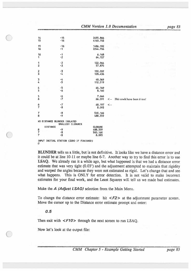
CMM Version 1. Documentation page 83. . . . .__..... >.. ._. ..... ....I.... .... .......................... ,_.... . {.;¢g,;.g,;.¢.g.g¢;ug.;.g. .;q«_.g.g.y,y,_~a_¢;a,.;.,y,;,°¢.4

14 -15 2455.86615 -16 4160.703

15 -16 1486.19216 -1 2244.706

16 -1 6.1681 -2 64.727

1 -2 122.9642 -3 57.870

2 -3 192.2023 -4 128.436

3 -4 48.0694 -5 112.519

4 -5 65.7695 -6 8.160

5 -6 7.6666 -7 66.591 <-- This couldhavebeen it too!

6 -7 68.197 <--7 -8 8.093

7 -8 500.1608 -9 488.359

NO DISTANCE BLUNDER ISOLATEDSNALLEST CLOSURES

DISTANCE CLOSURE8 -9 488.3597 -8 500.1607 -8 8.093

INPUT INITIAL STATION (ZERO IF FINISHED)0

BLUNDER tells us a little, but is not definitive. It looks like we have a distance error andit could be at line 10-11 or maybeline 6-7. Anotherway to try to find this error is to useLSAQ. We already ran it a whileago, but what happened is that we had a distance errorestimate that was very tight (0.03’) and the adjustmentattempted to maintain that rigidityand warped the angles becausethey were not estimated as rigid. Let’s change that and seewhat happens. This is ONLY for error detection. It is not valid to make incorrectestimates for your final work, and the Least Squares will tell us we made bad estimates.

Make the A {Adjust[SA0) selection from the Main Menu.

To change the distance error estimate: hit <F2> at the adjustment parameter screen.Move the cursor up to the Distance error estimate prompt and enter:

0.5

Then exit with <F10> through the next screen to run LSAQ.Now let’s look at the output file:

"‘" page 83.....................................................................................-

.

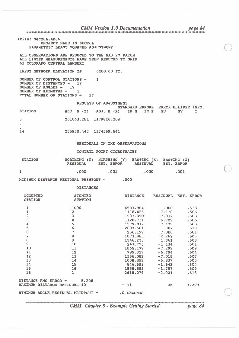
CMM Version 1.0 Documentation page 84. I -XeNi-1->2-t‘i‘§}9§9‘€->M‘h‘i'€'»}&fi3Q49¥N’:3¢?’k2'Z-#3'3’.<4':-1-:-2'3‘:-#5-2'2<~J-3‘3M'}N£

<Fi1e: sec26A.ADJ>PROJECT NAME IS SEC26A

PARAMETRIC LEAST SQUARES ADJUSTMENT

ALL OBSERVATIONS ARE REDUCED TO THE NAD 27 DATUMALL LISTED MEASUREMENTS HAVE BEEN REDUCED TO GRID61 COLORADO CENTRAL LAMBERT

INPUT NETWORK ELEVATION IS 6200.00 FT.

NUMBER OF CONTROL STATIONS = 1NUMBER OF DISTANCES = 17NUMBER OF ANGLES = 17NUMBER OF AZIMUTHS = 1TOTAL NUMBER OF STATIONS = 17

RESULTS OF ADJUSTMENTSTANDARD ERRORS ERROR ELLIPSE INFO.

STATION ADJ. N (2) ADJ. E (x) IN N IN E SU sv T

5 261043.281 1179826.2o8

14 255930.443 1174369.641

RESIDUALS IN THE OBSERVATIONS

CONTROL POINT COORDINATES

STATION NORTHING (Y) NORTHING (Y) EASTING (x) EASTING (x)RESIDUAL EST. ERRoR RESIDUAL EST. ERROR

1 .000 .001 .000 .001

MINIMUM DISTANCE RESIDUAL PRINTOUT = .000

DISTANCES

OCCUPIED SIGHTED DISTANCE RESIDUAL EST. ERRORSTATION STATION

1 1000 6597.904 .000 .5331 2 1118.423 7.118 .5062 3 1531.390 7.012 .5083 4 1120.731 6.729 .5064 5 1579.817 7.139 .5085 6 2607.581 .907 .5136 7 256.199 7.086 .5017 8 1073.885 2.262 .5058 9 1546.233 1.361 .5089 10 243.795 -1.134 .50110 11 1865.179 -7.299 .50911 12 795.319 -6.794 .50412 13 1356.082 -7.018 .50713 14 1038.852 -6.837 .50514 15 846.653 -1.642 .50415 16 1858.651 -1.787 .50916 1 2618.079 -2.021 .513

DISTANCE RMS ERRoR = 5.206MAXIMUM DISTANCE RESIDUAL 10 - 11 or 7.299

MINIMUM ANGLE RESIDUAL PRINTOUT = .0 sEcoNDs

“'-'-vw~** -- ~'-'- (4‘1.A':7£:-.».&?£5<~‘?§'IStarted pa 2 £1‘

_\

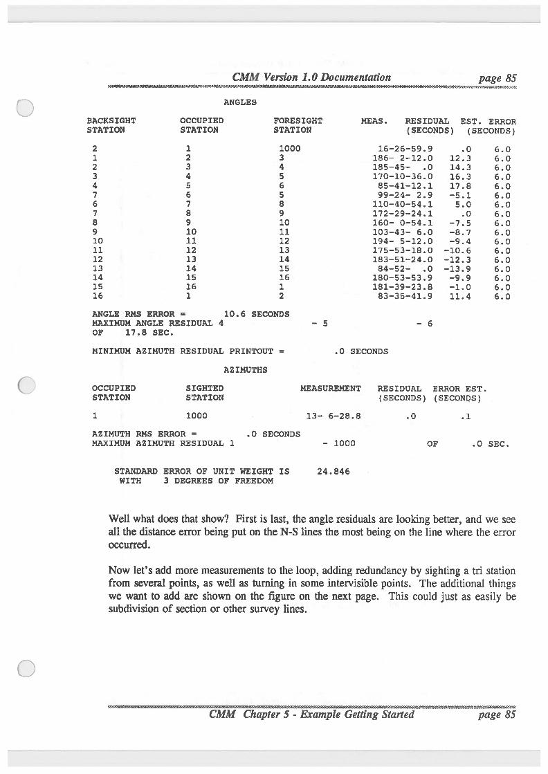
ANGLES

BACKSIGHT OCCUPIED FORESIGHT MEAS. RESIDUAL EST. ERRORSTATION STATION STATION (SECONDS) (SECONDS)

2 1 1000 16-26-59.9 .0 6.01 2 3 186- 2-12.0 12.3 6.02 3 4 185-45- .0 14.3 6.03 4 5 170-10-36.0 16.3 6.04 5 6 85-41-12.1 17.8 6.07 6 5 99-24- 2.9 -5.1 6.06 7 8 110-40-54.1 5.0 6.07 8 9 172-29-24.1 .0 6.08 9 10 160- 0-54.1 -7.5 6.09 10 11 103-43- 6.0 -8.7 6.010 11 12 194- 5-12.0 -9.4 6.011 12 13 175-53-18.0 -10.6 6.012 13 14 183-51-24.0 -12.3 6.013 14 15 84-52- .0 -13.9 6.014 15 16 180-53-53.9 -9.9 6.015 16 1 181-39-23.8 -1.0 6.016 1 2 83-35-41.9 11.4 6.0

ANGLE RMS ERROR = 10.6 SECONDSMAXIMUM ANGLE RESIDUAL 4 - 5 - 6OF 17.8 SEC.

MINIMUM AZIMUTH RESIDUAL PRINTOUT = .0 SECONDS

AZIMUTHS

OCCUPIED SIGHTED MEASUREMENT RESIDUAL ERROR EST.STATION STATION (SECONDS) (SECONDS)1 1000 13- 6-28.8 .0 .1

AZIMUTH RMS ERROR = .0 SECONDSMAXIMUM AZIMUTH RESIDUAL 1 - 1000 OF .0 SEC.

STANDARD ERROR OF UNIT WEIGHT IS 24.846WITH 3 DEGREES OF FREEDOM

Well what does that show? First is last, the angle residuals are looking better, and we seeall the distance error being put on theN-S lines the most being on the line where the erroroccurred.

Now let’s add more measurements to the loop, adding redundancy by sighting a tri stationfrom several points, as well as turning in some intervisible points. The additional thingswe want to add are shown on the figure on the next page. This could just as easily besubdivision of section or other survey lines.

‘(page 85

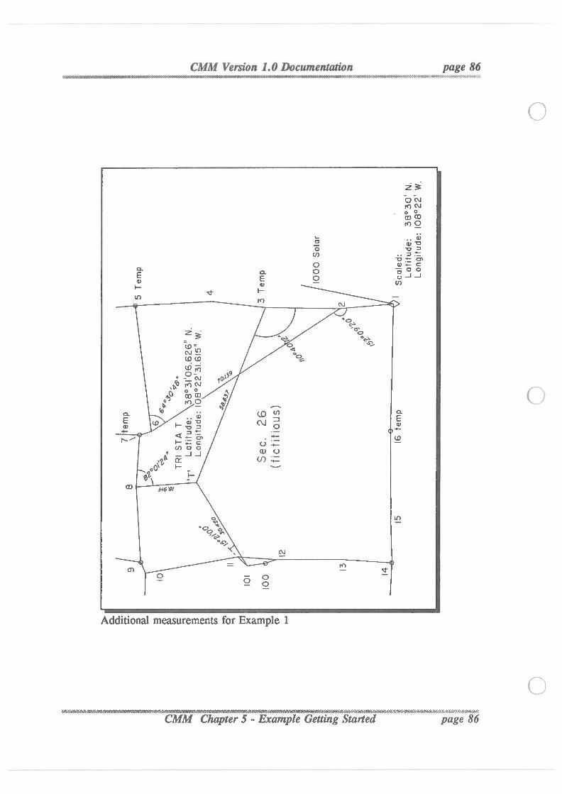
Sag,fined

Additionalmeasurements for Example 1

26(fic’ri‘fious)

Latnudez38°30'N. LongHude:|O8°22'W.

CMM Version 1.0 Documentation__ b

pagevvgo

CMM Version 1.0 Documentation page 87_ ._ . , . . . . ...... . . . . . . . ._ ..,. . . . . . . . . . . . . Nflvgz.-,.,‘v,_”:°.,..,»_.-_.;.;.;«_._t»,,;.r,_»mggag“;“ ;4wy,;.;;¢.;.,,;.;¢.;¢.;,;.¢.;.¢.;.;.,¢

Note: this is the end of the dialog on the tutorialfor Example 1, as of this Release.

Next, enter the additional data shown, rerun GENER, look at it's loop closures, runblunder with additional loops, run LSAQ with the 0.5 ft. distance float.

See if theadditional traverse links and observations help locate our error. AfterLSAQrun the CHECKER program holding each ‘comer’ of the square to see if the area ofthe distance blunder starts to become more obvious.

You should also delete the original scaled control on station 1 and add the tri stationvalues with GENER.

..

page 87

CMM Version .0 Documentation page 88 ¢%W9NVMWVM%)?fiZ¢?M->2<~m~?»VA

'-

. '<1‘Io'%’t2¢:‘v&%i:«':=:I:i:‘-:‘-.’v:‘~:‘«.¢:¢:3:i:=¢¢:<eCMM Chapter 5 - Exaple GettingSt page 88

CMM Version 1.0 Documentation page 89i

.A_D.l1lS.'I

AD

The purpose of ADJUST is to provide the Cadastral Surveyor with a comprehensive set oftools specifically for the "special case" adjustmentsoften found in the PLSS. The Manual ofSurveying Instructions, 1973 describes a number of unusual boundary determinationadjustment procedures that are not usually used in private sector work or dealt with intextbooks or availablesoftware. ADJUST provides solution for these methods, and anotherfeature is the ability to manually perform single and double proportions which are alsoavailable in PROPORT and AUTOPROP. This is useful for simple one—shot computations,or unusual situations which do not lend themselves to the automated capabilitiesof the otherprograms. The functionalityof ADJUST is analogous to thatof CSTUFor PROPORT. Theuser interface and method of operation has been intentionally kept similar to maintainconsistency where possible.The routines in ADJUST have been designed to provide the maximum flexibilityto the userwhile strictly conforming the guidelines set forth in The Manual of Surveying Instructions,1973. For example, the user is only allowed to perform double proportions geodetically; the‘Manual’ process requires proper allowance for cardinal equivalents of the record and cardinaloffsets to determine the true position. These can only be performed withina geodetic or truebearing frame of reference.

There is no substitute for user accountabilitywhen using this program or any other programin the CMM software package. The user is also reminded to be aware of the approriatesection of the ‘Manual’. For example:

1‘ The rules for the restoration of lost corners should not be applied until all originaland collateral evidence has been developed. When these means have been exhausted, thesurveyor will turn to proportionatemeasurement, which harmonizes surveying practicewithlegal and equitable considerations. This plan of relocating a lost comer is always employedunless outweighed by conclusive evidence of the original survey.

-ATA LAN E

Program Function:Miscellaneous PLSS AdjustmentRoutines

Computational Ability:Geodetic and Plane

Routines:North/SouthSingle Proportion, East/West Single Proportion, Double Proportion, OnePoint Control, Two Point Control, Three Point Control, Irregular Boundary Adjustment,Grant Boundary Adjustment,Compass Rule Adjustment

..........................-.

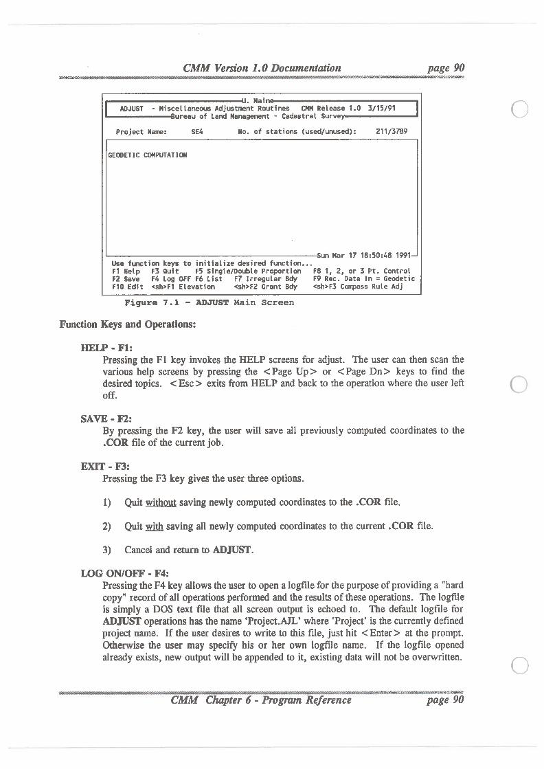
CMM Version 1.0 Documentation page 90

. Mail ADJUST - Miscellaneous Adjustment Routines CMM Release 1.0 3/15/91 |ureau of Land Management - Cadastral Surve

Project Name: SE4 No. of stations (used/unused): 211/3789

GEODETIC COMPUTATION Sun Mar 17 18:50:48 1991

Use function keys to initialize desired fuction...F1 Help F3 Quit F5 Single/Double Proportion F8 1, 2, or 3 Pt. ControlF2 Save F4 Log OFF F6 List F7 Irregular Bdy F9 Rec. Data In = GeodeticF10 Edit <sh>F1 Elevation <sh>F2 Grant Bdy <sh>F3 Compass Rule Adj

Figure 7.1 — ADJUST Main Screen

Function Keys and Operations:HELP - Fl:

Pressing the F1 key invokes the HELP screens for adjust. The user can then scan thevarious help screens by pressing the <Page Up> or <Page Dn> keys to find thedesired topics. < Esc> exits from HELP and back to the operation where the user leftoff.

SAVE- F2:By pressing the F2 key, the user will save all previously computed coordinates to the.COR fileof the current job.

EXIT - F3:Pressing the F3 key gives the user three options.1) Quit without saving newly computed coordinates to the .COR file.

2) Quit mm saving all newly computed coordinates to the current .COR file.

3) Cancel and return to ADJUST.

LOG ON/OFF - F4:Pressing theF4 key allows theuser to open a logfilefor thepurpose of providing a "hardcopy" record of all operations performed and the results of theseoperations. The logfileis simply a DOS text file that all screen output is echoed to. The default logfile forADJUSI‘ operations has the name ‘Project.AJL’where ‘Project’ is the currently definedproject name. If the user desires to write to this file, just hit <Enter> at the prompt.Otherwise the user may specify his or her own logfile name. If the logfile openedalready exists, new output will be appended to it, existing data will not be overwritten.

‘ ‘ -ezsssssssxsaeq

page 90

CMM Version 1.0 Documentation page 91}?'I'I‘l~2'I-¢‘n\-IA‘-'1):9>1£->W'WK'l-HK :-Dwéfléfifi-WflWW%¥fl4«'WFfiK

SINGLE/DOUBLEPROPORTIONTNG - F5:F5 will invoke the proportioning routines.

SINQLE PRQPQRTION - (Manual Section 5-30) Can be performed both geodeticallyand plane. The control points used must exist in the .COR file. Only one recorddistance is allowed from each control station to the reestablished point.DQQBLE PRQPORTION - (Manual Section 5-25) Can only be performed in geodeticmode. The four control points used must exist in the .COR file. Multiple recordcourses from each control point are allowed. To enter the record courses for each controlleg, input the information asked for at the prompts. To end record input for any leg,enter the identificationof thepoint being recovered thatwas previously input. ADJUSTwill then prompt for records for the next leg.

LIST - F6:The F6 function key invokes the list routine. This allows the user to list the coordinatesof points in the .COR fileby either individual names or all the points between a certainpair of points. If geodetic mode is in effect, screen output will be in sphericalcoordinates (Latitude and Longitude) otherwise output will be in State Plane. If thelogfile is active, all listed coordinates will be output to it. To list all points in a .CORfile, use 0 and z as upper and lower limits respectively of the range.

IRREGULAR BOUNDARY ADJUSTMENT - F7:Manual Section 5-36 describes an unusual adjustmentprocess that is used to restore lostcorners on irregular rectangular exteriors. It is in effect 2 adjustmentprocedures, 1 forE-W lines and 1 for N-S lines. F7 invokes the Irregular Boundary Adjustment. Tobegin, enter the starting and terminating control points of the adjustment (they must beresident in the .COR file). The record course data is then entered at the appropriateprompts. To end record input, enter the name of the terminating control station at the"To Station '2..." prompt. The adjustment will then proceed automatically. The firstthing the user will see is a report of misclosure similar to the below. The programdetermines which of methodologyto use based on the direction of the input record lines.

Report of Record Traverse Misclosure

Mean Geodetic Bearing to Closing Station: S 2°33’57" WGround Distance to Closing Station: 231.6252 Ft. at 1100 Ft. Elv.

Error in Latitude: 0° 0’ 2.2840"Error in Longitude: - 0° 0’.1489"

Error in State Plane Northing: 231.4168Error in State Plane Easting: 9.3592

The misclosure statement gives the user a measure of how good (or bad) a recordtraverse was. The bearingand distance to theclosing station is thedirection and distancefrom the end of the record traverse and the terminating station it was supposed to end upon.

s . nwmw9%w Referertce page 91

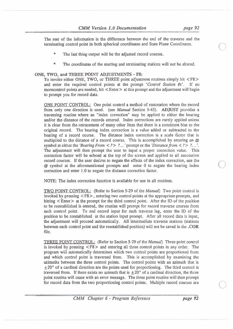
$'2C<"2!2-Z-€'€~1'is!!§¢s . .

ONE

CMM Version 1.0 Documentation page. .

395"/2¢.93€9s""l'.“l"EWQQWQ?flWQ K4‘3‘l‘P$$¢t’¢9PM&Y‘X’M&'#1‘2&-§M¢¢h‘¢3€'»??A('Q1’2’.§¢E~EZ'$2-2'2-E-2'3-1*€'5'I'f'Z‘I‘5'?I-2'53)‘:-I-I-Z~l'2-I-2'2-I‘74-35*!~Z-Z‘}¢§?Z~!¢-H-f-1V€‘HICvZ‘I-3*?IOCIIV1'“ - V. .1235:.... . .

The rest of the information is the difference between the end of the traverse and theterminating control point in both spherical coordinates and State Plane Coordinates.

* The last thingoutput will be the adjusted record courses.

* The coordinates of the starting and terminating stations will not be altered.

, TWO, and THREE POINT ADJUSTMENTS- F8:To invoke either ONE, TWO, or THREE point adjustmentroutines simply hit < F8>and enter the required control points at the prompt ‘Control Station #x’. If nomorecontrol points are needed, hit < Enter > at thisprompt and theadjustmentwill beginto prompt you for record data.

QNE PQINT QQNTRQL; One point control a method of restoration where the recordfrom only one direction is used. (see Manual Section 5-45). ADJUST provides atraversing routine where an "index correction" may be applied to either the bearingand/or the distance of the records entered. Index corrections are rarely applied unlessit is clear from the retracement of many other lines that there is a consistent bias to theoriginal record. The bearing index correction is a value added or subtracted to thebearing of a record course. The distance index correction is a scale factor that ismultiplied to the distance of a record course. This is accomplished by entering an @symbol at eitherthe ‘BearingFrom < ?> ?... ’ prompt or the ‘Distancefrom < ?> ?... '.The adjustment will then prompt the user to input a proper correction value. Thiscorrection factor will be echoed at the top of the screen and applied to all successiverecord courses. If the user desires to negate the effects of the index correction, use the@ symbol at the aforementioned prompts and enter 0 to negate the bearing indexcorrection and enter 1.0 to negate the distance correction factor.

NOTE: The index correction function is available for use in all routines.

TWQ POINT QQNTROL; (Refer to Section 5-29 of the Manual) Two point control isinvoked by pressing <F8> , entering two control points at the appropriate prompts, andhitting <Enter> at the prompt for the third control point. After the ID of the positionto be reestablished is entered, the routine will prompt for record traverse courses fromeach control point. To end record input for each traverse leg, enter the ID of theposition to be reestablished at the station input prompt. After all record data is input,the adjustment will proceed automatically. All intermediate traverse stations (stationsbetween each control point and the reestablished position) will not be saved in the .CORfile.

THREE POINT QQNTRQL: (Refer to Section 5-29 of theManual) Three point controlis invoked by pressing <F8> and entering all three control points in any order. Theprogram will automaticallydetermines which two control points are proportioned fromand which control point is traversed from. This is accomplished by examining theazimuths between the three control points. The control points with an azimuth that is-l_-20° of a cardinal direction are the points used for proportioning. The third control istraversed from. If there exists no azimuththat is 1-20° of a cardinal direction, the threepoint routine will cease withan error message. The three point routine will then promptfor record data from the two proportioning control points. Multiple record courses are

Sh‘Ri!39:&3fl23:Z2:J:i5S‘l85S§S>}>$'$‘}:1>‘£‘.23:1:1$$$‘J:l:2:I'$$'.>!‘d3:3:V}:7$Rfitlfizitzklzlfi Z ':l‘.i:=‘.i'.3$'-9’.-5155

page 92 5 -5‘ ‘I‘ ‘M? iSK'}5'.$.'-SG$‘5'.'&'/3:i9!%'-CMM Chapter 6 - Program Reference

.a-~_

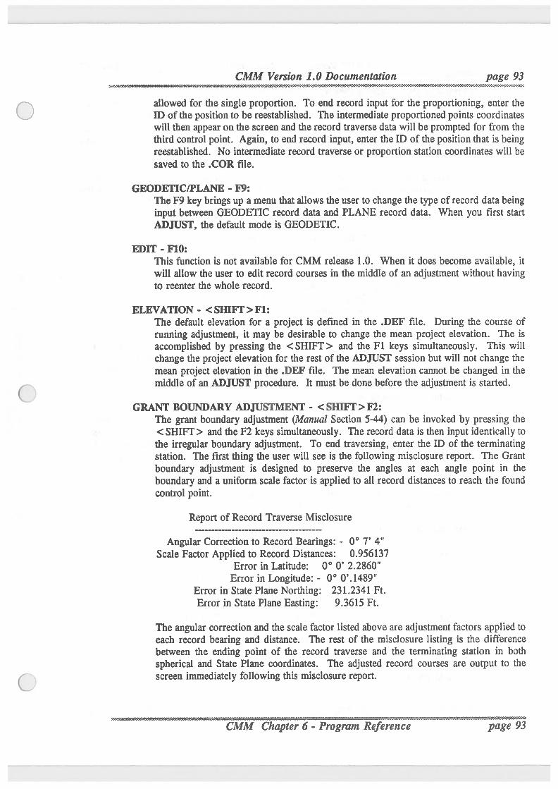
CMM Version 1.0 Documentation page 93

. r3¢,4r?¢¢"¢X'M¢2.¢'.. . .. . .

' €'3¢’.‘@‘¢‘i’4¢.’.¢¢»i"A'341’.‘¢~:-iwtflfibt-3'Z*>‘a€e3-2

allowed for the single proportion. To end record input for the proportioning, enter theID of the position to be reestablished. The intermediate proportioned points coordinateswill then appear on the screen and the record traverse data willbe prompted for from thethird control point. Again, to end record input, enter the ID of theposition that is beingreestablished. No intermediate record traverse or proportion station coordinates will besaved to the .COR file.

GEODETIC/PLANE - F9:The F9 key brings up a menu thatallows theuser to change thetype of record data beinginput between GEODETIC record data and PLANE record data. When you first startADJUST, the default mode is GEODE'I‘IC.

EDIT - F10:This function is not availablefor CMM release 1.0. When it does become available, itwill allow the user to edit record courses in the middle of an adjustmentwithouthavingto reenter the whole record.

ELEVATION - < SHIFI‘> F1:The default elevation for a project is defined in the .DEF file. During the course ofrunning adjustment, it may be desirable to change the mean project elevation. The isaccomplished by pressing the <SHIFT> and the F1 keys simultaneously. This willchange the project elevation for the rest of the ADJUST session but will not change themean project elevation in the .DEF file. The mean elevation cannot be changed in themiddle of an ADJUST procedure. It must be done before the adjustment is started.

GRANT BOUNDARY ADJUSTMENT - < SHIFI‘>F2:The grant boundary adjustment (Manual Section 5-44) can be invoked by pressing the< SHIFT> and theF2 keys simultaneously. The record data is then input identically tothe irregular boundary adjustment. To end traversing, enter the ID of the terminatingstation. The first thingthe user will see is the following misclosure report. The Grantboundary adjustment is designed to preserve the angles at each angle point in theboundary and a uniform scale factor is applied to all record distances to reach the foundcontrol point.

Report of Record Traverse Misclosure

Angular Correction to Record Bearings: - 0° 7’ 4"Scale Factor Applied to Record Distances: 0.956137

Error in Latitude: 0° 0’ 2.2860"Error in Longitude: - 0° 0’.1489"

Error in State Plane Northing: 231.2341 Ft.Error in State Plane Easting: 9.3615 Ft.

The angular correction and the scale factor listed above are adjustmentfactors applied toeach record bearing and distance. The rest of the misclosure listing is the differencebetween the ending point of the record traverse and the terminating station in bothspherical and State Plane coordinates. The adjusted record courses are output to thescreen immediately following this misclosure report.

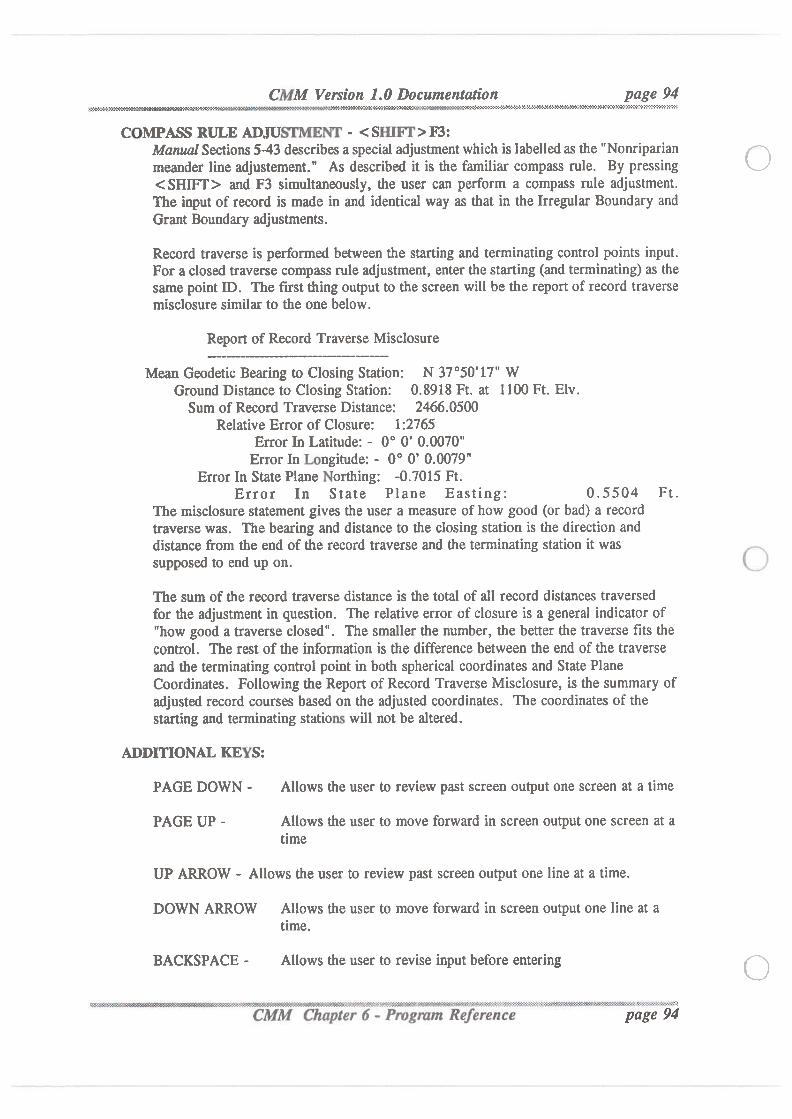
CMM Version 1.0 Documentation page 94

, .‘fiNNW%WMR

.3W\'.°'.‘V?>1'3->2-I-Z'M':>.'72~2-3'I-7I'W¢3K¢'»!~?N‘}N¢2'!AX'$'2‘?'2~X‘>€-9I-I-519¢-2'?!-{'9-3‘}1‘i'!-2*:-524':-2‘2'?1

COMPASS RULE ADJUSTMENT - < SHIFT> F3:Manual Sections 5-43 describes a special adjustmentwhich is labelledas the "Nonriparianmeander line adjustement." As described it is the familiar compass rule. By pressing<SHIFT> and F3 simultaneously, the user can perform a compass rule adjustment.The input of record is made in and identical way as that in the Irregular Boundary andGrant Boundary adjustments.Record traverse is performed between the starting and terminating control points input.For a closed traverse compass rule adjustment, enter thestarting (and terminating) as thesame point ID. The first thingoutput to the screen will be the report of record traversemisclosure similar to the one below.

Report of Record Traverse Misclosure

Mean Geodetic Bearing to Closing Station: N 37°50’17" WGround Distance to Closing Station: 0.8918 Ft. at 1100 Ft. Elv.

Sum of Record Traverse Distance: 2466.0500Relative Error of Closure: 122765

Error In Latitude: - 0° 0’ 0.0070"Error In Longitude: — 0° 0’ 0.0079"

Error In State Plane Northing: -0.7015 Ft.Error In State Plane Easting: 0.5504 Ft.

The misclosure statement gives the user a measure of how good (or bad) a recordtraverse was. The bearing and distance to the closing station is the direction anddistance from the end of the record traverse and the terminating station it was

supposed to end up on.

The sum of the record traverse distance is the total of all record distances traversedfor the adjustment in question. The relative error of closure is a general indicator of"how good a traverse closed". The smaller the number, the better the traverse fits thecontrol. The rest of the information is the difference between the end of the traverseand the terminating control point in both spherical coordinates and State PlaneCoordinates. Following the Report of Record Traverse Misclosure, is the summary ofadjusted record courses based on the adjusted coordinates. The coordinates of thestarting and terminating stations will not be altered.

ADDITIONALKEYS:

PAGE DOWN - Allows the user to review past screen output one screen at a time

PAGE UP - Allows the user to move forward in screen output one screen at a

time

UP ARROW - Allows the user to review past screen output one line at a time.

DOWN ARROW Allows the user to move forward in screen output one line at atime.

BACKSPACE - Allows the user to revise input before entering

'- -“ '(v$‘7.7’-‘.'€59351’?!-"’9€3)5$59V- 3S¢S&!i¥5Y?39»¢i:l‘3S:Zli'»'&3 i:?26$wW .?H2E&‘%51Z3:5$> 3‘-"123:

6 - Pmgram Reference page 9

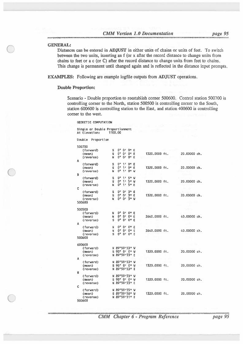
GENERAL:

CMM Version 1.0 Documentation

page 95. . . %NX“9WFJM4€

Distances can be entered in ADJUST in either units of chains or units of feet. To switchbetween the two units, inserting an f (or x after the record distance to change units fromchains to feet or a c (or C) after the record distance to change units from feet to chains.This change is permanent until changed again and is reflected in the distance input prompts.

EXAMPLES: Following are example logfileoutputs from ADJUST operations.Double Proportion:

Scenario - Double proportion to reestablish corner 500600. Control station 500700 iscontrolling corner to the North, station 500500 is controlling comer to the South,station 600600 is controlling station to the East, and station 400600 is controllingcomer to the west.

GEODETIC COMPUTATION

Single or Double ProportionmentAt Elevation:

Double Proportion500700

(forward)(mean)(reverse)

(forward)(mean)(reverse)

(forward)(mean)(reverse)

(forward)(mean)(reverse)

500600

500500(forward)(mean)(reverse)

(forward)(mean)(reverse)

500600

600600(forward)(mean)(reverse)

(forward)(mean)(reverse)

(forward)(mean)(reverse)

(forward)(mean)(reverse)

500600

Z100!Z100)ZUDUDZUIUD

GOO 000

(I322(D22

GOOGOO

canone

GOOGOO

usss-

ZUIZZIIIZZ102Z012

1100.00

0! oilOI Ollol 0“

1 I olloll

1 I oil

1: 5n1! SH1’ 5HO00

O00OOO

oneonecan

—I ~

on 3n0: 3nor 3n

ollolloll

OHonon

89°59'53"90° 0' 0"89°59'53"

89°59'53"90° 0' 0'-89°59'53"

89°59'53"90° 0' 0"89°59'53"

89°59'55"89°59'58"89°59'51"

I:H'||'nHIE:£l'l'Il'1IITIHII11

l'fll'fll'l'll'|'Il'Hl'|'|

mI:I:rnttrnlzl:mil‘:

1320.0000

1320.0000

1320.0000

1320.0000

2640.0000

2640.0000

1320.0000

1320.0000

1320.0000

1320.0000

ft.

ft.

20.00000

20.00000

20.00000

20.00000

40.00000

40.00000

20.00000

20.00000

20.00000

20.00000

ch.

ch.

ch.

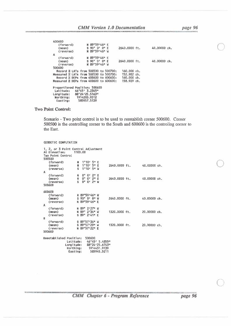
400600(forward) N 89°59'46" E(mean) 5 90° 0’ 0" E(reverse) N 89°59'46" H

A(forward) N 89°59'46" E(mean) S 90° 0' 0" E(reverse) N 89°59'46" H

500600Record 2 LATs from 500500 to 500700:

Measured 2 LATs from 500500 to 500700:Record 2 DEPs from 400600 to 600600:

Measured Z DEPs from 400600 to 600600:

Proportioned Position: 500600Latitude: 46°45’ 3.2345"

Longitude: 88°24'25.5163"Northing: 1914203.9312Easting: 585957.5139

Two Point Control:

’-:‘>:3:3::$:<5S.’-$$‘.3.'~$t~'$$5'S';";’

CMM Version 1.0 Documentation page 96- WWV ‘flflXi9§§®C2‘4‘1'K6N‘IfiZ'1'Z'Z'ZW&2Kfi¢NIV4¢W'5fiRfi» fi C-1-1+3-£’£~1~L

2640.0000 ft.

2640.0000 ft.

160.000 ch.152.982 ch.160.000 ch.158.929 ch.

40.00000 ch.

40.00000 ch.

Scenario — Two point control is to be used to reestablish corner 500600. Corner500500 is the controlling corner to the South and 600600 is the controling corner tothe East.

GEOOETIC COMPUTATION

1, 2, or 3 Point Control AdjustmentAt Elevation: 1100.00Two Point Control500500

(forward) N 1°10’ 5" E(mean) N 1°10’ S" E 2640.

A(reverse) S 1°10’ S" H

(forward) N 0° 0' 2" E(mean) N 0° 0' 2" E 2640.(reverse) S 0° 0' 2" H

500600

600600(forward) N 89°59'46" H(mean) 5 90° 0' 0" H 2640.(reverse) N 89°59'46" E

A(forward) N 89° 2'27" H(mean) N 89° 2'34" U 1320.(reverse) S 89° 2'41" E

B(forward) S 89°57'36" H(mean) S 89°57'29" H 1320.(reverse) N 89°57'22" E

500600

Reestablished Position: 500600Latitude: 46°45’ 5.4855"

Longitude: 88°24'25.6743"Northing: 1914431.9139Easting: 585945.5211

oooo ft. 4o.ooooo ch.

oooo ft. 4o.ooooo ch.

oooo ft. 4o.ooooo ch.

oooo ft. 2o.ooooo ch.

oooo ft. 2o.ooooo ch.

.» »\\...-.~.-. -.\.~.--............. ._ g”5m$S§$§5;:Reflnence pnge96

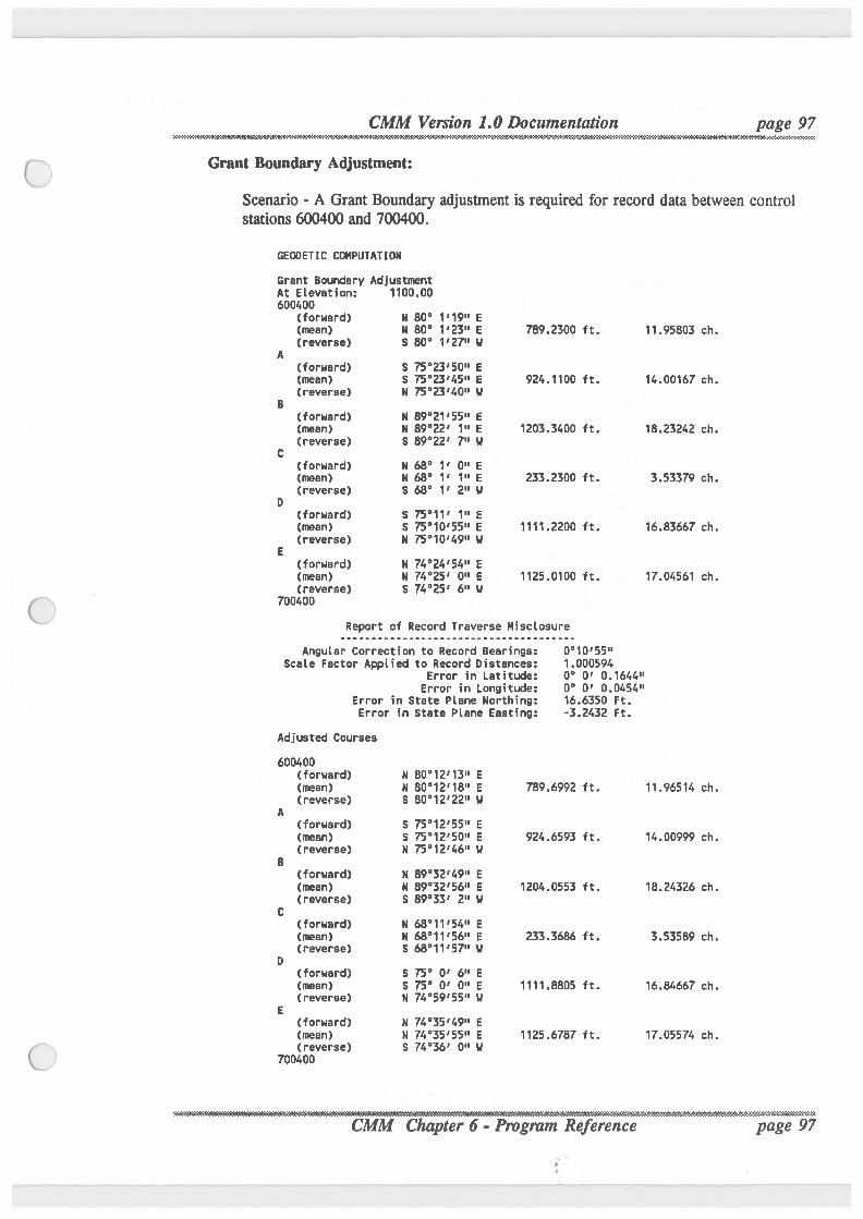
CMM Version 1.0 Documentation page 97. ; ..VN‘2'3'W4¢¢¢M'‘‘9".9%N-N'€’M‘!'X{

Grant Boundary Adjustment:Scenario - A Grant Boundary adjustment is required for record data between controlstations 600400 and 700400.

GEOOETIC COMPUTATION

Grant Boundary AdjustmentAt Elevation: 1100.00600400

(forward) N 80° 1'19" E(mean) N 80° 1'23" E 789.2300 ft. 11.95803 ch.

A(reverse) S 80° 1'27" H

(forward) S 75°23'50" E(mean) S 75°23'45" E 924.1100 ft. 14.00167 ch.

B(reverse) N 75°23'40" H

(forward) N 89°21'55" E(mean) N 89°22’ 1" E 1203.3400 ft. 18.23242 ch.

C(reverse) S 89°22’ 7" H

(forward) N 68° 1' 0" E(mean) N 68° 1' 1" E 233.2300 ft. 3.53379 ch.

D(reverse) S 68° 1' 2" H

(forward) 5 75°11’ 1" E(mean) 8 75°10'55" E 1111.2200 ft. 16.83667 ch.(reverse) N 75°10'49" H

E(forward) N 74°24'54" E(mean) N 74°25’ 0" E 1125.0100 ft. 17.04561 ch.(reverse) S 74°25’ 6" N

700400

Report of Record Traverse Nisclosure

Angular Correction to Record Bearings: 0°10'55"Scale Factor Applied to Record Distances: 1.000594

Error in Latitude: 0° 0' 0.1644"Error in Longitude: 0° 0' 0.0454"

Error in State Plane Northing: 16.6350 Ft.Error in state Plane Easting: -3.2432 Ft.

Adjusted Courses

600400(forward) N 80°12'13" E(mean) N 80°12'18" E 789.6992 ft. 11.96514 ch.(reverse) S 80°12'22" H

A(forward) 5 75°12'55" E(mean) 5 75°12'50" E 924.6593 ft. 14.00999 ch.(reverse) N 75°12'46" H

8(forward) N 89°32'49" E(mean) N 89°32'56" E 1204.0553 ft. 18.24326 ch.(reverse) 5 89°33’ 2" H

C(forward) N 68°11'54" E(mean) N 68°11'56" E 233.3686 ft. 3.53589 ch.(reverse) S 68°11'57" H

D(forward) S 75° 0' 6" E(mean) S 75° 0' 0" E 1111.8805 ft. 16.84667 ch.(reverse) N 74°59'55" U

E(forward) N 74°35'49" E(mean) N 74°35'55" E 1125.678? ft. 17.05574 ch.(reverse) 5 74°36’ 0" N

700400

.“' ---.--.- - -. '.-\. .\-.'..-r -\. ‘ .- .. -.-.-..-.-. ‘ . -. -.r.- {\m15R1 $2

mgram Reec

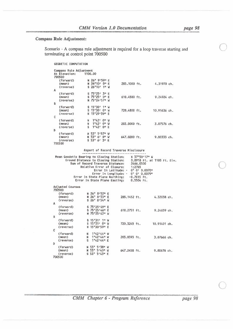
1.0 Documentation ~m»mmmmr:m%w-xem-x-m-:

CMM Version

Compass Rule Adjustment:Scenario - A compass rule adjustmentis required for a loop traverse starting andterminating at control point 700500

GECDET I C CCHPUTATION

Compass Rule AdjustmentAt Elevation: 1100.00700500

(forward) N 26° 9'59" E(mean) N 26°10’ 0" E 285.1000 ft. 4.31970 ch.(reverse) S 26°10’ 1" H

A(forward) S 75°25’ 3" E(mean) S 75°25’ 0" E 610.4500 ft. 9.24924 ch.(reverse) N 75°24'57" H

8(forward) 8 15°30’ 1" H(mean) 8 15°30’ 0" H 720.4800 ft. 10.91636 ch.(reverse) N 15°29'59" E

C(forward) N 1°42’ 0" H(mean) N 1°42’ 0" H 203.0000 ft. 3.07576 ch.(reverse) S 1°42’ 0" E

0(forward) N 53° 5'57" H(mean) N 53° 6' 0" H 647.0200 ft. 9.80333 ch.(reverse) S 53° 6’ 3" E

700500

Report of Record Traverse Misclosure

Mean Geodetic Bearing to Closing Station: N 37°50'17" HGround Distance to Closing Station: 0.8918 Ft. at 1100 Ft. Elv.

Sum of Record Traverse Distance: 2466,0500Relative Error of Closure: 1:2765

Error In Latitude: - 0° 0' 0.0070"Error In Longitude: - 0° 0' 0.0079"

Error In State Plane Northing: -0.7015 Ft.Error In State Plane Easting: 0.5504 Ft.

Adjusted Courses700500

(forward) N 26° 8'52" E(mean) N 26° 8'53" E 285.1452 ft. 4.32038 ch.(reverse) 5 26° 8'54" H

A(forward) S 75°25'49" E(mean) S 75°25'46" E 610.2751 ft. 9.24659 ch.(reverse) N 75°25'42" H

B(forward) S 15°31’ 1" H(mean) S 15°31’ 0" H 720.3245 ft. 10.91401 ch.(reverse) N 15°30'59" E

C(forward) N 1°42'44" H(mean) N 1°42'44" H 203.0593 ft. 3.07666 ch.(reverse) S 1°42'44" E

0(forward) N 53° 5'38“ H(mean) N 53° 5'40" H 647.2458 ft. 9.80676 ch.(reverse) S 53° 5'43" E

700500

-'-‘-'-W-'‘:3:~‘SS$.‘1!bif~b1‘€:3$$$1'¢‘ci$:§$:C:2'-$$$$c£$$:»‘5$:-557‘ :1tA.\'*I.Reference page 9 .-.-.-.a.-.a.a. ., .-».-. ~.

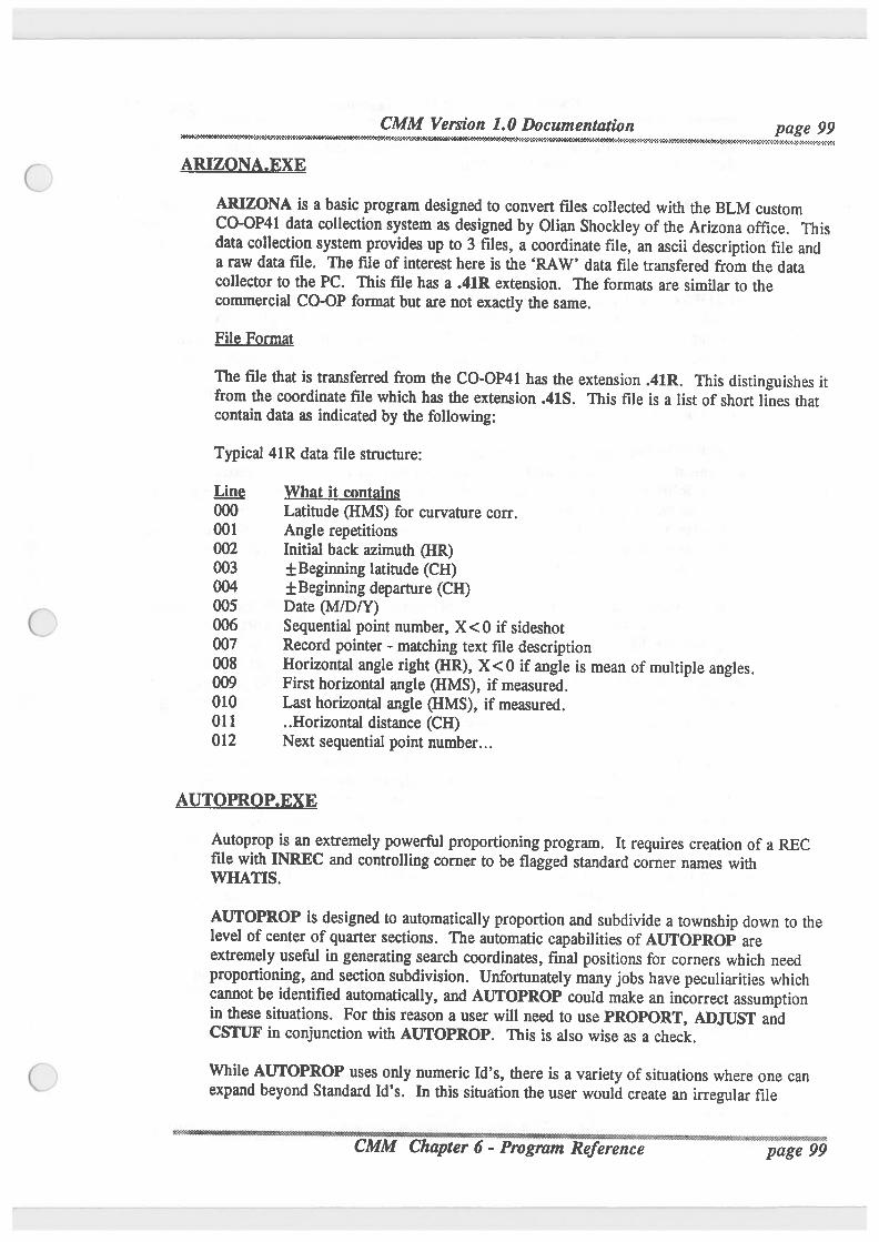
ARIZ A EXE

ARIZONA is a basic program designed to convert files collected with the BLM customCO-OP41 data collection system as designed by Olian Shockley of the Arizonaoffice. Thisdata collection system provides up to 3 files, a coordinate file, an ascii description file anda raw data file. The fileof interest here is the ‘RAW’ data filetransfered from the datacollector to the PC. This filehas a .4lR extension. The formats are similar to thecommercial C0-OP format but are not exactlythe same.

FileFormatThe file that is transferred from the CO-OP4l has the extension .41R. This distinguishes itfrom the coordinate filewhich has the extension .4lS. This file is a list of short lines thatcontain data as indicated by the following:Typical 41R data filestructure:

Q13; What it contains000 Latitude (HMS) for curvature corr.001 Angle repetitions002 Initial back azimuth (HR)003 iBeginning latitude (CH)004 iBeginning departure (CH)005 Date (M/D/Y)006 Sequential point number, X<0 if sideshot007 Record pointer - matching text filedescription008 Horizontal angle right (HR), X<0 if angle is mean of multiple angles.009 First horizontal angle (HMS), if measured.010 Last horizontal angle (HMS), if measured.011 ..Horizontal distance (CH)012 Next sequential point number...

A T PROP EXE

Autoprop is an extremely powerful proportioning program. It requires creation of a RECfilewith INREC and controlling comer to be flagged standard corner names withWI-IATIS.

AUTOPROP is designed to automaticallyproportion and subdivide a township down to thelevel of center of quarter sections. The automaticcapabilitiesof AUTOPROP areextremely useful in generating search coordinates, final positions for corners which needproportioning, and section subdivision. Unfortunately many jobs have peculiarities whichcannot be identified automatically,and AUTOPROP could make an incorrect assumptionin these situations. For this reason a user will need to use PROPORT, ADJUST andCSTUF in conjunctionwith AUTOPROP. This is also wise as a check.

While AUTOPROP uses only numeric Id’s, there is a variety of situations where one canexpand beyond Standard Id’s. In this situation the user would create an irregular file

A .\ &' age 9

_ .

CMM Version 1.0 Documentation page 100- 3a?&QO9¢'O¢\?99?4'>94'3<~>l'3'2'2'2€'i¢'!'I'?.‘$-$'.‘°¢4‘Z’-R3:3K'€¢¢¢<'§Z‘PX'2‘1-35‘N¢-5Z\‘¢9€'5€°O0$¢€5\D~D'3M‘1I°C'€':

(.IRR) using AUTOPROP’s built in editor. This irregular filewould contain user definedsubdivisions which are not standard GCDB format.

AUTOPROP reads the .DEF, .COR, .REC, AND .IRR files. The output file is labeledwith a .SUB fileextension. The importance of the .SUB filecannot be emphasized enough- it is the surveyor’s verificationthat the proportions and subdivisions were handled in whathe or she deems a correct fashion.

AUTOPROP first allows the user to proportion all stations in the .REC filebased oncontrolling information in the .COR file. If this computation is selected, AUTOPROPwill single proportion stations on the cardinal exterior lines of the data (not necessarily atownship line) in the .REC file. The remaining "interior" lines are then used in doubleproportion, followed by single proportion of anythingwhich cannot be doubleproportioned. No generation of positions occurs outside of the controlling coordinates inthe .COR file.

AUTOPROP has a unique fashion for identifying closing corners. Since closing cornersare generally not used as controlling for single proportions on a township exterior,AUTOPROP will not use any station on the exterior as controlling which has a non-zerounit in the third digit for lines running E-W (199700 would not be used as controlling on anorth edge of a township) or in the sixth digit for lines running N-S (100199 would not beused as controlling on a west edge of a township). AUTOPROP can handle closingcorners on all 4 sides of a township.To utilizeclosing comers when appropriate as controlling, AUTOPROP always searchesfor one station beyond a standard Id. on a line. For example, if AUTOPROP wascomputing the 200000 line and the largest station ID. in the line was 200640, the .REC filewould be scanned for an additional line from 200640 to a station within45 degrees ofcardinal north. This would identify a closing line from 200640 to 199700 (a closingcorner). The same methodologycan be used on the smallest ID. end of a line. Closinglines to the south and east are also handled.

Once this part of AUTOPROP is complete, the user can selectively compute all quartercorners not in the .REC file (assumed geodetic midpoint between respective StandardNumbered section comers), center of sections, sixteenth corners on township and sectionlines, sixteenth corners inside sections, and centers of quarter sections. Again, thecomputation only proceeds if the appropriate controlling stations exist. When computingsixteenth corners inside sections, parentheticaldistances are automaticallyidentified andused by finding a 120xxx, 660xxx, xxx120, or xxx660 in the .REC file and traversinguntil an exterior line is reached. If one controlling parentheticaldistance exists in the.REC fileand the other does not, the non-existent one is assumed to be 20 chains.

In using this automaticsubdivision, one can over-ride standard GCDB station ID.’s anddefine new point ID.’s at a midpoint between two user-defined stations. In utilizingthemidpoint override the user inputs the station to be positioned and the two controllingstations. As an example, one could position 100140 between 100101 and 100203, or put ina new station 900900 between 200100 and 301100.

In computation of centers of sections or quarter sections one can substitute controlling

-x---— -v ' -:mmmss2z:mmmw3 :22::&wwWwu-I::-.-;-me.»"“Reference page

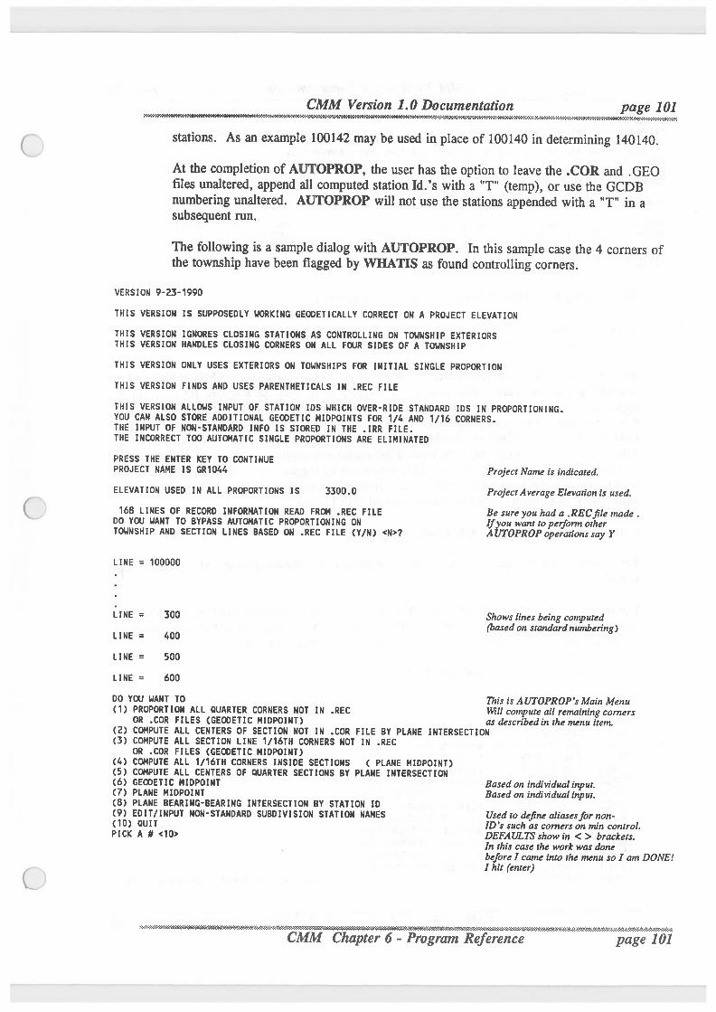
stations. As an example 100142 may be used in place of 100140 in determining 140140.

At the completion of AUTOPROP, the user has the option to leave the .COR and .GEOfiles unaltered, append all computed station Id.’s with a "T" (temp), or use the GCDBnumberingunaltered. AUTOPROP will not use the stations appended with a "T" in asubsequent run.

The following is a sample dialog with AUTOPROP. In this sample case the 4 corners ofthe township have been flagged by WHATIS as found controlling corners.

VERSION 9-23-1990

THIS VERSION IS SUPPOSEDLY WORKING GEODETICALLY CORRECT ON A PROJECT ELEVATION

THIS VERSION IGNORES CLOSING STATIONS AS CONTROLLING ON TOWNSHIP EXTERIORSTHIS VERSION HANDLES CLOSING CORNERS ON ALL FOUR SIDES OF A TOWNSHIP

THIS VERSION ONLY USES EXTERIORS ON TOWNSHIPS FOR INITIAL SINGLE PROPORTION

THIS VERSION FINDS AND USES PARENTHETICALS IN .REC FILE

THIS VERSION ALLOWS INPUT OF STATION IDS WHICH OVER-RIDE STANDARD IDS IN PROPORTIONING.YOU CAN ALSO STORE ADDITIONAL GEODETIC MIDPOINTS FOR I/4 AND 1/16 CORNERS.THE INPUT OF NON-STANDARD INFO IS STORED IN THE .IRR FILE.THE INCORRECT TOO AUTOMATIC SINGLE PROPORTIONS ARE ELIMINATED

PRESS THE ENTER KEY TO CONTINUEPROJECT NAME IS GR1044 ProjectName is indicated.ELEVATION USED IN ALL PROPORTIONS IS 3300.0 ProjectAverageElevationis used.

168 LINES OF RECORD INFORMATION READ FROM .REC FILE Be sure you hada .RECfiIe made.DO YOU WANT TO BYPASS AUTOMATIC PROPORTIONING ON Ifyou want‘ to perform other

TOWNSHIP AND SECTION LINES BASED ON .REC FILE (Y/N) <N>? AUT0PR0Poperat1'onssayY

LINE = 100000

LINE = 300 Shows lines being computed(based on standardnumbering)LINE = 400

LINE = 500

LINE = 600

DO YOU WANT TO This is AUTOPROP’:Main Menu(1) PROPORTION ALL QUARTER CORNERS NOT IN .REC Will congpute all remaining comersOR .COR FILES (GENETIC MIDPOINT) as describedin the menu item.(2) COMPUTE ALL CENTERS OF SECTION NOT IN .COR FILE BY PLANE INTERSECTION

(3) COMPUTE ALL SECTION LINE 1/16TH CORNERS NOT IN .RECOR .COR FILES (GECDETIC MIDPOINT)

(4) COMPUTE ALL 1/16TH CORNERS INSIDE SECTIONS ( PLANE MIDPOINT)(5) COMPUTE ALL CENTERS OF QUARTER SECTIONS BY PLANE INTERSECTION(6) GEODETIC MIDPOINT Based on individualinput.(7) PLANE MIDPOINT Based on individualinput.(8) PLANE BEARING-BEARING INTERSECTION BY STATION ID(9) EDITI INPUT NON-STANDARD SUBDIVISION STATION NAMES Used to define aliasesfor non-(10) QUIT ID ’s such as comers on min control.PICK A # <10> DEFAULTSshow In < > brackets.

In this case the work was donebeforeI came into the menu so I am DONE!I hit (enter)

-*~v- ' " -' ‘ ' ‘- “ " RZ2&<%&&23%¢#».%'t}h&k35:1R&3:~‘:€‘:=:€:5$'.1'J$:35:?~35‘.Z$:3:<:tI frence page 101

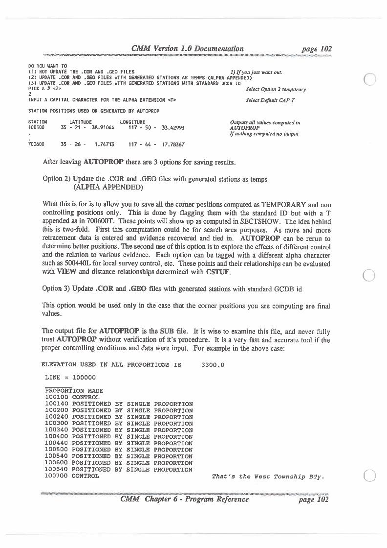
CMM Version 1.0 Documentation pageV102. . .¥€hWMNOhW3M¢N¢N 1*&WVflV£¢4MN WM>3*?i\">>7'>3¢-."‘Z‘I°f-3174?}-}<'5'C'3-25' k?t3'hWW€Q.

. .

DO YOU WANT TO(1) NOT UPDATE THE .COR AND .GEO FILES 1) [fyoujust wantout.(2) UPDATE .COR AND .GEO FILES HITH GENERATED STATIONS AS TEMPS (ALPHA APPENDED)(3) UPDATE .COR AND .GEO FILES HITN GENERATED STATIONS HITN STANDARD GCDB IDPICK A # <2> Select Option 2 temporary2INPUT A CAPITAL CHARACTER FOR THE ALPHA EXTENSION <T> SeIectDefaul!CAP T

STATION POSITIONS USED OR GENERATED BY AUTOPROP

STATI ON LATITUDE LONG I TUDE Outputs all values computed in100100 35 - 21 - 38.910419 117 - 50 - 33.42993 AUTOPROP. Ifnothingcomputed no output700600 35 - 26 - 1.7/c713 117 - 44 - 17.78367

After leaving AUTOPROP there are 3 options for saving results.

Option 2) Update the .COR and .GEO files with generated stations as temps(ALPHA APPENDED)

What this is for is to allow you to save all the corner positions computed as TEMPORARYand noncontrolling positions only. This is done by flagging them with the standard ID but with a Tappended as in 700600T. These points will show up as computed in SECTSHOW. The idea behindthis is two-fold. First this computation could be for search area purposes. As more and moreretracement data is entered and evidence recovered and tied in. AUTOPROP can be rerun todetermine better positions. The second use of thisoption is to explore the effects of different controland the relation to various evidence. Each option can be tagged with a different alpha charactersuch as 500440L for local survey control, etc. These points and their relationships can be evaluatedwith VIEW and distance relationships determined with CSTUF.

Option 3) Update .COR and .GEO files with generated stations with standard GCDB id

This option would be used only in the case that the comer positions you are computing are finalvalues.

The output file for AUTOPROP is the SUB file. It is wise to examine this file, and never fullytrust AUTOPROP withoutverificationof it’s procedure. It is a very fast and accurate tool if theproper controlling conditions and data were input. For example in the above case:

ELEVATION USED IN ALL PROPORTIONS IS 3300.0

LINE = 100000

PROPORTION MADE100100 CONTROL100140 POSITIONED BY SINGLE PROPORTION100200 POSITIONED BY SINGLE PROPORTION100240 POSITIONED BY SINGLE PROPORTION100300 POSITIONED BY SINGLE PROPORTION100340 POSITIONED BY SINGLE PROPORTION100400 POSITIONED BY SINGLE PROPORTION100440 POSITIONED BY SINGLE PROPORTION100500 POSITIONED BY SINGLE PROPORTION100540 POSITIONED BY SINGLE PROPORTION100600 POSITIONED BY SINGLE PROPORTION100640 POSITIONED BY SINGLE PROPORTION100700 CONTROL That's the West Township Bdy.

ce page

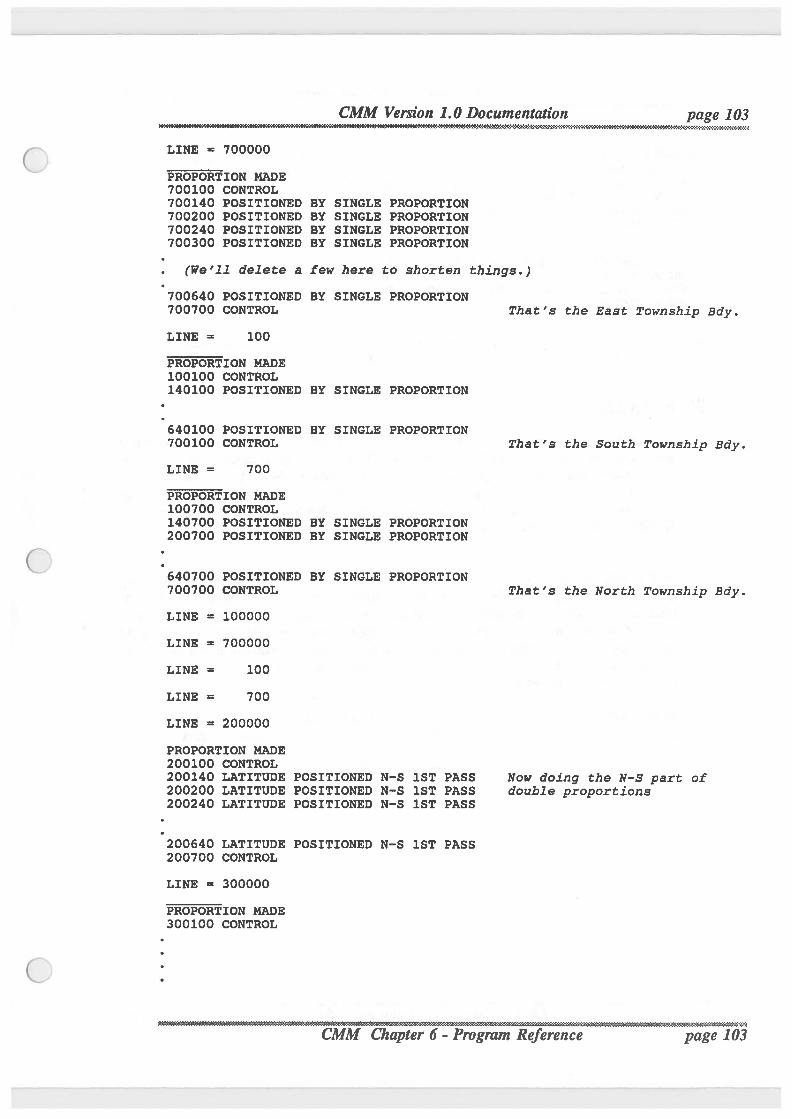
LINE = 700000

PROPORTION MADE700100700140700200700240700300

. (We'll delete a

'7oo54o7oo7oo

LINE =

CONTROLPOSITIONED BY SINGLE PROPORTIONPOSITIONED BY SINGLE PROPORTIONPOSITIONED BY SINGLE PROPORTIONPOSITIONED BY SINGLE PROPORTION

POSITIONED BY SINGLE PROPORTIONCONTROL

100

PROPORTION MADE100100140100

.640100700100

LINE =

CONTROLPOSITIONED BY SINGLE PROPORTION

POSITIONED BY SINGLE PROPORTIONCONTROL

700

PROPORTION MADE100700140700200700

'64o7oo7oo7oo

LINE =

LINE =

LINE

LINE =

LINE =

CONTROLPOSITIONED BY SINGLE PROPORTIONPOSITIONED BY SINGLE PROPORTION

POSITIONED BY SINGLE PROPORTIONCONTROL

100000

700000

100

700

200000

PROPORTION MADE200100200140200200200240

.200640200700

LINE =

CONTROLLATITUDE POSITIONED N-S 1ST PASSLATITUDE POSITIONED N-S 1ST PASSLATITUDE POSITIONED N-S 1ST PASS

LATITUDE POSITIONED N-S 1ST PASSCONTROL

300000

PROPORTION MADE300100

CONTROL

few here to shorten things.)

That's the East Township Edy.

That's the South Township Bdy.

That's the North Township Edy.

Now doing the N-S part ofdouble proportions

IV -r.-.-J.'.-a¢.-.'..- .- .-.-.-.-

ce

CMM Version 1.0 Documentation p 104... .. rmuwseymmrmmam?x-M-:~>a»c-.~»>»o:~:~::-:-:~:«>:»>mc~:-:>:-:-:—:»>>:~¢:4:.-::-:~:-»>»x«:-x-:-2-aw:-2-c«:~:-.

LINE = 200

PROPORTION MADE Now doing the E-W part of100200 CONTROL double proportions finishing140200 LONGITUDE POSITIONED E-W 1ST PASS them.200200 POSITIONED BY DOUBLE PROPORTION240200 LONGITUDE POSITIONED E-W 1ST PASS300200 POSITIONED BY DOUBLE PROPORTION

540200 LONGITUDE POSITIONED E-W 1ST PASS600200 POSITIONED BY DOUBLE PROPORTION640200 LONGITUDE POSITIONED E-W 1ST PASS700200 CONTROL

etc. etc. Now each 1/4 section corner or 1/16 cor. in the .REC file issolves. The file is too long too show here.

BL ER EXE

Blunder is as it's name implies, a blunder detection program. It searches for distance andangleblunders using some basic loop techniques. The technique for distance blunder detectiondoes not work well withrectangular cardinal course traverses, so do not be surprised if it doesnot pop out those types of errors. It is one tool that MAY help you find blunders or largeerrors, but not necessarilyso. BLUNDER works only on RAW data, and so can be run afterGENER coordinate generation is complete.

BLUNDER performs 2 basic geometry based blunder detection checks on user-defined looptraverses. Both angle and distance blunder detection are built into this program. Angularblunders are bound in this option by systematically computing a loop closure beginning atdifferent stations on the loop (and not using the angle at the beginning station). One goodclosure amid a series of bad closures indicates a possible angular blunder at thatpoint. Thedistance blunder detection is a series of bearing-bearingintersections to generate distances,which are then compared to their measured values.

BLUNDER works on angle closed loops only. It can be used before LSAQ is run and isthereforeusefill in conjunctionwith GENER to locate possible data input blunders.

For additional information and use see the use of BLUNDER in the Example in Chapter 5.

\\ ' '~®1$QX$$@i$i1 %$$§ ¢erence page 104

CMM Version 1.0 Documentation page 105. . {*3¢‘M‘i¢£'I'?.4'<'.‘4\"0<‘!¢€€

QHE§KER,EXECHECKER is a program thatgenerates verificationof closure by comparing thefinal adjustedlines to the original measurements on those lines. In addition by careful use it is one of themost powerful error and blunder detection programs in thesystem. CHECKER uses both theRAW data contained in the .LSA fileand the adjustedresults of LSAQ contained in the .CORfile and thus should be run after LSAQ do provide additional information concerning thelocation of problems and blunders.

This file uses the .LSA and .COR files to compute automaticpost-adjustment closures onroutes through a network in the same way thatGENER finds traverse routes. The user canalso input other routes for closure computation. Output is written to a .CHK file. State planereductions utilizedare in LSAQ.A user is allowed to input otherunknownstations to be "held" for closure computations. Thisis useful, as an example, if one wanted closures between section corners or other traversejunctionpoints. Holding such points willgive closures which indicatehow much each traverse‘link’ of the networkadjusted. This can point to the link where the blunder occured, as withredunancy it will be the one that adjusted the most.

Closure informationincludes misclosure in X and Y based on thedetermined direction for thefirst line in the route, angular closure based on closure of direction of observed angles withthe adjusted closing direction, linear error of closure based on raw traverse length comparedto adjusted traverse length, precision based on described X and Y misclosures, and precision

,based on described linear error of closure (precision after rotation of the traverse).

CHE KER INP I UTPUT

Input :1 station other than control you wish to hold for closure purposes -

If you want to ensure CHECKER reports a closure on a desired section of traverse,input the endpoint stations at this point. CHECKER will treat these as "control" andthus will report closures that end at these points.

Closure in northing or casting - CHECKER

Inverses the adjusted coordinates of the first line to get a starting azimuth, and then usesmeasured angles and distances reduced to grid in coordinate computations until theclosing station is reached. The computed closing coordinate is subtracted from its leastquares adjusted equivalent to get a latitude or departure closure.

Angular closure

The last line in the traverse has its least squares adjusted coordinates inversed fordirection, and the azimuth computed from the traverse computations is subtracted fromthis value to obtain the angular closure.

.............................‘\- ----------------------------. .pa 1

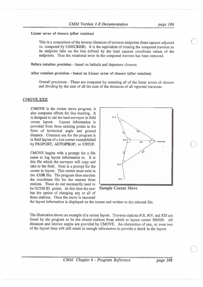
CMM Version 1.0 Documentation page 106- - .».~-¢.' »?WNN%2N:N} -I-Q\'*9#2¢\?¢~§s“I}5~}I-9->z?Z‘Z‘1‘54‘>X¢W€'

Linear error of closure (after rotation)This is a comparisonof the inverse distances of traverse endpoints (least squares adjustedvs. computed by CHECKER). It is the equivalent of rotating the computed traverse soits endpoint falls on the line defined by the least squares coordinate values of theendpoints. Thus the rotational error in the computed traverse has been removed.

Before rotation precision - based on latitude and departure closures

After rotation precision - based on Linear error of closure (after rotation)Overall precisions - These are computed by summing all of the linear errors of closureand dividing by the sum of all the sum of the distances of all reported traverses.

CMVE XE

CMOVE is the corner move program, italso computes offsets for line marking. Itis designed to aid the land surveyor in fieldcorner layout. Layout information isprovided from three existing points in theform of horizontal angle and grounddistance. Common use for the program isin field layout of a lost comer reestablished

mmby PROPORT, AUTOPROP, or CSTUF.

CMOVE begins with a prompt for a filename to log layout information to. It isthis filewhich the surveyor will copy andtake to the field. Next is a prompt for thecorner to layout. This corner must exist inthe .COR file. The program then searchesthe coordinate file for the nearest threestations. These do not necessarilyneed tobe GCDB ID. points. At this time theuser Sample Corner Movehas the option of changing any or all ofthese stations. Once the move is executedthe layout information is displayed on the screen and written to the selected file.

The illustrationshows an example of a comer layout. Traversestations #18, #19, and #20 arefound by the program to be the closest stations from which to layout comer 500500. Alldistances and interior angles are provided by CMOVE. An obstruction of one, or even twoof the layout lines will still result in enough informationto provide a check in the layout.

XE

COMBIN is a program thattakes two .LSA files for GENER or LSAQ and combines them.Common control stations or observations are only input in the output fileonce. A series oferror messages (same observation - different value, similar coordinates with different stationname, same station name with different coordinates, etc.) is output.

Two input filenames and one output filename are prompted for.

The program can handle 3000 stations, 4000 angles, 4000 distances, and 3500 azimuths on aPC.

This is useful if a project is worked in small parts, or by different crews, then combinedonceeach data set is evaluated.

MPAR EXE

COMPAR is a program thatallow you to compare two .COR coordinate files. The value ofthis is as a check to see theabsolute and relative effects of different weighting of measurementsor the effect of adding new data on resultant coordinates.

NVERT.EXE

QQELEEE Convert allows conversion between state plane and latitude-longitudein NAD 27and NAD 83 in all zones.

CONVERT can beused for conversion betweengeodetic and state plane coordinates in eitherNAD 27 or NAD 83 datums. All state plane zones are included.

CONVERT is completely menu driven. You will be initiallyprompted for input and outputfile format names. The input filecan be constructed using a word processor.

If you are converting from geodetic coordinates to state plane coordinates each line of yourinput fileshould look like this:

Statign name Latiggge Longitudealphanumeric degrees minutes seconds degrees minutes seconds

The station name can be up to 10 characters in length and should contain no blank spaces.Degrees and minutes should not contain decimal points, and seconds can be with or withouta decimal point. Any number of spaces is allowed between each entity on a line of input.Spaces must exist between degrees, minutes, and seconds of latitude and longitude (45 2346.32456 is correct, 452346.32456 is incorrect). The order must be as shown. Any line ofinput not having this format is ignored.

. ._.

_.,.,.

_. ,.

_.

A.,_

._.

_.,._.,._.,.

_.

_.

_., ,_

._.

_.

_.

_.

_.

_, _,.

_.

_.

_.,.,

.V.

_._.

_ , _ _ , _ _ _ ,_

CMM Version 1.0 Documentation page 108.

¢'r3'3¢9'."V<‘9'V.’0M'/.'2*.V.‘Z‘I'K

If you are converting from state plane coordinates to geodetic coordinates each line of yourinput fileshould look like this:

i n n X Yalphanumeric real real

The station name can be up to 10 characters in length and should contain no blank spaces.The coordinates can be with or without a decimal point. Any number of spaces is allowedbetween each entity on a line of input. The order must be as shown. Any line of input nothaving this format is ignored.In NAD 27 all state plane linear units are assumed to be U.S. survey feet.For NAD 83, you will be asked if input state plane coordinates are metric, U.S. survey feet,or internationalfeet. Output state plane coordinates in NAD 83 will always be metric, and theuser has the option of also outputting either or botl1 English equivalents of the coordinates.

CONVERT requires four files for operation:(1) NAD83.CON(2) NAD27.CON(3) TABLE.DAT(4) ZONE.DAT

These 4 files must exist in the directory CONVERT is being run from.

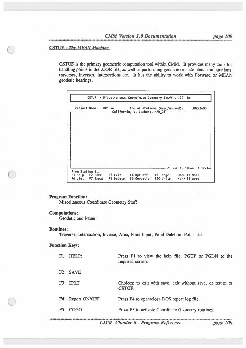
CMM Version 1.0 Documentation __page 109

- Mk‘

CSTUF is the primary geometric computation tool withinCMM. It provides many tools forhandling points in the .COR file, as well as performing geodetic or state plane computations,traverses, inverses, intersections etc. It has the ability to work with Forward or MEANgeodetic bearings.

CSTUF - Miscellaneous Coordinate Geometry Stuff v1.00 bp

Project Name: No. of stations (used/unused): 392/3608alifornia, V, Lambert, NAD_27

Fri Mar 15 10:46:51 1991From Station 7..F1 Help F2 Save F3 Exit F4 Rpt off F5 Cogo <sh> F1 ShellF6 List F7 Input F8 Delete F9 Geodetic F10 Units <sh> F2 Area

Program Function:

Miscellaneous Coordinate Geometry Stuff

Computations:Geodetic and Plane

Routines:Traverse, Intersection, Inverse, Area, Point Input, Point Deletion, Point List

Function Keys:F1: HELP: Press F1 to view the help file, PGUP or PGDN to the

required screen.

F2: SAVE

F3: EXI'I‘ Choices: to exit with save, exit without save, or return toCSTUF.

F4: Report ON/OFF Press F4 to open/closeDOS report log file.

F5: COGO Press F5 to activate Coordinate Geometry routines.

I c -' %"£?:'.32‘-3 iIi'.,_.,,,.-...,,..-.......-.w .». .-.—.,.;.-.\....,..t

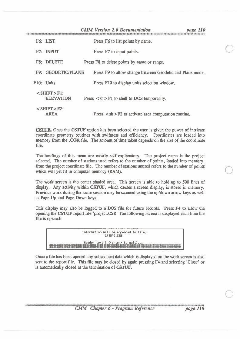
page 110' 9W£#Mfi% fi§Vfl«%VV 1505 96-?-

F6: LIST Press F6 to list points by name.

F7: INPUT Press F7 to input points.F8: DELETE Press F8 to delete points by name or range.

F9: GEODETIC/PLANE Press F9 to allow change between Geodetic and Plane mode.

F10: Units Press F10 to display units selection window.

< SHIFT> F 1:ELEVATION Press < sh>Fl to shell to DOS temporarily.

< SHIFT> F2:AREA Press < sh >F2 to activate area computation routine.

QEE Once the CSTUF option has been selected the user is given the power of intricatecoordinate geometry routines with swiftness and efficiency. Coordinates are loaded intomemory from the .COR file. The amount of time taken depends on the size of the coordinatefile.

The headings of this menu are mostly self explanatory. The project name is the projectselected. The number of stations used refers to the number of points, loaded into memory,from theproject coordinate file. The numberof stations unused refers to thenumberof pointswhich will yet fit in computer memory (RAM).The work screen is the center shaded area. This screen is able to hold up to 500 lines ofdisplay. Any activity within CSTUF, which causes a screen display, is stored in memory.Previous work during the same session may be scanned using theup/down arrow keys as wellas Page Up and Page Down keys.This display may also be logged to a DOS file for future records. Press F4 to allow theopening the CSTUFreport file ‘project.CSR’ The following screen is displayed each time thefileis opened:

lnformaion Hill be appended to file:GR101o1o.CSR

Once a filehas been opened any subsequent data which is displayed on thework screen is alsosent to the report file. This filemay be closed by again pressing F4 and selecting ‘Close’ oris automaticallyclosed at the terminationof CSTUF.

‘A

page 110

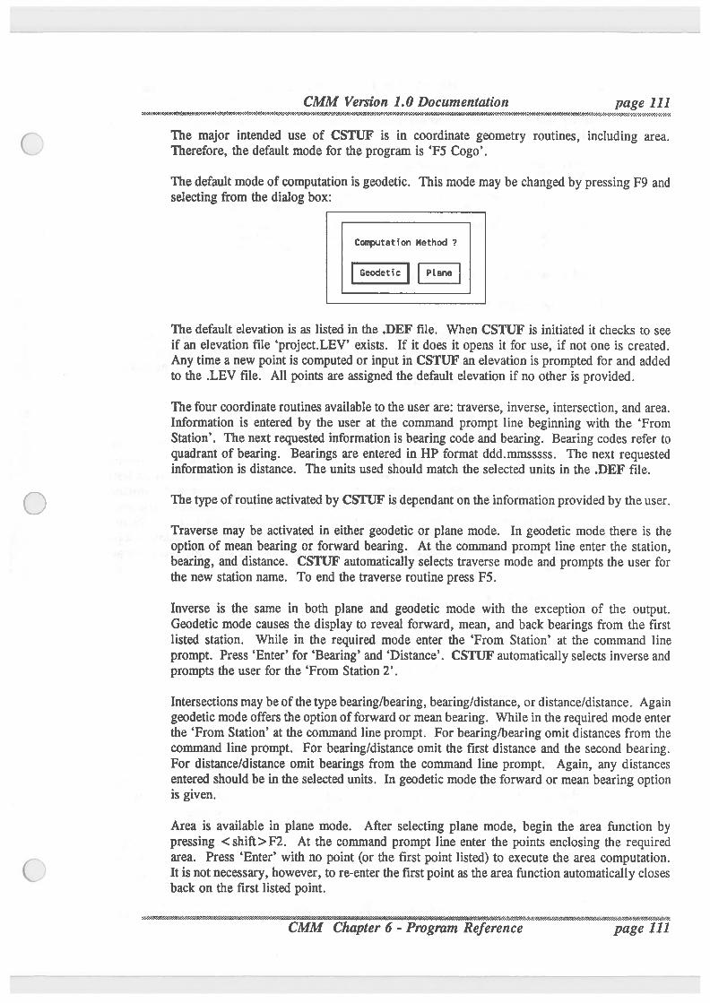
CMM Version 1.0 Documentation page 111.

".4’€§'."-N’¢¢'WOW'€'W'W(<¢9.‘39S. . ‘-4'4-0.D"J<<<.9°.€’.-2-I-2’.‘t~'.~3~':-4-H-2~:-‘.-2<r’.4

The major intended use of CSTUF is in coordinate geometry routines, including area.Therefore, the default mode for the program is ‘F5 Cogo’.The default mode of computation is geodetic. This mode may be changed by pressing F9 andselecting from the dialog box:

Computation Method ? The default elevation is as listed in the .DEF file. When CS'I'UF is initiated it checks to seeif an elevation file ‘project.LEV’ exists. If it does it opens it for use, if not one is created.Any time a new point is computed or input in CSTUF an elevation is prompted for and addedto the .LEV file. All points are assigned the default elevation if no other is provided.The four coordinate routines availableto theuser are: traverse, inverse, intersection, and area.Information is entered by the user at the command prompt line beginning with the ‘FromStation’. The next requested information is hearing code and bearing. Bearing codes refer toquadrant of bearing. Bearings are entered in HP format ddd.mmsssss. The next requestedinformation is distance. The units used should match the selected units in the .DEF file.

The type of routine activatedby CSTUF is dependant on the informationprovided by theuser.

Traverse may be activated in either geodetic or plane mode. In geodetic mode there is theoption of mean bearing or forward bearing. At the command prompt line enter the station,bearing, and distance. CSTUF automaticallyselects traverse mode and prompts the user forthe new station name. To end the traverse routine press F5.

Inverse is the same in both plane and geodetic mode with the exception of the output.Geodetic mode causes the display to reveal forward, mean, and back bearings from the firstlisted station. While in the required mode enter the ‘From Station’ at the command lineprompt. Press ‘Enter’ for ‘Bearing’ and ‘Distance’. CSTUFautomaticallyselects inverse andprompts the user for the ‘From Station 2’.

Intersections may beof thetype bearing/bearing,bearing/distance,or distance/distance. Againgeodetic mode offers theoption of forward or mean bearing. While in therequired mode enterthe ‘From Station’ at the command line prompt. For bearing/bearingomit distances from thecommand line prompt. For bearing/distanceomit the first distance and the second bearing.For distance/distance omit bearings from the command line prompt. Again, any distancesentered should be in the selected units. In geodetic mode the forward or mean bearingoptionIS given.

Area is available in plane mode. After selecting plane mode, begin the area function bypressing <shift>F2. At the command prompt line enter the points enclosing the requiredarea. Press ‘Enter’ with no point (or the first point listed) to execute the area computation.It is not necessary, however, to re-enter thefirst point as the area functionautomaticallyclosesback on the first listed point. - 'r- "¢i:G5‘~'.§$‘.°:fl."r.£.‘i:€6»5':" ''

page 111

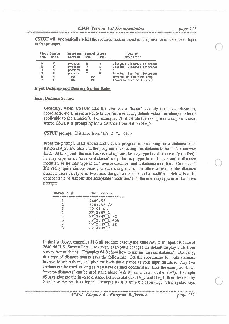
CMM Version 1.0 Documentation page 112

1¢}OOG"‘20".

¥5‘}M!>}0".Oi"NN>.'3"/>}>‘}'."‘.-.\fi'}:'1W3'3 .-M¢MW’fiW¥N~2'92-DZ-?Z->Z'>3-IV'II£-392*:

CSTUFwillautomaticallyselect therequired routinebased on thepresence or absence of input

at the prompts.First course Intersect Second Course Type ofBng. Dist. Station Bng. Dist. computation

N Y prompts N Y Distance Distance IntersectN Y prompts Y N Bearing Distance IntersectY N prawns N Y " " "

Y N prompts Y N Bearing Bearing IntersectN N no no Inverse or MidPoint CompY Y no no Traverse Mean or Forward

Input Distance and firing Smtax RulfiIn Din

nt

Generally, when CSTUF asks the user for a ‘linear’ quantity (distance, elevation,coordinate, etc.), users are able to use ‘inverse data’, default values, or change units (ifapplicable to the situation). For example, I'll illustratethe example of a cogo traverse,where CSTUF is prompting for a distance from station HV_2:CSTUF prompt: Distance from ‘HV__2’ ?.. <ft>

_

From the prompt, users understand that the program is prompting for a distance fromstation HV_2, and also that the program is expecting this distance to be in feet (surveyfeet). At thispoint, theuser has several options; he may type in a distance only (in feet),he may type in an ‘inverse distance’ only, he may type in a distance and a distancemodifier, or he may type in an ‘inverse distance’ and a distance modifier. Confused ?It’s really quite simple once you start using them. In other words, at the distanceprompt, users can type in two basic things: a distance and a modifier. Below is a listof acceptable ‘distances’ and acceptable ‘modifiers’ thattheuser may type in at the aboveprompt:

Example # User reply1 2640.662 5281.32 /23 40.01 ch4 I-IV_2:HV_l5 av 2:nv_1 /26 I-IV:2:HV_1 +667 HV 2:HV 1 if8 I-IV:4:HV:9

In the list above, examples #1-3 all produce exactlythe same result; an input distance of2640.66 U.S. Survey Feet. However, example 3 changes the default display units fromsurvey feet to chains. Examples #4-8 show how to use an ‘inverse distance’. Basically,this type of distance syntax says the following: Get the coordinates for both stations,inverse between them, and give me back the distance as your input distance. Any twostations can be used as long as they have defined coordinates. Like the examples show,‘inverse distances’ can be used stand alone (4 & 9), or with a modifier (5-7). Example#5 says give me the inverse distance between stations HV_2 and HV_1, then divide it by2 and use the result as input. Example #7 is a little bit deceiving. This syntax says

' ~‘- ‘-rES6$f$$S56$o3S$:6f0:l?k3?S9$5:2Z»k5f$R‘-527.524:-'9$$$§6£<55$$:i:i3k5:i:$5:3:iS:£>zZ€:I:-W' Iference page 112

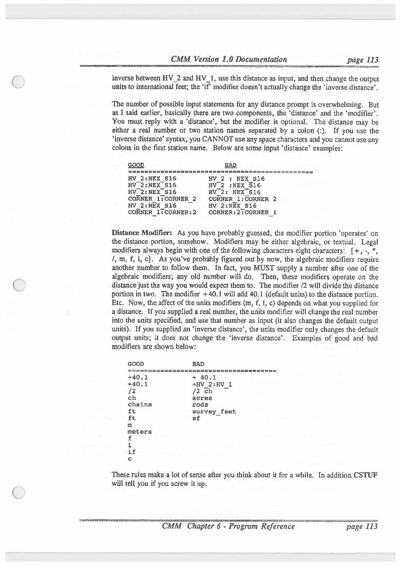
CMM Version 1.0 Documentation page 113.. . . -X’.‘3'€'%€"'.i9’.o'0,¢f'>Z£’-'.'l'2'b2‘30'>X

inverse between HV_2 and HV_l, use this distance as input, and then change the outputunits to internationalfeet; the ‘if’ modifier doesn’t actuallychange the ‘inverse distance’.

The numberof possible input statements for any distance prompt is overwhelming. Butas I said earlier, basically there are two components, the ‘distance’ and the ‘modifier’.You must reply with a ‘distance’, but the modifier is optional. The distance may beeither a real number or two station names separated by a colon (:). If you use the‘inverse distance’ syntax, you CANNOT use any space characters and you cannot use anycolons in the first station name. Below are some input ‘distance’ examples:

coon BAD

1_r\—I:§:NEx_s16 —

HV_2 : NEX__Sl6- "-

I-IV_2:NEX_S16 HV_2 :NEX_S16HV_2:NEX S16 HV 2: NEX_S16

OcoaNEa_1?coaNr:a_2 o§NEa_1:coaNEa 2HV_2 :NEX_S16 av 2 :NEX_Sl6CORNER_1 : comma: 2 coamsa: 2 :CORNER_l

Distance Modifier: As you have probably guessed, the modifier portion ‘operates’ onthe distance portion, somehow. Modifiers may be either algebraic, or textual. Legalmodifiers always begin with one of the following characters eight characters: {+ , —, *,/, m, f, i, c}. As you’ve probably figured out by now, the algebraic modifiers requireanother number to follow them. In fact, you MUST supply a number after one of thealgebraic modifiers; any old number will do. Then, these modifiers operate on thedistancejust theway you would expect themto. The modifier /2 will divide the distanceportion in two. The modifier +40.1 will add 40.1 (defaultunits) to thedistance portion.Etc. Now, the affect of the units modifiers (m, f, i, c) depends on what you supplied fora distance. If you supplied a real number, theunits modifier will change the real numberinto the units specified, and use that number as input (it also changes the default outputunits). If you supplied an ‘inverse distance’, the units modifier only changes the defaultoutput units; it does not change the ‘inverse distance’. Examples of good and badmodifiers are shown below:

GOOD BAD

+40 1 + 40.1+40 1 +HV_2:HV 1/2 /2 chch acreschaxna rodsft aurvey_feetft sfmmetersfiif

These rules make a lot of sense after you thinkabout it for a while. In addition CSTUFwill tell you if you screw it up.

- ence

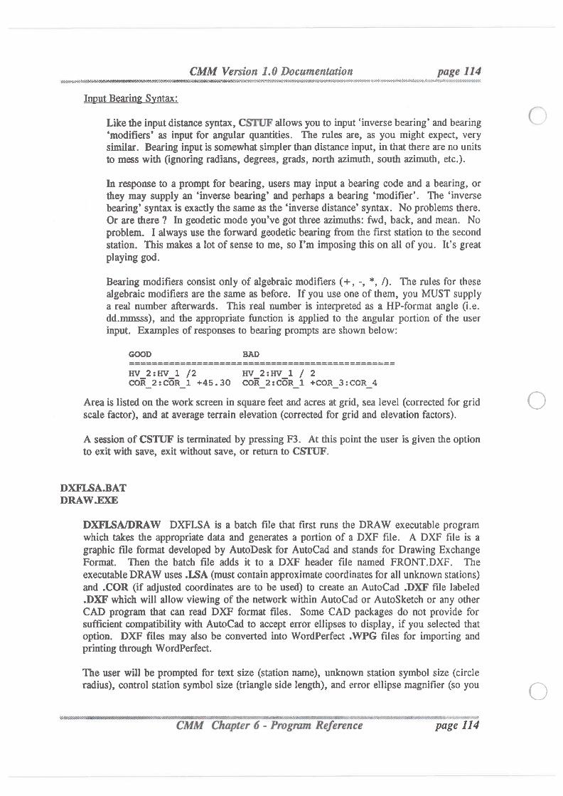
CMM Version 1.0 Documentation page_I1._4.'.' .4143"?24¢‘C'2~K-Ki-I~Z'X'X<§&K‘Z¢Wh SMXéXW'5E‘CVd'WI'I'Z‘Z I'34‘?Z*?I'3'K§'Z¢!'.‘5'1‘:-$‘3‘K*¢~2*?£w?§?~Z'1'14"-2~}9?2~2~I-I-1'1-HI. M%WEfi3? «%WNfl&Wk

Input Baring Syntax:Like the input distance syntax, CSTUFallows you to input ‘inverse bearing’ and bearing‘modifiers’ as input for angular quantities. The rules are, as you might expect, verysimilar. Bearing input is somewhat simpler thandistance input, in thatthere are no unitsto mess with (ignoring radians, degrees, grads, north azimuth, south azimuth, etc.).

In response to a prompt for bearing, users may input a bearing code and a bearing, orthey may supply an ‘inverse bearing’ and perhaps a bearing ‘modifier’. The ‘inversebearing’ syntax is exactlythe same as the ‘inverse distance’ syntax. No problems there.Or are there ? In geodetic mode you’ve got three azimuths: fwd, back, and mean. Noproblem. I always use the forward geodetic hearing from the first station to the secondstation. This makes a lot of sense to me, so I’m imposing this on all of you. It’s greatplaying god.Bearing modifiers consist only of algebraic modifiers (+, -, *, I). The rules for thesealgebraic modifiers are the same as before. If you use one of them, you MUST supplya real number afterwards. This real number is interpreted as a HP-format angle (i.e.dd.rmnsss), and the appropriate function is applied to the angular portion of the user

input. Examples of responses to bearing prompts are shown below:

HV_2:HV_1 /2 I-IV_2:HV_1 / 2COR___2:COR_1 +4s.3o COR_2:COR_1 +COR_3:COR_4

Area is listed on the work screen in square feet and acres at grid, sea level (corrected for gridscale factor), and at average terrain elevation (corrected for grid and elevation factors).A session of CSTUF is terminated by pressing F3. At this point the user is given the optionto exit with save, exit without save, or return to CSTUF.

D)fl7LSA.BATDRAW.EXE

DXFLSA/DRAW DXFLSA is a batch file that first runs the DRAW executable programwhich takes the appropriate data and generates a portion of a DXF file. A DXF file is agraphic file format developed by AutoDesk for AutoCad and stands for Drawing ExchangeFormat. Then the batch file adds it to a DXF header file named FRONT.DXF. TheexecutableDRAW uses .LSA (must contain approximate coordinates for all unknown stations)and .COR (if adjusted coordinates are to be used) to create an AutoCad .DXF file labeled.DXF which will allow viewing of the networkwithin AutoCad or AutoSketch or any otherCAD program that can read DXF format files. Some CAD packages do not provide forsufficient compatibilitywith AutoCad to accept error ellipses to display, if you selected thatoption. DXF files may also be converted into WordPerfect .WPG files for importing andprinting through WordPerfect.

The user will be prompted for text size (station name), unknown station symbol size (circleradius), control station symbol size (triangleside length),and error ellipse magnifier (so you

' -'-ms-i\".w"“'<K£!.'-k:$r!t:®22R53eJcR9956!J!£!kI€9-!'.9s‘9s&5252'0!:1.?-‘1wA2'2'-'-'-'QI?.'1‘1'Z'¥l'

page 114

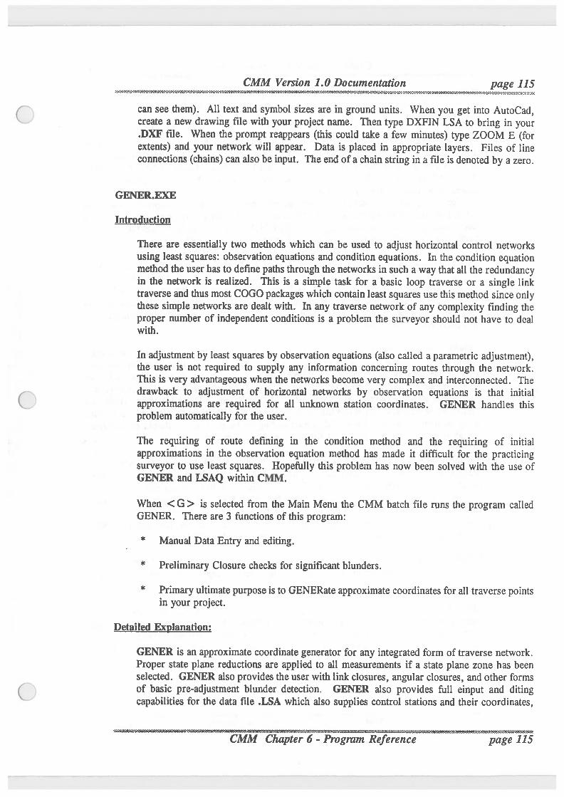
CMM Version 1.0 Documentation page 115

can see them). All text and symbol sizes are in ground units. When you get into AutoCad,create a new drawing filewith your project name. Then type DXFIN LSA to bring in your.DXF file. When the prompt reappears (this could take a few minutes) type ZOOM E (forextents) and your network will appear. Data is placed in appropriate layers. Files of lineconnections (chains) can also be input. The end of a chain string in a fileis denoted by a zero.

GENER.EXE

Lrttmuctinn

There are essentially two methods which can be used to adjust horizontal control networksusing least squares: observation equations and condition equations. In the condition equationmethodtheuser has to define paths throughthenetworksin such a way thatall the redundancyin the network is realized. This is a simple task for a basic loop traverse or a single linktraverse and thus most COG0 packages which contain least squares use thismethod since onlythese simple networks are dealt with. In any traverse networkof any complexity finding theproper number of independent conditions is a problem the surveyor should not have to dealwith.

In adjustmentby least squares by observation equations (also called a parametric adjustment),the user is not required to supply any information concerning routes through the network.This is very advantageous when the networksbecome very complex and interconnected. Thedrawback to adjustment of horizontal networks by observation equations is that initialapproximations are required for all unknown station coordinates. GENER handles thisproblem automaticallyfor the user.

The requiring of route defining in the condition method and the requiring of initialapproximations in the observation equation method has made it difficult for the practicingsurveyor to use least squares. Hopefully this problem has now been solved with the use ofGENER and LSAQ withinCMM.

When < G > is selected from the Main Menu the CMM batch file runs the program calledGENER. There are 3 functions of this program:

* Manual Data Entry and editing.* Preliminary Closure checks for significant blunders.

* Primaryultimate purpose is to GENERate approximate coordinates for all traverse pointsin your project.

Dgtgilgg Explanation:GENER is an approximate coordinate generator for any integrated form of traverse network.Proper state plane reductions are applied to all measurements if a state plane zone has beenselected. GENER also provides theuser withlink closures, angular closures, and other formsof basic pre-adjustment blunder detection. GENER also provides full einput and ditingcapabilitiesfor the data file .LSA which also supplies control stations and their coordinates,

MM Version 1.0 Documentation page 116' ' " ' '-' 3fi'3°0QK<\'({

. . 3‘-"D'N'6\'¢'1«K¢¢¢M-1‘>€'&¢9M&0N<€2Z¢'§¢':€'”¢¢!?N5¢¢¢ON09§XV&€4¢'Z¢}BW\W51#>3C-249%.‘)?-}3€4‘2*VJ€r1

measurements, and unknown stations and their approximate coordinates for the least squaresadjustmentof horizontal survey information. The editor checks for input errors, and is fullyexplanatory in use.

When using GENER it is optimal that all station names should be entered in capital letters astheprograms are case sensitive (keep CAPS LOCK on at all times). Towards thatend a DOSutility is used to force your keyboard to upper case lock when entering GENER thru CMM.What can happen if you don't use upper case only is confusion that arises between a stationnamed ‘a’ and station named ‘A’, for example. These could be considered as one point, ortwo depending on the concentrationof the data entry person. To avoid thisproblem most (butnot all) of the CMM utilities see both these types as the same, therefore the requirementresolves any potential problems. Currently the CMM batch filewhich invokes GENER usesa utility to set CAPS LOCK On and then off when GENER is exited.

All angular quantities are input in ‘HP-format’ That is DD.MMSS where DD is degrees, MMis minutes, and SS is seconds. Minutes or seconds should not contain any additional decimalpoints. GENER does not generate coordinates for bearing-bearingor distance-distancesituations, but it is possible to type approximate coordinates for these situations directly intothe .LSA file. That is each station located needs to have at least one angle and distance to it,or a coordinate estimate input.GENER does not require the user to define the traverse routes which enable coordinategeneration, as traverse routes are automaticallygenerated. This means the user does not needto order his data in any fashion. If GENER finds it cannot generate coordinates for anunknown station due to omission of data or highly unusual network connectivity, thisinformation is output to the user. If the user desires to add information to the .LSA filewithoutusing GENER’s input functions, thestructure of thefileis easilyinterpreted and couldeasily be input using any line or full screen editing package. Caution should be exercisedthough since the format of the .LSA filemust be strictly adhered to.

It is recommended that manual data entry be made through GENER’S own input editor, as itcontains very exclusive data checking capabilities for survey type information which cannotbe found in any general editor. Input directly to the .LSA file with an editor or a wordprocessor runs a risk of leaving some improperly formated data. It is almost always wise tothen run the utility SETUP which checks and formats the data properly for subsequentprograms. It is a good idea to input networks a traverse link at a time, then allow GENERto check its closure, so thatblunders can be systematicallyeliminated.

GENER can accept any alphanumeric station name up to 16 characters in length. Stationnames should not contain blank spaces, and should always be input without adding any blankspaces before the actual name.

GENER primarilysearches for "link" traverses which connect two distinctstations with knowncoordinates (control or previously computed by GENER). Known coordinates at both endsof the link permit rotation of the link traverse into proper directional orientation. Thisorientation can only be done on a loop traverse if it has a direction (azimuth)observation onit, or an angle connects it to a line of known orientation.

' '\-"'CM Chapter 6 — rence page 116

CMM Version 1.0 Documentation page 117‘X' '

. . . ¢wMkV&hH{'51}X#¢M‘P#E-FWW

A networkwithonly one control point and an input direction is handled as a link traverse byassuming a distance connected to the control point as due north (thusmaking the other stationa "pseudo" control point). Once all stationshave generated coordinates in thisarbitrary systemthe input direction is used as a basis for rotation of the network into proper orientation.

Closures of link traverses are output as coordinates are being generated. These closures areincredibly helpful in blunder detection. LSAQ (the least squares analysis program), RAW,BLUNDER and CHECKER also afford many blunder detection abilities.

In GENER traverse computations cease when approximate coordinates for all stations havebeen generated. It is entirely possible that all traverse closures seem reasonable and yet ablunder still exists. This is becauseGENER uses only the minimal portion of the redundantdata set in coordinate generation. These blunders can often be detected in GENER aftercoordinate generation, since GENER computes pre-adjustmentresiduals for all observations.A user should be careful in using this information, since the coordinate generation will forcemuch of the random error into the observations which were not used in the coordinategeneration process.

Closures output are always the result of a link traverse between two stations with generatedcoordinates. The distance between the traverse link end points based on the measurements,compared to thedistance computed by inversing betweenknown traverse link end coordinates,represents a closure.

The precision is the closure divided by the sum of the distances in the link traverse, output asthe traditional ratio error of closure. It is when a link traverse is found that coordinates ofintermediate stations along it can be rotated based on the existing azimuthbetween end points.Closures calculated by GENER will tend to be larger than those computed if loop closureswere computed since closures are often made betweenend stations whose coordinates were justcomputed by GENER. Since the end station’s coordinates are not yet adjusted, and theprevious coordinates have misclosure, closing against them will tend to be larger than ifadjusted coordinates were known. This will occur in any redundant traverse network. This,of course, would require the subsequent least squares adjustment. If a poor traverse closureis detected, that closure may affect the closure of traverse links computed subsequent to it.

Always look for theblunder in theobservations on the first link traverse with a poorclosure.

GENER only uses the average project elevation (not a series of elevations as can be used inLSAQ with LEV.LSA) in applying the sea level factor, so in rugged terrain this could alsoslightly affect GENER’s closures.

GENER will attempt formationof link traverses followed by closure computation and rotationuntil all stations have generated coordinates or no more traverse links can be found. If somestations still do not have coordinates, GENER will look for an angle—distance combinationwhere one leg of the angle is between stations with coordinates, and the other leg has adistance to a station without coordinates, which will enable calculation of rotated coordinatesfor the undetermined station.

I‘ '~ -' '~'-‘-‘-'-Wr-‘-r. ., .

page 11 7

CMM Version 1.0 Documentation page 118 - ‘€9Q’.‘€‘?N‘Q’.‘QQ'7'Z'I'3’.‘}G'2'X?3<‘I"I . . .'2'3'I'5'?')¢€-2-£<¢0'2 xamo...

Often, forgetting to input an angle on a traverse route forces GENER to use angle-distanceintersection. GENER will then reattempt a link traverse generation, with a return to a searchfor an angle-distancecombinationif necessary. If all angle-distancepossibilitiesare exhausted,a warning is output to the user indicatingwhich stations could not have coordinates generatedfor them. This warning can also be a good sign if you have eliminated all observationscontaining the station from the data. This can happen when you mistakenly name a station inan observation, and later change thatstation name.

It is wise to resolve all such problems before going forward to the LeastSquares analysisprocess. In some cases incomplete data in the .LSA fileorincomplete coordinate generation as indicated by GENER will cause LSAQtofailor even crash.

When one selects the "quit" option from the editor, GENER will regenerate all non-controlcoordinates. If you are creating a large network you will generally want to input data for awhile, then quit the input editor and generate coordinates (and thenpossibly run LSAQ) to seeif the data you added is free of problems. If a problem is detected, use the editor to correctit and re-generate all coordinates.

GENER looks for unknown stations which are not on a distance measurement or not on anangle measurement. If such a station exists, it will be impossible for GENER to computecoordinates for thatstation since it is not on an angle-distancecombination. This could meanmeasurements need to be added to the data, or the station is included on a bearing-bearingordistance—distance intersection. If the latter situation is true, approximate coordinates can beinput to the .LSA file using a line or full screen editor, followed by execution of programSETUP to properly reformat the .LSA file.

If a message appears for a station which was not intended to be deleted from (or added to) thenetwork, it will be necessary to check thatall necessary observations have been input relativeto thatpoint.If the editor in GENER is not invoked, coordinate generation begins immediately. In theeditor one can list control stations, distances, angles, or azimuths (input of bearings is alsoallowed and they are converted to azimuths); or edit any of those four data types. Data canbe added, changed, or deleted. Deleting can be performed by station names or by observationnumber (ordered # in the file).Afterthecompletionof coordinategenerationand pre-adjustmentresidual calculation, GENERautomaticallyupdates the .LSA filewith added observations and generated coordinates. Thatfile is now ready for LSAQ.GENER creates an output file named .GEN which will contain all warning messages, allgenerated traverse links and closure information, a list of generated coordinates, and a list ofpre-adjustrnentresiduals. Traverse closure informationis also output to thescreen as GENERis running, but it often whisks by you faster than you can read. The .GEN file is useful inblunder detection and checking which observations you have input to the .LSA file.

For step by step operation of GENER follow the Example contained in Chapter 6.

CMM Version 1.0 Documentation page 119' ‘}»N9fi9Kfi#WMM¢m¢>»2

INREC

.................................................................................................................................................................................................................................................................-

Computer program INREC is a hard core data entry tool designed to provide any easy wayto create the .REC (record) file. One can thinkof the .REC record file as a digital filerepresentatio of the record plat bearings and distances.

Record Data: Any measurement management system operates successfully only if blundersin the data being managed do not exist. For this reason it is important that blunders intranscription from paper plat to digital record he kept to a minimum. Record plat data is oneof the most important types of data to be entered. Many decisions are based on thisinformation. An example would be a double proportion to locate the legal replacementof asection comer. In this case retracement measurements are related to record plat data. If thisdigital plat data contains a blunder, the proportioned comer will be positioned incorrectly.Measurement management software has the abilityto convert plat data to observation format.This enables thesame mathematicalchecks of integrity to beused on it thatare used on surveyfield data.

One method of record data entry is by measurement management designed software. Thissoftware should make use of the township structure from which to base data input. Forinstance, the eastern boundary of Township 57 South, Range 73 East is designed to have amean bearing of north, with comers set every 40 chains. The data entry would simply beautomated,withthe operator needing only to accept thedefault values of the next bearing anddistance. Only in the less common case, where a comer was not set or distance/bearingwas

irregular, would theuser have to override thedefaultvalues withdifferent input. A secondarybenefitof this system is the self-formattingdata structure. The software automates the formatprocess withminimal prompts to theuser. Many checks can also be incorporated into the dataentry which take advantage of the GCDB naming scheme. For example, an entry of south forthe direction from 100100 to 100200 can be trapped by software as an entry error.

The alternative method of plat data entry is by a simple text editor. Although this method isstraight forward it may often lead to transposed numbers and other transcription errors due tooperator fatigue or inattention.

Since .REC is a fileand not a visually aided graphic representation of the record information,it is required that bearings and distances be defined with a systematic from station and tostation designation. Both INREC and the proportioning utilities can provide more automatedforms of input and computations if a standard numbering scheme is adopted for recordinformation. One can input an entire township’s record information not using standardnumbering, but it is not conducive to efficient work. INREC assumes all station ID’s arenumeric since that is the essence of the standard numbering system. The numeric names areconverted to alphanumeric in subsequent programs. A maximum ID lengthof 6 numerics isassumed, which is converted to 16 alphanumeric in later programs.

The standard numbering system used in this system is similar in most respects to the GCDB(BLM’s Geographic Coordinate Data Base) identificationsystem, but due to application is notas strictlydefined. The standard system as defined for use with CMM is described elsewherein this reference.

If INREC is being run for the first time (the .REC does not exist or one has erased it for

..........................

CMM Chapter 6 - ProgmmRe

CMM Version L0 Documentation page 120..

‘:44Q§$99¢$«$2W3@fi$W<’kPkW93{¢%9H99NWV°§N«WK'I{4¢¢¢(£€<<¢A€M¢3K

some logical reason) the user is prompted through the standard numbering for N-S lines(assumed running north) followed by E-W lines (assumed running west). If a user wantssoutherlyor easterly input one must change the initial from designation to 700 instead of 100.

One will have to take time getting used to INREC input. The efficient techniques built intothe entry take time to learn. The following items should be noted:

(1)

(2)

(3)

(4)

(5)

(6)

Three numbers of the name are assumed, so the user is only inputting three integers ata time. As the l00xxx line is being input theuser only inputs the xxx part. A zero inputindicates to the program that the from station should be changed. A zero input at thefrom station indicates to switch to the next line.

The user has the ability to automatically input series of lines which have commonbearings and/or distances. THIS ABILITYIS LIMITED TO GROUPS OF LINESLONGER THAN ONE MILE IN STATION DESIGNATION. As an example if one isstarting the 100xxx line (from station is 100100) and theuser inputs a ‘to’ station of 700,80.02 chains, and due north; if the automatic input option is selected 6 lines:100100-100200, 100200-100300, ..., 100600-100700would all be assigned thatdistanceand bearing.If the distance input was closer to 40 chains all quarter corners would be included.Similarlyan input closer to 20 chains would create distances between sixteenth corners.If one input 600 instead of 700 all automaticcreation would quit at 5 miles.

One can also select non-automatic line generation, where one would input distancesand/or bearingswith automaticstation numbering.This input is very powerful but confusing at first. Please take your time in learning it.

All bearinginput is checked for proper quadrant and value. One can override the check.All bearing input is N, S, E, or W for cardinal or 1, 2, 3, 4 for quadrant followed byHP time input for value of the bearing. All bearings are assumed to be mean geodetic.All distances are assumed to be input in chains.

THE AUTOMATIC ENTRY WORKS FOR INITIAL ENTRY. Once a .REC file iscreated you automaticallymove to more manual forms of entry when you run INREC.

After automaticentry you have an editor which lets you add more data, list data, deletedata, and edit data.

Afterone quits the editor you asked if you want to create an adjustmentdata file (.LSA)for adjustment of record. THIS IS ONLY FOR VERIFICATION THAT NOBLUNDERS EXIST IN THE RECORD. If you select this option you are asked to inputstate plane coordinates for one station (the "control" for the adjustment). This filewillnot contain any control of have a project .DEF file for it. Therefor copy your projects.DEF file to a new name, for example REC.DEF. Make your .LSA file namedREC.LSA, then change to thatproject withCMM, run GENER and enter a control pointin the project area for one of the record comers, of use the LAt/Long off of the plat.

.._,,u ....._,._\-_-.-..-.-1. _.,~

CMM Version 1.0 Documentation page 121, '¥WW¢>?>WWWfi¢QM$X¢ #$'3WZKW¢W:4¢WrWflfl~ZW-?M~l4<

You are required to input a new project name for the .LSA file, or else you could easilybe overwriting your field measurement .LSA file. That file is created, and one can nowreturn to project management to change the project name. GENER must then be runbefore a least squares adjustmentusing LSAQ can be performed.

One should remember the .REC is the computer version of the record plat. Its correctnessis vital to any dependent re-survey, and thus proper use of INREC is of vital importance.Examination of a printout of the .REC filemay help in checking agaionst the plat. I is alsopossible to VIEW the created LSA fileonce it has been processed thru GENER to see if thereare glaring errors and omissions.

LOOPER

LOOPER is a graphics base utility that allows you to cut up a large project into smallportions. This can beuserful for 2 reasons. First if you are trying to locate errors or blunderswithin a large data set, this can be very time consuming as each run of GENER, LSAQ takea considerable amount of time. Generally it is very apparent the general location of theproblem, and matters can be expedited by ‘cuttingout’ a section of theproject surrounding theproblem area and working with that as a seperate little project. Thus isolate errors moreefficientlyby eliminating wasting time reprocessing good data.

L&Q

EAQ Detailed Dgcription: This program uses the parametric method, sometimes knownas the observation equation method, to obtain the least squares adjustment of a horizontalcontrol network. The adjustment is performed in a planar x,y coordinate system. Theprogram has the ability to reduce distance and azimuth observations to the state planecoordinate system of your choice in either the NAD 1927 or theNAD 1983 datums. The usercan also input an average network elevation so the sea level factor used in state planecoordinates can be applied.If the terrain is fairly undulating, requiring more than one elevation in reduction to datum,station/elevationor X,Y,Zinformation can be read from a file call ‘project.LEV’ (each lineof this file is a station name followed by an elevation or a line of X Y Z). If both end pointsof a distance are input the mean of the two elevations is applied. If only one end point is usedits elevation is used. If neitherend point has an elevation, the closest elevation to themidpointof the line is used for the reduction. All elevation information is assumed to be in feet.

Note: If working in NAD27 state plane coordinates, all coordinate values anddistances should be in feet. If you are working in NAD83, you indicate ifyourcoordinates and distances are metric, U. S. Survey Foot or SI Internationalfootforunits. I not workin in state lan coor inat s it do not matter wh t our linearun r .

Initial approximations are required for all unknown coordinates since the solution uses aTaylor’sseries expansion in linearizationof all observation equations. Initial approximationscan be automaticallygenerated for all traverse situations, and are input into the data file, by

-----------------------------------------------------------.A

page 1 ...................._ _

CMM Version 1.0 Documentation page 122' #14-MQQWI 1QW&WG¢~?fifi%WKfiW&NWMWVWW>EVAfi(¢WWMm¢M°N9W}1-9%?>V4M«>WK-Z

using computer program GENER. Station names essentially come from GENER, and are thuslimited to 16 alphanumericcharacters.

The program uses Cholesky decomposition in solution of the normal equations. Bandwidthoptimization reorders the stationing sequence to fully utilize the sparsity of the normalequations, and only theupper triangularportion of thebanded normal equations are stored dueto its symmetric nature. In providing error analysis only the diagonal and first off-diagonalterms of thevariance-covariancematrix are computed as this is all that is necessary to comptethe error ellipse informationat a given station.

Output from theprogram includes all adjustedcoordinates withtheir respective standard errorsand error ellipse informationif it is desired. This is followed by a list of all observations withtheir respective residuals and standard error estimates, root—mean-square errors for allobservation types, largest residual for all observation types, and the adjustmentstandard errorof unit weight. Adjustedbearingsand distances can be computed, adjustedplane and geodeticcoordinate files can be created, and the network may be readjusted for blunder detectionpurposes using new standard error estimates for selected observations, which are computed byvery simplistic robustness techniques.FILE INFQRMATIQN:

The software will read data from a filewith the extension .LSA. All output will be sent toa filewiththe extension .ADJ. In only very rare circumstances should the .LSA filebe editedby any fashion other than the editor which is a part of computer program GENER. Oneshould be familiar with the basic system file copying, deleting, and renaming commands sothat data and output files can be saved. It is also important to know how to displayinformation on the screen (editor or TYPE command) and how to send files to a printer.Important files should always be copied to a secondary storage device (floppy disks) in caseanythingever happened to your primary storage device (hard disk).

D TA FILE °

The .LSA file consists of 5 subgroups. The order of the subgroups carmot be altered. Thefive groups, in their required order of input, are:

(1) control station coordinate information,

(2) distance measurement information,

(3) angle measurement information,

(4) azimuth measurement information,

(5) unknown station approximate coordinate information.

All data is read in one line at a time by a formatted read, so data not input through GENERneeds to be formatted using SETUP. If the correct number of data strings does not exist onthat line, program execution will terminate with output of an appropriate message. One line

‘$$:&'$‘A¢5e?$$-)2-‘<a‘.-'*é i22'V¢ \.. htér 6

CMM Version 1.0 Documentation page 123.

3.\‘$>3¢H'. . . . .‘>M‘fiN€‘>C‘6¢\7\"I1’>M‘C'l'i'i'5-D'C#}.‘7'}9}!-3+2€rZ-3

of data corresponds to one station or one measurement. Required input for a given line of datamust be in a prescribed order. All lines of data are finished with a "0" (zero) or "1" (one).A zero indicates the following line includes data in the same subset. A one indicates the nextline includes data which belongs to the next subgroup of data. The last line of input insubgroup five should end with a one, indicatingthe end of the data file. The zero or one iscalled a flag, and is always an integer.Stations can have alphanumeric names up to 16 characters in length. A station name shouldnot have blank spaces in it. All angle and azimuth degrees and minutes should be in integerform, whiletheseconds can be a real or integer (reals contain decimal points, integers do not).All distances and coordinates should be input as real numbers.

GENER sets up the data fileproperly for you. Use it and you can ignore all the discussionof data filestructure.

All angles are assumed to be measured clockwise, i.e interior angles right. Allazimuths (solars, etc.) are assumed to be measured clockwise from north (northazimuth).If using state plane coordinates astronomic or geodetic azimuths can be convertedto grid azimuths using a program option. All input azimuths must be of one typeeither all geodetic or all grid.

Coordinates should not be negative and should be less than 10,000,000.00 to meet outputformat restrictions.

If you have negative control coordinates, GENER will be very mad at you.

QA FileFgrmat;DATA FILE SUBGROUP #1 - CONTROL COORDINATES

All lines in this group have the following form:station X coordinate Y coordinate flag(character) (real) (real) (integer)

DATA FILE SUBGROUP #2 - Distance measurements

All lines in this supgrogg have the following form:Occupied SightedStation Station Distance flag(character) (character) (real) (integer)

DATE FILE SUBGROUP #3 - ANGLE MEASUREMENTS (Assumed clockwise)All lines in thi§ sgggroug have the following form:Backsight Occupied ForesightStation Station Station Degrees Minutes Seconds flag(char) (char) (char) (int) (int) (real) (int)

QATA FILE SUBGROUP #4 - AZIMUTN MEASUREMENTS (assumed from north)All lines in this subgrggp have the following form:Occupied Sightedstation Station Degrees Minutes Seconds flag(char) (char) (int) (int) (real) (int)

% ge 123

¢;4¢_.;.;.;.«_.x.; \._. .. ._ . . _ .. . . .

C M Version 1.0 Documentation pa e 123'34

. . . . .

' AWQHW fi'£¢¢$§¢9WN+?M¢9C£wK¢9~?3#?Z35r3-X'?I-7¢'i-2~Z~Z‘2-3-2-}A?2'I¢<‘l\7~Z‘£">K4'NW/’a:¢N>:<>:¢V-C-bK-1-:- -I-‘Iii-2

QAM FLLE SUBGRNP #5 - UNKNOHN STATION APPROXIMATE COORDINATESAll lines in this sy_l'_>grot_:p have the same format as in sulggroup #1.If there are no measurements of one type (like azimuths) insert zeroes for a line of asubgroup with a flag of one. For azimuths this would look like: 0 0 0 0 0. 1

All estimates of standard errors of observations are generated internallyby the program fromuser input and are thus left out of the data file. The user is given the option of changing thedefault standard errors, or can input individual standard errors for each observation usingcomputer program SD.

The following error estimates are being generated by default:

* Distance error estimate = 0.03 ft. + (3/1,000,000)* distance;

(the error estimates will be in meters if distances and coordinates are in meters)* Angle error estimate = 6 seconds;* Azimutherror estimate = 0.1 seconds;* X or Y control coordinate error estimate = 0.001 ft.

Note: Ihe actual default values are different than specified here, and depend onwhether thejob definitionfile was created with CMM-MANAGE or the stand aloneprogram PROJEC.

The small azimuthdefault standard error is used becausean azimuth is often used to orient anetworkwith only one control station, thus thatstandard error essentially "holds" that line atthatorientation. If control coordinate standard errors are left at theirdefault values it is highlyunlikely that any adjustmentof their input positions will occur. It is important to get used tothefactthatcontrol coordinates contain error, too, so in networkswhere more thanone controlstation exists (as an example, a township with GPS stations at certain points with redundanttraverse in between), it may bejustifiable to assign standard errors to the control coordinateswhich will enable their adjustmentalong with the rest of the unknown station coordinates.

Before theactual least squares solutionbegins, a reordering of stations occurs which minimizesthe bandwidthof the normal equations so the solution will occur much faster. The iterativesolution for the bandwidth will appear on the screen. Larger networks will generally havelarger bandwidths, as will networks of high redundancy. Lots of sideshots and open endedtraverses make the bandwidth increase dramatically,and thus the solution slows way down.Try to add sideshots and open ended traverse to thenetworkusing computer program SSHOT.

The solution begins after the minimum bandwidth is found, and each iteration of updates tocoordinates will appear on the screen (quicklyfor small networks, slowly for large networks).A rough estimate of time for an iteration on a 20 mHz PC—AT is 30 seconds for 100 stations,10 minutes for 500 stations, 30 minutes for 1000 stations, and 1.5 hours for 2000 stations.These times are dependent on thebandwidthof the network, and are based on some "typical"actual survey networks.

‘ '- 5."£'.3:2¥ J%& iafl7£:?222i232k=:zZ3!E¢2i9$t&BZm’<°J6:3?k>2¥c>.;?29'.5WR3129222512’-52222-3-E1‘2R'£:CMM' Reference page 124

,2-\_

CMM Version 1.0 Documentation page 125. ¢W¢'&t$*M.'*9N9£>.‘-W9

. . '¢v:~:«.'s:-».'-:-:-:::-:~.~,:-tv>:<

The standard error of unit weight for the iteration will appear. This number should go downas iterations occur. If it does not you have blunders in your data. A final standard error ofunit weight of close to one (between0.7 and 2) indicates you did a good job of estimating therandom errors in your observations. A final standard error of unit weight of much greaterthan 2.5 should be considered suspect. If this occurs and you are certain of the estimation ofyour observation standard errors, and you are certain there are no blunders in yourmeasurements, it usually indicates problems with the control stations in your network. Trychanging some of the control points to unknowns, or assign their coordinates larger errorestimates, and see if you can isolate the problem.The number of iterations will usually never exceed 3 since the approximations for unknowncoordinates computed by GENER are generally fairly reliable. Iteration will quit for one ofthe following reasons:

(1) The largest coordinate update is less than 0.005 ground units.

(2) The standard error of unit weight is not improving.(3) 4 iterations have occurred and (1) and (2) are not yet satisfied.

A large increase in the standard error of unit weight usually indicates a blunder is in the data.A very small increase in thestandard error of unit weight means thesolutionhas stabilizedanditeration should cease since the solution will probably not improve.Afier iteration is terminated, error analysis is performed if the user has selected this option.Error analysis means standard errors for all coordinates and error ellipse information for allstations will be computed. In large networks there is a significant amount of computationsrequired for thisprocess, so if the error informationis not required you will usually not selectthisoption. If later you needed thatinformation,all you would have to do is run the programagain with the error analysis option selected. Very large networks which require temporarystorage of the least squares equation coefficients is a fileon your hard disk. This fileis erasedfrom your hard disk when program execution terminates. In cases where this temporarystorage is required (usually 400+ stations) error analysis will not be allowed by the programdue to the extensive execution time thatwould be required for it to complete.Residuals are now calculated for all observations and written to the .ADJ file. Only residualsabove user-selected limits are output (inputting a zero means all residuals of thatobservationtype willbeoutput). Remember control coordinates may adjustso theycan also have residualscalculated for them. Root-mean-square (RMS) values for all observation types are calculatedand the largest residual for each observation type is highlighted. The coordinate output, erroranalysis, and residual information is not written to the screen (only to the .ADJ file) becauseit moves by your eyes too fast to be interpreted.LSAQ runs completely without prompts unless the re-weight prompt is selected in projectdefinition. Weights are inversely proportional to standard errors. Re-weighting invokes a toolcalled robustness which is very useful in blunder detection. In robustness a new standard erroris calculated by averaging its original standard error with the absolute value of its post-adjustmentresidual. This creates a filteringprocess where observations withlow residuals willget lower standard errors, and thosewithlarger residuals will get larger standard errors. This

........................................................................................................................................................................................................................................................................................‘ ,. M,‘ _ _ _ _ A _._ _._ _ _ _ M._. . . ._,

CMM Chapter 6 - Program Referenc page

CMM Version 1.0 Documentation page 126' ‘i'H‘>?fi'’v‘>G'3¢¢‘I'>09¢9CQ" . %’A"l‘¢O'3'YI¢49>M{'¢

process can often result in theblunder (or potential blunders) having unusually large residualsin the post-adjustmentstatistics, thereby isolating the problem.It is really amazing how successfully this operation can be in blunder isolation even when thenetwork has little redundancy. One should try this tool by inducing a blunder in a networkon purpose, and seeing if it will find it. The softwaregives you theoption of re-weighting anytype or combinationof observations. If there-weighting algorithmis invoked thesoftware willreturn to the actual adjustmentphase of the software.

If selected in the project definition, the software will next compute adjusted bearings anddistances.

The lastdefined option from project definitionof LSAQ is thecreation of the.CORfile, whichis an ASCII listing of station ID, adjusted X, adjusted Y, point scale factor (no elevationfactor),and convergence angle (the last two items are not output if a state plane zone was notselected). If a state plane zone was selected, the .GEO is also created which is a list ofadjusted latitudes and longitudes. The output file(.ADJ) can now be viewed on the screen orprinted.The creation of the .COR fileis essential for use of computer program CHECKER as it usesthe coordinates in this file.

LSAQ is set up to adjust maximums of 3000 stations, 4000 distances, 4000 angles, and 3500azimuths on an PC-AT with 550 k of availableRAM. Bigger networks can be adjusted if auser asks for a larger version (thereis a trade—off between larger versions and efficiency of thesystem).

LSSM

LSAQ is a high performance Least Squares AnalysisProgram for a PC, and as such it requiresapproximately 547K of free ram. In many cases such large network solutions are notnecessary and sufficient RAM is not available. In that case, a smaller memory model isprovided and named LSSM. It can be ‘installed’ in the system by running the batch fileLTLLSAQ. This copies LSSM.EXE to LSAQ.EXE. The batch fileBIGLSAQ is providedto restore the original LSAQ.

MANA EEXE

MANAGE is the executable portion of a partnership CMM-MANAGE that are responsiblefor themain menu. CMM is a batch filethatactuallyruns each selection after MANAGE hasexited. The system was designed in this bizarre fashion to make the maximum amount ofRAM available to LSAQ. With this system MANAGE is no longer in memory when theselected programs run. MANAGE does contain the project definition screens. You cannotrun MANAGE as a stand alone program and have it work, it must be called throughCMM.BAT.

r“-\,‘

xx.‘

CMM Version 1.0 Documentation page 127. . . . . .,...... .... ................. _ ,._.._ ..... . V. . . . . . . . . . . . . . . . .. .............

CMM is used to maintain default parameters for your survey networkprojects. It also allowsyou to select appropriateprograms, edit files (which also allows one to view files),and changeprojects.CMM allows you to directly run GENER (approximatecoordinate generation),LSAQ (adjustnetwork), CI-IECKER (post-adjustment closures), and DXFLSA (creation of .DXF file oftraverse data).

All of the Cadastral PLSS computation utilities are accessed by selecting theutilitiesoption.

Th nA in nhMinMn

Selection of the G (Adjust)option in CMM leads you to define 19 parameters for a leastsquares adjustmentof a survey. Options 1 - 5 pertain to state plane information. If no stateplane zone is selected these first five options are ignored. Any state plane zone can be selectedin option 1. In option two theuser can select NAD 27 or NAD 83. Option 3 has no meaningin NAD 27 as the U.S. Survey Foot is assumed. In NAD 83 the user can select units ofmeters, U.S. Survey Foot, or U.S. InternationalFoot. All distances and control coordinatesmust be in the same units.

Q2g;'o_n_,§ is a project elevation for reduction of distances to a sea level datum. If the terrainis very undulating, the user may want to input a series of elevations into LEV.LSA (option 5,see LSAQ user's manual) for a better estimate of elevations at stations. If option 4 is selected(Yes input) one should still input a reasonable project elevation as that quantity is used inelevation reductions in computer program GENER and as a default for all utilityprograms.

Qggioié tells the adjustmentprograms if the azimuths are geodetic, (Yes) and thus need to bereduced to their state plane grid equivalents, or if the azimuths are already reduced to grid(No)-If a user desires to read individual error estimates from a file a ’Yes’ is answered to thestandard error question. You must have run SD prior to create this file. If a ‘No’ is answeredto the standard error question the user is allowed to edit default error estimates for distances,angles, azimuths, and control coordinates. Control coordinates error estimates should remainat 0.001 unless it is really desired that control coordinates be allowed to adjust.The next page of LSAQ options involve if error analysis (standard errors and ellipseinformation) is to occur. In large networks a ’Yes’ input will be overridden due to theinordinate time required to perform these computations.The next inputs define limits for residual printout. If the absolute value of a residual is lessthan the limit it will not be printed. A limit of zero will result in all residuals of thatobservation type to be printed.The next option is selected if one desires to print adjusteddistances and bearings in theLSAQoutput file.

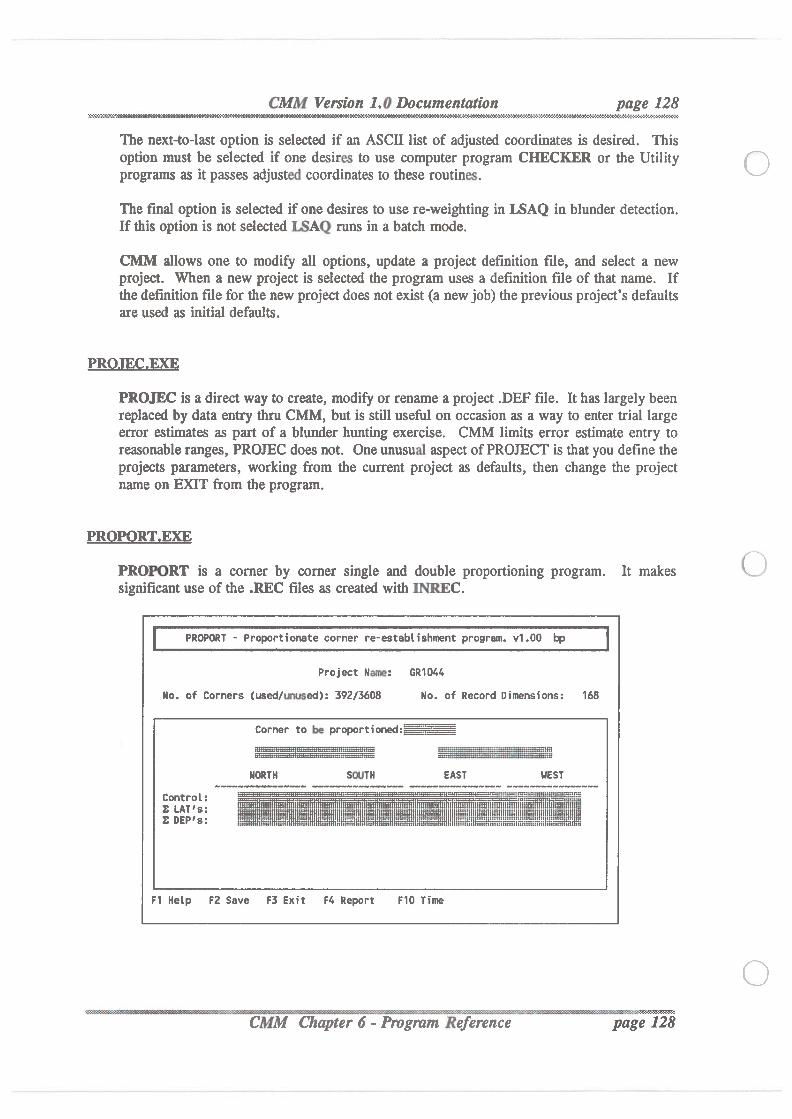
CMM Version 1.0 Documentation.

page 128.

Nfi MZ'2MW. .93“£~£-‘I1-K-3-?'¢24‘2’N\‘<

The next-to-last option is selected if an ASCII list of adjusted coordinates is desired. Thisoption must be selected if one desires to use computer program CHECKER or the Utilityprograms as it passes adjusted coordinates to these routines.

The final option is selected if one desires to use re-weighting in LSAQ in blunder detection.If this option is not selected LSAQ runs in a batch mode.

CMM allows one to modify all options, update a project definition file, and select a newproject. When a new project is selected the program uses a definition fileof that name. Ifthedefinition filefor thenew project does not exist (a new job) theprevious project’s defaultsare used as initial defaults.

PROJEQEE

PROJEC is a direct way to create, modify or rename a project .DEF file. It has largely beenreplaced by data entry thru CMM, but is still useful on occasion as a way to enter trial largeerror estimates as part of a blunder hunting exercise. CMM limits error estimate entry toreasonableranges, PROJEC does not. One unusual aspect of PROJECT is thatyou define theprojects parameters, working from the current project as defaults, then change the projectname on EXIT from the program.

PROERT.EXEPROPORT is a comer by corner single and double proportioning program. It makessignificant use of the .REC files as created with INREC.

PROPORT - Proportionate corner re-establishment program. V1.00 bp

Project Name: GR1D44 No. of Corners (used/mused): 392/3608 No. of Record Dimensions: 168

Corner to be proportioned:'L3‘ ?5"é:3

F1 Help F2 Save F3 Exit Flo Report

-- -.-.-we - e.- ..w. ‘(A

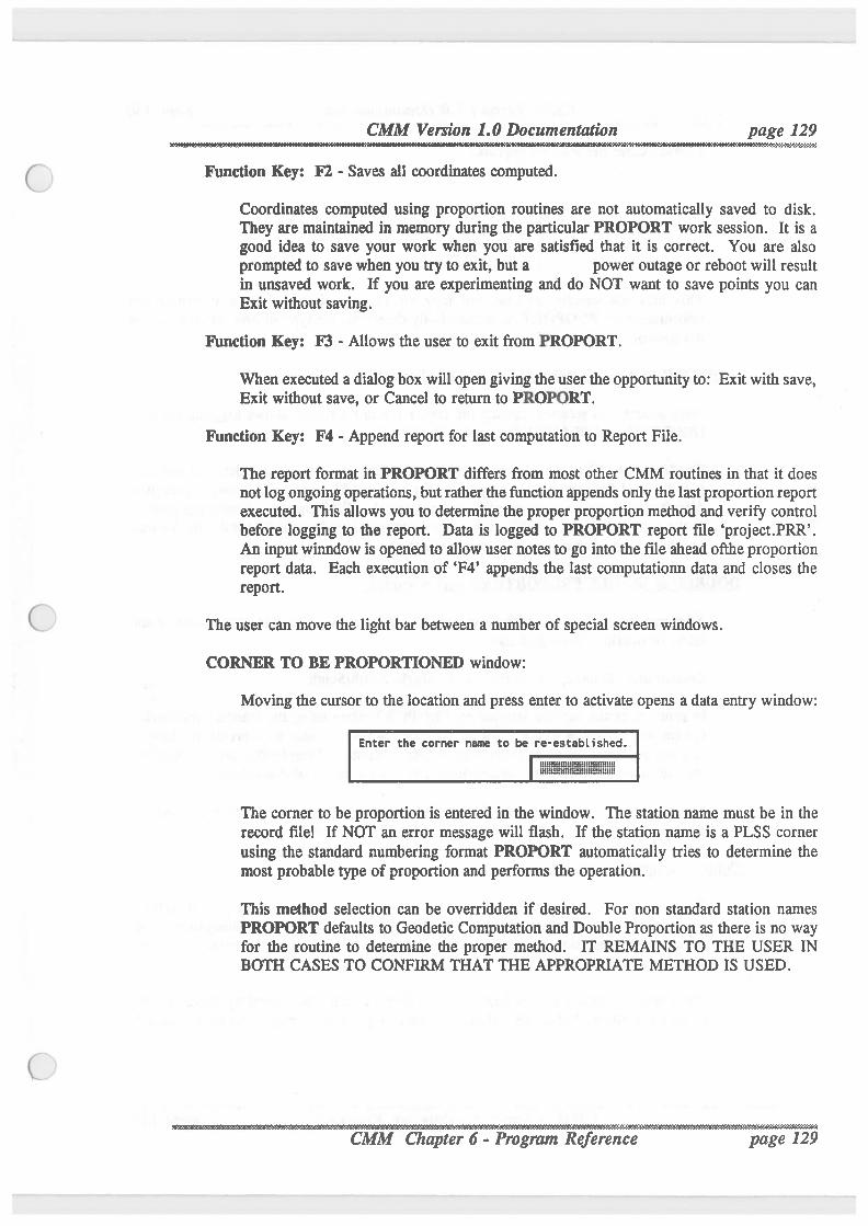
.f"‘\

CMM Version 1.0 Documentation page 129

Function Key: F2 - Saves all coordinates computed.Coordinates computed using proportion routines are not automaticallysaved to disk.They are maintained in memory during the particular PROPORT work session. It is agood idea to save your work when you are satisfied that it is correct. You are alsoprompted to save when you try to exit, but a power outage or reboot will resultin unsaved work. If you are experimenting and do NOT want to save points you canExit without saving.

Function Key: F3 - Allows the user to exit from PROPORT.

When executed a dialog box willopen giving theuser theopportunity to: Exit withsave,Exit without save, or Cancel to return to PROPORT.

Function Key: F4 - Append report for last computation to Report File.

The report format in PROPORT differs from most other CMM routines in that it doesnot log ongoing operations, but ratherthefunctionappends only thelastproportion reportexecuted. This allows you to determine theproper proportion method and verify controlbefore logging to the report. Data is logged to PROPORT report file ‘project.PRR’.An input winndow is opened to allow user notes to go into thefileahead oftheproportionreport data. Each execution of ‘F4’ appends the last computationn data and closes thereport.

The user can move the light bar between a number of special screen windows.

CORNER TO BE PROPORTIONED window:

Moving the cursor to the location and press enter to activateopens a data entry window:

The corner to be proportion is entered in the window. The station name must be in therecord file! If NOT an error message will flash. If the station name is a PLSS corner

using the standard numbering format PROPORT automaticallytries to determine themost probable type of proportion and performs the operation.This method selection can be overridden if desired. For non standard station namesPROPORT defaults to Geodetic Computation and Double Proportion as there is no wayfor the routine to determine the proper method. IT REMAINS TO THE USER INBOTH CASES TO CONFIRM THAT THE APPROPRIATEMETHOD IS USED.

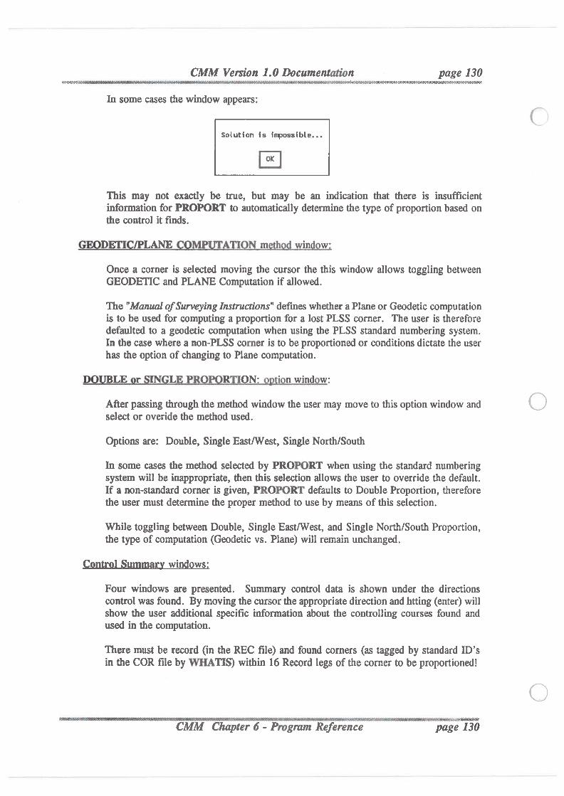
CMM Version 1.0 Documentation page 130S-%WMW%%K¢HfiWVflK40MW MMMQ”¢'M¢fifiW.¥V#4W¢'

In some cases the window appears:

Solution is inpossible. . . IEIThis may not exactly be true, but may be an indication that there is insufficientinformationfor PROPORT to automaticallydetermine the type of proportion based onthe control it finds.

D LANE m in w’

Once a corner is selected moving the cursor the this window allows toggling betweenGEODETIC and PLANE Computation if allowed.

The "Manual ofSurveying Instructions" defines whether a Plane or Geodetic computationis to be used for computing a proportion for a lost PLSS comer. The user is thereforedefaulted to a geodetic computation when using the PLSS standard numbering system.In the case where a non—PLSS corner is to be proportioned or conditionsdictate the userhas the option of changing to Plane computation.

LE r L R0 R ON: ion wind w:

Afterpassing throughthe method window theuser may move to thisoption window andselect or overide the method used.

Options are: Double, SingleEast/West, Single North/South

In some cases the method selected by PROPORT when using the standard numberingsystem will be inappropriate, then this selection allows the user to override the default.If a non-standard corner is given, PROPORT defaults to Double Proportion, thereforethe user must determine the proper method to use by means of this selection.

While toggling between Double, Single East/West, and Single North/SouthProportion,the type of computation (Geodetic vs. Plane) will remain unchanged.

nrl mmr win w‘

Four windows are presented. Summary control data is shown under the directionscontrol was found. By moving the cursor theappropriate direction and htting (enter) willshow the user additional specific information about the controlling courses found andused in the computation.There must be record (in the REC file) and found comers (as tagged by standard ID’sin the COR fileby WHATIS) within 16 Record legs of the corner to be proportioned!

i" e 130

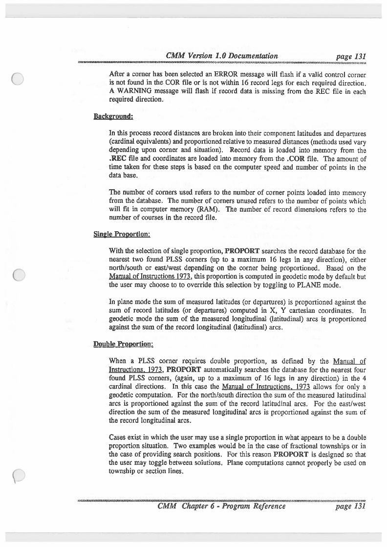
CMM Version 1.0 Documentation page 1319'8?

.. . , . , .2-W-9".‘-H-I-K*X<

After a corner has been selected an ERROR message will flash if a valid control corneris not found in the COR fileor is not within 16 record legs for each required direction.A WARNING message will flash if record data is missing from the REC file in eachrequired direction.

B 0 nd'

In thisprocess record distances are broken into their component latitudes and departures(cardinal equivalents) and proportioned relative to measured distances (methodsused varydepending upon corner and situation). Record data is loaded into memory from the.REC fileand coordinates are loaded into memory from the .COR file. The amount oftime taken for these steps is based on the computer speed and number of points in thedata base.

The number of comers used refers to the number of corner points loaded into memoryfrom the database. The numberof corners unused refers to the number of points whichwill fit in computer memory (RAM). The number of record dimensions refers to thenumber of courses in the record file.

Singlg Proportion:With the selection of singleproportion, PROPORT searches the record database for thenearest two found PLSS corners (up to a maximum 16 legs in any direction), eithernorth/southor east/west depending on the corner being proportioned. Based on theManual of Instructions 1973, thisproportion is computed in geodetic mode by defaultbutthe user may choose to to override this selection by toggling to PLANE mode.

In plane mode the sum of measured latitudes (or departures) is proportioned against thesum of record latitudes (or departures) computed in X, Y cartesian coordinates. Ingeodetic mode the sum of the measured longitudinal (latitudinal) arcs is proportionedagainst the sum of the record longitudinal (latitudinal) arcs.

Double Proportion:When a PLSS comer requires double proportion, as defined by the Manual ofInstmggions, 1273, PROPORT automaticallysearches the database for the nearest fourfound PLSS comers, (again, up to a maximum of 16 legs in any direction) in the 4cardinal directions. In this case the Manual of Instructions, 1973 allows for only ageodetic computation. For the north/southdirection the sum of the measured latitudinalarcs is proportioned against the sum of the record latitudinal arcs. For the east/westdirection the sum of the measured longitudinal arcs is proportioned against the sum ofthe record longitudinal arcs.

Cases exist in which theuser may use a singleproportion in what appears to be a doubleproportion situation. Two examples would be in the case of fractional townships or inthe case of providing search positions. For this reason PROPORT is designed so thatthe user may toggle between solutions. Plane computations carmot properly be used ontownship or section lines.

<._,.._............................................................................................................................................................................................................................................................_ ._, ., _,.CMM Chapter 6 - Program Reference ‘ H ' ?e 131'

CMM Version 1.0 Documentation page 132.<‘X40G-‘\'s'N'2*3¢C~Z-Z*I"aC\'

SD.EXE

SQ This program is an option which sets up :1 .SD filewhich looks exactlylike the .LSA fileexcept error estimates replacethecorrespondingmeasurements. This is useful when you havesurveys of varying accuracy. The .SD fileis not read fixed format so theuser can use a wordprocess or to edit existing standard errors. This is helpful when you only want to change asmall number of standard error estimates. SD has similar input and editing capability toGENER built in.

SECT§I;IOW,EXEIt is often useful to graphicallydisplay a township to identify which PLSS corners exist in the.COR database (created withWHATIS). For this reason SECTSHOW has been developed.Upon selection from the UTCOMM menu SECTSHOW displays a picture of a standard

township on the screen. The main heading includes pertinent informationabout the project:- project name,- project datum and state plane zone,- number of points withinthe .COR file,- numberof regular PLSS comers, and- number of temporary PLSS comers.

Regular PLSS section comers are graphicallydisplayed as green squares. Quarter corners aredisplayed as yellow circles. Sixteenthcomers are displayed as red triangles. TemporaryPLSScomers are displayed with the same shape in white color. These are the corners tagged withthe standard id with a T extension.

E EXE

SEE For efficiency,LSAQ, GENER, CHECKER, SSHOT, and DXFLSA now readformatted data structures in .LSA. To convert old data files or ones created using a wordprocessor run SETUP. It will prompt you for the filename, and that filewill bereformatted. Problems in the old filewill be identified. This should only be necessarywhen you manually edit the .LSA file.

-« ->a-292»aa1s¢2mssa:maw2::::mxasa&2<9ssuy;sxe»:2s-xx4:-.CMM. page

CMM Version 1.0 Documentation page 133. -Q§»9WW¢»¢>M'M%WW}W¢#P%¢ P» X

SSHQT

This program is for adding sideshots and open ended traverses to a fileof coordinatesordered by point ID #93 which is generated by LSAQ. The reason for using this in lieu ofmerely keeping the sideshots in the .LSA fileas maintained by GENER and used in LSAQanalysis is that the sideshots will greatly slow the overall Least Squares process, andcontribute nothingto the analysis as they provide no redundancy. For small jobs this maynot matter, but for moderately sized jobs, where you may be waiting for a matter of hoursin processing time, removing sideshots may be worthwhile. It has most of the same editingcapabilitiesas GENER and uses the state plane scale factor of the station on the maintraverse in reducing distances (if state plane coordinates are being used), and uses the sameelevation reductions to grid as in LSAQ. You can separate sideshots from other stations inthe .COR filesince they will not have convergence angles tagged to them.

Input (data) file is .SSS

No output file is created.

SSHOT has a complete but simplified editor.

Allows updating of the .SSS and .COR files

SSHOT can handle up to 800 stations, 800 angles, and 800 distances.

TD§I_§ATDS is a preliminary program thatwas designed to convert files collected with thecommercial Tripod Data Systems CO—OP4l data collection system.

UTQOMM,EXE

UTCOMM is simply the utilitiesmenu system. It uses the file ‘UTCOMM.PRG’ for it’sdefinition. Information is available in the installation section and in the UTCOMM.PRGfileheader concerning how to install programs of your own in the menu system.

VIEW.EXE

VIEW allows screen viewing of a horizontal network. VIEW uses the project .LSA file.Coordinates are read from the .LSA file, so GENER must have been executed. VIEWallows station name display to be toggled on or off, and allows parming and zooming byinput of ground coordinates. VIEW requires the provided MODERN.FON file to exist,and Microsoft’s MSHERC may have to be run to use a Hercules graphics card with CMM.

_., ._____________________________________________________________________________________________________________________________________________CMM Chapter 6 - Program Reee page 133

CMM Version 1.0 Documentation page 134%5W“K~'€fl5u\W INNC%VN¢WhW%X*N€%W#5'?Wi¢WW’$9MOKSNQWK01WK4-I'Hr}-PX'4‘I‘Z4r€I¢5C‘Z-I'2-I'Z'I'Z<‘2'I'2'2'Z'£-73-34-3~7X'WO-ZrWu‘K".60'1'2#3'9‘:-I-4-2-I-:'2€-L-Div?->5“-Z-Z-C-II

WHATI EXE

Whatis is an extremely important program. It’s most important function is to identifywhich traverse points are to be used as accepted corners used in proportions. The cornersthus indentified are recognized by AUTOPROP and PROPORT as control forproportions. It is also possible to tag each traverse point and/or corner with attributes suchas original, local etc. This does not serve any function at present, but may be used in thefuture to provide symbology with the output graphics.Computer program WHATIS is used to manage your station names and help you keeptrack of what each station is. After you have run a least squares adjustmentof yourtraverse data you will have created a .COR file. This is the least squares adjusted stateplane coordinates of your traverse stations.

This tagging can be obtained in one of two ways:

(1) WHATIS can be used to give a standard designation to a traverse station. This is thecase when evidence in the field is found. In this case the user assigns the traversecoordinates to a new station name (copies the point). The traverse station name is noteliminated.

(2) A coordinate position of a comer is computed using the utilities and identified with astandard corner name. This station will thus appear in the .COR filevia the utilitiesand WHATIS can be used to assign a properties to that station ID.

The first thingWHATIS allows you to do is back up the existing .COR file (from thetraverse adjustment) into a .TRA file. This preserves a copy of the final traverse results.You can assign a traverse designation to all points at this time.

After this is completed, WHATIS is capable of assigning coordinates to a new station ID,querying what is the status of a station and updating that status, and listing stations andcoordinates.

The following numberingtoggles what a station is:

1 - original GLO (found)2 - original GLO (remonumented)3 - local (found)4 - local (remonumented)5 - temporary6 - proportioned or set7 - BLM control8 - NGS-USGS control9 - traverse

A station can have any number of these nine designations.

IVProgram Reference page 134

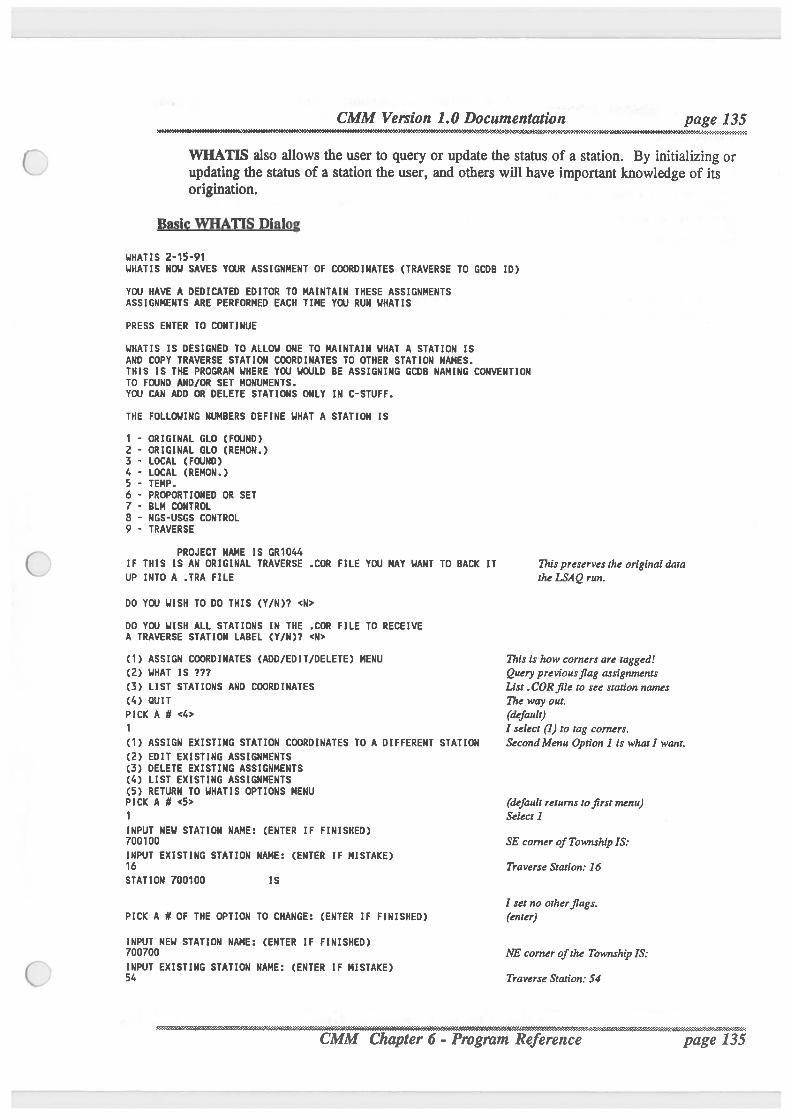
CMM Version 1.0 Documentation page 135

WHATIS also allows the user to query or update the status of a station. By initializingorupdating the status of a station the user, and others will have important knowledge of itsorigination.

Bgsig EHATIS DiglggHHATIS 2-15-91UHATIS NOH SAVES YGJR ASSIGNMENT OF COORDINATES (TRAVERSE TO GCDB ID)YOU HAVE A DEDICATED EDITOR T0 MAINTAIN THESE ASSIGNMENTSASSIGNMENTS ARE PERFORMED EACH TIME YOU RUN HHATIS

PRESS ENTER TO CONTINUE

UHATIS IS DESIGNED TO ALLOW ONE TO MAINTAIN HHAT A STATION ISAND COPY TRAVERSE STATION COORDINATES TO OTHER STATION NAMES.THIS IS THE PROGRAM UHERE YUJ UCXJLD BE ASSIGNING GCDB NAMING CONVENTIONTO FCXJND AND/OR SET MONUMENTS.YOU CAN ADD OR DELETE STATIONS ONLY IN C-STUFF.

THE FOLLOHING NLMBERS DEFINE HHAT A STATION IS

ORIGINAL GLO (FGJND)ORIGINAL GLO (REMON.)LOCAL (FWND)LOCAL (REMON.)TEMP.PROPORTIONED OR SETBLM CONTROLNGS-USGS CONTROLTRAVERSE

O®NQxLI|“UJI’\J—Iu

|

IllllllPROJECT NAME IS GR104/o

IF THIS IS AN ORIGINAL TRAVERSE .COR FILE YOU MAY HANT TO BACK IT Thispreserves the original dataUP INTO A .TRA FILE theLSAQ run.

DO YOU HISH TO DO THIS (Y/N)? <N>

DO YOU HISH ALL STATIONS IN THE .COR FILE TO RECEIVEA TRAVERSE STATION LABEL (Y/N)? <N>

(1) ASSIGN COORDINATES (ADD/EDIT/DELETE)MENU This is how comers are tagged!(2) WHAT IS 7?? Query previousflag assignments(3) LIST STATIONS AND COORDINATES List .CORfileto see station names(4) QUIT Iheway out.PICK A # <4> (default)1 I select (1) to tag corners.(1) ASSIGN EXISTING STATION COORDINATES TO A DIFFERENT STATION SecondMenu Option 1 is whatlwant.(2) EDIT EXISTING ASSIGNMENTS(3) DELETE EXISTING ASSIGNMENTS(4) LIST EXISTING ASSIGNMENTS(5) RETURN TO HHATIS OPTIONS MENUPICK A # <5> (defaultreturns tojirst menu)1 Select]INPUT NEH STATION NAME: (ENTER IF FINISHED)700100 SE comer of Township IS:INPUT EXISTING STATION NAME: (ENTER IF MISTAKE)1 6 TraverseStation.‘ 16STATION 700100 IS

I set no otherflags.PICK A # OF THE OPTION TO CHANGE: (ENTER IF FINISHED) (enter)INPUT NEH STATION NAME: (ENTER IF FINISHED)700700 NE corner of the Township IS:INPUT EXISTING STATION NAME: (ENTER IF MISTAKE)51. TraverseStation: 54

......... ._,,... ,._ ._ ._ ‘ __

page 135

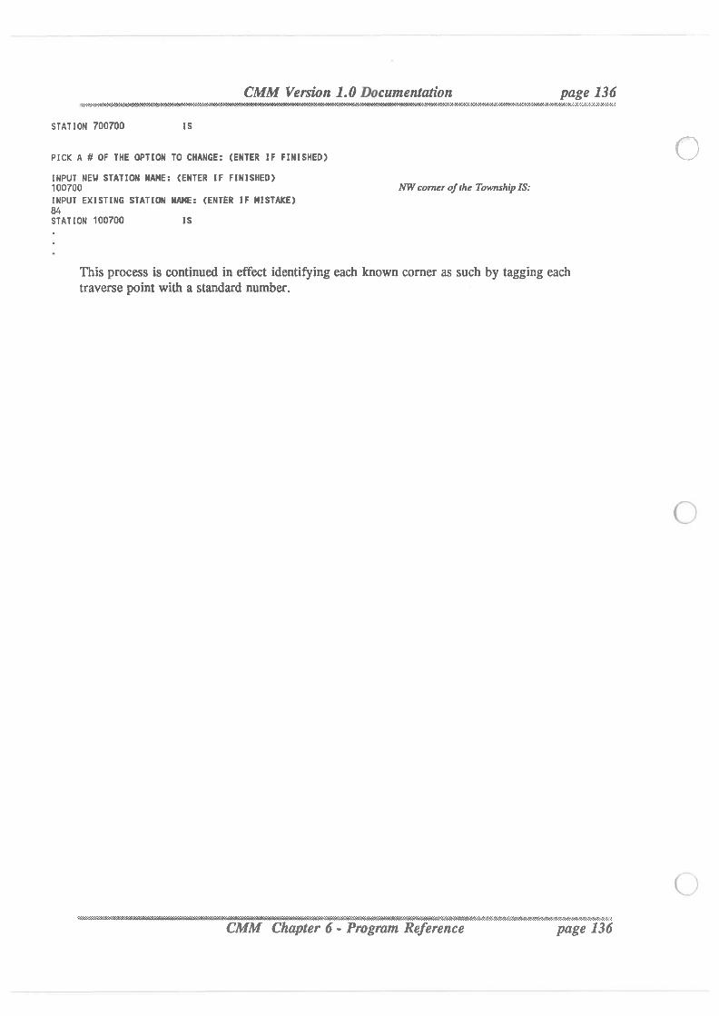
CMM Version.;.;.;.;,- . . . . . .. . . . . . . .. . I. . . . . . . . .. . . .

I

.............. .. _ ........_

1.0 Documentation page 136.

7'1’-42'!‘9%”IfW‘3‘?34‘I<‘WI~34“<<‘E‘I*3¢Z¢¢'Z'€<'Ir9'Z'Z¢'5¢D°%C4’c<¢Z'¢<t>’#}Z4'I~ I‘Z‘Z‘3'."J'3'Z'5'Z

STAT ION 700700 IS

PICK A # OF THE OPTION TO CHANGE: (ENTER IF FINISHED)

INPUT NEH STATION NAME: (ENTER IF FINISHED)100700 NW corner of the Township IS:INPUT EXISTING STATION NAME: (ENTER IF MISTAKE)84STATION 100700 IS

This process is continued in effect identifying each known corner as such by tagging eachtraverse point with a standard number.

' ' 'rence page 136.....................................................................................................2.-.... ..................................... "----------------------------------CM haptef 6 -'Refe

,..,\

CMM Version 1.0 Documentatio page 137-

....... ...................... . . . . . . . . . . . . . . . . . . . . . . . . . . . . . . . . . . . . . . .. . . . . ..................... _ _ _ 3- - ‘__ . _5;,¢¢¢g,;.,-,g.,;.;,;¢¢¢.y,,.°.°.;_,¢¢,m_,,»5,,,°‘

A nixl— f rlntlltin

Installation Notes — CMM Version 1.0 Release

Cadastral Survey Measurement Management Software may be contained on differing media.It is distributed on either:

2 - 1.2 Meg 5-1/4" diskette.

or

1 - 1.4M 3.5" diskette.

it can be recopied in a way to be distributed on either

4 - 360K 5-1/4" diskettes.

2 - 720K 3.5" diskettes.

In addition, a hard copy of the documentation should be obtained. It contains a tutorial andother informationESSENTIAL for effective operation of the software.

CMM requires a IBM compatible PC with a full 640K base RAM, a hard disk with atleast 3MB free space. A mathcoprocessor is required. An AT 286 or 386 withan EGAor VGA compatible graphics card and monitor, is preferred. We have experiencedproblems with some portions of CMM on PC’s with CGA and monochrome graphicscards. Hercules mono graphics cards can be made to function with most programs ifproper emulation routines are run.

Note: If you have your own text compatible (ascii) editor that you would prefer touse with the system, the install process requires that you know it's directory pathand name.

What Instgll dog;

The CMM Install process the drive you are installing from and the drive and path you areinstalling to from the user, then creates that directory, then creates and runs a batch file thatmanages installingall of thesystem files and programs. The files are contained in compressedarchive format on the installation disk and cannot be run from the floppy, or merely copiedto a hard disc and work.

If you do not have sufficient room on the target drive, the install will finish and may appearto complete, but files not fitting will not have been installed. Please be sure you havesufficient space on your disk before proceeding with the installation.

If the source archive file is not found on the selected installation drive, the batch file willprompt you to insert the next diskette. Of course, this will not occur if all the files are on asingle source floppy.

M Appendix 1 - Installationt I ipa e 13

CMM Version 1.0 Documentation page 13. ..>. . . . . . . . . . . . . . . . . . ... . . . . \. . . . . . . . . . . . . . . . ,. . . . . . . . . . . . . . . . . . . . . . . .. _ >«.;¢.;4.;.;;.,~¢¢.¢¢¢,;.¢.¢.¢¢.;.;.w¢g¢_.;, - .x¢w_9g¢«.;.;.;.;,-.\s .3-._.;.;.¢.;.;.;

When the file installation process is complete (whether or not successfully) the installationresumes by allowing you to specify your own preferred editor or an (enter) will select thedefault PD editor provided.The final act of the complete installation process is to create 2 DOS batch files in the rootdirectory of your C: drive. The first of these is critical to the operation of CMM and it iscalled CMM.BAT. This batch file is the access method to the CMM system and handlesCMM’s main menu operations. The second batch file created is called GMM.BAT, and it'ssole purpose is to allow you to quickly move to the selected CMM drive and directory at theDOS level if you choose.

The second option in the install program can also be used to make a new CMM.BATwhenever necessary, if for example, you move your CMM files to a different drive, directoryOR you want to change the default editor choice.

INSTALL S‘

1) Place the CMM Beta Release diskette in either drive A or B as appropriate for yoursystem. For the multi disk sets, be sure you inserted disk 1.

2) Log to thatdrive, for example if drive A: Type:

a:(enterl

3) then type:

lNSTALl.(enter)

4) follow the prompts, and the process is rather straightforward.Note: Ifyou have previously installed CMMor MM in the same directory youwill be prompted to verify overwriting eachfile that is installed. Use yourjudgement about whether this is appropriate or not and answer Y or Naccordingly. The install willskip overfilesthatare the same or oflater date,so there is no risk ofoverwriting a later version ofa file.

5) After the program exits, you should be able to invoke the system by typing:CMM(enterl

Note: the adjustmentportions of CMM require at least 545K of available RAM,therefore it is not advisable to run CMMfrom many memory resident menu systems.It is best to invoke CMMfiom the DOS > prompt.

-----------------.t , '.'2')\i-l5l-‘J;'.'’.').'i'$‘$‘.-.-,:’ ‘H age 138

CMM Version 1.0 Documentation.

page 139.

r

Boththe Manage ‘Main Menu’, and theUTCOMM ‘Utilities’menu have entries for an editor.The entry on the distributionsystem is set for a Public Domain editor called TE.

It is expected thatpeople will want to install their own editor, and the system accommodatesthis. The editor should be an ASCII or TEXT editor, preferrably not a word processingeditor. WordPerfect, Wordstar and many other word processors can be used to edit TEXTfiles if care is taken, but there is also danger that files may be corrupted with specialformatting characters used by such systems. One good choice would be WP Library’sProgram Editor which is a text editor thatworks a lot like WordPerfect., Norton Editor, PCWrite, etc. although the provided PD editor is virtually as powerful. Documentation for theprovided editor is installed with the system and is called TE.DOC.

Since the CMM.BAT file is a normal DOS batch file, user’s may customize it to some extentso as to exit in a different way. Currently the system returns the user to the C:\ rootdirectory. '

UT MM-Utilii Mnu

Any program may be installed in the UtilitiesMenu by editing the fileUTCOMM.PRG. Theprogram must exist in the DOS pathof be in the chosen CMM subdirectory. Batch files willNOT function. Information on how to install programs or otherwise customiseUTCOMM.PRG are contained in theheader to thatfile The Version 1.0 release of UTCOMMallows for defining menu colors and defining the menu item ‘hot’ key with theUTCOMM.PRG file. This is an ASCH filewhich can be edited by the user.

If you have a program such as Autosketch that requires a batch file to run in order to installdrivers, change directories, etc. Create an appropriate batch file that functions from DOSthen compile the batch filewith the supplied utilityBATZEXEC. This will then be useableonce setup in UTCOMM.PRG.

D I tin or movin MM

You may encounter difficulties if you attempt to erase CMM, this should only be due to thefact that several of the critical Zone parameter files have been set to DOS’s READ-ONLYstatus. This keeps them from being corrupted inadvertently. There are a number of utilitiesthat can easily remove this flag and allow the files to be deleted, however DOS’s A'I'I‘RIBcommand is sufficient. In your CMM directory determine the filesthatremain undeleted. Forexample: ZONE.DATor TABLE.DATare the offending files:

Type ATTRIB-R *.DAT(enter)will clear the read-only attribute for those files.

Jfi?#

ge 139..............~ ....................._.

CMM Version 1.0 Documentation page 14-:(~x~:v:(~{-;-,, --.~ -.- - -.«.-.<- - - -.-.-.~ -.- -.-.- - - - - - - - -

‘- - <.- - - - - - -->-.- - - - - - < - - - - - * - - - -.- - - - - - - - - ~ - - ‘ ' ~ , -. . OK: »&0¢W€<W%KV1“'KWNhWW'E€WW%VG£<'%hK'Y&“'&I¢I4W‘Z‘0C'3'lrI'Z~Z'£'l'§1‘Z¢<'J'3‘Z'2

Appendix 2 - Standard Qgmgr Numbering

Many of the proportion routines for rectangular corners in CMM are dependent upon or canperform more automated operations if the standard numbering system is used to identify thecontrollingor ‘found’ corners. Those of you familiarwith the Bureau of Land ManagementsGeographic Coordinate Data Base (GCDB) Project will recognize similaritiesto their system.However the system in use within CMM is simpified and has some significant differencesrequired to meet CMM requirements. Someplaces in thedocumentationdo refer to the systemas the GCDB system. Initially it was intended to make CMM independent of the corneridentificationsystem, as thereare many effective rectangular comer identificationsystems thathave beenused throughouttheyears by different people and agencies. However the improvedfunctionality that accrues in using a specific standard began to emerge as an importantattribute. As a result at this point in the system development and use several programs makeextensive use of the system:

AUTOPROP for example is dependent upon the system.INREC’s efficient record entry capabilities are only realised when using the standardnumbering.PROPORT is not dependent on the system however it is capable of making a betterdetermination of the proper proportion method when the system is used.

ADJUST is independent of the system.

WHATIS’s controlling corner tagging and SECTSHOW’s control corner depictionalgorythms are dependent upon the system.

For more details see the Reference section documentation for the above programs.

The em

The system consists of a base 6 digit number. The first 3 digits, somewhat like an Xcoordinate represent corners on the N-S section lines, counting from the West boundary of astandard township. The second 3 digits, similar to a Y coordinate, represent corners locatedon the the E-W section lines counting from the south. Corners below the section corner levelare indicated in approx. chain units i.e. counting from the West and South boundaries of thesection. For example the 1/4 comer bet. 20 and 21 is: 300340.

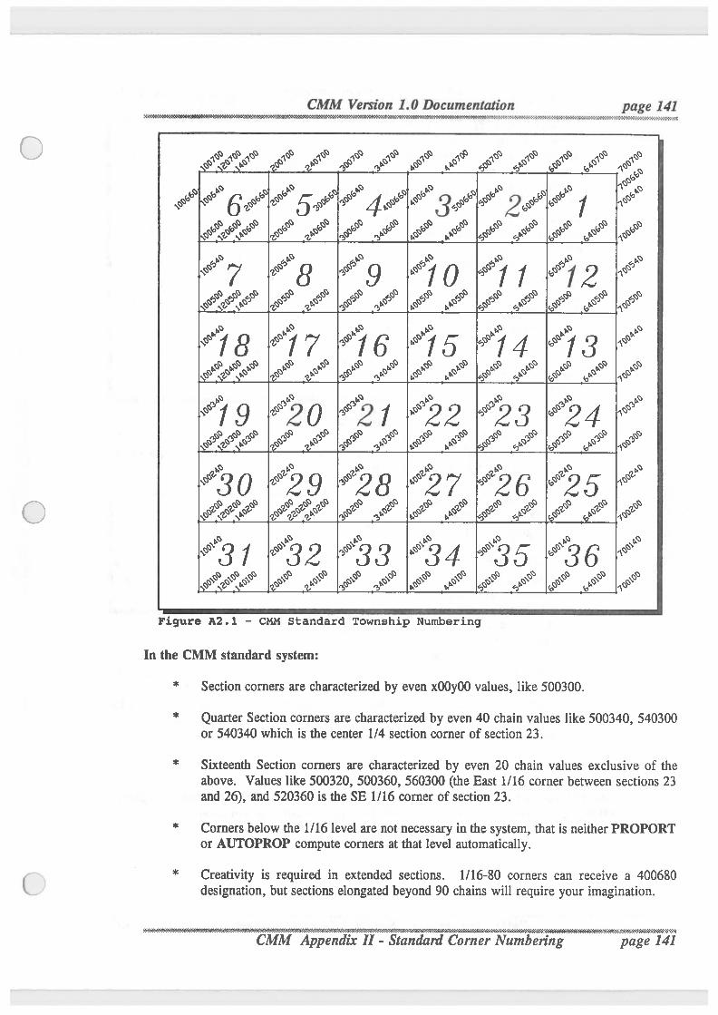
CMM Version 1.0 Documentation page 141VS‘I'fl'l<‘!'N->#>>‘.~'-6‘:-I-I-4"?1’<‘i41'l-’l*A>9<')b\Xn>X02594-J'2§s\‘?iN'C\\“I'3»"‘}'DOID-0&0:-3??-Er:-}I'3‘1‘N?'?€

Figure 112.1 — CMM Standard Township Numbering

In the CMM standard system:* Section corners are characterizedby even xOOy00 values, like 500300.

* Quarter Section corners are characterizedby even 40 chain values like 500340, 540300or 540340 which is the center 1/4 section comer of section 23.

* Sixteenth Section corners are characterized by even 20 chain values exclusive of theabove. Values like 500320, 500360, 560300 (theEast 1/16 corner between sections 23and 26), and 520360 is the SE 1/16 comer of section 23.

* Comers below the 1/16 level are not necessary in the system, that is neitherPROPORTor AUTOPROP compute comers at that level automatically.

* Creativity is required in extended sections. 1/16-80 corners can receive a 400680designation, but sections elongated beyond 90 chains will require your imagination.

.- . . . . . . . . .. _ . ..............................................................., ..CMM Appendix II - StC"

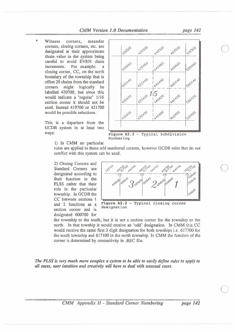
Witness corners, meandercomers, closing corners, etc. aredesignated at their approximatechain value in the system beingcareful to avoid EVEN chainincrements. For example: aclosing corner, CC, on the northboundary of the township that isoffset 20 chains from thestandardcomers might logically belabelled 420700, but since thiswould indicate a ‘regular’ 1/16section comer it should not beused. Instead 419700 or 421700would be possible selections.

This is a departure from theGCDB system in at least twoways: Figure A2.3 — Typical Subdivision

Numbering1) In CMM no particularrules are applied to these odd numbered corners, however GCDB rules that do notconflictwith this system can be used.

2) Closing Comets andStandard Corners aredesignated according totheir function in thePLSS rather that theirrole in the particulartownship. In GCDB theCC between sections 1and 2 functions as asection corner and isdesignated 600700 forthe township to the south, but it is not a section corner for the township to thenorth. In that townhip it would receive an ‘odd’ designation. In CMM this CCwould receive the same first 3 digit designation for both townhips i.e. 617700 forthe south township and 617100 in the north township. In CMM the function of thecorner is determined by connectivity in .REC file.

Figure A2.2 - Typical closing cornerdesignation

The PLSS is very much more complex a system to be able to easilydefine rules to apply toall cases, user intuition and creativity will have to deal with unusual cases.

. ' '- . k7RW&B 5?595%I3§t<35'Appendix II - Standard .$W&E%9%ffl6$W%5$rWdfi2M :4:K¢¢:-7~:»:b'-'1'-'-'-'-:-'1'-:=?.z?‘ComerNumbering page 142

CMM Version 1.0 Documentation page 143 WK'N?W“§lMW°K< fl“%W€¢I€“Z¢$¢€'°0'X4'€'Z+€‘X')00€¢¢’-'l'I'3

A ndi - MM lo r

LEA AR ANALY I E TI N

Parametric Adjustment - also called the observation equation method - it is an approach toadjustmentsin which each measurement is described in equation form (such as describinga distanceby inverse coordinates)Observation - a fancy word for measurement

Redundancy - measurements which are not required to determine unique coordinates for stationsin a traverse. These measurements could include closing angles, closing distances, or multiplesolar/polaris shots.

ConditionalAdjustment- an approach to adjustments in which the results are based upon a seriesof conditions which must be satisfied - such as sum of latitudes and departures of a closed figuremust be zero. In complicated surveys finding all of the conditions possible cannot be automated,and thus the parametric adjustment is the desired approach.Linear Equation - this is an equation which has no trigonometric functions in it or variables topowers (or square roots). An equation defining an elevation difference is a linear equation.Non-LinearEquation - An equation with trigonometric functions and/or powers in it, such as theinverse distance or azimuth equationsLinearization - a process which transforms a non-linear equation into a linear equation. Sincenothing in this world is free by linearizingequations you force a least squares adjustmentto use aniterative approach in the solution process. Differential levelingnetworkshave linear equations andthus require no iteration. Traverses have non-linear equations and thus iterate to a solution

Iteration - one update of the solution of a set of linearized equations; In horizontal traverses thesolution is updates to N,E coordinates. Iteration generally ceases when all updates to coordinatesare insignificant (less than 0.005 ft. is appropriate).In1'tiaIApproximations- thesolutionof linearizedequations requires initial estimates of all unknowncoordinates as first "guesses"; The updates in each iteration refine the approximationstowards theirleast squares adjusted results.

Simultaneous Solution - this means all coordinates are being solved for in one solution; In thecompass rule process you must adjustone traverse into another traverse which is held as "fixed".This is not correct since the fixed traverse contains error.

System ofEquations — in a least squares adjustmentyou solve an "n x 11" system of equations eachiteration where n equals the number of unknown quantities. In a 20 station traverse there are 40unknowns (20 N, 20 E coordinates). This means a 40 equations, 40 unknowns system of equationsmust be solved. Even for a computer this is a slow process.

- --$$$-3 *A”: page 1

CMM Version 1.0 Documentation page 14ft.

¢NW}%WEfiV:¢%§'??W‘H9 '&$K#Yfl'W&hH'I’l'I'I~I..' '2' "Z'l"4K'iI/.4'M¢}Zs‘-1'$¢':':'3'DC4':-Itfiv '3':-v't\'n"<':i§'fo‘3‘C:‘' ’ ' ‘OWZQV

Bandwidth Optimization - There are many ways to speed up the solution of a system of equationsand reduce thenumberof terms in the equations. Some methods other than bandwidthoptimizationinclude column profileminimization, Helmert blocking, and recursive partitioning. If a computerprogram does not use one of these methods the results will be produced very slowly. LSAQ usesa bandwidthoptimizationroutine which has been extensively modified for better performance. Formost survey networks the bandwidth will probably range from 5-30% of the total number ofstations. This process enables more efficient solution of least sqaures problems, and especiallyallows "big" problems to be solved on a personal computer

Solution Convergence - the last iteration has insignificantupdates and thus the solution terminates.

Solution Divergence - blunders or poor initial approximations will cause updates to grow asiterations proceed; This indicates something is wrong with the data, and it needs to be corrected.

Numberof measurements - equals # of distances + number of angles + number of azimuths +number of control coordinates

Numberofunknowns - 2 * total number of stations (1 N, 1 E coordinate)

Degrees offreedom — number of measurements minus number of unknowns; or the number ofmeasurements beyond what is necessary to uniquely define coordinates for each station

Residual — the difference between a measurement and its computed quantity based on coordinates;It is how much the measurement adjusted.Error estimate - A surveyor’s error estimates of measurements assigns appropriate weighting ofmeasurements in a least squares adjustment. An angle with an error estimate of 2 seconds will betreated as more weighted (stronger, less chance of adjustment)than an angle with an error estimateof 10 seconds. This does not mean the angle with the smaller error estimate will always get asmalleradjustmentsince geometric constraints (such as sum of angles in a closed figure) also playa major role in dictating amount of adjustment. A distance error estimate is usually modelled bya constant plus a ppm addition to account for larger errors generally occurring in longer lines. Anangle or azimuth error estimate is a function of the instrument’s least count, the number ofrepetitions, the instrument operator's abilities, and the prevailing environmental conditions.Experiencewith instrumentationand the least squares adjustmentwill allow thesurveyor to developconfidence in error estimation. Error estimating allows the simultaneous analysis of differentmeasurement types (distances, angles, azimuths, control coordinates).RMS error - root mean square error — it is the average of a series of residuals in which the sign ofthe residual is eliminated through summing squared residuals, dividing by the number of that typeof measurement, then computed that value’s square root.

Residual vs. error estimate - These quantities should be of approximately the same magnitude.Since measurements contain random error a plot of residuals should look like the "bell-shaped"curve from statistics which centers about zero. If residuals tend to be predominantly of one signthismeans systematic error may exist. This would occur if your survey tied into two precise controlcoordinates and your EDM was measuring sytematically long. All adjusted distances would beshorter than their measured values. It could also occur if horizontal angles were only measured in

‘r\

CMM Version 1.0 Documentation page 145\'o'3N99'29’X‘. . q . .

'

, , ..s1¢€9.¢.Q°.'i‘€'i*W'D.¢.‘I'Z'¢\“M4'3">1-3-R

the direct position and a large horizontal collimationerror existed. Residuals which are larger thanthree times their respective error estimate are generally considered suspect.

Standard error ofunit weight - This is a numberwhich tells you how well it appears you that youare estimatingyour measurement errors. It is generated by the summing thesquares of all residualsdivided by their error estimates. That quantity is divided by the degrees of freedom and the squareroot is taken. If a residual and error estimate are of the same magnitude note that the residualdivided by the error estimate will generally produce a number close to one. The standard error ofunit weight is a number that evaluates all residuals and corresponding error estimates. If thestandard error of unit weight is near one (0.7-2.5) you are estimatingyour errors well. Uncorrectedsystematic errors, blunders, or generally poor measurements will result in larger residuals and thusa large standard error of unit weight. If you are pessimistic in error estimationor you have very fewredundant measurements a very small standard error of unit weight will result.

Standard error ofadjustedcoordinates - these are theleast squares error estimates of adjustingN,Ecoordinates. They are a functionof proximity to existing control points. The statistical significanceof these quantities is that if you went and made the same measurements with the same instrumentusing thesame procedures, you would have a one sigma (68.3% confidence) chance of beingwithinplus or minus the standard error of the first solution’s coordinate. It has nothing to do withadditional traverse legs and readjustment, comparing to someone else’s coordinates, or evaluatingretracement evidence.

Error ellipses - It should be apparent thatthereliabilityof a traverse point’s position will not usuallybe the same in all directions. The position is generally stronger in the traverse direction, andweakest away from the traverse directions. The error region is an ellipse, defined by a radius(semi-major axis) of maximum error (SU), radius (semi-minor axis) of minimum error (SV), andthe angle from north (positive clockwise) of the direction of maximum error (T). Since an errorellipse is two-dimensional,theone sigma error ellipse onlydenotes 35% confidence (roughly68.3%squared). The same statistical significancereasoning for coordinate standard errors applies to errorellipses - it is an internal evaluation of your data and does not relate to external information suchas other surveys or existing coordinates.

Robustness - This is a method of using least squares as a filtering mechanism for detection ofblunders. Robustness averages the absolute value of a measurement’s residual with its errorestimate, and that average becomes the new error estimate in a readjustment. The measurementswith large residuals get reassigned larger error estimates, and vice-versa. This enables theadjustmentto befiltered to thesuspect measurement. The success of robustness in blunderdetectionis a function of size of the blunder, number of blunders, and the geometry and redundancy of thethe traverse network.

CMM Appen 3 — lossal p 92145

CMM Version 1.0 Documentation page 146, &s‘OO'&‘.".'Z4‘I<¢'C“.’X4<'I<>>M¢<-X'?¢¢'0¢O¢4'6-$209’:-029:‘:N'?!¢>€'1’fA-¢\X‘X¢??5‘fi%->W‘K'E-33-Y»:

GEODEY [ SIATEPLANE QOORDINATES SEQTION

NAD 27 - North American Datum of 1927 - a datum based on the Clarke Ellipsoid of 1866, andfixed position and orientation at Meade’s Ranch in Kansas. Based upon this information latitudesand longitudes were calculated for all National Geodetic Survey control points based primarilyontriangulation. The calculation involved a least squares adjustmentby hand calculations!

NAD 83 - North American Datum of 1983 — a datum based on the GRS 80 Ellipsoid, and fixedposition and orientation at the center of the earth. The measurements used in NAD 27, andadditional measurements made by theNational Geodetic Survey subsequent to 1927, were subjectedto a least squares adjustment - this time using a computer. This results in a different latitude andlongitude for a station when compared to its NAD 27 values, with the difference often amountingto hundreds of feet.

State Plane Coordinates - projections whichuniquely relates a geodetic position (latitude, longitude)to a plane coordinate pair (N,E). The relation is truly a one-to-one correspondence; for a uniquestate plane coordinate pair there is only one latitude, longitude pair, and vice-versa. The two typeof projections that exist are Lambert - a conic projection for states elongated east-west, andMercator - a cylindricalprojection for states elongated north—south. The size of a zone was limitedby defining a a state plane distance will not differ from its geodetic counterpart by 1/ 10000 of thedistance. Thus larger states are covered by more than zone.

NAD27 state plane coordinates — These are based on zone constants which include false northingsand eastings so thatnegative coordinates do not result. The published units are U.S. Survey Feet.

NAD 83 stateplane coordinates - These are based on different zone constants than NAD 27. Themost notable change is thatdifferent values were assigned for false northings and eastings, and thecoordinates published by NGS are in meters instead of U.S. Survey Feet. Even when convertedto feet, NAD 83 coordinates look dramaticallydifferent than theNAD 27 coordinates for the samepoint becausethe false northings and eastings are different.

Geodetic distance - a horizontal distance between two points measured on the earth.

Grid distance - a geodetic distance which has had scale and elevation factors applied to it to reduceit to the state plane zone.

Scale factor- Since a state plane zone intersects the earth geodetic distances must be projected tothe zone. If the distance is inside where the zone intersects the earth the scale factor is less thanone since the projection is inwards. If the distance is outside where the zone intersects the earththe scale factor is greater than one since theprojection is outwards. The scale factor for a distanceis the average of the scale factors at the two end points. The value of the scale factor is a functionof location in the zone, which has a one-to-one relationship with geodetic position.

wsnsasza-z~-append\..... .. -~__ ,.

page 147

Elevationfactor- Both the ellipsoids thatrepresent NAD 27 and NAD 83 are at sea level, and thusany measured distance must be reduced to a sea level equivalent by the elevation factor. Theelevation factor is based on the average of the elevations at the two end points of a line.

Elev. Factor = R / (R+h) where R = radius of the earth (20,906,000ft)h = elevation

Relation of Geodetic and Grid Distance

Grid Distance = Geodetic Distance * Scale Factor * Elevation Factor

Geodetic Distance = Grid Distance / (Scale Factor * Elevation Factor)Geodetic azimuth- the direction of a line relative to geodetic north

Grid north - thedirection of a line relative to state plane grid north. It will not equal geodetic northsince in the state plane grid all north directions are parallel and in a geodetic system north linesconverge to the polesConvergence angle - the angle between grid and geodetic north at a point. It is a function oflocation in the zone.

Second tenn correction - If converting a geodetic azimuth for a line to a grid azimuth (orvice-versa), a small correction must beapplied to convergence anglewhich accounts for the factthata geodetic azimuthexists on a curved surface (theearth) and a grid azimuth is on a flat surface (theprojection). It is a function of the lengthof the line and its location in the zone, and is generallyless than an are second. This correction must also be applied to horizontal angles to reduce themto their grid equivalents.Relation of Grid and Geodetic Admuth

Grid Azimuth = Geodetic Azimuth- Conv. Angle + second term correction

Geodetic Azimuth = Grid Azimuth + Conv. Angle - second term correction

CMM Version 1.0 Documentation page 148' 3M

.‘$%§23¢M’W2€¢WN WWO&VMWNflWW%?‘3WHWflW2¢

GENER grgr message explgnatigg

MISSING NECESSARY DATA FOR COORDINATEGENERATION

This means you are missing control coordinates, directional control, and/or measurementswhich enable coordinate generation by traverse.

NO DISTANCE TO CONTROL POINT. STOP

It is impossible to generate coordinates by traverse if there are no distances to any controlcoordinates.

APPROXIMATECOORDINATELINE NOT FORMATTEDCORRECTLY

If the "use existing coordinates" option is used any approximate coordinate line in the .LSAfilewhich is formatted incorrectlywill trigger thismessage and the line will be ignored. Thiscan only happen if one has been editing the .LSA filewith a text editor.

ERROR - TRAVERSELINK GENERATOR LIMITS EXCEEDED

A traverse has more than 3000 stations in it.

MISSING ANGLES ON TRAVERSESBETWEEN CONTROL STATIONSPROCEED WITH ANGLE-DIST ON ASSUMED DIRECTION

If more than one control station exists in your data this message will appear if inputangle/distancesdo not allow a traverse between control stations to be identified. GENER willthen compute a series of angle distance combinations from the first control station untiltraverse is possible. Rotation of the network to fit existing control occurs after a coordinatepair is generated for every station.

FROM STATION A TO STATION B DISTANCE CLOSURE = 1.23 FT.

This message is associated with the previous message. When rotation to fit control occurs(2 control stations required) a distance comparison of traverse to control can also be computed.

ROTATION NOT POSSIBLE - MISSING DATA

If only one control point exists, an azimuth must be used for directional control. If GENERcarmot compute coordinates for the azimuth endpoints due to an omission of data the rotationof the assumed coordinate system used in coordinate generation cannot occur.

DIRECTION ASSUMP'TION HAS BEEN CORRECTED

If only one control point exists, GENER computes all coordinates based on an assumeddirection. After all coordinates are generated the coordinates are rotated based on the firstinput azimuth.

S99%35 '-“V-' '2 ' .- &5$Vfi5flaitfitifltitit-$:3‘k1$:i:a’:2'§:3:W:CMM Appendixf ' - page 148 . :::>;ez

CMM Version 1.0 Documentation page 149

*** COORDINATES UNDETERMINEDFOR STATION A

This is a good message if you have intentionallyeliminated all messages regarding station A.It verifies you succeeded. If station A is supposed to be part of your traverse network forsome reason coordinates could not begenerated for it and you must correct thesituationbeforeprocedding any further.

ERROR - TOO MANY STATIONS IN INPUT NETWORK-STOP

The 3000 station limit has been exceeeded.

STATION A IS NOT ON A DISTANCE IN INPUT FILE

Usually each station should have a distance connected to it.

STATION A IS NOT ON AN ANGLE IN INPUT FILE

Usually each station should have an angle connected to it.

YOU NEED TO INPUT SOME CONTROL STATIONS

GENER cannot compute coordinates unless one control station and one azimuth, or more thanone control station, has been input.

YOU HAVEONLY ONE CONTROL POINT & NO AZIMUTHS- CANNOT BE SOLVED

There is no way to control direction.

DO YOU WANT TO QUIT WITHOUT COORDINATEGENERATION (Y/N)? < Y>

If either of the previous two situations exist you may exist GENER to save data withoutgenerating coordinates.

ERROR - INPUT FILE EXCEEDED ONE OF THE FOLLOWING LIMITSNUMBER OF STATIONS = 3000NUMBER OF DISTANCES = 4000NUMBER OF ANGLES = 4000NUMBER OF AZIMUTHS = 3500

GENER has some size restrictions.

page 149

CMM Version 1.0 Documentafion page 150 ¢WN8

.

' -r7W4.€'C'Z.s‘I\‘r3' ‘¢7I€~lrO3<NW(i}1"."/.4€~Z'Z42-2“.-1-1’.I¥JC'<4i'3\'4'.

FORMAT ERROR DETECTEDIN CONTROL STATIONS - RUN SETUP

FORMAT ERROR DETECTEDIN DISTANCES - RUN SETUP

FORMAT ERROR DETECTEDIN ANGLES - RUN SETUP

FORMAT ERROR DETECTEDIN AZIMUTHS - RUN SETUP

You have probably edited the .LSA file with an editor and the file is no longer correctlyformatted.

NO COORDINATES FOR STATION A WRI'ITENTO FILE

This is a good message if you have intentionallyeliminated all messages regarding station A.It verifies you succeeded. If station A is supposed to be part of your traverse network forsome reason coordinates could not be generated for it and you must correct thesituationbeforeprocedding any further.

TEMP.JOBIS MISSING PROJECT NAME - RUN PROGRAM PROJECThis fileholds the project name. For some reason it does not exist.

.DEF FILE FOR THIS PROJECT IS SCREWED UP - ERASE IT AND RUN PROJEC

The .DEF filecontains project definitions. It has probably been edited with a text editor andis no longer formatted correctly.

LSA rrrm saeexlnti

STATION A NOT ON ANY MEASUREMENTS - IGNORED

If an unknownstation has approximate coordinates for it in the .LSA filebut no measurementsto it it is ignored. This can only happen if the .LSA filewas editted with a text editor.

ONE OF THE FOLLOWING LIMITS HAS BEEN EXCEEDEDTOTAL NUMBER OF CONTROL STATIONS = 900TOTAL NUMBER OF STATIONS = 3000TOTAL NUMBER OF DISTANCES = 4000TOTAL NUMBER OF ANGLES = 4000TOTAL NUMBER OF AZIMUTHS = 900

LSAQ has some size restrictions.

sages

CMM Version 1.0 Documentation page 151

_.. . . . . . ._......................................... ............................................................................ _.._ _. -

FORMAT ERROR DETECTEDIN CONTROL STATIONS - RUN SETUPFORMAT ERROR DETECTEDIN DISTANCES - RUN SETUPFORMAT ERROR DETECTEDIN ANGLES - RUN SETUPFORMAT ERROR DETECTEDIN AZIMUTHS - RUN SETUPAPPROXIMATECOORDINATELINE NOT FORMATTEDCORRECTLY - RUN SETUP

UNEXPECTED END TO INPUT FILE - STOP

You have probably edited the .LSA file with an editor and the file is no longer correctlyformatted.

MEASUREMENT FOUND WITHOUT STANDARD ERRORRUN COMPUTERPROGRAM SD BEFORE RUNNING LSAQ - STOP

If you are using the read error estimates from .SD file option there must be a one-to-onecorrespondence of it to the .LSA file. This message appears if this is not true. Running SDfixes this. The error occurs when you add data in GENER and do not run SD prior to LSAQwhen this option is used.

MISSING PROJECT NAME - RUN PROJECT MANAGER

TEMPJOBholds the project name. For some reason it does not exist.

.DEF FILE FOR THIS PROJECT IS SCREWED UP - ERASE IT AND RUN PROJECTMANAGER

The .DEF filecontains project definitions. It has probably been edited with a text editor andis no longer formatted correctly.

*** INSUFFICIENT AMOUNT OF CONTROL TO PERFORM THE ADJUSTMENT ***

LSAQ carmot compute coordinates unless one control station and one azimuth, or more thanone control station, has been input.

CANNOT FIT INTO PAGING ALGORITHM - STOP

The least squares solution uses a technique called paging to store equations for very largesurveys. It is remotely possible to reach size restrictions of this algorithm.

CMM Version 1. Documentation page 152.......................................... .... _ . . . . . . I . . . . . . . . . . . . . . . . . . . . . . . . .... I . . . . . . , . . . . . . . . . ..

_ ‘r_.;.;.g;.;\r_g;.)g.;.g.;¢;.;.g

*** MAXIMUM NUMBER OF I'I'ERA'I‘IONS REACHED ***

LSAQ quits at 10 iterations if updates are still larger than 0.005 ft.

*** SOLUTION DIVERGING - ITERATIONHALTS***

In cases of large blunders the solution will not converge.

NO ERROR ANALYSIS DUE TO NETWORKSIZE

If paging has to be used LSAQ carmot compute error ellipses.

NO SUITABLEINFORMATION FOUND IN ELEVATION FILESO FIX FILE OR USE PROJECT ELEVATION - STOP

You have selected the read elevations from .LEV fileoption and no suitable information is inthatfile.