Eesti Maaülikooli doktoritööd

Doctoral Thesis of theEstonian University of Life Sciences

ON USING MATHCAD SOFTWARE FOR MODELLING, VISUALIZATION AND

SIMULATION IN MECHANICS

MATHCADI TARKVARAPÕHINE MODELLEERIMINE,VISUALISEERIMINE JA SIMULEERIMINE MEHAANIKAS

AARE AAN

A Thesis for applying for the degree of Doctor of Philosophy

in Production Engineering

Väitekirifi losoofi adoktori kraadi taotlemiseks tootmistehnika erialal

Tartu 2015

Institute of Technology, Eesti Maaülikool, Estonian University of Life Sciences

According to verdict No 1-4/30 of September 25, 2015, the Doctoral Committee of the Engineering Sciences of the Estonian University of Life Sciences has accepted the thesis for the defence of the degree of Doctor of Philosophy in Production Engineering. Opponent: Professor Valery Ochkov, DSc (Eng)

Department of Power Plants, National Research University Moscow Power Engineering Institute Opponent: Leading Research Scientist Jüri Majak, DSc

(Math) Department of Machinery,

Faculty of Mechanical Engineering, Tallinn University of Technology Supervisor: Professor Mati Heinloo, DSc (Math) Institute of Technology Estonian University of Life Sciences

Defence of the thesis: Estonian University of Life Sciences, room B136, Kreutzwaldi 56, Tartu on November 06, 2015, at 9:15. Publication of this theisis is supported by the Estonian University of Life Sciences.

© Aare Aan, 2015 ISSN 2382-7076 ISBN 978-9949-569-02-1 (trükis) ISBN 978-9949-569-03-8 (pdf)

5

CONTENTS

LIST OF ORIGINAL PUBLICATIONS ........................................... 8

INTELLECTUAL PROPERTY ....................................................... 10

ABBREVIATIONS AND SYMBOLS ............................................ 11

INTRODUCTION ............................................................................ 14

1. Literature overview ................................................................... 15

1.1 Visualization ...................................................................... 15

1.2 On using simulations in teaching ....................................... 16

1.3 Overview of the virtual models and their motion simulations in the program Mathcad ............. 18

1.4 The purpose and tasks of the doctoral thesis ..................... 23

2. Materials and Methods .............................................................. 26

2.1 Foreword ............................................................................ 26

2.2 Overview of some mass point equations in kinematics and dynamics ................................................... 26

2.2.1 On the mass point motion of Curved planar trajectories .......................................... 26

2.2.2 Mass point motion on a rotating disc ......................... 27

2.2.3 Mass point motion on a moving inclined plane ......... 28

2.3 Overview of the Lagrange and Hamilton’s equations ....... 29

2.4 Overview of the equations in the Mechanics of machinery ...................................................................... 29 2.5 IV order Runge-Kutta algorithm for differential equations’ numerical solutions. ......................................... 33

3. Using the program Mathcad ...................................................... 34

3.1 Mathcad worksheet ............................................................ 34

3.2 Implementation of the Runge-Kutta method using a Mathcad worksheet ............................................... 35

3.3 Motion simulation on a Mathcad worksheet ..................... 38

6

3.4 On the visualization of geometric vectors on a Mathcad worksheet ......................................................... 40

4. Overview of the research papers written by the author of the thesis ............................................................................... 42

4.1 On the creative teaching of engineering mechanics .......... 42

4.2 On research regarding linkages ......................................... 43

4.2.1 Study of the V-engine ................................................ 43

4.2.2 Study of the double connecting–rod linkage .............. 45

4.2.3 Study of the Theo Jansen walking mechanism .......... 48

4.3 On research on mass point motion .................................... 50

4.3.1 Mass point motion on curved trajectories .................. 50

4.3.2 Study of a granule’s motion on a fertilizer spreading disc ............................................................. 51 4.3.3 A sea buckthorn berry’s motion on a conveyor belt .. 52

4.4 Synthesis of a cam-follower mechanism ........................... 53

4.5 Study on the chaotic motion of a double pendulum .......... 57

4.6 Small oscillations of coupled pendulums .......................... 57

SUMMARY AND CONCLUSIONS ............................................... 59

REFERENCES ................................................................................. 63

KOKKUVÕTE ................................................................................. 70

ACKNOWLEDGEMENTS ............................................................. 73

PUBLICATIONS ............................................................................. 74

CURRICULUM VITAE ................................................................ 174

ELULOOKIRJELDUS ................................................................... 176

ETTEKANDED ............................................................................. 178

7

8

LIST OF ORIGINAL PUBLICATIONS

I. Aan, A., Aarend, E., Heinloo, M. 2011. On chaotic motion of a double pendulum. Agronomy Research, Volume 9, 5–12.

II. Aan, A., Heinloo, M., Aarend, E. 2011. Interactive Comput-er Aided Learning and Teaching of Analytical Mechanics. Int. J. Engn. Pedagogy (iJEP), Volume 1(3), pp. 4–8.

III. Aan, A., Heinloo, M. 2011. On creative teaching of engi-neering mechanics. Proc. 22nd International DAAAM World Symposium, pp. 1081–1082.

IV. Aan, A., Heinloo, M., Aarend, E., Mikita, V. 2012. Analysis of four-stroke cycle internal combustion V-engine in Mathcad environment. Proceedings of 8th International Con-ference of DAAAM Baltic Industrial Engineering, Tallinn, pp 389–394.

V. Aan, A., Heinloo, M. 2012. Computer based comparison analysis of single and double-connecting-rod slider-crank linkages. Agronomy Research, Volume 10, pp. 3–10.

VI. Aan, A., Heinloo, M. 2012. Visualization of the kinematics of a material point. Engineering for Rural Development: Pro-ceedings 11th International Scientific Conference - Engineer-ing for Rural Development, Jelgava, pp. 204–209.

VII. Aan, A., Heinloo, M. 2013. Composing and solving differen-tial equations for small oscillations of mathematical spring-coupled pendulum. Agronomy Research, Volume 11(1). Pp. 223–230.

VIII. Aan, A., Heinloo, M. 2014. Motion of a granule on fertilizer spreading disc. Proc. 42nd Int. symp. “Actual Tasks on Agri-cultural Engineering”, Opatia, pp. 101 - 111.

IX. Aan, A., Heinloo, M., Allas, J. 2014. Design of a radial cam for the cam-follower mechanism. Proceedings of 9th Interna-tional DAAAM Baltic Conference in Estonia: INDUSTRIAL ENGINEERING, Tallinn, pp. 11 – 16.

X. Aan, A., Heinloo, M. 2014. Analysis and synthesis of the walking linkage of Theo Jansen with a flywheel. Agronomy Research, Volume 12(2), pp. 657–662.

XI. Aan, A., Heinloo, M. 2015. Dynamics of a frozen sea buck-thorn berry in a separator. Procedia Engineering, Volume 100, pp. 689–698.

9

The author’s contribution to the paper: Paper Study design Data collec-

tion Data pro-

cessing Manuscript preparation

I MH, AA, EA MH, AA AA, MH AA, MH

II AA, MH, EA AA AA AA, MH

III MH, AA AA, MH AA, MH AA

IV MH, AA AA, MH AA, MH, EA AA, MH, VM

V MH, AA AA, MH AA, MH AA, MH

VI MH, AA MH, AA AA, MH AA, MH

VII MH, AA AA, MH AA, MH AA, MH

VIII MH, AA MH, AA AA, MH AA, MH

IX AA, MH, JA AA, MH AA, MH AA, MH, JA

X MH, AA MH, AA AA, MH AA, MH

XI MH, AA MH, AA AA, MH AA, MH

AA - Aare Aan, MH - Mati Heinloo, EA - Eino Aarend, VM - Villu Mikita, JA - Jaanus Allas

10

INTELLECTUAL PROPERTY

I. Title: Device for the separation of deep-frozen sea-buckthorn berries from twigs Patent number: EE 05717 B1 Filing date of the application: 19.07.2012 Priority date: 19.07.2012 Publication date: 15.04.2014 Inventors’ names: Nõmm, P., Aan, A.

The author’s contribution to the paper: Document Study design Preparation

and elabora-tion activities

Study of prior art

Manuscript preparation

I PN, AA AA AA AA, PN

AA - Aare Aan, PN - Peeter Nõmm

11

ABBREVIATIONS AND SYMBOLS

—function in the program Mathcad, which uses the algorithm of the Runge-Kutta fourth order method

—animation parameter used to define the variable for the generation of simulations on a Mathcad worksheet

Symbols

fertilizer granule’s current position; berry surface’s frontal area

fertilizer granule’s initial position ; , acceleration; projections of the acceleration

vector module in vector function notation of of the vector in vector function

air resistance constant

notation of the vector D piston diameter

friction force projection on axis between the spreading disc and the vane

inertial force projection on axis friction force projection on axis projection of the Coriolis inertial force magnitude of the resisting force

friction coefficient Hamiltonian; follower stroke

moment of inertia; matrix of the shape of a vector in the vector function

reduced moment of inertia value of the reduced moment of inertia at the beginning of

a cycle Lagrangian width of the conveyor belt; length

magnitude of the resisting torque on link one pivot’s resisting torque constant driving torque of the link

mass number of intervals between and

12

coefficient of dimensions in vector function p gas pressure in the engine cylinder

generalized momentum generalized momentum of the double pendulum

generalized force generalized coordinates

spreading disc radius radius of the curvature

cam base circle radius distance between the centre of the disc and a fertilizer

granule in the current position distance between the centre of the disc and a fertilizer

granule in the initial position used to define function axis along the conveyor belt berry’s acceleration

kinetic energy; denotes the transposed matrix in a vector function

first time value last value, where marks last value matrix of origin in vector function

velocity , projections of the velocity velocity of the conveyor belt; magnitude of the velocity

Greek

pressure angle angle between force and velocity

centre of the curvature coordinate centre of the curvature coordinate

inclination angle of the conveyor belt change in linkage kinetic energy

coefficient of speed fluctuation eccentricity of the follower

, inclination angles of the double pendulum axis between initial and current positions of a ferti-

lizer granule potential energy air density

follower rise angle

13

follower high dwell angle follower fall angle follower low dwell angle adjusting angle of the vane

angle between the polar radii of a fertilizer granule and the direction of the vane

matrix of transformation of the rotation in the vector func-tion

, angular velocity pivot’s angular velocity value of at the beginning of a cycle

14

INTRODUCTION

Learning and research are becoming increasingly more computer-based, which is supported by both the development of computing technology and better results in studying, teaching and research into engineering problems. According to Chonacky, 2006, computer modelling and simulation are some of the best methodologies that have been applied in science and engineering.

This doctoral thesis develops computer-based learning and research methods in engineering mechanics, analytical mechanics and ma-chinery mechanics. The results can be used in both teaching and practical engineering. In the current doctoral thesis, the objects that are automatically generated on the computer screen using a mathe-matical model are called virtual models for short. The process of creating images that correspond to calculation results (graphs, virtual models, simulations, etc.) is called visualization. The simulation of the movement of virtual models gives an idea of the movement of the object of study and the veracity of the solution calculated on the basis of the mathematical model. The use of computer-based visual-ization in teaching is very important. The analysis Höffler & Leutner, 2007 showed that the learning outcome improved by 37% on average when a simulation (animation) was used instead of a stat-ic picture. The simulations in the current thesis correspond to Recchi, et al., 2006 definition: an effective computer simulation is built on a mathematical model, which describes the process that is being studied. Visualization is interdisciplinary by nature, drawing on simulations, the psychology of perception, graphic art, computer graphics, picture editing, data management, etc. (Haber, 1990).

The mechanical problems explored in the current thesis have been solved with a computer on a PTC Mathcad worksheet. Unlike other mathematics programs, in which the formulas have to be pro-grammed as well, the engineering calculations software Mathcad allows writing formulas the way we are used to seeing them in books and writing them ourselves. The formulas and variables on a Mathcad worksheet can be changed on the computer screen and the changes in results can be directly observed in drawings, virtual mod-els and motion simulations for the virtual models.

15

1. Literature overview

1.1 Visualization

The visualization of the study object’s mathematical model helps a greater number of scientists, engineers and students to understand the work processes of physical systems, while taking into account the special types of people with increased neural activity.

Russian psychologist I. Pavlov divided people into three categories according to their neural activity: artistic, thinking and middle types (Leppik, 2001; Leppik, 2008). The memory of the artistic type is closely connected to senses, especially sight. In order to understand problems - this bears great significance in the learning process - it is important for the artistic type to see a diagram, picture, model, graph, film, etc. The studies have shown that these people value im-agery over concreteness. Additionally, it has been found that they respond to stimuli more directly, they have a closer connection to real experiences and react to reality more unwillingly than thinkers (Leppik, 2008). Thinkers are characterised by abstract thinking, log-ical analysis and good memory. They are good at math. Most think-ers are introverts: quiet, withdrawn and attentive. Teachers like this type of students. They are satisfied when the study material is verbal and abstract, relying on logic and analysis when absorbing infor-mation. They remember new material mostly semantically (concep-tually). Generally, they do not need visual explanation and enjoy abstract analysis and discussion instead (Leppik, 2008). The people who fall in the middle category extract information from the outside world using the strategies of both the previously described types. It has been found that the middle type is successful in both scientific and creative fields (Leppik, 2008). It is important for the teacher, lecturer or trainer to be aware of the different learning types. Conse-quently, they should use teaching methods that are suitable for the discussed types (Leppik, 2001).

Studies in cognitive psychology have proven that imagery is more important in teaching than the concrete presentation of information. The importance of imagery is regarded as twofold:

16

1. it helps some of the students to understand new material. The material that has been understood is stored in long-term memory;

2. it helps to create associative connections, which means that in-formation is stored more efficiently and it can later be easily re-trieved from long-term memory.

Primary schools and kindergartens traditionally engage all senses, but the teaching in higher grades and institutions of higher education is often verbal, which means that the teacher actually works with only some of the students. As a result, the teacher thinks that the students are not learning and this leads to teacher-student conflicts. Engaging all senses becomes especially important when presenting new material in class. Verbal and abstract methods can later be used when revising, practising and storing information, especially among older students (Leppik, 2001).

There are plenty of ways to engage different senses that are suitable for different subjects and ages, for instance: 1. demonstrations, experiments and models; 2. observation of the objects of study; 3. pictures, tables, diagrams; 4. slideshows; 5. video clips and films; 6. computer research; 7. field trips (Leppik, 2001).

Above all, visualization helps the artistic type to understand the pre-sented material. Mathcad’s interactive worksheets along with motion simulation offer better visualization compared to printed text.

1.2 On using simulations in teaching

Two groups were compared, one of which received traditional guid-ance in a classroom, whereas the other used additional computer simulations. The students’ understanding of kinematics was studied, whereas the topic was motion in the Earth’s gravitational field. The students who used computer simulations showed significantly better results in solving the task given to them. It was concluded that com-puter simulations are useful tools for understanding velocity and acceleration (Jimoyiannis & Komis, 2001; Rutten, et al., 2012). In

17

another study, two groups of students had to study particle kinetics. One group only studied in the classroom, whereas the other studied both in class and using computer simulations. The test results of the group who used computer simulations were better (Cohen’s d=0.81), even though the overall results of the test were low (Rutten, et al., 2012; Stern, et al., 2008). A comparative study of a traditional class and simulation-supported class was conducted in the field of genet-ics. The students were assessed in two ways, firstly, using statements (true/false) and secondly multiple choice questions. The study re-vealed that the class that used simulations achieved better results. When answering the question of whether the statement was true/false d=0.87 and d=0.80 when multiple choice questions were used (Rutten, et al., 2012; Gelbart, et al., 2009). In the field of for-estry, students used computer simulation to practise managing a for-est plot. The study assessed the simulation’s influence on solving the task and explaining the solution. The study found that in order to receive better results, it is useful to combine lessons with creating the opportunity for the students to figure things out themselves and to use computer simulations for practice (Riess & Mischo, 2010; Rutten, et al., 2012). Students’ interest in the studied material when using computer simulations has also been explored. For this, two simulations were created for the cell’s respiratory chain. The first simulation included tasks that needed to be solved and the second had examples which were designed to explain a specific part. The simulations with fully developed examples had a positive effect on the students’ interest. However, the students did not show height-ened interest in the simulations that used tasks. The students who had little interest in the subject beforehand expanded their factual knowledge despite the simulation type. The general understanding of the subject was created via simulations, which visualized the materi-al (Melek, et al., 2008). A study conducted at a high school physics course involved a group of students learning physics using special simulation software. The control group was taught in the traditional way without using this kind of software. The number of students in both groups was 15 and their age was in the range of 17 to 19. A test at the end of the course showed that the group of students who used simulation software scored 3.07 points more out of the maximum of 20 points on average than the control group (El Hassan, et al., 2014).

The aforementioned studies clearly show that the use of simulations improves students’ learning performance. The materials prepared in

18

relation to the current doctoral thesis have not been used in compara-tive groups and are based on other studies on the positive influence of simulations on learning and understanding.

The computer simulations presented in this doctoral thesis corre-spond to the solution of a specific task. For instance, the website Mekanizmalar offers numerous computer simulations (flash anima-tions) for the field of mechanics and technology, which visualize the work of mechanisms, but these are not based on solutions to specific tasks (Mekanizmalar). The learning process shows that the students understand the methodology of creating computer simulations on a Mathcad worksheet. It is important that each student can create these in order to visualize and check the solution to a specific task. The advantages of Mathcad in teaching mechanics have been highlighted by Novohatska, et al., 2014; Broman & Östholm, 1997; Soutas-Little, et al., 2008; Bertjaev, 2005 and Soutas-Little, et al., 2008.

1.3 Overview of the virtual models and their motion simula-tions in the program Mathcad

In their studies Heinloo & Olt, 2004a; 2004b and 2004c used the scheme in Figure 1.1a to create a virtual model of the disk-ridging tool on a Mathcad worksheet (Figure 1.1b) for studying the work process and simulations. The work process simulation of the virtual model is presented in the video clip Heinloo, 2015.

(a) (b) Figure 1.1. Scheme (a) and virtual model (b) of a disk–ridging tool (Heinloo & Olt, 2006).

In their studies Heinloo, et al., 2005; Heinloo & Leola, 2006a; 2006b and 2007 used the scheme in Figure 1.2a to generate a virtual model of a scraper performing press manure removal (Figure 1.2b). They used this virtual model to investigate the work process of the scrap-

19

er. This virtual model is displayed in action in the video clip Heinloo, 2011a.

(a) (b) Figure 1.2. Scheme (a) and virtual model (b) of a device for press manure remov-al (Heinloo, et al., 2005).

In the study Heinloo, 2007a composed a program on a Mathcad worksheet for the automatic generation of a four-bar linkage virtual model (Figure 1.3), which is often used in machine design linkage structures. If the user of this program defines the lengths of the links and the four-bar is kinematically possible, the virtual model is dis-played and the motion simulation can be executed. The four-bar vir-tual model’s motion simulation is displayed in the video clip Heinloo, 2011c.

Figure 1.3. Virtual model of the four-bar with the trajectory of a point of the connecting-rod (Heinloo, 2007a).

20

In the study Heinloo, 2007b a virtual model of a blueberry harvester picking reel was prepared on a Mathcad worksheet (Figure 1.4) ow-ing to derived equations. A video clip of the motion simulation of the picking reel’s virtual model upon simulating the harvesting pro-cess was prepared (Heinloo, 2014). In the video clip, the four-rake picking reel’s straight movement along the virtual field and the reel’s rotating movement with the rakes can be observed.

Figure 1.4. Virtual model of a blueberry harvester’s picking reel (Heinloo, 2007b).

In the study Olt & Heinloo, 2011a, the authors composed a virtual model of a plough stone protector according to derived equations on a Mathcad worksheet to study the device’s motion over stones. In this work, the stone protector linkage’s movement over stones was simulated and the linkage pivots’ velocities are displayed with vec-tors (Figure 1.5). In the video clip Heinloo, 2009, a stone protector’s virtual model’s simulated movement over “stone” is presented.

Figure 1.5. Positions of the virtual model of a stone protector in passing a „stone“ (Olt & Heinloo, 2011a).

21

In the study Heinloo, 2010a, the author researched the motion of virtual fertilizer granules in a virtual fertilizer’s spreading disc. The fertilizer granules are in complex motion: they rotate with the spreading disc and move along the disc’s vane. In the video clip Heinloo, 2010c, the virtual fertilizer granules’ motion in the four-vane virtual spreading disc is presented. Later on, this work was developed further with research on the effect of different vane angles (Olt & Heinloo, 2011a and 2011b).

Figure 1.6. Virtual model of the spreading disk together with the trajectories of fertilizer granules and the vectors of their velocities at the contour of the disc (Heinloo, 2010a).

Zhang, et al., 2010 studied linkage that can be used in a feeding mechanism in the Mathcad environment. They composed a mathe-matical model for the mechanism and a respective mathematical model they used to simulate the movement of the linkage.

Hess, et al., 2014 simulated the movement of a synchronous motor on a Mathcad worksheet. The simulation depends on different input values, which are adjustable: measurements, quantity of the magnet-ic poles and slots per pole, power and torque, simulation duration and step, etc. Accordingly, input values of the virtual model of the synchronous motor’s cross-section are displayed. On the cross-section, a stator corresponding to input measurements, slots, a rotor, arrows to visualize magnetic field, etc. (Figure 1.7) can be observed.

22

Figure 1.7. Virtual model of the cross-section of a synchronous motor (Hess, et al., 2014).

Different mechanisms have been simulated on a Mathcad worksheet by the author V. Ochkov. He has studied steam engines (Ochkov, 2011a), car windshield wipers (Ochkov, 2011b), the Chebyshev mechanism (Ochkov, 2011c), the Theo Jansen walking mechanism (Ochkov, 2011d), (Ochkov, 2013), etc.

23

1.4 The purpose and tasks of the doctoral thesis

Purpose

Developing computer-based learning and research methods in me-chanics.

In order to fulfil the purpose, tasks were set for each of the three categories of mechanics: analytical mechanics, engineering mechan-ics and machinery mechanics.

Tasks for developing learning methods:

1. Devising an interactive learning method in analytical mechanics. Demonstrate the compilation and use of interactive study notes for analytical mechanics. Create a system of Hamilton’s differ-ential equations, well-known in analytical mechanics, for a phys-ical double pendulum as a more specific example, along with the virtual model of the double pendulum and its motion simulation.

2. In the field of machinery mechanics, the task is to demonstrate how to make computer-based calculations for the kinematics and dynamics of the V-engine, along with creating a virtual model and its motion simulation. Demonstrate a method for finding an optimal profile for a radial cam in a cam-follower mechanism. Create a simulation of the movement of the optimal cam and its follower.

3. In the field of engineering mechanics, the task is to simulate the change in a mass point’s velocity and acceleration vectors, the centre of curvature, circle of trajectory curvature and evolute of the trajectory upon its movement on given trajectories.

4. Demonstrate the use of Mathcad’s symbolic calculation function and the Laplace transform for composing and solving motion equations for coupled pendulums along with the motion simula-tion of a virtual model.

Tasks for developing research methods:

1. Create mathematical and virtual models for single and double connecting-rod slider-crank mechanisms. Simulate their motion and perform a comparative analysis of the forces acting on it during motion. Present the results.

24

2. Create mathematical and virtual models for Jansen walking mechanism. Simulate the motion of the virtual model. Study the resisting environment’s influence on the fluctuation of the step and the possibilities of minimising it using a flywheel. Present the results.

3. Simulate the motion of fertilizer granules on a rotating spreading disc. Study the dependency of the motion on the adjusting angle of the vane, initial position of fertilizer granules and friction co-efficient between a fertilizer granule and the spreading disc. Pre-sent the results.

4. Simulate the motion of a frozen berry (mass point) on a moving conveyor belt and in free fall after leaving the belt. Study the de-pendency of the berry’s motion on the inclination angle of the belt, velocity of the belt and friction coefficient between the ber-ry and belt. Present the results.

The presented results and methods can be used in designing the aforementioned or other similar mechanisms.

The relevance of the doctoral thesis:

1. Using the possibilities of information technology to expand the teaching methods for mechanics increases the efficiency of teaching and learning and makes the learning process more mo-bile and interesting for the students.

2. Increasing the number of computer-based research methods for problems related to mechanics provides the engineers and scien-tists with better tools for research and development.

3. The visualization of the objects of study using virtual models and motion simulation is an easy way to check the accuracy of the solutions and a better way to understand the object than the alternative of conducting research and teaching only with the help of equations and their solutions.

Novelty:

The features of the computer program Mathcad are used in this the-sis for solution of the problems in analytical mechanics, engineering mechanics, mechanics of machinery and in agricultural machinery.

25

Solved new Mathcad based problems in this thesis:

1. Numerical analysis of chaotic motion for double pendulum. 2. E-teaching and e-training methods for analytical mechanics. 3. Visualization of kinematics of a material point. 4. Comparative analysis of motions the new double-connecting-rod

and a single-rod linkages. 5. Optimization method of the profile a cam in a cam-follower

mechanism. 6. Virtual model for the v-engine, simulation and analysis the mo-

tion of this model. 7. Virtual model for the Theo Jansen walking mechanism, simula-

tion its motion and optimization the trajectory of a leg endpoint. 8. Composition and solving the differential equations for spring-

coupled pendulum by using symbolic calculus. 9. Simulation the motion of a granule on the rotating spreading disc

and the analysis the dependency of this motion from various pa-rameters.

10. Analysis the motion of a berry in the separator of sea-buckthorn berries.

26

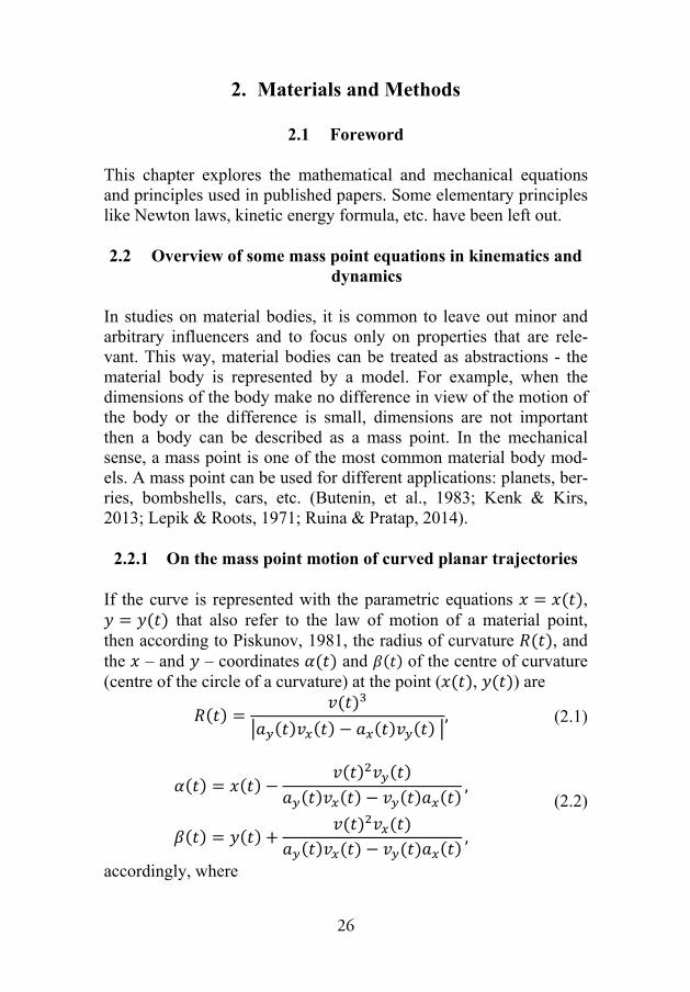
2. Materials and Methods

2.1 Foreword

This chapter explores the mathematical and mechanical equations and principles used in published papers. Some elementary principles like Newton laws, kinetic energy formula, etc. have been left out.

2.2 Overview of some mass point equations in kinematics and dynamics

In studies on material bodies, it is common to leave out minor and arbitrary influencers and to focus only on properties that are rele-vant. This way, material bodies can be treated as abstractions - the material body is represented by a model. For example, when the dimensions of the body make no difference in view of the motion of the body or the difference is small, dimensions are not important then a body can be described as a mass point. In the mechanical sense, a mass point is one of the most common material body mod-els. A mass point can be used for different applications: planets, ber-ries, bombshells, cars, etc. (Butenin, et al., 1983; Kenk & Kirs, 2013; Lepik & Roots, 1971; Ruina & Pratap, 2014).

2.2.1 On the mass point motion of curved planar trajectories

If the curve is represented with the parametric equations , that also refer to the law of motion of a material point,

then according to Piskunov, 1981, the radius of curvature , and the – and – coordinates and of the centre of curvature (centre of the circle of a curvature) at the point ( , ) are

(2.1)

(2.2)

accordingly, where

27

, , ,

, .

Paper VI is based on those equations.

2.2.2 Mass point motion on a rotating disc

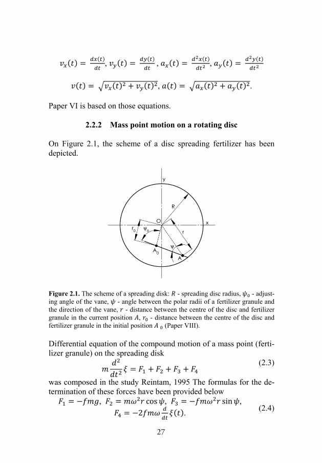
On Figure 2.1, the scheme of a disc spreading fertilizer has been depicted.

Figure 2.1. The scheme of a spreading disk: - spreading disc radius, - adjust-ing angle of the vane, - angle between the polar radii of a fertilizer granule and the direction of the vane, - distance between the centre of the disc and fertilizer granule in the current position , - distance between the centre of the disc and fertilizer granule in the initial position (Paper VIII).

Differential equation of the compound motion of a mass point (ferti-lizer granule) on the spreading disk

(2.3)

was composed in the study Reintam, 1995 The formulas for the de-termination of these forces have been provided below

, , , . (2.4)

28

Placing forces from equations (2.4) in the equation (2.3) and divid-ing them by results in an ordinary differential equation with the constant coefficients

(2.5)

Paper VIII is based on the solution of the differential equation (2.5).

2.2.3 Mass point motion on a moving inclined plane

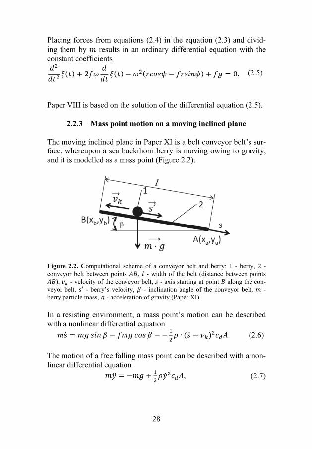
The moving inclined plane in Paper XI is a belt conveyor belt’s sur-face, whereupon a sea buckthorn berry is moving owing to gravity, and it is modelled as a mass point (Figure 2.2).

Figure 2.2. Computational scheme of a conveyor belt and berry: 1 - berry, 2 - conveyor belt between points , - width of the belt (distance between points

), - velocity of the conveyor belt, - axis starting at point along the con-veyor belt, - berry’s velocity, - inclination angle of the conveyor belt, - berry particle mass, - acceleration of gravity (Paper XI).

In a resisting environment, a mass point’s motion can be described with a nonlinear differential equation

. (2.6)

The motion of a free falling mass point can be described with a non-linear differential equation

, (2.7)

29

, (2.8)

where , , and are mass point (berry) accelerations and veloci-ties during the free fall respectively.

Paper XI is based on the solutions of the differential equations (2.5), (2.7) and (2.8).

2.3 Overview of the Lagrange and Hamilton’s equations

Hamilton’s canonical equations are (Lepik & Roots, 1971; Goldstein, et al., 2000; Thornton & Marion, 2007):

(2.9)

where .

Hamiltonian is defined as follows in equation (2.9):

(2.10)

where is Lagrangian, which is equal to the subtraction () of a mechanical system’s kinetic and potential energy.

Hamilton’s equations (2.9) were used in Paper I.

Second type Lagrange equations are (Lepik & Roots, 1971; Goldstein, et al., 2000; Thornton & Marion, 2007; Butenin, et al., 1986; Targ, 1968):

(2.11)

Second type Lagrange equations (2.11) were used in Paper VII.

2.4 Overview of the equations in the mechanics of machinery

All limiting conditions that restrict the motion of the mass point sys-tem are called restrictions in mechanics. Mathematically, restrictions

30

are expressed with the equations of restrictions, where the point co-ordinates that form a system must be satisfied (Lepik & Roots, 1971).

For example, the equations of restrictions (also circle equations) (Molian, 1982)

(2.12)

prescribe that a four-bar’s (Figure 2.3) links and have con-stant lengths during the entire movement.

Figure 2.3. Determination of a four-bar’s equations of restrictions for point .

The variable pressure angle is important for machinery. If we look at the linkages, the pressure angle is the angle between the linkage point’s velocity and applied force vector (Figure 2.4). The lower the pressure angle, the more work the force is doing and the lower are the reaction forces and friction losses (Kleis, 1988).

31

Figure 2.4. Fourbar: - force, - velocity, - pressure angle.

The pressure angle must be taken into account in the synthesis of the cam mechanisms. On the cam mechanism, the pressure angle is the angle between the cam follower’s common normal and the follower (Figure 2.5). It must be in the range (Norton, 2009).

Figure 2.5. The pressure angle between the cam and follower (Paper IX).

In radial cam mechanisms, it is possible to calculate the pressure angle with the following equation (Norton, 2009; Kleis, 1988):

(2.13)

It can be derived from the equations (2.13) that the value of the pres-sure angle depends on two variables and , but their values are unknown. To find the pressure angle, Norton, 2009 suggests consid-ering eccentricity and calculating the desired pressure angle

32

according to the base circle radius, then optimizing the pressure an-gle value with the value of eccentricity.

The following equation is used in the mechanics of machinery to reduce the forces acting on the link (Artobolevski, 1961):

(2.14)

The kinematic chain’s reduced moment of inertia on the linkage input link can be determined with the following equation (Artobolevski, 1961):

…

. (2.15)

A linkage input link’s angular velocity can be determined with the following equations (Artobolevski, 1961):

(2.16)

The precise calculation of angular velocity is impossible, there-fore, it is recommended to use an approximate formula (Lepikson, 1998)

(2.17)

In equation (2.16), the change in the linkage’s kinetic energy is de-termined with the following equation

. (2.18) The coefficient of speed fluctuation is important for machines and mechanisms, and it can be determined with the following equation (Shigley, et al., 2004):

(2.19)

Equations of the mechanics of machinery were used in Papers IV, V, IX and X.

33

2.5 IV order Runge-Kutta algorithm for differential equa-tions’ numerical solutions.

Mathematical models of mechanical problems must be solved with numerical algorithms in case we are dealing with nonlinear differen-tial equations (Tamme, 1973).

Runge-Kutta algorithms are some of the most common numerical algorithms for solving nonlinear differential equations. Carl Runge came up with the idea for these algorithms and it was improved by Wilhelm Kutta (Tamme, 1973).

The IV order Runge-Kutta algorithm is used the most because it is sufficiently precise (Tamme, 1973; Levin & Ulm, 1966). When peo-ple talk about the Runge-Kutta algorithm, they mostly mean the fourth order method without mentioning the number (Tamme, 1973).

When we use Runge-Kutta algorithms to solve differential equa-tions, the values of function will be calculated from the argument sequence .. and . When it is known in case of the algorithm how to find a starting point ( ) and the next point ( ) on the line, we can find with all the values of by repeating the algorithm. IV order Runge-Kutta algorithm is defined with the next equations:

(2.20)

The Runge-Kutta algorithm was used in Papers I and XI.

34

3. Using the program Mathcad

3.1 Mathcad worksheet

The computer program Mathcad enables to write equations in the form we are accustomed to reading from books and writing on pa-per, differently from other mathematical programs (Matlab, Mapel, Mathematica), where equations must be programmed. Additionally, there are built-in algorithms in Mathcad, for example, the IV order Runge-Kutta algorithm (2.20). Communication with built-in algo-rithms is achieved with special functions. These functions’ variables are easily changed and the changed parameters can be immediately observed from the results and virtual models.

A typical Mathcad worksheet is shown in Figure 3.1. In the top part of Figure 3.1, we can see the heading, then the angle ’s range of change, sine and cosine functions are defined, and, finally, there is a graph of the functions. Changing the angle or functions and

will automatically change the graphs on the worksheet.

Figure 3.1. Example of a Mathcad worksheet.

35

It can be observed from Figure 3.1 that the style of writing equations on a Mathcad worksheet is the same as in mathematic books. While using this worksheet for extra learning material, it is possible to show, or the students can try how the equations “work”, which is difficult with static books. Based on (Leppik, 2001; Leppik, 2008), these kinds of interactive worksheets will help artist-type students (ca 40% humans) understand mathematics, mechanics, physics and other sciences in a better manner.

All the problems featured in this thesis were solved using Mathcad worksheets.

3.2 Implementation of the Runge-Kutta method using a Mathcad worksheet

IV order Runge-Kutta algorithm (2.20) is a built-in function in Mathcad and it can be used with the function

. (3.1) Differential equation system

, (3.2) where is a one column matrix (vector) that is composed of the required functions

(3.3)

In the function (3.1), is a vector that is composed of the right-side equations in a differential equation system (3.2)

(3.4)

and

(3.5)

is a vector derived from the desired values.

36

In the function (3.1), is a vector which is composed of the right sides of a given differential equation system’s initial conditions

, ,...,

. (3.6)

The next members in the function (3.1) are and , which are ar-gument ’s first and last values respectively. The member is a number of integration interval, between the values and . is a notation of vector

For example, in the case of a double pendulum (Figure 3.2), the first two elements in the vector of a Hamilton’s equations’ (2.9) initial conditions (3.7) are the pendulums’ angles ( ) at the begin-ning of the oscillation, and two next elements are the pendulums’ initial impulses (Paper I):

. (3.7)

Figure 3.2. A physical double pendulum: - mass of the pendulum, - length of the pendulum, , - inclination angles of the pendulum (Paper I).

In the case of a double pendulum in the function (3.1), the value is the first time value and is the last time value. The greater the value of the integration interval , the smaller the calculation

37

step. In the case of a double pendulum’s Hamilton’s equation, vector D is

(3.8)

where

210

103221 cos916

cos326,,yy

yyyylm

ylmf ,

210

102322 cos916

cos386,,yy

yyyylm

ylmf ,

)sin(3)(2

,,, 0

2

3 ylgyAmlyglmf ,

)sin()(2

,,, 1

2

4 ylgyAmlyglmf ,

where

10410

1023103242 sin

cos916cos38cos3236)( yy

yyyyyyyyyy

lmyA .

In case of a Hamilton’s equation, the results of the function (3.1) are in a matrix, which can have the notation . In this case, a result can be calculated like it is shown in Figure 3.3.

Figure 3.3. Result matrix: first column - time, second to forth columns - desired variables.

There are time values with the step in the first column of the matrix . The first pendulum’s inclination angle values are in the second column and the second pendulum’s inclination angle values are in the third column. The first pendulum’s impulse values are in the fourth column and the second pendulum’s impulse values are in the fifth column.

38

Function (3.1) was used in Papers I and XI.

3.3 Motion simulation on a Mathcad worksheet

To simulate the motion of the virtual models with the computer pro-gram Mathcad 15’s worksheet, the dialogue window “Record Ani-mation” (Figure 3.4) must be used. The dialogue window can be opened from the drop-down menu “Tools” by selecting “Animation” and “Record”. The animation variable FRAME initial value “From” and final value “To” must be defined in the “Record Animation” window. The value Frames/Sec will define the speed with which the video frames will change. Holding down the left button of the mouse and moving the mouse arrow over the worksheet, a frame which can be used to select objects for simulation will appear. After selecting the object and clicking on the button “Animate”, the variable FRAME will start to display values. When the starting value is “From=0”, value steps will be 0, 1, 2, 3, etc. until the value of “To” is reached. When the FRAME value reaches the “To” value, the simulation ends and a new dialogue window pops up, where we can see the simulation’s video clip and also save it by clicking on the button “Save as” and selecting “video file”. To create simulations on a Mathcad worksheet, one must be find the parameter, the values of which define the simulated object’s positions, and express this pa-rameter with the variable FRAME (Heinloo, 2010b).

Figure 3.4. Dialogue window to start animation on a Mathcad worksheet.

39

Examine the mechanism (Figure 3.5) of motion simulation.

Figure 3.5. Kinematic scheme of an ellipse mechanism.

Let us agree that the length of the link is . It is rotating around the joint counter-clockwise and it is connected from the centre of the link to joint . The length of link is . Joints and (sliders) can move vertically on the y-axis and hori-zontally on the x-axis (Heinloo, 2010b).

Joint coordinates are , , (3.9)

slider coordinates are , , (3.10)

slider coordinates are , . (3.11)

To visualize this mechanism on a Mathcad worksheet figure, let us define the vectors

, ,

, .

(3.12)

The vectors in the Figure 3.6 are a visualized virtual model of the mechanism, when the angle .

40

Figure 3.6. Virtual model of an ellipse mechanism.

To simulate the motion of the virtual model (Figure 3.6), the value of angle must be defined with the variable FRAME. In this case:

. When the variable FRAME has automatic val-ues , the values of angle are

and the motion of the virtual model will be simulated. This virtual model simulation can be seen in the video clip Aan, 2014a.

3.4 On the visualization of geometric vectors on a Mathcad worksheet

In dealing with mechanical problems, it is often necessary to use vectors to show velocity applied to a point, acceleration or a force’s direction and value. Vectors in motion can be visualized on a Mathcad worksheet through a special program, which defines func-tions (3.13) (Bertjaev, 2005). The arguments of this function are time , for the notation of the direction angle function , for the notation of the vector module function and - the coeffi-cient of dimensions, which enables to make the vectors’ measures suitable for the figures. Before using the function (3.13) the laws governing the vector’s initial point’s change and the vector’s module must be defined: , .

41

,

(3.13)

where and are the co-ordinates of origin, is the direction angle.

The function for the visualization of the vectors was used in Papers I, V, VI, VIII, X. Vectors which are visualized with the function

can be seen in Figure 4.5, Figure 4.7 and Figure 4.9.

42

4. Overview of the research papers written by the au-thor of the thesis

4.1 On the creative teaching of engineering mechanics

This subject is featured in the author’s published Papers II and III.

In Paper III the idea of how to teach engineering and machine me-chanics interactively is explored. It is presented in video clips of the motion simulations of a four-bar, material point and double pendu-lum, which can be used to visualize the teaching process.

Paper II discusses the interactive teaching of analytical mechanics, which the current doctoral thesis defines as a teaching method, which allows both the teacher and student to be actively involved in calculations made in the course of the subject that is being taught and to observe the influence of the changes on the computer screen. The paper provides an overview of the compiled collection of inter-active revision notes on analytical mechanics, the different parts of which are connected to links that allow quick movement between different parts of the revision notes. The examples include links to Mathcad worksheets, which can be used interactively for visualizing and revising the theoretical part of the study notes. Even though the article concentrates on analytical mechanics, the discussed method-ology can be also used for teaching other subjects.

An interactive learning and teaching method is an active alternative for lecture-type learning, in which the students absorb information passively via one-way communication with a teacher or from a book (Manapa, et al., 2012; Preszler, et al., 2007).

In an interactive environment, the students are not simply trying to remember information, but their relationship with the materials is more cognitive. The more interesting the material, the more the stu-dent learns. Interactive materials allow the student to use them at home in order to study in their own way and choose their own pace. This saves teachers’ time, as school and university teachers are often overburdened and cannot offer individual guidance (Smith).

43

Interactive learning can be divided into three styles which are based on the way of engaging the student in the learning process. The first style is based on learner-content interaction, in which the student works with the material individually. The second style involves learner-instruction interaction, in which case the student learns with the help of an instructor. The third style is based on learner-learner interaction, in which case the course content is studied with a fellow student. The interactive revision notes discussed in Paper II are de-signed for the learner-instructor learning style, the theoretical part of the notes is to be introduced by the teacher and the student will then acquire extra knowledge by solving interactive examples on a Mathcad worksheet.

Papers II and III can be used to plan teaching.

4.2 On research regarding linkages

4.2.1 Study of the V-engine

Paper IV is an interactive V-engine (Figure 4.1) research guide on a Mathcad worksheet for the students of the Tallinn University of Technology (Lepikson, 1998).

Figure 4.1. Kinematic scheme of a V-engine (Paper IV).

44

To study kinematics, the following form of the equations of re-strictions was used:

(4.1)

and employed to find the displacements of the pistons 3 and 5 (Figure 4.1). To find the velocities and accelerations of the pistons, equations (4.1) were differentiated in view of time. In the equation system (4.1), the first equation angle between links and must have a constant value during the entire movement of the V-engine. In the third equation, the pivot must move along the line

. In the second and fourth equations, the lengths of the links and must have constant values during the entire movement of the V-engine.

In Paper IV, a different method compared to Lepikson, 1998 was used to find from indicator diagram the burning gas pressure exerted on the pistons. The a indicator diagram was converted to a indicator diagram (Figure 4.2). The indicator dia-gram shows pressure inside the engine cylinder according to the displacement of the piston in Cartesian coordinates.

Figure 4.2. P-S indicator diagram: p - pressure, S - piston displacement (Paper IV).

45

In Figure 4.2, the continuous line indicates gas pressure change in the cylinder during intake stroke and while the piston is moving from the top dead centre to the bottom dead centre. The dotted line indicates gas pressure changes during compression stroke. The dash line indicates gas pressure changes during power stroke and the dash dot line during exhaust stroke.

Accordingly, the indicator diagram’s (Figure 4.2) pressure values of the forces on the pistons were determined

. (4.2) All the reaction forces were found in consideration of the calculated accelerations, links’ mass and forces exerted on the pistons.

In the video clip Heinloo, 2012a, the motion simulation of the V-engine is displayed. The method demonstrated in Paper IV can be used in the teaching process and for engineering research.

4.2.2 Study of the double connecting–rod linkage

In Paper V, a double connecting–rod linkage (Evert) and the single connecting–rod linkage (Figure 4.3) very common in internal com-bustion engines were compared.

Figure 4.3. The scheme of a double–connecting–rod linkage: 1 - piston, 2 - swivel arm, 3 - crankshaft, 4 - two–part connecting rod.

Equations of restrictions were prepared and used to study the linkag-es’ positions, displacements, velocities and accelerations. The calcu-lated values were compared in figures. Pressure angle and reaction

46

forces between pistons and cylinder walls were compared separately. It was found that double connecting–rod linkage pressure angles and reaction forces are lower on average.

The comparison of the linkages’ displacement was visualised in a video clip Aan & Heinloo, 2012a. In the video clip, one can observe the comparison of the displacement according to the crank rotation angle and its current value (dots) when the rotation angle is (upper part on the Figure 4.4). The lower part of the figure features the simulation of the linkages’ movement.

Figure 4.4. Frame from video clip (Aan & Heinloo, 2012a).

A video clip Aan & Heinloo, 2012b, where forces applied to the pistons according to the rotation angle and and their current value (dots) when the rotation angle is (Figure 4.5) are displayed in the upper part of the figure. In the lower part of the figure, a simulation of the linkages’ movement with velocities and accelerations vectors can be observed.

47

Figure 4.5. Frame from the video clip (Aan & Heinloo, 2012b).

The method presented in paper V can be used in the teaching pro-cess and for engineering.

48

4.2.3 Study of the Theo Jansen walking mechanism

In Paper X, a 12-bar walking mechanism (Figure 4.6) that Theo Jan-sen used to create wind-powered walking machines was studied (Jansen, 2007).

Figure 4.6. A kinematic scheme of the walking linkage (Paper X).

All the pivot coordinates were determined and pivot and trajec-tories calculated with the equations of restrictions according to the input link (link OA) rotation angle . After the differentiation of the equations of restrictions, the velocities and accelerations were de-termined. After analysing the pivot and trajectories, the input link angle range was determined for when the pivot and are connected to the ground and when are they moving. Resisting forces were applied on the pivot and to simulate their movement in a resisting environment. To reduce the input link’s fluctuation coeffi-cient, a flywheel was synthesised on the input link (equations (2.14)–(2.19)). A motion simulation of the Jansen mechanism’s vir-tual model with velocities and accelerations vectors is presented in the video clip Aan, 2014b. A frame of the video clip is shown in Figure 4.7.

49

Figure 4.7. A frame from the video clip (Aan, 2014b).

The method presented in paper X can be used in the teaching pro-cess and for designing walking machines.

50

4.3 On research on mass point motion

4.3.1 Mass point motion on curved trajectories

In Paper VI the authors studied mass point motion on curved trajec-tories, which are mathematically based on equations (2.1) and (2.2). In the video clips Heinloo, 2011b and Heinloo, 2012b, simulations of the mass point on elliptical and sinusoidal trajectories with the circle of trajectory curvature, formation of the evolute of the trajec-tory, velocity and accelerations vectors are displayed. All the men-tioned trajectories and vectors shown in Figure 4.8 apply in case of a sinusoid mass point trajectory.

Figure 4.8. Point motion on sinusoidal trajectory: 1 - point , 2 - evolute of the trajectory of the point , 3 - circle of trajectory curvature at point , 4 - full ac-celeration at point , 5 - tangential acceleration of point , 6 - normal accelera-tion at point , 7 - trajectory of the point, 8 - velocity of point , 9 - vector con-necting point and the centre of curvature, 10 - centre of trajectory curvature at point .

A frame from the video clip Heinloo, 2011b is displayed in Figure 4.9.

51

Figure 4.9. Frame from the video clip (Heinloo, 2011b).

Methods, results and video clips presented in Paper VI can be used to teach kinematics. Additionally, users who learn this method can create mass point motion simulations with different trajectories on a Mathcad worksheet.

4.3.2 Study of a granule’s motion on a fertilizer spreading disc

In Paper VIII the mass point was modelled as a fertilizer granule on a spreading disc (Figure 2.1). The differential equation (2.5) was solved for fertilizer motion modelling.

In Paper VIII, fertilizer granule outlet time and velocity equations were calculated. The granule trajectories were compared with differ-ent spreading disc vane angles. Additionally, it was studied how outlet time and velocity are influenced by the coefficient of friction, vane angle and the initial position of the granule. Fertilizer granule motion simulations on a disc with four vanes are displayed in the video clips Heinloo, 2013a and Heinloo, 2013b. A frame from the video clip showing the moment in time before the granule leaves the rotating spreading disc can be observed in Figure 4.10. Fertilizer granules (dots), granules’ trajectories and their velocities’ vectors are shown in Figure 4.10.

52

Figure 4.10. A frame from the video clip (Heinloo, 2013a).

The results and methods of Paper VIII can be used in teaching the processes involved in the work and design of a spreading disc.

4.3.3 A sea buckthorn berry’s motion on a conveyor belt

In Paper XI, a sea buckthorn berry serves as a mass point, the movement of which is studied on a berry separator conveyor belt (Figure 4.11a) and during free fall after leaving the belt.

Paper XI is based on Patent I that describes the mechanical separa-tion of frozen sea buckthorn berries from branches, leaves and other twigs. The separation in performed in two stages, firstly with a sieve and secondly with a conveyor belt. The separator belt has an inclina-tion angle to assure that the berries will roll and be guided into a gathering box. The twigs that the sieve does not separate and that cannot roll (branches, leaves) will be transported away by the belt (Figure 4.11b).

(a) (b) Figure 4.11. A device for the separation of deep-frozen sea buckthorn berries from twigs (a) and (b) a principal scheme of the sea buckthorn berries’ separator sieve and conveyor belt, where: 1 - inclined conveyor belt, 2 - sieve, 3 - sea buck-thorn berries, 4 - leaves and small branches (Paper XI).

53

Non-linear differential equations (2.6), (2.7) and (2.8) were solved on a Mathcad worksheet with the IV order Runge-Kutta algorithm (sections 2.5 and 3.2). It was studied berry displacement, velocity and total motion time in view of different belt inclination angles, velocities and coefficients of friction. The motion of the berry on the conveyor belt and in the air after leaving the belt was simulated in a video clip Aan, 2014c. A frame of the video clip is shown in Figure 4.12.

Figure 4.12. A frame from the video clip (Aan, 2014c).

The results presented in Paper XI can be used for teaching and in designing conveyors.

4.4 Synthesis of a cam-follower mechanism

The optimal profile synthesis of a cam-follower mechanism (Figure 4.13) in a radial cam was studied in Paper IX. Restrictions are ap-

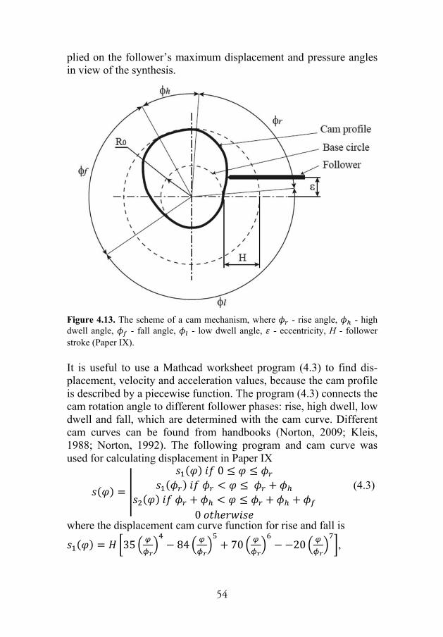
54

plied on the follower’s maximum displacement and pressure angles in view of the synthesis.

Figure 4.13. The scheme of a cam mechanism, where - rise angle, - high dwell angle, - fall angle, - low dwell angle, - eccentricity, H - follower stroke (Paper IX).

It is useful to use a Mathcad worksheet program (4.3) to find dis-placement, velocity and acceleration values, because the cam profile is described by a piecewise function. The program (4.3) connects the cam rotation angle to different follower phases: rise, high dwell, low dwell and fall, which are determined with the cam curve. Different cam curves can be found from handbooks (Norton, 2009; Kleis, 1988; Norton, 1992). The following program and cam curve was used for calculating displacement in Paper IX

(4.3)

where the displacement cam curve function for rise and fall is

,

55

.

A similar program was used to find follower velocity and accelera-tion (Paper IX).

According to Norton, 2009, the cam-follower mechanism’s pressure angle must be between - . The impact of the pressure angle value on the cam profile is determined with the function (2.13). In Paper IX, the following cam profile optimal pressure angle synthesis task was solved:

Find such values for and that guarantee the satisfaction of the restriction

(4.4)

in the rise, and restriction (4.5)

in the fall, when , (Paper IX).

Figure 4.14 shows pressure angle dependence on cam rotation angle before optimization and Figure 4.15 after optimization.

Figure 4.14. Cam mechanism’s pressure angle before optimization.

56

Figure 4.15. Cam mechanism’s pressure angle after optimization.

In the video clip Aan, 2013, the motion simulation of the optimal cam profile and follower is displayed. A frame of the video clip, where follower displacement, velocity and acceleration values can be also observed is shown in Figure 4.16.

Figure 4.16. A frame from the video clip (Aan, 2013).

The Cartesian coordinates of the cam profile were also given, and these can be used to manufacture the cam with a CNC mill (Paper IX).

The methods presented in Paper IX can be used for teaching and designing radial cams.

57

4.5 Study on the chaotic motion of a double pendulum

In Paper I, the author studied the physical double pendulum (Figure 3.2), which is composed of two links connected with pivots. It was assumed that the links are similar and that the only acting force is gravitation. The centre of masses ( ) and ( ) applied gravi-tation force , where is mass and gravitational acceleration are shown in Figure 3.2. The lengths of the links is and the inclina-tion angles are and The double pendulum is discussed in many mechanics books (Kenk & Kirs, 2013; Lepik & Roots, 1971; Butenin, et al., 1986).

Nonlinear differential equations in Hamilton form (2.9) and (2.10) were composed for the double pendulum. The double pendulum nonlinear differential equations were solved numerically with the IV order Runge-Kutta algorithm on a Mathcad worksheet (sections 2.5 and 3.2). A video clip Heinloo, 2010d was made, which shows that large oscillations of the double pendulum are chaotic. A frame from the video clip Heinloo, 2010d is shown in Figure 4.17.

Figure 4.17. A frame from the video clip (Heinloo, 2010d).

The methods presented in Paper I can be used for teaching and stud-ying similar mechanisms with chaotic motion.

4.6 Small oscillations of coupled pendulums

In Paper VII, it was demonstrated on a Mathcad worksheet how to compile equations on the motion of coupled pendulums (Figure 4.18) with the help of Lagrange’s equation of the second type (2.11). Additionally, pendulum motion equations were solved with symbol-ic calculations and the Laplace transform in case of small oscilla-tions.

58

Figure 4.18. Mathematical spring-coupled pendulums: - length between pendu-lums’ pivots, , - inclination angles of the pendulums (Paper VII).

The coupled pendulum has three types of oscillations: in phase, op-posite phase and beating phase (Picciarelli & Stella, 2010). With the obtained results, it is possible to show all three types of oscillations on a Mathcad worksheet, when the correct initial positons are deter-mined for the pendulums. A video clip was made on the motion simulation of coupled pendulums Aan & Heinloo, 2011 to visualise the results. A frame from the video clip is shown on Figure 4.19.

Figure 4.19. A frame from the video clip (Aan & Heinloo, 2011).

The method presented in Paper VII can be used for teaching and studying other oscillating mechanisms where symbolic calculations and the Laplace transform are used.

59

SUMMARY AND CONCLUSIONS

This doctoral thesis presents 11 publications and one patent, which are used to demonstrate how virtual models and their motion simula-tions can be created for the fields of engineering, analytical and ma-chinery mechanics, and used in teaching or studying problems. Cre-ating a virtual model of the object of study using a mathematical model and simulating its motion allows gaining better understanding of the problem at hand. This is especially important for people of the artistic type high neural activity, who need visualizing images of different objects in order to understand problems (Leppik, 2001; Leppik, 2008). The problem solutions found in the course of the work have been visualized as virtual models and motion simulations of the objects of study.

The following topics were discussed with regard to the development of learning methods:

1. On the creative teaching of engineering mechanics The doctoral thesis presents two articles on this topic. Article III explains how engineering and machinery mechanics could be taught creatively. The article gives examples of the solutions to problems in mechanics, which have been solved on a Mathcad worksheet and which were then used to produce video clips simu-lating the objects’ motion. Article II demonstrates how to use in-teractive examples when composing interactive revision notes for the subject Analytical Mechanics. The method can also be used for composing interactive revision notes for engineering mechan-ics and machinery mechanics.

Paper I explored the large oscillations of a double pendulum on a Mathcad worksheet as a more specific example of the interactive revision notes for analytical mechanics. The dependencies of the values of the angles determining the positions of the double pen-dulums on time were calculated by solving the Hamilton differen-tial equations’ system using the IV order Runge-Kutta method. A video clip was made of the motion simulation of the double pen-dulum’s virtual model, which demonstrates the pendulum’s cha-otic movement in detail.

60

2. Computer-based study of the V-engine and cam mechanism Article IV demonstrated how to make computer-based calcula-tions of the kinematics and dynamics of a V-engine and to create a virtual model and its motion simulation. The kinematics and dynamics of the model were discussed, whereas the determina-tion of the force acting on pistons was based on the indicator dia-gram of the four-stroke engine. The motion simulation of the en-gine’s virtual model was shown in a video clip.

Paper IX demonstrated the computer-based synthesis of an opti-mal radial cam. A program was devised on a Mathcad worksheet, which combines the equations for the follower’s rise and fall. Drawings were made to show the dependence of displacement, velocity, acceleration and pressure angle on the cam’s rotation angle. Optimal values for the base circle radius and the follower’s eccentricity were calculated in order to find the optimal profile for the cam. The paper provided Cartesian coordinates for an op-timal cam, which can be used for cutting the cam. The cam’s ro-tation and the motion of the follower’s virtual model were simu-lated in a respective video clip.

3. Tasks related to mass point motion This topic is discussed in three articles in the current doctoral the-sis. Article VI discussed mass point motion on a curved planar trajectory. The video clip simulated mass point motion on some curved trajectories, on which the normal acceleration, tangential acceleration, full acceleration and velocity were marked with ge-ometric vectors. The video clip shows the mass point’s given tra-jectory, vector directed from the location of the mass point at the centre of curvature, the circle of trajectory’s curvature at the point corresponding to the location of the mass point and evolute, which is formed by the centre of the circle of trajectory curvature.

4. Study of coupled pendulums using symbolic calculation and the Laplace transform Paper VII demonstrated how to derive differential equations for coupled pendulums in case of small oscillations and solve these using both the symbolic calculation function in Mathcad as well as the Laplace transform. The motion simulation of the coupled pendulum’s virtual model was shown in a video clip.

61

The following topics were discussed in relation to the development of research methods:

1. Study and visualization of the virtual models of some linkage mechanisms Article V compared the single connecting-rod slide-crank mecha-nism common in internal combustion engines and the double connecting-rod slide-crank mechanism, which has not been put to wider use. The piston displacements, velocities and accelerations were found for both mechanisms. The calculated values were compared in the same drawings. The sliders’ pressure angle and reaction forces a piston would apply on the cylinder wall were compared separately. Two comparative motion simulations were created for the mechanisms. The first simulation compared slider displacements and the other velocities, accelerations and pressure angles. The study revealed that both the values of the pressure angle and the reaction force for double connecting-rod slider-crank mechanism are smaller on average than those of a single connection-rod linkage mechanism. Article X discusses a mecha-nism consisting of 12 links, which moves similarly to a walking leg. It is presupposed that the motion of the observed mechanism takes place in a restricting environment. Changing drag force and inertia cause fluctuations in the speed of the input link. In order to decrease the fluctuation of this speed, the article shows how to find a flywheel for this kind of mechanism. A motion simulation was created for the mechanism.

2. Study of problems related to mass point motion and motion simulation In article VIII, a fertilizer granule was modelled as a mass point. The study explored the trajectories of a fertilizer granule on a spreading disc, time spent on the disc and the velocity of leaving the spreader with different values for the angles of the spreading disk’s vane, friction coefficient and the initial position of the fer-tilizer granule. The motion simulation of the fertilizer granule was shown in a video clip. Paper XI studied the motion of a sea buckthorn berry, modelled as a mass point, during the separation of berries from twigs on a conveyor belt and after it has left the belt. A mathematical model was created, which describes the mo-

62

tion of the berry on a conveyor belt and in the air after it has left the belt. The values for the berry’s displacement, velocity and general time in motion were calculated depending on the velocity of the conveyor belt, inclination angle and the friction coefficient between the berry and belt. A virtual model of the conveyor belt was created, which also depicted the berry. The motion of the berry on the conveyor belt at different inclination angles and after it has left the conveyor belt was illustrated in a video clip.

Conclusions

The methods and results presented in this thesis can be implemented in the teaching process of engineering subjects to visualize the solu-tions of mechanical problems and simulate the motion of composed virtual models on the screen of a computer.

The computer program Mathcad can be used as convenient tool for the composition of interactive lecture materials. It gives the possibil-ity of experimenting with lecture materials. Composing simulations by students makes studying engineering subjects interesting and attractive for them.

The computer program Mathcad can be used as a convenient tool for engineers for the calculation and simulation of the motion of studied objects to verify and visualize the obtained solutions.

63

REFERENCES

Aan, A. 2013. Cam-follower mechanism. Available at: http://youtu.be/c43JIq7-rvc (11.11.2014).

Aan, A. 2014a. Elliptical mechanism. Available at: http://youtu.be/1YnapCGOvQ4 (31.10.2014).

Aan, A. 2014b. Jansen linkage. Available at: https://www.youtube.com/watch?v=B_dR2_O3ujc (4 11 2014).

Aan, A. 2014c. Particle of the berry on inclined moving conveyor belt. Available at: http://youtu.be/g0Axk5gmwIk (10.11.2014).

Aan, A. & Heinloo, M. 2011. Oscillations of pendulums, coupled by a spring. Available at: http://youtu.be/Or9kAUY_gT8 (12.11.2014).

Aan, A. & Heinloo, M. 2012a. Comparison of piston displacements. Available at: http://youtu.be/LG2h8oiyjIU (4.11.2014).

Aan, A. & Heinloo, M. 2012b. Comparison of piston velocities accelerations and reactions. Available at: http://youtu.be/QvyZAo-Q3Rk (4 11 2014).

Artobolevski, I. 1961. Mehhanismide ja masinate teooria (in Estonian). Tallinn: Eesti Riiklik Kirjastus.

Bertjaev, B. D. 2005. Mathcad–based Training in Theoretical Mechanics (in russian). Sankt-Peterburg.

Broman, G. & Östholm, S. 1997. Mathcad in Teaching Rotor and. International journal of engineering education Structural Dynamics, 13(6), pp. 426-432.

Butenin, N., Lunts, J. & Merkin, D. 1983. Teoreetiline mehaanika: Staatika ja Kinemaatika. Tallinn: Valgus.

Butenin, N., Lunts, J. & Merkin, D. 1986. Teoreetiline mehaanika. Dünaamika. (in Estonian). Tallinn: Valgus.

Chonacky, N. 2006. Special thanks to CiSE’s peer reviewers. Computing in Science and Engineering, Volume 8(1), p. 14.

El Hassan, E. H., Fatiha, K., Abdelrhani, E. & Anouar, A. 2014. Teaching / Learning mechanics in high school with the help of Dynamic software. Procedia - Social and Behavioral Sciences, Volume 116, pp. 4617–4621.

64

Evert, A. Buckle- and Double-Connecting-Rod. Available at: http://www.evert.de/eft774e.htm (3.11.2014).

Gelbart, H., Brill, G. & Yarden, A. 2009. The impact of a web-based research simulation in bioinformatics on students’ understanding of genetics. Research in Science, Volume 39(5), pp. 725-751.

Goldstein, H., Poole, C. & Safko, J. 2000. Classical mechanics, third edition. Addison Wesley.

Haber, R. B. 1990. Visualization techniques for engineering mechanics. Computing Systems in Engineering, Volume 1(1), pp. 37-50.

Heinloo, M. 2007a. Automatic generation virtual models of fourbars for visualized e-courses of interactive engineering mechanics. Balkan Agricultural Engineering Review, Volume 10, p. 6.

Heinloo, M. 2007b. A Virtual Reality Technology–Based Method for the Study of the Working Process of a Blueberry Harvester's Picking Reel. Agricultural Engineering International: the CIGR Ejournal, Volume 9.

Heinloo, M. 2009. Manipulaator 2. Available at: http://youtu.be/MNTztcBsBoA (5.1.2015).

Heinloo, M. 2010a. Ketaslaoturi laotusketta virtuaalse tööprotsessi visualiseerimine (in Estonian). Agraarteadus, Volume 21(1), pp. 3-7.

Heinloo, M. 2010b. Mathcad algajaile. Available at: http://www.e-ope.ee/_download/euni_repository/file/623/MC%20Osa%202.xmcd?download=true (20.10.2014).

Heinloo, M. 2010c. Villete 4 vanes. Available at: http://youtu.be/bTxqdhjBOCU (5.1.2015).

Heinloo, M. 2010d. Physical double pendulum. Available at: http://youtu.be/BFIJTAzYdvo (11.11.2014).

Heinloo, M. 2011a. Manure skraper's manipulaator 1. Available at: https://www.youtube.com/watch?v=9TpXx2Xx3Rw (5.1.2015).

Heinloo, M. 2011b. Cinematics of a Point. Available at: http://youtu.be/zFbVcd4GOJw (31.10.2014).

Heinloo, M. 2011c. Four bar linkage. Available at: http://youtu.be/GgEra0JPoDU (5.1.2015).

65

Heinloo, M. 2012a. V-engine. Available at: https://www.youtube.com/watch?v=OyAiXVzfQkI (3.11.2015).

Heinloo, M., 2012b. Cinematics of a point 1. Available at: https://www.youtube.com/watch?v=2gPSalH9lxU&feature=youtu.be (7.11.2014).

Heinloo, M., 2013a. Motion the granules on fertilizer spreading disc 1. Available at: http://youtu.be/ZEh0Zv_gixQ (7.11.2014).

Heinloo, M., 2013b. Motion the granules on fertilizer spreading disc 2. Available at: http://youtu.be/8d9EYzzxw1s (7.11.2014).

Heinloo, M. 2014. Blueberry harvester picking reel. Available at: http://youtu.be/aRR80hbAlU0 (5.1.2015).

Heinloo, M. 2015. Disk ridging tool. Available at: http://youtu.be/bJqVqO0Ijzk (6.3.2015).

Heinloo, M. & Leola, T. 2006a. Virtual reality method supported synthesis of a plane manipulator. Proceedings 5th Int. DAAAM Conf. “Industrial Engineering – Adding Innovation Capacity of Labour Force and Entrepreneurs”, Tallinn.

Heinloo, M. & Leola, T. 2006b. Multiparametric Synthesis the Manipulator of the Scraper of the Press Manure Removal. Journal of Agricultural Science, Volume 17(2), pp. 88-95.

Heinloo, M. & Leola, T. 2007. Development of Virtual Reality Methods Based Analysis and Synthesis of Mechanisms. Proceedings 12-th World Congress in Mechanism and Machine Science, Besancon.

Heinloo, M., Leola, T. & Veinla, V. 2005. Synthesis of the Manipulator for the Scraper of a Press Manure Removal. Agricultural Engineering International: the CIGR Ejournal, Volume 7.

Heinloo, M. & Olt, J. 2004a. The Imagination of the Forced Driven Disk–ridging Tool and it’s Working Proccess in the Mathcad Environment. Proceedings 4th Int. DAAAM Conf. "Industrial Engineering – Innovation as Competitive Edge For SME”, Tallinn.

Heinloo, M. & Olt, J. 2004b. Animation of Motion of the Disk–ridging Tool. Proceedings Int. Conf. “Energy Efficiency and Agricultural Engineering". Rousse, pp. 137 – 135.

66

Heinloo, M. & Olt, J. 2004c. Animation of the Working Process of the Disk–ridging Tool. CD Papers Int. Conf. AgEng2004, Leuven.

Heinloo, M. & Olt, J. 2006. The Method of Virtual Reality for Creation a Disk–Ridging Tool. Agricultural Engineering International: the CIGR Ejournal, Volume 8.

Hess, H., Johnson, B. & Chapman, C. 2014. Synchronous machine winding layout & flux animation tool. Indianapolis.

Höffler, T. N. & Leutner, D. 2007. Instructional animation versus static pictures: A meta-analysis. Learning and Instruction, Volume 17, pp. 722-738.

Jansen, T. 2007. Theo Jansen: The Great Pretender. Rotterdam: 010 Publisher.

Jimoyiannis, A. & Komis, V. 2001. Computer simulations in physics teaching and learning: a case study on students' understanding of trajectory motion. Computers & Education, Volume 36(2), pp. 183-204.

Kenk, K. & Kirs, J. K. 2013. Mehaanika alused: Dünaamika Analüütiline mehaanika (in Estonian). Tallinn: TTÜ Press.

Kleis, I. 1988. Rakendusmehaanika (in Estonian). Tallinn: Valgus. Lepikson, H. 1998. V-kujulise neljataktilise sisepõlemismootori

kinemaatilise skeemi projekteerimine (in Estonian). Tallinn: TTÜ.

Lepik, Ü. & Roots, L. 1971. Teoreetiline mehaanika (In Estonian). Tallinn: Valgus.

Leppik, P. 2001. Tunni analüüsimine on huvitav. Tallinn. Leppik, P. 2008. Õpetajatöö psühholoogilisi probleeme. Tartu: Tartu

Ülikooli Kirjastus. Levin, M. & Ulm, S. 1966. Arvutusmeeetodite käsiraamat (in

Estonian). Tallinn: Valgus. Manapa, A. A., Sardanb, N. A. & Riasc, R. P. M. 2012. Interactive

Learning Application in Microbiology: The Design, Development and Usability. Procedia - Social and Behavioral Sciences, Volume 90, pp. 31 - 40.

Mekanizmalar, Available at: http://www.mekanizmalar.com (5.1.2015).

67

Melek, Y., Claudia, N. & Horst, B. 2008. The effects of instructional support and learner interests when learning using computer simulations. Computers & Education, Volume 51, pp. 1784-1794.

Molian, S. 1982. Mechanism Design: An Introductory Text. Cambridge University Press.

Norton, L. R. 1992. Design of machinery. McGraw-Hill. Norton, R. L. 2009. Cam design and manufac-turing handbook. New

York: Industrial Press Inc.. Novohatska, T., Grasmanis, B. & Vjaters, I. 2014. Theoretical

mechanics for students of engineering profile. Proceedings Engineering for rural development, pp. 485-490.

Ochkov, V. F. 2011a. Steam engine. Available at: http://communities.ptc.com/videos/2119 (8.10.2014).

Ochkov, V. F. 2011b. Windshield wipers. Available at: http://communities.ptc.com/videos/2060 (8.10.2014).

Ochkov, V. F. 2011c. Chebyshev's Foot Stepping Machine. Available at: http://communities.ptc.com/videos/2057 (8.10.2014).

Ochkov, V. F. 2011d. Walk Machine. Available at: http://communities.ptc.com/videos/2047 (8.10.2014).

Ochkov, V. F. 2013. MATHCAD. , Volume 2, pp. 27-33.

Olt, J. & Heinloo, M. 2011a. The Study of a New Manipulator for a Stone Protector of Stony Soil Tillage Implement. Journal of Agricultural Science and Technology, Volume 1(5B), pp. 751-755.

Olt, J. & Heinloo, M. 2011b. Visualization of motion of fertiliser granules on the planar of spinning spreading disc of a disc spreader. Proceedings XXXIV CIOCTA-CIGR, Vienna, pp. 292 - 296

Picciarelli, V. & Stella, R. 2010. Coupled pendulums: a physical system for laboratory investigations at upper secondary school. Physics Education, Volume 45(4), pp. 402-408.

Piskunov, N. 1981. Diferentsiaal- ja integraalarvutus 1. Tallinn: Valgus.

68

Preszler, R. W., Dawe, A., Shuster, C. B. & Shuster, M. 2007. Assessment of the Effects of Student Response Systems on Student Learning and Attitudes over a Broad Range of Biology Courses. CBE Life Sci Educ, Volume 6, pp. 29-41.

Recchi, M., Gagliardi, M., Grimellini, N. & Levrini, O. 2006. Different uses of ICT for modelling in Physics Education. Proceedings GIREP Conference 2006: Modeling in Physics and Physics Education, pp. 409-417.

Reintam, A. 1995. Mineraalväetiste ketaslaoturi laotusketta tööprotsessi uurimine matemaatilise modelleerimise teel (in Estonian). Agraarteadus, Volume 6(4), pp. 435–448.

Riess, W. & Mischo, C. 2010. Promoting systems thinking through biology lessons. International Journal of Science Education, Volume 32(6), pp. 705-725.

Ruina, A. & Pratap, R. 2014. Introduction to Statics and Dynamics. Oxford University Press.

Rutten, N., van Joolingen, W. R. & van der Veen, J. T. 2012. The learning effects of computer simulations in science education. Computers & Education, Volume 58(1), pp. 136-153.

Shigley, J., Mischke, C. & Brown, T. 2004. Standard handbook of machine design. McGraw-Hill.

Smith, S. What Are Interactive Learning Materials? Available at: http://www.ehow.com/info_7947754_interactive-learning-materials.html (30.10.2014).

Soutas-Little, R. W., Inman, D. J. & Balint, D. S. 2008. Engineering Mechanics: Dynamics - Computational Edition. Thomson.

Soutas-Little, R. W., Inman, D. J. & Balint, D. S. 2008. Engineering Mechanics: Statics-Computational Edition. Thomson.

Stern, L., Barnea, N. & Shauli, S. 2008. The effect of a computerized simulation on middle school students’ understanding of the kinetic molecular theory. Journal of Science Education and Technology, Volume 17(4), pp. 305-315.

Tamme, E. 1973. Arvutusmeetodid 2 (in Estonian). Tallinn: Valgus. Targ, S. 1968. Teoreetiline mehaanika (in Estonian). Tallinn:

Valgus.

69

Thornton, S. T. & Marion, J. B. 2007. Classical Dynamics of Particles and Systems, Fifth edition. Cengage Learning.

Zhang, M., Zhang, L. & Zhang, F. 2010. The analysis of link mechanism movement based on MathCAD. Proceedings - 2010 International Forum on Information Technology and Applications, Volume 1, pp. 281-287.

70

KOKKUVÕTE

Antud doktoritöös esitletakse 11 publikatsiooni ja ühte patenti, millede abil näidatakse, kuidas on võimalik virtuaalmudeleid ja nende liikumise simulatsioone luua inseneri- ja masinamehaanika ning analüütilise mehaanika valdkondadest, mida saab kasutada õpetamisel ja probleemide uurimisel. Luues uuritavast objektist matemaatilise mudeli abil virtuaalmudeli ja simuleerides selle liikumist on võimalik antud probleemist paremini aru saada. Eriti puudutab see inimesi, kes on kunstnikutüüpi kõrgema närvitegevusega ja vajavad arusaamiseks mitmesuguste objektide visualiseerivaid kujutisi (Leppik, 2001; Leppik, 2008). Antud töös leitud probleemide lahendid on visualiseeritud virtuaalmudelitena kui ka uuritud objektide liikumise simuleerimisega.

Õppemeetodite arendamise valdkonnast käsitleti järgnevaid teemasid:

1. Mehaanika loov õpetamine Selle teema kohta on doktoritöös esitletud kahte artiklit. Artiklis III selgitatakse, kuidas võiks loovalt õpetada inseneri- ja masinamehaanikat. Selles artiklis on toodud näiteid mehaanika probleemide lahenditest, mis on leitud Mathcadi töölehel ja milledele on koostatud objektide liikumist simuleerivad videoklipid. Artiklis II on näidatud, kuidas kasutada interaktiivseid näiteid õppeainele „Analüütiline mehaanika“ interaktiivse loengukonspekti koostamisel. Antud meetodit saaks ka kasutada insenerimehaanika ja masinamehaanika interaktiivse konspekti koostamiseks.

Analüütilise mehaanika interaktiivse konspekti täpsema näitena uuriti töös I kaksikpendli suuri võnkumisi Mathcadi töölehel. Hamiltoni diferentsiaalvõrrandite süsteemi lahendamisel Runge-Kutta IV järku meetodiga leiti kaksikpendlite asendeid määravate nurkade väärtuste sõltuvused ajast. Koostati kaksikpendli virtuaalmudeli liikumise simulatsiooni videoklipp, mis näitab ilmekalt selle pendli kaootilist liikumist.

71

2. V-kujuline mootori ja nukkmehhanismi arvutipõhine uurimine Artiklis IV näidati, kuidas arvutipõhiselt teha V-kujulise mootori kinemaatika ja dünaamika arvutusi, koos virtuaalmudeli koostamise ja selle liikumise simuleerimisega. Käsitleti mudeli kinemaatikat ja dünaamikat, kusjuures kolbidele mõjuva jõu määramisel lähtuti neljataktilise mootori indikaatordiagrammist. Koostati videoklipp simulatsiooniga mootori virtuaalmudeli liikumisest.

Töös IX näidati arvutipõhiselt optimaalse radiaalse nuki sünteesi tegemist. Selleks koostati Mathcadi töölehel programm, mis seob omavahel tõukuri eemaldumise ja naasmise võrrandid. Koostati siirde, kiiruse, kiirenduse ja survenurga sõltuvust nuki pöördenurgast näitavad joonised. Nuki optimaalse profiili saamiseks leiti optimaalsed väärtused algringjoone raadiusele ja tõukuri ekstsentrilisusele. Väljastati optimaalse profiiliga nuki koordinaadid, mida saab kasutada nuki väljalõikamisel. Nuki pöörlemist ja tõukuri virtuaalmudeli liikumist simuleeriti vastavas videoklipis

3. Punktmassi liikumisega seotud ülesanded Seda teemat käsitlevad doktoritöös kolm artiklit. Artiklis VI käsitleti punktmassi liikumist kõveral trajektooril. Videoklipis simuleeriti punktmassi liikumine mõnedel kõveratel trajektooridel, millel punktmassi normaalkiirendust, tangentsiaalkiirendust, täiskiirendust ja kiirust kujutati geomeetriliste vektoritega. Videoklipis on näha punktmassile etteantud trajektoor, punktmassi asukohast kõverustsentrisse suunatud vektor, punktmassi asukohale vastava trajektoori punkti kõverusringjoon ja evoluut, mida kujundab kõverusringjoone keskpunkt

4. Sümpaatiliste pendlite uurimine sümbolarvutuse ja Laplace teisendusega. Töös VII näidati kuidas tuletada diferentsiaalvõrrandeid sümpaatilistele pendlitele väikeste võnkumiste korral ja lahendada need nii programmi Mathcad sümbolarvutuse kui Laplace teisenduse abil. Koostati videoklipp sümpaatiliste pendlite virtuaalse mudeli liikumise simulatsiooniga.

72

Uurimismeetodite arendamise valdkonnast käsitleti järgnevaid teemasid:

1. Mõnede varbmehhanismide virtuaalmudelite uurimine ja visualiseerimine. Artiklis V võrreldi sisepõlemismootorites levinud ühe kepsuga väntmehhanismi ja kahe kepsuga väntmehhanismi, mis pole laialdast kasutust leidnud. Leiti kolvi siirded, kiirused ja kiirendused mõlemas mehhanismis. Leitud väärtusi võrreldi samadel joonistel. Eraldi võrreldi liugurite survenurka ja reaktsioonjõude, mida avaldaks kolb silindri pinnale. Koostati kaks võrdlevat mehhanismide liikumise simulatsiooni. Esimeses simulatsioonis võrreldi liugurite siirdeid ja teises simulatsioonis - kiirusi, kiirendusi ja survenurki. Leiti, et kahe kepsuga väntmehhanismi korral on nii survenurga kui ka reaktsioonjõu väärtus keskmiselt väiksem kui ühe kepsuga varbmehhanismis. Artiklis X käsitletakse 12 lülilist koostatud mehhanismi, mille liikumine on jala kõndimise liigutuse sarnane. Eeldatakse, et vaadeldava mehhanismi liikumine toimub liikumist takistavas keskkonnas. Muutuvad takistusjõud ja inertsijõud põhjustavad sisendlüli kiiruse kõikumist. Et vähendada selle kiiruse kõikumist näidatakse, kuidas leida sellisele mehhanismile hoorattast. Koostati simulatsioon mehhanismi liikumisest.

2. Punktmassi liikumisega seotud probleemide uurimine ja liikumiste simuleerimine. Artiklis VIII modelleeriti väetiseosakest punktmassina. Uuriti väetisosakese trajektoore jaotuskettal, sellel viibimise aega ja laoturilt lahkumise kiirust erinevate väetiselaoturi laba nurkade, hõõrdekoefitsiendi ja väetisosakese algpositsiooni korral. Koostati videoklipid simulatsioonidega väetiseosakese liikumisest. Töös XI uuriti punktmassina modelleeritud astelpaju marja liikumist, marjade okstest eraldamise konveieri lindil ja pärast sellelt lahkumist. Koostati matemaatiline mudel, mis kirjeldab marja liikumist konveierilindil ja õhus pärast selle eemaldumist lindilt. Leiti marja siire, kiirus, ja kogu liikumise aeg sõltuvalt konveierilindi liikumise kiirusest, kaldenurgast ja hõõrdetegurist marja ning lindi vahel. Koostati konveieri lindi virtuaalne mudel, millel on kujutatud mari. Koostati videoklipp, mis illustreerib marja liikumist konveieril erinevate kaldenurkade korral ja pärast konveierilt lahkumist.

73

Meetodid ja tulemused, mida antud töös näidati saab kasutada mehaanika ainete õpetamisel visualiseerimaks õpitava mehaanika ülesande objekti virtuaalse mudeli ja simuleerides tema liikumist arvuti ekraanil.

Arvuti programmi Mathcad saab kasutada hea abivahendina, et luua interaktiivseid õppematerjale, mis annavad võimaluse eksperimenteerida õppematerjalidega. Simulatsioonide loomise võimalus teeb õpilaste jaoks õppimise huvitavamaks.

Arvuti programmi Mathcad saab kasutada hea töövahendina, et teha inseneriarvutisi ja simulatsiooni. Simulatsioonid visualiseerivad saadud tulemusi aidates kontrollida lahenduse õigsust.

ACKNOWLEDGEMENTS

The thesis has been completed thanks to the Estonian University of Life Sciences, Institute of Technology. I would like to thank my supervisor

Professor Mati Heinloo for leading me and for being always ready to help me. Thanks to professor Jüri Olt for many advises during my studies. Special thanks to lecturer Eino Aarend for guiding me on the path of the mechanics. I would like to thank all my colleagues and friends, especially Mar-ten Madissoo, Tõnu Leemet, Valetina Prigoževa, Jaanus Allas, Peeter Nõmm, Villu Mikita, Aarne Küüt and Risto Ilves. Thanks to my mother Maimu, father Jaak, sister Terje and brother Teet for always supporting my studies. Last but not least, many thanks for the support, time and effort from my wife and child Janika and Eliis-Marii.

74ORIGINAL PUBLICATIONS

I

Aan, A., Aarend, E., Heinloo, M.On chaotic motion of a double pendulum Agronomy Research, 10(1), 5 – 12, 2011

76

77

78

10 0 10

10

10

10 0 10

10

10

79

80

81

82

10 0 10

10

10

10 0 10

10

10

10 0 10

10

10

10 0 10

10

10

10 0 10

10

10

10 0 10

10

10

10 0 10

10

10

10 0 10

10

10

10 0 10

10

10

10 0 10

10

10

10 0 10

10

10

10 0 10

10

10

83

84ORIGINAL PUBLICATIONS

II

Aan, A., Heinloo, M., Aarend, E.Interactive Computer Aided Learning and

Teaching of Analytical MechanicsInternational Journal of Engineering Pedagogy,

1(3), 4 – 8, 2011

86

PAPERINTERACTIVE COMPUTER AIDED LEARNING AND TEACHING OF ANALYTICAL MECHANICS

Interactive Computer Aided Learning and Teaching of Analytical Mechanics

http://dx.doi.org/ijep.v1i3.1788

A. Aan, M. Heinloo and E. AarendEstonian University of Life Sciences, Tartu, Estonia

Abstract—The aim of this paper is to introduce a new possi-bility for learning Analytical Mechanics via internet. This subject belongs to the field of engineering, the theoretical parts of lecture materials are available online in PDF format and have special links to switch on the interactive examples on the worksheets of the Computer Package Mathcad.

Index Terms—computer aided engineering, interactivity, attractiveness, internet, analytical mechanics, Computer Package Mathcad.

I. INTRODUCTION

The digital age has transformed education, both for-mally in the classroom and permanently in any other envi-ronment. Although there are many types of interactive materials that have been used in learning for decades, in most cases interactive learning materials are thought of as those that are done on a computer. Many of these materi-als are made available over the internet, although some are distributed in the form of software [1].

Interactive learning is most commonly defined into three distinct types. These learning types are grouped based on the types of interaction in which they engage students. The first, learner-content, is a type of teaching where the student interacts solely with the facts, readings and information. In the second style, learner-instructor, the primary interaction is with the instructor. The third style is called learner-learner, and this is where the student pri-marily interacts with his peers to learn new material [2, 3].

U.S. Department of Education report 2009 showed that the most effective interactive learning occurs when all three types of interaction are used [2].

Interactive learning is the counterpart of lecture-type learning. It is the active learning process as opposite to the passive system of a lecture-type. In interactive learning, the students use tangible objects to acquire information. Teachers do not directly pass the information to them. Students acquire the information themselves by allowing them to discover it. Of course, guidance by teachers is necessary. They still provide initial information to the students [4].

In interactive environment students are engaged with the materials rather than simply memorizing the informa-tion, the learning is deeper and more lasting. With more engagement student spent more time on the learning task [2]. In interactive learning materials student is in control of the progress of the lesson to some degree. This means in individual learning the learner can make his own pace and studying style of him. In many schools and universi-ties the teachers have lack of time and are unable to give dedicated attention to individual students for very long.

Interactive materials can help provide learning experience without the need for continuous teacher intervention [1].

Engineering teaching material has to be attractive and interactive to make students research technical problems. Attractive learning material means that it is visualized by using many schemes, figures, and animations. Students will understand learning materials better if they can ac-tively engage in the examples of problem-solving via computer screen and change relevant parameters, equa-tions, and simulate the motions. These are hands-on learn-ing materials on the computer. The students can approach to attain information through hands-on interactive experi-ence by using the computer.

There are articles available about interactive learning opportunities in other subjects. For example, Maxima Software – a tool for developing online applications in-tended for interactive solutions of the examples in Control Theory by K. Zakova [5]. The advantages of the Maxima software include its online availability via internet for all interested users any time, and it can be used locally on the desktop computer or in the notebook. For all technical universities devoted to electrical engineering can use Maxima for computations like useful instrument in an educational process mainly in online and distance forms of education [5]. Also in mathematics we can find interac-tive learning materials. Heinloo [6] and Talman [7] have made e-courses of mathematics that are interactive and visualized with figures and animations. Heinloo [6] used interactive Mathcad worksheets for lecture notes, exam-ples and exercises. Also there are the links to the video clips, which provide a student with an opportunity to watch and review the example problem solutions at home.

From internet we can find lot of interactive learning materials for different subjects [8, 9, 10].

This paper introduces interactive learning materials on Analytical Mechanics, composed in the Institute of Tech-nology of Estonian University of Life Sciences in Esto-nian language [11]. These interactive materials are mostly learner-instructor type, but on the computer and over the internet they are also considered learner-content learning material.

II. MATERIALS AND METHODS

Main text of interactive learning materials have been composed by the program Microsoft Word [12] and con-verted to PDF (Portable Document Format) [13] format. In PDF format all the linked citations work normally as defined. The figures have been composed by using pro-gram Adobe Illustrator [14] with occasional addition of pictures. Interactive examples have been composed on the worksheets of the Computer Package Mathcad. Main text

87

PAPERINTERACTIVE COMPUTER AIDED LEARNING AND TEACHING OF ANALYTICAL MECHANICS

in PDF and Mathcad files are connected with links and are available in Estonian e-Learning Development Centre repository [15].

III. ON VISUALIZATION OF LEARNING MATERIAL

Colorful and, where possible, lifelike figures are used to make the material more attractive for students (Fig. 1). Some of examples in the learning materials are visualized by video clips, for example [16].

IV. INTERACTIVE LEARNING MATERIAL

If the learning materials are on the computer, student can use program features like search, zoom, copy, etc. that accentuate their interactivity.

In terms of collaboration with other computer program features, it is possible to make learning material more interactive by using inside the text links to citations or equation numbers. This gives an opportunity to move inside the text and switch between linked parts on differ-ent pages.

Fig. 2 shows a part of the contents of learning material [18] where clicking on the word “Näide 2.6” leads to the page with the solution of the example 2.6

Figure 1. Comparison of traditional (a) [17] and lifelike (b) [18] screw jack calculation figure

In Fig. 3 we can see an example (Näide 2.6), where mass A is connected with cylinder B over wheel O by rope. Cylinder B is moving down and pulling mass A downwards. At the same time cylinder B is spinning off the rope. The question is - what is the acceleration of point C.

In the problem solution (Fig. 4) we can see that one of the equations that has been used is Lagrange equations (Lagrange`i võrrandid) and in the main text it is equation 2.40. Clicking on equation number leads to the explana-tion (Fig. 5) of the Lagrange equations (Lagrange võrran-did) in the main text.

Figure 2. Links in the contents

Figure 3. The mechanical system in the example

Figure 4. A part of solution of the example problem

88

PAPERINTERACTIVE COMPUTER AIDED LEARNING AND TEACHING OF ANALYTICAL MECHANICS

If a student wishes to learn more about Lagrange equa-tions, he or she will be directed to corresponding literature by clicking on the citation (Fig. 6).

If the literature is available on the internet, the student can continue from there by using relevant internet ad-dresses. The name of the book can be connected with links to library internet catalog. In Estonia there is library e-catalog Ester that shows the quantity and availability of books in library [19].

Let us consider an interactive example about physical pendulum on Mathcad [20] worksheet to which leads a special link in the main text (Fig. 7).

Figure 5. A part in main text with Lagrange equations

Figure 6. Literature from main text

Figure 7. A physical pendulum in the example

Fig. 8 shows the first possible derivation of the equa-tions of motion of physical pendulum in the main text.

Fig. 9 shows the second possible derivation of the equa-tions of motion of physical pendulum, and the link leading to the interactive example on the worksheet of Mathcad.

On Mathcad worksheet a learner can visualize the mo-tion of pendulum by graphs (Fig. 10). A learner can also change the values of inclination angle and angular ve-locity ’ at the initial moment t = 0 and observe what happens on figures.

On the worksheet of Mathcad a learner can use controls like slider to define the parameters of pendulum. Fig. 11 shows the slider, defining the length of the pendulum.

Figure 8. Derivation of equation of motion for a physical pendulum

Figure 9. Link to Mathcad interactive example [21]

Figure 10. Pendulum angle (upper) and angular velocity (lower) change

89

PAPERINTERACTIVE COMPUTER AIDED LEARNING AND TEACHING OF ANALYTICAL MECHANICS

Frames in Fig. 12 from [22] visualize the motion of a double pendulum determined by their equations of mo-tion.

[5] K. Zakova, Maxima – An Open Alternative for Engineering Education. International Journal of Engineering Pedagogy (iJEP), North America, 1, apr. 2011. Available at: http://online-journals.org/index.php/i-jep/article/view/1598. Date accessed: 14.06. 2011. It is possible to hide equations and arguments on the

worksheet of Mathcad. This gives a possibility to provide interactive sheets with controls only. In Fig. 13 there are the sliders to change the pendulum’s mass and length. To change the initial angles of the pendulums we can use radio buttons on the worksheet of Mathcad (Fig. 13) and then visualize the motion of a double pendulum on the figure.

[6] M. Heinloo, T. Tärgla, Visuaalne e-matemaatika (in estonian), Available at: http://deepthought.ttu.ee/aa/artiklid/497.pdf. Date accessed: 15.06.2011.

[7] L. A. Talman, Mathematics animated, Available at: http://clem.mscd.edu/~talmanl/MathAnim.html, Date accessed: 15.06.2011.

[8] Teacher Tap, Available at: http://eduscapes.com/tap/index.htm,Date accessed: 20.06.2011.

[9] Active Math http://demo.activemath.org/ActiveMath2/main/menu.cmd, Date accessed: 20.06.2011. V. CONCLUSION

This paper presented opportunities to make learning materials more attractive and interactive using examples from subject analytical mechanics in Estonian University of Life Sciences.

[10] Füüsika koolitarkus, Available at: http://www.fyysika.ee/opik/index.php?tase=sisu&pid=17&nom=0, Date accessed: 20.06.2011.

[11] Estonian University of Life Sciences, Available at: http://www.emu.ee/en/, Date accessed: 20.06.2011.

[12] Microsoft Office, Word, http://office.microsoft.com/en-gb/word/,Date accessed: 09.05.2011.

The learning material has been made attractive and in-teractive by using different computer programs and inter-net. [13] Adobe PDF,

http://www.adobe.com/products/acrobat/adobepdf.html, Date ac-cessed: 10.06.2011. VI. REFERENCES [14] Adobe Illustrator, http://www.adobe.com/products/illustrator.html,Date accessed: 10.06.2011. [1] S. Smith, What are interactive learning materials? Available at:

http://www.ehow.com/info_7947754_interactive-learning-materials.html

[15] Estonian e-Learning Development Centre, Repository, Available at: http://www.e-ope.ee/repositoorium/otsing?@=6tsk#euni_repository_10895, Date accessed: 09.06.2011. [2] L. Brogan, Interactive Learning Definition, Available at:

http://www.ehow.com/about_5494900_interactive-learning-definition.html, Date accessed: 20.06.2011.

[16] Double pendulum, Available at: http://www.youtube.com/user/TheoreticalMechanics#p/a/u/1/6BHYuJwPw8I, Date accessed: 09.08.2011. [3] A. Stovall, Definition of Interactive Learning Content, Available

at: http://www.ehow.com/about_6727386_definition-interactive-learning-content.html, Date accessed: 20.06.2011.

[17] Ü. Lepik, L. Roots, Teoreetiline mehaanika (in Estonian). Tallinn: Valgus, 1971.

[4] K. Chapman, What is Interactive Learning, Available at: http://www.howtodothings.com/education/what-is-interactive-learning, Date accessed: 15.06.2011.

[18] A. Aan, M. Heinloo, E. Aarend, Interactive analytical mechanics, Available at: http://www.e-ope.ee/_download/euni_repository/file/1592/Anal%C3%BC%C3%BCtilise%20mehaanika%20konspekt.pdf, Date accessed: 07.06.2011.

Figure 11. A Slider on the worksheet of Mathcad, defining a pendulum length

Figure 12. Frames from animated pendulum move Figure 13. Slider and radio button controlled double pendulum [23]

90

PAPERINTERACTIVE COMPUTER AIDED LEARNING AND TEACHING OF ANALYTICAL MECHANICS

[19] E-catalog for Tartu libraries, Available at: http://tartu.ester.ee/search, Date accessed: 10.06.2011.

[20] PTC Mathcad, Available at: http://www.ptc.com/products/mathcad/index-v2.htm, Date accessed: 10.06.2011.

[21] A. Aan, M. Heinloo, Näide 4.1, Available at: http://www.e-ope.ee/_download/euni_repository/file/1592/N%C3%A4ide%204.1.xmcd?download=true, Date accessed: 10.06.2011.

[22] A. Aan, Pendulum, Available at: http://www.youtube.com/watch?v=Ag2MU5tMXj4, Date accessed: 11.06.2011.

[23] A. Aan, M. Heinloo, Double Pendulum, Available at: http://www.e-ope.ee/_download/euni_repository/file/1592/Double%20pendulum.xmcd?download=trueAuthors, Date accessed: 22.06.2011.

AUTHORS

A. Aan is with the Institute of Technology, Estonian University of Life Sciences, Kreutzwaldi 64, 51014, Tartu, Estonia (e-mail: aare.aan@emu.ee).

M. Heinloo is with the Institute of Technology, Esto-nian University of Life Sciences, Kreutzwaldi 64, 51014, Tartu, Estonia (e-mail: mati.heinloo@emu.ee).

E. Aarend is with the Institute of Technology, Estonian University of Life Sciences, Kreutzwaldi 64, 51014, Tartu, Estonia (e-mail: dmmd@emu.ee).

Received 31 August 2011. Published as resubmitted by the authors 26 September 2011.

91

92ORIGINAL PUBLICATIONS

III

Aan, A., Heinloo, M.On creative teaching of engineering mechanics

Annals of DAAAM for 2011 and Proceedings, 1081 – 1082, 2011

94

95

96ORIGINAL PUBLICATIONS

IV

Aan, A., Heinloo, M., Aarend, E., Mikita, V.Analysis of four-stroke cycle internal combustion

V-engine in Mathcad environmentProceedings of 8th International Conference of

DAAAM Baltic Industrial Engineering, 389 – 394, 2012

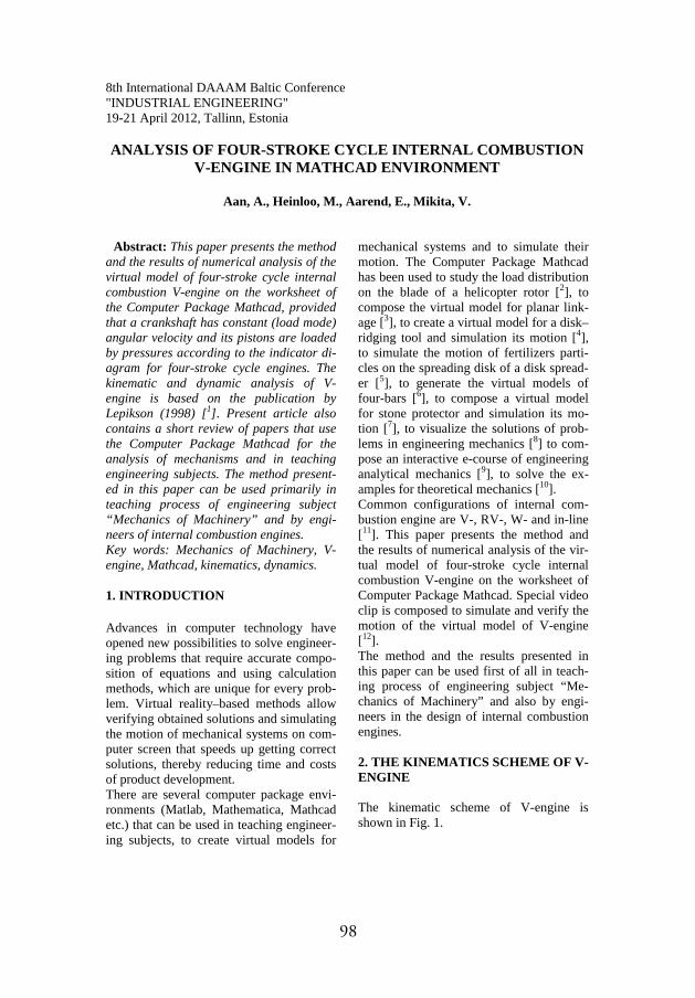
98

8th International DAAAM Baltic Conference"INDUSTRIAL ENGINEERING"19-21 April 2012, Tallinn, Estonia

ANALYSIS OF FOUR-STROKE CYCLE INTERNAL COMBUSTION V-ENGINE IN MATHCAD ENVIRONMENT

Aan, A., Heinloo, M., Aarend, E., Mikita, V.

Abstract: This paper presents the method and the results of numerical analysis of the virtual model of four-stroke cycle internal combustion V-engine on the worksheet of the Computer Package Mathcad, providedthat a crankshaft has constant (load mode) angular velocity and its pistons are loaded by pressures according to the indicator di-agram for four-stroke cycle engines. The kinematic and dynamic analysis of V-engine is based on the publication by Lepikson (1998) [1]. Present article also contains a short review of papers that use the Computer Package Mathcad for the analysis of mechanisms and in teaching engineering subjects. The method present-ed in this paper can be used primarily in teaching process of engineering subject “Mechanics of Machinery” and by engi-neers of internal combustion engines.Key words: Mechanics of Machinery, V-engine, Mathcad, kinematics, dynamics.

1. INTRODUCTION

Advances in computer technology haveopened new possibilities to solve engineer-ing problems that require accurate compo-sition of equations and using calculation methods, which are unique for every prob-lem. Virtual reality–based methods allowverifying obtained solutions and simulatingthe motion of mechanical systems on com-puter screen that speeds up getting correctsolutions, thereby reducing time and costs of product development.There are several computer package envi-ronments (Matlab, Mathematica, Mathcad etc.) that can be used in teaching engineer-ing subjects, to create virtual models for

mechanical systems and to simulate their motion. The Computer Package Mathcad has been used to study the load distributionon the blade of a helicopter rotor [2], to compose the virtual model for planar link-age [3], to create a virtual model for a disk–ridging tool and simulation its motion [4], to simulate the motion of fertilizers parti-cles on the spreading disk of a disk spread-er [5], to generate the virtual models of four-bars [6], to compose a virtual model for stone protector and simulation its mo-tion [7], to visualize the solutions of prob-lems in engineering mechanics [8] to com-pose an interactive e-course of engineering analytical mechanics [9], to solve the ex-amples for theoretical mechanics [10].Common configurations of internal com-bustion engine are V-, RV-, W- and in-line [11]. This paper presents the method and the results of numerical analysis of the vir-tual model of four-stroke cycle internal combustion V-engine on the worksheet of Computer Package Mathcad. Special video clip is composed to simulate and verify the motion of the virtual model of V-engine[12].The method and the results presented in this paper can be used first of all in teach-ing process of engineering subject “Me-chanics of Machinery” and also by engi-neers in the design of internal combustion engines.

2. THE KINEMATICS SCHEME OF V-ENGINE

The kinematic scheme of V-engine is shown in Fig. 1.

99

Fig. 1 The kinematic scheme of V-engine

Crankshaft 1 shown in Fig. 1 is supposed to rotate counter clockwise with angular velocity This crankshaft is joined by pivot B to the main connecting rod 2 which moves main piston 3 along track AC in the main cylinder. This connecting rod is alsojoined by pivot D to the secondary con-necting rod 4 that is joined by pivot E to the secondary piston 5 and moves it along the track AE in the secondary cylinder. Constructive angle between tracks AC, AE and the arms BD, BC of main connect-ing rod 2 is permanent.The following V-engine parameters wereused in the calculations: lengths of the links lAB=0.090m, lBC=0.322m,lBD=0.085m lDE=0.240m; constructive an-gle =60o; inside diameters for cylinders ds=0.15m; crankshaft rotation speed nm=1000rpm; masses of links: m1=13.7kg,m2=6.25kg, m3=3.6kg, m4=2kg andm5=3.6kg. Moments of inertia of links 2 and 4: = 0.174 ,= 0.083 .Maximum pressure inside the cylinders: pmax=4MPa.

3. DETERMINATION OF THE POSI-TIONS OF LINKS

Let us suppose that the origin of the co-ordinate system Axy is in pivot A (Fig. 1). The x-axis coincides with track AC. The rotation angle of crank AB is . Co-ordinates of pivots B and C are

= cos= sin , (1)= + , (2)= 0.Co-ordinates of pivot D can be determined from the following system of equations of restrictions( ) ( ) ( ) == cos( ) + ( ) = . (3)

The first equation in (3) means that during the motion the angle between arms BD and BC is permanent. The second equation in (3) means that during the motion the dis-tance between pivots B and D is perma-nent. Co-ordinates of pivot E can be de-termined from the following system of equations of restrictions= tan( ) + ( ) = . (4)

The first equation in (4) means that during the motion pivot E is permanently on track AE. The second equation in (4) means that during the motion the distance between the pivots D and E is permanent. Equations (1), (2) and systems of equations (3), (4) were solved in relation to the values of ro-tation angle of crank AB by using the solve block “Given-Find” of Mathcad. The virtual model in Fig. 2 was composed on Mathcad worksheet by using the results of computations of pivots co-ordinates.

Fig. 2. The virtual model of V-engine

Before composing the video clip with sim-ulation of motion of the composed virtual model in Fig. 2, rotation transformation

100

was used to turn it to the position (Fig. 3) of the kinematic scheme in Fig. 1.

Fig. 3. Virtual model of V-engine, in the position of the scheme in Fig. 1

On the basis of Fig. 3 a video clip [12] sim-ulating the motion of virtual model of V-engine was composed on Mathcad work-sheet.

Maximum values of displacements (S) of pivots C (piston 3) and E (piston 5) can be determined by equations= max ,= max + + .The results of computations are visualizedin Fig. 4.

Fig. 4. Maximum values of displacements of the pivots C (main piston 3) and E (sec-ondary piston 5) depending on the values of rotation angle of crank (Fig. 1)

Experimentally acquired p-V indicator dia-gram was used to create a diagram where volume (V) values are converted in dis-placement values in Fig. 5.Fig. 4 was used to compose four strokes (intake, compression, power, exhaust) in V-engine by the pistons 3 and 5, when the

pressures applied to the pistons change ac-cording to the indicator diagram in Fig. 5.

Fig. 5. The indicator diagram for the four-stroke cycle internal combustion engine, where p is the pressure applied to a piston and S is piston displacement

4. DETERMINATION OF THE VE-LOCITIES OF PIVOTS

The velocity projections of pivot B on the x- and y-axis can be obtained by differenti-ation of formulas (1)= , = ,where= cos , = sin , = .The velocity projection of pivot C (main piston 3, Fig. 6) on x-axis can be found out from formula = , (5)derived from the formula (2) by time-based differentiation. The results of computations are visualized in Fig. 6.

Fig. 6. Pivot C velocity projection vCx(main piston 3) depending on rotation an-gle

101

By differentiating the equations (3) and (4) in terms of time one can obtain two linear systems of equations for determining the projections = , = ,= , = ,of the velocity pivots D and E. Composed linear systems of equations were solved on Mathcad worksheet by using inverse ma-trix method known from linear algebra. The results of computations are visualizedin Fig. 7.

Fig. 7 Pivot E (secondary piston) velocity projections , depending on rotation angle

5. DETERMINATION OF THE AC-CELERATIONS OF PIVOTS

Time-based differentiation of equations (5) gives the following formula to determine the acceleration projection of pivot C (main piston) =( ) ( )( ) .

The results of computations are visualizedin Fig. 8.

Fig. 8 Pivot C (main piston) acceleration projection aCx depending on rotation angle

When using time-based differentiation of equations (3) and (4) twice one can obtain

two linear equations systems for determin-ing the projections= , = ,= , = ,where aEx, aEy are secondary piston accel-eration projections and aDx, aDy – the accel-erations of the main piston. The results of computations are visualized in Fig. 9.

Fig. 9 Pivot E (secondary piston) accelera-tion projections and depending on rotational angle

According to [1] links 2 and 4 centres of masses accelerations projections ,and , in points , and ,respectively were determined by the fol-lowing formulas= + ( ),= (1 ) ,= , = ,where =0.27.

6. DETERMINATION OF THE AN-GULAR VELOCITIES AND THE AC-CELERATIONS OF LINKS 2 AND 4

Let us consider the following equations:= cos , (6)= cos , (7)= sin , (8)= sin , (9)where 4 and 2 are the angles between x-axis and connecting links ED (4) and BC (2) accordingly, measured form x-axis counter clockwise. After time-based differ-entiation of the equations (6) and (9) we have = sin , (10)= cos , (11)

102

where = , = ,= , = 0,are the projections of the velocities of piv-ots E, D, B, C, already computed above. Substitution of (8) into (10) and (7) into (11) gives = ( ), (12)= ( ). (13)From (12) and (13) we can find the follow-ing formulas = , = , (14)that determine the angular velocities of links ED (4) and BC (2) in the case wherethe positions of pivots and their velocities are known. The results of computations of angular velocities are visualized in Fig 10.

Fig. 10 The dependence of angular veloci-ties , on rotation angle

Time-based differentiation of equations (14) gives the following formulas for de-termination of angular accelerations of links BC (2) and ED (4). = ( ) ( )( ) , (15)= ( ) ( ) ( ) ( )( ) .The results of computations of angular ac-celerations are visualized in Fig. 11.

Fig. 11 The dependence of angular veloci-ties , on rotation angle

7. DETERMINATION OF REACTION FORCES

Forces applied to the main piston E (3) and the secondary piston E (5) can be find out by using equations= , = .It is supposed that combustion gas pres-sures are the following max max 4 .It is assumed that the pressures pC and pE,applied to the pistons C (3) and E (5) fol-low the indicator diagram in Fig. 5. Before calculating the reaction forces it is necessary to determine the dependence of pressures pC and pE on rotation angle of the crank AB. Found dependencies are vis-ualized in Figs. 12 and 13.

Fig. 12 Displacement SC of piston C (3) and the pressure pC in cylinder depending on rotation angle

Fig. 13 Displacement SE of piston C (3) and the pressure pE in cylinder dependingon rotation angle

To determine the dynamic reaction forces in pivots and between cylinder walls and pistons, the system of equations on motion for all links was composed according to [13]. Since all accelerations and angular ac-celerations are determined above, the equa-tions on the motion of links are linear in respect of forces of reaction. The results of computations of reaction forces modules are visualized in Fig. 14.

103

Fig. 14 Reaction forces modules in pivots

8. CONCLUSIONS

1. The Computer Package Mathcad can be considered as a convenient tool for com-plex analysis of engines.2. The Computer Package allows the simu-lation of motion of virtual models of en-gines. 3. The method presented in this paper can be used in the teaching process of engi-neering subject “Mechanics of Machinery” and also by engineers of internal combus-tion engines. This method can also be fur-ther developed for more complex and accu-rate analysis.

9. REFERENCES

1. Lepikson, H. Design of kinematic scheme for four-stroke internal combustion V-engine (in Estonian). Tallinn, 1998, 76 p.2. Butoescu, V. A vortex model of a heli-copter rotor. INCAS, 2009, 1, 23-27.3. Heinloo, M., Aarend, E., Mägi, M. On The Experience of Mathcad-Aided Analy-sis of Planar Linkages. Proc. Tenth World Congress on the Theory of Machines and Mechanisms. 1999, 1, 392 – 397.4. Heinloo, M., Olt J. A Method of Virtual Reality for Creating a Disk-Ridging Tool. CIGR Ejournal. 2006, 8, 21. Available at: http://www.cigrjournal.org/ index.php/ Ejounral/article/view/624/618 (05.02.2012.5. Heinloo, M. Visualization of the work-ing process of a spreading disk of a disk spreader. Journal of agricultural science.2010, 21, 3-7. Available at: http://agrt.emu.ee/pdf/20101/heinloo.pdf (01.02.12).

6. Heinloo, M. Automatic Generation Vir-tual Models of Fourbars for Visualized e-Courses of Interactive Engineering Me-chanics. Balkan Agricultural Engineering Review. 2007, 10.7. Olt, J; Heinloo, M. Visualization of the Working Process of a Novel Manipulator for a Stone Protector of a Stony Soil Till-age Implement. Balkan Agricultural Engi-neering Review. 2010, 15.8. Aan, A., Heinloo, M. On creative teach-ing of engineering mechanics. Proc. 22ndInternational DAAAM World Symposium.2011, 1081–1082.9. Aan, A, Heinloo, M, Aarend, E. Interac-tive Computer Aided Learning and Teach-ing of Analytical Mechanics. Int. J. Eng. Pedagogy (iJEP). 2011, 1, 4-8.10. Bertjaev, B. D. Mathcad–based Train-ing in Theoretical Mechanics (in Russian). Sankt-Peterburg, 2005, 738 p.11. Pulkrabek, W. W. Engineering funda-mentals of the internal combustion engine.Prentice Hall, 1997, 411 p.12. Aan, A., Heinloo, M. Simulation of motion a virtual model of v-engine. Avail-able at: http://www.youtube.com/watch?v=OyAiXVzfQkI(01.02.12).

13. Frolov et al. Theory of mechanism and machines (in Russian). Moscow, 1987, 496 p.

10. ADDITIONAL DATA ABOUT AU-THORS

MSc (Engn Sc) Aan, Aare (author)e-mail: aare.aan@emu.ee.

Dr (math) Heinloo, Mati (co-author)e-mail: mati.heinloo@emu.ee.

MSc (Engn Sc) Aarend,Eino (co-author).

PhD (Engn) Mikita, Villu (co-author)e-mail: villu.mikita@emu.ee

Institute of Technology,Estonian University of Life Sciences,Kreutzwaldi 56, 51014, Tartu, Estonia

104ORIGINAL PUBLICATIONS

V

Aan, A., Heinloo, M.Computer based comparison analysis of single and

double-connecting-rod slider-crank linkagesAgronomy Research, 10, 3 – 10, 2012

106

Computer based comparison analysis of single and double–connecting–rod slider–crank linkages

A. Aan and M. Heinloo

Institute of Technology, Estonian University of Life Sciences, Kreutzwaldi 56, EE51014 Tartu, Estonia; e-mail: aare.aan@emu.ee

Abstract. This paper presents the results of comparative numerical analysis of single and double–connecting–rod slider–crank linkages on the worksheet of Computer Package Mathcad. On the base of composed virtual models of both linkages the motion of the slider (piston) in these linkages is studied thoroughly. This paper has the links to the video clips, comparing the motions of single and double–connecting–rod slider–crank linkages and visualizing the change of vectors of velocities and accelerations in the pivot, where connects two links of double connecting rod. Concluded, that the motion of the slider (piston) and the force of reaction to the track of slider (wall of a cylinder) in these linkages is quite different.

Key words: machine and mechanism theory, linkages, internal combustion engines.

Introduction

Slider–crank linkages can be used in pumps, compressors, internal combustion engines etc. A typical scheme of one cylinder of a four-stroke internal-combustion engine with single connecting rod crank-slider linkage is shown in Fig. 1 (Merriam-Webster, 2006).

Fig. 1. Cross section showing one cylinder of a four-stroke internal-combustion engine.

Agronomy Research Biosystem Engineering Special Issue 1, 3-10, 2012

107

A review of different internal combustion engines using single–connecting–rod crank–slider mechanism with multiple cylinders is given in Automotive Handbook (1996).

Mederer (Evert, 2003) proposed to use a double–connecting–rod linkage (Fig. 2) in combustion engines.

Fig. 2. The scheme of a double–connecting–rod linkage, proposed by Mederer to use in internal combustion engines.

Double–connecting–rod linkage (Fig. 2) consists of ground (cylinder), crank (on crankshaft), two part connecting rod, slider (piston) and a swivel arm. By Mederer this mechanism reduces consumption of fuel and lower emissions, because piston will stay relative long times at area of its uppermost position, and in the compression stroke large parts of counter-pressure is taken by swivel arm, that means less input power is needed for turning a crank in the compression stroke.

The aim of this paper is to present the method and results of comparative numerical analysis of single–connecting–rod and double–connecting–rod slider–crank linkages on the worksheet of Computer Package Mathcad, in the case of constant (idle) crank (crankshaft) angular velocity. On the base of composed virtual models of both linkages the motion of the slider (piston) in these linkages will be studied thoroughly. This paper will have also links to two composed video clips. First video clip compares the motions of single–connecting–rod and double–connecting–rod slider–crank linkages with the same maximum displacement of the slider (piston). Second video clip visualizes the changing geometrical vectors of velocities and accelerations in the pivot, where connects two links of double-connecting-rod slider–crank linkage. This video clip compares also the reaction force in the track of sliders (cylinder wall).

Composition of virtual models of linkages

The links OA, AE, and EC of the four-bar OAEC in the structure of double–connecting–rod linkage can rotate around pivots O, A, E and C, whereby pivots O and C are grounded (Fig. 3). For numerical computations let us assume that the lengths of

108

the links OA, AE and EC are lOA = 0.3 m, lAE = 0.7 m, lEC = 0.735 m accordingly and the coordinates of the pivot C are xC = 0.67 m, yC = 0.7 m. Let us suppose also that the rotational speed of crank OA is n = 700 rpm, that means angular velocity

= 73.304 rad s-1.The coordinates of pivot A (Fig. 3) can be found out by equations

, .

The four-bar OAEC has constraints that the distances between pivots A, E and E, C are permanent. Mathematically these constrains means the following system of nonlinear equations of constraints

(1)

where is the angle of rotation of the crank OA from y-axis clockwise. The system of equations (1) was solved on the worksheet of Mathcad numerically

relative to xE and yE (Fig. 3).

Fig. 3. The virtual model of four-bar OAEC under crank’s rotation angle =30 .

Let us compose the following column vectors

, .

Fig. 3 shows the virtual model of linkage OAEC, drawn by these vectors on the worksheet of Mathcad.

Connecting to the pivot E of four-bar in Fig. 3 by a link ED to the pivot pivot D, what is moving along y-axis, we get a virtual model of double-connecting-rod linkage on Figs 2 and 4. Let the length of the link ED be lED = 0.7 m. The y-coordinate of pivot D can be find out from the following equation of restriction

109

. (2) The following vectors

,

,

draw on the worksheet of Mathcad the virtual model of double–connecting–rod crank–slider linkage in Fig. 4a.

To compose the virtual model for typical single–connecting–rod crank-slider linkage in Fig. 4b, we used the following equation of constraint

, (3)

where is the permanent length of the link AD in Fig. 4b. In computations were taken m. Equation (3) determine the coordinate of the pivot D by the following formula

.

The following vectors

,

,

,

draw on the worksheet of Mathcad the virtual model of single–connecting–rod crank–slider linkage in Fig. 4b.

(a) (b)

Fig. 4. The virtual models of double–connecting–rod (a) and single–connecting–rod (b) crank–slider linkages under crank’s rotation angle = 30 .

110

Comparison of displacement, velocity and acceleration of a slider (piston)

To compare of displacement, velocity and acceleration, let´s give for rotation angle the values from 0 with step 0.1 up to . This means that the crank OA in Fig. 4 makes two rotations.

According to used assumption, in Fig. 5 at the bottom dead centre (BDC) and the top dead centre (TDC) the pivot D (slider) virtual model displacements for both cases (Fig. 4a and Fig. 4b) are coincidence, but between BDC and TDC displacements are different.

Fig. 5. The Displacement of pivot D (slider) for double–connecting–rod and single–connecting–rod crank–slider linkages dependence from rotational angle

The velocity projections of pivot’s D (Fig. 4) are

, .

Fig. 6 shows the change of projections of the velocity of the pivot D (Fig. 4) for both virtual models. One can conclude in range of TDC these projections are coincident for both virtual models, but in BTC are not.

Fig. 6. The velocity of pivot D (slider) for double–connecting–rod and single–connecting–rod crank–slider linkages dependence from rotational angle

111

The accelerations projections of pivot’s D (Fig. 4) are

, .

One can conclude from Fig. 7 shows that the projections of accelerations of the pivot D for both virtual models are quite different.

Fig. 7. The accelerations of pivot D (slider) for double–connecting–rod and single–connecting–rod crank–slider linkages dependence from rotational angle

Comparison of angles between the link, connected to the pivot of the slider (piston) and the track of motion

Angles between y-axis (pivot D track) and the links on single connecting rod AD and double connecting rod ED (pressure angle (Kleis, 1988), can be found out from the equations

, .

Fig. 8 shows that the pressure angle for double–connecting–rod linkage is lower than the correspondent angle for single–connecting–rod linkage.

Fig. 8. The pressure angle between the links ED and AD (Fig. 4) relative to the y-axis (track of pivot D) for double–connecting–rod and single–connecting–rod crank–slider linkages dependence from rotational angle

112

Comparison of the reaction force from the track of slider (the wall of cylinder)

Let´s apply force FD = 1000 N to the slider pivot (piston) and take the mass of slider (piston) equal to mk = 3 kg. The equations of motion of the slider (piston) are

, , (4)

where – is the reaction force, applied from link ED in Fig. 4 (a) to the pivot D, – is the projection of the reaction force, applied to the track of slider (cylinder

wall). From equations (4) one can get the following formula for determination the

projection of the reaction force

.

Analoguous formula is valid for the case Fig. 4b

.

From Fig. 9 follows that the average reaction force in the case double–connecting–rod linkage is lower than in the case of single–connecting–rod linkage that means less friction between slider and track (piston and cylinder wall) in double–connecting–rod linkage.

Fig. 9. The projections of the reaction forces between the slider and its track (piston and cylinder) for double–connecting–rod and single–connecting–rod crank–slider linkages dependence from rotational angle

113

Comparison of visualizing video clips

The Computer Package Mathcad allows also compose of video clips. To visualize the obtained solution and to verify it, two video clips were made. The video clip (Aan & Heinloo, 2012-1), composed on the base of Figs 4 and 5, show visually the change of co-ordinate of pivot D in accordance with motion of corresponding linkage. The video clip (Aan & Heinloo, 2012-2), composed on the base of Figs 4 and 9, shows visually the dependence of reaction force between the link D and the track of it (piston and cylinder wall) in accordance with motion of corresponding linkage. Also on that video clip is visualized change of geometrical vectors of velocity and acceleration of the pivot D and pivot E. These vectors were composed by using the special program on the worksheet of Mathcad, presented by Bertjajev (2005).

Conclusions

The motion of the slider (piston) in double-connecting-rod linkage and single–connecting–rod linkage is quite different. The slider (piston) of double-connecting-rod linkage has lower reaction force on the track of motion (cylinder wall). That means the force, applied to the slider (piston) in double–connecting–rod linkage makes more useful work. Therefore, the motor based on double–connecting–rod linkage could have lower consumption of fuel and lower emissions than the motor with single–connecting–rod linkage. The Computer Package Mathcad can be used as convenient tool for composition of video clips for visualization and verify the obtained solution. The method and the results of study may be used by teachers of engineering subject ‘Machine and Mechanism Theory’ and by automobile engineers.

References

Merriam-Webster. 2006. Internal combustion engine. Available at: http://www.merriam-web-ster.com/concise-images/72180.htm (02.02.2012).

Robert Bosch GmbH. 1996. Automotive Handbook 4th edition. Stuttgart, pp. 892. Evert, A. 2003. Buckle- and Double-Connecting-Rod. Available at:

http://www.evert.de/eft774e.htm (02.02.2012). Kleis, I. 1988. Applied mechanics. Valgus. Tallinn, pp. 423. (in Estonian). Aan, A., Heinloo, M. 2012. Comparison of piston displacements. Available at:

http://youtu.be/LG2h8oiyjIU (02.02.2012). Aan, A., Heinloo, M. 2012. Comparison of piston velocities accelerations and reactions. Avail-

able at: http://youtu.be/QvyZAo-Q3Rk (02.02.2012). Bertjaev, B. D. 2005. Mathcad–based Training in Theoretical Mechanics. Sankt-Peterburg,

pp. 738. (in Russian).

114ORIGINAL PUBLICATIONS

VI

Aan, A., Heinloo, M.Visualization of the kinematics of a material point

Engineering for Rural Development proceedings, 11, 204 – 209, 2012

116

ENGINEERING FOR RURAL DEVELOPMENT Jelgava, 24.-25.05.2012.

VISUALIZATION OF THE KINEMATICS OF A MATERIAL POINT

Aare Aan, Mati Heinloo Estonian University of Life Sciences

aare.aan@emu.ee, mati.heinloo@emu.ee

Abstract. The reader of this paper will be acquainted with the experiences of visualization of engineering mechanics on the computer screen. The present paper introduces the method of creating a video clip by using the worksheet of the Computer Package Mathcad in order to visualize the motion of a material point on its trajectory, the change of the circle of curvature, the directions of vectors of velocity and vectors of acceleration and the formation of evolute of the trajectory. The results of this paper are illustrated by the video clip and by the figures. Mathcad worksheet as well as already composed video clips can be used by students and teachers of engineering mechanics.

Keywords: visualization, engineering mechanics.

Introduction Due to the advances in computer technologies there have emerged many new ways to solve

engineering problems, the solution of which requires correct equations and calculation methods, which may be unique in each case. Visualization of the studies of mechanical systems on the computer screen accelerates the process of getting correct solutions and thereby reducing the time spent and costs incurred with regard to product development.

Currently there are several computer programs that can create virtual mechanical models, most common of them are Matlab, Mathematica, Maple, Mathcad, etc. In the environment of the Computer Package Matlab we can carry out the studies of virtual models of manipulators with multiple degrees of freedom [1], the study of robot motions [2], the study of the industrial spinning process [3], the visualization of four degrees of freedom parallelogram bipedal robot walking [4]. The Computer Package Mathematica has been used for composing virtual models of four-bar linkage [5], and for the study of the car steering mechanism [5] and vibrations [6].

The authors of the present paper have chosen Computer Package Mathcad [7] for research and teaching purposes, because it is permanently used in the Estonian e-studies community at the universities and vocational schools http://www.e-ope.ee/. The developer is periodically updating and upgrading Mathcad in the server of this community.

Mathcad was used to study and visualize the motion of a virtual linkage [8], the motion of the free-active circular link on the top of a potato ridge [9], the working process of the virtual disk-ridging tool of a wide row potato field tillage machine [10], the working process of the virtual model of a blueberry harvester picking reel [11], the distribution of loads on helicopter blades [12], the working process of a novel virtual manipulator for a stone protector of a stony soil tillage implement [13], the motion of fertiliser granules on the plane of the spinning spreading disc of a disc spreader [14], the chaotic motion of virtual double pendulum [15], etc.

There has been composed a review of studies of a virtual manipulator for a scraper of a manure press removal [16].

Visualization of mathematics, mechanics and other engineering subjects allows the engineering students to improve their understanding of these subjects. There has been described an attempt to use Mathcad in teaching of engineering mathematics [17]. Mathcad has been used for composing several e-courses on engineering mathematics and mechanics, available on the website of repository http://www.e-ope.ee/repositoorium of Estonia e-University. A proposal has been made to use the Mathcad in creative teaching of engineering mechanics [18]. Also the use of Mathcad in the teaching and learning of analytical mechanics has been described [19].

This paper shows how to create, on the Mathcad worksheet, video clips visualizing the motion of a material point on its trajectory, the change of the circle of curvature, the directions of the vectors of velocity and the vectors of acceleration and the formation of evolute of the trajectory. The Mathcad worksheet as well as the already composed video clips can be used by students and teachers of engineering mechanics.

117

ENGINEERING FOR RURAL DEVELOPMENT Jelgava, 24.-25.05.2012.

Basic formulas If the curve is represented by the parametric equations x = x(t), y = y(t), then the radius of

curvature at the point M (x(t), y(t)) is [20]

tvtatvta

tvtR

yxxy

3

(1)

The centre of curvature co-ordinates x and y are (t) and (t),respectively

.

,

2

2

tatvtvta

tvtvtyt

tatvtvta

tvtvtxt

xyxy

x

xyxy

y

(2)

In (1) and (2)

tydt

dtvtx

dt

dtv yx , (3)

tydt

dtatx

dt

dta yx

22

, (4)

22 tvtvtv yx (5)

Let us suppose now that a material point M is moving according to the law

tBty

tAtx

sin

cos (6)

where a, b and are constants and t is the time.

The formulas (6) determine the trajectory of the point M. The formulas (3) and (4) determine the projections of velocity and acceleration of the point M on the x – and y – co-ordinate axes of the co-ordinate system Oxy. The formulas (5) represent the modules of the vectors of velocity of the point M.

The direction angles between the x-axis and vectors of velocity tv and acceleration ta are

tataanglet

tvtvanglet

yxa

yxv

,

,

where angle(x, y) returns on the worksheet of Mathcad in the direction angle (in radians) of a vector.

The direction angle of the vector, directed from the point M to the centre of curvature, is

tyttxtangletp ,

where

22 tatata yx

The circle of curvature is determined by the following parametric equations

qtRtty

qtRttx

k

k

sin

cos

118

ENGINEERING FOR RURAL DEVELOPMENT Jelgava, 24.-25.05.2012.

where q = 0, 1, 2,…2 . The tangential acceleration is defined by the formula [22]

tv

tvtatvtata yyxx (7)

and the normal acceleration is defined by the formula

tR

tytta

tR

txttata yxn . (8)

The columns F(t, , b, n)(1) and F(t, , b, n)(2) of matrix function

F t b n( ) x x t( )

y y t( )

V0x

y

x

y

x

y

x

y

x

y

x

y

T

I0

0

0.85

0

0.85

0.03

1

0

0.85

0.03

0.85

0

T

cos t( )( )

sin t( )( )

sin t( )( )

cos t( )( )

V0 n b t( ) I

of Mathcad [21] can be used to simulate the movement of a geometric vector b on Mathcad worksheet. In the function F(t, , b, n) the following notations are used: x = x(t) and y = y(t) are the co-

ordinates of the origin, = (t) is the direction angle, b(t) is the module or projection (if the vector b

is determined only by one co-ordinate), and b is notation of b(t) of a vector b ; m is the coefficient of

dimensions and I is the matrix of the shape of a vector b on Mathcad worksheet; is the matrix of transformation of rotation, V0 is the matrix of origin, T denotes the transposed matrix, t is the time.

At the fixed moment of time t = T the columns of the matrix function F(t, , b, n)

1100 2.0,,,,2.0,,, vTFTVvTFTV vvvv ,

where v is the notation of module 22 tvtv yx , visualize the vector of velocity, the columns

1100 1.0,,,,1.0,,, vTFTVvTFTV aaaa ,

where a is the notation of module 22 tata yx visualize the vector of acceleration, the

columns

1100 1.0,,,,1.0,,, npannpan aTFTVaTFTV ,

where an is determined by the formula (8), visualize the vector of normal acceleration, the columns

1100 1.0,,,,1.0,,, aTFTVaTFTV vanva ,

where a is determined by the formula (7), visualize the vector of tangential acceleration, the columns

1100 1,,,,1,,, RTFTVRTFTV pappap ,

where R is determined by the formula (1), visualize the vector that begins from the point M and is directed towards the centre of curvature (Fig. 1 and Fig. 2).

119

ENGINEERING FOR RURAL DEVELOPMENT Jelgava, 24.-25.05.2012.

Results

Let us suppose, that T = 1.7 in (6) A = 3, B = 2, = Then the defined columns are

060.3

082.3

288.3

037.3

060.3

763.1

0TVv ,

990.0

036.1

879.0

944.0

990.0

618.1

1TVv ,

284.0

332.0

023.0

236.0

284.0

763.1

0TVa ,

261.0

208.0

021.0

313.0

261.0

618.1

1TVa ,

950.0

009.1

806.0

890.0

950.0

763.1

0TVan ,

062.0

091.0

358.0

033.0

062.0

618.1

1TVan ,

098.1

086.1

980.0

109.1

098.1

763.1

0TVa ,

940.1

917.1

997.1

964.1

940.1

618.1

1TVa ,

552.0

640.0

338.0

464.0

552.0

763.1

0TVap ,

883.0

925.0

324.1

840.0

883.0

618.1

1TVap .

In Fig. 2 these columns draw the vectors shown on the frame of the composed visualized video clip when T = 1.7, if in (6) A = 3, B = 2, = In Fig. 1 the trajectory of the moving point M is a bold curve, the circle of curvature is a thin curve, the curve with corners is the evolute drawn by the centre of curvature K, the bold vector of acceleration is directed to the centre of the co-ordinate system, the bold vector of normal acceleration is directed to the centre of curvature, the bold vector of tangential acceleration is directed opposite the bold vector of velocity (this means that the motion is slowing down at T = 1.7), the thin vector connects the point M and the centre of curvature K.

The video clip, with the frame in Fig. 1, clearly shows the change of the point M vector modules of velocity and acceleration in time t. One can also see the motion and change of the radius of the circle of curvature and the creation of the evolute as the trajectory of the centre of curvature.

The composed Mathcad worksheet allows easy modification of Fig. 1. When replacing the law (6) with

ttyttx 3sin8.0, ,

then the frame 1 in Fig. 1 changes to Fig. 2.

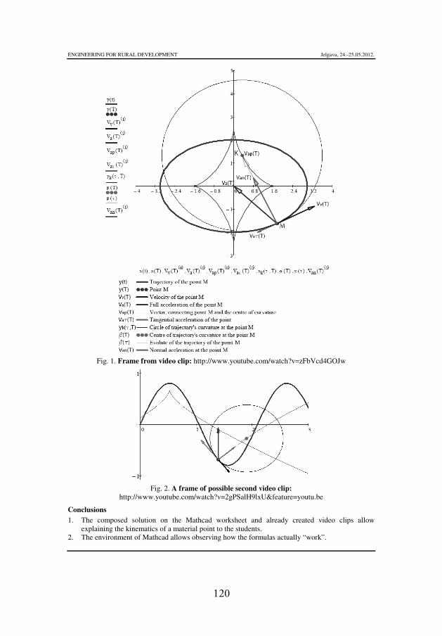
120

ENGINEERING FOR RURAL DEVELOPMENT Jelgava, 24.-25.05.2012.

Fig. 1. Frame from video clip: http://www.youtube.com/watch?v=zFbVcd4GOJw

Fig. 2. A frame of possible second video clip: http://www.youtube.com/watch?v=2gPSalH9lxU&feature=youtu.be

Conclusions 1. The composed solution on the Mathcad worksheet and already created video clips allow

explaining the kinematics of a material point to the students. 2. The environment of Mathcad allows observing how the formulas actually “work”.

121

ENGINEERING FOR RURAL DEVELOPMENT Jelgava, 24.-25.05.2012.

3. It is important that Mathcad detects most of syntax errors. 4. The possibility of experimentation with lecture materials and composing animations makes the

study of engineering subjects interesting and attractive for students. 5. Simple procedure of animation on Mathcad worksheet allows visualization of the problems of

engineering subjects for students.

References 1. Žlajpah, L. Simulation of n-R planar manipulators. Simulation Practice and Theory, vol. 6, 1998,

pp 305-321. 2. Žlajpah, L. 2008. Simulation in robotics. Mathematics and Computers in Simulation, vol. 79,

1998, pp. 879-897. 3. Tang, Z., Wang, X., Fraser W. B., Wang, L. Simulation and experimental validation of a ring

spinning process. Simulation Modelling Practice and Theory, vol. 14, 2006, pp. 809-816. 4. Jo H. S., Mir-Nasiri, N. Dynamic modeling and walk simulation for a new four-degree-of-

freedom parallelogram bipedal robot with sideways stability control. Mathematical and Computer Modelling, 2011

5. Peñuñuri, F., Peón-Escalante, R., Villanueva, C., Pech-Oy, D. Synthesis of mechanisms for single and hybrid tasks using differential evolution. Mechanism and Machine Theory, vol. 46, 2011, pp. 1335-1349.

6. Chen, J. T., Chou, K. S., Kao, S. K. One-dimensional wave animation using Mathematica. Computer Applications in Engineering Education, vol. 17, 2009, pp. 323–339.

7. Mathcad user's guide. Parametric Technology Corporation, 2007. [online] [31.01.2011]. Available at: http://www.msmiami.com/custom/downloads/Mathcad14_Users_Guide_English.pdf.

8. Heinloo, M., Aarend, E., Mägi, M. On the Experience of Mathcad-Aided Analysis of Planar Linkages. Proc. Tenth World Congress on the Theory of Machines and Mechanisms, vol. 1, 1999, pp. 392 – 397.

9. Heinloo, M., Olt, J. Motion of the Free-Active Circular Link on the Top of a Potato Ridge Modelled as a Polygonal Cylinder. Proc. Int. Conf. Perspective Sustainable Technological Process in Agricultural Engineering, 2001, pp. 99 – 104.

10. Heinloo, M., Olt J. A method of virtual reality for creating a disk-ridging tool. CIGR Ejournal, vol. 8, 2006, pp. 21. [online] [31.02.2011]. Available at: http://cigr-ejournal.tamu.edu/.

11. Heinloo, M. A virtual reality technology based method for study the working process of a blueberry harvester's picking reel. CIGR E-journal, vol. 9, 2007, pp. 12.

12. Butoescu, V. A vortex model of a helicopter rotor. INCAS, vol. 1, 2009, pp. 23-27. [online] [31.02.2011].Available at: http://bulletin.incas.ro/files/valentin_butoescu_v1no1_full.pdf.

13. Olt, J., Heinloo, M. Visualization of the working process of a novel manipulator for a stone protector of a stony soil tillage implement. Balkan Agricultural Engineering Review, vol. 15, 2010, pp. 9.

14. Olt, J., Heinloo M. Visualization of Motion of Fertiliser’s Granules on the Plane of Spinning Spreading Disc of a Disc Spreader. Proc. XXXIV CIOSTA CIGR VConference, 2011, pp. 292 – 296.

15. Aan, A., Aarend, E., Heinloo, M. On chaotic motion of a double pendulum. Agronomy Research, vol. 9, 2011, pp. 5 – 12.

16. Leola, T., Heinloo, M. Review of Studies on Press Manure Removal. Proc. 10.th Int. Sci. Conf. "Engineering for Rural Developments ", 2011, pp 82 – 87.

17. Heinloo, M., Saks, E. Review of Experiences in the Interactive Teaching of Mathematics and Mechanics. Proc. EFITA Conference, 2003, pp. 531–538.

18. Aare, A., Heinloo, M. On Creative Teaching of Engineering Mechanics. Proc. 22nd DAAAM International World Symposium, 2011, pp. 1081 – 1082.

19. Aan, A, Heinloo, M, Aarend, E. Interactive Computer Aided Learning and Teaching of Analytical Mechanics. Int. J. Eng. Pedagogy (iJEP), vol. 1, 2011, pp. 4 - 8.

20. Piskunov, N. Differential and Integral Calculus I. Moscow, 1969, pp. 492. 21. Bertjaev, B. D. Mathcad–based Training in Theoretical Mechanics (In Russian), Sankt-Peterburg,

2005, pp. 738. 22. Lepik, Ü., Roots, L. Theoretical mechanics (In Estonian). Tallinn, 1971, pp 483.

122ORIGINAL PUBLICATIONS

VII

Aan, A., Heinloo, M.Composing and solving diff erential equations for

small oscillations of mathematical spring-coupled pendulumsAgronomy Research, 11(1), 223 – 230, 2013

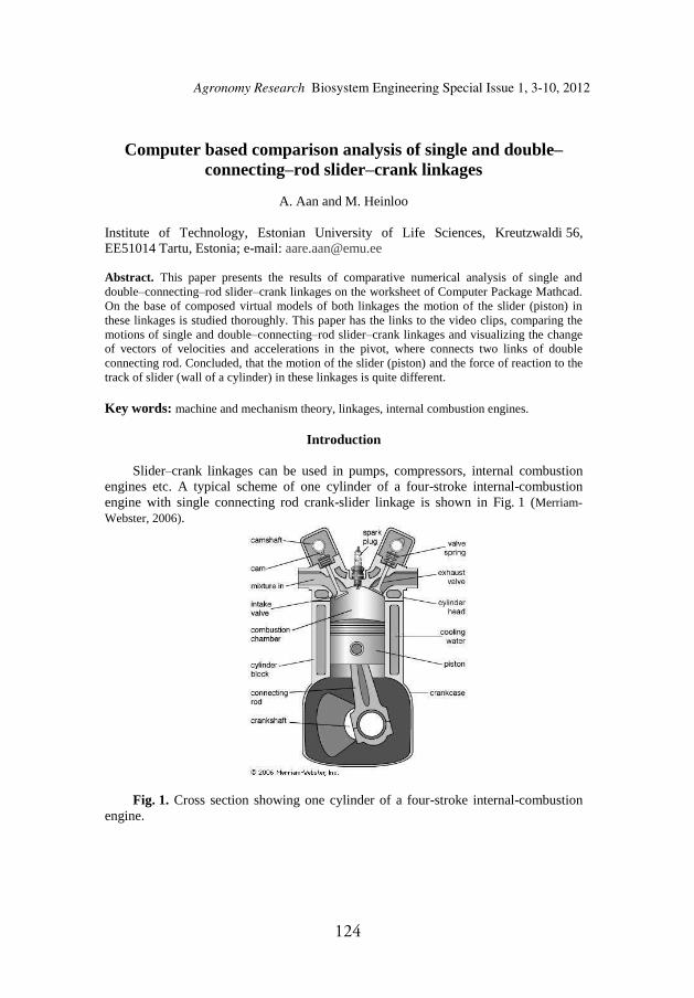
124

Computer based comparison analysis of single and double–connecting–rod slider–crank linkages

A. Aan and M. Heinloo

Institute of Technology, Estonian University of Life Sciences, Kreutzwaldi 56, EE51014 Tartu, Estonia; e-mail: aare.aan@emu.ee

Abstract. This paper presents the results of comparative numerical analysis of single and double–connecting–rod slider–crank linkages on the worksheet of Computer Package Mathcad. On the base of composed virtual models of both linkages the motion of the slider (piston) in these linkages is studied thoroughly. This paper has the links to the video clips, comparing the motions of single and double–connecting–rod slider–crank linkages and visualizing the change of vectors of velocities and accelerations in the pivot, where connects two links of double connecting rod. Concluded, that the motion of the slider (piston) and the force of reaction to the track of slider (wall of a cylinder) in these linkages is quite different.

Key words: machine and mechanism theory, linkages, internal combustion engines.

Introduction

Slider–crank linkages can be used in pumps, compressors, internal combustion engines etc. A typical scheme of one cylinder of a four-stroke internal-combustion engine with single connecting rod crank-slider linkage is shown in Fig. 1 (Merriam-Webster, 2006).

Fig. 1. Cross section showing one cylinder of a four-stroke internal-combustion engine.

Agronomy Research Biosystem Engineering Special Issue 1, 3-10, 2012

125

A review of different internal combustion engines using single–connecting–rod crank–slider mechanism with multiple cylinders is given in Automotive Handbook (1996).

Mederer (Evert, 2003) proposed to use a double–connecting–rod linkage (Fig. 2) in combustion engines.

Fig. 2. The scheme of a double–connecting–rod linkage, proposed by Mederer to use in internal combustion engines.

Double–connecting–rod linkage (Fig. 2) consists of ground (cylinder), crank (on crankshaft), two part connecting rod, slider (piston) and a swivel arm. By Mederer this mechanism reduces consumption of fuel and lower emissions, because piston will stay relative long times at area of its uppermost position, and in the compression stroke large parts of counter-pressure is taken by swivel arm, that means less input power is needed for turning a crank in the compression stroke.

The aim of this paper is to present the method and results of comparative numerical analysis of single–connecting–rod and double–connecting–rod slider–crank linkages on the worksheet of Computer Package Mathcad, in the case of constant (idle) crank (crankshaft) angular velocity. On the base of composed virtual models of both linkages the motion of the slider (piston) in these linkages will be studied thoroughly. This paper will have also links to two composed video clips. First video clip compares the motions of single–connecting–rod and double–connecting–rod slider–crank linkages with the same maximum displacement of the slider (piston). Second video clip visualizes the changing geometrical vectors of velocities and accelerations in the pivot, where connects two links of double-connecting-rod slider–crank linkage. This video clip compares also the reaction force in the track of sliders (cylinder wall).

Composition of virtual models of linkages

The links OA, AE, and EC of the four-bar OAEC in the structure of double–connecting–rod linkage can rotate around pivots O, A, E and C, whereby pivots O and C are grounded (Fig. 3). For numerical computations let us assume that the lengths of

126

the links OA, AE and EC are lOA = 0.3 m, lAE = 0.7 m, lEC = 0.735 m accordingly and the coordinates of the pivot C are xC = 0.67 m, yC = 0.7 m. Let us suppose also that the rotational speed of crank OA is n = 700 rpm, that means angular velocity

= 73.304 rad s-1.The coordinates of pivot A (Fig. 3) can be found out by equations

, .

The four-bar OAEC has constraints that the distances between pivots A, E and E, C are permanent. Mathematically these constrains means the following system of nonlinear equations of constraints

(1)

where is the angle of rotation of the crank OA from y-axis clockwise. The system of equations (1) was solved on the worksheet of Mathcad numerically

relative to xE and yE (Fig. 3).

Fig. 3. The virtual model of four-bar OAEC under crank’s rotation angle =30 .

Let us compose the following column vectors

, .

Fig. 3 shows the virtual model of linkage OAEC, drawn by these vectors on the worksheet of Mathcad.

Connecting to the pivot E of four-bar in Fig. 3 by a link ED to the pivot pivot D, what is moving along y-axis, we get a virtual model of double-connecting-rod linkage on Figs 2 and 4. Let the length of the link ED be lED = 0.7 m. The y-coordinate of pivot D can be find out from the following equation of restriction

127

. (2) The following vectors

,

,

draw on the worksheet of Mathcad the virtual model of double–connecting–rod crank–slider linkage in Fig. 4a.

To compose the virtual model for typical single–connecting–rod crank-slider linkage in Fig. 4b, we used the following equation of constraint

, (3)

where is the permanent length of the link AD in Fig. 4b. In computations were taken m. Equation (3) determine the coordinate of the pivot D by the following formula

.

The following vectors

,

,

,

draw on the worksheet of Mathcad the virtual model of single–connecting–rod crank–slider linkage in Fig. 4b.

(a) (b)

Fig. 4. The virtual models of double–connecting–rod (a) and single–connecting–rod (b) crank–slider linkages under crank’s rotation angle = 30 .

128

Comparison of displacement, velocity and acceleration of a slider (piston)

To compare of displacement, velocity and acceleration, let´s give for rotation angle the values from 0 with step 0.1 up to . This means that the crank OA in Fig. 4 makes two rotations.

According to used assumption, in Fig. 5 at the bottom dead centre (BDC) and the top dead centre (TDC) the pivot D (slider) virtual model displacements for both cases (Fig. 4a and Fig. 4b) are coincidence, but between BDC and TDC displacements are different.

Fig. 5. The Displacement of pivot D (slider) for double–connecting–rod and single–connecting–rod crank–slider linkages dependence from rotational angle

The velocity projections of pivot’s D (Fig. 4) are

, .

Fig. 6 shows the change of projections of the velocity of the pivot D (Fig. 4) for both virtual models. One can conclude in range of TDC these projections are coincident for both virtual models, but in BTC are not.

Fig. 6. The velocity of pivot D (slider) for double–connecting–rod and single–connecting–rod crank–slider linkages dependence from rotational angle

129

The accelerations projections of pivot’s D (Fig. 4) are

, .

One can conclude from Fig. 7 shows that the projections of accelerations of the pivot D for both virtual models are quite different.

Fig. 7. The accelerations of pivot D (slider) for double–connecting–rod and single–connecting–rod crank–slider linkages dependence from rotational angle

Comparison of angles between the link, connected to the pivot of the slider (piston) and the track of motion

Angles between y-axis (pivot D track) and the links on single connecting rod AD and double connecting rod ED (pressure angle (Kleis, 1988), can be found out from the equations

, .

Fig. 8 shows that the pressure angle for double–connecting–rod linkage is lower than the correspondent angle for single–connecting–rod linkage.

Fig. 8. The pressure angle between the links ED and AD (Fig. 4) relative to the y-axis (track of pivot D) for double–connecting–rod and single–connecting–rod crank–slider linkages dependence from rotational angle

130

Comparison of the reaction force from the track of slider (the wall of cylinder)

Let´s apply force FD = 1000 N to the slider pivot (piston) and take the mass of slider (piston) equal to mk = 3 kg. The equations of motion of the slider (piston) are

, , (4)

where – is the reaction force, applied from link ED in Fig. 4 (a) to the pivot D, – is the projection of the reaction force, applied to the track of slider (cylinder

wall). From equations (4) one can get the following formula for determination the

projection of the reaction force

.

Analoguous formula is valid for the case Fig. 4b

.

From Fig. 9 follows that the average reaction force in the case double–connecting–rod linkage is lower than in the case of single–connecting–rod linkage that means less friction between slider and track (piston and cylinder wall) in double–connecting–rod linkage.

Fig. 9. The projections of the reaction forces between the slider and its track (piston and cylinder) for double–connecting–rod and single–connecting–rod crank–slider linkages dependence from rotational angle

131

Comparison of visualizing video clips

The Computer Package Mathcad allows also compose of video clips. To visualize the obtained solution and to verify it, two video clips were made. The video clip (Aan & Heinloo, 2012-1), composed on the base of Figs 4 and 5, show visually the change of co-ordinate of pivot D in accordance with motion of corresponding linkage. The video clip (Aan & Heinloo, 2012-2), composed on the base of Figs 4 and 9, shows visually the dependence of reaction force between the link D and the track of it (piston and cylinder wall) in accordance with motion of corresponding linkage. Also on that video clip is visualized change of geometrical vectors of velocity and acceleration of the pivot D and pivot E. These vectors were composed by using the special program on the worksheet of Mathcad, presented by Bertjajev (2005).

Conclusions

The motion of the slider (piston) in double-connecting-rod linkage and single–connecting–rod linkage is quite different. The slider (piston) of double-connecting-rod linkage has lower reaction force on the track of motion (cylinder wall). That means the force, applied to the slider (piston) in double–connecting–rod linkage makes more useful work. Therefore, the motor based on double–connecting–rod linkage could have lower consumption of fuel and lower emissions than the motor with single–connecting–rod linkage. The Computer Package Mathcad can be used as convenient tool for composition of video clips for visualization and verify the obtained solution. The method and the results of study may be used by teachers of engineering subject ‘Machine and Mechanism Theory’ and by automobile engineers.

References

Merriam-Webster. 2006. Internal combustion engine. Available at: http://www.merriam-web-ster.com/concise-images/72180.htm (02.02.2012).

Robert Bosch GmbH. 1996. Automotive Handbook 4th edition. Stuttgart, pp. 892. Evert, A. 2003. Buckle- and Double-Connecting-Rod. Available at:

http://www.evert.de/eft774e.htm (02.02.2012). Kleis, I. 1988. Applied mechanics. Valgus. Tallinn, pp. 423. (in Estonian). Aan, A., Heinloo, M. 2012. Comparison of piston displacements. Available at:

http://youtu.be/LG2h8oiyjIU (02.02.2012). Aan, A., Heinloo, M. 2012. Comparison of piston velocities accelerations and reactions. Avail-

able at: http://youtu.be/QvyZAo-Q3Rk (02.02.2012). Bertjaev, B. D. 2005. Mathcad–based Training in Theoretical Mechanics. Sankt-Peterburg,

pp. 738. (in Russian).

132ORIGINAL PUBLICATIONS

VIII

Aan, A., Heinloo, M.Motion of a granule on fertilizer spreading disc

Proceedings of the 42nd international symposium on agricultural engineering: Actual Tasks on Agricultural Engineering,

101 – 111, 2014

134

135

136

137

138

139

140

141

142

143

144

145

146ORIGINAL PUBLICATIONS

IX

Aan, A., Heinloo, M., Allas, J.Design of a radial cam for the cam-follower mechanism

Proceedings of 8th International Conference of DAAAM Baltic Industrial Engineering, 11 – 16, 2014

148

9th International DAAAM Baltic Conference "INDUSTRIAL ENGINEERING"24 – 26th April 2014, Tallinn, Estonia

DESIGN OF A RADIAL CAM FOR THE CAM-FOLLOWER MECH-ANISM

Aan A., Heinloo M., Allas J.

Abstract: This paper presents a method for designing of a radial cam on the worksheet of Mathcad including the calculation of follower’s displacements, values of its ve-locities and accelerations, the optimization of the contour of a cam by choosing the eccentricity of follower and the radius of base circle of cam and the simulation of the working process of the cam mechanism. The optimal coordinates the contour of the cam were calculated. Finally, practical information for exporting cam contour data from Mathcad environment in data format necessary for CNC part program generation is discussed, considering CNC controllers using the most widespread ISO type program format and contouring with linear interpolation. Key words: cam mechanism, design, opti-mization, visualization.

1. INTRODUCTION

Cam mechanisms consisting of only two elements, the cam as mechanical driver element and the follower as driven ele-ment, are widely used in technical applica-tions due to reduced constructive com-plexity. Any functional motion of follower due to the movement of cam can be pro-duced [1].Cam mechanism can be classified in sever-al ways: by follower motion (translating, rotating), by type of cam (radial, cylindri-cal), by joint closure, by follower (flat, rolling, mushroom), by cam curves [2]. Alaci et al. [3] have showed some aspects concerning the design of cam mechanisms with oscillating flat faced follower by us-ing computer software. They also have generated figures of cam profiles as enve-

lopes of the straight lines paths on the Mathcad worksheet.In the study of Ahmet Shala and Ramë Likaj [4] an analytical method for synthesis of cam mechanism is presented. They use Mathcad for displacement, velocity and acceleration calculation of the follower.This paper presents the method and the results of numerical analysis of the radial cam, with translating follower on the work-sheet of Mathcad. The visualization of the cam and follower and the simulation of working process of cam-follower mecha-nism are presented. The coordinates of the visualized cam contour coordinates can beused in the CNC milling machine for the production of the real cam.

2. MATERIALS AND METHODS

2.1 The scheme of cam-follower mecha-nismFig 1 shows the scheme of a cam-follower mechanism

Fig. 1. The scheme cam mechanism, where is the rise angle, – the high dwell angle, – the fall angle, – the low dwell angle, – the eccentricity, H – the follower stroke

149

Let us consider the cam-follower mecha-nism by the following parameters: the rise angle of the follower = 60°; the high dwell angle of the follower = 60°; the fall (return) angle of the follower =60°; the stroke of the follower =0.005 ; the offset of the follower ; the radius of the base circle of the cam ; the number of positions of cam in computa-tions = 360; angular velocity of the cam= 10 / .

2.2 Follower’s displacementAccording to [2] let us describe the dis-placement of the follower in the rise by thelaw: ( ) = 35 84 +70 20 (1)and in the fall by the law( ) = 3584 + 7020 . (2)

In (1), (2) is the rotation angle of a cam from the initial position. The displacement of a follower in one cy-cle of cam's rotation can be determined by the following program on the worksheet of the Mathcad (Fig. 2)

Fig. 2. Program for determination of the follower displacement

Accordingly to program (Fig. 2) we get follower displacement on fig. 3.

Fig. 3. The dependence of the displacement of the follower on rotation angle of the cam

2.3 Follower’s velocityThe first derivative from equations (1) and (2) gives the velocity analogue functions: ( ) = ( ), (3) ( ) = ( ). (4) The velocity analogue in one cycle of cam's motion can be determined by the program on the figure 4.

Fig. 4. Program for determination of the follower velocity analogue

The program in fig. 4 computes the ana-logue of the follower’s velocity in the de-pendence on the rotation angle of the cam. To determine follower’s real velocity (fig. 5) the velocity analogue were multi-plied by the angular velocity of the cam.

Fig. 5. The dependence of the follower velocity on the rotation angle of the cam

150

2.4 Follower’s accelerationThe second derivative from equations (1) and (2) gives the acceleration analogue functions: ( ) = ( ), (5)( ) = ( ). (6)The acceleration analogue for one cycle of cam's motion can be determined by the program on the fig. 6.

Fig. 6. Program for determination of the follower acceleration analogue

The program in fig. 6 computes the follow-er’s acceleration analogue in the depend-ence on the rotation angle of the cam. To determine follower’s acceleration (fig. 7) the acceleration analogue were multiplied by the square of the cam angular velocity

.

Fig. 7. The dependence of the followeracceleration on the rotation angle of the cam

2.5 Optimization of the eccentricity andthe radius of the base circleThe pressure angle (fig. 8) is one of the limiting criteria’s for cam design. Accord-ingly to Norton [2] the pressure angle must be between 0 to ±30 degrees. Pressure angle value can be adjusted by the values of the eccentricity and radius R0 of base circle.

Fig. 8. The pressure angle between the cam and the follower

According to [2] the pressure angle of the cam determines the following formula: ( , , ) = ( )( ) . (7)

Base circle radius and eccentricity cannot be solved conveniently directly. To find proper and Norton [2] suggest to use special cam design program Dynacam or some equation solvers such as Matlab, TKSolver or Mathcad. To determine the radius of base circle R0and eccentricity let us formulate the fol-lowing problem of optimization: find such values for and that guaran-tee satisfaction of the restriction( , , ) = (8)in the rise and the restriction( , , ) = (9)in the fall.With lower accuracy the solution of system of equations (8) and (9) can be obtained also by hand [2], changing the values of and from initial values step by step. Do-ing so it is useful to know that the changeof value moves the graph of the function ( , , ) upwards or downwards without changing it shape and the change of valueR0 increases or decreases the external val-ues of the function ( , , ). In such way the solution for system of equations (8) and (9) by low accuracy can be ob-tained relatively quickly satisfying the need of teaching process.

151

The solution method of high accuracy for the system of equations (8) and (9) with respect to and by the help of Mathcad will be developed in future. Let us consider an example with the maxi-mal value of the pressure angle ( , , )= 20 (in rise) and minimal value of the pressure angle = 24 (in fall). Let´s take the initial values = 20and = 0 . In this case the curve of the function ( , , ) is presented in fig. 9, showing the pressure angle curve crossing the values of = 20 and = 24 .This means that the system of equations (8) and (9) is not satisfied.

Fig. 9 Cam mechanism pressure angle,R = 20mm and = 0By changing the values of and step by step one can visually observe the change of the graph of function ( , , ) and quickly obtain the position of this graph, shown in fig. 10. This means that the sys-tem of equations (8) and (9) is satisfied with some compromise of accuracy. The case in fig. 10 corresponds approximately to = 31 and = 1.5 .

Fig. 10 Cam mechanism pressure angle,R = 31mm and = 1.5mm

2.6 Visualization of the cam and simula-tion of the working process of cam-follower mechanism

The polar coordinates ( ) R( ) of con-tact point of the follower and the cam are( ) =( ) + + 2 ( ) , (10) ( ) = asin ( ) asin ,

(11) where ( ) is the polar radius and ( ) – the polar angle of the contour point in de-pendence of angle of cam’s rotation .To visualize the contour of the cam let us assume that the cam is not rotating but the follower rotates around the centre of the cam with angle of rotation . Then the con-tact point with polar coordinates ( ) R( ) draws the contour of the cam. Fig. 11 visualizes the initial position of the cam in the case = 31 and =1.5 .

Fig. 11 Cam contour in the polar coordi-nates ( ) R( )

The Cartesian coordinates of the cam con-tour at the initial position are( ) = ( ) cos( ( )), (12) ( ) = ( ) sin( ( )). (13) To simulate the working process of the cam-follower mechanism the cam in fig. 11 [5] is rotated by the angle t, where

is the angular velocity and t – the time. Equations ( ) = ( ) ( ), (14)( ) = ( ) ( ), (15) where ( ) = cos sinsin cos

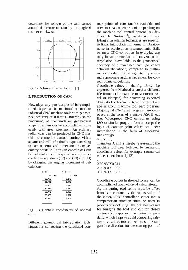
152

determine the contour of the cam, turnedaround the centre of cam by the angle counter clockwise.

Fig. 12 A frame from video clip [5]

3. PRODUCTION OF CAM

Nowadays any part despite of its compli-cated shape can be machined on modern industrial CNC machine tools with geomet-rical accuracy of at least 15 microns, so the machining of the modelled geometrical shape of a cam can be accomplished quite easily with great precision. An ordinary radial cam can be produced in CNC ma-chining centre by contour cutting with a square end mill of suitable type according to cam material and dimensions. Cam ge-ometry points in Cartesian coordinates can be calculated with required accuracy ac-cording to equations (12) and (13) (fig. 13) by changing the angular increment of cal-culations.

Fig. 13 Contour coordinates of optimal cam

Different geometrical interpolation tech-niques for connecting the calculated con-

tour points of cam can be available and used in CNC machine tools depending onthe machine tool control options. As dis-cussed by Norton [2], circular and spline fitting interpolation techniques are superiorto linear interpolation in terms of vibratory noise in acceleration measurements. Still, on most CNC controllers in everyday use only linear or circular tool movement in-terpolation is available, so the geometrical accuracy of a machined cam (so called “chordal deviation”) compared to mathe-matical model must be regulated by select-ing appropriate angular increment for con-tour points calculation.Coordinate values on the fig. 13 can be exported from Mathcad to another different file formats (for example to Microsoft Ex-cel or Notepad) for converting exported data into file format suitable for direct us-age in CNC machine tool part program.Majority of CNC part programs are com-posed in the form of a simple ASCII text file. Widespread CNC controllers using ISO or similar program format accept the input of contour point values for linear interpolation in the form of successive lines of type X…Y… , characters X and Y hereby representing the machine tool axes followed by numerical coordinate value, for example (numerical values taken from fig.13) …X30.989Y0.811 X30.981Y1.082 X30.971Y1.352 .

Coordinate output in showed format can be accomplished from Mathcad calculations.As the cutting tool centre must be offset from cam contour by the radius value of the cutter, CNC controller’s cutter radius compensation function must be used in process of machining. The optimal methodfor bringing the tool into cut for closed contours is to approach the contour tangen-tially, which helps to avoid contouring mis-takes caused by tool deflection, so the tan-gent line direction for the starting point of

153

contour cutting must be known. Consider-ing the fact the type of cam contour studied in this work is an arc between rotation an-

that the tangent line for contour isparallel to Y axis (fig. 14). As the machin-ing of contour is started and finished in point X and Y axis can be manually added to program for smooth tool transition into and out of the cut.

Fig. 14 Tool movement steps: 1 – initial position, 2 – beginning of contour start point tangent line, 3 – starting point of con-tour cutting, 4 - contour cutting, 5 – end point of contour cutting, 6 – end of contour end point tangent line, 7 – end position

In general the contours are milled using climb cutting, although conventional cut-ting may give better results in some special cases. The choice between climb and con-ventional cutting affects the machining direction of a contour, which are accord-ingly clockwise or counter clockwise for external contours. However, the choice between cutting direction can be easily taken into account while exporting coordi-nate data from Mathcad. Defining the rota-tion e(from 360 to 0 instead) results in contour point coordinates output in clockwise di-rection and vice versa.

4. CONCLUSION

1. The Computer Package Mathcad can be considered as a convenient tool for design of cams.

2. Mathcad allows the simulation of motion of virtual models of cam mechanisms.3. Mathcad can be used to compute cam contour coordinates, which can be used for CNC part program. 4. The method presented in this paper can be used in the teaching process of engi-neering subjects and also by engineers in their work.

5. REFERENCES

1. Shin, J.-H., Kwon, S.-M. & Nam, H. Ahybrid approach for cam shape design and profile machining of general plate cam mechanisms, International Journal of Precision Engineering and Manufacturing.2010, 11(3), 419-472. 2. Norton, R. L. Cam design and manufac-turing handbook. 2009, Industrial Press Inc., new York. 3. Alaci, S., Ciornei, F. C., Amarandei, D., Filote, C., Patras-Ciceu, S., Prodas, D.Some aspects regarding computer aided design of cam mechanism with flat face oscillating follower. Fiability & Durability,2011, 1(7). 4. Shala, A., Likaj, R. Analytical method for synthesis of cam mechanism. Interna-tional Journal of Current Engineering and Technology, 2013, 3(2).5. Aan, A. Simulation the working process of cam-follower mechanism. 2013. https://www.youtube.com/watch?v=c43JIq7-rvc

6. ADDITIONAL DATA

MSc (Eng Sc) Aan, Aare (author) e-mail: aare.aan@emu.ee.Dr (math) Heinloo, Mati (co-author) e-mail: mati.heinloo@emu.ee. MSc (Engn Sc) Allas, Jaanus (co-author) e-mail: jaanus.allas@emu.ee.

Institute of Technology, Estonian University of Life Sciences, Kreutzwaldi 56, 51014, Tartu, Estonia

154ORIGINAL PUBLICATIONS

X

Aan, A., Heinloo, M.Analysis and synthesis of

the walking linkage of Th eo Jansen with a fl ywheelAgronomy Research, 12(2), 657 – 652, 2014

156

157

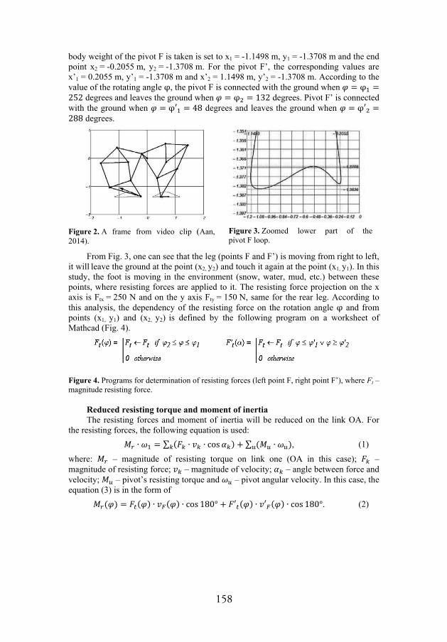
158

159

160

161

162ORIGINAL PUBLICATIONS

XI

Aan, A., Heinloo, M.Dynamics of a frozen sea buckhorn berry in a separator

Procedia Engineering, 100, 689 – 698, 2015

164

Procedia Engineering 100 ( 2015 ) 689 – 698

Available online at www.sciencedirect.com

1877-7058 © 2015 The Authors. Published by Elsevier Ltd. This is an open access article under the CC BY-NC-ND license (http://creativecommons.org/licenses/by-nc-nd/4.0/).Peer-review under responsibility of DAAAM International Viennadoi: 10.1016/j.proeng.2015.01.421

ScienceDirect

25th DAAAM International Symposium on Intelligent Manufacturing and Automation, DAAAM 2014

Dynamics of a Frozen Sea Buckhorn Berry Motion in a Separator

Aare Aan*, Mati Heinloo Estonian University of Life Sciences, Institute of Technology, Fr.R.Kreutzwaldi 56, Tartu 51014, Estonia

Abstract

After removing frozen sea buckthorn berries from the branches of sea buckthorn tree in a separator (patent EE05717B1), the s moving conveyer belt under a certain angle of inclination, thus guiding the berries in the collector of

separator. This paper presents the mathematical model of the berry motion along the conveyer and after falling from it. The nonlinear differential equations describing the berry motion on the conveyer and after falling from it take into account air

Runge-Kutta method of 4th order on Mathcad worksheet. This paper focuses on berry motion depending on belt velocity, friction coefficient between belt and berry, and inclination angle of the belt. Composed video clip visualizes berry motion and demonstrates how the berry moves from the initial position in the same direction as conveyer belt velocity, down to lower edge of the belt and falls from conveyer. Results of this paper can be used by engineers designing conveyors and by educators teaching agricultural machinery. © 2015 The Authors. Published by Elsevier Ltd. Peer-review under responsibility of DAAAM International Vienna.

Keywords: berry separator; mathematical modelling; berry motion; visualization; Mahtcad; belt conveyor

1. Introduction

Moving different materials on belt conveyors is a very common solution used in various industries because of their high efficiency in comparison to other transport methods [1]. Therefore, belt conveyors are widely researched and developed.

Ibishi et al. showed the method for calculating the tension force of the belt. The purpose of the method is to recognize the tension force upper limit, exceeding of which may damage belt transportation equipment [2]. Zanoelo

* Corresponding author. Tel.: +3727313302.

E-mail address: aare.aan@emu.ee

© 2015 The Authors. Published by Elsevier Ltd. This is an open access article under the CC BY-NC-ND license (http://creativecommons.org/licenses/by-nc-nd/4.0/).Peer-review under responsibility of DAAAM International Vienna

165

690 Aare Aan and Mati Heinloo / Procedia Engineering 100 ( 2015 ) 689 – 698

and et al. studied mate leaves dryer and proposed to control the velocity of the belt by the mathematical drying model to ensure the accepted range of moisture in mate leaves [3]. There are energy models that can be used for efficiency optimization of the belt conveyor´s operation [4]. In recent studies by Göttlich et al., mathematical model was used to simulate a conveyor belt where the cargo is separated by means of a rigid singularizer. They also validated their model with real data tests [5].

This paper aims at providing a model and simulation of continuous belt conveyor on sea buckhorn berry separator (Fig. 1). The function of this belt conveyor is to separate the frozen berries, leaves and small branches which cannot be removed with sieve. The belt carries leaves and branches away while berries roll over the belt due to its inclination (Fig. 1). This paper presents the possibility to model mathematically berry motion on the conveyor belt. Calculations are based on the numerical method Runge-Kutta that was also used by above-mentioned authors in the field of conveyor modelling. The motion of the berry is visualized by graphs and by a video clip. Results of this paper can be used for designing berry conveyors and for analysing their motion. It also introduces some methods to be used with math program Mathcad, which is used also in other studies for engineering calculations [6] [7].

Fig. 1. Left: device for separation of deep-frozen sea buckthorn berries from twigs [8]. Right: principal scheme of the sea buckthorn berries separator sieve and conveyor belt. Where: 1 - inclined conveyor belt, 2 - sieve, 3 sea buckhorn berries, 4 - leaves and small branches.

Nomenclature

velocity of the conveyor belt, m/s width of the belt, m axis, with origin at the point B along the conveyor belt, m initial value on s-axis, m ty, m/s inclination angle of the conveyor belt, degrees berry particle mass, kg acceleration of gravity, m/s2

f friction coefficient between berry particle and conveyor belt

166

691 Aare Aan and Mati Heinloo / Procedia Engineering 100 ( 2015 ) 689 – 698

air density, kg/m3

air resistance constant surface of the frontal area, m2

berry particle acceleration, m/s2

time, s the time when berry motion begins, s the time when berry motion ends, s the number of subintervals within the interval ( , )

2. Materials and Methods

The kinematic scheme of the cleaning belt conveyor of buckhorn berry separator is shown on Fig 2.

Fig. 2. The computational scheme of belt conveyor: 1 berry particle, 2 conveyor belt between points AB, width of the belt (distance between points AB), velocity of the conveyor belt, axis, with origin at the point B along the conveyor belt, -

inclination angle of the conveyor belt, berry particle mass, acceleration of gravity.

2.1. Berry motion on the belt

Berry particle motion can be modelled by using the following differential equation

, (1)

where f friction coefficient between berry particle and conveyor belt, air density, air resistance constant, A surface of the frontal area, - berry particle acceleration. Last part on the right in equation (1) models air resistance [9]. The initial conditions for equation (1) are

, (2)

where and .

167

692 Aare Aan and Mati Heinloo / Procedia Engineering 100 ( 2015 ) 689 – 698

The initial value must be chosen presuming that the solution meets the condition (Fig. 2). To solve the equation (1) on Mathcad worksheet, it had to be presented as the following system of two equations of the first order

(3)

where =s, . Nonlinear system of equations (3) was solved numerically by using the algorithm of Runge-Kutta IV order, under

conditions (2) by the following Mathcad function

where the function

is the differentiation equation solver. D - the notation of the function

,

of the right side of the system (3). Here y is the vector . the time when berry motion begins,

the time when berry motion ends, - the number of subintervals within the interval ( , ), the matrix of initial values. Function returns the matrix with columns ,

, , where <1>, <2>, <3> denote the 1st, 2nd, 3rd column of this matrix. At that is the vector of the values of time, is the vector of the berry

coordinates and is the velocity vector of the berry. While is also the value of time , when the berry reaches point A (Fig. 2), its value can be calculated from equation

, (4)

where the function ) returns the solution of an equation in the closed interval . In (4), gives the th value of the coordinate at point A (Fig. 2) and is the width of the belt. The value is supposed to be in the closed interval [0.1, 10].

The Cartesian coordinates of the berry on belt during motion are

, (5)

. (6)

Point B (Fig. 2) coordinates are

, (7)

168

693 Aare Aan and Mati Heinloo / Procedia Engineering 100 ( 2015 ) 689 – 698

. (8)

2.2. Berry falling in the air

oint A at the moment of the time , it starts free fall in the air. This motion is described by the following equations

, (9)

, (10)

where and are accelerations, and ´are velocities in the direction of - and -axis. Initial conditions for the equations (9) and (10) are

, , , . (11)

To determinate the coordinates and during free fall, equations (9) and (10) were solved under initial conditions (11) numerically similar to the solution of equation (1).

3. Results and discussion

3.1. Berry displacement and velocity on belt

, belt velocity , friction coefficient between berry particle and conveyor belt , air density , air

resistance constant (considering that sea buckthorn berry is almost a sphere), surface frontal area , width of the belt (distance between points AB) , point A coordinates

and . Under initial conditions (2) , it means that the berry touches the belt in the center, because .

adjusting the separation process of the conveyor belt: inclination angle, velocities and friction coefficient (Fig. 3 Fig. 5).

Fig. 3. Left: berry displacement along conveyor belt. Right: berry velocity along conveyor belt. Corresponding different inclination angles of the conveyor belt: 1) , 2) , 3) , 4) , 5) ; and .

169

694 Aare Aan and Mati Heinloo / Procedia Engineering 100 ( 2015 ) 689 – 698

Fig. 4. Left: berry displacement along conveyor belt. Right: berry velocity along conveyor belt. Corresponding different velocities of the conveyor belt: 1) , 2) , 3) , 4) , 5) ; and .

Fig. 5. Left: berry displacement along conveyor belt. Right: berry velocity along conveyor belt. Corresponding different friction coefficient between berry particle and conveyor belt: 1) , 2) , 3) , 4) , 5) ; and .

Figures 3-5 show that after contacting the belt, the berry first starts to move in the direction of belt with velocity and then, due to inclination angle and gravity, moves down along the belt until it reaches point A (Fig. 2).

Displacement decrease and negative velocity indicate berry movement along the belt with velocity . Negative displacement means that berry moves over the point B (Fig. 2). In reality, it means that berry will fall over point B along with leaves and small branches (Fig. 1).

The calculation of berry displacement and velocities indicates that there are possible values, in which case the berry moves along with velocity and will not move in the correct direction at all. This can be adjusted with all three parameters ( ) and also initial values and .

3.2. Berry trajectory on the belt and in the air

For visualization of the belt according to equations (5) and (6) (Fig. 2, line AB), the coordinates are defined as matrixes on the Mathcad worksheet

170

695 Aare Aan and Mati Heinloo / Procedia Engineering 100 ( 2015 ) 689 – 698

, .

Berry trajectory can be visualized with the following matrixes according to equations (3) and (4), where and ) are built-in Mathcad functions for finding minimum and maximum values

, .

On Fig. 6 we can see that if the berry touches the belt in point , it will first move in the direction of belt with velocity , like we saw on Fig. 3 - 5. On Fig. 6, when , the berry will move close to point B, i.e. berry can fall over the belt if point B is on the edge of the belt.

On Fig. 6, when and , the berry will not reach point B and will stay on the belt until point A. For example, if and , then, provided that , the berry will move towards point A

instantly after touching the belt (Fig. 7). When and , it will still show movement along the belt with velocity in the beginning (Fig. 7).

3

Fig. 6. The berry (continuous line) and the belt (dotted line) trajectories, location (large dot): 1) , 2) , 3) ; , , , .

Fig. 7. The berry (continuous line) and the belt (dotted line) trajectories, location (large dot): 1) , 2) , 3) ; , , , .

171

6 Aare Aan and Mati Heinloo / Procedia Engineering 100 ( 2015 ) 689 – 698

When summing up the solutions of equations (5), (6), (7), (8), (9) and (10), we get the entire trajectory of the berry on the belt and through the air (Fig 8). Based on the air trajectories, it is possible to determine the location of the collector or measuring box under the sea buckthorn berries separator.

The motion of the berry particle according to calculations, with different conveyor inclination angle, is visualized in video clip [10].

Fig. 8. , 2) , 3) ; , , , .

3.3. Total time of berry motion

The total time of berry motion depending on inclination angle , velocity of conveyer belt and friction coefficient was also determined.

Fig. 9 shows total time of berry motion according to the inclination angle (Fig. 2) of the conveyor belt. The total time decreases when angle increases.

Fig. 9. Total time of berry motion depending on inclination angle of conveyor belt if , , , .

Fig. 10 shows total time of berry motion according to different velocity of the conveyor belt (Fig. 2). The total time increases when velocity increases. The relation of total time and conveyor belt velocity increase are almost linear.

172

697 Aare Aan and Mati Heinloo / Procedia Engineering 100 ( 2015 ) 689 – 698

Fig. 10. Total time of berry motion depending on velocity of the conveyor belt if , , , .

Fig. 11 shows total time of berry motion depending on the friction coefficient. The total time increases when friction coefficient increases.

Fig. 11. Total time of berry motion according to different friction coefficients, berry particle and conveyor belt: , , , .

The outcomes indicated in the results and discussion sections are theoretical and must be validated with experimental data. First steps are made to build a prototype of the sea buckthorn berries separator according to patent EE05717B1. Results of experimental data will be discussed in future papers.

Conclusions

This paper shows that: 1) From the initial position at beginning of motion, a berry moves along the belt in the direction of the conveyer belt at certain velocity, stops and then moves along the belt to the lower point of the belt and falls down. 2) There are initial berry values and , in which case the berry does not reach the upper edge of the belt. 3) Total time of berry motion depends substantially on the inclination angle of the belt, coefficient of friction between berry and belt and velocity of the conveyer belt. 4) Composed video clip provides visual representation of full motion of the berry in separator under different angles of inclination of conveyer belt. Mathematical program Mathcad turned out to be a convenient tool for solving problems related to mechanics.

173

8 Aare Aan and Mati Heinloo / Procedia Engineering 100 ( 2015 ) 689 – 698

Results of this paper can be used by engineers for designing the conveyors and by educators for creative teaching of mechanics and engineering mechanics [11] of agricultural machinery.

References

[1] S. Zhang, X. Xia, Optimal control of operation efficiency of belt conveyor systems, in: J. Yan (edi.), Applied Energy, 87(6) (2010) 1929-1937 [2] I. Ibishi, A. Latifi, G. Ibishi, K. Sejdiu, M. Shala-Galica, B. Latifi, Calculation of tension force of belt conveyor, International Journal of

Engineering Science and Technology 4(12) (2012) 4886 4892. [3] E.F. Zanoelo, A. Abitante, L.A.C. Meleiro, Dynamic modeling and feedback control for conveyors-belt dryers of mate leaves, in: R.P. Singh

(edi.), Journal of Food Engineering, 84(3) (2008) 458-468. [4] S. Zhang, X. Xia, Modeling and energy efficiency optimization of belt conveyors, in: J. Yan (edi.), Applied Energy 88(9) (2011) 3061-3071 [5] S. Göttlich, S. Hoher, P. Schindler, V. Schleper, A. Verl, Modeling, simulation and validation of material flow on conveyor belts, in: J. Sienz

(edi.), Applied Mathematical Modelling 38(13) (2014) 3295-3313. [6] I. Pantea, I. Stanasel, F. Blaga, The simulation of the profiling technology of toothing knives, in: B. Katalinic (edi.), Annals of DAAAM for

2008 and 19th International DAAAM Symposium, Trnava, 2008, pp. 1015-1016. [7] M. Tierean, L. Baltes, L. Eftimie, Design of the bridges structures using MathCAD, in: B. Katalinic (edi.), Annals of DAAAM for 2008 and

19th International DAAAM Symposium, Trnava, 2008, pp. 1389-1390. [8] P. Nõmm, A. Aan, Device for separation of deep-frozen sea-buckthorn berries from twigs. Estonian patent: EE05717B1 (15.02.2014) [9] H. R. Harrison, T. Nettleton, Advanced Engineering Dynamics, John Wiley & Sons Inc., 1997. [10] A. Aan, (2014), Particle of the berry on inclined moving conveyor belt. Available at: http://youtu.be/g0Axk5gmwIk (2.09.2014) [11] M. Heinloo, A. Aan, On creative teaching of engineering mechanics, in: B. Katalinic (edi.), Annals of DAAAM for 2011 and proceedings:

22nd international DAAAM symposium, Vienna, 2011, pp. 1081 1082.

174

CURRICULUM VITAE

Personal data Name: Aare Aan Date of birth: 21. December 1983 Address: Estonian University of Life Sciences, Kreutzwaldi

56, Tartu Phone: +372 58088219 E-mail: aare.aan@emu.ee Education 2011 - … Phd studies, Estonian University of Life Sciences,

Institute of Technology 2009 – 2011 Master’s degree studies, Estonian University of Life

Sciences, Production Engineering 2006 – 2009 Bachelor’s degree studies, Estonian University of

Life Sciences, Production Engineering 2005 – 2006 Lapland Vocational College, Forwarder operator 2004 - 2005 Luua Forestry School, Forwarder operator 2002 - 2003 Tallinn Polytechnic School, Introduction to infor-

mation technology 1999 – 2002 Koeru High School Research activity Degree information: 2011 MSc Production Engineering, Estonian University

of Life Sciences, Institute of Technology Intellectual property: 2012 Device for the separation of deep-frozen sea-

buckthorn. EE 05717 B1. Nõmm, P., Aan, A. Own-er: Estonian University of Life Sciences

2013 Hemp harvester. EE 05740 B1. Olt, J., Aan, A. Owner: Estonian University of Life Sciences

Honours and degrees: 2012 Invention contest of Institute of Technology „Engi-

neering Student Invents 2012“ III place. „Device for separation of sea-buckthorn berries“

175

Complementary education: 2013 – 2014 Engineering pedagogy courses, Tallinn University

of Technology 2013 Intensive course: Current trends in process type pro-

duction and discrete type manufacturing, Estonian University of Life Sciences

2012 Intensive course: Scientific trends in automation and manufacturing, Tallinn University of Technology

2012 Seminar: Innovated production, Tallinn University of Technology

Career 2011 - … Estonian University of Life Sciences, Assistant

(Mechanis of machinery) 2010 – 2011 Estonian University of Life Sciences, Specialist 2007 – 2010 AS Info-Auto Tartu, Car spare parts salesman

176

ELULOOKIRJELDUS

Isikuandmed Nimi: Aare Aan Sünniaeg: 21. Detsember 1983 Aadress: Eesti Maaülikool, Kreutzwaldi 56, Tartu Telefon: +372 58088219 E-post: aare.aan@emu.ee Haridustee 2011 - ... Eesti Maaülikool, Tehnikainstituut, Doktorant 2009 - 2011 Eesti Maaülikool, Tootmistehnika, Magistriõpe 2006 – 2009 Eesti Maaülikool, Tootmistehnika, Bakalaureuseõpe 2005 – 2006 Lapin Ammattiopisto (Soome), Forwarderi operaator 2004 – 2005 Luua Metsanduskool, Forwarderi operaator 2002 – 2003 Tallinna Polütehnikum, Infotehnoloogiaalused 1999 - 2002 Koeru Keskkool Teadustegevus Teaduskraadi info: 2011 Magistrikraad tootmistehnika erialal, Eesti Maaülikool Patentsed leiutised: 2012 Sügavkülmutatud astelpajumarjade okstest

eraldamise seade. EE 05717 B1. Nõmm, P., Aan, A. Omanik: Eesti Maaülikool

2013 Kanepikoristi. EE 05740 B1. Olt, J., Aan, A. Omanik: Eesti Maaülikool

Teaduspreemiad ja –tunnustused: 2012 Üliõpilaste leiutuskonkursil „Tehnikatudeng leiutab

2012“ III koht tööga „Astelpaju eraldustrummel“ Täiendkoolitused: 2013 – 2014 Inseneripedagoogika kursused, Tallinna

Tehnikaülikool 2013 Kursus: Current trends in process type production

and discrete type manufacturing, Eesti Maaülikool

177

2012 Kursus: Scientific trends in automation and manufacturing, Tallinna Tehnikaülikool

2012 Täiendkoolitus: Uuenduslik tootmine (Masinaehituse TAK, Paindtootmissüsteemide tehnoloogiad ja automatiseerimine, Materjalid), Tallinna Tehnikaülikool

Teenistuskäik 2011 - … Eesti Maaülikool, assistent (masinamehaanika) 2010 – 2011 Eesti Maaülikool, Tehnikainstituut, spetsialist 2007 - 2010 AS Info-Auto Tartu, varuosamüüja

178

ETTEKANDED

Suulised ettekanded rahvusvahelistel konverentsidel: International Scientific Conference Biosystem Engineering 2011, Tartu, Eesti, Eesti Maaülikool, On chaotic motion of a double pen-dulum, Aan, A.; Aarend, E.; Heinloo, M. 22nd International DAAAM Symposium "Intellegent Manufacturing and automation: Power of Knowledge and Creativity", 2011, Aus-tria, Viin, On creative teaching of engineering mechanics, Aan, A.; Heinloo, M. 8th International Conference of DAAAM Baltic Industrial Engineer-ing, 2012, Tallinn, Eesti, Analysis of four-stroke cycle internal com-bustion V-engine in Mathcad environment, Aan, A.; Heinloo, M.; Aarend, E.; Mikita, V. International Scientific Conference Biosystem Engineering 2012, Tartu, Eesti, Eesti Maaülikool, Computer based comparison analysis of single and double-connecting-rod slider-crank linkages, Aan, A.; Heinloo, M. International Scientific Conference Biosystem Engineering 2013, Tartu, Eesti, Eesti Maaülikool, Composing and solving differential equations for small oscillations of mathematical spring-coupled pen-dulums, Aan, A.; Heinloo, M. 42nd international symposium on agricultural engineering: Actual Tasks on Agricultural Engineering, 2014, Opatija, Horvaatia, Mo-tion of a granule on fertilizer spreading disc, Aan, A.; Heinloo, M. 9th International Conference of DAAAM Baltic Industrial Engineer-ing, 2014, Tallinn, Eesti, Tallinna Tehnikaülikool, Design of a radial cam for the cam-follower mechanism, Aan, A.; Heinloo, M.; Allas, J. International Scientific Conference Biosystem Engineering 2014, Tartu, Eesti, Eesti Maaülikool, Analysis and synthesis of the walk-ing linkage of Theo Jansen with a flywheel, Aan, A.; Heinloo, M.

Stendettekanded rahvusvahelistel konverentsidel: 25th DAAAM International Symposium Intelligent Manufacturing & Automation: Focus on Sustainability, 2014, Viin, Austria, Dy-namics of a frozen sea buckhorn berry in a separaator, Aan, A.; Heinloo, M.