A Utility Framework for the Automatic Generation of Audio-Visual Skims

Hari Sundaram Lexing Xie Shih-Fu Chang Dept. Of Electrical Engineering, Columbia University,

New York, New York 10027. email: { sundaram, xlx, sfchang }@ee.columbia.edu

ABSTRACT In this paper, we present a novel algorithm for generating audio-visual skims from computable scenes. Skims are useful for browsing digital libraries, and for on-demand summaries in set-top boxes. A computable scene is a chunk of data that exhibits consistencies with respect to chromaticity, lighting and sound. There are three key aspects to our approach: (a) visual complexity and grammar, (b) robust audio segmentation and (c) an utility model for skim generation. We define a measure of visual complexity of a shot, and map complexity to the minimum time for comprehending the shot. Then, we analyze the underlying visual grammar, since it makes the shot sequence meaningful. We segment the audio data into four classes, and then detect significant phrases in the speech segments. The utility functions are defined in terms of complexity and duration of the segment. The target skim is created using a general constrained utility maximization procedure that maximizes the information content and the coherence of the resulting skim. The objective function is constrained due to multimedia synchronization constraints, visual syntax and by penalty functions on audio and video segments. The user study results indicate that the optimal skims show statistically significant differences with other skims with compression rates up to 90%.

1. INTRODUCTION This paper deals with the problem of automatic generation of audio visual skims. The problem is important because unlike the static, image based video summaries [20], video skims preserve the dynamism of the original audio-visual data. Applications of audio-visual skims include: (a) on demand summaries of the data stored in set-top boxes (interactive TV) (b) personalized summaries for mobile devices and (c) for news channels (e.g. CNN) that receive a tremendous amount of raw footage.

There has been prior research on generating video skims. In the Informedia skimming project [4], important regions of the video were identified via a TF/IDF analysis of the transcript. They also used face detectors and performed motion analysis for additional

cues. The MoCA project [13] worked on automatic generation of film trailers. They used heuristics on the trailers, along with a set of rules to detect certain objects (e.g. faces) or events (e.g. explosions). Work at Microsoft Research [9] dealt with informational videos; there, they looked at slide changes, user statistics and pitch activity to detect important segments. Recent work [11] has dealt with the problem of preview generation by generating “interesting” regions based on viewer activity in conjunction with topical phrase detecting. However, in order to generate the preview, some viewers need to have seen the video.

data

visual complexity

syntax analysis

sig. phrases

segmentation

objective function / constraints

skim minimization

computable scenes

Figure 1: the skim generation framework.

Skims can differ based on the user’s task (actively seeking information vs. passively watching a TV preview), the device constraints and on the form of the skim (semantic, affect-based, event-driven, and discourse centric). This work focuses on the generation of passive skims with the aim of maximizing the information content and coherence. We work on four specific areas that were not investigated in prior research: (a) the relationship between the length of a shot in a film and its comprehension time (b) analyzing the visual syntactical structure in the film and (c) prosodic analysis for determining significant portions of speech, and (d) a general utility framework for maximizing the skim information content and coherence.

We define a measure for visual complexity, and then relate this measure to comprehension time using a psychological

experiment. This helps us determine the minimum time allocated to a shot in the skim, for it to remain comprehensible. We also investigate the use of visual film-syntax for reducing the content of the scene. Film-syntax refers to the arrangement of shots by the director to give meaning to the shot sequence. Examples include, specification of (a) scale (b) duration (c) order of shots, amongst many others [15]. We investigate rules governing the duration of two syntactic elements (a visual phrase and a dialog) for content reduction.

We analyze the audio stream in two ways. First, we segment the audio data using Support Vector Machine (SVM) classifiers, organized in a tree structure into four classes: silence, clean speech, noisy speech, music / environmental sounds. In order to ensure coherent segments, we smooth the result using a duration dependent Viterbi decoder. Second, we analyze the discourse structure, for significant phrases, using the acoustic correlates of prosody [7][12] in conjunction with an SVM classifier. The two modes of analysis are then combined and the speech segments are ranked in order of significance.

We formulate the problem of skim generation in terms of utility maximization with constraints. We model the skim comprehensibility in terms of audio and video utility functions. The objective function that is to be minimized has constraints (audio / video duration constraints, visual syntax, synchronous multimedia constraints) that are constructed with the aim of maximizing the speech information content and the overall coherence of the video. The user studies indicate that the skims generated work well at high compression rates up to 90%.

The rest of this paper is organized as follows. We begin by defining the goals of this work. Then we briefly discuss the computable scene idea. In section 4, 5, we discuss visual complexity and syntax analysis and in section 6 we present our work on audio analysis. In section 7 we discuss the utility based skim generation framework. We present experimental results in section 8, and finally present the conclusions in section 9.

2. THE SKIM PROBLEM DEFINITION A skim is a audio-visual clip, that is a drastically condensed version of the original video. In this section, we shall discuss in order, the factors that affect skims, the different skim types, the specific goals in this paper and a summary of the computational architecture.

2.1 Factors that affect skims There are at least two factors that affect the skim generation algorithm — the task of the user and the device constraints. We divide up tasks into two broad categories: active and passive tasks. An task is defined to be active when the user requires certain information to be present in the final summary (e.g. “find me all videos that contain Colin Powell.”). In a passive task, the user does not have anything specific in mind, and is more interested in consuming the information. Examples include previews in a set-top box environment, browsing in a video digital library. The device on which the skim is to be rendered affects the skim in at least two ways: the nature of the user interface and the device constraints. The UI can be complex (e.g. the PC), medium (e.g. a palm pilot) and simple (e.g. a cell phone). The UI affects the resolution of the skim, and also

influences the kinds of tasks that the user has in mind (e.g. it is difficult to input a query on a cell phone). The computational resources available on the device — cpu speed, memory, bandwidth, availability an the audio rendering device, all effect the skim. The effect takes the form of the resolution of the skim, as well as the decision to include audio in the skim.

2.2 Skims come in different flavors In this section we attempt to identify some of the different skim forms. These forms are a function of the user’s information needs, the domain as well as the intent of the content provider.

Semantic: Here, we attempt to preserve the semantics in the data. These could be specified by the user (in the form of a query), or the content producer, who may specify (via MPEG-7 metatags) the content to be retained in the skim.

Affect based: In this form, we would like to retain the “mood” or the affect [1] generated by the content producer. The director controls the duration of shots in the sequence to produce a particular emotional response (e.g. fast cuts during an action sequence).

Event driven: This skim will contain all the events important in the domain. For example, a skim of a soccer game would contain all the goals. Clearly, this form is affected by the domain, and the users needs.

Discourse centric: This skim will attempt to parse the discourse structure of the speech in the video, and determine the most significant audio segments using prosody analysis.

2.3 Goals The goal of this work is the automatic generation of audio-visual skims for passive tasks, that summarize the video. This work focuses on creating discourse centric skims. We make the following assumptions:

1. We do not know the semantics of the original.

2. The data is not a raw stream (e.g. home videos), but is the result of an editing process (e.g. films, news).

3. The time that the user has to watch the skim is known.

Since we work on passive tasks, the information needs of the user are a priori unknown. A decision to detect certain set of predefined events will induce a bias in the skim, thereby conflicting with the assumption that the user needs are unknown. The assumption of the data stream being produced is an important one, since we shall attempt to preserve the grammar of the underlying produced video, so as to preserve meaning.

3. COMPUTABLE SCENES In our work we have focused on the detection of computable scenes [18][19]. They are formed by looking at the relationships between elementary computable audio and video scenes and structure. The elementary audio and video scenes represent contiguous chunks of audio and video respectively. These scenes are termed computable, since they can be automatically computed using low-level features in the data. There are four types of computable scenes that arise due to different kinds of

synchronizations between the elementary audio and visual computable scenes. Figure 2 shows one computable scene type.

We do not address the problem of semantics of the segments, since this is not a well posed problem. There are three novel ideas in our approach: (a) analysis of the effects of rules of production on the data (b) a finite, causal memory model for segmenting audio and video and (c) the use of top-down structural grouping rules that enable us to be consistent with human perception. These scenes form the input to our condensation algorithm.

The Informedia and the MoCA projects analyze data over the entire video. However, they do not perform scene level analysis for skim generation. In our current work, we analyze the data within one scene. In future work, we plan on utilizing the interesting syntactical relationships amongst scenes that exist in the video [15], for condensation.

4. VISUAL COMPLEXITY In this section, we shall present an overview of the relationship between visual complexity of an image and its time for comprehension. Since the work in sections 4 and 5 have been reported before [17] we shall only summarize the key issues here.

4.1 Insights: film making and psychology In film-making, there is a relationship between the size1 of the shot and its apparent time (i.e. time perceived by the viewer).:

“Close-ups seem to last relatively longer on the screen than long shots. The content of the close up is immediately identified and understood. The long shot on the other hand, is usually filled with detailed information which requires eye-scanning over the entire tableau. The latter takes time to do, thus robbing it of screen time” [15].

Recent results in experimental psychology [6] indicate the existence of an empirical law: the subjective difficulty in learning a concept is directly proportional to the Boolean complexity of the concept (the shortest prepositional formula representing the concept), i.e. to its logical incompressibility. Clearly, there is empirical evidence to suggest a relationship between visual “complexity” of a shot and its comprehensibility.

4.2 Measuring visual complexity We define the visual complexity of an shot to be its Kolmogorov complexity [5]. In [17], we showed that length of the Lempel-

Ziv 2 codeword asymptotically converges to the Kolgomorov complexity of the shot. The complexity is estimated using a single key-frame3. Representing each shot by its key-frame is reasonable since our shot detection algorithm [21], is sensitive to changes in color and motion. We conducted a simple psychological experiment to measure the average comprehension time (i.e. the average of the times to answer who? where? what? and when?) for shot key-frames in [17]. We generate histograms of the average comprehension time after discretizing the complexity axis. The lower-bound on the comprehension time is generated by determining a least squares fit to the minimum time in each histogram. The distribution of times in each histogram slice, above the minimum time, is well modeled by a Rayleigh distribution. By using the 95th percentile cut-off for each histogram we get an estimate of the upper-bound on the comprehension time. The equations for the lines are as follows:

Figure 2: A progressive scene followed by a dialog sequence.

( ) 2.40 1.11,( ) 0.61 0.68,

b

b

U c cL c c

= += +

<1>

where c is the normalized complexity and Ub and Lb are the upper and lower bounds respectively, in sec. The lines were estimated for c ∈ [0.25, 0.55] (since most of the data lies in this range) and then extrapolated. Hence, given a shot of duration to and normalized complexity cS, we can condense it to at most Ub(cS) sec by removing the last to - Ub(cS) sec. The upper bound comprehension time is actually a conservative bound. This is because of two reasons: (a) the shots in a scene in a film are highly correlated (not i.i.d ) and (b) while watching a film, there is no conscious attempt at understanding the scene.

5. VISUAL FILM SYNTAX In this section we shall give a brief overview of “film syntax.” Then, we shall discuss its utility in films and then give syntax based reduction schemes for two syntactic elements.

5.1 Defining film syntax The phrase film syntax refers to the specific arrangement of shots so as to bring out their mutual relationship [15]. In practice, this takes on many forms (chapter 2, [15]) : (a) minimum number of shots in a sequence (b) varying the shot duration, to direct attention (c) changing the scale of the shot (there are “golden ratios” concerning the distribution of scale) (d) the specific ordering of the shots (this influences the meaning). These syntactical rules lack a formal basis, and have been arrived at by trial and error by film-makers. Hence, even though shots in a scene only show a small portion of the entire setting at any one time, the syntax allows the viewers to understand that these shots belong to the same scene.

Let us contrast shots with words in a written document. Words have more or less fixed meanings and their position in a sentence is driven by the grammar of that language. However, in films it is

2 Lempel-Ziv encoding is a form of universal data coding that doesn’t depend on the probability distribution of the source [5]. 3 We choose the 5th frame after the beginning of the shot, to be its key-frame. We acknowledge that there are other more sophisticated strategies for choosing key-frames.

1 The size (long/medium/close-up/extreme close-up) refers to the size of the objects in the scene relative to the size of the image

the phrase (a sequence of shots) that is the fundamental semantic unit. Each shot can have a multitude of meanings, that gets clarified only by its relationship to other shots. An object detector based approach (e.g. Informedia project [4], MoCA [13]) to skims, for films, at a conceptual level, makes the analogy “shots as words.” However, this is in contrast to the way film-makers create a scene, where the syntax provides the meaning of the shot sequence. Hence, while condensing films, we must honor the film syntax.

5.2 Syntax rules for shot removal

A phrase is a sequence of shots designed to convey a particular semantic. According to the rules of cinematic syntax [15], a phrase must have at least three shots. “Two well chosen shots will create expectations of the development of narrative; the third well-chosen shot will resolve those expectations.” Sharff [15] also notes that depicting a meaningful conversation between m people requires at least 3m shots. Hence in a dialogue that shows two participants, this rule implies that we must have a minimum of six shots.

Let us assume that we have a scene that has k shots. Then, we perform three types of syntax reductions (break points based on heuristics) based on the on the number of shots k (Table 1). The number and the location of the dropped shots depend on k and the syntax element (i.e. dialog or progressive). In the following discussion, we use a fictional film with a character called Alice.

It is reasonable to expect that the number of phrases in a scene, increase with the number of shots. For short scenes (type I reduction) we assume that there is a single phrase, containing one principal idea, in the scene. For example, the director could show Alice, walking back to her apartment, in a short scene.

Table 1: Three types of syntax reductions that depend on the element (dialog/progressive) and the number of shots k.

Breakpoints for each type Element Min. phrase

length I II III

Dialog 6 k ≤ 15 15 < k < 30 k ≥ 30

Progressive 3 k ≤ 6 6 < k < 15 k ≥ 15

In scenes of medium duration (type II reduction) we assume that there are at most two phrases. For example, <1st phrase>: Alice could be shown entering her room, switching on the lights, and be shown thinking. <2nd phrase>: then, she is shown walking to the shelves looking for a book, and is then shown with the book. We assume that scenes of long duration, (type III reduction)

contain at most three phrases. Modifying the previous example — <1st phrase>: Alice is shown entering the room, <2nd phrase>: she is shown searching for the book, <3rd phrase>: she walks with the book to her desk and makes a phone call. Hence, the reduction attempts to capture the phrase in the middle and the two end phrases.

In type I reduction, figure 3 (I), we drop shots from the right, since the director sets up the context of the scene using the initial shots. In type II, we expect an initial context, followed by a conclusion. Here, we start dropping shots from the middle, towards the ends. In type III, the scene is divided into three equal segments, and shots are dropped from the two interior segment boundaries. Unlike written text, there are no obvious visual “punctuation marks” in the shots to indicate a “phrase change.” Hence our syntax reduction strategy, which will capture the phrases in scenes of short and medium duration, may cause error in scenes of long duration. All shot detection algorithms generate certain number of false alarms and misses, and this affects the syntactical rules that we’ve developed. In [17], we show how to modify the minimum number of shots retained in a progressive scene by computing a statistical upper bound on the false alarm probability of the shot detector.

Figure 3: Three syntax reduction mechanisms. The black boxes are the minimal phrases and will not be dropped, while the gray shots can be dropped.

( II )

( III )

( I )

6. ANALYZING AUDIO In this section we discuss our approach for analyzing the audio stream prior to skim generation. We begin by first defining the audio analysis task for skims; then we present audio segmentation and significant phrase detection algorithms both of which use SVM classifiers. We conclude by presenting results in section 6.4.

6.1 This is a hard problem! Audio skim generation aims at dramatic time reduction (up to 90%) while preserving perceptual coherence. There are some clear drawbacks to simple approaches to determining useful segments in the audio stream. Let us assume that we wish to compress an audio track that is 100 sec. long, by 90%. Then: (a) downsampling the audio by 90% will leave the audio to be severely degraded since the pitch of the speech segments will increase dramatically. (b) PR-SOLA [9] is a non-linear time compression technique that eliminates long pauses, and attempts to preserve the original pitch in the output. User studies indicate that users do not prefer to have the speech sped up beyond 1.6x (i.e. ~40% compression). (c) selecting only those segments that are synchronous with the pre-selected video shots makes the audio stream is choppy and difficult to comprehend [4]. We define an audio segment as a contiguous chunk of coherent audio. Our approach to automatically identify audio segments: (a) create robust classifiers on the audio data via SVM’s (b) detect significant phrases in speech via discourse structure analysis.

6.2 Audio segment classification We build a tree-structured to classify each frame (100ms) into four generic classes: silence, clean speech, noisy speech and music / environmental sounds. We use 16 features in our approach [10], [14] [16]): (1) loudness, (2) low-band energy (3) high-band energy (4) low energy ratio (5) spectral roll off (6)

spectral flux (7) spectral centroid (8) spectral entropy (9) MFCC (10) delta MFCC (11) RASTA, (12) PLP and four variants of the zero crossing rate (13) ZCR, (14) mean ZCR, (15) variance of the ZCR and (16) high ZCR-ratio [10]. The cepstral features, RASTA and PLP were chosen since they are well known to be good speech discriminators [14]. All other features were chosen for their ability to discriminate between music and speech.

Silence frames are first separated from the rest of the audio stream using an adaptive threshold on the energy. Two SVM classifiers (C-SVM with radial basis kernel [3]) are then used in cascade: the remaining frames are separated into speech vs. non-speech (music or environmental sounds); and the speech class is further classified as clean and noisy speech. We then apply a modified Viterbi decoding algorithm [14][19] to smooth the sequence of frame labels. The decoder makes use of the class transition probabilities, classifier error likelihood and a duration utility (a function of the prior duration distribution of each class) to find the maximum likelihood class path.

6.3 Detecting significant phrases In this section, we shall summarize our work on detecting segment beginnings (SBEG’s) in speech. These are important as they serve as the introduction of new topic in the discourse [7], Detecting these discourse boundaries is different from determining emphasized portions of speech [2], since these emphasized portions can occur anywhere in the discourse (including SBEG’s).

There has been much work in the computational linguistics community [8][7][12] to determine the acoustic correlates of the prosody in speech. Typically, SBEG’s have a preceding pause that is significantly longer than for other phrases, higher initial pitch values (mean, variance), and smaller pauses that end the phrase than for other phrases [7][8]. In our algorithm, we extract the following features per phrase: pitch and energy values (min, max, mean, variance) for the (initial, last and complete) portions of the phrase, pause durations preceding and following the phrase.

Prior work [2][9] that uses speech based summarization indicates that users prefer relatively long segments of speech. In this work we restrict our attention to phrases that last between five to fifteen seconds. Our approach is then summarized as follows: (a) we first detect all the silent portions in the data (b) candidate phrases are all segments of audio that lie between two silent portions, and which satisfy our phrase duration criterion. (c) We then extract the acoustic features per phrase, and the phrase is then classified using a C-SVM classifier, with a radial basis function kernel. Furthermore, we rank the significant segments as a function of the pause and pitch.

6.4 Results In this section, we present results on the audio segment classification as well as the significant phrase detection.

6.4.1 Segment classification We used 45 minutes of audio data from two films (Bladerunner, Four Weddings and a Funeral) to train our classifier. The data is complex containing speech overlaid with background sounds,

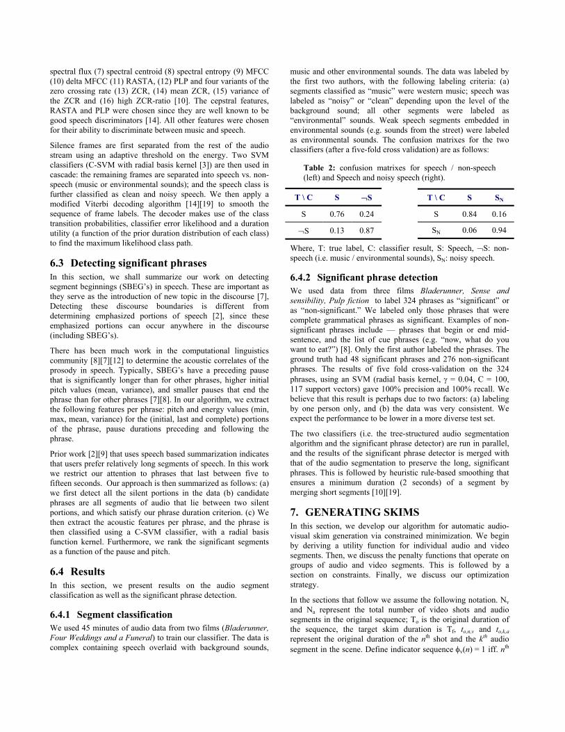
music and other environmental sounds. The data was labeled by the first two authors, with the following labeling criteria: (a) segments classified as “music” were western music; speech was labeled as “noisy” or “clean” depending upon the level of the background sound; all other segments were labeled as “environmental” sounds. Weak speech segments embedded in environmental sounds (e.g. sounds from the street) were labeled as environmental sounds. The confusion matrixes for the two classifiers (after a five-fold cross validation) are as follows:

Table 2: confusion matrixes for speech / non-speech (left) and Speech and noisy speech (right).

T \ C S ¬S

S 0.76 0.24

¬S 0.13 0.87

T \ C S SN

S 0.84 0.16

SN 0.06 0.94

Where, T: true label, C: classifier result, S: Speech, ¬S: non-speech (i.e. music / environmental sounds), SN: noisy speech.

6.4.2 Significant phrase detection We used data from three films Bladerunner, Sense and sensibility, Pulp fiction to label 324 phrases as “significant” or as “non-significant.” We labeled only those phrases that were complete grammatical phrases as significant. Examples of non-significant phrases include — phrases that begin or end mid-sentence, and the list of cue phrases (e.g. “now, what do you want to eat?”) [8]. Only the first author labeled the phrases. The ground truth had 48 significant phrases and 276 non-significant phrases. The results of five fold cross-validation on the 324 phrases, using an SVM (radial basis kernel, γ = 0.04, C = 100, 117 support vectors) gave 100% precision and 100% recall. We believe that this result is perhaps due to two factors: (a) labeling by one person only, and (b) the data was very consistent. We expect the performance to be lower in a more diverse test set.

The two classifiers (i.e. the tree-structured audio segmentation algorithm and the significant phrase detector) are run in parallel, and the results of the significant phrase detector is merged with that of the audio segmentation to preserve the long, significant phrases. This is followed by heuristic rule-based smoothing that ensures a minimum duration (2 seconds) of a segment by merging short segments [10][19].

7. GENERATING SKIMS In this section, we develop our algorithm for automatic audio-visual skim generation via constrained minimization. We begin by deriving a utility function for individual audio and video segments. Then, we discuss the penalty functions that operate on groups of audio and video segments. This is followed by a section on constraints. Finally, we discuss our optimization strategy.

In the sections that follow we assume the following notation. Nv and Na represent the total number of video shots and audio segments in the original sequence; To is the original duration of the sequence, the target skim duration is Tf, to,n,v and to,k,a represent the original duration of the nth shot and the kth audio segment in the scene. Define indicator sequence φv(n) = 1 iff. nth

video shot is present in the condensed scene. Define Nφ,v = ∑ φv(n), the number of video shots in the condensed

scene. φa(n) = 1 iff. nth is not silent, and Nφ,a = ∑ φa(n) is the number of non-silent audio segments.

, , ,

, ,

, ,, ,

, ,

, ,

( ) ( ) ( , )

1

( )

0

p i p i Lb i i

p i Ub i

p i Lb i, ,p i Lb i

Ub i Lb i

p i Lb i

P t t S t c

t t

t tt t t

t t

t t

= λ

≥

−λ = ≤ < −

<

i

p i Ub it <3>

7.1 The need for a utility function In order to determine the skim duration, we need to measure the comprehensibility of a video shot and a audio segment as a function of its duration. The shot utility function, models the comprehensibility of a shot as a continuous function of its duration and its visual complexity. This idea is connected to the results in section 4.2 in following way. Let us assume for the sake of definitiveness, that we have a 10 sec. shot of complexity 0.5. Then the upper bound duration Ub = 2.23 sec. We have argued that that if we reduce the shot duration to its upper bound, then there is a high probability that it will still be comprehensible. Note that the results in section 4.2 do not tell us how the comprehensibility of a shot changes when we decrease its duration. Hence the need for a shot utility function. We do not have any experimental results indicating a similar complexity-time relationship for audio, however, it seems fairly reasonable to conjecture its existence. Hence, the form of our audio utility function will be similar to the utility function that we shall derive in the next section for video shots. We model the utility of a video shot (audio segment) independently of other shots (segments).

where, λ modulates the shot utility, tp,i is the proportional time for shot i i.e. , ,i f ot T Tο i tLb,i and tUb,i are the lower and upper

time bounds for shot i, and S(t,c) is the shot utility function.

The utility function for the sequence of shots is the sum of the utilities of the individual shots:

, ,, : ( ) 1 : ( ) 0

1( , , ) ( , ) ( )v v

v v v i v i p jv i i j j

U t c S t c P tNφ φ = φ =

φ = − ∑ ∑ <4>

where, 0 1: , ...v Nt t t t and 0 1 .: , ... Nc c c c represent the durations and complexities of the shot sequence.

We conjecture the utility function of an non-silent audio segment of duration t belonging to a class k as follows:

( , ) (1 exp( ))k kA t k tβ λ= − − <5>

where, A is the utility function and where β and λ are class dependent parameters. When we need to remove an audio segment from the skim, we assign a negative utility to this silent (a dropped segment is silent) segment: 7.2 Defining the utility functions

The non-negative utility function of a video shot S(t, c), where t is the duration of the shot and c is its complexity, must satisfy the following constraints:

( 2( ) ( ) /i iL t t tο )θ= − <6>

where, ti is the duration of the ith silence, and where tο and θ are normalizing constants. Then, similar to equation <4>, we define the audio utility to be the sum of the utilities of the constituent segments.

1. For fixed c, S(t, c) must be a non-decreasing function of the duration t. i.e. This is intuitive since decreasing the shot duration by dropping frames from the end of the shot (section 4.2), cannot increase its comprehensibility.

1 2 1 2, ( , ) ( , ).t t S t c S t c∀ ≤ ≤

, ,, : ( ) 1 : ( ) 0

1( , , ) ( , ) ( )a a

a a a i a i i aa i i i i

U t k A t k L tNφ φ φ

φ= =

= − ∑ ∑ <7>

2. This is because complexity c = 0 implies the complete absence of any information, while c = 1 implies that the shot is purely random.

( ,0) 0, ( ,1) 0.t S t S t∀ = =

where, 0 1: ,a Nt t t t… and 0 1: , Nk k k k… represent the durations and the class labels of the audio segments in the skim. We model the shot utility function to be a bounded,

differentiable, separable, concave function:

<2> ( , ) (1 ) (1 exp( )).S t c c c t= β − − −αi7.3 The video rhythm penalty function The original sequence of shots have their duration arranged in a specific proportion according to the aesthetic wishes of the director of the film. Clearly, while condensing a scene, it is desirable to maintain this “film rhythm.” For example, in a scene with three shots of durations 5 sec. 10 sec. and 5 sec. maintaining the scene rhythm would imply that we preserve the ratios of the duration (i.e. 1:2:1) of the shots. We define the rhythm penalty function as follows:

The exponential is due to the first constraint and the fact that the utility function is assumed to bounded. Symmetry with respect to complexity is again reasonable and the functional form stems from second constraint and concavity.

When a shot i is dropped, we assign a negative utility P(tp,i) to the shot as follows:

,,

: ( ) 1

,,

,: ( ) 1 : ( ) 1

( , , ) ln ,

, .

io i

ii i

o i io i i

o i ii i i i

fR t t f

f

t tf ft t

οο

φ =

φ = φ =

φ =

= =

∑

∑ ∑ <8>

where R is the penalty function, and where, ti is the duration of the ith shot in the current sequence, while to,i is the duration of the ith shot in the original sequence. The ratios are recalculated with respect to only those shots that are not dropped, since the rhythm will change when we drop the shots. will change when we drop the shots.

7.4 The audio slack penalty function 7.4 The audio slack penalty function In film previews, one common method of packing audio segments tightly within a limited time, is to make them overlap by a slight duration. We associate a slack variable ξ, with each audio segment that allows it to overlap the previous segment by ξ sec (see fig. 4). This variable is bounded as –2 ≤ ξ ≤ 0, for all segments (the slack of the first segment is zero). This allows us to compress audio data a little more without losing too much comprehensibility. We need to penalize excessive slack, and hence we have a slack penalty function.

In film previews, one common method of packing audio segments tightly within a limited time, is to make them overlap by a slight duration. We associate a slack variable ξ, with each audio segment that allows it to overlap the previous segment by ξ sec (see fig. 4). This variable is bounded as –2 ≤ ξ ≤ 0, for all segments (the slack of the first segment is zero). This allows us to compress audio data a little more without losing too much comprehensibility. We need to penalize excessive slack, and hence we have a slack penalty function.

21

2

1( , ) ( , )aN

i i ii

E k k kEο

ξ η −=

= ∑ ξ <9>

where, ξi is the slack variable for the ith segment, Eo is a constant that normalizes the sum to 1, ki is the class label for the ith segment, and η is a class dependent coupling factor that weights the interaction between adjacent classes. For example, we never allow two adjacent speech segments to overlap.

7.5 Constraints There are four principal constraints in our algorithm: (a) audio-visual synchronization requirements (b) minimum and maximum duration bounds on the video shots and the audio segments (c) the visual syntactical constraints and (d) the total time duration. We shall only discuss the first two constraints since we’ve have extensively covered the syntactical constraints in section 5.2.

7.5.1 Tied multimedia segments

A multimedia segment is said to be fully tied if the corresponding audio and video segments begin and end

synchronously, and in addition are uncompressed. Note also, that video shots that are tied cannot be dropped from the skim. The multimedia segments can also be partially tied only on the left or on the right, but in this case the corresponding segments are only synchronous at one end, and the video (audio) can be compressed.

In figure 5, we show a fully tied segment corresponding to the section of audio marked as a significant phrase. Since the beginning (and ending) of a significant phrase will not in general coincide with a shot boundary, we shall split the shot intersected by the corresponding audio boundary into two fragments. To each fragment, we associate the complexity of the parent shot. Each tie boundary induces a synchronization constraint:

1 2

, ,1 1

N N

v i a j ji j

t t ξ= =

= +∑ ∑ <10>

where N1, N2 are the number of video and audio segments to the left of the boundary respectively, tv,i is the duration of the ith video segment, ta,j is the duration of the jth audio segment and ξj is the slack variable associated with each audio segment. In equation <10>, the left side is just the sum of the duration of all the video shots to the left of the synchronization boundary. Similarly, the right side is the sum of the duration of all the audio segments and their corresponding slack variables. Note, a fully tied segment will induce two synchronization constraints, while a partial tie will induce one synchronization constraint. A skim represents a highly condensed sequence of audio and video, with a high information rate. Hence, a tied segment by virtue of being uncompressed and synchronous allows the viewer to “catch-up.”

ξ Figure 4: the slack variable ξ

7.5.2 Bounds on duration Each video shot and audio segment in the skim satisfies minimum and maximum duration constraints. For the video shot fragments, the lower bounds are determined from the complexity lower bound (eq. <1>). For the audio segments, we have heuristic bounds: silences 150ms, music / environmental sounds: 3 sec. Speech segments are kept in their entirety and hence lower and upper bounds are made equal to the original duration. These heuristics will ensure that we have long audio segments in the skims, thus increasing the coherence of the skim. Note that each video shot and each audio segment is upper bounded by its original duration. We reduce the duration of the music / environmental sounds by trimming the end of the segment (except for the last segment, which is trimmed from the beginning). Speech segments are either kept in their entirety or dropped completely if the target time cannot be met. Trimming speech segments will make them sound incoherent since we may then cut a sentence mid-way.

tied

Video7.6 Constrained minimization We focus on the generation of passive discourse centric summaries that have maximum coherence. Since we deem the speech segments to contain the maximum information, we shall seek to achieve this in two ways: (a) by biasing the audio utility functions in favor of the clean speech class and (b) biasing the solution search in favor of the clean speech class. In case the audio segments do not contain clean speech, the skim generation

Audio

Figure 5: the gray box indicates a speech segment and the dotted lines show the corresponding tied video segment.

algorithm will work just as well, except that in this case we are not biased with respect to any one class.

In this implementation we construct fully tied multimedia segments the following way. We first assume that the audio has been segmented into classes with all the significant phrases marked. All the segments marked as “clean speech” are ranked depending on the significance of the segment. Then, we associate multimedia tied segments with these ranked speech segments only. All other segments (including “noisy speech”) have the same low rank and are not tied to the video. In order to ensure that the skim appears coherent, we do two things: (a) ensure that the principles of visual syntax are not violated and (b) have maximal number of tie constraints. These constraints ensure synchrony between the audio and the video segments. In the sections that follow, we assume the following: we are given Tf, the target duration of the skim, the audio has been segmented and the clean speech segments ranked, and that the video has been segmented into shots.

7.6.1 Constraint relaxation

We present the intuition behind our strategy for ensuring that a feasible solution region exists for the optimization algorithm. The detailed algorithm showing derivation of sufficient conditions for a solution region to exist can be found in [19]. We now present the key ideas:

1. A fully tied multimedia segment ensures the following: (a) the corresponding audio and video segments are uncompressed. (b) none of these segments can be dropped. Hence, removing one synchronization constraint from a fully tied segment allows us to compress the audio and video segments and if necessary, drop them from the final skim.

2. Only clean speech segments are fully tied. Since speech segments have been ranked according their significance, we

remove one constraint starting from the lowest ranked speech segment.

3. Once a feasible video solution region has been found, an audio feasible solution is guaranteed to exist, since we can always drop audio segments that are not in fully tied segments, by converting them to silence. The absence of syntactical rules governing audio segments, enables us to drop them. We pick the audio segments to drop in this order: pick noisy speech segments first. Then, if none exist, pick the segment that minimizes the deficit.

Briefly then, we do the following: (a) start will all clean speech segments tied. (b) drop shots and relax constraints till the video budget is met. (c) Once the video budget is met, meet the audio budget by dropping audio segments in order. This is summarized in figure 6.

The visual syntax constraints require that a minimum number of shots be present in the skim. Hence, there will some compression rates that cannot be met even after removing all the synchronization constraints. In that case, we create a “best” effort skim. This is done by first removing as many shots as allowed by the rules of syntax, and then setting the duration of each shot to its lower bound. The skim target duration is then modified to be the sum of the duration of these shots. We now present the optimization function.

constraints: 1. duration bounds 2. sync. constraints 3. visual syntax

7.6.2 Mathematical formulation

does a video solution exist?

relax sync constraints

no

We now define the objective function Of that gets minimized as a consequence of our minimization procedure. Then, given the target duration Tf :

1 2( , , , ) ( , ) ( )f a v c A a V vO t t n O t O tξ ω ξ ω= + <11>

minimization

find feasible audio solution

yes where, ω1, ω2 are constant weights. OA, OV, represent the audio, and video objective functions respectively and are defined as follows:

1

2

( , ) 1 ( , , ) ( )

( ) 1 ( , , ) ( )A a A a a

V v V v v v

O t U t k E

O t U t k R t

ξ φ λ ξ

φ λ

= − +

= − + <12> segment durations

Figure 6: searching for a feasible solution by successively relaxing the synchronization constraints.

where, λ1, λ2 are weighting factors. Note that once we have feasible solution regions, k , ,a vφ φ are constants. The individual shot durations are determined as follows:

, ,

, , ,

, , , , ,

, , , , mi

,: ( ) 1

,

, ,1 1

( , , , ) arg min ( , , , )

subject to:, : ( ) 1

( ) , ,

,

,

, :1

a v c

b

v

l v l a

a v c f a v ct t n

L i v i v i v v

i i a i a v

i v fi i

i a i fj

N N

v i a j ji j

t t n O t t n

t t t i i

T k t t N N

t T

t T

t t l N

ξ

ο

ο φ

φ

ο

ξ ξ

φ

ξ

ξ

∗ ∗ ∗ ∗

=

= =

=

n

,≤ ≤ =

≤ ≤ ≥

=

+ =

= +

∑

∑

∑ ∑ …

<13>

where No is the number of final synchronization constraints, T(k) is the class dependent audio lower bound. The first two constraints in equation <13> are duration constraints, the next two are total time budget constraints, while the last equation refers to the synchronization constraints. Note that Nmin is the minimum number of shots to be retained in the scene, and this arises from the syntactical rules discussed earlier. Also, the shots can be dropped only in a constrained manner using the rules in section 5.2.

8. EXPERIMENTS The scenes used for creating the skims were from three films: Blade Runner (bla), Bombay (bom), Farewell my Concubine (far). The films were chosen for their diversity in film-making styles. While we arbitrarily picked one scene from each film, we ensured that each scene had a progressive phrase and a dialog.

We conducted experiments with three different skim generation mechanisms: the

algorithm presented in this paper, a proportional skim (let us assume that we wish to compress the segment by 75%; then in a

proportional skim, each video shot and each audio segment would be compressed by 75%; in both

cases, we trim the data from the right of each video shot / audio segment) and a semi-optimal skim with proportional video and the optimal audio segments from our algorithm. Note that previous user study results [17] with visual skims (that contained no audio) showed that a utility based visual skims were perceptually better (in a statistically significant sense) than proportionally reduced visual skims. Since presence of the optimal audio segments will make the third skim more coherent than the proportional skim, we deem it semi-optimal. In figure 7, the red segments (appears as dark gray in print) represent the video data, while the green (light gray) segments represent the audio segments; the black rectangle shows the significant phrase. Note that the semi-optimal and the proportional skims have the same proportional video data, and the optimal and the semi-optimal skims have the same optimal audio data.

2.

We would liked to have created one skim per compression rate, per film. However, this would have meant that each user would have had to rate 27 skims, an exhausting task. Instead, we created three skims (one from each algorithm) at each of the three different compression rates (90%, 80%, and 50%), thus creating nine skims. We conducted a pilot user study with twelve graduate students. Each film was on the average, familiar to 2.33

students. The subjects were expected to evaluate each skim, on a scale of 1-7 (strongly disagree – strongly agree), on the following metric: Is the sequence coherent? They were additionally asked to indicate their agreement in answering the four generic questions of who? where? when? what? for the nine skims. The setup was double-blind and each user watched the skims in random order.

Table 3: User test scores. The columns: algorithms (optimal, semi-optimal, proportional), the film, compression rate, and the five questions. The table shows values of the optimal and the difference of the scores of the (semi / pr) skims from the optimal. Bold numbers indicate statistically significant differences.

Algo. Film Rate Coh? who? when? where? what?

Opt 5.25 5.92 5.50 6.00 5.58 semi / pr

bom 90 2.3 / 0.9 1.1/ 0.75 0.9 / 0.5 1 / 0.75 1.6 / 0.6

Opt 4.83 6.00 5.50 6.00 5.58 semi / pr

bla 80 1.8 / 1.7 0.5 / 1.3 0.3 / 0.8 0.3 / 0.9 1.1 / 1.2

Opt 4.75 5.92 5.75 6.00 5.25 semi / pr

far 50 -0.2/ 0.5 0.3 / 0.2 0.1 / 0.1 0.3 / 0.3 0.0 / 0.2

original optimal s-opt. prop.

The results are shown in table 3. The rows in table 3 show the averaged raw scores across users for the optimal algorithm and the raw score differences from the optimal, for the other two algorithms. The numbers in bold indicate statistically significant differences from the optimal skim. We computed the statistical significance using the standard Student’s t-test. The test scores indicates that the optimal skim is better than the other two skims, at a confidence level of 95% at the high compression rates (90% and 80%). Interestingly, the optimal skim was not significantly better than the other two skims at the 50% compression rate.

time

0

0.5

1

1.5

2

5

90

80

50

90

80

50

F t s

F s p g

Wahrfdordbc

story where what who whenigure 8: The difference between the raw optimal score and

he minimum of the other two scores. The differences areignificant at 80% and 90% compressions rates.

igure 7: The original video and the fourkims: optimal, semi-optimal androportional. segment types —red: video,reen: audio; black: discourse segment

hy do the significance tests yield different results at the high nd low rates? At low compression rates, our optimal skim, does ave proportionately reduced video shots; this is because of the hythm penalty function. (see section 7.3) and because the utility unction is exponential (see section 7.2) — hence flat at long urations. Hence the optimal result will be pretty similar to the ther two skims. At the high compression rates, proportionately educing the skim is not possible as this approach will severely ecrease the skim utility (it decays exponentially). This is ecause as some shots will fall below the lower bound for omprehension.

10. REFERENCES In figure 9, we show the parts of the optimal skim at 80% compression rate. Note that the skim has captured the dialog element, the significant phrases (the shots are uncompressed), and preserves the synchronized beginnings and endings. We do not have an gunshot detector, and it appears in the skim because the end is synchronized. The other two skims do not contain significant phrases, the audio and video will be completely unsynchronized.

[1] B. Adams et. al. Automated Film Rhythm Extraction for Scene Analysis, Proc. ICME 2001, Aug. 2001, Japan.

[2] B. Arons, Pitch-Based Emphasis Detection For Segmenting Speech Recordings, Proc. ICSLP 1994, Sep. 1994, vol. 4, pp. 1931-1934, Yokohama, Japan, 1994.

[3] N. Christianini, J. Shawe-Taylor, Support Vector Machines and other kernel-based learning methods, 2000, Cambridge University Press, New York. Do you make up these

questions, Mr. Holden? [4] M.G. Christel et. al Evolving Video Skims into Useful Multimedia Abstractions, ACM CHI ′98, pp. 171-78, Los Angeles, CA, Apr. 1998.

[5] T.M. Cover, J.A. Thomas, Elements of Information Theory, 1991, John Wiley and Sons.

[6] J. Feldman, Minimization of Boolean complexity in human concept learning, Nature, pp. 630-633, vol. 407, Oct. 2000. gunshot office sounds dialog

[7] J. Hirschberg, B. Groz, Some Intonational Characteristics of Discourse Structure, Proc. ICSLP 1992. Figure 9: the Blade Runner optimal skim showing the

important elements captured by our algorithm. The gray box shows the location of the sig. phrase. [8] J. Hirschberg D. Litman, Empirical Studies on the

Disambiguation of Cue Phrases, Computational Linguistics, 1992. 9. CONCLUSIONS

[9] L. He et. al. Auto-Summarization of Audio-Video Presentations, ACM MM ′99, Orlando FL, Nov. 1999. In this paper, we’ve presented a novel framework for condensing

computable scenes. The solution has three parts: (a) analysis of visual complexity and film syntax, (b) robust audio segmentation and significant phrase detection via SVM’s and (c) determining the duration of the video and audio segments via a constrained utility maximization.

[10] L. Lu et. al. A robust audio classification and segmentation method, ACM Multimedia 2001, pp. 203-211, Ottawa, Canada, Oct. 2001.

[11] T. S-Mahmood, D. Ponceleon, Learning video browsing behavior and its application in the generation of video previews, Proc. ACM Multimedia 2001, pp. 119 - 128, Ottawa, Canada, Oct. 2001.

We defined a measure for visual complexity and then showed how we can map visual complexity of a shot to its comprehension time. After noting that the syntax of the shots influences the semantics of a scene, we devised algorithms based on simple rules governing the length of the progressive phrase and the dialog. We devised a robust audio segmentation algorithm using SVM classifiers in a tree structure, and imposed duration constraints on the segments using a modified Viterbi algorithm. We also showed how we could analyze the prosody and detect significant phrases in the speech segments.

[12] D. O’Shaughnessy, Recognition of Hesitations in Spontaneous Speech, Proc. ICASSP, 1992.

[13] S. Pfeiffer et. al. Abstracting Digital Movies Automatically, J. of Visual Communication and Image Representation, pp. 345-53, vol. 7, No. 4, Dec. 1996.

[14] L. R. Rabiner B.H. Juang, Fundamentals of Speech Recognition, Prentice-Hall 1993.

[15] S. Sharff, The Elements of Cinema: Towards a Theory of Cinesthetic Impact, 1982, Columbia University Press.

We have focused on generating discourse centric skims with maximum coherence. First, we developed utility functions for both audio and video segments, and we minimized an objective function that was based on the sequence utility. We introduced the idea of tied multimedia segments that imposes synchronization constraints on the skim. Additionally, the objective function is subject to video and audio penalty functions and minimum duration requirements on the audio and video segments.

[16] E. Scheirer, M. Slaney, Construction and Evaluation of a Robust Multifeature Speech/Music Discriminator Proc. ICASSP ′97, Munich, Germany Apr. 1997.

[17] H. Sundaram, Shih-Fu Chang, Constrained Utility Maximization for generating Visual Skims, IEEE Workshop on Content-based Access of Image and Video Libraries (CBAIVL-2001) Dec. 2001 Kauai, HI USA.

[18] H. Sundaram, S.F. Chang, Computable Scenes and structures in Films, IEEE Trans. on Multimedia, Vol. 4, No. 2, June 2002. We conducted a pilot user study on three scenes, generating

skims using three skim generation algorithms, at three different compression rates. The results of the user study shows that while the optimal skims are all as coherent, the differences are statistically significant at the high rates (i.e. 80% and 90%).

[19] H. Sundaram, Segmentation, Structure Detection and Summarization of Multimedia Sequences, PhD thesis, Dept. Of Electrical Engineering, Columbia University NY, Aug. 2002.

[20] S. Uchihashi et. al. Video Manga: Generating Semantically Meaningful Video Summaries Proc. ACM Multimedia ′99, pp. 383-92, Orlando FL, Nov. 1999.

The algorithms presented here leave much room for improvement: (a) the creation of summaries for active tasks, in a constrained environment and (b) how to construct skims for raw video footage (e.g. home videos) by modifying the skim generation mechanism discussed here?

[21] D. Zhong, Segmentation, Indexing and Summarization of Digital Video Content PhD Thesis, Dept. Of Electrical Eng. Columbia University, NY, Jan. 2001.