
A User Manual for GINGER and its Post-Processor XPLOTGIN
86
LBNL-49625 — Rev. 1 LCLS-TN-04-03 A User Manual for GINGER and its Post-Processor XPLOTGIN William M. Fawley Lawrence Berkeley National Laboratory Version 1.4f — April 2004
-
Upload
khangminh22 -
Category
Documents
-
view
7 -
download
0
Transcript of A User Manual for GINGER and its Post-Processor XPLOTGIN

LBNL-49625 — Rev. 1LCLS-TN-04-03
A User Manual for GINGER and itsPost-Processor XPLOTGIN
William M. FawleyLawrence Berkeley National Laboratory
Version 1.4f — April 2004

GINGER FEL Code Manual: Version 1.4f — April 2004 i
Acknowledgments
The author has benefited from many useful discussions on simulation modeling from his colleaguesin the general FEL community. In particular, he would like to acknowledge E.T. Scharlemann, J.Wurtele, P. Pierini, H.-D. Nuhn, K.-J. Kim, M. Xie, J. Eddighoffer, A. Zholents, Z. Huang, S. Re-iche, L. Mezi and W. Graves as having contributed in one way or another to GINGER’s developmentover the past 18(!) years.
Work on the GINGER simulation code has been supported by the Director, Office of Science,Offices of Basic Energy Sciences and High Energy and Nuclear Physics, of the U.S. Department ofEnergy under Contracts No. DE-AC03-76SF00098 to LBNL and DE-AC03-76SF0015 to SLAC.Computational resources have been provided in part by NERSC. The author also wants to thankthe Accelerator and Fusion Research Division (AFRD) and the Center for Beam Physics (CBP) atLBNL and the Stanford Synchrotron Research Laboratory (SSRL) for support related to GINGERdevelopment.
Copyright & Distribution Restrictions
c©Regents of the University of California 2004. The Regents maintain legal copyright to the mate-rial contained in this document. However, this document may befreelycopied and distributed fornon-commercialuses and applications.
Disclaimer
NEITHER THE UNITED STATES DEPARTMENT OF ENERGY NOR THE LAWRENCE BERKE-LEY NATIONAL LABORATORY NOR THE REGENTS OF THE UNIVERSITY OF CALIFOR-NIA NOR ANY OF THEIR EMPLOYEES MAKE ANY WARRANTY, EXPRESS OR IMPLIED,OR ASSUME ANY LEGAL LIABILITY OR RESPONSIBILITY FOR THE ACCURACY, COM-PLETENESS, OR USEFULNESS FOR THE SOFTWARE AND/OR DOCUMENTATION PRO-VIDED INCLUDING WITHOUT LIMITATION WARRANTY OF FITNESS OR CORRECT-NESS FOR A PARTICULAR PURPOSE.

GINGER FEL Code Manual: Version 1.4f — April 2004 ii
Contents
Acknowledgments & Legalese i
1 Overview of GINGER and this manual 11.1 Introduction to GINGER . . . . . . . . . . . . . . . . . . . . . . . . . . . . . . . 11.2 Purpose and General Contents of this Manual . . . . . . . . . . . . . . . . . . . .11.3 Changes from User Manual Version 1.3 to 1.4 (December 2003) . . . . . . . . . .21.4 Changes from User Manual Version 1.2 to 1.3 (Dec. 2001) . . . . . . . . . . . . .21.5 Changes from User Manual Version 1.1 to 1.2 (Dec. 2000) . . . . . . . . . . . . .3
2 Running GINGER and its post-processor XPLOTGIN 32.1 Hardware Portability and Workstation Access . . . . . . . . . . . . . . . . . . . .32.2 Public Access to GINGER at NERSC . . . . . . . . . . . . . . . . . . . . . . . .42.3 GINGER Execute Lines and Standard Options . . . . . . . . . . . . . . . . . . . .42.4 Running GINGER on DOS/Windows Machines . . . . . . . . . . . . . . . . . . .62.5 Running GINGER on Massively Parallel Processors at NERSC . . . . . . . . . . .6
2.5.1 IBM-SP Multiprocessor Execute Lines . . . . . . . . . . . . . . . . . . .72.5.2 Cray-T3E Multiprocessor Execute Lines . . . . . . . . . . . . . . . . . . .8
2.6 Postprocessor XPLOTGIN Execute Line and Options . . . . . . . . . . . . . . . .8
3 GINGER “Modes” and Input File Details 103.1 Overview of GINGER “Run Modes” . . . . . . . . . . . . . . . . . . . . . . . . .103.2 Namelist Input Information . . . . . . . . . . . . . . . . . . . . . . . . . . . . . .113.3 Electron Beam Input Variables . . . . . . . . . . . . . . . . . . . . . . . . . . . .12
3.3.1 Macroparticle Number and Distribution . . . . . . . . . . . . . . . . . . .123.3.2 Electron Beam Emittance and Size . . . . . . . . . . . . . . . . . . . . . .123.3.3 Initial Tilts and/or Offsets inx, x′, y, y′ . . . . . . . . . . . . . . . . . . . 133.3.4 Instantaneous Energy Distributions and Chirping . . . . . . . . . . . . . .143.3.5 Longitudinal Current Profiles . . . . . . . . . . . . . . . . . . . . . . . .143.3.6 Beam Envelope Initialization from a External “Experimental Data” File . .153.3.7 Macroparticle Initialization from an Simple ASCII File . . . . . . . . . . .173.3.8 Macroparticle Initialization from ELEGANT tracking code output data . .183.3.9 Importing Macroparticles from the Output of a Previous GINGER Run . .193.3.10 “Quiet Starts” and Shot Noise . . . . . . . . . . . . . . . . . . . . . . . .203.3.11 Random Number Seeds . . . . . . . . . . . . . . . . . . . . . . . . . . . .21
3.4 Radiation Field Input Quantities . . . . . . . . . . . . . . . . . . . . . . . . . . .223.4.1 Optical Beam Size, Transverse Profile, and Waist Position . . . . . . . . .22

GINGER FEL Code Manual: Version 1.4f — April 2004 iii
3.4.2 Wavelength, Input Power, Slice #, and Temporal Resolution . . . . . . . .223.4.3 Setting Temporal Profile of Input Radiation Field in Short Pulse Mode . . .233.4.4 “Customizing” the Spectrum of the Input Radiation Field . . . . . . . . .233.4.5 Saving to and Initializing from Undulator Exit Radiation Field Restart Files243.4.6 Saving to and Initializing fromz−dependent “Beam Head” Radiation Field
Files . . . . . . . . . . . . . . . . . . . . . . . . . . . . . . . . . . . . . . 253.5 Wiggler and Electron Beam Focusing Input Variables . . . . . . . . . . . . . . . .26
3.5.1 Base Wiggler Input Parameters . . . . . . . . . . . . . . . . . . . . . . . .263.5.2 Constantaw(z) Wiggler Field . . . . . . . . . . . . . . . . . . . . . . . . 263.5.3 Using a Predeterminedaw(z) Tapered Wiggler Profile . . . . . . . . . . . 273.5.4 Tapered Wiggler Self-Design in FRED-Mode . . . . . . . . . . . . . . . .273.5.5 Wiggler Focusing: Simple and Curved Poleface . . . . . . . . . . . . . . .283.5.6 External Focusing: Continuous Quadrupoles and/or Ion Channels . . . . .283.5.7 External Focusing: Discrete Quadrupole Magnet Lattices . . . . . . . . . .293.5.8 Lattice Files, Wiggler and Quadrupole Errors, and Steering Corrections . .293.5.9 Generation of Lattice File via the XWIGERR Program . . . . . . . . . . .303.5.10 Checking Beam Transport Properties through the Lattice . . . . . . . . . .31
3.6 Wakefield, Space-charge, and Waveguide Specification . . . . . . . . . . . . . . .323.6.1 Wakefields and Uniform External Accelerating/Decelerating Fields . . . .323.6.2 Longitudinal Space-charge . . . . . . . . . . . . . . . . . . . . . . . . . .333.6.3 Specification of Waveguide Properties . . . . . . . . . . . . . . . . . . . .34
3.7 Drift Space and Dispersive Section/Optical Klystron Input Variables . . . . . . . .343.7.1 Periodic Drift Spaces . . . . . . . . . . . . . . . . . . . . . . . . . . . . .343.7.2 Dispersive Sections/Optical Klystron Configurations . . . . . . . . . . . .35
3.8 Oscillator Mode Input Variables . . . . . . . . . . . . . . . . . . . . . . . . . . .373.9 Segment Mode Description and Input Variables . . . . . . . . . . . . . . . . . . .373.10 Harmonic Cascade Capability . . . . . . . . . . . . . . . . . . . . . . . . . . . .383.11 FRED-mode Parameter Scanning Capability . . . . . . . . . . . . . . . . . . . . .40
3.11.1 General Parameter Scanning Input Variables . . . . . . . . . . . . . . . .403.11.2 FRED-Mode Parameter Scanning using Multiple Processors . . . . . . . .41
3.12 Grid and Numerical Integrator Input Parameters . . . . . . . . . . . . . . . . . . .413.12.1 Simulation Grid . . . . . . . . . . . . . . . . . . . . . . . . . . . . . . . .413.12.2 Numerical Integrator Input Variables . . . . . . . . . . . . . . . . . . . . .42
3.13 Output Diagnostics Control Variables . . . . . . . . . . . . . . . . . . . . . . . .423.13.1 Macroparticle Bunching Diagnostics . . . . . . . . . . . . . . . . . . . . .433.13.2 Macroparticle Phase Space Scatterplot Output . . . . . . . . . . . . . . . .433.13.3 Reducing thez-Frequency of Diagnostic Output to thePltfile . . . . . . . . 44
3.14 Sample GINGER and XWIGERR Input Files . . . . . . . . . . . . . . . . . . . .44

GINGER FEL Code Manual: Version 1.4f — April 2004 iv
3.14.1 Monochromatic, “Paladin” Tapered Wiggler Self-Design:inpalSD . . . 443.14.2 Paladin Sideband Growth in a Tapered Wiggler:inpalacSTD . . . . . . 453.14.3 Long pulse, LCLS 1.5A SASE x-ray FEL:inlcls fodoSb . . . . . . . 463.14.4 Sample LCLS Wiggler Error Input File for XWIGERR Program . . . . . .483.14.5 Example of a LCLS-parameter Template File Use:inlcls-errA2 . . . 493.14.6 Example of a NERSC Batch Script to run an LCLS Case . . . . . . . . . .503.14.7 LCLS-parameter Tail Segment Run:ins2e-tail-1nC-A . . . . . . . 513.14.8 “Mid” Segment Run:ins2e-tail-1nC-B . . . . . . . . . . . . . . . 523.14.9 Initial Modulator in Harmonic Cascade:inlux-500A-240nm-mod . . 533.14.10 Radiator in Harmonic Cascade:inlux-500A-48nm-rad . . . . . . . 543.14.11 Second Modulator in Harmonic Cascade:inlux-500A-48nm-mod . . 553.14.12 Short pulse, UCLA single-pass SASE expt.:inUCLAt2 . . . . . . . . . . 56
3.15 Names and Default Values for GINGER Input Namelist Parameters . . . . . . . .57
4 “Preferences” File for the XPLOTGIN Post-Processor 664.1 General Information . . . . . . . . . . . . . . . . . . . . . . . . . . . . . . . . . .664.2 Color, Logo, and Graphical Output Suppression Control Variables . . . . . . . . .664.3 Data File Input Read Control Variables . . . . . . . . . . . . . . . . . . . . . . . .674.4 Radiation Power and Bunching Plot Control Variables . . . . . . . . . . . . . . . .674.5 Spectrum Plot Control Variables . . . . . . . . . . . . . . . . . . . . . . . . . . .684.6 Generating Plots of Time-Resolved Phase . . . . . . . . . . . . . . . . . . . . . .694.7 Generating ASCII Output Tabular Data Files . . . . . . . . . . . . . . . . . . . . .694.8 Generating SDDS Format Output Files . . . . . . . . . . . . . . . . . . . . . . . .704.9 Generating “Special Purpose” SDDS Output Files . . . . . . . . . . . . . . . . . .714.10 Generating HDF Output Data Files . . . . . . . . . . . . . . . . . . . . . . . . . .714.11 Generating Wiggler Exit, Radiation Field Dump Files . . . . . . . . . . . . . . . .714.12 Generatingz-dependent, Single-Slice, Radiation Field Dump Files . . . . . . . . .724.13 Macroparticle Phase Space Plot Control Variables . . . . . . . . . . . . . . . . . .724.14 Default Values for Preference File Namelist Variables . . . . . . . . . . . . . . . .73
5 The Physics Model of GINGER 775.1 Application of the Paraxial Wave Equation . . . . . . . . . . . . . . . . . . . . . .775.2 Application of the KMR Equations . . . . . . . . . . . . . . . . . . . . . . . . . .785.3 GINGER’s Transverse Macroparticle Mover . . . . . . . . . . . . . . . . . . . . .785.4 Temporal Structure of GINGER . . . . . . . . . . . . . . . . . . . . . . . . . . .785.5 Discrete Slippage Model . . . . . . . . . . . . . . . . . . . . . . . . . . . . . . .795.6 Temporal/Frequency Window Duration and Resolution Considerations . . . . . .80

GINGER FEL Code Manual: Version 1.4f — April 2004 1
1 Overview of GINGER and this manual
1.1 Introduction to GINGER
GINGER is a multidimensional (r− z− t fields,x− y− z− t macroparticles), polychromatic FELsimulation code developed over the past 18 years. GINGER directly descends from FRED, the orig-inal LLNL 2-D FEL simulation code. FRED was a single-pass amplifier particle-in-cell (PIC) codewhich modeled the interaction between electrons in one ponderomotive well and a monochromatic,r- andz-dependent electromagnetic wave. By monochromatic, we mean that all field quantities (andmany particle quantities such as the particle bunching) varyexactlyasexp (−iωot). Other quantitiessuch as beam current and energy are presumed to be approximately time-invariant over “slow” timescales (i.e. when averaged over∼ dozens of wave periods). Hence, FRED and its monochromaticdescendents (e.g.FRED3D and the harmonic code NUTMEG) are useful in modeling FEL’s whereshot noise, slippage, current and energy variations, and sideband growth may be neglected.
GINGER was developed in the mid-1980’s primarily to examine the consequences of sidebandgrowth in single-pass amplifiers. Soon after, a shot noise package was added to examine the min-imum excitation level of sidebands and to model SASE growth in the LLNL microwave FEL ex-periments ELF (35-GHz) and IMP (140- and 250-GHz). In the early 1990’s, GINGER began tobe used for both SASE x-ray FEL studies (i.e. LCLS at SLAC and TESLA-FEL at DESY) and formodeling some of the longer wavelength proof-of-principle SASE experiments which have beendone at UCLA/LANL, Brookhaven, and Argonne. In the last couple years modifications to GIN-GER have been primarily directed toward increasing platform independenc, giving it greater abilityto model more exactly actual experimental conditions, and the capability to model relatively com-plicated scenarios such as harmonic cascade FEL’s. GINGER remains a work in progress and theuser should check for recent additions/changes by e-mailing the author or talking to other “power”users of the code. Additionally, if the user has access to NERSC (see§2.2), checking theREADMEandCHANGESfiles in the public archive space may also be useful.
1.2 Purpose and General Contents of this Manual
This manual is intended to give a brief introduction to the physics and necessary input parametersrelevant to the GINGER and its graphical postprocessor XPLOTGIN. The manual presumes that theinterested reader/user has a reasonably thorough knowledge of FEL physics, including those of time-dependent (i.e. polychromatic) effects such as slippage, sideband generation, and self-amplifiedspontaneous emission emission (SASE). Throughout the following text, input parameter names aretypeset inred bold Courier font , input parameter values inblue , and user input to theconsole ingreen . Recent changes since the last manual version are indicated byorange barsin the right margin. Since the first version of this manual was written in 1996, GINGER and its

GINGER FEL Code Manual: Version 1.4f — April 2004 2
postprocessor have been extensively rewritten in Fortran90 and have become more modularized toaid in porting to different hardware platforms. Additional features, such as the ability to exploit(in certain situations) multiple processor capabilities of the massively parallel machines at NERSC,have been added.
The remainder of this manual is organized as follows. The following subsections detail recentchanges/additons to GINGER. Section 2 gives instructions on both how to obtain and how to runGINGER and its post-processor XPLOTGIN while Section 3 gives details concerning the typesof runs possible and the input file variables which define and control a specific GINGER run. Anumber of sample input files are shown in§3.14 which will help a beginning GINGER user get upand running. Section 4 describes the post-processor and a user-modifiable “preferences” file whichcontrol the types and details of graphical and text output. Section 5 describes GINGER’s physics,structure, underlying assumptions, and thus limitations.
1.3 Changes from User Manual Version 1.3 to 1.4 (December 2003)
• Ability to input namelist variable values directly from a GINGER execute line (§2.3)
• Ability to import time-dependent, multiple slice, 5D phase space information from either user-supplied “simple” ASCII-formatted files or fromELEGANToutput files (§3.3.7)
• Improved namelist error diagnostics (§3.2)
• Improved ability to use externally-generatedt−dependent electron beam envelope parameters,including those generated by theelegant2genesis code (§3.3.6).
• Ability to specify initial t−dependent radiation power in short pulse mode (§3.4.3)
• Ability to keep the radiation beam artificially aligned with the electron beam centroid in pres-ence of transverse drifts/offsets
• Improved and extended restart capability, both in “time-segmented” mode and for multipleundulators (e.g.harmonic cascades) (§3.3.9,§3.4.5)
• Ability to use externally-generated wakefield information (§3.6.1)
• Ability to output macroparticle phase space dumps at user-specifiedz− andt−locations (i.e. inpolychromatic mode); a new ASCII format option now exists also (§3.13.2)
• Ability to artifically “lock” radiation transverse centroid to that of e-beam (§3.5.10)
• Full graphic Windows post-processor using DISLIN graphics (§2.6)
1.4 Changes from User Manual Version 1.2 to 1.3 (Dec. 2001)
• Help information from command line (-h option)

GINGER FEL Code Manual: Version 1.4f — April 2004 3
• New template file capability (-t option) to set “base” run parameters
• Windows (including non-graphical post-processor) and Linux ports
• Generation of and use of wiggler error lattice files including steeering and BPM errors
• Output diagnostics of microbunching at higher harmonics
• Multi-processor capability in short pulse mode
• Creating and restarting fromz-dependent radiation field files (§3.4.6)
• User-chosen input preference file for post-processor
• Options to generate special purpose SDDS output files from post-processor includingE(r, t),P (λ, z)
1.5 Changes from User Manual Version 1.1 to 1.2 (Dec. 2000)
• Ports to massively-parallel processor platforms (Cray-T3E and IBM-SP)
• Initial capability to output SDDS-formatted files from post-processor
• Discrete external magnet description for periodic lattice
• Ability to input electron beam Twiss parameters
• Improved shot noise initialization including higher harmonics
2 Running GINGER and its post-processor XPLOTGIN
2.1 Hardware Portability and Workstation Access
GINGER and its graphics postprocessor XPLOTGIN are written in Fortran90 and are targeted (pref-erentially) toward UNIX platforms. Access to and use of GINGER are particularly easy if the userhas an account at NERSC (National Energy Research Supercomputer Center), which is funded bythe Office of Science in the U.S. Department of Energy.
Alternatively, since both codes compile, link, and run on many UNIX (e.g.Sun/Solaris; SGI/IRIX;IBM/AIX) and Linux (e.g.X86/Intel&Portland Group F90 compilers; Alpha/DEC F90 Compiler)workstations with standard F90 compilers, arrangements can be made with the author by serioususers (from US govt. defined “non-sensitive” countries only, however) to obtain (or make) exe-cutables to run on their own desktop/laptop computers. Successful ports of GINGER have alsobeen made Windows NT (Alpha/DEC F90 compiler), DOS-Windows95/98/ME (Lahey F95 com-piler), and MacOS-X (PPC/Absoft compiler). Use of the multipass oscillator capability in GINGERcurrently requires a few matrix subroutines from the commercial IMSL libraries.

GINGER FEL Code Manual: Version 1.4f — April 2004 4
Under UNIX/LINUX, postprocessor relies upon a set of graphics subroutines which are builton top of the NCAR graphics libraries. tor graphics for Windows users, a port employing DISLINroutines was been done in 2003. Some output routines in XPLOTGIN also rely upon the publiclyavailable HDF library from NCSA. A non-graphical version of the post-processor which substitutestabular output (e.g.ASCII and/or SDDS files; see§4.7 and§4.8) for graphics is also available forWindows. At present, source code for the postprocessor is freely available from the author. How-ever, source code is normallynotavailable for GINGER itself, due both to U.S. Government exportcontrol considerations, and the author’s desire to avoid the generation/proliferation of incompatibleand/or possibly buggy versions.
2.2 Public Access to GINGER at NERSC
At NERSC, executables for both GINGER and XPLOTGIN, together with some sample input filesmay be copied (using the systemhsi program) from the publicly-readable HPSS directory named/nersc/mp40/fawley/pub . Currently, executables for the IBM-SP, DOS/Windows(X86) andLinux(X86) should be available from this directory. Since NERSC seems to change its HPSS direc-tory structure surprisingly often, you might need to contact me (e-mail:[email protected] )if you have problems locating the current equivalent of this directory. Thepub directory containsboth aREADMEfile with information concerning other files in the directory and also aCHANGESfilewhich attempts to list the more important modifications made to GINGER and XPLOTGIN. I willattempt to keep both older versions of these codes (in the/OLD subdirectory which also containsCray-J90 and Cray-T3E versions) and reasonably “fresh” ones with more current modifications.Please e-mail me if you have problems with either access or version compatibility.
2.3 GINGER Execute Lines and Standard Options
Ignoring temporarily the case of multiprocessor runs on MPP platforms, the command line to begina GINGER run from a terminal window is: xginger -r run name [ Options]Typingxginger alone orxginger -h will echo to the terminal window the source version andsome simple help instructions. Beginning with GINGER versions dated October 2001 or later, the-r run nameoption stringmustbe given on the execute line. Hererun name is a 1-24 characteralphanumeric string (e.g.“elf3a ”). It must not start with a dash(“-”) nor contain characters suchas “/*=+() ” which could play havoc with the system shell. Longer than 24-characterrun name’swill be truncated with possibly nasty consequences. Therun nameboth identifies the run and actsas a substring contained within the name of various disk files GINGER creates (e.g.“pltelf3a ”)or reads. If the input file isnot specified by the-i option, GINGER presumes that a proper inputfile namedin run name (e.g.inelf3a ) exists within the directory from which GINGER is beingrun.

GINGER FEL Code Manual: Version 1.4f — April 2004 5
In addition to the-r (required) option, other execute line options include:
-i infile Here infile is the name of the input file which will be read byxgingerand will override the name corresponding to therun name.
-b bwfile Herebwfile is the name of the tapered wiggler field file containingaw(z)to be either read (idesign=0 ) or to be created (idesign=2 ) (only possible when running inmonochromatic FRED-mode). See§3.5.3 for additional details.
-t template file A templatefile is a “normal” GINGER input file which contains theusual header lines and namelists. It is readbeforethe usual input file (whose name is set by therun name or -i option). The purpose of thetemplatefile is to set various common input pa-rameters for a general class of runs (e.g.standard LCLS parameters). The normal input file issubsequently read and can be used to override some of the specific namelist variable values set bythe templatefile and/or set additional values. For those users of the object-oriented mindset, thetemplatefile may be thought of as a “base class” whose namelist variable values the normal inputfile “inherits” and then can optionally extend.
For example, thetemplatefile might have ntestp=2048 but the input file might setntestp=8192 , nfold sym=12, andnhar io = 1 3 5 in order to examine fifth harmonicbunching properties. The “final” values actually used in the GINGER run will be properly echoedto thepltfile output data file. An example using templates is given in§3.14.5.
-v { special string input } The -v option became available in January 2003and provides a simple mechansim by which the user can specify a small number of input variablesin the &in namelistdirectly on the console/terminal execute line. For example,-v { ntestp= 6144 nfold sym = 12 } will set ntestp to 6144 andnfold sym to 12, irrespectiveof whatever values were chosen in the input file (and template file if present). The purpose of thisfeature is to allow the user to make an “on the fly” change to the input values and can also be used inbatch scripts for elaborate multi-run parameter scanning. The input string should be curly-bracketdelimited (i.e. {} ). Note that for some UNIX shells, it may be necessary to precede each of thecurly brackets by a backslash. Character-type namelist variables may also require “escaping” theshell by preceding single quotes which enclose the chosen value with a backslash. At present abracket-enclosed special input string should be 80 characters or less (including brackets).
-f fldfile A fldfile contains radiation field information at the undulator exit froma previous GINGER run and is used to initialize a new runs such as might be required in a radia-tor/modulator configuration (see§3.4.5 for details) or a multiple segment run (see§3.9).
-rs rstfile A rstfile contains 6D macroparticle phase space information at the un-dulator exit of a previous GINGER run. This file will be used (in the present run) to initialize theparticle distribution entering a new undulator such as might be required in a modulator/radiatorand/or harmonic cascade configurations (see§3.3.9 for details).

GINGER FEL Code Manual: Version 1.4f — April 2004 6
-h As mentioned above, this option leads to GINGER typing out some simple “help” instruc-tions to the user console and then exiting.
As GINGER initializes, it first echoes to the user console the underlying source version(e.g.GINGER source version − > gnx 20010201a), the various header lines at the top of theinput file, and then some general characteristics of the electron beam, radiation field, and magneticwiggler. While running, GINGER creates a so-calledpltfile (e.g.pltelfa3a ) containing the out-put field and particle diagnostics which will be subsequently analyzed by the postprocessor. Thisfile is currently in ASCII format and can exceed 10 megabytes ifnside , the number of electronbeam slices, is large (e.g.≥ 192). When running on single processors in periodic boundary con-dition mode, a binary formatparfile may be created for temporary storage of particle information.This file can be safely deleted at the conclusion of the run. When GINGER is instructed to dumpout macroparticle phase space information at variousz-locations via the input variables such asnspec or z scatterplot , a binary formatspcfileis created (e.g.spcelfa3a ) which can beread by the post-processor to create macroparticle scatter plots (see§4.13). When requested (via thel debug=.t input switch), GINGER can also create an ASCIIdebugfilewhich is a catch-bag ofnormally obscure numerical integrator diagnostics.
2.4 Running GINGER on DOS/Windows Machines
Although the author frowns upon usage of operating systems from the Evil Empire of Redmond,such occurs unfortunately (even by supposedly intelligent FEL scientists who should know bet-ter!). GINGER will now run under Windows via a DOS command window/terminal. I stronglysuggest getting the freeCygwin package (URLhttp://cygwin.com ) which provides a rea-sonably robust UNIX-like environment. Presuming you have obtained a Windows executable namedxginger.exe , you would run it with the exact same command line as on a UNIX box except ob-viously replace the name “xginger” with “xginger.exe” (of course, you could always make a softlink under Cygwin to allow you to use the name “xginger”). In single slice FRED-mode, GINGERitself can create a simpledatfilecontaining simple ASCII tables of items such as radiation power,rms delta gamma, microbunching fractionb versusz via the input parameterl datfile . Thislogical switch is defaulted to.true. for the DOS version. One can then usegnuplot or Excelto plot this file directly without having to use the post-processor at all.
2.5 Running GINGER on Massively Parallel Processors at NERSC
GINGER was first ported to the NERSC Cray-T3E in 1999 and then to the IBM-SP (seaborg.nersc.gov)in 2000. Given the retirement ofall NERSC Crays (i.e. the Cray-2, C90, J90, and the T3E), onehas no choice when running at NERSC but to use the IBM-SP (for which both serial and MPP

GINGER FEL Code Manual: Version 1.4f — April 2004 7
versions exist). IBM-SP executables are available in the the author’s public HPSS file space (see§2.2). GINGER can effectively use multiple processors for the following types of runs: (1) Inpolychromatic mode, both “long-pulse” runs (i.e. periodic boundary conditions in time) and shortpulse “transit-time” (non-periodic BC) runs. (2) In monochromatic FRED-mode, multiple slice,“parameter-scanning” runs (see§3.11). In serial (i.e. single-processor) mode, all run modes ofGINGER should work properly: monochromatic single slice and multi-slice parameter-scanningFRED-mode; single- and multipass, monochromatic and polychromatic oscillator mode; polychro-matic short pulse “transit-time” and periodic BC “long-pulse” modes. Earlier tests by H.-D. Nuhnof SLAC on the Cray-T3E for LCLS-type runs showed nearly exact linear speed-up as the numberof processors used increased from 2 to 64.
2.5.1 IBM-SP Multiprocessor Execute Lines
Multiple processors can be used effectively to run GINGER on the IBM-SP. Since the IBM-SPversion of GINGER (which contains “mpp” in its name) in the public HPSS directory was com-piled to be “MPP-ready” (i.e. one does not need to use “POE”), one uses a normal (i.e. singleprocessor) execute line for GINGER together (in interactive mode) with the additional phrase-procs NPROCwhereNPROCis the number of processors requested.NPROCshould be aninteger factor ofnside , the number of electron beam slices in the run. For example, whennside=64 , permitted choices forNPROCare 2, 4, 8, 16, 32, 64 but not 3, 17, 24, 36,etc.. Atpresent, GINGER createsNPROCseparate outputpltfiles, numbered 000 and up. For example,xginger-mpp -r palac -procs 8 will create 8 separatepltfiles, whose names begin withplt000palac and end withplt007palac . For later analysis by the postprocessor, these plt-files mustbe concatenated together into one big, single file. Theplt000... file also must be at thehead of the resultant concatenated file. The UNIXcat command is probably the simplest way to dothis: e.g.cat plt0*palac > pltpalac will put all the subfiles together in the correct order.
With the arrival at NERSC of the newest version of the IBM-SP (seaborg.nersc.gov) which iscomposed of 16-processor SMP nodes, it is most sensible to run in MPP batch mode with multiplesof 16 processors (in any case, you will be charged for the full 16 processors of each node). In batchmode, it is not necessary to use-procs NPROCbecause most batch scripts will set the number oftasks (i.e. processors) used per node (see§3.14.6 for a sample MPP GINGER batch script for use atNERSC).
The IBM-SP supports NCAR graphics and a version of the post-processor XPLOTGIN is avail-able viahsi access of HPSS. Consequently, it is not necessary to export outputpltfiles to anothermachine for post-processing.

GINGER FEL Code Manual: Version 1.4f — April 2004 8
2.5.2 Cray-T3E Multiprocessor Execute Lines
Although NERSC has recently retired its Cray-T3E, perhaps certain users have access to otherCRAY MPP platforms. To run in multiprocessor mode (at NERSC at least), the user should pre-cede the normal execute line (i.e. xginger r=... ) with the phrasempprun -n NPROCwhereNPROC≥ 1 is the number of T3E processors requested. The T3E version of GINGER has not beenupdated since early 2002 and interested users should contact the author concerning the possibilityof compiling an up-to-date T3E version.
2.6 Postprocessor XPLOTGIN Execute Line and Options
The execute line for the postprocessor XPLOTGIN is:xplotgin -r run name [ OPTIONS]The postprocessor presumes that a file namedplt r un name (e.g.pltelf3a ) exists in the work-ing directory. Presuming that the postprocessor can generate NCAR or DISLIN graphics, the usermay choose a particular output device/file by optionally adding to the XPLOTGIN execute line anuppercase mnemonic. For NCAR graphics under UNIX/LINUX, acceptable devices areX11 fordirect output to an X-windows screen,CGMto generate a CGM graphics file, orPOSTto gener-ate a Postscript file. When running under Windows with the DISLIN graphics package, permittedoutput devices include:X11 which produces screen output with a black bankground,CONSwhichproduces screen output with a white background,POSTfor a postscript file, andPDF for a PDFfile readable with the Adobe Acrobat reader. In addition to the DISLIN-capable executable, theuser must also have thedisdll library in an appropriate location in the Windows directory space.This library is available either from the author or directly from the DISLIN authors via the URLhttp://www.linmpi.mpg.de/dislin/ .
When running the postprocessor at NERSC, by default graphical output goes to a CGM filenamedrun name.cgm (e.g.elf3a.cgm ). When running the postprocessor at NERSC (espe-cially under “batch” mode), be sure that the list of your loaded “modules” includes the NCAR pack-age. Use themodule list command to check which modules are actually loaded; if “NCAR” isnot listed, typemodule load ncar . On UNIX/LINUX workstations, the default is X11 outputwhich leaves no residual file when XPLOTGIN finishes. Consequently, the user should use the op-tion CGMor POSTinstead if one expects to look at or use the output later. For those user running un-der LINUX or UNIX who donothave the full NCAR utilities package loaded, the postscript outputoption is preferrred because no NCAR utilities are needed to examine the graphics file (see below).For example, thegv and/orghostview programs are normally available under UNIX/LINUX toview and print postscript files.
If NCAR applications are available to the user, one or more of thectrans application familycan be used both to view output CGM files and to plot individual frames to various device drivers

GINGER FEL Code Manual: Version 1.4f — April 2004 9
such as X11, Postscript,etc.. The idt program is particularly useful under X11 for CGM filesbecause one can scroll interactively through the frames in a given file, simultaneously examinemultiple frames from one or more files, and do some rudimentary animation on screen.
A “preferences” file, if present in the local working directory, will be read by the post-processorand then used to control various plotting options and the generation of additional output files(e.g.SDDS format files) for further analysis. The default name for the preferences file isxplotgin.prefbut this name can be optionally overridden by typing on the XPLOTGIN execute line-prefpref file . Because many specialized features of the post-processor are now controlled by input-ing variable values in the preferences file (see§4.1 for more details), the user should make the effortto master the usage of this file.
Significant effort has been spent to ensureupwardcompatibility ofpltfilesfrom “old” GINGERruns with new versions of the post-processor. Please communicate any compatibility problemsencountered in this area (i.e. new postprocessor executable aborting when analyzing an oldpltfile).On the other hand, old versions of the post-processor can be seriously incompatible withpltfilescreated by more recent versions of GINGER both because the data format in thepltfilesoccasionallychanges (e.g.new variables are written out) and because occasionally new variables are added tothe&POSTPROCnamelist located near the begining of thepltfile. GINGER versions since fall 2002now insert into thepltfile the required “minimum” version of the post-processor. Similarly, post-processor versions of comparable or newer vintage check for this and will indicate immediately tothe user if a new post-processor version is required to reduce thepltfile.
If, due to a user mistake or whatever, either GINGER or the XPLOTGIN tries to open an inputor other such file which isnotpresent on disk, an error message will be sent to the console terminaland the user can type in a new name. Alternatively, the user can typeend and the code will exit.Obviously, if one runs the code in either “background” or batch mode, recovery from such an suchan error is difficult, if not impossible. Under Unix/Linux, one should kill the process (i.e. kill-9 pid wherepid is the process number). Typical run times for the post-processor are of orderone minute or less but can become larger if thepltfile is huge (i.e.≥ 20 MB) or significant post-processing is needed (e.g.far-field mode calculations).

GINGER FEL Code Manual: Version 1.4f — April 2004 10
3 GINGER “Modes” and Input File Details
3.1 Overview of GINGER “Run Modes”
Over the past decade, GINGER has evolved from a code targeted solely toward modeling side-band growth in single pass amplifiers to a beast with far greater pretensions. The author considersthese as “run modes” and they may be broken down into various classes via different criteria. Thefirst criterion is monochromatic simulation (known as “FRED mode” which is set by the inputvariable lfred=.t ) as compared with polychromatic simulation (“time-dependent mode” withlfred=.f ) involving a discrete band of wavelengths centered upon a central, usually resonantwavelength.
A second criterion is the type of FEL configuration. Normally, GINGER models single-passdevices but is also capable of modeling (in both FRED- and time-dependent modes) multi-passoscillators (§3.8) and, with far more effort, more complicated, multiple undulators configurations(e.g.oscillator-radiator combinations, harmonic “cascades” ). Both simple drift space and disper-sive/optical klystron sections (§3.7.2) may comprise part of an undulator.
For time-dependent simulations, the user chooses either the default “long-pulse” mode, in whichcase periodic boundary conditions are applied in time, or non-periodic mode. Within the latterthere are now a number of different cases possible. First, there is “short-pulse” mode (chosenvia the input variableltransit=.t ) in which the electron beam length is comparable to theslippage length in the undulator. Here, the temporal window normally includes the entire electronbeam pulse (+ slippage) and the user must specify a longitudinal current profile (§3.3.5). A newoption within non-periodic mode is the so-called “segment mode” (chosen via the input variablel segment mode=.t ) which divides a relatively long electron beam into multiple, continguoussegments, with radiation field information being effectively passed from one segment onto the next.This mode is more fully described in§3.4.6 and§3.9. Each of these time-dependent modes can alsoincorporate external time-dependent beam envelope or macroparticle data (see§3.3.6 and 3.3.8).There are also options to create and use various types of “restart” files (§3.3.9 and 3.4.5) ; however,beginning GINGER users are advised to postpone their use until they master run the code on simplerproblems.
Within FRED-mode, the user normally models single-pass amplifier configurations. However,one can also model multi-pass oscillators or use special restart radiation field files created by time-dependent runs (§3.4.5). One may also do a “parameter scanning” run (§3.11) to study output powersensitivity to individual input parameters such as electron beam current or undulator strengthaw. InFRED-mode, one can also do multislice runs utilizing time-dependent beam enevelope informationfrom external “data” files.

GINGER FEL Code Manual: Version 1.4f — April 2004 11
3.2 Namelist Input Information
GINGER uses the “namelist” capability of Fortran which (hopefully) minimizes the work requiredto keep a given input file “runnable”. Fortran90 prefers that the namelist identifier be preceded byan ampersand (e.g. &in ) rather than a dollar sign (e.g. $in ), and that the end of the namelistbe specified by a slash (e.g. “ /END”) (although, depending upon the F90 compiler, dollar signsmay work in both cases). For some versions of the F90 compiler, when giving input to set a one-dimensional multi-element array (i.e. vector) it may be necessary to specify indices. For example,iseeds(1:2) = 342845 663857 . Many F90 compilers (e.g.NERSC Crays) have quite lim-ited ability to handle arrays of “TYPE” structures in F90 namelists. This limitation has forced somerather inelegant (i.e. ugly) coding for inputting items such as periodic drift spaces.
Various examples of working GINGER input files are shown in§3.14. The beginning of an inputfile (and template file if present — see§2.3)mustcontain a one or more informational header lineswhose essential purpose is to be repeated verbatim within the first graphics frame of the postpro-cessor output. These header lines can help remind the user as to what was so incredibly special orimportant about this particular set of input parameters. The header must be at least one and no morethan 10 lines long; its end is indicated by the mandatory presence of a “$” symbol. Following theheader lines is the first (and, for most runs, only) namelist identifier “&in ”. Note that this iden-tifier mustbegin in thesecondcolumn (the Fortran namelist structure prohibits any symbol fromappearing within the first column). The namelist should terminated by “/END”, also beginning inthe second column. Most compilers permit a simple “/ ” but for readability “/END” is much safer.Likewise, each namelist line may contain multiple input variables but, for readability, one shoulduse this capability sparingly. As explained later, when simulating optical klystron configurations(§3.7.2), multipass oscillators (§3.8) and/or certain other situations, the input file will need a secondnamelist namedin extra .
If an error is encountered in the namelist, further reading ceases. Beginning with GINGERversions January 2003 and later, the code attempts to print out to the user terminal window theoffending input line from the input file together with one neighboring line. This should make it quiteeasy for the user to determine and then correct the error. Commonly-made errors in Fortran namelistinput include specifying floating point values for integer variables (e.g.nside=32.0 rather thannside=32 ), ASCII variables (i.e. strings) for reals or integers (e.g.nside=’32.0’ ), arrays forscalars (e.g.omgj = 0.33 0.45 ), and plain vanilla typos for variable names (e.g.nsise=32 ).All character strings in GINGER namelist input should be single-quote delimited (e.g.gam load= ’gaussian’ ).
Please note that for “historical” reasons, nearly all variables involving transverse dimensions(e.g.e-beam size) should be given in units ofcentimeterswhile those associated with longitudinaldimensions (i.e. wiggler wavelength) require units ofmeters. In a few rare cases, certain longitu-dinal variables require units of Rayleigh ranges but for nearly all of these, there are corresponding

GINGER FEL Code Manual: Version 1.4f — April 2004 12
alternative input variables for which meters are used (e.g.zmaxsim is in Rayleigh ranges whilezmxmeter is in meters). Also, for variables such as transverse emittance and Twiss parameters forwhich the general accelerator community normally uses MKS units, GINGER attempts to followsuit.
3.3 Electron Beam Input Variables
Setting up the electron beam for a very simple, standard GINGER run requires that the user needonly specify the beam current in Amperes (current ), the MKS normalized emittance in rad-m (emit mks), and the beam energy in MeV (energy ). Normally, one also gives the numberof beam slices (nside ) to be simulated in either polychromatic mode (default valuenside=4 ;see§3.4.2) or monochromatic “FRED” mode (lfred=.t has a default ofnside=1 ). The othervariables will be set to default values which will result in a beam loaded in equilibrium with thewiggler focusing, a uniform ellipsoid distribution in 4-D transverse phase space, and representationby 1024 macroparticles per slice. Usually, the user will want to set many other variables and wediscuss the most important ones in the following paragraphs.
3.3.1 Macroparticle Number and Distribution
GINGER uses a moderate number (ntestp ) of macroparticles (usually 512-8192 is adequate)per slice to represent the actual electrons in each beam slice. The default macroparticle loadwas changed in versions dated November 2001 and later to a Gaussian (jmg=+2 ). Alternativemacroparticle loads include “super-Gaussians” (jmg≥+3) and hard edge, uniformly-filled ellip-soids (i.e. waterbag) in 4-D phase space (jmg < 0 ) (which leads to parabolic radial density pro-file). If one is interested in accurately diagnosing bunching at higher harmonics, the number ofmacroparticles needed for good statistics will increase (e.g.≥16384 for the 7th harmonic).
3.3.2 Electron Beam Emittance and Size
By default, the ratio of thex, y andx′, y′ axes of the transverse emittance ellipsoid are chosensuch that the electron beam will be in a matched equilibrium (i.e. to prevent downstream mismatchoscillations) with the focusing properties of the wiggler at entrance. For equilibrium loads, the e-beam size is normally determined by input of the normalized MKS emittance (emit mks in rad-m)or normalized CGS emittance (emit0 in rad-cm). By default, the emittance is presumed the samein both transverse planes but a new feature permits one to specify different values for the MKSx−x′(emitx mks) andy − y′ (emity mks) projected emittances. If none of the emittance variablesis input, the code calculates the equivalent equilibrium emittance value if the namelist containseither (a) the beam radius (omgj ) in cm; or (b) the beam current AND the central beam brightness
GINGER FEL Code Manual: Version 1.4f — April 2004 13
(bright ). For historical reasons, the brightness is defined in “old LLNL” units of Amps/(rad-cm)2 with J ≡ 2I/(γεo)
2 for a uniformly-filled ellipsoid; note the absence of aπ2 factor in thedenominator.
GINGER also has a seldom-used capability which determines the beam current when just up-stream of the wiggler the electron beam passes through an emittance filter — such a situation wastrue for the 1980’s LLNL/LBNL ELF experiment. To do this, the user must input anegativevaluefor the beam current, apositivevalue for the electron beam brightness, and a positive value foreitherthe electron beam emittance or radius.
In cases where the focusing strength is different in thex-plane from that in they-plane, theequilibrium beam radius in each plane will differ if either the emittance or brightness is specified.One may also use the multiplicative scaling factorsxbscale andybscale to set the beam radiusin either plane to a larger or smaller value than that corresponding to equilibrium. For uniformellipsoid loads, the input emittance is the hard edge value; the corresponding RMS value is smallerby√
6. For Gaussian loads, the input emittance corresponds to the RMS value in each projectedplane (i.e. x− x′ or y − y′), not the edge value.
There are at least two ways in which the user can force the beam radius in each plane to particularvalues. The first is by giving the Twiss parameter beta inboth planes: betax twiss for x andbetay twiss for y, both inmeters(note that this is an exception to the “centimeter” units rulefor transverse quantities). Alternatively, one may set the radius in a given plane by inputting theparametersomgjx and/oromgjy , both in units of cm. This feature is particularly useful whenthere is no focusing in the wiggle plane of a linear wiggler. Input of the Twiss beta parametersoverrides any values specified foromgjx and/oromgjy . When specifying the Twiss parameters,one must also specify the emittance. Note: if in one transverse plane there is neither wiggler norexternal focusing (as might occur for a linear wiggler without curved pole face focusing — see§3.5.5), it ishighlyadvisable for the user to input the initial beam size in that plane manually.
The parameterrmaxcur sets the electron beam’s cutoff radius (in cm) when a Gaussian distri-bution has been chosen. The default value forrmaxcur is3∗omgj . At present, asrmaxcur/omgjapproaches 2 or smaller, the resultant particle load will result in an RMS emittance significantlysmaller than input.
3.3.3 Initial Tilts and/or Offsets in x, x′, y, y′
By default, there is no tilt of the initial emittance ellipse;i.e. the averages of< xx′ > and< yy′ >are zero. One can override this with the Twiss parametersalphax twiss andalphay twiss .One may also input the “thin lens” parametersxfocus mtr andyfocus mtr which set a hy-pothetical, zero emittance focal point (in meters) in the x- and y-planes respectively. For an indi-vidual macroparticle ”n”, this adds a term−pz ∗ xn/xfocus mtr and−pz ∗ yn/yfocus mtr ,respectively, to the particle’s transverse momenta. The net effect of specifying both the Twiss alpha

GINGER FEL Code Manual: Version 1.4f — April 2004 14
parameters and the thin lens lengths are additive -i.e. one does not override the other. One mayalso add either a constant transverse offset (xoff andyoff in cm) or transverse angle (xprimeandyprime in radians) to the electron beam centroid. However, one should remember that fornon-waveguide runs GINGER presumes axisymmetric radiation fields and the coupling between anoff-axis electron beam and the radiation will not be treated in a self-consistent manner.
3.3.4 Instantaneous Energy Distributions and Chirping
The default instantaneous electron beam energy distribution is a delta function centered at the input-specified Lorentz factorgammar0 or, alternatively, the beam energy in MeV (energy ). One mayspecify a non-zero energy spread by inputting values for the widthdgammaand the distribution typegamload . Permitted values forgamload are (1)’uniform’ , the default; (2)’random’ ’ or(3) ’gaussian’ . Note that these choices are all lower case. For a gaussian distribution,dgammais the RMS width while for the uniform and random loads, macroparticles are initialized betweengammar0±dgamma.
In time-dependent mode, one may also place a chirp onγ(t) with an amplitude ofgamchirp .If chirp type is set to its default value of’sinusoid’ , γ varies sinusoidally with a peak-to-peak amplitude of 2*gamchirp . Whenchirp type is ’linear’ , γ increases from a valuegammar0 at the beam tail to a value (gammar0 + gamchirp ) at the beam head.
3.3.5 Longitudinal Current Profiles
By default, the electron beam current is time-independent (pulse shape=’tophat’ ). For shortpulse, polychromatic simulations with eitherltransit=.t or losc=.t (both of which overrideperiodic boundary conditions in time) OR multislice, monochromatic FRED-mode runs (whichsuppress slippage effects), various longitudinal current profile options are permitted: (a) parabolic(pulse shape=’parabolic’ ), (b) sawtooth (pulse shape=’sawtooth’ ), (c) Gaus-sian (pulse shape=’gaussian’ ), (d) hyperbolic tangent (pulse shape=’tanh’ ), or(e) a modified tophat profile in which the current has both an exponential rise and fall with time(pulse shape=’exptail’ ).
For both parabolic and sawtooth profiles, the full pulse width (i.e. whereI(t) > 0) will beequal to thefull electron beam duration, namelynside × dt slice ≡ (nside/nphoton )×window . For Gaussian profiles, the input variabletbody sets the RMS electron beam pulsewidth; one must be careful thattbody is appropriately small enough for the choice ofnside andwindow . For hyperbolic tangent profiles,I(t) ∝ (1 + tanh[(t− τ−)/trise]) × (1 + tanh[(τ+−t)/trise]) with τ± ≡ t± tbody/2 wheret is the center of the temporal simulation window. Whenpulse shape=’exptail’ , trise sets an exponential rise and fall time (presumed identical).In all cases,tbody andtrise are measured in seconds. Similar temporal profiles may be chosen

GINGER FEL Code Manual: Version 1.4f — April 2004 15
for the input radiation field (see§3.4.3). Note that if one seeks a shortened “tophat” profile, onecan approximate this by choosing atanh profile with a very smalltrise andtbody equal to theduration sought. However, it is computationally more efficient just to reducenside .
At present, GINGER does not model thecoherentmicrobunching due to a time-varying current(i.e. the “shape-factor” term) on the electron beam at its entrance into the wiggler. Such bunching(which produces coherent spontaneous emission) can be important for electron beams whose pulselengths are a dozen radiation wavelengths or shorter, especially when the longitudinal profile is non-Gaussian. Since this coherent microbunching can in principle be much larger in magnitude than theincoherent shot noise term, its absence is an important limitation in GINGER.
3.3.6 Beam Envelope Initialization from a External “Experimental Data” File
GINGER can read and then use time-resolved electron beam envelope information from a datafile to initialize electron beam properties at the undulator entrance. This capability is available inpolychromatic mode both for short-pulse (i.e. ltransit=.t ) and segmented run mode. It is alsoavailable for multi-slice, monochromatic FRED mode. For the last case, a “parameter-scanning” runis done (see§3.11) with the independent scan parameter being the longitudinal position (i.e. time)in the electron beam frame. This type of run permits one to get a quick estimate of how FEL gainmight vary over a particular pulse profile.
The external data file must be in ASCII format and can either have the daat in simple columns(see below) or in SDDS format (preferred) as would be produced by the programelegant2genesis .The data filename is set by the GINGER input variableexp data file . GINGER parses the be-ginning of the data file to determine whether it is an SDDS or simple ASCII file.
The 2-element, real input variablet start end ebeam can be used to set (in seconds) thetemporal portion of the data which will be used by the simulation; this applies both for short-pulseand multislice FRED mode. In polychromatic mode, setting both elements oft start end ebeamtogether withnside definesdt slice and overrides any input value for this ornsidep . Sim-ilarly, if both dt slice and the “tail” position of the simulationt start end ebeam(2) areset, these together with the value ofnside will determinensidep andt start end ebeam(1) .If either edge of the simulation temporal window extends beyond the that corresponding to the datafile, GINGER attempts to do intelligent extrapolation of the various envelope quantities.
The following envelope parameters can be initialized from “experimental” datafiles: electronbeam current (label’CURRENT’; units = amps), average Lorentz factorγ (label ’GAMMA’), in-stantaneous energy spreadδγ (label’DGAMMA’), rms beam size inx (label‘XRMS’ ; units = m) andy (label ‘YRMS’ ; units = m); normalized emittanceεN (label ’EMIT’ , units = rad-m) when equalin both transverse projections, or for the individual planesεx,N (label ‘EMITX’ ) andεy,N (label‘EMITY’ ); Twiss parametersαx (label ‘ALPHAX’ ), αy (label ‘ALPHAY’ ), βx (label ‘BETAX’ ;units = m), andβy (label ‘BETAY’ ; units = m). There should also be a longititudinal position
GINGER FEL Code Manual: Version 1.4f — April 2004 16
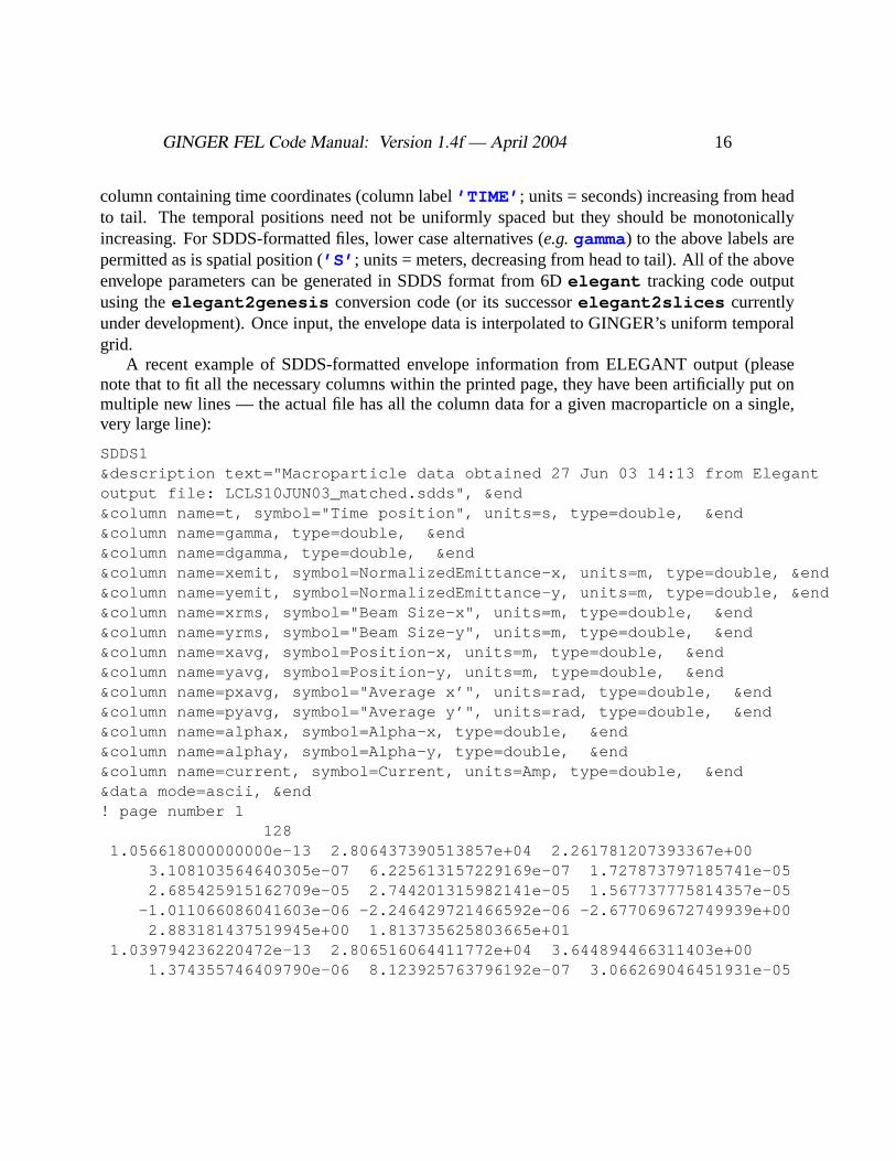
column containing time coordinates (column label’TIME’ ; units = seconds) increasing from headto tail. The temporal positions need not be uniformly spaced but they should be monotonicallyincreasing. For SDDS-formatted files, lower case alternatives (e.g.gamma) to the above labels arepermitted as is spatial position (’S’ ; units = meters, decreasing from head to tail). All of the aboveenvelope parameters can be generated in SDDS format from 6Delegant tracking code outputusing theelegant2genesis conversion code (or its successorelegant2slices currentlyunder development). Once input, the envelope data is interpolated to GINGER’s uniform temporalgrid.
A recent example of SDDS-formatted envelope information from ELEGANT output (pleasenote that to fit all the necessary columns within the printed page, they have been artificially put onmultiple new lines — the actual file has all the column data for a given macroparticle on a single,very large line):
SDDS1&description text="Macroparticle data obtained 27 Jun 03 14:13 from Elegantoutput file: LCLS10JUN03_matched.sdds", &end&column name=t, symbol="Time position", units=s, type=double, &end&column name=gamma, type=double, &end&column name=dgamma, type=double, &end&column name=xemit, symbol=NormalizedEmittance-x, units=m, type=double, &end&column name=yemit, symbol=NormalizedEmittance-y, units=m, type=double, &end&column name=xrms, symbol="Beam Size-x", units=m, type=double, &end&column name=yrms, symbol="Beam Size-y", units=m, type=double, &end&column name=xavg, symbol=Position-x, units=m, type=double, &end&column name=yavg, symbol=Position-y, units=m, type=double, &end&column name=pxavg, symbol="Average x’", units=rad, type=double, &end&column name=pyavg, symbol="Average y’", units=rad, type=double, &end&column name=alphax, symbol=Alpha-x, type=double, &end&column name=alphay, symbol=Alpha-y, type=double, &end&column name=current, symbol=Current, units=Amp, type=double, &end&data mode=ascii, &end! page number 1
1281.056618000000000e-13 2.806437390513857e+04 2.261781207393367e+00
3.108103564640305e-07 6.225613157229169e-07 1.727873797185741e-052.685425915162709e-05 2.744201315982141e-05 1.567737775814357e-05
-1.011066086041603e-06 -2.246429721466592e-06 -2.677069672749939e+002.883181437519945e+00 1.813735625803665e+01
1.039794236220472e-13 2.806516064411772e+04 3.644894466311403e+001.374355746409790e-06 8.123925763796192e-07 3.066269046451931e-05

GINGER FEL Code Manual: Version 1.4f — April 2004 17
2.096679996978939e-05 1.324073235334876e-05 -4.288142261091647e-06-3.625579076306638e-07 6.174544336401088e-07 -2.839956664706138e+00
1.411162359259141e+00 7.586315874850315e+01
et cetera ...
Although SDDS-formatted files are preferred, files with groups of simple columnar output canalso be used. In this case, for each envelope parameter, the code searches the data file to find a linewhich includes the appropriate label (e.g.CURRENT). If GINGER finds such a line, the next linemust contain the integer numbern of (ti, f(ti)) data pairs followed byn rows of 2-column data. Forexample:
CURRENT80.0 150.1.e-15 300.2.e-15 400.3.e-15 450.4.e-15 450.5.e-15 300.6.e-15 200.7.e-15 100.
RMSX8
0.0 88.3e-61.e-15 115.e-6
et cetera ...
3.3.7 Macroparticle Initialization from an Simple ASCII File
GINGER has a limited capability to read in a previously user-generated macroparticle distributionin columnar ASCII-format and use the information as the basis for its own macroparticle generation.The GINGER input variabletrackparfile should be set to the name of the ASCII file whichcontains the phase space information. The information can be used both in FRED- and full time-dependent mode; as of mid-2003, GINGER can directly import multiple independent groups ofmacroparticles from atrackparfile .
At present for single group input, thetrackparfile format should be laid out as follows:(1) an optional number (0-49) of comment lines(2) a single post-comment line, identified by the presence of the string’-----’ ;(3) the next line should contain the integer number of macroparticles (NP ) in the file (this value

GINGER FEL Code Manual: Version 1.4f — April 2004 18
will be used to override the value ofntestp input in the GINGER namelist(4) NP single lines, each containing (x, x′, y, y′, γ) for a single macroparticle, withx and y inmeters, x′ andy′ in radians (i.e. not normalized transverse momentaγx′!), andγ, the Lorentz factor.
To denote multi-group input, the post-comment line which contains the string’-----’ shouldalsocontain the string’MULTISLICE’ . The format is modifed from the single slice case as fol-lows:(3) A line containing the number of groups, the numbers of particles (NP ) per group, and thetemporal spacing between groups. These values will be used to set GINGER values ofnside ,ntestp anddt slice respectively; consequently, one should bear this in mind when generatingthe data externally.(4) Sets of macroparticle data for each group, which should be organized in the following structure:
• (a) A single line with the slice number (integer) and a an arbitrary real number (e.g.the timevalue at slice center) — at present, neither of these values is actually be used by GINGER.
• (b)NP lines of6 individual particle coordinates (x, x′, y, y′, γ, t∗). At presentt∗ is NOT usedand may contain any real value.
• (c) Following each set of individual group particle data (including the last), there must appeara single line containing the string’----’ . This line serves as a separator between groups toimprove eyeball readability of the data file.
For each user-supplied macroparticle, GINGER will supply a longitudinal phase coordinateθusing the same algorithms as its normal load process, which in general is a “quiet start” load — see§3.3.10. In this case, each particle’s 5D coordinate will be clonednfold sym times and each suc-cessive clone will have itsθ offset by2π/nfold sym. Thus, if the external distribution file contains512 distinct particles, each electron beam slice in GINGER will then contain 4096 macroparticlesif nfold sym is left at its default value of 8. Consequently, for FEL purposes the microbunchingoccurs initially only through the application of shot noise effects. For polychromatic runs for whichonly one macroparticle group has been input in thetrackparfile , each of thenside electronbeam slices will haveidenticaldistributions in (x, x′, y, y′, γ).
3.3.8 Macroparticle Initialization from ELEGANT tracking code output data
GINGER now has a limited capability to import actual macroparticle data from ELEGANT codeoutput. To do so,beforemaking the GINGER run, one uses a separate program (xconv eleg ) toread, convert, and finally output ELEGANT-related data in a format usable by GINGER; the For-tran90 source code forxconv eleg is freely available from the GINGER author. When compiledand then run as an executable without any further input,xconv eleg writes a simple “help” fileto the output terminal which illuminates details of its use.

GINGER FEL Code Manual: Version 1.4f — April 2004 19
Briefly, via namelist input, one instructsxconv eleg to construct either a simple, singleslice, ASCII trackparfile in the format described above in§3.3.7 or a “summary” file whichwill be read by GINGER to help construct time-dependent, multi-slice output. The single slicetrackparfile can be used without further changes by GINGER in either FRED- or time-dependent, polychromatic mode. When multi-slice output is desired,xconv eleg analyzes theELEGANT macroparticle data to determine both the mean and first-order temporal derivative oftime-dependent envelope quantities such asI, 〈x〉, 〈x′〉, etc.. It also creates a look-up tableassociating time with time-ordered particle index in the ELEGANT file. Note that this requiresthat the ELEGANT macroparticle datamustbe sorted in monotonically-decreasingtime before us-ing xconv eleg ; fortunately, the SDDS toolkit programsddssort can do this directly. Thesummary information (and the name of the original ELEGANT file) is output to a special ASCII-formatted file. Setting the input variabletracksumfile to the name of this summary file instructsGINGER to read both this file and the original ELEGANT file. Then (within GINGER), a “movingwindow” scheme is applied whose temporal thickness varies to enclose the wanted number of ELE-GANT macroparticles. The scheme also corrects for unphysical, numerical effects which arise froma non-zero window thickness when there are locally, non-zero time-derivatives for mean electronbeam properties (such as〈x〉). As the temporal macroparticle density increases in the ELEGANTfile, the thickness of the moving window and necessary coordinate corrections become correspond-ingly smaller. GINGER directly extractsI(t) from thetracksumfile .
In both single- and multislice cases, only the 5D ELEGANT coordinates (x, x′, y, y′, γ) aredirectly used by GINGER. The longitudinalθ position is independently set by GINGER applyingits “usual” methods (e.g.quiet start with shot noise — see§3.3.10). Please note that the coding andalgorithms for importing multi-slice, ELEGANT macroparticles are quite new and may be possiblyquite buggy.
3.3.9 Importing Macroparticles from the Output of a Previous GINGER Run
For both single- and multi-slice (i.e. scanning mode§3.11)), FRED-mode runs and multi-slice poly-chromatic runs, GINGER can both write and read arstfile containing a full 6D (x, x′, y, y′, γ, θ)macroparticle distribution. Normally, one writes such a file at the undulator exit of one run andthen reads in this information for a subsequent GINGER run to initialize the particle phase spacefor a following (in z) undulator. This capability was developed specifically for multiple undulatorscenarios such as modulator-radiator and harmonic cascade configurations.
To instruct GINGER to write a macroparticlerstfile file at completion, set the input switchl write rst=.t in the main input namelist. The resultant file will be in binary format andnamedrst run name. Note that if the GINGER run uses multiple processors (e.g.the IBM-SP),the file will be written using parallel MPI-IO subroutines and can lateronlybe read by another multi-processor run employing MPI-IO. In single-processor serial mode, the file is written in sequential

GINGER FEL Code Manual: Version 1.4f — April 2004 20
binary format and subsequent GINGER runs in either single processor or multi-processor mode cansuccessfully read the file. For polychromatic runs, therstfile can be very large (≈ 50 kB per sliceper 1024 macroparticles).
In addition to the actual macroparticle distribution, the restart file contains a header including thenumber of macroparticles per slice, the central wavelength, the temporal slice spacing, and variouscomputed envelope parameters (e.g.transverse emittance, energy spread, central energy) for the firstelectron beam slice.
To initialize the macroparticle distribution in a subsequent GINGER run from a previously writ-tenrstfile, set the input variablel read rst=.t andon the execute command line add the string-rs rstfile whererstfile is the file’s name (e.g.rstpalacA1 ). In general, the values readin from therstfile for macroparticle number (ntestp ), temporal slice spacing (dt slice ), num-ber of e-beam slices (nside ) and beam current will override those set by user input. However, inFRED-mode, ifnside=1 in the original run,nside can exceed one if this a parameter-scanningrun. At present, arstfile does not contain longitudinal current profile information. Consequently,if the first undulator GINGER run was done in short-pulse mode (see§3.1), the input file for thesecond and subsequent undulators should also indicate short-pulse mode and include the necessaryinformation (see§3.3.5) to create an identicalI(t) profile.
3.3.10 “Quiet Starts” and Shot Noise
By default (lquiet=.t ), the macroparticles are loaded in phase space with a bit-reversed quietstart with aN -fold symmetry in the longitudinal coordinateθ whereN is set by the input vari-ablenfold sym with a default value of 8. Thus, each macroparticle at(xn, x
′n, yn, y
′n, γn, θn) will
havenfold sym-1 “shadow” macroparticles with the identical(xn, x′n, yn, y
′n, γn), but whose
longitudinal phaseθ is successively incremented by2π/nfold sym. Choosingnfold sym=8will eliminate any initial bunching through the fourth harmonic. In studies of third harmonicbunching, we found it necessary to use seven rather than one shadow particle in order to cancelout all initial bunching at the fourth harmonic (which couples to growth of the third harmonic inthe exponential gain regime). If one is examining bunching through harmonicN , one should setnfold sym=2N+2 and simultaneously increasentestp appropriately to retain reasonable reso-lution in γ and transverse phase space quantities. However, if one is not concerned with accuratemodeling of higher harmonic bunching, pickingnfold sym=2 will give the best resolution of thetransverse phase space and longitudinal energy spread distributions for a given value ofntestp .
When shot noise fluctuations are desired (lshot=.t ) for SASE and similar studies, a randomδθn, which follows a Poisson distribution, is added to each macroparticle’s longitudinal phaseθn.There are no fluctuations in transverse phase space. In fall 1999, the shot noise algorithm was com-pletely rewritten to try to overcome a small bug observed whendgammawas non-zero. Now, eachgroup ofnfold sym macroparticles with the same(xn, x
′n, yn, y
′n, γn) has its own set of random

GINGER FEL Code Manual: Version 1.4f — April 2004 21
shot noise variables (e.g.bunching phase and amplitude at different harmonics of the fundamentalradiation wavelengthλs). The new algorithm appears to ensure that coarse-grained averages overboth< exp iθ > and< exp 3iθ > are correct (and have identical values in the limitnside →∞).One may increase/decrease the effective power level of initial shot noise bunching fluctuations bysetting the scaling factorpwrnoise different from its default value of one.
Shot noise bunching fluctuations may also be included in monochromatic, single-slice FRED-mode runs. This capability is useful if one wants to quickly examine the differences betweenMOPA’s and SASE-like input sources. However, one should remember that, given the absenceof slippage in FRED-mode runs, these fluctuations will be “coherent” (and thus monochromatic) ina longitudinal sense and will also produce a much larger effective input laser power than would betrue for the equivalent polychromatic run. Finally, when the macroparticle distribution is initializedfrom a rstfile created by a previous GINGER run (see§3.3.9), shot noise isnot re-initialized nor isa quiet start possible.
3.3.11 Random Number Seeds
Random number seed input variables (which, in principle at least, should allow the user to repeatexactlyprevious simulation runs) include: (1)iseeds for longitudinal shot noise (see§3.3.10); (2)iseed for the phase and amplitude of the different radiation field spectral components (see§3.4.4);and (3)iseedp for loading instantaneous energy spread (applicable whengam load=’random’ ;see§3.3.4). Due to recent changes in the shot noise algorithm, the variableiseedp no longer af-fects the electron beam’s transverse phase space distribution.
Each of the random seed variables is a 4-element array of decimal (i.e. not octal) integers. A“master seed” is created by a call to the system clock which is then used to generate those seedvariablesnot input by the user. In this case, the generated seed will lead to only the first element ofthe seed array being non-zero. However, if the user inputs a random seed variable (as might be trueto recreate a run), this variable is converted into an array of 4 12-bit integers (i.e. the effective seedis the input seed modulo 2**48). Hence, one should not input a seed greater than∼ 2.8× 10¹⁴. Forruns on the NERSC CRAYs (which have 64-bit size words), the first array input seed element canfully contain the 48-bit effective seed. On platforms with 32-bit integers (including the IBM-SP andmost workstations) one would need two array elements to get the full dynamic range of possibleinput seeds (however, it is not likely any user will do such a large number of runs that 2**32 uniqueseeds proves insufficient!).
For all runs (FRED-mode and polychromatic-mode, single and multiprocessor platforms) withGINGER versions beginning in November 2001, the random numbers have effective lengths of48-bits and are generated by a special numerical package provided by NERSC consultants. Forpolychromatic runs, this package has the distinct and needed property that the random numbersused to generate each beam slice will be independent of both the total processor number used in the

GINGER FEL Code Manual: Version 1.4f — April 2004 22
runAND the particular assignment order of individual processors to individual slices.
3.4 Radiation Field Input Quantities
3.4.1 Optical Beam Size, Transverse Profile, and Waist Position
Paralleling many of the electron beam input variables are those corresponding to the radiation field.The default initial transverse profile is Gaussian (nmg=+2) while “supergaussians” may be specifiedby nmg ≥ +3. The optical waist radiusω0 (≡omg0) corresponds to the1/e point in ~r of theradiation electric field when at a waist minimum. Normally,omg0 is determined by the inputvariableomg0fac , whose default value is 0.8, and the relationomg0≡omgj ×omg0fac , whereomgj is the electron beam radius. This can be overridden by giving a positive value foromg0,Optionally, one may also set the position inz of the focal point (i.e. waist) of the input radiationby giving a value either in meters (zfcmeter ) or in Rayleigh ranges (zfocus ). The RayleighrangeZr ≡ πω2
o/λs. A non-zero value for either leads to curved wavefronts atz = 0. Note thatalthough the electron beam model includes full 3-D non-axisymmetric dynamics which can resultin a non-circular shape, the radiation field and its source terms are presumed axisymmetric (in non-waveguide runs).
3.4.2 Wavelength, Input Power, Slice #, and Temporal Resolution
By default, GINGER presumes a time-dependent, polychromatic problem; this can be overriddenby setting eitherlfred=.t or nside=1 .
The optical wavelengthλs is specified bywavels in meters; this is the numerical value of thecentral wavelength of the effective bandpass in polychromatic runs. If one is running a microwaveproblem (lwavegd=.t ), one may alternatively specify the central frequency in GHz (ghz ). Nor-mally, one uses the input variableplaser to set the initial radiation power in watts.
There are a number of input parameters which define the temporal resolution of the input laserfield. The variablenphoton sets the total number of photon slices. For short-pulse, non-periodicboundary conditions (e.g.oscillator or “transit time” runs),nphoton mustbe input. For periodicboundary conditions in time (e.g.long pulse amplifier runs),nphoton = nside automaticallyandnside rather thannphoton should be input. In any case, the resultantnphoton should bea power of two or three times a power of two in order for the FFT spectral decomposition in thepostprocessor to run properly. To set the total temporal duration followed inz within the simulationand the time interval between individual photon (and electron beam) slices, one should set eitherwindow , which gives the equivalent longitudinal length (in meters) of the temporal window, ornsidep which gives the total number of discrete photon slices with which a particular electronbeam slice will interact over the full length of the wiggler. Numerically,window ≡ (nside /

GINGER FEL Code Manual: Version 1.4f — April 2004 23
nsidep ) × (Lw × λs/λw). Whennsidep =Nw, the full frequency span of the simulation equalscentral frequency (≡ c/λs). In the great majority of situations one will usually setnsidep ratherthanwindow .
At present with two exceptions,nsidep mustbe less or equal tonphoton . The first excep-tion exists for the multiple processor runs on MPP platforms (the CRAY-T3E and IBM-SP) where,nsidep can exceednside . In cases where the slippage length greatly exceeds the so-called“cooperation” or “coherence” length, one should consider employing this strategy to increase thez−resolution and spectral bandpass without having to increase the total number of slices. Thisoption is also useful for optical klystron configurations (§3.7.2).
A second exception exists when the run uses az−dependent field file to initialize the radiationfield for the tail slice of a new run (see§3.4.6). In this case,nside may be as small as 1.
3.4.3 Setting Temporal Profile of Input Radiation Field in Short Pulse Mode
As was true for the longitidinal current profileI(t), in short pulse mode the user may set a differentprofile for the input radiation field than the default time-independent “tophat”. The input variablelaser shape controlsP (t); the available choices are:
(a) parabolic (pulse shape=’parabolic’ )
(b) sawtooth (pulse shape=’sawtooth’ )
(c) Gaussian (pulse shape=’gaussian’ )
(d) hyperbolic tangent (pulse shape=’tanh’ ).The input variablelaser body set the full base width (in seconds) in the case of parabolic or
sawtooth profiles, and the RMS temporal width for Gaussian profiles. For the hyperbolic tangentprofile, laser body is the width between the two points in time where the argument of the tanhfunction go to zero. A shortened tophat profile may also be chosen by giving a positive value forlaser body which is less than the full temporal window. The temporal centroid ofP (t) maybe moved relative to that of the electron beam’sI(t) by giving a non-zero value (in seconds) tothe input variablelaser timing rel . A positive value moves the centroid ofP (t) toward theelectron beam tail, a negative value toward the electron beam head.
3.4.4 “Customizing” the Spectrum of the Input Radiation Field
The user has a fair amount of flexibility in “customizing” the spectrum of the input radiation field.If, for whatever reason, one wants the wavelength of the input radiation field (to whichplaserrefers) to be different from the central wavelength of the simulation (=wavels ), one can set this bygiving a value forwavelsin in meters. If one wants the input radiation power spread out equally

GINGER FEL Code Manual: Version 1.4f — April 2004 24
over a number of spectral bins, one gives a positive integral value fornfreqbin . Bothwavelsinandnfreqbin may be simultaneously input.
To generate a uniform spectrum with equal noise power in each of thenphoton frequency binsencompassing the complete frequency span, one sets the power level per bin by either inputtingwattpbin or wattpghz . The latter variable applies only to waveguide runs. Ifplaser = 0. ,the input radiation field will consistonlyof noise — note this is also true for the central wavelengthwavels . The total input power will benphoton ×wattpbin . Another means of starting witha uniform power spectrum without creating excess power at the central frequency is by giving apositive value forplaser and anegativevalue fornfreqbin in which case the total input poweris plaser exactly. Alternatively, anegativevalue ofampside together with a positive value ofplaser will also generate a flat noise spectrum over the full bandpass (in addition to the powerplaser at the central wavelength) with the total noise power equaling (plaser × ampside2). Anexample of this type of white noise initialization is given in§3.14.2.
Both ampside andwattpbin generate noise which in the time domain has both a randomamplitude and phase. A new input variable,field noise , allows one to generate each componentseparately. A positivefield noise(1) set the normalized RMS strength of the field amplitudenoise while a positivefield noise(2) gives the RMS phase noise in radians; both elements cansimultaneously be positive. This presumes thatplaser is positive.
If one wantsall the non-fundamental power at a single frequency or wavelength, one specifieseithersidewave in meters orsidefreq in Hz. The power level is set by apositivevalue ofampside with Psideband = plaser ×ampside2. A positiveampside without specifying eithersidewave or sidefreq sets up a white noise sideband field amplitudeE(r, t) fluctuating in timebetween±ampside× Eo(r) whereEo(r) is the electric field of the fundamental.
When running in short-pulse mode (i.e. ltransit=.t ), the radiation field is not presumedto be periodic in time and for various reasons GINGER does not initialize allnphoton locationsin time of the radiation field atz = 0 (essentially it needs only to initialize those radiation sliceswhich immediately interact with the electron beam). Consequently, even if one specifies a flat noisespectrum (e.g.via thewattpbin input variable), the post-processor power spectrum willnotshowa flat spectrum atz = 0.
Finally, one may place a sinusoidal temporal chirp on the input radiation’s wavelength by givinga positive value to the input variableampchirp , which defines the peak normalized (i.e. relativeto the simulation bandpass) wavelength shift. In general, one would use such a chirp only for “longpulse” simulations with temporally-periodic boundary conditions.
3.4.5 Saving to and Initializing from Undulator Exit Radiation Field Restart Files
In order to study multiple undulator configurations where the output radiation from one undulatoris used to initialize the field in a following undulator, GINGER has the capability to both read

GINGER FEL Code Manual: Version 1.4f — April 2004 25
and writet−dependent restart field files. This capability exists for both single-slice FRED modeand multi-slice polychromatic mode (including multi-processor mode). To write such a undulatorexit field file, set the main namelist input variablel write fld = .t . The resulting outputfield file will be namedfld run name and is written in sequential binary format. In addition tothe r− and t−dependent radiation field information, a field file also contains various simulationparameters such as the radial grid, the radiation central wavelengthwavels , the temporal slicespacingdt slice , and the number of radiation slicesnphoton .
To read a previous undulator’s field file, the command line switch-f fldfile should be used.The number of radiation slices, temporal slice spacing (i.e. dt slice ), radial grid dimensions andspacing,etc.for the new run will be set from information read from this field file. However, thecentral wavelengthλs in the field file isnot checked at present for self-consistency with the valuegiven in the input file. As explained in§3.3.9, GINGER has an equivalent IO capability for writingand reading macroparticle information from one undulator to the next.
3.4.6 Saving to and Initializing from z−dependent “Beam Head” Radiation Field Files
GINGER also allows a user to save to a special disk file the instantaneous state of the radiationfield “exiting” from the “head” e-beam slice (i.e. slice #nside because GINGER numbers slicesbeginning from the tail). Because GINGER applies slippage atnsidep discrete locations in thewiggler (see§5.5), this “exiting” field information is written at the samez− locations. This fieldinformation can subsequently be used at the beginning of a new GINGER run to initialize the radi-ation field for the new “tail” e-beam slice (i.e. slice #1). This procedure results in the equivalent ofstitching together of two temporally-adjoining electron beam sections;i.e. it is only through suchradiation slices that adjoining electron beam slices “communicate”.
There are two underlying purposes for this feature: (1) To permit a user to “cut” a relatively longelectron beam pulse (as compared with the slippage length) into a number of shorter sections, eachone of which can then be simulated sequentially with GINGER. In effect, each run following thefirst is similar to a short pulse, transit-time run but with no radiation field propagation into vacuumbeyond the electron beam body. (2) To allow a user to do a monochromatic, single-slice “FRED-mode” run using the radiation field from a polychromatic, time-dependent run. The macroparticleoutput diagnostics from such a “FRED-mode” run (via thenspec input variable) can be used toexamine in great detail thez−evolution of an electron beam slice’s longitudinalγ − θ phase space.
To save az−dependent field file, set the input variablel write fld z=.t in the main namelist.This “write”switch may be used in “long-pulse”, periodic BC polychromatic mode only (i.e. loscandltransit are both false) for both single- and multi-processor runs. At the completion of thesimulation, an SDDS ASCII-formatted file namedfld run name.sdds (e.g.fldpalac.sdds )is written to disk. In addition to the complex radiation field information, the numerical values ofthe radial grid are also stored (see§3.12.1) and various simulation parameters such as the temporal

GINGER FEL Code Manual: Version 1.4f — April 2004 26
spacing of slicesdt slice .To use a pre-existingz−dependent field file in a subsequent run, setl read fld z=.t in the
main namelist. Also, the execute line of GINGER must now include the option-f oldfldfile ,whereoldfldfile is thefull name of the previously created SDDS-formatted field file. The newrun can be either in single slice, FRED-mode or multiple slice, polychromatic-mode. In either case,the undulator parameters of the new run should beabsolutely identicalto those of the previous onewhich created the field file. In polychromatic mode, the value ofdt slice read from the field fileset the temporal spacing in the new run and override any user input of variables such asnsidepor window . However,nside can now take on any positive value≥ 4. In polychromatic mode,settingl write fld z=.t in the new run’s input will lead to the writing of a completely newfield file; be careful not to use the samerun name as that of the previous run or the old field filewill get overwritten. In FRED mode, the input variablencurve mustbe set to the previous run’svalue ofnsidep .
The post-processor XPLOTGIN also can generate az−dependent field file from the field infor-mation contained in thepltfile of a previous run; see§4.12 for details.
3.5 Wiggler and Electron Beam Focusing Input Variables
3.5.1 Base Wiggler Input Parameters
Nearly all GINGER runs require the user to set the following input variables to specify the wigglerconfiguration: polarization type withllinear=.t for linearly- or llinear=.f for helically-polarized undulators, wiggle periodwavelw in meters, and whether the wiggler field strength isconstant withz (lcnstwgl=.t ) or not (lcnstwgl=.f ). The total wiggler length (includingdrift spaces, if any) is set equal to the simulation’s longitudinal span in either Rayleigh ranges(zmaxsim ) or meters (zmxmeter ). Beginning in November 2001, an optional “lattice” file maybe used to set wiggler parameters (including pole strength errors and corrective steering) — see§3.5.8 for details.
3.5.2 Constantaw(z) Wiggler Field
The longitudinal dependence of the RMS normalized vector potentialaw(z) can be set in severalways. Aconstant strengthwiggler can be specified by giving one of the following: (1) a positivevalue foraw0, theRMSnormalized vector potential strength of the wiggler on axis; (2) a positivevalue forbw0, thepeak, on-axis wiggler field strength inTesla(note: changed from kG as of Nov2001); (3) settingidesign=1 , following which GINGER computes the appropriate resonant valuefor aw corresponding to the input values forgammar0, wavelw , andwavels . In the last case,no allowance is made for detuning effects such as non-zero emittance and/or quadrupole focusing

GINGER FEL Code Manual: Version 1.4f — April 2004 27
which normally will make peak gain occur at a slightly lower value ofaw. One can multiplicativelyscale the nominally computedaw up or down by giving a value for the input parameterawdmultdifferent from its default value of 1.0.
3.5.3 Using a Predeterminedaw(z) Tapered Wiggler Profile
In some cases one may want to use a previously determinedaw(z) tapered wiggler profile storedin a separate file. To do so, (a) setidesign=0 ; (b) set lcnstwgl=.f ; and (c) specify thename of the wiggler file by either using the-b mybwfile option on the execute lineOR setbwfile= ’mybwfile’ in the main input namelist. Otherwise, GINGER presumes that a taperedwiggler file (generally referred to as abwfile) exists with the namebwrun name (e.g.bwelf3a ).The previously mentioned input parameterawdmult can also be used to scale the values of theinput taperedaw(z).
Normally, such a tapered wiggler file will have been generated by a previous GINGER runoperating in FRED-mode. However, the user can also design such a file (which must be in ASCIIformat) adopting the following prescription:(1) the first line is simple text. Normally this contains some details about the GINGER run whichgenerated it but the user may put anything here.(2) The second line contains a single integer equal to the number (≡ N AW) of z positions to follow;a minimum of two such positions is needed.(3) N AWsingle lines containing two floating point variables: thez position (in meters) and theon-axis value foraw(z).
By default, GINGER will use a cubic spline fit to determine the localaw(z) from the discretevalues ofaw input in the wiggler file. If one desires abrupt shifts in eitheraw or its z-derivative, aspline fit require putting in many additional points to force such a shift in the fit. However, one canavoid this annoyance by setting the input namelist variablel bw linearfit=.t which replacesthe spline fit with simple linear interpolation ofaw between adjacent points inz.
3.5.4 Tapered Wiggler Self-Design in FRED-Mode
In FRED-modeonly, setting idesign=2 and lcnstwgl=.f uses GINGER’s self-design al-gorithm to compute a tapered wiggler. Theseaw(z) values will be written out to thebwfileat ncurve equally spaced locations inz. The algorithm determinesaw(z) by keeping its pon-deromotive well phaseψ(z) constant for an imaginary test particle initially located atψ=psir0 ,γ=gammad0, and transversely atr=rdesign . Default values arepsir0=0.4 andgammad0= gammar0. The switchlphase10=.t limits the z-rate of change ofaw(z) caused by theelectromagnetic field phase variationdφ/dz ; normally, this is only a concern for high gain mi-crowave FEL’s. In order to account for the radial increase ofaw off-axis and the radially local
GINGER FEL Code Manual: Version 1.4f — April 2004 28
value of the radiation field phaseφ(r), the parameterrdesign or rdesfac determines the radiusof the imaginary design particle, whererdesign = rdesfac × omgj . with a default valuesrdesfac=0.707 . A sample tapered wiggler input file is given in§3.14.1.
3.5.5 Wiggler Focusing: Simple and Curved Poleface
Wiggler focusing is controlled by a number of optional input parameters. Helical wigglers havenatural focusing in both transverse planes while linear wigglers have focusing only in the non-wiggle plane (y-direction in GINGER for non-waveguide FEL’s). If no other focusing than the“simplest”, natural wiggler focusing is desired, no additional input parameters are required.
However, for longer wigglers with linear polarization, one generally needs focusing in the non-wiggle plane. One method to achieve this is by using “curved” (aka“parabolic”) pole piece focusingby inputting a value forrkxkw which increases the focusing in the wigglex plane while simulta-neously reducing the focusing in the non-wiggley plane.rkxkw must lie within the interval[0, 1].Setting rkxkw=0.707 provides equal strength focusing in both planes, which is normally thedesired result.
3.5.6 External Focusing: Continuous Quadrupoles and/or Ion Channels
If one desires external focusing is addition to that provided naturally by the wiggler, GINGERprovides a number of choices:
(1) To add constant,z-independent, quadrupole focusing in the wiggle plane (andsimultane-ouslyequal magnitudedefocusingin the non-wiggle plane), specify a positive value forquad0 ,which has units of Gauss/cm, orwavelx , the desired betatron wavelength (m) in the wiggle plane.Alternatively, a positive value forfocusfac , which measures the ratio of the quad-inducedk2
β,x
relative to the value ofk2β,y associated with the natural wiggler focusing, will also give wiggle
plane focusing. Ifaw varies withz (i.e. a tapered wiggler), so will the actual quad gradient whenfocusfac is non-zero. Whenfocusfac=0.5 , the net focusing (i.e. quadrupolar plus wiggler)will be equal in the wiggle and non-wiggle planes. In general, one will inputquad0 , focusfacor rkxkw only for linearly-polarized wigglers.
(2) One may add “strong” and equal focusing in both planes by settingzlion equal to thewanted (external) betatron wavelength in meters for a particle atγ =gammar0. This is a ”kluge”to simulate the long-wavelength effects of AG quadrupole motion but ignores the short wavelengthAG flutter. zlion also simulates the effects of a focusing ion channel (hence the name).

GINGER FEL Code Manual: Version 1.4f — April 2004 29
3.5.7 External Focusing: Discrete Quadrupole Magnet Lattices
GINGER now can include discrete quadrupole magnets in a periodic lattice, which may range froma simple FODO system to more complicated systems such as triplets. At present, only one periodiclattice can be defined but each lattice cell may include up to ten individual quadrupoles, each ofwhich can have its own length and gradient. The necessary input variables are:(1) quad lattice zperiod , the full lattice period (m)(2) quad lattice zstart , the beginning position (m) of the first lattice cell(3) quad lattice zend , the end position (m) of the last lattice cell (the default value of106 mexceeds any reasonable wiggler length)(4)quad lattice mag gradient , an array containing the individual magnet gradients in G/cm.A positive gradient corresponds to focusing in thex-plane(5) quad lattice mag start andquad lattice mag zend , arrays defining the beginningand end (m) of the individual quadrupolesrelativeto the beginning of each periodic lattice cell(6) quad lattice nmag, the number of magnets in each cell. This is an optional parameterwhich need not be input because GINGER uses the input gradient values to determine how manymagnet truly exist in the lattice.
To make sure that each individual magnet will be “hit” at least once by GINGER’s PDE inte-grator, the maximum step sizehub min meters should be set to approximately 75% or less of theshortest quadrupole’s length (see§3.12 for information on numerical integrator parameters). Also,individual magnets should not overlap one another. At present, all magnets have “hard” edges andno fringe field effects are calculated.
3.5.8 Lattice Files, Wiggler and Quadrupole Errors, and Steering Corrections
As of November 2001, GINGER now has the capability for linearly-polarized undulators (only)to model the transport effects of pole excitation errors, quadrupole offset and gradient errors, anddipole steering corrections. As the treatment of these new features matures, they may evolve invarious ways including input format, physics description,etc. Currently, to input such errors andsteering corrections (if any) and model their effects, the user should set the main namelist input vari-ablelattice file equal to the name of special ASCIIlattice file. This file (which is normallyproduced by an external programxwigerr ; see§3.5.9 below) has the following format:
(1) a single line containing the string “GFLD”, starting in the first column
(2) an arbitrary number of comment lines with the last one signified by the string “$$” in thesecond and third

GINGER FEL Code Manual: Version 1.4f — April 2004 30
(3) a Fortran90 namelist&lattice which should contain the following variables:gammar0,wavelw , aw0 (these values should agree exactly without those input in the main GINGER namelist),nelement (the total number of discrete sections, including drifts, which describe the undulator)and the variablesnquad and nsteer which define the number of individual quadrupoles andsteering elements to be described.
After the namelist, the sets of individual quadrupoles, steering dipoles, and wiggler elementsare read (in that exact order). The individual quad format is the string “QUAD” in the first 10characters, followed by five real numbers giving the beginning and end z-position in meters, thequad gradient in T/m, and the x- and y-offsets in meters. The steering element format is “DIPOLE”in the first 10 characters, followed by 3 real numbers giving the z-position in meters and the x- and y-integrated fields in T-m. The wiggler element format is either “WIGGLER” or “DRIFT” in the first10 characters, followed by four real numbers. For the case of “WIGGLER”, these numbers comprisethe initial z-position in meters, the nominal value of aw0 (without errors), the pure “phase error”component of aw0, and the effective “kick error” component of aw0 (which is acts as a transversedipole magnetic field in the wiggle plane). These error values are usually specially-averaged valuesover multiple wiggle periods (see§3.5.9). For the “DRIFT” case”, only the first two numbers areused which give the beginning and end z positions in meters of the drift.
Note that the configuration described in thelattice file , including drift space and quadrupolelattice information if present, override any values set in the main GINGER input file. Conse-quently, to avoid inadvertent confusion, the user is advised that when modeling wiggler errors,the lattice file should serve as the primary source of undulator description.
3.5.9 Generation of Lattice File via the XWIGERR Program
A simple F90 program (xwigerr ), freely available from the author, generates for a linearly-polarized, constantaw wiggler the individual undulator pole errors and quadrupole gradient andoffset errors (if any), computes the appropriately-averaged (see below) errors in phase and drift, theproper transverse steering (if any) including the optional effects of beam position monitor offseterrors, and then writes a properly-formattedlattice file (see§3.5.8) to be used by GINGER.
xwigerr uses a simple F90 namelist&inwigerr which as much as possible uses the sameinput variable names as GINGER for equivalent items. However, units inxwigerr are MKSfor both longitudinaland transverse variables, which leads to some inconsistency with GINGERfor items such asxoff . Electron beam input parameters includegammar0 for Lorentz factor(alternativelyenergy in MeV may be given),xoff andyoff in metersfor initial beam offset,andxprime andyprime in radians for initial beam angle. Main undulator variables arewavelw(or period ) for undulator period,zmxmeter for wiggler length,rkxkw to set the amount ofcurved poleface focusing, andaw0 for RMS normalized vector potential. Undulator error variablesincludeaw rms err for RMS fractional aw error, iseed aw for the optional random number

GINGER FEL Code Manual: Version 1.4f — April 2004 31
seed for these errors, andnw avg which is the number of undulator periods over which to speciallyaverage the pole strength errors (default value 1). One should not average over a length greater thanabout one-eighth the effective betatron periodλβ of the system. Drift sections are described usingthe same variables as those in the lattice formulation of the main GINGER namelist (see§3.7.1).
If there are discrete external quadrupoles, the lattice may be described by the exact samevariables as in the main GINGER namelist (e.g.quad lattice zperiod ; see§3.5.7). Ad-ditional quad input variables includequad lattice rms offset for the RMS offset in me-ters,quad lattice rms grad err for the RMS fractional error in quadrupole gradient, andmag units which is either’T/m’ (default) or ’G/cm’ . The optional random number seediseed quad can be used to generate the offset and gradient errors.
If discrete dipole steering correction kicks are wanted, the following namelist variables ap-ply: zsteer beg end for z-interval in which steerer are placed (default full wiggler length),zsteer period for the period interval of steerers, andzsteer0 which gives location of anoptional steerer before the beginning of the periodic lattice — if used, this is normally placed atthe beginning of the wiggler. In place of these three variables, the user may instead input discretesteererz−locations via the real arrayzsteer . One may also input RMS beam position moni-tor transverse errors viabpm rms offset in meters and a random number seediseed bpm forsuch. Presently, the steerers are presumed to have infinitesimal longitudinal length and GINGERapplies them as delta-function transverse kicks.
Thexwigerr namelist variablesoutfile set the main output filename (≡ the GINGER inputlattice file ), sdds outfile the SDDS-formatted filename which contains the predictedbeamx− andy−centroid versusz (including effects of steering), anddescription an≤ 80-character string may be used to set a comment in theoutfile .
3.5.10 Checking Beam Transport Properties through the Lattice
In order to check the beam transport (i.e. beam envelope size and centroid motion) through thewiggler’s focusing lattice, it may be useful to do a single slice, FRED-mode run with the input pa-rameternspec , which controls the number of phase space dumps, being set to a moderate positivevalue. Then using thel plot xy=.t switch in the XPLOTGIN preferences file (see§4.13) forcesthe postprocessor to producex − y macroparticle scatter plots at various z-locations. History plotsof envelope variablesσx , σy , < x >, and< y > versusz are also automatically produced in sin-gle slice FRED-mode runs. To speed up this sort of debugging run, one can setlfixfld=.t toprevent anyz-evolution of the radiation field, andluncoupl=.t to decouple the macroparticles’sz-evolution inγ andθ from the radiation field. Also, the switchlmovxyt should be left at itsdefault value of.true. in order to retain macroparticle betatron motion.
For debugging and investigatory purposes, GINGER has a number of other logical switcheswhich control details of the physics included in the macroparticle motion. Whenlawaxis=.t ,

GINGER FEL Code Manual: Version 1.4f — April 2004 32
the radial variation inaw is ignored in the KMR equation for longitudinal phase advance. Using thisswitch leads to an unphysical variation inγ‖ over the betatron orbits of individual macroparticles.The switchlmovxyt=.f preventsall macroparticle betatron motion. The switchlxvxfix=.tfreezes motiononly in thex plane and was implemented for TE0n mode waveguide studies.
A new logical switch added in 2003 can (in effect) force the radiation field centroid to followthat of the electron beam in the transverse plane. Whenl centroid axis=.t , the transversecenter of the axisymmetric radiaiton field is artifically translated to that of the electron beam whenevaluating the electric field terms in the energy loss and phase dedrivatives for each individualmacroparticle. However, the undulator fieldaw is evaluated at the truex − y position. This allowsthe user to get an indication of phase drift effects for offset/kicked e-beams while still permittingthe use of an axisymmtric field solver.
3.6 Wakefield, Space-charge, and Waveguide Specification
3.6.1 Wakefields and Uniform External Accelerating/Decelerating Fields
In some situations, the effects of longitudinal wakefields or other sources of energy loss or gainmay be important to simulate. The simplest type of longitudinal field to model is that consistingof a superimposed uniform (in each oft, z andr) accelerating or decelerating longitudinal elec-tric field or equivalent energy loss term (e.g.incoherent synchrotron emission). The gain or lossterm is set by the input variabledgamdz0 , the change in Lorentz factorγ per meter. A positivevalue accelerates the macroparticles. A somewhat more complicated, time-dependent energy losscan be chosen by using the input variablewake profile in conjunction withdgamdz0 . Settingwake profile=’sinusoid’ will make the external∂γ/∂z sinusoidal in time with a time pe-riod equal to the simulation’s periodic window together with a peak amplitude ofdgamdz0 . Thischoice can give some indication of the resonance-detuning effects of longitudinal wakefields.
Beginning in late 2002, GINGER can now use externally-generated wakefield information tosimulate the effects of time-dependent (but presentlyz−independent) wakefields. This feature onlyworks in short-pulse mode (i.e. not in long pulse mode with temporally periodic boundary condi-tions). The wake information should be contained in an SDDS-formatted ASCII file whose nameis set by the input variablewakefile . This file must contain at least three columns: one shouldbe the longitudinal position in the beam either given in time (column label’t’ or ’time’ , units= seconds) increasing from head to tail or space (’S’ or ’s’ ; units = meters) decreasing fromhead to tail. A second column must contain the electron beam current (label’current’ ; units =amps) while the third should have the longitudinal wake (label’wake ez’ or ’WAKE EZ’ ; units= volts/m). Apositivevaluedecelerateselectrons. Note: theI(t) current profile in thewakefilewill override a profile set by the user either in the input namelist or in an external beam data file(§3.3.6).

GINGER FEL Code Manual: Version 1.4f — April 2004 33
Here is an example of SDDS-formatted wakefield file:
SDDS1&description
text =’’lcls-s2e-200pC-CSR-adj-time.slices;pipe r,sigma= 2.50E-03 5.90E+07;rough period, ampl= 5.00E-05 1.00E-07;geo-wake gap,T= 0.010" &end¶meter name="Peak_Current", fixed_value=2561.00122,type=double, units=Amps, description="peak current" &end&column name="time", units=seconds, type=double
description="Time" &end&column name="current", units=Amps, type=double
description="Beam Current" &end&column name="wake_EZ", units=volts/m, type=double
description="Total Wakefield Longitudinal Electric Field" &end&data mode="ascii", lines_per_row=0 &end
128-8.900E-14 12.9196 0.000E+00-8.763E-14 26.5499 -1.858E+02-8.626E-14 52.1701 -5.828E+02-8.489E-14 101.8216 -1.328E+03-8.352E-14 207.5974 -2.866E+03-8.215E-14 306.6741 -4.695E+03-8.078E-14 472.4413 -7.986E+03-7.941E-14 683.1721 -1.239E+04-7.804E-14 882.4681 -1.778E+04-7.667E-14 1107.1880 -2.475E+04
et cetera ...The temporal spacing of the wake information should be monotonic in longitudinal position but
need not be evenly spaced. A cubic spline fit is applied to the wakefile data for interpolation to theuniform temporal grid of the simulation. A simple Fortran90 code, primarily due to H.-D. Nuhn ofSLAC, which calculates the wake associated with resistive losses and beam pipe surface roughnessis available from the author.
3.6.2 Longitudinal Space-charge
When modeling high current microwave FEL’s such as the LLNL/LBNL ELF experiment, longitudi-nal space charge forces can become important and affect both particle microbunching and radiationfield gain. If lspacech=.t , GINGER follows these forces using the same approximations as didthe original FRED code; the interested user can find physics details in the paper by E. T. Scharle-mannet al., Nucl. Instr. Meth. Phs. Res.A250, 150 (1986). The space charge switch also works for

GINGER FEL Code Manual: Version 1.4f — April 2004 34
non-waveguide FEL’s. For most problems, inclusion of space charge forces will increase runningtimes by a factor of two or more. The effects oftransversespace charge fields are not modeled byGINGER; their net force relative to the “pressure” term corresponding to the electron beam trans-verse emittance is usually very small due to cancellation by the electron beam’s azimuthal magneticfield.
3.6.3 Specification of Waveguide Properties
By settinglwavegd=.t , one instructs GINGER to propagate the radiation within a rectangularwaveguide, in which case the radiation’s longitudinal wavenumberkz 6= ωo/c. The waveguidedimensions are specified viaxwidth andywidth , both in cm. Rather than using radial griddingas is true for non-waveguide simulations, in waveguide mode GINGER adopts a Cartesian gridin they plane and, by default (lte21=.f ), follows the TE01, TE03, TE05, ... modes. For thesemodes, the electromagnetic field is independent of the wiggle plane directionx, the (normally) largerwaveguide dimension (i.e. xwidth ≥ ywidth ). The code does not actually decompose the fieldinto the various TE modes; their strength is diagnosed only in the postprocessor through analysis ofthe spatial variation of the field on the grid. Note that when doing polychromatic runs, there isnovariation of group velocity withω or k⊥; in other words, the slippage velocity is independent ofω.
Whenlte21=.t , the code follows the TE01, TE21, TE41, ... modes and, somewhat confus-ingly, one must set the waveguide “on its side” by making the long dimension in they direction(this is required because of the internal gridding iny). In this latter case, the TE41 mode will followa cos (πx/xwidth)× cos (4πy/ywidth) spatial dependence with the coordinate origin lying at thecenter of the waveguide. Note: if one desires to set a positive quadrupole focusing in the wiggleplane, one still uses a positive value forwavelx or quad0 even when the wiggle plane is parallel toy for lte21=.t . This is also true for other focusing parameters such asrkxkw , andfocusfac .Internally, the code computeskβ with the wiggle plane parallel tox and then exchanges thex andydirections.
Since most microwave FEL’s operate at relatively low energies, the approximationβ‖ ≈ 1 −1/2γ2
‖ , which GINGER normally uses, can lead to inaccuracies. These can be prevented by settingthe input variablelbetapar=.t , which forces exact evaluation ofβ‖ in the equation determiningthe macroparticle longitudinal phase derivativedθ/dz.
3.7 Drift Space and Dispersive Section/Optical Klystron Input Variables
3.7.1 Periodic Drift Spaces
GINGER is capable of including spatiallyperiodicdrift spaces in which the wiggler field strengthis zero. Such spaces physically might be used for diagnostics and/or discrete quadrupole focusing.

GINGER FEL Code Manual: Version 1.4f — April 2004 35
At present, only one such periodic drift space lattice can be set but within the period, up to five indi-vidual drift spaces may be defined. Four input variables in the main namelist specify the drift spacelattice: (1)DL zperiod specifies the period in meters of the drift space lattice; (2)DL zstartspecifies the point at which the first drift space “lattice” period begins, with a default of the start ofthe wiggler; (3)DL zend specifies the point at which the last period of the drift space lattice ends,with a default of the end of the wiggler; and (4) the input arrayDL zdrift beg end specifies thephysical beginning and end in meters of each of the individual drift spacesrelativeto the beginningof each drift space lattice period.
For example, settingzmxmeter=100. , DL zperiod=10. , DL zstart=25. ,DL zend=75. , andDL zdrift beg end = 3. 5. 8.8 9.5 defines a 100-m wigglercontaining five drift space ’super-periods’ of ten meters each. Within each period, are two individualdrift spaces, one 2-m long and the other 0.7-m long. The first 2-m drift space begins atz = 28 mand the first 0.7-m long drift space begins atz = 33.8 m.
Within the drift space, both the electrons and radiation propagate “normally” but withaw ≡ 0which eliminates any coupling. Hence, there is radiation diffraction but no refraction or gain. Inpolychromatic mode, GINGER does compute the actual physical slippage occurring in drift sec-tions. In general, this slippage is much smaller than for normal wiggler sections (the opposite fromoptical klystron sections - see below).
3.7.2 Dispersive Sections/Optical Klystron Configurations
The net gain per pass in a low gain oscillator can often be significantly enhanced placing a disper-sive drift section with a non-zero R56 value in the central region of the undulator — this resultantconfiguration is generally called an “optical klystron”. Such devices have also on occasion beenproposed for single pass amplifier configurations to enhance gain and reduce overall wiggler length.GINGER has some ability to simulate optical klystron configurations and, at present, a wiggler mayinclude up to 5 individually unique dispersive sections.
To define their properties, one must setl extra=.t to force GINGER the read thein extranamelist within the input (and/or template file). Then, within thein extra namelist, the lo-cations of the individual dispersive sections in meters or are set by giving values in the interval[zstmeter ,zmxmeter ] to the arrayz OptKly (or t OptKly in Rayleigh ranges). The physi-cal lengths of the dispersive sections are controlled by the arrayOptKly zlen in meters. Theselengths define the distance that the radiation field propagates without interacting with the electronbeam (aw ≡ 0 as with drift sections). However, diffraction does occur in the dispersive section.Hence, the effective number of wiggle periods available for gain will be reduced from that of thesame length wiggler with no drift or dispersive sections.
The strengths of the dispersive sections can be set three different ways: directly by the arrayR56 in meters, and indirectly by either the arrayOptKly zwgl equiv or the arrayd colson .

GINGER FEL Code Manual: Version 1.4f — April 2004 36
The arrayOptKly zwgl equiv (defined in meters) sets R56 in each section to the equivalentdispersion produced by a wiggler of that length.d colson is defined as the ratio of the R56 dis-persion produced in each dispersive section divided by that which would be produced by a wigglerof lengthzmxmeter containing only “normal” wiggle periods (i.e. an undulator with neither dis-persive sections nor simple drift sections). Thus, ifd colson(2)=0.2 , the wiggler period is0.1 m, and the total undulator length is 10 m (i.e. 100 true periods), the second dispersive sectionwould produce dispersion equivalent to that normally produced in0.2 × (10/0.1) = 20 wigglerperiods. Mathematically,d colson ≡ 0.5 × R56/(Nw × λs), whereNw is the number of wigglerperiods. Note: previous versions of the GINGER manual incorrectly indicated that only the trueundulator length (i.e. that calculated by ignoring drift and dispersion sections) would be used forcalculating the dispersion. However, the code does not do this and thus adding a drift section canchange the equivalentR56 calculated for a givend colson . Consequently, for most simulations,it is probably safest to useR56 to set the dispersion.
In polychromatic mode, GINGER presumes that each dispersion section will produce extraphysical slippage between the e-beam slice and the radiation field. Numerically, the slippage ineach section is set tod colson ×Nw × λs. In reality, the exact value of the slippage will de-pend upon details of the magnetic design of each optical klystron and might be quite different fromthis presumed value. Note that whennsidep is given as an input parameter (as is normally donefor polychromatic runs), the increased slippage in dispersion sections effectively leads to shortenedslippage interactionz−intervals in each klystron andlengthenedinteraction distances in the normalwiggler sections.
For large values ofd colson , one can end up with nearly all the slippage advances occurringin the dispersive sections and very few in normal wiggler sections. This consequently reduces thez-resolution of the diagnosticpltfile. To provide partial alleviation for this problem, when runningwith multiple processors on a MPP platform such as the T3E, one may setnsidep larger thannside — this permits greaterz−resolution. Moreover, for each individual dispersion section,diagnostic output will be written out at no more than onez−location to thepltfile. This change wasmade to preventpltfiles from being completely dominated by output from the dispersion sections,where there is little physical change in either the e-beam or radiation. To more fully alleviate thisproblem and give the user more control over the slippage produced by a dispersive section, thenew input variablezslip equiv OptKly sets the slippage in terms equivalent undulator length.Thus, ifλw = .04 m andλs = 1.0µm, zslip equiv OptKly = 1.0 gives25.0µm of slippage.
One should note that only the differential phase advance (relative to a hypothetical resonantparticle) in a dispersion section is calculated for each macroparticle;i.e. the physical slippage men-tioned in the previous paragraph doesnot directly affect a macroparticle’s longitudinal phaseθ.Numerically,θout ,n ≡ θin ,n + (γn−gammar0) × 2π×d colson ×Nw. The rationale behinddecoupling the physical slippage and the dispersive phase slippage was to avoid having the user

GINGER FEL Code Manual: Version 1.4f — April 2004 37
have to worry about zero order (inγ) phase jumps inθ as compared with the more important as-pects of the energy-dependent phase jump. Nonetheless, there is an option to include an additionalenergy-independentphase jump by inputting a non-zero value fortheta drift in radians - thisterm doesnot lead to additional physical slippage between the radiation and electron beam in time-dependent mode. One might usetheta drift to unphysicallyadjust the net jump in the e-beamlongitudinal bunching phase relative to the radiation phaseφ,
3.8 Oscillator Mode Input Variables
GINGER currently has a limited capability to model FEL oscillator configurations. Settinglosc=.tin either FRED- or polychromatic mode instructs GINGER to model a “short” electron beam(i.e. nside < nphoton and non-periodic boundary conditions in time) with the radiation pulsepropagating between two mirrors. In fact, when GINGER (when running on a single processor)models a single-pass amplifier with non-periodic boundary conditions (i.e. ltransit=.t ), it se-cretly forceslosc to be true and treats the run as a single-pass oscillator. As mentioned previously,oscillator runs require linking the GINGER executable with the IMSL mathematical subroutinelibrary. Presently, GINGER can do oscillator mode runsonly in serial (single-processor) mode.
Nearly all oscillator input parameters are specified in thesecondnamelistin extra ; settinglosc=.t or l extra=.t in thefirst forces the reading of the second namelist. Oscillator inputparameters include:npass which specifies the total number of passes;npass out (default value≡ 1), the interval (in passes) to write the output radiation field to the postprocessor file;z m1 m2,the intra-mirror cavity length in meters;rc m1andrc m2, the radii of curvature in meters for thetwo mirrors respectively;rad mr, the actual radius of the mirrors in meters; andr cavity , thetotal surface reflectance (in power) of the two mirrors taken together. This value ofr cavity doesnot include the effects of the finite mirror size; hence, the net reflectivity will be less. The inputparameterd synch sets the cavity detuning length measured as a fraction of the slippage lengthLs. Note that, following Colson’s formalism, apositivevalue ofd synch shortens the actual cavitylength so that radiation field energy near the head keeps arriving earlier in time relative to the headof the e-beam pulse in successive passes.
3.9 Segment Mode Description and Input Variables
A new type of run mode within GINGER is “segment mode” which permits the user to break thesimulation of a very long electron beam pulse into multiple runs. This capability was added tohandle the situation in which the electron beam is many hundreds of so-called coherence lengthslong which requires the use of many thousands of electron beams slices for adequate simulation.For the∼ 200-fs LCLS, a slice spacing of≈ 10−17 sec leads to a need of≈ 20, 000 slices, generally

GINGER FEL Code Manual: Version 1.4f — April 2004 38
more than a thousand CPU hours, andpltfile sizes of tens of GB’s. Doing all this within a single runis not at all attractive.
In segment mode, one first simulates the tail segment (necessary because the radiation propa-gates from beam tail toward the beam head) by setting the input variablel segment mode=.t .This switch prevents periodic boundary conditions and also automatically saves thez−dependentradiation field of the “head” slice within the tail segment (see§3.4.6) in an output field file. Theuser must input the number of e-beam slices via thenside variable and also the temporal spacingvia either thensidep or dt slice variables. The capability to exploit time-dependent envelopeparameters (§3.3.6) or time-dependent macroparticle phase space reconstruction (§3.3.8) is fullyavailable within segment mode. For the first (i.e. tail) segment, it is safest to input the exact tempo-ral location of the tail slice by giving a value fort start end ebeam(2) .
After the run for the tail segment has been completed, one then simulates the next segmentby forcing GINGER to read in the field information (vial read fld z=.t in the main inputnamelist and use of the the option-f fldfile on the execute line); it is not necessary to setl segment mode=.t because the use ofl read fld z=.t instructs GINGER that it will besimulating a beam segment without periodic boundary conditions. For this second segment and allfollowing ones, one should force the writing of a newfldfile via thel write fld z=.t switch.Because afldfilecontains information concerning the temporal spacing between slices and the tem-poral location of the “head” slice corresponding to the radiation field information, it is not necessaryto input eitherdt slice or t start end ebeam for the second and following segments. Like-wise, the value ofnside need not be identical from one segment run to another. For the secondsegment and beyond, it may also be smaller quantitatively beyond. thannsidep since all tne nec-essary field information is in thefldfile. For post-processing purposes, it is best thatnside be apower of two or three times a power of two. For SASE runs, one should be careful to make surethat a different random number seed for shot noise inputiseeds is used for each segment (see§3.3.10 and§3.3.11). Also, one should obviously choose some sort of run name sequence by whichthe different segments can be identified straight-forwardly.
The outputpltfile from each segment run is fully self-contained and can be post-processed nor-mally. At present (late 2003), there is no automatic way to continguously weave the post-processoroutput from different segments together. However, via the creation of either ASCII or SDDS-formatted output files, a reasonably adept user can do so manually for time-resolved scalar quantitiessuch as output power or bunching. To date, no such capability exists for linking the spectral outputfrom different segments.
3.10 Harmonic Cascade Capability
Due to the increasing interest in reaching short wavelengths by use of harmonic FEL cascades, afair amount of work has been put into GINGER to allow the user to simulate such. The typical

GINGER FEL Code Manual: Version 1.4f — April 2004 39
configuration of such a cascasde is a series of paired undulators which alternately coherently mod-ulate (i.e. microbunch) the electron beam at a wavelengthλm and then allow the electron beam toradiate coherently at a harmonic wavelengthλm/N with N ranging from 2 to as much as 5 or 7.The output from each radiator is then used in the following modulator to microbunch the electronbeam modulator at wavelengthλm/N . This sequence can be continued through many stages, withharmonic multiplication occuring in each modulator-radiator pair. In general, the input radiation forthe first modulator is provided from a coherent, external source.
At present, a separate GINGER run must be done foreachmodulator and radiator (primar-ily because no coding exists to permit a jump in harmonic number within a given run). Bothmonochromatic (FRED-mode) and polychromatic simulation of cascades are supported (although“short-pulse” mode has not been extensively tested).
For each modulator run, one either uses an external radiation source (viaplaser ) or the ouputradiation from the previous radiator stage via afldfile (see§3.4.5) and the-f fld file optionon the execute line. If the cascade is configured such that a “fresh” electron beam segment isused for each modulator (via use of a delay chicane - not modeled in GINGER), the electron beaminput parameters should be chosen as in a normal (i.e. non-cascade) run. If the effects of shotnoise are to be included, be sure to setlshot=.t . If on the other hand, the same electron beamsegment previously used in the upstream radiator will be used, one must read in the restart filevia the l read rst=.t input switch -rs rstfile option on the execute line. In order tocreate a macroparticle restart file for the following radiator run, be sure to set the input switchl write rst=.t in the main input namelist. Please see§3.3.9 for details concerningrstfile IO.
For a radiator run, onemustread in macroparticle restart file as explained in the previous para-graph. One alsomust instruct GINGER that one is interested in radiation at a harmonic of theprevious modulator wavelength by giving an integral value≥ 2 for the main namelist variablenhar mult . GINGER uses this value to multiply the longitudinal phaseθ for each macoparticlein the rstfile and also to force the value of the radiatorsλs to be equal to the previous modulator’sλs/nhar mult . However, due to some coding intricacies, one must also setwavels in the radia-tor input file to the correct value. Finally, one must setl write fld=.t to write afldfilewith theoutput radiation field from the radiator.
If the “fresh” beam configuration is not used in the cascade (i.e. the same macroparticles are usedthroughout the cascade), one must be careful to set the input vairablenfold sym to a sufficientlyhigh value to account to prevent any artificial numerical microbunching at thefinal wavelengthdesired to be modeled. For example, if the input wavelength for the first stage modulator is 240 nmand the ultimate final radiator wavelength is 4 nm (i.e. a total harmonic upshift of a factor of 60),nfold sym should be at least 120 in the first stage. This can lead to a huge number of particlesbeing necessary to simulate the full cascade in polychromatic mode. Consequently, from both asimulation and gain point of view, the “fresh beam” approach is extremely attractive. For self-consistency in polychromatic simulation, one should adopt periodic boundary conditions in time

GINGER FEL Code Manual: Version 1.4f — April 2004 40
(i.e. “long pulse” assumption) for this approach.Finally, in many situations one is likely to use a dispersive section (see§3.7.2) following one
or more of the modulator undulators. For purposes of optimizing the R56 parameter in terms ofmicrobuncing, the author has found it most efficient to put the dispersive section at thebeginningofthe following radiator rather than at the end of the preceding modulator because this allows one to doartifically short radiator length runs to optimize the dispersive section. Furthermore, the diagnosticsconcerning bunching and macroparticle phase space scatterplots may be more informative whenexamining the wanted harmonic.
3.11 FRED-mode Parameter Scanning Capability
3.11.1 General Parameter Scanning Input Variables
On certain occasions, a user might want to know how sensitive a FRED-mode output parameter (e.g.power, saturation position inz, etc.) is to a particular input parameter (e.g. beam current, energyspread,etc.). One could follow a “brute force” approach and do a number of separate FRED-mode runs with the individual input decks scanning the appropriate range in the desired variableinput parameter. However, an alternative beckons due to the multidimensional nature of the time-dependent GINGERpltfile, It was relatively easy to change the post-processor to produce apltfilewith the scanning variable (e.g. beam current) replacing time as the independent third dimension(with the first two dimensions beingr andz). Likewise, GINGER’s monochromatic FRED-modewas then extended to be able to loop through the varying input parameter.
To use this capability, the input deck should be modified as follows: 1)nside should be setto the number of different values the input variable will take; in general this will probably bein the range 8-32 and need not be related to a power of two; 2) setlfred=.t to indicate amonochromatic FRED-mode scan rather than a polychromatic run; 3) setl extra=.t to forcethe reading of the&in extra namelist; 4) within the&in extra namelist, set the input variableparam name to one of the following allowed strings:AW0 PLASER CURRENT BRIGHT EMIT EMITMKS GAMMA DGAM DGAMDZ0
BETA TWISS ALPHATWISS RMISMATCH THETADRIFT D COLSON R56Note: the variablesmustbe given in upper case (capital letters); 5) set the scanning range for theinput variable by giving values toparam min andparam max in the&in extra namelist.
The default is a linear scan over the full range of the input variable. Ifl log param=.t , thenthe scan is done with a geometric scaling (i.e. equal increments in the logarithm as one probablywould want to use if scanningPLASERover the range 1 kW to 1 GW).DGAMrefers to scanning inthe instantaneous energy spread whileAW0is for scanningaw in a fixed (untapered) wiggler. Scansin aw can be very useful if the FEL parameterρ is quite small and one is trying to maximize gain ina situation where 2D or emittance effects are important. If eitherBETA TWISSor ALPHATWISS

GINGER FEL Code Manual: Version 1.4f — April 2004 41
are given, the values will be used forboththex andy planes (which may be inconsistent for unequalfocusing or a FODO lattice). As mentioned in§3.3.6, use of an “experimental data” file containingt−resolved beam envelope data in a multislice FRED-mode run results in parameter-scanning runwith time being the independent variable.
If one wants to do a multistage undulator run involving restart files, one can do a scanning moderun over a downstream stage so long as the immediate upstream stage (i.e. that which produced amacroparticle or field restart file) was done in single slice mode withnside=1 . However, evenin this situation the downstream run cannot scan in a quantity which attempts to change e-beamparameters such asGAMMA. One is allowed to do downstream scans in quantities such asAW0orR56. Such might be useful in trying to optimize a radiator wiggler or dispersion section immediatelyfollowing a modulating section (for which only a single slice run needed to be done). Note, whenthe beam current is the scanning parameter in an multislice upstream run, all downstream runswill use the same current variation. If a multislice upstream run used any other scanning variable(e.g.laser input power), a downstream run involving a macroparticle or field restart file can only“scan” over the effective variation of the restart file form slice to slice (e.g.one cannot scan overaw
in the downstream undulator).
3.11.2 FRED-Mode Parameter Scanning using Multiple Processors
When doing a FRED-mode parameter scan using the NERSC IBM-SP with its massively-parallelarchitecture, it is possible to use multiple processors simultaneously for a significant speedup. Forthe IBM-SP, one need only specify the wanted number of processors on the GINGER execute line(see§2.5.2), making sure thatnside is evenly divisible by the number of processors. Since theFRED-mode scanning main loop is “embarrassingly” parallel (i.e. no slippage effects), multipro-cessing here does not involve the complexity of message processing from one processor to another.
3.12 Grid and Numerical Integrator Input Parameters
3.12.1 Simulation Grid
For non-waveguide FEL simulations, GINGER uses a non-linear, expanding radial grid that nearthe axis is nearly linear inr and then exponentially expands for larger. The outer grid boundary isgiven byrmaxsim in centimeters while the number of radial grid zones is set bynnd ≤ 63. Theregion over which the grid is linear is controlled by the input parameterrlinear such that
rn = rlinear× sinh [(n− 1) ζ]
whereζ is determined by the conditionrnnd = rmaxsim . A good choice forrlinear is theexpected radiation mode size. In waveguide mode, the gridding is uniform in they plane.

GINGER FEL Code Manual: Version 1.4f — April 2004 42
3.12.2 Numerical Integrator Input Variables
The most important numerical integrator input parameter iseps , the maximum normalized errorallowed by the predictor-corrector for a step inz to be successful. Typical values lie in the range10−5 to 10−4 with the average step size being proportional toeps+1/2. One may also set the initialstep size (dt ) the lower bound on step size (hlb ), and the upper bound on step size (hub , defaultvalue0.5λw/Zr), all measured in Rayleigh lengths.hub mis the equivalent upper bound in meters,The final valuehlb also has a lower bound set by machine accuracy. The input parametermaxstepis an upper limit to the number of integrator steps permitted during a full integration interval inz (≡ Lw /ncurve for FRED mode andLw/nsidep for polychromatic mode). If this limit isexceeded the code will abort. The default value is 10,000 and a user should normally not need tosetmaxstep any higher but there can be situations where one might need a larger value. Runningwith a very high value is potentially dangerous in terms of excessive CPU costs if the code beginsacting bizarrely.
3.13 Output Diagnostics Control Variables
There are relatively few input variables to GINGER which control the contents and details of theoutput files generated for later analysis by the post-processor code XPLOTGIN. When GINGERis run in a polychromatic, multi-slice mode for a single pass amplifier, radially-resolved radiationfield quantities and various slice-averaged electron beam quantities are written at the end of every“interaction” interval inz, includingz = 0. Thus, there arensidep + 1 positions inz, nphotonpositions in time, andnnd positions inr for which both the real and imaginary components ofEare written to thepltfile. As explained in§3.4.5, one can set a switch in polychromatic mode towrite out a special radiation field file for restart purposes. For all modes, macroparticle diagnosticswritten to thepltfile for each slice as a function of(t, z) currently include the values of averagemacroparticle energy, the RMS energy spread, and the average bunching at the fundamental andpossibly additional harmonics.
When GINGER is run in monochromatic “FRED” mode (lfred=.t ), one uses the input vari-ablencurve to set the number of positions inz at which electron beam and radiation field diag-nostics will be written to thepltfile. In this mode, one can also request the creation of a simpleASCII datfile via the l datfile=.t switch. This file will contain simple columnar outputs ofitems such as the radiation power, macroparticle bunching, RMS delta gamma,etc.. For platformssuch as DOS/Windows for which presently the post-processor has no direct graphical capability, thisswitch is default to.true. . However, it can be used for all platforms in single slice, FRED-mode.This file can be used directly bygnuplot as the non-data rows are begun by “##”.

GINGER FEL Code Manual: Version 1.4f — April 2004 43
3.13.1 Macroparticle Bunching Diagnostics
Historically previous to 2001, GINGER had always computed macroparticle microbunching at thefundamental wavelength relative to the ponderomotive phaseψ ≡ θ + φ. The original rationale forthis choice was that in many cases there could be significant radiation phase front curvatureφ(r);this is especially true when the radiation mode size is significantly smaller than electron beam size.However, for comparison to coherent transition radiation (CTR) measurements, the bunching shouldbe calculated relative to a a hypothetical plane wave (i.e. θ rather thanψ). and it is necessary to do soat higher harmonics (because the field phaseφ is unknown in GINGER at present). Consequently,beginning in April 2001, the microbunching at the fundamental wavelength will now be calculatedrelative to a plane wave.
Beginning in GINGER versions of April 2001 and later, one can output diagnostics of mi-crobunching at harmonic number greater than 3. To do so, the vector input variablenhar io shouldbe set to the integer values wanted; notenhar io(1)=1 (i.e. the fundamental) is hard-wired andcannot be overridden. For example,nhar io(1)=1 2 3 4 5 7 will cause microbunching atharmonics from 1 through 5 plus the 7th to be output. The microbunching is a “complex” quantitywith both amplitude and phase; a new feature of the postprocessor allows one to calculate the powerspectrumb(λ) of the microbunching (see§4.5).
Another new diagnostic introduced in late 2003 is one which determines the correlation betweenparticle phaseθ and energyγ. If the string ’GAMBUNCH’ is included in the input for the mainnamelist string variablescalar diags , GINGER will calculate and ouput to thepltfile at eachz−diagnostic location the value of
∑j exp(iθj) (γj − γ). This diagnostic is useful for determining
the bunching in a modulator section of a multistage FEL.
3.13.2 Macroparticle Phase Space Scatterplot Output
Beginning in 2003, GINGER can now write macroparticle phase space information in a dumpspcfilefor both monochromatic FRED-mode runs and multislice polychromatic mode runs. Since eachscatterplot involves50kB of information for each 1024 macroparticles, one should be sparing in thenumber of slices in time for which output will be written. For all modes, the discretez locations forthe phase space information can be set in multiple ways:
(a) a positive integral value for eithernspec or nz scatterplot sets the number of suchlocations which include and are evenly spaced betweenz = 0 andz =zmxmeter .
(b) a positive real value todz scatterplot defines thez−spacing of the scatterplots (againbeginning withz = 0 and ending withz =zmxmeter
(c) inputting discrete values to real arrayz scatterplot

GINGER FEL Code Manual: Version 1.4f — April 2004 44
For multislice polychromatic (time-dependent) runs, the user has the choice of two positiveinteger input variables to define thet interval between scatterplots at a givenz:
(a) nt scatterplot which defines the total number of slices (approximately evenly spacedin t) for which scatterplot output will be generated
(b) nt scatterplot moddefines the interval in slice number between diagnosed slices.As of 2002, the output longitudinal phase of the individual macroparticles is now measured
relative to a hypothetical plane wave (i.e. θi) rather than their position relative to the instantaneousponderomotive well (i.e.ψi). However, the latest versions of thespcfilenow include both radial gridinformation and the complex radiation field for each output slice which allows the calculation of theponderomotive phaseψ if wanted.
3.13.3 Reducing thez-Frequency of Diagnostic Output to thePltfile
For a polychromatic, non-oscillator mode run, GINGER by default writes the radiation field andmacroparticle diagnostics for each slice at the end of every interaction (slippage advance) intervalin z. One can reduce thez−frequency of these diagnostics (and thus the total size of thepltfile), bysettingn diag mod to an integral value greater than one. A choice of three, for example, wouldproduce output at the end of every third interaction interval for each slice. Runs with long opti-cal klystron dispersive drift sections will generally produce output at fewer than (nsidep + 1 )z−locations (see§3.7.2). The postprocessor automatically deals with this change.
In multi-pass, oscillator mode, GINGER writes out field and particle quantities at only onezlocation (the physical end of the wiggler) for each pass. This is true for both monochromatic andpolychromatic oscillator runs. Hence, there is noz-resolved information within the wiggler. Theinput parameternpass out controls the frequency at which diagnostic information is written tothepltfile. The default ofnpass out=1 is equivalent to output being written every single pass; achoice ofnpass out=2 would lead to output every other pass,etc..
3.14 Sample GINGER and XWIGERR Input Files
The following input files were chosen as examples of the various types of FEL configurations whichcan be modeled with GINGER. They and some post-processor output CGM files are available within the “tar” archiveGNXTEST.tar which is stored in the public HPSS space at NERSC describedin §2.2.
3.14.1 Monochromatic, “Paladin” Tapered Wiggler Self-Design:inpalSD
This input file adopts “nominal” LLNL Paladin parameters and calculates the time-independent(i.e. monochromatic) power gain from a 10-MW input laser atλs = 10.6µm over a 80-mm period,

GINGER FEL Code Manual: Version 1.4f — April 2004 45
linearly-polarized 25-m long wiggler. Curved pole faces (rkxkw=0.707 ) are adopted for e-beamfocusing. This run also uses the GINGER tapered wiggler self-design algorithm (viaidesign=2 )to computeaw(z) and sets the design macroparticle at 0.285 cm. There will be 1024 macroparticleswith only 2-fold longitudinal symmetry as we are not concerned with third harmonic growth. In ad-dition to the creation of a “normal” post-processor file (namedpltpalSD ) which will have data at51z−locations, GINGER will also output abwfilenamedbwpalSD containingaw(z), a macropar-ticle dump file (spcpalSD ) containing 6-D phase space snapshots at six equally-spaced positionsin z down the wiggler (i.e. every 5 meters beginning atz = 0). This problem requires 3.9 seconds onthe Killeen Cray-J90 (SV1 processor), 8.0 seconds on a 1.1-GHz Pentium-3M under Linux, and 5.2seconds on the IBM-SP at NERSC. To run this problem one would type:xginger r=palSD
Paladin FRED-mode run - B=2.e5 ; 2.5 kA ; 10 MW input ;25-meter tapered wiggler self-design ; eps=6.7e-5 ;inpalSD $
&injmg = -1current = 2.5e3bright = 2.5e5gammar0 = 98.85lshot = .fntestp = 1024nfold sym = 2wavels = 1.06e-5plaser = 1.0e7wavelw = .08llinear = .trkxkw = 0.70711lcnstwgl = .fidesign = 2rdesign = 0.285lfred = .tncurve = 50nz scatterplot = 6rmaxsim = 4.nnd = 45zmxmeter = 25.0eps = 6.708e-5/END
3.14.2 Paladin Sideband Growth in a Tapered Wiggler:inpalacSTD
This simulation initializes a white noise spectrum to provide a seed for sideband growth to aPaladin-like e-beam. Withwattpbin=2000. ), the total noise power is 192 kW. The input valueidesign=0 andlcnstwgl=.f indicate that theaw(z) is pre-determined and tapered; it will be

GINGER FEL Code Manual: Version 1.4f — April 2004 46
read from an external file (bwpalac ). By default, there are periodic temporal boundary conditionswith 80 slippage advances over 25 m (or approximately every 30 cm, much smaller than the gainlength) and 96 separate e-beam slices. This example took 1250 seconds in serial mode (1 CPU)on the IBM-SP, 230 seconds in 6-CPU parallel mode on the IBM-SP, 1280 seconds in 4-CPU par-allel mode on the Cray-T3E, and 6630 seconds on a 400-MHz Pentium II under Linux. To runthis case on a single processor, the user would type:xginger r=palacSTD b=bwpalacTo run this case on an IBM-SP employing 4 processors in parallel, the execute line would be:xginger-mpp -procs 4 r=palacSTD b=bwpalac
Test case to study Paladin sideband growth -needs wiggler file bwpalacB=2.e5 ; 2.5 kA ; 10 MW input ; 25 meter wigglernsidep = 80 ; 96 e- slices ; eps=5.e-5 ;inpalacSTD $&injmg = -1current = 2.5e3bright = 2.5e5gammar0 = 98.85ntestp = 2048lshot = .fwavels = 1.06e-5plaser = 1.0e7zfocus = 0.0zmxmeter = 25.0wavelw = .08llinear = .trkxkw = 0.70711lcnstwgl = .fidesign = 0lfred = .fnside = 96nsidep = 80wattpbin = 2000.iseed = 453774rmaxsim = 4.nnd = 47dt = 1.e-6eps = 5.e-5/END
3.14.3 Long pulse, LCLS 1.5A SASE x-ray FEL: inlcls fodoSb
This particular input file sets up a full polychromatic simulation of the proposed LCLS x-ray FELat SSRL/SLAC, operating at 1.5 Angstroms with a 14.35-GeV electron beam. By default, this sim-
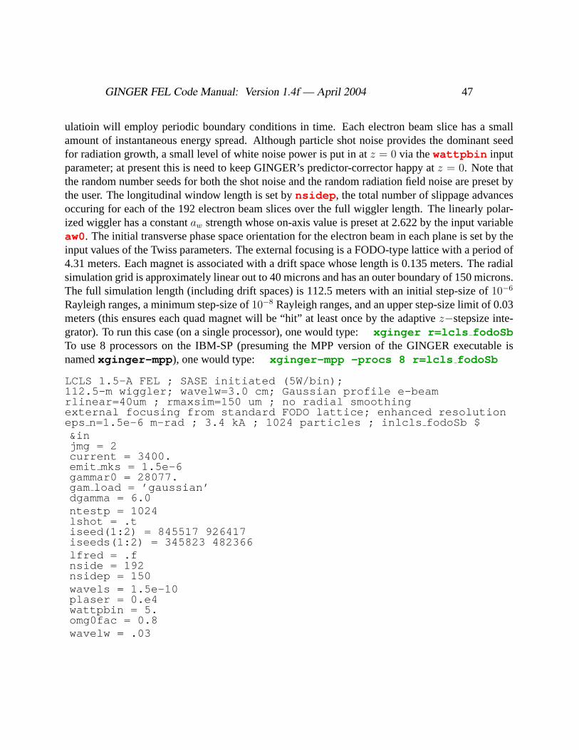
GINGER FEL Code Manual: Version 1.4f — April 2004 47
ulatioin will employ periodic boundary conditions in time. Each electron beam slice has a smallamount of instantaneous energy spread. Although particle shot noise provides the dominant seedfor radiation growth, a small level of white noise power is put in atz = 0 via thewattpbin inputparameter; at present this is need to keep GINGER’s predictor-corrector happy atz = 0. Note thatthe random number seeds for both the shot noise and the random radiation field noise are preset bythe user. The longitudinal window length is set bynsidep , the total number of slippage advancesoccuring for each of the 192 electron beam slices over the full wiggler length. The linearly polar-ized wiggler has a constantaw strength whose on-axis value is preset at 2.622 by the input variableaw0. The initial transverse phase space orientation for the electron beam in each plane is set by theinput values of the Twiss parameters. The external focusing is a FODO-type lattice with a period of4.31 meters. Each magnet is associated with a drift space whose length is 0.135 meters. The radialsimulation grid is approximately linear out to 40 microns and has an outer boundary of 150 microns.The full simulation length (including drift spaces) is 112.5 meters with an initial step-size of10−6
Rayleigh ranges, a minimum step-size of10−8 Rayleigh ranges, and an upper step-size limit of 0.03meters (this ensures each quad magnet will be “hit” at least once by the adaptivez−stepsize inte-grator). To run this case (on a single processor), one would type:xginger r=lcls fodoSbTo use 8 processors on the IBM-SP (presuming the MPP version of the GINGER executable isnamedxginger-mpp ), one would type: xginger-mpp -procs 8 r=lcls fodoSb
LCLS 1.5-A FEL ; SASE initiated (5W/bin);112.5-m wiggler; wavelw=3.0 cm; Gaussian profile e-beamrlinear=40um ; rmaxsim=150 um ; no radial smoothingexternal focusing from standard FODO lattice; enhanced resolutioneps n=1.5e-6 m-rad ; 3.4 kA ; 1024 particles ; inlcls fodoSb $&injmg = 2current = 3400.emit mks = 1.5e-6gammar0 = 28077.gam load = ’gaussian’dgamma = 6.0ntestp = 1024lshot = .tiseed(1:2) = 845517 926417iseeds(1:2) = 345823 482366lfred = .fnside = 192nsidep = 150wavels = 1.5e-10plaser = 0.e4wattpbin = 5.omg0fac = 0.8wavelw = .03

GINGER FEL Code Manual: Version 1.4f — April 2004 48
llinear = .tlcnstwgl = .tidesign = 1aw0 = 2.622rkxkw = 0.
quad lattice nmag = 2quad lattice zperiod = 4.310quad lattice zend = 500.quad lattice mag zstart = 1.9775 4.1325quad lattice mag zend = 2.0975 4.2525quad lattice mag gradient = 4440.0 -4413.0betax twiss = 16.0552alphax twiss = -0.8918betay twiss = 19.8175alphay twiss = 1.0952DL zperiod = 2.155DL zdrift beg end = 1.920 2.155rlinear = 40.0e-4rmaxsim = 150.e-4nnd = 47zmxmeter = 112.5dt = 1.e-6hlb = 1.e-8hub m = 0.03eps = 4.0e-05/END
3.14.4 Sample LCLS Wiggler Error Input File for XWIGERR Program
This input file is used by thexwigerr program to generate wiggler and quadrupole errors togetherwith corresponding steering for an LCLS run with parameters similar to the previous input file.The outputlattice file lcls bpm-50off.latcan subsequently be used by GINGER. The net ef-fects of the pole errors (normalized RMS size = 1 part in103, much larger than actually wantedfor the LCLS) are averaged over 6 wiggle periods, which leads to an output interval of 18 cm.Note that one needs to specifymag units = ’G/cm’ for the input quad magnet gradients be-cause the default unit used inxwigerr is T/m. The steering lattice has a 4.31-m period whichbegins at 2.04 m; there is an additional steerer atz = 0. The rms transverse position error forthe beam position monitors and the quadrupole centroids is set to 50 microns (note: this is morethan 10X greater than is expected for the actual LCLS). To run this input file, one would typexwigerr i=inlcls wigerr-A
sample input file for XWIGERR programLCLS-type undulator; 0.16-period undulator period averaginginlcls wiggerr-A

GINGER FEL Code Manual: Version 1.4f — April 2004 49
&INWIGERRgammar0 = 28077.zmxmeter = 120.00period = 0.03nw avg = 6aw0 = 2.622aw rms err = 0.001iseed aw(1) = 135598bpm rms offset = 50.e-6iseed bpm(1) = 1114011712quad lattice rms offset = 50.e-6iseed quad(1) = 123721quad lattice nmag = 2quad lattice zperiod = 4.310quad lattice zstart = 0.quad lattice zend = 500.quad lattice mag zstart = 1.9775 4.1325quad lattice mag zend = 2.0975 4.2525quad lattice mag gradient = 4440.0 -4413.0mag units = ’G/cm’DL zperiod = 2.155DL zdrift beg end = 1.920 2.155zsteer0 = 0.zsteer period = 4.31zsteer period = 2.155zsteer beg end(1) = 2.04outfile = ’lcls bpm-50off.lat’description = ’6 period avg w; quad + pole errors + steering’/END
3.14.5 Example of a LCLS-parameter Template File Use:inlcls-errA2
This input file relies upon the use ofinlcls fodoSb as a “template” file and extends it by us-ing the wiggler error file produced in the previous example. By settingdgamma, the input fileinlcls-errA2 also lowers the energy spread to 3.0 from the template’s 6.0, the normalizedemittance to 1.0 mm-mrad, increases the number of macroparticle’s to 2048, resets the randomnumber seeds for the energy spread and shot noise, and adds anx-offset of 30 microns to the initiale-beam centroid (remember, GINGER nominally uses units of centimeters for transverse quanti-ties such asxoff andyoff ). To run this example on a single processor, the user would type:xginger r=lcls-errA2 t=inlcls fodoSb
LCLS 1.5-A FEL ;relies on template file inlcls fodoSbemit -> 1 mm-mrad; 30 micron x-offset; dgamma -> 3.0 ;

GINGER FEL Code Manual: Version 1.4f — April 2004 50
2048 particles;uses lattice file lcls bpm-50off.latinlcls-errA2 $
&indgamma = 3.0ntestp = 2048iseedp(1:2) = 2001 1345iseeds(1:2) = 1492 2001xoff = 30.e-4emit mks = 1.0e-6lattice file = ’lcls bpm-50off.lat’/END
3.14.6 Example of a NERSC Batch Script to run an LCLS Case
The following script can be submitted to the NERSC batch system for the IBM-SP with thellsubmit command to run the previous example (lcls-errA2) under batch. Four multiproces-sor “nodes” are requested, each with 16 processors, for a grand total of 64 processors. NERSCstrongly suggests that batch runs be done in the user’s “scratch” directory, which thus requires thatthe necessary executables, input, lattice, and template files all be copied to that space. If the MPP-ready GINGER executable exists in a directory which lies in the user’s “path”, it is not necessaryto copy the executable. After completing the GINGER simulaton, the 64 resultantpltfiles will beconcatenated into one big file which then will both be stored in HPSS archive space and written tothe user’s local disk space.
#COMMENT: sample script for a GINGER LCLS batch run##@ class = regular#NOT USED: class = debug#NOT USED: class = premium##@ shell = /usr/bin/csh#@ node = 4#@ tasks per node = 16#@ network.MPI = csss,not shared,us#@ wall clock limit = 1:55:00#@ notification = always#@ job type = parallel#@ output = $(jobid).$(stepid).out#@ error = $(jobid).$(stepid).err
#COMMENT: following ’’mpXXX’’ should be replaced with# user’s NERSC account ##@ account no = mpXXX#@ environment = COPY ALL

GINGER FEL Code Manual: Version 1.4f — April 2004 51
#@ queue
set echoecho "IBM-SP seaborg batch run"alias cd cdalias cp cpalias rm rm -rf
#---copy GINGER executable and needed files to scratch space:cd $SCRATCHset IDIR = $HOME/FEL/LCLScp $HOME/FEL/MPP-OBJ/xginger ./xginger-mppset name = lcls-errA2set infile = in$namecp $IDIR/$infile .set template = inlcls fodoSbcp $IDIR/$template .latfile = lcls bpm-50off.latcp $IDIR/$latfile .
#--------------------- execute instructions:echo "beginning actual GINGER execution"xginger-mpp r=$name t=$template
#------concatenate multiple pltfiles to one big one:rm plt$namecat plt0*$name > plt$name#------save pltfile, fldfile to local disk space:cp plt$name $HOME/FEL/BATCHcp fld$name* $HOME/FEL/BATCH
#-------------------- HPSS storage instructions:echo "beginning HPSS storage sequence"hsi << EORcd BATCHput plt$namequitEOR
echo "completed BATCH run"exit
3.14.7 LCLS-parameter Tail Segment Run:ins2e-tail-1nC-A
This input file relies upon the use of an LCLS-parameter “template” file (e.g.inlcls fodoSb )for undulator and radiation input and extends it by giving the appropriate input describing thetail segment of a multi-segment run. In this particular class ELEGANT tracking particle in-formation will be used to reconstruct a detailed 6D phase space via use of a summary file(i.e. s2e-1nC-CSR-tail-slice-sum.time ). This summary file also contains the name of

GINGER FEL Code Manual: Version 1.4f — April 2004 52
the ELEGANT macroparticle file to be used in the phase space reconstruction. A temporal slicespacing of 12 attoseconds will be used here (and for all following segment runs in this series). Thetail slice of this run is located att = 105 fs (with absolute time defined in the ELEGANT macropar-ticle file). The head slice (for this particular run) will be at a point191× 12 as earlier in time. Thisparticular example is a SASE run and diagnostics from only every 4th slippage-advance locationin z will be saved to thepltfile. A z−dependent field file will be written to disk to permit properinitialization of the next electron beam segment in this run series. To run this example on a singleprocessor, the user would type:xginger r=s2e-tail-1nC-A t=inlcls fodoSb
Sample of input file for first (tail) segment rundata from emma’s standard ELEGANT S2E-ICFA03 output;current appropriately adjusted; full SASE runins2e-tail-1nC-A $
&intracksumfile = ’s2e-1nC-CSR-tail-slice-sum.time’current = 300.nfold sym = 2lfred = .fiseeds(1:2) = 142312 131203lshot = .tt start end ebeam(2) = 105.e-15l write fld z = .tl segment mode = .tplaser = 0.01wattpbin = 1.nside = 192dt slice = 1.2e-17n diag mod = 4/END
3.14.8 “Mid” Segment Run: ins2e-tail-1nC-B
This input file continues the multisegment run begun with the input file of the previous ex-ample. It both reads in thez−dependent field file of the previous run (and will write a newone following its own completion) and the tracking code summary file. Note that is not nec-essary to set eitherdt slice or t start end ebeam(2) as they are effectively containedwithin the field file. Furthermore, thenside in this run is quite different from that of theprevious, tail segment run. To run this example on a single processor, the user would type:xginger r=s2e-tail-1nC-B t=inlcls fodoSb f=flds2e-tail-1nC-A.sdds
runs to look at mid pulse region in LCLS for ICFA03-S2Edata from emma’s standard elegant outputfull SASE run using summary file using fldfile from run A

GINGER FEL Code Manual: Version 1.4f — April 2004 53
ins2e-tail-1nC-B $
&intracksumfile = ’s2e-1nC-CSR-tail-slice-sum.time’nfold sym = 2lfred = .fiseeds(1:2) = 7321122 131203lshot = .tl write fld z = .tl read fld z = .tplaser = 0.wattpbin = 1.nside = 1024n diag mod = 8/END
3.14.9 Initial Modulator in Harmonic Cascade: inlux-500A-240nm-mod
This input file corresponds to the first modulator stage of a harmonic cascade with parameters sim-ilar to the LUX project being studied at LBNL. The input external laser has a 240-nm wavelengthand 1 GW power which is focused to a 300-micron waist 1.25 m into the undulator. A dispersivesection atz = 3.6 m is used to improve the microbunching tob1 ≈ 0.5 before the electron beam isinserted into the next undulator. A 16-fold symmetric quiet start is employed (such a high numberis neeeded because the radiator will utilize the 5th harmonic of 240 nm). Bunching harmonics 1through 6 will be diagnosed via thenhar io input variable. A macroparticle restart file will bewritten at the end of the dispersive section. This is a single-slice, FRED-mode run and scatterplotphase space diagnostics are requested every 1.2 meters in the “normal” undulator and also at the endof the dispersive section atz = 4.0 m. This run took 27.1 seconds on a Sunblade150 (equivalent to a2-GHZ PC). To run this example, the user would type:xginger r=lux-500A-240nm-mod
Hypothetical LUX laser modulator at 240 nm ;500 Amps; 2 pi mm-mrad ; delta gamma = 1.381 GW input laser focused at z=1.25 m;dispersive section with R56=12 microns (d colson = 0.75)inlux-500A-240nm-mod $
&injmg = 2current = 500.emit mks = 2.0e-6gammar0 = 4894.dgamma = 1.38gam load = ’gaussian’
ntestp = 16384

GINGER FEL Code Manual: Version 1.4f — April 2004 54
lshot=.fnfold sym = 16nhar io = 1 2 3 4 5 6wavels = 240.0e-9plaser = 1.0e9zfcmeter = 1.25omg0 = 300.e-4wavelw = .12llinear = .tidesign = 1awdmult = 0.995rkxkw = 0.70711
nside=1l write rst = .tlfred = .tncurve = 40z scatterplot = 1.2 2.4 3.6 4.0rmaxsim = 0.25rlinear = 120.e-4nnd = 55zmxmeter = 4.0
dt=1.e-5hlb = 1.e-8eps = 4.e-5maxstep = 10000l extra = .t/END
&in extraz OptKly = 3.6d colson = 0.75OptKly zlen = 0.39/END
3.14.10 Radiator in Harmonic Cascade:inlux-500A-48nm-rad
This input file corresponds to the 48-nm wavelength radiator which follows the 240-nm modulatorof the previous example. For these parameters,≈ 185 MW of power is radiated by the end of theundulator. This example took 160 seconds on a SunBlade150. To run this example, the user wouldtype: xginger -r lux-500A-48nm-rad -rs rstlux-500A-240nm-mod
48-nm radiator; 4.0-m long undulator;bunched beam from 240-nm modulator rstfileinlux-500A-48nm-rad $
&in

GINGER FEL Code Manual: Version 1.4f — April 2004 55
wavels = 48.0e-9nhar mult = 5plaser = 100.zfocus = 1.0omg0 = 100.e-4wavelw = .075lcnstwgl = .tllinear = .tidesign = 1awdmult = 0.9975rkxkw = 0.70711nside=1lshot=.fl read rst = .tl write fld = .tlfred = .tncurve = 50rmaxsim = 0.12rlinear = 120.e-4nnd = 55zmxmeter = 4.0z scatterplot = 0.0 2.0 4.0
dt=1.e-5hlb = 1.e-8eps = 4.e-5maxstep = 10000/END
3.14.11 Second Modulator in Harmonic Cascade:inlux-500A-48nm-mod
This input file corresponds to the second modulator stage of the LUX-like harmonic cascade cor-responding to the previous 2 expamples. Since we are presuming we are starting with a “fresh”electron beam, we will use the first modulator input file as our template and only change thoseitems which are unique to this stage (e.g.wavelength, radiation from upstream radiator rather thanexternal laser,etc.).
This simulation took 25.5 seconds on a SunBlade 150. To run this example, the user would type:xginger r=lux-500A-48nm-mod t=inlux-500A-240nm-mod f=fldlux-500A-48nm-rad
500-amp 48-nm modulator to bunch beam; 5.0-m long undulatorfld from 48-nm radiator: fldlux-500A-48nm-radAaw chosen for peak bunching;disp section: R56=8.48 microns (equiv. d colson = 1.25)inlux-500A-48nm-modA $
&in

GINGER FEL Code Manual: Version 1.4f — April 2004 56
wavels = 48.0e-9plaser = 1.wavelw = .075aw0 = 5.4385awdmult = 1.0
l write rst = .tzmxmeter = 5.3z scatterplot = 3.0 4.0 5.0 5.3l extra = .t/END
&in extraz OptKly = 5.0R56 = 8.48e-6OptKly zlen = 0.29/END
3.14.12 Short pulse, UCLA single-pass SASE expt.:inUCLAt2
This input file is used to simulate the behavior of the mid-1990’s UCLA SASE IRFEL whichoperated at a central wavelength of 10.6 microns. This is a “short-pulse” simulation as set byltransit=.t . With a period of 15 mm and 0.6-m length, the wiggler is 40 periods long and,choosingnsidep=20 , the photon slices advance forward one electron beam slice every two wig-gle periods. Withnside=60 , the full width of the electron beam is 3 slippage distances long,which is equivalent to 1272 microns or 4.24 ps in time. The electron beam has a parabolic cur-rent profile (viapulse shape ) in time which leads to a FWHM pulse of 3.0 ps.nphoton=96is greater thannside+nsidep+1 as required. Shot noise is initialized vialshot=.t and theinitial radiation is composed a flat noise spectrum with exactly 100 nanowatts per bin. There is noexternal focusing in the wiggler plane, but there is presumed to be a simple lens atz = 0 whosefocal length in the wiggle plane (x) is set to 0.35 meters viaxfocus mtr . The initial beam sizein x is 0.03 cm (=300 microns); the y-size is set to be in equilibrium with natural wiggler focusing.This is a relatively fast running problem and took∼3400 CPU-seconds on the NERSC IBM-SP.The execute line to run this problem is:xginger r=UCLAt2
test input file for UCLA IR expt ;4 ps beam with a parabolic longitudinal profile (== 3.0 ps FHM)gaussian profile transversely;I b=200 A ; 0.1% energy spread ;linear wiggler with no external focusing ;shot noise input sourceinUCLAt2 $
&injmg = 2

GINGER FEL Code Manual: Version 1.4f — April 2004 57
current = 200.emit mks = 5.e-6gammar0 = 33.5dgamma = 0.0335gam load = ’gaussian’ntestp = 2048lshot = .tiseeds(1:2) = 22813 23785wavels = 10.6e-6plaser = 0.wattpbin = 1.e-7iseed(1:2) = 43242 97543omg0 = 0.04zfocus = 0.5ltransit = .tpulse shape = ’parabolic’nsidep = 20nside = 60nphoton = 96zmxmeter = 0.6rmaxsim = 0.75rlinear = 0.05nnd = 47wavelw = .015llinear = .tlcnstwgl = .tidesign = 1xfocus mtr = 0.35omgjx = 0.03dt = 1.e-5hlb = 1.e-8eps = 1.0e-04/END
3.15 Names and Default Values for GINGER Input Namelist Parameters
!..RADIATION FIELD Parameters:!
nmg = 2 ! radiation field radial profile indexomg0fac = 0.8 ! scale factor for input radiation field mode sizeomg0 = -1. ! if omg0<0, then omg0=omg0fac*omgjwavels = 1.06e-5 ! radiation wavelength (m)plaser = 2.4e9 ! initial radiation power (W)zfocus = 0. ! laser focus position in Rayleigh ranges

GINGER FEL Code Manual: Version 1.4f — April 2004 58
zfcmeter = -1. ! zfocus in metersdgamdz0 = 0. ! constant electrostatic accelerating fieldghz = -1. ! input radiation signal frequency in GHzlfixfld = .false. ! switch to force non z-evolving radiation fieldlvacfld = .false. ! radiation field evolves in an empty ‘‘vacuum’’
! (no gain or refraction)l_nodiffrac = .false. ! switch to turn off diffractionl1d = .false. ! switch for 1-D field and particle interactionl1d_par = .false. ! switch for 1-D particle interactionl_centroid_axis = .true. ! if .true., radiation centroid remains on axis
! if .false., radiation centroid follows e-beam centroid!!..ELECTRON BEAM Parameters:!
current = 2.e3 ! initial beam current (Amps)omgj = -1. ! e-beam gaussian half-width (cm)omgjx = -1. ! e-beam radius > x-planeomgjy = -1. ! e-beam radius > y-planeomgjfac = 1. ! multiplier of initial beam for equilibrium in rjmg = 2 ! electron beam profile index (Gaussian default)rmaxcur = -1. ! radius at which gaussian e-beam is truncated
betax_twiss = 0. ! Twiss beta parameter (m) in x planealphax_twiss = 0. ! Twiss alpha parameter in x planebetay_twiss = 0. ! Twiss beta parameter (m) in y planealphay_twiss = 0. ! Twiss alpha parameter in yplacexoff = 0. ! initial electron beam offset in x (cm)yoff = 0. ! initial electron beam offset in y (cm)xprime = 0. ! initial beam tilt in x (dx/dz)yprime = 0. ! initial beam tilt in y (dy/dz)
bright = -1. ! electron beam brightness (A/cm**2) [LLNL definition]emit0 = -1. ! beam normalized edge emittance (rad-cm)emit_mks = -1. ! beam normalized edge emittance (rad-m)
gammar0 = -1. ! initial electron gammaenergy = -1. ! beam energy in MeVdgamma = 0.0 ! half or RMS width of initial electron energy distrib.gam_load = ’uniform’! type of electron energy distributionntestp = 1024 ! total number of simulation macroparticles

GINGER FEL Code Manual: Version 1.4f — April 2004 59
nfold_sym = 8 ! symmetry in theta-load (>= 8 needed for 3rd harmonic)dpsir0 = -1. ! theta part. loader: half width of psi around psir0
exp_data_file = ’NOT SET’ ! input data file name containing arrays! of empirical beam parameter info
t_start_end_ebeam = (/ -1.e6, 1.e6 /) ! start & end position (sec) of! electron beam segment in data file or analytic profile
lmovxyt = .true. ! switch controlling macroparticle betatron motionlbetapar = .false. ! exact beta-parallel used in d theta/dz eqn.luncoupl = .false. ! uncouples particles from field for debugginglxvxfix = .false. ! constant transverse particle positions & velocitiesloval = .true. ! see settestp: oval-shaped particle beamlquiet = .true. ! switch to give ‘‘quiet-start’’, symmetric theta loadlshot = .true. ! switch for shot noise in e-beamlrandpsi = .false. ! switch for random rather than bit-reversed psilprobe = .false. ! switch to use probe particleslnouperp = .false. ! leaves out gam**2 betaperp**2 term in dpsidz eq
!..Wakefield energy loss input parameters:l_wakefield = .false. ! switch to set wakefield energy loss/gainwakefile = ’NOT_SET’ ! input file for wakefield descriptionwake_profile = ’NOT_SET’ ! hard-wired wake (linear, sinusoid, constant)
!!..FOCUSING Parameters:!
quad0 = 0.0 ! strength of external quadrupole focusing (G/cm)wavelx = -1. ! x-plane betatron wavelength (m) - waveguide moderkxkw = -1. ! curved poleface focusing parameterfocusfac = 1. ! tapered quadrupole focusing (if idesign >= 1)zlion = 0.0 ! betatron wavelength (m) of axisymmetric strong focus.xfocus_mtr = -1.e3 ! e-beam focus point (m) in x-planeyfocus_mtr = -1.e3 ! e-beam focus point (m) in y-planexbscale = 1.0 ! multiplier of initial x-beam size vs. equilibriumybscale = 1.0 ! multiplier of initial y-beam size vs. equilibriumlequil = .true. ! switch to load e-beam in equilibrium with focusing
lattice_file = ’NOT SET’ ! ‘‘lattice’’ file with a_w, quad, bpm errors! and dipole steering corrections

GINGER FEL Code Manual: Version 1.4f — April 2004 60
quad_lattice_cst_gradient = 0.0 ! gradient for AG quad focusing (G/cm)quad_lattice_mag_gradient = 0.0 ! gradient for quad(G/cm)
! (positive value for focusing in x)quad_lattice_zperiod = 20. ! full AG quad lattice period (2L)quad_lattice_zstart = 0.0 ! z-beginning of periodic quad lattice (m)quad_lattice_zend = 1.e6 ! z-end of periodic quad lattice (m)quad_lattice_nmag = 0 ! number of distinct quads perlattice periodquad_lattice_mag_zstart = 0.0 ! beginning z of individual quad in lat. pd.quad_lattice_mag_zend = 0.0 ! end z of individual quad in lattice period
DL_zperiod = -1.0 ! length of full drift section "module"DL_zstart = -1.0 ! point at which drift modules beginDL_zend = 1.e6 ! point at which drift modules beginDL_zdrift_beg_end = (/ -1., -1. /) ! beginning and end of actual
! drift section!!..WIGGLER Parameters:!
wavelw = 0.08 ! wiggler wavelength (m)llinear = .false. ! wiggler polarization; .false. => helicallcnstwgl = .true. ! forces constant wiggler strength aw when trueaw0 = 0.0 ! input constant RMS aw strengthawdmult = 1.00 ! dimensionless multiplier for awlawaxis = .false. ! if true, ignore radial variation of a_w strengthbw0 = 0.0 ! peak wiggler magnetic field (Tesla)nhar = 1 ! harmonic number for linear wigglernhar_mult = 1 ! harmonic # to multiply input particle phase
idesign = 1 ! wiggler self design flag! = 0 --> input bwfile determines a_w! = 1 --> code computes constant wiggler a_w! = 2 --> self-design of tapered wiggler
l_bw_linearfit = .false. ! switch for linear a_w interpolation in taper file
rdesign = -1. ! design particle radius (cm) in taper ‘‘self-design’’rdesfac = 0.707107 ! rdesign as a fraction of beam radiuslincrdes = .false. ! switch for rdesign to increase adiabaticallygammad0 = 0. ! design particle initial gammapsir0 = 0.4 ! design particle resonant psi (radians)zstm_taper= -1.e6 ! z position (m) to start tapering

GINGER FEL Code Manual: Version 1.4f — April 2004 61
z1psi = 0. ! :z2psi = 0. ! : more elaborate self design: see setawpsirinit = 0. ! :lphase10 = .false. ! .t limits d psi / dz term from radiation d phi/dz
! to being (relatively) <= 10% in wiggler self-designnside_sim = 1 ! osc. slice chosen to design taper
!!..Simulation dimensions, random seeds, restart switches!
zmxmeter = -1. ! run length in meterszmaxsim = 2. ! run length in Rayleigh rangeszstmeter = 0. ! zstart in meters (for restart)zstart = 0. ! zstart in in Rayleigh rangesrmaxsim = 3. ! max radius (cm) in simulation radial gridrlinear = -1. ! radius to which radial grid is roughly linearnnd = 40 ! number of radial grid points
iseed = 0 0 ! random number seed for radiation field fluctuationsiseedp = 0 0 ! random number seed for d gamma energy spread loaderiseeds = 0 0 ! random number seed for shot noise fluctuations
l_write_rst = .false. ! flag to write a restart particle filel_read_rst = .false. ! flag to read a restart particle file
l_trackcode = .false. ! flag to read and use input phase space infotrackparfile = ’NOT SET’ ! name of file containing input phase spacetracksumfile = ’NOT_SET’ ! file containing ELEGANT-derived time-dependent
! envelope info, lookup table for particles, etc.
l_write_fld = .false. ! flag to write E-field at wiggler end
l_write_fld_z= .false. ! flag to write z-dependent E-field of head e- slice! for purposes of a later, pulse-extending restart! or single slice FRED-mode run
l_read_fld_z = .false. ! flag to input E-field along wiggler from! previous polychromatic run
lrestart = .false. ! ** DEPRECATED** switch for restart files!!..Numerical Integrator Control Parameters:

GINGER FEL Code Manual: Version 1.4f — April 2004 62
!l_debug = .false. ! switch to turn on debugging diagnostics modemstep = 250 ! step interval DRIVIB for integrator diagsmaxstep = 10000 ! maximum number of steps in trying to convergeeps = 1.e-5 ! max permitted weighted error for Gear scheme integratorem8 = 0.04 ! set to 0.1 for 1D runsdt = 1.e-8 ! initial step size ----- Rayleigh lengthshlb = 1.e-11 ! lower bound on step size " "hub = -1. ! upper bound on step size " "hub_m = -1. ! upper bound on step size in >> meters <<ncpu = 1 ! number of CPUS to be used (SMP architecture)
! note: for MPP runs, set # CPU’s on execute line!!..Space-Charge and Waveguide Parameters:!
xwidth = 9.834 ! full width of waveguide parallel to E-field (cm)ywidth = 2.908 ! " " in direction of variationlwavegd = .false. ! flag for waveguide(.t) or free space(.f)ampmode = 0. ! init. rel. amplitude of TEM00-TEM05 modesampmode(1) = 1.0te0m = 0.0 ! fraction of input laser power not in TE01 modemode = 1 ! mode number of te0m power dependent on lte21phite0m = 0.0 ! phase of TE0m mode in waveguidelte21 = .false. ! switch to signal TE21,TE41,TE61, etc. modeslspacech = .false. ! switch to include longitudinal space charge
!!..Polychromatic, Multislice Input Parameters:!
lfred = .false. ! switch to run in "FRED" (monochromatic) model_segment_mode = .false. ! switch for non-periodic, "segment" run modewavelsin = -1. ! wavelength of injected signal
nside = -1 ! # electron beam slicesnsidep = -1 ! # e-slices overtaken in wiggler by each photon slicenphoton = -1 ! total # photon slices >= nside + nsidep ---
! needed for non-periodic BC (ltransit=.t)dt_slice = -1. ! temporal spacing between sliceswindow = -1. ! window width (m) for periodic BC in timedel_wavels = -1. ! wavelength resolution in meters

GINGER FEL Code Manual: Version 1.4f — April 2004 63
wattpghz = 0. ! amplitude of broadband flat noise in watts/GHzwattpbin = 0. ! amplitude of broadband flat noise in watts/binampside = 0. ! amplitude of initial sideband amp. rel. to fundpwrnoise = 1. ! POWER amplitude of shot noise/theoretical valuefield_noise= 0. ! element 1 = fractional RMS amplitude fluctuation
! element 2 = RMS phase jitter (radians)nfreqbin = 0 ! #freq. or wavelength bins containing laser input
! if = 0, just 1 bin; if < 0, set to nside
ampchirp = 0. ! radiation wavelength chirp fraction (of bandwidth)gamchirp = 0. ! chirp in avg. macroparticle gamma from
! pulse TAIL to pulse HEADchirp_type = ’sinusoid’ ! type of chirp (in gamma or wavelength)sidefreq = -1. ! freq. of initial sideband excitation (Hz)sidewave = -1. ! wavelength of " " (meters)
!!..Short Pulse Mode (non-periodic BC) Input Parameters:!
ltransit = .false. ! switch to put in non-periodic BC on rad. fieldpulse_shape = ’tophat’! longitudinal e-beam pulse shapetrise = -1. ! current rise and fall time in sectbody = -1. ! main current body duration in sec.: RMS pulse width
! for gaussian profile; separation between 1/e points! for tanh profile
laser_shape = ’tophat’! longitudinal pulse shape of laserlaser_body = -1. ! laser RMS pulse duration (sec) for
! gaussian profile, basewidth for tanh,parabolic profileslaser_rise = -1. ! rise, falltime in tanh laser profileslaser_timing_rel = 0. ! laser timing relative to e-beam pulse center
!!..Oscillator and Optical Klystron Parameters:!
l_extra = .false. ! switch to read "inextra" input namelistlosc = .false. ! switch to tell code if an oscillator runnpass = 1 ! # passes in oscillatornpass_out = 1 ! interval in pass # for writing output diagsr_cavity = 1. ! reflection coefficient for loss in cavityd_synch = 0. ! relative (to slippage) cavity detuning lengthz_m1_m2 = 12.5 ! cavity length in metersrad_mr = 0.01 ! radius of mirrors in meters

GINGER FEL Code Manual: Version 1.4f — April 2004 64
rc_m1 = 7.5 ! radius of curvature of first mirror in metersrc_m2 = 7.5 ! radius of curvature of second mirror in meters
fldfac = -1. ! factor to multiply input radiation field powerdel_j1strt = 0 ! offset to move photons in restart
nu0_colson = 0. ! norm. offset of particle energy a la Colsond_colson = 0. ! OK drift dispersion parameter norm. to undulator lengthR56 = 0. ! dispersion parameter in metersOptKly_zlen = 0.5 ! physical length (m) of OK drift for opt. propag.OptKly_zwgl_equiv= -1.! dispersion in terms of equivalent wiggler length (m)t_OKdrift = -1. ! dispersive length in Rayleigh rangeszslip_equiv_OptKly =-1. ! equivalent undulator length (m) corresponding to
! slippage produced by dispersive section
z_OptKly = -1. ! location (m) of drift section for OKt_OptKly = -1. ! location of drift section for OK in Rayl.theta_drift = 0. ! distance of drift space in radians
!!..Multislice, FRED-Mode Parameter-Scanning Variables:!
param_name = ’NOT SET’ ! name of physical parameter to vary in scanl_log_param = .false. ! flag to make geometrically-increasing
! (vs. linearly-increasing) set on parameter valuesparam_min = 1. ! initial (and lowest) parameter set valueparam_max = 0. ! final (and highest) parameter set value
!!..Diagnostic Output Control Variables!
ncurve = 50 ! number-1 of z locations in pltfile for FRED moden_diag_mod = 1 ! slippage-advance z-interval for output to pltfile
scalar_diags = ’ ’ ! string variable to force output of various diagnostics! in pltfile
n_scalar_out = 0 ! variable in postproc namelist which keeps! track of number of special scalars in pltfile
nhar_io = -1 ! bunching harmonic numbers to include in thenhar_io(1) = 3 ! output pltfile (1st and 3rd by default)

GINGER FEL Code Manual: Version 1.4f — April 2004 65
nspec = 0 ! total number of macroparticle scatterplot z-locationsz_scatterplot = -1. ! pre-set z-locations for scatterplotsnz_scatterplot = -1 ! # equally-spaced z-locations for scatterplotsdz_scatterplot = -1. ! z-interval for outputting scatterplotsnt_scatterplot = -1 ! number of e-beam slices in scatterplotsnt_scatterplot_mod = -1 ! e-beam slice index frequency of scatterplotsspcfile_fmt = ’BINARY’ ! format of macroparticle scatterplot dump files
l_datfile = .false. ! flag in FRED mode to write simple ASCII output file! with variables such as radiation P, bunching, etc.

GINGER FEL Code Manual: Version 1.4f — April 2004 66
4 “Preferences” File for the XPLOTGIN Post-Processor
4.1 General Information
The GINGER postprocessor XPLOTGIN employs anoptionalASCII “preferences” file to set vari-ous plotting options, including producing output in forms (i.e. ASCII, SDDS, HDF datafiles) otherthan graphical. The default name for the preferences file isxplotgin.pref . Beginning infall 2001, however, alternate files may be specified by typing the XPLOTGIN execute line optionpref=’’mypfile’’ where ’’mypfile’’ represents the wanted preferences file to be readby XPLOTGIN. The preferences file must exist (in actuality, or via a hard or “soft” UNIX link)in the samedirectory from which XPLOTGIN is being run. The preference file should contain aFortran90 namelist&inpref whose variables can control much of the behavior of XPLOTGIN.Some options have effects on all types of GINGER runs, others only for polychromatic runs, anda few apply only to monochromatic (FRED-mode) runs. Recent work on preference-file namelistoptions has concentrated extending the output data file generation capability to allow users to useother visualization tools (e.g.gnuplot , sddsplot ) to analyze and display GINGER simulationdata, and to control various details of the diagnostic plots.
The user should attempt to always use the most recent version of the postprocessor (which alsoavoids possible compatibility issues when using a very recent version of GINGER). Beginning inmid-2003, the GINGERpltfile contains information indicating the “minimum” version of XPLOT-GIN necessary for proper analysis. If an earlier version of XPLOTGIN is used, an error messagewill be sent to the user’s terminal window.
4.2 Color, Logo, and Graphical Output Suppression Control Variables
Settingl color=.false creates monochrome (B&W) graphical output; one might use this op-tion when needing Postcript output for a scientific paper and/or for later conversion to PDF format.Similarly l logo=.false. prevents the “logo” text (which contains the GINGER run name,date, and machine name) from being placed in the upper right-hand corner of the individual plotframes. To minimize the total number of plots generated, keepl fullplots=.f , the normal de-fault. This will skip various plots most users generally do not use,i.e. 3-D contour plots ofI(r, z),φ(r, z), and obscure plots like the synchrotron wavenumber, e-beam power loss,etc.. Many ofthese plots can be turned on individually via other preference file input variables.
To completelysuppress the creation of the output graphics file (be it X11, CGM or Postscriptoutput), setlnoplot=.true. . One normally does this only if, rather than graphical output,you want XPLOTGIN to create only (via thel datfile , l sdds output or l hdf switches)ASCII (§4.7), SDDS (§4.8), or HDF (§4.10) file output.

GINGER FEL Code Manual: Version 1.4f — April 2004 67
4.3 Data File Input Read Control Variables
One seldom needs to use any of these variables as they were developed mainly to deal with “faulty”pltfiles, e.g.one generated by a GINGER run that did not finish to completion. For example, if an os-cillator run did not reach the final pass specified by the valuenpass in the original GINGER inputfile (and which is echoed in the beginning of thepltfile), the preferences variablenpass i will over-ride this value. Similarly,nsidep i andnphoton i override thepltfile values ofnsidep andnphoton , respectively. However, it remains somewhat hit-or-miss whether the latter two variableswill allow the postprocessor to analyze a faultypltfile properly. The variablel read 3rd har=.finstructs XPLOTGIN not to to read 3rd harmonic bunching data. This capability exists to ensurecompatibility with quite oldpltfileswhich did not write such bunching data; most users will neveruse it.
4.4 Radiation Power and Bunching Plot Control Variables
Settingl plot engbal=.t generates plots of total energy balance versusz. To force the ordinatescale range for the microbunching snapshots to be [0.0, 1.0] rather than zero to the local (inz) maxi-mum, setl bunch max=.t . One may also choose a ordinate maximum other than 1.0 by giving apositive value for the variablebunch max. Settingl plot 3rd har=.f suppresses plots of 3rd(and higher if they exist) harmonic bunching fraction. To suppress plots of the instantaneous energyspread, set the switchl plot delta gamma=.f . To set the specific plot locations inz for thebunching and radiation power snapshots versust, use the real 1D arrayzsnap plot ; the “depre-cated” variablez snap previously controlled these locations. Presently, up to 9 values are allowedwith default locations being evenly spaced inz through the GINGER run. One can change the vari-able ifirst testp from its default value of1 to specify the index of the first snapshot plotzlocation; this is generally appropriate for shot-noise-initiated runs in which the initial radiation fieldis essentially zero (the preferences switchl sase=.t also does this).
To generate radial profile plots of the radiation intensity, setl plot radial profile=.t .Currently, these plots will be at the samez−locations as the power spectrum plots (see the nextsection). By default, these intensity profile plots are accompanied by plots of the “slowly-varying”(i.e. eikonal) radiation phaseφ(r). The latter can be separately turned off by settingl plot phase r=.f .To generate contour plots of the intensity, setl 3Dplots=.t . Section 4.9 discusses some addi-tional preference file variables which control generation of SDDS files with intensity and electricfield information.
The switchl plot farfield controls the calculation of and plotting of the far field radiationpattern. As of October 2001, it has a new default value of.false. .

GINGER FEL Code Manual: Version 1.4f — April 2004 68
4.5 Spectrum Plot Control Variables
The switchl plot spec , normally true, can be used to suppress all plots involving spectra. Anumber of variables can modify both the number andz−locations of the power spectrum plotsP (λ). Normally there are 5 such plots evenly spaced inz; the preferences variablen spec plotcan override this. Alternatively, the real 1D arrayzspec plot can override even spacing andset the actualz-locations. Up to 16 values may be input but remember there are onlynsidep+1available in the simulation. The equivalent array to controlz locations in ASCII/SDDS output filesis zspec print . The real arrayzgain plot will set z-locations at which the “instantaneous”gain (db/m) is plotted versus wavelength. By default such gain is averaged over az−interval ofone-tenth the simulation length; this averaging length can be changed by giving a value in meters tothe preferences variabledz gain .
Normally, the power spectrum plots are produced in a semi-log format. This can be changed toa linear scale by settingl linear specplot=.t . The variablespec pwr plot limit canset the range in watts of the spectral plot ordinate. The default in semi-log format is to allow up to 8-orders of magnitude in the range with the max and min values being exact powers of ten. To changethe wavelength interval in the power spectrum plots from the default value of the full simulationbandpass, give the wanted spectral range in meters to the two-element arraywspec plot limit .Setting the variablen avg spec > 1 instructs the postprocessor to average the spectral intensityover multiple neighboring frequency bins for smoothing purposes.
Beginning in fall 2001, XPLOTGIN now has the capability to generate power spectrum plotsof the calculated electron beam microbunching in the longitudinal direction. These spectra can becompared with experimental measurements of coherent transition radiation. They will be generatedif either l plot bunchspec=.t (in which case they will be plotted at the same locations as theradiation spectra) or if the user givesz−location values for the real arrayzbunchspec plot .
For time-dependent runs starting from noise, settingl sase=.t will start many plots versuszat thesecondoutputz-location where true incoherent noise effects should dominate over the initial(coherent) radiation power (which the user presumably set to a very low value). This switch alsosuppresses plots of the upper and lower sideband growth versusz. One should not use this switch ina MOPA configuration where there is a strong input source. Whenl plot fund =.f , the powerat the fundamental (i.e. central) wavelength is “suppressed” in spectrum plots; this option is usefulif one wants to examine sideband development in a single pass amplifier with a strong input signalstrongly dominating the sideband power.
To generate plots of the temporal autocorrelation function for the radiation electric field atvarious z-locations, setl autocorr=.t . As of spring 2001, the on-axis, far field complexamplitude is used in the autocorrelation calculation. The number of such plots is controlled bynplt autocorr (note: incorrectly given as “npltcorr” in previous versons of the manual) witha default of value of 5; Alternatively, the user use the arrayzautocorr plot . to input thez-

GINGER FEL Code Manual: Version 1.4f — April 2004 69
locations of the autocorrelation plots. Similar plots can be obtained for the microbunching autocor-relation function at the fundamental AND harmonics wavelengths previously specified bynhar ioin the GINGER run by specifying the individual harmonics wanted in the preference file namelistvariablenhar bunch corr . For example, ifnhar io = 1 3 5 7 9 andnhar bunch corr= 1 3 4 7 , microbunching correlation plots will be produced at harmonics 1, 3, and 7 (but not 4because it was not specified in the GINGER run).
4.6 Generating Plots of Time-Resolved Phase
XPLOTGIN now has a new diagnostic to generate various plots associated with the instantaneousphaseθ(t) and its temporal derivative. For the radiation field, the phase refers to that of the on-axis far field. For the electron beam microbunching, it refers to the phase of the complex bunchingb(t). The instaneous derivatives are useful to indicate the presence of “chirps” in the instanta-neous frequencyω(t) (i.e. a ∂θ/∂t which is linear indicates a constant chirp). The generationof these plots is controlled by giving appropriate numerical values to one of the following pref-erence file namelist variables:zphase t plot or nz phase t plot . Alternatively, settingl plot phase t =.t will set nz phase t plot=4 which produces output at 4 evenly-spacedlocations inz. Currently, the instantaneous derivative plot is normalized to the equivalent changein phase over one wavelength;i.e. θplot ≡ (λs/c) × dθ/dt. The normalized values of the ra-diation electric field and microbunching are also displayed on the bottom of the plots — this isparticularly useful in short-pulse mode to determine chirps over a short e-beam or radiation pulse.To reduces sensitivity to noise fluctuations where eitherb or E is small, the preference variablesdphase dt bun floor anddphase dt pwr floor can be used to zero out the derivativesof the normalizedb(t) andP (t), respectively, drop below the input values. Presently, the defaultvalues for the “floors” are set to 0.04 and 4.E-4 for non-SASE runs and 0.1 and 0.025 for SASEruns). Finally, ifl plot dphase axis=.t , a plot of the RMS value of the nonlinear (in time)component ofθ(t) is plotted versusz.
4.7 Generating ASCII Output Tabular Data Files
Several users have requested the ability to output simple ASCII files of variables such as< P (z) >for input to other visualization and/or analysis codes. This capability has been significantly extendedin XPLOTGIN over the last few years. To enable either simple tabular output (or SDDS-formattedfile generation as described in§4.8), set the variablel datfile = .t in the preferences file.
Non-SDDS output files are given names that begin with the GINGER runname followedby a mnemonic string indicating the physics type of data included therein. For example, ifthe GINGER run name is palac , the files palac data.zhist, palac data.time,
GINGER FEL Code Manual: Version 1.4f — April 2004 70
palac data.spec will be output. At present depending upon the type of GINGER run, 3 typesof simple ASCII tabular files can be generated:
’* data.zhist’ - this file contains separate columns of the outputz-location, time-averagedradiation power, bunching at both the fundamental FEL wavelength and the third harmonic, rmsradiation beam size, far field radiation mode size, and (in polychromatic mode) inverse rms spectralbandwidth.
’* data.time’ - this file contains time-resolved data at the wiggler end and is thus onlygenerated for GINGER runs done in polychromatic mode or monochromatic, parameter scanningFRED-mode, (see section 3.11) where the scanning variable (e.g.a w) replaces time as the inde-pendent variable. The first column contains the independent variable value, followed by separatecolumns for radiation power, electron beam power loss, and bunching at the fundamental FEL wave-length.
’* data.spec’ - this file contains wavelength-resolved radiation power spectra data at dif-ferent individualz−locations and will be generated only for polychromatic GINGER runs. Thelocations can be set by the preferences variable arrayzspec print , which may contain up to 8values. Ifzspec print is not input, there will be only one location, at the wiggler exit. The firstcolumn will contain the wavelength while the successive columns contain the power per wavelengthbin at the differentz values.
4.8 Generating SDDS Format Output Files
The Self-Describing Data System (SDDS) is a data format developed by M. Borland and ispresently in wide use at the APS facility at Argonne National Laboratory. An importantand attractive feature of the SDDS package is the existence of numerous processing and plot-ting tools which can be used directly to analyze data written in SDDS format; see the URLhttp://www.aps.anl.gov/asd/oag/oaghome.shtml and associated links for docu-mentation and download information concerning SDDS software. These tools exist for majorUNIX platforms and Windows. In late 2000, SDDS file generation capabilites were first imple-mented into XPLOTGIN and have been significantly extended since. Whenboth l datfile=.tand l sdds output=.t in the preference file namelist, output data of the type described insection 4.7 will be written into SDDS files. The SDDS output files are in ASCII and con-tain information essentially identical to that stored in ASCII format. Each will have a suffixof .sdds (i.e. palac-time.sdds , palac-spec.sdds , palac-zhist.sdds ). Whenl sdds output=.t , only SDDS format files (andnot the ASCII-style files described in the pre-vious section) will be output.

GINGER FEL Code Manual: Version 1.4f — April 2004 71
4.9 Generating “Special Purpose” SDDS Output Files
In addition to the “general” SDDS files mentioned in the previous section, one can also generate“special”-purpose SDDS output files. For these files, it is not necessary thatl sdds output=.t .Setting the input variablepwr lambda print to an array of radiation wavelengthsλi (units inmeters) will cause the generation of an SDDS file with the namerun name-pwr lambda.sddscontaining separate columns ofP (λi) versusz. If l write inten RZ =.t , an SDDS outputfile containing the time-averaged values of intensityI(r, z) will be created. Whenzefld printis set equal to an arrayzi of z locations, the slowly-varying, complex, time-dependent electric fieldE(r, t) (see§5.1) will be written out as a series of arrays to a file namedrun name-efld.sdds .A final option l write fld z controls generation of single slice radiation fields and is describedin §4.12.
4.10 Generating HDF Output Data Files
Hierarchical Data Format (HDF) is a reasonably widespread format used to create portable data files.The HDF system originated at and is currently supported by NCSA in Illinois. Whenl hdf=.t ,XPLOTGIN will write the following 3D data sets in HDF format: instantaneousP (z, t) and normal-ized (≡ P (z, t)/ < P (z) >) radiation power, instantaneousb(z, t) and normalized e-beam bunchingdata, and instantaneousP (λ, z) and normalized radiation power spectra (≡ P (λ, z)/ < P (z) >).Each of the aforementioned power diagnostics has units of watts/bin. HDF files may be generatedin addition to either ASCII- or SDDS-format data files mentioned in the previous two sections.The postprocessor HDF capability is targeted toward version 3.4 of the library and is thus VERYseriously out of date as of early 2004!
4.11 Generating Wiggler Exit, Radiation Field Dump Files
For various reasons it can be useful to generate an output file containing the time-dependent ra-diation fields at the wiggler exit. There are two methods to do this at present. For downstreamdiagnostic (andnot restart) purposes,l write outfld=.t will generate an ASCII file contain-ing the complexE(r, t) namedrun name.fld (e.g.palac.fld ). The file will also containlocations of the radial grid points and a normalization value for the electric fields (GINGER inter-nally scales electric field values). One can use this file to propagate the time-dependent radiationfield to the far field and/or an intermediate position. One can override the defaultz−location of thewiggler exit by also inputting a value in meters for the parameterz write outfld .
A second possibility is applicable to oscillator mode runs only and was developed to allow oneto extend the number of passes from one GINGER run to the next. Ifl write oscfld=.t ,the postprocessor dumps the radiation electric field information at the wiggler exit for oscillator

GINGER FEL Code Manual: Version 1.4f — April 2004 72
pass numbernpass w. If not input in the preferences file,npass w defaults tonpass . Thisshould work both in FRED- and polychromatic mode. The format at present is archaic, possiblybuggy, and relevantonly to oscillator runs and should not be used to create afldfile for a multi-stageradiator/modulator configuration.
4.12 Generatingz-dependent, Single-Slice, Radiation Field Dump Files
Knowledge of thez-dependent radiation field advancing (due to slippage) beyond a given electron-beam slice permits one to propagate a subsequent (actually preceding in time) slice. As explained in§3.4.5, one can use the field information from a polychromatic run to initialize a single-slice Fred-mode run with detailed output macroparticle diagnostics. To create such afield file from apltfile, inthe preferences file namelist one should set the input variablel write fld z=.t . If output fromother than the “head” electron beam slice is wanted, the variablenslice fld z should be set toan integer value in the interval 1 tonside with 1 corresponding to the tail slice andnside to thehead slice. Note, if thepltfile hadn diag mod6= 1, this feature will not work properly in a restartrun (due to missingz-location field information). The output field file will be in SDDS format andnamedrun name-fld z.sdds (e.g.palac-fld z.sdds ).
4.13 Macroparticle Phase Space Plot Control Variables
At present, macroparticle scatterplots are only available only for single-slice FRED-mode runswhose GINGER input file hadnspec ≥ 1. The scatterplots will automatically be produced byXPLOTGIN unless the variablel scatterplots=.f . The 2-element arraygammalimitspecifies the lower and upper limits inγ for theγ − θ scatterplots — this option is useful if one isattempting to generate a movie.l plotMeV = .t sets the ordinate scale in theγ − θ plots to bemegavolts rather than the default of Lorentz factor.l plot gammap=.t substitutes the computedvariableγ‖ ≡ (1 − β2
z )1/2 for γ in the scatterplots. This option can be useful when examining the
performance of a highly tapered wiggler. Settingl plot xy=.t will generatex − y, x − px,etc. scatterplots, permitting the user to check thez−dependent evolution of the e-beam transverseprofile in the focusing lattice.
If color output is produced (the default), by default the macroparticles are color coded by theirlongitudinal phase in thez−location corresponding to the first scatterplot. This coding remainsfixed for all the following plots. By setting the namelist variablevar colorsort to ’gamma’or ’r’ , the user can set the coding to be by particle energy or radial position, respectively.

GINGER FEL Code Manual: Version 1.4f — April 2004 73
4.14 Default Values for Preference File Namelist Variables
In general, logical variables in the preference file namelist are normally of the forml namewherenamerepresents some mnemonic for a plot function or whatever, integer variables start with the let-tersi-n , and real variables start with the remaining letters of the alphabet. The names and defaultvalues for&inpref namelist variables as of post-processor source version01-DECEMBER-2003-aare as follows:
lnoplot = .false. !* switch to turn off output graphics; normally used! only when writing data files
l_logo = .true. !* put plot runID, date, time, etc. in upper right cornerl_color = .true. !* switch for color plots; .f --> b&w plots
l_fullplots = .false. !* switch to produce "full" ensemble of plotsl_3Dplots = .false. !* switch to force 3D contour plot output
l_sase = .false. !* switch indicating growth from noise; this! starts many plots in z at iz=2 rather than 1! it also eliminates ‘‘sideband’’-related plots
l_plot_fund = .true. !* switch to plot fundamental wavelength power in! spectra; set to .f when looking at sidebands! in a MOPA configuration
l_plot_engbal =.false. !* switch to control plotting of energy balancel_plot_3rd_har=.false. !* switch to plot third harmonic bunchingl_read_3rd_har=.true. !* switch to read 3rd harmonic
l_plot_delta_gamma = .true. !* switch for delta-gamma plotsl_plot_farfield = .false. !* switch for plots of far field diagsl_plot_radial_profile = .false. !* switch for radial profile plotsl_plot_phase_r = .false. !* switch for plotting radiation phase vs. r
l_plot_phase_t = .false. !* switch to plot d(phase(t)/dtzphase_t_plot = -1.e6 !* z-locations for d(phase(t)/dt plotsnz_phase_t_plot = -1 !* #evenly-spaced z-locations for phase plotsdphase_dt_pwr_floor = -1.e6 !* ‘‘floor’’ value (rel to max) of pwr ordphase_dt_bun_floor = -1.e6 !* bunching to suppress d phi/dt plot values
l_plot_dphase_axis = .false. !* switch for plotting RMS far field phase noise

GINGER FEL Code Manual: Version 1.4f — April 2004 74
zgain_plot = -1.e6 !* z-locations to plot instantaneous gaingain_logfrac_limit = (/0.25, 0.75/) !* lower & upper fraction limits
! of the z-interval in log(Power)! to calculate gain length
!** the following control (normally 3x3) snapshots of! intensity, bunching, and delta-gamma vs time:zsnap_plot = -1. !* z locations (m) of snapshotsiz_snap = -1 !* # of z locations of snapshots (must lay in
! range from 1 to nsidep)nz_snap = -1 !* number of snapshots (equal intervals in z)ifirst_testp = 1 !* location index of 1st time-dependent snapshot
! (overridden by zsnap_plot or iz_snap)
l_bunch_max = .true. !* plot microbunching on interval [0.0, 1.0]bunch_max = -1. !* when >0, defines max ordinate on bunching snapshots
!** the following control locations of spectral plots:l_plot_spec = .true. !* switch to plot intensity vs. wavelength spectrazspec_plot = -1. !* z positions at which spectra desiredn_spec_plot = -1 !* #z positions (uniformly sep.) for spectra plotsn_avg_spec = 1 !* # freq pts to smooth power spectrazspec_print = -1. !* z positions (m) to print radiation spectrawspec_plot_limit = 0. !* wavelength (or freq) limits on spectrum plotsspec_pwr_plot_limit = -1.e6 !* to set ordinate range on plots of
! radiation power spectrum vs. wavelengthl_linear_specplot = .false. !* switch to have linear P(omega) plotsl_write_spec_WZ = .false. !* switch to output P(omega,z)
l_plot_bunchspec = .false. !* switch to plot microbunching power spectrazbunchspec_plot = -1.e6 !* individual z-locations for microbunching spectra
pwr_lambda_print = -1.e6 !* wavelengths for which to print P(lambda) versus zpwr_lambda_plot = -1.e6 !* wavelengths for which to plot P(lambda) versus zzefld_print = -1.e6 !* z-locations to print complex E-field (r,t)
l_autocorr = .false. !* switch to control plotting of autocorr.zautocorr_plot = -1.e6 !* z locations for autocorrelation plots

GINGER FEL Code Manual: Version 1.4f — April 2004 75
nplt_autocorr = 5 !* # of z-locations for autocorrelation plotsnhar_bunch_corr = -1 !* harmonic #’s to plot bunching autocorrelation
!** the following apply to single-slice FRED-mode,!** macroparticle scatterplots only:l_plot_xy = .false. !* switch for x-y, x’-y’ phase space plotsl_scatterplots =.true. !* if .false., suppress all scatter plotsl_plot_prof = .false. !* switch for radial intensity profile plotsl_plotMeV = .false. !* switch phase plot ordinate to be MeV, not gammagamma_limit(1) = -1. !* lower ordinate limit in theta-gamma scatterplotsgamma_limit(2) = 0. !* upper ordinate limit in ‘‘ ’’l_plot_gammap= .false. !* switch to plot gamma_parallel rather than
! gamma in theta-gamma scatterplotsvar_colorsort = ’NOT_SET’ !* particle variable for scatterplot color coding
!* allowable values: "gamma", "phase" (default), "r"!* coding done at first z-location
!** following control generation of output data files:l_datfile = .false. !* switch to write out ASCII data files containing
! laser power, bunching, output spectrum, etc.
l_sdds_output= .false. !* switch to write data files in SDDS formatl_hdf = .false. !* switch to write output HDF files containing
! intensity, bunching datal_write_fld_z =.false. !* switch to write indiv. slice rad. field vs. znslice_fld_z = -1 !* e-beam slice for radiation field vs. zl_write_inten_RZ =.false. !* switch to write time-averaged
radiation intensity(r,z)
l_write_outfld=.false. !* switch to write ASCII file containing! time-dependent radiation field at wiggler output
z_write_outfld= -1.e6 !* z-location to write radiation field file! (default location == wiggler exit)
l_write_fld = .false. !* switch to write file with output electric field! for restart purposes (osc. mode only)
npass_w = -1 !* pass number to write fld info if l_write_fld=.t
!** the following preference variables are used to override values in a

GINGER FEL Code Manual: Version 1.4f — April 2004 76
! GINGER-produced pltfile; they are only needed if the GINGER run! did not properly finish for some reason; >>> use with extreme caution! <<<
nphoton_i = -1 !* value to override pltfile value of nphotonnsidep_i = -1 !* value to override pltfile value of nsidepnpass_i = -1 !* value to override pltfile value of npass

GINGER FEL Code Manual: Version 1.4f — April 2004 77
5 The Physics Model of GINGER
GINGER uses various approximations, assumptions and physics models when simulating the behav-ior of free-electron lasers. This section discusses these issues and some others related to numericalaccuracy.
5.1 Application of the Paraxial Wave Equation
GINGER adopts the slowly-varying envelope approximation (SVEA), which is also widely knownas either the paraxial wave equation or the eikonal approximation. GINGER applies this approxi-mation by separating the local radiation electric fieldE(r, z, t) into a product of a “fast” modulationexp [i(ksz − ωot)] times a “slow” envelope modulationE(r, z, t), whoser andz spatial derivativescale lengths are much greater thanλs and whose time derivative is much slower thanωo.
The slow modulationE is a complex quantity whose spatial and temporal phaseφ(r, z, t) ismeasured relative to that of hypothetical plane wave whose phase varies exactly as(ksz − ωot).In GINGER, an individual macroparticle’s longitudinal phaseθ is also measured relative to thishypothetical plane wave. The “FEL” ponderomotive phaseψ of a macroparticle is thenψ ≡ θ + φ.Effects of diffraction, gain, and refraction all lead toφ becoming non-zero, while a non-resonantmacroparticle energy leads to a monotonic increase or decrease ofθ with z.
Neglecting the secondz− andt− derivatives ofE relative to−k2sE and−ω2
oE respectively, thefull wave equation may be approximated as
2i
(ks∂E
∂z+ωo
c2∂E
∂t
)+ ∇2
⊥E = −4πi
c2ωo J⊥ +
(ω2
o
c2− k2
s
)E
HereJ⊥ is the bunched component of the transverse e-beam current and, for non-waveguide cases,ωo = cks and∂ω/∂k ≡ c . The above equation may be rearranged to produce
1
c
∂E
∂T=
i
2ks
∇2⊥E − 2π
cJ⊥
The operatorc−1 ∂/∂T represents the co-moving derivative in the forward direction in the wiggler.For nearly all “normal” FEL problems, the scaling∇2
⊥, ∂2/∂z2 � k2s is well satisfied since
Rayleigh ranges and gain lengths are much longer thanλs. The temporal part of the SVEA, whichasserts|∂2E/∂t2| � ω2
o E, is similarly justified for FEL amplifiers whose gain bandpass is smallcompared toωo. The approximation begins to fails if one is interested in a device whose spectralwidth is comparable toωo, as might be true if one is examining incoherent spontaneous emissionover an extremely broad bandpass.

GINGER FEL Code Manual: Version 1.4f — April 2004 78
5.2 Application of the KMR Equations
In order to determine the value of the bunched transverse electron current and to advance themacroparticles’s energies and longitudinal phases, GINGER adopts the Kroll-Morton-Rosenbluth(KMR) (IEEE J. Quantum Elec., QE-17, pp. 1436-1468, 1981) wiggle-period-averaging approxi-mation. In this approximation, details of the so-called quiver (or “figure 8”) motion and thev⊥ · E⊥wave-macroparticle interaction are averaged over one or more wiggler wavelengthsλw in z. Thelatter averaging requires thatγ, aw, λw, andE⊥ be constant or slowly varying over a wiggler wave-length. Furthermore, FEL radiation is presumed to be emittedexactly in the forward direction.Nearly all FEL’s have gain lengths and Rayleigh ranges much longer thanλw and have wigglererrors small compared to a locally averagedaw. Hence, the KMR approximation is expected to beexcellent. Numerically, GINGER evaluates values for macroparticles, the radiation field, and thewiggler field locally in space as opposed, for example, of trying to use some averaged value overan interval∆z = λw. Note that the KMR equations generally assert a much slower variation inzthan does the SVEA for the radiation field (although in thee-beamframe the approximations areequivalent).
5.3 GINGER’s Transverse Macroparticle Mover
GINGER’s transverse particle mover is that of its monochromatic predecessor FRED and is fullythree-dimensional and relativistic. The mover uses a 4th-order Runge-Kutta algorithm and followsthe wiggler-period-averaged betatron motion only, and not the “fast” wiggle motion (as is appropri-ate for GINGER’s adoption of the KMR equations). At present, the particles are advanced at thesamez-locations as the radiation field, which typically involves a step size generally smaller thanλw which itself is much smaller than the betatron wavelength in either plane. Hence, the numericalerror in betatron motion is expected to be extremely small. As of late 2001, transverse drift termsdue to wiggler errors can be included vialattice file’s generated by the XWIGERR program (see§3.5.9). Longitudinal space charge forces are also evaluated over each field advance and are appliedwithin the KMRγ advance of the individual macroparticles.
5.4 Temporal Structure of GINGER
Following the approach pioneered by the work of W. Colson and D. Quimby, GINGER modelsthe ”slow” temporal modulationE of the ”complete” transverse electromagnetic field and particletransverse current source terms by resolving the radiation field and the particle beam into discrete,equally spaced transverse slices. In GINGER, the temporal separations between adjoining slicesis normally many timesλs/c, especially for FEL’s whose Pierce parameterρ � 10−2. Thus, themacroparticles and radiation field which belong to a given transverse slice should be thought of

GINGER FEL Code Manual: Version 1.4f — April 2004 79
those of a typical, “sample” ponderomotive well in the temporal center of a the slice. Following thisansatz, dynamically, when a given macroparticle’s longitudinal phase crosses one of the pondero-motive well boundariesθ = ±π, the particle instantly reappears at the other boundary (as opposedto jumping into a well of an adjacent slice). This treatment should work well for spectral bandpassessmall compared to the central wavelengthλs (i.e. each slice is manyλs/c wide temporally) but willbreak down as full bandpass∆λ becomes comparable to the central wavelengthλs.
Although some workers conceive of the electron beam and radiation slices in a polychromaticFEL code as being separated in space (as in a hypothetical snapshot in time), the correct picture(for GINGER at least) is a separation in time (as in an oscilloscope trace). Otherwise, one couldnot properly model very high gain FEL’s whose gain length is less than the equivalent length ofthe electron beam modeled in the code. Within GINGER itself, only the temporal modulation ofthe field is followed; decomposition into frequency components is done only by the postprocessorwhich uses FFT’s to determine the frequency content of the electromagnetic field at any position in(r, z).
5.5 Discrete Slippage Model
In optical FEL’s, light moves forward with a phase and group velocityc whereas the electron beamparticles move forward with a longitudinal velocityv‖ ≈ ks/(ks +kw) < c. This velocity differenceintroduces a “slippage” between the light and resonant electrons of one radiation wavelengthλs forevery wiggler period of propagation. In GINGER, this slippage is approximated in the followingway: A given electron beam slice interacts with a single radiation slice for a discrete distance∆zinteract ≡ Lw/nsidep. At the end of this interaction distance, the given electron beam sliceabruptly “falls back” in time to begin interacting with a new radiation slice (here time is measuredback from the head of the radiation pulse).
Due to considerations of computer memory management on non-MPP platforms (a problemfar more pressing in 1985 when GINGER was first written than it is today), the code actuallyfollows a given slice of beam particles through the entire wiggler, slipping it back in time relativeto the radiation slices at the appropriate discrete positions inz. With this choice, it was possibleto structure the code such that one and only only one set of macroparticles need be in memory atany given instant. Apart from some initial disk storage of particle phase space coordinates both atthe beginning and end of the simulation run necessary when periodic boundary conditions are used,no disk swapping of particle quantities is required during the main body of the run. When usingmultiple processors in SMP mode, there is some disk/memory swapping throughout the run. OnMPP’s when using multiple processors,all the particles are simultaneously in memory and all theslices are advanced simultaneously, lockstep inz.
As mentioned above, at any given positionz the beam slice interacts with one and onlyoneradiation slice. This ensures that information can move only from the front of the radiation beam

GINGER FEL Code Manual: Version 1.4f — April 2004 80
to the back and not visa versa (excepting the effects of the periodic boundary conditions). This isa noteworthy difference from some other polychromatic FEL codes where the field quantities areinterpolated in time to the particle positions and, similarly, the particle source terms are interpolatedto the field positions. This alternative choice, in principle at least, can allow some information tomove unphysically (i.e. faster thanc) from the tail of the radiation field toward the head.
5.6 Temporal/Frequency Window Duration and Resolution Considerations
There are two ways that one may then set the durationW of the simulation window in time: Thefirst is to specify the equivalent lengthcW using the input parameterwindow in meters. Thesecond and more common way is to specify the parameternsidep which is defined as the numberof photon slices that will slip over a given e-beam slice over the duration of the wiggler. Oneshould also note that asnsidep approachesNw, the polychromatic bandpass begins to include“slow” time variations whose equivalent frequencies are becoming an appreciable fraction ofωo.This violates the neglect of the second time derivatives ofE which underlies the slowly-varyingenvelope approximation (SVEA) used in the field equations. Moreover, the KMR wiggle-period-averaged equations also requirensidep ≤ Nw to be true.
There are a number of physics issues to consider when attempting to choose “good” values ofnsidep andnphoton . First, for a single pass amplifier, one wants the interaction distance
∆zinteract ≡ Lw/nsidep ≡ λw × [ window/(nphoton× λs) ]
between a given optical and e-beam slice to be a relatively small fraction (e.g.≤ 25%) of the electricfield gain length, which is approximatelyλw/4πρ. Equivalently then,
nsidep ≥ 16πρNw
At equality, the full normalized frequency bandpass,
(ωmax − ωmin)/ωo ≡ nsidep/Nw = 16πρ
should be more than sufficient to enclose the normalized gain bandpass whose full width∼ 2ρ.Sinceρ typically lies in the range10−2 to 10−4, nsidep is almost always significantly less thanNw. For cases beyond saturation where sidebands become important and/or where for one reason oranother the peak of the gain curve has a frequency chirp withz or time, one must ensurensidepis sufficiently large to include all frequencies of physics interest.
On the other hand, one probably wants reasonably good frequency resolution∆ω within thegain curve. Since
∆ω/ωo = λs/window = nsidep/(Nw × nphoton)

GINGER FEL Code Manual: Version 1.4f — April 2004 81
choosing∆ω/ωo ≤ ρ/2 is equivalent to
nphoton ≥ 32π [ nsidep / (16πρNw) ]
Consequently, requiring a goodz resolution of the field gain length together with reasonablefrequency resolution of the gain bandpass will probably requirenside = nphoton ≥ 96. For a“standard” LCLS-like run where there are∼ 15 power gain lengths in the wiggler, one will generallypick nsidep ≥ 64 andnphoton = nside ≥ 128. The CPU run time of the simulation will increaselinearly withnside but have a much slower than linear increase with increasingnsidep .
To summarize the above discussion, to increase the overall frequency bandpass, increasensidep .For more frequency resolution within a given bandpass, increasenphoton (while keepingnsidepor dt slice constant).
Another consideration which tends to make one increase bothnsidep andnside is the ac-curacy of GINGER’s discrete slippage algorithm for frequencies which lie a significant portion ofthe frequency bandpass away from the central frequencyωo. For nsidep sufficiently large that∆zinteract ≤ Lgain/8 (whereLgain is the power gain length), the frequencyωpeak correspondingto the peak of the exponential gain curve canpurposefully(by the user) be offset from the cen-tral frequencyωo of the simulation as much as±15% of full simulation spectral bandpass withoutappreciable (e.g.≥ 10% increase in gain length) from unphysical numerical effects. The usefulspectral bandpass increases linearly withnsidep . When modeling high gain SASE devices, onemust be careful in one’s choice ofλs for a givenaw or visa versaif there is not good resolution inz of an exponential gain length (i.e. a relatively smallnsidep ). Otherwise, the predicted gain willbe unphysically suppressed because the wavelength of peak gain becomes too close to the edges ofthe bandpass.