A Unified Framework for the Evaluation of Surrogate Endpoints in

Mental-Health Clinical Trials

Geert Molenberghs1,2 Tomasz Burzykowski1 Ariel Alonso1

Pryseley Assam1 Abel Tilahun1

Marc Buyse3,1

1 I-BioStat, Hasselt University, Diepenbeek, Belgium

2 I-BioStat, Katholieke Universiteit Leuven, Leuven Belgium

3 International Drug Development Institute, Ottignies Louvain-la-Neuve, Belgium

Abstract

For a number of reasons, surrogate endpoints are considered instead of the so-called true endpointin clinical studies, especially when such endpoints can be measured earlier, and/or with less burdenfor patient and experimenter. Surrogate endpoints may occur more frequently than their standardcounterparts. For these reasons, it is not surprising that the use of surrogate endpoints in clinicalpractice is increasing.

Building on the seminal work of Prentice (1) and Freedman, Graubard, and Schatzkin(2) , Buyseet al(3) framed the evaluation exercise within a meta-analytic setting, in an effort to overcomedifficulties that necessarily surround evaluation efforts based on a single trial. In this paper, wereview the meta-analytic approach for continuous outcomes, discuss extensions to non-normal andlongitudinal settings, as well as proposals to unify the somewhat disparate collection of validationmeasures currently on the market. Implications for design and for predicting the effect of treatmentin a new trial, based on the surrogate, are discussed. A case study in schizophrenia is analyzed.

Some Key Words: Hierarchical model; Information theory; Likelihood reduction factor; Meta-analysis; Random-effects model; Surrogate endpoint; Surrogate threshold effect.

1 Introduction

The rising costs of drug development and the challenges of new and re-emerging diseases are putting

considerable demands on efficiency in the drug candidates selection process. A very important factor

influencing duration and complexity of this process is the choice of endpoint used to assess drug efficacy.

Often, the most sensitive and relevant clinical endpoint might be difficult to use in a trial. This happens

if measurement of the clinical endpoint (1) is costly (e.g., to diagnose cachexia, a condition associated

with malnutrition and involving loss of muscle and fat tissue, expensive equipment measuring content of

1

nitrogen, potassium and water in patients’ body is required); (2) is difficult (e.g., involving compound

measures such as encountered in quality-of-life or pain assessment); (3) requires a long follow-up time

(e.g., survival in early stage cancers); or (4) requires a large sample size because of low event incidence

(e.g., short-term mortality in patients with suspected acute myocardial infarction). An effective strategy

is then proper selection and application of biomarkers for efficacy, replacing the clinical endpoint by

a biomarker that is measured more cheaply, more conveniently, more frequently, or earlier. From a

regulatory perspective, a biomarker is considered acceptable for efficacy determination only after its

establishment as a valid indicator of clinical benefit, i.e., after its validation as a surrogate marker(4).

These considerations naturally lead to the need of proper definitions. An important step came from

the Biomarker Definitions Working Group(6; 5), their definitions nowadays being widely accepted and

adopted. A clinical endpoint is considered the most credible indicator of drug response and defined

as a characteristic or variable that reflects how a patient feels, functions, or survives. During clinical

trials, endpoints should be used, unless a biomarker is available that has risen to the status of surrogate

endpoint. A biomarker is defined as a characteristic that can be objectively measured as an indicator of

healthy or pathological biological processes, or pharmacological responses to therapeutic intervention.

A surrogate endpoint is a biomarker, intended for substituting a clinical endpoint. A surrogate endpoint

is expected to predict clinical benefit, harm, or lack of these.

Surrogate endpoints have been used in medical research for a long time(7; 8). Owing to unfortunate

historical events and in spite of potential advantages, their use has been surrounded by controversy. The

best known case is the approval by the Food and Drug Administration (FDA) of three antiarrhythmic

drugs: encainide, flecainide, and moricizine. The drugs were approved because of their capacity to

effectively suppress arrhythmias. It was believed that, because arrhythmia is associated with an almost

fourfold increase in the rate of cardiac-complication-related death, the drugs would reduce the death

rate. However, a post-marketing trial showed that the active-treatment death rate was double the

placebo rate. A risk was also detected for moricizine(9). Another example came with the surge of the

AIDS epidemic. The impressive early therapeutic results obtained with zidovudine, and the pressure for

accelerated evaluation of new therapies, led to the use of CD4 blood count as a surrogate endpoint for

time to clinical events and overall survival(10), in spite of concern about its limitations as a surrogate

marker for clinically relevant endpoints(11).

2

The main reason behind failures was the incorrect perception that surrogacy simply follows from the

association between a potential surrogate endpoint and the corresponding clinical endpoint, the mere

existence of which is insufficient for surrogacy(8). Even though the existence of an association between

the potential surrogate and the clinical endpoint is undoubtedly a desirable property, what is required

to replace the clinical endpoint by the surrogate is that the effect of the treatment on the surrogate

endpoint reliably predicts the effect on the clinical endpoint. Partly owing to the lack of appropriate

methodology, this condition was not checked in the early attempts and, consequently, negative opinions

about the use of surrogates in the evaluation of treatment efficacy emerged(8; 12; 13).

Currently, the steady advance in many medical and biological fields is dramatically increasing the number

of biomarkers and hence potential surrogate endpoints. Additionally, an increasing number of new drugs

have well-defined mechanisms of action at molecular level, allowing drug developers to measure the effect

of these drugs on the relevant biomarkers(14). There is also increasing public pressure for fast approval

of promising drugs, which will have to be based on biomarkers rather than on long-term, costly clinical

endpoints(15). Obviously, the pressure will be especially high when a rapidly increasing incidence of

the targeted disease could become a serious threat to public health or the patient’s (quality of) life.

Shortening the duration of clinical trials not only can decrease the cost of the evaluation process but

also limit potential problems with noncompliance and missing data, which are more likely in longer

studies(4; 16).

Surrogate endpoints can play a role in the earlier detection of safety signals that could point to toxic

problems with new drugs. The duration and sample size of clinical trials aimed at evaluating the

therapeutic efficacy of new drugs are often insufficient to detect rare or late adverse effects(17; 18);

using surrogate endpoints in this context might allow one to obtain information about such effects even

during the clinical testing phase. Discoveries in medicine and biology are further creating a exciting

range of possibilities for the development of potentially effective treatments. This is an achievement,

but it also faces us with the challenge of coping with a large number of new promising treatments that

should be rapidly evaluated. This is already clear in oncology, because the increased knowledge about

the genetic mechanisms operating in cancer cells led to the proposing of novel cancer therapies, such

as the use of a genetically-modified virus that selectively attacks p53-deficient cells, sparing normal

cells(1). Validated surrogate endpoints can offer an efficient route. The role of surrogate endpoints may

3

depend on the trials phase. Nowadays, their use is more accepted in early phases of clinical research,

such as in phase II or early phase III clinical trials. Using them to substitute for the clinical endpoint in

pivotal phase III trials or to replace the clinical endpoint altogether in all clinical research past a certain

point is, however, a topic of ongoing debate. It is difficult to precisely define the future role of surrogate

endpoint in the various trial phases. Ultimately, the combination of medical and statistical elements,

together with practical and economical considerations, will help answer this question. While the huge

potential of surrogate endpoints to accelerate and improve the quality of clinical trials is unquestioned,

the above considerations indicate that only thoroughly evaluated surrogates should be used.

It is thus best to use validated surrogates, though one needs to reflect on the precise meaning and

extent of validation(19). Like in many clinical decisions, statistical arguments will play a major role, but

ought to be considered in conjunction with clinical and biological evidence. At the same time, surrogate

endpoints can play different roles in different phases of drug development. While it may be more

acceptable to use surrogates in early phases of research, there should be much more restraint in using

them as substitutes for the true endpoint in pivotal phase III trials, since the latter might imply replacing

the true endpoint by a surrogate for all future studies as well, a far-reaching decision. For a biomarker

to be used as a “valid” surrogate, a number of conditions must be fulfilled. The ICH Guidelines on

Statistical Principles for Clinical Trials state that “In practice, the strength of the evidence for surrogacy

depends upon (i) the biological plausibility of the relationship, (ii) the demonstration in epidemiological

studies of the prognostic value of the surrogate for the clinical outcome and (iii) evidence from clinical

trials that treatment effects on the surrogate correspond to effects on the clinical outcome”(20)

A motivating case study is introduced in Section 2. A perspective on data from a single trial is given in

Section 3. The meta-analytic evaluation framework is presented in Section 4, in the context of normally

distributed outcomes. Extensions to a variety of non-Gaussian settings are discussed in Section 5. Efforts

for unifying the scattered suite of validation measures are reviewed in Section 6. A number of alternative

computational techniques and validation paradigms is presented in Section 7. Implications for prediction

of the effect in a new trial and for designing studies based on surrogates are the topics of Section 8.

4

2 A Meta-analysis of Five Clinical Trials in Schizophrenia

The data come from a meta-analysis of five double-blind randomized clinical trials, comparing the effects

of risperidone to conventional anti psychotic agents for the treatment of chronic schizophrenia. The

treatment indicator for risperidone versus conventional treatment will be denoted by Z. Schizophrenia

has long been recognized as a heterogeneous disorder with patients suffering from both ‘negative’

and ‘positive’ symptoms. Negative symptoms are characterized by deficits in cognitive, affective and

social functions, for example poverty of speech, apathy and emotional withdrawal. Positive symptoms

entail more florid symptoms such as delusions, hallucinations and disorganized thinking, which are

superimposed on mental status(21). Several measures can be considered to asses a patient’s global

condition. Clinician’s Global Impression (CGI) is generally accepted as a clinical measure of change,

even though it is somewhat subjective. Here, the change of CGI versus baseline will be considered as

the true endpoint T . It is scored on a 7-grade scale used by the treating physician to characterize

how well a subject has improved since baseline. Another useful and sufficiently sensitive assessment

scales is the Positive and Negative Syndrome Scale (PANSS)(22). The PANSS consists of 30 items

that provide an operationalized, drug-sensitive instrument, which is highly useful for both typological

and dimensional assessment of schizophrenia. We will use the change versus baseline in PANSS as our

surrogate S. The data contain five trials and in all trials, information is available on the investigators

that treated the patients. This information is helpful to define group of patients that will become units

of analysis. Figure 1 displays the individual profiles (some of them have been highlighted) for each scale

by treatment group. It seems that, on average, these profiles follow a linear trend over time and the

variability seems to be constant over time.

3 Data from a Single Unit

In this section, we will discuss the single unit setting (e.g., a single trial). The notation and modeling

concepts introduced are useful to present and critically discuss the key ingredients of the Prentice–

Freedman framework. Therefore, this section should not be seen as setting the scene for the rest of the

paper. This is reserved for the multi-unit case (Section 4). Criticisms towards this framework can also

be found in Joffe and Greene(23).

Throughout the paper, we will adopt the following notation: T and S are random variables that denote

5

the true and surrogate endpoints, respectively, and Z is an indicator variable for treatment. For ease of

exposition, we will assume that S and T are normally distributed. The effect of treatment on S and T

can be modeled as follows:

Sj = µS + αZj + εSj , (1)

Tj = µT + βZj + εTj , (2)

where j = 1, . . . , n indicates patients, and the error terms have a joint zero-mean normal distribution

with covariance matrix

Σ =

(σSS σST

σT T

). (3)

In addition, the relationship between S and T can be described by a regression of the form

Tj = µ+ γSj + εj. (4)

Note that this model is introduced because it is a component of the Prentice–Freedman framework.

Given that the fourth criterion will involve a dependence on the treatment as well, as in (5), it is of

legitimate concern to doubt whether (4) and (5) are simultaneously plausible. Also, the introduction of

(4) should not be seen as an implicit of explicit assumption about the absence of treatment effect in

the regression relationship, but rather as a model that can be used, when the uncorrected association

between both endpoints is of interest.

We will assume later (Section 4) that the n patients come from N different experimental units, but for

now the simple situation of a single experiment will suffice to explore some fundamental difficulties with

the validation of surrogate endpoints.

3.1 Definition and Criteria

Prentice(1) proposed to define a surrogate endpoint as “a response variable for which a test of the

null hypothesis of no relationship to the treatment groups under comparison is also a valid test of

the corresponding null hypothesis based on the true endpoint” ((1) p. 432). In terms of our simple

model (1)–(2), the definition states that for S to be a valid surrogate for T , parameters α and β must

simultaneously be equal to, or different from, zero. This definition is not consistent with the availability

of a single experiment only, since it requires a large number of experiments to be available, each with

6

tests of hypothesis on both the surrogate and true endpoints. An important drawback is also that

evidence from trials with non-significant treatment effects cannot be used, even though such trials may

be consistent with a desirable relationship between both endpoints. Prentice derived operational criteria

that are equivalent to his definition. These criteria require that

• treatment has a significant impact on the surrogate endpoint (parameter α differs significantly

from zero in (1)),

• treatment has a significant impact on the true endpoint (parameter β differs significantly from

zero in (2)),

• the surrogate endpoint has a significant impact on the true endpoint (parameter γ differs signifi-

cantly form zero in (4)), and

• the full effect of treatment upon the true endpoint is captured by the surrogate.

The last criterion is verified through the conditional distribution of the true endpoint, given treatment

and surrogate endpoint, derived from (1)–(2):

Tj = µT + βSZj + γZSj + εTj, (5)

where the treatment effect (corrected for the surrogate S), βS, and the surrogate effect (corrected for

treatment Z), γZ, are

βS = β − σTSσ−1SS α, (6)

γZ = σTSσ−1SS , (7)

and the variance of εTj is given by

σTT − σ2TSσ−1

SS. (8)

It is usually stated that the fourth criterion requires that the parameter βS be equal to zero (we return to

this notion in Section 3.3). Essentially, this last criterion states that the true endpoint T is completely

determined by knowledge of the surrogate endpoint S. Buyse and Molenberghs(24) showed that the

last two criteria are necessary and sufficient for binary responses, but not in general. Several authors,

including Prentice, pointed out that the criteria are too stringent to be fulfilled in real situations(1).

7

In spite of these criticisms, the spirit of the fourth criterion is very appealing. This is especially true if

it can be considered in the light of an underlying biological mechanism. For example, it is interesting to

explore whether the surrogate is part of the causal chain leading from treatment exposure to the final

endpoint. While this issue is beyond the scope of the current paper, the connection between statistical

validation (with emphasis on association) and biological relevance (with emphasis on causation) deserves

further reflection.

3.2 The Proportion Explained

Freedman, Graubard, and Schatzkin(2) argued that the last Prentice criterion raises a conceptual diffi-

culty since it requires the statistical test for treatment effect on the true endpoint to be non-significant

after adjustment for the surrogate. The non-significance of this test does not prove that the effect of

treatment upon the true endpoint is fully captured by the surrogate, and therefore Freedman, Graubard,

and Schatzkin(2) proposed to calculate the proportion of the treatment effect mediated by the surrogate:

PE =β − βS

β,

with βS and β obtained respectively from (5) and (2). In this paradigm, a valid surrogate would be

one for which the proportion explained (PE) is equal to one. In practice, a surrogate would be deemed

acceptable if the lower limit of its confidence interval of PE was “sufficiently” large.

Some difficulties surrounding the PE have been described in the literature(24; 25; 26; 27; 28; 29). The

PE will tend to be unstable when β is close to zero, a situation that is likely to occur in practice. As

Freedman, Graubard, and Schatzkin(2) themselves acknowledged, the confidence limits of PE will tend

to be rather wide (and sometimes even unbounded if Fieller confidence intervals are used), unless large

sample sizes are available or a very strong effect of treatment on the true endpoint is observed. Note

that large sample sizes are typically available in epidemiologic studies or in meta-analyses of clinical

trials. Another complication arises when (5) is not the correct conditional model, and an interaction

term between Zi and Si needs to be included. In that case, defining the PE becomes problematic.

3.3 The Relative Effect

Buyse and Molenberghs(24) suggested to calculate another quantity for the validation of a surrogate

endpoint: the relative effect (RE), which is the ratio of the effects of treatment upon the final and the

8

surrogate endpoint. Formally:

RE =β

α, (9)

They also considered the treatment-adjusted association between the surrogate and the true endpoint,

ρZ:

ρZ =σST√σSSσTT

. (10)

Now, a simple relationship can be derived between PE, RE, and ρZ. Let us define λ2 = σT Tσ−1SS . It

follows that λρZ = σSTσ−1SS and, from (6), βS = β − ρZλα. As a result, we obtain

PE = λρZ

α

β= λρZ

1

RE. (11)

A similar relationship was derived by Buyse and Molenberghs(24) and by Begg and Leung(30) for

standardized surrogate and true endpoints. Let us now turn to the more promising meta-analytic

framework.

4 A Meta-analytic Framework for Normally Distributed Outcomes

Several methods have been suggested for the formal evaluation of surrogate markers, some based on

a single trial with others, currently gaining momentum, of a meta-analytic nature. The first formal

single trial approach to validate markers is due to Prentice(1), who gave a definition of the concept of a

surrogate endpoint, followed by a series of operational criteria. Freedman, Graubard, and Schatzkin(2)

augmented Prentice’s hypothesis-testing based approach, with the estimation paradigm, through the

so-called proportion of treatment effect explained. In turn, Buyse and Molenberghs(24) added two

further measures: the relative effect and the adjusted association. All of these proposals are hampered

by the fact that they are single-trial based, in which there evidently is replication at the patient level,

but not at the level of the trial.

4.1 A Meta-Analytic Approach

Although the single trial based methods are relatively easy in terms of implementation, they are sur-

rounded with the difficulties stated at the end of the previous section. Therefore, several authors, such

as Daniels and Hughes(25), Buyse et al(3), and Gail et al(31) have introduced the meta-analytic ap-

9

proach. This section briefly outlines the methodology, followed by simplified modeling approaches as

suggested by Tibaldi et al(32).

The meta-analytic approach was formulated originally for two continuous, normally distributed outcomes,

and extended in the meantime to a large collection of outcome types, ranging from continuous, binary,

ordinal, time-to-event, and longitudinally measured outcomes(4). First, we focus on the continuous

case, where the surrogate and true endpoints are jointly normally distributed.

The method is based on a hierarchical two-level model. Both a fixed-effects and a random-effects view

can be taken. Let Tij and Sij be the random variables denoting the true and surrogate endpoints for

the jth subject in the ith trial, respectively, and let Zij be the indicator variable for treatment. First,

consider the following fixed-effects models:

Sij = µSi + αiZij + εSij , (12)

Tij = µT i + βiZij + εT ij, (13)

where µSi and µT i are trial-specific intercepts, αi and βi are trial-specific effects of treatment Zij on

the endpoints in trial i, and εSi and εT i are correlated error terms, assumed to be zero-mean normally

distributed with covariance matrix

Σ =

(σSS σST

σTT

). (14)

In addition, we can decompose

µSi

µT i

αi

βi

=

µS

µT

α

β

+

mSi

mT i

ai

bi

, (15)

where the second term on the right hand side of (15) is assumed to follow a zero-mean normal distribution

with covariance matrix

D =

dSS dST dSa dSb

dTT dTa dTb

daa dab

dbb

. (16)

A classical hierarchical, random-effects modeling strategy results from the combination of the above

two steps into a single one:

Sij = µS +mSi + αZij + aiZij + εSij, (17)

10

Tij = µT +mT i + βZij + biZij + εT ij . (18)

Here, µS and µT are fixed intercepts, α and β are fixed treatment effects, mSi and mT i are random

intercepts, and ai and bi are random treatment effects in trial i for the surrogate and true endpoints,

respectively. The random effects (mSi, mT i ,ai , bi) are assumed to be mean-zero normally distributed

with covariance matrix (16). The error terms εSij and εT ij follow the same assumptions as in the fixed

effects models.

After fitting the above models, surrogacy is captured by means of two quantities: trial-level and

individual-level coefficients of determination. The former quantifies the association between the treat-

ment effects on the true and surrogate endpoints at the trial level, while the latter measures the

association at the level of the individual patient, after adjustment for the treatment effect. The former

is given by:

R2trial = R2

bi|mSi,ai=

(dSb

dab

)T (dSS dSa

dSa daa

)−1(dSb

dab

)

dbb. (19)

The above quantity is unitless and, at the condition that the corresponding variance-covariance matrix

is positive definite, lies within the unit interval.

Apart from estimating the strength of surrogacy, the above model can also be used for prediction

purposes. To this end, observe that (β + b0|mS0, a0) follows a normal distribution with mean and

variance:

E(β + b0|mS0, a0) = β +

(dSb

dab

)T (dSS dSa

dSa daa

)−1(µS0 − µS

α0 − α

), (20)

Var(β + b0|mS0, a0) = dbb −(dSb

dab

)T (dSS dSa

dSa daa

)−1(dSb

dab

). (21)

A prediction can be made using (20), with prediction variance (21). Of course, one has to properly

acknowledge the uncertainty resulting from the fact that parameters are not known but merely estimated.

We return to this issue in Section 8.

Models (12) and (13) are referred to as the full fixed-effects models. It is sometimes necessary, for

computational reasons, to contemplate a simplified version. A reduced version of these models is

obtained by replacing the fixed trial-specific intercepts by a common one. Thus, the reduced mixed

11

effect models result from removing the random trial-specific intercepts mSi and mT i from models (17)

and (18). The R2 for the reduced models then is:

R2trial(r) = R2

bi|ai=

d2ab

daadbb.

A surrogate could be adopted when R2trial is sufficiently large. Arguably, rather than using a fixed cutoff

above which a surrogate would be adopted, there always will be clinical and other judgment involved in

the decision process. The R2indiv is based on (14) and takes the following form:

R2indiv = R2

εTi|εSi=

σ2ST

σSSσT T

. (22)

4.2 Simplified Modeling Strategies

Though the above hierarchical modeling is elegant, it often poses a considerable computational challenge(4).

To address this problem, Tibaldi et al (32) suggested several simplifications, briefly outlined here. These

authors considered three possible dimensions along which simplifications can be undertaken.

The first choice is between treating the trial-specific effects as fixed or random. If the trial-specific

effects are chosen to be fixed, a two-stage approach is adopted. The first-stage model will take the form

(12)–(13) and at the second stage, the estimated treatment effect on the true endpoint is regressed on

the treatment effect on the surrogate and the intercept associated with the surrogate endpoint as

βi = λ0 + λ1µSi + λ2αi + εi. (23)

The trial-level R2trial(f) then is obtained by regressing βi on µSi and αi, whereas R2

trial(r) is obtained from

regressing βi on αi only. The individual-level value is calculated as in (22), using the estimates from

(14).

The second option is to consider the trial-specific effects as random. Depending on whether the endpoints

are considered jointly or separately (see next paragraph), two directions can be followed. The first one

involves a two-stage approach with at the first stage univariate models (17)–(18). A second stage model

consists of a normal regression with the random treatment effect on the true endpoint as response and

the random intercept and random treatment effect on the surrogate as covariates. The second direction

is based on a full random effects model.

12

Though natural to assume the two endpoints correlated, this can lead to computational difficulties in

fitting the models. The need for the bivariate nature of the outcome is associated with R2indiv, which is in

some cases of secondary importance. In addition, there is also a possibility to estimate it by making use

of the correlation between the residuals from two separate univariate models. Thus, further simplification

can be achieved by fitting separate models for the true and surrogate endpoints, the so-called univariate

approach.

If in the trial dimension, the trial-specific effects are considered fixed, models (12)–(13) are fitted

separately. Similarly, if the trial-specific effects are considered random, models (17)–(18) are fitted

separately, i.e., the corresponding error terms in the two models are assumed independent.

When the univariate approach and/or the fixed-effects approach are chosen, there is a need to adjust

for the heterogeneity in information content between trial-specific contributions. One way of doing so is

weighting the contributions according to trial size. This gives rise to a weighted linear regression model

(23) in the second stage.

In summary, the simplified strategies perform rather well, especially when outcomes are of a continuous

nature(33), and are a valuable addition to the fully specified hierarchical model, for those situations

where the latter is infeasible or less reliable.

4.3 Some Reflections

A cornerstone of the meta-analytic method is the choice of unit of analysis such as, for example, trial,

center, or investigator. This choice may depend on practical considerations, such as the information

available in the data, experts’ considerations about the most suitable unit for a specific problem, the

amount of replication at a potential unit’s level, and the number of patients per unit. From a technical

point of view, the most desirable situation is where the number of units and the number of patients

per unit is sufficiently large. This issue has been discussed by Cortinas et al(33). Of course, in cases

where one has to resort to simplified strategies, one has to reflect carefully on the status of the results

obtained. Arguably, they may not be as reliable as one might hope for, and one should undertake every

effort possible to increase the amount of information available. Clearly, even an analysis based on a

simplified strategy, especially in the light of good performance, may support efforts to make more data

13

available for analysis.

Most of the work reported in Burzykowski, Molenberghs, and Buyse(4) is for a dichotomous treatment

indicator. Two choices need to be made at analysis time. First, the treatment variable can be considered

continuous or discrete (a class variable). Second, when a continuous route is chosen, it is relevant to

reflect on the actual coding, 0/1 and −1/+ 1 being the most commonly encountered ones. For models

with treatment occurring as a fixed effect only, these choices are essentially irrelevant, since all choices

lead to an equivalent model fit, with parameters connected by simple linear transformations. Note that

this is not the case, of course, for more than three treatment arms. However, of more importance for

us here is the impact the choices can have on the hierarchical model. Indeed, while the marginal model

resulting from (17)–(18) is invariant under such choices, this is not true for the hierarchical aspects

of the model, such as, for example, the R2 measures derived at the trial level. Indeed, a −1/ + 1

coding ensures the same components of variability operate in both arms, whereas a 0/1 coding, for a

positive-definite D matrix, forces the variability in the experimental arm to be greater than or equal to

the variability in the standard arm. Both situations may be relevant, and it is of importance to illicit

views from the study’s investigators.

When the full bivariate random effect is used, the R2trial is computed from the variance-covariance matrix

(16). It is sometimes possible that this matrix be ill-conditioned and/or non-positive definite. In such

cases, the resulting quantities computed based on this matrix might not be trustworthy. One way to

assess the ill-conditioning of a matrix is by reporting its condition number, i.e., the ratio of the largest

over the smallest eigenvalue. A large condition number is an indication of ill-conditioning. The most

pathological situation occurs when at least one eigenvalue is equal to zero. This corresponds to a

positive semi-definite matrix, which occurs, for example, when a boundary solution is obtained. While it

is hard to definitively identify the reason for a zero eigenvalue, insufficient information, either in terms

of the number of trials, the simple size within trials, or both, may often be the cause and deserving of

careful assessment. Using the simplified methods is certainly an option in this case; apart from providing

a solution to the problem, it may give a handle on the problem at hand.

14

4.4 Analysis of the Meta-analysis of Five Clinical Trials in Schizophernia

Let us analyze the schizophrenia study. Here, trial seems the natural unit of analysis. Unfortunately,

the number of trials is not sufficient to apply the full meta-analytic approach. The use of trial as unit of

analysis for the simplified methods might also entail problems. The second stage involves a regression

model based on only five points, which might give overly optimistic or at least unreliable R2 values.

The other possible unit of analysis for this study is ‘investigator’. There were 176 investigators, each

treating between 2 and 60 patients. The use of investigator as unit of analysis is also surrounded with

problems. Although a large number of investigators is convenient to explain the between investigator

variability, because some investigators treated few patients, the resulting within-unit variability might

not be estimated correctly.

The basic meta-analytic approach and the corresponding simplified strategies have been applied, with

results displayed in Table 1. Investigator and trial were both used as units of analysis. However, as

there were only five trials, it became difficult to base the analysis on trial as unit of analysis in the case

of the full bivariate random-effects approach. The results have shown a remarkable difference in the

two cases. Consistently, in all of the different simplifications, the R2trial values were found to be higher

when trial was used as unit of analysis. The bivariate full random effect model does not converge when

trial is used as the unit of analysis. This might be due to lack of sufficient information to compute all

sources of variability. The reduced bivariate random effects model converged for both cases, but the

resulting variance-covariance matrices were not positive-definite and were ill-conditioned, as can be seen

from the very large value of the condition number. Consequently, the results of the bivariate random

effects model should be treated with caution. If we concentrate on the results based on investigator

as unit of analysis, we observe a low level of surrogacy of PANSS for CGI, with R2trial ranging roughly

between 0.5 and 0.68 for the different simplified models. This result, however, has to be coupled with

other findings based on expert opinion to fully guarantee the validation of PANSS as possible surrogate

for CGI. Turning to R2indiv, it ranges between 0.4904 and 0.5230, depending on the method of analysis,

which is relatively low. To conclude, based on the investigators as unit of analysis, PANSS does not

seem a promising surrogate for CGI.

15

5 Non-Gaussian Endpoints

Statistically speaking, the surrogate endpoint and the clinical endpoint are realizations of random vari-

ables. As will be clear from the formalism in Section 4, one is in need of the joint distribution of

these variables. The easiest, but not the only, situation is where both are Gaussian random variables,

but one also encounters binary (e.g., CD4+ counts over 500/mm3, tumor shrinkage), categorical (e.g.,

cholesterol levels <200 mg/dl, 200-299 mg/dl, 300+ mg/dl, tumor response as complete response,

partial response, stable disease, progressive disease), censored continuous (e.g., time to undetectable

viral load, time to cardiovascular death), longitudinal (e.g., CD4+ counts over time, blood pressure over

time), and multivariate longitudinal (e.g., CD4+ and viral load over time jointly, various dimensions of

quality of life over time) endpoints. The models used to validate a surrogate for a clinical endpoint

will depend on the type of variables observed in the problem at hand. Table 2 shows some examples

of potential surrogate endpoints in various diseases. In what follows, we will briefly discuss the settings

of binary endpoints, failure-time endpoints, the combination of an ordinal and a survival endpoint, and

longitudinal endpoints.

5.1 Binary Endpoints

Renard et al(34) have shown that extension to this situation is easily done using a latent variable

formulation. That is, one posits the existence of a pair of continuously distributed latent variable

responses (Sij, Tij) that produce the actual values of (Sij, Tij). These unobserved variables are assumed

to have a joint normal distribution and the realized values follow by double dichotomization. On the

latent-variable scale, we obtain a model similar to (12)–(13) and in the matrix (14) the variances are

set equal to unity in order to ensure identifiability. This leads to the following model:

Φ−1(P [Sij = 1|Zij, mSi, ai, mTi

, bi]) = µS +mSi+ (α+ ai)Zij,

Φ−1(P [Tij = 1|Zij, mSi, ai, mTi

, bi]) = µT +mT i+ (β + bi)Zij,

where Φ denotes the standard normal cumulative distribution function. Renard et al(34) used pseudo-

likelihood methods to estimate the model parameters. Similar ideas have been used in the case one of

the endpoints is continuous, with the other one binary or categorical(4) (Ch. 6).

The case of two binary outcomes has recently received further attention, encompassing flexible software

16

implementation, has been studied recently by Tilahun et al(35).

5.2 Two Failure-time Endpoints

Assume now that Sij and Tij are failure-time endpoints. Model (12)–(13) is replaced by a model for

two correlated failure-time random variables. Burzykowski et al(40) used copulas to this end(36; 37).

Precisely, one assumes the joint survivor function of (Sij, Tij) is written as:

F (s, t) = P (Sij ≥ s, Tij ≥ t) = Cδ{FSij(s), FT ij(t)}, s, t ≥ 0, (24)

where (FSij, FT ij) denote marginal survivor functions and Cδ is a copula, i.e., a distribution function

on [0, 1]2 with δ ∈ R1.

When the hazard functions are specified, estimates of the parameters for the joint model can be obtained

using maximum likelihood. Shih and Louis(38) discuss alternative estimation methods. The association

parameter is generally hard to interpret. However, it can be shown(39) that there is a link with Kendall’s

τ :

τ = 4

∫ 1

0

∫ 1

0

Cδ(u, v)Cδ(du, dv)− 1,

providing an easy measure of surrogacy at the individual level. At the second stage R2trial can be computed

based on the pairs of treatment effects estimated at the first stage.

5.3 An Ordinal Surrogate and a Survival Endpoint

Assume that T is a failure-time random variable and S is a categorical variable with K ordered cate-

gories. To propose validation measures, similar to those introduced in the previous section, Burzykowski,

Molenberghs, and Buyse(40) also used bivariate copulas, combining ideas of Molenberghs, Geys, and

Buyse(41)and Burzykowski et al(40). One marginal distribution is a proportional odds logistic regres-

sion, while the other is a proportional hazards model. The Plackett copula(42) was chosen to capture

the association between both endpoints. The ensuing global odds ratio is relatively easy to interpret.

5.4 Methods for Combined Binary and Normally Distributed Endpoints

Statistical problems where various outcomes of a combined nature are observed are common, especially

with normally distributed outcomes on the one hand and binary or categorical outcomes on the other

17

hand. Emphasis may be on the determination of the entire joint distribution of both outcomes or on

specific aspects, such as the association in general or correlation in particular between both outcomes.

Burzykowski, Molenberghs, and Buyse(4) review extensions of the meta-analytic approach, ranging over

continuous, binary, ordinal, time-to-event, and longitudinally measured outcomes. Here, we focus on

the combination of continuous and binary outcomes.

In this section, we start with a bivariate non-hierarchical setting, which can always be expressed as the

product of a marginal distribution of one of the responses and the conditional distribution of the remain-

ing response given the former one. The main problem with this approach is that no easy expressions for

the association between both endpoints are available. Thus, we opt for a symmetric treatment of both

endpoints. We focus on the case where the true endpoint is continuous and the surrogate is binary, the

reverse case being entirely similar.

Generalized linear mixed models for endpoints of different data types are challenging(43). Hence, we

concentrate on two-stage fixed-effects models. In the first stage, let Sij be a latent variable of which

Sij is the dichotomized version. A bivariate normal model for Sij and Tij is given by(41):

Sij = µSi + αiZij + εSij , (25)

Tij = µT i + βiZij + εT ij, (26)

where µSi and µT i are trial-specific intercepts, αi and βi are trial-specific effects of treatment Zij on

the endpoints in trial i, and εSi and εT i are correlated error terms, assumed to be zero-mean normally

distributed with covariance matrix

Σ =

(1

(1−ρ2)ρσ√

(1−ρ2)σ

), (27)

where σ is the variance of the continuous outcome and ρ is the correlation between both outcomes.

The variance of Sij is chosen for computational reasons. Using a probit formulation like Molenberghs

Geys, and Buyse(41) and owing to the replication at the trial level, we can impose a distribution on the

trial-specific parameters. At the second stage, we assume

µSi

µT i

αi

βi

=

µS

µT

α

β

+

mSi

mT i

ai

bi

, (28)

18

where the second term on the right hand of (28) is assumed to follow a zero-mean normal distribution

with dispersion matrix (16). Measures to assess the quality of the surrogate both at the trial and

individual level are then obtained. This case has received full attention in Assam et al(44).

5.5 Longitudinal Endpoints

Most of the previous work focuses on univariate responses. Alonso et al(45) showed that going from a

univariate setting to a multivariate framework represents new challenges. The R2 measures proposed by

Buyse et al(3), are no longer applicable. Alonso et al(45) based their calculations of surrogacy measures

on a two-stage approach rather than a full random effects approach. They assume that information from

i = 1, . . . , N trials is available, in the ith of which, j = 1, . . . , ni subjects are enrolled and they denoted

the time at which subject j in trial i is measured as tijk. If Tijk and Sijk denote the associated true

and surrogate endpoints, respectively, and Zij is a binary indicator variable for treatment then along

the ideas of Galecki(46), they proposed the following joint model, at the first stage, for both responses

Tijk = µT i + βiZij + gT ij(tijk) + εT ijk,

Sijk = µSi + αiZij + gSij(tijk) + εSijk,(29)

where µT i and µSi are trial-specific intercepts, βi and αi are trial-specific effects of treatment Zij on the

two endpoints and gT ij and gSij are trial-subject-specific time functions that can include treatment-by-

time interactions. They also assume that the vectors, collecting all information over time for patient j

in trial i, εTijand εSij

are correlated error terms, following a mean-zero multivariate normal distribution

with covariance matrix

Σi =

(ΣTT i ΣTSi

Σ′TSi ΣSSi

)=

(σTT i σTSi

σTSi σSSi

)⊗ Ri. (30)

Here, Ri is a correlation matrix for the repeated measurements.

If treatment effect can be assumed constant over time, then (19) can still be useful to evaluate surrogacy

at the trial level. However, at the individual level the situation is totally different, the R2ind no longer

being applicable, and new concepts are needed.

Using multivariate ideas, Alonso et al(45) proposed the variance reduction factor (V RF ) to capture

individual-level surrogacy in this more elaborate setting. They quantified the relative reduction in the

19

true endpoint variance after adjustment by the surrogate as

V RFind =

∑i{tr(ΣTT i) − tr(Σ(T |S)i)}∑

i tr(ΣTT i), (31)

where Σ(T |S)idenotes the conditional variance-covariance matrix of εTij

given εSij: Σ(T |S)i = ΣTT i −

ΣTSiΣ−1SSiΣ

′TSi. Here, ΣTT i and ΣSSi are the variance-covariance matrices associated with the true

and surrogate endpoint respectively and ΣTSi contains the covariances between the surrogate and the

true endpoint. Alonso et al(45) showed that the V RFind ranges between zero and one, and that

V RFind = R2ind when the endpoints are measured only once.

An alternative proposal is

θp =∑

i

1

Npitr{(

ΣTT i− Σ(T |S)i

)Σ−1TT i

}. (32)

Structurally, both V RF and θp are similar, the difference being the reversal of summing the trace and

calculating the ratio. In spite of this strong structural similarity the VRF is not symmetric in S and T

and it is only invariant with respect to linear orthogonal transformations, whereas θp is both symmetric

and invariant with respect to the broader class of linear bijective transformations.

A common problem of all previous proposals is that they are strongly based on the normality assumption

and extensions to non-normal settings are difficult. To overcome this limitation, Alonso et al(47),

introduced a new parameter, the so-called R2Λ, to evaluate surrogacy at the individual level when both

responses are measured over time or in general when multivariate or repeated measures are available

R2Λ =

1

N

∑

i

(1− Λi), (33)

where: Λi =|Σi|

|ΣTT i| |ΣSSi|. This parameter not only allows the detection of more general patterns

of association but can also be extended to more general settings than those defined by the normal

distribution. They proved that R2Λ ranges between zero and one, and that in the cross-sectional case

R2Λ = R2

ind. These authors have shown that R2Λ = 1 whenever there is a deterministic relationship

between two linear combinations of both endpoints, allowing the detection of strong associations in

cases where the VRF or θp would fail in doing so.

20

6 A Unified Approach

The longitudinal method of the previous section, while elegant, hinges upon normality of the outcome.

First using the likelihood reduction factor (Section 6.1) and then an information-theoretic approach

(Section 6.2), extension, and therefore unification, will be achieved.

6.1 The Likelihood Reduction Factor

Estimating individual-level surrogacy, as the previous developments clearly show, has frequently been

based on a variance-covariance matrix coming from the distribution of the residuals. However, if we

move away from the normal distribution, it is not always clear how to quantify the association between

both endpoints after adjusting for treatment and trial effect. To address this problem, Alonso et al(47)

and Alonso and Molenberghs(48) considered the following generalized linear models

gT{E(Tij)} = µTi + βiZij, (34)

gT{E(Tij|Sij)} = θ0i + θ1iZij + θ2iSij, (35)

where gT is an appropriate link function, µTi are the trial-specific intercepts and βi are trial-specific

effects of treatment Z on the true endpoint in trial i. θ0i and θ1i are trial-specific intercepts and effects

of treatment on the true endpoint when the surrogate endpoint is known. Note that (34) and (35)

can be readily extended to incorporate more complex settings. Other extensions, such as non-linearity

between Sij and gT{E(Tij)} are possible. We assume a linear relationship between Sij and gT{E(Tij)},

but consider extensions of (34) and (35) in the light of simplified modeling strategy, as presented by

Tibaldi et al(32). They suggested several simplifications for the case of continuous true and surrogate

endpoints. They have introduced the concept of three possible dimensions along which simplifications

can be made: the trial, endpoint, and measurement error dimensions. Their ideas can be applied outside

the original mixed model based framework. We consider their trial and measurement error dimensions.

The trial dimension provides a choice between treating the trial-specific effects as fixed or random. The

former is often chosen out of necessity, when the latter is too challenging. If the trial-specific effects

are chosen fixed, then (34) and (35) are used to validate the surrogate endpoint. On the other hand,

if the trial-specific effects are considered random, we extend (34) and (35) to appropriate generalized

21

linear mixed-effects models

gT{E(Tij)} = µT +mTi + βZij + biZij , (36)

gT{E(Tij|Sij)} = θ0 + cTi + θ1Zij + aiZij + θ2iSij, (37)

where µT and β are a fixed intercept and treatment effect on the true endpoint, while mTi and bi

are a random intercept and treatment effects on the true endpoint. θ0 and θ1 are a fixed intercept

and treatment effect on the true endpoint when the surrogate is known, and cTi and ai are a random

intercept and treatment effects on the true endpoint when the surrogate is known.

It is often the case in practice that different trials in meta-analysis have different sizes. Since univariate

models are used to evaluate surrogacy in the information-theoretic approach, there is a need to adjust

for the heterogeneity in information content between trial-specific contributions. This is the target of

the choices along the so-called measurement error dimension. One way to account for a variable amount

of information per trial is by weighting the contributions according to trial size, thus giving rise to a

weighted linear regression models, particularly when estimating measures for trial-level surrogacy.

Let us turn to the so-called likelihood reduction factor (LRF). Observe that, in the case where the true

endpoint is continuous and normally distributed, (34) and (35) reduce to normal regression models and

(36) and (37) reduce to linear mixed models. On the other hand, when the true endpoint is binary,

(34) and (35) reduce to logistic regression models. Alonso and Molenberghs (2007) used the LRF to

evaluate individual level surrogacy, which is obtained by

LRF = 1 − 1

N

∑

i

exp

(−G

2

i

ni

), (38)

where G2

i denotes the log-likelihood ratio test statistic to compare (34) and (35) or (36) and (37) within

trial i. Alonso et al (2005) established a number of properties for LRF, in particular its ranging in the

unit interval and, importantly, its reduction to R2ind in the cross-sectional case.

6.2 An Information-theoretic Unification

This proposal avoids the needs for a joint, hierarchical model, and allows for unification across dif-

ferent types of endpoints. The entropy of a random variable(49), a good measure of randomness or

uncertainty, is defined in the following way for the case of a discrete random variable Y , taking values

22

{k1, k2, . . . , km}, and with probability function P (Y = ki) = pi:

H(Y ) =∑

i

pi log

(1

pi

). (39)

The differential entropy hd(X) of a continuous variable X with density fX(x) and support SfXequals

hd(X) = −E[logfX(X)] = −∫

SfX

fX(x) logfX(x)dx. (40)

The joint and conditional (differential) entropies are defined in an analogous fashion. Defining the

information of a single event as I(A) = log pA, the entropy is H(A) = −I(A). No information is

gained from a totally certain event, pA ≈ 1, so I(A) ≈ 0, while an improbable event is informative.

H(Y ) is the average uncertainty associated with P . Entropy is always non-negative, satisfies H(Y |X) ≤

H(Y ) for any pair of random variables, with equality holding under independence, and is invariant under

a bijective transformation(50). Differential entropy enjoys some but not all properties of entropy: it can

be infinitely large, negative, or positive, and is coordinate dependent. For a bijective transformation

Y = y(X), it follows hd(Y ) = hd(X)− EY

(log∣∣∣dxdy (y)

∣∣∣).

We can now quantify the amount of uncertainty in Y , expected to be removed if the value of X were

known, by I(X, Y ) = hd(Y ) − hd(Y |X), the so-called mutual information. It is always non-negative,

zero if and only if X and Y are independent, symmetric, invariant under bijective transformations of X

and Y , and I(X,X) = hd(X). The mutual information measures the information of X , shared by Y .

We will now introduce the entropy-power(49) for comparison of continuous random variables. Let X

be a continuous n-dimensional random vector. The entropy-power of X is

EP(X) =1

(2πe)ne2h(X). (41)

The differential entropy of a continuous normal random variable is h(X) = 12 log

(2πσ2

), a simple

function of the variance and, on the natural logarithmic scale: EP(X) = σ2. In general, EP(X) ≤

Var(X) with equality if and only if X is normally distributed.

We can now define an information-theoretic measure of association(51):

R2h =

EP(Y )− EP(Y |X)

EP(Y ), (42)

23

which ranges in the unit interval, equals zero if and only if (X, Y ) are independent, is symmetric, is

invariant under bijective transformation of X and Y , and, when R2h → 1 for continuous models, there

is usually some degeneracy appearing in the distribution of (X,Y). There is a direct link between R2h

and the mutual information: R2h = 1 − e−2I(X,Y ). For Y discrete: R2

h ≤ 1 − e−2H(Y ), implying that

R2h then has an upper bound smaller than 1; we then redefine

R2h =

R2h

1 − e−2H(Y ),

reaching 1 when both endpoints are deterministically related.

We can now redefine surrogacy, while preserving previous proposals as special cases. While we will focus

on individual-level surrogacy, all results apply to the trial level too. Let Y = T and X = S be the true

and surrogate endpoints, respectively. We consider S a good surrogate for T at the individual (trial)

level, if a “large” amount of uncertainty about T (the treatment effect on T ) is reduced when S (the

treatment effect on S) is known. Equivalently, we term S a good surrogate for T at the individual level,

if our lack of knowledge about the true endpoint is substantially reduced when the surrogate endpoint

is known.

A meta-analytic framework, with N clinical trials, produces Nq different R2hi, and hence we propose a

meta-analytic R2h:

R2h =

Nq∑

i=1

αiR2hi = 1 −

Nq∑

i=1

αie−2Ii(Si,Ti),

where αi > 0 for all i and∑Nq

i=1 αi = 1. Different choices for αi lead to different proposals, producing

an uncountable family of parameters. This opens the additional issue of finding an optimal choice. In

particular, for the cross-sectional normal-normal case, Alonso and Molenberghs (2007) have shown that

R2h = R2

ind. The same holds for R2Λ for the longitudinal case. Finally, when the true and surrogate

endpoints have distributions in the exponential family, then LRFP→ R2

h when the number of subjects

per trial goes to infinity.

Alonso and Molenberghs(48) developed asymptotic confidence intervals for R2

h, based on the idea of(52),

to build confidence intervals for 2I(T, S). Let a = 2nI(T, S), where n is the number of patients. Define

κ1 : α(a) and δ1 : α(a) by P (χ2

1(κ1 : α(a)) ≥ a) = α and P (χ2

1(δ1 : δ(a)) ≤ a) = α. Here, χ2

1 is a chi-

squared random variable with 1 degree of freedom. If P (χ2

1(0) ≥ a) = α then we set κ1 : α(a) = 0. A

24

conservative two-sided 1 − α asymptotic confidence interval for R2

h is

∑

i

αi [n−1

iκi

1 : α(a), n−1

iδi

1 : α(a)] , (43)

where 1−αi is the Bonferroni confidence level for the trial intervals (Alonso and Molenberghs 2007). This

asymptotic interval has considerable computational advantage with respect to the bootstrap approach

used by Alonso et al (2005). Although ITA involves substantial mathematics, its implementation in

practice is fairly straightforward and less computer-intensive than the meta-analytic approach. This is

a direct consequence of the fact that the models used in the former are univariate models, which can

be fitted using any standard regression software. However, the performance of this approach has not

been studied in the mixed continuous and binary endpoint settings. In the next section, insight into

the performance of this approach, together with that of the asymptotic interval, is offered through a

simulation study.

6.3 Fano’s Inequality and the Theoretical Plausibility of Finding a Good Surrogate

Fano’s inequality shows the relationship between entropy and prediction:

E[(T − g(S))2

]≥ EP(T )(1− R2

h) (44)

where EP(T ) =1

2πee2h(T ). Note that nothing has been assumed about the distribution of our responses

and no specific form has been considered for the prediction function g. Also, (44) shows that the

predictive quality strongly depends on the characteristics of the endpoint, specifically on its power-

entropy. Fano’s inequality states that the prediction error increases with EP(T ) and therefore, if our

endpoint has a large power-entropy then a surrogate should produce a large R2h to have some predictive

value. This means that, for some endpoints, the search for a good surrogate can be a dead end street:

the larger the entropy of T the more difficult it is to predict. Studying the power-entropy before trying

to find a surrogate is therefore advisable.

6.4 Application to the Meta-analysis of Five Clinical Trials in Schizophrenia

We will treat CGI as the true endpoint and PANSS as surrogate, although the reverse would be sensible,

too. In practice, these endpoints are frequently dichotomized in a clinically meaningful way. Our binary

true endpoint T = CGId = 1 for patients classified from “Very much improved” to “Improved”, and 0

25

otherwise. The binary surrogate S = PANSSd = 1 for patients with at least 20 points reduction versus

baseline, and 0 otherwise. We will start from probit and Plackett-Dale models and compare results with

the ones from the information-theoretic approach.

In line with Section 5.1, we formulate two continuous latent variables (CGIij, ˜PANSSij) assumed to

follow a bivariate normal distribution. The following probit model can be fitted

µTijµSij

ln(σ2)

ln

(1 + ρ

1 + ρ

)

=

µTi+ βiZij

µSi+ αiZij

cσ2

ceρ

, (45)

where µTij = E(CGIij), µSij = E(PANSSij), Var(CGIij) = 1, σ2 = Var(PANSSij) and ρ =

corr(CGIij , PANSSij) denotes the correlation between the true and surrogate endpoint latent variables.

We can then use the estimated values of (µSi, αi, βi) to evaluate trial level surrogacy through the R2

trial.

At the individual level, ρ2 is used to capture surrogacy.

Alternatively, the Dale(42) formulation can be used, based on

logit(πTij)

logit(πSij)

ln(ψ)

=

µTi+ βiZij

µSi+ αiZij

cψ

(46)

where πTij = E(CGIdij), πSij = E(PANSSdij) and ψ is the global odds ratio associated to both endpoint.

As before, the estimated values of (µSi, αi, βi) can be used to evaluate surrogacy at the trial level and

the individual level surrogacy is quantified using the global odds ratio.

In the information-theoretic approach the following three models are fitted independently

Φ(πTij) = µTi+ βiZij , (47)

Φ(πT |Sij ) = µSTi

+ βSi Zij + γijSij, (48)

Φ(πSij) = µSi+ αiZij, (49)

where πTij = E(CGIdij), πT |Sij = E(CGIdij|PANSSdij), π

Sij = E(PANSSdij) and Φ denotes the cumulative

standard normal distribution. At the trial level, the estimated values of (µSi, αi, βi) obtained from (47)

and (49) can be used to calculate the R2trial, whereas at the individual level we can quantify surrogacy

26

using R2h. As it was stated before, the LRF is a consistent estimator of R2

h, however, in principle

other estimators could be used as well. We will then quantify surrogacy at the individual level by

R2h = 1 − exp

(−G2/n

), where G2 is the loglikelihood ratio test to compare (47) with (48) and n

denotes total number of patients. Furthermore, when applied to the binary-binary setting, Fanos’s

inequality takes the form

P (T 6= S) ≥ 1

log |Ψ|

[H(T )− 1 +

1

2ln(1− R2

h)

],

where Ψ = {0, 1} and |Ψ| denotes the cardinal of Ψ. Here, again, Fano’s inequality gives a lower bound

for the probability of incorrect prediction.

Table 3 shows the results at the trial and individual level obtained with the different approaches described

above. At the trial level, all the methods produced very similar values for the validation measure. In

all cases, R2trial ' 0.50. It is also remarkable that the probit approach, in spite of being based on

treatment effects defined at a latent level, produced a R2trial value similar to the ones obtained with the

information–theoretic and Plackett-Dale approaches. However, as Alonso et al (2003) showed, there is

a linear relationship between the mean parameters defined at the latent level and the mean parameters

of the model based on the observable endpoints and that could explain the agreement between the

probit and the other two procedures. Therefore, at the trial level, we could conclude that knowing the

treatment effect on the surrogate will reduce our uncertainty about the treatment effect on the true

endpoint by 50%.

At the individual level, the probit approach gives the strongest association between the surrogate and

the true endpoint. Nevertheless, this value describes the association at an unobservable latent level,

rendering its interpretation more awkward than with information theory, since it is not clear how this

latent association could be relevant from a clinical point of view or how it could be translated into

an association for the observable endpoints. The Plackett-Dale procedure quantifies surrogacy using a

global odds ratio, making the comparison between this method and the others more difficult. Note that

even though odds ratios are widely used in biomedical fields the lack of an upper bound makes difficult

their interpretation in this setting.

On the other hand, the value of the R2hmax illustrates that the surrogate can merely explain 39%

of our uncertainty about the true endpoint, a relatively low value. Additionally, the lower bound for

27

Fano’s inequality clearly shows that using the value of PANSS to predict the outcome on CGI would be

misleading in at least 8% of the cases. Even though this value is relatively low, it is only a lower bound

and the real probability of mistake could be much larger.

At the trial level, the information-theoretic approach produces results similar to the ones from the

conventional methods, but does so by means of models that are generally much easier to fit. At the

individual level, the information-theoretic approach avoids the problem common with the probit model in

that the correlation of the latter is formulated at the latent scale and therefore less relevant for practice.

In addition, the information-theoretic measure ranges between 0 and 1, circumventing interpretational

problems arising from using the unbounded Plackett-Dale based odds ratio.

7 Alternatives and Extensions

Even for continuous outcomes, the conventional meta-analytic framework and its associated estimation

methodology of a likelihood-based mixed-model nature, can pose computational challenges, while also

the issues outlined in Section 4.3 need to be given proper consideration. As a result, several alternative

strategies have been considered. For example, Shkedy and Torres Barbosa (2005) study in detail the

use of Bayesian methodology and conclude that even relatively non-informative prior have a strongly

beneficial impact on the algorithms’ performance.

Cortinas, Shkedy, and Molenberghs (2008) start from the information-theoretic approach, in the contexts

of: (1) normally distributed endpoints; (2) a copula model for a categorical surrogate and a survival

true endpoint; and (3) a joint modeling approach for longitudinal surrogate and true endpoints. Rather

than fully relying on the methods described in Section 5, they use cross-validation to obtain adequate

estimates of the trial-level surrogacy measure. Also, they explore the use of regression tree analysis,

bagging regression analysis, random forests, and support vector machine methodology. They concluded

that performance of such methods, in simulations and case studies, in terms of point and interval

estimation, ranges from very good to excellent.

The above are variations to the meta-analytic theme, as described here, in Burzykowski, Molenberghs,

and Buyse(4), and of which Daniels and Hughes (25) is an early instance. There are a number of

alternative paradigms. Frangakis and Rubin(53) employ so-called principal stratification, still using the

28

data from a single trial only. Drawing from the causality literature, Robins and Greenland(54), Pearl(55),

and Taylor, Wang, and Thiebaut(56) use the direct/indirect-effect machinery.

8 Prediction and Design Aspects

Thus far, we have focused on quantifying surrogacy through a slate of measures, culminating in the

information-theoretic ones. In practice, one may want to go beyond merely quantifying the strength of

surrogacy, and further use a surrogate endpoint to predict the treatment effect on the true endpoint

without measuring the latter. Put simply, the issue then is to obtain point and interval predictions

for the treatment effect on the true endpoint based on the surrogate. This issue has been studied by

Burzykowski and Buyse (2006) for the original meta-analytic approach for continuous endpoints and

will be reviewed here.

The key motivation for validating a surrogate endpoint is the ability to predict the effect of treatment on

the true endpoint based on the observed effect of treatment on the surrogate endpoint. It is essential,

therefore, to explore the quality of prediction by (a) information obtained in the validation process based

on trials i = 1, . . . , N and (b) the estimate of the effect of Z on S in a new trial i = 0. Fitting the

mixed-effects model (12)–(13) to data from a meta-analysis provides estimates for the parameters and

the variance components. Suppose then that a new trial i = 0 is considered for which data are available

on the surrogate endpoint but not on the true endpoint. We can then fit the following linear model to

the surrogate outcomes S0j:

S0j = µS0 + α0Z0j + εS0j. (50)

We are interested in an estimate of the effect β + b0 of Z on T , given the effect of Z on S. To this

end, one can observe that (β + b0|mS0, a0), where mS0 and a0 are, respectively, the surrogate-specific

random intercept and treatment effect in the new trial follows a normal distribution with mean linear in

µS0, µS , α0, and α, and variance

Var(β + b0|mS0, a0) = (1− R2trial)Var(b0). (51)

Here, Var(b0) denotes the unconditional variance of the trial-specific random effect, related to the effect

of Z on T (in the past or the new trials). The smaller the conditional variance (51), the higher the

precision of the prediction, as captured by R2trial. Let us use ϑ to group the fixed-effects parameters and

29

variance components related to the mixed-effects model (12)–(13), with ϑ denoting the corresponding

estimates. Fitting the linear model (50) to data on the surrogate endpoint from the new trial provides

estimates for mS0 and a0. The prediction variance can be written as:

Var(β + b0|µS0, α0, ϑ) ≈ f{Var(µS0, α0)} + f{Var(ϑ)} + (1− R2trial)Var(b0), (52)

where f{Var(µS0, α0)} and f{Var(ϑ)} are functions of the asymptotic variance-covariance matrices of

(µS0, α0)T and ϑ, respectively. The third term on the right hand side of (52), which is equivalent to

(51), describes the prediction’s variability if µS0, α0, and ϑ were known. The first two terms describe

the contribution to the variability due to the use of the estimates of these parameters. It is useful to

consider three scenarios.

Scenario 1. Estimation error in both the meta-analysis and the new trial. If the parameters

of models (12)–(13) and (50) have to be estimated, as is the case in reality, the prediction variance

is given by (52). From the equation it is clear that in practice, the reduction of the variability of the

estimation of β + b0, related to the use of the information on mS0 and a0, will always be smaller than

that indicated by R2trial. The latter coefficient can thus be thought of as measuring the “potential”

validity of a surrogate endpoint at the trial-level, assuming precise knowledge (or infinite numbers of

trials and sample sizes per trial available for the estimation) of the parameters of models (12)–(13) and

(50). See also Scenario 3 below.

Scenario 2. Estimation error only in the meta-analysis. This scenario is possible only in theory,

as it would require an infinite sample size in the new trial. But it can provide information of practical

interest since, with an infinite sample size, the parameters of the single-trial regression model (50) would

be known. Consequently, the first term on the right hand side of (52), f{Var(µS0, α0)}, would vanish

and (52) would reduce to

Var(β + b0|µS0, α0, ϑ) ≈ f{Var(ϑ)}+ (1−R2trial)Var(b0). (53)

Expression (53) can thus be interpreted as indicating the minimum variance of the prediction of β+ b0,

achievable in the actual application of the surrogate endpoint. In practice, the size of the meta-analytic

data providing an estimate of ϑ will necessarily be finite and fixed. Consequently, the first term on the

right hand side of (53) will always be present. Based on this observation, Gail et al(31) conclude that

30

the use of surrogates validated through the meta-analytic approach will always be less efficient than the

direct use of the true endpoint. Of course, even so, a surrogate can be of great use in terms of reduced

sample size, reduce trial length, gain in number of life years, etc.

Scenario 3. No estimation error. If the parameters of the mixed-effects model (12)–(13) and the

single-trial regression model (50) were known, the prediction variance for β + b0 would only contain

the last term on the right hand side of (52). Thus, the variance would be reduced to (51), which is

clearly linked with (44). While this situation is, strictly speaking, of theoretical relevance only, as it

would require infinite numbers of trials and sample sizes per trial available for the estimation in the

meta-analysis and in the new trial, it provides important insight.

Based on the above scenarios one can argue that in a particular application the size of the minimum

variance (53) is of importance. The reason is that (53) is associated with the minimum width of the

prediction interval for β + b0 that might be approached in a particular application by letting the sample

size for the new trial increase towards infinity. This minimum width will be responsible for the loss of

efficiency related to the use of the surrogate, pointed out in Gail et al(31). It would thus be important

to quantify the loss of efficiency, since it may be counter-balanced by a shortening of trial duration.

One might consider using the ratio of (53) to Var(b0), the unconditional variance of β + b0. However,

Burzykowski and Buyse (2006) considered another way of expressing this information, which should be

more meaningful clinically.

8.1 Surrogate Threshold Effect

We will outline the proposal made by Burzykowski and Buyse(57) and first focus on the case where the

surrogate and true endpoints are jointly normally distributed. Assume that the prediction of β + b0 can

be made independently of µS0. Under this assumption the conditional mean of β+ b0 is a simple linear

function of α0, the treatment effect on the surrogate, while the conditional variance can be written as

Var(β + b0|α0, ϑ) = Var(b0)(1 − R2

trial(r)

). (54)

The coefficient of determination R2trial(r) in (54) is simply the square of the correlation coefficient of

trial-specific random effects bi and ai. If ϑ were known and α0 could be observed without measurement

error (i.e., assuming an infinite sample size for the new trial), the prediction variance would equal (54).

31

In practice, an estimate ϑ is used and then prediction variance (53) ought to be applied:

Var(β + b0|α0, ϑ) ≈ f{Var(ϑ)} + (1− R2trial(r))Var(b0). (55)

Since in linear mixed models the maximum likelihood estimates of the covariance parameters are asymp-

totically independent of the fixed effects parameters(16), one can show that the prediction variance (55)

can be expressed approximately as a quadratic function of α0.

Let us consider a (1-γ)100% prediction interval for β + b0:

E(β + b0|α0, ϑ)± z1−γ

2

√Var(β + b0|α0, ϑ), (56)

where z1−γ/2 is the (1 − γ/2) quantile of the standard normal distribution. The limits of the interval

(56) are functions of α0. Define the lower and upper prediction limit functions of α0 as

l(α0), u(α0) ≡ E(β + b0|α0, ϑ)± z1−γ2

√Var(β + b0|α0, ϑ). (57)

One might then compute a value of α0 such that

l(α0) = 0. (58)

Depending on the setting, one could also consider the upper limit u(α0). We will call this value the

surrogate threshold effect (STE). Its magnitude depends on the variance of the prediction. The larger

the variance, the larger the absolute value of STE. From a clinical point of view, a large value of STE

points to the need of observing a large treatment effect on the surrogate endpoint in order to conclude a

non-zero effect on the true endpoint. In such a case, the use of the surrogate would not be reasonable,

even if the surrogate were “potentially” valid, i.e., with R2trial(r) ' 1. The STE can thus provide additional

important information about the usefulness of the surrogate in a particular application.

Note that the interval (56) and the prediction limit function l(α0) can be constructed using the variances

given by (54) or (55). Consequently, one might get two versions of STE. The version obtained from

using (54) will be denoted by STE∞,∞. The infinity signs indicate that the measure assumes the

knowledge of both of ϑ as well as of α0, achievable only with an infinite number of infinite-sample-size

trials in the meta-analytic data and an infinite sample size for the new trial. In practice, STE∞,∞ will

be computed using estimates. A large value of STE∞,∞ would point to the need of observing a large

32

treatment effect on the surrogate endpoint even if there were no estimation error present. In this case,

one would question even the “potential” validity of the surrogate.

If the variance (55) is used to define l(α0), we will denote the STE by STEN,∞, with N indicating the

need for the estimation of ϑ. STEN,∞ captures the “practical” validity of the surrogate, which accounts

for the need of estimating parameters of model (12)–(13). It is possible that a surrogate might seem to

be “potentially valid” (low STE∞,∞ value), but might not be valid “practically” (large STEN,∞ value),

owing to the loss of precision resulting from estimation of the mixed-effects model parameters. The

roots of (58) can be obtained by solving a quadratic equation. The number of solutions of the equation

depends on the parameter configuration in l(α0)(57).

STE∞,∞ and STEN,∞ can address concerns about the usefulness of the meta-analytic approach, ex-

pressed by Gail et al(31). They noted that, even for a valid surrogate, the variance of the prediction of

treatment effect on the true endpoint cannot be reduced to 0, even in the absence of any estimation

error. STEN,∞ can be used to quantify this loss of efficiency.

Interestingly, the STE can be expressed in terms of treatment effect on the surrogate necessary to be

observed to predict a significant treatment effect on the true endpoint. In a practical application, one

would seek a value of STE (preferably, STEN,∞) well within the range of treatment effects on surrogates

observed in previous clinical trials, as close as possible to the (weighted) mean effect.

STE and its estimation have been developed under the mixed-effects model (12)–(13), but Burzykowski

and Buyse(57) also derived the STE when, perhaps for numerical convenience, the two-stage approach

of Section 4.2 is used. Furthermore, STE can be computed for any type of surrogate. To this aim, one

merely needs to use an appropriate joint model for surrogate and true endpoints, capable of providing

the required treatment effect. Burzykowski and Buyse(57) presented time-to-event applications.

9 Concluding Remarks

Over the years, a variety of surrogate marker evaluation strategies have been proposed, cast within a

meta-analytic framework. With an increasing range of endpoint types considered, such as continuous,

binary, time-to-event, and longitudinal endpoints, also the scatter of types of measures proposed has

increased. Some of these measures are difficult to calculate from fully specified hierarchical models,

33

which has sparked off the formulation of simplified strategies. We reviewed the ensuing divergence

of proposals, which then has triggered efforts of convergence, eventually leading to the information-

theoretic approach, which is both general and simple to implement. These developments have been

illustrated using data from clinical trials in schizophrenia.

While quantifying surrogacy is important, so is prediction of the treatment effect in a new trial based

on the surrogate. Work done in this area has been reviewed, with emphasis on the so-called surrogate

threshold effect and the sources of variability involved in the prediction process. A connection with the

information-theoretic approach is pointed out.

Even though more work is called for, we believe the information-theoretic approach and the surrogate

threshold effect are promising paths towards effective assessment and use of surrogate endpoints in

practice. Software implementations for methodology described here and beyond are available from

www.uhasselt.be/censtat.

A key issue is whether a surrogate is still valid if, in a new trial, the same surrogate and true endpoints,

but a different drug is envisaged. This is the so-called “class” question. It is usually argued that a

surrogate could still be used if the new drug belongs to the same class of drugs as the ones in the

evaluation exercise. Of course, this in itself is rather subjective and clinical expertise is necessary to

meaningfully delineate a drug class.

Acknowledgment

The authors gratefully acknowledge support from Belgian IUAP/PAI network “Statistical Techniques

and Modeling for Complex Substantive Questions with Complex Data”.

References

[1] Prentice RL. Surrogate endpoints in clinical trials: definitions and operational criteria. Statistics in

Medicine 1989; 8: 431–440.

[2] Freedman LS, Graubard BI, Schatzkin A. Statistical validation of intermediate endpoints for chronic

diseases. Statistics in Medicine 1992; 11: 167–178.

34

[3] Buyse M, Molenberghs G, Burzykowski T, Renard D, Geys H. The validation of surrogate endpoints

in meta-analyses of randomized experiments. Biostatistics 2000; 1: 49–68.

[4] Burzykowski T, Molenberghs G, and Buyse M (2005). The Evaluation of Surrogate Endpoints.

New York: Springer.

[5] Ellenberg SS, Hamilton JM. Surrogate endpoints in clinical trials: cancer. Statistics in Medicine

1989; 8: 405–413.

[6] Biomarkers Definition Working Group. Biomarkers and surrogate endpoints: preferred definitions

and conceptual framework. Clinical Pharmacological Therapy 2001; 69: 89–95.

[7] Fleming TR, DeMets DL. Surrogate end points in clinical trials: are we being misled? Annals of

Internal Medicine 1996; 125: 605–613.

[8] The Cardiac Arrhythmia Suppression Trial (CAST) Investigators. Preliminary Report: effect of en-

cainide and flecainide on mortality in a randomized trial of arrhythmia suppression after myocardial

infraction. New England Journal of Medicine 1989; 321: 406–412.

[9] DeGruttola V, Tu XM Modelling progression of CD-4 lymphocyte count and its relationship to

survival time. Biometrics 1994; 50, 1003–1014.

[10] Lagakos SW, Hoth DF. Surrogate markers in AIDS: Where are we? Where are we going? Annals

of Internal Medicine 1992; 116: 599–601.

[11] DeGruttola V, Fleming TR, Lin DY, Coombs R. Validating surrogate markers - are we being naive?

Journal of Infectious Diseases 1997; 175: 237–246.

[12] Fleming TR. Surrogate markers in AIDS and cancer trials. Statistics in Medicine 1994; 13: 1423–

1435.

[13] Ferentz AE. Integrating pharmacogenomics into drug development. Pharmacogenomics 2002; 3:

453–467.

[14] Lesko LJ, Atkinson AJ. Use of biomarkers and surrogate endpoints in drug development and regu-

latory decision making: criteria, validation, strategies. Annu Rev Pharmacological Toxicology 2001;

41: 347–66.

35

[15] Dunn N, Mann RD Prescription-event and other forms of epidemiological monitoring of side-effects

in the UK. Clinical and Experimental Allergy 1999; 29: 217–239.

[16] Verbeke, G, Molenberghs G (2000). Linear Mixed Models for Longitudinal Data. New York:

Springer.

[17] Jones TC. Call for a new approach to the process of clinical trials and drug registration. British

Medical Journal 2001; 322: 920–923.

[18] Heise C, Sampson-Johannes A, Williams A, McCormick F, Von Hoff DD, Kirn DH. ONYX-015, an

E1B gene-attenuated adenovirus, causes tumor-specific cytolysis and antitumoral efficacy that can

be augmented by standard chemo-therapeutic agents. Nature Medicine 1997, 3: 639–645.

[19] Schatzkin A, Gail M. The promise and peril of surrogate end points in cancer research. Nature

Reviews Cancer 2002; 2: 19–27.

[20] International Conference on harmonisation of technical requirements for registration of pharmaceu-

ticals for human use. ICH Harmonised Tripartite Guideline. Statistical principles for clinical trials.

(http://www.ich.org/pdfICH/e9.pdf), Federal Register 1998, 63, No. 179, 49583.

[21] Kay SR, Fiszbein A, Opler LA The positive and negative syndrome scale (PANSS) for schizophrenia.

Schizophrenia Bulletin 1987; 13: 261–276.

[22] Kay SR, Opler LA, Lindenmayer JP. Reliability and validity of the Positive and Negative Syndrome

Scale for schizophrenics. Psychiatric Research 1988; 23: 99-110.

[23] Joffe MM, Greene T. Related causal frameworks for surrogate outcomes. Biometrics 2008; 64;

1–10.

[24] Buyse M, Molenberghs G. Criteria for the validation of surrogate end-points in randomized exper-

iments. Biometrics 1998; 54: 1014–1029.

[25] Daniels MJ, Hughes MD. Meta-analysis for the evaluation of potential surrogate markers. Statistics

in Medicine 1997; 16: 1515–1527.

36

[26] Volberding PA, Lagakos SW, Koch, MA, et al. Zidovudine in asymptomtic human immunodeficiency

virus infection: a controlled trial in persons with fewer than 500 CD4-positive cells per cubic

millimeter. New England Journal of Medicine 1990; 322: 941–949.

[27] Choi S, Lagakos S, Schooley RT, Volberding PA. CD4+ lymphocytes are an incomplete surrogate

marker for clinical progression in persons with asymptomatic HIV infection taking zidovudine.

Annals of Internal Med 1993; 118: 674–680.

[28] Lin DY, Fleming TR, DeGruttola V. Estimating the proportion of treatment effect explained by a

surrogate marker. Statistics in Medicine 1997; 16: 1515–1527.

[29] Flandre P, Saidi Y. Letter to the editor: estimating the proportion of treatment effect explained by

a surrogate marker. Statistics in Medicine 1999; 18: 107–115.

[30] Begg C, Leung D. On the use of surrogate endpoints in randomized trials. Journal of the Royal

Statistical Society , Series A 2000; 163: 26–27.

[31] Gail MH, Pfeiffer R, van Houwelingen HC, Carroll RJ. On meta-analytic assessment of surrogate

outcomes. Biostatistics 2000; 1: 231–246.

[32] Tibaldi FS, Cortinas Abrahantes J, Molenberghs G, Renard D, Burzykowski T, Buyse M, Parmar

M, Stijnen T, Wolfinger R. Simplified hierarchical linear models for the evaluation of surrogate

endpoints. Journal of Statistical Computation and Simulation 2003; 73: 643–658.

[33] Cortinas Abrahantes J, Molenberghs G, Burzykowski T, Shkedy Z, Renard D. Choice of units of

analysis and modeling strategies in multilevel hierarchical models. Computational Statistics and

Data Analysis 2004; 47: 537–563.

[34] Renard D, Geys H, Molenberghs G, Burzykowski T, and Buyse M. Validation of surrogate endpoints

in multiple randomized clinical trials with discrete outcomes. Biometrical Journal 2002; 44: 1–15.

[35] Tilahun A, Assam P, Alonso A, Molenberghs G. Information theory-based surrogate marker evalu-

ation from several randomized clinical trials with binary endpoints, using SAS. Journal of Biophar-

maceutical Statistics 2008; 18: 326–341.

37

[36] Clayton DG. A model for association in bivariate life tables and its application in epidemiological

studies of familial tendency in chronic disease incidence. Biometrika 1978; 65: 141–151.

[37] Hougaard P. Survival models for heterogeneous populations derived from stable distributions.

Biometrika 1986; 73, 387–396.

[38] Shih JH, Louis TA. Inferences on association parameter in copula models for bivariate survival data.

Biometrics 1995; 51: 1384–1399.

[39] Genest C, McKay J. The joy of copulas: bivariate distributions with uniform marginals. American

Statistician 1986; 40, 280–283.

[40] Burzykowski T, Molenberghs G, and Buyse M. The validation of surrogate endpoints using data

from randomized clinical trials: a case-study in advanced colorectal cancer. Journal of the Royal

Statistical Society, Series A 2004; 167: 103–124.

[41] Molenberghs G, Geys H, Buyse M. Evaluation of surrogate end-points in randomized experiments

with mixed discrete and continuous outcomes. Statist in Med 2001; 20: 3023–3038.

[42] Dale JR. Global cross ratio models for bivariate, discrete, ordered responses. Biometrics 1986; 42:

909–917.

[43] Molenberghs G, and Verbeke, G. (2005). Models for Discrete Longitudinal Data. New York:

Springer.

[44] Assam P, Tilahun A, Alonso A, Molenberghs G. Information-theory based surrogate marker evalu-

ation from several randomized clinical trials with continuous true and binary surrogate endpoints.

Clinical Trials 2007; 00: 000–000.

[45] Alonso A, Geys H, Molenberghs G, Vangeneugden T. Validation of surrogate markers in multiple

randomized clinical trials with repeated measurements. Biometrical Journal 2003; 45: 931–945.

[46] Galecki A. General class of covariance structures for two or more repeated factors in longitudinal

data analysis. Communications in Statistics: theory and methods 1994; 23: 3105–3119.

[47] Alonso A, Molenberghs G, Geys H, Buyse M. A unifying approach for surrogate marker validation

based on Prentice’s criteria. Statistics in Medicine 2005; 25: 205–211.

38

[48] Alonso A, Molenberghs G. Surrogate marker evaluation from an information theoretic perspective.

Biometrics 2007; 63: 180–186.

[49] Shannon C. A mathematical theory of communication, Bell System Technical Journal 1948; 27:

379–423 and 623–656.

[50] Cover, T. and Tomas, J. (1991). Elements of Information Theory. New York: Wiley.

[51] Schemper M, Stare J. Explained variation in survival analysis. Statistics in Medicine 1996; 15:

1999–2012.

[52] Kent, J. Information gain and a general measure of correlation. Biometrika 1983, 70, 163–173.

[53] Frangakis CE, Rubin DB. Principal stratification in causal inference. Biometrics 2004; 58: 21–29.

[54] Robins JM, Greenland S. Identifiability and exchangeability for direct and indirect effects. Epidemi-

ology 1992; 3,: 143–155.

[55] Pearl, J. (2001). Causality: Models, Reasoning, and Inference. Cambridge: Cambridge University

Press.

[56] Taylor JMG, Wang Y, Thiebaut R. Counterfactual links to the proportion of treatment effect

explained by a surrogate marker. Biometrics 2005; 61: 1102–1111.

[57] Burzykowski T, Buyse M. Surrogate threshold effect: an alternative measure for meta-analytic

surrogate endpoint validation. Pharmaceutical Statistics 2006; 5: 173—186.

39

Table 1: Schizophrenia study. Results of the trial-level (R2trial

) surrogacy analysis.

Fixed effects Random effects

Unit of analysis Unweighted Weighted Unweighted Weighted

Full Model

Univariate approach

Investigator 0.5887 0.5608 0.5488 0.5447

Trial 0.9641 0.9636 0.9849 0.9909

Bivariate approach

Investigator 0.5887 0.5608 0.9898∗Trial 0.9641 0.9636 —

Reduced Model

Univariate approach

Investigator 0.6707 0.5927 0.5392 0.5354

Trial 0.8910 0.8519 0.7778 0.8487

Bivariate approach

Investigator 0.6707 0.5927 0.9999∗Trial 0.7418 0.8367 0.9999∗

∗: The variance-covariance matrix is ill-conditioned; in particular, at least one eigen-value is very close to zero.The condition numbers for the three models with ill-condition

matrices, from top to bottom are 3.415E+18, 2.384E+18 and 1.563E+18 respectively.

Table 2: Examples of possible surrogate endpoints in various diseases (Abbreviations: AIDS = acquiredimmune deficiency syndrome; ARMD = age-related macular degeneration; HIV = human immunodefi-ciency virus).

Disease Surrogate Endpoint Type Final Endpoint Type

Resectable solid tumor Time to recurrence Censored Survival Censored

Advanced cancer Tumor response Binary Time to progression Censored

Osteoporosis Bone mineral density Longitudinal Fracture Binary

Cardiovascular disease Ejection fraction Continuous Myocardial infraction Binary

Hypertension Blood pressure Longitudinal Coronary heart disease Binary

Arrhythmia Arrhythmic episodes Longitudinal Survival Censored

ARMD 6-month visual acuity Continuous 24-month visual acuity Continuous

Glaucoma Intraoccular pressure Continuous Vision loss Censored

Depression Biomarkers Multivariate Depression scale Continuous

HIV infection CD4 counts + viral load Multivariate Progression to AIDS Censored

40

Table 3: Schizophrenia study. Trial-level and individual-level validation measures (95% confidence

intervals). Binary-binary case.

Parameter Estimate 95% C.I.

Trial-level R2trial measures

1.1 Information-theoretic 0.49 (0.21,0.81)

1.2 Probit 0.51 (0.18,0.78)

1.3 Plackett-Dale 0.51 (0.21,0.81)

Individual-level measures

R2h 0.27 (0.24,0.33)

R2hmax 0.39 (0.35,0.48)

Probit 0.67 (0.55,0.76)

Plackett-Dale ψ 25.12 (14.66;43.02)

Fano’s lower-bound 0.08

41

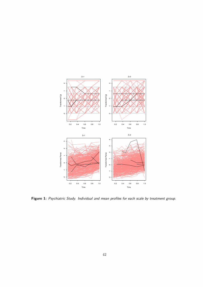
Time

Tra

nsfo

rme

d C

gi

0.2 0.4 0.6 0.8 1.0

-2-1

01

2

Z=1

Time

Tra

nsfo

rme

d C

gi

0.2 0.4 0.6 0.8 1.0

-2-1

01

2

Z=0

Time

Tra

nsfo

rmed P

anss

0.2 0.4 0.6 0.8 1.0

-2-1

01

23

Z=1

Time

Tra

nsfo

rmed P

anss

0.2 0.4 0.6 0.8 1.0

-2-1

01

23

4

Z=0

Figure 1: Psychiatric Study. Individual and mean profiles for each scale by treatment group.

42