A Transformation--Based Approach for the Design of Parallel/Distributed Scientific Software: the FFT

arX

iv:0

811.

2535

v1 [

cs.S

E]

15

Nov

200

8

A TRANSFORMATION–BASED APPROACH FOR THE DESIGN OFPARALLEL/DISTRIBUTED SCIENTIFIC SOFTWARE: THE FFT ∗

HARRY B. HUNT , LENORE R. MULLIN , DANIEL J. ROSENKRANTZ † , AND JAMES

E. RAYNOLDS‡

Abstract. We describe a methodology for designing efficient parallel and distributed scientificsoftware. This methodology utilizes sequences of mechanizable algebra–based optimizing transfor-mations. In this study, we apply our methodology to the FFT, starting from a high–level algebraicalgorithm description. Abstract multiprocessor plans are developed and refined to specify whichcomputations are to be done by each processor. Templates are then created that specify the loca-tions of computations and data on the processors, as well as data flow among processors. Templatesare developed in both the MPI and OpenMP programming styles.

Preliminary experiments comparing code constructed using our methodology with code fromseveral standard scientific libraries show that our code is often competitive and sometimes performsbetter. Interestingly, our code handled a larger range of problem sizes on one target architecture.

Keywords: FFT, design methodology, optimizing transformations, message pass-ing, shared memory.

1. Introduction. —We present a systematic, algebraically based, design methodology for efficient

implementation of computer programs optimized over multiple levels of the proces-sor/memory and network hierarchy. Using a common formalism to describe the prob-lem and the partitioning of data over processors and memory levels allows one tomathematically prove the efficiency and correctness of a given algorithm as measuredin terms of a set of metrics (such as processor/network speeds, etc.). The approachallows the average programmer to achieve high-level optimizations similar to thoseused by compiler writers (e.g. the notion of tiling).

The approach is similar in spirit to other efforts using libraries of algorithm build-ing blocks based on C++ template classes. In POOMA for example, expression tem-plates using the Portable Expression Template Engine (PETE)(http://www.acl.lanl.gov.pete) were used to achieve efficient distribution of array in-dexing over scalar operations [1, 2, 3, 4, 5, 6, 7, 8, 9, 10].

As another example, The Matrix Template Library (MTL) [11, 12] is a systemthat handles dense and sparse matrices, and uses template meta-programs to generatetiled algorithms for dense matrices.

For example:

(A+B)ij = Aij +Bij , (1.1)

can be generalized to the situation in which the multi-dimensional arrays A and Bare selected using a vector of indices ~v.

In POOMA A and B were represented as classes and expression templates wereused as re-write rules to efficiently carry out the translation to scalar operationsimplied by:

∗RESEARCH SUPPORTED BY NSF GRANT CCR–0105536.†Department of Computer Science, University at Albany, State University of New York, Albany,

NY 12203‡College of Nanoscale Science and Engineering, University at Albany, State University of New

York, Albany, NY 12203

1

http://arXiv.org/abs/0811.2535v1

http://www.acl.lanl.gov.pete

(A+B)~v = A~v +B~v (1.2)

The approach presented in this paper makes use of A Mathematics of Arrays(MoA) and an indexing calculus (i.e. the ψ calculus) to enable the programmer todevelop algorithms using high-level compiler-like optimizations through the ability toalgebraically compose and reduce sequences of array operations.

As such, the translation from the left hand side of Eq. 1.2 to the right side is justone of a wide variety of operations that can be carried out using this algebra. In theMoA formalism, the array expression in Eq. 1.2 would be written:

~vψ(A+B) = ~vψA+ ~vψB (1.3)

where we have introduced the psi-operator ψ to denote the operation of extracting anelement from the multi-dimensional array using the index vector (~v).

In this paper we give a demonstration of the approach as applied to the creation ofefficient implementations of the Fast Fourier Transform (FFT) optimized over multi-processor, multi-memory/network, environments. Multi-dimensional data arrays arereshaped through the process of dimension lifting to explicitly add dimensions toenable indexing blocks of data over the various levels of the hierarchy. A sequenceof array operations (represented by the various operators of the algebra acting onarrays) is algebraically composed to achieve the Denotational Normal Form (DNF).Then the ψ-calculus is used to reduce the DNF to the ONF (Operational NormalForm) which explicitly expresses the algorithm in terms of loops and operations onindices. The ONF can thus be directly translated into efficient code in the languageof the programmer’s choice be it for hardware or software application.

The application we use as a demonstration vehicle – the Fast Fourier Transform –is of significant interest in its own right. The Fast Fourier Transform (FFT) is one ofthe most important computational algorithms and its use is pervasive in science andengineering. The work in this paper is a companion to two previous papers [13] inwhich the FFT was optimized in terms of in-cache operations leading to factors of twoto four speedup in comparison with our previous records. Further background materialincluding comparisons with library routines can be found in Refs. [14, 15, 16, 17]and [18].

Our algorithm can be seen to be a generalization of similar work aimed at out-of-core optimizations [19]. Similarly, block decompositions of matrices (in general)are special cases of our rehape-traspose design. Most importantly, our designs aregeneral for any partition size, i.e. not necessary blocked in squares, and any numberof dimensions. Furthermore, our designs use linear transformations from an alge-braic specification and thus they are verified. Thus, by specifying designs (such asCormen’s and others [19]) using these techniques, these designs too could be verified.

The purpose of this paper IS NOT to attempt any serious analysis of the numberof cache misses incurred by the algorithm in the spirit of of Hong and Kung andothers [20, 21, 22]. Rather, we present an algebraic method that achieves (or iscompetitive) with such optimizations mechanically. Through linear transformationswe produce a normal form, the ONF, that is directly implementable in any hardwareor software language and is realized in any of the processor/memory levels [23]. Mostimportantly, our designs are completely general in that through dimension liftingwe can produce any number of levels in the processor/memory hierarchy.

2

One objection to our approach is that one might incur an unacceptable perfor-mance cost due to the periodic rearrangement of the data that is often needed. Thiswill not, however, be the case if we pre-fetch data before it is needed. The necessityto pre-fetch data also exists in other similar cache-optimized schemes. Our algorithmdoes what the compiler community calls tiling. Since we have analyzed the loop struc-tures, access patterns, and speeds of the processor/memory levels, pre-fetching be-comes a deterministic cost function that can easily be combined with reshape-transposeor tiling operations.

Again we make no attempt to optimize the algorithm for any particular architec-ture. We provide a general algorithm in the form of an Operational Normal Form thatallows the user to specify the blocking size at run time. This ONF therefore enablesthe individual user to choose the blocking size that gives the best performance forany individual machine, assuming this intentional information can be processed by acompiler1.

It is also important to note the importance of running reproducible and determin-istic experiments. Such experiments are only possible when dedicated resources existAND no interrupts or randomness effects memory/cache/communications behavior.This means that multiprocessing and time sharing must be turned off for both OS’sand Networks.

Conformal Computing2 is the name given by the authors to this algebraic ap-proach to the construction of computer programs for array-based computations inscience and engineering. The reader should not be misled by the name. Conformalin this sense is not related to Conformal Mapping or similar constructs from math-ematics although it was inspired by these concepts in which certain properties arepreserved under transformations. In particular, by Conformal Computing we meana mathematical system that conforms as closely as possible to the underlying struc-ture of the hardware. Further details of the theory including discussion of MoA andψ-calculus are provided in the appendix.

In this feasibility study, we proceed in a semi–mechanical fashion. At each step ofalgorithm development, the current version of the algorithm is represented in a code–like form, and a simple basic transformation is applied to this code–like form. Eachtransformation is easily seen to be mechanizable. We used the algebraic formalismdescribed in Section 1.2 to verify that each transformation produces a semanticallyequivalent algorithm. At each step, we use judgment in deciding which transforma-tion to carry out. This judgment is based on an understanding of the goals of thetransformations.

The following is a more detailed description of our methodology, as carried–outin this feasibility study:

1.1. Overview of Methodology. Phase 1. Obtain a high–level descriptionof the problem. In this study, a MATLAB–like description is used.

Phase 2. Apply a sequence of transformations to optimize the sequential ver-sion of the algorithm. The transformations used are of an algebraic nature, can beinterpreted in terms of operations on whole arrays, and should not negatively effectsubsequent parallelization.

Phase 3. Apply a sequence of transformations to develop a parallel computationplan. Such plans consists of sequential code that indicates which parts of the overall

1Processing intentional information will be the topic of a future paper2The name Conformal Computing c© is protected. Copyright 2003, The Research Foundation

of State University of New York, University at Albany.

3

work are to be done by each individual processor. For each iteration of an outer loop,the plan specifies which iterations of inner loops should be performed by each of theprocessors in a multiprocessor system.

Phase 4. Given a parallel computation plan, apply a sequence of transformationsto produce a parallel computation template. Such templates specify a parallel ordistributed version of the algorithm by indicating (1) which parts of the overall workare to be done by each individual processor, (2) where data is located, and (3) datamovement among processors. Various parallel programming language styles can beused to express such templates. In this study, we use both a message passing per–processor style, motivated by MPI [24], and an all–processor style, motivated byOpenMP [25].

There is also an implicit fifth phase, in which a parallel computation template istransformed into code expressed in a given programming language.

In the future, we envision that scientific programs will be developed in interactivedevelopment environments. Such environments will combine human judgment withcompiler–like analysis, transformation, and optimization techniques. A programmerwill use knowledge of problem semantics to guide the selection of the transformationat each step, but the application of the transformation and verification of its safetywill be done mechanically. A given sequence of transformations will stop at a pointwhere a version of the code has been obtained such that subsequent optimizationscan be left to an available optimizing compiler. This feasibility study is a first steptowards the development of such an interactive program development environment.

1.2. Program Development Via Use of Array and Indexing Algebra.Although not discussed further in this paper, Mullin’s Psi Calculus [26, 27, 28, 29]plays an underlying role in this feasibility study. This calculus provides a unifiedmathematical framework for representing and studying arrays, array operations, andarray indexing. It is especially useful for developing algorithms centered around trans-formations involving array addressing, decomposition, reshaping, distribution, etc.Each of the algorithm transformations carried out here can be expressed in terms ofthe Psi Calculus, and we used the Psi Calculus to verify the correctness of programtransformations in the development of our FFT algorithms.

1.3. Related Results. A general algebraic framework for Fourier and relatedtransforms, including their discrete versions, is discussed in [30]. As discussed in[31, 32] and using this framework, many algorithms for the FFT can be viewed interms of computing tensor product decompositions of the matrix BL, discussed inSection 2.1 below. Subsequently, a number of additional algorithms for the FFTand related problems have been developed centered around the use of tensor productdecompositions [33, 34, 35, 36, 37, 38]. The work done under the acronym FFTWis based on a compiler that generates efficient sequential FFT code that is adaptedto a target architecture and specified problem size [39, 40, 41, 42, 43]. A varietyof techniques have been used to construct efficient parallel algorithms for the FFT[44, 45, 46, 47, 48, 49].

Previously, we manually developed several distributed algorithms for the FFT[50], experimenting with variants of bit–reversal, weight computations, butterfly com-putations, and message generation mechanisms. In [50], we report on the evaluationof twelve resulting variant programs for the one–dimensional FFT, evaluated by run-ning a consistent set of experiments. In [14, 15], we compare the performance ofour programs with that of several other FFT implementations (FFTW, NAG, ESSL,IMSL). As in [51], we begin by developing sequential code for the radix 2 FFT, starting

4

from a high–level specification, via a sequence of optimizing algebra–based transfor-mations. This sequential code provides a common starting point for the developmentof sequential code for the general radix FFT in [51], and for the development of par-allel/distributed algorithms presented here. For the convenience of the reader and toprovide context for the transformations used here, we repeat this common develop-ment here in Section 3. Similarly, for the convenience of the reader, we also recallrelevant experimental results from [51] in Section 7. These experiments provide ev-idence that the design methodology outlined here can already produce competitivecode.

2. High–Level Description of Algorithm.

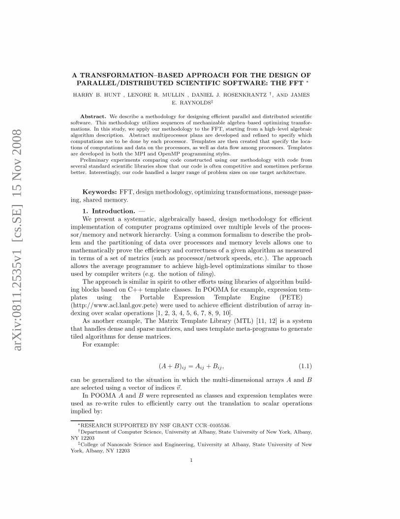
2.1. Basic Algorithm. Our approach to algorithm development begins by ex-pressing the algorithm in a suitable high–level mechanism. This specification maytake the form of a high–level statement of the algorithm, possibly annotated withadditional specifications, such as the specification of the array of weights for the FFT.Our design and development of efficient implementations of an algorithm for the FFTbegan with Van Loan’s [52] suitably commented high–level MATLAB program for theradix 2 FFT, shown in Figure 2.1.

Input: x in Cn and n = 2t, where t ≥ 1 is an integer.Output: The FFT of x.

x← Pn x (1)for q = 1 to t (2)

begin (3)L← 2q (4)r← n/L (5)xL×r ← BL xL×r (6)

end (7)Here, Pn is a n× n permutation matrix. Letting L∗ = L/2, and ωL

be the L’th root of unity, matrix BL =

[

IL∗ΩL∗

IL∗−ΩL∗

]

, where ΩL∗

is a diagonal matrix with values 1, ωL, . . . , ωL∗−1L along the diagonal.

Fig. 2.1. High–level algorithm for the radix 2 FFT

In Line 1, Pn is a permutation matrix that performs the bit–reversal permutationon the n elements of vector x. The reference to xL×r in Line 6 can be regardedas reshaping the n element array x to be a L × r matrix consisting of r columns,where each column can be viewed as a vector of L elements. This reshaping of x iscolumn–wise, so that each time Line 6 is executed, each pair of adjacent columns ofthe preceding matrix are concatenated to produce a single column of the new matrix.Line 6 can be viewed as treating each column of this matrix as a pair of vectors, eachwith L/2 elements, and doing a butterfly computation that combines the two L/2element vectors in each column to produce a vector with L elements. The butterflycomputation, corresponding to multiplication of the data matrix x by BL, combineseach pair of L/2 element column vectors from the old matrix into a new L elementvector for each column of the new matrix.

2.2. Components of the Basic Algorithm. By inspection of Figure 2.1, onecan identify the following five components of the high–level radix 2 FFT algorithm:

5

1. The computation of the bit–reversal permutation (Line 1).2. The computation of the complex weights occurring in the matrices ΩL∗

. Theseweights are discussed further in Section 3.1.

3. The butterfly computation that, using the weights, combines two vectors fromx, producing a vector with twice as many elements (Line 6). The butterflycomputation is scalarized, and subsequently refined in Sections 3.2–3.7.Contiguous memory access gives better performance at all levels of a memoryhierarchy. Consequently, making data access during the butterfly compu-tation contiguous is a driving factor throughout this paper in refining thebutterfly computation.

4. The strategy for allocating the elements of the reshaped array x (line 6)to the processors for use in parallel and distributed implementations of thecomputation loop (the q loop of Lines 2 through 7). Alternative strategiesfor which processor will compute which values of x during each iteration ofthe computation loop are discussed in Section 4. The actual location of thedata is discussed in Sections 5 and 6.

5. The generation and bundling of messages involving values from x (Lines 2through 7). Message passing of data in distributed computation is discussedin Section 5.

3. Development of Sequential Code.

3.1. Specification of the Matrix of Weight Constants. The description ofthe algorithm in Figure 2.1 uses English to describe the constant matrix BL. Thismatrix is a large two-dimensional sparse array. Of more importance for our purposes,this array can be naturally specified by using constructors from the array calculus witha few dense one dimensional vectors as the basis. This yields a succinct description ofhow BL can be constructed via a composition of array operations. Indeed, BL is neveractually materialized as a dense L×L matrix. Rather, the succinct representation isused to guide the generation of code for the FFT, and the generated code only hasmultiplications corresponding to multiplication by a nonzero element of BL.

On the top–level, BL is constructed by the appropriate concatenation of foursubmatrices. Only the construction of two of these submatrices, namely IL∗

andΩL∗

, need be separately specified. Matrix IL∗occurs twice in the decomposition of

BL. Matrix −ΩL∗can be obtained from matrix ΩL∗

by applying element–wise unaryminus.

Each of the two submatrices to be constructed is a diagonal matrix. For each ofthese diagonal matrices, the values along the diagonal are successive powers of a givenscalar. Psi Calculus contains a constructor that produces a vector whose elements areconsecutive multiples or powers of a given scalar value. There is another constructordiagonalize3 that converts a vector into a diagonal matrix with the values from thevector occurring along the diagonal, in the same order. We specified the matrices IL∗

and ΩL∗by using the vector constructor that produces successive powers, followed by

the diagonalize constructor.

Since L = 2q, matrix BL is different for each iteration of the loop in Figure 2.1.Accordingly, the specification of IL∗

and ΩL∗is parameterized by L (and hence im-

plicitly by q).

3 The diagonalize operation is itself specified as a composition of more primitive array opera-tions.

6

3.2. Scalarization of the Matrix Multiplication. A direct and easily au-tomated scalarization of the matrix multiplication in Line 6 of Figure 2.1 producedcode similar4 to that given in Figure 3.1. Here weight is a vector of consecutivepowers of ωL. Note that in Figure 3.1, the multiplication by the appropriate constantfrom the diagonal of matrix ΩL∗

is done explicitly, using a value from vector weight,and the multiplication by the constant 1 from the diagonal of matrix IL∗

is doneimplicitly. Because the scalarized code does an assignment to one element at a time,the code stores the result of the array multiplication into a temporary array xx, andthen copies xx into x. The sparseness of matrix BL is reflected in the assignments toxx(row,col). The right–hand side of these assignment statements is the sum of onlythe two terms corresponding to the two nonzero elements of the row of BL involved inthe computation of the left–hand side element. Moreover, the “regular” structure ofBL, expressed in terms of diagonal submatrices, provides a uniform way of selectingthe two terms.

do col = 0,r-1

do row = 0,L-1

if (row < L/2 ) then

xx(row,col) = x(row,col) + weight(row)*x(row+L/2,col)

else

xx(row,col) = x(row-L/2,col) - weight(row-L/2)*x(row,col)

end if

end do

end do

Fig. 3.1. Direct Scalarization of the Matrix Multiplication

3.3. Representing Data as a 1–Dimensional Vector. The data array x inFigure 2.1 is a 2-dimensional array, that is reshaped during each iteration. Computa-tionally, however, it is more efficient to store the data values in x as a one dimensionalvector, and to completely avoid performing this reshaping. Psi calculus easily han-dles avoiding array reshaping, and automates such transformations as the mapping ofindices of an element of the 2–dimensional array into the index of the correspondingelement of the vector. The L× r matrix xL×r is stored as an n–element vector, whichwe denote as program variable x. The elements of the two–dimensional matrix are en-visioned as being stored in column–major order, reflecting the column–wise reshapingoccurring in Figure 2.1. Thus, element xL×r(row, col) of xL×r corresponds to elementx(L*col+row) of x. Consequently, when L changes, and matrix xL×r is reshaped, nomovement of data elements of vector x actually occurs. Replacing each access toan element of the two dimensional matrix xL×r with an access to the correspondingelement of the vector x, produces the code shown in Figure 3.2.

As an alternative to the scalarized code of Figure 3.2, the outer loop variablecan iterate over the starting index of each column in vector x, using the appropriatestride to increment the loop variable. Instead of using a loop variable col, whichranges from 0 to r-1 with a stride of 1, we use a variable, say col′, such that col′

= L * col, and which consequently has a stride of L. By doing this, we eliminatethe multiplication L * col that occurs each time an element of the arrays xx or x isaccessed. This form of scalarization produces the code shown in Figure 3.3.

4 The data array was not reshaped for each value of q, so references to the data array elementswas more complicated than shown in Figure 3.1.

7

do col = 0,r-1

do row = 0,L-1


xx(L*col+row) = x(L*col+row) + weight(row)*x(L*col+row+L/2)

else

xx(L*col+row) = x(L*col+row-L/2) - weight(row-L/2)*x(L*col+row)

end if

end do

end do

Fig. 3.2. Scalarized Code with Data Stored in a Vector

do col′ = 0,n-1,L

do row = 0,L-1


xx(col′+row) = x(col′+row) + weight(row)*x(col′+row+L/2)

else

xx(col′+row) = x(col′+row-L/2) - weight(row-L/2)*x(col′+row)

end if

end do

end do

Fig. 3.3. Striding through the Data Vector

3.4. Elimination of Conditional Statement. The use of the conditionalstatement that tests row < L/2 in the above code can be eliminated automatically,as follows. We first re–tile the loop structure so that the innermost loop iterates overeach pair of data elements that participate in each butterfly combination. To accom-plish this re–tiling, we first envision reshaping the two–dimensional array xL×r intoa three–dimensional array xL/2×2×r. Under this reshaping, element xL×r(row, col)corresponds to element xL/2×2×r(rowmodL/2, ⌊row/(L/2)⌋, col). The middle di-mension of xL/2×2×r splits each column of xL×r into the upper and lower parts ofthe column. Scalarizing Line 6 of Figure 2.1 based on the three–dimensional arrayxL/2×2×r, and indexing over the third dimension in the outer loop, over the first di-mension in the middle loop, and over the second dimension in the innermost loop,produces the code shown in Figure 3.4.

To eliminate the conditional statement, we unroll the innermost loop, and producethe code shown in Figure 3.5.

When we represent the data array as a one–dimensional vector, the code shownin Figure 3.6 is produced.

3.5. Optimizing the Basic Block. The basic block in the inner loop of theabove code has two occurrences of the common subexpression weight(row)*x(col′+row+L/2).We hand–optimized this basic block, to compute this common subexpression onlyonce. This produces more efficient code for the basic block, as shown in Figure 3.7.

Incorporating all the transformations described so far, the loop in Figure 2.1 isscalarized as shown in Figure 3.8. In this code, pi and i are Fortran “parameters”,i.e., named constants.

3.6. Doing the Butterfly Computation In–Place. The use of the temporaryarray xx in the butterfly computation is unnecessary, and can be avoided by the

8

do col = 0,r-1

do row = 0,L/2-1

do group = 0,1

if ( group == 0 ) then

xx(row,group,col) =

x(row,group,col) + weight(row)*x(row,group+1,col)

else

xx(row,group,col) =

x(row,group-1,col) - weight(row)*x(row,group,col)

end if

end do

end do

end do

Fig. 3.4. Re–tiled Loop

do col = 0,r-1

do row = 0,L/2-1

xx(row,0,col) = x(row,0,col) + weight(row)*x(row,1,col)

xx(row,1,col) = x(row,0,col) - weight(row)*x(row,1,col)

end do

end do

Fig. 3.5. Unrolled Inner Loop

use of a scalar variable to hold the value of x(col′+row). Code incorporating thismodification is shown in Figure 3.9, where scalar variable d is used for this purpose.

3.7. Vectorizing the Butterfly Computation. An alternative coding stylefor the butterfly computation is to use monolithic vector operations applied to ap-propriate sections of the data array. This vectorization of the butterfly computationproduces the code shown in Figure 3.105. Here, cvec is a one–dimensional array usedto store the vector of values assigned to variable c during the iterations of the innerloop (the row loop) in Figure 3.9. Similarly, dvec is a one–dimensional array usedto store the vector of values assigned to variable d during the iterations of this innerloop.

4. Development of Plans for Parallel and Distributed Code.

4.1. An Overview of Plans, Templates, and Architectural Issues. Wewant to generate code for two types of architecture.

• Distributed memory architecture (where each processor has its own localaddress space).• Shared memory architecture with substantial amounts of local memory (where

there is a common address space that includes the local memories).To accommodate these architectures, we will develop an appropriate parallel com-

putation plan, followed by appropriate parallel computation templates.What we mean by a parallel computation plan is sequential code that indicates

which parts of the overall work is to be done by each individual processor. A plan

5We assume that code can select a set of array elements using a start, stop, and stride mechanism,with a default stride of 1.

9

do col′ = 0,n-1,L

do row = 0,L/2-1

xx(col′+row) = x(col′+row) + weight(row)*x(col′+row+L/2)

xx(col′+row+L/2) = x(col′+row) - weight(row)*x(col′+row+L/2)

end do

end do

Fig. 3.6. Unrolled Inner Loop With Data Stored as a Vector

c = weight(row)*x(col′+row+L/2)

xx(col′+row) = x(col′+row) + c

xx(col′+row+L/2) = x(col′+row) - c

Fig. 3.7. Optimized Basic Block

specifies for each iteration of an outer loop6, which iterations of inner loops should beperformed by each of the processors of a multiprocessor system. At each point in theparallel computation, we envision that responsibility for the n elements is partitionedamong the processors. Our intention is that this responsibility is based on an ownercomputes rule, namely a given processor is responsible for those data elements forwhich it executes the butterfly assignment.

What we mean by a template is distributed or parallel “generic code” that in-dicates not only which parts of the overall work is to be done by each individualprocessor, but also where data is located, and how data is moved. To convert a tem-plate into code, a specific programming language needs to be selected, and more detailneeds to be filled in. We use two styles of templates. The first style is a per–processorstyle, motivated by MPI [24]. The other style is an all–processor style, motivated byOpenMP [25].

It is our intention that in the transformation from an FFT parallel computationplan into a template for a distributed architecture or a shared memory architecturewhere substantial local memory is available to each processor, each of the processorswill hold in its local memory those data elements it is responsible for, and do thebutterfly operations on these data elements.

4.2. Splitting the Outer Loop of the Butterfly Computation. Supposethere arem processors, where m is a power of 2. We let psize denote n/m, the numberof elements that each processor is responsible for. Our parallel computation planswill assume that psize ≥ m. Now envision the data in the form of a two–dimensionalmatrix that gets reshaped for each value of q, as in Figure 2.1. During the initialrounds of the computation, for each processor, the value of psize is large enough tohold one or more columns of the two–dimensional data matrix, so we will make eachprocessor responsible for multiple columns, where the total number of elements inthese columns equals psize. For each iteration of q, the length of a column doubles,so that at some point, a column of the matrix will have more than psize elements.This first occurs when q equals log2(psize) + 1. We call this value breakpoint. Onceq equals breakpoint, each column has more than psize elements. Consequently, weno longer want only one processor to be responsible for an entire column, and so wechange plans. Before q equals breakpoint, the number of columns is a multiple of m.

6 For the FFT, this outer loop is the q loop of Figure 3.9.

10

do q = 1,t

L = 2**q

do row = 0,L/2-1

weight(row) = EXP((2*pi*i*row)/L)

end do

do col′ = 0,n-1,L

do row = 0,L/2-1


xx(col′+row) = x(col′+row) + c

xx(col′+row+L/2) = x(col′+row) - c

end do

end do

x = xx

end do

Fig. 3.8. Loop with Optimized Basic Block

do q = 1,t

L = 2**q

do row = 0,L/2-1


end do

do col′ = 0,n-1,L

do row = 0,L/2-1


d = x(col′+row)

x(col′+row) = d + c

x(col′+row+L/2) = d - c

end do

end do

end do

Fig. 3.9. Loop with In–Place Butterfly Computation

From breakpoint on, there are fewer than m columns, but the number of rows is amultiple of m.

As long as q is less than breakpoint, we can use a block approach to the compu-tation, with each processor computing the new values of several consecutive columnsof the two–dimensional matrix. Assume that the processors are numbered 0 throughm− 1. In terms of the one–dimensional vector of data elements, the columns whosenew values are to be computed by processor p are the psize consecutive vector ele-ments beginning with vector element p∗psize. When q equals breakpoint, the numberof elements in each column is 2 * psize, whereas we want each processor to computethe new value of only psize elements. Thus, when q equals breakpoint, we need toswitch to a different plan. To facilitate the switch to a different plan, we first modifyFigure 3.9 by splitting the q loop into two separate loops, as shown in Figure 4.1.

4.3. Parallel Computation Plan When Local Memory is Available. Con-sider the two q loops in Figure 4.1. For the first q loop, we will use a block approachto splitting the computation among the processors, as discussed in Section 4.2. Recallthat before q equals breakpoint, the number of columns is a multiple of m, and from

11

do col′ = 0,n-1,L

cvec(0:L/2-1) = weight(0:L/2-1) * x(col′+L/2:col′+L-1)

dvec(0:L/2-1) = x(col′:col′+L/2-1)

x(col′:col′+L/2-1) = dvec(0:L/2-1) + cvec(0:L/2-1)

x(col′+L/2:col′+L-1) = dvec(0:L/2-1) - cvec(0:L/2-1)

end do

Fig. 3.10. Vectorizing the Butterfly Computation

do q = 1,breakpoint - 1

L = 2**q

do row = 0,L/2-1


end do

do col′ = 0,n-1,L

do row = 0,L/2-1


d = x(col′+row)



end do

end do

end do

do q = breakpoint,t

L = 2**q

do row = 0,L/2-1


end do

do col′ = 0,n-1,L

do row = 0,L/2-1


d = x(col′+row)



end do

end do

end do

Fig. 4.1. Loop Splitting the Butterfly Computation

breakpoint on, the number of rows is a multiple of m. For the second q loop, whichbegins with q equal to breakpoint, we use a cyclic approach, with each processor pcomputing the new values of all the rows j of the two–dimensional matrix such thatj is congruent to p mod m. This corresponds to all the iterations of the inner loopwhere program variable row is congruent to p mod m.

We express a computation plan by modifying each of the q loops in Figure 4.1, sothat for each value of q, there is a new outer loop using a new loop variable p, whichranges between 0 and m − 1. Our intention is that all the computations within theloop for a given value of p will be performed by processor p. Figure 4.2 shows the

12

effect of restructuring each of the two q loops in Figure 4.1 by introducing a p loop toreflect the parallel computation plan. The first q loop uses a block approach for eachp, and the second q loop uses a cyclic approach for each p.


L = 2**q

do row = 0,L/2-1


end do

do p = 0,m-1

do col′ = p*psize,(p+1)*psize-1,L

do row = 0,L/2-1


d = x(col′+row)



end do

end do

end do

end do

do q = breakpoint,t

L = 2**q

do row = 0,L/2-1


end do

do p = 0,m-1

do col′ = 0,n-1,L

do row = p,L/2-1,m


d = x(col′+row)



end do

end do

end do

end do

Fig. 4.2. Initial Parallel Computation Plan

Each execution of a p loop in Figure 4.2 consists of m iterations. Note that foreach value of q, the sets of elements of the x vector accessed by these m iterations arepairwise disjoint. Our intention is that each of these m iterations will be performedby a different processor. Since these processors will be accessing disjoint sets ofelements from the x vector, the execution of different iterations of a p loop by differentprocessors can be done in parallel.

Now consider the first q loop in Figure 4.2. For each value of p within this first qloop, the data elements accessed are the psize elements beginning at position p∗psizeof x. Since for a given p, these are the same set of data elements for every valueof q in the outer loop, we can interchange the loop variables q and p in the first qloop. Now consider the second q loop in Figure 4.2. For each value of p within this

13

second q loop, the data elements accessed are the psize elements of x whose positionis congruent to p mod m. Since for a given p, these are the same set of data elementsfor every value of q in the outer loop, we can interchange the loop variables q and pin the second q loop. This analysis shows that we can interchange the loop variablesq and p in each of the two loops in Figure 4.2 to make p the outermost loop variable,resulting in Figure 4.3. Note that a consequence of this loop interchange is that thecomputation of the weight vector for each value of q is now done for each value of p.

do p = 0,m-1


L = 2**q

do row = 0,L/2-1


end do


do row = 0,L/2-1


d = x(col′+row)



end do

end do

end do

end do

do p = 0,m-1

do q = breakpoint,t

L = 2**q

do row = 0,L/2-1


end do

do col′ = 0,n-1,L

do row = p,L/2-1,m


d = x(col′+row)



end do

end do

end do

end do

Fig. 4.3. Local Memory Parallel Computation Plan with Processor Loops Outermost

4.4. Computing Only Needed Weights. In the second q loop in Figure 4.3,each p computes an entire weight vector of L/2 elements. However, for a given p,only those elements in the weight vector whose position is congruent to p mod m areactually used. We can change the plan so that only these L

2m elements of the weightvector are computed. The computation of weights in the second q loop would thenbe as follows.

14

do row = p,L/2-1,m


end do

4.5. Making Weight Vector Access Contiguous. Note that in the secondq loop, the weight vector is accessed with consecutive values of the program variablerow. These consecutive values of row are strided, with a stride of m. Consequently,the accesses of the weight vector in the second q loop are strided, with a stride of m.Within each iteration of the second q loop we can make the accesses to the weightvector contiguous, as follows. The key is to use a new weight vector weightcyclic,in which we store only the L

2m weight elements needed for a given value of p. Con-sequently, these needed elements of weightcyclic will be accessed contiguously. Therelationship between the weightcyclic and weight vectors is that for each j, 0 ≤ j < L

2m ,weightcyclic(j) will hold the value of weight(m ∗ j + p), i.e., for each value of rowoccurring in an inner loop with loop control

do row = p,L/2-1,m

the value of weight(row) will be held in weightcyclic( row−pm ).

With this change, the computation of weights in the second q loop becomes thefollowing

do row = p,L/2-1,m

weightcyclic((row-p)/m) = EXP((2*pi*i*row)/L)

end do

We can simplify the loop control and subscript computation for weightcyclic bychanging the loop control variable. In the loop which computes the needed weightelements, we use a loop index variable row′, where row′ = (row − p)/m, i.e. row =m ∗ row′ + p.

With this change, the weight computation within the second q loop becomes thefollowing, where row′ has a stride of 1.

do row′ = 0,L/(2*m)-1,1

weightcyclic(row′) = EXP((2*pi*i*(m*row′+p))/L)

end do

Within the butterfly computation, where the loop variable is row, a use ofweight(row) becomes a use of weightcyclic((row−p)/m).

Figure 4.4 shows the second q loop after incorporating the improvements fromSection 4.4 and this Section to the computation and access of weights.

4.6. Making Data Access Contiguous. Note that the accesses of data vectorx in the second q loop are strided, with a stride of m. We can make access to theneeded data in x in the second q loop contiguous, as follows. We introduce a newdata vector xcyclic to hold only those data elements accessed for each p. For eachp, the vector xcyclic contains L/m elements from each of the n/L columns, for a totalof n/m = psize elements. The relationship between the xcyclic and x vectors is thatfor each col′, where 0 ≤ col′ < n − 1 and col′ is a multiple of L, and row, where0 ≤ row < L and row is congruent to p mod m, xcyclic(col′/m+ (row − p)/m) willhold the value of x(col′ +row). Consequently, for each value of col′ and row occurringin the butterfly loop, x(col′ + row) will be held in xcyclic(col′/m+(row− p)/m) andx(col′ + row + L/2) will be held in xcyclic(col′/m+ (row + L/2− p)/m).

At the beginning of each iteration of the p loop, the required psize elements ofx must be copied into xcyclic, and at the end of each iteration of the p loop, thesepsize elements must be copied from xcyclic into x. At the template level, this copyingwill be done by either message passing or assignment statements, depending on the

15

do p = 0,m-1

do q = breakpoint,t

L = 2**q

do row′ = 0,L/(2*m)-1,1


end do

do col′ = 0,n-1,L

do row = p,L/2-1,m

c = weightcyclic((row-p)/m)*x(col′+row+L/2)

d = x(col′+row)



end do

end do

end do

end do

Fig. 4.4. Second q Loop with Contiguous Access of Needed Weights

architecture and programming language. Here, where we are developing a compilationplan, we indicate this copying abstractly, using function calls. We envision array xas containing a “centralized” copy of all the data elements, and xcyclic as containinga subset. The respective subsets of x used by the iterations of the p loop representa partition of the data elements in x. We envision the n elements of x as beingpartitioned into m subsets, where each iteration of the p loop copies one of thesesubsets into xcyclic. The copying from x to xcyclic of the psize elements of x whoseposition in x is congruent to p mod m is expressed using the function call

CENTRALIZED TO CYCLIC PARTITIONED(x,xcyclic,m,psize,p).The copying of the psize elements of xcyclic into x is expressed using the function call

CYCLIC PARTITIONED TO CENTRALIZED(xcyclic,x,m,psize,p).Figure 4.5 shows the effect of incorporating these changes to the second q loop.

Note that since the stride in the row loop is m, these changes do indeed providecontiguous data access.

We can simplify the loop control and subscript computation of vector elementsoccurring in Figure 4.5, by changing the loop control variables, as shown in Figure 4.6.

In Figure 4.6, we use a variable col′′ to range over all the columns, where col′ =m ∗ col′′ i.e. col′′ = col′/m. Since the bounds for loop control variable col′ inFigure 4.5 are 0,n-1,L, the bounds for the loop control variable col′′ in Figure 4.6are 0,psize-1,L/m.

Similarly, in Figure 4.6, we use a variable row′, where row = m ∗ row′ + p, i.e.row′ = (row − p)/m. Consider the bounds of the row loop in the second q loop;the start, stop, stride are p,L/2-1,m. For the corresponding row′ loop, the startbecomes 0, and the stop becomes L

2m −p+1m . Since 0 ≤ p < m, we can conclude that

0 < p+1m ≤ 1, so the stop can be simplified to L

2m − 1. Finally, the step is 1. So, thebounds for the row′ loop become 0,L/(2*m)-1,1.

Consequently, xcyclic(col′′+row′) will contain the value of x(m*col′′+m*row′+p).

4.7. Facilitating Exploitation of Local Memory. Note that in Figure 4.6,there is no data flow involving xcyclic between the iterations of the p loop. Aconsequence is that when the plan is subsequently transformed into a template for

16

do p = 0,m-1

CENTRALIZED TO CYCLIC PARTITIONED(x,xcyclic,m,psize,p)

do q = breakpoint,t

L = 2**q

do row′ = 0,L/(2*m)-1,1


end do

do col′ = 0,n-1,L

do row = p,L/2-1,m

c = weightcyclic((row-p)/m) *xcyclic(col′/m+(row-p)/m+L/(2*m))

d = xcyclic(col′/m+(row-p)/m)

xcyclic(col′/m+(row-p)/m) = d + c

xcyclic(col′/m+(row-p)/m+L/(2*m)) = d - c

end do

end do

end do

CYCLIC PARTITIONED TO CENTRALIZED(xcyclic,x,m,psize,p)

end do

Fig. 4.5. Plan for Second q Loop with Contiguous Data Access

do p = 0,m-1


do q = breakpoint,t

L = 2**q

do row′ = p,L/2-1,m


end do

do col′′ = 0,psize-1,L/m

do row′ = 0,L/(2*m)-1,1

c = weightcyclic(row′)*xcyclic(col′′+row′+L/(2*m))

d = xcyclic(col′′+row′)

xcyclic(col′′+row′) = d + c

xcyclic(col′′+row′+L/(2*m)) = d - c

end do

end do

end do

CYCLIC PARTITIONED TO CENTRALIZED(xcyclic,x,m,psize,p)

end do

Fig. 4.6. Plan for Second q Loop with Contiguous Data Access and Simplified Loop Control

parallel and distributed code, xcyclic can be a local variable of each processor.

A similar transformation to that in Section 4.6 can be done to the second qloop in the plan, although the payoff only occurs subsequently when templates areconstructed from the plan. We can facilitate making access to the data in the firstq loop be via a processor–local variable. This can be accomplished by introducing anew data vector xblock, to hold the data values accessed by each iteration of the ploop.

For each p, we will use the vector xblock to hold the psize elements accessed

17

during that iteration of the p loop. The relationship between the xblock and x vectorsis that for each col′, where 0 ≤ col′ < n − 1 and col′ is a multiple of L, and row,where 0 ≤ row < L, x(col′ + row) will be held in xblock(col′ + row − p ∗ psize).

Figure 4.7 shows the effect of incorporating the use of xblock in the first q loop.

do p = 0,m-1

CENTRALIZED TO BLOCK PARTITIONED(x,xblock,m,psize,p)


L = 2**q

do row = 0,L/2-1


end do


do row = 0,L/2-1

c = weight(row)*xblock(col′+row+L/2-p*psize)

d = xblock(col′+row-p*psize)

xblock(col′+row-p*psize) = d + c

xblock(col′+row+L/2-p*psize) = d - c

end do

end do

end do

BLOCK PARTITIONED TO CENTRALIZED(xblock,x,m,psize,p)

end do

Fig. 4.7. Plan for First q Loop

We can simplify the loop control and subscript computation of vector elementsby changing the loop control variable col′, as shown in Figure 4.8. We use a variablecol′′, where col′′ = col′ − p ∗ psize. So, the bounds for the loop control variablecol′′ are 0,psize-1,L. Consequently, xblock(col′′+row) will contain the value ofx(col′+row-p*psize).

Figure 4.9 shows the final plan, combining Figures 4.6 and 4.8.

4.8. Flexibility in Setting Breakpoint. Note that the split of the q loop ofFigure 3.9 into two separate q loops, as shown in Figure 4.1, is correct for any valueof breakpoint. However, for the transformation into the plan shown in Figure 4.2 tobe correct, breakpoint must satisfy certain requirements, as follows.

Requirement 1: Consider the first q loop in Figure 4.2. The correctness of this qloop requires that L ≤ psize, i.e. 2q ≤ psize. Thus, each value of q for which the loopis executed must satisfy q ≤ log2(psize). Since the highest value of q for which the loopis executed is breakpoint−1, the first q loop requires that breakpoint ≤ log2(psize)+1.

Requirement 2: Consider the second q loop in Figure 4.2. The correctness of thisq loop requires that L/2 ≥ m, i.e. 2q−1 ≥ m. Thus, each value of q for which the loopis executed must satisfy q ≥ log2(m)+1. Since the lowest value of q for which the loopis executed is breakpoint, the second q loop requires that breakpoint ≥ log2(m) + 1.

Together, these two requirements imply that:

log2(m) + 1 ≤ breakpoint ≤ log2(psize) + 1.

Since we are assuming that m ≤ psize, there is a range of possible allowablevalues for breakpoint. Thus far in Section 4, we have assumed that breakpoint is set

18

do p = 0,m-1



L = 2**q

do row = 0,L/2-1


end do

do col′′ = 0,psize-1,L

do row = 0,L/2-1

c = weight(row)*xblock(col′′+row+L/2)

d = xblock(col′′+row)

xblock(col′′+row) = d + c

xblock(col′′+row+L/2) = d - c

end do

end do

end do


end do

Fig. 4.8. Plan for First q Loop with Simplified Loop Control

at the high end of its allowable range, namely at log2(psize) + 1. In fact, breakpointcould be set anywhere within its allowable range. If the plan shown in Figure 4.4 isused, there is an advantage in setting breakpoint to the low end of its allowable range,for the following reason. Moving some values of q from the first q loop to the second qloop would reduce the number of weights that need to be computed by each processor.

5. Development of Per–Processor Templates for Distributed MemoryArchitectures.

5.1. Distributed Template Using Local Copy of Data Vector.

5.1.1. Partial Per–Processor Distributed Code Template. Figure 5.1 showshow the parallel computation plan from Figure 4.3 can be transformed into a partiallyspecified template (subsequently abbreviated as a partial template) for distributedcode7. The template in Figure 5.1 is intended to represent per–processor code to beexecuted on each of the m processors. We assume that each processor has a variable,named myid, whose value is the processor number, where the processor number rangesfrom 0 to m − 1. Thus, each of the m processors, say processor i, has its value oflocal variable myid equal to i. In Figure 4.3, each p loop has m iterations, with pranging from 0 to m− 1. In Figure 5.1, variable myid is used to ensure that processori executes iteration i of each p loop, i.e., the iteration where p equals i.

A SYNCHRONIZE command is inserted between the two q loops to indicate thatsome form of synchronization between processors is needed because data computedby each processor in its first q loop is subsequently accessed by all the processors intheir second q loop. We call Figure 5.1 a partial template because it does not addressthe issue of data location or data movement between processors. These issues must beresolved, and the SYNCHRONIZE command between the two q loops must be replaced

7 Any of the improvements from Section 4, such as computing only the needed weights, asdiscussed in Section 4.4, could be incorporated into the plan prior to this transformation, but forsimplicity, here we give a transformation from the plan in Figure 4.3.

19

do p = 0,m-1



L = 2**q

do row = 0,L/2-1


end do


do row = 0,L/2-1

c = weight(row)*xblock(col′′+row+L/2)

d = xblock(col′′+row)

xblock(col′′+row) = d + c

xblock(col′′+row+L/2) = d - c

end do

end do

end do


end do

do p = 0,m-1


do q = breakpoint,t

L = 2**q

do row′ = p,L/2-1,m


end do


do row′ = 0,L/(2*m)-1,1

c = weightcyclic(row′)*xcyclic(col′′+row′+L/(2*m))

d = xcyclic(col′′+row′)

xcyclic(col′′+row′) = d + c

xcyclic(col′′+row′+L/(2*m)) = d - c

end do

end do

end do

CYCLIC PARTITIONED TO CENTRALIZED(xcyclic,x,p,m,psize)

end do

Fig. 4.9. Combined Plan Using Partitioned Data

by statements using an appropriate implementation language mechanism that permitseach processor to proceed past the synchronization point only after all the processorshave reached the synchronization point. These statements must ensure that the dataneeded by each processor is indeed available to that processor.

5.1.2. Responsibility–Based Distribution of Data Vector on Local Mem-ories. In order to transform the partial template of Figure 5.1 into a (fully specified)template, we need to address the issue of where (i.e., on which processor) data islocated, and how data moves between processors. A straightforward approach is tolet each processor have space for an entire data vector x of n elements, but in each ofthe two q loops, only access those psize elements of x that the processor is responsible

20


L = 2**q

do row = 0,L/2-1


end do

do col′ = myid*psize,(myid+1)*psize-1,L

do row = 0,L/2-1


d = x(col′+row)



end do

end do

end do

SYNCHRONIZE

do q = breakpoint,t

L = 2**q

do row = 0,L/2-1


end do

do col′ = 0,n-1,L

do row = myid,L/2-1,m


d = x(col′+row)



end do

end do

end do

Fig. 5.1. Partial Per–Processor Parallel Code Template Obtained from Plan of Figure 4.3

for. To emphasize that space for all n elements of a vector x is allocated on eachprocessor, we refer to this space on a given processor p as xp.

For a distributed architecture or shared memory architecture with substantiallocal memories, the “current” value of each data element will reside on the processorthat computes its new value, i.e., is responsible for it. We now consider this assignmentof each element from the data array to the processor that is responsible for it. To start,consider the first q loop in Figure 5.1. Since q ranges between 1 and breakpoint−1,with breakpoint= log2(psize)+1 and L = 2q, we can conclude that L ranges between 2and psize. For each processor p, consider the data elements accessed in each iterationof this first q loop. These are data elements x(col′ + row) and x(col′ + row + L/2),where col′ ranges between p ∗ psize and (p + 1) ∗ psize − 1 in steps of L, and rowranges between 0 and L/2 − 1. Since L ≤ psize for each iteration of the q loop,the accessed data elements are psize consecutive elements, beginning with elementx(p ∗ psize). These elements can be described as x(p ∗ psize : ((p+1) ∗ psize)− 1 : 1).This is a block distribution of the responsibility for array x, corresponding to the blockapproach to the first p loop, as described in Section 4.3.

Now consider the second q loop in Figure 5.1. In each iteration of this q loop,

21

L/2 ≥ psize. Since psize ≥ m, we can conclude that L/2 ≥ m. For each processorp, consider the data elements accessed in each iteration of the q loop. These are dataelements x(col′ + row) and x(col′ + row + L/2), where col′ ranges between 0 andn − 1, in steps of L, and row ranges between p and L/2 − 1, in steps of m. SinceL/2 is a multiple of m, so is L, so that col′ ≡ 0 mod m for every value of col′. Also,row≡ p mod m. Consequently, col′ + row and col′ + row+L/2 are each congruent top mod m. Thus, every data element accessed by processor p is congruent to p modm. Now, note that there are n/L iterations of the col′ loop. Because L/2 ≥ m, foreach p and col′, there are L/(2m) iterations of the row loop. Each of these iterationsdoes the butterfly operation on two data elements of array x. Note that

n

L∗L

2m∗ 2 =

n

m= psize.

Thus for each iteration of the q loop, processor p does an assignment to psize dataelements. We now note that these are distinct elements, since for each value of rowand col′, different data elements are accessed. In conclusion, the elements accessedby processor p during each iteration of the loop are the set of elements x(i) such thati ≡ p mod m. Using Fortran90–like start–stop–stride notation these elements can bedescribed as x(p : n − 1 : m). This is a cyclic distribution of the responsibility forarray x, corresponding to the cyclic approach to the second p loop, as described inSection 4.3.

5.1.3. Construction of Messages. We now consider the construction of mes-sages between processors for distributed computation. This entails both bundling ofdata values into messages, and having both the sender and recipient of each messagespecify which of its data elements are included in each message.

The data can be initially stored in various ways, such as on disks, distributedamong the processors, or all on one processor. Each of these cases can be readilyhandled. Here, we envision that the data is initially centralized on one processor.

In describing the details of message passing, we assume that the numbering ofprocessors from 0 to m− 1 is such that initially all the data is on processor 0. Beforethe first q loop, as per the block approach, the initially centralized data must bedistributed among the processors. The processor with all the data must send everyother processor, otherp, the set of psize contiguous data elements, beginning with dataelement x(psize ∗ otherp), and each such processor must receive these data elements.The recipient processor then stores the received psize data values in the appropriateposition in its x vector.

A high–level description of message–passing code to perform the block distributionis shown in Figure 5.2. Since this code refers to the variable myid, the same code canbe used on each processor. Processor 0 will execute the otherp loop, sending a messageto each of the other processors. Each processor other than processor 0 will execute aRECEIVE command. The SEND command sends a message, and has three parameters:the first element to be sent, the number of elements to send, and the processor whichshould receive the message. The RECEIVE command receives a message, and has threeparameters: where to place the first element received, the number of elements toreceive, and the processor which sent the message to be received. In Figure 5.2, werefer to the local data array as xmyid, to emphasize that it is the local space for thedata array that is the source and destination of data sent and received by a givenprocessor.

We assume that the SEND command is nonblocking, and uses buffering. Thus,the contents of the message to be sent is copied into a buffer, at which point the

22

statement after the SEND command can be executed. We assume that the RECEIVE

command is blocking. Thus, the data is received and stored in the locations specifiedby the command, at which point the statement after the RECEIVE command can beexecuted.

! DISTRIBUTE CENTRALIZED TO BLOCK(xmyid,m,psize)

if myid = 0 then

do otherp = 1,m-1

SEND(xmyid(psize*otherp),psize,otherp)

end do

else

RECEIVE(xmyid(psize*myid),psize,0)

endif

Fig. 5.2. Centralized to Block Distribution

Now consider the block to cyclic redistribution that occurs after the first q loop,and before the second q loop. Recall that each processor has psize data elements.Of the psize elements on any given processor before the redistribution, psize/m mustwind up in each of the processors (including itself) after the redistribution. No messageneed be sent for the data values that are to wind up on the same processor as beforethe redistribution. Thus, each processor must send psize/m elements to each of theother processors. A high–level description of message–passing code to perform theblock to cyclic redistribution is shown in Figure 5.3. We assume that the SEND andRECEIVE commands are flexible enough so that the first parameter can specify a set ofarray elements using notation specifying start, stop, and stride. The SEND commandscan be nonblocking because for any given processor, disjoint sets of data elementsare involved in any pair of message commands on that processor. An alternative toFigure 5.3 is to first do all the SENDs, and then do all the RECEIVEs.

! DISTRIBUTE BLOCK TO CYCLIC(xmyid,m,psize)

do otherp = 0,m-1

if otherp 6= myid then

SEND(xmyid(psize*myid+otherp:psize*(myid+1)-1:m),psize/m,otherp)

RECEIVE(xmyid(psize*otherp+myid:psize*(otherp+1)-1:m),psize/m,otherp)

endif

end do

Fig. 5.3. Block to Cyclic Redistribution

Another alternative to Figure 5.3 is to first collect all the data at the centralizedsite, i.e. processor 0, and then do a centralized to cyclic redistribution. This strategyis described in more detail in Figure 5.4, where the block to cyclic redistribution isdone as block to centralized redistribution, followed by a centralized to cyclic redis-tribution. The approach in Figure 5.4 entails only 2(m − 1) messages, in contrastto the m(m − 1) messages entailed in Figure 5.3. However, the centralized site maybecome a bottleneck. Moreover, data elements are transmitted twice, to and from thecentralized site, rather than only once.

We envision that at the end of the FFT computation all the data elements are col-lected at the centralized processor, processor 0. A high–level description of message–passing code to perform this cyclic to centralized redistribution is shown in Figure 5.5.

23

! DISTRIBUTE BLOCK TO CYCLIC(xmyid,m,psize)

DISTRIBUTE BLOCK TO CENTRALIZED(xmyid,m,psize)

DISTRIBUTE CENTRALIZED TO CYCLIC(xmyid,m,psize,n)

! DISTRIBUTE BLOCK TO CENTRALIZED(xmyid,m,psize)

if myid = 0 then

do otherp = 1,m-1

RECEIVE(xmyid(psize*otherp),psize,otherp)

end do

else

SEND(xmyid(psize*myid),psize,0)

endif

! DISTRIBUTE CENTRALIZED TO CYCLIC(xmyid,m,psize,n)

if myid = 0 then

do otherp = 1,m-1

SEND(xmyid(otherp:n-1:m),psize,otherp)

end do

else

RECEIVE(xmyid(myid:n-1:m),psize,0)

endif

Fig. 5.4. Block to Cyclic Redistribution Using Centralized Site as Intermediary

! DISTRIBUTE CYCLIC TO CENTRALIZED(xmyid,m,psize,n)

if myid = 0 then

do otherp = 1,m-1

RECEIVE(xmyid(otherp:n-1:m),psize,otherp)

end do

else

SEND(xmyid(myid:n-1:m),psize,0)

endif

Fig. 5.5. Cyclic to Centralized Redistribution

5.1.4. Per–Processor Distributed Code Template. Figure 5.6 shows howthe partial parallel code template from Figure 5.1 is transformed into a template thatspecifies where data is located and how it moves between processors. In Figure 5.6,we refer to the arrays involved in the template as xmyid and weightmyid, to emphasizethat space local to a given processor is being accessed by the per–processor template.We assume that scalar variables, such as q and L are understood to be local variableswithin each processor. As discussed in Section 5.1.2, the distributed code templatewill perform a data redistribution from the initial centralized distribution to a blockdistribution, followed by the first q loop, followed by a block to cyclic redistribution,followed by the second q loop (which begins with q equal to breakpoint), followed by acyclic to centralized redistribution. The code in Figure 5.6 is executed on each of them processors. The DISTRIBUTE BLOCK TO CYCLIC command in Figure 5.6 serves asthe mechanism implementing the SYNCHRONIZE command in Figure 5.1. The block tocyclic redistribution can be performed either as described in Figure 5.3 or as describedin Figure 5.4. In either case, the blocking RECEIVEs do the synchronization.

24

DISTRIBUTE CENTRALIZED TO BLOCK(xmyid,m,psize)


L = 2**q

do row = 0,L/2-1

weightmyid(row) = EXP((2*pi*i*row)/L)

end do

do col′ = myid*psize,(myid+1)*psize-1,L

do row = 0,L/2-1

c = weightmyid(row)*xmyid(col′+row+L/2)

d = xmyid(col′+row)

xmyid(col′+row) = d + c

xmyid(col′+row+L/2) = d - c

end do

end do

end do

DISTRIBUTE BLOCK TO CYCLIC(xmyid,m,psize)

do q = breakpoint,t

L = 2**q

do row = 0,L/2-1


end do

do col′ = 0,n-1,L

do row = myid,L/2-1,m

c = weightmyid(row)*xmyid(col′+row+L/2)

d = xmyid(col′+row)

xmyid(col′+row) = d + c

xmyid(col′+row+L/2) = d - c

end do

end do

end do

DISTRIBUTE CYCLIC TO CENTRALIZED(xmyid,m,psize,n)

Fig. 5.6. Per–Processor Distributed Code Template Based on Partial Template of Figure 5.1

5.2. Distributed Template with Partitioned Data and Contiguous Ac-cess.

5.2.1. Development of Template from Plan Using Partitioned Data.Figure 5.7 shows a per–processor template obtained from Figure 4.9’s parallel com-bined computation plan using partitioned data. The template in Figure 5.7 assumesthat all n data elements are initially located on processor 0 and stored in array x0. Italso assumes that at the end of the algorithm, all n data elements are to be collectedtogether on processor 0 and stored in array x0. Each processor p is assumed to haveits own local arrays weightp, xblockp, weightcyclicp, and xcyclicp. The itera-tion over the p loops in Figure 4.9 is replaced by the execution of the per–processortemplate in Figure 5.7 on each of the m processors.

A high–level description of message–passing code to perform the four data redistri-bution commands in Figure 5.7 (centralized–to–block–partitioned, block–partitioned–to–centralized, centralized–to–cyclic–partitioned, and cyclic–partitioned–to–centralized)is shown in Figure 5.8.

25

DISTRIBUTE CENTRALIZED TO BLOCK PARTITIONED(x0,xblockmyid,m,psize)


L = 2**q

do row = 0,L/2-1


end do


do row = 0,L/2-1

c = weightmyid(row)*xblockmyid(col′′+row+L/2)

d = xblockmyid(col′′+row)

xblockmyid(col′′+row) = d + c

xblockmyid(col′′+row+L/2) = d - c

end do

end do

end do

DISTRIBUTE BLOCK PARTITIONED TO CENTRALIZED(xblockmyid,x0,m,psize)

DISTRIBUTE CENTRALIZED TO CYCLIC PARTITIONED(x0,xcyclicmyid,m,psize)

do q = breakpoint,t

L = 2**q

do row′ = 0,L/(2*m)-1,1

weightcyclicmyid(row′) = EXP((2*pi*i*(m*row′+myid))/L)

end do


do row′ = 0,L/(2*m)-1,1

c = weightcyclicmyid(row′)*xcyclicmyid(col

′′+row′+L/(2*m))

d = xcyclicmyid(col′′+row′)

xcyclicmyid(col′′+row′) = d + c

xcyclicmyid(col′′+row′+L/(2*m)) = d - c

end do

end do

end do

DISTRIBUTE CYCLIC PARTITIONED TO CENTRALIZED(xcyclicmyid,x0,m,psize)

Fig. 5.7. Per–Processor Distributed Code Template Obtained from Combined Plan Using Par-titioned Data of Figure 4.9

5.2.2. Eliminating Bottleneck in Block to Cyclic Redistribution. In Fig-ure 5.7, the pair of data redistribution commands

DISTRIBUTE BLOCK PARTITIONED TO CENTRALIZED(xblockmyid,x0,m,psize)

DISTRIBUTE CENTRALIZED TO CYCLIC PARTITIONED(x0,xcyclicmyid,m,psize)

occurring between the two q loops, together accomplish a block–partitioned–to–cyclic-partitioned data redistribution. This two–command sequence can be replaced by thesingle command

DISTRIBUTE BLOCK PARTITIONED TO CYCLIC PARTITIONED(xblockmyid,xcyclicmyid,m,psize)

This combined command can be implemented by doing a block–partitioned–to–centralizedredistribution followed by a centralized–to–block–partitioned redistribution, as indi-cated in Figure 5.7, in a manner analogous to that shown in Figure 5.4. Alternately,the block–partitioned–to–centralized redistribution can be done directly, as shown in

26

! DISTRIBUTE CENTRALIZED TO BLOCK PARTITIONED(x0,xblockmyid,m,psize)

if myid = 0 then

xblockmyid = x0(0:psize-1)

do otherp = 1,m-1

SEND(x0(psize*otherp),psize,otherp)

end do

else

RECEIVE(xblockmyid,psize,0)

endif

! DISTRIBUTE BLOCK PARTITIONED TO CENTRALIZED(xblockmyid,x0,m,psize)

if myid = 0 then

x0(0:psize-1) = xblockmyiddo otherp = 1,m-1

RECEIVE(x0(psize*otherp),psize,otherp)

end do

else

SEND(xblockmyid,psize,0)

endif

! DISTRIBUTE CENTRALIZED TO CYCLIC PARTITIONED(x0,xcyclicmyid,m,psize)

if myid = 0 then

xcyclicmyid = x0(0:n-1:m)

do otherp = 1,m-1

SEND(x0(otherp:n-1:m),psize,otherp)

end do

else

RECEIVE(xcyclicmyid,psize,0)

endif

! DISTRIBUTE CYCLIC PARTITIONED TO CENTRALIZED(xcyclicmyid,x0,m,psize)

if myid = 0 then

x0(0:n-1:m) = xcyclicmyiddo otherp = 1,m-1

RECEIVE(x0(otherp:n-1:m),psize,otherp)

end do

else

SEND(xcyclicmyid,psize,0)

endif

Fig. 5.8. Code for Distribution Commands Occurring in Figure 5.7’s Per–Processor TemplateUsing Partitioned Data

Figure 5.9, which is analogous to Figure 5.3. The direct implementation removes thecentralized site as a bottleneck, but increases the number of messages from 2(m− 1)to m(m− 1), as discussed in Section 5.1.3.

6. Development of All–Processor Templates for Shared Memory Ar-chitectures with Local Memory Availability.

27

! DISTRIBUTE BLOCK PARTITIONED TO CYCLIC PARTITIONED(xblockmyid,

xcyclicmyid,m,psize)

xcyclicmyid(myid*psize/m:(myid+1)*psize/m-1) =

xblockmyid(myid:psize-1:m)

do otherp = 0,m-1

if otherp 6= myid then

SEND(xblockmyid(otherp:psize-1:m),psize/m,otherp)

RECEIVE(xcyclicmyid(otherp*psize/m),psize/m,otherp)

endif

end do

Fig. 5.9. Block–Partitioned to Cyclic–Partitioned Redistribution

6.1. Shared Memory Template. The parallel computation plan of Figure 4.3can be converted into a shared memory template by converting each of the two p loopsinto a parallel loop, as shown in Figure 6.1. The template in Figure 6.1 is expressed ina style roughly based on OpenMP. We assume that there is a thread for each iterationof a parallel do loop, and that each thread can have data that is private to that thread.Moreover, we assume that each thread is assigned to a processor (with the possibilitythat multiple threads are assigned to any given processor), and data that is privateto a given thread is stored in the local memory of the processor for that thread. Inthe template, we use the notational convention that x is a shared data array; andthat scalar variables, such as q, are private to each thread. We also assume that eachthread p has a private array weightp for the weights used in the execution of thatthread. Within each thread, the assignments to scalar variables and to elements ofweightp modify private data. The assignment to elements of shared array x modifyshared data, but because we are starting with the computation plan of Figure 4.3,the elements of x accessed by the various threads of a given parallel do loop aredisjoint.

6.2. Shared Memory Template Using Private Local Memory. In Fig-ure 6.1, all the accesses to x are to a shared data vector. The template can bemodified so that the butterfly operates on private data, as shown in the all–processortemplate of Figure 6.2, which uses both a shared memory array x, and a privatememory array xp. Figure 6.3 shows the details of how the data copying is done. TheOpenMP–style all–processor template uses assignment statements within each threadto copy data between shared memory and the private memory of that thread.

Figure 6.2 is an all–processor analogue of the per–processor distributed code tem-plate shown in Figure 5.6. The data copying via assignment statements in Figure 6.3is analogous to the data copying via message–passing in Figures 5.2, 5.4, and 5.5.An OpenMP–style all–processor template permits a given thread to copy data be-tween shared memory and private memory of that thread, but does not permit directcopying of data from the private memory of one thread to the private memory ofa different thread. Accordingly, the DISTRIBUTE BLOCK TO CYCLIC command fromFigure 5.6 must be done as two commands (private block to centralized at the endof the first parallel do, followed by centralized to private block at the beginningof the second parallel do) in Figure 6.2, corresponding to the data movement inFigure 5.4, rather than that in Figure 5.3.

6.3. Shared Memory Template Using Partitioned Data and Contigu-ous Access. Figure 6.4 shows an OpenMP–style all–processor template for a shared

28

parallel do p = 0,m-1


L = 2**q

do row = 0,L/2-1

weightp(row) = EXP((2*pi*i*row)/L)

end do


do row = 0,L/2-1

c = weightp(row)*x(col′+row+L/2)

d = x(col′+row)



end do

end do

end do

end parallel do


do q = breakpoint,t

L = 2**q

do row = 0,L/2-1


end do

do col′ = 0,n-1,L

do row = p,L/2-1,m

c = weightp(row)*x(col′+row+L/2)

d = x(col′+row)



end do

end do

end do

end parallel do

Fig. 6.1. Simple Shared Memory All–Processor Template Obtained from Plan of Figure 4.3

memory, based on the plan of Figure 4.9. We assume that there is a thread for eachprocessor, and data that is private to a given thread is stored in the local memory ofthe processor for that thread. In the template, we use the notational convention that xis a shared data array; that weightp, weightcyclicp, xblockp, and xcyclicp denoteprivate data arrays for thread p; and that scalar variables are private to each thread.We assume that a given thread can access only shared data and its private data. Con-sequently, the block–to–cyclic redistribution cannot be done by moving data directlyfrom a private array in one thread into a private array in a different thread. In Fig-ure 6.4, the block–to–cyclic redistribution is done in two steps. In the first step, eachthread of the first p loop does a block–to–centralized copying of data from its privatearray xblockp into shared array x. Consequently, when the first p loop concludes, thedata from all the private xblockp arrays have been copied into shared array x. In thesecond step, each thread of the second p loop does a centralized–to–block copying ofdata from x into its private array xcyclicp.

29


COPY CENTRALIZED TO PRIVATE BLOCK(x,xp,p,psize)


L = 2**q

do row = 0,L/2-1


end do


do row = 0,L/2-1

c = weightp(row)*xp(col′+row+L/2)

d = xp(col′+row)

xp(col′+row) = d + c

xp(col′+row+L/2) = d - c

end do

end do

end do

COPY PRIVATE BLOCK TO CENTRALIZED(xp,x,p,psize)

end parallel do


COPY CENTRALIZED TO PRIVATE CYCLIC(x,xp,p,m,psize)

do q = breakpoint,t

L = 2**q

do row = 0,L/2-1


end do

do col′ = 0,n-1,L

do row = p,L/2-1,m

c = weightp(row)*xp(col′+row+L/2)

d = xp(col′+row)

xp(col′+row) = d + c

xp(col′+row+L/2) = d - c

end do

end do

end do

COPY PRIVATE CYCLIC TO CENTRALIZED(xp,x,p,m,psize)

end parallel do

Fig. 6.2. All–Processor Shared and Private Memory Template Based on Template of Figure 6.1

Figure 6.5 shows the details of the assignment statements that do the data copyingbetween shared memory and the private memory of each thread.

7. Preliminary Experimental Results. There are various commercial andvendor specific libraries which include the FFT. The Numerical Analysis Group (NAG)and Visual Numerics (IMSL) provide and support finely tuned scientific libraries spe-cific to various HPC platforms, e.g SGI and IBM. The SGI and IBM libraries, SCSLand ESSL, are even more highly tuned, due to their knowledge of proprietary infor-mation specific to their respective architectures. We ran experiments comparing ourcode to that in some of these libraries. We also did comparisons with the FFTW,although these results are harder to interpret because of the planning phase that is

30

! COPY CENTRALIZED TO PRIVATE BLOCK(x,xp,p,psize)

xp(psize*p:psize*(p+1)-1:1) = x(psize*p:psize*(p+1)-1:1)

! COPY PRIVATE BLOCK TO CENTRALIZED(xp,x,p,psize)

x(psize*p:psize*(p+1)-1:1) = xp(psize*p:psize*(p+1)-1:1)

! COPY CENTRALIZED TO PRIVATE CYCLIC(x,xp,p,m,psize)

xp(p:n-1:m) = x(p:n-1:m)

! COPY PRIVATE CYCLIC TO CENTRALIZED(xp,x,p,m,psize)

x(p:n-1:m) = xp(p:n-1:m)

Fig. 6.3. Data Copying for All–Processor Shared and Private Memory Template of Figure 6.2

part of the FFTW.

Our experiments are reported in [14, 15, 51]. Here, we give results from [15],where more details are available.

7.1. Experimental Environment. Our experiments were run on two systems:1. A SGI/Cray Origin2000 at NCSA8 in Illinois, with 48, 195Mhz R10000 pro-

cessors, and 14GB of memory. The L1 cache size is 64KB (32KB Icache and32 KB Dcache). The Origin2000 has a 4MB L2 cache. The OS is IRIX 6.5.

2. An IBM SP–2 at the MAUI High Performance Computing Center9, with 32P2SC 160Mhz processors, and 1 GB of memory. The L1 cache size is 160KB(32KB Icache and 128KB Dcache), and there is no L2 cache. The OS is AIX4.3.

We tested the math libraries available on both machines: on the Origin 2000,IMSL Fortran Numerical Libraries version 3.01, NAG version Mark 19, and SGI’sSCSL library; and on the SP–2, IBM’s ESSL library. We also ran the FFTW on bothmachines.

7.2. Experiments. Experiments on the Origin 2000 were run using bsub, SGI’sbatch processing environment. Similarly, experiments on the SP–2 were run using theloadleveler batch processing environment. In both cases we used dedicated networksand processors. For each vector size (23 to 224), experiments were repeated a minimumof three times and averaged. For improved optimizations, vendor compilers were usedwith the -O3 and -Inline flags. We used Perl scripts to automatically compile, run,and time all experiments, and to plot our results for various problem sizes.

7.3. Evaluation of Results. Our results on the Origin 2000 and the SP–2,as shown in Figures 7.1 and 7.2, and Tables 7.1 and 7.2, indicate a performance im-provement over standard libraries for many problem sizes, depending on the particularlibrary.

7.3.1. Origin 2000 Results. Performance results for our monolithic FFT,which we call here FFT-UA, indicate a doubling of time when the vector size isdoubled, for all vector sizes tried. IMSL doubled its performance up to 219. At 219

8This work was partially supported by National Computational Science Alliance, and utilizedthe NCSA SGI/CRAY Origin2000

9We would like to thank the Maui High Performance Computing Center for access to their IBMSP–2.

31


COPY CENTRALIZED TO PRIVATE BLOCK PARTITIONED(x,xblockp,m,psize,p)


L = 2**q

do row = 0,L/2-1


end do


do row = 0,L/2-1

c = weightp(row)*xblockp(col′′+row+L/2)

d = xblockp(col′′+row)

xblockp(col′′+row) = d + c

xblockp(col′′+row+L/2) = d - c

end do

end do

end do

COPY PRIVATE BLOCK PARTITIONED TO CENTRALIZED(xblockp,x,p,m,psize,n)

end parallel do


COPY CENTRALIZED TO PRIVATE CYCLIC PARTITIONED(x,xcyclicp,m,psize,p,n)

do q = breakpoint,t

L = 2**q

do row′ = 0,L/(2*m)-1,1

weightcyclicp(row′) = EXP((2*pi*i*(m*row′+p))/L)

end do


do row′ = 0,L/(2*m)-1,1

c = weightcyclicp(row′)*xcyclicp(col

′′+row′+L/(2*m))

d = xcyclicp(col′′+row′)

xcyclicp(col′′+row′) = d + c

xcyclicp(col′′+row′+L/(2*m)) = d - c

end do

end do

end do

COPY PRIVATE CYCLIC PARTITIONED TO CENTRALIZED(xcyclicp,x,m,psize,p,n)

end parallel do

Fig. 6.4. All–Processor Shared Memory and Private Partitioned Data Template Obtained fromCombined Plan of Figure 4.9

there is a 400% degradation in performance, presumably due to a change in the useof the memory hierarchy. For NAG this degradation begins at 218. The SGI library(SCSL) does not exhibit this degradation. SCSL may be doing machine specific op-timizations, perhaps using more sophisticated out of core techniques similar to thosedescribed by Cormen [53], as evidenced by nearly identical performance times for 217

and 218.

7.3.2. SP–2 Results. FFT-UA outperforms ESSL for vector sizes up to 214,except for two cases. For 215 and 216, the performance is slightly worse. ESSL doesincreasingly better as the problem size increases. The FFT-UA times continue to

32

! COPY CENTRALIZED TO PRIVATE BLOCK PARTITIONED(x,xblockp,p,psize)

xblockp = x(psize*p:psize*(p+1)-1:1)

! COPY PRIVATE BLOCK PARTITIONED TO CENTRALIZED(xblockp,m,psize,p)

x(psize*p:psize*(p+1)-1:1) = xblockp

! COPY CENTRALIZED TO PRIVATE CYCLIC PARTITIONED(x,xcyclicp,m,psize,p,n)

xcyclicp = x(p:n-1:m)

! COPY PRIVATE CYCLIC PARTITIONED TO CENTRALIZED(xcyclicp,x,m,psize,p,n)

x(p:n-1:m) = xcyclicp

Fig. 6.5. Data Copying for All–Processor Shared Memory and Private Partitioned Data Tem-plate of Figure 6.4

-100

-50

0

50

100

4 6 8 10 12 14 16 18 20 22 24

Per

cent

Impr

ovem

ent

Log2 of the Vector Size

Origin 2000 Performance Improvement

SGI LibraryNAGIMSL

FFTW

Fig. 7.1. Percent improvement of FFT-UA over library code and FFTW on Origin 2000

double from 217 to 223, reflecting the uniformity and simplicity of the code. TheFFT-UA code is machine–independent, and relies on the efficiency of the compilerused. Presumably, the ESSL code is tuned to the machine architecture, using machinespecific optimizations, and should be expected to perform better.

The ESSL code failed for problem sizes 222 and higher, whereas FFT-UA suc-cessfully processed problem sizes through 223, four times larger than the maximumhandled by ESSL. The FFTW code failed for problem sizes 223 and higher.

33

Origin 2000Execution Time in Seconds

Size FFT-UA IMSL NAG SCSL23 0.019 0.064 0.010 0.06524 0.018 0.061 0.010 0.04725 0.018 0.062 0.010 0.06526 0.017 0.116 0.011 0.07327 0.019 0.063 0.010 0.06828 0.018 0.062 0.011 0.10529 0.017 0.122 0.011 0.069210 0.021 0.065 0.013 0.056211 0.021 0.064 0.016 0.058212 0.021 0.067 0.023 0.067213 0.022 0.075 0.036 0.065214 0.024 0.144 0.065 0.066215 0.030 0.120 0.135 0.110216 0.040 0.209 0.296 0.080217 0.065 0.335 0.696 0.072218 0.126 0.829 3.205 0.075219 0.238 3.007 9.538 0.096220 0.442 9.673 18.40 0.143221 0.884 23.36 38.93 0.260222 1.910 46.70 92.75 0.396223 4.014 109.4 187.7 0.671224 7.550 221.1 442.7 1.396

Table 7.1Real Execution Times of FFT-UA and Comparative Libraries on Origin 2000

7.4. Conclusions from Experiments. As evidence of the potential value ofthe uniform program design methodology outlined here, we constructed a machine–independent portable solution to the complex problem of faster and bigger FFTs.Reproducible experiments indicate that our designs outperform IMSL in all cases,NAG for sizes greater than 211, SCSL for sizes less than 218, and ESSL in some cases.

Our single, portable, scalable executable of approximately 2,600 bytes also mustbe compared with the large suite of machine–specific software required by NAG,IMSL, SCSL, and ESSL. The user of these machine–specific libraries must have adeep understanding of the package itself and the system on which it runs. Many ofthese packages require numerous parameters: fifteen for ESSL, and eight for SCSL.An incorrect decision for these parameters can result in poor performance and evenpossibly incorrect results. In comparison, a naive user of FFT-UA need only knowthe vector size on any platform.

8. Conclusions, Extensions, and Future Research. We have outlined asemi–mechanical methodology for developing efficient scientific software, centered oninteractively developed sequences of algorithm transformations. We systematicallyimproved the efficiency of the sequential expression of the high–level specificationof the FFT algorithm, and formulated processor mapping and data decompositionsstrategies. As a phase of this methodology, abstract plans were constructed to specifywhich computations are to be done by each processor. Subsequently, templates were

34

-100

-50

0

50

100

4 6 8 10 12 14 16 18 20 22 24

Per

cent

Impr

ovem

ent

Log2 of the Vector Size

SP-2 Performance Improvement

NOTE : ESSL fails for N=22 and aboveNOTE : ESSL fails for N=22 and aboveNOTE : FFTW fails for N=23 and aboveNOTE : ESSL fails for N=22 and aboveNOTE : FFTW fails for N=23 and above

ESSLFFTW

Fig. 7.2. Percent improvement of FFT-UA over ESSL and FFTW on IBM SP–2

IBM SP–2Execution Time in Seconds

Size FFT-UA ESSL Size FFT-UA ESSL23 0.010 0.013 214 0.040 0.04324 0.010 0.053 215 0.070 0.06025 0.010 0.013 216 0.140 0.12026 0.010 0.013 217 0.280 0.16027 0.010 0.013 218 0.580 0.31028 0.010 0.016 219 1.216 0.61029 0.010 0.010 220 2.580 1.276

210 0.010 0.013 221 5.553 3.663211 0.013 0.010 222 12.12 Failed212 0.020 0.020 223 25.25 Failed213 0.033 0.030

Table 7.2Real Execution Times of FFT-UA and ESSL on IBM SP–2

created attuned to various high–level architectural paradigms, e.g. shared and dis-tributed memory multiprocessor computations. Parallel/distributed programs can beeasily built from templates. Experimental comparisons indicate that our programs canbe competitive in performance with software that has been hand–tuned to particulartarget architectures.

35

The algorithm variants developed here can be further optimized in several ways,consistent with our underlying methodology. Examples include tuning for sharedmemory, retiling to match the memory hierarchy, and better overlap of computationand communication. More generally, additional compiler–like analysis, transforma-tions, and optimizations can be used to improve performance. This can be done duringthe various phases of the methodology. Finally, our proposed methodology for soft-ware development can be enhanced by a script–based mechanism for experimentallyexploring the efficiency of alternative implementations for different ranges of problemsizes and different computing environments. The results of such experiments shouldprove useful in evaluating and guiding successive and/or alternative refinements.

The approach we have presented is similar in spirit to other efforts using librariesof algorithm building blocks based on C++ template classes such as POOMA. Basedon the formalism of A Mathematics of Arrays (MoA) and an indexing calculus (i.e.the ψ calculus) our approach enables the programmer to develop algorithms usinghigh-level compiler-like optimizations through the ability to algebraically composeand reduce sequences of array operations. The resulting ONF is a prescription forcode generation that can be directly translated into efficient code in the language ofthe programmer’s choice be it for hardware or software application.

Appendices:

Appendix A. Elements of the theory.

A.1. Indexing and Shapes. The central operation of MoA is the indexingfunction

pψA

in which a vector of n integers p is used to select an item of the n-dimensional arrayA. The operation is generalized to select a partition of A, so that if q has only k < ncomponents then

qψA

is an array of dimensionality n − k and q selects among the possible choices for thefirst k axes. In MoA zero origin indexing is assumed. For example, if A is the 3 by 5by 4 array

0 1 2 34 5 6 78 9 10 1112 13 14 1516 17 18 19

20 21 22 2324 25 26 2728 29 30 3132 33 34 3536 37 38 39

40 41 42 4344 45 46 4748 49 50 5152 53 54 5556 57 58 59

then

< 1 > ψA =

20 21 22 2324 25 26 2728 29 30 3132 33 34 3536 37 38 39

< 2 1 > ψA = < 44 45 46 47 >

36

< 2 1 3 > ψA = 47

Most of the common array manipulation operations found in languages like For-tran90, Matlab, ZPL, etc., can be defined from ψ and a few elementary vector oper-ations.

We now introduce notation to permit us to define ψ formally and to developthe Psi Correspondence Theorem [54], which is central to the effective exploitationof MoA in array computations. We will use A,B, ... to denote an array of numbers(integer, real, or complex). An array’s dimensionality will be denoted by dA and willbe assumed to be n if not specified.

The shape of an array A, denoted by sA, is a vector of integers of length dA, eachitem giving the length of the corresponding axis. The total number of items in anarray, denoted by tA, is equal to the product of the items of the shape. The subscriptswill be omitted in contexts where the meaning is obvious.

A full index is a vector of n integers that describes one position in an n-dimensionalarray. Each item of a full index for A is less than the corresponding item of sA. Thereare precisely tA indices for an array(due to a zero index origin). A partial index of Ais a vector of 0 ≤ k < n integers with each item less than the corresponding item ofsA.

We will use a tuple notation (omitting commas) to describe vectors of a fixedlength. For example,

< i j k >

denotes a vector of length three. <> will denote the empty vector which is alsosometimes written as Θ.

For every n-dimensional array A, there is a vector of the items of A, which wedenote by the corresponding lower case letter, here a. The length of the vector ofitems is tA. A vector is itself a one-dimensional array, whose shape is the one-itemvector holding the length. Thus, for a, the vector of items of A, the shape of a is

sa = < tA >

and the number of items or total number of components a10 is

ta = tA.

The precise mapping of A to a is determined by a one-to-one ordering function,gamma. Although the choice of ordering is arbitrary, it is essential in the followingthat a specific one be assumed. By convention we assume the items of A are placedin a according to the lexicographic ordering of the indices of A. This is often referredto as row major ordering. Many programming languages lay out the items of mul-tidimensional arrays in memory in a contiguous segment using this ordering. Fortranuses the ordering corresponding to a transposed array in which the axes are reversedcolumn major. Scalars are introduced as arrays with an empty shape vector.

There are two equivalent ways of describing an array A:(1) by its shape and the vector of items, i.e. A = sA, a, or

10We also use τa, δa, and ρa to denote total number of components, dimensionality and shape ofa.

37

(2) by its shape and a function that defines the value at every index p.These two forms have been shown to be formally equivalent [55]. We wish to use thesecond form in defining functions on multidimensional arrays using their Cartesiancoordinates (indices). The first form is used in describing address manipulations toachieve effective computation.

To complete our notational conventions, we assume that p, q, ... will be used todenote indices or partial indices and that u, v, .. will be used to denote arbitraryvectors of integers. In order to describe the ith item of a vector a, either ai or a[i]will be used. If u is a vector of k integers all less than tA, then a[u] will denote thevector of length k, whose items are the items of a at positions uj , j = 0, ..., k − 1.

Before presenting the formal definition of the ψ indexing function we define a fewfunctions on vectors:

u ++ v catentation of vectors u and vu + v itemwise vector addition assuming tu = tvu× v itemwise vector multiplicationn + u, u + n addition of a scalar to each item of a vectorn× u, u× n multiplication of each item of a vector by a scalarι n the vector of the first n integers starting from 0π v a scalar which is the product of the components of vk u when k ≥ 0 the vector of the first k items of u,(called take)

and when k < 0 the vector of the last k items of uk u when k ≥ 0 the vector of tu − k last items of u,(called drop)

and when k < 0 the vector of the first tu − |k| items of uk θ u when k ≥ 0 the vector of (k u) ++(k u)

and when k < 0 the vector or (k u) ++(k u)Definition A.1. Let A be an n-dimensional array and p a vector of integers. If

p is an index of A,

pψA = a[γ(sA, p)],

where

γ(sA, p) = xn−1 defined by the recurrence

x0 = p0,

xj = xj−1 ∗ sj + pj , j = 1, ..., n− 1.

If p is partial index of length k < n,

pψA = B

where the shape of B is

sB = k sA,

and for every index q of B,

qψB = (p++q)ψA

The definition uses the second form of specifying an array to define the result of apartial index. For the index case, the function γ(s, p) is used to convert an index p toan integer giving the location of the corresponding item in the row major order list

38

of items of an array of shape s. The recurrence computation for γ is the one used inmost compilers for converting an index to a memory address [56].

Corollary A.2. <> ψ A = A.The following theorem shows that a ψ selection with a partial index can be ex-

pressed as a composition of ψ selections.Theorem A.3. Let A be an n-dimensional array and p a partial index so that

p = q ++r. Then

pψA = rψ(qψA).

Proof: The proof is a consequence of the fact that for vectors u,v,w

(u++v) ++w = u++(v ++w).

If we extend p to a full index by p++p′, then

p′ψ(pψA) = (p++p′)ψA

= ((q ++r) ++p′)ψA

= (q ++(r ++p′))ψA

= (r ++p′)ψ(qψA)

= p′ψ(rψ(qψA))

pψA = rψ(qψA)

which completes the proof.We can now use psi to define other operations on arrays. For example, consider

definitions of take and drop for multidimensional arrays.Definition A.4 (take: ). Let A be an n-dimensional array, and k a non-

negative integer such that 0 ≤ k < s0. Then

k A = B

where

sB =< k > ++ (1 sA)

and for every index p of B,

pψB = pψA.

(In MoA is also defined for negative integers and is generalized to any vectoru with its absolute value vector a partial index of A. The details are omitted here.)

Definition A.5 (reverse: Φ). Let A be an n-dimensional array. Then

sΦA = sA

and for every integer i, 0 ≤ i < s0,

< i > ψΦA =< s0 − i− 1 > ψA.

This definition of Φ does a reversal of the 0th axis of A.Note also that all operations are over the 0th axis. The operator Ω [26] extends

operations over all other dimensions.

39

Example. Consider the evaluation of the following expression using the 3 by 5by 4 array, A, introduced in Section A.1.

< 1 2 > ψ(2 ΦA) (A.1)

where A is the array given in the previous section. The shape of the result is

2 s(2ΦA)

= 2 (< 2 > ++ (1 sΦA))

= 2 (< 2 > ++ (1 sA))

= 2 (< 2 > ++ < 5 4 >)

= 2 < 2 5 4 >

= < 4 > . (A.2)

The expression can be simplified using the definitions:

< 1 2 > ψ(2 ΦA)

= < 1 2 > ψΦA

= < 2 > ψ(< 1 > ψΦA)

= < 2 > ψ(< 3− 1− 1 > ψA)

= < 1 2 > ψA

(A.3)

This process of simplifying the expression for the item in terms of its Cartesian coor-dinates is called Psi Reduction. The operations of MoA have been designed so thatall expressions can be reduced to a minimal normal form [26]. Some MoA operationsdefined by psi are found in Fig.A.1.

Appendix B. Higher Order Operations.Thus far operation on arrays, such as concatenation, rotation, etc., have been

performed over their 0th dimensions. We introduce the higher order binary operationΩ, which is defined when its left argument is a unary or binary operation and itsright argument is a vector describing the dimension upon which operations are to beperformed, or which sub-arrays are used in operations. The dimension upon whichoperations are to be performed is often called the axis of operation. The result of Ωis a unary or binary operation.

B.1. Definition of Ω. Ω is defined whenever its left argument is a unary orbinary operation, f or g respectively (f and g include the outcome of higher order

operation). Ω’s right argument is a vector, ~d, such that ρ~d ≡< 1 > or ρ~d ≡< 2 >depending on whether the operation is unary or binary. Commonly, f (or g) willbe an operation which determines the shape of its result based on the shapes of itsarguments, not on the values of their entries, i.e. for all appropriate arguments ρfξis determined by ρξ and ρξlgξr is determined by ρξl and ρξr.

Definition 0: fΩ~d is defined when f is a one argument function, ~d ≡< σ >, withσ ≥ 0.

For any non-empty array ξ,

fΩ~dξ (B.1)

40

Symbol Name Description

δ Dimensionality Returns the number of dimensions of an array.ρ Shape Returns a vector of the upper bounds

or sizes of each dimension in an array.ιξn Iota When n = 0(scalar), returns a vector containing elements

0, to ξ0 − 1. When n = 1(vector), returns anarray of indices defined by the shape vector ξ1

ψ Psi The main indexing function of the Psi Calculuswhich defines all operations in MoA. Returns a scalarif a full index is provided, a sub-array otherwise.

rav Ravel vectorizes a multi-dimensional array basedon an array’s layout(γrow, γcol, γsparse, ...)

γ Gamma Translates indices into offsets given a shape.

γ′

Gamma Inverse Translates offsets into indices given a shape.~s bρ ξ Reshape Changes the shape vector of an array, possibly affecting

its dimensionality. Reshape depends on layout(γ).

π~x Pi Returns a scalar and is equivalent toQ(τx)−1

i=0 x[i]τ Tau Returns the number of components in an array,(τξ ≡ π(ρξ))ξl ++ξr Catenate Concatenates two arrays over their primary axis.ξlfξr Point-wise A data parallel application of f is performed

Extension between all elements of the arrays.σfξr Scalar Extension σ is used with every component of ξr in the data parallelξlfσ application of f . Take Returns a sub-array from the beginning or end of an array

based on its argument being positive or negative. Drop The inverse of Take

opred Reduce Reduce an array’s dimension by one by applyingop over the primary axis of an array.

Φ Reverse Reverses the components of an array.Θ Rotate Rotates, or shifts cyclically, components of an array.©\ Transpose Transposes the elements of an array based on

a given permutation vectorΩ Omega Applies a unary or binary function to array argument(s)

given partitioning information. Ω is used to perform all operations(defined over the primary axis only) over all dimensions.

Fig. A.1. Summary of MoA Operations

is defined provided (i) (δξ) ≥ σ, and provided certain other conditions, stated below,are met. Let

~u ≡ (−σ) ρξ. (B.2)

We can write

ρξ ≡ ~u++~z (B.3)

where ~z ≡ (−σ) ρξ.We further require (ii) there exists ~w such that for 0 ≤⋆ ~i <⋆ ~u,

f(~iψξ) (B.4)

is defined and has shape ~w. The notation 0 ≤⋆ ~i <⋆ ~u, is a shorthand which impliesthat we are comparing two vectors ~i and ~u component by component. With this

ρ(fΩ~d)ξ ≡ ~u++~w (B.5)

and for 0 ≤⋆ ~i <⋆ ~u,

~iψ(fΩ~d)ξ ≡ f(~iψξ) (B.6)

End of Definition 0

41

Note that condition (ii) is easily satisfied for common f ’s.Definition 1: We similarly define Ω when its function argument is a binary opera-

tion g. gΩ~d is defined when g is a two argument function, ~d ≡< σl σr >, with σl ≥ 0,and σr ≥ 0.

For any non-empty arrays, ξl, and ξr,

ξl(gΩ~d)ξr (B.7)

is defined provided (i) (δξl) ≥ σl and (δξr) ≥ σr, and provided certain other condi-tions, stated below, are met.

We let ⌊ denote the binary operation minimum and let

m ≡ ((δξl)− σl)⌊((δξr)− σr). (B.8)

We require that (ii) ((−m) (−σl) ρξl) ≡ ((−m) (−σr) ρξr).Let

~x ≡ ((−m) (−σl) ρξl) ≡ ((−m) (−σr) ρξr), (B.9)

~u ≡ (−m) (−σl) ρξl, (B.10)

~v ≡ (−m) (−σr) ρξr. (B.11)

Note that ~u ≡<> or ~v ≡<> (both could be empty). We can now write

ρξl ≡ ~u++~x++~y, (B.12)

and,

ρξr ≡ ~v ++~x++~z (B.13)

where ~y ≡ (−σl) ρξl and ~z ≡ (−σr) ρξr. Any of the vectors above could beempty.

We also require (iii) there exists a fixed vector ~w such that for 0 ≤⋆ ~i <⋆ ~u,

0 ≤⋆ ~j <⋆ ~v, 0 ≤⋆ ~k <⋆ ~x,

((~i++~k)ψξl)g((~j ++~k)ψξr) (B.14)

is defined and has shape ~w.With all this

ρ(ξl(gΩ~d)ξr) ≡ ~u++~v ++~x++~w (B.15)

and for 0 ≤⋆ ~i <⋆ ~u, 0 ≤⋆ ~j <⋆ ~v, 0 ≤⋆ ~k <⋆ ~x,

(~i++~j ++~k)ψξl(gΩ~d)ξr ≡ ((~i++~k)ψξl)g((~j ++~k)ψξr) (B.16)

End of Definition 1

REFERENCES

42

[1] W. Humphrey, S. Karmesin, F. Bassetti, and J. Reynders. Optimization of data–parallel fieldexpressions in the POOMA framework. In Y. Ishikawa, R. R. Oldehoeft, J. Reynders, andM. Tholburn, editors, Proc. First International Conference on Scientific Computing inObject–Oriented Parallel Environments (ISCOPE ’97), volume 1343 of Lecture Notes inComputer Science, pages 185–194, Marina del Rey, CA, December 1997. Springer–Verlag.

[2] S. Karmesin, J. Crotinger, J. Cummings, S. Haney, W. Humphrey, J. Reynders, S. Smith,and T. Williams. Array design and expression evaluation in POOMA II. In D. Caromel,R. R. Oldehoeft, and M. Tholburn, editors, Proc. Second International Symposium onScientific Computing in Object–Oriented Parallel Environments (ISCOPE ’98), volume1505 of Lecture Notes in Computer Science, Santa Fe, NM, December 1998. Springer–Verlag.

[3] Marnix Vlot. The POOMA architecture. j-LECT-NOTES-COMP-SCI, 503:365–, 1991.[4] Rogier Wester and Ben Hulshof. The POOMA operating system. j-LECT-NOTES-COMP-

SCI9, 503:396–??, 1991.[5] John V. W. Reynders, Paul J. Hinker, Julian C. Cummings, Susan R. Atlas, Subhankar Baner-

jee, William F. Humphrey, Steve R. Karmesin, Katarzyna Keahey, M. Srikant, and Mary-Dell Tholburn. POOMA. In Gregory V. Wilson and Paul Lu, editors, Parallel ProgrammingUsing C++. MIT Press, 1996.

[6] David R. Musser and Atul Saini. STL Tutorial and Reference Guide. Addison-Wesley, 1996.[7] Matthew H. Austern. Generic Programming and the STL: Using and Extending the C++

Standard Template Library. Addison-Wesley, 1998.[8] Mark Weiss. Algorithms, Data Structures, and Problem Solving C++. Addison-Wesley, 1996.[9] John V. W. Reynders, Paul J. Hinker, Julian C. Cummings, Susan R. Atlas, Subhankar Baner-

jee, William F. Humphrey, Steve R. Karmesin, Katarzyna Keahey, M. Srikant, and Mary-Dell Tholburn. ”POOMA”. In Parallel Programming Using C++. The MIT Press, Cam-bridge, 1996.

[10] Todd Veldhuizen. ”Expression Templates.” C++ Report 7:5 (June, 1995). Sigs Books, NY,1995.

[11] A. Lumsdaine and B. McCandless. Parallel extensions to the matrix template library. InSIAM, editor, Proceedings of the 8th SIAM Conference on Parallel Processing for ScientificComputing, 1997.

[12] A. Lumsdaine. The matrix template library: A generic programming approach to high perfor-mance numerical linear algebra. In Proceedings of International Symposium on Computingin Object-Oriented Parallel Environments, 1998.

[13] Papers I and II of this series have been submitted to the Journal of Computational Physics butare available as online ashttp://trr.albany.edu/documents/TR00004, andhttp://trr.albany.edu/documents/TR00005, respectively.

[14] L. R. Mullin and S. G. Small. Three easy steps to a faster FFT (no, we don’t need a plan).In M. S. Obaidat and F. Davoli, editors, Proceedings of 2001 International Symposium onPerformance Evaluation of Computer and Telecommunication Systems, SPECTS 2001,pages 604–611, Orlando, FL, July 2001.

[15] L. R. Mullin and S. G. Small. Three easy steps to a faster FFT (the story continues . . .). InH. R. Arabnis, editor, Proceedings of the International Conference on Imaging Science,Systems, and Technology, CISST 2001, pages 107–113, Las Vegas, NV, June 2001.

[16] L. R. Mullin and S. G. Small. Four easy ways to a faster fft. Journal of Mathematical Modellingand Algorithms, 1:193, 2002.

[17] L. Mullin. A uniform way of reasoning about array–based computation in radar: Algebraicallyconnecting the hardware/software boundary. Digital Signal Processing (to appear), toappear.

[18] J. E. Raynolds and L. R. Mullin. Computer Physics Communications, 170:1, 2005.[19] T. Cormen. Everything you always wanted to know about out–of–core FFTs but were aftaid

to ask. COMPASS Colloquia Series, U Albany, SUNY, 2000.[20] J.-W. Hong and H. T. Kung. I/o complexity: the red-blue pebble game., 1981.[21] J. E. Savage. Entending the Hong-Kung model to memory hierarchies. Lecture notes in Com-

puter Science, 959:270–281, 1995.[22] Jeffrey Scott Vitter and Elizabeth A. M. Shriver. Algorithms for parallel memory II: Hierar-

chical multilevel memories. Technical Report Technical report DUKE–TR–1993–02, 1993.[23] Lenore R. Mullin, Harry B Hunt III, and Daniel J. Rosenkrantz. A transformation-

based approach for the design of parallel/distributed scientific software: the FFT.http://trr.albany.edu/documents/TR00002.

[24] W. Gropp, E. Lusk, and A. Skjellum. Using MPI: Portable Parallel Programming with the

43

Message–Passing Interface. MIT Press, Cambrdge, MA, 1994.[25] R. Chandra, R. Menon, L. Dagum, D. Kohr, D. Maydan, and J. McDonald. Parallel Program-

ming in OpenMP. Morgan Kaufmann Publishers, Los Altos, CA, 2000.[26] L. M. R. Mullin. A Mathematics of Arrays. PhD thesis, Syracuse University, December 1988.[27] L. Mullin. The Psi compiler project. In Workshop on Compilers for Parallel Computers. TU

Delft, Holland, 1993.[28] L. R. Mullin, D. Dooling, E. Sandberg, and S. Thibault. Formal methods for scheduling, routing

and communication protocol. In Proceedings of the Second International Symposium onHigh Performance Distributed Computing (HPDC-2). IEEE Computer Society, July 1993.

[29] L. R. Mullin, D. Eggleston, L. J. Woodrum, and W. Rennie. The PGI–PSI project: Pre-processing optimizations for existing and new F90 intrinsics in HPF using compositionalsymmetric indexing of the Psi calculus. In M. Gerndt, editor, Proceedings of the 6th Work-shop on Compilers for Parallel Computers, pages 345–355, Aachen, Germany, December1996. Forschungszentrum Julich GmbH.

[30] Douglas F. Elliott and K. Ramamohan Rao. Fast Transforms: Algorithms, Analyses, Applica-tions. Academic Press, Inc., 1982.

[31] R. Tolimieri, M. An, and C. Lu. Algorithms for Discrete Fourier Tranform and Convolution.Springer-Verlag, 1989.

[32] R. Tolimieri, M. An, and C. Lu. Mathematics of Multidimensional Fourier Transform Algo-rithms. Springer-Verlag, 1993.

[33] D. L. Dai, S. K. S. Gupta, S. D. Kaushik, and J. H. Lu. EXTENT: A portable programmingenvironment for designing and implementing high–performance block–recursive algorithms.In Proceedings, Supercomputing ’94, pages 49–58, Washington, DC, November 1994. IEEEComputer Society Press.

[34] J. Granata, M. Conner, and R. Tolimieri. Recursive fast algorithms and the role of the tensorproduct. IEEE Transactions on Signal Processing, 40(12):2921–2930, December 1992.

[35] S. Gupta, C.-H. Huang, P. Sadayappan, and R. Johnson. On the synthesis of parallel programsfrom tensor product formulas for block recursive algorithms. In Uptal Banerjee, DavidGelernter, Alex Nicolau, and David Padua, editors, Proceedings of the 5th InternationalWorkshop on Languages and Compilers for Parallel Computing, volume 757 of LectureNotes in Computer Science, pages 264–280, New Haven, CT, August 1992. Springer-Verlag.

[36] S. K. S. Gupta, C.-H. Huang, P. Sadayappan, and R. W. Johnson. A framework for generatingdistributed–memory parallel programs for block recursive algorithms. Journal of Paralleland Distributed Computing, 34(2):137–153, May 1996.

[37] Jeremy Johnson, Robert W. Johnson, David A. Padua, and Jianxin Xiong. Searching for thebest FFT formulas with the SPL compiler. In S. P. Midkiff et al., editors, Proceedingsof the 13th International Workshop on Languages and Compilers for Parallel Computing2000 (LCPC 2000), volume 2017 of Lecture Notes in Computer Science, pages 112–126,Yorktown Heights, NY, August 2000. Springer.

[38] Jianxin Xiong, Jeremy Johnson, Robert Johnson, and David Padua. SPL: A language andcompiler for DSP algorithms. In Proceedings of the ACM SIGPLAN’01 Conference onProgramming Language Design and Implementation, pages 298–308, Snowbird, UT, 2001.ACM Press.

[39] M. Frigo and S. G. Johnson. The fastest Fourier transform in the West. Technical ReportMIT-LCS-TR-728, Massachusetts Institute of Technology, September 1997.

[40] M. Frigo and S. G. Johnson. FFTW: An adaptive software architecture for the FFT. In Proc.IEEE International Conf. on Acoustics, Speech, and Signal Processing, Vol. 3, pages 1381–1384, May 1998.

[41] M. Frigo. A fast Fourier transform compiler. In Proceedings of the ACM SIGPLAN ’99 Con-ference on Programming Language Design and Implementation, pages 169–180, Atlanta,GA, May 1999.

[42] Kang Su Gatlin and Larry Carter. Faster FFTs via architecture–cognizance. In Proceedings ofthe 2000 International Conference on Parallel Architectures and Compilation Techniques(PACT ’00), pages 249–260, Philadelphia, PA, October 2000. IEEE Computer SocietyPress.

[43] Dragan Mirkovic, Rishad Mahasoom, and Lennart Johnsson. An adaptive software library forfast Fourier transforms. In Conference Proceedings of the 2000 International Conferenceon Supercomputing, pages 215–224, Santa Fe, New Mexico, May 2000. ACM SIGARCH.

[44] R. C. Agarwal, F. G. Gustavson, and M. Zubair. A high performance parallel algorithm for1-D FFT. In Proceedings, Supercomputing ’94, pages 34–40, Washington, DC, November1994. IEEE Computer Society Press.

[45] D. Culler, R. Karp, D. Patterson, A. Sahay, K. E. Schauser, E. Santos, R. Subramonian, and

44

T. von Eicken. LogP: Toward a realistic model of parallel computation. In Proceedings of theFourth ACM SIGPLAN Symposium on Principles and Practice of Parallel Programming,pages 1–12, May 1993.

[46] Anshul Gupta and Vipin Kumar. The scalability of FFT on parallel computers. IEEE Trans-actions on Parallel and Distributed Systems, 4(8):922–932, August 1993.

[47] S. K. S. Gupta, C.-H. Huang, P. Sadayappan, and R. W. Johnson. Implementing fast Fouriertransforms on distributed–memory multiprocessors using data redistributions. ParallelProcessing Letters, 4(4):477–488, December 1994.

[48] Douglas Miles. Compute intensity and the FFT. In Proceedings, Supercomputing ’93, pages676–684, Portland, OR, November 1993. IEEE Computer Society Press.

[49] Pamela Thulasiraman, Kevin B. Theobald, Ashfaq A. Khokhar, and Guang R. Gao. Multi-threaded algorithms for fast Fourier transform. In Proceedings of the 12th Annual ACMSymposium on Parallel Algorithms and Architecture (SPAA-00), pages 176–185, NY, July2000. ACM Press.

[50] H. B. Hunt III, L. R. Mullin, and D. J. Rosenkrantz. Experimental construction of a fine–grainedpolyalgorithm for the FFT. In Proceedings of the International Conference on Parallel andDistributed Processing Techniques and Applications (PDPTA’99), pages 1641–1647, LasVegas, NV, June 1999.

[51] L. R. Mullin and S. G. Small. Four easy ways to a faster FFT. Journal of MathematicalModelling and Algorithms, 1(3):193–214, 2002.

[52] Charles Van Loan. Computational Frameworks for the Fast Fourier Transform. Frontiers inApplied Mathematics. SIAM, 1992.

[53] Thomas H. Cormen and David M. Nicol. Performing out–of–core FFTs on parallel disk systems.Parallel Computing, 24(1):5–20, 1998.

[54] L. Mullin and M. Jenkins. Effective data parallel computation using the Psi calculus. Concur-rency – Practice and Experience, September 1996.

[55] M. Jenkins, 94. Research Communications.[56] P. Lewis, D. Rosenkrantz, and R. Stearns. Compiler Design Theory. Addison-Wesley, 1976.

45

A Transformation--Based Approach for the Design of Parallel/Distributed Scientific Software: the FFT

Documents

Transcript of A Transformation--Based Approach for the Design of Parallel/Distributed Scientific Software: the FFT