A Study of its Impacts on the Natural Rubber Industry in ...

Oligopsony in the Tire Industry:

A Study of its Impacts on the Natural Rubber Industry in Thailand

By

Saowalak Trangadisaikul B.E., M.A. (Econ)

A Thesis submitted as part of the requirement for the award of the degree of

Doctor of Business Administration

The Faculty of Business

Charles Sturt University

Page i

Table of Contents

Abbreviations .......................................................................................................................... vii Certificate of Authorship.......................................................................................................... ix

Acknowledgement...................................................................................................................... x Abstract .................................................................................................................................... xi Chapter 1 .................................................................................................................................... 1 Introduction ................................................................................................................................ 1

1.1 Introduction ...................................................................................................................... 1

1.2 Justification for the Research ........................................................................................... 2 1.3 Methodology .................................................................................................................... 4 1.4 Empirical Application ...................................................................................................... 5 1.5 Outline of the Thesis ........................................................................................................ 6

Chapter 2 .................................................................................................................................... 7

Rubber as a Product: Nature, Production, Uses and Market ...................................................... 7 2.1 Introduction ...................................................................................................................... 7

2.1.1 Biology of Rubber Trees ........................................................................................... 7 2.1.2 Rubber as a Commercial Product .............................................................................. 7

2.1.3 Synthetic Rubber ....................................................................................................... 8 2.2 Natural Rubber Location and Production ........................................................................ 9

2.2.1 Location .................................................................................................................... 9 2.2.2. Production Methods ............................................................................................... 11

2.3 Uses of Natural Rubber .................................................................................................. 14

2.3.1 Uses of Natural and Synthetic Rubber in Tire Sector ............................................. 18 2.3.2 Natural Rubber and the Tire Industry ..................................................................... 20

2.4 Natural Rubber Market and Prices ................................................................................. 20 2.4.1 Thai Domestic Natural Rubber Prices .................................................................... 21 2.4.2 Thai Natural Rubber Export Prices ......................................................................... 24

2.4.3 Other Export Market Prices .................................................................................... 25

2.5 Thai Natural Rubber Market Structure .......................................................................... 25 2.5.1 Primary Producers Market ...................................................................................... 27 2.5.2 Export Market ......................................................................................................... 28

2.5.3 Tire Manufacturing Market ..................................................................................... 30 2.6 Global Level Natural Rubber Market Structure ............................................................. 31

2.6.1 World Primary Production ...................................................................................... 31 2.6.2 World Export Market .............................................................................................. 32 2.6.3 Natural Rubber Export Country and Buying Country Concentration ..................... 33 2.6.4 World Tire Market .................................................................................................. 37

2.7 Conclusion...................................................................................................................... 41

Chapter 3 .................................................................................................................................. 45 Market Power and the Natural Rubber Industry ...................................................................... 45

3.1 Introduction .................................................................................................................... 45 3.2 Competitive and Non Competitive Markets .................................................................. 45 3.3 Equilibrium Conditions in Input Markets ...................................................................... 46 3.4 Oligopsony Analysis ...................................................................................................... 50

3.4.1 Buyer Concentration Approach .............................................................................. 51

3.4.2 Structural Changes and Market Power Analysis ..................................................... 52 3.4.3 Cournot Model with Conjectural Variation Approach ........................................... 53

Page ii

3.5 Studies of Oligopsony Market Power Analysis with Conjectural Variation

Approach ................................................................................................................ 58

3.6 Empirical Studies of the Tire Industry ........................................................................... 70 3.6.1 Tire Production ....................................................................................................... 70 3.6.2 Tire Demand ........................................................................................................... 72

3.7 Empirical Studies of the Natural Rubber Industry. ........................................................ 73

3.7.1 Natural Rubber Supply Elasticity ........................................................................... 73 3.8 Natural Rubber and Price Stabilization .......................................................................... 74

3.8.1 Natural Rubber Prices and Currency Exchange Rates ............................................ 75 3.9 Conclusion...................................................................................................................... 75

Chapter 4 .................................................................................................................................. 77

A General Model of Oligopsony Market Power ...................................................................... 77 4.1 Introduction .................................................................................................................... 77 4.2 The General Model ........................................................................................................ 77

4.2.1 Optimality Condition and the Derivation of Market Power Index for Model 1 ..... 79 4.2.2 Reconciliation of the Derived Market Power Index and the Chang &

Tremblay Index ........................................................................................................ 83 4.2.3 Optimality Conditions and Derivation of Market Power Index for Model 2 .......... 84 4.2.4 The Derivation of Market Power Index for Model 3 .............................................. 85

4.2.5 The Derivation of Market Power Index for Model 4 .............................................. 86 4.3 Interpretation of the Market Power Index ...................................................................... 86 4.4 Application of the Model to Global Natural Rubber and Tire Industries ...................... 88

4.5 Conclusion and Summary .............................................................................................. 91 Chapter 5 .................................................................................................................................. 95 Data Analysis and Empirical Estimation ................................................................................. 95

5.1 Introduction .................................................................................................................... 95 5.2 Data Tests for Nonstationarity ....................................................................................... 95

5.3 Estimation of the Tire Demand Function ....................................................................... 96 5.3.1 Estimation Results for Tire Demand ....................................................................... 99

5.4 Estimation of the Natural Rubber Supply Function ..................................................... 103

5.4.1 Estimation Results of the Natural Rubber Supply ................................................ 111

5.5 Estimation of the Tire Production Function ................................................................. 116 5.5.1 US Tire Production Function Estimation .............................................................. 118 5.5.2 France‟s Tire Production Function Estimation ..................................................... 121 5.5.3 Japan‟s Tire Production Function Estimation ....................................................... 124

5.5.4 Germany‟s Tire Production Function Estimation ................................................. 127 5.6 Estimation of the Optimality Condition Function ........................................................ 130

5.6.1 US MPI Estimation Using Model 1 ...................................................................... 131 5.6.2 US MPI Estimation Using Model 2 ...................................................................... 135 5.6.3.France‟s MPI Estimation Using Model 1 ............................................................. 138

5.6.4 France‟s MPI Estimation Using Model 2 ............................................................. 141 5.6.5 Japan‟s MPI Estimation Using Model 1 ............................................................... 143 5.6.6. Japan‟s MPI Estimation Using Model 2 .............................................................. 146

5.6.7 Germany‟s MPI Estimation Using Model 1 ......................................................... 149 5.6.8 Germany‟s MPI Estimation Using Model 2 ......................................................... 152

5.7 Market Power Index Estimation Using Models 3 and Model 4 ................................... 155 5.8 Summary ...................................................................................................................... 161

Chapter 6 ................................................................................................................................ 173 Conclusions and Policy Recommendations ........................................................................... 173

6.1 Introduction .................................................................................................................. 173

6.2 Thesis Process and Outcomes ...................................................................................... 174

Page iii

6.3 Interpretation of Results and Implications for Policy Options ..................................... 178 6.4 Limitations ................................................................................................................... 188

6.5 Summary of Conclusions ............................................................................................. 189 6.6 Claims for the Thesis ................................................................................................... 190

References .............................................................................................................................. 192 Appendix ................................................................................................................................ 202

Appendix 2.1: Ownership Structures in Tire Manufacturing ............................................. 202 Appendix 2.2: International Natural Rubber Organization (INRO) .................................. 204 Appendix 5.1: Variable Tests for Stationary ...................................................................... 209 Appendix 5.2: Tests for Cointegrating Relationships ........................................................ 213 Appendix 5.3: Error Correction Models for Natural Rubber Price and Quantity .............. 214

Appendix 5.4 Variables and Data ...................................................................................... 217

List of Tables

Table 2.1 Elastomer Consumption ................................................................................... 9

Table 2.2 Areas under Natural Rubber Plantation (2004) ............................................. 10

Table 2.3 Natural Rubber Production in Thailand, Indonesia and Malaysia (1960-

2004) ............................................................................................................. 14

Table 2.4 Thai Natural Rubber Products Exports (fob Value, $US Million, 2004) ..... 17

Table 2.5 Tire Manufacture Ingredients......................................................................... 19

Table 2.6 Natural and Synthetic Rubber Used in US, France, Japan & Germany Tire

Sectors (1960-2004) ...................................................................................... 20

Table 2.7 Natural Rubber Price ...................................................................................... 21

Table 2.8 Natural Rubber Local Market Prices and Central Market Prices (1998-2007)

....................................................................................................................... 22

Table 2.9 Thai Domestic Natural Rubber Prices (1998-2007) ...................................... 23

Table 2.10 Thai Natural Rubber Export Market Prices (1996-2004) ($US/ton) ............ 24

Table 2.11 Concentration in Rubber Exporters by Number of Firms (1955-2000) ........ 28

Table 2.12 Natural Rubber Exporter Concentration by Company Sale Quantity (2000)29

Table 2.13 Thailand Tire Manufactures Capital Concentration (2003) .......................... 30

Table 2.14 Small Holdings and Estate Areas under Rubber Plantation .......................... 32

Table 2.15 World Net Exports Market Structure (2004) ................................................ 32

Table 2.16 Gross Exports from Thailand to Natural Rubber Consuming Countries

(1975 – 2000) ................................................................................................ 34

Table 2.17 Gross Exports from Indonesia Natural Rubber to Consuming Countries

(1975-2000) ................................................................................................... 35

Table 2.18 Gross Exports from Malaysia to Natural Rubber to Consuming Countries

(1975-2000) ................................................................................................... 35

Table 2.19 Export Shares of Natural Rubber Producing Countries and Natural Rubber

Imports of Consuming Countries .................................................................. 37

Table 2.20 Global Tire Sector Consumption of Natural and Synthetic Rubber (1946-

2004) ............................................................................................................. 38

Table 2.21 Concentration in Natural Rubber Consumption by Tire Producing Countries

....................................................................................................................... 39

Table 2.22 Concentration in Tire Sale Volume by Producing Countries ....................... 39

Table 2.23 Concentrations in Tire Sale Volume by Producing Companies (2000) ........ 40

Page iv

Table 3.1 Optimality Conditions for Input Employment and Input Price in Various

Types of Market Structure ............................................................................ 49

Table 3.2 Cournot Model with Conjectural Variation ................................................... 54 Table 3.3 Conjectural Variation and Market Performance ............................................. 55 Table 3.4 Comparing Conjecture Variation Definitions and Resulting Implications ..... 56 Table 3.5 Relevant Conditions in Oligopsony Studies .................................................. 63

Table 3.6 Tire Production .............................................................................................. 71 Table 3.7 Tire Demand Elasticity .................................................................................. 72 Table 3.8 Natural Rubber Supply Price Elasticity ......................................................... 74 Table 4.1 Market Power Index and Market Structures...................................................88

Table 5.1 Variable Description for the Estimation of the Tire Demand Function ......... 97 Table 5.2 Summary Statistics for Tire Demand ............................................................. 98 Table 5.3 Equation (5:1) Inverse Tire Demand Function Estimation Results ............. 100 Table 5.4 Equation (5:2): Direct Tire Demand Estimation Results ............................. 102 Table 5.5 Comparative Estimates of Tire Demand Elasticities ................................... 103

Table 5.6 Variable Descriptions for the Natural Rubber Supply Function .................. 104 Table 5.7 Summary Statistics for Natural Rubber Supply Function ............................ 108 Table 5.8 Equation (5:3) Inverse Natural Rubber Supply Function Estimation Results

..................................................................................................................... 112 Table 5.9 Equation (5:4) Direct Natural Rubber Supply Function Estimation Results

..................................................................................................................... 115

Table 5.10 Comparative Estimates of Natural Rubber Supply Elasticities .................. 116 Table 5.11 Variables Description for US Tire Production Function ............................ 119 Table 5.12 Data Summary for Variables in the US Tire Production Function ............. 119

Table 5.13 Equation (5.5US): US Tire Production Estimation Results ........................ 121 Table 5.14 Variable Description for France‟s Tire Production Function ..................... 122

Table 5.15 Data Summary for France‟s Tire Production Function ............................... 122 Table 5.16 Equation (5:5FR) France‟s Tire Production Estimation Results ................ 124 Table 5.17 Variable Description for Japan‟s Tire Production Function ....................... 125

Table 5.18 Data Summary for Japan Tire Production Function ................................... 125

Table 5.19 Equation (5:5JA) Japan‟s Tire Production Function Estimation Results ... 127 Table 5.20 Variable Description for Germany‟s Tire Production Function ................. 128 Table 5.21 Summary Statistics for Germany‟s Tire Production Function .................... 128 Table 5.22 Equation (5:5GR) Germany‟s Tire Production Function Estimation Results

..................................................................................................................... 130

Table 5.23 Equation (5:6.1US) Optimality Function for US Tire Manufacturing

(Model 1) Estimation Results ...................................................................... 132

Table 5.24 Hypothesis Tests for 11US, 21US, 31US (Estimation A) ............................... 133

Table 5.25 Hypothesis Tests for 31US (Estimation B) ................................................. 134 Table 5.26 Equation (5:6.2US) Optimality Function for US Tire Manufacturing


Table 5.27 Hypothesis Tests for 12US, 22US, 32US (Estimation A) .............................. 136

Table 5.28 Hypothesis Tests for 12US, 22US, 32US (Estimation B) .............................. 138 Table 5.29 Equation (5:6.1FR) Optimality Function for France‟s Tire Manufacturing


Table 5.30 Hypotheses Tests for 11FR, 21FR, 31FR (Estimation A) ........................... 140 Table 5.31 Equation (5:6.2FR) France‟s Optimality Function (Model 2) Estimation

Results ......................................................................................................... 142

Table 5.32 Hypotheses Tests for 12FR, 22FR, 32FR (Estimation B) ............................. 143

Page v

Table 5.33 Equation (5:6.1JA) Optimality Function for Japan‟s Tire Manufacturing


Table 5.34 Hypothesis Tests for 11JA, 21JA, 31JA (Estimation B) .............................. 146

Table 5.35 Equation (5:6.2JA) Optimality Function for Japan‟s Tire Manufacturing


Table 5.36 Hypothesis Tests for 12JA, 22JA and 32JA (Estimation A) ........................ 148

Table 5.37 Hypothesis Tests: 12JA, 22JA, 32JA (Estimation B) ................................... 149

Table 5.38 Equation (5:6.1GR) Optimality Function for German Tire Manufacturing


Table 5.39 Hypothesis Tests for 11GR, 21GR, 31GR (Estimation A) ............................ 151 Table 5.40 Equation (5:6.2GR) Optimality Function for German Tire Manufacturing


Table 5.41 Hypothesis Tests for 12GR, 22GR, 32GR (Estimation A) ............................. 154

Table 5.42 Hypothesis Tests for 32GR (Estimation B).................................................. 155 Table 5.43 Estimation Results for (5:12): Countries‟ Conjectural Elasticities in Global

Tire Industry ................................................................................................ 158

Table 5.44 Estimation Results for (5:13): Countries‟ Conjectural Elasticities in Global

Natural Rubber Supply Market. .................................................................. 159

Table 5.45 MPI Estimations Using Model 3 ................................................................. 160

Table 5.46 MPI Estimations Using Model 4 ................................................................. 161

Table 5.47 Demand and Supply Function Elasticity Estimates (, *,, *) ............... 163

Table 5.48 Natural Rubber Marginal Product Estimates( i: US, FR, JA, GR) ........ 163 Table 5.49 Hypothesis Test Summary for US (Models 1 and 2) .................................. 164

Table 5.50 Conjectural Elasticities for US and MPIUS Summary ................................. 165 Table 5.51 Hypothesis Test Summary for France (Models 1 and 2) ............................ 166 Table 5.52 Conjectural Elasticities for France and MPIFR Summary ........................... 166

Table 5.53 Hypothesis Test Summary for Japan (Models 1 and 2) .............................. 168 Table 5.54 Conjectural Elasticities for Japan and MPIJA Summary ............................. 168

Table 5.55 Hypothesis Test Summary for Germany (Models 1 and 2) ........................ 169

Table 5.56 Conjectural Elasticities for Germany and MPIGR Summary ....................... 170

Table 5.57 Market Power Index (Preferred Model Estimates) ..................................... 172

Table A2.1 Ownership in Tire Manufacturers .............................................................. 202 Table A2.2 World Natural Stocks and INRO Daily Market Indicator Prices (DMIP) . 207

Table A5.1 Variable Tests for Stationarity ................................................................... 209

Table A5.2 Cointegration Tests (Phillips-Perron Method on Residuals) ..................... 213

Table A5.3.1 Variable Description for Error Correction Models ................................. 214 Table A5.3.2 Error Correction Model for the Inverse Natural Rubber Supply ............ 215 Table A5.3.3 Error Correction Model for the Direct Natural Rubber Supply Function

..................................................................................................................... 216

Table A5.4 1 Variables and Data .................................................................................. 217

List of Figures

Figure 2.1 Uses of Natural Rubber ................................................................................ 16 Figure 2.2 Natural Rubber Price .................................................................................... 21

Figure 2.3 Thai Natural Rubber Prices .......................................................................... 23 Figure 2.4 World Natural Rubber Production (1900-2004) ........................................... 31

Page vi

Figure 3.1 Input Employment in a Competitive Input Market ...................................... 47 Figure 3.2a Input Employment in a Non-Competitive Input Market.............................. 48

Figure 3.3b Comparing Input Employment in Competitive and Non-Competitive Input

Markets .......................................................................................................... 48

Figure 4.1 The Flows of Natural Rubber from Producing Countries ...................................... 91 Figure 4.2a Summary Derivation of the Market Power Index for Model 1 and Model 2

....................................................................................................................... 93

Figure 4.3b Summary Derivation of the Market Power Index for Model 3 and Model 4

....................................................................................................................... 94

Figure 5.1 Tire Price Index (P) ...................................................................................... 98 Figure 5.2 Tire Price Index (P) (deflated by US consumer price index) ........................ 98

Figure 5.3 World Tire Production (Q) (mill) ................................................................. 99 Figure 5.4 World Passenger Car & Commercial Vehicle Production (VP) (mill.) ........ 99 Figure 5.5 World Passenger Car and Vehicle In-use (VI) (mill.)................................... 99 Figure 5.6 US Per Capita Income (GDPPUS) ($US deflated)..................................... 99 Figure 5.7 Natural Rubber Price (WR) (fob Malaysia Ringgit/ton) ............................. 109

Figure 5.8 Natural Rubber Price (WR) ($US/ton) ........................................................ 109 Figure 5.9 Natural Rubber Price (WR) (deflated by US consumer price index)

($US/ton) ..................................................................................................... 109

Figure 5.10 World Natural Rubber Production (XR) (1,000 tons) ................................ 109 Figure 5.11 Rainfall (RAIN) (millimetres) .................................................................... 109 Figure 5.12 Synthetic Rubber Price (WS) ($US/ton) .................................................... 109

Figure 5.13 Synthetic Rubber Price(WS) (deflated by US CPI) ($US/ton) .................. 110 Figure 5.14 Japan‟s Currency Exchange Rate (ERJA) (100 Yen / $US) ...................... 110 Figure 5.15 Japan‟s Currency Exchange Rate (deflated by Japan‟s CPI) (ERJA) (100

Yen / $US)................................................................................................... 110

Figure 5.16 Thai Currency Exchange Rate (ERTH) (Baht/$US) .................................. 110

Figure 5.17 Thai Currency Exchange Rate (deflated by Thai consumer price index)

(ERTH) (Baht / $US) ................................................................................... 110

Figure 5.18 Singapore‟s Currency Exchange Rate (ERSP) (S$ / $US) ........................ 110

Figure 5.19 Singapore‟s Currency Exchange Rate (deflated by Singapore consumer

price index) (ERSP) ($S/$US) .................................................................... 110

Figure 5.20 CR7 Concentration Ratio in World Tire Production (RQM) ..................... 110 Figure 5.21 The Ratio of Natural Rubber and Synthetic Rubber Consumption in World

Tire Sectors (RXSM)(Ratio) ........................................................................ 111

Figure 5.22 Quantity of US Tire Production (qUS) (1,000s) ......................................... 120 Figure 5.23 Quantity of Natural Rubber Used in US Tire Sector (xrUS) (1,000s) ........ 120 Figure 5.24 Quantity of Synthetic Rubber Used in US Tire Production (xsUS) (1,000s)

..................................................................................................................... 120

Figure 5.25 World Crude Oil Price (WO) ($US/barrel) ................................................ 120

Figure 5.26 World Crude Oil Price (WO) (deflated by US consumer price index) ...... 120 Figure 5.27 US Vehicle In-Use (VIUS) (1,000s) ............................................................ 120 Figure 5.28 Tire Production for France (qFR) (1,000s) ................................................. 123

Figure 5.29 France‟s Quantity of Natural Rubber Used in Tire Sector (xrFR) (1,000s) 123 Figure 5.30 France‟s Quantity of Synthetic Rubber Used in Tire Sector (xsFR) (1,000s)

..................................................................................................................... 123 Figure 5.31 France‟s Passenger Car and Commercial Vehicle Production (VPFR)

(1,000s)........................................................................................................ 123 Figure 5.32 Japan‟s Quantity of Tire Production (qJA) (1,000s) ................................... 126 Figure 5.33 Japan‟s Quantity of Natural Rubber Used in Tire Sector (xrJA) (1,000s) .. 126

Figure 5.34 Japan‟s Quantity of Synthetic Rubber Used in Tire Sector (xsJA) (1,000s) 126

Page vii

Figure 5.35 Tire Production for Germany (qGR) (1,000s) ............................................. 129 Figure 5.36 Germany‟s Quantity of Natural Rubber Used in Tire Sector (xrGR) (1,000s)

..................................................................................................................... 129 Figure 5.37 Germany‟s Quantity of Synthetic Rubber Used in Tire Sector (xsGR)

(1,000s)........................................................................................................ 129 Figure 5.38 Germany‟s Quantity of Passenger Car In-use (VIGR) (1,000s) .................. 129

Figure 6.1 Bilateral Monopoly Model ............................................................184

Figure A2.1 INRO Prices Setting.................................................................................. 205 Figure A2.2 RSS1 Natural Rubber Price, Changes in Stocks and INRO‟s Daily Market

Indicative Prices .......................................................................................... 208

Abbreviations

Organizations

AFET Agricultural Future Exchange of Thailand

INRO International Natural Rubber Organization

IRCO International Rubber Consortium Limited

IRSG International Rubber Study Group

OPEC Organization of the Petroleum Exporting Countries

SICOM Singapore Commodity Exchange

TOCOM Tokyo Commodity Exchange

UNTAD United Nations Conference on Trade and Development

USDA United States Department of Agriculture

Economic Terms

CR4 Four-firm Market Concentration Ratio

HHI Herfindahl-Hirschman Index

MRC Marginal Resource Cost

MRP Marginal Revenue Product

VMP Value of Marginal Product

Natural Rubber Industry Terms

ISR Indonesia Standard Rubber

MSR Malaysia Standard Rubber

RSS Ribbed Smoked Sheet Rubber

SBR Copolymer of Styrene and Butadiene

TSR Thai Standard Rubber

General Terms

Cif Cost, Insurance and Freight

Fob Freight on Board

Page viii

SDR Special Drawing Right

Exchange Rate Terms

Terms Currency Currency value / $US (2005)

ERML Malaysia Ringgit 3.79

ERJA Japan (100 Yen) 1.10

ERSP $ Singapore 1.67

ERTH Thai Baht 40.22

Source: Compiled from The Bank of Thailand

Measurement Terms

Metric System:

1 hectare = 10,000 square meters

1 acres = 4,050 square meters

Thai System1:

1 rai = 1,600 square meters

1 ngan = 400 square meters

1 tarangwa = 4 square meters

1Source: service.nso.go.th/nso/data/data07/07files/unit.doc (21Aug.2009)

Certificate of Authorship

I hereby declare that this submission is my own work and that, to the best of my knowledge and

belief, it contains no material previously published or written by another person nor material that to

a substantial extent has been accepted for the award of any other degree or diploma at Charles Sturt

University or any other educational institution, except where due acknowledgement is made in the

thesis. Any contributions made to the research by colleagues with whom I have worked at Charles

Sturt University or elsewhere during my candidature is fully acknowledged.

I agree that the thesis be accessible for the purpose of study and research in accordance with the

normal conditions established by the Executive Director, Division of Library Services or nominee, for

the care, loan and reproduction of theses.

Saowalak Trangadisaikul

30 Jan 2009

Page x

Acknowledgement

I would like to extend my appreciation and gratitude to my supervisor, Professor Greg

Walker, for his guidance, assistance and support provided throughout my candidature as

I have completed this thesis. His comments and advice have always been constructive in

generating a relevant issues and applications for my research. Residential schools given

by Professors from Charles Sturt University and supplementary courses in statistics

organized by Sukhothai Thammathirat Open University were helpful in developing my

thesis. The two institutes also provided accommodation throughout my candidature and

the librarians in both institutes provided a lot of assistance with my research and

literature review.

Dr Sanit Samosorn and Dr Viroj Na Ranong, via interviews, provided me with useful

background knowledge on the natural rubber industry. Dr Hidde Smit, provided me

with advice during a seminar in Bangkok and sent me some of his papers that proved

useful for this thesis.

The library of The Rubber Research Institute of Thailand provided a lot of useful data

without which I would not have been able to complete my research. Further essential

data were also provided by The Office of Rubber Replanting Aid Fund.

Mrs. Valerie Webb Suwanseree helped edit my writing in the initial chapters.

My relatives and friends have always supported me, leading to this achievement.

I extend my gratitude to all of the help provided to me at each stage of my candidature.

Any remaining errors and omissions are my own responsibility.

Page xi

Abstract

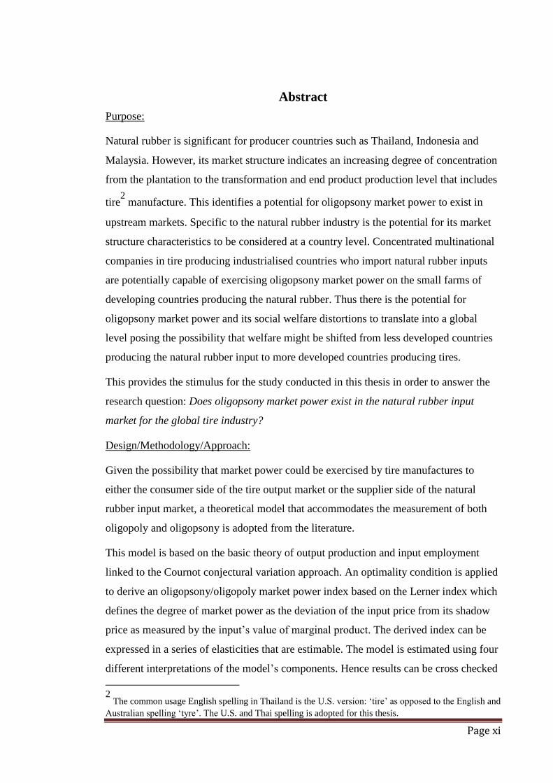
Purpose:

Natural rubber is significant for producer countries such as Thailand, Indonesia and

Malaysia. However, its market structure indicates an increasing degree of concentration

from the plantation to the transformation and end product production level that includes

tire2 manufacture. This identifies a potential for oligopsony market power to exist in

upstream markets. Specific to the natural rubber industry is the potential for its market

structure characteristics to be considered at a country level. Concentrated multinational

companies in tire producing industrialised countries who import natural rubber inputs

are potentially capable of exercising oligopsony market power on the small farms of

developing countries producing the natural rubber. Thus there is the potential for

oligopsony market power and its social welfare distortions to translate into a global

level posing the possibility that welfare might be shifted from less developed countries

producing the natural rubber input to more developed countries producing tires.

This provides the stimulus for the study conducted in this thesis in order to answer the

research question: Does oligopsony market power exist in the natural rubber input

market for the global tire industry?

Design/Methodology/Approach:

Given the possibility that market power could be exercised by tire manufactures to

either the consumer side of the tire output market or the supplier side of the natural

rubber input market, a theoretical model that accommodates the measurement of both

oligopoly and oligopsony is adopted from the literature.

This model is based on the basic theory of output production and input employment

linked to the Cournot conjectural variation approach. An optimality condition is applied

to derive an oligopsony/oligopoly market power index based on the Lerner index which

defines the degree of market power as the deviation of the input price from its shadow

price as measured by the input‟s value of marginal product. The derived index can be

expressed in a series of elasticities that are estimable. The model is estimated using four

different interpretations of the model‟s components. Hence results can be cross checked

2 The common usage English spelling in Thailand is the U.S. version: „tire‟ as opposed to the English and

Australian spelling „tyre‟. The U.S. and Thai spelling is adopted for this thesis.

Page xii

across four different approaches and transformed from a conventional industry/firm

level to a global industry/country level to answer the research question.

To implement the market power index, the global tire demand, the global natural rubber

supply and the tire production functions for the USA, France, Japan and Germany are

estimated. Data for variables in each equation are analysed and tested for

nonstationarity prior to functional specification. From each individual country data,

estimated coefficients are used for hypothesis tests for the existence of oligopsony

market power as well as oligopoly market power. If the hypothesis tests reject the null

hypothesis of competitive markets, the presence of oligopsony and/or oligopoly market

power is indicated. Derived elasticities enable the derivation of corresponding market

power indexes specific to each country.

Findings:

Results imply that the tire industries in USA, France, Japan and Germany do display

oligopsony power on the world natural rubber market. Policy implications are drawn

using the elasticity values of the market power indexes. They call for policies aimed at

raising the elasticity of demand for tire and supply of natural rubber and generating

more competition in the global tire market and natural rubber input market.

This supports the claim that typical agricultural policies designed to raise natural rubber

supply elasticity, such as price stabilization and subsidies, could be adopted to counter

oligopsony market power possessed by its downstream industries. Policies to raise

supply elasticity such as access to information, income equalization funds and risk

management are also supported.

Policy implementations to address oligopoly power in tire market support attempts to

increase competition in the global tire market from newly developing economies but

further studies are called for in this regard.

Originality/Value:

Oligopsony market power theory based on an industry/firm level is applied to a global

industry/country level. Hence, in addition to identifying economic inefficiency, this

approach is capable of identifying welfare shifting from less developed countries

producing commodity inputs to industrialised countries using the inputs. Furthermore,

the approach is innovative as it estimates a market power index derived from a Cournot

Page xiii

conjectural variation approach with four different variations. The multiple variation

approach provides stronger support for the tested outcomes.

Chapter 1 Page 1

Chapter 1

Introduction

1.1 Introduction

This thesis explores the extent of input price distortion on the world natural rubber

industry. As an agricultural commodity requiring specific plantation and climate

conditions, the production of natural rubber is restricted to certain countries,

predominantly the developing economies of Thailand, Indonesia and Malaysia of which

Thailand is the top producing country. The importance of the natural rubber industry for

Thailand is of particular significance for this thesis.

The natural rubber industry has a product chain that commences in plantation activity.

The producing trees are perennial crops and require as much as six to seven years before

they can produce the raw product latex. Latex outputs are not easily stored overtime like

manufacturing products. Production areas are spread across locations that involve

significant transport costs. Latex requires several production processes before it

becomes the rubber sheets and blocks that are important inputs for downstream

industries such as automotive tires. Much of the natural rubber production is conducted

on relatively small and low income farms. The markets for natural rubber progressively

increase in concentration for each down-stream industry stage, from field latex to un-

smoked sheets, smoked- sheets, block rubber and the major end product of automotive

and other vehicle tires. These conditions have the potential to generate a lack of

bargaining power for natural rubber farmers in the market for natural rubber.

In contrast the major end product of tire production is dominated by large multinational

companies in a relatively concentrated industry with production and sales concentrated

in wealthy developed countries. Consequently the market for natural rubber, as an input

for tire production, has both economic efficiency and welfare issues of interest. The

economic efficiency issue of concern is the possibility that tire manufacturers may be

able to exert market power in the market for natural rubber inputs such that natural

rubber prices paid to its producers are less than the marginal revenue product earned by

the tire producers from this input. The welfare issue of concern is the possible distortion

in income distribution between natural rubber producers and consumers of natural

rubber products. As natural rubber production is concentrated in a small number of less

wealthy producing countries and production of tires is concentrated in multinational

Chapter 1 Page 2

companies with developed country ownership and the sale of tires is concentrated in

these same developed countries, welfare issue of income distribution translates to a

country level. Accordingly, an assessment of oligopsony power of tire producing

countries on world natural rubber market is called for.

Therefore, this thesis examines the potential for market power in a global natural rubber

industry supplying inputs to the global automotive tire industry and the associated

welfare implications of an inefficient and inequitable income distribution that could

exist between the lesser developed countries producing the natural rubber inputs and

developed country producers and consumers of automotive tires.

The key research question is: Does oligopsony market power exist in the natural rubber

input market for the global tire industry?

1.2 Justification for the Research

Natural rubber is an important industry for the producing countries. It provides jobs for

rubber farmers and supplies raw material for rubber manufacturing industries. In the

year 2005 natural rubber production reached 2.91, 2.27 and 1.13 million metric tons for

Thailand, Indonesia and Malaysia respectively. A quantity of 2.46 million tons3or 40%

of the three countries‟ natural rubber outputs were used by major vehicle tire producing

countries.4

Natural rubber production in Thailand has been growing and currently Thailand is the

top producing country. Natural rubber is one of Thailand‟s major export earning crops.

There are about 1,088,000 farms producing natural rubber. The number of natural

rubber farmers is approximately six million. About one-third of world total supply

comes from Thailand. The industry generates jobs and decreases labour migration from

the provinces to Bangkok, which helps to improve provincial population welfare. The

number of employees in government institutions which are related to natural rubber

administration is about five thousand.

However, despite this significance, the income from natural rubber and natural rubber

products comprise only 1.24 % and 0.85 % of Thai GDP respectively. Natural rubber

value added industries are still small, using only 10% of total natural rubber output.

3 International Rubber Study Group (2005)

4This figure excludes some countries whose data for natural rubber consumed in the tire sector are not

available such as China and Russia.

Chapter 1 Page 3

However, they generate approximately40% of total natural rubber export income, which

illustrates the significance of value added products compared to intermediate rubber

products which generated approximately 60% of export income despite comprising 90%

of the natural rubber stocks that were not used for local consumption. Four economic

regions consumed up to 72% of Thai natural rubber exports (see Chapter 2): namely

Japan (38%), USA (12%), France (12%) and other EU countries (10%) during the

studied period.5 The global tire industry is dominated by a few well-known producer

countries. The average world tire sale volume concentration ratio for the period 1960-

2000 for the top four producing countries was 77 %. The largest producers in 2000

were: Japan (30%) followed by USA (22%), France (19%) and Germany (7%).6 Thus,

enhanced by the collapse of the International Natural Rubber Organization in 1999, the

potential for market power to be applied by a small number of multinational tire

manufacturers in the market for natural rubber is of considerable concern for natural

rubber producer countries such as Thailand.

This concern is related to the concept of market power and its consequences. The

conceptual basis is found in industrial economics. The consequences are that market

power can adversely affect economic welfare. Economic welfare depends on market

performance, which in turn is seen by mainstream industrial economic theory to be a

consequence of market structure. A concentrated market structure could enable a few

large firms to exploit consumers and input suppliers by producing at a lower than

optimal output level at higher than optimal output prices with lower than optimal

employment of inputs at lower than optimal input prices.

This outcome is unambiguously predicted in the extreme case of a monopoly producer

who is also a monopsony purchaser of inputs. Here the monopolist is in receipt of

economic rents that are generated in the output market by a price that is higher than the

marginal cost of the output sold and in the input market by paying an input price that is

less than the value of the marginal product derived from that output. Assessment of the

price – marginal cost differential and the value of marginal product – input price

differential is the fundamental approach to economic evaluation of output and input

market power respectively.

5 Chapter 2, Table 2.16

6 Chapter 2, Table 2.22

Chapter 1 Page 4

However, in the case of oligopoly and oligopsony, where there are a few firms,

economic theory does not provide an unambiguous predicted outcome. The outcome is

dependent on the conduct of the firms in reaction to each other. They may employ a

variety of strategies, resulting in a variety of outcomes. The resulting market

performance may or may not approach the optimal theoretical performance outcome. It

thus becomes an empirical question that requires case by case assessment of the price –

marginal cost differential and the value of marginal product – input price differential to

identify oligopoly or oligopsonistic market power respectively.

A consequence of possible market power that applies to this particular application is

that tire producers are located primarily in developed industrialized countries whereas

natural rubber is produced by small-scale farmers in developing agricultural countries.

Hence, if there are market power rents being earned from market power, then economic

welfare gains are being transmitted from less developed countries to more developed

countries. This enhances the concern over market power for the industries in question

and calls for analysis at a country level as the consequences of exploitation, leading to

economic welfare distortion, could occur at a national level.

1.3 Methodology

The literature on market power assessment is heavily focused on oligopoly applications

as opposed to assessment of oligopsony applications. Very few studies have been

applied to oligopoly and oligopsony power simultaneously and no study has been found

that analyses the markets researched in this thesis. Papers of special interest to the

methodology adopted in this thesis are Chang & Tremblay (1991) and Chang &

Tremblay (1994). These papers develop theoretical models that simultaneously assess

the market power on both the output and input market sides. This allows for tracing of

potential oligopsony power for an input market such as natural rubber and its

interrelationship with a potential oligopolistic downstream output market such as tire

manufacture. The model generates an index measure of market power for both market

types that is composed of empirical variables such as price and conjectural elasticities.

The methodology is based on comparing the value of marginal product (VMP) between

the profit maximizing optimal VMP and the observed marginal resource costs (MRC)

(see Chapter 3). The measurement is simplified to a single market power index

comprising four estimable elasticities. The index is capable of identifying the market

Chapter 1 Page 5

structure of the input and output markets ranging from competitive/competitive to

oligopsony/oligopoly and monopsony/monopoly performance (see Chapter 4). The

index is capable of covering the range of potential market conditions. For example, on

the industry level, given market shares as a weight, the Chang & Tremblay index

approaches the Herfindahl-Hirshman index. When each firm has equal market shares,

the case approaches a Cournot case. The index can also accommodate the

monopsony/monopoly Robinson case and the Lerner index case of market power in the

output market without market power in input markets.

This thesis extends the Chang & Tremblay (1991) model, to create a general model with

four variations depending on the interpretation and estimation approach adopted for the

elasticity terms involved. The development of this general model is described in

Chapter 4.

A further extension of the model is its application at a global market level with country

level output and input markets as opposed to the traditional firm – industry within a

country level application that is commonly found in industrial economics.

The model is empirically estimated and applied to the four major tire producing

countries, namely the USA, Japan, France and Germany as purchasers of natural rubber

inputs from the world natural rubber market which is dominated by three major supplier

countries, namely Thailand, Indonesia and Malaysia. Particular focus is placed on the

implications of the market power interrelationships in these markets for Thailand which

is the top natural rubber supplying country.

1.4 Empirical Application

The empirical analysis and results are provided in Chapter 5. The analysis involves

estimation of a number of demand and supply functions including: a world tire demand

function; tire production functions for each country; a world natural rubber supply

function and optimality condition functions for each country. These estimations are

used to derive values for key variables that are required for market power index

construction including: demand and supply elasticities, marginal products and

conjectural elasticities for the tire market (output) and natural rubber market (input) for

each country. These variables are then used to construct market power indexes for each

country for both their tire output and natural rubber input markets. In addition, in order

to accommodate a number of theoretical and empirical challenges encountered, the four

Chapter 1 Page 6

alternative approaches to index derivation are applied (see Chapters 4 and 5 for Models

1 to 4).

Results support the presence of the oligopsony market power in the natural rubber input

market for tire manufacture on a country level basis.

1.5 Outline of the Thesis

Chapter 1 provides an introduction to the thesis, the research problem, the relevance of

the study and its justification, a brief outline of the methodology used, and the basic

conclusion. Chapter 2 presents an overview of the natural rubber industry in Thailand

and at the world level and its relationship to the global tire industry. Chapter 3 surveys

the theoretical base for economic analysis of market power and the relevant literature.

The methodology to be applied, in the form of a general empirical model, is developed

in Chapter 4. Chapter 5 describes the empirical application of the model developed in

Chapter 4 to the tire and natural rubber industries. Results are presented and discussed

in Chapter 5. Chapter 6 provides a conclusion to the thesis and includes a discussion of

the implications of the findings for the natural rubber industry with particular emphasis

on Thailand. Policy options are also discussed.

Chapter 2 Page 7

Chapter 2

Rubber as a Product: Nature, Production, Uses and Market

2.1 Introduction

In 1770 an English chemist, Joseph Priestley, received a bouncing ball from a

colleague. He noticed that the interesting object could eliminate lines that are written by

pencils. He therefore named the material rubber. Rubber has since then been applied to

produce many useful objects that help develop a modern society. Its original source was

latex, a natural product from tree sap. However, in modern times, due to growing

demand, synthetic rubber derived from petroleum was invented to provide additional

sources of rubber.

2.1.1 Biology of Rubber Trees

There are more than 200 species of plants that produce rubber latex. However, there are

only two species that have become commercially significant. They are Hevea

Brasiliensis and Guayule bush. It is Hevea Brasiliensis that produces 99% of natural

rubber consumed today. Its origin is in Brazil. It has been introduced to other tropical

areas such as Malaysia, Indonesia, Thailand, India, and Sri Lanka. It has also been

planted in some African countries.

Due to high demand in recent years and increasing costs of synthetic rubber production,

there have been attempts to boost natural rubber supply by cultivating Hevea trees in

areas far from equator zones. Research on substitute trees such as the Guayule bush

found in Mexico and south western parts of USA is in progress as are attempts to

produce natural rubber by gene technology.

2.1.2 Rubber as a Commercial Product

Since the 11th

century the use of Hevea latex has been known in Central and South

America. However, it was not until 1736 that the first sample material from latex was

sent to Europe by the French scientist Charles Marie de La Condamine. More than thirty

years later, in 1770, the material was first named rubber by Joseph Priestley. In 1818,

rubber was first applied to modern uses such as raincoats. Rubber was first applied to

industrial uses after Charles Goodyear, in 1839, discovered a process to transform

http://en.wikipedia.org/wiki/Charles_Marie_de_La_Condamine

Chapter 2 Page 8

rubber into more flexible forms. He is said to have accidentally dropped a piece of

rubber and some sulphur into fire. After retrieving the material it was found to be

stronger and more elastic. The process of mixing rubber with sulphur under heating is

called vulcanization. In 1887 John Boyd Dunlop patented his pneumatic tire.

Subsequently the supply of rubber was depleted by strong demand. Hence British

rubber traders commenced cultivation of huge rubber plantations in India, Malaysia and

Ceylon. It was during this period that Hevea trees were first introduced to Thailand by

Phraya Ratsadanupradit Mahison Pakdi (Kor Sim Bee) in 1899.

2.1.3 Synthetic Rubber

Since the 1900‟s there have been many experiments to improve rubber quality. In 1910

sodium was found to be a catalyst for the polymerization process and this meant it was

possible to synthesize rubber by polymerization from a variety of molecular links. In

WWI Germany was cut off from natural rubber supplies, so they invented 2,500 tons of

synthetic rubber from dimethyl butadiene. Later, during WWII Japan gained control of

major natural rubber sources in Asia. This led the US to develop more than one million

metric tons of synthetic rubber during 1941-1944. In order to avoid having to rely on

overseas rubber supplies, other countries also produced their own synthetic rubber

supplies. Synthetic rubber thus became more common and its output reached 4 million

tons after the Korean War. Since then synthetic and natural rubber production and

consumption have grown in rough balance.

Rubber materials comprise millions of long and tangled polymeric molecules. Each

polymeric molecule consists of tens of thousands of linked isoprene molecules. Each

isoprene molecule of natural rubber has 13 atoms of carbon and hydrogen. Thus it is

known chemically as polyisoprene. If the polymer strands anywhere in the mass of

rubber are pulled, they can straighten and uncoil then re-coil when the pulling is

stopped.7

Although natural rubber and synthetic rubber are similar in chemical and physical

properties, they are produced differently. Natural rubber is a natural plantation crop. As

such it is less stable both in quantity and quality. However, it is environmentally

friendly. On the other hand, synthetic rubber output is more stable but lacks the full

qualities of natural rubber and as it is derived from petroleum, it is exposed to

7 Polymers are huge chainlike molecules composed of many smaller molecular links.

Chapter 2 Page 9

fluctuations in the world oil price. Table 2.1 displays the relative consumption rates in

recent years.

Table 2.1 Elastomer Consumption

(1,000 metric tons)

Year Natural Rubber Synthetic Rubber Total

2004 8,280 (41%) 11,800 (59%) 20,080

2005 9,001 (43%) 11,917 (57%) 20,918

Source: compiled from International Rubber Study Group (various copies).

From Table 2.1 it can be seen that world elastomer consumption in recent years has

been more than 20 million metric tons annually and is split roughly 40% to 60%

between natural and synthetic rubber.

2.2 Natural Rubber Location and Production

Natural rubber production is linked to the location of tree cultivation, latex tapping, the

production of rubber sheets and block rubber.

2.2.1 Location

Natural rubber trees were first discovered in the Amazon basin of South America

including Brazil, Bolivia, Venezuela and Peru. Historically more than 90% of natural

rubber was exported from Brazil. However, when natural rubber was commercialized,

natural rubber production could not meet demand because of natural restrictions on

production. First natural rubber was produced from wild natural rubber trees in

rainforests hence, production was limited. Secondly, the tapping cost structure was high.

The high costs were caused by tough working conditions including health problems

such as yellow fever and malaria in the forests. There was a scarcity of rubber tappers

and production facilities on top of high transportation costs from Brazil. In addition

tapping was restricted to the months of August to January to avoid the rainy season.

Consequently the demand for natural rubber soon outstripped the production capacity of

Brazil (Zephyr & Musacchio, 2002).

Consequently, attempts were made to plant more rubber trees in Southern parts of Asia.

Due to appropriate management and a suitable climate, Southeast Asia became the

Chapter 2 Page 10

essential geographic area for natural rubber supply. Currently there are three countries

that are the key supply sources of natural rubber: Thailand, Indonesia and Malaysia.

Other producing countries are in South Asia such as India, Sri Lanka and newcomers

such as Vietnam, Lao, Cambodia and Myanmar. In addition there is some supply from

China and Africa. By 2004 there was a total of 9,335.6 million hectares of rubber

planted globally.

Table 2.2 displays areas under natural rubber plantation for the year 2004.

Table 2.2 Areas under Natural Rubber Plantation (2004)

Country Area (1,000 hectares) % of Total

Asia

Indonesia 3262.0 34.94

Thailand 2083.4 22.32

Malaysia 1282.0 13.73

China 600.0 6.43

India 578.0 6.19

Vietnam 450.9 4.83

Sri Lanka 128.9 1.38

Myanmar 104.8 1.12

Philippines 92.0 0.99

Cambodia 52.3 0.56

Bangladesh 46.7 0.50

Papua New Guinea 13.7 0.15

Total area 8694.7 93.13

Africa

Nigeria 150.0 1.61

Liberia 108.9 1.17

Cote d’ Ivoire 95.8 1.03

Cameroon 48.3 0.52

D R of the Congo 35.0 0.37

Chapter 2 Page 11

Table 2.2 (continued)

Ghana 16.9 0.18

Gabon 13.0 0.14

Total area 467.9 5.01

South America

Brazil 117.3 1.26

Guatemala 44.5 0.48

Mexico 11.2 0.12

Total area 173 1.85

Total World Area 9335.6 100%

Source: Compiled from International Rubber Study Bulletins.

In 2004 Asia had 8,694,700 hectares (93%) of world natural rubber planting area

followed by Africa (5%) and South America (2%). Indonesia, Thailand and Malaysia

are the three largest producing countries, sharing 35%, 22% and 14% respectively for a

total of 71% of total world production. China, India and Vietnam form the second

largest group of countries producing 6%, 6%, and 5% respectively for a total of 17%.

2.2.2. Production Methods

2.2.2.1. Natural Rubber Plantation

In plantations a Hevea tree requires five to seven years to mature. They can then be

tapped for latex until they reach 30 years of age. Latex yield depends on the type of tree

clone and environmental conditions. Clone properties determine average yields,

productive years, pre-mature periods before tapping, wind susceptibility, resistance to

diseases and pests, and soil and terrain requirements. Average yield is around 250

kilogram per rai (1,600 kilogram per hectare). The clone that is mostly planted in

Thailand is RRIM600. The Rubber Research Institute of Thailand (RRIT) is actively

involved in research to develop more productive clones.

2.2.2.2.Tapping Natural Rubber Latex

Latex from Hevea trees accumulates in small vessels that spiral around trunks. To

collect latex, workers tap the Hevea tree by shaving off a slanted strip of bark halfway

Chapter 2 Page 12

around the tree, about 0.80 centimetres deep. It takes a few hours for the flowing latex

to dry up from each cut. Workers repeat tapping every other day, shaving the bark

below the previous cut. When the cut is about 30 centimetres above the ground, they tap

the other side of the tree leaving the first side to renew. There are attempts to develop

tapping technology in order to save labour cost including, puncture tapping, which uses

needles to tap instead of cutting the trees and technologies to nourish the tree in order to

produce more latex per tapping.

Preservative chemicals such as ammonia and formaldehyde are added to the tapped

latex in order to keep it from crumbing before being gathered and transported to

manufacturing factories. Production quantity depends on the area cultivated. Output per

hectare depends on premature periods, clone qualities, and growing nurseries. In

troubled economic times, farmers tap more intensely and hence cause damage to long-

term productivity.

2.2.2.3 Producing Rubber Stocks

There are a variety of natural rubber products at this stage. All are produced from fresh

latex which is tapped daily, except in rainy days. Major variations are ribbed-smoked

sheets, block rubber and concentrated liquid rubber.

At the factories latex is sieved to remove dirt. It is then blended with water to maintain a

uniform standard of rubber element which is 30%-40%. Some latex is transformed to

concentrated latex at this stage. Concentrated liquid latex has about 60% of natural

rubber substances. It is used in producing dipped rubber products including elastic

fabric, rubber thread, foams, adhesives and coating. Some latex is processed into a

variety of products, depending on drying condition and pigments added, such as pale

crepe rubber, which is used in footwear industry. Concentrated latex accounts for about

10% of rubber production.

The rest of the latex is transformed into other kinds of intermediate rubber stocks such

as rubber sheets and block rubber. To produce rubber sheets, latex is diluted and then

acid is added. Rubber particles bunch together and the coagulated rubber is then rolled

within 18 hours, to squeeze out water. Every 1.4 kilograms of latex produces 0.5

kilogram of rubber. The rubber is then left to dry and is smoked in smoking houses. The

smoked rubber sheets are collected a week later and packed into bales of different

grades from grade 1 (RSS1) to grade 5 (RSS5). Rubber sheets are used mostly in the tire

Chapter 2 Page 13

industry. Block rubber is made from mixing rubber sheets and coagulated rubber and is

also mostly used in the tire industry.

Some natural rubber farmers transform fresh latex into un-smoked sheets before selling

to factories. The process is to mix fresh latex with certain chemicals, which help the

latex to dry and form into sheets. These are called un-smoked sheets. Un-smoked sheets

are delivered to rubber smoking factories which turn them into smoked sheets.

Block rubbers are produced from mixing certain rubber outputs such as cup lump

(rubbers that are left in utensils that contain fresh latex) and ribbed-smoked rubber.

Block rubbers are called Thai Standard Rubber (TSR) in Thailand, Malaysia Standard

Rubber (MSR) in Malaysia and Indonesia Standard Rubber (ISR) in Indonesia. Block

rubber comprises different grades. Block rubber is used in tire production, mostly in the

USA. Sheet rubber and block rubber are the most consumed types. Indonesia and

Malaysia produce block rubber from most of the latex harvested. Thailand has both

rubber sheets and block rubber.

Natural rubber has been produced for over a hundred years. World production was

45,000 metric tons in 1900 and increased to 8,742,000 metric tons in 2004. Output

dropped during the world wars but has continued growing to date.

Table 2.3 summarizes world natural rubber production from 1960 to 2004. The

production and market share for Thailand, Indonesia, and Malaysia are also illustrated.

Thailand‟s production was only 171,000 tons (8%) in 1960 but it gradually expanded to

3 million tons by 2004 and its market share increased from 8% to 34%. Indonesia

produced 620,000 tons in 1960 it grew to 2 million tons in 2004 with a corresponding

market share decrease from 30% to 23%. Malaysia produced 764,000 tons in 1960 and

its current output fluctuates around one million tons. Its market share was 40% in 1970

but it dropped to 14% in 2004. The three country market share for these major

producers has varied from 76% in 1960 to 79% in 1980 and 71% in 2004.

Most of this production is consumed in the tire sector, as discussed in the next section.

Hence world tire manufacturers have a significant impact on the natural rubber industry

in these countries.

Chapter 2 Page 14

Table 2.3 Natural Rubber Production in Thailand, Indonesia and Malaysia

(1960-2004)

(1,000 tons (% share))

Year World Thailand Indonesia Malaysia 3 Countries

1960 2,040 171.0 (8.4) 620.0 (30.4) 764.0 (37.5) (76.23)

1970 3,140 287.0 (9.1) 815.0 (26.0) 1,269.0 (40.4) (75.51)

1980 3,850 501.0 (13.0) 1,020.0 (26.5) 1,530.0 (39.7) (79.25)

1990 5,120 1,275.3 (24.9) 1,262.0 (24.6) 1,291.0 (25.2) (74.77)

2000 6,730 2,346.4 (34.9) 1,501.1 (22.3) 927.3 (13.8) (70.95)

2004 8,620 2,959.4 (34.3) 2,006.2 (23.3) 1,168.7 (13.6) (71.16)

Source: Compiled from IRSG (various copies)

2.2.2.4 Producing Rubber Products

To produce rubber products, rubber inputs are treated through the processes of

mastication, vulcanization and moulding. The mastication process cuts natural rubber

into pieces and adds particular chemicals such as aniline and zinc oxide, which help to

accelerate vulcanization. Some chemicals act as age-resistors and anti-degradants. They

help the product last longer when exposed to sun light and high or low temperature.

Vulcanization is a process to put sulphur into natural rubber and heat for a specific time.

It helps polymers of rubber molecules transform into a substance that is stronger, more

elastic, does not dissolve in water and recoils when stretched. At the stage of

vulcanization, rubber can be put into moulds for specific end products. Specific

machines are used for each type of rubber formation. For example a calender is used to

form rubber into sheets, an extruder is used to produce tube and rubber foams are made

by adding air to latex before vulcanization. Adding hydrogen peroxide helps extract

water and oxygen causes air bubbles. A dipping method is used to produce a thin sheet

for covering glass, mosaic or metal utensils.

2.3 Uses of Natural Rubber

Natural rubber is used to produce a variety of products. As displayed in Figure 2.1.

From Figure 2.1 it can be seen that latex when transformed to sheet rubber and block

rubber, can be used for intermediate products such as reclaimed rubber and compound

rubber. When vulcanized, rubber can be used to produce a variety of products. The top

Chapter 2 Page 15

volume item is vehicle tires, which includes pneumatic tires, retreads, solid tires, tire

treads, tire flaps, cord and inner tubes. Other items are automotive accessories,

construction products, and other miscellaneous products. Another group of uses is

products produced from concentrated rubber. They are articles of apparel and clothing

accessories including gloves, mittens and mitts and hygienic or pharmaceutical articles.

Thailand produces and exports these products. The relative values of the different

rubber products are illustrated in Table 2.4.

Chapter 2 Page 16

Figure 2.1 Uses of Natural Rubber

Natural Rubber Trees

Fresh Latex

.

(14%)

Concentrated Latex

(86%)

Processed Rubber

Smoked Sheet Rubber Block Rubber Crepe Rubber

Air-Dried Rubber Cup Lump

Miscellaneous Types of Rubber

Dipped

Rubber Goods

1. Articles of apparel and clothing accessories including gloves, mittens and mitts.

2. Hygienic or pharmaceutical articles.

Un-vulcanized

Rubber Goods

1. Reclaimed

rubber, 2. waste or

parings and scrap,

3. compound rubber and other un-vulcanized rubber.

Vulcanized

Rubber Goods

New pneumatic tires, retreaded or used pneumatic tires, solid or cushion tires, tire treads and tire flaps, cord, inner tubes

Automotive Industry : tubes, pipes and hoses

Construction Industry: conveyor or transmission belts

Miscellaneous Industries: belting, hard rubber for example, ebonite.

Other articles of consumer products

Rubber wood

1. Para wood furniture 2. Wood toys 3. Miscellaneous items

Chapter 2 Page 17

Table 2.4 Thai Natural Rubber Products Exports (fob Value, $US Million, 2004)

HS-CODE Description $USmill %

40.07 Vulcanised rubber thread and cord 101 5.57

40.08 Plates, sheets, strip, rods and profile shapes, of vulcanised rubber other than hard rubber

16 0.88

40.09 Tubes, pipes and hoses, of vulcanised rubber other than hard rubber, with or without their fittings (for example, joints, elbows, flanges)

72 3.97

40.10 Conveyor or transmission belts or belting, of vulcanised rubber

23 1.27

40.11 New pneumatic tires 615 33.92

40.12 Retreaded or used pneumatic tires of rubber; solid or cushion tires, tire treads and tire flaps, of rubber

24 1.32

40.13 Inner tubes, of rubber 38 2.10

40.14 Hygienic or pharmaceutical articles (including teats) of vulcanised rubber other than hard rubber, with or without fittings of hard rubber

150 8.27

40.15 Articles of apparel and clothing accessories (including gloves, mittens and mitts), for all purposes, of vulcanised rubber other than hard rubber

497 27.41

40.16 Other articles of vulcanised rubber other than hard rubber 271 14.95

40.17 Hard rubber (for example, ebonite) in all forms, including waste and scrap; articles of hard rubber

6 0.33

Total 1,813 100%

Source: The Customs Department (2006). Values are transformed from baht at 40.22 baht/$US.

According to Table 2.4, natural rubber products yield export income of $US 1,813

million for Thailand. Pneumatic tires (item 40.11) are the top user of rubber consumer

products.

Finally a by-product use of natural rubber is the rubber wood. After some 30 years of

latex yielding periods, the rubber trees have to be re-planted. The replaced trees can be

processed into rubber wood which is highly demanded by the furniture industry as well

as the toy industry.

http://www.customs.go.th/Statistic/StatisticResult.jsp?productCode=4007&statType=export&productCodeCheck=Y&countryCheck=null&country=&month=12&year=2004










Chapter 2 Page 18

2.3.1 Uses of Natural and Synthetic Rubber in Tire Sector

One of the most discussed issues in the natural rubber industry is the substitution

between natural rubber and synthetic rubber. In the tire industry the two inputs are

closely related. A typical all season passenger tire (e.g.P195/75R14) which is the most

popular size, weighs about 21 pounds. It has the following approximate ingredients as

displayed in Table 2.5.

Synthetic rubber has endured a competing role with natural rubber since its invention.

Natural rubber consumption had fallen from 70% of total rubber consumption in 1950

to only 30 % in 1980. However, it stopped decreasing following the introduction of

radial tires in 1970s which helped to boost natural rubber consumption.

Natural rubber has done well in the tire sector due of its technical qualities such as

abrasiveness and elasticity. The competing synthetic rubber has specific qualities such

as resistance to heat, ozone and oil. Hence it meets special purpose needs in general

consumption of rubber. Although technology advancement and the attempts to invent

substitute materials for natural rubber have introduced various classes of automobile

and motor cycle tires, they still need an adequate quantity of natural rubber as a basic

ingredient. Truck tires, which have to carry a lot of weight, rely heavily on natural

rubber. Aircraft tires also need high quality natural rubber.8

Synthetic rubber can be used as substitute for natural rubber if pricing is advantageous.

However, technology is still a limiting factor for substitution. Thus natural rubber is

important for tire making and the tire sector is important for natural rubber since it is a

major rubber consuming industry.

8 IRSG 142/AE.

Chapter 2 Page 19

Table 2.5 Tire Manufacture Ingredients

Ingredient Weight %

Fabric Steel, nylon, aramid9 fibre,

rayon, fibre glass or polyester (usually a combination, e.g., polyester fabric in the body piles and steel fabric in the belts of most radial passenger tires.

1 lb of steel cord for belt, 1 lb of polyester and nylon, 1 lb of steel bead wire

14.26%

Rubber Natural rubber (NR) and Synthetic rubber (SR)

4 lbs of 8 types of NR +, 6 lbs of 5 types of SR

19.05% +

28.57% 47.62%

Reinforcing chemicals

Carbon black, silica, resins 5 lbs of 8 types of carbon black

23.81%

Anti-degradants Antioxidants / ozonants paraffin waxes

3 lbs of 40 different kinds of chemicals, waxes, oils, pigments, etc.

14.31%

Adhesion promoters

Cobalt salts, brass on wire, resins on fabrics

Curatives Cure accelerators, activators, sulphur

Processing aids Oils, tackifiers, peptizers10

, softeners

The natural rubber/synthetic rubber share depends on tire types as follows.

Natural Rubber /Synthetic Rubber Shares and Tire Types

Tire Types NR / SR shares

Race tire 35% / 65%

Passenger tire 45% / 55%

Light truck tire 50% / 50%

Off-highway tires (giant/earthmover) 80% / 20%

Source: compiled from http://www.goodyear.ca/tire_school/ingredients.html June 17, 2006

9 Aramid fibers are a class of heat-resistant and strong synthetic fibers. They are used in aerospace and

military applications, for ballistic rated body armor fabric and as an asbestos substitute. The name is a

shortened form of "aromatic polyamide". They are fibers in which the chain molecules are highly oriented

along the fiber axis so the strength of the chemical bond can be exploited.

10 These products are used as processing aids/viscosity reducers for natural and synthetic rubbers.

http://www.goodyear.ca/tire_school/ingredients.html

http://en.wikipedia.org/wiki/Synthetic_fiber

http://en.wikipedia.org/wiki/Bulletproof_vest

http://en.wikipedia.org/wiki/Cloth

http://en.wikipedia.org/wiki/Asbestos

http://en.wikipedia.org/wiki/Aromatic

http://en.wikipedia.org/wiki/Polyamide

http://en.wikipedia.org/wiki/Chemical_bond

Chapter 2 Page 20

2.3.2 Natural Rubber and the Tire Industry

Natural rubber products are exported from producing countries to tire producing

countries, as well as being used for some tire manufacturing within the exporting

countries. The top four tire producing countries in the years 1960 - 2000 are US, France,

Japan and Germany. The quantity of natural and synthetic rubber used in these four

countries was 559 thousand tons and 816 thousand tons respectively in 1960. By the

year 2004 the consumption had developed to 1,751 and 1,753 thousand tons of natural

rubber and synthetic rubber respectively. The percentage of natural rubber to synthetic

rubber use was 69% in 1960, dropped to 43% in 1970 and then rose to 100% in 2004.

Table 2.6 summarizes the rubber used in tire sectors of US, France Japan and Germany.

Table 2.6 Natural and Synthetic Rubber Used in US, France, Japan & Germany

Tire Sectors (1960-2004)

(1,000 tons)

Natural Rubber (NR) Synthetic Rubber (SR)

NR

World

NR in US FR JA GR

% SR

World

SR in US FR JA GR

% NR

/ SR

1960 2,120 559 26% 2,350 816 35% 69%

1970 3,035 764 25% 5,625 1,784 32% 43%

1980 3,760 1,041 28% 8,785 1,938 22% 54%

1990 5,200 1,484 29% 9,710 1,904 20% 78%

2000 7,320 1,973 27% 10,800 2,106 19% 94%

2004 8,280 1,751 21% 11,800 1,753 15% 100%

Source: Compiled from International Rubber Study Group

2.4 Natural Rubber Market and Prices

Natural rubber data used in the studied period (1960 -2000) are mostly rubber sheets

whose price per Malaysian ringgit of grade 1 product (RSS1) was the major guiding

price. The average price is 2136.5 ringgit ($US 771.30) / ton with a range 935.00 to

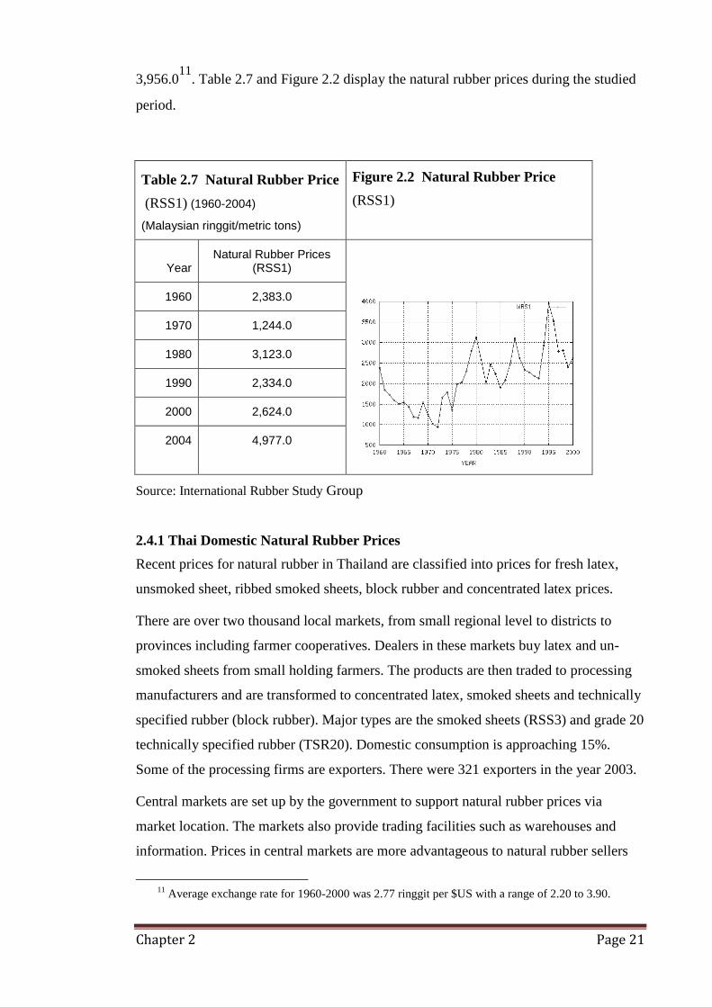
Chapter 2 Page 21

3,956.011

. Table 2.7 and Figure 2.2 display the natural rubber prices during the studied

period.

Table 2.7 Natural Rubber Price

(RSS1) (1960-2004)

(Malaysian ringgit/metric tons)

Figure 2.2 Natural Rubber Price

(RSS1)

Year Natural Rubber Prices

(RSS1)

1960 2,383.0

1970 1,244.0

1980 3,123.0

1990 2,334.0

2000 2,624.0

2004 4,977.0

Source: International Rubber Study Group

2.4.1 Thai Domestic Natural Rubber Prices

Recent prices for natural rubber in Thailand are classified into prices for fresh latex,

unsmoked sheet, ribbed smoked sheets, block rubber and concentrated latex prices.

There are over two thousand local markets, from small regional level to districts to

provinces including farmer cooperatives. Dealers in these markets buy latex and un-

smoked sheets from small holding farmers. The products are then traded to processing

manufacturers and are transformed to concentrated latex, smoked sheets and technically

specified rubber (block rubber). Major types are the smoked sheets (RSS3) and grade 20

technically specified rubber (TSR20). Domestic consumption is approaching 15%.

Some of the processing firms are exporters. There were 321 exporters in the year 2003.

Central markets are set up by the government to support natural rubber prices via

market location. The markets also provide trading facilities such as warehouses and

information. Prices in central markets are more advantageous to natural rubber sellers

11

Average exchange rate for 1960-2000 was 2.77 ringgit per $US with a range of 2.20 to 3.90.

Chapter 2 Page 22

than local markets but there are only a small number of them currently although more

central markets are to be established.

A sample of average yearly prices for the years 1998 – 2007 show how central market

auction trading has helped boost local market prices by an average of 5% (See Table

2.8).

Table 2.8 Natural Rubber Local Market Prices and Central Market Prices (1998-2007)

(Baht/ ton)

Year (1) USS3

Local Market

(2) USS3

Central Market (Had Yai)

(1) / (2)

1998 23,100 25,680 1.11

1999 18,550 19,770 1.07

2000 22,360 23,420 1.05

2001 21,450 22,530 1.05

2002 27,870 29,150 1.05

2003 38,860 40,170 1.03

2004 44,900 46,660 1.04

2005 53,540 55,230 1.03

2006 69,960 71,350 1.02

2007 70,250 72,140 1.03

Average

Min Max

39,084

18,550 70,250

40,610

19,770 72,140

1.05

1.02 1.11

Source: Compiled from The Rubber Research Institute of Thailand and The Office of Rubber

Replanting Aid Fund

The futures market in Thailand is The Agricultural Future Exchange of Thailand

(AFET). It started trading in 2004. Both smoked sheet and block rubber are traded in

AFET (The Rubber Research Institute of Thailand, 2007).

At the export level rubber prices are delivered in accordance with their exporting

country ports. The generally recognized and available prices are sheet rubber RSS3

prices, block rubber TSR20 prices, and concentrated latex prices coded in fob Bangkok.

The export prices of ribbed smoked sheet on average is 20% (15%-31%) higher than

Chapter 2 Page 23

fresh latex, 17% (12%-27%) higher than un-smoked sheets, and 10% (5%-18%) higher

than domestic ribbed smoked sheets, as displayed in Table 2.9 and Figure 2.3.

Table 2.9 Thai Domestic Natural Rubber Prices (1998-2007)

(Baht/ton)

Baht/ton

Year (1)

Fresh Latex

(2) USS3 Local

Market

(3) RSS3

Central Market

(Had Yai)

(4) RSS3

fob BKK

(4)/(1) (4)/(2) (4)/(3)

1998 24,800 23,100 25,680 29,350 1.18 1.27 1.14

1999 18,000 18,550 19,850 23,500 1.31 1.27 1.18

2000 22,310 22,360 23,430 26,660 1.19 1.19 1.14

2001 20,760 21,450 23,280 25,330 1.22 1.18 1.09

2002 26,310 27,870 30,110 32,890 1.25 1.18 1.09

2003 37,930 38,860 41,730 43,650 1.15 1.12 1.05

2004 43,690 44,900 48,090 51,700 1.18 1.15 1.08

2005 52,510 53,540 57,070 60,170 1.15 1.12 1.05

2006 67,880 69,960 74,210 79,860 1.18 1.14 1.08

2007 68,010 70,250 74,110 78,470 1.15 1.12 1.06

Average

Min Max

38,220

18,000 68,010

39,084

18,550 70,250

41,756

19,850 74,210

45,158

23,500 79,860

1.20

1.15 1.31

1.17

1.12 1.27

1.10

1.05 1.18

Source: Compiled from The Rubber Research Institute of Thailand and The Office of Rubber

Replanting Aid Fund

Figure 2.3 Thai Natural Rubber Prices

Local market grade 3 Unsmoked sheets (U3L)

Central Market grade 3 smoked sheets (U3C)

Export fob Bangkok grade 3 rib-smoked sheets (R3BK)

Chapter 2 Page 24

The sharp rise in natural rubber prices from 2001 is considered to be due to economic

growth especially in China, causing increases in demand for vehicles, tires and natural

rubber input respectively. Also the sharp rise in oil prices since 2001has raised the

relative price of synthetic rubber to natural rubber, which is a competing input in tire

manufacturing (United Nations Conference on Trade and Development, 2009). The

escalation in oil prices also led to price rises in commodities including natural rubber.

2.4.2 Thai Natural Rubber Export Prices

The RSS3 are coded fob Bangkok prices. Table 2.10 depicts the relevant price series in

current world natural rubber markets.

Table 2.10 Thai Natural Rubber Export Market Prices (1996-2004) ($US/ton)

Concentrated LATEX

fob BKK

RSS3 fob

BKK

RSS3 TOCOM

RSS3 AFET

TSR20 fob

BKK

TSR20 SICOM

TSR20 CIF NY

1996 1,091.82 1379.64 1157.06 - 1,321.07 1,136.00 1,420.00

1997 772.54 964.29 950.26 - 952.37 985.00 1,106.00

1998 611.72 709.62 698.98 - 673.61 651.00 776.00

1999 525.05 621.04 613.64 - 598.51 589.79 703.94

2000 572.99 664.18 696.31 - 640.26 629.05 726.46

2001 469.05 570.11 549.18 - 538.83 515.64 614.00

2002 599.39 765.60 795.39 - 754.19 752.79 857.08

2003 850.57 1052.06 1113.04 - 1,012.53 1,005.06 1,121.23

2004 993.54 1285.43 1420.00 1,195.47#

1,224.76 1,207.61 1,352.06

Source: Compiled from The International Rubber Study, The Rubber Research Institute of

Thailand, The Office of Rubber Replanting Aid Fund and The Agricultural Futures Exchange of

Thailand.

# The Agricultural Futures Exchange of Thailand started its operation in 2004. The record price

here was derived from the May – December average one month forward price 49.60

baht/kilogram at the exchange rate of 40.22 baht / $US.

In addition, natural rubber is also coded in futures markets. Most well-known prices are

in TOCOM (The Tokyo Commodity Exchange), SICOM (Singapore Commodity

Exchange) and the newly opened AFET (The Agricultural Futures Exchange of

Chapter 2 Page 25

Thailand). On the consuming country side the RSS3 prices are related to Japan imports.

TSR20 prices can be found cif in New York as well as European country ports.

2.4.3 Other Export Market Prices

In global export markets each producing country announces market prices. In Thailand,

prices in central markets are related to fob prices. In Indonesia, prices follow SICOM

prices and are discounted by a little. In Malaysia, prices announced by the country‟s

Rubber Board are based on reports from a panel of dealers, packers and latex producers.

In India, official prices are a little bit higher than international prices (Thevar, 2002).

Consuming country market prices are mostly from New York. Prices from future

markets, namely TOCOM, SICOM and AFET also have effects on overall market

prices.

This section has demonstrated the price structure of natural rubber. The high price

mark-up (Table 2.9 and Figure 2.3) is evident. When simultaneously considered with

the concentrated market structure as described in Section 2.5 and Section 2.6, some

potential for buyer market power to exist in the natural rubber industry is identified.

2.5 Thai Natural Rubber Market Structure

Natural rubber has developed from an indigenous product of the Amazon basin to a

global level useful commodity produced from more regions such as the South East Asia,

South Asia, South America and Africa. The supply chain starts from rubber tree

plantation mostly dominated by small holding farmers. Its domestic consumption in

producing countries is minimal. Major users are found in the world automotive industry

in industrialized countries including their multi-national enterprises in various markets

around the world. Hence the market structure of natural rubber supplies has developed

up to the global level as an upstream industry of many elastomer consumer products led

by the tire industry and automobile accessories.

Natural rubber is also significant as a social commodity. It involves more than thirty

million farmers worldwide producing up to 80 % of world natural rubber supply. The

importance of the small holder is increasing. Therefore, natural rubber industry has

social and political consequences (Budiman, 2004).

Hence the industry is important to the producing countries and there is a concern over

the economic efficiency of its trading between exporting countries like Thailand,

Indonesia and Malaysia and consuming countries like the US, France, Japan and

Chapter 2 Page 26

Germany. The critical evidence is that despite the growth in the automobile industry and

tire industry, the natural rubber industry does not reflect a corresponding outcome.

Instead, during recent decades there have been sustainability problems with low natural

rubber prices and hence low income for natural rubber farmers. Although natural rubber

prices have recovered due to some positive factors mainly led by the economic growth

in emerging regions many involved parties are still cautious about its sustainability.

As a producing and exporting country for natural rubber, the market structure of the

natural rubber industry in Thailand is not only on the firm and industry level but being

extended to a country and global level. In Thailand, natural rubber production has been

growing and Thailand has become the top producing country now. Natural rubber is one

of Thailand‟s relevant export earning crops in its agricultural sector. In the year 2007

production of natural rubber reached 3,056,005 tons. Three major stocks are smoked

sheets (31%), technically specified (block) rubber (40%) and concentrated rubber

(22%). In 2004 crude natural rubber export income comprised sheet rubber (36%),

technically specified rubber (40%), concentrated latex (24%) and other types.

In 2005 there were about 1,088,000 natural rubber farms with approximately six million

rubber farmers. The natural rubber industry creates jobs and reduces labour migration

from provinces to cities. There were 1.988 million hectares that are cultivated with

natural rubber trees and 1.588 million hectares are productive areas. Average output was

1,812.5 kilogram /hectare. Natural rubber annual yield is $US 4,000 per family12

. The

number of employees in government institutions related to natural rubber is 5,241.

Natural rubber export earnings in Thailand was $US2.3 billion in 1995. It dropped to

$US 1.5 billion in 2000 and recovered to $US 3.4 billion by the year 2004. Average

growth was only 1.43%. If not for the booming years of 2003 and 2004, the figure

would be even less. It can be seen that the increasing price in 2003 and 2004 helped to

increase natural rubber income significantly from 1.47% in 1995 to 2.10% in 2004.

Therefore, it is considered essential to have fair natural rubber prices. Thai export

income from natural rubber products comprised income from the group of vulcanized

rubber goods described in Figure 2.1. In the past decade they generated 33% (1995) to

53% (2000) of natural rubber income despite the fact that these rubber products

comprise only 10-11% of total natural rubber production. This is an issue that is

criticized frequently and there are attempts to boost value added to natural rubber rather

than merely exporting it as commodity. The quantity of natural rubber consumed in

12

At the price of 1,500 $US/metric ton

Chapter 2 Page 27

natural rubber consumer products are distributed across vehicle tires (42%), gloves

(19%), elastic products (9%), rubber brands (9%), the rest is used in other

miscellaneous products (Rubber Research Institute, 2007).

Major institutes administering the Thai natural rubber industry are:

The Rubber Estate Organization - a state enterprise first created for the

purposes of natural rubber planting, processing and marketing including

researching and promoting farmers (The Rubber Estate Organization, 2008);

The Office of the Rubber Replanting Aid Fund - a state enterprise

established to aid natural rubber tree replanting including supporting farmer‟s

natural rubber plantation, market distribution and farmer organization promoting

(The Office of the Rubber Replanting Aid Fund, 2008);

The Rubber Research Institute of Thailand - established mainly for

technological research and development and reporting on the results for natural

rubber planting, processing, manufacturing, marketing and liaison with foreign

institutions of natural rubber (The Rubber Research Institute of Thailand, 2008).

2.5.1 Primary Producers Market

Rubber farmers are the first unit in the supply chain. The Thai natural rubber industry

comprises of a lot of small farmers with a homogenous product. Total planting area is

2,083.4 hectares in Estates13

(which is 15 % of the total) with the rest in small holdings.

Mature area is 76%. The average yield per hectare is 1,812.5 kilograms.

Due to the small size of producing units and the homogeneity of the product,

natural rubber prices fluctuate but generally have followed a downward trend

in real terms. Natural rubber also has limited marketing channels due to

relatively small number of processors and exporters. Like other farmers of

agricultural products, natural rubber farmers are not sufficiently well

remunerated by their market price. Therefore, producing countries such as

Thailand have to provide price support and plantation subsidies. Exporters

have to pay taxes to subsidize plantations.14

13

An estate is defined to be a plantation if it is more than 40 hectares. 14

Export tax (cess) is 0.90 baht / kilogram: 5% is provided for research and development administration,

10% for operation costs of planting aids and about 85% for planting aid especially replanting specific

natural rubber trees.

Chapter 2 Page 28

The next unit in the supply chain is the distributor channel, which is divided

into 3 levels. The first level is the local or village level. At this level mobile

dealers buy crude rubber, which is un-smoked rubber sheets from small

farmers and sell to secondary markets. The second market level is at the town

level where dealers buy both smoked and un-smoked rubber. Next level is

exporters most of which manufacture the smoked rubber sheets and block

rubbers and export them. Exporters sometime buy from small farmers too.

There are five or six major firms who handle the bulk of exports. Table 2.11

displays concentration in export firms. The concentration ratios inform a rather

high concentration degree of export firms during part of the period.

Consequently this is a potential area where oligopsony power could develop.

2.5.2 Export Market

Table 2.11 Concentration in Rubber Exporters by Number of Firms (1955-2000)

Year 1955 1960 1965 1970 1972 2000

Top 4 firms % share 68 55 74 75 78 40

Total number of exporters 21 25 16 20 18 318

Source: Columns 1 to 5 are obtained from Jumpasut (1981). Last column 2000 is compiled from

The Rubber Research Institute (2001) and The Rubber International (2001).

From 1955 to 1972 there were approximately 20 exporters and market concentration

(CR4 ratio) increased as high as 78%. In 2000 exporter numbers had increased and the

CR4 ratio dropped to 40%. The structure of exporting firms can be assessed from the

four-firm ratio and the Herfindahl- Hirschmann Index found in the year 2000 as

displayed in Table 2.12 15

15 This HHI approach is used by the US Department of Justice for its merger guidelines (section 8.6),

squaring the percentage share of the market in deriving the indices. If the value is below 1,000 the market

is regarded as not concentrated. The market is regarded as highly concentrated if the value is above 1,800

(Ferguson & Ferguson, 1994 pp.41).

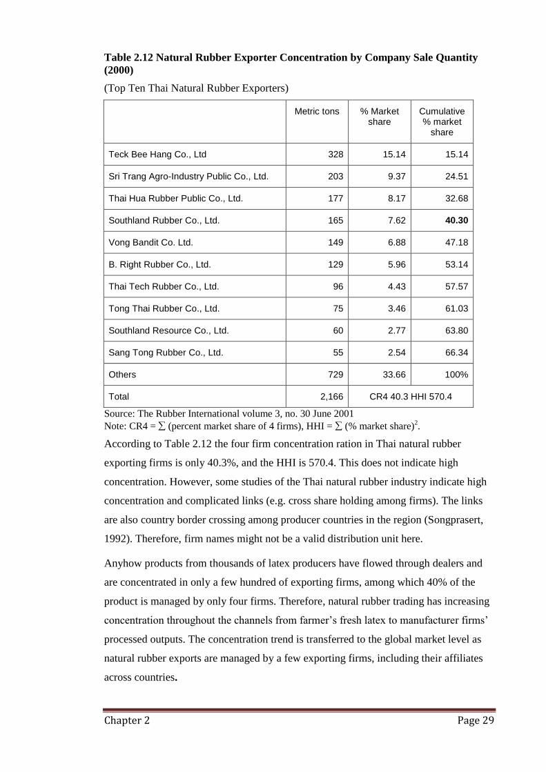
Chapter 2 Page 29

Table 2.12 Natural Rubber Exporter Concentration by Company Sale Quantity

(2000)

(Top Ten Thai Natural Rubber Exporters)

Metric tons % Market share

Cumulative % market

share

Teck Bee Hang Co., Ltd 328 15.14 15.14

Sri Trang Agro-Industry Public Co., Ltd. 203 9.37 24.51

Thai Hua Rubber Public Co., Ltd. 177 8.17 32.68

Southland Rubber Co., Ltd. 165 7.62 40.30

Vong Bandit Co. Ltd. 149 6.88 47.18

B. Right Rubber Co., Ltd. 129 5.96 53.14

Thai Tech Rubber Co., Ltd. 96 4.43 57.57

Tong Thai Rubber Co., Ltd. 75 3.46 61.03

Southland Resource Co., Ltd. 60 2.77 63.80

Sang Tong Rubber Co., Ltd. 55 2.54 66.34

Others 729 33.66 100%

Total 2,166 CR4 40.3 HHI 570.4

Source: The Rubber International volume 3, no. 30 June 2001

Note: CR4 = (percent market share of 4 firms), HHI = (% market share)2.

According to Table 2.12 the four firm concentration ration in Thai natural rubber

exporting firms is only 40.3%, and the HHI is 570.4. This does not indicate high

concentration. However, some studies of the Thai natural rubber industry indicate high

concentration and complicated links (e.g. cross share holding among firms). The links

are also country border crossing among producer countries in the region (Songprasert,

1992). Therefore, firm names might not be a valid distribution unit here.

Anyhow products from thousands of latex producers have flowed through dealers and

are concentrated in only a few hundred of exporting firms, among which 40% of the

product is managed by only four firms. Therefore, natural rubber trading has increasing

concentration throughout the channels from farmer‟s fresh latex to manufacturer firms‟

processed outputs. The concentration trend is transferred to the global market level as

natural rubber exports are managed by a few exporting firms, including their affiliates

across countries.

Chapter 2 Page 30

2.5.3 Tire Manufacturing Market

The motor vehicle tire industry is the most important natural rubber consumer industry

and hence is closely linked to sustainability and welfare issues in the natural rubber

industry in Thailand. Not all tire manufacturing is undertaken in the home countries of

the major tire manufacturers. These manufacturers have also set up subsidiary plants in

natural rubber producing countries such as Thailand. An examination of tire

manufacturing firms in Thailand reveals a mixture of both local and foreign owned

companies (Export Import Bank of Thailand, 2006). From Table 2.13, Siam Michelin

Co. Ltd is the largest firm representing almost half of the market capitalisation of tire

manufacturers. CR4 is 72.7 % and HHI is 2,662.4 surpassing the guideline of 1,800.

Table 2.13 Thailand Tire Manufactures Capital Concentration (2003)#

Capital investment

% share

Cumulative % market

share Million

baht Million $US

Siam Michelin Co. Ltd. 8,447.3 203.60 48.21 48.21

Otani Tire Co. Ltd. 1,528.4 36.84 8.72 56.93

Lion Tires (Thailand) Co. Ltd. 1,576.8 38.00 9.00 65.93

Siam Tire Prapadaeng Co. Ltd. 1,192.7 28.75 6.81 72.74

Goodyear (Thailand) Co. Ltd. 1,079.8 26.03 6.16 78.90

Thai Bridgestone Co. Ltd. 970.0 23.38 5.54 84.44

Inoue Rubber (Thailand) Co. Ltd. 963.0 23.21 5.50 89.94

SR Tire Co. Ltd. 784.1 18.90 4.48 94.42

Techno Asia Tire Co. Ltd. 498.9 12.02 2.85 97.27

V Rubber Co. Ltd. 479.6 11.56 2.74 100%

Total 17,520.6 422.29 CR4 72.7; HHI 2,662.4

Source: compiled from Export Import Bank of Thailand (2006) # Data are for the year 2003. Exchange rate was 41.49 baht/$US

However, the dominance of the major multinational tire manufacturers extends into

markets such as Thailand. Siam Michelin and Siam Tire Prapadaeng are majority owned

subsidiaries of Michelin Group of France. Goodyear (Thailand) is 60% owned by the

US Goodyear company, and Thai Bridgestone is 60% owned by the Japanese

Bridgestone company. Inoue Rubber Company has majority ownership from its parent

Chapter 2 Page 31

company incorporated in Japan and Lion Tires is a subsidiary of the Vittoria Group of

Italy. Otani Tire is a 100% Thai owned company and is a specialist producer of large

and heavy duty commercial tires; Lion Tires is a specialist producer of bicycle tubes and

tires and Inoue Rubber is a specialist producer of motorcycle tires and tubes.

Production costs for vehicle tire comprises raw materials (60%), wages (12%),

depreciation (8%), energy and public service 4% and other inputs 16%. Natural rubber

is an important component of the raw materials.

2.6 Global Level Natural Rubber Market Structure

At the global level, world natural rubber production averaged 62,800 tons for the time

period under study and increased to 9.7 million tons in 2007.

2.6.1 World Primary Production

Figure 2.4 displays global natural rubber production quantity. Output dropped during

the two World Wars but then continued growing.

Figure 2.4 World Natural Rubber Production (1900-2004)

World Rubber Production

0

2000

4000

6000

8000

10000

1880 1900 1920 1940 1960 1980 2000 2020

1,0

00 t

on

s

World Rubber Production

Table 2.14 demonstrates similar situations with the structure of natural rubber farming

in Thailand Indonesia and Malaysia.

Chapter 2 Page 32

Table 2.14 Small Holdings and Estate Areas under Rubber Plantation

(1,000 hectares, 2004)

Country Total Estates Small Holding Mature area Yield / hectare (kilogram)

Indonesia 3,262.0 493.0 15%

2,769.0 85%

76% 839.0

Thailand 2,083.4 200.0 10%

1,883.4 90%

80% 1,812.5

Malaysia 1,282.0 126.5 10%

1,155.5 90%

93% 1,300.0

Source: compiled from The Rubber Study Group and The Rubber Research Institute of

Thailand.

Clearly the farming stage is dominated by small holdings: above 85% of the total in

each country. Mature areas account for over 75% in all countries. Malaysia has the

highest proportion of small holding shares and almost all areas are mature, reflecting its

being the earlier producing country. Thailand‟s farms have the highest average yield

followed by Indonesia and Malaysia.

2.6.2 World Export Market

The world net imports market structure for the year 2004 is displayed in Table 2.15.

Table 2.15 World Net Exports Market Structure (2004)

Natural Rubber Net Exports 2004

1,000 tons % Market share

Cumulative % market

share

Thailand 2,627.4 42.11 42.11

Indonesia 1,875.1 30.05 72.16

Malaysia 679.9 10.90 83.06

Vietnam 351.0 5.63 88.69

Cote D Ivoire 136.0 2.18 90.87

Liberia 111.5 1.79 92.66

India 71.2 1.14 93.80

Cameroon 53.0 0.85 94.65

Chapter 2 Page 33

Table 2.15 (continue)

Guatemala 52.9 0.85 95.50

Philippines 43.9 0.70 96.20

Sri Lanka 40.6 0.65 96.85

Myanmar 30.5 0.49 97.34

Nigeria 24.0 0.38 97.72

Cambodia 11.0 0.18 97.90

Other Countries 132.0 2.12 100%

Total 6,240.0 CR4 88.7; HHI 2,838.3

Source: Compiled from The Association of Natural Rubber Producing Countries.

At the global level, total net exports in the world market for natural rubber was 1.83

million tons in 1950 and increased to 6.24 million tons in 2004. Major exporting

countries were Thailand, Indonesia, and Malaysia. Since 2000 there have been

significant emerging supplying countries such as Vietnam, Laos, Cambodia and

Myanmar. The world level overall export industry concentration can be viewed from the

selling countries concentration in world natural rubber markets as displayed in Table

2.15. The outcomes indicate CR4 = 88.7% and HHI = 2,838.3 indicating market

concentration. However, since each producer country‟s supply has a degree of

specialized product, such as Thailand for ribbed smoked sheets, Indonesia for block

rubber and Malaysia for concentrated latex, the effects of concentration could be partly

understated. It was not until the 1990s that Thailand had diversified non-latex natural

rubber exports from smoked sheets into both smoked sheets and block rubber.

This poses the possibility that concentration in the exporting country suppliers of

natural rubber may offset the concentration in the buyers‟ side of the market that is

considered below (Scherer & Ross, 1990).

2.6.3 Natural Rubber Export Country and Buying Country Concentration

When considered from the buyer country side, concentration for each particular

exporting country namely Thailand, Indonesia and Malaysia results is as follows.

Chapter 2 Page 34

2.6.3.1 Thailand

Thailand exported natural rubber to many countries in the regions of North America,

Asia Pacific and Europe. Table 2.16 summarizes the export destinations for Thai natural

rubber during 1975-2000, accompanied by the corresponding four-country

concentration ratio and (CR4) and the Herfindahl-Hirschman index. During 1975-2000

Thai gross natural rubber exports were dominated by Japan (38.4%), US (12.1%),

France (12.0%) and other countries in EU (9.5%). The CR4 is 72.0 % and the HHI is

1939.5. Overall outcome indicates buyer concentration.

Table 2.16 Gross Exports from Thailand to Natural Rubber Consuming Countries

(1975 – 2000)

(mill tons) % Market

share

Cumulative % market

share

Japan 10,344 38.39 38.39

US 3,256 12.08 50.47

France 3,240 12.02 62.49

EU 2,567 9.53 72.02

Singapore 1,685 6.25 78.27

Malaysia 1,484 5.51 83.78

USSR 694 2.58 86.36

Taiwan 652 2.42 88.78

China 418 1.55 90.33

Other countries 2,605 9.67 100%

Total 26,945 CR4 72.0; HHI 1,939.5

Source: Compiled from The Association of Natural Rubber Producing Countries.

2.6.3.2 Indonesia

Indonesia export natural rubber to US, Singapore and EU. The corresponding buyer

shares are displayed in Table 2.17. The CR4 during 1975-2000 for Indonesia was

81.1%. The HHI was 2,494.2, well over the benchmark level of 1800. The top four

buyers were US (42.9%), Singapore (22.3%), EU (11.3%), and Japan (4.5%).

Indonesia natural rubber export market structure is displayed in Table 2.17.

Chapter 2 Page 35

Table 2.17 Gross Exports from Indonesia Natural Rubber to Consuming Countries

(1975-2000)

(mill tons) %

Market share

Cumulative % market

share

US 12,275 42.92 42.92

Singapore 6,384 22.32 65.24

EU 3,227 11.28 76.52

Japan 1,295 4.53 81.05

USSR 694 2.43 83.48


Total 28,599 CR4 81.1; HHI 2,494.2

Source: The Association of Natural Rubber Producing Countries

2.6.3.3 Malaysia

Malaysia exports natural rubber to EU, Singapore and US. The buyer countries‟ shares

are informed by Table 2.18.

Table 2.18 Gross Exports from Malaysia to Natural Rubber to Consuming

Countries (1975-2000)

(mill tons) %

Market share

Cumulative % market

share

EU 9,335 26.92 26.92

Singapore 5,204 15.01 41.93

US 3,636 10.49 52.42

Republic of Korea 2,411 6.95 59.37

China 2,151 6.20 65.57

Japan 1,651 4.76 70.33

USSR 1,425 4.11 74.44

Australia 156 0.45 74.89


Total 34,677 CR4 59.4; HHI 1,186.4

Source: The Association of Natural Rubber Producing Countries

Chapter 2 Page 36

The CR4 during 1975-2000 for Malaysia is 59.4 %; HHI is 1,186.4. The four top buyers

are EU (26.9%), Singapore (15%), US (10.5%) and Republic of Korea (7%). Results do

not indicate potential high concentration. However, in the studied period Malaysia is

found to decrease its natural rubber production and becomes one of the importing

countries from Thailand.

When viewed from the importing country side, during 1975-2000 the combined

quantities of Thai, Indonesian and Malaysian natural rubber export to Japan, USA and

EU are as follows.

The USA imported 99.99 % of its natural rubber from Asia, with 13.3% from

Singapore, which is re-export trading since Singapore does not produce natural rubber.

The remaining 86.7% was attributed to Thailand, Indonesia and Malaysia as: 13.7%,

55.3% and 17.7% respectively. The EU imported 80.3% of its natural rubber from Asia,

with 15.5% from Singapore. The remaining 64.8% was imported from Thailand,

Indonesia and Malaysia as: 10.7%, 13.6% and 40.4% respectively. Japan imported

98.6% of its natural rubber from Asia, with 7.7% from Singapore. The remaining 90.9%

was imported from Thailand, Indonesia and Malaysia as: 70.5%, 8.3% and 12.1%

respectively.

It can be seen that the USA imported most of its natural rubber from Indonesia, the EU

from Malaysia and Japan from Thailand. This may reflect consumption purposes as the

USA uses a lot of block rubber and it is mostly produced by Indonesia. Thailand

produces mainly sheet rubber which is used by Japan for tire manufacturing.

Hence, global natural rubber consuming countries impact on Thailand, Indonesia and

Malaysia because they are essential consumers of natural rubber output from these

countries. The USA has the most impact on Indonesia, France and Europe on Malaysia

and Japan on Thailand.

Table 2.19 summarizes the specific trading feature between countries as follows.

Chapter 2 Page 37

Table 2.19 Export Shares of Natural Rubber Producing Countries and Natural Rubber

Imports of Consuming Countries

From Exporting Country:

To Importing Countries (% of Total Imports)

US. EU JAPAN

Thailand 13.68 10.73 70.49

Indonesia 55.34 13.63 8.28

Malaysia 17.67 40.44 12.1

Sub Total 1 86.69 64.80 90.87

Singapore 13.30 15.54 7.73

Sum Total 2 99.99 80.34 98.6

Other 0.01 19.66 1.4

Sri Lanka < 1%

Sources: compiled from International Rubber Study Group, Rubber Statistical Bulletin and

Quarterly Natural Rubber Statistical Bulletin, various copies. All rates are average rates between

the years 1975-2000.

2.6.4 World Tire Market

At the world level, rubber products are divided into tire sector consumption and general

sector consumption. Tire sector consumption comprises natural rubber and synthetic

rubber that are used in all kinds of vehicle tires production. General sector consumption

comprises natural rubber and synthetic rubber that are used to produce products other

than tires. Most general sector products are used in the automotive sector e.g. rubber

parts and accessories used in vehicles.

Table 2.20 displays natural rubber and synthetic rubber used in selected tire sectors

where data are available: USA, France, Japan, Germany, UK, Italy, and India.

Accordingly, tire sector consumption of natural rubber is almost 50% of total

consumption. It reduced to 32% in the year 1970 at the time of the synthetic rubber

boom. Then it recovered to 37% by the 1990s, which is the time of surging oil prices

and synthetic rubber prices. In 2004 tire sectors share of total natural rubber

consumption was 33%. In contrast, the tire sector‟s consumption share in synthetic

rubber increased to 25% by 1970s and reduced to 12% in 2004. In 2000 the tire sector

consumption of natural rubber was around 30% plus less than 15% for synthetic rubber.

Chapter 2 Page 38

Table 2.20 Global Tire Sector Consumption of Natural and Synthetic Rubber (1946-2004)

(1,000 tons)

Year

Natural Rubber

Use in Selected

Tire Sector

% to World

Natural Rubber

Consumption

Synthetic

Rubber Use in

Selected Tire

Sector

% to World

Natural Rubber

Consumption

1946 291.8 49.46 601.1 36.49

1950 679.4 39.79 363.5 14.30

1960 721.8 34.05 969.0 21.68

1970 956.1 31.50 2,168.8 25.04

1980 1,261.1 33.54 1,882.9 14.96

1990 1914 36.81 2,126.2 14.34

2000 2,482.4 33.91 2,391.0 13.17

2004 2,725.8 32.92 2,441.5 12.16

Source: Calculated from The International Rubber Study Group

The world level tire industry comprises several conglomerates that operate at a

multinational level. Prominent firms usually provide direct investment in new affiliates

and/or mergers with local country firms. Table A.2.1 in Appendix 2.1 reports the details

of such groups.16

Accordingly, the tire industry is covered by only a few business

groups, causing concentration in the market. In addition the group members have

established links among each member. Following sections evaluate the concentration

degrees in the tire industry at world level.

2.6.4.1 Tire Industry Concentration in Natural Rubber Consumption.

Within the one-third of natural rubber consumption by tire sector as revealed in Table

2.21, the quantities of natural rubber used are concentrated in the top four countries. The

CR4 is 76.9 %. HHI is 2164.6. Results provide concentration evidence.

16

By 2000, world employment in tire industry totals to 296,216 employees. It is made by USA (19%),

France (14%), China (10%), Japan (6%) and Germany (6%).

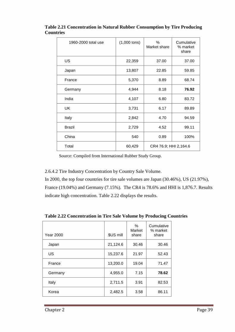
Chapter 2 Page 39

Table 2.21 Concentration in Natural Rubber Consumption by Tire Producing

Countries

1960-2000 total use (1,000 tons) % Market share

Cumulative % market

share

US 22,359 37.00 37.00

Japan 13,807 22.85 59.85

France 5,370 8.89 68.74

Germany 4,944 8.18 76.92

India 4,107 6.80 83.72

UK 3,731 6.17 89.89

Italy 2,842 4.70 94.59

Brazil 2,729 4.52 99.11

China 540 0.89 100%

Total 60,429 CR4 76.9; HHI 2,164.6

Source: Compiled from International Rubber Study Group.

2.6.4.2 Tire Industry Concentration by Country Sale Volume.

In 2000, the top four countries for tire sale volumes are Japan (30.46%), US (21.97%),

France (19.04%) and Germany (7.15%). The CR4 is 78.6% and HHI is 1,876.7. Results

indicate high concentration. Table 2.22 displays the results.

Table 2.22 Concentration in Tire Sale Volume by Producing Countries

Year 2000 $US mill

% Market share

Cumulative % market

share

Japan 21,124.6 30.46 30.46

US 15,237.6 21.97 52.43

France 13,200.0 19.04 71.47

Germany 4,955.0 7.15 78.62

Italy 2,711.5 3.91 82.53

Korea 2,482.5 3.58 86.11

Chapter 2 Page 40


China 2,462.5 3.55 89.66

India 2,076.0 2.99 92.65

Taiwan 1,027.0 1.48 94.13

Russia 466.0 0.67 94.80

Other Countries 3,599.1 5.19 100

Total 69,341.8 CR4 78.6;HHI 1,876.7

Source: Compiled from Tire business (2002).

2.6.4.3 Tire Industry Concentration by Company

When considered by company sale volume, as displayed in Table 2.23, the four top tire

companies are Bridgestone Corp (19.8% ), Groupe Michelin (19%), Goodyear Tire and

Rubber Co. Ltd (18.4%) and Continental A.G. (7.2% share). The CR4 is 64.4 and the

HHI is 1,200.3. Other companies have less than 5% shares.

Table 2.23 Concentrations in Tire Sale Volume by Producing Companies (2000)

Company Mill $US

% market share Cumulative % market share

Bridgestone Corp. 13,750.0 19.83 19.83

Groupe Michelin 13,200.0 19.04 38.87

Goodyear Tire & Rubber Co. Ltd 12,725.0 18.35 57.22

Continental A.G. 4,955.0 7.15 64.37

Sumitomo Rubber Industries Ltd 2,783.0 4.01 68.38

Pirelli S.P.A. 2,600.0 3.75 72.13

Yokohama Rubber Co. Ltd. 2,514.0 3.63 75.76

Cooper Tire & Rubber Co. 1,802.6 2.60 78.36

Toyo Tire & Rubber Co. Ltd. 1,322.6 1.91 80.27

Kumho Industrial Co. Ltd. 1,235.0 1.78 82.05

Others 12,454.6 17.96 100%

Total 69,341.8 CR4 64.4; HHI 1,200.3

Source: compiled from Tire Business (2002)

Chapter 2 Page 41

Overall results do not indicate extremely high concentration. However, global tire

manufacture is one industry that has had many mergers, resulting in groups of

conglomerate corporations that operate across countries. Examples are Goodyear,

Bridgestone, Michelin, and Continental, each of which has several majority-owned

subsidiaries abroad. They also have joint ventures across their groups, e.g. Continental

and Michelin, Goodyear and Toyo, and Continental and Yokohama. Details are

presented in Appendix 2.1. Hence the raw concentration ratios measured by company

name understate the position.

The above tables demonstrate a pattern of concentration in the tire manufacturing

industry with four dominant companies (Michelin, Bridgestone, Goodyear, Continental)

that are headquartered in four developed countries (France, Japan, USA and Germany

respectively). However, although these companies and their respective home countries

dominate the global tire manufacturing industry and the global consumption of natural

rubber, there is not total concordance of production and country location in this

industry. Tire manufacture is located in a number of countries, including, as

demonstrated in Table 2.13, natural rubber producing countries such as Thailand. The

dominant manufacturing companies retain significant control of the global industry

however by ownership of multiple subsidiary manufacturing companies both within and

without their home countries (see Appendix 2.1).

It is not possible to completely disentangle the company-country production data that

has been taken from different sources. Precise data on the country location of all tires

produced are not available. However, the data do provide strong evidence of

concentration in the global tire manufacture - natural rubber consumption industry

whether measured by company level data or country level data. There is also a strong

correlation between company level concentration and company home country level

concentration data. The home countries of the four top producers have 78.6% of the tire

market by sales volume (Table 2.22) and 76.9% of the natural rubber inputs into tire

manufacture (Table 2.21). The corresponding top four companies have 64.4% of the tire

market by sales volume (Table 2.23).

2.7 Conclusion

This chapter has outlined the supply chain for natural rubber industry at domestic and

global levels. In summary the key findings are as follows. The Havea tree produces up

Chapter 2 Page 42

to 99% of world natural rubber. The tree was introduced to some Asian and African

countries. Current major producing countries are Thailand, Indonesia and Malaysia.

During WWII, natural rubber production was restricted and synthetic rubber was

invented. Since then rubber consumption has comprised both natural rubber and

synthetic rubber.

Planting natural rubber takes 5-7 years for the tree to mature. Latex can be transformed

to different types of rubber stocks. Sheet rubber and block rubber are the most

consumed types. Indonesia and Malaysia produce block rubber from most of the

products. Thailand has both rubber sheets and block rubber.

Vehicle tires are the most prominent natural rubber product. A vehicle tire consumes 4

pounds of natural rubber and 6 pound of synthetic rubber on average. The ratio varies

by tire type and size. Natural rubber and synthetic rubber are substitutable to a degree

according to use and relative costs. During 1960-2000 the major tire industry countries

consumed 25-29% of the world‟s total natural rubber production and 19-35% of world

total synthetic rubber consumption.

Natural rubber is economically relevant since it generates considerable export income. It

is also important socially since it supports millions of small holder producing units (85-

90%) of all plantations. The natural rubber market in Thailand comprises local markets,

town markets and export markets. Central markets help support the prices in local and

town markets. Export market product is traded in fob Bangkok prices. Thai natural

rubber futures are traded in The Agricultural Futures Exchange of Thailand. Other

relevant prices are the TSR20 New York cif prices, the TOCOM futures, and SICOM

Futures.

Thailand, Indonesia, Malaysia and Vietnam were the top four net exporting countries in

2004 (42%, 30%, 11% and 6% respectively). The CR4 is 89% and the HHI is 2,838.

For the period of the study, the top four buying countries from Thailand were Japan

(39%), USA (12%), France (12%) and other EU countries (10%). The overall CR4 is

72%. The top four buyers for Indonesia were US (43%), Singapore (22%), EU (11%)

and Japan (5%). Malaysia‟s top four buyers were EU (27%), Singapore (15%), US

(11%) and Republic of Korea (7%). Results are supported by high HHI. There is a

potential for concentration on the exporting country side to be diminished by the

concentration effects on the importing side. This could be further diminished due to

Chapter 2 Page 43

each individual supplying country being closely tied to an individual buyer country.

Hence oligopsony market power is a potential feature in these markets.

Tire manufacturing is the relevant natural rubber consuming industry for this study. In

Thailand domestic tire firms consume up to 43% of locally consumed natural rubber,

but locally consumed natural rubber is only 10%-11% of the country‟s total natural

rubber production. At world level, natural rubber consumed in the tire sector is

concentrated in USA (37%), Japan (23%), France (9%) and Germany (8%). The CR4 is

77% and HHI is 2,165.

The top four producers based on country sale volume for the year 2000 were Japan

(30%), US (22%), France (19%) and Germany (7%). The CR4 is 79% and HHI is

1,877. The top four producers based on company sales volume for the year 2000 were

Bridgestone Corp (20%), Groupe Michelin (19%), Goodyear Tire & Rubber (18%) and

Continental A.G. (7%). CR4 is 64% and HHI is 1,200.

In conclusion, although natural rubber trading is a small economic item in each

producing country, it is significant for each producing country, impacting upon many

cultivating farmers. Throughout our study there are several areas in the natural rubber

industry that have potential for market power from the buyer side. The natural rubber

producer industry at the country level is concentrated in the hands of a few

manufacturers. Secondly, the natural rubber export industries are dominated by

particular buyer countries for each seller country namely: Japan for Thailand, US for

Indonesia and EU for Malaysia. As such there is potential for market power to be

exercised by the supplier countries of natural rubber could be counterbalanced by the

market power on the natural rubber buyer side. Finally, the natural rubber consumer

industry such as vehicle tire manufacture is concentrated in the hands of a small group

of conglomerate enterprises that cross national borders. As such there is potential for

market power to be exercised by the tire manufacturing countries on the global level tire

market (oligopoly). This concentration is also reflected in country level data with the

major developed countries dominating the consumption of natural rubber for tire

manufacture and the consumption of the manufactured tires. Hence there is potential for

market power to be exercised in the natural rubber markets from the buyer side

(oligopsony) and this potential can be analysed via company level or country level data.

The general information presented in this chapter establishes a basis for further

development of the thesis. In Chapter 3, the theoretical concepts required for economic

Chapter 2 Page 44

analysis and measurement of market power by the global tire industry over the natural

rubber industry are examined. It surveys microeconomic theory of market structure,

theoretical and empirical literature of a variety of methods to assess market power of

oligopoly as well as oligopsony. In addition, empirical studies of the tire industry and

natural rubber industry are reviewed. Given the potential for market power to be

exercised by the tire manufactures either as the buyers in the input market (the supplier

side of the natural rubber input market) or the seller in the output market (the consumer

side of the tire output market), a theoretical model that accommodates the measurement

of both oligopsony and oligopoly is adopted in Chapter 4 .

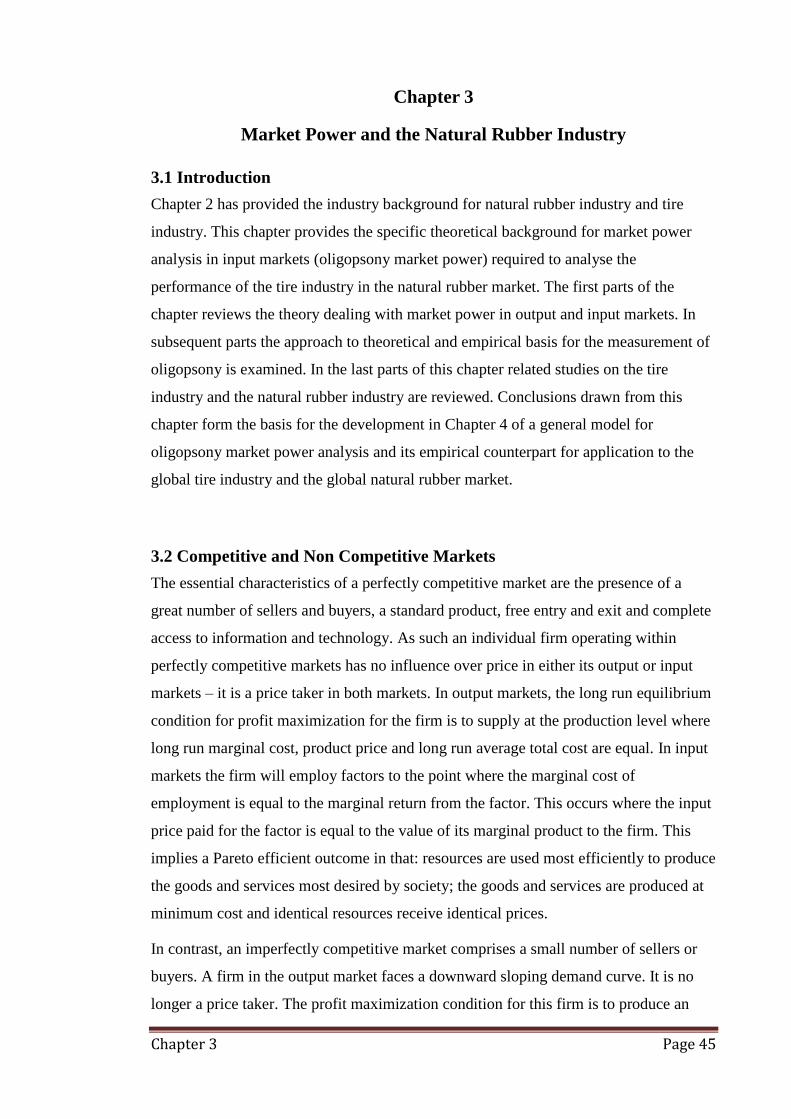
Chapter 3 Page 45

Chapter 3

Market Power and the Natural Rubber Industry

3.1 Introduction

Chapter 2 has provided the industry background for natural rubber industry and tire

industry. This chapter provides the specific theoretical background for market power

analysis in input markets (oligopsony market power) required to analyse the

performance of the tire industry in the natural rubber market. The first parts of the

chapter reviews the theory dealing with market power in output and input markets. In

subsequent parts the approach to theoretical and empirical basis for the measurement of

oligopsony is examined. In the last parts of this chapter related studies on the tire

industry and the natural rubber industry are reviewed. Conclusions drawn from this

chapter form the basis for the development in Chapter 4 of a general model for

oligopsony market power analysis and its empirical counterpart for application to the

global tire industry and the global natural rubber market.

3.2 Competitive and Non Competitive Markets

The essential characteristics of a perfectly competitive market are the presence of a

great number of sellers and buyers, a standard product, free entry and exit and complete

access to information and technology. As such an individual firm operating within

perfectly competitive markets has no influence over price in either its output or input

markets – it is a price taker in both markets. In output markets, the long run equilibrium

condition for profit maximization for the firm is to supply at the production level where

long run marginal cost, product price and long run average total cost are equal. In input

markets the firm will employ factors to the point where the marginal cost of

employment is equal to the marginal return from the factor. This occurs where the input

price paid for the factor is equal to the value of its marginal product to the firm. This

implies a Pareto efficient outcome in that: resources are used most efficiently to produce

the goods and services most desired by society; the goods and services are produced at

minimum cost and identical resources receive identical prices.

In contrast, an imperfectly competitive market comprises a small number of sellers or

buyers. A firm in the output market faces a downward sloping demand curve. It is no

longer a price taker. The profit maximization condition for this firm is to produce an

Chapter 3 Page 46

output where marginal cost equals marginal revenue but marginal revenue will be less

than product price. In the long run, the firm might not produce at the minimum average

cost and will likely earn economic profits (price exceeds average cost). With

imperfectly competitive input markets the firm will no longer be so small as to have no

influence on price. Again it will no longer be a price taker and as such will face an

upward sloping supply curve for each factor. These outcomes imply that resources are

not used efficiently to produce the goods and services desired by society and identical

resources do not receive identical prices.

3.3 Equilibrium Conditions in Input Markets

Price and employment conditions for inputs are different for different combinations of

input and output markets. For a firm in a competitive market the demand curve for an

input is the value of its marginal product (i.e. w = VMP). The firm producing for a

perfectly competitive output market is a price taker and hence VMP = P.MP where P is

the price for its output product.

However, the demand curve for an input from a firm producing for an imperfectly

competitive output market is its marginal revenue product (MRP) curve (i.e. w = MRP).

The distinction derives from the demand curve facing the firm in its product market: as

P = MR in a perfectly competitive market, then VMP = P.MP = MR.MP = MRP. For

the firm selling its product into an imperfectly competitive market its demand curve is

downward sloping and MR < P and hence MRP < P.MP.

The supply curve facing a firm for an input can also vary across market types. The

supply curve for the firm in a perfectly competitive input market is perfectly elastic (a

horizontal line). This is due to the firm being a price taker in the input market. However,

the supply curve for an input in an imperfectly competitive input market will be upward

sloping as the buyer will no longer be a price taker. Its relative market buying power

will be such as to influence the input supply price. Hence the effective supply curve for

the firm will be the marginal resource cost (MRC) curve where MRC > w (the input

supply price). The difference being the extra cost required to supply infra-marginal units

when the price of the marginal unit increases.

Assuming a linear demand curve for inputs, Figure 3.1 illustrates the position for firms

in a competitive input market with a market input supply curve that is infinitively

elastic. If output market is competitive also, then the equilibrium level of input

Chapter 3 Page 47

employment is where market input supply price (w) equals the value of marginal

product (VMP). The resulting input quantity employed is xcc, at price wcc. If the output

market is non-competitive, the equilibrium level of input employment is where input

supply intersects marginal revenue product (MRP) curve. The quantity employed is

xcm, at price wcm = wcc.

Figure 3.1 Input Employment in a Competitive Input Market

Figure 3.2a illustrates the equilibrium conditions for input employment when the input

market is non-competitive and the supply curve is upward sloping. If output market is

competitive, the employment level is determined by the intersection of the marginal

resource cost (MRC) and the value of marginal product (VMP). The quantity employed

is xmc, at price wmc. If the output market is non-competitive, the equilibrium will be

where marginal resource cost (MRC) intersects marginal revenue product (MRP). The

employment will be xmm, at price wmm.

Figure 3.2b compares the input employment results between competitive input market

and non-competitive input market. The employment in a competitive input market is

xcc, at price wcc if the output market is competitive (where S = VMP). The input

employment in a competitive input market is xcm at price wcm=wcc if the output

market is non-competitive (where S = MRP). The input employment is xmc, at price

wmc for a non-competitive input market and a competitive output market (MRC =

VMP). The input employment is xmm, at price wmm for a non-competitive input market

and a non-competitive output market (MRC = MRP).

VMP

Input Quantity

Input Price

Input inverse supply (S)

xcm

MRP

xcc

wcc

=

wcm

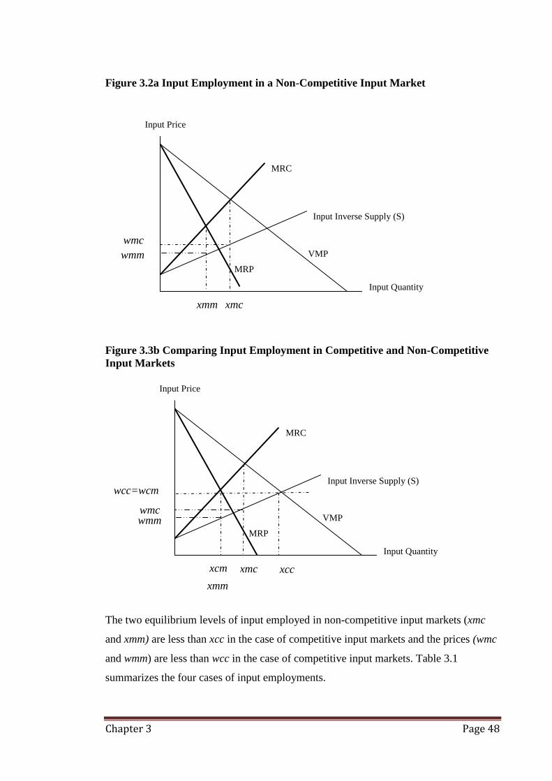
Chapter 3 Page 48

Figure 3.2a Input Employment in a Non-Competitive Input Market

Figure 3.3b Comparing Input Employment in Competitive and Non-Competitive

Input Markets

The two equilibrium levels of input employed in non-competitive input markets (xmc

and xmm) are less than xcc in the case of competitive input markets and the prices (wmc

and wmm) are less than wcc in the case of competitive input markets. Table 3.1

summarizes the four cases of input employments.

VMP

Input Inverse Supply (S)

MRC

Input Quantity

MRP

wmm

xmc

Input Price

xcc xcm

wmc

xmm

wcc=wcm

VMP

Input Inverse Supply (S)

MRC

Input Quantity

MRP

wmm

xmc

wmc

Input Price

xmm

mm

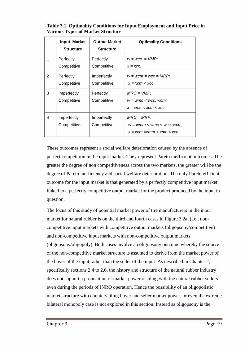
Chapter 3 Page 49

Table 3.1 Optimality Conditions for Input Employment and Input Price in

Various Types of Market Structure

Input Market

Structure

Output Market

Structure

Optimality Conditions

1 Perfectly

Competitive

Perfectly

Competitive

w = wcc = VMP;

x = xcc,

2 Perfectly

Competitive

Imperfectly

Competitive

w = wcm = wcc = MRP;

x = xcm < xcc

3 Imperfectly

Competitive

Perfectly

Competitive

MRC = VMP;

w = wmc < wcc, wcm;

x = xmc < xcm < xcc

4 Imperfectly

Competitive

Imperfectly

Competitive

MRC = MRP;

w = wmm < wmc < wcc, wcm;

x = xcm =xmm < xmc < xcc

These outcomes represent a social welfare deterioration caused by the absence of

perfect competition in the input market. They represent Pareto inefficient outcomes. The

greater the degree of non competitiveness across the two markets, the greater will be the

degree of Pareto inefficiency and social welfare deterioration. The only Pareto efficient

outcome for the input market is that generated by a perfectly competitive input market

linked to a perfectly competitive output market for the product produced by the input in

question.

The focus of this study of potential market power of tire manufacturers in the input

market for natural rubber is on the third and fourth cases in Figure 3.2a. (i.e., non-

competitive input markets with competitive output markets (oligopsony/competitive)

and non-competitive input markets with non-competitive output markets

(oligopsony/oligopoly). Both cases involve an oligopsony outcome whereby the source

of the non-competitive market structure is assumed to derive from the market power of

the buyer of the input rather than the seller of the input. As described in Chapter 2,

specifically sections 2.4 to 2.6, the history and structure of the natural rubber industry

does not support a proposition of market power residing with the natural rubber sellers

even during the periods of INRO operation. Hence the possibility of an oligopolistic

market structure with countervailing buyer and seller market power, or even the extreme

bilateral monopoly case is not explored in this section. Instead as oligopsony is the

Chapter 3 Page 50

proposition to be tested the next sections examine in more detail the theoretical base for

empirical analysis of oligopsony market power.

3.4 Oligopsony Analysis

A simple approach to oligopsony analysis is to adapt standard tests for output market

power (oligopoly) for input market power testing (oligopsony). A structural change

approach is also found in the literature as is the conjectural variation approach that has

the Cournot model as its theoretical foundation.

Conventional tests for the presence of oligopoly include market concentration ratios

such as the CR4 and the Herfindahl-Hirschman Index (HHI).Whereas the attractions of

this approach include their ease of application, critics argue that the concentration ratios

and the Herfindahl-Hirschman Index do not inform about market entry conditions and

the competitive behaviour of market participants (Ferguson & Ferguson, 1994 pp. 43-44

and Salvatore, 1997 pp.416-419).

The Lerner Index (Lerner, 1934) has been adopted as a basic general measurement of

market power in output markets. Since a monopolist can restrict output hence raising

prices, this basic general measurement of market power is derived as

p

MCpL

where L is the Lerner index, p is the product price and MC is the producing

firm‟s marginal cost. The Lerner index can be converted to

1L where is the direct

demand elasticity (q

p

p

q

), q is the producing firm‟s output).

17 Thus, the higher the

difference between price and marginal cost, the greater is the Lerner index of market

17

Proof: based on Martin (1994) pp.25-27.

Marginal revenue is )1

1()1(.

p

p

q

q

pp

q

pqp

q

qpMR where MR is marginal

revenue, p is market product price, q is individual firm‟s product quantity, and is the absolute value of

the conventional direct demand elasticity (q

p

p

q

). In addition, based on profit maximization condition,

marginal revenue (MR) = marginal cost (MC). It implies that )1

1(

pMRMC and

1)

11(

p

pp

p

MCpL

Chapter 3 Page 51

power. In addition, the higher the demand elasticity for the product, the less is the

market power.

However, it is argued that sometimes a high Lerner index does not imply high profits

because the firm might be benefitting from a low average cost at that specific

production level. Another issue is that prices might be altered by limit pricing, or by

attempts to avoid legal scrutiny. It is also argued to be in a static context, not

incorporating the shifts over time of demand and costs (Salvatore, 1997).

The Lerner index is constructed on the output market optimality condition (MR = MC).

For inputs the marginal rule has to be adapted to accommodate the input market

optimality condition (MRP = MRC). The Lerner index does not identify whether the

procurement for the input employed is via a competitive input market (input supply

curve is a horizontal line) or non-competitive input market (input supply curve is

upward sloping). These two market structures have different implications for price level

and output product quantity as described in previous sections.

Hence, in the context of a potential imperfectly competitive input market, such as

natural rubber market in this thesis, the Lerner index in its strict form is not directly

applicable to an oligopsony market. But its principle does lend itself to equivalent

measures for input markets as is discussed below.

To consider oligopsony market power, buyer side market power theories are required.

Studies that do include influences from the buyer side‟s market power can be classified

according to approaches on: buyer concentration, structural changes and market power

analysis, and Cournot models with conjectural variation. They are discussed as follows.

3.4.1 Buyer Concentration Approach

Studies of the impacts of buyer concentration on seller‟s profits are based on the

concept of countervailing power proposed by Galbraith (1952) who argued that the

conflict of interest between firms of equal power on different sides of the market could

be a factor limiting the exercise of market power. Lustgarten (1975) estimated the price-

cost margins of 327 four-digit US manufacturing industries as a function of seller

market structure variables (seller concentration and capital-sales ratio) and buyer market

structure variables (buyer concentration and purchase per firm per year, the dispersion

of sales across buying industries) whereas the buyer concentration ratios were computed

from the nation‟s input-output table and weighted by each industry‟s share on total

Chapter 3 Page 52

inputs. Results indicated that seller concentration variables had positive impacts on

price-cost margin. The impacts of buyer market structure variables on price-cost margin

were found negative. This implies that concentration on the buying side of the market

limits control of price on the supplying side of a market and hence price is lower. This

result supports the countervailing argument. However, the study did not contemplate

any welfare losses resulting from buyer concentration.

Decreases in profitability due to buyer concentration (as defined by the price-cost

margin) were found for a group of low seller concentration manufacturers but not for a

group of oligopolist manufacturers (Kelly & Goss, 2000). This study was applied to US

retailers‟ manufacturing suppliers. The study argued that the finding was contradictory

to economic theory which predicts that buyer concentration effects will be confined

largely to firms in oligopolistic industries because economic profits are available to be

redistributed to buyers with market power. A more recent study also found that the

number of buyers is a source of countervailing power (Engle-Warnick & Ruffle, 2005).

In this experiment, a two buyer session (case) was found to achieve significantly lower

prices than four buyers. Furthermore, it was found that the source of the price gap,

compared to other factors, is the number of buyers. This was identified in the

experiments of two-buyer cases where the monopolist adopts cautious or conservative

pricing for fear of provoking demand withholding, thus resulting in lower price than for

the four buyer case. The results are argued to provide the basis for a behavioural theory

of buyer countervailing power where the number of buyers may be a key parameter.

In addition, it was found that cost-important inputs (i.e. inputs that are highly relevant to

production) had negative impacts on price-cost margins. This implied that purchasing

industries tended to bargain down prices of inputs that were relevant to production more

than less important inputs. Relatively unimportant inputs were likely to have higher

margins (Bradburd 1982). The effect of buyer concentration can be offset by output

transfers under administrative control (Newmark 1989) and vertical integration (Martin

1986).

3.4.2 Structural Changes and Market Power Analysis

An example of a second approach to oligopsony market power was provided by an early

study by Just & Chern (1980) who argued that cost information is usually inadequate to

be applied to the testing of Lerner measure. However, one can obtain indirect evidence

Chapter 3 Page 53

of market power from market behaviour. If there is an exogenous shock on one side of

the market which is perfectly competitive, the resulting demand and supply, (i.e. price

and quantity equilibrium), should remain unaffected. However, if there is any market

power on the other side, the price cost relation will shift. The study by Just & Chern

(1980) was of the US tomato processing industry during the 1970s. During that time

there was an exogenous shift in the supply side due to the replacement of labour input

by machines. Hence variable costs were replaced by fixed costs. Supply was shifted to

the right and became more inelastic. The estimated demand was found to shift

downward and became more inelastic. However, competitive market theory would

indicate a price fall and quantity increase due to rightward supply curve shifts.

Consequently, it was concluded that the outcomes were evidence of oligopsony power

and price leadership behaviour in the tomato processing industry.

Limiting factors in this approach include correct identification of the possible causes of

the shifts and its sensitivity to specification errors in the demand and supply functions.

Bresnahan (1987, 1989) used the demand and supply structural approach to trace for

collusion in the automobile market. The analysis was based on the structure of the

residual demand curve facing the automobile manufacturing firms. Although it was a

study on oligopoly aspects, it provided a basis for an expansion to an oligopsonistic

analysis as for example in Durham & Sexton (1992) who analysed the oligopsonistic

market power potential via an inverse residual supply on the specific input to the

employer firm. If the residual supply comprises, in addition to input price elasticity, an

element of the reaction function of rival input suppliers, then it is considered that the

output producing firm facing this residual supply curve is capable of exploiting market

power on the input supplier.

Parallel to these examples of the structural changes approach is the conjectural variation

approach discussed in next section.

3.4.3 Cournot Model with Conjectural Variation Approach

The basic Cournot model is a well known simultaneous quantity setting model (Varian

1996). However, the Cournot model is criticized for two aspects: first for the

assumption that a firm perceives that the other firm‟s output is independent of its own

quantity setting decision and secondly for the assumption that a firm maximizes its own

profits without cooperative or collusive behaviour with other firms.

Chapter 3 Page 54

In order to generalize the basic Cournot model, some variations on the model‟s theme

are proposed. They allow for cost differences between oligopolists, quantity leadership

and limit pricing behaviour, conjectural variations and cooperation (Martin 1996).

Within the conjectural variation framework, the Cournot model is extended to relax the

assumption that a particular firm expects that rival firms do not adjust their outputs in

response to its own output changes. Consequently, the extended model allows for an

individual firm‟s expectation that the other firm (in the duopoly model), or firms (in the

n-firm model) might adjust their outputs with respect to the firm‟s output. The Cournot

model with conjectural variation is depicted in Table 3.2.

Table 3.2 Cournot Model with Conjectural Variation

Let I be firm I’s profit. p the market product price, ci firm i’s cost function, mci its marginal

cost. qi the firm’s output and Q the market output. is the product demand elasticity (Q

p

p

Q

).

Qi is the sum of rivals’ output changes (

jii

j

q

q), where qj is other firm’s output).

(1) Cournot General Model (n-firms, cost differences)

)( iiii qcpq

(2) 0

i

mcqQ

pp

qi

i

i

(3)

1

Q

q

p

mcp ii

Cournot General Model with Conjectural Variation (n-firms, cost differences)

(2a) 0)1(

i

mcqq

Q

Q

pp

qi

i

i

i

i

(3a) )1(1

i

iii

q

Q

Q

q

p

mcp

Source: Compiled from (Scherer & Ross, 1990)

From Table 3.2, firm i‟s profit in the Cournot general model is depicted by equation (1).

The optimality condition is derived in equation (2). Equation (3) manipulates (2) into

price-cost margin measurement of market power, which equals to market output

elasticity weighted by firm i‟s market share. When modified with conjectural variation,

the optimality condition is equation (2a), which allows for firm i‟s expectation (i

i

q

Q

)

about rivals‟ responses to its output changes. The derived price cost margin measure

Chapter 3 Page 55

(Lerner index) is depicted by equation (3a), where the term )(i

i

q

Q

becomes an indicator

for market performance, as summarized in Table 3.3.

Table 3.3 Conjectural Variation and Market Performance

Firm i’s Conjecture

Market Performance

1 Firm i expects rival firms to totally offset its output

changes. Result resembles a perfect competitive equilibrium condition i

i

q

Q

= -1

p

mcp i= 0

2 Firm i expects rival firms to offset some of its output changes.

i

i

q

Q

< 0

p

mcp i 0

3 Firm i expects rival firms not to respond to its output changes, being a basic Cournot case.

i

i

q

Q

= 0

p

mcp i 0

4 Firm i expects rival firms to match some of its output changes.

i

i

q

Q

> 0

p

mcp i 0

5 Firm i expects rival firms to fully match its output changes. This is a collusive behaviour and it equates to a monopoly equilibrium condition.

(*

1

p

mcp i if

Q

q

Q

q

q

Q

i

i

i

i

)1(

) where

* is output

demand elasticity:

Q

p

p

Q

i

i

q

Q

= 1

*

1

p

mcp i

Source: Compiled from (Scherer & Ross, 1990)

From Table 3.3 i

i

q

Q

varies from -1 to 1, reflecting rivals moving from offsetting to

matching firm i‟s output and equilibrium output falls while price rises. If conjectural

variation is zero, it implies that the firm expects that other firms do not react to its

output changes, reflecting a basic Cournot oligopoly model. If conjectural variation is 1

it implies that the firm expects its rivals to change output by the same amount. This

reflects an oligopoly with full collusion case (if the firm‟s market share is less than 1) or

a monopoly case (if the firm is the sole producer in the market). If the conjectural

variation is -1, it implies that the firm expects that other firms react by fully offsetting

Chapter 3 Page 56

its output changes and market output is not affected by its output. This is the same

characteristic for a competitive output market.

Of interest is the use of alternative measures for conjectural variation. For example

whereas Azzam (1997) employs a conjectural variation elasticity defined for its rivals

output responses as defined in Tables 3.2 and 3.3, Appelbaum (1982) defines the firm‟s

conjectural variation elasticity as Q

q

q

Q j

j

.

being the “… conjectural elasticity of total

industry output with respect to the output of the j‟th firm …” (p289). This alters the

interpretation of the measure values in Table 3.3 as is illustrated in Table 3.4.

Table 3.4 Comparing Conjecture Variation Definitions and Resulting Implications

Market Structure Firm i’s Conjecture

Market Performance

S&R, Az Appelb, C&T

1 Firm i expects rival firms to totally offset its output changes. Result resembles a perfect competitive equilibrium condition

i

i

q

Q

= -1 0

iq

Q

0

p

mcp i

2 Firm i expects rival firms to offset some of its output changes. i

i

q

Q

< 0 10

iq

Q

0

p

mcp i

3 Firm i expects rival firms not to respond to its output changes, being a basic Cournot case. i

i

q

Q

= 0 1

iq

Q

4 Firm i expects rival firms to match some of its output changes. i

i

q

Q

> 0 10

iq

Q

5 Firm i expects rival firms to fully match its output changes. This is a collusive behaviour outcome. It equates to a monopoly equilibrium condition.

i

i

q

Q

= 1 1

iq

Q

Q=qi

*

1

p

mcp i

where * is output

demand elasticity:

Q

p

p

Q

Notes: S&R = Scherer & Ross (1990), Az = Azzam (1997), Appelb = Appelbaum (1982), C&T

= Chang & Tremblay (1991)

From Table 3.4 Appelbaum (1982) and Chang & Tremblay (1991) define conjectural

variation as iq

Q

where Q is the sum of all firms‟ outputs, i.e. total market output. If the

Chapter 3 Page 57

market is competitive firm i would not expect market output to be affected by its output

changes because they would be offset by rival firm reactions, hence its conjectural

variation to market output is zero, whereas it is -1 in Scherer & Ross (1990) & Azzam

(1997). In case 2, firm i expects rival firms to partially offset its output changes and its

conjectural variation is between zero and 1, whereas it is between < 0 in Scherer & Ross

(1990) & Azzam (1997). In the Cournot case, firm i expects rival firms do not react to

its own output change hence the conjecture to total market output change by its own

output changes is 1, whereas it is zero in Scherer & Ross (1990) & Azzam (1997) and

the conjectural elasticity is simply the firm‟s market share. In case 4, firm i expects rival

firms to partially match its output changes and its conjectural variation is between zero

and 1, whereas it is > 0 in Scherer & Ross (1990) & Azzam (1997). In the monopoly

case the quantity of total market output changes is solely based on firm i and hence its

conjectural variation to market output and corresponding conjectural elasticity is 1. This

is the same for Scherer & Ross (1990) & Azzam (1997).

Therefore, firm i‟s conjectural variation varies from zero to 1. The corresponding

assessment of market performance by p

mcp i is identical in both approaches. The

approach can be analogously applied to an identification of firm i‟s conjectural variation

in input markets.

To expand the Cournot conjectural variation oligopoly model to an oligopsony model,

one must incorporate a measure of input market power, which can be achieved from

literature in oligopsony model discussed in section 3.5. The literature on oligopsony

market power that uses conjectural variation is generally found in markets for labour

and commodities, especially agricultural products. Both markets share a common

feature in that there are many homogenous suppliers versus a small number of buyers.

In most studies the concept of shadow price is employed. This is the optimal price in

perfectly competitive markets, as introduced in section 3.2. Consequently market power

is measured as the deviation of actual price from the shadow price in perfectly

competitive markets. Shadow price is the value of marginal product (VMP) that is

produced from the specific input. If resource price is less than the VMP, then there is

evidence of input price distortion, which indicates a less than competitive market for

outputs and/or inputs. Given the dominance of this theoretical framework, in the

oligopsony literature we examine examples of studies of oligopsony market power in

the next section.

Chapter 3 Page 58

3.5 Studies of Oligopsony Market Power Analysis with Conjectural

Variation Approach

Following an extensive literature review, no study was found to have been undertaken

of the impact of oligopsony, using the model extended from Cournot oligopoly with

conjectural variations, by the global tire industry on the Thai natural rubber industry.

Nevertheless, the literature does include a number of studies of market power in a

variety of industries that provide a basis for this research. These studies include

applications for oligopoly (output markets) and oligopsony (input markets). Key

examples are as follows.

Appelbaum (1982) provided an important early study using the conjectural variation

approach to assess the potential of oligopoly market power in output markets. Many

studies in the analysis of oligopoly and oligopsony have been based on this paper (for

examples: Schroeter, 1988; Azzam & Pagoulatos, 1990; Chang & Tremblay, 1991 and

Azzam, 1997). Appelbaum applied a measurement of oligopoly power to four industries

in the US, namely the textile, rubber, electrical machinery and tobacco industries during

1947-1971. Although it did not accommodate estimation of input market power, this

study is a heavily cited paper that provided a base for extensions to estimate both output

market and input market power. The measure developed by Appelbaum was based on

the definition of oligopoly being the difference between price and marginal cost.

Manipulation converted this definition to a measure that becomes the value of output

market conjectural elasticity times the elasticity of the inverse demand for input18

.

Therefore, it was argued that the degree of deviation from a perfectly competitive

market is determined by the combination of these two elasticities. Hence Appelbaum

identified the importance of both market demand and conjectural elasticity in generating

market power. Schroeter & Azzam (1990, 1991) extended the conjectural variation

models from single homogeneous product industries to joint production of two demand-

related products. They examined the issue of marginal cost, oligopoly and oligopsony

market power and price risk components. They incorporated a degree of price

uncertainty component in price margins and argued that ignoring this component would

lead to erroneous inferences of imperfectly competitive conduct in the product market.

18

i

P

MCP where i is the firm‟s conjectural elasticity in output market and is output

demand elasticity derived from an inverse demand function.

Chapter 3 Page 59

The link between market power, cost-efficiency and concentration was examined by

Azzam (1997) with a model that examined the concept of trade off between market

power and cost efficiency from a policy perspective. Lopez, Azzam & Espana (2002)

proposed that market power and its effects on market efficiency are mixed. Their study

applied the conjectural variation approach to oligopoly power to food industries in the

US. They linked the oligopoly power effects in output prices and cost-efficiency effects

of industrial concentration. They found that concentration increases were related to

oligopoly power in 81% of the industries studied and to significant gains in cost

efficiency in 34% of the industries. Combining oligopoly and cost efficiency effects,

concentration decreased prices in 9.4%, increased prices in 68.7% and had no effect on

prices in 21.9% of the industries.

As stated above the approach developed by Appelbaum (1982) has been extended to

include input market power. A good example is found in Schroeter (1988) who

converted marginal cost into an expression including input prices19

. The factors that

link marginal cost to input prices are the input supply elasticity and the firm‟s

conjectural variation in input market. Thus Schroeter extended the market power

concept to include two market components. One is the measurement of oligopoly power

in the output market: the ratio of firm output conjectural elasticity and price elasticity of

output demand; the other for measuring oligopsony power in the input market being the

ratio of firm output conjectural elasticity and price elasticity of input supply. Schroeter

applied his measure to the US beef packaging industry (1951-1983) and concluded that

it was not competitive since the output conjectural elasticity was non-zero. However,

the degree of output and input market power was small.

Azzam & Pagoulatos (1990) criticized Schroeter for his assumption of fixed proportions

between outputs and inputs thus forcing the corresponding conjectural elasticities for

inputs and outputs to be identical. They allowed inputs to be used in variable

proportions in their study of market power in the US meat packaging industry (1959-

1982). They found that both output and input conjectural elasticities were not zero thus

the industry was imperfectly competitive.

19

ii

Mi mcwp ')1()1(

where p is output price, wM is the price of input and is price

elasticity of an inverse supply for input , mc’i is other inputs‟ marginal cost , qi is the firm‟s output and i

is the firm‟s conjectural elasticity )(Q

q

q

Q i

i

.

Chapter 3 Page 60

Chang & Tremblay (1991) used the conjectural variation approach to develop an index

of oligopsony/oligopoly power. The index measures the extent that input price paid by a

firm deviates from the value of marginal product for the input. The index was also able

to be transformed to an industry level. It could also be reduced to the Lerner index or

the Herfindahl-Hirschman index. They extended these models to duopsony cases

(Chang & Tremblay, 1994) but did not provide an empirical application.

Durham & Sexton (1992) studied the oligopsony market power of tomato processors on

a group of competing regional farmers in California. They extended Bresnahan‟s

approach on the demand side (3.4.2) to Appelbaum‟s approach on the supply side

(3.4.3). The results found the processors‟ market power potential was not high and they

argued that this was due to increasing extensive rivalry between processors in

neighbouring regions.

Murray (1995) argued that previous studies were restricted by difficulties in measuring

VMP. His study of market power in the wood and sawlog industry incorporated the

estimation of VMP within a system of estimating equations based on a profit function

and shadow prices. His estimates for the average conjectural elasticities during the years

1958-1988 were non-zero but low (0.04 for sawlog industry and 0.2 for pulpwood),

indicating some oligopsony power. Despite these low values for market power, the

corresponding price distortion was as high as 0.24 because the sawlog supply had a low

elasticity. The pulpwood industry had a similar price distortion degree, 0.29, despite

higher oligopsony power because its supply elasticity was higher (0.17 for sawlog and

0.54 for pulp paper). A deficiency of this study was the absence of analysis of market

power on the output side and output market power tends to be a part of the overall effect

as demonstrated by Chang & Tremblay (1991) whose model is further developed in

Chapter 4 based on alternative interpretations of various components of the original

model. Different market power index measures are derived and subsequently

reinterpreted to provide a country level model for examination of the global tire

manufacturing industry and its link to a country level natural rubber industry.

Further examples of the conjectural variation approach that are of interest to this study

include the following. Huang &Sexton (1996) applied the conjectural variation

approach to measure returns to the mechanical potato harvesting in Taiwan. It was

found that imperfect market competition had distorted the benefit distribution of

innovation from farmers to marketing firms – an outcome predicted by oligopsony

theory. Alston et al. (1997) extended the model of Huang &Sexton (1996) to assess the

Chapter 3 Page 61

effects of supply shifting generated from research-induced technical changes on

participants in the agribusiness when markets are oligopolistic and oligopsonistic. It

was found that the total benefits were reduced by imperfect competition and the share

shift from producers and consumers to processors. Azzam (1998) applied the

conjectural variation framework to test the relationship between captive supplies and

open-market prices under imperfect competition. Alternatives to the conjectural

variation approach were considered necessary to identify factors other than market

power. Muth & Wohlgenant (1999) criticized the use of fixed proportions in production

functions and proposed a model with variable proportion technology which could be

applied to markets in which data for some inputs are not available. Their results

indicated lower levels of market power than those found in previous studies and they

argued that imposing restrictions such as fixed proportion technology on the structural

model tends to overstate the estimated results.

Sexton (2000) provided an extensive review and evaluation of empirical research of

market power in the US agricultural sector. Higaki et al. (2001) studied the state of

competition in the Japanese wholesale tomato market. Zhang & Sexton (2002) utilized

the conjectural approach as part of an analysis for the decreased effects that agricultural

food producer received due to oligopsony market power. Weerahewa (2003) applied the

conjectural variation approach to assess the degree of oligopoly and oligopsony power

the tea-processing industry in Sri Lanka, India Kenya and oligopoly power from US,

U.K. and Canada. Wilcox & Abbott (2004) tested for multinational corporations‟

potential oligopsony market power in the West African nations‟ farm level cocoa bean

markets. Anders (2005) applied the conjectural variation approach to assess the

oligopoly and oligopsony market power in German regional retail meat markets. Lloyd

et al. (2006) tested for the presence of downstream market power exerted by

supermarkets in vertically related UK food markets.

Sun (2006) applied the conjectural variation framework to evaluate the impact of US

regulations on the forest product industry which comprises landowners, loggers, millers,

retailers and consumers in the supply chain. It was found that the policy had welfare

transferring impacts with consumers experiencing much of the welfare loss from the

regulation policy. Hockmann (2007) assessed the degree of competition in milk

purchasing by the processing industries in Hungary during the transition period. A low

level of oligopsony market power was found despite a high level of domestic buyer

concentration. O‟Donnell et al. (2007) estimated the degree of competition in 13

Chapter 3 Page 62

Australian grains and oilseeds industries. They found evidence of market power by the

flour and cereal food product, beer and malt and other food product industries as buyers

of wheat, barley, oats and triticale from farmers.

Most of the studies identified above found evidence of oligopsony market power.

Although they approached the measurement of market power using a variety of

methods, one point of commonality was the employment of duality theory and shadow

price concepts. Typically under the application of duality theory, either Shephard's

Lemma or Hotelling's Lemma were invoked to generate input demand and output

supply functions. The shadow price was drawn from optimality conditions for profit

maximization. Oligopsony/oligopoly power was defined as the deviation of the input

price actually paid from the value of its marginal product. Their findings support the

claim that the higher the degree of imperfect competition, the higher is the degree of

oligopsony/oligopoly market power and vice versa. Hence an analysis of market

competitiveness (i.e. conjectural elasticities in output and input markets as well as the

elasticities of demand for inputs and supply of outputs) is needed to obtain a valid

measurement of market power.

These studies share a general methodology: from a profit function optimality condition

they derive hypothesis tests for the presence of any oligopsony behavior together with

measurement of the degree of oligopsony market power. Their differences derive

mainly from their cost and profit function specifications.

Table 3.5 summarizes some relevant issues arising from these studies.

Chapter 3 Page 63

Table 3.5 Relevant Conditions in Oligopsony Studies

Schroeter (1988)20

Profit function ),( wqcqwqp iiiMii

Optimality condition

ii

Mi mcwp ')1()1(

Hypothesis test for competitive market performance

0i

Market power measurement

il

Azzam & Pagoulatos (1990)21

Profit function

M

k

kjkjj xwqp1


)1()1( 11

j

jx

jwMPp


0 jj


jfor output market,

jfor input market

20

Given n firms in the industry: i is firm i‟s profit, p is market product price, qi is the firm‟s output, wM is

material input price, input is a fixed proportion to output, ci is the firm‟s cost function, mc’i is firm i‟s

marginal cost from other input, w is a vector of other inputs‟ prices, i is the firm‟s conjectural elasticity

)(Q

q

q

Q i

i

,

is the value of output demand elasticity (Q

p

p

Q

) and is the material input supply

elasticity (Q

w

w

Q M

M

).

21

Given n firms in the industry, j is firm j‟s profit. p is market product price, qj is the firm‟s output, wk is

input price, xk is input k, k= 1,..¸m, x1j is the specific input used by firm j,.

kj

j

kjx

qMP

is input xkj‟s

marginal product. j = )(Q

q

q

Q j

j

, j= )(

1

1

1

1

X

x

x

X j

j

,

is the absolute value of output demand elasticity

(Q

p

p

Q

) and

is the input elasticity (

1

1

1

1

X

w

w

X

). X1 is the specific input.

Chapter 3 Page 64


Chang & Tremblay (1991)22

Profit function iiii rkxwqp 11


011

1

1

1

1

11

w xdx

dX

dX

dwp

x

qq

x

Q

dQ

dQ

dQ

dpi

ii

ii

i

i

i


11 i and 032 ii


i

ii

i

i

VMP

wVMP

1

)( 1

Azzam (1997)23

Profit function ),())(( iiii qcqQwp


iii mc

w

Q

qwp )1(


1i


mcH

w

wpM

)1()(

Source: Compiled from Schroeter (1988), Azzam & Pagoulatos (1990), Chang & Tremblay

(1991), Azzam (1997).

22

Given n firms in the industry, i is firm i‟s profit, p is market product price, qi is the firm‟s output, x1i is

a specific input, w1 is the specific input price, k is capital input,, r is rental costs, VMP = value of marginal

product, i 1 is VMP‟s coefficient, i 2 is

iq

Q

, i 3 is

ix

X

1

1

, i is

Q

q

q

Q i

i

, i is

iix

X

x

X

1

1

1

1

, is the

value of output demand elasticity (-Q

p

p

Q

) and is the input supply elasticity (

1

1

1

1

X

w

w

X

).

23

Given n firms in the industry, i is firm i‟s profit, p is market product price, qi is the firm‟s output, w(Q)

is the input price where input is a fixed proportion of output, ci is the firm‟s cost function, is a vector of

other inputs‟ prices. is the input supply elasticity (Q

w

w

Q

), mci is firm i‟s marginal cost,

i

j

q

q

is firm

i‟s expectation about firm j‟s responses to its input changes, j = 1,…..n.

n

ij i

j

iq

q ,

ii

iii

q

q2

2 )(

,

a weighted average of the n firms‟ conjectural variations.

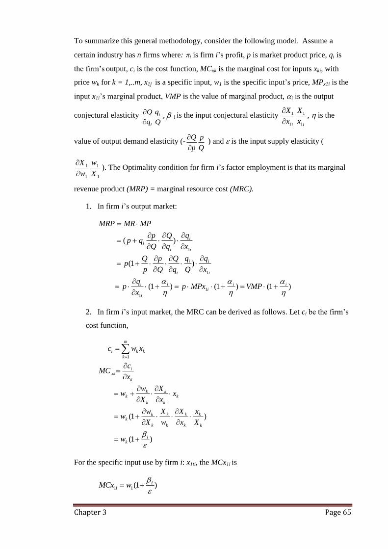
Chapter 3 Page 65

To summarize this general methodology, consider the following model. Assume a

certain industry has n firms where: i is firm i‟s profit, p is market product price, qi is

the firm‟s output, ci is the cost function, MCxk is the marginal cost for inputs xki, with

price wk for k = 1,..m, x1j is a specific input, w1 is the specific input‟s price, MPx1i is the

input x1i‟s marginal product, VMP is the value of marginal product, i is the output

conjectural elasticity Q

q

q

Q i

i

, i is the input conjectural elasticity ii

x

X

x

X

1

1

1

1

, is the

value of output demand elasticity (-Q

p

p

Q

) and is the input supply elasticity (

1

1

1

1

X

w

w

X

). The Optimality condition for firm i‟s factor employment is that its marginal

revenue product (MRP) = marginal resource cost (MRC).

1. In firm i‟s output market:

)1()1()1(

)1(

)(

1

1

1

1

iii

i

i

i

i

ii

i

i

i

i

i

VMPMPxpx

qp

x

q

Q

q

q

Q

Q

p

p

Qp

x

q

q

Q

Q

pqp

MPMRMRP

2. In firm i‟s input market, the MRC can be derived as follows. Let ci be the firm‟s

cost function,

)1(

)1(

1

ik

k

k

k

k

k

k

k

kk

k

k

k

k

kk

k

ixk

m

k

kki

w

X

x

x

X

w

X

X

ww

xx

X

X

ww

x

cMC

xwc

For the specific input use by firm i: x1ti, the MCx1i is

)1(11

ii wMCx

Chapter 3 Page 66

3. From firm i‟s optimality condition for input employment MRP = MRC,

)1(

iVMP = )1(1

iw .

This condition can be manipulated to provide for specific purpose analysis depending

on the purpose of each particular study. For instance, as will be developed in Chapter 4,

Chang & Tremblay (1991) derive VMP

wVMP k

i

ii

1

in order to measure the degree

of oligopsony market power. The symbols for elasticity variables for output market (

and ) and input market ( and ) were adopted from the original Chang & Tremblay

(1991) model whereas discussions elsewhere in this thesis are discussed in the reverse

order of input market / output market (oligopsony / oligopoly).

The weakness and strength of the conjectural variation approach are extensively

addressed in the literature. One limitation of these models is their application of firm

level model to industry level data. However, it is possible to use industry-level data in

place of firm-level data, given certain conditions. These conditions include a specific

level of marginal costs, marginal revenue and conjectural elasticities. That is the firms

in the industry are assumed to have linear and parallel expansion paths and therefore

values of marginal products and marginal costs are constant and equal across firms.

This is the so-called Gorman Polar form of production technology. This approach

allows different firms to have different cost curves but the curves are all linear and

parallel (Appelbaum, 1982). In equilibrium each firm equates marginal costs to its

perceived marginal revenue hence, their conjectural elasticities are guided along with

this condition and hence equal across firms.

Another critique for the framework is that it is a static analysis. Accordingly, given

other things remain static, it analyses whether output price, marginal resource cost and

input price are equal or not. But it should be noted that this requires some particular

conditions for the framework to be effective. For instance, the more mature the market,

the more constant the consumers‟ taste, the more saturate the level of technological

change, the more likely is the validity of the results. (Ferguson & Ferguson, 1994).

There are some limits to this structure-conduct-performance approach. In particular, it

tends to encounter problems with respect to the concepts of concentration and barriers

to entry. Concentration ratios make sense only when the large firms are distinctly large.

Chapter 3 Page 67

High profits may arise from efficiency due to their ability to operate at the minimum

efficiency scale. Finally, accounting measures of performance may not properly reflect

economic profits and costs such as in the case of long-lived capital assets (Carlton &

Perloff, 2000).

It is claimed that the net effects of the oligopoly and oligopsony market power can be

enhancing, weakening or indeterminate depending on the functional forms employed.

For instance Chen & Lent (1992) claim that use of linear output demand and linear

input supply models produces indeterminate effects.

The conjectural variation approach is criticized as weak by Hall (1988) because it

depends on the level of error variance and the returns to scale of the production

function. However, his alternative total factor model was seen to have weaknesses in

determining the degree of monopsony market power unless it was restricted to constant

returns to scale (Hyde & Perloff, 1994).

According to Hyde & Perloff (1994), the conjectural variation approach is weak

because it depends on the model specification, the level of error variance and the returns

to scale of the production function. They made a comparison between the structural

approach and the total factor production approach pioneered by Hall (1988). The results

indicated that the structural (conjectural variation) approach worked well if it was

properly specified and the variance of the error structure was not too high. The ability of

the model to distinguish various types of market structure was found to depend on the

returns to scale of the production function. The Hall‟s method worked well when

production function was constant returns to scale, otherwise there would be serious

biases; another weakness was that Hall‟s method was inadequate if one expected to

determine the degree of monopsony power.

Corts (1999) argued that the conjectural variation approach fails to measure market

power accurately. He pointed to the problems associated with assuming a firm‟s

observed behaviour captures the firm‟s conjectured views on its competitors‟ behavior.

At best this approach thus provides an average as against a marginal measurement of the

conduct parameter. He further commented that, despite increased criticism from a

theoretical viewpoint, the conjectural variation approach to generation of market power

measures was extremely popular for empirical studies (Corts, 1999, p228).

Chapter 3 Page 68

In response to these arguments some robustness tests were developed to compare the

results from conjectural testing with results from directly measured price-cost margins

(Genesove & Mullin, 1998 and Wolfram, 1997).

Alternative approaches to estimation of market power and industry conduct include a

latent modelling of structure model (Mccluskey & Quagrainie, 2004) and a

nonparametric measure (Love & Chumway, 1994). Alternative approaches such as these

can be used to compare with conjectural variation measures.

There may be other explanations for the price-cost margin results other than the effects

of concentration and market power. These could be regarded as structural changes in

social factors such as taste and healthy lifestyle concerns as well as economic factors

such as input substitution and technological progress. However, such factors could be

transformed into variables for application as exogenous variables in conjectural

variation models if deemed appropriate.

The issue of technology plays at least two roles in market power analysis. First via its

latent effects on cost efficiency that would widen the price cost margin by more than the

effect of market power and secondly via its cost saving effects that could be considered

as a trade off for welfare losses stemming from market power cases. Recent examples

include Morrison-Paul (2001a, 2001b) which carefully formulated various functional

forms to capture the cost structure of the US beef industry. The cost efficiency effect

was captured by the elasticity of total cost with respect to output. Azzam (1997)

measured the cost efficiency effect of marginal changes in price-cost margin by

industry concentration whereas Azzam et al. (2004) separated the cost efficiency effect

from the market power effect via the estimation of a total factor productivity growth

function. However, Sexton (2000) found that the gains from cost efficiency were

insufficient to cover welfare losses arising from oligopoly and oligopsony market

power.

The conjectural variation approach is appealing for the ability to identify the conduct of

firms in a general range covering competitive case, intermediate case, Cournot case and

monopsony (monopoly) case. Hence it has been frequently used and continues to be

gradually refined. Examples include Levinsohn (1993) who linked the conjectural

variation framework to an output growth function generated by a Taylor expansion. The

model was used to assess whether international trading has helped to curtail domestic

market power in certain import competing manufacturing industries. Hall (1988) and

Chapter 3 Page 69

Crespi et al. (2005) employed this framework to test for oligopsony market power in US

rice milling. Azzam et al. (2004) applied a total factor productivity growth model to

provide comparison tests for market power with results from a conjectural variation

approach.

The impact of exogenous shocks on key variables in conjectural variation models have

been examined by Chen & Lent (1992). Other refinements and applications include:

consideration of market power throughout each stage of the market supply chain from

the farm to the retail consumer; the distribution of welfare losses across consumers,

producers and marketers and estimation of social dead weight losses deriving from

market power. Studies of that illustrate such refinements and extended applications

include: Huang & Sexton (1996) Alston et al. (1997); Sexton (2000); Sexton & Zhang

(2001), Zhang & Sexton (2002) and Weldegebriel (2004).

The conjectural variation approach has also been applied to a wide range of applications

including examples at the macroeconomic level such as international trade agreements

in order to identify optimal trade conditions and optimal tax levels (Kiyono, 2006) and

to identify trade effects on domestic currency exchange rates (Yu, X, 2007).

Other applications that do not focus directly on market power assessment but are

implicitly linked to imperfect competition in a vertically coordinated market involving

such activities as: bidding procurement, contract- pricing procurement, processing,

wholesale selling and retail marketing, are found in Crespi & Sexton (2004), bidding,

(Xia & Sexton (2004), contract pricing and Saghaian (2007) wholesale and retail

markets.

For example the bidding for cattle in the US beef packing industry was found non

competitive (Crespi & Sexton, 2004). The common practice of contract- pricing in the

US cattle procurement tends to be based on the spot price. When the same set of buyers

operates in both the contract and cash markets, this practice will curtail prices in the

spot market, hence causing anticompetitive impacts (Xia & Sexton, 2004).

A study of price dynamics (the speed of price adjustment in wholesale market compared

to retail market) following demand shocks (due to food safety scares) using

cointegration analysis found that the wholesale market price was six times less flexible

than the retail market price hence reflecting a less competitive market at the wholesale

level with a tendency to absorb more of demand shocks than the retail market

(Saghaian, 2007). Although these studies did not explicitly employ the conjectural

Chapter 3 Page 70

variation approach, they all focused on the potential for market power along specific

supply chains.

In conclusion, acknowledging the weaknesses and restrictions of the Cournot model

with conjectural variation approach, the approach is still appealing to use for analysis,

not only for market power but also other aspects such as optimal tax levels and country

level optimal trade agreements. However, to apply this approach still requires some

extensions to the standard models

With respect to the pricing and market structure addressed in Chapter 2 Section 2.4 to

2.6, the natural rubber supply chain, specifically at the level of tire manufacturing,

demonstrates a potential for the tire industry oligopsony power on the natural rubber

industry as well as tire industry oligopoly market power on the tire consumers. In

contrast, the literature discussed above comprises studies that are mostly of oligopoly or

oligopsony alone. Only a few studies analysed oligopoly and oligopsony simultaneously

such as Schroeter (1988) and Azzam & Pagoulatos (1990). Nonetheless, they did not

estimate explicit output production functions to derive the exact marginal productivity

required in a conjectural variations approach. Even studies that had referred to the need

for directly estimated marginal productivity, did not present any empirical analysis

(Chang & Tremblay, 1991).

Thus, this thesis applies the theory of oligopsony by simultaneous analysis of

oligopsony / oligopoly of the natural rubber and tire industries using explicit estimation

of marginal productivity from an output production function. The findings from this

section are adopted in the next chapter for the development of a general theoretical

model for transformation into an empirical model to test for market power in the tire

and natural rubber industries. Accordingly, the next sections in this chapter provide a

survey of studies in the global tire and natural rubber markets.

3.6 Empirical Studies of the Tire Industry

3.6.1 Tire Production

Tire production can be considered to be divided into two categories of vehicles: cars and

commercial vehicles. Both are determined by the quantity of vehicle production and the

number of vehicles in-use. A new passenger car needs five tires. A new commercial

Chapter 3 Page 71

vehicle is estimated to need an average 6.8 tires (Burger & Smit, 1997). The demand for

tires on new cars is not related to the price for tires as tires represent only a small

portion of the costs of a vehicle. It is the replacement tire demand that is determined by

tire prices because users can delay the replacement if prices are high (Carree & Thurik,

2000). These figures produced by Burger & Smit (1997) provide a useful framework by

which one can trace the consumption of natural rubber for vehicle tire production,

which in turn, is led by vehicles production and vehicles in-use. The outcomes they

found for US, France, Japan and Germany can be summarized in Table 3.6.

Table 3.6 Tire Production

Passenger car tire production (tire units per vehicle per year)

Country Vehicle production

Vehicles

in-use

U.S. 8.11 -

France 8.33 -

Japan 3.20 -

Germany 6.86 -

Commercial vehicle tire production (tire units per vehicle per year)

Country Vehicle production

(units)

Vehicle

in-use

(units)

U.S. 5.79 -

France 3.62 -

Japan 5.15 1.56

Germany 2.94 1.82

Table 3.6 illustrates that using the identity of new vehicle tires plus replacement tires

equal to total tire production, each passenger car produced generates 8.11 units of tire

production in the US, 8.33 units in France, 3.20 units in Japan and 6.86 units in

Germany For vehicles in-use, they were only able to estimate a ratio of 1.56 tires per

vehicle per year in Japan and 1.82 tires per vehicle per year in. Other factors considered

were the impact of technology and learning for which they applied a time trend to proxy

the effect of learning-by-doing, based on the commonly accepted reason that cost

Chapter 3 Page 72

reduction always improves over time (Carree & Thurik, 2000).24

A second major factor

was the introduction of the radial tire in the 1970s that led to a reduction in tire

replacement need. The impact of the radial tire was less for commercial vehicle tires

than for passenger car tires.

No production function estimations were found in this or any other study of tire

production and hence there are no previous estimates of the marginal productivity of

natural rubber for tire production for use as benchmarks for the estimates produced in

this study.

3.6.2 Tire Demand

Previous studies of tire demand are found in Jovannovic & MacDonald (1994) and

Carree & Thurik (2000). Jovannovic & MacDonald (1994) used an inverse demand

function with a constant elasticity to model the tire demand equation for the time period

1913-1973. It was found that tire demand had a price elasticity of 0.76. Carree & Thurik

(2000), in a study of the life cycle of the US tire industry, extended the results of

Jovannovic & MacDonald (1994) using the same data in parts of their model. They used

output, price and a net entry system of equations estimation to obtain an average price

elasticity of demand for tires of 0.48.

The estimation results for these two studies are reported in Table 3.7. The estimated

price elasticities of -0.76 and -0.48, are useful benchmarks for the model results

reported for this study in subsequent chapters.

Table 3.7 Tire Demand Elasticity

Study Region/time Model Elasticity

Jovanovic & Macdonald (1994)

U.S. (1913-1973)

1

1

0

)(dt

td

pQ

Qt = tire quantity pt = tire prices.

-0.76

Carree & Thurick (2000)

U.S. (1913-1973)

tQ

ttttt SPaQUALaaMaQ ))log(( 3210

Where Qt is tire output, Mt is motor vehicle output, Pt is tire real price index, St is motor vehicles registered for 1 year or longer.

-0.4825

24

Since the first commercial tire was produced in 1906, the value of year – 1905 is employed to address

learning-by-doing effects.

25

This is calculated from average tire demand and motor vehicle registered.

Chapter 3 Page 73

3.7 Empirical Studies of the Natural Rubber Industry.

This section reviews a number of studies on natural rubber production and price that are

of relevance to this study.

3.7.1 Natural Rubber Supply Elasticity

Burger & Smit (1997) studied the natural rubber market policy and outlook. They

concluded that natural rubber is a competitive industry and that an important aspect of

natural rubber industry structure is that farming is mostly in small holdings (which are

less than 40 hectares). For definition purposes Estates are classified as having more than

40 hectares.

Natural rubber supply has elements of actual production and normal production. Normal

production is determined by the yielding quality of natural rubber trees and the planted

area. Yielding quality depends on tree vintages, as natural rubber trees take 7 years to

mature and stop producing latex upon reaching 30 years of age. It also depends on

technological progress. Therefore, normal production is a function of natural rubber tree

quality and area planted:

tti ayfq )(

where:

iq = normal production of natural rubber.

= year of planting

t = year of tapping

f() = embodied technical progress function

yt- = ideal yield profile, age = t-

at = area of vintage still remaining in year t.

Supply behaviour in the long-term is thus similar to that found with perennial crops, i.e.

current investment decision making in the production of natural rubber is based on

expectations about future prices.

In the short-term, actual production should be equivalent to total production less normal

production, hence the net changes in production is the response to weather and

economic factors, which have direct impact on tapping behaviour and uprooting.

Chapter 3 Page 74

Typically, when in the rainy season it is difficult to tap the natural rubber trees hence

outputs are reduced. In addition, when price increases, formers tend to tap more latex

for more income and uprooting and replanting are postponed.

To obtain projections for natural rubber supply, Burger & Smit (1997) used a two-stage

estimation technique to obtain a natural rubber supply function. In the first stage the

world natural rubber price was regressed on a vector of exogenous variables such as a

price-index of minerals, ores and metal, the total world consumption of rubber (natural

rubber plus synthetic rubber), and the calculated normal levels of production in the

world. The estimated values for natural rubber supply elasticity are provided in Table

3.8

Table 3.8 Natural Rubber Supply Price Elasticity

Country Natural Rubber

Supply Price elasticity

Thailand 0.22

Indonesia: Smallholdings 0.29

Malaysia: Estate and Small Holding26

0.14

These estimates provide useful benchmarks for the analysis in Chapter 5.

3.8 Natural Rubber and Price Stabilization

As described in Chapter 2, during 1980-2000, the International Natural Rubber

Organization (INRO) operated a buffer stock of natural rubber in order to stabilize its

prices. Accordingly, Na Ranong & Triumvorakul (2002) found that INRO was able to

generate some profits from the buying and selling of its stocks, (except for the INRO‟s

last term) and achieve a degree of prices stability. However, the problem for INRO was

the conflict of interest between importing (buyer) and exporting (seller) members and

the resultant prices which were not advantageous for natural rubber producers.

26

The elasticity for Malaysia was based on price / per capita income.

Chapter 3 Page 75

3.8.1 Natural Rubber Prices and Currency Exchange Rates

Burger, Smit & Vogelvang (2002) studied the effects of the 1997 exchange rate

depreciation in major producing countries on natural rubber prices. They found that the

combined effects of falls in the Thai baht, the Indonesia Rupiah and the Malaysian

ringgit was a drop in the world price for natural rubber by 15%. Given that the

combined real currency depreciation was 40%, the 15% fall in world price was argued

to have raised the real domestic price by 25%.

3.9 Conclusion

This chapter has provided the background theory for oligopsony/oligopoly analysis. It

began by reviewing the theory of production and price in output markets and

employment and price in input markets. The analysis was first framed for a perfectly

competitive market that was then used as a benchmark to evaluate production and

employment in imperfectly competitive markets. Consequently, the deviation from the

competitive standard is considered potential evidence of market power. A review of the

literature on measuring market power identified three approaches: buyer concentration,

effects from structural changes and the conjectural variation approach.

The conjectural variation approach is considered to be of most relevance for the

approach adopted in this thesis. Typically studies using this approach adopt a duality

theory approach namely the application of Shephard's Lemma and Hotelling's Lemma to

derive demand functions for inputs and supply functions for outputs respectively. The

degree of oligopsony/oligopoly power is defined as the deviation of actual input prices

from the value of their marginal products (shadow price) with the shadow price being

derived from the profit maximization conditions.

Findings support the claim that the higher the degree of imperfect competition, the

higher is the degree of oligopsony/oligopoly market power and vice versa. Hence, an

analysis of input and output market competitor behaviour, that is conjectural variation in

output and input markets, is needed as well as the elasticities of demand for inputs and

supply of outputs, to obtain a valid measurement of market power.

Following discussion of the theoretical background, this chapter has provided an

industry background into aspects of tire production and tire demand. In a review of

natural rubber supply studies it was found that tire demand has two components namely

demand from new vehicle production and demand for replacement tires. New vehicles‟

Chapter 3 Page 76

demand for tires does not have a price effect since it is a small item relative to the cost

of the whole vehicle. Demand for tires from vehicles in-use responds to tire prices.

Previous estimates of US tire demand elasticity are -0.76 (Jovanovic & Macdonald

1994) and -0.48 (Carree & Thurik, 2000).

The studies also concluded that the natural rubber industry is competitive. Supply is

price sensitive as farmers can vary tapping intensity and tree uprooting rates in

responses to price changes despite the fact that in the long term natural rubber planting

is based on perennial crop theory. Previous estimates of natural rubber elasticity for

Thailand, Indonesia and Malaysia are 0.22, 0.29 and 0.14 respectively (Burger & Smit

1997). The International Natural Rubber Organization (INRO) was found to have had a

degree of stabilization on natural rubber price during its existence.

Together with the background study of the markets for tires and natural rubber provided

in Chapter 2, the findings in this chapter assist the development of a general theoretical

model, and its corresponding empirical application in Chapters 4 and 5 to analyse the

degree of market power that global tire industry might exercise on the global natural

rubber market.

Chapter 4 Page 77

Chapter 4

A General Model of Oligopsony Market Power

4.1 Introduction

The theoretical concepts of market power and economic analysis were identified in

Chapter 3. This chapter develops a theoretical model from which a market power index

is derived. This model and its market power index forms the basis for the empirical

analysis of oligopsony power for global tire and natural rubber industries found in the

next chapter.

The theoretical model is derived from that developed by Chang & Tremblay (1991).

The market power index derived from their model comprises a series of elasticities that

all are potentially estimable even though Chang and Tremblay themselves do not apply

their index to empirical example. In this study, the market power index developed by

Chang and Tremblay is extended via identification of four different interpretations

according to alternative interpretations of various components of the original model.

Application of the four derived market power index measures is then reinterpreted to

provide for application to a global/country level model for examination of the global tire

manufacturing industry and its link to a country level natural rubber industry.

In the subsequent chapter, the theoretical model developed in this chapter is converted

to an empirical form for estimation. Market power indexes are then derived for each of

the four alternative model interpretations to evaluate whether oligopsony market power

is present at a country level for natural rubber inputs into the global tire manufacturing

market.

4.2 The General Model

A foundation concept for the measurement of market power is the Lerner index: that

market power is the difference in output price and marginal cost divided by output

price. Accordingly, many subsequent studies have extended the basic Lerner concept in

a variety of different ways. The Lerner index can be shown to be consistent with other

market power measures such as concentration ratios, market shares, and the Herfindahl-

Hirschman index. It also provides for measurement of both oligopsony and oligopoly

power simultaneously.

Chapter 4 Page 78

This study is based on the particular model developed by Chang & Tremblay (1991).

Their theoretical approach requires modelling both product and input markets for a

specific output and input commodity. It comprises an output product demand function,

the output product production function and the input supply function. The market power

index (based on the Lerner measure) is derived from the firm‟s optimality condition for

profit maximization with respect to the employment of the specific input. The derived

index is then able to be interpreted for a number of different market structures.

The model is found to be suitable for achievement of the aim of this study which is the

measurement for any possible existing market power in the global tire industry on the

natural rubber industry. Owing to the fact that world tire manufacturing is controlled by

a small number of multinational companies headquartered in the world‟s major

economies, whereas their natural rubber input are imported from other lesser developed

countries, this model is capable of modification from the original design application at

an industry/firm market power analysis level to a global/country market power analysis

level.

The Chang & Tremblay model and its variant versions developed for this study are

derived as follows.

Output Demand Function

The output commodity is assumed homogeneous and produced by i producing firms.

The inverse demand function for this output commodity is given by.

(4:1) p(Q)P

Where: P is output price, iqQ is market output and iq is the output of firm i for i =

1, 2, 3…n firms in the industry. A non-competitive output market is possible if n is

small enough such as when entry may be blocked by technology, which requires some

minimal scale sufficiency.

Input Supply Function

To produce this commodity, firm i requires inputs xki, where k = 1 … m. In this study

the specific input of interest (x1i) is natural rubber which is from this point on denoted as

xri. The firm also employs some other inputs which are traded in competitive markets.

Chapter 4 Page 79

As in the output case, if n is small, then non-competitive buyer behaviour is possible in

the market for xri. Let the inverse market supply of the specific input XR be given by:

(4:2) ) 1(XR hWR

Where: WR is the per unit price of XR and XR=xrj is total supply of the specific input

XR from j supplier firms. In addition: 0dXR

dWR.

Output Production Function

Let the production function of the firm be

(4:3) ) kiii (xfq

According to economic theory, the problem of the firm is to choose the optimal level of

inputs, including xr and all other inputs such as physical capital in order to maximize

the firm‟s profit. 27

4.2.1 Optimality Condition and the Derivation of Market Power Index for Model 1

The firm‟s profit function comprises:

(4:4)

m

k

kikiii xW - xrWR-qPπ2

where i denotes firm i‟s profits, Wk and xk , k = 2,….m are the vectors of prices and

quantities of other inputs respectively. Output prices (P) and input prices (WR) are

market determined prices as identified in (4:1) and (4:2). Hence (4:4) can also be

represented as:

(4:4a)

m

k

kikiii xW - xrXRh-qQpπ2

1

The input employment levels that maximize the firms‟ profits are derived from the

conditions 0

i

i

xr

π and 0

ik

i

x

π respectively. Given that input xr is the focus of our

model we derive the optimality condition for purchase of xr as follows.

27

For capital the input price would be the rental price of capital.

Chapter 4 Page 80

(4:5) 0 WR xrdxr

dXR

dXR

dWRP

xr

qq

xr

q

dq

dQ

dQ

dPi

ii

ii

i

i

i

; for input xri.

As discussed in Chapter 3, our index for measuring input price distortions is defined as

the difference between the value of the marginal product of the input (VMP) and the

input price (WR) divided by the value of the marginal product (VMP). This can be

presented in the following form.

XRi

XRi

iXRMPP

- WR MPPMPI ; where VMP is given by P(MPXRi).

Our market power index for XR namely MPIXRi is derived by rearranging the optimality

condition (4:5) such that it comprises measurable variables in the form of marginal

products and elasticities. First we rearrange (4:5) as follows.

(4:6)

0 WR WR XR

xr

dxr

dXR

WR

XR

dXR

dWRP

xr

qP

xr

q

Q

q

dq

dQ

P

Q

dQ

dP i

ii

i

i

ii

i

Within (4:6) we can identify a number of standard variables and denote these variables

as follows.

Q

q

dq

dQ i

i

i : is the i‟th firm‟s output conjectural elasticity with respect to total

industry output.

XR

xr

dxr

dXR i

i

i : is the i‟th firm‟s input conjectural elasticity with respect to the

industry‟s total factor demand for XR.

P

Q

Q

Pη

: is the inverse price elasticity of demand for product Q as derived from the

inverse demand curve.

WR

XR

XR

WRε

: is the inverse price elasticity of supply for input XR as derived from the

inverse supply curve.

i

iXRi

xr

qMP

: is the marginal product of the XR of the i firm.

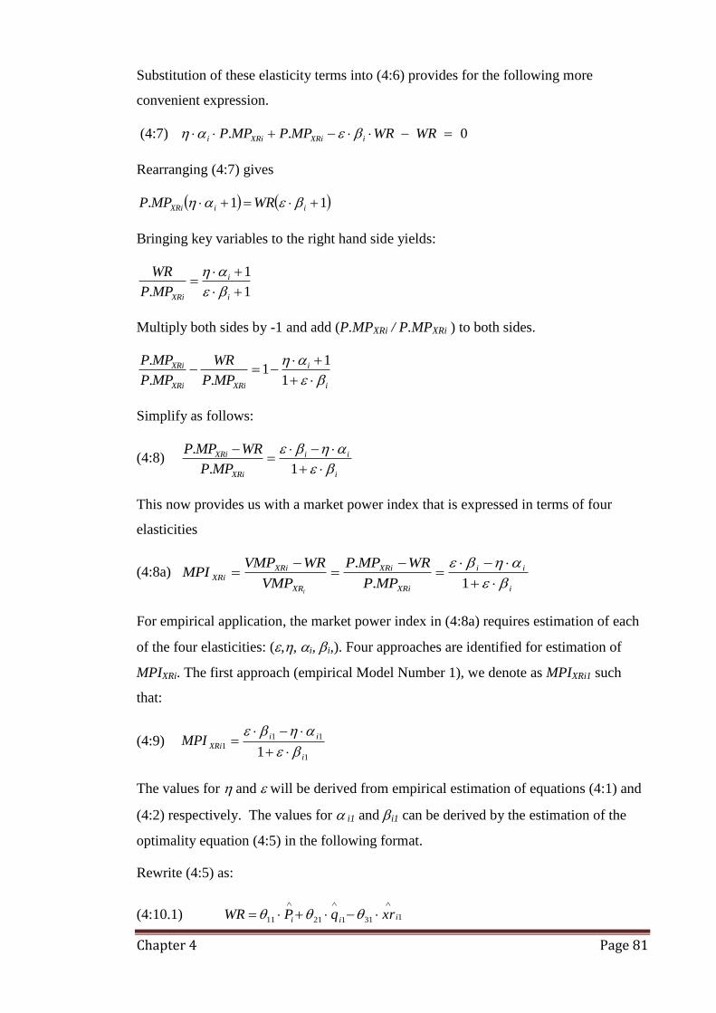
Chapter 4 Page 81

Substitution of these elasticity terms into (4:6) provides for the following more

convenient expression.

(4:7) 0.. WR WR MPPMPP iXRiXRii

Rearranging (4:7) gives

11. iiXRi WRMPP

Bringing key variables to the right hand side yields:

1

1

.

i

i

XRiMPP

WR

Multiply both sides by -1 and add (P.MPXRi / P.MPXRi ) to both sides.

i

i

XRiXRi

XRi

MPP

WR

MPP

MPP

1

11

..

.

Simplify as follows:

(4:8) i

ii

XRi

XRi

MPP

WRMPP

1.

.

This now provides us with a market power index that is expressed in terms of four

elasticities

(4:8a) i

ii

XRi

XRi

XR

XRi

XRiMPP

WRMPP

VMP

WRVMPMPI

i

1.

.

For empirical application, the market power index in (4:8a) requires estimation of each

of the four elasticities: (,, i, i,). Four approaches are identified for estimation of

MPIXRi. The first approach (empirical Model Number 1), we denote as MPIXRi1 such

that:

(4:9) 1

11

11 i

ii

XRiMPI

The values for and will be derived from empirical estimation of equations (4:1) and

(4:2) respectively. The values for i1 and i1 can be derived by the estimation of the

optimality equation (4:5) in the following format.

Rewrite (4:5) as:

(4:10.1) 13112111 iii xrqPWR

Chapter 4 Page 82

Where:

(4:11.1) idq

dQ21

(4:12.1) idxr

dXR31 .

(4:13.1) Pxr

qP

i

ii

(4:14.1) i

i

ii q

xr

q

dQ

dPq

1

(4:15.1) ii xrdXR

dWRxr

1

Three key components of the variables in (4:10.1) are: the slope of the output demand

curve (dQ

dP); the slope of the input supply curve (

dXR

dWR) and the marginal product of the

input xri (i

i

xr

q

) which are estimated from equations (4:1), (4:2) and (4:3) respectively.

After estimating equation (4:10.1) the values for 21 and 31 are then used to calculate

the two conjectural elasticities i and i as:

(4:16.1) Q

i211i

q

(4:17.1) XR

xri311i

Substituting the estimates for , , i1, i1 allows the market power index in (4:9)

1

111

1 i

iiXRiMPI

to be obtained.

The null hypothesis of input market efficiency (no market power) can be stated in terms

of the three coefficients in 4:10.1 as H0: 11 = 1, 21 = 31 = 0. If H0 is not rejected then:

Pxr

qWR

i

i

and hence the input xri is being paid the value of its marginal product.

Further, if 21 = 31 = 0, then i1 = i1 = 0 and MPIXRi1 = 0, thus indicating a perfectly

competitive input market. Rejection of Ho indicates the presence of non competitive

markets. In particular, significant positive values of 21 indicate the presence of

Chapter 4 Page 83

oligopoly in the output market and significant positive values of 31 indicate the

presence of oligopsony in the input market. The interpretation of MPI and the presence

of various market structures are considered in more detail later in this chapter.

4.2.2 Reconciliation of the Derived Market Power Index and the Chang &

Tremblay Index

The derived MPI in (4:9) above differs from that developed by Chang &Tremblay

(1991) article. Critical differences arise due to interpretation of the elasticities and ε

and the subsequent construction of the MPI. Chang &Tremblay defined output

commodity demand elasticity as: Q

P

P

Q

. This is the conventional price elasticity of

demand for a normal demand curve (Q = p(P)). In the market power index derived for

this study demand elasticity is defined as: P

Q

Q

P

as reflects its estimation from an

inverse demand curve P = p(Q). Hence as defined for the inverse demand curve

becomes -1/ = * for the Chang & Tremblay model. Similarly the input supply

elasticity (ε) in the derivation above is defined as WR

XR

XR

WR

as reflects its intended

derivation from the inverse supply curve WR=h1(XR). However, Chang &Tremblay

defined ε as: XR

WR

WR

XR

, as would be derived from a normal supply function. Hence ε as

defined for the inverse supply curve becomes 1/ ε = ε* for the Chang &Tremblay

model.

As a consequence Chang &Tremblay (1991) express their market power index as:

(4:8b)

*1

**2

ε

η

ε

MPIi

ii

iXR

;

in contrast to the market power index model 1 derived for this study as:

(4:8a) i

iiXRi

MPI

1

The mix of inverse and direct elasticities raises both theoretical and estimation

questions that are not addressed by Chang &Tremblay (1991) who recommended that

the direct elasticities (* and ε*) be derived from econometric estimations of inverse

Chapter 4 Page 84

demand curves (that is as and ε) and then inverted to obtain * and ε*. It is not

considered valid to assume -1/ = * and 1/ ε = ε*. These elasticities are derived from

different functional forms with different theoretical foundations in respect of the causal

relationships between dependent and independent variables. Econometric assumptions

can be violated by incorrect model specifications. The assumption that inverse

elasticities are equivalent to direct elasticities by implication assumes that inverse

functional forms are equivalent to direct functional forms.

However, it is possible to derive the Chang and Tremblay index without transgressing

the theoretical foundations. This index we refer to as Model 2 and its derivation is as

follows.

4.2.3 Optimality Conditions and Derivation of Market Power Index for Model 2

To derive the Chang and Tremblay index described in section 4.2.2, a direct version of

tire demand is given by:

(4:18) Q = q(P)

Where Q is market output, P is output price and Q

P

P

Qη

* is the direct price elasticity

of demand for product Q as derived from the direct demand curve.

(4:19) XR=h2(WR)

Where XR is the market supply of the specific input, WR is the per unit price of XR and

XR

WR

WR

XRε

* : is the direct price elasticity of supply for input XR as derived from the

direct supply curve.

The value for the market power of Model 2, namely MPIXRi2 is

(4:20)

*1

**

2

22

2

ε

η

ε

MPIi

ii

iXR

For empirical application, analogous to that adopted for Model 1, estimate equations

(4:18) for *, equation (4:19) for *

and in parallel to Model 1, estimate equation

(4:10.2) and calculate the conjectural elasticity estimates: i2, and i2.

Chapter 4 Page 85

(4:10.2) 232222212 iii xrqPWR

Where:

(4:11.2) idq

dQ22

(4:12.2) idxr

dXR32 .

(4:13.2) Pxr

qP

i

ii

2

(4:14.2) i

i

ii

qxr

q

dP

dQq

12

, where

dP

dQ

1 ≡

dQ

dP,

(4:15.2) ii xr

dWR

dXRxr

12 , where

dWR

dXR

1≡

dXR

dWR.

After estimating equation (4:10.2) the values for 22 and 32 are then used to calculate

two conjectural elasticities as:

(4:16.2) Q

i222i

q

(4:17.2) XR

xri322i

Substituting values for *, *

, i2, and i2 into (4:20), a value for the MPIXRi2 is derived.

4.2.4 The Derivation of Market Power Index for Model 3

An alternative approach to the derivation of the conjectural elasticities i and i is

possible. Consider the following approach that uses direct estimation of the i‟th firm‟s

(or in this case the i‟th country‟s) observed response to industry changes. This is then

used to develop a proxy measure for the individual firm‟s conjectures on industry

responses to its behaviour. Fundamentally this approach simply measures the average

response, over the studied time period, in each individual firm‟s (or country‟s) market

share of the global industry. Given:

(4:21) )(qfQ i2

Chapter 4 Page 86

(4:22) )(3 ixrfXR

For i = US, France, Japan and Germany. The values:

(4:23) Q

q

dq

dQα i

i

i 3 ; and,

(4:24)

β i3

XR

xr

dxr

dXR

i

i ; can then be derived. The market power index is:

(4:25) 3

333

1 i

iiXRiMPI

For empirical application, we estimate the following equations: equation (4:1) for ,

equation (4:2) for , equation (4:21) for i3, and equation (4:22) for i3 . Substituting

values for:, , i3 and i3 into the market power expression (4:25), delivers a value for

the market power index for Model 3.

4.2.5 The Derivation of Market Power Index for Model 4

For this model the conjectural elasticity values from (4:23) and (4:24) are applied to

direct versions for tire demand (4:18) and natural rubber supply (4:19), to provide the

market power index:

(4:26)

*1

**

3

33

4

ε

η

ε

MPIi

ii

iXR

.

For empirical application, we estimate equation (4:19) for *, equation (4:20) for *

,

equation (4:21) for i3, and equation (4:22) for i3. Substituting these values provides

the Market Power Index (4:26), for Model 4 which provides for an alternative

estimation approach for the Chang and Tremblay version of the market power index in

(4:8b).

4.3 Interpretation of the Market Power Index

The market power index (MPIXRi) measures the economic rents, i.e. a portion of the

value of the marginal product which is not covered by market prices hence could be

gained by the oligopsonist and oligopolist firms. Consequently, it implies that the

Chapter 4 Page 87

pricing mechanism is not perfect and thus inefficiency might be evident in input and

output allocation.

The index has some useful properties that should be examined. Firstly, by its definition,

the value of MPIXRi ranges from 0 to 1. It is 0 when input XR receives a price that equals

the value of its marginal product: WR=PMPXRi. It approaches 1 as the input price

approaches 0. Between these two extreme cases, the higher the MPIXRi, the greater is the

inefficiency in resource allocation.

Secondly, the MPIXRi index is general since it covers a variety of market structures.

Accordingly, Table 4.1 illustrates diverse types of market structures and their impact on

the value of the MPIXRi index. It can be seen that the index is general in that it covers

cases like the Lerner case (competitive input market and monopoly output market), the

Cournot equilibrium case (equal market shares in either markets) and the Robinson

classic case (monopsony input market and monopoly output market).28

It can be seen

also that the level of MPIXRi is determined by the values of , , i, and i. Consequently

inefficiency in resource allocation is increased by low values of , and , and high

values of i, and i.

28

From Chang & Tremblay (1991) pp. 407, when defining the industry market power index for input

(natural rubber) market as )(XR

xrMPI i

XRi , it approaches the Herfindahl-Hirshman index in the

input market if 1)(

i

idxr

dXR

. Similarly, when defining the industry market power index for output (tire)

market as )(Q

qMPI i

XRi it approaches the Herfindahl-Hirshman index in the output market if

1

idq

dQ

.

Chapter 4 Page 88

Table 4.1 Market Power Index and Market Structures

Market structure: Input / Output MPI

General Model (4:8a) i

ii

iXRε

ηεMPI

1

i = 0

1: i=0, i=0 Competitive / Competitive 0

2: i=0, 0<i<1 Competitive / Oligopoly iiXR ηMPI

3: i=0, i=1 Competitive / Monopoly

(Lerner case) ηMPI

iXR

0< i <1

4: 0<i<1, i=0 Oligopsony /Competitive i

i

iXRε

εMPI

1

5: 0<i<1, 0<i<1

Oligopsony / Oligopoly

1

12

1

11

X

x

X

x or

Q

q

Q

q 21 ,

implies Cournot case of equal market shares.

i

ii

iXRε

ηεMPI

1

6: 0<i<1, i=1 Oligopsony / Monopoly iε

ηεMPI i

iXR

1

i = 1

7: i=1, i=0 Monopsony / Competitive ε

εMPI

iXR

1

8: i=1, 0<i<1 Monopsony / Oligopoly ε

ηεMPI i

iXR

1

9: i=1, i=1 Monopsony / Monopoly

(Robinson case) ε

ηεMPI

iXR

1

4.4 Application of the Model to Global Natural Rubber and Tire Industries

Characteristics of the tire industry and natural rubber industry render it appropriate to

shift the model from an industry/firm level to global/country level. The nature and

background of the tire industry as discussed in chapter 2 outlined how the industry

began a hundred years ago and has since passed through phases of invention, production

innovation and structural change. Key amongst these were the invention of cord tires

and straight-side tires which replaced clincher tires in 1913, the invention of the

Banbury mixer in 1916 to mix rubber with other compounds, the use of rayon as the

Chapter 4 Page 89

fabric from which tire cords were made in 1930s, the subsequent replacement of rayon

by nylon and the invention of synthetic rubber as a substitute for natural rubber in the

1940s, the invention of the tube tire in 1950s, the subsequent replacement of nylon by

polyester and the invention of belted biased tire design in 1960s, and radial tires in the

1970s.

Advances in technology and management improvements, such as the advent of mass

marketing methods, (French 1991) generated lower marginal costs, higher output and

lower prices. Firms that did not have sufficient production scale could not afford these

technologies; consequently, they could not survive the competition (Gort & Klepper

1982, Jovanovic & MacDonald 1994, Klepper & Kenneth 2000 and Carree & Thurik

2000). Accordingly, marginal costs tend to be similar among firms and a few prominent

firms dominate the world tire industry, e.g. Goodyear in the USA, Michelin in France,

Bridgestone in Japan and Continental in Germany who produce and supply tires all over

the world.

As the tire producing countries do not produce natural rubber, this input is imported

from supplying countries. Specifically, during the time studied by this thesis (1960-

2000), countries such as Malaysia, Indonesia and Thailand supplied natural rubber to

the key tire producing countries: namely the USA, France and Japan. Therefore, the

world tire industry comprises a few multinational producers that not only are operating

in a global industry but are also purchasing inputs such as natural rubber from country

level suppliers.

The presence of a global industry structure also raises the question as to whether the

global tire manufacturing industry has the potential to exert market power over the

natural rubber industry at a country level. For empirical analysis, data are also more

readily available at a country level. These data also reveal a country-wise pattern of

natural rubber exports from supplying countries to tire manufacturing countries in that

the destination of most of natural rubber exports from Thailand is Japan, from Indonesia

is the USA and from Malaysia is the European Union.

However, the application of a firm level model to country level model poses theoretical

as well as conceptual and empirical considerations. The literature argues it is possible to

substitute industry-level data for firm-level data if the firms in the industry are assumed

to have linear and parallel expansion paths such that the values of marginal products and

marginal costs are constant and equal across firms. This is the so-called Gorman polar

Chapter 4 Page 90

form of production technology. It allows for different firms to have different cost curves

but the curves are all linear and parallel (Appelbaum 1982). With many small

competing natural rubber producers this is not considered an unreasonable assumption.

Hence, in equilibrium each firm equates marginal costs to its perceived marginal

revenue and their conjectural elasticities are hence equal across firms. 29

A detailed analysis of the data available for empirical analysis was undertaken in

Chapter 2. Data deficiencies were identified with respect to specific location of all tires

produced. The dominance of the industry by major producers with manufacturing plants

in both within and without their home countries via subsidiary and joint venture

companies was demonstrated. It was concluded that there was potential for market

power to be exercised in the natural rubber markets from the buyer side (oligopsony)

and this potential could be analysed via either company level or country level data.

The general model is thus capable of application from its original industry/firm level to

global industry/country level. This application requires all industry level variables to be

reinterpreted as global variables and firm level variables to be reinterpreted as country

level variables.

Figure 4.1 illustrates the flows of natural rubber from producing countries to its various

production uses in a global industry context. In addition, tire production is usually

classified by vehicle type namely: passenger car tires, commercial vehicle tires, truck

tires, bus tires and off-highway tires. Passenger car tire and commercial vehicle tires are

the two most important types.

As depicted by Figure 4.1, a portion of natural rubber production from country j such as

Thailand, Indonesia, Malaysia and other producing countries is consumed domestically.

The rest is exported to destination countries such as the USA, France, Japan, Germany

and other consuming countries. In the destination countries, some of the imported

natural rubber is consumed in the general sectors such as construction and irrigation.

The rest are employed by the tire sector, which is the major portion used to produce

passenger car tires and commercial vehicle tires.

29

However, it can be argued that conjectural elasticities are not constant over time. This is due to the

changing structure of the industry. Accordingly, the aggregate value of the conjectural elasticities over

time changes too (Gohin 2003).

Chapter 4 Page 91

Figure 4.1 The Flows of Natural Rubber from Producing Countries

Country j’s Natural Rubber Production

Country j’s

Domestic Natural

Rubber

Consumption

Country j’s Natural Rubber Exports to

Destination Country i

Natural

Rubber

Consumption

in Country i’s

General

Sector

Natural Rubber

consumption in

Country i’sTire

Sector

Tire Production in Country i

Passenger car tires

+ Commercial vehicle tires

= most of tire production

4.5 Conclusion and Summary

This chapter has described a general model for the derivation of a market power index

that can be used to assess the oligopsony/oligopoly power of global tire manufacturing

countries consuming natural rubber inputs from supplying countries. The model is

based on the model developed by Chang and Tremblay (1991). This model is extended

to incorporate 4 different interpretations which we labelled as models 1 to 4. These

models are designed for empirical application as described in the next Chapter.

A summary of the different market power index models and the different approaches to

their empirical application is summarized in Figure 4.2.

Model 1: the derivation of the market power index starts from Step A. The inverse tire

demand function is estimated in order to obtain the tire price elasticity. In Step B the

natural rubber supply equation is estimated in order to retrieve the natural rubber price

elasticity. In Step C each specific country‟s tire production equation is estimated, to

yield a natural rubber marginal product for tire production in each country. In Step D

the estimated coefficients are used to transform tire price, tire demand and tire sector

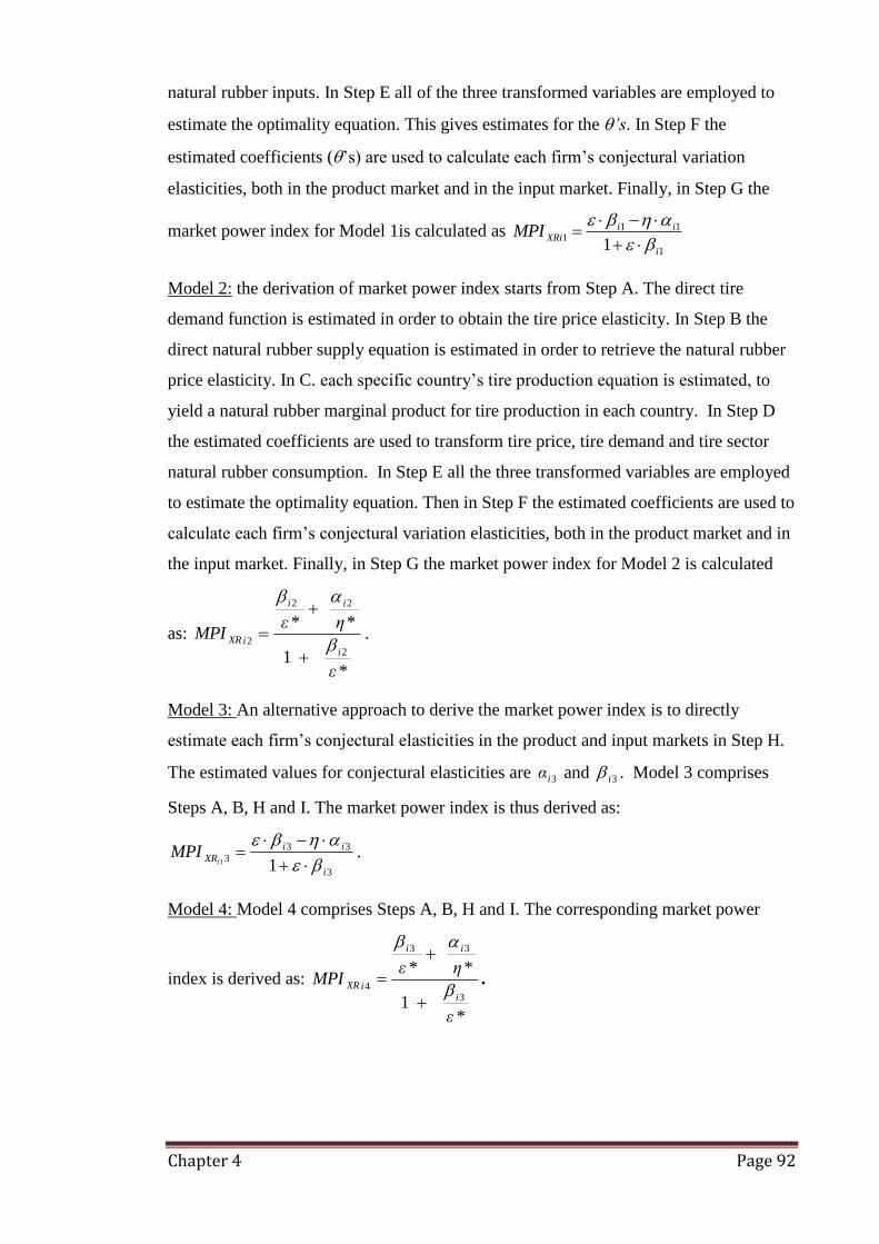
Chapter 4 Page 92

natural rubber inputs. In Step E all of the three transformed variables are employed to

estimate the optimality equation. This gives estimates for the ’s. In Step F the

estimated coefficients (‟s) are used to calculate each firm‟s conjectural variation

elasticities, both in the product market and in the input market. Finally, in Step G the

market power index for Model 1is calculated as 1

111

1 i

iiXRiMPI

Model 2: the derivation of market power index starts from Step A. The direct tire

demand function is estimated in order to obtain the tire price elasticity. In Step B the

direct natural rubber supply equation is estimated in order to retrieve the natural rubber

price elasticity. In C. each specific country‟s tire production equation is estimated, to

yield a natural rubber marginal product for tire production in each country. In Step D

the estimated coefficients are used to transform tire price, tire demand and tire sector

natural rubber consumption. In Step E all the three transformed variables are employed

to estimate the optimality equation. Then in Step F the estimated coefficients are used to

calculate each firm‟s conjectural variation elasticities, both in the product market and in

the input market. Finally, in Step G the market power index for Model 2 is calculated

as:

*1

**

2

22

2

ε

η

ε

MPIi

ii

iXR

.

Model 3: An alternative approach to derive the market power index is to directly

estimate each firm‟s conjectural elasticities in the product and input markets in Step H.

The estimated values for conjectural elasticities are 3iα and

3i . Model 3 comprises

Steps A, B, H and I. The market power index is thus derived as:

3

33

311

i

ii

XRiMPI

.

Model 4: Model 4 comprises Steps A, B, H and I. The corresponding market power

index is derived as:

*1

**

3

33

4

ε

η

ε

MPIi

ii

iXR

.

Chapter 4 Page 93

Figure 4.2a Summary Derivation of the Market Power Index for Model 1 and

Model 2

Steps

A

Model 1 & 3 Inverse Tire Demand

(4:1) p(Q)P ; P

Q

Q

P

Model 2 & 4 Direct Tire Demand

(4:18) q(P)Q ; Q

P

P

Q

*

B

Model 1 & 3 Inverse Rubber Supply

(4:2) ) 1(XR hWR ; WR

XR

dXR

dWR

Model 2 & 4 Direct Rubber Supply

(4:19) )2(WR hXR ; XR

WR

dWR

dXR*

C

Model 1 & 2 Tire Production Function and Marginal Products

(4:3) ) iii (xrfq → xr

q MP

i

i

iXR

D

Model 1

Calculate variables iixr, q, P

Pxr

qP

i

ii

; i

i

ii q

xr

q

dQ

dPq

;

ii xrdXR

dWRxr

Model 2

Calculate variables iixr, q, P

Pxr

qP

i

ii

2 ;

i

i

ii

qxr

q

dP

dQq

12

ii xr

dWR

dXRxr

1

E

Model 1 Estimate Optimality Condition

(4:10.1)

iii xrqPWR

312111

→ 21 and 31

Model 2 Estimate Optimality Condition

(4:10.2)

iii xrqPWR

3222212

→ 22 and 32

F

Model 1 Calculate Conjectural Elasticities

Q

i211i

q ;

XR

xri311i

Model 2 Calculate Conjectural Elasticities

Q

i222i

q ;

XR

xri322i

G

Model 1 Calculate MPIXRi1

(4:9)

1

111

1 i

iiXRiMPI


(4:20)

*1

**

2

22

2

ε

η

ε

MPIi

ii

iXR

Chapter 4 Page 94

Figure 4.3b Summary Derivation of the Market Power Index for Model 3 and

Model 4

H

Model 3 & 4 Direct Estimation of Conjectural Variation Elasticities

Tire Market: (4:21) )(qf Q i2

→ (4:23) Q

q

q

Qα i

i

i

3

Natural Rubber Market: (4:22) )(3 ixrfXR → (4:24)

XR

xr

dxr

dXR β i

i

i 3

I


(4:25)

3

33

311

i

ii

XRiMPI


(4:26)

*1

**

3

33

4

ε

η

ε

MPIi

ii

iXR

Chapter 5 Page 95

Chapter 5

Data Analysis and Empirical Estimation

5.1 Introduction

This chapter provides the empirical application of the general model developed in

Chapter 4. The approach adopted was summarized in the concluding section of Chapter

4. Regression analysis was employed for the analysis. The first step requires

specification of functional forms for estimation of each of the general model equations.

However, model specification is contingent on data characteristics so variables for each

equation are analysed and tested for nonstationarity prior to functional specification.

Estimation results are reported and the required elasticities for each version of the

market power index are obtained and used to derive market power indexes on a country

basis.

5.2 Data Tests for Nonstationarity

Time series data are typically nonstationary. That is they do not exhibit time invariant

mean, variance and serial correlation found with stationary data series. Nonstationary

data can generate spurious regression results when using OLS estimation techniques

(Ramanathan, 1998). Standard approaches to testing for nonstationarity were applied to

all key variables. Results using both Dickey-Fuller (DF & ADF) and Phillips-Perron

(PP) tests confirm nonstationarity across all series. However, further testing confirmed

all series were stationary in first difference form (integrated to order one I(1)). The

results were consistent for all variables using PP tests but a small number of variables

failed to reject the null hypothesis of nonstationarity using the DF and ADF approach.

Test results are summarised in Appendix 5.1

Nonstationary data series may still exhibit a long run relationship. If two or more series

are I(1) and a linear combination of them is stationary then the series are said to be

cointegrated and hence exhibit a long run relationship. Testing for cointegration is

undertaken by assessing whether or not the residuals from an OLS estimation of the

relationship are stationary. This is undertaken by application of DF, ADF and / or PP

approaches to the residuals of the OLS regression. Rejection of the null of

nonstationarity in the residuals is used to confirm that OLS estimation can be used to

Chapter 5 Page 96

identify the long run relationship (Enders, 1995; SHAZAM, 1997 and Ramanathan,

1998 ). This approach was applied to all the major functional relationships and the

results confirmed the presence of a cointegrating relationship.

A further extension of the cointegration concept involves the estimation of an error

correction model that can be used to identify the short run relationship between the

particular series. Significantly a negative error correction coefficient is required in such

a model to confirm the relationship and its adjustment to the long run equilibrium

relationship is not explosive (Ramanathan, 1998). Tests on error correction models for

the major functional forms found correctly signed error correction coefficients. These

results also support the cointegration test findings of a long run relationship. A

summary of the test results is found in Appendix 5.2 and estimation results for error

correction models of inverse and direct natural rubber supply functions are found in

Appendix 5.3.

Given the focus of this study is long term and requires estimation of long run

elasticities, the estimation approach uses OLS estimations of long run relationships

rather than short run error correction model relationships.

5.3 Estimation of the Tire Demand Function

Tire demand is modelled in both inverse and direct form. The inverse demand function

(5:1), models tire price (P) as a function of world tire production output (Q), world

vehicle production (VP) , the interaction of world vehicle in-use (VI) and Q, and US per

capita income (GDPPUS).

(5:1) )ln()ln()ln()ln()ln()ln( 1413121110 GDPPUSQVIVPQ P

A log-log functional form is employed for (5:1), from which we derive the slope

Q

PVI

Q

P)].ln([ 1311

; and the inverse elasticity:

)ln()ln(

)ln(1311 VI

Q

P

P

Q

Q

P

;

For the direct tire demand model, the world tire demand (Q) is modelled as a function of

tire price (P) and the corresponding vector of shifting variables comprises world vehicle

production (VP), world vehicle in-use (VI) and a time trend (T).

Chapter 5 Page 97

(5:2) )ln()ln()ln()ln()ln( 2423222120 TVIVPP Q

A log-log functional form is employed for (5:2), from which we derive the slope * =

P

Q

P

Q21

and the direct elasticity

21

*

)ln(

)ln(

P

Q

Q

P

P

Q

Variables that are employed to estimate the demand functions are summarised in Table

5.1

Table 5.1 Variable Description for the Estimation of the Tire Demand Function

Variable Description

P Tire prices: US tire price index deflated by US consumer price index, base year: 1995=100

Q World tire production

VP World passenger car and commercial vehicle production

VI World passenger car and commercial vehicles in-use.

GDPPUS US per capita income deflated by US consumer price index. Base year 1995 = 100

T A time trend.

Tire production is classified as passenger car tires plus commercial vehicle tires since

data records for some countries such as China, Russia and the Republic of Korea, did

not have separate data until recent years. The summation is also based on the

consideration that natural rubber and synthetic rubber input ratios used in passenger car

tire and commercial vehicle tire are very close viz: 55% / 45% and 50% / 50%

respectively. In contrast the ratios vary more significantly for special tires such as racing

tires (35% / 65%) and off-highway tires (80% / 20%). Accordingly the selected

definition for tire production is also more suitable for tire production function

estimation.

Data for natural rubber and synthetic rubber consumption in tire manufacture are

available for USA, France, Japan, Germany, Italy, Spain, U.K., Brazil and India. A

significant omission from the data is China and hence despite its significant

consumption since 1990s China is excluded30

.

30

Of course, natural rubber consumption data could be used in place of natural rubber used in tire sector

in such cases.

Chapter 5 Page 98

As previously noted, each new car requires at least five tires. Therefore, tire production

should be determined by both vehicle production and vehicles in-use. US per capita

income is used as a proxy for income factor determining demand for tires.

Summary statistics for the tire demand variables are displayed in Table 5.2.

Table 5.2 Summary Statistics for Tire Demand

Variable Mean Standard Deviation Minimum Maximum

P 71.83 25.94 35.70 100.00

P (Deflated) 145.92 35.27 81.26 199.10

Q (mill) 674.92 246.34 231.00 1,147.80

VP (mill) 37.46 12.00 13.35 54.90

VI (mill) 408.77 197.63 116.18 748.00

GDPPUS ($) 22,501.00 4,114.00 14,576.00 30,923.00

These data are represented graphically in Figures 5.1 to 5.6.

Figures 5.1 to 5.6: Tire Demand Variables

Figure 5.1 Tire Price Index (P)

Figure 5.2 Tire Price Index (P)

(deflated by US consumer price

index)

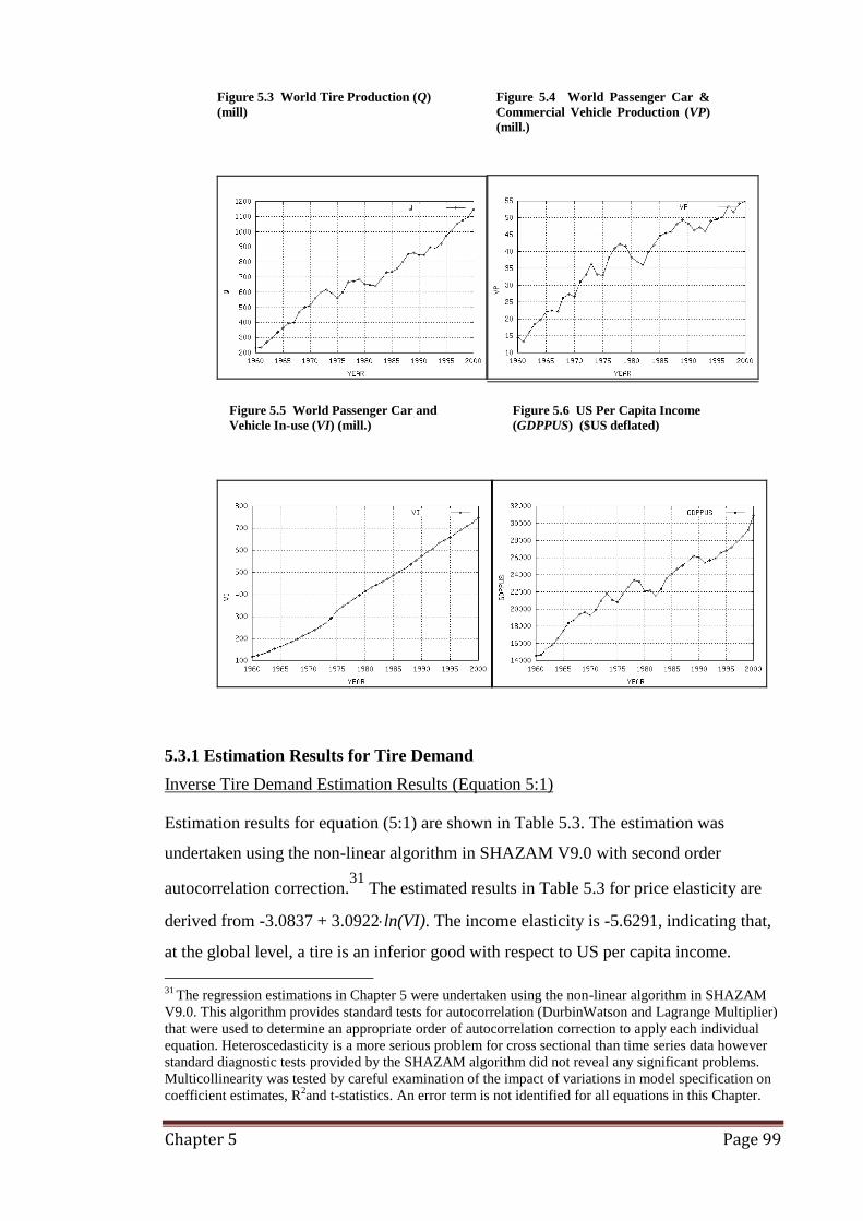
Chapter 5 Page 99

Figure 5.3 World Tire Production (Q)

(mill)

Figure 5.4 World Passenger Car &

Commercial Vehicle Production (VP)

(mill.)

Figure 5.5 World Passenger Car and

Vehicle In-use (VI) (mill.)

Figure 5.6 US Per Capita Income

(GDPPUS) ($US deflated)

5.3.1 Estimation Results for Tire Demand

Inverse Tire Demand Estimation Results (Equation 5:1)

Estimation results for equation (5:1) are shown in Table 5.3. The estimation was

undertaken using the non-linear algorithm in SHAZAM V9.0 with second order

autocorrelation correction.31

The estimated results in Table 5.3 for price elasticity are

derived from -3.0837 + 3.0922ln(VI). The income elasticity is -5.6291, indicating that,

at the global level, a tire is an inferior good with respect to US per capita income.

31

The regression estimations in Chapter 5 were undertaken using the non-linear algorithm in SHAZAM

V9.0. This algorithm provides standard tests for autocorrelation (DurbinWatson and Lagrange Multiplier)

that were used to determine an appropriate order of autocorrelation correction to apply each individual

equation. Heteroscedasticity is a more serious problem for cross sectional than time series data however

standard diagnostic tests provided by the SHAZAM algorithm did not reveal any significant problems.

Multicollinearity was tested by careful examination of the impact of variations in model specification on

coefficient estimates, R2and t-statistics. An error term is not identified for all equations in this Chapter.

Chapter 5 Page 100

Overall price elasticity is determined by quantity demanded and vehicles in-use. The

average value during 1962-2000 is -3.3439. It ranges from -6.5875 to -1.2152. The

corresponding direct demand elasticity is -0. 3804. It ranges from -0.8229 to -0.1518.

The slope dQ

dP is -4.9624. It ranges from -20.5900 to -0.3979.

The inverse demand function estimated as (5:1) can be compared to that estimated by

Carree & Thurik (2000, p.260): Q

ttttt SPaQUALaaMaQ ))log(( 3210

where Q is output of tires, M is output of motor vehicles, QUAL is a quality index

applied as a dummy variable (QUAL = year – 1930 for the period 1913-1930 and 0

afterward), P is the price index of tires and S is the number of motor vehicles registered.

Carree & Thurik expected a0 to be greater than five because each new vehicle needs at

least 5 tires. They compensated the potential negative effects of tire quality (QUAL) and

tire prices (P) on tire output (Q) by assigning a1, which they expected to be positive and

greater than these two negative effects.

Equation (5:1) applies a simpler structure to estimate an inverse demand curve. The

argument that each new vehicle needs at least 5 tires is applied by fixing 12 = 5. This

reflects the need to deduct 5VI from total tire output in the demand equation because it

will not be altered by tire price changes.

Table 5.3 Equation (5:1) Inverse Tire Demand Function Estimation Results

)ln()ln()ln()ln()ln()ln( 1413121110 GDPPUSQVIVPQ P

Coefficient (t-value)

Constant 10 -0.1738 (-1.9589)

Tire quantity (Q) 11 -3.0837 (-5.039)***

Vehicle production (VP) 12 5.0000#

Vehicles in-use Tire quantity (VI.Q) 12 3.0922 (4.709)***

US per capita income (GDPPUS) 13 -5.6291 (-5.152)***

Chapter 5 Page 101


Durbin-Watson 2.0164

R2 0.8080

Inverse demand elasticity () Mean Min to Max

-3.3439 -6.5875 to -1.2152

Slope=´ = dQ

dP = () (P/Q)

Mean Min to Max

- 4.9624 -20.5900 to - 0.3979

Direct demand elasticity (*=1/)

Mean Min to Max

-0.3804 -0.1518 to -0.8229

*** denotes rejection of null hypothesis at less than 1% level of significance,

** denotes rejection of null hypothesis at 5% level of significance,

* denotes rejection of null hypothesis at 10 % level of significance. # denotes imposed value

Direct Tire Demand Estimation Results (Equation 5:2)

The direct tire demand function models world tire demand (Q) as a function of tire price

(P), world vehicle production (VP), world vehicles in-use (VI) and a time trend (T).

T is included in equation 5.2 in order to address the net effect of tire demand growth

(which increases overtime due to the growth in population as well as economic

transaction) and tire demand decreases (due to tire quality improvement, as argued by

Carree & Thurik (2000, p.260) who proposed that tire quality has been improving

overtime and help users to postpone new tire demand). GDPPUS did not display

significant results in our estimation for equation 5.2.

The equation is estimated in log-log form and estimation results are displayed in Table

5.4. The estimation was undertaken using SHAZAM V9.0 via OLS with second order

autocorrelation correction. From Table 5.4, the results indicate that the direct price

elasticity of world tire demand is -0.3705. The slope of the demand function with

respect to price is -3.1439.

Chapter 5 Page 102

Table 5.4 Equation (5:2): Direct Tire Demand Estimation Results

)ln()ln()ln()ln()ln( 2423222120 TVIVPP Q


Tire Quantity (Q)

Constant 20 -1.1022 (-4.606)***

Tire price (P) 21 -0.3705 (-5.034)***

Vehicle production (VP) 22 0.4956 (6.008)***

Vehicles in-use (VI) 23 -0.2424 (-2.226)**

Time trend (T) 24 0.3600 (4.551)***


R2 0.9955

Direct demand elasticity * -0.3705

dQ

dP= (1/

*) *(P/Q)

-3.1439



* denotes rejection of null hypothesis at 10 % level of significance.

Table 5.5 compares the estimated results above with the results from other studies.

Jovanovic & Macdonald (1994) estimated direct US market tire elasticity as -0.76 but

they were derived from inverse functions. Carree & Thurik (2000) estimated direct US

tire market elasticity as -0.48 for the same period. In contrast, this study estimates two

values for direct world tire market elasticities. The first value is estimated from an

inverse tire demand, that is -0.38. The second value is estimated from a direct tire

demand and the value is -0.37.

Chapter 5 Page 103

Table 5.5 Comparative Estimates of Tire Demand Elasticities

Study Region Direct elasticity

Jovanovic & Macdonald (1994) U.S.A.

(1913-1973)

-0.76

Carree & Thurik (2000) -0.48

This study:

Inverse demand function (1/)

Direct demand function (*)

World

(1960-2000)

-0.3804

-0.3705

The inverse elasticity and direct elasticity estimated from this section will be employed

to measure market power in following sections.

5.4 Estimation of the Natural Rubber Supply Function

Natural rubber supply is modelled in both inverse and direct form. The inverse natural

rubber supply function (5:3) models natural rubber price (WR) as a function of world

natural rubber supply (XR), world natural rubber supply (XRt-2) with a two-year lag, the

interaction of rain quantity (RAIN) and world natural rubber supply XR, the synthetic

rubber price (WSt-3) with a three year lag, the interaction of the presence of International

Natural Rubber Organization (INRO) and world natural rubber supply XR, the currency

exchange rates of Japan (ERJA), Thailand (ERTH), Singapore (ERSP), the

concentration ratio for the tire industry (RQM) and a time trend (T).

(5:3)

)ln()ln()ln()ln()ln()ln(

)3

ln()ln()ln()ln()ln()ln(

1201918171615

14132121110

TRQMERSPERTHERJAXRINRO

tWSXRRAINXRXRWR t

A log-log functional form is also applied for (5:3), from which we derive the slope: =

dXR

dWR=

XR

WRINRORAIN })ln({ 151311 ; and the inverse elasticity:

)ln(

)ln(

XR

WR

WR

XR

dXR

dWR

= INRORAIN 151311 )ln( .

For the direct natural rubber supply function (5:4), world natural rubber supply (XR) is

modelled as a function of natural rubber price (WR), the interaction of the presence of

the Natural Rubber Organization (INRO) and natural rubber price WR, the interaction of

Japan‟s currency exchange rates (ERJA) and natural rubber price WR, Thai currency

exchange rate (ERTH), a structural change dummy variable for a change in the mix of

Chapter 5 Page 104

natural rubber and synthetic rubber following introduction of the radial tire (DRXSM)

and a time trend (T).

(5:4)

TDRXSM

ERTHWRERJAWRINROWRXR

2625

2423222120 )ln()ln()ln()ln()ln()ln(

A log-log functional form is employed for (5:4), from which we derive the slope:

= dWR

dXR=

WR

XRERJAINRO )}ln({ 232221 and the natural rubber supply

direct elasticity )ln(

)ln(*

WR

XR

XR

WR

dWR

dXR

= )ln(232221 ERJAINRO .

Variables that are employed to estimate the natural rubber supply functions are

summarized in Table 5.6.

Table 5.6 Variable Descriptions for the Natural Rubber Supply Function

The variables for natural rubber supply functions are selected on the following basis.

Natural Rubber Prices (WR)

32

To divide the country currency exchange rates (ERJA, ERTH and ERSP ) by their CPI is to remove the

inflationary component of local country nominal exchange rates caused by ordinary economic

transactions as well as government monetary and fiscal policies.

WR Natural Rubber Price: RSS1 natural rubber prices, fob Malaysia ringgit/ton, transferred to $us/ tons and deflated by US consumer price index, 1995 = 100

XR World Natural Rubber Production

RAIN Rainfall quantity in millilitres.

WSt-3 Synthetic rubber price lagged by 3 years

INRO The International Natural Rubber Organization

ERJA Japan’s currency exchange rates (100Yen/US$), deflated by Japan’s consumer price index 1995=100.32

ERTH Thailand’s currency exchange rates (Baht/US$), deflated by Thailand’s consumer price index 1995=100.

ERSP Singapore’s currency exchange rates(S$/ $US), deflated by Singapore’s consumer price index 1995=100.

RQM Top seven countries’ quantity /total quantity ratio. Top seven tire producing countries are US, France, Japan, Germany, Italy, UK and India.

T A time trend

DRXSM Structural change dummy variable for a change in the mix of natural rubber and synthetic rubber following introduction of the radial tire .(1970 -2000 = 1)

Chapter 5 Page 105

Natural rubber has local prices, export prices (fob), import prices (cif) and futures

market prices. Local prices are derived from local central markets. Export prices are

announced by producing countries daily. Major import prices are in London, New York,

Japan and Singapore. The natural rubber futures market prices which are frequently

referred to are prices from: The Tokyo Commodity Exchange (TOCOM), the Singapore

Commodity Exchange (SICOM) and the Agricultural Exchange of Thailand (AFET).

Natural rubber prices are classified according to product types such as ribbed-smoked

sheets (RSS1 to RSS5), blocked rubber or standard rubber and concentrated latex.

Prices of each of type are closely related. A number of natural rubber price series are

candidates for the natural rubber price variable (WR).

First, some studies such as Burger & Smit (1997) investigated individual country

natural rubber supplies and adopted local country prices deflated by local country

consumer price indexes. Secondly, SICOM‟s RSS3 rubber prices can be applied for WR

since most rubber used in the tire industry is RSS3 type and much trading is done

through Singapore. However, the RSS3 price series is not readily available for early

periods. Thirdly, RSS1 prices can also represent natural rubber prices. The series is

continuous, able to be traced back to 1960 and it is a price of sheet rubber, which has

been applied in tire manufacturing33

. Therefore, this thesis applies the fob Malaysia

Ringgit price series for RSS1 as data for WR. It is then transformed to $US and deflated

by the US consumer price index, which is considered the best reflection of global

inflation.

World Natural Rubber Production (XR)

World natural rubber production is dominated by the three largest producers namely:

Thailand, Indonesia and Malaysia. There are three alternative variables for world

natural rubber production: actual natural rubber production, natural rubber exports and

natural rubber used in tire sector. This thesis adopts the data from all countries‟ natural

rubber production data. Natural rubber exports and natural rubber used in the tire sector

have been tested but results indicate that they do not produce statistically significant

relationships to natural rubber prices as well as natural rubber production.

Other studies have used alternative data. According to Burger & Smit (1997), natural

rubber production is affected from two factors. The first factor is normal production

which is determined by the quantity of planted areas plus planting technology including

33

Block rubber is applied in tire industry too but less so than sheet rubber until recent years.

Chapter 5 Page 106

vintages of the trees. The second factor is from tapping intensity which responds to

natural rubber prices and other economic factors such as income. Therefore, the natural

rubber supply data used in estimation should be the relative quantity of actual

production to normal production. In addition, when considering the production data,

Burger, Smit & Volgelvang (2002) argue that the nature of data gathering in natural

rubber producing countries is based on exports. Consequently, natural rubber

production is derived from the sum of exports, domestic consumption and domestic

stocks. Thus production data involves some elements of consumption and does not fully

represent production. This study applied a time trend to incorporate for normal

production, which develops along with time trend. Lagged production tends to increase

stocks hence decreases price.

Other variables that affect natural rubber prices (i.e. supply shifters for natural rubber)

are considered as follows.

Rain quantity in millilitres (RAIN)

Data for the rain variable can be measured by rain quantity. Rain prevents natural

rubber tapping hence reduces natural rubber supply. However, it has been argued that

farmers often compensate by tapping more frequently. Data for rain quantity is adopted

from Thailand since Thailand, Malaysia and Indonesia are all in the same climate zone,

namely the tropical zone. Besides, Thai natural output is the largest during the study

period. Thus, the quantity of rainfall in Songkhla, which is a major natural rubber

producing province in Thailand, is adopted for the estimation variable.

Synthetic Rubber Prices (WS)

A Proxy for Synthetic Rubber Prices is adopted from the Export value of the copolymer

of styrene and butadiene (SBR) from the USA (International Rubber Study Group,

various issues). Synthetic rubber is considered a competing input to natural rubber,

although only to a certain extent. Whenever synthetic rubber prices are not competitive,

natural rubber would be used more, following more natural rubber tree cultivation.

Price Stabilization Regulatory (INRO)

INRO was established to stabilize natural rubber prices. It acted as a buffer when price

was on a down trend. A dummy variable for the presence of the International Natural

Rubber Organization (INRO) is applied to the natural rubber supply equation. INRO is

Chapter 5 Page 107

expected to eliminate price fluctuations, and hence should have intervening effects on

the relation between natural rubber price and production.

Currency Exchange Rates (ERJA, ERTH, ERSP)

Generally, a depreciation of a country‟s currency decreases that country‟s imports and

increases that country‟s exports. This might apply to natural rubber import behaviour.

During the period of study, except for Thailand in 1997 onwards, producing countries‟

currencies were quite stable. However, they are tested in the model too. Data for each

country‟s currency exchange rate per $US are employed.

Increases in the currency exchange rates of Japan and Singapore (100 Yen/US$ and

S$/US$) should be a positive shifting factor as they should render the natural rubber

price more profitable. On the other hand it might lead to selling of natural rubber in

futures markets namely: the Osaka market and the Tokyo Commodity Exchange

(TOCOM) in order to gain from future exchange rate fluctuations and thus depressing

rubber prices. As the Thai exchange rate (Baht/$US) increases, the natural rubber price,

which used to be intuitively set as 1$US/kilogram, becomes less profitable hence should

have downward shifting effects. Singapore‟s currency exchange rate affects natural

rubber prices in both exporting and importing aspects since Singapore re-exports natural

rubber to third countries. Impacts on natural rubber prices are also possible through the

future commodity exchange market namely the Singapore Commodity Exchange

(SICOM).

The Concentration of Tire Producers (RQM)

The concentration ratio for the seven top tire producing countries in total world tire

production (CR7 concentration ratio) is used to measure changes in competitiveness of

the tire manufacturing industry. The seven countries are the US, France, Japan,

Germany, Italy, U.K. and India.34

The Structural Changes in the Natural Rubber / synthetic Rubber Consumption Rates

(DRXSM)

A structural change in the manufacturing mix of natural rubber and synthetic rubber

occurred when radial tires were introduced. This is accommodated in the natural rubber

supply estimation by a dummy variable dating from the introduction of radial tires in

1970.

34

These are the top seven countries that data are available from the International rubber Study Group.

Chapter 5 Page 108

Technology (T)

Technological progress overtime is represented by a time trend. Technology advances

overtime increase yields per area. Hence natural rubber supply is increased and this has

downward shifting effects on natural rubber prices. The time trend also helps to address

growth in the area planted and the normal production as against actual production of

natural rubber (Smit, 2001).

Summary statistics for these natural rubber supply variables are displayed in Table 5.7.

Table 5.7 Summary Statistics for Natural Rubber Supply Function


WR (fob Mal.ringgit/ton) 2,136.50 684.29 935.00 3,956.00

$US 798.99 311.05 327.74 1582.40

$US (deflated) 1709.60 745.03 563.91 3956.20

XR (1,000 tons) 4,109.40 1,442.30 2,040.00 6,840.00

RAIN (millimetres) 2,053.90 456.89 1,288.10 3,268.60

WS (US$/ton) 821.20 267.42 395.00 1,331.00

(deflated) 1737.80 666.05 930.38 3515.10

ERJA (100 Yen/US$) 237.88 98.84 94.06 360.00

(deflated) 618.50 593.05 94.06 1968.40

ERTH (Baht/US$) 24.00 5.20 20.34 41.36

(deflated) 62.71 35.65 23.93 130.66

ERSP (S$/US$) 2.32 0.57 1.41 3.06

(deflated) 3.06 0.98 1.42 4.63

RQM (CR7 Ratio) 0.68 0.07 0.56 0.79

Figures 5.7-5.21 illustrate the data graphically.

Chapter 5 Page 109


(WR) (fob Malaysia Ringgit/ton)


(WR) ($US/ton)


(WR) (deflated by US consumer

price index) ($US/ton)

Figure 5.10 World Natural Rubber

Production (XR) (1,000 tons)

Figure 5.11 Rainfall (RAIN)

(millimetres)

Figure 5.12 Synthetic Rubber Price

(WS) ($US/ton)

Chapter 5 Page 110

Figure 5.13 Synthetic Rubber

Price(WS) (deflated by US CPI)

($US/ton)

Figure 5.14 Japan’s Currency

Exchange Rate (ERJA)

(100 Yen / $US)

Figure 5.15 Japan’s Currency

Exchange Rate (deflated by

Japan’s CPI) (ERJA)

(100 Yen / $US)

Figure 5.16 Thai Currency

Exchange Rate (ERTH) (Baht/$US)

Figure 5.17 Thai Currency

Exchange Rate (deflated by Thai

consumer price index) (ERTH) (Baht

/ $US)

Figure 5.18 Singapore’s Currency

Exchange Rate (ERSP) (S$ / $US)

Figure 5.19 Singapore’s Currency

Exchange Rate (deflated by Singapore

consumer price index) (ERSP)

($S/$US)

Figure 5.20 CR7 Concentration

Ratio in World Tire Production

(RQM)

Chapter 5 Page 111

Figure 5.21 The Ratio of Natural

Rubber and Synthetic Rubber

Consumption in World Tire Sectors

(RXSM) (Ratio)

The natural rubber price dropped to its bottom level in the year 1972 and then recovered

until 1980. During the presence of INRO, prices fluctuated through cycles of 5-6 years.

This might reflect attempts to restrict prices within a range of 800-1,200 $US/ton. When

considered in real terms, Figure 5.9 displays a downward movement in natural rubber

prices except for two peaks in 1973 and 1979. Based on the 1995 price, natural rubber

prices dropped from 3,956 $US in 1960 to 563 $US in 1999.

5.4.1 Estimation Results of the Natural Rubber Supply

In equation (5:3), the endogenous variable, natural rubber price (WR) is regressed on

natural rubber production quantity (XR) and a vector of shifting variables comprising:

two-year lagged natural rubber production (XRt-2), rainfall (RAIN), three-year lagged

synthetic rubber prices (WSt-3), the presence of the International Natural Rubber

Organization (INRO), Japan‟s currency exchange rates (ERJA), Thailand‟s currency

exchange rate (ERTH), Singapore currency exchange rate (ERSP), the CR7

Chapter 5 Page 112

concentration ratio (top seven tire producing countries market share RQM), and a time

trend (T). The equation is estimated in log-log form.

Three variables that did not provide significant estimates were the number of raining

days (rain quantity provided statistically significant results), planted area and palm oil

prices. Rubber trees take about six years to become mature and produce natural rubber

therefore natural rubber output should have a 6-7 year lag behind cultivation. However,

the planted area did not produce significant results as the data series is not continuous.

Palm oil was considered relevant as a substitute product since the late 1970s but various

measures for palm oil were found to be not significant.

Inverse Natural Rubber Supply Function (Equation 5:3)

Estimation results for equation (5:3) are shown in Table 5.8 The estimation was

undertaken using the SHAZAM V9.0 via OLS with first order autocorrelation

correction. Estimated results indicated that whereas quantity supplied is positively

related to natural rubber price, other variables have negative effects on natural rubber

prices. Two variables have lagged effects on natural rubber prices. They are natural

rubber production, lagged by two years, and synthetic rubber price, lagged by three

years.

Price elasticity to quantity supplied is derived as 3.4930 – 0.7369ln(RAIN) –

0.3106(INRO). The overall average inverse price elasticity is = 3.3405, with a range

from 2.9063 to 3.8368. The average slopedXR

dWR = 3.4980 with a range from 0.5785

to 9.2983. The direct supply elasticity is

1* = 0.3005 with a range from 0.2606 to

0.3441.

Table 5.8 Equation (5:3) Inverse Natural Rubber Supply Function Estimation

Results

)ln()ln()ln()ln()ln()ln(

)3

ln()ln()ln()ln()ln()ln(

1201918171615

14132121110

TRQMERSPERTHERJAXRINRO

tWSXRRAINXRXRWR t


Constant 10 3.9583 (11.950)***

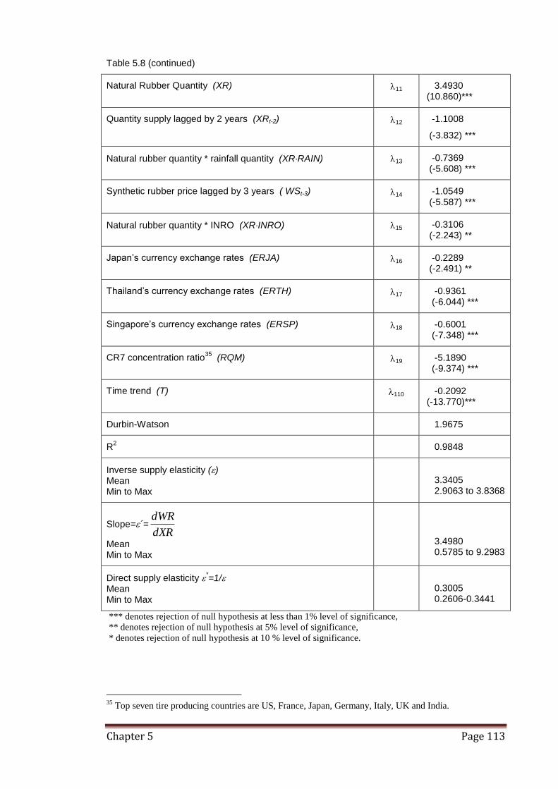
Chapter 5 Page 113


Natural Rubber Quantity (XR) 11 3.4930 (10.860)***

Quantity supply lagged by 2 years (XRt-2) 12 -1.1008

(-3.832) ***

Natural rubber quantity * rainfall quantity (XRRAIN) 13 -0.7369 (-5.608) ***

Synthetic rubber price lagged by 3 years ( WSt-3) 14 -1.0549 (-5.587) ***

Natural rubber quantity * INRO (XRINRO) 15 -0.3106 (-2.243) **

Japan’s currency exchange rates (ERJA) 16 -0.2289 (-2.491) **

Thailand’s currency exchange rates (ERTH) 17 -0.9361 (-6.044) ***

Singapore’s currency exchange rates (ERSP) 18 -0.6001 (-7.348) ***

CR7 concentration ratio35

(RQM) 19 -5.1890 (-9.374) ***

Time trend (T) 110 -0.2092 (-13.770)***


R2 0.9848

Inverse supply elasticity () Mean Min to Max

3.3405 2.9063 to 3.8368

Slope=´=dXR

dWR

Mean Min to Max

3.4980 0.5785 to 9.2983

Direct supply elasticity *=1/

Mean Min to Max

0.3005 0.2606-0.3441




35

Top seven tire producing countries are US, France, Japan, Germany, Italy, UK and India.

Chapter 5 Page 114

Direct Natural Rubber Supply Function (Equation 5:4)

Equation (5:4) estimates a direct natural rubber supply function. World natural rubber

production (XR) is regressed on natural rubber price (WR) with a vector of shift

variables comprising: the presence of the International natural Rubber Organization

(INRO), Japan‟s currency exchange rate (ERJA), Thailand‟s currency exchange rate

(ERTH), changes in the ratio of natural rubber to synthetic used in world tire sector

(DRXSM) and a time trend (T). The model is estimated in log-log functional form.

Estimates results are displayed in Table 5.9.

Equation (5:4) was estimated using the SHAZAM V9.0 via OLS with first order

autocorrelation. Estimated results indicate that the natural rubber supply direct elasticity

= 0.1551 – 0.0555(INRO) - 0.0417ln(ERJA). The average natural rubber supply

price elasticity is = 0.1494 with a range of 0.1091 to 0.2285. The slope of the natural

rubber supply function with respect to price is 8.83 with a range of 0.9342 to 31.4550.

Chapter 5 Page 115

Table 5.9 Equation (5:4) Direct Natural Rubber Supply Function Estimation

Results

TDRXSM

ERTHWRERJAWRINROWRXR

2625

2423222120 )ln()ln()ln()ln()ln()ln(


Constant 20 -0.9993 (-20.450)***

Natural rubber price (WR) 21 0.1551 (6.223)***

Natural rubber price INRO (INRO WR) 22 -0.0555 (-2.679)**

Natural rubber pricex Japan exchange rate (ERJA WR) 23 -0.0417 (-2.046)**

Thailand’s exchange rate (ERTH) 25 0.2881 (5.804)***

Structural Change in the ratio of natural to synthetic rubber consumption in tire sector (DRXSM)

24 0.0491 (2.030)**

Time trend (T) 26 0.0460 (16.430)***


R2 0.9965

Direct supply elasticity *

Mean Min to Max

0.1494 0.1091 to 0.2285

dXR

dWR

Mean Min to Max

8.8307 0.9342 to 31.455




Table 5.10 compares the above estimated results to results from other studies.

Burger & Smit (1997) studied natural rubber supply from different countries during

1973-1993. In contrast this study examines the elasticity at a world level during the

period 1960-2000. Elasticities are estimated from both inverse and direct supply curves.

The estimated elasticity of natural rubber supply will be used to calculate the market

power in next sections.

Chapter 5 Page 116

Table 5.10 Comparative Estimates of Natural Rubber Supply Elasticities

Thailand

Indonesia

Estate

Indonesia

small holding

Malaysia

Estate

Malaysia

small holding

World

1973-1993 1976-1993 1975-1993 1976-1993 1978-93 1960-2000

Burger & Smit (1997) Direct Elasticity

0.22 0.29 -#1

0.14 0.14 -#2

This Study: Inverse supply function (1/)

0.30

This Study: Direct supply function (*)

0.15

#1 No significant estimate are available.

#2 No estimation in world level.

5.5 Estimation of the Tire Production Function

A tire production function of the general form )f(xrq ii is required to obtain a value

for marginal product of natural rubber ( xriMP ). A Generalized Leontief functional form

(GL) is employed for estimation of the production function. The GL functional form is

one that is frequently employed when estimating production functions, cost functions

and profit functions. Examples for its applications can be found in Schroeter (1990),

Murray (1994), Diewert (1971), Diewert (1978), Diewert (2003), Fox & Diewert (1997)

and Cohen & Paul (2003).

The GL is a flexible functional form. Flexible functional forms can accommodate

second-order derivatives and provide useful applications of the production function

such as permitting partial elasticities of substitution between inputs to vary36

.

The tire production function (5:5) is transformed from a firm level production function

to a producing country (qi) production function. Accordingly, the tire output for country

i (qi where i refers to USA, France, Japan and Germany) is set as a function of a natural

rubber input (xri), a synthetic rubber input (xsi), the world oil price (WO), the country‟s

vehicle production (VPi), the country‟s vehicles in-use (VIi) and a time trend (T).

36

Discussion on properties of Generalized Leontief flexible functional form can be found in Diewert

(1971), (1978), (2003).

Chapter 5 Page 117

(5:5)

)(9

)(8

276

542121

32

210

iVIδ

iVPδT δT δ

T ixs δTixr δWO /

ixs/

ixrδ ixs δ ixr δ δ i

q

From (5:5) the marginal product for natural rubber is obtained as:

T δWO /

ixs/

ixr δ δxr

q MPxr

i

i

ii

42121

31

The data applied to the tire production model are selected on the following basis.

Tire Production (qi)

In accordance with tire demand estimation, tire production is classified as passenger car

tires plus commercial vehicle tires since most countries have separate data records

except for some countries such as China, Russia and the Republic of Korea, which did

not have separate data until recent years. Given that the input ratio of natural rubber to

synthetic rubber used in passenger car tire and commercial vehicle tires are close

(55%/45% and 50%50%) total tire production is defined as the sum of passenger and

commercial tires.

It is recognized that the ratios of natural rubber to synthetic rubber varies more

significantly in specialist tires. For example racing tires and off-highway tires have

natural rubber /synthetic rubber ratios of 35%/65% and 80%/20% respectively.

However, these categories are small items relative to passenger and commercial vehicle

tires hence their production data is not individually reported in world level data

(International Rubber Study, various copies).

Natural Rubber and Synthetic Rubber Inputs (xrUS and xsUS)

Consumption of elastomer is often divided into two sectors, namely tire sector and

general sector consumption. Tire sector consumption comprises natural rubber and

synthetic rubber that are used in all kinds of vehicle tires production. General sector

consumption comprises natural rubber and synthetic rubber that are used to produce

products other than tires. Most general sector products are used in automotive sector i.e.

rubber parts and accessories used in vehicles.

Data for natural rubber and synthetic rubber consumption in the tire sector can be

obtained for USA, France, Japan, Germany, Italy, Spain, U.K. and Brazil and India.

Chapter 5 Page 118

However, they are not available for some countries such as China. Hence the study

does not test for market power from China tire manufacturing on the natural rubber

market despite its significant growth in natural rubber consumption since the 1990s37

.

World Oil Prices (WO)

As petroleum is a key manufacturing input for synthetic rubber, its price impacts on the

price of synthetic rubber, which is a substitute input for natural rubber in tire

production. Thus, tire production is affected by world oil prices.

Country Vehicle Production and Vehicle In-Use (VPi and VIi)

As already noted, each new car requires at least five tires and a vehicle in-use also

consumes tires. Therefore, tire production should be determined by vehicle production

and vehicles in-use.

Time Trend (T)

Technology improves manufacturing costs overtime. A time trend is used as a proxy

measure for the impact of technology.

Estimations were undertaken using the non-linear algorithm in SHAZAM V9.0 via OLS

with corrections for autocorrelation using an iterative Cochrane-Orcutt procedure.

5.5.1 US Tire Production Function Estimation

When the tire production function (5:5) is applied to USA (5:5US), US tire output (qUS)

is modelled as a function of US natural rubber inputs used in its tire sector (xrUS), the

quantity of synthetic rubber used in its tire sector (xsUS), world crude oil price (WO), US

vehicles in-use (VIUS) and a time trend.

Interaction terms such as: US quantity of natural rubber used in the tire sector (xrUS) and

the time trend T, US quantity of synthetic rubber used in the tire sector (xsUS) and the

37

However, natural rubber consumption data could be used in place of natural rubber used in tire sector in

such cases.

Chapter 5 Page 119

time trend T, the term T2 and US vehicle Production (VPUS) did not provide significant

estimates. The tire production function for USA was hence simplified to:

(5:5US)

T δUS

VIδWO /

USxs

/US

xrδ US

xs δ US

xr δ δ US

q 5

)(4

21213

2210

From (5:5US) the US marginal product for natural rubber is:

xr

q MPxr

US

US

USUS

= WO

/ US

XS/

USXR δ δ

212131

The variables employed to estimate the US tire production function are summarized in

Table 5.11. Summary statistics for the US tire production function are displayed in

Table 5.12.

Table 5.11 Variables Description for US Tire Production Function


qUS Tire production (US passenger car tires and truck tires)

xrUS Quantity of natural rubber used in tire sector in the US.

xsUS Quantity of synthetic rubber used in tire sector in the US.

WO World crude oil price, Spot Oil Price (West Texas Intermediate). Deflated by US consumer price index. 1995=100.

VIUS Total vehicle in-use in the US.(passenger car and commercial vehicle)

T A time trend

Table 5.12 Data Summary for Variables in the US Tire Production Function


qUS (mill) 203.37 39.63 116.78 276.76

xrUS (1,000) 545.34 170.32 282.60 947.00

xsUS (1,000) 1130.90 208.37 682.00 1507.10

WO (US$/barrel) 15.18 10.66 2.92 37.38

Deflated 25.49 14.18 12.97 69.14

VIUS (mill) 149.24 45.04 73.58 221.48

Chapter 5 Page 120

Figures 5.22 to 5.27 display these variables in graphs38

.

Figure 5.22 Quantity of US Tire

Production (qUS) (1,000s)

Figure 5.23 Quantity of Natural

Rubber Used in US Tire Sector

(xrUS) (1,000s)

Figure 5.24 Quantity of Synthetic

Rubber Used in US Tire Production

(xsUS) (1,000s)

Figure 5.25 World Crude Oil Price

(WO) ($US/barrel)

Figure 5.26 World Crude Oil Price (WO)

(deflated by US consumer price index)

Figure 5.27 US Vehicle In-Use (VIUS)

(1,000s)

38

Note some figures include a notation change however QUS = qUS, XRUS = xrUS, XSUS = xsUS, VIUS =

VIUS.

Chapter 5 Page 121

Table 5.13 Equation (5.5US): US Tire Production Estimation Results

T δUS

VIδWO /

USxs

/US

xrδ US

xs δ US

xr δ δ US

q 5

)(4

21213

2210


Constant 0US 0.5344 (3.310)***

Natural rubber inputs - US (xrUS) 1 US 0.3717 (6.350) ***

Synthetic rubber inputs - US (xsUS) 2 US 0.4240 (7.937) ***

2(xrUS)1/2

(xsUS) 1/2

(WO) 3 US -0.0157 (-1.985)**

US’s vehicles in-use (VIUS) 4 US -0.6942 ( -2.106)**

Time trend (T) 4 US 0.0192 (2.258)**


R2 0.9796

Natural rubber marginal product

US =

US

US

xr

q

= WO

/ xs

/xr δ δ USUS

212131

Mean Min to Max

0.3556 0.3254 to 0.3646




The estimation was undertaken using the non-linear algorithm in SHAZAM V9.0 with

second order autocorrelation correction. Results are summarized in Table 5.13. The

marginal product for natural rubber in the US was estimated as US=US

US

xr

q

= 0.3556

with a range from 0.3254 to 0.3646.

5.5.2 France’s Tire Production Function Estimation

When the tire production function (5:5) is applied to France (5:5FR), it estimates

France‟s tire output (qFR) as a function of France‟s quantity of natural rubber used in its

tire sector (xrFR), the quantity of synthetic rubber used in its tire sector (xsFR), world

crude oil price (WO), France‟s vehicle production (VPUS), and a time trend.

Chapter 5 Page 122

The interaction terms: quantity of natural rubber used (xrFR) and the time trend T,

synthetic rubber used (xsFR) and the time trend T, the term T2 and France‟s vehicles in-

use (VIFR) did not provide significant estimates.

The tire production function for France (5:5FR) was:

(5:5FR)

T δFR

VPδWO /

FRxs

/FR

xrδ FR

xs δ FR

xr δ δ FR

q 54

21213

2210

From (5:5FR) France‟s marginal product for natural rubber is derived as:

WO /

FRxs

/FR

xr δ δ xr

q MPxr

FR

FRFRFR

212131

The variables that were employed to estimate the France‟s tire production function are

listed in Table 5.14. The data for these variables are summarized in Table 5.15.

Table 5.14 Variable Description for France’s Tire Production Function


qFR Tire production (France’s passenger car tires and truck tires)

xrFR Quantity of natural rubber used in Tire sector in France.

xsFR Quantity of synthetic rubber used in Tire sector in France.


VPFR Total vehicle production in France (passenger car and commercial vehicle)

Table 5.15 Data Summary for France’s Tire Production Function


qFR (mill) 45.620 15.38 14.35 67.71

xrFR (1,000) 130.98 35.72 76.60 205.00

xsFR (1,000) 147.60 41.59 49.40 197.60

WO US$/barrel) 15.18 10.66 2.92 37.38

Deflated 25.49 14.18 12.97 69.14

VPFR (mill) 2.90 0.74 1.25 3.92

Chapter 5 Page 123

These data are represented graphically in Figures 5.28 to 5.3139

.

Figure 5.28 Tire Production for

France (qFR) (1,000s)

Figure 5.29 France’s Quantity of

Natural Rubber Used in Tire Sector

(xrFR) (1,000s)

Figure 5.30 France’s Quantity of

Synthetic Rubber Used in Tire Sector

(xsFR) (1,000s)

Figure 5.31 France’s Passenger Car

and Commercial Vehicle Production

(VPFR) (1,000s)

The estimation was performed using the non-linear algorithm in SHAZAM V9.0 with

fourth order autocorrelation correction. Estimation Results for (5:5FR) are shown in

Table 5.16. The marginal product for natural rubber in France was estimated as

FR=FR

FR

xr

q

= 0.6343 with a range from 0.5586 to 0.6583.

39 Note some figures include a notation change however QFR = qFR, XRFR = xrFR, XSFR = xsFR, VPFR =

VPFR. The figures for WO and WO (deflated) are found in figures 5.25 and 5.26 above.

Chapter 5 Page 124

Table 5.16 Equation (5:5FR) France’s Tire Production Estimation Results

T δFR

VPδWO /

FRxs

/FR

xrδ FR

xs δ FR

xr δ δ FR

q 54

21213

2210


Constant 0FR -0.1378 (-5.818)***

Natural rubber inputs - France (xrFR) 1 FR 0.6795 (9.563)***

Synthetic rubber inputs – France (xsFR) 2 FR 0.1100 (3.249)***

2(xrFR)1/2

(xsFR) ½ WO 3 FR -0.0422

(-21.069)***

France’s vehicle production (VPFR) 4 FR 0.2985 (16.971)***

Time trend (T) 4 FR 0.0071 (5.426)***


R2 0.9932


WO /

FRxs

/FR

xr δ δ xr

q MPxr

FR

FRFRFR

212131

Mean Min to Max

0.6343 0.5586 to 0.6583




5.5.3 Japan’s Tire Production Function Estimation

When the tire production function (5.5) is applied to Japan (5:5JA), it estimates Japan‟s

tire output (qJA) as a function of natural rubber input (xrJA), synthetic rubber inputs

(xsJA), world crude oil price (WO) and a time trend (T).

The interaction terms: synthetic rubber (xsJA) and the time trend T, the term T2, Japan‟s

vehicle production (VPJA) and Japan‟s vehicle in-use (VIJA) did not provide significant

estimates.

The tire production function for Japan is:

(5:5JA)

T δT xr δWO /

xs/

xrδ xs δ xr δ δ q JAJAJAJAJAJA 542121

32

210

Chapter 5 Page 125

From (5:5JA) Japan‟s marginal product for natural rubber is derived as:

T δWO /

xs/

xr δ δxr

q MPxr JAJA

JA

JA

JAJA

42121

31 .

The variables employed to estimate the Japan‟s tire production function are summarized

in Table 5.17. Summarized statistics for the Japan‟s tire production function are

displayed in Table 5.18. Figures 5.32 to 5.34 display Japan‟s Tire Production

Variables40

.

Table 5.17 Variable Description for Japan’s Tire Production Function


qJA Tire production (Japanese passenger car tires and truck tires)

xrJA Quantity of natural rubber used in Tire sector in Japan.

xsJA Quantity of synthetic rubber used in tire sector in Japan.


T Time trend

Table 5.18 Data Summary for Japan Tire Production Function


qJA mill 95.33 52.49 5.56 164.42

xrJA 1,000 336.75 197.29 76.90 649.00

xsJA 1,000 350.47 163.73 22.10 527.00

WO (US$/barrel) 15.18 10.66 2.92 37.38

deflated 25.49 14.18 12.97 69.14

40

Note some fires include a notation change however QJA = qJA, XRJA = xrJA, XSJ = xsJA.

The figures for WO and WO (deflated) are found in figures 5.25 and 5.26 above.

Chapter 5 Page 126

Figure 5.32 Japan’s Quantity of

Tire Production (qJA) (1,000s)


Natural Rubber Used in Tire

Sector (xrJA) (1,000s)


Synthetic Rubber Used in Tire

Sector (xsJA) (1,000s)

Estimation Results for the Japan‟s tire production function are depicted in Table 5.19.

Estimation was undertaken using the non-linear estimation algorithim in SHAZAM

V9.0 with first order autocorrelation correction. The marginal product for natural rubber

in Japan‟s tire industry was estimated to be JA=JA

JA

xr

q

= 0.5673 with a range from

0.4097 to 0.7341.

Chapter 5 Page 127

Table 5.19 Equation (5:5JA) Japan’s Tire Production Function Estimation Results

T δT xr δWO /

xs/

xrδ xs δ xr δ δ q JAJAJAJAJAJA 542121

32

210


Constant 0JA -0.1671 (-5.159)***

Natural rubber inputs – Japan (xrJA) 1JA 0.7948 (8.060)***

Synthetic rubber inputs - Japan (xsJA) 2JA 0.3685 (6.284) ***

2(XRJA)1/2

(XSJ) 1/2

WO 3JA -0.0112 (-1.852) *

Natural rubber inputs time trend (xrJA.T) 4JA -0.0091

(-4.080)***

Time trend (T) 4JA 0.0134 (3.100) ***


R2 0.9979

Japan’s Natural rubber marginal product

T δWO /

xs/

xr δ δxr

q MPxr JAJA

JA

JA

JAJA

42121

31

Mean Min to Max

0.5673 0.4097 to 0.7341




5.5.4 Germany’s Tire Production Function Estimation

The tire production function (5:5) applied to Germany (5:5GR) models Germany‟s tire

output (qGR) as a function of natural rubber inputs used in its tire sector (xrGR), synthetic

rubber inputs used in its tire sector (xsGR), world crude oil price (WO), Germany‟s

vehicles in-use (VIGR) and a dummy variable to address data deficiency resulting from

the re-unification (1991-2000). The vehicles in-use variable did not yield a significant

result when measured as the sum of passenger cars and commercial vehicles. Removal

of commercial vehicles from the measure provided a significant result.

The interaction terms: natural rubber (xrGR) and the time trend T, synthetic rubber (xsGR)

and the time trend T, the time trend (T) and Germany‟s vehicle production did not

provide significant estimates.

Chapter 5 Page 128

The tire production function for Germany was estimated as:

(5:5GR)

91591

)(4

21213

2210

DδDVIδWO /

xs/

xrδ xs δ xr δ δ q GRGRGRGRGRGR

From (5:5GR) Germany‟s tire industry marginal product for natural rubber is derived

as: WO /

xs/

xr δ δxr

q MPxr GRGR

GR

GRGRGR

212131

.

The variables employed to estimate Germany‟s tire production function are summarized

in Table 5.20.

Table 5.20 Variable Description for Germany’s Tire Production Function


qGR Tire production (Germany’s passenger car tires and truck tires).

XrGR Quantity of natural rubber used in tire sector in Germany.

XsGR Quantity of synthetic rubber used in tire sector in Germany.


VIGR Vehicle in-use in Germany (only Passenger cars).

T A time trend.

Summarized statistics for the variables are list in Table 5.21.

Table 5.21 Summary Statistics for Germany’s Tire Production Function


qGR (mill) 43.05 11.76 16.35 63.14

XrGR (1,000) 120.58 31.20 70.70 173.00

XsGR (1,000) 143.23 29.01 62.90 182.00

WO ($US/barrel) deflated

15.18 10.66 2.92 37.38

25.49 14.18 12.97 69.14

VIGR (mill) 23.68 11.82 4.86 43.77

T

Chapter 5 Page 129

Figures 5.35 to 5.38: display these variables graphically41

.

Figure 5.35 Tire Production for

Germany (qGR) (1,000s)

Figure 5.36 Germany’s Quantity of

Natural Rubber Used in Tire

Sector (xrGR) (1,000s)


Synthetic Rubber Used in Tire

Sector (xsGR) (1,000s)


Passenger Car In-use (VIGR)

(1,000s)

The estimation was undertaken using the non-linear estimation algorithim in SHAZAM

V9.0 with first order autocorrelation correction. Results are provided in Table 5.22. The

marginal product for natural rubber in Germany‟s tire industry was estimated as:

GR=GR

GR

xr

q


41

Note some figures include a notation change however QGR = qGR, XRGR = xrGR, XSGR = xsGR.

The figures for WO and WO (deflated) are found in figures 5.25 and 5.26 above.

Chapter 5 Page 130

Table 5.22 Equation (5:5GR) Germany’s Tire Production Function Estimation

Results

91591)(

42121

32

210DδDVIδWO

/ xs

/xrδ xs δ xr δ δ q GRGRGRGRGRGR


Constant 0GR 0.3658 (1.890)**

Natural rubber input – Germany (xrGR) 1GR 0.3917 (2.805)**

Synthetic rubber input –Germany (xsGR) 2GR 0.4089 (3.452)***

2(xrGR)1/2

(xsGR)1/2WO 3GR -0.0257

(-2.143)**

Germany’s passenger car in-use dummy variable D91 (VIGRD91) 4GR 0.6992 (1.947)*

dummy variable (D91) 5GR -1.2131 (-2.113)**


R2 0.9748


WO /

xs/

xr δ δxr

q MPxr GRGR

GR

GR

GRGR

212131

Mean Min to Max

0.3654 0.3191 to 0.3793




5.6 Estimation of the Optimality Condition Function

As outlined in Chapter 4, derivation of the market power index (MPI) for each

manufacturing country can be derived via 4 different models. Models 1 and 2 use the

optimality condition (4:8a) and (4:8b) developed in Chapter 4 to derive estimates for the

two conjectural elasticities (αi and βi). Models 3 and 4 apply the direct estimation

approach developed in Chapter 4 to obtain estimates of the two conjectural elasticities.

Chapter 5 Page 131

5.6.1 US MPI Estimation Using Model 1

The MPI Model 1 is derived using inverse tire demand and natural rubber supply

functions with conjectural elasticities estimated via the optimality condition derived in

Chapter 4 as (5:6.1). This condition is estimated using the variables defined in (5:7.1,

5:8.1 and 5:9.1) for US data.

(5:6.1US) USUSUS xrqPWR

312111

From (5:6.1US) estimates of the slope of inverse tire demand (´=dQ

dP), the slope of

inverse natural rubber supply (´=dXR

dWR) and the natural rubber marginal productivity

in the US tire industry (US= US

US

xr

q

) are used to obtain the following terms.

(5:7.1US) PPxr

qP US

US

USUS

(5:8.1US) USUSUS

US

US

US qqxr

q

dQ

dPq

(5:9.1US) USUSUS xrxr

dXR

dWRxr

The three terms are used to estimate the optimality function (5:6.1US) to derive values

for coefficients 11, 21 and 31. These three coefficients provide the means for

hypothesis testing for the presence of market power plus estimations of the two

conjectural elasticities required to calculate our market power index (MPI) for each

manufacturing country.

The estimation results for (5:6.1US) are provided in Table 5.23. Two estimation results

are reported (A and B).

As outlined in Chapter 4, the null hypothesis of input market efficiency (no market

power) can be stated in terms of the three coefficients in 5:6.1 as H0: 11 = 1, 21 = 31 =

0. If H0 is not rejected then: Pxr

qWR

i

i

and hence the input xri is being paid the

value of its marginal product. Further, if 21 = 31 = 0, then i1 = i1 = 0 and MPIXRi1 =

0, thus indicating a perfectly competitive input market. Rejection of Ho indicates the

presence of non competitive markets. In particular, significant positive values of 21

Chapter 5 Page 132

indicate the presence of oligopoly in the output market and significant positive values of

31 indicate the presence of oligopsony in the input market.

Results from estimation A in Table 5.23 (11US = 1.1867, 21US = 0.0739, and 31US = -

0.1881) can be used to test the null hypotheses that: 11US = 1, 21US = 0.00, and 31US =

0.00.


(Model 1) Estimation Results

USUSUS xrqPWR

312111

Estimation A Estimation B



Constant - 0.2344 (4.427)***

USP

11US 1.1867 (6.047)***

-

USq

21US 0.0739 (2.817)***

-

USxr

31US -0.1881

(-10.050)*** -0.2119

(-13.450)***

Durbin-Watson 1.9861 1.9331

R2 0.9123 0.8954




If the null hypotheses are not rejected then it implies the natural rubber market, as a

specific factor market to tire production in the US, is competitive. If the hypotheses are

rejected it implies that world natural rubber price is less than its value of marginal

product and that there is US oligopoly power in the world tire market and oligopsony

power in the world rubber market. Table 5.24 provides these hypothesis tests.

The hypothesis tests confirm: 11US = 1 cannot be rejected; hence H1:11US = 1 is

accepted; 21US = 0 is rejected (< 0.02%) hence H1:21US 0 is accepted; 31US = 0 is

rejected (< 0.01%) hence H1: 31US 0; is accepted. The joint test: 11US = 1 and 21US =

31US = 0 is rejected (< 0.01%) hence either 11US 1, 21US 0 or 31US 0.

Chapter 5 Page 133

In conclusion, although the hypothesis that 11US = 1 cannot be rejected, the hypotheses

that 21US= 0 and 31US= 0 are rejected. Hence there is evidence of oligopoly and

oligopsony market power from the US tire industry on world tire market and world

natural rubber market.

Table 5.24 Hypothesis Tests for 11US, 21US, 31US (Estimation A)

Estimation A H0:11US = 1

H1:11US 1

H0:21US = 0

H1:21US 0

H0:31US = 0

H1:31US 0

H0:11US =1,21US =31US =0

H1:11US 1 or 21US 0 or 31US 0

Test value

T statistic

Df

P-value

F statistic

Df

P-value

0.1867

0.9512

31

0.3488

0.9048

1,31

0.3488

0.0738

2.8170

31

0.0083

7.9356

1,31

0.0084

-0.1881

-10.0525

31

0.0000

101.0533

1,31

0.0000

369.6176

3,31

0.0000

Conclusion Not reject H0

11US = 1

Reject H0 (< 0.02%)

21US 0

Reject H0 (< 0.01%)

31US 0

Reject H0 (< 0.01%)

11US 1or 21US 0or 31US 0

The next step is to derive the conjectural elasticities in order to obtain the MPI measure

of market power. The estimates for 21US and 31US are used to derive the two

conjectural elasticities according to the approach outlined in (5:10.1) and (5:11.1).

Accordingly the US conjectural elasticity on world tire markets is:

(5:10.1US) Q

q

Q

q

q

Q USUS

US

US

US

211

This generates a mean value of αUS1 = 0.0732 with a range from 0.0587 to 0.1062.

The US conjectural elasticity on world natural rubber market is:

(5:11.1US) XR

xr

XR

xr

xr

XR USUS

US

US

US 311

This generates a mean value of βUS1 = 0.1884 with a range from 0.1615 to 0.2415.

Having obtained estimates for all key variables it is now possible to estimate the market

power index for natural rubber as an input into US tire manufacturing. We substitute the

values for: , , US1 and US1 in the MPIXRUS1 expression to obtain:

Chapter 5 Page 134

1

11

11 US

USUS

USXRε

ηεMPI


However, the initial estimation (A) found an estimate for11US > 1 which implies WR >

VMPxr (assuming that concurrently: 21US = 31US = 0). This implies the input XR is

being paid more than the value of its marginal product ( PMPPxr

qWR xr

i

i

)

whereas theory predicts 1US ≤ 1 (that is: WR ≤ VMPxr). Despite non-rejection of H0:

11US = 1, supplementary estimations were conducted. Inclusion of a constant to test for

other factors yielded insignificant coefficients for 11US and 21US so estimation version

B is applied with11US and 21US forced to zero and a constant to test for the oligopsony

coefficient 31US. Results are found in Table 5.23. Hypothesis tests reject the null

hypothesis that 31US = 0 (<0.01%) for this estimation as displayed in Table 5.25.

Table 5.25 Hypothesis Tests for 31US (Estimation B)

H0: 31US = 0

H1: 31US 0

Test value

T statistic

Df

P-value

F statistic

Df

P-value

-0.2119

-13.4125

32

0.0000

179.8962

1,32

0.0000

Conclusion Reject H0 (< 0.01%)

31US 0

The corresponding conjectural elasticity in (US1) is zero from estimation B due to 21US

being forced to be zero. The conjectural elasticity in natural rubber market (US1) is

derived from the estimate for 31US from B to yield a mean value of:

XR

xr

XR

xr

xr

XR USUS

US

US

US 311


The market power index using the conjectural elasticities from estimation B is:

Chapter 5 Page 135

1

11

11 US

USUS

USXRε

ηεMPI

=0.4133 with a range from 0.3523 to 0.5008.

The MPIXRUS1 results from both estimations (A & B) are very similar. Both find

oligopsony market power in the natural rubber industry.

5.6.2 US MPI Estimation Using Model 2

The MPI Model 2 is derived using direct tire demand and direct natural rubber supply


Chapter 4 as (5:6.2). This condition is estimated using the variables defined in (5:8.2

and 5:9.2) for US data.

(5:6.2US) USUSUS xrqPWR

322212

From (5:6.2US) estimates of the slope of direct tire demand (dP

dQ), the slope of direct

natural rubber supply (dWR

dXR) and the natural rubber marginal productivity in the US

tire industry (US= US

US

xr

q


(5:8.2US) US

US

USUS

qxr

q

dP

dQq

12

(5:9.2US) USUS xr

dWR

dXRxr

12

Applying the estimates for natural rubber marginal productivity, to the slope of the

direct tire demand and the slope of the direct natural rubber supply, to estimate the

optimality function (5:6.2US) gives the results displayed in Table 5.26. Hypothesis

tests on Estimation A results are listed in Table 5.27. The null hypothesis that 12US = 1

is rejected at less than 0.01%; the null hypothesis that 22US = 0 and the null hypothesis

that 32US = 0 are rejected at less than 0.01%.

Chapter 5 Page 136


(Model 2) Estimation Results

USUSUS xrqPWR

322212




Constant - -

USP

12US 2.1128 (8.638)***

0.5580 (2.192)**

USq

22US 0.5971 (6.772)***

-

USxr

32US -0.1224

(-14.020)*** -0.1072

(-10.470)***


R2 0.9582 0.9229




Table 5.27 Hypothesis Tests for 12US, 22US, 32US (Estimation A)

H0:12US = 1

H1:12US 1

H0:22US = 0

H1:22US 0

H0:32US = 0

H1:32US 0

H0:12US =1, 22US =32US = 0

H1:12US 1or22US 0 or32US 0

Test value 1.1128 0.5971 -0.1224

T statistic

Df

P-value

4.5495

34

0.0001

6.7719

34

0.0000

-14.0197

34

0.0000

F statistic

Df

P-value

20.6983

1,34

0.0001

45.8585

1,34

0.0000

196.5513

1,34

0.0000

385.7968

3

0.0000

Reject H0 (< 0.01%)

Reject H0 (< 0.01%)

Reject H0 (< 0.01%)

Reject H0 (< 0.01%)

Conclusion 12US 1 22US 0 32US 0 12US 1 or 22US 0 or 32US 0

The corresponding conjectural elasticities obtained from the coefficient values in

Estimation A are:

Chapter 5 Page 137

Q

q

Q

q

q

Q USUS

US

US

US

222 = 0.6171 with a range from 0.4744 to 0.9337

and;

XR

xr

XR

xr

xr

XR USUS

US

US

US 322 0.1239: with a range from 0.1051 to 0.1572.

The corresponding market power index (MPIUS2) is:

*1

**

2

22

2

ε

η

ε

MPIUS

USUS

USXR

=1.3517 at the mean with a range from 1.1163 to

1.7329.

The MPIXRUS2 formula is that derived in Chapter 4 as (4:8b). It is the formula that

captures the approach adopted by Chang & Tremblay (1991). The MPIXRUS2 result is not

supported by the underlying theory which requires 0 ≤ MPI ≤ 1. However, as the

estimated value for 12US > 1 is also not supported by theory, this may be the factor

generating MPIUS2 > 1. Therefore, a supplementary estimation (B) is undertaken. This

estimation forces the oligopoly power variable coefficient (22US) to zero but retains the

critical oligopsony variable coefficient (32US). Estimation B is undertaken as a contrast

to the initial model. Coefficient values from estimation B are 12US = 0.56, 22US = 0 and

32US = - 0.11 as listed in Table 5.26 and the hypothesis tests on these coefficients are

listed in Table 5.28.

The hypothesis tests conclude: 12US 1(< 0.10%) and 32US 0(< 0.01%).

The corresponding conjectural elasticity in (US2) is zero from estimation B due to 22US

being forced to be zero. The conjectural elasticity in natural rubber market (US2) is

derived from the estimate for 32US from B to yield a mean value of:

XR

xr

XR

xr

xr

XR USUS

US

US

US 322 0.1086. It has a range of 0.0921 to 0.1377.


*1

**

2

22

2

ε

η

ε

MPIUS

USUS

USXR

=

0.4180 at the mean with a range from 0.3297 to

0.5198.

Chapter 5 Page 138

Table 5.28 Hypothesis Tests for 12US, 22US, 32US (Estimation B)

H0:12US = 1

H1:12US 1

H0:22US = 0

H1:22US 0

H0:32US = 0

H1:32US 0

H0:12US =1, 32US =0

H1:12US 1 or 32US 0

Test value -0.4420 -0.1072

T statistic

Df

P-value

-1.7365

35

0.0913

-10.4672

35

0.0000

F statistic

Df

P-value

3.0156

1,35

0.0912

109.5633

1,35

0.0000

111.4320

2,36

0.0000


12US 1

Reject H0 (< 0.01%)

32US 0

Reject H0 (< 0.01%)

12US 1 or 32US 0

The MPI values for Model 2 that is derived from estimation B are consistent with those

provided by Model 1 above. This supports the finding of oligopsony market power from

the US tire manufacturers over their natural rubber input. However, this finding is only

obtained at the expense of imposing an assumed competitive US tire industry (i.e. no

oligopoly power).

5.6.3.France’s MPI Estimation Using Model 1

The approaches adopted for the US are applied to France‟s data. The MPI Model 1 is

derived using inverse tire demand and natural rubber supply functions with conjectural

elasticities estimated via the optimality condition. The equation (5:6.1) representing the

optimality condition is estimated using the variables defined in (5:7.1, 5:8.1 and 5:9.1)

for France‟s data as follows.

(5:6.1FR) FRFRFR xrqPWR

312111

From (5:6.1FR) estimates of the slope of inverse tire demand (Q

P

), the slope of

the inverse natural rubber ( = dXR

dWR) and the natural rubber marginal productivity in

the France‟s tire industry (FR

FRFR

xr

q


Chapter 5 Page 139

(5:7.1FR) PPxr

qP FR

FR

FRFR

(5:8.1FR) FRFRFR

FR

FRFR qq

xr

q

dQ

dPq

(5:9.1FR) FRFR xrxr

dXR

dWRxr

FR

The three terms are use to estimate the optimality function (5:6.1FR) to derive values


hypothesis testing for the presence of market power plus estimation of the two

conjectural elasticities required to calculate our market power index (MPI) for France.

The estimated results for (5:6:1FR) are provided in Table 5.29.

Table 5.29 Equation (5:6.1FR) Optimality Function for France’s Tire

Manufacturing (Model 1) Estimation Results

FRFRFR xrqPWR

312111


Constant -

FRP

11FR 0.3126

(1.995)**

FRq

21 FR 0.0599

(1.724)*

FRxr

3 1FR -0.2601

(-15.730)***


R2 0.9620




Results from Table 5.29 (11FR = 0.3126, 21FR = 0.0599, and 31FR = - 0.2601) can be

used to test the null hypotheses that: 11FR = 1, 21FR = 0.00, and 31FR = 0.00. If the null

hypotheses are not rejected then it implies the natural rubber market, as a specific factor

market to tire production in France, is competitive. If the null hypotheses are rejected it

implies that world natural rubber price is less than its value of marginal product and that

Chapter 5 Page 140

there is France‟s oligopoly power in the world tire market and oligopsony power in the

world rubber market.

The hypothesis tests are provided in Table 5.30.

Table 5.30 Hypotheses Tests for 11FR, 21FR, 31FR (Estimation A)

H0:11FR = 1

H1:11FR 1

H0:21FR = 0

H1:21FR 0

H0:31FR = 0

H1:31FR 0

H0:11FR =1,21FR =31FR=0

H1:11FR 1 or 21FR 0 or

31FR 0

Test Value =

-0.6875 0.0598 -0.2601

T statistic Df P-value

-4.3883 31

0.0001

1.7243 31

0.0946

-15.7298 31

0.0000

99.8907 3,31

0.0000

F statistic Df P-value

19.2572 1,31

0.0001

2.9732 1,31

0.0946

247.4275 1,31

0.0000


11FR1

Reject H0 (< 0.10%)

21FR0

Reject H0 (< 0.01%)

31FR0

Reject H0(< 0.01%)

11FR 1 or 21FR 0 or 31FR

0

The hypothesis tests reject 11FR = 1 (less than 0.01%), hence H1:11FR 1 is accepted,

21FR = 0 is rejected (< 0.10%), hence H1:21FR 0 is accepted, 31FR = 0 is rejected (<

0.01%) hence H1: 31FR 0 is accepted. The joint test 11FR = 1 and 21FR = 31FR = 0 is

rejected (<0.01 %) thus either 11FR 1, or 21FR 0 or 31FR 0.


of market power. The estimates for 21FR and 31FR are used to derive the two

conjectural elasticities according to the approaches outlined in (5:10.1) and (5:11.1).

Accordingly the conjectural elasticity on world tire market for France is:

(5:10.1FR) Q

q

Q

q

dq

dQFR

FRFR

FR

FR 211

This generates a mean value of 0.0606 with a range from 0.0522 to 0.0696. The

conjectural elasticity on world natural rubber market for France is:

(5:11.1FR) XR

xr

XR

xr

dxr

dXR FRFR

FR

FR

FR 311

Chapter 5 Page 141

This generates a mean value of 0.2640 with a range from 0.2180 to 0.3326.


power index for natural rubber as an input into tire manufacturing. We substitute the

values,,FR1 and FR1 for the MPI 1FRXR to obtain:

1

111

1 FR

FRFRXRFR

ε

ηεMPI


5.6.4 France’s MPI Estimation Using Model 2

The MPI model 2 is obtained using direct tire demand and direct natural rubber supply


Chapter 4 as (4.10.2). This condition is estimated using the variables defined in (5:8.2

and 5:9.2) for France‟s data as follows.

(5:6.2FR) FRFRFR xrqPWR

322212

From (5:6.2FR) estimates of the slope of the direct tire demand function (dP

dQ), the

slope of direct natural rubber supply (dWR

dXR) and the natural rubber marginal

productivity in France‟s tire industry (FR= FR

FR

xr

q

) are used to obtain the following

terms.

(5:8.2FR) FR

FR

FRFR

qxr

q

dP

dQq

12

(5:9.2FR) FRFR xr

dWR

dXRxr

12

Applying the estimates of natural rubber marginal productivity to the slope of the direct

tire demand and the slope of direct natural rubber supply to estimate the optimality

function (5:6.2FR) gives the results displayed in table 5.31.

As revealed in Table 5:31, coefficients for Estimation A are significant for 32FR only.

Thus the conjectural variation in the tire market (2FR) and France‟s market power index

(MPI) cannot be derived. Therefore, a supplementary model (Estimation B) is tested by

Chapter 5 Page 142

forcing zero the 22FR value given that the initial model yields insignificant estimates

for 22FR but retains the coefficient 32FR. In contrast to Estimation A, Estimation B

provides results of 12FR = 0.50 and 32FR = -0.09.

Table 5.31 Equation (5:6.2FR) France’s Optimality Function (Model 2) Estimation

Results




Constant - -

FRP

12FR 0.8005

(1.568) 0.5202 (3.895)***

FRq

22FR 0.1129

(0.579) -

FRxr

32FR -0.0930

(-7.730)*** -0.0900 (-8.169)***


R2 0.8990 0.8989




The hypothesis tests on these two coefficients are listed in Table 5.32. If the null

hypotheses cannot be rejected, then it can be concluded that the France‟s tire industry

was operating in a perfectly competitive markets, i.e., it does not have oligopoly neither

on world tire market nor oligpopsony power on world natural rubber market.

The hypothesis tests conclude 12FR 1 (< 0.01%), 32FR 0 (< 0.01%). The joint

hypotheses test indicates that either 12FR 1 or 32FR 0 (< 0.01%).

Chapter 5 Page 143

Table 5.32 Hypotheses Tests for 12FR, 22FR, 32FR (Estimation B)

H0: 12FR = 1

H1:12FR 1

H0:22FR = 0

H1:22FR 0

H0: 32FR = 0

H1:32FR 0

H0:12FR = 1 or 32FR = 0

H1: 12FR 1 or 32FR 0

Test Value -0.4798 - -0.0900


-3.5924 33

0.0011

- -8.1690 33

0.0000


12.9056 1,33

0.0011

- 66.7332 1,33

0.0000

64.9368 2,33

0.0000


12FR 1

- Reject H0 (< 0.01%)

32FR 0

Reject H0 (< 0.01%)

12FR 1, or 32FR 0

Since the 22FR estimate is forced to zero, the corresponding conjectural elasticity on

world tire markets ( 2FR ) is zero. The conjectural elasticity in world natural rubber

market is

XR

xrFRFRFR 322

This generates a mean value of 0.0914 with a range of 0.0754 to 0.1151.

The corresponding market power index is derived as

*1

**

2

22

2

ε

η

ε

MPIFR

FRFR

FRXR

This generates a mean MPIXRFR2 value of 0.3740 with a range of 0.2711 to 0.4693. The

outcome is obtained by imposing an assumed competitive state for France‟s tire

industry (no oligopoly market). However, MPI results from Model 1 and 2 are

consistent and support the finding of oligopsony market power from the France‟s tire

manufacturers over the world natural rubber input market.

5.6.5 Japan’s MPI Estimation Using Model 1

The MPI Model 1 for Japan is derived using inverse tire demand and natural rubber

supply functions with conjectural elasticities estimated via the optimality condition

derived in (5:6.1). This condition is estimated using the variables defined in (5:7.1,

5:8.1 and 5:9.1) for Japan‟s data.

Chapter 5 Page 144

(5:6.1JA) JAJAJA xrqPWR

312111

From (5:6.1JA) estimates of the slope of inverse tire demand (´=dQ

dP), the slope of



in the Japan‟s tire industry (JA=JA

JA

xr

q


(5:7.1JA) PPxr

qP JA

JA

JAJA

(5:8.1JA) JAJAJA

JA

JAJA qq

xr

q

dQ

dPq

(5:9.1JA) JAJAJA xrxr

dXR

dWRxr

These three terms are used to estimate the optimality function (5:6.1JA) so as to derive

values for the coefficients 11, 21 and 31. These three coefficients provide the means

for hypothesis testing for the presence of market power plus estimations of the two

conjectural elasticities required to calculate our market power index (MPI) for Japan.

The estimation results for (5:6.1JA) are provided in Table 5.33. Two estimation results

are reported (A and B). Results from Estimation A can be used to test the null

hypotheses that: 11JA = 1, 21JA = 0.00, and 31JA = 0.00. If the null hypotheses are not

rejected then it implies the natural rubber market, as a specific factor market to tire

production in Japan, is competitive. If the hypotheses are rejected then it implies that

world natural rubber price is less than its value of marginal product and that there is

Japan‟s oligopoly power in the world tire market and oligopsony power in the world

rubber market.

From Table 5.33 11JA = 0.1710, 21JA = -0.0937, and 31JA = - 0.2795 but 11JA and 21JA

are not significant and hence cannot provide the above described hypothesis test for

11JA.

Chapter 5 Page 145

Table 5.33 Equation (5:6.1JA) Optimality Function for Japan’s Tire


JAJAJA xrqPWR

312111




Constant - -

JAP

11JA 0.1710

(0.311) 0.5090 (4.921)***

JAq

21JA -0.0937

(-0.590) -

JAxr

31JA -0.2795

(-13.050)*** -0.2784 (-13.200)***


R2 0.9488 0.9485




Therefore, we conduct a supplementary Estimation B that forces 21JA to zero. A

significant model estimate is obtained but at the expense of imposing an assumed

competitive tire market for Japan. Hypothesis tests for Estimation B are listed in Table

5.34. Results reject the null hypothesis that 11JA = 1 (<0.01%), hence accept that 11JA

1, reject that 31JA=0 (<0.01%), hence accept that31JA 0, reject that 11JA=0 and 31JA

=0 (< 0.01%) hence accept that 11JA 0 or 31JA 0.

The corresponding conjectural elasticity in (JA1) is zero from estimation B due to

21JAbeing forced to be zero. The conjectural elasticity in natural rubber market (JA1) is

derived from the estimate for 31JA from B to yield a mean value of:

XR

xr

XR

xr

xr

XR JAJA31

JA

JA

1JA


The market power index using the conjectural elasticities from Estimation B is:

1

11

1JA1 JA

JAJAXR

ε

ηεMPI


Chapter 5 Page 146

Table 5.34 Hypothesis Tests for 11JA, 21JA, 31JA (Estimation B)

Estimation A H0:11JA = 1

H1:11JA 1

H0:21JA = 0

H1:21JA 0

H0:31JA = 0

H1:31JA 0

H0:11JA=1,31JA = 0

H1:11JA 1 or 3JA 0

Test value -0.4910 - -0.2784

T statistic

Df

P-value

-4.7474

31

0.0000

- -13.1978

31

0.0000

F statistic

Df

P-VALUE

22.5376

1,31

0.0000

- 174.1812

1,31

0.0000

89.0066

2,31

0.0000


11JA 1

- Reject H0 (< 0.01%)

31JA 0

Reject H0 (< 0.01%)

11JA 1 or 31JA 0

5.6.6. Japan’s MPI Estimation Using Model 2



(5:6.2). This condition is estimated using the variables defined in (5:8.2 and 5:9.2) for

Japan‟s data.

(5:6.2JA) JAJAJA xrqPWR

322212

From (5:6.2JA) estimates of the slope of direct tire demand (dP



dXR) and the natural rubber marginal productivity in the

Japan‟s tire industry (JA= JA

JA

xr

q


(5:8.2JA) JA

JA

JAJA

qxr

q

dP

dQq

12

(5:9.2JA) JAJA xr

dWR

dXRxr

12

Chapter 5 Page 147



optimality function (5:6.2JA) gives the results displayed in Table 5.35.

Table 5.35 Equation (5:6.2JA) Optimality Function for Japan’s Tire


JAJAJA xrqPWR

322212




Constant - -

JAP

12JA 1.1472

(6.029)*** 0.7381 (4.817)***

JAq

22JA 0.3111

(3.000)*** -

JAxr

32JA -0.1246

(-7.946)*** -0.1060 (-7.092)***

DW 1.9196 1.9229

R2 0.9065 0.8870




Hypothesis tests on estimation A results are listed in Table 5.36. The null hypothesis

cannot be reject hence the concluding results are 12JA = 1, 22JA 0 (< 0.02%) and 32JA

0 (< 0.01%). The joint test concludes that 12JA 1 or 22JA 0 or 32JA 0(<0.01%).


of market power. The estimates for 21JA and 31JA are used to derive the two


Accordingly Japan‟s conjectural elasticities on world tire markets are:

Q

q

Q

q

q

Q JAJA

JA

JA

JA

222

This generates a mean value of αJA2 = 0.3087 with a range of 0.1243 and 0.3966 and

Chapter 5 Page 148

XR

xr

XR

xr

xr

XR JAJA

JA

JA

JA 322 0.1209 with a range of 0.0607 to 0.0.1664.

The corresponding market power index (MPIJA2) is 0.8937 at the mean with a range of

0.5593 to 1.0331.

Table 5.36 Hypothesis Tests for 12JA, 22JA and 32JA (Estimation A)

H0:12JA = 1

H1:12JA 1

H0:22JA = 0

H1:22JA 0

H0:32JA = 0

H1:32JA 0

H0:12JA = 1, 22JA =32JA = 0

H1:12JA 1 or22JA 0 or32JA 0

Test value 0.1472 0.3111 -0.1246


0.7735 33

0.4447

2.9999 33

0.0051

-7.9457 33

0.00


0.5984 1,33

0.4447

8.9991 1,33

0.0051

63.1346 1,33 0.00

35.2103 3

0.00

Conclusion Cannot reject H0 12JA =1

Reject H0 (< 0.02%)

22JA 0

Reject H0 (< 0.01%)

32JA 0

Reject H0 (< 0.01%)

12JA 1 or22JA 0 or 32JA 0

From the above result, the hypothesis tests cannot reject that 12JA =1 implying that the

Japan‟s tire market is competitive. However, the tests reject the null hypothesis that

22JA and 32JA = 0 implying that Japan has market power in the tire market and natural

rubber market. Therefore, the results are conflicting and we present a supplementary

model (Estimation B) to contrast with the initial model (Estimation A). Accordingly,

based on the data available, significant results for Estimation B are derived when

restricting the oligopoly power variable coefficient (22JA) to zero but retains the critical

oligopsony variable coefficient (32JA). Coefficient values from Estimation B are listed

in Table 5.35 (12JA= 0.7381, 22JA is forced to zero, 32JA = -0.1060)

The hypothesis tests on these coefficients are listed in Table 5.37.

The hypothesis tests conclude: 12JA 1(< 0.10%) and 32JA 0(< 0.01%). The

corresponding conjectural elasticity (JA2) is zero from Estimation B due to 22JA being

forced to be zero. The conjectural elasticity in natural rubber market (JA2) is derived

from the estimate for 32JA in Estimation B:

Chapter 5 Page 149

XR

xrJAJAJA 322 ,which yields a mean value of 0.1029 with a range of 0.0517 to

0.1416.

The market power values for Model 2 that are derived from Estimation B are:

*1

**

2

22

2

ε

η

ε

MPIJA

JAJA

JAXR

= 0.3950 with a range of 0.3019 to 0.4908

The estimated MPI from Model 2 is consistent with Model 1 (0.4754). Both models

support the presence of market power from Japan‟s tire manufactures over their natural

rubber inputs (oligopsony) in the world market.

Table 5.37 Hypothesis Tests: 12JA, 22JA, 32JA (Estimation B)

H0: 12JA = 1

H1:12JA1

H0:32JA = 0

H1:32JA 0

H0:12JA = 1,32JA = 0

H1: 12JA 1 or 32JA 0

Test value -0.2619 -0.1060


-1.7091 34

0.0965

-7.0918 34

0.0000


2.9212 1,34

0.0965

50.2937 1,34

0.0000

36.0870 2,34

0.0000

Conclusion Reject H0 (<0.10%)

12JA 1.

Reject H0 (<0.01%)

32JA 0

Reject H0 <0.01%)

12JA 1 or 32JA 0

5.6.7 Germany’s MPI Estimation Using Model 1

The MPI Model 1 for Germany is derived using inverse tire demand and natural rubber

supply functions with conjectural elasticities estimated via the optimality condition

derived in (5:6.1). This condition is estimated using the variables defined in (5:7.1,

5:8.1 and 5:9.1) for Germany‟s data.

(5:6.1GR) GRGRGR xrqPWR

312111

Chapter 5 Page 150

From (5:6.1GR) estimates of the slope of inverse tire demand (´=dQ

dP), the slope of



in the German tire industry (GR=GR

GR

xr

q


(5:7.1GR) PPxr

qP

GR

GRGR

GR

(5:8.1GR) GRGRGR

GR

GR qqxr

q

dQ

dPq

GR

(5:9.1GR) GRGRGR xrxr

dXR

dWRxr

The three terms are used to estimate the optimality function (5:6.1GR) to derive values


hypothesis testing for the presence of market power plus estimations of the two

conjectural elasticities required to calculate our market power index (MPI) for

Germany. The estimation results for (5:6.1GR) are provided in Table 5.38.

Results from Estimation A in Table 5.38 (11GR = 0.4894, 21GR = 0.0709, and 31GR = -

0.2608) can be used to test the null hypotheses that: 11GR = 1, 21GR = 0.00, and 31GR =

0.00. If the null hypotheses are not rejected then it implies the natural rubber market, as

a specific factor market to tire production in Germany, is competitive. If the hypotheses

are rejected it implies that world natural rubber price is less than its value of marginal

product and that there is Germany‟s oligopoly power in the world tire market and

oligopsony power in the world rubber market.

The hypothesis tests in Table 5.39 confirm: 11GR = 1 is rejected(<0.03%), 21GR = 0 is

rejected (< 0.08 %), 31GR = 0 is rejected (< 0.01%). The joint test: 11GR = 1 and 21GR =

31GR = 0 is rejected (< 0.01%) and hence it can be concluded that 11GR 1, 21GR 0 or

31GR 0. Therefore, the evidence supports the presence of oligopoly and oligopsony

market power in the German tire industry on world tire market and world natural rubber

market.

Chapter 5 Page 151

Table 5.38 Equation (5:6.1GR) Optimality Function for German Tire


GRGRGR xrqPWR

312111

Estimation A


Constant -

GRP

11GR 0.4894

(2.208)*

GRq

21GR 0.0709

(1.817)*

GRxr

31GR -0.2608

(-14.830)***


R2 0.9597




Table 5.39 Hypothesis Tests for 11GR, 21GR, 31GR (Estimation A)

Estimation A H0:11GR =1

H1:11GR 1

H0:21GR= 0

H1:21GR 0

H0:31GR = 0

H1:31GR 0

H0:11GR =1,21GR =31GR =0

H1:11GR 1 or 21GR 0 or 31GR 0

Test value -0.5106 0.0709 -0.2608


-2.3035 31

0.0281

1.8172 31

0.0789

-14.8265 31

0.0000

F statistic Df

P-value

5.3059 1,31

0.0281

3.3024 1,31

0.0789

219.8253 1,31

0.0000

249.1557 3,31

0.0000

Conclusion Reject H0 (<0.03%)

11GR 1

Reject H0 (<0.08%)

21GR 0

Reject H0 (<0.01%)

31GR 0

Reject H0 (<0.01%)

11GR 1or 21GR 0 or 31GR 0


of market power. The estimates for 21GR and 31GR are used to derive the two


Chapter 5 Page 152

Accordingly the German conjectural elasticity on the world tire markets is:

(5:10.1GR) Q

q

Q

q

q

Q GRGR

GR

GR

GR

211

This generates a mean value of αGR1 = 0.0721 with a range from 0.0537 to 0.0916.

The German conjectural elasticity on the world natural rubber market is:

(5:11.1GR) XR

xr

XR

xr

xr

XR GRGR

GR

GR

GR 311

This generates a mean value of βGR1 = 0.2616 with a range from 0.2153 to 0.3010.


power index for natural rubber as an input into German tire manufacturing. We

substitute the values for , , GR1 and GR1 in the MPIXRGR1 expression to obtain:

1

11

11 GR

GRGR

GRXRε

ηεMPI

= = 0.5805 with a range from 0.4442 to 0.7220.

The MPIXRGR1 results from both estimations find that Germany has both oligopoly

market power in the world tire market and oligopsony market power in the natural

rubber industry. However, a weak point in these results is that the estimate for

Germany‟s oligopoly conjectural elasticity in the world tire market (21GR) has only a

0.08% significant level.

5.6.8 Germany’s MPI Estimation Using Model 2



(5:6.2). This condition is estimated using the variables defined in (5:8.2 and 5:9.2) for

Germany‟s data.

(5:6.2GR) GRGRGR xrqPWR

322212

From (5:6.2GR) estimates of the slope of direct tire demand (dP



dXR) and the natural rubber marginal productivity in the

Germany‟s tire industry (GR=GR

GR

xr

q


Chapter 5 Page 153

(5:8.2GR) GR

GR

GRGR

qxr

q

dP

dQq

12

(5:9.2GR) GRGR xr

dWR

dXRxr

12



optimality function (5:6.2GR) gives the results displayed in Table 5.40.

Hypothesis tests on Estimation A results are listed in Table 5.41. The null hypothesis

that 12GR = 1 is rejected (< 0.03%); the null hypothesis that 22GR = 0 is rejected (<

0.02%); the null hypothesis that 32GR = 0 is rejected (<0.01%). Therefore, we conclude

that 12GR 1, 22GR 0, 32GR 0. The joint test confirms that 12GR 1, or 22GR 0, or

32GR 0 (< 0.01%).

The corresponding conjectural elasticities obtained from the coefficient values in

Estimation A are:

Q

q

Q

q

q

Q GRGR

GR

GR

GR

222 = 0.7819 with a range of 0.5796 to 0.9883 and

XR

xr

XR

xr

xr

XR GRGR

GR

GR

GR 322 0.1108 with a range of 0.0909 to 0.1271.

The corresponding market power index (MPIGR2) is:

*1

**

2

22

2

ε

η

ε

MPIGR

GRGR

GRXR

= 1.6314 with a range of 1.3692 to 1.8596.

The MPIXRGR2 result is not supported by the underlying theory which requires 0 ≤ MPI ≤

1. In addition Estimation A gives the value for 12GR that is greater than 1. This also

conflicts with theory which requires that 12GR 1 (less than one when there is market

power in the output market and equal to one when the output market is competitive).

Thus to confirm the results, a supplementary estimation is tried; one of which produces

significant estimates (Estimation B) combines the coefficient values for 12GR and 22GR

with effects from unidentified factors embodied in a constant term. This approach

sacrifices estimates for 12GR and 22GR but retains the critical oligopsony variable

Chapter 5 Page 154

coefficient (32GR). Estimation B is used to contrast with the initial model. Coefficient

values from Estimation B are constant = 0.2675 and 32GR = - 0.0984 as listed in Table

5.40 and the hypothesis tests on these coefficients are listed in Table 5.42.

Table 5.40 Equation (5:6.2GR) Optimality Function for German Tire


GRGRGR xrqPWR

322212




Constant - 0.2675 (3.762)***

GRP

12GR 2.747

(3.848)*** -

GRq

22GR 0.7657 (2.822)**

-

GRxr

32GR -0.1101

(-7.764)*** -0.0984 (-10.650) ***


R2 0.9148 0.9071




Table 5.41 Hypothesis Tests for 12GR, 22GR, 32GR (Estimation A)

H0: 12GR = 1

H1:12GR 1

H0: 22GR = 0

H1: 22GR 0

H0: 32GR= 0

H1:32GR 0

H0: 12GR = 1,22GR =32GR =0

H1:or 12GR 1or 22GR =0or 32GR 0

Test value 1.7466 0.7657 -0.1101


2.4470 32

0.0201

2.8217 32

0.0081

-7.7636 32

0.0000


5.9878 1,32

0.0201

7.9620 1,32

0.0081

60.2739 1,32

0.0000

114.3238 3

0.0000


12GR 1

Reject H0 (< 0.02%)

22GR 0

Reject H0 (< 0.01%)

32GR 0

Reject H0 (< 0.01%)

12GR 1or22GR 0 or 32GR 0

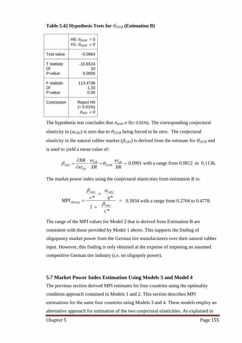
Chapter 5 Page 155

Table 5.42 Hypothesis Tests for 32GR (Estimation B)

H0: 32GR = 0

H1: 32GR 0

Test value -0.0984


-10.6524 33

0.0000


113.4738 1,33 0.00


3GR 0

The hypothesis test concludes that 32GR 0(< 0.01%). The corresponding conjectural

elasticity in (GR2) is zero due to 22GR being forced to be zero. The conjectural

elasticity in the natural rubber market (GR2) is derived from the estimate for 32GR and

is used to yield a mean value of:

XR

xr

XR

xr

xr

XR GRGR

GR

GR

GR 322 0.0991 with a range from 0.0812 to 0.1136.


*1

**

2

22

2

ε

η

ε

MPIGR

GRGR

GRXR

=

0.3934 with a range from 0.2704 to 0.4778.

The range of the MPI values for Model 2 that is derived from Estimation B are

consistent with those provided by Model 1 above. This supports the finding of

oligopsony market power from the German tire manufacturers over their natural rubber

input. However, this finding is only obtained at the expense of imposing an assumed

competitive German tire industry (i.e. no oligopoly power).

5.7 Market Power Index Estimation Using Models 3 and Model 4

The previous section derived MPI estimates for four countries using the optimality

condition approach contained in Models 1 and 2. This section describes MPI

estimations for the same four countries using Models 3 and 4. These models employ an

alternative approach for estimation of the two conjectural elasticities. As explained in

Chapter 5 Page 156

Chapter 4, this approach involves direct estimation of the i‟th country‟s observed

response to industry changes which is then used to derive a proxy measure of the

individual country (firm‟s) conjecture as to the global industry‟s response to its

behaviour. Fundamentally this approach simply measures the average response, over the

studied time period, in each individual firm‟s (or country‟s) market share of the global

industry which is then used to calculate the conjectural elasticities (αi and βi).

The direct estimation approach to the estimation of the conjectural elasticities (αi and βi)

first requires estimation of equations (5:12) and (5:13) followed by calculation of the

two conjectural elasticities as per (5:14) and (5:15).

(5:12) )(qfQ i2

(5:13) )(3 ixrfXR

For i = US, France, Japan and Germany. The values:

(5:14) Q

q

dq

dQα i

i

i 3 and,

(5:15)

β i3

XR

xr

dxr

dXR

i

i can then be derived.

On the output side, the individual country‟s conjectural elasticity in the global tire

market is defined as: Q

q

dq

dQα i

i

i 3 . It can be interpreted as the conjectural variation

idq

dQweighted by the country‟s own market share

Q

qi . If estimated by a linear model

5:12 gives the coefficient estimates idq

dQ and we obtain the conjectural elasticity by

multiplying each estimate with that country‟s market share. If the estimation is in the

double-log form, then the term Q

q

dq

dQ i

i

can be directly derived mathematically.

If idq

dQis found to be 1 then it implies that the market is the specific case of collusive

Cournot market behaviour and the conjectural elasticity then reduces to market share.

More general market structure interpretations were shown in Table 3.4.

Chapter 5 Page 157

However, the estimated Q

q

dq

dQ i

i

here is derived from a post-event measurement of

the quantity of tire produced (qi). Hence to interpret the estimated term Q

q

dq

dQ i

i

as a

conjectural elasticity requires the assumption that the prevailing observed response is

the same as the firm conjectured pre-event. This implies that ex ante conjectured

behaviour of the firm is always correct. Although this is not the case for every

behaviour, it helps provide a frame of possible outcomes to be used as robust testing

with outcomes from Model 1 and Model 2.

In comparison to this approach, other studies provide a variety of estimation methods,

based on each specific study context, to obtain the conjectural elasticity. Examples of

other estimations of conjectural elasticity are found in Appelbaum (1982) who

approximated the conjectural elasticity using a linear function of input prices such as

interest rate, wage rate and intermediate input prices; Murray (1994) who estimated a

function of transportation costs and border rival spatial competition ratio; Lopez et.al

(2002) who assigned the conjectural elasticity as a constant but also tested it as a

function of the concentration variable; Wilcox & Abott (2003) who estimated the

conjectural elasticity as a function of product price, demand elasticity, supply elasticity

and number of firms and Zhang & Sexton (2002) who simply adopted conjectural

elasticity values from previous studies. However, there is criticism that conjectural

behaviour should incorporate a sequence of actions in reaction to rivals‟ quantity

changes, not just be estimated from a static model. Thus, the term idq

dQ in the literature

is sometime reduced to be a market conduct parameter instead of a conjectural elasticity

(Sexton, 2000). In contrast, there are alternative approaches to study market power

based on games theory (Sexton, 2000) and experimental analysis (Engle-Warnick &

Ruffle 2005).

On the input market side, the derivation of each country‟s conjectural elasticity on its

input market, specifically the global natural rubber market,

β i3

XR

xr

dxr

dXR

i

i could be

obtained in analogous to the derivation of Q

q

dq

dQα i

i

i 3 described above.

Results for estimation of (5:12) - world tire production as a function of tire production

outputs in US, France, Japan, Germany and a time trend is reported in Table 5.43.

Chapter 5 Page 158

Table 5.43 Estimation Results for (5:12): Countries’ Conjectural Elasticities in

Global Tire Industry

tTqqqqQ GRGRJAJAFRFRUSUS 0


Constant 0 -0.2807

(-21.200)***

U.S. ‘s tire production (qUS) US 0.3385

(18.200)***

France’s tire production (qFR) FR 0.1705

(7.001) ***

Japan’s tire production (qJA) JA 0.1168

(8.894) ***

Germany’s tire production (qGR) GR 0.1427

(5.134) ***

Time trend (T) t 0.0124

(23.730) ***

Durbin-Watson 2.00

R2 0.9996




The estimation results in Table 5.43 were generated in a log-log form with first order

correction for autocorrelation. The time trend representing technological development is

found to be statistically significant in the global tire market. Given the log-log

specification for (5:12) the conjectural elasticities (5:14) for each country are derived as:

Q

q

q

Q US

US

US

3 = 0.3385

Q

q

q

Q FR

FR

FR

3

= 0.1705

Q

q

q

Q JA

JA

JA

3

= 0.1168

Q

q

q

Q GR

GR

GR

3

= 0.1427 for US, France, Japan and Germany respectively.

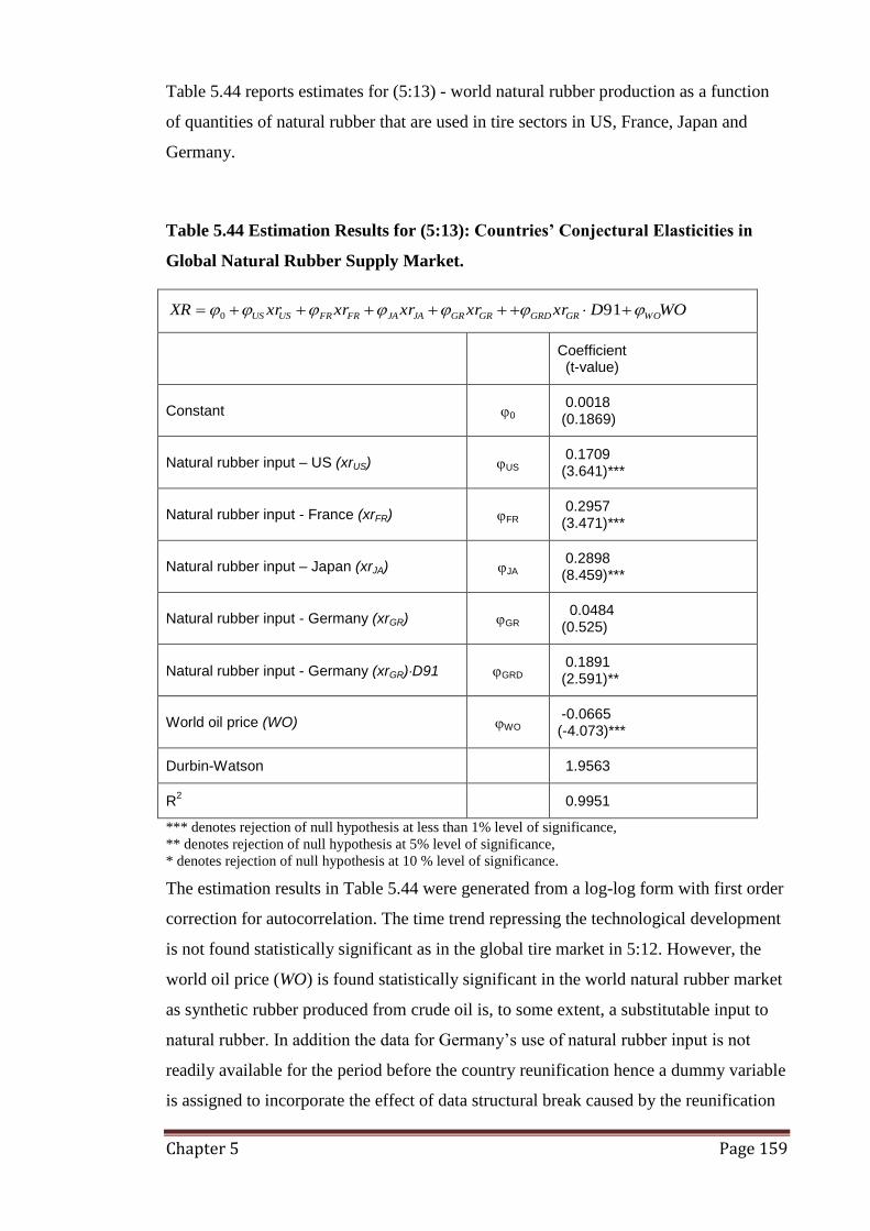
Chapter 5 Page 159

Table 5.44 reports estimates for (5:13) - world natural rubber production as a function

of quantities of natural rubber that are used in tire sectors in US, France, Japan and

Germany.

Table 5.44 Estimation Results for (5:13): Countries’ Conjectural Elasticities in

Global Natural Rubber Supply Market.

WODxrxrxrxrxrXR WOGRGRDGRGRJAJAFRFRUSUS 910


Constant 0 0.0018 (0.1869)

Natural rubber input – US (xrUS) US 0.1709 (3.641)***

Natural rubber input - France (xrFR) FR 0.2957 (3.471)***

Natural rubber input – Japan (xrJA) JA 0.2898 (8.459)***

Natural rubber input - Germany (xrGR) GR 0.0484 (0.525)

Natural rubber input - Germany (xrGR)D91 GRD 0.1891 (2.591)**

World oil price (WO) WO -0.0665 (-4.073)***


R2 0.9951




The estimation results in Table 5.44 were generated from a log-log form with first order

correction for autocorrelation. The time trend repressing the technological development

is not found statistically significant as in the global tire market in 5:12. However, the

world oil price (WO) is found statistically significant in the world natural rubber market

as synthetic rubber produced from crude oil is, to some extent, a substitutable input to

natural rubber. In addition the data for Germany‟s use of natural rubber input is not

readily available for the period before the country reunification hence a dummy variable

is assigned to incorporate the effect of data structural break caused by the reunification

Chapter 5 Page 160

in 1991. Estimation results for Germany data reflect that its estimates (GR) are not

statistically significant except for the years after 1991 (GRD).

Given the log-log specification for (5:13), the derived average conjectural elasticities for

each country are:

XR

xr

xr

XR US

US

US

3

= 0.1709

XR

xr

xr

XR FR

FR

FR

3 = 0.2957

XR

xr

xr

XR JA

JA

JA

3

= 0.2898

XR

xr

xr

XR GR

GR

GR

3

= 0.1046 (1962-1990 =0.0484, 1991-2000 = 0.2375)

for US, France, Japan and Germany respectively.

The two directly estimated conjectural elasticities (I and i) for each country i can be

used to derive new estimates for MPI for each country. The results for Model 3 (market

power index derived from inverse tire demand elasticity (), inverse natural rubber

supply elasticity (), and directly estimated conjectural elasticities for the world tire

industry (i3) and the world natural rubber industry (i3) for each country, is reported in

Table 5.45. MPI results using Model 4 (market power index derived from direct tire

demand elasticity (*), direct natural rubber supply elasticity (*

), and directly estimated

conjectural elasticities for the world tire market (i3) and the world natural rubber

market (i3) for each country, is reported in Table 5.46.

Table 5.45 MPI Estimations Using Model 3

3

33

31 US

USUS

USXR

ηεMPI

Mean 1.0442 Min to Max 0.6266 - 1.6500

3

33

31 FR

FRFR

FRXR

ηεMPI

Mean 0.7672 Min to Max 0.5830 – 1.0211

3

33

31 JA

JAJA

JAXR

ηεMPI

Mean 0.6787 Min to Max 0.5407– 0.8649

3

33

31 GR

GRGR

GRXR

ηεMPI

Mean 0.5907 Min to Max 0.3916 – 0.8949

Chapter 5 Page 161

Table 5.46 MPI Estimations Using Model 4

*1

**

3

33

4

ε

η

ε

MPIUS

USUS

USXR

Mean 0.9598 Min to Max 0.9506 – 0.9658

*1

**

3

33

4

ε

η

ε

MPIFR

FRFR

FRXR

Mean 0.8190 Min to Max 0.7647 – 0.8518

*1

**

3

33

4

ε

η

ε

MPIJA

JAJA

JAXR

Mean 0.7673 Min to Max 0.6981 – 0.8092

*1

**

3

33

4

ε

η

ε

MPIGR

GRGR

GRXR

Mean 0.5935 Min to Max 0.5131 – 0.7509

5.8 Summary

This chapter has derived four different estimations of the market power index for four

individual countries: the US, France, Japan and Germany. The estimates are derived

from the four estimation models developed in Chapter 4. A summary of the estimation

methods involved for each of the 4 models are summarised in Chapter 4 in Figures 4.2a

and 4.2b. Model 1 and Model 2 use indirectly estimated conjectural elasticities for tire

and natural rubber industries market. Model 1 differs from Model 2 in that Model 1

uses an inverse tire demand elasticity and an inverse natural rubber supply elasticity

whereas Model 2 uses a direct tire demand elasticity and a direct natural rubber supply

elasticity.

In contrast, Model 3 and Model 4 use directly estimated conjectural elasticities.

Analogous to Models 1 and 2, Model 3 uses the inverse tire demand elasticity and

inverse natural rubber supply elasticity whereas Model 4 uses the direct tire demand

elasticity and the direct natural rubber supply elasticity.

For Models 1 and 2, a two-step procedure for market power analysis is used. This

allows for the estimation of the optimality equation (equation 5:6i), which gives the

Chapter 5 Page 162

estimates of 1, 2, 3. In the first step hypothesis tests are applied to the estimates of

1, 2 & 3. The null hypotheses for a competitive market are: 1 = 1 and 2 = 3 = 0.

This implies that the natural rubber price is equal to the value of the marginal product of

natural rubber in tire manufacturing.

If 1 <1 and 2 0, 3 0, then the implication is that the natural rubber market is not

competitive and oligopoly market power could be present in the tire output industry and

oligopsony market power could be present in the tire input natural rubber industry. Step

2 is then called for and it involves measurement of the degree of market power via the

market power index (MPI). This requires two more components in addition to the tire

demand elasticity and the natural rubber elasticity. They are the conjectural elasticity in

tire market (i1), which is derived from 2 and the conjectural elasticity in the natural

rubber market (i1), which is derived from 3.

The MPI will have values of 0 to 1 and is general in its application to a range of market

power cases including both oligopoly in the output market (tires) and oligopsony in its

input market (natural rubber). The range of test values is detailed in Chapter 4 in Table

4.1. The critical test for oligopsony is based on the conjectural elasticity βi. A

competitive input market is implied by βi = 0. Oligopsony is implied by 0<i<1 and

monopsony is implied by i=1. The degree of oligopsony market power is then given by

MPI.

The tests for market power in this study thus depend on the values of: world tire

demand elasticity, world natural rubber supply elasticity, natural rubber marginal

productivity in each country‟s tire production function and output and input conjectural

elasticities. The elasticity estimates are derived from both inverse and direct demand

and supply functions. The conjectural elasticity estimates are derived from two

approaches.

The demand and supply elasticity estimates are summarised in Table 5.47.

Estimates of natural rubber marginal productivity for tire production for each country

are summarised in Table 5.48.

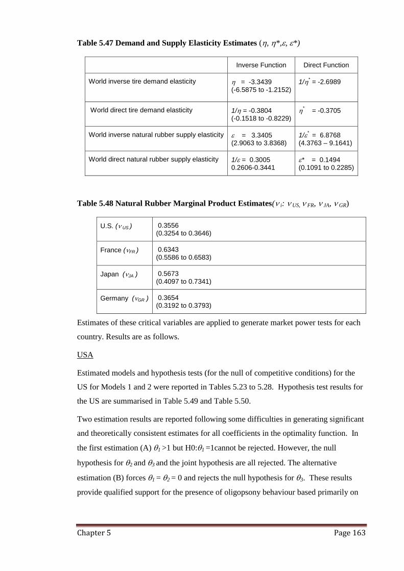
Chapter 5 Page 163

Table 5.47 Demand and Supply Elasticity Estimates (, *,, *)

Inverse Function Direct Function

World inverse tire demand elasticity = -3.3439 (-6.5875 to -1.2152)

1/* = -2.6989

World direct tire demand elasticity 1/ = -0.3804 (-0.1518 to -0.8229)

* = -0.3705

World inverse natural rubber supply elasticity = 3.3405 (2.9063 to 3.8368)

1/* = 6.8768

(4.3763 – 9.1641)

World direct natural rubber supply elasticity 1/ = 0.3005 0.2606-0.3441

* = 0.1494 (0.1091 to 0.2285)

Table 5.48 Natural Rubber Marginal Product Estimates( i: US, FR, JA, GR)

U.S. ( US ) 0.3556 (0.3254 to 0.3646)

France (FR ) 0.6343 (0.5586 to 0.6583)

Japan (JA ) 0.5673 (0.4097 to 0.7341)

Germany (GR ) 0.3654 (0.3192 to 0.3793)

Estimates of these critical variables are applied to generate market power tests for each

country. Results are as follows.

USA

Estimated models and hypothesis tests (for the null of competitive conditions) for the

US for Models 1 and 2 were reported in Tables 5.23 to 5.28. Hypothesis test results for

the US are summarised in Table 5.49 and Table 5.50.

Two estimation results are reported following some difficulties in generating significant

and theoretically consistent estimates for all coefficients in the optimality function. In

the first estimation (A) 1 >1 but H0:1 =1cannot be rejected. However, the null

hypothesis for 2 and 3 and the joint hypothesis are all rejected. The alternative

estimation (B) forces 1 = 2 = 0 and rejects the null hypothesis for 3. These results

provide qualified support for the presence of oligopsony behaviour based primarily on

Chapter 5 Page 164

the results for 3. This is supported by the derived market power index results with

average MPIUS values of 0.5243 from estimation A and 0.4133 from B.

Test results for Model 2 also reflect difficulties in generating a significant and

theoretically consistent value for 1. The first estimation (A) could not reject the

theoretically inconsistent finding of: 1 >1. This outcome was corrected by forcing 2 =

0 in Estimation B. However, as for Model 1, the null for 2 and 3 as well as the joint

null is rejected. Hence Model 2 tests also provide qualified support for oligosony

behaviour. The theoretically inconsistent size of 1 is assumed responsible for a

theoretically incorrect value for the resulting market power index. The mean MPIUS

value of 1.3517 is > 1. However, the mean MPIUS of value of 0.4180 from Estimation B

is consistent with both Model 1 results and the hypothesis test conclusions.

The MPI values from Models 3 and 4 are consistent but significantly higher than those

derived from Models 1 and 2. The average market power index is 1.0442 for Model 3

and 0.9598 for Model 4. These values imply near maximum levels of oligopsony

behaviour and market power.

Overall it is considered that the results values support the presence of oligopsony

market power for the U.S. tire industry for its world natural rubber market input.

Table 5.49 Hypothesis Test Summary for US (Models 1 and 2)#1

H0:1 = 1 H0:2 = 0 H0:3 = 0 H0:1 =1, 2 = 0, 3 = 0

Model 1

Estimate A Not reject#2

Reject Reject Reject

Estimate B - - Reject

Model 2

Estimate A Reject#2


Estimate B Reject - Reject Reject

#1 All i estimates are significant unless otherwise stated.

#2 1 > 1 whereas theory predicts 1 1.

Chapter 5 Page 165

Table 5.50 Conjectural Elasticities for US and MPIUS Summary#1

Variable Model 1 Model 2 Model 3 Model 4

I (Estimate A) 0.0732#2

(0.0587 to 0.1062)

0.6171#2

(0.4744 to 0.9337 )

I (Estimate B) - -

I 0.3385

i (Estimate A) 0.1884#2

(0.1615 to 0.2415)

0.1239#2

(0.1051 to 0.1572)

i (Estimate B) 0.2124 (0.1820 to 0.2721)

0.1086 (0.0921 to 0.1377)

i 0.1709

MPIXRUS (Estimate A) 0.5243

#2

(0.3787 to 0.7527) 1.3517

#2,#3

(1.1163 to 1.7329)

MPIXRUS (Estimate B) 0.4133 (0.3523 to 0.5008)

0.4180 (0.3297 to 0.5198)

MPIXRUS 1.0442#3

0.9598

#1 Values in parentheses are minimum and maximum values.

#2values involve 1 > 1 whereas theory predicts 1 1.

#3Theory predicts MPI 1.

France

Results for France are summarised in Table 5.51 and Table 5.52. Estimated models and

hypothesis tests (for the null of competitive conditions) for the France for Models 1 and

2 were reported in Tables 5.29 - 5.32. In the first estimation (A) for Model 1, the null

hypotheses that 1 =1, 2 =0 and 3 = 0 as well as the joint hypothesis test are all

rejected. This is consistent with the derived market power index results with average

MPIFR values of 0.5608, thus all tests support the evidence of France‟s tire

manufacture‟s market power both in tire market and the natural rubber market.

The results for Model 2 involve difficulties in generating significant values for 1 and

2. Hence an alternative estimation (B) which forces 2 = 0 is provided. Corresponding

results allow for the rejection of the null hypothesis tests for competitive market

condition. Specifically, the null that 3 = 0 is rejected. The MPIFR of 0.3740 supports the

test results and is consistent with Model 1 results.

Chapter 5 Page 166

As in the US case, the average MPI values for France from Models 3 and 4 are

consistent but higher, exceeding the upper bound of those derived from Models 1 and 2.

The average market power index is 0.7672 for Model 3 and 0.8190 for Model 4.

Table 5.51 Hypothesis Test Summary for France (Models 1 and 2)#1

H0:1 = 1 H0:2 = 0 H0:3 = 0 H0:1 =1, 2 = 0, 3 = 0

Model 1

Estimate A Reject Reject Reject Reject

Model 2

Estimate A Not reject #2

Not reject#2

Reject Reject



#2 1 and 2 are not significant.

Table 5.52 Conjectural Elasticities for France and MPIFR Summary#1


i (Estimate A) 0.0606

(0.0522 to 0.0696)

#2

i (Estimate B) -

i 0.1705

i (Estimate A) 0.2640

(0.2180 to 0.3326)

#2

i (Estimate B) 0.0914

(0.0754 to 0.1151)

i 0.2957

MPIXRFR (Estimation A) 0.5608

(0.4541 to 0.6720)

#2

MPIXRFR (Estimation B) 0.3740

(0.2711 to 0.4693)

MPIXRFR 0.7672 0.8190


#2 1 and 2 are not significant.

Chapter 5 Page 167

Overall it is considered that the results values support the presence of oligopsony

market power for the France‟s tire industry for its world natural rubber market input.

Japan

Results for Japan are summarised in Table 5.53 and Table 5.54. Estimated models and

hypothesis tests for Models 1 and 2 were reported in Tables 5.33- 5.37. Two estimation

results are reported following some difficulties in generating significant and

theoretically consistent estimates for all coefficients in the optimality function.

In Model 1 initial estimation (A), 1 and 2 estimates are statistically insignificant. A

supplementary estimation (B) is thus given. This test tries forcing 2 = 0; its results find

the null hypotheses that 1 = 1 and 3 = 0 are rejected. These results provide qualified

support for the presence of oligopsony behaviour based primarily on the results for 3.

This is confirmed by the derived market power index results with average MPIJA values

of 0.4754.

Although test results for Model 2 do not reflect difficulties in generating significant

estimates and provide the MPIJA= 0.8937, the first estimation (A) could not reject the

theoretically inconsistent finding of: 1 >1. This outcome is corrected by forcing 2 = 0

in estimation B and the null that 1 = 1 and 3 = 0 as well as the joint null are rejected.

The resulting value of MPIJA = 0.3950 confirms support of the presence of market

power, specifically the oligopsony power as found by Model 1.

The conjectural elasticity in the input market (natural rubber) is consistent with results

from Model 1 and 2. The MPI values from Models 3 and 4 are 0.6787 and 0.7673,

higher than those derived from Models 1 and 2.

The consistent results from each model qualifies the inference for the presence of

market power of Japan‟s tire manufacturing industry in the world market, specifically

oligopsony power in the world natural rubber input market for tire industry in Japan.

Chapter 5 Page 168

Table 5.53 Hypothesis Test Summary for Japan (Models 1 and 2)#1

H0:1 = 1 H0:2 = 0 H0:3 = 0 H0:1 =1, 2 = 0, 3 = 0

Model 1

Estimate A

Not reject#2

Not reject#2

Reject Reject


Model 2

Estimate A Not reject#3




#2 1 & 2 are not significant.

#3 Value involves estimated 1 >1 whereas theory predicts 1 1.

Table 5.54 Conjectural Elasticities for Japan and MPIJA Summary#1


i (Estimation A) #2

0.3087#3

(0.1243 to 0.3966)

i (Estimation B ) 0.0000 0.0000

i 0.1168

i (Estimation A ) #2

0.1209#3

(0.0607 to .1664)

i (Estimation B ) 0.2816

(0.1567to 0.3720) 0.1029

(0.0517 to 0.1416)

i 0.2898

MPIXRJA (Estimation A) #2

0.8937#3

(0.5593 to 1.0331)

MPIXRJA (Estimation B) 0.4754

(0.3384 to 0.5584) 0.3950

(0.3019 to 0.4908)

MPIXRJA 0.6787 0.7673


#2 1 and 2 are not significant


Chapter 5 Page 169

Germany

Summary results for Germany are presented in Table 5.55 and 5.56. Estimation and

hypothesis tests were detailed in Tables 5.38 - 5.42.

Overall they do not have statistical significant problems in any model. Model 1 results

reject all hypotheses for the competitive markets (reject the null that 1 = 1, 2 = 0 and

3 = 0). The MPIGR result is 0.5805. However, Model 2 involves difficulty in that

estimated 1 > 1 which is not consistent with its theoretical prediction. However, the

hypothesis tests reject the null hypotheses that 2 = 0 and 3 = 0 implying that output

market (tire) as well as the input market (natural rubber) is not competitive; the MPIGR

is 1.6314. To correct for the 1‟s estimation result, a supplementary estimation (B)

forced all effects other than input market into a constant term. Results found 3 strongly

significant hence rejected the null hypothesis that 3 = 0. The average MPIGR is 0.3934,

being in the range of Model 1‟s results and thus indicating consistency of results from

both models that qualifies estimation A‟s finding of the evidence for oligopsony market

power. The average MPI values from Models 3 and 4 is 0.5907 for Model 3 and 0 5935

for Model 4. These values are consistent with those derived from Models 1 and 2.

Overall it is considered that the results support the presence of oligopsony market power

for the German tire industry upon its world natural rubber market input.

Table 5.55 Hypothesis Test Summary for Germany (Models 1 and 2)#1

H0:1 = 1 H0:2 = 0 H0:3 = 0 H0:1 =1, 2 = 0, 3 = 0

Model 1

Estimate A Reject Reject Reject Reject

Model 2

Estimate A Reject# 2


Estimate B - - Reject -

# 1 All i estimates are significant unless otherwise stated.

# 2

Value involves estimated 1 >1 whereas theory predicts 1 1.

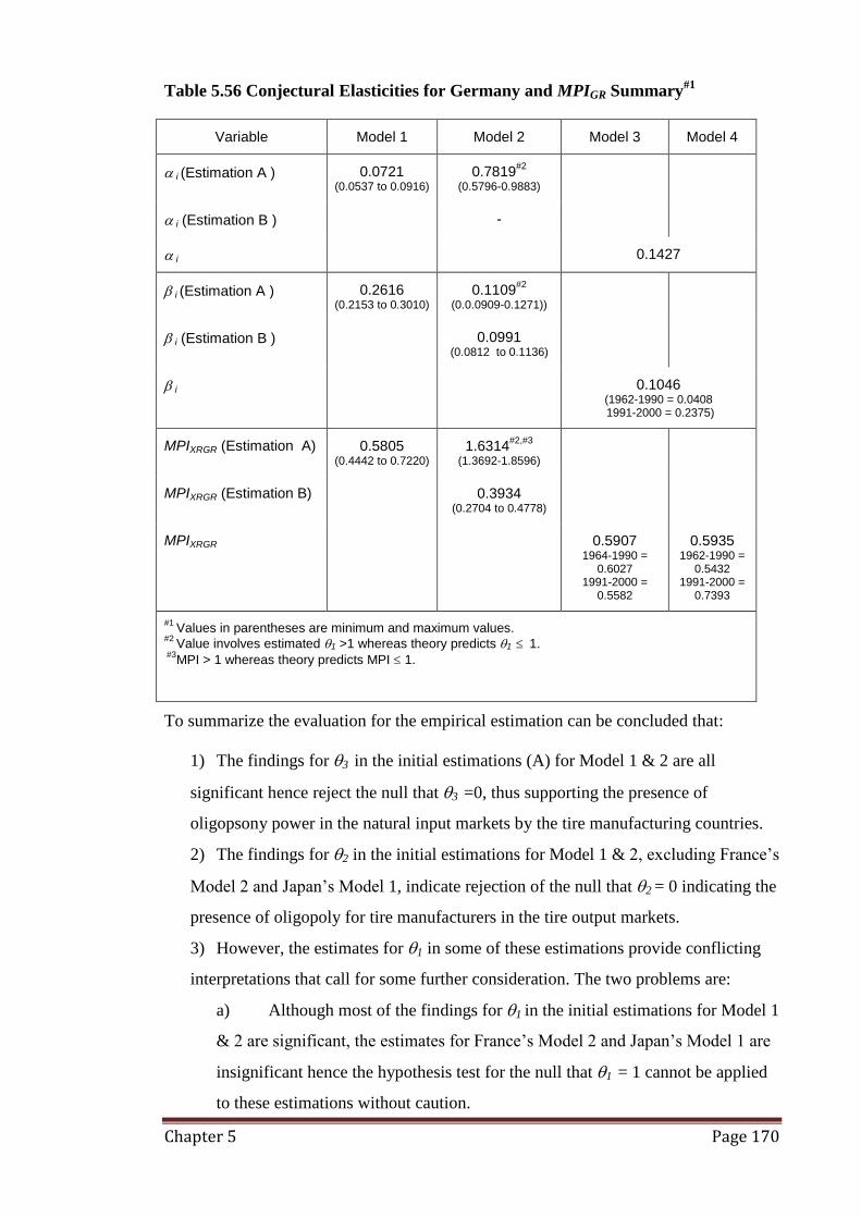
Chapter 5 Page 170

Table 5.56 Conjectural Elasticities for Germany and MPIGR Summary#1


i (Estimation A ) 0.0721

(0.0537 to 0.0916) 0.7819

#2

(0.5796-0.9883)

i (Estimation B ) -

i 0.1427

i (Estimation A ) 0.2616

(0.2153 to 0.3010) 0.1109

#2

(0.0.0909-0.1271))

i (Estimation B ) 0.0991

(0.0812 to 0.1136)

i 0.1046

(1962-1990 = 0.0408 1991-2000 = 0.2375)

MPIXRGR (Estimation A) 0.5805

(0.4442 to 0.7220) 1.6314

#2,#3

(1.3692-1.8596)

MPIXRGR (Estimation B) 0.3934

(0.2704 to 0.4778)

MPIXRGR 0.5907

1964-1990 = 0.6027

1991-2000 = 0.5582

0.5935

1962-1990 = 0.5432

1991-2000 = 0.7393



#3MPI > 1 whereas theory predicts MPI 1.

To summarize the evaluation for the empirical estimation can be concluded that:

1) The findings for 3 in the initial estimations (A) for Model 1 & 2 are all

significant hence reject the null that 3 =0, thus supporting the presence of

oligopsony power in the natural input markets by the tire manufacturing countries.

2) The findings for 2 in the initial estimations for Model 1 & 2, excluding France‟s

Model 2 and Japan‟s Model 1, indicate rejection of the null that 2 = 0 indicating the

presence of oligopoly for tire manufacturers in the tire output markets.

3) However, the estimates for 1 in some of these estimations provide conflicting

interpretations that call for some further consideration. The two problems are:

a) Although most of the findings for 1 in the initial estimations for Model 1

& 2 are significant, the estimates for France‟s Model 2 and Japan‟s Model 1 are

insignificant hence the hypothesis test for the null that 1 = 1 cannot be applied

to these estimations without caution.

Chapter 5 Page 171

b) Secondly, although most of the estimated values for 1 are less than 1,

estimations from US‟s Model 1& 2, Japan‟s Model 2 and Germany' Model 2 are

greater than 1 whereas theory predicts 1 1; they are hence theoretically

inconsistent and call for further investigations.

Therefore, appropriate supplementary estimations are undertaken to qualify each of

these particular estimations involving interpretation problems.

4) Thus only Model 1 for France and Germany can produce significant and

theoretically consistent evaluation for market power existence. Other estimations

involving problems are resolved by supplementary estimations (B) restricting 2 =0.

All outcomes in the supplementary estimations confirm the rejection of the null that

3 = 0 as found in their corresponding initial estimations (A). Thus even if it is

assumed that output market is competitive, market power evidence still exists, with

some lower resulting MPIXRi results42

. Hence, this helps to confirm the evidence of

oligopsony market power potential in the natural rubber input markets.

5) The outcomes from Model 3 & 4 are consistent with Model 1 & 2 with higher

levels of the MPI index for each country.

Finally Table 5.57 compares the market power index for each country. The MPI values

reported are selected from preferred models. Results that involve statistically

insignificant estimates (Estimation A for France‟ Model 2 and Japan‟s Model 1) as well

as theoretically conflicting estimates (Estimation A for US‟s Model 1 &2, Japan‟s

Model 2 and Germany‟s Model 2) are provided in the corresponding remarks.

From Table 5.57, US has the top market power index, judged by Model 2, 3, and 4.

France has the second highest level of market power, judged by Model 1, 3, and 4.

Japan has the third highest level of market power, judged by Model 1, 3, and 4.

Germany has the least market power, judged by Model 3 and Model 4. Model 3 and

Model 4 give similar ranking results.

In conclusion, estimated results imply that the tire industry in US, France, Japan and

Germany have market power (oligopsony) on the world natural rubber market. Results

are reconciled between inverse and direct function approaches for tire demand and

natural rubber supply. In addition, in each approach outcomes are confirmed between

the derived and directly estimated conjectural elasticities in tire and natural rubber

42

This might imply an industry wide level of inefficiency which could also increase the price-cost margin

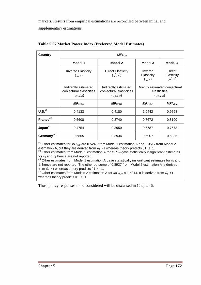
Chapter 5 Page 172

markets. Results from empirical estimations are reconciled between initial and

supplementary estimations.

Table 5.57 Market Power Index (Preferred Model Estimates)

Country MPIXRi

Model 1 Model 2 Model 3 Model 4

Inverse Elasticity

(, )

Direct Elasticity

(*,

*)

Inverse Elasticity

(, )

Direct Elasticity

(*,

*)

Indirectly estimated conjectural elasticities

(i1,i1)

Indirectly estimated conjectural elasticities

(i2,i2)

Directly estimated conjectural elasticities

(i3,i3)

MPIXRi1 MPIXRi2 MPIXRi3 MPIXRi4

U.S.#1

0.4133 0.4180 1.0442 0.9598

France#2

0.5608 0.3740 0.7672 0.8190

Japan#3

0.4754 0.3950 0.6787 0.7673

Germany#4

0.5805 0.3934 0.5907 0.5935

#1 Other estimates for MPIUS are 0.5243 from Model 1 estimation A and 1.3517

from Model 2

estimation A, but they are derived from 1 >1 whereas theory predicts 1 1.

#2 Other estimates from Model 2 estimation A for MPIFR gave statistically insignificant estimates

for 1 and 2 hence are not reported.

#3 Other estimates from Model 1 estimation A gave statistically insignificant estimates for 1 and

2 hence are not reported. The other outcome of 0.8937 from Model 2 estimation A is derived

from 1 >1 whereas theory predicts 1 1. #4

Other estimates from Models 2 estimation A for MPIGR is 1.6314. It is derived from 1 >1

whereas theory predicts 1 1.

Thus, policy responses to be considered will be discussed in Chapter 6.

Chapter 6 Page 173

Chapter 6

Conclusions and Policy Recommendations

6.1 Introduction

This thesis has examined the research question: Does oligopsony market power exist in

the natural rubber input market for the global tire industry?

The research question is of specific importance to countries such as Thailand as the

production of natural rubber, which is an important input to the production of tires, is

restricted to certain countries, predominantly the developing economies of Thailand,

Indonesia and Malaysia of which Thailand is the top producing country.

Much of the natural rubber production is conducted on relatively small and low income

farms. In contrast tire production is dominated by large multinational companies in a

relatively concentrated industry with production and sales concentrated in wealthy

developed countries. Consequently the market for natural rubber, as an input for tire

manufacture has both economic efficiency and welfare issues of interest. The economic

efficiency issue of concern is the possibility that tire manufacturers may be able to exert

market power in the market for natural rubber inputs, such that natural rubber prices

paid to its producers are less than the marginal revenue product earned by the tire

producers from this input. The welfare issue of concern is the possible distortion in

income distribution between natural rubber producers and consumers of natural rubber

products. As natural rubber production is concentrated in a small number of less

wealthy producing countries and the production of tires is concentrated in multinational

companies with developed country ownership and the sale of tires is concentrated in

these same developed countries, a welfare issue of income distribution translates to a

country level.

Therefore, this thesis has focused on the assessment of market power in a global

industry of producers of natural rubber inputs to the global tire industry. If market

power was found to exist then this indicated the potential for its associated welfare

implications of an inefficient and inequitable income distribution between the lesser

developed countries producing the natural rubber input and developed country

producers and consumers of tires.

Chapter 6 Page 174

6.2 Thesis Process and Outcomes

The background of the natural rubber industry was surveyed in Chapter 2 from the

beginning stage of the natural rubber tree plantation through to latex tapping,

intermediate product manufacturing of smoked-sheet and block rubber and the

manufacture of tires. The importance of synthetic rubber as a substitute input for natural

rubber in tire manufacturing was also identified.

The industry structure of the downstream product cycle of natural rubber was found to

be increasingly concentrated through the various stages of tapping, processing,

exporting and tire manufacturing. As such there are several stages in the natural rubber

industry that have potential for market power from the buyer side. The natural rubber

export industry is dominated by particular buyer countries for each seller country

namely: Japan for Thailand, US for Indonesia and EU for Malaysia. As such there is

potential also for market power to be exercised by the supplier countries of natural

rubber (oligopoly).

The natural rubber consumer industry such as vehicle tire manufacture is concentrated

in the hands of a small group of conglomerate enterprises that cross national borders.

This concentration is also reflected in country level data with the major developed

countries dominating the consumption of natural rubber for tire manufacture and the

consumption of the manufactured tires. Hence there is potential for market power to be

exercised in the natural rubber markets from the buyer side (oligopsony) and that

potential can be analysed via company level or country level data. Industries that

possess oligopsony market power in their input markets may or may not also possess

oligopoly market power in their output markets. In this case the tire industry has

structural features consistent with potential oligopsony market power in its natural

rubber input market and oligopoly market power in its tire output market.

The potential for oligopoly market power (by seller countries), based on the fact that

market is dominated by three supplier countries, is more problematic. It could be

analysed using country level data but based on an analysis of the natural rubber industry

supply chain in Thailand, there is not the same strong level of concentration in a

company – country relationship as found for the tire industry. Hence this thesis tests for

the presence of market power by the tire industry in its tire output market

(oligopoly)and market power in its natural rubber input market (oligopsony).

Chapter 6 Page 175

The theoretical background for the analysis of oligopoly and oligopsony power was

examined in Chapter 3 by means of a review of the theory of production and price in

output markets and employment and price in input markets. The analysis was first

framed for a perfectly competitive market that was then used as a benchmark to evaluate

production and employment in imperfectly competitive markets. Deviations from the

competitive standard are considered potential evidence of market power.

A review of the literature on measuring market power identified three approaches: buyer

concentration, effects from structural changes and the conjectural variation approach.

The conjectural variation approach was considered to be of most relevance for the

approach adopted in this thesis. Typically studies using this approach adopt a duality

theory approach namely the application of Shephard's Lemma and Hotelling's Lemma to

derive demand functions for inputs and supply functions for outputs respectively. The

degree of oligopsony/oligopoly power is then defined as the deviation of actual input

prices from the value of their marginal products (shadow price) with the shadow price

being derived from the profit maximization conditions.

Given the potential for mixed oligopsony/oligopoly market power to exist in the

markets considered in this study, the literature supports an analysis of both output and

input market competitor behaviour. Conjectural elasticities in output and input markets

are needed as well as the elasticities of demand for inputs and supply of outputs, to

obtain a valid measurement of market power.

This chapter also provided a review of the literature on tire production, tire demand and

natural rubber supply. It was found that tire demand has two components namely: new

vehicle production demand that is not price sensitive and replacement tire demand that

is price sensitive. Natural rubber studies generally support the claim that the industry is

competitive and that supply is price sensitive as farmers can vary tapping intensity and

tree uprooting rates in responses to price changes. It is also widely concluded that The

International Natural Rubber Organization (INRO) did achieve a degree of price

stabilization in the natural rubber market during its existence. However, it did not

operate as a supplier cartel to impose market power in the manner of The Organization

of the Petroleum Exporting Countries (OPEC) in the oil market. A general model for the

application of an oligopsony/oligopoly model using the conjectural variation approach

was developed in Chapter 4. The outcome was the derivation of a market power index

that could be used to assess oligopsony/oligopoly market power. The approach was

based on the model developed by Chang and Tremblay (1991) that was extended to

Chapter 6 Page 176

incorporate 4 different interpretations which were identified as models 1 to 4. Model 1

and Model 2 used indirectly estimated conjectural elasticities for tire and natural rubber

industries market. Model 1 differs from Model 2 in that Model 1 uses an inverse tire

demand elasticity plus an inverse natural rubber supply elasticity whereas Model 2 uses

a direct tire demand elasticity and a direct natural rubber supply elasticity. In contrast,

Model 3 and Model 4 use directly estimated conjectural elasticities. Analogous to

Models 1 and 2, Model 3 uses the inverse tire demand elasticity and inverse natural

rubber supply elasticity whereas Model 4 uses the direct tire demand elasticity and the

direct natural rubber supply elasticity.

The general model thus provided four contrasting market power indexes to evaluate if

oligopsony/oligopoly market power is present.

An important adaptation of this general model was its transformation from the

conventional industry/firm level to a global/country industry level so that it could be

applied to test for the presence of oligopsony market power deriving from the global tire

industry comprising tire producing countries (as proxies for multinational companies

headquartered in these countries) on the global natural rubber industry comprising

natural rubber input producing countries.

The general model with its four variants was converted into empirical models and

estimated in Chapter 5. The outcome was the derivation of market power indexes (MPI)

for each of the four major tire producing countries. The MPI were then used to test for

the presence of oligopoly market power in the tire output market for each of these

countries and the presence of market power exerted by each tire producing country over

the natural rubber input producing industry that is dominated by the three major natural

rubber producing countries in South East Asia.

The MPI requires values for four key elasticities, tire demand elasticity, input supply

elasticity and conjectural elasticities for the tire output market in each country and

conjectural elasticities for the natural rubber input market. These elasticities in turn

require estimation of a number of market, production and optimality functions. Prior to

estimation all data series were examined for possible non-stationarity using standard

Dickey-Fuller and Phillips-Perron tests. The data were found to be non-stationary.

Further testing for the presence of cointegrating relationships was undertaken and the

results confirmed almost all series to be I(1) and the relationships of interest to be

cointegrated. Error correction model estimations supported this finding. Given the long

Chapter 6 Page 177

term focus of the study model conventional OLS estimations were therefore used to

obtain the long term functional relationships required for MPI derivations.

The elasticity values for tire demand and natural rubber supply were first estimated

from inverse tire demand and natural rubber supply functions. The conjectural

elasticities were derived from estimation of an optimality function and the tire

production function. Market power indexes were obtained for the USA, France, Japan

and Germany (Model 1). The process was repeated using direct tire demand and natural

rubber supply functions (Model 2). Given certain difficulties associated with the

conjectural elasticity estimations, the Models 1 and 2 were duplicated using an

alternative procedure to directly estimate ex-post proxies for the conjectural elasticities

(Model 3 and 4).

Results from the four contrasting approaches supported the hypothesis that oligopsony

market power was present in the tire industry of the USA, France, Japan and Germany

over the global natural rubber market. The USA had the highest market power index,

judged by Models 2, 3, and 4. France had the second highest market power index,

judged by Models 1, 3, and 4. Germany had the third highest market power index,

judged by Models 2, 3, and 4. Japan had the fourth highest market power index, judged

by Model 3 and Model 4.

The results for joint oligopsony/oligopoly in the tire and natural rubber industry

relationship were somewhat compromised by conflicting estimation results for the two

conjectural elasticities from the optimality functions used in Models 1 and 2. Although

there was support for oligopoly market power in the tire industries‟ tire output markets

in each of the four countries, significant estimates for the input market conjectural

elasticities could only be obtained in some cases by forcing an assumed competitive tire

market into the optimality function estimation. This effectively reduced the empirical

model from a joint oligopsony/oligopoly model to an oligopsony model only in those

cases. The general theoretical model has the flexibility to accommodate this separation

and as the key research question for this thesis relates to the oligopsony component, in

such cases the oligopoly testing component of the model was sacrificed.

Important for this thesis however, is the consistent finding of oligopsony market power

in the natural rubber market across four different model variants and for each of the

major tire producing countries.

Chapter 6 Page 178

6.3 Interpretation of Results and Implications for Policy Options

Interpretation of these results and the implications for policy can be approached by

examining the underlying components of the market power measure that have been used

to conclude the presence of oligopsony market power. The MPI used for the

measurement of market power comprises four components: the world tire demand

elasticity (

1* ), the tire producing country‟s conjectural elasticity on the world tire

industry (i), the world natural rubber supply elasticity (

1* ) and the tire producing

country conjectural elasticity in the world natural rubber market (i). From Table 4.1 the

smallest market power index (MPIXRi) is derived when both the markets for tires and

natural rubber are competitive. This can occur if zero values are found for i and i as

then a zero value will be generated for the market power index (MPIXRi) indicating no

oligopoly or oligopsony market power. Alternatively no market power is indicated

when * and * are perfectly elastic (approaching infinity) as this will also result in a

zero value for the market power index.

However, these conditions are rarely found in reality, as reflected by our findings of an

inelastic tire demand (0.3804 from inverse tire demand function and 0.3705 from direct

tire demand function) and an inelastic natural rubber supply (0.2993 from inverse

supply function and 0.1494 from direct supply function). Non-zero values are also

found for tire output market conjectural elasticity (i) and the tire input natural rubber

market (i) (Table 5.50 for US, Table 5.52 for France, Table 5.54 for Japan and Table

5.56 for Germany).

However, any policies that could raise the values of * and * and/or reduce the values

of i and i would reduce the level of market power because the higher is the *, the

lower is the MPIXRi; the higher is the *, the lower is the MPIXRi; the lower is the i, the

lower is the MPIXRi and the lower is the i, the lower is the MPIXRi. Hence it is useful to

explore the industry and or market policy options for each of these elasticities.

The tire demand elasticity (*) has a strong theoretical propensity to be inelastic based

on the review of earlier studies as well as this thesis. Tire demand has a large derived

demand component that is price insensitive. This derives from the fact that new vehicle

production demands at least five tires per unit with the tire cost a minor component of

Chapter 6 Page 179

the other vehicle cost. Demand from the vehicle in-use sector, is potentially competitive

and price sensitive. However, it is only part of the overall tire market, it has a relatively

rigid total market size based on vehicle numbers and average use and there is likely a

degree of brand loyalty. The potential to alter tire demand elasticity via policy is thus

considered very limited.

The tire producing country‟s conjectural elasticity in the global tire market (i) is a

direct function of the industry structure. Within the existing dominant countries,

competition policies could be employed. But such policies are beyond the legislative

powers of the natural rubber producing countries such as Thailand. Other options

include the growth of other tire producers and within the country context of this thesis,

other tire producing countries with producer companies independent of the current

dominant US, Japanese, French and German multinationals would be called for. In this

respect the potential for independent tire production in countries such as China and

Russia is of considerable importance. The data available for this study excluded these

two rapidly industrialising countries. However, it is clear that tire demand has grown

strongly in these two countries and China‟s expansion has been particularly rapid since

2000 to the extent that it was reported to be the largest producer country in 2008 with

approximately 300 tire manufacturing firms (Business Wire, 2008). The industry is not

yet as highly concentrated as in the traditional manufacturing companies of the USA,

France, Japan and Germany however, three large Chinese manufacturers are emerging

and the dominant western country manufacturers are actively engaged in the industry. A

similar experience is evident in Russia with rapid expansion since 2002 and active

involvement by European tire manufacturers in particular43

.

It would be in Thailand‟s interest to support an expanded independent domestic tire

manufacturing industry in such countries as a force to dilute the existing oligopsony

market power of the dominant western country manufacturers. The risk is that the same

market forces that lead to industry concentration within these countries will also impact

on the China and Russia industries to produce domestic industry concentration which

together with strong state control in these two countries could result in merely an

43

The Russian tire producer group Sibur -Russian Tires started expanding its production from 2002. The

AMTEL Group acquired the Dutch tire producer Vredestein Banden B.V.in 2005. When Sibur –Russian

joined The AMTEL Group they became the largest tire producer in Europe and one of the top ten

producers in the global market. In 2008 the Pirelli Group reached agreement with the Russian Federation

government to manufacture tires in Russia and the Commonwealth of Independent States. In the same

year Continental of Germany acquired a Finnish tire firm which has operations in Russia. Hence Russia

appears a promising market for natural rubber as a tire input.(Sources: Tire Review Online (2009)).

Chapter 6 Page 180

extension of the same form of oligopsony market power identified in this thesis for the

dominant western country tire producers. Whether the previously dominant western

country multinationals could extend their existing levels of control into China and

Russia via a process of multinational merger and acquisition is yet to be revealed. It

may be more difficult due to the political factors involved but the major western

multinationals are actively pursuing involvement in China and Russia.

The natural rubber supply elasticity ( * ) and the global tire industry natural rubber

input conjectural elasticity (i) are the two elasticities from the natural rubber market

side that impact on the market power index. The potential for a country such as

Thailand to influence these two factors is much greater. The presence of an inelastic

supply curve coupled with an inelastic tire demand curve means demand shocks feeding

through to the natural rubber supply market are likely to impact mainly on price. This

has social as well as economic impacts on the industry as income fluctuations will likely

be greatest in the less concentrated upstream section of the industry. Policies to increase

supply elasticity are effectively aimed at reducing the price impact of market shocks by

increasing supply flexibility and a number of agricultural policies can be targeted at

achieving this outcome.

In general agricultural policies are aimed at: increasing demand, decreasing supply,

providing direct income supplementation, stabilising price and/or income, and providing

risk management (Jones, 1994). Supporters for agricultural policy support argue that

technology developments over time tend to reduce supply costs but natural rubber

prices fall further thus keeping incomes low. Natural rubber prices were examined in

Chapter 2 (Figure 2.2) and Chapter 5 (Figure 5.7, 5.8 and 5.9) and a decreasing real

price trend was evident. Export prices fluctuated over the studied period and in recent

times experienced a significant slump post 1996 followed by a recovery. However, by

2004 US dollar exports prices had still not recovered to their 1996 levels. Prices in local

currency (Thai baht) for domestic natural rubber increased steadily since 2001.

Although current as well as real prices in Thai baht were raised by the impact of the oil

price surge in commodity market hedging transactions ahead of the financial crisis, it

was only a short term trend as natural rubber prices suddenly dropped in late 2008 as

the US financial crisis extended into the world economic slump. However, the finding

of oligopsony market power predicts the price would be driven to a competitive market

price for the suppliers regardless as to whether that price is rising or falling over time.

Chapter 6 Page 181

An industry dominated by small plantation operators will find it difficult to finance

research and development projects and hence government support for industry level

research and development can be justified for natural rubber. However, the risk remains

that the benefits of cost reduction policies will be expropriated by the oligopsony tire

buyers if they do not target supply elasticity.

Policies that are more likely to impact on supply elasticity would include policies that

would provide for better access to information on future market trends to better plan for

plantation production. Monoculture reinforces supply inelasticity. Policies designed to

expand product diversity in small plantation farms could increase supply elasticity by

enabling farmers to vary production levels without adversely impacting on their

incomes. Risk management supported through initiatives such as farm insurance either

private or government supplied would also help introduce greater supply flexibility

(higher elasticity).

Arguments for industry support can also be based on social and political grounds in that

natural rubber planting provides income, home and lifestyle benefits in country regions

that discourage population drift to overcrowded cities.

Policies directed towards increasing demand for products are not likely to be effective if

the increased demand is from an industry such as the tire industry that exercises

oligopsony market power in the market for natural rubber inputs. Such policies will

only benefit the natural rubber industry if they are directed to increasing demand from

substitute markets with competitive structures.

Direct supplementation grants or payments to farmers based on output quantity or

applied to producers of relevant factors of production such as fertilizers also risk

expropriation by consumers (tire industry) in markets with inelastic demand and supply

functions.

Price and/or income stabilisation policies can have different forms. Equalization funds

require farmers to pay money into the fund in boom periods and receive price

supplementation in recession. They are self funding schemes that transfer income

between periods. Buffer stock schemes typically operate with a market board that

targets a certain price level (maybe government set). The Board buys quantities of the

product when supply is high and price is low and then resell when the price has risen. It

transfers quantities of supply between periods. In both cases the government could leave

the stabilization fund to manage the price and ignore the need to equalise income or

Chapter 6 Page 182

supply over time. However, in practice this can lead to extensive subsidisation costs for

the government and problems with managing excess stocks of the product as typically

the government will be pressured to maintain prices above market levels.

Examples of such agricultural policies can be found in the USA and European Union.

The United States Department of Agriculture (USDA) has policies that include, for a

number of agricultural products, price support, domestic supply control, loan schemes,

direct income support, insurance support for natural disasters and a number of trade

support policies for US producers: import quotas and tariffs, export subsidies and

government funded trade missions (The United States Department of Agriculture,

2008).

Such measures are highly discriminatory against poorer competing economies as they

are not only anti-trade but also can only be afforded by the richer countries of the world.

However, there have been a number of initiatives applied to the natural rubber industry.

At the world market level the most notable example is found in the operation of the

International Rubber Organization (INRO) which provided price stabilisation through

the holding of buffer stocks of natural rubber. However, as discussed in Chapter 2 A2.2,

inherent conflicts between consumer and producer members eventually lead to its

demise in 1999.

In Thailand many policies have been implemented to assist the industry. These include

demand increasing policies via encouragement of the diversification of natural rubber

consumption into sectors other than the tire industry such as the irrigation and

construction sectors. Price support was provided during 1992-2002. A number of central

markets have been opened for auction trading to guide market prices. Diversification of

country natural rubber processing into block rubber in addition to sheet rubber has been

encouraged. Establishment of farmer organizations has been supported and encouraged

to process latex output into sheet and block rubber. Since 2002 supply restriction

schemes have been introduced for natural rubber production and exports as the result of

an agreement among the producing countries via the International Rubber Consortium

Limited (IRCO) comprising Thailand, Indonesia and Malaysia (International Rubber

Consortium Limited, 2008).

However, natural rubber supply is still inelastic. The estimated results for the indirect

natural rubber supply function give an average supply elasticity of 0.299 with the

impact of INRO and rainfall having negative effects on supply elasticity. The direct

Chapter 6 Page 183

natural rubber supply function‟s average elasticity is even lower at 0.149 with INRO

and Japan‟s currency exchange rates having negative effects on supply elasticity.

One important policy area that has not yet been generally considered is that of risk

management. Risk management is another measure to improve supply elasticity.

Natural rubber supply could be more elastic if farmers had risk management support

against crop failure, price falls and seasonal fluctuation as many USA agricultural

producers do. Approaches could focus on more effective forward contract markets with

weather linked forward contract derivative products (Sharma & Vashishtha, 2007) or

through market-based price floor insurance (Gilbert et al., 2001). The United Nations

also has assigned the International Task Force to work on providing knowledge of risk

managements to commodity supplying countries but it still requires funding support44

.

An equalization fund is another risk management alternative. Estimation results from

cointegration models for the inverse and direct natural rubber supply functions found

that the natural rubber prices and quantities supplied adjusted towards equilibrium by

67% and 87% respectively in the first year. Results confirm the adjustment back to

equilibrium price and quantity is stabilising and relatively rapid. This adds to the

potential for a successful implementation of an equalization fund.

The discussion on these various agricultural policies has focused mainly on their

potential to improve the natural rubber supply elasticity component of the market power

index. However, the world natural rubber industry may require more than agricultural

policies to tackle its concentrated market structure that contributes to its oligopsony

market power potential as reflected in the fourth component of the market power index:

the conjectural elasticity (i) for the global tire industry input of natural rubber.

Past attempts with INRO focused on price stabilisation without regulating the buyer

countries‟ oligopsony power over the producing countries‟ natural rubber markets. The

introduction of supply restriction via IRCO to stabilise natural rubber prices coincides

with other emerging conditions such as the economic growth in emerging economies

such as China and India (International Rubber Consortium Limited, 2008). The surge in

commodity prices in the early part of 2008 assisted in raising natural rubber prices but

this was followed by an even faster collapse in oil prices in the second half of 2008 as

the global financial crisis took hold. However, supply restriction policies alone do not

44

The International Taskforce on Commodity Risk Management Conference, October 2008 was

sponsored by the World Bank and other institutions ( http://www.euacpcommodities.eu/fr/node/289)

http://www.euacpcommodities.eu/fr/node/289

Chapter 6 Page 184

seem sufficient as they ignore the structural problems on the demand side. The risk is

that, if successful, the higher prices stimulated by supply restriction policies will

stimulate efforts to break the supply restrictions: either by existing producer regions

contravening restrictions or by encouraging plantations in new regions.

If IRCO were to be successful in controlling natural rubber supply then the natural

rubber market would move closer to an oligopsony/oligopoly (or even monopoly

model). Further insight as to the possible outcomes of such a market structure might

therefore be gained by reference to the theory of bilateral monopoly behaviour. Figure

6.1 is adapted from Scherer & Ross (1991) and Salvatore (1997) to describe such a

market model.

Figure 6.1 Bilateral Monopoly Model

A competitive outcome would see an output of xc at a price of wc. A bilateral monopoly

for this market would see only one natural rubber buyer (say a tire industry cartel) and

one natural rubber supplier (say a supplier country cartel). The tire industry buyer of

natural rubber buyer will provide a demand curve that reflects the marginal revenue

product (MRP) that it earns from purchasing natural rubber inputs. However, for profit

maximisation it needs to match its marginal revenue (MRP) with its marginal cost. It

faces a supply curve (S) from the natural rubber monopolist supplier (the monopsonist‟s

MC curve). But its marginal cost curve will be its marginal resource cost (MRC) curve

(that is the marginal curve for S). The tire industry monopsonist will thus maximise

profit by equating its MR and MC. That is where MRP = MRC at point T where it pays

MRP of Tire Industry (D for

Natural Rubber)

Supply (S) of

Natural Rubber

MRC of Tire Industry

Natural Rubber

Quantity (X)

MMRP

Natural Rubber Price

wn

wt

wt*

wn* T

xj

N

wj

xt xn

S VMP

C

xc

wc

Chapter 6 Page 185

a price of wt for its natural rubber input quantity of xt and earns a profit on each unit

purchased of wt*- wt. The monopolist seller of natural rubber however, faces a demand

curve for natural rubber that is MRP and a marginal cost curve that is S. Its marginal

revenue curve is MMRP (the marginal curve for MRP) and it will attempt to maximise

profit by equating marginal revenue with marginal cost which is where MMRP = S at

point N where it sells natural rubber to the tire industry at a price of wn* and makes a

profit per unit of wn* - wn. The outcome is indeterminate. The price paid to natural

rubber producers will vary between wn* demanded by the producers and wt offered by

the tire buyers. The quantity supplied will vary between xt and xn. Both outcomes

produce an inefficient restriction of output below competitive market outcomes.

The eventual outcome will depend on the relative bargaining power of each party.

Given that the empirical estimates support an inelastic natural rubber supply curve the

possible price range could be wide. Relative bargaining interaction would also have

political dimensions as IRCO is an organisation composed of three developing countries

and the oligopsonist market power is based in four major developed countries.

Two other outcomes are possible. A joint profit sharing outcome would occur where

MRP = S at a quantity of xj and a price range from wj to the intersection of xj with VMP

(not shown but between wt* and wn* on this diagram). This would likely approximate a

bargaining outcome where the two parties had equal bargaining power. However, even

this outcome involves a price for natural rubber that will be less than the value of its

marginal product given by the VMP curve. A competitive outcome would require an

output of xc at a price of wc.

Figure 6.1 also provides a diagrammatic illustration of the potential distortion that

market power can impose on a market outcome. Given the evidence provided in this

thesis of oligopsony market power imposed by the tire producing countries over the

natural rubber producing countries the natural rubber input market price would be closer

to that produced by the bilateral monopoly model where bargaining power resides with

the monopsonist buyer; that is wt. This is a lower price and quantity supplied than that

suggested for a joint profit outcome (wj and xj) and a competitive outcome (wc and xc).

In theory a joint buyer and seller country market organisation such as INRO was should

have been expected to achieve something approximating the joint profit outcome

illustrated in Figure 6.1. However, the history of INRO suggests that the relative

bargaining power in that organisation was biased towards the buyer countries. As such

Chapter 6 Page 186

the bilateral monopoly model predicts the outcome would have been closer to the wt

and xt outcome illustrated in Figure 6.1 and supported by the MPI results provided by

this thesis.

INRO was primarily aimed at price stabilisation rather than market cartelisation and

sellers‟ joint profit maximization as its members comprised both the producing and

consuming countries of natural rubber. However, IRCO has a stronger focus on market

power rebalance and as such may achieve a different outcome.

Transposing this model from a bilateral monopoly to our oligopsony/oligopoly market

for natural rubber and tires adds even more indeterminacy. If the tire producer is not a

monopoly seller but an oligopolist seller in its tire output market then it may or may not

operate in a price competitive manner. If pricing behaviour is near competitive its

decisions to increase output may not affect market price and as such its demand curve

would be MRP and not MMRP. Then the outcome would likely be closer to the joint

profit outcome of the bilateral monopoly model but still with an indeterminate price

range. However, based on the model results in Chapter 5 from this thesis the predicted

outcome in this scenario would see prices driven down to the supply curve (marginal

cost) level with the excess value (VMP – S) being expropriated by the tire industry.

As this industry is global the data are impacted upon by multiple currencies. This was

an area of difficulty faced by INRO during its operation and will be a problem for any

other international marketing organisation such as IRCO in the future. However,

individual countries‟ macroeconomics policies can influence currency exchange rates

which in turn can affect commodity prices. Mundell (2002) argued that commodity

prices are mostly quoted in US Dollars but the US dollar has its own cycle based on

home country monetary policy. Hence US dollars are not stable and their instability is

transferred to commodity prices that are quoted in US dollars. This can be seen from a

comparison of the US dollar cycle and the commodity price cycle during 1970 to 2001.

During this period commodity prices in US dollars were high when the US dollar was

depreciating during US recessions and low interest rate US monetary policies.

Commodity prices in US dollars were low when US monetary policy was tight and US

dollar was appreciating.

Mundell argues that commodity prices should be quoted in a medium that is more stable

for example the SDR (Special Drawing Right). Evidence of the impact of currency

fluctuations on natural rubber is found with the estimates of the natural rubber supply

Chapter 6 Page 187

function. This was strongest for Japan‟s currency and for Thailand as Japan is the

biggest purchaser of Thai natural rubber. Japan yen exchange rates impact not only via

spot purchases by the Japanese tire industry but also by trading in TOCOM Futures

market. Perhaps the natural rubber producing countries should consider reducing their

reliance on TOCOM and SICOM market prices and consider setting prices in their

home country‟s currency in order to avoid exchange rate risks. The Agricultural Future

Exchange of Thailand (AFET) has commenced commodity futures trading and this

should assist such a move.

In contrast to Mundell‟s argument, prices set in local currencies can also affect the

natural rubber prices. For instance, reference prices for natural rubber were required in

the various price stabilising programs that have operated in the past. In the INRO case,

changes in exchange rates were factors that obstructed its operation. Since reference

prices were set as a Malaysia/Singapore composite price, it did not accommodate price

falls in the US dollar. In the 1997 the Asian currency crisis saw the currencies of

Thailand, Malaysia and Indonesia depreciate against the US dollar. The US dollar value

of natural rubber prices fell sharply but INRO did not intervene because the prices

measured in Malaysia/Singapore did not fall to their reference levels. Tire industry

buyers with US dollars received a windfall price reduction.

Therefore, any new policy for a natural rubber price stabilization fund should recognise

the role of macro-economic variables such as currency exchange rates. A composite

reference price is critical for determining supply and demand management. Mundell‟s

comment that commodities should be quoted in a stable currency could, in this case,

involve a weighted basket of producing consuming countries‟ currencies. As well a

moving average of currency exchange rates over time should be used instead of the spot

currency values.

The market model illustrated in Figure 6.1 identifies the potential for monopoly market

power to override and change market prices whereas both insurance and income

equalization funds are not aimed at altering market prices; merely dampening income

fluctuations caused by market price volatility. Hence such schemes are potentially not

distorting of resource allocation and income distribution and do not have tax payers or

consumer burden impacts. This is not so for other assistance programs outlined above.

As is more commonly found, agricultural commodity assistance policies usually are

administered using complex regulations with a heavy administrative and market

distortion cost. Programs for price support (minimum prices) and supply restriction

Chapter 6 Page 188

(production quotas, import tariffs, export subsidies), usually alter the market prices and

hence generate economic inefficiencies in resource allocation and income distribution.

However, as such policies also have social and political dimensions they cannot be

evaluated solely on economic grounds.

6.4 Limitations

The extensive model estimations conducted in Chapter 5 are heavily dependent on data

availability and quality. The results are therefore qualified by certain data limitations.

As mentioned previously, a significant gap in the country level data is the absence of

long term data on China and Russia. Both countries, but especially China, have rapidly

expanded their tire industries in recent years and as such must be considered an

influence on future market outcomes. The existing country data could also have been

distorted by the re-exporting of natural rubber from Singapore that might have been

consumed in tire producing countries but is not included in the data for natural rubber

consumed in these countries. It would have impacted on world tire market prices.

If more detailed tire price data were available, the models could have been extended to

accommodate different tire types. Similarly if natural rubber products used in the tire

industry were able to be classified into specific rubber types, such as rubber sheet and

block rubber, then the model could have been modified to test for market power at

different stages of the natural rubber supply chain index which was identified in Chapter

2 as composed of increasingly concentrated stages from the upstream raw material

plantation stage to the downstream export stage.

Incomplete data on the distribution of tire producers across companies and countries

means the adoption of a country level model is not underpinned by fully reconcilable

data.

With respect to estimation techniques adopted, a justification for adoption of

conventional OLS estimation techniques for long term functional relationships is based

on testing that supported the presence of cointegrated relationships in nonstationary data

series. Adoption of a full error correction modelling for all functional forms required to

generate the required market power indexes was ruled out on the grounds of excessive

complexity. It was also considered to be unnecessary for the objectives of this thesis.

Chapter 6 Page 189

Finally, the estimations of the optimality equation were based on estimated coefficients

from tire demand, natural rubber supply and each specific country‟s tire production

function. Hence, such estimations were made on predicted variables. As such, the

coefficients obtained certainly contain errors from the first round estimation. The

standard errors subsequently found for the optimality equation estimates are thus

compromised. Methods exist to obtain asymptotically correct standard errors. Chang &

Tremblay (1991) referred to methods advanced by Murphy & Topel (1985) and

examples for deriving asymptotically correct standard errors in two-step econometric

models can be found in Greene (1998), Kartz (2000) and Hole (2006). However, such

methods were not adopted in this case. Instead an alternate approach to obtain proxy

values for the conjectural variables was adopted as a means of cross checking for

estimation consistency.

6.5 Summary of Conclusions

This thesis has examined the research question: Does oligopsony market power exist in

the natural rubber input market for the global tire industry?

It concludes that the world natural rubber market does display oligopsony market

power.

To obtain this conclusion, this thesis: reviewed the theoretical literature on the

assessment of the market power; developed a general model capable of measuring

oligopsony/oligopoly in linked output and input markets and generated empirical

estimations of the model for the global tire industry and its natural rubber inputs.

Estimation results suggest the presence of oligopoly market power in the global tire

industry on the output side and the presence of oligopsony in the global natural rubber

industry on the input side.

Whereas the oligopoly and oligopsony conditions both require appropriate policy

responses, this thesis has focused on the natural rubber industry and as such has

restricted discussion on possible policy responses to addressing the oligopsony market

power in that industry. The focus has further been directed to the implications of this

oligopsony market power for Thailand which is the major world producer of natural

rubber. Consideration of tire industry policies are reserved for further studies.

Policy options to address the oligopsony market power have been discussed in the

context of the critical factors in the general model that indicate the presence of

Chapter 6 Page 190

oligopsony market power. These are the elasticity of the natural rubber supply function

in the market and the conjectural elasticity for the natural rubber input market for tires.

The finding of an inelastic supply function for this market suggests policies that might

increase the elasticity of this function would reduce the degree of oligopsony in this

market. In this regard, agricultural policies that focus on altering supply characteristics

are called for. Addressing the impact of the conjectural elasticity factor requires a focus

on competition policies. Here the options are limited if, as is indicated by the estimation

results, the prime source of oligopsony power comes from competition deficiencies in

major tire producer countries. Consideration of intervention policies to promote

countervailing power in the natural rubber market then becomes an alternative option to

pursue.

Income equalization schemes (in which farmers make payments into the fund in boom

times and receive the income back in depressed times) are an attractive option as are

risk management insurance policies Both income equalization and insurance policies

are potentially non market distorting and hence not distorting economic efficiency.

The global nature of the natural rubber industry requires policies of a macroeconomic

focus to manage exchange rate risk including that induced by currency cycle and

arbitrage effects on natural rubber prices.

The oligopoly market power that was identified in the global level tire market calls for

further study of this market and appropriate regulation policies. The global nature of the

industry poses challenging regulation issues. However, for this study the primary focus

is on the implications for the natural rubber industry and Thailand as the major producer

of this product. In this regard further study into the market conditions at each stage of

the natural rubber supply chain could be pursued. As previously mentioned the natural

rubber supply chain displays increasing levels of concentration from upstream

plantation farming to downstream export and end product manufacturing.

6.6 Claims for the Thesis

This thesis has tested for the existence of market power in the global market for natural

rubber as an input for the tire industry. This issue is of significant importance for natural

rubber producing countries as it has the potential to lower the value of vital export

income for natural rubber producing countries such as Thailand, Indonesia and Malaysia

as well as some newly emerging producer countries of less developed status than these

Chapter 6 Page 191

three major supplier countries. Issues of potential market distortion and market

regulation policies have long been a matter of interest to the three countries who

dominate the natural rubber production industry.

The research methodology adopted an innovative approach in its application of

economic theory from an industry – supplier firm framework to a global industry –

supplier country framework. The basic assumption applied in this translation being that

country level tire production data can be used as proxies for company level production

data for the assessment of market power exerted by tire producing countries against

natural rubber supplier countries. A theoretical model was developed based on using

models of market power from the literature. Several models exist but the particular

model chosen was one that provided for a general model of oligopsony/oligopoly

market power but which, at the time of writing was not known to have been empirically

applied. Fundamental to the application of the selected model was the estimation of

output demand (tire) and input supply (natural rubber) elasticities as well as output and

input conjectural elasticities. These estimates were obtained by econometrical modelling

and the estimates were used to generate a market power index.

Deficiencies inherent in the model (and elsewhere in the literature) associated with

assumed equivalence between direct and inverse demand and supply functions and

estimation problems considered to be due to data deficiencies are addressed by a

number of alternative estimation approaches to that recommended in the literature.

The results reveal a consistent set of market power index estimates, from different

estimation approaches, that support the hypothesis of oligopsony market power being

exerted by tire producing countries over natural rubber supplier countries. Given the

close correlation between firm concentration and country location data examined in

Chapter 2, it is considered valid to conclude that the evidence of oligopsony market

power generated from this country level producer – supplier model is applicable to a

producer industry –supplier firm model.

The industry to firm level implications for a market policy response, are given added

welfare and international political significance by the country producer – country

supplier results from this research.

Reference Page 192

References

The Agricultural Futures Exchange of Thailand. (2008). Market data. (online). (2 Aug.

2008). http://www.afet.or.th/v081/thai/

Alston, J.M., Sexton, R.J., & Zhang, M. (1997). The effects of imperfect competition on the

size and distribution of research benefits. American Journal of Agricultural

Economics, 79, pp.1252-1265.

Anders, S. (2005). Measuring market power in German food retailing: Regional evidence.

Discussion Paper, University of Giessen: Germany.

Appelbaum, E. (1982). The estimation of the degree of oligopoly power. Journal of

Econometrics, 19, pp. 287-299.

The Association of Natural Rubber Producing Countries. Quarterly Natural Rubber Statistical

Bulletin, various issues.

Azzam, A. (1997). Measuring market power and cost-efficiency effects of industrial

concentration. Journal of Industrial Economics, 45, pp. 377-386.

Azzam, A. (1998). Captive supplies, market conduct, and the open-market price. American

Journal of Agricultural Economics, 80, pp.76-83.

Azzam, A. & Pagoulatos, E. (1990). Testing for oligopolistic and oligopsonistic behavior: an

application to the U.S. meat packaging industry. Journal of Agricultural Economics,

41, pp. 362-370.

Azzam, A., Lopez, E. & Lopez, R. (2004). Imperfect competition and total factor productivity

growth. Journal of Productivity Analysis, 22, pp.173–184.

The Bank of Thailand, Quarterly Bulletin, various issues: Bangkok.

Bradburd, R.M. (1982). Price-cost margins in producer goods industries and the importance of

being unimportant. Review of Economic and Statistics, 64(3), pp. 504-12.

Bresnahan , T.F. (1987). Competition and collusion in the American automobile industry. The

Journal of Industrial Economics, 35, pp. 457-482.

http://www.afet.or.th/v081/thai/

Reference Page 193

Bresnahan, T.F. (1989). Empirical studies of industries with market power. In Handbook of

Industrial Organization, ed. R. Schmalensee & R. Willig. pp. 1011-57. Amsterdam.

North-Holland.

Budiman, A. F. S., Natural rubber: Its present and future. In International Rubber Study

Group, Stuff Paper, 2004G, the 45th

AGM, the International Institute of Synthetic

Rubber Products (IISRP), Warsaw: Poland, 17-20 May 2004.

Bureau of Labor Statistics. Producer Price Index. (online). (30 Jan. 2004). www.bls.gov/

Burger K. & Smit, H. (1997). The Natural Rubber Market: Review, Analysis, Policies and

Outlook. Woodhead: London.

Burger, S., Smit, H. & Vogelvang, B. (2002). Exchange Rates and Natural Rubber Price:

“The Effect of the Asian Crisis, Vrige Universiteit: the Netherlands.

Business Wire. (2008). Business Library. (online). (2 Jan. 2009). www.findarticles.com

Carlton, D.W. & Perloff, J.M. (2000). Modern Industrial Organization. Addison- Wesley.

Carree, M. & Thurik, R. (2000). The life cycle of the U.S. tire industry. Economic Journal,

67(2), pp. 257-278.

Chang, Y. & Tremblay, V.J. (1991). Oligopsony/oligopoly power and factor market

performance. Managerial & Decision Economics, 12(5), pp.405-409.

Chang, Y. & Tremblay V.J. (1994). Duopsony models with consistent conjectural variations.

Applied Economic Letters, 1(1), pp.8-11.

Chen, Z. & Lent, R. (1992). Supply analysis in an oligopsony model. American Journal of

Agricultural Economics, 74(4), pp. 973-979.

Cohen J.P. & Morrison Paul, C. J. (2003). Public infra structure investment, cost and inter-

state spatial spillovers in U.S. manufacturing: 1982-1996. Working Paper 01-009, UC

Davis Agricultural and Resource Economics.

Corts, K. S. (1999). Conduct parameter and the measurement of market power. Journal of

Econometrics, 88, pp. 227-250.

http://www.bls.gov/

Reference Page 194

Crespi J.M. & Sexton, R.J. (2004). Bidding for cattle in the Texas panhandle. American

Journal of Agricultural Economics, 86(3) pp. 660–674.

Crespi J.M., Gao Z., & Peterson, H.H. (2005). A simple test of oligopsony behavior with an

application of rice milling. Journal of Agricultural & Food Industrial Organization, 3,

Article 6.

The Customs Department. (2006). Export Statistics. (online). (30 May. 2005).

http://www.customs.go.th/Statistic/

Diewert W.E. (1971). An application of the Shephard duality theorem: a generalized Leontief

production function. Journal of Political Economy, 79, pp. 481-507.

Diewert W. E. (1978). Duality Approaches to Microeconomic Theory. University of British

Columbia: Vancouver.

Diewert W. E. (2003). Flexible functional forms, applied economics. Working Paper, the

University of British Columbia: Vancouver.

Durham C. & Sexton R. (1992). Oligopsony potential in agriculture: residual supply

estimation in California‟s processing tomato market. American Journal of Agricultural

Economics, November, 74(4), pp. 962-972.

Enders, W. (1995). Applied Econometric Time Series. John Wiley & Sons.

Engle-Warnick, J. & Ruffle, B.J. (2005). Buyer concentration as a source of countervailing

power: evidence from experimental posted-offer markets, Working Paper, Ben-Gurion

University: Canada.

Export Import Bank of Thailand. (2006). Vehicle Tire Industry (in Thai). Export Import Bank of

Thailand: Bangkok.

Ferguson, P.R. & Ferguson, G.L. (1994). Industrial Economics: Issues and Perspectives.

Macmillan.

Fox. K.J. & Diewert W.E.(1997). Is the Asia Pacific region different? Technical progress bias

and price elasticity estimates for 18 OECD countries 1960-1992. Working Paper, the

University of British Columbia: Vancouver.

http://www.customs.go.th/Statistic/

Reference Page 195

French, M.J. (1991). The U.S. Tire Industry - A History. Twayne: Boston.

Galbraith, J.K. (1952). American Capitalism: The Concept of Countervailing Power. Boston.

MA: Houghton Mifflin.

Genesove, D. & Mullin, W.P. (1998). Testing static oligopoly models: Conduct and cost in the

sugar industry, 1890-1914. RAND Journal of Economics, 29(2), pp. 355-377.

Gilbert C., Zant W., Smit H. , Jumpasut P., Yaron J. , & Connor J., (2001). Market-based

floor prices for Thai rubber farmers. In International Task Force on Commodity Risk

Management Meeting. London.

Goodyear. (2006). Basic Ingredients to Make a Tire.

http://www.goodyear.ca/tire_school/ingredients.html. 17 Jun. 2006.

Gort, M. & Klepper, S. (1982). Time path in the diffusion of product innovations. Economic

Journal, 92, pp.630-53.

Greene, W.H. (1998). Gender economics courses in liberal art colleges: further results.

Research in Economic Education, ed. Kennedy P., Fall, section 4.

Hall, R.E., (1988). The relation between price and marginal cost in U.S. industry. Journal of

Political Economy, 95(5), pp. 921-947.

Higaki, Y., Gunjal, K. & Coffin, G. (2001). Competition in the Japanese wholesale potato

market. Agribusiness, 17(3), pp.319–332.

Hockmann, H., (2007). Assessing market functioning: The case of the Hungarian milk chain.

In Papers Prepared for Presentation at the 104th

(joint) EAAE-LAAF Seminar

Agricultural Economics and Transition:“What was expected, What we observed,

Lessons Learned”, Budapest.

Hole, A.R. (2006). Calculating Murphy-Topel variance estimates in Stata, a simplified

procedure. Working Paper. University of New York.

Huang, S.Y. & Sexton, R.J. (1996). Measuring returns to an innovation in an imperfectly

competitive market: Application to mechanical harvesting of processing tomatoes in

Taiwan. American Journal of Agricultural Economics, 78, pp.558-571.

http://www.goodyear.ca/tire_school/ingredients.html.%2017%20Jun.%202006

Reference Page 196

Hyde, C.E. & Perloff, J.M. (1994). Can monopsony power be estimated? American Journal of

Agricultural Economics, 76, pp.1151-1155.

International Rubber Study Group. Rubber Statistical Bulletin, various issues.

International Rubber Study Group. Aircraft tyres, Secretariat Paper, 142/AE.

Jones, R. (1994). Australian Microeconomic Policies. Prentice Hall.

Jovanovic B. & MacDonald, G. (1994). The life cycle of a competitive industry. Journal of

Political Economy, 102(2), pp.322-347.

Jumpasut, P. (1981). The Natural Rubber Economy of Thailand, Ph.D. Dissertation,

University of Michigan.

Just R. & Chern W. (1980). Tomato, technology and oligopsony. Bell Journal of Economics,

11(2), Autumn, 584-602.

Katz, J.N. (2000). Correcting the survey misreports using auxiliary information, Working

Paper. California Institution of Technology.

Kelly T. & Gosman M. (2000). Increased buyer concentration and its effects on profitability in

manufacturing sector. Review of Industrial Organization, 17, pp. 41-59.

Kiyono, K. (2006). Optimal tariff discrimination in international oligopoly: alternative

approach to specific vs. ad valorem taxation. Working Paper. Faculty of Political

Science and Economics. Waseda University.

Klepper, S. & Kenneth, S. (2000). The making of an oligopoly: firm survival and

technological change in the evolution of the U.S. tire industry. Journal of Political

Economy, 108(4), pp.728-760.

Lerner, A.P. (1934). The concept of monopoly and the measurement of monopoly power.

Review of Economic Studies, 1 (June), 157-75.

Levinsohn, J. (1993). Testing the imports-as-market-discipline hypothesis. Journal of

International Economics, 35, pp.1-22.

Lloyd, T., McCorriston, S., Morgan, W., Rayner, T. & Weldegebriel, H. (2006). Market

Reference Page 197

power in UK food retailing: theory and evidence from seven product groups.

Contributed Paper Prepared for Presentation at the International Association of

Agricultural Economists Conference. Gold coast, Australia, August 12-18, 2006.

Lopez, R., Azzam & Espana, L. (2002). Market power and/or efficiency: a structure

approach. Review of Industrial Organization, 20(2), public policy. pp.115-126

Love, A. & Chumway, C.R. (1994). Nonparametric tests for monopsonistic market power

exertion. American Journal of Agricultural Economics, 76, pp.1156-1162.

Lustgarten, S. (1975). The impact of buyer concentration in manufacturing industry. Review of

Economics and Statistics, 57(2), pp.125-32.

Martin, S. (1986). Causes and effects of vertical integration. Applied Economics, 18, pp.737-

55.

McCluskey J.J. & Quagrainie, K.K. (2004). Measurement of industry conduct with a latent

structure. Journal of Applied Economics, 19, pp. 887-897.

Morrison Paul C. (2001a). Market and cost structures in the U.S. beef packing industry: a

plant level analysis. American Journal of Agricultural Economics, 83(1), pp.64-76.

Morrison Paul, C. (2001b) Cost economies and market power: the case of the U.S. Meat

packing industry. The Review of Economics and Statistics, 83(3): pp.531–540.

Mundell R. (2002). Commodity prices, exchange rates and the international monetary system.

Paper Presented in Consultation on Agricultural Commodity Price Problems,

Commodities and Trade Division, Food and Agriculture Organization of the United

Nations. Rome, 25-26 March 2002. (online). (25 Dec. 2008).

http://www.fao.org/Regional/Lamerica/prior/comagric/negocia/documentos/conap.pdf

Murphy K.M. & Topel R.H. (1985). Estimation and inferences in two-step econometric

models. Journal of Business and Economic Statistics, 3(4), pp.370-379.

Murray, B.C. (1994). Measuring oligopsony power with shadow prices: U.S. markets for

pulpwood and sawlogs. Review of Economics & Statistics, 77(3), pp.486-498.

Murray, B. C., (1995). Oligopsony, vertical integration, and output substitution: welfare

http://www.fao.org/Regional/Lamerica/prior/comagric/negocia/documentos/conap.pdf

Reference Page 198

effects in U.S. pulpwood markets. Land Economics, 71, pp.193-206.

Muth, M.K. & Wohlgenant, M.K., (1999). Measuring the degree of oligopsony power in the

beef packing industry in the absence of marketing input quantity data. Journal of

Agricultural and Resource Economics, 24(2), pp.299-312.

Na Ranong, V. & Triumvorakul, S. (2002). (In Thai). Export cooperation in Agriculture: A

case study of rubber and rice in Thailand. Working Paper. Thailand Development and

Research Institute, Bangkok.

Newmark, C. (1989). Administrative control, buyer concentration and price-cost margins.

Review of Economic and Statistics, 71(1), 74-9.

O‟Donnell, C.J, Griffith, G.R., Nightingale, J.J. & Piggott, R.R. (2007). Testing for market

power in the Australian grains and oilseeds industries. Agribusiness, 23(3), pp.349-

376.

Ownership in the tire community: Global tire report 2004. (2005). European Rubber Journal,

186, (online). (1 Sep. 2005). www.europeanrubberjournal.com

The Office of Rubber Replanting Aid Fund (2008). Rubber Prices (in Thai). (online). (2 Aug.

2008). http://www.thailandrubber.thaigov.net/index_home.php

Ramanathan, R. (1998). Introductory Econometrics with Applications. 4th edn. The Dryden

Press.

The Rubber Estate Organization. (2008). Vision and Mission (in Thai). (online). (4 Aug.

2008). http://www.reothai.co.th/

The Rubber International. (2001). Statistics. The Rubber International, volume 3, no.30 June.

The Rubber Research Institute of Thailand. (2001). Thailand Rubber Statistics. Bangkok.

The Rubber Research Institute of Thailand. (2007). Statistics (in Thai). (online). (30 Nov.

2007). http://www.thailandrubber.thaigov.net/rubber_price.htm

The Rubber Research Institute of Thailand. (2008). Operation Mission (in Thai). (online). (2

Aug. 2008 ) http://www.rubberthai.com/

Saghaian, S.H., (2007). Beef safety shocks and dynamics of vertical price adjustment: The

http://www.europeanrubberjournal.com/

http://www.thailandrubber.thaigov.net/index_home.php

http://www.reothai.co.th/

http://www.thailandrubber.thaigov.net/rubber_price.htm

http://www.rubberthai.com/

Reference Page 199

case of BSE discovery in the U.S. beef sector. Agribusiness, 23(3), 333–348.

Salvatore, D. (1997). Microeconomics: Theory and Applications. Addison Wesley.

Scherer, F. & Ross, D. (1990). Industrial Market Structure and Economic Performance. 3rd

ed. Houghton Mifflin: Boston.

Schroeter, J. (1988). Estimating the market power in the beef packaging industry. The Review

of Economics and Statistics, 70, pp.158-162.

Schroeter, J. & Azzam A. (1990). Measuring market power in multi-product oligopolies: the

US meat industry. Applied Economics, 1990, 22, pp.1365-1376.

Schroeter, J. & Azzam A. (1991). Marketing margin, market power and price uncertainty.

American Journal of Agricultural Economics, 73, pp.990-999.

Schroeter J., Azzam, A. & Zhang, M. (2000). Measuring market power in bilateral oligopoly:

the wholesale market for beef. Southern Economic Journal, 66(3) public policy,

pp.526- 547.

Sexton, R. (2000). Industrialization and consolidation in the U.S. food sector: Implications for

competition and welfare. American Journal of Agricultural Economics, 82 (5),

pp.1087-1104.

Sexton, R. & Zhang, M. (2001). An assessment of the impact of food industry market power

on U.S. consumers. Agribusiness, 17 (1) 59–79.

Sharma, A. & Vashishtha, A. (2007). Weather derivatives: risk-hedging prospects for

agriculture and power sectors in India, The Journal of Risk Finance, 8(2), pp. 112-132.

SHAZAM, (1997). SHAZAM User’s Reference Manual Version 8. McGraw-Hill, 1997.

Smit, H. (2001). Assessing The Feasibility of Transmission of Risk Management Instruments

to Natural Rubber Smallholders in Thailand. Final Report. Economic and Social

Institute: Amsterdam.

Songprasert, P. (1992). Singapore Capital and Monopoly in Thai Natural Rubber and Tin

Markets (in Thai). Institute of Asian Studies, Chulalongkorn University.

Sun, C. (2006). Welfare effects of forestry best management practices in the United States.

Reference Page 200

Canadian Journal of Forest Research, 36, pp. 1674-1683.

Thevar, A. (2002). Natural rubber prices, what are they? The Rubber International, 4(43),

July.

Tire Business. (2002). Statistics. (online). (30 Jan. 2002). http//:www.Tirebusiness.com

Tire Review Online. (2009). Global Tire News.(online). (8 Feb. 2009).

http://www.tirereview.com

United Nations Conference on Trade and Development (2009): UNTAD INFO COMM:

Market Information in the Commodities Area. (online). (19 Aug. 2009).

http://www.unctad.org/infocomm/anglais/rubber/market.htm

The United States Department of Agriculture. (2008). Policy Topics. (online). (13 Aug.2008).

http://www.usda.gov/wps/portal/usdahome

Varian, H.R. (1996). Intermediate Microeconomics: A Modern Approach. 4th

edn. W.W.

Norton & Company.

Weerahewa, J. (2003). Estimating market power of tea processing sector. Sri Lanka Journal of

Agricultural Economics, 5(1), pp. 69-82.

Weldegebriel, H.T. (2004). Imperfect price transmission: Is market power really to blame?

Journal of Agricultural Economics, 55(1), pp.101-114.

Wilcox, Jr. M.D. & Abbott, P.C. (2004). Market power and structural adjustment: the case of

west African cocoa market liberalization. Selected Paper Prepared for Presentation at

the American Agricultural Economics Association Annual Meeting, Denver. Colorado,

August 1-4, 2004.

Wolfram, C.D. (1997). Measuring duopoly power in the British electricity spot market. The

American Economic Review, 89(4), pp. 805-826.

Xia, T. & Sexton, R.J. (2004). The competitive implications of top-of-the-market and related

contract-pricing clauses. American Journal of Agricultural Economics, 86(1), pp. 124-

138.

http://www.usda.gov/wps/portal/usdahome

Reference Page 201

Yu, X. (2007). The pattern of exchange rate effects on Chinese prices, 1980–2002. Review of

International Economics, 15(4), 683–699.

Zephyr, F & Musacchio, A. (2002). The natural rubber market, 1870-1930. In EH.Net

Encyclopaedia, ed. R. Whaples. (online). (13 Apr. 2007).

http://eh.net/encyclopedia/article/frank.international.rubber.market

Zhang & Sexton (2002). Optimal commodity promotion when downstream markets are

imperfectly competitive. The American Journal of Agricultural Economics, 84(2) pp.

352–365.

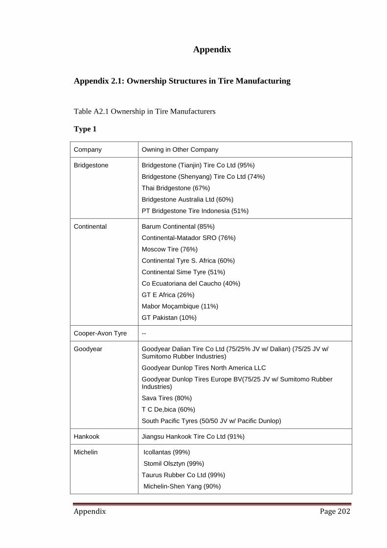
http://eh.net/encyclopedia/article/frank.international.rubber.market

Appendix Page 202

Appendix

Appendix 2.1: Ownership Structures in Tire Manufacturing

Table A2.1 Ownership in Tire Manufacturers

Type 1

Company Owning in Other Company

Bridgestone Bridgestone (Tianjin) Tire Co Ltd (95%)

Bridgestone (Shenyang) Tire Co Ltd (74%)

Thai Bridgestone (67%)

Bridgestone Australia Ltd (60%)

PT Bridgestone Tire Indonesia (51%)

Continental Barum Continental (85%)

Continental-Matador SRO (76%)

Moscow Tire (76%)

Continental Tyre S. Africa (60%)

Continental Sime Tyre (51%)

Co Ecuatoriana del Caucho (40%)

GT E Africa (26%)

Mabor Moçambique (11%)

GT Pakistan (10%)

Cooper-Avon Tyre --

Goodyear Goodyear Dalian Tire Co Ltd (75/25% JV w/ Dalian) (75/25 JV w/ Sumitomo Rubber Industries)

Goodyear Dunlop Tires North America LLC

Goodyear Dunlop Tires Europe BV(75/25 JV w/ Sumitomo Rubber Industries)

Sava Tires (80%)

T C De,bica (60%)

South Pacific Tyres (50/50 JV w/ Pacific Dunlop)

Hankook Jiangsu Hankook Tire Co Ltd (91%)

Michelin

Icollantas (99%)

Stomil Olsztyn (99%)

Taurus Rubber Co Ltd (99%)

Michelin-Shen Yang (90%)

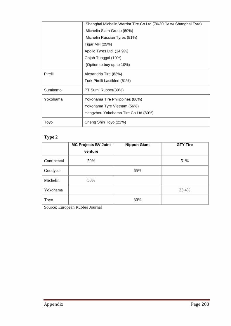
Appendix Page 203

Shanghai Michelin Warrior Tire Co Ltd (70/30 JV w/ Shanghai Tyre)

Michelin Siam Group (60%)

Michelin Russian Tyres (51%)

Tigar MH (25%)

Apollo Tyres Ltd. (14.9%)

Gajah Tunggal (10%)

(Option to buy up to 10%)

Pirelli

Alexandria Tire (83%)

Turk Pirelli Lastikleri (61%)

Sumitomo PT Sumi Rubber(80%)

Yokohama Yokohama Tire Philippines (80%)

Yokohama Tyre Vietnam (56%)

Hangzhou Yokohama Tire Co Ltd (80%)

Toyo Cheng Shin Toyo (22%)

Type 2

MC Projects BV Joint

venture

Nippon Giant GTY Tire

Continental 50% 51%

Goodyear 65%

Michelin 50%

Yokohama 33.4%

Toyo 30%

Source: European Rubber Journal

Appendix Page 204

Appendix 2.2: International Natural Rubber Organization (INRO)

The INRO Establishment

Major attempts to address issues of price fluctuation date back to 1976, when the United

Nations Conference on Trade and Development (UNCTAD) agreed to set up some

organizations to resolve for the problem of commodity price fluctuation. Consequently,

the International Natural Rubber Organization (INRO) was set up. INRO is the

operating body for the International Natural Rubber Agreement (INRA), which was

arranged by UNCTAD since 1979. The agreement was continued in 1987 as INRA II

and 1995 as INRA III. The aim is to maintain balancing between rubber demand and

supply; the only tool is a buffer stock of 550,000 tons of rubber. There are 22 member

countries, each member sends payment to support the maintenance of the buffer stock.

The Operation Feature of INRO

INRO operated through:

Buffer stock.

o Its quantity was 400,000 tons plus a contingency quantity of

150,000 tons.

Reference price.

o The buying and selling of the stock was operated with a set of

benchmarked prices. It comprises reference price, upper intervention

price, lower intervention price, upper trigger action price, lower trigger

action price, upper indicative price and lower indicative price. The prices

are based on a price basket (Kuala Lumpur RSS1, Bangkok RSS3 and

New York TSR20 are items in the DMIP45

price basket.) in

Malaysia/Singapore cents per kilogram.

45

Malaysian/Singapore cent is defined as the average of the Malaysian sen and the Singapore cent at the

prevailing rates of exchange (South Centre, 2004).

Appendix Page 205

Figure A2.1 INRO Prices Setting

Upper Indicative Price = 270 Malaysia/Singapore cents per kilogram.

Upper Trigger Action Price = Reference Price + 20%

(must sell)

Upper Intervention Price = Reference Price +15%

(may sell)

Reference Price

Lower Intervention Price = Reference Price -15%

(may buy)

Lower Trigger Action Price = Reference Price - 20%

(must buy)

Lower Indicative Price

When adjusting reference price, the corresponding trigger price cannot exceed the limit =157 Malaysia/Singapore cents per kilogram.

Daily Market Indicative Prices (DMIP)

This is a composite price based on 5 days average of prices of RSS1, RSS3 and TSR20

by the ratio 2:3:5. The three prices are coded from four markets namely USA, UK,

Malaysia and Singapore markets.

Operation Criteria

If DMIP is higher (or lower) than upper intervention price, the buffer stock manager

may sell (buy) the stocks.

If DMIP is higher (or lower) than upper triggering price, the buffer stock manager must

sell (buy) the stocks.

Appendix Page 206

Adjustment of the Reference Price

Every 12 months

When the DMIP was different from intervention prices for over 6

months.

When buffer stocks were less than 100,000 tons or over 300,000

tons.

Upper and lower indicative prices will be revised every 24

months (INRA III).

INRA I had more than 65% from each side of countries. INRA II had more than 89%

producers and 75% consumer country. INRA III had more than 94% producer but only

48% consumer countries.

INRO Operation Results

Operation outcomes: INRA I and INRA II gained 144.77 and 136.16 $US/tons

respectively. INRA III lost 103.27 $US/ton due to inability to operate effectively.

Although INRO managed to achieve a degree of price stabilization, helped generate

capital from member country to hold the buffer stock, and generated some rubber R&D,

the results were far from adequate. It was argued that:

Natural rubber supply outgrew demand so much that the buffer stock was

not effective.

Member countries were slow in submitting the payments;

INRO did not buy equally from each country

The types of rubber that were bought by INRO did not match the types

that were produced

Most of the stocks were kept in some specific countries and did not

provide storage income to other countries

Appendix Page 207

The exchange rate crisis significantly increased foreign exchange rates

thus increasing the weight of fees for Asian currency suppliers to keep the buffer

stock.

From 1998, member counties refused to pay their fees. This made it difficult for INRO

to manage the buffer stock and as a result rubber prices decreased tremendously. When

Malaysia quit INRO the remaining five members from the supplying countries were left

to bear the expenses. The fees that producer member countries had to submit were about

31.5 % greater than the fees paid by consuming countries. The bargaining power of the

remaining supplying members also decreased. Consequently, all the producing countries

quit the INRO which was then abolished in October 1999 leaving 138,296 tons of

rubber stocks to be sold before 30 June 2001.

Table A2.2 depicts INRO‟s DMIP and world stocks level during its operation. Figure

A2.1 compares the changes in natural rubber prices, stocks and INRO‟s daily market

indicative prices (DMIP)46

. Graphics are revealed in standardized values.

The changes in world stocks and INRO DMIP display some association. However,

appropriate empirical evaluation is required to identify this relation.

Table A2.2 World Natural Stocks and INRO Daily Market Indicator Prices

(DMIP)

Year

Stocks

(1,000 tons)

DMIP

Year

Stocks

(1,000 tons)

DMIP

1981 1755.0 224.1 1991 1600.0 176.2

1982 1825.0 176.5 1992 1680.0 174.0

1983 1855.0 225.2 1993 1640.0 168.2

1984 1875.0 205.6 1994 1700.0 229.1

1985 1860.0 170.6 1995 1790.0 307.9

1986 1790.0 184.1 1996 2080.0 267.0

1987 1840.0 217.4 1997 2010.0 209.3

1988 1800.0 254.8 1998 2140.0 191.0

1989 1730.0 207.1 1999 2550.0 160.6

1990 1530.0 181.6 2000 2040.0 113.0

Source: International Rubber Study Group

46

WRS1 is natural rubber price (RSS1), stocks is natural rubber stock.

Appendix Page 208

The relationship among the three variables can be seen in figure A2.2 where DMPI was

above WRS1 from 1981 to 1989; from 1989 to mid 1997 it was close to WRS1; and it is

below WRS1 from mid 1997 to 2000, demonstrating a sharp fall coincident with the

rising stock level.

Figure A2.2 RSS1 Natural Rubber Price, Changes in Stocks and INRO’s Daily Market Indicative

Prices

Appendix Page 209

Appendix 5.1: Variable Tests for Stationary

Variables are tested using the Phillips-Perron unit root tests (PP). The PP test uses a

non-parametric correction for serial correlation. It uses the same critical value as the

Dickey-Fuller tests (SHAZAM, 1997 pp. 166-167). If tests on the first differences of

variables reject the null hypothesis of unit root then the series are stationary at I(1).

Table A5.1 Variable Tests for Stationarity

PP I(1) With constant A(0),

lagged term coefficient A(1), no trend

With constant A(0), lagged term coefficient A(1),

trend coefficient A(2)

Test Variable Critical Values

Test A(1)=0

10% -2.57 5% -2.86 1% -3.43

Test A(0)=A(1)=0

10%3.78 5% 4.59 1% 6.43

Test A(1)=0

10% -3.13 5% -3.41 1% -3.96

Test A(0)=A(1)=A(2)=0

10%4.03 5% 4.68 1% 6.09

Test A(1)=A(2)=0

10% 5.34 5% 6.25 1% 8.27

Variables in Equations (5:1), (5:2): Tire Demand Function

P -4.84 11.74 -5.57 10.49 15.72

Q -4.49 10.12 -4.70 7.56 11.29

VP -5.47 15.02 -5.88 11.71 17.45

VI -1.98 2.05 -4.06 5.59 8.26

GDPPUS -4.32 9.39 -4.23 6.17 9.25

All variables reject the null hypothesis of unit root at 1% significant level except for vehicle in-use (VI) which rejects only the model with a trend (5%).

Variables in Equations (5:3), (5:4) Natural Rubber Supply Function


Test A(1)=0

10% -2.57 5% -2.86 1% -3.43

Test

A(0)=A(1)=0 10%3.78 5% 4.59 1% 6.43

Test A(1)=0

10% -2.57 5% -2.86 1% -3.43

Test

A(0)=A(1)=A(2)=0 10%4.03 5% 4.68 1% 6.09

Test A(1)=A(2)=0 10% 5.34 5% 6.25 1% 8.27

WR -5.39 14.57 -5.33 9.50 14.25

XR -6.06 18.36 -6.02 12.08 18.12

RAIN -9.43 44.31 -9.32 28.82 43.23

Appendix Page 210

WSt-3 -5.87 17.22 -7.65 20.09 30.10

ERJA -4.41 9.74 -4.50 6.77 10.15

ERTH -4.10 8.09 -4.13 5.74 8.59

ERSP -3.88 7.63 -3.83 4.97 7.41

RQM -5.56 15.52 -5.55 10.34 15.49

All variables reject the null hypothesis of unit root at 1% significant level except for Thai exchange rate (ERTH) and Singapore currency exchange rate (ERSP) (with trend, rejected at 5% significant level).

Variables in Equation (5:5US) US Tire Production Function


Test A(1)=0

10% -2.57 5% -2.86 1% -3.43

Test A(0)=A(1)=0

10%3.78 5% 4.59 1% 6.43

Test A(1)=0

10% -3.13 5% -3.41 1% -3.96

Test A(0)=A(1)=A(2)=0

10%4.03 5% 4.68 1% 6.09

Test A(1)=A(2)=0

10% 5.34 5% 6.25 1% 8.27

qUS -6.59 21.72 -6.50 14.08 21.12

xrUS -6.90 23.94 -6.88 15.89 23.67

xsUS -5.99 18.01 -6.04 12.20 18.25

WO -5.22 13.66 -5.16 8.92 13.35

VIUS -4.44 9.87 -4.50 6.78 10.14

All variables reject the null hypothesis of unit root at 1% significant level

Variables in Equation (5:5FR) France Tire Production Function


Test A(1)=0

10% -2.57 5% -2.86 1% -3.43

Test A(0)=A(1)=0

10%3.78 5% 4.59 1% 6.43

Test A(1)=0

10% -3.13 5% -3.41 1% -3.96

Test A(0)=A(1)=A(2)=0

10%4.03 5% 4.68 1% 6.09

Test A(1)=A(2)=0

10% 5.34 5% 6.25 1% 8.27

qFR -5.75 16.58 -5.74 11.02 16.52

xrFR -5.12 13.14 -5.09 8.66 13.00

xsFR -5.31 14.09 -5.50 10.11 15.17

VPFR -6.17 19.00 -6.26 13.08 19.61


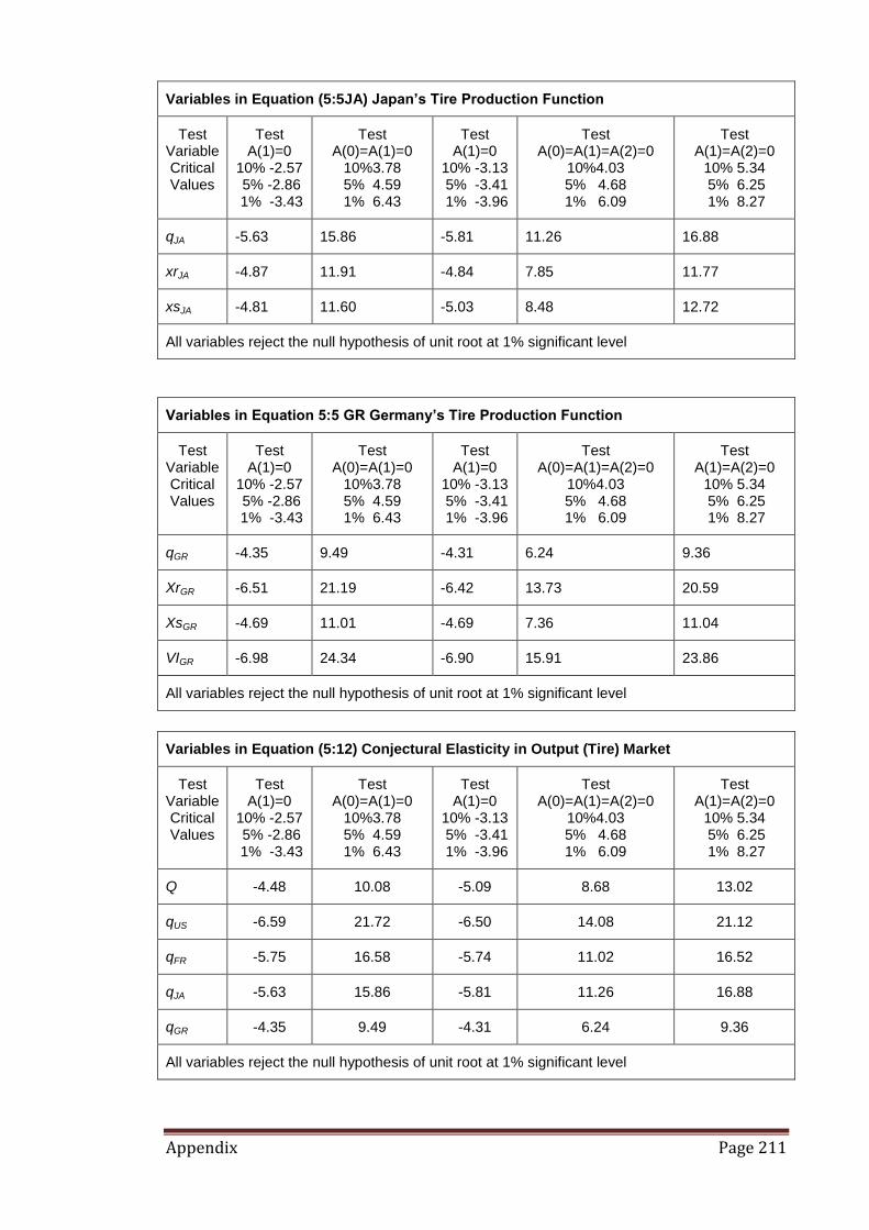
Appendix Page 211

Variables in Equation (5:5JA) Japan’s Tire Production Function


Test A(1)=0

10% -2.57 5% -2.86 1% -3.43

Test A(0)=A(1)=0

10%3.78 5% 4.59 1% 6.43

Test A(1)=0

10% -3.13 5% -3.41 1% -3.96

Test A(0)=A(1)=A(2)=0

10%4.03 5% 4.68 1% 6.09

Test A(1)=A(2)=0

10% 5.34 5% 6.25 1% 8.27

qJA -5.63 15.86 -5.81 11.26 16.88

xrJA -4.87 11.91 -4.84 7.85 11.77

xsJA -4.81 11.60 -5.03 8.48 12.72


Variables in Equation 5:5 GR Germany’s Tire Production Function


Test A(1)=0

10% -2.57 5% -2.86 1% -3.43

Test A(0)=A(1)=0

10%3.78 5% 4.59 1% 6.43

Test A(1)=0

10% -3.13 5% -3.41 1% -3.96

Test A(0)=A(1)=A(2)=0

10%4.03 5% 4.68 1% 6.09

Test A(1)=A(2)=0

10% 5.34 5% 6.25 1% 8.27

qGR -4.35 9.49 -4.31 6.24 9.36

XrGR -6.51 21.19 -6.42 13.73 20.59

XsGR -4.69 11.01 -4.69 7.36 11.04

VIGR -6.98 24.34 -6.90 15.91 23.86


Variables in Equation (5:12) Conjectural Elasticity in Output (Tire) Market


Test A(1)=0

10% -2.57 5% -2.86 1% -3.43

Test A(0)=A(1)=0

10%3.78 5% 4.59 1% 6.43

Test A(1)=0

10% -3.13 5% -3.41 1% -3.96

Test A(0)=A(1)=A(2)=0

10%4.03 5% 4.68 1% 6.09

Test A(1)=A(2)=0

10% 5.34 5% 6.25 1% 8.27

Q -4.48 10.08 -5.09 8.68 13.02

qUS -6.59 21.72 -6.50 14.08 21.12

qFR -5.75 16.58 -5.74 11.02 16.52

qJA -5.63 15.86 -5.81 11.26 16.88

qGR -4.35 9.49 -4.31 6.24 9.36


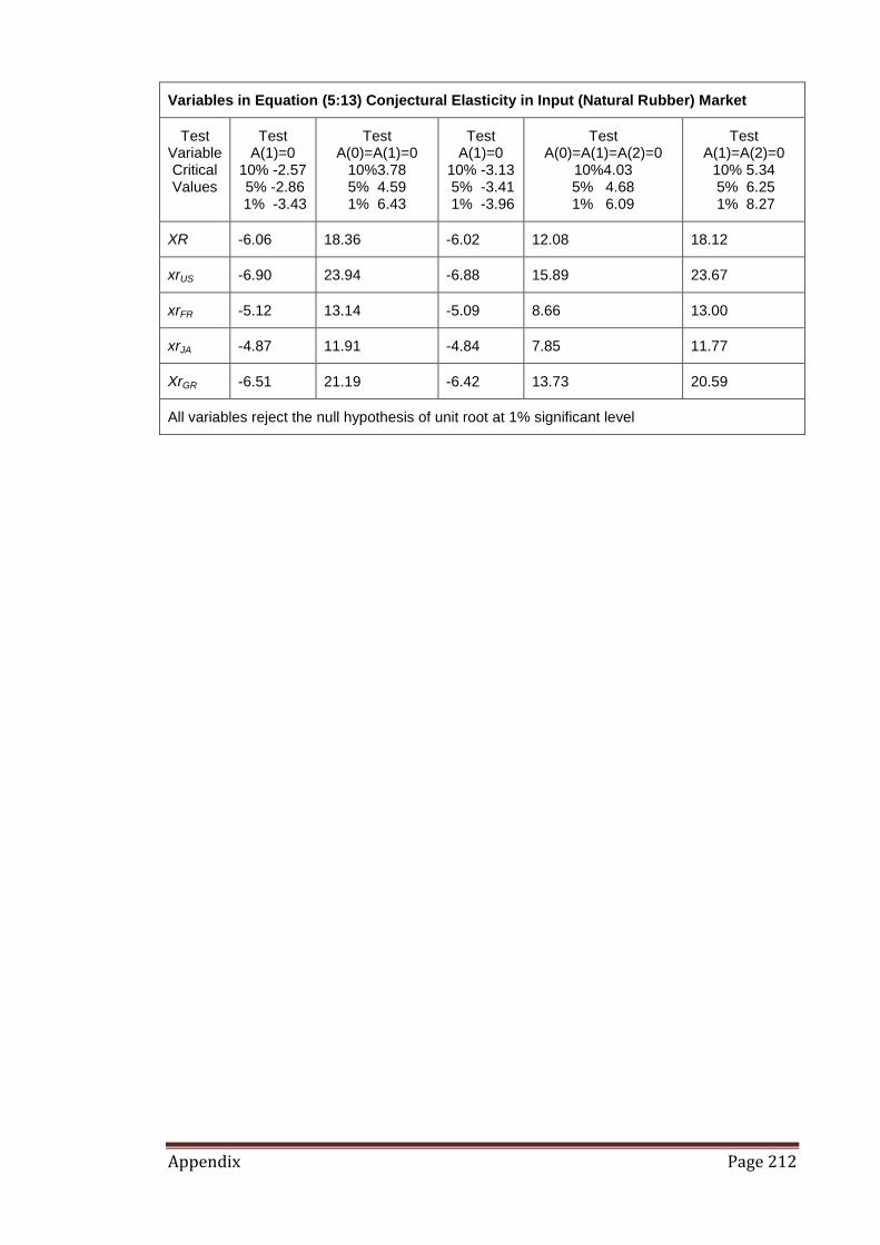
Appendix Page 212

Variables in Equation (5:13) Conjectural Elasticity in Input (Natural Rubber) Market


Test A(1)=0

10% -2.57 5% -2.86 1% -3.43

Test A(0)=A(1)=0

10%3.78 5% 4.59 1% 6.43

Test A(1)=0

10% -3.13 5% -3.41 1% -3.96

Test A(0)=A(1)=A(2)=0

10%4.03 5% 4.68 1% 6.09

Test A(1)=A(2)=0

10% 5.34 5% 6.25 1% 8.27

XR -6.06 18.36 -6.02 12.08 18.12

xrUS -6.90 23.94 -6.88 15.89 23.67

xrFR -5.12 13.14 -5.09 8.66 13.00

xrJA -4.87 11.91 -4.84 7.85 11.77

XrGR -6.51 21.19 -6.42 13.73 20.59


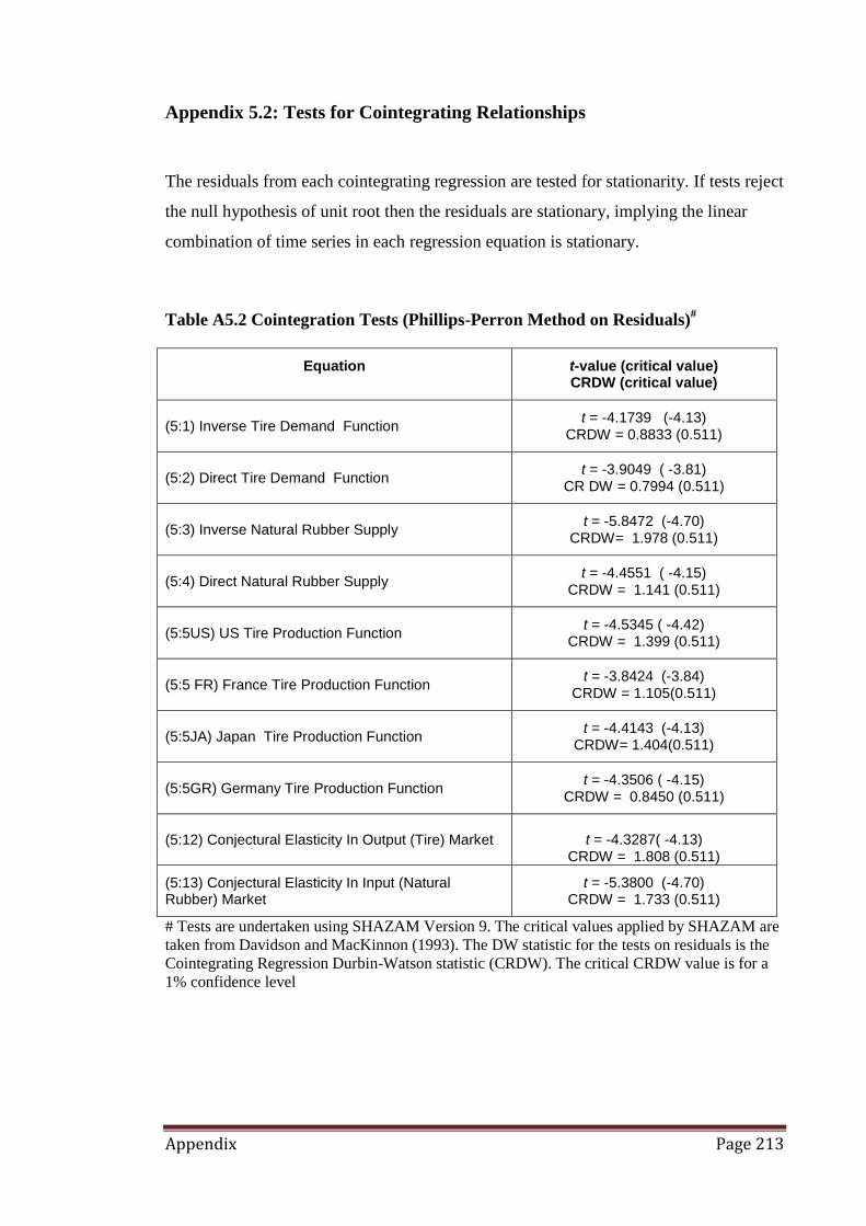
Appendix Page 213

Appendix 5.2: Tests for Cointegrating Relationships

The residuals from each cointegrating regression are tested for stationarity. If tests reject

the null hypothesis of unit root then the residuals are stationary, implying the linear

combination of time series in each regression equation is stationary.

Table A5.2 Cointegration Tests (Phillips-Perron Method on Residuals)#

Equation t-value (critical value)

CRDW (critical value)

(5:1) Inverse Tire Demand Function t = -4.1739 (-4.13)

CRDW = 0.8833 (0.511)

(5:2) Direct Tire Demand Function t = -3.9049 ( -3.81)

CR DW = 0.7994 (0.511)

(5:3) Inverse Natural Rubber Supply t = -5.8472 (-4.70)

CRDW= 1.978 (0.511)

(5:4) Direct Natural Rubber Supply t = -4.4551 ( -4.15)

CRDW = 1.141 (0.511)

(5:5US) US Tire Production Function t = -4.5345 ( -4.42)

CRDW = 1.399 (0.511)

(5:5 FR) France Tire Production Function t = -3.8424 (-3.84)

CRDW = 1.105(0.511)

(5:5JA) Japan Tire Production Function t = -4.4143 (-4.13)

CRDW= 1.404(0.511)

(5:5GR) Germany Tire Production Function t = -4.3506 ( -4.15)

CRDW = 0.8450 (0.511)

(5:12) Conjectural Elasticity In Output (Tire) Market

t = -4.3287( -4.13) CRDW = 1.808 (0.511)

(5:13) Conjectural Elasticity In Input (Natural Rubber) Market

t = -5.3800 (-4.70) CRDW = 1.733 (0.511)

# Tests are undertaken using SHAZAM Version 9. The critical values applied by SHAZAM are

taken from Davidson and MacKinnon (1993). The DW statistic for the tests on residuals is the

Cointegrating Regression Durbin-Watson statistic (CRDW). The critical CRDW value is for a

1% confidence level

Appendix Page 214

Appendix 5.3: Error Correction Models for Natural Rubber Price and

Quantity Figure A.1 Changes in World

Natural Rubber Price RSS1

(WR)

Figure A.2 Changes in World

Natural Rubber Quantity

Production

Figure A.3 Changes in Residual

Terms (Inverse Natural Rubber

Supply)

Figure A.4 Changes in Residual

Terms (Direct Natural Rubber

Supply)

Table A5.3.1 Variable Description for Error Correction Models

WR Changes in Natural rubber price

1 tWR

One year lag of Changes in Natural rubber price

XR Changes in world natural rubber production

1 tXR

One year lag of Changes in world natural rubber production

2 tXR

two years lag of Changes in world natural rubber production

)( XRINRO Changes in

)( XRINRO

ERJA Changes in Japan’s currency exchange rates

ERSP Changes in Singapore’s currency exchange rates

2)( tXRRAIN Two years lag of changes in

)( XRRAIN

Appendix Page 215

Table A5.3.1 (cont.)

1 tERTH

One year lag of changes in Thailand’s currency exchange rates

1

ˆt

WR

Estimated natural rubber price residuals

1

ˆt

XR

Estimated natural rubber production residual

Table A5.3.2 Error Correction Model for the Inverse Natural Rubber Supply

1

ˆ)(

)(

1019282716

543211

tWRtttt

t

aERTHaXRRAINaXRaXRa

ERSPaERJAaXRINROaXRaWRaWR

Coefficient

(t-value)

1)( tWR 1a

0.43462*** (4.011)

XR 2a

3.4076 (7.624)***

)( XRINRO 3a

-0.7107 (-3.846)***

ERJA 4a

-0.3971** (-2.413)

ERSP 5a

-0.7793 (-4.286)***

1)( tXR 6a

-2.6397 (-5.169)***

2)( tXR 7a

-1.4151 (-3.241)***

2))(( tXRRAIN 8a

0.4505 (3.057)***

1)( tERTH 9a

0.7030 (3.006)***

1

ˆt

WR

10a

-0.6693 (-1.839)*

DURBIN-WATSON 2.1576

R2 0.8966

Price adjusted 67% in the consecutive year.

Appendix Page 216

Table A5.3.3 Error Correction Model for the Direct Natural Rubber Supply

Function

1

ˆ413211

tXRtt bWRbWRbXRbXR

Coefficient

(t-value)

1)( tXR 1b

0.8099 (6.523)***

WR 2b

0.1082 (4.671)***

1)( tWR 3b

-0.1053 (-4.321)***

1

ˆt

XR

4b

-0.8713 (-3.302)***

DURBIN-WATSON 2.0691

R2 0.4538

Quantity adjusted by 87 % in the consecutive year.

Appendix Page 217

Appendix 5.4 Variables and Data

Table A5.4 1 Variables and Data

Variable Description Source

CPIJA Japan’s consumer price index

United Nations Economic and Social Commission for Asia and the Pacific (ESCAP)

CPISP

Singapore’s consumer price index


CPITH

Thailand’s consumer price index


CPIUS1

US consumer price index

Us Bureau of Labor Statistics

DRXSM

Structural change dummy variable for a change in the mix of natural rubber and synthetic rubber following introduction of the radial tire .(1970 -2000 = 1)

(Dummy variable)

ERJA Japan’s currency exchange rates (100Yen/$US)

The Bank of Thailand

ERML Malaysia’s currency exchange rates (ringgit/$US)

ERSP Singapore’s currency exchange rates(S$/ $US)


ERTH Thailand’s currency exchange rates (Baht/$US)


INRO The International Natural Rubber Organization

(Dummy variable)

GDPPUS US per capita income The World Bank

P Tire prices: US tire price index US Bureau of Labor Statistics

Q World tire production International Rubber Study Group

qFR Tire production (France’s passenger car tires and truck tires)

International Rubber Study Group

qGR Tire production (Germany’s passenger car tires and truck tires).


qJA Tire production (Japanese passenger car tires and truck tires)


Appendix Page 218

Table A5.4.1 Variables (cont.)


qUS Tire production (US passenger car tires and truck tires)


RAIN Rainfall quantity The Royal Irrigation Department, Thailand

RQM

Top seven countries’ quantity / total quantity ratio. Top seven tire producing countries are US, France, Japan, Germany, Italy, UK and India.

Compiled from International Rubber Study Group

T A time trend. -

VI World passenger car and commercial vehicles in-use.


VIGR Vehicle in-use in Germany (only Passenger cars).


VIUS Total vehicle in-use in the US.(passenger car and commercial vehicle)


VP World passenger car and commercial vehicle production


VPFR Total vehicle production in France (passenger car and commercial vehicle)


WO World crude oil price, Spot Oil Price (West Texas Intermediate)

Federal Reserve Bank of St. Louis, Economic Research.

WR Natural Rubber Price: RSS1 natural rubber prices, fob Malaysia ringgit/ton


WSt-3 Synthetic rubber price lagged by 3 years International Rubber Study Group

XR World Natural Rubber Production International Rubber Study Group

xrFR Quantity of natural rubber used in Tire sector in France.


xrGR Quantity of natural rubber used in tire sector in Germany.


xrJA Quantity of natural rubber used in Tire sector in Japan.


Appendix Page 219

Table A5.4.2 Variables (cont.)


xrUS Quantity of natural rubber used in tire sector in the US.


xsFR Quantity of synthetic rubber used in Tire sector in France.


xsGR Quantity of synthetic rubber used in tire sector in Germany.


xsJA Quantity of synthetic rubber used in tire sector in Japan.


xsUS Quantity of synthetic rubber used in tire sector in the US.


Appendix Page 220

Table A5.4.2 Data

year

CPIJA

CPISP

CPITH

CPIUS1

ERJA (100 Yen/$US)

ERML (Ringgit/$US)

ERSP (S$/$US)

ERTH (Baht/$US)

1960 21.80 76.82 20.49 88.70 360.00 3.10 3.06 21.18

1961 23.00 76.16 22.00 89.60 360.00 3.10 3.06 21.06

1962 24.60 88.46 22.82 90.60 360.00 3.10 3.06 20.88

1963 26.40 92.30 22.82 91.70 360.00 3.10 3.06 20.83

1964 27.40 97.75 22.64 92.90 360.00 3.10 3.06 20.80

1965 29.50 88.12 22.67 94.50 360.00 3.10 3.06 20.80

1966 31.00 84.65 23.59 97.20 360.00 3.10 3.06 20.80

1967 32.30 81.82 24.61 100.00 360.00 3.10 3.06 20.80

1968 34.00 78.51 25.05 104.20 360.00 3.10 3.06 20.80

1969 35.80 77.47 25.66 109.80 360.00 3.10 3.06 20.80

1970 38.50 76.81 25.64 116.30 360.00 3.10 3.06 20.80

1971 40.90 76.51 25.76 121.30 349.33 3.10 3.05 20.80

1972 42.90 80.36 27.01 125.30 303.17 2.80 2.81 20.80

1973 47.90 99.44 31.20 133.10 271.70 2.40 2.46 20.62

1974 59.10 107.63 38.78 147.70 292.08 2.40 2.44 20.38

1975 66.00 100.12 40.85 161.20 296.79 2.40 2.37 20.38

1976 72.20 90.12 42.54 170.50 296.55 2.50 2.47 20.38

1977 78.10 86.31 45.78 181.50 268.51 2.50 2.44 20.38

1978 81.40 90.02 49.40 195.40 210.44 2.30 2.27 20.34

1979 84.40 92.98 54.29 217.40 219.14 2.20 2.17 20.42

1980 90.90 97.76 64.99 246.80 226.74 2.20 2.14 20.48

1981 95.40 91.12 73.22 272.40 220.54 2.30 2.11 21.82

1982 98.00 82.69 77.07 289.10 249.08 2.30 2.14 23.00

1983 99.80 83.79 79.94 298.40 237.51 2.30 2.11 23.00

1984 102.10 83.27 80.64 311.10 237.52 2.30 2.13 23.64

1985 104.20 78.26 82.60 322.20 238.54 2.50 2.20 27.16

1986 104.80 76.58 84.12 328.40 168.52 2.60 2.18 26.30

1987 104.90 79.04 86.22 340.40 144.64 2.50 2.11 25.72

1988 105.70 80.29 89.50 354.30 128.15 2.60 2.01 25.29

1989 108.10 81.71 94.40 371.30 137.96 2.70 1.95 25.70

1990 111.40 90.18 99.97 391.40 144.79 2.70 1.81 25.59

1991 115.10 93.08 105.70 408.00 134.71 2.80 1.73 25.52

1992 117.00 97.31 110.00 420.30 126.65 2.50 1.63 25.40

1993 118.50 101.00 113.70 432.70 111.20 2.60 1.62 25.32

1994 119.30 106.87 119.50 444.00 102.21 2.60 1.53 25.15

1995 119.20 115.27 126.40 456.50 94.06 2.50 1.42 24.92

1996 119.30 114.64 133.80 469.90 108.78 2.50 1.41 25.34

1997 121.50 110.49 141.20 480.80 120.99 2.80 1.48 31.36

1998 122.20 95.40 152.70 488.30 130.91 3.90 1.67 41.36

1999 121.80 93.25 153.20 499.00 113.91 3.90 1.69 37.84

2000 121.00 92.08 155.65 515.80 107.77 3.84 1.72 40.14

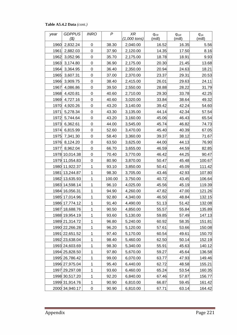
Appendix Page 221

Table A5.4.2 Data (cont.)

year

GDPPUS

($) INRO

P

XR (1,000 tons)

qFR

(mill) qGR

(mill) qJA

(mill)

1960 2,832.24 0 38.30 2,040.00 16.52 16.35 5.56

1961 2,882.03 0 37.90 2,120.00 14.35 17.50 8.16

1962 3,052.96 0 35.70 2,175.00 18.78 18.91 9.93

1963 3,174.80 0 36.90 2,175.00 20.30 21.45 13.68

1964 3,364.95 0 36.40 2,350.00 20.94 24.63 18.21

1965 3,607.31 0 37.00 2,370.00 23.37 29.31 20.53

1966 3,909.75 0 38.40 2,415.00 26.01 29.63 24.11

1967 4,086.86 0 39.50 2,550.00 28.88 28.22 31.79

1968 4,420.81 0 40.60 2,710.00 29.30 33.78 42.25

1969 4,727.16 0 40.60 3,020.00 33.84 38.64 49.32

1970 4,920.26 0 43.20 3,140.00 39.42 42.24 54.60

1971 5,278.34 0 43.30 3,135.00 44.14 42.34 57.54

1972 5,744.64 0 43.20 3,160.00 45.06 46.43 65.54

1973 6,362.61 0 44.00 3,545.00 45.74 46.82 74.73

1974 6,815.99 0 52.60 3,470.00 45.40 40.39 67.05

1975 7,341.30 0 58.40 3,360.00 39.37 38.12 71.67

1976 8,124.20 0 63.50 3,625.00 44.00 44.13 76.90

1977 8,962.04 0 66.70 3,655.00 46.59 44.59 82.85

1978 10,014.38 0 70.40 3,770.00 46.42 44.25 90.47

1979 11,054.83 0 80.90 3,870.00 50.47 45.48 100.67

1980 11,922.37 1 93.10 3,850.00 50.41 45.09 111.42

1981 13,244.87 1 98.30 3,705.00 43.46 42.93 107.80

1982 13,635.93 1 100.00 3,750.00 40.72 43.45 106.64

1983 14,598.14 1 96.10 4,025.00 45.56 45.19 119.39

1984 16,056.31 1 94.90 4,260.00 47.82 47.00 121.26

1985 17,014.96 1 92.80 4,340.00 46.50 48.84 132.15

1986 17,774.12 1 91.40 4,490.00 51.13 51.42 132.08

1987 18,688.76 1 90.50 4,850.00 55.57 55.84 135.89

1988 19,954.19 1 93.60 5,130.00 59.85 57.49 147.13

1989 21,314.72 1 96.80 5,240.00 60.92 58.35 151.81

1990 22,266.28 1 96.20 5,120.00 57.61 53.66 150.08

1991 22,651.52 1 97.40 5,170.00 60.54 49.61 150.70

1992 23,638.04 1 98.40 5,460.00 62.50 50.14 152.19

1993 24,603.69 1 98.30 5,340.00 55.91 45.63 140.12

1994 25,828.50 1 97.80 5,670.00 59.27 45.64 136.58

1995 26,786.42 1 99.00 6,070.00 63.77 47.93 149.46

1996 27,975.04 1 95.40 6,440.00 62.72 48.58 155.21

1997 29,297.08 1 93.60 6,460.00 65.24 53.54 160.35

1998 30,517.20 1 92.20 6,840.00 67.46 57.87 156.77

1999 31,914.76 1 90.90 6,810.00 66.87 59.45 161.42

2000 34,940.17 0 90.90 6,810.00 67.71 63.14 164.42

Appendix Page 222


year

Q

(mill) QM7 (mill)

qUS (mill)

RAIN (millimetres)

VI (mill)

VIUS

(mill)

1960 231.11 183.12 119.82 1,807.80 116.18 73.58

1961 234.24 184.84 116.78 2,143.30 123.11 75.60

1962 268.87 209.71 133.87 1,947.10 131.64 78.65

1963 296.22 231.26 139.07 2,198.50 141.72 82.12

1964 335.56 257.71 158.11 1,321.00 152.75 86.10

1965 363.95 283.14 167.83 2,927.80 163.69 90.36

1966 392.79 300.19 177.46 3,268.60 174.70 93.96

1967 399.08 298.96 163.19 1,671.00 186.07 96.93

1968 468.35 357.02 202.94 1,769.50 198.25 100.89

1969 501.80 383.58 207.83 2,821.90 211.34 105.10

1970 513.34 386.49 190.40 2,561.90 223.78 108.41

1971 560.90 421.80 216.36 2,269.10 237.64 112.99

1972 599.24 435.03 229.61 1,883.40 254.15 118.80

1973 617.55 439.27 223.87 2,500.50 270.59 125.65

1974 591.15 416.77 211.35 2,113.00 291.44 129.93

1975 561.10 392.61 186.71 2,028.00 326.60 132.96

1976 598.50 412.63 185.95 2,519.00 344.70 138.54

1977 669.40 447.99 231.64 1,578.70 360.80 142.09

1978 673.00 446.12 223.41 1,288.10 380.00 148.05

1979 685.70 444.74 206.69 1,706.40 396.80 151.87

1980 654.80 419.12 159.26 1,784.20 414.70 155.80

1981 646.80 426.13 181.76 2,232.50 429.40 158.29

1982 640.80 419.62 178.50 1,963.60 442.40 159.64

1983 683.20 442.52 186.92 2,137.50 458.10 163.75

1984 729.70 471.04 209.38 2,217.60 468.70 166.25

1985 733.90 474.89 196.92 1,983.80 485.90 171.69

1986 755.20 481.56 190.29 1,789.10 502.90 175.70

1987 802.10 504.48 202.98 1,628.10 516.40 178.91

1988 851.90 530.54 211.35 1,684.80 535.70 184.39

1989 860.70 545.04 212.87 1,586.80 555.20 187.36

1990 847.50 537.46 210.66 1,454.80 573.60 188.80

1991 845.30 540.77 202.39 1,784.80 593.10 188.14

1992 899.30 573.59 230.25 1,467.70 608.90 190.36

1993 890.90 551.51 237.45 2,414.10 631.80 194.06

1994 917.80 561.56 243.70 1,838.20 645.40 198.05

1995 972.90 598.84 255.52 2,274.70 660.10 201.50

1996 1006.80 604.94 255.72 2,363.00 677.50 206.37

1997 1052.50 624.71 263.86 2,192.00 692.90 207.75

1998 1074.20 628.07 270.91 1,698.60 709.30 211.62

1999 1095.60 625.19 267.65 2,969.50 723.80 216.31

2000 1147.80 638.36 276.76 2,417.90 748.00 221.48

Appendix Page 223


year

VPFR (mill)

VP

(mill) VIGR

(mill) WO

($US/barrel) WR

(Ringitt/ton) WS

($US/ton)

1960 1.37 14.47 4.86 2.97 2,383.00 683.00

1961 1.25 13.35 5.77 2.97 1,842.00 655.00

1962 1.54 16.04 6.77 2.97 1,724.00 573.00

1963 1.74 18.41 7.75 2.97 1,597.00 582.00

1964 1.62 19.64 8.69 2.95 1,502.00 540.00

1965 1.64 22.02 9.72 2.92 1,544.00 553.00

1966 2.03 22.53 10.65 2.94 1,441.00 540.00

1967 2.01 22.22 11.29 3.03 1,192.00 509.00

1968 2.08 26.23 12.05 3.07 1,171.00 534.00

1969 2.46 27.33 13.17 3.30 1,539.00 467.00

1970 2.75 26.75 14.38 3.35 1,244.00 434.00

1971 3.01 31.12 15.48 3.56 1,016.00 432.00

1972 3.02 33.16 16.32 3.56 935.00 395.00

1973 3.22 36.39 17.04 3.87 1,655.00 408.00

1974 3.08 33.09 17.36 10.37 1,794.00 628.00

1975 2.86 32.90 18.16 11.16 1,357.00 657.00

1976 3.40 38.20 19.18 12.65 1,991.00 677.00

1977 3.51 40.90 20.38 14.30 2,028.00 803.00

1978 3.51 42.20 21.62 14.85 2,300.00 832.00

1979 3.61 41.50 22.61 22.40 2,794.00 931.00

1980 3.38 38.30 23.24 37.38 3,123.00 885.00

1981 3.02 37.00 23.68 36.67 2,578.00 1,042.00

1982 3.15 36.00 24.04 33.64 2,000.00 1,008.00

1983 3.34 39.90 24.69 30.40 2,469.00 974.00

1984 3.06 42.10 25.38 29.28 2,243.00 975.00

1985 3.02 44.70 26.10 27.97 1,886.00 975.00

1986 3.20 45.40 27.22 15.04 2,083.00 813.00

1987 3.49 46.00 28.30 19.16 2,481.00 836.00

1988 3.70 48.10 29.19 15.96 3,098.00 897.00

1989 3.92 49.30 30.15 19.59 2,625.00 1,139.00

1990 3.77 48.30 30.70 24.49 2,334.00 1,104.00

1991 3.61 46.20 37.46 21.48 2,267.00 995.00

1992 3.77 47.20 37.58 20.56 2,189.00 949.00

1993 3.16 46.00 39.20 18.46 2,135.00 1,007.00

1994 3.56 49.00 39.92 17.19 2,933.00 1,002.00

1995 3.48 49.60 40.50 18.43 3,956.00 1,331.00

1996 2.39 50.20 41.05 22.15 3,518.00 1,286.00

1997 2.57 53.40 41.33 20.60 2,787.00 1,245.00

1998 2.95 51.70 41.72 14.39 2,813.00 1,193.00

1999 3.18 54.20 42.42 19.25 2,404.00 1,017.00

2000 3.35 54.90 43.77 30.30 2,624.00 1,163.00

Appendix Page 224


year

xrFR

(1,000) xrGR

(1,000) xrJA

(1,000) xrUS

(1,000) xsFR

(1,000) xsGR

(1,000) xsJA

(1,000) xsUS

(1,000)

1960 76.60 76.60 76.90 328.80 49.40 62.90 22.10 682.00

1961 78.90 70.70 86.40 282.60 51.70 70.80 34.50 690.30

1962 78.40 74.30 90.10 309.50 56.90 78.30 46.80 774.00

1963 76.60 77.80 93.80 299.80 67.20 87.50 65.00 798.20

1964 77.10 78.10 98.30 318.50 77.20 101.80 80.50 898.90

1965 76.60 83.00 94.70 361.00 83.80 124.40 88.10 966.30

1966 78.60 80.10 101.30 393.20 95.10 122.60 102.70 1,041.30

1967 82.20 71.60 117.10 340.70 104.80 118.90 133.90 1,006.20

1968 86.40 80.00 125.00 402.60 109.60 139.80 175.20 1,229.50

1969 100.70 99.00 139.50 435.70 129.40 175.80 212.00 1,313.50

1970 114.20 102.70 154.00 393.00 148.20 181.30 245.00 1,209.90

1971 116.60 106.20 165.80 425.40 158.70 171.40 258.30 1,374.30

1972 119.00 105.00 188.30 469.40 173.70 173.70 293.00 1,479.70

1973 119.60 106.80 217.10 515.20 178.10 167.20 345.30 1,507.10

1974 123.80 113.30 218.20 561.10 183.60 165.40 326.90 1,404.60

1975 118.50 106.30 197.10 497.40 165.20 156.10 343.00 1,196.20

1976 127.90 114.90 207.50 491.00 175.90 165.50 367.30 1,221.80

1977 130.10 120.90 223.00 622.80 184.30 171.50 393.30 1,463.90

1978 132.60 117.30 250.40 590.60 178.10 161.40 413.80 1,377.60

1979 145.90 121.60 290.20 577.90 192.30 165.00 455.80 1,324.30

1980 156.90 120.30 324.80 438.80 197.60 154.80 503.70 1,082.20

1981 138.50 109.80 336.20 469.70 170.10 141.40 466.10 1,111.20

1982 126.90 110.20 334.90 433.20 155.60 138.50 410.90 960.60

1983 132.00 119.50 396.10 480.60 163.00 137.40 445.10 1,026.00

1984 135.00 129.80 414.50 575.10 159.00 137.70 476.80 1,093.90

1985 129.00 137.30 430.30 554.00 159.00 134.20 475.50 958.80

1986 134.40 137.70 433.90 520.60 157.20 140.20 426.60 919.30

1987 146.00 139.50 472.10 563.50 144.00 146.40 432.30 992.70

1988 157.00 146.70 518.60 657.30 153.00 144.40 502.70 1,011.00

1989 163.00 158.00 538.10 663.20 163.00 155.40 510.80 997.20

1990 155.30 151.50 555.10 621.90 150.20 152.10 500.20 1,101.70

1991 159.70 151.00 566.00 590.80 150.70 152.80 478.20 1,001.90

1992 156.80 159.00 569.30 680.40 162.70 155.30 467.60 1,129.30

1993 150.80 133.20 527.80 739.00 152.00 134.70 421.60 1,205.30

1994 161.80 139.20 536.50 758.50 161.20 140.30 421.60 1,196.80

1995 165.40 152.20 598.00 792.30 171.10 145.70 466.00 1,237.70

1996 174.10 156.00 615.00 775.70 170.10 135.00 487.00 1,232.20

1997 176.70 172.80 613.00 820.70 179.90 142.00 516.00 1,269.00

1998 182.70 169.00 616.00 862.40 186.70 166.00 506.00 1,340.90

1999 202.70 173.00 627.00 798.00 186.20 175.00 527.00 1,338.00

2000 205.00 172.00 649.00 947.00 196.00 182.00 525.00 1,203.00

Appendix Page 225


year

RQM

(CR7 Ratio) DRXSM

1960 0.79 0

1961 0.79 0

1962 0.78 0

1963 0.78 0

1964 0.77 0

1965 0.78 0

1966 0.76 0

1967 0.75 0

1968 0.76 0

1969 0.76 0

1970 0.75 1

1971 0.75 1

1972 0.73 1

1973 0.71 1

1974 0.71 1

1975 0.70 1

1976 0.69 1

1977 0.67 1

1978 0.66 1

1979 0.65 1

1980 0.64 1

1981 0.66 1

1982 0.65 1

1983 0.65 1

1984 0.65 1

1985 0.65 1

1986 0.64 1

1987 0.63 1

1988 0.62 1

1989 0.63 1

1990 0.63 1

1991 0.64 1

1992 0.64 1

1993 0.62 1

1994 0.61 1

1995 0.62 1

1996 0.60 1

1997 0.59 1

1998 0.58 1

1999 0.57 1

2000 0.56 1

A Study of its Impacts on the Natural Rubber Industry in ...

Documents

Transcript of A Study of its Impacts on the Natural Rubber Industry in ...