Biodiversity Data Journal 6: e28073doi: 10.3897/BDJ.6.e28073

Research Article

A story of data won, data lost and data re-found:

the realities of ecological data preservation

Alison Specht , Matthew P. Bolton , Bryn Kingsford , Raymond L. Specht , Lee Belbin‡ University of Queensland, Brisbane, Australia§ Corymbia Ecospatial Consultants, Canberra, Australia| Structured Data, Canberra, Australia¶ Emeritus Professor, Brisbane, Australia# Atlas of Living Australia, CSIRO, Canberra, Australia

Corresponding author: Alison Specht (a.specht@uq.edu.au)

Academic editor: Quentin Groom

Received: 29 Jun 2018 | Accepted: 29 Oct 2018 | Published: 07 Nov 2018

Citation: Specht A, Bolton M, Kingsford B, Specht R, Belbin L (2018) A story of data won, data lost and data re-found: the realities of ecological data preservation. Biodiversity Data Journal 6: e28073. https://doi.org/10.3897/BDJ.6.e28073

Abstract

This paper discusses the process of retrieval and updating legacy data to allow on-linediscovery and delivery. There are many pitfalls of institutional and non-institutionalecological data conservation over the long term. Interruptions to custodianship, old media,lost knowledge and the continuous evolution of species names makes resurrection of olddata challenging. We caution against technological arrogance and emphasise theimportance of international standards.

We use a case study of a compiled set of continent-wide vegetation survey data for which,although the analyses had been published, the raw data had not. In the original study,publications containing plot data collected from the 1880s onwards had been collected,interpreted, digitised and integrated for the classification of vegetation and analysis of itsconservation status across Australia. These compiled data are an extremely valuablenational collection that demanded publishing in open, readily accessible online repositories,such as the Terrestrial Ecosystem Research Network (http://www.tern.org.au) and the Atlasof Living Australia (ALA: http://www.ala.org.au), the Australian node of the GlobalBiodiversity Information Facility (GBIF: http://www.gbif.org). It is hoped that the lessons

‡ § | ¶ #

© Specht A et al. This is an open access article distributed under the terms of the Creative Commons Attribution License (CC BY4.0), which permits unrestricted use, distribution, and reproduction in any medium, provided the original author and source arecredited.

learnt from this project may trigger a sober review of the value of endangered data, the costof retrieval and the importance of suitable and timely archiving through the vicissitudes oftechnological change, so the initial unique collection investment enables multiple re-use inperpetuity.

Keywords

data conservation, data retrieval, legacy data, data curation, long-term data accessibility

Introduction

An argument without evidence is mere assertion (Parsons et al. 2010). Knowledge ofchange is fundamental to our custodianship of the Earth’s biodiversity. To appreciate andquantify the effects on biodiversity of changes in climate and land use, for example, it iswell recognised that we need to call on information from the past and to repeat datacollection effort (Lindenmayer and Likens 2009; Jetz et al. 2012; Morris and White 2013;Schimel et al. 2013; Wyborn 2015; Kissling et al. 2017). There are many challenges,however, to realising past data for future use.

The scale of past data collections is often beyond today’s means so replication may benearly impossible. Cook’s various explorations of the Pacific, Humbolt’s expedition to SouthAmerica, and Darwin’s voyages in the Beagle required great planning, the assembly ofmany personnel across many disciplines, and occurred over great distances and time.Data-collecting expeditions of similar scale would be prohibitively expensive to launch inmodern times (Powney and Isaacs 2015). The wealth of data acquired on such expeditionscontinues to inform our understanding of the world and how it functions, and it could beargued they are even more valuable in consequence of their very unrepeatability.

These famous expeditions are mere examples of an abundance of organised datacollections made over the centuries. We benefit from only a fraction of this knowledge as ahuge mass of data from the filing cabinets and the computers of scientists and researchteams, despite the best intentions, are poorly described and managed, unavailable, orcompletely lost (Nordling 2010; Vines et al. 2014). The longer the time-span since an initialcollection effort, the harder (and more costly) these data are to retrieve (Vines et al. 2014).

Routine long-term data collection and its ongoing management and conservation is often alow priority in policy-driven government departments, while physical and digital datastorage has been increasingly ‘rationalised’ as data custodians have been made redundantand agencies are either downsized, re-structured or abolished (Pickrell 2017; Phillips2017). Amongst the benefits of archiving data for future use is that new and totallyunanticipated uses and value can be found for them. This is well illustrated by the later useof whale catch data collected for taxes and excise duty in the nineteenth and earlytwentieth centuries for the detection of the effect of climate change in the Southern Ocean(de la Mare 1997). This re-use was only made possible because the data were openly

2 Specht A et al

available and fully described. The whalers could never have anticipated that their catchdata would be used to detect evidence of climate change. Modern intellectual property lawsstructured to protect rights to information, however, can discourage or prevent analyses ofthis nature. Sadly, many data owners are fearful of their data being used for purposes otherthan those for which it was originally collected (Tenopir et al. 2011; Specht et al. 2015; Millset al. 2015; Mills et al. 2016). The advent of metadata has at least exposed that data exist,even if they may not currently be publicly available (Bagley 1968). Initiatives such as datacarpentry and the integration of mandatory data management plans in research grantapplications have increased the acceptance of data publication amongst scientists assomething in which they can engage (Teal et al. 2015; Curty et al. 2017). Scientists willalways need support in the process of data publication as they need to focus on theirprimary research (Lynch 2008; Martin et al. 2017).

Recovery of past data is a difficult challenge depending on how the data have been stored(see Specht et al. 2015). Data storage systems have changed profoundly since thebeginning of the digital age. Punch cards and paper tape have been superseded bymagnetic tape (in a myriad of formats), floppy discs, hard discs, optical discs, flash drivesand cloud storage. Even when stored digitally, changes to storage media and formatsrequire continual inspection and potential intervention, without which the data are put atrisk of loss (Bergeron 2001; Vines et al. 2014; Michener 2016). Devices that read obsoletemedia require connection with old cables to old computers and software. Such systems areincreasingly hard to find or adapt to modern systems. Even if the media are supported, adata file written in a particular format may not be readable with newer software and, insome cases, even with later version releases of the same software (for example the variousversions of Microsoft Excel). Documents written using Wordstar or SuperCalc on 5.25-inchfloppy discs using a CP/M operating system (the original documentation for our casestudy), although stored, are lost for most practical purposes. Some data may need to berecovered from hard copy printouts using, for instance, optical character recognition (OCR),but this recovery process, even if possible, is extremely costly in time and money.

Data may further be broken up across multiple files, in various formats, and may violatebasic principles of current best-practice data structures. Although the principles of relationaldatabase design were well established by the 1980s (Codd 1970), the computers and toolsavailable to ecologists until recently were often unreliable and expensive or difficult to use(e.g. 1022 on a DEC PDP-10 mainframe).

Data communities (e.g. Data Science Central: https://www.datasciencecentral.com and theResearch Data Alliance: https://www.rd-alliance.org), data repositories (e.g. PANGAEA: https://www.pangaea.de; the Australian Antarctic Data Centre: https://data.aad.gov.au; theKnowledge Network for Biodiversity: https://knb.ecoinformatics.org; DRYAD: https://datadryad.org; the Atlas of Living Australia and the Terrestrial Ecosystem ResearchNetwork) and data management support initiatives such as DataONE have beendeveloped to facilitate systematic data sharing and long-term data preservation byscientists. Such good intentions will require, however, consistent advocacy and ongoingmonitoring.

A story of data won, data lost and data re-found: the realities of ecological ... 3

Ecological data present a particular challenge for management and preservation becausethey are:

• geographically, taxonomically and temporally unique (Ellison 2010);• heterogeneous (Reichman et al. 2011; Wieczorek et al. 2012);• frequently disaggregated and held in the hands of individuals and small

organisations (Heidorn 2008).

The heterogeneity of ecological datasets is arguably a consequence of the nature of theprofession. A survey of 751 Australian ecologists in 2011 produced more than 160 self-identified sub-categories of ‘ecologist’ (Keniger and Specht 2012) and ecologists typicallycollect and integrate different types of data simultaneously (Hampton et al. 2013; Garnier etal. 2017). The distance between data collectors and those skilled in delivering the data isconsiderable (Campbell et al. 2015). We propose that the arduous and costly nature ofecological data collection, reliant on individual effort in remote and often perilous locations,further contributes to a sense of personal ownership of research outputs and a reluctanceto share hard-won data.

Although great strides have been made in the past twenty years towards the routinepublication of data, properly described, protected and archived for future use, the recoveryof past ecological data remains in its infancy. Synthesis centres such as NCEAS, CESAB,sDiv, John Wesley Powell and ACEAS (see www.synthesis-consortium.org) supportecological analyses that only use existing data (Curty et al. 2017). In these centres, smallgroups of people organise and synthesise existing data for analysis, and release new,cleaned datasets (e.g. Haberle et al. 2014; Sosef et al. 2017). Such work is focussed ondefined ranges of data relating to a particular question and, although immensely valuableboth for training scientists in data recovery and in the release of datasets that mightotherwise have been lost, synthesis groups generally work at a project-by-project level.

We present a case study of a continental set of ecological data that has had a long historyof recovery and digitisation: once in the 1980-90s and again this century. Through thisexample, we illustrate the challenges imposed by changing norms of publication andtechnology, the benefits of deposition in a curated repository and provide some guidancefor data management.

The original data collection

The chosen case study arose at the dawn of ‘Big Data in Biology’ sensu Aronova et al.(2014), when the ability of computers to aggregate and analyse large amounts of data wasbecoming a reality. A study had been made of the conservation status of vegetationformations across Australia and New Guinea (Specht et al. 1974), using an assessmentmethod developed in Australia (Specht and Cleland 1963; Frankenberg 1971) and adoptedby the Conservation Section of the International Biological Programme (Peterken 1967).These assessments were generated through expert opinion, considered appropriate for thetime, but were limited by gaps in information and bias. With the advent of mainframe

4 Specht A et al

computers by the mid-1970s, an objective approach to the classification of major plantcommunities became possible, and a grant from the Australian Heritage Commission wasobtained for that purpose. Thus, a new project commenced to repeat and update the 1974assessment taking advantage of the new analytical algorithms, which resulted (inter alia) inthe 'Conservation Atlas of Plant Communities in Australia' (Specht et al. 1995).

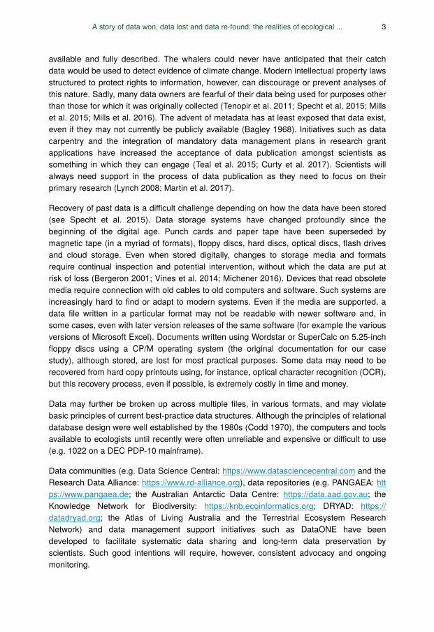
Published data in refereed journal articles and ‘grey’ literature (i.e. government andresearch reports) were retrieved in hard copy (Fig. 1A) and full species lists and metadata(vegetation structure, soil type and landscape descriptions) were extracted (Fig. 1B). Partiallists and those without ‘accurate’ geo-references (for the time) were rejected. This was amajor task, requiring manual extraction and evaluation by the supervising team and dataentry by postgraduate students: 711 ecological surveys incorporating 4088 floristic listswere assembled.

Due to the computational limitations of the time, the data were organised according tovegetation formation (e.g. forests, sclerophyll vegetation, mallee; Specht et al. 1995;Specht and Specht 2013) and each species was given a unique 9-character alphanumericcode to enable data handling and subsequent analysis. These codes necessitated thedevelopment of a bespoke system for the creation of two main digital files for eachformation: the site metadata (including provenance) with alphanumeric lists of species, anda ‘conversion’ file for the link between the alphanumeric codes and their full scientific

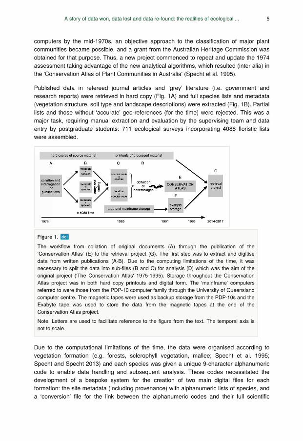
Figure 1.

The workflow from collation of original documents (A) through the publication of the‘Conservation Atlas’ (E) to the retrieval project (G). The first step was to extract and digitisedata from written publications (A-B). Due to the computing limitations of the time, it wasnecessary to split the data into sub-files (B and C) for analysis (D) which was the aim of theoriginal project ('The Conservation Atlas' 1975-1995). Storage throughout the ConservationAtlas project was in both hard copy printouts and digital form. The ‘mainframe’ computersreferred to were those from the PDP-10 computer family through the University of Queenslandcomputer centre. The magnetic tapes were used as backup storage from the PDP-10s and theExabyte tape was used to store the data from the magnetic tapes at the end of theConservation Atlas project.Note: Letters are used to facilitate reference to the figure from the text. The temporal axis isnot to scale.

A story of data won, data lost and data re-found: the realities of ecological ... 5

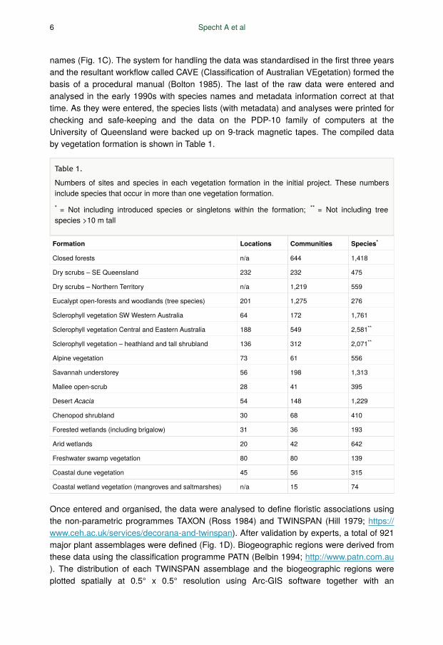
names (Fig. 1C). The system for handling the data was standardised in the first three yearsand the resultant workflow called CAVE (Classification of Australian VEgetation) formed thebasis of a procedural manual (Bolton 1985). The last of the raw data were entered andanalysed in the early 1990s with species names and metadata information correct at thattime. As they were entered, the species lists (with metadata) and analyses were printed forchecking and safe-keeping and the data on the PDP-10 family of computers at theUniversity of Queensland were backed up on 9-track magnetic tapes. The compiled databy vegetation formation is shown in Table 1.

Formation Locations Communities Species

Closed forests n/a 644 1,418

Dry scrubs – SE Queensland 232 232 475

Dry scrubs – Northern Territory n/a 1,219 559

Eucalypt open-forests and woodlands (tree species) 201 1,275 276

Sclerophyll vegetation SW Western Australia 64 172 1,761

Sclerophyll vegetation Central and Eastern Australia 188 549 2,581

Sclerophyll vegetation – heathland and tall shrubland 136 312 2,071

Alpine vegetation 73 61 556

Savannah understorey 56 198 1,313

Mallee open-scrub 28 41 395

Desert Acacia 54 148 1,229

Chenopod shrubland 30 68 410

Forested wetlands (including brigalow) 31 36 193

Arid wetlands 20 42 642

Freshwater swamp vegetation 80 80 139

Coastal dune vegetation 45 56 315

Coastal wetland vegetation (mangroves and saltmarshes) n/a 15 74

Once entered and organised, the data were analysed to define floristic associations usingthe non-parametric programmes TAXON (Ross 1984) and TWINSPAN (Hill 1979; https://www.ceh.ac.uk/services/decorana-and-twinspan). After validation by experts, a total of 921major plant assemblages were defined (Fig. 1D). Biogeographic regions were derived fromthese data using the classification programme PATN (Belbin 1994; http://www.patn.com.au). The distribution of each TWINSPAN assemblage and the biogeographic regions wereplotted spatially at 0.5° x 0.5° resolution using Arc-GIS software together with an

*

**

**

Table 1.

Numbers of sites and species in each vegetation formation in the initial project. These numbersinclude species that occur in more than one vegetation formation.

= Not including introduced species or singletons within the formation; = Not including treespecies >10 m tall* **

6 Specht A et al

assessment of the conservation status of each floristic assemblage and published as anAtlas (Specht et al. 1995; Fig. 1E). The original project spanned a period of 20 years (1975to 1995), involved several scientists and was funded by additional small research grants.

In 1991, when the mainframe computers at the University of Queensland were de-commissioned, the data from four of the five magnetic tapes – only readable on the PDPs –were transferred to exabyte tape, considered the best option at the time. The informationon the fifth tape could not be retrieved. The company making Exabyte tapes ceasedoperations in 2006 (Fig. 1F). Despite attempts at the time, the raw data contributing to thisstudy were not stored digitally.

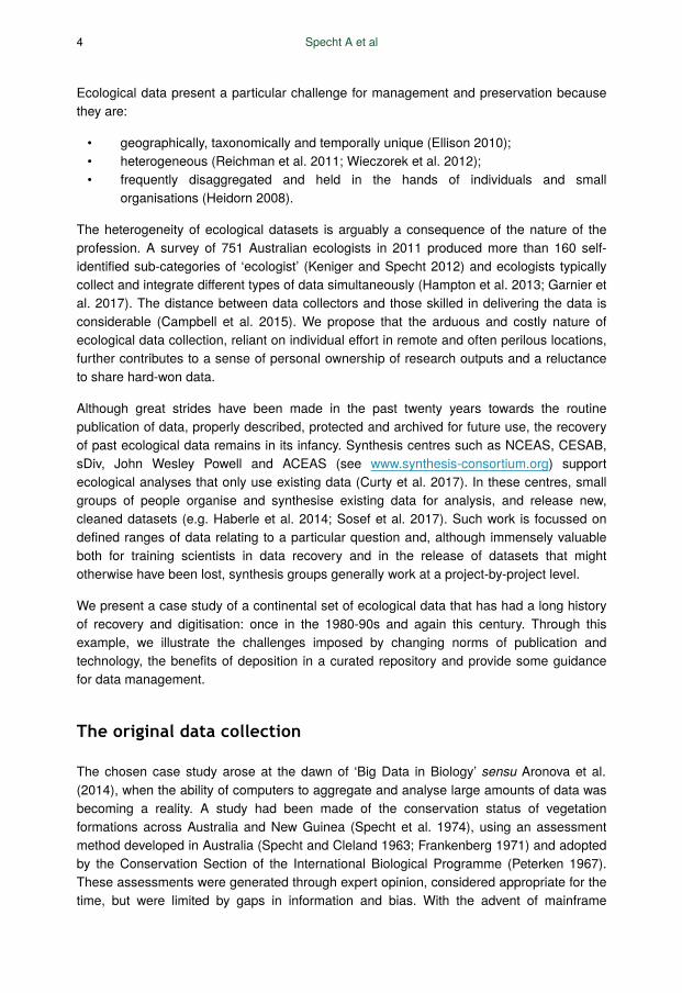
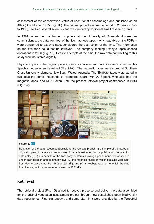
Physical copies of the original papers, various analyses and data files were stored in RaySpecht’s house when he retired (Fig. 2A-C). The magnetic tapes were stored at SouthernCross University, Lismore, New South Wales, Australia. The ‘Exabyte’ tapes were stored intwo locations some thousands of kilometres apart (with A. Specht, who also had themagnetic tapes, and M.P. Bolton) until the present retrieval project commenced in 2014(Fig. 1G).

Retrieval

The retrieval project (Fig. 1G) aimed to recover, preserve and deliver the data assembledfor the original vegetation assessment project through now-established open biodiversitydata repositories. Financial support and some staff time were provided by the Terrestrial

Figure 2.

Illustration of the data resources available to the retrieval project: (i) a sample of the boxes oforiginal copies of papers and reports (A), (ii) a table extracted from a publication prepared fordata entry (B), (iii) a sample of the hard copy printouts showing alphanumeric lists of speciesunder each location and community (C), (iv) the magnetic tapes on which backups were keptfrom day to day during the 1980s project (D), and (v) an exabyte tape on to which the datafrom the magnetic tapes were transferred in 1991 (E).

A story of data won, data lost and data re-found: the realities of ecological ... 7

Ecosystem Research Network (TERN) and the Atlas of Living Australia (ALA), the tworepositories identified as most relevant for these data.

The first challenge was to develop a system for checking and updating the species namesat the time of the ‘Conservation Atlas’ data collection. The most efficient and relevantmechanism to do this was through a web-service interface with the ALA (see http://api.ala.org.au, accessed 3 May 2018) which is the relevant authority for Australian species(see https://www.rbg.vic.gov.au/science/projects/taxonomy/atlas-of-living-australia-national-species-lists-project, accessed 11 December 2017).

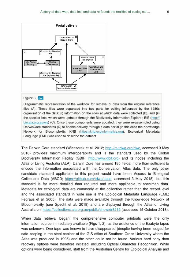
The plot-based, species structure of the original data was converted to individualobservations of species with freely associated data, such as location, date and time,observer, vegetation classification, source and team comments. We wanted to ensure thatno information was lost in re-structuring the data for publication using the widely-supportedDarwin Core Standard (Wieczorek et al. 2012). The planned process was as follows :

1. Recover all available data from ◦ Hard copy◦ Exabyte tape◦ Other data in digital form (e.g. Excel spreadsheets) (Fig. 3)

2. Design a structure that reflects how the data should be viewed from currentperspectives (Fig. 3)

◦ Site data/metadata (latitude/longitude by vegetation structure by comments)(Fig. 3B)

◦ Species alphanumeric codes and their associated scientific names◦ Sites by species codes (some with multiple communities)

3. Update the species codes/names to current nomenclature (Fig. 3C)◦ Use the Atlas of Living Australia’s web services (http://api.ala.org.au,

accessed 3 May 2018), the National Species Lists and Australian PlantCensus (CHAH: https://www.anbg.gov.au/chah/apc) to semi-automate thecurrent identification of species names

◦ Manually check any ambiguous or missing names4. Map the fields used in the Conservation Atlas project to the Darwin Core

standard (Fig. 3D)◦ Collate the terms used in the previous studies◦ Determine the intent of the fields◦ Find the best equivalent term in the Darwin Core standard

5. Collate and integrate the data ◦ Produce a list of species observations using the Darwin Core terms at each

site (defined by a consensus latitude/longitude) with metadata includingvegetation type/structure, source reference details (Fig. 3A) and processingcomments.

6. Generate a collection-level metadata record.

8 Specht A et al

The Darwin Core standard (Wieczorek et al. 2012; http://rs.tdwg.org/dwc, accessed 3 May2018) provides maximum interoperability and is the standard used by the GlobalBiodiversity Information Facility (GBIF; http://www.gbif.org) and its nodes including theAtlas of Living Australia (ALA). Darwin Core has around 185 fields, more than sufficient toencode the information associated with the Conservation Atlas data. The only othercandidate standard applicable to this project would have been Access to BiologicalCollections Data (ABCD; https://github.com/tdwg/abcd, accessed 3 May 2018), but thisstandard is far more detailed than required and more applicable to specimen data.Metadata for ecological data are commonly at the collection rather than the record leveland the associated standard in wide use is the Ecological Metadata Language (EML;Fegraus et al. 2005). The data were made available through the Knowledge Network ofBiocomplexity (see Specht et al. 2018) and are displayed through the Atlas of LivingAustralia on: https://collections.ala.org.au/public/show/dr8212 (accessed 15 October 2018).

When data retrieval began, the comprehensive computer printouts were the onlyinformation source immediately available (Figs 1, 2), as the existence of the Exabyte tapeswas unknown. One tape was known to have disappeared (despite having been lodged forsafe keeping in the steel cabinet of the GIS office of Southern Cross University where theAtlas was produced in 1995) and the other could not be found. Various hard copy datarecovery options were therefore initiated, including Optical Character Recognition. Whileoptions were being considered, staff from the Australian Centre for Ecological Analysis and

Figure 3.

Diagrammatic representation of the workflow for retrieval of data from the original referencefiles (A). These files were separated into two parts for editing influenced by the 1980sorganisation of the data: (i) information on the sites at which data were collected (B), and (ii)the species lists, which were updated through the Biodiversity Information Explorer, BIE (http://bie.ala.org.au/ws) (C). Once these components were updated, they were re-assembled usingDarwinCore standards (D) to enable delivery through a data portal (in this case the KnowledgeNetwork for Biocomplexity, KNB (https://knb.ecoinformatics.org). Ecological MetadataLanguage (EML) was used to describe the dataset.

A story of data won, data lost and data re-found: the realities of ecological ... 9

Synthesis (ACEAS-TERN) led by A. Specht, assisted by R.L. Specht, entered the locationdetails from the printouts into a spreadsheet (Microsoft Excel).

A total of 461 locations (135 of these had multiple survey sites within each broad location)were identified from the paper copies and these provided a checklist and structure for thefuture data compilation. After locating an Exabyte tape reader (not an easy matter either),we found that the tape was fortunately readable but had overlapping content, containingseveral different file types including basic species and site data, computer programmes forthe original data transformation and intermediate and final analysis results (as had theoriginal magnetic tapes and printouts). As noted previously, most of the basic species andsite files were consistently structured and were named according to vegetation formationleading to duplication. While confusing, duplication was far preferable to gaps in data. Nodata remained in either paper or digital form for the rainforest, dry scrubs, alpine vegetationand coastal wetland vegetation formations. This proved to be a loss of a large proportion ofthe data originally digitised.

Data on 1390 communities were recovered across the remaining formations, withalphanumeric codes for 9450 taxa and associated metadata. The estimated present cost ofrepeating the collection of raw data from the 461 locations, including species identification,preservation and documentation, would be conservatively AU$29 million. The estimatedpresent cost of extracting and digitising the species lists from the initial articles collatedwould be around AU$8 million.

The raw data files

Core data

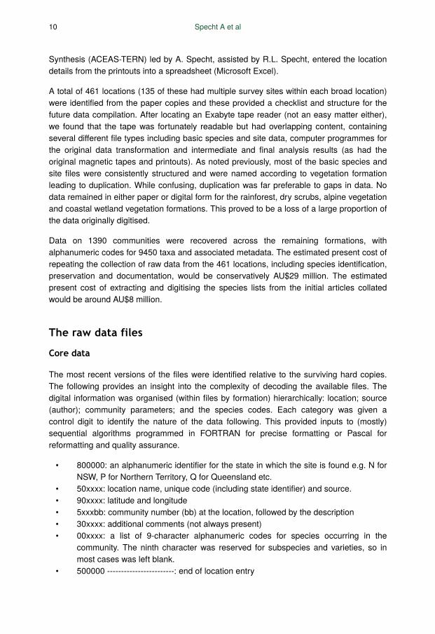
The most recent versions of the files were identified relative to the surviving hard copies.The following provides an insight into the complexity of decoding the available files. Thedigital information was organised (within files by formation) hierarchically: location; source(author); community parameters; and the species codes. Each category was given acontrol digit to identify the nature of the data following. This provided inputs to (mostly)sequential algorithms programmed in FORTRAN for precise formatting or Pascal forreformatting and quality assurance.

• 800000: an alphanumeric identifier for the state in which the site is found e.g. N forNSW, P for Northern Territory, Q for Queensland etc.

• 50xxxx: location name, unique code (including state identifier) and source.• 90xxxx: latitude and longitude• 5xxxbb: community number (bb) at the location, followed by the description• 30xxxx: additional comments (not always present)• 00xxxx: a list of 9-character alphanumeric codes for species occurring in the

community. The ninth character was reserved for subspecies and varieties, so inmost cases was left blank.

• 500000 ------------------------: end of location entry

10 Specht A et al

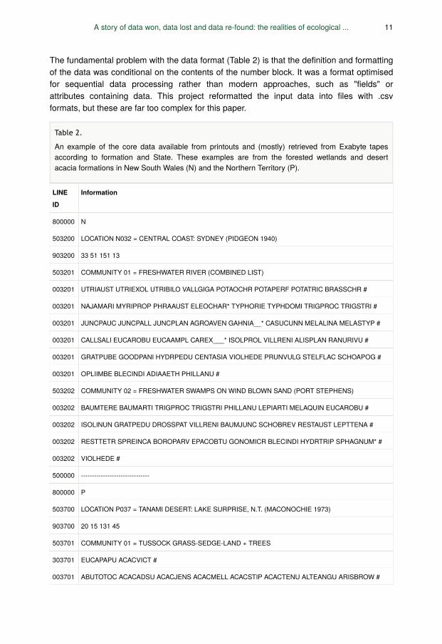
The fundamental problem with the data format (Table 2) is that the definition and formattingof the data was conditional on the contents of the number block. It was a format optimisedfor sequential data processing rather than modern approaches, such as "fields" orattributes containing data. This project reformatted the input data into files with .csvformats, but these are far too complex for this paper.

LINE

ID

Information

800000 N

503200 LOCATION N032 = CENTRAL COAST: SYDNEY (PIDGEON 1940)

903200 33 51 151 13

503201 COMMUNITY 01 = FRESHWATER RIVER (COMBINED LIST)

003201 UTRIAUST UTRIEXOL UTRIBILO VALLGIGA POTAOCHR POTAPERF POTATRIC BRASSCHR #

003201 NAJAMARI MYRIPROP PHRAAUST ELEOCHAR* TYPHORIE TYPHDOMI TRIGPROC TRIGSTRI #

003201 JUNCPAUC JUNCPALL JUNCPLAN AGROAVEN GAHNIA__* CASUCUNN MELALINA MELASTYP #

003201 CALLSALI EUCAROBU EUCAAMPL CAREX___* ISOLPROL VILLRENI ALISPLAN RANURIVU #

003201 GRATPUBE GOODPANI HYDRPEDU CENTASIA VIOLHEDE PRUNVULG STELFLAC SCHOAPOG #

003201 OPLIIMBE BLECINDI ADIAAETH PHILLANU #

503202 COMMUNITY 02 = FRESHWATER SWAMPS ON WIND BLOWN SAND (PORT STEPHENS)

003202 BAUMTERE BAUMARTI TRIGPROC TRIGSTRI PHILLANU LEPIARTI MELAQUIN EUCAROBU #

003202 ISOLINUN GRATPEDU DROSSPAT VILLRENI BAUMJUNC SCHOBREV RESTAUST LEPTTENA #

003202 RESTTETR SPREINCA BOROPARV EPACOBTU GONOMICR BLECINDI HYDRTRIP SPHAGNUM* #

003202 VIOLHEDE #

500000 -------------------------------

800000 P

503700 LOCATION P037 = TANAMI DESERT: LAKE SURPRISE, N.T. (MACONOCHIE 1973)

903700 20 15 131 45

503701 COMMUNITY 01 = TUSSOCK GRASS-SEDGE-LAND + TREES

303701 EUCAPAPU ACACVICT #

003701 ABUTOTOC ACACADSU ACACJENS ACACMELL ACACSTIP ACACTENU ALTEANGU ARISBROW #

Table 2.

An example of the core data available from printouts and (mostly) retrieved from Exabyte tapesaccording to formation and State. These examples are from the forested wetlands and desertacacia formations in New South Wales (N) and the Northern Territory (P).

A story of data won, data lost and data re-found: the realities of ecological ... 11

003701 ARISINAE BERGTRIM BONALINE BRACHOLO BRUNAUS2 BULBBARB CANTATTE CASSCOST #

003701 CASSHELM CASSOLIG CASSFILI CLEOVISC CLERFLOR COMESYLV CROTCUNN CROTEREM #

003701 CYPEBULB CYPECUNN CYPEHOLO CYPEIRIA DAMPCAND DESMMUEL DICRLEWE DODOPETI #

003701 ECTRSCHU ELYTSPIC ERAGLANF ERIAARIS ERIABENT EUCAASPE EUCAPRUI EUCASETO #

003701 EUCATERM EULAFULV EUPHDRUM EUPHWHEE GOODAZUR GOODENIA*GOMPCONI

GREVJUNC #

003701 GREVWICK HALGSOLA HELIAMBI HIBILEPT HIBISTURC HIBISTURP INDIBREV IPOMMUEL #

003701 ISOTATRO LOMALEUC MARSEXAR MELAGLOM MELALASI MELANERV MELHOBLO MELOMADE #

003701 MERRDAVE MIRBVIMI MORGFLOR NEPTDIMO PANIAUST PARAMUEL PHYLCARP PHYLHUNT #

003701 PHYLRHYT PIMEAMMO PLECPUNG PLUCTETR PLUCTETRT POLYSYNA POLYGALA *PORTFILI #

003701 PORTOLER PSORMART PTILARTH PTILASTR PTILCALO RULILOXO SANTLANC SCAEPARV #

003701 SCIRLAEV SIDAPLAT STACMEGA SWAIBUR3 SYNATILL TINOSMIL TRIAPILO TRIOPUNG #

003701 TRIUGLAU WALTINDI ZORNALBI #

500000 -------------------------------

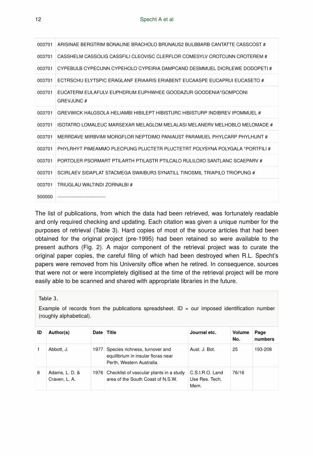
The list of publications, from which the data had been retrieved, was fortunately readableand only required checking and updating. Each citation was given a unique number for thepurposes of retrieval (Table 3). Hard copies of most of the source articles that had beenobtained for the original project (pre-1995) had been retained so were available to thepresent authors (Fig. 2). A major component of the retrieval project was to curate theoriginal paper copies, the careful filing of which had been destroyed when R.L. Specht’spapers were removed from his University office when he retired. In consequence, sourcesthat were not or were incompletely digitised at the time of the retrieval project will be moreeasily able to be scanned and shared with appropriate libraries in the future.

ID Author(s) Date Title Journal etc. VolumeNo.

Pagenumbers

1 Abbott, J. 1977 Species richness, turnover andequilibrium in insular floras nearPerth, Western Australia.

Aust. J. Bot. 25 193-208

8 Adams, L. D. &Craven, L. A.

1976 Checklist of vascular plants in a studyarea of the South Coast of N.S.W.

C.S.I.R.O. LandUse Res. Tech.Mem.

76/16

Table 3.

Example of records from the publications spreadsheet. ID = our imposed identification number(roughly alphabetical).

12 Specht A et al

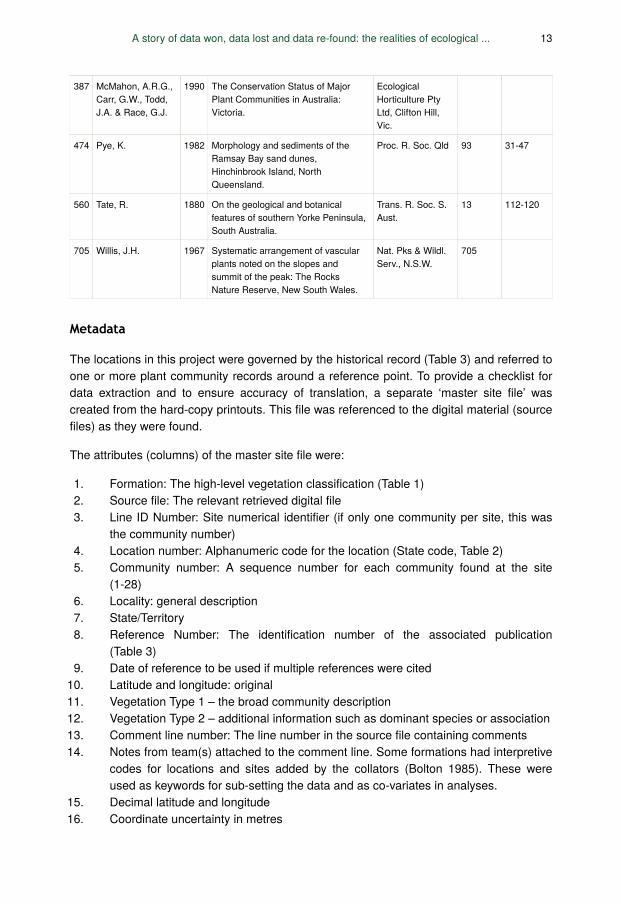
387 McMahon, A.R.G.,Carr, G.W., Todd,J.A. & Race, G.J.

1990 The Conservation Status of MajorPlant Communities in Australia:Victoria.

EcologicalHorticulture PtyLtd, Clifton Hill,Vic.

474 Pye, K. 1982 Morphology and sediments of theRamsay Bay sand dunes,Hinchinbrook Island, NorthQueensland.

Proc. R. Soc. Qld 93 31-47

560 Tate, R. 1880 On the geological and botanicalfeatures of southern Yorke Peninsula,South Australia.

Trans. R. Soc. S.Aust.

13 112-120

705 Willis, J.H. 1967 Systematic arrangement of vascularplants noted on the slopes andsummit of the peak: The RocksNature Reserve, New South Wales.

Nat. Pks & Wildl.Serv., N.S.W.

705

Metadata

The locations in this project were governed by the historical record (Table 3) and referred toone or more plant community records around a reference point. To provide a checklist fordata extraction and to ensure accuracy of translation, a separate ‘master site file’ wascreated from the hard-copy printouts. This file was referenced to the digital material (sourcefiles) as they were found.

The attributes (columns) of the master site file were:

1. Formation: The high-level vegetation classification (Table 1)2. Source file: The relevant retrieved digital file3. Line ID Number: Site numerical identifier (if only one community per site, this was

the community number)4. Location number: Alphanumeric code for the location (State code, Table 2)5. Community number: A sequence number for each community found at the site

(1-28)6. Locality: general description7. State/Territory8. Reference Number: The identification number of the associated publication

(Table 3)9. Date of reference to be used if multiple references were cited

10. Latitude and longitude: original11. Vegetation Type 1 – the broad community description12. Vegetation Type 2 – additional information such as dominant species or association13. Comment line number: The line number in the source file containing comments14. Notes from team(s) attached to the comment line. Some formations had interpretive

codes for locations and sites added by the collators (Bolton 1985). These wereused as keywords for sub-setting the data and as co-variates in analyses.

15. Decimal latitude and longitude16. Coordinate uncertainty in metres

A story of data won, data lost and data re-found: the realities of ecological ... 13

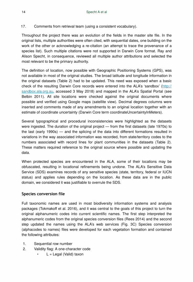
17. Comments from retrieval team (using a consistent vocabulary).

Throughout the project there was an evolution of the fields in the master site file. In theoriginal lists, multiple authorities were often cited, with sequential dates, one building on thework of the other or acknowledging a re-citation (an attempt to trace the provenance of aspecies list). Such multiple citations were not supported in Darwin Core format. Ray andAlison Specht, in consequence, reviewed all multiple author attributions and selected themost relevant to be the primary authority.

The definition of location, now possible with Geographic Positioning Systems (GPS), wasnot available in most of the original studies. The broad latitude and longitude information inthe original datasets (Table 2) had to be updated. This need was exposed when a basiccheck of the resulting Darwin Core records were entered into the ALA’s ‘sandbox’ (http://sandbox.ala.org.au, accessed 3 May 2018) and mapped in the ALA’s Spatial Portal (seeBelbin 2011). All site locations were checked against the original documents wherepossible and verified using Google maps (satellite view). Decimal degrees columns wereinserted and comments made of any amendments to an original location together with anestimate of coordinate uncertainty (Darwin Core term coordinateUncertaintyInMeters).

Several typographical and procedural inconsistencies were highlighted as the datasetswere ingested. The duration of the original project — from the first datasets (late 1970s) tothe last (early 1990s) — and the splicing of the data into different formations resulted invariations in the way associated information was recorded, from state/territory codes to thenumbers associated with record lines for plant communities in the datasets (Table 2).These matters required reference to the original source where possible and updating thedata.

When protected species are encountered in the ALA, some of their locations may beobfuscated, resulting in locational refinements being undone. The ALA’s Sensitive DataService (SDS) examines records of any sensitive species (state, territory, federal or IUCNstatus) and applies rules depending on the location. As these data are in the publicdomain, we considered it was justifiable to overrule the SDS.

Species conversion file

Full taxonomic names are used in most biodiversity information systems and analysispackages (Tokmakoff et al. 2016), and it was central to the goals of this project to turn theoriginal alphanumeric codes into current scientific names. The first step interpreted thealphanumeric codes from the original species conversion files (Rees 2014) and the secondstep updated the names using the ALA’s web services (Fig. 3C) Species conversion(alphacodes to names) files were developed for each vegetation formation and containedthe following attributes:

1. Sequential row number2. Validity flag: A one-character code

◦ L = Legal (Valid) taxon

14 Specht A et al

◦ S = Synonym◦ M = Misspelling.

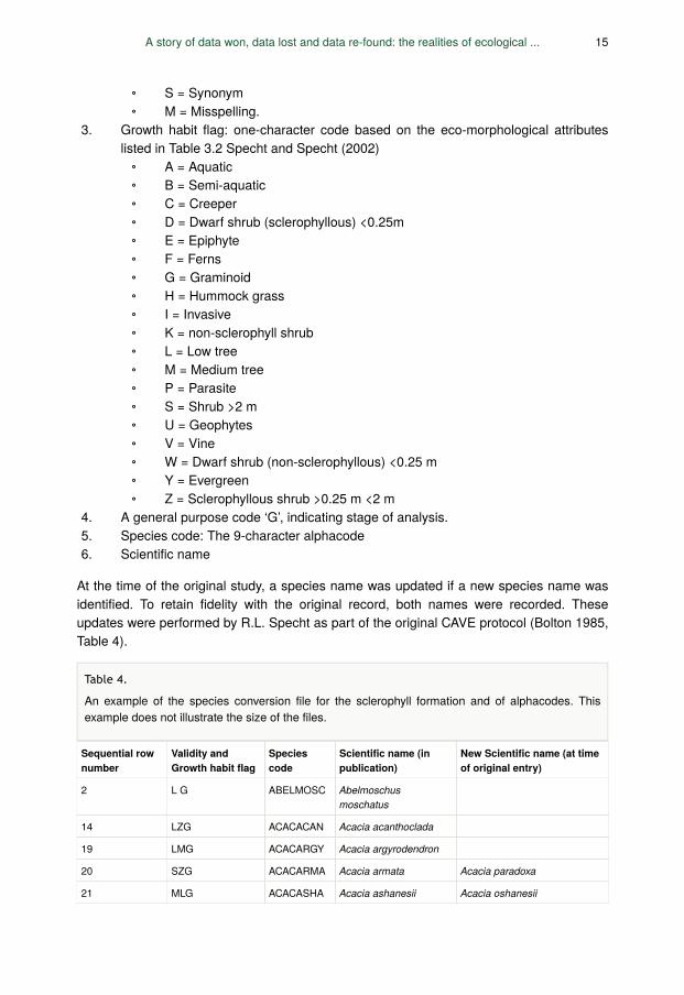
3. Growth habit flag: one-character code based on the eco-morphological attributeslisted in Table 3.2 Specht and Specht (2002)

◦ A = Aquatic◦ B = Semi-aquatic◦ C = Creeper◦ D = Dwarf shrub (sclerophyllous) <0.25m◦ E = Epiphyte◦ F = Ferns◦ G = Graminoid◦ H = Hummock grass◦ I = Invasive◦ K = non-sclerophyll shrub◦ L = Low tree◦ M = Medium tree◦ P = Parasite◦ S = Shrub >2 m◦ U = Geophytes◦ V = Vine◦ W = Dwarf shrub (non-sclerophyllous) <0.25 m◦ Y = Evergreen◦ Z = Sclerophyllous shrub >0.25 m <2 m

4. A general purpose code ‘G’, indicating stage of analysis.5. Species code: The 9-character alphacode6. Scientific name

At the time of the original study, a species name was updated if a new species name wasidentified. To retain fidelity with the original record, both names were recorded. Theseupdates were performed by R.L. Specht as part of the original CAVE protocol (Bolton 1985,Table 4).

Sequential rownumber

Validity andGrowth habit flag

Speciescode

Scientific name (inpublication)

New Scientific name (at timeof original entry)

2 L G ABELMOSC Abelmoschus moschatus

14 LZG ACACACAN Acacia acanthoclada

19 LMG ACACARGY Acacia argyrodendron

20 SZG ACACARMA Acacia armata Acacia paradoxa

21 MLG ACACASHA Acacia ashanesii Acacia oshanesii

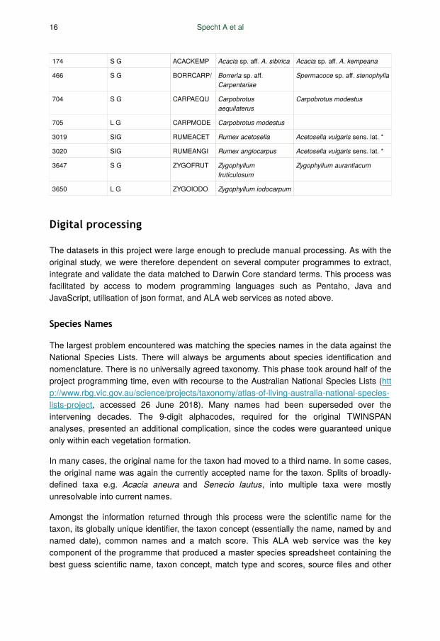
Table 4.

An example of the species conversion file for the sclerophyll formation and of alphacodes. Thisexample does not illustrate the size of the files.

A story of data won, data lost and data re-found: the realities of ecological ... 15

174 S G ACACKEMP Acacia sp. aff. A. sibirica Acacia sp. aff. A. kempeana

466 S G BORRCARP/ Borreria sp. aff. Carpentariae

Spermacoce sp. aff. stenophylla

704 S G CARPAEQU Carpobrotus aequilaterus

Carpobrotus modestus

705 L G CARPMODE Carpobrotus modestus

3019 SIG RUMEACET Rumex acetosella Acetosella vulgaris sens. lat. *

3020 SIG RUMEANGI Rumex angiocarpus Acetosella vulgaris sens. lat. *

3647 S G ZYGOFRUT Zygophyllum fruticulosum

Zygophyllum aurantiacum

3650 L G ZYGOIODO Zygophyllum iodocarpum

Digital processing

The datasets in this project were large enough to preclude manual processing. As with theoriginal study, we were therefore dependent on several computer programmes to extract,integrate and validate the data matched to Darwin Core standard terms. This process wasfacilitated by access to modern programming languages such as Pentaho, Java andJavaScript, utilisation of json format, and ALA web services as noted above.

Species Names

The largest problem encountered was matching the species names in the data against theNational Species Lists. There will always be arguments about species identification andnomenclature. There is no universally agreed taxonomy. This phase took around half of theproject programming time, even with recourse to the Australian National Species Lists (http://www.rbg.vic.gov.au/science/projects/taxonomy/atlas-of-living-australia-national-species-lists-project, accessed 26 June 2018). Many names had been superseded over theintervening decades. The 9-digit alphacodes, required for the original TWINSPANanalyses, presented an additional complication, since the codes were guaranteed uniqueonly within each vegetation formation.

In many cases, the original name for the taxon had moved to a third name. In some cases,the original name was again the currently accepted name for the taxon. Splits of broadly-defined taxa e.g. Acacia aneura and Senecio lautus, into multiple taxa were mostlyunresolvable into current names.

Amongst the information returned through this process were the scientific name for thetaxon, its globally unique identifier, the taxon concept (essentially the name, named by andnamed date), common names and a match score. This ALA web service was the keycomponent of the programme that produced a master species spreadsheet containing thebest guess scientific name, taxon concept, match type and scores, source files and other

16 Specht A et al

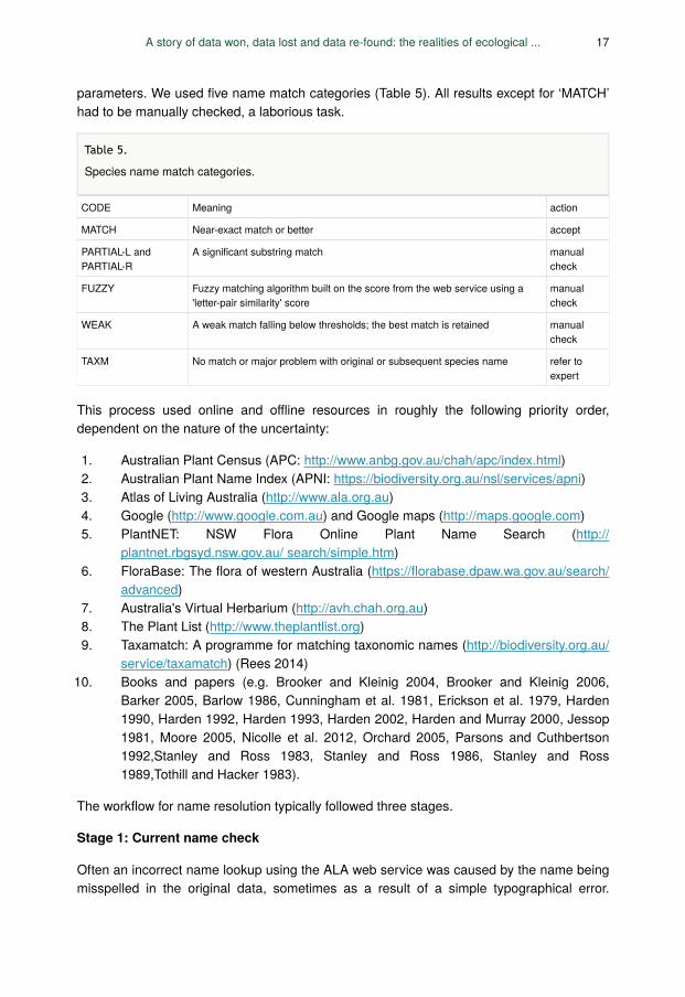
parameters. We used five name match categories (Table 5). All results except for ‘MATCH’had to be manually checked, a laborious task.

CODE Meaning action

MATCH Near-exact match or better accept

PARTIAL-L andPARTIAL-R

A significant substring match manualcheck

FUZZY Fuzzy matching algorithm built on the score from the web service using a'letter-pair similarity' score

manualcheck

WEAK A weak match falling below thresholds; the best match is retained manualcheck

TAXM No match or major problem with original or subsequent species name refer toexpert

This process used online and offline resources in roughly the following priority order,dependent on the nature of the uncertainty:

1. Australian Plant Census (APC: http://www.anbg.gov.au/chah/apc/index.html)2. Australian Plant Name Index (APNI: https://biodiversity.org.au/nsl/services/apni)3. Atlas of Living Australia (http://www.ala.org.au) 4. Google (http://www.google.com.au) and Google maps (http://maps.google.com)5. PlantNET: NSW Flora Online Plant Name Search (http://

plantnet.rbgsyd.nsw.gov.au/ search/simple.htm)6. FloraBase: The flora of western Australia (https://florabase.dpaw.wa.gov.au/search/

advanced)7. Australia's Virtual Herbarium (http://avh.chah.org.au)8. The Plant List (http://www.theplantlist.org)9. Taxamatch: A programme for matching taxonomic names (http://biodiversity.org.au/

service/taxamatch) (Rees 2014) 10. Books and papers (e.g. Brooker and Kleinig 2004, Brooker and Kleinig 2006,

Barker 2005, Barlow 1986, Cunningham et al. 1981, Erickson et al. 1979, Harden1990, Harden 1992, Harden 1993, Harden 2002, Harden and Murray 2000, Jessop1981, Moore 2005, Nicolle et al. 2012, Orchard 2005, Parsons and Cuthbertson1992,Stanley and Ross 1983, Stanley and Ross 1986, Stanley and Ross1989,Tothill and Hacker 1983).

The workflow for name resolution typically followed three stages.

Stage 1: Current name check

Often an incorrect name lookup using the ALA web service was caused by the name beingmisspelled in the original data, sometimes as a result of a simple typographical error.

Table 5.

Species name match categories.

A story of data won, data lost and data re-found: the realities of ecological ... 17

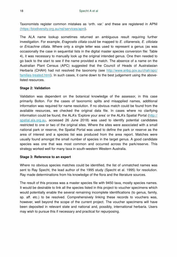
Taxonomists register common mistakes as ‘orth. var.’ and these are registered in APNI(https://biodiversity.org.au/nsl/services/apni).

The ALA name lookup sometimes returned an ambiguous result requiring furtherinvestigation. For example, Eragrostis ciliata could be mapped to E. cilianensis, E. ciliolataor Ericachne ciliata. Where only a single letter was used to represent a genus (as wasoccasionally the case in sequential lists in the digital master species conversion file: Table4), it was necessary to manually look up the original intended genus. One then needed togo back to the start to see if the name provided a match. The absence of a name on theAustralian Plant Census (APC) suggested that the Council of Heads of AustralasianHerbaria (CHAH) had not resolved the taxonomy (see http://www.anbg.gov.au/chah/apc/families-treated.html). In such cases, it came down to the best judgement using the above-listed resources.

Stage 2: Validation

Validation was dependent on the botanical knowledge of the assessor, in this caseprimarily Bolton. For the cases of taxonomic splits and misapplied names, additionalinformation was required for name resolution. If no obvious match could be found from theavailable resources, we checked the original data file. In cases where no clarifyinginformation could be found, the ALA’s ‘Explore your area’ or the ALA’s Spatial Portal (http://spatial.ala.org.au, accessed 26 June 2018) was used to identify potential candidatesrestricted to one or two of the original sites. Where the sites were associated with a smallnational park or reserve, the Spatial Portal was used to define the park or reserve as thearea of interest and a species list was produced from the area report. Matches wereusually found amongst the small number of species in the target genus. A good candidatespecies was one that was most common and occurred across the park/reserve. Thisstrategy worked well for many taxa in south-western Western Australia.

Stage 3: Reference to an expert

Where no obvious species matches could be identified, the list of unmatched names wassent to Ray Specht, the lead author of the 1995 study (Specht et al. 1995) for resolution.Ray made determinations from his knowledge of the flora and the literature sources.

The result of this process was a master species file with 9450 taxa, mostly species names.It would be desirable to link all the species listed in this project to voucher specimens whichwould potentially enable the several remaining incomplete identifications (to genus, family,sp. aff. etc.) to be resolved. Comprehensively linking these records to vouchers was,however, well beyond the scope of the current project. The voucher specimens will havebeen deposited in relevant state and national and, possibly, international herbaria. Usersmay wish to pursue this if necessary and practical for repurposing.

18 Specht A et al

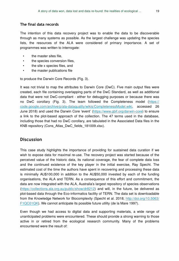
The final data records

The intention of this data recovery project was to enable the data to be discoverablethrough as many systems as possible. As the largest challenge was updating the specieslists, the resources of the ALA were considered of primary importance. A set ofprogrammes was written to interrogate:

• the master sites file,• the species conversion files,• the site x species files, and• the master publications file

to produce the Darwin Core Records (Fig. 3).

It was not trivial to map the attributes to Darwin Core (DwC). Five main output files werecreated, each file containing overlapping parts of the DwC Standard, as well as additionaldata that were not DwC-compliant - either for debugging purposes or because there wasno DwC corollary (Fig. 3). The team followed the Completeness model (https://code.google.com/archive/p/ala-dataquality/wikis/CompletenessModel.wiki, accessed 26June 2018) and used the Darwin Core 'event’ (https://www.gbif.org/darwin-core) to ensurea link to the plot-based approach of the collection. The 47 terms used in the database,including those that had no DwC corollary, are tabulated in the Associated Data files in theKNB repository (Cons_Atlas_DwC_fields_181009.xlsx).

Discussion

This case study highlights the importance of providing for sustained data curation if wewish to expose data for maximal re-use. The recovery project was started because of theperceived value of the historic data, its national coverage, the fear of complete data lossand the continued existence of the key player in the initial exercise, Ray Specht. Theestimated cost of the time the authors have spent in recovering and processing these datais minimally AU$100,000 in addition to the AU$50,000 invested by each of the fundingorganisations, the ALA and TERN. As a consequence of this effort and commitment, thedata are now integrated with the ALA, Australia’s largest repository of species observations(https://collections.ala.org.au/public/show/dr8212) and will, in the future, be delivered asplot-based data through the Eco-informatics facility of TERN. The data set is downloadablefrom the Knowledge Network for Biocomplexity (Specht et al. 2018; http://doi.org/10.5063/F1QC01QK). We cannot anticipate its possible future utility (de la Mare 1997).

Even though we had access to digital data and supporting materials, a wide range ofunanticipated problems were encountered. These should provide a strong warning to thoseactive in or retired from the ecological research community. Many of the problemsencountered were the result of:

A story of data won, data lost and data re-found: the realities of ecological ... 19

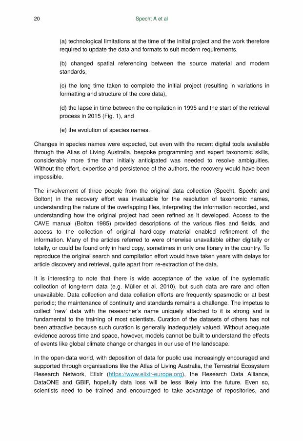
(a) technological limitations at the time of the initial project and the work thereforerequired to update the data and formats to suit modern requirements,

(b) changed spatial referencing between the source material and modernstandards,

(c) the long time taken to complete the initial project (resulting in variations informatting and structure of the core data),

(d) the lapse in time between the compilation in 1995 and the start of the retrievalprocess in 2015 (Fig. 1), and

(e) the evolution of species names.

Changes in species names were expected, but even with the recent digital tools availablethrough the Atlas of Living Australia, bespoke programming and expert taxonomic skills,considerably more time than initially anticipated was needed to resolve ambiguities.Without the effort, expertise and persistence of the authors, the recovery would have beenimpossible.

The involvement of three people from the original data collection (Specht, Specht andBolton) in the recovery effort was invaluable for the resolution of taxonomic names,understanding the nature of the overlapping files, interpreting the information recorded, andunderstanding how the original project had been refined as it developed. Access to theCAVE manual (Bolton 1985) provided descriptions of the various files and fields, andaccess to the collection of original hard-copy material enabled refinement of theinformation. Many of the articles referred to were otherwise unavailable either digitally ortotally, or could be found only in hard copy, sometimes in only one library in the country. Toreproduce the original search and compilation effort would have taken years with delays forarticle discovery and retrieval, quite apart from re-extraction of the data.

It is interesting to note that there is wide acceptance of the value of the systematiccollection of long-term data (e.g. Müller et al. 2010), but such data are rare and oftenunavailable. Data collection and data collation efforts are frequently spasmodic or at bestperiodic; the maintenance of continuity and standards remains a challenge. The impetus tocollect ‘new’ data with the researcher’s name uniquely attached to it is strong and isfundamental to the training of most scientists. Curation of the datasets of others has notbeen attractive because such curation is generally inadequately valued. Without adequateevidence across time and space, however, models cannot be built to understand the effectsof events like global climate change or changes in our use of the landscape.

In the open-data world, with deposition of data for public use increasingly encouraged andsupported through organisations like the Atlas of Living Australia, the Terrestrial EcosystemResearch Network, Elixir (https://www.elixir-europe.org), the Research Data Alliance,DataONE and GBIF, hopefully data loss will be less likely into the future. Even so,scientists need to be trained and encouraged to take advantage of repositories, and

20 Specht A et al

sustained funding is required to support the infrastructure necessary for good dataconservation outcomes.

The original project was envisioned as a stock-take of the past, and by its conversion toand storage in digital form, a resource for the future. Despite initial enthusiasm for theproject, lack of subsequent funding and continuity of effort meant this resource was almostlost. This is a common story even in cases where there was more substantial initialinvestment (Aronova et al. 2014; Michener 2015).

As our environment and our technological sophistication change, we need to respectinformation as it was originally reported. An object lesson from this project is not to bescornful of the efforts of times past, but to value them for the information they provide.

Sufficient resources need to be set aside to ensure that:

(a) scientists deposit their data as closely as possible to the time of their creationin appropriate, sustainable digital repositories,

(b) the technology of repositories is updated, and

(c) the data are appropriately conserved, allowing access, while maintainingintegrity.

Only thus will data be useful to a myriad of future applications. If not, the cost of recovery ofdata in the future will be far higher than you may imagine and may, in fact, be impossible.

Acknowledgements

As is clear from the article, this recovery project was only possible through the contributionof an array of people and organisations over a sustained period of time. This includes theinitial data collectors and their organisations, funding obtained in the 1980s from a vastnumber of organisations listed in the Conservation Atlas and latterly material and librarysupport from the University of Queensland and the financial and collegial support providedby the Terrestrial Ecosystem Research Network (TERN: www.tern.org.au). AS would like tothank Bob Parsons and Peter Saenger for providing critical missing data, Eric Garnier andBill Michener for valuable comments on earlier versions of this manuscript and severalpeople, including Siddeswara Guru, Baptiste Laporte, Todd Vision and Chris Lortie for theirencouragement.

We particularly thank the late John LaSalle, Director of the Atlas of Living Australia (ALA: www.ala.org.au) for supporting this recovery project through funding Bryn Kingsford forcoding the scripts and providing the time of Lee Belbin (Advisor to the ALA) and MilesNicholls (the ALA's Data Manager): John had a rare understanding of the true value ofthese data.

A story of data won, data lost and data re-found: the realities of ecological ... 21

Author contributions

AS & LB devised project, AS was primarily responsible for article.

AS, MPB, LB and RLS verified data collation, geographical and taxonomic mapping.

BK was primarily responsible for developing the code to retrieve the data from the originalfiles and deliver in DarwinCore format.

BK and MPB monitored programme linkages.

References

• Aronova E, Baker KS, Oreskes N (2014) Big Science and Big Data in biology: from theInternational Geophysical Year through the International Biological Program to the LongTerm Ecological Research (LTER) Network, 1957-Presentamore. Historical Studies ofNatural Science 40 (2): 183‑224. https://doi.org/10.1525/hsns.2010.40.2.183

• Bagley PR (1968) Extension of programming language concepts. University CityScience Center, Philadelphia, USA.

• Barker WR (2005) Standardising informal names in Australian publications. AustralianSystematic Botany Society Newsletter 122: 11‑12. URL: http://www.anbg.gov.au/asbs/newsletter/pdf/05-march-122.pdf

• Barlow BA (1986) Flora and Fauna of Alpine Australasia. CSIRO in association with theAustralian Systematic Botany Society, Melbourne, Australia, 543 pp. [ISBN0643040242]

• Belbin L (1994) PATN: Pattern analysis package: technical reference. CSIRO, Divisionof Wildlife Ecology, Australia.

• Belbin L (2011) The Atlas of Living Australia’s spatial portal. pp. 39-43. In: Jones MB,Gries C (Eds) Proceedings of the Environmental Information Management Conference2011 (EIM 2011), Santa Barbara, September 28–29.

• Bergeron B (2001) Dark Ages II: when the digital data die. 1. Pearson Educational, 336pp. [ISBN 10: 0130661074]

• Bolton MP (1985) Classification of Australian Vegetation (CAVE) Software Manual.Version A1. unpublished, Brisbane, Australia.

• Brooker MI, Kleinig DA (2004) Field Guide to Eucalypts. Volume 3. Northern Australia.2nd Edition. Bloomings Books, Melbourne, Australia. [ISBN 1876473282]

• Brooker MI, Kleinig DA (2006) Field Guide to Eucalypts. Volume 1. South-easternAustralia. 3rd Edition. Bloomings Books, Melbourne, Australia, 356 pp. [ISBN9781876473525]

• Campbell HA, Beyer HL, Dennis TE, Dwyer RG, Forester JD, Fukuda Y, Lynch C,Hindell MA, Menke N, Morales JM, Richardson C, Rodgers E, Taylor G, Watts ME,Westcott DA (2015) Finding our way: on the sharing and reuse of animal telemetry datain Australasia. Science of the Total Environment 534: 79‑84. https://doi.org/10.1016/j.scitoenv.2015.01.089

22 Specht A et al

• Codd EF (1970) A relational model of data for large shared data banks.Communications of the Association for Computing Machinery (ACM) 13 (6): 377‑387. https://doi.org/10.1145/362384.362685

• Cunningham GM, Mulham WE, Milthorpe PL, Leigh JH (1981) Plants of Western NewSouth Wales. N.S.W. Government Printing Office in association with the SoilConservation Service of NSW, Australia. [ISBN 0724020039]

• Curty RG, Crowston K, Specht A, B.W. G, Dalton ED (2017) Attitudes and normsaffecting scientists’ data reuse. PLOS One 12 (12): e0189288. https://doi.org/10.1371/journal.pone.0189288

• de la Mare WK (1997) Abrupt mid-twentieth century decline in Antarctic sea ice extentfrom whaling records. Nature 389: 57‑60. https://doi.org/10.1038/37956

• Ellison AM (2010) Repeatability and transparency in ecological research. Ecology 91(9): 2536‑2539. https://doi.org/10.1890/09-0032.1

• Erickson R, George AS, Marchant NG, Morcombe MK (Eds) (1979) Flowers and Plantsof Western Australia. Reed, Sydney, Australia, 231 pp. [ISBN 058950116X]

• Fegraus E, Andelman SJ, Jones MB, Schildhauer M (2005) Maximizing the value ofecological data with structured metadata: an introduction to ecological metadatalanguage (EML) and principles for metadata creation. Bulletin of the Ecological Societyof America 86 (3): 158‑168. https://doi.org/10.1890/0012-9623(2005)86[158:MTVOED]2.0.CO;2

• Frankenberg J (1971) Nature Conservation in Victoria. Victorian National ParksAssociation, Melbourne, Australia, 145 pp.

• Garnier E, Stahl U, Laporte M, Kattge J, Mougenot I, Kühn I, Laporte B, Amiaud B,Ahrestani FS, Bönisch G, Bunker DE, Cornelissen JHC, Díaz S, Enquist B, Gachet S,Jaureguilberry P, Kleyer M, Lavorel S, Maicher L, Pérez-Harguindeguy N, Poorter H,Schildhauer M, Shipley B, Violle C, Weiher E, Wirth C, Wright IJ, Klotz S (2017)Towards a thesaurus of plant characteristics: an ecological contribution. Journal ofEcology 105: 298‑309. https://doi.org/10.1111/1365-2745.12698

• Haberle SG, Bowman DM, Newnham RM, Johnston FH, Beggs PJ, Buters J, CampbellB, Erbas B, Godwin I, Green BJ, Huete A, Jaggard AK, Medek D, Murray F, Newbigin E,Thibaudon M, Vicendese D, Williamson GJ, Davies JM (2014) The macroecology ofairborne pollen in Australian and New Zealand urban areas. PLOS One 9 (5): e97925. https://doi.org/10.1371/journal.pone.0097925

• Hampton SE, Strasser CA, Tewksbury JJ, Gram WK, Budden AE, Batcheller AL, DukeCS, Porter JH (2013) Big data and the future of ecology. Frontiers in Ecology andEnvironment 11 (3): 156‑162. https://doi.org/10.1890/120103

• Harden GJ (1990) Flora of New South Wales, Vol. 1. University of New South WalesPress, Kensington, NSW, Australia.

• Harden GJ (1992) Flora of New South Wales, Vol. 3. University of New South WalesPress, Kensington, NSW, Australia.

• Harden GJ (1993) Flora of New South Wales, Vol. 4. University of New South WalesPress, Kensington, NSW, Australia.

• Harden GJ, Murray LJ (2000) Supplement to Flora of New South Wales, Vol. 1.University of New South Wales Press, Kensington, NSW, Australia.

• Harden GJ (2002) Flora of New South Wales, Vol. 2, Revised Edition. University of NewSouth Wales Press, Kensington, NSW, Australia.

A story of data won, data lost and data re-found: the realities of ecological ... 23

• Heidorn PB (2008) Shedding light on the dark data in the long tail of science. LibraryTrends 57 (2): 280‑299. https://doi.org/10.1353/lib.0.0036

• Hill MO (1979) TWINSPAN– A FORTRAN program for arranging multivariate data in anordered two-way table by classification of the individuals and attributes. Section ofEcology and Systematics, Cornell University, Ithaca, New York, USA.

• Jessop J (1981) Flora of Central Australia. Reed and the Australian Systematic BotanySociety, Sydney, Australia.

• Jetz W, McPherson JM, Guralnik R (2012) Integrating biodiversity distributionknowledge: toward a global map of life. Trends in Ecology and Evolution 27 (3):151‑159. https://doi.org/10.1016/j.tree.2011.09.007

• Keniger L, Specht A (2012) Exploring interdisciplinary collaboration in Australia'secosystem science and management community. unpublished, Brisbane, Australia.URL: http://www.aceas.org.au/index.php?option=com_content&view=article&id=107&Itemid=109#Report%202

• Kissling WD, Ahumada JA, Bowser A, Fernandez M, Fernández N, Alonso Garcia E,Guralnick RP, N.J.B. I, Kelling S, Los W, McRae L, Mihoub J, Obst M, Santamaria M,Skidmore AK, Williams KJ, Agosti D, Amariles D, Arvanitidis C, Bastin L, De Leo F,Egloff W, Elith J, Hobern D, Martin D, Pereira HM, Pesole G, Peterseil J, Saarenmaa H,Schigel D, Schmeller DS, Segata N, Turak E, Uhlir PF, Wee B, Hardisty AR (2017)Building essential biodiversity variables (EBVs) of species distribution and abundance ata global scale. Biological Reviews 93 (1): 600‑625. https://doi.org/10.1111/brv.12359

• Lindenmayer DB, Likens GE (2009) Adaptive monitoring: a new paradigm for long-termresearch and monitoring. Trends in Ecology and Evolution 24 (9): 482‑486. https://doi.org/10.1016/j.tree.2009.03.005

• Lynch C (2008) How do your data grow? Nature 455 (4): 28‑29. https://doi.org/10.1038/455028a

• Martin P, Chen Y, Hardisty A (2017) Computational challenges in global environmentalresearch infrastructures. pp. 305-340. In: Chabbi A, Loescher H (Eds) TerrestrialEcosystem Research Infrastructures: challenges and opportunities. CRC Press, BocaRaton, Florida, USA, 534 pp.

• Michener WK (2015) Ten simple rules for creating a good data management plan.PLOS Computational Biology 11 (10): e1004525. https://doi.org/10.1371/journal.pcbi.1004525

• Michener WK (2016) Advances in managing long term ecological research data.Ecological Informatics 36: 199‑200. https://doi.org/10.1016/j.ecoinf.2016.11.009

• Mills JA, Teplinsky C, Arroyo B (2015) Archiving primary data: solutions for long-termstudies. Trends in Ecology and Evolution 30 (10): 581‑589. https://doi.org/10.1016/j.tree.2015.07.006

• Mills JA, Teplitsky C, Arroyo B (2016) Solutions for archiving data in long-term studies: areply to Whitlock et al. Trends in Ecology and Evolution 31 (2): 85‑87. https://doi.org/10.1016/j.tree.2015.12.004

• Moore P (2005) A Guide to Plants of Inland Australia. New Holland Publishers, Sydney,Australia. [ISBN 9781876334864]

• Morris BD, White EP (2013) The EcoData Retriever: Improving access to existingecological data. PLOS One 8 (6): e65848. https://doi.org/10.1371/journal.pone.0065848

• Müller F, Gnauck A, Wenkel K, Schubert H, Bredemeier M (2010) Theoretical demandsfor long-term ecological research and the management of long-term datasets. pp.

24 Specht A et al

11-26. In: Müller F, Baessler C, Schubert H, Klotz S (Eds) Long-term EcologicalResearch: between theory and application. Springer Netherlands, Dordrecht, 456 pp.[ISBN 978-90-481-8781-2]. https://doi.org/10.1007/978-90-481-8782-9

• Nicolle D, French ME, Thiele K (2012) Notes on the identity and status of WesternAustralian phrase names in Corymbia and Eucalyptus (Mytaceae). Nuytsia 22 (3):93‑110. URL: https://florabase.dpaw.wa.gov.au/science/nuytsia/629.pdf

• Nordling L (2010) Researchers launch hunt for endangered data. Nature 468: 17. https://doi.org/10.1038/468017a

• Orchard T (2005) The Australian Plant Census ('Consensus Census'). ABRS Biologue30 URL: http://www.anbg.gov.au/chah/apc/background-orchard-2005.html

• Parsons MA, Duerr R, Minster J (2010) Data citation and peer review. Earth and SpaceScience News 91 (34): 297‑298.

• Parsons WT, Cuthbertson EG (1992) Noxious Weeds of Australia. Inkata Press,Melbourne and Sydney, Australia, 692 pp. [ISBN 0909605815]

• Peterken GP (1967) Guide to the check sheet for IBP Areas. IBP Handbook 4. BlackwellScientific, Oxford, UK, 144 pp.

• Phillips N (2017) Ecologists protest Australia’s plans to cut funding for environment-monitoring network. Nature 548: 381‑382. https://doi.org/10.1038/nature.2017.22453

• Pickrell J (2017) Research cuts rile Australian ecologists. Science 357 (6352): 632‑633. https://doi.org/10.1126/science.357.6352.632

• Powney GD, Isaacs N (2015) Beyond maps: a review of the applications of biologicalrecords. Biological Journal of the Linnean Society 115: 532‑542. https://doi.org/10.1111/bij.12517

• Rees T (2014) Taxamatch, an algorithm for near (‘Fuzzy’) matching of scientific mamesin taxonomic databases. PLOS One 9 (9): e107510. https://doi.org/10.1371/journal.pone.0107510

• Reichman OJ, Jones MB, Schildhauer MP (2011) Challenges and opportunities of opendata in ecology. Science 311: 703‑705. https://doi.org/10.1126/science.1197962

• Ross D (1984) Taxon Users' Manual. Edition P-3B. CSIRONet Manual No. 6. CSIRO(Aust.) Division of Computing Research, Canberra, Australia, 174 pp.

• Schimel DS, Asner GP, Moorcroft P (2013) Observing changing ecological diversity inthe Anthropocene. Frontiers of Ecology and Environment 11 (3): 129‑137. https://doi.org/10.1890/120111

• Sosef MS, Dauby G, Blach-Overgaard A, van der Burgt X, Catarino L, Damen T,Deblauwe V, Dessein S, Dransfield J, Droissart V, Duarte MC, Engledow H, Fadeur G,Figueira R, Gereau RE, Hardy OJ, Harris DJ, de Heij J, Janssens S, Klomberg Y, LeyAC, Mackinder BA, Meerts P, ven de Poel JL, Sonké B, Stévart T, Stoffelen P, SvenningJ, Sepulchre P, Zaiss R, Weiringa JJ, Couvreur TL (2017) Exploring the floristic diversityof tropical Africa. BMC Biology 15: 15. https://doi.org/10.1186/s12915-017-0356-8

• Specht A, Guru S, Houghton L, Keniger L, Driver P, Ritchie E, Lai K, Treloar A (2015)Data management challenges in analysis and synthesis in the ecosystem sciences.Science of the Total Environment 534: 144‑158. https://doi.org/10.1016/j.scitotenv.2015.03.092

• Specht A, Bolton M, Kingsford B, Specht R, Belbin L (2018) Data from the ConservationAtlas of Australian Plant communities 1879-1989 (1995). Knowledge Network forBiocomplexity. URL: https://knb.ecoinformatics.org/view/doi:10.5063/F1QC01QK

A story of data won, data lost and data re-found: the realities of ecological ... 25

• Specht RL, Cleland JB (1963) Flora conservation in South Australia. 2. Thepreservation fo species recorded in South Australia. Transactions of the Royal Societyof South Australia 85: 177‑196.

• Specht RL, Roe EM, Boughton VH (1974) Conservation of major plant communities inAustralia and Papua New Guinea. Australian Journal of Botany 4 (7): 1‑667.

• Specht RL, Specht A, Whelan MB, Hegarty EE (1995) Conservation Atlas of PlantCommunities in Australia. Southern Cross University Press in association with theCentre for Coastal Management, Lismore, NSW, Australia. [ISBN 1875855122]

• Specht RL, Specht A (2013) Australia: Biodiversity of Ecosystems, pp 291-306. In:Levin S (Ed.) The Encyclopedia of Biodiversity Vol. 1. Academic Press, Waltham,Massachusetts, USA, 5504 pp. [ISBN 9780123847195].

• Stanley TD, Ross EM (1983) Flora of South-eastern Queensland, Vol. 1. Qld Dept ofPrimary Industries, Brisbane, Australia.

• Stanley TD, Ross EM (1986) Flora of South East Queensland, Vol. 2. Qld Dept ofPrimary Industries, Brisbane, Australia.

• Stanley TD, Ross EM (1989) Flora of South East Queensland, Vol. 3. Qld Departmentof Primary Industries, Brisbane, Australia.

• Teal TK, Cranston KA, Lapp H, White E, Wilson G, Ram K (2015) Data carpentry:workshops to increase data literacy for researchers. International Journal of DigitalCuration 10 (1): 135‑143. https://doi.org/10.2218/ijdc.v10i1.351

• Tenopir C, Allard S, Douglass K, Aydinoglu AU, Wu L, Read E, Manoff M, Frame M(2011) Data Sharing by Scientists: Practices and Perceptions. PLOS One 6 (6): e21101.https://doi.org/10.1371/journal.pone.0021101

• Tokmakoff A, Sparrow B, Turner D, Lowe A (2016) AusPlots Rangelands field datacollection and publication: Infrastructure for ecological monitoring. Future GenerationComputer Systems 56: 537‑549. https://doi.org/10.1016/j.future.2015.08.016

• Tothill JC, Hacker JB (1983) The Grasses of Southern Queensland. University ofQueensland Press, Brisbane, Australia, 475 pp. [ISBN 0702218812]

• Vines TH, Albert AY, Arianne RL, de Barre F, Bock DG, Franklin MT, Gilbert KJ, MooreJ, Renaut S, D.J. R (2014) The availability of research data declines rapidly with age.Current Biology 24: 94‑97. https://doi.org/10.1016/j.cub.2013.11.014

• Wieczorek J, Bloom D, Guralnick R, Blum S, Döring M, Giovanni R, Robertson T,Vieglais D (2012) Darwin Core: An evolving community-developed biodiversity datastandard. PLOS One 7 (1): e29715. https://doi.org/10.1371/journal.pone.0029715

• Wyborn L (2015) Special issue rescuing legacy data for future science. GeologicalResearch Journal 6: 106‑107. https://doi.org/10.1016/j.grj.2015.02.017

26 Specht A et al