A Spatial Analysis Using Senatorial Districts- level Data

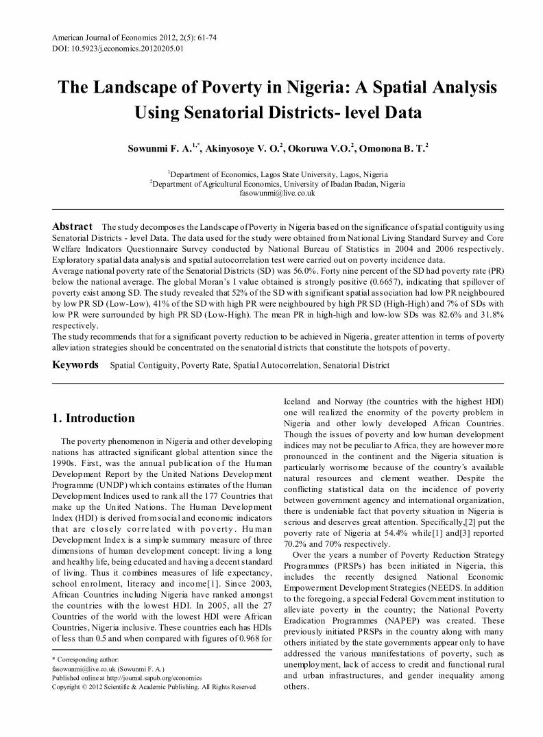
American Journal of Economics 2012, 2(5): 61-74 DOI: 10.5923/j.economics.20120205.01

The Landscape of Poverty in Nigeria: A Spatial Analysis Using Senatorial Districts- level Data

Sowunmi F. A.1,*, Akinyosoye V. O.2, Okoruwa V.O.2, Omonona B. T.2

1Department of Economics, Lagos State University, Lagos, Nigeria 2Department of Agricultural Economics, University of Ibadan Ibadan, Nigeria

[email protected]

Abstract The study decomposes the Landscape of Poverty in Nigeria based on the significance of spatial contiguity using Senatorial Districts - level Data. The data used for the study were obtained from Nat ional Living Standard Survey and Core Welfare Indicators Questionnaire Survey conducted by National Bureau of Statistics in 2004 and 2006 respectively. Exp loratory spatial data analysis and spatial autocorrelation test were carried out on poverty incidence data. Average national poverty rate of the Senatorial Districts (SD) was 56.0%. Forty nine percent of the SD had poverty rate (PR) below the national average. The global Moran’s I value obtained is strongly positive (0.6657), indicating that spillover of poverty exist among SD. The study revealed that 52% of the SD with significant spatial association had low PR neighboured by low PR SD (Low-Low), 41% of the SD with high PR were neighboured by high PR SD (High-High) and 7% of SDs with low PR were surrounded by high PR SD (Low-High). The mean PR in high-high and low-low SDs was 82.6% and 31.8% respectively. The study recommends that for a significant poverty reduction to be achieved in Nigeria, greater attention in terms of poverty allev iation strategies should be concentrated on the senatorial d istricts that constitute the hotspots of poverty.

Keywords Spatial Contiguity, Poverty Rate, Spatial Autocorrelation, Senatorial District

1. Introduction

The poverty phenomenon in Nigeria and other developing nations has attracted significant global attention since the 1990s. First , was the annual pub licat ion o f the Human Development Report by the United Nat ions Development Programme (UNDP) which contains estimates of the Human Development Indices used to rank all the 177 Countries that make up the United Nat ions. The Human Development Index (HDI) is derived from social and economic indicators that are c los ely cor re lated w ith poverty . Hu man Development Index is a simple summary measure of three dimensions of human development concept: liv ing a long and healthy life, being educated and having a decent standard of living. Thus it combines measures of life expectancy, school enro lment, literacy and income[1]. Since 2003, African Countries including Nigeria have ranked amongst the countries with the lowest HDI. In 2005, all the 27 Countries of the world with the lowest HDI were African Countries, Nigeria inclusive. These countries each has HDIs of less than 0.5 and when compared with figures of 0.968 for

* Corresponding author: [email protected] (Sowunmi F. A.) Published online at http://journal.sapub.org/economics Copyright © 2012 Scientific & Academic Publishing. All Rights Reserved

Iceland and Norway (the countries with the highest HDI) one will realized the enormity of the poverty problem in Nigeria and other lowly developed African Countries. Though the issues of poverty and low human development indices may not be peculiar to Africa, they are however more pronounced in the continent and the Nigeria situation is particularly worrisome because of the country’s available natural resources and clement weather. Despite the conflicting statistical data on the incidence of poverty between government agency and international organization, there is undeniable fact that poverty situation in Nigeria is serious and deserves great attention. Specifically,[2] put the poverty rate of Nigeria at 54.4% while[1] and[3] reported 70.2% and 70% respectively.

Over the years a number of Poverty Reduction Strategy Programmes (PRSPs) has been initiated in Nigeria, this includes the recently designed National Economic Empowerment Development St rategies (NEEDS. In addition to the foregoing, a special Federal Government institution to allev iate poverty in the country; the National Poverty Eradication Programmes (NAPEP) was created. These previously initiated PRSPs in the country along with many others initiated by the state governments appear only to have addressed the various manifestations of poverty, such as unemployment, lack of access to credit and functional rural and urban infrastructures, and gender inequality among others.

62 Sowunmi F. A. et al.: The Landscape of Poverty in Nigeria: A Spatial Analysis Using Senatorial Districts- level Data

While the above mentioned Poverty Reduction Strategy Programmes (PRSPs) were well intentioned, none had any significant, lasting, or sustainable positive effects on the people they were p lanned for[3],[4]. This can be attributed among others to the non consideration of the heterogeneous nature of poverty and spatial contiguity of geographical units in the design of PRSPs. Existing poverty studies treat a geographical unit, such as a local government area, a state, or a senatorial district, or a county, as an independent isolated entity rather than as an entity surrounded by other geographic units with which it may interact is being considered by this study. Moreover, there is scarce informat ion on spatial decomposition of poverty incidence among SD in Nigeria. Hence, the landscape of Poverty in Nigeria is investigated using Senatorial Districts (SDs) in Nigeria as geographic units.

Senatorial district is composed of Federal constituencies while federal constituency is made up of Local Government Areas. Each state is made up of three senatorial d istricts while the federal capital territory (Abuja) has one senatorial district. This means that each state in Nigeria is represented by three elected senators in the national assembly (upper legislative chamber). Delineation of the country into senatorial district by National Population Commission is based on population distribution. Apart from performing the legislative duties, senators are also task with the economic development of their respective senatorial d istrict through lobby for sitting capital pro jects and judicious use of monthly constituency allowance meant for execution of projects in senatorial d istricts.

The study utilized spatial econometrics technique instead of the conventional econometrics methods. Spatial econometrics technique has the advantage of addressing the problem of spillover effect or spatial autocorrelation if present in the data set. According to[5], studies that ignore spatial autocorrelation (dependence) can produce biased results (coefficient estimates) and lead to ineffective and possibly counterproductive – recommendations for policies targeted at poverty alleviation.

The study identified the locations of senatorial districts with similar and dissimilar (outlier) pattern of poverty incidence. Knowing this will afford researchers to determine the factors that are specific to each of the identified groups. The finding of this study is expected to assist government in localizing poverty alleviat ion strategy of senatorial d istricts that exhib it similar spatial pattern of poverty.

2. Conceptual Framework and Previous Literature

2.1. Conceptual Framework

The philosophy behind this study is based on Tobler First Law of Geography:"everything is related to everything else, but near things are more related than distant things." Spatial clustering shows the similarity or dissimilarity of poverty in

neighbouring units and spatial autocorrelation measures the strength of the spatial clustering[6],[7],[8],[9],[10]. Global spatial autocorrelat ion (Moran’s I) analysis yields only one statistics to summarize the pattern of poverty in the whole study area. That is, global Moran’s I assumes homogeneity of the study area (that poverty pattern is the same in all the senatorial districts). This is the limitation of global Moran’s I. To localize the presence and magnitude of spatial autocorrelation, a measure such as Anselin’s Local Indicators of Spatial Association (LISA) is necessary (see equation 7). This approach is most useful when, in addition to global trends in the entire sample o f observations, there exist also pockets of localities exh ibit ing heterogeneous values that do not follow the global trend. This leads to identification of so-called hot spots -regions where the considered phenomenon is extremely pronounced across localities- as well of spatial outliers[11].

‘Moran scatter plot’ p lots a variab le o f interest against spatial weighted component of that variable. This measure permits a more disaggregated view of the type of spatial autocorrelation that exists in a data. Local Indicators of Spatial Association[12] and Moran scatter plot[13] are valuable for gain ing a ‘‘local’’ understanding of the extent and nature of spatial clustering in a geographical unit. LISA indicates significant spatial clustering for each location.

Moran scatter plot utilizes graph only to identify observations (extent of poverty) that are similar as well as different (outliers: neighbouring senatorial districts that has contrasting poverty rates) from their neighbours while formula is used in Local Moran’s I to identify similarity or dissimilarity of poverty rates in neighbouring units. For each location (senatorial d istrict), LISA values allow for the computation of its similarity with its neighbours and also to test its significance. Spatial association can be decomposed into four components, viz: ■Senatorial districts with h igh concentration of poverty

with similar neighbours: high-high. Also known as “hot spots”. ■Senatorial districts with low concentration of poverty

with similar neighbours: low-low. Also known as “cold spots”. ■Senatorial districts with h igh concentration of poverty

with low concentration of poverty neighbours: high-low. Potential “spatial outliers”.

■Senatorial districts with low concentration of poverty with high concentration of poverty neighbours: low-high. Potential “spatial outliers”.

■ Senatorial districts with no significant local autocorrelation.

Reference[13] demonstrated that the slope of the regression line through the points in Moran scatter plot expresses the global Moran’s I value. A strong positive statistic indicates positive spatial autocorrelation (clustering of like values). This means that most senatorial d istricts would be found in the high-high or low-low (first and third quadrants) areas of the country.

American Journal of Economics 2012, 2(5): 61-74 63

A strong negative statistic indicates negative spatial autocorrelation suggests most senatorial districts with high (low) poverty concentration would be found in the vicinity of low (high) poverty senatorial districts (outliers).

2.2. Review of Previous Literature

Poverty is not only a state of existence but also a process with many dimensions and complexities. Generally, poverty has attracted a lot o f attention from the academia and non-academia globally. Few recent studies are based on the premise that individuals and households with common characteristics sometimes are found clustered together either by choice or because they are constrained to co-locate by coercive operation of social, economic, geographic or political forces[14]. Identification of these households has been made possible through the advancement in spatial analytical techniques; which has also enables spatial pattern of poverty (concentration of poverty rates and outliers) to be quantified[15],[16],[17]. References[18],[19] showed that poverty rate in nearby locations are likely to be similar to one another, or error for the model in one area or location is correlated with the error terms in its neighboring locations; hence the need to pay attention to the structure of spatial dependence or autocorrelation in our data.

Reference[20] posited that knowing precisely where concentration of poverty exit will help the policy maker, social scientist and all other stake holders in continuing challenge of combating this fundamental threat (poverty) to well-being. Ignoring spatial autocorrelat ion will make it : ■ impossible to measure the strength of spatial

concentration of poverty. ■difficu lt to exp lain substantial variation in the incidence

of poverty across senatorial d istricts. In a study on the topography of poverty in US,[20]

findings showed that 51.9% of the total counties belong to similar spatial concentration (low – low and high-high), whereas only 7.8% were categorized as being spatial outliers (high – low and low – high). The remain ing 40.3% were neither. The categorization of spatial concentration into high or low poverty rate neighbourhood is in relat ionship with average national poverty rate. Most counties in US are found in the high-high and low-low subregions[14]. That is, the counties whose poverty rate is above (below) the average poverty rate are surrounded by counties with poverty rate above (below) average national poverty rate.

Reference[21] conducted a research on the application o f a spatial regression model to analysis and poverty mapping in Ecuador; their results confirmed the significant effects of spatial autocorrelation variable that denotes the presence of clusters in the spatial distribution of poverty and the influence between neighbourhood households on the probability of being poor. A combination of processes

(socioeconomic, polit ical, demographic and geographic) operating in space over time has somehow conspired to partition countries into large reg ions of high and large regions of low poverty—with occasional ‘‘island’’ geographic units here and there that are very different from their neighbors[14].

Similarly,[22] in study on spatial clustering of ru ral poverty in Sri Lanka found that Divisional Secretariat (DS) divisions with a high percentage of poor households are found in four rural districts where agricu lture is the main source of livelihood of the majority of households. The clustering of DS div isions of low poverty around major urban centres suggests that, in predominantly agricultural areas, poor people have only limited economic opportunities to escape poverty. They revealed that availability of and access to water and land resources are the major factors of spatial concentration of poverty in rural areas. In another study on spatial approach to social and polit ical forces as a determinant of poverty in US,[5] stated that a positive and significant spatial dependence in the dependent variable (poverty rate) indicates that the poverty rate in a part icular county is associated with poverty rates in surrounding counties/local government areas. According to them, the value of the spatial autocorrelation coefficient (ρ = 0.21 in the model for all counties) obtained indicates that a 10 percentage point increase in the poverty rate in a county results in a 2% increase in the poverty rate in a neighbouring county. This is strong evidence that spillover effects exist between counties with respect to poverty. This finding is corroborated by[23]. They reasoned that poverty of a neighbourhood is tied to the fortunes of neighbouring areas: there are geographic spillovers in poverty reduction. Reducing poverty in particular neighbourhoods affects the poverty of neighbouring tracts.

3. Methodology

3.1. Study Area

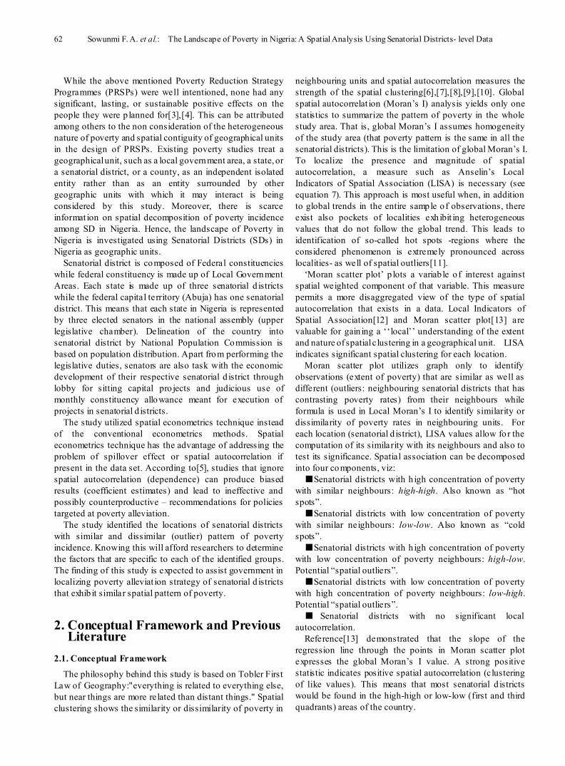
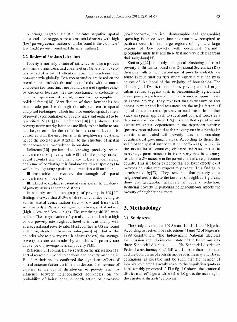
The study covered the 109 Senatorial districts of Nigeria. According to section five subsections 71 and 72 of Nigeria’s 1999 constitution, “the Independent National Electoral Commission shall div ide each state of the federat ion into three Senatorial d istricts………. No Senatorial district or Federal constituency shall fall within more than one state, and the boundaries of each district or constituency shall be as contiguous as possible and be such that the number of inhabitants thereof is nearly equal to the population quota as is reasonably practicable.” The fig. 1.0 shows the senatorial district map of Nigeria while table 1.0 gives the meaning of the senatorial districts’ acronyms.


Source: Adapted from NBS (2007)

Figure 1. Senatorial District Map of Nigeria 3.3. Methods of Data Analysis

The study utilized descriptive and exploratory spatial data analyses (ESDA). The GIS software (ArcGIS 8.1) was used to ensure the compatibility of the senatorial district map with Geoda 0.9.5i

The most common measure of spatial autocorrelation, a statistic called g lobal Moran’s I[24],[25] is defined as follows:

( )( )( )

−

−−

=

∑

∑∑∑∑

≠

≠ ii

jii j

ij

i jij

global xx

xxxxw

wnI 2

1

1

(1)

Where: i and j index the area units of which there are n, wij is a spatial weight measure of contiguity defining the

connection between area unit i and area unit j. w is 1 if location i is contiguous to location j and 0 (zero)

otherwise. xi is the poverty rate for each senatorial district x is the average poverty rate for 109 senatorial d istricts

Positive values of Moran’s I suggest spatial clustering of similar values across geo - space. A significant negative value (infrequent in the social sciences) indicates that neighbouring values are more d issimilar than expected by chance, that is high values are frequently found in the

vicinity of low values.. The I statistic is similar to the familiar Pearsonian product-moment correlation coefficient, however, the maximum and min imum possible values of Moran’s I are not constrained to lie in the (–1, 1) range[26],[27].

The expected value and variance of Moran’s I for a sample of size n could be calculated according to the assumed pattern of the spatial data distribution[24].

For the assumption of a normal d istribution:

( ) ( )11−

−=n

IEn (2)

( ) ( ) ( )IEnw

wnwwnIVar nn2

220

2021

2

13

−−+−

= (3)

For the assumption of random d istribution:

( ) ( )11−

−=n

IEr (4)

( )( ) ( )( )( )( )( ) ( )

2 2 2 21 2 0 2 1 2 0 2

20

( )

3 3 3 2 6

1 2 3

r

r

VAR I

n n n w nw w K n n w nw wE I

w n n n

− + − + − − − +−

− − −

= (5)

where: ( )

( )

∑ −

∑ −=

n

ii

n

ii

xx

xxnK

2

4

2, ∑∑=

n

i

n

jijww0 ,

BoN

BoC

BoS

YoE YoN

YoS BaN

JiNE JiNW

JiSW

BaC

BaS

KaS

KaC KaN

GoN

GoC

GoS AdC

AdN

TaN

AdS

TaC

TaS

PlS

PlC PlN

NaS NaN

NaW

BeNW

BeNE

KadN KadC

KadS

NiNE NiN

NiS FCT

KwN

SoN SoE

SoS

ZaW KeC

KeN

KeS

ZaN

ZaC

KatC KatN

KatS

CrN

CrC

CrS

BeS

KoE

KoW

KoC

EdN

EdC EnW

EnN EbC

EbS

AiS

AiN W

AbN

AbC

RiSE

EdS

OnN

KwC KwS

OyN

OyC

OyS

OgC OgE

OnS

OnC

DeC

DeS

DeN

RiE

RiSW

BayW

BayE BayC

LaW LaE

OgW

ImN ImE

AbS

O W O E

O C

EkS

EkC

E E EbN


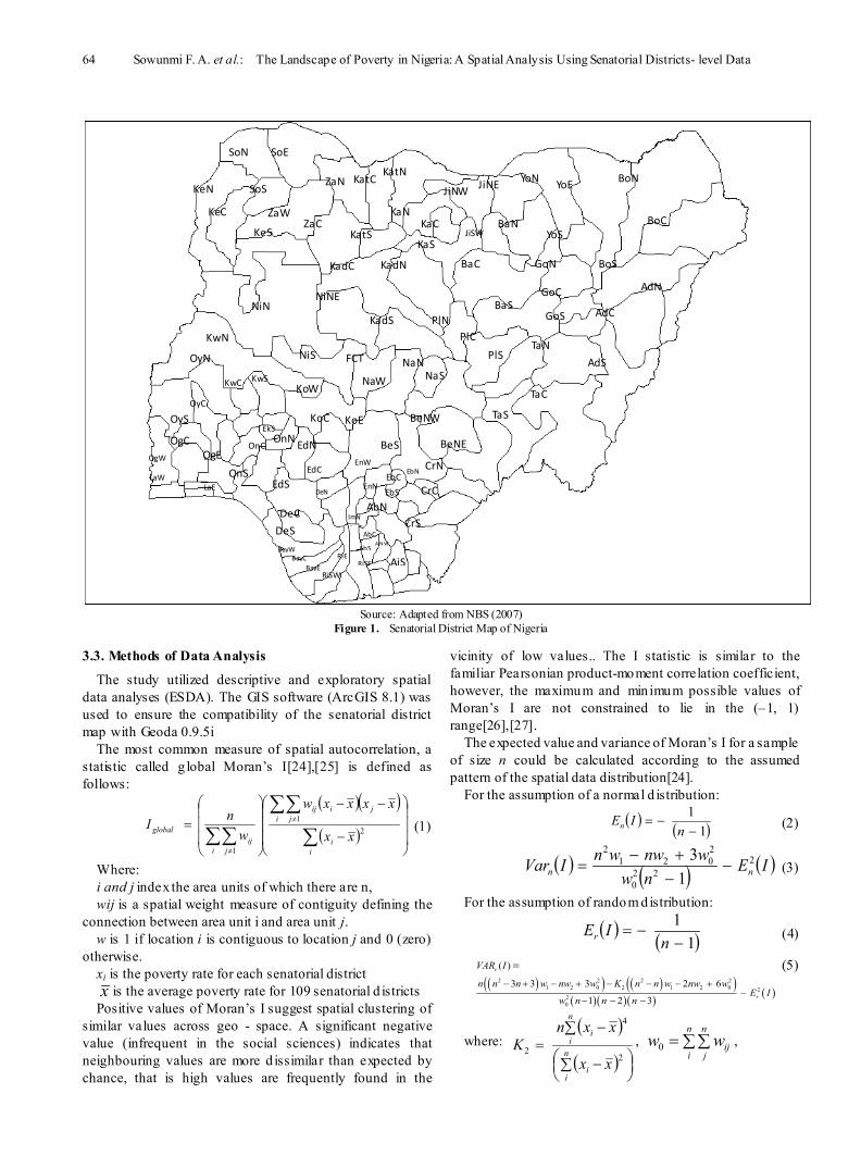
Table 1. Senatorial Districts’ Identity

Senatorial District ID Senatorial District ID Senatorial District ID Senatorial District ID Abia Central AbC Cross River South CrS Kaduna South KadS Ogun West OgW

Abia North AbN Delta Central DeC Kano Central KaC Ondo Central OnC

Abia South AbS Delta North DeN Kano North KaN Ondo West OnW Adamawa Central AdC Delta South DeS Kano South KaS Ondo East OnE

Adamawa North AdN Ebonyi Central EbC Katsina Central KatC Osun Central OsC

Adamawa South AdS Ebonyi North EbN Katsina North KatN Osun East OsE Akwa Ibom North West AiNW Ebonyi South EbS Katsina South KatS Osun West OsW

Akwa Ibom North East AiNE Edo Central EdC Kebbi Cental KeC Oyo Central OyC

Akwa Ibom South AiS Edo North EdN Kebbi North KeN Oyo North OyN Anambra Central AnC Edo South EdS Kebbi South KeS Oyo South OyS

Anambra North AnN Ekiti Central EkC Kogi West KoW Plateau Central PlC

Anambra South AnS Ekiti North EkN Kogi Central KoC Plateau North PlN Bauchi Central BaC Ekiti South EkS Kogi East KoE Plateau South PlS

Bauchi North BaN Enugu East EnE Kwara Centarl KwC Rivers East RiE

Bauchi South BaS Enugu North EnN Kwara North KwN Rivers South East RiSE Bayelsa Central BayC Enugu West EnW Kwara South KwS Rivers South West RiSW

Bayelsa East BayE Gombe Central GoC Lagos central LaC Sokoto East SoE

Bayelsa West BayW Gombe North GoN Lagos East LaE Sokoto North SoN Benue North East BeNE Gombe South GoS Lagos West LaW Sokoto South SoS

Benue North West BeNW Imo East ImE Nassarawa North NaN Taraba Central TaC

Benue South BeS Imo North ImN Nassarawa South NaS Taraba North TaN Borno Central BoC Imo West ImW Nassarawa Central NaC Taraba South TaS

Borno North BoN Jigawa North East JiNE Niger East NiE Yobe East YoE

Borno South BoS Jigawa North West JiNW Niger North NiN Yobe North YoN Borno South BoS Jigawa South West JiSW Niger South NiS Yobe South YoS

Cross River Central CrC Kaduna Central KadC Ogun Central OgC Zamfara Central ZaC

Cross River North CrN Kaduna North KadN Ogun East OgE Zamfara North ZaN Zamfara West ZaW

FCT AbJ

Source: Survey Data, 2010

( )∑∑ +=n

i

n

jjiij www 2

1 21

, ( )∑ +=n

iji www 2

2

wi. and w.i are the sum of the row i and column i of the weight matrix respectively.

The test of the null hypothesis that there is no spatial autocorrelation between observed values over the n locations can be conducted on the basis of the standardized statistics as follows:

( ) ( ) ( )( )IVAR

IEdIdZ −= (6)

Moran’s I is significant and positive when the observed values of locations within a certain d istance (d) tend to be similar, negative when they tend to be dissimilar, and approximately zero when the observed values are arranged randomly and independently over space.

Spatial analysis (Local indicator of Spatial Association

Indices, Local indicator of Spatial Association Cluster Map, Local indicator o f Spatial Association Significance Map and Moran scatter plot) is employed to identify the senatorial districts with similar spatial pattern of poverty incidence. The analysis is carried out whether spatial autocorrelat ion is significantly present in the geo-referenced data set or not. Local Moran’s I is computed using the formula below:

( )( )( )∑

∑−

−−=

ii

ijiij

local xx

xxxxwI 2 (7)

The result from the spatial analysis above (LISA) identifies the senatorial districts with similar pattern of spatial distribution of poverty incidence as well as outliers (high – high, low – low, low – high and high - low). The significance or non significance of spatial autocorrelation is a prerequisite for the choice of corrective measure.


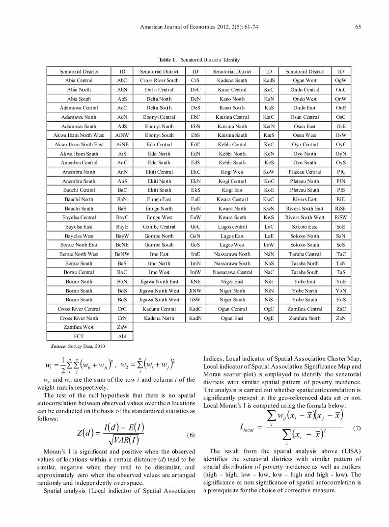
4. Empirical Results and Discussion The study showed a low poverty incidence (%) in the

southern part of the country which ranges from 8.1 to 36.9. In the north central, the poverty incidence ranges from 55.4% to 78.1%. The core north which (comprises of north west and north east) has the highest poverty incidence ranging from 78.4 % in Zamfara central to 97.7% in Jigawa northeast. Generally, the study revealed an average poverty rate of 56.04% among the 109 senatorial districts (see figure 1.1). Federal Capital Territory, Kaduna central, Kano central and Borno central are the three senatorial districts in the north that the poverty rates are substantially lower than the national poverty rate. This may be attributed to the location of state capitals (seat of government) in these senatorial districts where basic infrastructures are concentrated.

Moreover, the three senatorial districts in Lagos state (Lagos east, Lagos west and Lagos central), one in Edo

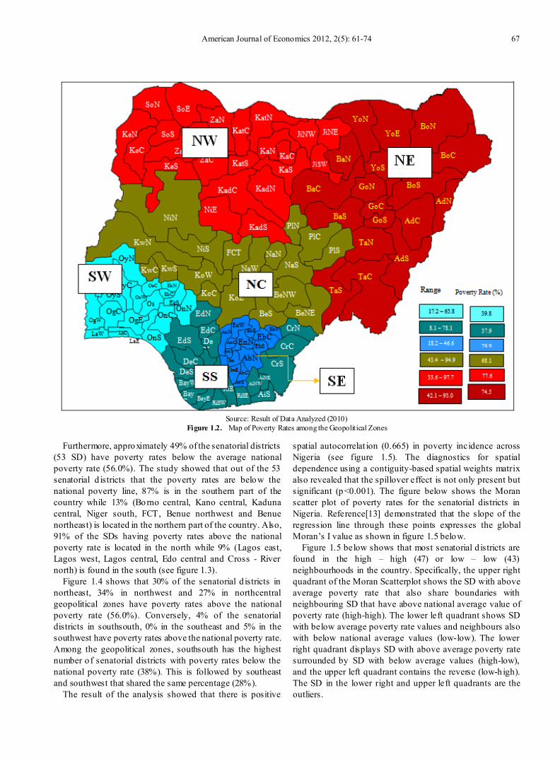
state (Edo central) and Cross – River (Cross – River north) have the poverty rates higher than the national poverty rate in the south. The poverty rates in the six geopolit ical zones corroborate the findings above (see figure 1.2). Specifically, the average poverty rate in the southeast is the lowest (29.9%), while average poverty rates of southsouth and southwest are 39.8% and 37.9% respectively. The northwest geopolitical zone has the highest average poverty rate (77.6%); this is followed by northeast (74.5%) and northcentral (68.1%). The h igh average poverty rates in the northern geopolitical zones may be attributed to long – standing lags in provision of health, education and other social services resulting in p roportionately more poor in the north[28]. He reasoned that the southern zone has most of the industries and many export crops while the northern zone is largely rural and agricultural with a frag ile agro – climat ic environment and a different socioeconomic h istory.

Source: Result of Data Analyzed (2010)

Figure 1.1. Map of Poverty Rates based on 109 Senatorial Districts

BoN

BoC

BoS

YoE YoN

YoS BaN

JiNE JiNW

JiSW

BaC

BaS

KaS

KaC KaN

GoN

GoC

GoS AdC

AdN

TaN

AdS

TaC

TaS

PlS

PlC PlN

NaS

NaN

NaW

BeNW

BeNE

KadN KadC

KadS

NiNE NiN

NiS FCT KwN

SoN SoE

SoS

ZaW KeC

KeN

KeS

ZaN

ZaC

KatC KatN

KatS

CrN

CrC

CrS

BeS

KoE

KoW

KoC

EdN

EdC EnW

EnN EbC

EbS

AiS

AiNW

AbN

AbC

RiSE

EdS

OnN

KwC KwS OyN

OyC OyS

OgC OgE

OnS

OnC

DeC DeS

DeN

RiE

RiSW

BayW

Bay

BayC

LaW LaE

OgW

ImN

ImE

AbS

A C

A S

O W Os

O C

EkS

EkN EkC

EnE EbN 35 7 – 54 9

55 4 – 78 1

78 4 – 97 7

8 1 - 36 9

Poverty Rate (%) Range



Figure 1.2. Map of Poverty Rates among the Geopolitical Zones

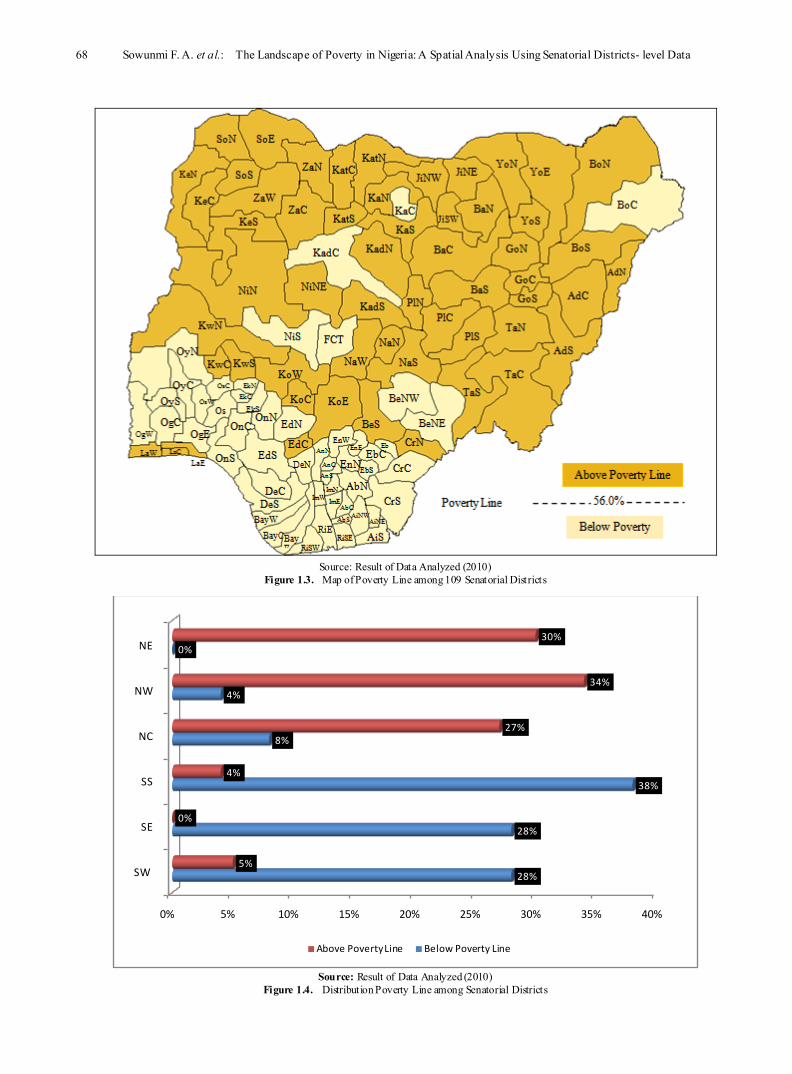
Furthermore, approximately 49% of the senatorial districts (53 SD) have poverty rates below the average national poverty rate (56.0%). The study showed that out of the 53 senatorial d istricts that the poverty rates are below the national poverty line, 87% is in the southern part of the country while 13% (Borno central, Kano central, Kaduna central, Niger south, FCT, Benue northwest and Benue northeast) is located in the northern part of the country. Also, 91% of the SDs having poverty rates above the national poverty rate is located in the north while 9% (Lagos east, Lagos west, Lagos central, Edo central and Cross - River north) is found in the south (see figure 1.3).

Figure 1.4 shows that 30% of the senatorial d istricts in northeast, 34% in northwest and 27% in northcentral geopolitical zones have poverty rates above the national poverty rate (56.0%). Conversely, 4% of the senatorial districts in southsouth, 0% in the southeast and 5% in the southwest have poverty rates above the national poverty rate. Among the geopolitical zones, southsouth has the highest number o f senatorial districts with poverty rates below the national poverty rate (38%). This is followed by southeast and southwest that shared the same percentage (28%).

The result of the analysis showed that there is positive

spatial autocorrelat ion (0.665) in poverty incidence across Nigeria (see figure 1.5). The diagnostics for spatial dependence using a contiguity-based spatial weights matrix also revealed that the spillover effect is not only present but significant (p<0.001). The figure below shows the Moran scatter plot of poverty rates for the senatorial districts in Nigeria. Reference[13] demonstrated that the slope of the regression line through these points expresses the global Moran’s I value as shown in figure 1.5 below.

Figure 1.5 below shows that most senatorial d istricts are found in the high – high (47) or low – low (43) neighbourhoods in the country. Specifically, the upper right quadrant of the Moran Scatterplot shows the SD with above average poverty rate that also share boundaries with neighbouring SD that have above national average value of poverty rate (high-high). The lower left quadrant shows SD with below average poverty rate values and neighbours also with below national average values (low-low). The lower right quadrant displays SD with above average poverty rate surrounded by SD with below average values (high-low), and the upper left quadrant contains the reverse (low-h igh). The SD in the lower right and upper left quadrants are the outliers.



Figure 1.3. Map of Poverty Line among 109 Senatorial Districts


Figure 1.4. Distribution Poverty Line among Senatorial Districts

0% 5% 10% 15% 20% 25% 30% 35% 40%

SW

SE

SS

NC

NW

NE

28%

28%

38%

8%

4%

0%

5%

0%

4%

27%

34%

30%

Above Poverty Line Below Poverty Line


Table 1.1. Diagnostics for Spatial DependenceFOR WEIGHT MATRIX : koloqueenPlA.GAL (row-standardized weights)

TEST MI/DF VALUE PROB

Moran's I (error) 0.125539 3.3653048 0.0007647

Lagrange Multiplier (lag) 1 11.677104 0.0006327

Robust LM (lag) 1 7.6509946 0.0056741

Lagrange Multiplier (error) 1 4.0263889 0.0447937

Robust LM (error) 1 0.0002795 0.9866617


The study did not only reveal the significant presence of spatial dependence but also the type of spatial dependence that is more likely, using the robust Lagrange Multiplier indicators[13]. The table 1.1 shows that spatial lag is the type of spatial dependence present in poverty incidence in Nigeria. The value for robust Lagrange multiplier (lag) is high and significant (p<0.01). This means that poverty incidence in one SD is not only influenced by factors within but also by the poverty incidence in nearby SD. That is, proximity of senatorial districts in fluences the poverty rates. The implicat ion of this result is that spatial dimension has to be given consideration in any causal relationship between poverty rate and factors influencing it.


Figure 1.5. Moran Scatter Plot of Poverty Incidence

4.1. Location of Senatorial Districts with Similar Pattern of Poverty Incidence.

The result obtained from Local Indicator of Spatial Association (LISA) revealed that out of 90 senatorial districts that have similar spatial pattern of poverty incidence (high-high and low-low), 51 have similar spatial patterns that are statistically significant (at p≤ 5%, see table 1.2 below). The high – high constitutes the senatorial districts with more pronounced poverty incidence as well as their neighbouring SD.

Source: Result of Analyzed Data (2010)

Figure 1.6. Local Indicator of Spatial Association (LISA) Map for Significant Spatial Pattern


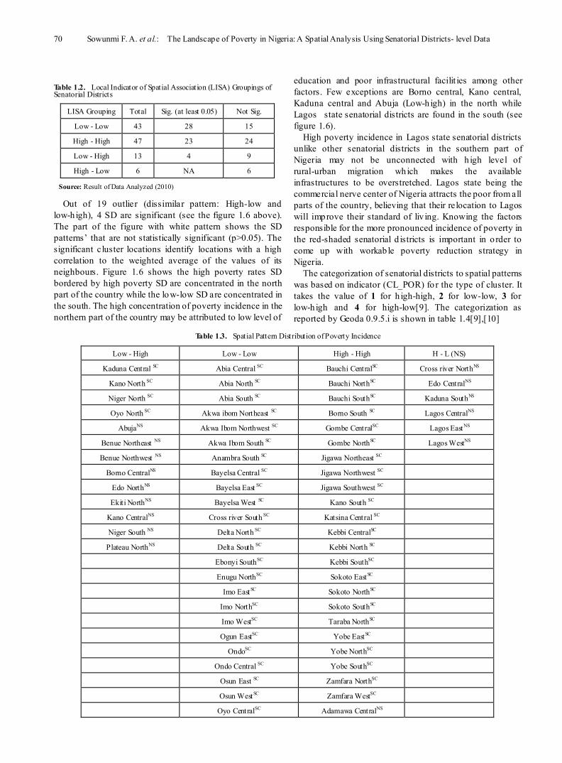
Table 1.2. Local Indicator of Spatial Association (LISA) Groupings of Senatorial Districts

LISA Grouping Total Sig. (at least 0.05) Not Sig.

Low - Low 43 28 15

High - High 47 23 24

Low - High 13 4 9

High - Low 6 NA 6


Out of 19 outlier (dissimilar pattern: High-low and low-h igh), 4 SD are significant (see the figure 1.6 above). The part of the figure with white pattern shows the SD patterns’ that are not statistically significant (p>0.05). The significant cluster locations identify locations with a high correlation to the weighted average of the values of its neighbours. Figure 1.6 shows the high poverty rates SD bordered by high poverty SD are concentrated in the north part of the country while the low-low SD are concentrated in the south. The high concentration of poverty incidence in the northern part of the country may be attributed to low level of

education and poor infrastructural facilit ies among other factors. Few exceptions are Borno central, Kano central, Kaduna central and Abuja (Low-h igh) in the north while Lagos state senatorial districts are found in the south (see figure 1.6).

High poverty incidence in Lagos state senatorial districts unlike other senatorial districts in the southern part of Nigeria may not be unconnected with h igh level of rural-urban migration which makes the available infrastructures to be overstretched. Lagos state being the commercial nerve center of Nigeria attracts the poor from all parts of the country, believing that their relocation to Lagos will improve their standard of liv ing. Knowing the factors responsible for the more pronounced incidence of poverty in the red-shaded senatorial d istricts is important in o rder to come up with workab le poverty reduction strategy in Nigeria.

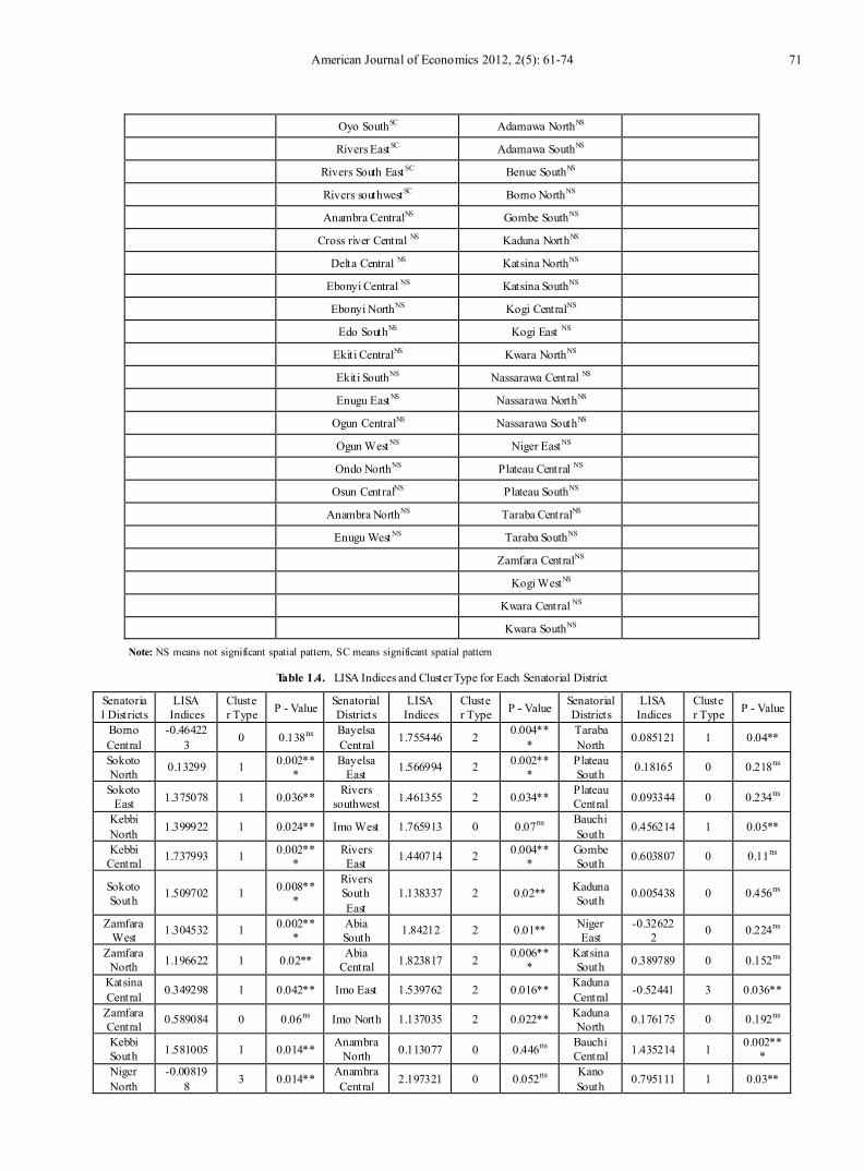
The categorization of senatorial districts to spatial patterns was based on indicator (CL_POR) fo r the type of cluster. It takes the value of 1 for h igh-high, 2 for low-low, 3 for low-h igh and 4 for high-low[9]. The categorization as reported by Geoda 0.9.5.i is shown in table 1.4[9],[10]

Table 1.3. Spatial Pattern Distribution of Poverty Incidence

Low - High Low - Low High - High H - L (NS)

Kaduna Central SC Abia Central SC Bauchi CentralSC Cross river NorthNS

Kano North SC Abia North SC Bauchi NorthSC Edo CentralNS

Niger North SC Abia South SC Bauchi SouthSC Kaduna SouthNS

Oyo North SC Akwa ibom Northeast SC Borno South SC Lagos CentralNS

AbujaNS Akwa Ibom Northwest SC Gombe CentralSC Lagos EastNS

Benue Northeast NS Akwa Ibom South SC Gombe NorthSC Lagos WestNS

Benue Northwest NS Anambra South SC Jigawa Northeast SC Borno CentralNS Bayelsa Central SC Jigawa Northwest SC

Edo NorthNS Bayelsa East SC Jigawa Southwest SC Ekiti NorthNS Bayelsa West SC Kano South SC

Kano CentralNS Cross river South SC Katsina Central SC Niger South NS Delta North SC Kebbi CentralSC

Plateau NorthNS Delta South SC Kebbi North SC

Ebonyi SouthSC Kebbi SouthSC

Enugu NorthSC Sokoto EastSC

Imo EastSC Sokoto NorthSC

Imo NorthSC Sokoto SouthSC

Imo WestSC Taraba NorthSC

Ogun EastSC Yobe EastSC

OndoSC Yobe NorthSC

Ondo Central SC Yobe SouthSC

Osun East SC Zamfara NorthSC

Osun WestSC Zamfara WestSC

Oyo CentralSC Adamawa CentralNS


Oyo SouthSC Adamawa NorthNS

Rivers EastSC Adamawa SouthNS

Rivers South EastSC Benue SouthNS

Rivers southwestSC Borno NorthNS

Anambra CentralNS Gombe SouthNS

Cross river Central NS Kaduna NorthNS

Delta Central NS Katsina NorthNS

Ebonyi Central NS Katsina SouthNS

Ebonyi NorthNS Kogi CentralNS

Edo SouthNS Kogi East NS

Ekiti CentralNS Kwara NorthNS

Ekiti SouthNS Nassarawa Central NS

Enugu EastNS Nassarawa NorthNS

Ogun CentralNS Nassarawa SouthNS

Ogun WestNS Niger EastNS

Ondo NorthNS Plateau Central NS

Osun CentralNS Plateau SouthNS

Anambra NorthNS Taraba CentralNS

Enugu WestNS Taraba SouthNS

Zamfara CentralNS

Kogi WestNS

Kwara Central NS

Kwara SouthNS Note: NS means not significant spatial pattern, SC means significant spatial pattern

Table 1.4. LISA Indices and Cluster Type for Each Senatorial District

Senatorial Districts

LISA Indices

Cluster Type P - Value Senatorial

Districts LISA

Indices Cluster Type P - Value Senatorial

Districts LISA

Indices Cluster Type P - Value

Borno Central

-0.464223 0 0.138ns Bayelsa

Central 1.755446 2 0.004***

Taraba North 0.085121 1 0.04**

Sokoto North 0.13299 1 0.002**

* Bayelsa

East 1.566994 2 0.002***

Plateau South 0.18165 0 0.218ns

Sokoto East 1.375078 1 0.036** Rivers

southwest 1.461355 2 0.034** Plateau Central 0.093344 0 0.234ns

Kebbi North 1.399922 1 0.024** Imo West 1.765913 0 0.07ns Bauchi

South 0.456214 1 0.05**

Kebbi Central 1.737993 1 0.002**

* Rivers East 1.440714 2 0.004**

* Gombe South 0.603807 0 0.11ns

Sokoto South 1.509702 1 0.008**

*

Rivers South East

1.138337 2 0.02** Kaduna South 0.005438 0 0.456ns

Zamfara West 1.304532 1 0.002**

* Abia South 1.84212 2 0.01** Niger

East -0.32622

2 0 0.224ns

Zamfara North 1.196622 1 0.02** Abia

Central 1.823817 2 0.006***

Katsina South 0.389789 0 0.152ns

Katsina Central 0.349298 1 0.042** Imo East 1.539762 2 0.016** Kaduna

Central -0.52441 3 0.036**

Zamfara Central 0.589084 0 0.06ns Imo North 1.137035 2 0.022** Kaduna

North 0.176175 0 0.192ns

Kebbi South 1.581005 1 0.014** Anambra

North 0.113077 0 0.446ns Bauchi Central 1.435214 1 0.002**

* Niger North

-0.008198 3 0.014** Anambra

Central 2.197321 0 0.052ns Kano South 0.795111 1 0.03**


Kwara North 1.079825 0 0.072ns Abia

North 0.889468 2 0.004***

Katsina North 0.723859 0 0.09ns

Ogun West 0.463057 0 0.172ns Akwa Ibom

Northwest 1.084156 2 0.004**

* Kano

Central -0.19382

1 0 0.148ns

Lagos West

-0.339704 0 0.144ns

Akwa Ibom South

0.715628 2 0.028** Jigawa

Northwest

1.860673 1 0.002***

Lagos Central -0.01579 0 0.486ns

Akwa Ibom

Northeast 0.767667 2 0.036**

Jigawa Southwes

t 2.428236 1 0.002**

*

Lagos East 0.027419 0 0.14ns

Cross river South

0.815704 0 0.068ns Jigawa Northeast 2.407263 1 0.004**

*

Ogun Central 0.480427 0 0.094ns

Cross river

Central 0.170273 0 0.302ns Bauchi

North 2.202587 1 0.002***

Oyo South 1.352365 2 0.006**

* Ebonyi South 0.312115 0 0.074ns Yobe

North 1.530074 1 0.002***

Oyo Central 1.742068 2 0.026** Enugu

North 0.503644 2 0.008***

Gombe North 0.823629 1 0.008**

* Kwara Central 0.890275 0 0.066ns Enugu

West 0.307916 0 0.244ns Gombe Central 0.829602 1 0.028**

Kwara South 0.721746 0 0.092ns Enugu

East 0.543905 0 0.186ns Adamawa South 0.456606 0 0.212ns

Osun West 0.933906 2 0.008**

* Ebonyi Central 0.213703 0 0.096ns Adamawa

Central 0.143101 0 0.072ns

Osun East 0.90421 2 0.028**

* Ebonyi North

-0.209278 0 0.338ns Adamawa

North 0.093192 0 0.418ns

Ogun East 1.112751 2 0.004**

*

Cross river North

-0.254197 0 0.286ns Yobe

South 1.336898 1 0.012**

Ekiti South 0.279504 0 0.18ns Kogi East 0.198294 0 0.34ns Yobe East 1.134799 1 0.01**

Senatorial Districts

LISA Indices

Cluster Type P - Value Senatorial

Districts LISA

Indices Cluster Type P - Value Senatorial

Districts LISA

Indices Cluster Type P - Value

Ondo Central 0.582487 2 0.014** Benue

South -0.03422

6 0 0.426ns Borno North 0.383302 0 0.332ns

Ondo North 0.127022 0 0.216ns Benue

Northeast -0.05224

6 0 0.2ns Borno South 0.113653 1 0.028**

Kogi West 0.417307 0 0.126ns Benue

Northwest -0.02907

4 0 0.372ns Ekiti Central 0.343983 2 0.042**

Kogi West 0.417307 0 0.126 Benue

Northwest -0.02907

4 0 0.372 Ekiti Central 0.343983 2 0.042**

Kogi Central 0.946763 0 0.064 Taraba

Central 0.084992 0 0.148 Ekiti North

-0.129294 0 0.34

Edo North

-0.062722 0 0.292 Taraba

South 0.073737 0 0.366 Anambra South 1.433544 2 0.026**

Edo South 0.455539 0 0.192 Niger

South -0.15267

1 0 0.08 Kano North 0 3 0.002**

* Edo

Central -0.15622

1 0 0.318 Abuja -0.278874 0 0.128 Oyo

North 0 3 0.002***

Delta North 0.567632 2 0.022** Nassaraw

a Central 0.157945 0 0.148 Osun Central 0.035184 0 0.428

Delta Central 0.220928 0 0.136 Nassaraw

a North 0.030504 0 0.358 Ondo 0.517628 2 0.02***

Bayelsa West 1.832168 2 0.044** Nassaraw

a South 0.030894 0 0.26 Plateau North

-0.008957 0 0.178

Delta South 0.309415 2 0.008**

* Source: Result of Data Analyzed (2009) Note: ***p-value < 0.01 and **p-value< 0.05, ns means not significant, 1 = HH, 2 = LL and 3 = LH (Geoda 0.9.5i reports only the significant clusters)

5. Conclusions and Recommendations

The application of spatial data analysis methods revealed

strong evidence of spatial interaction across senatorial district boundaries. Using a binary weight matrix in the estimation of spatial effects, we found that proximity to senatorial districts that have a h igh (low) poverty rate will


increase the probability that household in a senatorial district will itself have a high (low) incidence of poverty.

The landscape of poverty incidence obtained from the study identified the hot spots and cold spots of poverty in Nigeria. Knowing precisely where concentrations and isolated islands of poverty exist will help various government owned organizations with the mandate of allev iating poverty (NAPEP, NEPAD and NEEDS) and state governments in their continuing challenge of combating this fundamental threat to well-being and economic development of Nigeria. Moreover, this finding will assist government agencies saddled with poverty alleviat ion in applying specific strategy to different landscape of poverty. Also, the elected representatives (senators) are afforded the opportunity of knowing the poverty landscape of their respective senatorial districts so that their constituency development fund can be property channeled to poverty allev iation.

ACKNOWLEDGEMENTS The authors are thankful to Dr. Julia Koschinsky

(Assistant Research Professor & Research Director of GeoDa Center, Arizona State University, Tempe, AZ, 85287, United States) for her technical assistance.

REFERENCES [1] United Nations Development Programme (UNDP), Nigeria

Human Development Report. Millennium Edition, Lagos, 2005.

[2] National Bureau of Statistics (NBS), Poverty Profile for Nigeria. Federal Republic of Nigeria, 2005.

[3] International Monetary Fund (IMF), “National Economic Empowerment and Development Strategy (NEEDS)”, Nigeria Poverty Reduction Strategy Paper. IMF Country Report. No. 05/433, 2005.

[4] V. O. Akinyosoye, Government and Agriculture in Nigeria: Analysis of Policies, Programmes and Administration. Macmillan Publishers Limited: Lagos, Nigeria, 2005.

[5] Rupasingha, S. J. Goetz, “Social and Political Forces as Determinants of Poverty: A Spatial Analysis.” The Journal of Socio-Economic, vol. 36. pp. 650 –671, 2007.

[6] D. Cliff, J. K. Ord, Spatial Autocorrelation, Pion Limited, London, England, 1973.

[7] Getis, J. K. Ord, “The Analysis of Spatial Association by use of Distance Statistics”, Geographical Analysis, vol. 24, pp. 189–206, 1992.

[8] L. Anselin, “Local Indicators of Spatial Association–LISA”. Geographical Analysis, vol. 27, pp. 93 –115, 1995.

[9] L. Anselin, GeoDaTM 0.9.5-i Release Notes, Center for Spatially Integrated Social Science, 2004.

[10] L. Anselin, Exploring Spatial Data with GeoDaTM : A Workbook, Spatial Analysis Laboratory, Department of Geography, University of Illinois, Urbana-Champaign, Urbana, IL 61801, 2005.

[11] Z. Guilmoto, S. Oliveau, “Spatial Regression and Determinants of Juvenile Sex Ratio in India”, A paper Presented at the Seminar on Female Deficit in Asia: Trends and Perspectives, Singapore, 5-7 December, 2005.

[12] L. Anselin, “Local Indicators of Spatial Association — LISA”, Geographical Analysis, vol. 27, pp. 93–115, 1995.

[13] L. Anselin,The Moran Scatterplot as an ESDA Tool to Assess Local Instability in Spatial Association, in M. Fischer, H. J. Scholten, D. Unwin (Eds.), Spatial analytical perspectives on GIS (pp. 111–125). Taylor & Frances, London, England, 1996.

[14] P. R. Voss, D. D. Long, B. H. Roger, S. Friedman, “County Child Poverty Rates in the US: A Spatial Regression Approach”, Popul Res Policy Rev, no. 25, pp. 369–391, 2006.

[15] L. Anselin, Spatial Econometrics: Methods and Models, Kluwer Academic Publishers, The Netherlands, 1988.

[16] L. Anselin, “Rao’s Score Test in Spatial Econometrics”, Journal of Statistical Planning and Inference, vol. 97, pp.113–139. 2001a.

[17] L. Anselin, A. K. Bera, Spatial Dependence Linear in Regression Models With an Introduction to Spatial Econometrics, in A. Ullah, D. A. Giles (Eds.), Handbook of Applied Economic Statistics (pp. 237–289), Marcel Dekker, New York, USA, 1998.

[18] N. Minot, B. Baulch, “Poverty and Inequality in Vietnam: Spatial Patterns and Geographic Determinants”. Inter-Ministerial Poverty Mapping Task Force. International Food Policy Research Institute (IFPRI) and Institute of Development Studies, 2003.

[19] L. Anselin, “Under the hood: Issues in the Specification and Interpretation of Spatial Regression Models.” Agricultural Economics, vol. 27, pp. 247-267, 2002.

[20] J. B. Holt, “The Topography of Poverty in the United States: A Spatial Analysis Using County-Level Data”, Prevention of Chronic Disease, vol. 4, no. 4, 2007.

[21] Petrucci, N. Salvati, C. Seghieri, “The Application of a Spatial Regression Model to the Analysis of Mapping of Poverty.” Environmental and Natural Resource Services, Sustainable Development Department. Working Paper Series No. 7. Food and Agriculture Organization (FAO) of the United Nations, 2003.

[22] U. Amarasinghe, M. Samad, M. Anputhas, “Spatial Clustering of Rural Poverty and Food Insecurity in Sri Lanka.” International Water Management Institute, 127, Sunil Mawatha, Pelawatta, Battaramulla, Colombo, Sri Lanka, 2004.

[23] M. S. Crandall, B. A. Weber, “Local Social and Economic Conditions, Spatial Concentrations of Poverty, and Poverty Dynamics”. American Journal of Agricultural Economics, 2004.

[24] D. Cliff, J. K. Ord, Spatial Processes: Models and Applications, Pion Limited, London, England, 1981.


[25] P. Moran, “A Test for the Serial Dependence of Residuals”, Biometrika, vol. 37, pp. 178–181, 1950.

[26] T. C. Bailey, A. C. Gatrell, Interactive Spatial Data Analysis, Addison Wesley Longman Limited, Harlow, England, 1995.

[27] A. Griffith, Spatial Autocorrelation and Spatial Filtering: Gaining Understanding through Theory and Scientific Visualization, Springer, Berlin, Germany, 2003.

[28] S. Thomas, S. Canagarajah, “Poverty in a Wealthy Economy: The Case of Nigeria”, International Monetary Fund (IMF) Working Paper, 2002.

[29] T. Benson, “Application of Poverty Mapping to World Food Programme Activities in Malawi”, International Food Policy Research Institute, Washington DC, USA, (2004).

A Spatial Analysis Using Senatorial Districts- level Data

Documents

Transcript of A Spatial Analysis Using Senatorial Districts- level Data