Ecological Modelling 189 (2005) 413–424

A semi-analytical model for the tritium dispersion simulationin the PBL from the Angra I nuclear power plant

Davidson M. Moreiraa,∗, Tiziano Tirabassib,Marco T. Vilhenac, Jonas C. Carvalhoa

a Universidade Luterana do Brasil, Engenharia Ambiental, Rua Miguel Tostes, 101 Predio 11, Sala 230,CEP 92420-280, Bairro Sao Luıs, Canoas, RS, Brazil

b Institute of Atmospheric Sciences and Climate, Bologna, Italyc Universidade Federal do Rio Grande do Sul, Instituto de Matematica, Porto Alegre, Brazil

Received 8 July 2004; received in revised form 5 April 2005; accepted 15 April 2005Available online 14 June 2005

Abstract

In this work we check the reability of an air pollution model to simulate within the planetary boundary layer (PBL) theconcentration of radioactive material emitted from the nuclear power plant of Angra dos Reis. We used a dispersion model thatemploys a new analytical solution of the advection–diffusion equation. This solution for non-stationary and non-homogeneousconditions and radioactive contaminant is obtained by applying the Laplace transform, considering the PBL subdivided inNmultilayers where the meteorological parameters can be considered constant. Given that the simulations are in a complex terrain,

experimental

ome

inceeac-leard byely,

nt atuch

ctive

the analysis of the results shows a reasonably good agreement between the values computed by the model against theones.© 2004 Elsevier B.V. All rights reserved.

Keywords: Nuclear power plant; Hybrid model; Planetary boundary layer; Air pollution; Model evaluation

1. Introduction

With the advance of power engineering and as thescope of works in the field of thermonuclear powerincreases the prediction of tritium behavior in the envi-ronment both at normal functioning of the relative

∗ Corresponding author. Tel.: +55 51 477 9285;fax: +55 51 477 1313.

E-mail address: davidson@ulbra.tche.br (D.M. Moreira).

facilities and in the eventuality of accidents has becan issue of great importance.

Safety has been an important consideration sthe very beginning of the development of nuclear rtors. Although construction and operation of nucpower plants are closely monitored and regulatethe Research Council, an accident, though unlikis possible. The potential danger from an accidea nuclear power plant is exposure to radiation. Sexposure could come from the release of radioa

0304-3800/$ – see front matter © 2004 Elsevier B.V. All rights reserved.doi:10.1016/j.ecolmodel.2005.04.012

414 D.M. Moreira et al. / Ecological Modelling 189 (2005) 413–424

Nomenclature

List of symbolsai, aj weights of the Gaussian quadrature

schemeC average concentration (g/m3)C crosswind integrated concentration

(g/m2)Cn crosswind integrated concentration in

the regionn (g/m2)fc Coriolis coefficientFA2 factor twoFA5 factor fiveFB fractional biasFS fractional standard deviationsh planetary boundary layer height (m)H Heaviside functionHs effective stack height (m)Hse modified plume stabilization height (m)Kx longitudinal eddy diffusivity (m2/s)Kx,n longitudinal eddy diffusivity in the

regionn (m2/s)Kz vertical eddy diffusivity (m2/s)Kz,n vertical eddy diffusivity in the regionn

(m2/s)L Monin-Obukhov length (m)NMSE normalised mean square errorPe Peclet numberPi, Pj roots of the Gaussian quadrature schemeQ rate emission (g/s)R correlation coefficientS source termt time (s)u* friction velocity (m/s)u, v, w cartesian components of the wind speed

(m/s)un wind speed in the regionn (m/s)w∗ convective velocity scale (m/s)x distance (m)X non-dimensional distancez height above the ground (m)z0 aerodynamic roughness length (m)zr reference height (m)

Greek symbolα decay constantδ Dirac delta

κ von Karman constantσy lateral dispersion parameter (m)

Subscriptso observed quantity for the statistical

analysisp predicted quantity for the statistical

analysis

material from the plant into the environment, usuallycharacterized by a plume (cloud-like) formation. Thearea the radioactive release may affect is determined bythe amount released from the plant, wind direction andspeed and weather conditions (i.e., rain, snow, etc.),which would swiftly drive the radioactive material tothe ground, with an ensuing increase in the depositionof radionuclides.

The management and safeguard of air quality implya knowledge of the state of the environment. Suchknowledge properly involves both a cognitive and inter-pretative aspect. The survey net, together to the inven-tory of the emission sources, are crucial to the construc-tion of the cognitive picture, but not of the interpretativeone. In fact, the control of air quality calls for interpre-tative tools that are able to extrapolate in space and timethe measured values at the postings from the analysers.Moreover the formulation of emergency plans is basedon the possible scenarios of concentrations in the airand, therefore, requires tools (e.g. the mathematicalmodels of dispersion in atmosphere) able to tie the pol-lution causes (sources) with the relative effects (pollu-tant concentrations), and to foresee the concentrationsat the ground and at various heights. Thus, only withmathematical models it is possible to forecast or sim-ulate concentration fields of contaminants in accidentsin accordance with action plans ensuring safety to thepopulation. In fact models are instruments for controlstrategies and pollutants emissions (Finzi and Guariso,1992; Parra-Guevara and Skiba, 2003; Skiba, 2003).

e inm atedt edgeo sultsp rror.T intyl re

When using the models, it must also be bornind that, although they have proved sophistic

ools and represent the actual state of the knowlf the turbulent transport in the atmosphere, the reroduced have revealed a considerable margin of ehis is due to various factors, among which uncerta

inked to the intrinsic variability of the atmosphe

D.M. Moreira et al. / Ecological Modelling 189 (2005) 413–424 415

assumes particular importance. Some models attemptto overcame this problem using an artificial neural net-work approach (Viotti et al., 2002; Peliccioni et al.,2003).

A proper use of the models of transport and dif-fusion in atmosphere must be based on a study ontheir capacity to represent real situations correctly.If possible, verification is recommended to test theirreliability when used with the data and the topograph-ical and meteorological scenarios typifying the areaof their employment. For example, models consideredreliable in the USA and applied in particular config-urations cannot have a behavior corresponding to thesame expectations in another country.

The first work to realize a simulation utilizingthe experimental data with releases of tritiated waterobtained from the nuclear plant of Angra dos Reis wasperformed byMartano (1992). Here, he made a recon-struction of a (stationary) wind field in the dispersionarea for each of the modelled experiments. He thenapplied a dispersion model over the obtained windfield,paying attention to the local dispersion characteris-tics of the atmospheric boundary layer (Martano andPaschoa, 1997). The scarcity of the available mete-orological data set in describing the wind field overthe complex topography of Itaorna Beach imposedadditional information to be added to data initialis-ing the prognostic models utilized in the simulations,to increase the spatial resolution. It was found that,given the small expanse of the monitored area and thec uset fieldr

g an iono thep ions.T nso werp telyum odela ationd indm l beu listicp iona

Analytical solutions of equations are of funda-mental importance in understanding and describingphysical phenomena, since they allow us to takeinto the account all the parameters of a problem andinvestigate their influence. Unfortunately, no generalsolution is known for equations describing air pollutiontransport and dispersion. Therefore, the work presentsan improvement of an analytical model proposed byVilhena et al. (1998). The improved model is basedon a discretization of the PBL inN sub-layers; in eachsub-layer the advection–diffusion equation is solvedby the Laplace transform technique, considering anaverage value for eddy diffusivity and wind speed. Inaddition, the analytical method also generates numer-ical results with small computational time, taking intoaccount the decay reactive that was incorporated intothe diffusion advection model as a source term in suchmanner that does not introduce additional difficultyfor the solution of the advection–diffusion equation,because concerns the particular solution.

2. Experimental data

The dispersion experiment is described inBiagio etal. (1985). The experiment consisted of the controlledreleases of radioactive tritiated water vapour from themeteorological tower, of 100 m height, close to thepower plant at Itaorna Beach (Angra dos Reis), during 5days from 28 November to 4 December 1984. The totalt sesa ouro ca-t mine llowt oseds

icalt inds s (10,6 ientb rela-t lings on ofr ingt antd ndi-t ribed

omplex topography, it was more satisfactory tohe meteorological measurements, rather than theeconstructed by the wind field models.

In this work we investigate the possibility of usinew model developed in Brazil with the collaboratf the Italian CNR to study the dispersion andossible scenarios arising from accidental emisshus, the aim of this work is to report new simulatiof experimental data obtained at the nuclear polant of Angra dos Reis under neutral/moderanstable conditions (Biagio et al., 1985). This newodel runs much faster than that a numerical mnd can be used for a fast screening of concentristribution from a given source. Then, direct weasurements of the meteorological station wilsed in the new dispersion model. Besides, rearognostic models require a lot of input informatnd have a large execution time.

ime of emission was 90 min for each day, in all caround midday LST. The collection of water vapver cooled aluminium plates in the numbered loion took place in three subsequent periods of 20ach, 30 min after the beginning of the release, to a

he source and the plume transport to reach a supptationary condition on the measurement area.

Throughout the experiment, four meteorologowers collected the relevant meteorological data. Wpeed and direction were measured at three level0 and 100 m), along with the temperature gradetween 10 and 100 m. Some additional data of

ive humidity were available in some of the sampites, and were used to calculate the concentratiadiactive tritiated water in the air (after measurhe radioctivity of the collected samples). All relevetails, as well as the synoptic meteorological co

ions during the dispersion campaign are also desc

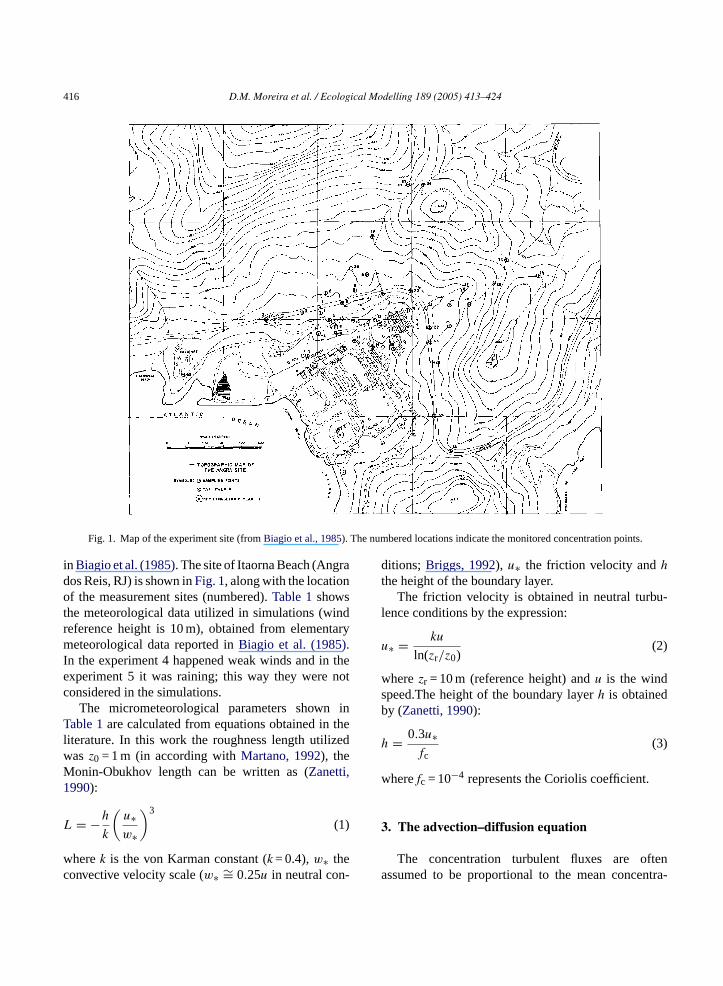
416 D.M. Moreira et al. / Ecological Modelling 189 (2005) 413–424

Fig. 1. Map of the experiment site (fromBiagio et al., 1985). The numbered locations indicate the monitored concentration points.

in Biagio et al. (1985). The site of Itaorna Beach (Angrados Reis, RJ) is shown inFig. 1, along with the locationof the measurement sites (numbered).Table 1showsthe meteorological data utilized in simulations (windreference height is 10 m), obtained from elementarymeteorological data reported inBiagio et al. (1985).In the experiment 4 happened weak winds and in theexperiment 5 it was raining; this way they were notconsidered in the simulations.

The micrometeorological parameters shown inTable 1are calculated from equations obtained in theliterature. In this work the roughness length utilizedwas z0 = 1 m (in according withMartano, 1992), theMonin-Obukhov length can be written as (Zanetti,1990):

L = −h

k

(u∗w∗

)3

(1)

wherek is the von Karman constant (k = 0.4),w∗ theconvective velocity scale (w∗ ∼= 0.25u in neutral con-

ditions; Briggs, 1992), u∗ the friction velocity andhthe height of the boundary layer.

The friction velocity is obtained in neutral turbu-lence conditions by the expression:

u∗ = ku

ln(zr/z0)(2)

wherezr = 10 m (reference height) andu is the windspeed.The height of the boundary layerh is obtainedby (Zanetti, 1990):

h = 0.3u∗fc

(3)

wherefc = 10−4 represents the Coriolis coefficient.

3. The advection–diffusion equation

The concentration turbulent fluxes are oftenassumed to be proportional to the mean concentra-

D.M. Moreira et al. / Ecological Modelling 189 (2005) 413–424 417

Table 1Micrometeorological parameters and emission rate for each experi-ment and period

Parameters Period 1 Period 2 Period 3

Experiment 1u (m/s) 1.9 2.4 2.8h (m) 965 1260 1448u* (m/s) 0.3 0.4 0.5−L (m) 810 1057 1214w∗ (m/s) 0.5 0.6 0.7Q (MBq/s) 20.5

Experiment 2u (m/s) 2.5 2.2 2.2h (m) 1322 1153 1134u* (m/s) 0.4 0.4 0.4−L (m) 1109 967 951w∗ (m/s) 0.6 0.6 0.6Q (MBq/s) 25.3

Experiment 3u (m/s) 2.2 2.0 2.6h (m) 1153 1027 1367u* (m/s) 0.4 0.3 0.5−L (m) 967 861 1147w∗ (m/s) 0.6 0.5 0.7Q (MBq/s) 20.5

tion gradient. This assumption, along with the equationof continuity, leads to the advection–diffusion equa-tion. For a cartesian coordinate system in which thexdirection coincides with that of the average wind, theadvection–diffusion equation is written as (Blackadar,1997):

∂C

∂t+ u

∂C

∂x+ v

∂C

∂y+ w

∂C

∂z

= ∂

∂x

(Kx

∂C

∂x

)+ ∂

∂y

(Ky

∂C

∂y

)+ ∂

∂z

(Kz

∂C

∂z

)+ S (4)

whereC denotes the average concentration,Kx, Ky,Kz andu, v, w are the cartesian components of eddydiffusivity and wind, respectively, andS is the sourceterm. The crosswind integration of Eq.(4) leads to:

∂C

∂t+ u

∂C

∂x+ w

∂C

∂z

= ∂

∂x

(Kx

∂C

∂x

)+ ∂

∂z

(Kz

∂C

∂z

)+ S (5)

where

C =∫ +∞

−∞C(x, y, z, t) dy (6)

is the crosswind integrated concentration. In this workS = −αC (α is the decay constant).

3.1. Air pollution model based onadvection–diffusion equation

Transport and diffusion models of air pollution arebased either on simple techniques, such as the Gaus-sian approach, or on more complex algorithms, suchas theK-theory differential equation. The Gaussianequation is an easy and fast method which, however,cannot properly simulate complex non-homogeneousconditions. TheK-theory can accept virtually anycomplex meteorological input, but generally requiresnumerical integration which is computationally expen-sive (Dimov et al., 2004) and is often affectedby large numerical advection errors. The Gaussianmodel has to be completed by empirically determinedstandard deviations (the so called “sigmas”) whilesome commonly measurable turbulent exchange coef-ficient has to introduce in the advection–diffusionequation.

Analytical solutions to the complete advection–diffusion equation cannot be given but in a few special-ized cases, and numerical solutions are expansive andcannot be easily “interpreted” as the simple Gaussianm tionst theG ere end PBLu tendt ofa

ua-t thee o-s linkb : weu ione ffi-c L ind iffu-s odel

odel. As a consequence, the major part of applicao practical problems are currently done by usingaussian model (i.e.:Taylor et al., 1987; Spijkerbot al., 2002), and great deal of empirical work has beone to determinate the sigmas appropriate to thender various meteorological conditions and to ex

he basic formulation of this model and its rangepplicability (Zanetti, 1990).

Notwithstanding this, the advection–diffusion eqion is believed to give a better representation offfects due to the vertical stratification of the atmphere. We face then the problem to finding aetween the two approaches in the following sensetilized an analytical solution of advection–diffusquation that accepts wind and eddy diffusivity coeients constant with height, but subdividing the PBifferent layer, where an average value for eddy divity and wind speed are considered, the hybrid m

418 D.M. Moreira et al. / Ecological Modelling 189 (2005) 413–424

is able to represent conditions of a height structuredPBL (Vilhena et al., 1998).

Validations of the model against experimental datasets and other models can be found inVilhena et al.(1998), Moreira et al. (1999), Degrazia et al. (2001),Mangia et al. (2001), Rizza et al. (2001)andMangia etal. (2002).

3.2. The model (ADMM – analytical dispersionmultilayer model)

The Laplace transform is a well-known techniquefor solving the linear differential equations whichappear in many applied mathematics and engineeringproblems. The method can be utilized also in the envi-ronmental problems described by Eq.(5), i.e., in anair-pollution context. In the first step of this procedure,the given differential equation (Eq.(5)) is transformedinto an algebraic equation or ordinary differential equa-tion by applying the Laplace transform. After solvingthese equations by standard procedure, the contami-nant concentration is obtained performing the Laplacetransform inversion technique.

The mathematical description of the dispersionproblem represented by Eq.(5) is well posed, when itis provided by initial and boundary conditions. Indeed,it is assumed that at the beginning of the contaminantrelease the dispersion region is not polluted; this means:

C(x, z, 0) = 0 att = 0 (7)

A n-s

C

wh

daryc

K

w Lh

czi

assume the average value:

Kx,n = 1

zn+1 − zn

∫ zn+1

zn

Kx(z) dz,

Kz,n = 1

zn+1 − zn

∫ zn+1

zn

Kz(z) dz (10)

un = 1

zn+1 − zn

∫ zn+1

zn

u(z) dz,

wn = 1

zn+1 − zn

∫ zn+1

zn

w(z) dz (11)

Therefore the solution of Eq.(5) is reduced to the solu-tion of N problems of the type:

∂C

∂t+ un

∂C

∂x+ wn

∂C

∂z= Kx,n

∂2C

∂x2 +Kz,n

∂2C

∂z2 −αC,

zn ≤ z ≤ zn+1 (12)

for n = 1:N, whereC = Cn denotes the concentrationat thenth sub-interval.

Applying the Laplace transform in Eq.(12), it turnsout that:

∂2 Cn(s, z, p)

∂z2 − wn

Kz

∂ Cn(s, z, p)

∂z

− (p + sun − α − Kxs2)Cn(s, z, p)

K

n

t the point (0,Hs, t) a continuous source of the cotant emission rateQ is assumed:

¯(0, z, t) = Q

uδ(z − Hs) atx = 0 (8)

hereδ is the Dirac delta function andHs the sourceeight.

The contaminants are also subjected to the bounonditions of zero flux at ground and PBL top:

z

∂C

∂z= 0 atz = 0, h (9)

hereh is the vertical depth of the mixing region (PBeight).

Bearing in mind the dependence of theKx andKz

oefficients and wind speed profilesu andw on variable, the heighth of a PBL is discretized inN sub-intervalsn such a way that inside each intervalKx, Kz andu, w

z

= (Kxs − un)Cn(0, z, p)

Kz

(13)

where Cn(s, z, p) = Lp{Cn(x, z, t); x → s; t → p}(Kz = Kz,n and Kx = Kx,n) which has the well-knowsolution:Cn(s, z, p) = An e−Rnz + Bn eRnz

+ Q

Ra

(e−Rn(z−Hs) − eRn(z−Hs)) (14)

where

Rn = wn

2Kz

±1

2

√(wn

Kz

)2

+ 4

Kz

[p − α+sun

(1−Kxs

un

)]

D.M. Moreira et al. / Ecological Modelling 189 (2005) 413–424 419

Ra =

√w2

n + 4Kz

[p − α + sun

(1 − Kxs

un

)](

1 − Kxsun

)Now, given a closer look to the solution in Eq.(14), wepromptly realize that exist 2N integration constants.Therefore, to make possible the determination of theseintegration constants we need to impose (2N − 2) inter-face conditions, namely the continuity of concentrationand flux concentration at interface. These conditionsare expressed as:

Cn = Cn+1, n = 1, 2, . . . , N − 1 (15a)

Kz,n

∂Cn

∂z= Kz,n+1

∂Cn+1

∂z, n = 1, 2, . . . , N − 1

(15b)

Finally, applying the initial and boundary conditionsa linear system is built for the integration constants.Subsequently, the concentration is obtained by numer-

ically inverting the transformed concentrationC by theGaussian quadrature scheme:

Cn(x, z, t)

=k∑

i=1

ai

(Pi

t

) m∑j=1

aj

(Pj

x

)

×[An e−Gnz + Bn eGnz

w

G

F

q workf

are the weights and roots of the Gaussian quadra-ture scheme and are tabulated in the book byStroudand Secrest (1966), while k andm are the quadraturepoints. Furthermore,H(z − Hs) is the Heaviside func-tion andPe = unx

Kxis the well-known Peclet number and

essentially represents the ratio between the advectivetransport to diffusive transport. This can be physicallyinterpreted as the parameter whose magnitude indicatesthe atmospheric conditions in terms of the strength ofwinds. Small values of this number can be related toweak winds, when the downwind diffusion becomesimportant and the region of interest remains close tothe source. Conversely, large values imply moderate tostrong winds when the downwind diffusion is neglectedin comparison to the advective, and the region of inter-est extends to a larger distance from the source.

In this work, for the purpose of comparison withexperimental data,wn = 0 was used. Therefore, finally,the following is obtained:

Cn(x, z, t)

=k∑

i=1

ai

(Pi

t

) m∑j=1

aj

(Pj

x

)

×[An e−

(√Pi/tKz−α/Kz+(Pjun/xKz)(1−Pj/Pe)

)z

+Bn e(√

Pi/tKz−α/Kz+(Pjun/xKz)(1−Pj/Pe))z

1 Q(

1 − Pj

Pe

)H(z − Hs)

Atw n-aa 2

restt theG formi -

+ Q

Fn

(e−(z−Hs)Gn − e(z−Hs)Gn )H(z − Hs)

](16)

here

n = wn

2Kz

±1

2

√(wn

Kz

)2

+ 4

Kz

[Pi

t−α+Pj

xun

(1−Pj

Pe

)]

n =

√w2

n + 4Kz

[Pi

t− α + Pj

xun

(1 − Pj

Pe

)](

1 − Pj

Pe

)The solution is valid forx > 0 and t > 0, as the

uadrature scheme of Laplace inversion does notor x = 0 and t = 0. The constantsai, aj, and Pi, Pj

+2

√(Pi

t− α + Pjun

x

(1 − Pj

Pe

))Kz

×(

e−(z−Hs)(√

Pi/tKz−α/Kz+(Pjun/xKz)(1−Pj/Pe))

−e(z−Hs)(√

Pi/tKz−α/Kz+(Pjun/xKz)(1−Pj/Pe)))]

(17)

n important aspect of Eq.(17) is that, by takinghe limit t → ∞ (steady state),Pe→ ∞ (no weakinds) andα = 0, the original equation for the statiory regime is obtained (Vilhena et al., 1988;Moreira etl., 1999; Degrazia et al., 2001; Mangia et al., 200).

It can be noticed in the book of Stroud and Sechat the modulus of the real part of the root ofaussian quadrature scheme for the Laplace trans

nversion, increases withN (the order of approxima

420 D.M. Moreira et al. / Ecological Modelling 189 (2005) 413–424

tion). Bearing in mind that the solution for the Laplacetransformed concentration has exponential terms oftype exp(±(

√Pi/t)z), it is readily observed from

numerical simulation the appearing of overflow for thepositive argument of the exponential and underflowfor the negative argument when the quadrature pointsassumes values larger than 8. It is important to point outthat the calculations were performed in a personal com-puter with double precision floating point arithmetic.Therefore to eliminate any floating point exception itis needed to perform the calculations on establishedlimits for k andm, it meansk, m ≤ 8. Even so, we areconfident in stressing again that a good accuracy wasachieved with the quadrature points used in this work.

The lateral dispersion parameterσy is important forcalculating the concentration in the ground-level cen-terline concentration:

C(x, 0, 0) = C(x, 0)√2πσy

(18)

where, in this study, the ground-level crosswind inte-grated concentration in Eq.(18) is calculated employ-ing the multilayered slabK-diffusion model (Eq.(17)).

4. Tubulence parameterization and wind profile

In atmospheric diffusion problems the choice ofa turbulent parameterization represents a fundamen-t roma iza-t t wea atedr gatef ofe rbu-l rrentu

N :

wla-

tw low

expression for large variations (Nieuwstadt and VanDop, 1982):

σy

x= σθ

(1 + 0.031x0.46)(20)

whereσθ = 15 (Blackadar, 1997) for unstable/neutralconditions.

In terms of the convective scaling parameters, thevertical eddy diffusivity derived fromBatchelor (1949)can be formulated as (Degrazia et al., 1997):

Kz

w∗h= 0.22

( z

h

)1/3(1 − z

h

)1/3

×[1 − exp

(−4z

h

)− 0.0003 exp

(8z

h

)](21)

In all simulations moderate winds were considered(U > 1.5 m/s). This way, as usual, the longitudinal eddydiffusivity Kx was not considered (Kx = 0), because thisterm is important in weak wind conditions (U < 1 m/s).

The wind speed profile used in Eq.(17) has beenparameterized following the Monin-Obukhov similar-ity theory and OML model (Berkowicz et al., 1986):

u = u∗k

[ln

(z

z0

)− Ψm

( z

L

)+ Ψm

(z0

L

)]if z ≤ zb (22)

u

wg

Ψ

w

A

er-s ydt is-s ce in

al aspect for contaminant dispersion modelling. Fphysical point of view, a turbulence parameter

ion is an approximation to nature, in the sense thare putting in mathematical models an approximelation that in principle can be used as a surroor the natural true unknown term. The reliabilityach model strongly depends on the way that tu

ent parameters are calculated and related to the cunderstanding of the PBL (Mangia et al., 2002).

For lateral dispersion parameterσy, we followedieuwstadt and Van Dop (1982), who present the form

σy

h=

[0.26X

(1 + 0.91X)

]1/2

(19)

hereX is a non-dimensional distance (X = xw∗/uh).For small variations of the wind direction in re

ion to the position of the receptors the expression(19)as utilized as lateral dispersion, along with the fol

= u(zb) if z > zb (23)

herezb = min[|L|,0.1zi], andΨm is a stability functioniven by (Paulsen, 1975):

m = 2 ln

[1 + A

2

]+ ln

[1 + A2

2

]−2 tan−1(A) + π

2(24)

ith

=(

1 − 16z

L

)1/4

(25)

Thus, in this study we introduce the lateral dispion parameter (Eqs.(19)or (20)) and the vertical eddiffusivity (Eq. (21)) in the ADMM model (Eq.(17))

o calculate the ground-level concentration of emions released from an elevated continuous sour

D.M. Moreira et al. / Ecological Modelling 189 (2005) 413–424 421

an unstable/neutral PBL. We also accomplished simu-lations with constant wind.

5. Terrain

In the present work we simulate over the terrain withtwo sets of assumptions. Firstly, the assumptions aboutplume behavior in elevated simple terrain (i.e., terrainthat exceeds the stack base elevation but is below therelease height) are: (a) the plume axis remains at theplume stabilization height above mean sea level as itpasses over elevated or depressed terrain; (b) the mixingheight follows the terrain. Thus, the modified plumestabilization heightHse is:

Hse = Hs + zs − hr (26)

whereHs is the effective stack height,hr the heightabove mean sea level of terrain at the receptor locationandzs the height above mean sea level of the base ofthe stack.

Secondly, in the case of complex terrain disper-sion, the assumptions about plume behavior are: (a)the plume axis uses a “half-height” correction factorfor unstable and neutral conditions; (b) the plume cen-terline height is never less than 10 m above the groundin complex terrain.

Thus, a modified plume stabilization heightHse issubstituted for the effective stack heightHs:

H

w t ther r,w fors

hatt ardsb s itp utralc rainu

6

dia-g brid

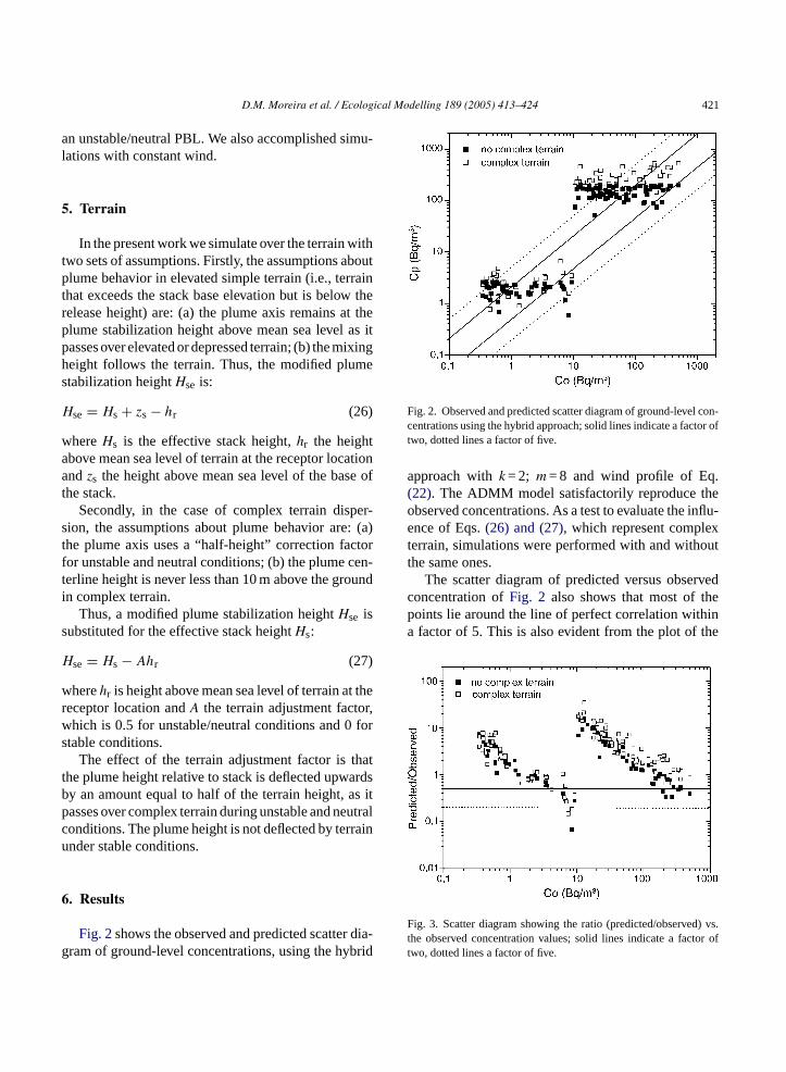
Fig. 2. Observed and predicted scatter diagram of ground-level con-centrations using the hybrid approach; solid lines indicate a factor oftwo, dotted lines a factor of five.

approach withk = 2; m = 8 and wind profile of Eq.(22). The ADMM model satisfactorily reproduce theobserved concentrations. As a test to evaluate the influ-ence of Eqs.(26) and (27), which represent complexterrain, simulations were performed with and withoutthe same ones.

The scatter diagram of predicted versus observedconcentration ofFig. 2 also shows that most of thepoints lie around the line of perfect correlation withina factor of 5. This is also evident from the plot of the

Fig. 3. Scatter diagram showing the ratio (predicted/observed) vs.the observed concentration values; solid lines indicate a factor oftwo, dotted lines a factor of five.

se = Hs − Ahr (27)

herehr is height above mean sea level of terrain aeceptor location andA the terrain adjustment factohich is 0.5 for unstable/neutral conditions and 0table conditions.

The effect of the terrain adjustment factor is the plume height relative to stack is deflected upwy an amount equal to half of the terrain height, aasses over complex terrain during unstable and neonditions. The plume height is not deflected by ternder stable conditions.

. Results

Fig. 2shows the observed and predicted scatterram of ground-level concentrations, using the hy

422 D.M. Moreira et al. / Ecological Modelling 189 (2005) 413–424

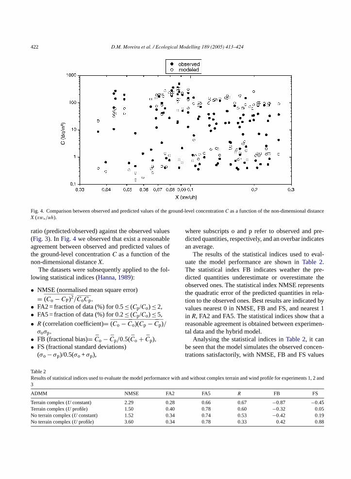
Fig. 4. Comparison between observed and predicted values of the ground-level concentrationC as a function of the non-dimensional distanceX (xw∗/uh).

ratio (predicted/observed) against the observed values(Fig. 3). In Fig. 4 we observed that exist a reasonableagreement between observed and predicted values ofthe ground-level concentrationC as a function of thenon-dimensional distanceX.

The datasets were subsequently applied to the fol-lowing statistical indices (Hanna, 1989):

• NMSE (normalised mean square error)

= (Co − CP)2/CoCp,

• FA2 = fraction of data (%) for 0.5≤ (Cp/Co) ≤ 2,• FA5 = fraction of data (%) for 0.2≤ (Cp/Co) ≤ 5,

• R (correlation coefficient)= (Co − Co)(Cp − Cp)/σoσp,

• FB (fractional bias)= Co − Cp/0.5(Co + Cp),• FS (fractional standard deviations)

(σo − σp)/0.5(σo +σp),

where subscripts o and p refer to observed and pre-dicted quantities, respectively, and an overbar indicatesan average.

The results of the statistical indices used to eval-uate the model performance are shown inTable 2.The statistical index FB indicates weather the pre-dicted quantities underestimate or overestimate theobserved ones. The statistical index NMSE representsthe quadratic error of the predicted quantities in rela-tion to the observed ones. Best results are indicated byvalues nearest 0 in NMSE, FB and FS, and nearest 1in R, FA2 and FA5. The statistical indices show that areasonable agreement is obtained between experimen-tal data and the hybrid model.

Analysing the statistical indices inTable 2, it canbe seen that the model simulates the observed concen-trations satisfactorily, with NMSE, FB and FS values

Table 2Results of statistical indices used to evaluate the model performance with and without complex terrain and wind profile for experiments 1, 2 and3

ADMM NMSE FA2 FA5 R FB FS

Terrain complex (U constant) 2.29 0.28 0.66 0.67 −0.87 −0.45Terrain complex (U profile) 1.50 0.40 0.78 0.60 −0.32 0.05No terrain complex (U constant) 1.52 0.34 0.74 0.53 −0.42 0.19No terrain complex (U profile) 3.60 0.34 0.78 0.33 0.42 0.88

D.M. Moreira et al. / Ecological Modelling 189 (2005) 413–424 423

relatively small andR and FA5 relatively near to 1.A closer inspection ofTable 2reveals that the hybridmodel presents best values of NMSE,R and FA5 forthe case of complex terrain (Eqs.(26) and(27)) andwind speed profile (Eq.(22)).

7. Conclusions

Air pollution models are an important technicalinstrument for identifying and managing accidentalreleases from nuclear plants. In this work, we com-pared computed concentrations against data used forsimulating accidental release from the nuclear powerplant of Angra dos Reis. The experimental simula-tion was performed by releasing tritiated water underneutral/moderately unstable conditions (Biagio et al.,1985). In the numerical simulations a time-dependenthybrid model was used. The model overcomes thelimits of the existing analytical ones, because theanalytical solutions of the advection–diffusion equa-tion are usually obtained just for stationary condi-tions and by making strong assumptions about theeddy diffusivity coefficients (K) and wind speed pro-files (U). They are assumed to be either constantthroughout the whole PBL or to follow a powerlaw. The statistical indices show that a reasonablygood agreement is obtained between experimentaldata and hybrid model. A closer inspection of theresults reveals that the hybrid model presents bestv ro),F lext

uchf ere-f tiond iaryt airq

A

naldF dod orto

References

Batchelor, G.K., 1949. Diffusion in a field of homogeneous turbu-lence, Eulerian analysis. Aust. J. Sci. Res. 2, 437–450.

Berkowicz, R.R., Olesen, H.R., Torp, U., 1986. The Danish Gaus-sian air pollution model (OML): description, test and sensitivityanalysis in view of regulatory applications. In: De Wispeleare,C., Schiermeirier, F.A., Gillani, N.V. (Eds.), Air Pollution Mod-eling and its Application. Plenum Publishing Corporation, pp.453–480.

Biagio, R., Godoy, G., Nicoli, I., Nicoli, D., Thomas, P., 1985. Firstatmospheric diffusion experiment campaign at the Angra site –KfK 3936, Karlsruhe and CNEN 1201, Rio de Janeiro.

Blackadar, A.K., 1997. Turbulence and Diffusion in the Atmo-sphere: Lectures in Environmental Sciences. Springer-Verlag,185 pp.

Briggs, G.A., 1992. Plume dispersion in the convective boundarylayer. Part II. Analyses of CONDORS field experimental data. J.Appl. Meteorol. 32, 1388–1425.

Degrazia, G.A., Campos Velho, H.F., Carvalho, J.C., 1997. Nonlocalexchange coefficients for the convective boundary layer derivedfrom spectral properties. Contr. Atmos. Phys., 57–64.

Degrazia, G.A., Moreira, D.M., Vilhena, M.T., 2001. Derivation of aneddy diffusivity depending on source distance for vertically inho-mogeneous turbulence in a convective boundary layer. J. Appl.Meteorol. 40, 257–264.

Dimov, I., Georgiev, K., Ostromsky, T., Zlatev, Z., 2004. Computa-tional challenges in the numerical treatment of large air pollutionmodels. Ecol. Model. 179, 187–203.

Finzi, G., Guariso, G., 1992. Optimal air pollution control strategies:a case study. Ecol. Model. 64, 221–239.

Hanna, S.R., 1989. Confidence limit for air quality models as esti-mated by bootstrap and jacknife resampling methods. Atmos.Environ. 23, 1385–1395.

Mangia, C., Moreira, D.M., Schipa, I., Degrazia, G.A., Tirabassi,am-ility

M .A.,dis-ions.ss,

M ce

M s: the

M iontical

N Pol-

P aticaldel.

alues of NMSE, FS and FB (values nearest zeA2 (40%) and FA5 (78%) for the case of comperrain.

The computer code of a hybrid model runs master than that of a numerical model, and can thore be used for a fast screening of concentraistribution from a given source and as an auxil

ool in the control of critical events related touality.

cknowledgements

The authors thank CNPq (Conselho Nacioe Desenvolvimento Cientıfico e Tecnologico) andAPERGS (Fundac¸ao de Amparoa Pesquisa do Estao Rio Grande do Sul) for the partial financial suppf this work.

T., Rizza, U., 2002. Evaluation of a new eddy diffusivity pareterisation from turbulent eulerian spectra in different stabconditions. Atmos. Environ. 36, 67–76.

angia, C., Schippa, I., Moreira, D.M., Tirabassi, T., Degrazia, GRizza, U., 2001. A new eddy diffusivity parameterisation forpersion models: evaluation in different atmospheric conditIn: Latini e, G., Trebbia, C.A. (Eds.), Air Pollution IX. WIT PreSouthampton, pp. 105–112.

artano, 1992. Dinamica de fluxo turbulento sobre relevo e aplica¸aoa difusao em pequena escala na camada limite atmosferica. Tesde doutorado. Departamento de Fısica, PUC-RJ, 117 pp.

artano, P., Paschoa, A.S., 1997. Dispersion modelling studie1984 experiment in Angra dos Reis. Revista de Fısica Aplicadae Instrumentac¸ao 12 (4), 107–118.

oreira, D.M., Degrazia, G.A., Vilhena, M.T., 1999. Dispersfrom low sources in a convective boundary layer: an analymodel. Il Nuovo Cimento 22C (5), 685–691.

ieuwstadt, Van Dop, 1982. Atmospheric Turbulence and Airlution Modelling. D. Reidel Publishing Company.

arra-Guevara, D., Skiba, Y.N., 2003. Elements of the mathemmodeling in the control of pollutants emissions. Ecol. Mo167, 263–275.

424 D.M. Moreira et al. / Ecological Modelling 189 (2005) 413–424

Paulsen, C.A., 1975. The mathematical representation of wind andtemperature profiles in a unstable atmospheric surface layer. J.Appl. Meteor. 9, 857–861.

Peliccioni, A., Gariazzo, C., Tirabassi, T., 2003. Coupling of neu-ral network and dispersion models: a novel methodology for airpollution models. Int. J. Environ. Pollut. 20, 1–6.

Rizza, U., Degrazia, G.A., Moreira, D.M., Brauer, C.R.N., Mangia,C., Campos, C.R.J., Tirabassi, T., 2001. Turbulent dispersionfrom tall stack in the unstable boundary layer: a comparisonbetween Gaussian andK-diffusion modelling for nonbuoyantemissions. Nuovo Cimento 24C, 805–814.

Skiba, Y.N., 2003. On a method of detecting the industrial plantswhich violate prescribed emission rates. Ecol. Model. 159,125–132.

Spijkerboer, H.P., Beniers, J.E., Jaspers, D., Schouten, H.J., Goudri-aan, J., Rabbinge, R., van der Werf, W., 2002. Ability of the

Gaussian plume model to predict and describe spore dispersalover a potato crop. Ecol. Model. 155, 1–18.

Stroud, A.H., Secrest, D., 1966. Gaussian Quadrature Formulas.Prentice-Hall, Englewood Cliffs, NJ.

Taylor, J.A., Simpson, R.W., Jakeman, A.J., 1987. A hybrid modelfor predicting the distribution of sulphur dioxide concentrationsobserved near elevated point sources. Ecol. Model. 36, 269–296.

Vilhena, M.T., Rizza, U., Degrazia, G.A., Mangia, C., Moreira, D.M.,Tirabassi, T., 1998. An analytical air pollution model: develop-ment and evaluation. Contr. Atmos. Phys. 71, 315–320.

Viotti, P., Liuti, G., Di Genova, P., 2002. Atmospheric urban pollu-tion: applications of an artificial neural network (ANN) to thecity of Perugia. Ecol. Model. 148, 27–46.

Zanetti, P., 1990. Air Pollution Modeling. Comp. Mech. Publications,Southampton, UK.