Expert Systems with Applications 38 (2011) 106–115

Contents lists available at ScienceDirect

Expert Systems with Applications

journal homepage: www.elsevier .com/locate /eswa

A rough set based approach to distributor selection in supply chain management

Zhonghai Zou a, Tzu-Liang (Bill) Tseng b,*, Hansuk Sohn c, Guofang Song a, Rafael Gutierrez b

a School of Management, Shanghai University, Shanghai, Chinab Department of Industrial Engineering, The University of Texas at El Paso, TX 79968, USAc Department of Industrial Engineering, New Mexico State University, NM 88003 , USA

a r t i c l e i n f o

Keywords:Distributor selectionsData miningRough set theory (RST)Supply chain management (SCM)

0957-4174/$ - see front matter � 2010 Elsevier Ltd. Adoi:10.1016/j.eswa.2010.06.021

* Corresponding author. Tel.: +1 915 241 2838; faxE-mail address: btseng@utep.edu (T.-L. Tseng).

a b s t r a c t

Distributor’s selection is an important issue in Supply chain management, particularly in the currentcompetitive environment. The current research works provide only conceptual, descriptive, and simula-tion results, focusing mainly on firm resources and general marketing factors. The selection and evalua-tion of distributors generally incorporate qualitative information; however, analyzing qualitativeinformation is difficult by standard statistical techniques. Consequently, a more suitable approach isdesired. In this paper, a method based on Rough set theory, which has been recognized as a powerful toolin dealing with qualitative data in the literature, is introduced and modified for preferred distributorselection. We derived certain decision rules which are able to facilitate distributor selection and identi-fied several significant features based on an empirical study conducted in China.

� 2010 Elsevier Ltd. All rights reserved.

1. Introduction Rough set theory (RST) has also been applied for preferred suppli-

Industry is now strongly recognizing that total management ofthe supply chain enhances the competitive edge of all ‘‘players”therein. As a result, Supply chain management (SCM) has receivedmore attentions from both academicians and practitioners in thepast decade. Many articles and books have been published forthe methods and opinions about the application of supply chainmanagement. Although there is no generally accepted notion ofsupply chain, at least it should contain the suppliers’ suppliersand the customers’ customers. Supply chain in this paper refersto a network of integrated and dependent process throughwhich specifications are transformed to finished deliverables.Fig. 1 depicts a conceptual framework for supply chain.

Supplier selection and evaluation play an important role in thesupply chain process and are crucial to the success of manufactur-ing firms (Sevkli, Lenny Koh, Zaim, Demirbag, & Tatoglu, 2008).There are many researchers in supplier selection, and many meth-odologies are applied in practice, such as the cost-ratio method,linear or mixed integer programming to goal and multi-objectivelinear programming models (Ghodsypour & O’Brien, 1998; Oliveria& Lourenco, 2002; Yan, Yu, & Cheng, 2003). Although these meth-ods have been widely used in the area of supplier selection, thereare certain drawbacks associated with the implementation of thesemethods. Apart from these traditional methods for supplier selec-tion, recently fuzzy systems theory has been successfully appliedto supplier selection problems (Chan & Kumar, 2007; Kahraman,Cebeci, & Ruan, 2004; Kahraman, Cebeci, & Ulukan, 2003), and

ll rights reserved.

: +1 915 747 5019.

ers prediction (Tseng, Huang, Jiang, & Ho, 2006).To date, numerous literatures have explored the issues of sup-

plier selection. In contrast, little work has been done in selectionof distributor, particularly in empirical studies. Only conceptual,descriptive and simulation results focused primarily on firm re-sources and general marketing/selling factors were discussed (Abr-att & Pitt, 1989; Cavusgil, Yeoh, & Mitri, 1995; Shipley, Cook, &Barnett, 1989; Yeoh & Calantone, 1995). It should be noted thatdistributor selection has not been studied deeply and the theoret-ical methods developed by academics have not been fully appliedin industry. In this paper, we propose a rough set based methodol-ogy which is able to perform rule induction effectively. Moreover,the weight of each input feature is incorporated in the proposedapproach so as to enhance quality of the derived rules.

The remainder of this paper is organized as follows: The next sec-tion introduces the background of distributor rough set theory andthe standard rough set-based rule induction problem. Section 3 pre-sents the basic rule identification algorithm to determine the reductswith both equal and unequal weight features. A case study is pre-sented to show how the rule identification approach can be appliedto distributor selection in Section 4. Section 5 concludes the paperwith discussion of empirical findings and future research directions.

2. Literature review and rough set-based rule inductionproblem

2.1. Literature review on distributor research

As mentioned above, there are few empirical studies for manu-facturers’ distributor selection. Ross (1973) studied the selection of

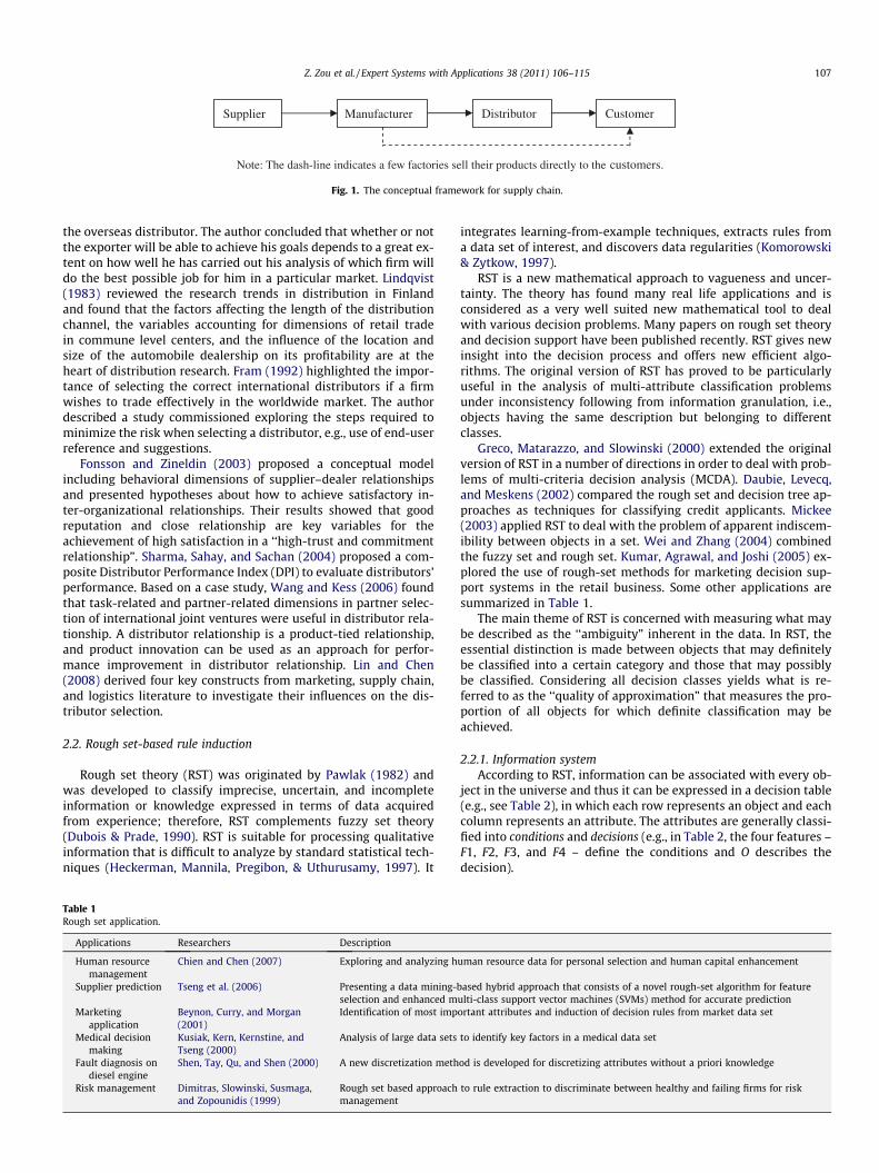
Supplier Manufacturer Distributor Customer

Note: The dash-line indicates a few factories sell their products directly to the customers.

Fig. 1. The conceptual framework for supply chain.

Z. Zou et al. / Expert Systems with Applications 38 (2011) 106–115 107

the overseas distributor. The author concluded that whether or notthe exporter will be able to achieve his goals depends to a great ex-tent on how well he has carried out his analysis of which firm willdo the best possible job for him in a particular market. Lindqvist(1983) reviewed the research trends in distribution in Finlandand found that the factors affecting the length of the distributionchannel, the variables accounting for dimensions of retail tradein commune level centers, and the influence of the location andsize of the automobile dealership on its profitability are at theheart of distribution research. Fram (1992) highlighted the impor-tance of selecting the correct international distributors if a firmwishes to trade effectively in the worldwide market. The authordescribed a study commissioned exploring the steps required tominimize the risk when selecting a distributor, e.g., use of end-userreference and suggestions.

Fonsson and Zineldin (2003) proposed a conceptual modelincluding behavioral dimensions of supplier–dealer relationshipsand presented hypotheses about how to achieve satisfactory in-ter-organizational relationships. Their results showed that goodreputation and close relationship are key variables for theachievement of high satisfaction in a ‘‘high-trust and commitmentrelationship”. Sharma, Sahay, and Sachan (2004) proposed a com-posite Distributor Performance Index (DPI) to evaluate distributors’performance. Based on a case study, Wang and Kess (2006) foundthat task-related and partner-related dimensions in partner selec-tion of international joint ventures were useful in distributor rela-tionship. A distributor relationship is a product-tied relationship,and product innovation can be used as an approach for perfor-mance improvement in distributor relationship. Lin and Chen(2008) derived four key constructs from marketing, supply chain,and logistics literature to investigate their influences on the dis-tributor selection.

2.2. Rough set-based rule induction

Rough set theory (RST) was originated by Pawlak (1982) andwas developed to classify imprecise, uncertain, and incompleteinformation or knowledge expressed in terms of data acquiredfrom experience; therefore, RST complements fuzzy set theory(Dubois & Prade, 1990). RST is suitable for processing qualitativeinformation that is difficult to analyze by standard statistical tech-niques (Heckerman, Mannila, Pregibon, & Uthurusamy, 1997). It

Table 1Rough set application.

Applications Researchers Description

Human resourcemanagement

Chien and Chen (2007) Exploring and analyzing h

Supplier prediction Tseng et al. (2006) Presenting a data mining-bselection and enhanced m

Marketingapplication

Beynon, Curry, and Morgan(2001)

Identification of most imp

Medical decisionmaking

Kusiak, Kern, Kernstine, andTseng (2000)

Analysis of large data sets

Fault diagnosis ondiesel engine

Shen, Tay, Qu, and Shen (2000) A new discretization meth

Risk management Dimitras, Slowinski, Susmaga,and Zopounidis (1999)

Rough set based approachmanagement

integrates learning-from-example techniques, extracts rules froma data set of interest, and discovers data regularities (Komorowski& Zytkow, 1997).

RST is a new mathematical approach to vagueness and uncer-tainty. The theory has found many real life applications and isconsidered as a very well suited new mathematical tool to dealwith various decision problems. Many papers on rough set theoryand decision support have been published recently. RST gives newinsight into the decision process and offers new efficient algo-rithms. The original version of RST has proved to be particularlyuseful in the analysis of multi-attribute classification problemsunder inconsistency following from information granulation, i.e.,objects having the same description but belonging to differentclasses.

Greco, Matarazzo, and Slowinski (2000) extended the originalversion of RST in a number of directions in order to deal with prob-lems of multi-criteria decision analysis (MCDA). Daubie, Levecq,and Meskens (2002) compared the rough set and decision tree ap-proaches as techniques for classifying credit applicants. Mickee(2003) applied RST to deal with the problem of apparent indiscem-ibility between objects in a set. Wei and Zhang (2004) combinedthe fuzzy set and rough set. Kumar, Agrawal, and Joshi (2005) ex-plored the use of rough-set methods for marketing decision sup-port systems in the retail business. Some other applications aresummarized in Table 1.

The main theme of RST is concerned with measuring what maybe described as the ‘‘ambiguity” inherent in the data. In RST, theessential distinction is made between objects that may definitelybe classified into a certain category and those that may possiblybe classified. Considering all decision classes yields what is re-ferred to as the ‘‘quality of approximation” that measures the pro-portion of all objects for which definite classification may beachieved.

2.2.1. Information systemAccording to RST, information can be associated with every ob-

ject in the universe and thus it can be expressed in a decision table(e.g., see Table 2), in which each row represents an object and eachcolumn represents an attribute. The attributes are generally classi-fied into conditions and decisions (e.g., in Table 2, the four features –F1, F2, F3, and F4 – define the conditions and O describes thedecision).

uman resource data for personal selection and human capital enhancement

ased hybrid approach that consists of a novel rough-set algorithm for featureulti-class support vector machines (SVMs) method for accurate predictionortant attributes and induction of decision rules from market data set

to identify key factors in a medical data set

od is developed for discretizing attributes without a priori knowledge

to rule extraction to discriminate between healthy and failing firms for risk

Table 2Five-object data set.

Object No. F1 F2 F3 F4 O

1 1 0 2 0 02 1 0 0 1 13 0 0 3 1 04 1 1 2 0 25 0 0 1 0 0

108 Z. Zou et al. / Expert Systems with Applications 38 (2011) 106–115

Therefore, knowledge can be described in an information sys-tem, containing four components as follows:

S ¼ ðU;A;V ; f Þ ð1Þ

where U, called the universe, is a nonempty set of all objects and A isthe finite set of all the attributes. Moreover, V is the set of all theattribute values such that,

V ¼[

a2A

Va ð2Þ

where Va is a finite attribute domain of attribute a. Finally, f denotesan information function such that, for every a e A and ui e U

f ðui; aÞ 2 Va ð3Þ

Table 2 illustrates the information of five objects that are character-ized with one decision attribute (O) and four condition attributes(F1, F2, F3, F4).

Note that other subjects (i.e., indiscernibility relationship andapproximation of sets) related to RST can be found in the Appendix.

3. Rule identification algorithms

The proposed conceptual framework to elicit decision rules con-sists of the following steps: problem definition, data preparation,data partition, reduct generation, and rule-validation as shown inFig. 2.

3.1. Problem definition, data preparation and data partition

First, the data exploration process starts by identifying the rightproblems to solve and structuring the corresponding objectivesand the associated attributes, that is, to make it clear what wewant. Then, the needed data should be collected for the objectsand the attributes of the objects. More important, a series of datapreprocessing tasks, including consistency checks to detect errors,removing noise or outliers where appropriate, and data complete-ness checks, should be done to ensure that the data are as accurateas possible. Next, the target dataset is randomly divided into the

Problem definition

Data preparation

Data partition

Testing da

Training

Reduct se

Fig. 2. The conceptual framewor

training data set and the testing data set. Kusiak (2001) suggeststhe split of the data using the bootstrapping method according tothe following ratios: 0.632 for training set and 0.368 for testingset. The training data set is used to build the model and derivethe rules. The testing data set is used to detect over fitting of themodeling tools.

3.2. Reduct generation

The basic construct in rough set theory is called a reduct. It is de-fined as a minimal sufficient subset of features RED # A such that:

(a) Relation R(RED) = R(A); that is, RED produces the same cate-gorization of objects as the collection A of all features.

(b) For any g 2 RED, R(RED � {g}) – R(A); that is, a reduct is aminimal subset of features with respect to the property (a).

The term reduct was initially defined for sets rather than ob-jects with input and output features or for decision tables withdecision features (attributes) and outcomes. Reducts of the objectsin a decision table have to be computed with consideration givento the value of the output feature. The original definition of reductconsiders features only. In this paper, each reduct is viewed fromfour perspectives – feature, feature value, object, and ruleperspective.

The reduct generation algorithm (based on Pawlak, 1991) is thefollowings:

Step 0. Initialize object number i = 1.Step 1. Select object i and find a set of o-reduct with one featureonly.

If found, go to Step 3; otherwise go to Step 2.Step 2. For object i, find an o-reduct with m � 1 features, wherem is the number of input features. This step is accomplished bydeleting one feature only at a time.Step 3. Set i = i + 1. If all objects have been considered, stop;otherwise go to step 1.

For example, a subset of all reducts generated for the objects inTable 2 is shown in Table 3. The entry ‘‘x” in each reduct impliesthat the corresponding feature is not considered in determiningthe feature output of an object.

3.3. Reduct selection and rule identification algorithm

The nine reducts in Table 3 could be chose in a number of dif-ferent ways. As we know that in the real world, the features (attri-butes) are not the same unique for depicting an object, some are

ta sets

Decision

data set Reduct generation

Candidate decision rules lection

Validation Accuracy>threshold

Accept

Y

Domainexpert

k of eliciting decision rules.

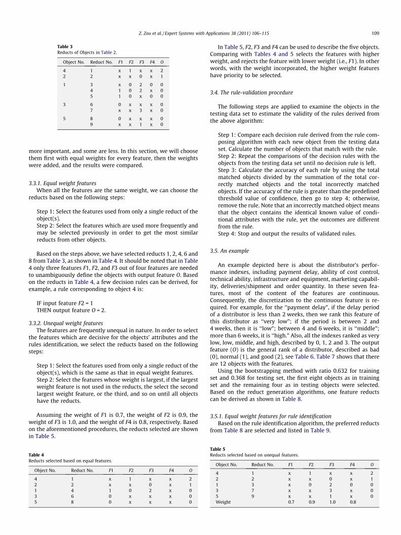
Table 3Reducts of Objects in Table 2.

Object No. Reduct No. F1 F2 F3 F4 O

4 1 x 1 x x 22 2 x x 0 x 1

1 3 x 0 2 0 04 1 0 2 x 05 1 0 x 0 0

3 6 0 x x x 07 x x 3 x 0

5 8 0 x x x 09 x x 1 x 0

Z. Zou et al. / Expert Systems with Applications 38 (2011) 106–115 109

more important, and some are less. In this section, we will choosethem first with equal weights for every feature, then the weightswere added, and the results were compared.

3.3.1. Equal weight featuresWhen all the features are the same weight, we can choose the

reducts based on the following steps:

Step 1: Select the features used from only a single reduct of theobject(s).Step 2: Select the features which are used more frequently andmay be selected previously in order to get the most similarreducts from other objects.

Based on the steps above, we have selected reducts 1, 2, 4, 6 and8 from Table 3, as shown in Table 4. It should be noted that in Table4 only three features F1, F2, and F3 out of four features are neededto unambiguously define the objects with output feature O. Basedon the reducts in Table 4, a few decision rules can be derived, forexample, a rule corresponding to object 4 is:

IF input feature F2 = 1THEN output feature O = 2.

3.3.2. Unequal weight featuresThe features are frequently unequal in nature. In order to select

the features which are decisive for the objects’ attributes and therules identification, we select the reducts based on the followingsteps:

Step 1: Select the features used from only a single reduct of theobject(s), which is the same as that in equal weight features.Step 2: Select the features whose weight is largest, if the largestweight feature is not used in the reducts, the select the secondlargest weight feature, or the third, and so on until all objectshave the reducts.

Assuming the weight of F1 is 0.7, the weight of F2 is 0.9, theweight of F3 is 1.0, and the weight of F4 is 0.8, respectively. Basedon the aforementioned procedures, the reducts selected are shownin Table 5.

Table 4Reducts selected based on equal features.

Object No. Reduct No. F1 F2 F3 F4 O

4 1 x 1 x x 22 2 x x 0 x 11 4 1 0 2 x 03 6 0 x x x 05 8 0 x x x 0

In Table 5, F2, F3 and F4 can be used to describe the five objects.Comparing with Tables 4 and 5 selects the features with higherweight, and rejects the feature with lower weight (i.e., F1). In otherwords, with the weight incorporated, the higher weight featureshave priority to be selected.

3.4. The rule-validation procedure

The following steps are applied to examine the objects in thetesting data set to estimate the validity of the rules derived fromthe above algorithm:

Step 1: Compare each decision rule derived from the rule com-posing algorithm with each new object from the testing dataset. Calculate the number of objects that match with the rule.Step 2: Repeat the comparisons of the decision rules with theobjects from the testing data set until no decision rule is left.Step 3: Calculate the accuracy of each rule by using the totalmatched objects divided by the summation of the total cor-rectly matched objects and the total incorrectly matchedobjects. If the accuracy of the rule is greater than the predefinedthreshold value of confidence, then go to step 4; otherwise,remove the rule. Note that an incorrectly matched object meansthat the object contains the identical known value of condi-tional attributes with the rule, yet the outcomes are differentfrom the rule.Step 4: Stop and output the results of validated rules.

3.5. An example

An example depicted here is about the distributor’s perfor-mance indexes, including payment delay, ability of cost control,technical ability, infrastructure and equipment, marketing capabil-ity, deliveries/shipment and order quantity. In these seven fea-tures, most of the content of the features are continuous.Consequently, the discretization to the continuous feature is re-quired. For example, for the ‘‘payment delay”, if the delay periodof a distributor is less than 2 weeks, then we rank this feature ofthis distributor as ‘‘very low”; if the period is between 2 and4 weeks, then it is ‘‘low”; between 4 and 6 weeks, it is ‘‘middle”;more than 6 weeks, it is ‘‘high.” Also, all the indexes ranked as verylow, low, middle, and high, described by 0, 1, 2 and 3. The outputfeature (O) is the general rank of a distributor, described as bad(0), normal (1), and good (2), see Table 6. Table 7 shows that thereare 12 objects with the features.

Using the bootstrapping method with ratio 0.632 for trainingset and 0.368 for testing set, the first eight objects as in trainingset and the remaining four as in testing objects were selected.Based on the reduct generation algorithms, one feature reductscan be derived as shown in Table 8.

3.5.1. Equal weight features for rule identificationBased on the rule identification algorithm, the preferred reducts

from Table 8 are selected and listed in Table 9.

Table 5Reducts selected based on unequal features.

Object No. Reduct No. F1 F2 F3 F4 O

4 1 x 1 x x 22 2 x x 0 x 11 3 x 0 2 0 03 7 x x 3 x 05 9 x x 1 x 0Weight 0.7 0.9 1.0 0.8

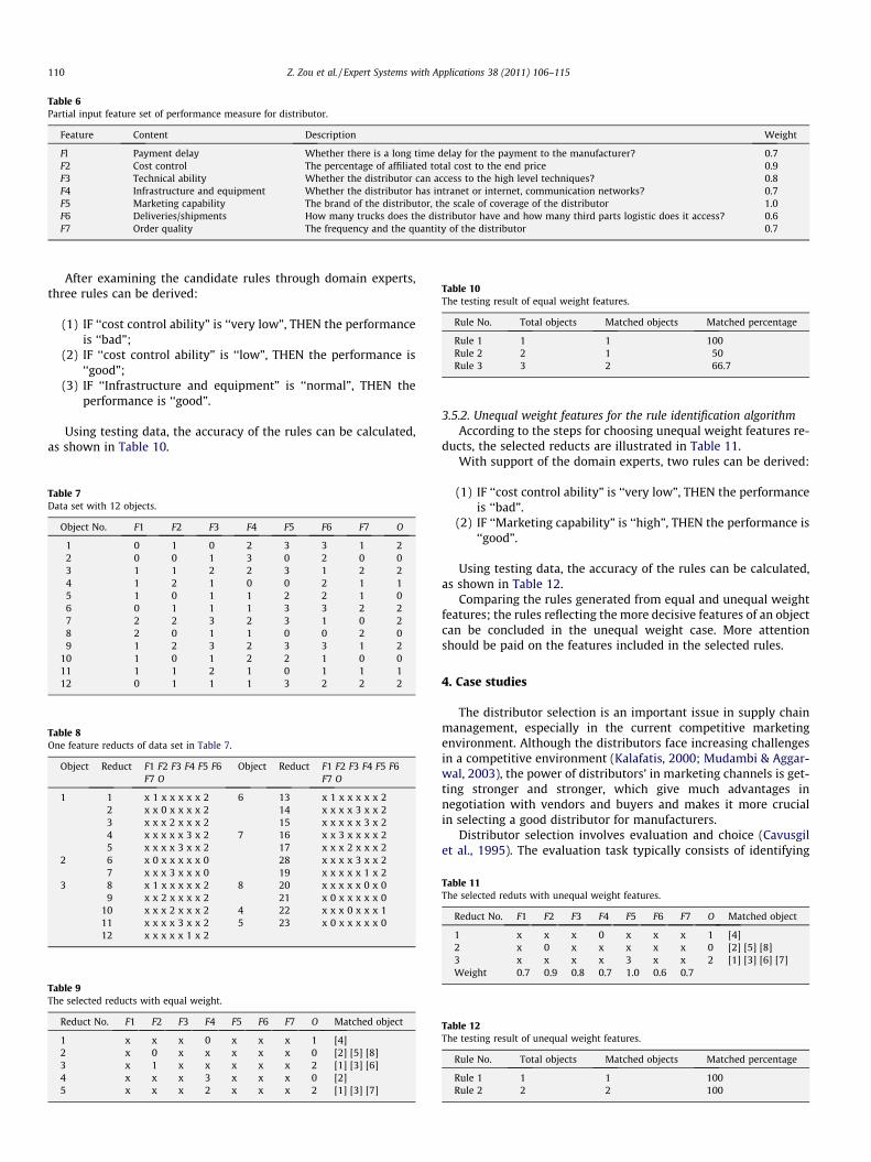
Table 6Partial input feature set of performance measure for distributor.

Feature Content Description Weight

Fl Payment delay Whether there is a long time delay for the payment to the manufacturer? 0.7F2 Cost control The percentage of affiliated total cost to the end price 0.9F3 Technical ability Whether the distributor can access to the high level techniques? 0.8F4 Infrastructure and equipment Whether the distributor has intranet or internet, communication networks? 0.7F5 Marketing capability The brand of the distributor, the scale of coverage of the distributor 1.0F6 Deliveries/shipments How many trucks does the distributor have and how many third parts logistic does it access? 0.6F7 Order quality The frequency and the quantity of the distributor 0.7

Table 10The testing result of equal weight features.

Rule No. Total objects Matched objects Matched percentage

Rule 1 1 1 100Rule 2 2 1 50Rule 3 3 2 66.7

110 Z. Zou et al. / Expert Systems with Applications 38 (2011) 106–115

After examining the candidate rules through domain experts,three rules can be derived:

(1) IF ‘‘cost control ability” is ‘‘very low”, THEN the performanceis ‘‘bad”;

(2) IF ‘‘cost control ability” is ‘‘low”, THEN the performance is‘‘good”;

(3) IF ‘‘Infrastructure and equipment” is ‘‘normal”, THEN theperformance is ‘‘good”.

Using testing data, the accuracy of the rules can be calculated,as shown in Table 10.

Table 7Data set with 12 objects.

Object No. F1 F2 F3 F4 F5 F6 F7 O

1 0 1 0 2 3 3 1 22 0 0 1 3 0 2 0 03 1 1 2 2 3 1 2 24 1 2 1 0 0 2 1 15 1 0 1 1 2 2 1 06 0 1 1 1 3 3 2 27 2 2 3 2 3 1 0 28 2 0 1 1 0 0 2 09 1 2 3 2 3 3 1 2

10 1 0 1 2 2 1 0 011 1 1 2 1 0 1 1 112 0 1 1 1 3 2 2 2

Table 8One feature reducts of data set in Table 7.

Object Reduct F1 F2 F3 F4 F5 F6F7 O

Object Reduct F1 F2 F3 F4 F5 F6F7 O

1 1 x 1 x x x x x 2 6 13 x 1 x x x x x 22 x x 0 x x x x 2 14 x x x x 3 x x 23 x x x 2 x x x 2 15 x x x x x 3 x 24 x x x x x 3 x 2 7 16 x x 3 x x x x 25 x x x x 3 x x 2 17 x x x 2 x x x 2

2 6 x 0 x x x x x 0 28 x x x x 3 x x 27 x x x 3 x x x 0 19 x x x x x 1 x 2

3 8 x 1 x x x x x 2 8 20 x x x x x 0 x 09 x x 2 x x x x 2 21 x 0 x x x x x 0

10 x x x 2 x x x 2 4 22 x x x 0 x x x 111 x x x x 3 x x 2 5 23 x 0 x x x x x 012 x x x x x 1 x 2

Table 9The selected reducts with equal weight.

Reduct No. F1 F2 F3 F4 F5 F6 F7 O Matched object

1 x x x 0 x x x 1 [4]2 x 0 x x x x x 0 [2] [5] [8]3 x 1 x x x x x 2 [1] [3] [6]4 x x x 3 x x x 0 [2]5 x x x 2 x x x 2 [1] [3] [7]

3.5.2. Unequal weight features for the rule identification algorithmAccording to the steps for choosing unequal weight features re-

ducts, the selected reducts are illustrated in Table 11.With support of the domain experts, two rules can be derived:

(1) IF ‘‘cost control ability” is ‘‘very low”, THEN the performanceis ‘‘bad”.

(2) IF ‘‘Marketing capability” is ‘‘high”, THEN the performance is‘‘good”.

Using testing data, the accuracy of the rules can be calculated,as shown in Table 12.

Comparing the rules generated from equal and unequal weightfeatures; the rules reflecting the more decisive features of an objectcan be concluded in the unequal weight case. More attentionshould be paid on the features included in the selected rules.

4. Case studies

The distributor selection is an important issue in supply chainmanagement, especially in the current competitive marketingenvironment. Although the distributors face increasing challengesin a competitive environment (Kalafatis, 2000; Mudambi & Aggar-wal, 2003), the power of distributors’ in marketing channels is get-ting stronger and stronger, which give much advantages innegotiation with vendors and buyers and makes it more crucialin selecting a good distributor for manufacturers.

Distributor selection involves evaluation and choice (Cavusgilet al., 1995). The evaluation task typically consists of identifying

Table 11The selected reduts with unequal weight features.

Reduct No. F1 F2 F3 F4 F5 F6 F7 O Matched object

1 x x x 0 x x x 1 [4]2 x 0 x x x x x 0 [2] [5] [8]3 x x x x 3 x x 2 [1] [3] [6] [7]Weight 0.7 0.9 0.8 0.7 1.0 0.6 0.7

Table 12The testing result of unequal weight features.

Rule No. Total objects Matched objects Matched percentage

Rule 1 1 1 100Rule 2 2 2 100

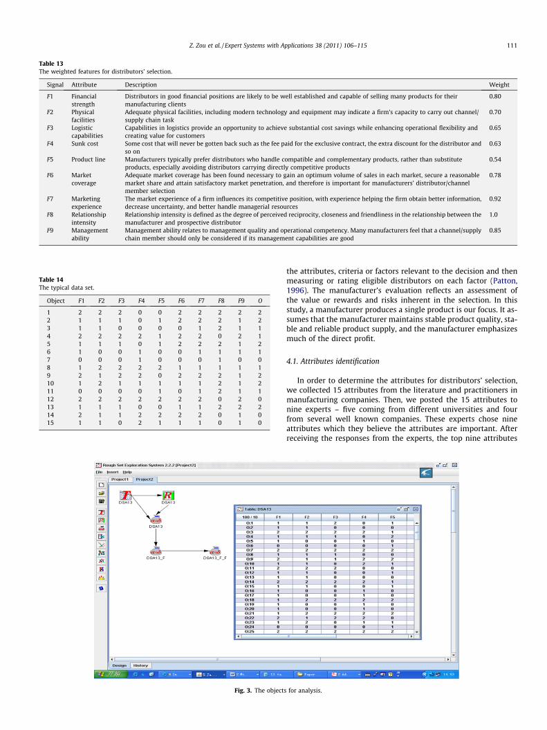
Table 13The weighted features for distributors’ selection.

Signal Attribute Description Weight

F1 Financialstrength

Distributors in good financial positions are likely to be well established and capable of selling many products for theirmanufacturing clients

0.80

F2 Physicalfacilities

Adequate physical facilities, including modern technology and equipment may indicate a firm’s capacity to carry out channel/supply chain task

0.70

F3 Logisticcapabilities

Capabilities in logistics provide an opportunity to achieve substantial cost savings while enhancing operational flexibility andcreating value for customers

0.65

F4 Sunk cost Some cost that will never be gotten back such as the fee paid for the exclusive contract, the extra discount for the distributor andso on

0.63

F5 Product line Manufacturers typically prefer distributors who handle compatible and complementary products, rather than substituteproducts, especially avoiding distributors carrying directly competitive products

0.54

F6 Marketcoverage

Adequate market coverage has been found necessary to gain an optimum volume of sales in each market, secure a reasonablemarket share and attain satisfactory market penetration, and therefore is important for manufacturers’ distributor/channelmember selection

0.78

F7 Marketingexperience

The market experience of a firm influences its competitive position, with experience helping the firm obtain better information,decrease uncertainty, and better handle managerial resources

0.92

F8 Relationshipintensity

Relationship intensity is defined as the degree of perceived reciprocity, closeness and friendliness in the relationship between themanufacturer and prospective distributor

1.0

F9 Managementability

Management ability relates to management quality and operational competency. Many manufacturers feel that a channel/supplychain member should only be considered if its management capabilities are good

0.85

Table 14The typical data set.

Object F1 F2 F3 F4 F5 F6 F7 F8 F9 O

1 2 2 2 0 0 2 2 2 2 22 1 1 1 0 1 2 2 2 1 23 1 1 0 0 0 0 1 2 1 14 2 2 2 2 1 2 2 0 2 15 1 1 1 0 1 2 2 2 1 26 1 0 0 1 0 0 1 1 1 17 0 0 0 1 0 0 0 1 0 08 1 2 2 2 2 1 1 1 1 19 2 1 2 2 0 2 2 2 1 210 1 2 1 1 1 1 1 2 1 211 0 0 0 0 1 0 1 2 1 112 2 2 2 2 2 2 2 0 2 013 1 1 1 0 0 1 1 2 2 214 2 1 1 2 2 2 2 0 1 015 1 1 0 2 1 1 1 0 1 0

Fig. 3. The objects

Z. Zou et al. / Expert Systems with Applications 38 (2011) 106–115 111

the attributes, criteria or factors relevant to the decision and thenmeasuring or rating eligible distributors on each factor (Patton,1996). The manufacturer’s evaluation reflects an assessment ofthe value or rewards and risks inherent in the selection. In thisstudy, a manufacturer produces a single product is our focus. It as-sumes that the manufacturer maintains stable product quality, sta-ble and reliable product supply, and the manufacturer emphasizesmuch of the direct profit.

4.1. Attributes identification

In order to determine the attributes for distributors’ selection,we collected 15 attributes from the literature and practitioners inmanufacturing companies. Then, we posted the 15 attributes tonine experts – five coming from different universities and fourfrom several well known companies. These experts chose nineattributes which they believe the attributes are important. Afterreceiving the responses from the experts, the top nine attributes

for analysis.

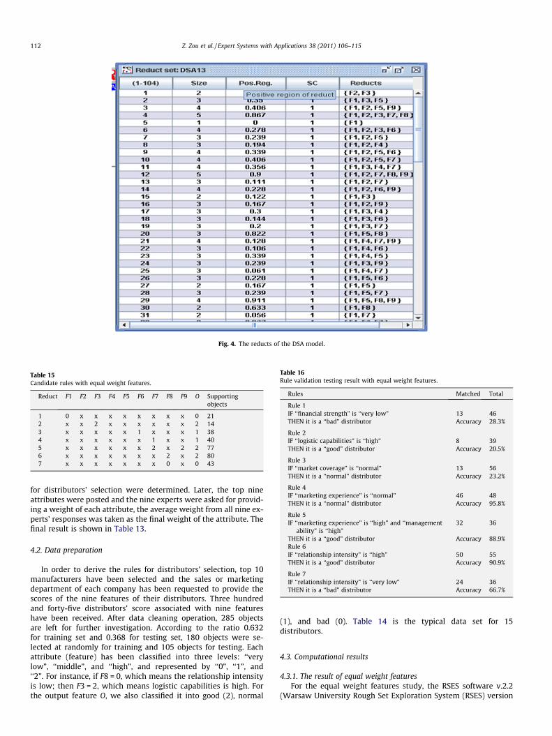
Fig. 4. The reducts of the DSA model.

Table 15Candidate rules with equal weight features.

Reduct F1 F2 F3 F4 F5 F6 F7 F8 F9 O Supportingobjects

1 0 x x x x x x x x 0 212 x x 2 x x x x x x 2 143 x x x x x 1 x x x 1 384 x x x x x x 1 x x 1 405 x x x x x x 2 x 2 2 776 x x x x x x x 2 x 2 807 x x x x x x x 0 x 0 43

Table 16Rule validation testing result with equal weight features.

Rules Matched Total

Rule 1IF ‘‘financial strength” is ‘‘very low” 13 46THEN it is a ‘‘bad” distributor Accuracy 28.3%

Rule 2IF ‘‘logistic capabilities” is ‘‘high” 8 39THEN it is a ‘‘good” distributor Accuracy 20.5%

Rule 3IF ‘‘market coverage” is ‘‘normal” 13 56THEN it is a ‘‘normal” distributor Accuracy 23.2%

Rule 4IF ‘‘marketing experience” is ‘‘normal” 46 48THEN it is a ‘‘normal” distributor Accuracy 95.8%

Rule 5IF ‘‘marketing experience” is ‘‘high” and ‘‘management

ability” is ‘‘high”32 36

THEN it is a ‘‘good” distributor Accuracy 88.9%Rule 6IF ‘‘relationship intensity” is ‘‘high” 50 55THEN it is a ‘‘good” distributor Accuracy 90.9%

Rule 7IF ‘‘relationship intensity” is ‘‘very low” 24 36THEN it is a ‘‘bad” distributor Accuracy 66.7%

112 Z. Zou et al. / Expert Systems with Applications 38 (2011) 106–115

for distributors’ selection were determined. Later, the top nineattributes were posted and the nine experts were asked for provid-ing a weight of each attribute, the average weight from all nine ex-perts’ responses was taken as the final weight of the attribute. Thefinal result is shown in Table 13.

4.2. Data preparation

In order to derive the rules for distributors’ selection, top 10manufacturers have been selected and the sales or marketingdepartment of each company has been requested to provide thescores of the nine features of their distributors. Three hundredand forty-five distributors’ score associated with nine featureshave been received. After data cleaning operation, 285 objectsare left for further investigation. According to the ratio 0.632for training set and 0.368 for testing set, 180 objects were se-lected at randomly for training and 105 objects for testing. Eachattribute (feature) has been classified into three levels: ‘‘verylow”, ‘‘middle”, and ‘‘high”, and represented by ‘‘0”, ‘‘1”, and‘‘2”. For instance, if F8 = 0, which means the relationship intensityis low; then F3 = 2, which means logistic capabilities is high. Forthe output feature O, we also classified it into good (2), normal

(1), and bad (0). Table 14 is the typical data set for 15distributors.

4.3. Computational results

4.3.1. The result of equal weight featuresFor the equal weight features study, the RSES software v.2.2

(Warsaw University Rough Set Exploration System (RSES) version

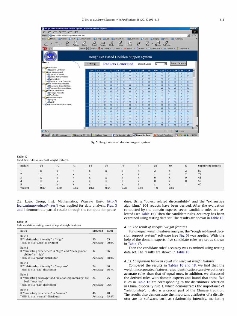
Fig. 5. Rough set-based decision support system.

Table 17Candidate rules of unequal weight features.

Reduct F1 F2 F3 F4 F5 F6 F7 F8 F9 O Supporting objects

1 x x x x x x x 2 x 2 802 x x x x x x 2 x 2 2 773 x x x x x x x 0 x 0 434 x x x x x 0 x 0 x 0 595 x x x x x x 1 x x 1 40Weight 0.80 0.70 0.65 0.63 0.54 0.78 0.92 1.0 0.85

Z. Zou et al. / Expert Systems with Applications 38 (2011) 106–115 113

2.2, Logic Group, Inst. Mathematics, Warsaw Univ., http://logic.mimuw.edu.pl/~rses/) was applied for data analysis. Figs. 3and 4 demonstrate partial results through the computation proce-

Table 18Rule validation testing result of equal weight features.

Rules Matched Total

Rule 1IF ‘‘relationship intensity” is ‘‘High” 50 55THEN it is a ‘‘Good” distributor Accuracy 90.9%

Rule 2IF ‘‘marketing experience” is ‘‘high” and ‘‘management

ability” is ‘‘high”32 36

THEN it is a ‘‘good” distributor Accuracy 88.9%

Rule 3IF ‘‘relationship intensity” is ‘‘very low” 24 36THEN it is a ‘‘bad” distributor Accuracy 66.7%

Rule 4IF ‘‘marketing coverage” and ‘‘relationship intensity” are

both ‘‘very low”24 25

THEN it is a ‘‘bad” distributor Accuracy 96%

Rule 5IF ‘‘marketing experience” is ‘‘normal” 46 48THEN it is a ‘‘normal” distributor Accuracy 95.8%

dure. Using ‘‘object related discernibility” and the ‘‘exhaustivealgorithm,” 104 reducts have been derived. After the evaluationconducted by the domain experts, seven candidate rules are se-lected (see Table 15). Then the candidate rules’ accuracy has beenexamined using testing data set. The results are shown in Table 16.

4.3.2. The result of unequal weight featuresFor unequal weight features analysis, the ‘‘rough set-based deci-

sion support system” software (see Fig. 5) was applied. With thehelp of the domain experts, five candidate rules are set as shownin Table 17.

Then the candidate rules’ accuracy was examined using testingdata set. The results are shown in Table 18.

4.3.3. Comparison between equal and unequal weight featuresCompared the results in Tables 16 and 18, we find that the

weight incorporated features rules identification can give out moreaccurate rules than that of equal ones. In addition, we discussedthe derived rules with domain experts and found that these fiverules in Table 18 are corresponding to the distributors’ selectionin China, especially rule 1, which demonstrates the importance of‘‘relationship”. It also is a crucial part of the Chinese tradition.The results also demonstrate the important attributes of a distrib-utor are its software, such as relationship intensity, marketing

114 Z. Zou et al. / Expert Systems with Applications 38 (2011) 106–115

experience and management ability, rather than its hardware, suchas financial strength, physical facilities or logistic capabilities.

5. Conclusions

In this paper, distributors’ selection is analyzed based on therough set theory approach in both equal and unequal weight fea-tures. Through this method, several rules are generated for distrib-utors’ evaluation and selection. The result not only shows theeffectiveness of unequal weight incorporated rules identification,but also it shows the importance of the relationship intensity, mar-keting experience, and the management ability in selecting the dis-tributors. These rules have been proved to be useful andconvenient to conduct a selection process for the manufacturers.Moreover, the derived rules provide us critical implication thatthe entire constituencies in the supply chain should maintain anintensity relationship with each other of the whole supply chaintherein.

There exist several avenues for further research. First, the ninefeatures are chose by only nine domain experts, which may havesome subjective effect. Second, there are only 285 objects in thedata set, and they were collected from only 10 manufacturers,the indication through the outputs from the algorithms mightnot be reliable. Furthermore, all these objects were selected fromChina. The result reflects the preference of the Chinese culture be-yond doubt.

Appendix A.

A.1. Indiscernibility relationship

The starting point of RST is the indiscernibility relation. Theindiscernibility relation identifies objects having the same proper-ties, i.e., objects of interest having the same properties are indis-cernible and consequently are treated as identical or similar. Inother words, the indiscernibility relation leads to clustering of ele-ments of interest into granules of indiscernible (similar) objects. InRST these granules, called elementary sets (concepts), are basicbuilding blocks (concepts) of knowledge about the universe.

Considering specific attributes, the objects are indiscernibleaccording to the available information. For example, as shown inTable 2, the condition attribute F1 of Objects 1, 2 and 4 is the same;hence, these three objects are indiscernible based on the attributeF1. In other words, the objects described by the identical data ofconsidered attributes are indiscernible. A set of all indiscernibleobjects with respect to specific considered attributes is called anelementary set. Let B be a nonempty subset of the set A of all attri-butes, i.e. B # A. The indiscernibility relation is an equivalencerelation on U. In particular, x, y e U, B-indiscernibility relation, de-noted by IB, defines that x and y are B-indiscernible with respect toB as follows:

ðx; yÞ 2 IB() f ðx; aÞ ¼ f ðy; aÞ; 8a 2 B ðA-1Þ

That is, x and y are B-indiscernible if considering only subset B of theattributes. The B-indiscernibility relation will induce the B-elemen-tary set in S. Moreover, the family of all equivalence classes definedby the relation is IB denoted by U/IB.

A partition of the universe can be generated based on indiscern-ibility relations; thus, the universe can be decomposed into blocksof indiscernible objects, i.e., elementary sets. For example, theattribute F1 will induce two elementary sets {1, 2, 4} and {3, 5}.Let B1 = {F1}, then two B-elementary sets can be generated. Thatis, IB1 = {1, 2, 4}, given F1 = ‘‘1”. Objects 1, 2 and 4 are indiscernible,since their attribute F1 are identical, that is, ‘‘1.” Similarly,IB1 = {3, 5} given F1 = ‘‘0.” Therefore, U/IB1 = {{1, 2, 4}, {3, 5}}. Con-

sidering both the attributes ‘‘F1” and ‘‘F2”, the elementary sets of{1, 2}, {4}, and {3, 5} will be generated. In other words, the B-ele-mentary set, where B2 = {F1, F2} generates three elementary sets{1, 2}, {4}, and {3, 5}. Hence, U/IB2 = {{1, 2}, {4}, {3, 5}}. Similarly,any subset of the attributes can generate elementary sets.

A.2. Approximation of sets

A rough set can be described as a collection of objects that ingeneral cannot be precisely characterized in terms of their valuesof their sets of attributes, but which can be characterized in termsof lower or upper approximations (Slowinski, 1992). The upperapproximation includes all objects that possibly belong to the con-cept; while the lower approximation contains all objects that def-initely belong to the concept. Let Y to be the subset of objects ofuniverse U. on one hand, the lower approximation of Y in B, de-noted as BY, is a set defined as follows:

BY ¼ fx 2 UjIBðxÞ# Yg ðA-2Þ

The lower approximation of a rough set contains all the objects thatcan be certainly classified into a set under the knowledge of consid-ered attributes. On the other hand, the upper approximation of Y inB, denoted as BY , is a set defined as follows:

BY ¼ fx 2 UjIBðxÞ \ Y – /g ðA-3Þ

That is, the upper approximation of a rough set contains all the ob-jects that can be possibly classified into a set under the knowledgeof considered attributes. Then, the boundary region of Y in B, de-noted as BNB(Y), is defined by the difference between the two setsof the upper and lower approximations as follows:

BNBðYÞ ¼ BY � BY ðA-4Þ

That is, the boundary region represents the area that cannot beproperly classified using the considered attributes.

For example, as shown in Table 2, the objects can be properlyclassified into three categories, Y1, Y2 and Y3, according to the va-lue of output feature O.

Y1 = {1, 3, 5}, where O = ‘‘0”Y2 = {2}, where O = ‘‘1”Y3 = {4}, where O = ‘‘2”

Let B = {F1, F2}, then U/IB = {{1, 2}, {4}, {3, 5}}.So, the elements can be contained by Y1 are {3, 5}, the lower

approximation of the set Y1 in B, that is BY1 = {3, 5}. On the otherhand, since

f1;2g \ f1;3;5g– £

f4g \ f1;3;5g ¼£

f3;5g \ f1;3;5g– £

Then the upper approximation of Y1 in B, BY1 ¼ f1;2;3;5g. Thusthe boundary region of Y1 in B can be derived as follows:

BNBðYÞ ¼ BY � BY ¼ f1;2;3;5g � f3;5g ¼ f1;2g

Similarly, we can get the lower and upper approximations of Y2 andY3 in B.Furthermore, the accuracy of the approximation for any set Yin B is defined as follows:

aBðYÞ ¼cardðBYÞcardðBYÞ

ðA-5Þ

where the cardinality is the number of objects within a set. Theaccuracy of approximation, aB(Y), is between zero and one. Thus,if aB(Y) = 1, Y is an ordinary (exact) set with respect to B; otherwise,i.e., aB(Y) < 1, Y is a rough (vague) set with respect to B.

So, for Y1 respecting to B,

Z. Zou et al. / Expert Systems with Applications 38 (2011) 106–115 115

aBðY1Þ ¼ cardðBY1ÞcardðBY1Þ

¼ 24¼ 1

2ðA-6Þ

That is to say, Y1 = {1, 3, 5} is rough set with respect to B.

References

Abratt, R., & Pitt, L. F. (1989). Selection and motivation of industrial distributors: Acomparative analysis. European Journal of Marketing, 23, 144–153.

Beynon, M., Curry, B., & Morgan, P. (2001). Knowledge discovery in marketing: Anapproach through rough set theory. European Journal of Marketing, 35, 915–935.

Cavusgil, S. T., Yeoh, P., & Mitri, M. (1995). Selecting foreign distributors: An expertsystems approach. Industrial Marketing Management, 24, 297–304.

Chan, F. T. S., & Kumar, N. (2007). Global supplier development considering riskfactors using fuzzy extended AHP-based approach. Omega, 35, 417–431.

Chien, C.-F., & Chen, L.-F. (2007). Using rough set theory to recruit and retain high-potential talents for semiconductor manufacturing. IEEE Transactions onSemiconductor Manufacturing, 20, 528–541.

Daubie, M., Levecq, P., & Meskens, N. (2002). A comparison of the rough sets andrecursive partitioning induction approaches: An application to commercialloans. International Transactions in Operational Research, 9, 681–694.

Dimitras, A. I., Slowinski, R., Susmaga, R., & Zopounidis, C. (1999). Business failureprediction using rough sets. European Journal of Operational Research, 114,263–280.

Dubois, D., & Prade, H. (1990). Rough fuzzy sets and fuzzy rough sets. InternationalJournal of General Systems, 17, 191–209.

Fonsson, P., & Zineldin, M. (2003). Achieving high satisfaction in supplier–dealerworking relationships. Supply Chain Management: An International Journal, 8,224–240.

Fram, E. H. (1992). We can do a better job of selecting international distributors.Journal of Business and Industrial Marketing, 7, 61–70.

Ghodsypour, S. H., & O’Brien, C. (1998). A decision support system for supplierselection using an integrated analytical hierarchy process and linearprogramming. International Journal of Production Economics(56/57), 199–212.

Greco, S., Matarazzo, B., & Slowinski, R. (2000). Extension of the rough set theoryapproach to multicriteria decision support. INFOR, 38, 161–196.

Heckerman, D., Mannila, H., Pregibon, D., & Uthurusamy, R. (1997). In Proceedings of3rd international conference on knowledge discovery and data mining. Menlo Park,CA: AAAI Press.

Kahraman, C., Cebeci, U., & Ruan, D. (2004). Multi-attribute comparison of cateringservice companies using fuzzy AHP: The case of Turkey. International Journal ofProduction Economics, 87, 171–184.

Kahraman, C., Cebeci, U., & Ulukan, Z. (2003). Multi-criteria supplier selection usingfuzzy AHP. Logistics Information Management, 16, 382–394.

Kalafatis, S. P. (2000). Buyer–seller relationships along channels of distribution.Industrial Marketing Management, 31, 215–228.

Komorowski, J., & Zytkow, J. (1997). Principles of data mining and knowledgediscovery. New York: Springer.

Kumar, A., Agrawal, D. P., & Joshi, S. D. (2005). Advertising data analysis using roughsets model. International Journal of Information Technology and Decision Making,4, 263–276.

Kusiak, A. (2001). Rough set theory: A data mining tool for semiconductormanufacturing. IEEE Transactions on Electronics Packaging Manufacturing, 24,44–50.

Kusiak, A., Kern, J. A., Kernstine, K. H., & Tseng, T.-L. (2000). Autonomous decision-making: A data mining approach. IEEE Transactions on Information Technology inBiomedicine, 4, 274–284.

Lin, F.-S., & Chen, C.-R. (2008). Determinants of manufacturers’ selection ofdistributor. Supply Chain Management: An International Journal, 13, 356–365.

Lindqvist, L. J. (1983). Current trends in distribution research in Finland.International Journal of Physical and Logistics Management, 13, 105–116.

Mickee, T. E. (2003). Rough sets bankruptcy prediction models versus auditorsignaling rates. Journal of Forecasting, 22, 569–586.

Mudambi, S., & Aggarwal, R. (2003). Industrial distributors: Can they survive in thenew economy? Industrial Marketing Management, 32, 317–325.

Oliveria, R. C., & Lourenco, J. C. (2002). A multicriteria model for assigning neworders to service suppliers. European Journal of Operational Research, 139,390–399.

Patton, W. E. (1996). Use of human judgment models in industrial buyers’ vendorselection decisions. Industrial Marketing Management, 25, 135–149.

Pawlak, Z. (1982). Rough sets. International Journal of Computer and InformationSciences, 11, 341–356.

Pawlak, Z. (1991). Rough sets. Dordrecht, The Netherlands: Kluwer AcademicPublishers.

Ross, R. E. (1973). Selection of the overseas distributor: An empirical framework.International Journal of Physical and Logistics Management, 3, 83–90.

Sevkli, M., Lenny Koh, S. C., Zaim, S., Demirbag, M., & Tatoglu, E. (2008). Hybridanalytical hierarchy process model for supplier selection. Industrial Managementand Data System, 108, 122–142.

Sharma, D., Sahay, B. S., & Sachan, A. (2004). Modeling distributor performanceindex using system dynamics approach. Asia Pacific Journal of Marketing andLogistics, 16, 37–67.

Shen, L., Tay, F. E. H., Qu, L., & Shen, Y. (2000). Fault diagnosis using rough set theory.Computers in Industry, 43, 61–72.

Shipley, D. D., Cook, D., & Barnett, E. (1989). Recruitment, motivation, training andevaluation of overseas distributors. European Journal of Marketing, 23, 79–93.

Tseng, T.-L., Huang, C.-C., Jiang, F., & Ho, J. C. (2006). Applying a hybrid data-miningapproach to prediction problems: A case of preferred suppliers prediction.International Journal of Production Research, 44, 2935–2954.

Wang, L., & Kess, P. (2006). Partnership motives and partner selection – Case studiesof Finnish distributor relationships in China. International Journal of Physical andLogistics Management, 36, 466–478.

Wei, L.-L., & Zhang, W.-X. (2004). Probabilistic rough sets characterized by fuzzysets. International Journal of Uncertainty, Fuzziness and Knowledge-Based Systems,12, 47–60.

Yan, H., Yu, Z., & Cheng, T. C. E. (2003). A strategic model for supply chain designwith logical constraints: Formulation and solution. Computers and OperationsResearch, 30, 2135–2155.

Yeoh, P., & Calantone, R. J. (1995). An application of the analytical hierarchy processto international marketing: Selection of a foreign distributor. Journal of GlobalMarketing, 8, 39–65.