This is the author’s version of a work that was submitted/accepted for pub-lication in the following source:

Nayak, Richi & Tran, Tien (2007) A Progressive Clustering Algorithm toGroup the XML Data by Structural and Semantic Similarity. InternationalJournal of Pattern Recognition and Artificial Intelligence, 21(4), pp. 723-743.

This file was downloaded from: http://eprints.qut.edu.au/13996/

c© Copyright 2007 World Scientific Publishing

Notice: Changes introduced as a result of publishing processes such ascopy-editing and formatting may not be reflected in this document. For adefinitive version of this work, please refer to the published source:

http://dx.doi.org/10.1142/S0218001407005648

A Progressive Clustering Algorithm to Group the XML

Data by Structural and Semantic Similarity

Richi Nayak and Tien Tran

School of Information Systems

Queensland University of Technology

Brisbane, Australia

r.nayak@qut.edu.au

Abstract. Since the emergence in the popularity of XML for data

representation and exchange over the Web, the distribution of XML

documents has rapidly increased. Therefore it is a new challenge for the

field of data mining to turn these documents into a more useful

information utility. We present a novel clustering algorithm PCXSS that

keeps the heterogeneous XML documents into various groups according

to the similar structural and semantic representations. We introduce a

global criterion function CPSim that progressively measures the

similarity between a XML document and existing clusters, ignoring the

need to compute the similarity between two individual documents. The

experimental analysis shows the method to be fast and accurate.

1. Introduction

As the World Wide Web (WWW) becomes more prevalent for exchanging

and discovering information, there is an increasing wealth of knowledge with the

potential for finding information about anything. Moreover XML (eXtensible Markup

Language) [35] has gained popularity for the representation and exchange of data over

the Web. The explosive growth in XML sources presents an enormous opportunity and

challenge for grouping XML data based on their context and structure for efficient data

management and retrieval.

Clustering of XML documents facilitates a number of applications such as

improved information retrieval, data and schema integration, document classification

analysis, structure summary and indexing, data warehousing, and improved query

processing [3, 25]. For example, the computation of structural similarity is a great

value to the management of Web data. Many techniques for the extraction and

integration of relevant information from Web data sources require grouping Web data

sources according to their structural similarity [9, 11]. Efficient data management

techniques such as indexing based on structural similarity can support an effective

document storage and retrieval [25].

The clustering process is an unsupervised data mining technique that

categories a large amount of data source without prior knowledge on the taxonomy

[11]. Clustering has frequently been used on database objects, flat file data such as

text files, and semi-structured documents like HTML. However, clustering of XML

documents is more challenging. XML allows the representation of semi-structured and

hierarchal data, containing not only the values of individual items but also the

relationships between data items by tagging the pertinent information. Due to the

inherent flexibility of XML, in both structure and semantics, clustering XML data is

2

faced with new challenges as well as benefits. Mining of structure along with content

provides new insights and means into the process of clustering.

Consider parts of two documents: <craft>boat building</craft> and <craft>

boat </craft>. The intended interpretation of the former is ‘occupation’, and of the

latter ‘vessel’. The similarity of the content does not distinguish the semantic intention

of the tags. Use of structural similarity in this case provides probabilities of a tag

having a particular meaning. For example, the paths \occupation\design\craft and

\vessel\type\craft assist to determine the appropriate interpretation for such

homographic tags. Hence, consideration of structure and content of documents in

mining assist to clarify in case when two documents appearing similar are actually

completely different.

A variety of clustering algorithms has recently emerged for XML document

clustering, majority of them are built on pair-wise similarity between documents or

schemas [4, 5, 8, 10, 15, 17, 21, 24]. The pair-wise similarity is measured using the

local criterion function between each pair of documents to maximize the intra-cluster

similarity and to minimize the inter-cluster similarity. Since each document is

composed of many elements, the similarity between each pair of elements of two

documents is measured and aggregated to form a similarity measure (distance)

between two documents. A similarity matrix is generated that contains the similarity

value for each pair of documents. This matrix is the input for the clustering process

using either the hierarchical agglomerative clustering algorithm or k-means algorithms

[13]. Pair-wise similarity can be computationally expensive when dealing with large

data sources due to the need of measuring similarity between each pair of data.

To reduce the computational efforts while maintaining the accuracy, we

develop a global criterion function CPSim (common path coefficient) that measures

the similarity between a XML data and existing clusters of XML data, instead of

computing pair-wise similarity between each pair of data. The CPSim function

includes the semantic as well as hierarchical structure similarity of elements. We then

incorporate CPSim into progressively grouping the XML data.

This paper presents the novel Progressively Clustering XML by Semantic and

Structural similarity (PCXSS) algorithm that quantitatively determines the similarity

between heterogeneous XML documents by considering the semantic as well as

hierarchical structure similarity of elements. We show the effectiveness of PCXSS

with several experiments. The results indicate that PCXSS is much faster than the pair-

wise similarity based method and provides a good quality clustering solution as well. It

is also not heavily influenced by thresholds such as the clustering and path similarity.

The next two sections briefly introduce the XML data and the PCXSS method.

Sections 4 and 5 explain the pre-processing and clustering phases included in this

method respectively. Section 6 details the empirical evaluation. Related work is

covered in section 7. We finally conclude the paper in section 8.

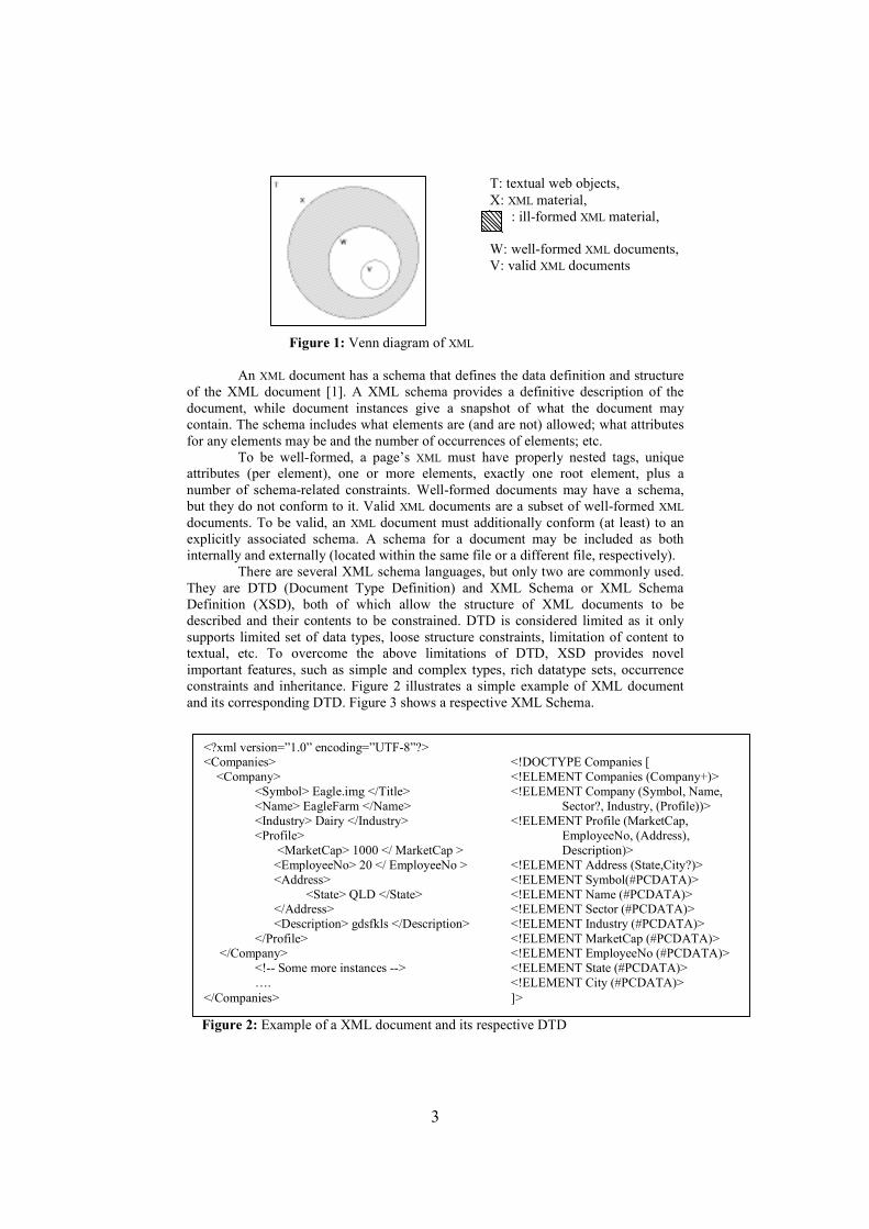
2. XML Documents and schemas

XML is a flexible representation language. There are many varieties of XML

material on the Web. Figure 1 illustrates the relationship between all XML materials.

Let all textual objects be the set T. Let web pages containing XML - to be called XML

material for the remainder of this discussion - be X, such that X ⊆ T. If D denotes the

set of XML documents, then D ⊂ X, that is, XML material is not automatically classed

as XML documents. Strictly, web pages are classed as XML documents only if they are

well formed, D = W, where W is the set of well-formed XML documents. Additionally,

V ⊆ W, where V is the set of valid XML documents. Finally, this allows the definition

of ill-formed XML material, given as X ∩ W .

3

T: textual web objects,

X: XML material,

: ill-formed XML material,

W: well-formed XML documents,

V: valid XML documents

Figure 1: Venn diagram of XML

An XML document has a schema that defines the data definition and structure

of the XML document [1]. A XML schema provides a definitive description of the

document, while document instances give a snapshot of what the document may

contain. The schema includes what elements are (and are not) allowed; what attributes

for any elements may be and the number of occurrences of elements; etc.

To be well-formed, a page’s XML must have properly nested tags, unique

attributes (per element), one or more elements, exactly one root element, plus a

number of schema-related constraints. Well-formed documents may have a schema,

but they do not conform to it. Valid XML documents are a subset of well-formed XML

documents. To be valid, an XML document must additionally conform (at least) to an

explicitly associated schema. A schema for a document may be included as both

internally and externally (located within the same file or a different file, respectively).

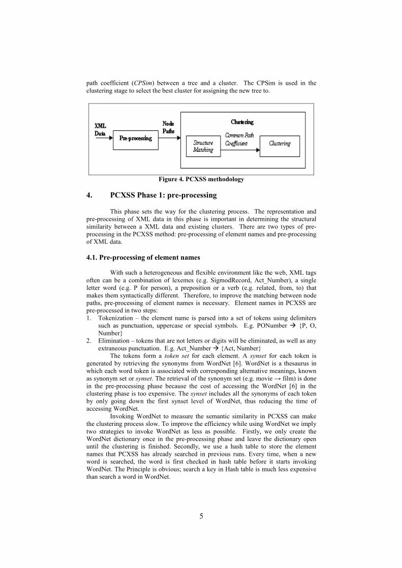
There are several XML schema languages, but only two are commonly used.

They are DTD (Document Type Definition) and XML Schema or XML Schema

Definition (XSD), both of which allow the structure of XML documents to be

described and their contents to be constrained. DTD is considered limited as it only

supports limited set of data types, loose structure constraints, limitation of content to

textual, etc. To overcome the above limitations of DTD, XSD provides novel

important features, such as simple and complex types, rich datatype sets, occurrence

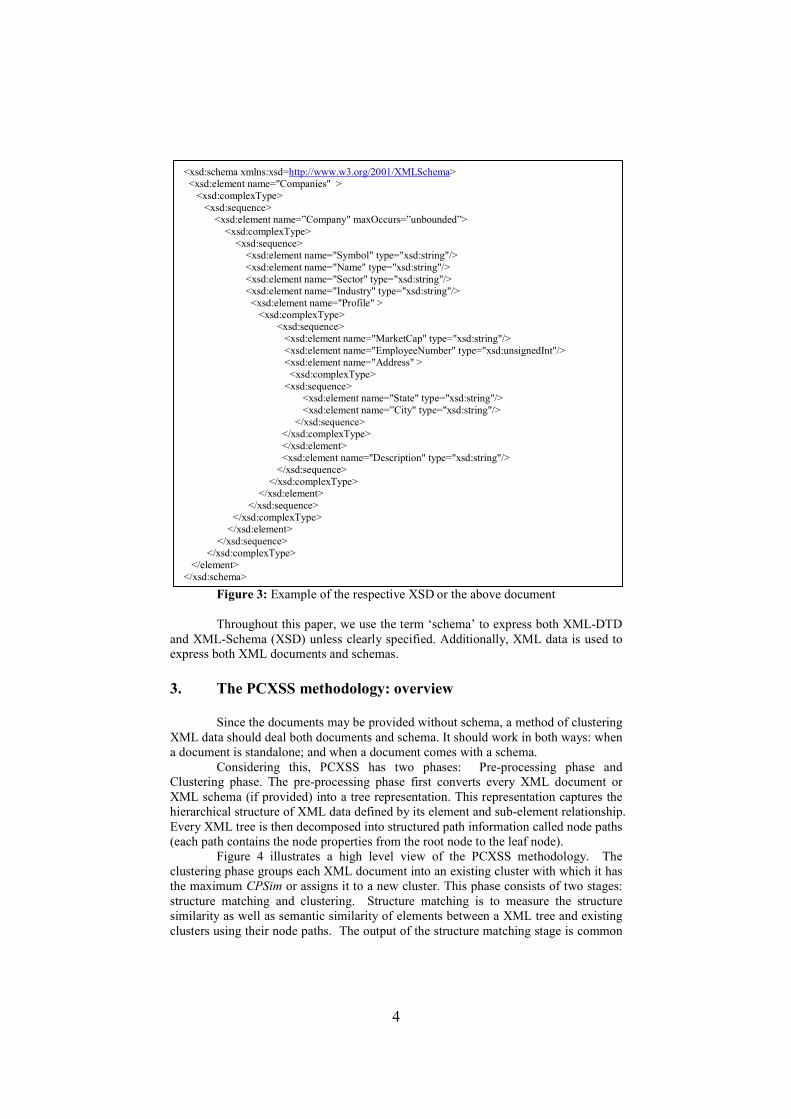
constraints and inheritance. Figure 2 illustrates a simple example of XML document

and its corresponding DTD. Figure 3 shows a respective XML Schema.

Figure 2: Example of a XML document and its respective DTD

<?xml version=”1.0” encoding=”UTF-8”?>

<Companies> <!DOCTYPE Companies [

<Company> <!ELEMENT Companies (Company+)>

<Symbol> Eagle.img </Title> <!ELEMENT Company (Symbol, Name,

<Name> EagleFarm </Name> Sector?, Industry, (Profile))>

<Industry> Dairy </Industry> <!ELEMENT Profile (MarketCap,

<Profile> EmployeeNo, (Address),

<MarketCap> 1000 </ MarketCap > Description)>

<EmployeeNo> 20 </ EmployeeNo > <!ELEMENT Address (State,City?)>

<Address> <!ELEMENT Symbol(#PCDATA)>

<State> QLD </State> <!ELEMENT Name (#PCDATA)>

</Address> <!ELEMENT Sector (#PCDATA)>

<Description> gdsfkls </Description> <!ELEMENT Industry (#PCDATA)>

</Profile> <!ELEMENT MarketCap (#PCDATA)>

</Company> <!ELEMENT EmployeeNo (#PCDATA)>

<!-- Some more instances --> <!ELEMENT State (#PCDATA)>

…. <!ELEMENT City (#PCDATA)>

</Companies> ]>

4

Figure 3: Example of the respective XSD or the above document

Throughout this paper, we use the term ‘schema’ to express both XML-DTD

and XML-Schema (XSD) unless clearly specified. Additionally, XML data is used to

express both XML documents and schemas.

3. The PCXSS methodology: overview

Since the documents may be provided without schema, a method of clustering

XML data should deal both documents and schema. It should work in both ways: when

a document is standalone; and when a document comes with a schema.

Considering this, PCXSS has two phases: Pre-processing phase and

Clustering phase. The pre-processing phase first converts every XML document or

XML schema (if provided) into a tree representation. This representation captures the

hierarchical structure of XML data defined by its element and sub-element relationship.

Every XML tree is then decomposed into structured path information called node paths

(each path contains the node properties from the root node to the leaf node).

Figure 4 illustrates a high level view of the PCXSS methodology. The

clustering phase groups each XML document into an existing cluster with which it has

the maximum CPSim or assigns it to a new cluster. This phase consists of two stages:

structure matching and clustering. Structure matching is to measure the structure

similarity as well as semantic similarity of elements between a XML tree and existing

clusters using their node paths. The output of the structure matching stage is common

<xsd:schema xmlns:xsd=http://www.w3.org/2001/XMLSchema> <xsd:element name="Companies" >

<xsd:complexType>

<xsd:sequence> <xsd:element name=”Company" maxOccurs=”unbounded”>

<xsd:complexType>

<xsd:sequence> <xsd:element name="Symbol" type="xsd:string"/>

<xsd:element name="Name" type="xsd:string"/>

<xsd:element name="Sector" type="xsd:string"/> <xsd:element name="Industry" type="xsd:string"/>

<xsd:element name="Profile" > <xsd:complexType> <xsd:sequence>

<xsd:element name="MarketCap" type="xsd:string"/>

<xsd:element name="EmployeeNumber" type="xsd:unsignedInt"/> <xsd:element name="Address" >

<xsd:complexType>

<xsd:sequence> <xsd:element name="State" type="xsd:string"/>

<xsd:element name=”City" type="xsd:string"/>

</xsd:sequence> </xsd:complexType>

</xsd:element>

<xsd:element name="Description" type="xsd:string"/> </xsd:sequence>

</xsd:complexType> </xsd:element>

</xsd:sequence>

</xsd:complexType> </xsd:element>

</xsd:sequence>

</xsd:complexType> </element>

</xsd:schema>

5

path coefficient (CPSim) between a tree and a cluster. The CPSim is used in the

clustering stage to select the best cluster for assigning the new tree to.

Figure 4. PCXSS methodology

4. PCXSS Phase 1: pre-processing

This phase sets the way for the clustering process. The representation and

pre-processing of XML data in this phase is important in determining the structural

similarity between a XML data and existing clusters. There are two types of pre-

processing in the PCXSS method: pre-processing of element names and pre-processing

of XML data.

4.1. Pre-processing of element names

With such a heterogeneous and flexible environment like the web, XML tags

often can be a combination of lexemes (e.g. SigmodRecord, Act_Number), a single

letter word (e.g. P for person), a preposition or a verb (e.g. related, from, to) that

makes them syntactically different. Therefore, to improve the matching between node

paths, pre-processing of element names is necessary. Element names in PCXSS are

pre-processed in two steps:

1. Tokenization – the element name is parsed into a set of tokens using delimiters

such as punctuation, uppercase or special symbols. E.g. PONumber � {P, O,

Number}

2. Elimination – tokens that are not letters or digits will be eliminated, as well as any

extraneous punctuation. E.g. Act_Number � {Act, Number}

The tokens form a token set for each element. A synset for each token is

generated by retrieving the synonyms from WordNet [6]. WordNet is a thesaurus in

which each word token is associated with corresponding alternative meanings, known

as synonym set or synset. The retrieval of the synonym set (e.g. movie → film) is done

in the pre-processing phase because the cost of accessing the WordNet [6] in the

clustering phase is too expensive. The synset includes all the synonyms of each token

by only going down the first synset level of WordNet, thus reducing the time of

accessing WordNet.

Invoking WordNet to measure the semantic similarity in PCXSS can make

the clustering process slow. To improve the efficiency while using WordNet we imply

two strategies to invoke WordNet as less as possible. Firstly, we only create the

WordNet dictionary once in the pre-processing phase and leave the dictionary open

until the clustering is finished. Secondly, we use a hash table to store the element

names that PCXSS has already searched in previous runs. Every time, when a new

word is searched, the word is first checked in hash table before it starts invoking

WordNet. The Principle is obvious; search a key in Hash table is much less expensive

than search a word in WordNet.

6

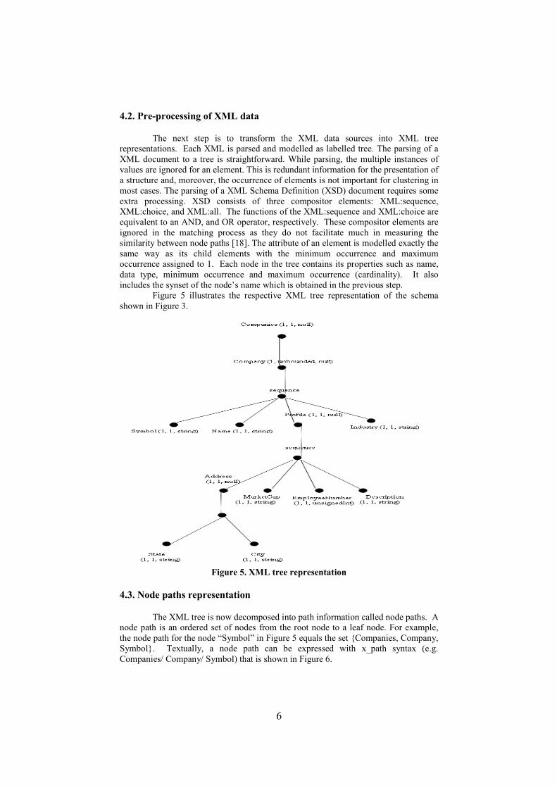
4.2. Pre-processing of XML data The next step is to transform the XML data sources into XML tree

representations. Each XML is parsed and modelled as labelled tree. The parsing of a

XML document to a tree is straightforward. While parsing, the multiple instances of

values are ignored for an element. This is redundant information for the presentation of

a structure and, moreover, the occurrence of elements is not important for clustering in

most cases. The parsing of a XML Schema Definition (XSD) document requires some

extra processing. XSD consists of three compositor elements: XML:sequence,

XML:choice, and XML:all. The functions of the XML:sequence and XML:choice are

equivalent to an AND, and OR operator, respectively. These compositor elements are

ignored in the matching process as they do not facilitate much in measuring the

similarity between node paths [18]. The attribute of an element is modelled exactly the

same way as its child elements with the minimum occurrence and maximum

occurrence assigned to 1. Each node in the tree contains its properties such as name,

data type, minimum occurrence and maximum occurrence (cardinality). It also

includes the synset of the node’s name which is obtained in the previous step.

Figure 5 illustrates the respective XML tree representation of the schema

shown in Figure 3.

Figure 5. XML tree representation

4.3. Node paths representation

The XML tree is now decomposed into path information called node paths. A

node path is an ordered set of nodes from the root node to a leaf node. For example,

the node path for the node “Symbol” in Figure 5 equals the set {Companies, Company,

Symbol}. Textually, a node path can be expressed with x_path syntax (e.g.

Companies/ Company/ Symbol) that is shown in Figure 6.

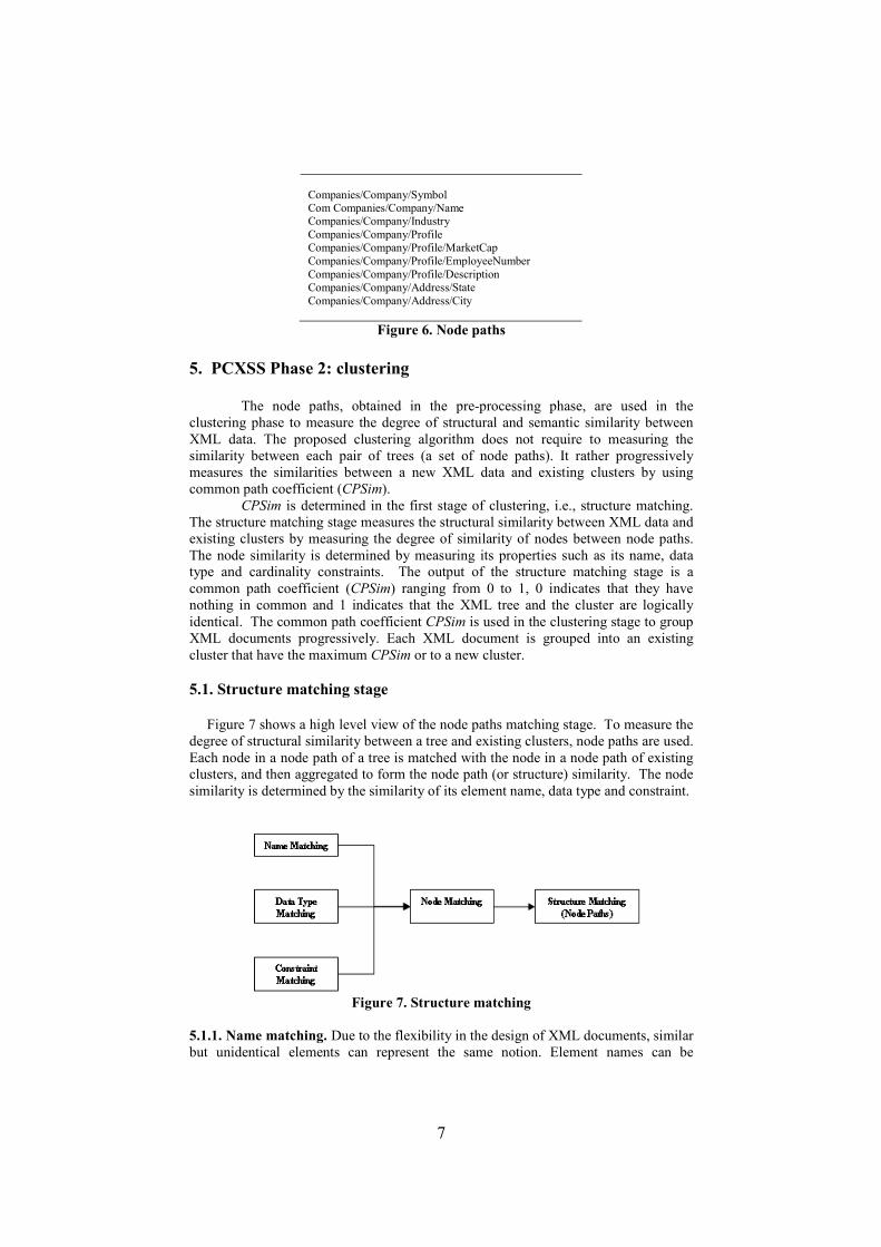
7

Companies/Company/Symbol Com Companies/Company/Name Companies/Company/Industry

Companies/Company/Profile Companies/Company/Profile/MarketCap

Companies/Company/Profile/EmployeeNumber

Companies/Company/Profile/Description Companies/Company/Address/State

Companies/Company/Address/City

Figure 6. Node paths

5. PCXSS Phase 2: clustering

The node paths, obtained in the pre-processing phase, are used in the

clustering phase to measure the degree of structural and semantic similarity between

XML data. The proposed clustering algorithm does not require to measuring the

similarity between each pair of trees (a set of node paths). It rather progressively

measures the similarities between a new XML data and existing clusters by using

common path coefficient (CPSim).

CPSim is determined in the first stage of clustering, i.e., structure matching.

The structure matching stage measures the structural similarity between XML data and

existing clusters by measuring the degree of similarity of nodes between node paths.

The node similarity is determined by measuring its properties such as its name, data

type and cardinality constraints. The output of the structure matching stage is a

common path coefficient (CPSim) ranging from 0 to 1, 0 indicates that they have

nothing in common and 1 indicates that the XML tree and the cluster are logically

identical. The common path coefficient CPSim is used in the clustering stage to group

XML documents progressively. Each XML document is grouped into an existing

cluster that have the maximum CPSim or to a new cluster.

5.1. Structure matching stage

Figure 7 shows a high level view of the node paths matching stage. To measure the

degree of structural similarity between a tree and existing clusters, node paths are used.

Each node in a node path of a tree is matched with the node in a node path of existing

clusters, and then aggregated to form the node path (or structure) similarity. The node

similarity is determined by the similarity of its element name, data type and constraint.

Figure 7. Structure matching

5.1.1. Name matching. Due to the flexibility in the design of XML documents, similar

but unidentical elements can represent the same notion. Element names can be

8

semantically similar (if they are in a semantic tag similarity relationship, e.g., person

or people) or syntactically similar (if they are in a syntactic tag similarity relationship,

e.g., edit or xedit).

Accordingly, PCXSS uses semantic and syntactic measures to calculate the

degree of similarity between a pair of names. Semantic measure considers the

meaning of the nodes’ name to determine the degree of similarity. For this measure to

be possible, WordNet [7] is used in the pre-processing phase to form a linguistic set

(synset). In this phase, we find a common element in the synsets of two names.

Syntactic measure considers the names syntax to determine the degree of

similarity. It is good for identifying abbreviation and acronym words that are most

commonly used in XML data. Sometime, however, it can lead to mismatches of

element names, e.g, ‘hot’ and ‘hotel’. To reduce the mismatches of element names, we

use string edit distance and n-gram methods to measure the syntactic relationship

between names. The average of both methods is used to measure the degree of

syntactic similarity.

String edit distance is based on the cost of transforming one label into another

label by using the editing operations (insertion, deletion, or substitution) [29]. It is

defined as:

−=

)}(),(max{

),(tan_1),(

21

2121

tlengthtlength

ttcediseditttsim

where edit_distance (t1 , t2) denotes the string edit distance function between two

strings t1 and t2. The n-gram method counts the same sequences of n characters

appearing between two words [10]. PCXSS uses 2-grams (di-grams). An example of

2-grams for the word ‘customer’ is cu, us, st, to, om, me, er. It is defined as:

)(

2),( 21

BA

Cttsim

+=

where A is the number of unique n-grams in the first word, B the number of unique n-

gram in the second word, and C is the number of unique n-grams common between

two words. For example, let the two tokens be customer and customer1, then the

syntactic similarity between two tokens is 0.933:

933.0)87(

)7(2),( 21 =

+=ttsim

By using both string edit distance and n-gram methods, PCXSS is effective in

matching acronyms and words with syntactic differences (e.g. PO and PO1).

1. Function sim (t1, t2)

2. if either t1 or t2 synset is empty /*Syntactic

Relationship*/

3. sim = (edit_distance(t1, t2) + n-gram(t1, t2) )/2;

4. else /* Semantic Relationship*/

5. sim= SemanticSim(t1, t2)

6. end 7. if sim ≥ threshold return sim;

8. else return 0; /* No match */

9. end

Figure 8. Measuring similarity between two name tokens

Figure 8 shows the pseudo code to combine the semantic and syntactic

similarity values. The semantic relationship is first applied to exploit the degree of

similarity between two tokens. If a pair of tokens is semantically matched then the

9

semantic similarity is returned 0.8. If there exists a case where semantic relationship

between two tokens can not be measured, syntactic relationship is then applied.

In the pre-processing phase, each element name is decomposed into a set of

tokens. Thus, each element name is defined as a set of element name tokens T. The

name similarity between two element names, name similarity coefficient (Nsim) is

defined by the average of the best similarity of each token with a token in the other set:

( ) ( )

21

2121

2122

1111

22

,max,max

),(TT

ttsimttsim

NNNsimTt

TtTt

Tt

+

+

=∑∑∈

∈∈

∈

where |T1| and |T2| are the length of the token sets for words N1 and N2, respectively.

The output of Nsim is in the range [0, 1]. High values correspond to similar strings (i.e.

1 indicates identical strings), whereas low values correspond to different strings.

Example 1: Consider two elements names N1: author_fname and N2: writerName of

two schemas. Tokens are derived T1: {author, fname} and T2: {writer, name}. sim (t1, t2)

is measured between each pair of tokens. (the calculation below does not show the pair

of tokens where the sim is equalled to 0):

sim (author, writer) = 0.8 (using the semantic similarity measure)

sim (writer, author) = 0.8 (using the semantic similarity measure)

sim (fname, name) = 0.83 (using the average of string edit and n-gram functions

because fname does not have synset)

sim (name, fname) = 0.83 (using the syntactic similarity measure)

Name Similarity Coefficient: (Nsim): 815.022

)83.08.0()83.08.0(=

+

+++

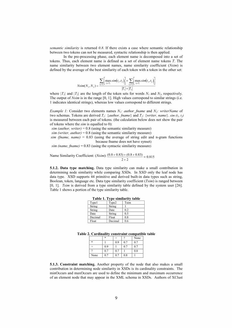
5.1.2. Data type matching. Data type similarity can make a small contribution in

determining node similarity while comparing XSDs. In XSD only the leaf node has

data type. XSD supports 44 primitive and derived built-in data types such as string,

Boolean, token, language etc. Data type similarity coefficient (Tsim) is ranged between

[0, 1]. Tsim is derived from a type similarity table defined by the system user [26].

Table 1 shows a portion of the type similarity table.

Table 1. Type similarity table Type1 Type2 Tsim

String String 1

String Date 0.2

Date String 0.5

Decimal Float 0.8

Float Decimal 0.6

Table 2. Cardinality constraint compatible table * + ? None

* 1 0.9 0.7 0.7

+ 0.9 1 0.7 0.7

? 0.7 0.7 1 0.8

None 0.7 0.7 0.8 1

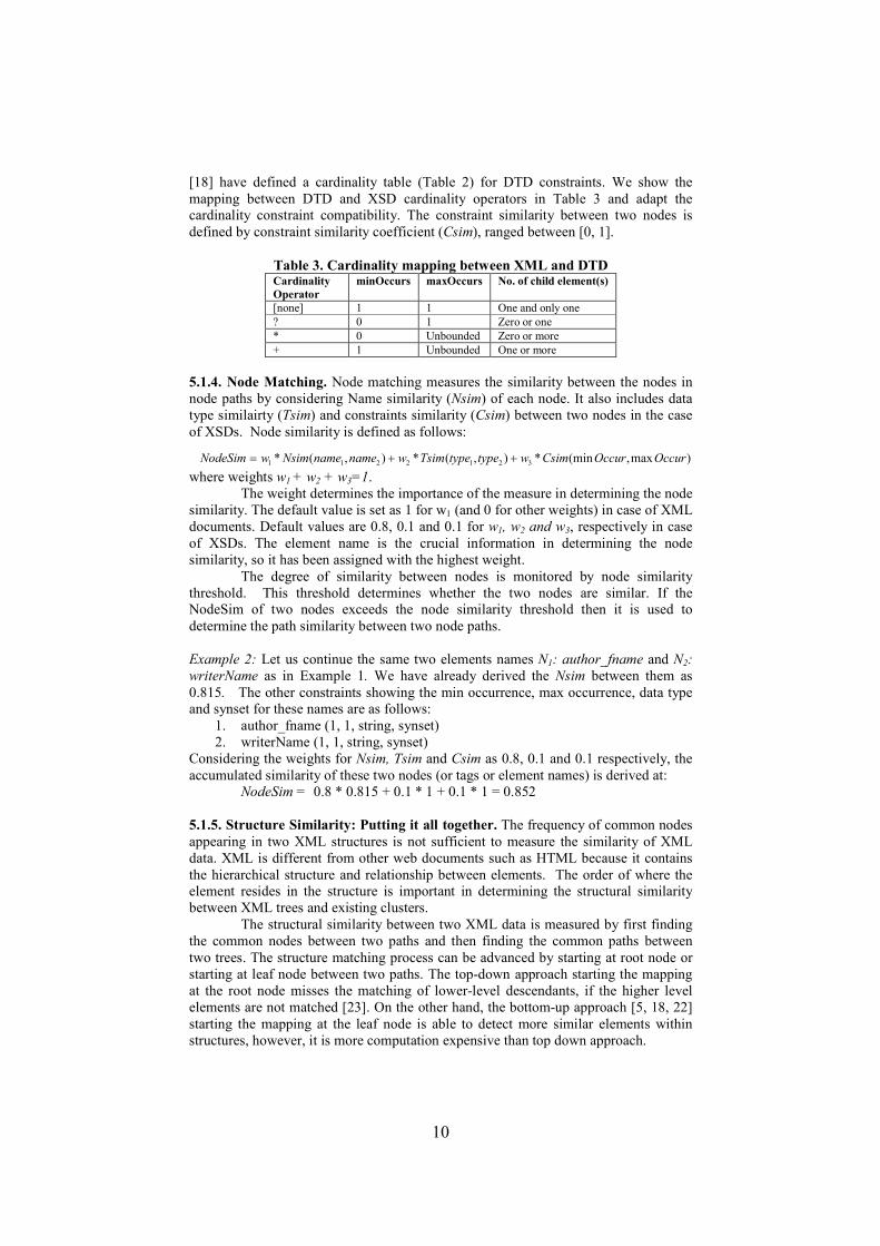
5.1.3. Constraint matching. Another property of the node that also makes a small

contribution in determining node similarity in XSDs is its cardinality constraints. The

minOccurs and maxOccurs are used to define the minimum and maximum occurrence

of an element node that may appear in the XML schema in XSDs. Authors of XClust

10

[18] have defined a cardinality table (Table 2) for DTD constraints. We show the

mapping between DTD and XSD cardinality operators in Table 3 and adapt the

cardinality constraint compatibility. The constraint similarity between two nodes is

defined by constraint similarity coefficient (Csim), ranged between [0, 1].

Table 3. Cardinality mapping between XML and DTD Cardinality

Operator

minOccurs maxOccurs No. of child element(s)

[none] 1 1 One and only one

? 0 1 Zero or one

* 0 Unbounded Zero or more

+ 1 Unbounded One or more

5.1.4. Node Matching. Node matching measures the similarity between the nodes in

node paths by considering Name similarity (Nsim) of each node. It also includes data

type similairty (Tsim) and constraints similarity (Csim) between two nodes in the case

of XSDs. Node similarity is defined as follows:

)max,(min*),(*),(* 3212211 OccurOccurCsimwtypetypeTsimwnamenameNsimwNodeSim ++=

where weights w1 + w2 + w3=1.

The weight determines the importance of the measure in determining the node

similarity. The default value is set as 1 for w1 (and 0 for other weights) in case of XML

documents. Default values are 0.8, 0.1 and 0.1 for w1, w2 and w3, respectively in case

of XSDs. The element name is the crucial information in determining the node

similarity, so it has been assigned with the highest weight.

The degree of similarity between nodes is monitored by node similarity

threshold. This threshold determines whether the two nodes are similar. If the

NodeSim of two nodes exceeds the node similarity threshold then it is used to

determine the path similarity between two node paths.

Example 2: Let us continue the same two elements names N1: author_fname and N2:

writerName as in Example 1. We have already derived the Nsim between them as

0.815. The other constraints showing the min occurrence, max occurrence, data type

and synset for these names are as follows:

1. author_fname (1, 1, string, synset)

2. writerName (1, 1, string, synset)

Considering the weights for Nsim, Tsim and Csim as 0.8, 0.1 and 0.1 respectively, the

accumulated similarity of these two nodes (or tags or element names) is derived at:

NodeSim = 0.8 * 0.815 + 0.1 * 1 + 0.1 * 1 = 0.852

5.1.5. Structure Similarity: Putting it all together. The frequency of common nodes

appearing in two XML structures is not sufficient to measure the similarity of XML

data. XML is different from other web documents such as HTML because it contains

the hierarchical structure and relationship between elements. The order of where the

element resides in the structure is important in determining the structural similarity

between XML trees and existing clusters.

The structural similarity between two XML data is measured by first finding

the common nodes between two paths and then finding the common paths between

two trees. The structure matching process can be advanced by starting at root node or

starting at leaf node between two paths. The top-down approach starting the mapping

at the root node misses the matching of lower-level descendants, if the higher level

elements are not matched [23]. On the other hand, the bottom-up approach [5, 18, 22]

starting the mapping at the leaf node is able to detect more similar elements within

structures, however, it is more computation expensive than top down approach.

11

PCXSS uses bottom-up approach because the main focus of PCXSS

methodology is to cluster a collection of heterogeneous XMLs with varied structures.

Structure matching in PCXSS is a process of determining the degree of structural

similarity between XML trees and existing clusters using node paths.

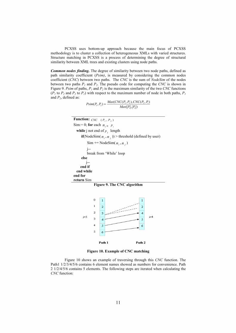
Common nodes finding. The degree of similarity between two node paths, defined as

path similarity coefficient (Psim), is measured by considering the common nodes

coefficient (CNC) between two paths. The CNC is the sum of NodeSim of the nodes

between two paths P1 and P2. The pseudo code for computing the CNC is shown in

Figure 9. Psim of paths, P1 and P2 is the maximum similarity of the two CNC functions

(P1 to P2 and P2 to P1) with respect to the maximum number of node in both paths, P1

and P2, defined as:

),(

),(),,((),(

21

122121

PPMax

PPCNCPPCNCMaxPPPsim =

Function: ),( 21 PPCNC

Sim:= 0; for each in 1P∈

while j not end of2P length

if(NodeSim(in ,

jn )) > threshold (defined by user)

Sim += NodeSim(in ,

jn )

j--

break from ‘While’ loop

else

j--

end if

end while

end for

return Sim

Figure 9. The CNC algorithm

Figure 10. Example of CNC matching

Figure 10 shows an example of traversing through this CNC function. The

Path1 1/2/3/4/5/6 contains 6 element names showed as numbers for convenience. Path

2 1/2/4/5/6 contains 5 elements. The following steps are iterated when calculating the

CNC function:

12

1. Start at the leaf element of both paths (j=5, i=4). If the NodeSim coefficient of the

leaf elements exceeds a threshold (a match) then increase Sim (Figure 9) with the

NodeSim value and go to step 2 else go to step 3.

2. Move both paths to the next level (j--, i--) and start element matching at this level.

If the NodeSim coefficient of these elements exceeds a threshold (a match) then

increase Sim with the NodeSim value and repeat step 2 else go to step 3.

3. Move only path 1 to the next level (j--) then start element matching in the original

level of path 2 (i) to the new element of path 1.

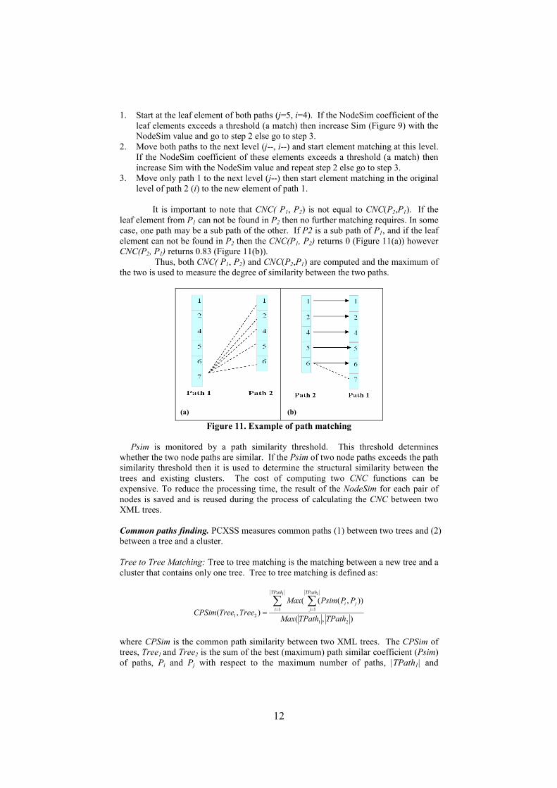
It is important to note that CNC( P1, P2) is not equal to CNC(P2,P1). If the

leaf element from P1 can not be found in P2 then no further matching requires. In some

case, one path may be a sub path of the other. If P2 is a sub path of P1, and if the leaf

element can not be found in P2 then the CNC(P1, P2) returns 0 (Figure 11(a)) however

CNC(P2, P1) returns 0.83 (Figure 11(b)).

Thus, both CNC( P1, P2) and CNC(P2,P1) are computed and the maximum of

the two is used to measure the degree of similarity between the two paths.

(a)

(b)

Figure 11. Example of path matching

Psim is monitored by a path similarity threshold. This threshold determines

whether the two node paths are similar. If the Psim of two node paths exceeds the path

similarity threshold then it is used to determine the structural similarity between the

trees and existing clusters. The cost of computing two CNC functions can be

expensive. To reduce the processing time, the result of the NodeSim for each pair of

nodes is saved and is reused during the process of calculating the CNC between two

XML trees.

Common paths finding. PCXSS measures common paths (1) between two trees and (2)

between a tree and a cluster.

Tree to Tree Matching: Tree to tree matching is the matching between a new tree and a

cluster that contains only one tree. Tree to tree matching is defined as:

),(

)),(((

),(21

1 1

21

1 2

TPathTPathMax

PPPsimMax

TreeTreeCPSim

TPath

i

TPath

j

ji∑ ∑= ==

where CPSim is the common path similarity between two XML trees. The CPSim of

trees, Tree1 and Tree2 is the sum of the best (maximum) path similar coefficient (Psim)

of paths, Pi and Pj with respect to the maximum number of paths, |TPath1| and

13

|TPath2| of trees, Tree1 and Tree2, respectively. The clustering process in PCXSS

works on the assumption that only one path from Tree1 matches with one path in Tree2.

Thus, it only selects the maximum path similarity coefficient (Psim) between each pair

of paths of Tree1 and Tree2.

Tree to Cluster Matching: Tree to cluster matching is the matching between a new tree

and the common paths in a cluster. The common paths are the similar paths that are

shared among the trees within the cluster (normally a cluster must contain at least 2 or

more trees in the cluster to have the common paths or else tree to tree matching is

required). Initially, the common paths are derived in tree to tree matching. Then every

time a new tree is assigned to the cluster, the similar paths are added to the cluster if

paths are not already in the cluster. Tree to cluster matching is defined as:

TPath

PPPsimMax

ClusterTreeCPSim

TPath

i

CPath

j

ji∑ ∑= == 1 1

)),(((

),(

Similar to tree to tree matching, CPSim between a tree and a cluster is the

sum of the best (maximum) path similar coefficient (Psim) of paths, Pi and Pj with

respect to the number of paths, |TPath| in Tree.

Example: Let us consider an example to compute CPSim using tree to tree matching.

Tree1

P11:Companies(1,1,null,synset)/Company(1,1,null,synset)/Symbol(1,1,string,synset) P12:Companies(1,1,null,synset)/Company(1,1,null,synset)/Name(1,1,string,synset)

P13:Companies(1,1,null,synset)/Company(1,1,null,synset)/Profile(1,1,null,synset)/

EmployeeNumber (1, unbound,string,synset) P14:Companies(1,1,null,synset)/Company(1,1,null,synset)/Profile(1,1,null,synset)/

Description(1,1,string,synset)

P15:Companies(1,1,null,synset)/Company(1,1,null,synset)/Address1(1,3,string,synset)

Tree2

P21:Companies(1,1,null,synset)/Company(1,1,null,synset)/Symbol(1,1,string,synset)

P22:Companies(1,1,null,synset)/Company(1,1,null,synset)/Name(1,1,string,synset)

P23:Companies(1,1,null,synset)/Company(1,1,null,synset)/Profile(1,1,null,synset)/ EmployeeNo(1,unbound,string,synset)

P24:Companies(1,1,null,synset)/Company(1,1,null,synset)/Profile(1,1,null,synset)/

Description(1,1,string,synset) P25:Companies(1,1,null,synset)/Company(1,1,null,synset)/Address(1,1,string,synset)

After applying the CNC algorithm, the following shows the best PSim for each pair of

node paths:

PSim(P11,P21) = Max(CNC(1+1+1),CNC(1+1+1))/ Max(3,3) = 1

PSim(P12,P22) =Max(CNC(1+1+1),CNC(1+1+1))/Max(3,3) = 1

PSim(P13,P23) = Max(CNC(0.6+1+1+1),CNC(0.6+1+1))/Max(4,4)= 0.9

PSim(P14,P24) = Max(CNC(1+1+1+1),CNC(1+1+1+1))/Max(4,4) = 1

PSim(P15,P25) =Max(CNC(0.764+1+1),CNC(0.764+1+1))/Max(3,3) = 0.92

These PSim are then used to compute CPSim using tree to tree matching.

CPSim(Tree1,Tree2):

(PSim(P11,P21) + PSim(P12,P22) + PSim(P13,P23) + PSim(P14,P24) + PSim(P15,P25))/

Max(5,5) = 0.964

14

5.2. Clustering stage

PCXSS is motivated by incremental hierarchical clustering methods. It first

starts off with no cluster. When a new tree comes in, it is assigned to a new cluster.

When the next tree comes in, it matches with the existing cluster. If they match then

the tree is assigned to that cluster else it is assigned to a new cluster. The number of

cluster is generated progressively at run-time according to the data set.

Figure 12 shows the algorithm for the clustering process. Initially, there is no

cluster. The first tree, T1 is assigned to a new cluster, C1 (step 1). When the next tree,

Ti comes in; CPSim is computed between Ti and the existing cluster, Cj (steps 5 to 7).

Ti is assigned to Cj if Cj has the largest CPSim with Ti and CPSim exceeds the

clustering threshold (steps 9 and 10). Otherwise assign Ti to new cluster (step 12). The

node paths of Ti (and Tj if tree to tree matching occurs) that are used to compute the

CPSim are then added to Cj if Ti is assigned to Cj (step 11). The node paths in Cj are

referred to as common paths. The common paths in Cj are then used to measure the

CPSim between Cj and new trees. Since the common paths (instead of all the node

paths of the trees held within a cluster) are used to compute CPSim with new trees, the

computation time reduces significantly. In addition, the cluster contains only the

distinct common paths (duplicate paths are removed from the cluster).

1. assign the first tree T1 to a new cluster C1

2. while tree file has more

3. read the next tree (i.e. a set of node paths,

denoted by Ti);

4. while cluster C has more

5. if Cj contains only one tree, Tj

6. compute sim =CPSim(Ti, Tj);

7. else compute sim=CPSim(Ti, Cj) end if

8. end while

9. if Max(sim) >= clustering threshold

10. assign Ti to Cj ;

11. add node paths to Cj ;

12. else assign Ti to new cluster end if

13. end while

Figure 12. PCXSS clustering process

6. Empirical evaluation and discussion

Experiments are conducted on both XML documents and XML schema

definition documents. The test data is carefully selected to ensure that the XMLs and

XSDs are derived from the same and different domains and that each has distinct

structure. To show the efficacy of PCXSS, the generated clustering solutions are

evaluated against wCluto clustering solution [30]. wCluto is a pair-wise hierarchical

clustering algorithm. In order to use wCluto, PCXSS first generated a matrix

containing the CPSim (common path similarity) coefficient between each pair of trees

in the data source using path similarity threshold of 0.7. The pair-wise similarity

matrix is then fed into wCluto to perform the clustering process.

6.1 Scalability Evaluation

The computation time for a pair-wise similarity between XML trees is at least

O(m2), where m is the number of elements in XML data that are used for the clustering.

15

This is infeasible for a large amount of data set. PCXSS measures the structural

similarity between a XML tree with existing clusters, therefore the time complexity of

PCXSS method is O(m*c*n), where m is the number of elements in XML data; c is the

number of cluster; and n is number of distinct elements in clusters.

The documents grouped into a cluster should have similar structures and

elements. So the number of distinct elements in clusters should always be less than the

distinct elements in documents. Therefore, if the number of clusters is less than the

number of documents (that is usually the case) the time cost is linear to the number of

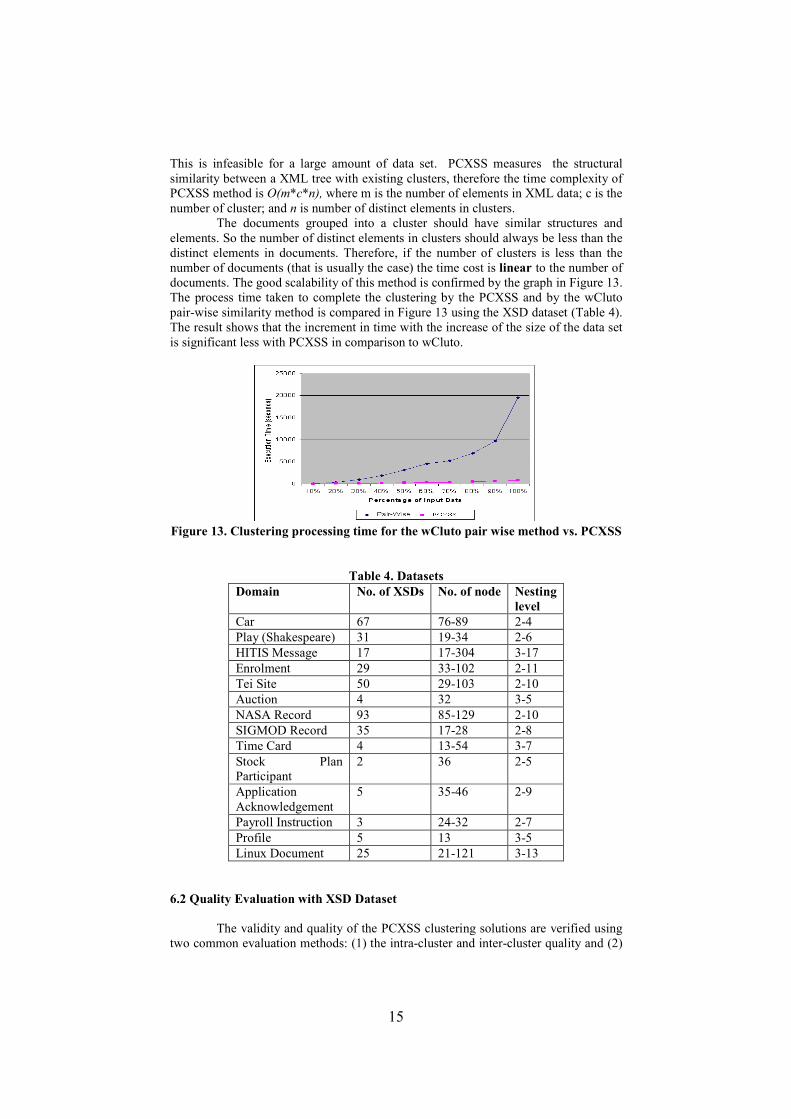
documents. The good scalability of this method is confirmed by the graph in Figure 13.

The process time taken to complete the clustering by the PCXSS and by the wCluto

pair-wise similarity method is compared in Figure 13 using the XSD dataset (Table 4).

The result shows that the increment in time with the increase of the size of the data set

is significant less with PCXSS in comparison to wCluto.

Figure 13. Clustering processing time for the wCluto pair wise method vs. PCXSS

Table 4. Datasets

Domain No. of XSDs No. of node Nesting

level

Car 67 76-89 2-4

Play (Shakespeare) 31 19-34 2-6

HITIS Message 17 17-304 3-17

Enrolment 29 33-102 2-11

Tei Site 50 29-103 2-10

Auction 4 32 3-5

NASA Record 93 85-129 2-10

SIGMOD Record 35 17-28 2-8

Time Card 4 13-54 3-7

Stock Plan

Participant

2 36 2-5

Application

Acknowledgement

5 35-46 2-9

Payroll Instruction 3 24-32 2-7

Profile 5 13 3-5

Linux Document 25 21-121 3-13

6.2 Quality Evaluation with XSD Dataset

The validity and quality of the PCXSS clustering solutions are verified using

two common evaluation methods: (1) the intra-cluster and inter-cluster quality and (2)

16

FScore (combination of recall and precision) measure. The major characteristics of the

XSD data set are shown in Table 4. Majority of them are derived from the

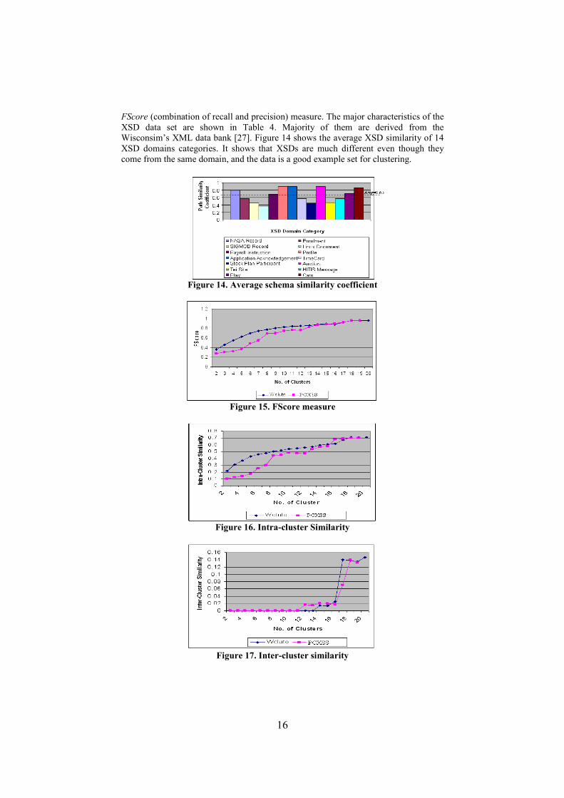
Wisconsim’s XML data bank [27]. Figure 14 shows the average XSD similarity of 14

XSD domains categories. It shows that XSDs are much different even though they

come from the same domain, and the data is a good example set for clustering.

Figure 14. Average schema similarity coefficient

Figure 15. FScore measure

Figure 16. Intra-cluster Similarity

Figure 17. Inter-cluster similarity

17

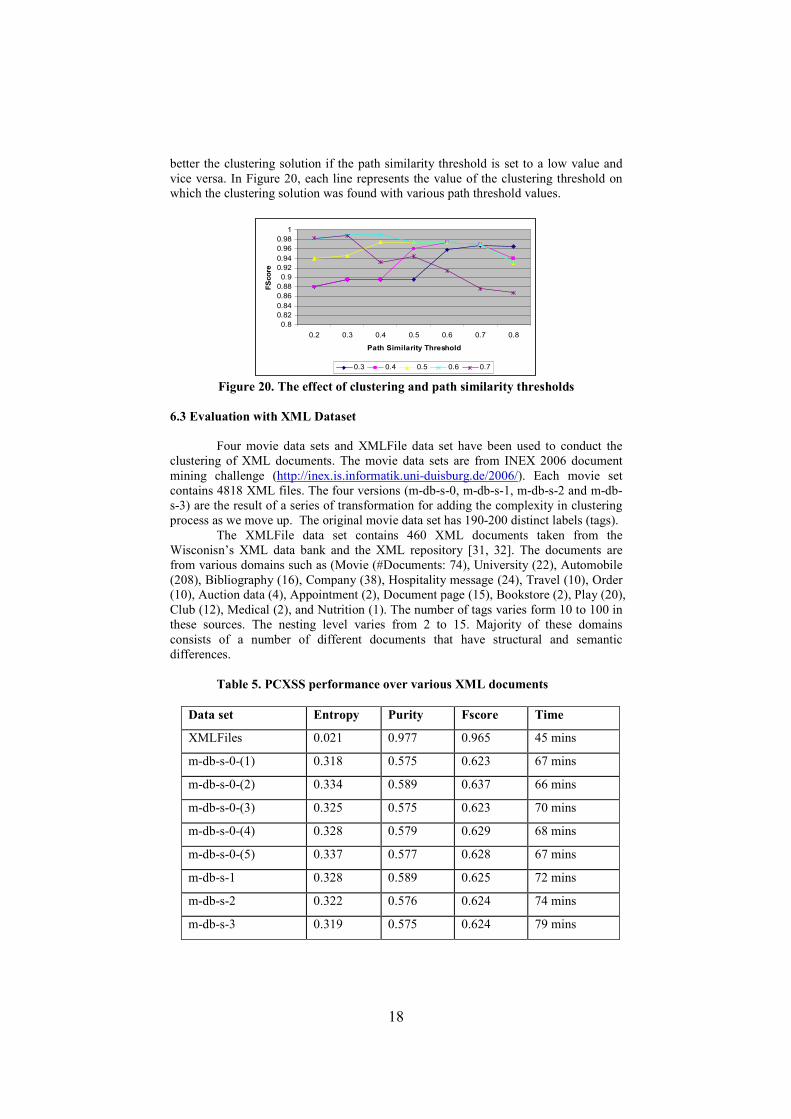
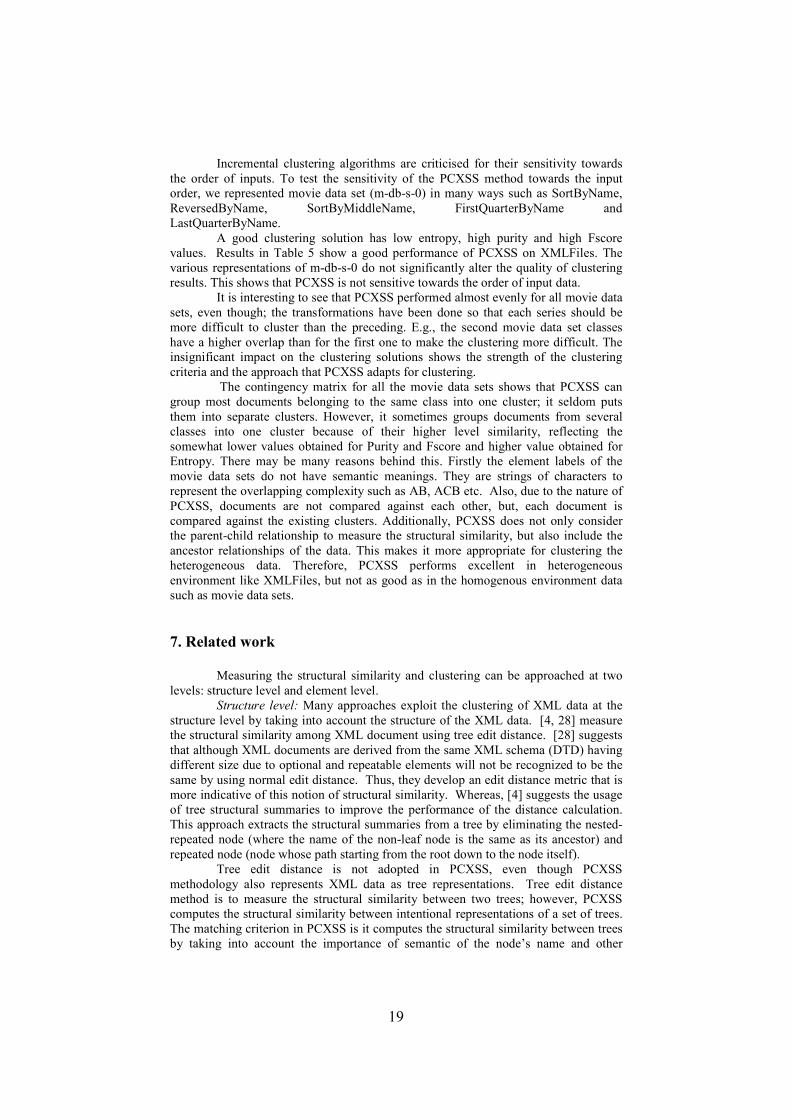
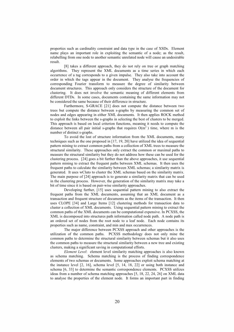
Figures 15, 16 and 17 show the FScore, intra-cluster and inter-cluster

similarity of the dataset respectively over the 20 different clustering solutions of

PCXSS and wCluto. These results show that the performance of PCXSS is equivalent

to wCluto, when the cluster number research to its optimal (in this case cluster number

19). PCXSS determines the optimal number of clusters during its processing, that is

why, its performance is not as good as wCluto for the solutions before the optimal

number of clusters. The results indicate that the incremental clustering algorithm

PCXSS is able to achieve the similar quality results as the pair-wise clustering

algorithms in much less time.

Sensitivity testing: PCXSS also examines the sensitivity in computing the common

path similarity coefficient (CPSim). During the experiment on the sensitive of PCXSS

using the syntactic relationship, it has been discovered that some results can produce a

worse clustering solution if we involve only one syntactic relationship, i.e. string edit

distance or n-gram. This shows that element name matching using syntactic

relationship may lead to mismatches of element name that may cause a poorer

clustering solution. However, the effective use of these measures can improve the

quality of clustering solution. It can be seen from Figures 18 and 19 that the semantic

relationship plays a more important role than syntactic relationship.

0.82

0.84

0.86

0.88

0.9

0.92

0.94

0.96

0.98

0.2 0.3 0.4 0.5 0.6 0.7 0.8

Path Similarity Threshold

FScore

without syntactic relationship with syntactic relationship

Figures 18. Effect of syntactic relationships on clustering

0.82

0.84

0.86

0.88

0.9

0.92

0.94

0.96

0.98

0.2 0.3 0.4 0.5 0.6 0.7 0.8

Path Similarity Threshold

FScore

without semantic matching with semantic matching

Figures 19. Effect of semantic relationships on clustering

A number of experiments have also been carried out to evaluate the

performance of PCXSS’s clustering solution using different clustering and path

similarity thresholds. The clustering threshold determines which clusters should the

new XML be put into or a new cluster is needed. On the other hand, path similarity

threshold determines the degree of similarity between two paths. It has been

ascertained from the experiments (Figure 20) that the clustering and path similarity

thresholds have an inverse relationship, meaning the higher the cluster thresholds, the

18

better the clustering solution if the path similarity threshold is set to a low value and

vice versa. In Figure 20, each line represents the value of the clustering threshold on

which the clustering solution was found with various path threshold values.

0.8

0.82

0.84

0.86

0.88

0.9

0.92

0.94

0.96

0.98

1

0.2 0.3 0.4 0.5 0.6 0.7 0.8

Path Similarity Threshold

FScore

0.3 0.4 0.5 0.6 0.7

Figure 20. The effect of clustering and path similarity thresholds

6.3 Evaluation with XML Dataset

Four movie data sets and XMLFile data set have been used to conduct the

clustering of XML documents. The movie data sets are from INEX 2006 document

mining challenge (http://inex.is.informatik.uni-duisburg.de/2006/). Each movie set

contains 4818 XML files. The four versions (m-db-s-0, m-db-s-1, m-db-s-2 and m-db-

s-3) are the result of a series of transformation for adding the complexity in clustering

process as we move up. The original movie data set has 190-200 distinct labels (tags).

The XMLFile data set contains 460 XML documents taken from the

Wisconisn’s XML data bank and the XML repository [31, 32]. The documents are

from various domains such as (Movie (#Documents: 74), University (22), Automobile

(208), Bibliography (16), Company (38), Hospitality message (24), Travel (10), Order

(10), Auction data (4), Appointment (2), Document page (15), Bookstore (2), Play (20),

Club (12), Medical (2), and Nutrition (1). The number of tags varies form 10 to 100 in

these sources. The nesting level varies from 2 to 15. Majority of these domains

consists of a number of different documents that have structural and semantic

differences.

Table 5. PCXSS performance over various XML documents

Data set Entropy Purity Fscore Time

XMLFiles 0.021 0.977 0.965 45 mins

m-db-s-0-(1) 0.318 0.575 0.623 67 mins

m-db-s-0-(2) 0.334 0.589 0.637 66 mins

m-db-s-0-(3) 0.325 0.575 0.623 70 mins

m-db-s-0-(4) 0.328 0.579 0.629 68 mins

m-db-s-0-(5) 0.337 0.577 0.628 67 mins

m-db-s-1 0.328 0.589 0.625 72 mins

m-db-s-2 0.322 0.576 0.624 74 mins

m-db-s-3 0.319 0.575 0.624 79 mins

19

Incremental clustering algorithms are criticised for their sensitivity towards

the order of inputs. To test the sensitivity of the PCXSS method towards the input

order, we represented movie data set (m-db-s-0) in many ways such as SortByName,

ReversedByName, SortByMiddleName, FirstQuarterByName and

LastQuarterByName.

A good clustering solution has low entropy, high purity and high Fscore

values. Results in Table 5 show a good performance of PCXSS on XMLFiles. The

various representations of m-db-s-0 do not significantly alter the quality of clustering

results. This shows that PCXSS is not sensitive towards the order of input data.

It is interesting to see that PCXSS performed almost evenly for all movie data

sets, even though; the transformations have been done so that each series should be

more difficult to cluster than the preceding. E.g., the second movie data set classes

have a higher overlap than for the first one to make the clustering more difficult. The

insignificant impact on the clustering solutions shows the strength of the clustering

criteria and the approach that PCXSS adapts for clustering.

The contingency matrix for all the movie data sets shows that PCXSS can

group most documents belonging to the same class into one cluster; it seldom puts

them into separate clusters. However, it sometimes groups documents from several

classes into one cluster because of their higher level similarity, reflecting the

somewhat lower values obtained for Purity and Fscore and higher value obtained for

Entropy. There may be many reasons behind this. Firstly the element labels of the

movie data sets do not have semantic meanings. They are strings of characters to

represent the overlapping complexity such as AB, ACB etc. Also, due to the nature of

PCXSS, documents are not compared against each other, but, each document is

compared against the existing clusters. Additionally, PCXSS does not only consider

the parent-child relationship to measure the structural similarity, but also include the

ancestor relationships of the data. This makes it more appropriate for clustering the

heterogeneous data. Therefore, PCXSS performs excellent in heterogeneous

environment like XMLFiles, but not as good as in the homogenous environment data

such as movie data sets.

7. Related work

Measuring the structural similarity and clustering can be approached at two

levels: structure level and element level. Structure level: Many approaches exploit the clustering of XML data at the

structure level by taking into account the structure of the XML data. [4, 28] measure

the structural similarity among XML document using tree edit distance. [28] suggests

that although XML documents are derived from the same XML schema (DTD) having

different size due to optional and repeatable elements will not be recognized to be the

same by using normal edit distance. Thus, they develop an edit distance metric that is

more indicative of this notion of structural similarity. Whereas, [4] suggests the usage

of tree structural summaries to improve the performance of the distance calculation.

This approach extracts the structural summaries from a tree by eliminating the nested-

repeated node (where the name of the non-leaf node is the same as its ancestor) and

repeated node (node whose path starting from the root down to the node itself).

Tree edit distance is not adopted in PCXSS, even though PCXSS

methodology also represents XML data as tree representations. Tree edit distance

method is to measure the structural similarity between two trees; however, PCXSS

computes the structural similarity between intentional representations of a set of trees.

The matching criterion in PCXSS is it computes the structural similarity between trees

by taking into account the importance of semantic of the node’s name and other

20

properties such as cardinality constraint and data type in the case of XSDs. Element

name plays an important role in exploiting the semantic of a node; as the result,

relabelling from one node to another semantic unrelated node will cause an undesirable

result.

[8] takes a different approach, they do not rely on tree or graph matching

algorithms. They represent the XML documents as a time series in which each

occurrence of a tag corresponds to a given impulse. They also take into account the

order in which the tags appear in the document. They analyse the frequencies of

corresponding Fourier transform to measure the degree of similarity between

document structures. This approach only considers the structure of the document for

clustering. It does not involve the semantic meaning of different elements from

different DTDs. In some cases, documents containing the same information may not

be considered the same because of their difference in structure.

Furthermore, S-GRACE [21] does not compute the distance between two

trees but compute the distance between s-graphs by measuring the common set of

nodes and edges appearing in either XML documents. It then applies ROCK method

to exploit the links between the s-graphs in selecting the best of clusters to be merged.

This approach is based on local criterion functions, meaning it needs to compute the

distance between all pair initial s-graphs that requires O(m2

) time, where m is the

number of distinct s-graphs.

To avoid the lost of structure information from the XML documents, many

techniques such as the one proposed in [17, 19, 20] have utilized the idea of sequential

pattern mining to extract common paths from a collection of XML trees to measure the

structural similarity. These approaches only extract the common or maximal paths to

measure the structural similarity but they do not address how these can be used for the

clustering process. [24] goes a bit further than the above approaches, it use sequential

pattern mining to extract the frequent paths between XML schemas. It then uses the

frequent paths to calculate the similarity between XML schemas; a similarity matrix is

generated. It uses wCluto to cluster the XML schemas based on the similarity matrix.

The main purpose of [24] approach is to generate a similarity matrix that can be used

in the clustering process. However, the generation of the similarity matrix may take a

bit of time since it is based on pair-wise similarity approaches.

Developing further, [15] uses sequential pattern mining to also extract the

frequent paths from the XML documents, assuming that an XML document as a

transaction and frequent structure of documents as the items of the transaction. It then

uses CLOPE [34] and Large Items [12] clustering methods for transaction data to

cluster a collection of XML documents. Using sequential pattern mining to extract the

common paths of the XML documents can be computational expensive. In PCXSS, the

XML is decomposed into structures path information called node path. A node path is

an ordered set of nodes from the root node to a leaf node. Each node contains its

properties such as name, constraint, and min and max occurrences.

The major difference between PCXSS approach and other approaches is the

utilization of the common paths. PCXSS methodology does not only mine the

common paths to determine the structural similarity between schemas but it also uses

the common paths to measure the structural similarity between a new tree and existing

clusters, making a significant saving in computational efforts.

Element Level: element level similarity matching approaches is also known

as schema matching. Schema matching is the process of finding correspondence

elements of two schemas or documents. Some approaches exploit schema matching at

the instance level [2, 16], schema level [5, 14, 18, 22] or using both instance and

schema [6, 33] to determine the semantic correspondence elements. PCXSS utilizes

ideas from a number of schema matching approaches [5, 18, 22, 24, 26] on XML data

to analyse the properties of the element node. It forms an important part in finding

21

common paths between a tree and existing clusters by analysing the linguistic of the

node label and its properties such as data type and constraints.

8. Conclusions and future work

XML has become quite popular in the exchange of a variety of data on the

Web and in the distribution of information related to various topics as well. With the

number of XML sources growing rapidly, it becomes necessary to cluster the

collection of the XML sources for effectively finding important information from them.

Due to its semi-structured and flexible feature compared to the data in traditional

databases, it poses challenge to develop an efficient and scalable clustering method.

We present a novel clustering method called PCXSS that progressively

clusters XML data by taking into account the structural and semantic information of

elements. PCXSS measures the structural similarity between XML data by finding the

common paths among them. To be applicable to any XML data, the PCXSS approach

employs a complex method for element matching that not only considers the element

name but also other properties such as data type and cardinality to ensure the accuracy

of element matching. It considers both the semantic and syntactic relationship of the

element name. Furthermore, the PCXSS clustering do not require the similarity

computation between each pair of data. It compares each new tree with existing

clusters where each cluster contains the common paths of the trees held within.

The empirical analysis shows that PCXSS significantly reduces the

computational time as compared to pair-wise computation as well as yields good

accuracy of the results. The several experiments also ascertain that PCXSS clustering

solution is not heavily influenced by thresholds such as the clustering and path

similarity. Furthermore, the syntactic and semantic relationship measurements have

also been tested. The semantic relationship has shown to be more important to

determine similarity.

The clustering solution produced by PCXSS can help in reducing the

complexity of integrating schemas from heterogeneous domains and in improving the

speed of the integration process. The structure matching (path matching) in PCXSS

can be used for finding correspondence element between two schemas that facilitate in

area such as schema integration. In addition, it can be used to improve the speed and

accuracy in structure indexing and information retrieval.

PCXSS needs some future work to improve its effectiveness. Both path and

element matching in this approach is still very complex. Therefore, it takes longer to

do the clustering process. To overcome this problem, path matching can be reduced by

grouping node paths that have the same ancestors into one path.

9. References

[1] Abiteboul, S., Buneman, P., & Suciu, D. (2000). Data on the Web: From

Relations to Semistructured Data and XML: California: Morgan Kaumann.

[2] Berlin, J., & Motro, A. (2001). Database Schema Matching Using Machine

Learning with Feature Selection. Paper presented at the 14th International

Conference on Advanced Information Systems Engineering.

[3] Boukottaya, A., & Vanoirbeek, C. (2005). Schema matching for transforming

structured documents. Paper presented at the Proceedings of the 2005 ACM

symposium on Document engineering, Bristol, United Kingdom.

[4] Dalamagas, T., Cheng, T., Winkel, K., & Sellis, T. K. (2004). Clustering

XML documents by Structure. Paper presented at the SETN.

22

[5] Do, H. H., & Rahm, E. (2002 August). COMA - A System for Flexible

Combination of Schema Matching Approaches. Paper presented at the 28th

VLDB, Hong Kong, China.

[6] Doan, A., Domingos, R., & Halevy, A. Y. (2001). Reconciling schemas of

disparate sources: a machine-learning approach. Paper presented at the

ACM SIGMOD, Santa Barbara, California, United States.

[7] Fellbaum, C. (1998). WordNet: An Electronic Lexical Database. MIT Press.

[8] Flesca, S., Manco, G., Masciari, E., Pontieri, L., & Pugliese, A. (2002, June

6-7). Detecting Structural Similarities between XML Documents. Paper

presented at the 5th International Workshop on the Web and Databases

(WebDB'02), Madison, Wisconsin.

[9] Flesca, S., Manco, G., Masciari, E., Pontieri, L., & Pugliese, A. (2005). Fast

Detection of XML Structural Similarities. IEEE Transaction on Knowledge

and Data Engineering, 7(2), 160-175.

[10] Giumchiglia, F., & Yatskevich, M. (2004). Element level semantic matching.

Paper presented at the Meaning Coordination and Negotiation workshop at

ISWC.

[11] Han, J., & Kamber, M. (2001). Data Mining: Concepts and Techiques. San

Diego, USA: Morgan Kaufmann.

[12] Huang, Z. (1997). A fast clustering algorithm to cluster very large categorical

data sets in data mining. Paper presented at the SIGMOD Workshop on

Research Issues on Data Mining and Knowledge Discovery.

[13] Jain, A. K., Murty, M. N., & Flynn, P. J. (1999). Data Clustering: A Review.

ACM Computing Surveys (CSUR), 31(3), 264-323.

[14] Jeong, E., & Hsu, C.-N. (2001). Induction of integrated view for XML data

with heterogeneous DTDs. Paper presented at the 10th International

Conference on Information and Knowledge Management, Atlanta, Georgia,

USA.

[15] Jeong, H. H., & Keun, H. r. (2004). A New XML Clustering for Structural

Retrieval. Paper presented at the 23rd International Conference on Conceptual

Modeling, Shanghai, China.

[16] Kurgan, L., Swiercz, W., & Cios, K. J. (2002). Semantic Mapping of XML

Tags using Inductive Machine Learning. Paper presented at the 11th

International Conference on Information and Knowledge Management,

Virginia, USA.

[17] Lee, J. W., & Park, S. S. (2004, October 20-24). Finding Maximal Similar

Paths Between XML Documents Using Sequential Patterns. Paper presented

at the ADVIS, Izmir, Turkey.

[18] Lee, L. M., Yang, L. H., Hsu, W., & Yang, X. (2002, November). XClust:

Clustering XML Schemas for Effective Integration. Paper presented at the

11th ACM International Conference on Information and Knowledge

Management (CIKM'02), Virginia.

[19] Leung, H.-p., Chung, F.-l., & Chan, S. C.-f. (2003). A New Sequential Mining

Approach to XML Document Similarity Computation. Paper presented at the

PAKDD.

[20] Leung, H.-p., Chung, F.-l., & Chan, S. C.-f. (2005). On the use of hierarchical

information in sequential mining-based XML document similarity

computation. Knowledge and Information Systems, 7(4), 476-498.

[21] Lian, W., Cheung, D. W., Maoulis, N., & Yiu, S.-M. (2004). An efficient and

scalable algorithm for clustering XML documents by structure. IEEE TKDE,

16(1), 82-96.

[22] Madhavan, J., Bernstein, P. A., & Rahm, E. (2001). Generic Schema

Matching with Cupid. Paper presented at the 27th VLDB, Roma, Italy.

23

[23] Milo, T., & Zohar, S. (1998). Using Schema Matching to Simplify

heterogeneous Data Translation. Paper presented at the VLDB.

[24] Nayak, R., & Iryadi, W. (2006, January). XMine: A methodology for mining

XML structure. Paper presented at the Asia Pacific Web Conference, ASWeb

2006, China.

[25] Nayak, R., Witt, R., & Tonev, A. (June 24-27 2002). Data Mining and XML

documents. Paper presented at the The 2002 International Workshop on the

Web and Database (WebDB 2002).

[26] Nayak, R., & Xia, F. B. (2004). Automatic integration of heterogeneous

XML-schemas. Paper presented at the Proceedings of the International

Conferences on Information Integration and Web-based Applications &

Services.

[27] NIAGARA query engine. (2005). Retrieved July 10, 2005, from

http://www.cs.wisc.edu/niagara/data.html

[28] Nierman, A., & Jagadish, H. V. (2002, December). Evaluating Structural

Similarity in XML Documents. Paper presented at the 5th International

Conference on Computational Science (ICCS'05), Wisconsin, USA.

[29] Rice, S. V., Bunke, H., & Nartker, T. A. (1997). Classes of Cost Functions for

String Edit Distance. Algorithmica, 18(2), 271-280.

[30] wCluto: Web Interface for CLustering TOolKit. (2003). Retrieved July 25,

2005, from http://cluto.ccgb.umn.edu/cgi-bin/wCluto/wCluto.cgi

[31] The Wisconisn's XML data bank. from

http://www.cs.wisc.edu/hiagara/data.html

[32] The XML data repository. from

http://www.cs.washington.edu/research/xmldatasets/

[33] Xu, L., & Embley, D. W. (2003). Discovering direct and indirect matches for

schema elements. Paper presented at the 8th International Conference on

Database Ssytems for Advanced Applications.

[34] Yang, Y., Guan, X., & You, J. (2002). CLOPE: A Fast and Effective

Clustering Algorithm for Transaction Data. Paper presented at the 8th ACM

SIGKDD International Conference on Knowledge Discovery and Data

Mining.

[35] Yergeau, F., Bray, T., Paoli, J., Sperberg-McQueen, C. M., & Maler, E.

(2004). Extensible Markup Language (XML) 1.0 (Third Edition) W3C

Recommendation. Retrieved February, 2004, from

http://www.w3.org/TR/2004/REC-XML-20040204/