A POWERFUL PORTMANTEAU TEST OF LACK OF FIT FOR TIME SERIES

Daniel Peiia Julio Rodriguez

00-82

Universidad Carlos 111 de Madrid

I I

I

Working Paper 00-82

Statistics and Econometrics Series 41

December 2000

Departamento de Estadistica y Econometria

Universidad Carlos m de Madrid

Calle Madrid, 126

28903 Getafe (Spain)

Fax (34) 91 624-98-49

A POWERFUL PORTMANTEAU TEST OF LACK OF FIT FOR TIME SERIES

Daniel Peiia y Julio Rodriguez*

A new portmanteau test for time series more powerful than the tests ofLjung and Box (1978) and Monti (1994} is proposed. The test is based on the pth root of the determinant of the pth autocorre­lation matrix. It is shown that this statistic can be interpreted as the geometric mean of the squared multiple correlation coefficients with m lag values when m goes from 1 to p. It can also be interpreted as a geometric mean of the partial autocorrelation coefficients. The asymptotic distribution of the test statistic is obtained. This distribution is a linear combination of chi-squared distributions and it is shown that it can be approximated by a gamma distribution. The power of the test is compared with that of the Ljung and Box and Monti tests and it is shown that the proposed test can be up to 50% more powerful depending upon the model and sample size.

The test is applied to the detection of nonlinearity by using the same matrix but with coefficients that are now the autocorrelations of the squared residuals. The new test is more powerful than the test of McLeod and Li (1983) for nonlinearity. An example is presented in which this test detects nonlinearity in the residuals of the sunpot series.

Keywords: Autocorrelation; dependency coefficient; nonlinearity test.

*Peiia, Department of Statistics and Econometrics, Universidad Carlos m de Madrid, e-mail: dpena@est-econ.uc3m.es; Rodriguez, Department of Statistics and Econometrics, Universidad Carlos m de Madrid, e-mail: puerta@est-econ.uc3m.es

I I

I

A Powerful Portmanteau Test of Lack of Fit for Time Series

Daniel Peiia and J ulio Rodriguez*

November 30, 2000

Abstract

A new portmanteau test for time series more powerful than the the tests of Ljung and Box (1978) and Monti (1994) is proposed. The test is based on the pth root of the determinant of the pth autocorrelation matrix. It is shown that this statistic can be interpreted as the geometric mean of the squared multiple correlation coefficients with m lag values when m goes from 1 to p. It can also be interpreted as a geometric mean of the partial autocorrelation coefficients. The asymptotic distribution of the test statistic is obtained. This distribution is a linear combination of chi-squared distributions and it is shown that it can be approximated by a gamma distribution. The power of the test is compared with that of the Ljung and Box and Monti tests and it is shown that the proposed test can be up to 50% more powerful depending upon the model and sample size.

The test is applied to the detection of nonlinearity by using the same matrix but with coefficients that are now the autocorrelations of the squared residuals. The new test is more powerful than the test of McLeod and Li (1983) for nonlinearity. An example is presented in which this test detects nonlinearity in the residuals of the sunpot series.

KEY WORDS: Autocorrelation; Dependency coefficient; Nonlinearity test.

1 INTRODUCTION

Suppose a time series {Xd generated by a stationary and invertible ARMA(p,q) process of the form 1J(B)Xt = fJ(B)ct, where ct rv N(O, eT;) and 1J(B) and fJ(B) are polynomials given by 1J(B) = 1 - 1J1B - ... - 1JpBP and fJ(B) = 1 - fJ1B - ... - fJpBP, where BkXt = X t- k. Usually Xt is some transformation of an observed time series such as differencing. The residuals of this model are defined by tt = e-l(B)~(B)Xt where e, ~ and 0-; are the maximum likelihood estimators of 1J = (1Jl, ... , 1Jp)', fJ = (fJl , ... , fJq)' and eT;, respectively. Several diagnostic goodness of fit tests for ARIMA models have been proposed based on the residual auto correlation coefficients given by

(k = 1,2, ... ).

Box and Pierce (1970) proposed a pormanteau test to check the adequacy of the fitted model using the statistic Q = n L:~=l f~, and they showed that the asymptotic distribution of Q can be approximated by a X2 distribution with m - (p + q) degrees of freedom. In order to improve the

"Department of Statistics and Econometrics, University Carlos III of Madrid, Calle Madrid 126, CP: 28903, Getafe, Madrid, Spain, (email: dpena@est-econ.uc3m.es-puerta@est-econ.uc3m.es)

1

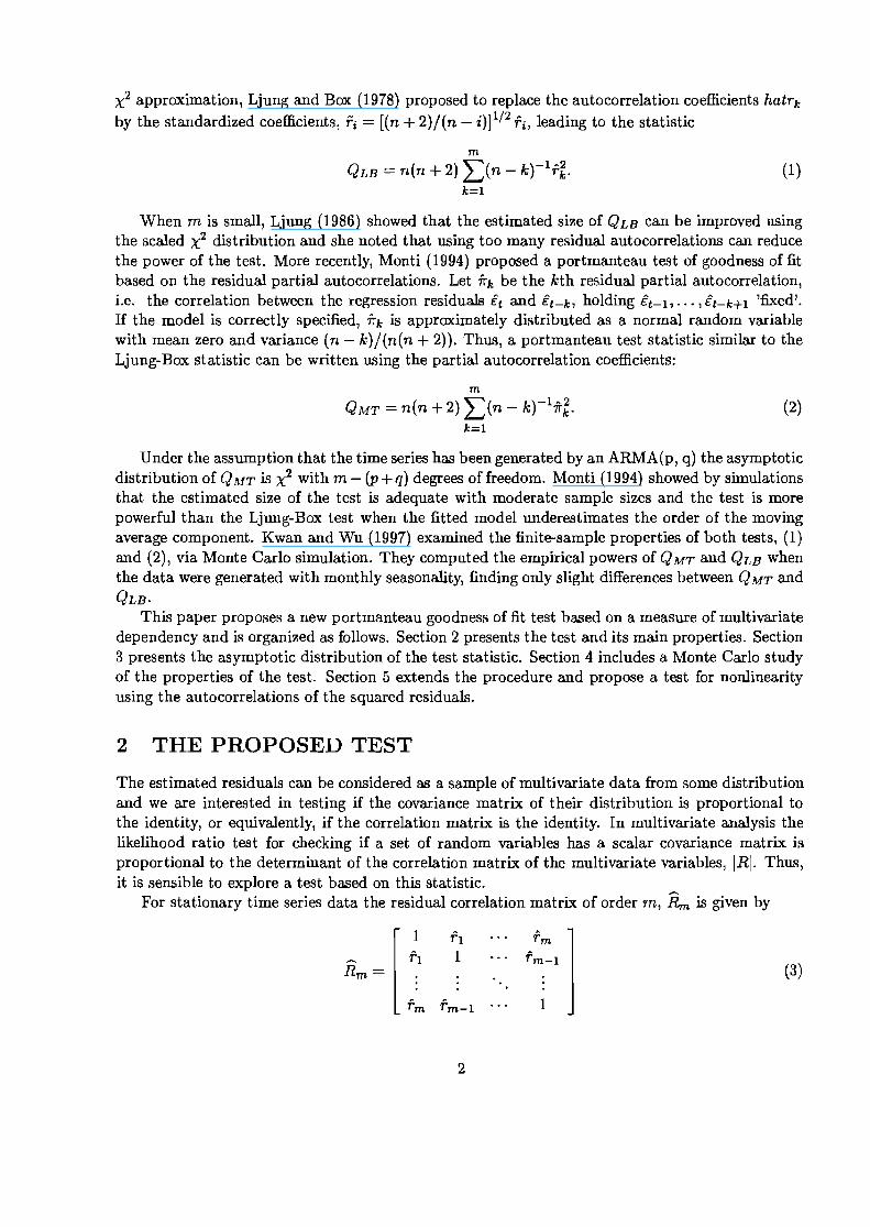
x2 approximation, Ljung and Box (1978) proposed to replace the auto correlation coefficients hatrk by the standardized coefficients, ri = [(n + 2)J(n i)]1/2 ri, leading to the statistic

m

QLB = n(n + 2) L:(n - k)-Ir~. (1) k=1

When m is small, Ljung (1986) showed that the estimated size of QLB can be improved using the scaled X2 distribution and she noted that using too many residual autocorrelations can reduce the power of the test. More recently, Monti (1994) proposed a portmanteau test of goodness of fit based on the residual partial autocorrelations. Let irk be the kth residual partial auto correlation, Le. the correlation between the regression residuals et and et-k, holding et-I, ... , et-k+l 'fixed'. If the model is correctly specified, irk is approximately distributed as a normal random variable with mean zero and variance (n - k)J(n(n + 2)). Thus, a portmanteau test statistic similar to the Ljung-Box statistic can be written using the partial autocorrelation coefficients:

m

QMT = n(n + 2) L:(n - k)-lirl· (2) k=1

Under the assumption that the time series has been generated by an ARMA(p, q) the asymptotic distribution of QMT is X2 with m- (p+q) degrees offreedom. Monti (1994) showed by simulations that the estimated size of the test is adequate with moderate sample sizes and the test is more powerful than the Ljung-Box test when the fitted model underestimates the order of the moving average component. Kwan and Wu (1997) examined the finite-sample properties of both tests, (1) and (2), via Monte Carlo simulation. They computed the empirical powers of QMT and QLB when the data were generated with monthly seasonality, finding only slight differences between Q MT and QLB.

This paper proposes a new portmanteau goodness of fit test based on a measure of multivariate dependency and is organized as follows. Section 2 presents the test and its main properties. Section 3 presents the asymptotic distribution of the test statistic. Section 4 includes a Monte Carlo study of the properties of the test. Section 5 extends the procedure and propose a test for nonlinearity using the autocorrelations of the squared residuals.

2 THE PROPOSED TEST

The estimated residuals can be considered as a sample of multivariate data from some distribution and we are interested in testing if the covariance matrix of their distribution is proportional to the identity, or equivalently, if the correlation matrix is the identity. In multivariate analysis the likelihood ratio test for checking if a set of random variables has a scalar covariance matrix is proportional to the determinant of the correlation matrix of the muItivariate variables, IRI. Thus, it is sensible to explore a test based on this statistic.

For stationary time series data the residual correlation matrix of order rn, Rm is given by

[ ~l Tl Tm

1 .-.. 1

TT' Rm=

rm-l rm

(3)

2

and we have that

where R; = T(m)R;lr(m) , with r(m) = (rl, ... , r m)', is the determination coefficient in the linear

fit Et = L:~=l bjEt_j + Ut. By recursive use of this expression we can write

(4)

We can define the residuals mean autodependency, D(Et, m), as the average value (in the log scale) of the squared correlations obtained when fitting autoregresive models of increasing order to the time series by

m 1 '""" A2 log(l- D(Et,m)) = - L,log(l- Rd· m i=l

(5)

This statistic has an alternative interpretation as a weighted average of the partial autocorre­lation coefficients, 1fi. It is well known that

(1- ~) = 1- R; 1fl 1- R~ ,

z-l

and using this expression in (5) it can be obtained that

m

log(l - D(Et, m)) = L Wi log(l - 1T;), i=l

(6)

where Wi = (m + 1 - i)/m. We propose to test for auto correlation in the estimated residuals with the portmanteau statistic:

(7)

3 DISTRIBUTION OF THE PROPOSED STATISTIC

In this section we first obtain the asymptotic distribution of the proposed statistic (7) for all m, where m is the number of sample auto correlations. As this distribution is complicated, we follow Box and Pierce (1970) in obtaining an approximation of this distribution when m is moderately high. Then, we will show by Monte Carlo simulation that this approximation work well in small samples.

3.1 Asymptotic distribution of Dm(€t)

The auto dependency is a continuous function of the sample partial auto correlations, 1Ti, as shown in equation (6). Defining 1T(m) = (1Tl, ... ,1Tm )" and using the result by Monti (1994) we have that nl/21T(m) is asymptotically multivariate normal with zero mean vector and covariance matrix (Im - Qm), where Qm = XmV- 1 X:n, V is the information matrix for the parameters cP and 8, and Xm is an m x (p + q) matrix, with elements cp' and 8' defined by 1/ cp(B) = L:~o cp~Bi and 1/8(B) = L:~o8~Bi, (see Brockwell and Davis, 1991, pp. 296-304). The coefficients cp~ and 8~ are readily computed using the recursive procedure of Box and Jenkins (1976, pp. 132-134).

3

-•

Theorem 1 If the model is correctly identified, Dm(tt) is asyr'nptotically distributed as 2:~1 AiXi,i

, where xi i (i = 1, ... , m) are independent xi random variables and Ai (i = 1, ... , m) are the eigenvalue; of {Im - Qm)Wm, where Wm is a diagonal matrix with elements Wii = (m - i + l)/m (i=l, ... ,m).

Proof. Suppose that under the null hypothesis, Dm(tt) is asymptotically distributed as the random variable X. Then, applying the 8-method (Arnold, 1990) to g(x) = 10g(1 - x), it follows that -nlogIRmI1/m is also asymptotically distributed as X. From (6) we obtain the equivalent expression

( ~ ) m m-i+1 -nlog IRmI 1/m = -n ~ m In (1- *;).

~=1

(8)

To find the distribution of (8), suppose that (n*i, n*i, ... , n*~) is asymptotically distributed as the random variable Y. Then, applying the multivariate 8-method (Arnold, 1990) to g(*?, ... , *~) = - 2:~1 m~+1 In (1 - *;) , it follows that

m . 1 ~m-z+ (~2) m-I 1) -n L...J m In 1 - 7ri ~ (1, ~ ... 'm Y. i=1

(9)

where ~ stands for convergence in distribution and from the Cramer-Wold theorem (Arnold 1990), it follows that

(1 m-I 1)( ~2 ~2 ~2 )' (1 m-I 1 )Y (10) '~···'m n7rI, n7r2,···,n7rm ~ '~···'m .

Using the fact that n 1/ 2*(m) is asymptotically distributed as N(O, Im - Qm) and from the theorem on quadratic forms given by Box (1954), it follows that

m

(1 m-I 1)( ~2 ~2 ~2 )' ~'D ~ ~ \ 2 , ~ ... 'm n7rl' n7r2, ... ,n7rm = n7ri m7ri ~ L...J AiXl,i· (11) i=1

Finally, from (10) and (11)

m

(1, m~1 ... , ik)Y ~ L AiXL. i=1

and from (9) m

Dm(t) ~ L Aixi,i· (12) i=1

• For a general ARMA model the expression for the eigenvalues of (Im - Qm)Wm is complicated.

However, the eigenvalues are readily calculated for any given </>, () and m. In the following subsection, we propose an approximation of the distribution (12) for a moderately high m.

3.2 Approximation of the distribution Dm(€t)

The probability pr(Dm(t) > x) can be evaluated by inverting the characteristic function of2:~1 AiXL (Imhof 1961). The procedure requires only one-dimensional numerical integration, but for simplic­ity, we prefer to use the approximation proposed by Box (1954). He suggested approaching a distribution of the form (12) by a distribution of the form ax~, with mean and variance equal to

4

I I!!

I

I

those of the exact distribution. Following this suggestion, we approximate the distribution (12) with parameters a and b defined by a = L: At / L: Ai and b = (L: Ai)2 / L: At, where Ai are the eigenvalues of the matrix (Im - Qm)Wm.

Box and Pierce (1970) and McLeod (1978) approximate the matrix Qm = Xm V-l X:n by the projection matrix Qm = Xm (X:nXm)-l X:n when m is moderately high. This approximation is useful for computing an expression for a and b that does not depend on the ARMA parameters tjJ and (). Then we have

m

I: Ai = tr«(Im - Qm) W m) = tr(Wm) tr(Qm) + (l/m)tr(QmCm) (13) i=l

where Cm is a diagonal matrix with elements Cii = i, i = 0, ... , (m - 1), and

m

I: At = tr( (Im - Qm) W;') = tr{W;') - tr (Qm) +

(14)

An alternative expression for L: Ai and L: At can be obtained using the Cholesky decomposition of the matrix (Im - Qm), see Velilla (1994). Using the fact that Qm is an idempotent matrix with rank p + q, then (13) and (14) can be written as a function of p, q, m and qii, where the qii are the elements in the diagonal of Qm,

m +1 1 m

~Ai = T - (p+q) + m ~(i -l)qii' i=l ~=2

(15)

m 1 ~A;= 6m (m+1)(2m+1) (p+q)+ t=l

2 m 1 m

+ - I:(i - l)qii - 2" I:(i 1)2qii. m i=2 m i=2

(16)

Now we will show that the terms (l/m) L:~2{i - l)qii and (1/m2) L:~2(i - 1)2qii tend to zero when m increases. As Qm is an idempotent matrix of rank p + q, then L:~1 % = P + q. Consider the sequences ai = i and bi = (i - l)qii. Then L:~1 (i - l)%/i ~ L:~1 qu = P + q < 00 as m --+ 00.

Then by Kronecker's lemma (Davidson, 1997, pp. 34-35) we obtain that (l/m) L:~1 (i -l)qii --+ O. A similar argument is used to show that (1/m2) L:~1 (i - 1)2qu --+ O. Thus, for large m we can approximate equations (15) and (16) by

m m+1 I: Ai = -2 - - (p + q), i=l

(17)

m 1 I: At = 6m (m + 1) (2m + 1) - (p + q). t=l

(18)

This approximation of the distribution (12) is stated in the next corollary.

Corollary 2 If ARMA model is correctly identified, when m is moderately high, the distribution of Dm(€t) can be approximated by a distribution ax~ with mean (m + 1) /2 - (p + q) and variance (m + 1) (2m + 1) /3m - 2(p + q).

5

3.3 Comparison between the empirical distribution and the approximation of the distribution of Dm(€t)

In this section we present the results of a Monte Carlo experiment which was carried out to check the approximation to the asymptotic distribution of Dm(€) indicated in Corollary 2. As the X2

approximation to the asymptotic distribution improves when using the standardized autocorrelation coefficients estimator T(m) = (TI' ... ' Tm)', where Ti = [(n + 2)/(n - i)]I/2 ri, we will consider in addition to Dm(€t), the statistic based on r(m), the statistic D:n(€t) based on T(m). Under the null hypothesis, Dm(€t) and D:n(€t) are asymptotically equivalent, but obviously, some differences may be expected in their small-sample behaviours. We have included in the study the Q LB and Q UT

statistics in order to compare the approximation we are proposing to those used for these statistics. The sample sizes used are 50,100 and 500. We report here only the results when the generating process is white noise. Similar results have been found when the generating process is a low order AR or MA model and are available upon request from the authors.

[TABLE 1 ABOUT HERE] [TABLE 2 ABOUT HERE]

In the white noise case, p = q = 0, Dm(at) can be approximated by ax~ where a = (2m + 1)/3m and b = 3m(m + 1)/(4m + 2) and it has asymptotic mean and variance (m + 1)/2 and (2m + l)(m + 1)/3m. Tables 1 and 2 show the mean and the variance of the empirical distribution of the statistics Dm, D:n, QLB and QMT, obtained by generating 10,000 replications of Gaussian white noise with sample size 50, 100 and 500 and computing the four statistics in each replication for lags 7, 15 and 20. The last row of Table 1 presents the asymptotic mean and the last row of Table 2 the asymptotic variance. The approximation is quite good in all four cases. In Table 2 we observe that in all cases the variance of D:n is closer to the asymptotic variance than that of Dm. The approximation in the distribution of D:n works better than in the case of QLB, where the empirical variance is clearly overestimated.

[FIGURE 1 ABOUT HERE] Figure 1 ilustrates the accuracy of the empirical distribution of Dm and D:n to the distribution

(12), with 10,000 replications of sample size 100 by an AR(l) process with ~I = .5, and m = 20. The approximation by the standardized estimators is better than the non-standardized estimators, and based on these simulations, we recomend use of D:n specially, for small sample size.

4 COMPARISON OF SIGNIFICANCE LEVELS AND POWER IN SMALL-SAMPLE OF D:n(Et)

[TABLE 3 ABOUT HERE] In this section we present a comparative study of significance level and power for the statistics D:n, QLB and QMT. The significance levels of QLB and QMT are obtained using the percentiles of the X2 distribution, and those of D:n, have been obtained by using the approximation of (12) by the ax~ with a and b obtained from (17) and (18). These significance levels are evaluated under both low order AR and MA models but we report here only the results for the AR(l). Similar results were found in the other cases and they are available upon request from the authors. In each case, 10,000 Gaussian series of 100 observations were generated and the performance of D:n was compared to that of the Ljung-Box and Monti statistics. Three values for m, 10, 15 and 20 were considered. Table 3 shows the significance levels, under the AR(l) model, when the nominal levels a are 0.05 and 0.01. The approximation seems to be satisfactory for the three statistics, and for QLB and QMT is similar to the results presented by Monti (1994). For a = 0.05, the significance

6

-..

level of D:n is between the significance level of QLB and QMT. The significance level of D:n does not seem to be affected by the value of m considered.

[TABLE 4 ABOUT HERE] The power is analyzed for the same models as proposed by Monti (1994) to compare the perfor­

mance of the Q MT and Q LB statistics. Table 4 shows the power of the three tests when, erroneously, an AR{l) or a MA{l) model is fitted to the data. Twenty four different ARMA{2,2) models are considered. In each case 1,000 series of 100 observations were generated and the power was com­puted with m = 10 and m = 20. The power decreases as m grows in the three tests, but the loss of power in D:n is relatively lower. The power of D:n is always the highest and the increase in power with respect to the best of QMT and QLB can in some cases be as high as 50% (see models 1, 11 and 23).

5 CHECKING THE LINEARITY ASSUMPTION

Granger and Anderson (1978) suggested that looking at the autocorrelation function of y; could be useful in identifying nonlinear time series. Maravall (1983) showed that the autocorrelation function, (ACF), of the squared residuals, provides a convenient tool for checking the linearity assumption. If the residuals tt are independent so the t; will be, but if the model is nonlinear and the residuals tt are not independent, this feature can appear in the ACF of t;, which is expected to be different from the ACF of a white noise process. McLeod and Li (1983) proposed to detect non linearity in time series data by computing the statistic QLB on the auto correlations of the squared residuals from a linear fit. The significance levels are based on the asymptotic x~ distribution of the test statistic when the process is linear. These same ideas could be applied to the statistic proposed by Monti (1994) and to the new statistic (7) proposed in this article. Then, the proposed nonlinearity test (7) can be written as

Dm{t;) = nD{t;, m),

where the auto correlation function of t; is estimated by

fk{t;) = t (t; - 0-2 ) (tLk - 0-2) It (t; - 0-2

)2

t=k+l t=l

(k=1,2, ... ,m).

where 0-2 = 'LJ;;n, and analogously for Monti's tests QMT{t;). In the next lemma we calculate the asymptotic distribution of the statistic Dm{tF} when ARMA model is correctly identified.

Lemma 3 If the ARMA model is correctly identified then Dm{t;) is asymptotically distributed as :E~l wiixi,i where xi,i (i = 1, ... , m) are independent xi random variables and Wii = (m-i+ l)/m (i=l, ... ,m).

Proof. This is based on the result by McLeod and Li (1983) for the distribution ofn1/ 2 f(m){t;), which is N{O,Im). Applying this result to that obtained by Monti (1994), the asymptotic distri­bution of nl/27?(m){tF} is N{O, Im). Following the same reasoning as in Theorem 1, the asymptotic distribution for QD{tF) is obtained. _

The asymptotic distribution of Lemma 3 can be approximated as before by distribution of form ax~ proposed by Box (1954). The following Corollary gives the details.

Corollary 4 If ARMA model is correctly identified, then the asymptotic distribution of Dm{tF) can be approximated by a distribution of form ax~, where a = (2m+1)/3m and b = 3m(m+l)/{4m+2).

7

I I!

5.1 Power comparison I

Davis and Petruccelli (1986) compared the statistics proposed by McLeod and Li (1983) and by I Keenan (1985). They concluded that the statistic proposed by Keenan is more powerful than the one proposed by Li and McLeod but that the power of both statistics is poor except for large sample size, n > 200. In this section we compare the power of the statistics D:n, QLB and QMT

for testing the linearity hypothesis, when applied to the squared residuals. As earlier, we use the correction of the statistic D:n for small samples based on the standardized auto correlations, Tk(tF) = [(n + 2)/(n - i)]1/2 Tk(tF). We will compare the power for the four nonlinear models that Keenan (1985) used in his study:

Model 1, Yt = et - OAet-l + 0.3et-2 + 0.5etet-2;

Model 2, Yt = et - 0.3et-l + 0.2et-2 + OAet-let-2 - 0.25e;_2;

Model 3, Yt = OAYt-l - 0.3Yt-2 + 0.5Yt-let-l + et;

Model 4, Yt = OAYt-l - 0.3Yt-2 + 0.5Yt-let-l + 0.8et-l + et,

where the et's are independent N(O,I). [TABLE 5 ABOUT HERE]

Table 5 summarizes the power results. For each model 1,000 replications of sample size n = 204 were generated and fitted with an AR(P) model, where p is selected by the Ale (Akaike 1974) with pE {I, 2, 3, 4}. The power of the proposed statistic, D:n(tF), is broadly between 6% (Model 4, m = 7) and 40% (Model 2, m = 24) higher than the ones based on QLB and QMT. None of these tests are powerful in handling Model 1, which contains a concurrent nonlinear term etet-2. The difficulty in finding the nonlinearity of Model 1 is observed in the study by Tsay (1986) which compares some statistics for checking the nonlinearity over the same four models. From the comparison of Table 5 and the results obtained by Tsay (1986) we conclude that the proposed test D:n(tF) is better than that proposed by Keenan for all lags, m = 7, 12 and 24 and for all the models except Model 2. However, the proposed portmanteau test is slightly worse than that proposed by Tsay.

We are interested in checking the behaviour of the proposed statistics in the detection of non linearity in Threshold Autorregressive models (TAR) which are among the most popular non linear time series models in applied research. With this aim 1,000 replications were generated with sample sizes 100, 200 and 500 from the TAR(2) model with 4 regimes proposed by Tiao and Tsay (1994). This model as an alternative to the AR(2) model to capture the structure of the U.S. real GNP series from the first quarter of 1947 to the first quarter of 1991 with a total of 177 observations. The regimes and their economic interpretation are described in Tiao and Tsay (1994).

[TABLE 6 ABOUT HERE] Table 6 shows the power of the statistics D:n, QLB and QMT using the residuals auto correlations

h with a = 0.05 to find structure in these samples when fitting an AR(2) model. The values shown in the table are close to the nominal level (0.05) confirming the lack of power of these statistics to detect nonlinearity. Table 7 displays the power of these statistics when the squared residuals t¥ of the AR(2) fit is used. The power of the three statistics increases as expected and now the power of D:n is clearly higher for all sample sizes. Large samples sizes are needed for these types of statistics to be useful and for n = 500 the increase of power of D:n with respect to the best of QLB and QMT

goes from 23% to 35%. [TABLE 7 ABOUT HERE]

8

5.2 An example with real data

[TABLE 8 ABOUT HERE] In this section we apply the D:n(€;) statistic to find nonlinearities in the well known Sunspot time series, Box and Jenkins (1976). This time series has been previously studied by various authors who have applied both linear and nonlinear models. A detailed description of some of the different models which have been proposed can be found in Priestley (1989). We have followed Priestley (1989, p. 882) and fitted an AR(9) model to the sample of 246 observations corresponding to the first 246 observations from 1700. The order of the linear model was determined according to Akaike's criterion. The model is estimated by maximum likelihood and statistics D:n, QLB and QMT, are computed from the residuals. No structure is found using the lags m = 12 and 24 and a = 0.05. However, when using the statistic D:n(€;) a clear indication of non linear structure is found. Table 8 presents the values of the three portmanteau statistics applied to the squared residuals. To facilitate the comparison columns 3, 5 and 7 show the ratio between the statistic and the percentile corresponding to a = 0.05 for each distribution. The results obtained with the statistic D:n(€F) are more conclusive than those with the statistics QLB and QMT, for checking the nonlinearity of the time series. The statistic D:n(€;) clearly suggests a nonlinear structure whereas the results from the Ljung-Box and Monti statistics are not decisive.

6 ACKNOWLEDGMENTS

This research has been sponsored by DGES (Spain) under project PB-96-0111 and the Catedra BBVA de Calidad. We are very grateful to Andres Alonso for many stimulating discussions and to Mike Wiper for his help with the final draft.

References

Akaike, H. (1974). A New Look at the Statistical Model Identification. IEEE Trans. Automat. Control AC 19, 203-17.

Arnold, S. F. (1990). Mathematical Statistics. Prentice-Hall International, Inc.

Box, G. E. P. (1954). Some Theorems on Quadratics Forms Applied in the Study of Analysis of Variance Problems I: Effect of the Inequality of Variance in the One-way Classification. Annals of Mathematical Statistics 25, 290-302.

Box, G. E. P. and G. M. Jenkins (1976). Time Series Analysis, Forecasting and Control. Holden­Day, San Francisco.

Box, G. E. P. and D. A. Pierce (1970). Distribution of Residuals Autocorrelations in Autoregressive-integrated Moving Average Time Series Models. Journal of the American Sta­tistical Association 65, 1509-26.

Brockwell, P. and R. A. Davis (1991). Time Series: Theory and Methods (2nd Edn ed.). New York: Springer Vedag.

Davidson, J. (1997). Stochastic Limit Theory. Oxford University Press.

Davis, G. E. P. and D. A. Petruccelli (1986). Detecting Non-linearity in Time Series. The Statis­tician 35, 271-280.

Granger, C. W. J. and A. P. Anderson (1978). An Introduction to Bilinear Time Series Models. Gtttingen,Vandenhoeck & Rpurecht.

9

Imhof, J. P. (1961). Computing the Distribution of Quadratics Forms in Normal Variables. Biometrika 48, 419-26.

Keenan, D. M. (1985). A Tukey Nonadditivity-type Test for Time Series Nonlinearity. Biometrika 72, 39-44.

Kwan, A. C. C. and Y. Wu (1997). Further Results on the Finite-sample Distribution of Monti's Portmanteau Test for the Adequacy o(an ARMA(p,q) Model. Biometrika 84, 733-36.

Ljung, G. M. (1986). Diagnostic Testing of Univariate Time Series Models. Biometrika 73, 725-30.

Ljung, G. M. and G. E. P. Box (1978). On a Measure of Lack of Fit in Time Series Models. Biometrika 65, 297-303.

Maravall, A. (1983). An Application of Nonlinear Time Series Forecasting. Journal of Business f3 Economics Statistics 1, 66-74.

McLeod, A. 1. (1978). On the Distribution of Residuals Autocorrelations in Box-Jenkins Models. Journal of the Royal Statistical Society, Ser. B 40, 296-302.

McLeod, A. 1. and W. K. Li (1983). Diagnostic Checking ARMA Time Series Models Using Squared-residuals Autocorrelations. Journal of Time Series Analysis 4, 269-273.

Monti, A. C. (1994). A Proposal for Residual Autocorrelation Test in Linear Models. Biometrika 81, 776-80.

Priestley, M. B. (1989). Spectral Analysis and Time Series, Vol. 1. Academic Press Inc., San Diego.

Tiao, G. C. and R. S. Tsay (1994). Some Advances in Non-linear and Adaptive Modeling in Time Series. Journal of Forecasting 13, 109-13l.

Tsay, R. S. (1986). Nonlinearity Test for Time Series. Biometrika 73, 461-466.

Velilla, S. (1994). A Goodness-of-fit Test for Autoregressive Moving-average Models Based on the Standardized Sample Spectral Distribution of the Residuals. Journal of Time Series Analysis 15, 637-47.

10

Table 1: Empirical means of Dm , D~ QLB and QMT with 10,000 replications of a white noise process. Sample sizes are n=50, 100 and 500 and m=7, 15 and 20 . In the last row the theoretical mean of each statistic is shown.

Empirical Mean

m=7 m=15 m=20

n Dm D* m QLB QMT Dm D* m QLB QMT Dm D* m QLB QMT

50 3.68 4.10 7.16 7.29 6.67 7.97 15.29 15.31 8.21 10.32 20.36 20.15

100 3.85 4.06 7.06 7.14 7.32 7.95 15.17 15.24 9.32 10.32 20.21 20.25

500 4.00 4.05 7.04 7.05 7.88 8.00 15.03 15.07 10.27 10.46 20.00 20.04

Theoretical Mean

00 4 4 7 7 8 8 15 15 10.5 10.5 20 20

Table 2: Empirical variance of Dm , D~ QLB and QMT with 10000 replications of a white noise process. Sample sizes are n=50, 100 and 500 and m=7, 15 and 20. In the last row the theoretical variance of of each statistic is shown.

Empirical Variance

m=7 m=15 m=20

n Dm D* m QLB QMT Dm D* m QLB QMT Dm D* m QLB QMT

50 4.42 5.38 16.57 14.24 6.80 9.49 44.86 28.81 7.71 11.86 65.54 36.48

100 5.04 5.53 15.03 13.92 8.62 9.92 37.95 30.04 10.44 12.42 53.67 39.53

500 5.82 5.92 14.50 14.12 10.50 10.77 30.82 29.37 13.38 13.79 42.10 39.58

Theoretical Variance

00 5.71 5.71 14 14 11.02 11.02 30 30 14.35 14.35 40 40

Table 3: Significance levels of QD, QLB and QMT under an AR(l) model. m=10 m=15 m=20

a = 0.05

<PI D* m QLB QMT D* m QLB QMT D* m QLB QMT

0.10 0.055 0.053 0.056 0.054 0.057 0.054 0.055 0.062 0.054

0.30 0.053 0.052 0.053 0.052 0.057 0.054 0.053 0.062 0.049

0.50 0.052 0.055 0.052 0.049 0.057 0.046 0.047 0.058 0.046

0.70 0.054 0.057 0.053 0.050 0.060 0.048 0.050 0.069 0.048

0.90 0.050 0.054 0.043 0.042 0.059 0.039 0.041 0.061 0.039

a = 0.01

<PI D* m QLB QMT D* m QLB QMT D* m QLB QMT

0.10 0.009 0.013 0.011 0.009 0.016 0.011 0.010 0.019 0.011

0.30 0.010 0.012 0.011 0.009 0.Q17 0.011 0.009 0.021 0.010

0.50 0.008 0.012 0.008 0.007 0.016 0.007 0.007 0.019 0.008

0.70 0.010 0.015 0.010 0.008 0.015 0.010 0.009 0.021 0.007

0.90 0.011 0.013 0.009 0.009 0.017 0.009 0.009 0.021 0.009

11

Table 4: Power level of QD, QLB and QMT when data are fitted by AR(l) and MA(l) models under various alternative ARMA(2,2) models

(a) Fitted by AR(l) model

m=lO m=20 M ~1 ~2 (h (J2 D* m QLB QMT D* m QLB QMT

1 - -0.50 0,415 0.234 0.278 0.299 0.189 0.178

2 -0.80 0.987 0.751 0.959 0.972 0.590 0.855

3 - -0.60 0.30 0.994 0.762 0.983 0.987 0.655 0.941

4 0.10 0.30 0.597 0,421 0.412 0,452 0.364 0.296

5 1.30 -0.35 0.807 0.620 0.605 0.649 0.540 0.415

6 0.70 - -0.40 0.781 0.542 0.609 0.637 0.428 0.415

7 0.70 - -0.90 1.000 0.982 0.998 0.998 0.905 0.992

8 0.40 -0.60 0.30 0.999 0.836 0.998 0.997 0.697 0.965

9 0.70 0.70 -0.15 0.216 0.175 0.169 0.182 0.173 0.111

10 0.70 0.20 0.50 0.858 0.759 0.763 0.781 0.658 0.621

11 0.70 0.20 -0.50 0.599 0.324 0.384 0.447 0.288 0.260

12 0.90 -0.40 1.20 -0.30 0.988 0.694 0.971 0.970 0.555 0.893

(b) Fitted by MA (1) model

m=lO m=20

13 0.50 0.366 0.295 0.265 0.287 0.243 0.189

14 0.80 0.993 0.984 0.980 0.987 0.969 0.939

15 LlO -0.35 1.000 1.000 0.999 0.999 0.986 0.988

16 0.80 -0.50 0.988 0.851 0.940 0.953 0.727 0.838

17 - -0.60 0.30 0.674 0,400 0.476 0.540 0.337 0.340

18 0.50 - -0.70 0.957 0.888 0.876 0.888 0.801 0.736

19 -0.5 0.70 0.957 0.893 0.876 0.908 0.807 0.758

20 0.30 0.80 -0.50 0.859 0.583 0.743 0.765 0,468 0.556

21 0.80 - -0.50 0.30 0.992 0.980 0.960 0.973 0.968 0.916

22 1.20 -0.50 0.90 0.706 0,467 0.696 0.708 0.393 0.570

23 0.30 -0.20 -0.70 0.426 0.278 0.280 0.306 0.233 0.208

24 0.90 -0,40 1.20 -0.30 0.965 0.780 0.923 0.932 0.638 0.822

Table 5: Empirical frequency of rejection of the null hypothesis of linearity, when the fitted model is an AR(p), and n=204 with 1,000 replications. Nominal significance level, a = 0.05.

m=7 m=12 m=24

D* m QLB QMT D* m QLB QMT D* m QLB QMT

Model 1 0.157 0.114 0.120 0.126 0.100 0.091 0.091 0.094 0.089

Model 2 0.566 0.497 0.480 0.511 0,426 0.394 0.406 0.289 0.277

Model 3 0.960 0.900 0.914 0.940 0.854 0.826 0.870 0.740 0.70

Model 4 0.914 0.860 0.830 0.874 0.805 0.760 0.788 0.686 0.614

12

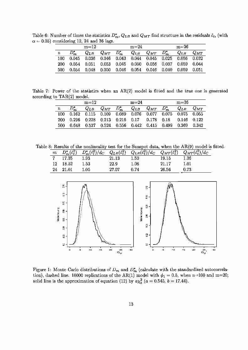
Table 6: Number of times the statistics D':n, QLB and QMT find structure in the residuals tt, (with a = 0.05) considering 12, 24 and 36 lags.

m=12 m=24 m=36 n D* m QLB QMT D* m QLB QMT D* m QLB QMT 100 0.045 0.036 0.046 0.043 0.044 0.045 0.025 0.056 0.032 200 0.054 0.051 0.053 0.045 0.050 0.056 0.037 0.059 0.044 500 0.054 0.048 0.050 0.046 0.054 0.046 0.040 0.059 0.051

Table 7: Power of the statistics when an AR(2) model is fitted and the true one is generated according to TAR(2) model.

m=12 m=24 m=36 n D* m QLB QMT D* m QLB QMT D* m QLB QMT 100 0.162 0.115 0.109 0.089 0.076 0.077 0.075 0.075 0.055 200 0.296 0.228 0.213 0.216 0.17 0.178 0.18 0.146 0.122 500 0.648 0.527 0.524 0.556 0.442 0.415 0.499 0.369 0.342

Table 8: Results of the nonlineality test for the Sunspot data, when the AR(9) model is fitted. m D:n(t¥) D':n(t¥)/dc QLB(tl) QLB(t¥)/dc QMT(tl) QMT(tl)/dc 7 17.35 1.93 21.13 1.50 19.15 1.36 12 18.52 1.53 22.9 1.08 21.17 1.01 24 21.01 1.05 27.07 0.74 26.56 0.73

~ ~ ;; ;;

ci

ci

;;

g J ci

j gs ci

:g !i' .!!' ci "@ :g ... J! ci ~

~

~ :::l ci

j?l

:::l ci

--:::l ci

0 5 10 15 20 25 30 0 5 10 15 20 25 30

OD OD·

Figure 1: Monte Carlo distributions of Dm and D:n (calculate with the standardized autocorrela­tion), dashed line. 10000 replications of the AR(l) model with 1>1 = 0.5, when n=lOO and m=20; solid line is the approximation of equation (12) by ax~ (a = 0.545, b = 17.44).

13