A Panel Analysis on the Cross Border E-commerce Trade
10
Yugang HE, Jingnan WANG / Journal of Asian Finance, Economics and Business Vol 6 No 2 (2019) 95-104 95 Print ISSN: 2288-4637 / Online ISSN 2288-4645 doi:10.13106/jafeb.2019.vol6.no2.95 A Panel Analysis on the Cross Border E-commerce Trade: Evidence from ASEAN Countries Yugang HE 1 , Jingnan WANG 2 Received: December 21, 2018 Revised: January 02, 2019 Accepted: March 30, 2019 Abstract Along with the economic globalization and network generalization, this provides a good opportunity to the development of cross-border e- commerce trade. Based on this background, this paper sets ASEAN countries as an example to exploit the determinants of cross-border e- commerce trade including the export and the import, respectively. The panel data from the year of 1998 to 2016 will be employed to estimate the relationship between cross-border e-commerce trade and relevant variables under the dynamic ordinary least squares and the error correction model. The findings of this paper show that there is a long-run relationship between cross-border e-commerce trade and relevant variables. Generally speaking, the GDP(+) and real exchange rate(-export & +import) have an effect on cross-border e-commerce trade. However, the population (+) and the terms of trade (-) only have an effect on cross-border e-commerce import. The empirical evidences show that the GDP and the real exchange rate always affect the development of cross-border e-commerce trade. Therefore, all ASEAN countries should try their best to develop the economic growth and focus on the exchange rate regime so as to meet the need of cross- border e-commerce trade development. Keywords: Cross-border E-commerce Trade, ASEAN Countries, Dynamic Ordinary Least Squares. JEL Classification Codes: B40, F10, F19. 1. Introduction 1 Along with the rapid development of modern economy, the cross-border e-commerce trade has become a new trade mode in the global economic activities. It can not only effectively remedy the predicament of the shortage of resources in various countries, but also optimize and rationalize the allocation of existing resources in various countries. The continuous development and popularization of cross-border e-commerce trade have a certain impact on a country's economic model. As for the cross-border e- commerce trade, It refers to an international business activity that belongs to different trading entities, through electronic commerce platform to achieve transactions, payment and settlement, and through cross-border logistics 1 First Author, PH.D Candidate, Department of International Trade, Chonbuk National University, South Korea. E-mail: [email protected] 2 Corresponding Author, Lecturer, College of Economics, Qufu Normal University, China. E-mail: [email protected] © Copyright: Korean Distribution Science Association (KODISA) This is an Open Access article distributed under the terms of the Creative Commons Attribution Non- Commercial License (https://creativecommons.org/licenses/by-nc/4.0/) which permits unrestricted non- commercial use, distribution, and reproduction in any medium, provided the original work is properly cited. to deliver goods and complete transactions. The flourishing development of cross-border e-commerce trade is obvious to all. However, The factors that affects cross-border e- commerce trade also arise at the historic moment. A great deal of scholars have noticed this problem. Blum and Goldfarb (2006) use the internet access data of 2654 local Americans from December 12, 1999 to March 31, 2000 to study the influencing factors of non-physical commodity trade in cross-border e-commerce under the gravity model. Gomez-Herrera, Martens, and Turlea (2014) set 27 EU countries as the research object with a questionnaire as data source, they use the revised gravity model to study the factors that affect the cross-border e-commerce trade between EU countries. This paper sets ASEAN countries (ASEAN countries include Brunei Darussalam, Cambodia, Indonesia, Laos, Malaysia, Myanmar, Philippines, Singapore, Thailand and Vietnam) an example to exploit the determinants (cross- border e-commerce export, cross-border e-commerce import, GDP, population, terms of trade and real exchange rate) of cross-border e-commerce trade. The panel data from the year of 1998 to 2016 will be employed to estimate the relationship between cross-border e-commerce trade
-
Upload
khangminh22 -
Category
Documents
-
view
7 -
download
0
Transcript of A Panel Analysis on the Cross Border E-commerce Trade

Yugang HE, Jingnan WANG / Journal of Asian Finance, Economics and Business Vol 6 No 2 (2019) 95-104 95
Print ISSN: 2288-4637 / Online ISSN 2288-4645 doi:10.13106/jafeb.2019.vol6.no2.95
A Panel Analysis on the Cross Border E-commerce Trade:
Evidence from ASEAN Countries
Yugang HE1, Jingnan WANG
2
Received: December 21, 2018 Revised: January 02, 2019 Accepted: March 30, 2019
Abstract
Along with the economic globalization and network generalization, this provides a good opportunity to the development of cross-border e-
commerce trade. Based on this background, this paper sets ASEAN countries as an example to exploit the determinants of c ross-border e-
commerce trade including the export and the import, respectively. The panel data from the year of 1998 to 2016 will be employed to estimate
the relationship between cross-border e-commerce trade and relevant variables under the dynamic ordinary least squares and the error
correction model. The findings of this paper show that there is a long-run relationship between cross-border e-commerce trade and relevant
variables. Generally speaking, the GDP(+) and real exchange rate(-export & +import) have an effect on cross-border e-commerce trade.
However, the population (+) and the terms of trade (-) only have an effect on cross-border e-commerce import. The empirical evidences
show that the GDP and the real exchange rate always affect the development of cross-border e-commerce trade. Therefore, all ASEAN
countries should try their best to develop the economic growth and focus on the exchange rate regime so as to meet the need of cross-
border e-commerce trade development.
Keywords: Cross-border E-commerce Trade, ASEAN Countries, Dynamic Ordinary Least Squares.
JEL Classification Codes: B40, F10, F19.
1. Introduction 1
Along with the rapid development of modern economy,
the cross-border e-commerce trade has become a new
trade mode in the global economic activities. It can not only
effectively remedy the predicament of the shortage of
resources in various countries, but also optimize and
rationalize the allocation of existing resources in various
countries. The continuous development and popularization
of cross-border e-commerce trade have a certain impact on
a country's economic model. As for the cross-border e-
commerce trade, It refers to an international business
activity that belongs to different trading entities, through
electronic commerce platform to achieve transactions,
payment and settlement, and through cross-border logistics
1 First Author, PH.D Candidate, Department of International Trade,
Chonbuk National University, South Korea.
E-mail: [email protected]
2 Corresponding Author, Lecturer, College of Economics, Qufu
Normal University, China. E-mail: [email protected]
© Copyright: Korean Distribution Science Association (KODISA) This is an Open Access article distributed under the terms of the Creative Commons Attribution Non-
Commercial License (https://creativecommons.org/licenses/by-nc/4.0/) which permits unrestricted non-
commercial use, distribution, and reproduction in any medium, provided the original work is properly cited.
to deliver goods and complete transactions. The flourishing
development of cross-border e-commerce trade is obvious
to all. However, The factors that affects cross-border e-
commerce trade also arise at the historic moment. A great
deal of scholars have noticed this problem. Blum and
Goldfarb (2006) use the internet access data of 2654 local
Americans from December 12, 1999 to March 31, 2000 to
study the influencing factors of non-physical commodity
trade in cross-border e-commerce under the gravity model.
Gomez-Herrera, Martens, and Turlea (2014) set 27 EU
countries as the research object with a questionnaire as
data source, they use the revised gravity model to study the
factors that affect the cross-border e-commerce trade
between EU countries.
This paper sets ASEAN countries (ASEAN countries
include Brunei Darussalam, Cambodia, Indonesia, Laos,
Malaysia, Myanmar, Philippines, Singapore, Thailand and
Vietnam) an example to exploit the determinants (cross-
border e-commerce export, cross-border e-commerce
import, GDP, population, terms of trade and real exchange
rate) of cross-border e-commerce trade. The panel data
from the year of 1998 to 2016 will be employed to estimate
the relationship between cross-border e-commerce trade

96 Yugang HE, Jingnan WANG / Journal of Asian Finance, Economics and Business Vol 6 No 2 (2019) 95-104
and relevant variables under the dynamic ordinary least
squares and the error correction model. The findings of this
paper show that there is a long-run relationship between
cross-border e-commerce trade and relevant variables. In
terms of cross-border e-commerce export, the GDP has a
positive effect on cross-border e-commerce export. The
terms of trade and the population have a positive effect on
cross-border e-commerce export, but both of them are not
significant in statistics. The real exchange rate has a
negative effect on cross-border e-commerce export, but only
significant at 10%. In terms of cross-border e-commerce
import, the GDP, the real exchange rate and the population
have a positive effect on cross-border e-commerce import.
The terms of trade have a negative effect on cross-border e-
commerce import.
The rest of this paper will be recognized as follows:
Chapter two presents the literature review that is a summary
of previous achievements so as to show the difference
between this paper and that of previous. Chapter three
provides the theoretical framework that forms a base for this
paper. Chapter four uses the dynamic ordinary least
squares and the error correction model to explore the
relationship between cross-border e-commerce trade and
relevant variables. Chapter five shows the conclusion and
the limitations of this paper.
2. Literature Review
With the popularization of internet and economic
globalization, the development of cross-border e-commerce
trade is advancing rapidly. Because the developing history
of cross e-commerce trade is relatively short, the factors
affecting its development are still unclear. Based on this
background, a large number of scholars have tried their best
to explore the factors that may affect the development of
cross-border e-commerce trade.
Terzi (2011) studies the determinants of e-commerce
trade in terms of international trade and employment. He
finds that e-commerce trade presents economy-wide
benefits to all countries. Concretely speaking, the developed
countries will benefit most in the short run while the
developing countries will benefit more than that of
developed countries in the long run. The e-commerce trade
has a positive effect on international trade. But its effect on
employment is not significant. Conversely, both of them can
affect the e-commerce trade to some degree. Kwon, Kim,
Yoon, and Jeon (2010) investigate the relationship between
MRO (maintenance, repair and operation) e-commerce
system and purchase effects. They find that business to
business e-marketplace will increase and diversify electronic
commerce continuously. Morganti, Seidel, Blanquart,
Dablanc, and Lenz (2014) investigate the relationship
between e-commerce trade and final deliveries from the
prospective of alternative parcel delivery services in France
and Germany. The e-commerce trade for physical goods
leads to a significant demand for dedicated delivery services,
and leads to increasingly difficult last mile logistics. They
find that the e-commerce trade can increase the number of
successful first-time deliveries, optimize delivery rounds and
lower operational costs. Liu (2012) figures out that in the
small cross-border e-commerce trade, customs clearance,
logistics and credit problems are prominent to impede the
small enterprises to perform the cross-border e-commerce
trade. Lai and Wang (2014) find that customs clearance,
market supervision and settlement restrict the development
of cross-border e-commerce. Wang and Yang (2014) also
point out that the cross-border logistics is the bottleneck of
cross-border e-commerce rule demand. Ren and Li (2014)
hold the view that the cross-border e-commerce trade has
an impact on transformation and upgrading of foreign trade,
and they put forward countermeasures and suggestions for
the problems of customs clearance, payment, credit and
logistics in cross-border e-commerce trade. Aydın and
Savrul (2014) set Turkish as an example to study the
relationship between globalization and e-commerce trade.
The globalization has become one of the most remarkable
phenomenon of the 20th century that has shaped the world
economy dramatically. Globalization process is followed
behind the decrease in administrative barriers to conduct
trade, sharp decreases in the costs of communication and
transportation, production processes fragmentation and
development in information and communication technology
which, by opening up new markets and acquiring new raw
materials and resources, lay a foundation for resource
diversification, creation and development of new investment
opportunities. They find that the globalization provides a
good channel for the development of e-commerce trade.
Yang and Lu (2014) find that cross-border e-commerce of
China's foreign trade enterprises has many problems in
electronic payment, customs clearance and logistics, and
lacks systematic laws and regulations. Moreover, Zhang
and Jang (2014) figure that the cross-border e-commerce
trade has such problems as consumer distrust, imperfect
service system, language and geographical barriers.
Liu and Zhao (2015) use the 2010-2016 import and export
of cross-border electricity trade size diagram to analyze the
development trend in recent years of cross-border electricity
supplier. They find that the logistics time, logistics cost,
relevant policies such as traditional customs policy and
cross-border return process are the most significant factors
that block the development of cross-border e-commerce
trade. Liu (2015) analyzes the influencing factors of cross-
border e-commerce trade development in terms of “cross-
Yugang HE, Jingnan WANG / Journal of Asian Finance, Economics and Business Vol 6 No 2 (2019) 95-104 97
border“. He finds that at present, the cross-border social
culture, the cross-border marketing, the cross-border e-
commerce platform, the cross-border payment, the cross-
border logistics, the cross-border inspection and the
customs are the main factors that affect the cross-border e-
commerce trade development. Anvari and Norouzi (2016)
use the panel data from 2005 to 2013 to explore the
relationship between e-commerce trade and economic
development in some selected countries. Via conducting the
empirical analysis under the generalized least square
regression approach, They find that the e-commerce trade
has a significant and positive impact on GDP per capita
based on purchasing power parity. Concomitantly, the
development of GDP per capita also has a positive effect on
e-commerce trade. Lu (2015) selects three main factors
(external marketing, internal management and leadership
decision-making) to describe the key factors that affect the
success of cross-border e-commerce trade. The cross-
border e-commerce trade can be said to be the product of
the combination of foreign trade and information technology.
He finds that in the process of internal operation of
enterprises, the degree of informatization has a great impact
on the development of cross-border e-commerce trade.
Moreover, the technology & quality of employees,
information system and maintenance technology of
enterprises directly determine the development trend of
cross-border e-commerce trade. Meanwhile, the external
market environment also has a certain impact on the
development of cross-border e-commerce trade. Still, the
decision-making of enterprise leaders is an important
guarantee for the normal development of cross-border e-
commerce trade.
Jiang, Wang, and Liu (2017) construct a revised trade
gravity model to empirically test the influencing factors of
cross-border e-commerce trade based on the cross-
sectional data of China's cross-border e-commerce goods
import & export trade in 2012 and the characteristics of
cross-border e-commerce trade. Their results show that the
theory of "trade gravity" is also applicable to the cross-
border e-commerce trade. The level of infrastructure of
trading partners and the quality of internet connection are
the most important factors affecting the scale of import and
export of cross-border e-commerce goods in China. He and
Wei (2017) employ the annual data from 2000 to 2016 to
analyze the relationship between e-business trade and
economic growth under the vector auto regressive model.
They find that the economic growth is a driving factor to
promote the development of e-business trade. Wang (2017)
also studies this proposition via the ordinary least squares.
His result matches that of He and Wei (2017). Valarezo,
Pérez-Amaral, Garín-Muñoz, García, and López (2018)
attempt to explore the determinants of the individual's
decision to conduct the cross-border e-commerce trade. By
using logistic regression techniques and a standard
neoclassical utility maximization framework, their findings
indicate that becoming a male has a positive effect on
probability of practicing the cross-border e-commerce trade.
Education has a significantly positive effect on probability of
being involved in the cross-border e-commerce trade with
European Union countries. Computer and internet skills are
regarded as significant and positive factors in explaining the
cross-border e-commerce trade (either with European Union
countries or with the rest of the world). Foreign nationality
also increases the likelihood of using the cross-border e-
commerce trade.
When summarizing the previous achievements, we can
find that most of them are only focusing on a specific
country to study the determinants of cross-border e-
commerce trade. In this paper, the panel data from the
ASEAN countries will be used to construct a panel data to
explore the determinants of cross-border e-commerce trade
under the dynamic ordinary least squares and the panel
vector error correction model. Said differently, this point is
one of the biggest innovations in this paper. All the previous
papers will be listed in <Table 1>.
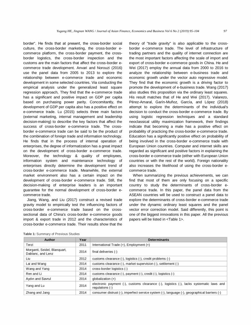
Table 1: Summary of Previous Studies
Author Year Determinants
Terzi 2011 International Trade (+), Employment (+)
Morganti, Seidel, Blanquart,
Dablanc, and Lenz 2014 final deliveries (-)
Liu 2012 customs clearance (-), logistics (-), credit problems (-)
Lai and Wang 2014 customs clearance (-), market supervision (-), settlement (-)
Wang and Yang 2014 cross-border logistics (-)
Ren and Li 2014 customs clearance (-), payment (-), credit (-), logistics (-)
Aydın and Savrul 2014 globalization (+)
Yang and Lu 2014 electronic payment (-), customs clearance (-), logistics (-), lacks systematic laws and regulations (-)
Zhang and Jang 2014 consumer distrust (-), imperfect service system (-), language (-), geographical barriers (-)
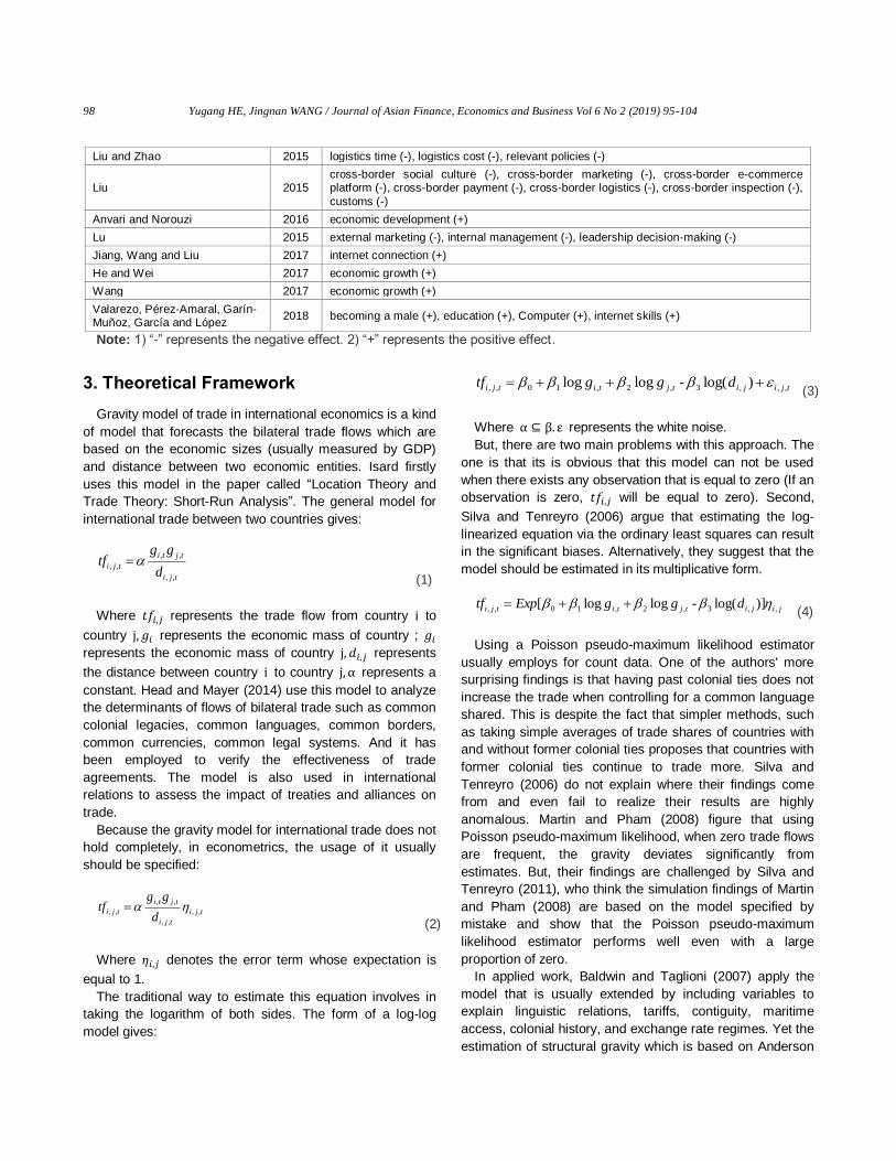
98 Yugang HE, Jingnan WANG / Journal of Asian Finance, Economics and Business Vol 6 No 2 (2019) 95-104
Liu and Zhao 2015 logistics time (-), logistics cost (-), relevant policies (-)
Liu 2015 cross-border social culture (-), cross-border marketing (-), cross-border e-commerce platform (-), cross-border payment (-), cross-border logistics (-), cross-border inspection (-),
customs (-)
Anvari and Norouzi 2016 economic development (+)
Lu 2015 external marketing (-), internal management (-), leadership decision-making (-)
Jiang, Wang and Liu 2017 internet connection (+)
He and Wei 2017 economic growth (+)
Wang 2017 economic growth (+)
Valarezo, Pérez-Amaral, Garín-Muñoz, García and López
2018 becoming a male (+), education (+), Computer (+), internet skills (+)
Note: 1) “-” represents the negative effect. 2) “+” represents the positive effect.
3. Theoretical Framework
Gravity model of trade in international economics is a kind
of model that forecasts the bilateral trade flows which are
based on the economic sizes (usually measured by GDP)
and distance between two economic entities. Isard firstly
uses this model in the paper called “Location Theory and
Trade Theory: Short-Run Analysis”. The general model for
international trade between two countries gives:
tji
tjti
tjid
ggtf
,,
,,
,, =
(1)
Where 𝑡𝑓𝑖,𝑗 represents the trade flow from country i to
country j, 𝑔𝑖 represents the economic mass of country ; 𝑔𝑖
represents the economic mass of country j, 𝑑𝑖,𝑗 represents
the distance between country i to country j, α represents a
constant. Head and Mayer (2014) use this model to analyze
the determinants of flows of bilateral trade such as common
colonial legacies, common languages, common borders,
common currencies, common legal systems. And it has
been employed to verify the effectiveness of trade
agreements. The model is also used in international
relations to assess the impact of treaties and alliances on
trade.
Because the gravity model for international trade does not
hold completely, in econometrics, the usage of it usually
should be specified:
tji
tji
tjti
tjid
ggtf ,,
,,
,,
,, =
(2)
Where 𝜂𝑖,𝑗 denotes the error term whose expectation is
equal to 1.
The traditional way to estimate this equation involves in
taking the logarithm of both sides. The form of a log-log
model gives:
tjijitjtitji dggtf ,,,3,2,10,, )log(-loglog +++= (3)
Where α ⊆ β. ε represents the white noise.
But, there are two main problems with this approach. The
one is that its is obvious that this model can not be used
when there exists any observation that is equal to zero (If an
observation is zero, 𝑡𝑓𝑖,𝑗 will be equal to zero). Second,
Silva and Tenreyro (2006) argue that estimating the log-
linearized equation via the ordinary least squares can result
in the significant biases. Alternatively, they suggest that the
model should be estimated in its multiplicative form.
jijitjtitji dggExptf ,,3,2,10,, )]log(-loglog[ ++= (4)
Using a Poisson pseudo-maximum likelihood estimator
usually employs for count data. One of the authors' more
surprising findings is that having past colonial ties does not
increase the trade when controlling for a common language
shared. This is despite the fact that simpler methods, such
as taking simple averages of trade shares of countries with
and without former colonial ties proposes that countries with
former colonial ties continue to trade more. Silva and
Tenreyro (2006) do not explain where their findings come
from and even fail to realize their results are highly
anomalous. Martin and Pham (2008) figure that using
Poisson pseudo-maximum likelihood, when zero trade flows
are frequent, the gravity deviates significantly from
estimates. But, their findings are challenged by Silva and
Tenreyro (2011), who think the simulation findings of Martin
and Pham (2008) are based on the model specified by
mistake and show that the Poisson pseudo-maximum
likelihood estimator performs well even with a large
proportion of zero.
In applied work, Baldwin and Taglioni (2007) apply the
model that is usually extended by including variables to
explain linguistic relations, tariffs, contiguity, maritime
access, colonial history, and exchange rate regimes. Yet the
estimation of structural gravity which is based on Anderson

Yugang HE, Jingnan WANG / Journal of Asian Finance, Economics and Business Vol 6 No 2 (2019) 95-104 99
and van winkle (2003), and requires the inclusion of fixed
effects on importers and exporters, thereby limiting the
gravity analysis of bilateral trade costs.
In this paper, GDP will be introduced to the gravity model.
Due to the characteristics of cross-border e-commerce trade
(population of a country represents the potential consumers
in the e-commerce market), the population is also
introduced to the gravity model. The real change rate also
affects the cross-border e-commerce trade. In therms of
domestic country, an increase in the real exchange rate will
lead to a decrease in the cross-border e-commerce import
due to depreciation of domestic currency. Conversely, an
increase in the real exchange rate will lead to an increase in
the cross-border e-commerce export due to depreciation of
domestic currency. Therefore, the real exchange rate will be
introduced into the gravity model. The terms of trade (ratio
of export price index to the import price index) also affect
the cross-border e-commerce trade. If the export price index
increase, the cross-border e-commerce export will decrease.
On the contrary, if the import price index increase the cross-
border e-commerce import will also decrease. So, the terms
of trade will be introduced into the gravity model.
Allayarov, Mehmed, Arefin, and Nurmatov (2018) and
Zebua (2016) apply the gravity model to discuss the export
and import. Based on their achievements, the export and
import of cross-border e-commerce of gravity model, namely,
the revised gravity model in this paper gives:
textjitjitititji totrerpopgdpex ,,,4,,3,2,10,, logloglogloglog +++++=
(5)
timtjitjitititji totrerpopgdpim ,,,4,,3,2,10,, logloglogloglog +++++=
(6)
Where 𝑒𝑥𝑖,𝑗 represents the volume of export of cross-
border e-commerce goods from country i to country j, 𝑖𝑚𝑖,𝑗
represents the volume of import of cross-border e-
commerce goods from country i to country j . 𝑔𝑑𝑝𝑖
represents the gross domestic productivity of country i, 𝑝𝑜𝑝𝑖
represents the population of country i. tot represents the
terms of trade (ratio of domestic export price index to foreign
export price index). 𝜀𝑒𝑥 and 𝜀𝑖𝑚 represents the white noise.
4. Estimation Model
4.1. Variable Description
This paper uses the panel data to explore the
relationship between cross-border e-commerce trade
and relevant variables. There are six variables in this
paper, including the cross-border e-commerce export,
the cross-border e-commerce import, the GDP, the
population, the terms of trade and the real exchange rate.
The cross-border e-commerce export and the cross-
border e-commerce import are treated as the dependent
variables. The GDP, the population, the terms of trade
and the real exchange rate are treated as the
independent variables. All the data used in this paper are
soured from UNCTAD, World Bank, National Bureau of
Statistics of China and Research Report on China's
Cross-border E-Commerce Market in 2017. Meanwhile,
all these data are logged so as to remove the outlires
and the heteroscedasticity. All variables will be shown in
<Table 2>.
Table 2: Variables
Variable Type Log form Definition
Dependent
Variable exlog
cross-border e-commerce export
(from China to each ASEAN country)
Dependent
Variable imlog
cross-border e-commerce import
(from each ASEAN country to China)
Independent
Variable gdplog GDP
Independent
Variable poplog population (each ASEAN country)
Independent
Variable totlog
terms of trade (each ASEAN country
in terms of China)
Independent
Variable rerlog
real exchange rate (each ASEAN
country in terms of RMB)
4.2. Panel Unit Root Test
The panel unit root test has a variety of test statistics
which mainly depend on the heterogeneity of each group
and the asymptotic characteristics of each group and time-
series data as well as the balanced or unbalanced panel.
Therefore, we should confirm what kinds of test statistics will
be used in this paper before conducting the panel data.
Essentially, the panel unit root test is the same as the Dicky-
Fuller test of time series. Namely, tiitititi zyy ,,1,, ++= −
is tested with a size hypothesis (null hypothesis: 𝐻0) that
ϕ = 0 for all i. In order to solve the sequence correlation
problem of intrinsic error terms, Levin-Lin-Chu (2002) tests
the size hypothesis that the lag dependent variables and all
panel groups have a unit root (LLC). The model gives:
=
−− +++=p
j
tjtijiitititi yzyy1
,,,1,,
(7)
100 Yugang HE, Jingnan WANG / Journal of Asian Finance, Economics and Business Vol 6 No 2 (2019) 95-104
LLC test assumes that the autoregressive parameters of
all panel groups are the same (𝜙𝑖 = 0), and the optimal time
lag (p) uses the time lag which obeys the minimization of
standard information (Harris & Tzavalis, 1999) test is based
on the ordinary least squares’ statistics ϕ of
titititi zyy ++= − ,1,, . It is assumed that the intrinsic
error term 𝜀𝑖,𝑡 has the same normal distribution with
independent and uniformed distribution of group-specific
constants. It is similar to the LLC test in that it has the same
parameters between panel groups to test the null hypothesis
(𝐻0: ϕ = 0). Breitung (2000) tests its own lag estimates as
explanatory variables, calculates test errors before
calculating test statistics, and then calculates test statistics.
Im-Persarm-Shin (2003) also conducts an estimation on the
panel unit root test. The model gives:
titititi Zyy ,,1,, ++= − (8)
This test is different from LLC test. It assumes that each
group (i) has different 𝜙𝑖. And for all i, 𝜙𝑖 is equal to zero
[The IPS test differs from the LLC test assuming that the
inherent error term for each panel group has this variance
(𝜎𝑖)]. Considering the cultural and institutional differences
among the panel groups, the IPS test is a more realistic
assumption (In the Fisher-type test, the unit root is tested
using equation (8) for panel group, and p is calculated. Then,
the equation p = −2 ∑ log 𝑝𝑖𝑛𝑖=1 is calculated, which follows
the 𝑋2(2𝑛) distribution and rejects the null hypothesis that
the panel unit root exists as the p value increases. Choi
(2001) and Hadri's (2000) LM test tests the null hypothesis
that panel data is stable, unlike other tests). Said differently,
the IPS test estimates the equation (8) for each panel group
and calculates the statistic by averaging t values, while the
LLC test calculates the statistics after pooling the index to
estimate a pooling regression model for equation (7). The
results of panel unit root test show in <Table 3>.
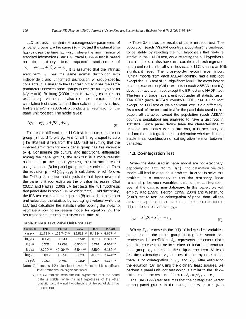
Table 3: Results of Panel Unit Root Test
Variable IPS Fisher LLC BR HADRI
poplog -11.789*** 123.747*** -12.518*** -5.482*** 5.697***
rerlog -0.176 1.239 -1.550* -0.531 6.867***
imlog 3.531 17.897 -6.053*** 3.201 4.964***
exlog -2.322*** 40.094*** -6.544*** 3.500 6.182***
totlog 0.035 18.796 7.023 -0.922 7.424***
gdolog 2.162 9.705 -1.293* 2.334 4.664***
Note: 1) * means 10% significant level, **means 5% significant
level, ***means 1% significant level.
2) HADRI statistic tests the null hypothesis that the panel
data is stable, while the null hypothesis of the other
statistic tests the null hypothesis that the panel data has
the unit root.
<Table 3> shows the results of panel unit root test. The
population (each ASEAN country’s population) is analyzed
to be stable by rejecting the null hypothesis that "data is
stable" in the HADRI test, while rejecting the null hypothesis
that all other statistics have unit root. the real exchange rate
has a unit root under all statistics except LLC statistic at 10%
significant level. The cross-border e-commerce import
(China imports from each ASEAN country) has a unit root
except the LLC test at 1% significant level. The cross-border
e-commerce export (China exports to each ASEAN country)
does not have a unit root except the BR test and HADRI test.
The terms of trade have a unit root under all statistic tests.
The GDP (each ASEAN country’s GDP) has a unit root
except the LLC test at 1% significant level. Said differently,
As a result of the unit root test for the panel data used in this
paper, all variables except the population (each ASEAN
country’s population) are analyzed to have a unit root in
statistics. Since panel datum have the characteristics of
unstable time series with a unit root, it is necessary to
perform the cointegration test to determine whether there is
stable linear combination or cointegration relation between
variables.
4.3. Co-integration Test
When the data used in panel model are non-stationary,
especially the first integral [I(1)], the estimation via this
model will lead to a spurious problem. In order to solve this
problem, it is necessary to test the stationary linear
relationship between variables, that is, the cointegration,
even if the data is non-stationary. In this paper, we will
employ Kao (1999), Pedroni (1999, 2004) and Westerlund
(2007) test to test the cointegration of panel data. All the
above test approaches are based on the panel model for the
I(1) of dependent variable 𝑦𝑖,𝑡.
tiitiititi ZXy ,,,, ++= (9)
Where 𝑋𝑖,𝑡 represents the I(1) of independent variables.
𝛽𝑖 represents the panel group conitegrated vector. 𝛾𝑖 .
represents the coefficient. 𝑍𝑖,𝑡 represents the deterministic
variable representing the fixed effect or linear time trend for
each group. 𝜀𝑖,𝑡 represents the unique error term. All tests
test the stationarity of 𝜀𝑖,𝑡 and test the null hypothesis that
there is no cointegration in 𝑦𝑖,𝑡 and 𝑋𝑖,𝑡 . After estimating
the equation (16) by using the ordinary least squares, we
perform a panel unit root test which is similar to the Dicky-
Fuller test for the residual of formula 𝜀�̂�,𝑡 = 𝜌𝜀�̂�,𝑡−1 + 𝜈𝑖,𝑡.
The Kao (1999) test assumes that the cointegrated vector
among panel groups is the same, namely, 𝛽𝑖 = 𝛽 (Kao

Yugang HE, Jingnan WANG / Journal of Asian Finance, Economics and Business Vol 6 No 2 (2019) 95-104 101
(1999) test takes into account the fixed effects of each
group but does not include time trends). Therefore, it is
assumed that the estimated coefficients of the residual
equations are all the same, namely, 𝜌𝑖 = 𝜌 . This test
presents modified DF, DF and ADF statistics, and estimated
coefficient ρ is estimated by using the Dicky-Fuller and
Augmented Dicky-Fuller regression method. The Pedroni
(1999, 2004) test is different from the Kao test, which
assumes that all panel groups have the same cointegrated
vector, and assumes that the panel groups have different
cointegrated vectors. It is also assumed that the AR (1) of
the residual term is also different for each panel group. The
Westerlund (2007) test uses different cointegrated vectors
and AR (1), and the variance ratio (VR) statistic is presented
to test the null hypothesis and some panel groups are
cointegrated (This test also tests the hypothesis that all
panel groups are cointegrated under the assumption of 𝜌𝑖 =
𝜌).
Table 4: Results of Cointegration Test
Equation Kao
statistic
Pedroni
Statistic
Westerlund
Statistic
(5) -11.619*** -8.142*** -2.778***
(6) -2.700*** -2.001*** -1.387*
Note: 1) * means 10% significant level, **means 5% significant
level, ***means 1% significant level.
<Table 4> shows the results of cointegration tests by Kao
(1999), Pedroni (1999, 2004) and Westerlund (2007),
respectively. As a result of the cointegration test for
equation (5), the null hypothesis is rejected at 1% significant
level in all statistics. Meanwhile, the test for equation (6)
also rejected the null hypothesis at the 1% or 10%
significance level in all statistics. These results suggest that
almost all variables (cross-border e-commerce export,
cross-border e-commerce import, real exchange rate, GDP,
population and ters of trade) have unit roots. So even if they
are non-stationary, the long-run stable linear relationship
(cointegration relation) exists.
4.4. Results
In order to quantitatively analyze the determinants of
cross-border e-commerce trade, equation (5) and equation
(6) will be estimated under the dynamic ordinary least
squares produced by Pedroni (1999, 2004) and Kao and
Chiang (1999), and estimated under the error correction
model including the cointegrated vector term of Westerlund
(2007) [Kao and Chiang (1997) analyze OLS, FMOLS, and
DOLS models using Monte Carlo simulation when panel
data are cointegrated. The OLS and FMOLS estimates are
not improved, but the DOLS estimates improve significantly].
The dynamic ordinary least squares model of Pedroni and
Kao and Chiang gives:
−=
− +++=p
pj
tijtititiiiti xxy ,,,,,
(10)
Where 𝛽𝑖 represents the estimated slope. 𝑥𝑖,𝑡 represents
the explanatory variables. ρ represents the past and
preceding time difference. In order to solve the
autocorrelation of inherent error and endogeneity among
variables. All these problems include in equation (10).
<Table 5> shows the results of dynamic ordinary least
squares.
Table 5: Results of Dynamic Ordiary Least Squares’ Estimation
Equation Explained
Variable
Explanatory
Variable
DOLS Statistic
(Pedroni)
DOLS Statistic (Kao and
Chiang)
(5) exlog
gdplog 1.730***
0.484*** (0.094)
poplog 1.135***
0.020 (0.141)
totlog
1.846*** -0.121
rerlog -0.572*** -0.080*** (0.014)
Equation Explained
Variable
Explanatory
Variable
DOLS
Statistic (Pedroni)
DOLS Statistic
(Kao and Chiang)
(6) imlog
gdplog 1.775***
0.282***
(0.021)
poplog 1.207***
0.334** (0.075)
totlog -2.045***
0.036 (0.145)
rerlog 0.629***
0.086
(0.051)
Note: 1) * means 10% significant level, **means 5% significant
level, ***means 1% significant level. ( ) means the
standard error.
As <Table 5> shows, the two approaches show that the
GDP, the population, the terms of trade have a positive
effect on cross-border e-commerce export and the real
exchange rate has a negative effect on cross-border e-
commerce export. Said differently, the GDP increases by 1%
will lead to 1.730% (Pedroni) and 0.484% (Kao-Chiang)
increase in the cross-border e-commerce export. The
population increases by 1% will lead to 1.135% increase in
the cross-border e-commerce export, but not significant in
Kao-Chiang approach. The terms of trade increases by 1%
will lead to 1.846% increase in the cross-border e-
commerce export, but not significant in Kao-Chiang
approach. The real exchange rate increase by 1% will lead
to 0.572% (Pedroni) and 0.080% (Kao-Chiang) decrease in
the cross-border e-commerce export. As for the cross-

102 Yugang HE, Jingnan WANG / Journal of Asian Finance, Economics and Business Vol 6 No 2 (2019) 95-104
border e-commerce import, the GDP, the population, the
real exchange rate have a positive effect on cross-border e-
commerce import and the terms of trade has a negative
effect on cross-border e-commerce import. Said differently,
the GDP increases by 1% will lead to 1.775% (Pedroni) and
0.282% (Kao-Chiang) increase in the e-commerce import.
The population increases by 1% will lead to 1.207%
(Pedroni) and 0.334% (Kao-Chiang) increase in the cross-
border e-commerce import, but not significant in Kao-Chiang
approach. The terms of trade increases by 1% will lead to
1.846% decrease in the cross-border e-commerce import,
but not significant in Kao-Chiang approach. The real
exchange rate increase by 1% will lead to 0.629% increase
in the cross-border e-commerce import, but not significant in
Kao-Chiang approach.
In order to obtain the robustness of estimated results,
equation (5) and equation (6) will be separately estimated
by using the error correction model (ECM) including the
cointegration vector term. The general equation for the ECM
model gives:
= =
−−− +++−+=p
j
p
j
tijtijijtijitiitiititi xyxydy1 1
,,,,,1,,, )(
(11)
Where 𝑑𝑖 represents the time trend and constant. 𝛽𝑖
represents the adjusted coefficient that measures the rate
at which the cointegrated vector converges back to
equilibrium when it deviates from long-term equilibrium.
represents the cointegrated vector. 𝜃𝑖,𝑗 and 𝜇𝑖,𝑗 represents
the coefficients of differencing terms. In this paper, the
model is estimated by two methods. The first one is the
dynamic fixed effect model considering heterogeneous
effects between panel groups. Another is the error
correction model that Westerlund (2007) applies. The
results show in <Table 6>.
Table 6: Results of Error Correction Estimation
Equation Explained Variable
Explanatory Variable
Dynamic Fixed
Effect
Westerlund Error Correct
Model
(5) exlog
Long-run Equilibrium
gdplog 1.498*** (0.057)
1.366*** (0.054)
Long-run Equilibrium
poplog 0.025 (0.068)
0.147 (0.166)
Long-run Equilibrium
totlog 0.033 (0.089)
0.060 (0.118)
Long-run Equilibrium
rerlog -0.209* (0.117)
-0.209* (0.106)
Adjusted
Coefficient
1.009***
(0.009)
0.502***
(0.042)
exlog 0.082*** (0.012)
0.091* (0.058)
gdplog 0.672** (0.324)
0.066 (0.442)
poplog 0.176***
(0.077)
0.120
(0.144)
totlog 0.278** (0.096)
0.133* (0.085)
rerlog 0.106* -(0.064)
-0.162 (0.153)
(6) imlog
Long-run Equilibrium
gdplog
1.108*** (0.044)
1.026** (0.383)
Long-run Equilibrium
poplog
0.151*** (0.052)
0.931** (0.461)
Long-run
Equilibrium
totlog
-0.165***
(0.068)
-2.717***
(0.826)
Long-run Equilibrium
rerlog
0.321*** (0.090)
2.717*** (0.831)
Adjusted Coefficient
0.976*** (0.007)
1.768*** (0.034)
imlog 0.247* (0.103))
0.133 (0.093)
gdplog 0.229***
(0.049)
0.401**
(0.184)
poplog 0.160*** (0.027)
0.762*** (0.158)
totlog -0.089** (0.034)
-0.036 (0.036)
rerlog 0.130**
(0.042)
0.029
(0.058)
Note: 1) * means 10% significant level, **means 5% significant
level, ***means 1% significant level. ( ) means the
standard error.
<Table 6> shows the estimated results of the two
approaches. When taking long-run relation (cointegrated
vector)about the equation (5) into consideration, we can
obtain the predicted direction (+) of population and the
terms of trade on cross-border e-commerce export, but not
significant. This is in contrast to the estimated result of the
dynamic ordinary least squares model. Concomitantly, an
increase in the economic growth can increase the cross-
border e-commerce export (1% significant in statistics). In
contrast, a depreciation of domestic currency (an increase in
the real exchange rate) will lead to an increase in the cross-
border e-commerce export (10% significant in statistics).
Meanwhile, The adjusted coefficients that indicate the
adjustment speed to the equilibrium are 1.009 and 0.502,
respectively, and when they deviate from the long term
equilibrium, they will converge to the equilibrium through
correcting the error. According to the different models, the
dynamic fixed effect model is analyzed to be converged
about two times faster than that of Westerlund error correct
model and statistically significant. As for the equation (6), An
increase in the GDP, the population and the real exchange
rate will increase in the cross-border e-commerce import.
Yugang HE, Jingnan WANG / Journal of Asian Finance, Economics and Business Vol 6 No 2 (2019) 95-104 103
Oppositely, an increase in the terms of trade will decrease in
the cross-border e-commerce import. Said differently, these
results are consistent with the theory in the dynamic fixed
effect model. Meanwhile, the adjusted coefficients are
significant in statistics. But, the convergence speed of
Westerlund error correct model (1.768) is two time faster
than that of dynamic fixed effect (0.976).
5. Conclusion
This paper sets ASEAN 10 countries as an example to
explore the determinants of cross-border e-commerce trade.
The panel data from the year of 1998 to 2016 are employed
to conduct a series of such as the panel unit root test and
the cointegration test. Concomitantly, the dynamic ordinary
least squares model and the error corretion model are also
used to estimate the long-run equilibrium relation between
cross-border e-commerce trade (cross-border e-commerce
export & cross-border e-commerce import) and relevant
variables (GDP, population, terms of trade and real
exchange rate). Especially, this paper divides the cross-
border e-commerce trade into two sectors. One is the cross-
border e-commerce export. Another is the cross-border e-
commerce import. This treatment is a novel way to display
how the relevant variables affect the cross-border e-
commerce trade more clearly. Of course, this kind of
process is an innovation that can distinguish from other
documents. This paper uses a various approaches such as
IPS, Fisher, LLC, BR and HADRI to conduct the panel unit
root test. Its results show that except the population, the rest
has a unit root. Namely, they are non-stationary. We also
apply a lot of approaches such as Kao, Pedroni, and
Westerlound to perform the cointegration test among cross-
border e-commerce export, cross-border e-commerce
import, GDP, population, terms of trade and real exchange
rate. Its results show that there is a long-run relationship
among them. Meanwhile, the dynamic ordinary least
squares and error correction model are adopted to estimate
the long-run equilibrium relationship among cross-border e-
commerce export, cross-border e-commerce import, GDP,
population, terms of trade and real exchange rate. Their
results show that the GDP, the population and the terms of
trade play a positive role in promoting the cross-border e-
commerce trade. Unfortunately, the population and the
terms of trade do not get through the significant test. At the
same time, the real exchange rate pose a negative effect on
cross-border e-commerce export, but only significant at 10%.
In terms of cross-border e-commerce import, the GDP, the
population and the real exchange rate have a positive effect
on cross-border e-commerce import. On the contrary, the
terms of trade has a negative effect on cross-border e-
commerce import.
In summary, the economic growth is a powerful to drive
the development of cross-border e-commerce trade. Still,
there are a lot of limitations in this paper. some other factors
such as social system, cultural system or something else
may affect the cross-border e-commerce trade. Due to that
it is hard to find out a proper index to measure them, the
models used in this paper do not include them. This
behavior may lead to an overestimation. Another significant
limitation is that the theoretical framework is based on
gravity model. because the distance between two country is
a constant, it can not be differenced (If it is differenced, the
value of it will be zero.). It also does not participate in our
estimation.
References
Anderson, J. E., & Van Wincoop, E. (2003). Gravity with
gravitas: A solution to the border puzzle. American
economic review, 93(1), 170-192.
Anvari, R. D., & Norouzi, D. (2016). The impact of e-
commerce and R&D on economic development in some
selected countries. Procedia-Social and Behavioral
Sciences, 229(2016), 354-362.
https://doi.org/10.1016/j.sbspro.2016.07.146
Allayarov, P., Mehmed, B., Arefin, S., & Nurmatov, N.
(2018). The Factors Affecting Kyrgyzstan’s Bilateral Trade:
A Gravity-model Approach. The Journal of Asian Finance,
Economics and Business, 5(4), 95-100.
Aydın, E., & Savrul, B. K. (2014). The relationship between
globalization and e-commerce: Turkish case. Procedia-
Social and Behavioral Sciences, 150(2014), 1267-1276.
https://doi.org/10.1016/j.sbspro.2014.09.143
Baldwin, R., & Taglioni, D. (2007). Trade effects of the euro:
A comparison of estimators. Journal of Economic
Integration, 22(4), 780-818.
Blum, B. S., & Goldfarb, A. (2006). Does the internet defy
the law of gravity? Journal of international economics,
70(2), 384-405.
Choi, I. (2001). Unit root tests for panel data. Journal of
international money and Finance, 20(2), 249-272.
Gomez-Herrera, E., Martens, B., & Turlea, G. (2014). The
drivers and impediments for cross-border e-commerce in
the EU. Information Economics and Policy, 28(2014), 83-
96. https://doi.org/10.1016/j.infoecopol.2014.05.002
Harris, R. D., & Tzavalis, E. (1999). Inference for unit roots
in dynamic panels where the time dimension is fixed.
Journal of Econometrics, 91(2), 201-226.
Hadri, K. (2000). Testing for stationarity in heterogeneous
panel data. The Econometrics Journal, 3(2), 148-161.
104 Yugang HE, Jingnan WANG / Journal of Asian Finance, Economics and Business Vol 6 No 2 (2019) 95-104
Head, K., & Mayer, T. (2014). Gravity equations: Workhorse,
toolkit, and cookbook. In Handbook of international
economics, 4(2014), 131-195.
https://doi.org/10.1016/B978-0-444-54314-1.00003-3
He, Y., & Wei, W. (2017). An Empirical Study on the
Dynamic Interaction between E-Business and Economic
Growth In China. The e-Business Studies, 18(5), 37-49.
Jiang, B., Wang, Z., & Liu, J. (2017). Empirical test of trade
gravity model in cross-border e-commerce in China.
Journal of Commercial Economics, 24(10), 32-34.
Kao, C. (1999). Spurious regression and residual-based
tests for cointegration in panel data. Journal of
Econometrics, 90(1), 1-44.
Kao, C., & Chiang, M. H. (1997). On the estimation and
inference of a cointegrated regression in panel data. In B.
H. Baltagi, Nonstationary panels, panel cointegration, and
dynamic panels (pp. 179-222). Bingley, England: Emerald
Group Publishing Limited. Retrieved from https://ssrn.com/
abstract=2379 or http://dx.doi.org/10.2139/ssrn.2379
Kwon, S. W., Kim, Y. E., Yoon, M. K., & Jeon, T. S. (2010).
The Relationship between MRO E-Commerce System and
Purchase Effects. Journal of Distribution Science, 8(3), 11.
Lai, Y. W., & Wang, K. Q. (2014). China’s Cross-border E-
commerce Development Patterns, Barriers and the Next
Step. Reform, 12(5), 68-74.
Liu, J. (2012). The Rise and Development of Small Cross-
border Trade in E-commerce: The Innovation of E-
commerce and Logistics Service in the Post Financial
Crisis Era. Practice in Foreign Economic Relations and
Trade, 12(2), 89-92.
Liu, X. B. (2015). Analysis on the "Cross-border" Influencing
Factors of Cross-border E-commerce Development in
China. Journal of Lanzhou Institute of Education, 6(2), 44-
45.
Liu, Z. K., & Zhao, S. S. (2015). Factors Affecting the
Development of Cross-border Electricity Supplier Analysis
and Countermeasures. Journal of Asia Trade and
Business, 2(1), 25-33.
Lu, X. D. (2015). Research on the Influencing Factors of
Cross-border E-Commerce Development in the Big Data
Era. Economic & Trade, 12(6), 207-208.
Martin, W., & Pham, C. S. (2016). Estimating the Gravity
Model When Zero Trade Flows are Frequent and
Economically Determined (World Bank Policy Research
Working Paper No. 7308). Retrieved from
https://ssrn.com/abstract=2619473
Morganti, E., Seidel, S., Blanquart, C., Dablanc, L., & Lenz,
B. (2014). The impact of e-commerce on final deliveries:
alternative parcel delivery services in France and
Germany. Transportation Research Procedia, 4(2014),
178-190. https://doi.org/10.1016/j.trpro.2014.11.014
Ren, Z. X., & Li, W. X. (2014). The Strategy of China’s
Cross-border E-commerce to Boost the Transformation
and Upgrading of Foreign Trade. Practice in Foreign
Economic Relations and Trade, 12(4), 25-28.
Silva, J. S., & Tenreyro, S. (2006). The log of gravity. The
Review of Economics and statistics, 88(4), 641-658.
Terzi, N. (2011). The impact of e-commerce on international
trade and employment. Procedia-Social and Behavioral
Sciences, 24(2011), 745-753.
https://doi.org/10.1016/j.sbspro.2011.09.010
Valarezo, Á ., Pérez-Amaral, T., Garín-Muñoz, T., García, I.
H., & López, R. (2018). Drivers and barriers to cross-
border e-commerce: Evidence from Spanish individual
behavior. Telecommunications Policy, 42(6), 464-473.
Wang, L., & Yang, J. Z. (2014). An Empirical Study on the
Influencing Factors of the Demand of Cross-border E-
commerce Rules. Contemporary Economic &
Management, 24(9), 18-23.
Wang, Q. Y. (2017). An Empirical Analysis of the
Relationship between Cross-border E-commerce and
Economic Growth in China. Market Modernization, 24(3),
48-50.
Yang, J. Z., & Lu, Y. (2014). Analysis on the Application of
Cross-border E-commerce in China’s Foreign Trade
Enterprises. Contemporary Economic & Management,
24(17), 18-23.
Zhang, J. Q., & Jang, F. J. (2014). Problems and
Development Countermeasures of Cross Border E-
commerce. Business Economy, 24(17), 55-58.
Zebua, H. I. (2016). Determinants of Bilateral Foreign Direct
Investment Intra-ASEAN: Panel Gravity Model. The East
Asian Journal of Business Management, 6(1), 19-24.