a package to embed chemistry in astrophysical simulations
34
MNRAS 439, 2386–2419 (2014) doi:10.1093/mnras/stu114 Advance Access publication 2014 February 19 KROME – a package to embed chemistry in astrophysical simulations T. Grassi, 1‹ S. Bovino, 2 D. R. G. Schleicher, 2 J. Prieto, 3 D. Seifried, 4 E. Simoncini 5 and F. A. Gianturco 1 , 6 , 7 1 Department of Chemistry, Sapienza University of Rome, P.le A. Moro 5, I-00185 Roma, Italy 2 Institut f ¨ ur Astrophysik, Georg-August-Universit¨ at, Friedrich-Hund Platz 1, D-37077 G¨ ottingen, Germany 3 ICC, University of Barcelona (IEEC-UB), Marti i Franques 1, E-08028 Barcelona, Spain 4 Hamburger Sternwarte, Universit¨ at Hamburg, Gojenbergsweg 112, D-21029 Hamburg, Germany 5 INAF-Arcetri Astrophysical Observatory, Largo Enrico Fermi 5, I-50125Firenze, Italy 6 Institute of Ion Physics and Applied Physics, University of Innsbruck, Technikerstrasse 25, A-6020 Innsbruck, Austria 7 Scuola Normale Superiore, Piazza dei Cavalieri, 7 I-56126 Pisa, Italy Accepted 2014 January 14. Received 2013 December 23; in original form 2013 November 5 ABSTRACT Chemistry plays a key role in many astrophysical situations regulating the cooling and the thermal properties of the gas, which are relevant during gravitational collapse, the evolution of discs and the fragmentation process. In order to simplify the usage of chemical networks in large numerical simulations, we present the chemistry package KROME, consisting of a PYTHON pre-processor which generates a subroutine for the solution of chemical networks which can be embedded in any numerical code. For the solution of the rate equations, we make use of the high-order solver DLSODES, which was shown to be both accurate and efficient for sparse networks, which are typical in astrophysical applications. KROME also provides a large set of physical processes connected to chemistry, including photochemistry, cooling, heating, dust treatment and reverse kinetics. The package presented here already contains a network for primordial chemistry, a small metal network appropriate for the modelling of low metallicities environments, a detailed network for the modelling of molecular clouds, a network for planetary atmospheres, as well as a framework for the modelling of the dust grain population. In this paper, we present an extended test suite ranging from one-zone and 1D models to first applications including cosmological simulations with ENZO and RAMSES and 3D collapse simulations with the FLASH code. The package presented here is publicly available at http://kromepackage.org/ and https://bitbucket.org/krome/krome_stable. Key words: astrochemistry – methods: numerical – ISM: evolution – ISM: molecules. 1 INTRODUCTION Chemistry plays a central role in many astrophysical environ- ments, including the formation of stars at low and high metal- licities (Omukai et al. 2005; Glover & Jappsen 2007), the inter- stellar medium (ISM; Hollenbach & McKee 1979; Wakelam et al. 2010), starbursts and active galactic nuclei (Maloney, Hollenbach & Tielens 1996; Meijerink & Spaans 2005), protoplanetary discs (Semenov, Wiebe & Henning 2004; Woitke, Kamp & Thi 2009), planetary atmospheres (Burrows & Sharp 1999; Lodders & Feg- ley 2002) and the early Universe (Dalgarno & Lepp 1987; Galli & Palla 1998; Stancil, Lepp & Dalgarno 1998; Schleicher et al. 2008). It is important as it regulates the cooling, therefore influ- encing gravitational collapse (Yahil 1983; Peters et al. 2012), disc stability (Lodato 2007) and fragmentation (Li, Klessen & Mac Low E-mail: [email protected] 2003). At the same time, the chemical abundances regulate the ap- pearance of astrophysical objects by influencing the line emission from atoms, ions and molecules. Both for an accurate modelling and to pursue a comparison with observations, it is thus necessary to include chemical models in numerical simulations. The required machinery is however complex for at least two rea- sons: (i) chemical kinetics has a non-negligible computational cost, which can be prohibitive for large numerical simulations even after a complexity reduction, as described by Grassi et al. (2012). It there- fore requires a sophisticated framework where the rate equations are efficiently solved. Moreover, (ii) building the set of ordinary differ- ential equations (ODEs) associated with a given chemical network (including the Jacobian and its sparsity structure for efficient eval- uation) can be difficult, especially when the number of reactions involved is large (150, up to more than 6000). As the latter presents an important problem, there are a number of attempts to make the incorporation of chemical networks in astro- physical simulations more feasible. For instance, XDELOAD performs C 2014 The Authors Published by Oxford University Press on behalf of the Royal Astronomical Society at Royal Library/Copenhagen University Library on June 13, 2014 http://mnras.oxfordjournals.org/ Downloaded from
-
Upload
khangminh22 -
Category
Documents
-
view
3 -
download
0
Transcript of a package to embed chemistry in astrophysical simulations

MNRAS 439, 2386–2419 (2014) doi:10.1093/mnras/stu114Advance Access publication 2014 February 19
KROME – a package to embed chemistry in astrophysical simulations
T. Grassi,1‹ S. Bovino,2 D. R. G. Schleicher,2 J. Prieto,3 D. Seifried,4 E. Simoncini5
and F. A. Gianturco1,6,7
1Department of Chemistry, Sapienza University of Rome, P.le A. Moro 5, I-00185 Roma, Italy2Institut fur Astrophysik, Georg-August-Universitat, Friedrich-Hund Platz 1, D-37077 Gottingen, Germany3ICC, University of Barcelona (IEEC-UB), Marti i Franques 1, E-08028 Barcelona, Spain4Hamburger Sternwarte, Universitat Hamburg, Gojenbergsweg 112, D-21029 Hamburg, Germany5INAF-Arcetri Astrophysical Observatory, Largo Enrico Fermi 5, I-50125 Firenze, Italy6Institute of Ion Physics and Applied Physics, University of Innsbruck, Technikerstrasse 25, A-6020 Innsbruck, Austria7Scuola Normale Superiore, Piazza dei Cavalieri, 7 I-56126 Pisa, Italy
Accepted 2014 January 14. Received 2013 December 23; in original form 2013 November 5
ABSTRACTChemistry plays a key role in many astrophysical situations regulating the cooling and thethermal properties of the gas, which are relevant during gravitational collapse, the evolutionof discs and the fragmentation process. In order to simplify the usage of chemical networksin large numerical simulations, we present the chemistry package KROME, consisting of aPYTHON pre-processor which generates a subroutine for the solution of chemical networkswhich can be embedded in any numerical code. For the solution of the rate equations, wemake use of the high-order solver DLSODES, which was shown to be both accurate and efficientfor sparse networks, which are typical in astrophysical applications. KROME also provides alarge set of physical processes connected to chemistry, including photochemistry, cooling,heating, dust treatment and reverse kinetics. The package presented here already contains anetwork for primordial chemistry, a small metal network appropriate for the modelling oflow metallicities environments, a detailed network for the modelling of molecular clouds, anetwork for planetary atmospheres, as well as a framework for the modelling of the dust grainpopulation. In this paper, we present an extended test suite ranging from one-zone and 1Dmodels to first applications including cosmological simulations with ENZO and RAMSES and 3Dcollapse simulations with the FLASH code. The package presented here is publicly available athttp://kromepackage.org/ and https://bitbucket.org/krome/krome_stable.
Key words: astrochemistry – methods: numerical – ISM: evolution – ISM: molecules.
1 IN T RO D U C T I O N
Chemistry plays a central role in many astrophysical environ-ments, including the formation of stars at low and high metal-licities (Omukai et al. 2005; Glover & Jappsen 2007), the inter-stellar medium (ISM; Hollenbach & McKee 1979; Wakelam et al.2010), starbursts and active galactic nuclei (Maloney, Hollenbach& Tielens 1996; Meijerink & Spaans 2005), protoplanetary discs(Semenov, Wiebe & Henning 2004; Woitke, Kamp & Thi 2009),planetary atmospheres (Burrows & Sharp 1999; Lodders & Feg-ley 2002) and the early Universe (Dalgarno & Lepp 1987; Galli& Palla 1998; Stancil, Lepp & Dalgarno 1998; Schleicher et al.2008). It is important as it regulates the cooling, therefore influ-encing gravitational collapse (Yahil 1983; Peters et al. 2012), discstability (Lodato 2007) and fragmentation (Li, Klessen & Mac Low
�E-mail: [email protected]
2003). At the same time, the chemical abundances regulate the ap-pearance of astrophysical objects by influencing the line emissionfrom atoms, ions and molecules. Both for an accurate modellingand to pursue a comparison with observations, it is thus necessaryto include chemical models in numerical simulations.
The required machinery is however complex for at least two rea-sons: (i) chemical kinetics has a non-negligible computational cost,which can be prohibitive for large numerical simulations even aftera complexity reduction, as described by Grassi et al. (2012). It there-fore requires a sophisticated framework where the rate equations areefficiently solved. Moreover, (ii) building the set of ordinary differ-ential equations (ODEs) associated with a given chemical network(including the Jacobian and its sparsity structure for efficient eval-uation) can be difficult, especially when the number of reactionsinvolved is large (�150, up to more than 6000).
As the latter presents an important problem, there are a number ofattempts to make the incorporation of chemical networks in astro-physical simulations more feasible. For instance, XDELOAD performs
C© 2014 The AuthorsPublished by Oxford University Press on behalf of the Royal Astronomical Society
at Royal L
ibrary/Copenhagen U
niversity Library on June 13, 2014
http://mnras.oxfordjournals.org/
Dow
nloaded from

KROME 2387
Table 1. List of the main processes for different environments. Note that this list is indicative and may depend on parameters otherthan temperature and density such as metallicity.
T(K) n(cm−3) Processes
HIM �3 × 10⁵ ∼0.004 Atomic coolingHII 104 0.3−104 Atomic and metal cooling, photoheatingWNM ∼5 × 10³ 0.6 Atomic and metal cooling, CR, photoheating, dust sputteringCNM ∼100 30 Metal and H2 cooling, dust growthDiff H2 ∼50 ∼100 H2 and metal coolingDense H2 10-50 1−106 CR and photoionization/dissociation, H2 and HD cooling, dust growthCold dense �102 106−1014 Dust cooling, photoheating, chemical heatingWarm collapsing ∼103 >1014 Chemical cooling, H2 cooling, chemical heating, CIE
a pre-processing task required for the modelling of astrochemical ki-netics, including the associated derivatives and the Jacobian (Nejad2005). The code is available on request, but currently not main-tained. ASTROCHEM is a network pre-processor that is based on theKinetic PreProcessor1 and is a proprietary code (Kumar & Fisher2013). Another code with a similar name is ASTROCHEM by Maret andaims at studying the evolution of the ISM. It allows to build the asso-ciated equations which can be employed within its own framework.This code can be forked on GitHub2, but a newer version has beenannounced in Maret, Bergin & Tafalla (2013). The same approachis followed by NAHOON3, calculating the chemical evolution of amolecular cloud with a pseudo time-dependent approach (Wakelamet al. 2012). The chemical network is created from on a data fileprovided by the user. Also this code can build the ODEs and theJacobian only within its framework. Finally, ALCHEMIC (Semenovet al. 2010) is a code optimized for the chemistry in protoplanetarydiscs employing the Differential Variable-coefficient ODE solverwith the Preconditioned Krylov method; this code is available onrequest by the authors. A recent tentative to provide a general pack-age has been made by extracting the ENZO chemistry module tocreate a sort of primordial chemistry library for astrophysical sim-ulations called GRACKLE4. Finally, the MEUDONPDR code5 (Le Petitet al. 2006) allows us to study the chemical evolution for a photon-dominated region (PDR) with an incident radiation field. This codeincludes some thermal processes and a default chemical network,in line with the PDR models.
However, not all of these codes are publicly available, and oftenthey are restricted to special purposes. An additional restriction isdue to the computational efficiency that can be achieved with a givenframework. While one-zone and even 1D calculations can still bepursued at a moderate efficiency, including even moderate-sizednetworks in 3D hydrodynamical simulations presents an additionalchallenge and requires the usage of optimized numerical techniquesthat are both accurate and efficient.
For this reason, we have developed the chemistry package KROME,which includes a pre-processor generating the subroutines forsolving the chemical rate equations for any given network thatis provided by the user. By default, it provides a set of chemi-cal networks including primordial chemistry, low metallicity gas,molecular clouds and planetary atmospheres. KROME is developednot only to study the evolution of a given chemical network, butalso to include many other processes that are tightly connected to
1 http://people.cs.vt.edu/~asandu/Software/Kpp/2 http://smaret.github.com/astrochem/3 http://kida.obs.u-bordeaux1.fr/models4 https://bitbucket.org/brittonsmith/grackle5 http://pdr.obspm.fr/PDRcode.html
astrochemistry (e.g. see Table 1). In particular KROME permits to addnot only thermal processes, as cooling from endothermic reactionsand from several molecules and atoms, but also heating from pho-tochemistry and exothermic chemical reactions. We also includea dust grain model with destruction and formation processes andcatalysis of molecular hydrogen on the grain surface. To increasethe applicability of KROME the current version allows one to usethe rate equation approximation for grain surface chemistry (e.g.see Semenov et al. 2010), as well as cosmic rays (CR) ionizationwhich follows a similar scheme. The KROME pre-processor builds theFORTRAN subroutines that can be directly included in other simula-tion codes. The rate equations are solved with the high-order solverDLSODES, which was recently shown to be both accurate and efficient,as it makes ideal usage of the sparsity in astrochemical networks(Bovino et al. 2013a; Grassi et al. 2013). As an additional optionwe also include the DVODE solver in its FORTRAN 90 version6.
The overall structure of this paper is as follows: in Section 2,we describe the physical modelling including the rate equations,photoionization reactions, the thermal evolution and the treatmentof dust. The computational framework of KROME is described inSection 3, including the code structure, the evaluation of the ODEs,the solver, the parsing of chemical species and the calculation ofinverse reactions (if not provided by the user). In Section 4, wepresent a test suite including the chemistry in molecular clouds,gravitational collapse in one-zone models with varying metallicityand radiation backgrounds, 1D shocks, tests for the dust imple-mentation, 1D planetary atmospheres and slow-manifold kinetics.To demonstrate the applicability of the package in 3D simulations,we employ KROME in Section 5 in the hydrodynamical codes ENZO,RAMSES, and FLASH to follow the evolution of primordial chemistryand during gravitational collapse. A summary and outlook is finallyprovided in Section 6.
2 T H E P H Y S I C A L F R A M E WO R K
2.1 Rate equations
The evolution of a set of initial species that react and form newspecies via a given set of reactions is described by a system ofODEs, and it is mathematically represented by a Cauchy problem.The ODE associated with the variation of the number density of theith species is
dni
dt=∑j∈Fi
⎛⎝kj
∏r∈Rj
nr(j )
⎞⎠ −
∑j∈Di
⎛⎝kj
∏r∈Rj
nr(j )
⎞⎠ , (1)
6 http://www.radford.edu/~thompson/vodef90web/
MNRAS 439, 2386–2419 (2014)
at Royal L
ibrary/Copenhagen U
niversity Library on June 13, 2014
http://mnras.oxfordjournals.org/
Dow
nloaded from

2388 T. Grassi et al.
where the first sum represents the contribution to the differentialby the reactions that form the ith species (belonging to the set Fi),while the second part is the analogous for the reactions that destroythe ith species (set Di). The jth reaction has a set of reactants (Rj),and the number density of each reactants at time t of the jth reactionis nr( j), while the corresponding reaction rate coefficient is kj, whichis often a function of the gas temperature, but it can be a function ofany parameter, including the number densities. The rate coefficientkj has units of cm3(n − 1) s−1, where n is the number of reactants ofthe jth reaction. Each species has an initial number density ni(t = 0),and our aim is to find a solution after a given �t to obtain the updatedset of number densities ni(t = �t).
In most cases of astrophysical interest, the system of equation(1) is a stiff system, i.e. it has two or more very different scalesof the independent variable on which the dependent variables arechanging (Press et al. 1992), which requires a solver that is tailoredfor this class of problems (see Section 3.4).
Finally, it is worth noting that also other physical quantities mayhave their own differential equations often coupled with equation(1), like the temperature which will be discussed in Section 2.3below.
2.2 Photoionization and photodissociation
To complete the set of the chemical reactions involved, we alsoconsider the reactions of photoionization and photodissociation inthe forms
A + hν → A+ + e−
A + hν → B + C, (2)
where in the first reaction A is an atom or an atomic ion, while inthe second case A is a molecule or a molecular ion, and B and Care two generic products. Following the scheme of Glover & Abel(2008) and Grassi et al. (2012) the ionization reaction is controlledby the rate
Rph = 4π
∫ ∞
Et
I (E)σ (E)
Ee−τ (E)dE, (3)
in units of s−1, where Et is the ionization potential of the ionizedspecies, I(E) is the energy distribution of the impinging photon flux,σ (E) is the cross-section of the given process, τ (E) is the opticaldepth of the gas and E is the energy. Standard units are E and Et ineV, σ in cm2, hence I is in eV s−1 cm−2 Hz−1.
The default cross-sections for atoms (and ions) are provided bythe fit of Verner & Ferland (1996), and for molecules we let theuser select his own functions, for example following Glover &Abel (2008). The flux is described based on Efstathiou (1992),Vedel, Hellsten & Sommer-Larsen (1994) and Navarro & Steinmetz(1997), namely
I (E) = 10−21J21
(E0
E
)α
, (4)
in erg s−1 cm−2 Hz−1, where E0 = 13.6 eV is the ionization potentialof the hydrogen atom, α = 1 is a coefficient that controls the slopeof the distribution and J21 = J/(10−21 erg s−1 Hz−1 str−1).
One of the main problems for this kind of reactions is that theintegral of equation (3) has a non-negligible computational cost,since in principle it must be evaluated whenever the impinging flux,or the number density of the ionized species are changing, since theoptical depth depends on it. To avoid time-consuming proceduresfor the tests presented with this release of KROME, we assume that
I(E) is constant with time, and neglect the frequency dependence ofτ (E) by considering only the dominant spectral contribution. It isthen only a function of the number density of the ionizing species.In this way, it is sufficient to integrate equation (3) only at thebeginning of a given simulation and directly update the e−τ , whichis now a function of the number density only. This approximationallows a faster integration of the ODE system associated with thechemical network, but it can be modified by the user to obtain moreaccurate results in small systems.
In the current version of KROME we do not include any self-shielding model.
2.2.1 Cosmic rays processes
Analogously, we include CR ionization and dissociation processesas
A + CR → A+ + e− + CR
A + CR → B + C + CR, (5)
modelled by using the following rate approximation
kCR = αζ , (6)
in units of s−1, where ζ is the molecular hydrogen ionization rate.
2.3 Thermal evolution
Many astrophysical problems require to consider the evolution ofthe temperature along with the evolution of the chemical species.This means that we introduce a new ODE to the system of equation(1), namely
dT
dt= (γ − 1)
(T , n) − �(T , n)
kb∑
i ni
, (7)
where is the heating term in units of erg cm−3 s−1 and is afunction of the temperature (T) and of the vector that contains theabundances of all the species (n), � is the analogous cooling term,kb is the Boltzmann constant in erg K−1, and the sum determinesthe total gas number density in cm−3. The dimensionless adiabaticindex γ is defined as in Grassi et al. (2011b)
γ = 5nH + 5nHe + 5ne + 7nH2
3nH + 3nHe + 3ne + 5nH2
, (8)
where nX is the number density of the element indicated by thesubscript. This equation gives γ = 5/3 for an ideal atomic gascomposed by hydrogen and γ = 7/3 if the gas is made only ofmolecular hydrogen (see option7-gamma=FULL). The argumentsof both the cooling and the heating function suggest that equations(1) and (7) are tightly coupled because of the rate coefficients kj(T)that control the behaviour of the differential equations associatedwith the species number densities are temperature dependent, andbecause the abundances of the species control the behaviour of and�, which determine the variation of the temperature of the system.In some cases, the two sets of equations can be decoupled andone can decide to calculate the temperature by using equation (7)independently at the beginning of the integration time step. With thisassumption the time step must be chosen small enough to avoid largechanges of the temperature. In the present scheme we solve both
7 Note that all the options are discussed with more details in the online guidehttp://kromepackage.org/
MNRAS 439, 2386–2419 (2014)
at Royal L
ibrary/Copenhagen U
niversity Library on June 13, 2014
http://mnras.oxfordjournals.org/
Dow
nloaded from

KROME 2389
Table 2. Cooling physical processes included in the KROME thermal model.
Process References
Atomic cooling
H, He, He+ collisional ionization Cen (1992)H+, He+, He2+ recombination Cen (1992)He dielectric recombination Cen (1992)H (all levels) collisional excitation Cen (1992)He (2, 3, 4 triplets) collisional excitation Cen (1992)He+ (n = 2) collisional excitation Cen (1992)Bremsstrahlung all ions Cen (1992)
Molecular cooling
H2 rotovibrational lines Galli & Palla (1998)H2 rotovibrational lines Glover & Abel (2008)CIE Ripamonti & Abel (2004)HD rotovibrational lines Lipovka, Nunez-Lopez & Avila-Reese (2005)H2 collisional dissociation Martin, Keogh & Mandy (1998), Glover & Jappsen (2007)
Other processes
Metals (C, O, Si, Fe and ions) Maio et al. (2007); Grassi et al. (2012)Compton cooling Cen (1992); Glover & Jappsen (2007)Dust cooling Hollenbach & McKee (1979)Continuum Omukai (2000), Lenzuni, Chernoff & Salpeter (1991)
equations simultaneously which is more stable and accurate, but theuser can also decide to solve the thermal evolution independentlyby introducing dT/dt = 0 and determining the temperature out ofthe system of ODEs with appropriate cooling and heating functions(see option-skipODEthermo).
2.3.1 Cooling
KROME already incorporates a variety of cooling functions that canbe employed for different applications. A short summary is givenin Table 2.
Atomic cooling: the cooling from Cen (1992) considers the colli-sional ionization of H, He, and He+ by electrons, the recombinationof H+, He+, and He++, the dielectronic recombination of He, thecollisional excitation of H (all levels), He (2, 3, 4 triplets) and He+
(level n = 2), and finally bremsstrahlung for all the ions. The ratesare included in KROME as they are listed in Cen (1992). In Fig. 1,we report the cooling rates obtained by following the approachdescribed in Katz, Weinberg & Hernquist (1996), i.e. considering
Figure 1. Cooling rates as a function of the temperature for a primordialgas in collisinal equilibrium.
collisional equilibrium abundances at any given temperature: thecollisional excitation contributions coming from H and He dom-inate the cooling until the free–free transitions (bremsstrahlung)become important (see option -cooling=ATOMIC).
Molecular hydrogen: the cooling by H2 has been included fol-lowing two models, namely Galli & Palla (1998) and Glover & Abel(2008). In both cases the final functional form of the total coolingin units of erg cm−3 s−1 is given as
�H2 = nH2�H2,LTE
1 + �H2,LTE/�H2,n→0, (9)
and the high-density limit is the same, expressed by �H2,LTE =HR + HV as the sum of the vibrational and the rotational cooling athigh densities
HR = (9.5 × 10⁻²²T 3.76
3
)/(1 + 0.12T 2.1
3
)× exp
[−(0.13/T3)3] + 3 × 10⁻²⁴ exp [−0.51/T3]
HV = 6.7 × 10⁻¹⁹ exp(−5.86/T3)
+ 1.6 × 10¹⁸ exp(−11.7/T3), (10)
with T3 = T/103 (Hollenbach & McKee 1979).The two cooling functions have however different low-density
limits: (i) in the Galli & Palla (1998) the following approximationis used
log(�H2,n→0) = [−103 + 97.59 log(T ) − 48.05 log(T )2
× 10.8 log(T )3 − 0.9032 log(T )4] nH, (11)
and the final cooling is valid in the range 13 < T < 105 K; (ii) the low-density limit cooling by Glover & Abel (2008) considers H and He asthe colliding partners in the temperature range 10 < T < 6 × 10³ K,and H+ and e− in the range 10 < T < 104 K, and is expressed as
�H2,n→0 =∑
k
�H2,knk, (12)
MNRAS 439, 2386–2419 (2014)
at Royal L
ibrary/Copenhagen U
niversity Library on June 13, 2014
http://mnras.oxfordjournals.org/
Dow
nloaded from

2390 T. Grassi et al.
Figure 2. Cooling functions for H2 as in Glover & Abel (2008) and Galli& Palla (1998) and HD as in Lipovka et al. (2005).
with k = H, H2, He, H+, e−. Each term of the sum is reported inTable A1 considering an ortho to para ratio of 3:1.
Both cooling functions are reported in Fig. 2 using nH = 1 cm−3,nH2 = 10−5 cm−3, ne− = 10−4 cm−3 and nHD = 10−8 cm−3 as inMaio et al. (2007).
It should be noted that the above approach is valid only in theoptically thin limit, while once the gas becomes optically thick(n � 1010 cm−3) an opacity term should be included. We follow themodel by Ripamonti & Abel (2004) and define the H2 cooling inthe optical thick regime as
�H2,thick = �H2,thin × min
[1,
(n
8 × 109 cm−3
)−0.45]
, (13)
where �H2,thin = �H2 as in equation (9). See options -cooling=H2
and -cooling=H2GP98.HD: we follow Lipovka et al. (2005), who provide a fit that is
a function of the gas temperature and the density. In KROME, it iscomputed by using two nested loops to give
�HD =⎡⎣∑
i
∑j
cij log(T )i log(ntot)j
⎤⎦ nHD, (14)
where cij are the fit data provided by Table 3. The cooling functionis reported in Fig. 2 as discussed in the previous paragraph. Notethat the HD cooling has been extended under 100 K following theimplementation of Maio et al. (2007). See option -cooling=HD.
Table 3. Coefficients cij used in the equation (14) and taken from Lipovkaet al. (2005).
i = 0 i = 1 i = 2 i = 3 i = 4
j = 0 −42.567 88 0.924 33 0.549 62 −0.076 76 0.002 75j = 1 21.933 85 0.779 52 −1.064 47 0.118 64 −0.003 66j = 2 −10.190 97 −0.542 63 0.623 43 −0.073 66 0.002 514j = 3 2.199 06 0.117 11 −0.137 68 0.017 59 −0.000 666 31j = 4 −0.173 34 −0.008 35 0.0106 −0.001 482 0.000 061 926
Collisionally induced emission (CIE): the CIE cooling is veryimportant at high densities and represents the continuum emis-sion of a photon due to the formation of a ‘supermolecule’ witha non-zero electric dipole induced by collisions between pairs ofatoms/molecules (H2-H2, H2-He, H2-H). We follow the fit given byRipamonti & Abel (2004) and also discussed in Hirano & Yoshida(2013):
�CIE,thick = �CIE,thin × min
[1,
1 − e−τCIE
τCIE
], (15)
where
τCIE =(
nH2
7 × 1015 cm−3
)2.8
. (16)
The optically thin term (�thin) has been fitted based on the valuesof Borysow (2002) and Borysow, Jorgensen & Fu (2001) whichinclude collisions between H2-H2 and H2-He. The original data,defined in the temperature range of 400–7000 K, have been extendedand fitted by using three different functions and are valid between100 and 106 K. The expressions are
log(�CIE,thin) =
⎧⎪⎪⎪⎪⎪⎪⎪⎪⎨⎪⎪⎪⎪⎪⎪⎪⎪⎩
5∑i=0
ai(log T )i 100 < T < 891 K
5∑i=0
bi(log T )i 891 ≤ T < 105 K
c log(T ) − d T ≥ 105 K
(17)
and the fitting coefficient are reported in Table 4.The fit provided by Ripamonti & Abel (2004) has been tested for
environments where the H2 fraction is still important (∼0.5) andmight not work for extremely dissociated media. In addition Hirano& Yoshida (2013) have shown a substantial difference between theapproximation by Ripamonti & Abel (2004) and their more detailedtreatment. They concluded that to accurately follow the thermal andchemical evolution of a primordial gas to high densities well-posedphysical assumptions should be made. We suggest the KROME usersto carefully use the current CIE implementation and to check if it issuitable for their specific problem. See option -cooling=CIE.
Continuum: the CIE cooling can be extended by including otherprocesses as bound-free absorption by H0 and H−, free–free absorp-tion by H0, H−, H2, H−
2 , H+2 , H+
3 , He0 and He−, photodissociationof H2 and H+
2 by thermal radiation, Rayleigh scattering by H0, H2
and He0, and Thomson scattering by e−. The gas has a continuumemission due to its temperature, but, in order to take into accountthe different processes that influence the opacity we use the opacitycalculations found in Lenzuni et al. (1991), which includes CIEand the other processes listed above. We follow the formulation
Table 4. CIE fitting coefficients for the fit provided in equation (17).
ai bi
i = 0 −30.331 421 655 9651 −180.992 524 120 965i = 1 19.000 401 669 8518 168.471 004 362 887i = 2 −17.150 793 787 4082 −67.499 549 702 687i = 3 9.494 995 742 187 39 13.507 584 124 5848i = 4 −2.547 684 045 382 29 −1.319 833 689 639 74i = 5 0.265 382 965 410 969 0.050 008 768 512 9987
c d
3.0 21.296 883 722 3113
MNRAS 439, 2386–2419 (2014)
at Royal L
ibrary/Copenhagen U
niversity Library on June 13, 2014
http://mnras.oxfordjournals.org/
Dow
nloaded from

KROME 2391
of Omukai (2000) that employs the Planck opacity as the processopacity into the cooling function
�cont = 4 σsbT4κpρgβ, (18)
where σ sb is the Stefan–Boltzmann constant, T is the gas tempera-ture, κP is the Lenzuni et al. (1991) opacity (see discussion below),ρ is the gas density, β is an opacity-dependant term given by
β = min(1, τ−2
), (19)
with
τ = λJκpρg + ε, (20)
where ε = 10−40 is intended to avoid a division by zero in equation(19) and λJ is the Jeans length defined by
λJ =√
πkbT
ρgmpGμ, (21)
being kb the Boltzmann constant, mp the proton’s mass and μ themean molecular weight (in our case we use a constant value of1.22, but in principle it can be evaluated from the specific gascomposition).
It is worth noting that the density- and temperature-dependent fitof κp proposed by Lenzuni et al. (1991) has a wrong formulation(probably a typo in their table 14) which leads to non-physicalresults. For this reason we propose here a simpler density-dependentfit which can be safely employed for T ≤ 3 × 10⁴ K regime. Wefound for κp in units of cm2 g−1
log(κp
) = a0 log(ρg
) + a1, (22)
with a0 = 1.000 042 and a1 = 2.149 89, while we assume that thefit is valid from ρg > 10−12 g cm−3 (otherwise κp = 0) and can beextrapolated over 0.5 g cm−3 by defining ρg = min (ρg, 0.5 g cm−3).See option -cooling=CONT.
Chemical cooling: according to Omukai (2000) the processesrelated to the reactions listed in Table 5 remove energy from thegas. The jth reaction removes an energy of Ej giving a cooling of
�j = Ej kj n(Rj1) n(Rj2), (23)
where kj is the reaction rate coefficient, while n(Rj1) and n(Rj2) arethe abundances of the two reactants. All these reactions listed inTable 5 are recognized by KROME from the user-defined chemicalnetwork and added automatically to the cooling calculation. Thetotal amount of cooling is then
�CHEM =∑
j
�j , (24)
with j that runs over the reactions of Table 5 found by KROME inthe given reaction network. The cooling is in unit of eV cm−3 s−1
if Ej in eV. See the analogous heating in Section 2.3.2. See option-cooling=CHEM.
Table 5. Reactions associated with the cooling processes recog-nized by KROME including the energy of the process in eV.
Reaction Energy (eV)
1 H + e− → H+ + 2e− 13.62 He + e− → He+ + 2e− 24.63 He+ + e− → He++ + 2e− 24.64 H2 + H → 3H 4.485 H2 + e− → 2H + e− 4.486 H2 + H2 → H2 + 2H 4.48
Table 6. Characteristics of the atomic systems adopted for metalcooling and colliding partners. Note that H2 is split in para and orthowith a standard default ratio of 1:3, but in principle it can be modifiedin the code.
Coolant Levels Transitions Partners
C 3 3 H2, H, H+, e−O 3 3 H2, H, H+, e−Si 3 3 H, H+Fe 5 6 H, e−C+ 2 1 H, e−O+ 3 3 e−Si+ 2 1 H, e−Fe+ 5 5 H, e−
Metals: each metal has a different number of energy levels, tran-sitions and colliding partners listed in Table 6, and their values arereported in several works (Hollenbach & McKee 1989; Glover &Jappsen 2007; Maio et al. 2007; Grassi et al. 2012). It is importantto remark that metal cooling requires a complex implementation,due to the fact that we must know the distribution of the metal pop-ulation in the fine-structure levels to determine the exact amountof cooling. These calculations have a non-negligible computationalcost since we need to solve a linear system of equations in whichthe number densities of the metals and their collision partners areinvolved.
Each metal has a matrix M that contains the transition probabili-ties between the levels and it has the following components
Mij =∑
k
nkγ(k)ij , (25)
Mji =∑
k
nkγ(k)ji + Aji, (26)
Mij =∑
k
nkγ(k)ij
Mji =∑
k
nkγ(k)ji + Aji, (27)
where k is the index of the kth collider, γ ji is the reaction rate forthe j → i transition (de-excitation), Aji is the Einstein coefficient forthe spontaneous transitions. Note that the rates for the de-excitationand the excitation are related by using
γij = gj
gi
γji exp
[−�Eji
kbT
], (28)
where gi and gj are the statistical weights, kb is the Boltzmannconstant, T is the gas temperature and �Eij is the energy separationbetween the ith and the jth levels.
To find the population distribution between N levels we mustsolve an N × N linear system consisting of (i) a conservationequation∑
i
ni = ntot, (29)
for the excited levels of the given metal and (ii) N − 1 equations as
ni
∑j
Mij =∑
j
njMji, (30)
where M is the matrix with the transition probabilities and ni arethe number densities of the ith level which represent the unknownsof this linear system (Santoro & Shull 2006; Maio et al. 2007). InKROME this linear system is solved using the LAPACK function DGESV
MNRAS 439, 2386–2419 (2014)
at Royal L
ibrary/Copenhagen U
niversity Library on June 13, 2014
http://mnras.oxfordjournals.org/
Dow
nloaded from

2392 T. Grassi et al.
Figure 3. Cooling functions for C II, O I, Si II, Fe II and their total (grey) asin Maio et al. (2007), and for C I, O II, Si I, and Fe I as in the text. Note thatthe solid black line represents the total of all the contributions. See the textand the appendix for details.
(Anderson et al. 1990) which is robust and can be found in severaloptimized libraries. Once the number densities of each level n arefound, the total metal cooling is �Z = ∑
ijni�EijAij, which is thesum of the energy losses in each level decay i → j of each metal(Maio et al. 2007; Grassi et al. 2012).
We report in Fig. 3 a comparison of the cooling rates for the C,O, Si, Fe and their first ions with nH = 1 cm−3, ne− = 10−4 cm−3
and each metal nX = 10−6 cm−3 as in Maio et al. (2007). See option-cooling=Z and the analogous for individual metals.
Dust: The dust cooling is included following Hollenbach &McKee (1979), Omukai (2000) and Schneider et al. (2006), whoemploy the expression
�dust = 2πa2ngndvgkb(T − Td), (31)
where ng and nd are the number densities of the gas and the dust,respectively, vg is the gas thermal velocity, kb is the Boltzmannconstant, while Td and T represent the temperature of the dust andthe gas, respectively, and π a2 is the grain cross-section. Note thatwhen the dust is hotter than the gas (i.e. Td > T ) equation (31) actsas a heating term for the gas. See option -cooling=DUST.
Compton cooling: according to Cen (1992), for cosmologicalsimulations of ionized media it is important to include the Comptonscattering of cosmic microwave background (CMB) photons by freeelectrons, the so-called Compton cooling. We employ the formulareported by Glover & Jappsen (2007) who refer to the original workof Cen (1992). Then the cooling function in units of erg cm−3 s−1
is expressed by
�compt = 1.017 × 10−37T 4CMB(T − TCMB)ne, (32)
with TCMB = 2.73(1 + z) in K and z being the redshift. See option-cooling=COMPTON.
2.3.2 Heating
The heating implemented in KROME is divided in three components:chemical (chem), compressional (compr) and photoheating (ph).The total heating in equation (7) is the sum of these three heating
terms in units of erg cm−3 s−1. Each heating term can be switched onor off depending on the type of the environment chosen. The com-pressional heating is included in order to simulate cloud collapseprocesses in one-zone tests.
Chemical heating: the main contribution that we currently con-sider is the heating due to the H2 formation. We choose to employthe heating functions from Omukai (2000) that describe the for-mation of H2 via H−, H+
2 and three-body reactions. According toHollenbach & McKee (1979) the heat deposited per formed molec-ular hydrogen is weighted by a critical density factor
f =(
1 + ncr
ntot
)−1
, (33)
with ncr in cm−3 defined as
ncr = 106T −1/2
{1.6 nH exp
[−(
400
T
)2]
(34)
+ 1.4 nH2 exp
[− 12000
T + 1200
]}. (35)
The total chemical heating is then given as
chem = H2,3b + H− + H+2, (36)
where the individual terms are based on the amount of energydeposited and the reaction rate of the process (see Table C1), whichleads to the formation of an H2 molecule
H2,3b = 4.48f kH2,3bn3H eV cm−3 s−1 (37)
H− = 3.53f kH−nHnH− eV cm−3 s−1 (38)
H+2
= 1.83f kH+2nHnH+
2eV cm−3 s−1, (39)
where ki represents the rate coefficient of the relative chemical pro-cess that KROME automatically chooses from the reactions network.The template reactions recognized by KROME are 3H → H2 + H and2H + H2 → 2H2 for processes in equation (37), H− + H → H2
+ e− for equation (38) and H+2 + H → H2 + H+ for equation (39).
See option -heating=CHEM.Molecular hydrogen formation on dust: analogously, the forma-
tion of H2 on dust grains (see Section 2.4.4) provides a contributionto the total heating
H2dust = kd(0.2 + 4.2f )nHnd eV cm−3 s−1, (40)
where kd is the rate coefficient for the formation of the dust onthe grain surface and nd is the dust number density. In KROME thisheating term is included in the chemical heating routine describedabove. See option -heating=CHEM.
Compressional: the compressional heating is defined as in Glover& Abel (2008) and Omukai (2000), from whom we derive thefollowing expression:
compr = ntotkbT
tff, (41)
where n is the total number density, kb is the Boltzmann constant,T is the gas temperature and tff is the free-fall time defined as
tff =√
3π
32Gρg(42)
MNRAS 439, 2386–2419 (2014)
at Royal L
ibrary/Copenhagen U
niversity Library on June 13, 2014
http://mnras.oxfordjournals.org/
Dow
nloaded from
2394 T. Grassi et al.
where ng is the total gas number density, nd(a) the amount of dustof the given size a, a2 the grain cross-section and vg the thermalspeed of the gas. Each impact has a yield factor from Nozawa et al.(2006) fitted together with the thermal speed as
log[Y (T ) vg
] = exp[−a0 log(T )
]a1 + a2 log(T )
+ a3, (48)
with a0 = −0.392 807, a1 = 19.746 828, a2 = −4.003 187 anda3 = 7.808 167, and the fit valid for T > 105 K. The yield in equation(48) represents the number of atoms removed per impact, and hencewe obtain
dn(a)
dt= Y (T )ngnd(a)a2
η, (49)
where η = ρda3/mp, being ρd the intrinsic grain density, a3 its
volume and mp the mass of the proton. We have employed thismodel for all the types of dust, and for any colliding species (ng
is the total gas number density): we note that the full model byNozawa et al. (2006) is more complex, but goes beyond the aims ofthis release of KROME. See option -dustOptions=SPUTTER.
2.4.3 Dust temperature
The dust temperature is mainly controlled by the radiation in theenvironment (Hollenbach & McKee 1979), following Kirchhoff’slaw that for a given dust size a allows to compute its temperatureTd(a) from the equation
em(a) = abs(a) + CMB(a), (50)
where em is the radiance (erg s−1 cm−2 sr−1) of the dust grain, abs
is the absorbed radiance by a generic photon flux (e.g. I(ν) em-ployed in Section 2.2) and CMB(z) is the same quantity, but for theCMB radiation, which is a blackbody with temperature TCMB(z) =T0(1 + z), z is the redshift and T0 = 2.73 K. These quantities aregiven as
em(a) =∫
Qabs(a, ν)B [Td(a), ν] dν (51)
abs(a) =∫
Qabs(a, ν)I (ν) dν (52)
CMB(a) =∫
Qabs(a, ν)B [TCMB, ν] dν, (53)
where Qabs(a, ν) is the dimensionless absorption coefficient8 thatdepends on the size of the grain and on the photon frequency ν
(Draine & Lee 1984; Laor & Draine 1993), B[T, ν] is the spectralradiance of a blackbody with temperature T and I(ν) is a genericspectral radiance.
By using equation (50) and a root-finding algorithm it is possibleto find the dust temperature Td(a). Note that when I(ν) = 0 weobtain Td(a) = TCMB.
It is important to include in this balance also the gas–dust thermalexchange as discussed by Hollenbach & McKee (1979), Omukai(2000) and Schneider et al. (2006), but we note that at high density(n > 1010 cm−3) this process increases the stiffness of the ODEssystem, influencing the stability of the solver. We plan to tackle thisproblem in a future release of KROME.
8 Downloadable for graphite and silicates at http://www.astro.princeton.edu/~draine/dust/dust.diel.html
2.4.4 Molecular hydrogen formation on dust
Dust grains catalyse the formation of molecular hydrogen on theirsurface (e.g. Gould & Salpeter 1963) through the reaction
H + H + dust → H2 + dust. (54)
In our model we employ the rate given in Cazaux & Spaans (2009)for carbon and silicon-based grains who give the total amount ofH2 catalysed on the dust surface as
dnH2
dt= π
2nHvg
∑j∈[C,Si]
∑i
nij a2ij εj (T , Ti) α(T , Ti), (55)
where each ith bin of the two grain species (i.e. C and Si) contributesto the total amount of molecular hydrogen. In the above equation nH
is the number density of atomic hydrogen in the gas phase, vg is thegas thermal velocity, nij is the number density of the jth dust typein the ith bin, aij is its size, and εj and α are two functions where Tand Ti are the temperature of the gas and of the dust in the ith bin,respectively. The function εj has two expressions depending on thetype of grain employed: for carbon-based dust it is
εC = 1 − TH
1 + 0.25(
1 +√
Ec−Es
Ep−Es
)2 exp
(−Es
Td
), (56)
with
TH = 4
(1 +
√Ec − Es
Ep − Es
)2
exp
(−Ep − Es
Ep + T
), (57)
where Ep = 800 K, Ec = 7000 K and Es = 200 K. Analogously,silicon grains have
εSi =[
1 + 16Td
Ec − Es
exp
(−Ep
Td− βapc
√Ep − Es
)]−1
+ F ,
(58)
where Ep = 700 K, Ec = 1.5 × 10⁴ K, Es = −1000 K, β = 4 × 10⁹,apc = 1.7 × 10⁻¹⁰ m (Cazaux, private communication) and
F = 2exp
(−Ep−Es
Ep+T
)(
1 +√
Ec−Es
Ep−Es
)2 . (59)
Finally, the sticking coefficient (not to be confused with the one inSection 2.4.1) is given as
α =[
1 + 0.4
√T2 + Td
100+ 0.2 T2 + 0.08 (T2)2
]−1
, (60)
with T2 = T/(100 K). See option -dustOptions=H2
3 TH E C O M P U TATI O NA L FR A M E WO R K
3.1 Code structure
The code KROME is based on a PYTHON pre-processor that createsthe necessary FORTRAN files to compute the chemical evolution, thecooling, the heating, and all the physical processes one wants toinclude in the model based on a user-defined list of reaction rates.The typical scenario is represented by an external code (called here-after framework code) that needs a call to a function that computesthe chemical evolution, e.g. a hydrodynamical model. The user canchoose one of the networks provided with the package or provide alist of reactions that contains for each reaction the list of the reac-tants and the products, the temperature limits and the rate coefficient
MNRAS 439, 2386–2419 (2014)
at Royal L
ibrary/Copenhagen U
niversity Library on June 13, 2014
http://mnras.oxfordjournals.org/
Dow
nloaded from

KROME 2395
Figure 5. Pictorial view of the graph representing subroutine and modules in the KROME package. MAIN is the framework program, KROME (greyed) is themain module of KROME, while the other modules are explained in detail within the text.
as a numerical constant or a FORTRAN expression. Finally, depend-ing on the physics involved, the various command-line options ofKROME allow to add or remove modules like cooling, heating anddust.
KROME has a main module that calls the solver and actually repre-sents an interface between the framework program and the selectedsolver. There are other modules that provide utilities, physical con-stants, problem parameters and common variables. The scheme inFig. 5 provides a pictorial view of the KROME package with its mod-ules and functions: MAIN is the framework program which needs tocall KROME for computing the chemical evolution. There are severalmodules (dotted contours in Fig. 5) that identify different featuresof the package:
(i) the part devoted to solving the ODE system employing theDLSODES solver (or DVODE), all the differential equations (FEX), theJacobian (JEX) and the rate coefficients (COE). Note that FEX isconnected to COE to determine the values of the rates at a giventime and thus retrieving dni/dt for each species, HEATING andCOOLING to obtain the dT/dt and finally, DUST to include dnj/dtin the ODE system for each bin of dust. Also JEX has the samelinks, but we omit them in Fig. 5 for the sake of clarity.
(ii) The cooling that contains the COOLING driver which callsthe individual cooling functions listed in Section 2.3.1: ATOMIC,both H2 models, HD and METAL that need a call to the LAPACK
libraries to solve the system of equation (30) via the DGESVfunction.
(iii) The HEATING has a similar structure, and it includes thechemical heating (CHEM), the compressional (COMPRESS) andthe photoheating (PHOTO), which is a module itself and contains acall to the routine QROMOS to compute the integrals in equations(3) and (43) by using Ronberg integration methods from Press et al.(1992).
(iv) The code has a module for dust modelling, including accre-tion (GROWTH) and destruction (SPUTTER), and a subroutine toinitialize the grain distribution (INIT).
(v) Finally, the package provides some utility functions (UTILS)to retrieve information on species and reactions, and a set of com-mon variables (USER_COMMONS) that allow the communicationbetween the framework program and the package modules (for the
sake of clarity in Fig. 5 the USER_COMMONS block is not con-nected to the other blocks).
The different parts of KROME resemble the physics of the processesthat are included in the package, in order to help the user to modifythe source code or to add new parts to study other phenomena thanthe ones embedded in the public version of our code. The FORTRAN
language allows a simple logical distribution through the moduleunits that collect the variables, the functions and the subroutinesthat match a specific criteria, in our case that belong to the samephysical process. In this sense the dotted contours in Fig. 5 give apictorial representation of these modules.
3.2 The system of ODEs
The system of ODEs is the core of the package (see Fig. 6), sincethe chemistry in the ISM is determined by the differential equationsof each species (including the dust bins), the temperature differen-tial and some species that by default do not participate directly tothe solution of the systems since their differential is always equalto zero. In fact, these species are included only for compatibilitypurposes with networks that include CR and photons (γ ) as regularspecies, even if these species have always unitary abundances dur-ing the whole simulation. The same considerations apply to dummywhich is employed to cope with the implicit ODE representation(see Section 3.2.1 below).
The ODEs are stored in the FEX module (see Fig. 5 in Section 3.1)which is called by the solver each time dni/dt must be evaluated. The
Figure 6. The scheme of the differential equations employed in the KROME
package. The label species indicates all the molecular and atomic speciesincluded their ions, dusti are the ODEs of the dust bins: the number of theseblocks depends on the Ntype of grain type employed, and each block hasNdust ODE (one for each bin). The last four ODEs are for photons (γ ), CR,temperature Tgas and the dummy species. The total number of ODEs is N.
MNRAS 439, 2386–2419 (2014)
at Royal L
ibrary/Copenhagen U
niversity Library on June 13, 2014
http://mnras.oxfordjournals.org/
Dow
nloaded from

2396 T. Grassi et al.
total number of differentials is N, which is divided in the followinggroups:
dni
dt=∑j∈Fi
Rj (n, T ) −∑j∈Di
Rj (n, T ) ∀ i ∈ species
dnij
dt= Gij (nj , T ) − Sij (nj , T ) ∀ i ∈ dust , j ∈ types
dnγ
dt= dndummy
dt= dnCR
dt= 0
dT
dt= (γ − 1)
(n, T ) − �(n, T )
kb∑
i ni
, (61)
where n is the array that contains the number densities of all thespecies. More in detail: the first set of equations represents the ODEsof the chemical species (molecules and atoms, including ions andanions), as already discussed in Section 2.1, equation (1). The nextset contains the differential equations that represent the evolution ofthe dust bins, where Gij and Sij are the rates of growth and destruction(via thermal sputtering) as indicated in Section 2.4, equations (45)and (49). The subscript i runs over the Ndust bins, while j runsover Ntype types (e.g. carbonaceous and silicates). The total numberof the ODEs in this second set is then Ndust × Ntype. The thirdset includes the ‘utility’ species (photons, CR and dummy) which,unless some user-defined exception is applied, are set to zero, sincetheir value has no need to change during the evolution of the system.In particular they are nγ = nCR = ndummy = 1 when they participatein the implicit ODE scheme (see Section 3.2.1). Finally, the lastset contains the differential equation that controls the evolution ofthe gas temperature which is determined by the cooling (�) andthe heating () as discussed in Section 2.3. It is worth noting thatthe first two sets and the last one contain functions on the RHSthat depend on the abundances of the species, the abundance of thegrains in the dust bins and the temperature: this suggests that theseN equations are tightly connected and for this reason a proper solverwith an high order of integration is needed (DLSODES or DVODE in ourcase).
3.2.1 Implicit versus explicit evaluation of the ODEs
In KROME we adopt two approaches to implement the ODE in theFEX module, namely implicit and explicit. These two terms arenot to be confused with the same terms employed for the solvingmethod: in our case the solver DLSODES is always an implicit back-ward differential formula (BDF). The most efficient way to writethe RHS term in the ODE is the explicit: for example we report atwo-reactions network with
H + Hk1→H2
H2 + Ok2→OH + H
OHk3→H + O,
where the first reaction is controlled by the rate coefficient k1 andthe second by k2 and so on, and following that the abundance of theatomic hydrogen changes as
dnH
dt= −k1 nH nH + k2 nH2 nO + k3nOH, (62)
and analogue differential can be written for the other species, for atotal of five differential equations. These equations in the explicitscheme are translated directly in the FORTRAN code in the form shown
by equation (62), while for the implicit evaluation we employ a loopcycle (see Algortithm 1)
Algorithm 1. Pseudo-algorithm of the implicit scheme for the ODEmodule. Note that this example is generated for the set of reactionslisted in equations (62), and it can be different for a different set ofreactions as discussed within the text.
for i ∈ reactions doF = kin(r1)n(r2)dn(r1) = dn(r1) − Fdn(r2) = dn(r2) − Fdn(p1) = dn(p1) + Fdn(p2) = dn(p2) + F
end for
where the loop is on the three reactions listed in equation (62),while rj and pj are the indexes of the jth reactants and products ofthe ith reaction, respectively. Note that KROME can handle reactionswith an arbitrary number of reactants and products, and it modifiesautomatically the implementation of the Algorithm 3.2.1 accordingto the chemical network employed. Finally, it is worth noting that inthe last reaction of the network in equation (62), only one reactantis present, and for this reason the evaluation of F will include thedummy element, which in fact is always equal to 1.
The implicit scheme is useful for large networks (�500 reac-tions), since it increases the efficiency during the compilation, itallows a more compact implementation of the ODE module, and itcan be employed for applying the reduction methods as discussed inGrassi et al. (2012, 2013). Conversely, the explicit scheme is fasterat run time, especially when compiled with Intel FORTRAN compiler.We always suggest to adopt an explicit evaluation when the networkis small.
3.3 Extra ODEs
KROME has the capability of handling extra ODE equations to beincluded in the system of equation (61). These extra equations canbe included simply indicating their FORTRAN expression in a user-defined file, and can be employed alongside the standard ‘chemical’ODE equations that are built from the chemical network. This fea-ture allows to add ODEs that do not arise directly from the chemicalnetwork, but that need to be coupled to the main ODE system. Toprovide an example we include in KROME a simple predator-preyLotka–Volterra model. The results of the test provided with thepackage follow the expected evolution both for predators and forpreys.
3.4 Solver
The ODE systems that represent astrochemical networks are of-ten stiff, and for this reason the solver employed must be suitablefor such kind of equations. There are several schemes proposedin literature, from simple first-order BDF as in ENZO (Anninoset al. 1997; O’Shea et al. 2004), to more complicated ones such asGears, Runge–Kutta with different orders of integration (even if themost employed is the fourth order), from implicit schemes to semi-implicit as in FLASH which employs a multiorder Bader–Deuflhardsolver (Bader & Deuflhard 1983) or the third-order Rosenbrockmethod (Rentrop & Kaps 1979).
For KROME we have chosen the widely used DLSODES
(Hindmarsh 1983) which takes advantage of compressing a sparse
MNRAS 439, 2386–2419 (2014)
at Royal L
ibrary/Copenhagen U
niversity Library on June 13, 2014
http://mnras.oxfordjournals.org/
Dow
nloaded from

KROME 2397
Figure 7. Pictorial view of the time-step hierarchy. Top to bottom: theframework code is divided into hydrodynamical time steps, the main moduleof KROME iterates calling the DLSODES solver that during its internal timesteps call the FEX routine inside the ODE module of the KROME package.
Jacobian matrix. Very often, in fact, astrochemical networks presenta sparse or a very sparse Jacobian matrix associated with theirODE system, and hence this solver can give a very large speed-upcompared for example with DVODE/CVODE in the SUNDIALS package9
(Hindmarsh et al. 2005), which is used for example in AREPO, thatemploys the same integration scheme but without any capability ofhandling the Jacobian sparsity (Nejad 2005; Grassi et al. 2013). Forthis reason DLSODES is employed in all the tests presented with theKROME package (see Section 4).
The behaviour of DLSODES is controlled via the MF flag (seesolver’s documentation) which is defined as
MF = 100 · MOSS + 10 · METH + MITER, (63)
where MOSS = 0 if KROME supplies the sparsity structure, MOSS = 1when KROME supplies the Jacobian and the sparsity is derived fromthe Jacobian and MOSS = 2 if both the Jacobian and the spar-sity structure are derived by the solver (see Section 3.4.3). Theterm METH = 1 is to use an Adams method, while METH = 2is for BDF as in our case. Finally, MITER = 1 describes the casescheme when KROME provides the Jacobian via the JEX module andMITER = 2 when the Jacobian is evaluated by the solver. The flagMF = 222 implies that the solver generates the sparsity structureand the Jacobian, while with MF = 21 our package must provideboth the sparsity structure and the Jacobian. The latter case canachieve better results since otherwise the solver must call the FEXfunction for NEQ + 1 times to evaluate the sparsity structure, andan unpredictable number of calls to evaluate the Jacobian. However,the performances are often problem dependent: in fact, in case ofvarying temperature KROME cannot provide an analytic Jacobian (seediscussion in Section 3.4.2).
In Fig. 7 we show the time-step hierarchy, where the frameworkcode at each hydrodynamical time step calls the KROME main moduleto determine the chemical and thermal evolution. KROME then callthe solver: if the solver finds a solution before reaching MAXSTEPinternal steps or without any warnings (see DLSODES manual forfurther details), KROME calls the solver only one time (i.e. a singleiteration time step); otherwise KROME calls the solver again until theend of the hydrodynamical time step has reached. At the bottom ofthe hierarchy the solver calls the FEX module (and JEX if MF = 21)
9 http://computation.llnl.gov/casc/sundials/main.html
at each internal time step to advance the solutions of the ODEsystem.
KROME provides also the DVODE solver in its FORTRAN 90implementation10 for people who are more confident with it. Notethat this version contains options to handle with sparse systems, butin the present release of KROME this capability is not enabled.
3.4.1 Tolerance
The accuracy and the computational efficiency of the DLSODES solveris controlled as usual by two tolerances, namely relative (RTOL)and absolute (ATOL), that are employed by the solver to computethe error as εi = RTOLi · ni + ATOLi for the ith species. Thefirst represents the error relative to the size of each solution, whilethe latter is the threshold below which the value of the solutionbecomes unimportant for the purpose of the ODE system discussed.KROME has the default values of RTOL=10−4 and ATOL=10−20,but they can be modified by the user according to the simulatedenvironment. Note that lower values give more accurate solutions,but conversely the computational time increases, and in some casesthis cost becomes prohibitive. In the 3D runs (Section 5) presentedhere we set RTOL=10−4 and ATOL=10−10.
3.4.2 Jacobian
For an ODE system with N equations, the Jacobian is a N × Nmatrix defined by
Jij = ∂2ni
∂t ∂nj
, (64)
where ni and nj are the abundances of the ith and the jth species,respectively. The Jacobian in the module JEX can be evaluated bythe solver itself (MITER = 2) or explicitly written by KROME andhence provided to the solver. This latter method is only availablewhen the explicit ODEs paradigm has been chosen, since it allowsus to write algebraically the Jacobian via the definition of equation(64).
When the temperature is not constant during the evolution, KROME
must include in the (N + 1) × (N + 1) Jacobian matrix the followingrows and columns:
JTj = ∂2T
∂t ∂nj
JiT = ∂2ni
∂t ∂T
JT T = ∂2T
∂t ∂T, (65)
where T is the gas temperature. However, the ODE for the tempera-ture depends on the cooling and heating functions, thus determiningalgebraically their derivatives is not as straightforward as for thespecies ODEs. For this reason the terms in equations (65) must beevaluated numerically with a linear approximation: this is possiblesince the solver accepts a rough estimate of the Jacobian elements,as suggested by Hindmarsh (1983). In particular, we evaluate theJacobian elements at a given time t as
JTj (t) = �(nj + δn) − �(nj )
δn, (66)
10 http://www.radford.edu/~thompson/vodef90web/
MNRAS 439, 2386–2419 (2014)
at Royal L
ibrary/Copenhagen U
niversity Library on June 13, 2014
http://mnras.oxfordjournals.org/
Dow
nloaded from

2398 T. Grassi et al.
where �(n) is the function to compute dT/dt, i.e. equation (7) andδn = εnj is the amount of change of the jth species, with ε = 10−3
(the other species keep the same values). Unfortunately, ε seems tobe problem dependent and one should tune it. The other terms (i.e.JiT and JTT) are evaluated by calling the FEX with T + δT giving
JTj (t) = FEXj (T + δT ) − FEXj (T )
δT, (67)
and analogously
JT T (t) = FEXT (T + δT ) − FEXT (T )
δT, (68)
by using δT = εT, where FEXj is the jth term of the function thatreturns the array of the RHSs of the differential equations.
This evaluation is not necessary when the Jacobian is internallygenerated by the solver by using the option MF = 222 as indicatedabove. Note that in many cases providing the Jacobian may help thecalculation, that otherwise would be impossible with the internallygenerated Jacobian, but in case of varying temperature the user mayneed to tune the ε parameter above.
3.4.3 Sparsity structure
The DLSODES solver takes advantage if the sparsity structure is pro-vided by the user instead of being calculated by the solver itself.This structure consists of a matrix that indicates the positions ofthe non-zero elements inside the Jacobian matrix. This sparsitymatrix is represented by the Yale Sparse Matrix Format (Eisenstatet al. 1977, 1982), which consists of two arrays (named IA and JAin the DLSODES documentation): for an m × n matrix IA has sizem + 1 and contains the index of the first non-zero element of the ithrow in the array A that represents the sequence of the NNZ non-zeroelements of the original matrix. JA has size NNZ and contains thecolumn index of each element of A. KROME automatically builds andprovides IA and JA to the FORTRAN routines of the solver.
Note that KROME builds the sparsity structure during the pre-processor stage calculating IA and JA from the chemical net-work, thus determining the non-zero elements algebraically insteadof numerically. For example in a network with a single reactionA + B → C the differential
dnA
dt= −k nA nB, (69)
has two associate Jacobian elements:
∂2nA
∂t ∂nA= −k nB, (70)
and
∂2nA
∂t ∂nB= −k nA, (71)
which are algebraically non-zero elements, and
∂2nA
∂t ∂nC= 0, (72)
which is algebraically a zero element. KROME identifies equations(70) and (71) as non-zero elements, while equation (72) is a zeroelement. This is not true if during the temporal evolution k, nA
and nB become zero, but in this case the pre-calculated sparsitystructure suggests that equation (70) is a non-zero element. Thisproblem does not affect the results of the ODE system, but reducesthe maximum speed-up. Depending on the chemical system thisoption can generate an overhead if the amount of time spent in
including false non-zero elements in the ODE is larger than thetime spent in evaluating the sparsity of the Jacobian by the solver:evaluating this overhead in the pre-processor stage is non-trivialwithout some tuning.
3.5 Parsing chemical species
KROME automatically determines the chemical species and theirproperties from the provided network file. It computes the mass,the charge and the atoms that form any molecule. It can also eval-uate the isotopes by using the [nX] notation where n is the atomicnumber and X is the atom (e.g. [14C] for 14C). KROME allows us to in-clude test species with unitary mass to test non-chemical networksby using the notation FKi where i = 0, 9 (e.g. FK3). Any othernon-recognized species is intended with mass and charge equal tozero.
The parser can recognize the excited level of selected moleculesas CH2 and SO2 using the notation CH2 i, where i is the excitedlevel, and also O(1D) and O(3P) by including them directly in thenetwork file (see Section 4.6).
KROME also recognizes special species as GRAIN0, GRAIN+and GRAIN− that represent a general neutral grain with the samemass of a carbon-based aggregate of 100 carbon atoms, hencehaving mg0 = 6 × 100 × (mp + mn + me), while the ionized grainhas mg+ = mg − me, and the anion mg− = mg + me, where mp
is the mass of the proton, mn the mass of the neutron and me
the mass of the electron. Another class of species are the PAHs(PAH, PAH+, PAH−) that are similar to grains but their massis mPAH0 = 6 × 30 × (mp + mn + me), mPAH+ = mPAH0 − me andmPAH− = mPAH0 + me, respectively. KROME can also handle generalcolliders (M), cosmic rays (CR) and photons (g), although the lasttwo species can be omitted in the network file. Note that the massesof these species are treated as zero.
Finally, KROME checks mass and charge conservation during thereaction parsing and warns the user with an error message in thepre-processor stage to avoid critical errors at runtime. It also checksthe correct bracket balancing in the FORTRAN expression employedfor the rate coefficient, but note here that KROME does not controlthe provided FORTRAN syntax.
3.6 Reverse kinetics
KROME offers an utility feature to compute the reverse kinetics ofthe reactions provided in the network file. It creates a new reversereaction for each forward reaction with a rate constant computed byusing a standard thermodynamical approach
kr = kf
Keq, (73)
where kf is the forward kinetic constant, kr is the reverse kineticconstant and
Keq = exp
(−∑
i∈P Gi −∑i∈R Gi
RT
)=∏
i∈P [i]νi∏i∈R[i]νi
(74)
is the equilibrium constant of the reaction, [i] the concentration ofreactants R and products P. The term Keq is related to the quotientof partial pressures, Kp, as
Kp = Keq · (kb · T )�n (75)
and then
kr = kf
Keq· (kb · T )�n , (76)
MNRAS 439, 2386–2419 (2014)
at Royal L
ibrary/Copenhagen U
niversity Library on June 13, 2014
http://mnras.oxfordjournals.org/
Dow
nloaded from

KROME 2399
where kb (J K−1) is the Boltzmann constant, �n = nP − nR isthe difference between the number of products and reactants, R(J mol−1 K−1) is the universal gas constant. The �n term is neededwhen there are different number of reactants and products (Lewis1997; Chase 1998; Visscher & Moses 2011). The units correc-tion factor for gas phase reactions (kb · T)�n must be employedwhen using cm−3 for species concentration. When using molarity,mol L−1, the correction factor becomes (R · T)�n.
In equation (74) Gi represents the Gibbs energy of the ithspecies evaluated at temperature T, while R is the gas constant(i.e. 8.314 4621 J mol−1 K−1). These terms are computed as
Gi = fi(T ) − gi(T ) + R · T ln
(pi
p0
), (77)
where pi and p0 are the partial pressure of the gas and the standardpressure, respectively, while fi and gi are the NASA polynomials11
being fi(T) = Hi(T) (enthalphy) and gi(T) = T Si(T) (entropy) as
Hi(T )
RT= a1 + a2
T
2+ a3
T 2
3+ a4
T 3
4+ a5
T 4
5+ a6
T, (78)
and
Si(T )
T= a1 ln(T ) + a2T + a3
T 2
2+ a4
T 3
3+ a5
T 4
4+ a7, (79)
with aj being the jth polynomial coefficient for the ith species givenby Burcat (1984) available on his website.12 Note that since theBurcat’s thermochemical data are intended for many different pur-poses, we do not provide his complete file, but a much smallerversion. If the user needs to include some species that are notpresent there, he/she can simply add them manually to the filedata/thermo30.dat in the package: if the species is not presentKROME writes a warning message.
A test for this method is included in the package: it consistsin deriving the inverse reactions for the Zel’dovich thermal nitricoxide (NO) mechanism as discussed in Al-Khateeb et al. (2009).This model is based on two forward reactions and the correspond-ing reverse reactions with the rate coefficients taken from Baulchet al. (1994). As expected KROME reproduces the results of the NOevolution, and correctly derives the reverse reactions.
4 T H E T E S T SU I T E
In the following, we present a range of astrophysically motivatedtests to illustrate the capabilities of the chemistry package KROME.
4.1 Chemistry in molecular clouds
Molecular clouds (e.g. TMC-1 and L134N) represent a standard en-vironment for testing extended chemical networks (Leung, Herbst& Huebner 1984; Wakelam & Herbst 2008; Walsh et al. 2009;Wakelam et al. 2010), since they include a large number of com-plex species like PAH and carbon linear chains that require severalthousands of reactions. Hence, these models represent an interest-ing computational challenge, as the evolution of the species mustbe accurate and they need to handle hundreds of ODEs with a RHSthat is formed of many terms. On the other hand these models, intheir one zone or 1D versions, do not require any parallel calcula-tion, as they are simple one-zone models and can run on a standardlaptop in a few seconds. These environments are largely studied by
11 http://www.me.berkeley.edu/gri_mech/data/nasa_plnm.html12 http://garfield.chem.elte.hu/Burcat/THERM.DAT
Table 7. Initial conditions for the molecular cloud test.Fraction of total hydrogen, where a(b) = a × 10b.
Species Abundance Species Abundance
He 9.00(−2) Fe+ 2.00(−7)N 7.60(−5) Na+ 2.00(−7)O 2.56(−4) Mg+ 2.40(−6)C+ 1.20(−4) Cl+ 1.8(−7)S+ 1.50(−5) P+ 1.17(−7)Si+ 1.70(−6) F+ 1.8(−8)e− See the text
the astrophysical community and several networks are available fordownloading.13 For these reasons, they represent valuable bench-marks for any code that is employed for determining the chemicalevolution of the ISM.
For this molecular cloud test we choose the osu_01_2007 net-work and the initial conditions proposed by Wakelam & Herbst(2008): a constant temperature of T = 10 K, H2 density of 104 cm−3,CR ionization rate of 1.3 × 10⁻¹⁷ s−1, and a visual extinction of10. The initial conditions of the species are listed in Table 7 andcorrespond to the EA2 model of Wakelam & Herbst (2008), an high-metal environment observed in the diffuse cloud ζ Ophiuchi, whilethe electron abundance is computed summing the number densitiesof all the ions together, i.e. ne− = ∑
i∈ions ni . The density and thetemperature of the model remains the same during the evolution,while the abundances of the species are computed following thenon-equilibrium evolution accordingly to the ODEs system gener-ated by the set of reactions indicated above. Note that this modeldoes not include PAHs nor dust.
The command line to generate the test is
> ./krome -test=WH2008
which is a short cut14 for
> ./krome -n network/react_cloud
-iRHS
-useN
where the path is the path of the file of the chemical network, -iRHSis the option for forcing the implicit ODE scheme (see Section 3.2.1)and -useN allows us to use the numerical densities (cm−3) as argu-ment in the KROME call instead of the default fractions of mass.
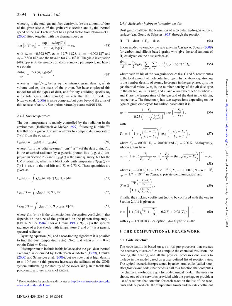
The results of the 108 yr time evolution are shown in Fig. 8for carbon, OH, HC3N and O2, reproducing the same evolution asshown in figs 3, 4 and 7 of Wakelam & Herbst (2008).
4.2 Cloud collapse (one zone)
We consider here a simple one-zone spherical cloud collapse includ-ing a primordial network listed in Table C1 based on Omukai (2000)with the one in table 1 of Omukai et al. (2005), labelled from Z1 toZ40. The initial conditions are set to T = 100 K, n = nH = 1 cm−3,ne− = 10−4 cm−3 and nH2 = 10−6 cm−3, following Omukai (2000).
13 See for example:http://www.physics.ohio-state.edu/~eric/research.htmlhttp://kida.obs.u-bordeaux1.fr/http://www.udfa.net/14 Note that the test option also copies the Makefile and the test.f90 file fromthe given test directory (tests folder) to the build directory: in this sense thetest option is not properly an alias or a short cut. In general KROME, when theoption -test=[name] is enabled, copies all the files from test/[name] to thebuild/ folder.
MNRAS 439, 2386–2419 (2014)
at Royal L
ibrary/Copenhagen U
niversity Library on June 13, 2014
http://mnras.oxfordjournals.org/
Dow
nloaded from

2400 T. Grassi et al.
Figure 8. Evolution of carbon (top left), OH (top right), HC3N (bottom left) and O2 (bottom right).
We assume also that all the metals are ionized, except for the oxy-gen as in e.g. Omukai et al. (2005), Santoro & Shull (2006) andMaio et al. (2007). The abundances of the metals are rescaled tothe metallicity using the solar abundances of Anders & Grevesse(1989). The time evolution of the collapsing core is calculatedassuming a free-fall collapse,
dρ
dt= ρ
tff. (80)
The thermal evolution as a function of density is reported inFig. 9. We can distinguish in the non-metal profile (Z = −∞)the typical features of the temperature evolution as consequenceof the processes involved. The cloud is heated up by compres-sion (n ∼ 10 cm−3), then starts to cool (n ∼ 102 cm−3) for theeffect of the H2 cooling and the gas temperature drops to ∼200 K(n ∼ 104 cm−3). Once the H2 approaches the local thermal equilib-rium (LTE) the cooling is less efficient and the temperature startsto increase again until densities of 108–1010 cm−3, when the three-body reactions come into play producing first a slight cooling dip(n ∼ 1010 cm−3). At higher densities the gas becomes opticallythick and the cooling is less efficient producing a net heating inthe cloud until the collisional-induced emission (n ∼ 1016 cm−3)cooling acts (n ∼ 1016 cm−3). Finally, the gas evolves adiabaticallysince it becomes also opaque to the continuum (CIE) emission: theevolution is a power law with a slope that depends on the adiabaticindex, that in this case is γ = 7/5 since the gas at this stage is fullymolecular.
Figure 9. Temperature profiles as a function of the total number densityfor the collapse of the primordial cloud at different metallicities, where -infrepresents the primordial case.
In Fig. 9, we show the thermal evolution for metallicities rangingfrom Z = −∞ to −1, as indicated in the labels. The metals increasethe gas cooling in the low-density regime, where the effects on theevolution are stronger. We also note that the metal cooling effectextends above densities of 106 cm−3 due to the presence of Si II
and Fe II, as shown in Fig. 10, where also the compressional andthe H2 heating are reported for comparison. In the very first stage
MNRAS 439, 2386–2419 (2014)
at Royal L
ibrary/Copenhagen U
niversity Library on June 13, 2014
http://mnras.oxfordjournals.org/
Dow
nloaded from

KROME 2401
Figure 10. Individual thermal contributions including the main metalcoolants (� C I, � C II, � Si II, � Fe II), the compressional and the molecularhydrogen heating (Compr, Chem), for a collapse with Z = −2.
Figure 11. Fractional abundance evolution for three carbon-based species,i.e. C, C+ and CO, for Z = −2 cloud collapse. See the text for details.
of the evolution the thermal history is dominated by C I and sub-sequentially by C II, while other coolants such as O I, O II, are lessimportant. In this test the chemical network does not include any Sior Fe chemistry, and for this reason the initial amounts of Si+ andFe+ remain unchanged during the whole evolution, and hence thecooling from neutral Si and Fe is not included. At the beginning ofthe density range 104 � n � 106 cm−3 the C I cooling drops becauseC is depleted into CO (Fig. 11), determining an interval withoutmetal cooling that ends when the Si II–Fe II cooling starts to act:in this region the thermal evolution is then controlled by the com-pressional heating determining an adiabatic temperature increase asshown in Fig. 9. However, different initial abundances of the metalspecies (i.e. with non-solar ratios) can lead to different thermalhistory and different interplay by the single metal contributions.
The command line to generate the test is
> ./krome -test=collapseZ
which is a short cut for
> ./krome -n network/react_primordialZ2
-useN
-cooling=H2,COMPTON,CI,CII,OI,OII,SiII,
FeII,CONT,CHEM
-heating=COMPRESS,CHEM
-useH2opacity
-ATOL=1d-40
-gamma=FULL
The options listed above as the previous tests, except for thewhere COMPTON and CONT are the flags for the Compton and thecontinuum cooling (Section 2.3.1), COMPRESS activates the com-pressional heating (Section 2.3.2), while useH2opacity allows toinclude the opacity term for the molecular hydrogen (also Sec-tion 2.3.1). Finally, gamma=FULL is for the species-dependent cal-culation of the adiabatic index as in equation (8). Individual metalcooling functions are from CI to FeII, and -ATOL=1d-40 forcesthe absolute tolerance to 10−40.
4.3 Cloud collapse under UV radiation
In this section we present results from a simple one-zone collapse asin the previous section, but under the presence of a UV backgroundand employing a different reaction network (see Table C1). Theinitial conditions are the same as discussed in Section 4.2, we onlyadd the H2 photodissociation rate as in Shang, Bryan & Haiman(2010) who provided the following rate parametrization
k = 10−12βJ21, (81)
with J21 being defined as in equation (4) and β = 0.9 assumes aT5 spectrum (Trad = 105 K). No self-shielding nor other processesas Rayleigh scattering or H− cooling are included. This run onlyprovides a simple test to check the behaviour of the gas under UVbackground. For a complete analysis we refer the reader to Omukai(2001) and Schleicher, Spaans & Glover (2010).
The results for four different J21 are reported in Fig. 12. Thestronger the UV flux, the larger the amount of H2 dissociation, andthe higher the temperature which is reached at low density. ForJ21 < 105 there is still enough H2 to allow the cooling to act, whilefor J21 = 105 the temperature heats up to ∼8000 K very quickly andthe H2 formation and its cooling are strongly reduced, as can be seenfrom Fig. 13. At this stage the hydrogen line emission of atomichydrogen is the only contribution which cools down the collapsingcloud.
The command line to generate the test is
> ./krome -test=collapseUV
alias for
> ./krome -n network/react_primordial_UV
Figure 12. Temperature profile in function of the total number density forthe collapse of the primordial cloud irradiated by different UV background.
MNRAS 439, 2386–2419 (2014)
at Royal L
ibrary/Copenhagen U
niversity Library on June 13, 2014
http://mnras.oxfordjournals.org/
Dow
nloaded from

2402 T. Grassi et al.
Figure 13. Molecular hydrogen fraction as a function of the total numberdensity for different UV background.
-cooling=H2,COMPTON,CIE,ATOMIC
-heating=COMPRESS,CHEM
-useN
-gamma=FULL
with the same meaning as in the previous tests.
4.4 Dust
As described in Section 2.4 KROME has the capability of handlingthe dust evolution and its interaction with the gas phase. The testproposed here consists of a gas with an initial population of dust,both silicon and carbon based, with 10 bins each (i.e. a total ofnd = 10 × 2 = 20 bins). The initial condition for the gas phase arethe same as for the primordial shock (Table 8) extended with carbonand silicon with a dust-to-gas ratio of 10−5, and the distributionfollows a MRN power law as described in Section 2.4.
The aim of the test is to analyse the influence of the dust growthand the dust destruction by changing the gas temperature artificiallyduring the simulation as
T (t) = (106 − 10
) t
tend+ 10 K, (82)
where t is the time reached by the simulation and tend = 108 yris the ending time. equation (82) represents a gas that linearly in-creases its temperature with time from 10 to 106 K: we expect thatat the beginning of the simulation when the temperature is higherthe effect of the growth will dominate the dust processes, whilewhen the temperature increases the dust will be sputtered by the hotgas. The results of this calculation is plotted in Fig. 14, for carbonand silicon-based dust. We represent the evolution with time of the
Table 8. Number densities for the cooling test, wherea(b) = a × 10b. All the abundances are mass fractions.
Species Abundance Species Abundance
H 0.9225 H+2 1.0(−20)
e− 1.0(−4) HD 1.0(−8)H+ 1.0(−4) H− 1.0(−20)D 1.0(−20) He++ 1.0(−20)D+ 1.0(−20) C+ 1.0(−6)He 0.0972 Si+ 1.0(−7)He+ 1.0(−20) O 1.0(−4)H2 1.0(−5) Fe+ 1.0(−8)
Figure 14. Evolution of the ratio between the number density n of the givenspecies at time t and the its initial value ni as a function of the temperature(see the text). Solid and dotted lines represent the largest and the smallestbins, respectively, while the dashed line indicates the species in the gasphase. Black lines are for carbon and grey for silicon. Note that black andgrey dotted lines overlap.
number density of dust for each bin size. As expected the amountof dust increases at the beginning of the evolution (lower tempera-tures), subtracting carbon and silicon from the gas phase, due to theinteraction between the two phases that are coupled within the sameODE system. In the later stages (higher temperatures) the sputteringdestroys the grains, therefore the species in the gas phase increaseagain, since the sum of the mass of C (and Si) in the dust phase andin the gas phase is constant. Note that small grains are not affectedby dust growth, since their smaller size reduces the probability of agas–dust encounter.
The command to run this test is
> ./krome -test=dust
alias for
> ./krome -n networks/react_primordial
-dust=10,C,Si
-useN
-dustOptions=GROWTH,SPUTTER
with -dust=10,C,Si to employ 10 bins of carbon-based and 10bins of silicon-based dust, and -dustOptions=GROWTH,SPUTTER
enables the growth and thermal sputtering processes as discussedin Sections 2.4.1 and 2.4.2, respectively.
4.5 1D shock
To test KROME in a hydrodynamical context we propose a 1D spher-ically symmetric shock as described by Bodenheimer et al. (2006),which provides a simple implementation of a high temperature anddensity region that expands into a lower density and cold envi-ronment. In this test we can see the effect of the chemical solverand the thermal processes on the evolution of the shock from acomputational point of view, but also from a physical perspectivewhen the cooling is turned on.
The numerical set-up consists in 100 shells, 20 in the inner region(the so-called fireball), with a temperature of 106 K, a density of1.24 × 10−23 g cm−3 and a mass of 3 × 10⁻⁴ M� per shell.Conversely, the outer region made of 80 shells is colder and lessdense with a temperature of 10 K, a density of 10−26 g cm−3 and
MNRAS 439, 2386–2419 (2014)
at Royal L
ibrary/Copenhagen U
niversity Library on June 13, 2014
http://mnras.oxfordjournals.org/
Dow
nloaded from
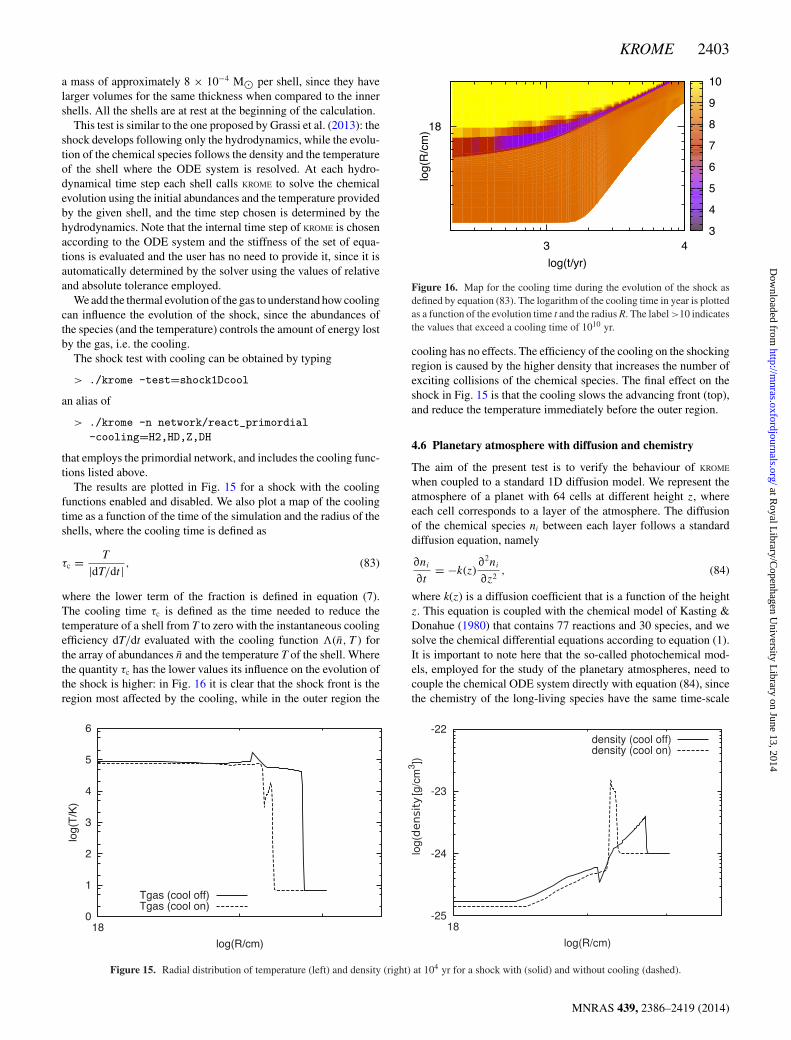
KROME 2403
a mass of approximately 8 × 10⁻⁴ M� per shell, since they havelarger volumes for the same thickness when compared to the innershells. All the shells are at rest at the beginning of the calculation.
This test is similar to the one proposed by Grassi et al. (2013): theshock develops following only the hydrodynamics, while the evolu-tion of the chemical species follows the density and the temperatureof the shell where the ODE system is resolved. At each hydro-dynamical time step each shell calls KROME to solve the chemicalevolution using the initial abundances and the temperature providedby the given shell, and the time step chosen is determined by thehydrodynamics. Note that the internal time step of KROME is chosenaccording to the ODE system and the stiffness of the set of equa-tions is evaluated and the user has no need to provide it, since it isautomatically determined by the solver using the values of relativeand absolute tolerance employed.
We add the thermal evolution of the gas to understand how coolingcan influence the evolution of the shock, since the abundances ofthe species (and the temperature) controls the amount of energy lostby the gas, i.e. the cooling.
The shock test with cooling can be obtained by typing
> ./krome -test=shock1Dcool
an alias of
> ./krome -n network/react_primordial
-cooling=H2,HD,Z,DH
that employs the primordial network, and includes the cooling func-tions listed above.
The results are plotted in Fig. 15 for a shock with the coolingfunctions enabled and disabled. We also plot a map of the coolingtime as a function of the time of the simulation and the radius of theshells, where the cooling time is defined as
τc = T
|dT/dt | , (83)
where the lower term of the fraction is defined in equation (7).The cooling time τc is defined as the time needed to reduce thetemperature of a shell from T to zero with the instantaneous coolingefficiency dT/dt evaluated with the cooling function �(n, T ) forthe array of abundances n and the temperature T of the shell. Wherethe quantity τc has the lower values its influence on the evolution ofthe shock is higher: in Fig. 16 it is clear that the shock front is theregion most affected by the cooling, while in the outer region the
Figure 16. Map for the cooling time during the evolution of the shock asdefined by equation (83). The logarithm of the cooling time in year is plottedas a function of the evolution time t and the radius R. The label >10 indicatesthe values that exceed a cooling time of 1010 yr.
cooling has no effects. The efficiency of the cooling on the shockingregion is caused by the higher density that increases the number ofexciting collisions of the chemical species. The final effect on theshock in Fig. 15 is that the cooling slows the advancing front (top),and reduce the temperature immediately before the outer region.
4.6 Planetary atmosphere with diffusion and chemistry
The aim of the present test is to verify the behaviour of KROME
when coupled to a standard 1D diffusion model. We represent theatmosphere of a planet with 64 cells at different height z, whereeach cell corresponds to a layer of the atmosphere. The diffusionof the chemical species ni between each layer follows a standarddiffusion equation, namely
∂ni
∂t= −k(z)
∂2ni
∂z2, (84)
where k(z) is a diffusion coefficient that is a function of the heightz. This equation is coupled with the chemical model of Kasting &Donahue (1980) that contains 77 reactions and 30 species, and wesolve the chemical differential equations according to equation (1).It is important to note here that the so-called photochemical mod-els, employed for the study of the planetary atmospheres, need tocouple the chemical ODE system directly with equation (84), sincethe chemistry of the long-living species have the same time-scale
Figure 15. Radial distribution of temperature (left) and density (right) at 104 yr for a shock with (solid) and without cooling (dashed).
MNRAS 439, 2386–2419 (2014)
at Royal L
ibrary/Copenhagen U
niversity Library on June 13, 2014
http://mnras.oxfordjournals.org/
Dow
nloaded from

2404 T. Grassi et al.
Figure 17. Evolution of the abundances of H2 (top) and CO (bottom)at different heights. Left-hand panel is with diffusion only, middle withchemistry only and right with both enabled. Note that the colour scale is inunits of 10−7.
of the vertical diffusion. The simplification made in this exampleis intended only for illustrative purposes and is not intended forreproducing a realistic atmospheric model. The interested readercan get more details in the thorough paper by Hu, Seager & Bains(2012), and the references therein.
The initial conditions of the model are taken from Segura et al.(2003) and the diffusion coefficients are from Jim Kasting’s mod-els website15, but, in order to keep the chemical time-scale similarto the dynamical time determined by equation (84), we normalizethe chemical abundances to the species with the maximum abun-dances considering all the layers, and the diffusion coefficients arenormalized to 0.5 in arbitrary units.
We follow the model for tend = 2 × 10⁴ with (i) diffusion only,(ii) chemistry only and (iii) chemistry and diffusion together. Theresults are shown in Fig. 17 for H2 and CO: in the left-hand panel thesystem follows equation (84) only, hence reaches the equilibriumafter tend. With the chemistry only (middle panel) the system acts as64 one zone models which evolve following the chemical network,with no species exchanged between each cell. Finally, when bothare enabled (right-hand panel) the species formed by the chemistryare diffused into the other layers.
To generate the test the short cut command line is
> ./krome -test=atmosphere
which is an alias for
> ./krome -n network/react_kast80
-useN
4.7 Slow-manifold kinetics
We propose here a test based on Reinhardt, Winckler & Lebiedz(2008) to model a simple chemical network in order to show therobustness of the numerical solver DLSODES. In the phase space ofchemical kinetics systems (the space of the species), there are fastand slow dynamics invariant manifolds. For a given set of initial
15 http://vpl.astro.washington.edu/sci/AntiModels/models09.html
Table 9. Reactions for the H2 combustion model including the temperature-independent rate coefficients, where kf represents the forward rate coeffi-cients and kr the reverse one. Note that the rate coefficient are in arbitraryunits of amount/time.
Reaction kf kr
H2k±1� 2H 2.0 2.16 × 10²
O2k±2� 2O 1.0 3.375 × 10²
H2Ok±3� H + OH 1.0 1.4 × 10³
H2 + Ok±4� H + OH 103 1.08 × 10⁴
O2 + Hk±5� O + OH 103 3.375 × 10⁴
H2 + Ok±6� H2O 102 7.714 × 10⁻¹
conditions a system quickly converges to a trajectory laying on theslow manifold, where the dynamics spends most of its evolutionarytime until the steady state (Fraser 1988; Jones 1995; Zagaris, Kaper& Kaper 2004; Nicolini & Frezzato 2013). In this test, we employ asimple H2 combustion model consisting of 12 reactions sketched inTable 9 together with the temperature-independent reaction rates,for both the forward (kf ) and the reverse process (kr), and involv-ing six species (i.e. H2, H, O2, O, H2O and OH). In this test, wedemonstrate that the slow-manifold features are well reproduced.
The initial conditions are varied over a grid of nH2 and nH2O
according to the constraint nH2 ≤ 0.96 − nH2O in order to selectonly the values in the lower left nH2 –nH2O space as discussed inReinhardt et al. (2008). The nH2 spans from 0.3 to 0.95 spacedby 0.1, while nH2O from 0.05 to 0.65 spaced by 0.05 in arbitraryunits. The system must satisfy the two following stoichiometricconstraints
2nH2 + 2nH2O + nH + nOH = 2
2nO2 + nH2O + nO + nOH = 1, (85)
which lead to
nO = nOH = 0
nO2 = (1 − nH2O − nOH − nO
)/2
nH = 2 − nOH − 2 nH2O − 2 nH2 , (86)
where the first condition is arbitrarily chosen. We follow the evolu-tion of the system until the steady state, and we show the results inFig. 18 panel (a). Our trajectories match the ones reported in fig. 1of Reinhardt et al. (2008) and the slow manifold is represented bythe transverse line where the system quickly lays before reachingthe equilibrium values located at (H2, H, O2, O, H2O, OH) = (0.27,0.05, 0.135, 0.02, 0.7, 0.01).
As an additional test we perform another calculation changing theinitial conditions according to equation (85), which leads also to
nO2 = nOH = 0
nO = 1 − nH2O − nOH − 2 nO
nH = 2 − nOH − 2 nH2O − 2 nH2 , (87)
since the first arbitrarily chosen condition also satisfies equations(85). In this test nO has a non-zero initial value enhancing theefficiency of the reaction H2 + O → H2O, which modifies thetrajectories in the very first part of the various evolutions as shown inFig. 18 panel (b). Also in this test the system converges to the slow
MNRAS 439, 2386–2419 (2014)
at Royal L
ibrary/Copenhagen U
niversity Library on June 13, 2014
http://mnras.oxfordjournals.org/
Dow
nloaded from

KROME 2405
Figure 18. Family of trajectories for the H2 combustion mechanism in Reinhardt et al. (2008), for two different sets of initial conditions: with a zero(panel A) and a non-zero (panel B) initial oxygen abundance. The slow manifold is clearly depicted by the transverse line where the trajectories converge.
manifold finally reaching the same equilibrium values discussedabove, proving the robustness of the solver employed in KROME.
The command line to generate the test is
> ./krome -test=slowmanifold
which is a short cut for
> ./krome -n network/react_SM
-useN
5 K RO M E E M B E D D E D IN 3 D
One of the aims of the KROME package is to allow an efficient embed-ding of the chemistry in 3D hydrodynamical codes. It is well knownthat an accurate treatment of the microphysical processes is veryimportant in describing the dynamics of small-scale objects (e.g.star formation processes or the ISM as well as in cosmological cal-culations). As already explained in Section 3.2, to solve a system ofODEs can be very demanding and often approximated approachesare preferred to deal with 3D hydrodynamic complexity. Hydrody-namical codes as ENZO (O’Shea et al. 2004; The Enzo Collaboration2013) and FLASH (Fryxell et al. 2000) include the chemical and ther-mal evolution in different ways. Most of them employ simple andvery small networks with no more than 13 species, including H,He, H+, H+
2 , H2, He+, He2+, D, HD, D+, H− and e−. Even in thelatter case, only a few reactions involving those species are consid-ered and often some approximations need to be introduced. Mostof the problems are related to the time needed in solving the sys-tem of ODEs and it became very common to include the followingapproximations: (i) a decoupling among slower and faster speciesevolution and (ii) the decoupling of temperature from the chemicalevolution. The latter can generate instabilities at very high density.For instance, a first-order BDF method is typically employed inENZO. The accuracy of such solvers is well known and their stabilitystrongly depends on the chosen time step and on the stiffness ofthe problem. As already discussed in Section 3.4, the KROME pack-age includes more accurate and stable solvers (DVODE and DLSODES)with a robust internal definition of the time step aimed at givingmore stability and a better solution. It is important to note here thatthese solvers are also generally slower than a simple first-order BDFand that optimization techniques (e.g. Grassi et al. 2013) should beapplied to speed up the calculations. On the contrary, we shouldconsider that an accurate solver is needed for high-resolution stud-
ies (Bovino et al. 2013a) and to solve more stiff problems (e.g.high-density environments, turbulent media).
In the following, we show how KROME interfaces with complex3D codes like ENZO, RAMSES (Teyssier 2002) and FLASH. We presenta typical cosmological problem in ENZO, some standard hydrody-namical tests and cosmological problem in RAMSES, and a 1D and3D collapse molecular cloud test in FLASH. The KROME patches forthese codes are included in the current release16 of KROME.
5.1 KROME IN RAMSES
RAMSES is an N-body and hydrodynamical code developed byTeyssier (2002). It has been designed to study structure formationwith high spatial resolution by using an adaptive mesh refinement(AMR) technique, with a tree-based data structure.
The RAMSES code solves the hydrodynamical equations in theirconservative form with the gravitational term included as a non-stiffsource term in the system of equations. Using the conservative formof the system, the discretized equations are solved computing theflux across the cell interfaces. In order to do that the code uses thesecond-order Godunov method (or piecewise linear method).
We employed KROME in the current version of the publicly avail-able RAMSES code and run a series of hydrodynamical and cosmo-logical tests aimed at testing KROME’s flexibility and the possiblesources of error when employed in such a complex code. We reportresults for a 1D test including Sod’s shock tube problem and fora 3D cosmological simulations of a collapsing minihalo. We cre-ated the KROME code patch following the RAMSES user guide. Thechemical species were initialized as passive scalars, and the codehas been accordingly modified to include the chemical evolutionfor each leaf cell. An additional flag (chemistry) has been addedto switch on/off the chemical evolution. KROME is called if the flagchemistry is TRUE. Note that the standard RAMSES flag ‘cooling’can be used to employ the standard cooling already implementedin RAMSES. All the tests presented in this work employed a simpleprimordial network involving H, He, H+, H+
2 , H2, He+, He2+, H−,and e− and 20 reactions. Atomic and H2 cooling are included aswell as the H2 three-body formation heating.
Sod shock tube: the Sod shock is initialized by two separate re-gions, each initially at rest. The left-hand region has higher pressure
16 http://kromechem.org
MNRAS 439, 2386–2419 (2014)
at Royal L
ibrary/Copenhagen U
niversity Library on June 13, 2014
http://mnras.oxfordjournals.org/
Dow
nloaded from

2406 T. Grassi et al.
and density so that when the system is evolved, the fluid on the leftmoves to the right supersonically. For instance the density is 10−20
and 0.125 × 10⁻²⁰ g cm−3 on the left and right, respectively. Thetemperature is about 103 K on both regions. The solution is simple:a contact discontinuity moves to the right, with a shock wave aheadof it, while a rarefaction wave moves leftwards. All features of thetest are well visible: the rarefaction waves, the contact discontinuityand the shocks. The snapshots are taken after 2.45 × 10⁴ yr. Theeffect of the chemistry is due to the cooling and causes a slowerevolution of the shock as shown by the results for the density, ve-locity and temperature profiles reported in Figs 19–21, respectively.The behaviour of the hydrodynamical quantities, in particular thelower velocities and temperatures, reflects the chemical evolutionreported in Fig. 22. It is important to discuss the H2 evolutionwhich is the main source of cooling. Indeed where the H2 fractionis smaller the temperature is higher (e.g. around 0.6 pc where thecontact discontinuity occurs).
In the same plots we also report a similar test performed with theAMR code FLASH, with identical initial conditions (see Sections 5.3and 5.2 for additional details).
Primordial minihalo evolution: to test the code’s capability tomanage non-equilibrium chemical systems within a cosmological
Figure 19. Sod’s tube shock density evolution in RAMSES, with (black solidcurve) and without (black dashed curve) chemistry. The results are givenin function of the radius expressed in parsec. The red curves are the resultsfrom FLASH. See the text for details.
Figure 20. Sod’s tube shock velocity evolution in RAMSES, with (black solidcurve) and without (black dashed curve) chemistry. The results are givenin function of the radius expressed in parsec. The red curves are the resultsfrom FLASH. See the text for details.
Figure 21. Sod’s tube shock temperature evolution in RAMSES, with (blacksolid curve) and without (black dashed curve) chemistry. The results aregiven in function of the radius expressed in parsec. The red curves are theresults from FLASH. See the text for details.
Figure 22. Sod’s shock tube chemical species evolution in RAMSES. H2
(top), H− (middle) and e− (bottom) mass fraction are shown. See the textfor details.
scenario we have simulated the chemothermal evolution of the gasinside a 1.3 × 10⁶ M� dark matter (DM) halo in the early Universe(see e.g. Abel, Bryan & Norman 2002; Bromm, Coppi & Larson2002; Yoshida, Omukai & Hernquist 2008; Bovino et al. 2013a;Latif et al. 2013b).
To solve the hydrodynamic equations we used the MUSCLscheme and the HLLC Riemann solver. The simulation has a start-ing redshift zi ≈ 95. The minihalo was selected from a DM sim-ulation of 2563 particles inside a (1 Mpc)3 volume. After that, were-simulated the selected halo inside the same box with three nestedgrids of 5123, 2563 and 1283 particles. In this cosmological hy-drodynamical simulation we set lmin = 7 and lmax = 18, reaching aresolution of �x ≈ 0.3 proper pc at zf ≈ 11.5. At this final redshiftthe simulation reached the maximum level of refinement.
Our refinement strategy is as follows: (i) each cell is refined ifit contains at least eight DM particles, (ii) each gas cell is refinedensuring that the local Jeans length is resolved by at least 16 cells,(iii) each cell is refined if the local pressure gradient �P/P > 2. Thehighest resolution region is contained inside a spherical volume ofradius r = 104 comoving kpc, which corresponds to three times thehalo virial radius at the final redshift zf , approximately.
MNRAS 439, 2386–2419 (2014)
at Royal L
ibrary/Copenhagen U
niversity Library on June 13, 2014
http://mnras.oxfordjournals.org/
Dow
nloaded from

KROME 2407
Fig. 23 shows the mass weighted projections for gas density (topleft), temperature (top right), H2 (bottom left) and H− (bottom right)mass fraction at zf = 11.5. These maps show the common featuresfor such systems: the central high-density region presents the highestH2 mass fraction producing a minimum in the gas temperature.Fig. 24 shows the same physical quantities at the same redshift butfor the highest level of refinement.
Fig. 25 shows the mass weighted spherical averaged radial pro-files for the gas density (top left), temperature (top right), H+ (bot-tom left) and H2 (bottom right) at zf = 11.5 for the highest resolu-tion central region. The H2 mass fraction in the halo central regionwell agrees with the reported values in the literature for such sys-tems (e.g. Bovino et al. 2013a; Bovino, Schleicher & Grassi 2013b).The gas temperature also follows the expected behaviour: it reachesa maximum (near the halo virial temperature) inside the virial ra-dius; it drops because the H2 effect at scales smaller than a few tensof pc and it increases again at scales �1 pc due to the molecularcooling saturation.
Fig. 26 shows the density–temperature phase plane at the simu-lation’s final redshift. The colour bar shows the mass of each cell
on the phase plane. The low-density (ρ/mH � 1 cm−3) points showthe common temperature rising due to the gas adiabatic contrac-tion. After reaching a maximum (near the halo virial temperature)at densities ρ/mH ≈ 0.3 cm−3 the H2 abundance is enough to coolthe gas reaching a minimum temperature of T ≈ 250 K.
5.2 KROME in ENZO: a first application
ENZO is an AMR code which is well suited to follow gravitationalcollapse over a large range of scales, which includes various phys-ical modules (O’Shea et al. 2004). The hydrodynamical equationsare solved in the comoving frame which takes into account the cos-mological expansion of the Universe employing a split third-orderpiecewise parabolic (PPM) solver. Any collisionless components(such as DM and stars) are modelled by N-body particles, whosedynamics are governed by Newton’s equations. The gravitationalpotential is taken into account by solving the Poisson equation viamultigrid solver.
The initial conditions for the three DM primordial minihaloesstudied here are the same already discussed in Bovino et al.
Figure 23. Mass weighted projections for the gas density (top left), gas temperature (top right), H2 mass fraction (bottom left) and H− mass fraction (bottomright) at a comoving resolution of �x ≈ 61 pc. The maps correspond to zf = 11.5. The maps show the common features of a ∼106 M� halo: the high-densitycentral region shows a high (∼10−3) H2 mass fraction and a low (∼200–300 K) temperature. The distances scales are in comoving units.
MNRAS 439, 2386–2419 (2014)
at Royal L
ibrary/Copenhagen U
niversity Library on June 13, 2014
http://mnras.oxfordjournals.org/
Dow
nloaded from
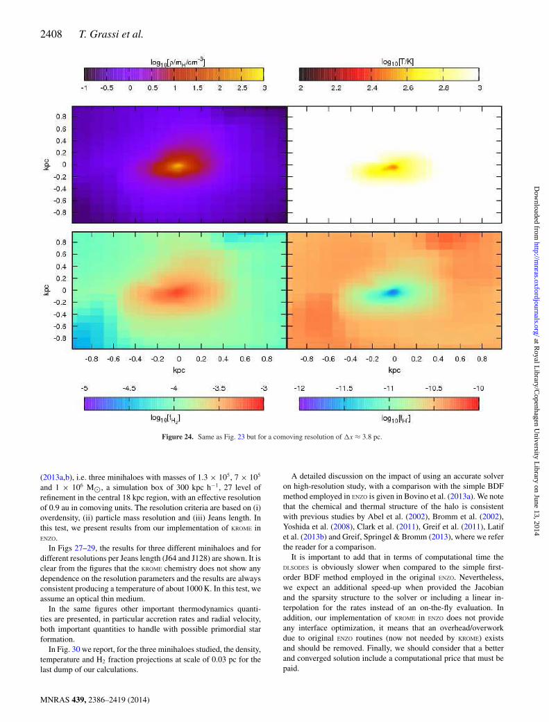
2408 T. Grassi et al.
Figure 24. Same as Fig. 23 but for a comoving resolution of �x ≈ 3.8 pc.
(2013a,b), i.e. three minihaloes with masses of 1.3 × 10⁵, 7 × 10⁵
and 1 × 10⁶ M�, a simulation box of 300 kpc h−1, 27 level ofrefinement in the central 18 kpc region, with an effective resolutionof 0.9 au in comoving units. The resolution criteria are based on (i)overdensity, (ii) particle mass resolution and (iii) Jeans length. Inthis test, we present results from our implementation of KROME inENZO.
In Figs 27–29, the results for three different minihaloes and fordifferent resolutions per Jeans length (J64 and J128) are shown. It isclear from the figures that the KROME chemistry does not show anydependence on the resolution parameters and the results are alwaysconsistent producing a temperature of about 1000 K. In this test, weassume an optical thin medium.
In the same figures other important thermodynamics quanti-ties are presented, in particular accretion rates and radial velocity,both important quantities to handle with possible primordial starformation.
In Fig. 30 we report, for the three minihaloes studied, the density,temperature and H2 fraction projections at scale of 0.03 pc for thelast dump of our calculations.
A detailed discussion on the impact of using an accurate solveron high-resolution study, with a comparison with the simple BDFmethod employed in ENZO is given in Bovino et al. (2013a). We notethat the chemical and thermal structure of the halo is consistentwith previous studies by Abel et al. (2002), Bromm et al. (2002),Yoshida et al. (2008), Clark et al. (2011), Greif et al. (2011), Latifet al. (2013b) and Greif, Springel & Bromm (2013), where we referthe reader for a comparison.
It is important to add that in terms of computational time theDLSODES is obviously slower when compared to the simple first-order BDF method employed in the original ENZO. Nevertheless,we expect an additional speed-up when provided the Jacobianand the sparsity structure to the solver or including a linear in-terpolation for the rates instead of an on-the-fly evaluation. Inaddition, our implementation of KROME in ENZO does not provideany interface optimization, it means that an overhead/overworkdue to original ENZO routines (now not needed by KROME) existsand should be removed. Finally, we should consider that a betterand converged solution include a computational price that must bepaid.
MNRAS 439, 2386–2419 (2014)
at Royal L
ibrary/Copenhagen U
niversity Library on June 13, 2014
http://mnras.oxfordjournals.org/
Dow
nloaded from

KROME 2409
Figure 25. Mass weighted radial profiles for the gas density (top left), gas temperature (top right), H+ mass fraction and H2 mass fraction at zf = 11.5. Thedistance scales are in proper-physical units. The H2 shows a well-known behaviour reaching a mass fraction �10−3 at scales �10 pc. The gas temperature alsoshows the expected features with a maximum inside the virial radius and a minimum at ≈1 pc. At smaller scales it rises due to the saturation of the H2 cooling.
5.3 KROME in FLASH
FLASH is a versatile AMR code for a wide field of astrophysicalapplications (Fryxell et al. 2000). It can handle 1D, 2D and 3Dproblems and incorporates several magnetohydrodynamic solvers.The gravitational potential is calculated by solving the Poissonequation either by making use of a multigrid solver or a Barnes–Hut tree code.
In the following we present results obtained with FLASH version4.0.1 in which the KROME package was implemented. The implemen-tation is straightforward. We handle the chemistry as an additionalsource term called after the hydro step update. The KROME moduleis called individually for each (active) cell in each block handingover the particle densities of each species as well as the gas temper-ature. All routines concerning the chemistry evolution, cooling andheating are provided by the KROME package as described before anddo not have to be implemented in FLASH itself.
Sod shock tube: here we present the results of the Sod shocktube test described in detail in Section 5.1 for RAMSES. We note thatwe use identical initial conditions for the test in FLASH. The resultsare plotted in Figs 19–22. As can be seen, the agreement betweenRAMSES and FLASH for the density, temperature and velocity as wellas the three species H2, H− and e− is almost perfect. We note thatalso for the other species not shown here the agreement is excellent.
It is worth noting that for the test in FLASH we use a higher ordersolver that is the PPM, compared to the lower order solver MUSCLused in the RAMSES runs. Small differences in the plots can then beattributed to the different solvers employed.
Cloud collapse: we have performed simulations of a primor-dial minihalo in 1D and 3D following the collapse up to densitiesof the order of 10−10 g cm−3 corresponding to particle densitiesof ∼1013 cm−3. The grid was adapted dynamically in order to guar-antee that the Jeans length is resolved everywhere with at least 32grid cells using 16 levels of refinement. We used the PPM solverfor updating the hydrodynamics and the Barnes–Hut tree code forsolving the Poisson equation in 3D and the multipole solver for1D. The initial conditions are chosen in order to mimic a highlyidealized minihalo with a diameter of 0.45 pc consisting of atomichydrogen and helium (mass fractions of 0.76 and 0.24, respectively)with a uniform number density of 1.67 × 10⁻¹⁸ g cm−3. The tem-perature of the minihalo is set to 1000 K. The core is initially atrest and no magnetic field is present. The ambient medium has a100 times lower density and is thus dynamically not important forthe simulation result. We note that we do not include deuteriumin this simulation as we expect no marked differences in the finalresults. In addition, for the 3D case we performed a run where atransonic turbulent velocity field is included. For all three cases, the(non-turbulent) 1D run, the non-turbulent 3D run and the turbulent
MNRAS 439, 2386–2419 (2014)
at Royal L
ibrary/Copenhagen U
niversity Library on June 13, 2014
http://mnras.oxfordjournals.org/
Dow
nloaded from

2410 T. Grassi et al.
Figure 26. Density–temperature phase plane for the simulated mini halo at zf = 11.5. The colour bar shows the mass of each point on the plane. The gastemperature shows the expected behaviour rising at low density due to the adiabatic contraction. Once the gas density reaches the ≈0.3 cm−3 value the H2
abundance is enough to drop the gas temperature till T ≈ 250 K in the high-density regions.
3D run we performed two simulations, one with and one withoutthe optically thick cooling correction term discussed in Section 2.3.
In the following we show the results of the simulations at the timethe highest refinement level is reached considering the runs with andwithout the optically thick correction separately. We first show thetemperature and the mass fraction of H2 and e− plotted against thedensity in Fig. 31, with the results including the optically thick cor-rection term shown in the left-hand panel. First, it can be seen thatthe results of the 1D run and the non-turbulent 3D run (red lines)are almost indistinguishable for both the case with the opticallythick correction (left-hand panel) and the one without it (right-handpanel). For both cases the temperature and mass fractions of H2 ande− reveal the expected behaviour in particular when comparing withFig. 9 for non-metal case. The optically thick correction term be-comes recognizable mainly at densities above 10−13 g cm−3 wherethe temperature keeps on increasing (top-left panel) in contrast tothe runs without the correction (top-right panel).
Furthermore, for the turbulent run the diminished cooling abilityresults in a small fraction of gas with a very low H2 fraction at highdensities (∼10−12–10−11 g cm−3, see middle-right panel). This isa consequence of the high gas temperature resulting in the disso-ciation of molecular hydrogen. In contrast, the high temperaturepeaks showing up around 10−13 g cm−3 in the turbulent runs withand without the optically thick correction term (top panel) are mostlikely due to the presence of shocks created by the turbulence and
do not arise in the non-turbulent simulations. In these hot, shockedregions the gas reveals a drop in the H2 fraction and a simultaneousincrease in the electron fraction (see also Fig. 33).
Next, we plot the radial dependence of selected hydrodynamicalvariables in Fig. 32 for the 1D and non-turbulent 3D run with theoptically thick correction.17 Although considering different spatialscales, there is a good qualitative agreement with the results shownin Figs 27–29, which confirms that KROME works properly in FLASH.
In order to get a visual impression of the simulation results, inFig. 33 we show some projected quantities at the end of the 3D runincluding turbulence and the optically thick correction term. Fromthe middle panel of Fig. 33 it can be seen that there are regions ofhot gas well off from the centre, e.g. the hot spots in the lower leftand upper right part of the figure. These regions are associated witha significant change in the gas flow indicating the presence of ashock. As stated already before, these hot regions have a relativelylow H2 fraction (see right-hand panel).
Finally, we state that for the 3D runs performed the amount ofcomputational time for an individual cell is approximately the sameindependently of whether turbulence is present or not or whetherthe optically thick cooling term was applied or not. Furthermore,
17 We do not show the result for the run including turbulence since here thecollapse occurs well off from the centre.
MNRAS 439, 2386–2419 (2014)
at Royal L
ibrary/Copenhagen U
niversity Library on June 13, 2014
http://mnras.oxfordjournals.org/
Dow
nloaded from

KROME 2411
Figure 27. Spherically averaged radial profiles for Halo A runs, taken at the same peak density. Upper left: total density, upper right: temperature, middle left:accretion rate, middle right: radial velocity, bottom left: the total energy and bottom right: the H2 mass fraction. See the text for further details.
Figure 28. Spherically averaged radial profiles for Halo B runs, taken at the same peak density. Upper left: total density, upper right: temperature, middle left:accretion rate, middle right: radial velocity, bottom left: the total energy and bottom right: the H2 mass fraction. See the text for further details.
we find that the time required for the chemistry is comparable tothe time required for the self-gravity module, i.e. for solving thePoisson equation. Each, the chemistry and the self-gravity module,make up about 45 per cent of the total required computing time. Wenote here again that we did not apply any optimization procedure
(e.g. explicit Jacobian and sparsity) that should improve the globalperformance.
To conclude, both, the Sod shock tube test and the collapse testshow that KROME works nicely within the FLASH code and producesreliable results.
MNRAS 439, 2386–2419 (2014)
at Royal L
ibrary/Copenhagen U
niversity Library on June 13, 2014
http://mnras.oxfordjournals.org/
Dow
nloaded from

2412 T. Grassi et al.
Figure 29. Spherically averaged radial profiles for Halo C runs, taken atthe same peak density. Upper left: total density, upper right: temperature,middle left: accretion rate, middle right: radial velocity, bottom left: thetotal energy and bottom right: the H2 mass fraction. See the text for furtherdetails.
6 SU M M A RY A N D O U T L O O K
We have presented the new chemistry package KROME for the mod-elling of chemical networks in numerical simulations. The packageconsists of a PYTHON pre-processor providing FORTRAN subroutinesto solve the rate equations for a given set of chemical reactionsprovided by the user. Our package provides a set of standard net-works as appropriate for primordial chemistry, low metallicity gas,molecular clouds or planetary atmospheres, as well as additionalmodules for treating photodissociation reactions, the heating andcooling of the gas and the evolution of the dust grain population. Inorder to solve the chemical rate equations, we employ the high-ordersolver DLSODES, which was shown to be both accurate and efficientwhen applied to sparse chemical networks, which are common inastrophysical applications (Bovino et al. 2013a; Grassi et al. 2013).
Our main goals were to create a package which is user friendlyand straightforward to apply for a given set of chemical reactions,
Figure 30. Density, temperature and H2 fraction projections at scale of 0.03 pc for the KROME runs in ENZO at the highest resolution J128 and for the highestrefinement level reached. See the text for further details.
MNRAS 439, 2386–2419 (2014)
at Royal L
ibrary/Copenhagen U
niversity Library on June 13, 2014
http://mnras.oxfordjournals.org/
Dow
nloaded from

KROME 2413
Figure 31. Phase diagram of density and temperature (top), mass fractionof H2 (middle) and e− (bottom) for the FLASH collapse runs at the time thehighest refinement level is reached. The results of the non-turbulent 1D and3D runs are shown by the red, almost completely overlapping lines, resultsof the turbulence runs by means of the coloured areas. Results of the runswith the optically thick correction term are shown in the left-hand panel,results without the correction term in the right-hand panel.
Figure 32. Radial dependence of density, temperature, specific total en-ergy and radial velocity for the non-turbulent FLASH collapse runs (with theoptically thick correction term) at the end of the simulation for the 1D and3D case.
and to combine that with an accurate and efficient numerical solver.The latter is particularly important for applications where the pack-age is employed in 3D hydrodynamical simulations, where a sub-stantial amount of time is already spent on solving the equations ofhydrodynamics of gravity, and exceeding this time by more than afactor of a few can typically not be afforded. At the same time, itis also important not to choose the simplest numerical technique,which often has the highest efficiency but does not necessarily pro-vide the correct solution. For instance in high-resolution simulationsfollowing gravitational collapse, first-order backward differencingtechniques fail to converge at high resolution, while the DLSODES
solver provides consistent results as shown in Section 5.2 and alsodiscussed in Bovino et al. (2013a).
In this paper, we have provided an extensive test suite includingone-zone models for the chemistry in molecular clouds, gravita-tional collapse at varying metallicity and radiative backgrounds,1D shocks, tests of the dust physics, planetary atmospheres andslow-manifold kinetics. In addition, we have applied KROME in thecosmological hydrodynamics codes ENZO and RAMSES to explore thechemical evolution in the early Universe and during the formationof the first minihaloes, while looking at the evolution of the chem-istry during gravitational collapse in the hydrodynamics code FLASH.The results obtained here are consistent with previous studies andshow that our package can be efficiently applied in hydrodynamicalsimulations.
The applications of KROME are not limited to this regime, but thegeneral framework can be employed to investigate the chemistryduring a much larger variety of situations, including the formationof molecular clouds (Glover & Mac Low 2007; Banerjee et al.2009), the formation of stars (Banerjee & Pudritz 2007; Hennebelleet al. 2011; Seifried et al. 2013), galactic discs (Tasker & Tan 2009;Shetty & Ostriker 2012), the environments of supermassive blackholes (Wada, Papadopoulos & Spaans 2009; Hocuk et al. 2012;Latif et al. 2013a) or planet formation (Lyra et al. 2009; Johansen,Klahr & Henning 2011).
Of course, pursuing such applications still requires a consid-eration of the chemical reactions that should be considered. Asdiscussed in Section 1, large compilations of chemical reactionsfor different applications are currently available, which can be di-rectly explored in one-zone or 1D models. For 3D simulations, it ishowever necessary to reduce the chemical complexity and choosingonly the main reactions that determine the chemical and in partic-ular the thermal structure. Appropriate reduction techniques havebeen presented by Wiebe, Semenov & Henning (2003), Semenovet al. (2004), Grassi et al. (2012) and Grassi et al. (2013), whichcan help to reduce the number of reactions to make more complexsimulations computationally feasible.
In a future release of KROME, we are planning to incorporate suchreduction techniques in order to simplify the derivation of newnetworks. Our current release however contains already a set ofdifferent networks which can be employed in astrophysical simula-tions, and many small astrophysical networks exist in the literaturethat can be adopted via the PYTHON pre-processor. We therefore ex-pect that our package will make the application of such networks innumerical simulations more straightforward, and encourages newusers to include them in their simulations.
The KROME release is available on https://bitbucket.org/krome/krome_stable and on http://kromepackage.org/ where also a quickguide is included.
AC K N OW L E D G E M E N T S
TG acknowledges the financial support from the CINECA and SBand DRGS thank for funding through the DFG priority programme‘The Physics of the Interstellar Medium’ (project SCHL 1964/1-1).DRGS thanks for funding via the SFB 963/1 on ‘Astrophysical FlowInstabilities and Turbulence’ (project A12). DS acknowledges fund-ing by the Deutsche Forschungsgemeinschaft via grant BA 3706/3-1within the SPP The Physics of the Interstellar Medium. ES thanksthe Agreement ASI/INAF I/025/10/0. FAG thanks the PRIN2009project by the Ministry of Research (MIUR). We all are gratefulto S. Danielache for the hints about the planetary atmosphere, S.C. O. Glover and K. Omukai for useful discussions on the metal
MNRAS 439, 2386–2419 (2014)
at Royal L
ibrary/Copenhagen U
niversity Library on June 13, 2014
http://mnras.oxfordjournals.org/
Dow
nloaded from

2414 T. Grassi et al.
Figure 33. Column density (left), line-of-sight averaged temperature (middle), H2 fraction (left) and velocity (green vectors) of the 3D run including turbulenceand the optically thick correction term.
cooling, C. Chiosi, D. Galli, M. A. Latif, E. Merlin and F. Palla,for the fruitful comments, P. Nicolini for having indicated us thereferences of the slow-manifold test and M. Satta for the usefulcomments on thermodynamics. TG also thanks J. R. Brucato atINAF-Arcetri, and the Institut fur Astrophysik in Gottingen for thekind hospitality during the preparation of the final draft. We thankthe anonymous referee for the useful suggestions.
R E F E R E N C E S
Abel T., Anninos P., Zhang Y., Norman M. L., 1997, New Astron., 2, 181Abel T., Bryan G. L., Norman M. L., 2002, Science, 295, 93Al-Khateeb A. N., Powers J. M., Paolucci S., Sommese A. J., Diller J. A.,
Hauenstein J. D., Mengers J. D., 2009, J. Chem. Phys., 131, 024118Anders E., Grevesse N., 1989, Geochim. Cosmochim. Acta, 53, 197Anderson E. et al., 1990, in Proceedings of the 1990 ACM/IEEE Conference
on Supercomputing, IEEE Computer Society Press. Los Alamitos, CA,p. 2
Anninos P., Zhang Y., Abel T., Norman M. L., 1997, New Astron., 2, 209Bader G., Deuflhard P., 1983, Numer. Math., 41, 373Banerjee R., Pudritz R. E., 2007, ApJ, 660, 479Banerjee R., Vazquez-Semadeni E., Hennebelle P., Klessen R. S., 2009,
MNRAS, 398, 1082Baulch D. L. et al., 1994, J. Phys. Chem. Ref. Data, 23, 847Bodenheimer P., Laughlin G., Rozyczka M., Yorke H., 2006, Numerical
Methods in Astrophysics: An Introduction, Series in Astronomy andAstrophysics. Taylor and Francis, London
Borysow A., 2002, A&A, 390, 779Borysow U. G., Jorgensen A., Fu Y., 2001, J. Quant. Spectrosc. Radiat.
Transf., 68, 235Bovino S., Grassi T., Latif M. A., Schleicher D. R. G., 2013a, MNRAS,
434, L36Bovino S., Grassi T., Schleicher D. R. G., 2013b, A&A, 561, A13Bromm V., Coppi P. S., Larson R. B., 2002, ApJ, 564, 23Burcat A., 1984, in William C. J., ed., Combustion Chemistry. Springer,
Berlin, p. 455Burrows A., Sharp C. M., 1999, ApJ, 512, 843Cazaux S., Spaans M., 2009, A&A, 496, 365Cen R., 1992, ApJS, 78, 341Chase M. W. J., 1998, NIST-JANAF Thermochemical Tables, 4th edn. Am.
Inst. Phys., New YorkClark P. C., Glover S. C. O., Smith R. J., Greif T. H., Klessen R. S., Bromm
V., 2011, Science, 331, 1040Dalgarno A., Lepp S., 1987, in Vardya M. S., Tarafdar S. P., eds, Proc. IAU
Symp. 120, Astrochemistry, Springer, Berlin, p. 109Draine B. T., Lee H. M., 1984, ApJ, 285, 89Dwek E., 1998, ApJ, 501, 643Efstathiou G., 1992, MNRAS, 256, 43P
Eisenstat S., Gursky C., Schultz H., Sherman A., YALE UNIV NEWHAVEN CONN DEPT OF COMPUTER SCIENCE, 1977, Yale SparseMatrix Package. II. The Nonsymmetric Codes. Defense Technical In-formation Center
Eisenstat S. C., Gursky M. C., Schultz M. H., Sherman A. H., 1982, Int. J.Numer. Methods Eng., 18, 1145
Fraser S. J., 1988, J. Chem. Phys., 88, 4732Fryxell B. et al., 2000, ApJS, 131, 273Galli D., Palla F., 1998, A&A, 335, 403Glover S. C. O., Abel T., 2008, MNRAS, 388, 1627Glover S. C. O., Jappsen A.-K., 2007, ApJ, 666, 1Glover S. C. O., Mac Low M.-M., 2007, ApJ, 659, 1317Gould R. J., Salpeter E. E., 1963, ApJ, 138, 393Grassi T., Krstic P., Merlin E., Buonomo U., Piovan L., Chiosi C., 2011a,
A&A, 533, A123Grassi T., Merlin E., Piovan L., Buonomo U., Chiosi C., 2011b, preprint
(arXiv:1103.0509)Grassi T., Bovino S., Gianturco F. A., Baiocchi P., Merlin E., 2012, MNRAS,
425, 1332Grassi T., Bovino S., Schleicher D., Gianturco F. A., 2013, MNRAS, 431,
1659Greif T. H., Springel V., White S. D. M., Glover S. C. O., Clark P. C., Smith
R. J., Klessen R. S., Bromm V., 2011, ApJ, 737, 75Greif T. H., Springel V., Bromm V., 2013, MNRAS, 434, 3408Hennebelle P., Commercon B., Joos M., Klessen R. S., Krumholz M., Tan
J. C., Teyssier R., 2011, A&A, 528, A72Hindmarsh A. C., 1983, IMACS Trans. Sci. Comput., 1, 55Hindmarsh A. C., Brown P. N., Grant K. E., Lee S. L., Serban R., Shumaker
D. E., Woodward C. S., 2005, ACM Trans. Math. Softw., 31, 363Hirano S., Yoshida N., 2013, ApJ, 763, 52Hirashita H., Kuo T.-M., 2011, MNRAS, 416, 1340Hirashita H., Yan H., 2009, MNRAS, 394, 1061Hocuk S., Schleicher D. R. G., Spaans M., Cazaux S., 2012, A&A, 545,
A46Hollenbach D., McKee C. F., 1979, ApJS, 41, 555Hollenbach D., McKee C. F., 1989, ApJ, 342, 306Hu R., Seager S., Bains W., 2012, ApJ, 761, 166Johansen A., Klahr H., Henning T., 2011, A&A, 529, A62Jones C., 1995, in Johnson R., ed., Lecture Notes in Mathematics, Vol. 1609,
Dynamical Systems. Springer, Berlin, p. 44Kasting J. F., Donahue T. M., 1980, J. Geophys. Res., 85, 3255Katz N., Weinberg D. H., Hernquist L., 1996, ApJS, 105, 19Kumar A., Fisher R. T., 2013, MNRAS, 431, 455Laor A., Draine B. T., 1993, ApJ, 402, 441Latif M. A., Schleicher D. R. G., Schmidt W., Niemeyer J., 2013a, MNRAS,
433, 1607Latif M. A., Schleicher D. R. G., Schmidt W., Niemeyer J., 2013b, ApJ,
772, L3Le Petit F., Nehme C., Le Bourlot J., Roueff E., 2006, ApJS, 164, 506Leitch-Devlin M. A., Williams D. A., 1985, MNRAS, 213, 295
MNRAS 439, 2386–2419 (2014)
at Royal L
ibrary/Copenhagen U
niversity Library on June 13, 2014
http://mnras.oxfordjournals.org/
Dow
nloaded from
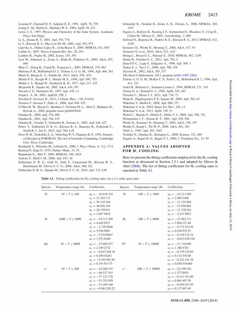
KROME 2415
Lenzuni P., Chernoff D. F., Salpeter E. E., 1991, ApJS, 76, 759Leung C. M., Herbst E., Huebner W. F., 1984, ApJS, 56, 231Lewis J. S., 1997, Physics and Chemistry of the Solar System. Academic
Press, San DiegoLi A., Draine B. T., 2001, ApJ, 554, 778Li Y., Klessen R. S., Mac Low M.-M., 2003, ApJ, 592, 975Lipovka A., Nunez-Lopez R., Avila-Reese V., 2005, MNRAS, 361, 850Lodato G., 2007, Nuovo Cimento Riv. Ser., 30, 293Lodders K., Fegley B., 2002, Icarus, 155, 393Lyra W., Johansen A., Zsom A., Klahr H., Piskunov N., 2009, A&A, 497,
869Maio U., Dolag K., Ciardi B., Tornatore L., 2007, MNRAS, 379, 963Maloney P. R., Hollenbach D. J., Tielens A. G. G. M., 1996, ApJ, 466, 561Maret S., Bergin E. A., Tafalla M., 2013, A&A, 559, A53Martin P. G., Keogh W. J., Mandy M. E., 1998, ApJ, 499, 793Mathis J. S., Rumpl W., Nordsieck K. H., 1977, ApJ, 217, 425Meijerink R., Spaans M., 2005, A&A, 436, 397Navarro J. F., Steinmetz M., 1997, ApJ, 478, 13Nejad L. A. M., 2005, Ap&SS, 299, 1Nicolini P., Frezzato D., 2013, J. Chem. Phys., 138, 234102Nozawa T., Kozasa T., Habe A., 2006, ApJ, 648, 435O’Shea B. W., Bryan G., Bordner J., Norman M. L., Abel T., Harkness R.,
Kritsuk A., 2004, preprint (astro-ph/0403044)Omukai K., 2000, ApJ, 534, 809Omukai K., 2001, ApJ, 546, 635Omukai K., Tsuribe T., Schneider R., Ferrara A., 2005, ApJ, 626, 627Peters T., Schleicher D. R. G., Klessen R. S., Banerjee R., Federrath C.,
Smith R. J., Sur S., 2012, ApJ, 760, L28Press W. H., Teukolsky S. A., Vetterling W. T., Flannery B. P., 1992, Numeri-
cal Recipes in FORTRAN. The Art of Scientific Computing. CambridgeUniv. Press, Cambridge
Reinhardt V., Winckler M., Lebiedz D., 2008, J. Phys. Chem. A, 112, 1712Rentrop P., Kaps P., 1979, Numer. Math., 33, 55Ripamonti E., Abel T., 2004, MNRAS, 348, 1019Santoro F., Shull J. M., 2006, ApJ, 643, 26Schleicher D. R. G., Galli D., Palla F., Camenzind M., Klessen R. S.,
Bartelmann M., Glover S. C. O., 2008, A&A, 490, 521Schleicher D. R. G., Spaans M., Glover S. C. O., 2010, ApJ, 712, L69
Schneider R., Omukai K., Inoue A. K., Ferrara A., 2006, MNRAS, 369,1437
Segura A., Krelove K., Kasting J. F., Sommerlatt D., Meadows V., Crisp D.,Cohen M., Mlawer E., 2003, Astrobiology, 3, 689
Seifried D., Banerjee R., Pudritz R. E., Klessen R. S., 2013, MNRAS, 432,3320
Semenov D., Wiebe D., Henning T., 2004, A&A, 417, 93Semenov D. et al., 2010, A&A, 522, A42Shang C., Bryan G. L., Haiman Z., 2010, MNRAS, 402, 1249Shetty R., Ostriker E. C., 2012, ApJ, 754, 2Stancil P. C., Lepp S., Dalgarno A., 1998, ApJ, 509, 1Tasker E. J., Tan J. C., 2009, ApJ, 700, 358Teyssier R., 2002, A&A, 385, 337The Enzo Collaboration, 2013, preprint (arXiv:1307.2265)Tielens A. G. G. M., McKee C. F., Seab C. G., Hollenbach D. J., 1994, ApJ,
431, 321Vedel H., Hellsten U., Sommer-Larsen J., 1994, MNRAS, 271, 743Verner D. A., Ferland G. J., 1996, ApJS, 103, 467Visscher C., Moses J. I., 2011, ApJ, 738, 72Wada K., Papadopoulos P. P., Spaans M., 2009, ApJ, 702, 63Wakelam V., Herbst E., 2008, ApJ, 680, 371Wakelam V. et al., 2010, Space Sci. Rev., 156, 13Wakelam V. et al., 2012, ApJS, 199, 21Walsh C., Harada N., Herbst E., Millar T. J., 2009, ApJ, 700, 752Weingartner J. C., Draine B. T., 2001, ApJ, 548, 296Wiebe D., Semenov D., Henning T., 2003, A&A, 399, 197Woitke P., Kamp I., Thi W.-F., 2009, A&A, 501, 383Yahil A., 1983, ApJ, 265, 1047Yoshida N., Omukai K., Hernquist L., 2008, Science, 321, 669Zagaris A., Kaper H. G., Kaper T. J., 2004, J. Nonlinear Sci., 14, 59
A P P E N D I X A : VA L U E S A D O P T E DF O R H 2 C O O L I N G
Here we present the fitting coefficients employed for the H2 coolingfunction as discussed in Section 2.3.1 and adopted by Glover &Abel (2008). The list of fitting coefficients for H2 cooling rates isreported in Table A1.
Table A1. Fitting coefficients for H2 cooling rates, for a 3:1 ortho–para ratio.
Species Temperature range (K) Coefficients Species Temperature range (K) Coefficients
H 10 < T ≤ 100 a0 = −16.818 342 H 100 < T ≤ 1000 a0 = −24.311 209a1 = 37.383 713 a1 = 3.569 2468a2 = 58.145 166 a2 = −11.332 860a3 = 48.656 103 a3 = −27.850 082a4 = 20.159 831 a4 = −21.328 264a5 = 3.847 9610 a5 = −4.251 9023
H 1000 < T ≤ 6000 a0 = −24.311 209 H2 100 < T ≤ 6000 a0 = −23.962 112a1 = 4.645 0521 a1 = 2.094 337 40a2 = −3.720 9846 a2 = −0.771 514 36a3 = 5.936 9081 a3 = 0.436 933 53a4 = −5.510 8047 a4 = −0.149 132 16a5 = 1.553 8288 a5 = −0.033 638 326
He 10 < T ≤ 6000 a0 = −23.689 237 H+ 10 < T ≤ 10000 a0 = −21.716 699a1 = 2.189 2372 a1 = 1.386 5783a2 = −0.815 204 38 a2 = −0.379 152 85a3 = 0.290 36281 a3 = 0.114 536 88a4 = −0.165 961 84 a4 = −0.232 141 54a5 = 0.191 913 75 a5 = 0.058 538 864
e− 10 < T ≤ 200 a0 = −34.286 155 e− 200 < T ≤ 10000 a0 = −22.190 316a1 = −48.537 163 a1 = 1.572 8955a2 = −77.121 176 a2 = −0.213 351 00a3 = −51.352 459 a3 = 0.961 497 59a4 = −15.169 160 a4 = −0.910 231 95a5 = −0.981 203 22 a5 = 0.137 497 49
MNRAS 439, 2386–2419 (2014)
at Royal L
ibrary/Copenhagen U
niversity Library on June 13, 2014
http://mnras.oxfordjournals.org/
Dow
nloaded from

2416 T. Grassi et al.
A P P E N D I X B : VA L U E S A D O P T E DF O R M E TA L C O O L I N G
In this section, we report the data used for the fine-structure metalcooling. The data are taken from Hollenbach & McKee (1989),Maio et al. (2007), Glover & Jappsen (2007) and Grassi et al. (2012).The transitions included in KROME implementation are sketched inFigs B1–B4. The rate coefficients with several colliders and theatomic data are reported in Tables B1–B4.
Figure B1. Pictorial view for the line transitions of carbon.
Figure B2. Pictorial view for the line transitions of oxygen.
Figure B3. Pictorial view for the line transitions of silicon.
Figure B4. Pictorial view for the line transitions of iron.
APPENDI X C : R EACTI ON R ATES EMPLOYEDI N T H E PR I M O R D I A L N E T WO R K
The reaction rates employed in the primordial network are listed inTable C1.
A P P E N D I X D : R E AC T I O N FI L E FO R M AT
The reaction file has a default template, namely
index, R1, R2, R3, P1, P2, P3, P4, Tmin, Tmax, rate
that can be modified according to other formats. In particular onecan indicate the number of items simply using the following casenon-sensitive tokens: R for reactants, P for products, Tmin and Tmaxfor the temperature limits, rate for the reaction rate and idx for theindex. The format string must begin with @format: to be recog-nized by the file parser of the KROME package. The user can employseveral format strings within the same reaction file, e.g.
@format:R, R, P, Tmin, Tmax, rate
H, H, H2, 1e1, 1e4, 1d-9
C, O, CO, 1e1, 1e4, 3d-9
@format:Tmin, Tmax, R, R, P, P rate
1e1, 1e4, H+, C, H, C+, 1d-10
where the first line indicates a block of reaction with two reactants,one product, the temperature limits and the rate coefficient, while
Table B1. De-excitation rate coefficients for neutral metals and atomic data for each transition. Note that a(b) = a × 10b.
Coolant j→i γ Hji (cm3 s−1) γ H+
ji (cm3 s−1) Aji(s−1) �Eji (K) gi gj
CI 1→0 1.6(−10)T 0.142 [9.6(−11) − 1.8(−14)T + 1.9(−18)T2]T0.45 7.9(−8) 24 3 1
if (T > 5 × 10³) 8.9(−10)T0.117
CI 2→0 9.2(−11)T 0.262 [3.1(−12) − 6(−16)T + 3.9(−20)T2]T 2.7(−7) 63 5 1
if (T > 5 × 10³) 2.3(−9)T0.0965
CI 2→1 2.9(−10)T 0.262 [1(−10) − 2.2(−14)T + 1.7(−18)T2]T0.7 2.1(−14) 39 5 3
if (T > 5 × 10³) 9.2(−9)T0.0535
OI 1→0 9.2(−11)(T2)0.67 6.38(−11)T0.4 8.9(−5) 230 3 5if (T > 194) 7.75(−12)T0.8
if (T > 3686) 2.65(−10)T0.37
OI 2→0 4.3(−11)(T2)0.80 6.1(−13)T1.1 1.8(−5) 330 1 5if (T > 511) 2.12(−12)T0.9
if (T > 7510) 4.49(−10)T0.3
OI 2→1 1.1(−10)(T2)0.44 2.03(−11)T0.56 1.3(−10) 98 1 3if (T > 2090) 3.43(−10)T0.19
SiI 1→0 3.5(−10)T −0.032 7.2(−9) 8.4(−6) 110 3 1
SiI 2→0 1.7(−11)T 0.172 7.2(−9) 2.4(−10) 320 5 1
SiI 2→1 5(−10)T 0.172 2.2(−8) 1.0(−9) 210 5 3
FeI 1→0 8(−10)T 0.172 – 2.5(−3) 594.43 9 7
FeI 2→0 6.9(−10)T 0.172 – 1.0(−9) 1012.9 9 5
FeI 2→1 5.3(−10)T 0.172 – 1.6(−3) 414.47 7 5
FeI 3→0 – – 2.0(−3) 594.43 9 11FeI 4→0 – – 1.5(−3) 1012.9 9 8FeI 4→3 – – 3.6(−3) 414.47 11 8
MNRAS 439, 2386–2419 (2014)
at Royal L
ibrary/Copenhagen U
niversity Library on June 13, 2014
http://mnras.oxfordjournals.org/
Dow
nloaded from

KROME 2417
Table B2. De-excitation rate coefficients for neutral metals with H2 ortho and para, and electrons. See Table B1 foradditional values, while other de-excitation rates are listed in Table B3. Note that a(b) = a × 10b and T2 = T/(100 K).
Coolant j→i γHo
2ji (cm3 s−1) γ
Hp2
ji (cm3 s−1) γ e−ji (cm3 s−1)
CI 1→0 8.7(−11) − 6.6(−11) exp (−T/218.3) 7.9(−11) − 8.7(−11) exp (−T/126.4) See Table B3CI 2→0 1.2(−11) − 6.1(−11) exp (−T/387.3) 1.1(−10) − 8.6(−11) exp (−T/223) See Table B3
+8.7(−11) exp (−2T/223)CI 2→1 2.9(−10) − 1.9(−10) exp (−T/348.9) 2.7(−10) − 1.9(−10) exp (−T/348.9) See Table B3
+1.8(−10) exp (2T/250.7)OI 1→0 2.7(−11)T 0.362 3.46(−11)T 0.316 5.12(−10)T−0.075
OI 2→0 5.49(−11)T 0.317 7.07(−11)T 0.268 4.86(−10)T−0.026
OI 2→1 2.74(−14)T 1.06 3.33(−15)T 1.36 1.08(−14)T 0.926
FeI 1→0 – – 1.2(−7)FeI 2→0 – – 1.2(−7)FeI 2→1 – – 9.3(−8)FeI 3→0 – – 2(−7)(T/104)0.57
FeI 4→0 – – 1(−7)(T/104)0.57
FeI 4→3 – – 1.5(−7)
Table B3. De-excitation rate coefficients for neutral carbon, Einstein’s coefficients, energylevel differences and level multiplicities. See Table B1 for additional atomic values. Note thata(b) = a × 10b.
Coolant j→i γ e−ji (cm3 s−1)
CI 1→0 2.88(6)T−0.5 exp (−9.25141 − 7.73782(−1) ln (T) + 3.61184(−1) ln (T)2
−1.50892(−2) ln (T)3 − 6.56325(−4) ln (T)4)if(T > 103) 2.88(−6)T−0.5 exp (−4.446(2) − 2.27913(2) ln (T)+4.2595(1) ln (T)2 − 3.4762 ln (T)3 + 1.0508(−1) ln (T)4)
CI 2→0 1.73(−6)T−0.5 exp (−7.697351.30743 ln (T) − 0.111338 ln (T)3
+0.705277(−2) ln (T)4)if(T > 103) 1.73(−6)T−0.5 exp (3.50609(2) − 1.87474(2) ln (T)+3.61803(1) ln (T)2 − 3.03283 ln (T)3 + 9.38138(−2) ln (T)4)
CI 2→1 21.73(−6)T−0.5 exp (−7.4387 − 0.57443 ln (T) + 0.358264 ln (T)2
−4.18166(−2) ln (T)3 + 2.35272(−3) ln (T)4)if(T > 103) 1.73(−6)T−0.5 exp (3.86186(2) − 2.02192(2) ln (T)+3.85049(1) ln (T)2 − 3.19268 ln (T)3 + 9.78573(−2) ln (T)4)
Table B4. De-excitation rate coeffients for ions, Einstein’s coefficients, energy level differencesand level multiplicities. Note that a(b) = a × 10b, T2 = T/(100 K) and T4 = T/(104 K).
Coolant j→i γ Hji (cm3 s−1) γ e−
ji (cm3 s−1) Aji(s−1) �Eji (K) gi gj
CII 1→0 8 · 10−10T 0.072 2.8 · 10−7T −0.5
2 2.4 · 10−6 91.2 4 2OII 1→0 1.3 · 10−8(T4)−0.5 5.1 · 10−5 385 74.4 11 7OII 2→0 1.3 · 10−8(T4)−0.5 1.7 · 10−4 386 03.2 7 7OII 2→1 2.5 · 10−8(T4)−0.5 1.3 · 10−7 28.8 7 11 11SiII 1→0 8 · 10−10T −0.07
2 1.7 · 10−6T −0.52 2.1 · 10−4 413.6 4 2
FeII 1→0 9.5 · 10−10 1.8 · 10−6T −0.52 2.13 · 10−3 553.58 10 8
FeII 2→1 4.7 · 10−10 8.7 · 10−7T −0.52 1.57 · 10−3 407.01 6 8
FeII 3→2 5.0 · 10−10 10−5T −0.5 1.50 · 10−9 280.57 6 4FeII 4→3 5.0 · 10−10 10−5T −0.5 1.88 · 10−4 164.60 4 2FeII 2→0 5.7 · 10−10 1.8 · 10−6T −0.5
2 1.5 · 10−9 960.59 10 6
MNRAS 439, 2386–2419 (2014)
at Royal L
ibrary/Copenhagen U
niversity Library on June 13, 2014
http://mnras.oxfordjournals.org/
Dow
nloaded from

2418 T. Grassi et al.
Table C1. List of reactions and rates included in our chemical network. See Abel et al. (1997) for further details.
Reaction Rate coefficient (cm3 s−1)
H + e− → H+ + 2e− k1 = exp[−32.713 967 86+13.536 5560 ln Te
−5.739 328 75 (ln Te)2+1.563 154 98 (ln Te)3
−0.287 705 60 (ln Te)4+3.482 559 77 × 10−2(ln Te)5
−2.631 976 17 × 10−3(ln Te)6+1.119 543 95 × 10−4(ln Te)7
−2.039 149 85 × 10−6(ln Te)8]H+ + e− → H + γ k2 = 3.92 × 10⁻¹³ Te
−0.6353 T ≤ 5500 Kk2 = exp [−28.613 033 806 892 32 T > 5500 K−7.241 125 657 826 851 × 10−1 ln Te
−2.026 044 731 984 691 × 10−2 (ln Te)2
−2.380 861 877 349 834 × 10−3 (ln Te)3
−3.212 605 213 188 796 × 10−4 (ln Te)4
−1.421 502 914 054 107 × 10−5 (ln Te)5
+4.989 108 920 299 510 × 10−6 (ln Te)6
+5.755 614 137 575 750 × 10−7 (ln Te)7
−1.856 767 039 775 260 × 10−8 (ln Te)8
−3.071 135 243 196 590 × 10−9 (ln Te)9]He + e− → He+ + 2e− k3 = exp [−44.098 648 86 Te > 0.8 eV
+23.915 965 63 lnTe
−10.753 2302 (ln Te)2
+3.058 038 75 (ln Te)3
−5.685 1189 × 10−1 (ln Te)4
+6.795 391 23 × 10−2 (ln Te)5
−5.009 056 10 × 10−3 (ln Te)6
+2.067 236 16 × 10−4 (lnTe)7
−3.649 161 41 × 10−6 (ln Te)8]He+ + e− → He + γ k4 = 3.92 × 10⁻¹³ Te
−0.6353 Te ≤ 0.8 eVk4 = + 3.92 × 10⁻¹³ T −0.6353
e T > 0.8 eV+1.54 × 10⁻⁹ T −1.5
e [1.0 + 0.3 / exp (8.099 328 789 667/Te)]/[exp (40.496 643 948 336 62/Te)]
He+ + e− → He2+ + 2e− k5 = exp [−68.710 409 902 120 01 Te > 0.8 eV+43.933 476 326 35 lnTe
−18.480 669 935 68 (ln Te)2
+4.701 626 486 759 002 (ln Te)3
−7.692 466 334 492 × 10−1 (ln Te)4
+8.113 042 097 303 × 10−2 (ln Te)5
−5.324 020 628 287 001 × 10−3 (ln Te)6
+1.975 705 312 221 × 10−4 (ln Te)7
−3.165 581 065 665 × 10−6 (ln Te)8]He2+ + e− → He+ + γ k6 = 3.36 × 10⁻¹⁰ T−1/2(T/1000)−0.2(1 + (T/106)0.7)−1
H + e → H− + γ k7 = 6.77 × 10⁻¹⁵ T 0.8779e
H− + H → H2 + e− k8 = 1.43 × 10⁻⁹ T ≤ 1160 Kk8 = exp [−20.069 138 975 870 03 T > 1160 K+2.289 800 603 272 916 × 10−1 ln Te
+3.599 837 721 023 835 × 10−2 (ln Te)2
−4.555 120 027 032 095 × 10−3 (ln Te)3
−3.105 115 447 124 016 × 10−4 (ln Te)4
+1.073 294 010 367 247 × 10−4 (ln Te)5
−8.366 719 604 678 64 × 10−6 (ln Te)6
+2.238 306 228 891 639 × 10−7 (ln Te)7]H + H+ → H+
2 + γ k9 = 1.85 × 10⁻²³ T1.8 T ≤ 6700 Kk9 = 5.81 × 10⁻¹⁶ (T/56200)(−0.6657 log10(T /562 00)) T > 6700 K
H+2 + H → H2 + H+ k10 = 6.0 × 10⁻¹⁰
H2 + H+ → H+2 + H k11 = exp [−24.249 146 877 315 36 Te > 0.3 eV
+3.400 824 447 095 291 ln Te
−3.898 003 964 650 152 (lnTe)2
+2.045 587 822 403 071 (ln Te)3
−5.416 182 856 220 388 × 10−1 (ln Te)4
+8.410 775 037 634 12 × 10−2 (ln Te)5
−7.879 026 154 483 455 × 10−3 (ln Te)6
+4.138 398 421 504 563 × 10−4 (ln Te)7
−9.363 458 889 286 11 × 10−6 (ln Te)8]H2 + e− → 2H + e− k12 = 5.6 × 10⁻¹¹T0.5exp (−102 124.0/T) Te > 0.3 eV
MNRAS 439, 2386–2419 (2014)
at Royal L
ibrary/Copenhagen U
niversity Library on June 13, 2014
http://mnras.oxfordjournals.org/
Dow
nloaded from

KROME 2419
Table C1 – continued
Reaction Rate coefficient (cm3 s−1)
H− + e− → H + 2e− k13 = exp (−18.018 493 342 73 Te > 0.04 eV+2.360 852 208 681 ln Te
−2.827 443 061 704 × 10−1 (ln Te)2
+1.623 316 639 567 × 10−2 (ln Te)3
−3.365 012 031 362 999 × 10−2 (ln Te)4
+1.178 329 782 711 × 10−2 (ln Te)5
−1.656 194 699 504 × 10−3 (ln Te)6
+1.068 275 202 678 × 10−4 (ln Te)7
−2.631 285 809 207 × 10−6 (ln Te)8
H− + H → 2H + e− k14 = 2.56 × 10⁻⁹ T 1.781 86e Te ≤ 0.04 eV
k14 = exp [−20.372 608 965 333 24 Te > 0.04 eV+1.139 449 335 841 631 ln Te
−1.421 013 521 554 148 × 10−1 (ln Te)2
+8.464 455 386 63 × 10−3 (ln Te)3
−1.432 764 121 2992 × 10−3 (ln Te)4
+2.012 250 284 791 × 10−4 (ln Te)5
+8.663 963 243 09 × 10−5 (ln Te)6
−2.585 009 680 264 × 10−5 (ln Te)7
+2.455 501 197 0392 × 10−6 (ln Te)8
−8.068 382 461 18 × 10−8 (ln Te)9]H− + H+ → 2H + γ k15 = 6.5 × 10⁻⁹ T −0.5
e
H− + H+ → H+2 + e− k16 = 10−8 × T−0.4
H+2 + e → 2H + γ k17 = 10−8 T ≤ 617 K
k17 = 1.32 × 10⁻⁶ T−0.76 T > 617 KH+
2 + H− → H + H2 k18 = 5.0 × 10⁻⁷ (102 × T)−0.5
3H → H2 + H k19 = 1.3 × 10⁻³²(T/300)−0.38 T ≤ 300 Kk19 = 1.3 × 10⁻³²(T/300)−1.00 T > 300 K
H2 + H → 3H k20 = (1.067 0825 × 10−10 × T 2.012e )/(exp(4.463/Te) × (1 + 0.2472Te)3.512)
the fourth line is employed to use a format that starts with thetemperature limits, then two reactants and two products, and therate coefficient. Note that the coefficient rates in this example haveonly an illustrative purpose, and do not represent the real coefficientsfor the reactions reported here.
Finally, KROME allows in the file to use comments and variables,as already discussed, and also individual temperature operators, e.g.
@format:Tmin, Tmax, R, R, P, P rate
>1e1, 1e4, H+, C, H, C+, 1d-10
where the > sign is employed for this reaction only.
This paper has been typeset from a TEX/LATEX file prepared by the author.
MNRAS 439, 2386–2419 (2014)
at Royal L
ibrary/Copenhagen U
niversity Library on June 13, 2014
http://mnras.oxfordjournals.org/
Dow
nloaded from