A Novel Voltage Sag Detection Method Based on a Selective ...

Citation: Li, Z.; Yang, R.; Guo, X.;

Wang, Z.; Chen, G. A Novel Voltage

Sag Detection Method Based on a

Selective Harmonic Extraction

Algorithm for Nonideal Grid

Conditions. Energies 2022, 15, 5560.

https://doi.org/10.3390/en15155560

Academic Editor: Julio Barros

Received: 13 July 2022

Accepted: 29 July 2022

Published: 31 July 2022

Publisher’s Note: MDPI stays neutral

with regard to jurisdictional claims in

published maps and institutional affil-

iations.

Copyright: © 2022 by the authors.

Licensee MDPI, Basel, Switzerland.

This article is an open access article

distributed under the terms and

conditions of the Creative Commons

Attribution (CC BY) license (https://

creativecommons.org/licenses/by/

4.0/).

energies

Article

A Novel Voltage Sag Detection Method Based on a SelectiveHarmonic Extraction Algorithm for Nonideal Grid ConditionsZhenyu Li * , Ranchen Yang, Xiao Guo, Ziming Wang and Guozhu Chen *

Department of Electrical Engineering, Zhejiang University, No. 38 Zheda Road, Xihu District, Hangzhou 310027,China; [email protected] (R.Y.); [email protected] (X.G.); [email protected] (Z.W.)* Correspondence: [email protected] (Z.L.); [email protected] (G.C.)

Abstract: Voltage sag detection is utilized to capture the sag occurrence moment and calculate the sagdepth of power grid voltage in real time, so as to generate reference voltage for controlling voltageinteractive equipment such as dynamic voltage restorers (DVRs). However, the traditional voltagesag detection methods based on synchronously rotating frames (SRFs) are unable to acquire high-precision sag information under nonideal grid conditions such as unbalance or harmonic interference.In order to enhance the immunity of the sag detection, a method based on a selective harmonicextraction algorithm (SHEA) is proposed in this paper. Firstly, the state-space model of SHEA isestablished using discrete orthogonal basis to decouple and separate the signal of target frequencyand the signal of interference frequency. The controllability, stability and convergence of SHEA areanalyzed theoretically and serve as the criteria for parameter tuning. Moreover, a gain compensator(GC) is used to improve the low and middle frequency gains of the voltage sag detection methodbased on SHEA so that the dynamic response speed for sag judgment can be optimized quantitatively.The simulation results indicate that the proposed voltage sag detection method has good dynamic andsteady-state performance under nonideal power grid conditions such as unbalanced sag, frequencydrift, phase variation and harmonic interference.

Keywords: voltage sag detection algorithm; dynamic voltage restorer; nonideal grid conditions;modeling and optimization

1. Introduction

Sensitive electronic equipment like computer system (CS), adjustable speed driver(ASD), and programmable logic controller (PLC) have been prevalent in industry, commerceand other fields as a result of the development of information and intelligent technology,which puts forward higher demand for the quality of power supply [1,2]. Voltage sags,unbalance, transients, harmonics, fluctuations and interruptions are the essential powerquality issues [3]. To solve these problems of power quality, power equipment based onpower electronics has been developed such as active power filter (APF), dynamic voltagerestorer (DVR), uninterruptable power supply (UPS) [4]. Voltage sag has emerged as one ofthe most serious problems deteriorating power quality [5,6], which can result in critical loaddisruption and data loss with significant financial damage. Among the power equipment,DVR has gradually become one of the most cost-effective solutions to address voltage sagdue to its high operational efficiency and low overall cost [7,8]. As user-side voltage-basedinteractive equipment in a conventional three-phase and three-wire (3ph-3w) power grid,DVR converts energy in the energy storage system (ESS) into the upstream of the sensitiveload via a series-coupled transformer (SCT) via a three-phase voltage source converter(VSC), so as to compensate and mitigate voltage sag on the user side. In Figure 1, thedetailed schematic [9] of DVR is presented.

Energies 2022, 15, 5560. https://doi.org/10.3390/en15155560 https://www.mdpi.com/journal/energies

https://doi.org/10.3390/en15155560

https://creativecommons.org/

https://creativecommons.org/licenses/by/4.0/

https://creativecommons.org/licenses/by/4.0/

https://www.mdpi.com/journal/energies

https://www.mdpi.com

https://orcid.org/0000-0001-6739-855X

https://doi.org/10.3390/en15155560

https://www.mdpi.com/journal/energies

https://www.mdpi.com/article/10.3390/en15155560?type=check_update&version=2

Energies 2022, 15, 5560 2 of 21Energies 2022, 15, x FOR PEER REVIEW 2 of 22

Figure 1. Schematic of DVR.

Rapid and precise voltage sag detection is a necessary prerequisite for DVR to achieve accurate compensation [3,8,10]. For one thing, if the judgment speed of sag is slug-gish, sensitive equipment can easily exceed its lower voltage tolerance limit and result in crash. For another thing, false positive events would trigger the DVR into compensation mode when no real voltage sag has occurred. Therefore, it is necessary to make a compro-mise between sensitivity and robustness. Moreover, if the calculated information such as sag depth is inaccurate, the sensitive load will not receive high-quality voltage provided by DVR. Currently, several techniques have been thoroughly researched for detecting voltage sag [11,12], including peak value, missing voltage, the root mean square (RMS), discrete Fourier transform (DFT), wavelet transform (WT), least error squares (LES), syn-chronously rotating frame (SRF), etc.

Peak voltage detection [11] searches for the peak value of sinusoidal waveform in no more than half of the grid cycle (20 ms) to determine the occurrence of voltage sag. The procedure is straightforward to implement but is susceptible to harmonics, noise, and phase jump. The time-domain method known as missing voltage [13] can also quickly identify voltage sag according to the difference between the actual and desired instanta-neous voltages. However, this method still suffers from poor immunity, making it impos-sible to obtain complete sag characteristic information. In contrast, RMS detection [14] has strong anti-disturbance ability but poor frequency adaptability and moderate detection speed of at least half a grid cycle. A voltage detection method based on least error squares (LES) is proposed in [15] that can effectively suppress specific harmonics and has good dynamic performance within a few sampling periods. However, this method will amplify the unconsidered high-frequency harmonics, thus affecting the precision of detection. A rapid method of detecting a sag event based on a numerical matrix is proposed in [16]. The method is also sensitive to unknown harmonics such as neglected high-frequency noise. Under nonideal grid conditions, this method can easily cause false judgment of sag events, which will result in frequent startup and malfunction of DVR. The authors of [17] utilized a rectifier to quickly capture the occurrence time of voltage sag, which requires repeated experiments to tune various control parameters before fitting the response value of the detection algorithm to 0.9 p.u.; that is, different application scenarios require differ-ent parameters. In addition, the detection algorithm has the probability of false detection and miss detection that cannot be ignored. WT is an increasingly popular time-frequency localization analysis method [18,19] that is extremely sensitive to signal jump and can quickly identify the start and end moments of voltage sag. Even so, the method needs proper selection of wavelet prototype, which depends on the user’s experience and exist-ing achievements [20]. The authors [21,22] proposed a detection method based on har-monic footprint that characterizes the voltage sag transient behavior with Exp2, the two-term exponential model using only seven data points (samples). To improve reliability, a recurrent neural network (RNN) is used with 680 recordings as a selected training set. The

Figure 1. Schematic of DVR.

Rapid and precise voltage sag detection is a necessary prerequisite for DVR to achieveaccurate compensation [3,8,10]. For one thing, if the judgment speed of sag is sluggish,sensitive equipment can easily exceed its lower voltage tolerance limit and result in crash.For another thing, false positive events would trigger the DVR into compensation modewhen no real voltage sag has occurred. Therefore, it is necessary to make a compromisebetween sensitivity and robustness. Moreover, if the calculated information such as sagdepth is inaccurate, the sensitive load will not receive high-quality voltage provided byDVR. Currently, several techniques have been thoroughly researched for detecting voltagesag [11,12], including peak value, missing voltage, the root mean square (RMS), discreteFourier transform (DFT), wavelet transform (WT), least error squares (LES), synchronouslyrotating frame (SRF), etc.

Peak voltage detection [11] searches for the peak value of sinusoidal waveform in nomore than half of the grid cycle (20 ms) to determine the occurrence of voltage sag. Theprocedure is straightforward to implement but is susceptible to harmonics, noise, and phasejump. The time-domain method known as missing voltage [13] can also quickly identifyvoltage sag according to the difference between the actual and desired instantaneousvoltages. However, this method still suffers from poor immunity, making it impossibleto obtain complete sag characteristic information. In contrast, RMS detection [14] hasstrong anti-disturbance ability but poor frequency adaptability and moderate detectionspeed of at least half a grid cycle. A voltage detection method based on least error squares(LES) is proposed in [15] that can effectively suppress specific harmonics and has gooddynamic performance within a few sampling periods. However, this method will amplifythe unconsidered high-frequency harmonics, thus affecting the precision of detection. Arapid method of detecting a sag event based on a numerical matrix is proposed in [16].The method is also sensitive to unknown harmonics such as neglected high-frequencynoise. Under nonideal grid conditions, this method can easily cause false judgment ofsag events, which will result in frequent startup and malfunction of DVR. The authorsof [17] utilized a rectifier to quickly capture the occurrence time of voltage sag, whichrequires repeated experiments to tune various control parameters before fitting the responsevalue of the detection algorithm to 0.9 p.u.; that is, different application scenarios requiredifferent parameters. In addition, the detection algorithm has the probability of falsedetection and miss detection that cannot be ignored. WT is an increasingly popular time-frequency localization analysis method [18,19] that is extremely sensitive to signal jumpand can quickly identify the start and end moments of voltage sag. Even so, the methodneeds proper selection of wavelet prototype, which depends on the user’s experience andexisting achievements [20]. The authors [21,22] proposed a detection method based onharmonic footprint that characterizes the voltage sag transient behavior with Exp2, thetwo-term exponential model using only seven data points (samples). To improve reliability,a recurrent neural network (RNN) is used with 680 recordings as a selected training set. Thedetection time can reach within 1 ms. However, the possibility of false detection is minimalonly if RNN is properly prepared; it may also be more suitable for offline scenarios such

Energies 2022, 15, 5560 3 of 21

as voltage fault characterization, classification, and big data analysis. Other mathematicalmethods such as Kalman filter [23] and S transform [24] are also more suitable for theoffline analysis of power quality because of their intricate calculation and subpar real-timeperformance.

Selective harmonic extraction (SHE) is a well-known concept that can extract orsuppress the required fundamental or harmonic component, which can be used for voltagesag detection in a harmonic distorted power grid. The main implementation method ofSHE is based on finite impulse response (FIR) filter structure, such as sliding recursivediscrete Fourier transform (SDFT), generalized delayed signal cancellation (GDSC) [25],and generalized discrete Fourier transform (GDFT) [26]. Traditional SDFT [27] uses acomplex resonator and a comb filter to extract the specific harmonic. The major drawback isthe slow dynamic responses, requiring at least one-cycle settling time. Additionally, carefulsynchronization between the sampling and fundamental frequency is needed in practicalapplications to minimize the leakage effects of DFT, and in case of large frequency deviation,significant errors in magnitude can be introduced. The traditional SDFT is improved in [28]by removing the redundant zeros in the comb filter to improve the dynamic response speed.Specifically, the zeros corresponding to the harmonic numbers (1st, 2nd, 3rd, 4th, 5th, 6th,etc.) are decreased to corresponding to 1st, 5th, 7th, 11th, 13th, etc. The response timeis reduced from one grid cycle to 1/3 cycle. In addition, variable sampling frequency isused to realize the grid frequency adaptation of GDFT, which can avoid the non-integersampling [29].

Aside from the aforementioned techniques, a number of voltage sag detection meth-ods [10,30] based on synchronously rotating frame (SRF) have gained widespread industrialrecognition for its excellent adaptability and simple implementation based on phase-lockedloop (PLL) embedded in DVR. According to the literature [3], in order to suppress theimpact of harmonics and negative-sequence fundamental components on the calculationof voltage sag depth, a low-pass filter (LPF) needs to be added after Park transformation.However, the bandwidth and harmonic suppression capability of LPF are incompatiblewith each other [31]. Low-bandwidth LPF, is only appropriate for equipment such asactive power filter (APF) that does not require rapid detection, rather than DVR applica-tion. The LPF with high cut-off frequency [32] can improve detection speed; however, theanti-disturbance ability of the algorithm will be significantly reduced. The multi-pointdifference concept was used in [33,34] to eliminate the influence of specific harmonicsand thereby reduce the delay effect compared with LPF; however, the anti-interferenceability of the difference method is poor, especially in the cases of frequency drift, phasejump, etc. A method of calculating grid voltage RMS based on SRF is proposed in [35]that can realize the convergence of voltage amplitude within half a grid cycle. The methodhas a strong robustness but an ordinary speed. Besides, the method will also producea steady-state double-frequency ripple in the face of frequency drift that will affect theaccuracy. Thanks to the frequency-adaptive bandpass characteristic [36], dual second-order generalized integrator (DSOGI) can be inserted before Park transformation to detectfundamental positive-sequence voltage when grid frequency drifts, but it has to makea compromise between dynamic performance and the ability to filter out low-frequencydisturbance [37]. The authors of [38] introduced a multiple second-order generalized in-tegrator (MSOGI) approach that accomplishes the decoupling of fundamental frequencyand harmonic frequency. Although the immunity of detection is improved, its dynamicresponse performance is still subpar. Introduced MAF [39] or cascaded DSC [40] afterPark transformation can realize notch suppression at each harmonic frequency. Like theaforementioned DFT, it is difficult for such two methods to achieve zero steady-state errorof voltage calculation even after taking frequency adaptation into account [29], and theresponse time is lengthy.

In this paper, a novel selective harmonic extraction algorithm (SHEA) combinedwith SRF is proposed to realize the accurate detection of voltage sag under nonidealgrid conditions such as unbalance and harmonic disturbances. The proposed SHEA is

Energies 2022, 15, 5560 4 of 21

not based on FIR structure like DFT, GDFT, etc.; instead, a discrete state-space model isestablished to flexibly suppress harmonic components and avoid the accuracy problemscaused by non-integer sampling related to grid frequency drift. The significant frequencydrift adaptation, meanwhile, is realized by a phase-locked loop (PLL). The proposedtechnique has excellent robustness and can be intended for low-frequency harmonics thathave a significant impact on sag state estimation. In addition, it should be noted that stronganti-interference performance sacrifices the convergence speed. To address this issue, again compensator (GC) for SHEA is designed to enhance the dynamic performance ofdetection from the standpoint of low and medium frequency gain.

The rest of this paper is organized as follows. Section 2 elaborates the performancedemands of voltage sag detection methods under nonideal grid conditions. In Section 3,the proposed SHEA based on the state-space model and the performance of the algorithmare analyzed theoretically, and the criteria for parameter selection are given. The dynamicresponse speed of the voltage sag detection method based on SHEA is optimized utilizingGC in Section 4. Section 5 shows the simulation results. Finally, the conclusions are givenin Section 6.

2. Voltage Sag and Traditional Detection Methods Based on SRF

The three primary factors that contribute to voltage sag in a three-phase and three-wire (3ph-3w) power system are short-circuit fault, induction motor starting, and lightningstrike [41]. Short-circuit fault is by far the most significant factor. According to features,voltage sags caused by short-circuit faults can be separated into 7 categories (A to G) [42],as illustrated in Figure 2 [43]. Sag types D, F, and G is the derived type propagated byvarious types of transformers, whereas sag types A, B, C, and E stands for three-phasesymmetrical short circuit, single-phase short circuit, phase-to-phase short circuit, andtwo-phase grounding short circuit, respectively.

Energies 2022, 15, x FOR PEER REVIEW 4 of 22

In this paper, a novel selective harmonic extraction algorithm (SHEA) combined with SRF is proposed to realize the accurate detection of voltage sag under nonideal grid con-ditions such as unbalance and harmonic disturbances. The proposed SHEA is not based on FIR structure like DFT, GDFT, etc.; instead, a discrete state-space model is established to flexibly suppress harmonic components and avoid the accuracy problems caused by non-integer sampling related to grid frequency drift. The significant frequency drift ad-aptation, meanwhile, is realized by a phase-locked loop (PLL). The proposed technique has excellent robustness and can be intended for low-frequency harmonics that have a significant impact on sag state estimation. In addition, it should be noted that strong anti-interference performance sacrifices the convergence speed. To address this issue, a gain compensator (GC) for SHEA is designed to enhance the dynamic performance of detection from the standpoint of low and medium frequency gain.

The rest of this paper is organized as follows. Section 2 elaborates the performance demands of voltage sag detection methods under nonideal grid conditions. In Section 3, the proposed SHEA based on the state-space model and the performance of the algorithm are analyzed theoretically, and the criteria for parameter selection are given. The dynamic response speed of the voltage sag detection method based on SHEA is optimized utilizing GC in Section 4. Section 5 shows the simulation results. Finally, the conclusions are given in Section 6.

2. Voltage Sag and Traditional Detection Methods Based on SRF The three primary factors that contribute to voltage sag in a three-phase and three-

wire (3ph-3w) power system are short-circuit fault, induction motor starting, and light-ning strike [41]. Short-circuit fault is by far the most significant factor. According to fea-tures, voltage sags caused by short-circuit faults can be separated into 7 categories (A to G) [42], as illustrated in Figure 2 [43]. Sag types D, F, and G is the derived type propagated by various types of transformers, whereas sag types A, B, C, and E stands for three-phase symmetrical short circuit, single-phase short circuit, phase-to-phase short circuit, and two-phase grounding short circuit, respectively.

Figure 2. The seven basic voltage sag types of the distribution network.

Except for type A in Figure 2, the voltage sag types belong to unbalanced voltage sag. If harmonic disturbance is also taken into account, the three-phase grid voltage can be assumed as

Figure 2. The seven basic voltage sag types of the distribution network.

Except for type A in Figure 2, the voltage sag types belong to unbalanced voltage sag.If harmonic disturbance is also taken into account, the three-phase grid voltage can beassumed as

ug_a(t) = ∑h=1,3,5,7,...

[U+

h cos(hωgt + ϕ+

h

)+ U−h cos

(hωgt + ϕ−h

)]ug_b(t) = ∑

h=1,3,5,7,...

[U+

h cos(hωgt + ϕ+

h −2π3)+ U−h cos

(hωgt + ϕ−h + 2π

3)]

ug_c(t) = ∑h=1,3,5,7,...

[U+

h cos(hωgt + ϕ+

h + 2π3)+ U−h cos

(hωgt + ϕ−h −

2π3)] (1)

where U+h (U−h ) and ϕ+

h (ϕ−h ) represent the amplitude and the phase angle of the hth har-monic component of the positive-sequence (negative-sequence) of the grid voltage, respec-

Energies 2022, 15, 5560 5 of 21

tively, and h = 1 represents the fundamental voltage. Furthermore, ωg is the actual angularfrequency of fundamental voltage of power grid.

Using Clark transformation [44], the three-phase grid voltage can be formulated as

[ug_α(t)ug_β(t)

]= Tαβ

ug_a(t)ug_b(t)ug_c(t)

=

∑h=1,3,5,7,...

[U+

h cos(hωgt + ϕ+

h

)+ U−h cos

(hωgt + ϕ−h

)]∑

h=1,3,5,7,...

[U+

h sin(hωgt + ϕ+

h

)−U−h sin

(hωgt + ϕ−h

)] (2)

where

Tαβ =23

[1 − 1

2 − 12

0√

32 −

√3

2

](3)

Applying Park transform [45] with the estimated fundamental positive-sequence phaseangle θ+1 , the three-phase grid voltage in synchronous reference frame can be expressed as

[u+

g_d(t)

u+g_q(t)

]= T+

dq

[ug_α(t)ug_β(t)

]=

∑h=1,3,5,7,...

[U+

h cos((hωg − ωg)t + (ϕ+

h − ϕ+1 ))+ U−h cos

((hωg + ωg)t + (ϕ−h + ϕ+

1 ))]

∑h=1,3,5,7,...

[U+

h sin((hωg − ωg)t + (ϕ+

h − ϕ+1 ))−U−h sin

((hωg + ωg)t + (ϕ−h + ϕ+

1 ))]

(4)

where

T+dq =

[cos θ+1 sin θ+1− sin θ+1 cos θ+1

](5)

Under a quasi-locked condition when the estimated angular frequency ωg is equal toωg, (4) can be approximated as[

u+g_d(t)

u+g_q(t)

]≈[

u+g_d(t)

u+g_q(t)

]+

[u+

g_d(t)u+

g_q(t)

](6)

where [u+

g_d(t)u+

g_q(t)

]=

[U+

1 cos(∆ϕ+

1)

U+1 sin

(∆ϕ+

1)] ≈ [ U+

1U+

1 ·θ+1

](7)

[u+

g_d(t)

u+g_q(t)

]=

[U−1 cos

((2ωg)t + (ϕ−h + ϕ+

1 ))

−U−1 sin((2ωg)t + (ϕ−h + ϕ+

1 )) ]+ ∑

h=3,5,7,...

[U+

h cos(((h− 1)ωg)t + (ϕ+

h − ϕ+1 ))+ U−h cos

(((h + 1)ωg)t + (ϕ−h + ϕ+

1 ))]

∑h=3,5,7,...

[U+

h sin(((h− 1)ωg)t + (ϕ+

h − ϕ+1 ))−U−h sin

(((h + 1)ωg)t + (ϕ−h + ϕ+

1 ))]

(8)

It is clear from Equations (7) and (8) that the numbers of positive-sequence or negative-sequence components of the hth harmonic will decrease or increase by 1 after Park trans-formation. For instance, the negative-sequence of the fundamental component will rise to2nd-frequency one, while the positive-sequence of the 5th harmonic will be transformed tothe 4th one, etc. Equation (8) can be simplified as[

u+g_d(t)

u+g_q(t)

]=

[fd(2ωg, 4ωg, 6ωg, 8ωg, . . .)fq(2ωg, 4ωg, 6ωg, 8ωg, . . .)

](9)

It can be seen that when asymmetric sag occurs with odd harmonics (3rd, 5th, 7thharmonic, etc.), the result of Park transformation includes even harmonics (2nd, 4th, 6thharmonic, etc.) in addition to the DC component corresponding to positive-sequencefundamental component. Traditional methods to calculate the voltage amplitude based onSRF are SRF-LPF and DSOGI-SRF, of which the structures are depicted in Figure 3. It shouldalso be noted that 0.9 p.u. was selected as the threshold for detecting the sag event accordingto IEC 61000-4-30 and IEEE Std 1159-2019. In order to limit the influence of low-frequencyharmonics after Park transformation on the calculation of the positive-sequence amplitudeof fundamental wave, the cut-off frequency of LPF is usually tuned to be relatively low

Energies 2022, 15, 5560 6 of 21

in SRF-LPF [32], which will result in a delay in the judgement of voltage sag. Owing tobandpass characteristics, DSOGI extracts of the fundamental positive-sequence componentin αβ synchronous reference frame [36]. However, in order to filter out low-frequencyharmonics before Park transformation, e.g., 3rd, 5th, or 7th harmonics, DSOGI generallyneeds to reduce the dynamic response performance.


1

1 g h 1g_

g_q g h 1

h g h h g h1 13,5,7,.

g h

d

..

h

cos (2 ) ( )

sin (2 ) ( )

cos (( 1) ) ( ) cos (( 1) ) ( )

(( 1

( )

( )

sin ) ) (

h

u U t

U t

U h t U

t

u

h t

U h t

t

ω ϕ ϕ

ω ϕ ϕ

ω ϕ ϕ ω ϕ ϕ

ω ϕ

+− −

+− −

+ ++ + −

+ +

+

=

+

−

+ + = + − + +

− + − + + + +

−

+

−

h g h1 1

3,5,7,...) sin (( 1) ) ( )

hU h tϕ ω ϕ ϕ

+ +− −

=

− + + +

(8)

It is clear from Equations (7) and (8) that the numbers of positive-sequence or nega-tive-sequence components of the hth harmonic will decrease or increase by 1 after Park transformation. For instance, the negative-sequence of the fundamental component will rise to 2nd-frequency one, while the positive-sequence of the 5th harmonic will be trans-formed to the 4th one, etc. Equation (8) can be simplified as

d g g g gg_

q g g g gg_q

d (2 ,4 ,6 ,8 ,...4

( )

(

)(2 , ,6 , ,..) 8 .)

u tfu

f

t

ω ω ω ωω ω ω ω

+

+

=

(9)

It can be seen that when asymmetric sag occurs with odd harmonics (3rd, 5th, 7th harmonic, etc.), the result of Park transformation includes even harmonics (2nd, 4th, 6th harmonic, etc.) in addition to the DC component corresponding to positive-sequence fun-damental component. Traditional methods to calculate the voltage amplitude based on SRF are SRF-LPF and DSOGI-SRF, of which the structures are depicted in Figure 3. It should also be noted that 0.9 p.u. was selected as the threshold for detecting the sag event according to IEC 61000-4-30 and IEEE Std 1159-2019. In order to limit the influence of low-frequency harmonics after Park transformation on the calculation of the positive-sequence amplitude of fundamental wave, the cut-off frequency of LPF is usually tuned to be rela-tively low in SRF-LPF [32], which will result in a delay in the judgement of voltage sag. Owing to bandpass characteristics, DSOGI extracts of the fundamental positive-sequence component in αβ synchronous reference frame [36]. However, in order to filter out low-frequency harmonics before Park transformation, e.g., 3rd, 5th, or 7th harmonics, DSOGI generally needs to reduce the dynamic response performance.

(a)

(b)

Figure 3. Traditional voltage sag detection methods based on SRF. (a) SRF-LPF; (b) DSOGI-SRF. Figure 3. Traditional voltage sag detection methods based on SRF. (a) SRF-LPF; (b) DSOGI-SRF.

In order to eliminate the influence of the low-frequency harmonic components of thepower grid on voltage sag detection, this paper proposes a flexibly configurable fundamen-tal or harmonic extraction algorithm (called SHEA) that can extract the selected harmoniccomponent and suppress the influence of other harmonics, realizing the decoupling calcu-lation of fundamental and harmonics of power grid voltage.

3. SHEA Principle and Performance Analysis3.1. Mathematical Modelling of SHEA

The actual control system completes the calculation of the control algorithm in eachdiscrete sampling period after sampling and holding, so the modeling and implementa-tion of the proposed method will be based on the discrete domain rather than the idealcontinuous domain. Considering the general situation, the measured voltage u(k) at thekth moment contains N harmonic components (0, 1,. . ., N−1), where the 0th harmonicrefers to the DC component. Firstly, assuming that the rated fundamental frequency ofu(k) is ω0, the discrete state variable xh(k) of the hth harmonic is constructed with a pair oforthogonal bases in αβ coordinate plane, as follows. Additionally, the linear combinationof orthogonal bases xh(k) can be used to represent vectors on any plane:

xh(k) =(

xh1(k)xh2(k)

)=

( √2

2 Uh sin(hω0kTs + ϕh + π4 )

−√

22 Uh cos(hω0kTs + ϕh + π

4 )

)(10)

where Ts is the sampling period and Uh and ϕh are the AC RMS and phase angle of thehth harmonic, respectively. Using the discrete state variables of the hth harmonic, theexpression of the hth harmonic uh(k) to be extracted from the measured voltage u(k) can bewritten as

uh(k) =(1 1

)xh(k) = Uh sin(hω0kTs + ϕh) (11)

Energies 2022, 15, 5560 7 of 21

The expression of the discrete state variable xh(k + 1) of the hth harmonic at (k + 1)thmoment is

xh(k + 1) =(

xh1(k + 1)xh2(k + 1)

)=

( √2

2 Uh sin(hω0kTs + ϕh + π4 + hω0Ts)

−√

22 Uh cos(hω0kTs + ϕh + π

4 + hω0Ts)

)=

(cos(hω0Ts) − sin(hω0Ts)sin(hω0Ts) cos(hω0Ts)

)(xh1(k)xh2(k)

)= Sh·xh(k)

(12)

where Sh is a second-order rotating transformation matrix of the hth harmonic and the statevariable is extended to all N harmonic points as (13):

x(k) =(x0(k) · · · xN−1(k)

)T (13)

Therefore, the state equation model of N harmonic is as follows:

x(k + 1) =

S0. . .

SN−1

x(k) = S·x(k) (14)

where S is a 2N-order square matrix, and x(k) is a 2N-dimensional column vector. Ascan be observed, the state variable x(k) is not affected by the input voltage u(k), so thesystem performs uncontrolled. After neglecting the high-frequency component with smallamplitude, the expression of u(k) can be written as

u(k) =N−1

∑h=0

uh(k) =((

1 1)· · ·

(1 1

)) x0(k)...

xN−1(k)

= E1×2N·x(k) (15)

where E1×2N represents a matrix of dimension (1 × 2N) with all elements of 1.After introducing the controllability factor µ associated with the input voltage u(k),

Equation (15) can be rewritten as

µ·u(k) = µE1×2N·x(k) (16)

Therefore, the equation of state model of the hth harmonic (Equation (12)) can beexpressed as

xh(k + 1) = Sh·xh(k)− µE2×2N·x(k) + µE2×1·u(k) (17)

The state-space model for the hth harmonic extraction is{xh(k + 1) = Sh·xh(k)− µE2×2N·x(k) + µE2×1·u(k)yh(k) =

(1 1

)xh(k) + (0)u(k)

(18)

and the state-space model of all N harmonic extraction can be derived asx(k + 1) = (S− µE2N×2N)·x(k) + µE2N×1·u(k)

y(k) =

(

1 1)

. . . (1 1

)

(N×2N)

x(k) +

0...0

(N×1)

u(k) (19)

Finally, the SHEA model considering N harmonic extraction is{x(k + 1) = Ax(k) + Bu(k)y(k) = Cx(k) + Du(k)

(20)

Energies 2022, 15, 5560 8 of 21

The expressions for system matrix A, control matrix B, output matrix C, and directtransfer matrix D of the state-space model are shown in Equation (19). All the parametricmatrices are time-independent constant–coefficient matrices, so the SHEA model is a lineartime invariant (LTI) system.

Figure 4 is the amplitude–frequency curve of SHEA. When the number of selectiveextraction h is equal to 0, the gain of SHEA in the low frequency band is 0 dB with adramatic negative gain at the even-frequency points, which indicates that SHEA caneffectively extract the selected DC component and suppress the impacts of other harmonicsat the same time. When h is equal to 2, SHEA has zero gain at the 2nd-frequency harmonic(100 Hz), with a great attenuation to other even-harmonic components. The other cases aresimilar; that is, SHEA can extract the selected harmonic and simultaneously suppress thenegative effect of other harmonics, realizing the decoupling of the desired signal and thedisturbed signal.


Figure 4. The amplitude–frequency curves of SHEA for different harmonic extractions.

3.2. Controllability and Stability Analysis of SHEA It is vital to theoretically analyze the controllability and stability of SHEA prior to

application because they are prerequisite for proper operation.

3.2.1. Controllability Analysis Firstly, the controllability of the system is analyzed. According to the control matrix

B (Equation (19)) of the established state-space model, the influence extent of the state variable x(k) by the unbound input signal u(k) can be characterized by controllability fac-tor µ. The discriminant criterion for the complete controllability of a LTI system [46,47] is that the controllability matrix Pc is a nonsingular matrix defined as

( )2 N-1c = P B AB A B A B (21)

Therefore, the controllability of the system is determined by the system matrix A and the control matrix B. Specifically, for the certain sampling period Ts and fundamental fre-quency ω0, matrix A and B are affected by the highest harmonic number Nmax and control-lability factor µ. Since the number of harmonics selectively extracted or eliminated by SHEA is 0, 2, 4, …, Nmax, the controllability criterion related to matrix rank can be calcu-lated as follows:

c maxrank( ) 2N= +P (22)

When Nmax is configured large, the system order is correspondingly high, and the calculation process of the analytical solution is laborious. Therefore, the parameter tra-versal approach is used to analyze the relationship between the numerical solution of the matrix rank and system parameters, as illustrated in Figure 5. The shaded area indicates that the controllability matrix Pc can achieve uninterrupted full rank, that is, the continu-ous controllable interval of SHEA. As can be observed, with the increase of Nmax, µ will gradually decrease to ensure that the model is controllable. For example, when Nmax ≤ 6, µ can be any value within (0,1), and the range of µ has been limited to (0.030,0.117) when Nmax = 16. Additionally, when Nmax = 18, the highest rank of the controllability matrix Pc is 19 (<20), which means that there is no µ capable of making Pc full rank. In other words, the system is uncontrolled. Consequently, the controllability of SHEA will decrease with the increase of the highest harmonic number Nmax. To ensure that the SHEA system is always controllable, Nmax in this paper is selected as 14 and the corresponding value range for parameter µ is (0,0.151).

Figure 4. The amplitude–frequency curves of SHEA for different harmonic extractions.

In order to achieve the detection of voltage sag, this paper mainly considers thecase h = 0. Specifically, SHEA is placed after Park transformation (similar to the SRF-LPFstructure in Figure 3a) to realize selective extraction of DC components and suppress even-harmonic interference (2nd, 4th, 6th harmonic, etc.). The details related to sag detectionwill be discussed in the next section.

3.2. Controllability and Stability Analysis of SHEA

It is vital to theoretically analyze the controllability and stability of SHEA prior toapplication because they are prerequisite for proper operation.

3.2.1. Controllability Analysis

Firstly, the controllability of the system is analyzed. According to the control matrixB (Equation (19)) of the established state-space model, the influence extent of the statevariable x(k) by the unbound input signal u(k) can be characterized by controllability factorµ. The discriminant criterion for the complete controllability of a LTI system [46,47] is thatthe controllability matrix Pc is a nonsingular matrix defined as

Pc =(B AB A2B · · · AN−1B

)(21)

Therefore, the controllability of the system is determined by the system matrix Aand the control matrix B. Specifically, for the certain sampling period Ts and fundamentalfrequency ω0, matrix A and B are affected by the highest harmonic number Nmax andcontrollability factor µ. Since the number of harmonics selectively extracted or eliminated

Energies 2022, 15, 5560 9 of 21

by SHEA is 0, 2, 4, . . . , Nmax, the controllability criterion related to matrix rank can becalculated as follows:

rank(Pc) = Nmax + 2 (22)

When Nmax is configured large, the system order is correspondingly high, and thecalculation process of the analytical solution is laborious. Therefore, the parameter traversalapproach is used to analyze the relationship between the numerical solution of the matrixrank and system parameters, as illustrated in Figure 5. The shaded area indicates thatthe controllability matrix Pc can achieve uninterrupted full rank, that is, the continuouscontrollable interval of SHEA. As can be observed, with the increase of Nmax, µ willgradually decrease to ensure that the model is controllable. For example, when Nmax ≤ 6,µ can be any value within (0,1), and the range of µ has been limited to (0.030,0.117) whenNmax = 16. Additionally, when Nmax = 18, the highest rank of the controllability matrix Pcis 19 (<20), which means that there is no µ capable of making Pc full rank. In other words,the system is uncontrolled. Consequently, the controllability of SHEA will decrease withthe increase of the highest harmonic number Nmax. To ensure that the SHEA system isalways controllable, Nmax in this paper is selected as 14 and the corresponding value rangefor parameter µ is (0,0.151).


Figure 5. The relationship between the rank of controllability matrix Pc and controllability factor µ under various Nmax.

3.2.2. Stability Analysis Lyapunov’s analysis methodology [48,49] is used to evaluate the stability of SHEA

model, which is a LTI discrete system. This is because Lyapunov is more direct for the analysis of a state-space model compared with the classical algebraic criterion, Nyquist criterion, eigenvalue criterion, etc., whether the original system is linear or nonlinear. Firstly, the Lyapunov function of the SHEA model is constructed as a quadratic function, as follows:

Ts( ( )) ( ) ( )V k k k=x x P x (23)

Combined with Equation (20) of the SHEA model, the corresponding Lyapunov al-gebraic equation can be obtained as

Ts s− = −A P A P Q (24)

The sufficient and necessary condition for the asymptotic stability of the system is that given a positive definite symmetric matrix Q, there exists a positive definite symmet-ric matrix Ps, which makes the algebraic Equation (24) hold. According to (24), the stability of the system is determined by the system matrix A, and for the system with specific sam-pling period Ts and fundamental frequency ω0, matrix A is influenced by the highest har-monic number Nmax and parameter µ.

Since the number of harmonics selectively extracted or eliminated by SHEA is 0, 2, 4, …, Nmax, the positive definite symmetric matrix Q can take the unit square matrix I of order (Nmax + 2). If the calculated matrix Ps is a real symmetric matrix by numerical analy-sis, sufficient and necessary conditions for Ps to be positive is that all the eigenvalues of the matrix are positive. Figure 6 illustrates the relationship between the symmetric posi-tive definiteness of the stability-related matrix Ps and parameter µ under various Nmax, where the shaded region represents that Ps has a symmetric positive definite property, that is, the asymptotic stability interval of the system. In order to ensure the stability of SHEA, the range of µ will gradually decrease as Nmax increases. For instance, when Nmax =

1, µ can be specified as any value within (0,1) while when Nmax = 18, the range narrows to (0,0.105). Therefore, the asymptotic stability of the SHEA model will decline with the in-crease of the highest harmonic number Nmax. In this paper, the selected Nmax is 14, and the range of µ is (0,0.133).

Figure 5. The relationship between the rank of controllability matrix Pc and controllability factor µ

under various Nmax.

3.2.2. Stability Analysis

Lyapunov’s analysis methodology [48,49] is used to evaluate the stability of SHEAmodel, which is a LTI discrete system. This is because Lyapunov is more direct for theanalysis of a state-space model compared with the classical algebraic criterion, Nyquistcriterion, eigenvalue criterion, etc., whether the original system is linear or nonlinear.Firstly, the Lyapunov function of the SHEA model is constructed as a quadratic function,as follows:

V(x(k)) = xT(k)Psx(k) (23)

Combined with Equation (20) of the SHEA model, the corresponding Lyapunovalgebraic equation can be obtained as

ATPsA− Ps = −Q (24)

The sufficient and necessary condition for the asymptotic stability of the system is thatgiven a positive definite symmetric matrix Q, there exists a positive definite symmetricmatrix Ps, which makes the algebraic Equation (24) hold. According to (24), the stability ofthe system is determined by the system matrix A, and for the system with specific sampling

Energies 2022, 15, 5560 10 of 21

period Ts and fundamental frequency ω0, matrix A is influenced by the highest harmonicnumber Nmax and parameter µ.

Since the number of harmonics selectively extracted or eliminated by SHEA is 0, 2,4, . . . , Nmax, the positive definite symmetric matrix Q can take the unit square matrix Iof order (Nmax + 2). If the calculated matrix Ps is a real symmetric matrix by numericalanalysis, sufficient and necessary conditions for Ps to be positive is that all the eigenvaluesof the matrix are positive. Figure 6 illustrates the relationship between the symmetricpositive definiteness of the stability-related matrix Ps and parameter µ under various Nmax,where the shaded region represents that Ps has a symmetric positive definite property,that is, the asymptotic stability interval of the system. In order to ensure the stabilityof SHEA, the range of µ will gradually decrease as Nmax increases. For instance, whenNmax = 1, µ can be specified as any value within (0,1) while when Nmax = 18, the rangenarrows to (0,0.105). Therefore, the asymptotic stability of the SHEA model will declinewith the increase of the highest harmonic number Nmax. In this paper, the selected Nmax is14, and the range of µ is (0,0.133).


Figure 6. The relationships between symmetric positive definiteness of the stability-related matrix Ps and parameter µ under various Nmax.

3.3. Performance Evaluation of SHEA When the SHEA model satisfies the controllability and stability conditions, the sys-

tem performance of the model needs to be investigated thoroughly, which consists of dy-namic and steady-state performance. Since SHEA selectively extracts the DC component after Park transformation in the disturbed signal, the dynamic performance of SHEA in the time domain can be characterized by the overshoot (σos) and the convergence time (ts) of the response error e(t) to a unit step. Additionally, the steady-state performance can be quantified by the steady-state error (ess) after convergence. It should be noted that ts is defined as the time required for e(t) to reach and maintain within ±2%, while σos is defined as the percentage of the overshoot peak of e(t) relative to ess, which can be expressed as (25):

[ ]0ss ( (= )- ) te t t ∞→u y (25)

Figure 7 depicts the convergence curve of SHEA error under different Nmax and µ. It can be seen that ess can always converge to zero, regardless of the parameters. Therefore, its steady-state performance is excellent. The increase of Nmax scarcely affects the value of σos and ts, that is, the dynamic property is almost irrelevant to the system’s order. How-ever, the effect of µ on the dynamic performance of SHEA is not monotonic. With the increase of µ, the convergence time (ts) tends to decrease and subsequently increase, which is brought on by the overshoot (σos) that is from scratch and progressively raised.

According to Figure 7, when Nmax = 14, the dynamic performance of SHEA is optimal when µ is 0.024. Additionally, the convergence time (ts) is 9.2ms, while the overshoot (σos) is only 0.72%. Combined with the above analysis, the SHEA model under this parameter is controllable and stable, so µ in this paper is set as 0.024.

Figure 6. The relationships between symmetric positive definiteness of the stability-related matrix Ps

and parameter µ under various Nmax.

3.3. Performance Evaluation of SHEA

When the SHEA model satisfies the controllability and stability conditions, the systemperformance of the model needs to be investigated thoroughly, which consists of dynamicand steady-state performance. Since SHEA selectively extracts the DC component afterPark transformation in the disturbed signal, the dynamic performance of SHEA in thetime domain can be characterized by the overshoot (σos) and the convergence time (ts) ofthe response error e(t) to a unit step. Additionally, the steady-state performance can bequantified by the steady-state error (ess) after convergence. It should be noted that ts isdefined as the time required for e(t) to reach and maintain within ±2%, while σos is definedas the percentage of the overshoot peak of e(t) relative to ess, which can be expressed as (25):

ess = [u(t)− y0(t)]t→∞ (25)

Figure 7 depicts the convergence curve of SHEA error under different Nmax and µ. Itcan be seen that ess can always converge to zero, regardless of the parameters. Therefore, itssteady-state performance is excellent. The increase of Nmax scarcely affects the value of σosand ts, that is, the dynamic property is almost irrelevant to the system’s order. However,the effect of µ on the dynamic performance of SHEA is not monotonic. With the increase ofµ, the convergence time (ts) tends to decrease and subsequently increase, which is broughton by the overshoot (σos) that is from scratch and progressively raised.


Figure 7. The relationships between the convergence curve of error e(t) and parameter µ under var-ious Nmax.

4. A Novel Voltage Sag Detection Method Based on SHEA and Its Optimization As stated previously, the application of SHEA in voltage sag detection can be flexible

in that it can be connected either after or before Park transformation. For the former, SHEA extracts the DC component and suppresses even-harmonic interference (2nd, 4th, 6th har-monic, etc.) simultaneously, similar to the SRF-LPF structure in Figure 3a. For the latter, it extracts the fundamental positive-sequence component and eliminates odd-harmonic disturbance (3rd, 5th, 7th harmonic, etc.), like the DSOGI-SRF structure in Figure 3b. To facilitate the subsequent optimization analysis, SHEA is placed after Park transformation in this paper. The voltage sag detection method based on SHEA is shown in Figure 8. The threshold for sag event is also defined as 0.9 p.u. Phase-locked loop (PLL) is integrated into the proposed method for frequency adaptation. In addition, the gain compensator (GC) in the figure is employed to improve the dynamic performance of SHEA, which will be discussed below.

Figure 8. The proposed voltage sag detection method based on SHEA.

SHEA realized the suppression of low- and medium-frequency harmonics that have a significant impact on the accuracy of voltage detection, which is vividly shown in Figure 4 (h = 0). Therefore, the gains of low- and medium-frequency bands can be considered to be compensated to enhance the dynamic performance. The proposed gain compensator (GC) consists of one zero and one pole. The discretized expression using bilinear transfor-mation is as follows:

Figure 7. The relationships between the convergence curve of error e(t) and parameter µ undervarious Nmax.

According to Figure 7, when Nmax = 14, the dynamic performance of SHEA is optimalwhen µ is 0.024. Additionally, the convergence time (ts) is 9.2ms, while the overshoot (σos)is only 0.72%. Combined with the above analysis, the SHEA model under this parameter iscontrollable and stable, so µ in this paper is set as 0.024.

4. A Novel Voltage Sag Detection Method Based on SHEA and Its Optimization

As stated previously, the application of SHEA in voltage sag detection can be flexiblein that it can be connected either after or before Park transformation. For the former, SHEAextracts the DC component and suppresses even-harmonic interference (2nd, 4th, 6thharmonic, etc.) simultaneously, similar to the SRF-LPF structure in Figure 3a. For the latter,it extracts the fundamental positive-sequence component and eliminates odd-harmonicdisturbance (3rd, 5th, 7th harmonic, etc.), like the DSOGI-SRF structure in Figure 3b. Tofacilitate the subsequent optimization analysis, SHEA is placed after Park transformationin this paper. The voltage sag detection method based on SHEA is shown in Figure 8. Thethreshold for sag event is also defined as 0.9 p.u. Phase-locked loop (PLL) is integrated intothe proposed method for frequency adaptation. In addition, the gain compensator (GC)in the figure is employed to improve the dynamic performance of SHEA, which will bediscussed below.


Figure 7. The relationships between the convergence curve of error e(t) and parameter µ under var-ious Nmax.

4. A Novel Voltage Sag Detection Method Based on SHEA and Its Optimization As stated previously, the application of SHEA in voltage sag detection can be flexible

in that it can be connected either after or before Park transformation. For the former, SHEA extracts the DC component and suppresses even-harmonic interference (2nd, 4th, 6th har-monic, etc.) simultaneously, similar to the SRF-LPF structure in Figure 3a. For the latter, it extracts the fundamental positive-sequence component and eliminates odd-harmonic disturbance (3rd, 5th, 7th harmonic, etc.), like the DSOGI-SRF structure in Figure 3b. To facilitate the subsequent optimization analysis, SHEA is placed after Park transformation in this paper. The voltage sag detection method based on SHEA is shown in Figure 8. The threshold for sag event is also defined as 0.9 p.u. Phase-locked loop (PLL) is integrated into the proposed method for frequency adaptation. In addition, the gain compensator (GC) in the figure is employed to improve the dynamic performance of SHEA, which will be discussed below.


SHEA realized the suppression of low- and medium-frequency harmonics that have a significant impact on the accuracy of voltage detection, which is vividly shown in Figure 4 (h = 0). Therefore, the gains of low- and medium-frequency bands can be considered to be compensated to enhance the dynamic performance. The proposed gain compensator (GC) consists of one zero and one pole. The discretized expression using bilinear transfor-mation is as follows:


SHEA realized the suppression of low- and medium-frequency harmonics that have asignificant impact on the accuracy of voltage detection, which is vividly shown in Figure 4(h = 0). Therefore, the gains of low- and medium-frequency bands can be considered to be

Energies 2022, 15, 5560 12 of 21

compensated to enhance the dynamic performance. The proposed gain compensator (GC)consists of one zero and one pole. The discretized expression using bilinear transformationis as follows:

GC(z) =1 + s/ωL

1 + s/ωH

∣∣∣∣s= 2

Tsz−1z+1

=(1 + 2

ωLTs)z + (1− 2

ωLTs)

(1 + 2ωHTs

)z + (1− 2ωHTs

)(26)

where ωL and ωH represent the transition angle frequency of the zero and the pole, re-spectively. The selection of ωH is determined according to the highest harmonic numberNmax of SHEA, which can retain a certain high-frequency attenuation ability of the algo-rithm. Additionally, ωL determines the gain compensation ability of GC for the low- andmedium-frequency bands of SHEA.

The Bode diagram of SHEA after GC compensation at various ωL is depicted inFigure 9. The gain of the envelope of SHEA with GC in the low- and medium-frequencybands will be higher along with the decrease of ωL; in other words, the loss of the side-lobegain around DC signal will be smaller, which means that the dynamic response speed ofthe system will be better theoretically.


s

L s L sL2 1H

1H s H s

2 2(1 ) (1 )1 /GC( ) 2 21 / (1 ) (1 )zs

T z

zT Tsz

s zT T

ω ωωω

ω ω−=+

+ + −+

= =+ + + −

(26)

where ωL and ωH represent the transition angle frequency of the zero and the pole, respec-tively. The selection of ωH is determined according to the highest harmonic number Nmax of SHEA, which can retain a certain high-frequency attenuation ability of the algorithm. Additionally, ωL determines the gain compensation ability of GC for the low- and me-dium-frequency bands of SHEA.

The Bode diagram of SHEA after GC compensation at various ωL is depicted in Fig-ure 9. The gain of the envelope of SHEA with GC in the low- and medium-frequency bands will be higher along with the decrease of ωL; in other words, the loss of the side-lobe gain around DC signal will be smaller, which means that the dynamic response speed of the system will be better theoretically.

However, the performance is not directly correlated with the GC’s compensation ca-pacity of gain. The dynamic performance of SHEA with GC should meet the demand of voltage sag detection. For instance, short rise time (tr) is needed to detect the occurrence of voltage sag promptly; short convergence time (ts) ensures the quick calculation of the accurate voltage compensation instructions for DVR; and small overshoot (σos) implies an accurate sag judgment and a low probability of incorrect identification.

Figure 9. Bode diagram of SHEA with GC with different zero-related parameters ωL.

Figure 10 shows the convergence curve of error (e(t)) for SHEA with GC under unit step with different ωL. As can be seen, with ωL decreases, the rise time (tr) decreases dra-matically (here, tr is defined as the moment when e(t) decreases to zero for the first time). However, the decrease in the rise time is at the expense of system overshoot. For example, when ωL = 314 rad/s, tr, decreased to 7.0 ms from 10.0 ms, but σos increased to 29.46% from 0.72% after compensation. In addition, the convergence time is hardly affected by the zero-related parameter ωL, and SHEA with GC can always converge around 10 ms.

Under the premise that the accuracy of sag judgment is guaranteed, the rapidity of the algorithm can be optimized according to Figure 10. The zero corresponding to σos =

15% is chosen as the parameter for GC: ωL = 540 rad/s, with tr = 8.2 ms.

Figure 9. Bode diagram of SHEA with GC with different zero-related parameters ωL.

However, the performance is not directly correlated with the GC’s compensationcapacity of gain. The dynamic performance of SHEA with GC should meet the demand ofvoltage sag detection. For instance, short rise time (tr) is needed to detect the occurrenceof voltage sag promptly; short convergence time (ts) ensures the quick calculation of theaccurate voltage compensation instructions for DVR; and small overshoot (σos) implies anaccurate sag judgment and a low probability of incorrect identification.

Figure 10 shows the convergence curve of error (e(t)) for SHEA with GC under unitstep with different ωL. As can be seen, with ωL decreases, the rise time (tr) decreasesdramatically (here, tr is defined as the moment when e(t) decreases to zero for the firsttime). However, the decrease in the rise time is at the expense of system overshoot. Forexample, when ωL = 314 rad/s, tr, decreased to 7.0 ms from 10.0 ms, but σos increased to29.46% from 0.72% after compensation. In addition, the convergence time is hardly affectedby the zero-related parameter ωL, and SHEA with GC can always converge around 10 ms.

Under the premise that the accuracy of sag judgment is guaranteed, the rapidity of thealgorithm can be optimized according to Figure 10. The zero corresponding to σos = 15% ischosen as the parameter for GC: ωL = 540 rad/s, with tr = 8.2 ms.


Figure 10. Convergence curves of SHEA error with GC under unit steps with different zero-related parameters ωL.

5. Simulation Results The performance of voltage sag detection based on SHEA with GC was verified in a

MATLAB/Simulink simulation toolbox and compared with traditional detection methods. The voltage sag detection method needs to adapt to the nonideal power grid environment, including three-phase unbalance, phase variation, frequency drift, low-frequency har-monic disturbance, etc. The detailed simulation parameters are summarized in Table 1.

Table 1. The main parameters.

Parameter Value Rated grid line voltage (Ug_line) 380 V (1.0 p.u.)

Rated frequency (f0) 50 Hz Symmetrical sag depth (Udepth1) 0.4 p.u.

Asymmetrical sag depth (Udepth2) 0.2 p.u. Variation of frequency (fvariation) +5 Hz

Variation of phase angle (θvariation) −20°

Background harmonic distortion 0.05 p.u. 5th positive-sequence harmonic 0.05 p.u. 7th negative-sequence harmonic

Injected harmonic disturbance 0.10 p.u. 3rd positive-sequence harmonic 0.05 p.u. 5th positive-sequence harmonic

0.01 p.u. 5 kHz noise Sampling frequency (fs) 10 kHz

Threshold for sag judgment (U+threshold) 0.9 p.u.

The adaptability and robustness of the method is confirmed by complex operating conditions. Several grid conditions are considered in this paper as follows:

(1) Symmetrical voltage sag with Udepth1 happens in a three-phase power grid. (2) The three-phase power grid undergoes an asymmetrical sag of type C (as shown

in Figure 2) with Udepth2. (3) Symmetrical voltage sag with Udepth1 occurs accompanied by phase variation θvari-

ation. (4) Symmetrical voltage sag with Udepth1 occurs accompanied by frequency drift of

fvariation. (5) Symmetrical voltage sag with Udepth1 occurs injected with harmonic disturbance,

which is given in Table 1.

Figure 10. Convergence curves of SHEA error with GC under unit steps with different zero-relatedparameters ωL.

5. Simulation Results

The performance of voltage sag detection based on SHEA with GC was verified in aMATLAB/Simulink simulation toolbox and compared with traditional detection methods.The voltage sag detection method needs to adapt to the nonideal power grid environment,including three-phase unbalance, phase variation, frequency drift, low-frequency harmonicdisturbance, etc. The detailed simulation parameters are summarized in Table 1.

Table 1. The main parameters.

Parameter Value

Rated grid line voltage (Ug_line) 380 V (1.0 p.u.)Rated frequency (f 0) 50 Hz

Symmetrical sag depth (Udepth1) 0.4 p.u.Asymmetrical sag depth (Udepth2) 0.2 p.u.Variation of frequency (f variation) +5 Hz

Variation of phase angle (θvariation) −20◦

Background harmonic distortion 0.05 p.u. 5th positive-sequence harmonic0.05 p.u. 7th negative-sequence harmonic

Injected harmonic disturbance0.10 p.u. 3rd positive-sequence harmonic0.05 p.u. 5th positive-sequence harmonic

0.01 p.u. 5 kHz noiseSampling frequency (f s) 10 kHz

Threshold for sag judgment (U+threshold) 0.9 p.u.

The adaptability and robustness of the method is confirmed by complex operatingconditions. Several grid conditions are considered in this paper as follows:

(1) Symmetrical voltage sag with Udepth1 happens in a three-phase power grid.(2) The three-phase power grid undergoes an asymmetrical sag of type C (as shown in

Figure 2) with Udepth2.(3) Symmetrical voltage sag with Udepth1 occurs accompanied by phase variation θvariation.(4) Symmetrical voltage sag with Udepth1 occurs accompanied by frequency drift of

f variation.(5) Symmetrical voltage sag with Udepth1 occurs injected with harmonic disturbance,

which is given in Table 1.(6) The three-phase power grid experiences an asymmetrical sag of type C accompanied

by phase variation of θvariation, frequency drift of f variation and harmonic disturbance.

Energies 2022, 15, 5560 14 of 21

Moreover, aside from SRF-LPF and DSOGI-SRF, the numerical matrix in [16], SRF-RMSin [35], and GDFT [27] are taken into account to make a comparison with the proposeddetection method. It should be noted that the feasibility and effectiveness of methods canbe validated by judge time tj and convergence time ts of zero steady-state error. The judgetime tj is the interval between the sag event occurrence and the moment when the methodreaches the threshold (0.9 p.u.).

5.1. Comparison with SRF-LPF and DSOGI-SRF

The performance of the proposed method is compared with that of the traditionalmethods SRF-LPF and DSOGI-SRF in the cases of six sag conditions.

The results of symmetrical sag (grid condition 1) are shown in Figure 11a. Among thethree schemes, SHEA with GC minimizes the interval (tj) to identify the sag occurrenceas 1.0 ms compared with SRF-LPF (2.9 ms) and DSOGI-SRF (1.9 ms). Although the 2%convergence time (ts) of SHEA with GC (10.4 ms) is a little longer than that of SRF-LPF(9.3 ms), the convergence time around 10 ms is reasonable since the system overshoot (σos)of SHEA with GC is in exchange for the judgment speed, which is consistent with the errorconvergence analysis in Figure 10.

In Figure 11b, the results of the asymmetric sag (grid condition 2) are displayed. Ittakes 5.4 ms, 4.5 ms, and 3.8 ms for SRF-LPF, DSOGI-SRF, and SHEA with GC respec-tively to detect the occurrence of voltage sag. Additionally, asymmetric voltage sag willinduce a fundamental negative-sequence component, so that SRF-LPF without funda-mental negative-sequence suppression ability has poor accuracy with steady-state ripplearound 10%Vp-p. In comparison, the fundamental negative-sequence component can beeffectively eliminated by both DSOGI-SRF and SHEA with GC, and the convergence isfinished at 7.4 ms and 5.5 ms, respectively. Specifically, SHEA with GC performs better inboth dynamic state and steady state.

The results for phase variation (grid condition 3) and frequency drift (grid condition 4)are shown in Figures 11c and 11d, respectively. SHEA with GC needs only 1.0 ms todetect the occurrence of voltage sag caused by additional phase jump, while the othertwo methods, SRF-LPF and DSOGI-SRF, need 2.8 ms and 1.6 ms, respectively. The case offrequency drift is analogous, where SRF-LPF, DSOGI-SRF, and SHEA with GC take 2.9 ms,1.5 ms, and 0.8 ms, respectively. The convergence times ts in these two grid conditions areclose to those in grid condition 1. The difference is that the time ts is influenced by thebackground harmonic distortion.

Figure 11e depicts the results of harmonic interference (grid condition 5). SHEA withGC takes only 1.3 ms to determine the occurrence of voltage sag, while the traditionalmethod takes 3.3 ms and 2.3 ms as a benchmark. In addition, due to the insufficientattenuation of SRF-LPF and DSOGI-SRF for low-frequency harmonics, there are low-frequency oscillations after stabilization, and the ripple amplitudes are 5% Vp-p and 7%Vp-p, respectively. In comparison, SHEA with GC completes zero-error convergence after10.2 ms, showing a strong ability to resist the harmonics.

In the face of complex operating conditions such as asymmetric sag, phase variation,frequency drift, and harmonic disturbance (grid condition 6 in Figure 11f), the dynamicand steady performance of SHEA with GC is outstanding compared with conventionaltechniques, especially when it comes to judging speed, convergence time, and steady-stateaccuracy. SRF-LPF and DSOGI-SRF require 6.3 ms and 6.7 ms to determine the occurrenceof sag, whereas SHEA with GC requires only 4.5 ms. The traditional approaches suffer fromlow-frequency oscillation following quasi-convergence, which is associated with negative-sequence and harmonic components, while SHEA with GC has almost no fluctuation afterconvergence at 12.3 ms and the steady-state accuracy is relatively high.


Figure 11. The results for different voltage detection methods (SRF-LPF, DSOGI-SRF, SHEA with GC) under different working conditions: (a) symmetrical sag; (b) asymmetrical sag; (c) symmetrical sag with phase variation; (d) symmetrical sag with frequency drift; (e) symmetrical sag with low-frequency harmonic interference and high-frequency noise; (f) asymmetrical sag with comprehen-sive disturbance.

5.2. Comparison with Other Methods The performance of the proposed method is compared with that of other methods

such as numerical matrix, SRF-RMS, and GDFT. The test cases are selected as symmetrical sag (grid condition 1) and harmonic interference (grid condition 5).

The results of symmetrical sag (grid condition 1) are shown in Figure 12a. The method of numerical matrix consumes 1.1 ms to detect the occurrence of the sag event, while it only takes 3.7 ms to finish the convergence for the voltage calculation after a sig-nificant oscillation. Furthermore, the proposed SHEA with GC minimizes the interval (tj) to identify the sag occurrence as 1.0 ms, in contrast with SRF-RMS (2.6 ms), GDFT (2.2 ms). Compared with the numerical matrix, the 2% convergence time (ts) for the other three methods are 9.6 ms, 6.9 ms, and 10.4 ms. Although the dynamic response speed of the numerical matrix is outstanding among the four schemes, the robustness is relatively poor, illustrated in Figure 12b (grid condition 5). When encountering high-frequency

Figure 11. The results for different voltage detection methods (SRF-LPF, DSOGI-SRF, SHEA withGC) under different working conditions: (a) symmetrical sag; (b) asymmetrical sag; (c) symmetricalsag with phase variation; (d) symmetrical sag with frequency drift; (e) symmetrical sag with low-frequency harmonic interference and high-frequency noise; (f) asymmetrical sag with comprehensivedisturbance.

5.2. Comparison with Other Methods

The performance of the proposed method is compared with that of other methodssuch as numerical matrix, SRF-RMS, and GDFT. The test cases are selected as symmetricalsag (grid condition 1) and harmonic interference (grid condition 5).

The results of symmetrical sag (grid condition 1) are shown in Figure 12a. The methodof numerical matrix consumes 1.1 ms to detect the occurrence of the sag event, while itonly takes 3.7 ms to finish the convergence for the voltage calculation after a significantoscillation. Furthermore, the proposed SHEA with GC minimizes the interval (tj) to identifythe sag occurrence as 1.0 ms, in contrast with SRF-RMS (2.6 ms), GDFT (2.2 ms). Comparedwith the numerical matrix, the 2% convergence time (ts) for the other three methods are9.6 ms, 6.9 ms, and 10.4 ms. Although the dynamic response speed of the numerical matrixis outstanding among the four schemes, the robustness is relatively poor, illustrated inFigure 12b (grid condition 5). When encountering high-frequency noise, which has been

Energies 2022, 15, 5560 16 of 21

neglected in the design process, the correct results will not be obtained by numerical matrix.That is, the sag event will be missing. Separately, the other three methods, SRF-RMS,GDFT, and SHEA with GC, spend, respectively, 3.0 ms, 2.6 ms, and 1.3 ms to determine theoccurrence of sag. In comparison with the results in Figure 12, SRF-RMS and GDFT havelonger judge times (tj) and faster convergence speeds. In other words, these two methodshave a strong robustness but a slow detection speed. Additionally, numerical matrix isnot suitable for nonideal grid conditions even though it has a relatively good dynamicspeed, and the proposed SHEA with GC performs well in both dynamic and steady-stateperformance.


noise, which has been neglected in the design process, the correct results will not be ob-tained by numerical matrix. That is, the sag event will be missing. Separately, the other three methods, SRF-RMS, GDFT, and SHEA with GC, spend, respectively, 3.0 ms, 2.6 ms, and 1.3 ms to determine the occurrence of sag. In comparison with the results in Figure 12, SRF-RMS and GDFT have longer judge times (tj) and faster convergence speeds. In other words, these two methods have a strong robustness but a slow detection speed. Ad-ditionally, numerical matrix is not suitable for nonideal grid conditions even though it has a relatively good dynamic speed, and the proposed SHEA with GC performs well in both dynamic and steady-state performance.

Figure 12. The results of different voltage detection methods (numerical matrix, SRF-RMS, GDFT, SHEA with GC) under different working conditions: (a) symmetrical sag; (b) symmetrical sag with high-frequency noise.

5.3. Reliability Discussion In order to confirm the reliability of the proposed method, a shallow sag (0.95 p.u.)

with frequency drift (+5 Hz) and large harmonic distortion (0.10 p.u. 5th positive-sequence harmonic and 0.10 p.u. 7th negative-sequence harmonic) is considered to be used as a false sag event.

The results of five detection methods for shallow sag event are shown in Figure 13. SRF-LPF, SRF-RMS, and SHEA with GC will not identify this event as a true sag event: The false margins, defined as the difference between the lowest detection value and the value (0.9 p.u.), are 0.04 p.u., 0.038 p.u., 0.015 p.u., respectively. Conversely, DSOGI-SRF and GDFT will recognize the shallow sag event as a real sag event as a result of the large harmonic distortion. Separately, numerical matrix will produce an incorrect judgement due to the oscillation related to its sensitivity to the nonideal conditions.

Figure 12. The results of different voltage detection methods (numerical matrix, SRF-RMS, GDFT,SHEA with GC) under different working conditions: (a) symmetrical sag; (b) symmetrical sag withhigh-frequency noise.

5.3. Reliability Discussion

In order to confirm the reliability of the proposed method, a shallow sag (0.95 p.u.)with frequency drift (+5 Hz) and large harmonic distortion (0.10 p.u. 5th positive-sequenceharmonic and 0.10 p.u. 7th negative-sequence harmonic) is considered to be used as a falsesag event.

The results of five detection methods for shallow sag event are shown in Figure 13.SRF-LPF, SRF-RMS, and SHEA with GC will not identify this event as a true sag event:The false margins, defined as the difference between the lowest detection value and thevalue (0.9 p.u.), are 0.04 p.u., 0.038 p.u., 0.015 p.u., respectively. Conversely, DSOGI-SRFand GDFT will recognize the shallow sag event as a real sag event as a result of the largeharmonic distortion. Separately, numerical matrix will produce an incorrect judgement dueto the oscillation related to its sensitivity to the nonideal conditions.


noise, which has been neglected in the design process, the correct results will not be ob-tained by numerical matrix. That is, the sag event will be missing. Separately, the other three methods, SRF-RMS, GDFT, and SHEA with GC, spend, respectively, 3.0 ms, 2.6 ms, and 1.3 ms to determine the occurrence of sag. In comparison with the results in Figure 12, SRF-RMS and GDFT have longer judge times (tj) and faster convergence speeds. In other words, these two methods have a strong robustness but a slow detection speed. Ad-ditionally, numerical matrix is not suitable for nonideal grid conditions even though it has a relatively good dynamic speed, and the proposed SHEA with GC performs well in both dynamic and steady-state performance.

Figure 12. The results of different voltage detection methods (numerical matrix, SRF-RMS, GDFT, SHEA with GC) under different working conditions: (a) symmetrical sag; (b) symmetrical sag with high-frequency noise.

5.3. Reliability Discussion In order to confirm the reliability of the proposed method, a shallow sag (0.95 p.u.)

with frequency drift (+5 Hz) and large harmonic distortion (0.10 p.u. 5th positive-sequence harmonic and 0.10 p.u. 7th negative-sequence harmonic) is considered to be used as a false sag event.

The results of five detection methods for shallow sag event are shown in Figure 13. SRF-LPF, SRF-RMS, and SHEA with GC will not identify this event as a true sag event: The false margins, defined as the difference between the lowest detection value and the value (0.9 p.u.), are 0.04 p.u., 0.038 p.u., 0.015 p.u., respectively. Conversely, DSOGI-SRF and GDFT will recognize the shallow sag event as a real sag event as a result of the large harmonic distortion. Separately, numerical matrix will produce an incorrect judgement due to the oscillation related to its sensitivity to the nonideal conditions.

Figure 13. The results of different voltage detection methods in case of shallow sag events.

Energies 2022, 15, 5560 17 of 21

False positive events will trigger the DVR into compensation mode when no realvoltage sag has occurred. The proposed SHEA with GC method has a relatively fastdetection speed (Figures 11 and 12) and an acceptable false margin (Figure 13); that is, themethod makes a reasonable compromise between sensitivity and robustness. Furthermore,the dynamic or steady-state performance of different voltage sag detection methods fordifferent nonideal grid conditions is summarized in Table 2. Additionally, the judge time ofGDFT under asymmetrical sag is smaller because it is based on the detection of each phaserather than a three-phase positive-sequence component.

Table 2. The performance of the different voltage detection methods.

Grid Conditions Performance Metrics SRF-LPF[32]

DSOGI-SRF[36]

NumericalMatrix [16]

SRF-RMS[35]

GDFT[25]

ProposedMethod

Symmetrical sag Judge time tj (0.9 p.u.) 2.9 ms 1.9 ms 1.1 ms 2.6 ms 2.2 ms 1.0 msConvergence time ts (2%) 9.3 ms 12.0 ms 3.7 ms 9.6 ms 6.9 ms 10.4 ms

Asymmetrical sag Judge time tj (0.9 p.u.) 5.4 ms 4.5 ms 1.2 ms 5.2 ms 3.5 ms 3.8 ms

Convergence time ts (2%) 10% Vp-pripple 7.4 ms 3.0 ms 7.5 ms 9.3 ms 5.5 ms

Symmetrical sag withphase variation

Judge time tj (0.9 p.u.) 2.8 ms 1.6 ms 1.1 ms 2.3 ms 1.7 ms 1.0 msConvergence time ts (2%) 9.2 ms 28.6 ms 3.8 ms 9.5 ms 15.2 ms 13.3 ms

Symmetrical sag withfrequency drift

Judge time tj (0.9 p.u.) 2.9 ms 1.5 ms 1.1 ms 2.5 ms 1.9 ms 0.8 ms

Convergence time ts (2%) 9.3 ms 24.4 ms 25% Vp-pripple 9.4 ms 11.9 ms 10.2 ms

Symmetrical sag withharmonic interference

Judge time tj (0.9 p.u.) 3.3 ms 2.3 ms missing 3.0 ms 2.6 ms 1.3 msConvergence time ts (2%) 5% Vp-p ripple 7% Vp-p ripple — 9.3 ms 6.5 ms 10.2 ms

Asymmetrical sagwith comprehensive

disturbance

Judge time tj (0.9 p.u.) 6.3 ms 6.7 ms missing 5.8 ms 2.2 ms 4.5 ms

Convergence time ts (2%) 7% Vp-p ripple 7% Vp-p ripple — 3.2% Vp-pripple 14.2 ms 12.3 ms

Shallowsymmetrical sag

False margin(relative to 0.9 p.u.) 0.04 p.u. false false 0.038 p.u. false 0.015 p.u.

6. Conclusions

Traditional voltage sag detection methods are unable to quickly and accurately identifythe occurrence of voltage sag in harmonically disturbed nonideal power grids. In thispaper, a novel selective harmonic extraction method (SHEA) is proposed, and a parameterconfiguration method based on controllability analysis, stability analysis, and convergenceanalysis is given. Additionally, the dynamic response speed of the sag detection based onSHEA is optimized with a well-designed gain compensator (GC). The simulation resultsshow that compared with the traditional sag detection methods, the method based on SHEAwith GC has good dynamic and steady-state performance as well as excellent disturbanceimmunity, which can meet requirements under nonideal grid conditions. The proposed sagdetection method can provide theoretical support for the rapid start-up and high-precisioncompensation of power quality equipment such as DVR.

Author Contributions: Conceptualization, Z.L. and G.C.; methodology, Z.L.; software, Z.L. and Z.W.;validation, Z.L., X.G. and Z.W.; formal analysis, R.Y.; investigation, Z.L.; resources, R.Y.; data curation,X.G.; writing—original draft preparation, Z.L.; writing—review and editing, R.Y.; visualization, X.G.;supervision, G.C.; project administration, G.C.; funding acquisition, G.C. All authors have read andagreed to the published version of the manuscript.

Funding: This work was supported in part by the National Natural Science Foundation of Chinaunder Grant 51777186.

Institutional Review Board Statement: Not applicable.

Informed Consent Statement: Not applicable.

Data Availability Statement: Not applicable.

Conflicts of Interest: The authors declare no conflict of interest.

Energies 2022, 15, 5560 18 of 21

Nomenclature

CS Computer systemASD Adjustable speed driverPLC Programmable logic controllerDVR Dynamic voltage restorerAPF Active power filterSHEA Selective harmonic extraction algorithmGC Gain compensatorESS Energy storage systemSCT Series-coupled transformerVSC Voltage source converterRMS Root mean squareFFT Fast Fourier transformDFT Discrete Fourier transformGDFT Generalized Discrete Fourier transformGDSC Generalized delayed signal cancellationWT Wavelet transformRNN Recurrent neural networkLES Least error squaresFIR Finite impulse responsePLL Phase-locked loopLPF Low-pass filterDSOGI Dual second order generalized integratorMSOGI Multi second order generalized integratorLTI Linear time invariantSRF Synchronously Rotating Frame3ph-3w Three-phase and three-wireug_a, ug_b, ug_c Instantaneous grid voltage

Uh+, Uh

− Amplitude of the hth harmonic component of the positive-sequence(negative-sequence) of the grid voltage

ϕh+, ϕh

− Phase angle of the hth harmonic component of the positive-sequence(negative-sequence) of the grid voltage

ωg Actual angular frequency of fundamental voltage of power gridωg Estimated angular frequency of fundamental voltage of power gridω0 Rated angular frequency of fundamental component of u(k)f 0 Rated frequency of power gridωL Transition angle frequency of the zeroωH Transition angle frequency of the poleTs Sampling periodfs Sampling frequencyθ+1 Estimated fundamental positive-sequence phase angleU+ Positive-sequence amplitude of fundamental voltage of power gridU+

threshold Threshold for sag judgmentu(k) Instantaneous measured voltageuh(k) hth harmonic of u(k)N Number of harmonic components of u(k)Nmax Highest harmonic number of SHEAxh(k) Discrete state variable of the hth harmonic component of u(k) in SHEAUh AC RMS of the hth harmonicϕh Phase angle of the hth harmonicµ Controllability factor for SHEASh Second-order rotating transformation matrix of the hth harmonicS 2N-order square matrixE1×2N Matrix of dimension (1 × 2N) with all elements of 1Pc Controllability matrix for SHEAQ Positive definite symmetric matrix in Lyapunov’s analysisPs Stability related matrix

Energies 2022, 15, 5560 19 of 21

e(t) Response erroress Steady-state error after convergenceσos Percentage of overshoot peak valuetr Rise time of error curvets Convergence time within ±2%tj Judge time of sag detection related to threshold (0.9 p.u.)Ug_line Rated grid line voltageUdepth1 Symmetrical sag depthUdepth2 Asymmetrical sag depthf variation Variation of frequencyθvariation Variation of phase angle

References1. Khergade, A.V.; Satputaley, R.J.; Borghate, V.B.; Raghava, B. Harmonics Reduction of Adjustable Speed Drive Using Transistor

Clamped H-Bridge Inverter Based DVR With Enhanced Capacitor Voltage Balancing. IEEE Trans. Ind. Appl. 2020, 56, 6744–6755.[CrossRef]

2. Emerging Power Quality Problems and State-of-the-Art Solutions. IEEE Trans. Ind. Electron. 2017, 64, 761–763. [CrossRef]3. Moghassemi, A.; Padmanaban, S. Dynamic Voltage Restorer (DVR): A Comprehensive Review of Topologies, Power Converters,

Control Methods, and Modified Configurations. Energies 2020, 13, 4152. [CrossRef]4. Ghodsi, M.; Barakati, S.M.; Guerrero, J.M.; Vasquez, J.C. Dynamic Voltage Restore Based on Switched-Capacitor Multilevel

Inverter with Ability to Compensate for Voltage Drop, Harmonics, and Unbalancing Simultaneously. Electr. Power Syst. Res. 2022,207, 107826. [CrossRef]

5. Abas, N.; Dilshad, S.; Khalid, A.; Saleem, M.S.; Khan, N. Power Quality Improvement Using Dynamic Voltage Restorer. IEEEAccess 2020, 8, 164325–164339. [CrossRef]

6. Khergade, A.; Satputaley, R.; Patro, S.K. Investigation of Voltage Sags Effects on ASD and Mitigation Using ESRF Theory-BasedDVR. IEEE Trans. Power Deliv. 2021, 36, 3752–3764. [CrossRef]

7. Tu, C.; Guo, Q.; Jiang, F.; Wang, H.; Shuai, Z. A Comprehensive Study to Mitigate Voltage Sags and Phase Jumps Using a DynamicVoltage Restorer. IEEE J. Emerg. Sel. Top. Power Electron. 2020, 8, 1490–1502. [CrossRef]

8. Zhang, H.; Xiao, G.; Lu, Z.; Chai, Y. Reduce Response Time of Single-Phase Dynamic Voltage Restorer (DVR) in a Wide Range ofOperating Conditions for Practical Application. IEEE J. Emerg. Sel. Top. Power Electron. 2022, 10, 2101–2113. [CrossRef]

9. Li, Z.; Guo, X.; Wang, Z.; Yang, R.; Zhao, J.; Chen, G. An Optimal Zero-Sequence Voltage Injection Strategy for DVR UnderAsymmetric Sag. IEEE J. Emerg. Sel. Top. Power Electron. 2022, 10, 2595–2607. [CrossRef]

10. Koroglu, T.; Tan, A.; Savrun, M.M.; Cuma, M.U.; Bayindir, K.C.; Tumay, M. Implementation of a Novel Hybrid UPQC TopologyEndowed With an Isolated Bidirectional DC–DC Converter at DC Link. IEEE J. Emerg. Sel. Top. Power Electron. 2020, 8, 2733–2746.[CrossRef]

11. Soomro, A.H.; Larik, A.S.; Mahar, M.A.; Sahito, A.A.; Soomro, A.M.; Kaloi, G.S. Dynamic Voltage Restorer—A ComprehensiveReview. Energy Rep. 2021, 7, 6786–6805. [CrossRef]

12. Chawda, G.S.; Shaik, A.G.; Mahela, O.P.; Padmanaban, S.; Holm-Nielsen, J.B. Comprehensive Review of Distributed FACTSControl Algorithms for Power Quality Enhancement in Utility Grid With Renewable Energy Penetration. IEEE Access 2020, 8,107614–107634. [CrossRef]

13. Pal, R.; Gupta, S. Topologies and Control Strategies Implicated in Dynamic Voltage Restorer (DVR) for Power Quality Improve-ment. Iran. J. Sci. Technol. Trans. Electr. Eng. 2020, 44, 581–603. [CrossRef]

14. Molla, E.M.; Kuo, C.-C. Voltage Quality Enhancement of Grid-Integrated PV System Using Battery-Based Dynamic VoltageRestorer. Energies 2020, 13, 5742. [CrossRef]

15. Chen, G.; Zhang, L.; Wang, R.; Zhang, L.; Cai, X. A Novel SPLL and Voltage Sag Detection Based on LES Filters and ImprovedInstantaneous Symmetrical Components Method. IEEE Trans. Power Electron. 2015, 30, 1177–1188. [CrossRef]

16. Fitzer, C.; Barnes, M.; Green, P. Voltage Sag Detection Technique for a Dynamic Voltage Restorer. IEEE Trans. Ind. Appl. 2004, 40,203–212. [CrossRef]

17. Florio, A.; Mariscotti, A.; Mazzucchelli, M. Voltage Sag Detection Based on Rectified Voltage Processing. IEEE Trans. Power Deliv.2004, 19, 1962–1967. [CrossRef]

18. Chen, C.-I.; Chen, Y.-C.; Chen, C.-H.; Chang, Y.-R. Voltage Regulation Using Recurrent Wavelet Fuzzy Neural Network-BasedDynamic Voltage Restorer. Energies 2020, 13, 6242. [CrossRef]

19. Chang, G.W.; Chen, C.-I. Performance Evaluation of Voltage Sag Detection Methods. In Proceedings of the IEEE PES GeneralMeeting, Minneapolis, MN, USA, 25–29 July 2010; pp. 1–6.

20. Gupta, N.; Seethalekshmi, K. Artificial Neural Network and Synchrosqueezing Wavelet Transform Based Control of PowerQuality Events in Distributed System Integrated with Distributed Generation Sources. Int. Trans. Electr. Energy Syst. 2021, 31,e12824. [CrossRef]

21. Katic, V.A.; Stanisavljevic, A.M. Smart Detection of Voltage Dips Using Voltage Harmonics Footprint. IEEE Trans. Ind. Appl. 2018,54, 5331–5342. [CrossRef]

http://doi.org/10.1109/TIA.2020.3013823

http://doi.org/10.1109/TIE.2016.2619663

http://doi.org/10.3390/en13164152

http://doi.org/10.1016/j.epsr.2022.107826

http://doi.org/10.1109/ACCESS.2020.3022477

http://doi.org/10.1109/TPWRD.2020.3048838

http://doi.org/10.1109/JESTPE.2019.2914308




http://doi.org/10.1016/j.egyr.2021.09.004


http://doi.org/10.1007/s40998-019-00287-3

http://doi.org/10.3390/en13215742

http://doi.org/10.1109/TPEL.2014.2318051

http://doi.org/10.1109/TIA.2003.821801


http://doi.org/10.3390/en13236242

http://doi.org/10.1002/2050-7038.12824

http://doi.org/10.1109/TIA.2018.2819621

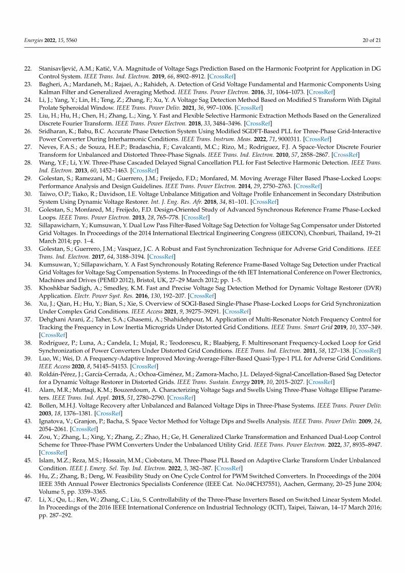
Energies 2022, 15, 5560 20 of 21

22. Stanisavljevic, A.M.; Katic, V.A. Magnitude of Voltage Sags Prediction Based on the Harmonic Footprint for Application in DGControl System. IEEE Trans. Ind. Electron. 2019, 66, 8902–8912. [CrossRef]

23. Bagheri, A.; Mardaneh, M.; Rajaei, A.; Rahideh, A. Detection of Grid Voltage Fundamental and Harmonic Components UsingKalman Filter and Generalized Averaging Method. IEEE Trans. Power Electron. 2016, 31, 1064–1073. [CrossRef]

24. Li, J.; Yang, Y.; Lin, H.; Teng, Z.; Zhang, F.; Xu, Y. A Voltage Sag Detection Method Based on Modified S Transform With DigitalProlate Spheroidal Window. IEEE Trans. Power Deliv. 2021, 36, 997–1006. [CrossRef]

25. Liu, H.; Hu, H.; Chen, H.; Zhang, L.; Xing, Y. Fast and Flexible Selective Harmonic Extraction Methods Based on the GeneralizedDiscrete Fourier Transform. IEEE Trans. Power Electron. 2018, 33, 3484–3496. [CrossRef]

26. Sridharan, K.; Babu, B.C. Accurate Phase Detection System Using Modified SGDFT-Based PLL for Three-Phase Grid-InteractivePower Converter During Interharmonic Conditions. IEEE Trans. Instrum. Meas. 2022, 71, 9000311. [CrossRef]

27. Neves, F.A.S.; de Souza, H.E.P.; Bradaschia, F.; Cavalcanti, M.C.; Rizo, M.; Rodriguez, F.J. A Space-Vector Discrete FourierTransform for Unbalanced and Distorted Three-Phase Signals. IEEE Trans. Ind. Electron. 2010, 57, 2858–2867. [CrossRef]

28. Wang, Y.F.; Li, Y.W. Three-Phase Cascaded Delayed Signal Cancellation PLL for Fast Selective Harmonic Detection. IEEE Trans.Ind. Electron. 2013, 60, 1452–1463. [CrossRef]

29. Golestan, S.; Ramezani, M.; Guerrero, J.M.; Freijedo, F.D.; Monfared, M. Moving Average Filter Based Phase-Locked Loops:Performance Analysis and Design Guidelines. IEEE Trans. Power Electron. 2014, 29, 2750–2763. [CrossRef]

30. Taiwo, O.P.; Tiako, R.; Davidson, I.E. Voltage Unbalance Mitigation and Voltage Profile Enhancement in Secondary DistributionSystem Using Dynamic Voltage Restorer. Int. J. Eng. Res. Afr. 2018, 34, 81–101. [CrossRef]

31. Golestan, S.; Monfared, M.; Freijedo, F.D. Design-Oriented Study of Advanced Synchronous Reference Frame Phase-LockedLoops. IEEE Trans. Power Electron. 2013, 28, 765–778. [CrossRef]

32. Sillapawicharn, Y.; Kumsuwan, Y. Dual Low Pass Filter-Based Voltage Sag Detection for Voltage Sag Compensator under DistortedGrid Voltages. In Proceedings of the 2014 International Electrical Engineering Congress (iEECON), Chonburi, Thailand, 19–21March 2014; pp. 1–4.

33. Golestan, S.; Guerrero, J.M.; Vasquez, J.C. A Robust and Fast Synchronization Technique for Adverse Grid Conditions. IEEETrans. Ind. Electron. 2017, 64, 3188–3194. [CrossRef]

34. Kumsuwan, Y.; Sillapawicharn, Y. A Fast Synchronously Rotating Reference Frame-Based Voltage Sag Detection under PracticalGrid Voltages for Voltage Sag Compensation Systems. In Proceedings of the 6th IET International Conference on Power Electronics,Machines and Drives (PEMD 2012), Bristol, UK, 27–29 March 2012; pp. 1–5.

35. Khoshkbar Sadigh, A.; Smedley, K.M. Fast and Precise Voltage Sag Detection Method for Dynamic Voltage Restorer (DVR)Application. Electr. Power Syst. Res. 2016, 130, 192–207. [CrossRef]

36. Xu, J.; Qian, H.; Hu, Y.; Bian, S.; Xie, S. Overview of SOGI-Based Single-Phase Phase-Locked Loops for Grid SynchronizationUnder Complex Grid Conditions. IEEE Access 2021, 9, 39275–39291. [CrossRef]

37. Dehghani Arani, Z.; Taher, S.A.; Ghasemi, A.; Shahidehpour, M. Application of Multi-Resonator Notch Frequency Control forTracking the Frequency in Low Inertia Microgrids Under Distorted Grid Conditions. IEEE Trans. Smart Grid 2019, 10, 337–349.[CrossRef]

38. Rodríguez, P.; Luna, A.; Candela, I.; Mujal, R.; Teodorescu, R.; Blaabjerg, F. Multiresonant Frequency-Locked Loop for GridSynchronization of Power Converters Under Distorted Grid Conditions. IEEE Trans. Ind. Electron. 2011, 58, 127–138. [CrossRef]

39. Luo, W.; Wei, D. A Frequency-Adaptive Improved Moving-Average-Filter-Based Quasi-Type-1 PLL for Adverse Grid Conditions.IEEE Access 2020, 8, 54145–54153. [CrossRef]

40. Roldán-Pérez, J.; García-Cerrada, A.; Ochoa-Giménez, M.; Zamora-Macho, J.L. Delayed-Signal-Cancellation-Based Sag Detectorfor a Dynamic Voltage Restorer in Distorted Grids. IEEE Trans. Sustain. Energy 2019, 10, 2015–2027. [CrossRef]

41. Alam, M.R.; Muttaqi, K.M.; Bouzerdoum, A. Characterizing Voltage Sags and Swells Using Three-Phase Voltage Ellipse Parame-ters. IEEE Trans. Ind. Appl. 2015, 51, 2780–2790. [CrossRef]

42. Bollen, M.H.J. Voltage Recovery after Unbalanced and Balanced Voltage Dips in Three-Phase Systems. IEEE Trans. Power Deliv.2003, 18, 1376–1381. [CrossRef]

43. Ignatova, V.; Granjon, P.; Bacha, S. Space Vector Method for Voltage Dips and Swells Analysis. IEEE Trans. Power Deliv. 2009, 24,2054–2061. [CrossRef]

44. Zou, Y.; Zhang, L.; Xing, Y.; Zhang, Z.; Zhao, H.; Ge, H. Generalized Clarke Transformation and Enhanced Dual-Loop ControlScheme for Three-Phase PWM Converters Under the Unbalanced Utility Grid. IEEE Trans. Power Electron. 2022, 37, 8935–8947.[CrossRef]

45. Islam, M.Z.; Reza, M.S.; Hossain, M.M.; Ciobotaru, M. Three-Phase PLL Based on Adaptive Clarke Transform Under UnbalancedCondition. IEEE J. Emerg. Sel. Top. Ind. Electron. 2022, 3, 382–387. [CrossRef]

46. Hu, Z.; Zhang, B.; Deng, W. Feasibility Study on One Cycle Control for PWM Switched Converters. In Proceedings of the 2004IEEE 35th Annual Power Electronics Specialists Conference (IEEE Cat. No.04CH37551), Aachen, Germany, 20–25 June 2004;Volume 5, pp. 3359–3365.

47. Li, X.; Qu, L.; Ren, W.; Zhang, C.; Liu, S. Controllability of the Three-Phase Inverters Based on Switched Linear System Model.In Proceedings of the 2016 IEEE International Conference on Industrial Technology (ICIT), Taipei, Taiwan, 14–17 March 2016;pp. 287–292.

http://doi.org/10.1109/TIE.2018.2881934

http://doi.org/10.1109/TPEL.2015.2418271


http://doi.org/10.1109/TPEL.2017.2703138

http://doi.org/10.1109/TIM.2021.3136172

http://doi.org/10.1109/TIE.2009.2036646

http://doi.org/10.1109/TIE.2011.2162715

http://doi.org/10.1109/TPEL.2013.2273461

http://doi.org/10.4028/www.scientific.net/JERA.34.81

http://doi.org/10.1109/TPEL.2012.2204276

http://doi.org/10.1109/TIE.2016.2636206

http://doi.org/10.1016/j.epsr.2015.08.002


http://doi.org/10.1109/TSG.2017.2738668

http://doi.org/10.1109/TIE.2010.2042420


http://doi.org/10.1109/TSTE.2018.2877505

http://doi.org/10.1109/TIA.2015.2397176



http://doi.org/10.1109/TPEL.2022.3153476

http://doi.org/10.1109/JESTIE.2021.3065205

Energies 2022, 15, 5560 21 of 21

48. Yu, J.; Cheng, M.; Gao, D.; Gu, Y.; Yu, J. A Lyapunov Stability Theory-Based Control Method for Three-Level Shunt Active PowerFilter. In Proceedings of the 2016 35th Chinese Control Conference (CCC), Chengdu, China, 27–29 July 2016; pp. 8683–8687.

49. Li, L.; Yang, H.; Guo, W.; Liu, Y. Analysis and Application of Lyapunov-Based Stable Control of the Single-Phase Shunt ActivePower Filter. In Proceedings of the 2012 Asia-Pacific Power and Energy Engineering Conference, Shanghai, China, 27–29 March2012; pp. 1–4.

A Novel Voltage Sag Detection Method Based on a Selective ...

Documents

Transcript of A Novel Voltage Sag Detection Method Based on a Selective ...