COGNITIVE SCIENCE 17, 3494% (1993)

A Neirral Network Model for Attribute-Based Decision Processes

MARIUS USHER California Institute of Technology

DAN ZAKAY Tel Aviv University

We propose a neural model of multiattribute-decision processes, based on an attractor neural network with dynamic thresholds. The model may be viewed as a generalization of the elimination by aspects model, whereby simultaneous selec- tion of several aspects is allowed. Depending on the amount of synaptic inhibi- tion, various kinds of scanning strategies may be performed, leading in some cases to vacillations among the alternatives. The model predicts that decisions of a longer time duration exhibit a lower violation of the simple scalability law, as opposed to shorter decisions. Furthermore, the model is suggested as a general attribute-based decision module. Accordingly, various decision strategies are manifested depending on the module's parameters.

1. INTRODUCTION

Decision making is a complex cognitive activity, sensitive to situational and enxrironmental conditions (Payne, 1982). The attempts to model individual choice behavior are, at best, incomplete (Tversky & Sattath, 1979). Yet, sig- nificant advancements in understanding decision-making behavior have occurred in the last 30 years. It has become clear that man is not an optimal decision maker (Kahaneman, Slovic, & Tversky, 1982), as intuitive decision behavior violates many axioms of utility theory (e.g., Tversky, 1975). Today, the illusiveness of rationality is obvious. It is clear that people do use choice heuristics that lead to consistent violations of even the most basic axioms of rational choice (e.g., Kahaneman & Tversky, 1979; Slovic & Lichtenstein,

We wish to thank, in alphabetical order, D. Horn, A. Rosenman, E. Ruppin, and two anonymous referees for very helpful comments. Marius Usher is supported by a Bantrell post- doctoral fellowship.

Correspondence and requests for reprints should be sent to Dan Zakay, Department of Psychology, Tel Aviv University, Ramat-Aviv 69978, Israel.

350 USHER AND ZAKAY

1971; Tversky, 1969). These observed violations have led to the emergence of the concept of "bounded rationality" (March, 1978; Simon, 1956, 1959). Simon suggested that instead of attaining the greatest goodness (i.e., maxi- mization of utility), the individual may wish to select an alternative that will maximize the probability of his or her attaining a certain level of "good- ness": his or her aspiration level. Simon called this approach "satisficing behavior. "

Since normative rationality wai refuted as a description of decision- making behavior (e.g., Rappoport & Wallsten, 1972), it has been argued (e.g., Abelson, 1964; Pitz, 1977) that appropriate decision-making models should draw their assumptions from psychological insights rather than axiomatic aesthetics. Indeed, process-tracing methods (Ford, Schmitt, Schechtman, Hults, & Doherty, 1989; Payne, 1976; Svenson, 1979) have revealed many unknown aspects of human decision-making behavior. A major empirical finding of recent decision research is that individuals employ a variety of choice strategies (Abelson & Levi, 1985). Decision makers are viewed as possessing a repertoire of strategies, and strategies are selected to fit a par- ticular decision in any given situation (Ford et d. , 1989; Johnson & Payne, 1985; Svenson, 1979). Two major questions related to this view, are the focus of recent decision-making research: (a) What are the decision strategies that are commonly used? and (b) What is the nature of the process leading to the selection of one strategy in a given situation? In the following sections, some factors that are relevant in the context of these questions are reviewed.

1.1 Decision-Strategy Characteristics It is well accepted that decision makers perceive choice alternatives as multi- dimensional entities including a number of dimensions or attributes (e.g., Svenson, 1979). A large number of strategies have been identified (e.g., E i o r n , 1970; Ford et al., 1989; Payne, Bettman, & Johnson, 1988; Svenson, 1979). These strategies can be characterized by several, partly overlapping, criteria. The characteristics that seem to be most important and relevant to the framework of this study, are described in the following.

Compensatory and Noncompensatory Strategies. Compensatory and noncompensatory strategies are the two major types of strategies de- scribed in the decision-making literature (Abelson & Levi, 1985; Einhorn, D. Kleinmuntz & B. Kleinmuntz, 1979; Svenson, 1979). Compensatory models (e.g., expected utility models) represent cognitively complex and sophisticated strategies for information integration (Einhorn & Hogarth, 1981). They refer to either the linear model or the additive difference model. Noncompensatory models are indicated by the inter- active use of informational cues in which a low score on one dimension

NEURAL NETWORK MODEL 351

cannot be compensated for by a high score on another dimension (Billings & Marcus, 1983). They involve the use of simplifying rules to reduce the complexity of the decision problem (Einhorn, 1970). The major non- compensatory models (Einhorn, 1970; Payne, 1976; Svenson, 1979) are the conjunctive, disjunctive, lexicographic, and elimination by aspects models. (A more detailed description of these strategies is given in later sections .) Stochastic Models of Decision Making. According to Becker, Degroat, and Marschak (1963), stochastic models are defined by specifying for each offered set M and each object X belonging to M, the probability that X will be chosen from M. Stochastic models generally fall into two categories: (a) constant utility models (CUMs) and (b) randon utility models (RUMs). CUMs assume or imply (Edwards & Tversky, 1967) that each stimulus (act or outcome) has a fixed location on a single under- lying utility scale. RUMS assume (Edwards & Tversky, 1967) that the decision maker chooses, with certainty, the stimulus that is highest in utility among those available at the moment of choice, but the locations of the stimuli on the utility scale fluctuate from moment to moment. In other words, the utility of each alternative is treated as a random variable rather than a constant (Block & Marschak, 1960). Accordingly, the probability of choosing an alternative X from the set M equals the probability that the utility of X will be greater or equal to that of any other alternative at the moment of choice. RUMS are further divided into two classes: independent RUMs and dependent RUMs. A RUM is independent if the fluctuations of the utilities of a given alternative in Mare independent of the fluctuations occurring in other alternatives in M. That is, the fluctuations of the utility of any alternative are governed by the properties and ways of perceiving each alternative by itself. A RUM is dependent if the fluctuations of the utilities of each alternative in M are dependent on those occurring in other alternatives in M. Therefore, the fluctuations of the utility of any alternative are at least partially influenced by the properties of the other relevant alternatives.

Dependent RUM models, like elimination by aspects @A1; Tversky, 1972), as well as some nonlinear-noncompensatory algebraic models, have the advantage over liner-compensatory models and independent RUMs, and CUMs, in being able to account for common violations of normative-axiomatic rationality; two examples of such violations follow.

' In general, the "elimination by aspects'' is denoted by "EBA," but we will use here "EA" in order to obtain a simpler notation (as we will present several variations to this deci- sion strategy.)

352 USHER AND ZAKAY

a. Intrasitivity of Choices. If x, y, z represent a set of alternatives, then one may sometimes prefer x over y, y over z, and z over x. In a prob- abilistic language, where P(x, y) represents the probability of choos- ing x over y, and P(x, y) > 1/2 and Po, z) > 1 /2, strong stochastic transitivity requires that

P(x, 2) > i a w [ ~ ( x , Y) , P(Y, z)l (1)

Because it was found that this inequality is not obeyed (Tversky, 1972), strong stochastic transitivity is violated. However, even weak stochastic transitivity {i.e., P(x, @>min[P(x, y), P(y, z)]) was shown to be violated in a predicted fashion (Tversky, 1969).

b. Dependence upon Nonrelevant Alternatives. It was shown that "simple scalability" [i.e., P(x, {x, y, z))/P(y, {x, y, z ) ) = P(x, y)/ Po, x)], which requires independence of irrelevant alternatives, is not generally fulfilled (Debreu, 1960). This violation of simple scala- bility also indicates that context effects influence actual choice behavior.

Search Direction in the Decision Process. Payne et al., (1988) defined three types of decision processes: holistic, alternative-based, and attri- bute-based processes. In a holistic process, alternatives are not decom- posed into dimensions or attributes, but are treated as whole entities. In an alternative-based process, each alternative is first processed along its attributes in order to arrive at some value. Comparisons among alterna- tives are then based on these representing values. In an attribute-based process, alternatives are compared on each dimension. An example is the additive difference model (Olshavsky, 1979; Tversky, 1969), which implies that decision makers compare alternatives on each dimension by computing the difference among alternatives on each dimension and then summing differences across dimensions. The summation of differ- ences results in a preference for one alternative. The Dynamics of the Decision Process. Decisions can be classified as either "static," "single stage," or as dynamic "multistage" decisions. Dynamic decision models account for the temporal aspects of the deci- sion (and not only for its outcome) such as vacillations and the decision time. Moreover, during the course of a decision process, strategies might change according to the characteristics of the task and the devel- opment of the decision process. It is clear that real-life decisions are mostly dynamic and multistage. Indeed, Payne (1976) found evidence for a mixture of strategies being used, and Bettman and Jacoby (1976) found that search patterns were characterized by alternating short se- quences of intra-alternative and intra-attribute search. Payne et al. (1988) argued that decision makers might change rules as context and time pressure change. Unfortunately, because of the complexity of

NEURAL NETWORK MODEL 353

dealing with dynamic multistage decisions, existing decision models are mostly static, single-stage models. However, static models provide only partial explanation for real decision processes. Edwards, Lindman, and Philips (1965) argued that only the dynamic approach can do justice to the complexity of the real world.

1.2 The Structure and Representation of Decision Strategies Appropriate representations of the alternatives in an offered set are a neces- sary, though not sufficient, condition for a particular strategy to be employed. For instance, an attribute-based process is not plausible when alternatives are presented one at a time. Empirical findings showing the im- pact of presentation format on information search patterns (e.g., Bettman & Jacoby, 1976; Bettman &Kakkar, 1977; D. Kleinmuntz & Schkade, 1990) support this assumption. Thus, when strategies are changed during the course of a decision process, the construction of an appropriate internal representation of the decision space might be required, if such a representa- tion is not already available.

Elementary Information Process (EIPs). Johnson and Payne (1985) sug- gested that decision strategies can be decomposed into EIPs. According to a symbolic approach, a decision strategy can then be seen as a set of EIPs (Huber, 1980; Johnson, 1979). Payne et al. (1988) suggested the following as examples of potential EIPs: read, compare, difference, add, move, choose, product, eliminate, announce preferred alternative, and stop process. They suggested that the number of component EIPs required to execute a particular strategy in a particular task environment is a general measure of decision effort.

1.3 The Selection Process Payne (1982) identified three theoretical frameworks for the strategy- selection process: the perceptual view, the cost-benefit view, and the pro- duction model. The perceptual view contests that basic principles governing human perception, in general, dictate the strategy-selection process. The production model assumes that decision strategies are associated to specific conditions, similarly to stimulus-response pairs (Pitz, 1977). According to the cost-benefit approach, strategy selection is contingent upon a com- promise between the decision maker's desire to make a correct decision and his or her negative feelings about investing time and effort in the decision- making process. Beach and Mitchell (1978) developed a model for the selec- tion of decision strategies which states that decision makers are motivated to choose the strategy that requires the least investment for a satisfactory decision. Consequently, a cost-benefit analysis in which potential strategies

354 USHER AND ZAKAY

are compared, is occurring. This process is contingent upon the type of deci- sion problem, the decision environment, and the personal characteristics of the decision maker (Zakay, 1990). Payne et al. (1988) argued that selection among strategies is adaptive, in that a decision maker will choose strategies that are relatively efficient in terms of effort and accuracy as task and con- text demands are varied.

The scope of this work is to propose a connectionist model, according to which various (and different) decision strategies can be obtained as manifes- tations of a unique decision module. An activation of a specific decision strategy is caused by changes in parameters of this decision module. Thus, the selection process is analogous, according to this approach, to a modification in the values of the molule's parameters.

We focus on the group of attribute-based decision strategies. This family includes Elimination by Aspects @A)-type strategies [e.g., lexicographic strategies, preference trees, and hierarchical elimination (Tversky & Sattath, 1979), the dominance rule, and the conjunctive and disjunctive model.] We focus on these models because it is plausible that the direction of search is an important parameter that characterizes a family of strategies. This family of decision strategies requires similar representation formats, does not demand high levels of cognitive effort, and is in common use under similar conditions. Indeed, Ford et al. (1989), who reviewed process-tracing deci- sion-making studies, concluded that the results firmly demonstrate that attribute-based decision strategies were the dominant mode used by decision makers. Alternative-based decision strategies (which are typically compen- satory) were employed only when the number of alternatives and dimensions were small or after a number of alternatives had been eliminated from con- sideration. Indeed, Isenberg (1984) reported that formal analytic strategies are seldom used, even by people who are aware of their existence, and con- cluded that most often, most people, for most problems, use some sort of a simple, easy, nonanalytic, rapid process. Similarly, Hogarth (1980) argued that, for the most part, judgments are made intuitively in an almost instinc- tive fashion, without apparent reasoning. In this research, the feasibility of an attribute-based decision module (ABM) will be demonstrated using a neural network approach.

2. GENERAL FRAMEWORK

The connectionist framework was shown to have several advantages over the symbolic one for modeling cognitive processes because it accounts for gradual and distributed processes (Grossberg, 1976; Hinton & Anderson, 198 1; Rumelhart & McClelland, 1986).

Most neural network models of cognitive processes are related to sensory perception, associative memory, and pattern recognition. For example, in

NEURAL NETWORK MODEL 355

the attractor neural network (ANN; Amit, 1989; Hopfield, 1982) approach, information retrieval is modeled by the convergence of the network's activity toward an attractor depending on stored synaptic connectivity, which reflects prior knowledge. In order to capture the multistage dynamic properties of the decision process, we will present a variant of ANN called transient attractor neural network UANN), in which the dynamics are characterized by succes- sive stages of convergence to transient attractors, and by transitions among them. Such dynamical systems have been recently proposed in the neural net- work literature (Horn & Usher, 1989,1990; Kleinfeld, 1986; Sompolinsky & Kanter, 1986; Zak, 1989, 1990).

Decision making is a natural candidate for connectionist modeling because it is a complex activity that is generally performed intuitively and that can benefit from the computational advantage of the neural parallel processing. However, a connectionist framework for decision making requires a shift in basic concepts from tradional A1 terms such as EIPs (read, compare, shift, etc.) to neural inspired terms such as activation, decay, competition, and so on. As we shall show, such a shift opens new possibilities for decision-making modeling. A neural model of decisions under risk, based on prospect theory (Kahaneman & Tversky, 1979), was presented by Grossberg and Guttowsky (1987). We will limit our model to decision making in multiattribute choice tasks (i.e., decisions in which one chooses among several alternatives that are mutually exclusive), and the topic of decision under risk will not be pursued here. Accordingly, each alternative of the decision process to be modeled is related to several attributes or aspects (e.g., the alternatives may be cars one could buy, and the attributes may be the price, size, color, etc.).

Our network model was inspired by two decision models presented in the psychological decision-making literature. The first one is Tversky's EA; 1972, and the second is Audley's (1960) model. In the following, these decision models will be briefly described.

According to EA, when deciding among several alternatives, one examines various aspects (attributes) of these alternatives. (In general, the situation is such that there are aspects related to only one specific alternative, and aspects related to several ones). The decision process is as follows: at each time step an aspect is stochastically chosen (with probability proportional to its weight), and the alternatives that are not related to the chosen aspect are eliminated. This process continues until only one alternative is left and the decision is accomplished.

The Audley (1960) model is a stochastic choice model, which explains several dynamic properties of decisions, such as response times (RTs) and vacillations among alternatives. According to this model, when one chooses among several alternatives, some intermediate choices toward these alterna- tives ('implicit responses') occur. Only when a consecutive set of k implicit responses of the same kind occurs, is a final response reached, and the deci- sion accomplished. Audley's model accounts for the distribution of RTs in

356 USHER AND ZAKAY

psychophysical decision experiments. It advantageously relates to the sub- jective "degree of confidence" feeling that one has toward a chosen alter- native as reflected by the number of vacillations (intermediate choices).

The model proposed here can be viewed as a generalization of EA and is formulated in a physical oriented language, characterized by continuous differential equations. As we shall show, the model also exhibits dynamic properties that are similar to the properties of Audley's (1960) model. More specifically, our model is based on a neural network in which neural assem- blies represent the various components of the decision process, such as alter- natives and their aspects. Varying some of the networks' parameters (such as the amount of synaptic inhibition), one can account for various decision strategies, such as focused versus broad attention given to the aspects.

In the next section, the network's architecture and dynamics are presented as well as a review of the properties of the formal neural networks on which the model relies. In the fourth section the decision scenario is discussed, exhibiting two attentional modes, and in the fifth section we illustrate two explicit simulations of the network's behavior. Afterward, some properties of the decision process, such as the distribution of response times and dependence upon alternatives, are discussed, leading to a predic- tion involving a specific correlation among the two. Finally, extensions of the model to other decision strategies are examined.

3. ARCHITECTURE AND DYNAMICS

The decision network is composed of two subnetworks, one for the aspects (AS) and the second for the alternatives (AL), connected through feed- forward projections from the (AS) subnetwork to the (AL) subnetwork, as illustrated in Figure 1.

For instance, consider the following situation, in which the aspects repre- sent six desirable characteristics of apartments that a person is choosing among to rent, and the alternatives represent three apartments that are offered to choice. The first AS node might represent "close to work" (and is possessed by Apartments 2 and 3, but not I), AS node 2 might represent "furnished" (possessed by 1 and 2, but not 3), and so on. We assume that when faced with such a decision situation, a decision maker constructs, first, a representation (such as in Figure 1, or uses an already existing repre- sentation from memory), on which the decision process will operate. The decision process is different from the pattern-recognition one, where assemblies are activated by an external input. In the case of decisions, there is no such external input. (The AS assemblies represent "the states of mind of the subject," which are not externally imposed over the system, like features in pattern recognition.) Accordingly, it is assumed that when an alternative has to be chosen, the AS subnetwork moves from one assembly to another, sending excitation to the AL assemblies connected with it.

NEURAL NETWORK MODEL

aspects ol ternatives Figure 1. Illustration of the decision network's architecture. The circles on the left column represent AS assemblies, the circles in the right columns represent alternatives, and the arrows represent synaptic projections among them. The ellipses represent inhibitory assemblies that mediate competition in each subnetwork. Full lines represent excitatory. and dashed lines represent inhibitory connections. Each assembly is alsa excitatorily con- nected to itself (not represented in the figure).

In order to model this behavior, we assume that in each subnetwork the various decision components (AS or AL) are represented by competing neural assemblies. The neurons belonging to each assembly are recurrently connected to each other, through excitatory synapses. For simplicity, we will assume that neurons belonging to different assemblies are not synap- tically connected (such connections would represent intrinsic associations between different aspects, i.e., we assume that "close to work" and "fur- nished" are independent variables). Each subnetwork contains an assembly of inhibitory neurons getting excitation from all the assemblies in the sub- network and returning inhibition (represented by ellipses in Figure 1). Through these inhibitory assemblies (which do not have any semantic role), an indirect competition among the various excitatory assemblies is generated. We should notice that in spite of the feedforward connectivity, from aspects to alternatives, such subnetwork is recurrent, due to the feedback via the in- hibitory assemblies and the self-excitations. Thus, once activated, the net- work's state does not require any input in order to continue reverberating. The behavior of such a network has been analyzed (Horn & Usher, 1990). It was shown that depending on the values of the parameters, such as the

358 USHER AND ZAKAY

synaptic inhibition and excitation coefficients, the network's behavior is dominated either by convergence toward "pure" attractors (a state where only one assembly is active and the other ones are silent), or (for a weaker inhibition coefficient), by convergence to a mixed attractor (in which two or more assemblies are active together). Whereas the first case is convenient for pattern recognition, the second one may be useful for modeling cogni- tive activities occurring simultaneously, such as broad attention processes.

We assume that the neurons contained in the AS assemblies have dynamic thresholds exhibiting adaptation (neural "fatigue"), leading the AS subnet- work into a dynamic process of sequential activation of the various aspects. Such dynamic thresholds can be physiologically motivated as representing neural adaptation (Horn & Usher, 1990) or slow delayedinhibition (Abbott, 1991). It was shown that when such dynamic thresholds are added to the dynamics (Horn & Usher, 1990), the previously mentioned attractors turn into transients, and therefore, the network's state converges to a transient on some short time intervals. However, on a longer time scale, as the neurons of this assembly accommodate, the network's state escapes from the previous transient and is attracted to another one. Depending on the value of the network's parameters, it was shown that the sequence of visits at the transients (pseudo attractors) may be either periodic or stochastic, ex- hibiting chaos (Hendin, Horn, & Usher, 1990). It is to be emphasized, that in all cases the trajectory passes through the transients (representing the various concepts), spending longer time in their vicinity and shorter time during transitions.

The architecture and dynamics governing the AL subnetwork is similar to the AS subnetwork, except that the threshold's variability is very low (the amount of adaptation or slow inhibition may be, in principle, modulated by various physiological factors), and that each AL assembly receives an addi- tional input from its corresponding AS assemblies. More simply stated, the thresholds in the AL subnetwork are chosen to be constant and, therefore, once an alternative is activated, it tends to stay, unless strongly conflicted by the input received from the AS subnetwork. The mathematical equations governing the network's dynamics are presented in Appendix A. These equations depend on several parameters, such as the synaptic inhibition and excitation coefficients in the network. The parameters can be grouped according to their influence on the network's behavior (see Appendix A). We should especially notice the importance of the synaptic inhibition coeffi- cient of the AS subnetwork, B, , which controls the average number of simultaneously activated aspects.

4. DECISION MODES

Several decision strategies may be obtained, depending on thevalues of the model's parameters. We will concentrate on two decision modes for which a

NEURAL NETWORK MODEL 359

detailed description of the network's behavior and characteristics wilI be given. (The values of the parameters for which these two decision modes are obtained are given in Appendix A.) Subsequently, the extension of the model to some other decision strategies will be presented briefly.

4.1 Focused Attention on Aspects If the inhibition parameters (see Appendix A) is high, so that the AS subnet- work has only one active assembly most of the time (resembling focused attention), then a scenario similiar to EA is obtained. Although the whole process is continuous, we illustrate it in the following, as a succession of stages analogous to EA.

1. Once an aspect is activated, its output causes the AL subnetwork to move into an attractor corresponding to the activated aspect. If, for ex- ample, the activated aspect is connected to both the alternatives x and y, then a mixed state in which both x and y assemblies are highly active (while the other ones, e.g., z, decay) is reached in the AL subnetwork. As we shall show in the next section, due to the alternatives' inertia, the probability that an assembly, whose activity has decayed will be reactivated, is very low in this decision mode. Thus, AL assemblies whose activation has decayed are "eliminated."

2a. If, subsequently, an aspect connected only to the x alternative will be activated, then its output will cause the AL subnetwork to converge into a state where only the x alternative is active and the other ones are not (i.e., the y alternative is eliminated and the x alternative is finally chosen).

b. If, after the common aspect of x and y decays, an aspect that is related neither to the x nor to they (but to z) alternative is activated, then, as in EA, the new alternative (2) cannot be reactivated. However, unlike Tversky's (1972) model, the AL subnetwork converges into either the x or the y attractor randomly, even before a new aspect is selected. The reason for this is that, in our model, mixed states are less stable than pure states, and therefore, when receiving conflicting input, they tend to destabilize and one of the assemblies composing the mixed state will take over. In order to reach the final decision, one AL assembly should remain continuously active for some duration. This will be discussed in the next section.

The model differs from EA in one more aspect. Although, according to EA the probability of selecting an aspect is constant, this is not the case in our model; the probability of an aspect being chosen consecutively is very low because the thresholds of the corresponding assembly are higher.

360 USHER AND ZAKAY

4.2 Broad Attention on Aspects A different set-up of the inhibition parameter B, can cause a situation where several AS assemblies are activated together (resembling broad attention). This would be equivalent to EA, where one chooses stochastically each time several aspects, and the alternatives that are not contributed by them are eliminated. According to this set-up, the decision process is much more com- plex, permitting vacillations among the various alternatives. This phenome- non occurs because it is possible that after one AL assembly is activated, the AS subnetwork will enter a state in which two assemblies-both contribut- ing to a nonactive alternative-will be activated together. In this case, it is possible that the strong conflicting input will induce a transition in the AL subnetwork towards a state in which the new AL assembly (previously elim- inated) is reactivated. Thus, in this decision mode, alternatives are not eliminated, but only suspended for some time. This process can account for the phenomenon of vacillation among the alternatives.

It is obvious that once the network operates in such a mode, there will be no end to its vacillations, and therefore, a criterion for what can be con- sidered to be a final response (decision) is necessary. We decided to impose, as a criterion for a decision, the requirement that the AL subnetwork spends a certain amount of time, To in a single state in which only one of the AL assemblies is a c t i ~ e . ~ If To is chosen to be larger than the characteristic time for transitions among the aspects, the similarity to Audley's (1960) model is evident; for a final decision to occur, the AS activation has to be such that no vacillation (from a specific alternative) will occur for some time dura- tion, and therefore, the process operates as if the same alternative were chosen several times consecutively. However, one should note an important difference between Audley's model and ours. Whereas in the former, the probability for an "implicit choice" is independent of the previous implicit choice, in our model, this condition is not obeyed. The probability of "choosing" an alternative once it is already activated is larger than the probability of choosing it when another alternative is activated because only very special sets of aspects can induce a vacillation.

' The "minimal time requirement" for a final decision, which we have imposed, may be biologically motivated, reflecting an assumption concerning the "final decision" mechanism. It is believed that synaptic learning (i.e., Hebbian) occurs on a much longer time scale com- pared to neurons' dynamics time scale. Therefore, it is plausible that although the same assembly is active for a prolonged time period, a reinforcement process for the synapses con- necting the neurons of the active assemblies, occurs. Once such a reinforcement is accom- plished, no vacillation is possible anymore, and the decision is accomplished. Alternatively, it is possible that the mechanism by which the minimal time requirement is imposed involves some higher cognitive system that controls the decision module.

NEURAL NETWORK MODEL 361

5. ILLUSTRATION OF THE NETWORK'S BEHAVIOR

We will now illustrate the network's behavior obtained by numerical solu- tions of Equations 6 and 7 in Appendix A. We considered for illustration a case of three AL and.six AS assemblies. The relations among the items are such that there are three aspects related to one specific alternative each, and three other aspects related to pairs of alternatives. The initial conditions for the activation of the AS assemblies were chosen randomly between zero and one (reflecting the initial state of mind of the agent), and the initial condi- tions for the alternatives were zero. The inhibition coefficient of the AS subnetwork BI was varied in order to achieve both the focused and broad attention schemes. The minimal time that an AL assembly has to be active for a decision to occur was taken to be 50 time units. The model has been tested with the parameters given in Appendix A under two possible conditions:

1. The decision maker's attention is focused on a single aspect at a time. 2. The decision maker's attention is broader, that is, two or more aspects

may be simultaneously activated.

These two conditions may represent different cognitive styles, or different strategies used under different contexts (e.g., familiar vs. unfamiliar).

5.1 Focused Attention For an inhibition parameter BI = 0.85, the AS subnetwork is, most of the time, in a state in which only one aspect is activated. In Figure 2, the activi- ties of the six AS and three AL assemblies as a function of time are illus- trated. In Figure 3, we diagrammatically display the network's state at five selected times that we considered to be especially illustrative. We observe that until t =7 time units, two AS assemblies (3 and 4) are active together. Later, when the AS inhibitory assembly accumulates sufficient activation, AS-3 decays, and we reach a situation where (lo< t< 30) only AS-4 remains active. Because that aspect is connected to the AL Assemblies 1 and 2, a mixed state composed of these two assemblies is reached in the AL subnet- work (12< t< 30). Successively, for 30< t < 50, AS-1 is activated, and thus, AL-1 (which is connected with this aspect) is "chosen." The activation of AS-2 (50< t<70) no longer influences the AL subnetwork and the final decision is accomplished at t = 80 time units.

5.2 Broad Attention For a lower inhibition parameter BI =0.45 (displayed in Figures 4 and S), two assemblies can be simultaneously active in the AS subnetwork. After an initial time duration when most of the assemblies are active (due to the fact that the inhibitory assembly has to accumulate enough activation in order to

Figure 2. Illustration of the network's behavior in the mode of focused attention over the aspects (B1=0.85). The six aspects and three alternatives are displayed as functions of time.

NEURAL NETWORK MODEL 363

Figure 3. Illustration of the network's dynamics in the mode of focused attention over the aspects (Bt=0.85). The six circles in the left column represent the six AS assemblies, and the three circles in the right column represent alternatives, connected each with two aspects. The circle's radius shows the assemblies' activation. Each frame shows another time stage of the decision process.

mediate inhibition among the other assemblies), a situation in which only AS Assemblies 2 and 6 are active is reached (lo< t<30).

As a result, only the AL assemblies connected with these aspects, that is, ALs-2 and 3, remain active. A successive activation of AS Assemblies 3 and 4 (30< t< 45) does not influence the AL subnetwork because these aspects are also connected to the active alternatives (2 and 3). At a later time 45 < t < 60, only AS Assemblies 1 and 5 are active. Consequently, the activity of AL Assembly 2 decays (it is not connected with either of these aspects), and AL-3 is "preliminarily chosen" (50< t< 70). For 60< t< 85, the AS Pair 2 and 6 is active again, causing the reactivation of AL Assembly 2 (which gets input from both aspects), and inducing the AL subnetwork into the mixed state composed by ALs-2 and 3, again. (This stage of the process may be regarded as a hesitation. This mixed state persists until, for 118<t< 122, AL Assemblies 1 and 2 (neither of which connected with AL 3) are active. Consequently, AL-3 begins to decay (t= 120), and thus, a vacillation from the third toward the second alternative occurs. Further changes in the AS activation no longer influence the AL subnetwork and the final decision is accomplished at t = 170 time units.

6. CHARACTERISTICS OF THE DECISION PROCESS

6.1 Periodicity and Chaos Although the final outcome depends on the initial state of the AS activa- tion, the general shape of the behavior (Figures 2-5) does not. Selecting dif- ferent initial conditions can influence which alternative will be chosen, but

Figure 4. Illustration of the network's dynamics in the mode of broad attention over the aspects (81 =0.45).

NEURAL NETWORK MODEL 365

Figure 5. Illustration of the network's dynamics in the mode of broad attention over the aspects' (81=0.45) selected time shots.

not the scanning mode (by single aspects or pairs), nor the statistical proper- ties such as the distribution of response times (RTs) and vacillations. More- over, even for very similar initial conditions, different outcomes may occur, due to two factors: (1) a small random noise fluctuation applied to Equa- tions 6 and 7 (see Appendix A); and (2) due to the chaotic properties of Equations 6 and 7 (even without any stochastic perturbation).

Examining the evolution of the AL subnetwork's activity (Figure 4), we observe that despite some tendency to periodicity (pairs of aspects such as (2,6), (1,5) and (3,4) tend to be phase-locked and activated together), some irregular behavior is also visible (the pairing of aspects in only transient, so that it brakes after some time and new pairs are formed). It was shown (Hendin et al., 1990) that the behavior of such a network may be either periodic or chaotic, depending on the value of its parameters. The distinc- tion between these two modes of operation may be crucial for the network's behavior when it operates in the mode of unfocused attention (low inhibi- tion which leads to a more chaotic dynamics). If the dynamics of the AS subnetwork are completely periodic, then alternation of pairs of aspects may cause an unbounded number of vacillations in the AL subnetwork. Such a situation might possibly represent a very "difficult" decision. In reality, such never-ending vacillations are improbable, even for parameters causing periodic motion, because fluctuations originating from random ex- ternal synaptic projections into the network will eventually lead to the decoupling of the oscillating pairs. Nevertheless, for network parameters leading to periodic orbits, longer decision processes are to be expected (compared to the chaotic case).

Moreover, in the chaotic case, the knowledge of the initial state with any finite degree of accuracy will not enable the prediction of the final outcome, due to exponential error amplification. Thus, in the deterministic chaotic

366 USHER AND ZAKAY

case (for broad attention) the decision process remains practically stochastic. The system's stability is not homogeneous. It was shown (Hendin et al., 1990) that the Liapunov exponents for Equation 6 (Appendix A), get posi- tive or negative contributions in different regions of the phase space (lead- ing to an intermittent behavior). While in regions that contribute negatively, the trajectory is rather insensitive to small perturbation; in regions that con- tribute positively, small deviations are expected to be amplified and ulti- mately lead to a different result. This effect is expected to be more significant when the decision process is longer (e.g., for broad attention).

6.2 Distribution of Response Times (RTs) According to our model, the final decision depends on the trajectory followed by the AS subnetwork. For various initial conditions of this sub- network, representing various initial states of mind, different alternatives will be chosen. If one considers these initial states of the AS subnetwork as hidden parameters, the whole process is stochastic. In order to study the statistical distribution of RTs, Equations 6 and 7 (Appendix A) were solved numerically for various randomly chosen initial conditions (the AS activa- tions), and the RTs were obtained. In all these samples, the criterion for a final decision is the same as previously mentioned, namely that a single AL assembly was active for a duration of 50 time units.

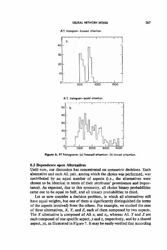
The distribution of RTs for the cases of focused and broad attention over the aspects are displayed in Figure 6. The distribution for the case of focused attention is considerably sharper (Figure 6a). Nevertheless, even in this case, a two-peek distribution is observed. The peek around t = 50 corresponds to decisions in which an aspect related to only one alternative was activated at the beginning; the second peek, centered at about t = 75, reflects decisions in which the aspect first activated was related to two alternatives. After each peek we observe a graded decrease in the frequency of the RT. This graded decrease is caused by a stochastic delay in the decision time, originating from the time period during which the inhibitory AS assembly accumulates enough activation (until this assembly is active, the AL network will hesitate in a state of two alternatives), and from the inherent stochasticity of the network.

The distribution of RT for unfocused attention, Figure 6b, is much broader, including decisions that exhibit as many as seven vacillations. The vacillation phenomenon is reflected in the 20 to 25 time-unit periodicity of the distribution (the characteristic transition time for the AS subnetwork is about 20 time units). A variation in the value of the minimal time require- ment To, will not influence the distribution of RTs for focused attention, but will strongly affect the RTs in the broad attention mode; an increase in To will lead to more vacillations because more coincidences of pairs of aspects are needed in order to reach a final decision (as in the Audley, 1960, model).

NEURAL NETWORK MODEL

R.T. histogram- focused attention .

t " " ' " " ' " " ' " j

R.T. histogram-broad attention.

Figure 6. RT histograms: (a) focused attention; (b) broad attention.

6.3 Dependence upon Alternatives Until now, our discussion has concentrated on symmetric decisions. Each alternative and each AL pair, among which the choice was performed, was contributed by an equal number of aspects (i.e., the alternatives were chosen to be identical in terms of their attributes' prominence and impor- tance). As expected, 'due to this symmetry, all choice binary probabilities came out to be equal to half, and all trinary probabilities to third.

Let us now consider a decision problem, in which all alternatives still have equal weights, but one of them is significantly distinguished (in terms of the aspects involved) from the others. For example, we studied the case of three alternatives, X, Y, and Z, each of them composed by two aspects. The X alternative is composed of AS x, and x2, whereas AL Y and Z are each composed of one specific aspect, y and z, respectively, and by a shared aspect, yz, as illustrated in Figure 7. It may be easily verified that according

USHER AND ZAKAY

z Figure 7. A schematic representation of a nonsymetric decision: The three alternatives, X, Y, and Z, each have a pair of aspects. However, although the alternatives Y and Z shareone aspect, yz, the alternative. X, is distinguished.

to EA (Tversky, 1972), the probability of choosing the "distinguished" alternative, namely X, is enhanced compared to the probability of choosing one of the similar alternatives, Y or 2: specifically, in the example described before Pm(X) =2/5 =0.4, and PEA(Y) = PEA(Z) = 1/2 . 3/5 = 0.3. (These probabilities should be compared to the baseline given by independent RUMS, i.e., PIN(X) = 1/3 =0.33.)

Statistics of simulation runs show that, in the mode of focused attention over the aspects (BI =0.85), the choice distribution is in accordance with EA model, thus the frequency with which the distinguished alternative is chosen is indeed 0.4. When running the network's simulation with inhibition level corresponding to broad attention over the aspects (B, =0.45), we found that the distinguished alternative is no longer dominant, that is, all trinary prob- abilities were almost equal. An intermediate situation was found for an inhibition parameter, BI =0.6, for which the probability of choosing the distinguished alternative was 0.353. Thus, the frequencies of choosing the X alternative satisfy

{Px(B, =0.45)=0.33) < {PX(B, =O.6)=0.353)< {Px(B, =0.05)=0.4)

A precise mathematical solution of our model, predicting the probability of choosing the distinguished alternative (X ) is rather difficult. However, several simplifications may enable the understanding of the trend described previously, involving a gradual change from dependent to independent RUM as the attention over the aspects is broadened. Because the network's state spends longer times in the vicinity of the pseudo attractors than during the transitions between them, we may approximate the continuous evolu- tion of the network by a discrete time model in which, at each time step, several aspects are selected. Let us assume, for example, that when the net- work operates in the mode of broad attention, two of the AS assemblies are

NEURAL NETWORK MODEL 369

simultaneously active, that is, the network scans the aspects by pairs. If we further neglect the vacillations (reactivation of eliminated alternatives), a scenario, which may be described as elimination by two aspects, E2A, emerges. In fact, this process still differs from EA because, as opposed to the latter (due to "fatigue"), the same aspect cannot be selected at two con- secutive time steps. In the following we shall use the notation E2A, in order to refer to the process in which this limitation on consecutive selection of aspects is neglected, and the notation E2AS for the process of elimination by two aspects, whereby aspects cannot be selected consecutively.

The probability of choosing the distinguished AL X (denoted by PgM) can be calculated following these simplifications by the recursive expression:

where the factors of 1/10 result from the 10 possible pairs among five aspects. (The first term results from the possibility of choosing both aspects from the X alternative at the first time step, the second term from the possibility of choosing, at the first step, one aspect of X and one aspect of either Y or Z, and the third one from the possibility of choosing one aspect from X and another one shared by Y and 2, whereafter the process is reinitialized. The resulting probability is PgM = 3/8.

A more elaborated calculation shows that the probability of choosing X according to E2A,* when the same aspect cannot be selected twice consecu- tively (denoted in the following by Pi'X,is equal to 11/30 (see Appendix B). Thus, the calculated probabilities satisfy the following order relationships:

where (with a common denominator), these probabilities are (in increasing order):

It can be shown that these order relationships characterize, also, more general decision processes, and not only the five AS and three AL decisions discussed before. Let us consider, for example, the case of three alterna- tives, X, Y, and 2, each related to n aspects in such a way that the alter- natives Y and Z share m aspects, whereas the aspects related to X are not shared by any other alternative. It can be shown, similar to equation 3, that the probability of choosing the X alternative according to E2A is:

USHER AND ZAKAY

P(x) E A , E2A

Figure 8. The probability of choosing the distinguished alternative, as a function of the ratio m/n: The solid line corresponds to EA (Equation Y); the dashed line gives probability according to E2A (Equation 3) for n=a; the dot-dash line gives the same probability (Equa- tion 3 for n=2).

where x is the ratio m/n. This probability may be compared to the EA prob- ability which gives

We observe (Figure 8) that although the two probability functions "agree" at the extreme values of x, that is, 0 and 1 (where they give 1/3 and 1/2, correspondingly), for all intermediate values of x, the probability of choosing the distinguished alternative according to E2A is closer to 1/3, which is the expected value for an independent RUM.

The trend by which the decision process gradually changes from a depen- dent to an independent RUM may be viewed as originating from a change in the strategy of scanning the aspects. The fact that a strategy of scanning the aspects by pairs leads to probabilities exhibiting less dependency among the alternatives is rather intuitive; selecting the aspects by pairs (E2A) is equivalent to a usual EA process where the new aspects are pairs of the orig- inal ones. It is clear that, after this tranformation, alternatives that did not have any aspect in common such as X and Y, will share some elements (pairs of aspects, one belonging to X and the other to Y); thus, the measure by which the X alternative is (aspectwise) different from the other alternatives is diminished, motivating the trend mentioned before. If this implication is true, an interesting prediction of the model arises. It may be natural to assume that various agents use specific scanning strategies, which may be correlated with some psychological personality characteristics. Therefore,

NEURAL NETWORK MODEL 371

we should expect that agents that perform choices with longer RTs, will . exhibit choice probabilities closer to the simple scalability relation.

7. FURTHER EXTENSIONS TO OTHER DECISION STRATEGIES

The decision network, which we presented in the previous sections, can account for two kinds of decision strategies, EA and E2A, via a change in the level of inhibition in the AS subnetwork. However, the model contains parameters whose variations were not yet discussed. In this section we show that modifications in the value of these other parameters can account for a behavior that exhibits a whole variety of decision strategies, such as the dominance rule, the conjunctive and disjunctive rules, elimination by least attractive aspect rule (ELAA), choice by most attractive aspect rule (CMAA), the lexicographic rule, elimination by tree rule (EBT), hierarchical elimina- tion method (HEM), and addition of utilities (AU) rule. The network's behavior for these cases is described in a more qualitative form. For each of these strategies, we present, in the following, a short description of the deci- sion rule (following Svenson, 1979) indicating the modifications in the parameters' values that are required for obtaining the strategy involved. For each case, a simulation test was performed establishing its validity.

The network that we presented in the preceding sections was based on only one type of connection between the aspects and the alternatives: all or none. In other words, the possibility of gradual aspects' weights was not taken into account. This choice does not reflect the nature of the model, but rather the original formulation of EA. In order to extend the range of the model to include the decision strategies listed before, the all-or-none connections were replaced by graded weights.

For the sake of demonstration, we have considered a network that per- forms decisions among three alternatives, each one related to the same three aspects, with different weights. Thus, each decision situation can be fully characterized by a 3 x 3 matrix of weights, characterizing the importance of the aspects to each alternative. For every decision strategy, the network was tested by presenting it with two or three different decisions (characterized by specific weight matrices).

For strategies that do not always result in a solution (e.g., dominance, conjunctive, disjunctive strategies), decision tests where chosen so that the set included both a solvable decision and a unsolvable one. We expect that for the first case, the network will converge to a solution (one alternative re- maining highly active), whereas for the second case, the network will vacillate among the three alternatives, and none of them will be persistently active at all times. In addition to these two decision situations, we also

372 USHER AND ZAKAY

focused on "limit cases" in which the advantage of one alternative over the others is marginal (e.g., weak dominance in the context of a dominance strategy). Such limit cases enable testing whether the transition between suc- cessful and unsuccessful solutions is smooth or sharp. Decision strategies that always provide a solution (like AU), were tested with decisions favoring different alternatives or providing an equal result for two of them.

I . Dominance Rule. One alternative is chosen over another one, if it is better than it, on at least one aspect and not worse than it on all other aspects.

The network is able to behave according to this rule if the foilowing con- ditions are satisfied:

The aspects are sequentially scanned (as in the focused mode for EA). The competition among the alternatives is increased, so that at any moment, only the alternative that receives higher excitation is activated. This increase in competition is reflected by an increase in the value of the B, parameter (we chose B, = 1.5). The alternatives have no inertia (unlike EA), that is, if on a second aspect the order of "attractiveness" towards the alternatives is reversed, the alternative that was previously activated decays. This lower inertia for the alternatives can be controlled by a modification of the parameter T, that regulates the slope of the input-output sigmoidal response curves of neurons (see Appendix A). In order to obtain a behavior that ex- hibits the dominance rule, T, was increased to the value of 0.18. This parameter is also related to the degree of "noiseness" in the network and to the signal to noise ratio of neural cells, which was argued to be modulated by neurophysiological factors (Mamelak & Hobson, 1989; Servan-Schreiber, Printz, & Cohen, 1990).

Accordingly, an alternative is chosen only if it remains active for a time long enough to scan all aspects, implying that it is better than all other alternatives (for all aspects).

Simulation Test. We tested the network by checking its behavior in the three decision situations represented by the following weight matrices.

I aspect1 1 aspect2 ( aspect3 A L I I 4 I 5 I 5

ALI AL2 AL3

aspect2

5 4 2

aspectl 4 3 2

,.,

aspect3

3.5 1 4

I aspect1 1 aspect2 I aspect3 A L l I 4 I 5 I 2

NEURAL NETWORK MODEL 373

Note that these matrices represent decision situations that are identical with the exception of the weight of the third aspect for the first alternative, which was systematically varied. The first case (a) stands for a decision situation that has a strong dominant alternative, whereas the second case (b) stands for a decision situation with no dominant alternative. The third case (c) is a limit case, which has only a slight deviation from dominance. The network behavior for all three decision situations is illustrated in Figure 9. We observe that, in all cases, the AS subnetwork performs a serial scan of aspects (Figures 9b, d, f). Figure 9 shows three scenarios for the AL subnetwork.

(a) For the dominant decision situation, [case (a)] the dominant alternative (illustrated by the full line in Figure 9a), although performing some oscillations (triggered by the input from the AS subnetwork), is domi- nating all other alternatives for all times, and thus can be chosen in accordance to the minimal time requirement previously discussed.

(b) For the nondominant case, (b), we see that no alternative dominates the network at all times. The first alternative dominates. the network only when its high weight aspects (AS 1 and AS 2) are scanned, but it declines when the AS 3 (which has a higher weight for AL 3) is scanned (Figure 9c).

(c) In the limit case, (c), we observe that although the decision situation is not strictly dominant, AL 1 still dominates the network (Figure 9e). However, as opposed to case (a), it strongly declines when the "weak" AS 3 is scanned. It is possible to consider this behavior to be an unsuc- cessful decision if we artifically impose a threshold of activation that an alternative should pass in order to qualify as "fully" active. However, we believe that such a criterion is too artificial. Instead, we prefer to consider the behavior in (c) as part of a continuum of decisions characterized by different conditions of confidence [varying from high confidence (a) to very low confidence (b)]. This gradual behavior is probably characteristic of neural network implementations, as opposed to their symbolic analogs.

2. Conjunctive Models. A criterion (or threshold) is defined, so that if an alternative does not meet the criterion on just one aspect, it is eliminated. An alternative is selected only if it is higher than the threshold on all aspects.

The network behaves according to this rule if the following conditions are satisfied:

The aspects are scanned sequentially. There is no competition among the alternatives (B, =O). In this case (as for the disjunctive rule), alternatives are not compared to each other (but to an external criterion) and thus an alternative is activated only when its corresponding aspects' weights are higher than a threshold, which is controlled by (but not identical to) the values of d 2 .

'-03 ID

U!~

~D

W

D J

Oj (j) PUD (a

) pUD :aA

!+DU

la+lD +U

DU

!

-uo

p D

+n

oq

+!~

uo!s!=p

eq+ J

O~

(p

) puo (q

) :(eu

!l~~

nj

' 1 1~

)

an!+

ouJa

+lo

+u~

u!u

op

o q+!m

uo!s!m

p D

104 Jo!m

qaq a

q+ a+oJ,

-SnIl! (9

) PU

D (0

) .s+>edso

aq+ jo

s>!uouA

p eq+ sA

qds!p

(4 'p 'q) u

o!+

~od uo

uo

q a

q+ :xu

!+ jo

uo!+

>unj so se

n!+

ouJa

+p aq

+

40

s>!uouA

p eq+ sA

olds!p (a '3

'o) u

o!u

od d

o+ a

ql :a

p a

>uou!u

op a

q+

~o

j

suo!+on+

!s uo!sp

ap p

s+sar a

a~

ql-6

ern

614

ooz OOC

0

- P'o

.9'0

- 8'0

NEURAL NETWORK MODEL 375

(In this simulation, 82 was chosen to be equal to 0.7 and this determined the threshold to be at about 0.18, or 1.8 in our notation.) The dynamics of the alternatives are characterized by a low degree of inertia (T2 = 0.18), and thus, an alternative that was activated for one aspect can be deactivated when another aspect is scanned.

Under these conditions, when an alternative has all aspects' weights above some threshold (case a. in the following simulation), it remains continuously activated, but when it has a low weight aspect (case b.), its activation decays (when this aspect is scanned) and cannot be chosen. The network operates identically as for the dominance rule, except that alternatives do not com- pete with each other, but with a common threshold.

Simulation Test. We tested the network in the three decision situations represented by the following weight matrices3:

These matrices represent decision situations that are identical besides the weight of the first aspect for the first alternative that was systematically varied; in case (a) the weight is above threshold, in case (b) it is below, and in case (c) it is approximately at threshold. The network behavior for all three decision situations is illustrated in Figure 10. As for the dominance rule, the AS subnetwork performs a serial scan of aspects (Figures lob, d, f). Figure 10 shows three scenarios for the AL subnetwork.

aspect1 aspect2 aspect3

(b) (a) AL2 AL3 4.5 1 4.5

(a) When there is one alternative (AL 1) that has all weights higher than the threshold, and all other alternatives have some aspects below it, we observe (Figure 10a) that AL 1 (full line) is fully active at all times, and the other alternatives decline when their weak aspect is scanned.

(b) When no alternative has all aspects above the threshold, (Figure lOc), we observe that the AL subnetwork vacillates among the alternatives, each one declining when its weak aspect is scanned.

(c) As for the case of the dominance rule, the transition from successful to unsuccessful decision is smooth. We observe that the activity of AL 1 declines partially when its weak aspect is scanned (Figure 10e).

The coefficients appearing in all the following matrices represent the weight coefficients between aspects and alternatives used in the simulations, multiplied by a factor of 10.

ti: AL3

aspect1

5 4.5

aspect2 3 4 1

aspect3 4 1

4.5

NEURAL NETWORK MODEL 377

3. Disjunctive Models. These models are the mirror image of the con- junctive rule. A chosen alternative should have at least one aspect higher than a given criterion, and all the aspects of the other alternatives should fall below the criterion.

A behavior that exhibits this rule is obtained if:

The aspects are sequentially scanned. There is no competition among the alternatives (low inhibition in the AL subnetwork, B2 =0). The threshold for the AL subnetwork is the same as for the previous rule, B2 = 0.7. The dynamics of the AL subnetwork should be characterized by a higher degree of inertia (T2 = 0.08, like the EA), thus, an alternative which was higher than the threshold for one aspect cannot be deactivated anymore.

If a single alternative has at least one aspect higher than the threshold, then only this alternative will be active at all times and will be chosen. The actual threshold depending on B2 (but also on other parameters such as T2) was determined in simulations to be equal to 5.5.

Simulation Test. We have performed a simulation test involving the following two decision situations.

I aspectl 1 aspect2 ( aspect3 A h I 1.5 I 5 I 4

In Case (a) the first alternative has an aspect (AS 2) with a weight above the threshold, whereas in Case (b) no alternative has aspects with weights above threshold. We observe the following behaviors.

Case (a). The AL 1 assembly was activated just when the strong aspect is scanned and remains active thereafter, but no other alternative is activated (Figure 1 la).

Case (b). When no aspect has a weight above the threshold (5.5), no alter- native could be activated (Figure 1 lc).

As opposed to the dominance and conjunctive rules, in this case, the transi- tion is sharp. The cause for the difference resides at the high slope-sigmoidal response function (controlled by T2) under which this strategy is obtained. (In general, steeper sigmoids lead to sharper transitions than shallow sigmoids.)

4. Elimination by Least Attractive Aspect (ELAA) Rule. The decision maker eliminates the alternative that has the worst overall aspect.

NEURAL NETWORK MODEL 379

This rule is a straightforward generalization of the conjunctive rule, and can be obtained if:

The network's parameters are set as they were for the conjunctive rule. The threshold of the AL subnetwork (controlling the criterion) is grad- ually modified until only one alternative remains active.

The threshold modification can be performed either by increasing the threshold or by decreasing it. In the first case, we obtain strictly ELAA. We begin at a low threshold with all alternatives active, then, as the threshold is increased, alternatives are eliminated until only one remains. A further in- crease in the threshold will finally deactivate the last alternative. In the sec- ond case, when the threshold is initially high and is gradually decreased, a variant of ELAA is obtained. We begin with a situation in which no alter- native is activated (conversely to the first case), and due to the threshold decrease, a first alternative will be activated (the first that has all aspects above the threshold). Continuing to decrease the threshold will lead to a situation where all alternatives are active. In both cases, the decision should operate at the intermediate stage, when only one alternative is per- sistently active (the same for both iinplementations). This can be achieved because, in accordance to requirement of minimal time, the process will be stopped as soon as a single alternative dominates the network for a certain amount of time. In the following, we used the second implementation, thus the threshold was decreased in steps of 0.05 at every 100 time steps.

Simulation Test. We have performed a simulation test for the decision situation (Case b) of the conjunctive rule. Beginning with the same threshold (02 =0.7) as for the conjunctive rule, we observe that during the first 100 time units the behavior is as in Figure 10c, that is, no alternatives remain continuously active. After 100 time steps, because the threshold is lower, AL 1 (Figure 12a, full line) gets active while all the other alternatives decline when their below-threshold aspects are scanned.

We should note that in order to implement this strategy, the time scale for the threshold variation should be of the same order as the time scale characterizing a complete scan over the aspects. Thus, although this rule is more efficient in obtaining a decision (as compared to the conjunctive one), it is also more time consuming.

5. Choice by Most Attractive Aspect (CMAA) Rule. The decision maker chooses the alternative that has the overall most attractive aspect.

The rule can be obtained in a network if:

The network's parameters are set as they were for the disjunctive rule. The threshold is initially high and is gradually decreased until the aspect with the highest weight overcomes the threshold. At that moment the corresponding alternative gets activated (and due to the high inertia, its activation persists while other aspects are scanned) and is chosen.

380 USHER AND ZAKAY

Time Units Figure 12. Illustration of the ELAA decision: The network is initialized at t=O with the same parameters as in Figure 10 (c. d): O1 was decreased by .05 after every 100 time steps. We observe that when the threshold is decreased. AL 1 [full curve in (a)] begins to dominate the AL subnetwork. All other alternatives (dashed lines) have moments of decline when their weak aspects are scanned.

Simulation Test. We have performed a simulation test for the decision situation.

This decision situation is just below the threshold for the disjunction model with =0.7. Like the ELAA rule, the threshold was decreased in steps of

NEURAL NETWORK MODEL 38 1

0.05 at every 100 time steps. The simulation shows (data not displayed) that for the first 100 steps, no alternative is active (as in case (b) for the disjunc- tive rule), however, after 100 time steps, once the threshold decreases, AL 1 (with the higher aspect) was the first to get activated. If the threshold con- tinues to decrease, eventually all dternatives will be active. However, because the threshold variation is slower than the scan of the aspects, the time requirement for a decision can be satisfied before the second alter- native is active too. Thus, for performing decisions with increasing weight resolution, a longer process is required.

6. Lexicographic Decision Rule. This rule is similar to EA, but the aspects are scanned in a fiied order determined by their importance.

This rule can be obtained in an EA network, if the aspects are scanned in a specific order. This can be achieved in the network, if, for example, the coefficients of the self-excitation of each aspect A, (in the previous section all these coefficients were equal to 1) have values that are ordered in a specific way, imposing a scanning order for the aspects. Thus, the aspect with higher self-excitation is scanned first, and so on, leading to an orderly scan of the aspects, provided that the recovery from fatigue is slow enough. This requires that an aspect with strong self-excitation will not be activated again until the other aspects are scanned. In a simulation test we found that the network described is able to exhibit such a behavior only up to a scan of three aspects. If more than three aspects are present, then the network will return to the most "important" aspect before the end of the scan. However, this limitation can be delayed if we introduce two different time scales for the dynamic thresholds.' For the fust one, the fatigue, we keep the same time constant c, = 1.2 as in the previous sections. However, for the "recovery from fatigue," we chose a slower time constant (1.03-1.05). With this mod- ification, the network is able to scan up to six aspects before it returns to the first one (data not shown).

7. Elimination by Tree (EBT), and Hierarchical Elimination Method (HEM). These are two related versions of a generalization of EA (Tversky & Sattath, 1979), which assume that the alternatives' and aspects' representa- tion on which the EA process operates, is hierarchically structured. In fact, the decision process illustrated in Section 5.3 is the simplest case of the EBT process. More complex tree structures can be incorporated naturally into our framework if we assume that the representations of the aspects and

' There are different physiological processes that contribute to adaptation and recovery, and our use of a single adaptation decay constant was motivated only by its simplicity.

382 USHER AND ZAKAY

alternatives, on which the decision operates, is analogous to the treelike memory structure proposed by Collins and Quillian (1969; alternatives cor- responding to objects and aspects corresponding to their attributes). A con- nectionist recurrent network that exhibits such a memory structure has been recently proposed by Ruppin and Usher (1990).

8. Addition of Utilities Rule (AU). The decision is based on the summa- tion of all aspects' utilities for each alternative, and the choice of the alter- native with the highest utility.

The AU rule is generally considered as a "highly cost demanding" strat- egy. This is correct according to a symbolic approach, as this rule necessi- tates a high number of operations or EIPs (Payne et al., 1988). However, the AU computational status is completely different according to a connec- tionist approach, where many operations can be performed in parallel. A network can behave in accordance to the AU rule if:

The activation is uniformly spread (possibly subject to random time fluctuations) over all aspects; these aspects then simultaneously trans- mit their activation weighted by the connection strengths to all related alternatives. The spread of the activation over the aspects can be ob- tained either by decreasing the inhibition parameter B, to lower values (compared to E2A), or by choosing a higher value for the noise factor in the AS subnetwork (T, = .l8). There is a strong competition (inhibition in the AL subnetwork, B, = 1.5).

Consequently, due to a strong competition, the alternative that gets the higher total activation is activated and all other alternatives decay. Moreover, this parallel computation of utilities may be even more rapid than the EA process. (The implication of this observation for the psycho- logical processes will be discussed later.) We should also notice that, in spite of being a compensatory strategy, AU, according to our parallel implemen- tation, is not alternative driven, but rather holistic (i.e., the process does not operate on one alternative at a time).

Simulation Test. We have tested the network's response in four decision situations reflected by the following weight matrices.

NEURAL NETWORK MODEL

TABLE 1 Choracteristics of Decision Strategies

Competition Inertia Competition Threshold Time Strotegy of Alternotives of Alternotives of Aspects of Alternotives Characteristics

Conjunctive none low high high ELAA none low high high Disjunctive none high high high CMAA none high high high Dominance high low high low EA, Lex medium high high low E2A medium mediumhigh medium high AU high high low low

quick if possible slow

quick if possible slow

quick if possible quick

slow brwd distribution auick

In accordance with AU, the network has "chosen" the first alternative in case (a), the second alternative in case (b), and the third alternative in case (c) (data not shown). In the decision situation (d) where two alternatives have equal utilities (AL 1 and AL 2), the network will stochastically choose one of the two alternatives with equal probability. (The actual alternative to be chosen depends on stochastic fluctuations of the aspects' activation.)

To summarize, all the decision strategies described according to our framework are illustrated in Table 1.

8. DISCUSSION

The neural network model was tested by computer simulations that produced behaviors compatible with EA's characteristics. Choice behavior was demonstrated to be context-dependent and sensitive to similarity among alternatives in an offered set. Futhermore, it was shown that by treating the parameters of the model as continuous variables, typical behavior of other ABMs, in addition to the EA model, could be obtained. For instance, the activation level of the various assemblies can be treated as a continuous variable controlled by the amount of synaptic inhibition in the network. Thus, a gradual change in scanning strategy is produced leading to vacilla- tions among alternatives. This property of the model enables the incorpora- tion of various, and seemingly different, models into a unified framework. Indeed, other models, such as the conjunctive, disjunctive (e.g., Svenson, 1979), EBT and HEM (Tversky & Sattath, 1979), and the dominance rule model were accounted for by varying the values of different parameters.

Thus, the neural network model proposed can be viewed as a basic ABM. Although, in principle, the generalization of the model to include compen- satory alternative-driven strategies is possible, we should also take into account an alternative possibility according to which decision making is a manifestation of several decision modules. If this is the case, then the

384 USHER AND ZAKAY

"selection" process is a result of the activation of the corresponding module and the adjusting of its parameters which determine a specific strategy. In any case, a view based on few decision modules is more par- simonious than a view of a repertoire of many different strategies. Some other advantages of the view presented here stem from its dynamic proper- ties. Possibly, some of the apparent differences among decision models pri- marily reflect different manifestations of the same single model operating under different circumstances.

8.1 Influence of Personal Characteristics on the Decision Process As was demonstrated earlier, changes in parameters' values yield different decision processes. It is argued that such changes might reflect specific motivational states as well as decision maker's characteristics. We shall presently focus on the inhibition parameter for the aspects. The higher the degree of inhibition, the faster the decision and the higher the degree of fix- ation on an alternative that had once been dominant during the vacillations of alternatives. Such characteristics of a decision process are typical in the case of dogmatic personalities (Kruglanski, Peri, & Zakay, 1991). The duality between the focused and broad scanning strategies (high and low in- hibition, respectively) may reflect the duality between two different epistemic motives that have been shown to influence decision processes (Krulanski et al., 1991; Mayseless & Kruglanski, 1987). One is the need for structure (Kruglanski, 1989, 1990), which reflects the need to bring an end to a con- flictual state as quickly as possible, and the other motive is the need for validity, which is the need to reach the correct decision. Thus, we may sup- pose that the level of inhibition is increased or decreased when the dominant motivation is the need for structure or for validity, respectively.

8.2 The Influence of Context The efficiency of the various decision strategies depends on various situa- tional factors such as "time pressures" and "significance of the alter- natives" consequences. According to our model, decision strategies depend on several of the module's parameters and on the fact that the ABM was ac- tivated. Therefore, it is possible to argue that, depending on the decision's situational context, an adaptive self-regulatory process in which the deci- sion maker modulates his or her own parameters, takes place. Such a pro- cess can take place due to the feedback characterizing the brain, and to the fact that decision making is a highly practiced and overlearned activity.

Let us first discuss the influence of context on the selection of the ABM module. The significance level of decision consequences and the effort re-

NEURAL NETWORK MODEL 385

quired for making a decision are two of the major factors influencing strat- egy selection (e.g., Beach & Mitchell, 1978). When the significance level of the consequences is low, the utility of using attribute-based strategies is high because of the low effort involved (Einhorn, 1970). The benefit of utilizing an attribute-based strategy is also high under severe time limitations. Payne et al. (1988) found that the EA strategy was the most accurate decision strategy for severe time pressure. Indeed, it was reported (e.g., Ben Zur & Breznitz, 1981; Wright, 1974; Zakay & Wooler, 1984) that decision makers shifted toward simpler strategies under time pressure. Another condition in which the ABM has a high probability of being selected is when the set of offered alternatives is large. Svenson (1979) noted that decision makers ini- tiate a decision process by using simplifying strategies. Payne et al. (1988) found an advantage for using an EA process until three or fewer alterna- tives remain, and then a more analytic strategy, like the weighted additive or the majority of confirming dimensions. States of boredom, fatigue, or inat- tention may also lead to selection of simple strategies (Slovic, Lichtenstein, & Edwards, 1965). Under such conditions, the ABM may be activated with the level of inhibition set on high.

Once the ABM has been activated, there may be several ways in which a decision maker could modulate the network's parameters in response to various situational changes. In the following we illustrate some typical scenarios involving modifications in the network's parameters that were tested in simulation tests. (Because the relevant parameter space is at least four-dimensional, the described scenarios are not exhaustive and other scenarios can occur.)

I . Familiarity and Number of Alternatives. As we have previously men- tioned, in decision tasks involving only a few alternatives that are well memorized (familiar), a compensatory strategy such as AU could be used. However, in most situations, when the decision involves novel elements, a noncompensatory strategy will be preferred. This could be achieved by a modulation of the inhibition or noise factor T of the AS subnetwork, leading to a higher competition among the aspects.

2. Time Pressure. In decision tasks involving a large number of alter- natives, the decision maker could first adopt a dominance strategy. How- ever, if this strategy does not enable him or her to reach a decision, he or she might modify one of the characteristic parameters in order to obtain a better strategy. Strategies such as E L M and CMAA are guaranteed to lead to a decision, but we saw that their implementation is highly time consuming.

386 USHER AND ZAKAY

Thus, under time pressure, increasing the inertia of the alternatives (via a change in the noise factor Tz), may lead to an EA or lexicographic strategy (that are always reaching quick decisions). When no severe time pressure exists, the decision maker could exhibit an E2A, which has a higher quality compared to EA (fewer dependencies and less intrasitivity), but may lead to some vacillations. If time pressure is present, the decision maker may in- crease the competition among the aspects, thereby increasing seriality and obtaining an EA strategy. It was indeed found that for decisions performed under time pressure, the dominant strategy is EA or lexicographic (Payne et al., 1988). Another possible strategy for conditions of time pressure is to reduce the minimal requirement time To. This will lead to fewer vacillations in the broad attention mode E2A, resulting, however, in a strategy charac- terized by a more random choice (choosing the first activated alternative, analogous to k = 1 in the Audley (1960) model).

3. Significance of Alternatives' Consequences. It is plausible that deci- sion makers take more time choosing among alternatives of higher impor- tance. Consider, for example, a decision network in the standard EA mode. Increasing the importance of the alternatives may lead to an external input to all AL assemblies (equivalent to a decrease in the threshold el). This could lead to a situation where all alternatives remain active and none decay. In order to resolve the conflict, the decision maker may increase the competition among the alternatives (via an increase in the inhibition parameter BZ). HOW- ever, these two factors are causing low inertia for the alternatives and thus the network operates in a mode characterizing the dominance strategy (see Table 1). However, if no dominant alternative exists, this strategy will not provide a solution, but will vacillate among the various alternatives. Alter- natively, some feedback from the AL subnetwork toward the AS subnet- work may cause the competition in the AS subnetwork to decrease, leading to an E2A strategy (also characterized by a broad distribution of decision times).

8.3 Conditions of Confidence One advantage of the dynamic nature of ABM is its potential for explaining the phenomenon of feeling of confidence accompanying decisions by using parameters of the decision process itself. Confidence is considered a reflec- tion of the amount of conflict posed by the decision (J. Adams & P. Adams, 1961; Janis & Mann, 1968). Sniezek, Paese, and Switzer (1990) as well as Zakay (1985) found a negative relationship between the amount of mental load invested in a choice (that is naturally associated with conflict) and the

NEURAL NETWORK MODEL 387

level of confidence in it. The parameters, which can reflect the level of inter- nal conflict and doubt, are decision time and number of vacillations among alternatives. One might expect that the faster a decision is reached and the lower the number of vacillations during the course of a decision, the higher the feeling of confidence. However, a problem of a speed-accuracy trade- off exists here because a longer decision process results in a better informa- tion search, eventually leading to a better decision: a property that was demonstrated in the simulation. Thus, no relationship should be expected between level of confidence in a decision and its quality. This conclusion is supported by empirical findings (e.g., Oskamp, 1965; Zakay & Tsal, 1993) and by the phenomenon of overconfidence (Koriat, Lichtenstein, & Fischhoff, 1980).

However, the criteria of minimal decision time and vacillations should not always be associated with decision confidence. If one selects a high-level analytic strategy (probably via an alternative model), then one might feel more confident the longer the decision process is, in contradiction to the confidence criteria formerly described. Thus, conditions of confidence change with the selected decision strategy.

Another issue of high significance for the feeling of confidence in a choice is the decision maker's awareness of (or ability to verbalize) the pro- cess by which he or she obtained the decision. This bears on the problemati- cal topic of consciousness whose complete treatment is beyond the scope of this work. Presently, we will mention only one approach to this topic that is compatible with the connectionist framework, and may shed light on the problem discussed. It has been proposed that "conscious" versus "uncon- scious" cognitive provesses are distinguished via a threshold of activation (Grobler, Marton, & Erdi, 1991; Smolensky, 1988). In Smolensky's formu- lation: "The contents of consciousness reflect only large scale structures of activity that are extended over spatially large regions and are stable for rela- tively long periods of time" (p. 13). Accordingly, although conscious states are realized via higher-than-threshold activity and are serial; uncon- scious states are realized via lower-than-threshold activity and are parallel (Kihlstrom, 1987). An obvious extention of this principle is to require also a temporal threshold, that is, conscious states represent neural assemblies that were activated for a sufficient amount of time. Thus, according to this approach, both the conscious and the unconscious aspects of cognition may be manifestations of a unified neural module.

A decision process encompassing vacillations, such as E2A, is character- ized by the fact that several aspects and alternatives are active simulta- neously, which, due to competition, decreases the time duration and degree of activation for the corresponding assemblies. Thus, decision strategies that encompass vacillations may result in a feeling of nonconfidence, relative

388 USHER AND ZAKAY

to decision strategies such as EA. The extreme case of nonconfidence, according to this principle, is obtained for the AU strategy and will be discussed in the next section.

8.4 Compensatory Strategies We have seen that the compensatory strategy of additive utilities (AU) can be easily modeled in a connectionistic framework. Moreover, the process exhibiting this strategy is not even time consuming. This raises an important question. If the AU strategy is superior from the normative point of view, and can be carried out via a parallel non-time-consuming computation, then why do decision makers not rely more on this strategy, and where do the capacity limitations related to this strategy originate from? A satisfactory solution to this problem is a challenge not only for ow model, but for any connectionist approach that assumes parallel computations. Although a comprehensive solution to this problem is not available at this stage of research, we can outline two potential lines of thought that deserve further exploration.

1. It is suggestive to consider the capacity limitations of the compensatory strategies as originating from the well-known limitations of working memory. According to our scheme, both the compensatory (AU) and noncompensatory strategies are using a rather similar representation of aspects and alternatives on which the decision process operates. How- ever, according to the connectionist approach discussed in the previous section, the same representation may serve for both long- and short- term memory; however, in order to reach working memory, an item has to reach a level of activation higher than some threshold. A well-known characteristic of working memory is its seriality (revealed, e.g., by Sternberg's 1966, short-term memory experiments). Thus, we may con- sider a strategy such as EA or dominance rule, as involving a rehearsal of all relevant aspects and alternatives in the working memory. This will imply that in cases where alternatives are composed of many aspects, even noncompensatory strategies might be victims of capacity limita- tions. One can imagine a situation in which a person faced with a com- plex decision (involving many aspects and alternatives), is loading and unloading groups of aspects and alternatives from working memory (in our framework, this would imply, for example, making the scans over different subsets of aspects). The essential difference between the AU and attribute-based decisions is that the former requires a simultaneous activation of many aspects and alternatives (the activity is spread uni- formly but weakly due to competition among all aspects involved),

NEURAL NETWORK MODEL 389

whereas in the latter case, activations of aspects are serial. Thus, the utilization of AU strategy might impose higher levels of mental effort than the utilization of attribute-based strategies. Empirical findings (e.g., Aschenbrenner, 1978; Schkade & D. Kleinrnuntz, in press) indi- cate that decreasing mental effort is a basic motive of decision makers.

2. Another possibility (which is quite speculative) is that level of aware- ness for the AU decision process is lower than that of attribute-based processes. The reason for this, according to our model, is that in the AU case, the activation of all AS and AL assemblies is below threshold until the final moment when one of the alternatives wins the competi- tion. Thus, if we accept the assumption advanced in the last section (concerning the correlation between awareness and level of activation), it can be argued that decision makers using AU strategy are aware of the result of the computation, but not of the process by which it was ob- tained. Thus, we can consider such a decision process as representing "intuitive" decisions that are less rationalized.

Such intuitive computations are, in fact, massively used by the cognitive system both at the sensory and semantic information-processing level. For example, it is an accepted fact that "heavy" computations, such as texture segmentation, are performed automatically and without awareness by the visual system, and there is no reason why such parallel computations could not take place in decision making too. However, if decision making is somehow closer to the "conscious" scale of cognitive processes, this could explain why human decision making involves the use of serial processes (e.g., scanning of aspects). In terms of our model, this would imply that the parameters that are actually at work in the decision making network are set up so that a relatively high competition among aspects occurs, leading to seriality. (This may relate to the fact that aspects, unlike low-level features, are already at the "conceptual level" and thus tend to seriality.) However, this phenomenon may not be so neatly divided and there could be interme- diate cases in which high individual differences could be found. This phe- nomenon should be subject to further investigation.

It can also be the case that, in the decision making activity, we are trained to rely more heavily on strategies perceived as rational. Of course, this might be an illusion: Objectively, the noncompensatory strategies are less rational than AU, but have the advantage of being tractable (the decision maker can give an account for the deliberation leading to the decision). The degree by which different subjects are biased for or against using intuitive compensatory strategy may be partly related, among other factors, to indi- vidual personality characteristics (Kruglanski et al., 1991). The E2A strategy, examined earlier, could be considered as a compromise between completely serial strategies like EA and compensatory strategies such as AU.

390 USHER AND ZAKAY

We have explored in this work a rather simple network architecture. However, it seems that even this simplified model can account for some typical characteristics of human decision making and opens some new theo- retical approaches. The proposed model yields several testable predictions about the relationships among choice characteristics, RTs, and factors that affect the spread of attention such as task familiarity, level of expertise, and certain personality characteristics. These predictions should be validated empirically in future research.

REFERENCES

Abbott, L.F. (1991). Firing-rates models for neural populations. In 0. Benhar, C. Bosio, P. Del Giudice, & E. Tabet (Eds,), Proceedings of the Workshop on Neural Networks: From Biology to Physics. ETS EDITRICE, Pisa, Italy.

Abelson, R.P. (1964). The choice of choice theories. In S. Messick & A.H. Brayfield (Eds.), Decision and choice. Contributions of Sidney Siegel. New York: McGraw-Hill.

Abelson, R.P., & Levi, A. (1985). Decision making and decision theory. In G. Lindzey & E. Aronson (Eds.), Handbook of socialpsychology. Hillsdale, NJ: Erlbaum.

Adams, J.K., & Adams, P.A. (1961). Realism of confidence judgments. Psychological Review. 68, 3345.

Amit, D.J. (1989). Modeling brain function. Cambridge: Cambridge University Press. Aschenbrenner, K.M. (1978). Single-peaked risk references and their dependability on the

gambles' presentation mode. Journal of Experimental Psychology: Human Perception and Performance. 4, 5 13-520.

Audley, R.J. (1960). A stochastic model for individual choice behavior. PsychologicalReview. 67. 1-15.

Beach, L.R., & Mitchell. T.R. (1978). A contingency model for the selection of decision strategies. Academy of Management Review. 3, 439-449.

Becker, G.M., Degroat, M.H., & Marschak, J. (1963). Stochastic models of choice behavior. Behavioral Science, 8, 4145.

Ben Zur. H., & Breznitz, S.J. (1981). The efFects of time pressure on risky choice behavior. Acta Psychologica, 47, 89-104.

Bettman, J.R., & Jacoby, J. (1976). Pattern of processing in consumer information acquisi- tion. In B. Beverlee & H. Anderson (Eds.), Advances in consumer research. Chicago: Association for Consumer Research.

Bettman, J.R., & Kakkar, P. (1977). Effects of information presentation format on consumer information acquisition strategies. Journal of Consumer Research, 3, 233-240.

Billings, R.S., & Marcus, S.A. (1983). Measures of compensatory and non-compensatory models of decision behavior: Process tracing versus policy capturing. Organization Behavior and Human Decision Processes, 31, 331-352.

Block, H.D., & Marschak, J. (1960). Random orderings and stochastic theories of response. In I. Olkin (Ed.), Contributions to probability and statistics. Stanford, CA: Stanford University Press.

Collins, A.M., & Quillian, M.R. (1969). Retrieval from semantic memory. Journal of Verbal Learning and Behavior, 8, 240-247.

Debreu, G. (1960). Review of R.D. Luce, "Individual choice behavior." American Economic Review, 50, 186-188.

Edwards, W., Lindrnan, H., & Philips. L.D. (1x5). Emerging technologies for making deci- sions. In New directions inpsychology (Vol. 2). New York: Holt, Rinehart, &Winston.

NEURAL NETWORK MODEL 391

Edwards, W., & Tversky. A. (1967). Decision making. ~iddlesex, England: Penguin Books. Einhorn, H.J. (1970). The use of nonlinear non-compensatory models in decision making.

Psychological Bulletin, 73. 221-230. Einhorn. H.J., & Hogarth, R.M. (1981). Behavioral decision theory: Processes of judgment

and choice. Annual Review of Psychology, 32, 53-88. Einhorn, H.J.. Kleinmuntz, D.M., & Kleinmuntz, B. (1979). Linear regression and process-

tracing models of judgment. Psychological Review, 86, 465-485. Ford, J.K.. Schmitt, N.. Schechtman, S.L., Hults, B.M., & Doherty, M.L. (1989). Process

tracing methods: Contributions, problems, and neglected research questions. Organiza- tion Behavior and Human Decision Processes, 43, 75-1 17.

Grobler, T., Marton, P., Erdi, P. (1991). On thedynamic organization of memory. Biological Cybernetics, 65, 73-79.

Grossberg, S. (1976). Adaptive pattern classification and universal recoding: 2. Feedback, expectation. olfaction and illusions. Biological Cybernetics, 23, 102-187.

Grossberg, S. , & Guttowsky, W. (1987). Neural dynamics of decision making under risk: Affective balance and cognitive-emotional interactions. Psychological Review. 94, 300-318.

Hendin, O., Horn, D., & Usher, M. (1990). Chaotic behavior in a excitatory-inhibitory net- work. International Journal of Neural Systems, I, 327-335.

Hinton, G.E.. & Anderson, J.A. (Eds.). (1981). Paraflelmodels of associative memory. Hills- dale, NJ: Erlbaum.

Hogarth, R. (1980). Judgement and choice. New York: Wiley. Hopfield. J.J. (1982). Neural networks and physical systems with emergent computational

abilities. Proceedings of the National Academy of Science (USA), 79, 2554-2558. Horn, D., & Usher, M. (1989). Neural networks with dynamical thresholds. Physical Review

A, 40, 1036-1044. Horn, D., & Usher, M. (1990). Excitatory-inhibitory networks with dynamical thresholds.

International Journal of Neural Systems, 1, 249-257. Huber, 0. (1980). The influence of some task variables on cognitive operations in an informa-

tion-processing decision model. Acta Psychologica, 45, 187-196. Isenberg, D.J. (1984, November/December). How senior managers think. Harvard Business

Review, 81 -90. Janis, I.L., & Mann, L.A. (1968). A conflict theory approach to attitude change and decision

making. In A. Greenwald, T. Brock, & B. Ostram (Eds.). Psychologicaf foundations of attitudes. New York: Academic.

Johnson, E.J. (1979). Deciding how to decide: The effort of making a decision. Unpublished manuscript, University of Chicago, Center for Decision Research, Chicago, IL.

Johnson. E.J., & Payne, J.W. (1985). Effort and accuracy in choice. Management Science, 31, 394-414.

Kahaneman. D., Slovic, P.. & Tversky. A. (Eds.). (1982). Judgement under uncertainty:

Heuristics and biases. New York: Cambridge University Press. Kahaneman, D., & Tversky, A. (1979). Prospect theory. Econometrics, 47, 263-291. Kihlstrom, J.F. (1987). The cognitive unconscious. Science, 237, 1145-1152. Kleinfeld, D. (1986). Sequential state generation by models of neural networks. Proceedings

of the National Academy of Science (USA). 83, 9469-9473. Kleinmuntz, D.N., & Schkade, D.A. (1990). Cognitiveprocesses and information displays in

computer-supported decision making: Implications for research. Unpublished manu- script, University of Chicago, Center for Decision Research, Graduate School of Business, Chicago, IL.

Koriat, A., Lichtenstein, S., & Fischhoff, B. (1980). Reasons for confidence. Journal of Experimental Psychology: Human Learning and Memory, 6, 107-1 18.

392 USHER AND ZAKAY

Kruglanski, A.W. (1989). Basic processes in social cognition: A theory of lay epistemology. , New York: Plenum.

Kruglanski, A.W. (1990). Lay epistemic theory in social-cognitive psychology. Psychological Inquiry, 1, 181-197.

Kruglanski, A.W., Pen, N., & Zakay, D. (1991). Interactive effects of need for closure and initial confidence on social information seeking. Social Cognition, 9, 127-148.

Mamelak, A.D.. & Hobson. J.A. (1989). Dream bizarreness as the cognitive correlate of alterated neuronal behavior in REM sleep. Journal of Cognitive Neuroscience, I, 201-221.

March, J.G. (1978). Bounded rationality, ambiguity, and the engineering of choice. Bell Journal of Economics, 9, 587-608.

Mayseless, O., & Kruglanski, A.W. (1987). What makes you so sure? Effects of epistemic motivation on judgmental confidence. Organization Behavior and Human Decision Processes, 39, 162-183.

Olshavsky, R.W. (1979). Task complexity and contingent processing in decision making: A replication and extension. Organization Behavior and Human Decision Processes, 24, 300-316.

Oskamp, S. (1965). Overconfidence in case-study judgments. Journal of Consulting Psychol- ogy, 29, 261-265.

Payne, J.W. (1976). Task complexity and contingent processing in decision making: An infor- mation search and protocol analysis. Organization Behavior and Human Decision Pro- cesses, 16, 366-387.

Payne, J.W. (1982). Contingent decision behavior. Psychological Bulletin, 93, 383402. Payne, J.W., Bettman. J.R., & Johnson, E.J. (1988). Adaptive strategy selection in decision

making. Journal of Experimental Psychology: Learning, Memory and Cognition, 14, 534-552.

Pitz, G.F. (1977). Decision making and cognition. In H. ~ u n ~ e r m k , & G. de Zeeuw (Eds.), Decision making and change in human qffairs. Dordrecht. Holland, Reidel.

Rappoport, A.. & Wallsten, T.S. (1972). Individual decision behavior. Annual Review of P S Y C ~ O ~ O ~ Y , 23, 13 1-176.

Rumelhart, D., & McClelland, J. (1986). Parallel distributed processing. Cambridge, MA: MIT Press.

Ruppin. E., &Usher, M. (1990). An attractor neural network model of semantic fact retrieval. Network, 1, 325-344.

Schkade, D.A., & Kleinmuntz, D.N. (in press). Information displays and choice processes: Differential effects of organization form and sequence. Organizational Behavior and Human Decision Processes.

Servan-Schreiber, D., Printz. H., & Cohen. J.D. (1990). A network model for catecholamine effects: Gain, signal to noise, and behavior. Science, 249, 892-895.

Simon, H.A. (1956). Rational choice and the structure of the environment. Psychological Review, 63. 129-1 38.

Simon, H.A. (1959). Theories of decision making in economics and behavioral science. Ameri- can Economic Review, 49, 253-283.

Slovic, P., & Lichtenstein, S. (1971). Comparison of Bayesian and regression approaches to the study of information processing in judgment. Orgonizafion Behavior and Human Decision Processes. 6. 649-744.

Slovic, P., Lichtenstein, S., & Edwards, W. (1965). Boredom-induced changes in preference among bets. The American Journal of Psychology, 78, 208-217.

Smolensky, P. (1988). On the proper treatment of connectionism. Behoviorialdi Bmin Science, 11, 1-74.

Sniezek, J.A., Paese. P.W., & Switzer, 111, F.S. (1990). The effect of choosing on confidence in choice. Organization Behavior and Human Decision Processes, 46, 264-282.

NEURAL NETWORK MODEL 393

Sompolinsky, H., & Kanter, I. (1986). Temporal associations in assymetric neural networks. Physical Review Letter, 57, 2861-2864.

Sternberg, S. (1966). High-speed scanning in human memory. Science, 153, 652-654. Svenson, 0. (1979). Process descriptions of decision making. Organizational Behavior and

Human Performance, 23,.86-112. Tversky, A. (1x9). Intrasitivity of preferences. Psychological Review, 26, 31-48. Tversky, A. (1972). Elimination by aspects. Psychological Review, 79, 281-299. Tversky, A. (1975). A critique of expected utility theory: Descriptive and nonnative considera-

tions. Erkenntnis, 9, 163-173. Tversky, A*, & Sattath, S. (1979). Preference trees. Psychological Review, 86, 542-573.

Wright, P.L. (1974). The harassed decision maker: Time pressure distraction, and the use of evidence. Journal of Applied Psychology, 59, 555-561.

Zak, M. (1989). Terminal attractors in neural networks. Neural Networks, 2, 259-274. Zak. M. (1990). Creative dynamics approach to neural intelligence. Biological Cybernetics, 64,

15-23. Zakay, D. (1985). Postdecisional confidence and conflict experienced in a choice process.

Acta Psychologica, 58, 75-80. Zakay, D. (1990). The role of personal tendencies in the selection of decision-making strate-

gies. The P~chological Record, 40, 207-213. Zakay, D., & Tsal, Y. (1993). The impact of using forced decision-making strategies on post-

decisional confidence. Journal of Behavioral Decision Making, 6, 53-68. Zakay, D.. & Wooler, S. (1984). Time pressure, training and decision effectiveness. Ergo-

nomics, 27, 273-284.

APPENDIX A

Mathematical Formulation

1. The mathematical equations describing the dynamics of the AS sub- network are:

ds' -- - - s P + F ~ , ( A s p - B , as1-be#-8 , ) dt

dr' -- -(l/c- l)rp+s' dt

dsl - - - -sr+Fr, (C, - S-Dl . s l - -81) dt

where s' is the variable denoting the activity of AS assembly p, s1is the activity for the inhibitory AS assembly, and FT(x) is the sigmoidal response function of the neuron,

where T modulates the slope of the sigmoidal response function and is related to the noise, or degree of stochasticity in the neurons' dynamics. We should notice that although individual neurons are characterized by stochastic dynamics, for the cell assemblies (sq the stochastic features are averaged out. In the limit of infinite systems, the cell assemblies

394 USHER AND ZAKAY

obey deterministic equations (Equation 6) where the slope of the sigmoidal response function is reminiscent of the originally stochastic dynamics of neurons. Small T leads to high slope sigmoid (approaching a threshold function in the limit).

Because cell assemblies are never infinite in the brain, Equation 6 should be considered as an idealization that is subject to some stochas- tic fluctuations. In simulations we have numerically integrated Equa- tions 6 and 7 with a small degree of noise (of the order .01). However, the behavior is not significantly altered for the purely deterministic case.

The average dynamic threshold of the p assembly is represented by rF, b is a positive constant, 8' is a constant threshold, and S=C,sp. The parameters BI, D l , and C, represent the amount of synaptic inhibition and excitation coefficients among the AS assemblies, and TI is the noise factor of the AS subnetwork. The mathematical equations describing the dynamics of the AL sub- network are:

- - - I*+F~,(~ ,P-B, . I'+Z K*'S~-O,) dt

(6)

dl' I -= -ll+FTt (C2L-Dl1 ) dt

where 1 5 s the activity of the alternative p, /'is the activity of the inhibi- tory assembly of the AS subnetwork, K is the connectivity matrix between the alternatives and the aspects, O2 is a constant threshold, B2, Dl, and C, represent the amount of synaptic inhibition and excitation coefficients among the AL assemblies, and T2 is the noise factor for the AL subnetwork.

The network's parameters used in the simulations of EA and E2A strate- gies were: AI = l , CI =0.8, D l =1.6,01 =0, 8[=0.55,a2= l,B2=0.9, C2=1.0, DZ = 1 .O, O2 = -0.1, b=0.085, C = 1.2, T=0.1; the elements of the connec- tion matrix K were chosen to be .21 for related alternative and aspects, and 0 otherwise; and the inhibition coefficient B, was varied, as explained in the text.

The parameters used in the simulations for the rest of the decision strate- gies were: A l = l , Bl=1.5, C I = l , D I = l , O,=0, 01=.55, Tl=.08, a z = l , BZ = 1.5, 02 = - 0.07, c= 1.15, b =0.085, unless specified otherwise in the text.

The Parameters' Influence on the Decision Strategy The network's parameters can be grouped according to their influence on the network's behavior as follows.

NEURAL NETWORK MODEL 395

1. TI-noise factor of AS network-controls the spread and competition among the aspects.

2. T2-noise factor of AL network-controls the competition and inertia among the alternatives.

3. BI (or CI)-inhibition in the AS network and -AS threshold- controls the competition of the aspects.

4. BI (or C,)-inhibition in the AL network-controls the competition of the alternatives.

5. 8,-threshold in the AL network-determines the external criterion for the conjunctive and disjunctive rules.

APPENDIX B

Calculation of the Probability PEZA

The E2A* decision process is defined by the following rules:

1. At each time step, two aspects are independently selected. 2. The alternatives that are not connected with either aspect are eliminated. 3. No aspect can be chosen at two consecutive time steps.

Consider the case of three alternatives and five aspects illustrated in Figure 7. In order to choose the distinguished alternative, X, at each time step at least one of the aspects x,, X, has to be selected. Three sequences of AS selec- tions leading to the choice of the X alternative are, for example,

The probability of selecting the first pair in any such sequence equals 1/10, whereas the probability for selecting any of the other pairs is 1/3 (due to the fact that the previously selected aspects are not candidates for selection at the new time step). A typical tree of decisions leading to the choice of the Xalter- native and beginning with the selection of the aspects (xl;*), where * denotes any aspect not included in X, is given in Figure 13. Another identical decision tree exists for AS sequences beginning with (x,;*). We observe that after the third bifurcation, the remaining tree of decision is self-similar. Taking into consideration all sequences of AS selections that contribute to the choice of X, we obtain:

USHER AND ZAKAY

self similar - Figure 13. illustration of the decision tree for the choice of the X alternative in the situation of Figure 7 for the process of E2AC. The diagram shows all sequences of AS selections beginning with the pair (XI,*: see Appendix 8) and leading to the choice of X. The figure shows only the + aspect of each selected pair, the first one being XI and x2, successfully. Each rectangle implies that at this stage the decision i s accomplished.

The first term originates from the selection of the (x,; x,) pair of aspects, and the second one from the two decision trees described previously.